HAL Id: hal-01943307https://hal.archives-ouvertes.fr/hal-01943307v2

Preprint submitted on 22 Oct 2019

HAL is a multi-disciplinary open accessarchive for the deposit and dissemination of sci-entific research documents, whether they are pub-lished or not. The documents may come fromteaching and research institutions in France orabroad, or from public or private research centers.

L’archive ouverte pluridisciplinaire HAL, estdestinée au dépôt et à la diffusion de documentsscientifiques de niveau recherche, publiés ou non,émanant des établissements d’enseignement et derecherche français ou étrangers, des laboratoirespublics ou privés.

Copyright

TIME DISCRETIZATION STRATEGIES FOR A 3DLID-DRIVEN CAVITY BENCHMARK WITH PETSc

Damien Tromeur-Dervout

To cite this version:Damien Tromeur-Dervout. TIME DISCRETIZATION STRATEGIES FOR A 3D LID-DRIVENCAVITY BENCHMARK WITH PETSc. 2018. hal-01943307v2

TIME DISCRETIZATION STRATEGIES FORA 3D LID-DRIVEN CAVITY BENCHMARK

WITH PETSc

D. Tromeur-Dervout1,21 Université de Lyon, Institut Camille Jordan UMR 5208 CNRS- Lyon 1,

43 bd du 11 novembre 1918, F-69622 Villeurbanne-Cedex

2 MAM dept of Polytech Lyon, University Lyon 1,15 bd Latarjet, F-69622 Villeurbanne-Cedex

July 1 2019

Abstract

This work presents implementation details of three time discretization strate-gies to solve the 3D incompressible Navier-Stokes equations in velocity-vorticityformulation using PETSc. These time discretization strategies take more and moreterms of the system of equation implicitly until to have a fully implicit system.Second order finite differences are used for the discretization in space. The tar-get application is the lid-driven cavity of spanwise aspect ratio 3:1 at a Reynoldsnumber Re = 3200 on uniform non-staggered grids covering all the span. Differ-ent features of the PETSC software are investigated allowing fast prototyping ofparallel numerical methods adapted to the proposed time discretization strategies.Comparisons on the parallel efficiency, numerical accuracy, and flow behavior forthese three time discretization strategies are given.

Keywords: High performance computing ; Navier-Stokes; lid-driven cavityproblem; Navier-Stokes system

IntroductionThis paper is devoted to the use of the Portable, Extensible Toolkit for Scientific Com-putation (PETSc) for solving the unsteady three-dimensional Navier-Stokes equationswritten in a conservative form of the velocity-vorticity formulation applied to the lid-driven cavity of spanwise aspect ratio 3:1 at a Reynolds number Re = 3200 on uniformnon-staggered grids covering all the span.

From the numerical viewpoint, the three-dimensional flows in a cavity serve asideal prototype non-linear problems for testing numerical codes. Geometry simplicity

1

and weIl defined flow structures make these flows very attractive as test cases for newnumerical techniques and also provide benchmark solutions to evaluate differencingschemes and problem formulation. We use this test case to study the PETSc featuresin the teaching of high performance computing to the fifth year engineer students inapplied mathematics at Polytech Lyon engineering school (graduate students that al-ready having 240 European Credit Transfer and Accumulation System (ECTS) and anM1 level in the bachelor’s master’s doctorate system ). These classes follow the teach-ing of the Message Passing Interface library, which facilitates the understanding of thePETSc data distribution and communication through MPI communicators.

We show how different time discretizations of this Navier-Stokes system of equa-tions obtained with writing implicit in the time formulation more and more terms canillustrate on this problem the use of linear and nonlinear solvers features of PETScsoftware. Further investigations on the French national resources permitted some com-parisons (up to 2048 cores) in terms of parallelism speed-up and efficiency of the timediscretization strategies .We also investigated the impact of the time discretizing strate-gies on the flow behavior, showing that having some term explicit in time on the bound-ary conditions leads to a delay in time in the flow behavior. From our knowledge thereno simulation of velocity-vorticity 3D formulation of Navier-Stokes with fully implicittime discretization in the literature. Some works can be found for the fully time implicit3D lid-driven cubic cavity in primitive variables with Reynolds 1000 [1] or also [2].Comparison between the flow behaviors in a cubical cavity and in a cavity of spanwiseaspect ratio 3:1 is over the scope of this paper. We are mainly focus to see how the timediscretisation strategies (semi implicit or fully implicit) with the same set order for thetime and the space discretizations impact the flow.

The plan of this paper is as follows: section 2 describes the 3D Navier-Stokesequations governing the flow written in vorticity-velocity formulation, and the specialcare needed to define the boundary conditions on the vorticity. Section 3 focuses on thetime discretization and its programming counterpart in the PETSc coding framework.We show three time discretizations strategies with taking implicitly more and moreterms in the system of equations. Section 4 gives the results in term of parallelism ofthe three discretizations in time strategies while section 5 exhibits the flow behaviorwith respect of the time strategies. Section 6 concludes this paper.

1 Lid-driven cavity test case and space discretization

1.1 Governing equationsThe velocity-vorticity formulation of the unsteady three-dimensional NavierStokes equa-tions is mathematically equivalent to the primitive variables velocity-pressure formula-tion as demonstrated in [3] [4]. It is often chosen, as opposed to the primitive variablevelocity-pressure ~V − p formulation, as transport is the critical physical phenomenonof unsteady viscous flows, it leads to a more natural decoupling of the governing equa-tion by separating the spin dynamic of a fluid particle (represented by the vorticitytransport equation) from its translation kinematics (represented by the elliptic velocityproblem) [5] [6] and is completely independent of the pressure. Notably, as pointed

by [7], the vorticity transport equation is quasi-linear in vorticity and independent ofpressure, whereas the velocity transport equation (momentum equation) is nonlinear invelocity and coupled to the pressure.

The lid-driven cavity is a classical test case in fluid mechanics. Several papers in-vestigated the flow behavior with respect to the Reynolds numbers [8, 9]. The flow ina lid-driven cavity of spanwise aspect ratio 3:1 at a Reynolds number Re = 3200 is achallenging problem as fully transient solutions are expected to show up. The diffi-culties for meaningful calculations come from both space and temporal discretizationswhich have to be sufficiently accurate to resolve detailed structures like Taylor-Görtler-like vortices and the appropriate time development. We expect to exhibit in the planparallel to the flow a primary eddy at the center and three secondary eddies that rotatein the opposite way than the primary eddy. In the plan orthogonal to the flow someTaylor-Görtler (TG) vortices in the flow appear after some time. The number of theseTG vortices seems to be 7 at time T = 100 and 9 at time T = 200 [10]. This flowstructures are depicted in the figure 1.

Figure 1: Lid-driven cavity with aspect ratio 3:1

The dimensionless unsteady incompressible Navier-Stokes equations in velocity-vorticity (~V −~ω) conservative form are formulated as folIows, neglecting body forces:

∂~ω

∂t−~∇× (~V ×~ω) =

1Re

∆~ω+B.C.+ I.C (1)

∆~V = −~∇×~ω+B.C.+ I.C. (2)

The Reynolds number is defined as Re=U∞L

νwhere ν is the kinematic viscosity, L= 1

is the characteristic length of the cavity and U∞ = 1 is the velocity modulus of the lid

driven. We have a transport equation with a time derivative for the vorticity~ωde f= ~∇×~V

while an elliptic equation gives the velocity. These equations have the advantages toavoid the difficult computing of the pressure that guarantees the incompressibility in

primitive variables and also to compute directly the vorticity for rotating flows. Thedrawback is the definition of the vorticity boundary condition that is not naturally de-fined and must be deduced from the vorticity definition. The elliptic equation must beaccurately solved as it guarantees the incompressibility. The other drawback is that wehave to solve six scalar equations: three for the velocity and three for the vorticity al-though some mathematical manipulations can reduced the number of equation for thevelocity.

1.2 Space discretizationWe discretize the computational domain using the same regular step size in the threedimensions. Then we approximate the differential operators using second order fi-nite differences. This leads to the standard discretization stencil with 7 points for theLaplacian and we use centered second order discretization for the first order partialderivatives of the convection term (for the forthcoming time discretization strategies 1and 3 and first order decentered finite differences discretization for time discretizationstrategy 2). This space discretization gives regular data dependencies that links eachpoints to its six neighbor points if they exist (see figure 2. Our approach has the ad-vantage to avoid the corner singularities in the computation but misses the effect on theflow of this corner singularities [11]. This effect should be taken in account in furtherdevelopments. Here, we are mainly focused on the effect of the time discretization onthe parallelism efficiency of its PETSc implementation and on the flow behavior.

Figure 2: Stencil of the data dependancies.

1.3 Boundary conditionsFor t ≥ 0 we impose no-slip boundary condition for the velocity:~V = (Vx = 0,Vy = 0,Vz = 0) for (x =± 3

2 ,y =±12 ,z =−

12 ),

~V = (0,1,0) for (z =+ 12 ).

For the vorticity boundary condition we use the vorticity definition, ~∇×~V asso-ciated to the values of the velocity derivatives at the walll. For example, at the wall

z0 =± 12 , we have :

Vx = Vy =Vz = 0, and∂Vx

∂x=

∂Vx

∂y=

∂Vy

∂x=

∂Vy

∂y=

∂Vz

∂x=

∂Vz

∂y= 0 (3)

Using the definition of the vorticity we obtain:

z0 =±12

: ωx(x,y,z0) =−∂Vy

∂z; ωy(x,y,z0) =

∂Vx

∂z; ωz(x,y,z0) = 0

The same considerations lead to the other vorticity boundary conditions:

x0 =±32

: ωx(x0,y,z) = 0; ωy(x0,y,z) =−∂Vz

∂x; ωz(x0,y,z) =

∂Vy

∂xy0 =±

12

: ωx(x,y0,z) =∂Vz

∂y; ωy(x,y0,z) = 0; ωz(x,y0,z) =−

∂Vx

∂y

In order to have a second order approximation for the vorticity boundary conditions,we use a limited development of the velocity components at the neighborhood of thewall of the cavity. Considering, the Poisson equations for the velocity on the wallz =− 1

2 , we have :

∂2Vx

∂z2 =∂ωy

∂z,

∂2Vy

∂z2 =−∂ωx

∂z

Using a Taylor series of Vx and Vy at the viscinity of the wall z0 =−12

, we have:

Vx(x,y,−12+∆z)−Vx(x,y,−

12) = ∆z

∂Vx

∂z(x,y,−1

2)+

∆z2

2∂2Vx

∂z2 (x,y,−12)+O(∆z3)

Vy(x,y,−12+∆z)−Vy(x,y,−

12) = ∆z

∂Vy

∂z(x,y,−1

2)+

∆z2

2∂2V2y∂z2 (x,y,−1

2)+O(∆z3)

With replacing the partial derivatives of Vx and Vy with respect of those of ωx and ωy:

Vx(x,y,−12+∆z)−Vx(x,y,−

12) = ∆zωy(x,y,−

12)+

∆z2

2∂ωy

∂z(x,y,−1

2)+O(∆z3)

Vy(x,y,−12+∆z)−Vy(x,y,−

12) =−∆zωx(x,y,−

12)− ∆z2

2∂ωx

∂z(x,y,−1

2)+O(∆z3)

With discretizing∂ωy

∂zand

∂ωx

∂zat the first order, we deduce the boundary condi-

tions at z =− 12 :

ωx(x,y,−12)+ωx(x,y,−

12+∆z) = − 2

∆z(Vy(x,y,−

12+∆z)−Vy(x,y,−

12))

ωy(x,y,−12)+ωy(x,y,−

12+∆z) =

2∆z

(Vx(x,y,−12+∆z)−Vx(x,y,−

12))

ωz(x,y,−12) = 0

We see that the boundary condition on the vorticity connects the point on the bound-ary and the neighbor point within the computational domain. This is an importantconsideration as all the flow dynamics come from the lid-driven. The other point tohighlight is the introduction of a certain delay in time between the vorticity and the ve-locity if these boundary conditions are not implicitly treated (considering the vorticityand the velocity at the same time step).

2 Time discretization strategies and their coding in PETScThis lid-driven cavity problem has been implemented in a research parallel code, re-quiring three years man of development, and using ADI for time marching on vorticity(second order in time) and multigrid accelerated by schur dual domain decompositionwith generalized conjugate residual Krylov method for the velocity [12]. This code im-plementation was efficient numerically and in elapsed time in the benchmark of codesdedicated to solve this test case in the workshop[10].

A direct implementation of this code in the PETSc framework would not be possi-ble without devoting a lot of effort as there is no ADI solvers implemented in PETSc.The two difficulties would have been to define Krylov solvers associated to the tridiag-onal operator in each direction of space and to split the vector of unknowns defiined onthe 3D distributed mesh in a set of vectors of unknowns associated to a 2D distributedmesh for each space direction. This can be an opportunity of development of PETScsolvers.

Instead, we investigate different features of the PETSc [13, 14] parallel softwareto implement three time discretization strategies for (1)-(2) that take more and moreterms implicitly in the equations and boundary conditions. This benchmark constitutesthe core content to teach PETSc software to engineer students in applied mathematicsin few hours. We must notice that the computational domain is simple with structureddata. If we need to deal with more complex geometries and still use this structureddata we should use some domain decomposition strategies to split the computationaldomain in block structured data and use some transformation mapping of the blockstructured meshes to fit the complex geometry. The other solution should be to workwith unstructured data, and use some graph partitioning such as par-metis available inPETSc to distribute the vector components between processors.

As the problem geometry is a cavity and the space discretization is with second or-der finite differences then the velocity and vorticity fields can be represented by struc-tured data like the PETSc distributed array (DA). This is done by the DMDACreate3Dfunction of Table 1. The User can let PETSc choose how to distribute the data betweenthe MPI processes. He has to give the dimensions in each direction, the type and thelength l of the computing stencils (stencil box for data dependencies in (i± l, j± l,k± l)or Stencil star for data dependencies in (i± l, j,k),(i, j± l,k),(i, j,k± l)) ) and thedegree of freedom per point DOF. This DA defines the data dependencies and conse-quently the maximum number of coefficient entries per row in the discretization matri-ces.

Table 1: PETSc coding to distribute the fields between processors

2.1 Strategy 1 : time explicit convection termThe first strategy solves (1) with taking the convection term explicitly and then solves(2) with taking the curl of the computed vorticity as right hand side:

(I− ∆tRe

∆)~ωn+1 = ~ωn +∆t~∇× (~V n×~ωn) (4)

∆~V n+1 = −~∇×~ωn+1, after solving (4) (5)

We use a distributed array with 3 DOF and we define two Krylov Space Projection

Table 2: PETSc coding of the KSP set up for velocity

solvers KSP one for the velocity (KSPV) and one for the vorticity (KSPW) (see Ta-ble 2). The KSP and its preconditioner PC have to be defined with the KSPSetTypeand PCSetType functions. The KSP is associated to the DM through the KSPSetDMfunction. This defines the potential matrix structure of the operator associated to the

KSP. The user provides two functions, one for building the matrix (here MatrixVe-locity) and for building the right hand side (here RHSVelocity) that are associated tothe KSP through the KSPSetComputeOperators and KSPSetComputeRHS functionsrespectively (see Table 2).

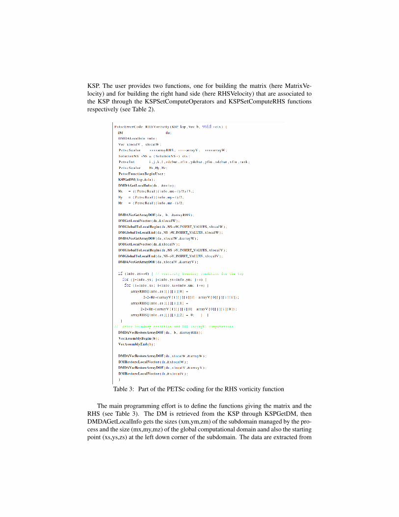
Table 3: Part of the PETSc coding for the RHS vorticity function

The main programming effort is to define the functions giving the matrix and theRHS (see Table 3). The DM is retrieved from the KSP through KSPGetDM, thenDMDAGetLocalInfo gets the sizes (xm,ym,zm) of the subdomain managed by the pro-cess and the size (mx,my,mz) of the global computational domain aand also the startingpoint (xs,ys,zs) at the left down corner of the subdomain. The data are extracted from

the vector by DMDAVecGetArrayDOF. Extracting the data field with its ghost pointsin the subdomain needs to create a local vector using DMGetLocalVector, then to ex-tract a localArray with again DMDAVecGetArrayDOF and finally to update the ghostpoint with neighbor subdomains with DMGlobalToLocalBegin and DMGlobalToLo-calEnd. The data of the RHS are then computed using the 4-index array [k][j][i][dof]The data associated to the RHS have to be restore in the vector using DMDAVecRe-storeArrayDOF and must be assembly with VecAssemblyBegin and VecAssemblyEnd.Local vectors have to been restored before leaving with DMRestoreLocalVector.

Then for strategy 1 one time step consists to solve the linear system with KSPSolveand to extract the solution from KSP with KSPGetSolution. We tested several KSP

Table 4: PETSc coding of the time loop for strategy 1

solvers associated to different preconditioners. It appears that the best pair KSP/PCfor the elliptic equation is the GMRES [15, 16] associated to the HYPRE Algebraicmultigrid [17] preconditioner that converges in 5 (respectively 3) iterations per timestep for the velocity (respectively the vorticity) for the 192×64×64 mesh.

As both operators for the vorticity solution and the velocity solution do not de-pend on the time iteration, we also studied the choice of KSP composed by KSPPRE-ONLY where only the PC is applied with the choice of Gauss factorizaton with theSuperLU dist package [18]. This is done simply by passing the "-ksp type preonly"option in the execution order.

2.2 Strategy 2 : semi-implicit convection termStrategy 2 solves (1)-(2) with taking the convection term semi-implicitly:(

(I− ∆tRe ∆).+∆t∇× (~Vn× .) 0

∇× . ∆.

)(~ωn+1

~V n+1

)=

(~ωn

0

)(6)

Let us notice that for strategy 2, we still use the boundary condition for the vorticityusing the ~Vn as we split the solution of (6) in two stages, the solution of the velocityand then the solution for the vorticity.

The PETSc implementation of strategy 2 involves two distributed array (DA) withthree degree of freedom (DOF) with two Krylov solvers (KSP) with updating a partof the matrix vorticity at each time step. The vorticity boundary condition would havebeen taken implicitly if we used a DA with six DOF and on KSP taking in account thesix equations. One time step for strategy 2 differs from those of strategy 1 with calling

Table 5: PETSc coding of the time loop for strategy 2

KSPSetComputeOperators function to update the matrix vorticity before KSPSolveassociated to the vorticity equation (see Table 5).

Again the best pair KSP/PC for strategy 2 is the GMRES/HYPRE pair , that con-verges in 5 (respectively 3) iterates per time step for the velocity (respectively thevorticity) for the 192×64×64 mesh and in 6 (respectively 4) iterates per time step forthe velocity (respectively the vorticity) for the 384×128×128 .

2.3 Strategy 3 : totaly implicit formulationThe third strategy solves (1)-(2) totally implicitly:(

(I− ∆tRe ∆)(~ωn+1−∆t~∇× (~Vn+1×~ω

n+1)− ~ωn

∆~Vn+1 +∇×~ωn+1

)= ~0 (7)

In this strategy the boundary condition for the vorticity is totally implicit as well as theconvection term as the six equations are solved together.

Table 6: PETSc coding of the SNES setup for strategy 3 and the time loop associated

For strategy 3 the DM has six DOF and we create a SNES (system of NonlinearEquations Solver) object. This DM is associated to the SNES through the commandSNESSetDM. Then the user has to provide the function to minimize, implementingthe six discretized equations and boundary conditions with SNESSetFunction. As theSNES may needs the Jacobian of the function to minimize we can provide the jacobianto the SNES with the SNESSetJacobian function or we can let the Jacobian be eval-uated with differentiating with providing a Index Set coloring associated to the datadependencies in the function to minimize in order to optimize the number of call to thefunction. This is done by the MatFDColoringCreate creating a MatFDColoring objectthat has been associated to the SNES through the SNESSetJacobian command.We alsocan change the KSP from the SNES through SNESGetKSP. One time step iterationconsists in applying SNESSolve and then get de solution with SNESGetSolution.

We also tested several SNES solver the two candidates have been newtonls (for

Newton based nonlinear solver that uses a line search [19]), and ngmres (for NonlinearGeneralized Minimum Residual method [20] [21] that combines m previous solutionsinto a minimum-residual solution by solving a small linearized optimization problemat each iteration, very similar to the Anderson mixing [22]). While newtonls was per-forming better to reach a relative tolerance of 1e-6 ,ngmres with up to 300 previoussolutions was prefered to reach a relative tolerance of 1e-8 as we will discuss in theflow behavior result.

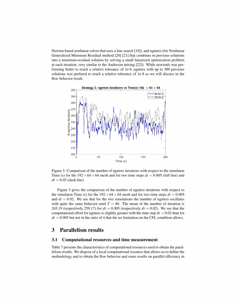
Figure 3: Comparison of the number of ngmres iterations with respect to the simulatonTime (s) for the 192×64×64 mesh and for two time steps dt = 0.005 (full line) anddt = 0.02 (dash line)

Figure 3 gives the comparison of the number of ngmres iterations with respect tothe simulaton Time (s) for the 192× 64× 64 mesh and for two time steps dt = 0.005and dt = 0.02. We see that for the two simulations the number of ngmres oscillateswith quite the same behavior until T = 40. The mean of the number of iteration is245.19 (respectively 259.17) for dt = 0.005 (respectively dt = 0.02). We see that thecomputational effort for ngmres is slightly greater with the time step dt = 0.02 than fordt = 0.005 but not in the ratio of 4 that the no limitation on the CFL condition allows.

3 Parallelism results

3.1 Computational resources and time measurementTable 7 presents the characteristics of computational resources used to obtain the paral-lelism results. We dispose of a local computational resource that allows us to define themethodology and to obtain the flow behavior and some results on parallel efficiency in

a shared memory environment. The national allocated computing resource occigen isfinite 50000 hours and is used to obtain parallel speed-up in an dedicated environmentwith up to date software framework by an expert dedicated team. The results on occi-gen will use as much as possible the load balancing between memory and CPU withusing, when is possible, not all CPUs of each node.

Computer glenan occigenModel Dell PE920 bulx DLCProcessor Xeon Xeon

E7-4880v2 E5-2690v34x15C 2.5Ghz 1x12C 2.6Ghz

Memory/Node 512Gb 110GbNetwork shared memory Infinityband FDRResource laboratory national (cines)

∞ hours 50000 hoursUse speed-up tests speed-up tests

flow behavior

Table 7: Computing resources characteristics

Table 8: Coding of the event log for parallel performances

PETSc provides a smart mechanism to monitor the performance with a commandline option -log view that provides counters on events defined by the user. The user hasto declare PetscLogStage and use the PetscLogStagePush(stage) and PetscLogStage-Pop(); before and after the portion of code that must be monitored as illustrated inTable 8. Then when the code terminates, the log of selected events with their timemeasurement are displayed as shown in table 9.

Table 9: PETSc log of the code for 10+1(first) time steps of strategy 1 on glenan forthe mesh 192×64×64

We made the observation that the first solve always takes more elapse time, thiswhy we separated the first solve from other iterations in the time measurement.

3.2 Speed-up for strategy 1

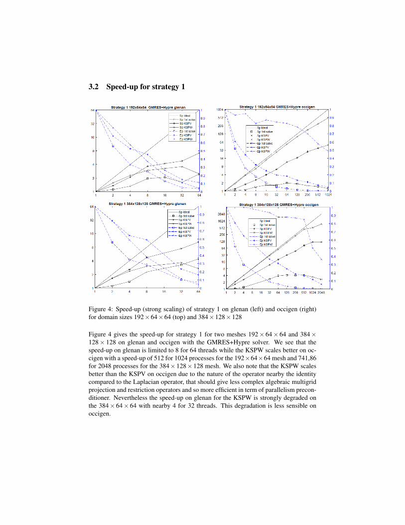
Figure 4: Speed-up (strong scaling) of strategy 1 on glenan (left) and occigen (right)for domain sizes 192×64×64 (top) and 384×128×128

Figure 4 gives the speed-up for strategy 1 for two meshes 192× 64× 64 and 384×128× 128 on glenan and occigen with the GMRES+Hypre solver. We see that thespeed-up on glenan is limited to 8 for 64 threads while the KSPW scales better on oc-cigen with a speed-up of 512 for 1024 processes for the 192×64×64 mesh and 741,86for 2048 processes for the 384×128×128 mesh. We also note that the KSPW scalesbetter than the KSPV on occigen due to the nature of the operator nearby the identitycompared to the Laplacian operator, that should give less complex algebraic multigridprojection and restriction operators and so more efficient in term of parallelism precon-ditioner. Nevertheless the speed-up on glenan for the KSPW is strongly degraded onthe 384× 64× 64 with nearby 4 for 32 threads. This degradation is less sensible onoccigen.

3.3 Speed-up for strategy 2

Figure 5: Speed-up (strong scaling) of strategy 2 on glenan (left) and occigen (right)for domain sizes 192×64×64 (top) and 384×128×128

Figure 5 gives the speed-up for strategy 2 for two meshes 192× 64× 64 and 384×128×128 on glenan and on occigen with the GMRES+Hypre solver. Again the speed-up is better for the KSPW than for KSPV, even if the stagnation of the speed-up comesmore early with the introduction of convective term in the vorticity operator that leadsto an operator with the diagonal dominance reinforced . A speed-up of 426.67 for 1024processes is reach on the 192×64×64 on occigen for KSPW. This speed-up stagnateson 2048 processes. The speed-up is again around 786.36 for 2048 processes on occigenfor the 384×128×128 mesh.

3.4 Speed-up for strategy 3Figure 6 gives the speed-up for the strategy 3 on occigen for a mesh of 192×64×64with Nonlinear GMRES with up to 300 previous solutions. A speed-up of is obtainedfor 1024 CPUs. We see that the SNES’s initialization (Snes init), that corresponds to the

Figure 6: Speed-up for strategy 3 with ngmres and 192×64×64

buliding of the data structures for the snes, scales until 64 and the scaling performancesare degraded after. As this initialization time is small compared to the time associatedto the number of time iterates, this result is not significant. We still spearate the firstsolve to the other iterations as it takes more time. The SNES solving scales well until64 processes on occigen, and a speed-up of 298 ( 357 respectively) is obtained on 1024processes (respectively 2048 processes).

3.5 Elapsed time comparison for the three strategiesTable 10 gives the elapse time per iteration for all the strategies for the 192×64×64mesh with dt = 0.005 on occigen computer.

• The strategy 1 with superLU didn’t run onto occigen due to lack of memorywith 110Gb. Strategies 1 and 2 take quite the same time on one processor whilestrategy 3 took 74.76 times more time than strategy 2 on one process. This ratiodrops to 20 on 256 processes. Strategy 3 still reduces the elapsed time after 256processes.

• Strategy 2 is quite always better than strategy 1 even if the matrix for the vorticitychange. This is quite surprising. This may due to the decentered discretizationof the convection term for the vorticity equation that leads to more diagonaldominant matrix than for the Laplacian and consequently has a better Krylovconvergence. The velocity equations are solved identically in both strategies.

• For 256 processors the strategy 3 becomes reachable as there is no CFL conditionon the time step.

P S1 S1 LU S2 S3 comments1 12.61 - 12.59 941.25 too much even with no CFL2 9.97 32.89 9.09 479.354 6.69 20.48 6.78 316.63 S1 vs S2 similar (<>tol)8 4.56 10.77 3.82 311.4516 2.91 8.50 2.52 99.1832 1.83 4.54 1.58 39.2064 0.99 4.16 0.83 17.84128 0.68 2.37 0.56 10.03256 0.40 2.42 0.34 6.04 S3 reachable with no CFL512 0.30 1.83 0.28 4.111024 0.23 5.05 0.28 3.152048 - - 0.26 2.63

Table 10: Time (s) per iteration: occigen dt=0.005 192x64x64

To be complete, we must notice that the elapsed time per point and time step isaround 1.60e−6 to 3e−7 for strategy 2 that is not impressive compared to the elapsedtime of the optimized research code with ADI and multigrid and domain decompositiondone on the CRAY YMP 25 years ago with 2.510−5 s per point and time step for a81×41×41 mesh [10].

Nevertheless the programming effort was low (once understanding the PETSc phi-losophy of implementation); we also let PETSc deciding of the data distribution andthe equations have been solved with a better accuracy at each time step.

4 Flow behaviorFor the flow behavior comparison between the three strategies, we restrict ourselvesto compare the flow behavior in the x− z plane at y = 1/6 where the Taylor-Gortlervortices should appear. We extract the distributed component ωy from the distributedmesh through MPI implementation although we could use some vecGather functionfrom the PETSc library. The figures have been generated with matlab contourf functionfor isovalues equal to [−10,−5,−3,−1,−0.5,0,0.5,1,3,5,10]

4.1 Underresolved problem for strategy 3

Figure 7: Effect on the undersolve time step solution on the flow behavior: up theNewton LS algorithm for strategy 3 with a tol = 1e−6 at T = 38 and bottom the lost ofthe flow symmetry at T = 60 .

Figure 7 exhibits a problem that occurred for the strategy 3 when the solver a newtonlswith a rtol = 1e− 6 was used. It presents the flow behavior at T = 38 that keeps itssymmetry while it loses its symmetry for T = 60. This is due to some underresolvedsolution at some time after T = 38. We advocate that as the equations are symmetric asthe boundary conditions also, we should keep the symmetry of the flow. The problemwas solved by changing the solver with the ngmres with up to 300 previous solutionsthat allows to solve the problem with a rtol = 1e−8.

Figure 7 gives the flow behavior for T = 38 and T = 60 for strategy 3 with newtonlssolver with a tolerance of 1e− 6. We see that the flow loses its symmetry due to anunderresolving during some time step. This why we easely changed the solver withngmres with 300 fixed-point iterations in order to reach a tolerance of 1e−8.

4.2 Flow behavior comparison for the three strategiesFigures 8 , 9, and 10 compare the flow behavior for the three strategies at time T =20.28,45.00,73.48 for the mesh 192×64×64 and a time step value of dt = 0.005(which is imposed by the CFL condition of strategy 1). The solvers used are su-perlu+dist, gmres+hypre and ngmres 300 for strategies 1, 2 and 3 respectively.

Figure 8 exhibits some quite similar results for strategy 1 and strategy 2 withslightly more strong vortex in position i=45 and k=50. The difference coming fromtaking the vorticity term implicit in time in the convection term but the treatment ofthe vorticity boundary conditions are unchanged between the two strategies. For thestrategy 3, it shows that the vortices attached to the boundaries are more strong, and theflow is slightly in advance compared to the two other strategies as the vortex in positioni=20, k=55 is already attached to the vortex on the boundary. We conclude that takingexplicit in time the convection term and with more impact taking explicit in time theright hand side of the vorticity boundary conditions introduce a delay on the flow.

The flow behavior at T=45 on Figure 9 still exhibits the quite same flow structurefor the three strategy, with more strong vortices for the strategy 3. The flow keepsits symmetry. This is also the case for Figure 10 where the strategy 3 exhibits moredefined vortices structures.

Figure 8: Comparison of the flow behavior for the three strategies (strategy 3 up, strat-egy 2 middle, strategy 1 bottom) at time t=20.

Figure 9: Comparison of the flow behavior for the three strategies (strategy 3 up, strat-egy 2 middle, strategy 1 bottom) at time t=45.

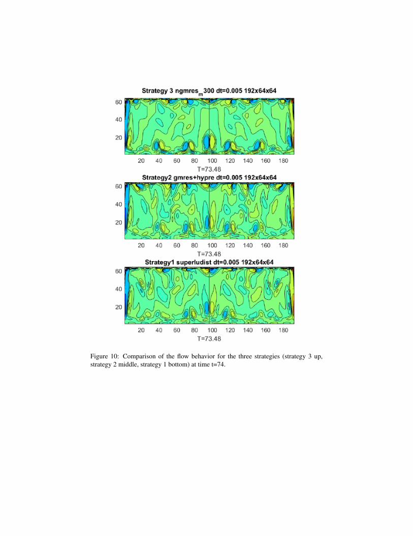
Figure 10: Comparison of the flow behavior for the three strategies (strategy 3 up,strategy 2 middle, strategy 1 bottom) at time t=74.

4.3 Flow behavior comparison with respect to the time step forstrategy 3

Figure 11 gives the flow behavior at time T = 76 for the strategy 3 with the ngmressolver for two time steps dt = 2.10−2 and dt = 5.10−3. We see a good agreementbetween the two computations and see the advantage of strategy 3 that has no CFLcondition. The limitation for the time step is only due to physics consideration, inorder to catch the right dynamics and we see that we can take a 4 times greater timestep for this flow behavior computation.

Figure 11: Comparison for strategy 3 (with no CFL time step limitation) for two timesteps dt = 2.10−2 (top) and dt = 5.10−3 (bottom).

5 ConclusionsThis paper shows the use of different functionalities of PETSc to solve the lid-drivencavity problem with aspect ratio 3:1 for Reynolds 3200 from a semi-implicit to a fullyimplicit in time formulations. We notably exhibits that writing all the terms of the

vorticity boundary condition at time step tn+1 leads to stronger vortices much morethan writing all the terms involved in the convective term at same time step tn+1. Thisconclusion is somewhat foreseeable as all the dynamics of the flow comes from theboundaries. The PETSc library permits us to tests different solvers and to choose thesolver and its parameters the best adapted for the computation. It was somewhat sur-prising in a first approach that taking the convective term implicit gives better resultson the parallelism for the solver associated to the vorticity. This is mainly due to theHYPRE preconditioner behavior, that creates algebraically the restriction and projec-tion operators, which performs well for the operator where we reinforce the diagonaldominance.

The fully implicit formulation has the advantage to not have CFL condition andallows us to violate at least 4 times this CFL of the strategy 1 with keeping the rightflow behavior. One output of this work, is to demonstrates that the fully implicit intime strategy can be competitive (reachable) with a sufficient number of processes.Nevertheless, we must mention that we could provide to the PETSc library with theKSPRegister instruction our owner implementation of gmres where we can stored thedirections of descent from different consecutive time steps in a cumulative Krylovspace since the operator for strategy 1 does not change. Then we can initialize the newtime step solution with projecting the new right hand side with respect to this Krylovspace [12, 23, 24]. We now have a non-trivial PETSc base test case that can allow usto develop non-linear acceleration methods by further entering in the PETSc codingto define our own SNES solvers, using for example singular value decomposition ofprevious time step solutions to accelerate the Newton [24]. The discretization couldalso be improve by several way, with at least better space discretization with compactschemes [25] for example and better discretization in time. The perspective of thiswork could be also to go further in controling the error on the solution with using forexample BDF schemes with adaptive time step of the SUNDIALS [26] library.

AcknowledgementsThis work was granted access to the HPC resources of CINES under the allocation12018-AP01061040 made by GENCI (Grand Equipement National de Calcul Intensif).Author thanks also the Center for the Development of Parallel Scientific Computing(CDCSP) of University of Lyon 1 for providing local computing resources to designthe methodology.

References[1] H. C. Elman, V. E. Howle, J. N. Shadid, R. S. Tuminaro, A parallel

block multi-level preconditioner for the 3D incompressible Navier-Stokesequations, Journal of Computational Physics 187 (2) (2003) 504 – 523.doi:https://doi.org/10.1016/S0021-9991(03)00121-9.URL http://www.sciencedirect.com/science/article/pii/S0021999103001219

[2] D. Loghin, A. J. Wathen, Schur complement preconditioners for the Navier-Stokes equations, International Journal for Numerical Methods in Fluids 40 (3-4)(2002) 403–412. arXiv:https://onlinelibrary.wiley.com/doi/pdf/10.1002/fld.296, doi:10.1002/fld.296.URL https://onlinelibrary.wiley.com/doi/abs/10.1002/fld.296

[3] O. Daube, J. Guermond, A. Sellier, On the Velocity-Vorticity formulation ofthe Navier-Stokes equations in incompressible flow, COMPTES RENDUS DEL ACADEMIE DES SCIENCES SERIE II 313 (4) (1991) 377–382.

[4] C. Speziale, On the advantages of the Vorticity Velocity formulation of the equa-tions of fluids-dynamics, JOURNAL OF COMPUTATIONAL PHYSICS 73 (2)(1987) 476–480. doi:10.1016/0021-9991(87)90149-5.

[5] T. Gatski, Review of incompressible fluid-flow computations using the VorticiyVelocity formulation, APPLIED NUMERICAL MATHEMATICS 7 (3) (1991)227–239. doi:10.1016/0168-9274(91)90035-X.

[6] G. A. Osswald, K. N. Ghia, U. Ghia, Direct method for solution of three-dimensional unsteady incompressible navier-stokes equations, in: D. L. Dwoyer,M. Y. Hussaini, R. G. Voigt (Eds.), 11th International Conference on Numeri-cal Methods in Fluid Dynamics, Springer Berlin Heidelberg, Berlin, Heidelberg,1989, pp. 454–461.

[7] Y. Huang, U. Ghia, G. A. Osswald, K. N. Ghia, Velocity-Vorticity Simulationof Unsteady 3-D Viscous Flow within a Driven Cavity, Vieweg+Teubner Verlag,Wiesbaden, 1992, pp. 54–66. doi:10.1007/978-3-663-00221-5_7.URL https://doi.org/10.1007/978-3-663-00221-5_7

[8] S. Bhaumik, T. K. Sengupta, A new velocity-vorticity formulation fordirect numerical simulation of 3d transitional and turbulent flows, Jour-nal of Computational Physics 284 (2015) 230 – 260. doi:https://doi.org/10.1016/j.jcp.2014.12.030.URL http://www.sciencedirect.com/science/article/pii/S002199911400847X

[9] G. Guj, F. Stella, A vorticity-velocity method for the numerical solution of 3dincompressible flows, Journal of Computational Physics 106 (2) (1993) 286 –298. doi:https://doi.org/10.1016/S0021-9991(83)71108-3.URL http://www.sciencedirect.com/science/article/pii/S0021999183711083

[10] D. Tromeur-Dervout, T. P. Loc, Parallelization via Domain Decomposition Tech-niques of Multigrid and ADI Solvers for Navier-Stokes Equations, Notes on Nu-merical Fluid Mechanics, Numerical Simulation of 3D Incompressible UnsteadyViscous Laminar Flows 36 (1992) 107–118, iSBN 3-528-07636-4.

[11] O. Botella, R. Peyret, Benchmark spectral results on the lid-driven cav-ity flow, Computers & Fluids 27 (4) (1998) 421 – 433. doi:https:

//doi.org/10.1016/S0045-7930(98)00002-4.URL http://www.sciencedirect.com/science/article/pii/S0045793098000024

[12] D. Tromeur-Dervout, Résolution des Equations de Navier-Stokes en FrmulationVitesse-Tourbillon sur Systèmes Multiprocesseurs à Mémoire Distribuée, Ph.D.thesis, University Paris 6 / ONERA (January 1993).

[13] S. Balay, S. Abhyankar, M. F. Adams, J. Brown, P. Brune, K. Buschelman, L. Dal-cin, V. Eijkhout, W. D. Gropp, D. Kaushik, M. G. Knepley, D. A. May, L. C.McInnes, K. Rupp, P. Sanan, B. F. Smith, S. Zampini, H. Zhang, H. Zhang,PETSc users manual, Tech. Rep. ANL-95/11 - Revision 3.8, Argonne NationalLaboratory (2017).URL http://www.mcs.anl.gov/petsc

[14] S. Balay, W. D. Gropp, L. C. McInnes, B. F. Smith, Efficient management ofparallelism in object oriented numerical software libraries, in: E. Arge, A. M.Bruaset, H. P. Langtangen (Eds.), Modern Software Tools in Scientific Comput-ing, Birkhäuser Press, 1997, pp. 163–202.

[15] Y. Saad, M. Schultz, GMRES - A Generalized Minimal RESidual algorithm forsolving nonsymmetric linear systems, SIAM Journal on SCIentific and StatisticalComputing 7 (3) (1986) 856–869. doi:10.1137/0907058.

[16] Y. Kuznetsov, Numerical methods in subspaces, in: G. I. Marchuk (Ed.), Vychis-litel’nye Processy i Sistemy II, Nauka, Moscow, 1985, pp. 265–350.

[17] R. Falgout, U. Yang, hypre: A library of high performance preconditioners, in:Sloot, P and Tan, CJK and Dongarra, JJ and Hoekstra, AG (Ed.), COMPUTA-TIONAL SCIENCE-ICCS 2002, PT III, PROCEEDINGS, Vol. 2331 of LEC-TURE NOTES IN COMPUTER SCIENCE, Univ Amsterdam, Sect ComputatSci; SHARCNET, Canada; Univ Tennessee, Dept Comp Sci; Power Comp &Commun BV; Elsevier Sci Publ; Springer Verlag; HPCN Fdn; Natl SupercompFacilities; Sun Microsyst Inc; Queens Univ, Sch Comp Sci, 2002, pp. 632–641,International Conference on Computational Science, AMSTERDAM, NETHER-LANDS, APR 21-24, 2002.

[18] X. S. Li, J. W. Demmel, SuperLU DIST: A scalable distributed-memory sparsedirect solver for unsymmetric linear systems, ACM Trans. Mathematical Soft-ware 29 (2) (2003) 110–140.

[19] P. Deuflhard, Newton Methods for Nonlinear Problems: Affine Invariance andAdaptive Algorithms, Springer Berlin Heidelberg, Berlin, Heidelberg, 2011.doi:10.1007/978-3-642-23899-4_2.URL https://doi.org/10.1007/978-3-642-23899-4_2

[20] C. Oosterlee, T. Washio, Krylov subspace acceleration of nonlinear multigrid withapplication to recirculating flows, SIAM JOURNAL ON SCIENTIFIC COM-PUTING 21 (5) (2000) 1670–1690, 5th Copper Mountain Meeting on Itera-

tive Methods, COPPER MOUNTAIN, ALASKA, APR, 1998. doi:10.1137/S1064827598338093.

[21] P. R. Brune, M. G. Knepley, B. F. Smith, X. Tu, Composing Scalable NonlinearAlgebraic Solvers, SIAM REVIEW 57 (4) (2015) 535–565. doi:10.1137/130936725.

[22] H. Walker, P. Ni, Anderson acceleration for fixed-point iterations, SIAM Journalon Numerical Analysis 49 (4) (2011) 1715–1735. arXiv:https://doi.org/10.1137/10078356X, doi:10.1137/10078356X.URL https://doi.org/10.1137/10078356X

[23] J. Erhel, F. Guyomarc’h, An augmented conjugate gradient method for solvingconsecutive symmetric positive definite linear systems, SIAM Journal on MatrixAnalysis and Applications 21 (4) (2000) 1279–1299. arXiv:https://doi.org/10.1137/S0895479897330194, doi:10.1137/S0895479897330194.URL https://doi.org/10.1137/S0895479897330194

[24] D. Tromeur-Dervout, Y. Vassilevski, Choice of initial guess in it-erative solution of series of systems arising in fluid flow simula-tions, Journal of Computational Physics 219 (1) (2006) 210 – 227.doi:https://doi.org/10.1016/j.jcp.2006.03.014.URL http://www.sciencedirect.com/science/article/pii/S0021999106001483

[25] S. K. Lele, Compact finite difference schemes with spectral-like res-olution, Journal of Computational Physics 103 (1) (1992) 16 – 42.doi:https://doi.org/10.1016/0021-9991(92)90324-R.URL http://www.sciencedirect.com/science/article/pii/002199919290324R

[26] A. C. Hindmarsh, P. N. Brown, K. E. Grant, S. L. Lee, R. Serban, D. E. Shumaker,C. S. Woodward, Sundials: Suite of nonlinear and differential/algebraic equationsolvers, ACM Transactions on Mathematical Software (TOMS) 31 (3) (2005)363–396.