Time-Dependent Shortest Path Problems

with Penalties and Limits on Waiting

Edward He*�1, Natashia Boland �1, George Nemhauser §1, and Martin Savelsbergh ¶1

1H. Milton Stewart School of Industrial and Systems Engineering, Georgia Institute ofTechnology, U.S.

April 11, 2020

Abstract

Waiting at the right location at the right time can be critically important in certain variantsof time-dependent shortest path problems. We investigate the computational complexity oftime-dependent shortest path problems in which there is either a penalty on waiting or a limiton the total time spent waiting at a given subset of the nodes. We show that some casesare NP-hard, and others can be solved in polynomial time, depending on the choice of thesubset of nodes, on whether waiting is penalized or is constrained, and on the magnitude of thepenalty/waiting limit parameter.

Keywords: shortest path, time-dependent travel time, time-expanded network, computationalcomplexity

1 Introduction

Time-dependent shortest path problems generalize the classical problem of finding a path in anetwork from a given origin node to a given destination node so as to minimize a function of thearcs used, by introducing the element of time. A time-dependent path is a path in time and space(the network) that departs the origin at a time no earlier than the start of a given time horizonand reaches the destination no later than the end of the horizon, where the time to traverse an arcin the network is a function of the time of departure at its tail node. Such problems are especiallyof interest in road networks, where traffic congestion conditions affect the time needed to traverselinks in the network (Letchner et al. 2006, Franceschetti et al. 2018).

Applications in transport logistics are emerging, in part because the now ubiquitous GPS-enabled devices supply the data needed to reliably estimate arc travel time functions in road net-works (Bertsimas et al. 2019), complementing the more traditional reliance on data from inductiveloops (Wang and Nihan 2000, Coifman 2002).

*Corresponding author.�edwardhe@gatech.edu�natashia.boland@isye.gatech.edu§gn3@gatech.edu¶martin.savelsbergh@isye.gatech.edu

1

A number of variants of the time-dependent shortest path problem have been studied, startingwith the minimum arrival time variant in Cooke and Halsey (1966), Orda and Rom (1990), andDean (2004b), the minimum duration variant in Orda and Rom (1990), Chabini (1998), Nachtigall(1995), Kanoulas et al. (2006), Ding et al. (2008), Foschini et al. (2014) and He et al. (2019), and,recently, the minimum travel time variant in He et al. (2019). These variants differ not only intheir choice of objective function, but also in the nodes at which waiting may occur in an optimalsolution. In the Minimum Travel Time Problem (MTTP), an optimal solution may wait at anynode, including the origin, to take advantage of shorter travel times that occur later in the timehorizon. The MTTP objective is to minimize the sum of the travel times along the arcs used;provided the path starts and ends within the given time horizon, time spent waiting is ignored. Inthe Minimum Arrival Time Problem (MATP), a path reaching the destination as soon as possible issought. Under the commonly assumed first-in-first-out (FIFO) property of arc travel time functions,which states that waiting at the tail node of an arc can never result in an earlier arrival at its headnode, waiting before departing a node is suboptimal for the MATP. In the Minimum DurationProblem (MDP) under FIFO, a path minimizing the difference between the arrival time at thedestination and the departure time at the origin is sought. Thus, waiting to depart at any nodeother than the origin is suboptimal for the MDP. It has been shown that for piecewise linear traveltime functions satisfying FIFO, all three variants can be solved in polynomial time (see Cooke andHalsey (1966), Foschini et al. (2014), and He et al. (2019)). We note that early algorithms onvariants in which waiting can be beneficial, e.g., the ones in Chabini (1998) and Dean (2004a), relyon time discretization, and, thus, provide only approximate solutions, whereas recent algorithms,e.g., the ones in Foschini et al. (2014) and He et al. (2019), however, properly handle continuoustime and provide optimal solutions.

That the study of different objective functions is not only of academic interest can be seen inCooper and Cowlagi (2018). They consider the problem of planning a route in which the objectiveis to minimize a “weighted sum of travel duration and exposure to traffic”, and argue that such anobjective may be of importance to reduce the health risks for long-haul truck drivers by reducingtheir exposure to emissions. They observe that because real-time traffic data is becoming widelyavailable, which allows accurate predictions of traffic, and, thus, travel times, an optimal routemay involve waiting for traffic to subside. They also comment that this type of objective may berelevant for motion-planning of aerial vehicles in inclement weather.

In this paper, we consider additional variants in which there is either a penalty incurred forwaiting, or there is a limit on the total time spent waiting, at a given subset of the nodes. Wedetermine the complexity of these additional variants. For variants that are NP-hard, we providea complexity proof and for variants that are polynomially solvable, we provide an algorithm. Wewill not discuss the variant in which there is a constraint on waiting at each individual node, whichhas been shown to be NP-hard, by Omer and Poss (2019b).

The remainder of the paper is organized as follows. In Section 2, we formally introduce thebasic variants of the time-dependent shortest path problem as well as the variants with penaltiesand constraints on waiting, which are the focus of our research. In Section 3, we discuss a fewnatural extensions of the basic variants. In Section 4. we present NP-completeness proofs for the(remaining) variants with penalties and constraints on waiting that are hard. In Sections 5 and 6.we present polynomial time algorithms for the (remaining) variants with penalties and constraintson waiting that are easy. Finally, in Section 7, we summarize the complexity status of all variantswith penalties and limits on waiting.

2

2 Problem Description and Preliminaries

2.1 Problem Setting Description and Illustration

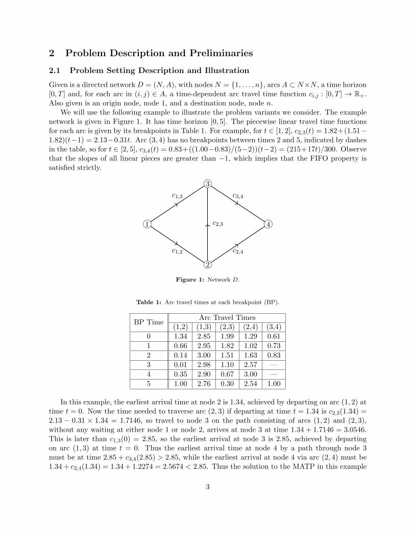
Given is a directed network D = (N,A), with nodes N = {1, . . . , n}, arcs A ⊂ N×N , a time horizon[0, T ] and, for each arc in (i, j) ∈ A, a time-dependent arc travel time function ci,j : [0, T ] → R+.Also given is an origin node, node 1, and a destination node, node n.

We will use the following example to illustrate the problem variants we consider. The examplenetwork is given in Figure 1. It has time horizon [0, 5]. The piecewise linear travel time functionsfor each arc is given by its breakpoints in Table 1. For example, for t ∈ [1, 2], c2,3(t) = 1.82+(1.51−1.82)(t−1) = 2.13−0.31t. Arc (3, 4) has no breakpoints between times 2 and 5, indicated by dashesin the table, so for t ∈ [2, 5], c3,4(t) = 0.83+((1.00−0.83)/(5−2))(t−2) = (215+17t)/300. Observethat the slopes of all linear pieces are greater than −1, which implies that the FIFO property issatisfied strictly.

c1,2

c1,3

c2,3

c2,4

c3,4

1

2

3

4

Figure 1: Network D.

Table 1: Arc travel times at each breakpoint (BP).

BP TimeArc Travel Times

(1,2) (1,3) (2,3) (2,4) (3,4)

0 1.34 2.85 1.99 1.29 0.61

1 0.66 2.95 1.82 1.02 0.73

2 0.14 3.00 1.51 1.63 0.83

3 0.01 2.98 1.10 2.57 —

4 0.35 2.90 0.67 3.00 —

5 1.00 2.76 0.30 2.54 1.00

In this example, the earliest arrival time at node 2 is 1.34, achieved by departing on arc (1, 2) attime t = 0. Now the time needed to traverse arc (2, 3) if departing at time t = 1.34 is c2,3(1.34) =2.13 − 0.31 × 1.34 = 1.7146, so travel to node 3 on the path consisting of arcs (1, 2) and (2, 3),without any waiting at either node 1 or node 2, arrives at node 3 at time 1.34 + 1.7146 = 3.0546.This is later than c1,3(0) = 2.85, so the earliest arrival at node 3 is 2.85, achieved by departingon arc (1, 3) at time t = 0. Thus the earliest arrival time at node 4 by a path through node 3must be at time 2.85 + c3,4(2.85) > 2.85, while the earliest arrival at node 4 via arc (2, 4) must be1.34 + c2,4(1.34) = 1.34 + 1.2274 = 2.5674 < 2.85. Thus the solution to the MATP in this example

3

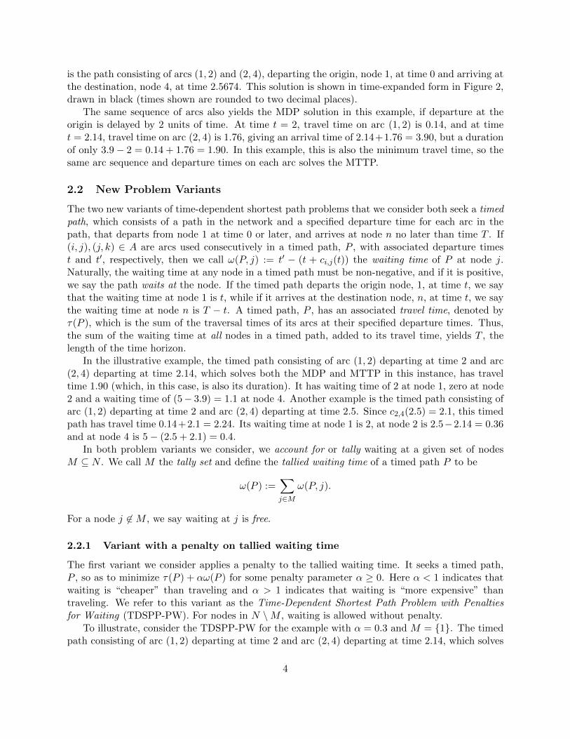
is the path consisting of arcs (1, 2) and (2, 4), departing the origin, node 1, at time 0 and arriving atthe destination, node 4, at time 2.5674. This solution is shown in time-expanded form in Figure 2,drawn in black (times shown are rounded to two decimal places).

The same sequence of arcs also yields the MDP solution in this example, if departure at theorigin is delayed by 2 units of time. At time t = 2, travel time on arc (1, 2) is 0.14, and at timet = 2.14, travel time on arc (2, 4) is 1.76, giving an arrival time of 2.14+1.76 = 3.90, but a durationof only 3.9− 2 = 0.14 + 1.76 = 1.90. In this example, this is also the minimum travel time, so thesame arc sequence and departure times on each arc solves the MTTP.

2.2 New Problem Variants

The two new variants of time-dependent shortest path problems that we consider both seek a timedpath, which consists of a path in the network and a specified departure time for each arc in thepath, that departs from node 1 at time 0 or later, and arrives at node n no later than time T . If(i, j), (j, k) ∈ A are arcs used consecutively in a timed path, P , with associated departure timest and t′, respectively, then we call ω(P, j) := t′ − (t + ci,j(t)) the waiting time of P at node j.Naturally, the waiting time at any node in a timed path must be non-negative, and if it is positive,we say the path waits at the node. If the timed path departs the origin node, 1, at time t, we saythat the waiting time at node 1 is t, while if it arrives at the destination node, n, at time t, we saythe waiting time at node n is T − t. A timed path, P , has an associated travel time, denoted byτ(P ), which is the sum of the traversal times of its arcs at their specified departure times. Thus,the sum of the waiting time at all nodes in a timed path, added to its travel time, yields T , thelength of the time horizon.

In the illustrative example, the timed path consisting of arc (1, 2) departing at time 2 and arc(2, 4) departing at time 2.14, which solves both the MDP and MTTP in this instance, has traveltime 1.90 (which, in this case, is also its duration). It has waiting time of 2 at node 1, zero at node2 and a waiting time of (5− 3.9) = 1.1 at node 4. Another example is the timed path consisting ofarc (1, 2) departing at time 2 and arc (2, 4) departing at time 2.5. Since c2,4(2.5) = 2.1, this timedpath has travel time 0.14+2.1 = 2.24. Its waiting time at node 1 is 2, at node 2 is 2.5−2.14 = 0.36and at node 4 is 5− (2.5 + 2.1) = 0.4.

In both problem variants we consider, we account for or tally waiting at a given set of nodesM ⊆ N . We call M the tally set and define the tallied waiting time of a timed path P to be

ω(P ) :=∑j∈M

ω(P, j).

For a node j 6∈M , we say waiting at j is free.

2.2.1 Variant with a penalty on tallied waiting time

The first variant we consider applies a penalty to the tallied waiting time. It seeks a timed path,P , so as to minimize τ(P ) + αω(P ) for some penalty parameter α ≥ 0. Here α < 1 indicates thatwaiting is “cheaper” than traveling and α > 1 indicates that waiting is “more expensive” thantraveling. We refer to this variant as the Time-Dependent Shortest Path Problem with Penaltiesfor Waiting (TDSPP-PW). For nodes in N \M , waiting is allowed without penalty.

To illustrate, consider the TDSPP-PW for the example with α = 0.3 and M = {1}. The timedpath consisting of arc (1, 2) departing at time 2 and arc (2, 4) departing at time 2.14, which solves

4

both the MDP and MTTP in this instance, has TDSPP-PW objective value of 1.9 + α × 2 = 2.5,since its waiting time at node 1 is 2. The optimal solution to this TDSPP-PW consists of the samearcs, but departs on (1, 2) at time 1, and on (2, 4) at time 1.66. It gives the optimal TDSPP-PWobjective value: (0.66 + 1.42) + α× 1 = 2.38.

Solutions to two other TDSPP-PW problems using the same network and travel time functionsare shown in Figure 2, presented in a time-expanded network. In both cases, the tallied waitingpenalty, α, exceeds 1 (any value greater than 1 yields the given solution). The solid path solves theTDSPP-PW with waiting tallied at all nodes other than the destination. Note that this is preciselythe MATP optimal solution. The dashed path solves the TDSPP-PW with waiting tallied at allnodes other than the origin. This is precisely the “reverse MATP” optimal solution: it is the paththat departs the origin as late as possible. As we shall prove shortly, these are not coincidences!

0 1 2 3 4 5

1

2

3

4

0

1.34

2.57

2.90

2.92

4.05

5.00

1.34

1.2

3

0.0

21.

13

0.95

Time

Node

Figure 2: The optimal solution to the TDSPP-PW with α > 1: the case of M = N \ {n} = {1, 2, 3} is shown assolid lines and the case of M = N \ {1} = {2, 3, 4} is shown as dashed lines.

2.2.2 Variant with a limit on tallied waiting time

The second variant we consider, rather that having a penalty associated with the tallied waitingtime, imposes a limit on it. For W ≥ 0 a given parameter, the Time-Dependent Shortest PathProblem with Limited Waiting (TDSPP-LW) seeks timed path P so as to minimize τ(P ) subjectto the constraint ω(P ) ≤W . For nodes in N \M , waiting is unrestricted by the limit, W .

In the illustrative example, taking tally set M = N \{n} = {1, 2, 3} and waiting limit W = 0.5,the optimal TDSPP-LW solution waits at the origin until time 0.5, then departs on arc (1, 2),arriving at time 0.5 + 1.0 = 1.5, departs immediately on arc (2, 4), (as it must, since it has alreadyreached the waiting time limit), arriving at time 1.5 + 1.325 = 2.825. The objective value is thepath’s total travel time: 2.325.

2.2.3 Recovering prior variants as special cases

These two variants provide natural generalizations of the MATP, MDP and MTTP, each of whichcan be recovered as a special case of TDSPP-PW and TDSPP-LW for a specific choice of M and ofα or W , respectively. The MTTP is the case of TDSPP-PW with α = 0: irrespective of the choiceof M , the waiting penalty is zero, so waiting is, in effect, ignored. Under the FIFO assumption,MATP is the case of TDSPP-LW with M = N \ {n} and W = 0, since in the MATP, waiting atany node other than the destination is suboptimal: this may be enforced as a constraint, in which

5

case minimizing arrival time is equivalent to minimizing total travel time. The MDP, under theFIFO assumption, is the case of TDSPP-LW with M = N \ {1, n} and W = 0, since waiting atany node other than the origin and destination is suboptimal for the MDP, so may be enforced asa constraint, in which case minimizing duration is equivalent to minimizing total travel time underthis constraint.

In the remainder of this paper, we analyze the complexity of the TDSPP-PW and the TDSPP-LW, to determine the effect of the choice of M and of α or W , respectively, on the problem’scomplexity. We do so under the following assumptions.

2.3 Assumptions

The following assumptions on the underlying data apply throughout the remainder of this paper.

Assumption 1. The time-dependent arc travel time functions are continuous piecewise linear.

This is a common assumption in the literature, see, for example, Ichoua et al. (2003) and Figliozzi(2012).

Assumption 2. The time-dependent travel time functions satisfy the first-in first-out (FIFO)property: for all (i, j) ∈ A and t, t′ ∈ [0, T ] with t < t′, ci,j(t

′) ≥ ci,j(t), guaranteeing that a laterdeparture implies a no earlier arrival.

For continuous piecewise linear functions, this is equivalent to the requirement that the slope of alllinear pieces is at least −1. For simplicity of exposition, we require that the FIFO property holdsstrictly (slopes of all linear pieces are strictly greater than −1). Only minor modifications need tobe made to the proofs in this paper to account for the non-strict FIFO property, mainly to dealcarefully with the case of multiple optimal solutions.

Assumption 3. For each node i ∈ N \ {1, n}, there exists a path from node 1 starting at time 0visiting node i and reaching node n at or before time T .

If there exists a node i for which Assumption 3 does not hold, it can be safely removed from thenetwork, as it cannot be used in any feasible solution.

3 Further Cases Equivalent to MATP, MDP or MTTP

In Section 2.1, we noted that specific choices of M and of the penalty/waiting limit parameters forTDSPP-PW/TDSPP-LW immediately results in the problem becoming equivalent to an MTTP,MATP or MDP (where the latter two cases used the FIFO assumption). Hence these parameterchoices lead to problems that are solvable in polynomial time. Here we provide arguments showingthat other choices also give rise to one of these previously-studied variants.

We begin by observing that there is a symmetry between the choice of M with n ∈M ⊆ N \{1}and 1 ∈M ⊆ N \ {n}, i.e., for a problem with one of these choices, there is an equivalent problemwith the other. To establish this, it is helpful to first formally define a timed path. For laterconvenience, we include in the notation for a timed path not only the departure time on each arcof the path, but also redundant information: the arrival time at the head node of each arc on thepath.

6

Definition 1. A timed path P = ((i1, t1), (i2, t2), . . . , (iK , tK)) consists of a sequence of K nodeand time pairs such that, for all k = 1, . . . ,K − 1, either ik = ik+1 and tk+1 > tk or (ik, ik+1) ∈ Aand tk+1 = tk + cik,ik+1

(tk). Furthermore, this description is minimal in the sense that at most twoof the nodes ik−1, ik and ik+1 may be identical, for any k = 2, . . . ,K − 1.

We say that P starts at node i1 and ends at node iK , starting at time t1 and ending at time tK .We may also say that P is a timed path from i1 to iK . If ik 6= ik−1 for all k = 2, . . . ,K, then wesay that P is waiting-free. P is contained in any time interval [t−, t+] with t− ≤ t1 and tK ≤ t+;the interval contains P . We use N(P ) = {i1, i2, . . . , iK} to denote the set of nodes in P . The traveltime and tallied waiting time of P are given by

τ(P ) =

K−1∑k=1,

ik 6=ik+1

cik,ik+1(tk) and ω(P ) =

K−1∑k=1,

ik=ik+1∈M

(tk+1 − tk).

Recall that if ik = ik+1 then ω(P, ik) = tk+1− tk. We also define Nw(P ) = {i ∈ N(P ) : ω(P, i) > 0}to be the set of nodes at which the path waits. So the tallied waiting time of P may be equivalentlywritten as

ω(P ) =K−1∑k=1,

ik=ik+1∈M

ω(P, ik) =∑

i∈Nw(P )∩M

ω(P, i).

For convenience, we require that timed path P = ((i1, t1), . . . , (iK , tK)) is feasible for the problemswe consider only if i1 = 1, t1 = 0, iK = n and tK = T . To illustrate using the example, thetimed path P = ((1, 0), (1, 2), (2, 2.14), (2, 2.5), (4, 4.6), (4, 5)) is feasible for the TDSPP-PW andhas τ(P ) = 0.14 + 2.1 = 2.24. For M = {1, 2}, it has ω(P ) = 2 + 0.36 = 2.36.

Proposition 1. Given a TDSPP-PW or TDSPP-LW instance with network (N,A), origin nodeo ∈ N , destination node d ∈ N , travel time function ca over time horizon [0, T ] for each a ∈ A andtally set M ⊆ N , there exists an equivalent instance of the same problem variant with the samenode set, N , and the same tally set, M , but with the origin and destination nodes swapped: it hasorigin node d and destination node o.

Proof. Consider a given instance (of either the TDSPP-PW or TDSPP-LW) as described in theproposition. Construct another instance by swapping the roles of 1 and n and of 0 and T , and

reversing the direction of the arcs, to create arc set←−A := {(j, i) : (i, j) ∈ A}. Construct the travel

time function on each reversed arc, (j, i) ∈←−A , by←−c j,i(s) := ci,j(t) where t solves T − t−ci,j(t) = s,

for all s ∈ [0, T ]. We claim that the instance having network (N,←−A ), origin node d, destination

node o, travel time function ←−c a over time horizon [0, T ] for each a ∈←−A and tally set M ⊆ N , is

equivalent to the original instance.To prove this claim, we consider an arbitrary timed path from o to d for the original instance.

Say P = ((i1, t1), (i2, t2), . . . , (iK , tK)) from i1 = o to iK = d is a timed path for the original instance.

This corresponds to a timed path←−P = ((iK , T−tK), (iK−1, T−tK−1), . . . , (i1, T−t1)) from d to o for

the new instance. For ik+1 6= ik, so (ik+1, ik) ∈←−A , the travel time ←−c ik+1,ik(T − tk+1) := cik,ik+1

(t)where t solves T − t − cik,ik+1

(t) = T − tk+1, which is equivalent to tk+1 = t − cik,ik+1(t). By the

definition of P as a timed path, this is solved by t = tk. Thus the two paths have identical traveltime. Furthermore, for ik+1 6= ik, we have that (T − tk)− (T − tk+1) = tk+1 − tk, so the two paths

7

also have identical waiting time at every node and hence identical tallied waiting time. The resultfollows.

Applying this result to the TDSPP-LW with M = N \ {1}, we obtain the following.

Corollary 1. The case of TDSPP-LW with M = N \ {1} and W = 0 is equivalent to the MATP.

Proof. By Proposition 1, any instance of TDSPP-LW with tally set N \ {1} and W = 0 has anequivalent instance of TDSPP-LW with tally set N \ {n} and W = 0. This variant is, as discussedin Section 2.1, equivalent to the MATP.

That the TDSPP-PW with M = N and 0 < α ≤ 1 can be solved in polynomial time followsfrom the following straightforward observation that it is equivalent to solving an MTTP.

Proposition 2. The TDSPP-PW with M = N and 0 < α ≤ 1 is equivalent to the MTTP.

Proof. The time in the planning horizon must be divided between travel time and waiting time,and since waiting costs no more than traveling, minimizing the combined objective is equivalentto minimizing travel time. More formally, when M = N , waiting time is tallied at every node,including the origin and destination, so for any timed path P from 1 to n starting and endingwithin the horizon [0, T ], it must be that τ(P ) + ω(P ) = T . Thus the problem of minimizingτ(P ) + αω(P ) = τ(P ) + α(T − τ(P )) = αT + (1− α)τ(P ) is equivalent to minimizing τ(P ) when1− α ≥ 0.

A critical concept used to prove some of the results that follow is that a timed path can bereplaced with one that follows the same sequence of arcs and waits for the same amount of timeat each node, but departs earlier (or arrives later) while taking “not much more” travel time. Thisconcept is formalized in the following lemma.

Lemma 1. Let P be a timed path starting at node i at time ti and ending at node j at time tj,that does not wait at either i or j. Let [t−, t+] be a time interval that contains P . Then for anyβ ∈ (0, ti − t−], the path Q that

1. has the same arc (and node) sequence as P ,

2. starts at node i at time ti − β ≥ t−, and

3. spends the same amount of time waiting at nodes as P does and so has ω(Q, h) = ω(P, h) forall h ∈ N(P ),

satisfies τ(Q) < τ(P ) + β. Similarly, for all β ∈ (0, t+ − tj ], the path Q that

1. has the same arc (and node) sequence as P ,

2. ends at node j at time tj + β ≤ t+, and

3. has ω(Q, h) = ω(P, h) for all h ∈ N(P ),

satisfies τ(Q) < τ(P ) + β.

8

Proof. Consider some β ∈ (0, ti − t−] and define Q to be the timed path that starts at node i attime ti − β, follows the same arc sequence as P does, waiting at each node for the same amountof time as P . By inductive application of the (strict) FIFO property, Q ends at node j before Pdoes. Say Q ends at time t′ < tj . Thus, since

τ(Q) +∑

h∈N(Q)

ω(Q, h) = t′ − (ti − β) and τ(P ) +∑

h∈N(P )

ω(P, h) = tj − ti,

it must be that

τ(Q) = t′ − ti + β −∑

h∈N(Q)

ω(Q, h) = t′ − ti + β −∑

h∈N(P )

ω(P, h) < tj − ti −∑

h∈N(P )

ω(P, h) + β

= τ(P ) + β,

as required.The case of β ∈ (0, t+ − tj ] with Q ending at node j at time tj + β ≤ t+ is similar; FIFO is

applied inductively in the reverse direction, backward along the path from j.

The proof of Lemma 1 employs the observation that (strict) FIFO extends to timed paths thatwait the same amount of time at each node, by inductive application of the (strict) FIFO property.Since this observation is useful in later proofs, we state it formally.

Observation 1. If two timed paths P1 and P2 have the same node sequence and wait at the samenodes for the same amount of time, but P1 departs earlier than P2, then the timed copy of eachnode in the sequence for P1 is earlier than the timed copy for that same node in P2.

We now give results for the TDSPP-PW with α > 1.

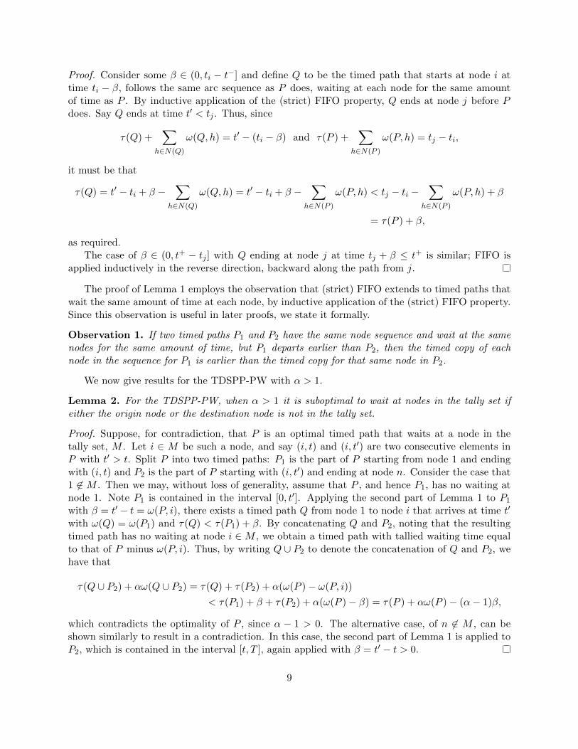
Lemma 2. For the TDSPP-PW, when α > 1 it is suboptimal to wait at nodes in the tally set ifeither the origin node or the destination node is not in the tally set.

Proof. Suppose, for contradiction, that P is an optimal timed path that waits at a node in thetally set, M . Let i ∈ M be such a node, and say (i, t) and (i, t′) are two consecutive elements inP with t′ > t. Split P into two timed paths: P1 is the part of P starting from node 1 and endingwith (i, t) and P2 is the part of P starting with (i, t′) and ending at node n. Consider the case that1 6∈ M . Then we may, without loss of generality, assume that P , and hence P1, has no waiting atnode 1. Note P1 is contained in the interval [0, t′]. Applying the second part of Lemma 1 to P1

with β = t′ − t = ω(P, i), there exists a timed path Q from node 1 to node i that arrives at time t′

with ω(Q) = ω(P1) and τ(Q) < τ(P1) + β. By concatenating Q and P2, noting that the resultingtimed path has no waiting at node i ∈M , we obtain a timed path with tallied waiting time equalto that of P minus ω(P, i). Thus, by writing Q ∪ P2 to denote the concatenation of Q and P2, wehave that

τ(Q ∪ P2) + αω(Q ∪ P2) = τ(Q) + τ(P2) + α(ω(P )− ω(P, i))

< τ(P1) + β + τ(P2) + α(ω(P )− β) = τ(P ) + αω(P )− (α− 1)β,

which contradicts the optimality of P , since α − 1 > 0. The alternative case, of n 6∈ M , can beshown similarly to result in a contradiction. In this case, the second part of Lemma 1 is applied toP2, which is contained in the interval [t, T ], again applied with β = t′ − t > 0.

9

Proposition 3. The case of TDSPP-PW where M = N \ {1, n} and α > 1 is equivalent to MDP.

Proof. By Lemma 2, any optimal solution to the TDSPP-PW in this case cannot wait at any nodein M . Therefore, this TDSPP-PW is equivalent to minimizing travel time subject to no waiting atany node except the origin or destination, which is exactly the MDP (under FIFO).

Proposition 4. The case of TDSPP-PW where M = N \ {n} or M = N \ {1}, and α > 1, isequivalent to MATP.

Proof. Suppose α > 1. By Lemma 2, any optimal solution to the TDSPP-PW cannot wait at anynode in M . Therefore, the TDSPP-PW with M = N \ {n} is equivalent to minimizing travel timesubject to no waiting at any node except the destination, which is exactly the MATP (under FIFO).The case of M = N \ {1} follows by equivalence to the M = N \ {n} case, from Corollary 1.

We have so far established that for specific choices of M and specific values of α and W , werecover MATP, MDP and MTTP. Hence, for these choices, the TDSPP-PW and TDSPP-LW aresolvable in polynomial time. Table 2 shows the cases for which the complexity status has beenestablished so far.

Table 2: Complexity results for variants of TDSPP-PW and TDSPP-LW obtained so far. Recall that the case ofthe TDSPP-PW with α = 0 is precisely the MTTP, irrespective of the choice of M .

TDSPP-PW TDSPP-LWTally Set 0 < α ≤ 1 α > 1 W = 0 W > 0

M = N Polytime (Prop. 2)N \M = {1, n} Polytime (Prop. 3) Polytime (MDP)N \M = {n} or {1} Polytime (Prop. 4) Polytime (MATP)

In what follows, we will provide results that allow us to complete the table, and to exhaustivelyresolve the complexity for all cases of the tally set M .

4 Cases that are NP-Hard

Some variants of TDSPP-PW and TDSPP-LW are generalizations of the exact path length (EPL)problem: given a directed graph D = (N,A) with integer costs on each arc, an integer B and twonodes i, j ∈ N , determine whether there is a path in D from node i to node j with cost exactly B.Without loss of generality, we assume i = 1 and j = n = |N |.

Theorem 1. (Nykanen and Ukkonen 2002) The EPL problem is weakly NP-hard even if the edgeweights of the graph G are non-negative integers.

Theorem 2. The variant of TDSPP-PW in which waiting is penalized at every node (M = N)and the waiting cost is greater than the travel cost (α > 1) is weakly NP-hard.

Proof. We provide a reduction from EPL. Given an instance of the EPL as described above, con-struct an instance of the TDSPP-PW on the same graph, with constant (time-independent) traveltimes on arcs equal to the cost of the arc in EPL and with time horizon [0, B]. We claim that theoptimal value of the TDSPP-PW is B if and only if the answer to EPL is ‘Yes’. To see this, firstconsider any feasible timed path, P , for the TDSPP-PW. The sum of the EPL costs on the arcs

10

used in P is precisely its travel time, τ(P ). Since waiting is tallied at every node, τ(P )+ω(P ) = B,and the objective value of P is τ(P ) + αω(P ). Thus for any choice of α > 1, the optimal value ofthe TDSPP-PW is at least B, and can only equal B if there exists a timed path with no waiting.Thus the optimal value of the TDSPP-PW is B if and only if there is a feasible timed path, P ,with ω(P ) = 0, which is equivalent to τ(P ) = B, and the claim is proved. It is clear that thisreduction is polynomial. EPL is NP-hard by Theorem 1, therefore this variant of TDSPP-PW isNP-hard.

Theorem 3. The variant of TDSPP-LW in which waiting is tallied at every node (M = N) isweakly NP-hard for W ≥ 0.

Proof. We provide a reduction from EPL to the problem of deciding whether or not the TDSPP-LWproblem is feasible. Given an instance of the EPL as described above, construct an instance of theTDSPP-LW on the same graph, with constant (time-independent) travel times on arcs equal to thecost of the arc in EPL and with time horizon [0, B]. Now for any W ∈ [0, 1), there exists a feasiblesolution to the resulting TDSPP-LW instance if and only if the answer to EPL is ‘Yes’. This isbecause any feasible solution, P , to the TDSPP-LW has τ(P ) +ω(P ) = B and 0 ≤ ω(P ) ≤W < 1.But B and τ(B) are integers, so ω(P ) is too: it must be that ω(P ) = 0 and hence τ(P ) = B. Thusthe TDSPP-LW instance has a feasible solution if and only if it has a timed path with travel timeexactly B. However, the sum of the EPL costs on the arcs used in a timed path for the TDSPP-LWis precisely its travel time and the claim follows. It is clear that this reduction is polynomial. EPLis NP-hard by Theorem 1, therefore this variant of TDSPP-LW is NP-hard.

Next, we consider the case of a general tally set M . Let {a1, a2, . . . , an} be a set of integers,I = {1, . . . , n},

∑j∈I aj = 2B, and bi :=

∑i−1j=1 3aj for i = 1, . . . , n (taking b1 := 0). Construct an

instance of TDSPP-LW as follows:

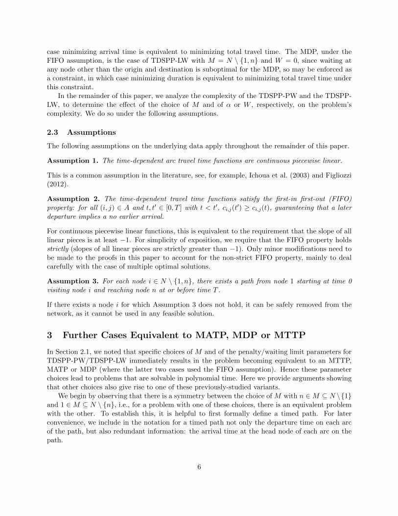
� nodes N = {1, 2, 3, . . . , 2n− 1, 2n, 2n+ 1}, with origin 1 and destination 2n+ 1;

� arcs A =⋃

i=1,2,...,n

{(2i− 1, 2i), (2i− 1, 2i+ 1), (2i, 2i+ 1)};

� tally set M = {2i | i = 1, 2, . . . , n};

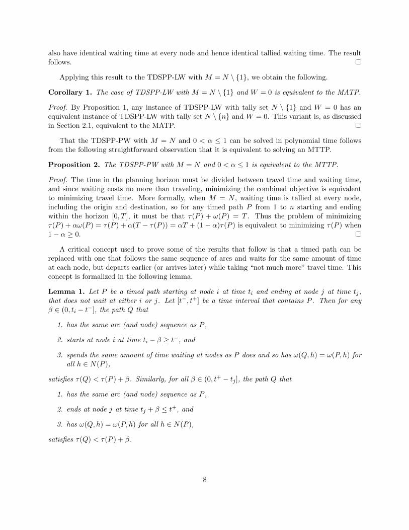
� arc travel time functions given by

� c2i−1,2i(t) = |bi − t|, for all i = 1, 2, . . . , n,

� c2i,2i+1(t) = |bi+1 − t|, for all i = 1, 2, . . . , n and

� c2i−1,2i+1(t) = |bi − t|+ ai, for all i = 1, 2, . . . , n, for all t ∈ R;

� time horizon [0, T ] with T = 4B; and

� tallied waiting time limit W = 3B.

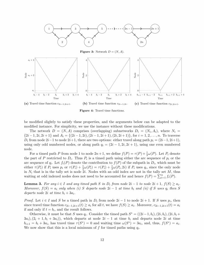
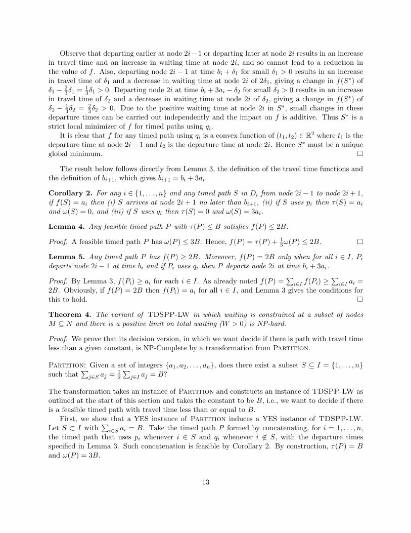
The network is shown in Figure 3 and the travel time functions are shown in Figure 4.For this instance, all travel time function gradients are in {−1, 1}, so the FIFO property is

satisfied, but not strictly, Furthermore, the travel time functions are nonnegative at all times,but do not satisfy the positive travel time assumption that we usually require. The instance can

11

1

2

3

4

5 2n− 1

2n

2n+ 1

Figure 3: Network D = (N,A).

bi − 4 bi − 2 bi bi + 2 bi + 4

ai

ai + 2

ai + 4

Time

Node

(a) Travel time function c2i−1,2i+1.

bi − 4 bi − 2 bi bi + 2 bi + 4

0

2

4

Time

Node

(b) Travel time function c2i−1,2i.

bi+1 − 4 bi+1 − 2 bi+1 bi+1 + 2 bi+1 + 4

0

2

4

Time

Node

(c) Travel time function c2i,2i+1.

Figure 4: Travel time functions.

be modified slightly to satisfy these properties, and the arguments below can be adapted to themodified instance. For simplicity, we use the instance without these modifications.

The network D = (N,A) comprises (overlapping) subnetworks Di = (Ni, Ai), where Ni ={2i− 1, 2i, 2i+ 1} and Ai = {(2i− 1, 2i), (2i− 1, 2i+ 1), (2i, 2i+ 1)}, for i = 1, 2, . . . , n. To traverseDi from node 2i−1 to node 2i+1, there are two options: either travel along path pi = (2i−1, 2i+1),using only odd numbered nodes, or along path qi = (2i − 1, 2i, 2i + 1), using one even numberednode.

For a timed path P from node 1 to node 2n+ 1, we define f(P ) = τ(P ) + 13ω(P ). Let Pi denote

the part of P restricted to Di. Thus Pi is a timed path using either the arc sequence of pi or thearc sequence of qi. Let fi(P ) denote the contribution to f(P ) of the subpath in Di, which must beeither τ(Pi) if Pi uses pi or τ(Pi) + 1

3ω(Pi) = τ(Pi) + 13ω(Pi, 2i) if Pi uses qi, since the only node

in Ni that is in the tally set is node 2i. Nodes with an odd index are not in the tally set M , thuswaiting at odd indexed nodes does not need to be accounted for and hence f(P ) =

∑ni=1 fi(P ).

Lemma 3. For any i ∈ I and any timed path S in Di from node 2i− 1 to node 2i+ 1, f(S) ≥ ai.Moreover, f(S) = ai only when (i) S departs node 2i − 1 at time bi and (ii) if S uses qi then Sdeparts node 2i at time bi + 3ai.

Proof. Let i ∈ I and S be a timed path in Di from node 2i − 1 to node 2i + 1. If S uses pi, thensince travel time function c2i−1,2i+1(t) ≥ ai for all t, we have f(S) ≥ ai. Moreover, c2i−1,2i+1(t) = aiif and only if t = bi, and the result follows.

Otherwise, it must be that S uses qi. Consider the timed path S∗ = ((2i−1, bi), (2i, bi), (2i, bi+3ai), (2i + 1, bi + 3ai)), which departs at node 2i − 1 at time bi and departs node 2i at timebi+1 = bi + 3ai, has travel time τ(S∗) = 0 and waiting time ω(S∗) = 3ai, and, thus, f(S∗) = ai.We now show that this is a local minimum of f for timed paths using qi.

12

Observe that departing earlier at node 2i−1 or departing later at node 2i results in an increasein travel time and an increase in waiting time at node 2i, and so cannot lead to a reduction inthe value of f . Also, departing node 2i − 1 at time bi + δ1 for small δ1 > 0 results in an increasein travel time of δ1 and a decrease in waiting time at node 2i of 2δ1, giving a change in f(S∗) ofδ1 − 2

3δ1 = 13δ1 > 0. Departing node 2i at time bi + 3ai − δ2 for small δ2 > 0 results in an increase

in travel time of δ2 and a decrease in waiting time at node 2i of δ2, giving a change in f(S∗) ofδ2 − 1

3δ2 = 23δ2 > 0. Due to the positive waiting time at node 2i in S∗, small changes in these

departure times can be carried out independently and the impact on f is additive. Thus S∗ is astrict local minimizer of f for timed paths using qi.

It is clear that f for any timed path using qi is a convex function of (t1, t2) ∈ R2 where t1 is thedeparture time at node 2i− 1 and t2 is the departure time at node 2i. Hence S∗ must be a uniqueglobal minimum.

The result below follows directly from Lemma 3, the definition of the travel time functions andthe definition of bi+1, which gives bi+1 = bi + 3ai.

Corollary 2. For any i ∈ {1, . . . , n} and any timed path S in Di from node 2i− 1 to node 2i+ 1,if f(S) = ai then (i) S arrives at node 2i + 1 no later than bi+1, (ii) if S uses pi then τ(S) = aiand ω(S) = 0, and (iii) if S uses qi then τ(S) = 0 and ω(S) = 3ai.

Lemma 4. Any feasible timed path P with τ(P ) ≤ B satisfies f(P ) ≤ 2B.

Proof. A feasible timed path P has ω(P ) ≤ 3B. Hence, f(P ) = τ(P ) + 13ω(P ) ≤ 2B.

Lemma 5. Any timed path P has f(P ) ≥ 2B. Moreover, f(P ) = 2B only when for all i ∈ I, Pideparts node 2i− 1 at time bi and if Pi uses qi then P departs node 2i at time bi + 3ai.

Proof. By Lemma 3, f(Pi) ≥ ai for each i ∈ I. As already noted f(P ) =∑

i∈I f(Pi) ≥∑

i∈I ai =2B. Obviously, if f(P ) = 2B then f(Pi) = ai for all i ∈ I, and Lemma 3 gives the conditions forthis to hold.

Theorem 4. The variant of TDSPP-LW in which waiting is constrained at a subset of nodesM ⊆ N and there is a positive limit on total waiting (W > 0) is NP-hard.

Proof. We prove that its decision version, in which we want decide if there is path with travel timeless than a given constant, is NP-Complete by a transformation from Partition.

Partition: Given a set of integers {a1, a2, . . . , an}, does there exist a subset S ⊆ I = {1, . . . , n}such that

∑j∈S aj = 1

2

∑j∈I aj = B?

The transformation takes an instance of Partition and constructs an instance of TDSPP-LW asoutlined at the start of this section and takes the constant to be B, i.e., we want to decide if thereis a feasible timed path with travel time less than or equal to B.

First, we show that a YES instance of Partition induces a YES instance of TDSPP-LW.Let S ⊂ I with

∑i∈S ai = B. Take the timed path P formed by concatenating, for i = 1, . . . , n,

the timed path that uses pi whenever i ∈ S and qi whenever i 6∈ S, with the departure timesspecified in Lemma 3. Such concatenation is feasible by Corollary 2. By construction, τ(P ) = Band ω(P ) = 3B.

13

Next, we show that a YES instance of TDSPP-LW with constant B induces a YES instance ofPartition. Lemmas 4 and 5 imply that a feasible timed path P with τ(P ) ≤ B has f(P ) = 2B.Now since the tallied waiting time limit W = 3B, it must be that ω(P ) ≤ 3B, so

f(P ) = τ(P ) + 13ω(P ) = 2B ⇒ τ(P ) + 1

3(3B) ≥ 2B ⇒ τ(P ) ≥ B.

Hence τ(P ) = B and ω(P ) = 3B. Furthermore, since equality holds, by Lemma 5 and Corollary 2,τ(P ) =

∑i∈I:Pi uses pi

τ(Pi). Thus selecting i to be in S whenever Pi uses pi is chosen (and notselecting i to be in S whenever qi is used), a feasible solution to the instance of PARTITION isobtained, since

B = τ(P ) =∑

i∈I:Pi uses pi

τ(Pi) =∑i∈S

ai,

by construction.

Because neither 1 nor n are in the tally set M in the transformation used to prove Theorem 4,we have the following theorem as an immediate consequence.

Theorem 5. The variant of TDSPP-LW in which waiting is constrained at a subset of nodesM ⊆ N with 1, n /∈M and a positive limit on total waiting (W > 0) is NP-hard.

5 Cases of TDSPP-PW Solvable in Polynomial Time via a Time-Expanded Network

We now discuss cases that can be reduced to solving a (standard) shortest path problem in a time-expanded network that has size polynomial in the size of the given instance. We first explain howthe time-expanded network is constructed.

5.1 The Time-Expanded Network

The time-expanded networks central to our polynomial time complexity results are constructed asa finite set of timed nodes, each a node-time pair of the form (i, t) with i ∈ N and t ∈ [0, T ], andtimed arcs, of the form ((i, t), (j, t′)) where (i, t) and (j, t′) are timed nodes and t′ ≥ t. We alsorefer to a timed node (i, t) as a timed copy of i. The timed node set is constructed by solving oneMATP and one reverse MATP (introduced in Section 2.2.1) for each breakpoint of an arc traveltime function, as follows. For arc a outgoing from node i and time t a breakpoint of its travel timefunction:

� (i, t) is included in the set of timed nodes,

� for each j ∈ N \ {i} reachable from (i, t) within the time horizon, (j, t′) is included in the setof timed nodes, where t′ is the earliest arrival time at j if departing i at time t (the value ofthe MATP with origin node i, destination node j and time horizon [t, T ]), and

� for each j ∈ N \ {i} with i reachable from (j, 0) no later than t, (j, t′) is included in the setof timed nodes, where t′ is the latest departure time from j to arrive at node i at time t (thevalue of the reverse MATP with origin node j, destination node i and time horizon [0, t]).

14

Algorithms for the MATP, described in Cooke and Halsey (1966), Orda and Rom (1990), Dean(2004b), for example, can easily be adapted to find the minimum arrival time path to all nodes inN \ {i} for the same computational effort as finding the minimum arrival time path to just onedestination. Such algorithms ensure that if the minimum arrival time path departing from nodei at time t arrives at node k at time t′′ along arc (j, k), having departed j at time t′, then t′ isthe minimum arrival time at j starting from (i, t). Thus such algorithms generate a timed versionof a forward shortest path tree, with at most one timed node per node in the network. As perProposition 1, reverse MATP is equivalent to MATP; solving reverse MATP generates a timedversion of a backward shortest path tree. Hence, the number of timed nodes in the time-expandednetwork is at most 2nK, where K is the total number of travel time function breakpoints.

The set of timed arcs is constructed by including ((i, t), (j, t′)) whenever arc (i, j) ∈ A is tra-versed starting at time t in any such forward or backward shortest path tree. In this case it mustbe that t′ = t + ci,j(t). We call such timed arcs travel arcs. We say that the travel time of timedarc ((i, t), (j, t′)) is ci,j(t) = t′ − t. In addition, the set of timed arcs also includes waiting arcs: if(i, t1), (i, t2), . . . , (i, tr) is the set of all timed copies of i, listed in increasing chronological order,then ((i, ts−1), (i, ts)), which is referred to as a waiting arc, is included in the set of timed arcs, foreach s = 2, . . . , r.

Clearly any path in the TEN corresponds to a timed path in the original network, which can beexpressed simply as the timed node sequence in the TEN path, omitting intermediate timed copiesof the same node whenever more than two appear consecutively.

In what follows, we will show that for all remaining cases of the TDSPP-PW, there exists anoptimal solution to any instance that corresponds to a path in its TEN. Furthermore, we will beable to construct lengths for the arcs in the TEN so that any shortest path, with respect to theselengths, from (1, 0) to (n, T ) in the TEN corresponds to an optimal solution to the TDSPP-PWinstance.

5.2 Preliminaries

Definition 2. A travel subpath of a given timed path is a maximal consecutive sequence of timednodes in the timed path with no consecutive timed copies of the same node.

Thus a timed path is the concatenation of a sequence of travel subpaths. Note that a node isa start or end of a travel subpath if and only if the node is 1 and the travel subpath starts with(1, 0), or n and the travel subpath ends with (n, T ), or if the node is in Nw(P ).

To illustrate, consider the example and the feasible timed path P = ((1, 0), (1, 2), (2, 2.14),(2, 2.92), (3, 4.05), (4, 5)). Here Nw(P ) = {1, 2} with ω(P, 1) = 2 and ω(P, 2) = 0.78, and P hasthree travel subpaths: ((1, 0)), ((1, 2), (2, 2.14)) and ((2, 2.92), (3, 4.05), (4, 5)).

If a timed path consists of three of more travel subpaths then we say that all but the first andlast travel subpaths are intermediate subpaths. A travel subpath is, itself, a timed path, and soproperties of timed paths and terms used to describe them may also be used for travel subpaths.

A key feature of a travel subpath is whether or not it contains a breakpoint. Note that weconsider time 0 to be a breakpoint at node 1 and time T to be a breakpoint at node n, regardlessof whether the travel time function for an arc leaving or entering these nodes, respectively, has abreakpoint at these respective times.

Definition 3. A travel subpath contains a breakpoint if it starts with (1, 0), or ends with (n, T ),or if there is an arc (i, j) ∈ A and a time t that is a breakpoint of ci,j(·) for which the timed node

15

(i, t) appears in the travel subpath.

Our argument that some solution to a TDSPP-PW instance must occur in its TEN involvesshifting travel subpaths that do not contain a breakpoint. We thus make use of the following idea.

Definition 4. A travel subpath P (∆) is a ∆-shifting of travel subpath P = ((i1, t1), . . . , (iK , tK))if P (∆) = ((i1, t

′1), . . . , (ik, t

′K)) where t′1 = t1 + ∆ and t′k = t′k−1 + cik−1,ik(t′k−1) for k = 2, . . . ,K.

Note that, from Observation 1, for P (∆) a ∆-shifting of P , if ∆ < 0 then t′k < tk for allk = 1, . . . ,K, while if ∆ > 0 then t′k > tk for all k = 1, . . . ,K.

As consequence of properties of compositions of piecewise affine functions, if a travel subpathdoes not contain a breakpoint, then its travel time is a locally affine function of the departure timeon its first node.

Observation 2. If travel subpath P does not contain a breakpoint, then there exist ε−, ε+ > 0such that τ(P (∆)) is an affine function of ∆ for all ∆ ∈ (−ε−, ε+). Furthermore, if ε−, ε+ are themaximal such values, then both P (−ε−) and P (ε+) contain a breakpoint.

In what follows, when we shift P back to a breakpoint, we mean that we replace P by P (−ε−)where ε− ≥ 0 is the largest value such that P (δ) does not contain a breakpoint for all δ ∈ (−ε−, 0).Similarly, we shift P forward to a breakpoint by replacing P with P (ε+) where ε+ ≥ 0 is the largestvalue such that P (δ) does not contain a breakpoint for all δ ∈ (0, ε+).

5.3 Complexity Results

In this section, we consider the TDSPP-PW with either waiting cost not more than travel cost(α ≤ 1) or at least one node at which waiting is not tallied (M ⊂ N). (Recall that the onlyremaining case of TDSPP-PW, namely that with α > 1 and M = N , is NP-hard, shown inTheorem 2.) Our approach is structured as follows.

We first show that there is an optimal solution to any TDSPP-PW instance with each of itstravel subpaths containing a breakpoint. We then show that if either α ≤ 1 or there is an optimalsolution with zero tallied waiting, then there must be an optimal solution in which each travelsubpath consists of two concatenated MATP solutions to/from a breakpoint. Thus each travelsubpath corresponds to a sequence of timed arcs of precisely the form of the travel arcs in the TENfor the instance.

It is then straightforward to prove that solving a TDSPP-PW instance with α ≤ 1 can be doneby solving a shortest path problem in its TEN. The case of α > 1 and M 6= N requires someadditional results, to establish that there is an optimal solution which has zero tallied waiting. Weconclude by showing that any instance of the TDSPP-PW with α > 1 and M ⊂ N can be solvedin polynomial time, by solving a shortest path in its associated TEN.

Our first result generalizes that of Foschini et al. (2014) for the MDP.

Proposition 5. For any instance of TDSPP-PW, there exists an optimal timed path such that eachof its travel subpaths includes at least one timed node at a breakpoint. Furthermore, if P is anyoptimal solution, there exists P ′, also an optimal solution, with a breakpoint in each of its travelsubpaths and with Nw(P ′) ⊆ Nw(P ).

Proof. Suppose that P is an optimal timed path having a travel subpath, S, that does not includea breakpoint. Recall that for P to be feasible, it must start with (1, 0) and end with (n, T ), which

16

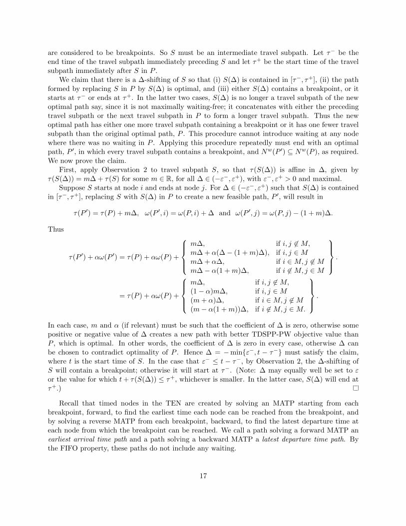
are considered to be breakpoints. So S must be an intermediate travel subpath. Let τ− be theend time of the travel subpath immediately preceding S and let τ+ be the start time of the travelsubpath immediately after S in P .

We claim that there is a ∆-shifting of S so that (i) S(∆) is contained in [τ−, τ+], (ii) the pathformed by replacing S in P by S(∆) is optimal, and (iii) either S(∆) contains a breakpoint, or itstarts at τ− or ends at τ+. In the latter two cases, S(∆) is no longer a travel subpath of the newoptimal path say, since it is not maximally waiting-free; it concatenates with either the precedingtravel subpath or the next travel subpath in P to form a longer travel subpath. Thus the newoptimal path has either one more travel subpath containing a breakpoint or it has one fewer travelsubpath than the original optimal path, P . This procedure cannot introduce waiting at any nodewhere there was no waiting in P . Applying this procedure repeatedly must end with an optimalpath, P ′, in which every travel subpath contains a breakpoint, and Nw(P ′) ⊆ Nw(P ), as required.We now prove the claim.

First, apply Observation 2 to travel subpath S, so that τ(S(∆)) is affine in ∆, given byτ(S(∆)) = m∆ + τ(S) for some m ∈ R, for all ∆ ∈ (−ε−, ε+), with ε−, ε+ > 0 and maximal.

Suppose S starts at node i and ends at node j. For ∆ ∈ (−ε−, ε+) such that S(∆) is containedin [τ−, τ+], replacing S with S(∆) in P to create a new feasible path, P ′, will result in

τ(P ′) = τ(P ) +m∆, ω(P ′, i) = ω(P, i) + ∆ and ω(P ′, j) = ω(P, j)− (1 +m)∆.

Thus

τ(P ′) + αω(P ′) = τ(P ) + αω(P ) +

m∆, if i, j 6∈M,m∆ + α(∆− (1 +m)∆), if i, j ∈Mm∆ + α∆, if i ∈M, j 6∈Mm∆− α(1 +m)∆, if i 6∈M, j ∈M

.

= τ(P ) + αω(P ) +

m∆, if i, j 6∈M,(1− α)m∆, if i, j ∈M(m+ α)∆, if i ∈M, j 6∈M(m− α(1 +m))∆, if i 6∈M, j ∈M.

.

In each case, m and α (if relevant) must be such that the coefficient of ∆ is zero, otherwise somepositive or negative value of ∆ creates a new path with better TDSPP-PW objective value thanP , which is optimal. In other words, the coefficient of ∆ is zero in every case, otherwise ∆ canbe chosen to contradict optimality of P . Hence ∆ = −min{ε−, t − τ−} must satisfy the claim,where t is the start time of S. In the case that ε− ≤ t − τ−, by Observation 2, the ∆-shifting ofS will contain a breakpoint; otherwise it will start at τ−. (Note: ∆ may equally well be set to εor the value for which t+ τ(S(∆)) ≤ τ+, whichever is smaller. In the latter case, S(∆) will end atτ+.)

Recall that timed nodes in the TEN are created by solving an MATP starting from eachbreakpoint, forward, to find the earliest time each node can be reached from the breakpoint, andby solving a reverse MATP from each breakpoint, backward, to find the latest departure time ateach node from which the breakpoint can be reached. We call a path solving a forward MATP anearliest arrival time path and a path solving a backward MATP a latest departure time path. Bythe FIFO property, these paths do not include any waiting.

17

Lemma 6. For any instance of the TDSPP-PW satisfying (i) α ≤ 1 or (ii) there is an optimalsolution, P , with ω(P ) = 0, there exists an optimal timed path, P ′, such that each of its travelsubpaths consists of a latest departure time path from a node to a breakpoint concatenated with anearliest arrival time path from the same breakpoint to another node. In case (ii), ω(P ′) = 0.

Proof. Consider an instance of the TDSPP-PW satisfying the required conditions. If α ≤ 1, applyProposition 5, to obtain an optimal timed path, P such that each of its travel subpaths containsa breakpoint. Otherwise, let P ∗ be an optimal solution with ω(P ∗) = 0, so travel subpaths startor end at nodes Nw(P ∗) ⊆ N(P ∗) \M . Apply Proposition 5, to obtain a new optimal solution, P ,with each of its travel subpaths containing a breakpoint and Nw(P ) ⊆ Nw(P ∗). So ω(P ) = 0.

Suppose that S is a travel subpath of P that is not the concatenation of a latest arrival pathand an earliest arrival path. Suppose S starts with (i, ti), includes breakpoint (k, tk) and endswith (j, tj). Let Sb be a latest departure path from i to (k, tk), and say it starts with (i, t′i). Byoptimality of Sb, it must be that t′i ≥ ti. Let Sf be an earliest arrival path from (k, tk) to j, andsay it ends with (j, t′j). It must be that t′j ≤ tj . Let P ′ denote the path formed by replacing S in

P by Sb concatenated with Sf , which do not include any waiting. Then

τ(P ′) = τ(P )− (t′i − ti)− (tj − t′j),ω(P ′, i) = ω(P, i) + (t′i − ti), and

ω(P ′, j) = ω(P, j) + (tj − t′j).

Now define αh = α if h ∈ M and αh = 0 otherwise, for h = i, j. By the conditions of the lemma,either α ≤ 1 or ω(P ) = 0, so since ω(P, i), ω(P, j) > 0, it must be that i, j 6∈ M , so αi = αj = 0.Thus, in every case, αi, αj ≤ 1. As a consequence,

τ(P ′) + αω(P ′) = τ(P )− (t′i − ti)− (tj − t′j) + αω(P ) + αi(t′i − ti) + αj(tj − t′j)

= τ(P ) + αω(P )− (1− αi)(t′i − ti)− (1− αj)(tj − t′j)≤ τ(P ) + αω(P )

since t′i ≥ ti and t′j ≤ tj . Since P is optimal for the TDSPP-PW instance, it must be that P ′ isoptimal, too. Furthermore, Nw(P ′) = Nw(P ), so if ω(P ) = 0 then ω(P ′) = 0 too. This procedurecan be repeated until an optimal solution satisfying the conditions of the lemma is generated.

Theorem 6. The variant of TDSPP-PW in which waiting costs less than traveling, i.e., 0 < α ≤ 1,is solvable in polynomial time.

Proof. By Lemma 6, there exists an optimal timed path P consisting of a sequence of travelsubpaths, each of which is the concatenation of a latest departure time path to a breakpoint andan earliest arrival time path from the same breakpoint. By construction, all timed nodes and timedarcs in these paths are included in the TEN. Furthermore, if a travel subpath of P ends with (i, t)and the travel subpath immediately after it in P starts with (i, t′), then by definition of the travelsubpaths, t′ > t. And by construction of the TEN, there must be a sequence of waiting arcs in theTEN forming a path from (i, t) to (i, t′).

Define the length of each travel arc in the TEN to be its travel time. Define the length ofeach waiting arc in the TEN, of the form ((i, t), (i, t′)) to be α(t′ − t) if i ∈M and zero otherwise.Then clearly any path from (1, 0) to (n, T ) in the TEN corresponds to a feasible timed path for the

18

TDSPP-PW and the length of the TEN path is precisely the corresponding timed path’s TDSPP-PW objective value. Thus solving a shortest path problem in the TEN with the given lengths mustyield an optimal solution to the TDSPP-PW. The TEN has O(2nK) nodes, for K the number ofbreakpoints, and hence the TDSPP-PW can be solved in polynomial time.

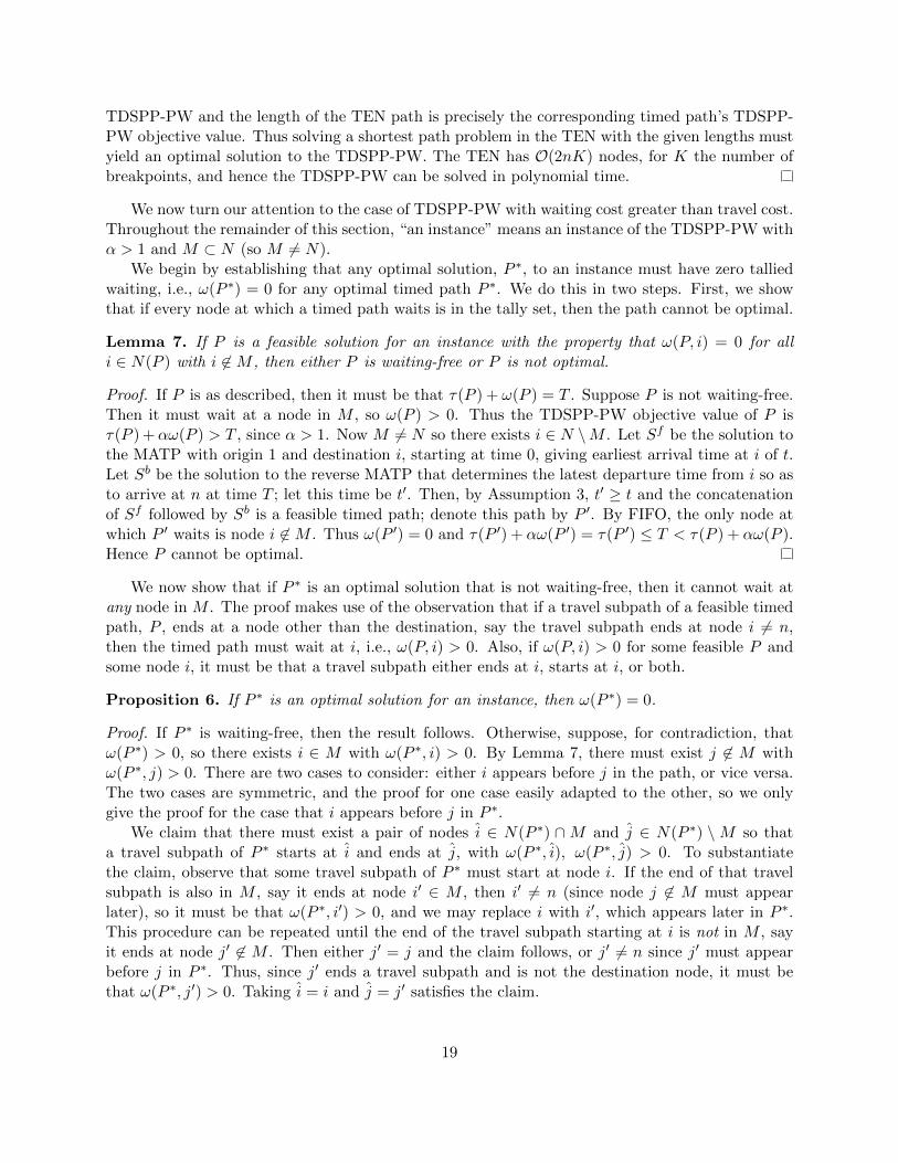
We now turn our attention to the case of TDSPP-PW with waiting cost greater than travel cost.Throughout the remainder of this section, “an instance” means an instance of the TDSPP-PW withα > 1 and M ⊂ N (so M 6= N).

We begin by establishing that any optimal solution, P ∗, to an instance must have zero talliedwaiting, i.e., ω(P ∗) = 0 for any optimal timed path P ∗. We do this in two steps. First, we showthat if every node at which a timed path waits is in the tally set, then the path cannot be optimal.

Lemma 7. If P is a feasible solution for an instance with the property that ω(P, i) = 0 for alli ∈ N(P ) with i 6∈M , then either P is waiting-free or P is not optimal.

Proof. If P is as described, then it must be that τ(P ) + ω(P ) = T . Suppose P is not waiting-free.Then it must wait at a node in M , so ω(P ) > 0. Thus the TDSPP-PW objective value of P isτ(P ) +αω(P ) > T , since α > 1. Now M 6= N so there exists i ∈ N \M . Let Sf be the solution tothe MATP with origin 1 and destination i, starting at time 0, giving earliest arrival time at i of t.Let Sb be the solution to the reverse MATP that determines the latest departure time from i so asto arrive at n at time T ; let this time be t′. Then, by Assumption 3, t′ ≥ t and the concatenationof Sf followed by Sb is a feasible timed path; denote this path by P ′. By FIFO, the only node atwhich P ′ waits is node i 6∈M . Thus ω(P ′) = 0 and τ(P ′) + αω(P ′) = τ(P ′) ≤ T < τ(P ) + αω(P ).Hence P cannot be optimal.

We now show that if P ∗ is an optimal solution that is not waiting-free, then it cannot wait atany node in M . The proof makes use of the observation that if a travel subpath of a feasible timedpath, P , ends at a node other than the destination, say the travel subpath ends at node i 6= n,then the timed path must wait at i, i.e., ω(P, i) > 0. Also, if ω(P, i) > 0 for some feasible P andsome node i, it must be that a travel subpath either ends at i, starts at i, or both.

Proposition 6. If P ∗ is an optimal solution for an instance, then ω(P ∗) = 0.

Proof. If P ∗ is waiting-free, then the result follows. Otherwise, suppose, for contradiction, thatω(P ∗) > 0, so there exists i ∈ M with ω(P ∗, i) > 0. By Lemma 7, there must exist j 6∈ M withω(P ∗, j) > 0. There are two cases to consider: either i appears before j in the path, or vice versa.The two cases are symmetric, and the proof for one case easily adapted to the other, so we onlygive the proof for the case that i appears before j in P ∗.

We claim that there must exist a pair of nodes i ∈ N(P ∗) ∩M and j ∈ N(P ∗) \M so thata travel subpath of P ∗ starts at i and ends at j, with ω(P ∗, i), ω(P ∗, j) > 0. To substantiatethe claim, observe that some travel subpath of P ∗ must start at node i. If the end of that travelsubpath is also in M , say it ends at node i′ ∈ M , then i′ 6= n (since node j 6∈ M must appearlater), so it must be that ω(P ∗, i′) > 0, and we may replace i with i′, which appears later in P ∗.This procedure can be repeated until the end of the travel subpath starting at i is not in M , sayit ends at node j′ 6∈ M . Then either j′ = j and the claim follows, or j′ 6= n since j′ must appearbefore j in P ∗. Thus, since j′ ends a travel subpath and is not the destination node, it must bethat ω(P ∗, j′) > 0. Taking i = i and j = j′ satisfies the claim.

19

Let i, j be as claimed. Let (i, s), (i, s′) with s′ > s denote the consecutive node-time pairs inP ∗ that appear before the consecutive node-time pairs (j, t), (j, t′) with t′ > t and let Q denote thetravel subpath of P ∗ that starts with (i, s′) and ends with (j, t). Let ∆ = s− s′ < 0 and considerQ(∆), the ∆-shifting of Q: it is a waiting-free timed path that starts with (i, s) and ends at j atsome time earlier than t. The path, P , formed by replacing Q in P ∗ by Q(∆) is feasible for theinstance. Furthermore, τ(Q(∆)) < t − s = τ(Q) + s′ − s and ω(P, i) = 0. Thus, since j 6∈ M , wehave that

τ(P ) + αω(P ) = (τ(P ∗)− τ(Q) + τ(Q(∆))) + α(ω(P ∗)− ω(P ∗, i) + ω(P, i))

< (τ(P ∗) + s′ − s) + α(ω(P ∗)− (s′ − s))= τ(P ∗) + αω(P ∗) + (1− α)(s′ − s)< τ(P ∗) + αω(P ∗)

since α > 1 and s′ < s. This contradicts the optimality of P ∗.

We are now able to show, as a consequence of the above result, that there is an optimal solutionfor an instance that has a corresponding path in its TEN. We do so by first establishing that everytravel subpath of an optimal solution must solve an MDP over the time interval containing boththe travel subpath and any waiting before or after it in the optimal solution.

Proposition 7. For any instance, there is a path in its TEN that corresponds to an optimal timedpath for the instance and that does not use any waiting arcs at nodes in M .

Proof. Let P be an optimal timed path for the instance with ω(P ) = 0, known to exist by Propo-sition 6. By Lemma 6, there exists another optimal timed path, P ′, such that every travel subpathconsists of a latest departure time path to a breakpoint concatenated with an earliest arrival pathfrom the same breakpoint. Thus every travel subpath is contained in the TEN for the instance,which also includes waiting arcs to link all timed copies of the same node. Since Lemma 6 alsoguarantees that ω(P ′) = 0, no waiting arc at a node in M is used. The result follows.

Theorem 7. The variant of TDSPP-PW in which waiting is penalized at nodes M ⊂ N and thewaiting cost is greater than the travel cost, i.e., α > 1, is solvable in polynomial time.

Proof. Consider an instance of this variant of TDSPP-PW, and its associated TEN. Remove allwaiting arcs at each node in M . Define the length of each travel arc in the TEN to be its traveltime. Define the length of each (remaining) waiting arc to be zero. Now the length of every pathfrom (1, 0) to (n, T ) in the TEN is its total travel time, which is also its TDSPP-PW objective,since no waiting at arcs in M is possible. Every path in the TEN corresponds to a feasible solutionof the TDSPP-PW, and, by Proposition 7, the optimal TDSPP-PW solution has a correspondingpath in the TEN. The result follows.

6 Cases of TDSPP-LW Solvable in Polynomial Time

6.1 Waiting not allowed (W = 0) at a subset of nodes M ⊂ N

When W = 0, i.e., waiting at nodes in M is not allowed, the TDSPP-LW resembles TDSPP-PWwith α > 1, where waiting at nodes in M is discouraged. Indeed, the proof that this variant is

20

solvable in polynomial time relies on showing that this variant of TDSPP-LW has a relaxationwhich is a variant of TDSPP-PW, and that solving this relaxation yields an optimal solution tothe TDSPP-LW.

Theorem 8. The variant of TDSPP-LW in which waiting is not allowed (W = 0) at a subset ofnodes M ⊂ N is solvable in polynomial time.

Proof. Any feasible path for an instance of TDSPP-LW with W = 0 is a feasible path for thecorresponding instance of TDSPP-PW with α > 1 (i.e., with the same tally set M) having thesame objective value. Hence, TDSPP-PW with α > 1 is a relaxation of TDSPP-LW with W = 0.By Theorem 7, solving the variant of TDSPP-PW with M ⊂ N with α > 1 can be done inpolynomial time and, by Proposition 7, yields an optimal TDSPP-PW solution P ∗ that does notuse any waiting arcs at nodes in M . In other words, for i ∈ M , we have that ω(P ∗, i) = 0, henceP ∗ is feasible for the TDSPP-LW with W = 0. Since P ∗ is an optimal solution to a relaxation ofTDSPP-LW and is also feasible, it is also an optimal solution of TDSPP-LW, and has been foundin polynomial time.

6.2 Waiting constrained at M ⊂ N with M = N \ {n} and a positive limit ontotal waiting time (W > 0)

The proofs in this section only use that n 6∈M , hence also apply to the case where M = N \{1, n}.For the case where M = N \ {1}, apply the transformation used in the proof of Proposition 1 toreturn an instance with M = N \ {n}.

Definition 5. A non-trivial travel subpath is a travel subpath that starts and ends at timed copiesof different nodes. In our context, the only possible trivial travel subpaths are (1, 0) and (n, T ).

Definition 6. A timed path P that begins at timed node (i, ti) and ends at timed node (j, tj) can becompleted by prepending a latest departure time path from 1 to i (arriving at node i at time ti) andappending an earliest arrival time path from j to n (departing from node j at time tj), and, if theresulting timed path is within the time horizon, adding timed node (1, 0) at the beginning and timednode (n, T ) at the end, to form a feasible timed path P ′ for the MTTP. If in addition, ω(P ′) ≤Wthen P ′ is feasible for the TDSPP-LW. If the resulting timed path has timed nodes outside the timehorizon, then the timed path P cannot be extended to a feasible solution for the TDSPP-LW and isremoved from consideration.

We begin by introducing three progressively more specific properties which an optimal timedpath P may have. We then show that if an optimal timed path exists, it is always possible to convertit to an optimal path with each of these properties. Importantly, we show that if an optimal pathwith the most specific property exists, it can be found in polynomial time.

Property 1. All travel subpaths of P except possibly the last non-trivial travel subpath contain abreakpoint. If ω(P ) < W , then the last non-trivial travel subpath also contains a breakpoint.

Property 2. Each travel subpath of P consists of a latest departure time path to a timed nodeconcatenated with an earliest arrival time path from the same timed node, where the timed node isa breakpoint if one exists in the travel subpath.

21

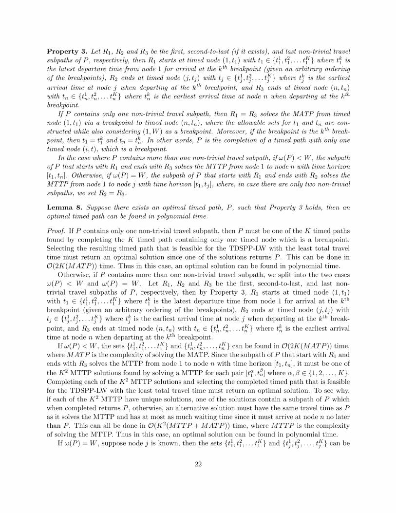
Property 3. Let R1, R2 and R3 be the first, second-to-last (if it exists), and last non-trivial travelsubpaths of P , respectively, then R1 starts at timed node (1, t1) with t1 ∈ {t11, t21, . . . tK1 } where tk1 isthe latest departure time from node 1 for arrival at the kth breakpoint (given an arbitrary orderingof the breakpoints), R2 ends at timed node (j, tj) with tj ∈ {t1j , t2j , . . . tKj } where tkj is the earliest

arrival time at node j when departing at the kth breakpoint, and R3 ends at timed node (n, tn)with tn ∈ {t1n, t2n, . . . tKn } where tkn is the earliest arrival time at node n when departing at the kth

breakpoint.If P contains only one non-trivial travel subpath, then R1 = R3 solves the MATP from timed

node (1, t1) via a breakpoint to timed node (n, tn), where the allowable sets for t1 and tn are con-structed while also considering (1,W ) as a breakpoint. Moreover, if the breakpoint is the kth break-point, then t1 = tk1 and tn = tkn. In other words, P is the completion of a timed path with only onetimed node (i, t), which is a breakpoint.

In the case where P contains more than one non-trivial travel subpath, if ω(P ) < W , the subpathof P that starts with R1 and ends with R3 solves the MTTP from node 1 to node n with time horizon[t1, tn]. Otherwise, if ω(P ) = W , the subpath of P that starts with R1 and ends with R2 solves theMTTP from node 1 to node j with time horizon [t1, tj ], where, in case there are only two non-trivialsubpaths, we set R2 = R3.

Lemma 8. Suppose there exists an optimal timed path, P , such that Property 3 holds, then anoptimal timed path can be found in polynomial time.

Proof. If P contains only one non-trivial travel subpath, then P must be one of the K timed pathsfound by completing the K timed path containing only one timed node which is a breakpoint.Selecting the resulting timed path that is feasible for the TDSPP-LW with the least total traveltime must return an optimal solution since one of the solutions returns P . This can be done inO(2K(MATP )) time. Thus in this case, an optimal solution can be found in polynomial time.

Otherwise, if P contains more than one non-trivial travel subpath, we split into the two casesω(P ) < W and ω(P ) = W . Let R1, R2 and R3 be the first, second-to-last, and last non-trivial travel subpaths of P , respectively, then by Property 3, R1 starts at timed node (1, t1)with t1 ∈ {t11, t21, . . . tK1 } where tk1 is the latest departure time from node 1 for arrival at the kth

breakpoint (given an arbitrary ordering of the breakpoints), R2 ends at timed node (j, tj) withtj ∈ {t1j , t2j , . . . tKj } where tkj is the earliest arrival time at node j when departing at the kth break-

point, and R3 ends at timed node (n, tn) with tn ∈ {t1n, t2n, . . . tKn } where tkn is the earliest arrivaltime at node n when departing at the kth breakpoint.

If ω(P ) < W , the sets {t11, t21, . . . tK1 } and {t1n, t2n, . . . , tKn } can be found in O(2K(MATP )) time,where MATP is the complexity of solving the MATP. Since the subpath of P that start with R1 andends with R3 solves the MTTP from node 1 to node n with time horizon [t1, tn], it must be one of

the K2 MTTP solutions found by solving a MTTP for each pair [tα1 , tβn] where α, β ∈ {1, 2, . . . ,K}.

Completing each of the K2 MTTP solutions and selecting the completed timed path that is feasiblefor the TDSPP-LW with the least total travel time must return an optimal solution. To see why,if each of the K2 MTTP have unique solutions, one of the solutions contain a subpath of P whichwhen completed returns P , otherwise, an alternative solution must have the same travel time as Pas it solves the MTTP and has at most as much waiting time since it must arrive at node n no laterthan P . This can all be done in O(K2(MTTP +MATP )) time, where MTTP is the complexityof solving the MTTP. Thus in this case, an optimal solution can be found in polynomial time.

If ω(P ) = W , suppose node j is known, then the sets {t11, t21, . . . tK1 } and {t1j , t2j , . . . , tKj } can be

22

found in O(2K(MATP )) time, where MATP is the complexity of solving the MATP. Since thesubpath of P that start with R1 and ends with R2 solves the MTTP from node 1 to node j withtime horizon [t1, tj ], it must be one of the K2 MTTP solutions found by solving a MTTP for each

pair [tα1 , tβj ] where α, β ∈ {1, 2, . . . ,K}. Append waiting of length W − ω(P ′) at node j to each of

the MTTP solutions found and complete the resulting timed paths. Selecting the completed timedpath that is feasible for the TDSPP-LW with the least total travel time must return an optimalsolution. To see why, if each of the K2 MTTP have unique solutions, one of the solutions containa subpath of P after appending waiting (since it is known that ω(P ) = W ) and completing returnsP , otherwise, an alternative solution must have the same travel time and tallied waiting time as thesubpath of P as it solves the MTTP the sum of tallied waiting and travel time must be tj , henceappending waiting also returns an optimal solution. This can be done in O(K2(MTTP+MATP )),where MTTP is the complexity of solving the MTTP. Since node j is not known beforehand, thisprocess needs to be repeated for each node j ∈ {2, 3, . . . , n− 1} which introduces another factor ofO(n) for a run-time of O(nK2(MTTP +MATP )). Thus in this case, an optimal solution can alsobe found in polynomial time.

It now remains to show that such a P satisfying Property 3 exists, we shall do so by first showingthat there exists P satisfying Properties 1 and 2.

Lemma 9. Any optimal timed path, P ∗, can be converted into an optimal timed path, P , for whichProperty 1 holds.

Proof. Let S1 be the last non-trivial travel subpath of P ∗, and suppose P ∗ contains at least onetravel subpath S2 6= S1 that does not contain a breakpoint. We claim that it is possible to apply∆-shifting such that (i) tallied waiting does not increase, (ii) travel time does not change and (iii)after ∆-shifting, the travel subpath S2(∆) contains a breakpoint or merges with another travelsubpath. It is clear that after such a ∆-shifting, the resulting timed path is still feasible by (i),optimal by (ii) and contains one less travel subpath without a breakpoint by (iii), thus, by applying∆-shifting repeatedly there exists an optimal timed path, P ′, such that all travel subpaths exceptpossibly the last travel subpath contain a breakpoint.

Let P ′ be an optimal timed path such that all travel subpaths except possibly the last travelsubpath contain a breakpoint. If ω(P ′) = W , then set P ← P ′ and we are done. Otherwise, ifω(P ′) < W , consider ∆-shifting the last non-trivial travel subpath of P ′, S3. The gradient of thefunction τ(S3(∆)) must be zero, otherwise there exists a ∆ such that ∆-shifting S3 reduces traveltime while remaining feasible, since both positive and negatives values of ∆ are allowed due towaiting on either side of S3 as it does not contain a (n, T ) which is a breakpoint. Now, perform∆-shifting on S3, selecting a value of ∆ such that the resulting travel subpath must either (1)contain a breakpoint, in which case we are done, or (2) merges with another travel subpath whichmust contain a breakpoint since all other travel subpaths contain a breakpoint, in which case weare done or (3) the resulting optimal timed path P satisfies ω(P ) = W , in which case we are alsodone. Hence, in any case, the desired optimal timed path, P , exists.

We now prove the earlier claim. By Observation 2, there exists a range for ∆ such that τ(Sk(∆))is an affine function of ∆ in that range. Let mk be the gradient of τ(Sk(∆)). Note that if m2 = 0,there exists a value of ∆ such that ∆-shifting travel subpath S2 by itself satisfies all of (i), (ii) and(iii), and thus the claim holds.

Assume now that m2 6= 0 and simultaneously shift S1 by ∆ and S2 by −m1m2

∆. Note that thevalue −m1

m2∆ has been carefully chosen such that (ii) holds. Selecting ∆ < 0 and simultaneously

23

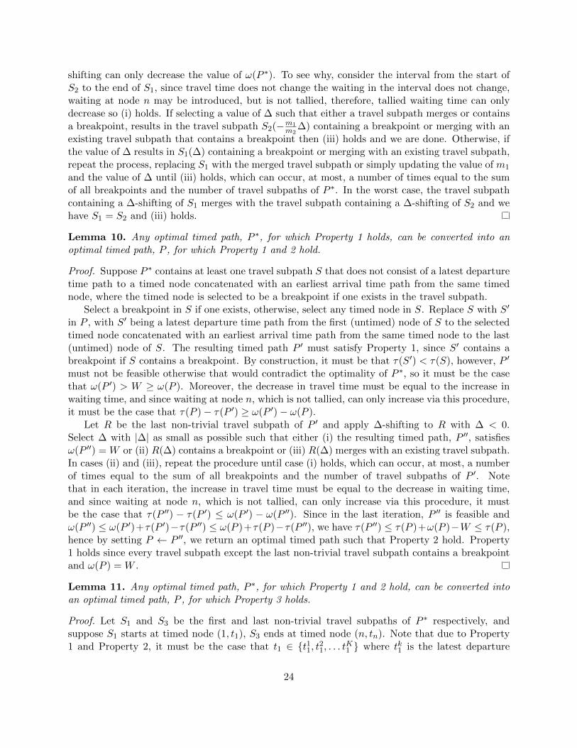
shifting can only decrease the value of ω(P ∗). To see why, consider the interval from the start ofS2 to the end of S1, since travel time does not change the waiting in the interval does not change,waiting at node n may be introduced, but is not tallied, therefore, tallied waiting time can onlydecrease so (i) holds. If selecting a value of ∆ such that either a travel subpath merges or containsa breakpoint, results in the travel subpath S2(−m1

m2∆) containing a breakpoint or merging with an

existing travel subpath that contains a breakpoint then (iii) holds and we are done. Otherwise, ifthe value of ∆ results in S1(∆) containing a breakpoint or merging with an existing travel subpath,repeat the process, replacing S1 with the merged travel subpath or simply updating the value of m1

and the value of ∆ until (iii) holds, which can occur, at most, a number of times equal to the sumof all breakpoints and the number of travel subpaths of P ∗. In the worst case, the travel subpathcontaining a ∆-shifting of S1 merges with the travel subpath containing a ∆-shifting of S2 and wehave S1 = S2 and (iii) holds.

Lemma 10. Any optimal timed path, P ∗, for which Property 1 holds, can be converted into anoptimal timed path, P , for which Property 1 and 2 hold.

Proof. Suppose P ∗ contains at least one travel subpath S that does not consist of a latest departuretime path to a timed node concatenated with an earliest arrival time path from the same timednode, where the timed node is selected to be a breakpoint if one exists in the travel subpath.

Select a breakpoint in S if one exists, otherwise, select any timed node in S. Replace S with S′

in P , with S′ being a latest departure time path from the first (untimed) node of S to the selectedtimed node concatenated with an earliest arrival time path from the same timed node to the last(untimed) node of S. The resulting timed path P ′ must satisfy Property 1, since S′ contains abreakpoint if S contains a breakpoint. By construction, it must be that τ(S′) < τ(S), however, P ′

must not be feasible otherwise that would contradict the optimality of P ∗, so it must be the casethat ω(P ′) > W ≥ ω(P ). Moreover, the decrease in travel time must be equal to the increase inwaiting time, and since waiting at node n, which is not tallied, can only increase via this procedure,it must be the case that τ(P )− τ(P ′) ≥ ω(P ′)− ω(P ).

Let R be the last non-trivial travel subpath of P ′ and apply ∆-shifting to R with ∆ < 0.Select ∆ with |∆| as small as possible such that either (i) the resulting timed path, P ′′, satisfiesω(P ′′) = W or (ii) R(∆) contains a breakpoint or (iii) R(∆) merges with an existing travel subpath.In cases (ii) and (iii), repeat the procedure until case (i) holds, which can occur, at most, a numberof times equal to the sum of all breakpoints and the number of travel subpaths of P ′. Notethat in each iteration, the increase in travel time must be equal to the decrease in waiting time,and since waiting at node n, which is not tallied, can only increase via this procedure, it mustbe the case that τ(P ′′) − τ(P ′) ≤ ω(P ′) − ω(P ′′). Since in the last iteration, P ′′ is feasible andω(P ′′) ≤ ω(P ′)+τ(P ′)−τ(P ′′) ≤ ω(P )+τ(P )−τ(P ′′), we have τ(P ′′) ≤ τ(P )+ω(P )−W ≤ τ(P ),hence by setting P ← P ′′, we return an optimal timed path such that Property 2 hold. Property1 holds since every travel subpath except the last non-trivial travel subpath contains a breakpointand ω(P ) = W .

Lemma 11. Any optimal timed path, P ∗, for which Property 1 and 2 hold, can be converted intoan optimal timed path, P , for which Property 3 holds.

Proof. Let S1 and S3 be the first and last non-trivial travel subpaths of P ∗ respectively, andsuppose S1 starts at timed node (1, t1), S3 ends at timed node (n, tn). Note that due to Property1 and Property 2, it must be the case that t1 ∈ {t11, t21, . . . tK1 } where tk1 is the latest departure

24

time from node 1 for arrival at the kth breakpoint (given an arbitrary ordering of the breakpoints)and tn ∈ {t1n, t2n, . . . tKn } where tkn is the earliest arrival time at node n when departing at the kth

breakpoint.Select an optimal solution to the MTTP from node 1 to node n with time horizon [t1, tn] such

that the solution satisfies Property 1 and Property 2. (The algorithm of He et al. (2019) for solvingMTTP produces such a solution.) It must be the case that for any travel subpath of the solutionthat ends at a node (j, tj), we have that tj ∈ {t1j , t2j , . . . tKj }, where tkj is the earliest arrival time

at node j when departing at the kth breakpoint. Complete the solution to the MTTP to obtain atimed path P ′, which must have τ(P ′) ≤ τ(P ), since the subpath of P starting with S1 and endingwith S3 is feasible for the MTTP.

Let R1 and R3 be the first and last non-trivial travel subpaths of P ′ respectively, and supposeR1 starts at timed node (1, t′1) and R3 ends at timed node (n, t′n).

If ω(P ′) < W then we are done since the subpath of P ′ that starts with R1 and ends with R3

solves the MTTP from node 1 to node n with time horizon [t′1, t′n] since it solves the MTTP from

node 1 to node n with larger time horizon [t1, tn] ⊇ [t′1, t′n]. If P ′ contains only one non-trivial travel

subpath R, then since R is a feasible timed path for the MATP from node 1 to node n starting att′1 is must also be optimal for that MATP.

Otherwise if ω(P ′) ≥ W , apply ∆-shifting to R3 with ∆ ≤ 0. Select ∆ with |∆| as small aspossible such that either (i) the resulting timed path, P ′′, satisfies ω(P ′′) = W or (ii) R3(∆) containsa breakpoint or (iii) R3(∆) merges with an existing travel subpath. In cases (ii) and (iii), repeatthe procedure until case (i) holds, which can occur, at most, a number of times equal to the sum ofall breakpoints and the number of travel subpaths of P ′. Note that in each iteration, the increase intravel time must be equal to the decrease in waiting time, and since waiting at node n which is nottallied can only increase via this procedure, it must be the case that τ(P ′′)−τ(P ′) ≤ ω(P ′)−ω(P ′′).Since in the last iteration, P ′′ is feasible and ω(P ′′) ≤ ω(P ′)+τ(P ′)−τ(P ′′) ≤ ω(P )+τ(P )−τ(P ′′)so τ(P ′′) ≤ τ(P ) + ω(P )−W ≤ τ(P ), hence by setting P ← P ′′, we return an optimal timed pathfor the TDSPP-LW. To see why Property 3 holds for P , note that any subpath of P ′ that starts ata timed node (i, ti) and ends at a timed node (j, tj) solves the MTTP from node i to node j withtime horizon [ti, tj ], otherwise replacing that subpath with the MTTP solution provides a timedpath with better objective value than P ′ which is a contradiction. Thus, if R2 is the second-to-lasttravel subpath of P and ends at timed node (j, tj), then the subpath of P (and also of P ′) thatstarts with R1 and ends with R2 solves an MTTP from node 1 to node j with time horizon [t1, tj ].If P ′ contains only one non-trivial travel subpath R that starts at timed node (1,W ) (since this isthe only node where tallied waiting can occur and ω(P ) = W ) and ends at timed node (n, t) thenR must solve an MTTP from node 1 to node n with time horizon [W, t] and since R is a feasibletimed path for the MATP from node 1 to node n starting at W it must also be optimal for thatMATP.

Theorem 9. The variant of TDSPP-LW in which waiting is constrained at intermediate nodesM = N \ {n} and the limit on total waiting is positive (W > 0) is solvable in polynomial time.

Proof. If an optimal timed path exists, consecutively applying Lemma 9, 10, and 11 guarantees theexistence of an optimal timed path, P , that satisfies Property 3. Lemma 8 specifies how an optimalsolution can be found in polynomial time given the existence of such a timed path, P .

We have recently been made aware of an alternative proof of Theorem 9, independently derived,provided in Omer and Poss (2019a).

25

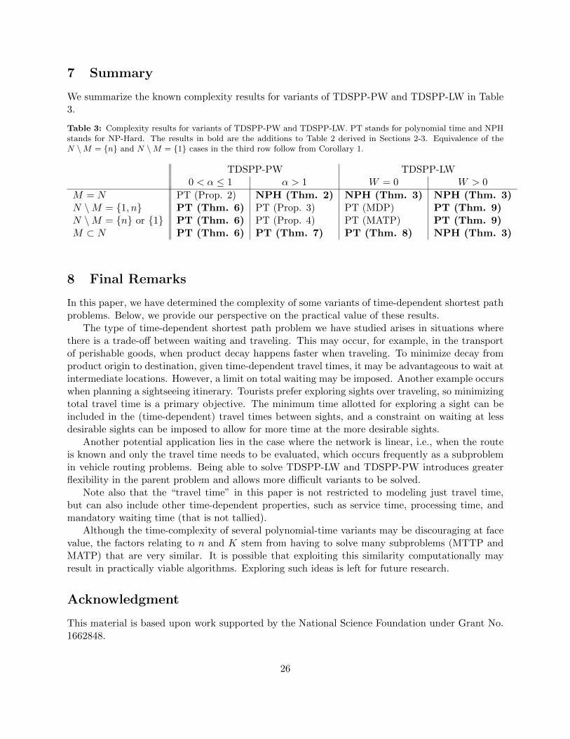
7 Summary

We summarize the known complexity results for variants of TDSPP-PW and TDSPP-LW in Table3.

Table 3: Complexity results for variants of TDSPP-PW and TDSPP-LW. PT stands for polynomial time and NPHstands for NP-Hard. The results in bold are the additions to Table 2 derived in Sections 2-3. Equivalence of theN \M = {n} and N \M = {1} cases in the third row follow from Corollary 1.

TDSPP-PW TDSPP-LW0 < α ≤ 1 α > 1 W = 0 W > 0

M = N PT (Prop. 2) NPH (Thm. 2) NPH (Thm. 3) NPH (Thm. 3)N \M = {1, n} PT (Thm. 6) PT (Prop. 3) PT (MDP) PT (Thm. 9)N \M = {n} or {1} PT (Thm. 6) PT (Prop. 4) PT (MATP) PT (Thm. 9)M ⊂ N PT (Thm. 6) PT (Thm. 7) PT (Thm. 8) NPH (Thm. 3)

8 Final Remarks

In this paper, we have determined the complexity of some variants of time-dependent shortest pathproblems. Below, we provide our perspective on the practical value of these results.

The type of time-dependent shortest path problem we have studied arises in situations wherethere is a trade-off between waiting and traveling. This may occur, for example, in the transportof perishable goods, when product decay happens faster when traveling. To minimize decay fromproduct origin to destination, given time-dependent travel times, it may be advantageous to wait atintermediate locations. However, a limit on total waiting may be imposed. Another example occurswhen planning a sightseeing itinerary. Tourists prefer exploring sights over traveling, so minimizingtotal travel time is a primary objective. The minimum time allotted for exploring a sight can beincluded in the (time-dependent) travel times between sights, and a constraint on waiting at lessdesirable sights can be imposed to allow for more time at the more desirable sights.

Another potential application lies in the case where the network is linear, i.e., when the routeis known and only the travel time needs to be evaluated, which occurs frequently as a subproblemin vehicle routing problems. Being able to solve TDSPP-LW and TDSPP-PW introduces greaterflexibility in the parent problem and allows more difficult variants to be solved.

Note also that the “travel time” in this paper is not restricted to modeling just travel time,but can also include other time-dependent properties, such as service time, processing time, andmandatory waiting time (that is not tallied).

Although the time-complexity of several polynomial-time variants may be discouraging at facevalue, the factors relating to n and K stem from having to solve many subproblems (MTTP andMATP) that are very similar. It is possible that exploiting this similarity computationally mayresult in practically viable algorithms. Exploring such ideas is left for future research.

Acknowledgment

This material is based upon work supported by the National Science Foundation under Grant No.1662848.

26

References

D. Bertsimas, A. Delarue, P. Jaillet, and S. Martin. Travel time estimation in the age of big data. OperationsResearch, 2019.

I. Chabini. Discrete dynamic shortest path problems in transportation applications: Complexity and algo-rithms with optimal run time. Transportation Research Record: Journal of the Transportation ResearchBoard, (1645):170–175, 1998.

B. Coifman. Estimating travel times and vehicle trajectories on freeways using dual loop detectors. Trans-portation Research Part A: Policy and Practice, 36(4):351–364, 2002.

K. L. Cooke and E. Halsey. The shortest route through a network with time-dependent internodal transittimes. Journal of mathematical analysis and applications, 14(3):493–498, 1966.

B. S. Cooper and R. V. Cowlagi. Path-planning with waiting in spatiotemporally-varying threat fields. PloSone, 13(8):e0202145, 2018.

B. C. Dean. Algorithms for minimum-cost paths in time-dependent networks with waiting policies. Networks:An International Journal, 44(1):41–46, 2004a.

B. C. Dean. Shortest paths in fifo time-dependent networks: Theory and algorithms. Rapport technique,Massachusetts Institute of Technology, 2004b.

B. Ding, J. X. Yu, and L. Qin. Finding time-dependent shortest paths over large graphs. In Proceedings ofthe 11th international conference on Extending database technology: Advances in database technology,pages 205–216. ACM, 2008.

M. A. Figliozzi. The time dependent vehicle routing problem with time windows: Benchmark problems,an efficient solution algorithm, and solution characteristics. Transportation Research Part E: Logisticsand Transportation Review, 48(3):616–636, 2012.

L. Foschini, J. Hershberger, and S. Suri. On the complexity of time-dependent shortest paths. Algorithmica,68(4):1075–1097, 2014.

A. Franceschetti, D. Honhon, G. Laporte, and T. Van Woensel. A shortest-path algorithm for the departuretime and speed optimization problem. Transportation Science, 52(4):756–768, 2018.

E. He, N. Boland, G. Nemhauser, and M. Savelsbergh. Computational complexity of time-dependent shortestpath problems. Optimization Online, pages Eprint ID 2019–02–7083, 2019.

S. Ichoua, M. Gendreau, and J.-Y. Potvin. Vehicle dispatching with time-dependent travel times. Europeanjournal of operational research, 144(2):379–396, 2003.

E. Kanoulas, Y. Du, T. Xia, and D. Zhang. Finding fastest paths on a road network with speed patterns. InData Engineering, 2006. ICDE’06. Proceedings of the 22nd International Conference on, pages 10–10.IEEE, 2006.

J. Letchner, J. Krumm, and E. Horvitz. Trip router with individualized preferences (trip): Incorporatingpersonalization into route planning. In Proceedings of the National Conference on Artificial Intelligence,volume 21, page 1795. Menlo Park, CA; Cambridge, MA; London; AAAI Press; MIT Press; 1999, 2006.

K. Nachtigall. Time depending shortest-path problems with applications to railway networks. EuropeanJournal of Operational Research, 83(1):154–166, 1995.

M. Nykanen and E. Ukkonen. The exact path length problem. Journal of Algorithms, 42(1):41–53, 2002.

J. Omer and M. Poss. A polynomial algorithm for minimizing travel time in time-dependent networks withwaits. working paper or preprint, 2019a. URL https://hal.archives-ouvertes.fr/hal-01836007.

J. Omer and M. Poss. Time-dependent shortest paths with discounted waits. Networks, 2019b.

A. Orda and R. Rom. Shortest-path and minimum-delay algorithms in networks with time-dependent edge-length. Journal of the ACM (JACM), 37(3):607–625, 1990.

Y. Wang and N. L. Nihan. Freeway traffic speed estimation with single-loop outputs. Transportation ResearchRecord, 1727(1):120–126, 2000.

27