Physica E 76 (2016) 12–27

Contents lists available at ScienceDirect

Physica E

http://d1386-94

n CorrE-m

journal homepage: www.elsevier.com/locate/physe

Time dependent electronic transport in chiral edge channels

G. Fève n, J.-M. Berroir, B. PlaçaisLaboratoire Pierre Aigrain, Ecole Normale Supérieure-PSL Research University, CNRS, Université Pierre et Marie Curie-Sorbonne Universités, Université ParisDiderot-Sorbonne Paris Cité, 24 rue Lhomond, 75231 Paris Cedex 05, France

H I G H L I G H T S

� We discuss Coulomb interaction effects on charge propagation along quantum Hall edge channels.

� Various experimental works are connected and analyzed in a unified theoretical framework.� Low frequency transport is described by a lumped element model.� High frequency transport is described by edge magnetoplasmon propagation.� Interchannel magnetoplasmon scattering leads to electron fractionalization and decoherence.

a r t i c l e i n f o

Article history:Received 1 July 2015Received in revised form1 October 2015Accepted 3 October 2015Available online 9 October 2015

Keywords:Quantum Hall effectTime dependent transportMesoscopic capacitorFractionalizationChiral Luttinger liquid

x.doi.org/10.1016/j.physe.2015.10.00677/& 2015 Elsevier B.V. All rights reserved.

esponding author.ail address: feve@lpa.ens.fr (G. Fève).

a b s t r a c t

We study time dependent electronic transport along the chiral edge channels of the quantum Hall re-gime, focusing on the role of Coulomb interaction. In the low frequency regime, the a.c. conductance canbe derived from a lumped element description of the circuit. At higher frequencies, the propagationequations of the Coulomb coupled edge channels need to be solved. As a consequence of the interchannelcoupling, a charge pulse emitted in a given channel fractionalized in several pulses. In particular, Cou-lomb interaction between channels leads to the fractionalization of a charge pulse emitted in a givenchannel in several pulses. We finally study how the Coulomb interaction, and in particular the fractio-nalization process, affects the propagation of a single electron in the circuit. All the above-mentionedtopics are illustrated by experimental realizations.

& 2015 Elsevier B.V. All rights reserved.

1. Introduction

The theoretical study of the dynamical properties of electronictransport in mesoscopic conductors has been pioneered by MarkusBüttiker and his collaborators in the 1990s [1–4]. Following thedescription of the dc conductance of multichannel mesoscopicconductors as the coherent scattering of electronic waves [5], theystudied the frequency dependent conductance G ω( ) arising whenthe conductor terminals are driven by a time dependent voltageexcitation. The latter case turns out to bring more complexity thanthe dc one, in particular as the role of Coulomb interaction iscrucial. In the dc case, the current is expressed as a function ofboth the probability to be transmitted from one contact to theother and the difference between the electrochemical potentials ofthe contacts. In most of the cases, the effects of Coulomb inter-action can be disregarded and remarkably, the conductance can beexpressed as a function of the scattering amplitudes of non-

interacting electronic waves. In the ac case, the time dependentcurrent resulting from the variation of the electrochemical po-tential of the contacts gives rise to a time dependent accumulationof charges in the conductor which in turn leads to the variation ofthe electrostatic potential mediated by the long range Coulombinteraction. It is clear that this contribution to the ac current whichdirectly stems from Coulomb interaction is crucial. Indeed, if onesimply applied scattering theory as in the dc case, no currentwould be predicted to flow between contacts capacitively coupled,as scattering theory only predicts non-zero conductance betweencontacts which are physically connected by some transmissionprobability. The method introduced by Büttiker and coworkers inRefs. [1–4] follows two steps. In the first one, the ac current iscalculated in a scattering formalism assuming a fixed value of theelectrochemical potential of the contacts and of the electrical po-tential in the conductor. In the second one, the electrical potentialis self-consistently calculated by relating the potential to thecharges accumulated in the conductor using the capacitance ma-trix. Following these two steps, two time scales naturally appear.The first one, related to the non-interacting scattering descriptionis the time of flight of non-interacting electron through the

V α

δ

V

Vβ

V

αIα,+I

α,-I

Fig. 1. Schematics of a generic Hall bar sample. Ohmic contacts and metallic gatesare driven by time dependent electrochemical potentials Vα .

G. Fève et al. / Physica E 76 (2016) 12–27 13

conductor of length l, l v/1τ = . The second one is related to theCoulomb interaction through the conductor capacitance C and thetypical impedance of a mesoscopic sample: hC e/2

2τ = . Combiningthese two time scales by v l e hC1/ / /2τ = + , one can define theimportant concept of electrochemical capacitance Cμ defined by

C C hv e l1/ 1/ / 2= +μ , where the second term is the quantum capa-citance of the conductor. The electrochemical capacitance is cen-tral to describe the effects of interactions in quantum conductorssuch as mesoscopic capacitors [1] but also the inductive like [4]behavior of quantum wires. Another major concept of time de-pendent transport is the charge relaxation resistance Rq [1] whichtogether with the electrochemical capacitance defines the time ittakes for charges to relax from the mesoscopic conductor to amacroscopic reservoir (contact). It differs from the dc resistancegiven by the Landauer formula. In particular, for a single modequantum coherent conductor, R h e/2q

2= [1,6,7], independently ofthe probability for charges to be transmitted from the conductor tothe reservoir. Remarkably, this universal behavior is robust tostrong electron–electron interactions [8–10]. Mesoscopic capaci-tors and charge relaxation resistance have applications beyond theobvious understanding of the dynamics of charge transfer in me-soscopic conductors such as dephasing induced by charge fluc-tuations [11–13] or the efficiency of mesoscopic detectors [14,15].

The present paper will address more specifically time depen-dent electronic transport along the chiral edge channels of thequantum Hall regime. The motivation is twofold. Firstly, chiraledge channels provide an ideal system to test quantum laws ofelectricity beyond the dc limit. The ballistic and one dimensionalnature of propagation, which can be implemented on long dis-tances, realizes a simple set of interacting single mode quantumwires. However, one specificity of quantum Hall systems distin-guishes them from usual wires: chiral propagation is enforced bythe strong magnetic field. This specificity makes chiral edgechannels particularly useful to study quantum coherence effects intime dependent situations. Indeed, the coherence of electronbeams can be probed in electronic interferometers [16]. Whentime-dependent drives are applied, quantum coherent electronicscan be pushed to the single electron scale where one studies theevolution of a single electron wavefunction in a quantum con-ductor. These electron quantum optics experiments [17] are thesecond motivation of this work. They have been pioneered byMarkus Büttiker as well in many ways: mesoscopic capacitors areused as single electron emitters [18–20] which statistical proper-ties can be accessed through the measurement of electronic noise[21–24] or the study of distribution of waiting times betweensuccessive electron emissions [25–27]. Next, the coherence prop-erties of single electron states [28,29] can be probed in the elec-tronic analog of the Hanbury–Brown and Twiss [30] or Hong–Ou–Mandel geometry [31] following a proposal by M. Büttiker and hiscollaborators [32] and paving the way for the coherent manip-ulations of a few charge quanta in quantum conductors based onmultiparticle interference effects [33–35]. Remarkably, these ex-periments [36] have been so far well accounted for by the timedependent Floquet scattering theory [37,38] of the mesoscopiccapacitor which builds on the generic scattering theory of timedependently driven mesoscopic conductors discussed above in theintroduction.

While the study of single electron coherence is a strong moti-vation of the work presented in this paper, quantum coherenceeffects on time dependent transport will not be directly addressed.However, the purpose of the manuscript is to discuss the role ofCoulomb interaction in charge propagation in quantum Hall sys-tems and to connect it to the issue of single electron coherence.This question naturally arises as, on one hand, understanding andmanipulating single electron coherence rely on a single-particlepicture where interactions are disregarded. On the other hand, as

mentioned above, Coulomb interaction plays a prominent role intime dependent charge propagation.

The paper will first review the lumped element description ofHall conductors at high frequency based on the calculation of thecircuit emittance introduced in Ref. [39]. In particular the role ofthe electrochemical capacitance in the ac properties of Hall con-ductors will be extensively discussed. At higher frequency thelumped element description of the circuit breaks down and pro-pagation effects need to be taken into account. The ac conductancethen stems from the propagation of edge magnetoplasmons. Therole of Coulomb interaction between edge channels will then bediscussed as the coupling leads to the emergence of new propa-gation eigenmodes responsible for the fractionalization of thecharge propagating in a given channel. Finally, fractionalizationwill be discussed at the single electron level, addressing thequestion of the death of the elementary quasiparticle caused bythe Coulomb interaction. All the above-mentioned topics will beillustrated with various experimental realizations (with an em-phasis put on our own). We would like to emphasize that the datapresented are extracted from already published works. The pur-pose of this manuscript is to connect together various experi-mental approaches and discuss them in a unified theoretical fra-mework inspired by the seminal works of Markus Büttiker and hiscollaborators.

2. Emittance of a Hall bar

We consider a generic quantum Hall circuit schematically re-presented in Fig. 1. Electronic transport occurs along the quantumHall edge channels [40–42] located at the edges of the sample, thenumber of flowing channels at each edge being fixed by thenumber of occupied spin polarized Landau levels (the filling factorN). The metal-like edge channels are separated by dielectric re-gions [43]. They are electrically connected to ohmic contacts actingas electronic reservoirs and imposing the electrochemical poten-tial Vα of the channels emerging from contact α. They are in ca-pacitive influence with each other and with nearby metallic gates.In a time dependent situation, the electrochemical potential V t( )βof the reservoirs or gates is subject to a periodic modulation:V t V e i t( ) =α α

ω− . We are interested in the time dependent currentresponse I t( )α flowing from contact α, defining the multiterminalac conductance:

I G V1

∑ ω= ( )( )

αβ

αβ β

For low enough drive frequency, G ω( )αβ can be expanded at firstorder in ω, providing the first correction to the well known dc-conductance, see Eq. (2), and defining the emittance Eαβ as done byChristen and Büttiker in Ref. [39].

G G i E 2dcω ω( ) = − ( )αβ αβ αβ

( )

V

C

C

C1

2I2

U1

U2g

g

h1

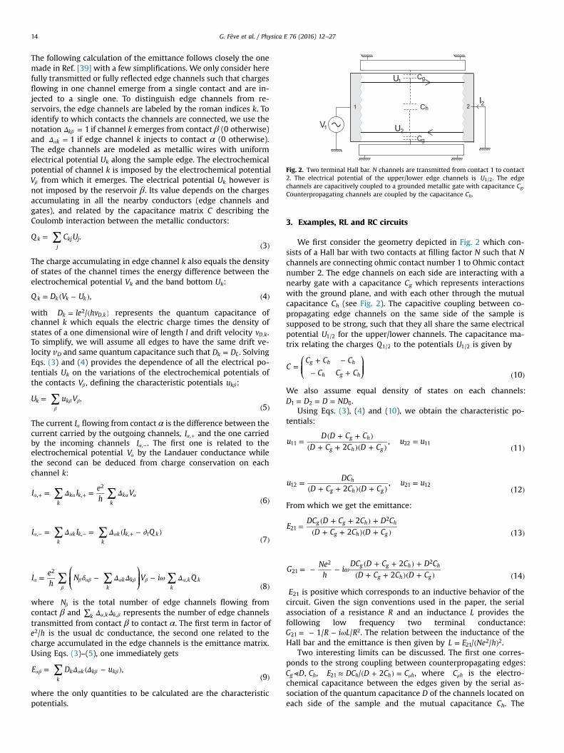
Fig. 2. Two terminal Hall bar. N channels are transmitted from contact 1 to contact2. The electrical potential of the upper/lower edge channels is U1/2. The edgechannels are capacitively coupled to a grounded metallic gate with capacitance Cg.Counterpropagating channels are coupled by the capacitance Ch.

G. Fève et al. / Physica E 76 (2016) 12–2714

The following calculation of the emittance follows closely the onemade in Ref. [39] with a few simplifications. We only consider herefully transmitted or fully reflected edge channels such that chargesflowing in one channel emerge from a single contact and are in-jected to a single one. To distinguish edge channels from re-servoirs, the edge channels are labeled by the roman indices k. Toidentify to which contacts the channels are connected, we use thenotation 1kΔ =β if channel k emerges from contact β (0 otherwise)and 1kΔ =α if edge channel k injects to contact α (0 otherwise).The edge channels are modeled as metallic wires with uniformelectrical potential Uk along the sample edge. The electrochemicalpotential of channel k is imposed by the electrochemical potentialVβ from which it emerges. The electrical potential Uk however isnot imposed by the reservoir β. Its value depends on the chargesaccumulating in all the nearby conductors (edge channels andgates), and related by the capacitance matrix C describing theCoulomb interaction between the metallic conductors:

Q C U .3

kj

kj j∑=( )

The charge accumulating in edge channel k also equals the densityof states of the channel times the energy difference between theelectrochemical potential Vk and the band bottom Uk:

Q D V U , 4k k k k= ( − ) ( )

with D le hv/k D k2

,= ( ) represents the quantum capacitance ofchannel k which equals the electric charge times the density ofstates of a one dimensional wire of length l and drift velocity vD k, .To simplify, we will assume all edges to have the same drift ve-locity vD and same quantum capacitance such that D Dk 0= . SolvingEqs. (3) and (4) provides the dependence of all the electrical po-tentials Uk on the variations of the electrochemical potentials ofthe contacts Vβ , defining the characteristic potentials ukβ:

U u V .5

k k∑=( )β

β β

The current Iα flowing from contact α is the difference between thecurrent carried by the outgoing channels, I ,α + and the one carriedby the incoming channels I ,α −. The first one is related to theelectrochemical potential Vα by the Landauer conductance whilethe second can be deduced from charge conservation on eachchannel k:

I Ieh

V6k

k kk

k, ,

2∑ ∑Δ Δ= =

( )α α α α+ +

I I I Q7k

k kk

k k t k, , ,∑ ∑Δ Δ= = ( − ∂ )( )

α α α− − +

⎛⎝⎜⎜

⎞⎠⎟⎟I

eh

N V i Q8k

k kk

k k

2

,∑ ∑ ∑δ Δ Δ ω Δ= − −( )

αβ

β αβ α β β α

where Nβ is the total number of edge channels flowing fromcontact β and k k k, ,Δ Δ∑ α β represents the number of edge channelstransmitted from contact β to contact α. The first term in factor ofe h/2 is the usual dc conductance, the second one related to thecharge accumulated in the edge channels is the emittance matrix.Using Eqs. (3)–(5), one immediately gets

E D u ,9k

k k k k∑ Δ Δ= ( − )( )

αβ α β β

where the only quantities to be calculated are the characteristicpotentials.

3. Examples, RL and RC circuits

We first consider the geometry depicted in Fig. 2 which con-sists of a Hall bar with two contacts at filling factor N such that Nchannels are connecting ohmic contact number 1 to Ohmic contactnumber 2. The edge channels on each side are interacting with anearby gate with a capacitance Cg which represents interactionswith the ground plane, and with each other through the mutualcapacitance Ch (see Fig. 2). The capacitive coupling between co-propagating edge channels on the same side of the sample issupposed to be strong, such that they all share the same electricalpotential U1/2 for the upper/lower channels. The capacitance ma-trix relating the charges Q1/2 to the potentials U1/2 is given by

⎛⎝⎜⎜

⎞⎠⎟⎟C

C C C

C C C 10

g h h

h g h=

+ −− + ( )

We also assume equal density of states on each channels:D D D ND1 2 0= = = .

Using Eqs. (3), (4) and (10), we obtain the characteristic po-tentials:

uD D C C

D C C D Cu u

2,

11g h

g h g11 22 11=

( + + )( + + )( + )

=( )

uDC

D C C D Cu u

2,

12h

g h g12 21 12=

( + + )( + )=

( )

From which we get the emittance:

EDC D C C D C

D C C D C2

2 13g g h h

g h g21

2=

( + + ) +( + + )( + ) ( )

GNe

hi

DC D C C D CD C C D C

22 14

g g h h

g h g21

2 2ω= − −

( + + ) +( + + )( + ) ( )

E21 is positive which corresponds to an inductive behavior of thecircuit. Given the sign conventions used in the paper, the serialassociation of a resistance R and an inductance L provides thefollowing low frequency two terminal conductance:G R i L R1/ /21

2ω= − − . The relation between the inductance of theHall bar and the emittance is then given by L E Ne h/ /21

2 2= ( ) .Two interesting limits can be discussed. The first one corres-

ponds to the strong coupling between counterpropagating edges:C D C,g h⪡ , E DC D C C/ 2h h h21 ≈ ( + ) = μ , where C hμ is the electro-chemical capacitance between the edges given by the serial as-sociation of the quantum capacitance D of the channels located oneach side of the sample and the mutual capacitance Ch. The

Cg

Cg

U2

U1

I221

V1

Fig. 3. Left panel: Schematics of the sample. A quantum point contact transmits T of the N edge channels from contact 1 to contact 2. The edge channels are capacitivelycoupled (with capacitance Cg to a grounded metallic gate. Counterpropagating edge channels are coupled by the capacitance Ch. Right panel: picture of the sample. Theelectron gas is colored in blue. The voltage Vg is applied on the gold top gate acting as a quantum point contact. Gray top gates are grounded and screen the Coulombinteraction. (For interpretation of the references to color in this figure caption, the reader is referred to the web version of this paper.)

G. Fève et al. / Physica E 76 (2016) 12–27 15

inductance is then given by L C Ne h/ /h2 2= ( )μ . If the coupling is very

strong ( C Dh⪢ ) corresponding to the limit of a non-chiral wire,E D/221 ≈ giving L h e D N/ /22 4

0= ( ) which corresponds to the usualkinetic inductance of a quantum wire [44,45].

The relevant experimental situation is the limit of weak cou-pling between counterpropagating edges, C Ch g⪡ in which case theemittance reduces to E DC D C C/g g g21 = ( + ) = μ , the electrochemicalcapacitance to the gate given by the serial association of thequantum capacitance D and the geometrical capacitance Cg. Theinductance is then given by L C Ne h/ /g

2 2= ( )μ .The differences between these two limits can be even more

emphasized if one can vary the number T of channels transmittedfrom contact 1 to contact 2 using a quantum point contact (seeFig. 3), thereby changing the dc conductance (and resistance) ofthe wire, G Te h/dc 2= , R h Te/ 2= . For a classical circuit, one expectsthe value of the inductance not to vary when the resistance ismodified, implying that E21 should vary like T2. To compute thecharges Q1/2 accumulated on the upper and lower side of the Hallbar, we assume again that interchannel interaction is so strongthat upper/lower channels have the same potential U1/2. The onlymodification compared to the previous case is the change in theelectrochemical potential of the lower channels as charges comeboth from contact 1 at V1 (reflected channels) and from contact2 at V2 (transmitted channels).

Q ND V U C U C U U 15g h1 0 1 1 1 1 2= ( − ) = + ( − ) ( )

Q D TV N T V U C U C U U 16g h2 0 2 1 2 2 2 1( )= + ( − ) − = + ( − ) ( )

uND ND C C

ND C C ND C

2

2 17

g hTN

g h g11

0 0

0 0

( )( ( )=

+ + −

( + + )( + ) ( )

E TD u1 1821 0 11= ( − ) ( )

ETD C

ND CT D C

ND C C ND C2 19g

g

h

g h g21

0

0

202

0 0=

++

( + + )( + ) ( )

E12 is the sum of two terms, the second one varying like T2 is theclassical term, predicting a classical RL circuit which inductance Ldoes not vary when the resistance R of the circuit is modified. Thefirst term predicts an emittance linear in the dc conductance,meaning a constant phase of the complex conductance. This be-havior cannot be understood as the serial addition of independent

resistance and inductance. Looking at the dependence of theclassical term, it emerges from the coupling between counter-propagating edges which tends to suppress the chiral nature of theHall bar. For C Ch g⪢ , we have E T N C/ h21

2 2= ( ) μ and we recoverL C Ne h/ /h

2 2= ( )μ , the value of the inductance is independent of thenumber of transmitted channels. On the contrary, when chirality ispreserved, C Cg h⪢ , E T N C/ g21 = ( ) μ and L N T C Ne h/ / /g

2 2= ( ) ( )μ . Thisexpected difference shows up spectacularly in the phase of the acconductance Im G Re G C Ne htan / / /g12 12

2ϕ ω= ( ) ( ) = ( )μ which be-comes independent of the number of transmitted channels andonly depends on the total number of channels (filling factor N).

The variation of the ac conductance of a Hall bar when thenumber of transmitted edge channels is modified has beenchecked experimentally in Ref. [46] on a 50 μm long and 6 μmwide Hall bar made in a GaAs/AlGaAs electron gas of nominaldensity ns 1.3 10 cm11 2= × − and mobility 3 10 cm V s6 2 1 1μ = × − − .The bar is interrupted in its middle by a pair of quantum pointcontacts (the right panel of Fig. 3). Only the first QPC is active witha negative voltage bias (V 1 Vg ≈ − ) fully depleting the electrongas beneath it resulting in a small gate to 2DEG capacitance. Thegrounded gate of the second QPC widely overlaps the electron gas.This results in a large gate-2DEG capacitance C fF30g ≈ (for a gatelength l 10 mg ≈ μ ) which efficiently screens the Coulomb inter-action. Two values of the magnetic field have been investigated,B 0.224 T= and B 0.385 T= corresponding to filling factors N¼24and N¼14 respectively. Fig. 4a represents the real and imaginaryparts of the ac conductance (a drive frequency of 1.5 GHz) atB 0.385 T= , as a function of the gate voltage Vg (which controls thenumber of transmitted edge channels). Both the real and imagin-ary parts exhibit steps each time one additional channel goesthrough the QPC as Vg is varied. The step height is e h2 /2 for the realpart of the conductance which equals twice the conductancequantum (spin degeneracy is not lifted). It is only coincidental thatthe steps in the imaginary part of the conductance are also close to

e h2 /2 . Fig. 4b shows a Nyquist representation (Im(G) as a functionof Re(G)) of the conductance. Remarkably, as a result of the chiralnature of the circuit, the phase stays constant when the number oftransmitted channels is varied as can easily be seen on the Nyquistrepresentation. As a comparison, the classical case of constantinductance ( L 0.7 H= μ ) is represented in black dashed line, itclearly does not reproduce the data.

The constant phase observed in the Nyquist representation canbe expressed as a transit time of charges through the Hall bar:tan ϕ ωτ= ρ defining a charge velocity renormalized by thescreened Coulomb interaction: v l/τ=ρ ρ where l is the propagationlength:

C Ne h l v Ne hC/ / / / 20g D g2 2τ = ( ) = ( + ˜ ) ( )ρ μ

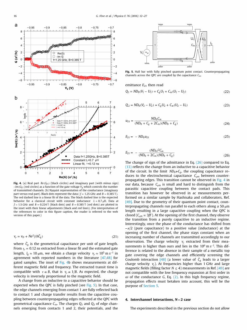
Fig. 4. (a) Real part Re G21( ) (black circles) and imaginary part (with minus sign)Im G21− ( (red circles) as a function of the gate voltage Vg which controls the number

of transmitted channels. (b) Nyquist representation of the conductance (imaginarypart versus real part). Black dots represent the data ( f 1.25 GHz= and B 0.385 T= ).The red dashed line is a linear fit of the data. The black dashed line is the expectedbehavior for a classical circuit with constant inductance L 0.7 H= μ . Data atf 1.5 GHz= and B 0.224 T= (black dots) and B 0.385 T= (red dots) are plotted inthe inset with their linear adjustments (black and red lines). (For interpretation ofthe references to color in this figure caption, the reader is referred to the webversion of this paper.)

Cg

Cg

U2U1I221

V1

Cm

Fig. 5. Hall bar with fully pinched quantum point contact. Counterpropagatingchannels across the QPC are coupled by the capacitance Cm.

G. Fève et al. / Physica E 76 (2016) 12–2716

v v Ne hC/ 21D g2= + ( ˜ ) ( )ρ

where Cg˜ is the geometrical capacitance per unit of gate length.

From 0.12 nsτ =ρ extracted from a linear fit and the estimated gatelength, l 10 mg ≈ μ , we obtain a charge velocity v 10 m s5 1≈ρ

− inagreement with reported numbers in the literature [47,48] forgated samples. The inset of Fig. 4b shows measurements at dif-ferent magnetic field and frequency. The extracted transit time iscompatible with Bτ ∝ , that is v B1/∝ρ . As expected, the chargevelocity is inversely proportional to the magnetic field.

A change from an inductive to a capacitive behavior should beexpected when the QPC is fully pinched (see Fig. 5). In that case,the edge channels emerging from contact 1 are fully reflected backto contact 1 and charge transfer results from the capacitive cou-pling between counterpropagating edges reflected at the QPC withgeometrical capacitance Cm. The charges Q1 and Q2 of edge chan-nels emerging from contacts 1 and 2, their potentials, and the

emittance E21 then read

Q ND V U C U C U U 22g m1 0 1 1 1 1 2= ( − ) = + ( − ) ( )

Q ND V U C U C U U 23g m2 0 2 2 2 2 1= ( − ) = + ( − ) ( )

uND C

ND C C ND C2 24m

g m g21

0

0 0=

( + + )( + ) ( )

E ND u 2521 0 21= − ( )

END C

ND C ND C2 26m

m g21

02

0 0= − ( )

( + )( + ) ( )

The change of sign of the admittance in Eq. (26) compared to Eq.(13) reflects the change from an inductive to a capacitive behaviorof the circuit. In the limit ND Cg0⪢ , the coupling capacitance re-duces to the electrochemical capacitance C mμ between counter-propagating edges. This transition cannot be observed in Fig. 4 inour data, because C mμ is small and hard to distinguish from theparasitic capacitive coupling between the contact pads. Thistransition has however be observed in ac measurements per-formed on a similar sample by Hashisaka and collaborators, Ref.[49]. Due to the geometry of their quantum point contact, coun-terpropagating channels run parallel to each others along a 50 mμlength resulting in a large capacitive coupling when the QPC isclosed (C fF3m ≈μ ). At the opening of the first channel, they observethe transition from a purely capacitive to an inductive regime.Interestingly, once the phase of the conductance has shifted from

/2π− (pure capacitance) to a positive value (inductance) at theopening of the first channel, the phase stays constant when anincreasing number of channels are transmitted accordingly to ourobservation. The charge velocity vρ extracted from their mea-surements is higher than ours and lies in the 10 m s6 1− . This dif-ference is related to the absence in their sample of a metallic topgate covering the edge channels and efficiently screening theCoulomb interaction [48] (a lower value of Cg

˜ leads to a largercharge velocity vρ). At frequencies higher than 1 GHz and largemagnetic fields (filling factor N 4≤ ) measurements in Ref. [49] arenot compatible with the low frequency expansion at first order inω of the conductance G, Eq. (2). In this high frequency regime,propagation effects must betaken into account, this will be thepurpose of Section 5.

4. Interchannel interactions, N¼2 case

The experiments described in the previous section do not allow

Cg

2

U1

41

2 3

V1

V

CU2

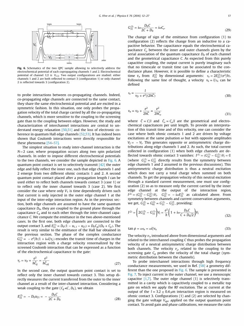
Fig. 6. Schematics of the two QPC sample allowing to selectively address theelectrochemical potential of each copropagating channels 1 and 2. Electrochemicalpotential of channel 1/2 is V1/2. Two output configurations are studied: eitherchannels 1 and 2 are both reflected to contact 3 (configuration 1) or only channel2 is reflected towards 3 (configuration 2).

G. Fève et al. / Physica E 76 (2016) 12–27 17

to probe interactions between co-propagating channels. Indeed,co-propagating edge channels are connected to the same contact,they share the same electrochemical potential and are excited in asymmetric fashion. In this situation, one only probes the propa-gation velocity of the total charge carried by all the co-propagatingchannels, which is more sensitive to the coupling to the screeninggate than to the coupling between edges. However, the study andcharacterization of interchannel interactions are central to un-derstand energy relaxation [50,51] and the loss of electronic co-herence in quantum Hall edge channels [52,53]. It has indeed beenshown that Coulomb interactions were directly responsible forthese phenomena [54–57].

The simplest situation to study inter-channel interaction is theN¼2 case, where propagation occurs along two spin polarizedchannels. In order to impose different electrochemical potentialsto the two channels, we consider the sample depicted in Fig. 6. Aquantum point contact is set to selectively transmit [42] the outeredge and fully reflect the inner one, such that edge channels 1 and2 emerge from two different ohmic contacts 1 and 2. A secondquantum point contact placed after a propagation length l can beused either to reflect both channels towards contact 3 (case 1) orto reflect only the inner channel towards 3 (case 2). We firstconsider the case where only V1 is time dependently driven suchthat current is only injected in the outer edge channel 1 at theinput of the inter-edge interaction region. As in the previous sec-tion, both edge channels are assumed to have the same quantumcapacitance D0, they are coupled to the ground plane through thecapacitance Cg and to each other through the inter-channel capa-citance C. We compute the emittance in the two above-mentionedcases. In the first one, both edge channels are connected to theoutput contact 3, and E D u u D C D C1 /g g31

10 1,1 21 0 0= ( − − ) = ( + )( ) . The

result is very similar to the emittance of the Hall bar obtained inthe previous section. The phase of the complex conductanceG e h i l v/ 1 /31

1 2 ω= − ( + )ρ( ) encodes the transit time of charges in the

interaction region with a charge velocity renormalized by thescreened Coulomb interaction that can be expressed as a functionof the electrochemical capacitance to the gate:

v ve

hCe

hC 27D

g g

2 2= + ˜ = ˜ ( )

ρμ

In the second case, the output quantum point contact is set toreflect only the inner channel towards contact 3. This setup di-rectly measures the current transferred from the outer to the innerchannel as a result of the inter-channel interaction. Considering aweak coupling to the gate (C C D,g 0⪡ ), we obtain

E D uD C

C D2 28312

0 210

0= − = −

+ ( )( )

G iD C

C Di C

2.

29312 0

0ω ω=

+=

( )μ( )

The change of sign of the emittance from configuration (1) toconfiguration (2) reflects the change from an inductive to a ca-pacitive behavior. The capacitance equals the electrochemical ca-pacitance Cμ between the inner and outer channels given by theserial association of the quantum capacitance D0 of each channeland the geometrical capacitance C. As expected from this purelycapacitive coupling, the output current is purely imaginary suchthat no timescale or transit time can be associated to the con-ductance phase. However, it is possible to define a characteristictime τn from E31

2( ) by dimensional arguments: E e h2 / /n 312 2τ = ( )( ) .

Following the same line of thought, a velocity v l/n nτ= can bedefined

lv e hC/ 2 30

nD

2τ =

+ ( ˜ ) ( )

v vehC

ehC2 2 31

n D

2 2= + ˜ = ˜ ( )μ

where C C l/˜ = and C C l/˜ =μ μ are the geometrical and electro-chemical capacitances per unit length. To provide an interpreta-tion of this transit time and of this velocity, one can consider thecase where both ohmic contacts 1 and 2 are driven by voltageexcitations at the same pulsation ω but with opposite amplitudesV V2 1= − . This generates opposite or antisymmetric charge dis-tributions along edge channels 1 and 2. As such, the total currentcollected in configuration (1) when both edge channels are de-flected towards ohmic contact 3 vanishes: I G G V 01

311

321

1= ( − ) =( ) ( ) ( )

(where G G311

321=( ) ( ) directly results from the symmetry between

edge channels 1 and 2 assumed in the previous discussions). Thisantisymmetric charge distribution is thus a neutral excitationwhich does not carry a total charge when summed on bothchannels. To get the propagation velocity of this neutral excitationthrough a standard current measurement, one must use config-uration (2) so as to measure only the current carried by the inneredge channel at the output of the interaction region,I G G V2

312

322

1= ( − )( ) ( ) ( ) . G i E312

312ω= −( ) ( ) as calculated above. From

symmetry between channels and current conservation arguments,we get, G G G G32

2412

311

312= = −( ) ( ) ( ) ( ), providing:

⎛⎝⎜

⎞⎠⎟

⎛⎝⎜

⎞⎠⎟I G G V

eh

iD C

C DV2 1

/2 322

312

311

1

20

01ω= − = +

+ ( )( ) ( ) ( )

l vtan / 33n nϕ ωτ ω= = ( )

The velocity vn introduced above from dimensional arguments andrelated to the interchannel coupling C thus probes the propagationvelocity of a neutral antisymmetric charge distribution betweenboth channels. The velocity vρ related to the coupling to thescreening gate Cg probes the velocity of the total charge (sym-metric distribution between the channels).

To probe interchannel interactions through high frequencyconductance measurements, we used in Ref. [58] a geometry dif-ferent than the one proposed in Fig. 6. The sample is presented inFig. 7. To inject current in the outer channel, we use a mesoscopiccapacitor [1,7]. The outer edge channel (1) is selectively trans-mitted in a cavity which is capacitively coupled to a metallic topgate on which we apply the RF excitation. The ac current at theoutput of the l 3.2 0.4 m= ± μ interaction region is measured onohmic contact 3. Configurations (1) and (2) are selected by chan-ging the gate voltage Vqpc applied on the output quantum pointcontact. To avoid gain and phase calibrations, we measure the ratio

Fig. 7. Modified scanning electronic microscope picture of the sample. The electron gas is in blue, metallic gates in gold, and edge channels 1 and 2 are represented by bluelines. Selective current injection on the outer edge channel (1) is performed by capacitively coupling edge channel 1 only to a metallic top gate on which time dependentvoltage V1 is applied. The current at the output of the l 3 m≈ μ interaction region is measured in configuration 1 (left panel) and in configuration 2 (right panel). (Forinterpretation of the references to color in this figure caption, the reader is referred to the web version of this paper.)

Fig. 8. Modulus (upper panel) and phase (lower panel) of the conductance G312( ) normalized G31

1( ) as a function of frequency. The data are represented by black dots, lowfrequency linear adjustments by black dashed lines. The red dashed lines represents the predictions of the propagation model Eq. (52) with parameters C 1.35=μ fF(v 4.6 10 m sn

5 1= × − ), imposed by the low frequency behavior, v 2.25 10 m sD4 1= × − , imposed by the high frequency behavior, and 4.1 psrτ = . (For interpretation of the

references to color in this figure caption, the reader is referred to the web version of this paper.)

G. Fève et al. / Physica E 76 (2016) 12–2718

of the conductance in the two configurations, G G/312

311ω ω= ( ) ( )( ) ( ) as

a function of the drive frequency from 1 GHz to 11 GHz. AssumingC Cg ⪡ , we have v vn⪢ρ and G e h/31

1 2ω( ) ≈( ) such that measures

G312 ω( )( ) in units of e h/2 . Measurements of the modulus and phase of

G312 ω( )( ) as a function of frequency are presented in Fig. 8. At low

frequency ( f 2.5 GHz≤ ), both the modulus and phase of the con-ductance evolve linearly with frequency (see the linear fits re-presented by the black dashed lines). The zero frequency interceptof the modulus is zero, while the phase goes to /2π . This lowfrequency dependence agrees with the capacitive coupling de-scribed by Eq. (29) with an electrochemical coupling capacitanceC f F f F1.35 0.15= ±μ , that is a neutral mode velocity ofv 4.6 0.5 10 m sn

5 1= ± × − . The linear dependence of the phase withfrequency provides the ω2 term in the power expansion of G31

2 ω( )( ) :

G i C i RC1 , 34312 ω ω ω( ) = ( + ) ( )μ μ

( )

corresponding to the serial addition of a capacitance and a re-sistance. From the slope of the linear dependence of the phasewith frequency, we deduce R k h e27 3.5 / 2Ω= ± ≈ . This is inagreement with Refs. [1] and [7] investigating the charge relaxa-tion resistance in an ac driven RC circuit. As discussed in the in-troduction, it equals h e/ 2 2( ) for a single spin polarized channel.Here charge transfer occurs from a single spin polarized channel toanother single spin polarized channel, charge relaxation resistancethus equals twice h e/2 2.

At frequencies higher than 3 GHz, the lumped element circuitdescription limited in second order in ω cannot account for thefrequency dependence of the ac conductance which exhibits anoscillating behavior. For such high frequencies, the wavelength of

L C

G. Fève et al. / Physica E 76 (2016) 12–27 19

the propagating modes becomes comparable with the circuit size(few microns) and the uniform potential assumption valid at lowfrequency does not hold anymore. One needs to take into accountpropagation effects along the edge channels.

C

L

R R

L

C

Fig. 9. (a) Transmission line description of propagation, C C g= μ , L h e C/ g2 4= ( ) μ .

(b) Dissipative transmission line with resistance R to the ground. (c) Dissipativetransmission line with resistance R in series with the capacitance C gμ .

5. Propagation and edge-magnetoplasmons

At high frequencies, one cannot neglect the space dependenceof the currents I x t,k ( ), charge densities x t,kρ ( ) and electrical po-tential U x t,k ( ) at position x of edge channel k. Current propagationis then described in terms of edge magnetoplasmon modes whichcirculate at the edges of the sample [59–61]. The charge density

x t,kρ ( ) is related to I x t,k ( ) through the usual current conservationequation: I 0x k t kρ∂ + ∂ = . The propagation equation for the current[62] is obtained by considering the sum of two contributions. Thefirst one comes from the excess charge ρk moving at the driftvelocity vD k, , the second one comes from the Hall current e h U/ k

2( )caused by the variation of the channel potential. Focusing on aharmonic variation of the current, potential and charge at pulsa-tion ω, we get

I x t x t veh

U x t, , , 35k k D k k,

2ρ( ) = ( ) + ( ) ( )

i v I xi e

hU x 36D k x k k,

2ω ω( − + ∂ ) ( ) = − ( ) ( )

The potential Uk(x) is related to the charge densities of all otheredge channels and conductors by the long range Coulomb inter-action:

U x dyU x y y,37

kj

kj j∫∑ ρ( ) = ( ) ( )( )

We start first with the simple limit of shirt range Coulomb inter-action: U x y U x y,kj kj δ( ) = ( − ). Note that this crude assumption willalways be valid at low enough frequency, when the wavelength ofthe propagation modes are larger than the interaction range. Inthis limit, the interaction parameters Ukj identify to the inverse

capacitance matrix elements per unit length: Cij1˜ − :

U x C x ,38

kj

ij j1∑ ρ( ) = ˜ ( )

( )

−

and the current propagation equation can be rewritten introdu-

cing the velocity matrix v with v v e h C/ij D i ij ij,2 1δ= + ( ) ˜ −

:

i v I x 0 39xω( − + ∂ ) ( ) = ( )

where is the identity matrix and I(x) is the vector of the currentspropagating along the edge channels.

Eq. (39) lends itself to a description in terms of voltage andcurrent propagation in a unidirectional transmission line [63]. Theelectrochemical potential of edge channel k, V x t,k ( ), is the sum ofthe electrical potential U x t,k ( ) and the chemical potential

x t D, /k 0ρ ( ) ˜ (where D0˜ is the quantum capacitance per unit length).

As such, V x t,k ( ) also depends on the position x along the edgechannel and is very simply related to the current I x t,k ( ):

V x t U x the

x t vhe

I x t, , , , 40k k k D k2 2ρ( ) = ( ) + ( ) = ( ) ( )

Eqs. (39) and (40) describe current propagation in terms of cou-pled unidirectional transmission lines of characteristic im-pedances R h e/K

2= . Let us discuss first the simple case N¼1 wherea single line is involved with charge velocity v e h C/ 1/ g

2= ( ) ˜ρ μ . Thencurrent propagation can be described as a distributed LC line (seFig. 9a) with a capacitance to the ground C g

˜μ and an inductanceL h e C/ g

2 4˜ = ( ) ˜μ per unit length. When several lines are coupled, the

solutions of Eq. (39) are found by diagonalizing the matrix v. La-beling Iλ an eigenmode of the velocity matrix and vλ the eigen-value, we obtain I x t I e, i x v t/( ) =λ λ

ω ( − )λ .In the specific case where two copropagating channels are

considered, the velocity matrix and its eigenvalues read

⎛

⎝

⎜⎜⎜⎜⎜

⎞

⎠

⎟⎟⎟⎟⎟v

veh

C C

C C Ceh

CC C C

eh

CC C C

veh

C C

C C C

2 2

2 2 41

Dg

g g g g

g gD

g

g g

2 2

2 2=

+˜ + ˜

˜ ( ˜ + ˜ )

˜˜ ( ˜ + ˜ )

˜˜ ( ˜ + ˜ )

+˜ + ˜

˜ ( ˜ + ˜ ) ( )

v veh C

ehC

I I I1

,42

Dg g

2 2

1 2= + ˜ = ˜ = +( )

ρμ

ρ

v veh C C

ehC

C C I I I1

2 2,

43n D

gg n

2 2

1 2= + ˜ + ˜ = ˜ ( ˜ ⪡ ˜ ) = −( )μ

Note that we restricted ourselves to the case of identical channels( C C Cg g g1 2

˜ = ˜ = ˜ , v v vD D D1 2= = ) which imposes the nature of theeigenmodes: the symmetric charge mode and the antisymmetricneutral mode already introduced in the previous sections. Differ-ent eigenmodes could be obtained considering that channels 1 and2 are different. However, if the interchannel interaction is strongerthan the asymmetry between channels : v v v /212 11 22⪢( − ) (stronginteraction regime), one recovers the charge and neutraleigenmodes.

The propagation model now allows us to calculate the currentsat all orders in the drive pulsation ω. Decomposing the edgecurrents I1 and I2 on the eigenmode basis, we can express I x l1( = )and I x l2 ( = ) as a function of their input values I x 01( = ) andI x 02 ( = ) using the 2�2 scattering matrix S l,ω( ) [64,55]:

I l S l I, , , 0 44ω ω ω( ) = ( ) ( ) ( )

⎛⎝⎜

⎞⎠⎟

⎛

⎝

⎜⎜⎜⎜

⎞

⎠

⎟⎟⎟⎟⎛⎝⎜

⎞⎠⎟

I l

I l

e e e e

e e e e

I

I2 2

2 2

00

45

i l v i l v i l v i l v

i l v i l v i l v i l v

1

2

/ / / /

/ / / /

1

2

n n

n n

( )( )

=

+ −

− +( )( )

( )

ω ω ω ω

ω ω ω ω

ρ ρ

ρ ρ

The conductance is then calculated first by relating I 01( ) and I 02 ( )to the electrochemical potentials of the contacts to which they areconnected: I e hV0 /1

21( ) = , I 0 02 ( ) = . Secondly by summing the

output currents measured in contact 3: I l I l1 2( ) + ( ) in configuration(1), I l2 ( ) only in configuration (2). We obtain the following acconductances in configurations (1) and (2) as a function of thescattering coefficients S l,ω( ):

k n (m

-1)

0

1e+06

2e+06

3e+06

f (MHz)0 2,000 4,000 6,000 8,000 10,000

data Re(kn)data Im(k n)model Re(kn ) and Im(k n)linear fit, v n=4.6 10 4m.s-1

Fig. 10. Real (black dots) and imaginary (red dots) parts of the wavevector kn as afunction of frequency. The black dashed line represents the constant velocity pre-diction (short range model). The red lines represent the full propagation modelincluding attenuation and long range interaction with parameters C 1.35=μ fF( v 4.6 10 m sn

4 1= × − ), imposed by the low frequency behavior,v 2.25 10 m sD

4 1= × − , imposed by the high frequency behavior, and 4.1 psrτ = . (Forinterpretation of the references to color in this figure caption, the reader is referredto the web version of this paper.)

G. Fève et al. / Physica E 76 (2016) 12–2720

Geh

S Seh

e 46i l v

311

2

11 21

2/ω( ) = ( + ) = ( )

ω( ) ρ

Geh

Seh

e e eh

e2

12 47

i l v i l v i l v

312

2

21

2 / / 2 /n nω( ) = = − ≈ −

( )ω ω ω

( ) ρ

Eq. (47) describes an oscillatory behavior as a function of eitherinteraction length l or pulsation ω. The current injected in theouter channel oscillates from the outer to the inner channel andback to the outer channel again. Such a behavior agrees qualita-tively with the one observed in Fig. 8, where the modulus of G31

2 ω( )increases up to E0.75 then decreases back down to E0.35 andrises up again to E0.7. Contrary to Eq. (47), G31

2 ω( ) does not go upto 1 then back down to zero, this attenuated oscillation signals thepresence of dissipation in the propagation. To capture the dis-sipation in the propagation process, we can rewrite the phasefactor l v/ nω as k ln where kn is the wavevector of the neutral mode.kn extracted from the measurements of G31

2 by inverting Eq. (47) isplotted in Fig. 10. As discussed above, dissipation is present andshows up as an imaginary part of kn which vanishes at low fre-quency. The real part of kn evolves linearly with frequency up tof 6 GHz≈ , which is consistent with a frequency independent ve-locity v 4.6 10 m sn

4 1= × − . At higher frequencies, Re kn( ) deviatesfrom a linear variation to reach again a linear evolution but with adifferent slope: v 2.25 10 m sn

4 1ω( → ∞) = × − . This ω dependenceof the velocity is not predicted by the short range interactionmodel presented above. It results from the finite range of inter-action. In the limit of high frequencies, when the wavelength ofthe propagating modes becomes smaller than the interactionrange, the role of interaction in the propagation velocity is sup-pressed and one recovers the non-interacting drift velocity vD. Wecan thus attribute the high limit of the velocity to the non-inter-acting value, v 2.25 10 m sD

4 1= × − . In order to add an interactionrange in the model, we assume that the interaction between xiρ ( )and yjρ ( ) does not depend on the distance x y− (for x y l0 ,≤ ≤ ).This crude assumption imposes an interaction range which equalsthe length of the interaction region l. U x y,k j, ( ) then becomes in-dependent of x and y, U x y U,k j kj, ( ) = where Ukj identify to the in-

verse capacitance matrix elements Ckj1− . Uk(x) becomes in-

dependent of x and Eq. (37) can be rewritten as

U U dy y C Q48

kj

kj jj

kj j1∫∑ ∑ρ= ( ) =

( )−

Dissipation can also be taken into account by adding a dissipativeterm in Eq. (36). Several possibilities can be considered which canbe illustrated by the unidirectional transmission line model. Let usconsider first the simple case of a single uncoupled line. Dissipa-tion can first be added by considering that some current leaks tothe ground for example through the bulk of the electron gas (seeFig. 9b). A second possibility is to consider that the line is capa-citively coupled to a dissipative conductor before reaching theground (see Fig. 9c). Computing the propagation equation and thedispersion relation k ω( ) in these two cases provide very differentresults:

⎛⎝⎜

⎞⎠⎟k LC

iRC, , 1

49g

rr g r

1ω ωτ

τ ωτ( ) = ˜ ˜ + = ˜ ⪢( )

μ μ( )

k LC iRC

1 ,2

, 1 50g r rg

r2ω ω ωτ τ ωτ( ) = ˜ ˜ ( + ) =

˜⪡ ( )μ

μ( )

k 1ω( )( ) describes an attenuation which does not depend on fre-quency such that dc current also leaks to the ground. The fre-quency independent damping does not properly account for ourobservation of Im kn( ) in Fig. 10. On the contrary, k 2ω( )( ) describes adamping increasing with frequency which fits more our observa-tion. We thus choose to add the r

2γ ω ω τ( ) = term in the propa-gation equation (36):

i v I xi e

hC Q

51r D x k

jkj j

22

1∑ω ω τ ω( − + + ∂ ) ( ) = −( )

−

Solving Eq. (51), we obtain the current I l2 ( ) as a function of theinput current I 01( ):

I le e

e eI

1

2 10

52

i

i

ii

2 1D r D

r CD r D

2

22

( ) = −+ ( − )

× ( )( )

ωτ ω τ τ

ω ω τ τωτ ω τ τ

−

( + )−

with l v/D Dτ = and R CC Kτ = . Eq. (52) obeys the same low frequencybehavior as the discrete element model, Eq. (29) and the propa-gation model with short range interaction, Eq. (47), with the sameexpression for the electrochemical capacitance Cμ. At second orderin ω, the charge relaxation resistance is slightly modified by dis-sipation effects and increases by C/2rτ μ compared to the dis-sipationless value h e/ 2 with e C h/2 1r

2τ ⪡μ if dissipation is small. Theeffect of the interaction range only appears at high frequencywhen the neutral mode wavelength becomes comparable with l.Predictions of Eq. (52) are plotted (red lines) in Figs. 8 and 10.Parameters are C fF1.35=μ (imposed by the low frequency beha-vior) and 4.1 psrτ = (adjustable parameter), v 2.25 10 m sD

4 1= × −

(imposed by the high frequency behavior of Fig. 10). The modelcaptures the period of the oscillations of the modulus as well asthe attenuation of the amplitude of these oscillations. In Fig. 10, itreproduces well the attenuation and captures the change in ve-locity as a function of the frequency although the change of ve-locity is much sharper in the experiment.

Another complementary simple geometry investigated in Refs.[63] and [65] to study Coulomb interaction effects between twoedge channels is the N¼1 case when two counterpropagatingchannels are brought close enough (see Fig. 11) such that theirmutual interaction cannot be neglected. A 1 mμ wide and 50 m≈ μlong gate, on which a negative voltage is applied so as to depletethe electron gas underneath, is used to define an interaction re-gion between the two single counterpropagating edge channelslocated on each side of the metallic gate. Compared to the co-propagating case, the opposite velocities of the two initially non-

Vg

C~

l=50μm

Fig. 11. Interaction between counterpropagating channels as implemented in Ref.[65]. At filling factor ν¼1, a single edge channel (represented in red) propagates atthe edges of the sample. A metallic gate (yellow on the sketch) is biased with anegative voltage Vg in order to deplete the electron gas underneath. Two coun-terpropagating edge channels separated by the gate width of approximately 1 μminteract through the Coulomb interaction on the gate length l 50 m≈ μ . Assumingshort range interaction, the interchannel interaction can be modeled by the capa-citance per unit length C̃ . (For interpretation of the references to color in this figurecaption, the reader is referred to the web version of this paper.)

I(t) (

a.u.

)

− 0.6

− 0.4

− 0.2

0

0.2

0.4

0.6

0.8

1

1.2

Time (a.u.)0 200 400 600 800 1,000

I1(x=0,t)I1(x=l,t)I2(x=l,t)

x=0

x=0

x=

Q Q/2 Q/2

Q/2

-Q/2

Q Q

-rQ

rQ

x=0l

x= l

x=l

x=l

x=0

I(t) (

a.u.

)

− 0.4

− 0.2

0

0.2

0.4

0.6

0.8

1

1.2

Time (a.u.)0 200 400 600 800 1,000

I1(x=0,t)I1(x=l,t)I2(x=l,t)

/vl n

/vl ρ

/vl +

/vl +

2

Fig. 12. (a) Upper panel: sketch of charge fractionalization in situation 1. The inputcharge pulse in channel 1 splits in a charge and neutral eigenmode. Lower panel:simulations of the input I x t0,1( = ) and output I x l t,1( = ), I x l t,2 ( = ) withv v2.5 n=ρ . (b) Upper panel: sketch of charge fractionalization in situation 2. Theinput charge pulse in channel 1 drags the charge rQ− in channel 2 in the inter-action region. Due to charge conservation, the pulse rQ is generated at t¼0 and x¼ lin channel 2. Lower panel: simulations of the input I x t0,1( = ) and outputI x l t,1( = ), I x l t,2 ( = ) with r¼0.3. The successive pulses result from successive re-flections at the edges of the interaction region and are separated by the delay l v2 /| |± .(For interpretation of the references to color in this figure caption, the reader isreferred to the web version of this paper.)

G. Fève et al. / Physica E 76 (2016) 12–27 21

interacting edge magnetoplasmons give rise to different eigen-modes when interchannel Coulomb interaction is turned on.Compared to Eq. (41), the sign of the velocities is changed for edgechannel 2 in the velocity matrix:

⎛

⎝

⎜⎜⎜⎜⎜

⎞

⎠

⎟⎟⎟⎟⎟v

veh

C C

C C Ceh

CC C C

eh

CC C C

veh

C C

C C C

2 2

2 2 53

Dg

g g g g

g gD

g

g g

2 2

2 2=

+˜ + ˜

˜ ( ˜ + ˜ )

˜˜ ( ˜ + ˜ )

−˜

˜ ( ˜ + ˜ )− −

˜ + ˜˜ ( ˜ + ˜ ) ( )

The eigenvalues and eigenmodes of v are given by

⎛⎝⎜⎜

⎞⎠⎟⎟

⎛⎝⎜⎜

⎞⎠⎟⎟v v

ehC

ve

h C C2 54D

gD

g/

2 2= ± + ˜ +

( ˜ + ˜ ) ( )+ −

v v v 55n/ = ± ( )ρ+ −

I I rI I I rI 561 2 2 1= − = − ( )+ −

⎜ ⎟⎜ ⎟⎛⎝

⎞⎠

⎛⎝

⎞⎠

rv v v

57

Deh

C C

C C C De

hC De

h C C

eh

CC C C

2 2

2

g

g g g g

g g

2 2 2

2=+ − + +

( )

˜ + ˜

( ˜ + ˜ ) ˜ ˜ ( ˜ + ˜ )

˜

( ˜ + ˜ ) ˜

The two eigenmodes have opposite velocities which is re-miniscent of the initial non-interacting case. Due to the couplingbetween the edge channels, the charge of the eigenmodes is dis-tributed on both channels. In the example of the eigenmode I+, thecurrent I1 propagating on channel 1 in the forward direction dragsthe charge rI1− on edge channel number 2 in the interaction re-gion. In the strong interchannel interaction limit, C D C, g0

˜ ⪢ ˜ , r 1→

and v e h C C/ 2 g2→ ± ˜ ˜μ μ± , the eigenmodes in the interaction region

correspond to antisymmetric charge distributions propagating inthe forward or backward direction. In the small interchannel in-teraction limit which corresponds to the relevant experimentalsituation of Ref. [65], C D C,g 0

˜ ⪢ ˜ , r C C/2 1g→ ˜ ˜ ⪡ and v e hC/ g2→ ± ˜μ± .

Only a small portion r− of the input charge carried in channel 1 isdragged on channel 2 in the interaction region.

6. Interchannel coupling and charge fractionalization

Charge fractionalization in the integer quantum Hall regime[65–69] occurs when a current pulse carrying charge Q is incom-ing at the input of the interchannel interaction region. There, as

Fig. 13. (a) Modified scanning electron microscope picture of the sample. The two sources generate the charge pulse synchronously. The quantum point contact is set topartition either the outer channel (1) or the inner channel (2). The low frequency partition noise is measured on output 4. (b) Noise measurements (normalized by therandom partition noise) qΔ as a function of the time delay τ between the sources. The upper/lower panel represents measurements of the outer (1)/inner (2) channels. Thesketches represent the shape of the current pulses colliding synchronously for the different values of delay τ. (c) Simulations of the excitation voltage and input currentI x t0,1( = ) (upper panel) and of the output currents I x l t,1( = ) and I x l t,2 ( = ).

G. Fève et al. / Physica E 76 (2016) 12–2722

G. Fève et al. / Physica E 76 (2016) 12–27 23

seen in the previous section, the propagation of currents obeyscoupled equations in which eigenmodes involve charge excitationson both channels. As a result, at the output of the interaction re-gion, charge excitations have been created in channel 2 and thecharge Q in channel 1 has fractionalized in several packets. Thetwo situations corresponding to interactions between copropa-gating channels (situation 1) or between counterpropagatingchannels (situation 2) are depicted in Fig. 12 on panels a and b.

In situation 1, the charge initially emitted in channel 1 decom-poses on the symmetric charge mode and antisymmetric neutralmode. As these two eigenmodes travel at different velocities, thepulse of charge Q fractionalizes in two pulses of charge Q /2 inchannel 1. A dipolar excitation consisting in two pulses of chargeQ /2 and Q /2− is left in channel 2. In situation 2, the propagatingeigenmode consists in the charge Q in channel 1 dragging charge

rQ− in channel 2, such that the total charge r Q1( − ) propagatesalong the coupled channels. Due to charge conservation in channel2, a charge rQ is reflected in channel 2 when the charge Q inchannel 1 enters the interaction region.

As can be seen in the sketches of Fig. 12, the observation ofcharge fractionalization calls for time resolved measurements ofthe currents flowing in each edge channel. Below the sketchesrepresenting each situation, a trace of the currents at the input,I x t0,1( = ) (black line), and output, I x l t,1( = ) (red dashed dottedline) and I x l t,2 ( = ) (blue dashed line), of the interaction region isplotted in Fig. 12. The current traces result from simulations usingthe input/ouptut relations for each situation. In situation 1, thetraces reproduce the above qualitative discussion: two pulses ofsame sign are observed on output 1 while two pulses of oppositesign are observed on output 2. In situation 2, a pulse rQ is observedin channel 2 simultaneously as the entrance of pulse Q in channel1 in the interaction region. A succession of pulses is observed atlater times in both channels, they result from successive reflec-tions of the pulses at the output of the interaction region (the timedelay between two pulses in one channel corresponds to l v2 /| |± ).The time unit in Fig. 12 is arbitrary but an estimate of the timeresolution needed to observe the splitting of charge in successivepulses can be obtained using a typical length l 10 m≈ μ and atypical velocity v 10 m s5 1≈ − giving a time resolution better than

100 psτ ≈ .Situation 2 has been experimentally investigated in Ref. [65] by

generating a current pulse of charge Q 150 e≈ and duration500 ps≈ and measuring the time dependent current resulting from

the fractionalization process. A time resolution of a few tens ofpicoseconds was obtained by varying on a short time the trans-mission of a quantum point contact placed at the output of theinteraction region. This allowed us to sample the current as afunction of the delay between the injection of the incoming chargepulse and the closing of the output QPC. The technique could ac-curately measure the reflected charge pulse on channel 2 at theinput of the interaction region providing r 0.04≈ and the velocityof the eigenmodes in the interaction region v 1.5 10 m s5 1≈ ×±

− .Both values are in agreement with calculations of the involvedcapacitances and the predictions of Eqs. (57) and (54).

In Ref. [69], we investigated charge fictionalization in situation1 by generating a current pulse in channel 1 using a mesoscopiccapacitor on which we applied a step voltage. The pulse carriescharge Q e≈ and its duration 40 psτ ≈ is limited by the risetime ofthe excitation pulse. The sample is identical to the one presentedin Fig. 7 but the excitation voltage differs: instead of a sine ex-citation of variable frequency, a periodic step voltage of frequencyf 0.9 GHz= (period T) is applied on the metallic top gate of thequantum dot. Note that the charge carried by the pulse is veryclose to the elementary electric charge, however in this experi-ment, the quantum dot is perfectly coupled to edge channelnumber 1 (outer edge) such that the emitted charge is not

quantized and does not correspond to single electron emission.Time domain information on the output current is obtained not bymeasuring directly the current but by performing the electronicanalog [31,32] of the Hong-Ou-Mandel [70] (HOM) experiment atthe output of the interaction region. It requires two sources placedat the input of a quantum point contact (see Fig. 13a). When in-distinguishable particles collide on the beam-splitter, two-particleinterference effects related to quantum exchange occur [71–73]and show up in the fluctuations of the number of particles countedat the output (noise). The output current noise thus measures thedegree of indistinguishability of the states incoming at the input ofthe splitter. As in the seminal HOM experiment, two-particle in-terference effects can be used to acquire short time information onthe shape of the current pulses at the input : it provided the lengthof a single photon wavepacket with a subpicosecond time re-solution in the original experiment, we use it to unveil the frac-tionalization in two charge pulses [74] with a resolution of tenpicoseconds in our case. In order to generate a charge pulse at eachinput of the QPC, the quantum dot placed in input 2 (source 2 inFig. 13a) is also time dependently driven by a step voltage in orderto generate a pulse identical to the one generated by source 1.

Interestingly, HOM interferometry can be performed on bothchannels 1 and 2 by setting the QPC to partition either channel1 or channel 2, so as to recover information on the current traceson these two channels. The resulting noise measurements as afunction of the time delay τ between the sources are presented inFig. 13b. The upper/lower traces represent the outer (1)/inner(2) channels partitioning measurements. On both traces a dip inthe noise can be seen at 0τ ≈ resulting from the antibunchingbetween undistinguishable pulses when the sources are perfectlysynchronized. Importantly the dip width observed on channel1 when the time delay is increased is twice larger than the oneobserved on channel 2 (80 ps compared to 40 ps). This increasedwidth results from the splitting of the charge pulse in channel 1 intwo separate pulses (see sketch in Fig. 13b, upper panel). As thetime separation l v/ 70 pss nτ ≈ ≈ is comparable with the pulsewidth 40 ps≈ , the separation is not complete but results in anincrease of the pulse width which matches the separation time. Onchannel 2 the dip at τ¼0 evolves to a small peak in the noise for

70 pssτ τ≈ = revealing the collision between charges of oppositesigns (electron vs holes) [75]. This shows the dipolar nature of thecurrent pulse in channel 2 as a result of the interchannel inter-action (see sketch in Fig. 13b, lower panel). On long time delay

T/2τ ≈ , the noise shows a peak on channel 1 which results, asstated before, from collisions between electrons and holes. Thisbehavior is expected as, the dot being ac coupled, emission of anelectron type pulse at time t 0≈ is followed by the emission of ahole one at time t T/2≈ . The noise trace is completely different onchannel 2. A peak is also observed for T/2τ = (for the same reasonas mentioned before) but a dip is observed for T/2 sτ τ≈ − which isnot present on channel 1. It signals an electron-electron typecollision which results from the fractionalization process: due tothe dipolar nature of the current on channel 2, collisions betweencharges of the same sign occur at T/2 sτ τ≈ − .

These results are nicely reproduced by the propagation modelpresented in the previous section, taking the input pulse re-presented in Fig. 13c (upper panel). The simulations of the currentsat the output of the interaction region are represented on thelower panel Fig. 13c resulting from the calculations of Eq. (45) with

70 pssτ = . As discussed before, the two pulses on channel 1 are notfully separated and the current trace on channel 2 has a dipolarform. The input current pulse shows a rebound at 150τ ≈ ps re-sulting from the rebound included on the excitation voltage pulse(black dashed line upper panel). This rebound has to obtain a goodquantitative agreement between the noise data and the simula-tions (red and black lines) in Fig. 13b. In particular, the additional

G. Fève et al. / Physica E 76 (2016) 12–2724

dip observed on the noise traces for channel 1 ( 400 psτ ≈ ± andchannel 2 ( 250 psτ ≈ ± ) are only reproduced when adding thisrebound.

7. Chiral Luttinger liquid description and single electronfractionalization

As seen in the previous sections, Coulomb interaction effectsplay a major role in the transport along chiral quantum Hall edgechannels. As seen in Sections 2, 3 and 4 at low frequency, they areencoded in the electrochemical capacitances in a lumped elementdescription of the circuit, which behavior can be either inductiveor capacitive depending on its geometry. At higher frequencies,propagation effects need to be taken into account and the lumpedelement description breaks down. Propagation is then described interms of a velocity matrix describing the coupling between theedge channels. As seen in Sections 5 and 6, Coulomb interactiondetermines the nature of the propagating eigenmodes and theirvelocity (related to the above-mentioned electrochemicalcapacitances).

At this point, the coherence of the electronic wavefunction andits effect on electronic propagation has not been discussed assingle electron interference effects were not considered. Theseinterferences between multiple paths can be introduced in ascattering matrix description of time dependent electronic trans-port developed by M. Büttiker and his collaborators in variousworks [2,4]. The purpose of this final section is not to introducethese interference effects but to discuss how electronic coherenceon which they rely is affected by Coulomb interaction. To addressthis question, we will consider the simple case of a single electronpropagating in the conductor. As we will see, it differs stronglyfrom the propagation of a classical pulse discussed in the previoussection. This single electron state with wavefunction xeϕ ( ) propa-gating above the Fermi energy of the edge channel k can bewritten in the following way:

dt x x F 58k e k k∫Ψ ϕ Ψ| ⟩ = ( ) ( )| ⟩ ( )†

where xkΨ ( )† creates an electron at position x of the edge channel k,on top of the fermi sea represented by the many-body state Fk| ⟩.

The sketch depicted in Fig. 12a representing charge fractiona-lization in the N¼2 case provides an insight on how Coulombinteraction affects single electron propagation. The single electronis emitted on channel 1, the blue pulse now representing thewavepacket xeϕ ( ). As the electron enters the interaction region, itfractionalizes in two distinct pulses, exactly as in the classical casestudied in the previous section. However, the consequences aremuch more drastic. Indeed, once the fractionalization process hastaken place, the pulses carrying charge e/2 cannot obviously bedescribed as single electron states, meaning that they involvenumerous electron/hole excitations of the Fermi sea which totalcharge matches half the electron charge. The fractionalizationprocess thus leads to the creation of collective excitations (elec-tron/hole pairs) in which the originally emitted electron dilutes. Inthe process, collective excitations are also created in channel2 which was originally empty. The energetic cost associated withthe creation of these collective excitations is associated with theenergy relaxation of the electron [51,55], it also leads to the de-coherence [69,74,76,77] of the single electron wavepacket.

To go beyond this simple picture, one needs to include Cou-lomb interaction effects in the single electron dynamics, which, ingeneral, is not a simple task. Here because of the specific one di-mensional nature of the problem, the full interaction problem canbe solved in terms of the propagation of bosonic modes [78] whichare nothing but the edge magnetoplasmon modes considered in

the two previous sections. In this bosonic description, a bosonic

field x t,kϕ̂ ( ) is introduced for each chiral edge channel. It is related

to the charge density x t,kρ̂ ( ) by x t e x t, / ,k x kρ π ϕ^ ( ) = − ( )∂ ^ ( ) and to

the electrical current by i x t e x t, / ,k t kπ ϕ^ ( ) = ( )∂ ^ ( ) (from the chargeconservation equation). The dynamics of the bosonic field is de-scribed with the chiral Luttinger liquid theory [79,80] which Ha-miltonian is the sum of the free motion plus the long range Cou-lomb interaction between the charge densities of the variouschannels [54]:

H v dx x te

dy dx x t

U x y y t

,2

,

, , 59

kD k x k

k jx k

kj x j

,2 2

,( )∫ ∫∑ ∑ϕ

πϕ

ϕ

= ∂ ^ ( ) + ∂ ^ ( )

( )∂ ^ ( ) ( )

From Eq. (59), we can deduce the equation of motion of the field

x t,kϕ̂ ( ) and of the current i x t,k^ ( ):

v x te

hU x t, , 60t D k x k k, ϕ π(∂ + ∂ ) ^ ( ) = ( ) ( )

U x t dyU x y x t, , ,61

kj

kj x j∫∑ ρ( ) = ( )∂ ^ ( )( )

v i x teh

U x t, , 62t D k x k t k,

2(∂ + ∂ )^ ( ) = ∂ ( ) ( )

Eq. (62) for the current operator is the exact analog of the classicalcalculation of the current made in Section 5, see Eq. (36).

As in Section 5, solutions are easier to express at a given pul-sation ω using the Fourier decomposition of the field and thecurrent:

x ti d

b e h c,4

. .63k k

i x v t/ D k,∫ϕπ

ωω

ω^ ( ) = − ^ ( ) −( )

ω ( − )

i x t ed

b e h c,2

. . 64k ki x v t/ D k,∫ ω

πω ω^ ( ) = − ^ ( ) + ( )

( − )

where bk ω^ ( ) annihilates a single boson (plasmon) at energy ω inedge channel k. Using the work developed in the previous sec-

tions, the solutions of the propagation equations for kϕ̂ and ik^ are

already known. Once the eignemodes of the velocity matrix havebeen found, one can compute the scattering matrix S l,ω( ) relatingthe field at pulsation ω at the output of the interaction region(x¼ l) to the field at the input (x¼0):

x l S l x, , , 0 65Φ ω ω Φ ω( = ) = ( ) ( = ) ( )

where Φ is the vector of the ω component of the field on all theedge channels. Finally, the connection to the original electronicproblem is made through the bosonization procedure relating thefermionic field to the bosonic one [78]:

xU

ae

2 66kk i x4 kΨπ

( ) =( )

π ϕ††

− ( )

where a is a short distance cutoff and Uk† a Klein factor which

ensures fermionic anticommutation relations. This provides astraightforward route to calculate the evolution of the singleelectron state when it goes through the interaction region. Firstlyone solves the dynamics of the coupled bosonic fields x t,kϕ ( ) byfinding the eigenmodes of propagation fromwhich the coefficientsof the scattering matrix are deduced. One then computes theelectron state at the output of the interaction region using Eqs.

ε ε ε

δn(ε) δn(ε) δn(ε)

0 0 0ω0 ω0

Z Z

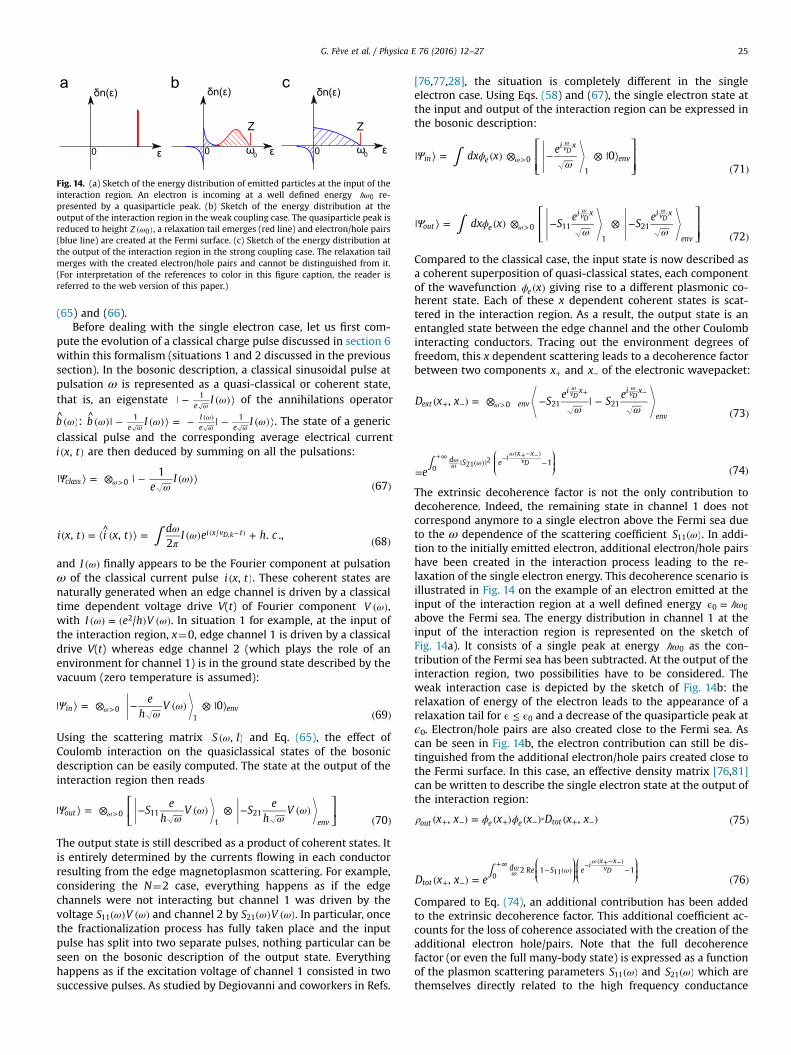
Fig. 14. (a) Sketch of the energy distribution of emitted particles at the input of theinteraction region. An electron is incoming at a well defined energy 0ω re-presented by a quasiparticle peak. (b) Sketch of the energy distribution at theoutput of the interaction region in the weak coupling case. The quasiparticle peak isreduced to height Z 0ω( ), a relaxation tail emerges (red line) and electron/hole pairs(blue line) are created at the Fermi surface. (c) Sketch of the energy distribution atthe output of the interaction region in the strong coupling case. The relaxation tailmerges with the created electron/hole pairs and cannot be distinguished from it.(For interpretation of the references to color in this figure caption, the reader isreferred to the web version of this paper.)

G. Fève et al. / Physica E 76 (2016) 12–27 25

(65) and (66).Before dealing with the single electron case, let us first com-

pute the evolution of a classical charge pulse discussed in section 6within this formalism (situations 1 and 2 discussed in the previoussection). In the bosonic description, a classical sinusoidal pulse atpulsation ω is represented as a quasi-classical or coherent state,that is, an eigenstate I

e1 ω| − ( )⟩ω

of the annihilations operator

b ω^ ( ): b I Ie

Ie e

1 1ω ω ω^ ( )| − ( )⟩ = − | − ( )⟩ω

ωω ω

( ) . The state of a genericclassical pulse and the corresponding average electrical currenti x t,( ) are then deduced by summing on all the pulsations:

eI

167class 0Ψ

ωω| ⟩ = ⊗ | − ( )⟩

( )ω>

i x t i x td

I e h c, ,2

. ., 68i x v t/ D k,∫ ω

πω( ) = ⟨^( )⟩ = ( ) + ( )

( − )

and I ω( ) finally appears to be the Fourier component at pulsationω of the classical current pulse i x t,( ). These coherent states arenaturally generated when an edge channel is driven by a classicaltime dependent voltage drive V(t) of Fourier component V ω( ),with I e h V/2ω ω( ) = ( ) ( ). In situation 1 for example, at the input ofthe interaction region, x¼0, edge channel 1 is driven by a classicaldrive V(t) whereas edge channel 2 (which plays the role of anenvironment for channel 1) is in the ground state described by thevacuum (zero temperature is assumed):

eh

V 069

in env01

Ψω

ω| ⟩ = ⊗ − ( ) ⊗ | ⟩( )ω>

Using the scattering matrix S l,ω( ) and Eq. (65), the effect ofCoulomb interaction on the quasiclassical states of the bosonicdescription can be easily computed. The state at the output of theinteraction region then reads

⎡⎣⎢

⎤⎦⎥S

eh

V Se

hV

70out

env0 11

121Ψ

ωω

ωω| ⟩ = ⊗ − ( ) ⊗ − ( )

( )ω>

The output state is still described as a product of coherent states. Itis entirely determined by the currents flowing in each conductorresulting from the edge magnetoplasmon scattering. For example,considering the N¼2 case, everything happens as if the edgechannels were not interacting but channel 1 was driven by thevoltage S V11 ω ω( ) ( ) and channel 2 by S V21 ω ω( ) ( ). In particular, oncethe fractionalization process has fully taken place and the inputpulse has split into two separate pulses, nothing particular can beseen on the bosonic description of the output state. Everythinghappens as if the excitation voltage of channel 1 consisted in twosuccessive pulses. As studied by Degiovanni and coworkers in Refs.

[76,77,28], the situation is completely different in the singleelectron case. Using Eqs. (58) and (67), the single electron state atthe input and output of the interaction region can be expressed inthe bosonic description:

⎡⎣⎢⎢

⎤⎦⎥⎥dx x

e0

71in e

i x

env0

1

vD∫Ψ ϕω

| ⟩ = ( ) ⊗ − ⊗ | ⟩( )

ω>

ω

⎡⎣⎢⎢

⎤⎦⎥⎥dx x S

eS

e

72out e

i x i x

env

0 11

1

21vD vD∫Ψ ϕω ω

| ⟩ = ( ) ⊗ − ⊗ −( )

ω>

ω ω

Compared to the classical case, the input state is now described asa coherent superposition of quasi-classical states, each componentof the wavefunction xeϕ ( ) giving rise to a different plasmonic co-herent state. Each of these x dependent coherent states is scat-tered in the interaction region. As a result, the output state is anentangled state between the edge channel and the other Coulombinteracting conductors. Tracing out the environment degrees offreedom, this x dependent scattering leads to a decoherence factorbetween two components x+ and x− of the electronic wavepacket:

D x x Se

Se

,73

ext env

i x i x

env

0 21 21vD vD

ω ω( ) = ⊗ − | −

( )ω+ − >

ω ω+ −

⎛⎝⎜⎜

⎞⎠⎟⎟

e 74d S e 1

ix x

vD0

212∫

= ( )ω

ω ω| ( ) | −ω+∞ − ( +− −)

The extrinsic decoherence factor is not the only contribution todecoherence. Indeed, the remaining state in channel 1 does notcorrespond anymore to a single electron above the Fermi sea dueto the ω dependence of the scattering coefficient S11 ω( ). In addi-tion to the initially emitted electron, additional electron/hole pairshave been created in the interaction process leading to the re-laxation of the single electron energy. This decoherence scenario isillustrated in Fig. 14 on the example of an electron emitted at theinput of the interaction region at a well defined energy 0 0ωϵ =above the Fermi sea. The energy distribution in channel 1 at theinput of the interaction region is represented on the sketch ofFig. 14a). It consists of a single peak at energy 0ω as the con-tribution of the Fermi sea has been subtracted. At the output of theinteraction region, two possibilities have to be considered. Theweak interaction case is depicted by the sketch of Fig. 14b: therelaxation of energy of the electron leads to the appearance of arelaxation tail for 0ϵ ≤ ϵ and a decrease of the quasiparticle peak atϵ0. Electron/hole pairs are also created close to the Fermi sea. Ascan be seen in Fig. 14b, the electron contribution can still be dis-tinguished from the additional electron/hole pairs created close tothe Fermi surface. In this case, an effective density matrix [76,81]can be written to describe the single electron state at the output ofthe interaction region:

x x x x D x x, , 75out e e totρ ϕ ϕ( ) = ( ) ( ) ( ) ( )+ − + −⁎

+ −

⎛⎝⎜⎜

⎞⎠⎟⎟

⎛⎝⎜⎜

⎞⎠⎟⎟

D x x e, 76tot

d Re S e2 1 1i

x xvD

011∫

( ) = ( )ω

ω ω

+ −

− ( ) −ω+∞ − ( +− −)

Compared to Eq. (74), an additional contribution has been addedto the extrinsic decoherence factor. This additional coefficient ac-counts for the loss of coherence associated with the creation of theadditional electron hole/pairs. Note that the full decoherencefactor (or even the full many-body state) is expressed as a functionof the plasmon scattering parameters S11 ω( ) and S21 ω( ) which arethemselves directly related to the high frequency conductance

R

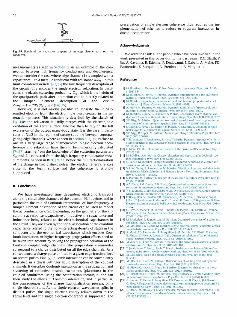
0 lCedge channel

Fig. 15. Sketch of the capacitive coupling of an edge channel to a resistiveconductor.

G. Fève et al. / Physica E 76 (2016) 12–2726

measurements as seen in Section 5. As an example of the con-nection between high frequency conductance and decoherence,we can consider the case where edge channel (1) is coupled with acapacitance C to a metallic conductor with resistance R RK⪡ . In thislimit considered in Refs. [82,76] the low frequency description ofthe circuit fully encodes the single electron relaxation. In parti-cular, the elastic scattering probability Z 0ω , which is the height ofthe quasiparticle peak after interaction can be directly related tothe lumped element description of the circuit:Z R R R C1 / K K0 0

2ω ω( ) = − ( )μ (Fig. 15).However, it is not always possible to separate the initially

emitted electron from the electron/hole pairs created in the in-teraction process. This situation is described by the sketch ofFig. 14c: the relaxation tail fully merges with the electron/holeexcitation of the Fermi surface. One has then to rely on the fullexpression of the output many-body state. It is the case in parti-cular at N¼2 in the regime of strong coupling between copropa-gating edge channels, where as seen in Section 5, S21 ω( ) is close toone in a very large range of frequencies. Single electron deco-herence and relaxation have then to be numerically calculated[74,77] starting from the knowledge of the scattering parametersS21 and S11 extracted from the high frequency conductance mea-surements. As seen in Refs. [74,77] before the full fractionalizationof the charge in two distinct pulses, the electron energy relaxesclose to the Fermi surface and the coherence is stronglysuppressed

8. Conclusion

We have investigated time dependent electronic transportalong the chiral edge channels of the quantum Hall regime, and inparticular, the role of Coulomb interaction. At low frequency, alumped element description of the circuit can be used to modelthe ac conductance G ω( ). Depending on the geometry of the cir-cuit, the ac response is capacitive or inductive, the capacitance andinductance being related to the electrochemical capacitances inthe circuit. They are given by the serial association of the quantumcapacitance related to the non-interacting density of states in theconductor and the geometrical capacitance which encodes Cou-lomb interaction. At higher frequency, propagation effects need tobe taken into account by solving the propagation equation of theCoulomb coupled edge channels. The propagation eigenmodescorrespond to a charge distributed on all the edge channels. As aconsequence, a charge pulse emitted in a given edge fractionalizeson several pulses. Finally, Coulomb interaction can be convenientlydescribed in a chiral Luttinger liquid description of the coupledchannels. It describes Coulomb interaction as the propagation andscattering of collective bosonic excitations (plasmons) in thecoupled conductors. Using the bosonization technique, one canthen study the effects of Coulomb interaction, and in particular,the consequences of the charge fractionalization process, on asingle electron state. As the single electron wavepacket splits indistinct pulses, the single electron energy relaxes down to theFermi level and the single electron coherence is suppressed. The

preservation of single electron coherence thus requires the im-plementation of schemes to reduce or suppress interaction in-duced decoherence.

Acknowledgments

We want to thank all the people who have been involved in thework presented in this paper during the past years: D.C. Glattli, Y.Jin, A. Cavanna, B. Etienne, P. Degiovanni, J. Gabelli, A. Mahé, F.D.Parmentier, E. Bocquillon, V. Freulon and A. Marguerite.

References

[1] M. Büttiker, H. Thomas, A. Prêtre, Mesoscopic capacitors, Phys. Lett. A 180(1993) 364.

[2] M. Büttiker, A. Prêtre, H. Thomas, Dynamic conductance and the scatteringmatrix of small conductors, Phys. Rev. Lett. 70 (1993) 4114.

[3] M. Büttiker, Capacitance, admittance, and rectification properties of smallconductors, J. Phys.: Condens. Matter 5 (1993) 9361.

[4] A. Prêtre, H. Thomas, M. Büttiker, Dynamic admittance of mesoscopic con-ductors: discrete-potential model, Phys. Rev. B 54 (1996) 8130.

[5] M. Büttiker, Y. Imry, R. Landauer, S. Pinhas, Generalized many-channel con-ductance formula with application to small rings, Phys. Rev. B 31 (1985) 6207.

[6] S.E. Nigg, M. Büttiker, Quantum to classical transition of the charge relaxationresistance of a mesoscopic capacitor, Phys. Rev. B 77 (2008) 085312.

[7] J. Gabelli, G. Fève, J.-M. Berroir, B. Plaçais, A. Cavanna, B. Violation of Kirch-hoff's laws for a coherent RC circuit, Science 313 (2006) 499–502.

[8] S.E. Nigg, R. Lopez, M. Büttiker, Mesoscopic charge relaxation, Phys. Rev. Lett.97 (2006) 206804.

[9] Y. Hamamoto, T. Jonckheere, T. Kato, T. Martin, Dynamic response of a meso-scopic capacitor in the presence of strong electron interactions, Phys. Rev. B 81(2010) 153305.

[10] C. Mora, K.L. Hur, Universal resistances of the quantum RC circuit, Nat. Phys. 6(2010) 697.

[11] M. Büttiker, A.M. Martin, Charge relaxation and dephasing in Coulomb-cou-pled conductors, Phys. Rev. B 61 (2000) 2737.

[12] G. Seelig, M. Büttiker, Charge-fluctuation-induced dephasing in a gated me-soscopic interferometer, Phys. Rev. B 64 (2001) 245313.

[13] V.S.-W. Chung, P. Samuelsson, M. Büttiker, Visibility of current and shot noisein electrical Mach–Zehnder and Hanbury Brown Twiss interferometers, Phys.Rev. B 72 (2005) 125320.

[14] S. Pilgram, M. Büttiker, Efficiency of mesoscopic detectors, Phys. Rev. Lett. 89(2002) 200401.

[15] A.A. Clerk, S.M. Girvin, A.D. Stone, Quantum-limited measurement and in-formation in mesoscopic detectors, Phys. Rev. B 67 (2003) 165324.

[16] Y. Ji, Y. Chung, D. Sprinzak, M. Heiblum, D. Mahalu, H. Shtrikman, An electronicMach–Zehnder interferometer, Nature 422 (2003) 415.

[17] E. Bocquillon, V. Freulon, F.D. Parmentier, J.-M. Berroir, B. Plaçais, C. Wahl,J. Rech, T. Jonckheere, T. Martin, Ch. Grenier, D. Ferraro, P. Degiovanni, G. Fève,Electron quantum optics in ballistic chiral conductors, Ann. Phys. 526 (2014)1–30.

[18] G. Fève, A. Mahé, J.-M. Berroir, T. Kontos, B. Plaçais, D.C. Glattli, A. Cavanna,B. Etienne, Y. Jin, An on-demand coherent single-electron source, Science 316(2007) 1169–1172.

[19] M. Moskalets, P. Samuelsson, M. Büttiker, Quantized dynamics of a coherentcapacitor, Phys. Rev. Lett. 100 (2008) 086601.

[20] M. Moskalets, G. Haack, M. Büttiker, Single-electron source: adiabatic versusnonadiabatic emission, Phys. Rev. B 87 (2013) 125429.

[21] A. Mahé, F.D. Parmentier, E. Bocquillon, J.-M. Berroir, D.C. Glattli, T. Kontos,B. Plaçais, G. Fève, A. Cavanna, Y. Jin, Current correlations of an on-demandsingle-electron emitter, Phys. Rev. B 82 (2010) 201309.

[22] M. Albert, C. Flindt, M. Büttiker, Accuracy of the quantum capacitor as a single-electron source, Phys. Rev. B 82 (2010) 041407.

[23] T. Jonckheere, T. Stoll, J. Rech, T. Martin, Real-time simulation of finite-fre-quency noise from a single-electron emitter, Phys. Rev. B 85 (2012) 045321.

[24] M. Moskalets, Noise of a single-electron emitter, Phys. Rev. B 88 (2013)035433.

[25] M. Albert, C. Flindt, M. Büttiker, Distributions of waiting times of dynamicsingle-electron emitters, Phys. Rev. Lett. 107 (2011) 086805.

[26] M. Albert, G. Haack, C. Flindt, M. Büttiker, Electron waiting times in meso-scopic conductors, Phys. Rev. Lett. 108 (2012) 186806.

[27] D. Dasenbrook, C. Flindt, M. Büttiker, Floquet theory of electron waiting timesin quantum-coherent conductors, Phys. Rev. Lett. 112 (2014) 146801.

[28] C. Grenier, R. Herve, E. Bocquillon, F.D. Parmentier, B. Plaçais, J.M. Berroir,G. Fève, P. Degiovanni, Single-electron quantum tomography in quantum Halledge channels, New J. Phys. 13 (2011) 093007.

[29] G. Haack, M. Moskalets, J. Splettstoesser, Markus. Büttiker, Coherence of sin-gle-electron sources from Mach–Zehnder interferometry, Phys. Rev. B 84(2011) 081303(R).

G. Fève et al. / Physica E 76 (2016) 12–27 27

[30] E. Bocquillon, F.D. Parmentier, C. Grenier, J.-M. Berroir, P. Degiovanni, D.C. Glattli, B. Plaçais, A. Cavanna, Y. Jin, G. Fève, Electron quantum optics:partitioning electrons one by one, Phys. Rev. Lett. 108 (2012) 196803.

[31] E. Bocquillon, V. Freulon, J.-M. Berroir, P. Degiovanni, B. Plaçais, A. Cavanna,Y. Jin, G. Fève, Coherence and indistinguishability of single electrons emittedby independent sources, Science 339 (2013) 1054–1057.

[32] S. Ol'khovskaya, J. Splettstoesser, M. Moskalets, M. Büttiker, Shot noise of amesoscopic two-particle collider, Phys. Rev. Lett. 101 (2008) 166802.

[33] P. Samuelssonn, M. Büttiker, Dynamic generation of orbital quasiparticle en-tanglement in mesoscopic conductors, Phys. Rev. B 71 (2005) 245317.

[34] J. Splettstoesser, M. Moskalets, M. Büttiker, Two-particle nonlocal Aharonov–Bohm effect from two single-particle emitters, Phys. Rev. Lett. 103 (2009)076804.

[35] G. Rossello, F. Battista, M. Moskalets, J. Splettstoesser, Interference and mul-tiparticle effects in a Mach–Zehnder interferometer with single-particlesources, Phys. Rev. B 91 (2015) 115438.

[36] F.D. Parmentier, E. Bocquillon, J.-M. Berroir, D.C. Glattli, B. Plaçais, G. Fève,M. Albert, C. Flindt, M. Büttiker, Current noise spectrum of a single-particleemitter: theory and experiment, Phys. Rev. B 85 (2012) 165438.

[37] M. Moskalets, M. Büttiker, Floquet scattering theory of quantum pumps, Phys.Rev. B 66 (2002) 205320.

[38] M. Moskalets, Scattering Matrix Approach to Non-Stationary QuantumTransport, Imperial College Press, London, 2011.

[39] T. Christen, M. Büttiker, Low-frequency admittance of quantized Hall con-ductors, Phys. Rev. B 53 (1996) 2064–2072.

[40] B.I. Halperin, Quantized Hall conductance, current-carrying edge states, andthe existence of extended states in a two-dimensional disordered potential,Phys. Rev. B 25 (1982) 2185.

[41] M. Büttiker, Absence of backscattering in the quantum Hall effect in multip-robe conductors, Phys. Rev. B 38 (1988) 9375.

[42] B.J. van Wees, L.P. Kouwenhoven, E.M.M. Willems, C.J.P.M. Harmans, J.E. Mooij,H. van Houten, C.W.J. Beenakker, J.G. Williamson, C.T. Foxon, Quantum ballisticand adiabatic electron transport studied with quantum point contacts, Phys.Rev. B 43 (1991) 12431.

[43] D.B. Chklovskii, B.I. Shklovskii, L.I. Glazman, Electrostatics of edge channels,Phys. Rev. B 46 (1992) 4026.

[44] P.J. Burke, Luttinger liquid theory as a model of the Gigahertz electricalproperties of carbon nanotubes, IEEE Trans. Nanotechnol. 1 (2002) 129.

[45] P.J. Burke, An RF circuit model for carbon nanotubes, IEEE Trans. Nanotechnol.2 (2003) 55.

[46] J. Gabelli, G. Fève, T. Kontos, J.-M. Berroir, B. Plaçais, D.C. Glattli, B. Etienne,Y. Jin, M. Büttiker, Relaxation time of a chiral quantum RL circuit, Phys. Rev.Lett. 98 (2007) 166806.

[47] G. Sukhodub, F. Hohls, R. Haug, Observation of an interedge magnetoplasmonmode in a degenerate two-dimensional electron gas, Phys. Rev. Lett. 93 (2004)196801.

[48] N. Kumada, H. Kamata, T. Fujisawa, Edge magnetoplasmon transport in gatedand ungated quantum Hall systems, Phys. Rev. B 84 (2011) 045314.

[49] M. Hashisaka, K. Washio, H. Kamata, K. Muraki, T. Fujisawa, Distributed elec-trochemical capacitance evidenced in high-frequency admittance measure-ments on a quantum Hall device, Phys. Rev. B 85 (2012) 155424.

[50] C. Altimiras, H. le Sueur, U. Gennser, A. Cavanna, D. Mailly, F. Pierre, Non-equilibrium edge-channel spectroscopy in the integer quantum Hall regime,Nat. Phys. 6 (2009) 34–39.

[51] H. le Sueur, C. Altimiras, U. Gennser, A. Cavanna, D. Mailly, F. Pierre, Energyrelaxation in the integer quantum Hall regime, Phys. Rev. Lett. 105 (2010)056803.

[52] P. Roulleau, F. Portier, P. Roche, A. Cavanna, G. Faini, U. Gennser, D. Mailly,Direct measurement of the coherence length of edge states in the integerquantum Hall regime, Phys. Rev. Lett. 100 (2008) 126802.

[53] P.-A. Huynh, F. Portier, H. le Sueur, G. Faini, U. Gennser, D. Mailly, F. Pierre,W. Wegscheider, P. Roche, Quantum coherence engineering in the integerquantum Hall regime, Phys. Rev. Lett. 108 (2012) 256802.

[54] I.P. Levkivskyi, E.V. Sukhorukov, Dephasing in the electronic Mach–Zehnderinterferometer at filling factor ν¼2, Phys. Rev. B 78 (2008) 045322.

[55] P. Degiovanni, C. Grenier, G. Fève, C. Altimiras, H. le Sueur, F. Pierre, Plasmonscattering approach to energy exchange and high-frequency noise in ν¼2quantum Hall edge channels, Phys. Rev. B 81 (2010) 121302.

[56] C. Grenier, R. Hervé, G. Fève, P. Degiovanni, Electron quantum optics inquantum Hall edge channels, Mod. Phys. Lett. B 25 (2011) 1053–1073.

[57] I.P. Levkivskyi, E.V. Sukhorukov, Energy relaxation at quantum Hall edge, Phys.Rev. B 85 (2012) 075309.

[58] E. Bocquillon, V. Freulon, J.-M. Berroir, P. Degiovanni, B. Plaçais, A. Cavanna,Y. Jin, G. Fève, Separation of neutral and charge modes in one-dimensionalchiral edge channels, Nat. Commun. 4 (2013) 1839.

[59] D.C. Glattli, E.Y. Andrei, G. Deville, J. Poitrenaud, F.I.B. Williams, Dynamical Halleffect in a two-dimensional classical plasma, Phys. Rev. Lett. 54 (1985) 1710.

[60] R.C. Ashoori, H.L. Stormer, L.N. Pfeiffer, K.W. Baldwin, K. West, Edge magne-toplasmons in the time domain, Phys. Rev. B 45 (1992) 3894–3897.

[61] N. Zhitenev, R. Haug, K.v. Klitzing, K. Eberl, Time resolved measurements oftransport in edge channels, Phys. Rev. Lett. 71 (1993) 2292.

[62] V. Talyanskii, A. Polisski, D. Arnone, M. Pepper, C. Smith, D. Ritchie, J. Frost,G. Jones, Spectroscopy of a two-dimensional electron gas in the quantum-Hall-effect regime by use of low-frequency edge magnetoplasmons, Phys. Rev.B 46 (1992) 12427–12432.

[63] M. Hashisaka, H. Kamata, N. Kumada, K. Washio, R. Murata, K. Muraki,T. Fujisawa, Distributed-element circuit model of edge magnetoplasmontransport, Phys. Rev. B 88 (2013) 235409.

[64] I. Safi, H.J. Schulz, Interacting electrons with spin in a one-dimensional dirtywire connected to leads, Phys. Rev. B 59 (1999) 3040.

[65] H. Kamata, N. Kumada, M. Hashisaka, K. Muraki, T. Fujisawa, Fractionalizedwave packets from an artificial Tomonaga–Luttinger liquid, Nat. Nanotechnol.9 (2014) 177–181.

[66] E. Berg, Y. Oreg, E.-A. Kim, F. von Oppen, Fractional charges on an integerquantum Hall edge, Phys. Rev. Lett. 102 (2009) 236402.

[67] Ch. Grenier, J. Dubois, T. Jullien, P. Roulleau, D.C. Glattli, P. Degiovanni, Frac-tionalization of minimal excitations in integer quantum Hall edge channels,Phys. Rev. B 88 (2013) 085302.

[68] H. Inoue, A. Grivnin, N. Ofek, I. Neder, M. Heiblum, V. Umansky, D. Mahalu,Charge fractionalization in the integer quantum Hall effect, Phys. Rev. Lett. 112(2014) 166801.

[69] V. Freulon, A. Marguerite, J.-M. Berroir, B. Plaçais, A. Cavanna, Y. Jin, G. Fève,Hong–Ou–Mandel experiment for temporal investigation of single-electronfractionalization, Nat. Commun. 6 (2015) 6854.

[70] C.K. Hong, Z.Y. Ou, L. Mandel, Measurement of subpicosecond time intervalsbetween two photons by interference, Phys. Rev. Lett. 59 (18) (1987)2044–2046.

[71] R.C. Liu, B. Odom, Y. Yamamoto, S. Tarucha, Quantum interference in electroncollision, Nature 391 (1997) 263.

[72] P. Samuelsson, E.V. Sukhorukov, M. Büttiker, Two-particle Aharonov–Bohmeffect and entanglement in the electronic Hanbury Brown–Twiss setup, Phys.Rev. Lett. 92 (2004) 026805.

[73] I. Neder, N. Ofek, Y. Chung, M. Heiblum, D. Mahalu, V. Umansky, Interferencebetween two indistinguishable electrons from independent sources, Nature448 (2007) 333.

[74] C. Wahl, J. Rech, T. Jonckheere, T. Martin, Interactions and charge fractionalizedin an electronic Hong–Ou–Mandel interferometer, Phys. Rev. Lett. 112 (2014)046802.

[75] T. Jonckheere, J. Rech, C. Wahl, T. Martin, Electron and hole Hong–Ou–Mandelinterferometry, Phys. Rev. B 86 (2012) 125425.

[76] P. Degiovanni, C. Grenier, G. Fève, Decoherence and relaxation of single-electron excitations in quantum Hall edge channels, Phys. Rev. B 80 (2009)241307(R).

[77] D. Ferraro, B. Roussel, C. Cabart, E. Thibierge, G. Fève, Ch. Grenier,P. Degiovanni, Real-time decoherence of Landau and Levitov quasiparticles inquantum Hall edge channels, Phys. Rev. Lett. 113 (2014) 166403.

[78] J. von Delft, H. Schoeller, Bosonization for beginners-refermionization forexperts, Ann. Phys. 7 (1998) 225.

[79] X.G. Wen, Chiral Luttinger liquid and the edge excitations in the fractionalquantum Hall states, Phys. Rev. B 41 (1990) 12838.

[80] A.M. Chang, Chiral Luttinger liquids at the fractional quantum Hall edge, Rev.Mod. Phys. 75 (2003) 1449.

[81] C. Grenier, Electronic quantum optics (Ph.D. thesis), tel-00617869, June 2011.[82] G. Feve, P. Degiovanni, T. Jolicoeur, Quantum detection of electronic flying

qubits in the integer quantum Hall regime, Phys. Rev. B 77 (2008) 035308.