Time-Consistency of Optimal Fiscal Policy in an

Endogenous Growth Model

Bego~na Dom�inguez Manzano�

Departament d'Economia i d'Hist�oria Econ�omica,

Universitat Aut�onoma de Barcelona.

22nd. of March, 2000.

Abstract

This paper analyses the time-consistency of optimal �scal policy in a model

with private capital and endogenous growth achieved via public capital. If a

full-commitment exists, the optimal policy is obviously sustainable. Neverthe-

less, in the absence of such a commitment, it is well known that debt restruc-

turing cannot make the optimal �scal policy time-consistent in economies with

private capital. Under a zero-tax rate on capital income, we prove that debt

restructuring can solve the time-inconsistency problem of �scal policy. We �nd

that the policy under debt-commitment is quite close to the full-commitment

policy both in growth and in welfare terms.

Keywords: Endogenous Growth; Optimal Fiscal Policy; Time Consistency.

JEL classi�cation: E61, E62, H21, O41.

�I am grateful to the Department of Economics of Universitat Aut�onoma de Barcelona and

especially to its Ph.D. students and to my family. Technical guidance by Dr. Jes�us Ruiz is ac-

knowledged. I also want to express my appreciation to Dr. Jordi Caball�e for his very useful

comments and kind guidance in the course of this research. All errors that remain are my own.

Financial support from the Spanish Ministry of Education through \Programa Sectorial de For-

maci�on de Profesorado Universitario y Personal Investigador" is also acknowledged.

1

1 Introduction.

This paper investigates under which conditions an optimal �scal policy can be made

time-consistent in an economy with both private and public capital, and how far in

terms of growth and welfare this policy would be from the full-commitment policy.

The economy is modelled in an endogenous growth framework where public capital

is not only essential for production, but also the engine of growth. This provides an

interesting setting for addressing time-consistency issues. Clearly, future allocations

are mostly driven by the future possibilities of growth. Moreover, in an endogenous

growth model, future allocations play a more important role for welfare. Thus, given

the relevant role that government plays in the growth process, it will be crucial to

make �scal policy time-consistent at a small welfare cost.

A benevolent government chooses both public spending and taxation plans for

the current and future periods so as to maximise the welfare of the representa-

tive individual. Most studies on optimal taxation assume that there exists a full-

commitment that enables the current government to bind the actions of future gov-

ernments. Nevertheless, actual policy design is better described as a policy plan

that is selected sequentially through time by a succession of governments. In this

case, the resulting policy will in general not coincide with the announced optimal

policy. Therefore, as shown by Kydland and Prescott (1977), the optimal policy will

be time-inconsistent.

An optimal policy selected by a government at a given period is said to be time-

inconsistent when it is no longer optimal when reconsidered at some later date, even

though no relevant information has been revealed. The time-inconsistency problem

of optimal �scal policy arises under very general conditions; it appears in dynamic

economies populated by individuals with rational expectations. In particular, in a

representative agent model with a benevolent government, the optimal policy will

be time-inconsistent when the government has no lump-sum taxes at its disposal. As

Chamley (1986) showed, capital taxation illustrates this problem clearly. In order

to encourage investment, a government should promise low future taxes on capital

income. In contrast, once this investment has taken place, capital is in inelastic sup-

2

ply and should be taxed heavily. This is known as the capital levy problem. Then,

in view of these incentives to renege on the previously selected policy, governments

face a credibility problem. Thus, in the absence of full-commitment, the optimal

policy cannot be implemented and this time-inconsistency implies a welfare loss.

In a barter economy without capital, Lucas and Stokey (1983) showed that an

optimal �scal policy could be made time-consistent through debt restructuring when

governments commit to honouring public debt, and are allowed to issue this debt

with a suÆciently rich maturity structure.1 This analysis was extended to an open

economy by Persson and Svensson (1986) and by Faig (1991) and to a monetary

economy by Persson, Persson and Svensson (1987). In a model with endogenous

government consumption and public capital, Faig (1994) made the optimal �scal pol-

icy time-consistent through this method. Nevertheless, in economies with privately

owned capital, debt restructuring is found unable to solve the time-inconsistency of

�scal policies because of the capital levy problem.2 Notice that debt restructuring

consists of selecting debt so that the incentives to abandon the previously selected

policy are neutralised. For example, taxing the labour income that is received at

a given period has a di�erent degree of distortion depending on the planning date.

Debt can neutralise such a change in the degree of distortion. In contrast, capi-

tal income taxation at t is distorsionary when it is planned at s < t, but lump-sum

when considered at t. Debt cannot change the non-distortionary nature of the initial

tax on capital income. Hence, in economies with private capital, debt restructur-

ing cannot solve the time-inconsistency of optimal policy, and thus full-commitment

policies and sustainable ones di�er. This problem has been widely recognised by

the literature, and it has led to limit the debt restructuring method to quite simple

models which, for instance, have no private capital and display no growth. However,

no solution and no appropriate measure of how important this problem is have been

provided yet.

1By debt restructuring is meant the redesigning of the level and maturity calendar of the public

debt that will be inherited by next period government.2Zhu (1995) solves the time-inconsistency problem in an economy with private capital, but this

capital is assumed to have an endogenous rate of utilisation, so it is never in inelastic supply.

3

In this paper we investigate under which conditions an optimal �scal policy

can be made time-consistent in an economy with private capital, abstracting from

reputational issues, and what e�ects on both growth and welfare this policy would

have. In order to do so, an economy with private capital and endogenous growth

achieved via public capital is modelled.3 First, the policy under full-commitment

is studied. However, in the absence of such a commitment, this policy cannot be

made time-consistent because of the capital levy problem. A natural solution would

be to exclude capital income taxation from the policy selection. In this context,

we show that a restricted optimal �scal policy, subject to a zero-tax rate on capital

income, can be made time-consistent through debt restructuring �a-la-Lucas and

Stokey. On the one hand, this restriction allows us to �nd a policy plan that is

sustainable. But on the other hand, when it is compared with the full-commitment

policy, it implies a welfare loss. Studies on tax reform may give rise to the idea that

this welfare loss could be large. In a model with exogenous government spending

and no growth, Chari, Christiano and Kehoe (1994) showed that about 80% of

the welfare gains in a Ramsey system comes from high tax rates on old capital

income. Thus, since the policy under debt-commitment does not make use of capital

taxation, it may imply a dramatic welfare loss. This argument raises the need for

measuring the welfare di�erential. Then, in order to compare this policy with the one

under full-commitment, we use a numerical solution method for non-linear rational

expectations models, in particular the eigenvalue-eigenvector decomposition method

suggested by Novales et al. (1999), which is based, in turn, on Sims (1998). Both

models are solved and we �nd that the policy under debt-commitment is quite close

to the full-commitment policy both in growth and in welfare terms.

The remainder of the paper is organised as follows. Section 2 presents the model.

In section 3, the policy plans under full-commitment and under debt restructuring

are solved, and compared. Section 4 concludes with a summary of the main �ndings.

Finally, the appendices include proofs and explain the numerical solution method.

3The importance of public capital in private production has been supported by several empirical

studies. See, for example, Aschauer (1989).

4

2 The model.

Our economy is a version of the endogenous growth model with public spending

presented by Barro (1990). Our version departs from the original model in the

policy selection. We shall also consider a second best framework, i.e. no lump-sum

taxation is available, but in our model government spending will take the form of a

public investment that can be �nanced through time-variant tax rates on labour and

capital income and through debt.4 We assume that public debt can be issued with a

suÆciently rich structure in terms of maturity calendar and debt-type variety. More

precisely, the government at date t can issue sequences f t+1bcs; t+1b

ws g1

s=t+1 of claims,

that exist at t + 1 and must be paid at s � t + 1, on debt indexed to consumption

and to after-tax wage respectively.5 Under such a variety of debt,6 governments

promise debt payments, interest and principal, that are valued a consumption good

and a unit of time devoted to production in a future period respectively.7

Consider an economy populated by identical in�nitely-lived individuals endowed

with a given initial capital k0, initial debt claims maturing at t � 0, and one unit of

time per period that can be either devoted to leisure 1� lt, or to output production

lt. The representative individual derives utility from consumption ct, and leisure so

that its objective is to choose both goods and investment on assets for every period

in order to maximise the sum of discounted utilities,

1Xt=0

�tU (ct; 1� lt) , (1)

4The �rst-best allocation would be attainable if the government could levy taxes on consump-

tion, capital income and labour income. In that case, the time-inconsistency problem would ob-

viously disappear. As usual in this literature, consumption taxes are excluded so as to work in a

second best framework.5If debt were indexed to before-tax wage, a government could default in debt payments through

changing the labour income tax rate. Hence, another source of time-inconsistency would appear.6This variety of debt can be also found in Faig (1994) and Zhu (1995).7Debt indexed to consumption can be identi�ed with Treasury In ation-Protected Securities

that are issued since 1997 by the U.S. Treasury and which vary with the consumer price index.

We may identify debt indexed to after-tax wage with the promise of future social security pensions

that are closely linked to the wage rate.

5

with � 2 (0; 1), and U(�; �) takes the following functional form:

U(ct; 1� lt) = � ln ct + (1� �) ln (1� lt) ; (2)

where � 2 (0; 1) re ects preferences between leisure and consumption. Taking se-

quences of prices and policy instruments as given, the consumer maximises welfare

(1) subject to the budget constraint,

pt

"ct + kt+1 +

1Xs=t+1

ps

pt( t+1b

cs � tb

cs) +

1Xs=t+1

ps

ptqs ( t+1b

ws � tb

ws )

#�

pt�tbct + (1� � lt)wt [lt + tb

wt ] +Rtkt

�; (3)

and to the no-Ponzi-game condition on assets,

limt!1

1Xs=t

ps tbcs = 0; lim

t!1

1Xs=t

psqs tbws = 0; lim

t!1ptkt+1 = 0; (4)

where pt is the price of a �nal good in period t, wt is the real wage received for the

fraction of time that the individual devotes to work at t, � lt is the labour income tax

rate at t, Rt is the gross return on capital kt, after tax �kt , and depreciation rates Æk,

and rt is the net return on capital at t, that is, Rt =�1 +

�1� �kt

�rt � Æk

. Finally,

qt is the price of a bond indexed to after-tax wage in terms of �nal goods in period

t: The �rst order conditions for this optimisation problem are the following:

Ux (ct; 1� lt)

Uc (ct; 1� lt)=�1� � lt

�wt; (5)

Uc (ct; 1� lt)

Uc (ct+1; 1� lt+1)= �

�1 +

�1� � kt+1

�rt+1 � Æk

; (6)

�t Uc (ct; 1� lt)

Uc (c0; 1� l0)=

pt

p0; and qt =

�1� � lt

�wt; (7)

where Uc (ct; 1� lt) and Ux (ct; 1� lt) denote the marginal utility with respect to

consumption and to leisure at t respectively. Following this notation, second-order

derivatives of the utility function will be denoted by Uctct, Uctxt and Uxtxt.

In the present model, public investment accumulates over time and amounts to

a stock of public capital gt that depreciates at a rate Æg. This public capital is a

publicly-provided good subject to complete congestion. For the purpose of ongoing

growth, public investment is tied to production in the following way:

gt+1 � (1� Æg) gt = 'tyt; (8)

6

with 0 � 't � 1 set optimally by the government. This condition does not only

preclude extreme growth rates, but also provides an accumulation rule for public

capital that is separated from the accumulation of private capital. Thus, the gov-

ernment cannot control all resources. Additionally, public capital must satisfy the

government intertemporal budget constraint, that is

1Xt=0

ptz0t � 0; (9)

where

z0t ��� ltwtlt + �kt rtkt � (gt+1 � (1� Æg) gt)� 0b

ct � qt 0b

wt

�; (10)

which is the government \cash- ow" that at date 0 becomes

1Xs=1

ps

p0( 0b

cs � 1b

cs) +

1Xs=1

ps

p0qs ( 0b

ws � 1b

ws ) ; (11)

that can be de�ned either as the excess of tax revenues over public spending and

debt payments or as the real value of the net issue of new debt. In order to allow

for a balanced growth path (BGP), initial inherited debt must satisfy that 0bct

ctand

0bwt take constant values in the long run. Given that 0b

ct

ctis an endogenous variable,

we shall rather assume that limt!1

0bwt = �w and lim

t!10b

ct = �c, where �c and �w are

arbitrary constant values. The latter is assumed so as to satisfy that 0bct

ctbecomes

constant under any possible growth process.

In this economy there is a �nal good that can be either consumed or invested.

This good is produced through the following technology:

yt = f(kt; lt; gt) = Ak�t (ltgt)

1��, (12)

where A > 0 and � 2 (0; 1). This production function is subject to diminishing

returns with respect to each factor, but it exhibits constant returns returns with

respect to kt and gt together. Hence, public capital is introduced as an essential

input that enhances both private capital and labour marginal products, and that

allows for endogenous growth. Thus, this technology includes two state variables and

makes our model exhibit transitional dynamics. Feasible allocations are described

by the resource constraint,

ct + kt+1 + gt+1 � Ak�t (ltgt)1��

+ (1� Æk) kt + (1� Æg) gt: (13)

7

A representative �rm produces the �nal good and maximises pro�ts given factor

prices. Necessary conditions for this optimisation program are

rt = fkt and wt = flt; (14)

where fkt and flt denote marginal products of capital and labour at t respectively.

Likewise, a similar notation will be followed by the marginal product of public capital

and by the second-order derivatives of the production function.

A competitive equilibrium for this economy is de�ned as follows:

De�nition 1 For a given policy�gt+1; �

kt ; �

lt

1t=0

and initial values of public cap-

ital g0, private capital k0, and initial debt sequence f 0bct ; 0b

wt g1

t=0, an allocation

fct; lt; kt+1g1

t=0 is a competitive equilibrium allocation if and only if there exists a

price sequence fpt; qt; rt; wtg1

t=0 such that the representative individual maximises

(1) subject to (3) and (4), factors are paid their marginal products according to

(14), and all markets clear.

3 The policy selection.

Once the behaviour of private agents has been described, we shall turn to the pol-

icy selection. First, the policy under full-commitment will be analysed. Next,

we compute the optimal policy under some restrictions and discuss whether debt-

restructuring can make this policy time-consistent. The resulting policy will be

named the policy under debt-commitment. Analytically, both policies are charac-

terised in the short and long run. Nevertheless, welfare and growth comparisons are

intractable. Given this diÆculty, we resort to numerical solution methods. Thus,

both policies under full-commitment and debt-restructuring are solved numerically

and compared.

3.1 The full-commitment policy.

For the time being, we assume that future governments do commit to the optimal

tax policy chosen by the current government. This assumption would be equivalent

8

to the existence of a full-commitment that makes the optimal policy planned at

date 0 sustainable. This policy is such that once the government at 0 selects a �scal

plan for t � 0, successive governments will be bound to set the policy that is the

continuation of the original plan chosen at 0. In this policy scheme, tax rates do

not need to be constant over time and may take positive or negative values. But we

shall restrict this policy by an upper bound on capital tax rates set equal to unity.8

This restriction translates into following equation:9

Uct � �Uct+1 f1� Ækg : (15)

In a second best problem, the government chooses an allocation among the dif-

ferent possible competitive equilibria in order to maximise the welfare of the repre-

sentative individual. This allocation together with the conditions for a competitive

equilibrium provide the optimal tax policy that supports this allocation. A compet-

itive equilibrium allocation is characterised by the upper bound on capital tax rates

(15), the accumulation rule for public capital (8), the transversality conditions, and

two restrictions: the resource constraint (13) ; and the implementability condition

1Xt=0

�t [(ct � 0b

ct)Uc (ct; 1� lt)� (lt + 0b

wt )Ux (ct; 1� lt)] � W0Uc (c0; 1� l0) ;

(16)

where W0 is the individual's initial capital income, that is W0 = R0k0. The imple-

mentability condition (16) results from adding the budget constraint of the individ-

ual (3) over time and introducing the �rst order conditions, (5)� (7) and (14) ; into

the resulting expression. Note also that if equations (13) and (16) hold, then the

intertemporal government budget constraint (9) is satis�ed. Finally, given that all

valuable assets will be rather consumed over the life-time, the following transversal-

ity conditions must hold:

limt!1

1Ps=t

�sUcs tb

cs = 0; lim

t!1

1Ps=t

�sUcs

�1� � ls

�fls tb

ws = 0;

limt!1

�tUctkt+1 = 0; lim

t!1�tUctgt+1 = 0:

(17)

8This upper bound could be justi�ed by means of limited-liability, there is a limit to the capital

income that the individual can be taxed.9This constraint results from combining �

kt� 1 and the �rst order condition for capital (6).

9

Now, let us de�ne the government optimisation program. This problem can be

expressed as choosing the initial tax rate on capital income � k0, and the sequences

fct; lt; kt+1; gt+1g1

t=0 that maximise the welfare of the representative individual (1)

subject to the resource constraint (13), the implementability condition (16), the

upper bound on capital tax rates (15), the accumulation rule for public capital (8),

and the transversality conditions on debt and on private and public capital (17),

given initial values for debt f 0bcs; 0b

ws g1

s=0, private k0 and public capital g0.

A solution to this problem is characterised by the constraints (13) ; (16) and (15)

together with the following �rst order conditions for consumption, labour, private

and public capital respectively:

�0t = Wc (ct; lt; 0bct ; 0b

wt ;�t

; �0) ; (18)

flt�0t = Wx (ct; lt; 0bct ; 0b

wt ;�t

; �0) ; (19)

�0t = ��0t+1

�1 + fkt+1 � Æk

; (20)

�0t = ��0t+1

�1 + fgt+1 � Æg

; (21)

with

Wct = (1 + �0)Uct + �0 [Uctct (ct � 0bct +�

t)� Uctxt (lt + 0b

wt )] ;

Wxt = (1 + �0)Uxt + �0 [Uxtct (ct � 0bct +�

t)� Uxtxt (lt + 0b

wt )] ;

and

�t=

8<: �W0 +

�00�0; for t = 0,

1�0

��0t � f1� Ækg�0t�1

�; for t > 0,

where �0t, �0, �0t are the multipliers associated to constraints (13), (16) and (15)

respectively.10

The transitional dynamics of this model can be attributed to a number of fac-

tors, namely, the individual's initial wealth, the restriction on capital taxation and

the initial private to public capital ratio. The �rst two factors are clearly re ected

by the �rst order conditions (18)� (21) : The initial capital income a�ects indirectly

10As pointed out by Lucas and Stokey (1983), second order conditions are not clearly satis�ed

because they involve third and second derivatives of the utility function. Then, let us assume that

an optimal solution exists and that this solution is interior.

10

the whole problem and directly decisions that involve variables at 0. Besides, the

initial debt structure a�ects directly all periods. In addition, economic decisions

are taken di�erently depending on whether the restriction on capital taxation is

binding. The last factor comes from the speci�c production function (12) and from

the fact that both types of capital follow a di�erent accumulation rule. Under these

assumptions, the ratio private to public capital cannot adjust instantaneously to

its steady-state value. Let us characterise the transition. At the initial date, given

that initial capital revenues constitute pure rents, the optimal tax rate on capital

income reaches obviously the upper bound, that is the unity. For t � 1, the opti-

mal tax policy results from combining the optimal allocation and the competitive

equilibrium conditions. However, the high non-linearity of these conditions makes

an analytical characterisation require a number of simplifying assumptions. In the

following proposition, the evolution of the consumption growth rate ct, the dynam-

ics of the labour income tax rate, and those of labour to their corresponding steady

state values, marked with an ss, are described:

Proposition 1 Let fct; lt; kt+1g1

t=0 and�gt+1; �

lt; �

kt

1t=0

be the optimal allocation

and optimal policy under full-commitment, respectively. Then, ct � css for all

t > 1 where � kt = 1:

Moreover, let�k0g0

�be close enough to its steady state value and 0b

wt = �w

and 0bct = 0 for all t > 1; then

(i) lt � lss, �lt � � lss when

�ktgt

���k

g

�ss; and lt � lss when

�ktgt

���k

g

�ss;

provided 1 � Æg > Æk � 0:

(ii) � lt � � lss when lt � lss; and�ktgt

�= �

1��for any lt; provided 1 � Æg = Æk � 0:

(iii) lt � lss, �lt � � lss when

�ktgt

���k

g

�ss; and lt � lss when

�ktgt

���k

g

�ss;

provided 1 � Æk > Æg � 0.

Proof. See the appendix.

Proposition 1 characterises the dynamics of the allocation and policy that solve

the full-commitment model under a number of assumptions: These requirements

reduce the sources of transition to the restriction on capital taxation. During the

�rst periods of transition, the restriction on capital taxation will be binding. Observe

11

that our economy exhibits a lower growth rate in this time interval. Given that lag

values of �0t enter into the necessary conditions, (18) � (21), the transition will

also include some periods in which this upper bound is non-binding. In this case,

the evolution of the labour income tax rate and of labour are described. However,

neither the sign of the capital tax rate nor the dynamics of the consumption growth

rate can be determined for those periods. In a BGP, the optimal tax policy is

characterised by the following statement:

Proposition 2 If�� kt ; �

lt

1t=0

is the optimal tax policy under full-commitment, then

�kss = 0 and

� lss =�0

h1+ 0b

wss

1�lss��0b

c

c

�ss

i1 + �0

h1+ 0bwss1�lss

iin a BGP.

Proof. See the appendix.

Proposition 2 states Chamley's (1986) result. Current capital income should be

taxed heavily, but in the long run it should not be taxed. Under full-commitment,

this optimal policy is sustainable independently of the debt structure. Indeed, one-

period consumption-indexed debt suÆce for that purpose. But, in the absence of

such a commitment, the government should reconsider its actions in period 1. Future

governments would choose an optimal �scal policy di�erent from the one chosen at

0 for those future dates and, hence, the latter policy is time-inconsistent.

The incentives to select an allocation di�erent from the one chosen for that date

by previous governments come from di�erent forces: the possibility of defaulting,

\devaluing" debt and changing public spending, and capital and labour income tax

rates. We assume that governments commit to honouring debt, but the two re-

maining forces are still active. The incentives to \devalue" debt come from the

fact that an unexpected change in �scal policy can lower the present value of out-

standing debt. These incentives could be neutralised through debt restructuring.

However, the change in the distortionary nature that capital taxation su�ers cannot

be modi�ed by this method. Therefore, the optimal �scal policy cannot be made

time-consistent through debt restructuring because of the capital levy problem.

12

3.2 The policy under debt commitment.

From this section on, we assume that future governments can reconsider both taxa-

tion and spending plans, but commit to honouring debt and are free to redesign the

public debt that will be inherited by next period government. In this context, we

investigate under which conditions an optimal policy can be made time-consistent.

A possible and natural solution would be to restrict our analysis to a zero-tax rate

on capital income and study whether it can be made sustainable. This restriction

on capital taxation implies that the following equation should hold:11

Uct = �Uct+1

�1 + fkt+1 � Æk

(22)

The optimisation program solved by the government consists in choosing the

sequences fct; lt; kt+1; gt+1g1

t=0 that maximise the welfare of the representative indi-

vidual (1) subject to the resource constraint (13), the implementability condition

(16), the zero-tax rate constraint on capital (22), the accumulation rule for pub-

lic capital (8), and the transversality conditions (17), given initial values for debt,

private and public capital. First order conditions for this problem are

�0t = Wc (ct; lt; 0 bct ; 0 b

wt ;�ct; �0) ; (23)

flt�0t = Wx (ct; lt; 0 bct ; 0 b

wt ;�xt; �0) ; (24)

�0t = ��0t+1

�1 + fkt+1 � Æk

� ��0tfkt+1kt+1Uct+1; (25)

�0t = ��0t+1

�1 + fgt+1 � Æg

� ��0tfkt+1gt+1Uct+1; (26)

where

Wct = (1 + �0)Uct + �0 [Uctct (ct � 0bct +�ct)� Uctxt (lt + 0b

wt )] ;

Wxt = (1 + �0)Uxt + �0 [Uxtct (ct � 0bct +�xt)� Uxtxt (lt + 0b

wt )] ;

with

�ct =

8<: �W0 +

�00�0; for t = 0,

1�0

��0t � f1 + fkt � Ækg �0t�1

�; for t > 0,

and

�xt =

8<:

�W0 +�00�0� fkl0

UctUctxt

k0; for t = 0,

1�0

��0t � f1 + fkt � Ækg �0t�1 � fktlt

UctUctxt

�0t�1

�; for t > 0,

11Introduce �kt= 0 and equation (14) into the �rst order condition for capital (6).

13

where �0t, �0; �0t are the multipliers associated to the constraints (13), (16) and

(22) respectively.12

These conditions, (23)-(26), together with (13) ; (16) and (22) describe the op-

timal allocation. The optimal tax policy is obtained through the competitive equi-

librium conditions. The transition is driven by the e�ect of the initial wealth, the

zero-tax rate constraint on capital income and the private to public capital ratio.

Next proposition describes the transitional dynamics of this policy and allocation:

Proposition 3 Let fct; lt; kt+1g1

t=0 and�gt+1; �

lt

1t=0

be the optimal allocation and

optimal policy under debt-commitment respectively, then close enough to a BGP it

holds that

(i) � lt � � lss, ct � css when lt � lss and�ktgt

���k

g

�ss; and :lt � lss, ct � css

when�ktgt

���k

g

�ss; provided 1 � Æg > Æk � 0.

(ii) � lt � � lss when lt � lss; provided 1 � Æg = Æk � 0:

(iii) lt � lss, �lt � � lss when

�ktgt

���k

g

�ss

provided 1 � Æk > Æg � 0.

Proof. See the appendix.

Proposition (3) characterises the dynamics of the debt-commitment model. By

restricting our analysis to the dynamics around a BGP, the sources of transition

amount to the zero-tax rate restriction on capital income. Observe that the evolution

of the tax rate on labour income and those of labour are similar to the transition that

the model under full-commitment displays. In contrast, we cannot conclude whether

the economy will exhibit a lower growth rate during the transition. Likewise, in a

BGP we can state the following:

Proposition 4 If�� lt

1t=0

is the optimal tax policy under a zero-tax rate on capital

income, then

� lss =�0

h1+ 0b

wss

1�lss��0b

c

c

�ss

i1 + �0

h1+ 0bwss1�lss

iin a BGP and, moreover, the zero-tax rate constraint on capital income does not

restrict the allocation and policy selection in a BGP, that is, �ss = 0:

12As in the previous section, we assume that an optimal solution that is interior exists.

14

Proof. See the appendix.

Let us turn now to the time-inconsistency problem. First, we have assumed that

governments commit to honouring debt. Moreover, by restricting our analysis to a

zero-tax rate on capital income, the capital levy problem disappears. Nevertheless,

the incentives to lower the present value of debt and change the public spending and

the labour income tax rate persist. In the absence of full-commitment, next period

government would reconsider the spending and taxation plans, and the policy plan

at 0 will be time-inconsistent. This time-inconsistency implies that the allocation

and policy described in this section would not take place and that the �nal result

would involve a welfare reduction. In order to prevent this welfare loss, we should

study whether debt restructuring can make this policy time-consistent.

Proposition 5 If the sequences fct; lt; kt+1g1

t=0 and�gt+1; �

lt

1t=0

are respectively

the optimal allocation and optimal policy under a zero-tax rate on capital income,

then it is always possible to choose f 1bct ; 1b

wt g1

t=1 at market prices (7) such that the

continuation fct; lt; kt+1g1

t=1 and�gt+1; �

lt

1

t=1of the same allocation and policy are

a solution for the government problem when it is reconsidered at date 1. This could

be done through the following debt-structure:

1bct � 0b

ct =

��0

�1� 1

�0b

ct + �ct ; (27)

1bwt � 0b

wt =

��0

�1� 1

�(0b

wt + 1) + �wt ; (28)

where

�ct =

8<:h�00��1k1

�1

i(1 + fkt � Æk) ; for t = 1;

0; for t > 1;

and

�wt =

8<: �

h�00��1k1

�1

i ��

1��

�(1�lt)

2

ctfktlt; for t = 1:

0; for t > 1:

By induction, the same is true for all later periods.

Proof. See the appendix.

15

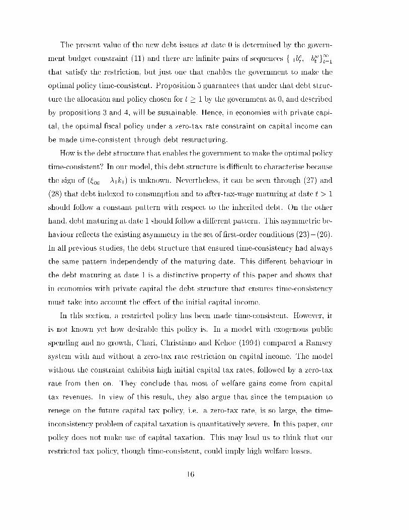
The present value of the new debt issues at date 0 is determined by the govern-

ment budget constraint (11) and there are in�nite pairs of sequences f 1bct ; 1b

wt g1

t=1

that satisfy the restriction, but just one that enables the government to make the

optimal policy time-consistent. Proposition 5 guarantees that under that debt struc-

ture the allocation and policy chosen for t � 1 by the government at 0, and described

by propositions 3 and 4, will be sustainable. Hence, in economies with private capi-

tal, the optimal �scal policy under a zero-tax rate constraint on capital income can

be made time-consistent through debt restructuring.

How is the debt structure that enables the government to make the optimal policy

time-consistent? In our model, this debt structure is diÆcult to characterise because

the sign of (�00 � �1k1) is unknown. Nevertheless, it can be seen through (27) and

(28) that debt indexed to consumption and to after-tax-wage maturing at date t > 1

should follow a constant pattern with respect to the inherited debt. On the other

hand, debt maturing at date 1 should follow a di�erent pattern. This asymmetric be-

haviour re ects the existing asymmetry in the set of �rst-order conditions (23)�(26).

In all previous studies, the debt structure that ensured time-consistency had always

the same pattern independently of the maturing date. This di�erent behaviour in

the debt maturing at date 1 is a distinctive property of this paper and shows that

in economies with private capital the debt structure that ensures time-consistency

must take into account the e�ect of the initial capital income.

In this section, a restricted policy has been made time-consistent. However, it

is not known yet how desirable this policy is. In a model with exogenous public

spending and no growth, Chari, Christiano and Kehoe (1994) compared a Ramsey

system with and without a zero-tax rate restriction on capital income. The model

without the constraint exhibits high initial capital tax rates, followed by a zero-tax

rate from then on. They conclude that most of welfare gains come from capital

tax revenues. In view of this result, they also argue that since the temptation to

renege on the future capital tax policy, i.e. a zero-tax rate, is so large, the time-

inconsistency problem of capital taxation is quantitatively severe. In this paper, our

policy does not make use of capital taxation. This may lead us to think that our

restricted tax policy, though time-consistent, could imply high welfare losses.

16

3.3 Numerical solution for both models.

In order to compare this policy with the one under full-commitment, we use a

numerical solution method for non-linear rational expectations models, in particular

the eigenvalue-eigenvector decomposition method that is suggested by Novales et al.

(1999) and based on Sims (1998). This method consists of the following. First, the

necessary conditions are obtained and transformed so that are functions of either

ratios or variables that are constant in a BGP.13 Their steady state values are found,

as table 1 shows. Then, these conditions are linearised around the steady state in

order to �nd the stability conditions. They are obtained by imposing orthogonality

between each eigenvector associated with an unstable eigenvalue of the linear system

and the variables of the system. These stability conditions are imposed into the

original non-linear model to compute a numerical solution.

[Insert Table 1 about here.]

In order to simulate the series, some realistic parameter values are chosen. The

discount rate � is 0:99: The coeÆcient A in the production function equals 0:48. The

parameter � is 0:25 as in Barro (1990). Depreciation rates for private Æk, and public

capital Æg, are 0:025 and 0:03 respectively.14 The preference parameter � is 0:3 so

as to have reasonable values for leisure. Initial values for private and public capital

are respectively 15 and 45. Initial debt values are zero for all periods. Both models

share the same set of parameter values and depart from the same initial state.

Series for both policies, under full-commitment and with debt restructuring,

are simulated.15 We report the main results. As �gure 1 shows, the policy under

debt-commitment yields a higher growth rate in the short run. In the long run, the

growth rate under debt restructuring approaches from below the rate attained under

full-commitment. In the BGP, growth rates under full-commitment and under debt

restructuring are respectively 3:83 and 3:84 per cent.

[Insert Figure 1 about here.]

13Note that all variables that are not constant grow at the same rate in a BGP.14Since public capital is provided without charge, it is expected to su�er a faster depreciation.15All simulations are carried out with the program GAUSS-386.

17

This similarity between long run growth rates may re ect that the di�erences

in welfare may not be so dramatic. Numerically, the welfare attained under full-

commitment and under debt restructuring take values of 76:3204 and 73:4250 re-

spectively; then, this debt restructuring policy involves a welfare reduction of 3:79%.

Therefore, the debt-commitment policy is quite close both in terms of growth and

welfare to the policy under full-commitment.16 One could argue that these re-

sults could hinge on the upper bound on capital tax rates in the full-commitment

policy. Nevertheless, under the same parameter values and initial conditions, an

unrestricted full-commitment policy yields a 4:27% growth rate and welfare sized by

84:3657. Additionally, the �rst best policy would allows us to test whether this nu-

merical closeness is signi�cant. Under the same circumstances, the �rst best policy

yields a 13:87% growth rate and a welfare value of 249:2070. This result allows us

to con�rm that the policy under debt commitment and the full-commitment policy

are very close both in growth and in welfare terms.

Our results contrast with Chari, Christiano and Kehoe's (1994) �ndings. This

di�erence may come from two facts: �rst, our model allows for endogenous growth, so

future allocations play a more important role for welfare; second, our taxes �nance

a productive public investment rather than an exogenous stream of government

spending. In comparison with lump-sum taxation, our tax structure distorts the

individual decisions and reduces welfare. The zero-tax rate restriction on capital

income makes the existing tax structure more distortionary. If the amount that the

government needs to raise through these taxes is endogenous rather than exogenous,

the �nal tax structure seems intuitively less distortionary. Moreover, in the present

model, public spending may be more important for welfare than the way of �nancing

it. Under both policies, full-commitment and debt restructuring, the stream of

public investment behaves similarly; in the short run, the public capital rate of

growth is higher under full-commitment, this inequality reverses in the medium

term, and both become quite similar in the long run as �gure 2 shows.

[Insert Figure 2 about here.]

16These results hold under di�erent changes in parameter and initial values.

18

The way of �nancing this spending di�ers in both models. Under full-commitment,

tax rates on capital income are high in the �rst periods and zero thereafter. On the

other hand, tax rates on labour income are negative in the initial period and positive

from then on. In comparison with the policy under debt restructuring, the tax rate

on labour income is smaller in the short under full-commitment and both become

quite similar in the long run. In order to spread the excess of burden, debt is issued

in an equivalent way in both models as �gure 5 shows. In the short run, the gov-

ernment incurs in cash ow surpluses, whereas in the medium and in the long run

this surplus vanishes. The main di�erence is that under full-commitment the �rst

period involves a cash ow de�cit that becomes surplus after few periods.

[Insert Figures 3, 4, 5, 6, and 7 about here.]

Finally, it would be interesting to see how the debt-structure that ensures time-

consistency behaves. As we have just mentioned, under debt-commitment, the gov-

ernment incurs in a surplus at date 0. How is this surplus distributed over time?

Observe that since we depart from zero initial debt holdings, a surplus implies that

negative claims are issued. In our numerical solution, positive debt indexed to after-

tax-wage is issued for all t. This debt evolves smoothly along t, but it takes a higher

value at date 1. Hence, this surplus is carried out through negative issues of debt

indexed to consumption. These debt issues take a very negative at date 1; and

zero thereafter. Given the way that the initial capital income and the debt indexed

to consumption enter into the implementability condition of government at date 1;

equation (39), these negative issues are intended to compensate the wealth e�ect.

4 Conclusions.

We have investigated the time-inconsistency problem of optimal �scal policy in a

model with private capital and endogenous growth achieved via public capital. A

policy restricted to a zero-tax on capital income has been made time-consistent

through debt restructuring. The Modigliani-Miller theorem breaks down and debt

19

serves as an incentive device to implement the selected allocation and optimal pol-

icy. We conclude that the tax policy under debt restructuring is quite close both

in growth and in welfare terms to the optimal policy under full-commitment. In

this sense, we can also argue that the time-inconsistency of capital taxation is not

quantitatively so severe.

In economies with privately-owned capital, it is well known that the debt re-

structuring method cannot make the optimal policy plan time-consistent. We have

reconsidered this issue and we have established that in economies with private cap-

ital, a time-consistent policy plan requires both a debt-commitment and a rule on

capital taxation. In this paper, we have chosen a zero-tax rate constraint on capital

income. However, if this tax-rate rule were to be chosen by the government, one

could wonder whether this rule would be set di�erent from zero.

A criticism that often emerges in this literature is that such a rich debt structure

in debt-variety and maturity calendar has no clear counterpart in actual economies.

One can argue that nowadays �nancial products indexed to very di�erent economic

variables are present in �nancial markets. Besides, as pointed out by Faig (1994),

future social security pensions form an example that resembles debt indexed to

after-tax wage. Nevertheless, it would be interesting to study what the government

could better do without such a rich debt structure. Then, it may be the case that

the optimal policy cannot be made time-consistent. Thus, policy selection should

be restricted to sustainable policies. In the choice of the best sustainable policy, it

would be interesting to see whether debt restructuring of the remaining instruments

still matters and how much. The economy performance would provide a measure

for the importance of a rich public �nancial structure.

References

[1] Aschauer, David A. (1989). \Is Public Expenditure Productive?" Journal of

Monetary Economics, 23, 177{200.

[2] Barro, Robert J. (1990). \Government Spending in a Simple Model of Endoge-

20

nous Growth." Journal of Political Economy, 98, S103-S125.

[3] Chamley, Christophe (1986). \Optimal Taxation of Capital Income In General

Equilibrium with In�nite Lives." Econometrica, 54, 607-622.

[4] Chari, V.V.; Christiano, Lawrence J. and Patrick J. Kehoe (1994). \Optimal

Fiscal Policy in a Business Cycle Model." Journal of Political Economy, 102,

617-652.

[5] Faig, Miquel (1991). \Time Consistency, Capital Mobility and Debt Restruc-

turing in a Small Open Economy." Scandinavian Journal of Economics, 93,

447{55.

[6] Faig, Miquel (1994). \Debt Restructuring and the Time Consistency of Optimal

Policies." Journal of Money, Credit, and Banking, 26, 171-181.

[7] Kydland, Finn E. and Edward C. Prescott (1977). \Rules Rather than Discre-

tion: The Inconsistency of Optimal Plans." Journal of Political Economy, 85,

473-491.

[8] Lucas, Robert and Nancy L. Stokey (1983). \Optimal Fiscal and Monetary

Policy in an Economy without Capital." Journal of Monetary Economics, 12,

55-93.

[9] Persson, Torsten, and Lars E. O. Svensson (1986). \International Borrowing

and Time Consistency of Fiscal Policy." Scandinavian Journal of Economics,

88, 273-295.

[10] Persson, Mats; Persson, Torsten and Lars E. O. Svensson (1987). \Time Con-

sistency of Fiscal and Monetary Policy." Econometrica, 55, 1419-1431.

[11] Novales, Alfonso; Dom�inguez, Emilio; P�erez, Javier and Jes�us Ruiz (1999).

\Solving Nonlinear Rational Expectations Models" in Computational Methods

for the Study of Dynamic Economics, R. Marim�on and A. Scott (eds.), Oxford

University Press.

21

[12] Sims, Christophe A. (1998). \Solving Linear Rational Expectations Models,"

mimeo.

[13] Zhu, Xiaodong (1995). \Endogenous Capital Utilization, Investor's E�ort, and

Optimal Fiscal Policy." Journal of Monetary Economics, 36, 655-677.

Appendix A.

Proof of Proposition 1.

Equate the RHS of (20) and (21), and solve for labour

lt =

�Æg � Æk

A

� 1

1��

�X�

1

1��

t ;

with

Xt =

"(1� �)

�kt

gt

��

� �

�kt

gt

��(1��)#: (29)

If Æg > (<) Æk; it can be seen that @Xt

@

�ktgt

� > 0 and @lt@Xt

< (>) 0. Hence, by the chain

rule @lt

@

�ktgt

� < (>) 0. Besides, if Æg = Æk;ktgt= �

1��: Finally, combining equations (18)

and (19) with (5) ; the labour income tax rate is

� lt =�0

h1

1�lt+ 0b

wt

1�lt� 0b

ct

ct

i�h1�

�ot�1

ct�1� �ot

ct

i1 + �0

h1

1�lt+ 0b

wt

1�lt

i ; (30)

which becomes

� lt =�0

h1

1�lt+ �w

1�lt

i�h1�

�ot�1

ct�1� �ot

ct

i1 + �0

h1

1�lt+ �w

1�lt

i ;

whereh1�

�ot�1

ct�1� �ot

ct

i� 0 given the initial debt structure and that

�otct

approaches

zero from above. Then it can be seen that when lt approaches from below its steady

state value so does � lt. Finally, by simple inspection of equation (15) ; if � kt = 1

holds, we have that ct < css:�

Proof of Proposition 2.

22

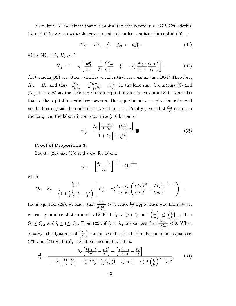
First, let us demonstrate that the capital tax rate is zero in a BGP. Considering

(2) and (18), we can write the government �rst order condition for capital (20) as

Wct = �Wct+1 f1 + fkt+1 � Ækg ; (31)

where Wct = UctHct;with

Hct = 1� �0

�0b

ct

ct�

1

�0

��0t

ct� f1� Ækg

�0t�1

ct�1

ct�1

ct

��: (32)

All terms in (32) are either variables or ratios that are constant in a BGP. Therefore,

Hct = Hc; and thus,Wct

Wct+1=

UctHc

Uct+1Hc=

UctUct+1

in the long run. Comparing (6) and

(31), it is obvious that the tax rate on capital income is zero in a BGP. Note also

that as the capital tax rate becomes zero, the upper bound on capital tax rates will

not be binding and the multiplier �0t will be zero. Finally, given that�otct

is zero in

the long run, the labour income tax rate (30) becomes

�lss =

�0

h1+ 0b

wss

1�lss��0b

c

c

�ss

i1 + �0

h1+ 0bwss1�lss

i :� (33)

Proof of Proposition 3.

Equate (25) and (26) and solve for labour

lt+1 =

�Æg � Æk

A

� 1

1��

�Q�

1

1��

t ;

where

Qt = Xt �

�0t�1

ct�1�1 + 1

�

�0t�1

ct�1� �0t

ct

�"� (1� �)

ct�1

ct

ct

kt

�kt

gt

��

+

�kt

gt

��(1��)

!#:

From equation (29), we know that @Xt

@

hktgt

i > 0. Since�0tct

approaches zero from above,

we can guarantee that around a BGP, if Æg > (<) Æk and�ktgt

���k

g

�ss; then

Qt � Qss and lt � (�) lss. From (22), if Æg > Æk, one can see that@ ct

@

�ktgt

� < 0. When

Æg = Æk , the dynamics of�ktgt

�cannot be determined. Finally, combining equations

(23) and (24) with (5), the labour income tax rate is

� lt =�0

h1+ 0b

wt

1�lt� 0b

ct

ct

i�h1�

�ot�1

ct�1� �ot

ct

i1 + �0

h1+ 0b

wt

1�lt

i�

�ot�1

ct�1

ct�1

ct

��

1��

�(1� lt)� (1� �)A

�ktgt

���1l��t

; (34)

23

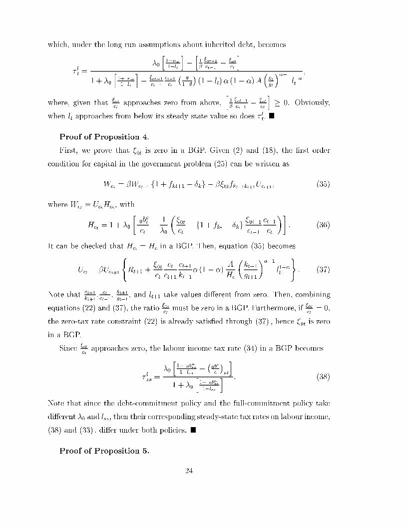
which, under the long run assumptions about inherited debt, becomes

� lt =�0

h1+�w1�lt

i�h1�

�ot�1

ct�1� �ot

ct

i1 + �0

h1+ �w1�lt

i�

�ot�1

ct�1

ct�1

ct

��

1��

�(1� lt)� (1� �)A

�ktgt

���1l��t

;

where, given that�otct

approaches zero from above,h1�

�ot�1

ct�1� �ot

ct

i� 0. Obviously,

when lt approaches from below its steady state value so does � lt: �

Proof of Proposition 4.

First, we prove that �0t is zero in a BGP. Given (2) and (18), the �rst order

condition for capital in the government problem (25) can be written as

Wct = �Wct+1 f1 + fkt+1 � Ækg � ��0tfkt+1kt+1Uct+1; (35)

where Wct = UctHct; with

Hct = 1 + �0

�0b

ct

ct�

1

�0

��0t

ct� f1 + fkt � Ækg

�0t�1

ct�1

ct�1

ct

��: (36)

It can be checked that Hct = Hc in a BGP. Then, equation (35) becomes

Uct = �Uct+1

(Rt+1 +

�0t

ct

ct

ct+1

ct+1

kt+1� (1� �)

A

Hc

�kt+1

gt+1

���1

l1��t+1

): (37)

Note thatct+1

kt+1, ctct+1

,kt+1

gt+1, and lt+1 take values di�erent from zero. Then, combining

equations (22) and (37), the ratio�0tct

must be zero in a BGP. Furthermore, if�0tct

= 0;

the zero-tax rate constraint (22) is already satis�ed through (37) ; hence �0t is zero

in a BGP.

Since�0tct

approaches zero, the labour income tax rate (34) in a BGP becomes

� lss =�0

h1+ 0b

wss

1�lss��0b

c

c

�ss

i1 + �0

h1+ 0b

wss

1�lss

i : (38)

Note that since the debt-commitment policy and the full-commitment policy take

di�erent �0 and lss, then their corresponding steady-state tax rates on labour income,

(38) and (33) ; di�er under both policies. �

Proof of Proposition 5.

24

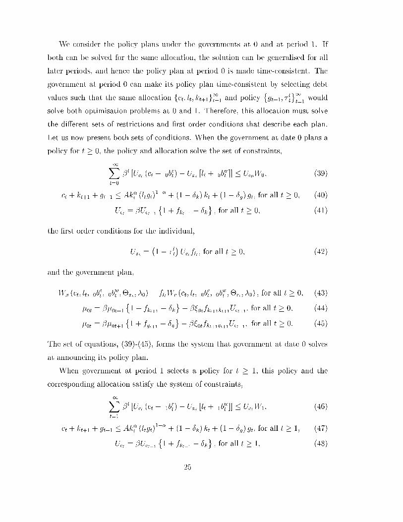
We consider the policy plans under the governments at 0 and at period 1. If

both can be solved for the same allocation, the solution can be generalised for all

later periods, and hence the policy plan at period 0 is made time-consistent. The

government at period 0 can make its policy plan time-consistent by selecting debt

values such that the same allocation fct; lt; kt+1g1

t=1 and policy�gt+1; �

lt

1

t=1would

solve both optimisation problems at 0 and 1. Therefore, this allocation must solve

the di�erent sets of restrictions and �rst order conditions that describe each plan.

Let us now present both sets of conditions. When the government at date 0 plans a

policy for t � 0, the policy and allocation solve the set of constraints,

1Xt=0

�t [Uct (ct � 0b

ct)� Uxt [lt + 0b

wt ]] � Uc0W0, (39)

ct + kt+1 + gt+1 � Ak�t (ltgt)1��

+ (1� Æk) kt + (1� Æg) gt, for all t � 0, (40)

Uct = �Uct+1

�1 + fkt+1 � Æk

, for all t � 0, (41)

the �rst order conditions for the individual,

Uxt =�1� � lt

�Uctflt, for all t � 0, (42)

and the government plan,

Wx (ct; lt; 0bct ; 0b

wt ;�xt; �0) = fltWc (ct; lt; 0b

ct ; 0b

wt ;�ct; �0) , for all t � 0, (43)

�0t = ��0t+1

�1 + fkt+1 � Æk

� ��0tfkt+1kt+1Uct+1, for all t � 0, (44)

�0t = ��0t+1

�1 + fgt+1 � Æg

� ��0tfkt+1gt+1Uct+1; for all t � 0. (45)

The set of equations, (39)-(45), forms the system that government at date 0 solves

at announcing its policy plan.

When government at period 1 selects a policy for t � 1; this policy and the

corresponding allocation satisfy the system of constraints,

1Xt=1

�t [Uct (ct � 1b

ct)� Uxt [lt + 1b

wt ]] � Uc1W1, (46)

ct + kt+1 + gt+1 � Ak�t (ltgt)1��

+ (1� Æk) kt + (1� Æg) gt, for all t � 1, (47)

Uct = �Uct+1

�1 + fkt+1 � Æk

, for all t � 1, (48)

25

and the �rst order conditions for the individual,

Uxt =�1� � lt

�Uctflt, for all t � 1, (49)

and the government program,

Wx (ct; lt; 1bct ; 1b

wt ;�xt; �1) = fltWc (ct; lt; 1b

ct ; 1b

wt ;�ct; �1) , for all t � 1, (50)

�1t = ��1t+1

�1 + fkt+1 � Æk

� ��1tfkt+1kt+1Uct+1, for all t � 1, (51)

�1t = ��1t+1

�1 + fgt+1 � Æg

� ��1tfkt+1gt+1Uct+1, for all t � 1: (52)

Equations, (46)-(52), form the system that the government at date 1 solves when

computing its policy plan.

Now, let us prove that the allocation fct; lt; kt+1g1

t=1 and policy�gt+1; �

lt

1t=1

that solve the policy plan at 0 for t � 1 can solve the policy plan at 1. Since the

sequences�ct; lt; kt+1; gt+1; �

lt

1t=1

solve the former, it is also a solution for equations

(47)� (49) : First, to solve (50) for the same allocation, one debt instrument at each

period is needed. Let us make (51) and (52) time-consistent. Equate both, �t can

be expressed as �t+1

�Rt+1�(1+fgt+1�Æg)

Uct+1(fkt+1kt+1�fkt+1gt+1)

�and (51) and (52) can be written as

�t = ��t+1

"Rt+1 � fkt+1kt+1

"Rt+1 �

�1 + fgt+1 � Æg

�fkt+1kt+1 � fkt+1gt+1

##;

�t = ��t+1

"Rt+1 � fkt+1gt+1

"Rt+1 �

�1 + fgt+1 � Æg

�fkt+1kt+1 � fkt+1gt+1

##:

Therefore, once �1t and �0t take the same value, the same allocation solves both

equations. In order to make �1t take that value, an extra debt instrument for each

date is needed. Note that when �1t = �0t, we have �1t = �0t for the same allocation:

So far, two debt instruments are needed in order to solve all equations, but (46). The

path for this debt is function of �1. Once the government at 0 �nds this function, it

is imposed into the budget constraint (3), which leads to a speci�c debt structure.

Then, by Walras' law, the implementability condition (46) holds. Thus, under that

debt structure, the continuing allocation and policy planned at 0 solves the policy

plan at 1.

26

Let us now �nd the debt structure that provides time consistency. Four types

of debt need to be found: (i) the new inherited debt indexed to consumption for

the �rst period; (ii) debt indexed to consumption for second period and on; (iii) the

new inherited debt indexed to after-tax-wage for the �rst period; (iv) debt indexed

to after-tax-wage for second period and on. Now, we �nd the evolution of debt

indexed to after-tax-wage from the second period on. Let us consider the �rst order

conditions for consumption and leisure under both plans (43) and (50),

Wx (ct; lt; 0bct ; 0b

wt ;�xt; �0)� fltWc (ct; lt; 0b

ct ; 0b

wt ;�ct; �0) = 0: (53)

Wx (ct; lt; 1bct ; 1b

wt ;�xt; �1)� fltWc (ct; lt; 1b

ct ; 1b

wt ;�ct; �1) = 0: (54)

When (53) and (54) are satis�ed, we can equate their LHS, and �nd

[�0 � �1] ((Uxt � fltUct) + (Uctxt � fltUctct) ct � (Uxtxt � fltUctxt) lt

�h�0t�1��1t�1

�0��1

iUctfktlt) = � (Uctxt � flUctct) (�1 1b

ct � �0 0b

ct + ((�0t � �1t)

��1 + fkt�1 � Æk

� ��0t�1 � �1t�1

�))� (Uxtxt � fltUctxt) [�1 1b

wt � �0 0b

wt ] :

(55)

Let us divide equation (55) by � (Uxtxt � fltUctxt)�1; take into account that �0t = �1t

and then add 0bwt

h�0�1� 1i; and rearrange terms to obtain

hUxtxt�fltUctxt

Uctxt�fltUctct

i nh�0�1� 1i h

lt + 0bwt �

Uxt�fltUct

Uxtxt�fltUctxt

i� [1b

wt � 0b

wt ]o=h

1bct �

�0�1

0bct +h�0�1� 1ict

i:

(56)

Now, let us �nd the equation for �0t = �1t: Substitute �t by its value, equation (23),

divide by �Uxtxt�1; consider that �0t = �1t and add 0bwt

h�0�1� 1i; we obtain

hUxtxtUctxt

inh�0�1� 1i h

lt + 0bwt �

hUxtUxtxt

ii� [1b

wt � 0b

wt ]o=h

1bct �

�0�1

0bct +h�0�1� 1ict

i:

(57)

Equate the LHS of (56) and (57) ; rearrange terms and obtain

1bwt � 0b

wt =

��0

�1� 1

� �0b

wt + lt �

�UctxtUct � UctctUxt

UctctUxtxt � (Uctxt)2

��:

Taking into account the speci�c utility function form (2), we have

1bwt � 0b

wt =

��0

�1� 1

�[0b

wt + 1] ;

27

which is the new inherited debt indexed to after-tax-wage for t > 1. This procedure

needs to be replicated for the three remaining debt types. �

Appendix B: Numerical Solution Method.In this appendix, we outline a more precise explanation of the eigenvalue-eigenvector

decomposition method.17 This method consists of the following:

i) Some reasonable values for the initial state variables and for the parameters

are selected.

ii) The model is solved for a steady state. The solution of the debt-commitment

model,�ct; lt; gt+1; kt+1; �

lt; �0t; �0t

t�0

and �0, is characterised by the set of necessary

conditions, (5) and (23) � (26), and the restrictions, (13) ; (16) and (22). If the

number of total periods were T , the system would have T �4+(T�1)�3+1 equations

and the same number of unknown variables. However, our economy extends over

an in�nity of periods. For each period, there are four equations involving variables

at that date, three equations that link future to current variables and one that is

a function of variables in all dates. For the purpose of solving the system, the

equations that link current and future variables need to be replaced by the stability

conditions that depend on variables at the current date. In an endogenous growth

model, steady-state levels of the variables change over time. These variables are

transformed so as to take constant values in a steady state, for example, wkgt = kt

gt;

wcct = ct

ct�1; wck

t = ctkt, and w

�ct =

�0tct. However, notice that to �nd the value of �0,

that is independent of the moment of time, we need to know the whole series of

variables and plugged them into (16). To solve this, a steady-state for a given value

of �0 can be computed, and later, we search for the value of �0 that solves (16).

Next, the conditions and restrictions, (5), (23)� (26), (13) and (22), are written as

functions of the new set of variables. Finally, since all new variables are constant in

a BGP, we can take away the t index, and �nd a steady-state.

iii) All restrictions and conditions are linearised around the steady state. These

equations can be viewed as a function f

�wckt ; lt; w

kg

t ; wcct ; w

�c

t

�: One can de�ne

17As an example, the equations that are included concern the debt-commitment policy.

28

yt =�wckt � wck

ss ; lt � lss; wkgt � wkg

ss ; wcct � wcc

ss; w�ct � w�c

ss

�and do a �rst order Tay-

lor approximation around the steady state

@f

@yt

����ss

yt +@f

@yt�1

����ss

yt�1 = Ayt +Byt�1 = 0:

iv) The unstable eigenvalues of the linear system are computed. We �nd the set

of eigenvalues and eigenvectors of the matrix �(A�1)�B. An unstable eigenvector is

de�ned as one that takes an absolute value greater than ��1

2 ; this number is chosen

so that the objective function is bounded.

v) The stability conditions are computed. They are obtained by imposing or-

thogonality between each eigenvector associated with an unstable eigenvalue and

the variables of this system, that is,

Cyt = 0;

where C is the matrix of eigenvectors associated to unstable eigenvalues. These

stability conditions guarantee that the transversality conditions hold.

vi) The stability conditions are imposed into the original non-linear model. The

equations that linked current to future variables are replaced by the stability condi-

tions. A solution can be now computed. Notice that since the stability conditions

are computed for the linearised system, the solution involves some numerical error.

For a more complete review, see Novales et al. (1999) and Sims (1998).�

29

Figures and tables.

Figure 1: Consumption growth rates.

30

Figure 2: Public capital growth rate.

31

Figure 3: Tax rates on capital income.

32

Figure 4: Tax rates on labour income.

33

Figure 5: Cash ow in present value.

34

Figure 6: Debt structure that makes the policy time-consistent.

Figure 7: Debt structure for t � 1. DC and DW stand for debt indexed to

consumption and to after-tax-wage respectively.

35

TABLE 1. Summary of Results from the Numerical Solution Method.

Variables Policy 0 Policy 1 Policy 2 Policy 3�c

k

�ss

0.03956 0.03858 0.03838 0.03849

lss 0.83333 0.29043 0.27352 0.27523�k

g

�ss

0.34284 0.35462 0.35589 0.35578

�lss � 0.83320 0.84134 0.84092

�kss � 0 0 0

M. E. K. 2.49e-7 1.95e-9 4.94e-5 0.71765

M. E. G. 2.49e-7 3.45e-10 4.94e-5 0.70100

M. E. T. � � 0 0.03586

E. I. � -5.2e-10 -1.83e-7 -2.17e-6

Growth rate 13.87% 4.274% 3.838% 3.849%

Welfare 249.207 84.3657 76.3204 73.4250

Policy 0 is the �rst best policy.

Policy 1 is the policy under full-commitment.

Policy 2 is the policy under full-commitment with �kt � 1.

Policy 3 is the policy under debt-commitment with � kt = 0.

M.E.K. and M.E.G. stand for maximum error at satisfying the �rst order condi-

tion for private and public capital respectively in the government program.

M.E.T. stands for maximum error at satisfying the capital tax rate restriction.

E.I. stands for the error that is made at satisfying the implementability condition.

36