time-changed markov processes in unified credit … · 2019-03-05 · time-changed markov processes...
TRANSCRIPT

Mathematical Finance, Vol. 20, No. 4 (October 2010), 527–569
TIME-CHANGED MARKOV PROCESSES IN UNIFIED CREDIT-EQUITYMODELING
RAFAEL MENDOZA-ARRIAGA
University of Texas
PETER CARR
New York University
VADIM LINETSKY
Northwestern University
This paper develops a novel class of hybrid credit-equity models with state-dependentjumps, local-stochastic volatility, and default intensity based on time changes ofMarkov processes with killing. We model the defaultable stock price process as a time-changed Markov diffusion process with state-dependent local volatility and killingrate (default intensity). When the time change is a Levy subordinator, the stock priceprocess exhibits jumps with state-dependent Levy measure. When the time change isa time integral of an activity rate process, the stock price process has local-stochasticvolatility and default intensity. When the time change process is a Levy subordinatorin turn time changed with a time integral of an activity rate process, the stock priceprocess has state-dependent jumps, local-stochastic volatility, and default intensity. Wedevelop two analytical approaches to the pricing of credit and equity derivatives in thisclass of models. The two approaches are based on the Laplace transform inversion andthe spectral expansion approach, respectively. If the resolvent (the Laplace transformof the transition semigroup) of the Markov process and the Laplace transform of thetime change are both available in closed form, the expectation operator of the time-changed process is expressed in closed form as a single integral in the complex plane.If the payoff is square integrable, the complex integral is further reduced to a spectralexpansion. To illustrate our general framework, we time change the jump-to-defaultextended constant elasticity of variance model of Carr and Linetsky (2006) and obtaina rich class of analytically tractable models with jumps, local-stochastic volatility, anddefault intensity. These models can be used to jointly price equity and credit derivatives.
KEY WORDS: default, credit spread, corporate bonds, equity derivatives, credit derivatives, impliedvolatility skew, CEV model, JDCEV model, Levy Subordinators, time change, jump-diffusion process,state dependent Levy measures, credit-equity model.
1. INTRODUCTION
Until recently, equity derivatives pricing models and credit derivatives pricing modelshave developed more or less independently of each other. Equity derivatives models
This research was supported in part by the grants from the Federal Deposit Insurance Corporation,Moody’s Investor Services, and the National Science Foundation under grant DMS-0802720.
Manuscript received April 2008; final revision received December 2008.Address correspondence to Vadim Linetsky, Department of Industrial Engineering and Management
Sciences, McCormick School of Engineering and Applied Sciences, Northwestern University, 2145 SheridanRoad, Evanston, IL 60208; e-mail: [email protected].
C© 2010 Wiley Periodicals, Inc.
527

528 R. MENDOZA-ARRIAGA, P. CARR, AND V. LINETSKY
largely concentrated on modeling the implied volatility smile by introducing jumps andstochastic volatility into the stock price process (see Gatheral 2006 for a survey), andignored the possibility of default of the firm underlying the option contract. At the sametime, credit models focused on modeling the default event and ignored the informationavailable in the equity derivatives market (see Bielecki and Rutkowski 2004, Duffie andSingleton 2003, and Lando 2004 for surveys of credit risk models). Recently, marketpractitioners have realized that equity derivatives markets and credit markets are closelyrelated, and a variety of cross-market trading and hedging strategies have emerged inthe industry under such names as equity-to-credit and credit-to-equity. Indeed, a deep-out-of-the-money put on a firm’s stock that has little chance to be exercised unless thefirm goes bankrupt and its stock price drops to zero or near zero is effectively a creditderivative that pays the strike price in the event of bankruptcy. Over the past severalyears, every time the credit markets become seriously concerned about the possibilityof bankruptcy of a firm, the open interest, daily volume of trading, and the impliedvolatility of deep-out-of-the-money puts on the firm’s stock explode many times overtheir historical average. In late 2005 and early 2006, the credit markets were concernedabout the possibility of a General Motors (GM) bankruptcy. While the GM stock tradedbetween $18 and $22 in the December 2005–January 2006 period, January 2007 putswith strikes of $10, $7.50, $5, and even $2.50 all had very substantial open interest,large daily trading volumes, and implied volatilities of between 100% and 140%. InAugust and September of 2007, a similar story took place with deep-out-of-the-moneyputs on Countrywide Financial based on Countrywide’s bankruptcy concerns due to itssubstantial exposure to subprime mortgages.
In this paper, we propose a flexible analytically tractable modeling framework whichunifies the valuation of all credit derivatives and equity derivatives related to a given firm.We model the firm’s stock price as the fundamental state variable that is assumed to followa time-changed Markov process with killing. Our model architecture is to start with ananalytically tractable Markov process with killing (e.g., a one-dimensional diffusion withkilling) and subject it to a stochastic time change (clock) with an analytically tractableLaplace transform. If the resolvent (the Laplace transform of the transition semigroup)of the Markov process and the Laplace transform of the time change are both known inclosed form, then the expectation operator of the time-changed process, and hence thecorresponding pricing operator, can be recovered via the Laplace transform inversion.Moreover, if the spectral representation of the transition semigroup is known in closedform, then the Laplace inversion for the time-changed process can also be accomplishedin closed form, leading to analytical pricing of credit and equity derivatives.
Many properties of the clock are inherited by the time-changed process, allowing us toproduce desired behavior in the stock price process modeled as a time-changed Markovprocess. To introduce jumps, we add a jump component into the clock. To introducestochastic volatility, we add an absolutely continuous component into the clock. Bycomposing the two types of time changes, we construct models that exhibit both state-dependent jumps and stochastic volatility. The time-changed process also inherits manyproperties of the original process. If the original process is a Markov process with killing,then the time-changed process also has killing with the state-dependent killing rate,leading to models with the default intensity dependent on the stock price. Thus, ourmodeling framework incorporates diffusive dynamics, state-dependent jumps, stochasticvolatility, and state-dependent default intensity in an analytically tractable way.
Our modeling framework can parsimoniously capture many fundamental empiricalobservations in equity and credit markets, including the well-known positive relationship

TIME-CHANGED MARKOV PROCESSES IN UNIFIED CREDIT-EQUITY MODELING 529
between credit default swap (CDS) spreads and corporate bond yields and impliedvolatilities of equity options, the leverage effect (the negative relationship between therealized volatility of a stock and its price level), the volatility skew/smile effects, andjumps in the stock price process. As such, the class of models we propose is very general,nesting many of the models already in the credit and equity derivatives literatures asspecial cases corresponding to a particular choice of the Markov process and the timechange.
The class of models developed in this paper can be thought of as a far-reachinggeneralization of the hybrid credit-equity models that describe the stock price dynamicsas a one-dimensional diffusion with the local volatility and default intensity specifiedto be some functions of the stock price. In this class of models, in the event of defaultthe stock price is assumed to drop to zero. Along these lines, Linetsky (2006) recentlysolved in closed form an extension of the Black–Scholes–Merton (BSM) model withbankruptcy, where the hazard rate of bankruptcy (default intensity) is a negative powerof the stock price. The limitation of this model is that, while the default intensity is afunction of the stock price, the local volatility of the diffusive stock price dynamics isconstant, as in the original BSM model. To relax this restriction, Carr and Linetsky(2006) proposed and solved in closed form a jump-to-default extended constant elasticityof variance model (JDCEV). This model introduces stock-dependent default intensityinto Cox’s CEV model. This model features state-dependent local volatility and defaultintensity. Moreover, the default intensity is specified to be a linear function of the localvariance. This specification provides a direct link between the stock price volatility anddefault intensity. However, the JDCEV is still a one-dimensional diffusion model, withall the attendant limitations. In particular, the stock price volatility does not have anindependent stochastic component, and there are no jumps in the stock price process.By appropriately time changing one-dimensional diffusions with killing, such as theBrownian motion with killing in Linetsky (2006) and the JDCEV diffusion in Carr andLinetsky (2006), we obtain models with jumps, stochastic volatility, and default.
The class of models developed in this paper can also be thought of as a far-reachinggeneralization of the framework of time-changed Levy processes with stochastic volatilityof Carr et al. (2003). Clark (1973) introduced into finance the notion of stochastictime changes, in which the observed price process is assumed to arise by running atime-homogeneous process on a second process called a clock. A clock is an increasingprocess which is normalized to start at zero and which can have a stochastic component.The requirement that time increases precludes the modeling of the clock as a diffusion,although it is frequently modeled as a time integral of a positive diffusion. Alternatively,the clock is often modeled as a Levy subordinator, a Levy process with positive jumps andnonnegative drift. Time changing (subordinating) with Levy subordinators goes back tothe pioneering work of Bochner (1949, 1955) and is often called Bochner’s subordination.It is well known that, if we subordinate a Levy process, we obtain another Levy process(see Sato 1999). In fact, many Levy processes popular in finance can be represented assubordinate Brownian motions with drift with appropriately chosen subordinators (seeGeman, Madan, and Yor 2001 for a survey). The variance gamma (VG) model of Madanand Milne (1991), Madan and Seneta (1990), and Madan, Carr, and Chang (1998); thenormal inverse Gaussian (NIG) model of Barndorff-Nielsen (1998); and the Carr et al.(2002) model (CGMY) can all be represented as subordinate Brownian motions (forthe latter, see Madan and Yor 2008). On the other hand, if one time changes Brownianmotion with a time change that is a time integral of a CIR diffusion, one obtainsHeston’s (1993) stochastic volatility model. Building on this idea, Carr et al. (2003) time

530 R. MENDOZA-ARRIAGA, P. CARR, AND V. LINETSKY
change general Levy processes with time changes that are time integrals of other positiveprocesses (e.g., CIR processes) and introduce a class of models termed Levy processeswith stochastic volatility. If the time change is an integral of another process, called theactivity rate process, then the Levy measure of the time-changed process scales with theactivity rate process. Thus, the activity rate speeds up or slows down jumps in the time-changed process, in addition to speeding up or slowing down diffusive dynamics whentime changing a Brownian motion (see also Barndorff-Nielsen, Nicolato, and Shephard2002 for related work on time changes and stochastic volatility).
However, there are two significant limitations in the framework of Carr et al. (2003).First, the process to be time changed is a space-homogeneous Levy process with state-independent Levy measure and constant volatility. Through the time change, both thevolatility and the Levy measure scale with the activity rate process, but there is noexplicit dependence of the volatility and the Levy measure on the stock price. Thisspace homogeneity contradicts the accumulated empirical evidence. In the context ofpure diffusion models, the so-called local-stochastic volatility models take the volatilityprocess to be a product of a function of the stock price (such as the power function inthe CEV model) and the stochastic volatility component (see Hagan et al. 2002; Lipton2002; Lipton and McGhee 2002). These models generalize stochastic volatility modelssuch as Heston’s to introduce explicit stock price dependence into the local volatility.In the context of jump models, we would like the Levy measure to include both someexplicit state dependence on the stock price as well as on the stochastic volatility. This isnot addressed in the framework of Carr et al. (2003). The second limitation of Carr et al.(2003) is that they do not include default in their models. The original process is a Levyprocess with infinite lifetime. As a result, the time-changed Levy process with stochasticvolatility also has infinite lifetime. Thus, these are pure equity derivatives models that donot capture the possibility of default of the firm.
Several interesting recent papers also exploit time changes in derivatives pricing.Albanese and Kuznetsov (2004) apply time changes to construct equity derivatives pric-ing models with stochastic volatility and jumps, Boyarchenko and Levendorskiy (2007)apply time changes to construct interest rate models with jumps, and Ding, Gieseckey,and Tomecekz (2009) apply time changes to birth processes to generate multiple defaultsprocesses for multiname credit derivatives. However, in contrast to the focus of this pa-per, neither of these references model equity derivatives and credit derivatives in a unifiedfashion.
This paper develops the next generation of hybrid credit-equity models with state-dependent jumps, local-stochastic volatility, and default intensity based on time changesof Markov processes with killing. The class of models proposed here remedy a numberof limitations of the previous generations of models. By starting from a one-dimensionaldiffusion with killing and time changing it with a composite time change that can berepresented as a subordinator in turn time changed with a time integral of another process(a subordinator with stochastic volatility), we construct processes with state-dependentjumps, local-stochastic volatility, and state-dependent default intensity. Moreover, dueto special properties of one-dimensional diffusions, we retain analytical tractability inthis general framework. This is in contrast with the previous generations of analyticallytractable jump diffusion and pure jump models based on Levy processes with spacehomogeneous jumps (Merton 1976; Kou 2002; Kou and Wang 2004; Barndorff-Nielsen1998; Eberlein, Keller, and Prause 1998; Madan et al. 1998; Carr et al. 2002). The statedependence of the Levy measure in our approach is inherited from the state dependenceof the local volatility of the original diffusion subject to time change. At the same time,
TIME-CHANGED MARKOV PROCESSES IN UNIFIED CREDIT-EQUITY MODELING 531
many existing models, including local volatility models (e.g., CEV), stochastic volatilitymodels (e.g., Heston), local-stochastic volatility models (e.g., SABR), Levy processes withstochastic volatility, and diffusion models with state-dependent default intensity are allnested as special cases in our general framework. Advantages of our hybrid credit-equitymodeling framework include the ability to consistently price the entire book of credit aswell as equity derivatives, in addition to the ability to incorporate a rich assortment ofempirically relevant features.
The rest of this paper is organized as follows. In Section 2, we present our modelarchitecture. We define the defaultable stock price process as a time-changed Markovdiffusion process with killing. In Section 3, we describe the four major classes of timechanges studied in this paper: subordinators, absolutely continuous time changes (timeintegrals of an activity rate process), sums of subordinators and absolutely continuoustime changes, and composite time changes (subordinators with stochastic volatility).In Section 4, we prove a series of key theorems on the martingale and Markov prop-erties of our time-changed stock price processes. In Section 5, we apply our default-able stock model to set up the general framework for the unified valuation of creditderivatives and equity derivatives. In Section 6, we present our Laplace transform ap-proach to the valuation of contingent claims on time-changed Markov processes withthe known resolvent (Laplace transform of the transition semigroup) and the knownLaplace transform of the time change. In Section 7, we present our spectral expansionapproach that works in the special case of symmetric Markov processes and contin-gent claims with square-integrable payoffs. In this case, the Laplace transform inversionis accomplished in closed form and results in a spectral expansion for the contingentclaim value function. To illustrate our general approach, in Section 8, we present adetailed study of time changing the JDCEV process of Carr and Linetsky (2006). Sect-ion 8.1 presents explicit expressions for the resolvent kernel, the spectral expansion of thetransition probability density, the survival probability for the JDCEV process, and thespectral expansion for put options under the JDCEV process (call options are obtainedvia the call-put parity). In Section 8.2, we introduce jumps and stochastic volatility intothe JDCEV process and construct and numerically illustrate the time-changed JDCEVby calculating default probabilities, term structures of credit spreads, and implied volatil-ity skews in a JDCEV time changed with an Inverse Gaussian subordinator in turn timechanged with a time integral of a CIR process (subordinator with stochastic volatility).The resulting stock price process is a pure jump process with state-dependent Levy mea-sure, stochastic volatility, and default intensity dependent both on the stock price and onthe stochastic volatility. The computations are done by applying our analytical methodsbased on the Laplace transform and on the spectral expansion. Section 9 summarizesour results and discusses avenues for further research and applications. The Appendixcontains the proofs. The paper also has an online companion appendix available fromthe authors upon request.
2. MODEL ARCHITECTURE
We assume frictionless markets and no arbitrage and take an equivalent martingalemeasure (EMM) Q chosen by the market on a complete filtered probability space(�,F, {Ft, t ≥ 0}, Q) as given. All stochastic processes defined in the following live onthis probability space, and all expectations are with respect to Q unless stated otherwise.

532 R. MENDOZA-ARRIAGA, P. CARR, AND V. LINETSKY
We model the stock price dynamics under the EMM as a stochastic process {St, t ≥ 0}defined by
St = 1{t<τd }eρt XTt ≡{
eρt XTt , t < τd ,
0, t ≥ τd .(2.1)
We now describe the ingredients in our model.
(i) Background Markov process X. {Xt, t ≥ 0} is a time-homogeneous Markov diffu-sion process starting from a positive value X0 = x > 0 and solving a stochasticdifferential equation (SDE)
dXt = [μ + h(Xt)]Xt dt + σ (Xt)Xt dBt,(2.2)
where σ (x) and μ + h(x) are the state-dependent instantaneous volatility and driftrate, μ ∈ R is a constant parameter, and {Bt, t ≥ 0} is a standard Brownian motion.We assume that σ (x) and h(x) are Lipschitz continuous on [ε, ∞) for each ε >
0, σ (x) > 0 on (0, ∞), h(x) ≥ 0 on (0, ∞), and σ (x) and h(x) remain bounded asx → ∞. We do not assume that σ (x) and h(x) remain bounded as x → 0. Underthese assumptions, the process X does not explode to infinity (infinity is a naturalboundary for the diffusion process; see Borodin and Salminen 2002, p. 14, forboundary classification of diffusion processes), but, in general, may reach zero,depending on the behavior of σ (x) and h(x) as x → 0. The SDE (2.2) has a uniquesolution up to the first hitting time of zero, H0 = inf{t ≥ 0 : Xt = 0}. If the processcan reach zero, we kill it at H0 and send it to an isolated state � called the cemeterystate in the terminology of Markov processes (see Borodin and Salminen 2002,p. 4), where it remains for all t ≥ H0 (zero is a killing boundary). If the processcannot reach zero (zero is an inaccessible boundary), we set H0 = ∞ by convention.We call the process X the background Markov process. We could have includedjumps in the process X , thus starting from a jump-diffusion process, rather thana pure diffusion as is done here. Instead, we start from a diffusion process andintroduce jumps through time changing the diffusion with a Levy subordinator. Byintroducing jumps via time changes we gain some important analytical tractabilityas will be seen later. After the jump-inducing time change, we have a Markovjump-diffusion process, which we can again time change to introduce stochasticvolatility.
(ii) Time change process T . The process {Tt, t ≥ 0} is a random time change (calleda directing process) assumed independent of X . It is a right-continuous with leftlimits (RCLL) increasing process starting at zero, T0 = 0. We also assume thatE[Tt] < ∞ for every t > 0. In this paper, we focus on two important classes oftime changes: Levy subordinators (Levy processes with positive jumps and non-negative drift) that are employed to introduce jumps and absolutely continuous timechanges Tt = ∫ t
0 Vu du with a positive rate process {Vt, t ≥ 0} called activity ratethat are employed to introduce stochastic volatility. We also consider time changesTt = T1
t + T2t with both jump and absolutely continuous components, as well as
composite time changes of the form Tt = T1T2
t, where T1
t is a Levy subordinatorand T2
t is an absolutely continuous time change with some activity rate processV . This can be thought of as first time changing the diffusion process X with theLevy subordinator T1 to introduce jumps, and then time changing the resultingMarkov jump-diffusion process with the absolutely continuous time change T2

TIME-CHANGED MARKOV PROCESSES IN UNIFIED CREDIT-EQUITY MODELING 533
to introduce stochastic volatility. Alternatively, the process T can be understoodas a subordinator with stochastic volatility along the lines of time-changed Levyprocesses of Carr et al. (2003). We describe these classes of time changes in detailin Section 3.
(iii) Default time τd . The stopping time τd models the time of default of the firm on itsdebt. We assume that in default strict priority rules are followed, so that while debtholders receive some recovery, the stock becomes worthless (stock price is equalto zero in default). The time of default τd is constructed as follows. Let H0 be thefirst time the diffusion process X reaches zero as defined previously. Let E be anexponential random variable with unit mean, E ∼ Exp(1), and independent of Xand T . Define
ζ := inf{
t ∈ [0, H0] :∫ t
0h(Xu) du ≥ E
},(2.3)
where h(x) is the function appearing in the drift of X (in equation [2.3] we assumethat inf{∅} = H0 by convention). It can be interpreted as the first jump time of adoubly stochastic Poisson process with the state-dependent intensity (hazard rate)h(Xt) if it jumps before time H0, or H0 if there is no jump in [0, H0]. At time ζ ,we kill the process X and send it to the cemetery state �, where it remains forall t ≥ ζ . We note that, in general, the process X may be killed either at time H0
via diffusion to zero if ζ = H0 or at the first jump time ζ of the doubly stochasticPoisson process with intensity h if ζ < H0 (according to our definition, ζ ≤ H0). Inthe latter case, the process is killed from a positive value Xζ− > 0. The process Xis thus a Markov process with killing with lifetime ζ .1
The drift in (2.2) includes the hazard rate h to make the process 1{t<ζ } Xt withμ = 0 into a martingale. The inclusion of the hazard rate in the drift compensatesfor the possibility of killing the process from a positive state, that is, a jumpof the process Xt from a positive value Xζ− > 0 to the cemetery state � and,correspondingly, a jump of the process 1{t<ζ } Xt from a positive value Xζ− > 0 tozero. This compensation of the jump to zero makes the process 1{t<ζ } Xt with μ = 0into a martingale (our assumptions on σ (x) and h(x) ensure that this process is atrue martingale and not just a local martingale).
After applying the time change T to the process X with lifetime ζ , the lifetime ofthe time-changed process XTt is
τd := inf{t ≥ 0 : Tt ≥ ζ }.(2.4)
Although the process Xt is in the cemetery state for all t ≥ ζ , the time-changedprocess XTt is in the cemetery state for all times t such that Tt ≥ ζ or, equivalently,t ≥ τd with τd defined by equation (2.4). That is, τd defined by equation (2.4) is thefirst time the time-changed process XTt is in the cemetery state. We take τd to be thetime of default. Because we assume that the stock becomes worthless in default,we set St = 0 for all t ≥ τd , so that St = 1{t<τd }eρt XTt .
1The process killed at ζ ≤ H0 is a subprocess of the process killed at H0. We could have used differentnotation for the process killed at ζ to distinguish it from the process killed at H0. To simplify notation,we denote both processes by X . It should not lead to any confusion as it should be clear from the contextwhether we are working with the process killed at H0 or its subprocess killed at ζ ≤ H0.

534 R. MENDOZA-ARRIAGA, P. CARR, AND V. LINETSKY
(iv) Scaling factor eρt. To gain some additional modeling flexibility, we also include ascaling factor eρt with some constant ρ ∈ R in our definition of the stock priceprocess (2.1).
(v) The Martingale condition. For the model (2.1) to be well defined, the functionsσ (x), h(x), the time-change process T , and the constant parameters μ and ρ mustbe such that the discounted stock price process with the dividends reinvested is anonnegative martingale under the EMM Q, that is,
E[St] < ∞ for every t(2.5)
and
E[St2 |Ft1 ] = e(r−q)(t2−t1)St1 for every t1 < t2,(2.6)
where r ≥ 0 is the risk-free interest rate and q ≥ 0 is the dividend yield (in thispaper, we assume r and q are constant). The martingale condition (2.5–6) imposesimportant restrictions on the model parameters. In Section 3, we describe theclasses of time changes we work with and, in Section 4, prove key theorems thatgive the necessary and sufficient conditions for the martingale condition (2.5–6) tohold.
3. TIME-CHANGE PROCESSES
3.1. Levy Subordinators
Let {Tt, t ≥ 0} be a Levy subordinator, that is, a nondecreasing Levy process withpositive jumps and nonnegative drift with the Laplace transform
E[e−λTt ] = e−tφ(λ)(3.1)
with the Laplace exponent given by the Levy–Khintchine formula
φ(λ) = γ λ +∫
(0,∞)(1 − e−λs)ν(ds)(3.2)
with the Levy measure ν(ds) satisfying∫
(0,∞)(s ∧ 1)ν(ds) < ∞, with nonnegative driftγ ≥ 0, and the transition probability Q(Tt ∈ ds) = πt(ds),
∫[0,∞) e−λsπt(ds) = e−tφ(λ).
The standard references on subordinators include Bertoin (1996, 1999) and Sato (1999)(see also Geman et al. 2001 for finance applications). A subordinator starts at zero, T0,drifts at the constant nonnegative drift rate γ , and experiences positive jumps controlledby the Levy measure ν(ds) (we exclude the trivial case of constant time changes withν = 0 and γ > 0). The Levy measure ν describes the arrival rates of jumps so that jumpsof sizes in some Borel set A bounded away from zero occur according to a Poisson pro-cess with intensity ν(A) = ∫A ν(ds). If
∫R+ ν(ds) < ∞, the subordinator is of compound
Poisson type with the Poisson arrival rate α = ∫R+ ν(ds) and the jump size probability
distribution α−1ν. If the integral∫
R+ ν(ds) is infinite, the subordinator is of infinite ac-tivity. Subordinators are processes of finite variation and, hence, the truncation of smalljumps is not necessary in the Levy–Khintchine formula (3.2).
Consider an exponential moment E[eμTt ] of a subordinator T with Levy measureν. When μ < 0, it is always finite and is given by the Levy–Khintchine formula withλ = −μ. We will also need to consider the case μ ≥ 0. Generally, we are interested in
TIME-CHANGED MARKOV PROCESSES IN UNIFIED CREDIT-EQUITY MODELING 535
the set Iν of all μ ∈ R such that E[eμTt ] < ∞. As a corollary of Theorem 25.17 of Sato(1999), E[eμTt ] < ∞ for all t ≥ 0 if and only if∫
[1,∞)eμsν(ds) < ∞.(3.3)
For a given subordinator with Levy measure ν, the set Iν of all μ such that (3.3) holds isan interval (−∞, μ) or (−∞, μ]. The right endpoint μ ≥ 0 may be finite or infinite and,if it is finite, may or may not belong to the set Iν . It is also possible that μ = 0. For allμ ∈ Iν we have
E[eμTt ] = e−tφ(−μ).(3.4)
Further information on subordinators can be found in Applebaum (2004), Bertoin (1996,1999), and Sato (1999). For applications in finance, see Geman et al. (2001), Boyarchenkoand Levendorskiy (2002), Cont and Tankov (2004), and Schoutens (2003). Some exam-ples of subordinators are listed in Appendix C in the companion appendix available fromthe authors upon request.
3.2. Absolutely Continuous Time-Change Processes
Let {Zt, t ≥ 0} be a conservative n-dimensional Markov process independent of X (Zcan have a diffusion component and a jump component, but no killing, so that Z hasinfinite lifetime). Consider an integral process Tt = ∫ t
0 V(Zu) du, where V (z) is somepositive function from the state space D ⊂ Rn of the process Z into (0, ∞) so that theactivity rate process {Vt := V(Zt), t ≥ 0} is positive (we exclude the trivial case of constanttime changes with constant V > 0). The process Tt is strictly increasing and starts at theorigin. We are interested in such Markov processes Z and such functions V (z) that theLaplace transform
Lz(t, λ) = Ez[e−λ∫ t
0 V(Zu ) du ](3.5)
is known in closed form (the subscript z signifies that the Laplace transform Lz(t, λ)explicitly depends on the initial state Z0 = z of the Markov process Z).
A key example is given by the CIR activity rate process (V(z) = z so that Vt = Zt)
dVt = κ(θ − Vt)dt + σV
√VtdWt,
where the standard Brownian motion W is independent of the Brownian motion B drivingthe SDE (2.2), the activity rate process starts at some positive value V0 = v > 0, κ > 0 isthe rate of mean reversion, θ > 0 is the long-run activity rate level, σV > 0 is the activityrate volatility, and it is assumed that the Feller condition is satisfied 2κθ ≥ σ 2
V to ensurethat the process never hits zero (zero is an inaccessible boundary for the CIR processwhen the Feller condition is satisfied). Due to the Cox, Ingersoll, and Ross (1985) resultgiving the closed-form solution for the zero-coupon bond in the CIR interest rate model(note that the Laplace transform (3.5) can be interpreted as the price of a unit face valuezero-coupon bond with maturity at time t when the short rate process is rt = λVt), wehave
Lv (t, λ) = A(t, λ)e−B(t,λ)v ,

536 R. MENDOZA-ARRIAGA, P. CARR, AND V. LINETSKY
where V0 = v is the initial value of the activity rate process and (here � =√
2σ 2Vλ + κ2)
A(t, λ) =(
2�e(�+κ)t/2
(� + κ)(e� t − 1) + 2�
) 2κθ
σ2V
, B(t, λ) = 2λ(e� t − 1)(� + κ)(e� t − 1) + 2�
.
Heston’s stochastic volatility model is based on Brownian motion time changed with theintegral of the CIR process. The CIR activity rate process has been used more generallyin Carr et al. (2003) to time change Levy processes to introduce stochastic volatility inthe popular Levy models, such as VG, NIG, CGMY, etc.
More generally, there are several known classes of Markov processes that yield closed-form expressions for the Laplace transform (3.5). The first class are affine jump-diffusionprocesses with the affine function V (z) (Duffie, Pan, and Singleton 2000; Duffie, Filipovic,and Schachermayer 2003). In this class, the Laplace transform of the time change is the ex-ponential of an affine function of the initial state Z0 = z of the Markov process Z drivingthe activity rate process. The CIR example is a particular representative of the affine class.The second class are the so-called quadratic models (Leippold and Wu 2002), where thefunction V (z) is quadratic in the state vector, and the state vector follows an n-dimensionalGaussian Markov process (an n-dimensional Ornstein–Uhlenbeck process). In this case,the Laplace transform of the time change is the exponential of a quadratic function of theinitial state Z0 = z of the Markov process. The third class are Ornstein–Uhlenbeck pro-cesses driven by Levy processes used by Carr et al. (2003) to time change Levy processes.Explicit expressions for the Laplace transforms of these time changes can be found in thisreference. Carr and Wu (2004) use all three of these classes of absolutely continuous timechanges to time change Levy processes (a listing of closed form expressions for Laplacetransforms of these time changes can be found in tables 1 and 2 in this reference). Herewe use them to time change Markov processes. We note that, while the Laplace trans-forms are known in closed form for these three classes of absolutely continuous timechanges, in general the transition probability distributions Qz(Tt ∈ ds) = πt(z, ds) canonly be obtained numerically by Laplace transform inversion (note that they explicitlydepend on the initial state Z0 = z of the Markov process Z driving the activity rateV ).
REMARK 3.1. Time changing Brownian motion with the integral of the CIR processleads to the zero-correlation Heston’s model. Carr and Wu’s (2004) complex-valuedmeasure change approach extends it to Heston’s model with nonzero correlation. Moregenerally, Carr and Wu’s approach is applicable to time changing general Levy processes.However, so far we have not been able to extend their approach to general Markovprocesses. This is an interesting problem for future research.
3.3. Combining and Composing Time Changes
We can also combine the two types of time changes Tt = T1t + T2
t , where T1t is a
subordinator with Laplace exponent φ and T2t is an integral of some positive function of
a Markov process with analytically tractable Laplace transform Lz(t, λ). The combinedtime change has a jump component, as well as an absolutely continuous component.

TIME-CHANGED MARKOV PROCESSES IN UNIFIED CREDIT-EQUITY MODELING 537
The Laplace transform of the combined time change is simply a product of the Laplacetransforms for its components
E[e−λTt ] = e−tφ(λ)Lz(t, λ).
Alternatively, we can compose the two types of time changes and consider a compositetime-change process
Tt = T1T2
t,(3.6)
where T1t is a subordinator with Laplace exponent φ and T2
t is an integral of some positivefunction of a Markov process with analytically tractable Laplace transformLz(t, λ). Thatis, the process T is obtained by time changing a Levy subordinator T1 with an absolutelycontinuous time change T2. The process T is in the class of Levy processes time changedwith an integral of an activity rate process studied by Carr et al. (2003). By conditioningon T2, the Laplace transform of the composite time change is
E[e−λTt ] = E[E[
exp(− λT1
T2t
) ∣∣T2t
]] = E[e−T2t φ(λ)] = Lz(t, φ(λ)).(3.7)
We note that, after we have done the absolutely continuous time change T2t , further time
changes will no longer have analytically tractable Laplace transforms, because, in contrastto subordinators with the Laplace transform e−tφ(λ) that depends on time exponentially,the Laplace transform Lz(t, λ) may have a complicated general dependence on time.
As we show in Section 4.3, diffusion processes time changed with a combined timechange acquire stochastic volatility in the diffusion component, but do not have stochas-tic volatility in the jump component. In contrast, diffusions time changed with a com-posed time change acquire stochastic volatility both in the diffusion and in the jumpcomponent.
4. MARTINGALE AND MARKOV PROPERTIES OF THE DEFAULTABLESTOCK MODEL
We now prove key theorems that establish when our stock price model (2.1) satisfies themartingale condition (2.5)–(2.6) and when it is a Markov process.
4.1. Time Changing with Levy Subordinators
THEOREM 4.1. Let X be a background diffusion process as described in Section 2(i)with μ ∈ R and h(x) and σ (x) satisfying the assumptions listed there, let T be a Levysubordinator with drift γ ≥ 0 and Levy measure ν with the characteristic exponent φ(λ)and with the interval Iν as described in Section 3.1, and let τd be the default time asdescribed in Section 2 (iii). Then the stock price process (2.1) satisfies the martingalecondition (2.5)–(2.6) if and only if
μ ∈ Iν(4.1)
and
ρ = r − q + φ(−μ).(4.2)
538 R. MENDOZA-ARRIAGA, P. CARR, AND V. LINETSKY
Proof. The proof is by conditioning on the time change T that is independent of Xand using Equation (3.4) to compute the expectation and is given in Appendix A. �
Thus, when the time change T is a Levy subordinator, our model (2.1) is characterizedby the local volatility function σ (x), hazard rate h(x), Levy measure ν and drift γ ≥ 0 ofthe Levy subordinator, and a constant μ ∈ Iν . Depending on the Levy measure, it mayor may not be possible to select μ ∈ Iν so that
ρ = r − q + φ(−μ) = 0.(4.3)
From (3.2) we see that −φ(−μ) is a strictly increasing function on Iν . Thus, the equa-tion (4.3) has at most one solution in Iν . If it exists, we denote it μ0 and call thecorresponding model (2.1) with μ = μ0 and ρ = 0 the zero-ρ model. If the equation (4.3)has no solution in Iν , one possible choice is to set μ = 0 so that ρ = r − q. We callthis choice the zero-μ model. For this choice, the process 1{t<ζ } Xt and the time-changedprocess 1{t<τd } XTt are both martingales, and the desired mean for the stock price processSt = 1{t<τd }e(r−q)t XTt is achieved by including the factor eρt = e(r−q)t. We now establishwhen equation (4.3) has a solution.
THEOREM 4.2. Equation (4.3) has at most one solution in Iν . If r < q, then equa-tion (4.3) has no solution in Iν if and only if γ = 0 and the subordinator is of finite activitywith finite Levy measure with Poisson intensity α = ∫(0,∞) ν(ds) such that −α > r − q. Ifr > q, then equation (4.3) has no solution in Iν if and only if μ is included in Iν (i.e.,∫
[1,∞) eμsν(ds) < ∞) and r − q > −φ(−μ). If r = q, equation (4.3) has a unique solutionμ = 0 in Iν .
Proof. The proof follows from the analysis of equation (3.2) and is given in Appen-dix A. �
We now turn to the question of whether the model (2.1) is Markovian. It turns out thatwhen T is a Levy subordinator, the time changed process XTt is again a Markov process.
THEOREM 4.3. Let X be a background diffusion process with lifetime ζ as described inSection 2(i) with assumptions listed there, and let T be a Levy subordinator with drift γ ≥ 0and Levy measure ν(ds) as described in Section 3.1. Then the time changed process (thesuperscript φ refers to the subordinate quantities with the subordinator with the Laplaceexponent φ)
Xφt := XTt =
{XTt , Tt < ζ
�, Tt ≥ ζ≡{
XTt , t < τd
�, t ≥ τd
(4.4)
is a Markov jump-diffusion process with lifetime τd and with the Levy-type infinitesimalgenerator Gφ that for any twice continuously differentiable function with compact supportf ∈ C2
c ((0, ∞)) can be written in the form
Gφ f (x) = 12γ σ 2(x)x2 d2 f
dx2(x) + b(x)
d fdx
(x) − k(x) f (x)
+∫
(0,∞)
(f (y) − f (x) − 1{|y−x|≤1}(y − x)
d fdx
(x))
�(x, dy)
(4.5)
TIME-CHANGED MARKOV PROCESSES IN UNIFIED CREDIT-EQUITY MODELING 539
with the jump measure (state-dependent Levy measure)
�(x, dy) = π (x, y)dy(4.6)
with the density defined for all x, y > 0, x = y, by
π (x, y) =∫
(0,∞)p(s; x, y)ν(ds),(4.7)
killing rate
k(x) = γ h(x) +∫
(0,∞)Ps(x, {�})ν(ds),(4.8)
and drift with respect to the truncation function 1{|y−x|≤1}
b(x) = γ [μ + h(x)]x +∫
(0,∞)
(∫{y>0:|y−x|≤1}
(y − x)p(s; x, y) dy)
ν(ds).(4.9)
Here p(t; x, y) is the transition probability density of the background Markov process Xwith lifetime ζ , so that the probability to find the process in a Borel set A ⊂ (0, ∞) at timet if the process starts at X0 = x at time zero is Pt(x, A) = ∫A p(t; x, y) dy, and
Pt(x, {�}) = 1 −∫
(0,∞)p(t; x, y) dy(4.10)
is the transition probability of the background process X with lifetime ζ from the statex > 0 to the cemetery state � by time t.
The transition density pφ(t; x, y) of the time-changed Markov process Xφ with lifetimeτd is given by
pφ(t; x, y) =∫
[0,∞)p(s; x, y)πt(ds),(4.11)
where p(s; x, y) is the transition density of the background Markov process X with lifetimeζ and πt(ds) is the transition measure of the subordinator T . The transition probability ofthe process Xφ with lifetime τd from the state x > 0 to the cemetery state � by time t isgiven by
Pφt (x, {�}) = 1 −
∫(0,∞)
pφ(t; x, y) dy =∫
[0,∞)Ps(x, {�})πt(ds).(4.12)
Proof. The proof relies on R.S. Phillips’ theorem on subordination of Markov semi-groups and is given in Appendix A. �
The theorem asserts that when the background process is Markov and the time changeis a Levy subordinator, the time-changed process is again Markov and gives explicitly itslocal characteristics (volatility, drift with respect to the truncation function, killing rate,and jump measure). Intuitively, for any x > 0 and a Borel set A ⊂ (0, ∞)\{x} boundedaway from x, the Levy measure �(x, A) gives the arrival rate of jumps from the state x intothe set A, that is, the transition probability from the state x into the set A bounded away

540 R. MENDOZA-ARRIAGA, P. CARR, AND V. LINETSKY
from x has the following asymptotics: Pt(x, A) ∼ �(x, A)t as t → 0. The truncationfunction in the integral in (4.5) is only needed when jumps are of infinite variation. When∫
{y>0:|x−y|≤1}|y − x|�(x, dy) < ∞(4.13)
for all x > 0, jumps of the time-changed process are of finite variation, the truncationis not needed, and the infinitesimal generator (4.5) of the time-changed Markov processsimplifies to
Gφ f (x) = 12γ σ 2(x)x2 d2 f
dx2(x) + γ [μ + h(x)]x
d fdx
(x) − k(x) f (x)
+∫
(0,∞)( f (y) − f (x)) �(x, dy).
(4.14)
If � is a finite measure with λ(x) := �(x, (0, ∞)) < ∞ for every x > 0, then the processhas a finite number of jumps in any finite time interval, and λ(x) is the (state-dependent)jump arrival rate. The subordinated process Xφ has finite activity jumps if and only ifthe subordinator T has finite activity jumps. Note that, while subordinators are jumpprocesses of finite variation, the subordinated processes Xφ may have jumps of eitherfinite or infinite variation, depending on whether the Levy measure (4.6)–(4.7) satisfiesthe integrability condition (4.13).
From equations (4.5)–(4.8), we see that time changing the process X with a Levysubordinator with drift γ ≥ 0 and Levy measure ν scales volatility and drift withγ , introduces jumps with state-dependent Levy measure with Levy density π (x, y) =∫
(0,∞) p(s; x, y)ν(ds) determined by the Levy measure of the subordinator and the tran-sition density of the diffusion process X , and modifies the killing rate by scaling theoriginal killing rate with γ and adding the term
∫(0,∞) Ps(x, {�})ν(ds) determined by
the Levy measure of the subordinator and the killing probability of the Markov pro-cess X . If γ > 0, we can set γ = 1 without loss of generality. Then the effect of thetime change is to introduce jumps into the original diffusion process, so that the result-ing process is a jump diffusion with the same diffusion as the original process X plusjumps induced by the time change, and to modify the killing rate. Thus, the subordina-tion procedure allows us to introduce jumps into any diffusion process. If γ = 0, thenthe time-changed process has no diffusion component and is a pure jump process withkilling.
Thus, we have a complete characterization of the time-changed process Xφt as a Markov
process with killing. The stock price process (2.1) can be written as St = 1{t<τd }eρt Xφt .
The stock price process stays positive prior to the default time τd (lifetime of Xφt ) and
jumps into zero at τd . We call this jump to default. It is thus a Markov jump-diffusionprocess with zero specified as an absorbing state.
4.2. Absolutely Continuous Time Changes
We now turn to absolutely continuous time changes.
THEOREM 4.4. Let X be a background diffusion process as described in Section 2(i)with μ ∈ R and h(x) and σ (x) satisfying the assumptions listed there, let T be an absolutelycontinuous time change with a positive activity rate process Vt as described in Section 3.2,

TIME-CHANGED MARKOV PROCESSES IN UNIFIED CREDIT-EQUITY MODELING 541
and let τd be the default time as described in Section 2(iii). Then the stock price process(2.1) satisfies the martingale condition (2.5)–(2.6) if and only if
μ = 0, ρ = r − q.(4.15)
Proof. The proof is given in Appendix A.
Because the time-change process {Tt, t ≥ 0} is continuous and strictly increasing (weassume the activity rate process V is strictly positive), the inverse process {At, t ≥ 0}defined by TAt = t is also continuous and strictly increasing and ATt = t. To understandthe effect of the absolutely continuous time change on the process X , we write for Tt < ζ
(equivalently t < τd )
XTt = x +∫ Tt
0h(Xu)Xu du +
∫ Tt
0σ (Xu)Xu dBu
= x +∫ t
0h(XTs )XTs dTs +
∫ t
0σ (XTs )XTs dBTs
= x +∫ t
0h(XTs )XTs V(Zs) ds +
∫ t
0σ (XTs )XTs
√V(Zs) dBs .
(4.16)
In the first equality, we did a change of variable in the integral, u = Ts (with the inverses = Au). In the second equality, we observed that dTs = Vsds and dBTs = √
VsdBs , whereBt = ∫ t
0dBTs√
Vsis a standard Brownian motion (it is a continuous martingale with quadratic
variation t and, hence, is a standard Brownian motion by Levy’s theorem). The processXt is killed at time ζ = inf{t ∈ [0, H0] :
∫ t0 h(Xu) du ≥ E}. Then the time-changed process
XTt is killed at time
τd = inf{t ∈ [0, AH0 ] :∫ Tt
0h(Xu) du ≥ E} = inf
{t ∈ [0, AH0 ] :
∫ t
0h(XTs )V(Zs) ds ≥ E
},
(4.17)
where we did a change of variable u = Ts in the integral. From equations (4.16) and(4.17), we observe that the time-changed process Yt = XTt has the local volatility
σ (x, z) =√
V(z)σ (x)(4.18)
and killing rate
k(x, z) = V(z)h(x)(4.19)
so that for t < τd the process Y solves the SDE
dYt = V(Zt)h(Yt)Ytdt +√
V(Zt)σ (Yt)YtdBt.(4.20)
Thus, the time change scales the volatility with the square root of the activity rate andscales the killing rate with the activity rate. The activity rate plays a role of stochasticvolatility that both drives the instantaneous volatility of the time-changed process andthe killing rate (default intensity). Thus, by construction, this class of models possessesa natural built-in connection between the stock price volatility and the firm’s defaultintensity. This manifests itself in the connection between the implied volatility skew in
542 R. MENDOZA-ARRIAGA, P. CARR, AND V. LINETSKY
the stock options market and the credit spreads in the credit markets. The linkagesbetween credit spreads and equity volatility (both realized and implied in options prices)have been widely documented in the empirical literature (see the discussion and thereferences in the introduction of Carr and Linetsky 2006). Our class of models basedon time changing a diffusion with killing with an integral of an activity rate (stochasticvolatility) process is ideally suited to the task of modeling the linkages between equityvolatility and credit spreads, as the activity rate drives both the local-stochastic volatilityof the stock price and the default intensity. See Carr and Wu (2009) for the empiricalsupport of the linkage between the volatility and default intensity in the framework ofaffine models.
We thus conclude that the time-changed process Y is no longer a one-dimensionalMarkov process. However, the process (Y, Z) is an (n + 1)-dimensional Markov processwith lifetime τd and with the infinitesimal generator G that for any twice continuouslydifferentiable function with compact support f ∈ C2
c ((0, ∞) × D) (where D ⊂ Rn is thestate space of the process Z) can be written in the form
G f (x, z) = V(z)GX f (x, z) + GZ f (x, z),(4.21)
where GX is the infinitesimal generator of the background process X with lifetime ζ ,
GX f (x) = 12σ 2(x)x2 ∂2 f
∂x2(x) + h(x)x
∂ f∂x
(x) − h(x) f (x)(4.22)
and GZ is the infinitesimal generator of the n-dimensional Markov process Z driving theactivity rate Vt = V(Zt).
The fact that, in general, the time-changed process is not Markovian is illustrated bythe Heston model. If we start with Brownian motion and do a time change with thetime-change process taken to be an integral of an independent CIR process, the resultingtime-changed process is no longer a one-dimensional Markov process because of thesecond source of uncertainty (stochastic volatility) entering through the time change.The Markov property is restored in an enlarged two-dimensional state space with boththe stock price and its instantaneous volatility as two state variables.
4.3. Combined and Composite Time Changes
We now turn to composite time changes where we first time change the diffusionprocess X with a Levy subordinator to introduce jumps, and then time change theresulting Markov jump-diffusion process with an absolutely continuous time change tointroduce stochastic volatility as described in Section 3.3. Equivalently, we can thinkof it as a single time change, where the process Tt is a time-changed Levy process withstochastic volatility as in Carr et al. (2003).
THEOREM 4.5. Let X be a background diffusion process as described in Section 2(i) withμ ∈ R and h(x) and σ (x) satisfying the assumptions listed there, let Tt be a composite timechange (3.6), where T1 is a Levy subordinator with drift γ ≥ 0 and Levy measure ν andT2 is an absolutely continuous time change with a positive activity rate process Vt = V(Zt)as described in Sections 3.2 and 3.3, and let τd be the default time as described in Sect-ion 2(iii). Then the stock price process (2.1) satisfies the martingale condition (2.5)–(2.6)if and only if μ = 0, ρ = r − q.

TIME-CHANGED MARKOV PROCESSES IN UNIFIED CREDIT-EQUITY MODELING 543
Proof. The proof is given in Appendix A. �
Recalling Theorem 4.2 and arguing as in Section 4.2, we conclude that the process(Y, Z), where Yt = XTt = XT1
T2t
, is an (n + 1)-dimensional Markov jump-diffusion process
with the infinitesimal generator G that for any twice continuously differentiable functionwith compact support f ∈ C2
c ((0, ∞) × D) (where D ⊂ Rn is the state space of the processZ) can be written in the form (we set μ = 0 in the drift of X according to Theorem 4.5;here Gφ is the infinitesimal generator (4.5) after the first time change with the Levysubordinator and GZ is the infinitesimal generator of the n-dimensional Markov processZ):
G f (x, z) = V(z)Gφ f (x, z) + GZ f (x, z)
= 12γ V(z)σ 2(x)x2 ∂2 f
∂x2(x, z) + b(x, z)
∂ f∂x
(x, z) − k(x, z) f (x, z)
+∫
(0,∞)
(f (y, z) − f (x, z) − 1{|y−x|≤1}(y − x)
∂ f∂x
(x, z))
× �(x, z; dy) + GZ f (x, z)
(4.23)
with the jump measure (state-dependent Levy measure)
�(x, z; dy) = π (x, z; y)dy(4.24)
with the density defined for all x, y > 0, x = y, z ∈ D by
π (x, z; y) = V(z)∫
(0,∞)p(s; x, y)ν(ds),(4.25)
killing rate
k(x, z) = V(z)(
γ h(x) +∫
(0,∞)Ps(x, {�})ν(ds)
),(4.26)
and drift with respect to the truncation function 1{|y−x|≤1}.
b(x, z) = V(z)[γ h(x)x +
∫(0,∞)
(∫{y>0:|y−x|≤1}
(y − x)p(s; x, y)dy)
ν(ds)]
.
(4.27)
Here p(t; x, y) is the transition probability density of the process X with lifetime ζ andPt(x, {�}) is the transition probability of the process X from the state x > 0 to thecemetery state � by time t given by equation (4.10).
The first time change T1 scales the volatility with γ , introduces jumps with the Levymeasure (4.6–7), and modifies the killing rate by scaling the old killing rate h with γ andadding the term to it as in (4.8). The second time change introduces stochastic volatilityby scaling the volatility with
√V(z), and scaling the Levy measure (4.25) and the killing
rate (4.26) with V (z).As an alternative to composing the time changes, we can also consider combined
time changes Tt = T1t + T2
t as discussed in Section 3.3. Theorem 4.5 carries throughverbatim to the combined time-change case. However, the Markov generator has a

544 R. MENDOZA-ARRIAGA, P. CARR, AND V. LINETSKY
different structure. In the combined time-change case, equation (4.23) is replacedwith
G f (x, z) = Gφ f (x, z) + V(z)GX f (x, z) + GZ f (x, z)
= 12
(γ + V(z))σ 2(x)x2 ∂2 f∂x2
(x, z) + b(x, z)∂ f∂x
(x, z) − k(x, z) f (x, z)
+∫
(0,∞)
(f (y, z) − f (x, z) − 1{|y−x|≤1}(y − x)
∂ f∂x
(x, z))
× �(x; dy) + GZ f (x, z)
with the jump measure given by equations (4.6)–(4.7), killing rate
k(x, z) = (γ + V(z))h(x) +∫
(0,∞)Ps(x, {�})ν(ds),
and drift with respect to the truncation function 1{|y−x|≤1}
b(x, z) = (γ + V(z))h(x)x +∫
(0,∞)
(∫{y>0:|y−x|≤1}
(y − x)p(s; x, y) dy)
ν(ds).
In contrast with the composite time change, the combined time change does not intro-duce stochastic volatility into the jump component. Stochastic volatility only enters intothe diffusion component of the process. If one is interested in constructing a pure jumpprocess with stochastic volatility and killing, then the composite time change is moresuitable. In applications where one would like to have both diffusion and jump compo-nents in the asset price process, whether to use combined or composite time changes isan empirical question that depends on whether or not jumps should exhibit stochasticvolatility.
REMARK 4.1. The explicit expressions for the infinitesimal generators provide explicitcharacterizations for local characteristics of the Markov processes: volatility, drift, killingrate, and jump measure. These explicit expressions are also necessary in order to priceAmerican-style and other derivatives numerically by solving the corresponding partialdifferential equations (PDEs) (or partial integro-differential equations [PIDEs] in case ofprocesses with jumps). While in this paper we study European-style securities and pursueanalytical methods, American-style securities can be priced in these models by numer-ically solving the corresponding pricing PDEs or PIDEs defined by these infinitesimalgenerators.
5. UNIFIED VALUATION OF CORPORATE DEBT, CREDIT DERIVATIVES,AND EQUITY DERIVATIVES
We assume that the stock price follows the process (2.1). We view the stock price asthe fundamental observable state variable and, within the framework of our reduced-form model (2.1), view all securities related to a given firm, such as corporate debt, creditderivatives, and equity derivatives, as contingent claims written on the stock price process(2.1). Before proceeding with the valuation of contingent claims, we first consider the

TIME-CHANGED MARKOV PROCESSES IN UNIFIED CREDIT-EQUITY MODELING 545
calculation of the (risk-neutral) survival probability—the probability of no default up totime t > 0. Conditioning on the time change, we have
Q(τd > t) = Q(ζ > Tt) =∫ ∞
0Q(ζ > s)πt(ds) =
∫ ∞
0Ps(x, (0, ∞))πt(ds),(5.1)
where Pt(x, (0, ∞)) = Q(ζ > t) is the survival probability for the Markov process Xwith lifetime ζ (transition probability for the Markov process X with lifetime ζ fromthe state x > 0 into (0, ∞), Pt(x, (0, ∞)) = 1 − Pt(x, {�})) and πt(ds) is the probabilitydistribution of the time change Tt. If the survival probability for the process X and theprobability distribution of the time change πt(ds) are known in closed form, then we canobtain the survival probability for the stock price process (2.1) by integration (5.1).
Next, consider a European-style contingent claim with the payoff �(St) at maturityt > 0 given no default by time t, and constant recovery payment R > 0 if default occursby t. Separating the claim into two building blocks, a claim with the payoff � and norecovery and the recovery payment, the valuation is done by conditioning on the timechange similar to the calculation of the survival probability (5.1). For the European claimwith the payoff �(St) given no default by time t and with no recovery if default occursby t we have
e−rtE[1{τd>t}�(St)] = e−rtE[1{ζ>Tt}�(eρt XTt )] = e−rt∫ ∞
0E[1{ζ>s}�(eρt Xs)
]πt(ds).
(5.2)
For the fixed recovery R paid at time t if default occurs by t we have
Re−rt[1 − Q(τd > t)],(5.3)
where the survival probability is given by equation (5.1).From equations (5.1)–(5.3), we observe that, by conditioning on the time change, the
calculation of the survival probability and the valuation of contingent claims reduce tocomputing expressions of the form
E[1{τd>t} f (XTt )] = E[1{ζ>Tt} f (XTt )] =∫ ∞
0E[1{ζ>s} f (Xs)]πt(ds),(5.4)
for some function f (to compute the survival probability set f = 1). This involves firstcomputing the expectation E[1{ζ>s} f (Xs)] for the background diffusion process X andthen integrating the result in time against the probability distribution of the time changeTt, if the probability distribution of the time change is known in closed form (e.g., theclosed-form expressions for compound Poisson, Gamma, and inverse Gaussian subordi-nators given in Appendix C from the companion appendix). In general, if the closed-formexpression for the distribution of the time change is not available, it can be recoveredby inverting the Laplace transform numerically, which involves numerical integration inthe complex plane by means of the Bromwich Laplace inversion formula. The secondstep is to compute the integral from zero to infinity in equations (5.1) and (5.2). Thus,if we can determine the expectation E[1{ζ>s} f (Xs)] for the original Markov process Xin closed form, we still need to perform double numerical integration to compute (5.4)for the time-changed process. Fortunately, when the function f satisfies an additionalintegrability condition, there is an alternative approach that avoids any need for Laplacetransform inversion to recover πt(ds) and for numerical integration in s in (5.4). In the

546 R. MENDOZA-ARRIAGA, P. CARR, AND V. LINETSKY
next section, we will present a remarkably powerful Laplace transform approach thatwill effectively evaluate both of these integrals in closed form.
The two building blocks (5.2) and (5.3) can be used to value corporate debt, creditderivatives, and equity derivatives. In particular, a defaultable zero-coupon bond with unitface value, maturity t > 0, and recovery R ∈ [0, 1] can be represented as the Europeanclaim with �(St) = 1 and valued at time zero by
BR(x, t) = e−rtQ(τd > t) + Re−rt[1 − Q(τd > t)] = e−rt R + e−rt(1 − R)Q(τd > t),
(5.5)
where we indicate explicitly the dependence of the bond value function on the initial stockprice S0 = X0 = x. Our recovery assumption corresponds to the fractional recovery oftreasury assumption (see, e.g., Lando 2004, p. 120). Defaultable bonds with coupons canbe valued as portfolios of defaultable zeros.
A European call option with strike K > 0 with the payoff (St − K)+ at expiration t hasno recovery if the firm defaults. A European put option with strike K > 0 with the payoff(K − St)+ can be decomposed into two parts: the put payoff (K − St)+1{τd>t}, given nodefault by time t, and a recovery payment equal to the strike K at expiration in the eventof default τd ≤ t. The pricing formulas for European-style call and put options take theform
C(x; K, t) = e−rtE[(
eρt XTt − K)+
1{τd>t}] = e−rt
∫ ∞
0E[(
eρt Xs − K)+
1{ζ>s}]πt(ds),
(5.6)
and
P(x; K, t) = P0(x; K, t) + PD(x; K, t),(5.7)
where
P0(x; K, t) = e−rt∫ ∞
0E[(
K − eρt Xs)+
1{ζ>s}]πt(ds)(5.8)
and
PD(x; K, t) = Ke−rt[1 − Q(τd > t)],(5.9)
respectively. One notes that the put pricing formula (5.7) consists of two parts: the presentvalue P0(x; K, t) of the put payoff conditional on no default given by equation (5.8) (thiscan be interpreted as the down-and-out put with the down-and-out barrier at zero), aswell as the present value PD(x; K, t) of the cash payment equal to the strike K in theevent of default given by equation (5.9). This recovery part of the put is a European-styledefault claim, a credit derivative that pays a fixed cash amount K at maturity t if andonly if the underlying firm has defaulted by time t. Thus, the put option contains anembedded credit derivative. Generally, we emphasize that, in our model, corporate debt,credit derivatives, and equity options are all valued in an unified framework as contingentclaims written on the defaultable stock.
Although we will now focus on deriving explicit closed-form expressions for European-style securities by probabilistic methods, the framework of this section can be extended tothe valuation of American-style options and more complicated securities with Americanfeatures, such as convertible bonds. The standard results imply that the value functionsolves the appropriate PIDE with the integro-differential operator G (the infinitesimal
TIME-CHANGED MARKOV PROCESSES IN UNIFIED CREDIT-EQUITY MODELING 547
generator of the time-changed Markov process; one-dimensional in the case of timechanges by Levy subordinators or (n + 1)-dimensional in the case of absolutely contin-uous or composite time changes) on the appropriate domain and subject to appropriateterminal and boundary conditions. The solution can be derived via numerical methods.
6. VALUATION OF CONTINGENT CLAIMS ON TIME-CHANGEDMARKOV PROCESSES: A LAPLACE TRANSFORM APPROACH
We now present a powerful method to compute expectations of the form (5.4) needed tovalue contingent claims in our model. We will tackle it in two steps. First, we show howto use the Laplace transform to compute the expectation operator
Pt f (x) = Ex[1{ζ>t} f (Xt)],(6.1)
where X is a one-dimensional diffusion process with lifetime ζ started at x at time zeroand the function f satisfies some integrability conditions to be specified later. Second,we show how the time change can be accomplished so that the integral with respect tothe time variable in the expectation (5.4) is evaluated in closed form from the knowledgeof the Laplace transform representation for the expectation (6.1) for the process X andthe Laplace transform of the time change T , without any need to recover the probabilitydistribution of the time change.
Taking the Laplace transform of the expectation operator, we define the resolventoperator Rs (e.g., Ethier and Kurtz 1986):
Rs f (x) :=∫ ∞
0e−stPt f (x) dt = 1
sEx[1{ζ>τs } f (Xτs )],
where τs is an independent exponential time with mean 1/s. For one-dimensional diffu-sions, it is well known (see Borodin and Salminen 2002) that resolvent operator can berepresented as an integral operator
Rs f (x) =∫ r
�
f (y)Gs(x, y) dy
= φs(x)ws
∫ x
�
f (y)ψs(y)m(y) dy + ψs(x)ws
∫ r
xf (y)φs(y)m(y) dy,
(6.2)
where the resolvent kernel or Green’s function Gs(x, y) is the Laplace transform of thetransition probability density, Gs(x, y) = ∫∞
0 e−st p(t; x, y) dt, that admits the followingexplicit representation (Borodin and Salminen 2002, p. 19; note that we define the Green’sfunction with respect to the Lebesgue measure, while Borodin and Salminen define itwith respect to the speed measure m(y)dy, where m(y) is the speed density, and so s(y)does not appear in their expression)
Gs(x, y) = m(y)ws
{ψs(x)φs(y), x ≤ y,
ψs(y)φs(x), y ≤ x.(6.3)
For s > 0, the functions ψs(x) and φs(x) can be characterized as the unique (up toa multiplicative factor independent of x) solutions of the Sturm-Liouville equation

548 R. MENDOZA-ARRIAGA, P. CARR, AND V. LINETSKY
associated with the infinitesimal generator G of the one-dimensional diffusion process,
Gu(x) = 12
a2(x)d2udx2
(x) + b(x)dudx
(x) − c(x)u(x) = su(x),(6.4)
by first demanding that ψs(x) is increasing in x and φs(x) is decreasing and, second,posing boundary conditions at accessible boundary points. For ψs(x), the boundarycondition is only imposed at � if � is an accessible boundary. Because in this paper weassume that accessible boundaries are specified as killing boundaries, we have a Dirichletboundary condition at �, ψs(�) = 0. For φs(x) we have, similarly, φs(r ) = 0 if r is anaccessible boundary specified as a killing boundary. The functions ψs(x) and φs(x) arecalled fundamental solutions of the Sturm–Liouville equation (6.4). They are linearlyindependent and all solutions can be expressed as their linear combinations. Moreover,the so-called Wronskian is independent of x
ws = 1s(x)
(ψ ′s(x)φs(x) − ψs(x)φ′
s(x)).(6.5)
In equation (6.3), the function m(x) is the so-called speed density of the diffusion processX and is constructed from the diffusion and drift coefficients as follows (see Borodin andSalminen 2002, p. 17)
m(x) = 2a2(x)s(x)
, where s(x) = exp(
−∫ x
x0
2b(y)a2(y)
dy)
,(6.6)
where x0 ∈ (�, r ) is an arbitrary point in the state space. The function s(x) is called thescale density of the diffusion process X .
In equation (6.2), we interchanged the Laplace transform integral in t and the expec-tation integral in y. This interchange is allowed by Fubini’s theorem if and only if thefunction f is such that
∫ r�
| f (y)Gs(x, y)| dy < ∞ or
∫ x
�
| f (y)|ψs(y)m(y) dy < ∞ and∫ r
x| f (y)|φs(y)m(y) dy < ∞ ∀ x ∈ (�, r ), s > 0.
(6.7)
For f satisfying this integrability condition, we can then recover the expectation (6.1) byfirst computing the resolvent operator (6.2) and then inverting the Laplace transformvia the Bromwich Laplace transform inversion formula (see Pazy 1983) for the Laplaceinversion formula for operator semigroups)
Pt f (x) = Ex[1{ζ>t} f (Xt)] = 12π i
∫ ε+i∞
ε−i∞estRs f (x) ds.(6.8)
A crucial observation is that in the representation (6.8) time only enters through theexponential est (the temporal and spatial variables are separated). We can thus write
E[1{ζ>Tt} f (XTt )] = 12π i
∫ ε+i∞
ε−i∞E[esTt ]Rs f (x) ds = 1
2π i
∫ ε+i∞
ε−i∞L(t, −s)Rs f (x) ds,(6.9)
where L(t, λ) = E[e−λTt ] is the Laplace transform of the time change (here we require thatE[eεTt ] = L(t, −ε) < ∞). This result has two significant advantages over the expression(5.4). First, it does not require the knowledge of the transition probability measure of
TIME-CHANGED MARKOV PROCESSES IN UNIFIED CREDIT-EQUITY MODELING 549
the time change, and only requires the knowledge of the Laplace transform of the timechange. Second, it does not require the knowledge of the expectation E[1{ζ>t} f (Xt)] forthe original process, and only requires the knowledge of the resolvent Rs f (x) given byequation (6.2).
The Laplace transform inversion in (6.9) can be performed by appealing to the CauchyResidue Theorem to calculate the Bromwich integral in the complex plane. To do this,we need to analyze singularities of the function Rs f (x) in the complex plane s ∈ C (dueto our assumption E[eεTt ] = L(t, −ε) < ∞, the Laplace transform of the time changeL(t, −s) is analytic in the half-plane to the left of the integration contour in [6.9]).
REMARK 6.1. If the background process X is a Levy process (in particular, Brownianmotion with drift), then the Laplace transform approach in this section can be shownto be equivalent to the fast Fourier transform (FFT) approach of Carr et al. (2003). Inthis case, we do not need to work with the resolvent and can work with the characteristicfunctions instead as is done in Carr et al. (2003), leading to the Fourier inversion bythe FFT. For Levy processes, the characteristic function/Fourier transform approach ismore straightforward to use in application. However, the Laplace transform approachin this section is much more general, as it can be applied to time changing any Markovprocess, not just a Levy process.
REMARK 6.2. Carr et al. (2003) work with Levy processes without killing. We notethat it is possible to introduce killing/default into the framework of time-changed Levyprocesses in Carr et al. (2003) as follows. Start with a Levy process with killing. Recallthat the killing rate k has to be constant in order for the killed process to be a Levyprocess. That is, the Levy process is killed at an independent exponential time. On timechanging the Levy process with an integral of an activity rate process Vt (such as theCIR), the time-changed process acquires a stochastic default intensity kVt. That is, thedefault intensity is the old constant killing rate scaled with the stochastic activity rateprocess that introduces stochastic volatility. To price contingent claims in this class ofmodels based on Levy processes with stochastic volatility and killing, one can directlyfollow the Fourier approach of Carr et al. (2003). However, the method developed hereis more general and is applicable to any Markov process with killing.
REMARK 6.3. If the background Markov process X is a one-dimensional diffusionand the time-change process is a Levy subordinator with the exponential Levy mea-sure ν(ds) = αηe−ηsds, then we note that the state-dependent Levy density (4.7) of thetime-changed process is the Green’s function of the diffusion X evaluated at s = η andscaled with αη. Indeed, from equation (4.7), we have π (x, y) = αη
∫∞0 p(s; x, y)e−ηs ds =
αηGη(x, y).
7. VALUATION OF CONTINGENT CLAIMS ON TIME-CHANGEDMARKOV PROCESSES: A SPECTRAL EXPANSION APPROACH
Studying the Green’s function as a function of the complex variable s, one can in-vert the Laplace transform and obtain a spectral representation of the transition den-sity for one-dimensional diffusions originally due to McKean (1956) (see also Itoand McKean 1974; Section 4.1, Wong 1964; Karlin and Taylor 1981). Indeed, con-sidered as a linear operator in the Hilbert space of functions square-integrable with

550 R. MENDOZA-ARRIAGA, P. CARR, AND V. LINETSKY
the speed density m(x), the expectation operator Pt is self-adjoint. Namely, definethe inner product ( f , g) := ∫ r
�f (x)g(x)m(x) dx and let L2((�, r ),m) be the Hilbert
space of functions on (�, r ) square-integrable with the speed density, that is, with‖ f ‖ < ∞, where ‖ f ‖2 = ( f , f ). Then the semigroup {Pt, t ≥ 0} of expectation oper-ators indexed by time is self-adjoint in L2((�, r ),m), that is, (Pt f , g) = ( f ,Ptg) for everyf , g ∈ L2((�, r ),m) and t ≥ 0. This follows from the symmetry property of the transitiondensity, p(t; x, y)m(x) = p(t; y, x)m(y) (note that this symmetry property is apparentfrom the structure of the Green’s function [6.3]). The infinitesimal generator G of a self-adjoint semigroup, as well as the resolvent operators Rs , are also self-adjoint, and we canappeal to the Spectral Theorem for self-adjoint operators in Hilbert space to obtain theirspectral representations. One-dimensional diffusions are examples of symmetric Markovprocesses with symmetric transition semigroups and self-adjoint infinitesimal generators(the standard reference is Fukushima, Oshima, and Takeda 1994).
In the important special case when the spectrum of G in L2((�, r ), m) is purely dis-crete, the spectral representation has the following form. Let {λn}∞n=1, 0 ≤ λ1 < λ2 <
, . . . , limn↑∞ λn = ∞, be the eigenvalues of −G and let {ϕn}∞n=1 be the correspondingeigenfunctions normalized so that ‖ϕn‖2 = 1. That is, (λn, ϕn) solve the Sturm-Liouvilleeigenvalue-eigenfunction problem for the (negative of the) differential operator in (6.4):−Gϕn = λnϕn (Dirichlet boundary condition is imposed at an endpoint if it is a killingboundary). Then the spectral representations for the transition density p(t; x, y) andthe expectation operator Pt f (x) for f ∈ L2((�, r ),m) take the form of eigenfunction ex-pansions (for t > 0 the eigenfunction expansion (7.1) converges uniformly on compactsquares in (�, r ) × (�, r )):
p(t; x, y) = m(y)∞∑
n=1
e−λn tϕn(x)ϕn(y),(7.1)
Pt f (x) = Ex[1{ζ>t} f (Xt)] =∞∑
n=1
cne−λn tϕn(x)(7.2)
with the expansion coefficients cn = ( f , ϕn) satisfying the Parseval equality ‖ f ‖2 =∑∞n=1 c2
n < ∞. The eigenfunctions {ϕn(x)}∞n=1 form a complete orthonormal basis in theHilbert space L2((�, r ),m), that is, (ϕn, ϕn) = 1 and (ϕn, ϕm) = 0 for n = m. They are alsoeigenfunctions of the expectation operator, Ptϕn(x) = e−λn tϕn(x), with eigenvalues e−λn t,and of the resolvent operator, Rsϕn(x) = ϕn(x)/(s + λn), with eigenvalues 1/(s + λn).
More generally, the spectrum of the infinitesimal generator G in L2((�, r ), m) may becontinuous, in which case the sums in (7.1)–(7.2) are replaced with the integrals. We donot reproduce general results on spectral expansions with continuous spectrum here andinstead refer the reader to the literature. For further details on the spectral representationfor one-dimensional diffusions and their applications in asset pricing we refer the readerto Davydov and Linetsky (2003), Lewis (1998, 2000), and Linetsky (2004a,b,c, 2007). Wealso refer the reader to Amrein, Hinz, and Pearson (2005) for a detailed mathematicaltreatment of the Sturm–Liouville theory and numerous references.
A key feature of the spectral representation is that it separates the temporal and spatialvariables. Moreover, time enters the expression (7.2) only through the exponentials e−λn t,thus setting the stage for time changes. We now turn to computing expectations of theform (5.4). Let f ∈ L2((�, r ),m). Substituting the eigenfunction expansion (7.2) into(5.4), we have
TIME-CHANGED MARKOV PROCESSES IN UNIFIED CREDIT-EQUITY MODELING 551
E[1{ζ>Tt} f (XTt )] =∞∑
n=1
cnE[e−λn Tt ]ϕn(x) =∞∑
n=1
cnL(t, λn)ϕn(x),(7.3)
where L(t, λ) is the Laplace transform of the time change. In particular, for the eigen-functions we have
Ex[1{ζ>Tt}ϕn(XTt )] = L(t, λn)ϕn(x).(7.4)
Due to the fact that time enters the spectral expansion only through the exponen-tials e−λns , integrating this exponential against the distribution of the time changeπt(ds), the integral in s in (5.4) reduces to the Laplace transform of the time change,∫
[0,∞) e−λnsπt(ds) = L(t, λn). Thus, in one shot, we both compute the integral in s in (5.4)and get rid of the necessity to invert the Laplace transform to recover the distributionof the time change. In effect, the spectral expansion approach reduces the total requirednumber of integrations by two. In general, the spectral expansion approach is tailor-madefor time changes due to the exponential dependence on time (see also Chen and Song2005, 2007; Linetsky 2007, for related results).
REMARK 7.1. We stress that the spectral expansion (7.2) is only valid for functions fthat are square-integrable with the speed density m. For those functions that are not inL2((�, r ),m) but satisfy the integrability conditions (6.7) one needs to apply the CauchyResidue Theorem directly to the expression (6.9) because the resolvent Rs f (x) may havesingularities that do not coincide with the singularities of the Green’s function Gs(x, y),and the evaluation of (6.9) has to be done case by case for each non-square-integrable f .
REMARK 7.2. If the process X is a Levy process (e.g., Brownian motion with drift),then the result of the spectral method can be shown to be equivalent to the Fouriertransform method based on the characteristic function. The Fourier method is morestraightforward in this case. However, the spectral method is much more general, as it isapplicable to any symmetric Markov process (and to any one-dimensional diffusion inparticular).
8. TIME CHANGING THE JDCEV PROCESS
8.1. The JDCEV Process
Carr and Linetsky (2006) recently proposed the following extension of the classicalCEV model of Cox (1975). Recall that, to be consistent with the leverage effect andthe implied volatility skew, the instantaneous volatility in the CEV model is specifiedas a power function (see Cox 1975; Schroder 1989; Davydov and Linetsky 2001, 2003;Linetsky 2004b, for background on the CEV process)
σ (x) = axβ,(8.1)
where β < 0 is the volatility elasticity parameter and a > 0 is the volatility scale param-eter. The limiting case with β = 0 corresponds to the constant volatility assumption inthe BSM model. To be consistent with the empirical evidence linking corporate bondyields and CDS spreads to equity volatility, Carr and Linetsky (2006) propose to specify

552 R. MENDOZA-ARRIAGA, P. CARR, AND V. LINETSKY
the default intensity as an affine function of the instantaneous variance of the underlyingstock price process
h(x) = b + c σ 2(x) = b + c a2x2β,(8.2)
where b ≥ 0 is a constant parameter governing the state-independent part of the intensityand c ≥ 0 is a constant parameter governing the sensitivity of the intensity to σ 2. In Carrand Linetsky (2006), a and b are taken to be deterministic functions of time. In this paper,we assume that a and b are constant. The infinitesimal generator of this diffusion processon (0, ∞) with killing at the rate (8.2) has the form
G f (x) = 12
a2x2β+2 d2 fdx2
(x) + (μ + b + c a2x2β)xd fdx
(x) − (b + c a2x2β) f (x).(8.3)
This model specification introduces the possibility of a jump to default from a positivevalue for the CEV process and is referred to as the JDCEV process. This model nests thestandard CEV model as a limiting case with vanishing default intensity b = c = 0. Inthe standard CEV model default can only occur when the stock price hits zero throughdiffusion. When c = 0, the intensity is independent of the stock price, and the model isthat of the CEV process killed at an independent exponential time with mean 1/b (thefirst jump time of a Poisson process with constant intensity b). In this case default canoccur either through hitting zero by diffusion or through a jump to zero from a positivestock price value. When b = 0, the intensity does not have a state-independent term andis entirely governed by the stock price process. When b > 0 and c > 0 the intensity hastwo parts—a state-independent part and a state-dependent part. When c > 0, default canonly occur through a jump from a positive value, because the default intensity increasesso fast as the stock falls that the jump to default will almost surely arrive prior to thediffusion process hitting zero.
In this section, we use the general theory developed in the previous sections to constructfar-reaching extensions of the original Carr–Linetsky JDCEV model. By assuming thatthe process X in (2.1) follows a JDCEV process and time changing it as described inSection 3, we introduce jumps and stochastic volatility into the JDCEV model. To beable to value contingent claims in time-changed JDCEV models, we need to be able tocompute expectations of the form (6.1) for the JDCEV process as described in Sections6 and 7. The scale and speed densities of the JDCEV process are
m(x) = 2a2
x2c−2−2βeAx−2β
, s(x) = x−2ce−Ax−2β
, where A := μ + ba2|β| .(8.4)
The following theorem presents the fundamental solutions ψs(x) and φs(x) entering theexpression for the Green’s function (6.3) and their Wronskian ws (6.5) for the JDCEVprocess. Without loss of generality we assume that μ + b ≥ 0.2 There are two distinctcases: μ + b > 0 and μ + b = 0.
THEOREM 8.1.
(i) For a JDCEV diffusion process with the infinitesimal generator (8.3) with pa-rameters β < 0, a > 0, b ≥ 0, c ≥ 0 and such that μ + b > 0, the increasing and
2For absolutely continuous and composite time changes, μ = 0 by Theorems 4.4 and 4.5, while b ≥ 0.For Levy subordinators, by Theorem 4.1 μ ∈ Iν can always be selected so that μ + b ≥ 0. Thus, we do notconsider the case μ + b < 0.

TIME-CHANGED MARKOV PROCESSES IN UNIFIED CREDIT-EQUITY MODELING 553
decreasing fundamental solutions ψs(x) and φs(x) are
ψs(x) = x12 +β−ce− 1
2 Ax−2β
Mκ(s), ν2(Ax−2β ),(8.5)
φs(x) = x12 +β−ce− 1
2 Ax−2β
Wκ(s), ν2(Ax−2β ),(8.6)
where Mk,m(z) and Wk,m(z) are the first and second Whittaker functions withindexes
ν = 1 + 2c2|β| , κ(s) = ν − 1
2− s + ξ
ω, where ω = 2|β|(μ + b), ξ = 2c(μ + b) + b,
(8.7)
and the constant A is defined in equation (8.4). The Wronskian ws defined byequation (6.5) reads
ws = 2(μ + b)�(1 + ν)a2�(ν/2 + 1/2 − κ(s))
.(8.8)
(ii) For a JDCEV diffusion process with the infinitesimal generator (8.3) with pa-rameters β < 0, a > 0, b ≥ 0, c ≥ 0 and such that μ + b = 0, the increasing anddecreasing fundamental solutions ψs(x) and φs(x) are
ψs(x) = x12 −c Iν
(x−β√
2(s + b)a|β|
), φs(x) = x
12 −c Kν
(x−β√
2(s + b)a|β|
),
(8.9)
where Iν(z) and Kν(z) are the modified Bessel functions with index ν given inequation (8.7). The Wronskian ws defined by equation (6.5) reads
ws = |β|.(8.10)
Proof. The proof is by reduction of the Sturm–Liouville equation (6.4) for the JDCEVoperator (8.3) to the Whittaker equation when μ + b > 0 and to the Bessel equation whenμ + b = 0. See Appendix A. �
Theorem 8.1 generalizes Proposition 5 in Davydov and Linetsky (2001) that gives thefundamental solutions for the standard CEV model. Their results are a special case of ourTheorem 8.1 for vanishing default intensity with b = c = 0. The Green’s function is givenby equation (6.3). Inverting the Laplace transform leads to the spectral representation ofthe transition density (7.1).
THEOREM 8.2.
(i) When μ + b > 0, the spectrum of the negative of the infinitesimal generator (8.3)is purely discrete with the eigenvalues and eigenfunctions
λn = ωn + ξ, ϕn(x) = Aν2
√(n − 1)!(μ + b)
�(ν + n)xe−Ax−2β
L(ν)n−1(Ax−2β ), n = 1, 2, . . . ,
(8.11)
554 R. MENDOZA-ARRIAGA, P. CARR, AND V. LINETSKY
where L(ν)n (x) are the generalized Laguerre polynomials and ξ and ω are defined in
(8.7). The spectral representation (eigenfunction expansion) of the JDCEV tran-sition density is given by equation (7.1) with these eigenvalues and eigenfunctionsand the speed density (8.4).
(ii) When μ + b = 0, the spectrum of the infinitesimal generator (8.3) is purely abso-lutely continuous and the spectral representation for the transition density reads
p(t; x, y) = 12|β|m(y)
∫ ∞
0e−(λ+b)t(xy)1/2−c Jν
(x−β
√2λ
a|β|
)Jν
(y−β
√2λ
a|β|
)dλ,
(8.12)
where Jν(x) is the Bessel function of the first kind with index ν given in (8.7).
Proof. The proof is based on applying the Cauchy Residue Theorem to calculate theBromwich Laplace inversion integral. See Appendix A. �
Theorem 8.2 generalizes Proposition 8(i) in Davydov and Linetsky (2003) that gives theeigenvalues and eigenfunctions for the standard CEV model. Their results are a specialcase of our Theorem 8.2 for vanishing default intensity with b = c = 0.
Carr and Linetsky (2006) present closed-form solutions for the survival probabilityand call and put options in the JDCEV model (Proposition 5.5, pp. 319–320). However,those expressions are not suitable for time changes because they depend on time in acomplicated fashion. Here, based on the theory in Sections 6 and 7 and Theorems 8.1and 8.2, we obtain alternative closed-form expressions for the survival probability andcall and put options in the JDCEV model with time entering only through exponentials.We first present the result for the survival probability.
THEOREM 8.3.
(i) For a JDCEV diffusion process with the infinitesimal generator (8.3) with pa-rameters β < 0, a > 0, b ≥ 0, c ≥ 0, μ + b > 0 and started at x > 0, the survivalprobability Q(ζ > t) is given by
Q(ζ > t) =∞∑
n=0
e−(b+ωn)t�
(1 + c
|β|)(
12|β|
)n
�(ν + 1)n!A
12|β| xe−Ax−2β
1 F1
(1 − n + c
|β| ; ν + 1; Ax−2β
),
(8.13)
where 1 F1(a; b; x) is the confluent hypergeometric function; (a)n := �(a +n)/�(a) = a(a + 1) · · · (a + n − 1) is the Pochhammer symbol; and the constantsA, ν, and ω are as defined in Theorem 8.1.
(ii) For μ + b = 0, the JDCEV survival probability Q(ζ > t) is given by
Q(ζ > t) = x1/2−c(√
2a|β|) 2c−12|β|
�
(1 + c
|β|)
�
(1
2|β|)
×∫ ∞
0e−(b+λ)tλ
− 2c−14|β| −1 Jν
(x−β
√2λ
a|β|
)dλ,
(8.14)
where Jν(x) is the Bessel Function of the first kind.

TIME-CHANGED MARKOV PROCESSES IN UNIFIED CREDIT-EQUITY MODELING 555
Proof. The proof is based on first computing the resolvent (6.2) with f (x) = 1 andthen inverting the Laplace transform (6.8) analytically. Because constants are not square-integrable on (0, ∞) with the speed density (8.4), we cannot use the spectral expansionapproach of Section 7 and instead follow the Laplace transform approach of Section 6.See Appendix A. �
We now present the result for the put option. The put option price in our model(2.1) is given by equations (5.7)–(5.9). In particular, to compute the price of the putpayoff conditional on no default before expiration, P0(x; K, t), we need to compute theexpectation E[(K − eρt Xs)+1{ζ>s}] = eρtE[(e−ρt K − Xs)+1{ζ>s}] for the JDCEV process(8.3). The survival probability entering the put pricing formula is already computed inTheorem 8.3. The pricing formula for the call option is obtained via the put-call parity.
THEOREM 8.4.
(i) For a JDCEV diffusion process with the infinitesimal generator (8.3) with pa-rameters β < 0, a > 0, b ≥ 0, c ≥ 0 and such that μ + b > 0, the expectationE[(k − Xt)+1{ζ>t}] is given by the eigenfunction expansion (7.2) with the eigenval-ues λn and eigenfunctions ϕn(x) given in Theorem 8.2 and expansion coefficients
cn = Aν/2+1k2c+1−2β√
�(ν + n)
�(ν + 1)√
(μ + b)(n − 1)!
×
⎧⎪⎪⎨⎪⎪⎩
|β|c + |β| 2 F2
⎛⎜⎜⎝
1 − n,c
|β| + 1
ν + 1,c
|β| + 2; Ak−2β
⎞⎟⎟⎠
− �(ν + 1)(n − 1)!�(ν + n + 1)
L(ν+1)n−1
(Ak−2β
)⎫⎪⎪⎬⎪⎪⎭ ,
(8.15)
where 2 F2 is the generalized hypergeometric function.(ii) For μ + b = 0, the expectation has a spectral expansion with absolutely continuous
spectrum
E[(k − Xt)+1{ζ>t}
] =∫ ∞
0e−(λ+b)tc(λ)x1/2−c Jν
(x−β
√2λ
a|β|
)dλ,(8.16)
with the expansion coefficients
c(λ) = λν/2k2c+1−2β
2ν/2+1�(ν + 1)(c + |β|)|β|ν+1aν+2 1 F2
⎛⎜⎜⎝
c|β| + 1,
ν + 1,c
|β| + 2; − k−2βλ
2a2|β|2
⎞⎟⎟⎠
− kc+1/2−β
√2λ|β|a Jν+1
(k−β
√2λ
a|β|
),
(8.17)
where 1 F2 is the generalized hypergeometric function.
556 R. MENDOZA-ARRIAGA, P. CARR, AND V. LINETSKY
Proof. The put payoff f (x) = (k − x)+ is in the Hilbert space L2((0, ∞),m) of func-tions square-integrable with the speed density (8.4) and, hence, the expectation has aspectral expansion. The proof follows by applying the spectral expansion approach. SeeAppendix A. �
REMARK 8.1. When b = c = 0, all results in this section reduce to the correspondingresults for the standard CEV model (without jump to default) in Davydov and Linetsky(2001, 2003). In the standard CEV model default can only occur through the stock pricehitting zero via diffusion. In this case, the survival probability in Theorem 8.3 is equal tothe probability of the CEV diffusion not hitting zero by time t.
REMARK 8.2. The series representation (8.14) for the survival probability is equivalentto the expression (5.14) in Carr and Linetsky (2006). To prove this one needs to apply themultiplication identity for the Whittaker functions given in equation (B.10) in AppendixB. Due to this identity, the series of hypergeometric functions in (8.13) collapses to theclosed-form expression (5.14) in Carr and Linetsky (2006). For μ + b = 0, one needsto use the integral (B.13) in Appendix B. Similarly, the eigenfunction expansion forthe put in Theorem 8.4 is equivalent to the closed-form expression (5.18) in Carr andLinetsky (2006). To prove this, one needs to apply the Hille–Hardy formula for Laguerrepolynomials (Erdelyi 1953, p. 189; valid for all |t| < 1, ν > −1, a, b > 0)
∞∑n=0
tnn!� (n + ν + 1)
Lνn (a) Lν
n (b) = (abt)−ν/2
1 − texp
{− (a + b) t
1 − t
}Iν
(2√
abt1 − t
).
(8.18)
The closed-form formulas in Carr and Linetsky (2006) are more suitable for pric-ing under the original JDCEV model without time changes than the series expansionsdeveloped in this paper, as they are easier to compute. However, they are generallynot suitable for time-changed models because they have complicated functional depen-dence on time. In contrast, the expansions in this paper explicitly depend on time onlythrough the exponentials and are thus ideally suited for time changes with known Laplacetransforms.
8.2. Introducing Jumps and Stochastic Volatility into the JDCEV Process via TimeChanges: Numerical Examples
In this section, we illustrate our approach with numerical examples. We take thebackground diffusion process X to be a JDCEV process with μ = 0 and time changeit with the composite time-change process Tt = T1
T2t, where T1 is the Inverse Gaussian
(IG) subordinator with the Levy measure ν(ds) = Cs−3/2e−ηs and the Laplace exponentφ(s) = γ s + 2C
√π (
√s + η − √
η) and T2 is the time integral of the activity rate follow-ing the CIR process. That is, the time-change process is an IG process with stochasticvolatility in the terminology of Carr et al. (2003). To satisfy the martingale condition, ac-cording to Theorem 4.5 we set μ = 0 and ρ = r − q. The time-changed process Yt := XTt
is a martingale and the process (Yt, Vt) is a two-dimensional Markov process with theinfinitesimal generator
TIME-CHANGED MARKOV PROCESSES IN UNIFIED CREDIT-EQUITY MODELING 557
G f (x, v) = 12γ va2x2β+2 ∂2 f
∂x2(x, v) + γ v(b + c a2x2β )x
∂ f∂x
(x, v) − k (x, v) f (x, v)
+∫
(0,∞)( f (y, v) − f (x, v))vπ (x, y) dy + σ 2
V
2v∂2 f∂v2
(x, v) + κ(θ − v)∂ f∂v
(x, v),
(8.19)
where the killing rate k(x) and the state-dependent Levy density π (x, y) are
k (x, v) = γ v(b + c a2x2β )
+ vC∫
(0,∞)
⎛⎜⎜⎝1 −
�
(c
|β| + 1)
(τ (s))1
2|β| e−τ (s)−b s
� (ν + 1) 1 F1
⎛⎝
c|β| + 1
ν + 1; τ (s)
⎞⎠⎞⎟⎟⎠
× s−3/2e−η s ds,(8.20)
where
τ (s) := ω x−2β
2|β|2a2 (1 − e−ω s)(8.21)
and
π (x, y) = 2|β|AC( y
x
)c− 12
y−(2β+1)
×∫
(0,∞)
s−3/2e
(ων
2− ξ − η
)s
eωs − 1exp
{−A
(x−2βeωs + y−2β
eωs − 1
)}
×Iν
(A(xy)−β
sinh (ωs/2)
)ds.
(8.22)
The stock price process in this model is a pure jump process with a jump to default thatsends the process to zero, an absorbing state.
REMARK 8.3. In equations (8.20) and (8.22) it is convenient to use the closed formexpressions for the survival probability and the transition density of the JDCEV processobtained in Carr and Linetsky (2006). The spectral expansion of the JDCEV transitionprobability of the form (7.1) with the eigenfunctions and eigenvalues given in Theorem8.2 collapses to the closed-form expression in terms of the Bessel function on applyingthe Hille–Hardy formula (8.18).
The parameter values in our numerical example are listed in Table 8.1. The JDCEVprocess parameter a entering into the local volatility function σ (x) = a xβ is selected sothat the local volatility is equal to 20% when the stock price is equal to fifty dollars,that is, a = 0.2 × 50−β = 10 for the case of β = −1 considered here. In this example,we select γ = 0, so the time-changed process is a pure jump process with no diffusioncomponent (recall that the diffusion component vanishes for time changes with γ = 0).For this particular choice of parameters of the IG time change and the CIR activity rateprocess the time change has the mean and variance E[T1] = 1 and Var[T1] = 1/16 at t = 1.If we replace the background JDCEV process with Brownian motion with drift, then

558 R. MENDOZA-ARRIAGA, P. CARR, AND V. LINETSKY
TABLE 8.1Parameter Values
JDCEV S 50 CIR V 1a 10 θ 1β −1 σV 1c 0.5 κ 4
b 0.01 IG γ 0r 0.05 η 8q 0 C 2
√2/π
Implied Volatility
13%
25%
37%
49%
61%
30 35 40 45 50 55 60 65
Strike
Implie
d V
ola
tility
1/4
1/2
1
2
3
FIGURE 8.1. Implied volatility smile/skew curves as functions of the strike price fortimes to maturity from 0.25 to 3 years. Current stock price level is 50.
the time-changed process is a Normal Inverse Gaussian (NIG) process with stochasticvolatility following the CIR process as in Carr et al. (2003). Our model extends Carret al. (2003) in two important respects. By taking the background process to be a diffusionprocess with state-dependent volatility and drift, the resulting Levy density after timechange is state dependent, in contrast to the space homogeneous Levy jumps. Second,the time-changed process has a state-dependent killing rate (default intensity) in contrastto the absence of default in Carr et al. (2003). By extending the framework of Carret al. (2003) to state-dependent jumps and default intensity, we gain the flexibility ofbeing able to calibrate the model jointly to options prices and CDS spreads. Moreover, thestate dependence of jumps allows for more flexibility in fitting implied volatility surfacesobserved in the equity options market than is available under space homogeneous Levymodels.
Figure 8.1 plots the implied volatility smile/skew curves of options priced underthis model for several different maturities. The implied volatility values are shown inTable 8.2. We compute options prices in this model using Theorem 8.4 and then computeimplied volatilities of these options by inverting the Black–Scholes formula. We observethat in this model shorter maturity skews are steeper and flatten out as maturity increases,

TIME-CHANGED MARKOV PROCESSES IN UNIFIED CREDIT-EQUITY MODELING 559
TABLE 8.2Implied Volatilities (in %) for Different Strike Prices and Times to Maturity (Years)
Time/strike 30 35 40 45 50 55 60 65
1/4 62.04 47.94 35.52 26.19 21.41 20.09 20.28 20.881/2 51.94 41.47 32.72 26.39 22.64 20.72 19.84 19.461 45.74 38.24 32.14 27.53 24.30 22.12 20.65 19.642 43.03 37.68 33.23 29.61 26.72 24.45 22.66 21.253 42.80 38.34 34.55 31.34 28.64 26.39 24.52 22.96
Note: Current stock price level is 50.
consistent with empirical observations in options markets. We also observe that the shortmaturity skew exhibits a true volatility smile with the increase in implied volatilities bothto the right and to the left of the at-the-money strike. This behavior cannot be capturedin the pure diffusion JDCEV model. In JDCEV, the implied volatility skew results fromthe leverage effect (the local volatility is a decreasing function of stock price) and thepossibility of default (the default intensity is a decreasing function of stock price). Theresulting implied volatility skew is a decreasing function of strike. After the time changewith jumps, the resulting jump process has both positive and negative jumps. This resultsin the implied volatility smile pattern with volatility “smiling” on both sides of the at-the-money level. Table 8.3 presents sample put prices for several strike and maturity combi-nations. The prices are computed to the accuracy of 10−4 (all of the decimals presentedin the table are correct) by computing the corresponding eigenfunction expansions. Allcomputations in this paper were performed in Mathematica. All the special functions ap-pearing in the JDCEV model solution are available as built-in functions in Mathematica.
Figure 8.2 plots the default probability and the credit spread (assuming zero recoveryin default) as functions of time to maturity for several different levels of the stock price.As the stock price decreases, the credit spreads of all maturities increase, but the shorterand intermediate maturities increase the fastest. In particular intermediate maturities ofbetween two and seven years increase the fastest. This results in a pronounced hump inthe term structure of credit spreads around these intermediate maturities. As the stockprice falls, the hump becomes more pronounced and shifts toward shorter maturities.This increase in credit spreads with the decrease in the stock price is accounted for boththe leverage effect through the increase in the local volatility of the original diffusionand, hence, more jump volatility for the jump process after the time change, as well asthe increase in the default intensity of both the original diffusion process and the jumpprocess after the time change. Figure 8.3 plots the default intensity (killing rate) in thismodel after the time change as a function of the stock price given by equation (8.20).The default intensity is a decreasing function of the stock price.
REMARK 8.4. We note the following interesting feature of our model. If we take thestandard Cox’s CEV diffusion process (without the jump to default introduced in Carrand Linetsky 2006) to serve as the background Markov process and time change it witha Levy subordinator, the resulting process acquires a default intensity, even though theoriginal CEV process does not have any killing rate. Indeed, the default event in the CEVprocess can only occur via hitting zero by diffusing down to the zero stock price. Thedefault time in the original CEV process is predictable with an announcing sequence of

560 R. MENDOZA-ARRIAGA, P. CARR, AND V. LINETSKY
TA
BL
E8.
3P
utP
rice
s
Stri
ke/t
ime
1/4
1/2
12
34
5
30(0
.222
7,0.
0006
)(0
.440
5,0.
0059
)(0
.863
3,0.
039)
(1.6
669,
0.13
34)
(2.4
2,0.
1855
)(3
.106
2,0.
189)
(3.7
063,
0.16
67)
0.22
330.
4464
0.90
231.
8003
2.60
553.
2952
3.87
3035
(0.2
598,
0.00
53)
(0.5
139,
0.03
17)
(1.0
072,
0.12
93)
(1.9
447,
0.30
88)
(2.8
233,
0.37
79)
(3.6
239,
0.36
46)
(4.3
241,
0.31
35)
0.26
500.
5457
1.13
652.
2535
3.20
123.
9885
4.63
7640
(0.2
969,
0.04
16)
(0.5
873,
0.14
94)
(1.1
511,
0.37
86)
(2.2
226,
0.64
89)
(3.2
266,
0.70
56)
(4.1
416,
0.64
63)
(4.9
418,
0.54
23)
0.33
850.
7368
1.52
972.
8715
3.93
234.
7879
5.48
4145
(0.3
34,0
.285
2)(0
.660
7,0.
5886
)(1
.295
,0.9
697)
(2.5
004,
1.25
05)
(3.6
3,1.
2261
)(4
.659
3,1.
0714
)(5
.559
5,0.
8786
)0.
6192
1.24
932.
2647
3.75
094.
8560
5.73
086.
4381
50(0
.371
1,1.
4541
)(0
.734
2,1.
8376
)(1
.438
9,2.
159)
(2.7
782,
2.22
48)
(4.0
333,
2.00
21)
(5.1
77,1
.680
1)(6
.177
2,1.
3499
)1.
8252
2.57
183.
5978
5.00
306.
0354
6.85
717.
5271
55(0
.408
2,4.
5108
)(0
.807
6,4.
3813
)(1
.582
7,4.
1757
)(3
.056
,3.6
744)
(4.4
366,
3.09
44)
(5.6
947,
2.51
21)
(6.7
95,1
.983
7)4.
9190
5.18
895.
7584
6.73
047.
5310
8.20
688.
7787
60(0
.445
3,8.
9164
)(0
.881
,8.1
355)
(1.7
266,
7.08
24)
(3.3
338,
5.66
61)
(4.8
4,4.
552)
(6.2
125,
3.60
29)
(7.4
127,
2.80
62)
9.36
189.
0165
8.80
909.
0000
9.39
199.
8153
10.2
189
65(0
.482
4,13
.726
5)(0
.954
4,12
.573
7)(1
.870
5,10
.734
1)(3
.611
7,8.
2104
)(5
.243
3,6.
4037
)(6
.730
2,4.
9796
)(8
.030
4,3.
8396
)14
.209
013
.528
112
.604
711
.822
011
.647
011
.709
811
.870
0
Not
e:F
orea
chco
mbi
nati
onof
stri
kean
dti
me
tom
atur
ity
two
valu
esar
egi
ven
inpa
rent
hesi
s.T
hefir
stva
lue
isth
epr
ice
P Dof
the
defa
ult
clai
meq
uati
on(5
.9).
The
seco
ndva
lue
isth
epr
ice
P 0of
the
putp
ayof
fpai
don
lyif
ther
eis
node
faul
tequ
atio
n(5
.8).
The
thir
dva
lue
belo
wis
the
put
opti
onpr
ice
equa
lto
P D+
P 0.
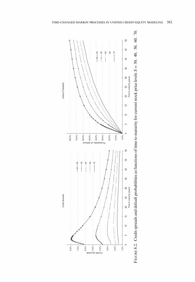
TIME-CHANGED MARKOV PROCESSES IN UNIFIED CREDIT-EQUITY MODELING 561
Cre
dit S
pre
ad
s
1.5
%
2.5
%
3.5
%
4.5
%
5.5
%
6.5
%
7.5
%
8.5
%
05
1015
2025
3035
4045
50
Tim
e t
o m
atu
rity
(ye
ars
)
Credit spreads
30
40
50
60
70
De
fau
lt P
rob
ab
ility
0.0
%
10
.0%
20
.0%
30
.0%
40
.0%
50
.0%
60
.0%
70
.0%
80
.0%
05
1015
2025
3035
4045
50
Tim
e t
o m
atu
rity
(ye
ars
)
Probability of default
30
40
50
60
70
FIG
UR
E8.
2.C
redi
tspr
eads
and
defa
ultp
roba
bilit
ies
asfu
ncti
ons
ofti
me
tom
atur
ity
for
curr
ents
tock
pric
ele
vels
S=
30,
40,
50,
60,
70.
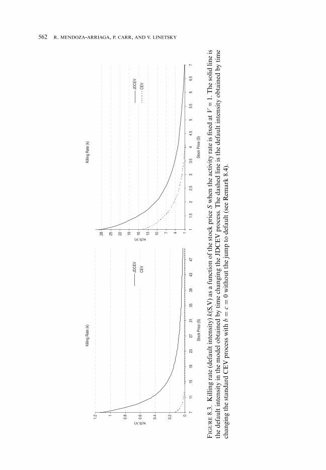
562 R. MENDOZA-ARRIAGA, P. CARR, AND V. LINETSKY
Kill
ing
Rat
e (k
)
0
0.2
0.4
0.6
0.81
1.2
711
1519
2327
3135
3943
47
Sto
ck P
rice
(S)
k(S,V)
JDC
EV
CE
V
Kill
ing
Rat
e (k
)
14710131619222528
11.
52
2.5
33.
54
4.5
55.
56
6.5
7
Sto
ck P
rice
(S)
k(S,V)
JDC
EV
CE
V
FIG
UR
E8.
3.K
illin
gra
te(d
efau
ltin
tens
ity)
k(S,
V)a
sa
func
tion
ofth
est
ock
pric
eS
whe
nth
eac
tivi
tyra
teis
fixed
atV
=1.
The
solid
line
isth
ede
faul
tin
tens
ity
inth
em
odel
obta
ined
byti
me
chan
ging
the
JDC
EV
proc
ess.
The
dash
edlin
eis
the
defa
ult
inte
nsit
yob
tain
edby
tim
ech
angi
ngth
est
anda
rdC
EV
proc
ess
wit
hb
=c
=0
wit
hout
the
jum
pto
defa
ult
(see
Rem
ark
8.4)
.

TIME-CHANGED MARKOV PROCESSES IN UNIFIED CREDIT-EQUITY MODELING 563
hitting times of stock price levels decreasing toward zero. However, after a pure jump timechange, the default time in the time-changed jump process becomes totally inaccessiblewith the intensity given by the integral of the default probability of the original CEVprocess with the Levy measure of the subordinator in equation (8.20) (in this case b = 0because the standard CEV process does not have any default intensity). This defaultintensity is plotted in Figure 8.3 as a dashed line. Intuitively, one can understand this asfollows. Suppose one observes a sample path of a diffusion process that hits zero. Becausethe process is continuous, one observes the announcing sequence of the default event.When the diffusion is subjected to a pure jump time change, one can no longer observethe announcing sequence, as the hitting times of the intermediate stock price levels areleft unobservable when the time jumps through them. As a result, the default event in thetime-changed process looks like an unpredictable jump to default from a positive valuegoverned by the default intensity induced by the time change.
9. CONCLUSION
This paper develops a novel class of hybrid credit-equity models with state-dependentjumps, local-stochastic volatility, and default intensity based on time changes of Markovprocesses with killing. We model the defaultable stock price process as a time-changedMarkov diffusion process with state-dependent local volatility and killing rate (defaultintensity). When the time change is a Levy subordinator, the stock price process exhibitsjumps with state-dependent Levy measure. When the time change is a time integralof an activity rate process, the stock price process has local-stochastic volatility anddefault intensity. When the time-change process is a Levy subordinator in turn timechanged with a time integral of an activity rate process, the stock price process has state-dependent jumps, local-stochastic volatility, and default intensity. This framework offersfar-reaching extensions of the framework of time-changed Levy processes with stochasticvolatility of Carr et al. (2003). By time-changing Markov processes we relax the spacehomogeneity assumption inherent in Levy models. Moreover, the mechanism of killinga Markov process at a state-dependent rate is well suited to modeling the default event.
This paper develops two analytical approaches to the pricing of credit and equityderivatives in this class of models. The two approaches are based on the Laplace transforminversion and the spectral expansion approach, respectively. If the resolvent (the Laplacetransform of the transition semigroup) of the diffusion process and the Laplace transformof the time change are both available in closed form, the expectation operator of the time-changed process is expressed in closed form as a single integral in the complex plane.If the payoff is square-integrable, the complex integral is further reduced to a spectralexpansion. To illustrate our general framework, we time change the JDCEV model ofCarr and Linetsky (2006) and obtain a rich class of analytically tractable models withjumps, local-stochastic volatility, and default intensity. These models can be used tojointly price equity and credit derivatives. In particular, we compute implied volatilitysurfaces, default probabilities, and credit spreads under the JDCEV process subject tothe time change that is an inverse Gaussian subordinator that is itself subject to a timechange with a CIR activity rate process. This process is a pure jump process with state-dependent jumps and killing (jump to default) in contrast to the pure diffusion JDCEVmodel of Carr and Linetsky (2006).
The contribution of this paper is in the development of a flexible modeling framework,as well as in the development of the analytical methods to solve this class of models.

564 R. MENDOZA-ARRIAGA, P. CARR, AND V. LINETSKY
A wide range of models can be constructed within this model architecture by pairingbackground diffusion processes with different time changes. We hope that this paperwill stimulate empirical research into the joint credit-equity dynamics and the interplaybetween credit and equity derivatives markets.
APPENDIX A: PROOFS
A.1. Proof of Theorem 4.1
Because by Theorem 4.3, the process e−ρt St = 1{t<τd } XTt is a time-homogeneousMarkov process, it is enough to prove that
E[1{t<τd } XTt ] = e(r−q−ρ)tx for all t > 0,(A.1)
where S0 = X0 = x > 0. Let F Xt = σ {Xs, s ≤ t} and FT
t = σ {Ts, s ≤ t} be the filtrationsgenerated by the background diffusion process X and the time change T . Observ-ing that 1{t<τd } = 1{Tt<ζ } = 1{Tt<H0}1{Tt<ζ } and E[1{t<H0}1{t<ζ }|F X
t ] = 1{t<H0}e− ∫ t
0 h(Xu ) du,
we can write
E[1{t<τd } XTt ] = E[1{Tt<H0}e
− ∫ Tt0 h(Xu ) du XTt
]= xE
[1{Tt<H0}e
− ∫ Tt0 h(Xu ) due
∫ Tt0 [μ+h(Xu )]du+∫ Tt
0 σ (Xu ) dBu− 12
∫ Tt0 σ 2(Xu ) du]
= xE[eμTt 1{Tt<H0}e
∫ Tt0 σ (Xu ) dBu− 1
2
∫ Tt0 σ 2(Xu ) du],
where in the second equality we used the SDE (2.2). Because the volatility σ (x) re-mains bounded as x → ∞, the process 1{t<H0}e
∫ t0 σ (Xu ) dBu− 1
2
∫ t0 σ 2(Xu ) du stopped at H0 is an
exponential martingale starting at one (e.g., Delbaen and Shirakawa 2002).Now suppose μ ∈ Iν . Then, conditioning on the time change, we have
xE[eμTt E]1{Tt<H0}e∫ Tt
0 σ (Xu ) dBu− 12
∫ Tt0 σ 2(Xu ) du |FT
t ]] = xE[eμTt ] = xe−tφ(−μ).
Comparing the right-hand side with that of equation (A.1), we conclude that equation(A.1) holds if and only if ρ = r − q + φ(−μ). If μ /∈ Iν , then E[eμTt ] is infinite and (A.1)cannot be satisfied and, hence, the process (2.1) does not satisfy the martingale condition(2.5)–(2.6). �
A.2. Proof of Theorem 4.2
Define f (μ) := −φ(−μ). If γ > 0 or γ = 0 and the subordinator is of infinite activity(∫
(0,∞) ν(ds) = ∞), then f (μ) tends to −∞ as μ → −∞. If γ = 0 and the subordinator isof finite activity (
∫(0,∞) ν(ds) = α < ∞), then f (μ) tends to −α. If μ is not included in Iν ,
then f (μ) tends to +∞ as μ → μ. If μ is included in Iν , then f (μ) = γ μ + ∫(0,∞)(eμs −
1)ν(ds) < ∞. We thus have the following alternatives for the existence of solutions of theequation f (μ) = r − q. If r < q, then there is a unique solution μ0 for all subordinatorsexcept for subordinators with zero drift and finite activity Levy measure with Poissonintensity α such that −α > r − q. If r > q, then there is a unique solution if either μ isnot included in Iν or μ is included in Iν and r − q ≤ f (μ). Otherwise, if μ is includedin Iν and r − q > f (μ), Equation (4.3) has no solution in Iν . The statement for the caser = q is immediate from the fact that φ(0) = 0. �
TIME-CHANGED MARKOV PROCESSES IN UNIFIED CREDIT-EQUITY MODELING 565
A.3. Proof of Theorem 4.3
The idea of time changing a Markov process with a Levy subordinator is originally dueto Bochner (1949, 1955). The following fundamental theorem due to Phillips (1952) (seeSato 1999, Theorem 32.1, p. 212) characterizes the time-changed transition semigroupand its infinitesimal generator.
THEOREM A.1 (Phillip’s Theorem; Sato 1999, p. 212). Let {Tt, t ≥ 0} be a subordinatorwith Levy measure ν, drift γ , Laplace exponent φ(λ), and transition kernel πt(ds). Let{Pt, t ≥ 0} be a strongly continuous contraction semigroup of linear operators in the Banachspace B with infinitesimal generator G. Define (the superscript φ refers to the subordinatedquantities with the subordinator with the Laplace exponent φ)
Pφt f =
∫[0,∞)
(Ps f )πt(ds), f ∈ B.(A.2)
Then {Pφt , t ≥ 0} is a strongly continuous contraction semigroup of linear operators on B.
Denote its infinitesimal generator by Gφ . Then Dom(G) ⊂ Dom(Gφ), Dom(G) is a core ofGφ , and
Gφ f = γG f +∫
(0,∞)(Ps f − f )ν(ds), f ∈ Dom(G).(A.3)
In our case, the Banach space B is C0(0, ∞) (the space of continuous bounded func-tions on (0, ∞) vanishing at infinity) and the semigroup {Pt, t ≥ 0} is the Feller transitionsemigroup of the diffusion process X with lifetime ζ . Given our assumptions, the one-dimensional diffusion X always has a transition density p(t; x, y) with respect to theLebesgue measure, so that Pt f (x) = ∫(0,∞) f (y)p(t; s, y) dy, and, moreover, p(t; x, y) iscontinuous in all its variables. Then from equation (A.2) we obtain the density (4.11)of the subordinate process Xφ = XTt . From equation (A.3) we can identify the infinites-imal generator of Xφ in equations (4.5)–(4.6) (see the online companion to this paperfor the explicit calculation; for mathematical references on the Levy characteristics ofsubordinate Markov processes, see Okura 2002; Theorem 2.1; Chen and Song 2005;Section 2). �
A.4. Proof of Theorem 4.4
The proof is similar to the proof of Theorem 4.1. Because the process (e−ρt St, Zt) =(1{t<τd } XTt , Zt) is an (n + 1)-dimensional time-homogeneous Markov process, it is enoughto prove that equation (A.1) holds. Suppose μ ∈ R is such that E[eμTt ] = L(t, −μ) < ∞.
Proceeding as in the proof of Theorem 4.1 and conditioning on the time change, theleft-hand side of equation (A.1) reduces to
xE[eμTt E
[1{Tt<H0}e
∫ Tt0 σ (Xu ) dBu− 1
2
∫ Tt0 σ 2(Xu ) du |FT
t
]] = xE[eμTt ] = xL(t, −μ).
We conclude that equation (A.1) holds if and only if L(t, −μ) = e(r−q−ρ)t. However,for μ = 0, the Laplace transform L(t, −μ) is an exponential function of time if andonly if the time change process has stationary and independent increments, that is,is a Levy subordinator. The only absolutely continuous time change that is a Levysubordinator is a trivial time change with constant activity rate Vt = γ so that Tt = γ t.

566 R. MENDOZA-ARRIAGA, P. CARR, AND V. LINETSKY
Hence we conclude thatL(t, −μ) = e(r−q−ρ)t cannot hold for any μ = 0 for any nontrivialabsolutely continuous time change. For μ = 0, we have thatL(t, 0) = 1, and e(r−q−ρ)t = 1is satisfied if and only if ρ = r − q. �
A.5. Proof of Theorem 4.5
The proof is completely analogous to that of Theorem 4.4. Suppose that μ ∈ Iν andsuch that E[eμTt ] = L(t, φ(−μ)) < ∞. Then arguing as in the proof of Theorem 4.4 wearrive at the following necessary and sufficient condition for the process S to satisfythe martingale condition (2.5)–(2.6): L(t, φ(−μ)) = e(r−q−ρ)t. The only solution for acomposite time change (3.6) with T2 having a nonconstant activity rate process V isμ = 0 and ρ = r − q. �
A.6. Proof of Theorem 8.1
(i) Consider the Sturm–Liouville equation (6.4) with the operator (8.3) with μ + b >
0. Substitute u(x) = x12 −c+βe− A
2 x−2β
v(y) with y = Ax−2β , where A is defined in(8.4). The Sturm–Liouville equation for the function u(x) reduces to the Whittakerequation for the function v(y)
d2vdy2
(y) +(
−14
+ κ(s)y
+ 1 − ν2
4y2
)v(y) = 0,(A.4)
with ν, κ(s), ξ , and ω as defined in (8.7). The increasing and decreasing solutionsof the Whittaker equation are given by the Whittaker functions v1(y) = Mκ(s), ν
2(y)
and v2(y) = Wκ(s), ν2
(y), respectively. Their Wronskian is given by W (v1, v2) (y) :=v1(y)v ′
2(y) − v ′1(y)v2(y) = −�(1 + ν)/�
( 1+ν2 − κ(s)
). Thus, the increasing and de-
creasing solutions of the original Sturm–Liouville equation are given by (8.5) and(8.6), and the Wronskian ws with respect to the scale density is given by (8.8).
(ii) When μ + b = 0, the substitution u(x) = x12 −cv(y) with y = x−β
a|β| reduces theSturm–Liouville equation (6.4) with the operator (8.3) to the modified Bessel equa-tion of order ν (with ν as in (8.7))
y2 d2vdy2
(y) + ydvdy
(y) − (ν2 + 2(s + b)y2)v(y) = 0.(A.5)
The increasing and decreasing solutions of the modified Bessel equation aregiven by the modified Bessel functions v1(y) = Iν
(y√
2 (s + b))
and v2(y) =Kν
(y√
2 (s + b))
, respectively. Their Wronskian is given by W (v1, v2) (y) = −1/y.
Thus, the increasing and decreasing solutions of the original Sturm–Liouville equa-tion are given by (8.9), and the Wronskian ws with respect to the scale density isgiven by (8.10). �
A.7. Proofs of Theorems 8.2, 8.3, and 8.4
Proofs of Theorems 8.2, 8.3, and 8.4 are included in the companion appendix availablefrom the authors upon request.

TIME-CHANGED MARKOV PROCESSES IN UNIFIED CREDIT-EQUITY MODELING 567
REFERENCES
ALBANESE, C., and A. KUZNETSOV (2004): Unifying the Three Volatility Models, Risk Magazine17(3), 94–98.
AMREIN, W. O., A. M. HINZ, and D. P. PEARSON (2005): Sturm-Liouville Theory: Past andPresent, Basel, Switzerland: Birkhauser Verlag AG.
APPLEBAUM, D. (2004): Levy Processes and Stochastic Calculus, Cambridge, UK: CambridgeUniversity Press.
BARNDORFF-NIELSEN, O. E. (1998): Processes of normal inverse Gaussian type, Finance Stoch.2, 41–68.
BARNDORFF-NIELSEN, O. E., E. NICOLATO, and N. SHEPHARD (2002): Some Recent Develop-ments in Stochastic Volatility Modelling, Quantit. Finance 2(1), 11–23.
BERTOIN, J. (1996): Levy Processes, Cambridge, UK: Cambridge University Press.
BERTOIN, J. (1999): Subordinators: Examples and Applications, Lecture Notes in Mathematics,Vol. 1727, Berlin: Springer.
BIELECKI, T. R., and M. RUTKOWSKI (2004): Credit Risk: Modeling, Valuation and Hedging, NewYork: Springer-Verlag.
BOCHNER, S. (1949): Diffusion Equation and Stochastic Processes, Proc. Natl. Acad. Sci. 35(7),368–370.
BOCHNER, S. (1955): Harmonic Analysis and the Theory of Probability (reprint 2005), Berkeley,CA: Dover Publications.
BORODIN, A. N., and P. SALMINEN (2002): Handbook of Brownian Motion: Facts and Formulae,Basel, Switzerland Birkhauser Verlag AG.
BOYARCHENKO, N., and S. LEVENDORSKII (2002): Non-Gaussian Merton-Black-Scholes Theory,Singapore: World Scientific Publishing Company.
BOYARCHENKO, N., and S. LEVENDORSKII (2007): The Eigenfunction Expansion Method inMulti-factor Quadratic Term Structure Models, Math. Finance 17(4), 503–539.
CARR, P., H. E. GEMAN, D. B. MADAN, and M. YOR (2002): The Fine Structure of Asset Returns:An Empirical Investigation, J. Business 75(2), 305–332.
CARR, P., H. E. GEMAN, D. B. MADAN, and M. YOR (2003): Stochastic Volatility for LevyProcesses, Math. Finance 13(3), 345–382.
CARR, P., and V. LINETSKY (2006): A Jump to Default Extended CEV Model: An Applicationof Bessel Processes, Finance Stoch. 10(3), 303–330.
CARR, P., and L. WU (2004): Time-Changed Levy Processes and Option Pricing, J. Finan. Econ.71(1), 113–141.
CARR, P., and L. WU (2009): Stock Options and Credit Default Swaps: A Joint Framework forValuation and Estimation, J. Finan. Econ. doi: nbp010v1-nbp010.
CHEN, Z.-Q., and R. SONG (2005): Two-Sided Eigenvalue Estimates for Subordinate Processesin Domains, J. Funct. Anal. 226(1), 90–113.
CHEN, Z. Q., and R. SONG (2007): Spectral Properties of Subordinate Processes in Domains, inStochastic Analysis and Partial Differential Equations, G.-Q. Chen, E. Hsu, and M. Pinsky,eds., New York: American Mathematical Society, 77–84.
CLARK, P. K. (1973): A Subordinated Stochastic Process Model with Finite Variance for Spec-ulative Prices, Econometrica 41(1), 135–155.
CONT, R., and P. TANKOV (2004): Financial Modelling with Jump Processes, Boca Raton, FL:CRC Press.

568 R. MENDOZA-ARRIAGA, P. CARR, AND V. LINETSKY
COX, J. C. (1975): Notes on Option Pricing I: Constant Elasticity of Variance Diffusions,J. Portfolio Manage. 23, 15–17 (Reprint).
COX, J. C., J. E. INGERSOLL, and S. A. ROSS (1985): A Theory of the Term Structure of InterestRates, Econometrica 53(2), 385–407.
DAVYDOV, D., and V. LINETSKY (2001): Pricing and Hedging Path-Dependent Options Underthe CEV Process, Manage. Sci. 47, 949–965.
DAVYDOV, D., and V. LINETSKY (2003): Pricing Options on Scalar Diffusions: An EigenfunctionExpansion Approach, Operat. Res. 51, 185–209.
DELBAEN, F., and H. SHIRAKAWA (2002): A Note of Option Pricing for Constant Elasticity ofVariance Model, Asia-Pacific Fin. Markets 9(2), 85–99.
DING, X., K. GIESECKEY, and P. I. TOMECEKZ (2009): Time-Changed Birth Processes andMultiname Credit Derivatives, Operat. Res. 57(4), 990–1005.
DUFFIE, D., and K. J. SINGLETON (2003): Credit Risk: Pricing, Measurement, and Management,Princeton, NJ: Princeton University Press.
DUFFIE, D., J. PAN, and K. SINGLETON (2000): Transform Analysis and Asset Pricing for AffineJump-Diffusions, Econometrica 68(6), 1343–1376.
DUFFIE, D., D. FILIPOVIC, and W. SCHACHERMAYER (2003): Affine Processes and Applicationsin Finance, Ann. Appl. Probab. 13, 984–1053.
EBERLEIN, E., U. KELLER, and K. PRAUSE (1998): New Insights into Smile, Mispricing, andValue at Risk: The Hyperbolic Model, J. Business 71(3), 371–405.
ERDELYI, A. (1953): Higher Transcendental Functions, Vol. II , New York: McGraw-Hill.
ETHIER, S. N., and T. G. KURTZ (1986): Markov Processes: Characterization and Convergence,New York: Wiley.
FUKUSHIMA, M., Y. OSHIMA, and M. TAKEDA (1994): Dirichlet Forms and Symmetric MarkovProcesses, Berlin: de Gruyter.
GATHERAL, J. (2006): The Volatility Surface: A Practitioner’s Guide, Hoboken, NJ: Wiley.
GEMAN, H., D. B. MADAN, and M. YOR (2001): Time Changes for Levy Processes, Math. Finance11(1), 79–96.
HAGAN, P. S., D. KUMAR, A. S. LESNIEWSKI, and D. E. WOODWARD (2002): Managing SmileRisk, Wilmott Magazine, 84–108.
HESTON, S. L. (1993): A Closed-form Solution for Options with Stochastic Volatility withApplications to Bond and Currency Options, Rev. Finan. Stud. 6(2), 327–343.
ITO, K., and H. P. MCKEAN (1974): Diffusion Processes and their Sample Paths, New York:Springer.
KARLIN, S., and H. M. TAYLOR (1981): A Second Course in Stochastic Processes, New York:Academic Press.
KOU, S. G. (2002): A Jump-Diffusion Model for Option Pricing, Manage. Sci. 48(2), 1086–1101.
KOU, S. G., and H. WANG (2004): Option Pricing Under a Double Exponential Jump DiffusionModel, Manage. Sci. 50(9), 1178–1192.
LANDO, D. (2004): Credit Risk Modeling: Theory and Applications, Princeton, NJ: PrincetonUniversity Press.
LEIPPOLD, M., and L. WU (2002): Asset Pricing under the Quadratic Class, J. Finan. Quantit.Anal. 37(2), 271–295.
LEWIS, A. L. (1998): Applications of Eigenfunction Expansions in Continuous-Time Finance,Math. Finance 8(4), 349–383.
TIME-CHANGED MARKOV PROCESSES IN UNIFIED CREDIT-EQUITY MODELING 569
LEWIS, A. L. (2000): Option Valuation under Stochastic Volatility, Newport Beach, CA: FinancePress.
LINETSKY, V. (2004a): The Spectral Decomposition of the Option Value, Int. J. Theor. Appl.Finance 7(3), 337–384.
LINETSKY, V. (2004b): Lookback Options and Diffusion Hitting Times: A Spectral ExpansionApproach, Finance Stoch. 8(3), 343–371.
LINETSKY, V. (2004c): Computing Hitting Time Densities for CIR and OU Diffusions: Appli-cations to Mean-Reverting Models, J. Comput. Finance 7(4), 1–22.
LINETSKY, V. (2006): Pricing Equity Derivatives Subject to Bankruptcy, Math. Finance 16(2),255–282.
LINETSKY, V. (2007): Spectral Methods in Derivatives Pricing, in Handbook of Financial En-gineering, J. R. Birge and V. Linetsky, eds. Series Handbooks in Operations Research andManagement Science, Vol. 15, Amsterdam: Elsevier, 223–300.
LIPTON, A. (2002): The Volatility Smile Problem, Risk 15(2), 61–65.
LIPTON, A., and W. MCGHEE (2002): Universal Barriers, Risk 15(5), 81–85.
MADAN, D. B., and E. SENETA (1990): The Variance Gamma (V.G.) Model for Share MarketReturns, J. Business 63(4), 511–535.
MADAN, D. B., and F. MILNE (1991): Option Pricing with V.G. Martingale Components, Math.Finance 1(4), 39–55.
MADAN, D. B., and M. YOR (2008): Representing the CGMY and Meixner Levy Processes asTime Changed Brownian Motions, J. Comput. Finance 12(1), 27–48.
MADAN, D. B., P. CARR, and E. C. CHANG (1998): The Variance Gamma Process and OptionPricing, Eur. Finance Rev. 2, 79–105.
MCKEAN, H. P. (1956): Elementary Solutions for Certain Parabolic Partial Differential Equa-tionsElementary Solutions for Certain Parabolic Partial Differential Equations, Trans. Am.Math. Soc. 82(2), 519–548.
MERTON, R. C. (1976): Option Pricing when Underlying Stock Returns are Discontinuous,J. Finan. Econ. 3(1), 125–144.
OKURA, H. (2002): Recurrence and Transience Criteria for Subordinated Symmetric MarkovProcesses, Forum Math. 14(1), 121–146.
PAZY, A. (1983): Semigroups of Linear Operators and Applications to Partial Differential Equa-tions, New York: Springer-Verlag.
PHILLIPS, R. S. (1952): On the Generation of Semigroups of Linear Operators, Pacific J. Math.2(3), 343–369.
SATO, K. (1999): Levy Processes and Infinitely Divisible Distributions, Cambridge, UK: Cam-bridge University Press.
SCHOUTENS, W. (2003): Levy Processes in Finance: Pricing Financial Derivatives, New York:Wiley.
WONG, E. (1964): The Construction of A Class of Stationary Markoff Processes, in SixteenthSymposium in Applied Mathematics—Stochastic Processes in Mathematical Physics and En-gineering, R. Bellman ed., Providence, RI: American Mathematical Society, 264–276.