Till Mamma och Pappa

List of Papers

This thesis is based on the following papers, which are referred to in the text by their Roman numerals.

I Karlsson, K.E., Wilkins, J.J., Jonsson, F., Zingmark, P-H.,

Karlsson, M.O., Jonsson, E.N. Modeling disease progression in acute stroke using clinical assessment scales. AAPS J. 2010 Sep 21. [Epub ahead of print]

II Plan, E.L., Karlsson, K.E., Karlsson, M.O. Approaches to Si-multaneous Analysis of Frequency and Severity of Symptoms. Clin Pharmacol Ther. 2010;88(2):255-9.

III Karlsson, K.E., Plan, E.L., Karlsson, M.O. Performance of three estimation methods in repeated time-to-event modeling. Submit-ted.

IV Baverel, P.G., Karlsson, K.E., Karlsson, M.O. Predictive per-formance of internal and external validation procedures. Sub-mitted.

V Karlsson, K.E., Grahnén, A., Karlsson, M.O., Jonsson, E.N. Randomized exposure-controlled trials; impact of randomiza-tion and analysis strategies. Br J Clin Pharmacol 2007;64(3):266-77.

VI Karlsson, K.E., Vong, C., Bergstrand, M., Jonsson, E.N., Karlsson, M.O. Comparison of analysis methods for proof-of-concept trials. In manuscript.

Reprints were made with permission from the respective publishers.

Contents

Introduction ................................................................................................... 11 Model-based drug development ............................................................... 11 Data structures .......................................................................................... 13

Non-continuous data ............................................................................ 13 Clinical assessment scales ................................................................... 14

Population modeling ................................................................................ 15 Mixed effects modeling ....................................................................... 15 Covariates ............................................................................................ 16 Model estimation ................................................................................. 16 Model selection and evaluation ........................................................... 17

Design and analysis of clinical trials ........................................................ 19 Statistical power and sample size ........................................................ 21

Clinical trial simulations .......................................................................... 21

Aims .............................................................................................................. 23

Material and Methods ................................................................................... 25 Clinical data.............................................................................................. 25

Acute stroke ......................................................................................... 25 Simulated data .......................................................................................... 25

Heartburn data ..................................................................................... 26 Repeated time-to-event data ................................................................ 26 Exposure data ...................................................................................... 26 A mechanistic pathway of drug response ............................................ 27 Acute stroke data (NIHSS scores) ....................................................... 28 Fasting glucose and glycosylated hemoglobin data ............................. 28

Model building ......................................................................................... 28 Clinical assessment scales in acute stroke ........................................... 28

Estimation algorithms .............................................................................. 30 First-order conditional estimation method ........................................... 30 Laplace method .................................................................................... 31 Stochastic approximation expectation-maximization method ............. 31 Importance sampling method .............................................................. 31 Nonparametric method ........................................................................ 31

Model evaluation ...................................................................................... 32 Bias and precision ................................................................................ 32 Visual predictive check ........................................................................ 33 Numerical predictive check ................................................................. 33 Internal and External validation ........................................................... 33

Hypothesis testing .................................................................................... 34 Pharmacometric model based hypothesis testing ................................ 34 Conventional hypothesis testing .......................................................... 36

Results ........................................................................................................... 37 Developed pharmacometric models ......................................................... 37

Models for stroke clinical assessment scales ....................................... 37 Pharmacometric models for graded events .......................................... 42

Estimation algorithms .............................................................................. 45 Model evaluation ...................................................................................... 48 Study design and data analysis ................................................................. 49

Discussion ..................................................................................................... 55

Conclusions ................................................................................................... 61

Populärvetenskaplig sammanfattning ........................................................... 62

Acknowledgements ....................................................................................... 64

References ..................................................................................................... 67

Abbreviations

BI Barthel index CI Confidence interval CTS Clinical trial simulation CV Coefficient of variation EBE Empirical Bayes estimate EM Expectation-maximization EV External validation FO First-order estimation method FOCE First-order conditional estimation method FPG Fasting plasma glucose H0 Null hypothesis H1 Alternative hypothesis HbA1c Glycosylated hemoglobin IIV Inter-individual variability IMP Importance sampling method IOV Inter-occasion variability iOFV Individual objective function value IV Internal validation Li Individual likelihood LLP Log likelihood profiling LP Laplace estimation method LR Likelihood ratio MAE Mean absolute error MBDD Model-based drug development NIHSS National institutes of health stroke scale NONP Nonparametric estimation method NPC Numerical predictive check OC Ordered categorical OFV Objective function value

OFV Difference in OFV; likelihood ratio PI Prediction interval PK Pharmacokinetics PD Pharmacodynamics POC Proof of concept PPC Posterior predictive check PsN Perl-speaks-NONMEM

PV Population validation RBC Red blood cell RBCT Randomized biomarker-controlled trial RCCT Randomized concentration-controlled trial RCEpT Repeated categorical events per time interval RDCT Randomized dose-controlled trial REE Relative estimation error RMSE Root mean squared error RTTCE Repeated time-to-categorical event RTTE Repeated time-to-event SAEM Stochastic approximation expectation-maximization

method SIM Original simulations TTE Time-to-event VPC Visual predictive check Difference between predicted and observed value

(residual error) Difference between population and individual para-

meter estimate Fixed effects parameter (typical value) Difference in individual parameter estimates be-

tween occasions Standard deviation of :s Standard deviation of :s Time interval Standard deviation of :s

11

Introduction

The ultimate goal in drug development clinical trials is to investigate the treatment effect and safety in the intended patient population. The present model for clinical drug development dates back to the 60's. Although science and technology have made tremendous advances since then clinical trials are still performed in a very traditional way utilizing quite uninformative ana-lyses1. The analyses of clinical trials are often based on pre-specified end-points that are commonly evaluated with rather simple statistical tests, com-paring patients who received active treatment with patients receiving placebo or a comparator treatment. The results of the present model of drug devel-opment are galloping costs and unpredictable attritions2 and the sustainabili-ty of this model has been seriously questioned3.

In the last two decades the development of mathematical models to estab-lish the pharmacokinetic (PK) and pharmacodynamic (PD) relationships of a drug system has increased tremendously. The aim is to quantitatively de-scribe the time course of a drug exposure (PK) and its effect on the physio-logical system (PD). PK-PD models are important tools in the investigation of drug effects and in the quest for optimal dosing regiments.

Quantitative PK-PD and disease progression models are the core of the science of pharmacometrics which has been identified as one of the strate-gies that can make drug development more effective. To adequately develop and utilize these models one need to carefully consider the nature of the data, choice of appropriate estimation methods, model evaluation strategies, and, most important, the intended use of the model.

Model-based drug development

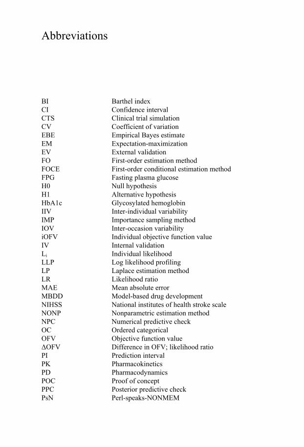
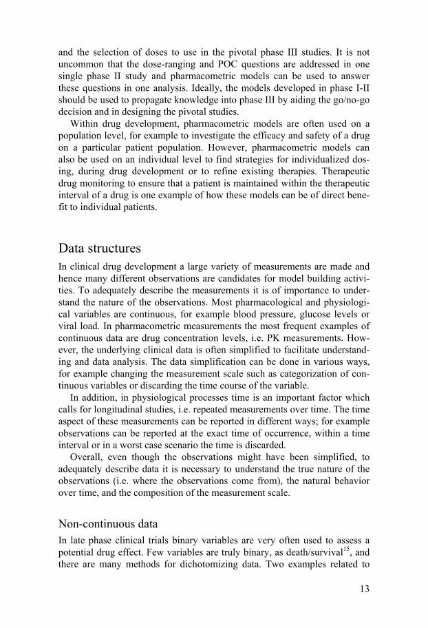
This issue of high attrition rates and increasing costs in drug development has been highlighted many times in the last decade by regulators4 and others3, 5, and model-based drug development (MBDD) has been identified as one methodology to make drug development more productive. MBDD involves mathematical and statistical approaches to construct and utilize models to increase the understanding of the drug and disease. Lalonde et al6 have described the key elements of MDBB as depicted in Figure 1. An es-sential part of MBDD is the discipline of pharmacometrics, which is a multi-

12

disciplinary field including clinical pharmacology, medicine, statistics, pharmacology, computational methods, engineering, etc7. Pharmacometrics is a relatively new scientific discipline, having evolved over the last 30 years and can be described as: “the science of developing and applying mathemat-ical and statistical methods to (a) characterize, understand, and predict a drug’s PK and PD behavior; (b) quantify uncertainty of information about that behavior; and (c) rationalize data-driven decision making in the drug development process and pharmacotherapy”8. With this definition pharma-cometrics could be considered the back bone of MBDD. Jonsson and Shein-er9 have shown that the use of scientific model-based statistical tests can improve the efficiency of clinical trials and the use of pharmacometric mod-els as decision making tools within drug development is increasing6, 10-14.

Figure 1. Key components of model-based drug development (MBDD). Reprinted with permission from Macmillan Publishers Ltd: Clinical Pharmacology & Thera-peutics (Lalonde et al6), copyright (2008).

Even though all phases of clinical drug development could benefit from a MBDD strategy, the most obvious stages to implement a pharmacometric approach are the early clinical development phases (phase I-II). Data from phase I often contain large amounts of information about the PK and safety profile of the drug, and models can be established to describe these relations. In phase II, proof-of-concept (POC) studies are designed to give preliminary evidence of efficacy and safety, with the aim to inform a decision about pro-ceeding into full development of the drug. In practice the POC decision is often based on whether a required effect size can be detected in comparison to placebo or a comparator treatment. Additionally, to be able to answer the addressed question within a reasonable time frame, the studies should be as small as possible. All of these aspects are well suited to model based analy-sis. Phase II also includes the identification of the dose-response relations

Model-based drug development

PK-PD and disease models

Competitor information and meta-analysis

Design and trial execution models

Trial performance metrics

Quantitative decision criteria

Data analysis model

13

and the selection of doses to use in the pivotal phase III studies. It is not uncommon that the dose-ranging and POC questions are addressed in one single phase II study and pharmacometric models can be used to answer these questions in one analysis. Ideally, the models developed in phase I-II should be used to propagate knowledge into phase III by aiding the go/no-go decision and in designing the pivotal studies.

Within drug development, pharmacometric models are often used on a population level, for example to investigate the efficacy and safety of a drug on a particular patient population. However, pharmacometric models can also be used on an individual level to find strategies for individualized dos-ing, during drug development or to refine existing therapies. Therapeutic drug monitoring to ensure that a patient is maintained within the therapeutic interval of a drug is one example of how these models can be of direct bene-fit to individual patients.

Data structures In clinical drug development a large variety of measurements are made and hence many different observations are candidates for model building activi-ties. To adequately describe the measurements it is of importance to under-stand the nature of the observations. Most pharmacological and physiologi-cal variables are continuous, for example blood pressure, glucose levels or viral load. In pharmacometric measurements the most frequent examples of continuous data are drug concentration levels, i.e. PK measurements. How-ever, the underlying clinical data is often simplified to facilitate understand-ing and data analysis. The data simplification can be done in various ways, for example changing the measurement scale such as categorization of con-tinuous variables or discarding the time course of the variable.

In addition, in physiological processes time is an important factor which calls for longitudinal studies, i.e. repeated measurements over time. The time aspect of these measurements can be reported in different ways; for example observations can be reported at the exact time of occurrence, within a time interval or in a worst case scenario the time is discarded.

Overall, even though the observations might have been simplified, to adequately describe data it is necessary to understand the true nature of the observations (i.e. where the observations come from), the natural behavior over time, and the composition of the measurement scale.

Non-continuous data In late phase clinical trials binary variables are very often used to assess a potential drug effect. Few variables are truly binary, as death/survival15, and there are many methods for dichotomizing data. Two examples related to

14

this thesis are: (i) the definition of a fully recovered stroke patient as a pa-tient with a stroke score of 1 at the last visit16, and (ii) a responder to heart-burn treatment as a patient with maximum one mild heartburn episode within the last week of treatment17.

Another common data class within clinical trials is ordered categorical da-ta. These observations are polychotomous with an internal ranking. A typical example of ordered categorical observations is the commonly used three-category reporting of side effects as “mild”, “moderate” or “severe”.

Many outcome measurements in clinical trials, disease symptoms or drug side effects, occur at a particular point in time. Examples of such outcome variables are: death, epileptic seizures, emesis or diarrhea episodes and bleeding events. And when the actual time point for the response, or event, is the main data feature of interest the data is classified as time-to-event (TTE) data, or repeated time-to-event (RTTE) data. Typically, TTE and RTTE data is described as event or no-event, however, many events can be associated with a graded scale; for example adverse events classified as mild, moderate or severe. When observations are reported along with the corresponding time of occurrence and grade of severity the data can be described as repeated time-to-categorical events (RTTCE), which is ideal for the ability of describ-ing the true occurrence of the data.

Clinical assessment scales A convenient tool for monitoring disease progression or to measure the treatment effect in a clinical trial is the use of clinical assessment scales. Examples of commonly used scales are Alzheimer's Disease Assessment Scale-cognitive subscale18 (ADAS-Cog), Positive and Negative Syndrome Scale19 (PANSS) for measuring symptom severity of patients with schizoph-renia, and NIH stroke scale20 (NIHSS) and Barthel Index21 (BI) to quantify neurological and functional impairments after stroke, respectively. These scores are generally comprised of a series of items divided into sections, each of which addresses a different aspect the disease. The scores from each section are added together to provide cumulative categorical scores, which address particular clinical questions. These questions, in turn, vary from scale to scale.

A feature of many clinical assessment scales, particularly within the neu-rological disease area, is that the scores are non-monotonic and unpredicta-ble. Additionally, as all longitudinal observations, the clinical assessment data may suffer from dropout, meaning that patients fail to complete the study resulting in missing data.

15

Population modeling As has been previously described, the aim with pharmacometric modeling is to define mathematical models to describe and quantify drug behavior and action, as well as disease progression, using data collected in clinical trials. As humans (patients and healthy volunteers) differ from one another it is of importance to consider these differences in the pharmacometric models. When population modeling was first introduced in the field of PK-PD analy-sis a two stage approach was used to characterize the PK-PD relationships. In the standard two stage approach each individual’s model parameters are estimated separately followed by calculating summary statistics on the indi-vidual parameters to assess population parameters (mean) and the variability in the data22-24. Limitations with this method include the large number of measurements per individual needed to obtain unbiased parameters, the possible inability to fit the same structural model to all individuals and more importantly, the inability to separate true biological variability between indi-viduals (inter-individual variability, IIV) from residual variability such as model misspecification and bioassay errors.

Mixed effects modeling Mixed effects modeling is an alternative to the standard two stage ap-

proach, where the data from all individuals are used to simultaneously obtain population parameters (means and variances)23, 25. The term “mixed” refers to the use of both fixed effects that characterize the typical individual (the mean) and random effects that describes the variability components of the data. The random effects are divided up into conceptually two levels: the difference between the individual prediction and the observation (residual error) and the variability between individuals (inter-individual variability, IIV). If the individual parameters change between occasions, randomly or due to some unknown physiological process, a third level of variability can be introduced; inter-occasion variability (IOV)26. Potentially, other sources of variability exist, for example inter-study variability, and these can be in-corporated in the same manner as IOV.

The general structure of a mixed effects model is expressed as follows:

(1)

where yijk is the jth observation at occasion k in individual i. yijk is described by a linear or nonlinear function f(…) of a vector of individual parameters Pik and a vector of independent variables Xijk. In pharmacometric modeling, typical independent variables are time, dose and exposure, although Xijk can also contain other predictors such as demographic covariates. The ijk de-scribes the difference between the individual prediction and the observation

16

at each measurement (residual variability), also known as the error model. In equation 1 the residual variability is expressed as an additive model, howev-er, the residual error may display any shape although the most commonly used error models are the additive, proportional or a combination of the two27.

The individual parameter Pik for the ith individual at the kth occasion can be described by the expression:

(2)

in which is the typical value (fixed effect) of parameter P in the studied population, and i and i are the random values (or random effects) that de-scribes the difference between the typical value and the individual parameter value, with respect to the individual and occasion, respectively. In the above equation the random effects are log-normally distributed with respect to the fixed effect, which is the most common model. Other models to describe the relationship are possible.

Covariates One aspect when developing pharmacometric models is to reduce the unex-plained IIV and to gain mechanistic understanding about the system, while still adhering to the paradigm of developing parsimonious models. This is achieved by including predictors, known as covariates. The most obvious covariates in pharmacometrics are time, dose and exposure (often defined as independent variables as above) but there are also other categories of cova-riates that contain information. Demographic covariates are the group of variables that describes the general characteristics of the individual, for ex-ample age, weight, sex, genotype and disease state. Another common class of covariates is concomitant medication, and these predictors give informa-tion on potential drug interactions, but also on influences of other diseases. A third group of covariates are so called Markovian predictors, which are data dependent variables such as previous observation, time since previous observation or change since previous observation.

Model estimation The nonlinear mixed effects modeling software NONMEM (Icon Develop-ment Solutions, Ellicott City, MD, USA)28 was used throughout this thesis. NONMEM is the most widely used software within PK-PD modeling and is based on maximum likelihood methods, in which the parameters of the mod-el are estimated by maximization of the likelihood of the data given the model. Due to the nonlinearity in the models (with respect to the random effects) the likelihood function can generally not be calculated exactly and

17

traditionally different types of linearization have been used to create a closed form solution to the likelihood. The options available in NONMEM have historically been the first-order method (FO), the first-order conditional es-timation method (FOCE), and the Laplace method. Additionally, a nonpara-metric maximum likelihood method (NONP) is included in the NONMEM package.

Recently however, several other estimation methods29 have become avail-able in NONMEM, increasing the possibility of using the most appropriate estimation method for the problem at hand without the inconvenience of moving to a different software. The newly available methods include: (i) the expectation maximization methods iterative two stage (ITS), importance sampling expectation maximization (IMP), and stochastic approximation expectation maximization (SAEM) and (ii) a Bayesian method named full Markov Chain Monte Carlo (MCMC) Bayesian analysis. The methods used in this thesis are further described in the methods section.

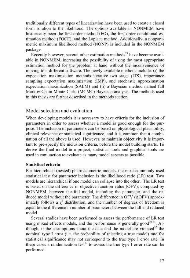
Model selection and evaluation When developing models it is necessary to have criteria for the inclusion of parameters in order to assess whether a model is good enough for the pur-pose. The inclusion of parameters can be based on physiological plausibility, clinical relevance or statistical significance, and it is common that a combi-nation of all the above is used. However, to maintain objectivity it is impor-tant to pre-specify the inclusion criteria, before the model building starts. To derive the final model in a project, statistical tools and graphical tools are used in conjunction to evaluate as many model aspects as possible.

Statistical criteria For hierarchical (nested) pharmacometric models, the most commonly used statistical test for parameter inclusion is the likelihood ratio (LR) test. Two models are hierarchical if one model can collapse into the other. The LR test is based on the difference in objective function value (OFV), computed by NONMEM, between the full model, including the parameter, and the re-duced model without the parameter. The difference in OFV ( OFV) approx-imately follows a 2 distribution, and the number of degrees of freedom is equal to the difference in number of parameters between the full and reduced model.

Several studies have been performed to assess the performance of LR test using mixed effects models, and the performance is generally good30-31. Al-though, if the assumptions about the data and the model are violated32 the nominal type I error (i.e. the probability of rejecting a true model) rate for statistical significance may not correspond to the true type I error rate. In these cases a randomization test33 to assess the true type I error rate can be performed.

18

If the competing models are not hierarchical, the Bayesian information criterion34 or Akaike information criterion35 can be used as statistical tests for parameter inclusion.

Simulation based diagnostics The actual performance of a model can be difficult to assess by only using statistical metrics, and as pharmacometric models are used more and more for future predictions and clinical trial simulations the predictive perfor-mance of these models has become increasingly important. Another reason for the increased use of simulation based diagnostics is the increasing use of models for non-continuous data, where the model is parameterized such that a probability or a hazard is estimated. To assess the predicted categorical observations or events, of these types of models, it is necessary to simulate from the model.

The numerical predictive check36 (NPC) is designed to numerically assess the appropriateness of model inferences by calculations of prediction inter-vals (PIs) derived by simulation from model parameters. The NPC is an overall metric for the predictive performance, but may be more difficult to derive information about which part of the model that might need improve-ment.

Visual predictive checks37-38 (VPC) are more or less mandatory model di-agnostics at the time of writing, and is a rapidly evolving topic. The ob-served data is graphically compared with data simulated from the model, using the same design as the original study. Although based on the same simulated data as the NPC, the VPC can add information about which part of the data profile a miss-specification has occurred. However, VPCs need to be evaluated with caution. Model miss-specifications can be hidden if the population predictions vary from individual to individual, and if inappro-priate stratifications have been used in the graphical display37.

All simulation based diagnostics are computer intensive to varying de-grees, and often require some programming skills. Fortunately for the user, both NPC and VPC are incorporated tools in PsN39-40 and graphical output is available in Xpose 441, making these methods more accessible.

To assess the predictive performance, accounting for the uncertainty in the model parameters, a posterior predictive check42 (PPC) should be used. Commonly, a descriptive measurement is used as the metric in the predictive performance such as maximum concentration or responder rate. The metric is obtained by simulations using parameter estimates sampled from the post-erior density of the parameters, i.e. the distribution of parameters values accounting for the standard error of the estimates. As the PPC necessitates intensive data simulation and involves programming exercises it is not used in every step of the model development, but rather as a tool to assess the performance of the, in other aspects, final model.

19

Internal and external model validation The model evaluation tools described above are all classified as internal validation (IV) techniques43, meaning that the data used in the evaluation of the model is the same as in the model development. Forecasting in new pa-tients or in novel situations given an internally validated model potentially provides over-optimistic projections, meaning that the model produces pre-dictions that are only valid for the sample of the population that it has been developed on. One approach to evaluate the confidence of the model para-meters is to externally validate (EV) predictive models44, meaning that the model is evaluated on a dataset from a separate study. Unfortunately, the existence of a dataset from a different clinical study performed under the same conditions is very rare. Instead, the analyst may consider a data-splitting alternative, which is often classified as an IV technique, however throughout this thesis it is noted as EV since data not used in the model de-velopment are used in the model validation. This is achieved by randomly splitting the original dataset into two portions, one for building the model (“learning dataset”) and one for model evaluation (“validation dataset”). However, as not all the available information is utilized to build the model structure, loss of study power, decreased prediction accuracy45, and a reduc-tion in model stability43 can occur. As a result, when a data-splitting proce-dure is used, the parameter estimates will be less informed, than when IV is applied, and this will propagate into the predictions from the model.

Design and analysis of clinical trials The design of a trial is closely linked to the analysis of the trial, since the design is dependent on what analysis approach is to be used. Both the design and the analysis strategy need to be decided prior to the start of the clinical trial.

The design of a clinical trial includes factors such as the type of design (e.g. parallel group or cross over), number of treatment arms, number of observations, length of the study, and study size, all dependent on the pur-pose of the study. Presently, the most used trial design is the randomized dose-controlled trial (RDCT) design. The simplicity in assigning the patients to different dose groups makes the RDCT easy to perform and cost effective compared with alternative designs. However, when characterizing an expo-sure–response relationship it has been suggested that the randomized con-centration-controlled trial (RCCT) is potentially a more informative design46-

47, and as an extension to the RCCT the randomized biomarker-controlled trial (RBCT) design has been described48. The drawback with an RCCT/RBCT, on the other hand, is that it is necessary to titrate each patient by some adaptive feedback strategy to ensure that the defined target concen-

20

tration or biomarker level is reached. A further issue is that it may not be possible to reach the specified target level in some patients, so called formal data loss, meaning that the desired reduction in variability due to the rando-mization scheme will not be achieved. These practical complications, in particular the first, in carrying out an RCCT or RBCT have limited their use.

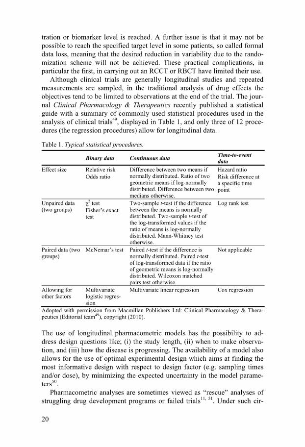
Although clinical trials are generally longitudinal studies and repeated measurements are sampled, in the traditional analysis of drug effects the objectives tend to be limited to observations at the end of the trial. The jour-nal Clinical Pharmacology & Therapeutics recently published a statistical guide with a summary of commonly used statistical procedures used in the analysis of clinical trials49, displayed in Table 1, and only three of 12 proce-dures (the regression procedures) allow for longitudinal data.

Table 1. Typical statistical procedures.

Binary data Continuous data Time-to-event data

Effect size Relative risk Odds ratio

Difference between two means if normally distributed. Ratio of two geometric means if log-normally distributed. Difference between two medians otherwise.

Hazard ratio Risk difference at a specific time point

Unpaired data (two groups)

2 test Fisher’s exact test

Two-sample t-test if the difference between the means is normally distributed. Two-sample t-test of the log-transformed values if the ratio of means is log-normally distributed. Mann-Whitney test otherwise.

Log rank test

Paired data (two groups)

McNemar’s test Paired t-test if the difference is normally distributed. Paired t-test of log-transformed data if the ratio of geometric means is log-normally distributed. Wilcoxon matched pairs test otherwise.

Not applicable

Allowing for other factors

Multivariate logistic regres-sion

Multivariate linear regression Cox regression

Adopted with permission from Macmillan Publishers Ltd: Clinical Pharmacology & Thera-peutics (Editorial team49), copyright (2010).

The use of longitudinal pharmacometric models has the possibility to ad-dress design questions like; (i) the study length, (ii) when to make observa-tion, and (iii) how the disease is progressing. The availability of a model also allows for the use of optimal experimental design which aims at finding the most informative design with respect to design factor (e.g. sampling times and/or dose), by minimizing the expected uncertainty in the model parame-ters50.

Pharmacometric analyses are sometimes viewed as “rescue” analyses of struggling drug development programs or failed trials11, 51. Under such cir-

21

cumstances the trial design has not been optimized for the analysis and even though a pharmacometric analysis might be successful, the full capacity of such analysis has not been utilized and was not pre-defined as the primary analysis.

Statistical power and sample size The statistical power of a trial is defined as 1-(type II error). The type II error describes the probability of the null hypothesis being incorrectly ac-cepted, also known as “a false negative” result. Taking the example of hypo-thesis testing of an existing drug effect of 0.5 units, the type II error de-scribes the probability of not detecting the 0.5 unit drug effect though it truly exists. In general, although depending on the hypothesis and the statistical test, the minimum accepted statistical power of a clinical trial is 80 percent. Apart from the statistical test, the statistical power is influenced by factors such as type I error (“a false positive” result), the expected standard devia-tion of the sample and the sample size52. The power to detect a pre-defined effect is used to determine the size of a study. As the statistical power in-creases with increasing sample size it is important to define the acceptable power of a study (for example 80 percent) to include a reasonable number of individuals in the study. If a study is under powered, the risk is that the study fails to detect the defined effect even though it exists, and patients have needlessly been put through a clinical trial. An over powered study means that an excessive number of patients have been exposed to an experimental drug. In both cases more money and time than necessary is spent.

One of the drawbacks with using a pharmacometric model-based analysis is that it can be time consuming and computer intensive to assess the statis-tical power of a study. To do so one needs to simulate a large number of trials (>1000 is not uncommon) and estimate parameters under both the full (with a drug effect) and reduced models (without a drug effect) for all simu-lated datasets. If the model takes more than a few minutes to run, this exer-cise quickly becomes unfeasible, excluding a pharmacometric model-based analysis as the primary analysis method. However, Vong et al53 have devel-oped a new method of calculating a model-based statistical power, making pharmacometric analysis an attractive alternative in clinical trial evaluations. This method is further described in the methods section of this thesis.

Clinical trial simulations Apart from addressing questions of descriptive nature, such as describing the PK properties of a drug, or a PK-PD relationship, pharmacometric models are well suited for future predictions. One of the exercises these models can be used for are clinical trial simulations54-56 (CTS), such as in power calcula-

22

tions. CTS can be useful for other reasons as well, to address different as-pects of design and predicting outcome of future trials57. CTS is a corner stone of MBDD, to investigate possible future scenarios in a drug’s devel-opment, not the least as an aid to exclude clinical trials that will not have the properties to address the question at hand58. Pharmacometric models some-times get critiqued for making too many assumptions, regarding parameter distributions, drug effect relationships, etc, CTS is an excellent tool to inves-tigate the impact of these assumptions.

The general procedure in a clinical trial simulation exercise is: (i) the de-sign of the study is decided (for example number of treatment groups, study size, dose levels), then (ii) the parameter estimates from an existing model is used to generate outcomes (this step is replicated many times to achieve a distribution of outcomes), and (iii) statistical tests to answer the question at hand are applied on the simulated distribution of outcomes (as is done in power calculations).

There are conceptually two types of simulations; deterministic and sto-chastic (Monte Carlo) simulations. In the case of Monte Carlo clinical trial simulations the hypothesized individuals correspond to a random sample. In mixed effects model terms, the random effects are used in the simulations. This is the most common way of performing CTS, since the idea is that a single clinical trial represents a sample of the full population. By creating many samples, one can get an indication on how the samples differ from each other, i.e. compute the uncertainty in the outcomes given the model.

In deterministic simulations the random components of a pharmacometric model are ignored, and only the typical values are used. This type of simula-tion can be of value if one wants to simulate values for a specific individual (which is usually not the case in CTS) or wants to investigate different struc-tural models without the influence of random variability.

Software packages used for parameter estimation, e.g. NONMEM, SAS (SAS Institute Inc, Cary, NC, USA), and R (http://www.r-project.org), can be used for CTS. There is also software dedicated to CTS; Pharsight Trial Simulator (Pharsight Corporation, Mountain View, CA, USA). A drawback, however, is that there is no automated procedure to model the datasets pro-duced by Pharsight Trial Simulator, which is necessary if hypothesis testing is to be performed.

23

Aims

The general aim of the thesis was to investigate how the use of pharmacome-tric models can improve the design and analysis of clinical trials within drug development. Specific aims were:

Develop pharmacometric models for clinical assessment scales in stroke

and for graded severity events. Evaluate three estimation methods in repeated time-to-event modeling.

Investigate the predictive performance of internal and external validation

procedures.

Compare the efficiency (study power) of pharmacometric model-based design and analysis compared to conventional analysis.

25

Material and Methods

The larger part of the work in this thesis is based on simulation studies using a variety of pharmacometric models. In simulations the true conditions are known allowing for investigations of; the impact of analysis strategy (paper II, V and VI), model selection (paper II), estimation method (paper III), and model evaluation (paper IV). Indeed, a necessity for performing a simulation study is the existence of an appropriate model and in paper I real clinical data was used to develop two models for disease progression in acute stroke.

Clinical data Acute stroke A novel compound, clomethiazole, was found to have neuroprotective ef-fects in animal models1-5 and therefore underwent clinical development as potential treatment of acute stroke. Model building was performed using a dataset composed of scores measured on the NIHSS and BI scales, collected from 580 patients, clinically diagnosed with acute ischemic stroke, enrolled in the placebo arm of a double-blind, multinational, multicenter, placebo-controlled investigation of the effectiveness of clomethiazole (the CLASS-I study)59. Patients eligible for enrollment in the study began treatment within 12 hours after stroke. The analysis dataset consisted of patients with an aver-age age of 71.7 years (range 26-90) and average baseline NIHSS score of 16.8 (range 4-31). Scores were assessed on the NIHSS at admission, and subsequently at 7, 30, and 90 days. BI assessments were made at 7, 30 and 90 days, as well as by telephone at 60 days.

Simulated data As have been mentioned, the majority of the work in this thesis is based on simulation studies which require models to generate of data. The pharmaco-metric models used for this purpose are listed in Table 2.

26

Table 2. A summary of pharmacometric models used for simulations of data in the included papers.

Data Model(s) Paper

PK 1-compartment, 1st order absorption, linear elimination

II, IV, Va

Biomarker Emax model V

Adverse event Inhibitory Emax model V

Binary endpoint Logistic model with a linear logit function V

Heartburn graded events Repeated time-to-event + ordered categorical models

II

Repeated events Constant hazard repeated time-to-event model III

Stroke scores NIHSS model (developed in paper I) VI

Glycosylated hemoglobin and fasting plasma glucose levels

FPG-HbA1c model60 VI

a Steady state conditions were assumed

Heartburn data Heartburn was used as an example when investigating events of graded se-verity. The study design included 72 patients suffering from gastroesopha-geal reflux disease, allocated to one of six treatment arms; placebo or one of the five drug treatment dose levels: 10, 50, 100, 200, or 400 mg. Data related to individual PK parameters (clearance, volume of distribution, and absorp-tion rate) were simulated separately from a one-compartment PK model and then used in an RTTCE model to generate symptoms. The time and graded symptoms (four categories) were recorded over 12 h, with a maximum of 360 events per individual (corresponding to one event every second minute).

Repeated time-to-event data The study design consisted of 120 individuals observed over 12 days. The datasets used for simulation consisted of records every hour, adding up to a possible total of 288 events per individual, under the assumption that an event could not occur more frequently than once every hour. The frequencies of individuals with events were varied between 6-99%, and the inter-individual variability in number of events was varied between 0-200% CV.

Exposure data In paper IV, a one-compartment, first-order absorption and linear elimination model was used to generate three concentration observations per individual. An inter-individual variability of 30% CV was applied on the absorption rate, clearance and volume of distribution together with a 10% CV propor-

27

tional residual error on the observations. The study size was varied between 6-384 individuals.

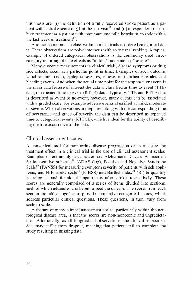
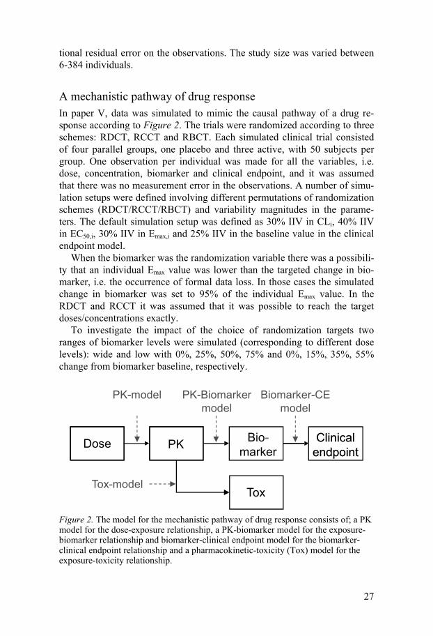
A mechanistic pathway of drug response In paper V, data was simulated to mimic the causal pathway of a drug re-sponse according to Figure 2. The trials were randomized according to three schemes: RDCT, RCCT and RBCT. Each simulated clinical trial consisted of four parallel groups, one placebo and three active, with 50 subjects per group. One observation per individual was made for all the variables, i.e. dose, concentration, biomarker and clinical endpoint, and it was assumed that there was no measurement error in the observations. A number of simu-lation setups were defined involving different permutations of randomization schemes (RDCT/RCCT/RBCT) and variability magnitudes in the parame-ters. The default simulation setup was defined as 30% IIV in CLi, 40% IIV in EC50,i, 30% IIV in Emax,i and 25% IIV in the baseline value in the clinical endpoint model.

When the biomarker was the randomization variable there was a possibili-ty that an individual Emax value was lower than the targeted change in bio-marker, i.e. the occurrence of formal data loss. In those cases the simulated change in biomarker was set to 95% of the individual Emax value. In the RDCT and RCCT it was assumed that it was possible to reach the target doses/concentrations exactly.

To investigate the impact of the choice of randomization targets two ranges of biomarker levels were simulated (corresponding to different dose levels): wide and low with 0%, 25%, 50%, 75% and 0%, 15%, 35%, 55% change from biomarker baseline, respectively.

Figure 2. The model for the mechanistic pathway of drug response consists of; a PK model for the dose-exposure relationship, a PK-biomarker model for the exposure-biomarker relationship and biomarker-clinical endpoint model for the biomarker-clinical endpoint relationship and a pharmacokinetic-toxicity (Tox) model for the exposure-toxicity relationship.

Dose PK Clinicalendpoint

Tox

Bio-marker

Clinicalendpoint

-

PK-model PK-Biomarker model

Biomarker-CE model

Tox-model

28

Acute stroke data (NIHSS scores) The design of the study was a parallel study with four arms; placebo and three active doses. Score assessments were made at day 0, 7, 30 and 90. A linear drug effect was added on the magnitude of improvement (using the NIHSS model developed on clinical data). The dose-effect relation was cali-brated such that a low, medium and high dose level would result in 25%, 33% and 55% increase in the proportion fully recovered patients at end of study compared to placebo (resulting in a drug parameter value of 0.1 and dose levels of 2.5, 3.8 and 5.8). The definition of a fully recovered patient was a NIHSS score of 0 or 116. 55% relative proportion of fully recovered patients was a clinically relevant effect, assuming an equal treatment effect as the comparator, t-PA treatment16.

A second study design, mimicking a pure proof-of-concept trial, was si-mulated excluding the low and medium dose.

Fasting glucose and glycosylated hemoglobin data The study design was a parallel four arm study; placebo and three active groups. Fasting plasma glucose (FPG) and sampled at -6, -4, -1, 0, 2, 4, 6, 8, 10, 12 and 15 weeks , glycosylated hemoglobin (HbA1c) at weeks -6, 0, 6, 12, and four trough PK samples were collected during the study period ac-cording to the study design presented by Hamrén et al60. The mean (standard deviation) baseline characteristics for FPG and HbA1c were 9.85(2.20) mmol/L and 7.1(1.1)%, respectively. A drug effect was assumed on the rate of elimination of FPG. The dose-effect relationship was calibrated such that a low, medium and high dose level would result in 0.17%, 0.50% and 0.63% average decrease in HbA1c at week 12 in comparison with the placebo group, where the 0.63% was considered a clinically meaningful effect which a proof-of-concept study should be able to detect with a defined power.

A pure POC study was designed excluding the low and medium doses, and the follow up FPG sample at week 15 was omitted. The drug effect was modified from a continuous exposure-response to a categorical dose effect.

Model building Clinical assessment scales in acute stroke

Scores of the kind recorded in acute stroke are non-monotonic and unpre-dictable: scores may increase or decrease (a score change of zero was re-garded as disease deterioration, except if complete recovery was reached) at any given measurement occasion, or, in the case of dropout, they may simply cease. The progression of disease (or recovery) could therefore be seen as a

29

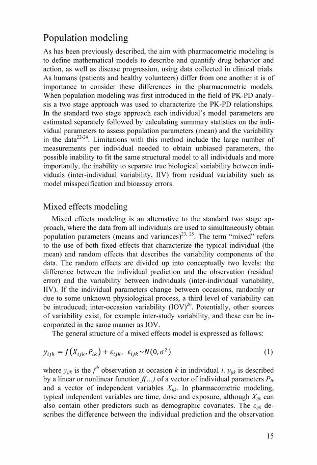
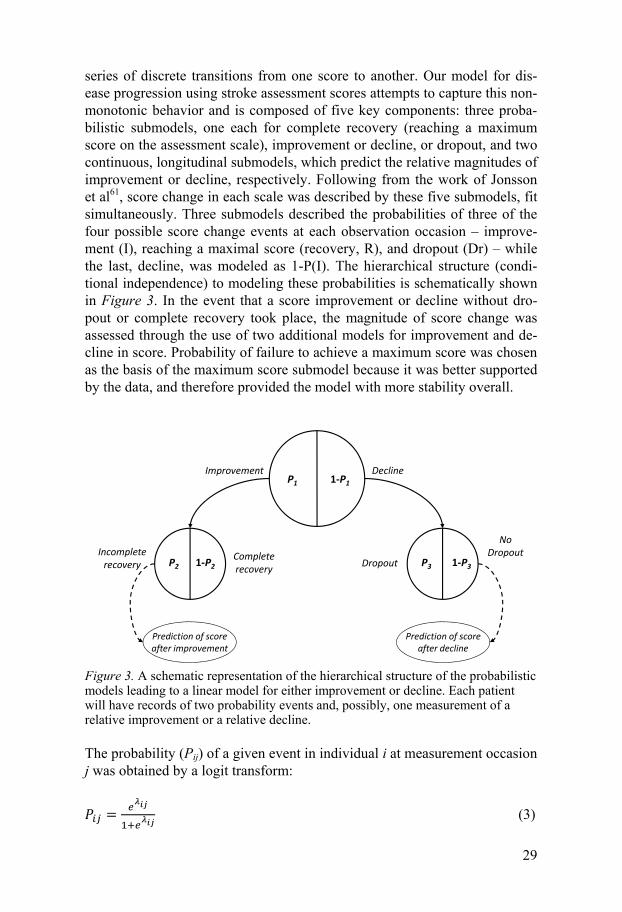
series of discrete transitions from one score to another. Our model for dis-ease progression using stroke assessment scores attempts to capture this non-monotonic behavior and is composed of five key components: three proba-bilistic submodels, one each for complete recovery (reaching a maximum score on the assessment scale), improvement or decline, or dropout, and two continuous, longitudinal submodels, which predict the relative magnitudes of improvement or decline, respectively. Following from the work of Jonsson et al61, score change in each scale was described by these five submodels, fit simultaneously. Three submodels described the probabilities of three of the four possible score change events at each observation occasion – improve-ment (I), reaching a maximal score (recovery, R), and dropout (Dr) – while the last, decline, was modeled as 1-P(I). The hierarchical structure (condi-tional independence) to modeling these probabilities is schematically shown in Figure 3. In the event that a score improvement or decline without dro-pout or complete recovery took place, the magnitude of score change was assessed through the use of two additional models for improvement and de-cline in score. Probability of failure to achieve a maximum score was chosen as the basis of the maximum score submodel because it was better supported by the data, and therefore provided the model with more stability overall.

Figure 3. A schematic representation of the hierarchical structure of the probabilistic models leading to a linear model for either improvement or decline. Each patient will have records of two probability events and, possibly, one measurement of a relative improvement or a relative decline.

The probability (Pij) of a given event in individual i at measurement occasion j was obtained by a logit transform:

(3)

1-P1P1

P2 1-P2Complete recovery

Incomplete recovery Dropout

No Dropout

Improvement Decline

P3 1-P3

Prediction of score after improvement

Prediction of score after decline

30

where ij is a linear function which follows the form

(4)

where C is a constant, and g(Xij) is a function of covariates. Similarly, rela-tive score change magnitude (yij,rel) was given by

(5)

Where Ci,j

(6)

The assessment of potential covariates was made in two parts; first Marko-vian predictors were tested and secondly demographic predictors were tested. In both cases the criteria for inclusion was based on the OFV (likelih-ood ratio test, p<0.05) and the visual predictive check. For a covariate to be included in the model it had to pass the likelihood ratio test and also to im-prove the graphs in the visual predictive check.

Estimation algorithms To obtain adequate parameter estimates it is of importance that the appropri-ate estimation method is selected. Maximum likelihood methods aim at es-timating parameters that maximizes the likelihood of the data given the model. The likelihood L is a product of the individual likelihoods Li as shown in Equation 7.

(7)

As the likelihood function does not have a closed form solution for nonlinear models, with respect to i, various approximations to the likelihood have been developed. Throughout this thesis maximum likelihood methods avail-able in NONMEM (Icon Development Solutions) were utilized.

First-order conditional estimation method The first-order conditional (FOCE) method performs a linearization of the nonlinear model using a first-order Taylor expansion around the conditional

31

estimate of i62. Interactions between i and ij can be accounted for by the

method FOCE with interaction (FOCE-I). FOCE and FOCE-I have to this date been the preferred method for models describing continuous data.

Laplace method In the Laplace method the closed form solution of the maximum likelihood integral is obtained by using the Laplace approximation. This is accom-plished by a linearization of the model involving a second-order Taylor ex-pansion around the conditional estimates of 62-63. The Laplace method is needed with highly nonlinear models, with respect to , such as logistic re-gression models and time-to-event models. This method was used in all projects except the work presented in paper IV.

Stochastic approximation expectation-maximization method The SAEM estimation method64 belongs to the family of expectation-maximization (EM) algorithms which are characterized by exact likelihood maximization65. In the E-step the expectation of the likelihood given current estimates of the population parameters is calculated, and in the M-step new population parameters maximizing the likelihood are computed given the expected likelihood in the E-step. The process is iterative and the parameter values are updated with the parameter estimates from the M-step until a sta-ble objective function value is obtained. In the SAEM method the E-step is divided into two parts: first a simulation of individual parameters using a Markov Chain Monte Carlo algorithm (S-step), followed by a stochastic approximation of the expected likelihood (SA-step).

Importance sampling method The importance sampling method66 is also an EM-algorithm, described in the SAEM section above. The E-step differs from the SAEM method in that a Monte Carlo integration using importance sampling around current individu-al estimates is performed to obtain the expected likelihood. Population pa-rameters are then updated from subjects’ conditional parameters by a single iteration in the M-step. Due to fewer stochastic processes, with intense sam-pling, the importance sampling method could be expected to result in more accurate parameter estimates than the SAEM method.

Nonparametric method The main difference between the previously described estimation methods and the nonparametric method is the relaxation of the distribution assump-

32

tion in the inter-individual variability present in the model. In NONMEM, the nonparametric maximum likelihood estimation is performed in two steps (i) the estimation of discrete support points at which the parameter distribu-tion is to be evaluated and (ii) estimation of the population probability at each support point. The estimation of the support points is equivalent to the estimation of empirical Bayes estimates (EBEs), and in this work the FOCE method was used to establish the EBEs. The second step, the joint probabili-ty estimation, operates as a large mixture model where the number of mix-tures/submodels is equal to the unique vectors of individual parameters. The entire joint nonparametric probability density, of the data given a model, is defined as the estimated probability of data belonging to each mixture67.

Model evaluation Bias and precision The parameter bias, in papers III and V, was assessed by calculating the relative estimation error (REE):

(8)

Where Pest is the estimated parameter value and the Ptrue is the value used in the generation of the data. The mean of the relative estimation error was defined as the parameter bias.

As composite measures of parameter bias and precision root mean squared error (RMSE, Equation 9) and relative RMSE (RRMSE, Equation 10) was used in papers III and V.

(9)

(10)

Where n is the total number of estimated parameters (i.e. number of simu-lated datasets).

In paper I log-likelihood profiling39 (LLP), as implemented in PsN, was used to determine confidence intervals for the parameter estimates. Each parameter is then fixed to a series of values around the mean, after which the model was re-fit. This procedure generates a 95% confidence interval for the parameter estimates.

33

Visual predictive check VPC is a graphical tool to assess the model performance and was used in papers I and II. The observed data is compared with data simulated from the model using, the same design as in the original study. Typically, VPC graphs consist of lines representing the median/mean and outer percentiles of the observed data together with lines representing the median/mean and outer percentiles of the multiple datasets simulated from the model. The lines representing simulated data are sometimes accompanied with confidence intervals for these values, visualized as shaded areas. For the VPC, the PIs are calculated for each defined interval of the independent variable, for ex-ample for all the data within every hour. Any potential model miss-specifications are visualized by discrepancies between the lines representing the observed and simulated data, respectively.

In paper III the characteristics of the estimated models with respect to fea-tures of the data were investigated graphically by calculating the normalized proportion of individuals without events, where the difference in proportion of individuals without events in the re-simulation and the original dataset was divided by the median proportion in all the original datasets. The norma-lized proportion mainly reflects the bias in the population parameter, while the average number of individual events is mostly affected by the bias in the variance parameter.

Numerical predictive check NPC is a simulation model-based diagnostic implemented in PsN, designed to numerically assess the appropriateness of model inferences through PIs derived by simulation from the model. For the NPC, a PI is computed sepa-rately for each data point, by simulation of numerous datasets following the same design as the original realized design, and the reported value describes the proportion of data points that fall outside of its own simulated PI. This is different from the VPC where the PI contains all data in an interval of the independent variable. NPC was the main metric of when evaluating internal and external validation in paper IV.

Internal and External validation To compare IV and EV predictive performance, a validation procedure, de-noted population validation (PV), was used. Conceptually, the PV procedure is analogous to an EV-based approach for which the external dataset pool intended for validation is enlarged to the extent that it can be considered to mimic the distribution of observations of the target population. In these ideal circumstances, conclusive evidence with regards to the predictive behavior of a model can be established. Therefore, PV was used as an objective crite-

34

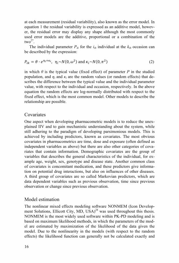
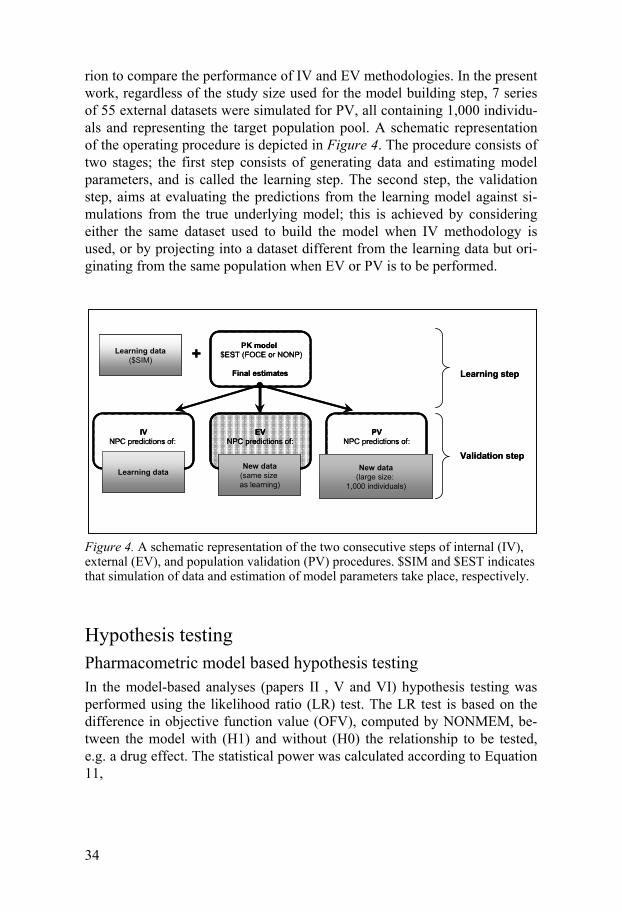
rion to compare the performance of IV and EV methodologies. In the present work, regardless of the study size used for the model building step, 7 series of 55 external datasets were simulated for PV, all containing 1,000 individu-als and representing the target population pool. A schematic representation of the operating procedure is depicted in Figure 4. The procedure consists of two stages; the first step consists of generating data and estimating model parameters, and is called the learning step. The second step, the validation step, aims at evaluating the predictions from the learning model against si-mulations from the true underlying model; this is achieved by considering either the same dataset used to build the model when IV methodology is used, or by projecting into a dataset different from the learning data but ori-ginating from the same population when EV or PV is to be performed.

Figure 4. A schematic representation of the two consecutive steps of internal (IV), external (EV), and population validation (PV) procedures. $SIM and $EST indicates that simulation of data and estimation of model parameters take place, respectively.

Hypothesis testing Pharmacometric model based hypothesis testing In the model-based analyses (papers II , V and VI) hypothesis testing was performed using the likelihood ratio (LR) test. The LR test is based on the difference in objective function value (OFV), computed by NONMEM, be-tween the model with (H1) and without (H0) the relationship to be tested, e.g. a drug effect. The statistical power was calculated according to Equation 11,

PK model $EST (FOCE or NONP)

Final estimates

IVNPC predictions of:

EVNPC predictions of:

PVNPC predictions of:

Learning data($SIM) +

New data(same size as learning)

New data(large size:

1,000 individuals)

Learning data

Learning step

Validation step

PK model $EST (FOCE or NONP)

Final estimates

IVNPC predictions of:

EVNPC predictions of:

PVNPC predictions of:

PK model $EST (FOCE or NONP)

Final estimates

IVNPC predictions of:

EVNPC predictions of:

PVNPC predictions of:

Learning data($SIM) +

New data(same size as learning)

New data(large size:

1,000 individuals)

Learning data

Learning step

Validation step

35

(11)

Where df is degrees of freedom, i.e. the difference in number of parameters between H1 and H0 models and N is the total number of simulated trials. The significance level required to reject the null hypothesis was set to 5%. This corresponds to differences in OFV of 3.84 and 5.99 for 1 and 2 degrees of freedom, respectively, following a 2 distribution.

Monte-Carlo Mapped Power In paper VI, the newly developed Monte-Carlo mapped power (MCMP) method53 was used to calculate the study power. The MCMP method is based on the hypothesis testing principle of the LR test in nonlinear mixed effect models, but with the MCMP method multiple random samples of in-dividual objective function values (iOFV) are used as a substitute for mul-tiple simulated and estimated studies. This substitution is based on the fact that the individual objective function values sum up to the overall OFV of a model for a given dataset as shown in Equation 12 (where Li denotes the individual likelihood and L the total likelihood).

(12)

The hypothesis of a possible drug effect can be tested with the LR test by assessing the difference in the objective function value ( OFV) between two nested models (i.e. including or not including the hypothesized drug effect). The OFV follows a 2 distribution with degrees of freedom corresponding to the difference in number of parameters between the two competing mod-els. A model that corresponds to the null hypothesis of no drug effect will hereafter be referred to as a reduced model, and a model corresponding to the alternative hypothesis of an existing drug effect will be referred to as a full model. With the MCMP method, iOFV values estimated with a single full and single reduced model are used to calculate many iOFV (Equation 13). The sum of n randomly sampled iOFV is used as a surrogate for the

OFV of a study with n number of subjects (Equation 14). The singe estima-tion step is performed with a large dataset (typically >20 times the sample size needed for 80% power) simulated under the full model to form a large pool of iOFVs.

36

(13)

(14)

The OFV calculation is repeated 10,000 times and the study power is com-puted as the percentage of OFVs greater than the significance level crite-rion defined by the LR test. The procedure is repeated with varying sample size (e.g. in increments of one patient per study arm) to map the power ver-sus sample size relationship up to a defined maximum power of interest.

Conventional hypothesis testing The conventional analyses of the data were group wise comparisons of the clinical endpoint. In the case of normally distributed continuous variables, as in paper VI, a two-sample t-test was employed with the null hypothesis that the means within each group are equal.

When comparing proportions, such as responder rates or with binary data, an unpaired 2 test was used to compare the study arms (papers II and V). The null hypothesis in a 2 test is that the proportions are equal across all groups.

As in the pharmacometric model-based analysis, the conventional statis-tical power was calculated as the sum of trials where the test statistic showed significance divided by the total number of simulated trials.

37

Results

Developed pharmacometric models In total four new pharmacometric models were developed; two models to describe the neurological and functional aspects, respectively, of disease progression after acute stroke, and two different models to simultaneously describe the frequency and severity of graded events. All four models were developed with the common goal of describing the reported data as closely as possible to the natural occurrence of the observations while retaining good prediction properties.

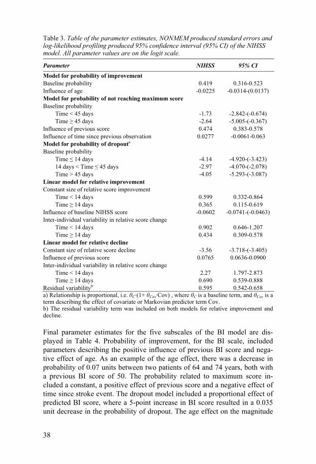
Models for stroke clinical assessment scales The final parameter estimates for the five submodels forming the NIHSS model are displayed in Table 3. The probability of improvement decreased by 0.05 units, between the ages of 64 and 74. The submodel for not reaching complete recovery (maximum score) was influenced by the previously ob-served score and the time elapsed since the previous observation. The proba-bility of dropout included a baseline term with change points at day 14 and 45, and a proportional effect of predicted NIHSS score (from the NIHSS relative score decline submodel) at the imputed time of dropout (i.e. halfway between the last measured observation and the subsequent intended observa-tion appointment). The effect of the NIHSS score was such that the probabil-ity of dropout increased approximately 0.015 units with an increase of 1 NIHSS score unit. The continuous model for relative improvement, meas-ured on the NIHSS scale, consisted of a baseline term, with a break point at day 14, and a negative effect of the baseline NIHSS observation (i.e. a se-vere baseline status decreases the magnitude of improvement) and terms for IIV and residual variability. Relative decline in score was described similar-ly, with a positive effect of previous score (i.e. larger decline), however no other changes over time could be supported.

38

Table 3. Table of the parameter estimates, NONMEM produced standard errors and log-likelihood profiling produced 95% confidence interval (95% CI) of the NIHSS model. All parameter values are on the logit scale.

Parameter NIHSS 95% CI

Model for probability of improvement Baseline probability 0.419 0.316-0.523 Influence of age -0.0225 -0.0314-(0.0137) Model for probability of not reaching maximum score Baseline probability Time < 45 days -1.73 -2.842-(-0.674) Time 45 days -2.64 -5.005-(-0.367) Influence of previous score 0.474 0.383-0.578 Influence of time since previous observation 0.0277 -0.0061-0.063 Model for probability of dropouta

Baseline probability Time 14 days -4.14 -4.920-(-3.423) 14 days < Time 45 days -2.97 -4.070-(-2.078) Time > 45 days -4.05 -5.293-(-3.087) Linear model for relative improvement Constant size of relative score improvement Time < 14 days 0.599 0.332-0.864 Time 14 days 0.365 0.115-0.619 Influence of baseline NIHSS score -0.0602 -0.0741-(-0.0463) Inter-individual variability in relative score change Time < 14 days 0.902 0.646-1.207 Time 14 day 0.434 0.309-0.578 Linear model for relative decline Constant size of relative score decline -3.56 -3.718-(-3.405) Influence of previous score 0.0765 0.0636-0.0900 Inter-individual variability in relative score change Time < 14 days 2.27 1.797-2.873 Time 14 days 0.690 0.539-0.888 Residual variabilityb 0.595 0.542-0.658 a) Relationship is proportional, i.e. C·(1+ Cov·Cov) , where C is a baseline term, and Cov is a term describing the effect of covariate or Markovian predictor term Cov. b) The residual variability term was included on both models for relative improvement and decline.

Final parameter estimates for the five subscales of the BI model are dis-played in Table 4. Probability of improvement, for the BI scale, included parameters describing the positive influence of previous BI score and nega-tive effect of age. As an example of the age effect, there was a decrease in probability of 0.07 units between two patients of 64 and 74 years, both with a previous BI score of 50. The probability related to maximum score in-cluded a constant, a positive effect of previous score and a negative effect of time since stroke event. The dropout model included a proportional effect of predicted BI score, where a 5-point increase in BI score resulted in a 0.035 unit decrease in the probability of dropout. The age effect on the magnitude

39

of improvement was very small, less than a 5-point change over 10 years, and was over-shadowed by the effect of baseline NIHSS and previous BI score.

Table 4. Table of the parameter estimates, NONMEM produced standard errors and log-likelihood profiling produced 95% confidence interval (95% CI) of the BI mod-el. All parameter values are on the logit scale.

Parameter BI 95% CI

Model for probability of improvement Baseline probability -0.027 -0.194-0.141 Influence of previous score 0.0113 0.0082-0.0145 Influence of age -0.0357 -0.0465-(-0.0253) Model for probability of not reaching maximum score Baseline probability 5.92 4.992-6.944 Influence of previous score -0.0984 -0.112-(-0.0860) Influence of time since baseline 0.0195 0.0097-0.0297 Model for probability of dropouta Baseline probability -0.511 -0.787-(-0.234) Influence of predicted score 0.128 0.0601-0.375 Linear model for relative improvement Constant size of relative score improvement -0.666 -1.0247-(-0.304) Influence of previous score 0.0156 0.0118-0.0194 Influence of baseline NIHSS score -0.0325 -0.0503-(-0.0143) Influence of age -0.0124 -0.0200-(-0.0049) Linear model for relative decline Constant size of relative score decline 0.0417 -0.345-0.507 Influence of time since previous observation -0.0332 -0.0497-(0.0205) Inter-individual variability in relative score change 1.25 0.748-1.934 Residual variabilityb 1.14 1.066-1.213 a) Relationship is proportional, i.e. C·(1+ Cov·Cov) , where C is a baseline term, and Cov is a term describing the effect of covariate or Markovian predictor term Cov. b) The residual variability term was included on both models for relative improvement and decline.

To highlight the similarities and differences of the NIHSS and BI models a summary of the included model components appears in Table 5. The cova-riates included in the two models are very similar; the only included demo-graphic covariate was age and all other predictors were Markovian covariates, It is worth pointing out that the two scales are opposite in direction, i.e. a complete recovery is noted as 0 on the NIHSS scale while it has a score of 100 on the BI scale. This has the effect that scale specific predictors such as previous score will appear to have different influences on the NIHSS model and the BI model, respectively, while these effects are truly in the same direc-tion. For example, a predicted NIHSS score of 5 has a low influence on prob-ability of dropout since that patient has almost fully recovered from the stroke, while a predicted BI score of 5 has a very strong influence on the probability of dropout since that patient has a severely diminished function.

40

Table 5. Model components in the final stroke score models. Filled square indicates an included parameter, upright filled triangle – parameter produces increase, and inverted triangle – parameter produces decline.

Parameter NIHSS BI

Model for probability of improvement Baseline probability Influence of previous score Influence of age Model for probability of not reaching maximum score Baseline probability Influence of previous scorea Influence of time since previous observationInfluence of time since baseline Model for probability of dropoutb Baseline probability Influence of predicted scorea Linear model for relative improvement Constant size of relative score improvement Influence of previous score Influence of baseline NIHSS score Influence of age Inter-individual variability in relative score changeLinear model for relative decline Constant size of relative score decline Influence of previous scoreInfluence of time since previous observation Inter-individual variability in relative score change Residual variability a) A low NIHSS score is positive while a low BI score is negative for the patient, which is the reason for the opposite influence of the previous observation in the two models.

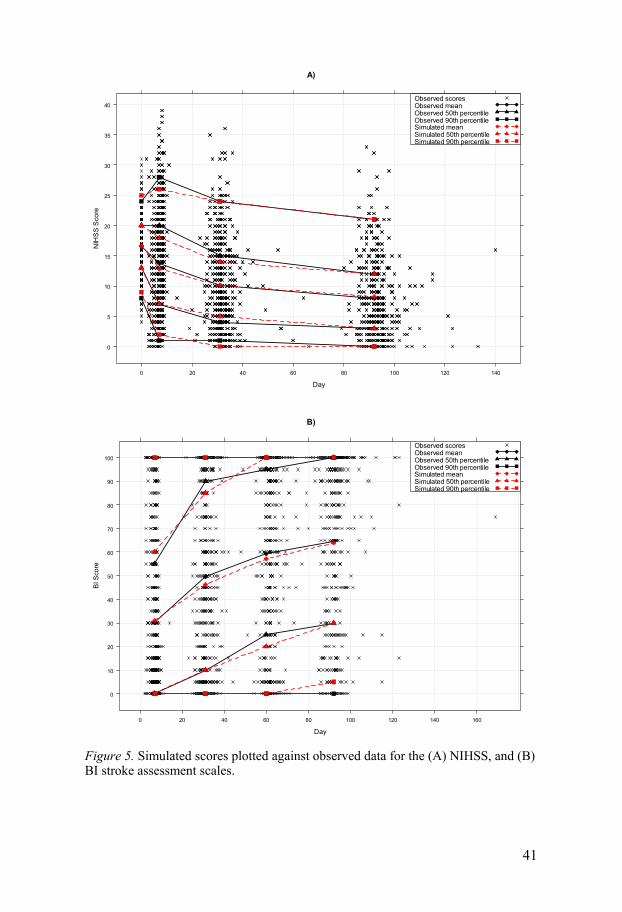
The predictive performance of the models for the NIHSS and BI scores was good, with 50th and 90th percentiles of simulated scores matching the corres-ponding observed score percentiles for both scales, displayed in Figure 5. Other diagnostics, however, indicated that the predictions from the NIHSS model were somewhat better than for the BI model.

41

Figure 5. Simulated scores plotted against observed data for the (A) NIHSS, and (B) BI stroke assessment scales.

A)

Day

NIH

SS

Sco

re

0

5

10

15

20

25

30

35

40

0 20 40 60 80 100 120 140

Observed scoresObserved meanObserved 50th percentileObserved 90th percentileSimulated meanSimulated 50th percentileSimulated 90th percentile

B)

Day

BI S

core

0

10

20

30

40

50

60

70

80

90

100

0 20 40 60 80 100 120 140 160

Observed scoresObserved meanObserved 50th percentileObserved 90th percentileSimulated meanSimulated 50th percentileSimulated 90th percentile

42

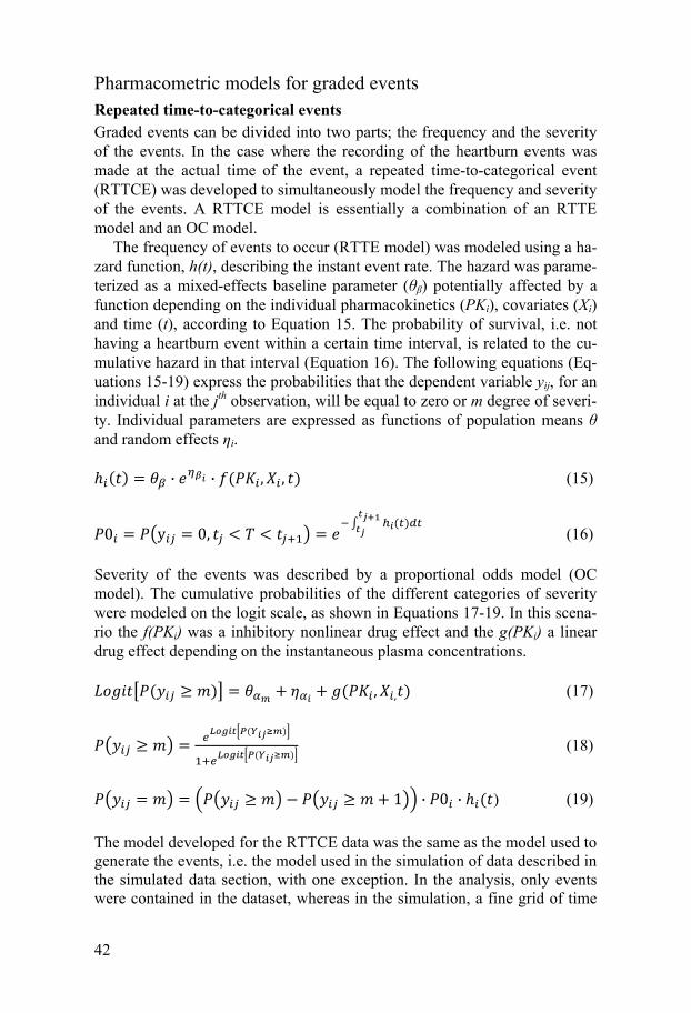
Pharmacometric models for graded events Repeated time-to-categorical events Graded events can be divided into two parts; the frequency and the severity of the events. In the case where the recording of the heartburn events was made at the actual time of the event, a repeated time-to-categorical event (RTTCE) was developed to simultaneously model the frequency and severity of the events. A RTTCE model is essentially a combination of an RTTE model and an OC model.

The frequency of events to occur (RTTE model) was modeled using a ha-zard function, h(t), describing the instant event rate. The hazard was parame-terized as a mixed-effects baseline parameter ( ) potentially affected by a function depending on the individual pharmacokinetics (PKi), covariates (Xi) and time (t), according to Equation 15. The probability of survival, i.e. not having a heartburn event within a certain time interval, is related to the cu-mulative hazard in that interval (Equation 16). The following equations (Eq-uations 15-19) express the probabilities that the dependent variable yij, for an individual i at the jth observation, will be equal to zero or m degree of severi-ty. Individual parameters are expressed as functions of population means and random effects i.

(15)

(16)

Severity of the events was described by a proportional odds model (OC model). The cumulative probabilities of the different categories of severity were modeled on the logit scale, as shown in Equations 17-19. In this scena-rio the f(PKi) was a inhibitory nonlinear drug effect and the g(PKi) a linear drug effect depending on the instantaneous plasma concentrations.

(17)

(18)

) (19)

The model developed for the RTTCE data was the same as the model used to generate the events, i.e. the model used in the simulation of data described in the simulated data section, with one exception. In the analysis, only events were contained in the dataset, whereas in the simulation, a fine grid of time

43

points was used to simulate both events and non-events (i.e. observation equal to zero) with the consequence that Equation 19 had to be modified to the following:

(20)

Repeated categorical events per time interval model (RCEpT) To accommodate events reported over a time interval, the original RTTCE data was summarized using the maximal scores within a time interval ( , one hour in this scenario), which is a common way to summarize event data. To be able to estimate the expected number of events within , a Poisson distri-bution function68 was added to the RTTCE model. The frequency part of the model was kept as Equations 15-16, now describing the probability of not having a maximum grade event within a fixed time interval.

Given that the data represent maximum grade m over n number of events experienced during , the discrete probability distribution of n entered the severity part of the RCEpT model, described in the equations below. The expected number of events, in the Poisson distribution function, is the inte-grated hazard over the time interval.

(21)

(22)

(23)

(24)

The functions of PK were the same as in the RTTCE model with the excep-tion that the plasma concentration corresponded to the average concentration within each time interval.

Ordered categorical data The most basic pharmacometric analysis of graded severity events is to dis-card the frequency of events and only analyze the severity (i.e. hourly max-imum severity in this study) in an OC model which corresponds to Equations 17-19 in the RTTCE model (removing the P0i·hi(t) component). In this anal-ysis the PK function was a linear drug effect based on average (hourly) con-centrations. However, the parameter estimates between the RTTCE and the

44

OC models are not comparable since the OC model consists of four catego-ries (none, mild, moderate and severe) while the severity portion of the RTTCE model only deals with three levels (mild, moderate and severe).

Model fit and simulation behavior Estimates obtained when fitting the RTTCE model to simulated data were found to be accurate both for fixed and random effects; as expected, given that the model is identical to the simulation model. This result also illustrates the reasonable properties of the used analysis method (Laplace). Interesting-ly, the RCEpT model also correctly retrieved parameters even from data simplified to the reporting of maxima within 12 equispaced time intervals. Figure 6 shows that the predictions from the RCEpT model display good agreement with the original data (i.e. RTTCE data), in both the frequency of events (lower panels) and the severity of the events (upper panels), for a randomly selected simulation.

Like the RCEpT model, the OC model also analyzes maximal grades of severity per interval of 1 h; however, because the parameterization is notice-ably different, especially as it sums up three m on the logit scale in contrast to two, it appears unsuitable to compare the obtained parameters to the “true” ones. Nevertheless, because the observation structure of the analyses is the same, the objective function values can be compared (using criteria applicable to non-nested models) with the ones obtained with RCEpT; with one additional degree of freedom, the Bayesian information criterion drops 12.5 points (on average) with RCEpT. Because the OC model cannot regene-rate the original data structure, only some types of simulation-based compar-isons between OC and RTTCE-type models are possible. Therefore, the per-patient occurrences of heartburn of the maximal grade of severity, computed over the entire observation period (12 h), were plotted (Figure 7). Although the type of diagnostic was selected to favor the OC model, poor prediction properties of the OC model are apparent. The right most bar in each panel contains the OC model predictions and obviously deviates from the original-ly simulated data (left most bar) whereas the predictions from the RTTCE and RCEpT models agree well with the original data.

45

Figure 6. Visual predictive checks from the RCEpT model. The severity and fre-quency features of the data are plotted versus six dose levels. The proportions of hourly maximums of each degree of severity are represented on the three top panels. The proportions of hourly intervals counting zero, one or more events are in the three lower panels. The median of one of the original datasets (red line) is compared to the 95 % confidence interval (grey area) around the predicted median (black line) obtained from 100 simulated samples.

Figure 7. Stacked bars of original simulations (SIM), simulations with final parame-ter estimates from RTTCE, RCEpT and OC models, stratified by dose level. Propor-tions of none, mild, moderate and severe hourly maximums were obtained from 100 sets of parameter estimates and simulated on a large sample.

Estimation algorithms A constant hazard repeated time-to-event model (according to Equation 15, omitting the PK component) was used to investigate the performance of three estimation algorithms; the Laplace method, the SAEM method, and the

Dose (mg)0 100 200 300 400

No event per hour

0 100 200 300 400

One event per hour

0 100 200 300 400

Two or more events per hour

0 100 200 300 400

Mild hourly maximum Moderate hourly maximum

0 100 200 300 400

Severe hourly maximum

Pro

po

rtio

n o

fTo

tal

Pro

po

rtio

n o

fTo

tal

0.05

0.10

0.15

0.00

0.10

0.15

0.05

0.6

0.8

0.9

0.7

0.10

0.20

0.25

0.15

0.30

0.35

0.10

0.20

0.00

0.15

0.05

0.00

0.10

0.15

0.05

Pro

po

rtio

n of

ma

xim

al s

eve

rity

0.0

0.2

0.4

0.6

0.8

1.0

SIM

RTT

CE

RC

EpT OC

Placebo

SIM

RTT

CE

RC

EpT OC

10 mg

SIM

RTT

CE

RC

EpT OC

50 mg

SIM

RTT

CE

RC

EpT OC

100 mg

SIM

RTT

CE

RC

EpT OC

200 mg

SIM

RTT

CE

RC

EpT OC

400 mg

None Mild Moderate Severe

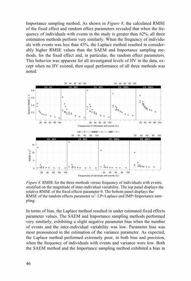
46

Importance sampling method. As shown in Figure 8, the calculated RMSE of the fixed effect and random effect parameters revealed that when the fre-quency of individuals with events in the study is greater than 62%, all three estimation methods perform very similarly. When the frequency of individu-als with events was less than 43%, the Laplace method resulted in consider-ably higher RMSE values than the SAEM and Importance sampling me-thods, for the fixed effect and, in particular, the random effect parameters. This behavior was apparent for all investigated levels of IIV in the data, ex-cept when no IIV existed, then equal performance of all three methods was noted.

Figure 8. RMSE for the three methods versus frequency of individuals with events, stratified on the magnitude of inter-individual variability. The top panel displays the relative RMSE of the fixed effects parameter . The bottom panel displays the RMSE of the random effects parameter 2. LP=Laplace and IMP=Importance sam-pling.

In terms of bias, the Laplace method resulted in under estimated fixed effects parameter values. The SAEM and Importance sampling methods performed very similarly, exhibiting a slight negative parameter bias when the number of events and the inter-individual variability was low. Parameter bias was most pronounced in the estimation of the variance parameter. As expected, the Laplace method performed extremely poor, in both bias and precision, when the frequency of individuals with events and variance were low. Both the SAEM method and the Importance sampling method exhibited a bias in

Frequencies of individuals with events (%)

Re

lativ

e R

MS

E in

0.2

0.4

0.6

0.8

20 40 60 80 100

: CV 0%

20 40 60 80 100

: CV 30%

20 40 60 80 100

: CV 50%

20 40 60 80 100

: CV 100%

20 40 60 80 100

: CV 200%

Frequencies of individuals with events (%)

RM

SE

in

2

0

5

10

15

20 40 60 80 100

: CV 30%

20 40 60 80 100

: CV 50%

20 40 60 80 100

: CV 100%

20 40 60 80 100

: CV 200%

LP SAEM IMP

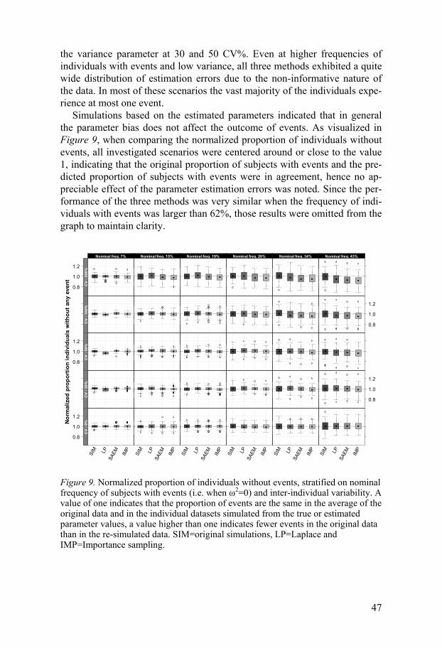
47

the variance parameter at 30 and 50 CV%. Even at higher frequencies of individuals with events and low variance, all three methods exhibited a quite wide distribution of estimation errors due to the non-informative nature of the data. In most of these scenarios the vast majority of the individuals expe-rience at most one event.

Simulations based on the estimated parameters indicated that in general the parameter bias does not affect the outcome of events. As visualized in Figure 9, when comparing the normalized proportion of individuals without events, all investigated scenarios were centered around or close to the value 1, indicating that the original proportion of subjects with events and the pre-dicted proportion of subjects with events were in agreement, hence no ap-preciable effect of the parameter estimation errors was noted. Since the per-formance of the three methods was very similar when the frequency of indi-viduals with events was larger than 62%, those results were omitted from the graph to maintain clarity.

Figure 9. Normalized proportion of individuals without events, stratified on nominal frequency of subjects with events (i.e. when 2=0) and inter-individual variability. A value of one indicates that the proportion of events are the same in the average of the original data and in the individual datasets simulated from the true or estimated parameter values, a value higher than one indicates fewer events in the original data than in the re-simulated data. SIM=original simulations, LP=Laplace and IMP=Importance sampling.

No

rmal

ized

pro

po

rtio

n i

nd

ivid

ual

s w

ith

ou

t an

y ev

ent

0.8

1.0

1.2

SIM LP

SA

EM

IMP

Nominal freq 7%

:

CV

0%

SIM LP

SA

EM

IMP

Nominal freq 15%

:C

V0

%

SIM LP

SA

EM

IMP

Nominal freq 19%

:C

V0

%

SIM LP

SA

EM

IMP

Nominal freq 26%

:C

V0

%

SIM LP

SA

EM

IMP

Nominal freq 34%

:C

V0

%

SIM LP

SA

EM

IMP

Nominal freq 43%

:C

V0

%

Nominal freq 7%

:

CV

30

%

Nominal freq 15%

:C

V3

0%

Nominal freq 19%

:C

V3

0%

Nominal freq 26%

:C

V3

0%

Nominal freq 34%

:C

V3

0%

0.8

1.0

1.2

Nominal freq 43%

:C

V3

0%

0.8

1.0

1.2

Nominal freq 7%

:

CV

50

%

Nominal freq 15%

:C

V5

0%

Nominal freq 19%

:C

V5

0%

Nominal freq 26%

:C

V5

0%

Nominal freq 34%

:C

V5

0%

Nominal freq 43%

:C

V5

0%

Nominal freq 7%

:

CV

10

0%

Nominal freq 15%

:C

V1

00

%

Nominal freq 19%

:C

V1

00

%

Nominal freq 26%

:C

V1

00

%

Nominal freq 34%

:C

V1

00

%

0.8

1.0

1.2

Nominal freq 43%

:C

V1

00

%

0.8

1.0

1.2

Nominal freq. 7%

:

CV

20

0%

Nominal freq. 15%

:C

V2

00

%

Nominal freq. 19%

:C

V2

00

%

Nominal freq. 26%

:C

V2

00

%

Nominal freq. 34%

:C

V2

00

%

Nominal freq. 43%

:C

V2

00

%

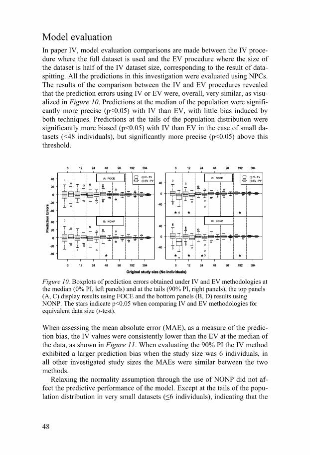
48

Model evaluation In paper IV, model evaluation comparisons are made between the IV proce-dure where the full dataset is used and the EV procedure where the size of the dataset is half of the IV dataset size, corresponding to the result of data-spitting. All the predictions in this investigation were evaluated using NPCs. The results of the comparison between the IV and EV procedures revealed that the prediction errors using IV or EV were, overall, very similar, as visu-alized in Figure 10. Predictions at the median of the population were signifi-cantly more precise (p<0.05) with IV than EV, with little bias induced by both techniques. Predictions at the tails of the population distribution were significantly more biased (p<0.05) with IV than EV in the case of small da-tasets (<48 individuals), but significantly more precise (p<0.05) above this threshold.

Figure 10. Boxplots of prediction errors obtained under IV and EV methodologies at the median (0% PI, left panels) and at the tails (90% PI, right panels), the top panels (A, C) display results using FOCE and the bottom panels (B, D) results using NONP. The stars indicate p<0.05 when comparing IV and EV methodologies for equivalent data size (t-test).

When assessing the mean absolute error (MAE), as a measure of the predic-tion bias, the IV values were consistently lower than the EV at the median of the data, as shown in Figure 11. When evaluating the 90% PI the IV method exhibited a larger prediction bias when the study size was 6 individuals, in all other investigated study sizes the MAEs were similar between the two methods.

Relaxing the normality assumption through the use of NONP did not af-fect the predictive performance of the model. Except at the tails of the popu-lation distribution in very small datasets ( 6 individuals), indicating that the

-40

-20

0

20

40

6 12 24 48 96 192 384

A: FOCE (i) IV - PV

(ii) EV - PV

Pre

dic

tio

n E

rro

rs

6 12 24 48 96 192 384

-40

-20

0

20

40 B: NONP

*

6 12 24 48 96 192 384

-40

0

40

C: FOCE (i) IV - PV

(ii) EV - PV

* * *

6 12 24 48 96 192 384

-40

0

40

D: NONP

* * * *

Original study size (No individuals)

-40

-20

0

20

40

6 12 24 48 96 192 384

A: FOCE (i) IV - PV

(ii) EV - PV

Pre

dic

tio

n E

rro

rs

6 12 24 48 96 192 384

-40

-20

0

20

40 B: NONP

*

6 12 24 48 96 192 384

-40

0

40

C: FOCE (i) IV - PV

(ii) EV - PV

* * *

6 12 24 48 96 192 384

-40

0

40

D: NONP

* * * *

Original study size (No individuals)

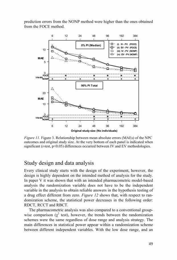
49

prediction errors from the NONP method were higher than the ones obtained from the FOCE method.

Figure 11. Figure 3. Relationship between mean absolute errors (MAEs) of the NPC outcomes and original study size. At the very bottom of each panel is indicated when significant (t-test, p<0.05) differences occurred between IV and EV methodologies.

Study design and data analysis Every clinical study starts with the design of the experiment, however, the design is highly dependent on the intended method of analysis for the study. In paper V it was shown that with an intended pharmacometric model-based analysis the randomization variable does not have to be the independent variable in the analysis to obtain reliable answers in the hypothesis testing of a drug effect different from zero. Figure 12 shows that, with respect to ran-domization scheme, the statistical power decreases in the following order: RDCT, RCCT and RBCT.

The pharmacometric analysis was also compared to a conventional group-wise comparison ( 2 test), however, the trends between the randomization schemes were the same regardless of dose range and analysis strategy. The main differences in statistical power appear within a randomization scheme between different independent variables. With the low dose range, and an

(i) IV - PV (FOCE)

(ii) EV - PV (FOCE)

(iii) IV - PV (NONP)

(iv) EV - PV (NONP)

+ + + + + + +NONP

5

10

0

6 12 24 48 96 192 384

MAE

* * * * *t-testsFOCE

0% PI (Median)

+ + + +NONP

Original study size (No individuals)

10

20

0

6 12 24 48 96 192 384

MAE

90% PI Total

* * *t-testsFOCE

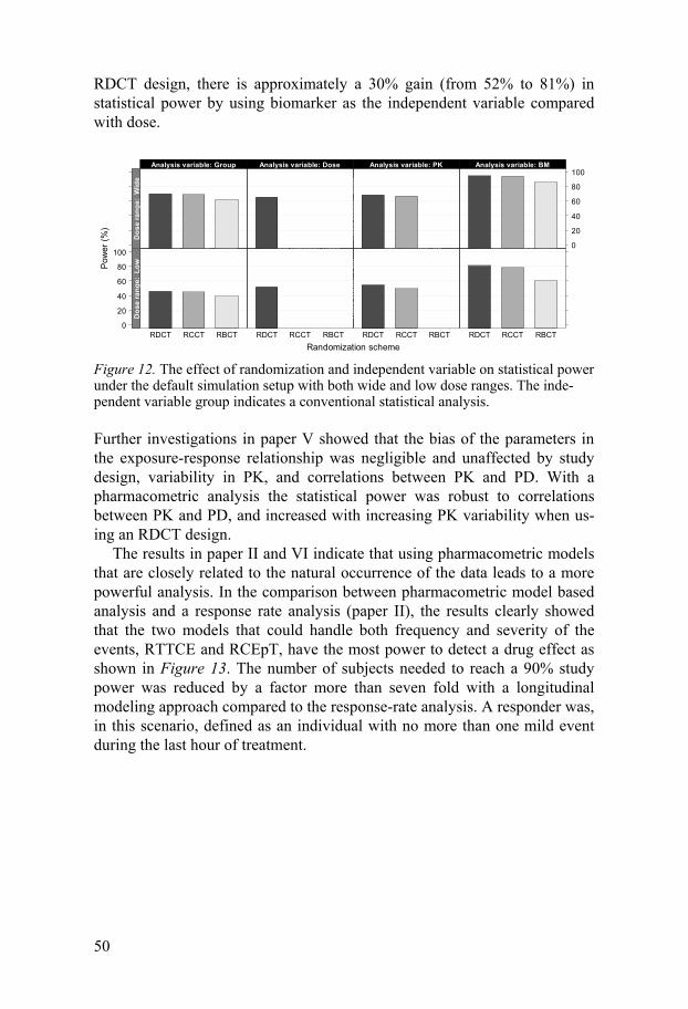
50

RDCT design, there is approximately a 30% gain (from 52% to 81%) in statistical power by using biomarker as the independent variable compared with dose.

Figure 12. The effect of randomization and independent variable on statistical power under the default simulation setup with both wide and low dose ranges. The inde-pendent variable group indicates a conventional statistical analysis.

Further investigations in paper V showed that the bias of the parameters in the exposure-response relationship was negligible and unaffected by study design, variability in PK, and correlations between PK and PD. With a pharmacometric analysis the statistical power was robust to correlations between PK and PD, and increased with increasing PK variability when us-ing an RDCT design.

The results in paper II and VI indicate that using pharmacometric models that are closely related to the natural occurrence of the data leads to a more powerful analysis. In the comparison between pharmacometric model based analysis and a response rate analysis (paper II), the results clearly showed that the two models that could handle both frequency and severity of the events, RTTCE and RCEpT, have the most power to detect a drug effect as shown in Figure 13. The number of subjects needed to reach a 90% study power was reduced by a factor more than seven fold with a longitudinal modeling approach compared to the response-rate analysis. A responder was, in this scenario, defined as an individual with no more than one mild event during the last hour of treatment.

Randomization scheme

Pow

er (

%)

0

20

40

60

80

100

RDCT RCCT RBCT

Analysis variable: Group

Do

se

ra

ng

e:

Lo

w

RDCT RCCT RBCT

Analysis variable: DoseD

os

era

ng

e:

Lo

w

RDCT RCCT RBCT

Analysis variable: PK

Do

se

ran

ge

:L

ow

RDCT RCCT RBCT

Analysis variable: BM

Do

se

ran

ge

:L

ow

Analysis variable: Group

Do

se

ra

ng

e:

Wid

e

Analysis variable: Dose

Do

se

ran

ge

:W

ide

Analysis variable: PK

Do

se

ran

ge

:W

ide

0

20

40

60

80

100Analysis variable: BM

Do

se

ran

ge

:W

ide

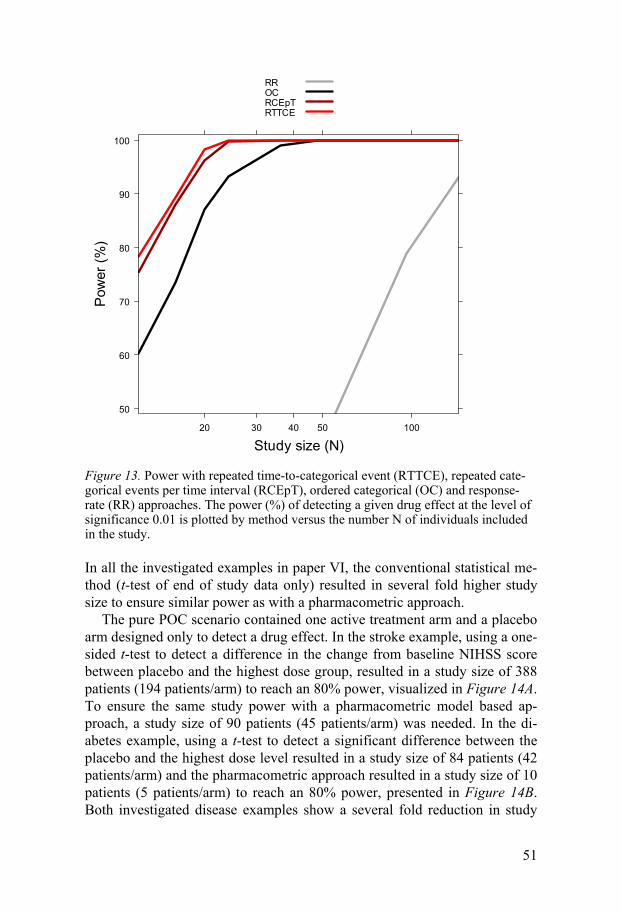
51

Figure 13. Power with repeated time-to-categorical event (RTTCE), repeated cate-gorical events per time interval (RCEpT), ordered categorical (OC) and response-rate (RR) approaches. The power (%) of detecting a given drug effect at the level of significance 0.01 is plotted by method versus the number N of individuals included in the study.

In all the investigated examples in paper VI, the conventional statistical me-thod (t-test of end of study data only) resulted in several fold higher study size to ensure similar power as with a pharmacometric approach.

The pure POC scenario contained one active treatment arm and a placebo arm designed only to detect a drug effect. In the stroke example, using a one-sided t-test to detect a difference in the change from baseline NIHSS score between placebo and the highest dose group, resulted in a study size of 388 patients (194 patients/arm) to reach an 80% power, visualized in Figure 14A. To ensure the same study power with a pharmacometric model based ap-proach, a study size of 90 patients (45 patients/arm) was needed. In the di-abetes example, using a t-test to detect a significant difference between the placebo and the highest dose level resulted in a study size of 84 patients (42 patients/arm) and the pharmacometric approach resulted in a study size of 10 patients (5 patients/arm) to reach an 80% power, presented in Figure 14B. Both investigated disease examples show a several fold reduction in study

Study size (N)

Pow

er (

%)

50

60

70

80

90

100

20 30 40 50 100

RROCRCEpTRTTCE

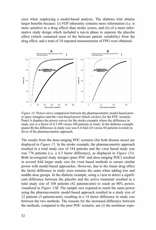
52

sizes when employing a model-based analysis. The diabetes trial obtains larger benefits because: (i) FGP inherently contains more information (i.e. is more sensitive to a drug effect) than stroke scores, and (ii) of a more infor-mative study design which included a run-in phase to separate the placebo effect (which contained most of the between patient variability) from the drug effect, and a total of 10 repeated measurements of FPG were obtained.

Figure 14. Power curve comparison between the pharmacometric model-based pow-er (gray triangles) and the t-test based power (black circles), for the POC scenario. Panel A displays the power curves for the stroke example where the difference in study size is a factor of 4.3 (90 versus 388 patients in total). In the diabetes example (panel B) the difference in study size was 8.4 fold (10 versus 84 patients in total) in favor of the pharmacometric approach.

The results from the dose-ranging POC scenario (for both disease areas) are displayed in Figure 15. In the stroke example, the pharmacometric approach resulted in a total study size of 184 patients and the t-test based study size was 776 patients (i.e. a 4.3 factor difference), as displayed in Figure 15A. Both investigated study designs (pure POC and dose-ranging POC) resulted in several fold larger study size for t-test based methods to ensure similar power with model-based approaches. However, due to the linear drug effect the factor difference in study sizes remains the same when adding low and middle dose groups. In the diabetic example, using a t-test to detect a signifi-cant difference between the placebo and the active treatment resulted in a total study size of 168 patients (42 patients/arm) to reach an 80% power, visualized in Figure 15B. The sample size required to reach the same power using the pharmacometric model-based approach resulted in a study size of 12 patients (3 patients/arm), resulting in a 14 factor difference in study size between the two methods. The reasons for the increased difference between the methods, compared to the pure POC scenario, are (i) the nonlinear expo-

Total number of patients

Po

we

r (%

)

20

40

60

80

100

0 50 100 150

Pharmacometric model-based power (POC)t-test based power

Total number of patients

Po

we

r (%

)

20

40

60

80

100

0 100 200 300 400 500 600

Pharmacometric model-based power (POC)t-test based power

A B

A factor 8.4 difference

A factor 4.3 difference

53

sure-response relation which is more informed by multiple dose groups, and (ii) the inclusion of a follow-up observation adding more support to the drug effect.

Figure 15. Power curve comparison between the pharmacometric model-based pow-er (gray squares) and the t-test based power (black circles), for the dose-ranging scenario, with four parallel arms. Panel A displays the power curves for the stroke example, where the difference in study size is a factor of 4.2 (184 versus 776 pa-tients in total). In the diabetes example (panel B) the difference in study size was 14 fold (12 versus 168 patients in total) in favor of the pharmacometric approach. The t-test was based on the difference between placebo and the highest dose group and the total study size was calculated with the addition of two equal sized treatment arms.

Total number of patients

Po

we

r (%

)

20

40

60

80

100

0 50 100 150 200 250 300

Pharmacometric model-based power (dose-range)t-test based power

Total number of patients

Po

we

r (%

)

20

40

60

80

100

0 200 400 600 800 1000 1200

Pharmacometric model based power (dose-range)t-test based power

A B

A factor 4.2 difference

A factor 14 difference

54

55

Discussion

When implementing a model-based drug development there are many as-pects that need consideration. To effectively put MBDD into practice it is necessary to understand the different aspects of a pharmacometric modeling approach.

Pharmacometric modeling starts with exploration of data, and whether it is a literature search, knowledge propagation from previously run studies or data from a present clinical study it is essential to understand the nature of the data to make decisions on what assumptions can be made regarding the data and what reasonable simplifications can be made of the physiological and pharmacological processes. In the first two papers in this thesis, models for data that are often extremely simplified in traditional analyses are pre-sented.

In data from stroke assessment scales, a non-monotonic behavior over time is often noted and in the conventional analysis of change from baseline at end of study16 this pattern is neglected. Another common feature of stroke data is a fairly large dropout rate, and in a traditional analysis this is often accounted for by a last observation carried forward procedure69. In therapeu-tic areas where there is an underlying disease progression it is not unreason-able to believe that these procedures are not appropriate and these inference techniques have been shown to reduce power, or introduce bias when dro-pout is not entirely attributable to random processes9, 70-71. In the developed models for NIHSS and BI all data points from the study are considered, non-monotonic behavior can be predicted and the dropout is integrated as a func-tion of the predicted scores (according to the principle of “informative mis-singness”70).

With the proposed structure of the stroke models, drug effects may be built into these models very easily. In the event of a pharmacological inter-vention being beneficial, it is reasonable to hypothesize that the frequency of dropout, for example, may be influenced by a drug effect. A drug effect might be equally suited to influencing relative score change between occa-sions, or indeed, probability of improvement or reaching a maximum score, and may be inspected or tested using the same approach we have used for the other covariates we have examined. The choice of which or any of these submodels to target using this approach would be suggested by the drug’s mode of action.

56

The models presented here consider the possibility of non-monotonic be-havior from one observation to the next. The models cannot, however, ac-count for unobserved changes between observations. The NIHSS and BI models are therefore design-dependent, the potential consequences of which may need to be explored using future simulation studies. Use of hidden Mar-kov models72 may help address this issue, although most mixed-effects mod-eling software implementations cannot handle models of this kind at the time of writing.

In the case of graded severity events, as exemplified with heartburn data, the ideal pharmacometric model would be the RTTCE model presented in paper II. The RTTCE model represents data as it naturally occurs, at any time and severity during the study period, which assigns the model the strongest prediction abilities. However, if the study was not designed for a model-based analysis, it is very likely that the observations will be reported as summary measures over a time interval, for example maximum severity within an hour. The proposed RCEpT model should then be the preferred model, which has the capability of predicting the frequency within the sum-marized time interval. Both these two models allow for detection of a drug effect on the frequency of events and/or severity of the symptoms which has advantages. These differential assessments represent information of greater value not only for patient therapy but also possibly for insights into mechan-isms of action of the drugs. For instance, an effect on the frequency may relate to disease modification, whereas an effect on symptom severity may signal symptomatic effects.

When developing a pharmacometric model, apart from selecting an ap-propriate model structure for describing the data, it is important to use an appropriate estimation method to obtain reliable parameter estimates24, 73-78. Bias in parameter estimates may have the consequence that the model cannot replicate original data in simulations, this is a concern if the model was to be used in clinical trial simulations as a tool in decision making in drug devel-opment. It has previously been reported that models for dichotomous and ordered categorical data are sensitive to the characteristics of responses and estimation methods79-81 resulting in parameter bias. The Laplace method depends on the empirical Bayes estimates (EBE) in its approximation and with low information content data , such as RTTE observations, the EBEs are not well characterized as have previously been discussed by e.g. Jönsson et al79. When the number of events in the study is low there is little informa-tion in the data to allow separation between the fixed effects and the random effects, and relatively small model misspecifications can give rise to large deviations in parameter estimates from true values. In a study by Lavielle and Savic78, the SAEM method was proven to perform better than to the Laplace method, exhibiting no appreciable parameter bias whereas the Lap-lace method resulted in severe parameter bias. Importance sampling and SAEM have also been shown to be more stable than the Laplace method

57

when analyzing sparse data and/or complex PK/PD data73. These previous studies made it very interesting to investigate the estimation performance of the Laplace, SAEM and Importance sampling methods in NONMEM, ap-plied to RTTE data. As expected, the Laplace method performed poorly at few events per individual (which is a common data structure in rare adverse event data) whereas the two EM methods resulted in reasonable parameter estimates. These results show that the EM methods should be preferred when fewer than approximately half of the individuals in the study report events, with high event frequency all three methods performed similarly and the runtimes then speak in favor of the Laplace method.

Yet another very important part of the pharmacometric model develop-ment is the assessment of the predictive performance of the model, as a common objective is to use the model for future predictions. In papers I- III internal validation techniques (mainly VPCs) were used to evaluate the per-formance of the models during the model development. It is often proposed that to assess the predictive performance of a model it should be applied to a new dataset arising from a different clinical trial82-83. However, it is rare that such a dataset is available and one could discuss whether such a dataset ever exists. To truly assess the predictive performance the dataset must come from an identical clinical trial where the only difference is the sample for the patient population, of course this is impossible to achieve. There will always be differences in the execution of the trial, for example different centers and new staff, that might influence the observations in the dataset and hence the performance assessment of the pharmacometric model. An alternative me-thod would be data-splitting, where a part of the dataset is set aside to act as an external dataset used in performance assessment (in this thesis defined as EV). EV has been proposed to reduce optimism in the parameter estimates, and using NPCs as the metric it was compelling to compare the results with an IV. The two validation methods showed very similar results, except for very small study sizes where the IV displayed some parameter optimism. Knowing that the model parameter estimates will consistently be more in-formed when applying IV over EV, due to the larger sample size, and based on the results in this work, data-splitting should be avoided when assessing the predictive capacity of a model in order to retain sufficient precision in both predictions and in predictive performance estimates. In the end, to ar-rive at the most predictive model one should use a battery of performance tests, for example NPC, VPC and PPC, to cover all aspects of the predic-tions. These results also further justified the choice of evaluation strategies used in the model developments within this thesis.

When all the model building steps have been completed and a proper pharmacometric model has been developed, how can the model be used? As a pharmacometrician, the most obvious choice would be to use the model to optimize the design and analysis of clinical trials. However, it is not always necessary to change the clinical trial design to benefit from a pharmacome-

58

tric model-based analysis, simply by making the most use of the available data increases the information content in the trial. The results in paper V show that the most beneficial trial design is the one letting the biological variability in PK and biomarker response inform the analysis, i.e. using an independent variable as close as possible to the clinical endpoint, while still randomizing on dose. From a modeling point of view, the increase in varia-bility increases the information content in the data, i.e. the greatest statistical power is obtained with a high variability in PK, randomization on dose and using the biomarker as the independent variable. An example of this pheno-menon is shown in paper VI, where the diabetes example resulted in almost the same total study size in two different RDCT designs, where the indepen-dent variable was dose and exposure, respectively. The pure POC had two treatment arms and a linear dose-response relationship was investigated (5 patients/arm), and in the dose-ranging POC there were four treatment arms and a nonlinear exposure-response relationship was investigated (3 pa-tients/arm). The advantage of randomizing on dose and using an indepen-dent variable as close as possible to the clinical endpoint became evident in this example.

However, when using an RDCT design and analyzing an exposure–response relationship there is a possibility of experiencing parameter bias if the randomization variability is less than the inter-individual variability. One example of this is when the variability between the dose levels (randomiza-tion variability) is less than the inter-individual variability in the pharmaco-kinetics. In paper V, the randomization variability was always greater than the inter-individual variability. For traditional analyses it is often assumed that to obtain an increase in statistical power a decrease in within-group va-riability in the data is needed. As seen in some of these results, the trend can be the opposite. In the group wise analysis the statistical power is also de-pendent on the randomization target range. When the target range is close to baseline response, increased variability in PK leads to a slightly higher sta-tistical power in an RDCT. This is because the increased variability in the response makes it easier to contrast between the placebo response and the highest exposure group. When the target range is closer to the maximal re-sponse, on the other hand, the increased variability in PK leads to formal data loss and therefore lower statistical power. Overall, these results indicate that alternative randomization schemes have no beneficial effect on the sta-tistical power regardless of analysis strategy and a model-based analysis will result in higher statistical power and therefore smaller group sizes compared with a group-wise analysis, given the same randomization scheme. The su-periority of RDCT over RCCT, when investigating exposure-response rela-tionships, has also been confirmed by Lledó-García et al84-85.

In paper II the power to detect a drug effect different from zero was calcu-lated for the response-rate analysis and the three pharmacometric models: OC, RCEpT and RTTCE. As expected, the power increased with increasing

59

accuracy of the description of the data, where the response-rate analysis re-sulted in the largest study sizes and the RTTCE model the smallest. Indeed, the response rate calculated from a data set has the advantage of providing a direct answer to a question regarding the efficacy of the treatment as it re-lates to the responder definition. Unfortunately, it does not provide any indi-cation of the relative importance of the different grades of severity, the time course of the symptoms, or the frequency of the events, and a more appeal-ing approach would be to use response-rates predicted from a pharmacome-tric model.

The models for stroke scales and the FPG-HbA1c model represent areas where a pharmacometric model-based analysis can have a large impact on drug development, due to fairly different reasons. Clinical trials of new drugs for the treatment of acute stroke have been very disappointing, and some of the reasons that have been pointed out are suboptimal designs and analysis strategies86-88. The example in paper VI indicate that without chang-ing the design of the clinical trial, using a pharmacometric model-based analysis can drastically reduce the study size making a POC or dose ranging trial much more feasible to run. The NIHSS model is an example of how a model for non-monotonous disease progression data can be used to improve the efficiency of drug development.

The diabetes example addresses a therapeutic area with the aim of affect-ing a very complex physiological system (glucose regulation). The conven-tional analysis of a POC study often involves an assessment of change from baseline HbA1c values at end of study. This type of analysis does not allow for any mechanistic interpretation of the drug effect. Using a model that includes the FPG, HbA1c and aging of RBC offers the possibility to evaluate different mechanisms for the drug effect as well as evaluation of other fac-tors, for example time related factors, which influence the drug response. The results in paper VI show that the pharmacometric analysis is more in-formed about the system than the conventional analysis since an equal statis-tical power leads to a large reduction in sample size.

As these results show, the use of a pharmacometric model based approach can drastically reduce the study sizes of clinical trials. This can be primarily attributed to the use of longitudinal data and the assumption of continuous relationships between dose/exposure and the response (allowing for infe-rence between treatment arms and placebo).

Although these results are convincing in the advocacy for a MBDD there are obstacles that need to be overcome before it can be fully implemented. For one thing the time lines in a project must be adapted to a pharmacome-tric analysis which can be more time consuming in the analysis phase (if a model has to be developed), and access to interim data might be necessary. Jönsson and Jonsson8 have published an appealing suggestion on how to implement a pharmacometric data analysis project. Some adaptations in data collection might also be necessary, for example the reporting of exact timing

60

of dose administration and of observations is very important in longitudinal data analysis. A third issue that might slow down the implementation of MBDD, is that currently there is a shortage in trained pharmacometricians and relatively few academic institutions offer training in pharmacometrics7.

Despite potential problems in implementing MBDD, this thesis highlights the different aspects that need consideration in developing pharmacometric models and how the models can be used. The pharmacometric model-based approach offers reductions in study size which naturally reduces costs of clinical trials, but more importantly it reduces the number of healthy volun-teers and patients, subject to experimental drugs.

61

Conclusions

The development of pharmacometric models for clinical assessment scales in stroke and graded severity events show the benefit of describing data as close to its true nature as possible as it increases the predictive abilities and allows for mechanistic interpretations. Non-monotonic assessment scales are used in a wide range of clinical applications, including traumatic brain injury and psychiatric illness, and combined longitudinal and probabilistic models is appropriate for any clinical scale in which scores exhibit variation in both positive and negative directions with time. Models that could handle both severity and frequency demonstrated multiple benefits, including good pre-dictive performance and extended simulation capabilities.

Every pharmacometric model relies on the use of an appropriate estima-tion method to obtain correct parameter estimates. The results in this thesis show that when modeling infrequent repeated event data, for example rare adverse events, the preferred estimation methods should be SAEM or Impor-tance sampling.

A very important part of pharmacometric model development is the as-sessment of a model’s predictive performance. The comparison between internal and external validation (data-splitting) techniques led to the conclu-sion that data-splitting should be discarded when evaluating predictive mod-els to retain sufficient precision both in predictions and in estimates of pre-dictive performance.

A pharmacometric model-based analysis has the possibility to take advan-tage of biological variability between individuals which means that the most beneficial trial design, in terms of randomization, when establishing expo-sure-response relationships is the dose-randomized trial. With a model-based analysis the practical and economic gain in performing an RDCT further outweighs the possible benefits of performing an alternative randomization scheme.

Throughout this thesis several examples have shown the possibility of significantly reducing sample sizes in clinical trials with a pharmacometric model-based analysis. This approach will reduce time and costs spent in the development of new drug therapies, but foremost reduce the number of healthy volunteers and patients exposed to experimental drugs.

62

Populärvetenskaplig sammanfattning

Den här avhandlingen visar att genom att förbättra den statistiska analysen av läkemedelsprövningar kan man minska kostnaden samt förkorta tiden till dess läkemedlet når patienterna. Att ta fram nya läkemedel är en kostsam och tidsödande process. Detta gäller i synnerhet de studier som görs på män-niskor, så kallade kliniska prövningar. Det sätt som nu används vid utförande och utvärdering av kliniska prövningar har därför starkt ifrågasatts av myn-digheter, externa utvärderare och läkemedelsföretagen själva.

Syftet med kliniska prövningar är att svara på huruvida läkemedlet är sä-kert, har önskad effekt, samt att ta fram den bästa läkemedelsdosen. För att svara på dessa frågor samlar man in uppgifter om läkemedlets bieffekter, läkemedlets påverkan på sjukdomen under en viss tidsperiod, samt hur dessa effekter varierar med olika doser av läkemedlet. Vanligtvis samlas det in information från patienterna vid flera tillfällen under studiens gång. Trots detta är det vanligt att man bara använder första och sista mätningen när man ska utvärdera läkemedlets effekt, eller på andra sätt inte utnyttjar all infor-mation man samlat in.

Ett läkemedels tidsförlopp i kroppen liksom hur halten av läkemedel på-verkar läkemedelseffekten kan beskrivas med matematiska modeller, så kal-lade farmakokinetiska och farmakodynamiska modeller. Genom att kombi-nera dessa modeller, gärna tillsammans med modeller för hur sjukdomar i sig förändras med tiden, kan man använda all insamlad information vid ut-värdering av kliniska prövningar samtidigt som man får förståelse för de biologiska mekanismerna. Farmakometri är samlingsnamnet för utveckling och användning av dessa matematiska modeller.

För att kunna utnyttja en farmakometrisk analys av kliniska prövningar måste man först utveckla modeller som korrekt beskriver data. Det innebär att man måste ställa sig ett antal frågor:

1) Hur ser den naturliga förekomsten av observationerna ut? Ändrar sig till exempel sjukdomsförloppet även utan behandling som vid Alzheimers sjukdom, eller uppkommer symptomen vid exakta tidpunkter som vid epi-leptiska anfall?

2) Vilken typ av analysmetod (algoritm) lämpar sig bäst för denna typ av observationer?

3) Hur utvärderar man på lämpligaste sätt huruvida modellen faktiskt be-skriver observationerna?

63

I den här avhandlingen presenteras först två modeller som beskriver neu-rologiska och funktionella symptom efter en akut stroke. De flesta strokepa-tienter blir spontant bättre med tiden, men det är vanligt att patienterna har både uppgångar och nedgångar vilket dessa modeller kan beskriva. I avhand-lingen beskrivs sedan två nya modeller för att hantera observationer som sker med en viss frekvens och svårighetsgrad, till exempel halsbränna som kan uppkomma när som helst och klassificeras som ”mild”, ”medel” eller ”svår”. Resultatet av metodutvärderingen och undersökningen av modellut-värdering visade att modellerna hade utvecklats på ett korrekt sätt.

Vad är då fördelen med farmakometriska modeller? För att svara på den frågan simulerades kliniska prövningar med läkemedelseffekt inom en rad olika behandlingsområden: halsbränna, akut stroke och diabetes. Alla studier analyserades med såväl farmakomterisk som traditionell metod. Samtliga resultat visade att den traditionell analys kräver större studier för att upp-täcka en viss läkemedelseffekt jämfört med farmakometrisk analys, eftersom den farmakometriska analysen kan använda samtliga insamlade observatio-ner. Detta har många fördelar, inte minst inom akut stroke där det finns flera exempel där läkemedel lagts ned i slutfasen av utvecklingen och där studier tenderar att bli väldigt stora redan tidigt i läkemedelsutvecklingen.

Sammanfattningsvis visar den här avhandlingen hur man genom att ut-nyttja informationen från läkemedelsprövningar på ett optimalt sätt kan man minska storleken på kliniska prövningar. Detta medför i sin tur minskade kostnader och förkortad utvecklingstid – men framför allt drastisk reducering av antalet patienter och friska frivilliga som utsätts för experimentella läke-medel.

64

Acknowledgements

This thesis was carried out at the Department of Pharmaceutical Biosciences, Pharmacy faculty, Uppsala University, Sweden.

AstraZeneca R&D, Södertälje, Sweden, is gratefully acknowledged for fi-nancial support.

I would like to thank the people who have contributed to this thesis and en-couraged me during my time as a research student.

My primary supervisor Professor Niclas Jonsson for your endless support (even though you did abandon me for a couple of years ), your admirable organization skills, fun conversations about photography and gadgets with accompanying manuals, and not the least for forcing me to code my graphs in R by forbidding Excel.

My co-primary supervisor Professor Mats Karlsson for sharing your know-ledge and passion about pharmacometrics, your enthusiasm and generosity is the foundation for an excellent work environment, both professionally and socially. Also, thank you for giving me opportunities to improve my phar-macometric skills in the real world. A special thank you for taking “an American that thinks he is going to be able to do cross-country skiing in Uppsala” in as a post-doc.

My secondary supervisor Professor Anders Grahnén for always being very encouraging and for your enthusiasm about my work, it is greatly appre-ciated. And thanks for many entertaining stories during coffee breaks.

Professors Margareta Hammarlund-Udenaes and Sven Björkman for contri-buting to such a nice working environment and for your devotion to teach-ing.

My co-authors: Dr Justin, Dr Per-Henrik, Dr Fredrik, Elodie, Paul, Camille and Martin thank you for all your inputs and efforts. A special thank you to Justin for not giving up on the stroke paper. Paul, Martin and Elodie, good luck on your upcoming dissertations.

65

Many thanks to my colleagues during my time at AstraZeneca, for teaching me about clinical drug development in real life. Thank you Dr Marie Sandström for offering this opportunity and for great support during this time.

Dr Lasse, Pontus, Dr Kajsa and Jerker, thank you for providing and caring for the computer cluster and software tools that have made this thesis possi-ble, and Magnus for caring for my laptop and for the most appreciated help with the layout of the unpublished manuscripts.

Dr Mia, my partner in crime, without all the discussions about science, which polymers plastic spoons are made of, neat perl coding, life decisions and all the fun we’ve had during the past 14 years, this thesis would not be. I hope this will continue for many years to come (without the thesis part).

Dr Hanna, thank you for all the great discussions about all and nothing and for always giving your honest opinion. I miss you in Uppsala.

Bettan, we are finally finishing! Thank you for all the talks about important things like sea food. It is nice to have a friend that knows what it is like to share your life with an exercise addict.

My roommates: Dr Lena, Dr Jörgen and Annika, thank you for the great company. Dr Jörgen – jag vann!

Present and former colleagues, for contributing to a creative and stimulating place to work. Thank you all for interesting scientific discussions, but equal-ly important thanks for all the non-work related discussions during “fika” and all the fun we have during travels and parties.

Till min familj och mina vänner:

Hjortronligan: Sara, Kajsa, Carina och Marith, mina äldsta vänner. Tack för alla trevliga tjejhelger och för att ni är ointresserade av vad jag sysslar med på jobbet. Det betyder mycket att ni finns även om vi inte ses så ofta.

Anne and Brian, for taking such an active part in our life even though you live so far away. Thank you for all the fun travels and for providing valuable tips about gardening and photography.

66

Mina bröder, Tor och Ola, tack för att ni drar med mig på roliga saker som föredrag, hockeymatcher och shopping, och för att ni vaktar så att jag inte blir allt för torr akademiker. Tor, tack för all när-hjälp med skjuts, blomvatt-ning och för att jag får komma och leka hos dig. Ola, tack för din journalis-tiska hjälp med den populärvetenskapliga sammanfattningen och för att du underhåller storasysterkänslorna med frågor om vägbeskrivning och annat.

Mamma och Pappa, tack för ert oförtrutna stöd trots att jag sällan tar raka vägen till målet. Utan er uppmuntran att bli en självständig person hade det inte blivit någon avhandling. Det betyder mycket att er dörr alltid är öppen när jag behöver komma bort från det akademiska livet och komma ut på landet. Lycka till med nya huset!

Andrew – Du é min man . Tusen tack för all din hjälp och för att du alltid får mig att känna mig bra på det jag gör. Jag ser fram emot många år som service team i Vasaloppet och alla andra roliga äventyr du drar med mig på.Go team Hooksson! Purp.

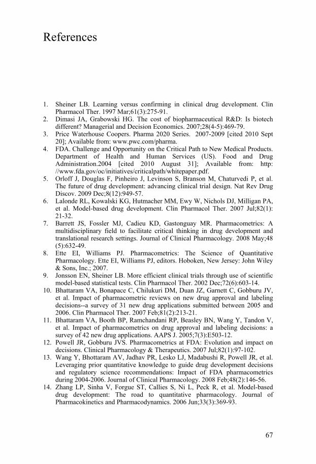
67

References

1. Sheiner LB. Learning versus confirming in clinical drug development. Clin Pharmacol Ther. 1997 Mar;61(3):275-91.

2. Dimasi JA, Grabowski HG. The cost of biopharmaceutical R&D: Is biotech different? Managerial and Decision Economics. 2007;28(4-5):469-79.

3. Price Waterhouse Coopers. Pharma 2020 Series. 2007-2009 [cited 2010 Sept 20]; Available from: www.pwc.com/pharma.

4. FDA. Challenge and Opportunity on the Critical Path to New Medical Products. Department of Health and Human Services (US). Food and Drug Administration.2004 [cited 2010 August 31]; Available from: http://www.fda.gov/oc/initiatives/criticalpath/whitepaper.pdf.

5. Orloff J, Douglas F, Pinheiro J, Levinson S, Branson M, Chaturvedi P, et al. The future of drug development: advancing clinical trial design. Nat Rev Drug Discov. 2009 Dec;8(12):949-57.

6. Lalonde RL, Kowalski KG, Hutmacher MM, Ewy W, Nichols DJ, Milligan PA, et al. Model-based drug development. Clin Pharmacol Ther. 2007 Jul;82(1):21-32.

7. Barrett JS, Fossler MJ, Cadieu KD, Gastonguay MR. Pharmacometrics: A multidisciplinary field to facilitate critical thinking in drug development and translational research settings. Journal of Clinical Pharmacology. 2008 May;48(5):632-49.

8. Ette EI, Williams PJ. Pharmacometrics: The Science of Quantitative Pharmacology. Ette EI, Williams PJ, editors. Hoboken, New Jersey: John Wiley & Sons, Inc.; 2007.

9. Jonsson EN, Sheiner LB. More efficient clinical trials through use of scientific model-based statistical tests. Clin Pharmacol Ther. 2002 Dec;72(6):603-14.

10. Bhattaram VA, Bonapace C, Chilukuri DM, Duan JZ, Garnett C, Gobburu JV, et al. Impact of pharmacometric reviews on new drug approval and labeling decisions--a survey of 31 new drug applications submitted between 2005 and 2006. Clin Pharmacol Ther. 2007 Feb;81(2):213-21.

11. Bhattaram VA, Booth BP, Ramchandani RP, Beasley BN, Wang Y, Tandon V, et al. Impact of pharmacometrics on drug approval and labeling decisions: a survey of 42 new drug applications. AAPS J. 2005;7(3):E503-12.

12. Powell JR, Gobburu JVS. Pharmacometrics at FDA: Evolution and impact on decisions. Clinical Pharmacology & Therapeutics. 2007 Jul;82(1):97-102.

13. Wang Y, Bhottaram AV, Jadhav PR, Lesko LJ, Madabushi R, Powell JR, et al. Leveraging prior quantitative knowledge to guide drug development decisions and regulatory science recommendations: Impact of FDA pharmacometrics during 2004-2006. Journal of Clinical Pharmacology. 2008 Feb;48(2):146-56.

14. Zhang LP, Sinha V, Forgue ST, Callies S, Ni L, Peck R, et al. Model-based drug development: The road to quantitative pharmacology. Journal of Pharmacokinetics and Pharmacodynamics. 2006 Jun;33(3):369-93.

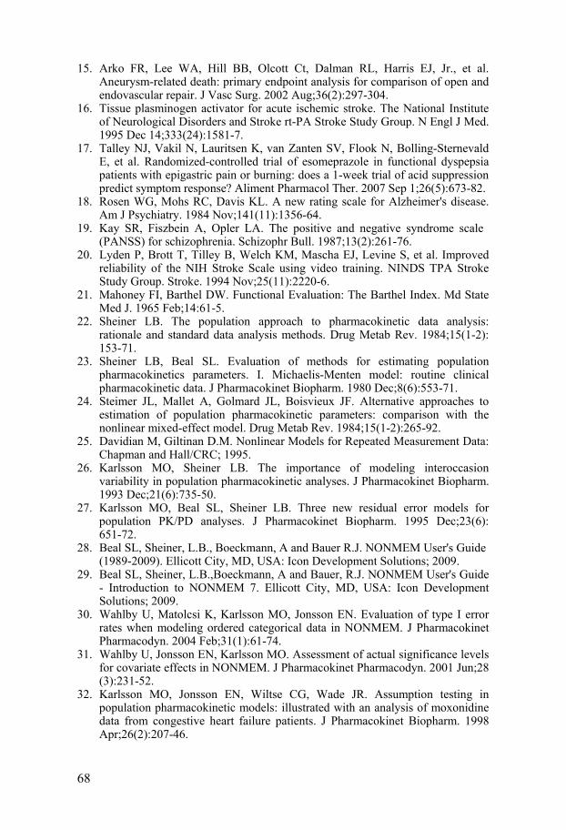
68

15. Arko FR, Lee WA, Hill BB, Olcott Ct, Dalman RL, Harris EJ, Jr., et al. Aneurysm-related death: primary endpoint analysis for comparison of open and endovascular repair. J Vasc Surg. 2002 Aug;36(2):297-304.

16. Tissue plasminogen activator for acute ischemic stroke. The National Institute of Neurological Disorders and Stroke rt-PA Stroke Study Group. N Engl J Med. 1995 Dec 14;333(24):1581-7.

17. Talley NJ, Vakil N, Lauritsen K, van Zanten SV, Flook N, Bolling-Sternevald E, et al. Randomized-controlled trial of esomeprazole in functional dyspepsia patients with epigastric pain or burning: does a 1-week trial of acid suppression predict symptom response? Aliment Pharmacol Ther. 2007 Sep 1;26(5):673-82.

18. Rosen WG, Mohs RC, Davis KL. A new rating scale for Alzheimer's disease. Am J Psychiatry. 1984 Nov;141(11):1356-64.

19. Kay SR, Fiszbein A, Opler LA. The positive and negative syndrome scale (PANSS) for schizophrenia. Schizophr Bull. 1987;13(2):261-76.

20. Lyden P, Brott T, Tilley B, Welch KM, Mascha EJ, Levine S, et al. Improved reliability of the NIH Stroke Scale using video training. NINDS TPA Stroke Study Group. Stroke. 1994 Nov;25(11):2220-6.

21. Mahoney FI, Barthel DW. Functional Evaluation: The Barthel Index. Md State Med J. 1965 Feb;14:61-5.

22. Sheiner LB. The population approach to pharmacokinetic data analysis: rationale and standard data analysis methods. Drug Metab Rev. 1984;15(1-2):153-71.

23. Sheiner LB, Beal SL. Evaluation of methods for estimating population pharmacokinetics parameters. I. Michaelis-Menten model: routine clinical pharmacokinetic data. J Pharmacokinet Biopharm. 1980 Dec;8(6):553-71.

24. Steimer JL, Mallet A, Golmard JL, Boisvieux JF. Alternative approaches to estimation of population pharmacokinetic parameters: comparison with the nonlinear mixed-effect model. Drug Metab Rev. 1984;15(1-2):265-92.

25. Davidian M, Giltinan D.M. Nonlinear Models for Repeated Measurement Data: Chapman and Hall/CRC; 1995.

26. Karlsson MO, Sheiner LB. The importance of modeling interoccasion variability in population pharmacokinetic analyses. J Pharmacokinet Biopharm. 1993 Dec;21(6):735-50.

27. Karlsson MO, Beal SL, Sheiner LB. Three new residual error models for population PK/PD analyses. J Pharmacokinet Biopharm. 1995 Dec;23(6):651-72.

28. Beal SL, Sheiner, L.B., Boeckmann, A and Bauer R.J. NONMEM User's Guide (1989-2009). Ellicott City, MD, USA: Icon Development Solutions; 2009.

29. Beal SL, Sheiner, L.B.,Boeckmann, A and Bauer, R.J. NONMEM User's Guide - Introduction to NONMEM 7. Ellicott City, MD, USA: Icon Development Solutions; 2009.

30. Wahlby U, Matolcsi K, Karlsson MO, Jonsson EN. Evaluation of type I error rates when modeling ordered categorical data in NONMEM. J Pharmacokinet Pharmacodyn. 2004 Feb;31(1):61-74.

31. Wahlby U, Jonsson EN, Karlsson MO. Assessment of actual significance levels for covariate effects in NONMEM. J Pharmacokinet Pharmacodyn. 2001 Jun;28(3):231-52.

32. Karlsson MO, Jonsson EN, Wiltse CG, Wade JR. Assumption testing in population pharmacokinetic models: illustrated with an analysis of moxonidine data from congestive heart failure patients. J Pharmacokinet Biopharm. 1998 Apr;26(2):207-46.

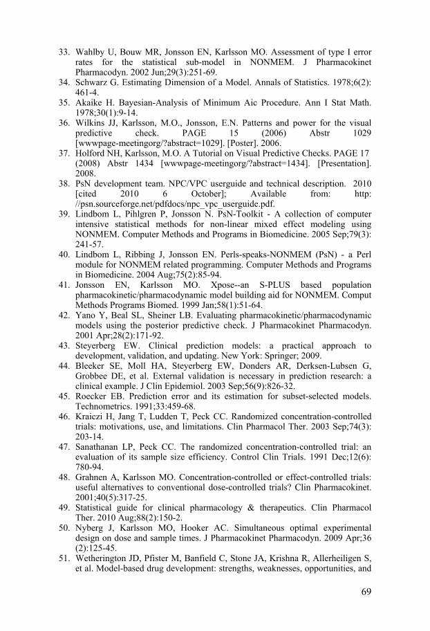
69

33. Wahlby U, Bouw MR, Jonsson EN, Karlsson MO. Assessment of type I error rates for the statistical sub-model in NONMEM. J Pharmacokinet Pharmacodyn. 2002 Jun;29(3):251-69.

34. Schwarz G. Estimating Dimension of a Model. Annals of Statistics. 1978;6(2):461-4.

35. Akaike H. Bayesian-Analysis of Minimum Aic Procedure. Ann I Stat Math. 1978;30(1):9-14.

36. Wilkins JJ, Karlsson, M.O., Jonsson, E.N. Patterns and power for the visual predictive check. PAGE 15 (2006) Abstr 1029 [wwwpage-meetingorg/?abstract=1029]. [Poster]. 2006.

37. Holford NH, Karlsson, M.O. A Tutorial on Visual Predictive Checks. PAGE 17 (2008) Abstr 1434 [wwwpage-meetingorg/?abstract=1434]. [Presentation]. 2008.

38. PsN development team. NPC/VPC userguide and technical description. 2010 [cited 2010 6 October]; Available from: http://psn.sourceforge.net/pdfdocs/npc_vpc_userguide.pdf.

39. Lindbom L, Pihlgren P, Jonsson N. PsN-Toolkit - A collection of computer intensive statistical methods for non-linear mixed effect modeling using NONMEM. Computer Methods and Programs in Biomedicine. 2005 Sep;79(3):241-57.

40. Lindbom L, Ribbing J, Jonsson EN. Perls-speaks-NONMEM (PsN) - a Perl module for NONMEM related programming. Computer Methods and Programs in Biomedicine. 2004 Aug;75(2):85-94.

41. Jonsson EN, Karlsson MO. Xpose--an S-PLUS based population pharmacokinetic/pharmacodynamic model building aid for NONMEM. Comput Methods Programs Biomed. 1999 Jan;58(1):51-64.

42. Yano Y, Beal SL, Sheiner LB. Evaluating pharmacokinetic/pharmacodynamic models using the posterior predictive check. J Pharmacokinet Pharmacodyn. 2001 Apr;28(2):171-92.

43. Steyerberg EW. Clinical prediction models: a practical approach to development, validation, and updating. New York: Springer; 2009.

44. Bleeker SE, Moll HA, Steyerberg EW, Donders AR, Derksen-Lubsen G, Grobbee DE, et al. External validation is necessary in prediction research: a clinical example. J Clin Epidemiol. 2003 Sep;56(9):826-32.

45. Roecker EB. Prediction error and its estimation for subset-selected models. Technometrics. 1991;33:459-68.

46. Kraiczi H, Jang T, Ludden T, Peck CC. Randomized concentration-controlled trials: motivations, use, and limitations. Clin Pharmacol Ther. 2003 Sep;74(3):203-14.

47. Sanathanan LP, Peck CC. The randomized concentration-controlled trial: an evaluation of its sample size efficiency. Control Clin Trials. 1991 Dec;12(6):780-94.

48. Grahnen A, Karlsson MO. Concentration-controlled or effect-controlled trials: useful alternatives to conventional dose-controlled trials? Clin Pharmacokinet. 2001;40(5):317-25.

49. Statistical guide for clinical pharmacology & therapeutics. Clin Pharmacol Ther. 2010 Aug;88(2):150-2.

50. Nyberg J, Karlsson MO, Hooker AC. Simultaneous optimal experimental design on dose and sample times. J Pharmacokinet Pharmacodyn. 2009 Apr;36(2):125-45.

51. Wetherington JD, Pfister M, Banfield C, Stone JA, Krishna R, Allerheiligen S, et al. Model-based drug development: strengths, weaknesses, opportunities, and

70

threats for broad application of pharmacometrics in drug development. J Clin Pharmacol. 2010 Sep;50(9 Suppl):31S-46S.

52. Woodward M. Formulae for Sample Size, Power and Minimum Detectable Relative Risk in Medical Studies. The statistician. 1992;41(2):185-96.

53. Vong C, Bergstrand, M., Karlsson, M.O. Rapid sample size calculations for a defined likelihood ratio test based power in mixed effects models. PAGE 19 (2010) Abstr 1863 [wwwpage-meetingorg/?abstract=1863]. [Poster]. 2010.

54. Bonate PL. Clinical trial simulation in drug development. Pharm Res. 2000 Mar;17(3):252-6.

55. Girard P, Cucherat M, Guez D. Clinical trial simulation in drug development. Therapie. 2004 May-Jun;59(3):287-95, 97-304.

56. Holford NH, Kimko HC, Monteleone JP, Peck CC. Simulation of clinical trials. Annu Rev Pharmacol Toxicol. 2000;40:209-34.

57. Kimko HC, Reele SS, Holford NH, Peck CC. Prediction of the outcome of a phase 3 clinical trial of an antischizophrenic agent (quetiapine fumarate) by simulation with a population pharmacokinetic and pharmacodynamic model. Clin Pharmacol Ther. 2000 Nov;68(5):568-77.

58. Girard P. Clinical trial simulation: a tool for understanding study failures and preventing them. Basic Clin Pharmacol Toxicol. 2005 Mar;96(3):228-34.

59. Lyden P, Shuaib A, Ng K, Levin K, Atkinson RP, Rajput A, et al. Clomethiazole Acute Stroke Study in ischemic stroke (CLASS-I): final results. Stroke. 2002 Jan;33(1):122-8.

60. Hamren B, Bjork E, Sunzel M, Karlsson M. Models for plasma glucose, HbA1c, and hemoglobin interrelationships in patients with type 2 diabetes following tesaglitazar treatment. Clin Pharmacol Ther. 2008 Aug;84(2):228-35.

61. Jonsson F, Marshall S, Krams M, Jonsson EN. A longitudinal model for non-monotonic clinical assessment scale data. J Pharmacokinet Pharmacodyn. 2005 Dec;32(5-6):795-815.

62. Beal SL, Sheiner, L.B.,Boeckmann, A and Bauer, R.J. NONMEM User's Guide - Part VII: Conditional Estimation Methods. Ellicott City, MD, USA: Icon Development Solutions; 2009.

63. Pinheiro JC, Bates DM. Approximations to the Log-Likelihood Function in the Nonlinear Mixed-Effects Model. Journal of Computational and Graphical Statistics. 1995;4(1):12-35.

64. Delyon B, Lavielle V, Moulines E. Convergence of a stochastic approximation version of the EM algorithm. Annals of Statistics. 1999 Feb;27(1):94-128.

65. Dempster AP, Laird NM, Rubin DB. Maximum Likelihood from Incomplete Data Via Em Algorithm. Journal of the Royal Statistical Society Series B-Methodological. 1977;39(1):1-38.

66. Bauer RJ, Guzy, S. Monte Carlo Parametric Expectation Maximization Method for Analyzing Population PK/PD Data. In: D'Argenio DZ. Advanced Methods of PK and PD Systems Analysis 2004. p. 135-63.

67. Savic RM, Kjellsson MC, Karlsson MO. Evaluation of the nonparametric estimation method in NONMEM VI. Eur J Pharm Sci. 2009 Apr 11;37(1):27-35.

68. Frame B, Miller R, Lalonde RL. Evaluation of mixture modeling with count data using NONMEM. J Pharmacokinet Pharmacodyn. 2003 Jun;30(3):167-83.

69. Unnebrink K, Windeler J. Intention-to-treat: methods for dealing with missing values in clinical trials of progressively deteriorating diseases. Stat Med. 2001 Dec 30;20(24):3931-46.

70. Hu C, Sale ME. A joint model for nonlinear longitudinal data with informative dropout. J Pharmacokinet Pharmacodyn. 2003 Feb;30(1):83-103.

71

71. Mandema JW, Stanski DR. Population pharmacodynamic model for ketorolac analgesia. Clin Pharmacol Ther. 1996 Dec;60(6):619-35.

72. Altman RM. Mixed Hidden Markov models: An extension of the Hidden Markov model to the longitudinal data setting. Journal of the American Statistical Association. 2007;102(477):201-10.

73. Bauer RJ, Guzy S, Ng C. A survey of population analysis methods and software for complex pharmacokinetic and pharmacodynamic models with examples. AAPS J. 2007;9(1):E60-83.

74. Kuhn E, Lavielle M. Maximum likelihood estimation in nonlinear mixed effects models. Computational Statistics & Data Analysis. [doi: DOI: 10.1016/j.csda.2004.07.002]. 2005;49(4):1020-38.

75. Roe DJ. Comparison of population pharmacokinetic modeling methods using simulated data: results from the Population Modeling Workgroup. Stat Med. 1997 Jun 15;16(11):1241-57; discussion 57-62.

76. Sheiner BL, Beal SL. Evaluation of methods for estimating population pharmacokinetic parameters. II. Biexponential model and experimental pharmacokinetic data. J Pharmacokinet Biopharm. 1981 Oct;9(5):635-51.

77. Plan EL, Maloney A, Troconiz IF, Karlsson MO. Performance in population models for count data, part I: maximum likelihood approximations. J Pharmacokinet Pharmacodyn. 2009 Aug;36(4):353-66.

78. Lavielle MaS, R.M. A new SAEM algorithm for ordered-categorical and count data models: implementation and evaluation. PAGE 18 (2009) Abstr 1526 [wwwpage-meetingorg/?abstract=1526]. 2009.

79. Jonsson S, Kjellsson MC, Karlsson MO. Estimating bias in population parameters for some models for repeated measures ordinal data using NONMEM and NLMIXED. J Pharmacokinet Pharmacodyn. 2004 Aug;31(4):299-320.

80. Lin XaB, N.E. Bias correction in generalized linear mixed models with multiple components of dispersion. Journal of the American Statistical Association. 1996;91: 1007-16.

81. Rodriguez G, Goldman N. An Assessment of Estimation Procedures for Multilevel Models with Binary Responses. Journal of the Royal Statistical Society Series a-Statistics in Society. 1995;158:73-89.

82. Steyerberg EW, Bleeker SE, Moll HA, Grobbee DE, Moons KG. Internal and external validation of predictive models: a simulation study of bias and precision in small samples. J Clin Epidemiol. 2003 May;56(5):441-7.

83. Steyerberg EW, Harrell FE, Jr., Borsboom GJ, Eijkemans MJ, Vergouwe Y, Habbema JD. Internal validation of predictive models: efficiency of some procedures for logistic regression analysis. J Clin Epidemiol. 2001 Aug;54(8):774-81.

84. Lledo-Garcia R, Hennig S, Karlsson MO. Comparison of dose-finding designs for narrow-therapeutic-index drugs: concentration-controlled vs. dose-controlled trials. Clin Pharmacol Ther. 2009 Jul;86(1):62-9.

85. Lledo-Garcia R, Hennig S, Karlsson MO. The influence of underlying assumptions on evaluating the relative merits of concentration-controlled and dose-controlled trials. Clin Pharmacol Ther. 2009 Jul;86(1):70-6.

86. Calculation of sample size for stroke trials assessing functional outcome: comparison of binary and ordinal approaches. Int J Stroke. 2008 May;3(2):78-84.

87. Grotta J. Neuroprotection is unlikely to be effective in humans using current trial designs. Stroke. 2002 Jan;33(1):306-7.

88. Young FB, Lees KR, Weir CJ. Improving trial power through use of prognosis-adjusted end points. Stroke. 2005 Mar;36(3):597-601.