tilburg university detecting and explaining person misfit ... · detecting and explaining person...
TRANSCRIPT

Tilburg University
Detecting and explaining person misfit in non-cognitive measurement
Conijn, J.M.
Publication date:2013
Link to publication
Citation for published version (APA):Conijn, J. M. (2013). Detecting and explaining person misfit in non-cognitive measurement Ridderkerk:Ridderprint
General rightsCopyright and moral rights for the publications made accessible in the public portal are retained by the authors and/or other copyright ownersand it is a condition of accessing publications that users recognise and abide by the legal requirements associated with these rights.
- Users may download and print one copy of any publication from the public portal for the purpose of private study or research - You may not further distribute the material or use it for any profit-making activity or commercial gain - You may freely distribute the URL identifying the publication in the public portal
Take down policyIf you believe that this document breaches copyright, please contact us providing details, and we will remove access to the work immediatelyand investigate your claim.
Download date: 07. Sep. 2018

Detecting and Explaining Person Misfit in Non-Cognitive Measurement
Judith Maaria Conijn

Printed by Ridderprint BV, Ridderkerk, the Netherlands © Judith Maaria Conijn, 2013
No part of this publication may be reproduced or transmitted in any
form or by any means, electronically or mechanically, including photocopying, recording or using any information storage and retrieval
system, without the written permission of the author, or, when
appropriate, of the publisher of the publication.
ISBN/EAN: 978-90-5335-659-3
This research was supported by a grant from the Netherlands
Organisation for Scientific Research (NWO), grant number 400-06-087.

Detecting and Explaining Person Misfit in Non-Cognitive Measurement
Proefschrift ter verkrijging van de graad van doctor
aan Tilburg University
op gezag van de rector magnificus,
prof. dr. Ph. Eijlander,
in het openbaar te verdedigen ten overstaan van een
door het college voor promoties aangewezen commissie
in de aula van de Universiteit
op woensdag 27 maart 2013 om 14.15 uur
door
Judith Maaria Conijn,
geboren op 5 november 1982 te Amsterdam

Promotor: Prof. dr. K. Sijtsma
Copromotores: Dr. W. H. M. Emons
Dr. M. A. L. M van Assen
Overige leden van de Promotiecommissie:
Prof. dr. R. R. Meijer
Prof. dr. J. K. L. Denollet
C. M. Woods, Ph.D.
Dr. J. M. Wicherts
Dr. ir. B. P. Veldkamp

Contents
1. Introduction ........................................................................................................................ 1
2. On the usefulness of a multilevel logistic regression approach to person-fit analysis .. 7
2.1 Introduction ..................................................................................................................... 8
2.2 Theory of multilevel person-fit analysis ...................................................................... 10
2.3 Evaluation of multilevel person-fit analysis ................................................................. 14
2.4 Monte Carlo study: Bias due to model mismatch ........................................................ 20
2.5 Conclusions on multilevel person-fit analysis ............................................................. 25
2.6 An alternative explanatory multilevel person-fit approach: Real-data example ......... 27
2.7 Discussion .................................................................................................................... 28
Appendix: Software ............................................................................................................ 31
3. Explanatory, multilevel person-fit analysis of response consistency on the
Spielberger State-Trait Anxiety Inventory .................................................................... 33
3.1 Introduction ................................................................................................................... 34
3.2 Method .......................................................................................................................... 38
3.3 Results ........................................................................................................................... 42
3.4 Discussion ..................................................................................................................... 53
4. Person-fit methods for non-cognitive measures with multiple subscales ................... 57
4.1 Introduction ................................................................................................................... 58
4.2 Multiscale person-fit analysis ....................................................................................... 59
4.3 Study 1: Simulation study ............................................................................................. 63
4.4 Study 2: Real-data applications .................................................................................... 69
4.5 General discussion ........................................................................................................ 80
5. Using person-fit analysis to detect and explain aberrant responding to the
Outcome Questionnaire-45 .............................................................................................. 85
5.1 Introduction ................................................................................................................... 86
5.2 Method ......................................................................................................................... 90

5.3 Results ........................................................................................................................... 97
5.4 Discussion ................................................................................................................... 102
6. Epilogue ................................................................................................................................ 107
References.................................................................................................................................. 111
Summary ................................................................................................................................... 121
Samenvatting ............................................................................................................................ 123
Woord van dank ....................................................................................................................... 127

1
Chapter 1: Introduction
Meaningful interpretations of self-report measurements of latent traits such as
depression, mood state, and extraversion, require tests to have good validity and reliability
for the population of interest. However, for a meaningful use of an individuals’ test score,
sound psychometric properties are necessary but not sufficient. Equally crucial is the
individuals’ response behavior in a particular test situation. The respondent should be
motivated, understand the instructions well, read the items carefully, answer honestly, and
consider all response categories. If the response process is dominated by influences other
than the latent trait of interest, the person’s response behavior is aberrant and the resulting
test score may inadequately reflect the latent trait. This may lead to biased research results
and erroneous individual decision-making. Person-fit methods are statistical methods for
detecting persons whose answers to items give rise to doubt the validity of the
measurement, and for inferring plausible explanations for the unexpected pattern of
answers so that an appropriate solution can be sought. In this thesis, we concentrate on the
usefulness of person-fit methods for non-cognitive measurement.
Person-Fit Analysis
In person-fit analysis (PFA), aberrant item-score patterns are identified by means of
statistics that signal whether an individual’s item scores are consistent with expectation or
not (Meijer & Sijtsma, 2001). Expectation refers to the item scores most likely under a
particular item response theory (IRT) model or given the item scores produced by the
majority of the group to which the person belongs (Meijer & Sijtsma, 1995, 2001). If the
discrepancy between the observed item-score pattern and the expected item-score pattern is
large, we have evidence of person misfit.
Altogether, approximately 40 different person-fit statistics have been proposed in
the literature (Karabatsos, 2003). A distinction can be made between IRT based person-fit
statistics and group-based statistics. IRT based person-fit statistics include residual
statistics that add the differences between the observed item scores and expected item
scores under the IRT model (e.g., statistics U and W, Wright & Stone, 1979, 1982) and
statistics that use the likelihood function of an observed item-score pattern under the IRT
model (e.g., statistic , Drasgow, Levine, Williams, 1985). Group-based person-fit
Chapter 1
2
statistics count the number of Guttman errors in an item-score pattern, and are different due
to the differential weighting of the Guttman errors (Meijer & Sijtsma, 2001).
PFA originated in cognitive and educational measurement (Levine & Drasgow,
1982), but more recent research also showed the potential of PFA for studying aberrant
response behavior in personality measurement (Ferrando, 2010, 2012; Reise, 1995; Reise
& Flannery, 1996). Most person-fit research focused on the sampling distributions of
person-fit statistics (Molenaar & Hoijtink, 1990), their Type I error and power for detecting
misfit (Karabatsos, 2003), the effect of test length, different item properties, and type of
misfit on the performance of person-fit statistics (Reise & Due, 1991), and the effect of
deletion of detected misfitting item-score vectors on validity estimates (Schmitt, Cortina, &
Whitney, 1993). These properties were mainly examined in simulated data sets. Overall,
the log-likelihood statistic and its corrected version (Snijders, 2001) have been found to
perform best, particularly in personality measurement (Emons, 2008). Recently, person-fit
statistics have been used more often in substantive research using real data (Conrad et al.,
2010; Meijer, Egberink, Emons, & Sijtsma, 2008; Engelhard, 2009). For example,
Engelhard (2009) used PFA to study whether different modes of test administration
affected the person fit of disabled students on a mathematics test. However, compared to
the number of simulation studies, the number of substantive applications of person-fit
statistics is small. This means that we know quite well how PFA methods work under ideal
conditions, but lack a profound understanding of how the PFA methods work in practice.
Causes of Aberrant Response Behavior and Person Misfit
Aberrant response behavior is a concern in both cognitive measurement (e.g.,
abilities, proficiency, and capacity) and in non-cognitive measurement (e.g., personality
traits, psychopathology, and attitudes). In both contexts, possible causes of aberrant
responding are concentration lapses, idiosyncratic interpretation of item content, and lack
of language skills (Tellegen, 1988). Furthermore, particularly important causes of aberrant
responding in cognitive testing are test anxiety and cheating. In non-cognitive testing,
important causes are lack of motivation, response styles, faking behavior, and lack of
traitedness, which refers to the applicability of the trait construct to the respondent
(Tellegen, 1988). Lack of traitedness comes closest to the definition of person misfit.
Although aberrant response behavior is a potential source of person misfit, it does
not always lead to person misfit. For example, a respondent may consistently fake being
extraverted on a personality scale in a personnel-selection procedure or a student may copy
Introduction
3
all answers on a math test from a more proficient neighbor student. The resulting item-
score patterns may fit the postulated measurement model well because they are as expected
given high levels of extraversion or math proficiency. Aberrant response behavior only
leads to person misfit if the behavior produces inconsistencies within the item-score pattern
relative to expectation.
Alternative Methods for Detecting Aberrant Responding
To understand the potential of PFA for non-cognitive measurement it is useful to
compare person-fit statistics to other methods used for detecting aberrant responding to
non-cognitive tests. Alternative methods include validity scales for detecting specific types
of aberrant response behavior, such as faking, malingering, and social desirability
(Piedmont, McCrae, Riemann, & Angleitner, 2000). These scales consist of items that
assert highly improbable qualities or behaviors that are unlikely to be endorsed given
normal response behavior. Furthermore, sum-score indices based on specific item scores
on the substantive scale are used to detect different response styles. For example, the
frequency with which the extreme answer categories or the positive answer categories are
chosen are used as measures of extreme response style and agreement response style,
respectively (Van Herk, Poortinga, & Verhallen, 2004). Variable Response Inconsistency
(VRIN) scales provide an index of inconsistent responding by counting inconsistent
responses on item pairs that are either similar or opposite in content (Handel, Ben-Porath,
Tellegen, & Archer, 2010). Alternative statistical methods for detecting aberrant response
behavior include differential item functioning (DIF; Thissen, Steinberg, & Wainer, 1993)
analysis and latent class mixture models (Rost, 1990). These approaches can be used to
identify subgroups of respondents for which items have different measurement properties
compared to the majority of the respondents. Observed differences between the item
properties in different subgroups suggest how the members of a particular group produce
aberrant responses.
The PFA methods discussed in this thesis are more general than the alternative
methods; that is, the person-fit statistics detect item-score vectors that deviate from the IRT
model whatever the behavior that caused the deviation. The general definition of person
misfit that PFA employs can be considered as an advantage because PFA can potentially
detect aberrant responding due to different causes, such as carelessness, faking, response
styles, and DIF. In contrast, alternative methods such as validity scales and sum-score
indices can only detect specific aberrant response behavior. DIF analysis and latent class
Chapter 1
4
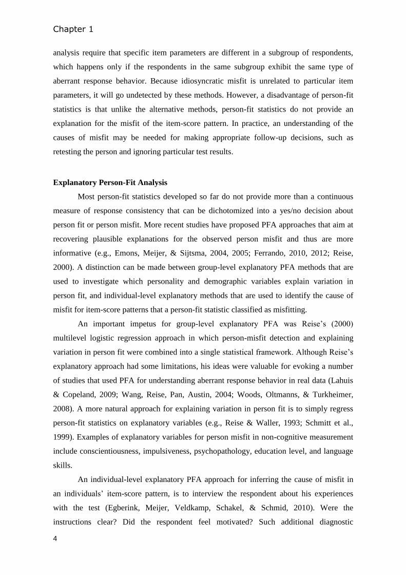
analysis require that specific item parameters are different in a subgroup of respondents,
which happens only if the respondents in the same subgroup exhibit the same type of
aberrant response behavior. Because idiosyncratic misfit is unrelated to particular item
parameters, it will go undetected by these methods. However, a disadvantage of person-fit
statistics is that unlike the alternative methods, person-fit statistics do not provide an
explanation for the misfit of the item-score pattern. In practice, an understanding of the
causes of misfit may be needed for making appropriate follow-up decisions, such as
retesting the person and ignoring particular test results.
Explanatory Person-Fit Analysis
Most person-fit statistics developed so far do not provide more than a continuous
measure of response consistency that can be dichotomized into a yes/no decision about
person fit or person misfit. More recent studies have proposed PFA approaches that aim at
recovering plausible explanations for the observed person misfit and thus are more
informative (e.g., Emons, Meijer, & Sijtsma, 2004, 2005; Ferrando, 2010, 2012; Reise,
2000). A distinction can be made between group-level explanatory PFA methods that are
used to investigate which personality and demographic variables explain variation in
person fit, and individual-level explanatory methods that are used to identify the cause of
misfit for item-score patterns that a person-fit statistic classified as misfitting.
An important impetus for group-level explanatory PFA was Reise’s (2000)
multilevel logistic regression approach in which person-misfit detection and explaining
variation in person fit were combined into a single statistical framework. Although Reise’s
explanatory approach had some limitations, his ideas were valuable for evoking a number
of studies that used PFA for understanding aberrant response behavior in real data (Lahuis
& Copeland, 2009; Wang, Reise, Pan, Austin, 2004; Woods, Oltmanns, & Turkheimer,
2008). A more natural approach for explaining variation in person fit is to simply regress
person-fit statistics on explanatory variables (e.g., Reise & Waller, 1993; Schmitt et al.,
1999). Examples of explanatory variables for person misfit in non-cognitive measurement
include conscientiousness, impulsiveness, psychopathology, education level, and language
skills.
An individual-level explanatory PFA approach for inferring the cause of misfit in
an individuals’ item-score pattern, is to interview the respondent about his experiences
with the test (Egberink, Meijer, Veldkamp, Schakel, & Schmid, 2010). Were the
instructions clear? Did the respondent feel motivated? Such additional diagnostic
Introduction
5
information may also be provided by others who observed the respondent when he
completed the test. For example, the teacher may see that children were not concentrating
during the test (Meijer et al., 2008). Alternatively, Emons et al. (2004, 2005) and Ferrando
(2010, 2012) proposed PFA methods for inferring the cause of an individuals’ misfit that
do not use additional diagnostic information. Ferrando (2010) used item-level residuals to
identify subsets of items containing the most unexpected item scores and formulated
probable causes for the misfit based on the items’ content. Emons et al. (2004, 2005)
proposed a similar approach that also allows statistical testing whether misfit is related to
specific subsets of items. Even though these methods have been around for a while, they do
not yet seem to have stimulated real-data applications of person-fit methods for explaining
misfit of individual respondents’ item-score patterns.
Outline of the Thesis
This thesis focuses on explanatory PFA and the suitability of PFA for identifying
misfitting item-score patterns in non-cognitive data. We evaluated the performance of
existing and newly developed PFA methods using simulation studies and real-data
applications. We also used real data to address substantive questions about the nature of
aberrant response behavior. Finally, we discuss the practical value of PFA for non-
cognitive measurement.
In Chapter 2, we discuss Reise’s (2000) multilevel logistic regression (MLR)
approach to PFA. Reise proposed to use MLR for estimating a logistic IRT model for
person-response probability as a function of item location. This multilevel PFA approach
has the potential advantage of combining person-misfit detection and explanatory PFA in
the same statistical model. First, we used a logical analysis to evaluate whether MLR is
compatible with the logistic IRT model and produces correct statistical information for
PFA. Second, we conducted a simulation study to determine whether the parameter
estimates of the multilevel PFA model are biased.
In Chapter 3, we use an alternative explanatory multilevel PFA approach to
investigate response consistency in a sample of cardiac patients and their partners on the
repeated measurements of the Spielberger State-Trait Anxiety Inventory (STAI;
Spielberger, Gorsuch, Lushene, Vagg, & Jacobs, 1983). Symptoms of anxiety in cardiac
patients and their partners can induce health risks and need to be monitored accurately. Our
aim was to understand which situational and individual characteristics induce person
misfit. We addressed this question by modeling within-person and between-person
Chapter 1
6
variation in repeated observations of the person-fit statistic by means of time-dependent
(e.g., mood state) and stable (e.g., education level) explanatory variables.
In Chapter 4, we focus on the potential of PFA for non-cognitive measures with
multiple short subscales assessing different latent traits. Multiscale measures are common
in non-cognitive measurement. However, person-fit statistics assume unidimensionality
and are not readily applicable to multiscale data. We therefore evaluated several methods
for combining person-fit information from different subscales into an overall person-fit
measure. We used both a simulation study and three real-data applications to investigate
the usefulness of the multiscale person-fit methods with respect to (1) detecting person
misfit, (2) improving accuracy of research results, and (3) understanding causes of aberrant
response behavior.
In Chapter 5, we evaluate the usefulness of PFA for outcome measurement using
data of the Outcome Questionnaire-45 (OQ-45; Lambert et al., 2004). OQ-45 results are
used in mental health care for individual treatment planning and in large scale cost-
effectiveness assessments. We hypothesized that the multiscale version of the statistic
may be useful for detecting aberrant item-score patterns and for studying whether patients
with specific types of disorders are particularly prone to aberrant response behavior.
Furthermore, we investigated if the standardized residual statistic may be useful for
explaining misfit of individual respondents. First, we used a simulation study to determine
the performance of the person-fit methods for tests that have psychometric properties such
as those of the OQ-45. Second, we used the PFA methods to detect and explain aberrant
response behavior in the OQ-45 data collected in a clinical sample.

7
Chapter 2
On the usefulness of a multilevel logistic regression approach
to person-fit analysis
Abstract The logistic person response function (PRF) models the probability of a
correct response as a function of the item locations. Reise (2000) proposed to use the slope
parameter of the logistic PRF as a person-fit measure. He reformulated the logistic PRF
model as a multilevel logistic regression model, and estimated the PRF parameters from
this multilevel framework. An advantage of the multilevel framework is that it allows
relating person fit to explanatory variables for person misfit/fit. We critically discuss
Reise’s (2000) approach. First, we argue that often the interpretation of the PRF slope as an
indicator of person misfit is incorrect. Second, we show that the multilevel logistic
regression model and the logistic PRF model are incompatible, resulting in a multilevel
person-fit framework, which grossly violates the bivariate normality assumption for
residuals in the multilevel model. Third, we use a Monte Carlo study to show that in the
multilevel logistic regression framework estimates of distribution parameters of PRF
intercepts and slopes are biased. Finally, we discuss the implications of these results and
suggest an alternative multilevel regression approach to explanatory person-fit analysis.
We illustrate the alternative approach using empirical data on repeated anxiety
measurements of cardiac arrhythmia patients who had a cardioverter-defibrillator
implanted.
This chapter was published as: Conijn, J. M., Emons, W. H. M., Van Assen, M. A. L. M, & Sijtsma, K.
(2011). On the usefulness of a multilevel logistic regression approach to person-fit analysis. Multivariate
Behavioral Research, 46, 365-388.
Chapter 2
8
2.1 Introduction
Reise (2000) proposed a multilevel logistic regression (MLR) approach to the
assessment of person fit in the context of the 1- and 2-parameter logistic item response
theory (IRT) models for dichotomous item scores. Henceforth, we call this approach
multilevel person-fit analysis (PFA). Whereas traditional methods for PFA (Karabatsos,
2003; Meijer & Sijtsma, 1995, 2001) provide little more than a yes/no decision rule for
whether test performance is aberrant, Reise’s proposal offers great potential for explaining
person misfit by including explanatory variables in the statistical analysis. Several studies
provide real-data examples of this potential (Wang, Reise, Pan, & Austin, 2004; Woods,
2008). For example, multilevel PFA was used to study faking on personality scales
(LaHuis & Copeland, 2009) and to explain aberrant responding of military recruits to
personality scales (Woods, Oltmanns, & Turkheimer; 2008).
What none of these studies have questioned is whether the combination of MLR
and a logistic IRT model for the person-response probability as a function of item location,
here denoted person response function (PRF; Sijtsma & Meijer, 2001), is compatible and
produces correct statistical information for PFA. Our study demonstrates that the
combination is incompatible, assesses the degree of bias the inconsistency causes in the
multilevel-model parameter estimates used for person-fit assessment, and discusses the
consequences for the viability of MLR for PFA.
PFA studies the fit of IRT models to individual examinees’ item-score vectors of 0s
(e.g., for incorrect answers) and 1s (for correct answers) on the J items from the test of
interest. The 1- and 2-parameter logistic models (1PLM, 2PLM; Hambleton &
Swaminathan, 1985) assume that one underlying ability or trait affects an examinee’s
responses to the items. However, for some examinees unwanted attributes may affect the
responses. For example, in ability testing test anxiety, incorrect learning strategy, answer
copying, and guessing may affect responses in addition to an examinee’s ability level. In
personality assessment response styles, faking, and untraitedness (Reise & Waller, 1993;
Tellegen, 1988) may produce item scores different from what was expected from the trait
level alone. Aberrant responding produces item-score vectors that are inconsistent with the
IRT model, and likely results in invalid latent-variable estimates (Meijer & Nering, 1997).
Identification of such item-score vectors is imperative so as to prevent drawing the wrong
conclusions about examinees.
Multilevel logistic regression in person-fit analysis
9
PFA based on the 1PLM or the 2PLM identifies item-score vectors, which are
either consistent or inconsistent with these models. Inconsistent vectors contain unusually
many 0s where the IRT model predicts more 1s, and 1s where more 0s are expected. A
limitation of traditional PFA is that it only identifies fitting and misfitting item-score
vectors but leaves the researcher speculating about the causes of the misfit. Multilevel PFA
attempts to move PFA from only signaling person misfit to also understanding its causes
by introducing an explanatory model of the misfit. It uses the PRF for this purpose (Emons,
Sijtsma, & Meijer, 2004, 2005; Lumsden, 1977, 1978; Nering & Meijer, 1998; Sijtsma &
Meijer, 2001; Trabin & Weiss, 1983). For dichotomously scored items, the PRF provides
the relationship between an examinee’s probability of having a 1 score on an item as a
function of the item’s location. Lumsden (1978), Ferrando (2004, 2007), and Emons et al.
(2005) noticed that the PRF based on the 1PLM decreases. Emons et al. (2005) argued that
a PRF that increases locally indicates misfit to the 1PLM and that the location of the
increase in the PRF on the latent scale and also the shape of the PRF provide diagnostic
information about misfit. For example, for average-ability examinees low probabilities of
correct responses on the first and easiest items might signal test anxiety, and for low-ability
examinees high probabilities of correct responses on the most difficult items might signal
cheating.
Reise’s multilevel PFA is based on logistic PRFs to assess person fit in the context
of the 1PLM and the 2PLM. Multilevel PFA focuses on the PRF slope, which is taken as a
person-fit measure quantifying the degree to which examinees are sensitive to differences
in item locations. The MLR framework allows modeling variation in PRF slopes using
explanatory variables such as verbal skills, motivation, anxiety, and gender. This renders
multilevel PFA useful for explaining person misfit and investigating group differences in
person fit.
Multilevel PFA is valuable and original but also evokes the question whether the
multilevel model and the logistic PRF model are compatible. Hence, we submitted
multilevel PFA to a thorough logical analysis and a Monte Carlo simulation study. First,
we discuss the PRF definition used in multilevel PFA. Second, we explain multilevel PFA.
Third, unlike Reise (2000) and Woods (2008) we argue that the interpretation of the PRF
slope as a person-fit measure is only valid for the 1PLM but invalid for the 2PLM. Fourth,
we show that the PRF model under the 1PLM is not compatible with the MLR framework
from which the PRF parameters are estimated. Fifth, the results of a Monte Carlo study
show the effect of the model mismatch on the bias in the estimates of distribution
Chapter 2
10
parameters of PRF intercepts and slopes. Sixth, we discuss our findings and their
consequences for multilevel PFA. Seventh, we suggest an alternative multilevel approach
to explanatory PFA. We illustrate the alternative approach using empirical data on repeated
anxiety measurements of cardiac arrhythmia patients who had a cardioverter-defibrillator
implanted. Finally, we discuss the viability of multilevel PFA and our proposed alternative
approach to explanatory PFA.
2.2 Theory of Multilevel Person-Fit Analysis
2.2.1 Person Response Function
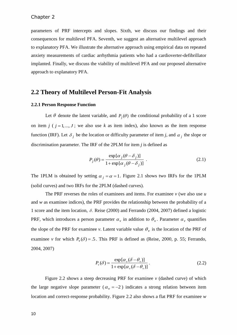
Let denote the latent variable, and )(jP the conditional probability of a 1 score
on item j ( Jj ..., ,1 ; we also use k as item index), also known as the item response
function (IRF). Let j be the location or difficulty parameter of item j, and j the slope or
discrimination parameter. The IRF of the 2PLM for item j is defined as
)](exp[1
)](exp[)(
jj
jjjP
. (2.1)
The 1PLM is obtained by setting 1 j . Figure 2.1 shows two IRFs for the 1PLM
(solid curves) and two IRFs for the 2PLM (dashed curves).
The PRF reverses the roles of examinees and items. For examinee v (we also use u
and w as examinee indices), the PRF provides the relationship between the probability of a
1 score and the item location, . Reise (2000) and Ferrando (2004, 2007) defined a logistic
PRF, which introduces a person parameter v in addition to v . Parameter v quantifies
the slope of the PRF for examinee v. Latent variable value v is the location of the PRF of
examinee v for which 5.)( vP . This PRF is defined as (Reise, 2000, p. 55; Ferrando,
2004, 2007)
)](exp[1
)](exp[)(
vv
vvvP
. (2.2)
Figure 2.2 shows a steep decreasing PRF for examinee v (dashed curve) of which
the large negative slope parameter ( 2v ) indicates a strong relation between item
location and correct-response probability. Figure 2.2 also shows a flat PRF for examinee w

Multilevel logistic regression in person-fit analysis
11
(solid curve) of which the small negative slope parameter ( 2.0w ) indicates a weak
relation. Large negative slopes indicate high person reliability (Lumsden, 1977, 1978), low
individual trait variability (Ferrando, 2004, 2007), and good person fit (Reise, 2000).
Figure 2.1: Two Item Response Functions Under the 1PLM (Solid Curves) and 2PLM
(Dashed Curves).
Note.
Multilevel PFA rephrases Equation 2.2 as a 2-level logistic regression model, and
estimates the PRF parameters from the latter model. This is innovative relative to existing
methods. For example, Ferrando (2004, 2007) developed a PRF model based on
Lumsden’s Thurstonian model (1977), and Strandmark and Linn (1987) formulated the
PRF as a generalized logistic response model. In the context of nonparametric IRT, Sijtsma
and Meijer (2001) and Emons et al. (2004, 2005) estimated PRFs using nonparametric
regression methods such as binning and kernel smoothing, and for parametric IRT, Trabin
and Weiss (1983) and Nering and Meijer (1998) used binning to estimate the PRF.
-3 0 3
0.0
0.5
1.0
Latent Variable
Pro
ba
bility o
f C
orr
ect
Re
sp
on
se
1 2 3 4
Chapter 2
12
2.2.2 Multilevel Approach to Person-Fit Analysis
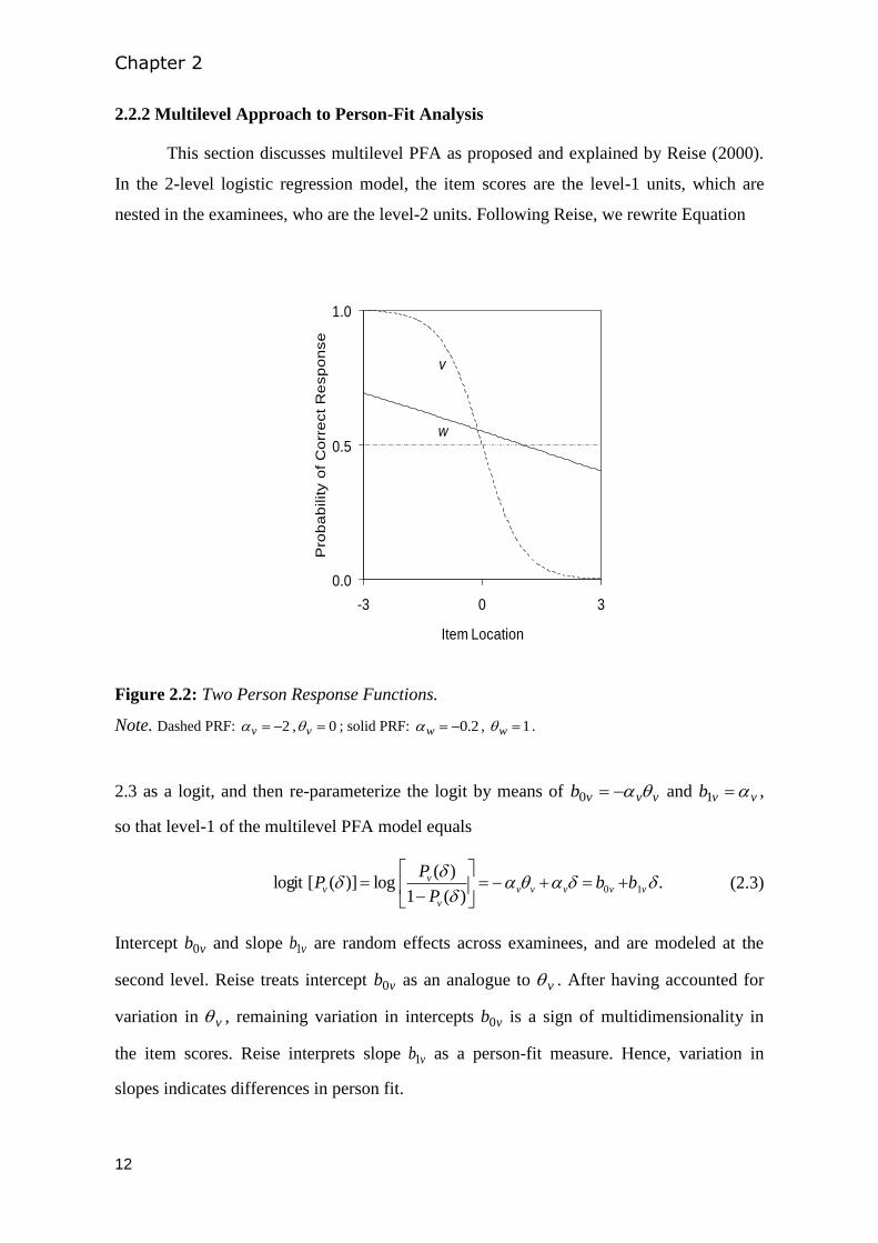
This section discusses multilevel PFA as proposed and explained by Reise (2000).
In the 2-level logistic regression model, the item scores are the level-1 units, which are
nested in the examinees, who are the level-2 units. Following Reise, we rewrite Equation
Figure 2.2: Two Person Response Functions.
Note. Dashed PRF: 2v , 0v ; solid PRF: 2.0w , 1w .
2.3 as a logit, and then re-parameterize the logit by means of vvvb 0 and vvb 1 ,
so that level-1 of the multilevel PFA model equals
. )(1
)( log)]([logit 10
vvvvv
v
vv bb
P
PP
(2.3)
Intercept vb0 and slope vb1 are random effects across examinees, and are modeled at the
second level. Reise treats intercept vb0 as an analogue to v . After having accounted for
variation in v , remaining variation in intercepts vb0 is a sign of multidimensionality in
the item scores. Reise interprets slope vb1 as a person-fit measure. Hence, variation in
slopes indicates differences in person fit.
-3 0 3
0.0
0.5
1.0
Item Location
Pro
ba
bility o
f C
orr
ect
Re
sp
on
se
v
w

Multilevel logistic regression in person-fit analysis
13
Reise (2000, pp. 558-562) distinguishes three steps in multilevel PFA. These steps
are preceded by the estimation of the item locations j and the latent variable values v
from either the 2PLM or the 1PLM.
Step 1 estimates the PRF in Equation 2.3. For this purpose, the item location
estimates, j , are used. In the level-2 model, the level-1 intercept vb0 is split into an
average intercept 00 and a random intercept effect vu0 , and the slope vb1 into an average
slope 10 and a random slope effect vu1 , so that
.
,
1101
0000
vv
vv
ub
ub
(2.4)
Step 2 explains the variance of the estimated intercepts vb0 , which is denoted
)()( 0000 uVarbVar . For this purpose, the estimated latent variable, , is used as an
explanatory variable of intercept 0b , so that the level-2 model equals
.
,ˆ
1101
001000
vv
vvv
ub
ub
(2.5)
Reise (2000) claims that under a fitting IRT model, variation in explains all intercept
variance, so that 00 is not significantly greater than 0.
Step 3 estimates the variance in the slopes, denoted )()( 1111 uVarbVar . For
this purpose, the level-1 intercepts are fixed given v , meaning that 000 , and the level-
1 slopes, vb1 , are assumed random, so that
.
,ˆ
1101
01000
vv
vv
ub
b
(2.6)
Significant slope variance, 11 , indicates systematic differences in person fit, and the
Empirical Bayes (EB) estimates, vb1ˆ , are used as individual person-fit measures. Larger
negative values of vb1ˆ reflect greater sensitivity to item location, and are interpreted as a
sign of person fit, whereas smaller negative values and positive values of vb1ˆ are
Chapter 2
14
interpreted as signs of person misfit. One may include explanatory variables in the level-2
model for the slope to explain variation in person fit. Reise discussed the multilevel PFA
approach only for the 1PLM, but also claimed applicability to the 2PLM.
We return to Step 2 and notice that significant intercept variance provides evidence
of multidimensionality in the form of either violation of local independence (or
unidimensionality) or differential test functioning (Reise, 2000, pp. 560-561). Following
Reise (2000), LaHuis and Copeland (2009) suggest including exploratory variables in the
intercept model to study causes of this model misfit.
2.3 Evaluation of Multilevel Person-Fit Analysis
We identify two problems with respect to multilevel PFA. First, the interpretation
of the PRF slopes v in Equation 2.2 and vb1 in Equation 2.3 as person-fit measures is
only valid under restrictive assumptions for the items. Second, the PRF model (Equation
2.2) and the multilevel PFA models (equations 2.3 through 2.6) used to estimate the PRF
are incompatible. Next, we discuss these problems and their implications for multilevel
PFA.
2.3.1 Problem 1: Interpretation of the Variance in PRF Slope Parameters in PFA
Multilevel PFA posits that when either the 1PLM or the 2PLM is the true model, all
examinees have the same negative PRF slope parameter (Reise, 2000, pp. 560, 563, speaks
of non-significant variation in person slopes). However, Sijtsma and Meijer (2001; Emons
et al., 2005) showed that PRFs are only monotone nonincreasing if the IRFs of the items in
the test do not intersect anywhere along the θ scale. In the 2PLM, IRFs intersect by
definition if item discrimination varies over items, and PRFs are not decreasing functions
but show many local increases. Hence, PRF slope parameters do not have a clear-cut
definition, and we therefore ask whether Reise’s position concerning variation in PRF
slopes is correct. First, we discuss this question for the 1PLM and then for the 2PLM.
Based on the IRF defined in Equation 2.1, we write the difference of the logits for
examinee v and arbitrary items j and k as,
.)()]([logit)]([logit jjkkjkvvjvk PP (2.7)
Multilevel logistic regression in person-fit analysis
15
For the 1PLM, by definition kj , so that Equation 2.7 reduces to ( kj ).
Hence, the difference depends on item parameters j , and k but not on .v
Furthermore, for arbitrary item locations such that kj the difference is negative, hence
the PRF decreases. Thus, under the 1PLM the PRF slope parameters are equal and
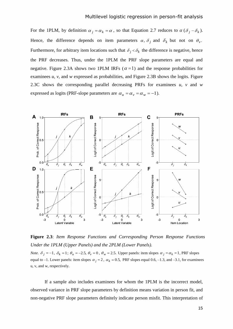
negative. Figure 2.3A shows two 1PLM IRFs ( 1 ) and the response probabilities for
examinees u, v, and w expressed as probabilities, and Figure 2.3B shows the logits. Figure
2.3C shows the corresponding parallel decreasing PRFs for examinees u, v and w
expressed as logits (PRF-slope parameters are 1 wvu ).
Figure 2.3: Item Response Functions and Corresponding Person Response Functions
Under the 1PLM (Upper Panels) and the 2PLM (Lower Panels).
Note. 1j , 1k ; ,5.2u 0v , .5.2w Upper panels: item slopes 1 kj , PRF slopes
equal to –1. Lower panels: item slopes 2j , ,5.0k PRF slopes equal 0.6, –1.3, and –3.1, for examinees
u, v, and w, respectively.
If a sample also includes examinees for whom the 1PLM is the incorrect model,
observed variance in PRF slope parameters by definition means variation in person fit, and
non-negative PRF slope parameters definitely indicate person misfit. This interpretation of
Chapter 2
16
variance in PRF slopes v is identical to the interpretation under multilevel PFA. This
means that under the 1PLM observed variance in PRF slopes can be validly interpreted as
variation in person fit across examinees.
Under the 2PLM, Equation 2.7 clarifies that, if kj , the difference in logits for
two items also depends on an examinee’s v value; hence, differences in cause
differences in PRF slopes. Moreover, the difference in logits is not always negative for
kj . For instance, if 0v then the difference is positive for those items j and k for
which kjk
j
; hence, for examinee v the PRF slope does not decrease everywhere.
Figure 2.3D shows two 2PLM IRFs and the response probabilities for examinees u,
v, and w expressed as probabilities, and Figure 2.3E shows the logits. Figure 2.3F shows
the corresponding PRFs for examinees u, v and w expressed as logits. For IRF slopes
2j and 5.0k , the two IRFs intersect. Consequently, the resulting PRFs have
different slopes, and the PRF for examinee u even increases. This result illustrates that
under the 2PLM, PRF slopes vary and PRFs do not necessarily decrease monotonically and
may even increase monotonically. In Figure 2.3F, the large variation in PRF slopes is due
to the large difference between IRF slopes j and k given the difference between IRF
locations j and k (Figure 2.3D and 2.3E) but smaller IRF-slope differences also lead to
variation in PRF slopes. Sijtsma and Meijer (2001) and Emons et al. (2005) discuss similar
results. Thus, under the 2PLM, the PRF slopes are expected to show variation also in the
absence of person misfit.
To conclude, under the multilevel PFA model variation in person slopes provides
valid information about person fit only if the items vary in difficulty but not in
discrimination power (i.e., the items satisfy the 1PLM). If items also vary in their
discrimination power (i.e., items satisfy the 2PLM), PRF slopes will vary even in the
absence of person misfit. Hence, in real data, for which the 1PLM is often too restrictive
and more flexible IRT models such as the 2PLM are appropriate, relating person fit to PRF
slopes may lead to overestimation of individual differences in person fit and increase the
risk of incorrectly identifying an examinee as misfitting or fitting.
Multilevel logistic regression in person-fit analysis
17
2.3.2 Problem 2: Incompatibility Between the PRF Model and the Multilevel PFA
Model
We assume that the 1PLM holds (i.e., items only differ in difficulty) in the
population of interest but that the fit of individual examinees varies randomly, which is
reflected by positive PRF-slope variance. Under this assumption, slope variance only
reflects random variation in person fit and does not result from differences in item
discrimination. For multilevel PFA (equations 2.3 through 2.6), we discuss whether under
these conditions the MLR formulation of the logistic PRF model leads to correct estimates
of the means and the variances of the slopes and the intercepts in the PRF model. If
estimates are biased, analyzing PRF slope variance based on multilevel PFA would be
misleading with respect to the true variation in person fit.
The MLR level-1 intercept and slope parameters (Equation 2.3) and the PRF
examinee parameters (Equation 2.2) are related by vvvb 0 and vvb 1 . For the
multilevel PFA model, in the intercept vvv ub 001000 (Equation 2.5) the effect
01 of v is fixed across examinees. For the PRF model, in the intercept vvvb 0
(Equation 2.3) the effect v of v is variable. Hence, the models do not match. This
mismatch has the following consequences.
In multilevel models, the level-2 random effects, vu0 and vu1 , are assumed to be
bivariate normal (Raudenbush & Bryk, 2002, p. 255; Snijders & Bosker, 1999, p. 121). It
may be noted that, from vvvb 0 and vvb 1 , it follows that vvv bb 10 . Thus,
intercept vb0 depends on slope vb1 , and in subgroups having the same slope value (i.e.,
11 bb v ) intercept variance across examinees is smaller the closer the slope value is to 0
(from 22
12
1|0 bbb ). This dependence implies a violation of bivariate normality of vu0
and vu1 . The next example illustrates this violation.
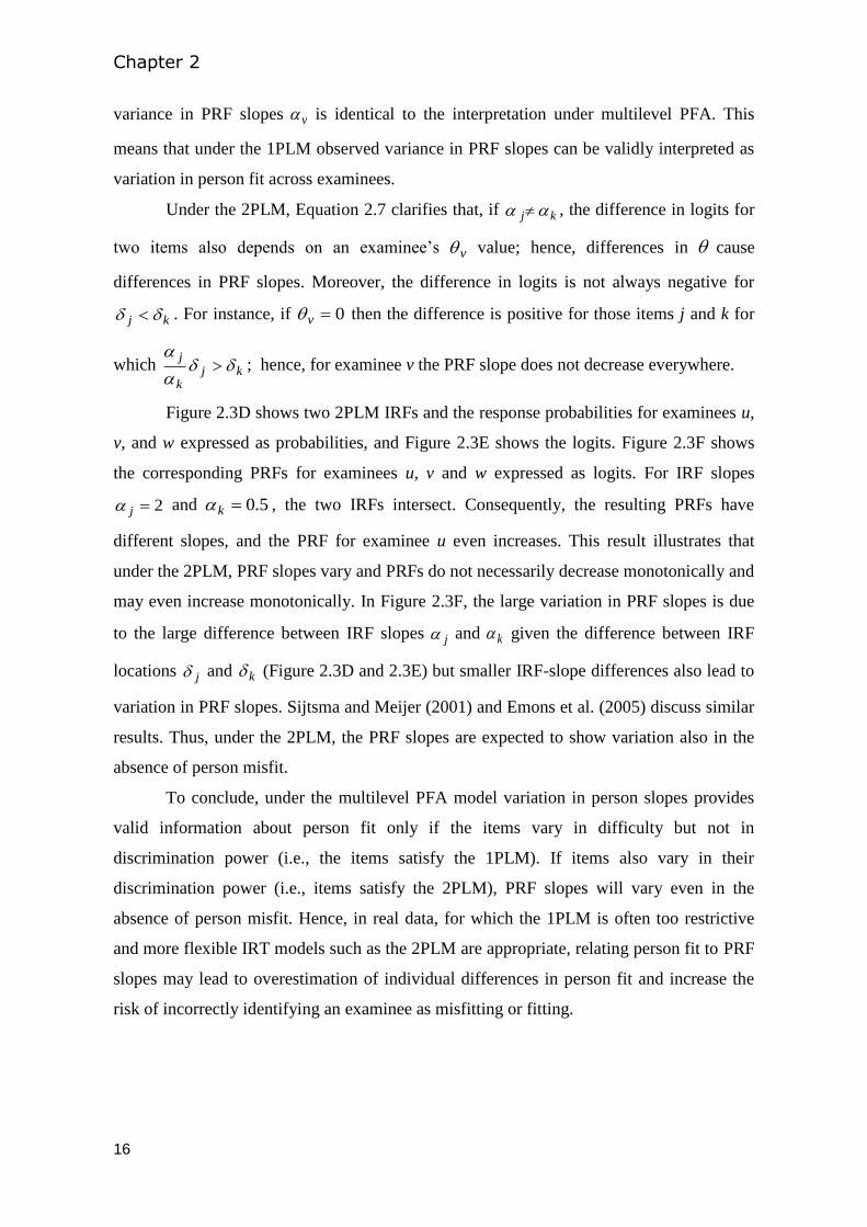
We consider that a PRF model in which )1 ,2(~ N and )1 ,0(~ N generated the
data. Figure 2.4A shows the resulting bivariate distribution of vu0 and vu1 for the level-2
model without v (Equation 2.4). We computed vu0 based on vvvb 0 and vu1 based
on vvb 1 (the note below Figure 2.4 provides computational details). Parameter vu0 is
the person-specific intercept deviation from the mean vb0 (i.e., the mean of vv , which
equals 00 ; see Equation 2.4), and vu1 is the person-specific slope deviation from the mean
Chapter 2
18
vb1 (i.e., the mean of v , which equals 10 ; see Equation 2.4). It follows that the vu0
values on the ordinate in Figure 2.4A equal the corresponding vb0 values (because 000
if 0 ). The vu1 values on the abscissa correspond to vb1 values between 6 and 2
(because 210 ).
Figure 2.4: Bivariate Distribution of Random Slope Effect ( vu1 ) and Random Intercept
Effect ( vu0 ) for Multilevel PFA Model Excluding v (Panel A) and Including v (Panel
B).
Note. ).( );1 ,2(~ and 1) ,0(~ 1 vvv MEANuNN In Panel A, vu0 is computed for Equation 2.4:
)(0 vvvvv MEANu , and in Panel B, vu0 is computed for Equation 2.5:
vvvvv MEANu )(0 .
-4 -2 0 2 4
-15
-10
-5
0
5
10
15
Inte
rce
pt
Eff
ect
u0v
A
-4 -2 0 2 4
-15
-10
-5
0
5
10
15
Inte
rce
pt
Eff
ect
u0v
B
Slope Effect u1v
Multilevel logistic regression in person-fit analysis
19
Figure 2.4A shows that bivariate normality is violated in the multilevel PFA model
defined by equations 2.3 and 2.4. The figure shows smaller variation in vu0 for large
positive vu1 (corresponding to near-0 vb1 ) than for large negative vu1 (corresponding to
large negative vb1 ). Thus, poorly fitting examinees who have near-0 PRF slopes (i.e., large
positive random slope effects) have smaller intercept variation than well-fitting examinees
who have steep negative PRF slopes (i.e., large negative random slope effects). The
explanation is that differences in are ineffective when examinees respond randomly
(reflected by flat PRFs) but effective when examinees respond according to the 1PLM
(reflected by decreasing PRFs) because then differences in determine differences in
response probabilities. Figure 2.4B shows that when is included in the multilevel PFA
model to explain intercept variance (Equation 2.5), the joint distribution of vu0 and vu1
again is not bivariate normal. The examples in Figure 2.4 show that one consequence of
using the MLR framework for estimating the distribution of PRF parameters is that
estimates are based on assumptions that are unreasonable when data satisfy the logistic
PRF model (Equation 2.3).
The mismatch of the multilevel PFA model and the PRF model also affects the
usefulness of Reise’s (2000) 3-steps procedure. In Step 2, residual intercept variance is
taken as a sign of multidimensionality. However, because the effect v of v on the
intercept vb0 (i.e., vvvb 0 ) is perfectly negatively related to the PRF slope ( v ), this
effect differs across examinees when there is variation in PRF slopes. As a result, if the
PRF slope varies v cannot be expected to explain all variation in the intercepts and,
therefore, residual intercept variance in the multilevel PFA model does not necessarily
represent multidimensionality. This is illustrated by Figure 2.4B in which the ordinate
values show variability in vu0 after having accounted for differences in v . If vu1 equals 0,
the standard deviation of vu0 equals 0. The standard deviation appears to increase linearly
in || 1vu . This shows that if PRF slopes vary, residual intercept variance is larger than 0.
This result has consequences for the usefulness of Step 3 in multilevel PFA. In Step 3, PRF
slope variation is studied restricting the residual intercept variance to 0. However, residual
intercept variance is only 0 if slope variance is 0 (i.e., all vu1 s equal 0), rendering Step 3
useless. Thus, only Step 1 and Step 2 are meaningful.
Chapter 2
20
To conclude, the multilevel PFA model is incompatible with the PRF model even if
the items satisfy the 1PLM. The mismatch refutes the interpretation of positive intercept
variance as an unambiguous sign of multidimensionality, because in multilevel PFA slope
variance necessarily implies intercept variance. Apart from whether multilevel PFA model
parameters can be interpreted meaningfully in each situation, the mismatch also questions
the validity of the parameter estimates under the multilevel PFA model. We showed that
the multilevel model does not adequately capture the bivariate distribution of residuals
( vu0 and vu1 ) to be expected if data comply with the PRF model. So the more problematic
consequence of the mismatch is that the multilevel model may produce biased estimates of
means and variances of PRF slopes and intercepts, as we demonstrate next.
2.4 Monte Carlo Study: Bias Due to Model Mismatch
We conducted a Monte Carlo study to examine whether estimates of multilevel
PFA model parameters 00 , 01 , 10 , and 11 (Equation 2.5; Step 2 in Reise’s 3-steps
procedure) are biased due to the mismatch between the multilevel PFA model and the PRF
model, and the resulting violation of bivariate normality of level-2 random effects. We
focused primarily on slope variance 11 , which is most relevant for explaining and
detecting person misfit.
We compared bias in the absence of model mismatch with bias in the presence of
mismatch. Mismatch of the multilevel PFA model with the PRF model is absent if in the
latter the effect of v is equal across examinees. We call this version of the PRF model the
‘Compatible PRF model’ (C-PRF model). Let denote the fixed effect of v . The C-
PRF model is defined as
)exp(1
)exp()(
vv
vvvP
. (2.8)
If the C-PRF model underlies the data and we find bias in the multilevel PFA model
estimates, this bias is inherent in MLR. However, if the PRF model generated the data, bias
is caused by both MLR and model mismatch. Thus, if model mismatch also causes bias,
we expect bias to be larger under the PRF model than the C-PRF model.
Multilevel logistic regression in person-fit analysis
21
2.3.1 Method
We simulated data consistent with the C-PRF model (Equation 2.8) and the PRF
model (Equation 2.2). Item and person parameters were estimated under the 1PLM. Bias in
multilevel PFA was studied under four conditions. In conditions ‘C-PRF true’ and ‘PRF
true’, we used the parameter values of and to estimate the multilevel PFA model. In
conditions ‘C-PRF est’ and ‘PRF est’, we used the parameter estimates and to
examine the bias found in practical data analysis where the true parameter values are
unknown and substituted by their sample estimates.
Parameters used to generate the data were distributed as ) ,(~ 2 N and
) ,(~ 2 N and, following Reise (2000), the item location was an equidistant sequence
from )2 ,2(~ U , with increments of 0.08. In the ‘true’ conditions we assessed bias of
estimates of the C-PRF model and the PRF model using 2242 combinations of
(valued 1, 2), 2 (0, 0.1, 0.5, 1), (0, 1), and 2
(0.2, 1). The C-PRF model and the
PRF model coincide in the eight combinations with 02 ; that is, for both models the
effect of v equals for all testees. The values for and 2 are based on empirical
multilevel PFA results by Woods (2008) and Woods et al. (2008), who used multilevel
PFA to analyze empirical data. The conditions with the largest ,2 which are )1 ,1(~ N
and )1 ,2(~ N , resulted in 16% and 2% increasing PRFs ( 0v ), respectively, and
14% and 4% nearly flat PRFs ( 0 5.0 v ).
For the ‘est’ conditions, we studied fewer combinations because this study focused
more on bias due to model mismatch than on bias due to estimates and . In the ‘est’
conditions, we assessed bias of the C-PRF and the PRF models in 22 combinations of
2) (1, and 1) (0.1, 2 using )1 ,0(~ N throughout. In all conditions, 000 (because
it is the adjusted mean outcome, see Raudenbush & Bryk, 2002, pp. 112-113), 01 ,
10 , and 211 .
We generated 1,000 datasets for each combination of parameter values. Because
Moineddin, Matheson, and Glazier (2007) showed that a level-1 sample size of at least 50
is required to obtain unbiased MLR parameter estimates, we chose a test length of 50
items. For several C-PRF conditions, we tried different level-2 sample sizes, and concluded
Chapter 2
22
that a level-2 sample size of 500 examinees throughout resulted in sufficient precision. The
Appendix provides information on the software used in this study.
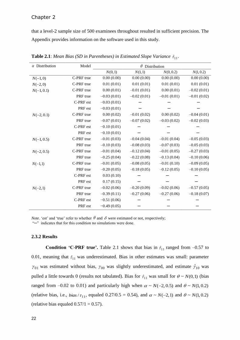
Table 2.1: Mean Bias (SD in Parentheses) in Estimated Slope Variance 11 .
Distribution Model Distribution
)1 ,0(N )1 ,1(N )2.0 ,0(N )2.0 ,1(N
)0 ,1(N
C-PRF true 0.00 (0.00) 0.00 (0.00) 0.00 (0.00) 0.00 (0.00)
)0 ,2(N
C-PRF true 0.01 (0.01) 0.01 (0.01) 0.01 (0.01) 0.01 (0.01)
)1.0 ,1(N C-PRF true 0.00 (0.01) –0.01 (0.01) 0.00 (0.01) –0.02 (0.01)
PRF true –0.03 (0.01) –0.02 (0.01) –0.01 (0.01) –0.01 (0.02)
C-PRF est −0.03 (0.01) ─ ─ ─
PRF est −0.03 (0.01) ─ ─ ─
)1.0 ,2(N C-PRF true 0.00 (0.02) –0.01 (0.02) 0.00 (0.02) –0.04 (0.01)
PRF true –0.07 (0.01) –0.07 (0.02) –0.03 (0.02) –0.02 (0.03)
C-PRF est −0.10 (0.01) ─ ─ ─
PRF est −0.10 (0.01) ─ ─ ─
)5.0 ,1(N C-PRF true –0.01 (0.03) –0.04 (0.04) –0.01 (0.04) –0.05 (0.03)
PRF true –0.10 (0.03) –0.08 (0.03) –0.07 (0.03) –0.05 (0.03)
)5.0 ,2(N C-PRF true –0.01 (0.04) –0.12 (0.04) –0.01 (0.05) –0.27 (0.03)
PRF true –0.25 (0.04) –0.22 (0.08) –0.13 (0.04) –0.10 (0.06)
)1 ,1(N C-PRF true –0.01 (0.05) –0.08 (0.05) –0.01 (0.10) –0.09 (0.05)
PRF true –0.20 (0.05) –0.18 (0.05) –0.12 (0.05) –0.10 (0.05)
C-PRF est 0.03 (0.10) ─ ─ ─
PRF est 0.17 (0.15) ─ ─ ─
)1 ,2(N C-PRF true –0.02 (0.06) –0.20 (0.09) –0.02 (0.06) –0.57 (0.05)
PRF true –0.39 (0.11) –0.27 (0.06) –0.27 (0.06) –0.18 (0.07)
C-PRF est −0.51 (0.06) ─ ─ ─
PRF est −0.49 (0.05) ─ ─ ─
Note. ‘est’ and ‘true’ refer to whether and were estimated or not, respectively;
“─” indicates that for this condition no simulations were done.
2.3.2 Results
Condition ‘C-PRF true’. Table 2.1 shows that bias in 11 ranged from –0.57 to
0.01, meaning that 11 was underestimated. Bias in other estimates was small: parameter
01 was estimated without bias, 00 was slightly underestimated, and estimate 10 was
pulled a little towards 0 (results not tabulated). Bias for 11 was small for )1 ,0(~ N (bias
ranged from –0.02 to 0.01) and particularly high when )0.5 ,2(~ N and )2.0 ,1(~ N
(relative bias, i.e., 11/bias , equaled 0.27/0.5 = 0.54), and )1 ,2(~ N and )2.0 ,1(~ N
(relative bias equaled 0.57/1 = 0.57).
Multilevel logistic regression in person-fit analysis
23
Condition ‘PRF true’. Similar to the ‘C-PRF true’ conditions, 10 and 11 were
pulled towards 0 but in contrast to the ‘C-PRF true’ conditions, 00 was overestimated and
01 underestimated (results only tabulated for 11 ).
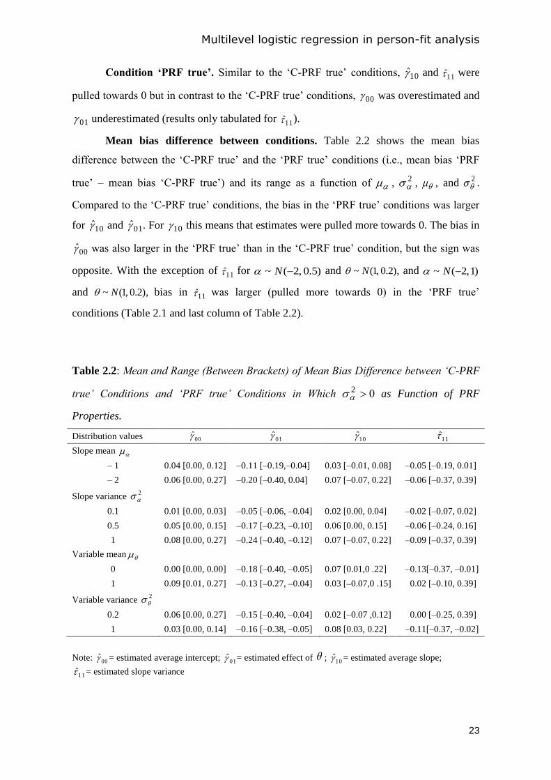
Mean bias difference between conditions. Table 2.2 shows the mean bias
difference between the ‘C-PRF true’ and the ‘PRF true’ conditions (i.e., mean bias ‘PRF
true’ – mean bias ‘C-PRF true’) and its range as a function of , 2 , , and 2
.
Compared to the ‘C-PRF true’ conditions, the bias in the ‘PRF true’ conditions was larger
for 10 and 01 . For 10 this means that estimates were pulled more towards 0. The bias in
00 was also larger in the ‘PRF true’ than in the ‘C-PRF true’ condition, but the sign was
opposite. With the exception of 11 for )0.5 ,2(~ N and ),2.0 ,1(~ N and )1 ,2(~ N
and ),2.0 ,1(~ N bias in 11 was larger (pulled more towards 0) in the ‘PRF true’
conditions (Table 2.1 and last column of Table 2.2).
Table 2.2: Mean and Range (Between Brackets) of Mean Bias Difference between ‘C-PRF
true’ Conditions and ‘PRF true’ Conditions in Which 02 as Function of PRF
Properties.
Distribution values 00 01 10 11
Slope mean
– 1 0.04 [0.00, 0.12] –0.11 [–0.19,–0.04] 0.03 [–0.01, 0.08] –0.05 [–0.19, 0.01]
– 2 0.06 [0.00, 0.27] –0.20 [–0.40, 0.04] 0.07 [–0.07, 0.22] –0.06 [–0.37, 0.39]
Slope variance 2
0.1 0.01 [0.00, 0.03] –0.05 [–0.06, –0.04] 0.02 [0.00, 0.04] –0.02 [–0.07, 0.02]
0.5 0.05 [0.00, 0.15] –0.17 [–0.23, –0.10] 0.06 [0.00, 0.15] –0.06 [–0.24, 0.16]
1 0.08 [0.00, 0.27] –0.24 [–0.40, –0.12] 0.07 [–0.07, 0.22] –0.09 [–0.37, 0.39]
Variable mean
0 0.00 [0.00, 0.00] –0.18 [–0.40, –0.05] 0.07 [0.01,0 .22] –0.13[–0.37, –0.01]
1 0.09 [0.01, 0.27] –0.13 [–0.27, –0.04] 0.03 [–0.07,0 .15] 0.02 [–0.10, 0.39]
Variable variance 2
0.2 0.06 [0.00, 0.27] –0.15 [–0.40, –0.04] 0.02 [–0.07 ,0.12] 0.00 [–0.25, 0.39]
1 0.03 [0.00, 0.14] –0.16 [–0.38, –0.05] 0.08 [0.03, 0.22] –0.11[–0.37, –0.02]
Note: 00 = estimated average intercept; 01 = estimated effect of ; 10 = estimated average slope;
11 = estimated slope variance
Chapter 2
24
Table 2.2 shows that the mean bias difference in 00 (second column) was larger
for larger negative , increased in 2 and , and decreased in 2
. The bias differences
in 01 , 10 , and 11 (third to fifth column) were larger for larger negative , increased in
2 and 2
, and decreased in . In sum, model mismatch and violation of bivariate
normality caused biased estimates.
Conditions ‘C-PRF est’ and ‘PRF est’. Table 2.1 (third column) shows the bias in
11 in the ‘est’ conditions when )1 ,0(~ N . Parameter 11 was overestimated in the
conditions in which )1 ,1(~ N but underestimated in all other conditions. Bias also
differed from the ‘true’ conditions; except for )1 ,1(~ N , bias in 11 was larger and bias
in the ‘C-PRF est’ and ‘PRF est’ conditions was equal. Interestingly, mean 11 was 0 if
)0.1 ,2(~ N in both the ‘C-PRF est’ and ‘PRF est’ conditions. Thus, person misfit was
not detected in the ‘est’ conditions when misfit was modest but it was detected in the ‘true’
conditions. Estimate 00 was unbiased but 01 and 10 were substantially biased in most
of the ‘est’ conditions. Thus, multilevel PFA also yields biased estimates when using
and , and the results suggest that multilevel PFA does not detect person misfit in some
conditions when the variance in PRF slopes is small.
Intercept variance. Results for 00 were troublesome. Agreeing with our
theoretical analysis, if 02 , in the ‘true’ conditions 0ˆ00 but in the ‘est’ conditions
surprisingly we found 0ˆ00 . This result suggests that true intercept variance may be
concealed when estimated item and person parameters are used in multilevel PFA. Indeed,
additional simulations showed that also when multidimensionality holds one may find
0ˆ00 in the ‘est’ conditions. Thus, finding 0ˆ00 does not imply unidimensionality
because including in the multilevel PFA model may render multidimensionality
undetectable.
2.3.3 Summary of Monte Carlo Study
The Monte Carlo study showed that due to the mismatch between MLR and the
PRF model MLR yields biased estimates of the distributions of the person intercepts and
slopes from the PRF model. The variance of the PRF slopes, which is of primary interest in
PFA, tended to be underestimated in most cases. The other parameters were also biased,
Multilevel logistic regression in person-fit analysis
25
but no clear trends in the direction of the bias were found. Bias became even more serious
when estimated person and item parameters were used.
2.5 Conclusions on Multilevel Person-Fit Analysis
Multilevel PFA has serious limitations. First, multilevel PFA takes the slope of the
PRF as a valid person-fit measure, which is only correct under the 1PLM but contrary to
Reise’s suggestion not under the 2PLM. Second, MLR is incompatible with the PRF model
even if items satisfy the 1PLM. As a result, the assumption of bivariate normality of
random effects is violated when PRF slopes are different. Third, the mismatch between
MLR and the PRF model leads to biased estimates of multilevel PFA model parameters.
Most importantly, PRF-slope variance is underestimated or not even detected.
Part of the problem revolves around the interpretation of PRF slope variation.
Reise’s (2000) methodology argues that variation in PRF slopes indicates variation in
person fit, but does not recognize that under the 2PLM, in which items have different
discrimination parameters, PRF slopes vary by definition because the PRF slope depends
on the examinee’s latent variable value. This also means that, as a person-fit measure, the
PRF slope is inherently contaminated by the latent variable value. Obviously, this is an
undesirable property for person-fit statistics. Using PRF slopes for assessing person fit is
even more problematic because near-0 or positive PRF slopes, which Reise qualifies as
indicators of uninterpretable item-score patterns, can be fully consistent with the 2PLM.
Thus, person-fit assessment based on the PRF slopes is inappropriate under the 2PLM. On
the other hand, under the 1PLM, PRF slope variance is 0 by definition and deviant PRF
slopes found in a sample may flag person misfit.
The other part of the problem involves using the MLR framework for estimating the
PRF model, and appears fundamental. In the PRF model, both the location and slope vary
over examinees and need to be estimated as random effects. The multilevel approach
assumes bivariate normality for the level-2 random effects. We showed that the PRF slope
restricts the variation in the intercept and, as a result, the level-2 random effects do not
follow a bivariate normal distribution.
Our simulation study using item and person parameters showed that multilevel PFA
produces biased estimates of the systematic differences in person fit. Studies in other
research areas also found that non-normally distributed random effects in MLR lead to bias
in variance and fixed effects estimates (Heagerty & Kurland, 2001; Litière, Alonso, &
Chapter 2
26
Molenberghs, 2007; Litière, Alonso, & Molenberghs, 2008). The PRF-slope variance was
underestimated; hence, differences in person fit came out too small. The underestimation of
PRF-slope variance became greater when item and person parameter estimates were used,
which is what researchers do, thus showing that the problem is greater in real-data analysis.
Ironically, multilevel PFA only provides correct estimates when PRF slopes are equal but
then person misfit is absent. In real data it is unknown whether there is variation in person
fit or no misfit at all; this is exactly what multilevel PFA was designed to find out. Finally,
we found that multilevel PFA sometimes does not pick up multidimensionality (Step 2).
The key advantage of multilevel PFA over traditional person-fit methods is to
detect individual differences in person fit and explain these differences by including
explanatory variables in the model. The multilevel PFA model parameter estimates were
expected to provide information about person-fit variation and explanatory variables for
person fit and person misfit. However, we showed that multilevel parameters are biased
and that under the 2PLM the PRF slope is confounded with the latent variable distribution.
These results suggest that multilevel PFA has limited value as an explanatory tool in
person fit research. Contrary to Reise’s (2000) suggestions we also found that multilevel
PFA is inappropriate for studying multidimensionality.
Furthermore, Reise (2000) proposed to use the EB slopes from the multilevel PFA
model for identifying respondents having aberrant item-score patterns. Woods (2008)
studied the Type I error and the power of the EB slope in multilevel PFA and concluded
that in most conditions its performance was adequate. However, Woods also found
occasionally increased Type I error rates for the EB slopes and showed that it is difficult to
specify the cutoff criteria for EB slopes needed to operationalize misfit. Thus, even though
these results suggest that EB slopes have potential for identifying person misfit, their
usefulness requires additional research. However, given the theoretical limitations of
interpreting EB slopes as a measure of person fit, and also the bias in EB slope estimates
caused by biased slope variance estimates of the multilevel model (e.g., Collett, 2003, pp.
274-275), we consider further study on the usefulness of the EB slopes not a fruitful
contribution to person-fit assessment.
Multilevel logistic regression in person-fit analysis
27
2.6 An Alternative Explanatory Multilevel Person-Fit
Approach: Real-Data Example
An alternative multilevel PFA approach that we have started pursuing in our
research has similarities with Reise’s (2000) approach and aims, but avoids the problems
we identified. We tentatively advocate this approach using what we believe is an
interesting data example concerning cardiac patients who had a cardioverter-defibrillator
implanted, inducing anxiety in many patients due to anticipation of a sudden, painful
electrical shock responding to cardiac arrhythmia. A sample of cardiac patients and their
partners (N = 868) completed the state-anxiety scale from the State-Trait Anxiety
Inventory (Spielberger, Gorsuch, Lushene, Vagg, & Jacobs, 1983) in a longitudinal study
comprising five measurement occasions. Here, the repeated measurements constitute the
multilevel nature of the data. Using multilevel modeling, we assessed whether person fit is
a reliable individual-difference variable that may be explained by demographic,
personality, medical, psychological distress, and mood variables.
At each occasion, we used the widely accepted and much-used zl person-fit
statistic (Drasgow, Levine, & McLaughlin, 1987; Drasgow, Levine, & Williams, 1985; Li
& Olejnik, 1997) for assessing person fit on the anxiety-state scale of the STAI. Given the
4-point rating-scale data collected by means of the STAI, we used statistic zl to assess
person fit relative to the graded response model (Samejima, 1997). We assessed goodness
of fit of the GRM to the data for each measurement occasion, and found satisfying results
(Conijn, Emons, Van Assen, Pedersen, & Sijtsma, 2012). Several authors noticed that, in
particular for small numbers of dichotomous items, the sampling distribution of statistic zl
depends on latent-variable level (Nering, 1995; Snijders, 2001; Van Krimpen-Stoop &
Meijer, 1999). We implemented a parametric bootstrap procedure developed by De la
Torre and Deng (2008) to make sure that the zl statistic was standard normally distributed
at all values of the latent variable.
The zl statistic was modeled as a dependent variable in a 2-level model. As
independent variables we used measures of mood state and psychological distress, which
are time-dependent, and demographic characteristics, personality traits, and medical
conditions, known to be stable across time. The level-1 model describes within-individual
variation in person fit across repeated measures, and the level-2 model describes variation
across individual patients. An unconditional random intercept model estimated within-
Chapter 2
28
person and between-person variance in statistic zl . The ICC (Snijders & Bosker, 1999, pp.
16-18) provides evidence for or against substantive systematic between-person differences
in the data, and indicates whether a multilevel approach is useful. If significant between-
person variance is found, respondents differ systematically in person fit, and given this
result, this variation may be explained using the independent variables at level 1 and level
2. Explanatory variables specific to measurement occasions at level 1 may be added to
explain within-person variation in statistic zl .
The results were the following. The ICC equaled 0.31, suggesting that multilevel
analysis was appropriate and that of the total variation in zl 31% was attributable to
differences between persons and 69% to differences within persons. The unconditional
random intercept model revealed significant between-person variance in zl . We were able
to explain 8% of the between-person differences and 4% of the within-person differences
in person fit. Patients having more psychological problems, higher trait anger, and lower
education level showed more person misfit. When patients had higher anxiety level at the
measurement occasion than usual they also showed more misfit than usual. Thus, patients
showing poor fit at previous measurements, having low education level, and experiencing
psychological problems are at risk of producing invalid test results. Also, assessment
shortly before ICD implantation likely produces person misfit due to higher state anxiety.
Our results show that multilevel modeling can be highly useful in gaining a better
understanding of the person and situational characteristics that may produce person misfit
and, consequently, distort valid test performance.
One final remark is that in other studies researchers may not have access to repeated
measures but multilevel modeling of person misfit may well be possible, thus facilitating
the explanatory analysis so badly needed in person fit research. For example, for data based
on one measurement occasion the multilevel aspect may be the person-fit statistic obtained
on scales measuring different attributes or even on subsets of items coming from the same
scale.
2.7 Discussion
We showed that Reise’s (2000) multilevel PFA approach suffers from serious
theoretical and statistical problems, rendering the method questionable as an explanatory
tool in PFA. Exactly because the idea of constructing such an explanatory tool was so
Multilevel logistic regression in person-fit analysis
29
strong, and because multilevel analysis is a powerful approach that produces explanations
at different levels in the data, we suggested a simple alternative that avoids the technical
problems of Reise’s approach and maintains the explanatory ambitions so badly needed in
PFA.
A reviewer suggested finding a solution for the problem of non-normally
distributed random effects in the multilevel PFA model by estimating the bivariate
distribution of the random effects from the data. Thus far, for generalized linear models
only methods have been developed for estimating the univariate distribution of random
effects (Chen, Zhang, & Davidian, 2002; Litière et al., 2008). Maybe these methods could
be extended to the bivariate case, but if they could, implementation of these extensions
would only possibly repair the 1PLM version but not the much more flexible and for
practitioners more interesting 2PLM version of the multilevel PFA model. Moreover, for
researchers advocating the 1PLM our alternative approach may be used because statistic zl
is also adequate for 1PLM data (and Snijders, 2001, solved the distributional problems due
to dependence on latent-variable level). As an aside, one may note that our approach does
not hinge on statistic zl . For example, when the 1PLM is consistent with the data one may
use a statistic proposed by Molenaar and Hoijtink (1990) as the dependent variable, and if
parametric IRT models are inconsistent but a nonparametric model does fit, the normed
count of Guttman errors (Emons, 2008) may be used. Most important is the awareness that
our approach uses the multilevel model in a regular context without the technical problems
induced by Reise’s multilevel PFA model, and that the choice of the most appropriate
dependent variable for person fit is up to the researcher.
Another reviewer suggested that PFA in general has been rarely applied to real-data
problems, which questions the usefulness of PFA. Although some promising examples are
available (e.g., Conrad et al., 2010; Engelhard, 2009; Meijer, Egberink, Emons, & Sijtsma,
2008; Tatsuoka, 1996), we agree that more applications are needed. Conijn et al. (2012)
further elaborated the example using the sample of cardiac patients. More generally, PFA
suffers from low power because the number of items in the test is the “sample size” that
determines the power of a person-fit statistic (e.g., Emons et al., 2005; Meijer & Sijtsma,
2001), and this is a problem that is not easily solved. Nevertheless, the assessment of
individual test performance is highly important, and highly invalid item-score vectors can
be identified, even if the power for finding moderate violations is low and some invalid
vectors may be missed.

Chapter 2
30
Approaches focusing on PRFs and multilevel models have in common that they try
to incorporate PFA in an explanatory framework, thus strengthening the methods and
lending them more practical relevance. We believe that in spite of the problems such
attempts must be further pursued so as to improve the assessment of individual test
performance.
Multilevel logistic regression in person-fit analysis
31
Appendix: Software
We used the ltm R-package (Rizopoulos, 2009) to obtain the marginal maximal
likelihood estimates of under the 1PLM. We used the irtoys R-package (Partchev, 2008)
to obtain the expected a posteriori (EAP) estimates of i given the estimates from the
ltm R-package. Pan (2010) found that the ltm R-package provided parameter estimates at
least as accurate as IRT programs such as MULTILOG (Thissen, Chen, & Bock, 2003).
We used HLM 6.06 (Raudenbush, Bryk, & Congdon, 2008) to estimate the
multilevel PFA model. Parameter estimation was done with the Laplace6 (Raudenbush,
Yang, & Yosef, 2000) procedure in HLM 6.06. Laplace6 uses a sixth order approximation
to the likelihood based on a Laplace transform, using the EM algorithm. The maximum
number of iterations was set at 20,000. If convergence was not achieved, the parameter
estimates were not included in computing summary statistics on the bias. Simulation of
datasets was continued until the number of converged models was 1,000 in each condition.
Raudenbush et al. (2000) found that Laplace6 provided more accurate parameter
estimates than penalized quasi-likelihood, and was at least as accurate as Gauss-Hermite
quadrature using 10 to 40 quadrature points and adaptive Guass-Hermite quadrature using
seven quadrature points. Furthermore, Laplace6 was faster in terms of processing time than
(adaptive) Gauss-Hermite quadrature. An additional reason to use Laplace6 instead of
adaptive Gauss-Hermite quadrature was that the latter method converged slowly in the
PRF conditions when the lme4 package (Bates, Maechler, & Dai, 2008) was used in R.
Laplace6 did not provide any serious convergence problems.

Chapter 2
32
33
Chapter 3
Explanatory, multilevel person-fit analysis of response
consistency on the Spielberger State-Trait Anxiety Inventory
Abstract Self-report measures are vulnerable to concentration and motivation
problems, leading to responses that may be inconsistent with the respondent’s latent trait
value. We investigated response consistency in a sample (N = 860) of cardiac patients with
an implantable cardioverter defibrillator and their partners who completed the Spielberger
State-Trait Anxiety Inventory (STAI) on five measurement occasions. For each occasion
and for both the state and trait subscales, we used the 𝑝
person-fit statistic to assess
response consistency. We used multilevel analysis to model the between-person and
within-person differences in the repeated observations of response consistency using time-
dependent (e.g., mood states) and time-invariant explanatory variables (e.g., demographic
characteristics). Respondents with lower education, undergoing psychological treatment,
and with more posttraumatic stress disorder symptoms tended to respond less consistently.
The percentages of explained variance in response consistency were small. Hence, we
conclude that the results give insight into the causes of response inconsistency, but that the
identified explanatory variables are of limited practical value for identifying respondents at
risk of producing invalid test results. We discuss explanations for the small percentage of
explained variance and suggest alternative methods for studying causes of response
inconsistency.
This chapter has been submitted for publication
Chapter 3
34
3.1 Introduction
Aberrant responding to self-report questionnaires produces invalid test scores, and
may result in incorrect individual classification decisions (Hendrawan, Glas, & Meijer,
2005). The consistency of an item-score pattern is informative about the validity of the test
score. Response consistency is the degree to which the observed item scores agree with the
expected item scores based on the latent trait value. For example, in an anxiety
questionnaire, agreeing with the item “I’m calm” and disagreeing with the item “I feel
tense” is consistent with a low latent trait value because both responses are expected for a
non-anxious person. However, agreeing with the item “I’m afraid” but disagreeing with a
less extreme item such as “I’m worried” is inconsistent with any latent trait value. Person-
fit analysis (PFA) is a well-established method to assess response consistency (Meijer &
Sijtsma, 2001) that is based on item response theory (IRT), and assesses which patterns of
item scores may be considered outliers. In this study, we combine PFA with multilevel
regression analysis to explain between-person and within-person differences in response
consistency of cardiac patients and their partners on the Spielberger State-Trait Anxiety
Inventory (STAI; Spielberger, Gorsuch, Lushene, Vagg, & Jacobs, 1983). Our aim was to
obtain a better understanding of aberrant responding to self-reports for respondents
confronted with a life-threatening disease.
Several studies used person-fit statistics to investigate whether there are stable
individual differences in the tendency to respond consistently to personality items and if
there are differences, which traits and demographic variables characterize persons prone to
inconsistency. Schmitt, Chan, Sacco, McFarland, and Jennings (1999) found response
consistency on each of the five subscales of the NEO-Five Factor Inventory (Costa &
McCrae, 1992) to be weakly correlated (mean 24.r ; range: .04 - .38). The weak
correlations indicate that the tendency to respond consistently is to a large extent either
trait-specific or unsystematic (Reise & Waller, 1993; Tellegen, 1988). Woods, Oltmanns,
and Turkheimer (2008) found higher correlations (mean r = .41; range: .17 - .63) across
five temperament and trait scales of the Schedule for Nonadaptive and Adaptive
Personality (Clark, 1996). The positive correlations of which some are substantial suggest
that persons who respond consistently to one personality scale also tend to respond more
consistent to scales measuring different personality traits.
Response consistency was found to relate to certain individual characteristics. For
scales assessing different traits, it was found that males (Pinsoneault, 2002; Schmitt et al.,
Response consistency on the STAI
35
1999; Woods, 2008) and respondents low in conscientiousness (Ferrando, 2009; LaHuis &
Copeland, 2009; Schmitt et al., 1999) responded less consistent than females and
respondents high in conscientiousness. In addition, indicators of negative affect including
low well-being, aggression, stress reaction, and alienation (Reise & Waller, 1993) and
severe personality pathology (Woods et al., 2008) were found to relate negatively to
consistency. Test-taking motivation (Schmitt et al., 1999), intelligence, verbal fluency, and
reading skills related positively to consistency (Meijer, Egberink, Emons, & Sijtsma, 2008;
Pinsoneault, 1998).
Most of the prior research investigated response consistency on only one
measurement occasion but Meijer et al. (2008) re-assessed response inconsistency found in
a subgroup of primary school students on a second measurement occasion. Three questions
with respect to longitudinal variation in response consistency remain unaddressed. These
questions are important to understand which of the respondents are at risk of producing
invalid test results, and under which circumstances respondents are most likely to do so.
The research questions and the motivations for the questions are:
1. Do stable between-person differences in response consistency exist across time?
Stability of response consistency over time supports the hypothesis that response
inconsistency is due to a stable tendency rather than merely being due to a momentary
lapse in motivation or concentration on a specific measurement occasion. Stable between-
person differences imply that results of persons responding inconsistently on a particular
measurement occasion should be interpreted with caution on subsequent occasions.
2. Are stable between-person differences in response consistency related to
particular demographic or psychological variables?
Explanatory variables for the stable between-person differences in response consistency
can be used for identifying respondents at risk of producing invalid test results.
3. Are within-person differences in response consistency across time related to
differences in mood or psychological distress across time?
For example, if a respondent is stressed, tired, or restless, (s)he likely responds less
consistently than when (s)he is rested and relaxed. The results can provide knowledge
about the circumstances in which self-report scales should be administered.
To address the research questions, we first used the well-established IRT-based 𝑝
person-fit statistic (Drasgow, Levine, & Williams, 1985) to quantify response consistency
on different measurement occasions. In the second step, we used a two-level multilevel
model for repeated measurements to model the within- and between-person variation in 𝑝.
Chapter 3
36
Reise (2000) was the first to recognize the value of estimating and explaining stable
individual differences in response consistency. He proposed a multilevel PFA approach
that has similarities with our approach. However, Conijn, Emons, Van Assen, & Sijtsma
(2011) showed that this method suffers from technical problems and provides biased
estimates of the stable differences in response consistency. Hence, in this study we used an
alternative method that does not suffer from these problems.
3.1.1 Response Consistency of Cardiac Patients and their Partners on the STAI
We addressed the research questions for the anxiety self-reports provided by a
sample of cardiac patients treated with an implantable cardioverter-defibrillator (ICD) and
their partners. The ICD corrects potential life-threatening arrhythmias by means of an
electrical shock. However, because the shocks come unexpected and can be very painful
ICD treatment can also lead to chronic and clinical levels of anxiety, both in patients and
their partners (e.g., Pedersen et al., 2009a, 2009b). High levels of anxiety in ICD patients
are associated with poor health outcomes such as increased arrhythmic events and
mortality (e.g., Pedersen, Van den Broek, Erdman, Jordaens, & Theuns, 2010).
Furthermore, anxiety in their partners may also negatively affect prognosis of ICD patients
due to reduced partner support (Pedersen et al., 2009a).
To prevent anxiety-induced health risks, it is important to accurately monitor
symptoms of anxiety in ICD patients and their partners and provide psychological
intervention if needed (Pedersen et al., 2009b). Usually, self-report measures are used for
assessment of anxiety in cardiac patients (DeJong & Hall, 2003). However, the use of self-
reports for measuring anxiety in respondents confronted with a life-threatening disease
may be problematic (DeJong & Hall, 2003). For example, concentration problems related
to one’s medical condition, tension resulting from an impending operation, or reluctance to
disclose psychological symptoms may disturb accurate responding. Particularly the STAI,
which is the most frequently used anxiety scale in research on cardiovascular disease, was
suggested to be too long for both acutely ill and older cardiac patients, and may lead them
to respond inconsistently (DeJong & Hall, 2003).
To obtain a better understanding of the causes of inconsistent responding of ICD
patients and their partners, we studied response consistency on the STAI trait-anxiety and
state-anxiety subscales. Based on the results, we discuss whether it is possible to identify
respondents who are at risk of producing invalid test results based on (1) previous response
Response consistency on the STAI
37
behavior, (2) individual characteristics such as demographic, medical, and psychological
variables, and (3) the respondent’s mental state.
After assessing stable between-person differences in response consistency across
time (research question 1), we tested a series of hypotheses using different types of
explanatory variables for response consistency. The explanatory variables were
demographic, medical, personality trait, psychological distress, and mood state variables.
We formulated hypotheses about between-person differences (research question 2) and
within-person differences (research question 3) in response consistency.
Between-person differences. Following the literature (Pinsoneault, 2002; Schmitt
et al., 1999; Woods, 2008), we hypothesized that males respond less consistently than
females. The previously discussed results of Meijer et al. (2008) and Pinsoneault (1998)
suggest that low cognitive ability may result in response inconsistency. Cognitive ability is
expected to be lower for lower-educated persons and older adults (e.g., Schaie, 1994).
Hence, we hypothesized that response consistency is positively related to education level
and negatively related to old age.
Physical symptoms (e.g., pain or fatigue) may disturb accurate responding. Hence,
we hypothesized that patients respond less consistently than their partners, and that
response consistency is negatively related to the extent of heart failure, ICD related
complications, and having received an ICD shock.
Response consistency was found to be negatively related to psychopathology
(Woods et al., 2008), stress reaction, alienation, and aggression, and positively related to
well-being (Reise & Waller, 1993). Using these results, we formulated hypotheses about
three types of psychological variables. First, response consistency is negatively related to
the personality traits of negative affectivity, social inhibition, trait anger, and trait anxiety.
Second, response consistency is negatively related to indicators of psychological distress
including posttraumatic stress disorder (PTSD) symptoms, being treated with
psychopharmaca, and seeing a psychologist or psychiatrist. Third, response consistency is
negatively related to negative mood states including state anxiety, state anger, state
depression, and having ICD concerns.
Within-person differences. Time-dependent variables like indicators of
psychological distress and mood state may vary across measurement occasions, and may
therefore lead to within-person differences in response consistency across measurement
occasions. We hypothesized that the time-dependent variables’ within-person effects on
response consistency have the same direction as the corresponding between-person effects.
Chapter 3
38
For example, we hypothesized that persons with higher levels of state anger respond less
consistently than persons with lower levels of state anger (i.e., a negative between-person
effect). Hence, we also hypothesized that when a person’s level of state anger on a
particular measurement occasion is higher than usual, the person’s consistency level also is
lower than usual (i.e., a negative within-person effect).
3.2 Method
3.2.1 Participants and Procedure
Participants were patients being implanted with an ICD at the Erasmus Medical
Center in Rotterdam between August 2003 and March 2010, and for each patient a close
relative. For 94% of the patients, the relative was the partner and for eight other patients no
relative participated. The participants met several inclusion criteria. Patients on the waiting
list for heart transplantation, having a life expectancy of less than a year, or a history of
psychiatric illness other than affective anxiety disorders were excluded. Also, participants
having insufficient knowledge of the Dutch language were excluded. Of the initial sample
meeting the inclusion criteria, 95% agreed to participate. The final study sample (N = 860)
consisted of 434 patients (78% male) and 426 partners (22% male). At the start of the
study, the age of the participants ranged from 18 to 101 years (M = 57, SD = 12).
On five consecutive measurement occasions, the participants completed a booklet
containing Dutch versions of several self-report scales and demographic questions: one day
before ICD implantation, and ten days, three months, six months, and a year after ICD
implantation. Most participants (64%) were assessed on each measurement occasion. For
2% of the participants, we only had data for occasion 1, and for 6%, 7%, and 10% of the
participants we only had data up to and including occasion 2, occasion 3, and occasion 4,
respectively. For other participants (13%), data were available for some occasions but not
for others, but occasion-missingness did not show a pattern. The samples from different
measurement occasions did not show significant differences in age, gender, or group
composition (i.e., patient or partner). For the scale scores that we entered as explanatory
variables, we used two-way imputation for separate scales (Van Ginkel & Van de Ark,
2008) to impute missing item scores if participants had no more than 40% missing item
scores on a scale on a particular measurement occasion.
Response consistency on the STAI
39
3.2.2 Measures
Instruments. The STAI (Spielberger et al., 1983; Van der Ploeg, Defares, &
Spielberger, 1980) consists of two 20-item subscales, one of which measures state anxiety
and the other trait anxiety. Respondents rated 4-point rating scales that were scored from 1
(not at all) through 4 (very much) for the STAI-State, and from 1 (almost never) through 4
(almost always) for the STAI-Trait. The STAI subscales are balanced; that is, half of the
items are positively worded and the other half is negatively worded. Example items for the
STAI-State are “I feel safe” and “I’m confused”, and for the STAI-Trait “I feel nervous
and restless” and “I feel comfortable”. A higher score indicates a higher level of trait
anxiety.
The State-Trait Anger Scale (STAS; Spielberger, Jacobs, Russell, & Crane, 1983;
Van der Ploeg, Defares, & Spielberger, 1982) consists of two 10-item subscales, one of
which measures state anger and the other trait anger. Respondents rated 4-point rating
scales that were scored from 1 (state: not at all or trait: almost never) through 4 (state: very
much or trait: almost always).
The Type D Scale-14 (DS-14; Denollet, 2005) consists of two 7-item subscales, one
of which measures negative affectivity and the other social inhibition. Respondents rated 5-
point rating scales (scored 0 = false, 1 = rather false, 2 = neutral, 3 = rather true, and 4 =
true).
The Posttraumatic Diagnostic Scale (PDS; Foa, Cashman, Jaycox, & Perry, 1997)
contains a PTSD symptom scale that consists of three subscales measuring reexperiencing
symptoms (5 items), avoidance symptoms (7 items), and arousal symptoms (5 items)
experienced during the last month. Respondents rated 5-point rating scales that were scored
from 0 (not at all or only once) through 4 (five or more times per week). One total score
summarizing information from the three subscales quantified PTSD symptoms.
The Hospital Anxiety and Depression Scale (HADS; Spinhoven, Ormel, Sloekers,
Kempen, Speckens, & Van Hemert, 1997; Zigmond & Snaith, 1983) contains a depression
subscale consisting of seven items measuring state depression symptoms. Respondents
rated 4-point rating scales.
The ICD Patient Concerns Questionaire (ICDC; Frizelle, Lewin, Kaye, & Moniz-
Cook, 2006) assesses ICD-related fears and concerns. We used the Dutch shortened 8-item
version (Pedersen, Van Domburg, Theuns, Jordaens, & Erdman, 2005). All items tap into
Chapter 3
40
patients’ fear about the ICD giving a shock, and respondents rated 5-point rating scales that
were scored from 0 (not at all) through 4 (very much so).
Clinical and background variables. Three medical variables were recorded. The
extent of heart failure was assessed using the New York Heart Association (NYHA)
functional classification system. This classification is based on the limitations during
physical activity and ranges from I (no limitations) through IV (severe limitations). “ICD
complications” is a dichotomous indicator variable for ICD device and implant related
complications. “ICD shock” is a dichotomous variable indicating whether the patient has
received at least one ICD shock during the study, be it appropriate or inappropriate. Two
yes/no questions addressed psychological treatment: “Are you in treatment with a
psychologist or psychiatrist for psychological problems?” and “Do you use medication
because of psychological complaints?” Because cognitive functioning tends to decline
from the age of 67 onwards (Schaie, 1994), we considered finer age distinctions irrelevant
and dichotomized age considering participants older than 66 to be of old age.
Response consistency. IRT-based person-fit statistics quantify the degree to which
observed item scores are consistent with the expected item scores under the postulated IRT
model. We used the 𝑝 person-fit statistic (Drasgow, Levine, & Williams, 1985) to assess
response consistency on the STAI with respect to the graded response model (GRM;
Samejima, 1997). The GRM is an IRT model for data with ordered item scores and has
been shown to be appropriate for modeling data from state-anxiety and trait-anxiety scales
(e.g., Kirisci, Clark, & Moss, 1996).
Suppose the data are polytomous item scores of N persons on J items (items are
indexed j; j = 1,…, J) with M +1 ordered answer categories. Let the score on item j be
denoted by with possible realizations . The probability of a score equal to
or higher is modeled as a function of a latent trait θ using logistic item step response
functions (ISRFs). The ISRFs for item j have a location parameter ( ) and
a common discrimination parameter, . Parameter equals the θ value for which
( | ) , and parameter determines the ISRF slope. The ISRF is defined as
( | ) [ ( )]
[ ( )]
Response consistency on the STAI
41
The GRM is based on three assumptions: unidimensionality of , local item-independence
conditional on , and logistic ISRFs as in Equation 3.1. The probability of a score equal to
, ( | ) can be obtained from the ISRFs (Embretson & Reise, 2000, p. 99).
Statistic 𝑝 is the standardized log-likelihood of an individual’s item-score vector
given the GRM response probabilities. Let indicator function if
, and 0 otherwise. The unstandardized log-likelihood of an item-score
vector x is given by
𝑝 ∑ ∑ ln ( | ). ( )
The standardized log-likelihood equals
𝑝
𝑝 [ 𝑝 ]
[ 𝑝 ]
where 𝑝 is the expected value and 𝑝 the variance of 𝑝.
Under the null model of response consistency to the GRM and given the true latent
trait values, the 𝑝
statistic is standard normally distributed (Drasgow et al., 1985).
However, Nering (1995) showed that the sampling distribution deviates from the standard
normal distribution if an estimated latent trait value is used to compute 𝑝. Therefore, we
used a parametric bootstrap procedure to obtain 𝑝
values that have a standard normal
distribution under the null model (De la Torre & Deng, 2008). Larger negative 𝑝 values
indicate a higher degree of misfit, and are of special interest as they identify inconsistent or
outlying item-score patterns.
Because the GRM is a model for unidimensional data, we assessed response
consistency on the STAI-State and the STAI-Trait separately. We computed the 𝑝 values
at each separate measurement occasion using GRM parameter estimates obtained at the
specific occasion. We used MULTILOG 7 (Thissen, Chen, & Bock, 2003) to estimate the
GRM parameters. On both STAI subscales, on average only 5% of the participants chose
the response category indicating the highest anxiety level, and the small frequencies
produced estimation problems. We solved this problem by joining the two highest
categories into a single category. All analyses were based on these combined categories.
The GRM must fit sufficiently well to the STAI data to allow a meaningful
assessment of response consistency relative to the GRM. We assessed GRM fit by
checking its assumptions of unidimensionality, local independence, and logistic IRFs. To
Chapter 3
42
assess dimensionality and local independence we used Mplus (Muthén & Muthén, 2007) to
perform factor analysis on categorical data. We compared the 1-factor solution with the 2-
factor solution, and inspected residuals under the 1-factor model. We used a graphical
analysis to assess the logistic shape of ISRFs by comparing the observed response
probabilities given the estimated trait value with the corresponding probabilities simulated
under the GRM (Drasgow, Levine, Tsien, Williams, & Mead, 1995). For both STAI
subscales, we found that the GRM fitted well. As a final check to verify the
appropriateness of the IRT-based PFA, we inspected the estimated item parameter values
and found that items had favorable properties for PFA (following criteria Reise & Due,
1991, suggested). Hence, for both STAI subscales the GRM fit and the GRM item
parameters justified the use of the 𝑝 statistic.
The sensitivity of the 𝑝 statistic for picking up response inconsistencies depends on
the number of item scores used (e.g., Reise & Due, 1991). Therefore, we treated 𝑝 values
for item-score patterns with more than 75% missing item scores as missing values. We also
treated 𝑝 values of patterns with either all item scores in the lowest category or in the
highest category as missing values because these patterns are uninformative about response
consistency. The percentage of such item-score patterns was higher for the STAI-State than
for the STAI-Trait, and increased over measurement occasions from 2.6% to 12.2%. The
total percentage of missing 𝑝
values increased over occasions, and ranged from 8% to
37% for the STAI-State and from 7% to 33% for the STAI-Trait.
3.3 Results
3.3.1 Descriptive Statistics of Explanatory Variables
Fifty-one percent of the participants was male and 23% percent of the participants
was 67 years or older. The highest level of completed education was elementary school or
lower (24%), high school (37%), professional or vocational education (35%), and
university (4%). The percentage of participants seeing a psychologist or a psychiatrist
ranged from 4% to 7% across measurement occasions. The percentage of participants using
psychopharmaca ranged from 16% to 18%. The percentage of patients in NYHA functional
class I (no limitations) through IV (severe limitations) was 21%, 47%, 29%, and less than
1% (two patients), respectively. Eight percent of the patients had ICD complications, and
14% had received at least one ICD shock during the study period.
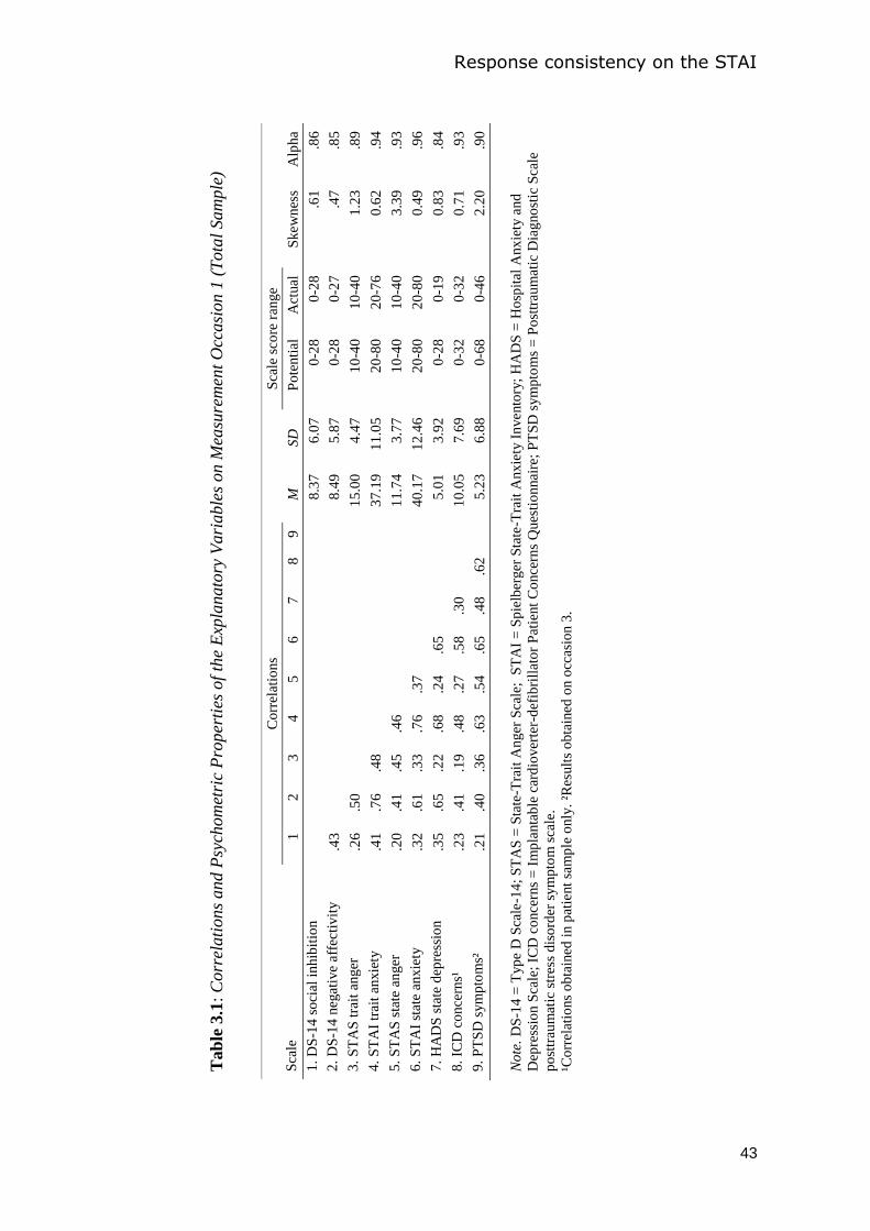
Response consistency on the STAI
43
Tab
le 3
.1:
Corr
elati
ons
and P
sych
om
etri
c P
rop
erti
es o
f th
e E
xpla
nato
ry V
ari
ab
les
on M
easu
rem
ent
Occ
asi
on
1 (
Tota
l Sam
ple
)
C
orr
elat
ions
S
cale
sco
re r
ange
Sca
le
1
2
3
4
5
6
7
8
9
M
SD
P
ote
nti
al
Act
ual
S
kew
nes
s A
lpha
1.
DS
-14
so
cial
in
hib
itio
n
8
.37
6.0
7
0
-28
0
-28
.6
1
.86
2.
DS
-14
neg
ativ
e aff
ecti
vit
y
.43
8.4
9
5
.87
0-2
8
0-2
7
.47
.85
3.
ST
AS
tra
it a
nger
.2
6
.50
1
5.0
0
4.4
7
10
-40
10
-40
1.2
3
.89
4.
ST
AI
trai
t an
xie
ty
.41
.76
.48
37
.19
11
.05
20
-80
20
-76
0.6
2
.94
5.
ST
AS
sta
te a
nger
.2
0
.41
.45
.46
1
1.7
4
3.7
7
10
-40
10
-40
3.3
9
.93
6.
ST
AI
stat
e an
xie
ty
.32
.61
.33
.76
.37
40
.17
12
.46
20
-80
20
-80
0.4
9
.96
7.
HA
DS
sta
te d
epre
ssio
n
.35
.65
.22
.68
.24
.65
5
.01
3
.92
0
-28
0
-19
0
.83
.84
8.
ICD
co
nce
rns¹
.2
3
.41
.19
.48
.27
.58
.30
10
.05
7.6
9
0-3
2
0-3
2
0.7
1
.93
9.
PT
SD
sym
pto
ms²
.2
1
.40
.36
.63
.54
.65
.48
.62
5
.23
6.8
8
0-6
8
0-4
6
2.2
0
.90
No
te.
DS
-14
= T
yp
e D
Sca
le-1
4;
ST
AS
= S
tate
-Tra
it A
nger
Sca
le;
ST
AI
= S
pie
lber
ger
Sta
te-T
rait
Anxie
ty I
nvento
ry;
HA
DS
= H
osp
ital
Anx
iety
an
d
Dep
ress
ion S
cale
; IC
D c
once
rns
= I
mp
lanta
ble
car
dio
ver
ter-
def
ibri
llat
or
Pat
ient
Co
nce
rns
Ques
tio
nnai
re;
PT
SD
sym
pto
ms
= P
ost
trau
mat
ic D
iag
no
stic
Sca
le
po
sttr
aum
atic
str
ess
dis
ord
er s
ym
pto
m s
cale
.
¹Co
rrel
atio
ns
ob
tain
ed i
n p
atie
nt
sam
ple
only
. ²R
esult
s o
bta
ined
on o
ccas
ion 3
.
Chapter 3
44
For the first measurement occasion, Table 3.1 shows the psychometric properties of
the scales and the correlations between the scale scores (i.e., total scores). For all but one
scale score, the mean, the standard deviation, and the range did not vary substantially
across measurement occasions (variation across time is not tabulated). The exception was
the decrease in the mean scale score of ICD concerns (10.05 on occasion 1 and 5.98 on
occasion 5). All scale-score distributions were positively skewed. For most scales,
skewness increased somewhat over time. Coefficient alpha was high (alpha .84) for all
scales and varied little across occasions. All scale scores were positively correlated. The
correlations between state depression, state anxiety, and trait anxiety with most other
explanatory variable increased over occasions. The increase was the largest for the
correlation between state anxiety and trait anxiety ( 76.r on occasion 1 and 91.r on
occasion 5). Apart from the modest correlations between being patient and male ( 57.r )
and being patient and state depression ( 30.r ), the categorical explanatory variables
correlated only weakly with the other explanatory variables (Spearman’s ;22.r not
tabulated). The across-occasion correlations of the scale scores were the lowest for state
anger (range: .33 - .52) and the highest for PTSD symptoms (range: .70 - .76).
3.3.2 Variation in Response Consistency
For the STAI-State and STAI-Trait, Table 3.2 shows the descriptive statistics for
the 𝑝 statistic for each measurement occasion and the across-occasion correlations of
𝑝
for patients (below diagonal) and partners (above diagonal). The means of the 𝑝
distributions were close to their expected value of 0 under the null model of no
inconsistency (range: 0.02 - 0.15), but the standard deviations were larger than the
expected value of 1 (range: 1.44 - 1.73). The average percentage of participants having 𝑝
values smaller than –2.34 and –1.64 (i.e., the 1% and 5% percentile rank scores under the
normal distribution) equaled 6.7% and 12.2%, respectively. Hence, we found that the data
included a substantial number of highly inconsistent item-score patterns.
The across-occasion correlations ranged from .18 to .61. The correlations in the
partner sample were on average –.02 and –.17 higher than in the patient sample for the
STAI- State and the STAI-Trait, respectively. We determined the effect of extreme
negative 𝑝 values (
𝑝 < –7) on the across-time correlations. We found that the correlations
for partners were on average .04 (range: –.01 - .12) lower when excluding respondents with
extreme 𝑝 values. For patients, the correlations were on average .01 (range: –.07 - .03)
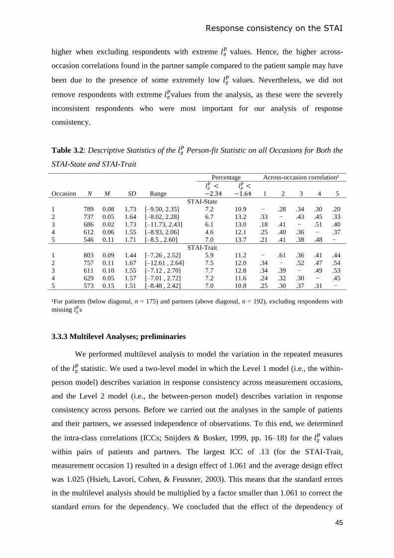
Response consistency on the STAI
45
higher when excluding respondents with extreme 𝑝
values. Hence, the higher across-
occasion correlations found in the partner sample compared to the patient sample may have
been due to the presence of some extremely low 𝑝
values. Nevertheless, we did not
remove respondents with extreme 𝑝values from the analysis, as these were the severely
inconsistent respondents who were most important for our analysis of response
consistency.
Table 3.2: Descriptive Statistics of the 𝑝 Person-fit Statistic on all Occasions for Both the
STAI-State and STAI-Trait
Percentage Across-occasion correlation¹
Occasion N M SD Range
𝑝
𝑝
1 2 3 4 5
STAI-State
1 789 0.08 1.73 [–9.50, 2.35] 7.2 10.9 − .28 .34 .30 .20
2 737 0.05 1.64 [–8.02, 2.28] 6.7 13.2 .33 − .43 .45 .33
3 686 0.02 1.73 [–11.73, 2.43] 6.1 13.0 .18 .41 − .51 .40
4 612 0.06 1.55 [–8.93, 2.06] 4.6 12.1 .25 .40 .36 − .37
5 546 0.11 1.71 [–8.5 , 2.60] 7.0 13.7 .21 .41 .38 .48 −
STAI-Trait
1 803 0.09 1.44 [–7.26 , 2.52] 5.9 11.2 − .61 .36 .41 .44
2 757 0.11 1.67 [–12.61 , 2.64] 7.5 12.0 .34 − .52 .47 .54
3 611 0.10 1.55 [–7.12 , 2.70] 7.7 12.8 .34 .39 − .49 .53
4 629 0.05 1.57 [–7.01 , 2.72] 7.2 11.6 .24 .32 .30 − .45
5 573 0.15 1.51 [–8.48 , 2.42] 7.0 10.8 .25 .30 .37 .31 −
¹For patients (below diagonal, n = 175) and partners (above diagonal, n = 192), excluding respondents with
missing 𝑝s
3.3.3 Multilevel Analyses; preliminaries
We performed multilevel analysis to model the variation in the repeated measures
of the 𝑝 statistic. We used a two-level model in which the Level 1 model (i.e., the within-
person model) describes variation in response consistency across measurement occasions,
and the Level 2 model (i.e., the between-person model) describes variation in response
consistency across persons. Before we carried out the analyses in the sample of patients
and their partners, we assessed independence of observations. To this end, we determined
the intra-class correlations (ICCs; Snijders & Bosker, 1999, pp. 16–18) for the 𝑝 values
within pairs of patients and partners. The largest ICC of .13 (for the STAI-Trait,
measurement occasion 1) resulted in a design effect of 1.061 and the average design effect
was 1.025 (Hsieh, Lavori, Cohen, & Feussner, 2003). This means that the standard errors
in the multilevel analysis should be multiplied by a factor smaller than 1.061 to correct the
standard errors for the dependency. We concluded that the effect of the dependency of
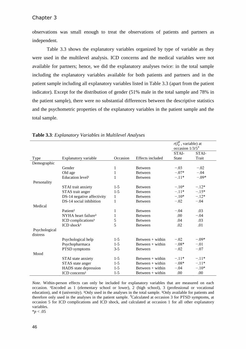
Chapter 3
46
observations was small enough to treat the observations of patients and partners as
independent.
Table 3.3 shows the explanatory variables organized by type of variable as they
were used in the multilevel analysis. ICD concerns and the medical variables were not
available for partners; hence, we did the explanatory analyses twice: in the total sample
including the explanatory variables available for both patients and partners and in the
patient sample including all explanatory variables listed in Table 3.3 (apart from the patient
indicator). Except for the distribution of gender (51% male in the total sample and 78% in
the patient sample), there were no substantial differences between the descriptive statistics
and the psychometric properties of the explanatory variables in the patient sample and the
total sample.
Table 3.3: Explanatory Variables in Multilevel Analyses
r( 𝑝
, variable) at
occasion 1/3/54
Type Explanatory variable Occasion Effects included
STAI-
State
STAI-
Trait
Demographic
Gender 1 Between −.03 −.02
Old age 1 Between −.07* −.04
Education level¹ 1 Between −.11* −.09*
Personality
STAI trait anxiety 1-5 Between −.10* −.12*
STAS trait anger 1-5 Between −.11* −.15*
DS-14 negative affectivity 1 Between −.10* −.12*
DS-14 social inhibition 1 Between −.02 −.04
Medical
Patient² 1 Between −.04 .03
NYHA heart failure³ 1 Between .00 −.04
ICD complications³ 5 Between .04 .03
ICD shock³ 5 Between .02 .01
Psychological
distress
Psychological help 1-5 Between + within −.02 −.09*
Psychopharmaca 1-5 Between + within −.08* −.01
PTSD symptoms 3-5 Between −.02 −.07
Mood
STAI state anxiety 1-5 Between + within −.11* −.11*
STAS state anger 1-5 Between + within −.08* −.11*
HADS state depression 1-5 Between + within −.04 −.10*
ICD concerns¹ 1-5 Between + within .00 .00
Note. Within-person effects can only be included for explanatory variables that are measured on each
occasion. ¹Encoded as 1 (elementary school or lower), 2 (high school), 3 (professional or vocational
education), and 4 (university). ²Only used in the analyses in the total sample. ³Only available for patients and
therefore only used in the analyses in the patient sample. 4Calculated at occasion 3 for PTSD symptoms, at
occasion 5 for ICD complications and ICD shock, and calculated at occasion 1 for all other explanatory
variables.
*p < .05
Response consistency on the STAI
47
The data consisted of explanatory variables measured once, and time-dependent
explanatory variables measured repeatedly. For most time-dependent explanatory
variables, we included in the model both the person’s average value across occasions
(which is a between-person effect) and the person’s deviations from that average value
(which is a within-person effect). This approach, called within-person centering (Snijders
& Bosker, 1999, pp. 52–56), allowed us to separately test for effects on between-person
differences in response consistency (i.e., research question 2) and effects on within-person
differences in response consistency (i.e., research question 3).
Table 3.3 shows the occasion(s) on which explanatory variables were measured,
and whether explanatory variables were included in the model only as a between-person
effect or as both a within-person and a between-person effect. Except for the dichotomous
explanatory variables, for all other between-person explanatory variables we used grand-
mean centering.
Correlations among explanatory between-person variables were substantial (not
tabulated). Because between-person state anxiety was indistinguishable from between-
person trait anxiety ( 92.r ), we only included between-person trait anxiety into the
model. For the remaining between-person variables, inspection of the pairwise correlations
and variance inflation factors (VIFs) did not suggest serious multicollinearity. The
correlations were at most .79, which was found for between-person trait anxiety and
between-person state depression. VIF values were below six (Keith, 2006, pp. 201-202).
Correlations between the within-person variables did not exceed .54. For the STAI-State
and the STAI-Trait for the first occasion, the last two columns of Table 3.3 show the
correlations of the explanatory variables with statistic 𝑝
. Absolute correlations ranged
from 0 to .15.
All analyses were carried out in SPSS 17.0 for Windows. Models for comparing
fixed effects were estimated using maximum likelihood. Models for comparing covariance
structures of the residuals or random effects were estimated using restricted maximum
likelihood (Snijders & Bosker, 1999, pp. 82–83). We used the likelihood ratio test for
comparing nested models, and the Akaike information criterion (AIC) and the Bayesian
information criterion (BIC) for comparing non-nested models (Singer & Willett, 2003, pp.
119–122). Explained variance in the multilevel model was defined as the proportional
reduction of prediction error (Snijders & Bosker, 1999, pp. 101–104).
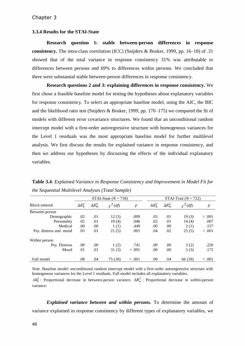
Chapter 3
48
3.3.4 Results for the STAI-State
Research question 1: stable between-person differences in response
consistency. The intra-class correlation (ICC) (Snijders & Bosker, 1999, pp. 16–18) of .31
showed that of the total variance in response consistency 31% was attributable to
differences between persons and 69% to differences within persons. We concluded that
there were substantial stable between-person differences in response consistency.
Research questions 2 and 3: explaining differences in response consistency. We
first chose a feasible baseline model for testing the hypotheses about explanatory variables
for response consistency. To select an appropriate baseline model, using the AIC, the BIC
and the likelihood ratio test (Snijders & Bosker, 1999, pp. 170–175) we compared the fit of
models with different error covariance structures. We found that an unconditional random
intercept model with a first-order autoregressive structure with homogenous variances for
the Level 1 residuals was the most appropriate baseline model for further multilevel
analysis. We first discuss the results for explained variance in response consistency, and
then we address our hypotheses by discussing the effects of the individual explanatory
variables.
Table 3.4: Explained Variance in Response Consistency and Improvement in Model Fit for
the Sequential Multilevel Analyses (Total Sample)
STAI-State (N = 718) STAI-Trait (N = 722)
Block entered
2 (df) p
2 (df) p
Between person
Demographic .02 .01 12 (3) .009 .03 .01 19 (3) < .001
Personality .02 .01 10 (4) .046 .02 .01 14 (4) .007
Medical .00 .00 1 (1) .449 .00 .00 2 (1) .157
Psy. distress and mood .03 .01 21 (5) .001 .04 .02 25 (5) < .001
Within person
Psy. Distress .00 .00 1 (2) .741 .00 .00 3 (2) .220
Mood .01 .01 31 (3) < .001 .00 .00 5 (3) .172
Full model .08 .04 75 (18) < .001 .09 .04 66 (18) < .001
Note. Baseline model: unconditional random intercept model with a first-order autoregressive structure with
homogenous variances for the Level 1 residuals. Full model includes all explanatory variables. 2bR : Proportional decrease in between-person variance.
2wR : Proportional decrease in within-person
variance.
Explained variance between and within persons. To determine the amount of
variance explained in response consistency by different types of explanatory variables, we
Response consistency on the STAI
49
sequentially entered blocks of the same type of explanatory variables into the baseline
model. The first column of Table 3.4 shows the six blocks of explanatory variables in the
order they were entered in the model. We first entered four blocks of between-person
effects (i.e., research question 2), and then two blocks of within-person effects (i.e.,
research question 3). To estimate the total variance explained by each block, explanatory
variables that are assumed to causally precede the explanatory variables in the blocks
added in later steps need to be included first (Keith, 2006, pp. 82–84). The blocks of
demographic and personality variables for which the mutual causal precedence is
questionable, were included first. The order of entry among the other between-person
blocks and among the within-person blocks was based on causal precedence.
For the total sample, Table 3.4 (columns 2 and 3) shows the proportional decrease
in between-person variance ( 2bR ) and within-person variance ( 2
wR ) with respect to the
previous model after blocks of explanatory variables were entered. Columns 4 and 5 show
the corresponding likelihood-ratio test statistics. The significance level was .05. We first
discuss the results for the total sample, and then the most important results for the patient
sample.
Apart from the block of medical variables (i.e., including only the patient indicator
for the total sample), when a block of between-person effects was included the model fit
improved significantly. The demographic variables explained 2% of the between-person
variance. Inclusion of the personality variables resulted in another 2% increase in
explained between-person variance. These percentages were not affected by reversing the
order of entry of the first two blocks. The between-person psychological distress and mood
variables explained an additional 3% of the between-person variance. As for the two blocks
of within-person effects, only inclusion of the mood variables led to a significant
improvement of model fit. The increase in explained within-person variance equaled 1%.
All explanatory variables together explained 8% of the between-person variance and 4% of
the within-person variance in response consistency.
Compared to the total sample, in the patient sample the percentages of variance the
blocks of explanatory variables explained were similar (results not tabulated). However,
only inclusion of the demographic variables and the within-person mood variables caused
the model fit to improve significantly. The total between-person variance and within-
person variance explained by all explanatory variables together was 9% and 5%,
respectively.
Chapter 3
50
Explanatory variables. For the total sample, Table 3.5 shows the estimated
regression coefficients for different multilevel models. The first model (third column)
included only stable respondent characteristics as explanatory variables (i.e., demographic
and personality trait variables). We also fitted a series of extensions of the first model.
Each extended model included the stable explanatory variables and a single additional
explanatory variable. Thus, in each of these extended models we estimated the effect of
one explanatory variable while controlling for stable respondent characteristics. For all
extended models, Table 3.5, first column, shows the estimated coefficient for the additional
explanatory variable. We call the models including only stable explanatory variables and
the extensions of this model ‘reduced models’. The ‘full model’ including all explanatory
variables (fifth column) was used to estimate the unique effects of the explanatory
variables, controlling for the effect of the other predictors. We used both the results from
the reduced models and the full model to address our hypotheses about explanatory
variables.
Because the hypotheses about the explanatory variables were directional, we used a
lopsided test (Abelson, 1995, p. 59), which is a compromise between a one-tailed and a
two-tailed test. This test has a rejection area of 5% in the expected tail and .5% in the
unexpected tail. We first discuss the results for the total sample, and then the most
important results for similar models in the patient sample.
Research question 2: between-person differences. For the total sample, all
significant between-person effects in the reduced models (columns 3 and 4) were in the
hypothesized direction. Education level had a significant positive effect on response
consistency. Trait anger, PTSD symptoms, and between-person psychological help had
significant negative effects on response consistency. Except for the effect of trait anger, all
these effects were also significant in the full model (column 5). The effects were small
given the observed standard deviation of 𝑝
, which equaled 1.67. Compared to persons
having the lowest education level, persons having the highest level had a predicted 𝑝 that
was 0.80 higher (based on the reduced model). Compared to persons with a PTSD
symptoms score of two standard deviations below average, persons having a score of two
standard deviations above average had a predicted 𝑝
that was 0.72 lower. The other
significant between-person effects had similar size. The effect of trait anxiety was not
significant in the reduced model but it was significant in the full model. Contrary to our
hypothesis, the effect of trait anxiety was positive.
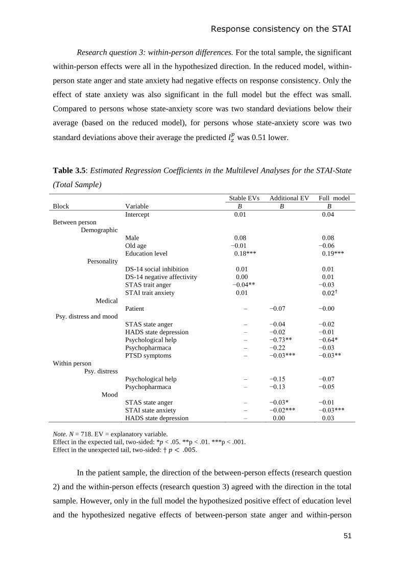
Response consistency on the STAI
51
Research question 3: within-person differences. For the total sample, the significant
within-person effects were all in the hypothesized direction. In the reduced model, within-
person state anger and state anxiety had negative effects on response consistency. Only the
effect of state anxiety was also significant in the full model but the effect was small.
Compared to persons whose state-anxiety score was two standard deviations below their
average (based on the reduced model), for persons whose state-anxiety score was two
standard deviations above their average the predicted 𝑝 was 0.51 lower.
Table 3.5: Estimated Regression Coefficients in the Multilevel Analyses for the STAI-State
(Total Sample)
Stable EVs Additional EV Full model
Block Variable B B B
Intercept 0.01 0.04
Between person
Demographic
Male 0.08 0.08
Old age −0.01 −0.06
Personality
Education level 0.18***
0.19***
DS-14 social inhibition 0.01 0.01
DS-14 negative affectivity 0.00 0.01
STAS trait anger −0.04** −0.03
STAI trait anxiety 0.01
Medical
Patient – −0.07 −0.00
Psy. distress and mood
STAS state anger – −0.04 −0.02
HADS state depression – −0.02 −0.01
Psychological help – −0.73** −0.64*
Psychopharmaca – −0.22 −0.03
PTSD symptoms – −0.03*** −0.03**
Within person
Psy. distress
Psychological help – −0.15 −0.07
Psychopharmaca – −0.13 −0.05
Mood
STAS state anger – −0.03* −0.01
STAI state anxiety – −0.02*** −0.03***
HADS state depression – 0.00 0.03
Note. N = 718. EV = explanatory variable.
Effect in the expected tail, two-sided: *p < .05. **p < .01. ***p < .001.
Effect in the unexpected tail, two-sided: .
In the patient sample, the direction of the between-person effects (research question
2) and the within-person effects (research question 3) agreed with the direction in the total
sample. However, only in the full model the hypothesized positive effect of education level
and the hypothesized negative effects of between-person state anger and within-person
Chapter 3
52
state anxiety were significant. None of the patient-specific between-person or within-
person effects (i.e., the medical variables and between-person and within-person ICD
concerns) was significant.
3.3.5 Results for the STAI-Trait
Due to space limitations and because the STAI-Trait appears to be less frequently
used in cardiovascular research than the STAI-State (e.g., Pedersen, Van den Broek, &
Sears, 2007), we give a brief summary of the results for the STAI-Trait and compare the
results with the results for the STAI-State.
The ICC of .38 indicated that there were stable between-person differences in
response consistency on the STAI-Trait that were somewhat larger than for the STAI-State.
Table 3.4 (columns 6 - 9) shows the results for explained variance in response consistency
for the total sample. The results were similar to those for the STAI-State. Apart from the
medical block, inclusion of all blocks of between-person effects led to consecutive,
significant improvements of model fit. The main difference was that for the STAI-Trait,
inclusion of the block of within-person mood variables did not lead to a significant
improvement of model fit. The total percentages of between-person and within-person
variance that all explanatory variables together explain equaled 9% and 4%, respectively.
In the patient sample, the main difference between the results for the STAI-Trait and the
STAI-State was the larger variance explained for the STAI-Trait (results not tabulated).
The total percentages of explained between-person and within-person variance were 18%
and 8%, respectively.
For the total sample, Table 3.6 shows the estimated regression coefficients. The
significant between-person effects were similar those for the STAI-State. We found the
hypothesized positive effect of education level, negative effects of trait anger, between-
person psychological help, PTSD symptoms, and the unexpected positive effect of trait
anxiety. In addition, two hypothesized between-person effects on response consistency
were only significant for the STAI-Trait. These were the negative effects of old age and
between-person state depression. As for the within person-effects, we found a significant
negative within-person effect of state anger. Similar to the STAI-State, in the patient
sample the medical and ICD concerns variables did not have significant effects on response
consistency.
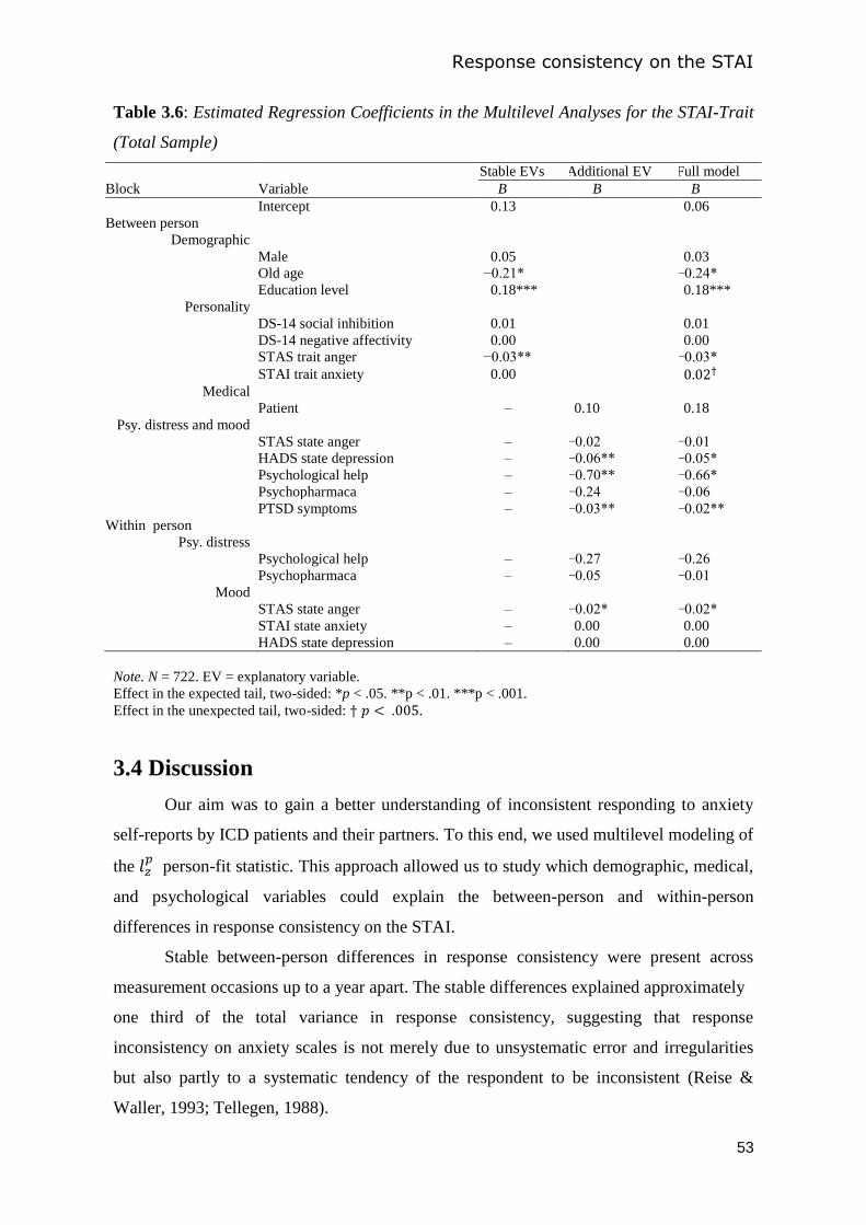
Response consistency on the STAI
53
Table 3.6: Estimated Regression Coefficients in the Multilevel Analyses for the STAI-Trait
(Total Sample)
Stable EVs Additional EV Full model
Block Variable B B B
Intercept 0.13 0.06
Between person
Demographic
Male 0.05 0.03
Old age −0.21* −0.24*
Education level 0.18*** 0.18***
Personality
DS-14 social inhibition 0.01 0.01
DS-14 negative affectivity 0.00 0.00
STAS trait anger −0.03** −0.03*
STAI trait anxiety 0.00
Medical
Patient – 0.10 0.18
Psy. distress and mood
STAS state anger – −0.02 −0.01
HADS state depression – −0.06** −0.05*
Psychological help – −0.70** −0.66*
Psychopharmaca – −0.24 −0.06
PTSD symptoms – −0.03** −0.02**
Within person
Psy. distress
Psychological help – −0.27 −0.26
Psychopharmaca – −0.05 −0.01
Mood
STAS state anger – −0.02* −0.02*
STAI state anxiety – 0.00 0.00
HADS state depression – 0.00 0.00
Note. N = 722. EV = explanatory variable.
Effect in the expected tail, two-sided: *p < .05. **p < .01. ***p < .001.
Effect in the unexpected tail, two-sided: .
3.4 Discussion
Our aim was to gain a better understanding of inconsistent responding to anxiety
self-reports by ICD patients and their partners. To this end, we used multilevel modeling of
the 𝑝 person-fit statistic. This approach allowed us to study which demographic, medical,
and psychological variables could explain the between-person and within-person
differences in response consistency on the STAI.
Stable between-person differences in response consistency were present across
measurement occasions up to a year apart. The stable differences explained approximately
one third of the total variance in response consistency, suggesting that response
inconsistency on anxiety scales is not merely due to unsystematic error and irregularities
but also partly to a systematic tendency of the respondent to be inconsistent (Reise &
Waller, 1993; Tellegen, 1988).

Chapter 3
54
The percentage of stable between-person differences the explanatory variables
accounted for ranged from 8% in the total sample to 18% in the patient sample. The
percentage of within-person differences explained ranged from 4% in the total sample to
8% in the patient sample. Less educated respondents, respondents with higher trait anger,
respondents with more PTSD symptoms, and respondents seeing a psychologist or
psychiatrist tended to respond less consistently. Furthermore, respondents tended to be less
consistent than usual when they were angrier than they usually are. Feelings of anger may
have led to concentration problems or uncooperativeness when responding to the STAI.
These results are consistent with previous research results for explanatory variables for
response consistency (Pinsoneault, 1998; Reise & Waller, 1993; Woods et al., 2008). Also,
these variables were found to have explanatory power for response consistency across the
two STAI subscales. Despite the consistency of the results, the small percentages of
variance the variables explained in response consistency calls their practical value for
identifying respondents at risk of producing invalid test results into question.
We found the same unexpected result for both the STAI-State and the STAI-Trait,
which was that after controlling for all other explanatory variables persons with higher trait
anxiety tended to respond more consistently. A plausible explanation is that motivated
respondents were more consistent but also scored higher on trait anxiety. To admit
suffering from psychological symptoms probably requires more effort than denying or
ignoring these symptoms. Furthermore, reluctance to disclose psychological distress may
have led to both inconsistency and low trait anxiety scores. Another finding contrary to our
expectations was that patients were not more inconsistent than partners. For patients, the
extent of heart failure, ICD related complications, or having received an ICD shock did not
affect response consistency. Hence, physical symptoms and complications do not seem to
result in response inconsistency.
An explanation for the low percentage of explained variance in response
consistency is that data of important explanatory variables for response consistency such as
test-taking motivation and conscientiousness (Ferrando, 2009; LaHuis & Copeland, 2009;
Schmitt et al., 1999) were not available and thus could not be included in the explanatory
PFA. This is a limitation of the current study. In previous research, conscientiousness has
been found to explain more variance in response consistency, approximately 11%
(Ferrando, 2009; Schmitt et al., 1999). However, absence of important explanatory
variables may not be the only explanation for small effect sizes. Other explanatory
variables expected to be highly related to response consistency were also found to have
Response consistency on the STAI
55
small effects. For example, test-taking motivation explained only 7% of the variation in a
multitest version of the 𝑝
statistic based on five different personality scales, and test
reaction, which was quantified by perceptions of face validity, predictive validity, and
fairness, explained only 1% (Schmitt et al., 1999). What are other possible explanations for
the small percentages of explained variance in response consistency?
One possible explanation is that variation in response consistency may be largely
due to variation in traitedness. Traitedness refers to the degree to which the trait is relevant
for the respondent (Tellegen, 1988). As traitedness is an idiosyncratic phenomenon it is not
necessarily related to explanatory variables. Second, some causes of aberrant responding
may not always produce an inconsistent item-score pattern. For example, although lack of
motivation or concentration in some situations may produce random responding leading to
response inconsistency, in other situations they might stimulate blindly choosing the
categories indicating least extreme anxiety, oppositely producing response consistency. A
related explanation is that person-fit statistics such as 𝑝
quantify different types of
inconsistencies that are not related to the same explanatory variables. Third, unreliability in
the measure of response consistency may attenuate the effects of explanatory variables on
response consistency (Ferrando, 2009). In this study and previous studies, response
consistency was measured using scales that were designed to measure traits, not response
consistency. Research shows that reliable measurement of response consistency requires
other scale properties than valid trait measurement (Reise & Flannery, 1996).
Future explanatory PFA research might consider the following topics. A new line of
research that we have started is using latent class analysis to distinguish classes of
respondents based on their person-fit statistic values obtained for different scales. Instead
of explaining variation of a continuous person-fit statistic such as 𝑝, the different classes
or ‘person-fit profiles’ can be related to explanatory variables. Furthermore, to investigate
whether variation in response consistency is due to variation in traitedness, the multilevel
approach used in this study may be applied to person-fit indices computed for different
self-report measures instead of repeated measures. This way, the multilevel modeling
approach enables testing whether response consistency is more strongly correlated across
items measuring the same trait than across items measuring different traits. This finding
would support the low-traitedness explanation for response inconsistency. Another
interesting possibility is to analyze the pattern of misfit on the item (or item subset) level
(e.g., Ferrando, 2010). This way, finer-grained diagnostic information about response
inconsistency of individual respondents can be obtained. For example, in a clinical context

Chapter 3
56
it may be useful for the psychologist to know whether a pattern of misfit suggests a lack of
motivation or socially desirable responding.
57
Chapter 4
Person-fit methods for non-cognitive measures with
multiple subscales
Abstract Person-fit statistics could be a useful tool for detecting individuals with
aberrant item-score vectors on non-cognitive questionnaires. However, for non-cognitive
measures that consist of multiple short subscales standard person-fit statistics are not
readily applicable. We therefore propose to combine subscale person-fit information to
detect aberrant item-score vectors on non-cognitive multiscale measures. We evaluated the
performance of five different multiscale person-fit methods based on the person-fit
statistic with respect to (1) identifying aberrant item-score vectors; (2) improving the
accuracy of research results; and (3) understanding the causes of aberrant responding. To
this end, we used both a simulation study and several applications to empirical personality
and psychopathology test data. The simulation study showed that the person-fit methods
had good detection rates for item-score vectors with substantial misfit. Application of the
person-fit methods to real data identified 5% to 17% misfitting item-score vectors, but
removal of these vectors hardly affected results on model fit and test score validity.
Finally, the person-fit methods were useful for understanding the causes of aberrant
responding, but only after controlling for response style on the explanatory variables. We
conclude that more real-data applications are needed to demonstrate the usefulness of the
multiscale person-fit methods for non-cognitive multiscale measures. This study
demonstrates the value of combining simulation study results with real-data study results
for a comprehensive evaluation of person-fit methods.
This chapter has been submitted for publication
Chapter 4
58
4.1 Introduction
Aberrant response behavior on self-report measures of typical performance can be
due to a lack of motivation, misunderstanding of questions, untraitedness, stylistic
responding, or social desirability (Ferrando, 2012; Tellegen, 1988). As it leads to test
scores that are not interpretable in terms of the trait being measured, aberrant responding
may adversely affect individual decision-making, for example, in personnel selection
(Christiansen, Goffin, Johnston, & Rothstein, 1994) and treatment planning in clinical
practice (Egberink & Meijer, 2010; Piedmont, McCrae, Riemann, & Angleitner, 2000), and
can invalidate research conclusions about the psychometric properties of questionnaires
(Meijer, 1997; Woods, 2006).
Person-fit analysis (PFA; Meijer & Sijtsma, 2001) is a well-established method for
detecting aberrant item-score vectors. Person-fit statistics quantify the difference between
the person’s observed item scores and expectations derived from the postulated
measurement model. Numerous person-fit statistics were developed (e.g., Meijer &
Sijtsma, 2001). One of the most popular person-fit statistics continues to be the statistic
(Drasgow, Levine, & McLaughlin, 1987) and its corrected version (Snijders, 2001). The
statistic is an item response theory (IRT) based person-fit statistic, which is defined as
the standardized log-likelihood of an item-score vector given the estimated IRT model.
PFA has its roots in cognitive and educational measurement (Levine & Drasgow,
1982). More recently, the potential of PFA for detecting aberrant responding to non-
cognitive measures (i.e., producing typical performance data) has been recognized (e.g.,
Egberink & Meijer, 2010; Emons, 2008; Ferrando, 2010, 2012; Reise, 1995; Reise &
Flannery, 1996). However, in these studies it was also concluded that non-cognitive
measures typically have characteristics that constrain successful application of PFA.
Particularly, non-cognitive measures often consist of a number of short unidimensional
subscales (i.e., say, containing fewer than 15 items each), each measuring a different trait.
Examples in personality measurement include the NEO Five Factor Inventory (NEO-FFI;
Costa & McCrae, 1992; consisting of five 12-item subscales), and the Big-Five factor
markers International Personality Item Pool 50-item questionnaire (IPIP-50; Goldberg et
al., 2006; five 10-item subscales). Examples in the context of psychopathology include the
Brief Symptom Inventory (BSI; Derogatis, 1993; nine subscales having 5 to 8 items) and
its shortened version, the BSI-18 (Derogatis, 2001; three 6-item subscales). The main
problem is that person-fit statistics assume unidimensionality, hence they have to be
Person-fit methods for multiple subscales
59
computed for each subscale separately. However, person-fit statistics lack power to detect
misfit on scales containing fewer than 20 items (Emons, 2008; Reise, 1995; Reise &
Flannery, 1996). Furthermore, in many applications of trait measurement a conclusion is
required about fit or misfit of individuals with respect to a general trait measured by means
of the combination of subscales (e.g., general psychopathology in case of the BSI). In these
applications, the information about fit or misfit of individuals on the separate subscales
needs to be combined.
The aim of this study was to compare different methods based on the statistic that
combine person-fit information obtained from different scales into one overall person-fit
measure. The methods include the statistic applied as if the multiscale data were
unidimensional, the statistic applied to each subscale separately, the sum of the values
of different subscales (Drasgow, Levine, & McLaughlin, 1991), and combinations of the
latter two methods.
We evaluated the multiscale person-fit methods with respect to three potential uses
of PFA: (1) identifying persons who have invalid test scores; (2) identifying persons that
deteriorate the accuracy of research results; and (3) providing insight into the causes of
aberrant responding. To address the first issue, we used a simulation study to determine the
Type I error rate and the detection rate of the person-fit methods. To address the remaining
two issues we applied the multiscale person-fit methods to IPIP-50 data from a panel
sample and BSI data from a clinical sample.
Previous research on the performance of person-fit methods mainly consisted of
simulation studies whereas empirical applications were rare (Meijer & Sijtsma, 2001).
Although simulations are necessary to validate new person-fit methods, we believe that
empirical research is crucial for demonstrating the usefulness of a person-fit method in
applied research. Hence, based on results of the simulation study and the empirical study
we draw an overall conclusion about the usefulness of the -based multiscale person-fit
methods for non-cognitive assessment.
4.2 Multiscale Person-Fit Analysis
4.2.1 The Statistic for Polytomous Items
Because most non-cognitive questionnaires use a rating-scale response format, we
used statistic for polytomous items, denoted by 𝑝
(Drasgow, Levine, & Williams,
Chapter 4
60
1985). Statistic 𝑝 was found to have higher detection rates than several other person-fit
statistics for polytomous items (Emons, 2008). Here we define 𝑝
under the graded
response model (GRM; Samejima, 1997).
Suppose the data are polytomous item scores of N persons on J items (items are
indexed j; j = 1,…, J) with M +1 ordered answer categories. Let the score on item j be
denoted by with possible realizations . In the GRM, the probability of a
score or higher as a function of a latent trait θ is modeled by item step response
functions (ISRFs). The logistic ISRFs for item j have a location parameter (
) and a common discrimination parameter . Parameter equals the θ value for
which ( | ) , and parameter determines the ISRF slope. The ISRF is
defined as
( | ) [ ( )]
[ ( )]
The GRM is based on three assumptions: unidimensionality of , local independence
conditional on , and logistic ISRFs as in Equation 4.1.
Statistic 𝑝 is the standardized log-likelihood of an individual’s item-score vector
given the response probabilities under the GRM. Let indicator function if
, and 0 otherwise. The unstandardized log-likelihood of an item-
score vector x is given by
𝑝 ∑ ∑ ( | ) ( )
The standardized log-likelihood is
𝑝
𝑝 [ 𝑝 ]
[ 𝑝 ]
where 𝑝 is the expected value and 𝑝 the variance of 𝑝 . Larger negative 𝑝
values indicate a higher degree of misfit.
4.2.2 Multiscale Person-Fit Approaches
We evaluated five different approaches to identify person misfit for multiscale
measures. The first three methods are existing approaches. The fourth and fifth methods

Person-fit methods for multiple subscales
61
are new and introduced in this paper because they solve several problems of the existing
three approaches. We discuss the five approaches for 𝑝
. We notice that the five
approaches are general and hence can also be applied to other person-fit statistics.
Approach 1: The unidimensional approach. The first approach is to treat the
multiscale measure as a unidimensional scale and apply 𝑝 to all subscales simultaneously
as if they constituted one common scale (Conrad et al., 2010). Henceforth, we denote the
unidimensional approach by 𝑝
. This method is only useful if the subscale traits are
positively correlated due to the existence of a general higher-order trait but is not useful if
the subscales measure distinct traits (e.g., the NEO-FFI or the IPIP-50). The advantage of
this approach, if applicable, is that the number of items to determine person-fit is large,
thus producing more statistical power and probably higher detection rates. However, the
approach may readily suffer from grave violations of unidimensionality when subscales
represent traits that differ too much. The multidimensionality in the data may deteriorate
the performance of statistic 𝑝
due to biased IRT parameter estimates and may lead to
incorrectly classifying non-aberrant persons as misfitting.
Approach 2: Subscale analysis. The second approach is to apply 𝑝
to each
subscale separately (e.g., Emons, 2008; Ferrando, 2009; Reise & Waller, 1993).
Henceforth, we denote the subscale-analysis approach by 𝑝
. The problem with this
approach is that the subscales of non-cognitive multiscale measures typically have a small
number of items and low item discrimination. These characteristics result in low power to
detect misfit (Emons, 2008; Ferrando, 2010; Reise & Flannery, 1996). For example, for a
12-item scale with item parameters based on the NEO-FFI, power was only .50 if the
aberrance was that half of the item scores were randomly generated (Emons, 2008). Also,
if this approach is used to obtain a conclusion about fit or misfit on the complete multiscale
measure, it requires control of the Type I error rate.
Approach 3: Multiscale extension. The third approach is based on the multitest
extension of statistic for dichotomous item scores proposed by Drasgow et al. (1991).
Extending their proposal, the multiscale version of statistic 𝑝
for polytomous items,
denoted 𝑝
, is defined as the sum of the 𝑝
values of S ( ) unidimensional
subscales, such that 𝑝 ∑
𝑝
The advantage of 𝑝
is that it quantifies person fit by means of a single statistic
using items of all subscales. The disadvantage of 𝑝
is that it allows for compensation of
misfit on one scale by good fit on another scale. This compensation does not interfere with

Chapter 4
62
detecting persons that are consistently misfitting across subscales, for example, due to a
lack of motivation or concentration throughout the whole test. However, some persons
only show misfit on specific subscales (Schmitt, Chan, Sacco, McFarland, & Jennings,
1999; Conijn, Dolan, & Vorst, 2007; Krosnick, 1996). For example, a person may only
show misfit on subscales measuring emotionally sensitive traits (Conijn et al., 2007). Also,
a person who loses concentration or motivation at the end of the multiscale measure may
respond randomly only to the last few subscales (Krosnick, 1996). Hence, the problem
with statistic 𝑝
is that persons who show severe misfit on only one or a few subscales
may go undetected.
Approaches 4 and 5: Combining
and
. In this study, we propose an
alternative approach that combines subscale 𝑝
values and statistic 𝑝
. We expect that
combining subscale 𝑝
s with 𝑝
improves detection rates for persons that consistently
show misfit across several subscales compared to separate-subscale analysis. However,
because in contrast to 𝑝
, subscale-specific information is used separately, detection rates
for persons that show misfit on only one or a few subscales may also be improved.
For method 𝑝
, for all possible subsets out of a total of S subscales, including
the S single subscales and all subscales, the 𝑝
(or 𝑝) values are computed. For example,
for , 𝑝
or 𝑝 is computed for seven subsets ( , , ), ( , ), ( , , ( , ),
and ( , ( , and ( . An item-score vector is classified as misfitting if at least one of the
resulting statistics suggests significant misfit. In the next sections, we discuss how we
calculate the p-values of the 𝑝 and
𝑝 statistics and how we prevent inflated Type I error
rates.
A variant of 𝑝
is to only make use of the 𝑝
statistic based on all subscales
and the 𝑝s for the single subscales. This means that for , an item-score vector is
classified as misfitting if 𝑝
for at least one of the subsets ( , , ), ( , ( , or ( is
significant. This method based on a selection of statistics is denoted 𝑝
.
4.2.3 Common Issues for -Multiscale Methods
To apply the 𝑝-multiscale methods, two issues need to be solved. First, how should
one compute the p-values? Second, how should one control Type I error rates for methods
𝑝
, 𝑝
, and 𝑝
?
Person-fit methods for multiple subscales
63
Bootstrap p-values. Under the null model of response consistency to the IRT
model and given the true values, statistic 𝑝 is standard normally distributed (Drasgow et
al., 1985). However, Nering (1995) showed that the sampling distribution of 𝑝 deviates
from the standard normal distribution if an estimate of is used to compute 𝑝. Therefore,
we used a parametric bootstrap procedure (De la Torre & Deng, 2008) to compute the 𝑝
and 𝑝
values and the corresponding p-values. For each person, we generated bootstrap
replications of the item-score vector under the GRM using the estimated item parameters
and the person’s value. Based on these data replications, we determined the person-
specific null distribution of 𝑝 that allowed us to calculate standardized
𝑝 and
𝑝 values
and the corresponding p-values.
Control of the Type I error rate. To prevent inflated Type I error rates for methods
𝑝
, 𝑝
, and 𝑝
we controlled the false discovery rate (FDR; Benjamini &
Hochberg, 1995). The FDR is the expected proportion of false rejections of the null
hypothesis among the total number of rejections. We chose to control the FDR instead of
the more traditional approach of family-wise error rate control (e.g., Bonferroni correction)
because it is more powerful. Controlling the FDR also controls the family-wise error rate if
all null hypotheses are true but it is less conservative when at least one of the null
hypotheses is false. To control the FDR, we used the Benjamini and Hochberg procedure
(BH procedure; Benjamini & Hochberg, 1995). In the BH procedure, the -values
corresponding to the m test statistics are ordered from smallest to largest, …
Let α be the desired FDR level and k the largest value of i for which
; then, all hypotheses are rejected corresponding to the -values for which i k.
4.3 Study 1: Simulation study
4.3.1 Research Questions
In a simulation study, we investigated whether the 𝑝-multiscale methods are useful
for detecting persons having invalid test scores. More specifically, we address the
following research questions:
1. Do empirical Type I error rates adhere to the nominal Type I error rates?
2. What are the detection rates for realistic test length and realistic item properties?
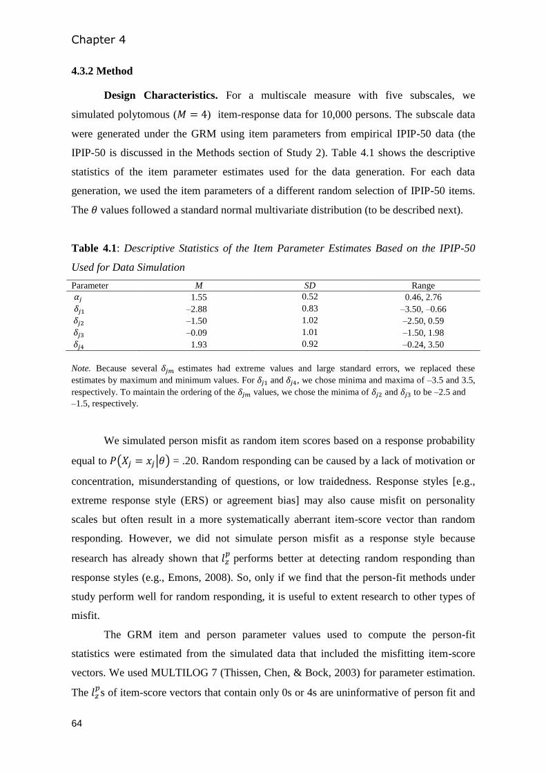
Chapter 4
64
4.3.2 Method
Design Characteristics. For a multiscale measure with five subscales, we
simulated polytomous ( ) item-response data for 10,000 persons. The subscale data
were generated under the GRM using item parameters from empirical IPIP-50 data (the
IPIP-50 is discussed in the Methods section of Study 2). Table 4.1 shows the descriptive
statistics of the item parameter estimates used for the data generation. For each data
generation, we used the item parameters of a different random selection of IPIP-50 items.
The values followed a standard normal multivariate distribution (to be described next).
Table 4.1: Descriptive Statistics of the Item Parameter Estimates Based on the IPIP-50
Used for Data Simulation
Parameter M SD Range
1.55 0.52 0.46, 2.76
–2.88 0.83 –3.50, –0.66
–1.50 1.02 –2.50, 0.59
–0.09 1.01 –1.50, 1.98
1.93 0.92 –0.24, 3.50
Note. Because several estimates had extreme values and large standard errors, we replaced these
estimates by maximum and minimum values. For and , we chose minima and maxima of –3.5 and 3.5,
respectively. To maintain the ordering of the values, we chose the minima of and to be –2.5 and
–1.5, respectively.
We simulated person misfit as random item scores based on a response probability
equal to ( | ) = .20. Random responding can be caused by a lack of motivation or
concentration, misunderstanding of questions, or low traidedness. Response styles [e.g.,
extreme response style (ERS) or agreement bias] may also cause misfit on personality
scales but often result in a more systematically aberrant item-score vector than random
responding. However, we did not simulate person misfit as a response style because
research has already shown that 𝑝 performs better at detecting random responding than
response styles (e.g., Emons, 2008). So, only if we find that the person-fit methods under
study perform well for random responding, it is useful to extent research to other types of
misfit.
The GRM item and person parameter values used to compute the person-fit
statistics were estimated from the simulated data that included the misfitting item-score
vectors. We used MULTILOG 7 (Thissen, Chen, & Bock, 2003) for parameter estimation.
The 𝑝s of item-score vectors that contain only 0s or 4s are uninformative of person fit and
Person-fit methods for multiple subscales
65
are treated as missing values. We excluded item-score vectors with missing 𝑝s for at least
one of the subscales from the analyses. We used 1,000 bootstrap replications to obtain the
bootstrap 𝑝
or 𝑝
values and the corresponding p-values. For classifying item-score
vectors as misfitting we used one-tailed significance testing with an level of .05. For
methods 𝑝
, 𝑝
, and 𝑝
, an item-score was classified as misfitting if at least one
of the resulting statistics 𝑝
and 𝑝 was significant using the BH procedure to control the
FDR at level .
Independent variables. Four factors were combined in a cross-factorial design,
resulting in sixty different conditions. First, the percentage of misfitting item-score vectors
in the data was either 10% or 30%. Second, the correlation between the latent traits θ
corresponding to the five subscales was .4, .6, or .8. Third, the number of items per
subscale was either 6 or 12, resulting in a 30-item or 60-item multiscale measure,
respectively. Fourth, we evaluated the performance of methods 𝑝
𝑝,
𝑝,
𝑝,
and 𝑝
. For each condition, 50 data replications were simulated.
Each replicated data set consisted of two different kinds of misfitting item-score
vectors. We simulated item-score vectors with either “global misfit” or “subscale misfit”
and for each kind of misfit we varied the percentage of random item scores. For each
person separately, we simulated global misfit for a random selection of items from all
subscales, where the number of items was equal for each person but the composition of
sets of items varied across persons. Random selection ensured that the expected number of
random item scores was equal across subscales. We simulated item-score vectors with
global misfit having either 20%, 40%, 60%, or 80% random item scores. To simulate
subscale misfit, first the subscales that showed misfit were randomly selected. Then, misfit
was simulated for a randomly selected subset of items from these subscales. We simulated
four kinds of subscale misfit: 50% random item scores in one subscale, 100% random
scores in one subscale, 50% random item scores in each of two subscales, and 100%
random item scores in two subscales. To summarize, by varying the location and degree of
misfit each simulated dataset included eight different kinds of misfitting item-score
vectors. Each kind of misfitting item-score vector was equally represented in the data.
Dependent variables. We evaluated the Type I error rates and the detection rates
of the five 𝑝
-based methods. The Type I error rate is the number of fitting item-score
vectors that were classified as misfitting divided by the total number of fitting item-score
Chapter 4
66
vectors. The detection rate is the number of misfitting item-score vectors that were
classified as misfitting divided by the total number of misfitting item-score vectors.
4.3.3 Results
Table 4.2 shows the Type I error rates (i.e., in the rows corresponding to ‘No
misfit’) and the detection rates for methods 𝑝
, 𝑝
𝑝,
𝑝, and
𝑝. For
𝑝
, we report the results for all three θ-correlation levels. Because variation in the θ-
correlation hardly affected the performance of the other methods, we only report the results
for these methods for a θ-correlation of .6 (detailed results are available from the first
author on request). Due to missing 𝑝s, on average 1.2% and 0.1% item-score vectors were
excluded from the analyses for the 30-item condition and the 60-item condition,
respectively.
Research Question 1: Adherence to Nominal Type I error. Empirical Type I
error ranged from .01 to .05 in the 10% misfit condition (left half of the table), and from
.00 to .01 in the 30% misfit condition (right half). Hence, all methods were too
conservative. A plausible explanation for the low Type I error is bias in the estimates
resulting from the presence of random item scores in the data. A comparison of the true
values with the estimated s in the simulated data showed that the s were on average
underestimated by 0.13 and 0.32 units in the 10% misfit and 30% misfit condition,
respectively. As a result, the 𝑝 values were overestimated and too few fitting item-score
vectors were classified as misfitting. Additional simulations showed that if the true and
values were used to calculate 𝑝, Type I error was on average .05, .05, .03, and .04 for
𝑝
, 𝑝
, 𝑝
,and 𝑝
, respectively. In case of 𝑝
, instead of the true and
values, we used and estimated in a dataset without person misfit. This resulted
in Type I error rates between .05 and .08, with higher values for a lower θ-correlation.
Research Question 2: Detection rates. All methods showed good detection rates
(range: .73 to 1.00) for the 60-item condition (lower half of the table) if at least 40% of the
item scores were random, and for the 30-item condition (upper half) if at least 60% of the
item scores were random. None of the methods had good detection rates in any of the other
conditions. As expected, detection rates decreased with percentage of misfitting item-score
vectors, and increased with the number of items, and with the percentage of random item
scores. On average, detection rates were .15 higher in the 10% misfit condition than in the
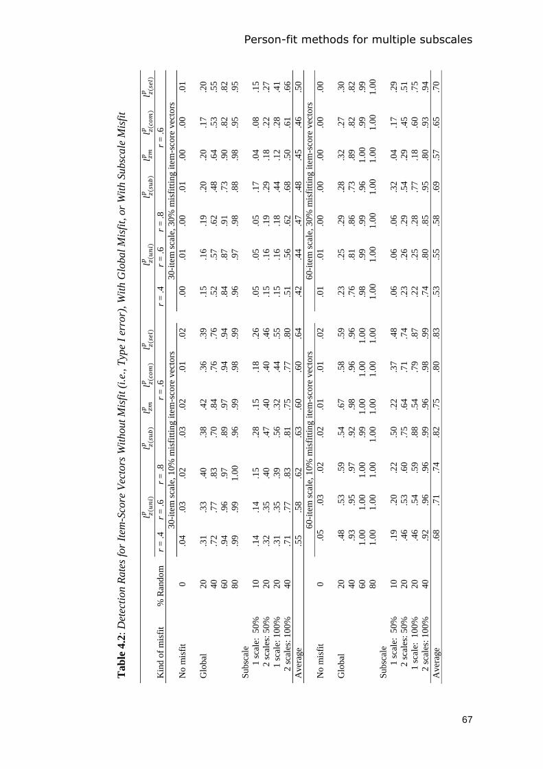
Person-fit methods for multiple subscales
67
Tab
le 4
.2:
Det
ecti
on R
ate
s fo
r It
em-S
core
Vec
tors
Wit
hout
Mis
fit
(i.e
., T
ype
I er
ror)
, W
ith G
lobal
Mis
fit,
or
Wit
h S
ubsc
ale
Mis
fit
𝑙 𝑧
𝑢𝑛𝑖
𝑝
𝑙 𝑧
𝑠𝑢𝑏
𝑝
𝑙 𝑧𝑚𝑝
𝑙 𝑧
𝑐𝑜𝑚
𝑝
𝑙 𝑧
𝑠𝑒𝑙
𝑝
𝑙 𝑧 𝑢𝑛𝑖
𝑝
𝑙 𝑧
𝑠𝑢𝑏
𝑝
𝑙 𝑧𝑚𝑝
𝑙 𝑧
𝑐𝑜𝑚
𝑝
𝑙 𝑧
𝑠𝑒𝑙
𝑝
Kin
d o
f m
isfi
t %
Rand
om
r
= .
4
r =
.6
r
= .
8
r =
.6
r =
.4
r
= .
6
r =
.8
r
= .
6
30
-ite
m s
cale
, 1
0%
mis
fitt
ing i
tem
-sco
re v
ecto
rs
3
0-i
tem
sca
le,
30
% m
isfi
ttin
g i
tem
-sco
re v
ecto
rs
No
mis
fit
0
.04
.03
.02
.03
.02
.01
.02
.00
.01
.00
.01
.00
.00
.01
Glo
bal
2
0
.31
.33
.40
.38
.42
.36
.39
.1
5
.16
.19
.20
.20
.17
.20
4
0
.72
.77
.83
.70
.84
.7
6
.76
.5
2
.57
.62
.48
.64
.53
.55
6
0
.94
.96
.97
.89
.97
.94
.94
.84
.87
.91
.73
.90
.82
.82
8
0
.99
.99
1.0
0
.96
.99
.98
.99
.9
6
.97
.98
.88
.98
.95
.95
Sub
scal
e
1 s
cale
: 5
0%
1
0
.14
.14
.15
.28
.15
.18
.26
.05
.05
.05
.17
.04
.08
.15
2 s
cale
s: 5
0%
20
.32
.35
.40
.47
.40
.40
.46
.15
.16
.19
.29
.18
.22
.27
1 s
cale
: 1
00
%
20
.31
.35
.39
.56
.32
.44
.55
.15
.16
.18
.44
.12
.28
.41
2 s
cale
s: 1
00
%
40
.71
.77
.83
.81
.75
.77
.80
.51
.56
.62
.68
.50
.61
.66
Aver
age
.55
.58
.62
.63
.60
.60
.64
.4
2
.44
.47
.48
.45
.46
.50
60
-ite
m s
cale
, 1
0%
mis
fitt
ing i
tem
-sco
re v
ecto
rs
6
0-i
tem
sca
le,
30
% m
isfi
ttin
g i
tem
-sco
re v
ecto
rs
No
mis
fit
0
.05
.03
.02
.02
.01
.01
.02
.0
1
.01
.00
.00
.00
.00
.00
Glo
bal
2
0
.48
.53
.59
.54
.67
.58
.59
.2
3
.25
.29
.28
.32
.27
.30
4
0
.93
.95
.97
.92
.98
.96
.96
.7
6
.81
.86
.73
.89
.82
.82
6
0
1.0
0
1.0
0
1.0
0
.99
1.0
0
1.0
0
1.0
0
.9
8
.99
.99
.96
1.0
0
.99
.99
80
1.0
0
1.0
0
1.0
0
1.0
0
1.0
0
1.0
0
1.0
0
1
.00
1.0
0
1.0
0
1.0
0
1.0
0
1.0
0
1.0
0
Sub
scal
e
1
sca
le:
50
%
10
.19
.20
.22
.50
.22
.37
.48
.0
6
.06
.06
.32
.04
.17
.29
2 s
cale
s: 5
0%
2
0
.46
.53
.60
.75
.64
.71
.74
.2
3
.26
.29
.54
.29
.45
.51
1 s
cale
: 1
00
%
2
0
.46
.54
.59
.88
.54
.79
.87
.2
2
.25
.28
.77
.18
.60
.75
2 s
cale
s: 1
00
%
40
.92
.96
.96
.99
.96
.98
.99
.7
4
.80
.85
.95
.80
.93
.94
Aver
age
.68
.71
.74
.82
.75
.80
.83
.5
3
.55
.58
.69
.57
.65
.70

Chapter 4
68
30% misfit condition. Detection rates were on average .17 lower in the 30-item condition
than in the 60-item condition. Contrary to what we expected, 𝑝
was rather insensitive
to the size of the correlation between θ values. For a θ-correlation of .8, 𝑝
had
detection rates comparable to 𝑝
.
Detection of Global Misfit. Method 𝑝
had the highest detection rates for global
misfit, in all conditions. In all 60-item conditions and the 30-item conditions including
10% misfit, detection rates (range: .86 to 1.00) of 𝑝
were good for item-score vectors
having at least 40% random scores. In the 30-item condition including 30% misfit,
detection rates of 𝑝
were only good for item-score vectors having at least 60% random
scores. Detection rates of 𝑝
were the lowest. The differences in detection rates
between 𝑝
and 𝑝
ranged from .00 to .17.
Detection of Subscale Misfit. Method 𝑝
had the highest detection rates for
subscale misfit, in all conditions. In the 60-item condition, detection rates (range: .77 to
1.00) of 𝑝
were good for item-score vectors with 100% random scores on one or two
subscales. In the 30-item condition, 𝑝
generally had low detection rates. Method 𝑝
had the lowest detection rates for subscale misfit. The differences between 𝑝
and 𝑝
ranged from .03 to .59.
Overall detection. Method 𝑝
on average had the best performance. This means
that although 𝑝
had higher detection rates for global misfit and 𝑝
had higher
detection rates for subscale misfit, detection rates of 𝑝
were generally not much lower
than detection rates of the best performing statistic; differences with respect to the best
performing statistic ranged from .00 to .09 for global misfit, and from .00 to .03 for
subscale misfit. Method 𝑝
performed similarly to 𝑝
across different conditions
and types of misfit, but performance was also always somewhat worse than that of 𝑝
.
4.3.4 Conclusions from Study 1
All methods are conservative when the items are calibrated in samples that include
misfitting item scores. The detection rates of different methods strongly depend on the type
of the misfit. Compared to the other methods, methods 𝑝
and 𝑝
had higher detection
rates for global misfit and methods 𝑝
and 𝑝
had higher detection rates for

Person-fit methods for multiple subscales
69
subscale misfit. An advantage of method 𝑝
is that it had relatively high detection rates
for both subscale and global misfit. The results suggest that if one does not have articulated
expectations of the manifestation of misfit, method 𝑝
is a safe choice in terms of
power. Nevertheless, the advantage of 𝑝
over 𝑝
for detecting global misfit was
substantial in some conditions. Hence, if global misfit is expected, for example, due to
similar subscale content or short test length, method 𝑝 may be preferred over method
𝑝
.
4.4 Study 2: Real-Data Applications
4.4.1 Research Questions
Using real data, we investigated whether the 𝑝-multiscale methods are useful for
two potential applications of PFA: correcting bias in research results due to aberrant
responding, and understanding the causes of aberrant responding. More specifically, we
addressed two research questions:
1. Does removal of misfitting item-score vectors as identified by the 𝑝
-multiscale
methods improve the fit of confirmatory factor analysis (CFA) models and provide
more convincing evidence of discriminant and convergent validity?
2. Does statistic 𝑝
relate to explanatory variables for abberant responding?
We adressed these questions using empirical data collected by means of three multiscale
measures with short subscales: the IPIP-50, the BSI, and the BSI-18. The IPIP-50 is an
example of a personality test that measures distinct traits. The BSI and the BSI-18 are
examples of psychopathology scales that measure a global trait as well as subtraits. We
addressed the first question for all three datasets. As we only had access to relevant
explanatory variables for the IPIP-50 data, we addressed the second question only for the
IPIP-50 data. Statistic 𝑝
quantifies person fit by means of a single continuous statistic,
and was used in this study.
The IPIP-50 data came from a panel sample, and the BSI and the BSI-18 data came
from a clinical sample. For panel members, the repeated administration of questionnaires,
the length of the surveys, and a lack of self-interest in responding accurately may lead to
unmotivated responding and systematic response styles (Krosnick, Narayan, & Smith,
1996). Such abberant response behavior likely produces item-score vectors that are
inconsistent with the GRM and therefore detectable by means of the 𝑝
-multiscale
Chapter 4
70
methods. In clinical data, person misfit is also expected. Several studies found a positive
relationship between person misfit and indicators of psychological problems and negative
affect (Conijn, Emons, Van Assen, Pedersen, & Sijtsma, 2012; Reise & Waller, 1993;
Woods, Oltmanns, & Turkheimer, 2008). Given our expectations, for both datasets it is of
interest to investigate person misfit.
4.4.2 Method
Participants. The IPIP-50 data come from the LISS (Longitudinal Internet Studies
for the Social sciences) panel and were collected by CentERdata (Tilburg University, The
Netherlands) in 2008. The panel completed a survey that included the IPIP-50 and several
other personality, mood, and attitude scales. The study sample consisted of 6,791
participants (45.4% male). The highest level of completed education was university (8%),
higher vocational education (23%), higher secondary education (11%), intermediate
vocational education (25%), intermediate secondary education (28%), and primary school
(5%). The BSI data were collected in a sample of 1,270 clinical outpatients (38.6% male)
that completed the BSI at intake at four sites of a Dutch public mental health care
institution.
Measures. The IPIP-50 (Goldberg et al., 2006) consists of five 10-item subscales,
each measuring one factor of the Big-Five personality factors: extraversion, agreeableness,
conscientiousness, neuroticism, and intellect. All items have a 5-point rating scale. We
used the Dutch version of the IPIP-50 (Hendriks, Hofstee, & De Raad, 1999). The IPIP-50
has adequate reliability and validity, and a factor structure consistent with the theoretical 5-
factor model (Gow, Whiteman, Pattie, & Deary, 2005; Hendriks et al., 1999).
The BSI (Derogatis, 1993) consists of 53 items of which 49 items are divided
across nine subscales. The subscales measure different symptoms of psychopathology,
including phobic anxiety, psychoticism, and depression. The number of items per subscale
ranges from four to seven. In practice, subscale scores are used and also a total score
referred to as the global severity index. All items have a 5-point rating-scale. We used the
Dutch version of the BSI (De Beurs, 2004). Consistent with the results of Derogatis and
Melisaratos (1983) for the original BSI, research results support the theoretical 9-factor
structure for the Dutch BSI and have demonstrated adequate reliability and validity (De
Beurs & Zitman, 2006).
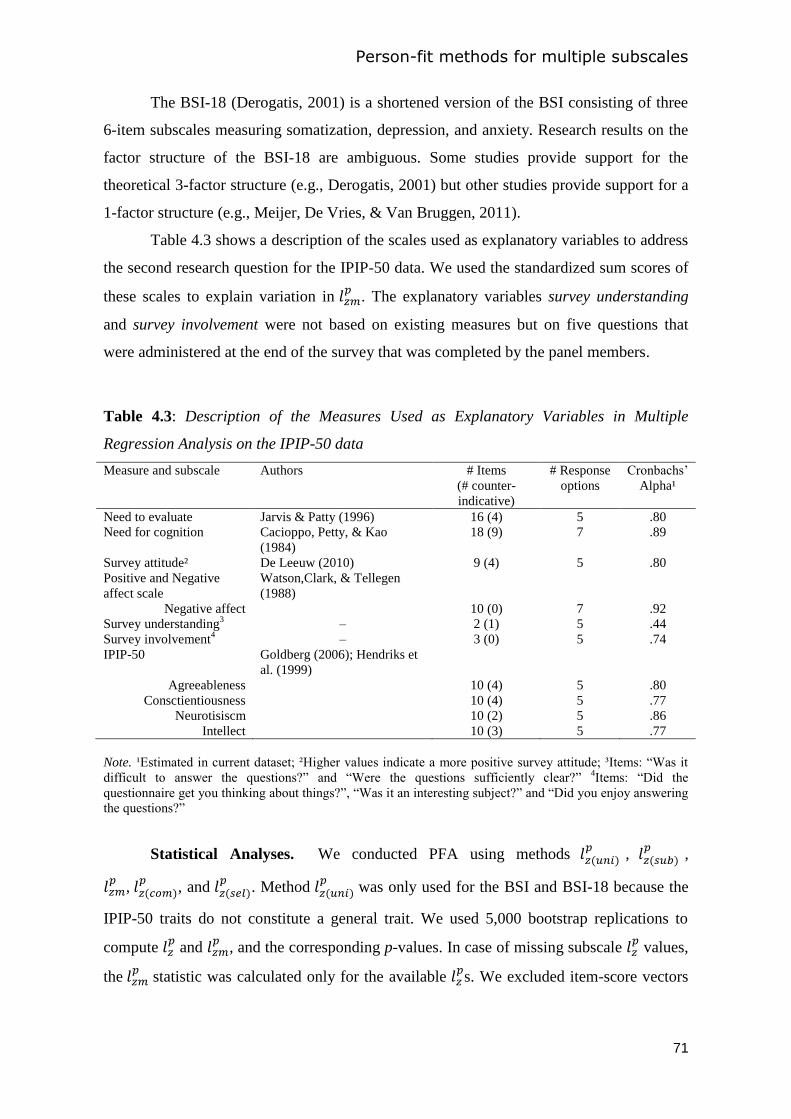
Person-fit methods for multiple subscales
71
The BSI-18 (Derogatis, 2001) is a shortened version of the BSI consisting of three
6-item subscales measuring somatization, depression, and anxiety. Research results on the
factor structure of the BSI-18 are ambiguous. Some studies provide support for the
theoretical 3-factor structure (e.g., Derogatis, 2001) but other studies provide support for a
1-factor structure (e.g., Meijer, De Vries, & Van Bruggen, 2011).
Table 4.3 shows a description of the scales used as explanatory variables to address
the second research question for the IPIP-50 data. We used the standardized sum scores of
these scales to explain variation in 𝑝
. The explanatory variables survey understanding
and survey involvement were not based on existing measures but on five questions that
were administered at the end of the survey that was completed by the panel members.
Table 4.3: Description of the Measures Used as Explanatory Variables in Multiple
Regression Analysis on the IPIP-50 data
Measure and subscale Authors # Items
(# counter-
indicative)
# Response
options
Cronbachs’
Alpha¹
Need to evaluate Jarvis & Patty (1996) 16 (4) 5 .80
Need for cognition Cacioppo, Petty, & Kao
(1984)
18 (9) 7 .89
Survey attitude² De Leeuw (2010) 9 (4) 5 .80
Positive and Negative
affect scale
Watson,Clark, & Tellegen
(1988)
Negative affect 10 (0) 7 .92
Survey understanding3 – 2 (1) 5 .44
Survey involvement4
– 3 (0) 5 .74
IPIP-50 Goldberg (2006); Hendriks et
al. (1999)
Agreeableness 10 (4) 5 .80
Consctientiousness 10 (4) 5 .77
Neurotisiscm 10 (2) 5 .86
Intellect 10 (3) 5 .77
Note. ¹Estimated in current dataset; ²Higher values indicate a more positive survey attitude; ³Items: “Was it
difficult to answer the questions?” and “Were the questions sufficiently clear?” 4Items: “Did the
questionnaire get you thinking about things?”, “Was it an interesting subject?” and “Did you enjoy answering
the questions?”
Statistical Analyses. We conducted PFA using methods 𝑝
, 𝑝
,
𝑝
, 𝑝
, and 𝑝
. Method 𝑝
was only used for the BSI and BSI-18 because the
IPIP-50 traits do not constitute a general trait. We used 5,000 bootstrap replications to
compute 𝑝 and
𝑝, and the corresponding p-values. In case of missing subscale
𝑝 values,
the 𝑝
statistic was calculated only for the available 𝑝s. We excluded item-score vectors
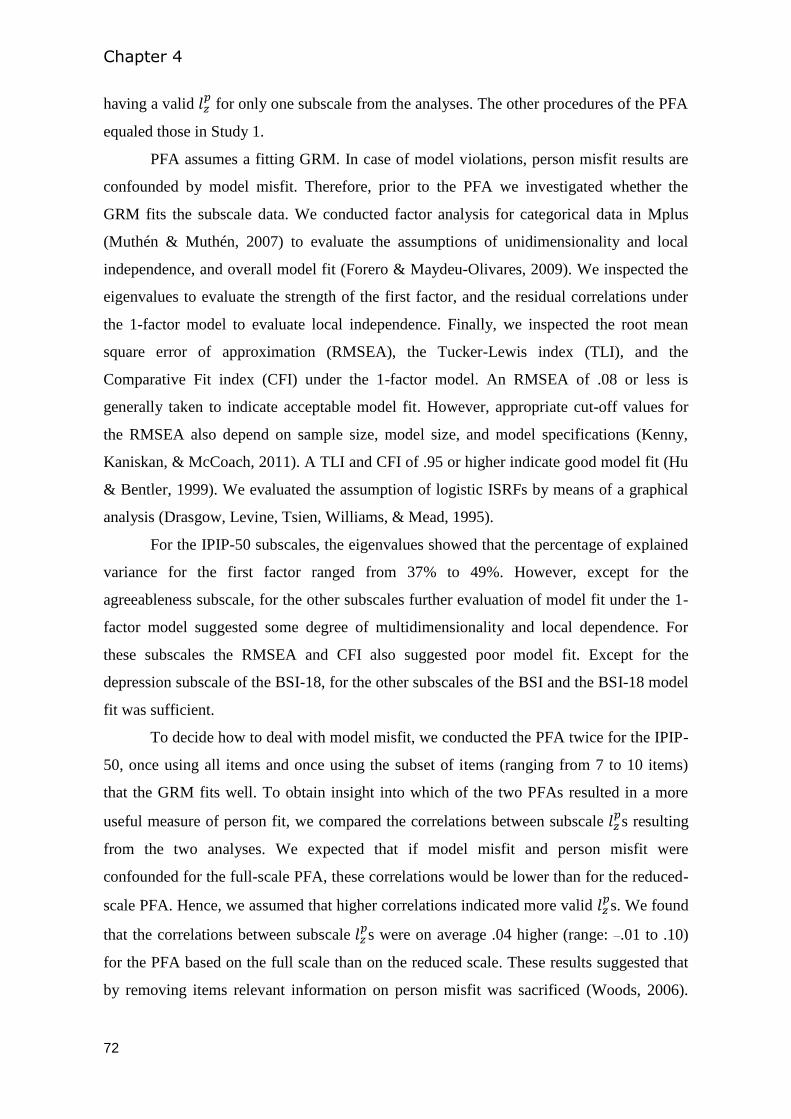
Chapter 4
72
having a valid 𝑝 for only one subscale from the analyses. The other procedures of the PFA
equaled those in Study 1.
PFA assumes a fitting GRM. In case of model violations, person misfit results are
confounded by model misfit. Therefore, prior to the PFA we investigated whether the
GRM fits the subscale data. We conducted factor analysis for categorical data in Mplus
(Muthén & Muthén, 2007) to evaluate the assumptions of unidimensionality and local
independence, and overall model fit (Forero & Maydeu-Olivares, 2009). We inspected the
eigenvalues to evaluate the strength of the first factor, and the residual correlations under
the 1-factor model to evaluate local independence. Finally, we inspected the root mean
square error of approximation (RMSEA), the Tucker-Lewis index (TLI), and the
Comparative Fit index (CFI) under the 1-factor model. An RMSEA of .08 or less is
generally taken to indicate acceptable model fit. However, appropriate cut-off values for
the RMSEA also depend on sample size, model size, and model specifications (Kenny,
Kaniskan, & McCoach, 2011). A TLI and CFI of .95 or higher indicate good model fit (Hu
& Bentler, 1999). We evaluated the assumption of logistic ISRFs by means of a graphical
analysis (Drasgow, Levine, Tsien, Williams, & Mead, 1995).
For the IPIP-50 subscales, the eigenvalues showed that the percentage of explained
variance for the first factor ranged from 37% to 49%. However, except for the
agreeableness subscale, for the other subscales further evaluation of model fit under the 1-
factor model suggested some degree of multidimensionality and local dependence. For
these subscales the RMSEA and CFI also suggested poor model fit. Except for the
depression subscale of the BSI-18, for the other subscales of the BSI and the BSI-18 model
fit was sufficient.
To decide how to deal with model misfit, we conducted the PFA twice for the IPIP-
50, once using all items and once using the subset of items (ranging from 7 to 10 items)
that the GRM fits well. To obtain insight into which of the two PFAs resulted in a more
useful measure of person fit, we compared the correlations between subscale 𝑝s resulting
from the two analyses. We expected that if model misfit and person misfit were
confounded for the full-scale PFA, these correlations would be lower than for the reduced-
scale PFA. Hence, we assumed that higher correlations indicated more valid 𝑝s. We found
that the correlations between subscale 𝑝s were on average .04 higher (range: –.01 to .10)
for the PFA based on the full scale than on the reduced scale. These results suggested that
by removing items relevant information on person misfit was sacrificed (Woods, 2006).
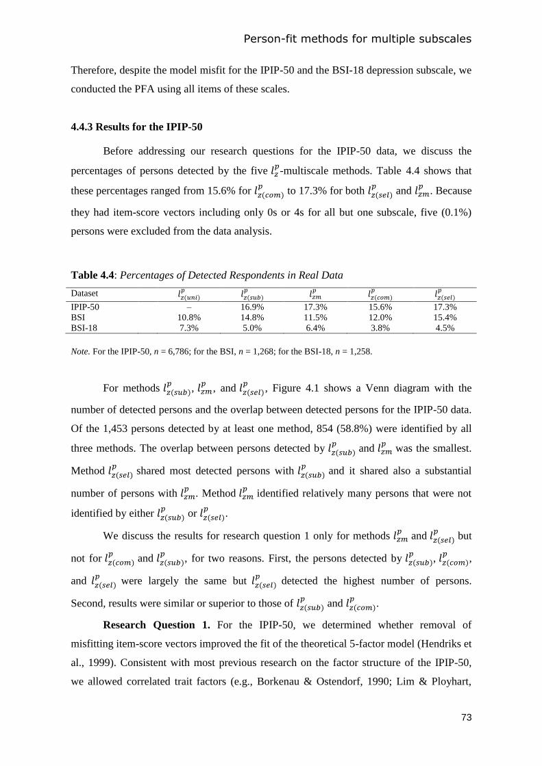
Person-fit methods for multiple subscales
73
Therefore, despite the model misfit for the IPIP-50 and the BSI-18 depression subscale, we
conducted the PFA using all items of these scales.
4.4.3 Results for the IPIP-50
Before addressing our research questions for the IPIP-50 data, we discuss the
percentages of persons detected by the five 𝑝-multiscale methods. Table 4.4 shows that
these percentages ranged from 15.6% for 𝑝
to 17.3% for both 𝑝
and 𝑝
. Because
they had item-score vectors including only 0s or 4s for all but one subscale, five (0.1%)
persons were excluded from the data analysis.
Table 4.4: Percentages of Detected Respondents in Real Data
Dataset 𝑝
𝑝
𝑝
𝑝
𝑝
IPIP-50 – 16.9% 17.3% 15.6% 17.3%
BSI 10.8% 14.8% 11.5% 12.0% 15.4%
BSI-18 7.3% 5.0% 6.4% 3.8% 4.5%
Note. For the IPIP-50, n = 6,786; for the BSI, n = 1,268; for the BSI-18, n = 1,258.
For methods 𝑝
, 𝑝
, and 𝑝
, Figure 4.1 shows a Venn diagram with the
number of detected persons and the overlap between detected persons for the IPIP-50 data.
Of the 1,453 persons detected by at least one method, 854 (58.8%) were identified by all
three methods. The overlap between persons detected by 𝑝
and 𝑝
was the smallest.
Method 𝑝
shared most detected persons with 𝑝
and it shared also a substantial
number of persons with 𝑝
. Method 𝑝
identified relatively many persons that were not
identified by either 𝑝
or 𝑝
.
We discuss the results for research question 1 only for methods 𝑝
and 𝑝
but
not for 𝑝
and 𝑝
, for two reasons. First, the persons detected by 𝑝
, 𝑝
,
and 𝑝
were largely the same but 𝑝
detected the highest number of persons.
Second, results were similar or superior to those of 𝑝
and 𝑝
.
Research Question 1. For the IPIP-50, we determined whether removal of
misfitting item-score vectors improved the fit of the theoretical 5-factor model (Hendriks et
al., 1999). Consistent with most previous research on the factor structure of the IPIP-50,
we allowed correlated trait factors (e.g., Borkenau & Ostendorf, 1990; Lim & Ployhart,
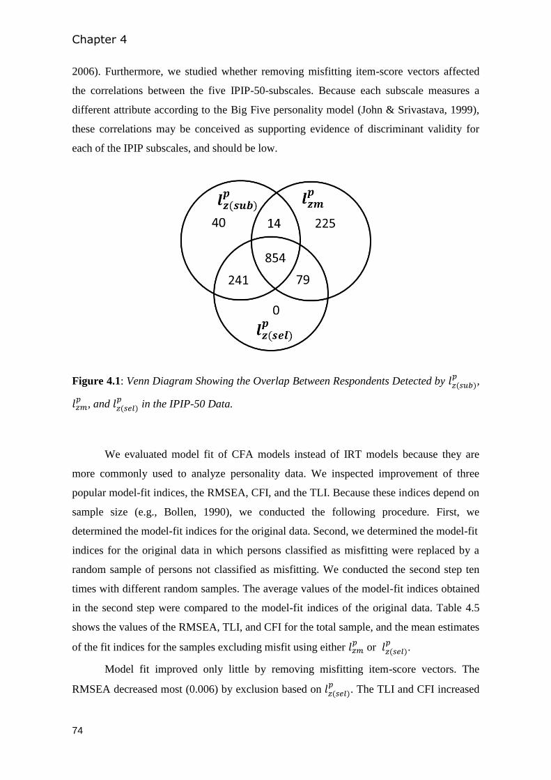
Chapter 4
74
2006). Furthermore, we studied whether removing misfitting item-score vectors affected
the correlations between the five IPIP-50-subscales. Because each subscale measures a
different attribute according to the Big Five personality model (John & Srivastava, 1999),
these correlations may be conceived as supporting evidence of discriminant validity for
each of the IPIP subscales, and should be low.
Figure 4.1: Venn Diagram Showing the Overlap Between Respondents Detected by 𝑝
,
𝑝
, and 𝑝
in the IPIP-50 Data.
We evaluated model fit of CFA models instead of IRT models because they are
more commonly used to analyze personality data. We inspected improvement of three
popular model-fit indices, the RMSEA, CFI, and the TLI. Because these indices depend on
sample size (e.g., Bollen, 1990), we conducted the following procedure. First, we
determined the model-fit indices for the original data. Second, we determined the model-fit
indices for the original data in which persons classified as misfitting were replaced by a
random sample of persons not classified as misfitting. We conducted the second step ten
times with different random samples. The average values of the model-fit indices obtained
in the second step were compared to the model-fit indices of the original data. Table 4.5
shows the values of the RMSEA, TLI, and CFI for the total sample, and the mean estimates
of the fit indices for the samples excluding misfit using either 𝑝
or 𝑝
.
Model fit improved only little by removing misfitting item-score vectors. The
RMSEA decreased most (0.006) by exclusion based on 𝑝
. The TLI and CFI increased
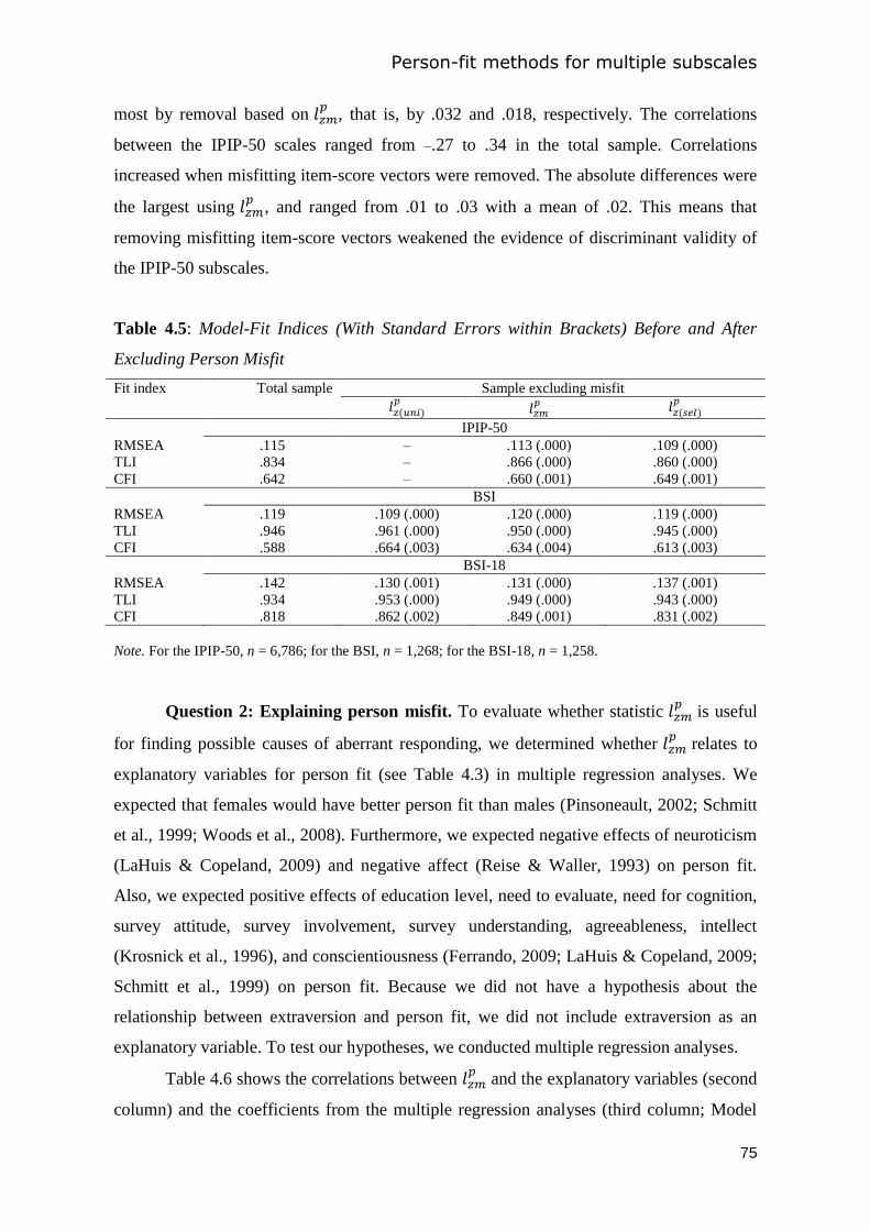
Person-fit methods for multiple subscales
75
most by removal based on 𝑝
, that is, by .032 and .018, respectively. The correlations
between the IPIP-50 scales ranged from –.27 to .34 in the total sample. Correlations
increased when misfitting item-score vectors were removed. The absolute differences were
the largest using 𝑝
, and ranged from .01 to .03 with a mean of .02. This means that
removing misfitting item-score vectors weakened the evidence of discriminant validity of
the IPIP-50 subscales.
Table 4.5: Model-Fit Indices (With Standard Errors within Brackets) Before and After
Excluding Person Misfit
Fit index Total sample Sample excluding misfit
𝑝
𝑝
𝑝
IPIP-50
RMSEA .115 – .113 (.000) .109 (.000)
TLI .834 – .866 (.000) .860 (.000)
CFI .642 – .660 (.001) .649 (.001)
BSI
RMSEA .119 .109 (.000) .120 (.000) .119 (.000)
TLI .946 .961 (.000) .950 (.000) .945 (.000)
CFI .588 .664 (.003) .634 (.004) .613 (.003)
BSI-18
RMSEA .142 .130 (.001) .131 (.000) .137 (.001)
TLI .934 .953 (.000) .949 (.000) .943 (.000)
CFI .818 .862 (.002) .849 (.001) .831 (.002)
Note. For the IPIP-50, n = 6,786; for the BSI, n = 1,268; for the BSI-18, n = 1,258.
Question 2: Explaining person misfit. To evaluate whether statistic 𝑝
is useful
for finding possible causes of aberrant responding, we determined whether 𝑝
relates to
explanatory variables for person fit (see Table 4.3) in multiple regression analyses. We
expected that females would have better person fit than males (Pinsoneault, 2002; Schmitt
et al., 1999; Woods et al., 2008). Furthermore, we expected negative effects of neuroticism
(LaHuis & Copeland, 2009) and negative affect (Reise & Waller, 1993) on person fit.
Also, we expected positive effects of education level, need to evaluate, need for cognition,
survey attitude, survey involvement, survey understanding, agreeableness, intellect
(Krosnick et al., 1996), and conscientiousness (Ferrando, 2009; LaHuis & Copeland, 2009;
Schmitt et al., 1999) on person fit. Because we did not have a hypothesis about the
relationship between extraversion and person fit, we did not include extraversion as an
explanatory variable. To test our hypotheses, we conducted multiple regression analyses.
Table 4.6 shows the correlations between 𝑝
and the explanatory variables (second
column) and the coefficients from the multiple regression analyses (third column; Model
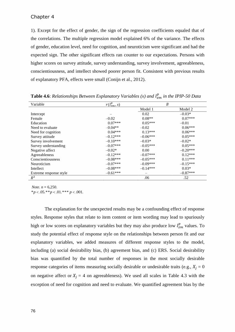
Chapter 4
76
1). Except for the effect of gender, the sign of the regression coefficients equaled that of
the correlations. The multiple regression model explained 6% of the variance. The effects
of gender, education level, need for cognition, and neuroticism were significant and had the
expected sign. The other significant effects ran counter to our expectations. Persons with
higher scores on survey attitude, survey understanding, survey involvement, agreeableness,
conscientiousness, and intellect showed poorer person fit. Consistent with previous results
of explanatory PFA, effects were small (Conijn et al., 2012).
Table 4.6: Relationships Between Explanatory Variables (x) and 𝑝
in the IPIP-50 Data
Variable 𝑝
, x)
Model 1 Model 2
Intercept – 0.02 –0.03*
Female –0.02 0.08** 0.07***
Education 0.07*** 0.05*** –0.01
Need to evaluate –0.04** –0.02 0.06***
Need for cognition 0.04*** 0.13*** 0.06***
Survey attitude –0.12*** –0.06*** 0.05***
Survey involvement –0.10*** –0.03* –0.02*
Survey understanding –0.07*** –0.05*** 0.05***
Negative affect –0.02* 0.00 –0.20***
Agreeableness –0.12*** –0.07*** 0.12***
Conscientiousness –0.08*** –0.05*** 0.11***
Neuroticism –0.07*** –0.09*** –0.15***
Intellect –0.08*** –0.14*** 0.03*
Extreme response style –0.61*** – –0.87***
.06 .52
Note. n = 6,250.
.001.*** .01.** .05.* ppp
The explanation for the unexpected results may be a confounding effect of response
styles. Response styles that relate to item content or item wording may lead to spuriously
high or low scores on explanatory variables but they may also produce low 𝑝
values. To
study the potential effect of response style on the relationships between person fit and our
explanatory variables, we added measures of different response styles to the model,
including (a) social desirability bias, (b) agreement bias, and (c) ERS. Social desirability
bias was quantified by the total number of responses in the most socially desirable
response categories of items measuring socially desirable or undesirable traits (e.g., = 0
on negative affect or = 4 on agreeableness). We used all scales in Table 4.3 with the
exception of need for cognition and need to evaluate. We quantified agreement bias by the
Person-fit methods for multiple subscales
77
total number of agreements (e.g., ≥ 3 for = 0,…,4) and ERS by the total number of
responses in the most extreme categories (e.g., = 0 or 4 for = 0,…,4).
Results suggest that the unexpected effects of survey attitude, survey
understanding, survey involvement, agreeableness, conscientiousness, and intellect were
probably due to a confounding effect of ERS. Table 4.6 (Model 2) shows the results for a
regression model that included the measure of ERS. Including ERS in our model led to an
increase of explained variance equal to 46%. As expected, the effect of ERS on person fit
was negative. Furthermore, after accounting for ERS most explanatory variables that
initially had an unexpected effect on 𝑝
now had an effect in the expected direction. The
effects of survey attitude, survey understanding, agreeableness, conscientiousness, and
intellect were positive and significant. Also as expected, after accounting for ERS, negative
affect had a significant negative effect on 𝑝
. Only the change in the effect of education
level was contrary to our expectations. After accounting for ERS, this effect was not
significant anymore. The measure of ERS correlated .92 to the measure of social
desirability bias. We concluded that an ERS related to social desirability led to biased test
scores on the explanatory variables and interfered with the explanatory PFA.
4.4.4 Results for the BSI and the BSI-18
Table 4.4 shows that in the BSI data the percentage of detected persons ranged from
10.8% for 𝑝
to 15.4% for 𝑝
. In the BSI-18 data, this percentage ranged from 3.8%
for 𝑝
to 7.3% for 𝑝
. Because they had item-score vectors including only 0s or 4s
for all but one subscale, two (0.2%) and twelve (0.9%) persons were excluded from the
analyses for the BSI and the BSI-18, respectively.
The BSI-18 data was a subset of the BSI data. Nevertheless, on the longer BSI more
persons were identified as misfitting than on the shorter BSI-18. Also, it was often found
that persons misfitting on one scale fitted on the other scale. For example, 132 persons
were identified as misfitting on the BSI-18 by at least one of the 𝑝-multiscale methods and
only 36 (27.3%) of them were identified as misfitting on the BSI. Thus, person misfit may
depend on the specific subset of items but another explanation for the inconsistent results is
that PFA methods performed poorly.
Chapter 4
78
Next, we discuss the results concerning the effect of excluding misfit on research
results (question 1) for methods 𝑝
, 𝑝
, and 𝑝
. For similar reasons as for the IPIP-
50, we do not report results on 𝑝
and 𝑝
.
Research Question 1. To evaluate the improvement of model fit by excluding
misfitting item-score vectors we first fit the theoretical 9-factor and 3-factor models to the
BSI and the BSI-18 data, respectively (Derogatis & Melisaratos, 1983; Derogatis, 2001).
However, in both cases the covariance matrix of the latent factors was not positive definite
due to too much overlap between subscale traits. Hence, we could not use these models to
evaluate the improvement of model fit. To solve this problem for the BSI, we used a
second-order factor model instead of the 9-factor model (Hoe & Brekke, 2009). The
second-order factor model included nine uncorrelated first-order factors corresponding to
the subscale traits, each loading on the second-order factor. For the BSI-18, we used a 1-
factor model (Meijer et al., 2011). Furthermore, we also studied whether removing
misfitting item-score vectors changed the correlations of the BSI and BSI-18 with the
symptom distress subscale of the Dutch version of the Outcome Questionnaire-45 (OQ-45;
Lambert et al., 2001). These correlations provide supporting evidence that the BSI and
BSI-18 have convergent validity (De Jong et al., 2007).
Table 4.5 shows the changes in the model-fit indices for the BSI and the BSI-18 by
removing misfitting item-score vectors based on 𝑝
, 𝑝
, and 𝑝
. Results were
similar for the BSI and the BSI-18. Removing misfitting item-score vectors based on
𝑝
had the largest effects, and removing based on 𝑝
had the smallest effects. For
both scales, removal based on 𝑝
led to a RMSEA decrease of approximately .01. The
TLI increased by about .017 and, unlike in the total sample, the TLI criterion in the
reduced sample exceeded the criterion good model fit. The CFI increased by .076 for the
BSI and .044 for the BSI-18. Both the BSI and the BSI-18 correlated .76 with the OQ-45
symptom distress subscale in the total sample. The correlation changed by no more than
.006 when misfitting item-score vectors were removed using either 𝑝
, 𝑝
, or 𝑝
.
4.4.5 Conclusions from Study 2
We found that model fit improved but only little when misfitting item-score vectors
were removed from the data. Correlations supporting either discriminant or convergent
validity were hardly affected by excluding person misfit and sometimes contrary to
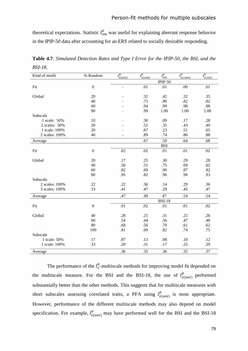
Person-fit methods for multiple subscales
79
theoretical expectations. Statistic 𝑝
was useful for explaining aberrant response behavior
in the IPIP-50 data after accounting for an ERS related to socially desirable responding.
Table 4.7: Simulated Detection Rates and Type I Error for the IPIP-50, the BSI, and the
BSI-18.
Kind of misfit % Random 𝑝
𝑝
𝑝
𝑝
𝑝
IPIP-50
Fit 0 – .01 .01 .00 .01
Global 20 – .32 .42 .32 .35
40 – .73 .90 .82 .82
60 – .94 .99 .98 .98
80 – .99 1.00 1.00 1.00
Subscale
1 scale: 50% 10 – .30 .09 .17 .28
2 scales: 50% 20 – .51 .35 .43 .49
1 scale: 100% 20 – .67 .23 .51 .65
2 scales: 100% 40 – .89 .74 .86 .88
Average .67 .59 .64 .68
BSI
Fit 0 .02 .02 .01 .01 .02
Global 20 .17 .25 .30 .29 .28
40 .56 .51 .75 .69 .62
60 .82 .69 .90 .87 .82
80 .95 .82 .96 .96 .93
Subscale
2 scales: 100% 22 .22 .36 .14 .29 .36
3 scales: 100% 33 .41 .47 .29 .45 .47
Average .47 .49 47 .54 .54
BSI-18
Fit 0 .01 .02 .01 .01 .02
Global 40 .28 .25 .31 .25 .26
60 .54 .44 .56 .47 .48
80 .68 .56 .70 .61 .62
100 .81 .69 .82 .74 .75
Subscale
1 scale: 50% 17 .07 .13 .08 .10 .12
1 scale: 100% 33 .20 .31 .17 .25 .29
Average .36 .35 .36 .35 .37
The performance of the 𝑝-multiscale methods for improving model fit depended on
the multiscale measure. For the BSI and the BSI-18, the use of 𝑝
performed
substantially better than the other methods. This suggests that for multiscale measures with
short subscales assessing correlated traits, a PFA using 𝑝
is most appropriate.
However, performance of the different multiscale methods may also depend on model
specification. For example, 𝑝
may have performed well for the BSI and the BSI-18
Chapter 4
80
because for these measures we specified models with a general-trait factor instead of only
subscale-trait factors.
A lack of power may partly explain the small effect of excluding person misfit from
the data on model fit and indicators of the validity. Low power means that many misfitting
item-score vectors go undetected (Type II errors). To investigate the possibility that our
PFA was underpowered, we determined the detection rates of the 𝑝-multiscale methods
given the properties of the IPIP-50, the BSI, and the BSI-18 data. That is, we conducted
simulations similar to those of Study 1. We used the GRM in which estimated item
parameters were inserted, and the estimated latent trait variance-covariance matrix to
generate data. We included 20% misfitting item-score vectors. Table 4.7 shows the results.
For the IPIP-50, the person-fit methods had good power for detecting substantial misfit.
However, for the BSI and the BSI-18 we only found good detection rates for item-score
vectors with at least 60% random item scores (BSI) and item-score vectors with 100%
aberrant item scores (BSI-18). As item-score vectors including more than 60% aberrant
item scores seem to be unusual, we expect low power to identify person misfit for the BSI
and BSI-18.
Meijer (2003) recommends to choose a more liberal α level so as to increase power
in PFA, such as . Using this value, we used 𝑝
for the IPIP-50 and 𝑝
for
the BSI and the BSI-18, and found that the number of detected persons was 21.5% (IPIP-
50), 15.2% (BSI), and 11.6% (BSI-18). After removal of misfitting item-score vectors,
improvement of model fit relative to was small for all measures. For example, for
the BSI-18, removal of misfitting item-score vectors based on produced changes
in RMSEA, TLI, and CFI equal to –.012, .019, .044, respectively, and for
additional changes equaled –.002, .005, and .013, respectively. Removing misfitting item-
score vectors using instead of .05 did not affect the estimated correlations with
other measures. These results suggest that adopting a higher level does not change the
effects of the PFA on model fit or evidence about the measures’ validity.
4.5 General Discussion
We compared the performance of five different 𝑝-multiscale methods for detecting
aberrant responding to non-cognitive multiscale measures. We used simulations to
compare the methods’ Type I error rates and detection rates. Additionally, we did real-data
Person-fit methods for multiple subscales
81
analyses to evaluate the methods’ usefulness for correcting bias in results on model fit and
validity estimates, and for understanding the causes of person misfit.
The simulation study showed that for multiscale measures with a total test length of
60 items, the 𝑝-multiscale methods had good power for detecting substantial person misfit.
For multiscale measures with a total test length of 30 items, power was only good when the
data included little person misfit. As expected, our proposed method of combining subscale
𝑝 values and
𝑝 resulted in relatively high detection rates for both subscale specific and
global misfit.
A comparison of our results with those of Emons (2008) shows the advantage of
combining person misfit information from different subscales. Emons found that for a 12-
item subscale with 50% random item-scores the detection rate of 𝑝 was only .50, even if
the item parameters used to compute 𝑝 were estimated in a dataset without misfit. Our
study showed that the best-performing multiscale method, 𝑝
, had a detection rate of
.96 for five 12-item scales with 40% random item scores across all subscales, and a
detection rate of .47 if one of the five subscales included 50% random item scores. The
comparison suggests that if misfit is to some extent consistent across subscales, a
substantial gain in power can be obtained, and if misfit is subscale-specific, the loss in
power is small. Hence, we advise to use multiscale person-fit statistics for non-cognitive
multiscale measures with short subscales. As the performance of the 𝑝-multiscale methods
depended on the manifestation of the person misfit in the data, the choice of the 𝑝
-
multiscale method should be based on expectations of whether misfit is present in only few
subscales or many subscales.
We used the BH procedure to control the Type I error rate for methods 𝑝
,
𝑝
, and 𝑝
. An advantage of the method is its simplicity. A limitation of the BH
procedure is that it tightly controls the FDR at a desired level only if test statistics are
independent, but for positively dependent test statistics such as those involved in methods
𝑝
and 𝑝 the procedure is conservative (Benjamini & Yekutieli, 2001).
Nevertheless, we found that method 𝑝
outperformed the other methods in many
conditions, and method 𝑝
outperformed the other methods in some conditions for the
BSI properties (see Table 4.7).
An interesting finding from the simulation study was that the 𝑝 statistic performed
relatively well when unidimensionality was violated. This suggests that for conducting
Chapter 4
82
PFA, data may not need to strictly satisfy GRM model assumptions. Several solutions have
been suggested for PFA when the model does not fit the data (Emons, 2008; Woods,
2008). For example, prior to PFA balanced scales with poor model fit should be separated
into subsets of items with only positively worded or only negatively worded items (Woods,
2008), or non-parametric person-fit statistics instead of more powerful parametric person-
fit statistics such as 𝑝 should be used (Emons, 2008). However, if PFA is robust against
model violations, as our results suggest, these alternative approaches may actually lead to
worse PFA results. More research should be done on this topic.
Most research on the Type I error rate and detection rate of person-fit statistics uses
item parameters estimated in datasets without person misfit (e.g., Emons, 2008; Reise,
1995). This procedure is only valid when researchers have access to unbiased, calibrated
item parameters. However, for non-cognitive test data either a lack of self-interest or the
possibility of faking good or bad is practically always a potential cause of aberrant
responding. Therefore, misfitting item-score vectors and biased item parameter estimates
are usually unavoidable. Based on our finding, we speculate that previous studies
overestimated the performance of PFA in real-life settings.
The results of the real-data applications suggest that the usefulness of the 𝑝
-
multiscale methods for correcting bias in research results may be limited. Statistic 𝑝
was
useful for exploring the causes of aberrant responding in a multiple regression analysis and
related to explanatory variables for person fit as expected from previous research.
However, the results also suggest that one needs to account for response styles when using
explanatory variables that can be affected by aberrant response behavior.
The results of this study are consistent with previous research showing that
excluding misfitting item-score vectors based on statistic had minor effects on criterion-
related validity (Meijer, 1997; Schmitt, Cortina, & Whitney, 1993; Schmitt et al., 1999).
The additional analyses conducted in this study using a liberal α level of .10 did not show
improved effects of the PFA. Hence, a lack of power may not be the only problem.
Possibly, the type of person misfit detected by statistic (and 𝑝
) is not relevant for
improving validity estimates. One explanation may be that statistic has relatively low
power for detecting aberrant item-score vectors due to a systematic response style, for
example, agreement bias or ERS (e.g., Emons, 2008). Another possible explanation is that
due to the bias in trait estimates caused by aberrant responding, power is low to detect the

Person-fit methods for multiple subscales
83
aberrant item-score vectors that lead to the largest bias in test scores. More research should
be done on this topic.
Previous research on the performance of person-fit methods consists for the most
part of simulation studies only. In this study, the empirical analyses based on the IPIP-50,
the BSI, and the BSI-18 data provided additional insights in the performance of the 𝑝-
multiscale methods. Although the simulation study suggested reasonable performance, the
real-data analyses suggested that the methods may not detect misfit that negatively affect
model fit or distort indicators of validity. However, as detection rates were found to be
sufficient, future studies may demonstrate the usefulness of the 𝑝-multiscale methods for
other functionalities of PFA, for example for improving individual decision-making.
Overall, we conclude that more real-data studies are needed to demonstrate the usefulness
of the 𝑝-multiscale methods for non-cognitive measurement.

Chapter 4
84
85
Chapter 5*
Using person-fit analysis to detect and explain aberrant
responding to the Outcome Questionnaire-45
Abstract Self-report outcome measures are used in mental health care for individual
treatment planning and in large scale cost-effectiveness assessments. We investigated the
usefulness of person-fit analysis (PFA) for detecting and explaining aberrant responding to
the Outcome Questionaire-45 (OQ-45; Lambert et al., 2004). The PFA involved the
statistic for detecting misfitting item-score patterns and the standardized residual statistic
for identifying the source of the misfit. We used OQ-45 data collected in a sample of
outpatients (N = 2,906). First, we conducted a simulation study using artificial data
resembling the OQ-45 data and found that the detection rate of the statistic was high for
item-score patterns including many random item scores but low for acquiescence. The
results also suggested that the statistic was robust against violations of unidimensionality
in the OQ-45 data. Furthermore, we found that the standardized residual statistic performed
poorly. Second, we applied the PFA methods to the empirical OQ-45 data. The statistic
classified 12.6% of the item-score patterns as misfitting. We used logistic regression
analysis and found that patients having more severe distress and patients with psychotic
disorders, somatoform disorders, and substance-related disorders were particularly likely to
show misfit. We concluded that PFA has potential in outcome measurement for detecting
aberrant response behavior and identifying subgroups of patients that are at risk of
producing invalid test results.
* This chapter has been submitted for publication
Chapter 5
86
5.1 Introduction
During the previous two decades, the growing interest in the quality of mental
health care has led to an increase in the use of self-report outcome measures (De Beurs et
al., 2011; Holloway, 2002). To monitor the effectiveness of treatments for individual
patients, outcome measures that assess symptom severity and daily functioning are
repeatedly administered during treatment. Based on the repeated measurements, the
treatment plan can be altered if recovery does not proceed as expected (Duffy et al., 2008;
Lambert & Shimokawa, 2011). Furthermore, mental-health care providers use these
outcome data to evaluate treatment results at the institutional level, and insurance
companies, health-care managers, and other regularity bodies use outcome measures for
policy decisions aimed at improving cost effectiveness (Bickman & Salzer, 1997; Slade,
2002). Examples of frequently used outcome measures are the Outcome Questionnaire-45
(OQ-45; Lambert et al., 2004), the Brief Symptom Inventory (BSI; Derogatis, 1993), and
the Clinical Outcomes in Routine Evaluation − Outcome Measure (CORE-OM; Evans et
al., 2002).
Given the importance of outcome measures for decision making in mental health
care, their psychometric properties are a major concern (e.g., Doucette & Wolf, 2009;
Pirkis et al., 2005). However, on high-quality measurement instruments aberrant response
behavior may also produce invalid test scores. Research results suggest that respondents in
mental health care may be particularly prone to aberrant response behavior (Conijn,
Emons, Van Assen, Pedersen, & Sijtsma, 2012; Reise & Waller, 1993; Woods, Oltmanns, &
Turkheimer, 2008). Response inconsistency on personality and psychopathology
inventories was found to be positively related to indicators of psychological distress,
psychological problems, and negative affect. An explanation for this result may be that the
cognitive deficits that are commonly observed in mental illness lead to concentration
problems that interfere with the quality of self-reports (Altre-Vaidya et al., 1998; Cuijpers,
Li, Hofann, & Andersson, 2010; Rief & Broadbenth, 2007). However, potential causes of
aberrant response behavior are numerous, including lack of motivation, response styles,
idiosyncratic interpretation of item content, and low traitedness, which refers to
applicability of the trait to the respondent (Tellegen, 1988).
Aberrant response behavior provides clinicians with invalid information and, as a
result, adversely affects the quality of treatment and diagnosis decisions (Conrad et al.,
2010; Handel, Ben-Porath, Tellegen, & Archer, 2010). The importance of detecting
Person-fit analysis in outcome measurement
87
aberrant response behavior has been recognized for a long time. The original version of the
Minnesota Multiphasic Personality Inventory (MMPI-2; Butcher et al., 2001), for example,
already included several scales to detect aberrant responding. Its current version includes
Variable Response Inconsistency (VRIN) and True Response Inconsistency (TRIN) scales
(Handel et al., 2010) to detect random responding and acquiescence (i.e., the tendency to
endorse items regardless of item content). However, with the increasing demand of cost
effectiveness, time for assessment is heavily reduced (Wood, Garb, Lilienfeld, &
Nezworski, 2002). Outcome questionnaires should be short and efficient and typically do
not include specialized scales for detecting aberrant responding (Lambert & Hawkins,
2004). As a result, despite its recognized importance, there is no routine screening for
aberrant response patterns in outcome measurement.
Person-fit analysis (PFA) involves statistical methods to detect aberrant response
patterns. Conrad et al. (2010) provided a first example of the potential of PFA to mental
health care. Specifically, the authors used PFA to screen for atypical symptom profiles
among persons at intake for drug or alcohol dependence treatment. They found that the
detected persons required different treatments than persons with model consistent item-
score patterns and concluded that PFA may detect inconsistencies that have important
implications for treatment and diagnosis decisions. The goal of this study was to
investigate the usefulness of item response theory (IRT) based PFA for detecting and
understanding aberrant responding to outcome measures in clinical practice.
5.1.1 Person-Fit Analysis
The main aim of IRT based PFA is to identify aberrant item-score patterns for
which the test score may be invalid (Meijer & Sijtsma, 2001). Person-fit statistics quantify
the differences between the observed item-score pattern and the expected item-score
pattern based on the IRT model that is assumed to underlie the item scores. For item-score
patterns that are consistent with the IRT model, the test score reflects the trait being
measured. However, for item-score patterns to which the IRT model shows misfit, the
resulting test score is the outcome of inconsistencies and is unlikely to be meaningful.
Numerous person-fit statistics were developed (e.g., Meijer & Sijtsma, 2001). One of the
best performing and most popular person-fit statistics is the statistic (Drasgow, Levine,
& McLaughlin, 1987; Snijders, 2001), which is defined as the standardized log-likelihood
of an item-score pattern given the estimated IRT model. Statistic can be used to detect
Chapter 5
88
different types of aberrant item-score patterns, including acquiescence and extreme
response style, but detection rates are the highest for random responding (Emons, 2008).
To determine whether an item-score pattern shows significant misfit, statistic is
compared to a cut-off value based on its theoretical or simulated distribution under the null
model of consistency with the IRT model.
PFA can also be useful to gain insight into possible explanations for observed
aberrant response behavior. For misfitting item-score patterns, standardized residuals may
show which of the observed item scores deviate most from the IRT model’s expectation
and in which direction (Emons, 2004, 2005; Ferrando, 2010, 2012). For example, Ferrando
(2010) used the item-score residuals to infer the causes of aberrant responding to an
extraversion scale. He found that one aberrant item-score pattern included many
unexpected low scores on items concerning situations where the person could make a fool
of himself. He conjectured that the aberrant responding was due to fear of being rejected.
For another aberrant pattern, residuals suggested that aberrance was due to inattentiveness
to negative item wording. Furthermore, PFA can also be used to investigate whether
specific persons are prone to aberrant response behavior. To this end, person-fit statistics
can be related to explanatory variables, for example, in multiple regression analyses
(Conijn, Emons, & Sijtsma, 2013). Previous research showed that persons low in
conscientiousness and lowly educated persons were more likely to produce misfitting item-
score patterns (e.g., Conijn et al., 2012; Schmitt, Chan, Sacco, McFarland, & Jennings,
1999).
5.1.2 Applications of PFA in Outcome Measurement
PFA may be useful for detecting invalid test scores in outcome measurement. A
disadvantage of commonly used validity scales in clinical practice (e.g., VRIN or TRIN
scales) is that they can only be used in combination with the self-report inventory for
which they have been designed. In contrast, person-fit statistics such as can be applied to
any self-report scale that is consistent with an IRT model. This results in a yes/no decision
whether an item-score pattern is aberrant. Follow-up analysis using item-score residuals
can inform the clinician about the source of the misfit and provide an opportunity to
discuss the deviant item scores with the patient.
PFA may also be used to investigate to what extent outcome measures are suitable
for patients with different disorders. A typical feature of general outcome measures, such as
Person-fit analysis in outcome measurement
89
the OQ-45 and the CORE-OM, is that they are used for patients with a wide range of
disorders, ranging from mild depression to psychotic disorders and addiction. However,
outcome measures are based on the most common symptoms of psychopathology such as
those observed in depression and anxiety disorders (Lambert & Hawkins, 2004). One can
imagine that for rare or specific disorders several of these symptoms are irrelevant and low
traitedness may lead to inconsistent or unmotivated completion of outcome questionnaires.
Despite the potential applications of PFA to outcome measurement, commonly
used outcome measures have characteristics that may constrain successful application of
PFA. First, recent research suggested that IRT models poorly fit data from
psychopathology measures (Doucette & Wolf, 2009; Meijer & Baneke, 2004; Reise &
Waller, 2003). Adequate model fit is necessary to have meaningful PFA results (e.g.,
Woods et al., 2008). Second, outcome measures typically include fewer than fifty items,
often distributed across different subscales, each measuring a different attribute (Lambert
& Hawkins, 2004). These properties have negative consequences for the power to detect
aberrant item-score patterns (Reise & Due, 1991). Conijn et al. (2013), for example, found
that for tests with multiple subscales person-fit statistics only have good power when the
total number of items exceeds 50.
In this study, we investigated the potential of PFA for detecting and understanding
aberrant responding to the OQ-45 (Lambert et al., 2004). We used the person-fit statistic
(Drasgow et al., 1987; Snijders, 2001) to detect aberrant responding and standardized item-
score residuals (Ferrando, 2010, 2012) to identify the source of the misfit for the detected
item-score patterns. We addressed three research goals using OQ-45 data of a clinical
outpatient sample.
First, we investigated whether IRT model assumptions were tenable for the OQ-45
data. Application of the statistic and the standardized residual statistic rests on the
assumption that the postulated IRT model fits the subscale data. Second, we examined the
performance of PFA when applied to OQ-45 data. Performance is defined by the Type I
error rate and the power of statistic and the standardized residual statistic for detecting
aberrant item-score patterns and deviant item scores, respectively. To this end, we did a
simulation study in which we simulated item-score patterns using item parameters
estimated in the OQ-45 data. Third, we used the statistic and standardized residuals for
detecting and explaining aberrant response behavior to the OQ-45. We used the results of
the simulation study for a comprehensive interpretation of real-data results. Furthermore,
by relating statistic to diagnosis we investigated whether patients with specific disorders,
Chapter 5
90
such as somatoform disorder and ADHD, and more severely distressed patients were more
likely to produce aberrant item-score patterns on the OQ-45 than other patients. Finally, we
provide a discussion on the usefulness of PFA for outcome measurement.
5.2 Method
5.2.1 Participants
Participants were 2,906 clinical outpatients (42.1% male) from four different
locations of a mental health care institution in the Netherlands. The age of the participants
ranged from 17 to 77 years (M = 37; SD = 13). Most patients completed the OQ-45 at
intake but 160 (5.5%) patients completed the OQ-45 after treatment started. The sample
included 2,632 patients with a clinician rated Diagnostic and Statistical Manual of Mental
Disorders (4th Edition) (DSM-IV) primary diagnosis at Axis I and 192 persons with a
primary diagnosis at Axis II. For 82 patients the primary diagnosis was missing. Although
the clinician had access to the OQ-45 data, it was unlikely that diagnosis was based on the
OQ-45 results because the OQ-45 is not a diagnostic instrument.
5.2.2 The Outcome Questionnaire-45
The OQ-45 (Lambert et al., 2004) uses three subscales to measure symptom
severity and daily functioning. The Symptom Distress (SD) subscale measures symptoms
of the most frequently diagnosed mental disorders, in particular anxiety and depression.
The SD scale consists of 25 items of which three are reversely worded. An example of a
reversely worded item is “I feel no interest in things” and an example of a positively
worded items is “I am satisfied with my life”. The Interpersonal Relations (IR) subscale
measures difficulties with family, friends, and marital relationships. The IR subscale
consists of eleven items of which four items are reversely worded. Example items are “I
get along well with others” and “I feel lonely”. The Social Role Performance (SR) subscale
measures dissatisfaction, distress, and conflicts concerning one’s employment, education,
or leisure pursuits. The SR subscale consists of nine items of which three items are
reversely worded. Example items are “I enjoy my spare time” and “I feel stressed at
work/school”. Respondents are instructed to rate their feelings with respect to the past
week on a 5-point rating scale with scores ranging from 0 (never) through 4 (almost
always), with higher scores indicating more psychological distress.
Person-fit analysis in outcome measurement
91
In this study, we used the Dutch OQ-45 (De Jong & Nugter, 2004). The Dutch OQ-
45 has good concurrent and criterion-related validity (De Jong et al., 2007). With the
exception of the SR subscale, the Dutch OQ-45 has adequate total-score reliability. Results
concerning the factor structure of the OQ-45 are ambiguous. Some studies provide support
for the theoretical 3-factor model for the original OQ-45 and the Dutch OQ-45 (Bludworth,
Tracey, & Glidden-Tracey, 2010; De Jong et al., 2007). Other studies found poor fit of the
theoretical 3-factor model (Kim, Beretvas, & Sherry, 2010; Mueller, Lambert, &
Burlingame, 1998).
5.2.3 Person-Fit Methods
Statistic for Multiscale Measures and Polytomous Items. We used statistic
for polytomous item scores, denoted by 𝑝 (Drasgow, Levine, & Williams, 1985) to detect
item-score patterns that show misfit relative to the graded response model (GRM;
Samejima, 1997). The GRM is an IRT model for unidimensional data with ordered item
scores. Suppose the data are polytomous item scores of N respondents on J items (items are
indexed j; j = 1, …, J) with M +1 ordered answer categories. Let the score on item j be
denoted by with possible realizations . The GRM models the probability of
observing a score or higher as a function of a latent trait θ by means of item-step
response functions (ISRFs). The ISRFs for item j have a common discrimination parameter
that reflects the degree to which an item can differentiate between levels, and M category
threshold parameters that reflect the categories’ popularity. The GRM is defined by three
assumptions: unidimensionality of , local independence conditional on , and logistic
ISRFs.
Statistic 𝑝 is the standardized log-likelihood of a person’s item-score pattern given
the response probabilities under the GRM. Let if , and 0
otherwise. The unstandardized log-likelihood of an item-score pattern x of person i is given
by
𝑝 ∑ ∑ ( | ) ( )
The standardized log-likelihood is defined as
𝑝
𝑝 [ 𝑝 ]
[ 𝑝 ]

Chapter 5
92
where 𝑝 is the expected value and 𝑝 the variance of 𝑝 . Larger negative 𝑝
values indicate a higher degree of misfit. Item-score patterns that contain only 0s or only 4s
cannot provide information about person fit and corresponding 𝑝 statistics are therefore
treated as missing values.
Because the GRM is a model for unidimensional data, we computed statistic 𝑝 for
each of the OQ-45 subscales separately. To categorize persons as fitting or misfitting with
respect to the complete OQ-45, we used the multiscale person-fit statistic 𝑝
(Conijn et
al., 2013; Drasgow, Levine, & McLaughlin, 1991), which is the sum of the 𝑝 values of
several unidimensional subscales. Alternative statistics were proposed that combine
subscales 𝑝
s into an overall measure of person fit (Conijn et al., 2013). Based on
preliminary simulations we found that 𝑝
was the best choice given the properties of the
OQ-45.
When statistic 𝑝 is computed using the estimated trait value instead of the true
value, the sampling distribution of 𝑝 under the null hypothesis of no misfit is no longer the
standard normal distribution (Nering, 1995). Therefore, we used a parametric bootstrap
procedure to compute 𝑝 and
𝑝 values that have a standard normal distribution under the
null model of person fit and to obtain the p-values of 𝑝 and
𝑝 to test for misfit (De la
Torre & Deng, 2008). We used one-tailed significance testing with an level of .05. For
the persons with a missing 𝑝 for one of the subscales, we tested for misfit using the
𝑝s of
the other subscales.
Standardized Residual Statistic. To determine which of the item scores deviate
from the expected score under the GRM, we used standardized residuals (Ferrando, 2010,
2012). The unstandardized residual for person i on item j is given by
𝑒 ( )
where is the expected value of , which equals ∑ ( | ) . The
residual 𝑒 has a mean of 0 and variance equal to
(𝑒 ) ( ) ( )
The standardized residual is given by
𝑧𝑒 𝑒
√ (𝑒 )
Person-fit analysis in outcome measurement
93
Negative values indicate that the persons’ observed score is much lower than expected
under the GRM and positive values that the item score is much higher than expected. We
used cut-off values of –1.96 and 1.96 to identify deviant item scores, and this amounts to
two-tailed significance testing as if the level was .05. We may note that in applications,
for computing 𝑧𝑒 a persons’ trait value needs to be replaced by its estimated value.
This may bias the standardization of 𝑒 . As a result, the actual Type I error rate, which is
unknown to the researcher, may be smaller or larger than the nominal significance level
alpha.
5.2.4 Statistical Analyses
Model-Fit Evaluation. We assessed GRM fit for each of the three OQ-45 subscales
by evaluating the GRM assumptions of unidimensionality, local independence, and logistic
ISRFs. For assessing dimensionality and local dependence we conducted exploratory factor
analysis (EFA) for categorical data (Forero & Maydeu-Olivares, 2009) in Mplus (Muthén
& Muthén, 2007). To evaluate dimensionality, we inspected the eigenvalues of the inter-
item covariance matrix and compared the 1-factor model with multidimensional EFA
models. For model comparison, we used the root mean squared error of approximation
(RMSEA) and the standardized root mean residual (SRMR) (Muthén & Muthén, 2007).
RMSEA ≤ .08 and SRMR < .05 indicate acceptable model fit (MacCallum, Browne, &
Sugawara, 1996; Muthén & Muthén, 2009). To detect local dependence, we used the
residual correlations under the 1-factor solution. We assessed the logistic shape of ISRFs
by means of a graphical analysis in which we compared the observed response
probabilities given the estimated trait value to the corresponding probabilities simulated
under the GRM (Drasgow, Levine, Tsien, Williams, & Mead, 1995).
Performance of Person-Fit Methods. Following the approach of Conijn et al.,
(2013), we first conducted a small-scale simulation study to examine the performance of
the 𝑝
statistic and the standardized residual statistic when applied to the OQ-45. We
generated data using item parameter estimates from exploratory IRT models based on
results of the OQ-45 model-fit assessment. The simulation study included 100 replications,
each replication following four steps:
1. We generated a replicated OQ-45 data set (N = 2,906).
2. We replaced 20% of the model fitting item-score patterns with misfitting item-
score patterns.
Chapter 5
94
3. We computed 𝑝
and the corresponding p-value for each item-score pattern
and computed standardized residuals for the item-score patterns 𝑝
classified
as misfitting.
4. We computed the Type I error rates and the detection rates of 𝑝
and the
residual statistic.
For computing 𝑝
and the residuals, we used GRM item parameters and θ values
estimated in data obtained in Step 2 (i.e., including person misfit) using MULTILOG 7
(Thissen, Chen, & Bock, 2003). For most data replications, person and model misfit led to
extreme answer category thresholds. We therefore fixed the minimum and maximum
absolute value of the category thresholds to 7, which equaled the maximum absolute value
of the thresholds estimated in the observed OQ-45 data.
In each data replication, we included five kinds of misfitting item-score patterns,
including three levels of random error (e.g., due to random responding or low traitedness)
and two levels of acquiescence (i.e., a bias towards agreeing). Each kind of misfitting item-
score pattern was equally represented in the data. To simulate increasing levels of random
error (on 10, 20, and 30 items), items that represented random error, which was generated
by ( | ) = .20, were randomly selected from the OQ-45 items. To simulate
moderate and high levels of acquiescence, item scores were simulated after subtracting 1.5
and 2.5 points from the item category thresholds, respectively (Cheung & Rensvold, 2000).
To check the appropriateness of the manipulation in the simulated data, we determined the
average acquiescence index (Van Herk, Poortinga, & Verhallen, 2004), which is found by
subtracting the number of negative item scores (i.e., ) from the number of positive
item scores (i.e., > ) and dividing this value by the total number of items. We found
that this index equaled on average .66 for moderate acquiescence and .87 for strong
acquiescence. These results suggest that the manipulation was appropriate (Van Herk et al.,
2004).
For the 𝑝
statistic, the Type I error rate is the proportion of item-score patterns
generated to be model-consistent but classified as misfitting. The detection rate is the
proportion of item-score patterns generated to be misfitting and detected by 𝑝
. For the
residual statistic, the Type I error rates and the detection rates were calculated in the same
way as for 𝑝
, but now these quantities concerned the item scores of the detected item-
score patterns. Because residual statistics were used to identify item scores that deviate
substantially from the expectation under the GRM, we only recorded the detection rates for
Person-fit analysis in outcome measurement
95
item scores that deviated from the original fitting item score (i.e., data generated in Step 1)
by at least two item-score points.
Application to OQ-45 Data. To detect misfitting item-score patterns, we used
statistic 𝑝
. To identify deviant item scores in detected item-score patterns, we used
standardized residuals. To investigate whether the type and the severity of psychological
distress is related to person misfit on the OQ-45, we conducted logistic regression analyses.
The dependent variable was the dichotomous person-fit classification based on 𝑝
(1 =
significant misfit at the 5% level, 0 = no misfit).
Gender (0 = men, 1 = female) and measurement occasion (0 = intake, 1 =
treatment) were included in the regression model as control variables. Gender has been
found to relate to misfit (e.g., Schmitt et al., 1999; Woods et al., 2008). Most patients
completed the OQ-45 at intake and the estimated GRM parameters were adapted to this
sample. Hence, measurement occasion may relate to misfit because the estimated
parameters were different for patients who completed the OQ-45 during treatment (Pitts,
West, & Tein, 1996).
Explanatory variables were the clinician rated DSM-IV diagnosis and DSM-IV
Global Assessment of Functioning (GAF) code, and the OQ-45 total score. The GAF code
and OQ-45 total score are taken as measures of the patient’s level of distress. The GAF
code ranges from 1 to 100 with higher values indicating better psychological, social, and
occupational functioning. The possible range of the GAF code depends on the diagnosis
and is lower as disorders are more severe. The GAF code was missing for 187 (6%)
patients.
Diagnosis was classified into ten categories representing the most common types of
disorders present in the sample. Table 5.1 describes the diagnosis categories and the
number of patients classified in each category. Three remarks are in order. First, patients
with mood and anxiety disorders were classified into the same category because they were
used as a baseline for testing the effects of the other diagnosis categories on person fit. The
OQ-45 is dominated by mood and anxiety symptoms (Lambert et al., 2004) and we
therefore assumed that for patients showing these symptoms misfit was unlikely compared
to patients with other disorders.
Second, because we expected that symptoms experienced by the patient relate to
the probability of responding aberrantly, we classified diagnoses into categories based on
the symptoms expected for the diagnosis. Other categorizations of the DSM-IV diagnoses
are more common, for example, in which different types of personality disorders and
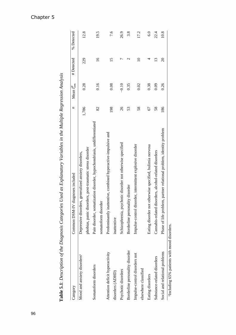
Chapter 5
96
Tab
le 5
.1:
Des
crip
tion o
f th
e D
iagn
osi
s C
ate
gori
es U
sed a
s E
xpla
nato
ry V
ari
ab
les
in t
he
Mult
iple
Reg
ress
ion A
naly
sis
Cat
ego
ry
Co
mm
on D
SM
-IV
dia
gno
ses
incl
ud
ed
n
Mea
n 𝑙𝑧𝑚𝑝
#
Det
ecte
d
% D
etec
ted
Mo
od
and
anxie
ty d
iso
rder
s¹
Dep
ress
ive
dis
ord
ers,
gener
aliz
ed a
nxie
ty d
iso
rder
s,
pho
bia
s, p
anic
dis
ord
ers,
po
st-t
rau
mati
c st
ress
dis
ord
er
1,7
86
0
.28
22
9
12
.8
So
mat
ofo
rm d
iso
rder
s P
ain d
iso
rder
, so
mat
izat
ion d
iso
rder
, hyp
och
ond
rias
is,
und
iffe
renti
ate
d
som
ato
form
dis
ord
er
82
0.1
6
16
19
.5
Att
enti
on d
efic
it h
yp
erac
tivit
y
dis
ord
ers
(AD
HD
)
Pre
do
min
antl
y i
natt
enti
ve,
co
mb
ined
hyp
erac
tive-i
mp
uls
ive a
nd
inat
tenti
ve
19
8
0.0
8
15
7.6
Psy
cho
tic
dis
ord
ers
S
chiz
op
hre
nia
, p
sycho
tic
dis
ord
er n
ot
oth
erw
ise
spec
ifie
d
26
−0
.10
7
26
.9
Bo
rder
line
per
sonal
ity d
iso
rder
B
ord
erli
ne
per
sonal
ity d
iso
rder
5
3
0.3
5
2
3.8
Imp
uls
e-co
ntr
ol
dis
ord
ers
no
t
else
wher
e cl
ass
ifie
d
Imp
uls
e-co
ntr
ol
dis
ord
er,
inte
rmit
tent
exp
losi
ve
dis
ord
er
58
0.0
2
10
17
.2
Eat
ing d
iso
rder
s E
atin
g d
iso
rder
no
t o
ther
wis
e sp
ecif
ied
, b
uli
mia
ner
vo
sa
67
0.3
8
4
6.0
Sub
stance
-rel
ated
dis
ord
ers
Can
nab
is-r
elat
ed d
iso
rder
s, a
lco
ho
l-re
late
d d
iso
rder
s 5
8
0.0
9
13
22
.4
So
cial
and
rel
atio
nal
pro
ble
ms
Phas
e o
f li
fe p
rob
lem
, p
artn
er r
elat
ional
pro
ble
m,
iden
tity
pro
ble
m
18
6
0.2
6
20
10
.8
¹Incl
ud
ing 6
5%
pat
ien
ts w
ith m
oo
d d
iso
rder
s.
Person-fit analysis in outcome measurement
97
different types of adjustment disorders (e.g., ‘adjustment disorder with depressed mood’
and ‘adjustment disorder with disturbance of conducted’) each constitute a single category.
However, this results in patients suffering from completely different symptoms being
classified in the same category.
Third, if we could not categorize the patients’ diagnosis unambiguously in one of
the specified categories (e.g., adjustment disorder with predominant disturbance of
conduct) we treated the diagnosis as missing. Our approach resulted in 2,514 categorized
patients (87%).
5.3 Results
5.3.1 OQ-45 Model Fit
Inspection of multiple correlation coefficients and item-rest correlations showed
that the items measuring substance abuse (items 11, 26, and 32) and item 14 (‘I work/study
too much’) fitted poorly in their subscales. These results are consistent with previous
research conducted with both the original and the Dutch OQ-45 (De Jong et al., 2007;
Mueller et al., 1998). We excluded these items from further analyses. The coefficient
alphas for the remaining items of the SR (7 items), IR (10 items), and SD (24 items)
subscales equaled .67, .78, and .91, respectively.
For the subscale data, EFA showed that the first factor explained 38.6% to 40.0% of
the variance. Also, we found that the 1-factor models fitted poorly to the subscale data
(RMSEA > .10 and SRMR >.06). For each subscale, we therefore used the RMSEA and
SRMR to determine the number of factors required for acceptable model fit. For the IR
subscale, we found that a 2-factor solution provided acceptable fit (RMSEA = .08 and
SRMR = .04) and for the SD subscale a 3-factor solution provided acceptable fit (RMSEA
= .07 and SRMR = .03). For the SR subscale, we found that 3 factors were required to
obtain an acceptable RMSEA. However, this result was probably due to the small number
of items included in the SR subscale (Kenny, Kaniskan, & McCoach, 2011) and we
concluded that a 2-factor solution was more appropriate (RMSEA = .13; SRMR = .05).
Under the 1-factor model, only the SD subscale included several large residual correlations
(i.e., > .20). Graphical analyses showed that only for the SR subscale the ISRFs showed
substantial deviations from a logistic shape.
To summarize, EFA results suggested poor fit of the GRM to the subscale data.
Although we also found violations of local independence and logistic ISRFs,

Chapter 5
98
multidimensionality is likely to be the main source of model misfit. Because GRM misfit
may deteriorate the performance of PFA, we used multidimensional data based on the
observed OQ-45 data in the simulation study.
5.3.2 Simulation Study: Performance of Person-Fit Methods for the OQ-45
We used multidimensional IRT (MIRT) (Reckase, 2009) models to generate
representative OQ-45 data. For each subscale, we estimated an exploratory MIRT model
using the ‘mirt’ R package (Chalmers, 2012) and used the parameter estimates for data
generation. Based on the EFA results, for the SR and IR subscales we used MIRT models
with two factors for data generation and for the SD subscale we used a 3-factor model. The
θ values were sampled from the multivariate standard normal distribution, with θ
correlations equal to those from the fitted MIRT model.
The
Statistic. The results showed that the average Type I error rate for 𝑝
equaled .01, which was well below the nominal Type I error of .05. The average detection
rate of 𝑝
for item-score patterns with 10, 20, and 30 random item scores was .30, .76, .95,
respectively. The detection rates for moderate and strong acquiescence were .09 and .35,
respectively. Hence, the results suggest that 𝑝
classifies only few item-score vectors as
aberrant and has good power for detecting item-score patterns with at least 20 (i.e., 49%)
random item scores but lacks power for detecting acquiescence.
The Residual Statistic. Table 5.2 shows the average Type I error rates and the
detection rates of the residual statistic for different kinds of misfit, for each OQ-45
subscale separately. The first two columns show the results when using cut-off values of
–1.96 and 1.96. Except for strong acquiescence, the Type I error rates were below the
nominal level of .05. For patterns with random error, detection rates ranged from .20 to
.54. Detection rates were lower as item-score patterns contained more random item scores.
For moderate and high levels of acquiescence, detection rates were too low for the
residuals to be useful. Probably, the θ estimates based on item-score patterns with many
random item scores and item-score patterns resulting from acquiescence were more
severely biased and adapted to the misfit.
Because detection rates were generally low, we also determined Type I error and
detection rates when using cut-off values of –1.64 and 1.64 (Table 5.2, last two columns).
Except for strong acquiescence, Type I error rates did not exceed .11, thus stayed close to
the nominal significance level. Detection rates ranged from .32 to .66 for random misfit. To
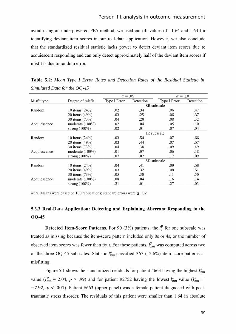
Person-fit analysis in outcome measurement
99
avoid using an underpowered PFA method, we used cut-off values of –1.64 and 1.64 for
identifying deviant item scores in our real-data application. However, we also conclude
that the standardized residual statistic lacks power to detect deviant item scores due to
acquiescent responding and can only detect approximately half of the deviant item scores if
misfit is due to random error.
Table 5.2: Mean Type I Error Rates and Detection Rates of the Residual Statistic in
Simulated Data for the OQ-45
Note. Means were based on 100 replications; standard errors were
5.3.3 Real-Data Application: Detecting and Explaining Aberrant Responding to the
OQ-45
Detected Item-Score Patterns. For 90 (3%) patients, the 𝑝 for one subscale was
treated as missing because the item-score pattern included only 0s or 4s, or the number of
observed item scores was fewer than four. For these patients, 𝑝
was computed across two
of the three OQ-45 subscales. Statistic 𝑝
classified 367 (12.6%) item-score patterns as
misfitting.
Figure 5.1 shows the standardized residuals for patient #663 having the highest 𝑝
value ( 𝑝
= 2.04, p > .99) and for patient #2752 having the lowest 𝑝
value ( 𝑝
7 9 ). Patient #663 (upper panel) was a female patient diagnosed with post-
traumatic stress disorder. The residuals of this patient were smaller than 1.64 in absolute
Misfit type Degree of misfit Type I Error Detection Type I Error Detection
SR subscale
Random 10 items (24%) .02 .34 .06 .47
20 items (49%) .03 .25 .06 .37
30 items (73%) .04 .20 .08 .32
Acquiescence moderate (100%) .02 .04 .05 .10
strong (100%) .02 .01 .07 .04
IR subscale
Random 10 items (24%) .03 .54 .07 .66
20 items (49%) .03 .44 .07 .57
30 items (73%) .04 .38 .09 .49
Acquiescence moderate (100%) .01 .07 .06 .18
strong (100%) .07 .02 .17 .09
SD subscale
Random 10 items (24%) .04 .41 .09 .58
20 items (49%) .03 .32 .08 .51
30 items (73%) .05 .30 .11 .50
Acquiescence moderate (100%) .08 .04 .16 .14
strong (100%) .21 .01 .27 .03
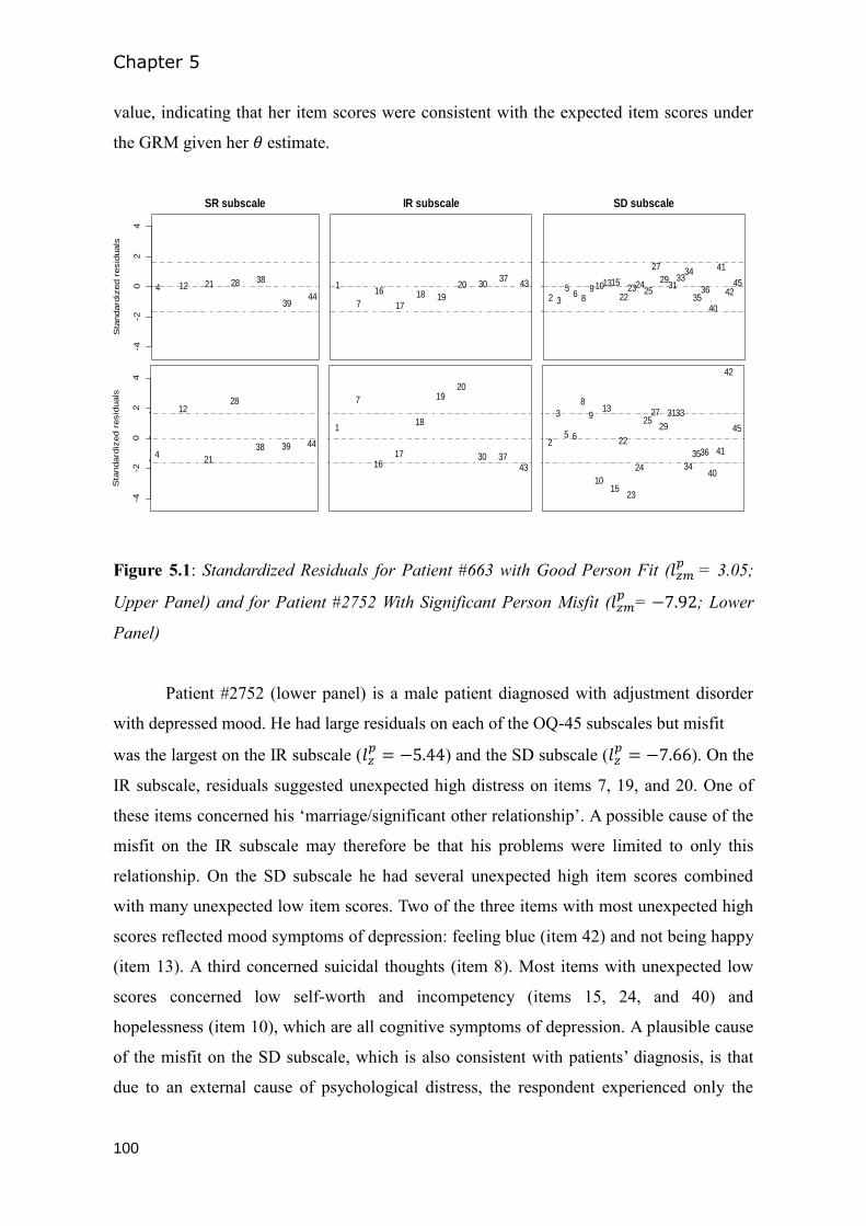
Chapter 5
100
value, indicating that her item scores were consistent with the expected item scores under
the GRM given her estimate.
Figure 5.1: Standardized Residuals for Patient #663 with Good Person Fit ( 𝑝
= 3.05;
Upper Panel) and for Patient #2752 With Significant Person Misfit ( 𝑝
= 7 9 ; Lower
Panel)
Patient #2752 (lower panel) is a male patient diagnosed with adjustment disorder
with depressed mood. He had large residuals on each of the OQ-45 subscales but misfit
was the largest on the IR subscale ( 𝑝 ) and the SD subscale (
𝑝 7 ). On the
IR subscale, residuals suggested unexpected high distress on items 7, 19, and 20. One of
these items concerned his ‘marriage/significant other relationship’. A possible cause of the
misfit on the IR subscale may therefore be that his problems were limited to only this
relationship. On the SD subscale he had several unexpected high item scores combined
with many unexpected low item scores. Two of the three items with most unexpected high
scores reflected mood symptoms of depression: feeling blue (item 42) and not being happy
(item 13). A third concerned suicidal thoughts (item 8). Most items with unexpected low
scores concerned low self-worth and incompetency (items 15, 24, and 40) and
hopelessness (item 10), which are all cognitive symptoms of depression. A plausible cause
of the misfit on the SD subscale, which is also consistent with patients’ diagnosis, is that
due to an external cause of psychological distress, the respondent experienced only the
-4-2
02
4
Sta
ndard
ized r
esid
uals
4 12 21 28 38
3944
SR subscale
Sta
ndard
ized r
esid
uals
1
7
16
17
18 19
20 3037
43
IR subscale
Sta
ndard
ized r
esid
uals
2 3
56
89 101315
222324
25
27
2931
3334
3536
40
41
4245
SD subscale
-4-2
02
4
Sta
ndard
ized r
esid
uals
4
12
21
28
38 39 44
Sta
ndard
ized r
esid
uals
1
7
1617
18
1920
30 3743
Sta
ndard
ized r
esid
uals
2
3
5 6
8
9
10
13
15
22
23
24
2527
29
3133
34
3536
40
41
42
45
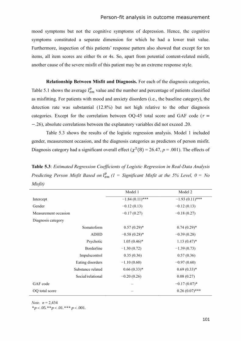
Person-fit analysis in outcome measurement
101
mood symptoms but not the cognitive symptoms of depression. Hence, the cognitive
symptoms constituted a separate dimension for which he had a lower trait value.
Furthermore, inspection of this patients’ response pattern also showed that except for ten
items, all item scores are either 0s or 4s. So, apart from potential content-related misfit,
another cause of the severe misfit of this patient may be an extreme response style.
Relationship Between Misfit and Diagnosis. For each of the diagnosis categories,
Table 5.1 shows the average 𝑝
value and the number and percentage of patients classified
as misfitting. For patients with mood and anxiety disorders (i.e., the baseline category), the
detection rate was substantial (12.8%) but not high relative to the other diagnosis
categories. Except for the correlation between OQ-45 total score and GAF code (
.26), absolute correlations between the explanatory variables did not exceed .20.
Table 5.3 shows the results of the logistic regression analysis. Model 1 included
gender, measurement occasion, and the diagnosis categories as predictors of person misfit.
Diagnosis category had a significant overall effect (𝜒 8 = 26.47, p = .001). The effects of
Table 5.3: Estimated Regression Coefficients of Logistic Regression in Real-Data Analysis
Predicting Person Misfit Based on 𝑝
(1 = Significant Misfit at the 5% Level, 0 = No
Misfit)
Model 1 Model 2
Intercept −1.84 (0.11)*** −1.93 (0.11)***
Gender −0.12 (0.13) −0.12 (0.13)
Measurement occasion −0.17 (0.27) −0.18 (0.27)
Diagnosis category
Somatoform 0.57 (0.29)* 0.74 (0.29)*
ADHD −0.58 (0.28)* −0.39 (0.28)
Psychotic 1.05 (0.46)* 1.13 (0.47)*
Borderline −1.30 (0.72) −1.39 (0.73)
Impulscontrol 0.35 (0.36) 0.57 (0.36)
Eating disorders −1.10 (0.60) −0.97 (0.60)
Substance related 0.66 (0.33)* 0.69 (0.33)*
Social/relational −0.20 (0.26) 0.08 (0.27)
GAF code – −0.17 (0.07)*
OQ total score – 0.26 (0.07)***
Note. n = 2,434
.001.*** .01.** .05.* ppp
Chapter 5
102
somatoform disorder, ADHD, psychotic disorder, and substance abuse disorder were
significant. Patients with ADHD were unlikely to show misfit relative to the baseline
category of patients with mood or anxiety disorders. Patients with somatoform disorders,
psychotic disorders, and substance-related disorders were more likely to show misfit.
In Model 2 (Table 5.3, third column), we also included the GAF code and the OQ-
45 total score. OQ-45 score had a significant negative effect on person fit and GAF code
had a significant positive effect. These results suggest that patients with higher levels of
distress were more likely to show misfit. After controlling for GAF code and OQ-45 score,
the positive effect of ADHD was not significant. Hence, patients with ADHD were less
likely to show misfit because they had less severe symptoms. In Model 2, the estimated
probability of misfit was .13 for the baseline category. For patients with somatoform
disorders, psychotic disorders, and substance related disorders, this probability was .23,
.31, and .22, respectively.
We used the standardized residuals of the detected patients with psychotic disorders
(n = 7), somatoform disorders (n = 16), and substance related disorders (n = 13) to
understand whether the patients in the same diagnosis category showed similar person
misfit. Specifically, we inspected whether patients had large residuals for the same items.
Most detected patients with a psychotic disorder had low or average trait levels for each of
the subscales and misfit was due to several item scores indicating unexpected severe
symptoms. These results suggest that patients with psychotic disorders showed misfit
because most OQ-45 items were not relevant to them. In general they did not have large
residuals for the same items. However, unexpected high item scores on item 25 “disturbing
thoughts come into my mind that I cannot get rid of” were frequent (4 patients). We did not
find that either patients with a somatoform disorder or patients with a substance related
disorder showed similar person misfit.
5.4 Discussion
We investigated the usefulness of PFA for detecting and explaining aberrant
responding to the OQ-45. As we found substantial misfit of the GRM to the OQ-45 data,
we used a simulation study to determine the performance of a PFA to the OQ-45 given the
observed model violations. For statistic 𝑝
, we found that there was only a small risk of
incorrectly classifying normal respondents as misfitting. Furthermore, detection rates were
Person-fit analysis in outcome measurement
103
good for item-score patterns that included many random item scores. For aberrant item-
score patterns resulting from acquiescence detection rates were low. The most likely
explanation is the low number of reversely worded items in the OQ-45. Only the
inconsistency between item scores to the reversely and positively worded items led to
substantial misfit with respect to the GRM. Furthermore, the simulation study showed that
the standardized item-score residual statistic performed poorly detecting deviant item
scores on the OQ-45. This result is likely related to bias in estimated trait values caused by
person misfit.
The real-data application of PFA suggests that the 𝑝
statistic is useful for
detecting misfit and identifying patients that are prone to respond aberrantly to the OQ-45.
Consistent with previous research (Conijn et al., 2012; Reise & Waller, 1993; Woods et al.,
2008), we found that patients were more likely to show misfit as they experienced higher
levels of psychological distress. This result stresses the importance of person misfit
detection in outcome measurement. It suggests that the patients for whom sound
psychological intervention is mostly needed are particularly likely to produce invalid test
scores.
Furthermore, we found that patients with somatoform disorders, psychotic
disorders, and substance-related disorders were likely to show misfit. Plausible
explanations for these results are the following. Patients diagnosed with a somatoform
disorder may respond aberrantly because they often do not acknowledge their mental
problems but focus on their physical complaints. For patients having a psychotic disorder
aberrant responding may be due to symptoms of disorder and confusion. Another
explanation, which is consistent with the results from the residual analysis, is that most of
the typical complaints and symptoms of psychotic disorders are not included in the OQ-45.
Patients suffering from a substance-related disorder may have been under the influence
while completing the OQ-45. Furthermore, long-term substance use may negatively affect
cognitive capacities. We found that patients having ADHD were not likely to show misfit,
although their symptoms of inattentiveness and impulsiveness could potentially lead to
misfit.
5.4.1 Implications of the Simulation Study
The performance of PFA depends on the properties of the questionnaire for which it
is used (Conijn et al., 2013; Reise & Due, 1991) and it was therefore valuable to determine
Chapter 5
104
performance of PFA specifically for the OQ-45. Based on the results, what can we say in
general about the usefulness of PFA for outcome measurement?
It has been suggested that IRT models poorly fit psychopathology data, and this
misfit may adversely impact PFA (Reise & Waller, 2003). Consistent with previous
research results (Conijn et al., 2013), our results suggest that 𝑝
can be used even when
the postulated IRT model fails to fit the data well. However, our findings cannot be
generalized to GRM misfit that has different psychometric properties than the misfit
concerning the OQ-45. The simulation study generated data resembling the characteristics
of the OQ-45 data at hand but we did not systematically determine the effects of different
model violations. Future studies should systematically investigate how robust PFA methods
are to different IRT model violations.
We conclude that for outcome measures including at least 40 items, statistic 𝑝
is
useful for detecting item-score patterns containing many inconsistencies. Probable causes
of inconsistencies may be low traitedness, low motivation, cognitive deficits, or
concentration problems. An important limitation of PFA for outcome measurement is that
person-fit statistics may not find response styles and malingering because these unwanted
processes nevertheless may result in item-score patterns that are consistent across the
complete measure (Sullivan & King, 2010; Ferrando & Chico, 2001).
Although residual statistics have shown useful in real-data applications for
analyzing causes of aberrant responding (Ferrando, 2010, 2012), there have not been
simulation studies validating their performance for detecting deviant item scores
previously. Our simulation study showed that for outcome measurement these methods’
usefulness is questionable. An alternative to using item-score residuals for identifying
unexpected item scores is to inspect the observed item scores themselves and identify
unlikely combinations of item scores based on the items’ content. For outcome measures
this alternative approach may be feasible because they contain only few items. In our real-
data application, we used item residuals to study whether patients with the same disorder
showed similar patterns of misfit. Future research may use group-level analysis such as
such as differential functioning analysis (DIF; Thissen, Steinberg, & Wainer, 1993) or IRT
mixture modeling (Rost, 1990) for this purpose.
5.4.2 Implications of the Real-Data Application
The importance of PFA for outcome measurement not only depends on Type I error
Person-fit analysis in outcome measurement
105
and detection rates, but also on the prevalence of aberrant response behavior. If prevalence
is low, the number of item-score patterns incorrectly classified as aberrant (i.e., Type I
errors) may outnumber the correctly identified aberrant item-score patterns (Piedmont
McCrae, Riemann, & Angleitner, 2000). We expected a substantial number of aberrant
respondents in the OQ-45 data as research results suggest a relationship between response
inconsistency and psychological problems (e.g., Woods et al., 2008). The detection rate of
12.6% in the OQ-45 data is high, but not particularly high compared to detection rates
found in other studies. For example, Conijn et al. (2012) found detection rates of 11% to
14% misfit in a sample of cardiac patients for repeated measurements on the State-Trait
Anxiety Inventory (STAI; Spielberger, Gorsuch, Lushene, Vagg, & Jacobs, 1983) and
Conijn et al. (2013) found a detection rate of 16% misfit in a panel sample on the
International Personality Item Pool 50-item questionnaire (IPIP-50; Goldberg et al., 2006).
The detection rate in the OQ-45 data may not be particularly high because the sample was
well motivated to respond accurately as results influenced intake decisions for
psychological treatment. Motivation may deteriorate if outcome measures are frequently
administered. Future studies could investigate the effect of repeated administration of
outcome measures on person fit.
The results of this study suggest that OQ-45 measurement is not equally suitable for
patients with different disorders. In general, there are two potential explanations for high
detection rates for patients with specific disorders. Misfit may be due either to a mismatch
between the OQ-45 and the disorder or misfit may be due to a general tendency to show
misfit on self-report measures. This is an important distinction that has different
implications for outcome measurement of these patients. The first explanation implies that
instead of general outcome measures, disease-specific outcome measures should be used.
For example, the Severe Outcome Questionnaire (S-OQ; Burlingame, Thayer, Lee, Nelson,
& Lambert, 2007) is an alternative version of the OQ-45 specifically designed for patients
suffering from more severe psychopathology such bipolar, schizophrenia and other
psychotic illnesses. The second explanation implies that other methods than self-report
measurement should be used for patients’ diagnosis and treatment decisions, for example,
clinician-rated outcome measures such as the Health of the Nation Outcome Scales
(HoNOS; Wing et al., 1998). Also, the self-report results of these patients should be
excluded from cost-effectiveness studies to prevent potential negative effects on policy
decisions. To address this issue in future studies, similar explanatory PFA should be
conducted with data from other outcome measures.

Chapter 5
106
IRT has been shown useful in applications to clinical practice for scale linking,
computer adaptive testing, and DIF analysis (Reise & Waller, 2009; Thomas, 2011). The
existing research on IRT-based PFA so far is dominated by technical reports on new
methods and comparisons of existing methods. The results of this study give a first,
promising insight into the potential of PFA for outcome measurement in mental health care.
107
Chapter 6: Epilogue
In this thesis, our aim was to provide insight into the potential of item response
theory (IRT) based person-fit analysis (PFA) for studying aberrant response behavior in
non-cognitive measurement. We evaluated person-fit statistics with respect to the
possibility of detecting aberrant response behavior taking into account the typical
characteristics of non-cognitive measures. We also studied the potential of different
explanatory person-fit methods for providing a better understanding of aberrant response
behavior. In this concluding chapter, we reflect on the practical usefulness of person-fit
methods, discuss overarching methodological challenges in explanatory person-fit
research, and provide recommendations for future research based on our findings.
Detecting Aberrant Response Behavior
Applied researchers who want to use person-fit statistics to detect aberrant response
behavior in non-cognitive measurement are faced with several problems, such as short
scale length, bias in estimated item parameters, multidimensionality, and IRT model
violations. In the fourth and fifth chapters, we conducted simulation studies on the
performance of person-fit statistics given the properties of real test data encountered in the
measurement of personality and psychopathology. The results suggested that likelihood-
based person-fit methods have good power for detecting item-score patterns containing
many different inconsistencies with the IRT model at low levels of the type I error rate.
Real-data applications showed that personality and psychopathology data include a
substantial number of aberrant item-score patterns that are detectable by means of person-
fit statistics. Based on the combined results, we conclude that PFA is useful for detecting
aberrant response behavior encountered in non-cognitive measurement. Next, we discuss
for which purposes person-misfit detection may be most useful in non-cognitive
measurement practice.
One practical goal of person-misfit detection is to correct for the bias aberrant
response behavior causes in group-level research results (Meijer & Sijtsma, 2001; Reise &
Flannery, 1996). However, the results of Chapter 4 suggest that for non-cognitive measures
removal of many item-score patterns a person-fit statistic classified as misfitting may not
substantially affect indices of overall model fit or correlations supporting test-score
Epilogue
108
validity. Our findings in Chapter 4 are consistent with previous research conducted in the
context of cognitive measurement that showed that using person-fit statistics for excluding
misfit hardly affects estimates of predictive validity, indices of model fit, item-parameter
estimates, or aggregate proficiency scores (Brown & Villarreal, 2007; Phillips, 1986;
Rudner, Bracey, & Skaggs, 1996; Schmitt, Cortina & Whitney, 1993; Meijer, 1997). One
explanation for the absence of effect on group-level research results may be that PFA
detects item-score patterns with a large deviation from the expectation under the IRT
model, but the detected patterns may not necessarily comprise a group of aberrant
respondents who answer similarly or persons that have a systematic bias across all items.
Aberrant response behavior likely has a major impact on group-level research findings if it
is systematic. In contrast, for the item-score patterns including random inconsistencies and
the different types of misfit that are detected by PFA, the effects of misfitting item scores
on group-level results may cancel one another. Hence, even if many misfittting item-score
patterns are detected, the heterogeneity of the detected misfit across detected persons and
within detected item-score patterns may result in an absence of an effect of removing
person misfit on group-level research results. Future research could compare person-fit
statistics and response style detection methods with respect to their usefulness for
correcting bias in group-level research results.
Another practical goal of person-misfit detection is to prevent incorrect decisions
about individuals in, for example, clinical practice or personnel selection. The efficacy of
PFA for this goal depends on whether the types of aberrant response behaviors that are
typically encountered in particular individual-decision making settings are detectable by
means of person-fit statistics. Compared to academic research settings, individual-decision
making settings are less likely to induce the type of aberrant response behavior that is
easily detected by person-fit statistics. For example, due to the respondent’s self-interest
involved, random responding or carelessness is probably uncommon. ‘Faking good’ or
malingering may be more common and lead to severely biased trait estimates, but the
patterns of scores may be consistent with the postulated response model, and difficult for
PFA to detect. Despite good test-taking motivation, other causes such as idiosyncratic item
content interpretation, lack of traitedness, or lack of reading skills may result in aberrant
responding that PFA may detect. However, the effect of these types of aberrant behaviors
on individual trait estimates may not be substantial enough to affect individual-decision
making. Future research should investigate whether person-fit statistics can detect those
Chapter 6
109
types of aberrant response behavior that substantially impair correct individual decision-
making.
Explaining Aberrant Response Behavior
In the chapters 2 through 4, we discussed different approaches to explaining
variation in response consistency by means of explanatory variables. In particular, we
showed how multilevel modeling can be used to obtain a comprehensive understanding of
response consistency by separating the stable individual differences in person fit from
unsystematic differences in person fit. This way, explanations for both the between-person
differences in response consistency and within-person differences in response consistency
across different measurements can be studied. However, the proposed multilevel approach
requires repeated measures of person fit, which may often not be available in practice.
Regressing person-fit statistics on explanatory variables is a conceptually adequate and
generally applicable alternative to examine plausible explanations of response
inconsistency.
The regression approaches have in common that they treat the dependent variable
of person fit as a continuous variable. As an alternative to treating person fit as a
continuous variable, another possibility in explanatory PFA, which was used in Chapter 5,
is to treat person fit as a dichotomous variable indicating person fit and person misfit.
Whether or not to dichotomize the person-fit statistic depends on the purpose of the
explanatory PFA. If the goal is theoretical, for example, aimed at obtaining insight in the
nature of response consistency, treating person fit as a continuous variable may be
preferred. This way, no information is lost and no arbitrary cut off needs to be used for
dichotomizing. However, if the primary interest is in explaining the distinction between fit
and misfit (given an accurate cut-off value) and the variation within categories (e.g.,
perfect fit versus moderately good fit) is considered irrelevant or error, using the
dichotomized person-fit variable as the response variable in the regression analysis may be
preferred.
When we treated person fit as a continuous variable, we found that presumably
relevant covariates, such as conscientiousness or psychopathology, only explained small
proportions of variation in person fit and hence the results were of little practical value. In
Chapter 3, we discussed several possible explanations for the low explanatory power. For
example, misfit may be mainly caused by lack of traitedness, which is an idiosyncratic
Epilogue
110
phenomenon that may be unrelated to explanatory variables. The results of the real-data
analyses of Chapter 4 suggested an additional explanation: Aberrant response behavior, in
particular response styles, may confound the effects of explanatory variables on person
misfit. Another explanation may be the general definition of person misfit PFA employs.
Person-fit statistics quantify different types of IRT-model misfit that may be related to
different explanatory variables. For example, agreement response style has been found to
positively relate to optimism and cheerfulness (Pedersen, 1967) whereas lack of traitedness
has been found to positively relate to negative affect (Reise & Waller, 1993). This means
that systematic variation in person fit cannot be explained by a single regression model, but
one needs different regression models for different types of misfit. Hence, for a more
comprehensive explanatory analysis of aberrant response behavior future studies may
distinguish different types of person misfit, such as random inconsistencies and various
response styles. To this end, latent class IRT mixture models may be useful to detect
subgroups of respondents with similar patterns of misfit. The resulting latent class
membership could be related to explanatory variables for person misfit.
In Chapter 5, we used item residuals for inferring possible causes of misfit for
individual item-score patterns that were classified as aberrant. Explanatory PFA at the
individual level may be useful for deciding on the course of actions to be taken next. For
example, if the residuals suggest a misinterpretation of items addressing specific item
content not relevant to the respondent, the test score may be based on the remaining items.
However, if misfit was presumably due to a misunderstanding of the instructions, it may be
better to administer the questionnaire a second time. Although individual-level explanatory
PFA analysis is potentially useful, residuals only provide suggestions for what caused the
misfit, but the evidence is never conclusive. Hence, the respondent may be needed to
explain the inconsistencies in the item-score pattern as reflected by the pattern of item
residuals. This renders individual-level explanatory PFA mainly useful for test-taking
situations where the aim is not only to make a correct (classification) decision but also to
obtain a more comprehensive insight about the respondent. An example of such a setting is
mental health care.
111
References
Abelson, R. P. (1995). Statistics as a principled argument. Hillsdale, NJ: Lawrence
Erlbaum Associates.
Atre-Vaidya, N., Taylor M. A., Seidenberg M., Reed R., Perrine A., & Glick-Oberwise F.
(1998). Cognitive deficits, psychopathology, and psychosocial functioning in
bipolar mood disorder. Neuropsychiatry, Neuropsychology, and Behavioral
Neurology, 11, 120-126.
Bates, D., Maechler, M., & Dai, B. (2008). lme4: Linear mixed effects models using
S4 classes. Retrieved April 5, 2009, from http://cran.r-project.org/web/packages/
lme4/index.html.
Benjamini, Y., & Hochberg, Y. (1995). Controlling the false discovery rate: a practical and
powerful approach to multiple testing. Journal of the Royal Statistical Society, 57,
289-300.
Benjamini Y., & Yekutieli D. (2001). The control of the false discovery rate in multiple
testing under dependency. The Annals of Statistics, 29, 1165-1188.
Bickman, L., & Salzer, M. S. (1997). Introduction: Measuring quality in mental health
services. Evaluation Review, 21, 285-291.
Bludworth, J. L., Tracey, T. J. G., & Glidden-Tracey, C. (2010). The bilevel structure of
the Outcome Questionnaire-45. Psychological Assessment, 22, 350-355
Bollen, K. A. (1990). Overall fit in covariance structure models: Two types of sample size
effects. Psychological Bulletin, 107, 256-259.
Borkenau, P., & Ostendorf, F. (1990). Comparing exploratory and confirmatory factor
analysis: A study on the 5-factor model of personality. Personality and Individual
Differences, 11, 515-524.
Brown, R. S., & Villareal, J. C. (2007). Correcting for person misfit in aggregated score
reporting. International Journal of Testing, 7, 1-25.
Burlingame, G. M., Thayer, S. D., Lee, J. A., Nelson, P. L., & Lambert, M. J. (2007).
Administration & Scoring Manual for the Severe Outcome Questionnaire (SOQ).
Salt Lake City, UT: OQ Measures, [email protected].
Butcher, J. N., Graham, J. R., Ben-Porath, Y. S., Tellegen, A., Dahlstrom, W. G., &
Kaemmer, B. (2001). MMPI-2 (Minnesota Multiphasic Personality Inventory-2):
Manual for administration and scoring (rev. ed.). Minneapolis: University of
Minnesota Press.
Cacioppo, J. T., Petty, R. E., & Kao, C. F. (1984). The efficient assessment of need for
cognition. Journal of Personality Assessment, 48, 306-307.
Carey, J. A. (2001). The Severe Outcome Questionnaire: a preliminary study of reliability
and validity. Dissertation Abstracts International: Section B. The Sciences and
Engineering, 61(10-B), 5554.
Chalmers, P. (2012). Mirt: Multidimensional Item Response Theory. Retrieved August 25,
2012, from http://cran.r-project.org/web/packages/mirt/index.html.
Chen, J., Zhang, D., & Davidian, M. (2002). A Monte Carlo EM algorithm for generalized
linear mixed models with flexible random-effects distribution. Biostatistics, 3, 347-
360.
Cheung, G. W., & Rensvold, R. B. (2000). Assessing extreme and acquiescence response
sets in cross-cultural research using structural equations modeling. Journal of
Cross-Cultural Psychology, 31, 187-212.

References
112
Christiansen, N. D., Goffin, R. D., Johnston, N. G., & Rothstein, M. G. (1994). Correcting
the 16PF for faking: Effects on criterion-related validity and individual hiring
decisions. Personnel Psychology, 47, 847-860.
Clark, L. (1996). Schedule for nonadaptive and adaptive personality (SNAP). Manual for
administration, scoring and interpretation. Minneapolis: University of Minnesota
Press.
Collett, D. (2003). Modelling binary data (2nd edition). London: Chapman & Hall/CRC.
Conijn, J. M., Dolan, C. V., & Vorst, H. C. M. (2007). Method effects due to item wording
and their underlying causes (Unpublished master’s thesis). University of
Amsterdam, Amsterdam.
Conijn, J. M., Emons, W. H. M., & Sijtsma, K. (2013). Statistic Based Person-Fit
Methods for Non-Cognitive Multiscale Measures. Manuscript submitted for
publication.
Conijn, J. M., Emons, W. H. M., Van Assen, M. A. L. M., Pedersen, S. S., & Sijtsma, K.
(2012). Explanatory, multilevel person-fit analysis of response consistency on the
Spielberger State-Trait Anxiety Inventory. Manuscript submitted for publication.
Conijn, J. M., Emons, W. H. M., Van Assen, M. A. L. M., & Sijtsma, K. (2011). On the
usefulness of a multilevel logistic regression approach to person-fit analysis.
Multivariate Behavioral Research, 46, 365-388.
Conrad, K. J., Bezruczko, N., Chan, Y. F., Riley, B., Diamond, G., & Dennis, M. L.
(2010). Screening for atypical suicide risk with person fit statistics among people
presenting to alcohol and other drug treatment. Drug and Alcohol Dependence, 106,
92-100.
Costa, P. T., Jr., & McCrae, R. R. (1992). Revised NEO Personality Inventory (NEO-PI-R)
and NEO Five-Factor Inventory (NEO-FFI). Odessa FL: Psychological Assessment
Resources.
Cuijpers, P., Li, J., Hofann, S. G., & Andersson, G. (2010). Self-reported versus clinician-
rated symptoms of depression as outcome measures in psychotherapy research on
depression: A meta-analysis. Clinical Psychology Review, 30, 768-778.
De Beurs, E. (2004). De Brief Symptom Inventory: Handleiding. [The Brief Symptom
Inventory (BSI): Manual]. Leiden: Pits Publishers.
De Beurs, E., Den Hollander-Gijsman, M. E., Van Rood, Y. R., Van der Wee, N. J. A.,
Giltay, E. J., Van Noorden, M. S., Van der Lem, R., Van Fenema, E., & Zitman, F.
G. (2011). Routine outcome monitoring in the Netherlands: Practical experiences
with a web-based strategy for the assessment of treatment outcome in clinical
practice. Clinical Psychology and Psychotherapy, 18, 1-12.
De Beurs E., & Zitman F. G. (2006). De Brief Symptom Inventory (BSI). De
betrouwbaarheid en validiteit van een handzaam alternatief voor de SCL-90 [The
Brief Symptom Inventory (BSI): The reliability and validity of a brief alternative
for the SCL-90]. Maandblad Geestelijke Volksgezondheid, 61, 120-41.
DeJong, M. J., & Hall, L. A. (2006). Measurement of anxiety for patients with cardiac
disease: A critical review and analysis. Journal of Cardiovascular Nursing, 21,
412-419.
De Jong, K., & Nugter, A. (2004). De Outcome Questionnaire: Psychometrische
kenmerken van de Nederlandse vertaling. [The Outcome Questionnaire:
Psychometric properties of the Dutch translation]. Nederlands Tijdschrift
Psychologie, 59, 76-79.
De Jong, K., Nugter, M. A., Polak, M. G., Wagenborg, J. E. A., Spinhoven, P., & Heiser,
W. J. (2007). The Outcome Questionnaire-45 in a Dutch population: A cross
cultural validation. Clinical Psychology & Psychotherapy, 14, 288-301.

References
113
De la Torre, J., & Deng, W. (2008). Improving person-fit assessment by correcting the
ability estimate and its reference distribution. Journal of Educational Measurement,
45, 159-177.
De Leeuw, E. (2010, May). Measuring and comparing survey attitude among new and
repeat respondents cross-culturally. Paper presented at the 63rd Annual Conference
World Association for Public Opinion Research (WAPOR), Chicago.
Denollet, J. K. L. (2005). DS14: Standard assessment of negative affectivity, social
inhibition, and Type D personality. Psychosomatic Medicine, 67, 89-97.
Derogatis, L. R. (1993). BSI Brief Symptom Inventory: Administration, scoring, and
procedures manual (4th Ed.). Minneapolis, MN: National Computer Systems.
Derogatis, L. R. (2001). Brief Symptom Inventory (BSI)-18: Administration, scoring and
procedures manual. Minneapolis, MN: NCS Pearson.
Derogatis, L. R., & Melisaratos, N. (1983). The Brief Symptom Inventory: An introductory
report. Psychological Medicine, 13, 595-605.
Doucette, A., & Wolf, A. W. (2009). Questioning the measurement precision of
psychotherapy research. Psychotherapy Research, 19, 374-389. Drasgow, F., Levine, M.V., & McLaughlin, M. E. (1987). Detecting inappropriate test
scores with optimal and practical appropriateness indices. Applied Psychological
Measurement, 11, 59-79.
Drasgow F., Levine, M. V., & McLaughlin, M. E. (1991). Appropriateness measurement
for some multidimensional test batteries. Applied Psychological Measurement, 15,
171-191.
Drasgow, F., Levine, M. V., Tsien, S., Williams, B., & Mead, A. D. (1995). Fitting
polytomous item response theory models to multiple-choice tests. Applied
Psychological Measurement, 19, 143-165.
Drasgow, F., Levine, M. V., & Williams, E. A. (1985). Appropriateness measurement with
polychotomous item response models and standardized indices. British Journal of
Mathematical and Statistical Psychology, 38, 67-86.
Drasgow, F., & Parsons, C. K. (1983). Application of unidimensional item response theory
models to multidimensional data. Applied Psychological Measurement, 7, 189-199.
Duffy, F. F., Chung, H., Trivedi, M., Rae, D. S., Regier, D. A., & Katzenick, D. J. (2008).
Systematic use of patient-rated depression severity monitoring: Is it helpful and
feasible in clinical psychiatry? Psychiatric Services, 59, 1148-1154.
Egberink, I. J. L., & Meijer, R. R. (2010). The use of different types of validity indicators in
personality assessment. Manuscript submitted for publication.
Emons, W. H. M. (2008). Nonparametric person-fit analysis of polytomous item scores.
Applied Psychological Measurement, 32, 224-247.
Emons, W. H. M., Sijtsma, K., & Meijer, R. R. (2004). Testing hypotheses about the
person response function in person-fit analysis. Multivariate Behavioral Research,
39, 1-35.
Emons, W. H. M., Sijtsma, K., & Meijer, R. R. (2005). Global, local, and graphical,
person-fit analysis using person response functions. Psychological Methods, 10,
101-119.
Embretson, S. E., & Reise, S. P. (2000). Item response theory for psychologists. Mahwah,
NJ: Lawrence Erlbaum.
Engelhard, G. (2009). Using item response theory and model data fit to conceptualize
differential item and person functioning for students with disabilities. Educational
Psychological Measurement, 69, 585-602.
References
114
Evans, C., Connell, J., Barkham, M., Margison, F., Mellor-Clark, J., McGrath, G., &
Audin, K. (2002). Towards a standardised brief outcome measure: Psychometric
properties and utility of the CORE-OM. British Journal of Psychiatry, 180, 51-60.
Ferrando, P. J. (2004). Person reliability in personality measurement: An item
response theory analysis. Applied Psychological Measurement, 28, 126-140.
Ferrando, P. J. (2007). A person-type-VII item response model for assessing person
fluctuation. Psychometrika, 72, 25-41.
Ferrando, P. J. (2009). A graded response model for measuring person reliability. British
Journal of Mathematical and Statistical Psychology, 62, 641-662.
Ferrando, P. J. (2010). Some statistics for assessing person-fit based on continuous-
response models. Applied Psychological Measurement, 34, 219-237.
Ferrando, P. J. (2012). Assessing inconsistent responding in E and N measures: An
application of person-fit analysis in personality. Personality and Individual
Differences, 52, 718-722.
Ferrando, P. J., & Chico, E. (2001). Detecting dissimulation in personality test scores: A
comparison between person-fit indices and detection scales. Educational and
Psychological Measurement, 61, 997-1012.
Foa, E. B., Cashman, L., Jaycox, L., & Perry, K. (1997). The validation of a self-report
measure of posttraumatic stress disorder: The posttraumatic diagnostic scale.
Psychological Assessment, 9, 445-451.
Forero, C. G., & Maydeu-Olivares, A. (2009). Estimation of IRT graded response models:
Limited versus full information methods. Psychological Methods, 14, 275-299.
Frizelle, D. J., Lewin, B., Kaye G., & Moniz-Cook, E. (2006). Development of a new tool
for assessing automatic implanted cardioverter defibrillator patient concerns: the
ICDC. The British Journal of Health Psychology, 11, 293-301.
Goldberg, L. R., Johnson, J. A., Eber, H. W., Hogan, R., Ashton, M. C., Cloninger, C. R.,
& Gough, H. C. (2006). The International Personality Item Pool and the future of
public-domain personality measures. Journal of Research in Personality, 40, 84-96.
Gow, A. J., Whiteman, M. C., Pattie, A., & Deary, I. J. (2005). Goldberg's 'IPIP' Big-Five
factor markers: Internal consistency and concurrent validation in Scotland.
Personality and Individual Differences, 39, 317-329.
Hambleton, R. K., & Swaminathan, H. (1985). Item Response Theory: Principles and
applications. Norwell, MA: Kluwer Academic Publishers.
Handel, R. W., Ben-Porath, Y. S., Tellegen, A., & Archer, R. P. (2010). Psychometric
functioning of the MMPI-2-RF VRIN-r and TRIN-r scales with varying degrees of
randomness, acquiescence, and counter-acquiescence. Psychological Assessment,
22, 87-95.
Heagerty, P. J., & Kurland, B. F. (2001). Misspecified maximum likelihood estimates and
generalised linear mixed models. Biometrika, 88, 973-985.
Hendrawan, I., Glas, C. A. W., & Meijer, R. R. (2005). The effect of person misfit on
classification decisions. Applied Psychological Measurement, 29, 26-44.
Hendriks, A. A. J., Hofstee, W. K. B., & De Raad, B. (1999). The Five-Factor Personality
Inventory (FFPI). Personality and Individual Differences, 27, 307-325.
Hoe, M., & Brekke, J. (2009). Testing the cross-ethnic construct validity of the Brief
Symptom Inventory. Research on Social Work Practice, 19, 93-103.
Holloway, F. (2002). Outcome measurement in mental health – welcome to the revolution.
British Journal of Psychiatry the Journal of Mental Science, 181, 1-2.
Hsieh, F. Y., Lavori, P. W., Cohen, H. J. & Feussner, J. R. (2003). An overview of
variance inflation factors for sample-size calculation. Evaluation and the Health
Professions, 26, 239-257.

References
115
Hu, L.T., & Bentler, P. M. (1999). Cutoff criteria for fit indexes in covariance structure
analysis: Coventional criteria versus new alternatives. Structural Equation
Modeling, 6, 1-55.
Jarvis, W. B. G., & Petty, R. E. (1996). The need to evaluate. Journal of Personality and
Social Psychology, 70, 172-194.
John, O. P., & Srivastava, S. (1999). The Big Five trait taxonomy: History, measurement,
and theoretical perspectives. In L. A. Pervin, & O. P. John (Eds.), Handbook of
personality: Theory and research (pp. 102-138). New York, NY: Guilford.
Karabatsos, G. (2003). Comparing the aberrant response detection performance of
thirty-six person-fit statistics. Applied Measurement in Education, 16, 277-298.
Keith, T. Z. (2006). Multiple regression and beyond. Boston: Allyn and Bacon.
Kenny, D. A., Kaniskan, B., & McCoach, D. B. (2011). The performance of RMSEA in
models with small degrees of freedom. Unpublished paper, University of
Connecticut.
Kim, S., Beretvas, S. N., & Sherry, A. R. (2010). A validation of the factor structure of
OQ-45 scores using factor mixture modeling. Measurement and Evaluation in
Counseling and Development, 42, 275-295.
Kirisci, L., Clark, D. B., & Moss, H. B. (1996). Reliability and validity of the State-Trait
Anxiety Inventory for Children in adolescent substance abusers: Confirmatory
factor analysis and item response theory. Journal of Child and Adolescent
Substance Abuse, 5, 57-69.
Krosnick, J. A., Narayan, S., & Smith, W. R. (1996). Satisficing in surveys: Initial
evidence. In M. T. Braverman & J. K. Slater (Eds.), Advances in Survey Research
(Vol. 70, pp. 29-44). San Francisco: Jossey-Bass Publishers.
LaHuis, D. M., & Copeland, D. (2009). Investigating faking using a multilevel
logistic regression approach to measuring person fit. Organizational Research
Methods, 12, 296-319.
Lambert, M. J., Hansen, N. B., Umpress, V., Lunnen, K., Okiishi, J., Burlingame, G. M., &
Reisinger, C. W. (2001). Administration and scoring manual for the OQ-45. Orem,
UT: American Professional Credentialing Services.
Lambert, M. J., & Hawkins, E. J. (2004). Measuring outcome in professional practice:
Considerations in selecting and utilizing brief outcome instruments. Professional
Psychology: Research and Practice, 35, 492-499.
Lambert, M. J., Morton, J. J., Hatfield, D., Harmon, C., Hamilton, S., Reid, R. C.,
Shimokawa, K., Christopherson, C., & Burlingame, G. M. (2004). Administration
and scoring manual for the OQ-45.2 (Outcome Questionnaire) (3th ed.) Wilmington
DE: American Professional Credential Services LLC.
Lambert, M. J., & Shimokawa, K. (2011). Collecting client feedback. Psychotherapy, 48,
72-79.
Levine, M. V., & Drasgow, F. (1982). Appropriateness measurement: Review, critique and
validating studies. British Journal of Mathematical and Statistical Psychology, 35,
42-56.
Li, M. F., & Olejnik, S. (1997). The power of Rasch person-fit statistics in detecting
unusual response patterns. Applied Psychological Measurement, 21, 215-231.
Lim, B. C., & Ployhart, R. E. (2006). Assessing the convergent and discriminant validity of
Goldberg’s International Personality Item Pool: A multitrait-multimethod
examination. Organizational Research Methods, 9, 29-54.
Litière, S., Alonso, A., & Molenberghs, G. (2007). Type I and type II error under random-
effects misspecification in generalized linear mixed models. Biometrics, 63, 1038-
1044.
References
116
Litière, S., Alonso, A., & Molenberghs, G. (2008). The impact of a misspecified random-
effects distribution on maximum likelihood estimation in generalized linear mixed
models. Statistics in Medicine, 27, 3125-3144.
Lumsden, J. (1977). Person reliability. Applied Psychological Measurement, 1, 477-
482.
Lumsden, J. (1978). Tests are perfectly reliable. British Journal of Mathematical and
Statistical Psychology, 31, 19-26.
MacCallum, R. C., Browne, M. W., & Sugawara, H. M. (1996). Power analysis and
determination of sample size for covariance structure modeling. Psychological
Methods, 1, 130-149.
Marsh, H. W., Hau, K., & Grayson, D. (2005). Goodness of fit in structural equation
models. In A. Maydeu-Olivares & J. J. McArdle (Eds.), Contemporary
psychometrics: A festschrift for Roderick P. McDonald (pp. 275-340). Mahwah,
NJ: Erlbaum.
Meijer, R. R. (1997). Appropriateness-fit and criterion related validity: an extension of the
Schmitt, Cortina, and Whitney (1993) study. Applied Psychological Measurement,
21, 99-113.
Meijer, R. R. (2003). Diagnosing item score patterns on a test using item response theory
based person-fit statistics. Psychological Methods, 8, 72-87.
Meijer, R. R., & Baneke, J. J. (2004). Analyzing psychopathology items: A case for
nonparametric item response theory modeling. Psychological Methods, 9, 354-368.
Meijer, R. R., De Vries R. M., & Van Bruggen, V. (2011). An evaluation of the Brief
Symptom Inventory–18 using item response theory: which items are most strongly
related to psychological distress? Psychological Assessment, 23, 193-202.
Meijer, R. R., Egberink, I. J. L., Emons, W. H. M., & Sijtsma, K. (2008). Detection and
validation of unscalable item score patterns using item response theory: An
illustration with Harter's Self-Perception Profile for Children. Journal of
Personality Assessment, 90, 227-238.
Meijer, R. R., & Nering, M. L. (1997). Trait level estimation for nonfitting response
vectors. Applied Psychological Measurement, 21, 321-336.
Meijer, R. R., & Sijtsma, K. (1995). Detection of aberrant item score patterns: A review
and new developments. Applied Measurement in Education, 8, 261-272.
Meijer, R. R., & Sijtsma, K. (2001). Methodology review: Evaluating person-fit.
Applied Psychological Measurement, 25, 107-135.
Moineddin, R., Matheson, F. I., & Glazier, R. H. (2007). A simulation study
of sample size for multilevel logistic regression models. BMC Medical Research
Methodology, 7, 34-43.
Molenaar, I. W., & Hoijtink, H. (1990). The many null distributions of person-fit indices.
Psychometrika, 55, 75-106.
Mueller, R. M., Lambert, M. J., & Burlingame, G. M. (1998). Construct validity of the
Outcome Questionnaire: A confirmatory factor analysis. Journal of Personality
Assessment, 70, 248-262.
Muthén, B. O., & Muthén, L. K. (2007). Mplus: Statistical analysis with latent variables
(Version 5.0). Los Angeles: Statmodel.
Muthén, L. K., & Muthén, B. O. (2009). Mplus Short Course Videos and Handouts.
Muthén & Muthén -- Home Page. Retrieved from http://www.statmodel.com/
download/Topic%201-v11.pdf.
Nering, M. L. (1995). The distribution of person fit using true and estimated person
parameters. Applied Psychological Measurement, 19, 121-129.
Nering, M. L., & Meijer, R. R. (1998). A comparison of the person response function
References
117
and the lz person-fit statistic. Applied Psychological Measurement, 22, 53-69.
Pan, T. (2010). Comparison of six IRT computer programs in estimating the Rasch model.
Unpublished manuscript.
Partchev, I. (2008). irtoys: Simple interface to the estimation and plotting of IRT
models. Retrieved May 10, 2009, from http://cran.r project.org/web/packages/
irtoys/index.html.
Pedersen, D. M. (1967). Acquiescence and social desirability response sets and some
personality correlates. Educational and Psychological Measurement, 27, 691-697.
Pedersen, S. S., Van den Berg, M. J., Erdman, R. A. M., Van Son, J., Jordaens, L. &
Theuns, D. A. (2009a). Increased anxiety in partners of patients with a cardioverter-
defibrillator: The role of indication for ICD therapy, shocks, and personality. Pace.
Pacing and Clinical Electrophysiology, 32, 184-192.
Pedersen, S. S., Van den Broek, K. C., Erdman, R. A. M., Jordaens, L., & Theuns, D. A.
M. J. (2010). Pre-implantation ICD concerns and Type D personality increase the
risk of mortality in patients with an implantable cardioverter defibrillator.
Europace, 12, 1446-1452.
Pedersen, S. S., Van den Broek, K. C., & Sears, S. F. (2007). Psychological intervention
following implantation of an implantable defibrillator: A review and future
recommendations. Pace, 30, 1546-1554.
Pedersen, S. S., Van den Broek, K. C., Theuns, D. A., Erdman, R. A. M., Alings,
M., Meijer, A., . . . Denollet, J. (2009b). Risk of chronic anxiety in implantable
defibrillator patients: A multi-center study. International Journal of Cardiology,
147, 420-423.
Pedersen, S. S., Van Domburg, R. T., Theuns, D. A., Jordaens, L., & Erdman, R. A. M.
(2005). Concerns about the Implantable Cardioverter Defibrillator: A determinant
of anxiety and depressive symptoms independent of shocks. American Heart
Journal, 149, 664-669.
Phillips, S. E. (1986). The effects of deletion of misfitting persons on vertical equating via
the Rasch model. Journal of Educational Measurement, 23, 107-118.
Piedmont, R. L., McCrae, R. R., Riemann, R., & Angleitner, A. (2000). On the invalidity
of validity scales: Evidence from self-reports and observer ratings in volunteer
samples. Journal of Personality and Social Psychology, 78, 582-593.
Pinsoneault, T. B. (1998). A variable response inconsistency scale and a true response
inconsistency scale for the Jesness Inventory. Psychological Assessment, 10, 21-32.
Pinsoneault, T. B. (2002). A variable response inconsistency scale and a true response
inconsistency scale for the Millon Adolescent Clinical Inventory. Psychological
Assessment, 14, 320-328.
Pirkis, J. E., Burgess, P. M., Kirk, P. K., Dodson, S., Coombs, T. J., & Williamson,
M. K. (2005). A review of the psychometric properties of the Health of the
Nation Outcome Scales (HoNOS) family of measures. Health and Quality of
Life Outcomes, 3, 76-87.
Pitts, S. C., West, S. G., & Tein, J. (1996). Longitudinal measurement models in evaluation
research: Examining stability and change. Evaluation and Program Planning, 19,
333-350.
Raudenbush, S. W., & Bryk, A. S. (2002). Hierarchical linear models. Applications
and data analysis methods. Thousand Oaks, CA: Sage.
Raudenbush, S. W., Bryk, A. S., & Congdon, R. (2008). HLM: Hierarchical linear
and nonlinear modeling (Version 6.06). Lincolnwood, IL: Scientific Software
International.
References
118
Raudenbush, S. W., Yang, M. L., & Yosef, M. (2000). Maximum likelihood for
generalized linear models with nested random effects via high-order, multivariate
Laplace approximation. Journal of Computational and Graphical Statistics, 9, 141-
157.
R Development Core Team (2008). R: A language and environment for statistical
computing. R Foundation for Statistical Computing, Vienna, Austria. Retrieved
April 5, 2009, from http://www.R-project.org.
Reckase, M. D. (2009). Multidimensional Item Response Theory. New York: Springer.
Reise, S. P. (1995). Scoring method and the detection of person misfit in a personality
assessment context. Applied Psychological Measurement, 19, 213-229.
Reise, S. P. (2000). Using multilevel logistic regression to evaluate person-fit in IRT
models. Multivariate Behavioral Research, 35, 543-568.
Reise, S. P., & Due, A. M. (1991). The influence of test characteristics on the detection of
aberrant response patterns. Applied Psychological Measurement, 15, 217-226.
Reise, S. P., & Flannery, W. P. (1996). Assessing person-fit on measures of typical
performance. Applied Measurement in Education, 9, 9-26.
Reise, S. P., & Waller, N. G. (1993). Traitedness and the assessment of response pattern
scalability. Journal of Personality and Social Psychology, 65, 143-151.
Reise, S. P., & Waller, N. G. (2003). How many IRT parameters does it take to model
psychopathology items? Psychological Methods, 8, 164-184.
Reise, S. P., & Waller, N. G (2009). Item response theory and clinical measurement.
Annual Review of Clinical Psychology, 5, 27-48.
Rief, W., & Broadbent, E. (2007). Explaining medically unexplained symptoms-models
and mechanisms. Clinical Psychology Review, 27, 821-841.
Rizopoulos, D. (2009). ltm: An R package for latent variable modeling and item response
analysis. Retrieved May 10, 2009, from http://cran.r-project.org/web/packages/ltm/
index.html.
Rost, J. (1990). Rasch models in latent classes: An integration of two approaches to
item analysis. Applied Psychological Measurement, 3, 271-282.
Rudner, L. J., Bracey, G., & Skaggs, G. (1996). The use of person-fit statistic with one
high-quality achievement test. Applied Measurement in Education, 9, 91-109.
Samejima, F. (1997). Graded response model. In: W. J. van der Linden, & R. Hambleton
(Eds.), Handbook of modern item response theory (pp. 85-100). New York, NY:
Springer.
Schaie, K. W. (1994). The course of adult intellectual development. American
Psychologist, 49, 304-313.
Schmitt, N., Chan, D., Sacco, J. M., McFarland, L. A., & Jennings, D. (1999). Correlates
of person-fit and effect of person-fit on test validity. Applied Psychological
Measurement, 23, 41-53.
Schmitt, N., Cortina, J. M., & Whitney, D. J. (1993). Appropriateness fit and criterion-
related validity. Applied Psychological Measurement, 17, 143-150.
Sijtsma, K., & Meijer, R. R. (2001). The person response function as a tool in person-
fit research. Psychometrika, 66, 191-207.
Singer, J. D., & Willett, J. B. (2003). Applied longitudinal data analysis: Modeling
change and event occurrence. Oxford: Oxford University Press.
Slade, M. (2002). What outcomes to measure in routine mental health services, and how to
assess them: a systematic review. Australian and New Zealand Journal of
Psychiatry, 36, 743-753.
Snijders, T. A. B. (2001). Asymptotic null distribution of person fit statistics with
estimated person parameter. Psychometrika, 66, 331-342.

References
119
Snijders, T. A. B., & Bosker, R. J. (1999). Multilevel analysis. An introduction to
basic and advanced multilevel modeling. Thousand Oaks, CA: Sage.
Spielberger, C. D., Gorsuch, R. L., Lushene, R., Vagg, P. R., & Jacobs, G. A. (1983).
Manual for the State-Trait Anxiety Inventory (Form Y). Palo Alto, CA: Consulting
Psychologists Press.
Spielberger, C. D., Jacobs, G. H., Russell, S. F., & Crane, R. S. (1983). Assessment of
anger: the State-Trait Anger Scale. In J. N. Butcher & C. D. Spielberger (Eds.),
Advances in personality assessment (Vol. 2, pp. 159-187). Hillsdale, NJ: Lawrence
Erlbaum Associates, Inc.
Spinhoven, P., Ormel, J., Sloekers, P. P. A., Kempen, G. I. J. M., Speckens, A. E. M., &
Van Hemert, A. M. (1997). A validation study of the Hospital Anxiety and
Depression Scale (HADS) in different groups of Dutch subjects. Psychological
Medicine, 27, 363-370.
Strandmark, N. L., & Linn, R. L. (1987). A generalized logistic item response model
parameterizing test score inappropriateness. Applied Psychological Measurement,
11, 355-370.
Sullivan, K. A., & King, J. K. (2008). Detecting faked psychopathology: a comparison of
two tests to detect malingered psychopathology using a simulation design.
Psychiatry Research, 176, 75-81.
Tatsuoka, K. K. (1996). Use of generalized person-fit indexes, zetas for statistical
pattern classification. Applied Measurement in Education, 9, 65-75.
Tellegen, A. (1988). The analysis of consistency in personality assessment. Journal of
Personality, 56, 621-663.
Thissen, D., Chen, W. H., & Bock, R. D. (2003). MULTILOG for Windows (Version 7).
Lincolnwood, IL: Scientific Software International.
Thissen, D., Steinberg, L., & Wainer, H. (1993). Detection of differential functioning using
the parameters of item response models. In P. W. Holland & H. Wainer (Eds.),
Differential Item Functioning (pp. 67-113). Hillsdale, NJ: Lawrence Erlbaum.
Thomas, M. L. (2011). The value of item response theory in clinical assessment: a review.
Assessment, 18, 291-307.
Trabin, T. E., & Weiss, D. J. (1983). The person response curve: Fit of individuals to
item theory models. In D. J. Weiss (Ed.), New horizons in testing (pp. 83-108).
New York: Academic Press.
Van der Ploeg, H. M., Defares, P. B., & Spielberger, C. D. (1982). ZAV. A
Dutch-Language Adaptation of the Spielberger State-Trait Anger Scale.
Lisse, The Netherlands: Swets & Zeitlinger.
Van Ginkel, R. J., & Van der Ark, A. L. (2008). SPSS syntax for two-way imputation of
missing test data for separate scales. Retrieved March 28, 2010, from
http://www.datatheory.nl/pages/ginkel.html.
Van Herk, H., Poortinga, Y. H., & Verhallen, T. M. M. (2004). Response styles in rating
scales: Evidence of method bias in data from six EU countries. Journal of Cross-
Cultural Psychology, 35, 346-360.
Van Krimpen-Stoop, E. M. L. A., & Meijer, R. R. (1999). The null distribution of person-
fit statistics for conventional and adaptive tests. Applied Psychological
Measurement, 23, 327-345.
Wang, L., Reise, S. P., Pan, W., & Austin, J. T. (2004). Multilevel modeling
approach to detection of differential person functioning in latent trait models. Paper
presented at the American Educational Research Association, San Diego, CA.
References
120
Watson, D., Clark, L. A., & Tellegen, A. (1988). Development and validation of brief
measures of Positive and Negative Affect: The PANAS Scales. Journal of
Personality and Social Psychology, 54, 1063-1070.
Wing, J. K., Beevor, A. S., Curtis, R. H., Park, B. G., Hadden, S., & Burns, H. (1998).
Health of the Nation Outcome Scales (HoNOS): research and development. British
Journal of Psychiatry, 172, 11-8.
Wood, J. M., Garb, H. N., Lilienfeld, S. O., & Nezworski, M. T. (2002). Clinical
assessment. Annual Review of Psychology, 53, 519-543.
Woods, C. M. (2006). Careless responding to reverse-worded items: Implications for
confirmatory factor analysis. Journal of Psychopathology and Behavioral
Assessment, 3, 189-194.
Woods, C. M. (2008). Monte Carlo evaluation of two-level logistic regression for
assessing person-fit. Multivariate Behavioral Research, 43, 50-76.
Woods, C. M., Oltmanns, T. F., & Turkheimer, E. (2008). Detection of aberrant
responding on a personality scale in a military sample: An application of evaluating
person fit with two-level logistic regression. Psychological Assessment, 20, 159-
168.
Zickar, M. J., & Drasgow, F. (1996). Detecting faking on a personality instrument using
appropriateness measurement. Applied Psychological Measurement, 20, 71-87.
Zigmond, A. S., & Snaith, R. P. (1983). The Hospital Anxiety and Depression Scale. Acta
Psychiatrica Scandinavica, 67, 361-370.
121
Summary
The score of an individual respondent on a personality questionnaire may be
unrelated to the trait of interest even when the questionnaire has excellent psychometric
properties. For example, a lack of test-taking effort, malingering, or a response style may
dominate the person’s response process instead of the trait the questionnaire measures. The
resulting test score will be invalid and may lead to biased research results and incorrect
individual decision making. The main aim of person-fit analysis (PFA) is to detect item-
score patterns that are unexpected given the postulated measurement model and therefore
likely to be invalid. In this thesis, we evaluate the usefulness of PFA based on item
response theory for detecting aberrant response behavior in non-cognitive measurement—
specifically, personality and psychopathology measurement—and for understanding the
causes of aberrant response behavior.
In Chapter 2, we submitted Reise’s (2000) explanatory multilevel person-fit
approach to a logical analysis and a Monte Carlo simulation study. Reise proposed to use
multilevel logistic regression (MLR) for estimating the slope of the person response
function (PRF) and to interpret the slope parameter as measure of person fit. The logical
analysis showed that (1) the interpretation of the PRF slope as a person-fit measure is only
valid for the one-parameter logistic model, and (2) the MLR model assumption of bivariate
normality of random effects is violated in the multilevel formulation of the PRF. The
simulation study showed that the model violation biases the MLR estimate of the PRF
slope parameter. We concluded that Reise’s approach suffers from serious theoretical and
statistical problems and proposed an alternative explanatory multilevel PFA approach.
In Chapter 3, we used the alternative explanatory PFA approach to explain response
consistency in a sample of cardiac patients and their partners on repeated measurements of
the Spielberger State-Trait Anxiety Inventory (STAI, Spielberger, Gorsuch, Lushene,
Vagge, & Jacobs, 1983). We used the person-fit statistic to assess response consistency
at five measurement occasions. Using multilevel analysis, we modelled the between-person
and within-person differences in response consistency using time-dependent and time-
invariant explanatory variables. We found substantial stable differences in response
consistency across time. Respondents having lower education levels, undergoing
psychological treatment, or suffering from more posttraumatic stress disorder symptoms
Summary
122
tended to respond less consistently. We could only explain a small percentage of the
variance in response consistency. We discussed the possible explanations for the low
percentage of explained variance and concluded that alternative explanatory PFA methods
may provide more insight into the causes of aberrant response behavior.
In Chapter 4, we evaluated the performance of multiscale statistic 𝑝
and four
alternative -based approaches with respect to detecting and explaining aberrant response
behavior. To this end, we used a simulation study and studied applications of the five
multiscale person-fit methods to empirical personality and psychopathology questionnaire
data. The simulations showed that all approaches have good detection rates for item-score
patterns having substantial misfit on multiscale measures with at least 50 items. However,
the real-data applications showed that removal of misfitting item-score patterns detected by
the multiscale person-fit methods did not lead to considerable changes in the results on
model fit and test score validity. Multiscale statistic 𝑝
was useful for explanatory PFA,
but only after accounting for the biasing effect of stylistic responding on the explanatory
variables. We concluded that more real-data applications are required to demonstrate the
usefulness of the multiscale person-fit methods in non-cognitive measurement.
In Chapter 5, we used PFA to detect and explain person misfit on the Dutch
Outcome Questionnaire-45 (OQ-45; De Jong et al., 2004). First, we conducted a simulation
study to determine the performance of the 𝑝
statistic and standardized residuals, which
quantify misfit at the item level, given the characteristics of OQ-45 data. We found that
despite violations of unidimensionality in the OQ-45 data, the 𝑝
statistic had good
detection rates for item-score patterns with many random item scores. The standardized
residual statistic had low power for detecting deviant item scores. Next, we applied the
PFA methods to OQ-45 data of a sample of clinical outpatients. The 𝑝
statistic classified
12.6% of the item-score patterns as misfitting. Explanatory PFA showed that self-report
outcome measurement may not be appropriate for patients suffering from severe
psychological distress and for patients suffering from psychotic disorders, somatoform
disorders, or substance related disorders. We concluded that for outcome measurement in
mental health care, PFA has good potential for detecting misfit and identifying subgroups
of patients that are at risk of producing invalid test results.

123
Samenvatting
De score van een individu op een zelfrapportage vragenlijst kan een onjuiste
weergave zijn van het construct wat men beoogde te meten, ook al heeft de afgenomen
vragenlijst uitstekende psychometrische eigenschappen in de populatie. Gezien de vele
mogelijke onbedoelde factoren die de testuitslag kunnen beïnvloeden, zoals slordigheid,
gebrek aan motivatie en antwoordtendenties, is het zelfs waarschijnlijk dat een steekproef
diverse personen bevat voor wie de testscore niet valide is. Het voornaamste doel van
person-fit analyse (PFA) is om patronen van itemscores op te sporen die, gegeven het
gekozen meetmodel, dermate afwijkend zijn dat de validiteit van de meting ernstig in
twijfel kan worden getrokken. In dit proefschrift onderzochten we de bruikbaarheid van
PFA gebaseerd op item-responstheorie (IRT) voor het detecteren en verklaren van
afwijkend antwoordgedrag op vragenlijsten voor niet-cognitieve constructen, zoals
persoonlijkheidstrekken en psychisch welzijn.
In het tweede hoofdstuk wordt Reise’s (2000) multilevel person-fit methode aan
een logische analyse en een simulatiestudie onderworpen. Reise stelde voor om multilevel
logistische regressieanalyse te gebruiken om de hellingsparameter van de person response
function (PRF) te schatten en deze schatting te interpreteren als maat voor person fit. Ook
stelde hij voor om variatie in person fit te verklaren door covariaten in het multilevel model
op te nemen. De resultaten van de logische analyse toonden aan dat (1) Reise’s
interpretatie van de PRF hellingsparameter alleen valide is voor het één-parameter
logistisch IRT model, en dat (2) in Reise’s multilevel formulering van de PRF een
belangrijke modelassumptie wordt geschonden. De simulatiestudie toonde aan dat de
modelschending resulteert in vertekende schattingen van de PRF hellingsparameter. We
concludeerden dat Reise’s methode door ernstige theoretische en statistische problemen
niet bruikbaar is om variatie in person fit te kwantificeren en te verklaren en we stelden een
alternatieve verklarende multilevel PFA methode voor.
In het derde hoofdstuk gebruiken we de alternatieve multilevel PFA methode om
variatie in person fit te verklaren in een steekproef van hartpatiënten en hun partners op de
herhaalde metingen van de Spielberger State-Trait Anxiety Inventory (STAI; Spielberger,
Gorsuch, Lushene, Vagge, & Jacobs, 1983). We gebruikten de 𝑝 person-fit index om voor
elk meetmoment person fit te kwantificeren. Vervolgens gebruikten we multilevelanalyse

Samenvatting
124
om de tussen-persoons- en binnen-persoons variatie in person fit te modeleren door middel
van tijdsafhankelijke en stabiele verklarende variabelen. De resultaten wezen uit dat van de
totale variatie in person fit, het aandeel stabiele individuele verschillen substantieel was.
We vonden dat respondenten die een laag opleidingsniveau hadden of onder behandeling
van een psycholoog waren of leden aan posttraumatische stresstoornis symptomen geneigd
waren tot afwijkend antwoordgedrag. Het percentage verklaarde variantie in person fit was
echter gering. We bespraken de mogelijke oorzaken voor het lage percentage verklaarde
variantie en concludeerden dat alternatieve verklarende PFA methoden mogelijk meer
inzicht kunnen geven in de oorzaken van afwijkend antwoordgedrag.
In het vierde hoofdstuk vergelijken we de bruikbaarheid van 𝑝
en een aantal
voorgestelde varianten van deze methode voor het detecteren en verklaren van afwijkend
antwoordgedrag op non-cognitieve tests die zijn samengesteld uit twee of meer subschalen.
Voor de vergelijking gebruikten we een simulatiestudie en empirische data die waren
verzameld met persoonlijkheids- en psychopathologievragenlijsten. De simulatiestudie
wees uit dat de multischaal person-fit methoden voldoende power hebben om afwijkende
itemscorepatronen te detecteren voor multischaal-vragenlijsten met in totaal ten minste 50
items. In toepassingen op echte data detecteerden de multischaal person-fit methoden 6%
tot 17% respondenten met afwijkende item-scorepatronen. De empirische analyses wezen
echter ook uit dat het verwijderen van de gedetecteerde itemscorepatronen niet leidde tot
substantiële verandering in de resultaten van het onderzoek naar modelpassing en validiteit.
De 𝑝
methode bleek nuttig te zijn voor het verklaren van person misfit nadat er voor
vertekende effecten van antwoordneigingen op de verklarende variabelen was
gecontroleerd. We concludeerden dat meer empirische toepassingen nodig zijn om de
praktische bruikbaarheid van de multischaal person-fit methoden te onderbouwen voor
toepassing op niet-cognitieve testdata.
In het vijfde hoofdstuk onderzoeken we de bruikbaarheid van PFA om afwijkend
antwoordgedrag te detecteren en te verklaren voor de uitkomstmetingen in de geestelijke
gezondheidszorg. Hiervoor gebruiken we data van de Outcome Questionnaire-45 (OQ-45;
De Jong et al., 2004). Als eerste onderzochten we door middel van een simulatiestudie de
bruikbaarheid van de 𝑝
person-fit index en de gestandaardiseerde residuenindex, een
maat voor person misfit op individuele items, gegeven de eigenschappen van de OQ-45
data. De resultaten wezen uit dat ondanks de schendingen van eendimensionaliteit in de
OQ-45 data, de 𝑝
index genoeg power had om itemscorepatronen met veel willekeurige

Samenvatting
125
itemscores te detecteren. De residuenindex bleek weinig power te hebben om afwijkende
itemscores te detecteren. Vervolgens pasten we de person-fit methoden toe op empirische
OQ-45 data. De 𝑝
index classificeerde 12.6% van de itemscorepatronen als afwijkend.
Echter, voor patiënten met ernstige psychologische problemen, en voor patiënten met een
somatoforme stoornis, een psychotische stoornis, of een stoornis gerelateerd aan
middelenmisbruik was dit percentage ten minste 20%. De resultaten suggereren dat
uitkomstmeting door middel van zelfrapportage wellicht niet geschikt is voor deze
patiënten. We concludeerden dat het nut van de residuenindex twijfelachtig is maar dat
voor PFA een nuttige toepassing is weggelegd in uitkomstonderzoek in de geestelijke
gezondheidszorg.

Samenvatting
126

127
Woord van dank
Allereerst wil ik mijn begeleiders Klaas Sijtsma, Wilco Emons, en Marcel van Assen
bedanken voor de mogelijkheid die ze me hebben gegeven om dit proefschrift te schrijven.
Klaas wil ik in het specifiek bedanken voor zijn aansturingen bij het schrijfproces en zijn
vertrouwen in mijn keuzes. Marcel wil ik graag bedanken voor zijn kritische blik en
openheid. Wilco, die naast mij het meeste heeft bijgedragen aan dit proefschrift en van wie
ik ook het meeste heb geleerd, wil ik graag bedanken voor het overbrengen van zijn
expertise en de prettige samenwerking.
Vervolgens wil ik mijn kamergenootjes Renske en Gabriela voor de gezelligheid
bedanken, wat trof ik het om jullie om me heen te hebben! Daarnaast wil ik alle andere
(ex)collega’s van het MTO departmenent bedanken, in het bijzonder Meike, Natalia en
Wobbe. Ik wil ook het Warande bos naast de campus bedanken voor het mogelijk maken
van verfrissende en gezellige wandelingen. Het IOPS wil ik graag bedanken voor de
interessante cursussen en congressen.
Mijn familie en goede vrienden wil ik bedanken voor de steun en het vertrouwen.
Mijn moeder, vader, en broer Olaf, en Nienke, Sanne, Nina, Janneke en Lieke, bedankt!
Alex, door jouw kon ik alles makkelijk relativeren, en wat fijn dat je ruim voor het einde
van het project heerlijk lange nachten begon te maken. Nienke en Olaf, ik kan me geen
beter paranimfen wensen dan jullie!
Enrico, mijn superman, wil ik ten slotte heel graag bedanken. We hebben elkaar zo
ongeveer ontmoet toen ik aan dit proefschrift begon. Je hebt me er terecht van afgeleid
maar vooral ook de energie en steun gegeven om het project tot een goed einde te brengen.