tides on the west florida shelf on the... · tides on the west florida shelf ... semidiurnal tides...

DECEMBER 2002 3455H E A N D W E I S B E R G

q 2002 American Meteorological Society

Tides on the West Florida Shelf

RUOYING HE AND ROBERT H. WEISBERG

College of Marine Science, University of South Florida, St. Petersburg, Florida

(Manuscript received 3 October 2001, in final form 22 May 2002)

ABSTRACT

The principal semidiurnal (M2 and S2) and diurnal (K1 and O1) tidal constituents are described on the westFlorida continental shelf (WFS) using a combination of in situ measurements and a three-dimensional, primitiveequation numerical model. The measurements are of sea level and currents along the coastline and across theshelf, respectively. The model extends from west of the Mississippi River to the Florida Keys with an openboundary arcing between. It is along this open boundary that the regional model is forced by a global tidemodel. Standard barotropic tidal analyses are performed for both the data and the model, and quantifiable metricsare provided for comparison. Based on these comparisons, the authors present coamplitude and cophase chartsfor sea level and velocity hodographs for currents. The semidiurnal constituents show marked spatial variability,whereas the diurnal constituents are spatially more uniform. Apalachicola Bay is a demarcation point for thesemidiurnal tides that are well developed to the southeast along the WFS but are minimal to the west. Thelargest semidiurnal tides are in the Florida Big Bend and Florida Bay regions with a relative minimum in betweenjust to the south of Tampa Bay. These spatial distributions may be explained on the basis of local geometry. ALagrangian Stokes drift, coherently directed toward the northwest, is identified but is of relatively small magnitudewhen compared with the potential for particle transport by seasonal and synoptic-scale forcing. Bottom stress-induced tidal mixing is examined and estimates are made of the bottom logarithmic layer height by the M2 tidalcurrents.

1. Introduction

The Gulf of Mexico is a semienclosed basin con-nected to the Atlantic Ocean by the Straits of Floridaand to the Caribbean Sea by the Yucatan Channel. Anotable feature of the Gulf of Mexico tides as comparedwith other places around the world is a dominance ofthe diurnal over the semidiurnal constituents (Reid andWhitaker 1981). This is in contrast with the east coastof the United States, where the tides are predominantlysemidiurnal (Zetler and Hansen 1971). Previous Gulf ofMexico tides studies concluded that the diurnal tide isprimarily co-oscillating, entering the Gulf of Mexicothrough the Straits of Florida and exiting through theYucatan Channel. (Grace 1932; Zetler and Hansen1971).

Located on the eastern side of the Gulf of Mexico,the west Florida continental shelf (WFS) is one of NorthAmerica’s broadest continental shelves. Apparently dif-ferent from most of the Gulf of Mexico basin, semi-diurnal tides are appreciable here. Although this tidalstructure was discussed in previous studies (Clarke1991; Reid and Whitaker 1981), descriptions of WFS

Corresponding author address: Ruoying He, College of MarineScience, University of South Florida, 140 7th Avenue South, St.Petersburg, FL 33701.E-mail: [email protected]

tides are limited to coastal sea level and a few regionalcurrent measurements. Koblinsky (1981) described theM2 tide over the southern portion of the WFS usingvelocity measurements from five moorings over a 2-yrduration. The surface wave crests of the M2 tide, con-sidered to be stationary, linear, and barotropic, werefound to parallel the isobaths. Internal tides were notfound and the temperature distribution was only slightlydistorted by the surface wave. Marmorino (1983) addedanalyses of velocity data from four moorings deployedin the Florida Big Bend region. Semidiurnal tidal con-stituent (M2 and S2) energy was found to decrease inthe offshore direction, whereas the diurnal tidal con-stituent (K1 and O1) energy was more uniform acrossthe shelf. As a result, the characterization of the tidalfluctuations changes from predominantly diurnal in deepwater to semidiurnal near the coast. Such spatial in-homogeneity exists throughout the WFS. Weisberg etal. (1996) using velocity data from the 47-m isobath,showed that particle displacements in the semidiurnaland diurnal bands are typically about 1 km. However,inertial oscillations, during months when the water col-umn is stratified, can cause an increase in the diurnalband particle excursions to about 5 km.

A deficiency of moored current meter data alone isthat realistic arrays are insufficient to map the tides overthe entire WFS. To do this we need a combination of

3456 VOLUME 32J O U R N A L O F P H Y S I C A L O C E A N O G R A P H Y

FIG. 1. Model domain and observational locations. The nine tide gauges (denoted by asterisks) are South Pass, Waveland, Pensacola,Panama City, Apalachicola, Cedar Key, St. Petersburg, Naples, and Key West. The 12 moorings for velocity data (denoted by open triangles)are AS1 (47 m), TS1 (31 m), TS2 (47 m), TS3 (46 m), TS4 (63 m), TS5 (142 m), TS6 (296 m), EC2 (50 m), EC3 (30 m), EC4 (20 m),EC5 (10 m), and EC6 (10 m).

in situ data and a high-resolution, area-encompassingmodel. The present paper combines recent in situ mea-surements with a three-dimensional, primitive equationnumerical model to describe and map the four majortidal constituents (M2, S2, K1, and O1) on the shelf fromthe Florida Keys to the Mississippi River. We concen-trate on the barotropic tides since the baroclinic tidesare seasonally modulated and an order of magnitudesmaller. Exceptions to the baroclinic motions being rel-atively small are seasonally modulated inertial oscilla-tions whose frequency overlaps with the diurnal tides.Baroclinic tides and inertial oscillations, whose effectson the deterministic barotropic tides are negligible(Clarke 1991), will be the subject of a future corre-spondence.

We begin in section 2 with the observations of coastalsea level and shelfwide currents, analyzing the baro-tropic tides by standard methods. Section 3 then intro-duces the regional model and discusses how it is drivenat the open boundary by deep-ocean barotropic tides.The modeled tides and their comparisons with the in

situ data for the M2, S2, K1, and O1 constituents aredescribed in section 4. Based on these comparisons weprovide maps of the principal constituent tidal ellipsesover the entire domain using the model. We also usethe model to estimate the Lagrangian transports inducedby the barotropic tides and their attendant nonlinearinteractions. Since the amplitude of the tides determinestheir contribution to turbulent mixing, this is a topic ofdiscussion in section 5. The results are summarized insection 6.

2. Observations

The in situ observations are taken from nine tidegauges operated by NOAA National Ocean Service(NOS) and 12 current meter moorings deployed by theUniversity of South Florida (Fig. 1). The nine tide gaug-es, referred to as South Pass, Waveland, Pensacola, Pan-ama City, Apalachicola, Cedar Key, St. Petersburg, Na-ples, and Key West span the northeast Gulf of Mexicofrom the Mississippi River to the Florida Keys. The


velocity data are from acoustic Doppler current profilersdeployed across the WFS between the 300-m and 10-m isobaths.

a. Tidal height

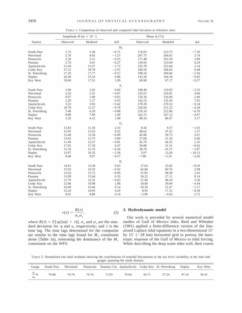
The sea level data are analyzed using the least squareserror method of Foreman and Henry (1979). The anal-ysis includes as many as 146 possible tidal constituents,45 of these being astronomical in origin and the re-maining 101 being shallow water constituents (e.g.,Godin 1972) that arise by distortions of the astronomicaltidal constituents due to the nonlinear effects of shoalingdepth. Year-long time series of sea level are used foreach of the nine sea level station analyses inclusive ofthe years 1996–99. Data gaps preclude using the sameyear for all stations. Table 1 lists the amplitudes andphases (relative to the Greenwich meridian) for the M2,S2, K1, and O1 constituents, which in sum contain over90% of the tidal variance. We note that the semidiurnaltides to the south of are larger than those west of Ap-alachicola Bay. In contrast with the diurnal tides thathave similar amplitudes at all nine stations, the semi-diurnal tides show large spatial variations. All of thefour major constituents have amplitudes that peak nearCedar Key.

To quantify the contribution that the tides make tothe total sea level variance, a predicated tidal heighttime series, zp, is constructed by adding the four majortidal constituents. With z0 being the observed sea sur-face height time series after removing the mean, theroot-mean-square tidal residual (i.e., the subtidal com-ponent), sr, and the normalized residual, sr/s0, wheres0 is the standard deviation of z0, are calculated overthe time series record length, T, as

12s 5 [z (t) 2 z (t)] dt. (1)r E p 0!T

The ratios of the subtidal variability to the total sea levelvariability, sr/s0, are given as percentages in Table 2.We note that west of Apalachicola Bay, where the tidesare generally small, the subtidal variability accounts formore than 70% of total variability. South of Apalach-icola Bay, where the tides are larger, the tidal and thesubtidal variabilities contribute about equally to the totalsea level variability.

b. Tidal currents

In parallel with sea level the tidal analyses for themoored velocity data are performed using the leastsquares error method of Foreman (1978). Since the 12mooring locations were generally not codeployed, theanalysis intervals (between 1996 and 1999) differ inrecord length and time origin. We generally used theentire record length available at each site, and thesevaried from around three months to one year.

Parameters describing the tidal hodographs are cal-

culated at each depth bin (from 0.5 to 10 m dependingon water depth) for each mooring. The amplitudes ofthe ellipse semimajor axis and the ellipse orientations(measured anticlockwise from east) are shown as a func-tion of depth in Figs. 2 and 3 for the four major con-stituents: M2, S2, O1, and K1. For a purely barotropictide the amplitude and orientation would be independentof depth and appear as vertical lines. Depth profile de-viations from straight lines are related to bottom friction,baroclinicity, contamination by inertial motions, or com-binations of these. As shown in Fig. 2 for relativelyshallow depths and in Fig. 3 for relatively deeper depths,the semidiurnal tides indeed appear to be barotropic,which agrees with the finding of Koblinsky (1981) forthe WFS M2 tide. In contrast, the diurnal tides, espe-cially in deeper water, tend to show vertical structure.This is most likely due to contamination by inertial mo-tions since in the central WFS the inertial period is about25.90 h, which is close to the O1 and K1 periods of 25.82and 23.93 h, respectively. WFS inertial oscillations aremodulated in time along with the seasonally varyingstratification (Weisberg et al. 1996), and they are evidentin velocity component plots as baroclinic modes con-sistent with the orientation reversals seen for the deeperrecords in Fig. 3.

Overall, the observed tidal current amplitudes on theWFS are weak (on the order of a few centimeters persecond). Of the principal constituents, the M2 current isthe strongest; its amplitude tends to increase shoreward,and its ellipse orientation tends to align perpendicularto the isobaths. While weaker, the diurnal constituentamplitudes are more uniformly distributed across theshelf, and these findings agree with those of Marmorino(1983) for the Florida Big Bend region.

c. Phases of tidal height and tidal currents

One question of interest (particularly for recreationalfishermen) is the relative phase between the tidal heightat the coast and the tidal currents on the WFS. We ad-dress this question relative to the St. Petersburg tidegauge, the reference gauge for much of the WFS, intwo different ways. Table 3a shows the phases (andcorresponding time lags) between high tide at St. Pe-tersburg and maximum tidal currents (directed towardthe coast) at the 12 ADCP mooring sites for each of themajor tidal constituents. For the semidiurnal tides, thetimes of maximum tidal current generally lead the hightide at St. Petersburg by 2–9 h. On the other hand, themaximum tidal currents of the diurnal tide, lag the hightide time at St. Petersburg by 10–20 h.

A second approach is to construct time series of thetidal height at St. Petersburg and the tidal currents atthe 12 ADCP sites by combining the four major tidalconstituents, and then producing a set of lags for thesecomposite time series. Table 3b gives these maximumcorrelation time lags between the water level h and themajor component of tidal current u defined as


TABLE 1. Comparison of observed and computed tidal elevation at reference sites.

Station

Amplitude H (m 3 1022)

Observed Modeled DH

Phase f (8G)

Observed Modeled Df

M2

South PassWavelandPensacolaPanamaApalachicolaCedar KeySt. PetersburgNaplesKey West

1.732.782.262.74

11.6437.3117.2026.4018.60

2.444.052.513.01

13.3739.7817.7725.5417.51

20.7121.2720.2520.2721.7322.4720.57

0.861.09

116.65207.75171.48139.93255.78186.50198.10143.3666.90

123.75204.01165.59133.64253.64186.02200.66144.1867.17

27.103.745.896.292.140.48

22.5620.8220.27

S2


1.062.240.971.203.53

10.795.408.895.20

1.022.311.001.173.95

11.576.287.894.12

0.0420.0720.03

0.0320.4220.7820.88

1.001.08

108.40225.67159.36142.23278.28226.94216.10162.1588.24

110.92220.81156.96135.20278.52231.22222.86167.1286.07

22.524.862.407.03

20.2424.2826.7624.97

2.17

O1


13.8315.8513.4913.6511.4617.6515.5013.979.40

11.5015.6313.5812.7512.2717.1815.7616.359.97

2.330.22

20.090.90

20.810.47

20.2622.3820.57

8.5648.6242.8027.6045.7030.8938.703.07

27.80

9.5747.2539.7321.2044.3531.5141.5713.20

25.35

21.011.373.076.401.35

20.6222.87

210.1322.45

K1


14.0115.9313.6313.9912.7021.8616.6015.249.02

13.3816.3513.7213.6413.3519.9816.4614.958.88

0.6320.4220.09

0.3520.65

1.880.140.290.14

17.6362.8451.8536.2551.6034.6050.508.93

23.90

25.8260.7648.4027.1148.2439.0451.6717.3126.62

28.192.083.459.143.36

24.4421.1728.38

2.72

TABLE 2. Normalized rms tidal residuals showing the contributions of nontidal fluctuations to the sea level variability at the nine tidegauges spanning the study domain.

Gauge South Pass Waveland Pensacola Panama City Apalachicola Cedar Key St. Petersburg Naples Key West

%sr

s0

70.88 74.74 70.76 71.03 70.64 50.71 57.24 47.14 56.41

R(t)r(t) 5 , (2)

s sh u

where R(t) 5 E[h(t)u(t 1 t)]; sh and su are the stan-dard deviation for h and u, respectively; and t is thetime lag. The time lags determined for the compositeare similar to the time lags found for M2 constituentalone (Table 3a), reiterating the dominance of the M2

constituent on the WFS.

3. Hydrodynamic model

Our work is preceded by several numerical modelstudies of Gulf of Mexico tides. Reid and Whitaker(1981) applied a finite-difference version of the line-arized Laplace tidal equations in a two-dimensional 159by 159 (;28 km) horizontal grid to portray the baro-tropic response of the Gulf of Mexico to tidal forcing.While describing the deep water tides well, their coarse


FIG. 2. Vertical profiles of the velocity hodograph ellipses semimajor axis amplitudes and orientations (measured anticlockwise from east)for the EC designated moorings. The thick solid and dashed lines denote M2 and S2, respectively. The thin solid and dashed lines denoteO1 and K1, respectively.


FIG. 3. Vertical profiles of the velocity hodograph ellipse semimajor axis amplitudes and orientations (measured anticlockwise from east)for the TS designated moorings. The thick solid and dashed lines denote M2 and S2, respectively. The thin solid and dashed lines denote O1

and K1, respectively.


TABLE 3a. Greenwich phases of the major tidal constituents at the St. Petersburg tide gauge and at the 12 ADCP stations (left-handcolumns), plus the relative times between high water at St. Petersburg and maximum (shoreward directed) semimajor axis tidal currents atthe 12 ADCP stations (right-hand columns). Phase differences are converted to time differences using speeds of M2, S2, O1 and K1 of 29.98deg h21, 30.00 deg h21, 13.94 deg h21 and 15.04 deg h21, respectively, where ‘‘1’’ and ‘‘2’’ indicate time lags and leads, respectively.

Station

M2

(deg) (h)

S2

(deg) (h)

O1

(deg) (h)

K1

(deg) (h)

St. PetersburgAS1TS1TS2TS3TS4TS5TS6EC2EC3EC4EC5EC6

198.10148.80

51.3921.3963.5752.0854.1653.5645.1747.0920.35

29.64293.69

0.0021.7025.0626.1024.6425.0424.9724.9825.2725.2126.1326.9329.76

216.10123.81

70.4133.3784.8469.0168.9469.7358.1356.7240.2333.71

2106.10

0.0023.0724.8626.0924.3724.9024.9024.8725.2625.3125.8626.07

210.74

38.7023.26

269.34250.58246.39239.42261.06322.91260.83256.08226.26221.70159.10

0.0021.1016.5415.1914.8914.3915.9520.3815.9315.5913.4513.12

8.63

50.50311.92262.49237.69280.66250.05241.93208.68286.86284.58270.08275.70139.98

0.0017.3814.0912.4415.3013.2612.7210.5115.7115.5614.5914.975.94

TABLE 3b. The time lags between high tide at St. Petersburg and the maximum (shoreward directed) semimajor axis tidal currents at the12 ADCP stations determined by the maximum lag-correlation coefficient between the composites of the M2, S2, O1, and K1 constituents.

Station St. Petersburg AS1 TS1 TS2 TS3 TS4 TS5 TS6 EC2 EC3 EC4 EC5 EC6

Time lag (h) 0.00 22.31 25.53 26.45 25.25 25.18 25.65 25.68 25.77 25.86 26.36 27.37 28.16

grid size was insufficient to describe the tidal structureson the shelf. Westerink et al. (1993) applied a finite-element-based hydrodynamic model (ADCIRC-2DDI),also depth integrated and two-dimensional, to the west-ern North Atlantic, the Gulf of Mexico, and the Carib-bean Sea, to develop a tidal constituent database. Com-putations were presented for varying horizontal reso-lutions ranging from coarse (1.68 3 1.68) to fine (69 369), and discussion was given to the importance of mod-el resolution. Their model comparisons with sea leveldata show good agreements in the Atlantic Ocean, butpersistent errors occurred in the Gulf of Mexico and theCaribbean Sea. These authors suggested that insufficientresolution over the continental shelf, particularly in theshallowest regions, might be responsible for the rela-tively poor numerical convergence in those regions.More recently, L. Kantha et al. (2002, personal com-munication; material available online at http://www.ssc.erc.msstate.edu/Tides2D/) developed a data-assimilative, barotropic tidal model for the Gulf of Mex-ico with similar grid resolution as Reid and Whitaker(1981). Improved results follow from the assimilationof selected coastal tide gauge data. Nevertheless, thismodel has insufficient resolution to describe the struc-ture of the tidal variations on the WFS.

Our approach is therefore a regional one. The hydro-dynamic model used is the Princeton Ocean Model(POM), a three-dimensional, nonlinear, primitive equa-tion model with Boussinesq and hydrostatic approxi-mations (Blumberg and Mellor 1987). The model usesan orthogonal curvilinear coordinate system in the hor-izontal and a sigma

z 2 hs 51 2h 1 H

coordinate system in the vertical, where z is the con-ventional vertical coordinate (positive upward from zeroat the mean water level), H is the local water depth, andh is the tidal variation about the mean water depth. Ourmodel domain (Fig. 4) extends from the MississippiRiver in the northwest to the Florida Keys in the south-east, with one open boundary that arcs between thesetwo locations. Horizontal resolution varies from lessthan 2 km near the coast to about 6 km near the openboundary, and the minimum water depth is set at 2 m.This grid allows us to resolve the complicated featuresof the coastline and the isobath geometries in order toexplore the associated structures of the WFS tides. Weuse 21 sigma layers in the vertical with higher resolutionnear the bottom to better resolve the frictional boundarydynamics. Bottom stress is obtained by a quadratic draglaw in which a nondimensional drag coefficient is cal-culated on the basis of a specified (0.01 m) bottomroughness length. The model has a total of 121 3 813 21 grid points, and the time step for the externalmode is 12 s.

Water density is assumed homogeneous in this three-dimensional barotropic tide study. The three-dimen-sional distribution of the vertical eddy viscosity is com-puted using the Mellor and Yamada (1982) level-2.5turbulence closure scheme, and the horizontal eddy vis-cosity is calculated using the shear-dependent Smago-rinsky formulation (Smagorinsky 1963) with a coeffi-


FIG. 4. The model grid used for the regional tidal simulation.

cient of 0.2. Dissipation by vertical friction is found tolargely exceed that by horizontal friction.

The bathymetry adopted in the model begins with theWorld Ocean Elevation Data ETOPO5 59 3 59 globalbathymetry dataset. Since this dataset is inaccurate inthe southern portion of WFS we corrected it by incor-porating data from NOAA navigation charts and Na-tional Geophysical Data Center (NGDC) bathymetrycontours. Our modified bathymetry has been used inother WFS modeling studies with satisfactory results(e.g., He and Weisberg 2002; Weisberg et al. 2001; Yanget al. 1999).

Tidal forcing of the model is exclusively at the openboundary. There, the tidal elevations are specified by alinear interpolation of the output from the TOPEX/Po-seidon data assimilated global tidal model of Tierney etal. (2000). This barotropic model, with 159 resolution,provides eight tidal constituents (M2, S2, N2, K2, K1,O1, P1, and Q1) over a nearly global domain that extendsfrom 808S to 668N. The model assimilates both coastaltide gauge data and ocean tides derived from four yearsof TOPEX/Poseidon satellite altimetry data. Since ituses procedures that tend to preserve the spatial tidalstructures in shallow water, it is considered to be a suit-able product for forcing higher-resolution regional tidalmodels. Figure 5 shows the distributions of tidal am-plitudes and phases for M2, S2, K1, and O1 constituentsalong the open boundary where we have a total of 121model grids.

4. Modeled elevations and currents

a. General features

The model is forced at the open boundary by spec-ifying the composite M2, S2, K1, and O1 constituentelevations there. Elevations, currents, and turbulencequantities are computed over the model interior by in-tegrating forward in time beginning from a state of rest.An initial spinup period of five inertial cycles (aboutfive days) is used to suppress transients. The subsequent30 days are then analyzed using the same techniques asfor the in situ data to retrieve individual constituentamplitude and phase distributions over the model do-main. Table 1 provides amplitude and phase compari-sons between the modeled and observed elevations ofM2, S2, K1, and O1 at the nine coastal tide gauge stationsspanning the analysis domain. Amplitude differencesare generally less than 2 cm; the singular exceptionbeing at Cedar Key where it is 2.5 cm for M2. Phasedifferences are generally less than 108; with Naples at10.18 for O1 being the largest. Both amplitude and phasedifferences show equally likely plus or minus valuesdemonstrating that the modeled tides are not biased.Root-mean-square (rms) values of the phase differences,when converted to time, amount to less than 10 min (20min) for the semidiurnal (diurnal) species. Consideringthe model tide gauge sampling relative to the actual tidegauge positions and the nearshore masking (2 m beingthe shallowest model depth), these phase agreements are


FIG. 5. The distributions of tidal (top) amplitudes and (bottom) phases along the model open boundaryfor the M2, S2, K1, and O1 constituents (see legend provided). The abscissa is the grid index that includesboth points over land and water. The land points are masked, and so only the points over water are shown.

both good and as good as can be expected. Therefore,no model tuning was considered.

The alongcoast variations of the amplitudes and phas-es of the four major tidal constituents are graphicallyshown in Fig. 6, where circles denote the observationsand crosses indicate the model results. Allowing forscale changes in the abscissa we see a relative spatialhomogeneity in the diurnal species compared with amore spatial inhomogeneous distribution for the semi-diurnal species. We also note several bull’s-eyes in themodel–observation comparison.

The agreements of Table 1 and Fig. 6 justify usingthe model to produce coamplitude and cophase chartsfor the M2, S2, O1, and K1 constituents (Fig. 7). In gen-eral agreement with the findings of the previously citedGulf of Mexico tide studies, these maps provide furtherdetails of the tidal structures on the WFS. The semi-diurnal and diurnal species are distinctly different. Thephase of the M2 tide advances toward the northwest.Apalachicola Bay separates the M2 tidal regime into twoparts. To the west the M2 tide is weak. To the east it isstrong. Both the Florida Big Bend and the Florida Bayregions show relative maxima with a relative minimumin between just to the south of Tampa Bay. The S2

constituent shows features similar to the M2 constituent,but with a much smaller amplitude. The phase patternsfor the semidiurnal species appear to result by diffrac-tion around the Florida Keys and onto Cape San Blas.

Amplification of the semidiurnal tides in the FloridaBig Bend has been discussed by previous investigators.Reid and Whitaker (1981) considered a resonance de-riving from the counterclockwise speed of propagationmatching the group speed for a gravest mode edge wave(gS/ f where S is the bottom slope—Kajiura 1958). Withthese speeds in close alignment and with the M2 tidewrapping around the basin approximately once per tidalcycle, near resonance may be achieved (these authorsestimated an average M2 propagation speed of 98 m s21

and an edge wave speed of 120 m s21). While this typeof resonance is possible, we note that bottom topographyand edge wave speeds vary around the shelf as does theM2 tide amplitude and phase gradient.

Local geometry may also induce amplification. Theisobath (Fig. 1) and the coamplitude plots for the semi-diurnal tides (Fig. 7) show similarity. Where the shelfis narrow the amplitudes are small, and conversely. Thetwo regions of widest shelf are the Florida Big Bendand Florida Bay with a relative minimum in between,


FIG. 6. Comparisons between modeled and observed (left) amplitudes and (right) Greenwich phases for the M2, S2, K1,and O1 constituents at the nine coastal tide gauge locations. Crosses (circles) denote modeled (observed) values. Bull’s-eyes are where they overlay.


FIG. 7. Modeled coamplitude and cophase (relative to the Greenwich meridian) distributions for the M2, S2, O1, and K1 tidal constituents.Solid (dashed) lines denote amplitudes (phases), and the contour intervals are indicated in the lower-left corner of each panel.

as reflected in the coamplitude distributions. Effects oflocal geometry are considered in the analytical treat-ments of Battisti and Clarke (1982a,b) and Clarke(1991). For a continental shelf with an along-shore scalemuch greater than the shelf width these authors devel-oped a one-dimensional tide model to explain some ofthe observed barotropic tidal characteristics. Using alinearized bottom stress (ru/h), the linear Laplace tidalequations are

] r1 u 2 f y 5 2gh ,x1 2]t h

] r1 y 1 fu 5 2gh . (3)y1 2]t h

For tidal motions over a continental shelf with constantslope a and width a, that is, h(x) 5 ax, 0 # x # a,they expressed sea level in terms of a zero order Besselfunction as

h(a)1/25 J [2(ma) ],0h(0)

where2 2v 2 f

ma ø a. (4)1 2ga

For the semidiurnal tide (v2 2 f 2 . 0) on a wide shelf(a/a is large), ma → 1 and h(a)/h(0) → 0, implyingamplification of semidiurnal tides across a wide shelf.To account for alongshore variations in the tides, Lentzet al. (2001) developed an analytical, flat-bottom, two-dimensional model with varying shelf width. These an-alytical models are both consistent with the observedsemidiurnal tide behaviors on the WFS. They suggestthat the coamplitude distributions may be the result oflocal geometry, as contrasted with the previous basin-scale resonance arguments.

Unlike the semidiurnal tides, the diurnal tides showlittle coamplitude variations across the analysis domain.Both amplitudes and phases for the O1 and K1 constit-uents are nearly spatially uniform. This is consistent


FIG. 8. The amplitude ratio between the principal semidiurnal and diurnal tides.

with the Zetler and Hansen (1971) finding that the di-urnal tide is essentially in phase throughout the Gulf ofMexico. It is also consistent with Eq. (4) (Clarke 1991),since for v ø f on the WFS, ma → 0, so the diurnaltides do not amplify toward the coast. The O1 and K1

constituents also have comparable amplitudes withmean ratio of 0.95. Basin-scale resonance for these con-stituents is not expected because their propagationspeeds are about half those of the semidiurnal constit-uents, so they do not circumscribe the basin within atidal period as do the semidiurnal species (R. Reid 2001,personal communication).

The ratio between the amplitudes of the principalsemidiurnal and diurnal tide constituents, (M2 1 S2)/(K1 1 O1), is shown in Fig. 8. While the WFS tidalregime is generally characterized as mixed and mainlyof diurnal type, this is not true of the inner half of theWFS where the ratio exceeds 0.5 and especially of theFlorida Big Bend and Florida Bay regions where thesemidiurnal tides dominate. It is only over the outerportion of the WFS and to the west of Apalachicola Baywhere the diurnal species dominate.

Given the model sea level descriptions and the modeland in situ data agreements for sea level at the coast,we now examine the tidal currents in a similar manner.Figure 9 compares the depth-averaged tidal current ho-dographs (calculated for all of the in situ data locationsof Fig. 1) with the depth-averaged tidal current hodo-graphs calculated from the model, sampled at all of thesein situ data sites. Qualitatively, the comparisons are verygood for the semidiurnal constituents with ellipse sem-imajor amplitudes, eccentricities, and orientations all inagreement (see Table 4 for listings of the hodograph

ellipse semimajor axes, semiminor axes, and orienta-tions). Particularly notable is how the ellipse orienta-tions diverge away from the region of relative minimumsemidiurnal tide elevation just south of Tampa Bay. Ec-centricities at the stations close to the coast show thelargest departures between the data and the model,which may be a consequence of the model turbulenceparameterization. Deviations from an inviscid fluid sem-iminor to semimajor axis ratio of v f 21 are due to thefriction, which is consistent with the largest departuresbeing in the shallowest water. Nevertheless, the agree-ments are still very good. The overall agreements be-tween the observed and modeled diurnal constituents,while also good, are degraded somewhat from those oftheir semidiurnal brethren, and there are additional rea-sons for this behavior.

As pointed out by Reid and Whitaker (1981), modeledcurrents are more sensitive to factors such as bottomfriction, horizontal eddy diffusivity, and topographythan are modeled water levels. A particular problem inthe Gulf of Mexico for diurnal constituents is the close-ness in frequency between these and the local inertialperiod. Large inertial oscillations exist in the WFS ob-servations when the water column is stratified. Whilenot a subject of this paper, we did investigate severaldifferent techniques in attempting to minimize inertialoscillation interference in the data. For instance, webroke the data records into month-long pieces to dis-tinguish barotropic tides during months without strati-fication versus mixed barotropic tides and inertial os-cillations during months with stratification. Nonuniformmodulation made this too subjective, however. Recog-nizing that the inertial oscillations when present are pre-


FIG. 9. A comparison between the (left) observed and (right) modeled M2, S2, O1, and K1 tidal current hodographellipses at the 12 moored ADCP locations.


TABLE 4. A comparison of computed and observed tidal ellipse parameters.

Semimajor (31022 m s21)

Observed Modeled

Semiminor (31022 m s21)

Observed Modeled

Orientation (deg)

Observed Modeled

M2

AS1TS1TS2TS3TS4TS5TS6EC2EC3EC4EC5EC6

9.3810.21

8.129.957.213.831.795.825.244.402.75

14.35

9.528.787.388.926.193.491.965.845.074.152.22

12.01

22.0121.3022.1421.8421.7021.5220.2822.4822.6822.7121.9222.03

22.2220.9721.3421.7921.5720.8920.4921.1220.7020.4920.4921.03

29.0549.5231.9432.9923.9524.0525.6423.0522.1330.5879.44

151.08

31.3442.9833.2634.2926.3725.0629.5818.9319.7122.7359.75

155.76

S2


4.652.813.082.823.831.600.701.981.691.520.865.91

2.552.632.162.571.801.010.561.861.631.340.684.23

20.7120.0920.4120.5820.7020.6620.2120.9321.1220.7520.4421.03

20.5420.0520.2620.3620.3820.2420.1520.3720.2520.2020.1720.52

35.8850.4833.0426.1725.4329.4638.6121.3018.8822.3826.32

150.65

29.4741.3730.8732.1324.0222.9328.1715.9414.9616.4735.76

154.71

O1


5.442.682.253.712.062.951.472.432.382.272.633.50

4.273.173.083.722.931.951.242.102.011.791.302.53

24.0821.4020.6922.6921.2421.0920.6621.8721.5020.5120.4321.36

23.1822.4922.5123.0822.5021.5320.8821.9521.6421.3220.7420.81

29.4464.8849.1939.1340.4840.7865.5270.87

105.01103.83106.65134.03

20.8165.8858.9845.8446.5651.0544.8286.65

117.00129.66137.52132.82

K1


4.344.384.346.113.803.873.002.773.532.751.743.44

4.933.903.654.413.402.191.382.472.262.031.562.83

23.4923.5323.0924.6122.6423.4122.2721.4122.9721.9420.2320.69

23.3222.7022.6823.2422.6421.6020.9122.1821.9521.6020.9020.33

19.1250.5640.1432.4938.5855.5823.7938.07

112.20105.56141.99134.64

24.4457.0549.9341.5939.4344.2041.9854.62

100.32119.29129.42130.94

dominantly of first baroclinic mode structure we optedto perform the data analyses on depth-averaged currents,effectively averaging out the inertial oscillations. Nev-ertheless, some nontidal inertial oscillatory behaviormay still be contaminating the diurnal constituent ho-dographs of Fig. 9. Similar problems do not exist forthe semidiurnal constituents since they are removed in

frequency from the inertial oscillations. Some amplifi-cation is observed in the data during months when theWFS is stratified, but this is small relative to the bar-otropic tides. Whether such amplification is the resultof internal tide generation or a reduction in the effectsof bottom friction by the stratification remains to bedetermined.


FIG. 10. The distributions over the entire model domain of the modeled M2, S2, O1, and K1 tidal current hodograph ellipses.

The agreements between the observed and modeledtidal current ellipses are sufficiently good to warrant themapping of these ellipses over the entire model domain.These are shown in Fig. 10 for the M2, S2, O1, and K1

constituents. The general patterns seen in the coampli-tude contours are reflected here. The M2 currents am-plify from very small values in deep water to largestvalues (approaching 20 cm s21) near shore in the FloridaBig Bend and Florida Bay. The relative minimum inbetween to the south of Tampa Bay is evident with thehodograph orientations diverging away from this point.To the west of Apalachicola Bay we see very little M2

tidal current except just to the east of the MississippiRiver where the shelf again widens away from theDeSoto Canyon. The S2 tidal currents behave very sim-ilarly to the M2 tidal current except that they are weaker.The O1, and K1 ellipses appear very similar to one an-other, being weaker than the M2 and stronger than theS2 ellipses over the WFS, but stronger than either ofthese to the west of Apalachicola Bay. Eccentricities ingeneral agree with the tendencies from inviscid theory

that the tidal ellipses should be more circular (v f 21)for the diurnal species than for the semidiurnal species,and the polarizations are clockwise.

b. Tidal residual current and the Lagrangiantransport

The model, being fully nonlinear, is capable of gen-erating responses in addition to the four linear tidal har-monics with which it is forced. Here we investigate thesetidal residual currents (Ures, Vres) defined as the differ-ence between the model responses (U, V) and the fourconstituent tidal harmonic currents analyzed from themodel output. Thus, the Eulerian residual current is cal-culated as

U 5 U 2 u cos(s t 2 a )Ores i i i

V 5 V 2 y cos(s t 2 b ), (5)Ores i i i

where (ui, y i) and (ai, bi) are the analyzed harmonicconstants for the M2, S2, K1 and O1 tidal constituents.


FIG. 11. (top) Eulerian and (bottom) Lagrangian representations ofthe tidal residual surface circulation.

Figure 11 presents the residual currents in both Eulerianand Lagrangian frameworks. The Eulerian representa-tion (upper panel) is the residual surface current fieldafter subtracting from each grid point the linear leastsquares fit of the four major tidal constituents. The Eu-lerian residual field is weak (generally less than 0.01 ms21) and generally directed toward the north or north-west consistent with the propagation direction for thesemidiurnal tides. Vectors appear largest in the FloridaBig Bend where they also form an anticyclonic gyre.The Lagrangian representation (lower panel) is calcu-lated by tracking surface drifters originating at everyfourth grid point over a 30-day period; that is, they are

Lagrangian trajectories for dynamically passive parti-cles released at the surface on day 6 (after the five dayspinup period) and tracked through day 35. The patternsappear very similar to the Eulerian representation. Par-ticle displacements are small (order 10 km month21)suggesting that barotropic tidal current rectification isnot a mechanism of major importance in transportingmaterials on the WFS.

5. Bottom stress and turbulence mixing

Turbulence mixing in this POM-based barotropic tidemodel derives from bottom stress calculated using aquadratic drag law. Here we examine the bottom stressdistribution, its mixing ramifications for the water col-umn, and the implications of these findings for simplermodels that employ a linear drag law. For simplicity,only the M2 current is considered since it is the dominantcontributor to the WFS tidal currents.

Bottom stress, for either depth-dependent or depth-averaged models, may be defined in several differentways, such as

2t 5 ru 5 rC | u | u 5 rru ,b D* (6)

where r is the water density and for the first two (depth-dependent) cases, u* is the friction velocity, CD is abottom drag coefficient, and u is the near-bottom cur-rent. For the third (depth averaged) case is the depth-uaveraged current and r is a resistance coefficient. Forour application, we consider the rms value of tb cal-culated over 10 M2 tidal cycles from which the frictionvelocity u* is obtained as (tb/r)1/2. A map of this u*for the WFS M2 tide is given in the upper panel of Fig.12. The spatial variations of u* or the magnitude ofturbulence mixing reflects the spatial variations in thetidal current magnitude. Regions of the largest tidal mix-ing are associated with regions of the strongest tidalcurrents found in relatively shallow water. In particularthe maximum values of u* (greater than 0.36 cm s21)are found in the Florida Big Bend and in Florida Bay.

Since bottom stress is calculated by a quadratic draglaw, it is of interest to check the sensitivity of our resultsto the bottom drag coefficient CD. The adjustable pa-rameter in

221 1 1 sbC 5 max 0.0025, ln (7)D 5 1 2 6[ ]k z /D0

is the bottom roughness length z0. The default value forz0 is 0.01 m. For sensitivity studies we ran a series ofmodel experiments in which we varied z0 between 0.002and 0.05 m and found no significant differences in mod-el performance. We then replaced Eq. (7) with a smallerspatially uniform drag coefficient (CD 5 0.001). Thissubstantial change in drag coefficient, especially in shal-low water, resulted in a disproportionately small changein the model response. In analogy to a damped harmonicoscillator, where proportionately small (large) increases


FIG. 12. The spatial distribution of mixing properties inferred fromthe M2 tidal currents. From the top to bottom are the friction velocity(u

*), the resistance coefficient (r), and the log-layer thickness. Units

are provided in each panel, as are bathymetric contours (light lines)for isobaths 20, 50, 100, 200, 1000, and 2000 m.

in response occur away from (near)resonance, our sen-sitivity findings suggest that tidal amplifications in theBig Bend and Florida Bay regions are nonresonant, sup-porting the earlier assertion that geometry is the causeof the observed amplification.

For the case of linear, depth-averaged models bottomstress is set by the resistance coefficient r. As examples,

Clarke (1991) used r 5 2 3 1024 m s21, whereas Lentzet al. (2001) found r 5 5 3 1024 m s21 to be appropriatefor the North Carolina shelf. Using rms bottom stressand depth-averaged current distributions we arrive at restimations here [Eq. (6)] that range across the shelffrom 0.6 to 6 (31024 m s21) (middle panel of Fig. 12).Thus, the use of constant values for r, while appealingfor linear model calculations, may either overestimateor underestimate the bottom stress on continentalshelves. Value judgements about quadratic versus lineardrag laws, aside, we simply emphasize that bottom fric-tion parameterization for models remains a complex,empirical issue.

Boundary layer theory identifies different layers (e.g.,Soulsby 1983) each with different behaviors. The ‘‘bedlayer’’ immediately adjacent to the bottom is where mo-lecular viscosity n controls the dynamics. Within thislayer (of a few centimeters thickness) we have

dU U u*z2rn 5 t 5 t(0) 5 ru* or 5 . (8)

dz u* n

Above the bed layer is the ‘‘logarithmic layer’’ withinwhich neither the details of the bed nor the free-streamflow affect the local dynamics, and for which the ve-locity profile follows the universal form,

U 1 z5 ln , (9)

u* k z0

where k ø 0.4 is the von Karman constant.Above the logarithmic layer is the ‘‘outer layer’’ for

which the velocity and turbulence profiles depend onthe nature of flow and hence obviates universality.

Defining an eddy viscosity A (e.g., Wimbush andMunk 1970) as

dUt 5 r(A 1 n) , (10)

dz

noting that A k n where the constant stress and loga-rithmic regions overlap and using Eqs. (8) and (10), wearrive at

A 5 cu z.* (11)

By similarity we can use this specification for A to es-timate the Ekman layer thickness d for steady-state flowregimes; that is,

] ]U U u*f U 5 A 5 cu* ⇒ d 5 c , (12)1 2]z ]z d f

where f is the local Coriolis parameter and c 5 0.1–0.4 (e.g., Loder and Greenberg 1986; Weatherly andMartin 1978).

Oscillatory boundary layers require further analysisif the local acceleration becomes of equal or greaterimportance as the Coriolis acceleration. Introducing thecomplex current, W 5 u 1 iy, into the momentum equa-tions,


]u ] ]u ]u ] ]y2 f y 5 A , 1 fu 5 A , (13)1 2 1 2]t ]z ]z ]t ]z ]z

and assuming W } eist, where s is the frequency ofoscillation, we arrive at [in analogy to Eq. (12)]

] ]W Wi(s 1 f )W 5 A } cu* ⇒ |d |1 2]z ]z d

cu*5 . (14)

(s 1 f )

For the case of the M2 tide-induced bottom boundarylayer on the WFS, with s ø 2 f , the bottom boundaryM2

layer thickness may be estimated as d ø cu*/(3 f ). Usinga midrange value of c 5 0.2, the bottom boundary thick-ness induced by the M2 tidal current over most of theWFS is estimated at about 2–5 m (except near CedarKey and in Florida Bay where it is comparable to thewater depth). Therefore, tidal mixing alone is insuffi-cient to mix the water column on the WFS.

The height of the logarithmic layer is taken as somefraction of the Ekman depth. Soulsby (1983), for in-stance, defines the logarithmic layer height as 0.1d andwith this definition the lower panel of Fig. 12 showsthe M2 tidal-current-induced logarithmic layer height forthe WFS. Values are generally less than 1 m. Empiricaldeterminations of the log layer based on the in situbottom boundary layer measurement on the WFS arepresently in progress and these will be reported on sep-arately.

6. Summary

Using in situ data and a numerical circulation modelwe examine the structure of the WFS tides and the ef-fects of the tides in distributing water properties and inmixing the water column vertically. Attention is limitedto barotropic tides and to the four major tidal constit-uents (M2, S2, O1, and K1) that account for the bulk ofthe tidal variance (;90%) of the region. The data arefrom coastal sea level stations ranging from the Mis-sissippi River delta to the Florida Keys, and from currentmeter moorings deployed across the shelf between the10-m and 300-m isobaths. The model is a regional ad-aptation of the POM extending from west of the Mis-sissippi River to the Florida Keys with a single openboundary arcing between these land termini. Regionaltides are produced by forcing the model at its openboundary using the composite M2, S2, O1, and K1 sealevel variability from the global (TOPEX/Poseidon as-similated) tide model of Tierney et al. (2000). Withstandard tidal analysis tools, we produce coamplitudeand cophase maps for each constituent and compare bothsea level and currents against actual observations. Basedon the fidelity of comparison we then use the modelproducts to discuss the WFS barotropic tides.

Apalachicola Bay, in the Florida Panhandle, is a di-

viding point between appreciable semidiurnal tides tothe east over the WFS and minimal semidiurnal tidesfrom there to the Mississippi River delta. In contrastwith the semidiurnal tides, the diurnal tides are spatiallymore uniform. With respect to overall rms sea levelvariability, tides account for about 30% west of, versusabout 50% southeast of Apalachicola Bay, respectively.The balance of the rms variability is due to synopticscale weather-induced sea level change. Coamplitudemaps show largest tides in the regions where the shelfis widest, that is, in the Florida Big Bend and in FloridaBay. The region just south of Tampa Bay shows a rel-ative minimum. Both the amplification of the semidi-urnal constituents and the spatial variations with shelfwidth are consistent with linear theory (e.g., Clarke1991; Lentz et al. 2001). Such theory also accounts forthe relative spatial uniformity of the diurnal constitu-ents. We conclude that the spatial distributions of thetides on the WFS are the result of local geometry, ascontrasted with previous ideas about basinwide tidal res-onance.

The tidal currents on the WFS, especially the semi-diurnal constituents, are primarily barotropic. Very goodagreements are obtained between the in situ data derivedand the modeled tidal hodograph ellipses. Semimajoraxes are generally less than 0.1 m s21, and the ellipsesare generally oriented normal to the shoreline. Ellipseorientation, however, does reflect the coamplitude dis-tributions with tidal currents tending to diverge (con-verge) on regions of relative minima (maxima). A rel-atively small seasonal modulation is observed in thesemidiurnal tidal currents due to either internal tides orreductions in friction by stratification. Larger seasonalmodulation is observed in the diurnal constituents dueto the generation of inertial oscillations under stratifiedconditions. Inertial oscillations, when present, are gen-erally organized as first baroclinic modes, so they tendto cancel out when performing vertical averages. Thishelps to facilitate the barotropic tidal analyses. Baro-clinic tides and inertial oscillations will be reported onseparately.

The nonlinearity of the model allows it to generatemean currents despite its linear harmonic forcing. Wepresent these residual currents in both Eulerian and La-grangian frameworks to assess their potential effects ontidal residual material transports. While a coherentStokes-drift pattern toward the northwest emerges, themagnitudes are small (one to two orders of magnitudeless than the semimajor axis speeds) amounting to netparticle trajectories of generally less than 10 km permonth. Albeit persistent, this is smaller than the poten-tial particle trajectories for either seasonal or synopticscale forcing (e.g., Weisberg et al. 1996).

With the M2 tide having the largest tidal current mag-nitude we use this constituent to examine the spatialdistribution of bottom stress by tides on the WFS andthe role that this may play in water column mixing.Except for the shallow regions of the Florida Big Bend


and Florida Bay, the potential for mixing by tides isweak. Attempting to parameterize friction in a linearmodel using a resistance coefficient is limited by thespatial variability in bottom stress; nevertheless, the val-ues estimated are within the range of values used inother studies. Estimates of logarithmic layer thicknessby the M2 tide are generally less than 1 m and empiricalstudies are under way to quantify this better.

In closing, with quantifiable metrics we show thatregional tides on the WFS may be adequately describedby forcing a regional, primitive equation, three-dimen-sional model with a global tide model at the open bound-ary, and that the properties of the tidal variations resultprimarily from the local geometry.

Acknowledgments. The in situ data collection and nu-merical model developments benefited from severalsponsors. The measurements were initiated under a co-operative agreement between the U.S. Geological Sur-vey, Center for Coastal Geology and the USF Collegeof Marine Science. Subsequent support by the MineralsManagement Service, Cooperative Agreement 14-35-0001-30787, is noted. Our work continues under supportby the Office of Naval Research Grant N00014-98-1-0158 and the National Oceanic and Atmospheric Ad-ministration Grant NA76RG0463. Special thanks areoffered to the family of Elsie and William Knight forthe research fellowship endowment that helped to sup-port R. He. Messrs. R. Cole, J. Donovan, and C. Merzare largely responsible for the success of the field pro-gram. Dr. S. Meyers contributed analyses and discus-sions, and we are particularly grateful for the helpful e-mail discussions provided by Prof. Robert Reid. Thesensitivity test on the drag coefficient in section 5 wasat the suggestion of an anonymous reviewer.

REFERENCES

Battisti, D. S., and A. J. Clarke, 1982a: A simple method for esti-mating barotropic tidal currents on continental margins with spe-cific application to the M2 tide off the Atlantic and Pacific coastsof the United States. J. Phys. Oceanogr., 12, 8–16.

——, and ——, 1982b: Estimation of nearshore tidal currents onnonsmooth continental shelves. J. Geophys. Res., 87, 7873–7878.

Blumberg, A. F., and G. L. Mellor, 1987: A description of a three-dimensional coastal ocean circulation model. Three-DimensionalCoastal Ocean Models, N. Heaps, Ed., Vol. 4, Amer. Geophys.Union, 208–233.

Clarke, A. J., 1991: The dynamics of barotropic tides over the con-tinental shelf and slope (review). Tidal Hydrogynamics, B. Park-er, Ed., John Wiley and Sons, 79–108.

Foreman, M. G. G., 1978: Manual for tidal currents analysis and

prediction. Pacific Marine Science Rep. 78-6, Institute of OceanScience, Patricia Bay, Sidney, BC, Canada, 70 pp.

——, and R. F. Henry, 1979: Tidal analysis based on high and lowwater observations. Pacific Marine Science Rep. 79-15, Instituteof Ocean Science, Patricia Bay, Sidney, BC, Canada, 39 pp.

Godin, G., 1972: The Analysis of Tides. University of Toronto Press,264 pp.

Grace, S. F., 1932: The principle diurnal constituent of tidal motionin the Gulf of Mexico. Mon. Not. Roy. Astron. Soc. Geophys.,3 (Suppl.), 70–83.

He, R., and R. H. Weisberg, 2002: West Florida shelf circulation andtemperature budget for the spring transition, 1999. Cont. ShelfRes., 22, 719–748.

Kajiura, K., 1958: Effect of Coriolis force on edge waves. (II) Specificexamples of free and forced waves. J. Mar. Res., 16, 145–157.

Koblinsky, C. J., 1981: The M2 tide on the West Florida Shelf. Deep-Sea Res., 28A, 1517–1532.

Lentz, S., M. Carr, and T. H. Herbers, 2001: Barotropic tides on theNorth Carolina shelf. J. Phys. Oceanogr., 31, 1843–1859.

Loder, J. W., and D. A. Greenberg, 1986: Predicted positions of tidalfronts in the Gulf of Maine region. Cont. Shelf Res., 6, 394–414.

Marmorino, G. O., 1983: Variability of current, temperature, andbottom pressure across the West Florida continental shelf, winter1981–1982. J. Geophys. Res., 88 (C7), 4439–4457.

Mellor, G. L., and T. Yamada, 1982: Development of a turbulenceclosure model for geophysical fluid problems. Rev. Geophys.,20, 851–875.

Reid, R. O., and R. E. Whitaker, 1981: Numerical model for astro-nomical tides in the Gulf of Mexico. Texas A&M Rep. for U.S.Army Engineers Waterway Experiment Station, 115 pp.

Smagorinsky, J., 1963: General circulation experiments with primi-tive equations. I. The basic experiment. Mon. Wea. Rev., 91,99–164.

Soulsby, R. L., 1983: The bottom boundary layer of shelf seas. Phys-ical Oceanography of Coastal and Shelf Seas, B. Johns, Ed.,Oceanography Series, Vol. 35, Elsevier, 189–266.

Tierney, C. C., L. H. Kantha, and G. H. Born, 2000: Shallow anddeep water global ocean tides from altimetry and numerical mod-eling. J. Geophys. Res., 105, 11 259–11 277.

Weatherly, G. L., and P. Martin, 1978: On the structure and dynamicsof the oceanic bottom boundary layer. J. Phys. Oceanogr., 8,557–570.

Weisberg, R. H., B. D. Black, and H. Yang, 1996: Seasonal modu-lation of the West Florida continental shelf circulation. Geophys.Res. Lett., 23, 2247–2250.

——, Z. Li, and F. Muller-Karger, 2001: West Florida shelf responseto local wind forcing, April 1998. J. Geophys. Res., 106 (C12),31 239–31 262.

Westerink, J. J., R. A. Luettich, N. Scheffner, 1993: ADCIRC: Anadvanced three-dimensional circulation model for shelves, coast,and estuaries. Report 3: Development of a tidal constituent da-tabase for the western North Atlantic and Gulf of Mexico. Tech.Rep. DRP-92-6, U.S. Army Corps of Engineers, 154 pp.

Wimbush, M., and W. H. Munk, 1970: The benthic boundary layer.The Sea, M. N. Hill, Ed., New Concepts of Sea Floor Evolution.Part I: General Observations, Vol. 4, Wiley and Sons, 731–758.

Yang, H., R. H. Weisberg, P. P. Niiler, W. Sturges, W. Johnson, 1999:Lagrangian circulation and forbidden zone on the West FloridaShelf. Cont. Shelf Res., 19, 1221–1245.

Zetler, B. D., and D. V. Hansen 1971: Tides in the Gulf of Mexico.Contributions on the Physical Oceanography of the Gulf of Mex-ico, Vol. 2, L. R. A. Capurro and J. L. Reid, Eds., Gulf Pub-lishing, 265–275.

tides on the west florida shelf on the... · tides on the west florida shelf ... semidiurnal tides...

Documents