tidal triggering of low frequency earthquakes near ... · other subduction zones and tremor on the...

Tidal triggering of low frequency earthquakes near Parkfield,California: Implications for fault mechanics withinthe brittle-ductile transition

A. M. Thomas,1 R. Bürgmann,1 D. R. Shelly,2 N. M. Beeler,2 and M. L. Rudolph1

Received 16 November 2011; revised 13 March 2012; accepted 15 March 2012; published 4 May 2012.

[1] Studies of nonvolcanic tremor (NVT) have established the significant impact of smallstress perturbations on NVT generation. Here we analyze the influence of the solid earthand ocean tides on a catalog of �550,000 low frequency earthquakes (LFEs) distributedalong a 150 km section of the San Andreas Fault centered at Parkfield. LFE families areidentified in the NVT data on the basis of waveform similarity and are thought to representsmall, effectively co-located earthquakes occurring on brittle asperities on an otherwiseaseismic fault at depths of 16 to 30 km. We calculate the sensitivity of each of these 88 LFEfamilies to the tidally induced right-lateral shear stress (RLSS), fault-normal stress(FNS), and their time derivatives and use the hypocentral locations of each family to mapthe spatial variability of this sensitivity. LFE occurrence is most strongly modulated byfluctuations in shear stress, with the majority of families demonstrating a correlation withRLSS at the 99% confidence level or above. Producing the observed LFE rate modulationin response to shear stress perturbations requires low effective stress in the LFE source region.There are substantial lateral and vertical variations in tidal shear stress sensitivity, which weinterpret to reflect spatial variation in source region properties, such as friction and porefluid pressure. Additionally, we find that highly episodic, shallow LFE familiesare generally less correlated with tidal stresses than their deeper, continuously activecounterparts. The majority of families have weaker or insignificant correlation with positive(tensile) FNS. Two groups of families demonstrate a stronger correlation with fault-normaltension to the north and with compression to the south of Parkfield. The families thatcorrelate with fault-normal clamping coincide with a releasing right bend in the surface faulttrace and the LFE locations, suggesting that the San Andreas remains localized andcontiguous down to near the base of the crust. The deep families that have high sensitivity toboth shear and tensile normal stress perturbations may be indicative of an increase ineffective fault contact area with depth. Synthesizing our observations with those of otherLFE-hosting localities will help to develop a comprehensive understanding of transient faultslip below the “seismogenic zone” by providing constraints on parameters in physicalmodels of slow slip and LFEs.

Citation: Thomas, A. M., R. Bürgmann, D. R. Shelly, N. M. Beeler, and M. L. Rudolph (2012), Tidal triggering of lowfrequency earthquakes near Parkfield, California: Implications for fault mechanics within the brittle-ductile transition,J. Geophys. Res., 117, B05301, doi:10.1029/2011JB009036.

1. Introduction

[2] Large slow-slip events in deep subduction zoneenvironments are recorded geodetically, as periodic transient

reversals of long term GPS velocities or tilt measurements,and seismically, as long duration, low frequency seismicsignals, dubbed non-volcanic tremor (NVT) due to theirsimilarity to volcanic tremor [Obara, 2002]. Though slow-slip and NVT occur simultaneously, inversions of GPSdisplacements during slip events in the Cascadia subductionzone result in strain release equivalent to Mw �6 events[Schmidt and Gao, 2010], while the total seismic moment ofNVT are orders of magnitude smaller [Kao et al., 2010]. Slipand tremor in subduction zone environments reflect slow-slipevents (SSEs) that propagate along the subduction interfaceat velocities of �10 km/day and are largely confined to theregion downdip of the locked subduction thrust [Obara et al.,2004; Dragert et al., 2004]. As these SSEs propagate, small

1Department of Earth and Planetary Science, University of California,Berkeley, California, USA.

2Earthquake Science Center, U.S. Geological Survey, Menlo Park,California, USA.

Corresponding Author: A. M. Thomas, Department of Earth andPlanetary Science, University of California, 169 McCone Hall, Berkeley,CA 94720, USA. ([email protected])

Copyright 2012 by the American Geophysical Union.0148-0227/12/2011JB009036

JOURNAL OF GEOPHYSICAL RESEARCH, VOL. 117, B05301, doi:10.1029/2011JB009036, 2012

B05301 1 of 24

http://dx.doi.org/10.1029/2011JB009036

on-fault asperities capable of generating seismic radiation failin earthquake-like events or low-frequency earthquakes(LFEs). The collocated, coeval evolution of NVT, SSEs, andLFEs led Shelly et al. [2007a] to suggest that part if not all ofthe seismic signature of NVT could represent a superpositionof multiple LFEs. Focal mechanism inversions of LFEs inShikoku indicate that LFEs are a manifestation of shear sliplocated largely on the plate boundary [Ide et al., 2007];however other studies have reported intraplate NVT loca-tions which may suggest they can take place on any localizedslip surface if source region conditions are agreeable [Kaoet al., 2005]. Application of matched filter techniques toother subduction zones and tremor on the deep San Andreasfault (SAF) indicate that global observations of NVT can beexplained as a superposition of many LFEs [Shelly et al.,2007a; Brown et al., 2009; Shelly and Hardebeck, 2010].The similarities between LFEs in different tectonic settingssuggests that the same slip phenomena that take place insubduction zone environments such as Cascadia and Shikokumay also occur on transform systems such as the SAF.[3] In idealized models of deformation in fault zones, slip

is accommodated in one of two ways: seismically, in earth-quakes that occur in the shallow, brittle regions of the crust,or aseismically, in deep shear zones where pressure andtemperature conditions are more amenable to ductile defor-mation. Shallow aseismic slip also occurs on some faults,however the mechanisms for this shallow creep may not bethe same as those in deep faults [Marone, 1998]. The iden-tification of highly episodic, non-volcanic tremor and slowslip below the seismogenic zone [Hirose et al., 1999;Dragert et al., 2001; Obara, 2002; Miller et al., 2002] hasmodified our notion of seismic coupling and the relativepartitioning between seismic and aseismic deformation.While aseismic slip is not explicitly hazardous there areimplicit or indirect implications for hazard; deformation indeep fault zones transfers stress to shallow faults where large,devastating earthquakes can occur. Since shallow and deepslip are potentially related, developing a comprehensiveunderstanding of fault zone anatomy, meaning where andhow different slip mechanisms operate, the physics thatgoverns deformation style, and stress transfer between thedeep and shallow crust may mitigate seismic hazard.[4] One characteristic common to global observations of

NVT and LFEs is extreme sensitivity to small stress pertur-bations. Studies of static stress changes from regional earth-quakes report both an aftershock-like response of deep NVTon the SAF to increases of 6 and 10 kPa in shear stress fromthe 2003 Mw 6.5 San Simeon and the 2004 Mw 6.0 Parkfieldearthquakes respectively, and quiescent response to decrea-ses in failure stress [Nadeau and Guilhem, 2009; Shelly andJohnson, 2011]. Several studies report triggering of NVTby teleseismic surface and body waves that imposed stresstransients as small as a few kilopascals [Gomberg et al.,2008; Miyazawa and Brodsky, 2008; Peng et al., 2009;Hill, 2010; Ghosh et al., 2009; Shelly et al., 2011]. Addi-tionally, studies of tidal stress perturbations conclude thatNVT are sensitive to stress changes as small as fractions of akilopascal [Rubinstein et al., 2008; Nakata et al., 2008;Lambert et al., 2009; Thomas et al., 2009; Hawthorne andRubin, 2010]. While these stress changes are exceedinglysmall, a number of other geological phenomena including

volcanoes, landslides, and glaciers are influenced by kPa-level stress changes caused by the tides [McNutt and Beavan,1984; Schulz et al., 2009; de Juan et al., 2010].[5] Early investigations of tidal triggering of earthquakes

find no relationship between earthquakes and tidal forcing[Heaton, 1982; Vidale et al., 1998]. Lockner and Beeler[1999] and Beeler and Lockner [2003] used laboratory fric-tion experiments and rate and state dependent friction theoryto argue tides and earthquakes are correlated but catalogswith large event numbers are required to detect a very modestcorrelation and the degree of correlation increases as the ratioof the amplitude of the tidal shear stress to the effectiveconfining stress increases. A number of later studies sub-stantiate the latter point, most notably Cochran et al. [2004]find a robust correlation between tidal stress and earth-quakes in shallow subduction environments (i.e. where theocean tidal loads can be as large as 10 kPa and the confiningstress is relatively low). High fluid pressures in both Nankaiand Cascadia are inferred from the high Vp /Vs ratios in theNVT source region documented by Shelly et al. [2006] andAudet et al. [2009] which may explain the robust correla-tion of NVT to small stress perturbations. Thomas et al.[2009] show that NVT rates on the Parkfield section of theSAF vary substantially in response to small fault-parallelshear stresses induced by the solid earth tides and were onlymodestly influenced by the much larger fault-normal andconfining stress cycles. Thomas et al. [2009] appeal to thepresence of pressurized pore fluids in the NVT source regionto explain their observations. They calculated effective nor-mal stresses between 1 and 10 kPa suggesting that pore fluidpressures in the NVT source region are very near lithostatic.[6] In this study we use the response of LFEs near

Parkfield to tidally induced stress perturbations to infermechanical properties of the LFE source region on thedeep SAF. Previous studies of tidal modulation of NVT inParkfield used start times and durations of NVT events inthe catalog described by Nadeau and Guilhem [2009]. Thepresent study utilizes the added spatial and temporal resolu-tion gained in using matched filter and stacking techniques toidentify and locate LFE families [Shelly and Hardebeck,2010] to map the spatial variability of sensitivity to tidallyinduced stresses and effective stress. We present observa-tions of the tidal influence on slip on the central SAF, infer-ences about properties of the LFE source region informed bythose observations, and when possible, comparisons betweenour findings and relevant observations in other tectonicenvironments.

2. Data and Methods

2.1. Low Frequency Earthquake Catalog

[7] The 2001-January 2010 low-frequency earthquakecatalog of Shelly and Hardebeck [2010] is composed of�550,000 LFEs grouped into 88 different families based onwaveform similarity. Locations of LFE families in Parkfieldare tightly constrained by numerous P- and S-wave arrivaltimes at densely distributed stations. The location procedureinvolves visually identifying individual LFE template eventcandidates and then cross-correlating and stacking thosewaveforms with continuous seismic data to detect other LFEsin the same family. The most similar events are stacked at all

THOMAS ET AL.: TIDAL TRIGGERING OF LFES NEAR PARKFIELD B05301B05301

2 of 24

regional stations, and P- and S-wave arrivals are identified onthese stacked waveforms. LFEs are located by minimizingtravel time residuals in the 3D velocity model of Thurber et al.[2006] with estimated location uncertainties of 1–2 km (forfurther details see Shelly and Hardebeck [2010]). Hypocentersof LFE families, shown in Figure 1, are distributed along

�150 km of the SAF from Bitterwater to south of Cholame.Estimated source depths extend from just below the base of theseismogenic zone to the Moho (16–30 km depth) on the deepextension of the SAF, a zone previously thought incapable ofradiating seismic waves.[8] Locations separate into two distinct groups: one to the

northwest below the creeping section of the SAF, and oneextending to the southeast from below the rupture area of the2004 Mw 6.0 earthquake into the locked section of the faultthat last ruptured in the 1857 Fort Tejon earthquake. Thesegroups are separated by a 15 km gap beneath the town ofParkfield, where no tremor has yet been detected. The pres-ence of a gap in the locations is not a product of stationcoverage or the location procedure. Very low tremor ampli-tudes on each side of this gap suggest that tremor amplitudesin this zone may simply fall below current detection thresh-olds [Shelly and Hardebeck, 2010].[9] Tremor amplitudes (maximum recorded ground veloc-

ities) and recurrence patterns vary considerably, and semi-coherently, along fault strike and with depth. The strongesttremor is consistently generated along a �25 km sectionof the fault south of Parkfield, near Cholame [Shelly andHardebeck, 2010]. Activity in some families is highly epi-sodic, with episodes of very high activity concentrated withina few days, followed by 2–4 months of quiescence. Anexample of highly episodic behavior is shown in Figure 2,family 65, where individual slip events can host over200 LFEs in a five day period. These punctuated episodesconcentrate in several relatively shallow neighboring fami-lies whereas the deepest families (e.g. family 85 in Figure 2)recur frequently, with small episodes of activity as often asevery 2 days with few intermittent periods of increasedactivity [Shelly and Johnson, 2011].[10] Oftentimes adjacent or nearby LFE families have

nearly identical event histories suggesting that they failtogether and experience very similar stressing histories.Neighboring, highly-episodic families generally producebursts of activity almost simultaneously [Shelly et al., 2009].In Parkfield, this observation is most robust in the shallowestfamilies; however there is also evidence for interaction indeeper families that still occur episodically. If LFE recur-rences track the rate of dominantly aseismic fault slip, thenthese episodes likely represent propagating slip fronts, anal-ogous to slow slip events in subduction zone settings. Nogeodetic manifestation of deep slow slip episodes has yetbeen observed in Parkfield, and slow slip events on the deepSan Andreas probably produce surface deformation thatfalls below the detection threshold for borehole strain, GPSor laser strainmeter instrumentation [Smith and Gomberg,2009].

2.2. Tidal Model

[11] We compute tidally-induced strains at the centroid ofthe tremor source region (�120.525, 35.935, 25 km depth)using the tidal loading package Some Programs for OceanTide Loading, which considers both solid earth and oceanload tides [Agnew, 1997]. For the solid earth contribution,displacements are very long wavelength compared to thesource region depth, thus we assume that the strains modeledat the surface are not significantly different from those at25 km depth. Unlike the body tides, the strain field computed

Figure 1. (top) Parkfield area location map with LFElocations are plotted as circles color-coded by family IDnumbers organized from northwest to southeast along thefault. Relocated earthquakes (post 2001) from the catalogof Waldhauser and Schaff [2008] are shown as gray dots.The Hosgri (H), Rinconada (R), and San Andreas (SA) faultsare shown in orange. Surface seismic stations used fordetection and borehole stations used for location are shownby white and black triangles respectively. The September 28,2004 Mw 6.0 Parkfield earthquake epicenter is indicated bythe yellow star. Inset map shows area of map view marked inred and locations of San Francisco (SF) and Los Angeles(LA). (bottom) Along fault cross section of the San Andreasviewed from the southwest (vertical exaggeration is 4:3)showing locations of LFE families shown in top panel andcolor coded by their family ID number. Families that arehighlighted in the text are labeled by their ID numbers.Relocated earthquakes shown in top panel within 10 km ofthe fault are plotted as gray dots. The slip distribution of the2004 M6.0 Parkfield earthquake from Murray and Langbein[2006] is shown in shades of gray. Stations shown in toppanel and relevant landmarks are indicated by triangles andred squares respectively.


3 of 24

at the surface cannot be applied at depth, as the magnitudeof the ocean loading component may change significantlybetween the surface and 25 km. To resolve this potentialissue, we calculate depth dependent, spherical Green’sfunctions using a finite element model of the layered earthmodel ofHarkrider [1970] which we then use to compute thestrains from only the ocean loading component at depth.A comparison of the load tides reveals that there are smallamplitude and phase shifts between the load tides at zero and25 km depth. However, once the load tides are superimposedon the solid earth tides, which are roughly an order of mag-nitude larger, the differences between the two become neg-ligibly different.[12] Given the degree two pattern of the tides, we assume

that tidal stress changes are small over the �140 km sectionof the SAF under consideration and that a single tidal timeseries computed at the centroid of the LFE source region canbe applied to all 88 hypocentral locations. To validate thisassumption, we computed and compared volumetric straintime series at the center and ends of the LFE source regionand found that the difference between the two time series hasaverage and maximum values of 1% and 5% respectively.[13] We compute the shear and normal stresses on the SAF

by converting strain to stress using a linear elastic constitu-tive equation and resolving those stresses onto a verticalplane striking N42�W. The relevant elastic parameters werechosen to be equivalent to those in the top layer of the con-tinental shield model of Harkrider [1970]. A representative14-day time series of the fault-normal and right-lateral shearstresses, FNS and RLSS respectively, are shown in Figure 3.The vast majority of the stress amplitudes are due to only thebody tides, as the ocean loading contribution diminishes withdistance inland. The solid earth tides induce largely volu-metric stresses thus the resulting shear stress on the SAF isapproximately an order of magnitude smaller than the normalstress. We also note that while the shear and normal stresscomponents are due to a common forcing function, they arenot directly correlated (see section 2.4).

2.3. LFE Correlation With Tidal Stress

[14] For each LFE we can compute the tidally inducedstresses at the time of the event, as event durations of �10 sare short relative to tidal periods [Shelly and Hardebeck,2010]. To quantify the overall correlation with tidal load-ing, we first define the “expected number of events”, or thenumber of events that occur under a particular loading con-dition assuming that LFEs occurrence times are randomlydistributed with respect to the time. The degree of correlationis defined by the percent excess value (Nex) defined as thedifference between the actual and expected number of eventsdivided by the expected number of events [Cochran et al.,2004; Thomas et al., 2009]. Positive Nex values indicate asurplus of events and negative values, a deficit. Loadingcondition can refer to the sign of a given stress component orto a particular stress-magnitude range. The load componentswe consider for the remainder of this manuscript are the

Figure 2. Example time series of cumulative number of LFEs over a two year time period for threeLFE families (65, 19, and 85, see Figure 1 for locations in cross section). Family 65 is highly episodicwith 2–4 month quiescent periods punctuated by few-day periods with extremely high LFE rates. In con-trast, family 85 recurs frequently, with a general absence of quiescence and a few intermittent episodes ofmuch smaller magnitude than family 65. Family 19 is an example of transitional behavior between the twoend-member cases.

Figure 3. A representative 14 day time series of tidallyinduced shear (red) and normal (blue) stresses resolved ontothe SAF striking N42�W.


4 of 24

tidally induced fault normal stress (FNS), fault normal stressrate (dFNS), right-lateral shear stress (RLSS), and right-lateral shear stress rate (dRLSS). We compute Nex values forall families relative to the sign of FNS, RLSS, dFNS, anddRLSS (shown in Figure 4). Nex values corresponding to99% confidence intervals are indicated in the lower left ofeach panel in Figure 4. Confidence intervals are computedby randomly selecting N times (where N corresponds to thenumber of LFEs in an LFE family) from the tidal time seriesto represent times of LFEs making up a synthetic catalog.FNS, RLSS, dFNS, and dRLSSNex values are then computedfrom the synthetically generated catalog. This process isrepeated 25,000 times to construct Nex distributions for eachof the four stress components, which are then used to con-struct the two-sided 95% and 99% confidence intervals.

Confidence intervals as a function of N are shown in theauxiliary material (Figure S5).1 The values reported at the99% confidence intervals in Figure 4 correspond to the LFEfamily with the fewest number of LFEs. Nex values differentfrom zero by more than the 99% confidence level are lessthan 1% likely to occur by random chance assuming thattides and LFEs are not correlated.

2.4. Hypothesis Testing for Spurious Correlations

[15] One caveat of the aforementioned analysis is that eachof the tidally induced stresses and stressing rates observed

1Auxiliary materials are available in the HTML. doi:10.1029/2011JB009036.

Figure 4. (a) NW-SE cross-section of LFE locations together with shallow microseismicity and slip dis-tribution of the 2004 Parkfield earthquake fromMurray and Langbein [2006]. (b–e) The locations of LFEscolor-coded by the Nex values corresponding to the tidal FNS, RLSS, dFNS, and dRLSS componentscalculated for the average fault strike of N42�W. 99% confidence intervals calculated for the family withthe fewest events (largest uncertainty) are reported in the bottom left of each panel.


5 of 24

arises from a common forcing and thus they are inevitablyrelated to one another (non-zero mutual information).However, the relationship between components cannot becharacterized as a simple phase shift or amplitude scaling(Figure 3). Before interpreting the observed LFE sensitivitiesto tidal stress components we first address the potential forspurious correlations that have no physical meaning to arisedue to the inherent correlation of the stressing functions.Artifacts can arise when one tidal component induces LFEoccurrence due to some physical process and a second tidalcomponent, which has no effect on LFE occurrence, is cor-related with the first. In our interpretation of correlations ofLFE timing to tidal stresses, we want to avoid interpretingspurious correlations in light of physical processes, whichrequires determining the sensitivity of tidal stressing com-ponents to one another.[16] To test for spurious correlations, we use a bootstrap

methodology to generate a large number of synthetic LFEcatalogs based on the observed distribution of LFEs relativeto a particular primary stressing function. These syntheticcatalogs are then used to calculate confidence intervals forthe expected Nex values of the secondary stressing functions.To construct synthetic catalogs, we consider one stressingfunction (or null hypothesis) and one LFE family at a time.Instead of assuming LFEs are randomly distributed withrespect to time as in the Nex calculation, we assume (1) theyare distributed in the way we observe for that particularcomponent and (2) they are randomly distributed withrespect to all other components. To construct the syntheticcatalogs, we use the frequency distribution of LFEs relativeto the primary stressing function, so each bin represents somerange of stress and has a corresponding number of LFEs. Foreach bin, we randomly select an equal number of times outof the tidal time series that have stress values within thecorresponding stress interval meant to represent times ofLFEs in the synthetic catalog. We then compute the Nex

values for each of the secondary stressing functions basedon this synthetic catalog of LFEs. We repeat this procedure1000 times and use the resulting values to construct 95% and99% confidence intervals. Finally, these confidence intervalsare compared to the observed Nex values for the secondarycomponents.[17] Models of frictional strength of faults depend on

more than a single loading function, for example Coulombfailure strength is a function of both shear and normalstress. To test for this type of dependence, we also exploredistributing synthetic catalog events randomly with respectto two different primary stressing components for a totalof eleven different null hypotheses: one considering nocorrelation between LFEs and tides, four for each stressingcomponent, and six for all possible combinations of twostressing components. The two component case is imple-mented with the same procedure as described above,except events are distributed relative to the joint frequencydistributions of the two components. To quantify how well thenull hypotheses characterize the remaining components, wedefine a misfit by determining the average number of standarddeviations between the observed Nex and 50th percentile of thesynthetically derived Nex values. For each family, the null

hypothesis that best characterizes the event times of that familyis the one with the smallest misfit.

3. Results

3.1. Spatial Distribution of Sensitivity of LFEsto Tidal Stresses

[18] Since each family has more than 2,000 LFEs, we cancalculate their sensitivity to tidal stresses at each location,which allows for a detailed view of the variability of tidalcorrelation with distance along the fault and depth. Figure 4shows the along-fault cross sections of the locations of the88 LFE families identified by Shelly and Hardebeck [2010]viewed from the southwest. Each family is color-codedby its sensitivity to the respective stressing condition (Nex

value). Sensitivities to all stressing components vary in aspatially coherent way, with nearby families often havingsimilar triggering characteristics, along both strike and dip.To the northwest, within the creeping segment of the SanAndreas, all but families 1 and 2 are either uncorrelated withthe FNS or correlate with tensile FNS at a significance levelof 99% or greater (panel B). The families with the highestFNS Nex values are the deepest families that locate between�15 and �45 km along-fault distance from Parkfield (labeledPositive FNS families in Figure 4). The majority of familiesto the southeast of Parkfield are either not significantly cor-related with the FNS or correlate in a less robust way than thehighly correlated families within the creeping section (10%versus 30% Nex). The notable exception to the overall cor-relation with tensile FNS is the localized group of familiescharacterized by negative FNS Nex values located along a15 km-long stretch of fault beneath Parkfield. The results ofthe statistical analysis presented in section 3.2 indicate thatthe correlation with clamping is authentic as none of the nullhypotheses are capable of explaining the observed deviationfrom zero as being due to inherent correlations with otherstress components (see families 45–52 in Figure 5). Theseevents are located along a releasing right bend of the SAF andvariation in fault orientation provides a potential explanationfor this correlation with clamping, which we discuss insection 4.6 [Shelly and Hardebeck, 2010].[19] Correlation with positive, right-lateral shear stress

(Figure 4c), is ubiquitous with all families correlating withshear stresses, which are an order of magnitude smaller thanassociated normal stresses, at a confidence level of 99% orgreater. Again, triggering sensitivities vary in a systematicway, with the families that are most sensitive to shear stressfluctuations locating to the northwest below the creepingsection. RLSS sensitivity in the families to the northwest ofParkfield appears to correlate with depth (Figure 4c). RLSSNex values transition smoothly from approximately 10% inthe families between 16 and 20 km depth to values of 30%below, and reach nearly 50% in families further to the north-west at depths of up to �28 km. The spatial pattern of RLSSNex values to the southeast of Parkfield appears to be morecomplex. The magnitudes of the dFNS sensitivity are about afactor of three smaller than the RLSS Nex values. The spatialvariation in dFNS mirrors that of the RLSS as families withsignificantly positive RLSS values also have significantlynegative dFNS correlations (Figure 4d). The significance


6 of 24

associated with the dFNS values is largely due to spuriouscorrelation with RLSS as discussed in sections 3.2 and 4.5.[20] Of the 88 LFE families, only five have statistically

significant values of positive dRLSS at 99% confidence.Most dRLSS Nex values are negative; that is, LFE are corre-lated with times of decreasing right-lateral stress. As shownin Figure 5,the correlation of LFEs with FNSmay be partiallyresponsible for the magnitude of the dRLSS Nex values;however most of the correlation cannot be explained as aproduct of aliasing (see section 3.2 and Figure S1 of theauxiliary material). Within the creeping section of the fault,dRLSS values transition between statistically insignificantto around �10% Nex values with depth/along strike fromParkfield to the northwest. Many of the most robustly cor-related families are those within the fault-bend region to thesoutheast of Parkfield. However, several of the southeasternmost families (along-fault distance of 20 km or greater) havesignificant negative values that are not associated with thebend.

3.2. Hypothesis Tests

[21] The hypothesis testing results for the one-componentcase of the RLSS are shown in Figure 5. Observed Nex valuesfor each of the four stressing components are indicated asblack dots, while the 95% and 99% confidence intervals

derived by creating synthetic catalogs matching the RLSSdistribution are shown in light and dark gray bars respec-tively. Figures 5 and S1 contain information about the rela-tionship between the observedNex values and the tidal model,which can help to distinguish spurious and authentic corre-lations by minimizing the misfit between the observed Nex

values (black dots in Figure 5) and the 50th percentile of theconfidence intervals generated from the synthetic popula-tions for the eleven different null hypotheses. One principalresult of the hypothesis testing procedure described above isthat of the 88 LFE families, none is best described by the nullhypothesis that LFEs are randomly distributed with respect totides, meaning that at 99% confidence or greater one ormore tidally induced stressing component is modulatingLFE occurrence.[22] A second important result is that LFE occurrence is

most strongly associated with the RLSS. We come to thisconclusion by considering that 73 of the 88 families are bestcharacterized (lowest misfit) by the null hypotheses thateither the LFE family members are preferentially triggered bythe RLSS alone or that two components play a role in trig-gering, one of which is the RLSS. Of the 66 families thatare best described by a two-component null hypothesis,26 families are best described by the FNS-RLSS nullhypothesis. These families preferentially trigger in response

Figure 5. Results of bootstrap analysis with the null hypothesis that LFEs event times are influenced bythe RLSS only. FNS, RLSS, dFNS, and dRLSS Nex values for 88 LFE families are shown as black dots.Light and dark gray bars represent 95 and 99% confidence intervals derived from synthetic populations.The RLSS Nex observations (marked NULL) have no confidence intervals because the synthetic catalogsare generated to match the RLSS Nex values. Misfits are listed in Table S1 of the auxiliary material.


7 of 24

to a tidal stressing function that incorporates some normal-stress dependence. The second and third most abundantgroups of 17 and 15 families are best described by the RLSS-dFNS and the RLSS-dRLSS respectively. The dRLSSdependence of some families may be related to factors wewill discuss in sections 3.6 and 4.6.[23] The correlation of 17 families with both RLSS and

dFNS is likely a spurious correlation. In Figures 5 and S1, thedeviation of the computed confidence intervals from zero isa measure of how sensitive each component is to the nullhypothesis in the tidal model, independent of the obser-vations and the sign of the deviation relative to the valueof the primary component from which the distributions weregenerated. If the observed Nex values fall within the boundsof the computed confidence intervals then the correlationbetween the LFEs and the secondary stressing functions maybe an artifact. If, on the other hand, the observed Nex valuesfall outside the computed confidence interval, then theycannot be explained as a spurious correlation, or aliasingresulting from the component or components used as the nullhypothesis. In Figure 5, confidence intervals for the FNS anddRLSS are mostly centered on zero suggesting little to nocorrelation with the RLSS. This is to be expected for thedRLSS, as when the RLSS is positive, half the time thedRLSS is also positive and half the time it’s negative whichshould result in a distribution centered on zero. However, thisis not the case for the dFNS, as almost none of the confidenceintervals are centered on zero, indicating that the value ofthe dFNS is quite sensitive to the RLSS value. The extremesensitivity of the dFNS values to the RLSS null hypothesissuggests that while the dFNS Nex values for many LFEfamilies are statistically significant relevant to the nullhypothesis that there is no correlation between LFEs andtides, this significance is likely a spurious correlation causedby the robust correlation of those families with the RLSS.Hence, many of the observed dFNS Nex values can beexplained by accounting for this sensitivity (in Figure 5,observed dFNS Nex falls within the 99% confidence range).The correlation between the RLSS and the dFNS is alsoevident in the observed Nex values (Figure 6). The coefficientof determination, R2, resulting from a linear regression ofthe RLSS and dFNS Nex values is 0.66 indicating a robustcorrelation between the two (see Table S2 in the auxiliarymaterial for associated significance values).[24] While Figures 5 and 6 clearly demonstrate the sensi-

tivity of dFNS to RLSS in the tidal model, there are signifi-cant correlations of some LFE families that cannot beexplained by matching only the RLSS. Even the best fittingone or two-component hypotheses may have observationsthat lie outside of the generated confidence intervals. Thisdiscrepancy could be due a number of factors includingunmodeled stress influences and assumptions such as faultorientation that go into our model of tidal stresses on theSAF. For these reasons, we do not require that the observedNex values for all families fall within the generated confi-dence intervals from a given hypothesis, but we simplyconsider the best-fitting hypothesis the one that minimizesthe misfit between the data and the models (or hypotheses).For the remainder of this analysis, Nex values are reportedwith respect to the null hypothesis that LFEs have no corre-lation with tidally induced stress, as they are a good metric

for reporting the sensitivity of LFEs to tidally inducedstresses and can be compared between components.

3.3. Tidal Sensitivity as a Function of RecurrenceInterval

[25] Hawthorne and Rubin [2010] document the contem-poraneous increase of tidal stresses on the plate interface andmeasured surface strain rates due to accelerated slip in theCascadia subduction zone. Using this result, they inferredthat tides are capable of modulating the slip rate of SSEs[Hawthorne and Rubin, 2010]. More recent studies of spa-tiotemporal characteristics of slow-slip fronts find that inaddition to quasi-continual slip front advance, rapid back-propagating slip pulses, called rapid tremor reversals, are alsoapparent [Houston et al., 2011]. Rapid tremor reversals mayalso be tidally correlated [Houston et al., 2011], which sug-gests that tidally correlated strain rates could be caused bytidal influence on the slip velocity, slip front advance, orboth. Recent studies of slip in Cascadia argue that slip andtremor are spatially and temporally coincident; hence NVTcan be considered a proxy for the location of deep fault slip[Bartlow et al., 2011]. If we extend this result to Parkfield,we may be able to gain additional insight into the mechanicsof slow-slip fronts by using the recurrence times withinrespective families to separate the catalog into two end-member groups: LFEs that represent the initiation of slip on aparticular asperity following a slip hiatus, and those thatoccur either as part of an ongoing episode (intra-event LFEs)or between episodes. We then examine the tidal correlation ofthese different populations which allows us to assess whethertides modulate the slip rate and/or the slip front velocity.[26] The majority of LFE families have average recurrence

intervals less than three days, including both the deep, con-stant rate families with repeat times averaging two to threedays and intra-event LFEs that occur in the shallow episodicfamilies with repeat times of much less than one day. We candistinguish initiating LFEs, or those that signal when a creeppulse arrives at an LFE hypocenter, from those that take placeeither as part of a creep event or those that occur in morecontinuous families (e.g. family 85 in Figure 2) by filteringLFEs as a function of the duration of the preceding recur-rence interval, tr. The population of LFEs with large valuesof tr, should largely consist of initiating LFEs. A small frac-tion of events within the most episodic families do occurbetween large creep events so to further distinguish initiatingevents, we also require that the time between a particular LFEand the subsequent LFE be less than one day to exclude suchevents.[27] The results of this analysis are shown in Figure 7,

which plots the FNS and RLSS Nex values for each popula-tion of events with recurrence intervals greater than tr. Forsmall values of tr (minute timescales) nearly all events in thecatalog are included, as indicated by the y-axis in Figure 7.As tr increases, first the events with very short recurrenceintervals, such as those that within the slip episodes experi-enced by families 19 and 65 (Figure 2) are filtered followedby events that take place as part of the deep, continuousfamilies such as family 85 (Figure 2) which correspond tomultiday tr values. Finally, at many day timescales, initiatingLFEs in families of intermediate episodicity are also filteredout leaving only the initiating LFEs in the highly episodic


8 of 24

families. The corresponding RLSS Nex values appear todecrease systematically with increasing tr but remain signif-icant over a wide range of interval durations. As the size ofeach population of events decreases with increasing tr, theNex confidence intervals associated with each populationshown in panels A and B grow wider. The FNS and RLSSNex values fall above the 99% confidence intervals for cor-relation until 43 and 25 days respectively. Slip events inParkfield appear to vary in size, pattern, and duration, so it isdifficult to place a definitive tr cutoff to differentiate initiatingevents from all others. The most episodic families haveaverage inter-episode periods of �60 days and episodes at agiven family typically last �5 days. While the 43 and 25 dayvalues are less than the average inter-episode period, they are

much greater than the average duration of a creep event in ahighly episodic family. This result indicates that the popu-lation of LFEs that occur when a creep event arrives at anLFE hypocenter is correlated with both positive RLSS andtensile FNS. We discuss the implications of this findingin section 4.2.

3.4. LFE Rate Variation as a Function of Tidal StressMagnitude

[28] In addition to quantifying the influence of tidal stres-ses on LFEs in the binary sense (Figure 4), we further explorehow specific stress levels influence LFE production bycomputing LFE rates as a function of the magnitude ofthe applied stress. Figure 8 is constructed by dividing the

Figure 6. All possible combinations of Nex values plotted against one another. Associated R2 values areshown on each plot. The highest R2 value, 0.66, suggests a spurious correlation may exist between theRLSS and dFNS components.


9 of 24

observed number of LFEs for a particular family that fallwithin a given stress range for the stress component underconsideration by the expected value based on the nullhypothesis that LFEs and tides are randomly correlated. Theresulting quantity is equivalent to 1 + Nex for each stress bin.This process is repeated for each stress range of a given stresscomponent and for all families. In Figure 8, the ratios ofactual to expected number of LFEs are color-coded so valuesabove one (warm colors), indicate a surplus of LFEs in thatparticular stress range and ratios below one (cool colors)indicate a deficit relative to the expected value. The abun-dance of values near one for the FNS plots confirms mostfamilies are generally not strongly influenced by the faultnormal stress (or at least not to the degree of the RLSS).A few notable exceptions include families 19–22 and 26–29which have LFE surpluses that correlate with peak tensileFNS. In addition, families 41, 44, 45, and 49–57 correlatewith fault-normal clamping. In contrast to the FNS, sub-stantial modulation of LFEs by the RLSS is almost ubiqui-tous for all 88 LFE families and well correlated with thestress magnitudes. Correlation between the stress amplitudeand LFE rates is strongest in families 1–13, with a smoothrise of LFE rates with increasing RLSS. For families withstrong RLSS correlation, LFE families are nearly quiescentwhen tidal stress is negative, with ratios near zero for RLSSless than �100 Pa.

[29] The results of the hypothesis testing analysis reportedin section 3.2 indicate that the majority of the deviation of thedFNS Nex values from zero is a spurious product of the robustcorrelation with RLSS. The correlation between triggeringpatterns of RLSS and dFNS are fairly evident in the 2nd and3rd panels of Figure 8 with families with rate ratios thatsystematically increase as a function of the RLSS (gradualtransition from blue to red) having a large excess number ofevents at negative values of dFNS (transition from tension toclamping). This is most evident in families 1–13, 32–36, and47–54 however there are counterexamples, such as 69–74,that have LFE deficits at low dFNS values, despite robustcorrelation with RLSS.[30] We reserve the detailed analysis of the dRLSS

dependence for section 3.6, however, to first order an excessnumber of LFEs occur when dRLSS values are negative (i.e.with decreasing stress magnitude). For most families withsignificant dRLSS dependence, the highest ratios of actualto expected number of LFEs occur at negative but notextreme rate values.

3.5. Optimal Fault Azimuth for Tidal Correlationand the Role of Friction

[31] Tidal stresses are largely volumetric with a very smalldeviatoric contribution. For this reason, the FNS and dFNSNex values are relatively insensitive to the choice of faultazimuth, while the RLSS and dRLSS substantially changeas a function of the assumed strike of the fault. Thomas et al.[2009] found that when the azimuth of the plane onto whichthe tidal stresses were resolved was allowed to vary, theorientation that maximized the excess percentage of NVTrelative to the expected number of events was W44�N, par-allel to the SAF strike. To further explore azimuthal depen-dence, we determine the optimal azimuth for each LFEfamily by finding the fault orientation that maximizes thenumber of LFEs that occur when tidally induced stressespromote slip in a right-lateral sense. To characterize thestressing function we consider two different friction coeffi-cients: m = 0.1 and m = 0 or purely right-lateral shear stressdependence. Low friction values are suggested by the strongdependence on RLSS and optimal correlation of tidal stressand tremor at m = 0.02 found by Thomas et al. [2009]. If weconsider m values greater than 0.1, the order-of-magnitudehigher FNS stresses dominate the change in Coulomb failurestress, resulting in substantially reduced Nex values andsometimes spurious orientations of peak correlation azi-muths. Figure 9 illustrates the dependence of Nex on faultazimuth and m for four example families. Family 4 locatedalong the creeping SAF shows maximum correlation (Nex =48%) at m = 0 and azimuth of N40�W. As the assumed fric-tion value increases above 0.2 Nex values drop to less than20% with the optimal azimuth remaining roughly alignedwith the SAF. Family 21 is part of a deep-seated group ofsequences with significant correlation with RLSS and withtensile FNS. Peak correlation occurs at low friction valuesbut Nex values remain significant at greater values of m for allorientations due to the small variation of FNS with azimuth.The shallow family 65 shows peak correlation (Nex = 10%)for fault azimuths of N30-40�W and m = 0. However, whenhigher contributions of FNS are considered, the orientation ofpeak correlation becomes highly variable and Nex values fallto below 5% and are not statistically significant. Family 41 is

Figure 7. (a and b) The FNS and RLSS Nex values (darkgray lines) calculated for all LFE events whose precedingrecurrence interval is longer than the respective x-axis value(tr). White background color represents Nex values that arestatistically significant at the 99% confidence level whilevalues in the gray region are statistically insignificant. (c) Thenumber of events in each population; since populationsize rapidly decreases with tr, 99% confidence regions inFigures 7a and 7b grow larger. Note that the�450,000 LFEscorresponding to the shortest time intervals are not shown.


10 of 24

located along a right bend in the SAF and belongs to a groupthat exhibits pronounced correlation with compressionalFNS. We again find peak correlation at zero friction alongN40�W. As the contribution of FNS to the failure function isincreased, Nex values decrease but do not show a strongchange in their spatial distribution. Peak Nex values are gen-erally found at very low or zero m values. As tidal FNS isabout an order of magnitude greater than RLSS, the correla-tion rapidly decreases with increasing m.Corresponding plots

for all 88families are shown in Figure S2 of the auxiliarymaterial.[32] Figure 10 shows the optimal orientation and corre-

sponding Coulomb stress Nex values for m = 0 and m = 0.1showing lines aligned with the optimal orientation centeredon the respective LFE hypocenter and circle colors indicat-ing the corresponding Nex values. The mean and standarddeviations for both populations are reported in the bottom leftof Figures 10a and 10b. One immediately obvious feature forboth friction coefficients is the tight clustering of the axes

Figure 8. LFE rate plots for each tidally induced stressing component. Panels correspond to fault-normalstress, right-lateral shear stress, and their respective rates. Each column corresponds to an individual LFEfamily and each row, a stress interval. Each square is color-coded by the ratio of the actual number of LFEswithin a given stress range over the expected number of LFEs that should occur within that range if tidesand LFEs are uncorrelated (this reflects the amount of time the tides spend in the given range assuming aconstant rate of LFE production). Cool colors represent a deficit of LFEs in the respective bin while warmcolors indicate a surplus.


11 of 24

around the average orientation of the San Andreas (N42�W).A few families’ peak-correlation orientation diverges fromthe fault strike by as much as 30� counterclockwise. Theoptimal orientation for these families more closely alignswith the San Andreas when we consider the modestly raisedfriction coefficient.

3.6. Phase of LFE Failure Times Relative to Tidal Load

[33] An effective tidal phase is assigned to each LFE bynormalizing the magnitude and rate of the FNS and the RLSSat the time of the event by the absolute value of the mostpositive (or negative depending on the sign) value the stress

Figure 9. Nex values as a function of azimuth and friction coefficient, m, used to calculate tidal Coulombstress (CFF = RLSS + mFNS) for four families (4, 21, 65 and 41 see Figure 4a for locations). Vertical lineindicates the average local strike of the SAF (N42�W) and a black dot indicates peak Nex for Coulombstressing.

Figure 10. Rotated map view of SAF with LFE hypocenters color-coded with respect to Nex valuecorresponding to the optimal orientation. Optimal orientations, defined as the orientation that maximizesthe Nex value, for each family are shown as black lines centered on the respective LFE hypocenter. Frictioncoefficients of (a) 0 and (b) 0.1 demonstrate the sensitivity of the optimal orientation to choice of frictioncoefficient. Mean orientations in degrees west of north and standard deviations for all families are shownin bottom left corner.


12 of 24

or stressing rate can attain. In this way, x- (magnitude) andy-values (rate) range between�1 and 1 and a phase value canbe obtained for each event. A phase of zero (up) correspondsto the maximum rate and zero magnitude, a phase of 90corresponds to maximum magnitude and zero rate, etc. Polarhistograms are constructed by grouping the phases of allLFEs within a particular family in 10 degree bins and thennormalizing each bin by the number of events expected tooccur in that range based on the tidal stress distribution.Thus, the radial dimension of the histogram is the actual overthe expected number (Nex + 1) of events for that particularrange of phases (expressed as a percentage in Figure 11a).A bin that contains the number of LFEs expected based onthe tidal distribution has a radius of one (i.e. the expected100% value assuming no tidal triggering). The full radialdimension of the phase plots corresponds to double theexpected number of events.[34] Results for example families 4, 22, 35, 41 (locations

labeled in Figure 4a), and the complete catalog are shown inFigure 11 (see Figure S3 of the auxiliary material). Family 4generally shows very weak FNS dependence and extremesensitivity to tidally induced RLSS (RLSSNex value of 48%),which is evident from the phase plots in Figure 11b. Radialvalues on the right half of the diagram corresponding topositive magnitude are almost entirely above the expectedvalue, with a corresponding depletion of LFEs during nega-tive magnitude RLSS on the left half of the plot. The eventexcess also seems to be rate dependent as evidenced by thepost-maximum magnitude RLSS peak which indicates pref-erential failure during times of moderate negative dRLSS.[35] Family 22 is an example from the cluster of deeper

families with moderate to strong RLSS correlation (23%RLSS Nex) also characterized by preferential failure duringtimes of extensional normal stress (16% FNS Nex). The FNSphase plot for family 22 shows preferential failure duringtimes of peak-positive FNS. Family 22 also has a substantialpositive RLSS dependence which may explain why there aresometimes more events than expected during times of nega-tive (compressive), decreasing FNS. The correlation withdecreasing FNS is likely due to the aliasing effect betweenthe RLSS and dFNS mentioned in section 3.2. Family 35 isshallow and less sensitive to tidally induced stresses asevidenced by the majority of bins within the phase plot fall-ing near the expected value, within the 99% confidence bins.Family 41 (�12% FNS Nex, 32% RLSS Nex) is a member ofthe anomalous group of families that fail preferentially dur-ing times of negative FNS. The correlation with negative,decreasing FNS is apparent in the phase plot of family 41.In family 41 events cluster with broad peak in the positive,

Figure 11. (a) A schematic phase plot labeling the 50%,100%, 150% and 200% expected value contours. (b) FNS(left) and RLSS (right) phase plots for a stack of all eventsin the catalog and four example families (4, 22, 35, and 41).Gray shaded areas indicate ratio of observed to expectednumber of events in each 10 degree phase bin. Thin dark bluelines are 99% confidence intervals for each population. Thindashed red lines are 100% expected value contours. The solidred line in the RLSS phase plot for the bulk catalog marks thehalf hour phase shift discussed in the text.


13 of 24

decaying RLSS and strong FNS peak in the quadrant ofincreasing compression.[36] Families 4 and 35 represent two end-member types of

behavior; however, some families have patterns that are notas readily interpretable. The general correlation of all familieswithin the catalog to RLSS is apparent in the stacked phaseplot of all LFEs within the catalog. The large number ofevents (N = 544,369) reduces the confidence intervals to verynear the expected value, hence any deviations from that valueare highly significant. If LFEs correlated with only RLSSmagnitude, then we would expect the region that exceeds theexpected value to be symmetric about the magnitude axis.However, the phasing of failure times with respect to RLSSseem to be phase dependent, as the majority of LFEs failduring times of large, positive RLSS magnitude and small,negative dRLSS which produces an �30 minute phase shiftin the time of the peak radial value with respect to the peakRLSS. This effect is also apparent in the dRLSS Nex valuesreported above and shown in Figure 4e. Families that arehighly sensitive to negative FNS are generally most robustlycorrelated with negative dRLSS. However, these families arenot solely responsible for the apparent phase shift as the samedRLSS dependence is still present when we iterate the anal-ysis while excluding families correlated with negative FNS.We discuss the possible causes of this apparent phase shift inthe correlation with tidal RLSS in section 4.5.

4. Discussion

[37] As the most studied continental transform environ-ment known to host tremor and transient fault slip, diagnosticobservations of slow slip in Parkfield complement those insubduction zones providing additional information about themechanics of slip in deep fault zones. Full azimuthal stationcoverage, a high-resolution seismic network, and detailedwaveform analysis help us better constrain the location andtiming of individual LFEs in Parkfield. If the same under-lying physics for slow-slip generation applies to both sub-duction zone environments and continental settings, then theobservations of LFEs in Parkfield may aid in developinggenerally applicable models of SSEs not limited to tectonicenvironment. In this section we discuss the implications ofthe results presented in section 3.

4.1. Spatial Distribution of Tidal Sensitivityand LFE Episodicity

[38] Our observations of tidal modulation of LFEs inParkfield is generally consistent with previous studies thatreport statistically significant influence of the ocean and solidearth tides on slow slip and NVT in subduction zones[Rubinstein et al., 2008; Nakata et al., 2008; Lambert et al.,2009; Hawthorne and Rubin, 2010; Ide, 2010]. The enhancedspatial and temporal resolution afforded by studying LFEsallows us to map the spatial variability of tidal influence andinfer from those observations the spatial heterogeneity offault mechanical properties. We are able to separate thecontribution of shear and normal stress components and theirrates to the triggering.[39] The majority of LFE families are highly correlated

with RLSS, however the spatial variability of tidal correlationbelow the creeping and locked sections of the SAF hasdifferent characteristics. Along the creeping section of the

SAF to the northwest of Parkfield, the correlation systemat-ically increases from less than 10% Nex, below the Parkfieldearthquake at 16 km depth, to above 50% Nex with bothdistance to the northwest and depth. To the southeast ofParkfield RLSS Nex values continue to be high, but theirspatial distribution is more complex with substantial along-fault changes and lack of a consistent change with depth(Figure 4c). A number of factors can influence the sensitivityof LFE sources to small stress perturbations, however, themagnitudes of the RLSS sensitivity in nearly all familiesrequire that elevated pore fluid pressures be present on thedeep SAF (section 4.3). Most families are weakly correlatedwith positive FNS, however there are two groups of familiesthat correlate with positive and negative FNS (labeled inFigure 4b). From the analysis presented in section 4.2, anddue to the spatially localized nature of these groups,we believe these correlations are not artifacts. We discusspotential causes of the negative and positive FNS Nex valuesin sections 4.6 and 4.7 respectively.[40] Study of LFEs also allows for a more detailed

assessment of the relationship between the distribution ofLFEs in time (i.e. episodic versus continuous) and tidalinfluence. To quantify the episodicity of individual LFEfamilies, Shelly and Johnson [2011] used the minimumfraction of days required to contain 75% of all events withina family (MFD75). Highly episodic families (e.g., 65 inFigure 2) are characterized by MFD75 values around zerowhile continuous families (e.g. family 85 in Figure 2) havevalues around 0.25. The relationship between episodicity,depth, and tidal modulation is shown in Figure 12. We findthat highly episodic families with bursts of LFEs interspersedwith episodes of quiescence are less tidally influenced thanthe deeper, continuously deforming families. Families withlow MFD75 values tend to be shallower and have eitherinsignificant or small Nex values when compared with the restof the catalog. If we consider the fault essentially lockedduring quiescent periods with the punctuated LFE burstsrepresenting times when the fault is slipping at the particularhypocenter, then weaker tidal modulation may suggest themagnitude of tidal correlation decreases during stronglyaccelerated fault slip, as the stress applied to any asperity dueto an accelerated background slip rate is likely much largerthan the tidal stress contribution. More continuously activeLFE families (high MFD75 values in Figure 12) show a widerange of Nex values in both FNS and RLSS components thatsuggest that other factors can dominate the degree of tidalcorrelation.[41] There are similarities and differences with the tem-

poral and spatial patterns of tremor found in subductionzones. Ide [2010] explored the relationship between tremorand tidal sensitivity in Shikoku, and found a correlationbetween deformation style, depth, and tidal influence. AtShikoku, the longer-lasting tremor events occur at greaterdepths in small and frequent episodes while the duration ofshallow NVT events are shorter and occur primarily duringlarge and infrequent tremor episodes, two or three times peryear [Obara, 2010; Ide, 2010]. However, to first order thesensitivity to tidal stress appears to be strongest in the shal-low portions of the tremor region at Shikoku, in contrast toour results [Ide, 2010]. Ide [2010] did not explicitly modelthe distribution of tidal stresses in space and time so it isdifficult to ascertain if the distribution in tidal sensitivity


14 of 24

reflects differences in tidal stress or source region behavior.Further comparisons are difficult to make due to the appli-cation of different detection and location methodologies.Smaller tremor episodes without geodetically detectable slowslip identified in Cascadia [Wech et al., 2009; Wech andCreager, 2011], Mexico [Brudzinski et al., 2010], andOregon [Boyarko and Brudzinski, 2010] also occur downdipof the section of the megathrust that hosts larger SSEs. Thissuggests a transition from highly episodic to continuousdeformation with depth in those locations, which is qualita-tively consistent with Parkfield. Correlation with tidal stresshas so far only been documented during large and shallowSSEs in Cascadia [Rubinstein et al., 2008; Lambert et al.,2009; Hawthorne and Rubin, 2010]. Future work shouldevaluate to what degree tidal sensitivity of tremor changeswith depth and/or size and recurrence interval of NVT epi-sodes in these areas.

4.2. Slip Front Propagation and Slip Velocity

[42] We motivated section 3.3 by asking if increased strainrates during periods when tides are encouraging slip were dueto tidal modulation of slip velocity or tidal influence on slipfront velocity [Hawthorne and Rubin, 2010]. Since most ofthe very episodic LFE families have statistically significantRLSS Nex values, and the vast majority of LFEs within thesefamilies occur during slip events, we can confirm that sliprates are tidally modulated during an ongoing slip episode.The modulation of LFE rates in the presence of an ongoingslip episode suggests that the slip velocity is tidally modu-lated, consistent with the findings of Hawthorne and Rubin[2010] for the Cascadia SSEs.[43] To address whether tides also control slip front

or propagation velocity we analyzed the tidal correlation ofLFE populations filtered by the duration of the precedingrecurrence interval tr (Figure 7). The majority of LFEs withlarge prior recurrence intervals represent the first event in anepisode at a family location, and thus may indicate whena creep front arrives at the location of a particular LFEhypocenter. From our analysis in section 3.3, we find that thepopulation of LFEs following a quiescence of several daysare still strongly tidally correlated. So why should the firstseismic signature of a slip pulse at an LFE family hypocenter

correlate with the tides? One possibility is that creep frontpropagation is tidally controlled; meaning the shear andnormal stress perturbations are of sufficient magnitude toaccelerate or decelerate the advance of the slipping region ofa fault. If is were true, slip fronts may advance faster duringtimes when tides are inducing stresses favoring slip frontpropagation. At present, geodetic studies of the spatiotem-poral progression of slip in Cascadia are not of sufficientprecision to resolve if slip front propagation speeds are tid-ally controlled [Hawthorne and Rubin, 2010; Bartlow et al.,2011]. The tremor locations in Houston et al. [2011] doprovide the required temporal resolution however, to ourknowledge, time-dependent changes in slip front advancehave not been explored.[44] A second cause of this apparent correlation could

be that the onset of a slow slip front occurs on timescalesthat are either equivalent to, or greater than tidal timescales.If slip were to nucleate and accelerate to slow slip speedson timescales much shorter than tidal periods, we wouldexpect to see no tidal dependence of slip nucleation, as LFEsshould behave in an aftershock-like manner to the near-instantaneous application of stress. For example, Shelly andJohnson [2011] show that LFEs respond to stress transferfrom the Parkfield and San Simeon earthquakes with a near-instantaneous increase in event rate. However, if the durationof onset is greater or equal to tidal periods then LFEs maypreferentially trigger at times that are tidally favorable. Manyslip episodes, like those shown in Figure 2 Family 65, doappear to onset gradually with several hours between the firstevent within an episode and sustained elevated event rates.This gradual onset of slip events qualitatively supports thishypothesis, as LFE rates during some slip episodes acceleratebetween the first discernable onset of slip and peak event rateover hourly timescales.

4.3. Tidal Sensitivity and LFE Source Properties

[45] What do the spatial variations in tidal sensitivityreveal about underlying changes in source properties orconditions? Multiple studies have inferred high pore fluidpressures in the tremor source region of subduction zonesfrom high Vp /Vs ratios and the influence of small stressperturbations on tremor rates [Audet et al., 2009; Shelly et al.,

Figure 12. Variation in FNS and RLSS Nex values for all LFE families plotted as a function of depth.Families are color-coded by their MFD75 value from Shelly and Johnson [2011]. Lower MFD75 valuescorrespond to highly episodic families while higher values correspond to more continuous families. Theshallow and episodic family 65 and deep and continuous family 85 shown in Figure 2 are labeled.


15 of 24

2007b]. Laboratory experiments and numerical models offaults with rate and state dependent strength suggest earth-quakes have a greater probability of being triggered as theratio of the oscillatory stress amplitude, t, to the effectivefault-normal stress, sn, increases [Lockner and Beeler, 1999;Beeler and Lockner, 2003]. Since the ratio t/sn for a fixedamplitude perturbation is greater in regions with high porefluid pressure, low effective stress also provides a potentialexplanation for the sensitivity of LFEs to extremely smallstress changes. We can quantify the effective normal stressrequired to produce the observed rates of LFE occurrence foreach family using the equation

RðtÞ ¼ r exptasn

� �ð1Þ

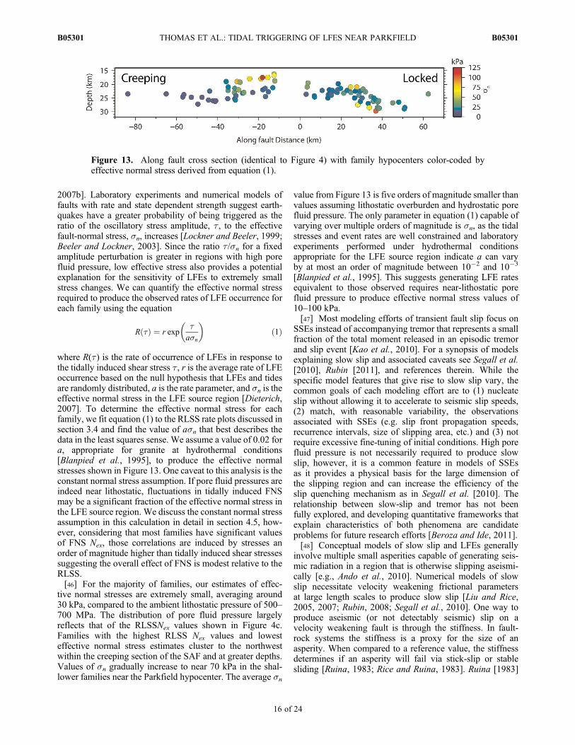
where R(t) is the rate of occurrence of LFEs in response tothe tidally induced shear stress t, r is the average rate of LFEoccurrence based on the null hypothesis that LFEs and tidesare randomly distributed, a is the rate parameter, and sn is theeffective normal stress in the LFE source region [Dieterich,2007]. To determine the effective normal stress for eachfamily, we fit equation (1) to the RLSS rate plots discussed insection 3.4 and find the value of asn that best describes thedata in the least squares sense. We assume a value of 0.02 fora, appropriate for granite at hydrothermal conditions[Blanpied et al., 1995], to produce the effective normalstresses shown in Figure 13. One caveat to this analysis is theconstant normal stress assumption. If pore fluid pressures areindeed near lithostatic, fluctuations in tidally induced FNSmay be a significant fraction of the effective normal stress inthe LFE source region. We discuss the constant normal stressassumption in this calculation in detail in section 4.5, how-ever, considering that most families have significant valuesof FNS Nex, those correlations are induced by stresses anorder of magnitude higher than tidally induced shear stressessuggesting the overall effect of FNS is modest relative to theRLSS.[46] For the majority of families, our estimates of effec-

tive normal stresses are extremely small, averaging around30 kPa, compared to the ambient lithostatic pressure of 500–700 MPa. The distribution of pore fluid pressure largelyreflects that of the RLSSNex values shown in Figure 4c.Families with the highest RLSS Nex values and lowesteffective normal stress estimates cluster to the northwestwithin the creeping section of the SAF and at greater depths.Values of sn gradually increase to near 70 kPa in the shal-lower families near the Parkfield hypocenter. The average sn

value from Figure 13 is five orders of magnitude smaller thanvalues assuming lithostatic overburden and hydrostatic porefluid pressure. The only parameter in equation (1) capable ofvarying over multiple orders of magnitude is sn, as the tidalstresses and event rates are well constrained and laboratoryexperiments performed under hydrothermal conditionsappropriate for the LFE source region indicate a can varyby at most an order of magnitude between 10�2 and 10�3

[Blanpied et al., 1995]. This suggests generating LFE ratesequivalent to those observed requires near-lithostatic porefluid pressure to produce effective normal stress values of10–100 kPa.[47] Most modeling efforts of transient fault slip focus on

SSEs instead of accompanying tremor that represents a smallfraction of the total moment released in an episodic tremorand slip event [Kao et al., 2010]. For a synopsis of modelsexplaining slow slip and associated caveats see Segall et al.[2010], Rubin [2011], and references therein. While thespecific model features that give rise to slow slip vary, thecommon goals of each modeling effort are to (1) nucleateslip without allowing it to accelerate to seismic slip speeds,(2) match, with reasonable variability, the observationsassociated with SSEs (e.g. slip front propagation speeds,recurrence intervals, size of slipping area, etc.) and (3) notrequire excessive fine-tuning of initial conditions. High porefluid pressure is not necessarily required to produce slowslip, however, it is a common feature in models of SSEsas it provides a physical basis for the large dimension ofthe slipping region and can increase the efficiency of theslip quenching mechanism as in Segall et al. [2010]. Therelationship between slow-slip and tremor has not beenfully explored, and developing quantitative frameworks thatexplain characteristics of both phenomena are candidateproblems for future research efforts [Beroza and Ide, 2011].[48] Conceptual models of slow slip and LFEs generally

involve multiple small asperities capable of generating seis-mic radiation in a region that is otherwise slipping aseismi-cally [e.g., Ando et al., 2010]. Numerical models of slowslip necessitate velocity weakening frictional parametersat large length scales to produce slow slip [Liu and Rice,2005, 2007; Rubin, 2008; Segall et al., 2010]. One way toproduce aseismic (or not detectably seismic) slip on avelocity weakening fault is through the stiffness. In fault-rock systems the stiffness is a proxy for the size of anasperity. When compared to a reference value, the stiffnessdetermines if an asperity will fail via stick-slip or stablesliding [Ruina, 1983; Rice and Ruina, 1983]. Ruina [1983]

Figure 13. Along fault cross section (identical to Figure 4) with family hypocenters color-coded byeffective normal stress derived from equation (1).


16 of 24

defined the critical stiffness or the boundary between thesetwo end-member behaviors as

Kcrit ¼ ðb� aÞsn

dcð2Þ

where a and b are the rate and state parameters, sn is theeffective normal stress, and dc is a characteristic dimensionover which slip evolves. For an asperity with stiffness abovethis critical value, slip will be stable even with velocityweakening frictional parameters. The actual stiffness of anasperity is

K ¼ CG

ð1� nÞL ð3Þ

where G is the shear modulus, n is the Poisson ratio, L is acharacteristic slip dimension, and C is a coefficient close toone assuming a uniform stress drop. Equating the criticalstiffness with the stiffness (equations (2) and (3)) gives aformulation for critical slip dimension, above which slip willbe unstable. It is worth noting that high pore fluid pressuredoes not promote slip on small patches, as the minimum slipdimension is inversely proportional to sn, so lower effectivestress calls for larger slip dimensions. The effective normalstress is, however, the most flexible parameter capable ofvarying by multiple orders of magnitude.[49] Unstable slip on small asperities in the presence of

substantially elevated pore fluid pressure is still possible, butrequires Kcrit > K. While detailed source studies of LFEwaveforms have not yet been performed, Shelly [2010] esti-mated between 0.25 and 0.5 mm of slip per episode in oneparticular family. If we assume average slip of 0.25 mm and acharacteristic Mw of 1.6, then for a circular asperity we wouldexpect a typical rupture dimension of �200 m, correspond-ing to a stiffness of 180 MPa/m assuming n = 0.25 andG = 3 ∗ 1010 Pa. For the critical stiffness, we fix b � a to be0.004, take a dc value of 1 mm from Marone and Kilgore[1993], and use an effective normal stress value of 105 Pa,we find a critical stiffness value of 400 MPa/m which wouldallow unstable slip to occur on a typical LFE patch. If insteadwe use an effective normal stress of 104 Pa consistent withaverage values from Figure 13, then the patch stiffness isgreater than the critical stiffness and unstable slip should notoccur.[50] This back-of-the-envelope calculation could be

improved in several ways, which may reconcile theory andobservation. Fletcher and McGarr [2011] estimated momentmagnitudes between 1.6 and 1.9 for eleven tremor events. Ifthe larger magnitudes are representative, they would perhapscorrespond to a larger slip dimension, reducing the patchstiffness to values below the critical value for our estimatednormal stress values in Figure 13. Second, it is possible thatLFEs within the same family actually correspond to slip onmultiple asperities separated by distances below the spatialresolution of the location procedure. If this were true, theanalysis related to Figure 13 may overestimate the pore fluidpressure. However, pore fluid pressure is likely still close tolithostatic as Thomas et al. [2009] analyzed a catalog oftremor envelopes made up of many constituent LFEs and stillfound near-lithostatic pore fluid pressure. Third, while var-iations in stiffness can be responsible for LFE production, it

is worth noting that other factors can influence the transitionbetween stable and unstable sliding. For example, Gu et al.[1984] point out that nominally stable regions can haveunstable slip if loading rates are high. Finally, equation (1)was derived using a model that considers the effect of sus-tained periodic loads on a stuck asperity on a slipping fault[Dieterich, 1987; Beeler and Lockner, 2003]. We use thisrelationship because it seems to do well in describing tidaltriggering of regular earthquakes [e.g., Cochran et al., 2004]and it provides a means of estimating effective normal stressusing seismicity rate variations. However, this model maynot be applicable to many LFE families or to LFEs in generalbecause it neglects the important effect of coupling betweenthe tides and surrounding fault creep. If the effect of faultcreep were considered, the effective normal stress valuespresented in Figure 13 could be revised upwards and hencerepresent a lower bound. While the specific values of effec-tive normal stress are model dependent, high pore fluidpressure is one of the only mechanisms capable of explainingthe extreme sensitivity of LFEs to small tidally-induced shearstresses and are likely present on the deep SAF. In sections4.4 and 4.5, we continue to discuss the application of themodel behind equation (1) to LFEs noting both when itsucceeds and fails to predict our observations. In ongoingwork, we are pursuing more detailed models of the influenceof fault creep on LFE nucleation.[51] To summarize, we find effective normal stresses of

�30 kPa near Parkfield using the response of LFEs to tidalstress perturbations. Elevated pore fluid pressures seem to bean omnipresent characteristic of NVT/LFE source regions,but low effective normal stress does not facilitate unstableslip on small asperities as reduction in effective stress canreduce the critical stiffness for seismic slip to below theasperity stiffness. Low effective stress may promote slowslip, however, which would generally explain why slow sliphas been observed without NVT, but NVT has not beenobserved without slow slip. Parkfield is the notable exceptionas no surface deformation signal associated with tremoractivity has been detected with existing instrumentation.However, Smith and Gomberg [2009] found that even M5events at 15 km depth may not produce a geodeticallydetectable strain signal at the surface. Additionally, the cor-related slip histories of a number of shallow families stronglysuggests that slow slip occurs in Parkfield [Shelly, 2009].

4.4. Implications for Frequency Dependent Frictionof LFE Sources

[52] Why are LFEs so strongly correlated with tidalstresses while earthquakes are not? Theoretical and labora-tory studies on tidal modulation of earthquakes were ableto explain the weak, oftentimes ambiguous correlation ofearthquakes with tides as resulting from the inherent timedependence of earthquake nucleation [Lockner and Beeler,1999; Beeler and Lockner, 2003]. Beeler and Lockner[2003] found that the amplitude of a given periodic stress,and its period relative to the nucleation timescale, governedby the in situ properties of the earthquake source region,dictate whether the stress perturbation is capable of modu-lating event occurrence. The duration of nucleation is definedas, tn ¼ 2pasn= _t , where _t is the stressing rate [Beeler andLockner, 2003]. The nucleation timescale represents theamount of time required for the slip velocity to evolve to


17 of 24

seismic slip speeds and also defines the boundary betweentwo frequency-dependent regimes of how earthquake failuretime is influenced by sustained periodic stressing such as dueto the solid earth tides. In the low-frequency, long periodregime (i.e., oscillatory stress period > tn), events are effec-tively characterized by threshold failure because the nucle-ation timescale is much shorter than the period. Once thestress threshold is breached, earthquakes nucleate and occurimmediately (with respect to the period of the loading func-tion) and fault strength is effectively constant throughout thenucleation process. Events preferentially correlate with peakloading rates in this regime, as the greatest probability ofbeing triggered occurs at times when stress is increasingfastest. In the high-frequency regime, nucleation times arelong with respect to the period of the load, and the loadingfunction controls the evolution of fault strength. Faultstrength depends positively on slip rate, resulting in a higherprobability of failure when stressing amplitude is positive.Laboratory experiments exploring the effect of increasingfluid pressure on tn validate the proportionality between thetwo [Bartlow et al., 2010].[53] Our observations of a first-order correlation with

stress amplitude (high frequency regime) suggest tidalperiods are shorter than the nucleation timescale for LFEs.Additionally, the effective stress calculation (equation (1))inherently assumes a tn greater than tidal periods [Beeler andLockner, 2003]. We determine if the observed correlationwith amplitude is consistent with the Beeler and Locknerframework by computing the nucleation timescale for LFEsin Parkfield. We again let a = 0.02, relevant for hydrothermalconditions in the deep crust [Blanpied et al., 1995], and usean effective normal stress of 105 Pa. We calculate a stressingrate by taking the product of the stiffness of a characteristicLFE asperity and the background fault slip rate Vl. Com-bining the 180 MPa/m stiffness calculated in section 4.3 withthe 33 mm/yr average deep slip rate estimate of Ryder andBürgmann [2008], we find a value of tn = �18 hours. Sincethis timescale is longer than the predominant 12.4 hour tidalperiod, the Beeler and Lockner [2003] model predicts thattidal stressing magnitude should modulate LFE rate consis-tent with our observations. It is worth noting that this value ismuch smaller than the nucleation time of >1 year calculatedby Beeler and Lockner [2003] for shallow earthquakes,which may be important for explaining the observed differ-ences in tidal triggering between earthquakes and LFEs.[54] While the Beeler and Lockner [2003] model is seem-

ingly appropriate, there are a few additional factors that limitits general applicability to LFEs. First, while the above cal-culation is consistent with effective normal stresses of 105 Pa,using the average effective normal stress of 104 Pa fromFigure 13 yields a tn of �1.8 hours which would put LFEsinto the threshold regime where a correlation with peakstressing rate, not stress amplitude, should be observed. Onepossible explanation for this contradiction is that effectivenormal stress estimates in Figure 13 are underestimates, asdiscussed in section 4.3. Second, many LFEs, in particularthose in the highly episodic families, have recurrence inter-vals less than the calculated nucleation time. This is likelydue to the assumption that the stressing rate is constant andproportional to the plate velocity which is almost certainlyuntrue for the most episodic families as the highly variableinter-episode event rates suggest that the stressing rate is

orders of magnitude higher during episodes than betweenepisodes.[55] In summary, we find that previously theorized fra-

meworks for earthquake nucleation in response to periodicloads are consistent with our primary findings that LFEscorrelate with stress amplitude if the duration of slip nucle-ation for tremor is slightly larger than the tidal period.However, they may not be capable of explaining all of theobservations associated with tidal triggering of LFEs, such asthe weaker rate dependences and LFE repeat times that fallwell below the calculated nucleation timescale.

4.5. Negative Shear Stress Rate Dependenceof Failure Times

[56] There are multiple potential explanations for theapproximately half hour phase shift in the distribution offailure times relative to the peak tidal shear stress described insection 3.6. The majority of LFE families exhibit a correla-tion with negative dRLSS (Figure 4e) that does not appear tobe due to correlation with other stress components (Figure 5).One possible source of this time delay is the tendency forLFEs to occur in multievent episodes sometimes involvinghundreds of events. Such episodes, if generally initiated atpeak shear stress, may cause LFE activity initiated at a tidallyoptimal time to continue into a time that is less tidallyfavorable. However, if clustering is responsible for the bulkphase shift we would also expect a correlation between thetendency of an LFE family to cluster and phase shift. We notethat the highly episodic, shallow families with relatively lowRLSS Nex values generally have insignificant correlationwith dRLSS. Qualitatively there does not seem to be anycorrelation between the existence/magnitude of a phase shiftand episodicity so clustering cannot be solely responsible forthe observed phasing in all families.[57] Alternatively, the phase shift in Figure 11 may par-

tially reflect how the background loading rate influencesthe timing of LFEs in response to the cyclical tidal load.We consider a simple threshold failure model for asperitystrength with a stressing function consisting of a superposi-tion of the background plate velocity plus a periodic load

tðtÞ ¼ kVlt þ A sinð2pt=twÞ ð4Þ

where t is the stress, and A is a constant amplitude and twthe period of the cyclical load. In this failure model, LFEscan only occur when the stressing function exceeds somestress threshold. If the background stressing rate is larger thanthe maximum tidal stressing rate, the stressing function ismonotonically increasing and LFEs can occur during alltimes of the tidal cycle. If the background loading rate and thepeak tidal stressing rate are of comparable magnitude, LFEscan only occur once the stressing function has emerged fromthe “stress shadow” of the previous cycle during which thenet loading rate becomes negative. In this case, for a constantbackground loading rate, the peak in the stressing functionoccurs slightly after the peak in the tidal stressing functionalone [Lockner and Beeler, 1999]. Since we measure LFErates relative to only the tidal component, and not the overallloading function, it is possible that the slight phase delay is amanifestation of the magnitude of the background loadingrate. If we let A = 100 Pa, the mean tidal shear stress ampli-tude, tw = 12.4 hours, stiffness k = 180 MPa/m, and assume


18 of 24

that the peak loading amplitude should correspond to peakLFE rate, we find that a loading velocity, Vl, three orders ofmagnitude smaller than the 33 mm/yr deep slip rate reportedby Ryder and Bürgmann [2008] is required to match thehalf hour phase shift. Additionally, for constant Vl and tidalamplitude A, this model predicts that no LFEs should occurwhile the net loading rate is negative following each cyclicalload peak, which directly contradicts our observations.However, tidal amplitudes are not constant and the episodicnature of most LFE families suggests that fault slip rates arehighly variable. If these additional complexities were incor-porated into equation (4), then the model may be able toreproduce the observed phase delays (Figure 11), while alsoproducing failure times at all phases but predominantly cor-related with amplitude.[58] A third potential cause of the phase shift in Figure 11

could be fluctuations in tidally-induced normal stress. Ourfindings indicate that LFEs are most sensitive to RLSShowever most families have a weaker, yet still significantcorrelation with FNS. Despite the fact that tides are primarilyvolumetric stresses and cause normal stress changes nearlyan order of magnitude larger than shear stresses, neither ofthe studies that explore the dependence of earthquake failuretimes on periodic stress consider variations in normal stress[Dieterich, 1987; Beeler and Lockner, 2003]. While constantnormal stress is likely a reasonable assumption for shallowfaults, the environments that are most likely to experiencetidal modulation of earthquakes (i.e. where the effectiveconfining stress is low) are also those where the fluctuationsin normal stress induced by the tides are likely to have thegreatest impact. An exploration of the characteristics of amodel like that of Beeler and Lockner [2003] incorporatingnormal-stress fluctuations is beyond the scope of the currentstudy. However, we speculate that normal stress oscillationsmay play an increasingly important role in the timing ofslip in environments with substantially elevated pore fluidpressures.

4.6. Fault Geometry at Depth and Correlationof Tremor With Fault-Normal Compression

[59] While the 88 hypocentral locations are too sparseto map details of fault geometry to depth over the 160 kmsection of the SAF, the majority of locations seem to lie onone coherent fault strand with very few events deviatingsubstantially from the mapped trace (Figures 1 and 10). Thelocations of the LFEs between Parkfield and Cholameclosely follow a bend in the SAF surface trace suggesting asimilar first-order geometry from the surface to near the baseof the crust. This observation suggests that while some smallamount of the total slip budget may be accommodated off-fault, tremor-producing deformation largely remains local-ized at depths up to 25 km, and the geometry of closelyspaced hypocenters may reflect the geometry of the SAF atdepth. If the majority of LFE hypocenters are on the fault, thesimilar morphology of both the LFE hypocentral locationsand the mapped fault trace within the surface fault-bendregion (Figure 10) suggests that the bend is preserved atdepth.[60] The SAF fault geometry and localized deformation

continue to depths well below the base of the seismogeniczone at temperatures and pressures that suggest that defor-mation should be by distributed ductile deformation

[Bürgmann and Dresen, 2008]. If near lithostatic pore fluidpressures are present in the LFE source region, they provide apotential mechanism for sustaining localized slip in the lowercrust. Typically, deformation transitions between brittle andductile at the depth that strength (differential stress) derivedfrom Byerlee’s law exceeds the strength from an Arrhenius-type flow law with parameters appropriate for the region ofinterest. If pore fluid pressure increases dramatically belowthe brittle-ductile transition, then brittle failure would remainthe preferred mode of deformation as increased fluid pres-sures dramatically reduce the effective friction coefficient,lowering the differential stress required for brittle failure, andincreasing the depth of the transition between brittle and fullyductile deformation.[61] Conventional models of crustal rheology suggest that

below the brittle-ductile transition deformation delocalizesfrom a narrow fault zone to a wider zone of more distributedshear due to the onset of plasticity in the mineral constituentsof the host rock [Bürgmann and Dresen, 2008]. Exhumedmid-crustal shear zones along the Alpine fault in NewZealand [e.g., Little et al., 2002] and the Liquine-Ofqui faultin Chile [e.g., Cembrano et al.. 2002] provide structuralevidence of ductile flow between 20–30 km depth underpressure and temperature conditions that are likely similar tothose on the deep SAF. These deep shear zones are generallycharacterized by mylonitic fabrics that are progressivelyoverprinted by more localized regions of ductile shear, andthen brittle faulting during exhumation. While exhumedfaults do display evidence of ductile flow, one strikingobservation common to both of the examples is that the zoneof distributed shear is relatively narrow: less than 5 km on theLiquine-Ofqui fault and 1–2 km on the Alpine fault and muchof the deformation appears highly localized in even narrowerultra-mylonitic shear zones. These observations also suggestthat deep, yet localized deformation on continental trans-forms may be more common than previously thought.[62] Local fault geometry may also provide a potential

explanation for the correlation of a cluster of families withnegative FNS (Figure 4b). Figure 14 compares the strike ofthe SAF to the FNS Nex values for all families. The dramaticchange in strike between N43�W and N30�W occurs over adistance of �10 km on a section of the SAF in the Gold Hillregion between Parkfield and Cholame [Simpson et al., 2006;Bilham and King, 1989]. The location of this releasing rightbend, indicated in red, correlates well with the locations ofnegative FNS Nex values. Further evidence for the bend atdepth can be found in the optimal orientations for tidal cor-relation shown in Figure 11. If we compare the mean orien-tations for families with statistically significant negativevalues of FNS to those of the entire population we find thatfor both the m = 0.0 and m = 0.1 cases, orientations thatmaximize Nex are rotated clockwise by an average of 4� and8� respectively.[63] The presence of the fault bend at depth may also relate

to the mechanically implausible correlation with clamping ofa number LFE families (Figure 4b, negative FNS families).In conventional frictional failure models, earthquakes shouldpreferentially occur during times of reduced fault-normalstress making this a surprising finding. The hypothesis test-ing results discussed in section 3.2 indicate that the signifi-cant negative FNS values are not an artifact of correlationwith another stressing function (see families 41, 44, 45, and


19 of 24

49–57 in Figures 5 and S1). As each LFE family is analyzedas an independent data set and all families are compared tothe same stressing functions the spatial concentration of thefamilies with negative Nex values also supports the hypothe-sis testing results.

4.7. Evidence for Evolution of Effective Contact Area

[64] In section 4.3, we appealed to near-lithostatic valuesof pore fluid pressure to explain the robust sensitivity ofLFEs to tidally-induced RLSS and the relatively low toinsignificant FNS Nex values. While this framework is con-sistent with our observations of tidal triggering in mostfamilies, it cannot explain the robust correlation of severalfamilies with both tensile FNS and RLSS. These families,labeled positive FNS families in Figure 4b, are somewhatparadoxical in that they have RLSS Nex values of �30%indicative of elevated pore fluid pressures, yet they also haveFNS Nex values of �25%, suggesting that the fault may nolonger be desensitized to normal-stress changes. However,if the fault is once again sensitive to normal stress, then howis it possible for it to feel the effect of small RLSS changesin the presence of an overburden pressure of hundreds ofmegapascal?[65] One potential mechanism for this may be the evolu-

tion of the real area of contact across the fault with depth.Scholz [2002] suggested an effective stress law for friction ofthe form

sn ¼ s � ð1� Ar=AÞp ð5Þ

where Ar is the area of contact in the fault zone, A is the totalarea of the fault, s is the applied normal stress, and p isthe pore fluid pressure. The a = 1� Ar /A factor measures thesensitivity of effective stress to pore pressure and reflects theinfluence of fault topography. When two surfaces withroughness are put in contact, they physically touch on contactpoints known as asperities. At low normal stress such as for

shallow fault zones, the sum of the areas of all these asperities(Ar) is generally only a very small fraction of the total faultarea (A), so if Ar ≪ A, the effective normal stress can beapproximated as the normal stress minus the pore fluidpressure. As depth increases, the real area of contact increa-ses, and asperities within the fault zone bear a progressivelylarger fraction of the load. Thus for shallow faulting a is nearone and the effective stress is determined by how effectivelychanges in pore fluid pressure can buffer changes in appliedstress. In a similar model, Hawthorne and Rubin [2010]found that for reasonable choices of parameters, the changein pore fluid pressure was greater than 90% the change inapplied normal stress. At great depths where rocks begin todeform ductily, a tends toward zero, and effective stressbecomes insensitive to the absolute level of pore pressure.Accordingly, if the pore pressure between the base of theseismogenic zone and the Moho is nearly lithostatic, assuggested by the dramatic effect small magnitude shearstresses have on LFE occurrence, families that correlate withFNS at depth would be those in regions where the real area ofcontact approaches the entire fault area.[66] Figure 15 is a schematic diagram showing the influ-

ence of both near-lithostatic pore fluid pressure and changesin effective contact area on crustal strength. The colors cor-respond to different layers representing the brittle section ofthe crust which extends between the surface and 15 km, thetransition zone between 15 and 30 km depth, and a nominallyductile region below the Moho at�30 km depth. We have nodirect constraints about the nature or degree of localization ofdeformation in the upper mantle below Parkfield, but post-seismic deformation studies across the western US suggestthat upper mantle deformation is by distributed ductile flowin a hot and hydrated asthenosphere [Bürgmann and Dresen,2008]. In the left panel in Figure 15, we specify a pore fluidpressure profile that transitions from hydrostatic to near-lithostatic at the top of the transition zone, consistent with ourinferences in section 4.3. On the basis of laboratory

Figure 14. (a) A rotated map view of LFE locations color-coded by family ID number as in Figure 1. Thefault bend region is outlined in red to highlight the common morphology of the surface fault strike and theLFE hypocentral locations at depth. (B) The mapped fault strike, dark gray solid line, in degrees west ofnorth (left axis) derived from the strike in panel A as a function of distance along the fault. Colored circlescorrespond to families in Figure 14a. Their vertical position, measured relative to the right axis, is their FNSNex value. Dark gray dashed line marks the zero FNS Nex value with 99% confidence intervals indicated inlight gray.


20 of 24

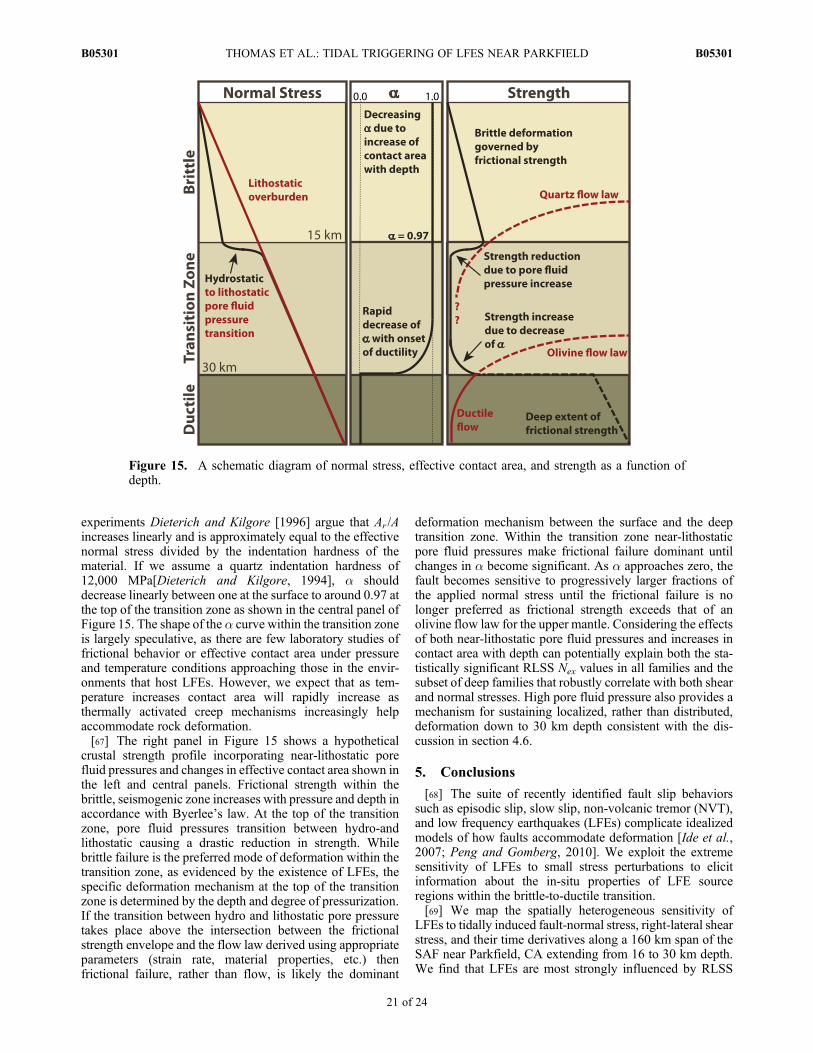
experiments Dieterich and Kilgore [1996] argue that Ar /Aincreases linearly and is approximately equal to the effectivenormal stress divided by the indentation hardness of thematerial. If we assume a quartz indentation hardness of12,000 MPa[Dieterich and Kilgore, 1994], a shoulddecrease linearly between one at the surface to around 0.97 atthe top of the transition zone as shown in the central panel ofFigure 15. The shape of the a curve within the transition zoneis largely speculative, as there are few laboratory studies offrictional behavior or effective contact area under pressureand temperature conditions approaching those in the envir-onments that host LFEs. However, we expect that as tem-perature increases contact area will rapidly increase asthermally activated creep mechanisms increasingly helpaccommodate rock deformation.[67] The right panel in Figure 15 shows a hypothetical

crustal strength profile incorporating near-lithostatic porefluid pressures and changes in effective contact area shown inthe left and central panels. Frictional strength within thebrittle, seismogenic zone increases with pressure and depth inaccordance with Byerlee’s law. At the top of the transitionzone, pore fluid pressures transition between hydro-andlithostatic causing a drastic reduction in strength. Whilebrittle failure is the preferred mode of deformation within thetransition zone, as evidenced by the existence of LFEs, thespecific deformation mechanism at the top of the transitionzone is determined by the depth and degree of pressurization.If the transition between hydro and lithostatic pore pressuretakes place above the intersection between the frictionalstrength envelope and the flow law derived using appropriateparameters (strain rate, material properties, etc.) thenfrictional failure, rather than flow, is likely the dominant

deformation mechanism between the surface and the deeptransition zone. Within the transition zone near-lithostaticpore fluid pressures make frictional failure dominant untilchanges in a become significant. As a approaches zero, thefault becomes sensitive to progressively larger fractions ofthe applied normal stress until the frictional failure is nolonger preferred as frictional strength exceeds that of anolivine flow law for the upper mantle. Considering the effectsof both near-lithostatic pore fluid pressures and increases incontact area with depth can potentially explain both the sta-tistically significant RLSS Nex values in all families and thesubset of deep families that robustly correlate with both shearand normal stresses. High pore fluid pressure also provides amechanism for sustaining localized, rather than distributed,deformation down to 30 km depth consistent with the dis-cussion in section 4.6.

5. Conclusions

[68] The suite of recently identified fault slip behaviorssuch as episodic slip, slow slip, non-volcanic tremor (NVT),and low frequency earthquakes (LFEs) complicate idealizedmodels of how faults accommodate deformation [Ide et al.,2007; Peng and Gomberg, 2010]. We exploit the extremesensitivity of LFEs to small stress perturbations to elicitinformation about the in-situ properties of LFE sourceregions within the brittle-to-ductile transition.[69] We map the spatially heterogeneous sensitivity of

LFEs to tidally induced fault-normal stress, right-lateral shearstress, and their time derivatives along a 160 km span of theSAF near Parkfield, CA extending from 16 to 30 km depth.We find that LFEs are most strongly influenced by RLSS

Figure 15. A schematic diagram of normal stress, effective contact area, and strength as a function ofdepth.


21 of 24

with a surplus of LFEs occurring when the tides are pro-moting slip on the fault. Some families also have significantsensitivity to both positive and negative FNS. The familiesthat correlate with extension generally occur deep in thecreeping section, and their correlation may be a manifestationof the increase in effective contact area with depth. Familiesthat correlate with fault normal clamping are spatially local-ized and coincide with a right-stepping fault bend evident inthe surface fault trace. If the change in fault geometry isresponsible for the anomalous correlations, it would arguethat the San Andreas remains localized to depths near theMoho and that large scale (�10 km) fault morphology pres-ent at the surface is also preserved at depth.[70] The incontrovertible correlation of high pore fluid

pressures and slow slip across tectonic environments sug-gests a causative relationship between the two. Our analysissuggests low effective stress is required to produce the robustresponse of LFEs to the tides. It is worth noting, however,that high pore fluid pressures do not facilitate LFE produc-tion as decreasing effective stress requires increasing sourcedimensions to host unstable slip, making unstable slip onsmall asperities more difficult. The recurrence characteristicsof LFEs are some of the few observational constraints illu-minating the style of deformation in deep fault zones. Wealso find a first-order correlation between deformation styleand tidally induced RLSS, as highly episodic, shallow fam-ilies generally have smaller RLSS Nex values than the deeper,continuously deforming families.[71] The duration and style of loading, and the timing of

earthquakes relative to the application of a load is of con-siderable interest to those studying the roles of static anddynamic stresses in earthquake triggering and the mechanicalimplications of those observations. We find that the timing ofLFEs with respect to tidally induced stresses is consistentwith some aspects of a previously proposed model of earth-quake triggering in response to tidal loading [Beeler andLockner, 2003]. There are, however, some inconsistenciessuch as recurrence times less than the computed LFE nucle-ation time, failure times that correlate with stressing rate, andthe neglected effect of fault creep that limit general applica-bility of the Beeler and Lockner [2003] model.[72] A second order dependence on dRLSS is also present

in the phases of triggering times relative to the tidal load. Astatistically significant number of LFEs trigger preferentiallywhen RLSS magnitude is positive but decreasing. A numberof possible causes could potentially explain the phase shift,including clustering, superposition of the background platerate and the tidal load, or the weak influence of normalstresses that were not considered in previous models. Whileour data cannot resolve if slip events in Parkfield are trig-gered by the tides, the population of events that initiate a slipepisode on a particular asperity are tidally correlated, sug-gesting that tidal forces play a role in slip front propagationspeeds, and/or the onset of slow slip pulses is comparable totidal timescales.

[73] Acknowledgments. We wish to thank David Brillinger for assis-tance in developing the hypothesis testing procedure, Brent Delbridge forproviding us with data related to the Cascadia slip events, Greg Hirth for sug-gestions and conversations which greatly improved this manuscript, FredPollitz for assistance with validating that our Green’s functions are accurate,and Allan Rubin for comments relating to the limitations of the model weconsider in the manuscript. We would also like to thank Michael Manga,

Steve Hickman, Jeanne Hardebeck, and two anonymous reviewers for pro-viding insightful comments and efficiently reviewing a lengthy manuscript.A.M.T. and M.L.R. were supported by the National Science Foundationgraduate research fellowship program. This is Berkeley Seismological Lab-oratory publication 11-8.

ReferencesAgnew, D. C. (1997), NLOADF: A program for computing ocean-tideloading, J. Geophys. Res., 102(B3), 5109–5110.

Ando, R., R. Nakata, and T. Hori (2010), A slip pulse model with faultheterogeneity for low-frequency earthquakes and tremor along plate inter-faces, Geophys. Res. Lett., 37, L10310, doi:10.1029/2010GL043056.

Audet, P., M. G. Bostock, N. I. Christensen, and S. M. Peacock (2009),Seismic evidence for overpressured subducted oceanic crust and mega-thrust fault sealing, Nature, 457, 76–78, doi:10.1038/nature07650.

Bartlow, N. M., D. Lockner, and N. M. Beeler (2010), The effect of wateron triggering of stick slip by oscillatory loading meeting, paper presentedat Southern California Earthquake Center Annual Meeting, Palm Springs,Calif.

Bartlow, N. M., S. Miyazaki, A. M. Bradley, and P. Segall (2011), Space-time correlation of slip and tremor during the 2009 Cascadia slow slipevent, Geophys. Res. Lett., 38, L18309, doi:10.1029/2011GL048714.

Beeler, N. M., and D. A. Lockner (2003), Why earthquakes correlateweakly with the solid Earth tides: Effects of periodic stress on the rateand probability of earthquake occurrence, J. Geophys. Res., 108(B8),2391, doi:10.1029/2001JB001518.

Beroza, G. C., and S. Ide (2011), Slow earthquakes and nonvolcanic tremor,Annu. Rev. Earth Planet. Sci., 39, 271–296, doi:10.1146/annurev-earth-040809-152531.

Bilham, R., and G. King (1989), The morphology of strike-slip faults:Examples from the San Andreas Fault, California, J. Geophys. Res.,941, 10,204–10,216, doi:10.1029/JB094iB08p10204.

Blanpied, M. L., D. A. Lockner, and J. D. Byerlee (1995), Frictional slip ofgranite at hydrothermal conditions, J. Geophys. Res., 100, 13,045–13,064,doi:10.1029/95JB00862.

Boyarko, D. C., and M. R. Brudzinski (2010), Spatial and temporal patternsof nonvolcanic tremor along the southern Cascadia subduction zone,J. Geophys. Res., 115, B00A22, doi:10.1029/2008JB006064.

Brown, J. R., G. C. Beroza, S. Ide, K. Ohta, D. R. Shelly, S. Y. Schwartz,W. Rabbel, M. Thorwart, and H. Kao (2009), Deep low-frequency earth-quakes in tremor localize to the plate interface in multiple subductionzones, Geophys. Res. Lett., 36, L19306, doi:10.1029/2009GL040027.

Brudzinski, M. R., H. R. Hinojosa-Prieto, K. M. Schlanser, E. Cabral-Cano,A. Arciniega-Ceballos, O. Diaz-Molina, and C. DeMets (2010), Nonvol-canic tremor along the Oaxaca segment of the Middle America subduc-tion zone, J. Geophys. Res., 115, B00A23, doi:10.1029/2008JB006061.

Bürgmann, R., and G. Dresen (2008), Rheology of the lower crust andupper mantle: Evidence from rock mechanics, geodesy, and field obser-vations, Annu. Rev. Earth Planet. Sci., 36, 531–567, doi:10.1146/annurev.earth.36.031207.124326.

Cembrano, J., A. Lavenu, P. Reynolds, G. Arancibia, G. Lopez, andA. Sanhueza (2002), Late Cenozoic transpressional ductile deformationnorth of the Nazca-South America-Antarctica triple junction, Tectono-physics, 354, 289–314, doi:10.1016/S0040-1951(02)00388-8.

Cochran, E. S., J. E. Vidale, and S. Tanaka (2004), Earth tides can triggershallow thrust fault earthquakes, Science, 306, 1164–1166, doi:10.1126/science.1103961.

de Juan, J., et al. (2010), Sudden increase in tidal response linked to calvingand acceleration at a large Greenland outlet glacier, Geophys. Res. Lett.,371, L12501, doi:10.1029/2010GL043289.

Dieterich, J. H. (1987), Nucleation and triggering of earthquake slip: Effectof periodic stresses, Tectonophysics, 144, 127–139, doi:10.1016/0040-1951(87)90012-6.

Dieterich, J. H. (2007), Applications of rate- and state-dependent frictionto models of fault slip and earthquake occurrence, in Treatise on Geo-physics, vol. 4, Earthquake Seismology, pp. 107–129, Elsevier, NewYork,doi:doi:10.1016/B978-044452748-6.00065-1.

Dieterich, J. H., and B. D. Kilgore (1994), Direct observation of frictionalcontacts: New insights for state-dependent properties, Pure Appl. Geophys.,143, 283–302, doi:10.1007/BF00874332.

Dieterich, J. H., and B. Kilgore (1996), Implications of fault constitutiveproperties for earthquake prediction, Proc. Natl. Acad. Sci. U. S. A., 93,3787–3794, doi:10.1073/pnas.93.9.3787.

Dragert, H., K. Wang, and T. S. James (2001), A silent slip event onthe deeper Cascadia subduction interface, Science, 292, 1525–1528,doi:10.1126/science.1060152.

Dragert, H., K. Wang, and G. Rogers (2004), Geodetic and seismic signa-tures of episodic tremor and slip in the northern Cascadia subductionzone, Earth Planets Space, 56, 1143–1150.


22 of 24

Fletcher, J. B., and A. McGarr (2011), Moments, magnitudes, and radiatedenergies of non-volcanic tremor near Cholame, CA, from ground motionspectra at UPSAR, Geophys. Res. Lett., 381, L16314, doi:10.1029/2011GL048636.

Ghosh, A., J. E. Vidale, Z. Peng, K. C. Creager, and H. Houston (2009),Complex nonvolcanic tremor near Parkfield, California, triggered bythe great 2004 Sumatra earthquake, J. Geophys. Res., 114, B00A15,doi:10.1029/2008JB006062.

Gomberg, J., J. L. Rubinstein, Z. Peng, K. C. Creager, J. E. Vidale, andP. Bodin (2008), Widespread triggering of nonvolcanic tremor in California,Science, 319, 173, doi:10.1126/science.1149164.

Gu, J., J. R. Rice, A. L. Ruina, and S. T. Tse (1984), Slip motion andstability of a single degree of freedom elastic system with rate and statedependent friction, J. Mech. Phys. Solids, 32, 167–196, doi:10.1016/0022-5096(84)90007-3.

Harkrider, D. G. (1970), Surface waves in multilayered elastic media.Part II. Higher mode spectra and spectral ratios from point sources inplane layered Earth models, Bull. Seismol. Soc. Am., 60(6), 1937–1987.

Hawthorne, J. C., and A. M. Rubin (2010), Tidal modulation of slow slip inCascadia, J. Geophys. Res., 115, B09406, doi:10.1029/2010JB007502.

Heaton, T. H. (1982), Tidal triggering of earthquakes, Bull. Seismol. Soc.Am., 72(6), 2181–2200.

Hill, D. P. (2010), Surface-wave potential for triggering tectonic (nonvolca-nic) tremor, Bull. Seismol. Soc. Am., 100, 1859–1878, doi:10.1785/0120090362.

Hirose, H., K. Hirahara, F. Kimata, N. Fujii, and S. Miyazaki (1999), Aslow thrust slip event following the two 1996 Hyuganada earthquakesbeneath the Bungo Channel, southwest Japan, Geophys. Res. Lett., 26,3237–3240, doi:10.1029/1999GL010999.

Houston, H., B. G. Delbridge, A. G. Wech, and K. C. Creager (2011),Rapid tremor reversals in Cascadia generated by a weakened plate inter-face, Nat. Geosci., 4, 404–409, doi:10.1038/ngeo1157.

Ide, S. (2010), Striations, duration, migration and tidal response in deeptremor, Nature, 466, 356–359, doi:10.1038/nature09251.

Ide, S., G. C. Beroza, D. R. Shelly, and T. Uchide (2007), A scaling law forslow earthquakes, Nature, 447, 76–79, doi:10.1038/nature05780.

Kao, H., S.-J. Shan, H. Dragert, G. Rogers, J. F. Cassidy, andK. Ramachandran (2005), A wide depth distribution of seismic tremorsalong the northern Cascadia margin, Nature, 436, 841–844, doi:10.1038/nature03903.

Kao, H., K. Wang, H. Dragert, J. Y. Kao, and G. Rogers (2010), Estimatingseismic moment magnitude (Mw) of tremor bursts in northern Cascadia:Implications for the “seismic efficiency” of episodic tremor and slip,Geophys. Res. Lett., 371, L19306, doi:10.1029/2010GL044927.

Lambert, A., H. Kao, G. Rogers, and N. Courtier (2009), Correlation oftremor activity with tidal stress in the northern Cascadia subduction zone,J. Geophys. Res., 114, B00A08, doi:10.1029/2008JB006038.

Little, T. A., R. J. Holcombe, and B. R. Ilg (2002), Kinematics of obliquecollision and ramping inferred from microstructures and strain in middlecrustal rocks, central Southern Alps, New Zealand, J. Struct. Geol., 24,219–239, doi:10.1016/S0191-8141(01)00060-8.

Liu, Y., and J. R. Rice (2005), Aseismic slip transients emerge spon-taneously in three-dimensional rate and state modeling of subductionearthquake sequences, J. Geophys. Res., 110, B08307, doi:10.1029/2004JB003424.

Liu, Y., and J. R. Rice (2007), Spontaneous and triggered aseismic defor-mation transients in a subduction fault model, J. Geophys. Res., 112,B09404, doi:10.1029/2007JB004930.

Lockner, D. A., and N. M. Beeler (1999), Premonitory slip and tidal trigger-ing of earthquakes, J. Geophys. Res., 104, 20,133–20,152, doi:10.1029/1999JB900205.

Marone, C. (1998), Laboratory-derived friction laws and their application toseismic faulting, Annu. Rev. Earth Planet. Sci., 26, 643–696.

Marone, C., and B. Kilgore (1993), Scaling of the critical slip distance forseismic faulting with shear strain in fault zones, Nature, 362, 618–621,doi:10.1038/362618a0.

McNutt, S. R., and R. J. Beavan (1984), Patterns of earthquakes and theeffect of solid earth and ocean load tides at Mount St. Helens prior tothe May 18, 1980, eruption, J. Geophys. Res., 89, 3075–3086,doi:10.1029/JB089iB05p03075.

Miller, M. M., T. Melbourne, D. J. Johnson, and W. Q. Sumner (2002),Periodic slow earthquakes from the Cascadia subduction zone, Science,295, 2423, doi:10.1126/science.1071193.

Miyazawa, M., and E. E. Brodsky (2008), Deep low-frequency tremor thatcorrelates with passing surface waves, J. Geophys. Res., 113, B01307,doi:10.1029/2006JB004890.

Murray, J., and J. Langbein (2006), Slip on the San Andreas Fault atParkfield, California, over two earthquake cycles, and the implications

for seismic hazard, Bull. Seismol. Soc. Am., 96, S283–S303, doi:10.1785/0120050820.

Nadeau, R. M., and A. Guilhem (2009), Nonvolcanic tremor evolution andthe San Simeon and Parkfield, Science, 325, 191–194, doi:10.1126/science.1174155.

Nakata, R., N. Suda, and H. Tsuruoka (2008), Non-volcanic tremor result-ing from the combined effect of Earth tides and slow slip events, Nat.Geosci., 1, 676–678, doi:10.1038/ngeo288.

Obara, K. (2002), Nonvolcanic deep tremor associated with subduction insouthwest Japan, Science, 296, 1679–1681, doi:10.1126/science.1070378.

Obara, K. (2010), Phenomenology of deep slow earthquake family in south-west Japan: Spatiotemporal characteristics and segmentation, J. Geophys.Res., 115, B00A25, doi:10.1029/2008JB006048.

Obara, K., H. Hirose, F. Yamamizu, and K. Kasahara (2004), Episodicslow slip events accompanied by non-volcanic tremors in southwestJapan subduction zone, Geophys. Res. Lett., 312, L23602, doi:10.1029/2004GL020848.

Peng, Z., and J. Gomberg (2010), An integrated perspective of the con-tinuum between earthquakes and slow-slip phenomena, Nat. Geosci., 3,599–607, doi:10.1038/ngeo940.

Peng, Z., J. E. Vidale, A. G. Wech, R. M. Nadeau, and K. C. Creager(2009), Remote triggering of tremor along the San Andreas Fault incentral California, J. Geophys. Res., 114, B00A06, doi:10.1029/2008JB006049.

Rice, J. R., and A. L. Ruina (1983), Stability of steady frictional slipping,J. Appl. Mech., 50, 343, doi:10.1115/1.3167042.

Rubin, A. M. (2008), Episodic slow slip events and rate-and-state friction,J. Geophys. Res., 113, B11414, doi:10.1029/2008JB005642.

Rubin, A. M. (2011), Designer friction laws for bimodal slow slip propaga-tion speeds, Geochem. Geophys. Geosyst., 12, Q04007, doi:10.1029/2010GC003386.

Rubinstein, J. L., M. La Rocca, J. E. Vidale, K. C. Creager, and A. G. Wech(2008), Tidal modulation of nonvolcanic tremor, Science, 319, 186–189,doi:10.1126/science.1150558.

Ruina, A. (1983), Slip instability and state variable friction laws,J. Geophys. Res., 881, 10,359–10,370, doi:10.1029/JB088iB12p10359.

Ryder, I., and R. Bürgmann (2008), Spatial variations in slip deficit on thecentral San Andreas Fault from InSAR, Geophys. J. Int., 175, 837–852,doi:10.1111/j.1365-246X.2008.03938.x.

Schmidt, D. A., and H. Gao (2010), Source parameters and time-dependentslip distributions of slow slip events on the Cascadia subduction zonefrom 1998 to 2008, J. Geophys. Res., 115, B00A18, doi:10.1029/2008JB006045.

Scholz, C. H. (2002), The Mechanics of Earthquakes and Faulting,Cambridge Univ. Press, Cambridge, U. K.

Schulz, W. H., J. W. Kean, and G. Wang (2009), Landslide movement insouthwest Colorado triggered by atmospheric tides, Nat. Geosci., 2,863–866, doi:10.1038/ngeo659.

Segall, P., A. M. Rubin, A. M. Bradley, and J. R. Rice (2010), Dilatantstrengthening as a mechanism for slow slip events, J. Geophys. Res.,115, B12305, doi:10.1029/2010JB007449.

Shelly, D. R. (2009), Possible deep fault slip preceding the 2004 Parkfieldearthquake, inferred from detailed observations of tectonic tremor,Geophys. Res. Lett., 36, L17318, doi:10.1029/2009GL039589.

Shelly, D. R. (2010), Periodic, chaotic, and doubled earthquake recurrenceintervals on the deep San Andreas Fault, Science, 328, 1385–1388,doi:10.1126/science.1189741.

Shelly, D. R., and J. L. Hardebeck (2010), Precise tremor source locationsand amplitude variations along the lower-crustal central San AndreasFault, Geophys. Res. Lett., 37, L14301, doi:10.1029/2010GL043672.

Shelly, D. R., and K. M. Johnson (2011), Tremor reveals stress shadowing,deep postseismic creep, and depth-dependent slip recurrence on thelower-crustal San Andreas fault near Parkfield, Geophys. Res. Lett.,381, L13312, doi:10.1029/2011GL047863.

Shelly, D. R., G. C. Beroza, S. Ide, and S. Nakamula (2006), Low-frequency earthquakes in Shikoku, Japan, and their relationship to epi-sodic tremor and slip, Nature, 442, 188–191, doi:10.1038/nature04931.

Shelly, D. R., G. C. Beroza, and S. Ide (2007a), Non-volcanic tremor andlow-frequency earthquake swarms, Nature, 446, 305–307, doi:10.1038/nature05666.

Shelly, D. R., G. C. Beroza, and S. Ide (2007b), Complex evolution oftransient slip derived from precise tremor locations in western Shikoku,Japan, Geochem. Geophys. Geosyst., 81, Q10014, doi:10.1029/2007GC001640.

Shelly, D. R., W. L. Ellsworth, T. Ryberg, C. Haberland, G. S. Fuis,J. Murphy, R. M. Nadeau, and R. Bürgmann (2009), Precise location ofSan Andreas Fault tremors near Cholame, California using seismometerclusters: Slip on the deep extension of the fault?, Geophys. Res. Lett.,36, L01303, doi:10.1029/2008GL036367.


23 of 24

Shelly, D. R., Z. Peng, D. P. Hill, and C. Aiken (2011), Triggered creep as apossible mechanism for delayed dynamic triggering of tremor and earth-quakes, Nat. Geosci., 4, 384–388, doi:10.1038/ngeo1141.

Simpson, R. W., M. Barall, J. Langbein, J. R. Murray, and M. J. Rymer(2006), San Andreas Fault geometry in the Parkfield, California, region,Bull. Seismol. Soc. Am., 96, 28–37, doi:10.1785/0120050824.

Smith, E. F., and J. Gomberg (2009), A search in strainmeter data forslow slip associated with triggered and ambient tremor near Parkfield,California, J. Geophys. Res., 114, B00A14, doi:10.1029/2008JB006040.

Thomas, A. M., R. M. Nadeau, and R. Bürgmann (2009), Tremor-tide cor-relations and near-lithostatic pore pressure on the deep San Andreas fault,Nature, 462, 1048–1051, doi:10.1038/nature08654.

Thurber, C., H. Zhang, F. Waldhauser, A. Michael, J. Hardebeck, andD. Eberhart-Phillips (2006), Three-dimensional compressional wave-speed model, earthquake relocations (1966–2005), and focal mechanisms

for the Parkfield, California, region, Bull. Seismol. Soc. Am., 96, 38–49,doi:10.1785/0120050825.

Vidale, J. E., D. C. Agnew, M. J. S. Johnston, and D. H. Oppenheimer(1998), Absence of earthquake correlation with Earth tides: An indicationof high preseismic fault stress rate, J. Geophys. Res., 103, 24,567–24,572,doi:10.1029/98JB00594.

Waldhauser, F., and D. P. Schaff (2008), Large-scale relocation of twodecades of northern California seismicity using cross-correlation and dou-ble-difference methods, J. Geophys. Res., 113, B08311, doi:10.1029/2007JB005479.

Wech, A. G., and K. C. Creager (2011), A continuum of stress, strengthand slip in the Cascadia subduction zone, Nat. Geosci., 4, 624–628,doi:10.1038/ngeo1215.

Wech, A. G., K. C. Creager, and T. I. Melbourne (2009), Seismic andgeodetic constraints on Cascadia slow slip, J. Geophys. Res., 114,B10316, doi:10.1029/2008JB006090.


24 of 24

tidal triggering of low frequency earthquakes near ... · other subduction zones and tremor on the...

Documents