thÈse de doctorat physique
TRANSCRIPT
UNIVERSITÉ TUNIS-EL MANAR •
FACULTÉ DES SCIENCES DE TUNIS •
THÈSE DE DOCTORAT Discipline
PHYSIQUE
Titre
Investigations on quantum mechanics with minimal
length
YASSINE CHARGUI
Encadrée par :
MR. ADEL TRABELSI
Soutenue le : 2009 Devant le Jury composé par :
Table des matières
1 Abstract 5
Introduction and motivation 7
2 Quantum mechanics with minimal length 11
2.1 The minimal length uncertainty relation in one dimension 11
2.2 The uncertainty relation in multiple dimensions 13
2.3 Other forms of minimal length uncertainty relations 15
2.4 Differential operator representation 18
2.4.1 The Kempf reduction and momentum representation 19
2.4.2 The pseudo-position representation 21
2.4.3 The Brau reduction 22
2.4.4 The general first order reduction family 23
2.4.5 General case with minimal momentum 24
2.5 Recovering information on position 26
2.5.1 Maximal localization states 26
2.5.2 Transformation to quasiposition wave functions 28
2.5.3 Quasiposition representation 30
3 A simple system with minimal length : The harmonic oscillator 33
3.1 Solution of the Schrodinger equation 33
3.2 The path integral framework 37
4 Quantum systems with minimal length 41
4.1 The Klein-Gordon oscillator 42
4.1.1 The Klein-Gordon oscillator in one dimension 42
4.1.2 The Klein-Gordon oscillator in D dimensions 45
3
Table des matières 4
4.2 The Klein-Gordon and Dirac equation with mixed scalar and vector linear
potentials 51
4.2.1 The Klein-Gordon equation 51
4.2.2 The Dirac equation 55
4.3 The one-dimensional spinless Salpeter Coulomb problem 63
4.4 The _D-dimensional harmonic oscillator : path integral approach 71
Conclusion 81
A Proof of (2.21) 85
B Diagonalization of R2 87
Bibliographie 91

Chapitre 1
Abstract
We consider a modified quantum mechanics where the coordinates and momenta are assumed to satisfy a non-standard commutation relation of the form [X%)Pj\ = ih [6%j (l +/3P2) + f3'P%Pj\. Such an algebra results in a generalized uncertainty relation which leads to the existence of a minimal observable length. Moreover, it incorporates an UV/IR mixing and non-commutative position space. We analyze the possible representations in terms of differential operators. The latter are used to study the low energy effects of the minimal length by considering different quantum systems : the harmonic oscillator, the Klein-Gordon oscillator, the spinless Salpeter Coulomb problem, and the Dirac equation with a linear confining potential. We also discuss whether such effects are observable in precision measurements on a relativistic electron trapped in strong magnetic field.
5

Chapitre 1. Abstract 6

Introduction and motivation
In usual quantum mechanics, physical observables are described by operators acting on the Hilbert space of states. The most fundamental ones, the position operator x and momentum operator p satisfy the canonical commutation relation
[x, p] = xp — px = ih (1)
where h is Planck's constant. As a consequence, for the position and momentum uncertainties x and p of a given state, the Heisenberg uncertainty relation holds :
An important consequence is that in order to probe arbitrarily small length-scales, one has to use probes of sufficiently high energy, and thus momentum. This is the principle on which all our accelerators are based. While gravity (and technological and monetary constraints) are neglected, there is in principle no limit to researching smaller and smaller distances using beams of ever increasing energies.
There are reasons to believe, that at high energies, when gravity becomes important, this is no longer true. Namely, increasing a collision's energy above the Planck scale, the extreme energy concentration in a small space will create a black hole with an event horizon behind which we cannot see. It is not unreasonable to suppose that this is not a lack of our experimental sophistication, but nature possesses an absolute minimal length.
So far, attempts to incorporate gravity into relativistic quantum field theory run into problems, because taking into account smaller and smaller length-scales yields infinite results. A hypothetical minimal length could serve as a cutoff for a quantum gravity and remove the infinities.
More stringent motivations for the occurrence of a minimal length are manifold. A minimal length can be found in String Theory, Loop Quantum
7

Introduction and motivation 8
Gravity and Non-Commutative Geometries. It can be derived from various studies of thought-experiments, from black hole physics, the holographic principle and further more. Perhaps the most convincing argument, however, is that there seems to be no self-consistent way to avoid the occurrence of a minimal length scale [1, 2]. Here we expose some elements of the list :
1-In string theory, a minimal length is suggested since strings cannot probe distances smaller than the string scale. If the energy of a string reaches the Planck scale, string excitations can occur causing its extension [3].
2-Loop quantum gravity [4] is a non-perturbative approach to quantum gravity. Via the definition of so-called loop-states, the metric information is expressed in operators which in the classical limit yield the standard space-time picture. In the quantum gravity regime, it turns out that some of these operators, e.g. the area operator, have a discrete spectrum which gives rise to a smallest-distance structure.
3-Non-commutative geometries [5] modify the algebra of the generators of space-time translations such that position measurements fail to commute. The commutation relation is replaced with
ii j \ ij \ )
where the tensor 9 has a dimension of a length squared and measures the scale at which the non-local effects become important. This modification can be pursued throughout the usual development of quantum field theories, leading to a non-local theory. It can be shown [6] that within this approach a Gaussian distribution naturally exhibits a maximally possible localization of width ~ 9.
4-A minimal length can be found from the holographic principle, which states [7] that the degrees of freedom of a spatial region are determined through the boundary of the region and that the number of degrees of freedom per Planck area is no greater than unity. This leads to a minimal possible uncertainty in length measurements [8].
5-In the approach by Padmanabhan et al [9], the path integral amplitude is made invariant under a duality transformation which replaces a length, x,
I2
by x —>• —. The proper distance between two events in space-time, Ax2, then x
is replaced by Ax2 —>• I2 + Ax2, yielding a 'zero point length' of spacetime. Due to this, the divergences in quantum field theories are regularized by removing the small distance limit.

Introduction and motivation 9
6-Several phenomenological examinations of possible precision measurements [10], thought experiments about black holes [11] or the general structure of classical [12], semi classical [13] and quantum-foamy space-time [8]. All of them lead to the conclusion that there exists a fundamental limit to distance measurement.
The above listed points are cross-related in many ways. Point (3) arises as a limit of string theory and also the imposed duality in (5) is motivated by String T-duality. The holographic Principle has its origin in black hole physics and black hole physics itself connects to almost every point mentioned before.
It should be noted that all arguments predict a minimal length which is on a scale comparable to the Planck length, and such the energies involved in probing them are way beyond what we can produce on Earth today. However, there is the possibility that nature possesses large extra dimensions [14, 15]. In such scenarios, the Planck scale and minimal length might be within experimental reach in future accelerators, such as the Large Hadron Collider, which was recently developed at CERN in Geneva, Switzerland, or at the planned International Linear Collider.
Even if large extra dimensions will not be confirmed in the near future and even without a complete theoretical description of quantum gravity, one can gain considerable insight studying a low energy theory incorporating a minimal length.
From a quantum-theoretical point of view, it is a natural assumption that a minimal length should be introduced as an additional uncertainty in position measurements, so that the standard Heisenberg uncertainty relation becomes :
AX ~ \ (^ + PAp) (4)
with (3 a small positif parameter of dimension of inverse momentum squared. This implies the existence of a minimal length
(Ax)mm = hy/p (5)
below which the uncertainty in position, Ax, connot be reduced. Eq.(4) does embody an intriguing UV/IR relation : when Ap is large (UV), Ax is proportional to Ap and therefore is also large (IR). This type of UV/IR mixing has appeared in several other contexts : the AdS/CFT correspondence [16], non-commutative field theory [17], and more recently in attempts at understanding quantum gravity in asymptotically de Sitter spaces [18]. Furthermore,

Introduction and motivation 10
the UV/IR relation represented by Eq.(4) suggests that certain "stringy" short distance (UV) effects may manifest themselves at longer distances (IR). This lends an additional justification to the analysis of quantum mechanical problems in the presence of a minimal length.
Before closing this chapter, let us remark that, in addition to its importance in high energy physics, a minimal length may be of great interest in nonrelativistic or relativistic quantum mechanics. Indeed, it has been been argued [19, 20] that this length may be viewed as an intrinsic scale characterizing the system under study. Consequently, the formalism involving such a fundamental length may provide a new model for the description of complex system such as quasiparticles and various collective excitations in solids, or composite particles such as nucléons, nuclei and molecules [19].

Chapitre 2
Quantum mechanics with minimal length
As has been already mentioned, the idea of minimal length may be implemented by modifying the Heisenberg uncertainty relation to the form (4). In this way, this length will define a nonzero lower bound for the uncertainty in position measurements. The modified uncertainty principle, in turn, may be obtained by simply supposing that coordinates no longer commute in D-dimensional space. This leads to a deformation of the canonical commutation relations. This was the sprit of Kempf [19, 21, 22, 23] who have assumed that the fundamental commutation relation between position and momentum are non longer constant multiples of the identity, as an equivalent hypothesis which leads to uncertainty relation (4). Since it is the same assumption adopted in our works, we devote this chapter to study in full detail its quantum-mechanical contents.
2.1 The minimal length uncertainty relation in one dimension
We will mainly investigate the consequences of the following minimal-length relation [22]
[X, P] = ih (1 + (3P2) (2.1)
While we will assume that this form is exact, it can also be interpreted as a first order expansion of a relation of the form
[X, P] = ihf (P) (2.2)
11
Chapitre 2. Quantum mechanics with minimal length 12
<-very close for small energies
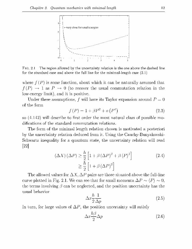
FIG. 2.1 - The region allowed by the uncertainty relation is the one above the dashed line for the standard case and above the full line for the minimal-length case (2.1)
where / (P) is some function, about which it can be naturally assumed that / (P) —>• 1 as P —>• 0 (to recover the usual commutation relation in the low-energy limit), and it is positive.
Under these assumptions, / will have its Taylor expansion around P = 0 of the form
/ (P) = 1 + (3P2 + o (P 4 ) (2.3)
so (4.142) will describe to first order the most natural class of possible modifications of the standard commutation relations.
The form of the minimal length relation chosen is motivated a posteriori by the uncertainty relation deduced from it. Using the Cauchy-Bunyakovski-Schwartz inequality for a quantum state, the uncertainty relation will read [22]
(AX) (AP) > | [l +(3 ( A P ) 2 +(3 ( P ) 2
> - i + (3(Apy
(2.4)
The allowed values for AX, A P pairs are those situated above the full-line curve plotted in Fig. 2.1. We can see that for small momenta A P ~ (P) ~ 0, the terms involving (5 can be neglected, and the position uncertainty has the usual behavior
(2-5) Ax 2Ap
In turn, for large values of A P , the position uncertainty will satisfy
Ax—A» 2 y (2.6)

Chapitre 2. Quantum mechanics with minimal length 13
in concordance with the UV/IR mixing mentioned above. Moreover, it transpires that we have a minimal position uncertainty of a state of
A X > ^ 2 ( l + +/3(P)2) (2.7)
and an absolute minimum uncertainty of
AX > (AX)m m = h ^ (2.8)
2.2 The uncertainty relation in multiple dimensions
When dealing with more than one dimensions D > 1, (4.142) can be generalized tonsorially to the form [22]
[Xi, P,\ = ih [Sij (1 + /3P2) + (3'nPj] . (2.9)
The additional parameter /3', with units of inverse momentum squared is again assumed to be small.
With such commutation relations we can no longer assume that both position operators on one hand, and momentum operators, on the other, commute among themselves. The reason for this is that the positions and momenta need to satisfy the Jacobi identity :
[[A, B],C} + [[C, A],B] + [[B, C],A] = 0, VA,B,Ce {P„ P3}%3 (2.10)
which is necessary for the existence of a representation of the observables as linear differential operators acting on some function space.
As the right-hand side of (2.9) depends explicitly on the momentum operators Pi: it is convenient to assume that they commute
[Pi,Pi\=0 (2.11)
Then the following Jacobi identities involving at least 2 momenta,
[[Pi, Pj], Pk] + circ.perm. = 0 (2.12)
[[Ph Pj], Xk] + circ.perm. = 0 (2.13)
are automatically satisfied. From the condition
[[X%, Xj], Pk] + circ.perm. = 0 (2.14)
Chapitre 2. Quantum mechanics with minimal length 14
one can obtain the commutator of positions up to a term depending on
momenta only. It is given by :
[*• *A = ~ ?S/' l 3 P 2 M - P*) + / (A, -, ft,) (2.15) If one assumes that the P-dependent function / is null, the final Jacobi identity, involving position operators only, is automatically satisfied. While the vanishing of / is sufficient for having a well-defined Heisenberg algebra, it is not obvious if, for arbitrary dimensions, this condition is also necessary. For example, in 3 dimensions, on tensorial considerations alone, a term proportional to
eijkPk9 (P2) (2-16)
is allowed on the right hand side for the commutator [Xi}Xj]. This term is odd under the parity transformation X% —>• — JQ, and P% —>• — P%. So including this term would have meant that we believe the interactions giving rise to minimal lengths intrinsically violate parity conservation. That is an intriguing possibility, but we will not consider it here ; we will assume that the P-dependent function / always vanishes.
The important point is that the position operators for different coordinates can no longer commute and we deal with a non-commutative Heisenberg algebra. It should be noted that this is an extra feature of the theory (not a bug, as a well-known software company would say), as most theories of quantum gravity seem to incorporate non-commutativity in some way.
In summary, the complete set of commutation relations read
[Xi, Pi\ = ih [Sij (1 + /3P2) + / 3 ' P ^ ] . (2.17)
[Pi,Pi\ = 0 (2.18
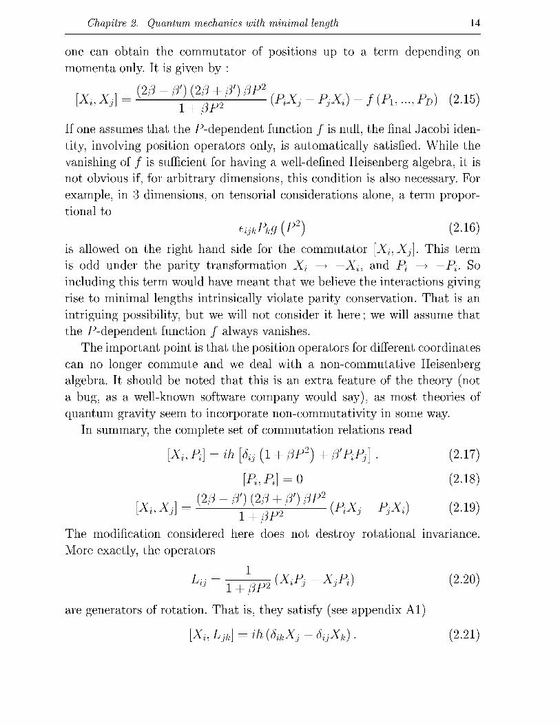
The modification considered here does not destroy rotational invariance. More exactly, the operators
Lij = T^p2(XiPj-XjPi) (2.20)
are generators of rotation. That is, they satisfy (see appendix AT
[X{, Ljk] = ih {ô%kXj — 6%jXk). (2.2T

Chapitre 2. Quantum mechanics with minimal length 15
[Pi,Ljk]=ih(6ikPj-6ijPk). (2.22)
and
[Lij, Lu] = ih {ô%kLji + ôjiLik — ôuLjk — SjkLn) (2.23)
This is very useful when dealing with systems with rotational symmetry.
2.3 Other forms of minimal length uncertainty relations
It should be noted that the uncertainty relations considered are not unique ; several forms, more or less different, have been considered in the existing literature.
Early papers Apparently the first articles to present a theory with quantized space-time
are due to Snyder [24, 25] and Yang [26]. The relative age of these papers, from the late 1940's, is not surprising as their intention was to find a way to remove the infinite results plaguing the early stages in the development of quantum field theory. The renormalization program for Yang-Mills theories provided an alternative way to resolve these problems for the electro-weak and strong interactions, but did not help in quantum gravity, which cannot be renormalized.
In [25], Snyder considers a de Sitter space, with real coordinates
{no^ViM^m} satisfying
-n2 = nl-1]\ - r i l - r i l - r i l (2.24)
and defines the position and time operators by
x* =ia ( m i r - Vi-zr) > « = i ,2 ,3 (2.25)
^ + r / o ^ - > ) , (2-26)
acting on a functions of variables 7/0, ...,7?4, and where a is a natural unit of length, and c is the speed of light. The spectrum of each position operator is discrete, but the theory is Lorentz invariant in the following sense : every linear transformation (Xi} T) —>• (JC-, T') that leaves the quadratic form

Chapitre 2. Quantum mechanics with minimal length 16
c 2 ^ 2 _ xf — X\ — X\ invariant, leaves the operators' spectrum invariant,
too.
In addition, the energy and momentum operators are defined as
P, = \ (J) (2.27)
P ~ I ( Ï ) <«" thus the commutators between positions and momenta are given by
a 2
[Xi,PÙ=ih[l + -sPt) (2.29) h
,2
[Xi, Pj\ = M [ 72pipj ) (2-3°) a
J" This algebra described by Snyder corresponds to our minimal length com-
«2
mutation relation with (3 = 0 and (3' = -r? Modified de Broglie relation To incorporate a minimal length scale Lf in their theory, in [28] and sub
sequent papers, Hossenfelder et al. start out by postulating a non-standard relation between the momentum and wavelength (and thus wave number) of a particle of the form
k = k{p) (2.31)
where k (p) is an odd function that is close to linear for small values of p, and asymptotically approaches some upper limit Mf ~ -£- for large ones. Such a function will have the small p expansion
k(v)=V-ljf2 (2-32)
where 7 is a unitless coefficient of order one that depends on the exact form of the function k(p): which is not determined from first principles. Postulating canonical commutation relations between x and k, this leads to a generalized uncertainty principle of the form
[Ax) (Ap) > 1 dp
~dk
^
f l + 7 ^ ] (2.33)
Chapitre 2. Quantum mechanics with minimal length 17
and a generalized commutation relation
%p]=i% = iK\l + i i H \ (2.34)
This is just (4.142) with (5 = fa.
A minimal m o m e n t u m also One problem of the minimal length commutation relation (2.9), even if
an aesthetic one, is that it destroys the symmetry between the position and momentum in the Hamiltonian formalism. Indeed, it is possible that nature possesses not only a minimal length, but also a minimal momentum. This can be possible if there held an uncertainty relation of the form
(AX) (AP) > 5 |"i + a (AX) 2 + j3 (AP) 2 ] (2.35)
To obtain such an expression, the commutator [X%) Pj] would need to depend not only on momentum P but also position X . For example, Kempf in [21] considered
[Xi, Pi\ = ihSij (1 + aX2 + /3P2) (2.36)
where the small parameter has the dimension of inverse length squared, and that of inverse momentum squared. Obviously this is not the most general tensorial form for arbitrary dimensions. One can include X^Xj and P%Pj
terms and even crossed ones. The analysis of such theories is further complicated by the fact that in ge
neral neither position nor momentum operators can commute among themselves, and thus there is no representation in which either set is diagonal. Consequently, there are few results pertaining to them [21, 29].
Alternative approaches wi th minimal length It should be mentioned that postulating non-standard commutation rela
tions between the position and momentum operators is not the only way to define a theory with minimal length. Two approaches seem to be especially promising.
First, the doubly relativistic Lorentz group studied by Amelino-Camelia [30] and collaborators centers on the group of transformations that have two invariants. In addition to the constant speed of light, it also assumes a constant minimal length.
Chapitre 2. Quantum mechanics with minimal length 18
Second, the postulate of Padmanabhan and his collaborators about the path integral invariance under a duality transformation mentioned in the first chapter.
2.4 Differential operator representation
In the following we will look at the representations in terms of differential operators of the minimal-length commutation relations (2.17) — (4.45) [21]
[Xi, Pil = ih [Sij (1 + /3P2) + p'P.Pj] .
[Pi,Pil = 0
. (2/3 - /3 ' ) (2/3 +/3')/3P2
(2.37)
(2.38)
(2.39) i - r jjr-
While quantum mechanical problems in this context can sometimes be solved by an elegant algebraic approach, for example by introducing ladder operators in the case of harmonic oscillator [19], or by SUSYQM factorization [28], this is not always possible.
The fail proof method, not unlike in regular quantum mechanics, seems to be finding a representation of the operators X%, Pj in terms of self-adjoint differential operators acting on some Hilbert space of functions. Various papers, treating quantum mechanical systems either analytically or perturbatively, have used quite a number of different representations. The common characteristic, though usually not explicitly stated, is that the representation can be found by a two-step process. First, the operators X%,Pj are expressed in terms of some operators x%,pj that satisfy the commutation relations of the canonical Heisenberg algebra,
[xi,pj] = ihôij, [xi7Xj] = [pi7Pj] = 0 (2.40)
Second, for the commutative xi}pj, one can use either the momentum representation
d Xi = ih—, pi =ph (2.41)
dpi acting on functions of variable p, or the position one
d Pi = ih—, Xi = Xi, (2.42)
OXi
Chapitre 2. Quantum mechanics with minimal length 19
acting on functions of variable x.
To differentiate between the two sets of operators, Xi}Pj on one hand, and Xi,Pj on the other, in this thesis we will always denote noncommutative variables with capital letters, and the underlying canonical/commutative ones by lowercase ones. We will also omit the "hat"s from these operators from now on. We will call a particular way of expressing the noncommuting operators in terms of commuting ones a reduction.
It should also be mentioned that the physical observables are the non-commuting, "up-percase" ones. The commuting operators are just helper variables ; we will see that they depend on the reduction chosen, and one should resist the temptation of assigning them general physical meaning. This should be kept in mind, even when for simplicity we use the terms "underlying position" or "underlying momentum" for them.
Let us review the reductions used so far in the literature, their domain of usability and relative strengths.
2.4.1 The Kempf reduction and m o m e n t u m representation
The original reduction, defined in paper [21] that introduced the form of the commutation relations considered here, is the Kempf reduction
2 2
Xi = Xi+ (5P Xl + XlV + p,PiPjXj + XjPiPj (2.43)
Pi = ft (2-44)
It can be said that this reduction is somehow the most natural ; its expression follows closely the one for the commutation relation [JQ,P^]. The only difference is that on the right hand side the order of operator products is symmetrized. This is done to ensure that, at least formally, the non-commutative operators are self-adjoint.
We will call momentum representation this reduction together with a momentum-diagonal representation of the underlying momentum p,
d Xi = ih—, Pi=Pi, (2.45)
dp
as used first in [21]. Explicitly, it is
X- = ih {1+m^+fjl9+L + R±lfAPi (2.46)

Chapitre 2. Quantum mechanics with minimal length 20
Pi = P* (2-47)
Refs. [30, 31] also use a closely related representation. There, the operators'
expressions are
X- = ih d d
(i + fjp2) — + p'piPj-Q- + m (2.48)
Pi = P* (2-49)
where 7 is an arbitrary parameter, and the operators are acting on the Hilbert space of functions normalizable with respect to the inner product
W'-lwïntf™9® (2'50) with
This reduces to the momentum representation for
7 = 7 o : = / 3 + / 3 ' ( ^ i ) (2.52)
in which case the weight function of the inner product has vanishing exponent
à = (70 — 7) / (P + /3/), and thus it simplifies to unity. This apparent generality given by the extra term turns out to be unim
portant. Indeed, we can observe at first that can be supposed to be real. Any complex part can be transformed away using a canonical transformation of the form P% —>• Pt, X% —>• X% + r)Pl. (See Appendix A.2.)
For real 7,and corresponding 6 given by (2.51), one can define A to be
the multiplication operator by [l + (/3 + ff) p2~^
i (p) - • Ai) (p) = [1 + (/3 + /3') p2]6/2 i{p) = i) (p) (2.53)
It is easy to see that a function \jj (p) is normalizable under the canonical inner product (., .)0 , if and only if ip (p) = Ai[) (p) is normalizable under (., .)s. Thus, the operator A is an isomorphism between the function spaces of physical states defined by the two inner products.
Chapitre 2. Quantum mechanics with minimal length 21
Moreover, A obviously commutes with the momenta P^ and for the position operators X%1 it can be veri ed using (2.48) that
XiA$ (p) = Xi1> (p) = A Xiî) (p)
where
Xi=Xi + ins (p + p') Pi
(2.54)
(2.55)
ifi
ifi
d d 0- + PP) 7T + / 5 V i ô - + (7 + HP + P')) V dp dPj
d d (1 + fjp2) — + (3'piPj-Q- + 7oP,
is just the position operator corresponding to 70 ! This shows that the representation (2.48) — (2.49) with arbitrary is equivalent to the momentum representation through the simple change of variable
^(p)=[l + (/3 + /3V l V 2 4 ) ( P ) . (2.56)
In calculational terms this means that, when explicitly trying to solve the differential Schrodinger equation, such a change of variable removes any dependence. An example of this happening appears in [31].
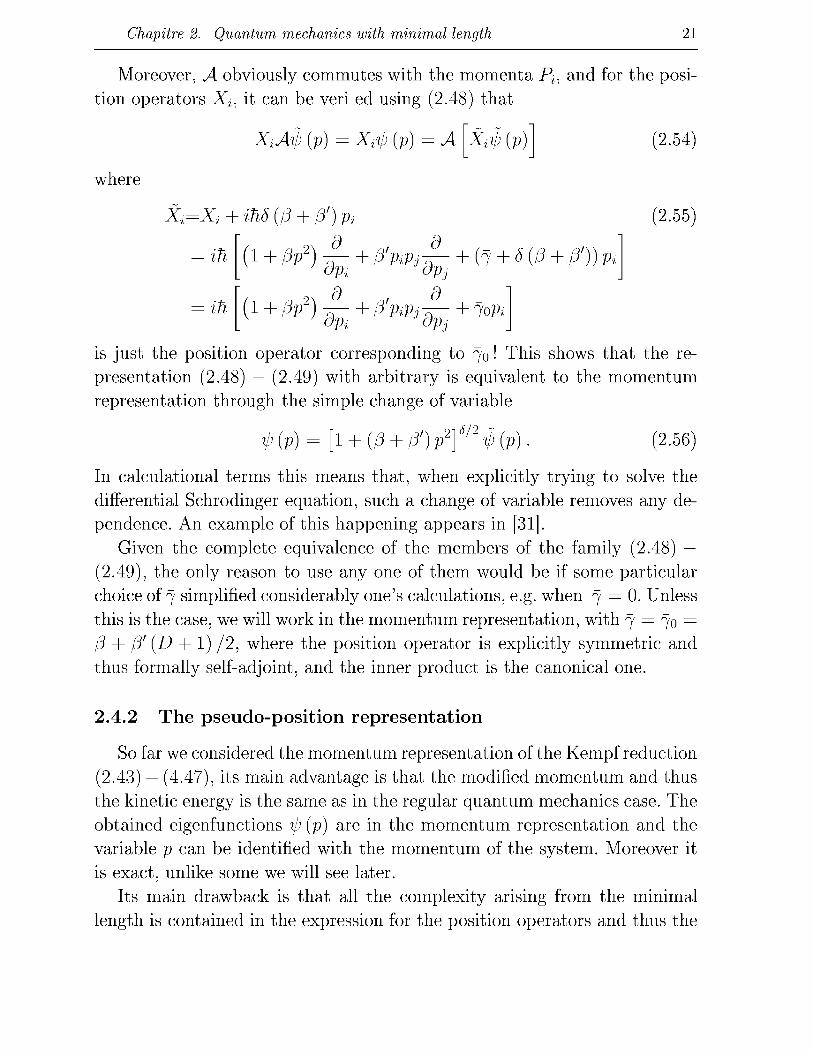
Given the complete equivalence of the members of the family (2.48) — (2.49), the only reason to use any one of them would be if some particular choice of 7 simplified considerably one's calculations, e.g. when 7 = 0. Unless this is the case, we will work in the momentum representation, with 7 = 70 = (5 + (5' (D + 1) / 2 , where the position operator is explicitly symmetric and thus formally self-adjoint, and the inner product is the canonical one.
2.4.2 The pseudo-posit ion representation
So far we considered the momentum representation of the Kempf reduction (2.43) — (4.47), its main advantage is that the modified momentum and thus the kinetic energy is the same as in the regular quantum mechanics case. The obtained eigenfunctions \\) (p) are in the momentum representation and the variable p can be identified with the momentum of the system. Moreover it is exact, unlike some we will see later.
Its main drawback is that all the complexity arising from the minimal length is contained in the expression for the position operators and thus the
Chapitre 2. Quantum mechanics with minimal length 22
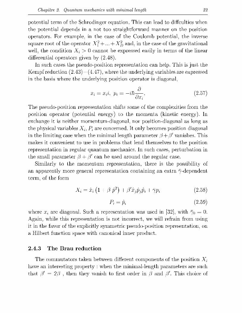
potential term of the Schrodinger equation. This can lead to diffculties when the potential depends in a not too straightforward manner on the position operators. For example, in the case of the Coulomb potential, the inverse square root of the operator X\ + . . . + Xp and, in the case of the gravitational well, the condition X% > 0 cannot be expressed easily in terms of the linear differential operators given by (2.48).
In such cases the pseudo-position representation can help. This is just the Kempf reduction (2.43) —(4.47), where the underlying variables are expressed in the basis where the underlying position operator is diagonal,
d Xi = Xii, p% = -itiT—, (2.57)
OXi
The pseudo-position representation shifts some of the complexities from the position operator (potential energy) to the momenta (kinetic energy). In exchange it is neither momentum-diagonal, nor position-diagonal as long as the physical variables X%) P% are concerned. It only becomes position diagonal in the limiting case when the minimal length parameter /3 + /3' vanishes. This makes it convenient to use in problems that lend themselves to the position representation in regular quantum mechanics. In such cases, perturbation in the small parameter /3 + f3' can be used around the regular case.
Similarly to the momentum representation, there is the possibility of an apparently more general representation containing an extra 7-dependent term, of the form
Xi = Xi(l + /3 f) + /3'xjPjPi + *fpi (2.58)
Pi = Pi (2-59)
where Xi are diagonal. Such a representation was used in [32], with 70 = 0. Again, while this representation is not incorrect, we will refrain from using it in the favor of the explicitly symmetric pseudo-position representation, on a Hilbert function space with canonical inner product.
2.4.3 The Brau reduction
The commutators taken between different components of the position X%
have an interesting property : when the minimal-length parameters are such that (5' = 2/3 , then they vanish to first order in (5 and (5'. This choice of

Chapitre 2. Quantum mechanics with minimal length 23
parameters has theoretical advantages in that it simplifies the way a translation operator can be defined [19]. For this particular case, there is a very simple reduction of the form
X% = Xi (2.60)
Pi = ft (1 + Pp2) (2.61)
usually used in the case when the underlying positions are diagonal. For this reduction, defined first in [34], we use the name Brau reduction.
It should be noted that this representation is only correct to the first order in f3' = 2/3. However, to this order it is position-diagonal. It is particularly convenient for doing perturbation theory around regular position-space ei-genfunctions of some systems. Suppose we deal with a Hamiltonian of the general form
H = ^ + V(X) (2.62)
and we know the exact solution for the /3 = 0 case corresponding to Ho = 2
^ + V (x). Then, the perturbing potential is simply
H' = H-H0 (2.63)
_P^_f_ 2m 2m
= lp* + o (if) m
2.4.4 The general first order reduction family
One might be tempted to prescribe the odd behavior of the Brau representation, which corrects the kinetic term instead of the potential ones, to some quirk of the case /3' = 2/3. It turns out this is not the case.
In [34], Stetsko and Tkatchuk introduced a representation which satisfies the minimal length commutation relations (2.17) — (4.45) up to first order in /3, /3' and generalizes the Brau representation for /3' 2/3. It is given by
2/3 — 8' X, = x,+ ' P (xiP
2 + p2Xi) (2.64)
Pi = ft 1 + 7TP2 (2-65)
Chapitre 2. Quantum mechanics with minimal length 24
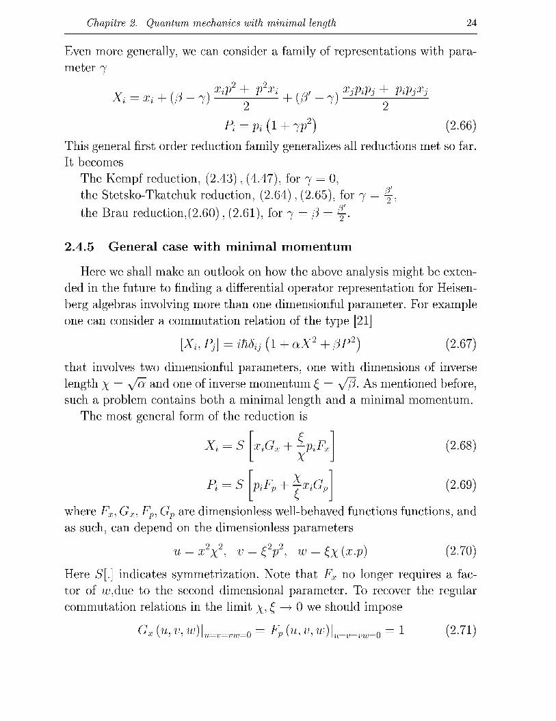
Even more generally, we can consider a family of representations with parameter 7
Xi = Xi + (P- 7) Xzp2 + p2Xi + (/?' - 7) XjPiPj + PiPjXj
ZJ ZJ
P* = P* (1 + IV2) (2-66)
This general first order reduction family generalizes all reductions met so far. It becomes
The Kempf reduction, (2.43), (4.47), for 7 = 0, the Stetsko-Tkatchuk reduction, (2.64), (2.65), for 7 = ^
the Brau reduction,(2.60), (2.61), for 7 = /3 = f /?' 2 '
2 •
2.4.5 General case wi th minimal m o m e n t u m
Here we shall make an outlook on how the above analysis might be extended in the future to finding a differential operator representation for Heisen-berg algebras involving more than one dimensionful parameter. For example one can consider a commutation relation of the type [21]
[Xh Pj] = ihôij (1 + aX2 + fJP2) (2.67)
that involves two dimensionful parameters, one with dimensions of inverse length x = y/oi. a n d one of inverse momentum £ = y//3. As mentioned before, such a problem contains both a minimal length and a minimal momentum.
The most general form of the reduction is
Xi = S
P = S
X
X Vi"p ' £ "Ei^Jp
(2.68
(2.69)
where Fx, Gx, Fp} Gp are dimensionless well-behaved functions functions, and as such, can depend on the dimensionless parameters
u = x2x2, V = C2P2, w = ^x(x.p) (2.70)
Here S[.} indicates symmetrization. Note that Fx no longer requires a factor of u;,due to the second dimensional parameter. To recover the regular commutation relations in the limit X-, £ ~^ 0 w e should impose
Gx(u,v,w)\u=v=vw=0 = Fp(u,v,w)\u=v=vw=0 = 1 (2.71)

Chapitre 2. Quantum mechanics with minimal length 25
and that the second term in both expressions vanishes in the same limit. The symmetrization (on the orders of factors of operators in the expres
sions of Xi, Pi) should be carried out to make the non-commutative operators self-adjoint. There is an additional diffculty here. The symmetrization operator is not unique. One possibility is to define
b [Oil-, 0L2 , ..., (ln\ (l\(l2---0bn + (ln...(l20b\
(2.72)
However for a well-chosen symmetrization functional, we can have the following property : for arbitrary operators A; B, the commutator can be calculated as
lhlXi'Pjl S dA dB dB dA
dxk dpk dxk dph {AB} s
Introducing the dimensionless
Pz = &i, Pi = £P{ = PzFp + XzGp
.Jui
the commutator of the position and momentum reads
4 [S [A], S [B] in
S dXi dP; dXi dP;
dx k vpk dx k
(2.73)
(2.74)
(2.75)
S[C] (2.76)
where C has 42 terms, 2 corresponding to 6%j, and 10 each to x%Xj, x%pj,p%Xj, and PiPj.
This is the expression of the commutator independent of the exact form of the Heisenberg algebra chosen. Now let us particularize to case of (2.67). The right-hand side, expressedin terms of the dimensionless variables, is
l+aX2+(3P2 = l + {G2p + G\) u+(F2 + F2) v+2 (FPGP + FXGX) w (2.77)
Imposing that this expression equals to C, (apart form a symmetrization), one obtains five (differential) equations. Solving them is not straightforward, so we might try to find a first order solution only. Let us expand each undetermined function in the form
Fx (u, v, w) = fx + fxuu + fxvv + fxww + o (u, v, w)' (2.78)
We will have a total of 14 parameters : four parameters each for four functions, less two, as fp = gx = 1 is determined from (4.113). In turn we have to satisfy

Chapitre 2. Quantum mechanics with minimal length 26
five relations between the functions, which translate to 4 x 5 = 20 equations to solve. So the general case is overdetermined, and not every Heisenberg algebra admits representations in terms of differential operators. In particular, (2.67) seems to have no solution.
2.5 Recovering information on position
Generally, in quantum mechanics all information on position is encoded in the matrix elements of the position operator. Matrix elements can of course be calculated in any basis, e.g., also in the momentum eigenbasis. We now no longer have any position eigenbasis of physical states \x) whose matrix elements (x \I/J) would have the usual direct physical interpretation about positions. Nevertheless, all information on position is of course still accessible. To this end let us study the states which realize the maximally allowed location.
2.5.1 Maximal localization states
Let us explicitly calculate the states \i^¥L) of maximal localization around a position £, i.e., states which have the properties
# L | xk ; f L )=£ (2.79) x \A\n
and (AX)^ML^ = Ax0. (2.80)
We know that A^o is (p) dependent. Recall that the absolutely smallest uncertainty can only be reached for (p) = 0.
Let us reconsider the (standard) derivation of uncertainty relation. For each state in the representation of the Heisenberg algebra (actually we need \ip) to be in a domain where x, x2 , p and p 2 are symmetric) we deduce from the from the positivity of the norm
> 0 (2.81) ^-^) + ^êr2(p-(p)))\^ 2(Ap)2
that (note that ([x,p]) is imaginary)
(V'l (x - <x»2 - (^gfiY(P - {P)f IV'} > 0, (2.82)
Chapitre 2. Quantum mechanics with minimal length 27
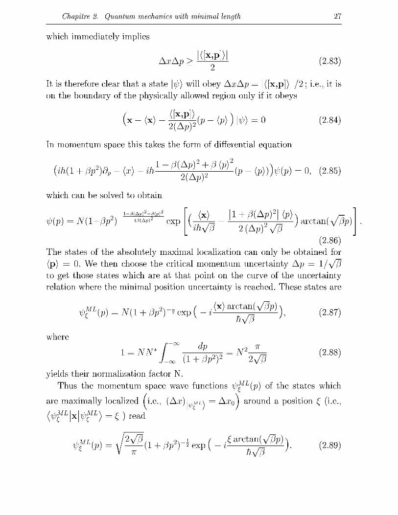
which immediately implies
AxAp > l x [ X 'P J / l (2.83)
It is therefore clear that a state \ip) will obey AxAp = |([x,p])| /2 ; i.e., it is on the boundary of the physically allowed region only if it obeys
(x - <x> + ^0jr2(p - (p) ) |V> = 0 (2.84)
In momentum space this takes the form of differential equation
(ih(l + {3p2)dp - (x) + ^ l + ^ l v y H P ) (P ~ (P)))1>(P) = 0, (2-85)
which can be solved to obtain
[1 + fJ(Ap) _ l + /3(Ap)z+/3<p)z
ip(p) = N(l+f3pz) w±p)2 exp
(2.86) The states of the absolutely maximal localization can only be obtained for (p) = 0- We then choose the critical momentum uncertainty Ap = l/y/]3 to get those states which are at that point on the curve of the uncertainty relation where the minimal position uncertainty is reached. These states are
^(p) = N(l + ^ ) " i exp ( - i < X > a r ; y P ) ) , (2.87)
where
1 = NN* I °° - — ^ - - = N2-^= (2.88) l o o ( 1 + / V ) 2 2 v ^ V '
yields their normalization factor N.
Thus the momentum space wave functions i[)¥L(p) of the states which
are maximally localized (i.e., (Ai) i ,M i \ = A^o) around a position £ (i.e.,
i/>fL|x|i/>fL) = 0 read
«= \ /W ( i + '* 2 ) _ é e x p ( -» c a r c ;y ) . (2.89)

Chapitre 2. Quantum mechanics with minimal length 28
3.0
2.5
2.0
1.5
1.0
0.5
0.0
' ' / " ; /
: /
: /
; /
: /
:p- y
• , , , _
\ :
\ :
\ :
\ :
\ :
>—^—7-
FlG. 2.2 - Plotting < ip^L \ ^ f L > over f - f in units of k^ = Ax0
These states generalize the plane waves in momentum space or Dirac 6 "functions" in position space which would describe maximal localization in ordinary quantum mechanics. Unlike the letter, the new maximal localization states are now proper physical states of finite energy :
t ML
2m 1>, ML 1V/3 dp p 1 (2.90)
/ n J^ ( l + /3p2)22m 2m/3 '
Because of the "fuzziness" of space, the maximal localization states are in general no longer mutually orthogonal :
< i^L | i)fL >--
2 v ^ dp
71
2 v ^
*, (1+/3P 2 ) 2
-*/2 dv 1
exp .(^-^OarcWv^p)
hyft )
71
1
71
J-TT/2
i - f )
Vfii + SHM COS2 (ft)
(t-Z
exp
i - i
K - £')
2hy/P v 2Ky/P \^T7W) S 1 IH
-p )
(2.91
(2.92)
2hy^3 •TT). (2.93)
The poles of the first factor are canceled by zeros of the sine function. For the width of the main peak note that this curve yields the overlap of two maximal localization states, each having a standard deviation A^o (see Fig. 2.2).
2.5.2 Transformation to quasiposit ion wave functions
While in ordinary quantum mechanics it is often useful to expand the states \I/J) in the position "eigenbasis" {\x)} as < x \ ifj >, there are now no
Chapitre 2. Quantum mechanics with minimal length 29
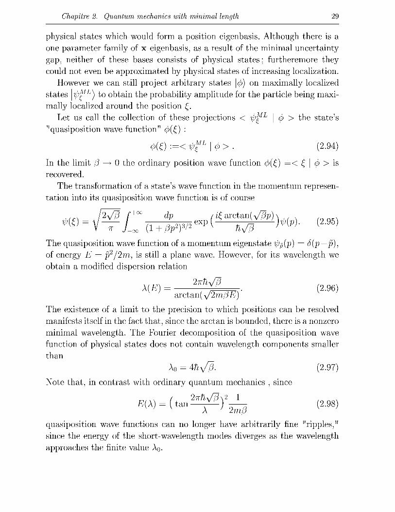
physical states which would form a position eigenbasis. Although there is a one parameter family of x eigenbasis, as a result of the minimal uncertainty gap, neither of these bases consists of physical states ; furtheremore they could not even be approximated by physical states of increasing localization.
However we can still project arbitrary states |0) on maximally localized states i[)¥L^ to obtain the probability amplitude for the particle being maximally localized around the position £.
Let us call the collection of these projections < il)¥L \ <f> > the state's "quasiposition wave function" (/>(£) :
m :=< ^fL I 0 > . (2.94)
In the limit (5 —>• 0 the ordinary position wave function (/>(£) = < £ | (f) > is recovered.
The transformation of a state's wave function in the momentum representation into its quasiposition wave function is of course
i(c\ J2^P f+°° dP f^^ctan(y/Jïp)\ m = y—L (i+i)P^exp{—wïï—)m- ( 95)
The quasiposition wave function of a momentum eigenstate ipp(p) = 5(p—p), of energy E = p2/2m, is still a plane wave. However, for its wavelength we obtain a modified dispersion relation
ar ct an ( y/2m/3E)
The existence of a limit to the precision to which positions can be resolved manifests itself in the fact that, since the arctan is bounded, there is a nonzero minimal wavelength. The Fourier decomposition of the quasiposition wave function of physical states does not contain wavelength components smaller than
A0 = 4h^. (2.97)
Note that, in contrast with ordinary quantum mechanics , since
£ ( A ) = (tan^)2_L (2.98 v ; v A ; 2m/3 v
quasiposition wave functions can no longer have arbitrarily fine "ripples," since the energy of the short-wavelength modes diverges as the wavelength approaches the finite value AQ.

Chapitre 2. Quantum mechanics with minimal length 30
The transformation (2.95) that maps momentum space wave function into quasiposition space wave functions is the generalization of the Fourier transformation and is still invertible. Explicitly, the transformation of a quasiposition wave function into a momentum space wave function is easily checked to be
Wp) = - = L = £ J dg(l + PPT2exP ( -»; a r C t^y } )m- (2-99)
Compare also with the generalized Fourier transformation of the discredited quantum mechanics [58].
2.5.3 Quasiposition representation
The Heisenberg algebra has a representation in the space of the quasiposition wave functions which we now describe. Using (2.95) the scalar product of states in terms of the quasiposition wave functions can be written as
-00 dP .,.*,..M,.^ -, / / o _ * 2
<^ I 0 >= J Y+0^*^^ = VCs Vffl x
-00 f'+OO f'+OO
dp di dC'exp (Hi - f)arCtfyP))V'-(CWf)(2.100) J — oo J — oo J — oo fly/p
We see from (2.99) that the momentum operator is represented as
P-TO) = J* - T O ) - (2-101)
on the quasiposition wave functions. From the action of x on momentum space wave functions and Eq. (2.99) we derive its action on the quasiposition wave functions :
* = ( î + ^ ) * K ) . (2.102)
We pause to comment on some important features of the quasiposition representation. We found that the position and momentum operators x,p can be expressed in terms of the multiplication and differentiation operators £, —ihdç which obey the commutation relations of ordinary quantum mechanics. However this does not mean that we are still dealing with the same

Chapitre 2. Quantum mechanics with minimal length 31
space of physical states with the same properties as in ordinary quantum mechanics. The scalar product (2.101) of quasiposition wave functions reduces to the ordinary scalar product on position space only for (5 —>• 0. Recall also that the quasiposition wave functions of physical states Fourier decompose into wavelengths strictly larger than a finite minimal wavelength. It is only on such physical wave functions that the momentum operator is defined. On general functions of £ the power series in the —ihdç which form the tangent would not be convergent. In addition the position operator is not diagona-lizable in any domain of the symmetric operators x2 and p 2 ; in particular the quasiposition representation does not diagonalize it. The main advantage of the quasiposition representation is that it has a direct physical interpretation. Recall that ip(£,) is the probability amplitude for finding the particle maximally localized around the position £, i.e., with standard deviation A^o-
Let us close with some general remarks on the existence of transformations to ordinary quantum with some general remarks on the existence of transformations to ordinary quantum mechanics and on the significance of the fact that those transformations are noncanonical.
There are (in n > 1 dimensions) algebra homomorphisms from generalized Heisenberg algebras 7i generated by operators x and p to the ordinary Heisenberg algebra TLQ generated by operators xo and po- In one dimension we have, e.g., the algebra homomorphism h : TL —>• TLQ which acts on the generators as h : p —>• po, h : x —>• xo + /3poXoPo- Such mappings h are of representation theoretic interest since they induce to any representation p of TLQ a representation p\h := p o h of the new Heisenberg algebra TL.
Crucially however, all h are noncanonical. In fact, since unitary transformations generally preserve the commutation relations, no representation of TL is unitarily equivalent to any representation of TLQ. Therefore the set of predictions, such as expectation values or transition amplitudes, of a system based on the new position and momentum operators can not be matched by the set of predictions of any system that is based on position and momentum operators obeying the ordinary commutation relations.

Chapitre 2. Quantum mechanics with minimal length 32

Chapitre 3
A simple system with minimal length The harmonie oscillator
Probably in every physics framework (classical mechanics, wave mechanics, path integrals etc.) the simplest, though not trivial system is the harmonic oscillator ; this happens in the minimal-length quantum mechanics also. It was studied in several papers : the first order corrections to the spectrum were obtained by Kempf [19, 21] in the momentum representation and by Brau [34] in his own representation. Later, Chang, Minic, Okamura, and Ta-keuchi [31] obtained the exact spectrum and eigenfunctions in the momentum representation. All results obtained so far are consistent.
In view of its interest, we expose in this chapter a detailed solution of the one-dimensional harmonic oscillator problem in the presence of minimal length, and we obtain the energy spectrum and the expression of the corresponding eigenfunctions. Two alternative approaches will be used, namely, the functional analysis and the path integral mehtod.
3.1 Solution of the Schrodinger equation
From the expression of the Hamiltonian
2 2
H = ^ - + muj2— (3.1) 2m 2 v ;
and the representation for x and p in the p space, we get the following form for the stationary state Schrodinger equation :
d24>(p) 2(3p dj)(p) 1 r 2 2i / M n fio\
- ^ + i + / v dP +j^m[e~llp]m=^ (3-2)
33
Chapitre 3. A simple system with minimal length : The harmonie oscillator 34
where we have defined
IE
' mti2^ ' V {rnhuf ' ( 3 - 3 )
and E is the energy.
The usual Schrôdinger equation (/3 = 0) for the linear harmonic oscillator only has one singularity at infinity, which is not, however, of the Fuchsian kind [59]. In that case the well-known procedure is to write the solution as the product of a decreasing Gaussian factor and of a new function satisfying an equation, leading to Hermite polynomials, where the quadratic term r]2p2 is canceled in the differential equation if the Gaussian factor is properly chosen. From Eq. (3.2) we see that the introduction of a finite value for /3 completely changes the singularity structure in the complex plane. Three singular points are now present : the usual point at infinity as well as p = ±i/y/~j3. These are all regular since the coefficient of the first derivative term only behaves as a simple pole in the neighborhood of each singularity ; the one in front of the function itself contains only double poles1 . Qualitatively the presence of a minimal length softens the behavior of the wave equation at the very large momenta, transforming the point at infinity into a Fuchsian singularity.
Equation (3.2) is a Riemann equation whose solution is given in terms of hypergeometric functions, which can always be expressed in terms of the Gauss hypergeometric series, up to some simple factors. In order to find the explicit solution it is useful to introduce, as usual a new variable ( in terms of which the poles are shifted to the reference values 0,1 and oo :
C = 2 + ? — ^ - (3-4)
Equation (3.2) then reads
" ^ + C ( C - i ) dC C 2 ( C - i ) 2 *(C) ' { '
with
q = e/4(3 , r = r]2/4fj2 , (3.6)
1We recall that in order to study the singular point at infinity one should rewrite the equation in terms of the new variable , shifting the singularity to the origin.

Chapitre 3. A simple system with minimal length : The harmonie oscillator 35
We therefore finally get, in terms of the real momentum variable p, the general form for the solution of Eq. (3.2) :
^ W " (1 + / 3 P 2 ) V ^ F ( ^ 6 ' c ' 2 + * ~ P ) • ( 3-7 )
Where
a - ( l - V l + 16r) - 2 V ^ T 7 , (3.8
b = Ul + Vl + 16r) - 2 v ^ T 7 , (3.9)
c=l-2y/q~Tr . (3.10)
Since we know that for /3 = 0 the eigenfunctions are simply the product of a Gaussian factor with Hermite polynomials, we now look for the solutions for /3 T 0 in the cases where the hypergeometric series F(a, b; c, z) reduces to a polynomial. This is know to occur whenever a or b is a negative integer :
1/ 1\ 1 a = —n => y/q + r = -\n + - J - - A / 1 + 16r , (3-11)
b = -n = > A A T T = - ( n + - ) + - V l + 16r , (3.12)
In both cases F(a, 6; c, 2) becomes a polynomial of degree n. However, if we choose a = — n, the wave function would not have the correct behavior at infinity and, in particular, will not belong to the domain of p2 . From Eq. (3.11) one has in fact, for large p,
ij(p) oc Kr^H -n,b;c;-+ i^-p) ~ p t ^ " 1 ' / 2 , (3.13)
which diverges. Hence the condition b = —n yields the energy spectrum and the corresponding proper eigenfunctions. In this case y/q + r > 0 for any n and for large p the wave functions behaves as
^p) oc \^=F(a -n; c; - + i^p) ~ p-(v/T+ +D/2 (314) ryFJ (l + [3p2)Vô+ï v ' ' ' 2 2 '
and so is normalizable with respect to the measure dp/{I + f3p2). It also belongs to the domain of p2, as it is immediately checked. Note that for any fixed n, the larger the value of r (i.e., the smaller the value of /3), the more
Chapitre 3. A simple system with minimal length : The harmonie oscillator 36
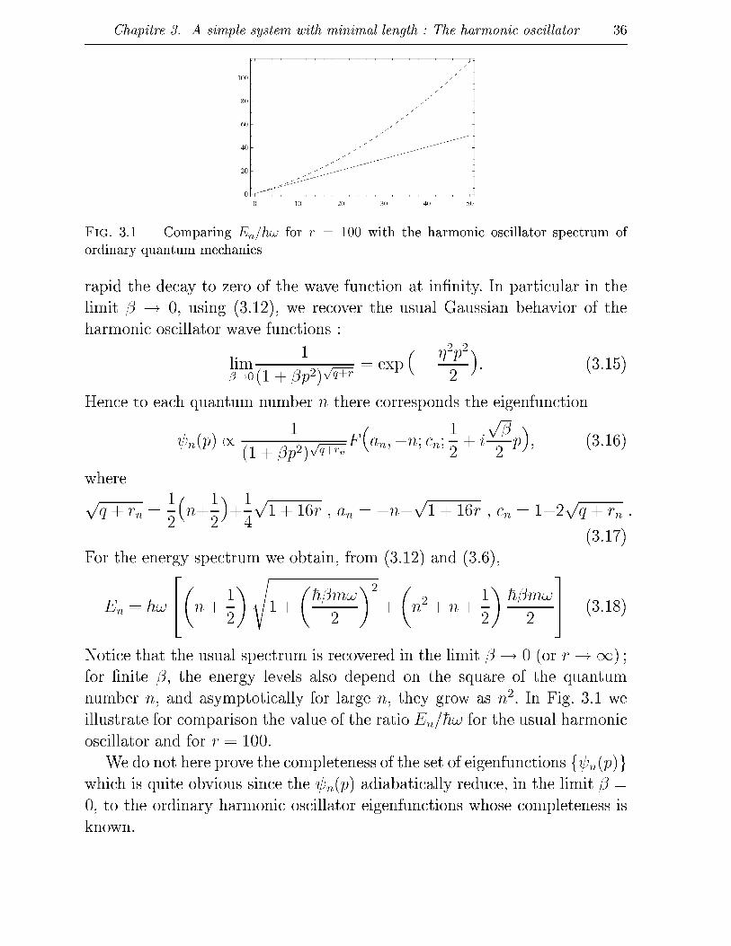
FIG. 3.1 Comparing En/%u for r ordinary quantum mechanics
= 100 with the harmonic oscillator spectrum of
rapid the decay to zero of the wave function at infinity. In particular in the limit /3 —>• 0, using (3.12), we recover the usual Gaussian behavior of the harmonic oscillator wave functions :
lim-1 2^2,
exp (-*f) / 3 - o ( l + / 3 p 2 ) v ^ —" v 2
Hence to each quantum number n there corresponds the eigenfunction
(3.15)
i)n(p) oc 1
where
VÔTTn = - ( n + - ) + - v/ l + 16
F(an, -n; cn; - + i—p), (3.16)
r , an -n—s/1 + 16r , cn = 1 - 2 ^ + ^ .
(3.17) For the energy spectrum we obtain, from (3.12) and (3.6),
En = îiuj ( o 1 \ hômu
(3.18
Notice that the usual spectrum is recovered in the limit (3 —>• 0 (or r -^ oo for finite /3, the energy levels also depend on the square of the quantum number n, and asymptotically for large n, they grow as n2 . In Fig. 3.1 we illustrate for comparison the value of the ratio En/fiuj for the usual harmonic oscillator and for r = 100.
We do not here prove the completeness of the set of eigenfunctions {t^n{p)} which is quite obvious since the ipn(p) adiabatically reduce, in the limit /3 = 0, to the ordinary harmonic oscillator eigenfunctions whose completeness is known.
Chapitre 3. A simple system with minimal length : The harmonie oscillator 37
3.2 The path integral framework
The construction of momentum space path integral representation of the transition amplitude for quantum systems with minimal length follows the well-known canonical steps. Indeed we have
(PbU \Pata) = (Pb\ U {tb, ta) \pa) = }™ (pb\ U (tj, tj-i) \p, N^oo a/ )
with the infinitésimal evolution operator
it
and e = t,
U(tj,tj-{) = exp-jH{tj)
tj-i = jfh- Inserting the closure relation given by
dp \P) (P\ J 1 + ftp1
between each pair of infinitesimal evolution operators we obtain
(3.19)
(3.20)
(3.21
N r d N+1
{PbU \Pata) = lim TT / 3 2 n fe^' j-jj-i (3.22
(3.23)
where the infinitesimal amplitude is defined by
{Pjtj \Pj-itj-i) = {pj\exp--H(tj) |p,_i
Now using the closure relation for the formal eigenvectors and () we obtain the following phase space path integral
(PA \Pj-itj-i, ^-L^--H(Xl,Pl)x
IX, exp
hy^V tan l \Jppj — tan l \Jpp ' i - i (3.24)
Substituting in (3.22) we get the final expression for the path integral representation of the transition amplitude for a nonrelativistic particle with nonzero minimum position uncertainty submitted to the potential V (X).
(PbU \Patc
N r A N+1
lim II hrrU n ,•=1- - + ^ i = i
it *XJ n
exp h I e v ^ L tan l \Jppj — tan l \Jpp ' i - i
EL 2m
f dxj
2^h
V (x-
x
(3.25)

Chapitre 3. A simple system with minimal length : The harmonie oscillator 38
Let us now consider the case of the harmonic oscillator potential given by V (X) = ^rrnJ2X2. Performing the multiple Gaussian integrations over Xj in the last equation we get
(PbU \Pata) = , lim W \ . ^ =-. -—- X V2i7Tehmu2 N^°° .J^ J \/2mehmuj2 (1 + fjpj)
l V2 1 t a n - 1 ^ffp3 - t a n - 1 \j~Jjp3-\ - ^TT~ \ (3-26)
2fjemu2
Using the mid-point expansion we show that we have
1 r / A , ^ 2
t a n - 1 \ffjpj — t a n - 1 \ff5pj-\ 2(3emuj
1 (Apj) h mu(3
~ 2emu2 (l + {3p2)2 ' 2
(3.27) where the mid-point is defined by pj = (pj +pj-\) / 2 . The second term is a quantum correction due to the presence of the nonzero minimum position uncertainty. This is similar to the one generated by the motion of a point particles on curved spaces. This clearly suggests some "equivalence" between the effect induced by the minimal length and the ones induced by the space curvature [35].
Injecting (3.27) in the path integral (B.2) we obtain
(PbU \Pata) = , lim W \ . ^ =-. — - X V2i7Tehmu2 N^°° .J^ J \/2mehmuj2 (1 + fjpj)
1h h 12tW (!+/*?) 2 2m\\ Let us now brought the kinetic term to the conventional form by using the following coordinate transformation
^(-oc+oeî^^-^tan-^p, * e ( - J ^ ) (3.29)
The effective potential generated by this transformation [36] contains the Ti mujfj . . . . . . . _ . _ .
term which cancels exactly the quantum correction (3.27). Ihen we are left with
(PbU \Pata) = {Obtb \0ata) (3-30)
Chapitre 3. A simple system with minimal length : The harmonie oscillator 39
where (6btb \9ata) is given by
1 N f do-
\f2mehmuj2 N^°° J^ J \f2mehmuj2
i
3=1
exp < - y ^ < -—3—^ - —— tan \fô9j tan \fô9j-\ I ^~i I ^
In the continuum limit, this expression is exactly the path integral representation of the transition amplitude of a point particle moving in the symmetric Poschl-Teller potential :
(9btb \6ata) = jDOxexphjcttl ^ 2 - fl^lX (A - 1) tan2 y/pe
(3.32)
where the measure DO is defined as
1 N r riff D6 = . lim FT / J (3.33)
VZiTrehmu2 w->oo - ^ J ^2i7rehmu2
and À = ^ l ± W l + ( J-^JÔ ) ). The solution of this path integral is given
by [36]
Ane n=0 E
ih(3m co itfo—ta / , , \ A
Ane s [cos y/peb cos y/pea) x (3.34) n=0
Cxn (sin V/30&) C* (sin y ^ a ) (3.35)
where Cx (9) are Gengenbauer polynomials and the normalization constant An is given by
2 ^ - ' n ! (n + A) T (A)2 y/g A » = rf> + 2A) ( 3 ' 3 6 )
Then returning to the old variables by means of of the following relation
cosv//3fl = l sin JJ39 = —, (3.37) VïTW2
VÏH¥
Chapitre 3. A simple system with minimal length : The harmonie oscillator 40
we finally obtain the spectral decomposition of the transition amplitude for the one-dimensional harmonic oscillator with nonzero minimum position uncertainty
oo
(PbU \pata) = J2^n M fâ M e " ^ " ^ (3.38 n=0
where the momentum eigenfunctions are given by
"n!(n + A)v^ l l / 2
1>n (P) = 2Ar (A) 2nT(n + 2A) ( i + / v r A / 2 ^ A ( ^ ^
(3.39) The choice of the sign in A is determined by imposing the condition
f^-2p2\iPn(p)\2 <oc (3.40)
J 1 + /V An elementary examination of the convergence criterion of the above integral shows that we must have A > \. Then we must choose the positive sign in the definition of A given above.
The energy eigenvalues En are easily obtained from (3.34) and (3.38)
Er, h muj2[3
[n + (2n + 1) A] (3.41
Using the expression of A with the positive sign, we get
En = îiuj r
n + - 1 + h(3m(jjs
+ I n +n + -1 \ h(3muj
(3.42)
which is exactly the same expression given by (3.18).

Chapitre 4
Quantum systems with minimal length
In this chapter, we shall apply the formalism exposed above, for quantum mechanics with generalized uncertainty principle, to study exact solutions of some examples of quantum mechanical problems. This allows for a concrete view of the effect of minimal length at low energies. To recapitulate, the operators X%)Pj satisfying the minimal-length uncertainty relation
X%) Pj ihiôij + fiPHij + ^PiP, (4.1
are represented in the momentum representation by
Xo = ih d d
(1 + (3p ) — + (3'piPj— + IP dp dpi
Pi ft (4.2
Hence the position operators for different coordinates can no longer commute and we are dealing with a non-commutative Heisenberg algebra. We can also check that this algebra respects the Jacobi identity. The operators X% and P%
are acting on the Hilbert space of normalizable functions with respect to the scalar product
ID
(fttl) dvp 1 + ((3 + /3f)p 211-»? 0* (P) ^ (P)
with
V 7 - (f m
(4.3)
(4.4) (fi + fi')
Note that the arbitrary constant 7 does not affect the observable quantities, its choice determines only the weight function in the above definition of the scalar product. A consequence of the existence of a minimal length (Ar
mm
41

Chapitre 4- Quantum systems with minimal length 42
is that the notion of localized states in the position space disappears since space coordinates can no longer be probed with accuracy more than (Ar) m i n . Then momentum space is more convenient in order to solve any eigenvalue problem.
4.1 The Klein-Gordon oscillator
The Klein-Gordon oscillator can be viewed as the relativistic partner of the harmonic oscillator since it reduces to it in the nonrelativistic limit.
4.1.1 The Klein-Gordon oscillator in one dimension
The stationary equation describing the Klein-Gordon oscillator in one di
mensional space is given by
[c2 (Px + imuX) (Px - imuX) + m2à - E2] i/j = 0 (4.5)
where m is the rest mass of the particle, u is the classical frequency of the oscillator. Using the commutation relation (4.1), we rewrite the above equation as
[m2uj2c2X2 + c2 (1 - mufi(3) P2 + m2à - E2 - muhc2] I/J = 0. (4.6)
Substituting the momentum space realization (4.2) of the operators X and Px we get the following equation
{t1+ /*2'2 w1+w (A+1] (1+'*2) p i +
,32[A(A + l ) - J ; g | ^ ] p 2 + ,3(A + £)}vi(p) = 0 (4.7)
where we have set E2+'mujhc2 —'m2c4 \ ]_ ( A Q
m2uj2h c2(3 ' R ^
With the aid of the variable change
q = 4j jarctan ( \Jpp j (4.9)

Chapitre 4- Quantum systems with minimal length 43
IT IT which maps the interval p G (—00,00) to q G (— YTB^YTB
Eq.(4.7) to
we simplify
oqz c oq A(A + I;
+/3(A + e)}^(<?) = 0
where we have used the notations
s = sin ( \Jpq J , c = cos ( \//3q J
1 — mujfi/3~\ s2
m2u2h2f32\ c2
(4.10)
(4.11)
(4.12)
Now, we introduce a change of function defined by
i/j (q) = étp (q) (4.13)
where 6 is a constant to be determined. Then the obtained equation for ip (q) is
r d2 •s d
dq2 ' v" v' ' v' 'cdq + 2 (A - £) \ / ^ - — + /3 £ (£ - 1) + A (A + 1) - 2£A l—mujhf3
m2uj2h (32
—+/3(A + e ) | ^ ( g ) = 0
(4.14)
2
We choose # to eliminate the term proportional to % by demanding
5(5-l)-25\ + \(\ + l)- ^§f2 = 0 (4.15)
This leads to the following expression of 6
6 = \ + 1
muhfi 6 = \ + l
1 muhfi
(4.16)
We keep only the first solution to guarantee a good behavior of the function I/J (q) at c = 0. We will see later that the second solution leads to a non physically acceptable wave function. This simplifies Eq.(4.14) to
| L + 2(A-^|+/S(A + s-*) <p(q) = 0 (4.17)

Chapitre 4- Quantum systems with minimal length 44
At this stage, we introduce an other change of variable defined by
z = sin (y/fiq) (4.18
The range of the new variable is — 1 < z < 1. Then Eq.(4.17) reduces to
d2 r, _ d
(l-z*) — -ll + 2(6-\)]z-+e + \ - 6 dz2 dz
ifi(z) = 0 (4.19)
We require a polynomial solution to Eq.(4.19) to guarantee regularity of the function ip (z) at z = ± 1 . This is obtained by imposing the following condition
e + A - 5 = n (n + 2 (Ô - A)) (4.20)
where n is a non-negative integer [37]. Then Eq.(4.19) becomes
d2 d (l-z2)7—-[l + 2{6- A)] z— + n {n + 2 (5 - A)) <p{z) = 0 (4.21
dz2 dz
whose solution is given in terms of Gengenbauer's polynomials by
y (z) = NCôn~
X (z) (4.22
where iV is a normalization constant. The energy spectrum is extracted from Eq.(4.20). On inserting the expressions of 6 and e we obtain
2 * 2
En = ±mc2^/1 + 2n^ + n 2 ^ A - , n = 0 , l ,2 . . . (4.23)
This is the same expression of the energy spectrum obtained in Ref. [38] when studying the Dirac oscillator under a minimal length constraint. The obtained energy levels depend on the square of the quantum number n, and grows as n2 for large n. This can be explained by the fact that the variable change from p to p maps our original problem to a tan2 {yffip) potential problem. For higher energy levels this is in essence a square well problem (the boundaries of the well are i j ^ ) . This leads to the n2 dependence of the energy eigenvalues. The complete wave function should satisfy the following normalization condition
-00 dp
-oo ( 1 + ^ " A | ^ ( p ) | 2 = l (4.24)
Chapitre 4- Quantum systems with minimal length 45
Using the following property of Gengenbauer's polynomials [37]
'^('-^KWf = <4-25> we get for the normalized energy wave function the expression
26-x(3 S-X ( yfflp
Let us now check that these wave functions are physically acceptable. In quantum mechanics the wave function should be in the domain of p, to be physically acceptable. This physically means that it should have a finite uncertainty in momentum. Thus we impose
2\ _ f dp J|j,^|2
It is easy to check that the integrand in Eq.(4.91) behaves for p —>• oo as p-2(S-X) ^ g m c e for p ^ 0 the integrand behaves as p2, the convergence of the integral (4.91) will be ensured provided Ô — X > \. This condition is not satisfied by the second solution in Eq.(4.16). Indeed, a minimal length hy/]3:
if it exists, must be of perturbational nature, and must then ranks below the
characteristic length of the oscillator \ —. ° y rnuj
4.1.2 The Klein-Gordon oscillator in D dimensions
The D-dimensional Klein-Gordon oscillator is given by the following equation
[c2 (P + imuX) (P - imuX) + m2cA - E2] ip = 0 (4.28)
which can be written with the help of commutation relations (4.1) as
[m2u2c2X2 + c2 [1 - muhD (fj + (5')\ P 2 + m2cA - E2 - mufiDc2] i\) = 0. (4.29)
Due to the rotational symmetry of this equation, we can separate the angular and the radial part of the momentum wave function as follows
il> (p) = Yi (p) <p (p) (4.30)
where Y^ (p) are D-dimensional ultra-spherical harmonics, p is the unit vector pointing in the direction of p . The label m stands collectively for the
Chapitre 4- Quantum systems with minimal length 46
set of magnetic quantum numbers mi, m-2,..., rno-i and p denotes |p| . With this separation, we can make the following replacements in the momentum space realization of the operator X2[39]
D D
X^J>l=dL + D^isL_!l V D - ^ = » ^ (4 31 / j dp2 dp2 p dp p2 ' / j *^1 dpi " dp V i=\ i=\
with L2 = l(l + D-2) , 1 = 0,1,2,... (4.32)
Then, the obtained equation for the radial momentum wave function reads
[l + (,3 + / 3 V l 2 1 9 2
dp^ + D-l + [ p - l ) / 3 + 2(/3 + /3' + 7)]p
d [i+^+^p^-^-^ + yi^D+p+^-^L - — ^
+ (7L> - 2/3L2) +
2 r 2 _ l-mujhDjP+P')
2A , E2+mujhDc2-m2c4
P
} p (p) =(4133) m2uj2h c2
To solve this equation, we begin by making the following change of variable
2 = T ^ F a r c t a n (V/ 5 + £ ' P ) (4-34)
7 ) and brings Eq.(4.33) which maps the interval p G (0, oo) to q G ( 0, YTB+B-
to the following form
+ (£> -1) v^T^f + (D-l)/?+27 s d_
dq / w 2 i (/3 + /?') L
+ 7(/3D+/3 /+7)-/32L2 _ l-mujhD(/3+/3')
/?+/?' (/3+/3')m2w2?i2
2 A i E2+mujhDc2—m2c4
V ' ' / m2<jj2% c2
where we have introduced the notations
s = sin (v //^ + ^ ) 5 c = cos (^/fi + ft
By setting
£ 2 + muHDc2 - m2c4 ^D - 2/3L2
£ = „ „ . o „ h
}^(ç) = 0 (4.35)
9 (4.36)
( D - l ) / 3 + 2 7
((3 + /?') m2u2h2c2 (3 +(3' ' /3 + (3'
7 (L>/3 + (3' + 7) - /32L2 1 - muhD {(3 + (3') K,
(P + « {(3 + (3'Y m2u2h2 (4.37)
Chapitre 4- Quantum systems with minimal length 47
we can rewrite Eq.(4.35) as
{ J + [(D - 1) -, + «?] y/ÏÏ+P^ - (/J + ff) L% + (/J + ff) 4
+ (P + P')e}V(q) = Hi.3S)
Making now the following change of function
V (q) = c6e (q) (4.39)
where Ô is a constant to be determined. We obtain for 9 (q) the equation
+ (13 + ji') [K + S(S-a-l)\§ + ()) + /}') (e - SD)} 6 (g) = 0 (4.40)
2
To further simplify this equation, we cancel the term proportional to % by choosing Ô as
K + 6{6-a-l) = 0 (4.41) As in the one dimensional case, the allowed expression of 6 is
S = s±l + V ^ " « (4-42)
Then Eq.(4.40) reduces to
{ J +[(*>- 1) Î + (« - 2*) H VÏÏT^§-q - (13 + ff) L% + (l3 + f3')(e-SD)}6(q) = 0 (4.43)
2
In order to eliminate the term proportional to % we set
9 (q) = s1^ (q) (4.44)
The obtained equation for 9 (q) reads ( 82 8
l ^ + ^ + - ^ + ^ - ^ a v ^ ^ + {P + l3,)[e-ÔD-l{2ô-a + l)]}Ç{q) = 0 (4.45)
Let us now change the variable from q to z G (—1,1), by setting z = 2s2 - 1

Chapitre 4- Quantum systems with minimal length 48
This cats Eq.(4.45) into the form
{(i-^S+t 21+D+0.-2Ô-1 (i +
21+D+2Ô-0.-1 )']
d 2 \ 2 J ~J Qz
+\[e-5D-l(25-a + 1)]} £ (z) = 0 (4.46)
The wave function will be regular at z = ±1 if the solution £ (2) is a polynomial. This is obtained by imposing the condition
\[E-5D-1(25-OL + 1) n n' + -(21 + D + 25-OL-1) (4.47)
with n' a non-negative integer. Then Eq.(4.46) takes the form
{(!-*•)£+[ +ri
21+D+0.-20-1
1
(1 + 21+D+20-0.-1
)*] d
n' + -(2l + D + 25-a-l) ZJ
dz
(4.48)
Its solution is given in terms of Jacobi polynomials by
i(z) = NDP^b)(z)
where NJJ is a normalization constant and parameters a and b are defined by
I-I <«°> The energy eigenvalues are obtained from Eq.(4.47) which can be rewritten as
/ _ 2{I3-I3')L2+{DI3+I3')D , ,n„, , n 2 , / < w , n n , [n„, , , , D
a = / + — - 1 ZJ
b = 6
(4.49)
2(/3+/?') • + (2n' + 0 +{2n' + I) D+ [2n' + I + (g+iy
with / E2+mujhDc2—m2c4
(4.51)
~~ (fj+fjr)m2uj2h2c2 V*'0*)
Defining the quantum number n by n = 2n' + /. The resulting expression of the energy levels reads
Enl = ±mc2 \1 - ^ ? + ^ | {(n + Ç) X
\
1 + p/3 + /?')
+ /32L2 m
2w2/i2 - mw/iD {(3 + /3'
+ (/3 + /3')(n + f ) 2 + ( /3- /3 ' ) (L 2 + f ) + ^ } ] 5 , n = 0,1, 2.(4.53)

Chapitre 4- Quantum systems with minimal length 49
As in the one dimensional case, we note the n2 dependence of the energy levels related to the fact that for higher energy eigenvalues, our original problem is equivalent to a square wells problem. We also point the additional / dependence of the energy levels which was absent in the original case (with vanishing /3). As a consequence, the degeneracy of the nth energy state reduces from rjj^iJi in the conventional case to \j^_ïy]{ — (D-IYJI-2Y ^or e a c n
value of / in the presence of a minimal length [40]. This can be viewed as a sign of a self-supersymmetry breaking of the Klein-Gordon oscillator [41].
The expression (4.23) of the energy spectrum in one dimension can be recovered by setting D = 1, L2 = 0 and f3' = 0.
Relativistic electrons in a penning trap
In the following, we will use the above expression of the energy to improve the hypothetical bound of the minimal length found in Ref. [39] when discussing the condition that can be placed on the parameter /3 by the measuring the energy levels of an electron trapped in a strong magnetic field. To this end, we first expand the nth energy eigenvalue up to the first order in (5 as
2fc2 9
En = mc2\j\ + 2n^ + H (4.54) 2A / l + 2 n ^
mc*
The deviation of the nth energy level from the usual case caused by the modified commutation relations is given by
AEn fjmuhn2
~T = — / (4-55) un 2A / l + 2n^%
The cyclotron frequency of an electron of mass me trapped in a magnetic field of strength B is
eB uc = — 4.56
me
For a magnetic field of strength B = 6T we have
mehuc = 1.0 x 10-52kg2m2/s2 (4.57)
Following Ref. [39], we assume that only a deviation of the scale of huc can be detected. Then if no perturbation of the nth energy level is observed, we
Chapitre 4- Quantum systems with minimal length 50
may conclude that (3ehBnz
2A/l + 2nSS This leads to the following constraint
< 1 (4.58
h^<\ 2/H/1 + 271 ehB
e B * - ( 4 5 9 )
This condition includes relativistic corrections, hence the maximum value of n is not constrained by the requirement that the electron remains nonrela-tivistic, it depends only on the experimental setting (we should be able to accurately measure its corresponding energy eigenvalue). Assuming for instance that we can accurately measure the energy eigenvalue corresponding to level n = 1010, then we obtain the following upper bound for the minimal length :
h\fp < 0.34 x 10"18m (4.60)
Let us now turn to the examination of the radial momentum wave functions. These should satisfy the following normalization condition
roc *2 dp
(i+/V) : —p <p (p)' l (4.61)
Using the following property of Jacobi polynomials [37]
du (1 u)a (1 +u) p(a,b) U)
>a+6+l r(n+a+l)r(n+6+l)
In + a + b «!r(n+«+6+i) (4.62)
we get for the normalized energy radial momentum wave function the expression
<Prd {P)= P 4 (2n'+a+b)T(n'+a+b+l)n'\
r(n'+a+l)r(n'+6+l) Pl [1 + (P + P') p • Y X
p(a,b) ( tf+ptf-l n [n (/3+/3V+Î / ' '" — V" 0 / 2 (4-63)
As mentioned before, a physically acceptable wave function should be in the domain of p. This means that the radial momentum wave function must satisfy the condition
dp ,13+1 —p + (p (p) < oo. (4.64)

Chapitre 4- Quantum systems with minimal length 51
We can easily check that the integrand in Eq.(4.64) behaves for p —>• 0 as pD+1 and for p —>• oo as p°~26. Thus the convergence criterion is 25 — a < —1, the condition which is already satisfied.
4.2 The Klein-Gordon and Dirac equation with mixed scalar and vector linear potentials
The linear potential is an important quantum mechanical model which has been widely used especially with relativistic wave equations in the investigation of quark confinement in particle physics.
4.2.1 The Klein-Gordon equation
In one spatial dimension, the Klein-Gordon equation for a particle of mass m in the presence of a scalar potential S (X) and a vector potential V (X) is given by
L2P2 + [me2 + S (X)]2 - [E - V (X)]2} # = 0 (4.65)
In what follows, we shall examine the case where
S (X) = AX, V (X) = kX (4.66)
with À and k two constants characterizing the strengths of the potentials. Note that such a linear vector term provides a constant electric field always pointing to, or from, the point charge. Substituting the momentum space realization of the operators X and P , we obtain the following differential equation
9 82
-h2 (A2 - k2) (1 + (5p2) — + [2ih (Xmc2 + kE) - 2h2 (A2 - k2) fjp] x
(1 + (3p2) — + c2p2 + m2cA - E2 v ' op
\& (p) =(4167)
Introducing the following change of variable
p = —j= arctan ( \Jpp j (4.68)
Chapitre 4- Quantum systems with minimal length 52
IT IT which maps the region p G (—00, 00) to p G . —^73, Y/B
dimensionless parameters
m2cA — E2
e = o , „ —, a Xmc2 + kE
6 h2 (A2 - k2) /3' h(\2-h2)y/F h2 (A2 - k2) (32
Eq.(4.142) simplifies to
— - 2ia^— - /3£tan2 [y/^pj -fie # (p) = 0
Making now the substitution
we obtain the following equation for ip (p)
d2
, and defining the
(4.69)
dp2 (3ôtân2 (y/fip) + fi{a2-s) <P(P) = O
Next, let us set
ip(p) = cœv(y/(3p)f(p)
(4.70)
(4.71)
(4.72)
(4.73)
hence, Eq.(4.72) becomes
d2 d dp2 2vy/fitan ( y ^ p ) -Q-+ P[v(v-I) - S\ tan2 ( y ^ p )
+fi [a2 - s - u)} f(p) = 0 (4.74)
we choose v to cancel the tangent squared term :
u(u-l)-o = 0 (4.75)
Since the wave function should be nonsingular at cos (\ffip) = 0, we must take
» = \ + û+ô (4.76)
We will see later that the second choice of v leads to a non physically acceptable bound state wave functions. Then Eq.(4.74) reduces to
dp2 2v v ^ t a n (\ffip\ — + fi (a2 - e - v) f(p) = 0 (4.77)

Chapitre 4- Quantum systems with minimal length 53
At this stage, we introduce an other change of variable defined by
1 Z=2
1 - sin (yflp) (4.78)
where the range of the new variable is — 1 < z < 1. This casts Eq.(4.77) into the form
r d2
z [ z 1 } ^ 2 + v + \-{2v + l)z 9 2
oz — £ — V f(z) = 0 (4.79)
This is just a hypergeometric equation, and its solution is the hypergeometric function
f(z) = F(a,b;c;z) (4.80)
where the parameters a, 6, c are given by
a = v \/ô + œ v + \/ô + œ 1
(4.81)
For bound states, we need polynomial solutions to / (z) in order to keep the wave function regular at z = 0, 1. Since the hypergeometric function reduces to a polynomial of degree n when either a or b equals a negative integer — n, one must impose the condition
v Vs + œ -n, n = 0,1, 2... (4.82)
From this condition follows the energy equation :
\En + kmc2 = ±h^ | A2 - k2\ [n2 + (2n + 1)*/ ] ^ , n = 0,1, 2... (4.83)
Using the expressions of v and Ô, we obtain
\En + kmc2 = ±h\X2 -k2\ (3 In2 + 7i + 1
+(2n + r '/5J
+ 4 a2 (A2 - fc2) n = 0 , l , 2 5 - " " 5
(4.84)
We see that the energy spectrum depends on the deformation parameter /3 ; this is not surprising, since the introduction of the modified Heisenberg algebra affects physical results.
We also note that the energy levels depend on the square of the quantum number n, which is a feature of hard confinement. This can be explained by

Chapitre 4- Quantum systems with minimal length 54
the fact that the variable change from p to p maps our original problem to a tan2 {yffip) potential problem. For higher energy levels the later is in essence a square well problem (the boundaries of the well are ILJTJ) . This leads to the n2 dependence of the energy eigenvalues.
An other property of the energy eigenvalues is the constant energy level spacing for large n :
A2 - k2
lim \AEn\ = h^(3 A
(4.85)
A2-fc2
Hence our problem can be described for large n by a non-relativistic harmonic
oscillator with frequency u = y/j3
We end our comments by noting that in the limit /3 = 0, the expression of the energy spectrum reduces to
XEn + kmc2 = ± (A2 - k2)'4 ^{2n + 1) he (4.86)
which coincides exactly the result obtained in the case where the minimal length is absent.
Let us now write the complete expression of the normalized bound state wave functions. These should satisfy the following normalization condition
f dp l^tol 1
J (1 + /V) Expressing / (z) in terms of Gengenbauer's polynomials as
and using the following integral property [29]
(4.87)
>i )l-2a du(l-u2) ~2[at
rf-T2« + n u
(4.88)
(4.89) -i n\ (a + n) [T (a)\
we obtain the following expression for the normalized energy wave functions
i2"
Vn(p) T(P
2n
n\ [v + n) [r {v)
r (2i/ + n) (l + /3p2)-^G PP
VÏTPP2' (4.90)
Let us examine the necessary condition on parameter v in order to have a physical bound states. The wave function should be in the domain of p to

Chapitre 4- Quantum systems with minimal length 55
be physically acceptable. This physically means that it should have a finite uncertainty in momentum
(p2) = jjTTw/l%,M2<œ- (4'91)
It is easy to check that the integrand in Eq.(4.91) behaves for p —>• oo as p~2v. Since for p —>• 0 the integrand behaves as p2, the convergence of the integral (4.91) will be ensured provided v > \. The second solution of Eq.(4.75) does not satisfy this condition therefore it was ignored.
From the previous discussion we can see that the existence of physical bound states remains possible as long as the following constraint is fulfilled
4 r2fe2
(A*)4mm > ^ - ^ (4.92)
This means that confinement solutions can occur even when the electric field is stronger than the scalar potential (which must be non null) provided that inequality (4.92) is respected. However, this conclusion remains purely mathematical since in real situations condition (4.92) is far from being realized. Indeed, the largest upper bound of the minimal length found in the literature is [34, 42]
(Ax)mm < If m (4.93)
In the case when condition (4.92) is not satisfied, parameter v becomes complex with Re (v) = \ ; the integrand in Eq.(4.91) behaves as 1/p at momentum infinity, leading to a logarithmic divergence of integral (4.91). Hence the particles cannot be bounded in this case. Only scattering solutions occur and the whole spectrum is continuous.
4.2.2 The Dirac equation
In one-dimensional case, the stationary Dirac equation describing a particle of mass m in the presence of a vector potential V (X) and a scalar potential S (X) reads
caPip + (3 [mc2 + S (X)] ip=[E-V (X)} i\) (4.94)
where \\) is a two-component spinor. Here we choose the following representation of the Dirac matrices a and /3 :
Chapitre 4- Quantum systems with minimal length 56
To solve Eq.(4.142) we use the following ansatz for the spinor tp :
t/j = {caP + (3 [mc2 + S (X)] + [E - V (X)}} 0 (4.96)
Then we obtain for the two-component function 0, the following equation :
ic2P2 + [mc2 + S (X)]2 - [E - V {X)}2 - c [P, (5S + V] a\ 0 = 0 (4.97)
We now take the vector and scalar potentials to be of the form
V (X) = kX , S (X) = XX (4.98)
with k and À two constants characterizing the strength of the potentials. Furthermore we suppose |A| > \k\. Substituting in system (4.97) the operators X and P by their momentum space realization (4.2), we get for the function (f) (p), the following differential equation :
d 2
%2{\2-k2) (l + (3p2) — +2ih(\mc2 + kE) (l + (3p2) d
dp
+c2p2 + m2cA -E2 + 7ic\]\2 - k2 (l + (3p2) M\ 0 (p) = 0(4.99)
where M is the matrix defined as
Af = l / x / A ^ I ^ ( A ° f c A
Qf c ) (4.100)
Introducing the following change of variable
p = —j= arctan ( \Jpp ) (4.101)
which maps the region p G (—oo, oo) t o p G — irmi 27Ë ) ' anc^ defining the dimensionless quantities
m2cA — E2 Xmc2 + kE c 6 = n2(3 (A2 - A;*) ' = hVp(\*-k?y = n^7W=¥ [ }
Eq.(4.99) simplifies to
f d2 „.„ r-d 2ie^/J3— - /3£2tan2 U/^p\ - f3e
dp2 dp
-[35 1 + tan2 (s/Pp) M\ (f)(p) = 0 (4.103)

Chapitre 4- Quantum systems with minimal length 57
Since eigenvalues of the matrix M are r\ = ± 1 , the solution of the last equation can be constructed as
(f) (p) = uv(pv (p) (4.104)
where uv is a two-component eigenvector of matrix M with eigenvalue 7/, and the function cpv (p) is the solution of the following equation
d2 d ZiO^— -fi6{6 + 7]) tan2 ( y ^ p ) - /? (e + r/£)
dp2 "" v 'dp
Making now the substitution
¥>„ (p) = e ' ^ % (p)
Then the obtained equation for fv (p) is
d2
i0y/pp
<Pv ( P ) = ° (4.105)
(4.106)
dp2
Next, let us set
(30 (Ô + 7]) tan2 UfPp\ + (3 (ô2 - i]ô - s) fv(p) = 0 (4.107)
fv (P) = COS" (y/Pp) ^ (p)
where v is a constant to be determined. Then Eq.(4.107) becomes
(4.108)
0>p2
G> 2z/v^tan ( y ^ p ) Ô~ + /3 [i/ (i/ - 1) - ô {Ô + r/)] tan2 ( y ^ p )
+/3(02-7/tf-e-i/) } £ » = () (4.109)
We fix zv by requiring the coefficient of the tangent squared term to vanish :
v{v-\) -ô(ô + 7]) = 0 (4.110)
The wave function should be nonsingular at cos {yffip) = 0, which implies that v = l/2+7]/2+5. We will show in a later discussion that the second value of v does not lead to a physical bound state wave function. Then Eq.(4.109) reduces to :
dp2 2z/y//3tan ( y ^ p ) j - + P {ô2 - r,ô - e - v) 6 ,M = o (4.111;

Chapitre 4- Quantum systems with minimal length 58
At this stage, we make the change of variable z = sin (\ff3f)). This simplifies the last equation to :
dz2 > +1) ^- + e2 - nô oz
V £r,{z) 0 (4.112
In order to guarantee a well behavior of the function £,v(z) at z = ± 1 , we require a polynomial solution for Eq.(4.112). This leads to impose the following condition on the coefficient of ^ :
Ô2 - 7)5 - e - v = n' (n' + 2v) (4.113)
where n' is a non-negative integer [43] ; n' = 0, 1, 2, . . . With this condition Eq.(4.112) becomes
d2
dz2 {2u + 1) ^ + n' {n' + 21/) Uz) 0
the solution of which is given by the Gegenbauer polynomial
£„ (z) = NC»n, (z)
(4.114)
(4.115)
where iV is a normalization constant. The energy spectrum is immediately deduced from condition (4.113) :
XEn + kmc = ± 2nhc (A2 - k2) 2\3/2
+Pn2h2(\2-tf)' 1/2
n = n' + 1/2 + r//2 = 0,1,2, (4.116)
We first remark that the energy spectrum depends on the deformation parameter (3. This is not surprising, since the introduction of the modified Hei-senberg algebra affects physical results. Furthermore, we see that the effect of the introduction of the minimal length is the appearance of an n2—dependent term in the expression of the energy levels which then grows as n2 for large n. This is a feature of hard confinement which makes the considered model with nonzero minimal uncertainty in position more suitable for the description of quark confinement. Note that the n2 behavior of the energy levels can be explained by the fact that our original problem is mapped, through the change of variable from p to p, to a tan2
(A//^P) potential problem. For higher energy eigenstates, this potential is in essence a square well with boundaries placed at ±7T/2A/ /3 . This leads to the n2 dependence of the energy eigenvalues.
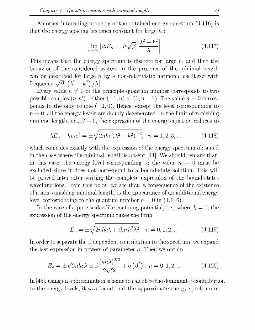
Chapitre 4- Quantum systems with minimal length 59
An other interesting property of the obtained energy spectrum (4.116) is that the energy spacing becomes constant for large n :
lim \AEn\ = fi^ffi X2-k' X
(4.117)
This means that the energy spectrum is discrete for large n, and then the behavior of the considered system in the presence of the minimal length can be described for large n by a non-relativistic harmonic oscillator with frequency A//3 | (A2 — k2) /\\.
Every value n ^ 0 of the principle quantum number corresponds to two possible couples (7/, n') : either (—1, n) or (1, n — 1). The value n = 0 corresponds to the only couple (—1,0). Hence, except the level corresponding to n = 0, all the energy levels are doubly degenerated. In the limit of vanishing minimal length, i.e., (3 = 0, the expression of the energy equation reduces to
XEn + kmc2 = ±\J2nhc (A2 - fc2)3/2, n = 1, 2, 3 , . . . (4.118)
which coincides exactly with the expression of the energy spectrum obtained in the case where the minimal length is absent [44]. We should remark that, in this case, the energy level corresponding to the value n = 0 must be excluded since it does not correspond to a bound-state solution. This will be proved later after writing the complete expression of the bound-states wavefunctions. From this point, we see that, a consequence of the existence of a non-vanishing minimal length, is the appearance of an additional energy level corresponding to the quantum number n = 0 in (4.116).
In the case of a pure scalar-like confining potential, i.e., where k = 0, the expression of the energy spectrum takes the form
En = ±^2nhcX + f3n2h2X2, n = 0 ,1 ,2 , . . . (4.119)
In order to separate the (3 dependent contribution to the spectrum, we expand the last expression in powers of parameter (3. Then we obtain
En = ±V2nhcX ± [3^nh)\L + o (/32) , n = 0 ,1 , 2, . . . (4.120)
In [45], using an approximation scheme to calculate the dominant /3-contribution to the energy levels, it was found that the approximate energy spectrum of

Chapitre 4- Quantum systems with minimal length 60
the one-dimensional Dirac equation with a scalar-like linear potential is of the form
En = ±y/2(n + l)hcX (h\)3/2
T/3o ;o ; . (2n2 - 6n + l) + o (/32) , n = 0,1, 2,... (4.121) 8y2c(n + 1)
As we can see, although the dominant correction term is of the form fj y (hX) /c as in (4.120), the numerical factor and the n—dependence of the /3-contribution differ form that we have found in (4.120). In particular, contrary to what was concluded in [45], the generalized uncertainty principle shift lowers an un-deformed negative energy level and raises an un-deformed positive energy level. An other consequence of the presence of the minimal length, which was missed in [45], is the appearance of an additional energy level with quantum number n = 0.
Now, let us write the complete expression of the non-normalized momentum-space spinor ipn (p) corresponding to energy spectrum (4.116). Using Eq.(4.96) and the following property of Gegenbauer's polynomials [43] :
^(Z(z) = 2vC£l(z) (4.122
the expression of the bound-states spinor ipn (p) can be put under the form
^n (p) = Nn (1 + (3p2yv/2 e ^ a r c t a n ( v ^ ) UnC"' \V^
2iv „ , /^+l / VPP :VL/n'-i n = n' + 1/2 + rç/2 (4.123)
where un and v are two-component vectors defined as
uTn = (8n - iulP, r 3 (7jSn + iu2p)) , vT = (l, -ryr3) (4.124)
where we have used the following abbreviations :
XEn + kmc2 r, 9N
U2 = 6{1/T2+T,) + (1 + V)/2, r = J ^ (4.125)
Chapitre 4- Quantum systems with minimal length 61
Note that the normalization constant Nn can be obtained from the normalization condition of the spinor \\)n (p), which follows from the modified definition (4.3) of the scalar product :
dP ^ ( P ) ^ n ( p ) = l (4.126) I + PP
Let us now focus on the case corresponding to n = 0. This level is not degenerated and the value n = 0 corresponds to n' = 0 and r] = —1. In this case, the expression of the normalized bound-state spinor I/JQ (p) is given by :
if)o (p) = N0 ( _* ] p (1 + (3p2yS/2 e^ o a r c t a n (^ ) (4.127)
where the normalization constant is given by
1/2
iVn ( 2 £ - l ) / 3 3 / 2
T T M + T 2 ) (4.128
In the limit (3 —>• 0, the spinor ip0 (p) behaves as /31,/4 which means that this wavefunction vanishes in the usual case with (3 = 0, and then the corresponding energy level present in the case with minimal length disappears in the case where the minimal length is absent.
Let us now check that the wavefunctions given by (4.123) are physically acceptable. The latter property requires that the wavefunctions be in the domain of p, which means that they should have a finite uncertainty in momentum :
+oo
2\ f dP pz)n = I YTW ^(p) ^{p) < °° (4'129)
It is easy to check that the integrand in (4.129) behaves for large p as p2<^~v\ Hence the convergence of the integral will be ensured provided v > 3/2. This is the condition to solve in order to guarantee the existence of physical bound state wavefunctions. Remark that the second solution of Eq.(4.110) does not satisfy this condition therefore it was rejected.
The undeformed limit

Chapitre 4- Quantum systems with minimal length 62
We now study the limit of the wave function when /3 —>• 0. We consider the particular case corresponding to n = 1 (n' = 0, r] = —1), in which the expression of the momentum space wave function takes the form
^r~1] (p) ^ = - i ) m"-~L> ( i + /3p2)" < x 6+1
2 1
exp i0\ (»?=-!) ,(»7=-l)
arctan PP £\' ' — iuip
.i» (£t~V + ÎUJ2P
(4.130)
In order to examine the limit of a given wave function when fj —>• 0, one must have in hand the full normalized expression of this wave function. This is because the involved normalization constant it self depends on the parameter fj. This constant is obtained by calculating integral (4.126) for ip^ (p).
Since
^r~1] (p) N-(r,= -l) 1 ( i + m 2\-(*+l) X
^ - ^ ( l + r V ^ + rVV
the normalization constant for \pf (p) reads
N-(r,=-l) 1
(»?=-!) (l + r6)l0+(ujl+rW2)h 1-1/2
where we have used the notation
- 0 0
Ik dp (1 + f3p2) 2 ^ + V f c , A; = 0,1
(4.131
(4.132)
(4.133)
with
where B (x, y) = rfJ_p^ is the beta function. In the limit fj —>• 0, we have
I0 = (5-l/2B (1 /2 ,6 + 3/2) , h = f3~3/2B (3/2, 6 + 1/2) (4.134)
-Wr(y) T(x+y)

Chapitre 4- Quantum systems with minimal length 63
These limits can be obtained either using the asymptotic form of the gamma function for large arguments :
r (z) ~ V2^e~zzz-1/2 (4.136)
or by directly remarking that the limit of Ik when /3 —> 0 is
- 0 0
o2 h - J dp e - - y = ^ ^ (4.137) — OO
which follows from the limit
(l + / 3 p 2 ) " ' ^ ^ 0 e - ^ 2 (4.138)
Thus, the limit of Ik when (5 —>• 0 is a constant independent of p\ Since in the limit /3 —>• 0
{£Ï*=~1]Î ~ JV W + ^ ) ~ ^ (4-139)
we deduce that in this limit we have
N^-V ~ - (4.140) P
Finally we conclude that
^=~X) (P) - / ^ o AT0*2 (4.141)
where yl is a two-component constant vector. This is the form of the wave function \pf~ (p) that we would obtain if one solves the problem in the momentum space and without minimal length. The above analysis shows that the expression of the wave function reduces, in the limit (5 —>• 0, to the same expression obtained when the undeformed problem is solved directly. Unfortunately, this result cannot be established for the wave function in its general form due to complications that arise when one tries to calculate the expression of the normalization constant corresponding to i/4 (p) •
We close this section by noting that the above results could be relevant for the study of meson spectra [46]. In particular, experimental data in this domain can be confronted with our obtained theoretical results to find an upper bound for the minimal length.

Chapitre 4- Quantum systems with minimal length 64
4.3 The one-dimensional spinless Salpeter Coulomb problem
The spinless Salpeter equation (SSE) may be viewed as a natural approximation to the Bethe-Salpeter formalism which constitutes the basic framework for the description of bound states within relativistic quantum field theory. More precisely, the spinless Salpeter equation can be derived from the Bethe-Salpeter equation [1] upon performing the following approximations :
* The elimination of any dependence on timelike variable by assuming a static or instantaneous interactions. This results in the so-called Salpeter equation [47].
* The neglect of any references to the spin degrees of freedom of particles and the restriction to positive energy solutions.
In addition, this equation represents one of the simplest relativistic generalizations of the Shrôdinger formalism towards the reconciliation with all the requirements of special relativity through the incorporation of the exact relativistic relation between energy and momentum. This equation is generally used when kinetic relativistic effects cannot be neglected. It is suitable for the description of scalar bosons as well as the spin averaged spectra of bound states of fermions. It appears, for example, in the description of hadrons as bound states of quarks in the context of potential models [48, 49, 50, 51, 52].
In the one-particle case, the spinless Salpeter equation takes the form of an eigenvalue problem (h = c = 1)
H\ipk) = Ek\ipk) , fc = 1,2,3,. . .
with Ek the energy eigenvalues corresponding to Hilbert-space eigenvectors |i/>fc), and H the hamiltonian of the system being of the form
H = \ / p 2 + m2 + V (r)
where \ / p 2 + m2 is the relativistic kinetic energy of the particle of mass m and momentum p and V (r) is an arbitrary position-dependent static interaction potential. In this section, we shall solve in the momentum space representation the following eigenvalue problem
if}) = E\if}) (4.142) P2 + m2 + V X

Chapitre 4- Quantum systems with minimal length 65
with a Coulomb type interaction
V(x) = - , x e R (K > 0) (4.143)
where position and momentum operators satisfy deformed commutation relation (4.1). Due to its singularity at the origin, the Coulomb potential is in particular sensitive to whether there is a fundamental minimal length.
Potential (4.143) was not investigated so widely as potential —K,/ \X\. However it may have interesting applications in theoretical physics. For example, this potential appears in the investigation of mass spectra of mesons [53]. Note also that potential (4.143) has the same bound states as the hard-core amended Coulomb potential considered in [54]. Indeed, bound states are determined by the potential well of the right half space which is the same for the two interactions and the boundary condition tp (x = 0) = 0. In our case, this condition follows from the infinite barrier that has the potential in hand in the left half space.
Operating now on the both sides of Eq.(4.142) with X and replacing the position operator by its momentum representation (4.2) (with 7 = 0) we get the following differential equation
d (1 + /V) dp
E \Jp2 + m? \\) (p) — IK\\) (p) = 0
Defining a new function ip (p) by
<P(P) E Vf + m2 ) \\) (p)
Eq.(4.144) becomes
d
dp <P(P) IK
•v (P) = 0
(4.144)
(4.145)
(4.146) E - \Jp2 + m2 ) (l+(3p2)
the solution of which is given by
(p (p) = exp id (p) (4.147)
where À is an arbitrary constant and the function 9 (p) is defined as
Chapitre 4- Quantum systems with minimal length 66
It is possible to write the explicit expression of the function ip (p) by performing the integration in the last equation. However, we will keep the above form for <p (p) which is more relevant for the following manipulations. The resulting expression of the momentum space wave function tp (p) reads
\\) (p) = -, N exp iO (p) (4.149) IE- \]p2 + m2J
Note that the constant À can be determined from the normalization condition of the wave function \\) (p) which follows from the modified definition of the scalar product (4.3)
+oo
dp
[l + (3p \tjj{p)\z = l (4.150)
We now turn to the determination of the quantification condition. To this end we will follow the same method used in [55]. In standard quantum mechanics, the action of the operator 1/X has been expressed as [56]
p
jipip) = ~i / ip(q)dq (4.151)
—oo
When extended to the deformed case, this definition becomes
—oo
On the other hand, the wave function tp (p) given by Eq.(4.149) is a solution of Eq.(4.144) but does not satisfy the initial equation (4.142) with definition (4.152) for the action of the operator 1/X. In order to overcome this situation, we slightly modify the definition of the action of 1/X as
^ w = - < / ( n S 5 y d g + " (4'153) —oo
where r] is a constant which will be determined from the requirement that the wave function I/J (p) given by Eq.(4.149) should be a solution of eigneva-lue problem (4.142). Replacing now in Eq.(4.142) the operator 1/X by its

Chapitre 4- Quantum systems with minimal length 67
expression (4.153) we obtain the following equation
p i/j(q)
(E - v V + m 2 ) if; (p) - in / P[q) dq + KTJ = 0 (4.154)
- 0 0
In order to determine r\ we substitute in the last equation the function tp (p)
by its expression (4.149). This results in
7] = — lim (p (p) (4.155) K, p^oo
Note that performing the integration which appears in Eq.(4.154) becomes easy if one observes that the function I/J (p) can be alternatively expressed as
^ (P ) = - ( 1 + / V ) | - ^ ( P ) (4-156) IK, Op
In order to obtain the quantification condition, we demand that Hamiltonian corresponding to eigenvalue equation (4.142) should be an Hermitian operator on its eigenfunction (4.149). This condition is well satisfied by the kinetic
energy operator + m2. Hence our requirement amounts to imposing
that operator 1/X must be Hermitian on the set of eigenfunctions I/JE (p)
— ^E J
I/>E>) = {I/>E\ ^h>) (4-157)
Replacing the operator 1/X by its momentum space representation (4.153)
with expression (4.155) for constant r] the last condition reduces to
+oo p +oo
. f J'E- (P) f nil) , , , , r , , f <PE>(P) _ —oo —oo —oo
+oo p +oo
. f i'"E(p) f i>E'(q) ,, ,, , r , , f i'"E(p) ,, , , , „ • . "J JTTmJ (TTW)dqdp + v[,pE']J ( T T M * (4158)
—oo —oo —oo
Using the following integral formula
+oo x +oo +oo +oo y
f(x) 9 (y) dydx = g{y)dy f(x)dx- g {y) / / (x) dxdy
—oo —oo —oo —oo —oo —oo
(4.159)
Chapitre 4- Quantum systems with minimal length 68
together with property (4.156) and taking into account the orthogonality condition of the wave functions
+oo
—oo
equation (4.158) simplifies to
sm[OE-0Ei} = 0 (4.161)
where we have noted
BE = lim 9E(p) (4.162)
This entails that 0E_0E, = n7T (4.163)
where n is integer. Performing the required integrations in the expression of BE-, results in two energy equations corresponding to two distinct cases depending on the value of the deformation parameter (3
TTK^E 2KE ( m + E
arctan 2{l-(3e2) (l-f3e2)e \ V m-E
+ m r + £ = 0, for (3m2 < 1 (4.164) l-/3e<
and
irKy/fiE 2KE ( m + E arctan 2 ( l - / 3 e 2 ) (l-^e2)e \ \ m - E
<KU^+mr + 5 = 0} for (3m2 > 1 (4.165) l-(3e 2
with
e = y V 2 - E27 £ {(3) = V l - Z ^ t a n r T 1 U/l - (3mA ,
u ((3) = ^(3m2 - 1 arctan (j f3m2 - l\ (4.166)
and Ô is an arbitrary constant. Unfortunately Eqs.(4.164, 4.165) are too complicated so that they cannot be solved analytically. In order to see the effect
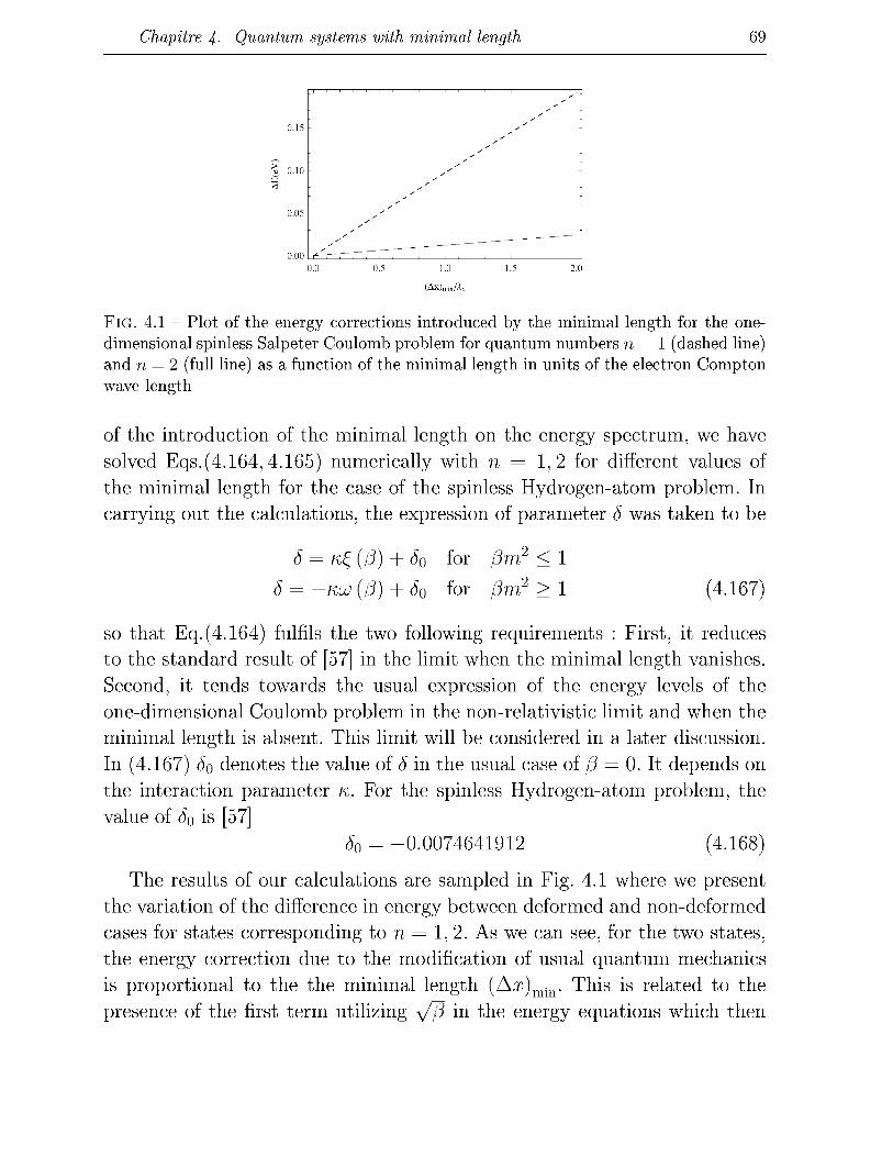
Chapitre 4- Quantum systems with minimal length 69
0.15 -
% 0.10 -
<
0.05 -
0.0 0.5 1.0 1.5 2.0
(AxWAo
FIG. 4.1 - Plot of the energy corrections introduced by the minimal length for the one-dimensional spinless Salpeter Coulomb problem for quantum numbers n = 1 (dashed line) and n = 2 (full line) as a function of the minimal length in units of the electron Compton wave length
of the introduction of the minimal length on the energy spectrum, we have solved Eqs. (4.164, 4.165) numerically with n = 1, 2 for different values of the minimal length for the case of the spinless Hydrogen-atom problem. In carrying out the calculations, the expression of parameter 6 was taken to be
6 = K£ {(5) + ô0 for (5m2 < 1
5 = -Ku {(5) + ô0 for (5m2 > 1 (4.167)
so that Eq.(4.164) fulfils the two following requirements : First, it reduces to the standard result of [57] in the limit when the minimal length vanishes. Second, it tends towards the usual expression of the energy levels of the one-dimensional Coulomb problem in the non-relativistic limit and when the minimal length is absent. This limit will be considered in a later discussion. In (4.167) #o denotes the value of 6 in the usual case of (5 = 0. It depends on the interaction parameter K. For the spinless Hydrogen-atom problem, the value of #o is [57]
£0 = -0.0074641912 (4.168)
The results of our calculations are sampled in Fig. 4.1 where we present the variation of the difference in energy between deformed and non-deformed cases for states corresponding to n = 1, 2. As we can see, for the two states, the energy correction due to the modification of usual quantum mechanics is proportional to the the minimal length (Ax)min. This is related to the presence of the first term utilizing y/~/3 in the energy equations which then

Chapitre 4- Quantum systems with minimal length 70
dominates the other correction terms brought by the minimal length. This can be clearly seen if one develops expression (4.164) in powers of parameter (3 by assuming yffle <C 1. We also note that the energy corrections due to the minimal length are much significant for the ground state, i.e., higher-??, energy levels get smaller corrections. Then, let us examine the non-relativistic limit of (4.164). The latter is obtained as in the usual case by setting E = Enr+m with the assumption that Enr <C m, where Enr denotes the non-relativistic binding energy. A Taylor expansion of Eq.(4.164) gives
/~^nrl + « ( l + W ^ - e C f l ) ) + n 7 r + * = 0 (4.169) y — z E n r / m \ z J
This yields the following expression of the non-relativistic binding energy
2
EZ = — * (4.170) 2[n-f + j ( l + fmV3-e(/5))]
Here n may be either a positif or a negative integer. The domain of variation of n is restricted by the condition
7T 7T \ Z J
which follows from Eq.(4.169). In the case when Ô = K, (1 — £ ((3)) , it is obvious that for /3 = 0 we recover the usual non-relativistic energy levels of the Coulomb potential in one dimension. Note also that, in this case, the energy spectrum has the form
2
Enr = ~mK (4 172) n z[n + '?fv%2
with n > —^Tjry/p. Hence due to the regularizing effect of the minimal length we obtain a finite energy for the ground state corresponding to quantum number n = 0. This was not the conclusion when the non-relativistic treatment of the one-dimensional Coulomb potential in the usual quantum mechanics (with (3 = 0) was considered. The latter predicts an infinite binding energy for the ground state with quantum number n = 0.
The correction terms brought by the minimal length are obtained by expanding expression (4.172) in powers of (3 (we assume that m^/]3 <C 1 i.e.

Chapitre 4- Quantum systems with minimal length 71
the Compton wave length of the considered particle 1/m is greater than the minimal length y/j3). This gives
.2 ^ 2 , ^ 3 3m3 K4
We see that, besides numerical factors, we reproduce the same correction terms found in [55]. As has been already mentioned, the dominant correction term is proportional to the minimal length. Also, this term is proportional to 1/n3 so that corrections for lower-n energy levels are more significant.
Note that the non-relativistic limit of (4.165) can be obtained in a similar manner. We just have to substitute £ ((3) by u ((3) to get the same expression (4.172) of the non-relativistic binding energy.
Let us end this section with the following remark. The Coulomb potential possesses an infinitely repulsive barrier at the left-vicinity of x = 0. Hence, the position-space wave function tp (x) is required to satisfy the boundary condition tp (x = 0) = 0. Since ip (x) is just the Fourier transform of ip (p), in the usual quantum mechanics with /3 = 0, the latter condition can be written as
^{p)dp = 0 (4.174)
The expression of the wave function I/J (p) is given by (4.149) with (3 = 0. Hence, the integrand in the last equation behaves for large p as l/p. Then integral (4.174) has a logarithmic divergency. This problem makes nonsense the boundary condition tp (x = 0) = 0 in the non-deformed case with (3 = 0. With deformed quantum mechanics, the situation changes completely. Using the modified expression of the transformation from momentum space states to "quasiposition wave function" [22], condition (4.174) becomes
' / J ( P ) dp = 0 (4.175)
The integrand in the above equation behaves for large p as p~2 which means that integral (4.175) is well convergent. From this point, we see that the existence of a non-zero minimal length in coordinate space is equivalent to the introduction of a momentum space cutoff A with boundary condition
Chapitre 4- Quantum systems with minimal length 72
îfj (A) = 0 which eliminates the contribution of high momentum in integral (4.174) responsible of its divergency.
4.4 The /^-dimensional harmonic oscillator : path integral approach
In this section, we use the path integral method to treat the problem of the D-dimensional harmonic oscillator in the presence of a minimal position uncertainty. In higher dimensions, the task is more complicated due to difficulties arising from the non-commutativity of position operators.
We shall consider a simplified version of commutation relation (4.1) given by by :
X{, £,•] = ihôij ( l + /3P2) (4.176)
These operators are realized in momentum space as
Xi = a ( l + / 5 p 2 ) ^ - , Pi=Pi, i = l,...,D (4.177) opi
In conventional non-relativistic quantum mechanics, one constructs a path integral representations for matrix elements (in a momentum representation) of the evolution operator U (tb, ta). In the quantum mechanics under consideration, we also start with a such operator. For a time independent Hamiltonian H, the latter has the form
Û (tb, ta) = exp j]-H (tb, ta). (4.178)
The transition amplitude is given by
N+l
(Pbh\ Pata) = (Pb\ U(tb,ta) |p«) = mil (p6 | TT U{tj,tj-i) \pa) (4.179)
i=i
with the infinitesimal evolution operator U (tj,tj-i) = exp^H, e = tj —
tj-i = j^h and ta = to, tb = tw+i- Since the coordinate operators X% do
not commute, they do not posses a common complete set of eigenvectors. We
introduce a complete set of eigenvectors |q) of some commuting operators q
which are canonically conjugated to p :
[qi,qj] = 0, [qi,Pj] = ihôij. (4.180)
Chapitre 4- Quantum systems with minimal length 73
In the new phase-space we have
Pj IP/ = Pj
p q
|p), ( P I P ^ ^ C P - P O , J\p)(p\dp = l,
{27ih) - e x p — p . q , p q{ p - /i
z/ï P P (4.181)
and
Qj |q> = ^ |q>, (q| q') = $D (q - q') > / |q> (q| ^q = i- (4.182)
In terms of p% and ^-, the coordinate operators are :
Xi= ( l + /5p2)ft. (4.183)
The hamiltonian i J of the D-dimensional isotropic harmonic oscillator reads
(4.184) H f^ + \™w2 (1 + /3P2) qt (l + /3p2) &
with the convention of summing over repeated indices. Using the completeness relation of the set |p) , one can write
AT
{Pbh\ Pate lim TT J^m -I- -L N->O0
n=\
dp7
N+l
I I i^Pn^nl P n - l ^ n - l ; ( 4 . 1 8 5 )
n=\
Where we have set po = pa and PN+I = P&- The infinitesimal transition amplitude is given by
-it KPntn\ Pn-ltn-l) = (Pn | exp—H | p n— 1 (4.186)
With the help of the completeness relation for the eigenvectors |q) , it can be written as
yPnJ"n\ P n - P n - l , -ie
dqn (Pn\ exp —-H |q„) (q„| Pn—1
(4.187)
In general case, the result of this calculation will depend on the choice of the operator ordering in the Hamiltonian H, i.e., the correspondence rule between classical functions and quantum operators [60]. Here we point out that, in path integral quantization, there is no preference for any particular operator
Chapitre 4- Quantum systems with minimal length 74
orderings of the Hamiltonian [61]. This is closely related to the freedom of choice of the lattice formulations in the path integral [62]. For our calculations we choose to work with a symmetric ordering of the Hamiltonian operator in which each term is written as an average of the term ordered with all the p's on the left and the term ordered with all the p's on the right, i.e., given an operator O (p, q) = F (p) G (q), its symmetric ordered partner Os (p, q) is
Os(p,q) = ±[F(p)G(q)+G(q)F
With this choice the matrix element (4.187) will take the form
f dq
(4.188)
yPnJ"n\ P n - P n - l , ink exp h
q«- (Pn - Pn-l) + G P 2
2m
+-muz (1 + /3p2)2 q2 - 2ihP (1 + (3p2n) qn.pn
+h2f32{D + 2)vi + h2f3D]]}. (4.189)
The last three terms in the action arise from the symmetric ordering of the hamiltonian (4.184) [63]. Using the above expression and taking the limit iV —>• oo in the integral (4.185), we get for the transition amplitude the following path integral representation :
{Pbh\ Pate Dp J Dq exp <J —
tb
• , 1 + P + 3K2 2
q.p H p 2m
+^2[(l+/3P2)q-^/3p]2 + g J dt\ 4.190)
where we have used the notation £ = f3muh and the functional measure symbols
N N+l
Dp = lim 1 [ dp n=l
Shifting now the coordinate q by
q = q
n-, Dq = lim 1 f
N—t^r, i - J-
dqr (4.191
ihfj
;i + /3P2) (4.192)
cancels the q.p term and produces a total derivative involving p which can

Chapitre 4- Quantum systems with minimal length 75
be integrated out. Dropping the bar over q, the resulting amplitude is
(Pbh\ Pate 1 + /3P 2 \ 2
ta
Dp / Dq exp —-./ n
. , i + (p+3)e 2 q p + 0 p 2m
to
+-mu (1 + fjp ) q + 1
'2' 2m/3 ^ (4.193)
This have the following time sliced version
{Pbh\ Pat a) = l + / t o 2 \ 3 —i N
h ' exp —mw2ftf3D (tb — ta) lim TT l + /3pl n=\
dpr
n AT+l
n J n = l
2 T T ^
. AT+1
exP i r E a n = l
q« (Pn - P n - l ) + G
1
1 + (D + 3K 2 , Pn 2m
+-mw2(l + /3Py q 2 A 2 „ 2 n (4-
Performing the Gaussian integrals over qn we obtain
/ l + /3p2V 1 (P&4| Pa c , F exp -—muj2ft(3D (tb - tc
1 + /3p2y (X + ^ 2 ) ^ ( 2 w e / z m w 2)T 2 AT
lim 1 f J—>^ -I- -1-N^OO
n = l
dpr
'1 + /3p2) (2i7reftmuj2)
exp iE AT+l
n=\
(AP r
2mw2e2(l + /3p2;
l + P + 3)^2 2' Pn 2m
with Ap n = p n — Pn-i- Now we will follow the well Known steps to reduce this D-dimensional time evolution amplitude to a radial path integral. We begin by writing the "kinetic term" as :
(4.195)
exp i (Ap r
2/imw2e2(l + /3p2)2 exp (Pn + Pn-1 ~ 2 p n . p n _ i COS Atfn)
2ftmuj2ê{l + (5plf (4.196)
Chapitre 4- Quantum systems with minimal length 76
where A $ n is the relative angle between D-dimensional vectors pn and p n _i . Using the expansion formula [64] :
oo
exp h cos Mn = J2ai (h) J2 Ylm (P») ^ (Pn-i) (4-197) ;=o
where
fliW = eM T j / I+fiW (4-198
/ (z) are the modified Bessel functions. Yim (p) are D-dimensional ultra-spherical harmonics [65]. p is the unit vector pointing in the direction of p . The label m stands collectively for the set of magnetic quantum numbers mi , 777-2, •••, TUD-1 with 1 < mi < 7772 < ... < \m,D-2\- The direction p of the vector p is specified by D — 1 polar angles
Pi = sin (fiD-i ••• sin Lp\
p 2 = sin(/?jD_i...cos(/?i
Y>D = cos (/?u_i (4.199)
with the ranges 0 < ip\ < 2TT, 0 < ip% < IT, i ^ 1. Writing the integration measure in (4.195) as
dpn TT /" ,- / Pn ldV W / 7^ D- = TT / d&> l n t J (1 + folf (2inehm^)- t \ J { (1 + fiftf (2iirehrmj2)*
(4.200) where pn = \pn\ and J dpn denotes the integral over surface of D-dimensional unit sphere :
dpn = dLpD-ismD l <fiD_2—d<fiism<fi2- (4.201)

Chapitre 4- Quantum systems with minimal length 77
This leads to the following D-dimensional time-sliced path integral
/ 1 + / 3 P 2 V 1 (Pbtbl Pate , exp —mu2h[3D (tb - tc
1 + (3p2J (X + pp2^D {2mehmuj2)- 2
N
n n=l
oo
dp r Pn
J (1 + (3p2n)
D (2i7Tefimuj2)
oo
AT+1
n n = l
2 \ 2
uo /
J2 K+%-i ( ; 7 _ n V '
PnPn—1
i = 0 Jehmu2 (1 + /3p2)2 7 m
. AT+l
n = l
(Ap r
2iirehmu2 ( l + /3p2)
PnPn—1
l + (D + 3)£2 2
"Pr 2mw 2e 2 ( l + /3p 2 r 2m
By performing the angular integrals and using the orthogonality relations
(4.202)
dpnYim (p) Yym, (p) = 5ii>5, mm' 5 (4.203)
the product of sums over ln) m n reduces to a single sum over /, m. The result is the spherical decomposition
1 oo
{PbUl Pat a) = S~T J2 M Pata) J2 ^ m (P & ) ^ m (Pa) ( 4 - 2 0 4 )
(P6P«) 2 z=o where (pbh\ pata) is the purely radial amplitude given by
(PbUl Pata) • 1 1 —i
exp —mw2h2 (3D (tb — tc 1 1 I w v p
1 + /3p2)2 (1 + /3p2)2 V2«7re/imw2 2 AT
n n=l
oo dpr
'1 + /3p2) \/2mefimuj2
. N+l
h n=\
N+l
n n=l
(Apn
/ , PnPn—1
\iehmu2 (1 + /3p2)
l + (D + 3)e2 2
2muj2e2 (1 + /3p; 2^2 2m -P, (<>.205)
In the continuum limit e —>• 0, The asymptotic expression for the modified Bessel function [64]
m2 - 1/4 i m ( 2 ) ^ 0 0 - > e x p -
2* (4.206)
Chapitre 4- Quantum systems with minimal length 78
brings the radial amplitude to the form
{Pbtbl Vota) • 2fe2,
1 1 / w v p
1 + /3p2)2 (1 + /3p2)2 V2i7Tehmu2 2 exp —mu h (3D (tb — t
N
n n = l
dpr
'1 + /3p2) \/2mefimuj2
. N+l ie e x P i E &
n = l
(Apr
2mw2e2(l + /3p2;
(/ + ^ / 2 - l ) 2 - l / 4 ^ 2 ( l + / 3^ ) 2 _ l + ( ^ + 3)C2 2
Ç o Pn 2m(3' PnPn—l 2m (4.207)
Now, let us bring the kinetic term to the standard form by using the following coordinate transformation, which maps the region p G ( 0 , o o ) t o i G (0,f) :
p = ^ = t a n x . (4.208) v ^
This generates the following effective potential term [64]
e Veff (X)
2mf3 (1 + 4tan 2 x) (4.209)
— i —i
and cancels the (l + /3p2) 2 (l + /3p2) 2 prefactor in the above expression of the radial amplitude. Then we are left with
(Pbh\ Pate (5 exp (U ~ tc 2mh(5
where the amplitude (xbh\ xata) is given by
1X565 •LaLc
1X565 XaZc
1 AT
\j2mefi(5muj2 ^
KJjtXj 1
\j2mtîi(5muJ1
N+l
n=\
(4.210)
(Axn)2
2muj2(3e2
l+(l(l + D-2) + (D2- l)/4)e {(l + D/2 - l)z - 1/4) £
2m(5 cos2 xr 2m(5 sin xr
(4211)
In the continuum limit, this expression is exactly the path integral represen tation of the transition amplitude relative to the Pôschel-Teller potential :
a " M . 2 K(K-i)h2 x(\-i)h2
1X565 XaZc Dxexp h
tb
-x 2M sin2 x 2M cos2 x dt
(4.212)

Chapitre 4- Quantum systems with minimal length 79
where the functional measure is given by
N
Dx = lim — z . . N^°° ^2i7rehf3mu2 ^
n KJjtXj y
\j2mtU(5muj2 (4.213)
and parameters M, K, A are defined as
M 1
f3moj2) K, = ±[l + D
1 +
D2 1 /(/ + ^ - 2 ) + T + ? J
(4.214)
The solution of the later path integral is given by [66]
-ii2 {K + A + 2n'f
,Xl)Zl)\ XaZc ^ e x p n'=0
2h(3 (tb - tc
(4.215) with
(f)n(x) 2n\ (K + \ + 2nr) T (K + A + n')
T (K + ri + \) T (A + n' + \) [smxY fcosrz?) x
Pn(,A *'" ^ ( 2 s i n 2 x - l ) (4.216)
where Pn '7 denotes Jacobi Polynomials. The final expression obtained for the purely radial transition amplitude relative to the D-dimensional harmonic oscillator with nonzero position minimum uncertainty is then
(PbU\ Pate n'=0 ^
2mh(3 . C2 (« + A + 2n'f - 1 (*6 - ta) } (p0) ^ (pb
(4.217) where \I/n (p) are the normalized radial momentum eigenfunctions given by
Vn> (p) 2(3K+în\ (K + A + 2n') Y (K + A + n')
T (K + n' + ±) T (A + n' + i ) ^ ( l + /V) -A 2
X ^ ' (A-i A - i ) f(5P
2-l'
V/3p2 + l, .218^

Chapitre 4- Quantum systems with minimal length 80
Next we will proceed to fixe the correct signs in the parameters K, and A. Since for p —>• 0 the radial wave function tyn (p) behaves as pK
} the normalizability condition
f°° pD~ldp | T . . , 2 \^n'(p)\ < OO (4.219)
Jo 1 + / V
imposes the choice K = I + -j — \. Let us remark that in fact, the normalizability is not a sufficient condition
for a wave function to be physically acceptable [1], it should indeed be in the domain of p, which physically means that it should have a finite uncertainty in momentum, which implies the following condition
V
B~xdp
l + (5p2 p p2\^n,(p)\ < o c . (4.220)
This can be used to fixe the correct sign in A. As for p —>• oo, the last integral behaves like pD~2X~l ^ the convergence of (4.220) will be ensured by choosing
A \ + l{l + D-<2) + ^ + rn^uP-fb /32
Now, in order to obtain the energy spectrum, we identify the expression (4.217) of the radial transition amplitude with its spectral decomposition
oo
(PbUlPata) = ^ e x p
n = 0
-JE* h
{h - U % (Pa) ^ n (Pb (4.221
This leads to the following expression for the energy eigenvalues Eri
En = fuj < I n + 1(1+ D-2) + D2
n + j ) +l(l + D-2)+ 4 (4.222
0,1,2, where we have defined n = In' + 1, n The one dimensional case can be reproduced by setting in the above equa
tion D = 1 and / = 0. Expression (4.222) shows that the energy levels are quadratic in n. This
behavior can be understood from the equivalence between the radial problem of the D-dimensional harmonic oscillator with minimal length and the
Chapitre 4- Quantum systems with minimal length 81
conventional Pôschl-Teller one which is in essence a square well problem. An other interesting consequence of the modified commutation relations (4.176) is the additional / dependence of the energy levels which was absent in the original case (with vanishing /3). This leads to the reduction of the degeneracy of the nth energy state from rj^^Ji m the conventional case to
(D-i)\u ~ (D-i)\(i-2)\ ^or e a c h v a m e °f ^ [67] which can be interpreted as a self-supersymmetry breaking of the harmonic oscillator [68

Chapitre 4- Quantum systems with minimal length 82
Conclusion
In the present thesis, we have studied how the idea of minimal length, first proposed in high energy physics, e.g. quantum gravity and string theory, may be manifested at low energies. We consider a modified quantum mechanics, where the position and momentum operators satisfy a non-standard commutation relation of the form
[Xi, Pj] = ih {Sij (1 + /3P2) + (i'P.Pj)
where /3 and f3' are small positive parameters. These commutation relations result in a generalized uncertainty principle which leads to the existence of a nonzero minimal uncertainty in position, i.e., a minimal observable length. Moreover, the implied theory contains other attractive features such as UV/IR mixing and a non-commutative position operator algebra. This lends additional justification to the present work.
In a first step, we analyze the possible representations of the above algebra in terms of differential operators. To do so, we assume that momentum operators commute, and we determine the commutation relations among position operators by the Jacobi identity. Then, the latter are expressed in terms of commutative ones which can be realized using one of the usual representations.
The main objective of the thesis is initiated in the third chapter when we present detailed studies of several systems within the framework of quantum mechanics with minimal length.
The momentum space representation was used to solve the Klein-Gordon oscillator problem in arbitrary dimensions. We obtained the exact energy spectrum in the presence of a minimal length. This result was used to discuss the constraint that can be placed on the minimal length by measuring the energy levels of an electron trapped in a strong magnetic field, i.e. in a so-called Penning trap. Under the optimistic assumptions that the energy
83

Conclusion 84
corresponding to level n = 10 can be measured with the required accuracy, we have found that the hypothetical bound cannot exceed 10~18m.
Using the same technique, we have also treated the problem of the Dirac equation in the presence of linear confining potential. The latter is an important quantum mechanical model which has been widely used especially with relativistic wave equations in the investigation of quark confinement in particle physics. The obtained results could be relevant for the study of meson spectra. In particular, within the next few years, experimental data in this domain can be confronted with our theoretical spectrum to estimate an upper bound for the minimal length.
The one-dimensional spinless Salpeter Coulomb problem has been also studied. This system has a potential that is singular at the origin, and is therefore particularly sensitive to whether there is a fundamental minimal length. The correction to the energy spectrum was found to be proportional to A//3. This brings more opportunities to detect the effect of the minimal length in future experiments.
Since the s-states spectrum in a three dimensional problem coincides with the spectrum relative to the one-dimensional case, our results can be in particular used to obtain a constraint on the minimal length by comparing with precision hydrogen spectroscopy relative to the IS — 2S splitting.
The second alternative approach to quantum mechanics, namely the Feyn-man integral method, has been also considered in this thesis. Precisely, this technique was used to treat the harmonic oscillator in arbitrary dimensions and in the presence of a minimal length. Here the difficulty arises from the fact that the coordinate operators of the modified Heisenberg algebra do not commute. The situation has been remedied by introducing an auxiliary "pseudo-position" representation. The D-dimensional path integral was then reduced to a purely radial one, and then mapped to the Poschl- Teller path integral problem whose exact solution is well known. Our results are in agreement with those obtained in the literature via the functional analysis method.
Finally, we would like to point that a quantum theory with a minimal position uncertainty, might be useful as an effective theory of nonpointlike particles. This also suggests investigating whether this formalism may be used to effectively describe compound particles such as mesons in situations where their nonzero size matters but where details of their internal structure does not contribute. The minimal length would then of course not be at the

Conclusion 85
Planck scale but at a scale that would relate the extension of the particle to the minimal uncertainty. Furthermore, since quasiparticles and collective excitations cannot be localized to arbitrary precision, there might be a possibility of improving their description using the minimal length formalism.

Conclusion 86
Annexe A
Proof of (2.21)
While the the relation (2.21)
[Pi, Ljk] = ih (5ikPj - ôijPk) (A.1)
can be obtained easily, because the momenta commute, (1.23) is far from obvious. It can be proven starting from the definition (1.22) of L%j written as
(1 + (3P2) L{j = (XiPj - XjPi) (A.2)
and taking the commutator with Xkl which leads to
— [Xk, X{]Pj — X{[Xk, Pj] + [Xk, Xj]P%
+X3[Xk) Pi\ + [Xk, P2\Ll3 + (1 + P2)[Xk) Lij\ = 0 (A.3)
Using Jacobi's identity the second term can be re-expressed as
—X{[Xk,Pj] = —X{[Xk,Pj] — [Xk,Pj]Xi
= Xk[Pj, X{] + Pj[X{, Xk] — [Xk, Pj]X%
= Xk[P3) Xz\ + Pj[Xi, Xk] - [Xi, Xk]Pj - [Xk, Pj]X, (A.4)
and similarly the fourth one as
Xj[Xk, P] = -Xk[P, X3\ - Pi[Xj, Xk] + [Xjy Xk]Pi + [Xk, P,]X, (A.5)
Substituting the last two relations into (A3) , canceling the common terms, and finally expressing expressing [X., Xk] through (1.20), L%j through (1.22), leads straightforwardly to the desired result
[Xk, Lij] = ih(6jkXi - ôikXj) (A.6)
87

Annexe A. Proof of (2.21)

Annexe B
Diagonalization of R 2
We will work in the momentum representation, more exactly in the one given by (2.48) with
X, = ih d d
( l + fjp2) — + p'piPj-Q- + m (B.l)
(B.2
where the operators are acting on the Hilbert space of functions normalizable under the inner product of weight factor
ID dvp ,-D-l dftr
p dp
with
[1 + (/3 + pf) p2}6 J PJ [1 + {P + P') p2}6
1 / D + l a \ D + l D-l
(B.3)
P + P (B.4)
fi using the dimensionless r\ — 0 0I.
Due to rotational symmetry, we can again factor the R2 operator's eigen-functions into a radial and angular part. The radial part R(p) satisfies the eigenvalue equation :
-hz
L2(i + p P2 ) 2
d_
dp
pz R(p) = r2R{ffi.5)
89
Annexe B. Diagonalization of R2 90
where the operator L2 acts on the subspace of functions with definite angular momentum / through multiplication by
The change of variable
with shorthand notations
L2 = i (i + D -1;
9 = arctan \/(3 + (3'p
s = sin (9, c = cos9
transforms the integration measure into
l pD~1dp
(B.6)
(B.7)
(B.8)
OO
l + (/3 + /3')p: 21* (/3 + /3 /)-D/2 dssD-lc-^D-^ (B.9)
0 0
while the eigenvalue equation becomes
d2 , „ jX /c s\ d
d92 + v-Hi+>®*+'-«&$ R(9) = 0 (B.10)
where p is the dimensionless form of the radial eigenvalue r2
2
9 rz
P h2 ((3 + (3') (B.ll)
Using it!(0) = cxf(s), with À to be determined, the equation for f(s) becomes
(1 - s2) f» + \ - [2A + 1 + (D - 1) (1 - r/)] s + p - i ;
/' +
{ [ p 2 - ( 2 r / - l ) L 2 - A ^ - g + [ A 2 - A ( l + ^- l )r / ) -r /2 L 2 ]J} 2 , 4H112)
We can choose A to cancel the tangent squared term by imposing
A2 - A (1 + (D - 1) rj) - ifL2 = 0 (B.13)
with solution
X=1 + (D-1)V± [! + (£>-1)7/] + T]2L2 (B.14)

Annexe B. Diagonalization of R2 91
Here we note that the integration measure (B.9) is singular as c —>• 0 (9 —>• | ) . Moreover, this singularity is an apparent one due to the choice of variables, because the weight factor expressed in terms of p, (B.3), is regular as p —>• oo. Therefore, for a normalizable R(p), we will chose À large enough such that the singularity is canceled out in the norm of R(9). This translates into 2A - [1 + (D - 1) T]\ > 0, or
A > i ± < ^ (B.15)
which eliminates the solution with the negative sign in (5.14). Next, we can eliminate the centrifugal barrier term \ with the substitu
tion f(s) = slg(s), resulting in the equation
(1 - s2) ff + j - [2A + 21 + 1 + (D - 1) (1 - r])} s + 2l + Ds ~ 1 \g'
+ {[p2- 2i]L2 - (21 + D) A] + I [(D - 1) i] - 1]} g = (B.16)
Finally, the change of variable
z = 2s2 - 1 (B.17)
yields the integration measure l l f n 1 h i m 1M D+l-(D-l)ri f , s l-(D-l)r) D I
/ ds SD-1C-[1+V(D-1)] = 2 h ^ dz(l- Z) 5 — 1 + z T - 1
-1 (B.18)
and leads to the equation
- ^ , LV„ „,, v ~ , „ , - , ~ ,
cfe2 cfe ( i -^)ê+[(6-«)-(«+6+2)^î + i { [p2 - 27,L2 - (2/ + i?) A] + / [(D - 1) r, - 1]} S = 0 (B.19)
where we set
Assuming that the normalizable solutions of this equation are the polynomial ones, the condition the distance squared eigenvalues have to satisfy is
j { [p2 - 2T]L2 - (21 + D) A] + I [(D - 1) 7] - 1]} = n (n + a + b + 1)
(B.21)
Annexe B. Diagonalization of R2 92
with n = 0, 1, 2,... in which case the solutions of (B.19) are just the Jacobi polynomials
g (z) = P<?» (z). (B.22)
The eigenvalues are given by
2
P D , [l + {D-l)r,\2
9r9 2n + — + l + y ± y— J-±- + ifL2 [î-nf (D-l)
+ u
while the eigenfunctions are
Rraip) = Nnlc\slP^ (z)
(B.23)
(B.24)
where the normalization factor Nni, (with the sign included for later convenience) is
Nnl
and
i r f , , ^ f l / 4 2{2n + a + b + l)n\T{n + a + b + l)
c = cos 9
s = sin 9
z = 2s2 - 1
VïTWTWÏf7
(/3 + / 3 > 2 - l
(/3 + /3')p2 + l (B.26)
Bibliographie
[1] L. J. Garay, Int. J. Mod. Phys. A 10, 145 (1995).
[2] Y. J. Ng, Mod. Phys. Lett. A 18, 1073 (2003).
[3] E. Witten Phys. Today 49, 24 (1996)
[4] C. Rovelli, Living Rev. Rel. 1, 1 (1998) ; A. Perez, Class. Quant. Grav. 20, R43 (2003) ; T. Thiemann, Lect. Notes Phys. 631, 41 (2003) ;A. Ashtekar and J. Lewandowski, Class. Quant. Grav. 21, R53 (2004).
[5] R. J. Szabo, Phys. Rept. 378, 207 (2003).
[6] M. R. Douglas and N. A. Nekrasov, Rev. Mod. Phys. 73 977 (2001).
[7] G. t Hooft, [arXiv :gr-qc/9310026], L. Susskind, J. Math. Phys. 36 6377 (1995).
[8] Y. J. Ng and H. van Dam, [arXiv :gr-qc/0403057].
[9] T. Padmanabhan, Phys. Rev. Lett. 78 1854 (1997) ; A. Smailagic, E. Spallucci and T. Padmanabhan, [arXiv :hep-th/0308122].
[10] E. P.Wigner, Rev. Mod. Phys. 29, 255 (1957), H. Salecker and E. P. Wigner, Phys. Rev. 109, 571 (1958), J. D. Barrow, Phys. Rev. D 54, 6563 (1996), N. Sasakura, Prog. Theor. Phys. 102, 169 (1999).
[11] F. Scardigli, Phys. Lett. B 452, 39 (1999) ; T. Padmanabhan, T. R. Seshadri and T. P. Singh, Int. J. Mod. Phys. A 1, 491 (1986).
[12] X. Calmet, M. Graesser and S. D. H. Hsu, [arXiv :hep-th/0405033] ; V. Daftardar and N. Dadhich, Int. J. Mod. Phys. A 1 (1986) 731 ; Y. J. Ng and H. Van Dam, Mod. Phys. Lett. A 9, 335 (1994).
[13] C. I. Kuo and L. H. Ford, Phys. Rev. D 47, 4510 (1993).
[14] N.vArkani-Hamed, S. Dimopoulos and G. R. Dvali, Phys. Lett. B 429 263 (1998).
[15] L. Randall and R. Sundrum, Phys. Rev. Lett. 83 4690 (1999).
93

Bibliographie 94
[16] A.W. Peet and J. Polshinski, Phys. Rve. D 59 065011 (1999)
[17] M.R. Douglas and N.A. Nekrasov, Rev. Mod. Phys. 73 977 (2002)
[18] CM. Hull, J. High Energy Phys. 07 021 (1998) ; CM. Hull, ibid. 11, 017 (1998)
[19] A. Kempf, J. Phys. A 30 2093 (1997).
[20] R. Sastry Ramchander, J. Phys. A 33 8305 (2000).
[21] A. Kempf, J. Math. Phys.35 4483 (1994).
[22] A. Kempf, G. Mangano and R.B. Mann, Phys. Rev. D 52 1108 (1995).
[23] H. Hinrichsen, A. Kempf, J. Math. Phys. 37 2121 (1996).
[24] H. S. Snyder, Phys. Rev. 72 68 (1947).
[25] H. S. Snyder, Phys. Rev. 71 38 (1947).
[26] L. Susskind, Nature Phys. 2 665 (2006).
[27] S. Hossenfelder, et al., Phys. Lett. B 575 85 (2003)
[28] C. Quesne and V. M. Tkachuk, J. Phys. A 36 10373 (2003).
[29] G. Amelino-Camelia, Int. J. Mod. Phys. D 11 1643 (2002).
[30] S. Benczik, et al., Phys. Rev. D 66 026003 (2002).
[31] L. N. Chang, D. Minic, N. Okamura and T. Takeuchi, Phys. Rev. D 65 125027 (2002).
[32] S. Benczik, L. N. Chang, D. Minic, and T. Takeuchi, Phys. Rev. A 72 012104 (2005).
[33] F. Brau, J. Phys. A 32 7691 (1999).
[34] M. M. Stetsko and V. M. Tkachuk, e-print hep-ph/9609357.
[35] L.M. Nieto, et al Mod. Phys. Lett. A 14 2463 (1999)
[36] D.C Khandekar, S.V. Lawande, K.V. Bhagwat, Path Integrals Methods and their Applications, World Sientific, Singapore, 1993.
[37] M. Abramowitz and I. Stegun, Handbook of Mathematical Functions, Dover, New York (1974).
[38] Kh. Nouicer, J. Phys. A39 (2006) 5125.
[39] L.N Chang, D. Minic, N. Okamura and T. Takeuchi, Phys. Rev. D 65 (2002) 125027.

Bibliographie 95
[40] N.IA. Vilenkin, Special Functions and the Theory of Group Representations. AMS, Providence, RI (1968).
[41] F. Cooper and B. Freedman, Ann. Phys. (N.Y.) 146 (1983) 262.
[42] Nouicer Kh 2006 J. Phys. A 39 5125
[43] I.S. Gradshteyn and I.M. Ryzhik, Table of Integrals Series and Products, Academic, New York, 2000.
[44] R.-K. Su, Y. Zhang, J. Phys. A 17 (1984) 851.
[45] Md. Sakhawat Hossain, S.B. Faruque, Phys. Scr. 78 (2008) 035006.
[46] J.S. Kang, H.J. Schnitzer, Phys.Rev D 12 (1979) 841.
[47] Salpeter E E 1952 Phys. Rev. 87 328
[48] Lucha W, Schoberl F F and Gromes D 1991 Phys. Rep. 200 127
[49] Lucha W and Schoberl F F 1992 Int. J. Mod. Phys. A 7 6431
[50] Semay C and Silvestre-Brac B 1997 Nucl. Phys. A 618 455
[51] Brau F and Semay C 1998 Phys. Rev. D 58 034015
[52] Brau F, Semay C and Silvestre-Brac B 2002 Phys. Rev. C 66 055202
[53] Moshinsky M 1993 J. Phys. A 26 2445
[54] Brau F 1999 J. Math. Phys. 40 1119
[55] Fityo T V, Vacarchuk I O and Tkachuk V M 2006 J. Phys. A 39 2143
[56] Nunez H N Yepez, Vargas C A and Brito A L S, 1978 Eur. J. Phys. 8 189
[57] Chargui Y, Chetouani L and Trabelsi A to appear in J. Phys. A
[58] Hebecker A, Schreckenberg S, Schwenk J, Weich W and Wess J, 1994 Lett. Math. Phys. 31 279
[59] Smirov V I, A Course of Higher Mathematics, Pergamon, New York, 1964.
[60] Mayes I W and Dowker J S 1973 J. Math. Phys. 14 434
[61] Cohen L 1970 J. Math. Phys. 11 3296
[62] Testa F J 1971 J. Math. Phys. 12 471
[63] Anderson A and Anderson S B 1990 Ann. Phys. 199 155
[64] Kleinert H 1990 Path Integral in Quantum Mechanics, Statistics and Polymer Physics (Singapore : World Scientific)

Bibliographie 96
[65] Bateman H 1953 Higher Transdental Functions Vol 2 (New York : McGraw-Hill)
[66] Dura I H 1984 Phys. Rev. D 30 2121 Inomata A and Kayed M A 1985 Phys. Lett. A 1089
[67] Chodos A and Myers E 1984 Ann. Phys. (N.Y.) 156 412
Higuchi A 1987 J. Math. Phys. 28 1553
Vilenkin N Ja 1968 Special Functions and the Theory of Group Representations (Providence RI : AMS)
[68] Cooper F and Freedman B 1983 Ann. Phys. (N.Y.) 146 262

Exact solution of the D-dimensional Klein-Gordon oscillator with minimal length
Y Chargui1, L Chetouani2, A Trabelsi1'3
1Unité de Recherche de Physique Nucléaire et des Hautes Energies, Faculté des Sciences de Tunis, 1080 Tunis, Tunisia 2Département de Physique Théorique, Institut de Physique, Université de Constantine, Route Ain El Bey, Constantine, Algeria 3Centre National des Sciences et Technologies Nucléaires, Technopole de Sidi-Thabet 2020, Tunisia
E-mail: yassine . charguiQgmail. corn
Abstract. Spécifie modifications of the usual canonical commutation relations between position and momentum operators have been proposed in the literature in order to implement the idea of the existence of a minimal observable length. Here, we study a consequence of this proposal in relativistic quantum mechanics by solving in the momentum space representation the Klein-Gordon oscillator in arbitrary dimensions. The exact bound states spectrum and the corresponding momentum space wave function are obtained. Following Chang et al (Réf. [5]), we discuss constraint that can be placed on the minimal length by measuring the energy levels of an electron in a penning trap.
PACS numbers: 02.40.Gh, 03.65.Ge
Keywords : Klein-Gordon oscillator, minimal length, energy spectrum
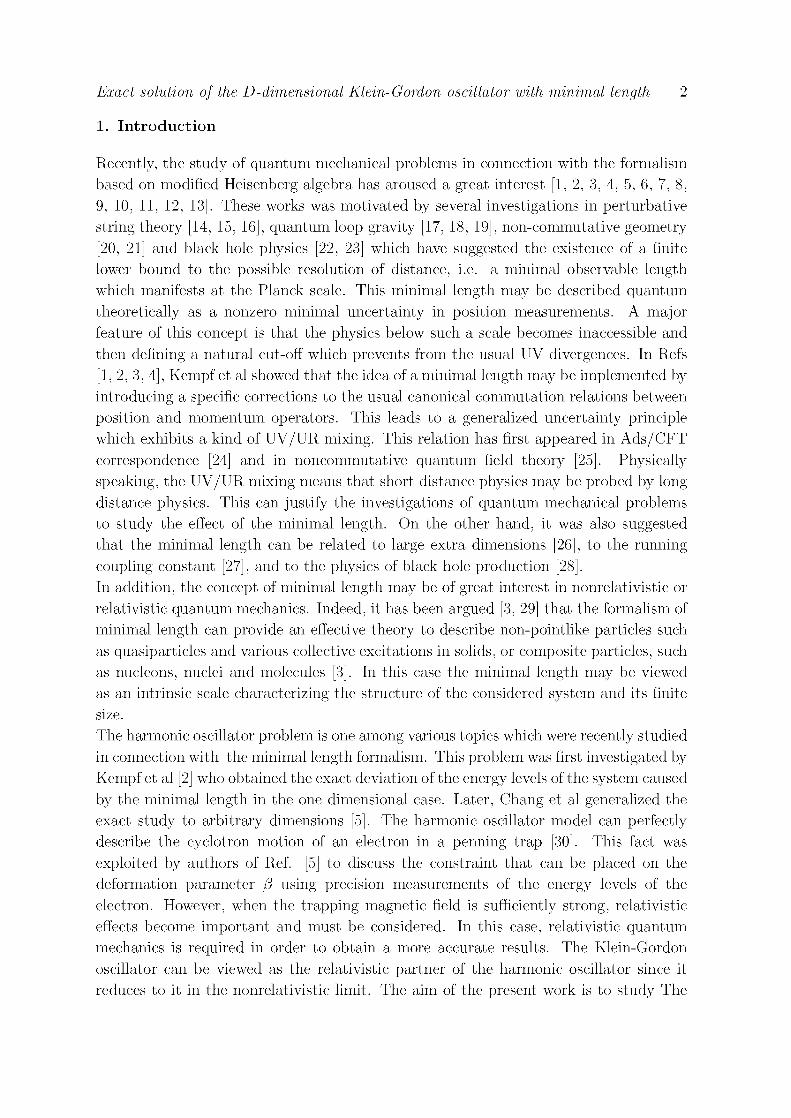
Exact solution of the D-dimensional Klein-Gordon oscillator with minimal length 2
1. Introduction
Recently, the study of quantum mechanical problems in connection with the formalism
based on modified Heisenberg algebra has aroused a great interest [1, 2, 3, 4, 5, 6, 7, 8,
9, 10, 11, 12, 13]. These works was motivated by several investigations in perturbative
string theory [14, 15, 16], quantum loop gravity [17, 18, 19], non-commutative geometry
[20, 21] and black hole physics [22, 23] which have suggested the existence of a finite
lower bound to the possible resolution of distance, i.e. a minimal observable length
which manifests at the Planck scale. This minimal length may be described quantum
theoretically as a nonzero minimal uncertainty in position measurements. A major
feature of this concept is that the physics below such a scale becomes inaccessible and
then defining a natural cut-off which prevents from the usual UV divergences. In Refs
[1, 2, 3, 4], Kempf et al showed that the idea of a minimal length may be implemented by
introducing a specific corrections to the usual canonical commutation relations between
position and momentum operators. This leads to a generalized uncertainty principle
which exhibits a kind of UV/UR mixing. This relation has first appeared in Ads /CFT
correspondence [24] and in noncommutative quantum field theory [25]. Physically
speaking, the UV/UR mixing means that short distance physics may be probed by long
distance physics. This can justify the investigations of quantum mechanical problems
to study the effect of the minimal length. On the other hand, it was also suggested
that the minimal length can be related to large extra dimensions [26], to the running
coupling constant [27], and to the physics of black hole production [28].
In addition, the concept of minimal length may be of great interest in nonrelativistic or
relativistic quantum mechanics. Indeed, it has been argued [3, 29] that the formalism of
minimal length can provide an effective theory to describe non-pointlike particles such
as quasiparticles and various collective excitations in solids, or composite particles, such
as nucléons, nuclei and molecules [3]. In this case the minimal length may be viewed
as an intrinsic scale characterizing the structure of the considered system and its finite
size.
The harmonic oscillator problem is one among various topics which were recently studied
in connection with the minimal length formalism. This problem was first investigated by
Kempf et al [2] who obtained the exact deviation of the energy levels of the system caused
by the minimal length in the one dimensional case. Later, Chang et al generalized the
exact study to arbitrary dimensions [5]. The harmonic oscillator model can perfectly
describe the cyclotron motion of an electron in a penning trap [30]. This fact was
exploited by authors of Ref. [5] to discuss the constraint that can be placed on the
deformation parameter (3 using precision measurements of the energy levels of the
electron. However, when the trapping magnetic field is sufficiently strong, relativistic
effects become important and must be considered. In this case, relativistic quantum
mechanics is required in order to obtain a more accurate results. The Klein-Gordon
oscillator can be viewed as the relativistic partner of the harmonic oscillator since it
reduces to it in the nonrelativistic limit. The aim of the present work is to study The
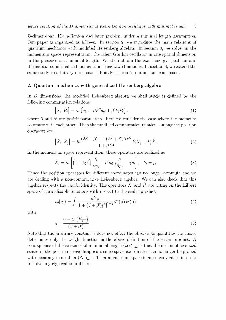
Exact solution of the D-dimensional Klein-Gordon oscillator with minimal length 3
_D-dimensional Klein-Gordon oscillator problem under a minimal length assumption. Our paper is organized as follows. In section 2, we introduce the main relations of quantum mechanics with modified Heisenberg algebra. In section 3, we solve, in the momentum space representation, the Klein-Gordon oscillator in one spatial dimension in the presence of a minimal length. We then obtain the exact energy spectrum and the associated normalized momentum space wave functions. In section 4, we extend the same study to arbitrary dimensions. Finally section 5 contains our conclusion.
2. Quantum mechanics with generalized Heisenberg algebra
In D dimensions, the modified Heisenberg algebra we shall study is defined by the following commutation relations
= ih(5lJ+pP25lJ+p'PlPJ). (1)
where ft and ft' are positif parameters. Here we consider the case where the momenta commute with each other. Then the modified commutation relations among the position operators are
X*. Pi
Xi,Xj ih (2ft -ft') + (2ft + ft')ftP2
PiXj PjXi 1 + ftP2
In the momentum space representation, these operators are realized as
(2)
Xi = ih I + PP' ft'pipj d
ipi Pi Pi (3) _d_ dpi ' '"' *"lt'Jdpj
Hence the position operators for different coordinates can no longer commute and we are dealing with a non-commutative Heisenberg algebra. We can also check that this algebra respects the Jacobi identity. The operators Xi and Pi are acting on the Hilbert space of normalizable functions with respect to the scalar product
dD~ <0| V)
with
V = 1
[l + (ft + ft')p
p,,D-l
,21 l~V f (P) ^ (P) (4)
(5) (J3 + P')
Note that the arbitrary constant 7 does not affect the observable quantities, its choice determines only the weight function in the above definition of the scalar product. A consequence of the existence of a minimal length (Ar)min is that the notion of localized states in the position space disappears since space coordinates can no longer be probed with accuracy more than (Ar)min. Then momentum space is more convenient in order to solve any eigenvalue problem.
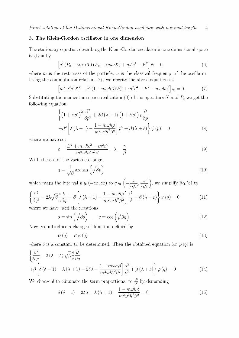
Exact solution of the D-dimensional Klein-Gordon oscillator with minimal length 4
3. T h e Klein-Gordon oscillator in one dimension
The stationary equation describing the Klein-Gordon oscillator in one dimensional space
is given by
c2 (Px + imuX) (Px - imuX) + m V - E2] ip = 0 (6)
where m is the rest mass of the particle, UJ is the classical frequency of the oscillator.
Using the commutation relation (2), we rewrite the above equation as
m V c 2 X 2 + c2 (1 - mu)h(3) Pi + TOV - E2 - muhc2] xp = 0. (7)
Substituting the momentum space realization (3) of the operators X and Px we get the
following equation
l + / 3 p 2 ) 2 ^ + 2 / 3 ( A + l ) ( l + /3p2)p
-P2 A(A + 1) 1 — mujhf3
2h2(32 rn^uj
dp
p2 + (3 (A + e) U (p) = 0
where we have set
E2 + mujhc2 — m2cA
rn^uj 2Ti2c2(3
, A 1 P
With the aid of the variable change
q = ~fB arc tan {yftPj
which maps the interval p G ( - co , oo) to g G
(8)
(9)
(10)
7T 7T
2*7/9 V / 3 we simplify Eq.(8) to
oq2 v coq A(A + 1)
1 — mujhf3 2h2(32
rn^uj + (3{\ + e) U(g) = 0
where we have used the notations
s = sin ( \j(3q ) , c = cos ( \J (3q
Now, we introduce a change of function defined by
ip (q) = cSp (q)
where 8 is a constant to be determined. Then the obtained equation for <p (q) is
+(3 8{8-\) + \{\ + l)-28\
(H)
(12)
(13)
1 — mujhf3 2h2(32
rn^uj + P(\ + e)}p(q) = 0
We choose 8 to eliminate the term proportional to %• by demanding
6{6-l)-26\ + \{\ + l)-^M = 0 m*uj
2h2(32
(14)
(15)
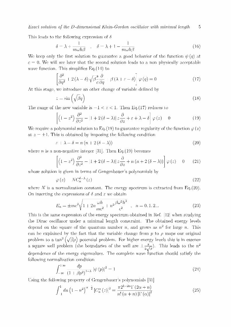
Exact solution of the D-dimensional Klein-Gordon oscillator with minimal length 5
This leads to the following expression of 8 1
8 = A + 8 = A + l 1
(16) muhp muhp
We keep only the first solution to guaran tee a good behavior of the function ip (q) at c = 0. We will see la ter t h a t t he second solution leads to a non physically acceptable wave function. This simplifies Eq.(14) to
— + 2{\- 5) fpS-— + (3{\ + e - 5) <p(q) = 0 (17)
At this stage, we in t roduce an other change of variable defined by
w sin (18)
The range of the new variable is — 1 < z < 1. T h e n Eq.(17) reduces to
1 rj2 f)
[l + 2(8-X)]z— + e + X-8 <p(z) = 0 (19) dz2 dz
We require a polynomial solution to Eq.(19) to guarantee regularity of the function p (z) at z = ±1 . This is obtained by imposing the following condition
e + X-8 = n(n + 2(8-X)) (20)
where n is a non-negat ive integer [31]. T h e n Eq.(19) becomes
1 dz2 [1 + 2(8-X)]z-^ + n(n + 2(8-X)) <p(z) = 0 (21)
whose solution is given in te rms of Gengenbauer ' s polynomials by
p (z) = NCtX (z) (22)
where AMs a normal izat ion constant . The energy spec t rum is ex t rac ted from Eq.(20) . On insert ing the expressions of 8 and e we ob ta in
E„ ±mc \ 1 + 2n-UJTI
n" ^u2h2
n mc*
0 ,1 ,2 . . . (23)
This is the same expression of the energy spec t rum obta ined in Ref. [12] when s tudying the Dirac oscillator under a minimal length constraint . T h e obta ined energy levels depend on the square of the q u a n t u m number n, and grows as n2 for large n. This can be explained by the fact t h a t t he variable change from p to p maps our original problem to a t a n 2 \\fPp) potent ia l problem. For higher energy levels this is in essence
a square well problem (the boundar ies of the well are ±—^=) . This leads to the n
dependence of the energy eigenvalues. T h e complete wave function should satisfy the following normal iza t ion condit ion
r+°° dp A-\ iv(p)r = i
-oo (l+/3p2Y
Using the following proper ty of Gengenbauer ' s polynomials [31]
du ( 1 u [c: (z)f vr2 l - 2 a Y{2a + n)
n\ (a + n) [T (a)]'
(24)
(25)

Exact solution of the D-dimensional Klein-Gordon oscillator with minimal length 6
we get for the normalized energy wave function the expression
-><5-A
V'n(p) P
2vr
n\(8-X + n)[T(8-X)f
T[2(8- A) n\ I + PP' a •s-x VPP
Vi + PP2 (26)
Let us now check that these wave functions are physically acceptable. In deformed
quantum mechanics governed by the commutation relations (2), it has been shown that
the wave function should be in the domain of p, to be physically acceptable [2]. This
physically means that it should have a finite uncertainty in momentum. Thus we impose
dp P a-A P IV' (p)\ < °°- (27)
(l+Pp2Y It is easy to check that the integrand in Eq.(27) behaves for p —• oo as p~2(-s~x\ Since for
p —• 0 the integrand behaves as p2, the convergence of the integral (27) will be ensured
provided 8 — X > \. This condition is not satisfied by the second solution in Eq.(16).
Indeed, a minimal length %\/~P, if it exists, must be of perturbational nature, and must
then ranks below the characteristic length of the oscillator
4. T h e Klein-Gordon oscillator in D dimensions
The D-dimensional Klein-Gordon oscillator is given by the following equation
c2 (P + imuX) (P - imuX) + m2c4 - E2] ip = 0 (28)
which can be written with the help of commutation relations (2) as
m V c 2 X 2 + c2 [1 - muhD (p + (31)} P 2 + m2c4 - E2 - muhDc2] ip = 0. (29)
Due to the rotational symmetry of this equation, we can separate the angular and the
radial part of the momentum wave function as follows
^ (P) = YL (P) <P (P) (30)
where Y^ (p) are D-dimensional ultra-spherical harmonics, p is the unit vector pointing
in the direction of p . The label m stands collectively for the set of magnetic quantum
numbers mi ,m 2 , . . . ,mD_i and p denotes |p| . With this separation, we can make the
following replacements in the momentum space realization of the operator X 2 [5] Dff^_d2_ D - 1 d L2 ^ d d
dp2 p dp p2
with
L2 = l(l + D-2) , / = 0,1,2, . . .
E -{dp2
i=\ dpi dp (31)
(32)
Then, the obtained equation for the radial momentum wave function reads
V + ^+^A2^ +
L + (/3 + / 3 V ] ; f - ^ J op p2
~D
+
1
p l(D-l)(3 + 2((3 + (3> + 1)]p
1 - mujhD (p + 13')
7L> - 2pV E2 + mojTiDc2
rn^uj
7 (J3D + P' + 7 ) - P2L2
<p(p) = 0
m2uj2h2 P
2 4 ' m c
2k2c2 (33)
Exact solution of the D-dimensional Klein-Gordon oscillator with minimal length 7
To solve this equation, we begin by making the following change of variable
Q === arctan Up + P'p) VÏÏ^P'
(34)
which maps the interval p G (0, oo) to g G ( 0 , — j =l \ a n d brings Eq.(33) to the
following form
\dq2 *-^\ + (J*$er*\ | - < / 3 + «4 7 (pD + p' + 7) - (32L2 1 - mujhD {(3 + /?')! s2
P + P> E2 + mojhDc2 — m2c4
{(3 + p>) m2uj2h2 jD - 2{3L''
m2u)2h2c2
where we have introduced the notations
s = sin Up + p'q) , c = cos Up + f3'q
By setting
_ E2 + mujhDc2 - m2c4 ^D - 2pL2
£~ (p + p')m2u2h2c2 + p + p' ' _ 7 {Dp + /?' + 7) - /32L2 1 - mujhD (p + /?')
(P + /3')z
we can rewrite Eq.(35) as
\dq2
(p + p'f m2L02h2 (D-l)P + 21
P + P'
(D-l)- + a-s c
d ^P + P'ôq ~ (/3 + ^ L
+ {P + P') K- + {P + P')e\^{q) = Q
Making now the following change of function
<p(q) = <?0(q)
where ô is a constant to be determined. We obtain for 9 (q) the equation
dq2 (D-l)- + (a- 26) d ^P + P'^-q-(P + P')L
+ (p + p') [K + 6 (5 - a - 1)] - + (p + p') (e -6D)}6 (q) = 0 c
(35)
(36)
(37)
(38)
(39)
(40)
To further simplify this equation, we cancel the term proportional to ^ by choosing ô as
K + ô(ô-a-l) = 0
As in the one dimensional case, the allowed expression of ô is
a + 1 6 '(a + iy
K
(41)
(42)
Exact solution of the D-dimensional Klein-Gordon oscillator with minimal length 8
Then Eq.(40) reduces to
[dq2
+ (P + P')(e-5D)}9(q) = Q
(D-l)- + (a- 25) -s c
d y/P + / V ~(J3 + P) L2
dq
In order to eliminate the term proportional to % we set
9 (q) = slÇ (q)
The obtained equation for 9 (q) reads
r d2
(43)
(44)
(21 1) - + (a - 25) -s c. y/P + P'
d dq dq2
+ {P + 13') [e-5D-l(25-a + l)]}i (q) = 0
Let us now change the variable from q to z G (—1,1), by setting
(45)
z = 2s< 1
This cats Eq.(45) into the form
dz2 21 + D a 25-1 2l + D + 26-a-ly
[e-5D l(25-a + l)]^(z) = 0
d_ dz
(46)
The wave function will be regular at z = ±1 if the solution £ (z) is a polynomial. This is obtained by imposing the condition
[s-5D-l {25 a 1)] n 1
n (21 + D + 25 a
with n' a non-negative integer. Then Eq.(46) takes the form
1 dz2
1
21+ D a 25-1 1
21 + D + 25 a 1
-1)
d_ dz
(47)
2 V 2 )
-n' rv + - ( 21 + JJ + 2^ - a - 1) I £ (z) = 0
Its solution is given in terms of Jacobi polynomials by
£ (z) = NDPfrb) (z) where ND is a normalization constant and parameters a and b are defined by
, D 1 , r « ! a = / H 1 , o = o 2 2 2
The energy eigenvalues are obtained from Eq.(47) which can be rewritten as
(48)
(49)
(50)
e = 2V-^+W + nD + (2n' + l)> + W + l)D
2 (fi + P')
2n' + / + D- \a + \y
K (51)

Exact solution of the D-dimensional Klein-Gordon oscillator with minimal length 9
with E2 + mujhDc2 2 4
m c e = (P + P') m2uj2h2c2
Defining the quantum number n by n -
levels reads
ujfiD 2OJ%
(52)
2n! + /. The resulting expression of the energy
E, nl ±mc 1
(J3 + p)(n D
~2
2
m r
(P ~ P')
P2L2 m2u)2h2 — mujhD (P
ra = 0,l,2...
P')
(53)
As in the one dimensional case, we note the n2 dependence of the energy levels related to the fact that for higher energy eigenvalues, our original problem is equivalent to a square wells problem. We also point the additional / dependence of the energy levels which was absent in the original case (with vanishing p). As a consequence, the degeneracy of the
-1)! (p+i-sy. nth energy state reduces from (D^_"7!ra!' in the conventional case to (^_1\m — m-iwz-2)! for each value of / in the presence of a minimal length [32]. This can be viewed as a sign of a self-supersymmetry breaking of the Klein-Gordon oscillator [33].
The expression (23) of the energy spectrum in one dimension can be recovered by setting D = 1, L2 = 0 and P' = 0. In the following, we will use this expression to improve the hypothetical bound of the minimal length found in Ref. [5] when discussing the condition that can be placed on the parameter P by the measuring the energy levels of an electron trapped in a strong magnetic field. To this end, we first expand the nth energy eigenvalue up to the first order in P as
E„ mc Pmu2h2n2
(54)
The deviation of the nth energy level from the usual case caused by the modified commutation relations (2) is given by
AEn Pmujhn2
uh 2 J l + 2n uih (55)
The cyclotron frequency of an electron of mass me trapped in a magnetic field of strength B is
eB UJ, =
m. For a magnetic field of strength B = 6T we have
rriehuc = 1.0 x 1(T52kg2m2/s2
(56)
(57)
Following Ref. [5], we assume that only a deviation of the scale of TIUJC can be detected. Then if no perturbation of the nth energy level is observed, we may conclude that
pehBn2
2Jl + 2n ehB < 1 (58)

Exact solution of the D-dimensional Klein-Gordon oscillator with minimal length 10
This leads to the following constraint
hyfp<\ 2hJi 2n^h
eBn2 (59)
This condition includes relativistic corrections, hence the maximum value of n is not constrained by the requirement that the electron remains nonrelativistic, it depends only on the experimental setting (we should be able to accurately measure its corresponding energy eigenvalue). Assuming for instance that we can accurately measure the energy eigenvalue corresponding to level n = 1010, then we obtain the following upper bound for the minimal length:
h^<0Mx 10" 18 m (60)
Let us now turn to the examination of the radial momentum wave functions. These should satisfy the following normalization condition
dp P " - V ( P ) = I
/o (I + PP2)1^1
Using the following property of Jacobi polynomials [31]
du{l-u)a{l + u)b\P^'b){u) 2a+fe+i r(n + a + l)T(n + b + l)
2n + a + b n\T (n + a + b + 1)
we get for the normalized energy radial momentum wave function the expression
{2ri + a + b) T {ji! + a + b + 1) n'\
(61)
(62)
<Prd (P) = P 4
T (n' + a + 1) T (n' + b + 1)
V 1 + (P + P')p2 S+l (a,b)((P + P')p2 1
n (n-l)/2 (63) y({3 + (3') P2 + I )
As mentioned before, a physically acceptable wave function should be in the domain of p. This means that the radial momentum wave function must satisfy the condition
dp aJJ D+l ( \2 . (64)
We can easily check that the integrand in Eq.(64) behaves for p -^ 0 as pD+1 and for p -^ oo as pa~2S. Thus the convergence criterion is 25 — a < — 1, the condition which is already satisfied.
5. Conclusion
In summary, we have solved in the momentum space representation the Klein-Gordon oscillator in arbitrary dimension in the framework of quantum mechanics with minimal length. Then, we have obtained the energy spectrum and the associated normalized momentum space wave functions. Unlike the usual case (with vanishing (3), the energy levels are n2 dependent. This can be explained by the fact that for higher energy eigenvalues our original problem is equivalent to the square wells problem. Another interesting consequence of the modified commutation relations is the additional /
Exact solution of the D-dimensional Klein-Gordon oscillator with minimal length 11
dependence of the energy levels which was absent in the standard case. This leads to a degeneracy reduction of the energy eigenvalues and can be interpreted as a breaking of self-supersymmetry of the Klein-Gordon oscillator. The harmonic oscillator model can perfectly describe the cyclotron motion of an electron trapped in a strong magnetic field. Using precision measurements of the energy levels of the electron, we have discussed possible improvement of the upper bound for the minimal length previously found by Chang et al.
References
A. Kempf, J. Math. Phys. 35 (1994) 4483. A. Kempf, G. Mangano and R.B. Mann, Phys. Rev. D52 (1995) 1108. A. Kempf, J. Phys. A30 (1997) 2093. H. Hinrichsen and A. Kempf, J. Math. Phys. 37 (1996) 2121. L.N Chang, D. Minic, N. Okamura and T. Takeuchi, Phys. Rev. D65 (2002) 125027. T.V. Fitio, I.O. Vacarchuk and V.M. Tkachuk, J. Phys. A39 (2006) 2143. F. Brau, J. Phys. A32 (1999) 7691. R. Akhoury and Y-P. Yao, Phys. Lett. B572 (2003) 37. S. Benczik, L.N. Chang, D. Minic and T. Takeuchi, Phys. Rev. A72 (2002) 012104. L.N. Chang, D. Minic, N. Okamura and T. Takeuchi, Phys. Rev. D65 (2002) 125028. S. Benczik, L.N. Chang, D. Minic, N. Okamura, S. Rayyan and T. Takeuchi, Phys. Rev. D66
(2002) 026003. Kh. Nouicer, J. Phys. A39 (2006) 5125. C. Quesne and V.M. Tkachuk, J. Phys. A38 (2005) 1747. D.J. Gross and P.F. Mende, Nucl. Phys. B303 (1988) 407. K. Konishi, G. Paffuti and P. Provero, Phys. Lett. B234 (1990) 276. D. Amati, M. Ciafaloni and G. Veneziano, Phys. Lett. B216 (1989) 41. C. Rovelli, Living Rev. Rel. 1 (1998) 1. T. Thiemann, Lect. Notes Phys. 631 (2003) 41. A. Perez, Class. Quant. Grav. 20 (2003) R43. M.R. Douglas and N.A. Nekrasov, Rev. Mod. Phys. 73 (2001) 977. F. Girelli, E.R. Livine and D. Oriti, Nucl. Phys. B708 (2005) 411. T. Padmanabhan, T.R. Seshadri and T.P. Singh, Int. J. Mod. Phys. A l (1986) 491. F. Scardigli, Phys. Lett. B452 (1999) 39. A.W. Peet and J. Polchinski, Phys. Rev. D59 (1999) 065011. M.R. Douglas and N.A. Nekrasov, Rev. Mod. Phys. 73 (2002) 977. S. Hossenfelder, Mod. Phys. Lett. A19 (2004) 2727. S. Hossenfelder, Phys. Rev. D70 (2004) 1054003. S. Hossenfelder, Phys. Lett. B 598 (2004) 92. R.S. Ramchander, J. Phys. A33 (2000) 8305. L.S. Brown and G. Gabrielse, Rev. Mod. Phys. 58 (1986) 233;
R.K. Mittleman, LI. Ioannou, H.G. Dehmelt and N. Russell, Phys. Rev. Lett. 83 (1999) 2116; H. Dehmelt, R. Mittleman, R.S. van Dyck and P. Schwinberg, Phys. Rev. Lett. 83 (1999) 4694.
M. Abramowitz and I. Stegun, Handbook of Mathematical Functions, Dover, New York (1974). N.IA. Vilenkin, Special Functions and the Theory of Group Representations. AMS, Providence, RI
(1968). [33] F. Cooper and B. Freedman, Ann. Phys. (N.Y.) 146 (1983) 262.
IOP PUBLISHING JOURNAL OF PHYSICS A: MATHEMATICAL AND THEORETICAL
J. Phys. A: Math. Theor. 42 (2009) 355203 (lOpp) doi:10.1088/1751-8113/42/35/355203
Analytical treatment of the one-dimensional Coulomb problem for the spinless Salpeter equation
Y Chargui1, L Chetouani2 and A Trabelsi13
1 Unité de Recherche de Physique Nucléaire et des Hautes Energies, Faculté des Sciences de Tunis, 1080 Tunis, Tunisia 2 Département de Physique Théorique, Institut de Physique, Université de Constantine, Route Ain El Bey, Constantine, Algeria 3 Centre National des Sciences et Technologies Nucléaires, Technopole de Sidi-Thabet 2020, Tunisia
E-mail: [email protected]
Received 25 February 2009, in final form 1 July 2009 Published 11 August 2009 Online at stacks.iop.org/JPhysA/42/355203
Abstract Using the momentum space representation, we present an analytical treatment of the one-dimensional spinless Salpeter equation with a Coulomb interaction. The exact bound-state energy equation is determined. The results obtained are shown to agree very well with exact numerical calculations existing in the literature.
PACS numbers: 03.65.Pm, 03.65.Ge
(Some figures in this article are in colour only in the electronic version)
1. Introduction
The spinless Salpeter equation (SSE) is a simple semi-relativistic version of the Schrôdinger equation which incorporates the exact free-particle relativistic relation between energy and momentum. This equation is generally used when kinetic relativistic effects cannot be neglected. It is suitable for the description of scalar bosons as well as the spin-averaged spectra of bound states of fermions. Moreover, the spinless Salpeter equation appears as a standard approximation to the Bethe-Salpeter formalism which is the basic description of bound states within the framework of relativistic quantum field theory [1]. It can be deduced from the so-called Salpeter equation [2] by neglecting the spin degree of freedom and disregarding negative-energy solutions. The Salpeter equation, in turn, approximates the Bethe-Salpeter equation by assuming an instantaneous interaction [3]. The one-particle spinless Salpeter equation for stationary states has the form of an eigenvalue problem (h = c = 1):
H\fk} = Ek\fk), k = 1 , 2 , 3 , . . . ,
1751-8113/09/355203+10$30.00 © 2009 IOP Publishing Ltd Printed in the UK 1
J. Phys. A: Math. Theor. 42 (2009) 355203 Y Chargui et al
with Ek being the energy eigenvalues corresponding to Hilbert-space eigenvectors \irk), and the Hamiltonian H of the system being of the form
H = Vp2 + m2 +V(r),
where ^ p 2 + m2 is the relativistic mass plus kinetic energy of the particle of mass m and momentum p, and V(r) is an arbitrary position-dependent static interaction potential. Due to the presence of the square root which renders the Hamiltonian non-local, the construction of analytical solutions to this equation is generally not a trivial task. Therefore, the investigation of this equation always implies either the use of approximating methods or the application of numerical approaches. The one-dimensional Coulomb potential is one among several problems which have been investigated on the basis of the spinless Salpeter equation [4-8, 10]. However, to our knowledge, an exact analytic expression of its energy eigenvalues is still absent from the literature (for a detailed history review of the spinless Salpeter Coulomb problem we refer the reader to [11]). In this paper, we fill this gap and present an exact analytical treatment of the one-dimensional spinless Salpeter Coulomb problem in the momentum space representation. Note that besides the interesting applications of the one-dimensional Coulomb potential in theoretical physics (such as the investigation of the mass spectra of mesons [12]), the solution of this problem may serve as a toy model which can be instructive for the analysis of the more important three-dimensional case.
Our paper is organized as follows. In section 2, we find the exact solution of the one-dimensional spinless Salpeter Coulomb problem in the momentum space. In section 3, we determine the quantization condition and obtain the exact energy spectrum. The resulting binding energy levels are then calculated and compared to those found in the literature by exact numerical treatment of the problem. The final section contains our conclusions.
2. One-dimensional spinless Salpeter Coulomb problem in the momentum space
In this section, we are interested in the solution of the one-dimensional eigenvalue equation,
[j p2 + m2 + V (x)]\f) = E\f), (1)
with a Coulomb-type interaction,
V(x) = - - , x e R (K > 0). (2) x
The same problem was considered in [10], but the configuration space was restricted to the positive half line:
f{x)=0 for x < 0 . (3)
This restriction may be interpreted as due to the presence of a 'hard-core' interaction potential effective for x < 0. Before starting our solution, let us review the main features of this work and make some comments on it. In [10], the author began by showing that the action of the kinetic energy operator y/' p2 + m2 on an element \\r (x) of L2 (R) can be expressed as
J-d2 + m2f(x) = —(-d2x+m2) I dy K0(my)[f(x + y) + f(x - y)], (4)
where d\ = d2/Ax2, and K0 (x) is the modified Bessel function of order 0. He worked out this action for the special case of the function x" e~^x and put it under the form
-d2 + m2x" t-px = t-px J2 Fk,n(m, P)x"-k, (5) k=0
2
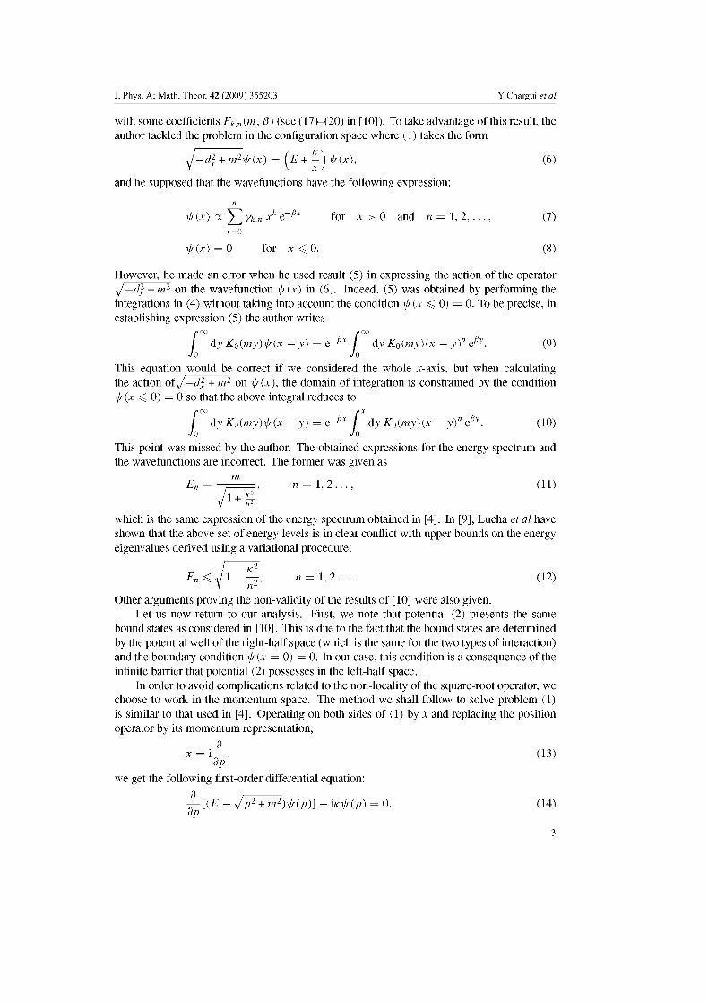
J. Phys. A: Math. Theor. 42 (2009) 355203 Y Chargui et al
with some coefficients Fkt„(m, ft) (see(17)-(20)in [10]). To take advantage of this result, the author tackled the problem in the configuration space where (1) takes the form
^-d2x+m2fix) =(E+-\ f(x), (6)
and he supposed that the wavefunctions have the following expression:
n
f{x) oc ^2yk,„ xk Q~PX for x > 0 and « = 1 , 2 , . . . , (7) k=0
fix)=0 for x < 0 . (8)
However, he made an error when he used result (5) in expressing the action of the operator y/—d% + m2 on the wavefunction fix) in (6). Indeed, (5) was obtained by performing the integrations in (4) without taking into account the condition f (x < 0) = 0. To be precise, in establishing expression (5) the author writes
/>O0 />O0
/ dy Koimy)fix - y) = e ^ x / dy K0(my)(x - y)n éy. Jo Jo
(9)
This equation would be correct if we considered the whole x-axis, but when calculating the action of^-d2 + m2 on fix), the domain of integration is constrained by the condition f (x < 0) = 0 so that the above integral reduces to
/>O0 r-x
\ dyK0imy)fix-y) = e-flx dyKoimyXx-yT^y. (10) Jo Jo
This point was missed by the author. The obtained expressions for the energy spectrum and the wavefunctions are incorrect. The former was given as
m E„= . « = 1 , 2 . . . , (11)
which is the same expression of the energy spectrum obtained in [4]. In [9], Lucha et al have shown that the above set of energy levels is in clear conflict with upper bounds on the energy eigenvalues derived using a variational procedure:
En^^\-—, « = 1 , 2 . . . . (12)
Other arguments proving the non-validity of the results of [10] were also given. Let us now return to our analysis. First, we note that potential (2) presents the same
bound states as considered in [10]. This is due to the fact that the bound states are determined by the potential well of the right-half space (which is the same for the two types of interaction) and the boundary condition f (x = 0) = 0. In our case, this condition is a consequence of the infinite barrier that potential (2) possesses in the left-half space.
In order to avoid complications related to the non-locality of the square-root operator, we choose to work in the momentum space. The method we shall follow to solve problem (1) is similar to that used in [4]. Operating on both sides of (1) by x and replacing the position operator by its momentum representation,
9 x = i—, (13)
dp we get the following first-order differential equation:
— HE - Jp2 + m2)fip)] - vcfip) = 0. (14) dp
3
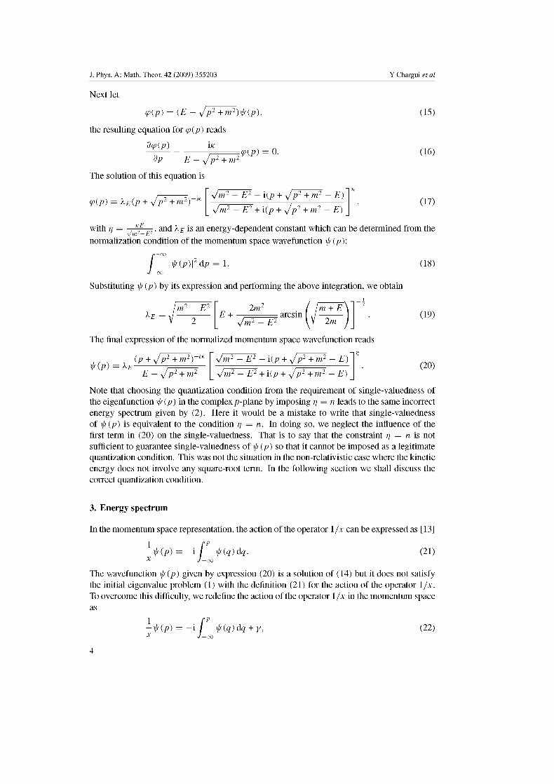
J. Phys. A: Math. Theor. 42 (2009) 355203 Y Chargui et al
Next let
<P(P) = (E - y/p2+m2)f(p)
the resulting equation for <p(p) reads
dcp(p) IK
dp E - y/p2 + m2
The solution of this equation is
cp(p) = 0.
<P(p) = XE(p + y/p2 +m2)
with r]
\Jm2 E2 - i(p + V/?2 + m2 - E)
^/m2 E2 + i(p + TJP2 +I E)
(15)
(16)
(17)
, * „_, and XE is an energy-dependent constant which can be determined from the \/mz—Ez
normalization condition of the momentum space wavefunction f (p):
f J — (.
\f(p)\iAP = l. (18)
Substituting <\i (p) by its expression and performing the above integration, we obtain
2m2 I m + E Xr
E2
E + \fm E2 : arcsin 2m
The final expression of the normalized momentum space wavefunction reads
f(p) = A., (p + y p2 + m2) 2\-IK
s + m
\Jm2 E2 - \{p + y/'P2 + I ,2 E)
\fm E2 + i(p + y/p2+m2 -E)
(19)
(20)
Note that choosing the quantization condition from the requirement of single-valuedness of the eigenfunction <\i (p) in the complexp-plane by imposing r] = n leads to the same incorrect energy spectrum given by (2). Here it would be a mistake to write that single-valuedness of i/f (p) is equivalent to the condition r] = n. In doing so, we neglect the influence of the first term in (20) on the single-valuedness. That is to say that the constraint r] = n is not sufficient to guarantee single-valuedness of^(p) so that it cannot be imposed as a legitimate quantization condition. This was not the situation in the non-relativistic case where the kinetic energy does not involve any square-root term. In the following section we shall discuss the correct quantization condition.
3. Energy spectrum
In the momentum space representation, the action of the operator 1/x can be expressed as [13]
1 -f{p)
J — oo
f{q)Aq. (21)
The wavefunction \\r (p) given by expression (20) is a solution of (14) but it does not satisfy the initial eigenvalue problem (1) with the definition (21) for the action of the operator 1/x. To overcome this difficulty, we redefine the action of the operator 1/x in the momentum space as
1 -f{p)
J — (.
f{q)Aq + Y, (22)
4
J. Phys. A: Math. Theor. 42 (2009) 355203 Y Chargui et al
where y is a constant to be determined from the requirement that the eigenfunction \\r (p) given by (20) should be a solution of the eigenvalue equation (1). The constant y is then obtained from the following equation:
(E — y/p2 + m2)ip(p) — IK I J — CO
fiq)dq + tcy = 0 . (23)
Substituting the eigenfunction ir(p) by its expression (20), we get
y = - — [-===-—) exp[-tf£] (24) K \jm2 - E2 -\E }
with fœ du
eE = K (25) Jo E — \Ju2 + m2
Note that due to the indétermination of the limit, lim (p + jp2 + m2yiK, (26)
an explicit expression for y cannot be obtained. However, we can content ourselves with the form (24) which is rather more appropriate for the following manipulations.
Next, the quantization condition is obtained by demanding that the Hamiltonian of the system,
H = jp2 + m2 - -, (27) x
should be a Hermitian operator on its eigenfunction ir(p) given by (20). Obviously, the operator ^'p2 +m2 satisfies this condition; then our requirement implies that the operator 1/x should be Hermitian on the set of eigenfunctions irE(p):
-fE\fE>) = {fE\-fE\- (28) x x I
Replacing the operator 1/x by its momentum representation (22), the last condition reduces to
/
+ CO pf /»+00
fE'(p)\ fE(q)dqdp + y*[i/E] fE'(p)dp -co J —co J —co
/
+CO pf /»+00
flip) / fE'{q)dqdp + y[fEI]\ rE(p)dP. (29) -co J—co J —co
Taking into account the following integral formula,
/+co px /»+oo /»+oo /»+co py
fix) I giy)dydx= g(y) f(x)dydx- g(y) f(x)dxdy, -co J-co J— co J— co J—co J— co
(30) together with the orthogonality relation of the wavefunctions and observing that the eigenfunction irE(p) can be expressed as
i Bwp(p)
fEip) = ^ P ^ , (31) K dp
where the function <p(p) given by (17) is rewritten in a more useful form as du
(\jm2 -E2 + XE\
VE{P) = XEV7^TW^) exp \K f JO
E -4, o t — VuA + mz (32)
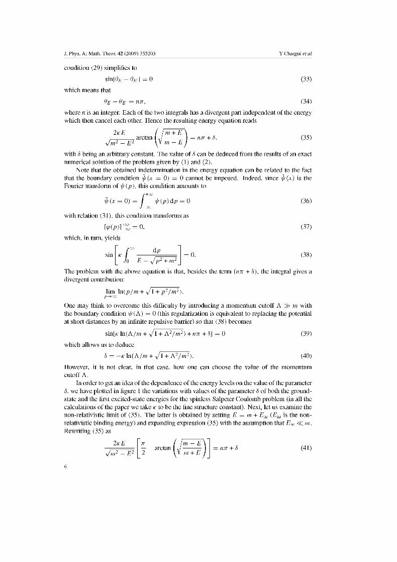
J. Phys. A: Math. Theor. 42 (2009) 355203 Y Chargui et al
condition (29) simplifies to
sin[<9£ - 9E>] = 0 (33)
which means that
BE - 6E< = nn, (34)
where n is an integer. Each of the two integrals has a divergent part independent of the energy which then cancel each other. Hence the resulting energy equation reads
IK E / m + E \ = arctan J = nn + 5, (35)
Vm2 - E2 \ym-Ej
with 5 being an arbitrary constant. The value of 5 can be deduced from the results of an exact numerical solution of the problem given by (1) and (2).
Note that the obtained indétermination in the energy equation can be related to the fact that the boundary condition \jr{x = 0) = 0 cannot be imposed. Indeed, since ïr(x) is the Fourier transform of xjr (/?), this condition amounts to
f f(x = 0)= f{p)Ap = Q (36) J — CO
with relation (31), this condition transforms as
[<P(P)]-Z = 0, (37)
which, in turn, yields
dp sin
Jo E — y' p2 + m2 0. (38)
The problem with the above equation is that, besides the term {nit + 5), the integral gives a divergent contribution:
lim ln(p/m +^/l + p2/m2). p—?co
One may think to overcome this difficulty by introducing a momentum cutoff A ^> m with the boundary condition xjr (A) = 0 (this regularization is equivalent to replacing the potential at short distances by an infinite repulsive barrier) so that (38) becomes
sin[K ln(A/m + y/l + A2/m2) + tin + 5] = 0 (39)
which allows us to deduce
5 = -K ln(A/m + j l + A2/m2). (40)
However, it is not clear, in that case, how one can choose the value of the momentum cutoff A.
In order to get an idea of the dependence of the energy levels on the value of the parameter 5, we have plotted in figure 1 the variations with values of the parameter 5 of both the ground-state and the first excited-state energies for the spinless Salpeter Coulomb problem (in all the calculations of the paper we take K to be the fine structure constant). Next, let us examine the non-relativistic limit of (35). The latter is obtained by setting E = m + Em (Em is the non-relativistic binding energy) and expanding expression (35) with the assumption that Em « r a . Rewriting (35) as
2K E
\Jm2 — E2
n arctan L ,,
2 \V m + E nn + S (41)
6

J. Phys. A: Math. Theor. 42 (2009) 355203 Y Chargui et al
- 1 0 - _ _ „ - • - -
>" ^-"^ 3, -15 -W ; ;
- 2 0 : ^ ' ' :
y
- 2 5 - , ' ' :
/
-1.0 -0.5 0.0 0.5 1.0
Figure 1. Plot of the energy eigenvalues of the Coulomb potential as a function of the parameter S. Two energy levels are represented: the ground-state energy (dashed line) and the first excited-state energy (full line).
and expanding the above equation to leading terms in Em/m, we obtain Kit
.. nn + 8. (42) *J-2Em/m
The usual non-relativistic energy spectrum is recovered by setting 8 = —K. However, this requirement cannot be used to fix 5 in (35) since the same limit would be obtained if one replaced 5 by a function of K : 8(K), satisfying the condition
lim 8(K)/K = - 1 (43)
and expanded (42) to first order in K. In the following, we will compare our analytical finding with exact numerical calculations
existing in the literature. We will use the results of [14] where exact numerical solutions of both the one-body spinless Salpeter equation for an electron moving in a central Coulomb potential (spinless Salpeter hydrogen-atom problem) and the two-body spinless Salpeter equation for two equal-mass electrons interacting via a central Coulomb potential (spinless positronium problem) are presented in the momentum space. In the two-body case, the comparison is made possible by the equivalence of the one-particle and the equal-mass two-particle equations [15]. Let us recall how the two equations can be equated. Given the following two relativistic Coulombic Hamiltonians for the one- and two-particle problems:
(44)
(45)
(46)
/ / ( 1 ) = V P 2 + ™ 2 - - , r
and
/ / ( 2 )=2VP 2 + M 2 - - , R
r = \x\
R = \X\,
respectively. Applying the canonical transformation,
X P = 2P, x = - ,
and identifying the mass and the Coulomb strength parameters as a
m = 2M, K = - , 2
(47)
7

J. Phys. A: Math. Theor. 42 (2009) 355203 Y Chargui et al
Table 1. Comparison of the binding energies obtained by exact analytical solution (Analytical) and exact numerical solution (Numerical) of the one-dimensional spinless Salpeter equation with a Coulomb interaction. Upper bounds calculated from (12) are also listed. A negative sign before the energy values has been omitted. All values are given in eV.
n
1 2 3 4 5 6 7 8 9
10
Analytical
13.606 595 3.401 5698 1.5117904 0.850 3762 0.544 2384 0.377 9422 0.277 6712 0.2125916 0.167 9734 0.136 0583
Numerical
13.606 595 3.401 5706 1.5117909 0.850 3765 0.544 2386 0.377 9423 0.277 6713 0.2125918 0.167 9735 0.136 0585
Upper bounds
13.605 873 3.401 4344 1.5117458 0.850 3565 0.544 2280 0.377 9360 0.227 6673 0.2125890 0.1679715 0.136 0569
we end up with
H(X) = H(2)_ ( 4 8 )
Note that the energy spectrum in the one-dimensional case is exactly identical to that corresponding to the three-dimensional case with vanishing orbital angular momentum. To obtain the energy levels from (35), in the two cases (one- and two-body problems) we choose to fix the value of the parameter 5 by demanding that the ground-state energy of [14] should be a solution of (35) with n = 1. This condition gives
5 =-0.0074641912 and 5 = - 0 . 0 0 3 6910191 (49)
for the one- and the two-particle problem, respectively. Then our energy eigenvalues are calculated by solving equation (35) numerically for different values of quantum number n where the parameters m, K and 5 are each time replaced by their corresponding values. The results of our calculations together with the comparison to those of [14] are presented in tables 1 and 2. The values of the binding energy upper bounds calculated from (12) are also reported in the same tables. As we can see, our calculations are in perfect agreement with numerical findings, and upper bounds (12) are well respected by the obtained sets of energy levels.
Let us make a remark concerning the check of the respect of energy upper bounds. The obtained energy equation (35) contains an unknown parameter 5 which should naturally depend on the coupling constant K. Unfortunately, this fact makes it impossible to check the respect of available energy upper bounds by the energy levels given by (35) for arbitrary values of the coupling constant K. Therefore, the upper-bounds check was made only in the two cases where the parameter 5 was initially fixed.
We turn now to the examination of the obtained momentum space wavefunctions. With condition (35), the expression of the norm of bound-state wavefunctions takes the form
/ (m2 _ E2)E2
\fn(P)\=J^-i 2 . " ; " Ay/p* + m*-Enr\ « = 1,2,. . . . (50) y 2[E2 + m2(n7T + S)/K\
To get an insight into the effect of relativistic kinematic on the wavefunction, figure 2 compares norm (50) with the norm of the Schrodinger momentum space wavefunction for the ground state. We see that for low momentum values, the two curves fit together. Hence, relativistic
8

J. Phys. A: Math. Theor. 42 (2009) 355203 Y Chargui et al
0.0005
0.0004
^ 0.0003
> 0.0002
0.0001
0.0000
0 2 4 6 8 10 p/mc
Figure 2. Comparison between ground-state momentum space wavefunctions corresponding to the Schrodinger equation (dashed line) and the spinless Salpeter equation (full line).
Table 2. Same as table 1 except for a spinless electron-positron bound state.
n
1 2 3 4 5 6 7 8 9
10
Analytical
6.8029616 1.700 7306 0.755 8780 0.4251806 0.2721153 0.188 9688 0.138 8342 0.106 2949 0.083 9861 0.068 0288
Numerical
6.8029616 1.700 7302 0.755 8777 0.4251805 0.2721152 0.188 9687 0.138 8341 0.106 2948 0.083 9860 0.068 0286
Upper bounds
6.802 8687 1.700 7129 0.755 8721 0.425 1780 0.2721139 0.188 9680 0.138 8336 0.106 2945 0.083 9858 0.068 0285
corrections to the Schrodinger wavefunction are minor for small momentum. However, as the momentum value grows, the two curves separate. This is related to the different behaviours of the two wavefunctions at large momentum. Indeed, the Schrodinger wavefunction is equivalent to l/p2 for p -> oo; however, the spinless Salpeter wavefunction scales as l/p when p -> oo. The non-relativistic wavefunction decreases with the momentum faster than the relativistic wavefunction.
4. Conclusion
In summary, using functional analysis, we have solved exactly the one-dimensional spinless Salpeter equation for a Coulomb potential in the momentum space. Then we have derived the exact corresponding energy equation. To check the validity of the obtained results, we have compared the resulting binding energy levels to those previously found in the literature using exact numerical calculations for two different cases: the spinless Salpeter hydrogen-atom problem and the spinless Salpeter positronium problem. In the latter case, the comparison was made possible using the equivalence between the one-particle and the equal-mass two-particle equation. The agreement between the two results is almost perfect. We have also verified
9
J. Phys. A: Math. Theor. 42 (2009) 355203 Y Chargui et al
that our sets of energy levels respect well energy upper bounds obtained using a variational method. Finally, we hope that the study presented in this paper will be helpful for the exact treatment of the still-unsolved three-dimensional spinless Salpeter Coulomb problem.
References
[1] Nambu Y 1950 Prog. Theor. Phys. 5 614 Salpeter E E and Bethe H A 1951 Phys. Rev. 84 1232
[2] Salpeter E E 1952 Phys. Rev. 87 328 [3] Greiner W and Reinhardt J 1994 Quantum Electrodynamics 2nd edn (Berlin: Springer) p 297 [4] Durand B and Durand L 1983 Phys. Rev. D 28 396 [5] Castorina P, Cea P, Nardulli G and Paiano G 1984 Phys. Rev. D 29 2660 [6] Hardekopf G and Sucher J 1984 Phys. Rev. A 30 703
Hardekopf G and Sucher J 1985 Phys. Rev. A 31 2020 [7] Martin A and Roy S M 1989 Phys. Lett. B 233 407 [8] Raynal J C, Roy S M, Singh V, Martin A and Stubbe J 1994 Phys. Lett. B 320 105 [9] Lucha W and Schoberl F F 2000 J. Math. Phys. 41 1778
[10] Brau F 1999 J. Math. Phys. 40 1119 Brau F 1999 J. Math. Phys. 40 6125 (erratum)
[11] Lucha W and Schoberl F F 1994 Proc. Int. Conf. on Quark Confinement and the Hadron Spectrum (Como, Italy, June) ed N Brambilla and G M Prosperi (River Edge, NJ: World Scientific) p 100
[12] Moshinsky M 1993 J. Phys. A: Math. Gen. 26 2445 [13] Nunez Yepez H N, Vargas C A and Brito A L S 1987 Eur. J. Phys. 8 189 [14] Norbury J W, Maung K M and Kahana D E 1994 Phys. Rev. A 50 3609 [15] Lucha W, Schoberl F F and Gromes D 1991 Phys. Rep. 200 127
10

Exact solution of the one-dimensional Klein-Gordon equation with scalar and vector linear potentials in the presence of a minimal length
Y Chargui1 , L Chetouani2 , A Trabelsi1 '3
1Unité de Recherche de Physique Nucléaire et des Hautes Energies, Faculté des Sciences de Tunis, 1080 Tunis, Tunisia 2Département de Physique Théorique, Institut de Physique, Université de Constantine, Route Ain El Bey, Constantine, Algeria 3Centre National des Sciences et Technologies Nucléaires, Technopole de Sidi-Thabet 2020, Tunisia
E-mail: yassine . charguiQgmail. corn
Abstract. Using the momentum space representation, we solve the Klein-Gordon equation in one spatial dimension for the case of mixed scalar and vector linear potentials in the context of deformed quantum mechanics characterized by a finite minimal uncertainty in position. The expressions of bound state energies and the associated wave functions are exactly obtained.
PACS numbers: 02.40.Gh, 03.65.Ge
2
1. Introduction
The linear potential is an important mechanical model which has been widely used
especially with relativistic wave equations in the investigation of quark confinement
[1, 2]. When this potential is introduced as the time component of a Lorentz vector no
bound states are found [3, 4] and only tunneling solutions arise. This is related to the
existence of the Klein paradox. On the contrary, when the potential is considered as a
Lorentz scalar, confinement becomes possible. Also for a mixture of a scalar-like and a
vector-like linear potentials, it was established that bound states can occur only when
the scalar term is sufficiently strong compared with the electric field [5, 6, 7, 8]. All these
results valid for (3 + 1)- and for (3 + 1)-dimensional space-time was established within
the framework of usual quantum mechanics, where position and momentum operators
acting on the Hilbert space of states verify the usual Heisenberg algebra. However, if one
takes into account the effects of quantum fluctuations of the gravitational field in order
to incorporate gravity into quantum mechanics, an induced minimal length, i.e. a lower
bound to the possible resolution of distances appears. This idea was mainly motivated
by string theory [9, 10, 11] and loop quantum gravity [12, 13, 14]. The minimal length
may be described quantum theoretically as a nonzero minimal uncertainty in position
measurements. In Refs.[15, 16, 17, 18] Kempf et al showed that such a minimal length
can be naturally obtained from a specific modification of the usual commutation relations
between position and momentum operators. An important feature of the resulting
uncertainty principle is the intriguing UV/IR mixing which has appeared in several
other contexts such as ADS/CFT correspondence [19], and noncommutative field theory
[20]. Physically speaking, the UV/UR mixing means that short distance physics may be
probed by long distance physics. This lends an additional justification to the analysis
of quantum mechanical problems in the presence of a minimal length.
On the other hand, it has been argued [17, 21] that the formalism of minimal length
can provide an effective theory to describe non-pointlike particles such as quasi-particles
and various collective excitations in solids, or composite particles, such as nucléons,
nuclei and molecules [17]. In this case the minimal length may be interpreted as an
intrinsic scale characterizing the structure of the considered system and its finite size.
Recently, several quantum mechanical problems have been reinvestigated within the
framework of the minimal length formalism. Among them, we cite the solution of the
harmonic oscillator in arbitrary dimensions in momentum space [15, 16, 22], the study
of the coulomb potential in one and three dimensions [23, 24, 25, 26], the investigation
of the cosmological constant problem and the classical limit of the physics with nonzero
minimum uncertainties [27, 28], the solution of the Dirac oscillator problem in one
dimension [29] and in three dimensions using supersymmetric quantum mechanics [30].
In the present work, we study the effect of a minimal length in relativistic quantum
mechanics by considering the Klein-Gordon equation in one spatial dimension in the
presence of an electrostatic and a scalar-like linear potentials. The paper is organized as
follows. In section 2, we introduce the main relations of quantum mechanics based on

3
modified Heisenberg algebra. In section 3, using the momentum space representation, we solve exactly the Klein-Gordon equation in one spatial dimension with an electrostatic and a scalar-like linear potentials in the presence of a minimal length. We then deduce the bound state energy spectrum and the associated wave functions. The final section contains our conclusion.
2. Quantum mechanics with generalized Heisenberg algebra
Consider in one dimensional momentum space the following realization of the position and momentum operators [16]
d X = ih 1 J op IP
where (3 and 7 are arbitrary parameters, commutation relation
x,p] =ih(i + pp
The resulting uncertainty relation reads
(AX) (AP) > ^ fl + p (Ap)
P = p, (1)
These operators satisfy the deformed
(2)
(3)
which implies a nonzero minimal uncertainty in position
(Ax)min = hyfp. (4)
As mentioned above, the peculiarity of (3) is that it exhibits a form of the UV/IR mixing: when A P is large (UV), AX is proportional to AP, and therefore is also large (IR). This phenomena seems to be necessary in dealing with certain types of new physics [31] being considered recently.
A consequence of equation (4) is that the notion of localized states in the position space disappears since space coordinates can no longer be probed with accuracy more than (Ax)min . Hence momentum space is more convenient in order to solve any eigenvalue problem. With the new modified algebra, the identity operator can be expanded as
dp \P) (P\ (5)
(1+/3P2)1
where \p) are eigenstates of the momentum operator. Note that the arbitrary constant 7 does not affect the observable quantities, it determines only the weight function in the above definition of the identity operator. In order to simplify the calculations, in the following we will set 7 = 0 in the realization (1) of the position operator.
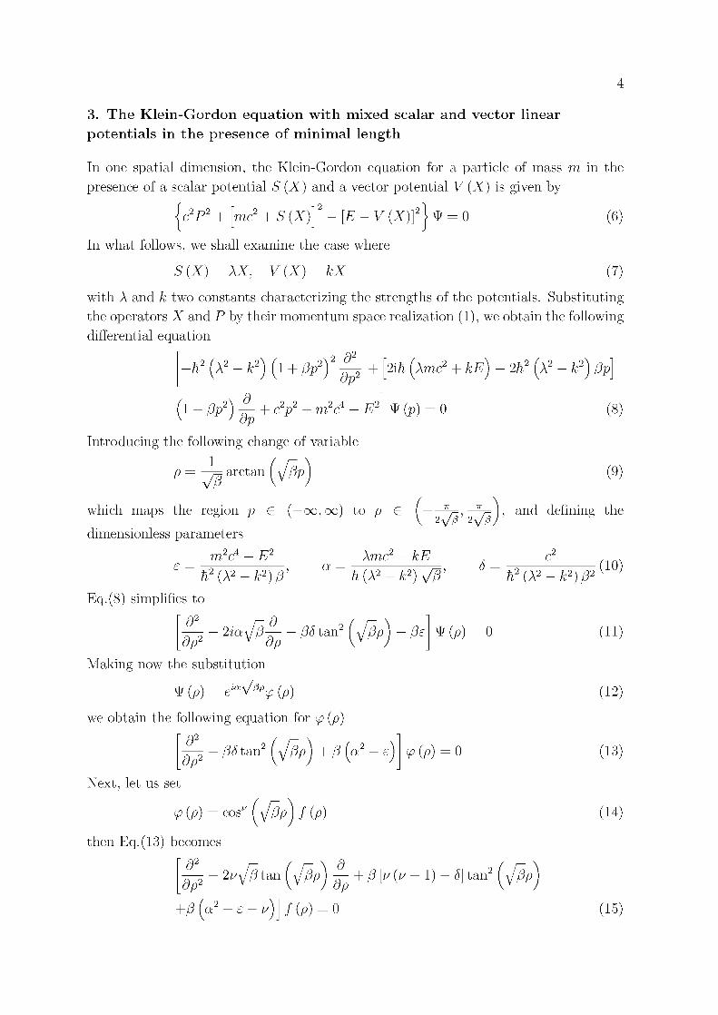
c2P2
3. The Klein-Gordon equation with mixed scalar and vector linear potentials in the presence of minimal length
In one spatial dimension, the Klein-Gordon equation for a particle of mass m in the presence of a scalar potential S (X) and a vector potential V (X) is given by
~mc2 + S (X)]2 - [E - V (X)]2\y = 0 (6)
In what follows, we shall examine the case where
S (X) = XX, V (X) = kX (7)
with A and k two constants characterizing the strengths of the potentials. Substituting the operators X and P by their momentum space realization (1), we obtain the following differential equation
dp2 h2 (A2 - k2) (l + pp2) — + [2ih (Xmc2 + kE) - 2h2 (A2 - k2) [3p
d 1 + PP2 ) TT- + c2p2 + m2c4 - E2
J op tf (p) = 0
Introducing the following change of variable
p = —7= arctan ( y /3p )
which maps the region p G (—00,00) to p G
dimensionless parameters
7T 7T
2 j a' 2 J a
e = m2à - E2
%2{X2-k2)^ a =
Xmc2 + kE h{X2-k2)^
5 =
(8)
(9)
and defining the
c2
2(\2 _ i,2\ R2 ( 1 0 ) ft2 (A2 - k2) (3
2ia^fp— - /3£tan2 l^fpp) - (3e
Eq.(8) simplifies to
" d2 r 9
W2 ~ 2m^dp-Making now the substitution
* (p) = e ^ v ^ V (p)
we obtain the following equation for ip (p)
*(p) = 0
dp2 /3£tan2 (\[Pp\ + /3 {a2 - e) <p(p) = o
Next, let us set
ip{p) = cosîy (y/Pp)f{p)
(H)
(12)
(13)
(14)
then Eq.(13) becomes
d2
d 2 2 z / ^ t a n (jpp^j — +p[u(u-l)-S\ tan2 (jpp
+(3(a2-e-v)]f(p) = 0 (15)
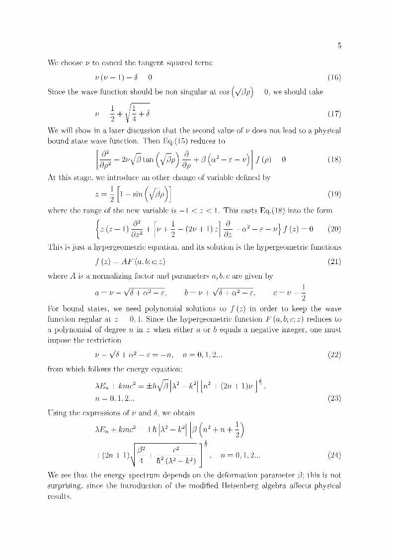
We choose v to cancel the tangent squared term:
u(u-l)-8 = 0 (16)
Since the wave function should be non singular at cos \^/j3p) = 0, we should take
8 (17)
We will show in a later discussion that the second value of v does not lead to a physical bound state wave function. Then Eq.(15) reduces to
^-2^tan(^pj-+/3(t
At this stage, we introduce an other change of variable defined by
1
a e — v / (p ) = 0 (18)
1 — sin f J(3p (19)
where the range of the new variable is — 1 < z < 1. This casts Eq.(18) into the form
d2
Z{Z~l)d? + + --(2u+l)z d_ dz
+a2 - e - i/} / (z) = 0 (20)
This is just a hypergeometric equation, and its solution is the hypergeometric functions
f(z) = AF(a,b;c;z) (21)
where A is a normalizing factor and parameters a,b,c are given by
•\A + a2 — e, b = v + \fb a = v a" £, c = v
For bound states, we need polynomial solutions to / (z) in order to keep the wave function regular at z = 0,1. Since the hypergeometric function F (a,b;c; z) reduces to a polynomial of degree n in z when either a or b equals a negative integer, one must impose the restriction
VI a" -n, ra = 0,l,2... (22)
from which follows the energy equation:
\En + kmc2 = ±hijp\\2 - k2
ra = 0,l,2...
Using the expressions of v and 8, we obtain
n2 + (2n+ \)v
(23)
XEn + kmc = ±h \2-k< p(n2 + n + -j
+ (2TI+1)« (32
7i = 0 , l , 2 . . . (24) \ 4 n2(x2-k2)
We see that the energy spectrum depends on the deformation parameter (3; this is not surprising, since the introduction of the modified Heisenberg algebra affects physical results.
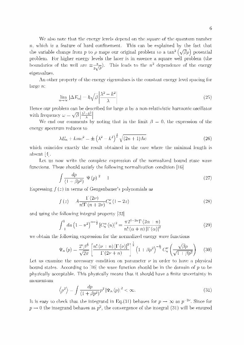
6
We also note that the energy levels depend on the square of the quantum number
n, which is a feature of hard confinement. This can be explained by the fact that
the variable change from p to p maps our original problem to a tan2 (\^/3p) potential
problem. For higher energy levels the later is in essence a square well problem (the
boundaries of the well are ±—z^=). This leads to the n2 dependence of the energy
eigenvalues.
An other property of the energy eigenvalues is the constant energy level spacing for
large n:
A2 - k2
A k (25) lim \AE„ hJ(3 A
Hence our problem can be described for large n b y a non-relativistic harmonic oscillator
with frequency UJ = \ffi X2-k2
We end our comments by noting that in the limit (3 = 0, the expression of the
energy spectrum reduces to
\En + kmcf = ± ( V - r J \J(2n + 1) he (26)
which coincides exactly the result obtained in the case where the minimal length is
absent [4].
Let us now write the complete expression of the normalized bound state wave
functions. These should satisfy the following normalization condition [16]
dp |1T„_„2 , ( 2 7 )
(28)
(1 + / W Wl
Expressing / (z) in terms of Gengenbauer's polynomials as
T{2u) f W = A: -cz (l - 2z) n\T(n + 2u)
and using the following integral property [32]
du ( 1 - u2) ~2 \Can (u)f
vr2 l - 2 a T(2a + n)
-i / n\ (a + n) [T (a)Y
we obtain the following expression for the normalized energy wave functions
2vfi \n\ {v + n) [Y (u)]2] * , , Q 2 x - f ^ ( ^(3p *n(p) i + frs
2 y-IU
(29)
(30) T (2u + n)
Let us examine the necessary condition on parameter v in order to have a physical
bound states. According to [16] the wave function should be in the domain of p to be
physically acceptable. This physically means that it should have a finite uncertainty in
momentum
dp p y\Vn(p)\ <00. (31)
(l+(3p2Y
It is easy to check that the integrand in Eq.(31) behaves for p —• oo as p~2v. Since for
p —• 0 the integrand behaves as p2, the convergence of the integral (31) will be ensured

7
provided v > \. The second solution of Eq.(16) does not satisfy this condition therefore it was ignored.
Prom the previous discussion we can see that the existence of physical bound states remains possible as long as the following constraint is fulfilled
(A^)min > ^rry2 (32)
This means that confinement solutions can occur even when the electric field is stronger than the scalar potential (which must be non null) provided that inequality (32) is respected. However, this conclusion remains purely mathematical since in real situations condition (32) is far from being realized. Indeed, the largest upper bound of the minimal length found in the literature is [24, 29]
(Ax)min < Ifm (33)
In the case when condition (32) is not satisfied, parameter v becomes complex with Re (u) = | ; the integrand in Eq.(31) behaves as 1/p at momentum infinity, leading to a logarithmic divergence of integral (31). Hence the particles cannot be bounded in this case. Only scattering solutions occur and the whole spectrum is continuous.
4. Conclusion
In this paper, using the momentum space representation, we have solved exactly the Klein-Gordon equation with linear scalar-like and vector-like potentials, in the framework of quantum mechanics with generalized uncertainty relation implying the existence of a minimal length. The bound states energy spectrum and the corresponding normalized wave functions was exactly obtained. In contrast to the usual case the energy eigenvalues show an n2 dependence, this is due to the fact that our initial problem is mapped via an appropriate change of variable to that of a particle in a well potential whose corresponding energy levels are n2 dependent.
Given the interesting role of the linear potential in nuclear and hadron physics, we expect that the results exposed in this work may have a relevant applications, especially in the quarkonium phenomenology.
References
[1] [2] [3] [4] [5] [6]
[7] [8] [9]
[10]
't Hooft G. 1974 Nucl. Phys. B 75 461 Kogut J. and Susskind L. 1974 Phys. Rev. D 9 3501 Classer M. L. and Shawagfeh N 1984 J. Math. Phys. 25 2533 Dommguez-Adame F and Mendez B 1992 Nuovo Cimento B 107 489 Su R K and Yuhong Z 1984 J. Phys. A 17 851 Su R K and Ma Z Q 1986 J. Phys. A 19 1739 Capri A Z and Ferrari R 1985 Can. J. Phys. 63 1029 Gali'c H 1988 Am. J. Phys. 56 312 Gross D J and Mende P F 1988 Nucl. Phys. B 303 407 Konishi K Paffuti G and Provero P 1990 Phys. Lett. B 234 276
8
Amati D Ciafaloni M and Veneziano G 1989 Phys. Lett. B 216 41 Rovelli C 1998 Living Rev. Rel. 1 1 Thiemann T 2003 Led. Notes Phys. 631 41 Perez A 2003 Class. Quant. Grav. 20 43 Kempf A 1994 J. Math. Phys. 35 4483 Kempf A Mangano G and Mann R B Phys. Rev. D 52 1108 Kempf A 1997 J. Phys. A 30 2093 Hinrichsen H and Kempf A J. Math. Phys. 37 2121 Susskind L and Witten E hep-th/9805114; Peet A W and Polchinski J 1999 Phys. Rev. D 59
065011 Douglas R M and Nekrasov N A 2002 Rev. Mod. Phys. 73 977 Ramchander R Sastry 2000 J. Phys. A 33 8305 Chang L N, Minic D, Okamura N and Takeuchi T 2002 Phys. Rev. D 65 125027 Fitio T V, Vacarchuk I O, and Tkachuk V M 2006 J. Phys. A 39 2143 Brau F 1999 J. Phys. A 32 7691 Akhoury A and Yao Y-P 2003 Phys. Lett. B 572 37 Benczik S Chang L N Minic D and Takeuchi T 2002 Phys. Rev. A 72 012104 Chang L N Minic D Okamura N and Takeuchi T 2002 Phys. Rev. D 65 125028 Benczik S Chang L N Minic D Okamura N Rayyan S and Takeuchi T 2002 Phys. Rev. D 66 026003 Nouicer Kh 2006 J. Phys. A 39 5125 Quesne C and Tkachuk V M 2005 J. Phys. A 38 1747 Douglas M R and Nekrasov N A 2001 Rev. Mod. Phys. 73 977 Hull C M JHEP 1998 9807 021 Hull C M JHEP 1998 9811 017
Balasubramanian V Horava P and Minic D 2001 JHEP 0105 043 Witten E 2001 Quantum Gravity In De Sitter Space Preprint hep-th/0106109; Strominger A 2001 JHEP 0110 034 Strominger A 2001 JHEP 0111 049 Balasubramanian V De Boer and J Minic D 2002 Phys. Rev. D 65 123508.
[32] Abramowitz M and Stegun I 1965 Handbook of Mathematical Fundions (New York: Dover).