three-parameter elliptical aperture dis- …jpier.org/pier/pier143/35.13103105.pdf · with just a...
TRANSCRIPT

Progress In Electromagnetics Research, Vol. 143, 709–743, 2013
THREE-PARAMETER ELLIPTICAL APERTURE DIS-TRIBUTIONS FOR SUM AND DIFFERENCE ANTENNAPATTERNS USING PARTICLE SWARM OPTIMIZATION
Arthur Densmore and Yahya Rahmat-Samii*
Department of Electrical Engineering, University of California, LosAngeles, Los Angeles, CA 90095-1594, USA
Abstract—This paper presents a unified analysis of the three-parameter aperture distributions for both sum and difference antennapatterns, suitable for communications or telemetry applications witheither a stationary or tracking antenna, and with the parametersautomatically determined by Particle-Swarm Optimization (PSO).These distributions can be created, for example, by reflector, phasedarray, or other antenna systems. The optimizations involve multipleobjectives, for which Pareto efficiency concepts apply, and areaccelerated by compact, analytical closed-form equations for keymetrics of the distributions, including the far-field radiation patternand detection slope of the difference pattern. The limiting cases of thethree-parameter distributions are discussed and shown to generalizeother distributions in the literature. A derivation of the generalizedvector far fields provides the background for the distribution studyand helps clarify the definition of cross-polarization in the far-field. Examples are given to show that the three-parameter (3P)distributions meet a range of system-level constraints for variousapplications, including a sidelobe mask for satellite ground stationsand maximizing pointing error detection sensitivity while minimizingclutter from sidelobes for tracking applications. The equations for therelative angle sensitivity for the difference pattern are derived. A studyof the sensitivity of the 3P parameter values is presented.
Received 31 October 2013, Accepted 27 December 2013, Scheduled 3 January 2014* Corresponding author: Yahya Rahmat-Samii ([email protected]).
Invited paper dedicated to the memory of Robert E. Collin.

710 Densmore and Rahmat-Samii
1. INTRODUCTION
Unlike its other chapters, chapter seven of the book Antenna Theory,by Collin and Zucker [1], deals uniquely with antenna pattern synthesis— the determination of an antenna aperture distribution to producea given radiation characteristic — and points out that there are manymethods of antenna synthesis, each of which is developed in responseto a given class of problems. This paper provides a unified methodfor antenna pattern synthesis for the broad classes of antennas havinga single main beam, with some constraint on the sidelobe levels, andincluding tracking antennas. This 3P unification provides closed-formequations for key metrics associated with each aperture distribution,including the radiation patterns for both sum and difference patterns,allowing quick calculation analytically rather than by brute forceintegration.
An antenna’s radiation characteristics are largely determined byits aperture fields, which are respectively determined by the antenna’sdesign and construction. When a realistic, comprehensive model ofaperture field distribution is available with a relatively small numberof parameters, the overall antenna design process can be effectivelydivided into two sequential steps: first identifying an aperturedistribution model that meets the given system-level design constraints(considering antenna system metrics such as beamwidth, sidelobe level,and pointing error detection sensitivity) and subsequently designingthe antenna to provide the chosen aperture distribution. Ideally sucha model would provide analytical relationships between the apertureparameters and the system metrics, and this paper provides thoserelationships as equations for the 3P distribution, generalized forsum and difference patterns. The three parameters are α, β, and c.With just a few parameters for the aperture distribution the top-levelantenna system design can be completed quickly.
The 3P distribution, as originally published [2], applies only tosum patterns. Here we extend it to include difference patterns as welland analyze both the sum and difference distributions in a unifiedmanner. The 3P distributions provide considerable flexibility, as theremainder of this paper shows: the 3P sum distribution generalizesseveral other distributions in the literature, including Hansen’s 1Pdistribution [3], the parabolic 2P, and the Bickmore-Spellmire 2P: all asdiscussed in [2]. These other distributions are represented by limitingcases of the 3P general distribution, as discussed below. What is meantby a sum pattern is the radiation pattern from the fields in the entireaperture, all in phase (adding constructively). On the other hand,the difference pattern negates the sign of the fields on one side of the

Progress In Electromagnetics Research, Vol. 143, 2013 711
aperture so as to cancel out the fields on the other side and produce adifference pattern null in the central direction that coincides with thesum pattern’s main beam. Antenna tracking systems track the nullin the difference pattern to keep the main (sum) beam peaked on thesignal.
An antenna’s radiation pattern is determined from the aperturefields by the field equivalence principle according to Maxwell’sequations. A radiation pattern varies in shape as a function ofdistance from the aperture: reactive near field zone closest to theantenna, radiating near field (Fresnel zone) and radiating far-field(Fraunhofer) zone. Beyond a certain distance from the aperture, whichdepends on the antenna size, the radiation pattern remains effectivelyconstant in shape. In this paper the true (infinitely distant) far-fields are considered. The radiation characteristics of taper efficiency,beamwidth, sidelobe level, and the asymptotic trend of the far-outsidelobe levels are addressed for the 3P distributions.
The 3P model assumes a planar aperture, and there are severalmethods by which to synthesize planar apertures, e.g., [1] Chapter 7,[3], or [4] Chapter 6, that must relate the aperture parameters toa given set of design constraints. A manual design of an aperturedistribution can require considerable time, and as Hansen mentions [3]can result in a suboptimal result. An optimizer that automaticallysearches the available range of distribution model parameter valuescan significantly reduce the time and effort required to meet particulardesign constraints — even finding unexpected solutions that might bemissed if designed manually.
Metaheuristic optimization is discussed, identifying the commonmethods currently in use, followed by a discussion of the fundamentalsof the PSO algorithm [5–10], and several examples are given for 3Pdistributions designed by PSO to meet common design constraints,which can involve multiple competing factors. Multiple-objectiveoptimization is addressed from the perspective of Pareto efficiency [9].The PSO algorithm serves the purposes of 3P distribution design quitewell, as the examples reveal.
A number of mathematical appendices are included, in whichthe closed form equations discussed in the body of the text are eachderived, in order to make the paper more complete. The followingspecial functions are used:
Jv (z) = Bessel function of the first kind, of order v.
Iv (z) = modified Bessel function of the first kind, of order v.Hv (z) = Struve function, of order v.pFq (g1, . . . , gp; h1, . . . , hq; z) = generalized hypergeometric series.

712 Densmore and Rahmat-Samii
2. CONSTRUCTING FAR-FIELDS FROM APERTUREDISTRIBUTION
In this section the aperture geometry is summarized, a set of equationsthat represent the vector far-fields in a general form are derived(applicable to both sum and difference, and providing insight regardingthe issue of the definition of cross-polarization), basic conceptspertaining to antenna radiation patterns are presented, includingdirectivity, and the particulars regarding both sum and differencedistributions are discussed, relating the model equations presented hereto real-life applications.
2.1. Aperture Geometry
Consider an elliptical aperture, representing an exit aperture of areflector or an array antenna, with major and minor axes, a and b,centered about the origin in the xy-plane bounded by
(x
a
)2+
(y
b
)2= 1 (1)
Any point inside the planar aperture is represented by a relative radialterm, t, an angle, ψ, and vector ~ρ ′.
~ρ ′ = xx′ + yy′, wherex′ = at cosψ, y′ = bt sinψ, t ∈ [0, 1], ψ∈ [0, 2π](2)
2.2. Generalized Vector Far-Fields
This section reviews the construction of the vector far-field equationsfor an elliptical aperture distribution. The time-convention is exp[jωt],where j =
√−1. The real-valued aperture distribution functionQ(t, ψ) represents the magnitude and sign of unidirectional (e.g.,x- or y-directed) aperture fields, ~Eap and ~Hap, assuming transverseelectromagnetic mode (TEM) [11], with constant aperture phaseother than a possible sign reversal defined by the distribution. Theassumption of TEM mode in the aperture imposes
η ~Hap = n× ~Eap, (3)
where η is the free-space impedance and n the outward aperture surfacenormal vector — the z-axis in this paper. The aperture distributiondefines the aperture fields as a function of the aperture coordinatesaccording to (4), where p is the polarization orientation of the electricfield in the aperture.
~Eap (t, ψ) /√
2η = pQ (t, ψ) , (4)

Progress In Electromagnetics Research, Vol. 143, 2013 713
The Schelkunoff field equivalence theorem [12] relates the aperturefield, given by the distribution, to equivalent electric and magneticcurrents tangential to the aperture and related to vector potentials.The vector potentials then determine the radiating far-fields associatedwith the given aperture distribution. The equivalent currents relate tothe aperture fields by the following equations.
~Jeq = n× ~Hap and ~Meq = −n× ~Eap (5)
Following (6-95), (6-101), and (6-102) from [11], the radiated electricfar-field, ~Eff , is proportional to the magnetic and electric vectorpotentials as given by the equations below, where the magnetic vectorpotential in the far-field is Aff , the electric vector potential Fff , µfree-space permeability, ε free-space permittivity, k = 2π/λ, λ isthe wavelength, and ds′ the elemental aperture surface area. Thevector from the origin in the center of the aperture to a given far-fieldobservation point is ~r (r, θ, φ), with corresponding unit vector r.
~Eff = ~EAff + ~EFff ≈[θθ ·+φφ·
]jω
(− ~Aff + η r × ~Fff
), (6)
where
~Aff =exp [−jkr]
4πrµ
∫∫~Jeq exp
[jk(~ρ′ · r)] ds′, (7)
and
~Fff =exp [−jkr]
4πrε
∫∫~Meq exp
[jk
(~ρ′ · r)] ds′. (8)
These equations reduce in the far-field to
~Eff =jk exp [−jkr]
4πr
[θθ ·+ φφ·
] ∫∫ [η
(−n× ~Hap
)
+r ×(−n× ~Eap
)]exp
[jk(~ρ′ · r)] ds′. (9)
Working out the math for the two primary polarizations yields aconditional equation:
~Eff√2η
=jk exp [−jkr]
4πr(1 + cos θ) T
{θ cosφ− φ sinφ, ~p = x;θ sinφ + φ cosφ, ~p = y;
and ~Hff = r ×~Eff
η. (10)
Equation (10) shows that the θ and φ TEM spherical components ofthe far-field radiated from a TEM aperture are related via sine andcosine, which is a definition of a Huygens source [13] (18), for which

714 Densmore and Rahmat-Samii
the Ludwig third definition of cross-polarization [14] applies. T in (10)is defined as
T (θ, φ) =∫∫
Q (t, ψ) exp[jk(~ρ′ · r)] ds′, (11)
or
T (θ, φ) =∫ 2π
0
∫ 1
0Q (t, ψ) exp [jk (at cosψ sin θ cosφ
+bt sinψ sin θ sinφ)] abt dtdψ. (12)
Substituting
u(θ, φ) = kB(φ) sin θ, (13)
where
B (φ) =√
a2 cos2 φ + b2 sin2 φ, (14)
and
Φ (φ) = arctan [(b sinφ) / (a cosφ)] , (15)
and noting that u(θ, φ) is the normalized radian angle, simplifies (12)to
T (u) =∫ 2π
0
∫ 1
0Q (t, ψ) exp [jut cos(ψ − Φ)] abt dtdψ. (16)
In order to generalize for both sum and difference patterns, Q is definedby (17), where R(t) ≥ 0 and n is zero for sum patterns or unity fordifference patterns. ψ = ∆ is the orientation of the plane perpendicularto the aperture in which the difference pattern is intended.
Q (t, ψ) = R (t) cos [n (ψ −∆)] ; n = 0 or 1 (17)
With the help of [15] (3.915.2) (16) reduces to
T (u) |n=0 or 1 = 2πabjn cos [n (∆− Φ)]∫ 1
0R (t)Jn (ut) tdt. (18)
The superscript norm is used to denote normalization by aperture area;e.g.,
T normS = TS/ (πab) . (19)
The above equations specify the form of the vector far-fields in sphericalcoordinates for a general elliptical aperture distribution Q. n = 0produces a sum pattern and n = 1 a difference pattern. If the apertureis electrically large (yielding a pattern with a narrow beamwidthcentered at θ = 0) then the (1− cos θ) term, referred to as elementfactor of a Huygens source, can be neglected: in that case a study ofthe radiation patterns associated with various aperture distributions

Progress In Electromagnetics Research, Vol. 143, 2013 715
can focus entirely on T , the radiation pattern space factor, and that isthe path taken in this paper.
In the remainder of this paper the properties of the space factorare studied for two distinctly different types of distributions: that forproducing a radiation pattern with a main beam central peak (referredto as a sum pattern and commonly used for data communications), andalso that for producing a radiation pattern with a central null (referredto as a difference pattern and typically used to detect antenna pointingerror for tracking). The distribution and space factor functionsassociated with the sum pattern type are respectively distinguishedas QS and TS ; whereas, those for the difference pattern type as QD
and TD.
2.3. Radiation Pattern Characteristics
In reference to the radiation patterns there are a few terms to define.A sum pattern has a central peak on-axis (zero angle), and a differencepattern has a central null. The angular width of a sum pattern’s mainbeam at the points where the radiated power pattern drops to half itspeak value is the half-power beamwidth, or HPBW. A radiation patternfrom an aperture with uniform phase typically has pattern nulls atregular angular intervals off-axis. The angular distance between thetwo first off-axis nulls, one on each side of the axis, is the pattern’s first-null beamwidth (FNBW). Other than the main central beam of a sumpattern — or dual off-axis main beams of a difference pattern — thesub-beams between the off-axis nulls are the sidelobes, and the level ofthe highest sidelobe in the pattern, with respect to the level of the mainbeam(s), is the peak sidelobe level (PSLL). Taper (or illumination)efficiency, et, is defined by (20), which for an aperture with uniform-phase and zero crosspol is the ratio of the effective radiating area tothe physical area. Zero crosspol occurs when the aperture fields, allthroughout the aperture, are all oriented in the same direction, as givenin (4).
et.=
∣∣∣∣∫∫
Qds
∣∣∣∣2
Aap
∫∫|Q|2 ds
(20)
Equation (14) in [2] gives the taper efficiency as the ratio of the squaredmagnitude of the aperture-area-normalized on-axis space factor dividedby the aperture-area-normalized area integral of the square of thedistribution.
Aperture directivity is 4πr2 times the ratio of the power radiatedin one direction to the total power radiated in all directions. The

716 Densmore and Rahmat-Samii
directivity is approximated in [2], for electrically large apertures,by (21), below, where Pap is the total TEM aperture power.
D (θ, φ) ∼ D0|T norm|2P norm
ap
(1 + cos θ
2
)2
, (21)
where
D0 = πab4π
λ2, (22)
and
P normap =
Pap
πab
.=
12
∫∫ ∣∣∣ ~Eap × ~Hap
∣∣∣ ds′
πab=
∫∫|Q|2 ds′
πab. (23)
Borrowing terminology from antenna array theory, the T term in(10) is referred to as the radiation pattern’s space factor [16], andthe (1 + cos θ) term in (10) as the element factor, or obliquityfactor, of a Huygen’s source [17]. The aperture-power normalizeddirectivity pattern of an electrically large aperture (with narrowbeamwidth), for sum or difference in general, is thereby approximatedby |T norm|2/P norm
ap , the squared magnitude of the area-normalizedspace factor divided by the area-normalized aperture power.
A simple normalization is suitable to provide a basic comparison ofthe radiation patterns among candidate aperture distributions. Sincesidelobe level with respect to the beam peak is typically one of themost significant requirements for an antenna, a suitable normalizationis simply with respect to the peak of the sum pattern, so that allnormalized sum patterns peak at unity (zero dB). Difference patterns,on the other hand, don’t have a main beam peak: A natural alternativenormalization for a difference pattern is with respect to the peak ofits matching sum pattern, which places the difference pattern’s dualpeaks at a level of about −2 dB. The difference patterns plotted inthe figures simply normalize to the pattern peak, in order emphasizethe relative sidelobe levels. The matching sum pattern results from ahypothetical aperture distribution equal to the absolute value of thedifference pattern’s aperture distribution, and its on-axis peak value isdenoted T|D|(0), defined in (24). RD(t) is a difference pattern’s radialdistribution according to (17).
T|D| (0) .=∫∫
|QD| ds′ =∫ 2π
0
∫ 1
0RD (t) |cos (ψ −∆)| abt dtdψ
= 4ab
∫ 1
0RD (t) tdt (24)

Progress In Electromagnetics Research, Vol. 143, 2013 717
Equation (25), the taper efficiency of a difference pattern, isconstructed using (20), (23), and (24).
etD.=
[T norm|D| (0)
]2
P normapD
(25)
One of the most important features of the difference distribution isthe slope of its radiation pattern about its central null. That slopedetermines the sensitivity of its detection of pointing error and isthe primary coefficient in any feedback tracking control system thatuses the antenna pointing error detected by this slope. Equation (26)represents the slope normalized by aperture area.
Snorm .=dT norm
D (u)du
∣∣∣∣u=0
(26)
For the purpose of comparing slopes among candidate aperturedistributions it’s appropriate to further normalize Snorm by
√P norm
apD
or T norm|D| (0). Normalizing with respect to the square root of the area-
normalized aperture power would effectively reduce the slope by thetaper efficiency; whereas, the normalization of (27) by the peak of thematching sum pattern sets the (dual) peaks of all difference patternsat the same level of about −2 dB and so provides normalizationindependent of the taper efficiency. Bayliss [18] suggests comparingdistributions by relative angle sensitivity, defined as normalizing bythe maximum possible slope. The relative angle sensitivity, basedon normalization by the matching sum pattern, is defined in (28),where SnormT
max is the maximum matching-sum-pattern-normalized anglesensitivity for the class of aperture distributions in consideration.
SnormT = Snorm/T norm|D| (0) (27)
Srelative .= SnormT/SnormTmax (28)
3. SUM AND DIFFERENCE PATTERN 3PDISTRIBUTIONS
The terms 3PS and 3PD distinguish between a 3P distribution intendedrespectively for a sum and difference pattern.
3.1. Basic Sum and Difference Patterns
The simplest aperture distribution that produces a sum pattern is aconstant, and in that case the resulting space factor T is solved with

718 Densmore and Rahmat-Samii
the help of [15] (5.52.1) as
T normS |QS=1 = 2
J1 (u)u
. (29)
The simplest elliptical aperture distribution that produces a differencepattern effectively involves the difference rather than the sum of thefields on either side of the aperture. Distinguishing respective sidesimplies the choice of a particular φ angle, in which phi-plane pattern cutthe difference pattern is intended, and that angle is defined as φ = ∆.The line that divides the two halves of the aperture is at an angleperpendicular to ∆. Instead of simply negating the sign of the fieldson one half of the aperture, the method given in [4] is used to create adifference pattern from a radial aperture distribution: by multiplyingthe radial distribution by cosψ. In this manner, the simplest exampleof a distribution that produces a difference pattern is a constant timescosψ, in which case (30) is the space factor for the resulting differencepattern, determined using [15] (6.561.1), where H0(z) and H1(z) arerespectively the Struve functions of order zero and one.
T normD |QD=cos(ψ−∆) =jπ cos (∆− Φ)
J1(u)H0(u)−H1(u)J0(u)u
(30)
3.2. Sum Pattern Distributions (3PS)
The 3PS distribution, introduced in [2], is defined over an ellipticalaperture, depicted in Figure 1. Each unique 3P distribution isrepresented by a triplet of parameter values: α, β and c. For the 3PSdistributions these three parameters represent respectively: α) the tail
Figure 1. Elliptical aperture geometry, with generic sum anddifference patterns.

Progress In Electromagnetics Research, Vol. 143, 2013 719
shape, β) steepness, and c) pedestal height of the distribution. Each 3Pdistribution has a characteristic radiation pattern that is convenientlyexpressed by a modest closed-form equation. The fact that the 3Pdistribution has a closed-form radiation pattern equation providesfaster convergence for any optimization algorithm that utilizes it: ineach cycle of an iterative optimization the candidate three-parameterdistribution is quickly evaluated (in closed-form) as the optimizationalgorithm proceeds. Without the closed-form equation the far-fieldradiation pattern of the distribution would have to be computedby numerical integration, which tends to require substantially morecompute time.
The 3P sum distribution is defined in [2] as Q(t) and here renamedQS(t).
QS(t) = c + (1− c)(√
1− t2)α Iα
(β√
1− t2)
Iα (β), (31)
where the domains of the three parameters (α, β, c) are α ≥ 0, β ≥ 0,0 ≤ c ≤ 1. The far-field radiation integral for the 3P sum distributionis solved in closed form using [15] (6.683.2).
T normS (u) = 2c
J1 (u)u
+ (1− c)2βαJα+1
(√u2 − β2
)
Iα (β)(√
u2 − β2)α+1 (32)
The asymptotic behavior of TS for large u describes the level of thefar-out sidelobes, and for the 3PS distribution that behavior is in (33).Note that for large argument, z, Jν(z) ∼ z−1/2.
TS (u)|u→∞ ∼{
u−3/2, c 6= 0;u−3/2−α, c = 0.
(33)
The normalization of the 3P sum distribution is discussed in [2], wherethe choice is made to normalize by the square root of the normalizedaperture power integral. The aperture-area normalized power integralis
P normapS = c2 + 4c (1− c)
Iα+1 (β)βIα (β)
+(1− c)2
2α + 1
(1− I2
α+1 (β)I2α (β)
). (34)
The limiting cases for the 3PS distribution are discussed in [2] andbecome the Bickmore-Spellmire distribution when c = 0, the parabolic2P model when β = 0, and the 1P model when α = 0 and c = 0. Thesethree limiting cases are given respectively by (35), (36), and (37), andseveral example distributions for each case are displayed respectively

720 Densmore and Rahmat-Samii
in Figures 2–4.
B-SQS(t) =(√
1− t2)α Iα
(β√
1− t2)
Iα (β)(35)
2PQS(t) = c + (1− c)(1− t2
)α (36)
1PQS(t) =I0
(β√
1− t2)
I0 (β)(37)
Since the broad classes of antennas that the 3P distributions applyto are mainly concerned with tradeoffs between directivity and PSLL,an appreciation of the main distinctions between the three limitingcases can be obtained by considering the uniquely different tradeoffthat each case provides between PSLL and FNBW/2, the angle (u)at which the first off-axis null occurs, which is an indirect measure of
Figure 2. Example distributionsfor 3PS limiting case of c = 0.
Figure 3. Example distributionsfor 3PS limiting case of β = 0.
Figure 4. Example distributions for 3PS limiting case of α = c = 0.

Progress In Electromagnetics Research, Vol. 143, 2013 721
(a) (b)
Figure 5. (a) PSLL versus FNBW/2 Pareto fronts for 3PS limitingcases of c = 0, a = c = 0, and β = c = 0. (b) PSLL versus FNBW/2Pareto front for 3PS limiting case of β = 0.
directivity. A multi-objective optimization, such as a tradeoff betweenPSLL and FNBW, is effectively summarized by a Pareto front [19, 20].Pareto fronts for the radiation patterns of these three limiting cases ofthe 3PS distribution are given by the perimeters of sample-populatedareas presented respectively in Figures 5(a) and 5(b). The case ofc = 0 appears as essentially a fan sector and fills the region betweenthe curves, and that of β = 0 has particularly detailed features. Forreduction of the radiation pattern (32) in the limiting case of β → 0,note that
limβ→0
[βα/Iα (β)] = 2αΓ (α + 1) . (38)
3.3. Difference Pattern Distributions (3PD)
The most commonly referenced distribution for a difference patternappears to be that of Bayliss [18], which presents a two-parametercircular aperture distribution as an analog to the Taylor n sumdistribution [17]. Section IV in [3] references the discussion in [4]of a circular Bayliss distribution based on multiplying by cosψ.This is a natural method of producing a difference pattern, judgingby the fact that the higher-order mode (HE21) linearly-polarizedfields in the mouth of a large corrugated horn (commonly used fordetecting tracking error in satellite earth stations) have the cosψdependence [21]. A difference pattern distribution for a line sourceis suggested in [22] as a complement to the 3P sum distribution in [2].That suggestion is basically to multiply the radial Q(t) distributionin [2] by t. Heeding that suggestion, along with the cosψ factor, the

722 Densmore and Rahmat-Samii
3P difference pattern distribution reviewed in this paper for a generalelliptical aperture is defined as
QD (t, ψ) .= cos (ψ −∆) {c + (1− c)t [QS (t)|c=0]} , (39)
or
QD(t, ψ)=cos(ψ−∆)
c+(1−c) t
(√1−t2
)α Iα
(β√
1−t2)
Iα(β)
. (40)
The 3P difference pattern far-field is solved using [15] (3.915.2, 6.561.1,and 6.682.2):
T normD (u) = 2j cos (∆− Φ)
{c
π
2u[J1 (u) H0(u)−H1(u)J0(u)]
+(1− c)uβαJα+2
(√u2 − β2
)
Iα (β)(√
u2 − β2)α+2
. (41)
The asymptotic behavior of T for large u describes the level of thefar-out sidelobes, and for the 3P difference distribution that behavioris given in (42). This is steeper than for the sum distribution whenc = 0.
TD (u)|u→∞ ∼{
u−3/2, c 6= 0;u−5/2−α, c = 0.
(42)
On-axis field strength of the matching sum pattern corresponding tothe absolute value of the 3PD distribution, solved using [15] (6.683.6),is
T norm|D| (0) = 2
{c
π+ (1− c)
√2π
Iα+3/2(β)β3/2Iα(β)
}. (43)
The total aperture power in the 3PD distribution is similarly found:
P normapD =
{c2
2+
2c (1−c)β3/2
√π
2Iα+3/2 (β)
Iα (β)+
(1− c)2
2
1− I2α+1 (β)I2α (β)
2α + 1−
β2α2F3
[2α + 2, α + 1/2] ;[2α+1, 2α+3, α+1] ;
β2
22α+1 (α + 1) Γ2 (α + 1) I2α (β)
(44)
The limiting cases for the 3PD distribution that correspond to the sameaforementioned cases as for 3PS, (35)–(37), are presented in (45)–(47),

Progress In Electromagnetics Research, Vol. 143, 2013 723
Figure 6. Example distributionsfor 3PD limiting case of c = 0.
Figure 7. Example distributionsfor 3PD limiting case of β = 0.
Figure 8. Example distributions for 3PD limiting case of α = c = 0.
and example distributions for each case are displayed respectively inFigures 6–8.
c=0RD(t) = t(√
1− t2)α Iα
(β√
1− t2)
Iα (β)(45)
2PRD(t) = c + (1− c) t(1− t2
)α (46)
1PRD(t) = tI0
(β√
1− t2)
I0 (β)(47)
Pareto fronts that reveal the uniquely different tradeoff that each caseprovides between PSLL and FNBW are presented in Figures 9(a)and 9(b). The case of c = 0 appears as a fan sector, and that ofβ = 0 has particularly detailed features. Pareto fronts revealing thetradeoffs between PSLL and relative angle sensitivity are presented inFigures 10(a) and 10(b). The case of c = 0 is similar in shape to
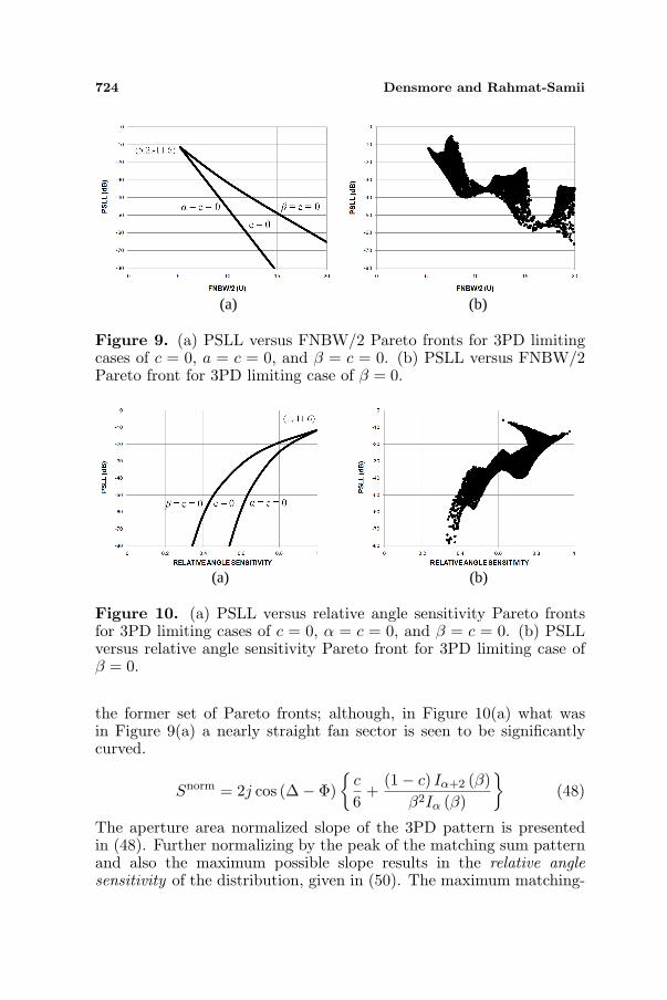
724 Densmore and Rahmat-Samii
(a) (b)
Figure 9. (a) PSLL versus FNBW/2 Pareto fronts for 3PD limitingcases of c = 0, a = c = 0, and β = c = 0. (b) PSLL versus FNBW/2Pareto front for 3PD limiting case of β = 0.
(a) (b)
Figure 10. (a) PSLL versus relative angle sensitivity Pareto frontsfor 3PD limiting cases of c = 0, α = c = 0, and β = c = 0. (b) PSLLversus relative angle sensitivity Pareto front for 3PD limiting case ofβ = 0.
the former set of Pareto fronts; although, in Figure 10(a) what wasin Figure 9(a) a nearly straight fan sector is seen to be significantlycurved.
Snorm = 2j cos (∆− Φ){
c
6+
(1− c) Iα+2 (β)β2Iα (β)
}(48)
The aperture area normalized slope of the 3PD pattern is presentedin (48). Further normalizing by the peak of the matching sum patternand also the maximum possible slope results in the relative anglesensitivity of the distribution, given in (50). The maximum matching-

Progress In Electromagnetics Research, Vol. 143, 2013 725
sum-pattern-normalized angle sensitivity, SnormTmax , for a 3PD pattern
occurs in the limit as all three of the 3P parameters approach zero, inwhich case the 3PD distribution has a triangular shape peaking at theaperture edge.
SnormTmax =
limα=β=c→0
Snorm
limα=β=c→0
T norm|D| (0)
=√
π
2Γ
(52
)
Γ (3)(49)
Srelative = SnormT
/[√π
2Γ
(52
)
Γ (3)
](50)
4. METAHEURISTIC OPTIMIZATION METHODS
Optimization techniques used in the electromagnetic engineeringcommunity are often metaheuristic because of the complexity ofthe tradeoffs involved. Metaheuristic methods involve stochasticoptimization to distinguish global from local optimal solutions, asopposed to classical optimizers that are meant to produce exactsolutions for simpler classical models with local extrema, which ifapplied to real-world engineering problems tend to get stuck on localoptimum solutions.
A basic overview of metaheuristic methods is provided in [23].Such methods include Ant Colony Optimization [24], CovarianceMatrix Adaptation Evolution Strategy (CMA-ES) [25], GeneticAlgorithms (GA) [26], Invasive Weed Optimization (IWO) [27],PSO [5–10], Simulated Annealing [28], and Tabu Search [29]. Amongthese optimization techniques, the PSO is a practical balance betweenmodel simplicity and robust, rapid, global solution convergence.Examples of the state of the art of the application of PSO to fractaland adaptive phased-array antennas are given in [30–32].
Optimization can pertain to a system with one or more variableswith one or more optimization objectives, goals, or constraints. Withonly one objective the optimization can evaluate it with a fitnessfunction. If there are multiple (competing) objectives evaluationof the optimality becomes more complicated. There are generallytwo approaches to multi-objective optimization: 1) combining fitnessfunctions and 2) referring to a Pareto front [9, 19, 20]. A classicalway of combining multiple objectives into a single fitness functionis a weighted sum of fitness functions — one from each objective —where the result of the overall optimization can depend on the choiceof weighting. An example is given in (51), which involves the twocompeting objectives of peak sidelobe level and first-null beamwidth.Pareto optimality represents the trade-off between multiple goals: A

726 Densmore and Rahmat-Samii
solution is Pareto optimal when it is not possible to improve one goalwithout degrading at least one of the others. Optimization by Paretofront involves more intensive numerical investigation to determine theactual boundary of optimality between competing objectives, and afew examples of Pareto fronts are given below. In general there is nosingly optimal solution to a multi-objective optimization: the set ofPareto optimal multi-objective solutions is called a Pareto front.
4.1. Particle Swarm Optimization (PSO)
The PSO algorithm is similar to the concept of a swarm of bees in afield, effectively communicating their individual findings and so guidingthe swarm as a whole ever closer to a suitable location to convergeupon. A PSO algorithm directs the search and evaluates a fitnessfunction, customized for the particularly specified goal(s), to evaluatethe merit of each candidate solution considered by any member of theswarm. Example PSO convergence plots are shown in Figures 11(a)and 11(b), using respective fitness functions given by (51) and (52),and each with twenty agents per swarm and thirty swarm trials periteration. These two are comparable since they both have the same goalof −40 dB PSLL; although, one is for a sum pattern and the other fora difference pattern. Note that the convergence plot in Figure 11(a)involves a fitness function that is not conditional; whereas, that inFigure 11(b) is conditional: in the former case the average fitness isconsiderably larger than in the latter; although, the rate of convergence
(a) (b)
Figure 11. (a) PSO convergence for design of 3PS pattern with−40 dB PSLL and minimum FNBW. (b) PSO convergence for designof 3PD pattern with −40 dB PSLL and minimum FNBW.

Progress In Electromagnetics Research, Vol. 143, 2013 727
appears to be a bit faster in the former than the latter.
fitness 11(a) = (PSLL (dB)− goal)2 + FNBW(u) /2, (51)
fitness 11(b) ={
FNBW(u) /2, if PSLL ≤ goal;999, otherwise. , (52)
The position, in model parameter space, of the search agent (swarmmember) with the best fitness value among the swarm at any iterationis the global best for that iteration. Each search agent moves about theparameter space and its flight path is pulled toward that global best.It is also pulled toward its own personal best location, and its flightpath is also affected by its own inertia and random motion.
Consider the flight trajectory of any particular swarm member(“search agent”, or “bee”) in the PSO model n-dimensional parameterspace, letting n = 2 here for simplicity. Applying real-world physicsand assuming each bee naturally counteracts the force of gravity, weimagine that each bee has some linear momentum that Newton’s Lawpreserves until external forces are applied or the bee alters its path.External winds and individual bee behavior combine to provide aseeming randomness to the individual flight paths. By means of thewaggle dance a bee communicates to its hive-mates in which directionwith respect to the Sun and how far it flew to reach the food sourceit found. So we can imagine that each bee’s flight path is affectedby 1) Newton’s Law, 2) random motion, 3) its own knowledge ofthe best place at which it has found food (personal best, or pbest),and 4) the best overall location found by any member of the swarm(the global best, or gbest). This is represented by (53) for the motionof any PSO search agent. vn represents the search agent’s velocityvector in the current (nth) iteration, xn represents its current positionvector, w is the momentum factor, c1 and c2 effectively represent springconstants pulling the search agent respectively towards its personaland the overall swarm’s global best locations, and rand () is a strictly-positive valued random number function ranging between the zero andone. ∆t is a discrete step representing the time between iterations.
xn+1 = xn + vn∆t, andvn+1 = wvn + c1rand () (pbest − xn) + c2rand () (gbest − xn) (53)
5. PARTICLE SWARM OPTIMIZATION OF 3PDISTRIBUTIONS
The goal for the 3P distribution is to provide an antenna aperturedistribution that provides specified radiation pattern characteristics,such as beamwidth, PSLL, taper efficiency, sidelobe level limit (mask)

728 Densmore and Rahmat-Samii
as a function of angle, and for the difference pattern: relativeangle sensitivity. These characteristics are translated into a fitnessfunction for the optimizer, which by convention the PSO minimizes.Throughout the optimization process the PSO varies the 3P parametervalues automatically, within any parameter value constraints imposedon the algorithm. Convergence is faster when any of the 3P parametersare constrained to within a range known to provide the desired solution.
Several examples of the application of PSO to the 3P distributionsare given. Two examples of the design of 3PS distributions by PSOare presented: maximizing aperture taper efficiency while satisfying asidelobe mask, and minimizing the beamwidth with the peak sidelobelevel (PSLL) set to a target value. A study of the sensitivity ofthe 3P parameter values is presented, followed by examples of 3PDdistributions design by PSO for a range of PSLL constraints.
5.1. Example 1: 3PS Maximum Gain with a Sidelobe Mask
The first example maximizes the gain with a sidelobe constraint.Given a uniform phase aperture, which the 3P distribution assumes,maximum gain is associated with peak taper efficiency. A formalconstraint for the sidelobes of a geostationary satellite ground stationantenna is the FCC 25.209 mask [33], which starts at 1.5 degfrom beam peak with sidelobe directivity constraint of twenty-ninedecibels isotropic gain minus twenty-five decibels times the base tenlogarithm of the pattern angle in degrees (for conventional Ku- or Ka-band geostationary service ground stations). The conditional fitness
Figure 12. PSO 3PS radiationpattern achieving maximum taperefficiency while also meeting asidelobe mask.
Figure 13. PSO 3PS distribu-tion and radiation pattern achiev-ing PSLL of −30 dB peak withminimum beamwidth.

Progress In Electromagnetics Research, Vol. 143, 2013 729
function which PSO minimizes for this example is
fitness 12 ={−et, if all sidelobes below the mask;
999, otherwise. (54)
If any sidelobe exceeds the mask then the candidate 3P distributionis deemed out-of-bounds and discarded with a very large fitnessvalue. This out-of-bounds treatment is the same as how search agentsthat wander outside an acceptable range of parameter values can bedealt with in the PSO algorithm by applying invisible boundaries [6].Figure 12 shows the 3P distribution and radiation pattern from thisPSO run, which yielded 3P parameter values of alpha = 1.9389, beta= 1.6928, and c = 0.5581. The locus of the sidelobe peaks is seento follow the mask, and a 96.6% taper efficiency is achieved with anaperture diameter of 68 wavelengths.
5.2. Example 2: 3PS Minimum Beamwidth with SpecifiedPSLL
The second example provides a 3P antenna aperture distribution thatachieves a radiation pattern with sidelobe level (PSLL) less than−30 dB peak while minimizing beamwidth. For this example the fitnessfunction is the square of the difference between the PSLL and the goal,in dB, plus the angle, u, of the first null.
fitness 13 = (PSLL− goal)2 + FNBW/2, (55)
where the PSLL goal is −30 dB peak. The 3P parameters producedby one PSO run meeting these constraints are alpha = 2.002, beta= 2.877, and c = 0.306, and the resulting radiation pattern and 3Pdistribution are shown in Figure 13. This figure also superimposes(light shading) the uniform-amplitude aperture radiation pattern forcomparison — in which case the sidelobes would be considerably higherthan that provided by the optimized 3P distribution.
5.3. Example 3: 3PS Family of PSO Solutions
PSO typically yields a family of solutions, all of which satisfy theconstraints to some degree. Figure 14 shows such a family, with a PSLLof −40 dB. The selected family of solutions is: 1) alpha = 2.2390, beta= 0.5625, c = 0.139, 2) alpha = 1.2196, beta = 3.7930, c = 0.1015,and 3) alpha = 0.6207, beta = 4.5970, c = 0.0757. This familyrepresent only three of many PSO solutions that were found to meetthe given requirements, and these three were chosen because of thesubstantial variation in their alpha parameter values, to show that thecombination of a high alpha value and low beta value can provide a

730 Densmore and Rahmat-Samii
Figure 14. PSO 3PS distributions and radiation patterns for a familyof PSO solutions all achieving PSLL of −40 dB peak with minimumbeamwidth.
similar distribution as the combination of a low alpha value and highbeta. There is little difference between the distributions of each of thesefamily members, as the inset distribution shows (since they all meetthe same design requirements). The fitness function is given by (55).
5.4. Example 4: 3P Pattern Sensitivity to Variation ofParameter Values
A practical design must account for implantation error, and so asensitivity analysis was conducted to determine how sensitive the 3Pdistribution might be to variations in each of the parameter values.The first PSO family member 3PS solution in Figure 14 is used as thebasis for the parameter sensitivity analysis. Figure 15(a) shows thata 10% variation in the alpha parameter value can cause as much as5–10 dB variation in the level of the first sidelobe. Figure 15(b) showsthat the beta parameter value is the least sensitive to variation of itsvalue: only a fewdB variation in the level of the first sidelobe levelresult from a significant variation in the beta value from −100% to+300%. Figure 15(c) shows that the 3P c-parameter has intermediatesensitivity. The level of the first sidelobe level varies several dB with a10% variation in the value of the c-parameter value. The correspondingvariations in 3PD patterns are comparable to those given here for 3PS.
5.5. Examples 5–7: 3PD Maximum Angle Sensitivity withSpecified PSLL
PSO examples are presented in Figures 16(a)–(c) for 3PD distributionswith PSLL design goals of respectively −30, −48 and −55 dB, while

Progress In Electromagnetics Research, Vol. 143, 2013 731
(a) (b)
(c)
Figure 15. (a) PSO parameter sensitivity, showing variation ofradiation pattern when only the 3PS alpha parameter value is changedfrom the PSO solution value by ±10%. (b) PSO parameter sensitivity,showing variation of radiation pattern when only the 3PS betaparameter value is changed by −100% and +300%. (c) PSO parametersensitivity, showing variation of radiation pattern when only the 3PSc parameter value is changed from the PSO solution value by ±10%.
simultaneously maximizing the relative angle sensitivity, using thefitness function of (56). The 3P parameter values for Figure 16(a)are alpha = 1.9949, beta = 0.0194, and c = 0.0804, in which case arelative angle sensitivity of 79% is achieved with −30 dB PSLL. Thosefor Figure 16(b) are alpha = 2.3292, beta = 1.3064, and c = 0.0460, inwhich case a relative angle sensitivity of 75% is achieved with −38 dBPSLL. The 3P parameter values for Figure 16(c) are alpha = 0.0318,beta = 8.3484, and c = 0.0031, in which case a relative angle sensitivityof 67% is achieved with −55 dB PSLL. The 3PD distribution can meeteven considerably deeper PSLL limits than given by these examples,indicated by Figure 9(a). These optimal multi-objective solutions are

732 Densmore and Rahmat-Samii
(a) (b)
(c)
Figure 16. (a) PSO 3PD designed for −30 dB PSLL and maximumrelative angle sensitivity. The inset 3PD distribution is shownnormalized to its peak height. (b) PSO 3PD designed for −38 dB PSLLand maximum relative angle sensitivity. The inset 3PD distributionis shown normalized to its peak height. (c) PSO 3PD designed for−55 dB PSLL and maximum relative angle sensitivity. The inset 3PDdistribution is shown normalized to its peak height.
typically found on the edge of a Pareto front. Bayliss [18] revealsthat for a difference pattern to realistically achieve maximum relativeangle sensitivity with a given maximum PSLL requires that its firstsidelobes be of uniform level, and Figures 16(a)–(c) show that the 3PDdistributions determined by PSO with those constraints have that verycharacteristic.
fitness 16 =
{− (relative angle sensitivity) , if PSLL ≤ goal;
999, otherwise.(56)

Progress In Electromagnetics Research, Vol. 143, 2013 733
6. CONCLUSION
The 3P distribution is presented for both sum and difference patternsin the context of providing a versatile amplitude distribution modelof for an entire class of uniform-phase elliptical antenna apertures.Analytical closed form equations for several characteristics of a general3PS or 3PD distribution were derived: the far-field radiation pattern,taper efficiency, aperture power, asymptotic sidelobe level, and forthe 3PD also the relative angle sensitivity. The PSO algorithm wasdiscussed, and references for other metaheuristic optimization methodswere given. Several examples of designing 3P distributions by PSOdemonstrate that the 3P distribution can meet a range of real-worlddesign constraints. The PSO algorithm converges to a solution in eachcase with different 3P antenna aperture design constraints. Radiationpatterns and distributions for a family of solutions which all satisfy thesame requirements were presented, and the sensitivity of each of the 3Pparameter values was investigated. The PSO optimized 3P patternsmeet peak sidelobe, taper efficiency and sidelobe mask requirements.The PSO optimized 3P patterns display the ideal characteristic ofuniform close-in sidelobe levels when in addition to constraining theoptimization by a specified PSLL it is also additionally constrained bymaximum taper efficiency, in the case of a sum pattern, or by maximizeangle sensitivity in the case of a difference pattern. The versatility ofthe 3P distribution and PSO’s utility as a metaheuristic optimizercombine to provide customized aperture distributions for a versatilerange of applications.
ACKNOWLEDGMENT
Rahmat-Samii’s reflection: I am delighted to contribute thispaper to the special issue of PIERS dedicated to the memory ofProf. Robert E. Collin, whose contributions and services to theelectromagnetic community are immeasurable. We have all benefittedfrom his wisdom and his technical excellence. His papers are original,mathematically detailed and always address some interesting concepts.His books have inspired and provided solid foundation for the educationof numerous students worldwide. I have also tremendously enjoyedmy encounters with Prof. Collin. When I was a graduate student atthe University of Illinois Urban-Champaign, Prof. Collin was a guestspeaker and delivered a paper on the Dyadic Green’s function andits singularities. His talk inspired me to write a short paper on thissubject based on the application of distribution theory and the paperhas been one of my most referenced papers [34]. In 2000, Prof. Collinand I organized two millennium sessions at the IEEE Antennas and

734 Densmore and Rahmat-Samii
Propagation Society Annual International Symposium held in SaltLake City, Utah. These sessions were tremendously successful andwe were able to blend some of the pioneering developments alongwith more recent advances. (The contributors for session I wereJ. Van Bladel, M. Iskander, C. Butler, M. Stuchly, Y. Rahmat-Samii,K. Warble, R. C. Hansen, J. Huang, T. Sarkar, L. Katehi and thecontributors for session II were, S. Gillespie, G. Hindman, R. Collin,A. Ishimaru, H. Bertoni, T. Senior, P. Pathak, R. Harrington,A. Taflove, W. Cho. These are some of biggest names in ourprofession). I had a great time organizing these sessions alongwith Prof. Collin. It is so humbling to be able to dedicate thispaper to the memory of Prof. Collin. My Ph.D. student, ArthurDensmore, and I have assembled this paper in order to provide arevisit and also enhancement of the utilization of 3-parameter (3P)aperture distributions for both sum and difference antenna patterns.In particular, the mathematical development has been made foran elliptical aperture whereby a circular aperture is a special case.Additionally the power of Particle Swarm Optimization (PSO) methodis used to design some very interesting aperture distributions forvarious applications. It is in the spirit of Prof. Collin’s research styleto strive for mathematical rigor and apply it to engineering problems. Iam also thankful to Prof. Weng Cho Chew for extending the invitationto contribute this paper.
APPENDIX A. MATHEMATICAL APPENDICES
A.1. Derivation of (18), the Generalized Space FactorIntegral
T (θ, φ)|n=0 or 1 = 2πabjn cos [n (∆− Φ)]∫ 1
0R (t)Jn (ut) tdt (A1)
From (16) and (17),
T (θ, φ) = I1
∫ 1
0R (t) abt dt, (A2)
where after substituting x = ψ − Φ,
I1 =∫ 2π
0{cos (nx) cos [n (Φ−∆)]
− sin (nx) sin [n (Φ−∆)]} exp [jut cosx] dx. (A3)Using [15] (3.915.2), and noting that the term with sine is zero becauseit’s an odd function:
I1 = 2πjn cos [n (Φ−∆)]Jn (ut) (A4)Q.E.D.

Progress In Electromagnetics Research, Vol. 143, 2013 735
A.2. Derivation of (30), the Space Factor of the SimplestDifference Pattern
T normD |QD=cos(ψ−∆) =jπ cos(∆− Φ)
J1(u)H0(u)−H1(u)J0(u)u
(A5)
From (18):
T normD (θ, φ)=2j cos (∆− Φ)
∫ 1
0R(t)J1(ut)tdt =
∫ 1
0J1(ut)tdt. (A6)
[15] (6.561.1) provides∫ 1
0xvJv (ax) dx = 2v−1a−vπ
12 Γ
(v+ 1
2
)[Jv(a)Hv−1(a)−Hv(a)Jv−1(a)] ,
(A7)thus
T normD (θ, φ) = 2j cos(∆−Φ)
(√π
uΓ(
32
))[J1 (u) H0(u)−H1(u)J0(u)] .
(A8)where Γ
(32
)=√
π/2. Q.E.D.
A.3. Derivation of (32), the 3PS Radiation Pattern SpaceFactor
T normS (u) = 2c
J1 (u)u
+ (1− c)2βαJα+1
(√u2 − β2
)
Iα (β)(√
u2 − β2)α+1 (A9)
From (18)
T normS (θ) = 2
∫ 1
0R (t)J0 (ut) tdt
= 2∫ 1
0
c + (1− c)
(√1− t2
)α Iα
(β√
1− t2)
Iα (β)
J0 (ut) tdt
(A10)
Consider first the constant term, utilizing [15] (5.52.1):
(5.52.1):∫
xp+1Zp (x) dx = xp+1Zp+1 (x) (A11)

736 Densmore and Rahmat-Samii
Thereby,
2c
∫ 1
0J0 (ut) tdt = 2c
J1 (u)u
(A12)
Let I2 symbolize the second term on the RHS of (A10), utilizing [15](6.683.2).
I2 =2 (1− c)Jα (jβ)
∫ 1
0
(√1− t2
)αJα
(jβ
√1− t2
)J0 (ut) tdt (A13)
Then substitute√
1− t2 = sin x:
I2 =2 (1− c)Jα (jβ)
∫ π/2
0Jα (jβ sinx) J0 (u cosx) sinα+1 x cosxdx (A14)
(6.683.2):∫ π/2
0Jv (z1 sinx) Ju (z2 cosx) sinv+1 x cosu+1 xdx
=zv1zu
2 Jv+u+1
(√z21 + z2
2
)√(
z21 + z2
2
)v+u+1(A15)
Thus
I2 =2 (1− c)Jα (jβ)
(jβ)α Jα+1
(√u2 − β2
)√
(u2 − β2)α+1
= (1− c)2βαJα+1
(√u2 − β2
)
Iα (β)√
(u2 − β2)α+1, (A16)
Q.E.D.
A.4. Derivation of (34), the 3PS Aperture Power Integral
P normapS = c2 + 4c (1− c)
Iα+1 (β)βIα (β)
+(1− c)2
2α + 1
(1− I2
α+1 (β)I2α (β)
)(A17)
The aperture power integral according to (23) is
PapS =∫ 2π
0
∫ 1
0Q2
S (t, ψ)abtdtdψ, (A18)
where
QS (t, ψ) = c + (1− c)(√
1− t2)α Iα
(β√
1− t2)
Iα (β). (A19)

Progress In Electromagnetics Research, Vol. 143, 2013 737
Thus
P normapS = 2
∫ 1
0
c + (1− c)
(√1− t2
)α Iα
(β√
1− t2)
Iα (β)
2
tdt. (A20)
Let
P normapS
.= c2 + 4c (1− c)Jα (jβ)
I3 +(1− c)2
J2α (jβ)
I4, (A21)
where
I3 =∫ 1
0Jα
(jβ
√1− t2
)(√1− t2
)αtdt, (A22)
and
I4 = 2∫ 1
0J2
α
(jβ
√1− t2
) (1− t2
)αtdt. (A23)
I3 is solved by change of variables x = jβ√
1− t2 to reduce it to theform of (A11).
I3 =1
(jβ)α+2
∫ jβ
0xα+1Jα (x) dx =
Jα+1 (jβ)jβ
(A24)
For I4 let x = 1− t2 to put it into a form that Maple solves:
I4 =∫ 1
0J2
α
(jβ√
x)xαdx =
J2α (jβ) + J2
α+1 (jβ)2α + 1
(A25)
Q.E.D.
A.5. Derivation of (41), the 3PD Radiation Pattern SpaceFactor
T normD (u) = 2j cos (∆−Φ)
{c
π
2u[J1 (u) H0 (u)−H1 (u) J0 (u)]
+(1− c)uβαJα+2
(√u2 − β2
)
Iα (β)(√
u2 − β2)α+2
(A26)
From (18),
T normD (θ, φ) = 2j cos (∆− Φ)
∫ 1
0R (t)J1 (ut) tdt (A27)

738 Densmore and Rahmat-Samii
where
RD (t) = c + (1− c) t(√
1− t2)α Iα
(β√
1− t2)
Iα (β)(A28)
The first term on the RHS with the c coefficient was derived abovestarting with (A5). For the second term, define
I5 =∫ 1
0
t
(√1− t2
)α Iα
(β√
1− t2)
Iα (β)
J1 (ut) tdt. (A29)
Let t = sinx:
I5 =1
jαIα (β)
∫ π/2
0J1 (u sinx) Jα (jβ cosx) sin2 x cosα+1 xdx (A30)
Utilizing (A15),
I5 =uβαJα+2
(√u2 − β2
)
Iα (β)√
(u2 − β2)α+2(A31)
Q.E.D.
A.6. Derivation of (43), 3PD Matching Sum Pattern SpaceFactor
T norm|D| (0) = 2
{c
π+ (1− c)
√2π
Iα+3/2 (β)β3/2Iα (β)
}(A32)
From Equation (24),
T norm|D| (0) =
1π
∫ 2π
0
∫ 1
0RD (t) |cos (ψ −∆)| t dtdψ
=4π
∫ 1
0RD(t)tdt (A33)
=4π
∫ 1
0
c+(1−c)t
(√1−t2
)α Iα
(β√
1−t2)
Iα(β)
tdt(A34)
Let t = cos θ:
T norm|D| (0) =
2c
π+
4 (1− c)πJα (jβ)
∫ π/2
0Jα (jβ sin θ) sinα+1 θ cos2 θdθ (A35)

Progress In Electromagnetics Research, Vol. 143, 2013 739
Using [15] (6.683.6)
(6.683.6):∫ π/2
0Ju (a sin θ) (sin θ)u+1 (cos θ)2p+1 dθ
2pΓ (p + 1) a−p−1Jp+u+1 (a) (A36)
T norm|D| (0)=
2c
π+
4(1−c)πJα(jβ)
[2
12 Γ
(32
)(jβ)−3/2Jα+3/2(jβ)
](A37)
Q.E.D.
A.7. Derivation of (44), the 3PD Aperture Power Integral
P normapD =
{c2
2+
2c (1− c)β3/2
√π
2Iα+3/2 (β)
Iα (β)+
(1− c)2
2
1− I2α+1(β)I2α(β)
2α + 1−
β2α2F3
[2α+2, α+1/2] ;[2α+1, 2α+3, α+1] ;
β2
22α+1(α+1)Γ2(α+1)I2α(β)
(A38)
The aperture power integral according to (23) is
PapD =∫ 2π
0
∫ 1
0Q2
D (t, ψ)abtdtdψ, (A39)
where
QD(t, ψ)=cos(ψ−∆)
c+(1− c)t
(√1−t2
)α Iα
(β√
1−t2)
Iα(β)
. (A40)
Thus
P normapD =
∫ 1
0
c + (1− c) t
(√1− t2
)α Iα
(β√
1− t2)
Iα (β)
2
tdt. (A41)
Let
P normapD
.=c2
2+ 2
c (1− c)Jα (jβ)
I6 +(1− c)2
2J2α (jβ)
I7, (A42)
where
I6 =∫ 1
0Jα
(jβ
√1− t2
)(√1− t2
)αt2dt, (A43)

740 Densmore and Rahmat-Samii
and
I7 = 2∫ 1
0J2
α
(jβ
√1− t2
) (1− t2
)αt3dt. (A44)
For I6 let x =√
1− t2 to yield a form that Maple and Mathematicawill solve:
I6 =∫ 1
0Jα (jβx) xα+1
√1− x2dx =
√π
2Jα+3/2 (jβ)
(jβ)3/2. (A45)
For I7 let x = 1− t2:
I7 =∫ 1
0xαJ2
α
(jβ√
x)dx−
∫ 1
0xα+1J2
α
(jβ√
x)dx
.= I8 − I9 (A46)
From Maple:
I8 =∫ 1
0xαJ2
α
(jβ√
x)dx =
J2α (jβ) + J2
α+1 (jβ)2α + 1
(A47)
Maple:
I9 =(jβ)2α
2F3
([2α + 2, α + 1
2
]; [2α + 1, 2α + 3, α + 1] ;β2
)
22α+1 (α + 1)Γ2 (α + 1)(A48)
Q.E.D.
A.8. Derivation of (48), the Slope of the Difference Pattern
Dnormslope
.=dT norm
D (u)du
∣∣∣∣u=0
=2j cos(∆−Φ){
c
6+
(1− c)Iα+2(β)β2Iα(β)
}(A49)
Recalling (41):
T normD (u)
2j cos (∆− Φ)=
{c
π
2u[J1 (u) H0 (u)−H1 (u)J0 (u)]
+ (1− c)uβαJα+2
(√u2 − β2
)
Iα (β)(√
u2 − β2)α+2
}(A50)
Equation (26) defines the slope:
Dnormslope
.=dT norm
D (u)du
∣∣∣∣u=0
(A51)
Using either Maple, Mathematica or working out the arithmetic byhand, noting that lim
x→0H0(x)/x = 2/π and lim
x→0H1(x)/x2 = 2/(3π),
yields the given result.

Progress In Electromagnetics Research, Vol. 143, 2013 741
REFERENCES
1. Collin, R. E. and F. J. Zucker, Antenna Theory, Volume 2,McGraw-Hill Companies, New York, 1969.
2. Duan, D.-W. and Y. Rahmat-Samii, “A generalized three-parameter (3-P) aperture distribution for antenna applications,”IEEE Transactions on Antennas and Propagation, Vol. 40, No. 6,697–713, 1992.
3. Hansen, R. C., “Array pattern control and synthesis,” Proceedingsof the IEEE, Vol. 80, No. 1, 141–151, 1992.
4. Elliott, R. S., Antenna Theory and Design, Englewood Cliffs, NewJersey, 1981.
5. Kennedy, J. and R. Eberhart, “Particle swarm optimization,”IEEE International Conference on Neural Networks Proceedings,Vol. 4, 1942–1948, 1995.
6. Robinson, J. and Y. Rahmat-Samii, “Particle swarm optimizationin electromagnetics,” IEEE Transactions on Antennas andPropagation, Vol. 52, No. 2, 397–407, Feb. 2004.
7. Xu, S., Y. Rahmat-Samii, and D. Gies, “Shaped-reflector antennadesigns using particle swarm optimization: An example of a direct-broadcast satellite antenna,” Microwave and Optical TechnologyLetters, Vol. 48, No. 7, 1341–1347, 2006.
8. Yen, G. G. and W.-F. Leong, “Dynamic multiple swarms inmultiobjective particle swarm optimization,” IEEE Transactionson Systems, Man and Cybernetics, Part A: Systems and Humans,Vol. 39, No. 4, 890–911, 2009.
9. Goudos, S. K., Z. D. Zaharis, D. G. Kampitaki, I. T. Rekanos,and C. S. Hilas, “Pareto optimal design of dual-band base stationantenna arrays using multi-objective particle swarm optimizationwith fitness sharing,” IEEE Transactions on Magnetics, Vol. 45,No. 3, 1522–1525, 2009.
10. Chen, M., “Second generation particle swarm optimization,”IEEE Congress on Evolutionary Computation, (IEEE WorldCongress on Computational Intelligence), CEC 2008, 90–96, 2008.
11. Balanis, C., Advanced Engineering Electromagnetics, Wiley, 1989.12. Schelkunoff, S. A., “Some equivalence theorems of electromag-
netics and their application to radiation problems,” Bell SystemTechnical Journal, Vol. 15, No. 1, 92–112, 1936.
13. Koffman, I., “Feed polarization for parallel currents in reflectorsgenerated by conic sections,” IEEE Transactions on Antennas andPropagation, Vol. 14, No. 1, 37–40, 1966.

742 Densmore and Rahmat-Samii
14. Ludwig, A., “The definition of cross polarization,” IEEETransactions on Antennas and Propagation, Vol. 21, No. 1, 116–119, Jan. 1973.
15. Gradshteyn, I. S. and I. M. Ryzhik, Table of Integrals, Series andProducts, 2nd Edition, Academic Press Inc., 1980.
16. Schelkunof, S. A., “A mathematical theory of linear arrays,” BellSystem Technical Journal, Vol. 22, No. 1, 80–107, Jan. 1943.
17. Taylor, T. T., “Design of circular apertures for narrowbeamwidth and low sidelobes,” IRE Transactions on Antennasand Propagation, Vol. 8, No. 1, 17–22, 1960.
18. Bayliss, E. T., “Design of monopulse antenna difference patternswith low sidelobes,” Bell System Technical Journal, Vol. 47, No. 5,623–650, 1968.
19. Mostaghim, S. and J. Teich, “Covering Pareto-optimal frontsby subswarms in multi-objective particle swarm optimization,”Congress on Evolutionary Computation, CEC2004, Vol. 2, 1404–1411 2004.
20. Jin, Y. and B. Sendhoff, “Pareto-based multiobjective machinelearning: An overview and case studies,” IEEE Transactionson Systems, Man, and Cybernetics, Part C: Applications andReviews, Vol. 38, No. 3, 397–415, May 2008.
21. Densmore, A., Y. Rahmat-Samii, and G. Seck, “Corrugated-conical horn analysis using aperture field with quadratic phase,”IEEE Transactions on Antennas and Propagation, Vol. 59, No. 9,3453–3457, Sep. 2011.
22. Guo, Y. and N. Lin, “A three-parameter distribution for differ-ence pattern,” Antennas and Propagation Society InternationalSymposium, AP-S. Digest, Vol. 3, 1594–1597, 1993.
23. Yang, X.-S., Introduction to Mathematical Optimization: FromLinear Programming to Metaheuristics, Cambridge InternationalScience Publishing, 2008.
24. Dorigo, M., M. Birattari, and T. Stutzle, “Ant colonyoptimization,” IEEE Computational Intelligence Magazine, Vol. 1,No. 4, 28–39, 2006.
25. Gregory, M. D., Z. Bayraktar, and D. H. Werner, “Fastoptimization of electromagnetic design problems using thecovariance matrix adaptation evolutionary strategy,” IEEETransactions on Antennas and Propagation, Vol. 59, No. 4, 1275–1285, 2011.
26. Rahmat-Samii, Y. and E. Michielssen, Electromagnetic Optimiza-tion by Genetic Algorithms, J. Wiley, 1999.

Progress In Electromagnetics Research, Vol. 143, 2013 743
27. Karimkashi, S. and A. A. Kishk, “Invasive weed optimization andits features in electromagnetics,” IEEE Transactions on Antennasand Propagation, Vol. 58, No. 4, 1269–1278, Apr. 2010.
28. Wang, Y., W. Yan, and G. Zhang, “Adaptive simulatedannealing for the optimal design of electromagnetic devices,”IEEE Transactions on Magnetics, Vol. 32, No. 3, 1214–1217, 1996.
29. Fanni, A., A. Manunza, M. Marchesi, and F. Pilo, “Tabusearch metaheuristics for global optimization of electromagneticproblems,” IEEE Transactions on Magnetics, Vol. 34, No. 5, 2960–2963, 1998.
30. Azaro, R., F. De Natale, M. Donelli, E. Zeni, and A. Massa,“Synthesis of a prefractal dual-band monopolar antenna for GPSapplications,” IEEE Antennas and Wireless Propagation Letters,Vol. 5, No. 1, 361–364, 2006.
31. Azaro, R., G. Boato, M. Donelli, A. Massa, and E. Zeni, “Designof a prefractal monopolar antenna for 3.4–3.6 GHz Wi-Max bandportable devices,” IEEE Antennas and Wireless PropagationLetters, Vol. 5, No. 1, 116–119, 2006.
32. Donelli, M., R. Azaro, F. G. B. De Natale, and A. Massa, “Aninnovative computational approach based on a particle swarmstrategy for adaptive phased-arrays control,” IEEE Transactionson Antennas and Propagation, Vol. 54, No. 3, 888–898, 2006.
33. “Code of Federal Regulations, Title 47 Telecommunications,Chapter 1 Federal Communications Commission, Subchapter BCommon Carrier Services, Part 25 Satellite Communications,Subpart C Technical Standards, Section 25.209 AntennaPerformance Standards,” US Government Printing Office.
34. Rahmat-Samii, Y., “On the question of computation of the dyadicGreen’s function at the source region in waveguides and cavities(short papers),” IEEE Transactions on Microwave Theory andTechniques, Vol. 23, No. 9, 762–765, 1975.