three-fund constant proportion portfolio insurance strategy

Three-fund Constant Proportion Portfolio Insurance Strategy

Ze Chena, Bingzheng Chena, Yi Hub and Hai Zhang c1

a School of Economics and Management, Tsinghua University,Beijing, China; b Hanqing AdvancedInstitute of Economics and Finance, Renmin University, Beijing, China; c Department of Accounting &

Finance, Strathclyde Business School, UK

Abstract

Specific purpose guarantee funds (SPGFs) such as pension guarantee funds are becomingmuch popular among loss averse investors with common peculiar investment purpose, butreceive few academic attention regarding to its investment strategy, hedging techniqueand performance. In this paper we propose a more practical constant proportion port-folio insurance (CPPI) strategy, three-fund CPPI (hereafter 3F-CPPI) strategy, whichoptimally allocates its assets in three funds: a risk-free fund, a stock-index fund and apurpose-related stock fund, to maximize the loss averse investor’s utility and to controlthe downside risk as well. Closed-form solutions of the optimal allocations of 3F-CPPIand its outcome distribution have been derived first under the continuous time case, fol-lowed by an extensive Monte Carlo simulation under the discrete time case to compare3F-CPPI with other benchmark strategies such as CPPI. Our simulation results show thatthe proposed 3F-CPPI dominates other benchmark strategies in almost all the aspectssuch as the mean return, downside risk control and loss averse utility.

Keywords: Portfolio insurance strategies; Specific purpose guarantee funds; CPPI;3F-CPPI.

1. Introduction

There is an increasing number of funds whose investors anticipate a minimum guar-anteed return and plan a specific intended use of the investment, which is called specialpurpose guarantee funds (SPGFs henceforth). Take the retirement purpose as an in-stance, one typical SPGFs is the guaranteed minimum income benefit (GMIB) annuityfund, which provides life-long pension payments to investors after retirement and guar-antees a certain one-off payment in the case of early death. Another SPGFs example ischildren future education expense fund, such as F&C’s Children’s Investment Plan, whichenables parents to contribute a monthly or lump sum investment today to cover children’seducation-related expenses in years, like the college education costs. The price inflationwith respect to the specific purpose of the investment outcome makes the SPGFs different

1CONTACT Hai Zhang, [email protected]

Preprint submitted to Elsevier January 14, 2019

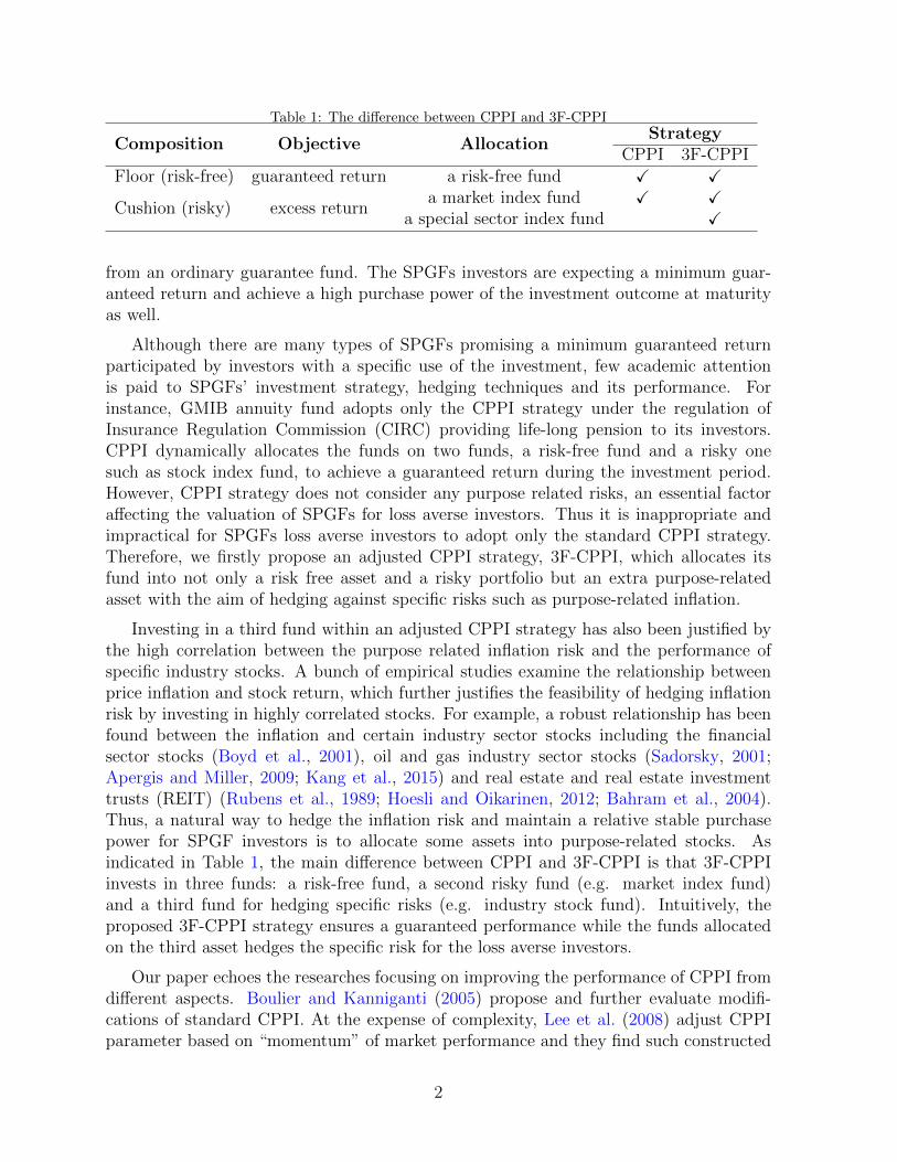
Table 1: The difference between CPPI and 3F-CPPI

Composition Objective AllocationStrategy

CPPI 3F-CPPIFloor (risk-free) guaranteed return a risk-free fund X X

Cushion (risky) excess returna market index fund X X

a special sector index fund X

from an ordinary guarantee fund. The SPGFs investors are expecting a minimum guar-anteed return and achieve a high purchase power of the investment outcome at maturityas well.

Although there are many types of SPGFs promising a minimum guaranteed returnparticipated by investors with a specific use of the investment, few academic attentionis paid to SPGFs’ investment strategy, hedging techniques and its performance. Forinstance, GMIB annuity fund adopts only the CPPI strategy under the regulation ofInsurance Regulation Commission (CIRC) providing life-long pension to its investors.CPPI dynamically allocates the funds on two funds, a risk-free fund and a risky onesuch as stock index fund, to achieve a guaranteed return during the investment period.However, CPPI strategy does not consider any purpose related risks, an essential factoraffecting the valuation of SPGFs for loss averse investors. Thus it is inappropriate andimpractical for SPGFs loss averse investors to adopt only the standard CPPI strategy.Therefore, we firstly propose an adjusted CPPI strategy, 3F-CPPI, which allocates itsfund into not only a risk free asset and a risky portfolio but an extra purpose-relatedasset with the aim of hedging against specific risks such as purpose-related inflation.

Investing in a third fund within an adjusted CPPI strategy has also been justified bythe high correlation between the purpose related inflation risk and the performance ofspecific industry stocks. A bunch of empirical studies examine the relationship betweenprice inflation and stock return, which further justifies the feasibility of hedging inflationrisk by investing in highly correlated stocks. For example, a robust relationship has beenfound between the inflation and certain industry sector stocks including the financialsector stocks (Boyd et al., 2001), oil and gas industry sector stocks (Sadorsky, 2001;Apergis and Miller, 2009; Kang et al., 2015) and real estate and real estate investmenttrusts (REIT) (Rubens et al., 1989; Hoesli and Oikarinen, 2012; Bahram et al., 2004).Thus, a natural way to hedge the inflation risk and maintain a relative stable purchasepower for SPGF investors is to allocate some assets into purpose-related stocks. Asindicated in Table 1, the main difference between CPPI and 3F-CPPI is that 3F-CPPIinvests in three funds: a risk-free fund, a second risky fund (e.g. market index fund)and a third fund for hedging specific risks (e.g. industry stock fund). Intuitively, theproposed 3F-CPPI strategy ensures a guaranteed performance while the funds allocatedon the third asset hedges the specific risk for the loss averse investors.

Our paper echoes the researches focusing on improving the performance of CPPI fromdifferent aspects. Boulier and Kanniganti (2005) propose and further evaluate modifi-cations of standard CPPI. At the expense of complexity, Lee et al. (2008) adjust CPPIparameter based on “momentum” of market performance and they find such constructed

2

variable proportion portfolio insurance (VPPI) outperform the standard CPPI. Chen et al.(2008) propose a dynamic proportion portfolio insurance (DPPI) strategy by identifyingrisk variables that are related to market conditions and used to build the equation treefor the risk multiplier by genetic programming.

Also as SPGFs investors tend to be loss averse, a feature which is quite different fromthe classical mean-variance framework, thus mutual fund separation derived from mean-variance framework might be inappropriate for SPGFs. Dichtl and Drobetz (2011) findthat the investors who prefer guarantee funds are proven to be loss averse and the popu-larity of PI strategies can only be explained in a behavioural finance context. The mostpopular CPPI strategy firstly proposed by Black and Jones (1987) and Black and Perold(1992) is a two-fund investment strategy by investing assets into a risk-free fund and adiversified asset. The CPPI strategy seems to follow the logic or principle of the famoustwo-fund separation, however, they are not belong to the same investment categories.The two-fund separation is firstly developed by Tobin (1958) and Markowitz (1959) un-der a mean-variance framework, and further proved by Merton (1973) in continuous-timecapital asset pricing model independent of preferences, wealth distribution, and time hori-zon. Nevertheless, there has been plenty much discussion questioning the hold of mutualfund separation: for instance, some literatures believe that when agents do not havemean-variance preferences or the investment opportunities are not constant, alternativeassumptions are needed in support of mutual fund separation.2

Further, three-fund or even K-fund separation theorem has been developed as theinvalidity of mutual fund separation.(Merton, 1973; Cairns et al., 2006; Dahlquist et al.,2016; Dybvig and Liu, 2018). Our innovative solution for SPGFs by investing in an ex-tra fund is inspired by the loss aversion feature of SPGFs investors, a utility frameworkwhich is quite different from the classical mean-variance one. However, we do not claim3F-CPPI is a direct application of three-fund separation theorem, neither do we statethe optimal allocation strategy for SPGFs investors be necessarily 3F-CPPI. Most impor-tantly, proposing an innovative 3F-CPPI for loss averse SPGFs investors and testing itssuperiority over benchmark PI strategies are the main contributions of this paper.

Within the general portfolio insurance setting featuring loss averse utility, we havederived the explicit optimal allocation rule for the 3F-CPPI strategy and its final payoffdistribution as well. Further extensive Monte Carlo simulations have been conducted togive further intuitive insights of 3F-CPPI’s superiority over other benchmark strategies.More specifically, the proposed 3F-CPPI strategy outperforms the standard CPPI andother strategies in various aspects such as mean return, expected fall and protection ratioetc. Despite both 3F-CPPI and CPPI are well able to hedge against the downside risk,3F-CPPI proves to be superior to the CPPI strategy with regards to reshaping returndistribution and investor’s utility. We prove further that the 3F-CPPI are most favouredby loss averse investors compared with other strategies.

The rest of the paper is structured as follows. Section 2 briefly introduces the financialmarket. An innovative 3F-CPPI strategy with closed-form solutions for its optimal alloca-

2See details in Pye (1967), Samuelson (1967), Hakansson (1969) and Ross (1978) among others

3

tion rules and leverage has been constructed in Section 3, followed by an extensive MonteCarlo simulations comparing the 3F-CPPI strategy among several contrastive strategiesin Section 4. Finally, Section 5 concludes and the proof techniques can be found in theAppendix.

2. Financial market and loss averse utility

2.1. Financial market

First, a stock market index, denoted by SIt , has been established using all n stocks inthe financial market. Further, we assume the dynamic process of the stock index SIt andrisk free asset Sft are captured by geometric Brownian motions as follows

dSItSIt

= µidt+ σsi dZs, (1)

dSf = rSfdt, (2)

where µi is the expected growth rate, σi is the volatility of the stock market, r is therisk-free interest rate and Zs is the Brownian motion which drives the stock market.

We further assume there exists a market sector consisting of m (m < n) stocks and itis closely related to the special purpose of a given SPGFs. As in the example of pensionfunds, the sector that consists medicine and health-related industry stocks is defined asthe purpose-related market sector. Similar to the stock market index, the dynamic processof the purpose-related market sector index, denoted by SPt , is given by

dSPtSPt

= µpdt+ σspdZs + σppdZp

= µpdt+ σPdZP , (3)

where Zs and Zp are two orthogonal Brownian motions, and σPdZP = σspdZs + σppdZp.Thus, Brownian motion ZP is correlated with Zs :

dZPdZs =σsp√

(σsp)2 + (σpp)2

dt. (4)

The SIt fund and SPt fund are driven by two different but correlated Brownian motions.For simplicity, we hereafter refer the market index fund SIt and the specific purpose relatedindex SPt to I-fund and P -fund respectively.

As the SPGFs’ payoff is to be used for a specific purpose such like hedging medicalcosts for pension funds, the inflation of purposed-related expense shall definitely reduceinvestors’ utility from the investment. More specifically, we denote the given SPGFs’purpose related expense inflation index as Yt, and refer it to the purpose-related expenseinflation index. As Yt represents the price level, we normalize Y0 = 1 for simplicity, it’sgenerally expected that YT > 1 at maturity due to inflation.

4

We assume further Yt is jointly driven by stock market risk and other risk (e.g. id-iosyncratic risk) that has not been traded in the stock market. The process of Yt is givenby:

dYtYt

= µydt+ σsydZs + σpydZp + σeydZe, (5)

where Zi, Zp, Ze are orthogonal Brownian motions. It is noteworthy that Yt can not beperfectly hedged by neither the I-fund nor the purpose-related P -fund.

By SDE process (5), one can write stochastic integration:

Yt = Y0 exp{(µy −1

2(σsy)

2 − 1

2(σpy)

2 − 1

2(σey)

2)t+ σsyWst + σpyWpt + σeyWet}

= Y0 exp{µY t+ σYWY t}, (6)

where Y0 = 1, and µY = µy − 12(σiy)

2− 12(σpy)

2− 12(σey)

2, σYWY t = σsyWst + σpyWpt + σeyWet.

So far, we have introduced SDE process of Yt, Zi and Zp, which are jointly driven bythree orthogonal BMs Zi, Zp and Ze. To write down as a unified form, we define:

dNt = µNdt+ σsndZs + σpndZp + σendZe, (7)

where Nt = SIt , SPt , Yt, and n = i, p, y correspondingly. −→σ n = (σsn, σ

pn, σ

en) is the volatility

vector of process of Nt, thus, −→σ i = (σsi , 0, 0), −→σ p = (σsp, σpp, 0) and −→σ y = (σsy, σ

py , σ

ey).

2.2. Loss averse utility

Generally, investors of guaranteed funds tend to be loss averse, which explains thepopularity of guaranteed funds and portfolio insurances (Dichtl and Drobetz, 2011). Incontrast to the expected utility theory, the guaranteed fund investors are proven to beloss averse with the following behavioural characteristics: 1. evaluate investment outcomeby its deviation from some specific reference point; 2. value potential gains and lossesasymmetrically, i.e. the marginal utility of the potential is higher than that of the gains.Therefore, we adopt the loss averse utility defined as follows in our framework.

More specifically, loss averse investors have an S-shaped utility function being concavefor gains and convex for losses. Investment outcome has been considered as either positiveor negative deviations from a reference point. Following Dichtl and Drobetz (2011) andTversky and Kahneman (1992), the loss averse utility function is defined as follows:

ν(∆V ) =

{(∆V )γ

−λ(−∆V )γfor ∆V > 0for ∆V < 0

, (8)

where ∆V is the deviation from reference point, 1 > γ > 0 and λ > 1. It’s noteworthythat the concave part of utility (8) is equivalent to the form of Constant Relative RiskAversion (CRRA) utility 3 given by

uCRRA(∆V ) =1

γ(∆V )γ, where 0 < γ < 1. (9)

3In fact, the concave part of utility in (8) can also take the form of other utility functions, e.g. aConstant Absolute Risk Aversion (CARA) function.

5

Due to the specific investment purpose, the investors’ utility is not only determined bythe investment outcome, but also by the inflation of purpose-related expense, YT . As theprice index YT at maturity dramatically affects the real wealth level of the investment.Similar to the concept of real income, the SPGFs investors’ utility or subject value ofSPGFs should be deflated by the price inflation index as well.

After considering the purpose-related inflation risk, at time t, the SPGFs investor’sloss averse utility is defined as follows

U(VT , YT ) =

{(VT−PT

YT)γ

−λ · (−VT−PTYT

)γfor VT > PTfor VT < PT

, (10)

where γ is the risk averse parameter of the SPGFs investors. The relative risk aversion

(RRA) coefficient of utility U(∆V ) is R = −xU′′2

U′2

= 1− γ.

We add the reference point and the purpose-related inflation risk in our utility func-tion (10) for the following two reasons4. First, Dichtl and Drobetz (2011) demonstratesthat the investors of guarantee funds are loss averse and the reference point is based onthe principal investment which is related to the absolute return of the guarantee funds.Second, the impact of inflation on consumption or utility has been commonly capturedas the denominator in most economic literature.

3. Three-fund CPPI strategy

In this section, we briefly review the standard CPPI strategy in 3.1, followed by adetailed construction of the innovative 3F-CPPI strategy in 3.2. Further 3.3 proposes theloss averse investors’ utility maximisation problem and presents explicitly results as well.

3.1. Standard CPPI strategy

Constant proportion portfolio insurance (CPPI) is a trading strategy that allows aportfolio to maintain an exposure to the upside potential of a risky asset while providinga capital guarantee against downside risk. The outcome of the CPPI strategy is somewhatsimilar to a call option. Since CPPI is firstly proposed by Black and Jones (1987), it iswidely used in many guaranteed funds as it maintains the portfolio value above a certainpredetermined level (floor) and allows upside potential as well.

CPPI, a self-financing strategy, not only guarantees a fixed payoff PT at maturity butchases the upside potentials via dynamic trading using leverage as well. According tothe CPPI strategy, the fund value Vt is invested on the risk free fund (often referred as

4Admittedly, the reference point with a guaranteed utility is also a potential candidate form, butthis alternative choice leads to a fluctuating amount of PT and lacks literature supports. Moreover, thesimulation result shows that the 3F-CPPI outperforms CPPI in the manners of achieving a higher meanreturn, better protecting the downside risk, and higher utility level as well. It rules out the possibilitythat our conclusion on the superiority of 3F-CPPI strongly relies on our utility assumption.

6

“floor”) and the mutual fund (the “cushion”). Denote Pt and Ct as the floor and cushioninvested at time t respectively, then, they satisfies

Ct = Vt − Pt, t ∈ [0, T ]. (11)

We assume the capital amount to be guaranteed at maturity is PT , then a typical floorstrategy at time t is a fixed-rate floor, which is given by,

Pt = e−d(T−t)PT , t ∈ [0, T ], (12)

where d is the required return by investors for risk free asset and d 6 r. Also d is referredas the fixed rate of floor strategy, and d < r reflects a conservative case which allocatesmore assets in the risk-free fund. The most common floor strategy is to allocate theminimum amount of assets into the risk-free fund, i.e. d = r, then the floor amount attime t is determined by

Pt = e−r(T−t)PT , t ∈ [0, T ]. (13)

The cushion, the difference between portfolio value and floor, will be invested in themutual fund i.e. I-fund. A CPPI portfolio usually leverages its cushion Ct to chasehigher return, and its leverage ratio m stays constant as “constant proportion”. Thus,the portfolio’s exposure in stock market Et is

Et = mCt = m(Vt − Pt), t ∈ [0, T ], (14)

where m > 1. Constant proportion m is determined at the time 0 and stays constantduring the investment horizon. The cushion value Ct fluctuates with the market, once itapproaches zero all the fund will be invested in the risk-free asset till the maturity.

Therefore, a standard CPPI strategy is, in fact, a two-fund separation investment. Atany time t, we have:

• if Vt > Pt, the portfolio allocates amount Pt in the risk-free fund, and amount Ct inthe I-fund with leverage m;

• if Vt 6 Pt, the entire portfolio is invested in the risk-free fund.

If using time-continuous rebalancing, the CPPI fund value Vt never falls below the guar-anteed floor.

3.2. Three-fund CPPI

The famous mutual fund theorem holds only for “normal” investors with mean-variancepreference. Due to the invalidity of mutual fund separation in incomplete markets, wepropose a 3F-CPPI strategy to hedge these risks in a general portfolio insurance settingas well.

3F-CPPI is a self-financing strategy which dynamically rebalances portfolio amounton the risk-free asset and two risky funds (I-fund and P -fund). Similar to CPPI, we

7

denote Pt and Ct as the floor and the cushion respectively. Unlike CPPI, the cushion of3F-CPPI fund is invested in two risky funds: the I-fund and the P -fund. Denote α as theproportion of cushion to be invested in I-fund, then the remaining 1− α part is assignedto P -fund.

Define Vt as the SPGF value and its evolution is given by

dVt = Et[αdSItSIt

+ (1− α)dSPtSPt

] + VtdSfSf− Etrdt, (15)

where Et = mCt is the exposure to the risky asset. Now we summarise our main resultsin the following proposition:

Proposition 1. Under the continuous time setting, for t ∈ [0, T ] a 3F-CPPI portfoliovalue at time t follows the distribution:

Vt = Pt + C0 exp(Bt −1

2At) + (r − d)

∫ t

0

exp{Bt −Bξ −1

2A(t− ξ)}Pξdξ, (16)

and the expected portfolio value of the 3F-CPPI portfolio at time t is

E(Vt) = Pt + C0eµBt + (r − d)p0e

µBt1− e(d−µB)t

µB − d, (17)

where A = m2α2σ2i +m2(1− α)2σ2

P + 2m2α(1− α)σspσi andBt = {r +m[ασiθi + (1− α)σP θP ]}t+m[ασiWst + (1− α)σPWpt];P0 + C0 = V0.

Proof: The proof of proposition 1 is in Appendix.

For simplicity and without loss of generalization, hereafter we consider only the mostcommon floor strategy(d = r) for the proposed 3F-CPPI strategy. Then, based on Equa-tion (16), a 3F-CPPI portfolio value at time t follows the following distribution

Vt = Pt +C0 exp{{r+m[ασiθi + (1−α)σP θP ]− 1

2A}t+mασiWst + (1−α)σPWPt}. (18)

In fact, the CPPI can be viewed as a special case of 3F-CPPI with α = 1 and thedistribution of a CPPI portfolio value at time t is


2m2σ2

i t) + (r − d)

∫ t

0

exp{Bt −Bξ −1

2m2σ2

i (t− ξ)}Pξdξ, (19)

where Bt = {(r +mσiθi)t+mσiQWst}, t ∈ [0, T ].

3.3. Optimal 3F-CPPI allocation rules

Suppose a SPGFs manager aims to maximize the investor’s utility U(VT , YT ) in (10)by choosing leverage m and I-fund proportion α at the commence of the fund. Theoptimization problem is given by

Maxm,α

E[U(VT , YT )|F0] (20)

⇐⇒ Maxm,α

E[U(VT −RT

YT)|F0]. (21)

8

To determine the optimal allocation (α∗,m∗), we first introduce the purpose-relatedrisk-aversion adjusted return (PRA return henceforth). The PRA return is a modifiedindicator which reflects the effect of risk aversion and purpose-related inflation risk onevaluating the I-fund and P -fund.

Definition 1. For the stock index I-fund and purpose-related market sector P -fund, thepurpose-related risk-aversion adjusted return (PRA return) is:

µ(γ)n = µn − γ−→σ n · −→σ y, n = i, p. (22)

where −→σ n = (σsn, σpn, σ

en), −→σ y = (σsy, σ

py , σ

ey).

In the definition of risk-aversion adjusted return, −→σ n · −→σ y is always positive. The

possible range of γ for loss averse investors is 0 < γ 6 1, thus there always is µ(γ)n 6 µn.

The “punishment” of I-fund or P -fund increases with investors’ risk aversion and thefund’s volatility’s vector correlation with inflation Yt. Thanks to the concept of PRAreturn, we solve the global optimal allocation parameters m∗ and α∗ of the 3F-CPPIportfolio as follows:

Proposition 2. The optimal allocation parameters m∗ and α∗ of the 3F-CPPI portfoliosatisfy

F (m∗) = 0, (23)

α∗ = α∗(m∗), (24)

where

F (m) = α∗(m)µ(γ)i + (1− α∗(m))µ(γ)

p − r + (µ(γ)i − µ(γ)

p )α∗(m) (25)

+ (γ − 1){[(σsp)

2 + (σpp)2 − σspσsi

(σsi − σsp)2 + (σpp)2+ (σpp)

2 + (σsp)2]m− σiyσsp − σpyσpp}.

α∗(m) =(σsp)


(σsi − σsp)2 + (σpp)2+

µ(γ)i − µ

(γ)p

(σi − σsp)2 + (σpp)21

(1− γ)m, (26)

Proof: The proof of proposition 2 and expressions of optimal m∗ and α∗ are provided inAppendix.

Proposition 2 illustrates the optimal m∗ and α∗ without considering the limited pos-sible range of parameters in practise. However, in real-world scenarios, there is an upperbound of the leverage m because of the regulation and fund’s borrowing capability. Alsothe portfolio cannot be rebalanced continuously in practice due to the gap risk. Besides,the range of α may be limited to [0, 1] because of the short-sale constraints. Therefore, wediscuss further the optimal ratio α∗ for a given the leverage ratio m in the next subsection.

Now we look a special example of optimal 3F-CPPI allocation: the SPGFs participatedby risk neutral investors case with γ = 1. We further assume the parameter ranges are:m ∈ [1,M ] and α ∈ [0, 1].

9

According to the Proposition 2, the optimal 3F-CPPI in the risk-neutral case de-generates into the two-fund separation, the optimal allocation α∗ and m∗ are given asfollows

α∗ =

1

α, α ∈ [0, 1]0

if µ(1)i − µ

(1)p > 0

if µ(1)i − µ

(1)p = 0

if µ(1)i − µ

(1)p < 0

, (27)

and

m∗ =

M

m, m ∈ [1,M ]1

if α∗µ(γ)i + (1− α∗)µ(γ)

p − r > 0

if α∗µ(γ)i + (1− α∗)µ(γ)

p − r = 0

if α∗µ(γ)i + (1− α∗)µ(γ)

p − r < 0

, (28)

where the excess PRA return is αµ(1)i + (1− α)µ

(1)p − r, and M is the maximum possible

value of m. Optimal allocation in (27) is intuitive in explaining the 3F-CPPI’s optimal

allocation principle: the optimal proportion α∗ depends on comparison of PRA return µ(1)i

and µ(1)p to a great extent, and the optimal leverage m∗ is greatly influenced by portfolio’s

average excess PRA return, αµ(1)i + (1− α)µ

(1)p − r.

3.3.1. Continuous time: optimal α∗ for given leverage m

Now we turn to determine the optimal proportion α∗ invested in I-fund for givenleverage m. In practice, the leverage m is limited and even regulated because of gaprisk. According to the findings from ?, Balder et al. (2009) and Dichtl and Drobetz(2011) among others, the leverage has been found to have significant impact on the CPPIportfolio’s outcome and it is normally below 10. For example, Dichtl and Drobetz (2011)consider m 6 10 cases while? compares CPPI’s performances for m = 3, 4, 5 cases. Fora given range of m (1 6 m 6 10), we investigate the optimal proportion α∗.

Equation (26) shows the relation between optimal m∗ and α∗ without considerationof range, the following corollary reveals that the monotonicity of α∗(m) depends on the

relativity of PRA return of I-fund and P -fund, µ(γ)i − µ

(γ)p .

Corollary 1. Given a leverage m, the optimal ratio α∗(m) satisfies:

(1) If µ(γ)i > µ

(γ)p , then α∗(m) is a decreasing function of m;

(2) If µ(γ)i < µ

(γ)p , then α∗(m) is an increasing function of m;

(3) If µ(γ)i = µ

(γ)p , then α∗ is not correlated with m.

Proof: If µ(γ)i > µ

(γ)p , then α∗(m) is a function of m in form of 1

mby (26), which is

decreasing function of m. The remaining proof is similar and trivial.

Corollary 1 shows a “diversification” effect of optimal allocations: α∗(m) graduallyshifts to the fund with less PRA as the increase of leverage ration m. This is an interestingfeature of optimal allocation, whose diversification offsets the risk caused by the highleverage.

On the basis of monotonicity of α∗(m), we show the relation between the optimalproportion α∗ and given leverage m. Assume M is the upper bound of leverage and there

10

are constraints on short-sale, then the parameters ranges are m ∈ [1,M ] and α ∈ [0, 1].With consideration of the bounds, we have the following proposition 3, whose proof istrivial.

Proposition 3. For a regulated leverage m ∈ [1,M ], the optimal ratio α∗c(m) ∈ [0, 1] is:

α∗c(m) =

1

α∗(m)0

if α∗(m) > 1if α∗(m) ∈ [0, 1]

if α∗(m) < 0. (29)

So far, we have only considered the optimal allocation in a continuous time case, underwhich the portfolio is continuously rebalanced. As the portfolio value never falls belowthe floor in the continuous time case, the investor’s loss averse feature does not play arole in optimal allocation.

3.3.2. Discrete time: optimal α∗ for given leverage m

Due to the constraints of the continuous time case, we here consider a more practicalcase, the discrete time case, under which the portfolio cannot be rebalanced continuously.In the discrete time case, there is a gap risk that the cushion value of 3F-CPPI fund mightturn to a negative value between two rebalance time, which means the portfolio is failingto achieve the guaranteed return. Therefore, the investor’s loss aversion characteristicplays a vital role in determining the optimal allocation.

Monte Carlo simulation method is adopted to solve the optimal proportion α∗ for agiven leverage m. Within the parameters ranges, for each m, we run simulations throughthe range α ∈ [0, 1] to search for the optimal α∗, the interval is 0.005. For each (m,α)pair, 100000 times simulations are run to calculate allocation outcome. In the simulation,we assign γ = 0.88, which is consistent with Tversky and Kahneman (1992) and Dichtland Drobetz (2011). We consider the following three different scenarios of I-fund andP -fund: 5

• Case 1: µ(γ)i > µ

(γ)p ;

• Case 2: µ(γ)i = µ

(γ)p ;

• Case 3: µ(γ)i < µ

(γ)p .

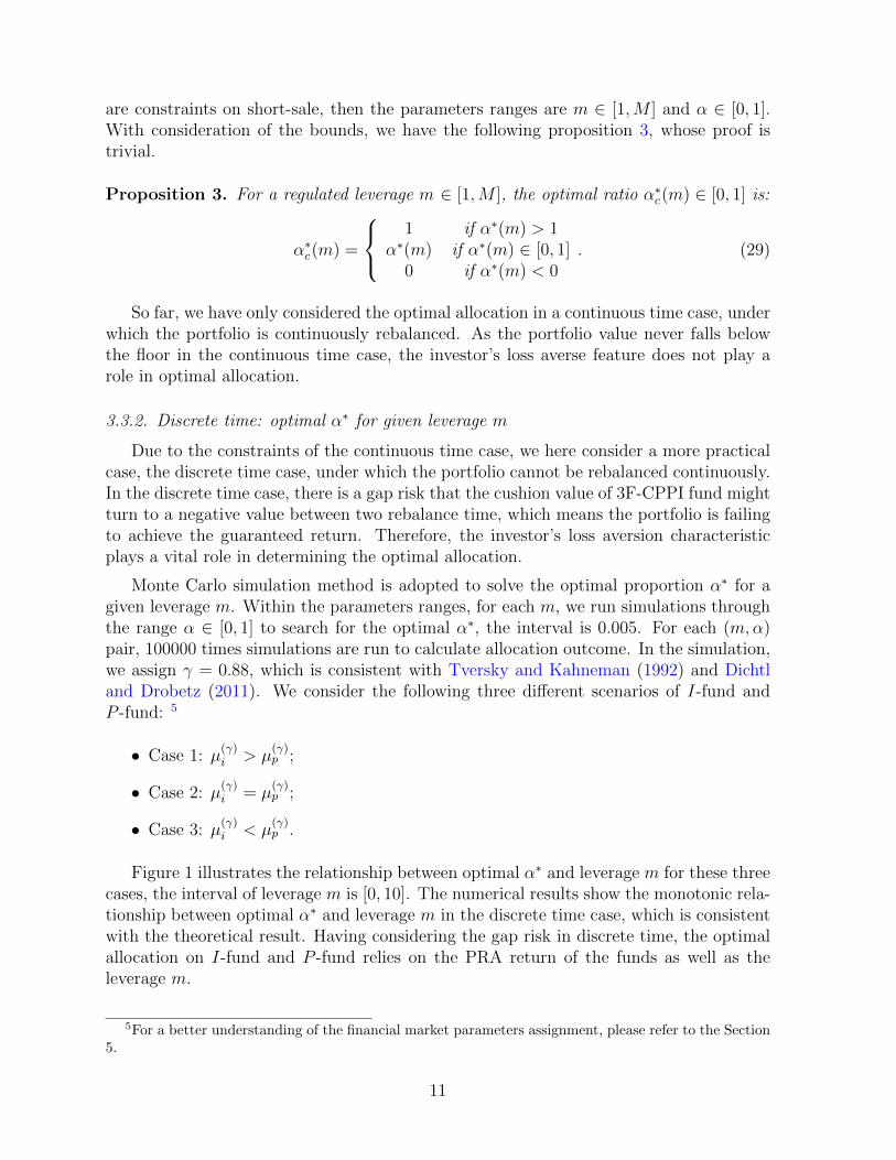
Figure 1 illustrates the relationship between optimal α∗ and leverage m for these threecases, the interval of leverage m is [0, 10]. The numerical results show the monotonic rela-tionship between optimal α∗ and leverage m in the discrete time case, which is consistentwith the theoretical result. Having considering the gap risk in discrete time, the optimalallocation on I-fund and P -fund relies on the PRA return of the funds as well as theleverage m.

5For a better understanding of the financial market parameters assignment, please refer to the Section5.

11

Case1

1 2 3 4 5 6 7 8 9 10

0.65

0.7

0.75

0.8

0.85

Case2

1 2 3 4 5 6 7 8 9 10−0.4

−0.2

0

0.2

0.4

0.6

0.8

1

1.2

1.4

1.6

Case3

1 2 3 4 5 6 7 8 9 100

0.05

0.1

0.15

0.2

0.25

Figure 1: The relationship between optimal allocation α and leverage m for three differentcases, i.e. Case 1 µ

(γ)i > µ

(γ)p , Case 2 µ

(γ)i = µ

(γ)p and Case 3 µ

(γ)i < µ

(γ)p .

3.4. An example: pension guarantee funds in China

Here we use an example of pension guarantee funds in China to show the advantageof the proposed 3F-CPPI strategy. The medical and health-related expense is one ofthe major parts of living cost for retirees in China, and its price inflation significantlyaffects the retiree’s utility of pension savings. Using historical data from Shanghai StockExchange, we simulate the performance for both the 3F-CPPI and CPPI strategy.

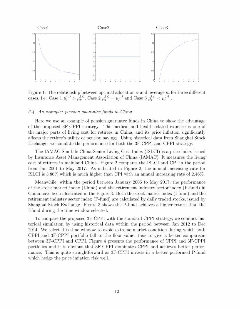
The IAMAC-SinoLife China Senior Living Cost Index (ISLCI) is a price index issuedby Insurance Asset Management Association of China (IAMAC). It measures the livingcost of retirees in mainland China. Figure 2 compares the ISLCI and CPI in the periodfrom Jan 2001 to May 2017. As indicated in Figure 2, the annual increasing rate forISLCI is 3.86% which is much higher than CPI with an annual increasing rate of 2.46%.

Meanwhile, within the period between January 2006 to May 2017, the performanceof the stock market index (I-fund) and the retirement industry sector index (P-fund) inChina have been illustrated in the Figure 3. Both the stock market index (I-fund) and theretirement industry sector index (P-fund) are calculated by daily traded stocks, issued byShanghai Stock Exchange. Figure 3 shows the P-fund achieves a higher return than theI-fund during the time window selected.

To compare the proposed 3F-CPPI with the standard CPPI strategy, we conduct his-torical simulation by using historical data within the period between Jan 2012 to Dec2014. We select this time window to avoid extreme market condition during which bothCPPI and 3F-CPPI portfolio fall to the floor value, thus to give a better comparisonbetween 3F-CPPI and CPPI. Figure 4 presents the performance of CPPI and 3F-CPPIportfolios and it is obvious that 3F-CPPI dominates CPPI and achieves better perfor-mance. This is quite straightforward as 3F-CPPI invests in a better performed P-fundwhich hedge the price inflation risk well.

12

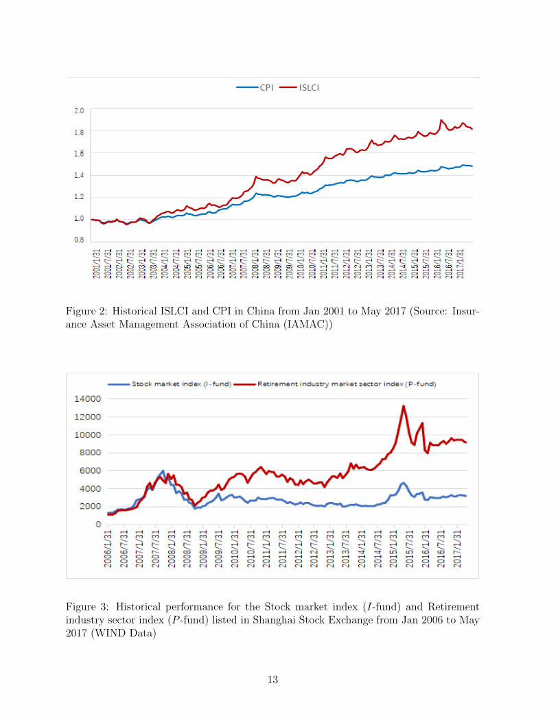
Figure 2: Historical ISLCI and CPI in China from Jan 2001 to May 2017 (Source: Insur-ance Asset Management Association of China (IAMAC))

Figure 3: Historical performance for the Stock market index (I-fund) and Retirementindustry sector index (P -fund) listed in Shanghai Stock Exchange from Jan 2006 to May2017 (WIND Data)

13

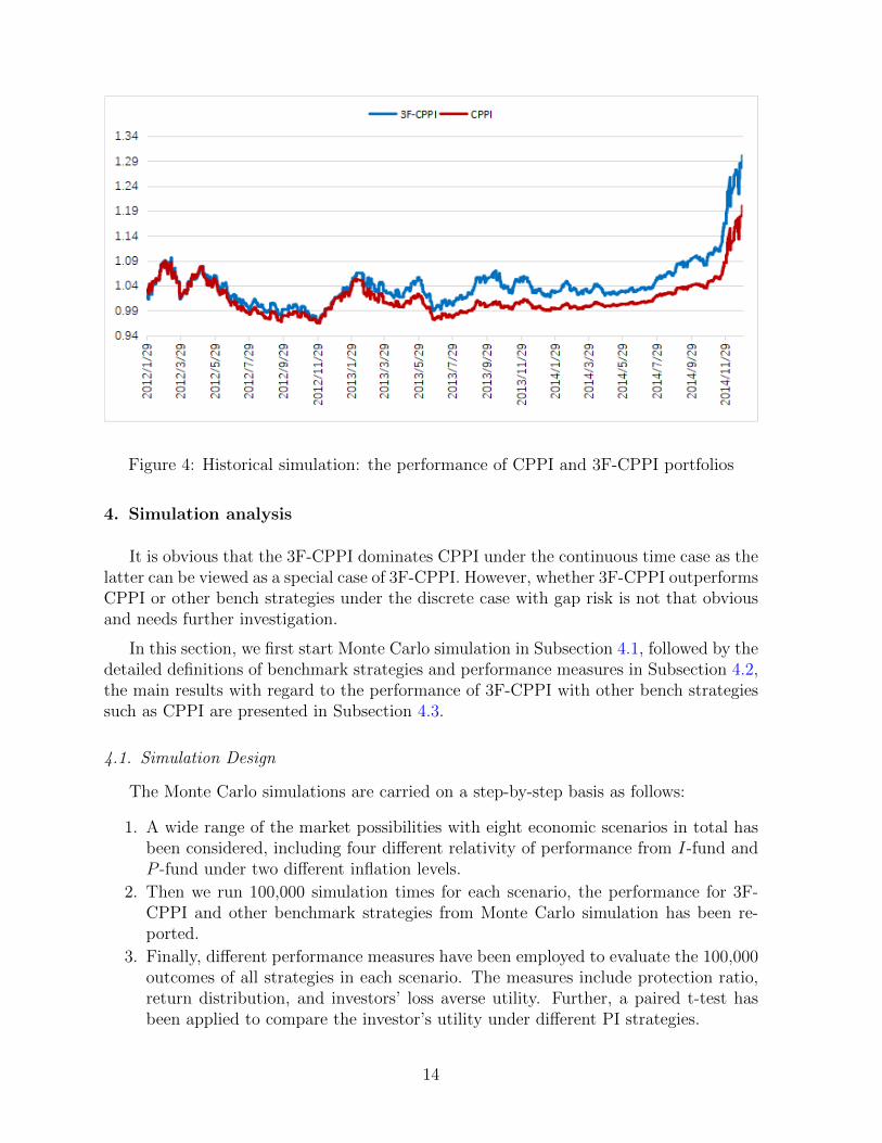
Figure 4: Historical simulation: the performance of CPPI and 3F-CPPI portfolios

4. Simulation analysis

It is obvious that the 3F-CPPI dominates CPPI under the continuous time case as thelatter can be viewed as a special case of 3F-CPPI. However, whether 3F-CPPI outperformsCPPI or other bench strategies under the discrete case with gap risk is not that obviousand needs further investigation.

In this section, we first start Monte Carlo simulation in Subsection 4.1, followed by thedetailed definitions of benchmark strategies and performance measures in Subsection 4.2,the main results with regard to the performance of 3F-CPPI with other bench strategiessuch as CPPI are presented in Subsection 4.3.

4.1. Simulation Design

The Monte Carlo simulations are carried on a step-by-step basis as follows:

1. A wide range of the market possibilities with eight economic scenarios in total hasbeen considered, including four different relativity of performance from I-fund andP -fund under two different inflation levels.

2. Then we run 100,000 simulation times for each scenario, the performance for 3F-CPPI and other benchmark strategies from Monte Carlo simulation has been re-ported.

3. Finally, different performance measures have been employed to evaluate the 100,000outcomes of all strategies in each scenario. The measures include protection ratio,return distribution, and investors’ loss averse utility. Further, a paired t-test hasbeen applied to compare the investor’s utility under different PI strategies.

14

According to the model in Section 2, the stock market and the purpose-related inflationindex follow multivariate correlated Brownian motion processes. Before running MonteCarlo simulation, some key parameters have to be assigned: the return and volatility ofthe I-fund : µi and −→σ i; the return and volatility of the P -fund : µp,

−→σ p; and the growthrate and volatility of the purpose-related expense risk: µy,

−→σ y.

We refer to the existing literature for assigning parameters value. Similar to Arnott andBernstein (2002), we first assume the risk free rate rf is fixed at 4.5% within the investmentperiod. According to Dimson et al. (2008), the mean annual equity excess return fordeveloped stock markets was approximately 7% between 1900 and 2005, resulting in anexpected excess return around 4.5% per year. In our simulation, we then estimate that ahigh state of stock market excess return is 6.5%, and a low state is 4.5%. Last, Dimsonet al. (2008) find the long-run stock return volatility was roughly 20% per year that hasbeen used in simulation by other scholars like Benninga (1990) and Figlewski et al. (1993).Therefore, we estimate the stock market volatility with a range from a high state of 30%to a low state of 20%.

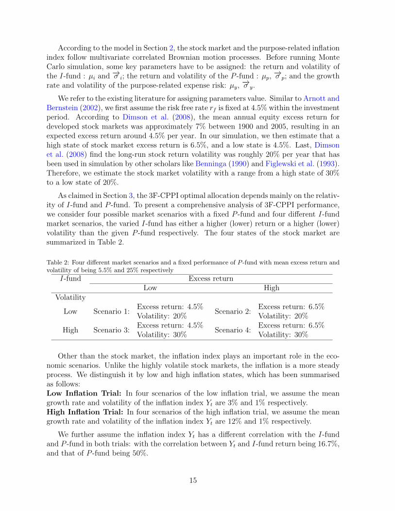
As claimed in Section 3, the 3F-CPPI optimal allocation depends mainly on the relativ-ity of I-fund and P -fund. To present a comprehensive analysis of 3F-CPPI performance,we consider four possible market scenarios with a fixed P -fund and four different I-fundmarket scenarios, the varied I-fund has either a higher (lower) return or a higher (lower)volatility than the given P -fund respectively. The four states of the stock market aresummarized in Table 2.

Table 2: Four different market scenarios and a fixed performance of P -fund with mean excess return andvolatility of being 5.5% and 25% respectively

I-fund Excess returnLow High

Volatility

Low Scenario 1:Excess return: 4.5%Volatility: 20%

Scenario 2:Excess return: 6.5%Volatility: 20%

High Scenario 3:Excess return: 4.5%Volatility: 30%

Scenario 4:Excess return: 6.5%Volatility: 30%

Other than the stock market, the inflation index plays an important role in the eco-nomic scenarios. Unlike the highly volatile stock markets, the inflation is a more steadyprocess. We distinguish it by low and high inflation states, which has been summarisedas follows:Low Inflation Trial: In four scenarios of the low inflation trial, we assume the meangrowth rate and volatility of the inflation index Yt are 3% and 1% respectively.High Inflation Trial: In four scenarios of the high inflation trial, we assume the meangrowth rate and volatility of the inflation index Yt are 12% and 1% respectively.

We further assume the inflation index Yt has a different correlation with the I-fundand P -fund in both trials: with the correlation between Yt and I-fund return being 16.7%,and that of P -fund being 50%.

15

Similar to Benartzi and Thaler (1995) and Dichtl and Drobetz (2011), we consider aone-year investment horizon and simulate 250 daily observations for each scenario. Theguarantee level of the SPGF is set to be 100% (full capital guarantee). We normalizethe initial SPGFs value V0 as 100. We run 100,000 simulation times for each scenario toprovide a stable and convincing test. T-test has been applied to compare performancesamong 3F-CPPI and other benchmark strategies. All portfolio insurance strategies inthe simulation adopt a base case leverage of m = 5, which has been commonly used inpractise (Herold et al., 2005).

4.2. Benchmark strategies and performance measures

4.2.1. Benchmark strategies

We select a variety of benchmark strategies, including CPPI, TIPP, stop-loss, buy-and-hold strategy and the risk-free investment, to test the superiority of the proposed3F-CPPI.

CPPI strategiesCPPI strategy has been introduced in 3.1. The benchmark strategies consider two CPPIstrategies with a difference in the risky fund: i.e. the risky asset of CPPI-I strategy is theI-fund while that of the CPPI-P is the P -fund.

TIPP strategyTime invariant portfolio protection (TIPP) strategy proposed by Estep and Kritzman(1988), not only ensures a protection of the investor’s initial wealth but also any interimcapital gains during the investment. Instead of having a fixed-rate floor like CPPI, TIPP’sfloor is ratchet up with the value of the portfolio during the investment period. Therefore,TIPP portfolio’s exposure in stock market Et is

Et = mCt = m(Vt − Pt), t ∈ [0, T ], (30)

the floor isPt = max(e−d(T−t)PT , f · Vt), t ∈ [0, T ], (31)

where f is a predetermined protection ratio of whole portfolio value Vt. f · Vt shows the“ratcheting up”effect of TIPP, which transfers gains in the risky asset to the risk-freeasset irreversibly once there are interim capital gains.

Stop loss (S-L) strategyStop loss is one of the simplest portfolio insurance strategies to protect a risky portfolioagainst losses. Under the stop loss strategy, the fund initially invests all the wealth V0in the risky assets, the position of which will be maintained as long as the market valueof the portfolio exceeds the net present value floor Vt > Pt. Once the market value ofthe portfolio reaches or falls below the discounted floor Vt < Pt, all of the risky portfoliopositions are cleared off and to be reinvested in the risk-free asset till maturity.

Buy-and-hold (B&H) strategies

16

B&H strategy is not a portfolio insurance strategies as it doesn’t have a protection ratio.B&H-P strategy invests total value of the fund V0 in the stock market I-fund during thewhole investment horizon while B&H-P strategy invests in the P -fund. B&H strategiesachieve a high return in a bull market while a low return in a bear market.

Cash investment strategyA cash investment strategy simply invests the total fund wealth V0 in the risk-free fund(Cash Asset) during the whole investment horizon.

4.2.2. Performance measures

To provide a sound assessment, measures are applied to evaluate the 100,000 outcomesof all strategies in each scenario, in terms of its success rate to protect the insured valueand the return distribution. The performance measures include average annual return,annual volatility, Sharpe ratio, protected ratio, 1% value at risk, 1% expected shortfalland investor’s prospect utility, with loss aversion parameters λ = 1 and λ = 2.25. Pairedt-tests of investors’ utility are conducted to compare 3F-CPPI with benchmark strate-gies. Some measures like annual return, volatility, Sharpe ratio and value at risk arewell-known, the other measures, which are widely adopted in portfolio insurance relatedliterature, are briefly explained in the following.

Protection ratioThe protection ratio is defined as the probability that the strategy successfully protectsthe insured value (Huu Do, 2002). It measures the ability in sustaining a pre-specifiedguarantee return.

1% Expected shortfallFor a given strategy, 1% Expected shortfall measures the average return of the poorest-performed 1% scenarios. Its calculation follows two steps: firstly sort the realized portfoliovalues in ascending order, then calculate the average value in the poorest-performed 1%group. Expected shortfall focuses on the left tail of the distribution and measures theability of controlling the downside risk.

Loss averse utilityWe first compare the mean loss averse utility value of the 100,000 times simulated port-folio outcomes. Being consistent with Tversky and Kahneman (1992) and Dichtl andDrobetz (2011), we assign λ = 2.25 and γ = 0.88 in the simulation.Then two loss aver-sion parameters, λ = 1 and λ = 2.25 in Equation (8), has been used in our simulation.λ = 1 indicates that no loss averse for investors as they treat the loss and gain equally.While λ = 2.25 reflects loss averse investors with the most common type of loss averseparameters.

4.3. Simulation Results

The Monte Carlo simulation results of performance measures for different strategieshave been presented in Table 3, while simulation results of utility value under two different

17

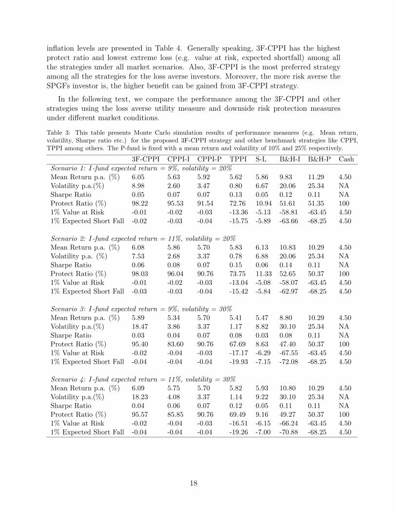
inflation levels are presented in Table 4. Generally speaking, 3F-CPPI has the highestprotect ratio and lowest extreme loss (e.g. value at risk, expected shortfall) among allthe strategies under all market scenarios. Also, 3F-CPPI is the most preferred strategyamong all the strategies for the loss averse investors. Moreover, the more risk averse theSPGFs investor is, the higher benefit can be gained from 3F-CPPI strategy.

In the following text, we compare the performance among the 3F-CPPI and otherstrategies using the loss averse utility measure and downside risk protection measuresunder different market conditions.

Table 3: This table presents Monte Carlo simulation results of performance measures (e.g. Mean return,volatility, Sharpe ratio etc.) for the proposed 3F-CPPI strategy and other benchmark strategies like CPPI,TPPI among others. The P-fund is fixed with a mean return and volatility of 10% and 25% respectively.

3F-CPPI CPPI-I CPPI-P TPPI S-L B&H-I B&H-P Cash

Scenario 1: I-fund expected return = 9%, volatility = 20%Mean Return p.a. (%) 6.05 5.63 5.92 5.62 5.86 9.83 11.29 4.50Volatility p.a.(%) 8.98 2.60 3.47 0.80 6.67 20.06 25.34 NASharpe Ratio 0.05 0.07 0.07 0.13 0.05 0.12 0.11 NAProtect Ratio (%) 98.22 95.53 91.54 72.76 10.94 51.61 51.35 1001% Value at Risk -0.01 -0.02 -0.03 -13.36 -5.13 -58.81 -63.45 4.501% Expected Short Fall -0.02 -0.03 -0.04 -15.75 -5.89 -63.66 -68.25 4.50

Scenario 2: I-fund expected return = 11%, volatility = 20%Mean Return p.a. (%) 6.08 5.86 5.70 5.83 6.13 10.83 10.29 4.50Volatility p.a. (%) 7.53 2.68 3.37 0.78 6.88 20.06 25.34 NASharpe Ratio 0.06 0.08 0.07 0.15 0.06 0.14 0.11 NAProtect Ratio (%) 98.03 96.04 90.76 73.75 11.33 52.65 50.37 1001% Value at Risk -0.01 -0.02 -0.03 -13.04 -5.08 -58.07 -63.45 4.501% Expected Short Fall -0.03 -0.03 -0.04 -15.42 -5.84 -62.97 -68.25 4.50



18

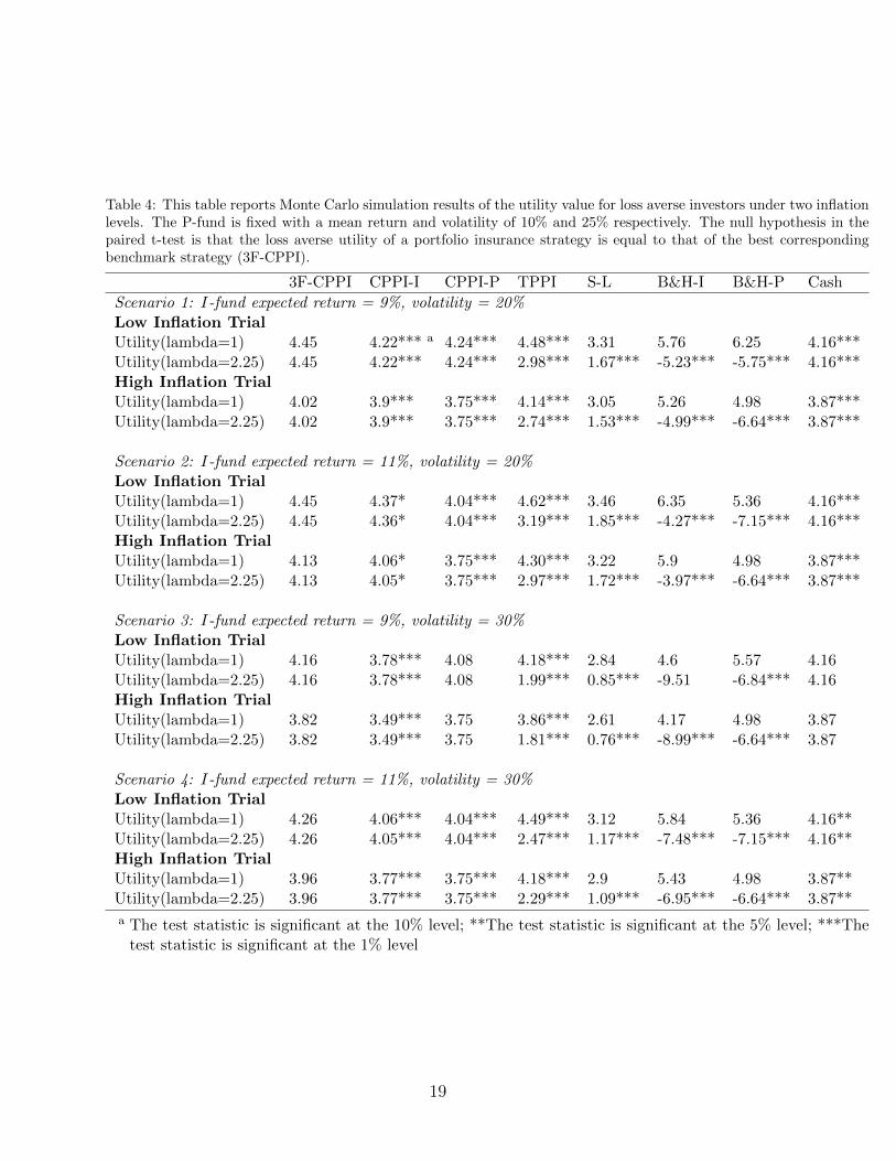
Table 4: This table reports Monte Carlo simulation results of the utility value for loss averse investors under two inflationlevels. The P-fund is fixed with a mean return and volatility of 10% and 25% respectively. The null hypothesis in thepaired t-test is that the loss averse utility of a portfolio insurance strategy is equal to that of the best correspondingbenchmark strategy (3F-CPPI).

3F-CPPI CPPI-I CPPI-P TPPI S-L B&H-I B&H-P Cash

Scenario 1: I-fund expected return = 9%, volatility = 20%Low Inflation TrialUtility(lambda=1) 4.45 4.22*** a 4.24*** 4.48*** 3.31 5.76 6.25 4.16***Utility(lambda=2.25) 4.45 4.22*** 4.24*** 2.98*** 1.67*** -5.23*** -5.75*** 4.16***High Inflation TrialUtility(lambda=1) 4.02 3.9*** 3.75*** 4.14*** 3.05 5.26 4.98 3.87***Utility(lambda=2.25) 4.02 3.9*** 3.75*** 2.74*** 1.53*** -4.99*** -6.64*** 3.87***

Scenario 2: I-fund expected return = 11%, volatility = 20%Low Inflation TrialUtility(lambda=1) 4.45 4.37* 4.04*** 4.62*** 3.46 6.35 5.36 4.16***Utility(lambda=2.25) 4.45 4.36* 4.04*** 3.19*** 1.85*** -4.27*** -7.15*** 4.16***High Inflation TrialUtility(lambda=1) 4.13 4.06* 3.75*** 4.30*** 3.22 5.9 4.98 3.87***Utility(lambda=2.25) 4.13 4.05* 3.75*** 2.97*** 1.72*** -3.97*** -6.64*** 3.87***

Scenario 3: I-fund expected return = 9%, volatility = 30%Low Inflation TrialUtility(lambda=1) 4.16 3.78*** 4.08 4.18*** 2.84 4.6 5.57 4.16Utility(lambda=2.25) 4.16 3.78*** 4.08 1.99*** 0.85*** -9.51 -6.84*** 4.16High Inflation TrialUtility(lambda=1) 3.82 3.49*** 3.75 3.86*** 2.61 4.17 4.98 3.87Utility(lambda=2.25) 3.82 3.49*** 3.75 1.81*** 0.76*** -8.99*** -6.64*** 3.87

Scenario 4: I-fund expected return = 11%, volatility = 30%Low Inflation TrialUtility(lambda=1) 4.26 4.06*** 4.04*** 4.49*** 3.12 5.84 5.36 4.16**Utility(lambda=2.25) 4.26 4.05*** 4.04*** 2.47*** 1.17*** -7.48*** -7.15*** 4.16**High Inflation TrialUtility(lambda=1) 3.96 3.77*** 3.75*** 4.18*** 2.9 5.43 4.98 3.87**Utility(lambda=2.25) 3.96 3.77*** 3.75*** 2.29*** 1.09*** -6.95*** -6.64*** 3.87**

a The test statistic is significant at the 10% level; **The test statistic is significant at the 5% level; ***Thetest statistic is significant at the 1% level

19

4.3.1. Investor utility

Overall, the simulation results show that 3F-CPPI significantly outperforms otherbenchmark strategies regardless of investors’ utility functions.

In the non-loss-averse case with λ = 1, 3F-CPPI dominates all the benchmark strate-gies except TIPP and B&H. Almost in all four scenarios, TIPP and B&H exhibits higherutility value for non-loss-averse SPGFs investors. However, it is not significantly higherthan 3F-CPPI according to the t-test.

While in the loss averse with λ = 2.25, 3F-CPPI dominates almost all strategies in thetotal eight scenarios of two trails. More specifically, in Scenario 1 of Table 4, the 3F-CPPIexhibits the highest prospect utility in the case of loss averse across all the strategies, witha value of 4.45. Moreover, 3F-CPPI is more favoured by SPGFs investors with higher lossaverse utility. This is because for higher risk averse investors, there is almost no reductionof utility for 3F-CPPI strategy while other strategies experience drastically fall of utilityvalue. For instance, TIPP, stop-loss and especially B&H-P strategies experience a big fall(from 6.25 to -5.75) as the increase of loss averse parameter λ from 1 to 2.25.

4.3.2. Downside risk protection

Sustaining a guaranteed return and preventing loss are the main purposes of a port-folio insurance strategy. In both trials, 3F-CPPI reveals the superiority of managing thedownside risk. Our numerical results indicate that 3F-CPPI dominates almost all theother strategies except the cash investment in term of the protect ratio, 1% value at riskand 1% expected shortfall.

As can be seen in the Scenario 1 of Table 3, the 1% value at risk of 3F-CPPI is -0.01%, much higher than TIPP (-13.36 %), S-L (-5.13 %), and B&H-P (-63.45 %). 3F-CPPIalso has the highest 1% expected shortfall and the protection ratio as well compared withother benchmark strategies. Overall 3F-CPPI proves to be a competent strategy withregard to preventing downward return and sustaining guaranteed return.

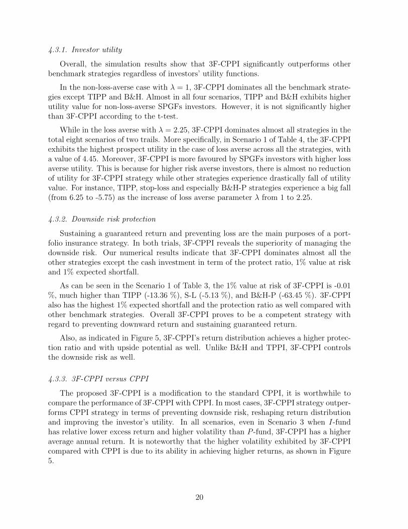
Also, as indicated in Figure 5, 3F-CPPI’s return distribution achieves a higher protec-tion ratio and with upside potential as well. Unlike B&H and TPPI, 3F-CPPI controlsthe downside risk as well.

4.3.3. 3F-CPPI versus CPPI

The proposed 3F-CPPI is a modification to the standard CPPI, it is worthwhile tocompare the performance of 3F-CPPI with CPPI. In most cases, 3F-CPPI strategy outper-forms CPPI strategy in terms of preventing downside risk, reshaping return distributionand improving the investor’s utility. In all scenarios, even in Scenario 3 when I-fundhas relative lower excess return and higher volatility than P -fund, 3F-CPPI has a higheraverage annual return. It is noteworthy that the higher volatility exhibited by 3F-CPPIcompared with CPPI is due to its ability in achieving higher returns, as shown in Figure5.

20

Figure 5: The return distributions of all strategies in the Scenario 1

Moreover, 3F-CPPI outperforms CPPI in preventing downside risk. For example, inScenario 1 of Table 4, CPPI-P has only a protection ratio value of 91.54% while 3F-CPPI has a much higher value of 98.22%. The superiority of 3F-CPPI also holds inother measures such as 1% value at risk. Overall 3F-CPPI has proven to be a competentstrategy with higher return and volatility as well as a better downside risk protection.

4.3.4. Market condition effect

Although 3F-CPPI dominates other strategies in almost all scenarios, the superior-ity has been mainly affected by market conditions, i.e. the relativity between I-fundand P -fund. In particular, 3F-CPPI loses its advantages when the stock market I-fundoutperforms the purpose-related market sector P -fund. The reason is straightforward as3F-CPPI invests in an extra third fund P -fund to hedge the purpose-related inflation risk.

For example, in Scenario 1 of Table 4, the I-fund has the same volatility but a lowerreturn than that of Scenario 2, however, 3F-CPPI exhibits less competitive edge in Sce-nario 2. The loss averse SPGF investor’s mean utility (λ = 2.25) gap between 3F-CPPIand CPPI-I is 0.23 in the Low Inflation Trial of Scenario 1, while the gap is 0.08 inscenario 2. In addition, the Scenario 3 shows that 3F-CPPI do not outperform CPPI-Pstrategy when the I-fund is behind P -fund in both aspects of mean return and volatility.Still, 3F-CPPI exhibits a higher performance than the traditional CPPI-I in all marketconditions. Thus, as one cannot predict the market conditions, the 3F-CPPI is proved tobe the best strategy among all strategies.

21

5. Conclusion

Loss averse investors, especially pensioners, has an increasingly high demand for hedg-ing special purpose risks like medical and education costs. Although there are varioustypes of funds promising a minimum guaranteed return plus a common specific use of theinvestment like pension, the investment strategies adopted is way out of optimal. There-fore, an innovative 3F-CPPI strategy has been constructed in this paper with the aim ofimproving the performance of SPGF for loss averse investors.

Overall, the proposed 3F-CPPI outperforms other strategies in terms of hedgingagainst the downside risk and satisfying the investors’ utility. We first derive explicitoptimal allocations for 3F-CPPI and discuss further the relationship between the optimalproportion of purpose-related fund and leverage ratio. Generally the optimal proportionof purpose-related fund mainly depends on the performance relativity of stock index andpurpose-related fund.

We theoretically prove that the proposed 3F-CPPI dominates CPPI in both the dis-crete and continuous time cases, followed by extensive Monte Carlo simulation checkingthe practicability of 3F-CPPI. Theoretical analysis shows that the investment in a thirdfund to hedge purpose-related risk contributes to 3F-CPPI’s superior performance andhigher investor utility. Under the discrete time case with gap risk, the Monte Carlo sim-ulation has been adopted for performance comparison among the proposed 3F-CPPI andother benchmark strategies, including CPPI, TIPP, stop-loss and B&H. The numericalanalysis illustrates that 3F-CPPI demonstrates in achieving relatively higher mean re-turn, better portfolio protection and higher investor’s prospect utility as well. Moreover,our findings claim that the advantage of 3F-CPPI increases with loss aversion, indicatingthat 3F-CPPI is much more preferred to the standard CPPI and other strategies for lossaverse investors.

In summary, this paper proposed an applicable modified CPPI strategy, 3F-CPPI,within a general portfolio insurance setting. both theoretical and practical insights. 3F-CPPI dominates other strategies in many aspects such as the protection ratio, downsiderisk and loss averse utility. In this paper we apply only the three fund allocation rule tostandard CPPI strategy, while, it is worthwhile to extend it to other portfolio insurancestrategies, which we leave for future research.

Acknowledgements

Ze Chen acknowledges the support of the Bilateral Cooperation Project TsinghuaUniversity - KU Leuven (ISP/14/01TS) and the research Project from the InsuranceInstitute of China (JIAOBAO2018-06). We are grateful for helpful discussions with andcomments from Dimitris Andriosopoulos, Daniel Broby, John Crosby, Christian Ewald andespecially Liu Yang, and participants on the China International Conference on Insuranceand Risk Management 2016 & 2017 (CICIRM) and IAFDS Conference 2018, PrifysgolBangor University.

22

Appendices

Appendix A Proof of Propositions

A.1 Proof of Proposition 1

Proof: The stochastic process of a 3F-CPPI portfolio value at time t follows

dVt = Et[αdSItSIt

+ (1− α)dSPtSPt

] + (Vt − Et)rdt (A.1)

= mCt{[α(µi − r) + (1− α)(µp − r)dt+ ασidZs + (1− α)σpdZP}+ rVtdt. (A.2)

Denote risk premium of I-fund and P -fund by

θi =µi − rσi

, θP =µp − rσP

, (A.3)

respectively. (A.1) can be simplified to

dVt = rPtdt+ Ct{r +m[ασiθi + (1− α)σP θP ]}dt+mCt[ασidZs + (1− α)σPdZP ].

Define stochastic process Bt as follows, with B0 = 0 :

dBt = {r +m[ασiθi + (1− α)σP θP ]}dt+m[ασidZs + (1− α)σPdZP ], (A.4)

Bt = {r +m[ασiθi + (1− α)σP θP ]}t+m[ασiWst + (1− α)σPWpt], t ∈ [0, T ].

Then, Vt is driven by Bt,dVt = rPtdt+ CtdBt. (A.5)

By (A.4) the dBtdBt is

dBtdBt = [m2α2σ2i +m2(1− α)2σ2

P + 2m2α(1− α)ρsPσiσp]dt. (A.6)

For simplification, denote

A = m2α2σ2i +m2(1− α)2σ2

P + 2m2α(1− α)ρsPσiσp. (A.7)

Then, consider an exponential process f(Z):

f(Bt) = exp(−Bt +1

2At). (A.8)

By Ito’s lemma:

df(Bt) = −f(Bt)dBt +1

2Af(Bt)dt+

1

2f(Bt)dBtdBt

= −f(Bt)dBt + Af(Bt)dt. (A.9)

23

By (A.5),

dVt = dCt + dPt

= dCt + dPtdt

= rPtdt+ CtdBt, (A.10)

we have:dCt = CtdBt + (r − d)Ptdt. (A.11)

Thus, consider the SDE process of the Ctf(Bt):

d[Ctf(Bt)] = f(Bt)dCt + Ctdf(Bt) + dCtdf(Bt)

= f(Bt)[CtdBt + (r − d)Ptdt] + Ct[−f(Bt)dBt + Af(Bt)dt]− Ctf(Bt)Adt

= f(Bt)(r − d)Ptdt, t ∈ [0, T ]. (A.12)

Due to f(B0) = 1, we have:

Ctf(Bt) = C0 + (r − d)

∫ t

0

f(Bξ)Pξdξ,


2At) + (r − d)

∫ t

0

exp{Bt −Bξ −1

2A(t− ξ)}Pξdξ. (A.13)

As for the expected value of a 3F-CPPI portfolio at time t is:

E(Vt) = Pt + C0eµBt + (r − d)p0e

µBt1− e(d−µB)t

µB − d, (A.14)

as Vt is in the (A.13):


2At) + (r − d)

∫ t

0

exp{Bt −Bξ −1

2A(t− ξ)}Pξdξ. (A.15)

By property of log-normal distribution, expectation of exp(Bt − 12At) is:

E{exp(Bt −1

2At)} = exp(−1

2At)E{exp(Bt)} (A.16)

= exp(−1

2At) exp(µBt+

1

2At)

= exp(µBt).

Then,

E(Vt) = Pt + eµBt{C0 + (r − d)E[

∫ t

0

exp(−Bξ +1

2Aξ)Pξdξ]}. (A.17)

24

Fubini-Tonelli theorem ensures that taking the expectation it becomes:

E(Vt) = Pt + eµBt{C0 + (r − d)E[

∫ t

0

exp(−Bξ +1

2Aξ)Pξdξ]}

= Pt + eµBt{C0 + (r − d)P0

∫ t

0

E[exp(−Bξ +1

2Aξ)Pξ]dξ}

= Pt + eµBt{C0 + (r − d)P01− e(d−µB)t

µB − d}. (A.18)

Therefore, for any t ∈ [0, T ], we can have:

E(Vt) = Pt + eµBt{C0 + (r − d)P0eµBt

1− e(d−µB)t

µB − d}. (A.19)

A.2 Proof of Proposition 2

Proof: Consider a representative investor with risk averse attitude γ < 1, the maximiza-tion problem with utility in (10) is equivalent to:

Maxm,α{−1

2A− µY + r +m(ασsi θi + (1− α)σpθp) (A.20)

+γ

2[(mασsi +m(1− α)σsp − σiy)2 + (m(1− α)σpp − σpy)2 + (σey)

2]}. (A.21)

If we consider the most common the fixed-rate floor strategy r = d case, the opti-mization problem is equivalent to

Maxm,α

µx +1

2(γ − 1)σ2

x, (A.22)

where σ2x = [mασi + m(1 − α)σsp − σiy]

2 + [m(1 − α)σpp − σpy ]2 + (σey)

2. Therefore, themaximization function (A.22) punishes for investment volatility as the investors’ γ is lessthan 1, with RRA = 1− γ > 0.

Maxm,α

E[U(VT , YT |F0) (A.23)

= Maxm,α

E[u(RT

YT) + v(

VT −RT

YT)|F0] (A.24)

⇐⇒ Maxm,α

E[v(VT −RT

YT)|F0] (A.25)

= Maxm,α

E[(VT −RT

YT)γ] (A.26)

As stated earlier, a typical reference point RT is the SPGF guaranteed amount PT , thusu(RT

YT) part does not play a role in the utility maximization. In the following, we consider

this typical case that RT = PT .

25

Consider the representative investors’ risk averse attitude is γ < 1, denote

xt = (Vt − Pt)/Yt = Ct/Yt.

xt indicates 3F-CPPI portfolio’s deviation compared to reference at time t. By the explicitform of Ct and Yt, we have

xt =C0 exp(Bt − 1

2At) + (r − d)

∫ t0

exp{Bt −Bξ − 12A(t− ξ)}Pξdξ

exp(µY t+ σYWY t). (A.27)

If we further assume the fixed-rate floor case with r = d, (A.27) is simplified into:

xt = C0 exp(Bt −1

2At− µY t− σYWY t)

= C0 exp(−1

2At− µY t) exp(Bt − σYWY t),

then,

E[1

γ(xt)

γ] =Cγ

0

γexp(−1

2γAt− γµY t)E[exp(Bt − σYWY t)]

=Cγ

0

γexp{−1

2γAt− γµY t+ γ[r +m(ασsi θi + (1− α)σpθp)]t}

exp{γ2


2]t}. (A.28)

Hence, the maximization problem in (10) is equivalent to:

Maxm,α{−1


+γ


2]}. (A.30)

(A.29) can also be deduced by Ito’s lemma. In the fixed-rate floor r = d case,

dCt = CtdBt, (A.31)

anddYt = µY dt+ σY dZY , (A.32)

by ito’s lemma,dx

x= µxdt+ σxdZx, (A.33)

where

µx = r−µY +σ2Y +m[ασsi θi+(1−α)σP θP ]−m[ασsiσ

iy+(1−α)σspσ

iy+(1−α)σppσ

py ], (A.34)

and

σxdZx = [mασsi +m(1− α)σsp − σiy]dZs + [m(1− α)σpp − σpy ]dZp + σeydZe.

26

Thus,

E(xγ) = exp{[γµx +1

2γ(γ − 1)σ2

x]t}. (A.35)

the optimization problem is equivalent to

Maxm,α

µx +1

2(γ − 1)σ2

x, (A.36)

where σ2x = [mασi +m(1−α)σsp− σsy]2 + [m(1−α)σpp − σpy ]2 + (σey)

2. It’s noteworthy thatwhen γ = 0, the utility v(xt) = log(xt), the equivalent maximization form (A.36) stillholds, as E[U(xt)] equals to E[log(xt)] = µx − 1

2σ2x for the case γ = 0.

Another poof to get (A.36) is by the Ito’s lemma. The optimization problem is:

Maxm,α

E[U(VT , YT |F0) (A.37)

= Maxm,α

E[U(VT − PTYT

)|F0], (A.38)

where PT is the SPGF guaranteed amount. Consider a representative investor with a riskaverse attitude γ < 1, then denote

xt = (Vt − Pt)/Yt = Ct/Yt.

xt indicates 3F-CPPI portfolio’s deviation at time t. By the explicit form of Ct and Yt,we have

xt =C0 exp(Bt − 1

2At) + (r − d)

∫ t0

exp{Bt −Bξ − 12A(t− ξ)}Pξdξ

exp(µY t+ σYWY t). (A.39)

If we further assume the fixed-rate floor case with r = d, (A.39) is simplified into:

xt = C0 exp(Bt −1

2At− µY t− σYWY t)

= C0 exp(−1

2At− µY t) exp(Bt − σYWY t),

then,

E[1

γ(xt)

γ] =Cγ

0

γexp(−1

2γAt− γµY t)E[exp(Bt − σYWY t)]

=Cγ

0

γexp{−1

2γAt− γµY t+ γ[r +m(ασsi θi + (1− α)σpθp)]t}

exp{γ2

2[(mασsi +m(1− α)σsp − σsy)2 + (m(1− α)σpp − σpy)2 + (σey)

2]t}. (A.40)

Hence, the maximization problem is equivalent to:

Maxm,α{−1


+γ


2]}. (A.42)

27

(A.41) can also be deduced by Ito’s lemma. In the fixed-rate floor r = d case,

dCt = CtdBt, (A.43)

anddYt = µY dt+ σY dZY , (A.44)

by ito’s lemma,dx

x= µxdt+ σxdZx, (A.45)

where

µx = r−µY +σ2Y +m[ασsi θi+(1−α)σP θP ]−m[ασsiσ

sy+(1−α)σspσ

sy+(1−α)σppσ

py ], (A.46)

and

σxdZx = [mασsi +m(1− α)σsp − σsy]dZs + [m(1− α)σpp − σpy ]dZp + σeydZe.

Thus,

E(xγ) = exp{[γµx +1

2γ(γ − 1)σ2

x]t}. (A.47)

the optimization problem is equivalent to

Maxm,α

µx +1

2(γ − 1)σ2

x, (A.48)

where σ2x = [mασi +m(1−α)σsp− σsy]2 + [m(1−α)σpp − σpy ]2 + (σey)

2. It’s noteworthy thatwhen γ = 0, the utility v(xt) = log(xt), the equivalent maximization form (A.48) stillholds, as E[U(xt)] equals to E[log(xt)] = µx − 1

2σ2x for the case γ = 0.

Then, we consider the first order conditions (FOCs) for the problem (A.36) are asfollows:

αµ(γ)i +(1−α)µ(γ)p −r+(γ−1){[mασi+m(1−α)σsp−σsy][ασsi+(1−α)σsp]+[m(1−α)σpp−σpy ](1−α)σpp}=0,

(A.49)

(µ(γ)i −µ(γ)

p )+(γ−1){[mασsi +m(1−α)σsp−σsy](σsi−σsp)−[m(1−α)σpp−σpy ]σpp} = 0. (A.50)

The optimal m∗ and α∗ is straightforward by solving the FOC equations, we get

α∗(m∗)µ(γ)i + (1− α∗(m∗))µ(γ)

p − r + (µ(γ)i − µ(γ)

p )α∗(m∗) (A.51)

+ (γ − 1){[(σsp)



2 + (σsp)2]m∗ − σiyσsp − σpyσpp} = 0,

α∗(m) =(σsp)


(σsi − σsp)2 + (σpp)2+

µ(γ)i − µ

(γ)p

(σi − σsp)2 + (σpp)21

(1− γ)m. (A.52)

28

To solve the expressions of m∗ and α∗, in the following we denote some terms by D,E, Ffor simplicity,

D = (γ − 1) · [(σsp)



2 + (σsp)2],

E = 2(µ(γ)i − µ(γ)

p ) · [(σsp)


(σsi − σsp)2 + (σpp)2+ µ(γ)

p − r − (γ − 1)(σsyσsp + σpyσ

pp)],

F =(µ

(γ)i − µ

(γ)p )2

(σsi − σsp)2 + (σpp)2· 2

1− γ.

The m∗ is the solution of the following quadratic equation:

Dm2 + Em+ F = 0.

It is easy to find out that in most cases, the solution ism∗ = max(−E+√E2−4DF2D

, −E−√E2−4DF2D

),

then α∗ =(σsp)

2+(σpp)2−σspσsi

(σsi−σsp)2+(σpp)2+

µ(γ)i −µ

(γ)p

(σi−σsp)2+(σpp)21

(1−γ)m∗ .

References

Apergis, N. and Miller, S. M. (2009), ‘Do structural oil-market shocks affect stock prices?’,Energy Economics 31(4), 569–575.

Arnott, R. D. and Bernstein, P. L. (2002), ‘What risk premium is normal?’, FinancialAnalysts Journal 58(2), 64–85.

Bahram, A., Arjun, C. and Kambiz, R. (2004), ‘Reit investments and hedging againstinflation’, Journal of Real Estate Portfolio Management 10(2), 97–112.

Balder, S., Brandl, M. and Mahayni, A. (2009), ‘Effectiveness of cppi strategies underdiscrete-time trading’, Journal of Economic Dynamics and Control 33(1), 204–220.

Benartzi, S. and Thaler, R. H. (1995), ‘Myopic loss aversion and the equity premiumpuzzle’, The quarterly journal of Economics 110(1), 73–92.

Benninga, S. (1990), ‘Comparing portfolio insurance strategies’, Finanzmarkt und Port-folio Management 4(1), 20–30.

Black, F. and Jones, R. W. (1987), ‘Simplifying portfolio insurance’, The Journal ofPortfolio Management 14(1), 48–51.

Black, F. and Perold, A. (1992), ‘Theory of constant proportion portfolio insurance’,Journal of Economic Dynamics and Control 16(3-4), 403–426.

Boulier, J.-F. and Kanniganti, A. (2005), Expected performance and risk of various port-folio insurance strategies, in ‘Proceedings of the 5th AFIR International Colloquium’.

29

Boyd, J. H., Levine, R. and Smith, B. D. (2001), ‘The impact of inflation on financialsector performance’, Journal of Monetary Economics 47(2), 221–248.

Cairns, A. J., Blake, D. and Dowd, K. (2006), ‘Stochastic lifestyling: Optimal dynamicasset allocation for defined contribution pension plans’, Journal of Economic Dynamicsand Control 30(5), 843–877.

Chen, J.-S., Chang, C.-L., Hou, J.-L. and Lin, Y.-T. (2008), ‘Dynamic proportion port-folio insurance using genetic programming with principal component analysis’, ExpertSystems with Applications 35(1), 273–278.

Dahlquist, M., Farago, A. and Tedongap, R. (2016), ‘Asymmetries and portfolio choice’,The Review of Financial Studies 30(2), 667–702.

Dichtl, H. and Drobetz, W. (2011), ‘Portfolio insurance and prospect theory investors:Popularity and optimal design of capital protected financial products’, Journal of Bank-ing & Finance 35(7), 1683–1697.

Dimson, E., Marsh, P. and Staunton, M. (2008), The worldwide equity premium: a smallerpuzzle, in ‘Handbook of the equity risk premium’, Elsevier, pp. 467–514.

Dybvig, P. and Liu, F. (2018), ‘On investor preferences and mutual fund separation’,Journal of Economic Theory 174, 224–260.

Estep, T. and Kritzman, M. (1988), ‘Tipp: Insurance without complexity’, The Journalof Portfolio Management 14(4), 38–42.

Figlewski, S., Chidambaran, N. and Kaplan, S. (1993), ‘Evaluating the performance ofthe protective put strategy’, Financial Analysts Journal pp. 46–69.

Hakansson, N. H. (1969), ‘Risk disposition and the separation property in portfolio selec-tion’, Journal of Financial and Quantitative Analysis 4(4), 401–416.

Herold, U., Maurer, R. and Purschaker, N. (2005), ‘Total return fixed-income portfoliomanagement’, The Journal of Portfolio Management 31(3), 32–43.

Hoesli, M. and Oikarinen, E. (2012), ‘Are reits real estate? evidence from internationalsector level data’, Journal of International Money and Finance 31(7), 1823–1850.

Huu Do, B. (2002), ‘Relative performance of dynamic portfolio insurance strategies: Aus-tralian evidence’, Accounting & Finance 42(3), 279–296.

Kang, W., Ratti, R. A. and Yoon, K. H. (2015), ‘The impact of oil price shocks onthe stock market return and volatility relationship’, Journal of International FinancialMarkets, Institutions and Money 34, 41–54.

Lee, H.-I., Chiang, M.-H. and Hsu, H. (2008), ‘A new choice of dynamic asset management:the variable proportion portfolio insurance’, Applied Economics 40(16), 2135–2146.

30

Markowitz, H. (1959), ‘Portfolio selection, cowles foundation monograph no. 16’, JohnWiley, New York. S. Moss (1981). An Economic theory of Business Strategy, HalsteadPress, New York. TH Naylor (1966). The theory of the firm: a comparison of marginalanalysis and linear programming. Southern Economic Journal (January) 32, 263–74.

Merton, R. C. (1973), ‘Theory of rational option pricing’, The Bell Journal of economicsand management science pp. 141–183.

Pye, G. (1967), ‘Portfolio selection and security prices’, The Review of Economic andStatistics pp. 111–115.

Ross, S. A. (1978), ‘Mutual fund separation in nancial theory: The separating distribu-tions’, Journal of Economic Theory pp. 254–286.

Rubens, J., Bond, M. and Webb, J. (1989), ‘The inflation-hedging effectiveness of realestate’, Journal of Real Estate Research 4(2), 45–55.

Sadorsky, P. (2001), ‘Risk factors in stock returns of canadian oil and gas companies’,Energy economics 23(1), 17–28.

Samuelson, P. A. (1967), ‘General proof that diversification pays’, Journal of Financialand Quantitative Analysis 2(1), 1–13.

Tobin, J. (1958), ‘Liquidity preference as behavior towards risk’, The review of economicstudies 25(2), 65–86.

Tversky, A. and Kahneman, D. (1992), ‘Advances in prospect theory: Cumulative repre-sentation of uncertainty’, Journal of Risk and uncertainty 5(4), 297–323.

31

three-fund constant proportion portfolio insurance strategy

Documents