Three Essays in Corporate Finance

Jeong Hwan Lee

Submitted in partial ful�llment of therequirements for the degree of

Doctor of Philosophyin the Graduate School of Arts and Sciences

COLUMBIA UNIVERSITY

2014

c 2014

Jeong Hwan Lee

All rights reserved

ABSTRACT

Three Essays in Corporate Finance

Jeong Hwan Lee

This dissertation consists of three essays on corporate �nance. In the �rst chapter, I

investigate how a liquidity cost associated with debt- �debt servicing cost�a¤ects a �rm�s

capital structure policy. In contrast to the standard capital structure theory prediction that

builds on a trade-o¤between interest tax shields and expected bankruptcy costs, public �rms

use debt quite conservatively. To address this well known debt conservatism puzzle (Graham

2000), I argue that servicing debt drains valuable liquidity for a �nancially constrained �rm

and hence endogenously creates �debt servicing costs,�which have received little attention in

the literature. To examine the in�uence of debt servicing costs on capital structure choices,

I develop and estimate a dynamic corporate �nance model with interest tax shields, liquidity

management, investment, external debt and equity �nancing costs, and capital adjustment

costs. By using the marginal value of liquidity as a natural measure of the debt servicing

costs, I �nd that (1) an increase in �nancial leverage results in higher debt servicing costs,

even with risk-free debt. (2) a smaller �rm tends to experience greater debt servicing costs

because of its endogenously large investment demands; and (3) in the majority of cases,

equity proceeds are used for cash retention as well as capital expenditure, especially when

a �rm faces large current and future investment needs. In addition, I quantitatively show

that large debt servicing costs are closely associated with low leverage and frequent equity

�nancing by analyzing the role of �xed operating costs and convex capital adjustment costs.

In the second chapter, I empirically support the theoretical debt servicing costs analysis

of the previous chapter. I �rstly examine the structural estimation method used for the cal-

ibration of my model in the �rst chapter. The statistical property of the simulated method

of moments estimator and detailed identi�cation scheme for the calibration are investigated

in the �rst half of this chapter. Then I cross-sectionally con�rm the validity of debt ser-

vicing costs predictions on capital structure choices. I study how each �rm�s convex capital

adjustment costs, operating leverage, pro�t volatility, and future investment needs in�uence

capital structure policies. Consistent with the debt servicing costs predictions, �rms with

higher convex capital adjustment costs, higher operating leverage, higher pro�t volatility

and larger future investment demands show lower leverage ratios and more frequent equity

�nancing activities. These �ndings shed new lights on pervasively conservative debt policy in

U.S. public �rms. A higher pro�tability observed in large future investment demands �rms

also suggests the importance of debt servicing costs consideration in resolving the puzzling

negative correlation between pro�tability and leverage ratios.

In the third chapter, I examine how macroeconomic conditions a¤ect the cyclical varia-

tions in capital structure policies. As in the �nancial crisis of 2008, economic contractions

a¤ect a �rm�s pro�tability, investments and external �nancing conditions altogether. To

address the e¤ects of these simultaneous changes on capital structure dynamics, I develop

and estimate a dynamic trade-o¤ model with investment, payouts, and liquidity policies

with macroeconomic pro�tability and �nancing shocks. Investment dynamics and a higher

value of liquidity of economic downturn are pivotal in capital structure dynamics; the former

drives the issuance of debt and equity, and the latter leads to active debt retirements and

conservative debt issues in upturns. My model yields the following main results: (1) Equity

issues are pro-cyclical, and concentrated for small, low pro�t, and large investment demand

�rms in earlier stage of economic upturns. (2) Payouts peak in later stages of upturns and

co-move positively with equity issues; (3) Debt policies move counter-cyclically, and leverage

ratios after debt issuance and retirement are even higher during economic downturns. My

comparative static analysis predicts pro-cyclical debt policy for �nancially constrained �rms,

and pervasively conservative use of debt for �rms expecting �nancial market shutdowns.

Table of Contents

List of Tables iv

List of Figures vi

1 Debt Servicing Costs and Capital Structure 11.1 Introduction . . . . . . . . . . . . . . . . . . . . . . . . . . . . . . . . . . . . 1

1.2 Model . . . . . . . . . . . . . . . . . . . . . . . . . . . . . . . . . . . . . . . 5

1.2.1 Pro�ts and Investment . . . . . . . . . . . . . . . . . . . . . . . . . . 5

1.2.2 Liquidity and Debt . . . . . . . . . . . . . . . . . . . . . . . . . . . . 6

1.2.3 Tax, Payout, and Valuation . . . . . . . . . . . . . . . . . . . . . . . 8

1.3 Quantitative Analysis . . . . . . . . . . . . . . . . . . . . . . . . . . . . . . . 10

1.3.1 Calibration . . . . . . . . . . . . . . . . . . . . . . . . . . . . . . . . 10

1.3.2 Growing Debt Obligations: Investment and Financing Policies . . . . 13

1.3.3 Debt Servicing Costs . . . . . . . . . . . . . . . . . . . . . . . . . . . 16

1.3.4 Equity Financing and Cash Retention . . . . . . . . . . . . . . . . . . 24

1.4 Comparative Statics . . . . . . . . . . . . . . . . . . . . . . . . . . . . . . . 27

1.4.1 Comparative Statics I: Fixed Operating Cost . . . . . . . . . . . . . . 27

1.4.2 Comparative Statics II: Convex Capital Adjustment Costs . . . . . . 31

i

1.5 Concluding Remarks . . . . . . . . . . . . . . . . . . . . . . . . . . . . . . . 37

2 Empirical Analysis on Debt Servicing Costs 392.1 Introduction . . . . . . . . . . . . . . . . . . . . . . . . . . . . . . . . . . . . 39

2.2 Calibration: Simulated Method of Moments . . . . . . . . . . . . . . . . . . 42

2.2.1 Simulated Method of Moments . . . . . . . . . . . . . . . . . . . . . 42

2.2.2 Identi�cation . . . . . . . . . . . . . . . . . . . . . . . . . . . . . . . 43

2.2.3 Estimation Results . . . . . . . . . . . . . . . . . . . . . . . . . . . . 45

2.3 Tests for Debt servicing Costs Predictions . . . . . . . . . . . . . . . . . . . 46

2.3.1 Data Construction . . . . . . . . . . . . . . . . . . . . . . . . . . . . 46

2.3.2 Convex Capital Adjustment Costs . . . . . . . . . . . . . . . . . . . . 51

2.3.3 Fixed Operating Costs . . . . . . . . . . . . . . . . . . . . . . . . . . 55

2.3.4 Pro�t Volatility . . . . . . . . . . . . . . . . . . . . . . . . . . . . . . 59

2.3.5 Future Investment Demands . . . . . . . . . . . . . . . . . . . . . . . 63

2.4 Concluding Remarks . . . . . . . . . . . . . . . . . . . . . . . . . . . . . . . 67

3 Macroeconomic Conditions and Capital Structure

Dynamics 693.1 Introduction . . . . . . . . . . . . . . . . . . . . . . . . . . . . . . . . . . . . 69

3.2 Model . . . . . . . . . . . . . . . . . . . . . . . . . . . . . . . . . . . . . . . 74

3.2.1 Macroeconomic States . . . . . . . . . . . . . . . . . . . . . . . . . . 74

3.2.2 Pro�ts and Investment . . . . . . . . . . . . . . . . . . . . . . . . . . 75

3.2.3 Liquidity and Debt . . . . . . . . . . . . . . . . . . . . . . . . . . . . 76

3.2.4 Tax, Payout, and Valuation . . . . . . . . . . . . . . . . . . . . . . . 78

ii

3.3 Quantitative Analysis . . . . . . . . . . . . . . . . . . . . . . . . . . . . . . . 80

3.3.1 Calibration . . . . . . . . . . . . . . . . . . . . . . . . . . . . . . . . 80

3.3.2 Equity Issues and Payouts . . . . . . . . . . . . . . . . . . . . . . . . 83

3.3.3 Debt Dynamics . . . . . . . . . . . . . . . . . . . . . . . . . . . . . . 89

3.4 Quantitative Analysis: Comparative Statics . . . . . . . . . . . . . . . . . . 94

3.4.1 Counter-cyclical Debt Financing Costs . . . . . . . . . . . . . . . . . 94

3.4.2 Financial Market Shutdowns . . . . . . . . . . . . . . . . . . . . . . . 96

3.4.3 Deeper Economic Downturns . . . . . . . . . . . . . . . . . . . . . . 97

3.5 Concluding Remarks . . . . . . . . . . . . . . . . . . . . . . . . . . . . . . . 100

Bibliography 103

A Data Description 108

A.1 Data Description: Structural Estimation . . . . . . . . . . . . . . . . . . . . 108

A.2 Data Description: Cross-sectional Analysis . . . . . . . . . . . . . . . . . . . 109

B Numerical Solutions 110

B.1 Numerical Solutions: Chapter 1 . . . . . . . . . . . . . . . . . . . . . . . . . 110

B.2 Numerical Solutions: Chapter 3 . . . . . . . . . . . . . . . . . . . . . . . . . 111

C Identi�cation: Chapter 3 112

iii

List of Tables

1.1 Moments Selection: Acutal and Simulated Values . . . . . . . . . . . . . . . 12

1.2 Structural Parameter Estimation Results . . . . . . . . . . . . . . . . . . . 13

1.3 Financing and Investment Policies at Equity Issuance . . . . . . . . . . . . 24

1.4 Fixed Operating Cost Variation . . . . . . . . . . . . . . . . . . . . . . . . . 29

1.5 Fixed Operating Cost Variation: Robustness . . . . . . . . . . . . . . . . . . 30

1.6 Convex Capital Adjustment Cost Variation . . . . . . . . . . . . . . . . . . . 33

1.7 Convex Capital Adjustment Costs Variations: Robustness . . . . . . . . . . 36

2.1 Moments Selection: Acutal and Simulated Values . . . . . . . . . . . . . . . 45

2.2 Structural Parameter Estimation Results . . . . . . . . . . . . . . . . . . . 46

2.3 Summary Statistics : Convex Capital Adjustment Cost Quartile . . . . . . . 51

2.4 Cross-sectional Analysis : Convex Capital Adjustment Cost Quartile . . . . 53

2.5 Summary Statistics : Fixed Operating Costs . . . . . . . . . . . . . . . . . . 56

2.6 Cross-sectional Analysis : Fixed Operating Costs . . . . . . . . . . . . . . . 58

2.7 Summary Statistics : Pro�t Volatility . . . . . . . . . . . . . . . . . . . . . . 60

2.8 Cross-sectional Analysis : Pro�t Volatility . . . . . . . . . . . . . . . . . . . 62

2.9 Summary Statistics : Future Investment Demands . . . . . . . . . . . . . . . 63

2.10 Cross-sectional Analysis : Future Investment Demands . . . . . . . . . . . . 65

iv

3.1 Moments Selection: Acutal and Simulated Values . . . . . . . . . . . . . . . 81

3.2 Structural Parameter Estimation Results . . . . . . . . . . . . . . . . . . . 83

3.3 Equity Issue and Payout: An Example . . . . . . . . . . . . . . . . . . . . . 84

3.4 Equity Financing Firm Characteristics: An Example . . . . . . . . . . . . . 85

3.5 Equity Issue and Payout Dynamics . . . . . . . . . . . . . . . . . . . . . . . 87

3.6 Firm Characteristics: Deb Issuance and Retirement . . . . . . . . . . . . . . 89

3.7 Debt Dynamics . . . . . . . . . . . . . . . . . . . . . . . . . . . . . . . . . . 91

3.8 Debt Dynamics: Low Debt Financing Costs . . . . . . . . . . . . . . . . . . 92

3.9 Counter-cyclical Debt Financing Costs . . . . . . . . . . . . . . . . . . . . . 95

3.10 Financial Market Shutdowns . . . . . . . . . . . . . . . . . . . . . . . . . . . 96

3.11 A Sharper Di¤erence in Aggregate Pro�tability . . . . . . . . . . . . . . . . 98

3.12 A Longer Duration of Economic Contraction . . . . . . . . . . . . . . . . . 99

A.1.1De�nition of Variables used in the SMM estimation . . . . . . . . . . . . . . 108

A.2.1De�nition of Variables used in the Empirical Analyses . . . . . . . . . . . . . 109

v

List of Figures

1.1 Growing Debt Obligations: Investment and Financing Policies . . . . . . . . 14

1.2 Marginal Value of Liquidity . . . . . . . . . . . . . . . . . . . . . . . . . . . 17

1.3 Marginal Value of Liquidity: Capital Stocks . . . . . . . . . . . . . . . . . . 19

1.4 Marginal Value of Liquidity: Pro�tability Shocks . . . . . . . . . . . . . . . 21

1.5 Marginal Value of Liquidity: High Equity Financing Costs . . . . . . . . . . 22

1.6 Marginal Value of Liquidity: Fixed Operating Cost . . . . . . . . . . . . . . 28

1.7 Marginal Value of Liquidity: Convex Capital Adjustment Costs . . . . . . . 32

1.8 Marignal Value of Liquidity: Convex Capital Adjustment Costs and Prof-

itability Shock . . . . . . . . . . . . . . . . . . . . . . . . . . . . . . . . . . 35

vi

ACKNOWLEDGMENTS

It would not have been possible to complete this doctoral thesis without the guidance and

support of the kind people around me, to only some of whom it is possible to give particular

mention here.

I would like to express my deepest gratitude to my advisor, Professor Neng Wang for

his excellent guidance, caring and patience. His wisdom, knowledge and commitment to the

highest standards inspired and motivated me. His advice on both research as well as on my

career have been invaluable.

I would also like to thank my committee members Professor John B. Donaldson, and

Professor Patrick Bolton for guiding my research for my Ph.D. years and helping me to

present the research works as clearly as possible. It was a great privilege and honor to work

and study under their guidance.

I am extending my special thanks to Professor Jushan Bai, and Professor Martin Uribe,

who were willing to participate in my �nal defense committee.

I am grateful to friends and classmates, Jongsuk Lee, Youngwoo Koh, Hyunseung Oh,

and Jaehyun Cho for their kindness. They were always supporting and encouraging me with

their best wishes.

Finally, I would like to express my heartfelt thanks to my wife and family members. My

wife, Minkyung Lee was always there cheering me up and stood by me through the good times

and bad. My parents, Yoon-chul Lee and Oksoon Chang. Their devotion, unconditional love

and support, sense of humour, patience, optimism and advice was priceless in the completion

of my thesis. I am also grateful to my brother for his encouragements and kindness.

vii

DEDICATION

To my wife and family members

viii

Chapter 1

Debt Servicing Costs and Capital Structure

1.1 Introduction

Graham (2000) documents that public �rms tend to forgo potentially large tax shields and

that this tendency is paradoxically more signi�cant for the �rms with low �nancial distress

costs. These �ndings pose strong challenges to the standard capital structure theory that

builds on a trade-o¤ between interest tax shields and expected bankruptcy costs (Modigliani

and Miller 1958). Graham (2000) concludes that public �rms are leaving a signi�cant sum

of money on the table by remaining underlevered.

To address this debt conservatism puzzle, I argue that servicing debt drains valuable

liquidity for a �nancially constrained �rm and thus endogenously creates �debt servicing

costs.� A �rm retains cash to avoid costly external �nancing but servicing debt obligations

depletes such valuable cash holding. When a �rm faces a highly valuable liquidity from

large acquisition plans or poor business performance, large debt servicing costs may lead to

the �rm�s conservative debt policy even with a negligible likelihood of �nancial distress. As

servicing debt drains a �rm�s valuable cash, the debt servicing cost is naturally measured

by the marginal value of liquidity, which is also a critical determinant of a �rm�s net payout

1

and liquidity policies (Bolton, Chen, and Wang 2011, hereafter BCW).

I develop and estimate a dynamic capital structure model with precautionary liquidity

holding to examine how debt servicing costs a¤ect a �rm�s capital structure choice. A �rm

makes investment, cash retention, capital structure, and payout decisions by considering

interest tax shields, external �nancing costs and capital adjustment costs. Debt and equity

�nancing costs are pivotal elements underlying a �rm�s precautionary cash saving incentives

(BCW). Capital adjustment costs shape intertemporal investment demands and determine

the cost of asset sales (DeAngelo, DeAngelo, and Whited 2011, hereafter DDW). An endoge-

nous investment decision crucially in�uences the value of liquidity, as it utilizes currently

accumulated cash stocks.

My model analysis on the relationship between debt servicing costs and a �rm�s leverage,

pro�tability shock, and capital stock yields a number of interesting results. Most notably,

a �rm with large debt obligations faces higher debt servicing costs, even with risk-free debt

issuance. To pay down large debt obligations, a �rm with limited liquidity holding tends to

rely more heavily on capital resale and external �nancing, both of which involve increasing

marginal costs. Current asset sales also incur additional future pro�t losses by reducing a

�rm�s pro�t generation capacity. The increase in debt servicing costs re�ects explicit costs

and ine¢ ciency from asset sales and external �nancing.

This rise in debt servicing costs is closely associated with the debt conservatism puzzle

(Graham 2000). Most of all, this �nding provides an economic ground for a �rm�s conserva-

tive use of debt even in the face of large unused tax bene�ts and low �nancial distress costs.

Economic factors closely associated with conservative debt policy also reinforce the potential

importance of debt servicing costs in resolving the debt conservatism puzzle; future growth

options to fund, large acquisition plans, asset intangibility, and excess cash holding are all

closely connected with a large marginal value of liquidity.

2

Next, a �rm with low pro�tability shocks tends to experience large debt servicing costs.

A currently low operating pro�t realization directly indicates low internal funds to service

debt obligations, given a limited amount of cash holding. It further predicts low expected

future pro�ts due to the positive serial correlations in a �rm�s operating pro�ts. Both forces

increase a �rm�s marginal value of liquidity considerably; indeed, they do so in spite of

currently small investment demands implied by the low pro�tability shock realization.

Moreover, a �rm with low capital stocks confronts large debt servicing costs. A smaller

�rm must investment more in the current and future periods, due to a decreasing returns

to scale pro�t technology. Such additional funding demands for capital expenditures raise

the marginal value of liquidity, which potentially leads to lower leverage ratios in smaller

�rms. Consistent with this debt servicing costs prediction, small �rms tend to show lower

leverage ratios (Frank and Goyal 2003; 2008) and large �rms rely more heavily on debt

issuance (Shyam-Sunder and Myers 1999). The marginal value of liquidity directly connects

large investments in smaller �rms with low leverage, even without limited debt capacity

considerations as in DDW.

I shall now turn to my model simulation results. Most remarkably, equity proceeds, in the

majority of cases, are used for cash retention as well as capital expenditure, especially when

a �rm faces large current and future investments. While large future investment demands

imply highly valuable liquidity for a �rm, the �rm has to use a considerable amount of cash

stocks for currently vast investments. To stockpile a substantial amount of cash stocks, the

�rm not only uses its operating pro�ts, but also relies on equity �nancing that does not drain

valuable liquidity in the future. Consistent with this �nding, equity proceeds are primarily

used for near term cash saving (DeAngelo, DeAngelo, and Stulz 2010) and equity �nancing is

concurrent with large current and future investments (Loughran and Ritter 1997; Fama and

French 2002). Unlike prior security issuance theories highlighting the use of equity proceeds

3

for debt payments (Strebulaev 2007) or large asymmetric information costs of equity issuance

(Myers and Majluf 1984), the model simulation results emphasize the use of equity proceeds

for cash retention.

The model simulations for di¤erent levels of �xed operating costs and convex capital

adjustment costs demonstrate that large debt servicing costs are closely associated with

low leverage and frequent equity �nancing. An increase in �xed operating costs lowers a

�rm�s pro�tability, but it does not change investment demands signi�cantly. Given a similar

investment needs, a �rm with lower pro�ts tends to experience a higher marginal value of

liquidity. An increase in convex capital adjustment costs is also closely related to large debt

servicing costs because it raises the cost of asset sales. In both �xed operating costs and

convex capital adjustment costs simulations, �rms with large debt servicing costs tend to

maintain lower leverage and issue equity more frequently.

These quantitative predictions are in line with prior empirical studies. Kahl, Lunn, and

Nilsson (2012) �nd that higher operating leverage �rms tend to use less debt and collect

large amounts of equity proceeds, consistent with the �xed operating costs analysis. R&D

expenditures are closely associated with large convex capital adjustment costs and R&D

intensive �rms are well known for their low leverage and frequent equity �nancing (Hall

2002), as predicted in the quantitative analysis on convex capital adjustment costs.

In summary, this chapter investigates the interdependence between liquidity policy and

capital structure choices, which is a key missing link in existing literature. The standard

trade-o¤ theory (Modigliani and Miller 1958) balances the value of tax shields against �nan-

cial distress costs without liquidity considerations. BCW and Riddick and Whited (2009)

highlight the interaction between external equity �nancing and liquidity management policy

but ignore the role of debt �nancing. Recent dynamic trade-o¤ models with endogenous

investments (DDW; Hennessy and Whited 2005; 2007) primarily focus on debt dynamics

4

and pay little attention to liquidity and equity �nancing policy. Gamba and Triantis (2008)

emphasize the relationship between the value of liquidity and economic conditions such as

tax environments and external �nancing costs. Yet, the link between liquidity value and

capital structure choice is largely unexamined in their analysis.

The next section introduces the baseline model in detail. Section 3 calibrates the model

and analyzes debt servicing costs and equity �nancing policy implications from the baseline

model. Section 4 reports the comparative static analysis results. Section 5 concludes.

1.2 Model

Amanager decides the representative �rm�s investment and �nancing policies for each period

to maximize the discounted value of future net dividends stream. Her choice set consists

of liquidity management, debt and equity �nancing, real investment, and dividends payout

decisions to shareholders.

1.2.1 Pro�ts and Investment

The �rm�s pro�t function, �(k; z); depends on capital stock, k, pro�tability shock, z; and

�xed operating cost, f . I choose a standard functional form for �(k; z):

�(k; z) = zk� � f (1.1)

where � captures the returns to scale of the pro�t function. The pro�tability shock, z;

follows an AR(1) process in logs:

log z0 = � log z + " (1.2)

5

in which " has normal distribution with mean zero and variance �2. All primed variables

indicate next period ones.

Investment, I, is de�ned as the di¤erence between next period capital stock and current

capital stock after depreciation:

I = k0 � (1� �)k; (1.3)

in which � is the depreciation rate of capital stock.

The installation and resale of capital stock incur organizational adjustment costs, Gk(k; I); that

are given by

Gk(k; I) = kk1I 6=0 +�k(I)2

k; (1.4)

where 1I 6=0 is an indicator function, the value of which is equal to one if investment is

nonzero, and zero otherwise. This functional formulation includes both �xed and convex

capital adjustment costs, which is a standard one in empirical literature. The �xed cost is

proportional to the level of current capital stock, k and a large �xed cost parameter k implies

more lumpy investment. The convex cost is a quadratic function of investment, I and a large

convex cost parameter �k indicates smoother investment demands and high capital resale

costs. See Cooper and Haltiwanger (2006) and DDW for more detailed discussion for this

formulation.

1.2.2 Liquidity and Debt

A state variable, c; represents the �rm�s cash holding at the end of the previous period. Cash

stocks earn interests at the risk-free rate, r, and current liquidity holding is the sum of the

previous period cash holding and its interest earnings, c(1 + r). Carrying cash stock does

not involve any other explicit costs.

The manager issues a one period bond that pays interests at the same risk-free rate, r.

6

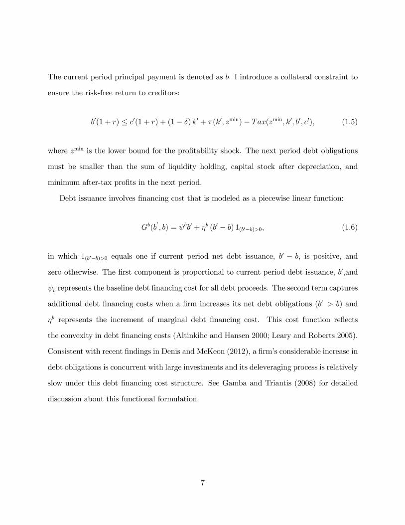
The current period principal payment is denoted as b. I introduce a collateral constraint to

ensure the risk-free return to creditors:

b0(1 + r) � c0(1 + r) + (1� �) k0 + �(k0; zmin)� Tax(zmin; k0; b0; c0); (1.5)

where zmin is the lower bound for the pro�tability shock. The next period debt obligations

must be smaller than the sum of liquidity holding, capital stock after depreciation, and

minimum after-tax pro�ts in the next period.

Debt issuance involves �nancing cost that is modeled as a piecewise linear function:

Gb(b0; b) = bb0 + �b (b0 � b) 1(b0�b)>0; (1.6)

in which 1(b0�b)>0 equals one if current period net debt issuance, b0 � b, is positive, and

zero otherwise. The �rst component is proportional to current period debt issuance, b0,and

b represents the baseline debt �nancing cost for all debt proceeds. The second term captures

additional debt �nancing costs when a �rm increases its net debt obligations (b0 > b) and

�b represents the increment of marginal debt �nancing cost. This cost function re�ects

the convexity in debt �nancing costs (Altinkihc and Hansen 2000; Leary and Roberts 2005).

Consistent with recent �ndings in Denis and McKeon (2012), a �rm�s considerable increase in

debt obligations is concurrent with large investments and its deleveraging process is relatively

slow under this debt �nancing cost structure. See Gamba and Triantis (2008) for detailed

discussion about this functional formulation.

7

1.2.3 Tax, Payout, and Valuation

The �rm�s earnings before taxes (EBT), g; are equal to the sum of the �rm�s operating pro�ts

and interest earnings less depreciation and interest expenses:

g = �(k; z)� �k � r(b� c): (1.7)

The marginal tax rate depends on the sign of EBT. The tax rate for positive EBT, �+c ,

exceeds the tax rate for negative EBT, ��c : The positive tax rate for negative EBT is

considered as a rebate provided by the government. Accordingly, the �rm�s tax bill is

Tax = �+c g1g�0 � ��c g(1� 1g�0); (1.8)

where 1g�0 is an indicator function that takes one if the �rm�s EBT are positive, and zero

otherwise. This corporate taxation environment is identical to that of Hennessy and Whited

(2007).

The manager�s payout before equity �nancing cost, e, is the sum of current pro�ts and

net debt issuance less net debt payout, investment, tax bill, capital adjustment costs, and

debt �nancing costs. Thus e can be summarized by the following equation:

e(z; k; b; c) = �(k; z) + (b0 � c0)� (b� c) (1 + r)� I � Tax�Gb(b0; b)�Gk(k; I): (1.9)

External equity �nancing, e < 0; incurs �otation costs, Ge(e; k): The cost function is modeled

in a reduced form that includes both �xed and quadratic components:

Ge(e; k) =� ek� + �ee2

�1e<0; (1.10)

8

where 1e<0 is an indicator function that is equal to one if the �rm issues equity, and zero

otherwise. Empirical studies such as Altinkihc and Hansen (2000) and Leary and Roberts

(2005) con�rm the importance of both cost components in explaining public �rms�equity

issuance activities. Similar to BCW, the �xed cost depends on a �rm�s pro�t generation

capacity, k�, and e governs the size of �xed equity �nancing costs. The second term

captures the importance of quadratic costs and �" controls the curvature of the cost function.

Hennessy and Whited (2007) and Riddick and Whited (2009) use the same formulation for

convex equity �nancing costs.

The net payout to shareholders, d, is given by:

d(z; k; b; c) = (1�Ge(e; k)1e<0)e; (1.11)

in which 1e<0 is an indicator function that assumes the value one if the �rm issues equity

and zero otherwise. The shareholders do not pay the tax on dividends income in accordance

with DDW.

The manager maximizes the discounted value of net payouts to shareholders. The dis-

count rate for the shareholders takes account of the interest income tax and I assume a �at

tax rate of � i on the shareholders�interest income. Therefore, the equity value of �rm at

time 0 is

V0 = E

" 1Xt=0

�1

1 + r(1� � i)

�tdt

#: (1.12)

The Bellman equation for the �rm�s equity value is

V (z; k; b; c) = maxk0;b0;c0

d(z; k; b; c; k0; b0; c0) +1

1 + r(1� � i)EV (z

0; k0; b0; c0); (1.13)

where the �rm�s optimal policy is subjected to the collateral constraint (1.5). See Hennessy

9

and Whited (2005) for the contraction mapping property of this Bellman equation.

The model includes the following elements: interest tax shields, liquidity management,

endogenous investments, persistency in the pro�tability shock evolution, capital adjustment

costs, and external �nancing costs. Among of the model�s features, one period maturity and

the following debt �nancing cost structure are the key elements. Prior models largely ignore

debt �nancing costs (e.g. DDW) or set the maturity structure as in�nity (e.g. Gamba and

Triantis 2008), even though they share similar tax bene�ts, pro�t generation processes, and

capital adjustment costs. Without debt �nancing costs, a �rm almost freely rolls over its debt

obligations and hence confronts insigni�cant servicing costs of debt. With the perpetuity

maturity structure, a �rm may be able to delay the payment of principals inde�nitely, which

also leads to very low debt servicing costs. A deliberately chosen one period debt structure

highlights the importance of debt servicing costs in the model analysis.

1.3 Quantitative Analysis

1.3.1 Calibration

To investigate quantitative implications of the model precisely, I choose the baseline parame-

ters via the simulated method of moments (SMM) by following DDW. The SMM estimation

�nds a set of structural parameters driving the moments of arti�cially simulated data from

the model as close as possible to the corresponding empirical moments. This estimation

procedure helps ensure tight connections between the model�s quantitative predictions and

a �rm�s �nancing and investment policy in the real world.

To gain e¢ ciency in the structural estimation procedure, I �rst parameterize the �xed

operating cost as follows:

f = �kss;

10

where kss indicates the steady state level of capital stock. � governs the size of the �xed

operating costs.

I also �x a group of structural parameters at economically reasonable levels to improve the

e¢ ciency of the estimation procedure. The tax rate for positive taxable corporate income, �+c ;

is set to 0.35, which is the maximum of corporate tax rate during the sample period. DDW

use the same value for their corporate tax rate. The tax rate for negative taxable income, ��c ;

is �xed at 0.09 re�ecting the e¤ective tax rate on negative EBT from the taxation function

of Hennessy and Whited (2005). The depreciation rate, � is 0.12 similar to Hennessy and

Whited (2005) and DDW. The risk free interest rate, r; is 0.025 and the interest income tax,

� i, is 0.25, consistent with Hennessy and Whited (2005).

The following parameters are estimated via the SMM procedure: the uncertainty �; and

serial correlation �; of the pro�tability shock; the pro�t function curvature �; the �xed capital

adjustment cost k and convex capital adjustment cost �k; the �xed equity �nancing cost e

and convex equity �nancing cost �e; the baseline debt �nancing cost b and the additional

debt �nancing cost �b; and the �xed operating cost parameter �:

Table 1.1 reports the selected moments variables for the identi�cation of the model. The

table also documents the empirical moments based on CRSP/Compustat merged database

from 1988 to 2010 and the simulated moments from the model at the baseline SMM estimates.

These moments consist of the �rst and second moments of investment, operating pro�ts,

leverage and cash holding. The average of dividends and equity �nancing, the autocorrelation

of operating pro�ts, equity �nancing frequency and the Tobin�s q values are also included.

This moment selection is closely related to the identi�cation strategy of DDW. The next

chapter includes detailed information about the model�s identi�cation, and SMM procedure.

Table 1.2 reports the baseline economic parameters estimated via the SMM procedure.

The estimation results are consistent with the prior estimates. The persistency parameter

11

Table 1.1: Moments Selection: Acutal and Simulated Values

Variables Actual Moments Simulated Moments

Avg. Investment(I=k) 0.1341 0.1314

Avg. Leverage(b=k) 0.2251 0.2267

Avg. Tobin�s q(V + b� c)=k) 1.7013 1.7095

Avg. Pro�t (�=k) 0.1731 0.1741

Equity Issuance Freq. (d < 0) 0.1072 0.1017

Avg. Equity Financing(�d=k; d < 0) 0.0597 0.0554

Avg. Dividends (d=k; d > 0) 0.0374 0.0323

Var. Investment(I=k) 0.0225 0.0239

Var. Pro�t (�=k) 0.0045 0.0037

SerialCor. Pro�t (�=k) 0.6315 0.6327

Var. Leverage(b=k) 0.0124 0.0149

Avg. Cash Holding (c=k) 0.1150 0.1144

Var. Cash Holding (c=k) 0.0170 0.0163

The actual moments calculations are based on a sample of non �nancial, unreg-

ulated �rms from the CRSP/Compustat Merged Database. The sample period is

1988�2010. The simulated moments are from the baseline model simulation eval-

uated at the SMM estimates. All moment variables are self-explanatory and the

construction of empirical moments is described in Appendix A.

� is 0.6718, the uncertainty parameter � is 0.1995, and the returns to scale parameter � is

0.7435, all of which are in line with DDW and Hennessy andWhited (2005). The �xed capital

adjustment cost parameter k is 0.0090 and the convex capital adjustment cost �k is 0.1163.

Both parameters estimates are within economically reasonable ranges, consistent with DDW,

Cooper and Haltiwanger (2006), and Whited (1992). The convex equity �nancing cost �e is

0.0003, similar to the estimate of Hennessy and Whited (2007). The baseline debt issuance

cost b is 0.11% for all proceeds. The maximum debt �nancing cost� b + �b

�is 0.82% of

debt proceeds, lower than average debt issuance cost in Altinkihc and Hansen (2000).

12

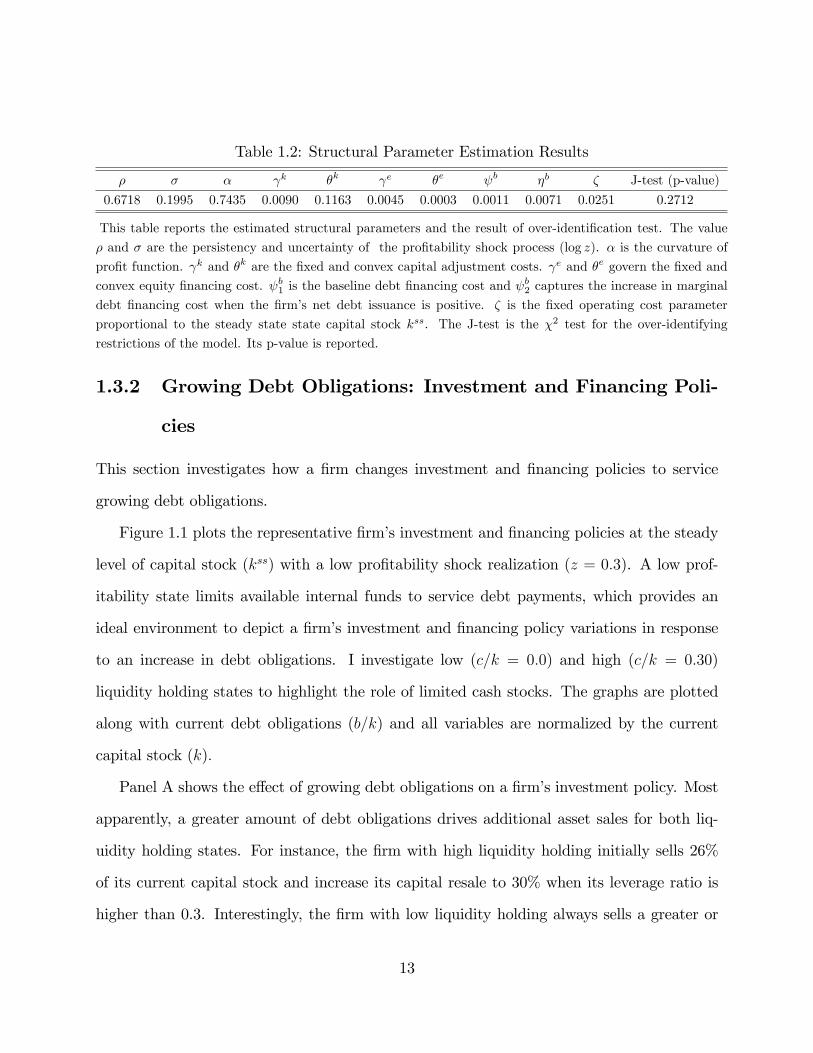
Table 1.2: Structural Parameter Estimation Results

� � � k �k e �e b �b � J-test (p-value)

0.6718 0.1995 0.7435 0.0090 0.1163 0.0045 0.0003 0.0011 0.0071 0.0251 0.2712

This table reports the estimated structural parameters and the result of over-identi�cation test. The value

� and � are the persistency and uncertainty of the pro�tability shock process (log z). � is the curvature of

pro�t function. k and �k are the �xed and convex capital adjustment costs. e and �e govern the �xed and

convex equity �nancing cost. b1 is the baseline debt �nancing cost and b2 captures the increase in marginal

debt �nancing cost when the �rm�s net debt issuance is positive. � is the �xed operating cost parameter

proportional to the steady state state capital stock kss. The J-test is the �2 test for the over-identifying

restrictions of the model. Its p-value is reported.

1.3.2 Growing Debt Obligations: Investment and Financing Poli-

cies

This section investigates how a �rm changes investment and �nancing policies to service

growing debt obligations.

Figure 1.1 plots the representative �rm�s investment and �nancing policies at the steady

level of capital stock (kss) with a low pro�tability shock realization (z = 0:3). A low prof-

itability state limits available internal funds to service debt payments, which provides an

ideal environment to depict a �rm�s investment and �nancing policy variations in response

to an increase in debt obligations. I investigate low (c=k = 0:0) and high (c=k = 0:30)

liquidity holding states to highlight the role of limited cash stocks. The graphs are plotted

along with current debt obligations (b=k) and all variables are normalized by the current

capital stock (k):

Panel A shows the e¤ect of growing debt obligations on a �rm�s investment policy. Most

apparently, a greater amount of debt obligations drives additional asset sales for both liq-

uidity holding states. For instance, the �rm with high liquidity holding initially sells 26%

of its current capital stock and increase its capital resale to 30% when its leverage ratio is

higher than 0.3. Interestingly, the �rm with low liquidity holding always sells a greater or

13

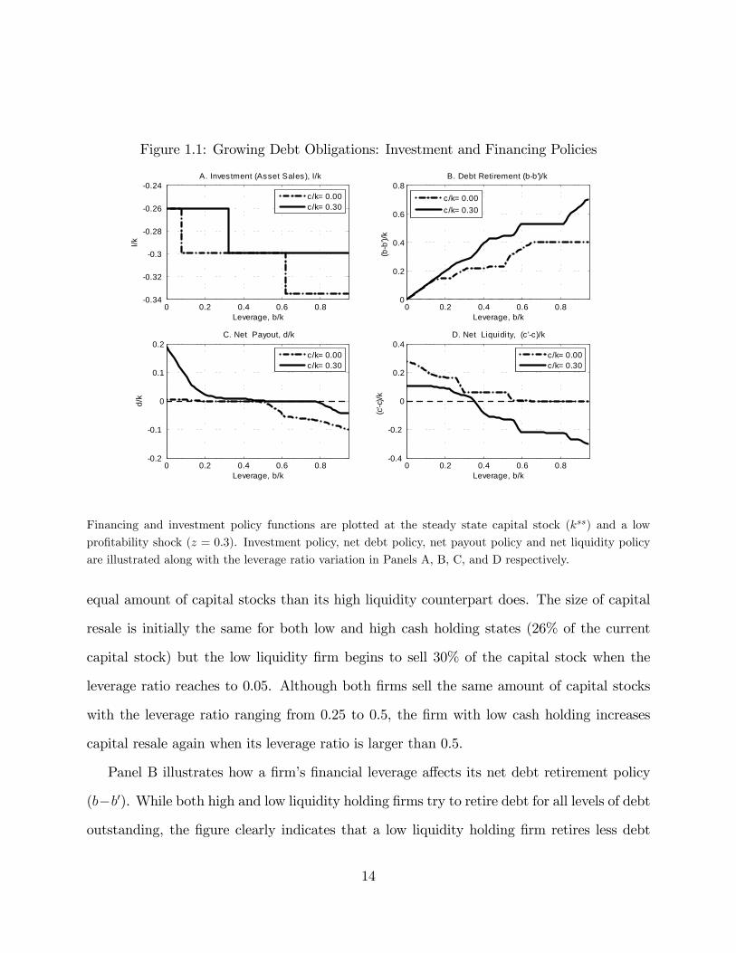
Figure 1.1: Growing Debt Obligations: Investment and Financing Policies

0 0.2 0.4 0.6 0.80

0.2

0.4

0.6

0.8B. Debt Retirement (b­b')/k

Leverage, b/k

(b­b

')/k

0 0.2 0.4 0.6 0.8­0.2

­0.1

0

0.1

0.2C. Net  Payout, d/k

Leverage, b/k

d/k

0 0.2 0.4 0.6 0.8­0.4

­0.2

0

0.2

0.4D. Net  Liquidity,  (c'­c)/k

Leverage, b/k

(c'­c

)/k

0 0.2 0.4 0.6 0.8­0.34

­0.32

­0.3

­0.28

­0.26

­0.24A. Investment (Asset Sales), I/k

Leverage, b/k

I/k

c /k= 0.00c/k= 0.30

c/k= 0.00c/k= 0.30

c/k= 0.00c/k= 0.30

c/k= 0.00c/k= 0.30

Financing and investment policy functions are plotted at the steady state capital stock (kss) and a low

pro�tability shock (z = 0:3). Investment policy, net debt policy, net payout policy and net liquidity policy

are illustrated along with the leverage ratio variation in Panels A, B, C, and D respectively.

equal amount of capital stocks than its high liquidity counterpart does. The size of capital

resale is initially the same for both low and high cash holding states (26% of the current

capital stock) but the low liquidity �rm begins to sell 30% of the capital stock when the

leverage ratio reaches to 0.05. Although both �rms sell the same amount of capital stocks

with the leverage ratio ranging from 0.25 to 0.5, the �rm with low cash holding increases

capital resale again when its leverage ratio is larger than 0.5.

Panel B illustrates how a �rm�s �nancial leverage a¤ects its net debt retirement policy

(b�b0). While both high and low liquidity holding �rms try to retire debt for all levels of debt

outstanding, the �gure clearly indicates that a low liquidity holding �rm retires less debt

14

than its high liquidity holding counterpart. For example, the �rm with high liquidity holding

discharges all debt obligations when its leverage ratio is 0.2. Yet, the net debt retirement

by the low liquidity holding �rm is 12% of the capital stock or only 60% of current debt

obligations, given the same leverage ratio of 0.2. In fact, the high liquidity holding �rm

always retires debt to a greater extent when the leverage ratio is higher than 0.12.

Panel C depicts the relationship between the amount of debt obligations and a �rm�s net

payout policy (d). The �gure demonstrates that large debt obligations decrease a �rm�s net

payout to shareholders and eventually lead to equity �nancing (d < 0) for both high and

low liquidity holding �rms. Noticeably, the high liquidity holding �rm begins to its equity

issuance at a higher leverage ratio than the low liquidity holding �rm does. The �rm with

high liquidity holding gradually reduces its dividends payout to zero and sustains its zero

payout until the leverage ratio reaches to 0.8. Then the �rm begins to use equity �nancing

and increases the amount of equity proceeds afterwards. The low liquidity holding �rm

maintains zero dividends payout but begins to issue equity when the �rm�s leverage ratio

becomes 0.43.

Panel D describes net cash holding policy (c0 � c) variations in responses to a �rm�s

growing debt obligations. The net cash holding policy of the high liquidity holding �rm

is remarkable. The �rm initially tries to accumulate additional cash stocks (c0 � c > 0),

but then begins to liquidate current cash to service growing debt obligations (c0 � c < 0).

Eventually, the �rm uses up all of its current cash stock, when the leverage reaches to 0.9.

Similarly, the �rm with zero liquidity holding initially stockpiles its cash balance but ceases

its cash stock accumulation, when the leverage ratio becomes 0.5.

Panel D highlights a key aspect of debt servicing costs: servicing debt drains a �rm�s

valuable liquidity. The high liquidity holding �rm initially accumulates cash inventory to

the future by selling its capital stock, which implies a large value of liquidity given the level

15

of capital and pro�tability shock. Nevertheless, the �rm utilizes its cash holding to service

growing debt obligations and eventually uses up all of current cash stocks.

Panels A, B, and C illustrate a �rm�s investment and external �nancing policy variations

according to its current debt outstanding and liquidity holding. Given the same amount of

liquidity holding, a �rm with large debt obligations sells a greater amount of capital stock

and uses external �nancing to a larger extent. Both high and low liquidity �rms tend to

increase the amount of asset sales and collect additional equity proceeds to pay down large

debt obligations (Panels A and C). Similarly, given the same amount of debt obligations, a

�rm with low liquidity holding relies more heavily on capital resale and external �nancing.

The low liquidity �rm initiates its equity �nancing at a lower leverage, retires less debt, and

sells a greater amount of capital stock than the high liquidity holding �rm does (Panels A,

B, and C).

In sum, servicing large debt obligations leads to additional reductions in a �rm�s valuable

cash stocks. A �rm with more limited cash holding or with larger debt obligations tends to

rely more heavily on costly capital resale or external �nancing to service debt obligations,

which potentially increases debt servicing costs.

1.3.3 Debt Servicing Costs

This section studies the e¤ect of debt obligations, pro�tability shocks, and the levels of capital

stock on debt servicing costs. I use the marginal value of liquidity as a natural measure of

debt servicing costs, as this formulation represents a �rm�s equity value change from an

additional $1 of cash stock. The marginal value of liquidity, given a state of pro�tability,

capital stock, debt obligation and liquidity holding (z; k; b; c); is de�ned as follows:

Marginal Value of Liquidity =@

@cV (z; k; b; c): (1.14)

16

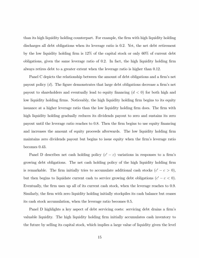
Figure 1.2: Marginal Value of Liquidity

0 0.1 0.2 0.3 0.4 0.5 0.6 0.7 0.8 0.9 11

1.005

1.01

1.015

1.02

1.025

1.03

1.035Marginal Value of Liquidity

Leverage, b/k

c/k = 0c/k = 0.3

The marginal value of liquidity is plotted at the steady state level of capital stock (kss) with a neutral

pro�tability shock (z = 1). The values from two di¤erent levels of cash holding states (c=k = 0; 0:3) are

depicted along with the leverage ratio variation.

BCW emphasize the marginal value of liquidity as a critical determinant of a �rm�s dividends,

equity �nancing and liquidity policy. The marginal value of liquidity is a nexus controlling a

�rm�s overall internal and external �nancing policies, considering all of its close connections

to debt servicing costs, equity �nancing, dividends payout, and cash retention policy.

Figure 1.2 depicts the e¤ect of the leverage variation on the marginal value of liquidity

at the steady state level of capital stock (kss), and a neutral pro�tability shock realization

(z = 1). I plot the marginal value of liquidity for high (c=k = 0:3) and low (c=k = 0) liquidity

states to check the robustness of qualitative predictions.

Most remarkably, Figure 1.2 points out that a �rm with larger debt obligations faces

higher debt servicing costs, measured by the marginal value of liquidity. With no liquidity

holding, the marginal value of liquidity begins at 1 but increases to 1.025, when the leverage

17

ratio increases from 0 to 0.9. Considering the low risk free rate, 2.5%, of this model, the

increase of 2.5% in the marginal value of liquidity is quite material. For the high liquidity

holding �rm, similarly, the marginal value of liquidity initially stays at 0 but begins to

escalate when the leverage ratio grows above 0.4.

The rising debt servicing costs are closely associated with costly capital resale and exter-

nal �nancing. With limited cash holding, a �rm tends to rely more heavily on capital resale

and external �nancing to service larger debt obligations, as illustrated in Figure 1.1. Both

capital resale and external �nancing involve increasing marginal costs, which directly raise

the marginal value of liquidity. Moreover, capital resale incurs a loss in the future pro�t

generation capacity and current debt roll-over leads to future debt servicing costs, both of

which drive additional ine¢ ciency. The increase in marginal value of liquidity re�ects explicit

funding costs and ine¢ ciency from asset sales and external �nancing.

This rising marginal value of liquidity sheds new lights on the debt conservatism puzzle

(Graham 2000). Crucially, this �nding provides an economic ground for prevailing conser-

vative debt policy. To avoid higher servicing costs from large debt obligations, a �rm may

exercise conservative debt policy even with large tax bene�ts and low �nancial distress costs.

Economic factors associated with conservative debt policy, such as growth options to �nance,

large future acquisition plan, asset intangibility and excess cash holding, all argue for the

signi�cance of debt servicing costs in resolving the debt conservatism puzzle. Growth options

to fund and a large scale investment plan indicate large funding demands in the future, which

increases a �rm�s precautionary value of liquidity. Asset intangibility is closely related to

higher costs of asset sales, which may lead to large costs in servicing debt payments. Excess

cash holding with conservative debt policy potentially stems from a �rm�s optimal decision

in the face of a large value of liquidity. All of these factors are closely related to large debt

servicing costs.

18

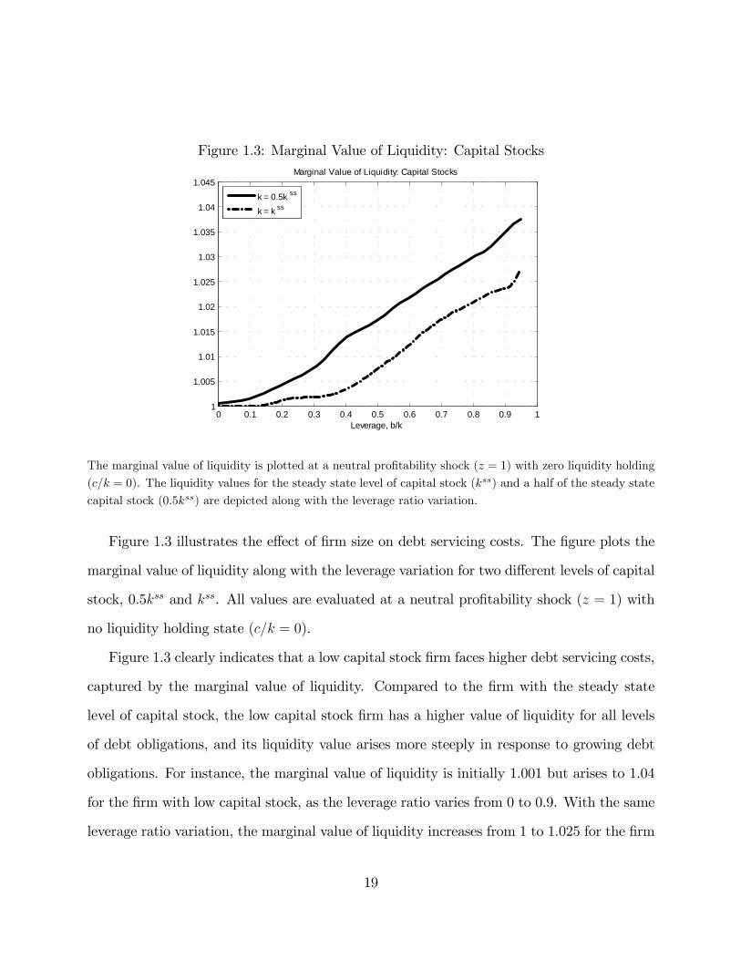
Figure 1.3: Marginal Value of Liquidity: Capital Stocks

0 0.1 0.2 0.3 0.4 0.5 0.6 0.7 0.8 0.9 11

1.005

1.01

1.015

1.02

1.025

1.03

1.035

1.04

1.045Marginal Value of Liquidity: Capital Stocks

Leverage, b/k

k = 0.5k ss

k = k ss

The marginal value of liquidity is plotted at a neutral pro�tability shock (z = 1) with zero liquidity holding

(c=k = 0). The liquidity values for the steady state level of capital stock (kss) and a half of the steady state

capital stock (0:5kss) are depicted along with the leverage ratio variation.

Figure 1.3 illustrates the e¤ect of �rm size on debt servicing costs. The �gure plots the

marginal value of liquidity along with the leverage variation for two di¤erent levels of capital

stock, 0.5kss and kss. All values are evaluated at a neutral pro�tability shock (z = 1) with

no liquidity holding state (c=k = 0).

Figure 1.3 clearly indicates that a low capital stock �rm faces higher debt servicing costs,

captured by the marginal value of liquidity. Compared to the �rm with the steady state

level of capital stock, the low capital stock �rm has a higher value of liquidity for all levels

of debt obligations, and its liquidity value arises more steeply in response to growing debt

obligations. For instance, the marginal value of liquidity is initially 1.001 but arises to 1.04

for the �rm with low capital stock, as the leverage ratio varies from 0 to 0.9. With the same

leverage ratio variation, the marginal value of liquidity increases from 1 to 1.025 for the �rm

19

with the steady state level of capital stock.

Large current and future investments drive such a large marginal value of liquidity in

the low capital stock �rm. Due to a decreasing returns to scale pro�t technology, the low

capital stock �rm tends to invest more in the current and future periods, and has to create

more funds for capital expenditures. Such large funding demands raise the marginal value of

liquidity more substantially for the �rm with low capital stock, given the same pro�tability

and liquidity holding state.

Empirically, large debt servicing costs in the low capital stock �rm predict lower leverage

ratios in small �rms. Prior empirical results support the debt servicing cost prediction

between the �rm size and debt policy as well as the validity of decreasing returns to scale

pro�t technology. Smaller �rms indeed grow faster than large size �rms (Hall 1987), which

seems to a¢ rm the validity of the decreasing returns to scale pro�t technology. The book

asset size of �rm is positively correlated with leverage ratio for a number of di¤erent cross-

sectional models (Frank and Goyal 2008). Small growth �rms tend to maintain low leverage

(Frank and Goyal 2003) and large cash �ow rich �rms heavily rely on debt �nancing (Shyam-

Sunder and Myers 1999), consistent with the debt servicing cost prediction.

The marginal value of liquidity directly connects large investments in smaller �rms with

low leverage, which di¤ers markedly from the existing literature such as Titman (1988) and

DDW. Titman (1988) emphasizes low �nancing costs or low bankruptcy costs in large �rms to

explain the relationship between �rm size and debt policy. DDW highlight the importance of

intertemporal allocation of limited debt capacity in the link between large future investments

and a currently low leverage ratio.

Figure 1.4 investigates how a �rm�s pro�tability shock a¤ects debt servicing costs. The

�gure plots the marginal value of liquidity as a function of leverage ratio for two di¤erent

pro�tability shock scenarios, a low pro�tability shock, z = 0:3 and a neutral pro�tability

20

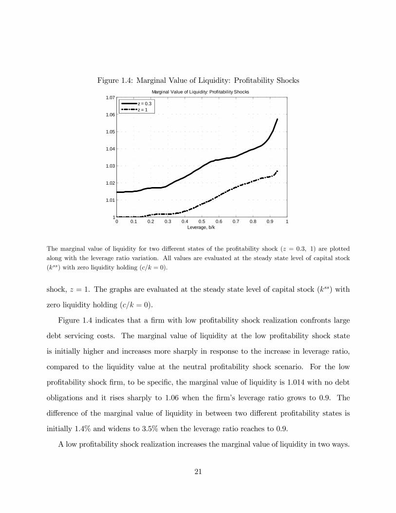
Figure 1.4: Marginal Value of Liquidity: Pro�tability Shocks

0 0.1 0.2 0.3 0.4 0.5 0.6 0.7 0.8 0.9 11

1.01

1.02

1.03

1.04

1.05

1.06

1.07

Leverage, b/k

Marginal Value of Liquidity: Profitability Shocks

z = 0.3z = 1

The marginal value of liquidity for two di¤erent states of the pro�tability shock (z = 0:3; 1) are plotted

along with the leverage ratio variation. All values are evaluated at the steady state level of capital stock

(kss) with zero liquidity holding (c=k = 0).

shock, z = 1. The graphs are evaluated at the steady state level of capital stock (kss) with

zero liquidity holding (c=k = 0).

Figure 1.4 indicates that a �rm with low pro�tability shock realization confronts large

debt servicing costs. The marginal value of liquidity at the low pro�tability shock state

is initially higher and increases more sharply in response to the increase in leverage ratio,

compared to the liquidity value at the neutral pro�tability shock scenario. For the low

pro�tability shock �rm, to be speci�c, the marginal value of liquidity is 1.014 with no debt

obligations and it rises sharply to 1.06 when the �rm�s leverage ratio grows to 0.9. The

di¤erence of the marginal value of liquidity in between two di¤erent pro�tability states is

initially 1.4% and widens to 3.5% when the leverage ratio reaches to 0.9.

A low pro�tability shock realization increases the marginal value of liquidity in two ways.

21

Figure 1.5: Marginal Value of Liquidity: High Equity Financing Costs

0 0.2 0.4 0.6 0.8 11

1.5

2

2.5

3

3.5

4

4.5

5

5.5

6

Leverage, b/k

Panel B. Higher Equity Financing Costs

z = 0.3z = 1

0 0.2 0.4 0.6 0.8 11

1.05

1.1

1.15

1.2

1.25

1.3

1.35

1.4

1.45

1.5

Leverage, b/k

Panel A. High Equity Financing Costs

z = 0.3z = 1

Panel A describes the marginal value of liquidity where �xed and convex equity �nancing costs are 10 times

higher than the baseline estimates. Panel B depicts the marginal value of liquidity where �xed and convex

equity �nancing costs are 100 times higher than the baseline estimates. In both Panels A and B, the marginal

value of liquidity for two di¤erent states of the pro�tability shock (z = 0:3; 1) are plotted along with the

leverage ratio variation. All values are evaluated at the steady state level of capital stock (kss) with zero

liquidity holding (c=k = 0).

First, a low operating pro�t implies more limited internal funds to service debt payments,

given a speci�c amount of cash stock. Second, a currently low pro�tability shock predicts

low future operating pro�ts in the future, due to the positive serial correlation in a �rm�s

pro�t generation. The parameter � captures this persistency of pro�tability shock in the

model. Low current internal funds and low expected operating pro�ts altogether increase the

marginal value of liquidity, in spite of low investment demands implied by a low pro�tability

shock.

Figure 1.5 analyzes the e¤ect of large external �nancing costs on the marginal value of

liquidity. The �gure plots the marginal value of liquidity for a neutral pro�tability shock

22

(z = 1) and a low pro�tability shock (z = 0:3) scenarios at the steady state level of capital

stock (kss) with zero liquidity holding (c=k = 0). In Panel A, the �xed and convex equity

�nancing costs are 10 times higher than the baseline estimates. In Panel B, both equity

�nancing costs are 100 times larger than the baseline costs.

Figure 1.5 indicates that higher equity �nancing costs considerably raise debt servicing

costs. Both Panels A and B show the soaring marginal value of liquidity in response to

growing debt obligations. As expected, the marginal value of liquidity arises more sharply in

Panel B where both equity �nancing costs are far higher than those of Panel A. For instance,

the marginal value of liquidity with a low pro�tability shock (z = 0:3) is 1.5 in Panel A and

5.5 in Panel B, when the leverage ratio is 0.9.

Figure 1.4 and 1.5 provide new insights on a �rm�s disaster risk and debt policy. In

a disaster period as the recent �nancial crisis of 2008, a �rm�s pro�tability drops sharply

and equity �nancing costs tends to increase considerably. Figure 1.4 points out that a low

pro�tability shock raises debt servicing costs substantially even in the absence of any �nancial

distress costs. Figure 1.5 veri�es the material combined e¤ect of low pro�tability shocks and

high external �nancing costs on debt servicing costs. A �rm may use debt conservatively

to avoid massive debt servicing costs in disaster periods, even if the �rm has a negligible

likelihood of bankruptcy during the disaster periods.

To summarize, debt servicing costs are positively related with large debt obligations,

a low level of capital stock, a low current pro�tability, and large external �nancing costs.

These �ndings provide new insights on a number of empirical puzzles, such as the debt

conservatism puzzle, low leverage in small �rms and the relationship between disaster risk

and debt policy.

23

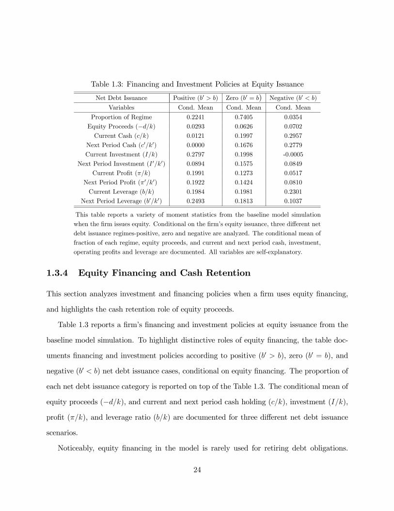
Table 1.3: Financing and Investment Policies at Equity Issuance

Net Debt Issuance Positive (b0 > b) Zero (b0 = b) Negative (b0 < b)

Variables Cond. Mean Cond. Mean Cond. Mean

Proportion of Regime 0.2241 0.7405 0.0354

Equity Proceeds (�d=k) 0.0293 0.0626 0.0702

Current Cash (c=k) 0.0121 0.1997 0.2957

Next Period Cash (c0=k0) 0.0000 0.1676 0.2779

Current Investment (I=k) 0.2797 0.1998 -0.0005

Next Period Investment (I 0=k0) 0.0894 0.1575 0.0849

Current Pro�t (�=k) 0.1991 0.1273 0.0517

Next Period Pro�t (�0=k0) 0.1922 0.1424 0.0810

Current Leverage (b=k) 0.1984 0.1981 0.2301

Next Period Leverage (b0=k0) 0.2493 0.1813 0.1037

This table reports a variety of moment statistics from the baseline model simulation

when the �rm issues equity. Conditional on the �rm�s equity issuance, three di¤erent net

debt issuance regimes-positive, zero and negative are analyzed. The conditional mean of

fraction of each regime, equity proceeds, and current and next period cash, investment,

operating pro�ts and leverage are documented. All variables are self-explanatory.

1.3.4 Equity Financing and Cash Retention

This section analyzes investment and �nancing policies when a �rm uses equity �nancing,

and highlights the cash retention role of equity proceeds.

Table 1.3 reports a �rm�s �nancing and investment policies at equity issuance from the

baseline model simulation. To highlight distinctive roles of equity �nancing, the table doc-

uments �nancing and investment policies according to positive (b0 > b), zero (b0 = b), and

negative (b0 < b) net debt issuance cases, conditional on equity �nancing. The proportion of

each net debt issuance category is reported on top of the Table 1.3. The conditional mean of

equity proceeds (�d=k), and current and next period cash holding (c=k), investment (I=k),

pro�t (�=k), and leverage ratio (b=k) are documented for three di¤erent net debt issuance

scenarios.

Noticeably, equity �nancing in the model is rarely used for retiring debt obligations.

24

Only 3.5% of equity issuance is associated with negative net debt issuance, which points to a

minor role of equity �nancing in retiring debt obligations. This �nding is consistent with the

infrequent use of proactive equity �nancing in Denis and McKeon (2012). They document

that public �rms rarely use equity �nancing to retire prior surges in debt obligations.

In the majority of cases, a �rm�s equity proceeds are used for cash retention as well as

capital expenditure, especially when it faces large current and future investments. The cash

retention role of equity �nancing is highlighted in the zero net debt issuance case, accounting

for more than 74% of total equity �nancing. Most noticeably, a �rm faces large current and

future investment demands above average in the zero net debt issuance regime. While large

next period investments (I 0=k0 = 0:1575) imply a large value of liquidity, a �rm has to

drain its cash stocks (c=k = 0:1997) to fund currently vast investments (I=k = 0:1998).

To accumulate a substantial amount of cash stock again, the �rm tries to use its current

operating pro�ts (�=k = 0:1273) and equity proceeds (d=k = 0:0626). This cash retention

role hinges on no servicing cost property of equity �nancing. A �rm can stockpile cash for

the future use by issuing equity because current equity �nancing does not deplete valuable

liquidity in the future.

This �nding is closely associated with a number of empirical regularities in equity �-

nancing. Equity proceeds are largely used for near term cash saving (DeAngelo et al. 2010)

and the cash saving propensity of equity proceeds is far higher than that of debt proceeds

(McLean 2011). An equity issuance decision is generally concurrent with large current and

future investments (Loughran and Ritter 1997; Fama and French 2002). Large current and

future investments may also drive frequent equity �nancing in small growth �rms (Frank and

Goyal 2003). Large cash �ow rich �rms can avoid equity �nancing because these �rms can

easily use their operating pro�ts for cash saving, which incur neither �nancing nor servicing

costs (Shyam-Sunder and Myers 1999).

25

The emphasis on the cash retention role of equity issuance di¤ers markedly from prior

security choice theories. The dynamic trade-o¤models with infrequent leverage adjustments

focus on the role of equity proceeds in paying down debt obligations (Strebulaev 2007).

The pecking-order theory underlines large asymmetric information cost involved in equity

�nancing and emphasizes its inferiority to debt �nancing (Myers and Majluf 1984). In

contrast, the model simulation result highlights the cash retention role of equity �nancing in

the view of servicing costs; equity �nancing can be used for cash retention because it does

not deplete liquidity in the future.

Finally, a �rm uses equity proceeds solely for capital expenditure in the case of positive

net debt issuance, which takes account of 22% of total equity �nancing. All operating

pro�ts, current cash stocks and equity proceeds are used to �nance currently large capital

expenditure (I=k = 0:2797). High pro�tability (�0=k0 = 0:1922) and low investment needs

(I 0=k0 = 0:0894) in the next period imply a low marginal value of liquidity. As a result,

the �rm has low incentive to save cash stock from additional equity proceeds and carries

no cash for the future use (c0=k0 = 0). Empirically, this �nancing role of equity proceeds is

particularly signi�cant in human capital intensive �rms. Brown, Fazzari and Petersen (2009)

document the importance of equity issuance for funding investments in R&D intensive �rms

during 1990s.

To summarize, in the majority of cases, equity proceeds are used for cash retention as well

as capital expenditure, particularly when a �rm faces large current and future investments.

This �nding is consistent with recent empirical studies such as DeAngelo et al. (2010),

Loughran and Ritter (1997) and Fama and French (2002). On the other hand, a �rm rarely

issues equity for retiring debt obligations. This result is consistent with the minor role of

proactive equity �nancing (Denis and McKeon 2012), but contradicts recent dynamic trade-

o¤ models with infrequent leverage adjustment (Strebulaev 2007).

26

1.4 Comparative Statics

This section investigates how large debt servicing costs a¤ect a �rm�s capital structure choice.

It emphasizes low leverage and frequent equity �nancing tendencies for a �rm with large debt

servicing costs. The variations of �xed operating costs and convex capital adjustment costs

are considered here to capture the in�uence of large debt servicing costs on debt and equity

�nancing policies.

1.4.1 Comparative Statics I: Fixed Operating Cost

A higher �xed operating cost is closely associated with large debt servicing costs. An in-

crease in �xed operating costs decreases a �rm�s pro�tability without incurring considerable

changes in a �rm�s investment demands because this adjustment does not a¤ect the mar-

ginal pro�tability of investments. Therefore, a �rm with large �xed operating costs tends to

confront a higher marginal value of liquidity.

Figure 1.6 con�rms this e¤ect of �xed operating costs on the marginal value of liquidity.

The marginal value of liquidity is plotted against the leverage ratio variation for the baseline

�xed operating costs, � = 0:0251, and for high �xed operating costs, � = 0:035, in the case

of no liquidity holding (c = 0). The marginal value of liquidity is evaluated at the steady

state level of capital stock (kss) with a neutral pro�tability shock (z = 1).

The �gure demonstrates that a �rm with higher �xed operating costs faces a large mar-

ginal value of liquidity. The marginal value of liquidity is initially higher and grows more

sharply for the �rm with high �xed operating costs. Although the detailed variations are

not documented here, this qualitative prediction remains unchanged for di¤erent levels of

capital stock, pro�tability shock and liquidity holding.

Table 1.4 shows the e¤ects of �xed operating cost variations on a �rm�s investment and

27

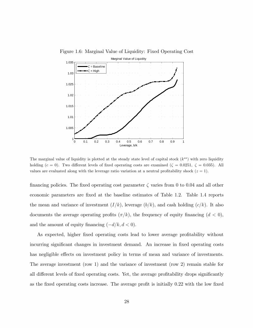
Figure 1.6: Marginal Value of Liquidity: Fixed Operating Cost

0 0.1 0.2 0.3 0.4 0.5 0.6 0.7 0.8 0.9 11

1.005

1.01

1.015

1.02

1.025

1.03

1.035Marginal Value of Liquidity

Leverage, b/k

ζ = Baselineζ = High

The marginal value of liquidity is plotted at the steady state level of capital stock (kss) with zero liquidity

holding (c = 0). Two di¤erent levels of �xed operating costs are examined (� = 0:0251; � = 0:035). All

values are evaluated along with the leverage ratio variation at a neutral pro�tability shock (z = 1).

�nancing policies. The �xed operating cost parameter � varies from 0 to 0.04 and all other

economic parameters are �xed at the baseline estimates of Table 1.2. Table 1.4 reports

the mean and variance of investment (I=k), leverage (b=k), and cash holding (c=k). It also

documents the average operating pro�ts (�=k), the frequency of equity �nancing (d < 0),

and the amount of equity �nancing (�d=k; d < 0):

As expected, higher �xed operating costs lead to lower average pro�tability without

incurring signi�cant changes in investment demand. An increase in �xed operating costs

has negligible e¤ects on investment policy in terms of mean and variance of investments.

The average investment (row 1) and the variance of investment (row 2) remain stable for

all di¤erent levels of �xed operating costs. Yet, the average pro�tability drops signi�cantly

as the �xed operating costs increase. The average pro�t is initially 0.22 with the low �xed

28

Table 1.4: Fixed Operating Cost Variation

Fixed Operating Costs Low High

Avg. Investment (I=k) 0.1310 0.1310 0.1314 0.1315 0.1320

Var. Investment(I=k) 0.0230 0.0228 0.0239 0.0242 0.0243

Avg. Leverage (b=k) 0.7675 0.3751 0.2271 0.0892 0.0213

Var. Leverage (b=k) 0.0245 0.0103 0.0149 0.0136 0.0031

Avg. Pro�t (�=k) 0.2199 0.2019 0.1741 0.1648 0.1463

Equity Issuance Freq. (d < 0) 0.0195 0.0305 0.1017 0.1193 0.1288

Avg. Equity Financing (�d=k; d < 0) 0.0354 0.0387 0.0555 0.0579 0.0764

Avg. Cash Holding (c=k) 0.0975 0.0969 0.1150 0.1634 0.4185

Var. Cash Holding (c=k) 0.0130 0.0123 0.0164 0.0321 0.1040

This table reports a variety of �nancing and investment moments along with �xed

operating cost variations. I simulate the model for 102,000 periods and drop �rst

2000 observations. The representative �rm changes its investment and �nancing pol-

icy in response to the series of pro�tability shock realizations. Each column reports

selected �nancing and investment variables corresponding to di¤erent �xed operating

cost parameters (�) of 0, 0.01, 0.0251, 0.03 and 0.04, respectively. All variables are

self-explanatory and other structural parameters are set to the baseline estimates of

Table 1.2.

operating cost scenario, � = 0, but it decreases to 0.145 when the �xed operating cost

parameter � becomes 0.04 (row 5).

Table 1.4 highlights that a �rm with higher �xed operating costs tends to have lower

leverage and rely more heavily on equity �nancing. To be speci�c, the average leverage

decreases by more than 95% and the variance of leverage diminishes by almost 90% as the

�xed operating cost parameter � increases from 0 to 0.04 (row 3 and 4). Given the same

�xed operating cost variation, equity �nancing frequency increases more than ten times and

the amount of equity proceeds becomes more than doubled (row 6 and 7).

The e¤ect of �xed operating costs on cash holding policy is indeterminate. The aver-

age cash holding slightly decreases between the �rst two columns but gradually increases

afterwards (row 8). This inconclusive direction may stem from the endogeneity in the joint

decisions of liquidity and debt policies. A higher marginal value of liquidity indicates large

29

Table 1.5: Fixed Operating Cost Variation: Robustness

Variables Serial Corr.(�) Uncertainty(�) DRS(�)

Low High Low High Low High

Panel A: Low Cost (�=0.0)

Avg. Leverage(b=k) 0.8670 0.3672 0.9326 0.3708 0.9007 0.3982

Equity Freq. (d < 0) 0.0302 0.0354 0.0393 0.0091 0.0111 0.0041

Avg. Equity Financing (�d=k; d < 0) 0.0309 0.0451 0.0265 0.0435 0.1365 0.0167

Panel B: Baseline (�=0.0251)

Avg. Leverage(b=k) 0.2984 0.1190 0.2731 0.0553 0.2350 0.1590

Equity Freq. (d < 0) 0.1013 0.1009 0.0810 0.0472 0.0484 0.0448

Avg. Equity Financing (�d=k; d < 0) 0.0563 0.0710 0.0549 0.0651 0.1983 0.0280

This table reports average leverage(b=k), equity �nancing frequency(d < 0) and average equity

�nancing amount (�d=k, d < 0) based on the model with a low �xed operating cost (� = 0;

Panel A) and with the baseline �xed cost (� = 0:0251; Panel B). The �rst two columns contrast

low and high serial correlation cases in the pro�tability shock, where � = 0:6 and � = 0:8,

respectively. The next two columns are for low and high uncertainty cases in the pro�tability

shock where � is 0.12 and 0.3, respectively. The last two columns are for low and high returns

to scale scenarios of the pro�t function, where � = 0:6 and � = 0:8, respectively.

debt servicing costs given the same amount of debt obligations, ex-ante. Yet, a �rm with

large debt servicing costs endogenously selects a low leverage ratio, which potentially un-

dermines the �rm�s cash retention incentives, ex-post. The average liquidity holding ratio

re�ects these counter-balancing e¤ects from growing debt servicing costs.

Table 1.5 shows the robustness of the �xed operating cost predictions on the capital

structure choice. The �rm with low �xed operating costs (Panel A) always relies more

heavily on debt �nancing for high and low uncertainty scenarios of the pro�tability shock,

for high and low serial correlations in operating pro�ts, and for high and low decreasing

returns to scale parameters. A �rm with low �xed operating costs also uses equity �nancing

less frequently than the �rm with the baseline �xed operating costs does, in line with the

results of Table 1.4.

These quantitative predictions are consistent with recent empirical �ndings on the re-

30

lationship between operating leverage and external �nancing policies. Kahl et al. (2012)

uniquely analyze the e¤ect of operating leverage on a �rm�s �nancing policies. They mainly

show that higher operating leverage �rms tend to maintain lower leverage and issue equity

to a greater extent. Their �ndings are in line with the quantitative predictions of Table 1.4

and 1.5.

1.4.2 Comparative Statics II: Convex Capital Adjustment Costs

Capital installation and liquidation incur organizational costs (Hamermesh and Pfann 1997).

The accumulation and resale of capital stock lead to the hiring or �ring new workers, which

may involve training, search, or severance costs. In addition, the extant workers may �nd

their routine disrupted and their tasks reassigned when a �rm purchases or sells its capital

stock. This reallocation process may lower labor productivity and increase capital adjust-

ment costs.

Higher convex capital adjustment costs lead to slow adjustments of capital stock and

large costs of asset sales. A high capital resale cost is especially and closely associated with

large debt servicing costs. As depicted in Figure 1.1, a �rm increases its asset sales to service

large debt obligations and these asset sales tend to be more costly with higher capital resale

costs.

Figure 1.7 shows the implication of convex capital adjustment cost variations on debt

servicing costs. The marginal value of liquidity is plotted for two di¤erent levels of convex

capital adjustment costs, the baseline, �k = 0:1163, and high cost, �k = 3�0:1163, scenarios.

The marginal value of liquidity is evaluated along with the leverage ratio at the steady state

of capital stock (kss) with a neutral pro�tability shock (z = 1) and zero liquidity holding

(c = 0). All other economic parameters are set to the values of Table 1.2 except the �xed

capital adjustment costs: the parameter k is set to zero to isolate the e¤ect of convex capital

31

Figure 1.7: Marginal Value of Liquidity: Convex Capital Adjustment Costs

0 0.1 0.2 0.3 0.4 0.5 0.6 0.7 0.8 0.9 11

1.005

1.01

1.015

1.02

1.025

1.03

1.035Marginal Value of Liquidity

Leverage, b/k

θk=Baseline

θk=High

The marginal value of liquidity is plotted at the steady state level of capital stock (kss) with zero liquidity

holding (c = 0). Two di¤erent levels of convex capital adjustment cost are examined (�k = 0:1163; �k =

3�0:1163). All values are evaluated along with the leverage ratio variation with a neutral pro�tability shock(z = 1).

adjustment costs.

Figure 1.6 points out that a �rm with high convex capital adjustment costs faces large

debt servicing costs, especially those with a considerable amount of debt obligations. The

baseline and high convex capital adjustment cost �rms confront the same marginal value of

liquidity until the leverage ratio becomes 0.3. Yet, the high convex capital adjustment cost

�rm shows a greater marginal value of liquidity than the baseline cost �rm does when the

leverage ratio is larger than 0.3. This �nding is in line with the increasing tendency of asset

sales to service additional debt obligations, as illustrated in Figure 1.1.

Table 1.6 compares investment and �nancing policies for di¤erent levels of convex capital

adjustment costs, which vary from 0.1 to 3 times of the baseline convex capital adjustment

32

Table 1.6: Convex Capital Adjustment Cost Variation

Convex Capital Adjustment Cost Low High

Avg. Investment (I=k) 0.1625 0.1307 0.1248 0.1222 0.1214

Var. Investment(I=k) 0.0885 0.0215 0.0096 0.0044 0.0027

Avg. Leverage (b=k) 0.1952 0.1770 0.1761 0.1655 0.1419

Var. Leverage (b=k) 0.0171 0.0129 0.0084 0.0036 0.0034

Avg. Pro�t (�=k) 0.1647 0.1681 0.1701 0.1727 0.1743

Equity Issuance Freq. (d < 0) 0.0051 0.0095 0.0203 0.0368 0.0373

Avg. Equity Financing (�d=k; d < 0) 0.0548 0.0719 0.0558 0.0484 0.0548

Avg. Cash Holding (c=k) 0.2957 0.1096 0.0638 0.0370 0.0276

Var. Cash Holding (c=k) 0.1329 0.0260 0.0084 0.0026 0.0023

This table reports a variety of �nancing and investment moments along with �xed

operating cost variation. Each column indicates a di¤erent level of convex capital

adjustment cost; the values are 0.1, 0.5, 1, 2, and 3 times of the baseline convex capital

adjustment cost in Table 1.2. The �xed capital adjustment cost parameter is set to

0 and the other parameter values are from the baseline estimates of Table 1.2. All

variables are self explanatory.

cost estimate. To focus on the role of convexity in capital adjustment costs, the �xed cost

parameter k is set to zero. All other economic parameters are �xed at the baseline estimates

in Table 1.2. Table 1.6 reports the mean and variance of investment (I=k), leverage (b=k),

and cash stock (c=k). It also documents the average operating pro�ts (�=k), the frequency

of equity �nancing (d < 0), and the amount of equity proceeds (�d=k, d < 0):

Table 1.6 shows that a �rm with high convex capital adjustment costs is closely associated

with lower leverage and more frequent equity �nancing. The average leverage ratio drops

by almost 25% as convex capital adjustment costs increase. Notice that the leverage ratio

is 0.19 in the �rst column, but decreases to 0.14 in the last column (row 3). The frequency

of equity �nancing also gradually increases from 0.5% to 3% for the same convex capital

adjustment costs variation (row 6). The average equity proceeds are stable around 5% of

capital stock for all levels of convex capital adjustment costs (row 7). Even with slightly

higher pro�tability (row 5), a higher convexity in capital adjustment costs leads to lower

33

�nancial leverage and more frequent equity �nancing.

Interestingly, a higher convex capital adjustment cost �rm tends to hold lower cash hold-

ing (row 8). This appears inconsistent with a large value of liquidity from a higher convex

capital adjustment cost in Figure 1.7. Two economic forces may explain such decline in

average cash holding ratio. First, endogenous decisions of leverage and cash holding poten-

tially play an important role, as discussed in the previous section. An economic environment

generating large debt servicing costs raises the marginal value of liquidity, given the same

amount of debt obligations, ex ante. However, a �rm optimally maintains lower leverage,

which potentially undermines cash holding incentives, ex post. The latter e¤ects could be

more signi�cant in the convex capital adjustment costs variation.

To investigate another potential reason for the diminishing cash holding tendency, Figure

1.8 examines the relationship between convex capital adjustment costs and the marginal

value of liquidity, for two di¤erent levels of the pro�tability shock. The marginal value of

liquidity is evaluated for the baseline and high convex capital adjustment costs (�k = 0:1163,

�k = 3�0:1163) at the steady state level of capital stock (kss) with zero cash holding (c = 0).

Panel A describes the case with a low pro�tability shock, z = 0:3, whereas Panel B depicts

the case with a high pro�tability shock, z = 1:5. All other economic conditions are identical

to those explained in Figure 1.7.

Panels A and B illustrate contrasting patterns of the marginal value of liquidity for the

baseline and high convex capital adjustment cost �rms, depending on the pro�tability shock

realizations. While the baseline convex capital adjustment cost �rm shows a lower marginal

value of liquidity in Panel A consistent with Figure 1.7, the baseline cost �rm rather exhibits

a higher marginal value of liquidity than the high convex capital adjustment cost �rm does

in Panel B. This �nding is closely associated with the role of low convex capital adjustment

costs enabling more rapid accumulation of capital stocks. Given the same high pro�tability

34

Figure 1.8: Marignal Value of Liquidity: Convex Capital Adjustment Costs and Pro�tabilityShock

0 0.2 0.4 0.6 0.8 11.01

1.02

1.03

1.04

1.05

1.06

1.07

Leverage, b/k

Panel A. Low Profitability Shock, z=0.3

0 0.2 0.4 0.6 0.8 11

1.005

1.01

1.015

1.02

1.025

Leverage, b/k

Panel B. High Profitability Shock, z=1.5

θk= Baselineθk= High

θk= Baselineθk= High

The marginal value of liquidity is plotted at the steady state level of capital stock (kss) with zero cash

holding. Panel A describes a low pro�tability shock case (z=0.3) and Panel B describes a high pro�tability

shock case (z = 1:5). Two di¤erent levels of convex capital adjustment cost are examined (�k = 0:1163,

�k = 3� 0:1163). All values are evaluated along with the leverage ratio variation.

shock realization, the low convex capital adjustment cost �rm tries to build up a larger

amount of capital stock, which raises the marginal value liquidity more substantially. The

decreasing average cash holding ratio may stem from the higher marginal value of liquidity

in a lower convex capital adjustment cost �rm at high pro�tability shock states.

Table 1.7 shows the robustness of the convex capital adjustment cost predictions on the

capital structure choice. The external �nancing policy predictions from large debt servicing

costs remain unchanged for high and low uncertainty cases in the pro�tability shock, for

high and low serial correlations in operating pro�ts, and for high and low decreasing returns

to scale parameters. Consistent with the result in Table 1.6, the higher convex capital

35

Table 1.7: Convex Capital Adjustment Costs Variations: Robustness

Variables Serial Corr.(�) Uncertainty(�) DRS(�)

Low High Low High Low High

Panel A: Baseline

Avg. Leverage(b=k) 0.2051 0.1132 0.2037 0.0559 0.2045 0.1605

Equity Freq. (e > 0) 0.0154 0.1019 0.0077 0.0625 0.0163 0.0386

Avg. Equity Financing (e=k) 0.0579 0.0646 0.0480 0.0594 0.2354 0.0280

Panel B: High Convex Capital Adjustment Cost

Avg. Leverage(b=k) 0.1293 0.0936 0.1792 0.0165 0.1969 0.1276

Equity Freq. (e > 0) 0.0408 0.1330 0.0192 0.0705 0.0215 0.1257

Avg. Equity Financing (e=k) 0.0575 0.0674 0.0425 0.0854 0.2615 0.0306

This table reports average leverage (b=k), equity �nancing frequency (d > 0) and average equity �nancing

amount (d=k) calculated from the simulation of the baseline convex capital adjustment costs (�k = 0:1163;

Panel A) and high convex capital adjustment cost (�k = 3�0:1163); Panel B. The �rst two columns contrastlow and high serial correlation cases in the pro�tability shock, where � =0.6 and � =0.8, respectively. The

next two columns are for low and high uncertainty cases in the pro�tability shock where � is 0.12 and 0.3,

respectively. The last two columns are for low and high returns to scale scenarios of the pro�t function,

where � = 0.6 and � =0.8, respectively.

adjustment cost �rm (Panel B) always uses equity �nancing more frequently and maintains

lower leverage than the baseline cost �rm does (Panel A).

The frequent equity �nancing and low leverage in human capital intensive �rms are closely

associated with the results of Table 1.6 and 1.7. Hall (2002) points out the rigidity in wage

payments and the �rm speci�city of human capital stocks as economic forces behind large

organizational costs of adjusting R&D expenditures. Consistent with the external �nancing

regularities in R&D intensive �rms, my model predicts that a �rm with higher convex capital

adjustment costs tends to show low leverage and use equity �nancing more actively.

The debt servicing cost predictions on convex capital adjustment costs di¤er markedly

from DDW. In their model, a �rm with high convex capital adjustment costs shows higher

leverage, which contrasts the above predictions. With limited debt capacity, a low convex

capital adjustment cost �rm has an additional incentive to save its debt capacity to prepare

36

for highly volatile investment demands. This incentive of debt capacity preservation drives

lower leverage in a �rm with low convex capital adjustment costs. Yet, the issuance of

debt does not involve any explicit costs in their model, which potentially underestimates the

e¤ects of increasing asset sales cost on a �rm�s debt policy.

1.5 Concluding Remarks

I have examined the interdependence between liquidity policy and capital structure choice

and shown it to be a key missing link in the existing literature. Debt servicing costs lie at

the core of the analysis; servicing debt is costly because it drains a �rm�s valuable liquidity.

To examine the implications of debt servicing costs on a �rm�s external �nancing policies,

I developed a new dynamic trade-o¤ model with liquidity management and adopted the

marginal value of liquidity as a natural measure of debt servicing costs.

My model analysis yielded a number of interesting results. Most of all, a �rm with large

debt obligations faces a higher cost of debt, even in the absence of �nancial distress costs.

Next, a smaller �rm may have lower leverage ratio because its large investment demands

increase debt servicing costs. Lastly, equity �nancing could be used for cash retention,

especially for �rms with large current and future investments, because it does not deplete

valuable future liquidity.

These �ndings provide novel insights on a variety of puzzling empirical regularities. Most

of all, the debt servicing costs provide an economic explanation for why a �rm may exercise

conservative debt policy even in the face of low �nancial costs (Graham 2000). Indeed,

many economic factors closely associated with conservative debt policy suggest the potential

importance of debt servicing costs in resolving the debt conservatism puzzle. Next, the

marginal value of liquidity directly connects large investments with lower leverage in smaller

37

�rms (Frank and Goyal 2008), regardless of limited debt capacity considerations (DDW). In

fact, equity proceeds are primarily used for cash retention (DeAngelo et al. 2010) and equity

�nancing is generally concurrent with large current and future investments (Loughran and

Ritter 1997). This cash retention role of equity proceeds di¤ers markedly from prior theories

highlighting large informational costs in equity issuance (Myers and Majluf 1984) or the role

of equity proceeds for debt payments (Strebulaev 2007).

My study highlights several lucrative opportunities for future research. Most of all, the

risk premium involved in a �rm�s debt issuance is an important topic. A large risk premium

drains a �rm�s liquidity more substantially, but increases the amount of interest tax shields.

The trade-o¤between large debt servicing costs and growing tax shields provides more precise

understanding on a �rm�s capital structure choice. Incorporating market timing aspect of

equity �nancing is another direction. The market timing consideration of equity �nancing

is empirically important (Baker and Wurgler 2002), but is not well captured in my model.

38

Chapter 2

Empirical Analysis on Debt Servicing Costs

2.1 Introduction

This chapter empirically supports the theoretical considerations on debt servicing costs in the

previous chapter. For this purpose, I study the simulated method of moments estimation

in detail, and cross-sectionally investigate the debt servicing costs predictions on capital

structure policies.

I adopted the simulated method of moments (SMM) estimation to obtain important

structural parameters of my previous model. The SMM estimation �nds a set of structural

parameters driving the moments of arti�cially simulated data from a model as close as

possible to the corresponding empirical moments. In my model, this estimation procedure

helps ensure close relationships between the model�s quantitative predictions and a �rm�s

�nancing and investment policy in the real world. I investigate the statistical properties of

the SMM estimator and demonstrate the identi�cation strategy used for the baseline model

calibration in Chapter 1.

In the second half of this chapter, I study the validity of debt servicing costs predictions on

capital structure policy. I quantitatively predicted that an economic environment associated

39

with large debt servicing costs leads to lower leverage ratios and frequent equity �nancing

activities. I test these empirical predictions for publicly traded U.S. �rms.

For this purpose, I conduct four cross-sectional studies. First, I examine the role of

convex capital adjustment costs on a �rm�s capital structure policies. The previous chapter

demonstrated that higher convex capital adjustment costs raise the costs of asset sales that

lead to large debt servicing costs. To test the empirical predictions from large debt servicing

costs, I calculate each individual �rm�s convex capital adjustment costs based on Eberly

(1997)�s approach, and then introduce quartile dummy variables to indicate high and low

adjustment cost �rms. Consistent with the debt servicing cost predictions, my empirical

analysis con�rms more conservative debt policy and frequent equity �nancing activities for

�rms with higher convex capital adjustment costs.

Next, I investigate the relationship between �xed operating costs and capital structure

choice. My quantitative analysis in the previous chapter predicts lower leverage ratios and

frequent equity �nancing for �rms with higher �xed operating costs. To test these quantita-

tive predictions, I build up a measure of �xed operating costs by modifying the estimation

method used in Kahl et al. (2012). I obtain each individual �rm�s �xed operating mea-

sure �rst, which captures the sensitivity of operating cost growths to sales growths. Then I

construct quartile indicator variables from individual �rm�s estimates. In line with the quan-

titative predictions of Chapter 1, higher �xed operating costs �rms maintain lower leverage

ratios and issue equity more frequently than lower �xed operating costs �rms do.

Moreover, I cross-sectionally study the relationship between a �rm�s pro�t volatility and

capital structure policies. Provided the same pro�tability state, a higher volatility in pro�ts

indicates a greater likelihood of low pro�tability state realizations, which results in an expec-

tation of large debt servicing costs. I directly measure the volatility of pro�ts by calculating

the variance of operating pro�ts for each individual �rm. Then I construct quartile dummy

40

variables to select high and low pro�t volatility �rms and use these indicators as explanatory

variables for my cross-sectional analysis. Consistent with the debt servicing cost predictions,

�rms with highly volatile pro�ts tend to show lower leverage ratios and more frequent equity

�nancing activities.

Finally, I study how future investment demands a¤ect a �rm�s debt and equity �nancing

policies. Massive operating needs for future investment raise the marginal value of liquidity

next period, leading to an expectation of large debt servicing costs in current debt issuance.

To obtain the measure of future large investment demands, I �rstly assign the relative ranking

of investment-asset ratios to each individual �rm. I de�ne indicator variables for small and

large future investments based on this relative investment-asset ratio quartile. My cross-

sectional analysis con�rms that �rms expecting large future investment demands use debt

more conservatively and equity more frequently, in spite of their higher pro�tability. This

�nding contradicts the standard trade-o¤ theory predictions on equity �nancing where a

�rm avoids equity issuance in the face of large unused tax shields and high pro�tability. The

consideration of investment variables also weakens the puzzling negative correlation between

pro�tability and leverage ratios (Frank and Goyal 2008), which suggests a potential role of

debt servicing costs restraining debt issuance during high pro�tability states.

The �rst half of this chapter examines the statistical property of the SMM estimator and

detailed identi�cation scheme used for my baseline model calibration in the previous chapter.

The second half of this chapter con�rms the validity of debt servicing costs predictions

on capital structure policies. As expected, a �rm with higher convex capital adjustment

costs, higher �xed operating costs, highly volatile pro�tability generations, and larger future

investment needs is closely associated with lower leverage ratios and more frequent equity

�nancing activities. Especially, my empirical analysis on future investment needs suggests

that the debt servicing cost considerations could be potentially related with other empirical

41

puzzles in capital structure literature such as the puzzling negative correlation between

pro�ts and leverage ratios.

The next section investigates the SMM estimation procedure in detail. Section 3 cross-

sectionally analyzes the debt servicing costs predictions on capital structure policies. Section

4 concludes.

2.2 Calibration: Simulated Method of Moments

2.2.1 Simulated Method of Moments

The SMM objective function is a weighted sum of squared errors, in which the "errors"

are given by the di¤erence between the empirical moments vector and its model simulation

counterpart. The vector of empirical moments as M(x), in which x is an i.i.d data sample.

The vector of simulated moments is denoted as m(y; �), in which y is a simulated data

sample. I denote the objective function as Q(x; y; �):

Q(x; y; �) = (M(x)�m(y; �))0W (M(x)�m(y; �)); (2.1)

where W is a weighting matrix.

I denote J as the ratio of the number of observations in the simulated data set to the

number observations in the real data set, N . By choosing the optimal weighting matrix W,

the covariance matrix ofpN�� � �

�can be written as follows:

pN�� � �

�~

�1 +

1

J

��@

@�m(y; �)0W

@

@�m(y; �)

��1: (2.2)

42

The test of the over-identifying restrictions can be denoted as:

NJ

1 + JQ(x; y; �): (2.3)

2.2.2 Identi�cation

As brie�y illustrated in the previous chapter, I �x a group of structural parameters at

economically reasonable values to e¢ ciently estimate the model parameters. The tax rate

for positive taxable corporate income, �+c ; is set to 0.35, which is the maximum of corporate

tax rate during the sample period. DDW use the same value for their corporate tax rate. The

tax rate for negative taxable income, ��c ; is �xed at 0.09 re�ecting the e¤ective tax rate on

negative EBT from the taxation function of Hennessy and Whited (2005). The depreciation

rate, � is 0.12 similar to Hennessy and Whited (2005) and DDW. The risk free interest rate,

r; is 0.025 and the interest income tax, � i, is 0.25, consistent with Hennessy and Whited

(2005).

I estimate the following parameters via the SMM procedure: the uncertainty �; and serial

correlation �; of the pro�tability shock; the pro�t function curvature �; the �xed capital

adjustment cost k and convex capital adjustment cost �k; the �xed equity �nancing cost e

and convex equity �nancing cost �e; the baseline debt �nancing cost b and the additional

debt �nancing cost �b; and the �xed operating cost parameter �:

The global identi�cation of a SMM estimator is achieved if the expected value of the

di¤erence between the simulated moments and the data moments equals zero if and only if

the structural parameters equal their true values. To correctly identify structural parame-

ters, I pick up the following 13 moments; the �rst and second moments of investment, cash,

leverage and operating pro�ts; the �rst moment of dividends, Tobins�q, and equity proceeds;

the serial correlation of operating pro�ts and the frequency of equity �nancing. My identi-

43

�cation scheme is closely associated with the identi�cation strategy of DDW. The average

and variance of investment help identify the capital adjustment cost parameters, k and �k.

A higher convex capital adjustment cost decreases the average and variance of investment

and a higher �xed capital adjustment cost raises the variance of investment. The average

operating pro�ts help identity the curvature of pro�t function, a and the �xed operating

cost parameter, �: As discussed in DDW, a higher � raises average pro�t (zk�� �kss=k) and

a higher �xed operating cost parameter, � lowers average operating pro�ts. The serial cor-

relation of the pro�tability shock, �; and the �xed operating parameter, �; a¤ects the serial

correlations in operating pro�ts. A higher �xed operating cost increases the correlations in

pro�t generation. The variance of pro�t helps capture the uncertainty parameter of pro�t

evolution, �. The average dividends and Tobin�s q are closely associated with the value of

�rm.

The other moment selections pertain to a �rm�s �nancing decision. The frequency of

equity �nancing and average amount of equity �nancing play important roles in the iden-

ti�cation of �xed and convex equity issuance cost parameters, e and �e: The average and

variance of leverage help pin down the baseline debt �nancing cost, b and the additional

�nancing cost component, �b: A higher baseline �nancing cost lowers the average leverage.

A higher additional �nancing cost decreases the variance of leverage because it provides ad-

ditional incentive to maintain debt obligations from an option value of debt issuance. The

mean and variance of cash holding ratio also help identify these two debt �nancing costs.

A high debt �nancing costs, b provides additional incentive to cash retention because it

increases a �rm�s external �nancing costs. A higher additional cost parameter, �b implies

large incentives to save cash.

44

Table 2.1: Moments Selection: Acutal and Simulated Values

Variables Actual Moments Simulated Moments

Avg. Investment(I=k) 0.1341 0.1314

Avg. Leverage(b=k) 0.2251 0.2267

Avg. Tobin�s q(V + b� c)=k) 1.7013 1.7095

Avg. Pro�t (�=k) 0.1731 0.1741

Equity Issuance Freq. (d < 0) 0.1072 0.1017

Avg. Equity Financing(�d=k; d < 0) 0.0597 0.0554

Avg. Dividends (d=k; d > 0) 0.0374 0.0323

Var. Investment(I=k) 0.0225 0.0239

Var. Pro�t (�=k) 0.0045 0.0037

SerialCor. Pro�t (�=k) 0.6315 0.6327

Var. Leverage(b=k) 0.0124 0.0149

Avg. Cash Holding (c=k) 0.1150 0.1144

Var. Cash Holding (c=k) 0.0170 0.0163

The actual moments calculations are based on a sample of non �nancial, unreg-

ulated �rms from the CRSP/Compustat Merged Database. The sample period is

1988�2010. The simulated moments are from the baseline model simulation eval-

uated at the SMM estimates. All moment variables are self-explanatory and the

construction of empirical moments is described in Appendix A.

2.2.3 Estimation Results

Table 2.1 reports the selected moments variables for the identi�cation of the model. The table

also documents the empirical moments based on CRSP/Compustat merged database from

1988 to 2010 and the simulated moments from the model at the baseline SMM estimates.

Table 2.2 reports the baseline economic parameters estimated via the SMM procedure.

As explained in the previous chapter, the estimation results are all in line with the prior

estimates. The persistency parameter � is 0.6718, the uncertainty parameter � is 0.1995,

and the returns to scale parameter � is 0.7435, all of which are consistent with DDW and

Hennessy and Whited (2005). The �xed capital adjustment cost parameter k is 0.0090

and the convex capital adjustment cost �k is 0.1163. Both parameters estimates are within

economically reasonable ranges, in line with DDW, Cooper and Haltiwanger (2006), and

45

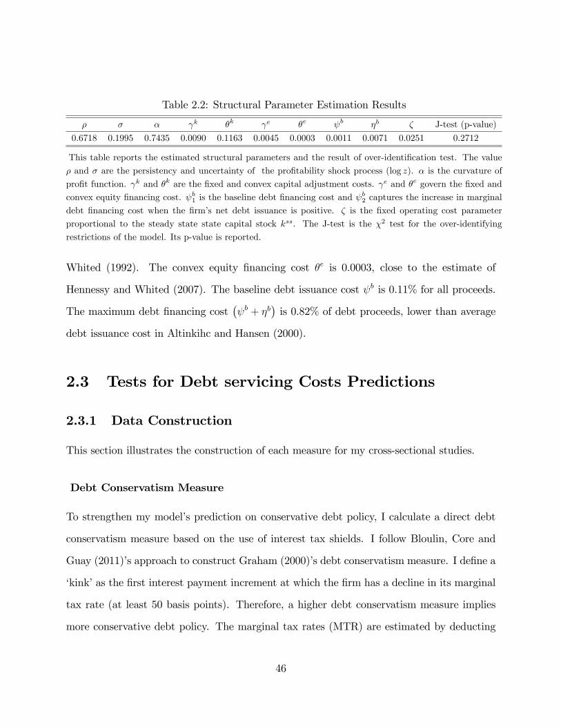
Table 2.2: Structural Parameter Estimation Results

� � � k �k e �e b �b � J-test (p-value)

0.6718 0.1995 0.7435 0.0090 0.1163 0.0045 0.0003 0.0011 0.0071 0.0251 0.2712

This table reports the estimated structural parameters and the result of over-identi�cation test. The value

� and � are the persistency and uncertainty of the pro�tability shock process (log z). � is the curvature of

pro�t function. k and �k are the �xed and convex capital adjustment costs. e and �e govern the �xed and

convex equity �nancing cost. b1 is the baseline debt �nancing cost and b2 captures the increase in marginal

debt �nancing cost when the �rm�s net debt issuance is positive. � is the �xed operating cost parameter

proportional to the steady state state capital stock kss. The J-test is the �2 test for the over-identifying

restrictions of the model. Its p-value is reported.

Whited (1992). The convex equity �nancing cost �e is 0.0003, close to the estimate of

Hennessy and Whited (2007). The baseline debt issuance cost b is 0.11% for all proceeds.

The maximum debt �nancing cost� b + �b

�is 0.82% of debt proceeds, lower than average

debt issuance cost in Altinkihc and Hansen (2000).

2.3 Tests for Debt servicing Costs Predictions

2.3.1 Data Construction

This section illustrates the construction of each measure for my cross-sectional studies.

Debt Conservatism Measure

To strengthen my model�s prediction on conservative debt policy, I calculate a direct debt

conservatism measure based on the use of interest tax shields. I follow Bloulin, Core and

Guay (2011)�s approach to construct Graham (2000)�s debt conservatism measure. I de�ne a

�kink�as the �rst interest payment increment at which the �rm has a decline in its marginal

tax rate (at least 50 basis points). Therefore, a higher debt conservatism measure implies

more conservative debt policy. The marginal tax rates (MTR) are estimated by deducting

46

various increments of the current interest payments from the taxable income, and the kink

is the increment of interest expense immediately before which results in the computed MTR

drop by at least 50 basis points. I follow the interest deduction schedule of Graham (2000); I

add the following increments of current interest payments to before-�nancing taxable income:

0%; 20%; 40%; 60%; 80%; 100%; 120%; 160%; 200%; 300%; 400%; 500%; 600%; 700%; and

800%. The income before tax is de�ned as follows:

EBIT+Special Items(SPI)

- Deferred Tax Expense (TXDC) /max. statutory tax rate

+Extraordinary Items and Discontinued Operations (XIDO)/(1-max. statutory tax rate),

where the symbols in parenthesis refer to the items in CRSP/Compustat merged database.

I simulate future interest expenses based on the changes in the interest coverage ratio.

So long as income at t is positive, future interest is changed by the ratio of income at t to

income at t � 1. If income at t is negative, I hold interest expenses constant for that year

(i.e., interest expenses at time t = 0 is equal to interest expenses at time t� 1). In terms of

past interest deductions, the interest expenses in historical taxable income is retroactively

adjusted. For example, when estimating the MTR at the 50% interest deduction increment

at time t, I assume that interest deductions in periods t�n to t� 1 are set to 50% of actual.

I do not incorporate the state tax rate and alternative minimum tax rate by following

the approach of Bloulin et al. (2011). They mainly point out the consistency problem in

the application of alternative minium tax rate. I re�ect the historical carry backward and

forward changes into my simulation as well.

47

Convex Capital Adjustment Costs

To analyze the implications of convex capital adjustment costs on capital structure choice,

I �rst calculate a �rm level convex adjustment cost estimate by using a modi�ed version

of Tobin�s q regression. Similar to Eberly�s (1997) approach, I regress a �rm�s investment-

asset ratio on Tobin�s q, operating pro�ts, and the investment good price for each �rm,

but only when the �rm�s investment is positive. The operating pro�t term is introduced

to capture the e¤ect of �nancing constraints, as in Fazzari, Hubbard and Petersen (1988).

This inclusion is in line with an important role of external �nancing costs in my model. To

capture non-convexity in capital expenditure, the regression is only conducted for positive

investment �rm-year observations. The regression model is summarized as follows:

I

K= �0 + �1Tobin�s q + �2pro�t+�3investment good price+ " for I > 0: (2.4)

After assignment of the �rm level convex capital adjustment cost estimate, I drop �rms

with negative capital adjustment costs because the quantitative predictions only hold for

the positive costs region. Each �rm is grouped by its two digit SIC code �rst, and then it is

categorized into convex capital adjustment cost quartiles within its industry group. Since the

convex capital adjustment cost is inversely related to �1, the �rms in the �rst quartile have

the highest convex capital adjustment cost estimates and the �rms in the fourth quartile

have the lowest ones.

Fixed Operating Costs

To construct �xed operating cost measure, I adopt a modi�ed version of the estimation

method used in Kahl et al. (2012). For this purpose, I �rstly generate ex-ante expectations

48

of sales and operating costs from the geometric growth rate over the previous two years:

E(Si;t) = Si;t�1

�Si;t�2Si;t�3

�and E(Xi;t) = Xi;t�1

�Xi;t�2

Xi;t�3

�(2.5)

in which Si;t and Xi;t indicate an individual �rm i0s sales and operating costs at time t,

respectively. I also calculate the innovations in growth rates as follows:

�Si;t =Si;t � E(Si;t)

Si;t�1and �Xi;t =

Xi;t � E(Xi;t)

Xi;t�1(2.6)

where �Si;t and �Xi;t point to the innovation of sales growth and operating cost growth, respec-

tively. To obtain a reliable estimate of �xed operating costs, I run the following regression

for the �rms with at least 12 years of observations in the sample period:

�Xi;t = FCi�Si;t + "i;t (2.7)

where FCi is an individual �rm�s �xed operating cost measure. This 12 year restriction

potentially relieves outlier problems from a limited horizon of observations. FCi re�ects the

sensitivity of operating cost growth to sales growth after taking account of growth trends.

Higher proportions of �xed costs to total operating costs will show a lower sensitivity and

consequently a lower estimate of FCi: Conversely, a higher estimate of FCi indicates more

variable costs relative to total costs. Then I introduce dummy variables indicating high and

low �xed operating costs �rms. The high �xed operating cost dummy variable is one if the

cost measure is in the �rst quartile and zero otherwise. The low �xed operating cost dummy

variable takes one if the cost measure is in the fourth quartile and zero, otherwise.

49

Pro�t Volatility

To construct a natural measure of pro�t volatility, I calculate the standard deviation of

operating pro�ts for each �rm that stays at least 12 years in the sample period. This

restriction potentially relieves outlier problems from young �rms. Then I generate dummy

variables indicating high and low pro�t volatility �rms. The high pro�t volatility indicator

variable takes the value of 1 if the standard deviation is in the fourth quartile. The low pro�t

volatility indicator variable is equal to 1 if the standard deviation is in the �rst quartile.

Future Investment Demands

For the measurement of expected future investment needs, I construct indicator variables

based on actual future capital expenditures. The use of indicator variables helps relieve a

potential measurement error problem stemming from the use of actual future investments

as explanatory variables. Unexpectedly great or poor investment opportunities in the next

period a¤ect actual future investment demands and the use of indicator variables partially

�lters out such unexpected components by covering a wide range of actual investments.

To construct dummy variables indicating large and small future investment, I �rst cal-

culate the ranking of the investment-asset ratio for each �rm-year observation relative to all

of the �rm�investment-asset ratios in the sample periods. Then I categorize each �rm-year

observation into a quartile corresponding to its investment-asset ratio ranking. The indicator

variable for large future investment takes one if a �rm�s next period investment-asset ratio

is in the fourth quartile, and zero otherwise. Similarly, the small investment dummy takes

one if a �rm�s next period investment-asset ratio is in the �rst quartile, and zero otherwise.

50

Table 2.3: Summary Statistics : Convex Capital Adjustment Cost Quartile

Observations Equity Freq. Leverage Cash Pro�t Conservatism

Panel A: All Firms

1st Quartile 6415 0.2023 0.2015 0.1817 0.0909 2.9844

2nd Quartile 6303 0.1988 0.2113 0.1668 0.0924 2.6283

3rd Quartile 6268 0.1903 0.2399 0.1415 0.0805 2.05

4th Quartile 5307 0.1577 0.2726 0.1225 0.0873 1.5757

Panel B: Non High-tech Firms

1st Quartile 4555 0.1488 0.2349 0.1182 0.1204 3.1229

2nd Quartile 4541 0.144 0.2406 0.1059 0.1202 2.6877

3rd Quartile 4658 0.1453 0.2634 0.0951 0.1139 2.2295

4th Quartile 3900 0.1131 0.3052 0.0781 0.1152 1.6128

Panel C:High-tech Firms

1st Quartile 1860 0.3333 0.1196 0.3373 0.0186 2.6232

2nd Quartile 1762 0.34 0.1356 0.3238 0.0207 2.4677

3rd Quartile 1610 0.3205 0.1718 0.2756 -0.0159 1.5127

4th Quartile 1407 0.2814 0.1823 0.2455 0.0099 1.4689

This table reports a variety of summary statistics for all �rms, high-tech �rms and non-high-

tech �rms according to convex capital adjustment cost quartiles. Only the �rms with at least

12 �rm-year observations are included in the calculations. Firms are included in the high-

tech category if their �rst three digit SIC code is 283, 357, 366, 382, 384, and 737, and all

other �rms are all in non high-tech category. All values are averaged except the number of

observations. The variable construction is illustrated in Appendix A.

2.3.2 Convex Capital Adjustment Costs

This section analyzes the in�uence of convex capital adjustment costs on a �rm�s capital

structure policies. As shown in Chapter 1, higher convex capital adjustment costs lead to

large costs in asset sales, which raise the marginal value of liquidity and debt servicing costs.

To investigate the role of convex capital adjustment costs on capital structure policies, I

adopt the quartile capital adjustment costs indicator variables, constructed in the previous

section. I cross-sectionally investigate the relationship between these indicator variables and

capital structure policies.

Table 2.3 reports summary statistics for each convex capital adjustment cost quartile

51

category. The table documents the average of leverage ratio, debt conservatism, cash holding,

and operating pro�ts. The frequency of equity �nancing is also reported. The table considers

only the �rms with at least 12 observations during the sample period, which provides a more

reliable convex capital adjustment cost estimate. High-tech and non high-tech sub-categories

are introduced to examine whether the overall summary statistics results stem from high-

tech industries, which are well known for low leverage and frequent equity �nancing (Hall

2002).

Table 2.3 indicates more conservative debt policy and frequent equity �nancing in high

convex capital adjustment cost �rms. Even though each category has stable average prof-

itability, high convex capital adjustment cost �rms tend to have low leverage ratios and large

debt conservatism measures. The average leverage ratio is 0.2015 in the �rst quartile and

rises to 0.2726 in the fourth quartile. Similarly, the debt conservatism measure decreases

from 2.98 to 1.58 in response to the same quartile variation. The �rms with higher convex

capital adjustment costs also use equity �nancing more frequently. The equity �nancing

frequency is 20% in the �rst quartile and decreases to 15% in the fourth quartile. The

sub-categorization of high-tech and non high-tech industry does not in�uence the qualitative

predictions from convex capital adjustment costs quartile variations.

Table 2.4 investigates the relationship between convex capital adjustment cost quartile

dummies and external �nancing policies in cross-sectional regression models. The leverage

ratio, debt conservatism measure, and binary decisions of equity �nancing are used as the

left-hand side variables. On the right hand side, I employ the convex capital adjustment

cost quartile dummies and a set of widely used �rm characteristics as control variables. The

control variables include the logged book asset values, asset tangibility, market to book ratio,

R&D expenditure, R&D activity and industry median leverage ratio, as suggested in Frank

and Goyal (2008). I also introduce the 3-year stock return in the equity �nancing analysis

52

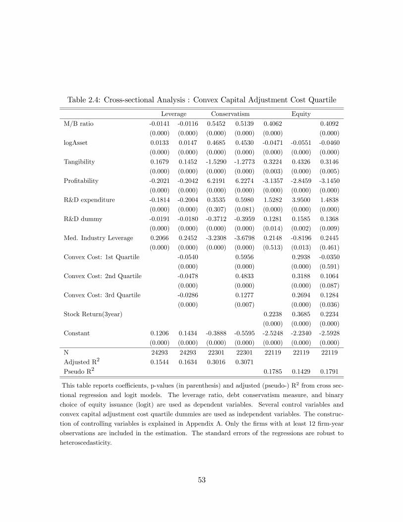
Table 2.4: Cross-sectional Analysis : Convex Capital Adjustment Cost Quartile

Leverage Conservatism Equity

M/B ratio -0.0141 -0.0116 0.5452 0.5139 0.4062 0.4092

(0.000) (0.000) (0.000) (0.000) (0.000) (0.000)

logAsset 0.0133 0.0147 0.4685 0.4530 -0.0471 -0.0551 -0.0460

(0.000) (0.000) (0.000) (0.000) (0.000) (0.000) (0.000)

Tangibility 0.1679 0.1452 -1.5290 -1.2773 0.3224 0.4326 0.3146

(0.000) (0.000) (0.000) (0.000) (0.003) (0.000) (0.005)

Pro�tability -0.2021 -0.2042 6.2191 6.2274 -3.1357 -2.8459 -3.1450

(0.000) (0.000) (0.000) (0.000) (0.000) (0.000) (0.000)

R&D expenditure -0.1814 -0.2004 0.3535 0.5980 1.5282 3.9500 1.4838

(0.000) (0.000) (0.307) (0.081) (0.000) (0.000) (0.000)

R&D dummy -0.0191 -0.0180 -0.3712 -0.3959 0.1281 0.1585 0.1368

(0.000) (0.000) (0.000) (0.000) (0.014) (0.002) (0.009)

Med. Industry Leverage 0.2066 0.2452 -3.2308 -3.6798 0.2148 -0.8196 0.2445

(0.000) (0.000) (0.000) (0.000) (0.513) (0.013) (0.461)

Convex Cost: 1st Quartile -0.0540 0.5956 0.2938 -0.0350

(0.000) (0.000) (0.000) (0.591)

Convex Cost: 2nd Quartile -0.0478 0.4833 0.3188 0.1064

(0.000) (0.000) (0.000) (0.087)

Convex Cost: 3rd Quartile -0.0286 0.1277 0.2694 0.1284

(0.000) (0.007) (0.000) (0.036)

Stock Return(3year) 0.2238 0.3685 0.2234

(0.000) (0.000) (0.000)

Constant 0.1206 0.1434 -0.3888 -0.5595 -2.5248 -2.2340 -2.5928

(0.000) (0.000) (0.000) (0.000) (0.000) (0.000) (0.000)

N 24293 24293 22301 22301 22119 22119 22119

Adjusted R2 0.1544 0.1634 0.3016 0.3071

Pseudo R2 0.1785 0.1429 0.1791

This table reports coe¢ cients, p-values (in parenthesis) and adjusted (pseudo-) R2 from cross sec-

tional regression and logit models. The leverage ratio, debt conservatism measure, and binary

choice of equity issuance (logit) are used as dependent variables. Several control variables and

convex capital adjustment cost quartile dummies are used as independent variables. The construc-

tion of controlling variables is explained in Appendix A. Only the �rms with at least 12 �rm-year

observations are included in the estimation. The standard errors of the regressions are robust to

heteroscedasticity.

53

to capture the market timing aspect of equity �nancing. I use the ordinary least squares

method in the leverage and debt conservatism measure analysis and adopt a logit model for

the binary choice of equity issuance decisions.

As expected, �rms with higher convex capital adjustment costs exercise more conservative

debt policy. Even after controlling for the �rm characteristics, the quartile dummies show a

monotonic relation with the leverage ratio and debt conservatism measure. Convex capital

adjustment costs are negatively correlated with the leverage ratio and positively correlated

with the debt conservatism measure.

The logit regression results partially support more frequent equity �nancing in large

convex capital adjustment cost �rms. Without inclusion of the market to book ratio, higher

convex capital adjustment cost dummies are positively and almost monotonically correlated

with equity issuance decisions. Yet, the inclusion of the market to book ratio drastically

changes the coe¢ cients of quartile dummies, especially for the �rms with the largest convex

capital adjustment cost estimates.

The drastic changes of quartile coe¢ cients in the logit model are probably related to

the information of the market to book ratio captured in the convex capital adjustment

cost dummies. In the estimation of �rm level convex capital adjustment costs, I use a

�rm�s Tobin�s q value as an independent variable, which is a modi�cation of the market to

book ratio. The market to book variation may directly re�ect more signi�cant information

regarding equity �nancing decisions.

To summarize, �rms with higher convex capital adjustment costs tend to use debt more

conservatively and equity �nancing more frequently, even after considering industry and

other �rm characteristics. Both of the summary statistics and regression analysis results

generally con�rm these tendencies. These �ndings are consistent with the debt servicing

cost predictions in Chapter 1.

54

2.3.3 Fixed Operating Costs

This section analyzes the relationship between �xed operating costs and a �rm�s capital

structure policies. In the previous chapter, I quantitatively showed large �xed operating

costs are closely associated with low leverage ratios and frequent equity �nancing activities.

Higher �xed operating costs raise the marginal value of liquidity and consequently drive large

debt servicing costs. To analyze the implications of higher �xed operating costs on �nancing

policies, I use the indicator variables constructed in the previous section and cross-sectionally

analyze the relationship between these dummy variables and capital structure choices.

Table 2.3 reports summary statics results according to the �xed operating costs indicator

variables. The table documents the average of leverage ratio, debt conservatism, cash hold-

ing, and operating pro�ts. The equity �nancing frequency is also included. The summary

statistics are calculated for di¤erent sub-categories such as high-tech industry, non high-tech

industries, young �rms and old �rms. I examine the high-tech category to capture the in-

�uence of human capital intensive �rms, well known for low leverage and frequent equity

�nancing (Hall 2002). The young-old �rm categories are also included because younger �rms

tend to maintain lower leverage and issue equity more frequently (Frank and Goyal 2003).

In line with the debt servicing cost predictions, higher �xed operating costs �rms are

closely associated with low leverage and frequent equity �nancing. Conversely, lower �xed

operating costs �rms show higher leverage ratios and inactive equity issuance activities. For

instance, the average leverage ratio for the low �xed operating costs �rms is 0.2705 but

decreases to 0.1657 for the high �xed operating costs �rms. Equity �nancing frequency is

10% for the low �xed operating costs �rms but becomes 28% for the high �xed operating costs

�rms. These qualitative predictions remain unchanged for the sub-categories of high-tech,

non-high-tech, young �rms, and old �rms.

However, the relationship between �xed operating costs and the debt conservatism mea-

55

Table 2.5: Summary Statistics : Fixed Operating Costs

Equity Leverage Cash Pro�t Conservatism

Panel A : All Firms

Low Fixed Operating Costs 0.1157 0.2705 0.0848 0.1407 3.0547

Others 0.148 0.2214 0.1383 0.1139 2.555

High Fixed Operating Costs . 0.3871 0.1657 0.3227 -0.0632 1.1718

Panel B: Old Firm-Year Observation

Low Fixed Operating Costs 0.0823 0.2788 0.0717 0.1375 3.0597

Others 0.102 0.2217 0.1298 0.1121 2.6731

High Fixed Operating Costs . 0.3021 0.1778 0.2923 -0.0334 1.3962

Panel C: Young Firm-Year Observation

Low Fixed Operating Costs 0.3021 0.1778 0.2923 -0.0334 1.3962

Others 0.1874 0.2527 0.113 0.1476 3.0418

High Fixed Operating Costs . 0.2302 0.2208 0.1535 0.117 2.2994

Panel D: Non High-tech Firms

Low Fixed Operating Costs 0.1007 0.289 0.0665 0.1423 2.8906

Others 0.1231 0.2469 0.1049 0.1217 2.5717

High Fixed Operating Costs . 0.3017 0.2105 0.2017 0.008 1.0805

Panel E : High-tech Firms

Low Fixed Operating Costs 0.2055 0.1599 0.1948 0.1313 4.105

Others 0.2219 0.1454 0.2378 0.0905 2.5045

High Fixed Operating Costs . 0.4484 0.1335 0.4095 -0.1143 1.2388

This table reports a variety of summary statistics for all �rms, young-�rm year old-�rm year, high-

tech �rms and non-high-tech �rms according to �xed operating costs dummies. Young �rm-year

observation indicates all �rms that stay less than 12 years in CRSP/Compustat database or the

�rst 12 �rm-year observations for the �rms that stay more than 12 years in the database. The other

descriptions are identical to those of Table 2.3

sure is not well aligned with the debt servicing cost predictions. Higher �xed operating

costs �rms rather use debt more aggressively than lower �xed operating costs �rms do. For

instance, the average debt conservatism measure for the high �xed operating costs �rms is

1.17 but increases to 3.0 for the low �xed operating costs �rms. This contradictory pattern

appears closely associated with the quite low pro�tability in the high �xed operating cost

category �rms. Even with low leverage ratios, lower pro�tability induces a signi�cant drop

in debt conservatism measure, which points to more aggressive use of interest tax shields for

56

these �rms. This correlation between the �xed operating cost dummy variables and prof-

itability suggests a potential measurement problem in Kahl et al. (2012)�s �xed operating

cost estimation.

Table 2.6 analyzes cross-sectional correlations between the �xed operating cost dummy

variables and capital structure choice. All regression and logit model speci�cations are

identical to those of Table 2.4, except the inclusion of the �xed operating cost indicator

variables replacing the convex capital adjustment cost dummies. The book asset value in

logs, tangibility, market to book ratio, R&D expenditure, R&D activity and industry median

leverage ratio are used as control variables in regressions. The logit model incorporates 3-year

stock returns to capture market timing aspects of equity �nancing.

My �ndings in cross-sectional models are consistent to the summary statics results in

Table 2.5. The high �xed operating cost indicator variable is associated with lower leverage

ratios and more frequent equity �nancing activities. Conversely, the low �xed operating

cost dummy variable is correlated positively with leverage ratios and negatively with equity

�nancing frequencies. Yet, an increase in �xed operating costs is still negatively related

with the measure of debt conservatism, which is inconsistent with the debt servicing cost

predictions.

The summary statistics results and regression analyses all con�rm the validity of the debt

servicing costs predictions in terms of leverage ratios and equity �nancing frequencies. Higher

�xed operating cost �rms maintain lower leverage ratios and use equity more frequently.

These results are also consistent with the empirical work of Kahl et al. (2012); their �xed

operating cost measure is negatively correlated with leverage ratios and positively associated

with equity issues. Yet, my results on the debt conservatism measure are not well aligned

with the debt servicing cost predictions. The �xed operating measure used in prior literature

appears to generate a tendency for selecting lower pro�tability �rms as high �xed operating

57

Table 2.6: Cross-sectional Analysis : Fixed Operating Costs

Leverage Conservatism Equity

M/B ratio -0.0138 -0.0129 0.5549 0.5685 0.3826 0.3602

(0.000) (0.000) (0.000) (0.000) (0.000) (0.000)

logAsset 0.0144 0.0131 0.4348 0.4160 -0.0751 -0.0538

(0.000) (0.000) (0.000) (0.000) (0.000) (0.000)

Tangibility 0.1830 0.1872 -1.8210 -1.7738 0.3631 0.2592

(0.000) (0.000) (0.000) (0.000) (0.000) (0.003)

Pro�tability -0.2120 -0.2265 6.7393 6.5343 -3.2067 -2.8903

(0.000) (0.000) (0.000) (0.000) (0.000) (0.000)

R&D expenditure -0.2586 -0.2289 1.0636 1.4765 1.6668 1.1899

(0.000) (0.000) (0.000) (0.000) (0.000) (0.000)

R&D dummy -0.0151 -0.0127 -0.4344 -0.4024 0.0786 0.0367

(0.000) (0.000) (0.000) (0.000) (0.050) (0.364)

Med. Industry Leverage 0.1692 0.1612 -2.8942 -3.0239 0.3355 0.4715

(0.000) (0.000) (0.000) (0.000) (0.197) (0.074)

Low Fixed Operating Costs 0.0095 0.1650 -0.1164

(0.000) (0.000) (0.006)

High Fixed Operating Costs -0.0311 -0.4180 0.4989

(0.000) (0.000) (0.000)

Stock Return (3year) 0.2441 0.2459

(0.000) (0.000)

Constant 0.1175 0.1251 -0.2205 -0.1146 -2.4266 -2.5651

(0.000) (0.000) (0.000) (0.038) (0.000) (0.000)

N 41399 41399 38000 38000 37709 37709

Adjusted R2 0.1726 0.1758 0.3049 0.3074

Pseudo R2 0.1746 0.1791

This table reports coe¢ cients, p-values (in parenthesis) and adjusted (pseudo-) R2 from

cross sectional regression and logit models. The leverage ratio, debt conservatism measure,

and binary choice of equity issuance (logit) are used as dependent variables. Several control

variables and the indicator variables for future investment demands are used as indepen-

dent variables. The construction of controlling variables is explained in Appendix A. The

standard errors of the regressions are robust to heteroscedasticity.

58

costs ones.

2.3.4 Pro�t Volatility

This section cross-sectionally investigates how the volatility of pro�t generation a¤ects a

�rm�s capital structure choice. Given the same pro�tability state, a highly volatile operating

pro�t implies a greater likelihood of lower pro�tability states in the future. As analyzed in

Chapter 1, such higher likelihoods of lower pro�tability states indicate a higher marginal

value of liquidity in the future, which induces an expectation of large debt servicing costs

in current debt issues. To examine the implications of pro�t volatilities, I use indicator

variables for high and low pro�t volatility �rms developed in the previous section.

Table 2.7 shows summary statics results in accordance with the pro�t volatility indica-

tors. The table describes the average of leverage ratio, debt conservatism, cash holding,

and operating pro�ts. The equity �nancing frequency is also documented. The summary

statistics are reported for di¤erent sub-categories such as high-tech industry, non high-tech

industries, young �rms and old �rms. I include the high-tech category to capture the in-

�uence of human capital intensive �rms, well known for low leverage and frequent equity

�nancing (Hall 2002). The young-old �rm categories are also included because younger �rms

tend to maintain lower leverage and issue equity more frequently (Frank and Goyal 2003).

Consistent with the debt servicing cost predictions, �rms with highly volatile pro�ts are

closely associated with low leverage ratios and active equity �nancing. Conversely, �rms with

low pro�t volatility are closely connected with higher leverage ratios and a lower frequency

of equity �nancing. For instance, the average leverage ratio for the low pro�t volatility

�rms is 0.2931 but drops to 0.1721 for the high pro�t volatility �rms. The equity �nancing

frequency is 0.0967 but increases to 0.3706 in response to the same �rm category changes.

These qualitative predictions remain stable for the sub-categories of high-tech, non-high-tech,

59

Table 2.7: Summary Statistics : Pro�t Volatility

Equity Leverage Cash Pro�t Conservatism

Panel A : All Firms

Low Pro�t Volatility 0.0967 0.2931 0.0634 0.1313 2.8711

Others 0.1385 0.2129 0.1456 0.1315 2.821

High Pro�t Volatility . 0.3706 0.1721 0.2848 -0.0474 1.1134

Panel B: Old Firm-Year Observation

Low Pro�t Volatility 0.0734 0.2962 0.0582 0.1303 2.8959

Others 0.0909 0.2104 0.1354 0.1286 2.9383

High Pro�t Volatility . 0.3706 0.1721 0.2848 -0.0474 1.1134

Panel C: Young Firm-Year Observation

Low Pro�t Volatility 0.1658 0.2839 0.0788 0.1342 2.7812

Others 0.2169 0.2171 0.1623 0.1363 2.5867

High Pro�t Volatility . 0.4382 0.1633 0.3019 -0.0603 1.047

Panel D: Non High-tech Firms

Low Pro�t Volatility 0.0971 0.3032 0.0555 0.1287 2.7336

Others 0.1117 0.2397 0.1064 0.1365 2.7523

High Pro�t Volatility . 0.2957 0.2104 0.1945 0.0204 1.2212

Panel E : High-tech Firms

Low Pro�t Volatility 0.0935 0.1983 0.1375 0.1562 4.177

Others 0.2147 0.1365 0.2571 0.1172 3.0218

High Pro�t Volatility . 0.4356 0.1389 0.3632 -0.1062 1.0185

This table reports a variety of summary statistics for all �rms, young-�rm year old-�rm year, high-

tech �rms and non-high-tech �rms according to �xed operating costs dummies. Young �rm-year

observation indicates all �rms that stay less than 12 years in CRSP/Compustat database or the

�rst 12 �rm-year observations for the �rms that stay more than 12 years in the database. The other

descriptions are identical to those of Table 2.3

young �rms, and old �rms.

Yet, the debt conservatism measure shows a distinctive pattern. The �rms with highly

volatile pro�ts rather use debt more aggressively than the �rms with low pro�t volatility

do. For example, the average debt conservatism measure for the �rms with highly volatile

pro�ts is 1.11 but increases to 2.87 for their low volatility counterparts. Similar to the result

of �xed operating costs, this contradictory pattern seems to be closely related with the quite

low pro�tability for the higher pro�t volatility �rms. In spite of lower leverage ratios, lower

60

pro�tability leads to more aggressive use of tax bene�ts.

Table 2.8 cross-sectionally investigates how the pro�t volatility indicator variables are

correlated with a �rm�s capital structure choices. All regression and logit model speci�ca-

tions are identical to those of Table 2.4, except the inclusion of the volatility dummy variables

replacing the convex capital adjustment cost dummies. The book asset value in logs, tangi-

bility, market to book ratio, R&D expenditure, R&D activity and industry median leverage

ratio are placed as control variables in regressions. The logit model incorporates 3-year stock

returns to capture market timing aspects of equity �nancing.

The cross-sectional correlations are in line with the summary statics results in Table 2.7.

The indicator variable for lower pro�t volatility shows a positive correlation with leverage

ratios and a negative correlation with the frequency of equity �nancing. This low pro�t

volatility variable is also negatively associated with the debt conservatismmeasure, consistent

with the debt servicing cost predictions. The indicator variable for higher pro�t volatility

is negatively associated with leverage ratios and positively associated with equity �nancing

activities even after controlling for other �rm characteristics. Yet, this high volatility variable

is negatively correlated with the debt conservatism measure pointing to more aggressive use

of tax bene�ts.

These �nding are well aligned with the debt servicing costs predictions on capital struc-

ture policies, as proposed in Chapter 1. Low pro�t volatility �rms maintain higher leverage

ratios, exercise more aggressive debt policy and issue equity less frequently, consistent with

the debt servicing costs predictions. High pro�t volatility �rms show lower leverage ratios

and more frequent equity �nancing activities, as expected in the debt servicing costs analy-

sis. Yet, the debt conservatism measure is negatively related with the indicator variable of

highly volatile pro�ts, which argues against the debt servicing cost predictions. A potential

association between lower pro�t generations and higher pro�t variations may be behind more

61

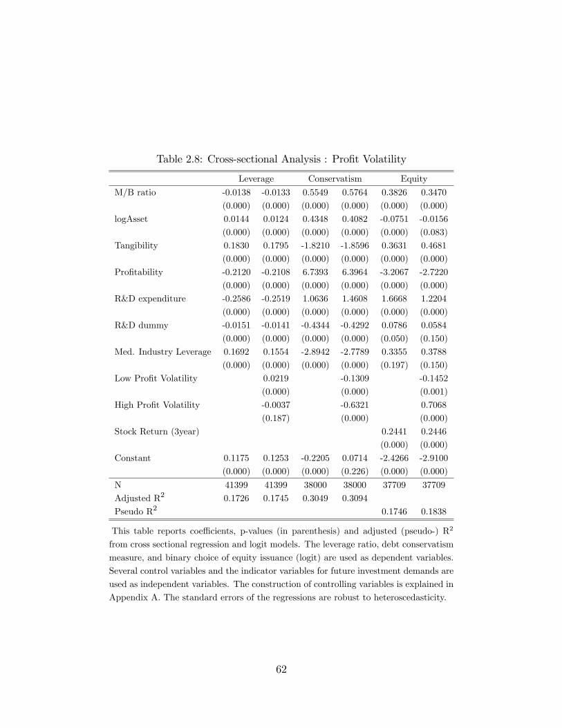
Table 2.8: Cross-sectional Analysis : Pro�t Volatility

Leverage Conservatism Equity

M/B ratio -0.0138 -0.0133 0.5549 0.5764 0.3826 0.3470

(0.000) (0.000) (0.000) (0.000) (0.000) (0.000)

logAsset 0.0144 0.0124 0.4348 0.4082 -0.0751 -0.0156

(0.000) (0.000) (0.000) (0.000) (0.000) (0.083)

Tangibility 0.1830 0.1795 -1.8210 -1.8596 0.3631 0.4681

(0.000) (0.000) (0.000) (0.000) (0.000) (0.000)

Pro�tability -0.2120 -0.2108 6.7393 6.3964 -3.2067 -2.7220

(0.000) (0.000) (0.000) (0.000) (0.000) (0.000)

R&D expenditure -0.2586 -0.2519 1.0636 1.4608 1.6668 1.2204

(0.000) (0.000) (0.000) (0.000) (0.000) (0.000)

R&D dummy -0.0151 -0.0141 -0.4344 -0.4292 0.0786 0.0584

(0.000) (0.000) (0.000) (0.000) (0.050) (0.150)

Med. Industry Leverage 0.1692 0.1554 -2.8942 -2.7789 0.3355 0.3788

(0.000) (0.000) (0.000) (0.000) (0.197) (0.150)

Low Pro�t Volatility 0.0219 -0.1309 -0.1452

(0.000) (0.000) (0.001)

High Pro�t Volatility -0.0037 -0.6321 0.7068

(0.187) (0.000) (0.000)

Stock Return (3year) 0.2441 0.2446

(0.000) (0.000)

Constant 0.1175 0.1253 -0.2205 0.0714 -2.4266 -2.9100

(0.000) (0.000) (0.000) (0.226) (0.000) (0.000)

N 41399 41399 38000 38000 37709 37709

Adjusted R2 0.1726 0.1745 0.3049 0.3094

Pseudo R2 0.1746 0.1838

This table reports coe¢ cients, p-values (in parenthesis) and adjusted (pseudo-) R2

from cross sectional regression and logit models. The leverage ratio, debt conservatism

measure, and binary choice of equity issuance (logit) are used as dependent variables.

Several control variables and the indicator variables for future investment demands are

used as independent variables. The construction of controlling variables is explained in

Appendix A. The standard errors of the regressions are robust to heteroscedasticity.

62

Table 2.9: Summary Statistics : Future Investment Demands

Equity Leverage Cash Pro�t Conservatism

Panel A : All Firms

Small Future Investment 0.1995 0.2555 0.174 0.0257 1.8741

Others 0.2404 0.2379 0.1705 0.0416 2.1588

Large Future Investment 0.2942 0.188 0.197 0.0905 2.8486

Panel B: Old Firm-Year Observation

Small Future Investment 0.1024 0.259 0.1307 0.0819 2.2973

Others 0.1196 0.2358 0.1286 0.0979 2.5487

Large Future Investment 0.1606 0.1888 0.1542 0.1321 3.2632

Panel C: Young Firm-Year Observation

Small Future Investment 0.2843 0.2524 0.2118 -0.0233 1.3488

Others 0.3372 0.2395 0.2041 -0.0036 1.7167

Large Future Investment 0.4005 0.1874 0.231 0.0573 2.3345

Panel D: Non High-tech Firms

Small Future Investment 0.1497 0.2969 0.1077 0.0667 1.9137

Others 0.1859 0.2735 0.1094 0.084 2.2437

Large Future Investment 0.2367 0.221 0.1333 0.126 2.9502

Panel E : High-tech Firms

Small Future Investment 0.3194 0.1556 0.3336 -0.0731 1.7712

Others 0.3692 0.1539 0.3149 -0.0588 1.9492

Large Future Investment 0.4326 0.1086 0.3504 0.005 2.595

This table reports a variety of summary statistics for all �rms, young-�rm year old-�rm year,

high-tech �rms and non-high-tech �rms according to future investment dummies. Young �rm-year

observation indicates all �rms that stay less than 12 years in CRSP/Compustat database or the

�rst 12 �rm-year observations for the �rms that stay more than 12 years in the database. The other

descriptions are identical to those of Table 2.3

aggressive debt policy for the �rms with highly volatile pro�ts.

2.3.5 Future Investment Demands

This section analyzes how future investment demands in�uence current external �nancing

policies. Large future investments increase the marginal value of liquidity, after controlling

for a �rm�s operating pro�ts. By similar reasoning, small future investment demands are

closely associated with low debt servicing costs.

63

Table 2.9 documents summary statistics results according to the future investment in-

dicator variables. The table reports the average of leverage ratio, debt conservatism, cash

holding, and operating pro�ts. The equity �nancing frequency is also documented. The

summary statistics are calculated for di¤erent sub-categories such as high-tech industry, non

high-tech industries, young �rms and old �rms. I introduce the high-tech category to capture

the in�uence of human capital intensive �rms, well known for low leverage and frequent eq-

uity �nancing (Hall 2002). The young-old �rm categories are also examined because younger

�rms tend to maintain lower leverage and use equity �nancing more frequently (Frank and

Goyal 2003).

Consistent with debt servicing cost predictions, �rms with large future investment are

closely associated with low leverage, conservative debt policy and frequent equity �nancing

despite higher pro�tability levels. Conversely, �rms with small future investment are cor-

related with higher leverage, less conservative debt policy and infrequent equity �nancing,

in spite of lower pro�tability levels. For instance, the average leverage ratio is 0.255 for

�rms with small future investment but 0.188 for �rms with large future investment. Equity

�nancing frequency is 29.5% for the �rms with large future investments but 20% for the

�rms with large future investments. The qualitative predictions remain unchanged for the

sub-categories of high-tech, non-high-tech, young �rms and old �rms.

Table 2.10 investigates the relationship between future investment demands and current

capital structure choice in cross-sectional regression models. All regression and logit model

speci�cations are identical to those of Table 2.4, except the inclusion of the future investment

indicator variables replacing the convex capital adjustment cost dummies. The book asset

value in logs, tangibility, market to book ratio, R&D expenditure, R&D activity and indus-

try median leverage ratio are still used as control variables. The 3-year stock returns are

additionally incorporated in the logit model for equity �nancing to capture market timing

64

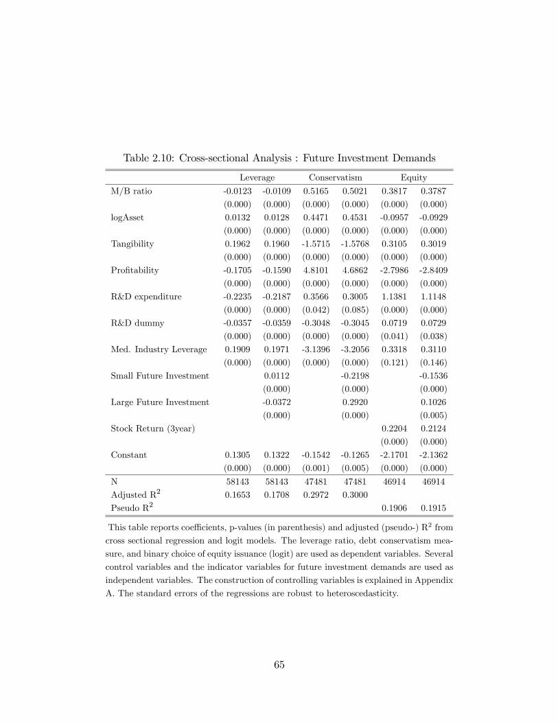
Table 2.10: Cross-sectional Analysis : Future Investment Demands

Leverage Conservatism Equity

M/B ratio -0.0123 -0.0109 0.5165 0.5021 0.3817 0.3787

(0.000) (0.000) (0.000) (0.000) (0.000) (0.000)

logAsset 0.0132 0.0128 0.4471 0.4531 -0.0957 -0.0929

(0.000) (0.000) (0.000) (0.000) (0.000) (0.000)

Tangibility 0.1962 0.1960 -1.5715 -1.5768 0.3105 0.3019

(0.000) (0.000) (0.000) (0.000) (0.000) (0.000)

Pro�tability -0.1705 -0.1590 4.8101 4.6862 -2.7986 -2.8409

(0.000) (0.000) (0.000) (0.000) (0.000) (0.000)

R&D expenditure -0.2235 -0.2187 0.3566 0.3005 1.1381 1.1148

(0.000) (0.000) (0.042) (0.085) (0.000) (0.000)

R&D dummy -0.0357 -0.0359 -0.3048 -0.3045 0.0719 0.0729

(0.000) (0.000) (0.000) (0.000) (0.041) (0.038)

Med. Industry Leverage 0.1909 0.1971 -3.1396 -3.2056 0.3318 0.3110

(0.000) (0.000) (0.000) (0.000) (0.121) (0.146)

Small Future Investment 0.0112 -0.2198 -0.1536

(0.000) (0.000) (0.000)

Large Future Investment -0.0372 0.2920 0.1026

(0.000) (0.000) (0.005)

Stock Return (3year) 0.2204 0.2124

(0.000) (0.000)

Constant 0.1305 0.1322 -0.1542 -0.1265 -2.1701 -2.1362

(0.000) (0.000) (0.001) (0.005) (0.000) (0.000)

N 58143 58143 47481 47481 46914 46914

Adjusted R2 0.1653 0.1708 0.2972 0.3000

Pseudo R2 0.1906 0.1915

This table reports coe¢ cients, p-values (in parenthesis) and adjusted (pseudo-) R2 from

cross sectional regression and logit models. The leverage ratio, debt conservatism mea-

sure, and binary choice of equity issuance (logit) are used as dependent variables. Several

control variables and the indicator variables for future investment demands are used as

independent variables. The construction of controlling variables is explained in Appendix

A. The standard errors of the regressions are robust to heteroscedasticity.

65

aspects.

The cross-sectional results are consistent with the debt servicing cost predictions devel-

oped in the previous chapter. The �rms with large future investment are closely associated

with low leverage, conservative debt policy and frequent equity �nancing, even after con-

trolling for other �rm characteristics. The small future investment dummy is negatively

related with the leverage ratio, and positively related with the debt conservatism measure

and equity �nancing, as expected. All coe¢ cients are highly signi�cant and the signs of

these coe¢ cients are in line with the debt servicing cost predictions.

The coe¢ cients of investment dummies in equity �nancing regression contradict the pre-

dictions of the standard trade-o¤models. The standard trade-o¤theory predicts less frequent

equity �nancing for �rms with conservative debt policy and high pro�tability. Yet, the �rms

with large future investment use equity �nancing more frequently in spite of their conserva-

tive use of debt and large operating pro�ts. The �rms with small investment are reluctant

to issue equity despite low pro�tability and large debt obligations, which also argues against

the standard trade-o¤ theory predictions.

The regression analysis for the leverage ratio provides an interesting result to the puzzling

negative correlation between leverage ratio and pro�tability (Frank and Goyal 2008). The in-

troduction of investment dummy variables slightly weakens the negative correlation between

pro�tability and leverage (�0:1705 ! �0:1590) and the change is statistically signi�cantly

at 95% level.1 The debt conservatism analysis shows a similar change of the pro�tability

coe¢ cient, which suggests the weaker correlation is not a mere coincidence. Debt servic-

ing costs considerations appear to have some explanatory power in resolving the puzzling

negative correlation between pro�tability and leverage ratio.

In summary, the relationship between future investment and current capital structure

1The p-value is not reported here.

66

choices is consistent with the debt servicing cost predictions. Large future investment de-

mands are closely associated with currently lower leverage and more frequent equity issuance.

Equity �nancing behaviors in both small and large future investment �rms contradict the

standard trade-o¤ theory predictions. The inclusion of investment variables weakens the

negative correlation between pro�tability and leverage ratio.

2.4 Concluding Remarks

This chapter empirically supports the theoretical analysis on debt servicing costs in the

previous chapter. In the �rst half of this chapter, I studied the statistical property of the

simulated method of moment estimator and investigated a detailed identi�cation procedure

used for the calibration of the baseline model in Chapter 1.

In the second half of this chapter, I empirically con�rmed the validity of debt servicing

costs predictions for public U.S. �rms. I proposed that large debt servicing costs are closely

associated with low leverage ratios and frequent equity �nancing activities in the previous

chapter. I conducted four cross-sectional studies to test these empirical predictions from

large debt servicing costs. The e¤ects of convex capital adjustment costs, �xed operating

costs, future investment demands and the volatility of pro�ts on capital structure policies

are analyzed in the second half.

All of the four empirical studies argue for the debt servicing cost predictions on capital

structure policies. Firms with high convex capital adjustment costs, high �xed operating

costs, large future investment needs, and highly volatile pro�ts are all negatively correlated

with leverage ratios and positively correlated with equity �nancing frequencies. These corre-

lations results are all consistent with the debt servicing costs predictions on capital structure

policies.

67

These �ndings also provide new insights on empirical regularities. Especially, �rms ex-

pecting large future investment demands use equity frequently, in spite of their higher prof-

itability level and large unused interest tax shields, contradictory to the standard trade-o¤

theory predictions. This correlation between future investment and pro�tability also weak-

ens the puzzling negative correlation between leverage ratio and pro�tability (Frank and

Goyal 2008). The analysis on convex capital adjustment costs is also closely associated with

lower leverage and frequent equity �nancing activities in human capital intensive �rms (Hall

2003). The results from �xed operating costs are consistent with the empirical �ndings of

Kahl et al. (2012) as well.

This cross-sectional analysis also provides lucrative future research directions. Even

though my cross-sectional results are all well aligned with the debt servicing cost predic-

tions, other empirical approaches resolving endogeniety issues will strengthen the validity of

the debt servicing cost predictions. Furthermore, this analysis on the debt servicing cost pre-

dictions could be extended internationally. This liquidity consideration on capital structure

policy is quite general to be tested for a di¤erent group of countries.

68

Chapter 3

Macroeconomic Conditions and Capital Structure

Dynamics

3.1 Introduction

The �nancial crisis of 2008 rea¢ rms that economic contractions critically a¤ect an individual

�rm�s investment needs, pro�ts, and external �nancing conditions altogether. Practitioners

widely recognize these macroeconomic conditions as key determinants in their �nancing

policies. A primary goal of chief �nancial o¢ cers is to maintain �nancial �exibility, so they

do not need to shrink their business in downturns (Graham and Harvey 2001). Financially

constrained �rms, indeed, cut their investments sharply and had substantial di¢ culties to

access external �nancing markets in the �nancial crisis of 2008 (Campello, Graham, and

Harvey 2011).

Yet, little theoretical inquiry explores how these simultaneous changes in investment

needs, pro�tability, and external �nancing conditions shape the cyclical variations of capital

structure policies. Indeed, research to date has largely ignored the following related ques-

tions: What factors drive empirically observed counter-cyclical debt policy and pro-cyclical

69

equity issues? How do investment dynamics in�uence the issuance of debt and equity? How

does a large value of liquidity in economic downturns change debt policies during economic

upturns? What are the implications of stochastic external �nancing conditions on capital

structure dynamics?

I develop and estimate a new dynamic corporate model with macroeconomic conditions

to address these questions. My model builds on recent dynamic trade-o¤ models with pre-

cautionary cash holding (Lee 2013; Gamba and Triantis 2008), mainly by adding macro-

economic pro�tability and �nancing cost shocks. A �rm makes investment, cash retention,

capital structure, and payout decisions. Both macroeconomic and idiosyncratic pro�tability

shocks a¤ect the �rm�s pro�t generations in persistent ways. Macroeconomic conditions also

in�uence the �rm�s external �nancing costs, which create the precautionary value of liquid-

ity. Capital accumulation and resale are not perfectly �exible due to the organizational costs

involved in investment decisions in my model.

Pro-cyclical pro�tability, investment dynamics, and stochastic external �nancing costs are

all pivotal in the capital structure dynamics. Lower pro�tability in downturns contributes

to counter-cyclical debt policy in a couple of ways. First, low operating pro�t generations

directly limit the use of internal funds for aggressive debt retirements in economic downturns.

Second, such lower pro�tability raises the marginal value of liquidity in contractions, leading

to active debt retirements and restrained debt issues in economic upturns. Servicing debt

obligations drains a �rm�s valuable liquidity and hence creates a liquidity cost associated

with debt, i.e., �debt servicing costs�(Bolton, Chen and Wang 2014; Lee 2013). To avoid

large liquidity costs of debt during economic downturns, a manager has strong incentives

to retire debt with ample operating pro�ts, and to optimally limit debt issuance during

economic upturns.

Next, investment dynamics drive the issuance of external debt and equity. In order to

70

fund larger investment needs, a manager relies more heavily on external debt and equity

issuance, ceteris paribus. The joint realization of pro�ts and investment demands critically

in�uences capital structure dynamics, unlike the standard trade-o¤ theory predictions that

focus primarily on pro�tability. This investment demand possibly induces active debt issues

during economic downturns, which also contributes to counter-cyclical debt policy.

Counter-cyclical equity �nancing costs lead to pro-cyclical equity issues, and more counter-

cyclical debt �nancing policy. A higher equity �nancing cost drives additional debt issues at

external �nancing margins in economic downturns. It also raises the marginal value of liq-

uidity, which, in turn, induces more conservative debt use in economic upturns. Pro-cyclical

equity issues critically depend on this cyclical variation of equity �nancing costs as well;

equity issues tend to be counter-cyclical under constant external �nancing conditions.

My quantitative analysis yields the following main results. First of all, equity issues are

pro-cyclical and concentrated for small, low pro�t, and large investment demand �rms in

earlier stages of upturns. Lower capital accumulations during economic downturns leave a

number of small �rms in earlier stage of economic upturns. Even with low current pro�ts,

these small �rms have large investment needs due to the decreasing returns to scale tech-

nology. To �nance such endogenously large investment needs, small �rms with low pro�ts

rely heavily on equity issuance; both large debt servicing costs predicted by currently low

pro�ts, and lower equity �nancing costs in upturns encourage equity �nancing at these ex-

ternal �nancing margins. These business cyclical property and �rm characteristics of equity

�nancing are consistent with recent empirical �ndings of Dittmar and Dittmar (2008) and

Frank and Goyal (2003).

Second, my model generates a positive correlation between payouts and equity issues,

and highlights the importance of stochastic equity �nancing costs in driving this positive

correlation. Payouts move pro-cyclically and peak at later stages of economic expansions

71

due to lower pro�tability in economic contractions and large investment needs in earlier

stages of upturns. Counter-cyclical equity �nancing costs drive pro-cyclical equity issuance,

resulting in a positive correlation with equity issues and payouts. Yet, constant external

�nancing conditions lead to counter-cyclical equity issuance and consequently its negative

correlation with payout. This business cyclical property of payout and its positive correlation

with equity issuance are all consistent with Dittmar and Dittmar (2008).

Third, and unlike the standard trade-o¤ theory predictions, my model generates counter-

cyclical debt policies, and higher leverage ratios after debt issues and retirements during

economic downturns. A �rm encounters external �nancing margins frequently to fund operat-

ing needs for investment, even during economic downturns. Lower pro�tability in downturns

raises the marginal value of liquidity, leading to active debt retirements and conservative

debt issues in upturns. Such low pro�ts limit aggressive debt retirements in downturns as

well. These economic forces induce counter-cyclical debt policy, and, higher leverage ratios

after debt adjustments in downturns, even under constant external �nancing conditions.

Counter-cyclical equity �nancing costs strengthen the above counter-cyclical trends in debt

policy. My model �ndings are consistent with the empirical work of Korajczyk and Levy

(2003) documenting counter-cyclicality in actual and target leverage ratios.

Fourth, my comparative static analysis points to pro-cyclical debt �nancing policies for

�nancially constrained �rms. The �ight-to-quality hypothesis predicts counter-cyclical debt

�nancing costs for lower credit rating or more �nancially constrained �rms. My model di-

rectly shows that counter-cyclical variations in debt �nancing costs drive pro-cyclical leverage

ratios and net debt issues. This �nding is in line with the empirical works of Eri, Julio, Kim

and Weisbach (2011), and Korajczyk and Levy (2003); both studies document pro-cyclical

debt policies for �nancially constrained �rms.

Finally, my comparative static analysis also predicts pervasively conservative debt policies

72

for the �rms expecting �nancial market shutdowns, a sharp pro�tability drop, or a longer

stay in economic downturns. All of these factors form an expectation of large debt servicing

costs in economic downturns. Such large debt servicing costs endogenously limit debt issues

during economic upturns, leading to pervasively conservative debt policy across the whole

business cycle (Graham 2000). Furthermore, even a very highly pro�table �rm in expansions

may maintain low leverage ratios due to a sharp drop of pro�tability in economic downturns;

as such, a positive correlation between average pro�ts and leverage ratios may no longer

hold. This latter �nding also provides a new insight on the puzzling negative correlation

between pro�tability and leverage ratios (Frank and Goyal 2008).

My analysis contributes to the literature in several ways. Most of all, I highlight invest-

ment dynamics as a key determinant in the cyclical variations of debt and equity issuance.

Lower pro�tability in economic downturns does not necessarily imply lower leverage ratios

if operating needs for investment is considered. Low capital accumulations during economic

contractions endogenously create a number of small, low pro�ts and large investment de-

mands �rms in early stages of economic expansions, leading to active equity issuance. Next,

I emphasize how a large value of liquidity in economic downturns a¤ects corporate debt

policies in economic upturns. Large debt servicing costs in contractions encourage debt

retirements and discourage debt issues during expansions, which contributes to the counter-

cyclical debt policy and pervasively conservative use of debt. Finally, my model stresses the

signi�cance of stochastic external �nancing conditions in a �rm�s �nancing policies. On the

one hand, counter-cyclical equity �nancing costs are critical in pro-cyclical equity issuance

and its positive correlation with payout. On the other hand, counter-cyclical debt �nancing

costs lead to pro-cyclical debt policies, widely observed in �nancially constrained �rms.

This joint consideration of investment dynamics, the marginal value of liquidity, and sto-

chastic equity �nancing costs on the cyclicality of capital structure choice di¤ers markedly

73

from prior literature in a number of aspects. Bhamra, Kuehn, and Strebulaev (2010) in-

vestigate how infrequent leverage adjustments and macroeconomic risk jointly a¤ect cyclical

variations of leverage ratios. Yet, they pay little attention to investment decisions and their

implications on the issuance of debt and equity. Bolton, Chen, andWang (2013), and Eistfeld

and Muir (2011) analyze how stochastic external �nancing costs a¤ect internal and external

�nancing policies but their models ignore the determinants of debt and equity �nancing.

While my model emphasizes the implications of liquidity management on capital structure

dynamics, macroeconomic models such as Jermann and Quadrini (2011), Hennessy and Levy

(2007), and Covas and Den Haan (2011) stress contractual frictions between economic agents

to address cyclical changes in external �nancing policies.

The next section introduces my model in detail. Section 3 studies the capital structure

dynamics in my baseline model. Section 4 conducts comparative static analysis to obtain

empirical predictions. Section 5 concludes.

3.2 Model

Macroeconomic shocks a¤ect a representative �rm�s pro�tability and external �nancing costs.

A manager decides the �rm�s investment and �nancing policies for each period to maximize

the discounted value of future net dividends stream. Her choice set consists of liquidity

management, debt and equity �nancing, real investment, and dividends payout decisions to

shareholders.

3.2.1 Macroeconomic States

A state variable, s ; represents the state of aggregate economy. There are two macroeconomic

states, economic expansion, s = h and economic contraction, s = l. The transition between

74

expansion and contraction states follows a Markov process. The transition probability matrix

is denoted as : 0B@ phh phl

plh pll

1CA (3.1)

in which phh+phl and plh+pll are all equal to 1: phl points to the transition probability from

economic expansions to economic contractions and plh indicates the transition probability in

the other way around.

3.2.2 Pro�ts and Investment

The �rm�s pro�t function, �(z; k; s); depends on capital stock, k, idiosyncratic pro�tability

shock, z, �xed operating cost, f; and macroeconomic states, s: I choose a standard functional

form for �(z; k; s):

�(z; k; s);= zszk� � f (3.2)

where � captures the returns to scale of the pro�t function. zh is the realization of macroeco-

nomic pro�tability shock in economic upturns and zl represents its counterpart in economic

downturns. The idiosyncractic pro�tability shock, z; follows an AR(1) process in logs:

log z0 = � log z + " (3.3)

in which " has normal distribution with mean zero and variance �2. All primed variables

indicate next period ones.

Investment, I, is de�ned as the di¤erence between next period capital stock and current

capital stock after depreciation:

I = k0 � (1� �)k; (3.4)

75

in which � is the depreciation rate of capital stock.

The installation and resale of capital stock incur organizational adjustment costs, Gk(k; I),

that are given by

Gk(k; I) = kk1I 6=0 +�k(I)2

k; (3.5)

where 1I 6=0 is an indicator function, the value of which is equal to one if investment is

nonzero, and zero otherwise. The capital adjustment cost is non-stochasitic because the

source of this cost is mainly an individual �rm�s organizational capability. This functional

formulation includes both �xed and convex capital adjustment costs, which is a standard one

in empirical literature. The �xed cost is proportional to the level of current capital stock,

k and a large �xed cost parameter k implies more lumpy investment. The convex cost is a

quadratic function of investment, I and a large convex cost parameter �k indicates smoother

investment demands and high capital resale costs. See Cooper and Haltiwanger (2006) and

DeAngelo, DeAngelo, and Whited (2011, hereafter DDW) for more detailed discussion for

this formulation.

3.2.3 Liquidity and Debt

A state variable, c; represents the �rm�s cash holding at the end of the previous period. Cash

stocks earn interests at the risk-free rate, r, and current liquidity holding is the sum of the

previous period cash holding and its interest earnings, c(1 + r). Carrying cash stock does

not involve any other explicit costs.

The manager issues a one period bond that pays interests at the same risk-free rate, r.

The current period principal payment is denoted as b. I introduce a collateral constraint to

76

ensure the risk-free return to creditors:

b0(1 + r) � c0(1 + r) + (1� �) k0 + �(zmin; k0; s = l)� Tax(zmin; k0; b0; c0; s = l); (3.6)

where zmin is the lower bound for the idiosyncratic pro�tability shock. The next period debt

obligations must be smaller than the sum of liquidity holding, capital stock after depreciation,

and minimum after-tax pro�ts in the next period. The minimum after tax pro�ts are eval-

uated at the state of economic contraction that accompanies a lower aggregate pro�tability

level, zl:

Debt issuance involves �nancing cost that is modeled as a piecewise linear function:

Gb(b0; b; s) = sb0 + �s (b0 � b) 1(b0�b)>0; (3.7)

in which 1(b0�b)>0 equals one if current period net debt issuance, b0 � b, is positive, and

zero otherwise. The �rst component is proportional to current period debt issuance, b0, and

s ( h; l) captures the magnitude of this baseline debt �nancing cost, which potentially

varies with the macroeconomic state, s. The second term captures additional debt �nancing

costs when a �rm increases its net debt obligations (b0 > b), and �s (�h; �l) represents

the increment of marginal debt �nancing cost, which may depend on the state of business

cycle, s; as well. This cost function re�ects the convexity in debt �nancing costs (Altinkihc

and Hansen 2000; Leary and Roberts 2005). See Gamba and Triantis (2008) for detailed

discussion about this functional formulation.

77

3.2.4 Tax, Payout, and Valuation

The �rm�s earnings before taxes (EBT), g; are equal to the sum of the �rm�s operating pro�ts

and interest earnings less depreciation and interest expenses:

g = �(z; k; s)� �k � r(b� c): (3.8)

The marginal tax rate depends on the sign of EBT. The tax rate for positive EBT, �+c ,

exceeds the tax rate for negative EBT, ��c : The positive tax rate for negative EBT is

considered as a rebate provided by the government. Accordingly, the �rm�s tax bill is

Tax = �+c g1g�0 � ��c g(1� 1g�0); (3.9)

where 1g�0 is an indicator function that takes one if the �rm�s EBT are positive, and zero

otherwise. This corporate taxation environment is identical to that of Hennessy and Whited

(2007).

The manager�s payout before equity �nancing cost, e, is the sum of current pro�ts and

net debt issuance less net debt payout, investment, tax bill, capital adjustment costs, and

debt �nancing costs. Thus e can be summarized by the following equation:

e(z; k; b; c; s) = �(z; k; s)+(b0�c0)� (b� c) (1+r)�I�Tax�Gb(b0; b; s)�Gk(k; I): (3.10)

External equity �nancing, e < 0; incurs time-varying linear �otation costs, Ge(e; s) :

Ge(e; s) = �se1e<0; (3.11)

where 1e<0 is an indicator function that is equal to one if the �rm issues equity, and zero

78

otherwise. �s (�h; �l) captures marginal equity �nancing costs which rely on the realization

of macroeconomic states, s. Hennessy and Whited (2005) adopt the linear function for their

equity �nancing costs.

The net payout to shareholders, d, is given by:

d(z; k; b; c; s) = (1�Ge(e; s)1e<0)e; (3.12)

in which 1e<0 is an indicator function that assumes the value one if the �rm issues equity

and zero otherwise. The shareholders do not pay the tax on dividends income in accordance

with DDW.

The manager maximizes the discounted value of net payouts to shareholders. The dis-

count rate for the shareholders takes account of the interest income tax and I assume a �at

tax rate of � i on the shareholders�interest income. Therefore, the equity value of �rm at

time 0 is

V0 = E

" 1Xt=0

�1

1 + r(1� � i)

�tdt

#: (3.13)

The Bellman equation for the �rm�s equity value is

V (z; k; b; c; s) = maxk0;b0;c0

d(z; k; b; c; k0; b0; c0; s) +1

1 + r(1� � i)EV (z; k0; b0; c0; s0); (3.14)

where the �rm�s optimal policy is subjected to the collateral constraint (3.6). See Hennessy

and Whited (2005) for the contraction mapping property of this Bellman equation.

The model includes the following key elements: interest tax shields, liquidity manage-

ment, endogenous investment, persistent macroeconomic and indiosyncratic pro�tability

shocks, and capital adjustment costs. Macroeconomic states also a¤ect the supply of credit,

which potentially induces stochastic variations in equity and debt �nancing costs. Contrary

79

to prior models, my model comprehensively incorporates the real and �nancing side implica-

tions of macroeconomic shocks - investment, pro�tability and external �nancing costs. For

instance, Bharma et al. (2010) ignore the implications on investment dynamics on �nancing

policies. Jermann and Quadrini (2011) pay little attention to the role of stochastic external

�nancing costs. Furthermore, a manager�s liquidity management is a key corporate policy

in my model, which di¤ers markedly from prior models.

3.3 Quantitative Analysis

3.3.1 Calibration

To precisely investigate quantitative implications of the model, I choose the baseline para-

meters via the simulated method of moments (SMM) by following DDW and Lee (2013).

The SMM estimation �nds a set of structural parameters driving the moments of arti�cially

simulated data from the model as close as possible to the corresponding empirical moments.

This estimation procedure helps ensure tight connections between the model�s quantitative

predictions and a �rm�s �nancing and investment policy in the real world.

To gain e¢ ciency in the structural estimation procedure, I �rst parameterize the �xed

operating cost as follows:

f = �kss;

where kss indicates the steady state level of capital stock. The parameter � governs the size

of the �xed operating costs.

In my baseline model, I set the debt �nancing cost parameters as time invariant ones,

h = l = and �h = �l = �. As the �ight to quality hypothesis predicts, an individual

�rm�s debt �nancing cost variations depend on its characteristics such as credit ratings or

80

Table 3.1: Moments Selection: Acutal and Simulated Values

Variables Actual Moments Simulated Moments

Avg. Investment(I=k) 0.1341 0.1324

Avg. Leverage: Contraction (b=k; s = l) 0.2321 0.2331

Avg. Leverage: Expansion (b=k; s = h) 0.2213 0.2234

Avg. Tobin�s q(V + b� c)=k) 1.7013 1.715

Avg. Pro�t (�=k) 0.1731 0.1748

Equity Fin. Freq: Contraction (d < 0; s = l) 0.0750 0.0752

Equity Fin. Freq: Expansion (d < 0; s = h) 0.1204 0.1244

Avg. Dividends (d=k; d > 0) 0.0374 0.0358

Var. Investment(I=k) 0.0225 0.0242

Var. Pro�t (�=k) 0.0045 0.0036

SerialCor. Pro�t (�=k) 0.6315 0.6296

Avg. Cash: Contraction (c=k) 0.1247 0.1267

Avg. Cash: Expansion (c=k) 0.1136 0.1152

The actual moments calculations are based on a sample of non �nancial, unregulated �rms

from the CRSP/Compustat Merged Database. The sample period is 1988�2010. The sim-

ulated moments are from the baseline model simulation evaluated at the SMM estimates.

All moment variables are self-explanatory and the construction of empirical moments is

described in Appendix A.

pro�t volatilities. For example, high credit rating �rms may have lower debt �nancing costs

during economic downturns due to the credit supplier�s preference on safer assets. Dittmar

and Dittmar (2008) also document relatively smaller cyclical variations in debt �nancing

costs than equity �nancing costs. Thus, it is quite reasonable to set the representative

�rm�s debt �nancing cost parameters as time invariant ones. I quantitatively analyze the

implications of time varying debt �nancing costs in later sections.

I also �x a group of structural parameters at economically reasonable levels to improve the

e¢ ciency of the estimation procedure. The tax rate for positive taxable corporate income,

�+c ; is set to 0.35, which is the maximum of corporate tax rate during the sample period. The

tax rate for negative taxable income, ��c ; is �xed at 0.09 re�ecting the e¤ective tax rate on

negative EBT from the taxation function of Hennessy and Whited (2005). The depreciation

81

rate, � is 0.12 similar to Hennessy and Whited (2005) and DDW. The risk free interest rate,

r; is 0.025 and the interest income tax, � i, is 0.25, consistent with Hennessy and Whited

(2005). The macroeconomic pro�tability in economic upturns, zh; and economic downturns,

zl are �xed at 1.09 and 0.91 respectively, to re�ect 18% pro�tability di¤erence in public �rms

between two macroeconomic states. The transition probability from economic upturns to

downturn, phl, is 0.2 to take account of the average duration of economic boom, 5 years.

The transition probability from economic downturn to upturn is 0.5 similar to Bolton, Chen,

and Wang (2013).

The following parameters are estimated via the SMM procedure: the uncertainty �; and

serial correlation �; of the pro�tability shock; the pro�t function curvature �; the �xed capital

adjustment cost k and convex capital adjustment cost �k; the linear equity �nancing cost in

economic expansions �h; and economic contractions �l; the constant baseline debt �nancing

cost and the additional debt �nancing cost �; and the �xed operating cost parameter �:

Table 3.1 reports the selected moments variables for the identi�cation of the model. The

table also documents the empirical moments based on CRSP/Compustat merged database

from 1988 to 2010 and the simulated moments from the model at the baseline SMM estimates.

These moments consist of the �rst and second moments of investment and operating pro�ts.

The autocorrelation of operating pro�ts, and the average dividends, and Tobin�s q values

are also included. The average of equity �nancing frequency, cash and leverage ratios are

reported according to the business cyclical variations. This moment selection is closely

related to the identi�cation strategy of DDW and Lee (2013). Appendix contains detailed

information about the model�s identi�cation, numerical solution, and SMM procedure.

Table 3.2 reports the baseline economic parameters estimated via the SMM procedure.

The estimation results are consistent with the prior estimates. The persistency parameter

� is 0.6891, the uncertainty parameter � is 0.1763, and the returns to scale parameter � is

82

Table 3.2: Structural Parameter Estimation Results

� � � k �k �l �h � � J-test (p-value)

0.6891 0.1763 0.7411 0.0088 0.1091 0.0365 0.0461 0.0012 0.0068 0.0273 0.1532

This table reports the estimated structural parameters and the result of over-identi�cation test. The value

� and � are the persistency and uncertainty of the pro�tability shock process (log z). � is the curvature of

pro�t function. k and �k are the �xed and convex capital adjustment costs. �l and �h are linear equity

�nancing costs for economic downturns and upturns, respectively. is the baseline debt �nancing cost and �

captures the increase in marginal debt �nancing cost when the �rm�s net debt issuance is positive. � is the

�xed operating cost parameter proportional to the steady state state capital stock kss. The J-test is the �2

test for the over-identifying restrictions of the model. Its p-value is reported.

0.7411, all of which are in line with DDW and Lee (2013). The �xed capital adjustment

cost parameter k is 0.0088 and the convex capital adjustment cost �k is 0.1091. Both

parameters estimates are within economically reasonable ranges, as in DDW, Cooper and

Haltiwanger (2006), and Whited (1992). The linear equity �nancing cost parameter of

economic downturn, �l is 0.0316 and that of economic upturns, �h is 0.0465, both of which

are smaller than the estimate of Hennessy and Whited (2005). The baseline debt issuance

cost b is 0.12% for all proceeds. The maximum debt �nancing cost� b + �b

�is 0.80% of

debt proceeds, lower than the average debt issuance cost estimate in Altinkihc and Hansen

(2000).

3.3.2 Equity Issues and Payouts

This section studies the cyclical variations of equity �nancing and payout policies in the

baseline economy.

Table 3.3 provides a representative example of equity issuance and payout dynamics by

examining a times series evolution of 3,000 �rms. The economy starts from an economic

contraction period (t = �1) and maintains economic expansions afterwards ( t = 0; 1; 2; 3).

The table reports aggregate dividends (payouts), equity proceeds, investments and pro�ts for

83

Table 3.3: Equity Issue and Payout: An Example

Time Period -1 0 1 2 3

Econ. State Contraction Expansion Expansion Expansion Expansion

Equity Freq (di < 0) 0.085 0.167 0.165 0.141 0.127

Equity Issue�P

i�di;(di<0)�

0.370 1.000 0.936 0.781 0.728

Payout�P

i di;(di>0)�

0.565 1.000 0.994 1.013 1.060

Investment (P

i Ii) 0.806 1.000 0.915 0.913 0.873

Pro�ts (P

i �i) 0.809 1.000 1.025 1.028 1.033

This table reports aggregate equity issues, payout, investments, and pro�ts for 2005 years simu-

lations of 3000 �rms. Initial 2000 years simulations are dropped for stationarity. All of the four

variables are normalized by their values at time 0. The table also includes equity �nancing fre-

quency for each time period. Macroeconomic state is initially contraction at time -1 but remains

expansion afterwards.

each time period. All variables are standardized by their values at the beginning of economic

expansion (t = 0). For instance, the equity issues at period 1 is 93.6% of equity issues at

period 0. The table also includes the equity �nancing frequency for the cross-section of 3,000

�rms.

Table 3.3 shows that equity �nancing activities are concentrated in early stages of eco-

nomic upturns and that payouts expand over economic upturns. Both equity �nancing

frequency and equity proceeds are quite low at the economic contraction, t = �1. (row 1

and 2) These two measures surge at the initial period of the economic upturn (t = 0) but

decrease monotonically over the economic expansion periods (t = 1; 2; 3). For instance, the

equity �nancing frequency of the period 3 drops by more than 25% compared to that of the

period 0. The payout stays low at the economic downturn (t = �1, row 3). Yet, the payout

signi�cantly grows at the beginning of economic expansion (t = 0) and gradually increases

afterwards (t = 1; 2; 3). For example, the payout of the period 3 is 6% larger than that of

the period 0.

The patterns of equity issues and payout are closely associated with the joint dynamics

84

Table 3.4: Equity Financing Firm Characteristics: AnExample

Time Period 0 1 2

Econ. State Expansion Expansion Expansion

Rel. Investment (I=k) 1.265 1.446 1.128

Rel. Pro�ts (�=k) 0.884 0.881 0.805

Rel. Cash (c=k) 0.974 1.242 1.668

Rel. Leverage (b=k) 0.622 0.540 0.669

Rel. Size (k) 0.820 0.795 0.746

This table reports the relative size of investments, pro�ts, cash,

leverage, and size of equity issuing �rms compared to an aver-

age �rm of each time period. All samples are selected from the

simulation of Table 3.3

of investment demands and pro�ts. While aggregate investment decreases over the economic

expansion, total pro�ts generally grow over the expansion periods (t = 0; 1; 2; 3). With large

investment needs and low pro�ts, these �rms appear to issue equity frequently in earlier

stages of economic expansions. Yet, such large capital accumulations diminish investment

needs and realize ample operating pro�ts in later stages of economic upturns. These �rms

try to payout a signi�cant amount of money as dividends in later stages of upturns.

Table 3.4 documents the characteristics of equity �nancing �rms for the time period

of 0, 1, and 2. The table reports the investment, leverage, pro�ts, liquidity, and size of

equity �nancing �rms for each time period, from the simulation of Table 3.3. Each �rm

characteristic is normalized by the cross-sectional average value of all 3,000 �rms for each

time period. For instance, the relative investment of equity �nancing �rms at period 0 is 1.26,

which indicates their investment demands are 26% larger than an average �rm�s investment

at period 0.

Table 3.4 reveals the characteristics of equity issuance �rms. The table shows that small,

low pro�table �rms with large investment issue equity frequently. For instance, the invest-

ment demands of equity �nancing �rms at period 0 are more than 20% larger than that of the

85

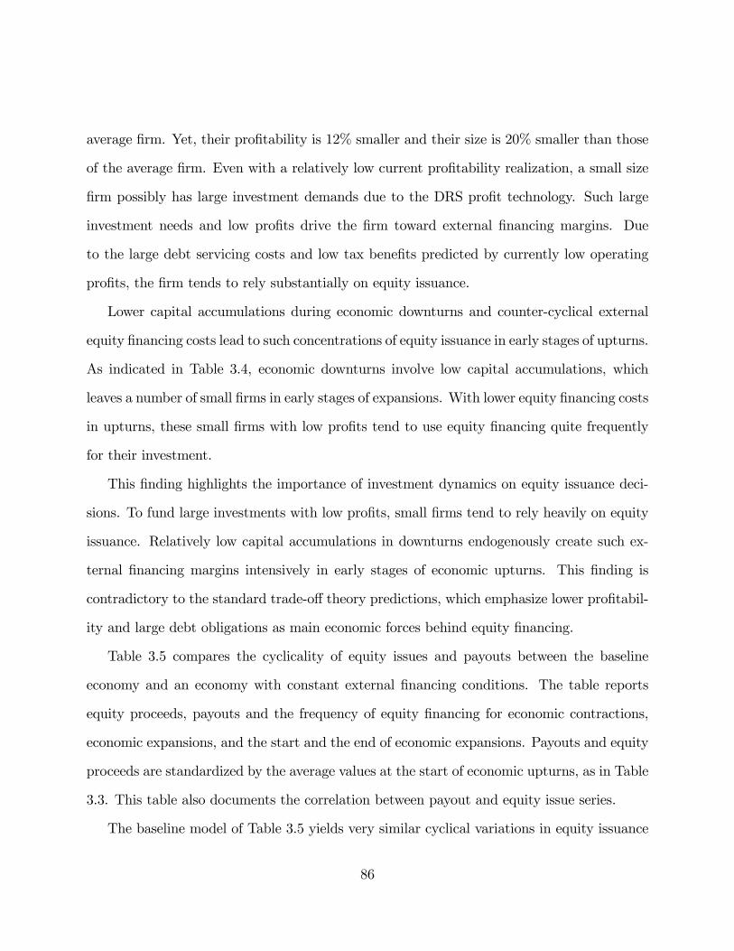
average �rm. Yet, their pro�tability is 12% smaller and their size is 20% smaller than those

of the average �rm. Even with a relatively low current pro�tability realization, a small size

�rm possibly has large investment demands due to the DRS pro�t technology. Such large

investment needs and low pro�ts drive the �rm toward external �nancing margins. Due

to the large debt servicing costs and low tax bene�ts predicted by currently low operating

pro�ts, the �rm tends to rely substantially on equity issuance.

Lower capital accumulations during economic downturns and counter-cyclical external

equity �nancing costs lead to such concentrations of equity issuance in early stages of upturns.

As indicated in Table 3.4, economic downturns involve low capital accumulations, which

leaves a number of small �rms in early stages of expansions. With lower equity �nancing costs

in upturns, these small �rms with low pro�ts tend to use equity �nancing quite frequently

for their investment.

This �nding highlights the importance of investment dynamics on equity issuance deci-

sions. To fund large investments with low pro�ts, small �rms tend to rely heavily on equity

issuance. Relatively low capital accumulations in downturns endogenously create such ex-

ternal �nancing margins intensively in early stages of economic upturns. This �nding is

contradictory to the standard trade-o¤ theory predictions, which emphasize lower pro�tabil-

ity and large debt obligations as main economic forces behind equity �nancing.

Table 3.5 compares the cyclicality of equity issues and payouts between the baseline

economy and an economy with constant external �nancing conditions. The table reports

equity proceeds, payouts and the frequency of equity �nancing for economic contractions,

economic expansions, and the start and the end of economic expansions. Payouts and equity

proceeds are standardized by the average values at the start of economic upturns, as in Table

3.3. This table also documents the correlation between payout and equity issue series.

The baseline model of Table 3.5 yields very similar cyclical variations in equity issuance

86

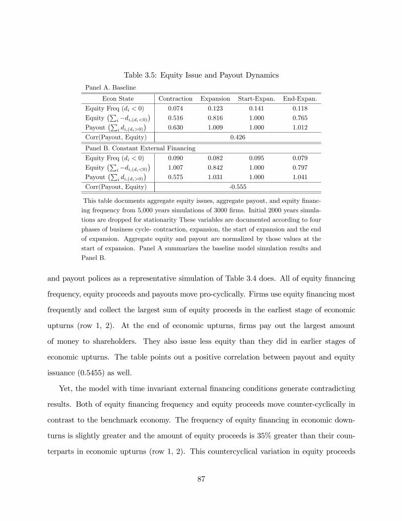
Table 3.5: Equity Issue and Payout Dynamics

Panel A. Baseline

Econ State Contraction Expansion Start-Expan. End-Expan.

Equity Freq (di < 0) 0.074 0.123 0.141 0.118

Equity�P

i�di;(di<0)�

0.516 0.816 1.000 0.765

Payout�P

i di;(di>0)�

0.630 1.009 1.000 1.012

Corr(Payout, Equity) 0.426

Panel B. Constant External Financing

Equity Freq (di < 0) 0.090 0.082 0.095 0.079

Equity�P

i�di;(di<0)�

1.007 0.842 1.000 0.797

Payout�P

i di;(di>0)�

0.575 1.031 1.000 1.041

Corr(Payout, Equity) -0.555

This table documents aggregate equity issues, aggregate payout, and equity �nanc-

ing frequency from 5,000 years simulations of 3000 �rms. Initial 2000 years simula-

tions are dropped for stationarity These variables are documented according to four

phases of business cycle- contraction, expansion, the start of expansion and the end

of expansion. Aggregate equity and payout are normalized by those values at the

start of expansion. Panel A summarizes the baseline model simulation results and

Panel B.

and payout polices as a representative simulation of Table 3.4 does. All of equity �nancing

frequency, equity proceeds and payouts move pro-cyclically. Firms use equity �nancing most

frequently and collect the largest sum of equity proceeds in the earliest stage of economic

upturns (row 1, 2). At the end of economic upturns, �rms pay out the largest amount

of money to shareholders. They also issue less equity than they did in earlier stages of

economic upturns. The table points out a positive correlation between payout and equity

issuance (0.5455) as well.

Yet, the model with time invariant external �nancing conditions generate contradicting

results. Both of equity �nancing frequency and equity proceeds move counter-cyclically in

contrast to the benchmark economy. The frequency of equity �nancing in economic down-

turns is slightly greater and the amount of equity proceeds is 35% greater than their coun-

terparts in economic upturns (row 1, 2). This countercyclical variation in equity proceeds

87

drives a negative correlation between equity issuance and payout under the economy with

constant external �nancing conditions.

This result highlights the importance of counter-cyclical equity �nancing costs in payout

and equity issue dynamics. The counter-cyclical variation drives pro-cyclical equity issues,

which leads to a positive correlation between equity issuance and payout. Table 3.5 clearly

indicates that equity issues tend to move counter-cyclically under constant external �nancing

conditions, consistent with the standard trade-o¤ theory predictions. Due to large debt

servicing costs and lower tax bene�ts, a �rm generally has stronger equity �nancing incentives

in economic downturns, under time invariant external �nancing conditions.

These �ndings are all in line with recent empirical �ndings. Ditmmar and Ditmmar

(2008) document that public �rms tend to issue equity in early stages of economic boom and

increase payouts (share repurchase) in later stages, observations which are exactly consistent

with the �ndings in Table 3.3 and 3.5. They also show that the correlation between aggregate

equity issuance and share repurchase is positive, which is also in line with the correlation

result of my baseline model. Equity �nancing is more likely to occur in small growth �rms

that generate lower operating pro�ts (Frank and Goyal 2003). These �rm characteristics are

well matched with the �ndings in Table 3.4.

To sum up, this section presents two interesting �ndings. First, endogenous investment

needs drive active equity issues for small, low pro�table, and large investment needs �rms

in earlier stages of economic upturns. This �nding is contradictory to the standard trade-o¤

theory predictions primarily focusing on a �rm�s pro�tability. Second, counter-cyclical equity

�nancing costs drive pro-cyclical equity issues, leading to a positive correlation between

payout and equity issuance.

88

Table 3.6: Firm Characteristics: Deb Issuance and Retirement

Debt Issuance (b0 > b) Debt Retirement (b0 < b)

Econ State Contraction Expansion Contraction Expansion

Rel. Investment (I=k) 2.872 2.275 0.000 0.007

Rel. Pro�ts (�=k) 1.465 1.386 0.810 0.779

Rel. Cash (c=k) 0.324 0.225 0.836 1.066

Rel. Leverage (b=k) 0.992 0.965 1.390 1.373

Investment (I=k) 0.324 0.314 0.000 0.001

Pro�ts (�=k) 0.218 0.259 0.121 0.145

Cash (c=k) 0.041 0.027 0.102 0.126

Leverage (b=k) 0.228 0.219 0.319 0.312

Next Period Lev. (b0=k0) 0.311 0.271 0.258 0.226

This table reports investments, pro�ts, cash and leverage from 3,000 years simula-

tions of 3000 �rms. All values are reported for debt issuance and debt retirements

�rms according to macroeconomic states. The �rst four rows document relative

ratio between these variables and their counterparts in an average �rm. The next

four rows summarize the absolute value of each variable. The last row reports next

period leverage ratios.

3.3.3 Debt Dynamics

This section analyzes the cyclical variations of debt �nancing policies in my baseline model.

Before entering the analysis of debt dynamics, Table 3.6 summarizes the characteristics of

debt issuance and debt retirement �rms in my baseline model simulation of 3,000 �rms. The

table reports investment, pro�t, cash and leverage ratios according to the macroeconomic

states. The �rst four rows compare these �rm characteristics with their counterparts in an

average �rm for each cross-section. For instance, debt issuance �rms�cash-asset ratio (row

3) is 32.4% of an average �rm�s cash-asset ratio. The next four rows document absolute

values of investment, pro�t, cash, and leverage ratios for debt issuance and retirement �rms.

The last row reports next period leverage ratios as well.

Table 3.6 clearly points to the importance of investment dynamics in debt issuance de-

cisions. While the pro�tability of debt issuance �rms is around 40% greater than that of an

89

average �rm, their investment demand is 2.5 times of an average �rm�s investment needs (row

1, 2). Such large investment needs over operating pro�ts endogenously create substantial

external �nancing demands, especially for low cash holding �rms (row 3). These �rms tend

to rely heavily on debt issuance because currently high pro�tability predicts large future

pro�t generations that accompany large tax bene�ts, and low liquidity costs of debt, i.e.

debt servicing costs.

Table 3.6 also indicates the signi�cant role of investment demands on debt retirement

policies. The debt obligations of debt retirement �rms are almost 40% larger than that of

an average �rm (row 4). Yet, they have almost zero investments, which allow an easier use

of operating pro�ts and internal funds for retiring debt obligations.

It is also noticeable that the leverage ratios after debt issuance or retirement are higher

during economic downturns even with pro-cyclical macroeconomic pro�tability variations

(row 9). For instance, leverage ratio after debt issuance is 0.31 during economic downturn

but is 0.27 during economic upturns. To fund quite large operating needs for investment, a

�rm considerably relies on debt �nancing even during economic downturns. Relatively low

operating pro�ts (row 6) deter aggressive use of internal funds for debt retirements, leading

to higher leverage ratios after debt retirement in economic downturns. Counter-cyclical

equity �nancing costs, of course, contribute to more aggressive debt issues during economic

downturns. Yet, these aggressive debt policies in downturn still hold for constant external

�nancing condition economy, even though the detailed results are not reported here.

These �rm characteristics highlight the importance of investment dynamics on debt is-

suance and retirement decisions, in contrast to the standard trade-o¤ theory predictions.

The standard trade-o¤ theory almost entirely relies on a �rm�s pro�tability in the determi-

nation of leverage dynamics. Yet, a �rm critically relies on debt issuance to fund operating

needs for large investment, particularly with low levels of cash. Lower investment demands

90

Table 3.7: Debt Dynamics

Equity Cost: Contraction Baseline �l= �h

Econ State Contraction Expansion Contraction Expansion

Leverage (P

i bi=P

i ki) 0.230 0.227 0.229 0.227

Equity Freq (d < 0) 0.074 0.123 0.119 0.112

Debt Issue (P

i b0 � b)=(

Pi I); b

0 > b 0.249 0.176 0.238 0.177

Debt Retirement (P

i b0 � b)=(

Pi I); b

0 < b 0.224 0.184 0.231 0.179

Net Debt Issue (P

i b0 � b)=(

Pi I) 0.025 -0.008 0.008 -0.002

This table reports aggregate leverage, debt issues, debt retirement, and net debt issues for the baselineand a constant external �nancing cost economy (�l= �h) from 3,000 years simulations of 3000 �rms.It also includes the frequency of equity �nancing. All values are documented according to the businesscyclical states.

also allow �exible use of internal funds to retire debt obligations given the same pro�tability.

Table 3.7 investigates debt and equity policies across the business cycle for the baseline

economy and an economy with constant external �nancing conditions (�l = �h). The table

reports aggregate leverage ratio, debt issues, debt retirements and net debt issues. It also

documents the frequency of equity �nancing. All values are evaluated in accordance with the

macroeconomic states. The debt issues, retirements, and net debt issues are standardized

by the sum of investment for each time period. This standardization re�ects the importance

of investment dynamics on debt issuance as analyzed in Table 3.6.

Table 3.7 clearly indicates counter-cyclical variations in debt policies. Both leverage ratio

and net debt issuance (row 1, 5) show weakly counter-cyclical movements, contradictory to

the standard trade-o¤ theory predictions. For example, the aggregate leverage ratio is 0.23 in

economic downturns but slightly goes down to 0.227 in economic upturns. The same pattern

holds for aggregate net debt issues. Furthermore, the aggregate debt issuance-investment

ratio is even larger during economic downturns (row 3), which points to a signi�cant role of

debt issuance for funding investments.

This counter-cyclical debt policy is not a mere result of counter-cyclical equity �nancing

costs. The constant external �nancing cost economy in Table 3.7 still shows weakly counter-

91

Table 3.8: Debt Dynamics: Low Debt Financing Costs

Equity Cost: Contraction Baseline �l= 0:3

Econ State Contraction Expansion Contraction Expansion

Leverage (P

i bi=P

i ki) 0.871 0.864 0.788 0.764

Equity Freq (d < 0) 0.229 0.125 0.008 0.160

Debt Issue (P

i b0 � b)=(

Pi I); b

0 > b 0.533 0.473 0.676 0.467

Debt Retirement (P

i b0 � b)=(

Pi I); b

0 < b 0.672 0.440 0.477 0.547

Net Debt Issue (P

i b0 � b)=(

Pi I) -0.139 0.032 0.199 -0.080

This table reports aggregate leverage, debt issues, debt retirement, and net debt issues for the baselineand higher equity �nancing cost model (�l= 0:3) from 3,000 years simulations of 3000 �rms. Debt�nancing costs ( ; �) are set to (0:0005; 0:0005). It also includes the frequency of equity �nancing. Allvalues are documented according to the business cyclical states.

cyclical leverage ratios and net debt issuance patterns (row 1, 5). The leverage ratio is slightly

higher and the amount of net debt issues is also slightly larger in economic downturns.

Lower pro�tability and consequently a higher value of liquidity play central roles in

this counter-cyclical debt policy. As indicated in Table 3.6, lower pro�tability in economic

downturns limits aggressive debt retirements during economic downturns. Furthermore, a

higher value of liquidity or large debt servicing costs in economic downturns induce active

debt retirements and conservative debt issues in economic upturns. A manager has strong

incentives to retire debt obligations by using ample operating pro�ts in economic upturns,

with the expectation of a highly valuable liquidity in downturns. She also limits the issuance

debt in anticipation of large debt servicing costs during economic downturns. All of these

factors contribute the counter-cyclical movements in debt policies.1

Table 3.8 simulates models under an economic environment with low debt �nancing

costs. The marginal equity �nancing cost in economic downturns is identical to the baseline

model in the �rst scenario, and quite higher in the second scenario. The table documents

aggregate leverage ratio, debt issues, debt retirements and net debt issues according to the

1I will mainly investigate how debt servicing costs in downturns a¤ect a �rm�s capital structure dynamicsin my comparative static analysis.

92

macroeconomic states. It also documents the frequency of equity �nancing. Debt issues,

retirements, and net debt issues are standardized by total investments for each time period

as in Table 3.7.

Table 3.8 emphasizes the "timing" aspect of debt retirement policies. Debt retirements

in economic upturn arise sharply from 0.44 to 0.54 with a substantial increase of equity

�nancing costs in economic downturns. Debt retirements in downturns rather decrease sub-

stantially from 0.67 to 0.47, given the same external equity �nancing cost changes. Low

debt �nancing costs imply relatively lower costs of maintaining debt obligations. A manager

could easily �time�debt retirements with such low debt �nancing costs. A higher external

equity �nancing cost raises the marginal value of liquidity in downturns and accordingly the

manager tries to retire debt obligations with ample operating pro�ts in economic upturns.

It is also remarkable that the leverage ratios drop substantially in the higher equity

�nancing cost case. For instance, the leverage ratio of economic downturn in the �rst sce-

nario is 0.86 but decrease to 0.76 in the second simulation. A higher equity �nancing cost

implies a large marginal value of liquidity and consequently large debt servicing costs in

economic downturns. To avoid such large debt servicing costs, a �rm optimally maintains

lower leverage ratios, as in Lee (2013).

The joint considerations of investment dynamics, pro-cyclical pro�tability, and stochastic

equity �nancing costs are pivotal in the counter-cyclical debt policies. A �rm may have

to use external debt issuance frequently to fund its operating needs for investments, even

during economic downturns. Lower pro�tability raises the marginal value of liquidity during

economic downturns, which encourages active debt retirements and discourages debt issues

during economic upturns. This lower pro�tability also limits the use of internal funds for

retiring debt obligations during economic downturns. Higher equity �nancing costs induce

additional debt issues at such external �nancing margins, and increase the marginal value

93

of liquidity more signi�cantly in economic downturns.

To summarize, my model highlights investment demand as a main economic force behind

debt issuance. It also generates counter-cyclical debt policies, and higher leverage ratios

after debt issuance and retirement during economic downturns, contradictory to the standard

trade-o¤ theory predictions. Operating needs for investment, pro-cyclical pro�tability, and

counter-cyclical equity �nancing costs all contribute to these cyclical properties of debt

�nancing policies.

3.4 Quantitative Analysis: Comparative Statics

3.4.1 Counter-cyclical Debt Financing Costs

This section analyzes how counter-cyclical variations of external debt �nancing costs a¤ect

capital structure dynamics.

The �ight to quality hypothesis predicts that an individual �rm�s credit quality is an

important determinant in its debt �nancing cost variation. For instance, Caballelo and

Krishmamurthy (2008) argue that investors become more risk averse in poor macroeconomic

conditions, which shifts their preference toward safer assets. Hence, the hypothesis predicts

that a lower credit rating �rm may access the debt �nancing market very limitedly during

economic downturns. Recent survey works of Campello, Graham, and Harvey (2011) indeed

document higher external �nancing costs for �nancially constrained �rms in the �nancial

crisis of 2008.

To examine the implications of limited access to the debt �nancing market during eco-

nomic downturns, Table 3.9 simulates an individual �rm at three di¤erent levels of debt

�nancing costs in economic downturns. The �rst scenario deals with an economy with pro-

cyclical debt �nancing costs. Debt �nancing cost parameters change to moderately counter-

94

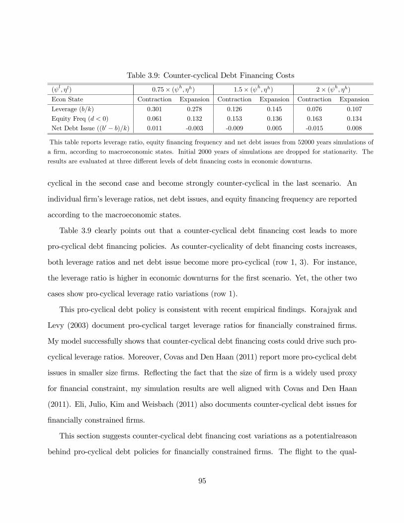
Table 3.9: Counter-cyclical Debt Financing Costs

( l; �l) 0:75� ( h; �h) 1:5� ( h; �h) 2� ( h; �h)

Econ State Contraction Expansion Contraction Expansion Contraction Expansion

Leverage (b=k) 0.301 0.278 0.126 0.145 0.076 0.107

Equity Freq (d < 0) 0.061 0.132 0.153 0.136 0.163 0.134

Net Debt Issue ((b0 � b)=k) 0.011 -0.003 -0.009 0.005 -0.015 0.008

This table reports leverage ratio, equity �nancing frequency and net debt issues from 52000 years simulations of

a �rm, according to macroeconomic states. Initial 2000 years of simulations are dropped for stationarity. The

results are evaluated at three di¤erent levels of debt �nancing costs in economic downturns.

cyclical in the second case and become strongly counter-cyclical in the last scenario. An

individual �rm�s leverage ratios, net debt issues, and equity �nancing frequency are reported

according to the macroeconomic states.

Table 3.9 clearly points out that a counter-cyclical debt �nancing cost leads to more

pro-cyclical debt �nancing policies. As counter-cyclicality of debt �nancing costs increases,

both leverage ratios and net debt issue become more pro-cyclical (row 1, 3). For instance,

the leverage ratio is higher in economic downturns for the �rst scenario. Yet, the other two

cases show pro-cyclical leverage ratio variations (row 1).

This pro-cyclical debt policy is consistent with recent empirical �ndings. Korajyak and

Levy (2003) document pro-cyclical target leverage ratios for �nancially constrained �rms.

My model successfully shows that counter-cyclical debt �nancing costs could drive such pro-

cyclical leverage ratios. Moreover, Covas and Den Haan (2011) report more pro-cyclical debt

issues in smaller size �rms. Re�ecting the fact that the size of �rm is a widely used proxy

for �nancial constraint, my simulation results are well aligned with Covas and Den Haan

(2011). Eli, Julio, Kim and Weisbach (2011) also documents counter-cyclical debt issues for

�nancially constrained �rms.

This section suggests counter-cyclical debt �nancing cost variations as a potentialreason

behind pro-cyclical debt policies for �nancially constrained �rms. The �ight to the qual-

95

Table 3.10: Financial Market Shutdowns

( l; �l) at �l= 0:3 0:75� ( h; �h) 1:5� ( h; �h) 2� ( h; �h)

Econ State Contraction Expansion Contraction Expansion Contraction Expansion

Leverage (b=k) 0.311 0.266 0.140 0.140 0.081 0.099

Equity Freq (d < 0) 0.000 0.145 0.000 0.150 0.000 0.156

Net Debt Issue ((b0 � b)=k) 0.017 -0.005 -0.003 0.003 -0.008 0.006

This table reports leverage ratio, equity �nancing frequency and net debt issues from 52000 years simulations of

a �rm, according to macroeconomic states. Initial 2000 years of simulations are dropped for stationarity. The

results are evaluated at three di¤erent levels of debt �nancing costs in economic downturns at �l = 0:3.

ity hypothesis predicts more counter-cyclical debt �nancing cost variations for �nancially

constrained �rms due to the shift of credit supply toward safer assets. My model directly

generates pro-cyclical debt policies under counter-cyclical variations in debt �nancing costs.

3.4.2 Financial Market Shutdowns

This section investigates the potential implications of �nancial market shutdowns in economic

downturns on a �rm�s capital structure choices.

Table 3.10 summarizes the potential e¤ects of �nancial market shutdowns. While the

debt �nancing costs in each scenario is identical to their counterparts in Table 3.9, I set

equity �nancing costs in downturns as 30% of equity proceeds to induce quite strong counter-

cyclicality for equity �nancing costs. As in Table 3.9, an individual �rm�s leverage ratios,

net debt issues, and equity �nancing frequency are reported according to the macroeconomic

states.

Table 3.10 indicates that the expectation of �nancial market shutdowns potentially drive

a conservative debt policy during economic upturns. As external �nancing conditions become

more deteriorated in economic downturns, leverage ratios decrease substantially (row 1) and

equity �nancing frequency increases slightly during economic upturns (row 2). For instance,

the leverage ratio of economic upturns is initially 0.266 but drops signi�cantly to 0.099 in the

96

third case (row 1). Furthermore, all of the leverage ratios during economic upturns slightly

lower than their counterparts in Table 3.9. Financial market shutdowns imply large debt

servicing costs in economic downturns, leading to more conservative debt issues in economic

upturns.

This �nding is closely associated with the debt conservatism puzzle (Graham 2000). The

considerations of �nancial market shutdowns during economic downturns limit the use of

debt �nancing in economic upturns. Therefore, a �rm may appear to use debt conservatively

across the whole period of business cycle.

To sum up, the expectation of �nancial market shutdowns in economic downturns leads

to conservative debt policy during economic upturns, which potentially drives a pervasively

conservative debt policy. The expectation of large debt servicing costs plays the central role

here.

3.4.3 Deeper Economic Downturns

This section studies the role of deeper economic downturns on capital structure dynamics.

For this purpose, I conduct two comparative static analyses. First, I increase the macroeco-

nomic pro�tability di¤erence between economic expansion and contraction states. Second, I

extend the duration of economic downturns.

Table 3.11 summarizes the �nancing and investment policies for two di¤erent scales of

macroeconomic pro�tability shock variations. The macroeconomic pro�tability of economic

upturns, zh, is 1.05 and that of downturns, zl, is 0.95 in the �rst economy. These values are

1.2 and 0.8 respectively in the second scenario. Table 3.11 reports the average leverage ratio

and pro�tability over the whole business cycle. It also documents investment, operating

pro�ts, cash, leverage and equity �nancing frequency in accordance with the macroeconomic

states.

97

Table 3.11: A Sharper Di¤erence in Aggregate Pro�tability

(zl; zh) Small: (0.95,1.05) Large: (0.8,1.2)

Pro�ts (�=k) 0.173 0.188

Leverage (b=k) 0.278 0.142

Econ State Contraction Expansion Contraction Expansion

Investment (I=k) 0.120 0.136 0.071 0.156

Pro�ts (�=k) 0.158 0.179 0.107 0.220

Cash (c=k) 0.114 0.111 0.119 0.104

Leverage (b=k) 0.280 0.278 0.142 0.142

Equity Freq (d < 0) 0.076 0.188 0.107 0.077

This table reports �nancing and investment variables from 52000 years simula-

tions of a �rm, for two di¤erent magnitude of aggregate pro�tability di¤erences.

Initial 2000 years of simulations are dropped for stationarity. First two rows

report operating pro�ts and leverage ratio over the whole business cycle. In-

vestments, operating pro�ts, cash, leverage and equity �nancing frequency are

separately documented for economic contraction and expansion periods.

Table 3.11 points out that a sharp drop in pro�tability during economic downturn could

drive a conservative debt policy over the whole business cycle. Even though the average

pro�tability increases by 10% (0:173! 0:188), the average leverage ratio decreases sharply

(0:278 ! 0:142). It is also remarkable that �rms expecting a sharp drop in pro�tability

maintain lower leverage ratios (0:278 ! 0:142) during economic upturns even with a sub-

stantial increase in their average pro�tability (0:179! 0:220). Lower pro�tability generates

large debt servicing costs in economic contractions, which restrains debt issuance during

economic upturns as well as downturns.

Table 3.12 documents the �nancing and investment policies for two di¤erent durations of

economic downturns. The transition probability from downturns to upturns, plh, is 0.4 and

the duration of economic downturn is 1.67 years (1=0:6) in the �rst scenario. The probability

and duration become 0.2 and 5 years (1=0:2) respectively in the second model simulation.

Table 3.12 reports the average leverage ratio and pro�tability over the whole business. It

also documents investment, operating pro�ts, cash, leverage and equity �nancing frequency

98

Table 3.12: A Longer Duration of Economic Contraction

Transition Probability plh= 0:4 plh= 0:8

Pro�ts (�=k) 0.177 0.169

Leverage (b=k) 0.260 0.151

Econ State Contraction Expansion Contraction Expansion

Investment (I=k) 0.121 0.135 0.105 0.159

Pro�ts (�=k) 0.149 0.186 0.150 0.188

Cash (c=k) 0.123 0.121 0.147 0.107

Leverage (b=k) 0.262 0.259 0.145 0.156

Equity Freq (d < 0) 0.065 0.113 0.172 0.183

This table reports �nancing and investment variables from 52000 years simula-

tions of a �rm, for two di¤erent durations of economic downturns. Initial 2000

years of simulations are dropped for stationarity. First two rows report operating

pro�ts and leverage ratio over the whole business cycle. Investments, operating

pro�ts, cash, leverage and equity �nancing frequency are separately documented

for economic contraction and expansion periods.

according to the macroeconomic states.

Table 3.12 also suggests that the expectation of deeper economic downturns limits the

use of debt over the whole business cycle. The average leverage ratio drops substantially

(0:260! 0:151) in spite of a moderate drop in average pro�tability between two simulations

(0:177! 0:169). Similar to the results of Table 3.8, a �rm with a longer duration of economic

downturns maintains lower leverage ratios even during economic upturns (0:259 ! 0:156).

These �rms rather rely more heavily on equity issuance even during economic upturns,

compared to their counterparts in the �rst scenario (0:113! 0:183).

These �ndings provide new insights on the debt conservatism (Graham 2000) and the

puzzling negative correlation between pro�tability and leverage ratios (Frank and Goyal

2008). A manager may exercise pervasively conservative debt policy across the business

cycle due to large debt servicing costs from a sharp pro�t drop or a longer stay in economic

downturns. Moreover, even a very highly pro�table �rm in economic expansions possibly

maintains lower leverages because of a sharp pro�tability drop and large debt servicing costs

99

in economic contraction. Therefore, a �rm�s pro�tability does not necessarily move positively

with leverage ratios, unlike the standard trade-o¤ theory predictions. With the expectation

of large debt servicing costs, a manager also relies more substantially on equity �nancing as

expected in Lee (2013).

To sum up, my model shows the expectation of deeper economic downturns leads to more

conservative debt policy over the whole business cycle. Lower pro�tability in economic down-

turns predicts more conservative debt policy during economic upturns, even with a higher

average pro�tability. A longer duration of economic downturn also drives more conservative

debt policy and frequent equity �nancing activities during economic upturns. These macro-

economic considerations possibly lead to pervasively conservative debt policy (Graham 2000)

and a negative correlation between pro�tability and leverage ratios (Frank and Goyal 2008).

3.5 Concluding Remarks

Macroeconomic conditions a¤ect a �rm�s investment demands, pro�tability, and external

�nancing conditions altogether. I studied how these simultaneous changes impact cyclical

variations in capital structure policies. Lower pro�tability in downturns, investment dynam-

ics, counter-cyclical equity �nancing costs are all pivotal in the capital structure dynamics.

Lower pro�tability increases the marginal value of liquidity in downturns leading to active

debt retirements and limited debt issues in upturns. Investment demands drive active debt

issues even during economic downturns. Counter-cyclical equity �nancing costs induce pro-

cyclical equity issues and intensify counter-cyclical movements in debt policies.

In line with recent empirical �ndings, my baseline model generates counter-cyclical debt

policy and pro-cyclical patterns of equity issues and payout. In particular, equity issues

are concentrated for small, low pro�table, large investment demand �rm in early stages of

100

upturns. Low capital accumulations in downturns lead to this business cyclical property.

Payouts peak in later stages of economic upturns due to the lower pro�tability in downturn

and large investment demands in early stages of upturns. Leverage ratios after debt issues

and retirements are even higher in economic downturns, unlike the standard trade-o¤ theory

predictions. These business cycle properties in debt, equity and payout policies are all

consistent with empirical works of Dittmar and Dittmar (2008) and Korajczyk and Levy

(2003).

My comparative static analysis also predicts pro-cyclical debt policies for �nancially

constrained �rms and pervasively conservative debt policies for �rms expecting �nancial

market shutdowns, a sharp pro�tability drop and a longer stay in economic downturns. The

�ight to quality hypothesis expects more counter-cyclical debt �nancing cost variations for

�nancially constrained �rms, which leads to pro-cyclical debt policies in my model. Financial

market shutdowns, a sharp pro�tability drop, and a longer stay in economic downturns all

indicate large debt servicing costs, leading to pervasively conservative debt policy across the

whole business cycle. These �ndings provides new insights on the pro-cyclical debt policy in

�nancially constrained �rms Korajczyk and Levy (2003), and Covas and Den Haan (2011)

, debt conservatism (Graham 2000), and puzzling negative correlation between pro�tability

and leverage ratios (Frank and Goyal 2008).

My study provides several fruitful opportunities for future research. The endogenous

determination of risk premium is an important topic. Counter-cyclical credit spread varia-

tions are widely recognized in empirical studies but largely unexamined in this study. The

examination of an individual �rm�s market timing aspect is another direction. I mainly con-

sider stochastic variation of external �nancing conditions according to the business cyclical

states. Yet, my model does not incorporate potential market timing opportunities relying

on an individual �rm�s valuation. The combinational e¤ects of macroeconomic and individ-

101

ual market timing aspects may have substantial implications on a �rm�s capital structure

dynamics.

102

Bibliography

Altinkihc, O. and R. S. Hansen (2000). Are there economies of scale in underwriting fees?

evidence of rising external �nancing costs. The Review of Financial Studies 13 (1), 191�218.

Ang, J. and A. Smedema (2011). Financial �exibility: Do �rms prepare for recession?

Journal of Corporate Finance 17 (3), 774�787.

Bhamra, H. S., L.-A. Kuehn, and I. A. Strebulaev (2010). The aggregate dynamics of

capital structure and macroeconomic risk. Review of Financial Studies 23 (12), 4187�4241.

Blouin, J., J. E. Core, and W. Guay (2010). Have the tax bene�ts of debt been overesti-

mated? Journal of Financial Economics 98 (2), 195�213.

Bolton, P., H. Chen, and N. Wang (2011). A uni�ed theory of tobin�sq, corporate invest-

ment, �nancing, and risk management. The Journal of Finance 66 (5), 1545�1578.

Bolton, P., H. Chen, and N.Wang (2013). Market timing, investment, and risk management.

Journal of Financial Economics 109 (1), 40�62.

Bolton, P., H. Chen, and N. Wang (2014). Debt, taxes, and liquidity. Columbia Business

School, Working Paper .

103

Brown, J. R., S. M. Fazzari, and B. C. Petersen (2009). Financing innovation and growth:

Cash �ow, external equity, and the 1990s R&D boom. The Journal of Finance 64 (1),

151�185.

Caballero, R. J. and A. Krishnamurthy (2008). Collective risk management in a �ight to

quality episode. The Journal of Finance 63 (5), 2195�2230.

Campello, M., E. Giambona, J. R. Graham, and C. R. Harvey (2011). Liquidity manage-

ment and corporate investment during a �nancial crisis. Review of Financial Studies 24 (6),

1944�1979.

Campello, M., J. R. Graham, and C. R. Harvey (2010). The real e¤ects of �nancial con-

straints: Evidence from a �nancial crisis. Journal of Financial Economics 97 (3), 470�487.

Cooper, R. W. and J. C. Haltiwanger (2006). On the nature of capital adjustment costs.

The Review of Economic Studies 73 (3), 611�633.

Covas, F. and W. J. Den Haan (2011). The cyclical behavior of debt and equity �nance.

American Economic Review 101 (2), 877�99.

David McLean, R. (2011). Share issuance and cash savings. Journal of Financial Eco-

nomics 99 (3), 693�715.

DeAngelo, H., L. DeAngelo, and R. M. Stulz (2010). Seasoned equity o¤erings, market

timing, and the corporate lifecycle. Journal of Financial Economics 95 (3), 275�295.

DeAngelo, H., L. DeAngelo, and T. M. Whited (2011). Capital structure dynamics and

transitory debt. Journal of Financial Economics 99 (2), 235�261.

Denis, D. J. and S. B. McKeon (2012). Debt �nancing and �nancial �exibility evidence

from proactive leverage increases. Review of Financial Studies 25 (6), 1897�1929.

104

Dittmar, A. K. and R. F. Dittmar (2008). The timing of �nancing decisions: An examination

of the correlation in �nancing waves. Journal of Financial Economics 90 (1), 59�83.

Eberly, J. C. (1997). International evidence on investment and fundamentals. European

Economic Review 41 (6), 1055�1078.

Erel, I., B. Julio, W. Kim, and M. S. Weisbach (2012). Macroeconomic conditions and

capital raising. Review of Financial Studies 25 (2), 341�376.

Fama, E. F. and K. R. French (2002). Testing trade-o¤and pecking order predictions about

dividends and debt. The Review of Financial Studies 15 (1), 1�33.

Fama, E. F. and K. R. French (2005). Financing decisions: who issues stock? Journal of

Financial Economics 76 (3), 549�582.

Fischer, E. O., R. Heinkel, and J. Zechner (1989). Dynamic capital structure choice: Theory

and tests. The Journal of Finance 44 (1), 19�40.

Frank, M. Z. and V. K. Goyal (2009). Capital structure decisions: Which factors are reliably

important? Financial Management 38 (1), 1�37.

Gamba, A. and A. Triantis (2008). The value of �nancial �exibility. The Journal of

Finance 63 (5), 2263�2296.

Graham, J. R. (2000). How big are the tax bene�ts of debt? The Journal of Finance 55 (5),

1901�1941.

Graham, J. R. and C. R. Harvey (2001). The theory and practice of corporate �nance:

evidence from the �eld. Journal of Financial Economics 60 (2â¼AS3), 187�243.

105

Hall, B. H. (1987). The relationship between �rm size and �rm growth in the us manufac-

turing sector. The Journal of Industrial Economics 35 (4), 583�606.

Hall, B. H. (2002). The �nancing of research and development. Oxford review of economic

policy 18 (1), 35�51.

Hennessy, C. A. and T. M. Whited (2005). Debt dynamics. The Journal of Finance 60 (3),

1129�1165.

Hennessy, C. A. and T. M. Whited (2007). How costly is external �nancing? evidence from

a structural estimation. The Journal of Finance 62 (4), 1705�1745.

Jermann, U. and V. Quadrini (2012). Macroeconomic e¤ects of �nancial shocks. American

Economic Review 102 (1).

Kahl, M., J. Lunn, and M. Nilsson (2012). Operating leverage and corpo-

rate �nancial policies. AFA 2012 Chicago Meetings Paper Available at SSRN:

http://ssrn.com/abstract=1787184 .

Korajczyk, R. A. and A. Levy (2003). Capital structure choice: macroeconomic conditions

and �nancial constraints. Journal of Financial Economics 68 (1), 75�109.

Leary, M. T. and M. R. Roberts (2005). Do �rms rebalance their capital structures? The

Journal of Finance 60 (6), 2575�2619.

Lee, J. H. (2013). Debt servicing costs and capital structure. Columbia University, Working

Paper .

Levy, A. and C. Hennessy (2007). Why does capital structure choice vary with macroeco-

nomic conditions? Journal of Monetary Economics 54 (6), 1545�1564.

106

Loughran, T. I. M. and J. R. Ritter (1997). The operating performance of �rms conducting

seasoned equity o¤erings. The Journal of Finance 52 (5), 1823�1850.

Modigliani, F. and M. H. Miller (1958). The cost of capital, corporation �nance and the

theory of investment. The American economic review 48 (3), 261�297.

Myers, S. C. and N. S. Majluf (1984). Corporate �nancing and investment decisions when

�rms have information that investors do not have. Journal of Financial Economics 13 (2),

187�221.

Riddick, L. A. and T. M. Whited (2009). The corporate propensity to save. The Journal

of Finance 64 (4), 1729�1766.

Shyam-Sunder, L. and S. C. Myers (1999). Testing static tradeo¤ against pecking order

models of capital structure. Journal of Financial Economics 51 (2), 219�244.

Strebulaev, I. A. (2007). Do tests of capital structure theory mean what they say? The

Journal of Finance 62 (4), 1747�1787.

Whited, T. M. (1992). Debt, liquidity constraints, and corporate investment: Evidence

from panel data. The Journal of Finance 47 (4), 1425�1460.

107

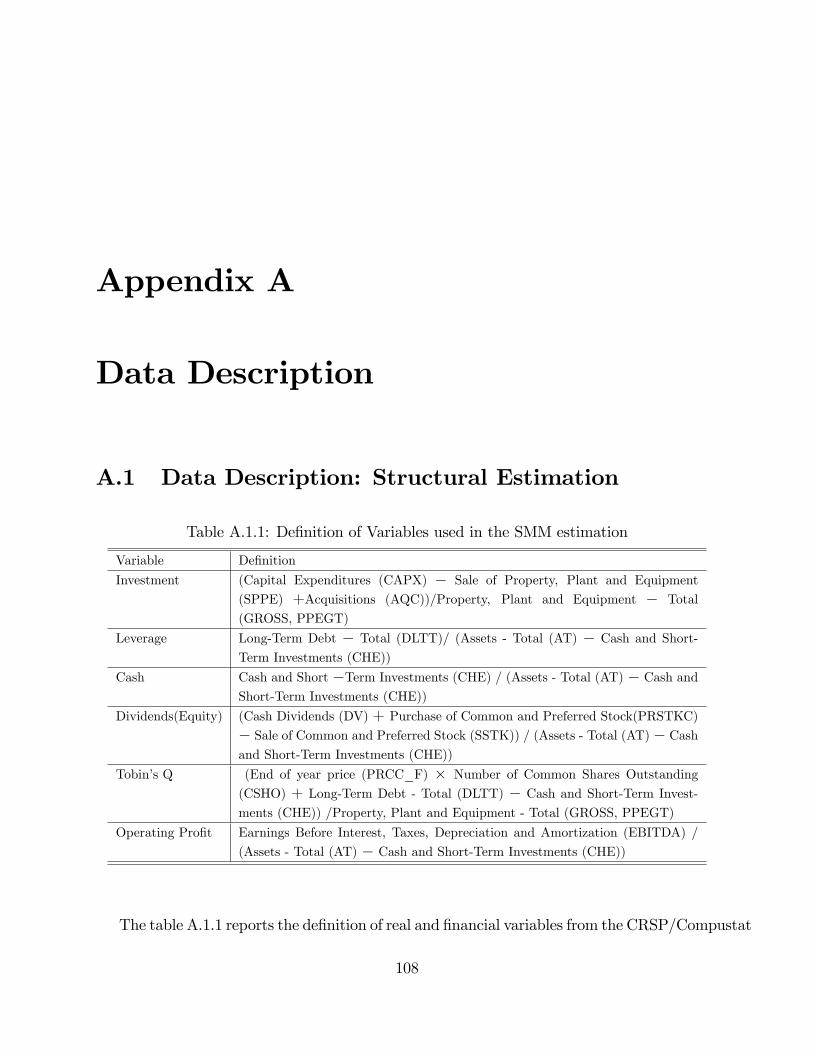
Appendix A

Data Description

A.1 Data Description: Structural Estimation

Table A.1.1: De�nition of Variables used in the SMM estimation

Variable De�nition

Investment (Capital Expenditures (CAPX) � Sale of Property, Plant and Equipment

(SPPE) +Acquisitions (AQC))/Property, Plant and Equipment � Total

(GROSS, PPEGT)

Leverage Long-Term Debt � Total (DLTT)/ (Assets - Total (AT) � Cash and Short-

Term Investments (CHE))

Cash Cash and Short �Term Investments (CHE) / (Assets - Total (AT) � Cash and

Short-Term Investments (CHE))

Dividends(Equity) (Cash Dividends (DV) + Purchase of Common and Preferred Stock(PRSTKC)

� Sale of Common and Preferred Stock (SSTK)) / (Assets - Total (AT)� Cash

and Short-Term Investments (CHE))

Tobin�s Q (End of year price (PRCC_F) � Number of Common Shares Outstanding

(CSHO) + Long-Term Debt - Total (DLTT) � Cash and Short-Term Invest-

ments (CHE)) /Property, Plant and Equipment - Total (GROSS, PPEGT)

Operating Pro�t Earnings Before Interest, Taxes, Depreciation and Amortization (EBITDA) /

(Assets - Total (AT) � Cash and Short-Term Investments (CHE))

The table A.1.1 reports the de�nition of real and �nancial variables from the CRSP/Compustat

108

database. The symbols in parenthesis refer to the items in CRSP/Compustat merged data-

base.

The business cyclical categorization in Chapter 3 is based on US Business Cycle Expan-

sions and Contractions.

A.2 Data Description: Cross-sectional Analysis

I introduce several control variables for empirical analyses on capital structure choices, as

proposed in Frank and Goyal (2008). Some variables are rede�ned by following prior litera-

ture. Table A.1.2 reports the detailed variable constructions.

Table A.2.1: De�nition of Variables used in the Empirical Analyses

Variable De�nition

Asset (De�ated) Assets - Total (AT)

Pro�tability Earnings Before Interest (EBITDA) / Assets - Total (AT)

Tangibility Property, Plant and Equipment - Total (Net, PPENT)/ Assets - Total (AT)

R&D expenditure Research and Development Expense (XRD)/ Assets - Total (AT)

Market to Book (End of year price (PRCC_F)�Number of Common Shares Outstanding

(CSHO) + Long-Term Debt - Total (DLTT))/Assets - Total (AT)

Investment (Capital Expenditures (CAPX)-Sale of Property, Plant and Equipment (SPPE)

+ Research and Development Expense (XRD)/)/ Assets - Total (AT)

Tobin�s Q (End of year price (PRCC_F)�Number of Common Shares Outstanding

(CSHO)+ Long-Term Debt - Total (DLTT)�Cash and Short-Term Investments

(CHE)) /Assets - Total (AT)

Leverage Long-Term Debt - Total (DLTT)/ Assets - Total (AT)

Cash Cash and Short-Term Investments (CHE) /Assets - Total (AT)

Equity Financing (Cash Dividends (DV) + Purchase of Common and Preferred Stock(PRSTKC)

� Sale of Common and Preferred Stock (SSTK)) / (Assets - Total (AT))

109

Appendix B

Numerical Solutions

B.1 Numerical Solutions: Chapter 1

To achieve a numerical solution of model, I use the value function iteration method, which

requires to discretize state spaces for the four state variables. The state variable constructions

are very similar to Hennessy and Whited (2005, 2007), and DDW. The space of capital stock

lies on the following points:

[�k(1� �)20; :::; �k(1� �)1=2; �k]:

The boundness of �k for a decreasing returns to scale pro�t function �; is discussed in Hennessy

and Whited (2005).

The pro�tability shock (z) is modelled to have 12 points. I transform AR(1) process into

a discrete state Markov chain on the interval of [�4�; 4�]. Tauchen (1986) argues that 8~9

points are enough to approximate the AR(1) process. The upper bound for debt balance��b�

is obtained if I assume the upper bound for cash balance(�c) is a half of the upper bound of

110

debt balance�12(�b)�; the same as in DDW. I let the debt (b) state have equally spaced 25

points in the interval of [0;�b] and the cash (b) state have equally spaced 12 points in the

interval of [0; �c]:1

B.2 Numerical Solutions: Chapter 3

To achieve a numerical solution of model, I use the value function iteration method, which

requires to discretize state spaces for the four state variables. The state variable constructions

are very similar to Hennessy and Whited (2005, 2007), and DDW. The space of capital stock

lies on the following points:

[�k(1� �)20; :::; �k(1� �)1=2; �k]:

The boundness of �k for a decreasing returns to scale pro�t function �; is discussed in Hennessy

and Whited (2005).

The individual pro�tability shock (z) is modelled to have 8 points. I transform AR(1)

process into a discrete state Markov chain on the interval of [�4�; 4�]. Tauchen (1986) argues

that 8~9 points are enough to approximate the AR(1) process. There are two macroeconomic

states zh and zl as well with the transition probability de�ned in the main body. The upper

bound for debt balance��b�is obtained if I assume the upper bound for cash balance(�c) is

a half of the upper bound of debt balance�12(�b)�; the same as in DDW. I let the debt (b)

state have equally spaced 25 points in the interval of [0;�b] and the cash (b) state have equally

spaced 12 points in the interval of [0; �c]:

1DDW has net debt space with 29 points covering both cash and debt balance.

111

Appendix C

Identi�cation: Chapter 3

The global identi�cation of a SMM estimator is achieved if the expected value of the di¤er-

ence between the simulated moments and the data moments equals zero if and only if the

structural parameters equal their true values. To correctly identify structural parameters, I

pick up the following 13 moments; these moments consist of the �rst and second moments of

investment and operating pro�ts. The autocorrelation of operating pro�ts, and the average

dividends, and Tobin�s q values are also included. The average of equity �nancing frequency,

cash and leverage ratios are reported according to the business cyclical variations. My iden-

ti�cation scheme is closely associated with the identi�cation strategy of DDW because I �x

the macroeconomic transition probability and pro�tability realizations. The average and

variance of investment help identify the capital adjustment cost parameters, k and �k. A

higher convex capital adjustment cost decreases the average and variance of investment and

a higher �xed capital adjustment cost raises the variance of investment. Average operat-

ing pro�ts helps to identity the curvature of pro�t function, a and the �xed operating cost

parameter, �: A higher � raises average pro�t (zk� � �kss=k) and a higher �xed operating

cost parameter, � lowers average operating pro�ts. The serial correlation of the pro�tability

112

shock, �; and the �xed operating parameter, �; a¤ects the serial correlations in operating

pro�ts. A higher �xed operating cost increases the correlations in pro�t generation. The

variance of pro�t helps capture the uncertainty parameter of pro�t evolution, �. The average

dividends and Tobin�s q are closely associated with a �rm valuation.

The other moment selections pertain to a �rm�s �nancing decision. The frequency of

equity �nancing over the macroeconomic states help the identi�cation of time-varying equity

�nancing costs, �h and �l. The leverage ratios in economic upturns and downturns help pin

down the baseline debt �nancing cost, and the additional �nancing cost component, �:

A large decreases leverage ratios in economic downturn more substantially due to the

lower interest tax shields in economic downturns. A large � conversely provides substantial

incentives to maintain higher leverage ratios in economic downturns. The business cyclical

variations of cash holding also assist the identi�cation of two debt �nancing cost parameters

by a similar reasoning.

113