THREE EMBEDDED TECHNIQUES FOR FINITE ELEMENT HEAT FLOW PROBLEM

WITH EMBEDDED DISCONTINUITIES

M.Davari1, R.Rossi2 and P.Dadvand2

1 Department of Strength of Materials and Structural Engineering, Polytechnic University of

Catalonia, Barcelona, Spain

2 International Center for Numerical Methods in Engineering (CIMNE), Department of Strength of

Materials and Structural Engineering, Polytechnic University of Catalonia, Barcelona, Spain

ABSTRACT

The present paper explores the solution of a heat conduction problem considering discontinuities

embedded within the mesh and aligned at arbitrary angles with respect to the mesh edges.

Three alternative approaches are proposed as solutions to the problem. The difference between

these approaches compared to alternatives, such as the eXtended Finite Element Method (X-FEM),

is that the current proposal attempts to preserve the global matrix graph in order to improve

performance. The first two alternatives comprise an enrichment of the Finite Element (FE) space

obtained through the addition of some new local degrees of freedom to allow capturing

discontinuities within the element. The new degrees of freedom are statically condensed prior to

assembly, so that the graph of the final system is not changed. The third approach is based on the

use of modified FE-shape functions that substitute the standard ones on the cut elements. The

imposition of both Neumann and Dirichlet boundary conditions is considered at the embedded

interface. The results of all the proposed methods are then compared with a reference solution

obtained using the standard FE on a mesh containing the actual discontinuity.

1. INTRODUCTION

This paper focuses on the solution of a conduction problem on a domain containing a gap at a

prescribed position in space. The salient feature of the work is that, instead of modifying the

geometry of the domain so that the gap is modelled as a physical boundary, we embed the

geometrical description of the structure in a mesh that is continuous across the gap.

The introduction of such a gap implies that the physical solution suffers from a discontinuity,

potentially both in the primary variable (the temperature) and in its gradients. This feature makes it

difficult to approximate the solution with a standard, continuous FE approach, unless the mesh is

body-fitted to the gap geometry.

Perhaps the most well-known approach to the treatment of discontinuities within the element is

eXtended Finite Element Method (X-FEM) [1–8]. The X-FEM is a numerical technique where

enrichment functions are added to the FE approximation space so as to provide it with the ability to

reproduce specific features of the solution. This enrichment is normally done only at the region near

the discontinuities such as cracks, holes, and similar material interfaces. In X-FEM the numerical

model comprises two types of elements at the region near the discontinuity: fully enriched elements

that are cut by the discontinuity and partially enriched elements (blending elements) that are not cut

by the discontinuity but have one or more enriched nodes (see Figure 1). Two disadvantages of

standard X-FEM specially for moving discontinuities may be mentioned:

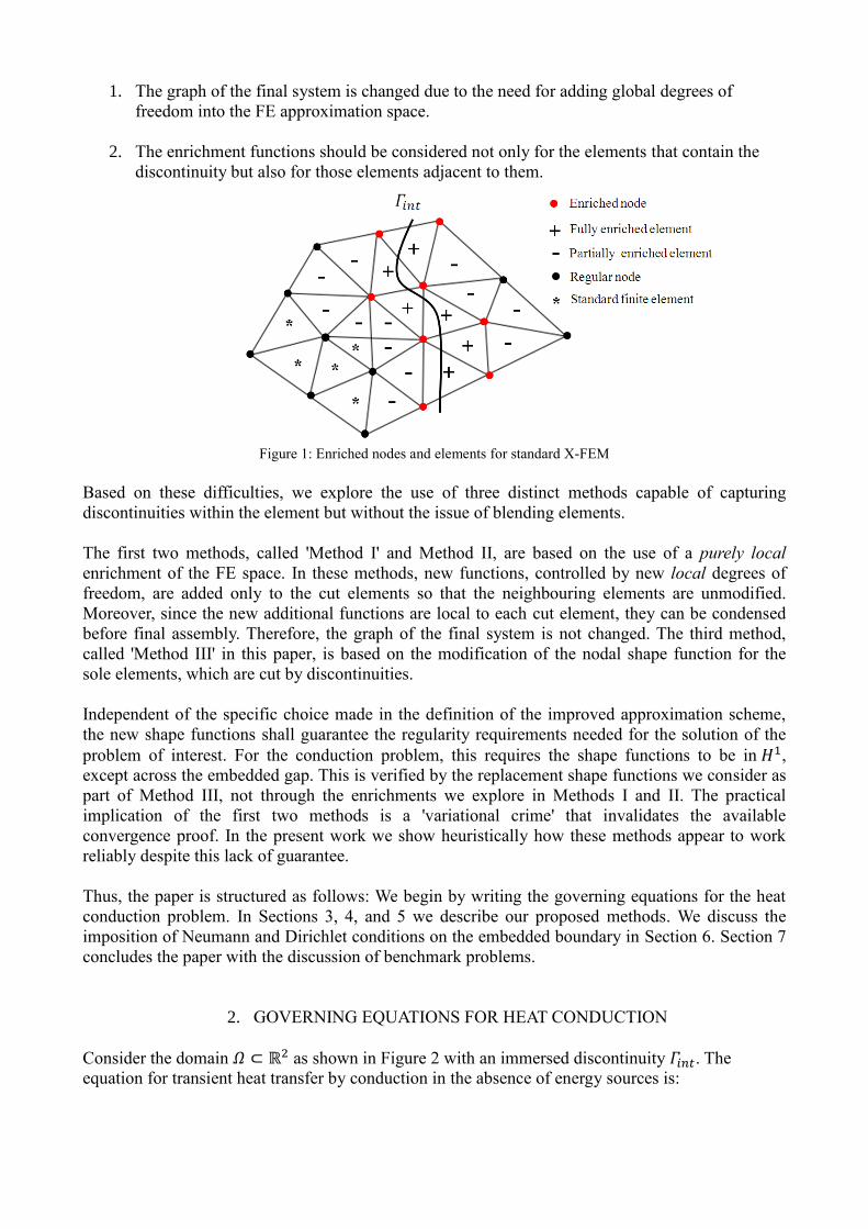
1. The graph of the final system is changed due to the need for adding global degrees of

freedom into the FE approximation space.

2. The enrichment functions should be considered not only for the elements that contain the

discontinuity but also for those elements adjacent to them.

Figure 1: Enriched nodes and elements for standard X-FEM

Based on these difficulties, we explore the use of three distinct methods capable of capturing

discontinuities within the element but without the issue of blending elements.

The first two methods, called 'Method I' and Method II, are based on the use of a purely local

enrichment of the FE space. In these methods, new functions, controlled by new local degrees of

freedom, are added only to the cut elements so that the neighbouring elements are unmodified.

Moreover, since the new additional functions are local to each cut element, they can be condensed

before final assembly. Therefore, the graph of the final system is not changed. The third method,

called 'Method III' in this paper, is based on the modification of the nodal shape function for the

sole elements, which are cut by discontinuities.

Independent of the specific choice made in the definition of the improved approximation scheme,

the new shape functions shall guarantee the regularity requirements needed for the solution of the

problem of interest. For the conduction problem, this requires the shape functions to be in 𝐻1,

except across the embedded gap. This is verified by the replacement shape functions we consider as

part of Method III, not through the enrichments we explore in Methods I and II. The practical

implication of the first two methods is a 'variational crime' that invalidates the available

convergence proof. In the present work we show heuristically how these methods appear to work

reliably despite this lack of guarantee.

Thus, the paper is structured as follows: We begin by writing the governing equations for the heat

conduction problem. In Sections 3, 4, and 5 we describe our proposed methods. We discuss the

imposition of Neumann and Dirichlet conditions on the embedded boundary in Section 6. Section 7

concludes the paper with the discussion of benchmark problems.

2. GOVERNING EQUATIONS FOR HEAT CONDUCTION

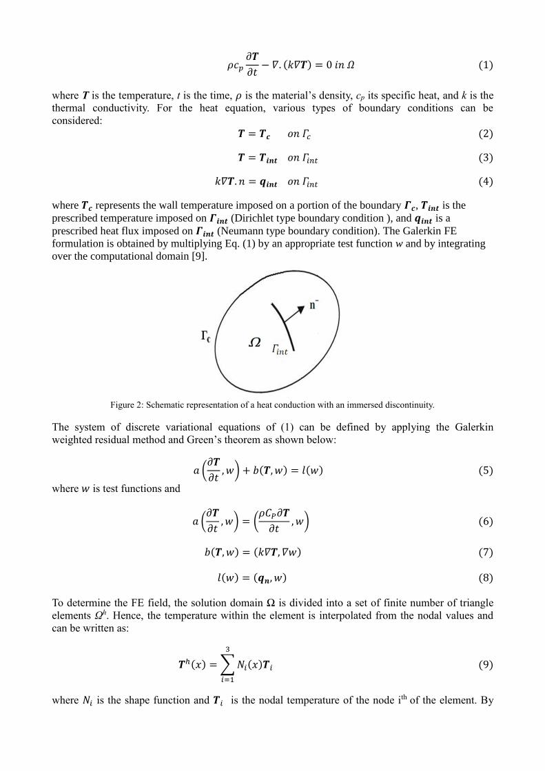
Consider the domain 𝛺 ⊂ ℝ2 as shown in Figure 2 with an immersed discontinuity 𝛤𝑖𝑛𝑡. The

equation for transient heat transfer by conduction in the absence of energy sources is:

𝜌𝑐𝑝𝜕𝑻

𝜕𝑡− 𝛻. (𝑘𝛻𝑻) = 0 𝑖𝑛 𝛺 (1)

where T is the temperature, t is the time, 𝜌 is the material’s density, cp its specific heat, and k is the

thermal conductivity. For the heat equation, various types of boundary conditions can be

considered:

𝑻 = 𝑻𝒄 𝑜𝑛 𝛤𝑐 (2)

𝑻 = 𝑻𝒊𝒏𝒕 𝑜𝑛 𝛤𝑖𝑛𝑡 (3)

𝑘𝛻𝑻. 𝑛 = 𝒒𝒊𝒏𝒕 𝑜𝑛 𝛤𝑖𝑛𝑡 (4)

where 𝑻𝒄 represents the wall temperature imposed on a portion of the boundary 𝜞𝒄, 𝑻𝒊𝒏𝒕 is the

prescribed temperature imposed on 𝜞𝒊𝒏𝒕 (Dirichlet type boundary condition ), and 𝒒𝒊𝒏𝒕 is a

prescribed heat flux imposed on 𝜞𝒊𝒏𝒕 (Neumann type boundary condition). The Galerkin FE

formulation is obtained by multiplying Eq. (1) by an appropriate test function w and by integrating

over the computational domain [9].

Figure 2: Schematic representation of a heat conduction with an immersed discontinuity.

The system of discrete variational equations of (1) can be defined by applying the Galerkin

weighted residual method and Green’s theorem as shown below:

𝑎 (𝜕𝑻

𝜕𝑡, 𝑤) + 𝑏(𝑻,𝑤) = 𝑙(𝑤) (5)

where 𝑤 is test functions and

𝑎 (𝜕𝑻

𝜕𝑡, 𝑤) = (

𝜌𝐶𝑃𝜕𝑻

𝜕𝑡, 𝑤) (6)

𝑏(𝑻,𝑤) = (𝑘𝛻𝑻, 𝛻𝑤) (7)

𝑙(𝑤) = (𝒒𝒏, 𝑤) (8)

To determine the FE field, the solution domain Ω is divided into a set of finite number of triangle

elements Ωh. Hence, the temperature within the element is interpolated from the nodal values and

can be written as:

𝑻ℎ(𝑥) =∑𝑁𝑖(𝑥)𝑻𝑖

3

𝑖=1

(9)

where 𝑁𝑖 is the shape function and 𝑻𝑖 is the nodal temperature of the node ith of the element. By

substituting (9) in the weak form (5), we obtain the following matrix form:

𝑪𝜕𝑻

𝜕𝑡− 𝑲𝑻 = 𝑸 + 𝑺 (10)

where T is the vector of nodal unknown temperatures, C is the capacitance matrix, K is the stiffness

or conductivity matrix, 𝑸 is the Neumann boundary or the flux term at the boundaries of the

triangle element, and 𝑺 is the external flux term at the immersed boundary and

𝑪𝑖𝑗 = ∫ 𝜌𝑐𝑝𝑁𝑖𝑁𝑗𝑑𝛺 𝛺ℎ

𝑖, 𝑗 = 1,3 (11)

𝑲𝑖𝑗 = −∫ 𝑘𝛻𝑁𝑖. 𝛻𝑁𝑗𝑑𝛺 𝛺ℎ

𝑖, 𝑗 = 1,3 (12)

𝑸𝑖 = ∫ 𝒒𝑛𝑁𝑖𝑑𝛤 𝛤ℎ

𝑖 = 1,3 (13)

𝑺𝑖 = ∫ 𝒒𝑛𝑁𝑖𝑑𝛤𝑖𝑛𝑡 𝛤𝑖𝑛𝑡

𝑖 = 1,3 (14)

𝑭𝑖 = ∫ 𝑓𝑁𝑖𝑑𝛺𝛺ℎ

𝑖 = 1,3 (15)

The system of differential Eq. (10) has to be integrated in the time. For the sake of simplicity, we

choose the backward Euler scheme. The resulting time-discrete problem is as follows:

𝑪𝑻𝑛 − 𝑻𝑛−1

𝛥𝑡− 𝑲𝑻𝑛 = 𝑸 + 𝑺 (16)

3. METHOD I (ENRICHMENT FINITE ELEMENT METHOD)

As already mentioned, we seek to propose three distinct techniques to embed the discontinuity of

interest in the search space. In this section, we introduce a purely local enrichment of the FE space.

Four new degrees of freedom are added locally to the sole elements intersected by the embedded

gap, with the objective of capturing discontinuities (kinks and jumps) in the solution. The enriched

basis is formed by the combination of the nodal shape functions associated with the mesh (standard

FE part) and discontinuous shape functions associated with additional degrees of freedom

(enrichment parts). For the rest of the elements, only the standard FE interpolation will be applied.

As mentioned in [8], one possible way to construct a suitable enriched space (𝐻1 everywhere apart

across the gap) is by adding some new degrees of freedom to the cut elements with enriched

functions. For example, if the field is scalar, a three-node triangular element that is not cut by the

Γint has one degree of freedom per node. However, the degree of freedom would be two if the

element were cut (one more due to using the enriched functions to capture discontinuity within the

element). Thus, the element adjacent to a cut element would have one or more enriched nodes even

though the element may not contain Γint. In other words, not only the elements that are cut by Γint

but also their immediate neighbours are enriched [10].

The key differentiator of our method with respect to what mentioned in [8] is that the enriched

functions are added to the cut elements using new local degrees of freedom, which do not depend

on any of the neighbouring elements. The key idea we exploit is that since the new degrees of

freedom are purely local, they can be statically condensed at the elementary level before the final

assembly. Therefore, the size and the graph of the final linear system to be solved are the same as in

the standard case.

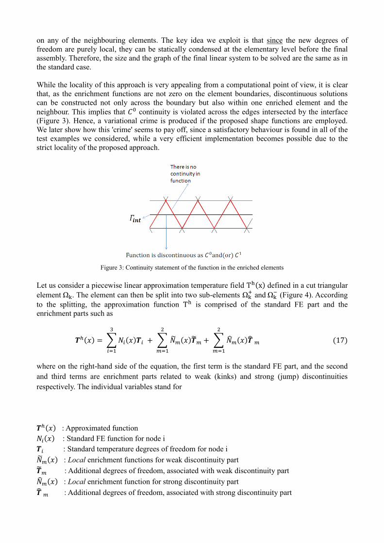
While the locality of this approach is very appealing from a computational point of view, it is clear

that, as the enrichment functions are not zero on the element boundaries, discontinuous solutions

can be constructed not only across the boundary but also within one enriched element and the

neighbour. This implies that 𝐶0 continuity is violated across the edges intersected by the interface

(Figure 3). Hence, a variational crime is produced if the proposed shape functions are employed.

We later show how this 'crime' seems to pay off, since a satisfactory behaviour is found in all of the

test examples we considered, while a very efficient implementation becomes possible due to the

strict locality of the proposed approach.

Figure 3: Continuity statement of the function in the enriched elements

Let us consider a piecewise linear approximation temperature field Th(x) defined in a cut triangular

element Ωk. The element can then be split into two sub-elements Ωk+

and Ωk−

(Figure 4). According

to the splitting, the approximation function Th is comprised of the standard FE part and the

enrichment parts such as

𝑻ℎ(𝑥) = ∑𝑁𝑖(𝑥)𝑻𝑖

3

𝑖=1

+ ∑ 𝑚(𝑥)𝑚

2

𝑚=1

+ ∑ 𝑚(𝑥) 𝑚

2

𝑚=1

(17)

where on the right-hand side of the equation, the first term is the standard FE part, and the second

and third terms are enrichment parts related to weak (kinks) and strong (jump) discontinuities

respectively. The individual variables stand for

𝑻ℎ(𝑥) : Approximated function

𝑁𝑖(𝑥) : Standard FE function for node i

𝑻𝑖 : Standard temperature degrees of freedom for node i

𝑚(𝑥) : Local enrichment functions for weak discontinuity part

𝑚 : Additional degrees of freedom, associated with weak discontinuity part

𝑚(𝑥) : Local enrichment function for strong discontinuity part

𝑚 : Additional degrees of freedom, associated with strong discontinuity part

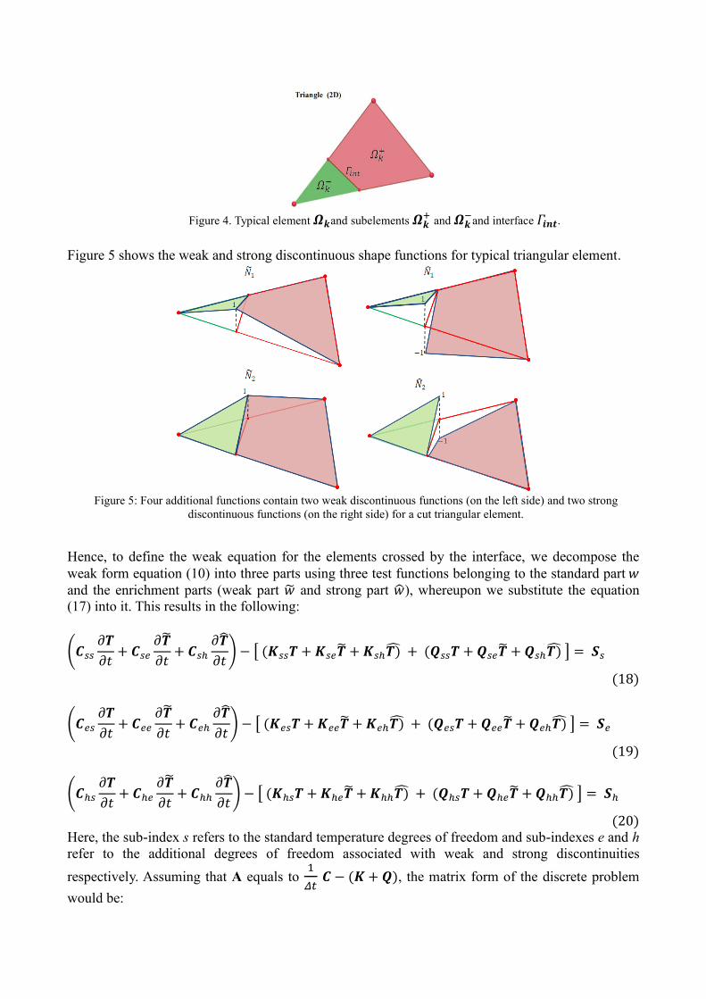
Figure 4. Typical element 𝜴𝒌and subelements 𝜴𝒌

+ and 𝜴𝒌

−and interface 𝛤𝒊𝒏𝒕.

Figure 5 shows the weak and strong discontinuous shape functions for typical triangular element.

Figure 5: Four additional functions contain two weak discontinuous functions (on the left side) and two strong

discontinuous functions (on the right side) for a cut triangular element.

Hence, to define the weak equation for the elements crossed by the interface, we decompose the

weak form equation (10) into three parts using three test functions belonging to the standard part 𝑤

and the enrichment parts (weak part and strong part ), whereupon we substitute the equation

(17) into it. This results in the following:

(𝑪𝑠𝑠𝜕𝑻

𝜕𝑡+ 𝑪𝑠𝑒

𝜕

𝜕𝑡+ 𝑪𝑠ℎ

𝜕

𝜕𝑡) − [ (𝑲𝑠𝑠𝑻 + 𝑲𝑠𝑒 + 𝑲𝑠ℎ𝑻) + (𝑸𝑠𝑠𝑻 + 𝑸𝑠𝑒 + 𝑸𝑠ℎ𝑻) ] = 𝑺𝑠

(18)

(𝑪𝑒𝑠𝜕𝑻

𝜕𝑡+ 𝑪𝑒𝑒

𝜕

𝜕𝑡+ 𝑪𝑒ℎ

𝜕

𝜕𝑡) − [ (𝑲𝑒𝑠𝑻 + 𝑲𝑒𝑒 + 𝑲𝑒ℎ𝑻) + (𝑸𝑒𝑠𝑻 + 𝑸𝑒𝑒 + 𝑸𝑒ℎ𝑻) ] = 𝑺𝑒

(19)

(𝑪ℎ𝑠𝜕𝑻

𝜕𝑡+ 𝑪ℎ𝑒

𝜕

𝜕𝑡+ 𝑪ℎℎ

𝜕

𝜕𝑡) − [ (𝑲ℎ𝑠𝑻 + 𝑲ℎ𝑒 + 𝑲ℎℎ𝑻) + (𝑸ℎ𝑠𝑻 + 𝑸ℎ𝑒 + 𝑸ℎℎ𝑻) ] = 𝑺ℎ

(20) Here, the sub-index s refers to the standard temperature degrees of freedom and sub-indexes e and h

refer to the additional degrees of freedom associated with weak and strong discontinuities

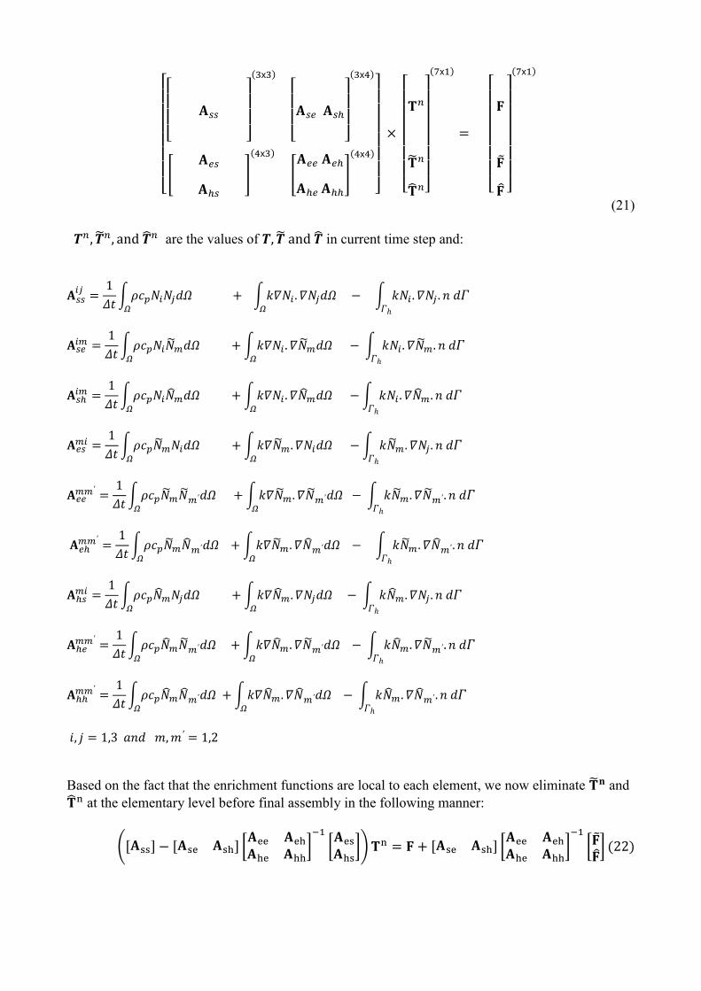
respectively. Assuming that A equals to 1

𝛥𝑡 𝑪 − (𝑲 + 𝑸), the matrix form of the discrete problem

would be:

[

[

𝐀𝑠𝑠

] (3𝗑3)

[

𝐀𝑠𝑒 𝐀𝑠ℎ

] (3𝗑4)

[𝐀𝑒𝑠

𝐀ℎ𝑠]

(4𝗑3)

[𝐀𝑒𝑒 𝐀𝑒ℎ

𝐀ℎ𝑒 𝐀ℎℎ]

(4𝗑4)

]

×

[

𝐓𝑛

𝑛

𝑛] (7𝗑1)

=

[

𝐅

] (7𝗑1)

(21)

𝑻𝑛, 𝑛, and 𝑛 are the values of 𝑻, and in current time step and:

𝐀𝑠𝑠𝑖𝑗=1

𝛥𝑡∫𝜌𝑐𝑝𝑁𝑖𝑁𝑗𝑑𝛺 𝛺

+ ∫ 𝑘𝛻𝑁𝑖 . 𝛻𝑁𝑗𝑑𝛺 𝛺

− ∫ 𝑘𝑁𝑖 . 𝛻𝑁𝑗 . 𝑛 𝑑𝛤 𝛤ℎ

𝐀𝑠𝑒𝑖𝑚 =

1

𝛥𝑡∫𝜌𝑐𝑝𝑁𝑖𝑚𝑑𝛺 𝛺

+ ∫𝑘𝛻𝑁𝑖 . 𝛻𝑚𝑑𝛺 𝛺

− ∫ 𝑘𝑁𝑖 . 𝛻𝑚. 𝑛 𝑑𝛤 𝛤ℎ

𝐀𝑠ℎ𝑖𝑚 =

1

𝛥𝑡∫𝜌𝑐𝑝𝑁𝑖𝑚𝑑𝛺 𝛺

+ ∫𝑘𝛻𝑁𝑖 . 𝛻𝑚𝑑𝛺 𝛺

− ∫ 𝑘𝑁𝑖 . 𝛻𝑚. 𝑛 𝑑𝛤 𝛤ℎ

𝐀𝑒𝑠𝑚𝑖 =

1

𝛥𝑡∫𝜌𝑐𝑝𝑚𝑁𝑖𝑑𝛺 𝛺

+ ∫𝑘𝛻𝑚. 𝛻𝑁𝑖𝑑𝛺 𝛺

− ∫ 𝑘𝑚. 𝛻𝑁𝑗. 𝑛 𝑑𝛤 𝛤ℎ

𝐀𝑒𝑒𝑚𝑚′

=1

𝛥𝑡∫𝜌𝑐𝑝𝑚𝑚′𝑑𝛺 𝛺

+ ∫𝑘𝛻𝑚. 𝛻𝑚′𝑑𝛺 𝛺

− ∫ 𝑘𝑚. 𝛻𝑚′ . 𝑛 𝑑𝛤 𝛤ℎ

𝐀𝑒ℎ𝑚𝑚′

=1

𝛥𝑡∫𝜌𝑐𝑝𝑚𝑚′𝑑𝛺 𝛺

+ ∫ 𝑘𝛻𝑚. 𝛻𝑚′𝑑𝛺 𝛺

− ∫ 𝑘𝑚. 𝛻𝑚′ . 𝑛 𝑑𝛤 𝛤ℎ

𝐀ℎ𝑠𝑚𝑖 =

1

𝛥𝑡∫𝜌𝑐𝑝𝑚𝑁𝑗𝑑𝛺 𝛺

+ ∫𝑘𝛻𝑚. 𝛻𝑁𝑗𝑑𝛺 𝛺

− ∫ 𝑘𝑚. 𝛻𝑁𝑗 . 𝑛 𝑑𝛤 𝛤ℎ

𝐀ℎ𝑒𝑚𝑚′

=1

𝛥𝑡∫𝜌𝑐𝑝𝑚𝑚′𝑑𝛺 𝛺

+ ∫ 𝑘𝛻𝑚. 𝛻𝑚′𝑑𝛺 𝛺

− ∫ 𝑘𝑚. 𝛻𝑚′ . 𝑛 𝑑𝛤 𝛤ℎ

𝐀ℎℎ𝑚𝑚′

=1

𝛥𝑡∫𝜌𝑐𝑝𝑚𝑚′𝑑𝛺 𝛺

+∫𝑘𝛻𝑚. 𝛻𝑚′𝑑𝛺 𝛺

− ∫ 𝑘𝑚. 𝛻𝑚′ . 𝑛 𝑑𝛤 𝛤ℎ

𝑖, 𝑗 = 1,3 𝑎𝑛𝑑 𝑚,𝑚′ = 1,2

Based on the fact that the enrichment functions are local to each element, we now eliminate 𝐧 and

n at the elementary level before final assembly in the following manner:

([𝐀ss] − [𝐀se 𝐀sh] [𝐀ee 𝐀eh𝐀he 𝐀hh

]−1

[𝐀es𝐀hs

])𝐓n = 𝐅 + [𝐀se 𝐀sh] [𝐀ee 𝐀eh𝐀he 𝐀hh

]−1

[] (22)

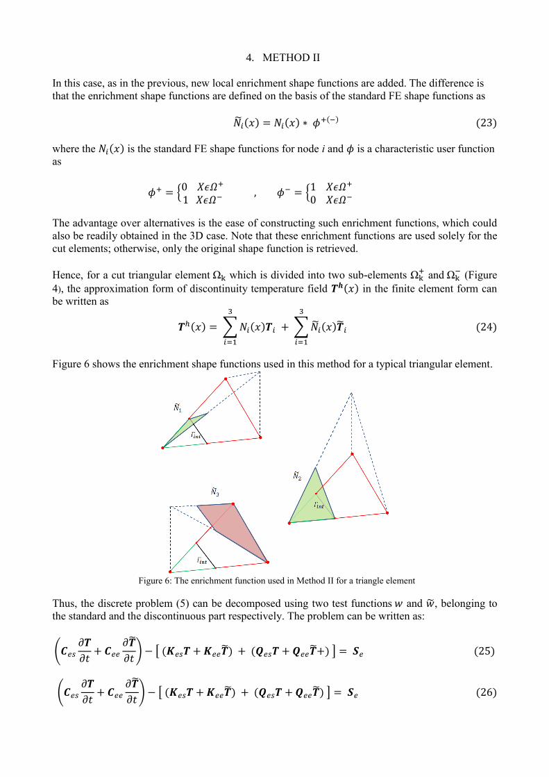
4. METHOD II

In this case, as in the previous, new local enrichment shape functions are added. The difference is

that the enrichment shape functions are defined on the basis of the standard FE shape functions as

𝑖(𝑥) = 𝑁𝑖(𝑥) ∗ 𝜙+(−) (23)

where the 𝑁𝑖(𝑥) is the standard FE shape functions for node i and 𝜙 is a characteristic user function

as

𝜙+ = 0 𝑋𝜖𝛺+

1 𝑋𝜖𝛺− , 𝜙− = 1 𝑋𝜖𝛺

+

0 𝑋𝜖𝛺−

The advantage over alternatives is the ease of constructing such enrichment functions, which could

also be readily obtained in the 3D case. Note that these enrichment functions are used solely for the

cut elements; otherwise, only the original shape function is retrieved.

Hence, for a cut triangular element Ωk which is divided into two sub-elements Ωk+

and Ωk−

(Figure

4), the approximation form of discontinuity temperature field 𝑻𝒉(𝑥) in the finite element form can

be written as

𝑻ℎ(𝑥) = ∑𝑁𝑖(𝑥)𝑻𝑖

3

𝑖=1

+ ∑𝑖(𝑥)𝑖

3

𝑖=1

(24)

Figure 6 shows the enrichment shape functions used in this method for a typical triangular element.

Figure 6: The enrichment function used in Method II for a triangle element

Thus, the discrete problem (5) can be decomposed using two test functions 𝑤 and , belonging to

the standard and the discontinuous part respectively. The problem can be written as:

(𝑪𝑒𝑠𝜕𝑻

𝜕𝑡+ 𝑪𝑒𝑒

𝜕

𝜕𝑡) − [ (𝑲𝑒𝑠𝑻 + 𝑲𝑒𝑒) + (𝑸𝑒𝑠𝑻 + 𝑸𝑒𝑒+) ] = 𝑺𝑒 (25)

(𝑪𝑒𝑠𝜕𝑻

𝜕𝑡+ 𝑪𝑒𝑒

𝜕

𝜕𝑡) − [ (𝑲𝑒𝑠𝑻 + 𝑲𝑒𝑒) + (𝑸𝑒𝑠𝑻 + 𝑸𝑒𝑒) ] = 𝑺𝑒 (26)

where the sub-indexes s and e refer to the standard and additional degrees of freedom respectively.

The linear system can be written by blocks as:

[𝐀𝑠𝑠 𝐀𝑠𝑒𝐀𝑒𝑠 𝐀𝑒𝑒

] × [𝐓𝑛

𝑛] = [

𝐅

] (27)

where 𝑻𝑛, 𝑛, and 𝑛 are the values of 𝑻, , and in current time step and for 𝑖, 𝑗 = 1,3

𝐀𝑠𝑠𝑖𝑗=1

𝛥𝑡∫𝜌𝑐𝑝𝑁𝑖𝑁𝑗𝑑𝛺 𝛺

+ ∫ 𝑘𝛻𝑁𝑖 . 𝛻𝑁𝑗𝑑𝛺 𝛺

− ∫ 𝑘𝑁𝑖 . 𝛻𝑁𝑗. 𝑛 𝑑𝛤 𝛤ℎ

𝐀𝑠𝑒𝑖𝑗=1

𝛥𝑡∫𝜌𝑐𝑝𝑁𝑖𝑗𝑑𝛺 𝛺

+ ∫𝑘𝛻𝑁𝑖 . 𝛻𝑗𝑑𝛺 𝛺

− ∫ 𝑘𝑁𝑖 . 𝛻𝑗. 𝑛 𝑑𝛤 𝛤ℎ

𝐀𝑒𝑠𝑖𝑗=1

𝛥𝑡∫𝜌𝑐𝑝𝑖𝑁𝑗𝑑𝛺 𝛺

+ ∫𝑘𝛻𝑖. 𝛻𝑁𝑗𝑑𝛺 𝛺

− ∫ 𝑘𝑖 . 𝛻𝑁𝑗. 𝑛 𝑑𝛤 𝛤ℎ

𝐀𝑒𝑒𝑖𝑗=1

𝛥𝑡∫𝜌𝑐𝑝𝑖𝑗𝑑𝛺 𝛺

+ ∫𝑘𝛻𝑖 . 𝛻𝑗𝑑𝛺 𝛺

− ∫ 𝑘𝑖 . 𝛻𝑗 . 𝑛 𝑑𝛤 𝛤ℎ

As mentioned before, since the new additional functions are local to each element, which is cut,

they can be statically condensed prior to assembly. Therefore, similar to the previous method, the

size and the graph of the final linear system to be solved are not changed, resulting in:

(𝐀ss − 𝐀se[𝐀ee]−1𝐀es)𝐓

n = 𝐅 + 𝐀se[𝐀ee]−1 (28)

5. METHOD III (MODIFIED XFEM METHOD)

We will now try out the method proposed in [11]. Here instead of adding special functions, the FE

shape functions of the cut elements are modified so as to capture discontinuities inside the element.

This is done without adding any extra degrees of freedom and by maintaining the continuity across

the cut borders. The modifications are local and can be computed element by element. They form a

nodal basis in the sense that they take the value one at their corresponding node and zero at the

other nodes. To define them, we simply carry the value at each node towards the intersection of any

edge emanating from it with the interface.

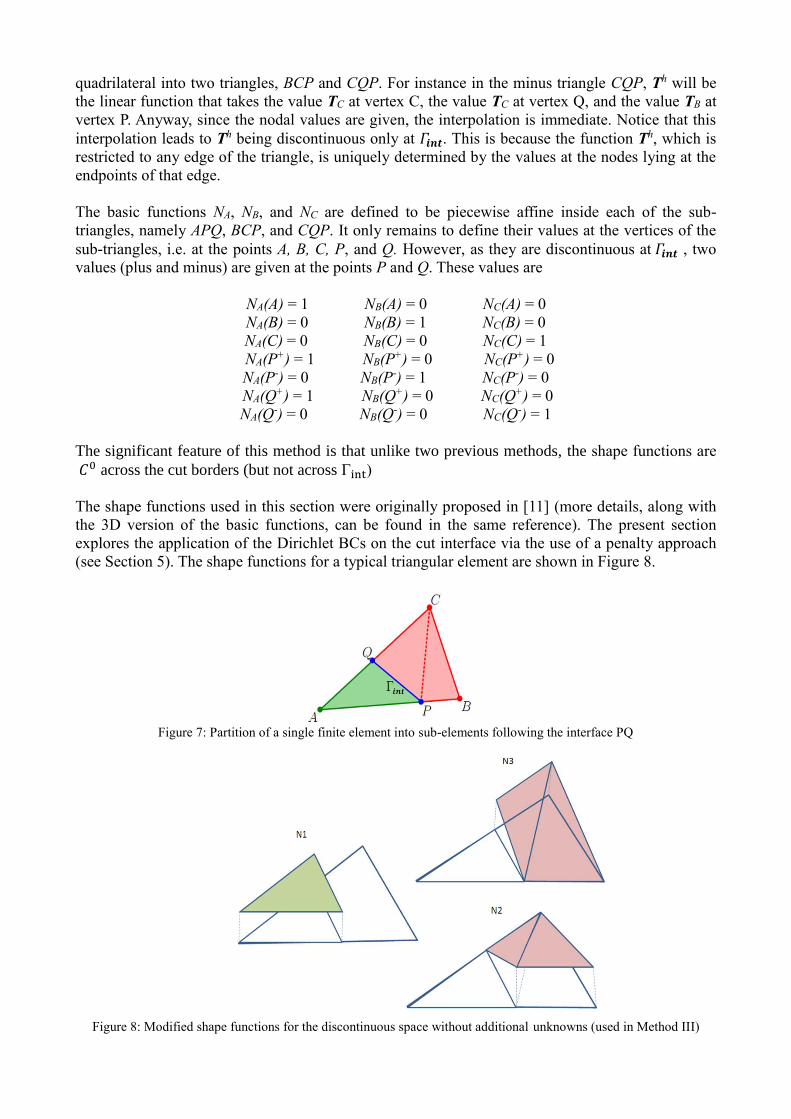
For more explanation, consider a triangular element ABC that is cut by interface 𝛤𝒊𝒏𝒕 at two points P

and Q, in such a manner that it is divided into two subparts, called sub-triangle APQ and sub-

quadrilateral BCQP (Figure 5). In this case, we assume that 𝛤𝒊𝒏𝒕 is a linear segment. Let TA, TB, and

TC denote the nodal values of the discrete variable Th, which is to be interpolated in the triangle

ABC. Let us arbitrarily denote the triangle APQ as a 'plus' side of 𝛤𝒊𝒏𝒕 and quadrilateral BCQP as a

'minus' side. For the approximation to be discontinuous, on the plus side, the function Th needs to be

determined only by the plus node (TA). Similarly, Th on the minus side must depend on just minus

nodes (TB and TC). The value of each point (P, Q) will be carried from the node of the original

triangulation lying on the same edge and the same side. Therefore, by using this way, on the plus

side of 𝛤𝒊𝒏𝒕, the values at P and Q will be TA, and thus Th will be constant:

𝑻𝐴𝑃𝑄ℎ = TA (29)

Similarly, on the minus side, the value at P will be TB, and the value at Q will be TC. One can

choose either to adopt a Q1 interpolation in BCQP from these nodal values or to subdivide the

quadrilateral into two triangles, BCP and CQP. For instance in the minus triangle CQP, Th will be

the linear function that takes the value TC at vertex C, the value TC at vertex Q, and the value TB at

vertex P. Anyway, since the nodal values are given, the interpolation is immediate. Notice that this

interpolation leads to Th being discontinuous only at 𝛤𝒊𝒏𝒕. This is because the function Th, which is

restricted to any edge of the triangle, is uniquely determined by the values at the nodes lying at the

endpoints of that edge.

The basic functions NA, NB, and NC are defined to be piecewise affine inside each of the sub-

triangles, namely APQ, BCP, and CQP. It only remains to define their values at the vertices of the

sub-triangles, i.e. at the points A, B, C, P, and Q. However, as they are discontinuous at 𝛤𝒊𝒏𝒕 , two

values (plus and minus) are given at the points P and Q. These values are

= 0 (A)CN= 0 (A)BN= 1 (A) AN

NA(B) = 0 NB(B) = 1 NC(B) = 0

NA(C) = 0 NB(C) = 0 NC(C) = 1

NA(P+) = 1 NB(P+) = 0 NC(P+) = 0

NA(P-) = 0 NB(P-) = 1 NC(P-) = 0

NA(Q+) = 1 NB(Q+) = 0 NC(Q+) = 0

NA(Q-) = 0 NB(Q-) = 0 NC(Q-) = 1

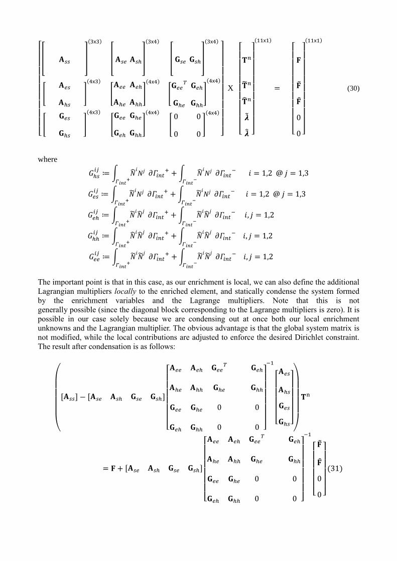
The significant feature of this method is that unlike two previous methods, the shape functions are

𝐶0 across the cut borders (but not across Γint)

The shape functions used in this section were originally proposed in [11] (more details, along with

the 3D version of the basic functions, can be found in the same reference). The present section

explores the application of the Dirichlet BCs on the cut interface via the use of a penalty approach

(see Section 5). The shape functions for a typical triangular element are shown in Figure 8.

Figure 7: Partition of a single finite element into sub-elements following the interface PQ

Figure 8: Modified shape functions for the discontinuous space without additional unknowns (used in Method III)

6. IMPOSING BOUNDARY CONDITIONS ON DISCONTINUOUS INSIDE THE

ELEMENT(INTERFACE)

Imposing the Neumann-type boundary condition on the interface that cuts the elements is

straightforward, since it is needed to compute the integral of the flux over the interface. In

particular, for the application of an adiabatic boundary condition (zero heat flux), the terms

including the flux at the interface, S, can even be omitted.

The imposition of the Dirichlet boundary conditions on 𝛤𝑖𝑛𝑡 is, on the other hand, a little more

involved since no node is present on the boundary 𝛤𝑖𝑛𝑡 to strongly apply the condition. Many

specific techniques for the implementation of the Dirichlet boundary conditions in X-FEM have

been proposed, such as the Lagrange multiplier method [12–15], the penalty method [16], and

Nitsche’s method [17–19]. In our case, the Lagrange multiplier method is considered for the first

two methods, while the penalty method is chosen for the third method in order to ensure that our

enriched variables assume the desired value on the boundary.

6.1: Implementation of Lagrange Multiplier in Method I

In Method I, four additional degrees of freedom as Lagrangian multipliers are used in order to

impose the Dirichlet constraint, e.g. a zero value of the temperature at the interface. Let us consider

a triangular FE mesh containing discontinuity 𝛤𝑖𝑛𝑡. As we know, the function is discontinuous at the

interface that we have decomposed into two sub-interfaces 𝛤𝑖𝑛𝑡+ and 𝛤𝑖𝑛𝑡

− (see Figure 9). This

approach is implemented by using two integral points on each sub-interface 𝛤𝑖𝑛𝑡+ and 𝛤𝑖𝑛𝑡

− .

Figure 9: A triangle element containing Γint with two gauss points on each sub-element Γint

+ and Γint−

Hence, after adding the Lagrange multiplier term to the equation (21), the system formed by the

enrichment variables and the Lagrange multipliers can be written by blocks in the following

manner:

[

[ 𝐀𝑠𝑠 ]

(3𝗑3)

[ 𝐀𝑠𝑒 𝐀𝑠ℎ]

(3𝗑4)

[ 𝐆𝑠𝑒 𝐆𝑠ℎ]

(3𝗑4)

[𝐀𝑒𝑠

𝐀ℎ𝑠

]

(4𝗑3)

[𝐀𝑒𝑒 𝐀𝑒ℎ

𝐀ℎ𝑒 𝐀ℎℎ]

(4𝗑4)

[𝐆𝑒𝑒

𝑇 𝐆𝑒ℎ

𝐆ℎ𝑒 𝐆ℎℎ

]

(4𝗑4)

[𝐆𝑒𝑠

𝐆ℎ𝑠

]

(4𝗑3)

[𝐆𝑒𝑒 𝐆ℎ𝑒

𝐆𝑒ℎ 𝐆ℎℎ]

(4𝗑4)

[0 0

0 0]

(4𝗑4)

]

X

[

𝐓𝑛

𝑛

𝑛

] (11𝗑1)

=

[

𝐅

0

0 ] (11𝗑1)

(30)

where

𝐺ℎ𝑠𝑖𝑗≔ ∫

𝑖𝑁𝑗

𝛤𝑖𝑛𝑡+

𝜕𝛤𝑖𝑛𝑡+ +∫

𝑖𝑁𝑗

𝛤𝑖𝑛𝑡−

𝜕𝛤𝑖𝑛𝑡− 𝑖 = 1,2 @ 𝑗 = 1,3

𝐺𝑒𝑠𝑖𝑗≔ ∫

𝑖𝑁𝑗

𝛤𝑖𝑛𝑡+

𝜕𝛤𝑖𝑛𝑡+ +∫

𝑖𝑁𝑗

𝛤𝑖𝑛𝑡−

𝜕𝛤𝑖𝑛𝑡− 𝑖 = 1,2 @ 𝑗 = 1,3

𝐺𝑒ℎ𝑖𝑗≔ ∫

𝑖𝑗

𝛤𝑖𝑛𝑡+

𝜕𝛤𝑖𝑛𝑡+ +∫

𝑖𝑗

𝛤𝑖𝑛𝑡−

𝜕𝛤𝑖𝑛𝑡− 𝑖, 𝑗 = 1,2

𝐺ℎℎ𝑖𝑗≔ ∫

𝑖𝑗

𝛤𝑖𝑛𝑡+

𝜕𝛤𝑖𝑛𝑡+ +∫

𝑖𝑗

𝛤𝑖𝑛𝑡−

𝜕𝛤𝑖𝑛𝑡− 𝑖, 𝑗 = 1,2

𝐺𝑒𝑒𝑖𝑗≔ ∫

𝑖𝑗

𝛤𝑖𝑛𝑡+

𝜕𝛤𝑖𝑛𝑡+ +∫

𝑖𝑗

𝛤𝑖𝑛𝑡−

𝜕𝛤𝑖𝑛𝑡− 𝑖, 𝑗 = 1,2

The important point is that in this case, as our enrichment is local, we can also define the additional

Lagrangian multipliers locally to the enriched element, and statically condense the system formed

by the enrichment variables and the Lagrange multipliers. Note that this is not

generally possible (since the diagonal block corresponding to the Lagrange multipliers is zero). It is

possible in our case solely because we are condensing out at once both our local enrichment

unknowns and the Lagrangian multiplier. The obvious advantage is that the global system matrix is

not modified, while the local contributions are adjusted to enforce the desired Dirichlet constraint.

The result after condensation is as follows:

(

[𝐀𝑠𝑠] − [𝐀𝑠𝑒 𝐀𝑠ℎ 𝐆𝑠𝑒 𝐆𝑠ℎ]

[ 𝐀𝑒𝑒 𝐀𝑒ℎ 𝐆𝑒𝑒

𝑇 𝐆𝑒ℎ

𝐀ℎ𝑒 𝐀ℎℎ 𝐆ℎ𝑒 𝐆ℎℎ

𝐆𝑒𝑒 𝐆ℎ𝑒 0 0

𝐆𝑒ℎ 𝐆ℎℎ 0 0 ] −1

[ 𝐀𝑒𝑠

𝐀ℎ𝑠

𝐆𝑒𝑠

𝐆ℎ𝑠]

)

𝐓n

= 𝐅 + [𝐀𝑠𝑒 𝐀𝑠ℎ 𝐆𝑠𝑒 𝐆𝑠ℎ]

[ 𝐀𝑒𝑒 𝐀𝑒ℎ 𝐆𝑒𝑒

𝑇 𝐆𝑒ℎ

𝐀ℎ𝑒 𝐀ℎℎ 𝐆ℎ𝑒 𝐆ℎℎ

𝐆𝑒𝑒 𝐆ℎ𝑒 0 0

𝐆𝑒ℎ 𝐆ℎℎ 0 0 ] −1

[

0

0 ]

(31)

6.2: Implementation of Lagrange Multiplier in Method II

In this method, due to the fact that three enrichment functions are added, three degrees of freedom

are used as Lagrangian multipliers, in order to impose the Dirichlet constraint.

Thus, the matrix formed by the system (27) may be rewritten as

[ [ 𝐀𝑠𝑠 ]

(3𝗑3)

[ 𝐀𝑠𝑒 ]

(3𝗑3)

[ 𝐆𝑠𝑒 ]

(3𝗑3)

[ 𝐀𝑒𝑠 ]

(3𝗑3)

[ 𝐀𝑒𝑒 ]

(3𝗑3)

[ 𝐆𝑒𝑒𝑇 ]

(3𝗑3)

[ 𝐆𝑒𝑠 ]

(3𝗑3)

[ 𝐆𝑒𝑒 ]

(3𝗑3)

[0 0

0 0]

(3𝗑3)

]

X

[

𝐓𝑛

𝑛

] (9𝗑1)

=

[

𝐅

0

0 ] (9𝗑1)

(32)

where

𝐺𝑒𝑠𝑖𝑗≔ ∫

𝑖𝑁𝑗

𝛤𝑖𝑛𝑡+

𝜕𝛤𝑖𝑛𝑡+ +∫

𝑖𝑁𝑗

𝛤𝑖𝑛𝑡−

𝜕𝛤𝑖𝑛𝑡− 𝑖, 𝑗 = 1,3

𝐺𝑠𝑒𝑖𝑗 = 𝐺𝑒𝑠

𝑗𝑖 𝑖, 𝑗 = 1,3

𝐺𝑒𝑒𝑖𝑗≔ ∫

𝑖𝑗

𝛤𝑖𝑛𝑡+

𝜕𝛤𝑖𝑛𝑡+ +∫

𝑖𝑗

𝛤𝑖𝑛𝑡−

𝜕𝛤𝑖𝑛𝑡− 𝑖, 𝑗 = 1,3

6.3: Implementation of Penalty in Method III

As stated earlier, in Method III no enrichment functions are added to capture discontinuities (see

Section 5). The practical consequence is that the static condensation procedure employed for the

first two alternatives is not viable here. For this reason, a penalty method is chosen to enforce the

Dirichlet boundary condition. For more explication, if the liner equation is KT=F, then the penalty

method can apply the boundary condition using a large number to modify the stiffness matrix as

well as the right-hand side vector as

(K+)T = F+ (33)

where

= ∫ 𝑇𝛤𝑖𝑛𝑡

+ 𝜕𝛤𝑖𝑛𝑡

+ +∫ 𝑇𝛤𝑖𝑛𝑡

− 𝜕𝛤𝑖𝑛𝑡

−

= ∫ 𝑇𝑇𝑖𝑛𝑡𝛤𝑖𝑛𝑡

+ 𝜕𝛤𝑖𝑛𝑡

+ +∫ 𝑇𝑇𝑖𝑛𝑡𝛤𝑖𝑛𝑡

− 𝜕𝛤𝑖𝑛𝑡

−

7. EXAMPLES SECTION

1. Example 1

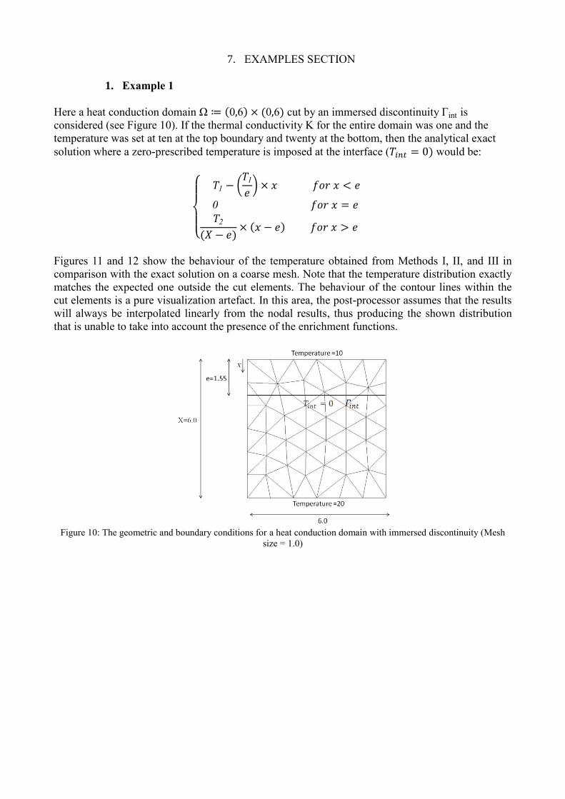
Here a heat conduction domain Ω ≔ (0,6) × (0,6) cut by an immersed discontinuity Γint is

considered (see Figure 10). If the thermal conductivity K for the entire domain was one and the

temperature was set at ten at the top boundary and twenty at the bottom, then the analytical exact

solution where a zero-prescribed temperature is imposed at the interface (𝑇𝑖𝑛𝑡 = 0) would be:

𝑇1 − (

𝑇1

𝑒) × 𝑥 𝑓𝑜𝑟 𝑥 < 𝑒

0 𝑓𝑜𝑟 𝑥 = 𝑒 𝑇2

(𝑋 − 𝑒)× (𝑥 − 𝑒) 𝑓𝑜𝑟 𝑥 > 𝑒

Figures 11 and 12 show the behaviour of the temperature obtained from Methods I, II, and III in

comparison with the exact solution on a coarse mesh. Note that the temperature distribution exactly

matches the expected one outside the cut elements. The behaviour of the contour lines within the

cut elements is a pure visualization artefact. In this area, the post-processor assumes that the results

will always be interpolated linearly from the nodal results, thus producing the shown distribution

that is unable to take into account the presence of the enrichment functions.

Figure 10: The geometric and boundary conditions for a heat conduction domain with immersed discontinuity (Mesh

size = 1.0)

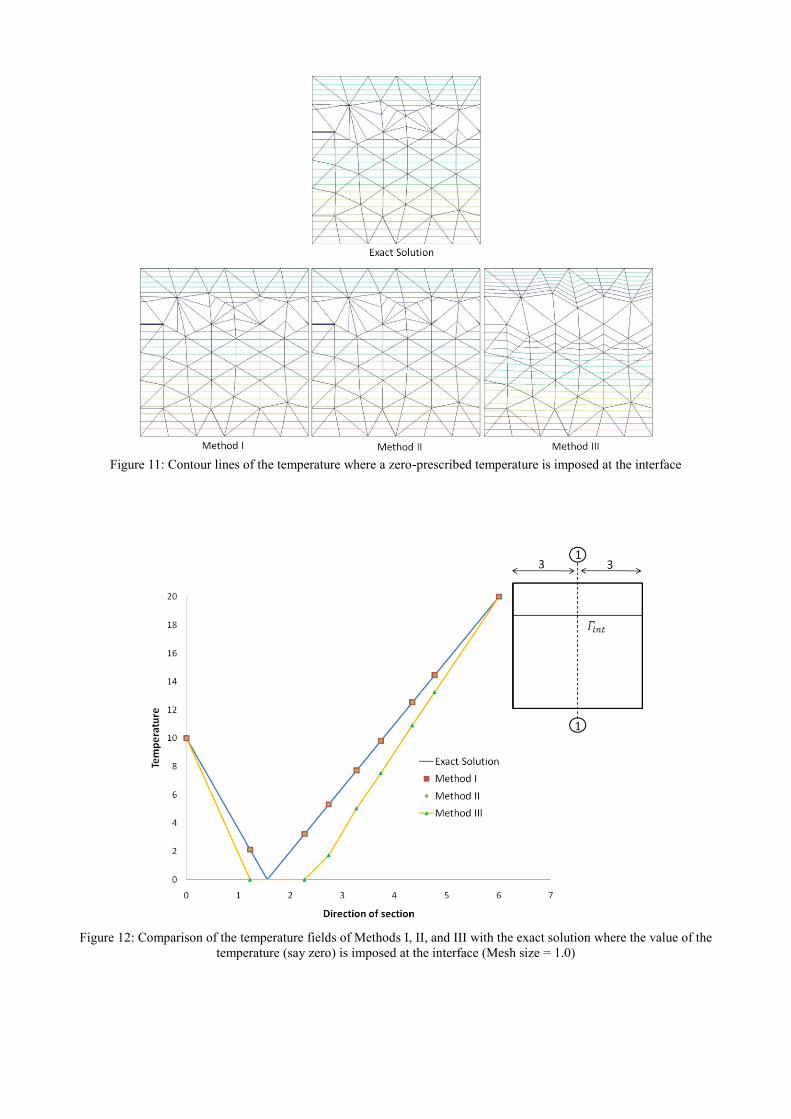
Figure 11: Contour lines of the temperature where a zero-prescribed temperature is imposed at the interface

Figure 12: Comparison of the temperature fields of Methods I, II, and III with the exact solution where the value of the

temperature (say zero) is imposed at the interface (Mesh size = 1.0)

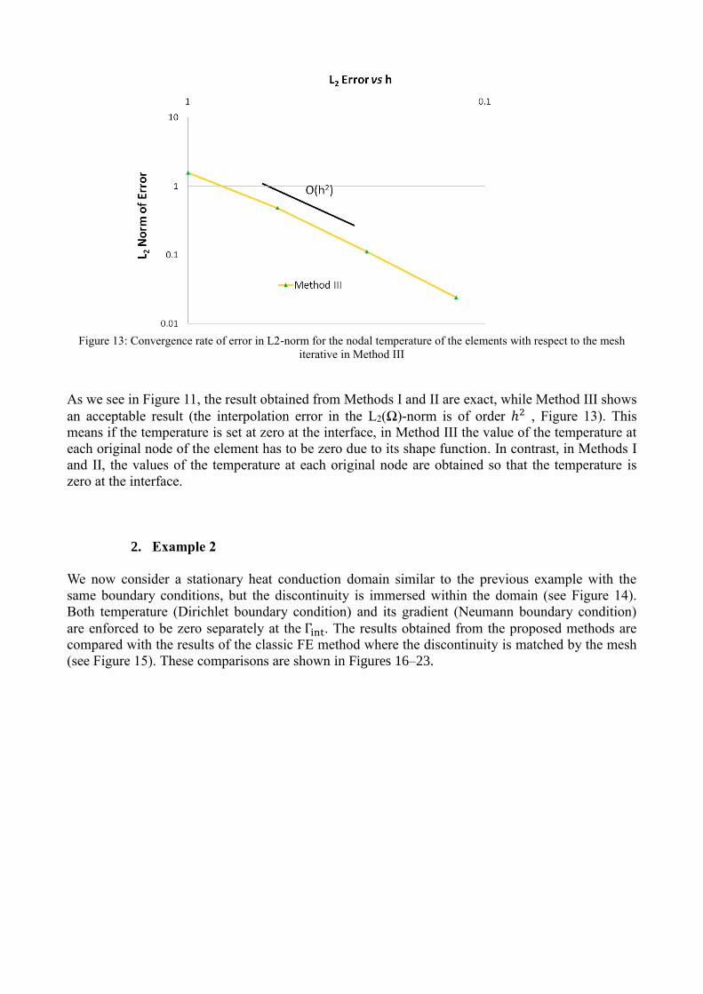
Figure 13: Convergence rate of error in L2-norm for the nodal temperature of the elements with respect to the mesh

iterative in Method III

As we see in Figure 11, the result obtained from Methods I and II are exact, while Method III shows

an acceptable result (the interpolation error in the L2(Ω)-norm is of order ℎ2 , Figure 13). This

means if the temperature is set at zero at the interface, in Method III the value of the temperature at

each original node of the element has to be zero due to its shape function. In contrast, in Methods I

and II, the values of the temperature at each original node are obtained so that the temperature is

zero at the interface.

2. Example 2

We now consider a stationary heat conduction domain similar to the previous example with the

same boundary conditions, but the discontinuity is immersed within the domain (see Figure 14).

Both temperature (Dirichlet boundary condition) and its gradient (Neumann boundary condition)

are enforced to be zero separately at the Γint. The results obtained from the proposed methods are

compared with the results of the classic FE method where the discontinuity is matched by the mesh

(see Figure 15). These comparisons are shown in Figures 16–23.

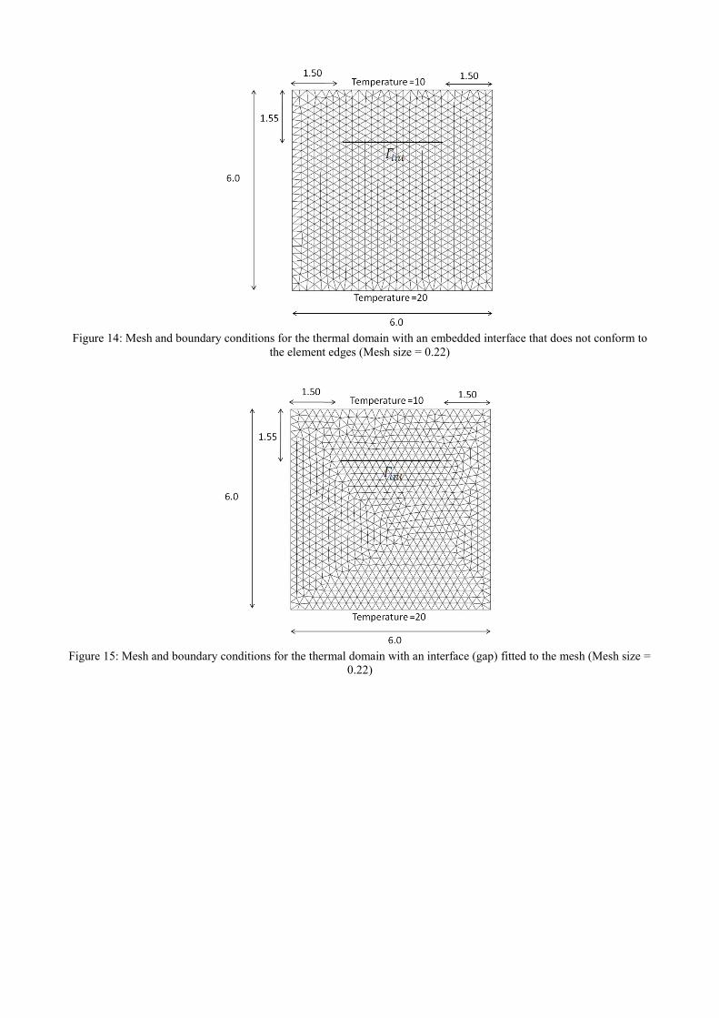
Figure 14: Mesh and boundary conditions for the thermal domain with an embedded interface that does not conform to

the element edges (Mesh size = 0.22)

Figure 15: Mesh and boundary conditions for the thermal domain with an interface (gap) fitted to the mesh (Mesh size =

0.22)

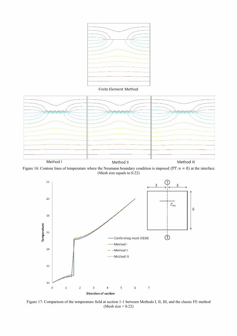
Figure 16: Contour lines of temperature where the Neumann boundary condition is imposed (𝛻𝑇. 𝑛 = 0) at the interface

(Mesh size equals to 0.22)

Figure 17: Comparison of the temperature field at section 1-1 between Methods I, II, III, and the classic FE method

(Mesh size = 0.22)

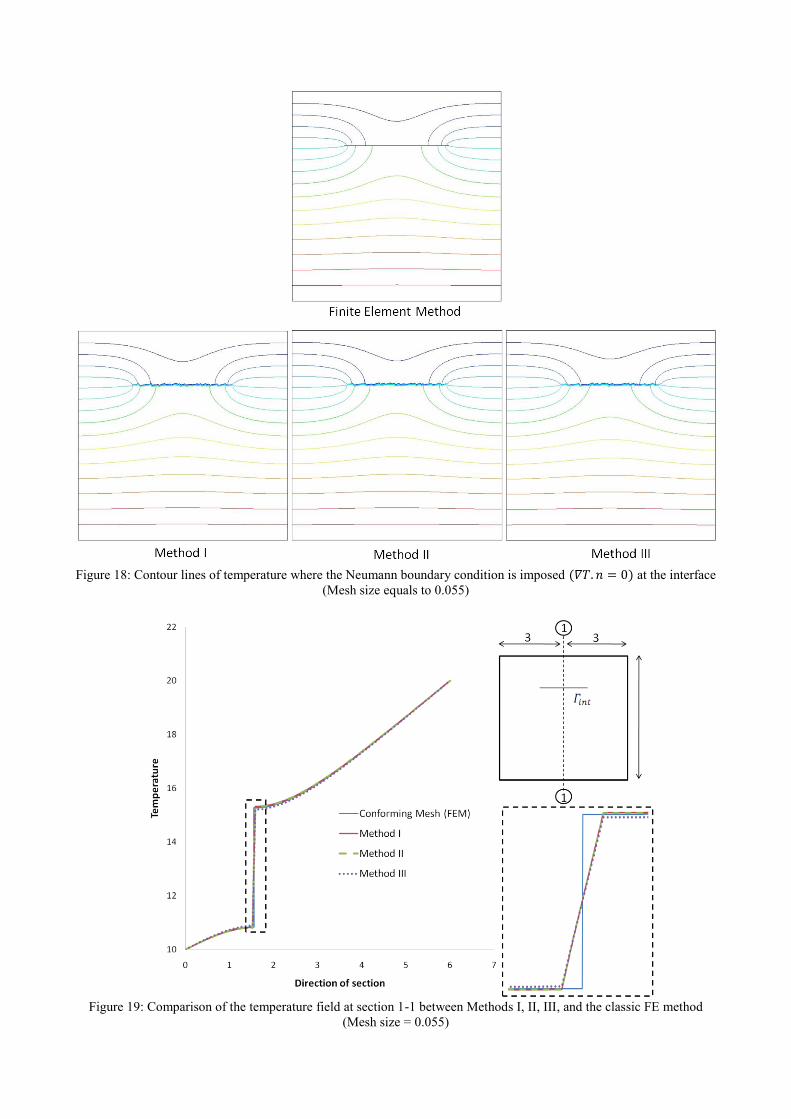
Figure 18: Contour lines of temperature where the Neumann boundary condition is imposed (𝛻𝑇. 𝑛 = 0) at the interface

(Mesh size equals to 0.055)

Figure 19: Comparison of the temperature field at section 1-1 between Methods I, II, III, and the classic FE method

(Mesh size = 0.055)

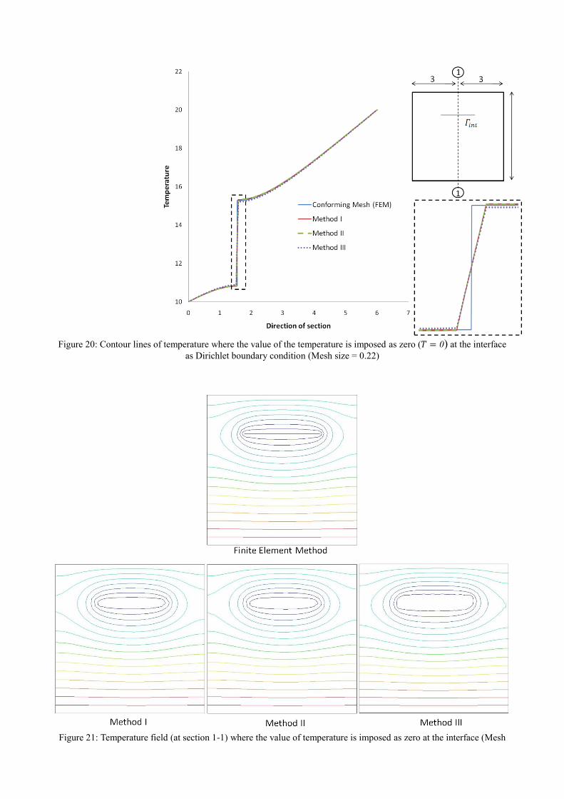
Figure 20: Contour lines of temperature where the value of the temperature is imposed as zero (𝑇 = 0) at the interface

as Dirichlet boundary condition (Mesh size = 0.22)

Figure 21: Temperature field (at section 1-1) where the value of temperature is imposed as zero at the interface (Mesh

size = 0.22)

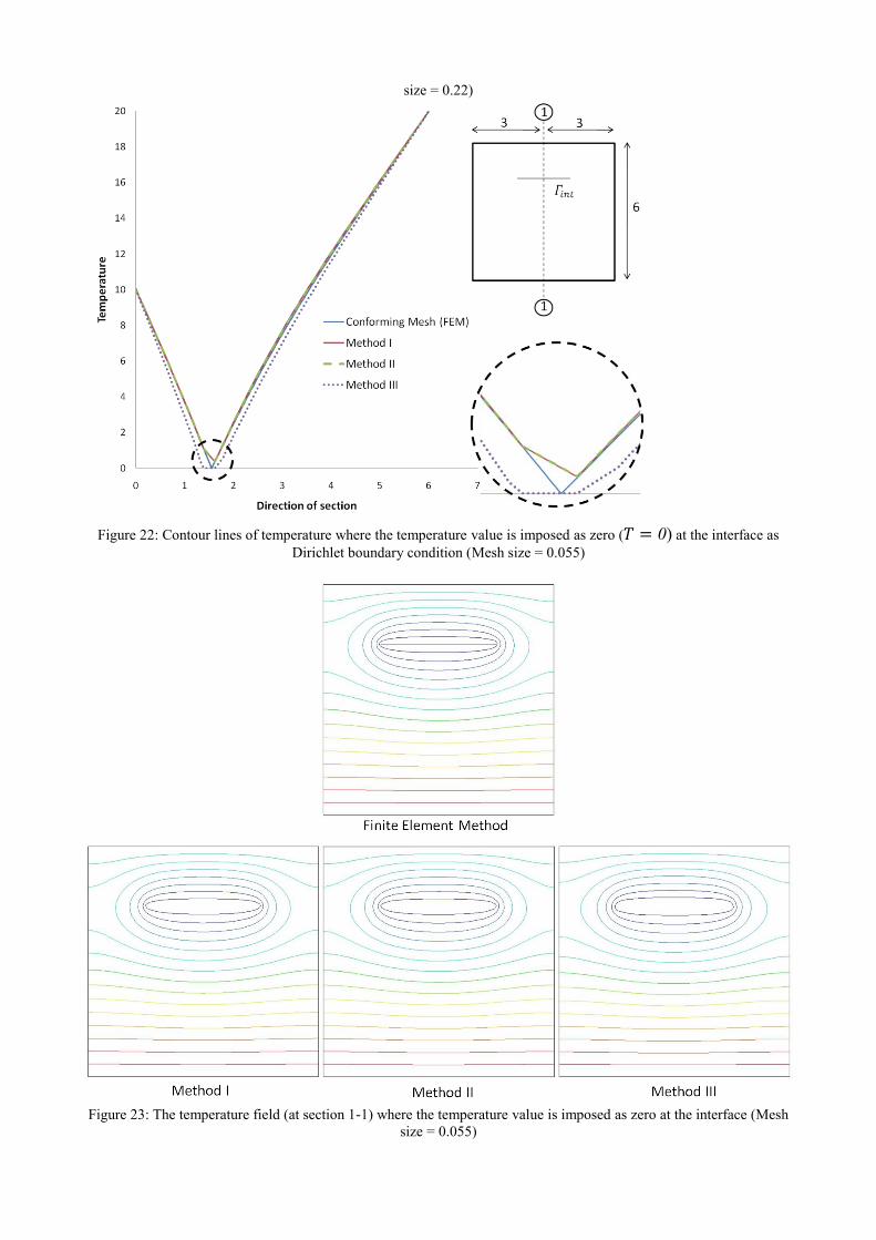
Figure 22: Contour lines of temperature where the temperature value is imposed as zero (𝑇 = 0) at the interface as

Dirichlet boundary condition (Mesh size = 0.055)

Figure 23: The temperature field (at section 1-1) where the temperature value is imposed as zero at the interface (Mesh

size = 0.055)

As we can see from the results, when discontinuity immerses with an adiabatic boundary condition

for temperature, Method III has better convergence than the others in a coarse mesh, while Methods

I and II have shown better results when the size of the mesh decreases. However, when a zero-

prescribed temperature (Dirichlet boundary condition) is imposed at the interface, the first two

proposed methods are shown more accurately than the third one in either coarse or fine mesh. This

result agrees with our expectation. For more explanation, this poor convergence in Method III

happens due to the concept of modified shape function, which is used in this method (see Section

5). Therefore, the value of temperature is zero not only at the interface but also on the whole cut

element. In contrast, in Methods I and II the temperature of the triangle nodes is calculated so that

the value of the temperature can be zero exactly at the interface.

3. Example 3

As a third experience, we investigate the heat conduction problem in a domain with the same

geometry, but an embedded diagonal discontinuity cuts the domain. The mesh and the boundary

conditions for the domain are shown in Figure 24. The gradient of the temperature is set at zero on

the embedded discontinuity. At the end, the results from the proposed methods are compared with

the reference solution where the discontinuity is fitted to the mesh (see Figures 25-31).

Figure 24: The mesh and the boundary conditions for the domain with an embedded diagonal discontinuity through it

(Mesh size = 0.22)

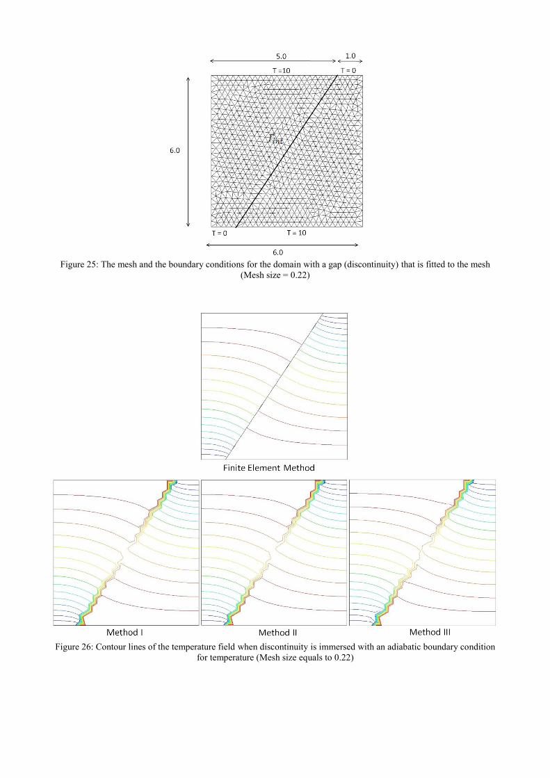
Figure 25: The mesh and the boundary conditions for the domain with a gap (discontinuity) that is fitted to the mesh

(Mesh size = 0.22)

Figure 26: Contour lines of the temperature field when discontinuity is immersed with an adiabatic boundary condition

for temperature (Mesh size equals to 0.22)

Figure 27: The discontinuities of the temperature field where the Neumann boundary condition is imposed

(Mesh size equals to 0.22)

Figure 28: Comparison of the temperature field at section 2–2 between the proposed methods and the classic FE method

(Mesh size = 0.22)

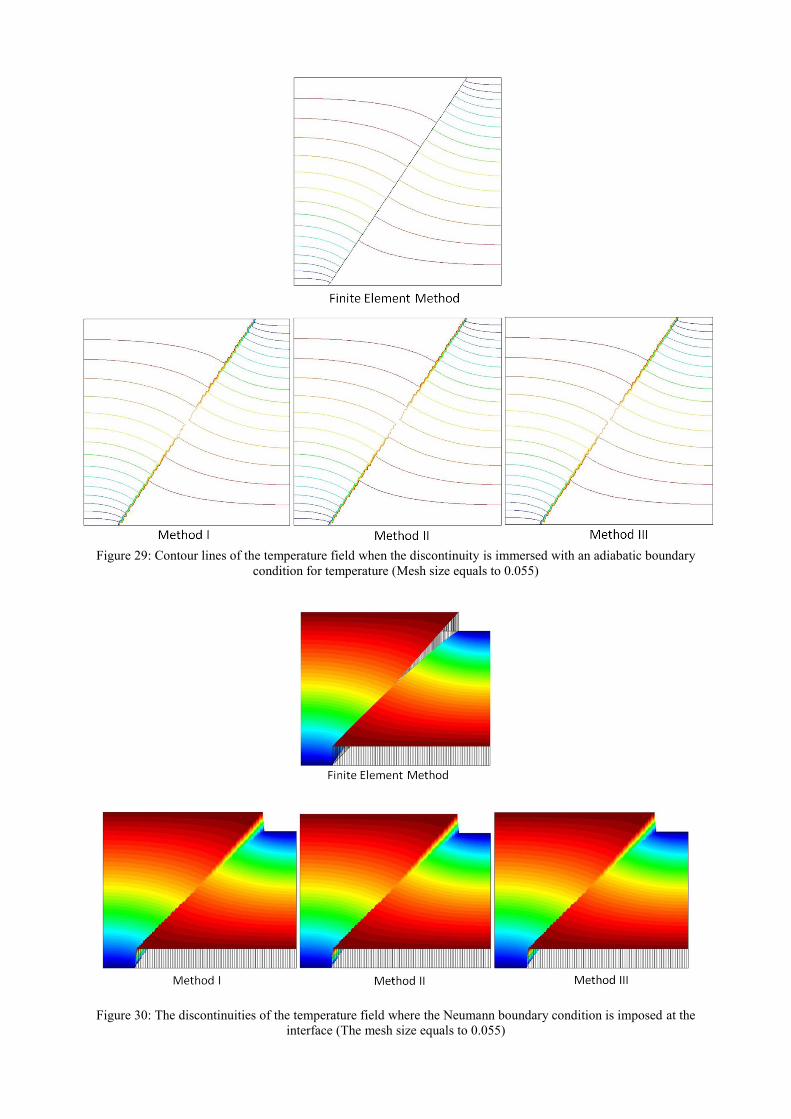
Figure 29: Contour lines of the temperature field when the discontinuity is immersed with an adiabatic boundary

condition for temperature (Mesh size equals to 0.055)

Figure 30: The discontinuities of the temperature field where the Neumann boundary condition is imposed at the

interface (The mesh size equals to 0.055)

Figure 31: Comparison of the temperature field at section 2–2 between the proposed methods and the classic FE method

(The mesh size = 0.055)

Figure 32: Convergence rate of the error in L2-norm for the nodal temperature of the elements with respect to the mesh

iterative in Methods I, II, and III

As is evident from Figure 32, when results obtained from the domain with a gap (discontinuity is

fitted to the mesh) are selected as reference solutions, the convergence rate of the interpolation error

for Methods I and II shows higher order than Method III.

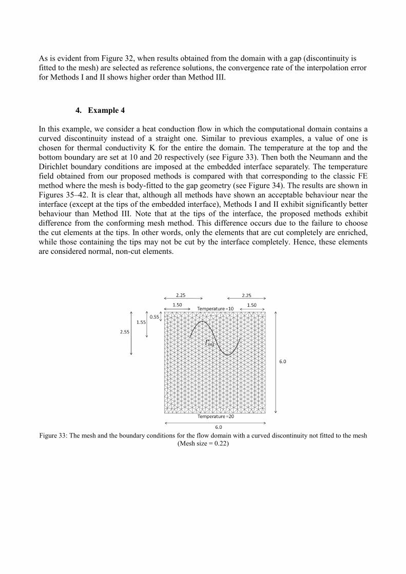
4. Example 4

In this example, we consider a heat conduction flow in which the computational domain contains a

curved discontinuity instead of a straight one. Similar to previous examples, a value of one is

chosen for thermal conductivity K for the entire the domain. The temperature at the top and the

bottom boundary are set at 10 and 20 respectively (see Figure 33). Then both the Neumann and the

Dirichlet boundary conditions are imposed at the embedded interface separately. The temperature

field obtained from our proposed methods is compared with that corresponding to the classic FE

method where the mesh is body-fitted to the gap geometry (see Figure 34). The results are shown in

Figures 35–42. It is clear that, although all methods have shown an acceptable behaviour near the

interface (except at the tips of the embedded interface), Methods I and II exhibit significantly better

behaviour than Method III. Note that at the tips of the interface, the proposed methods exhibit

difference from the conforming mesh method. This difference occurs due to the failure to choose

the cut elements at the tips. In other words, only the elements that are cut completely are enriched,

while those containing the tips may not be cut by the interface completely. Hence, these elements

are considered normal, non-cut elements.

Figure 33: The mesh and the boundary conditions for the flow domain with a curved discontinuity not fitted to the mesh

(Mesh size = 0.22)

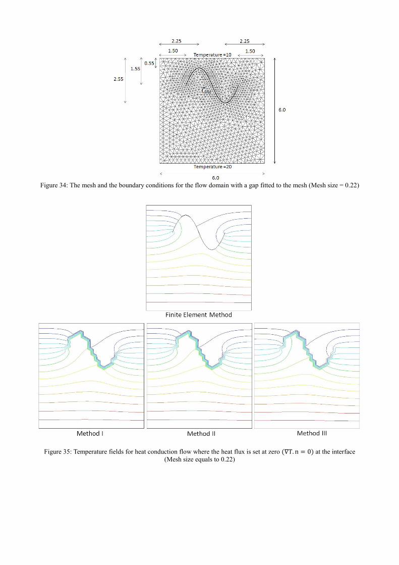
Figure 34: The mesh and the boundary conditions for the flow domain with a gap fitted to the mesh (Mesh size = 0.22)

Figure 35: Temperature fields for heat conduction flow where the heat flux is set at zero (∇T. n = 0) at the interface

(Mesh size equals to 0.22)

Figure 36: Comparison of the temperature field at section 3–3 where the heat flux is set at zero (∇T. n = 0) at the

interface (Mesh size = 0.22)

Figure 37: Temperature fields for the heat conduction flow where the heat flux is set at zero (∇T. n = 0) at the interface

(Mesh size equals to 0.055)

Figure 38: Comparison of the temperature field at section 3–3 for the heat conduction flow where the heat flux is set at

zero (∇T. n = 0) at the interface (mesh size equals to 0.055)

Figure 39: Temperature fields for the heat conduction flow where a zero-prescribed temperature (Tint = 0) is imposed at

the interface (Mesh size equals to 0.22)

Figure 40: Comparison of the temperature field at section 3–3 for the heat conduction flow where a zero-prescribed

temperature is imposed at the interface (Mesh size = 0.22)

Figure 41: Temperature fields for the heat conduction flow where a zero-prescribed temperature is imposed at the

interface (Mesh size = 0.055)

Figure 42: Comparison of the temperature field at section 3–3 for the heat conduction flow where a zero-prescribed

temperature is imposed at the interface (Mesh size = 0.055)

CONCLUSION

Three embedded methods have been proposed for a heat conduction problem with embedded

discontinuities so that aligned at arbitrary angles with respect to the mesh edges. The first one

comprises a local enrichment of the FE space. This approach adds four additional degrees of

freedom locally with the objective of capturing discontinuities within the element. In this case, in

order to impose the Dirichlet constraint, the Lagrange multiplier method has been considered. One

of the features of this method is that the system formed by the enrichment variables and the

Lagrange multipliers can be statically condensed at once prior to assembly.

The second method, similar to the first one, consists of an enrichment of the FE space. This method

differs from Method I due to the fact that the enriched functions are obtained by the incorporation

of a characteristic user function 𝜙 with the standard nodal shape functions. Thus, three enrichment

functions are used for the capturing of the discontinuity within the element (we add three new

additional degrees of freedom). Here, the Lagrange multipliers and the additional degrees of

freedom can be statically condensed at once before the final assembly, as well as the first method.

The third method having the ability to capture discontinuity within the element not by enrichment

functions but by local modifications in the nodal shape function of the elements has also been

explored. The penalty method has been chosen to impose the Dirichlet boundary condition on the

interface. Therefore, the size and the graph of the final linear system are not changed. The

computational cost is reduced due to the omission of the re-calculation of the matrix graph. The

obvious advantage of the third method, compared to the first two cases, is that the C0 continuity can

be ensured between the adjacent elements. So, finally it can be concluded that

In all methods, the computational cost is reduced because the size and the graph of the final

linear are kept the same as the standard case;

In the first two methods, we add some new functions whose amplitude is governed by the

internal degrees of freedom that do not depend on any of the neighbouring elements;

Although in the first two methods the C0 continuity is violated across the edges intersected

by the interface, it is seen how the methods appear to work satisfactorily in real cases

despite this defect; and

All the methods show acceptable results and exhibit the potential to be suitable alternative to

the other existing FE spaces with embedded discontinuities.

ACKNOWLEDGEMENT

The authors wish to acknowledge the support of the ERC through the uLites (FP7-314891),

NUMEXA (FP7-611636) and REALTIME (FP7-246643) projects

REFERENCES

1.

Sven, G. and R. Arnold, An extended pressure finite element space for two-phase

incompressible flows with surface tension. 2007, Academic Press Professional, Inc. p. 40-58.

2.

Sawada, T. and A. Tezuka, LLM and X-FEM based interface modeling of fluid thin structure

interactions on a non-interface-fitted mesh. Computational Mechanics, 2011. 48(3): p. 319-

332.

3.

Motasoares, C.A., et al., An enriched space-time finite element method for fluid-structure

interaction - Part I: Prescribed structural displacement, in III European Conference on

Computational Mechanics. 2006, Springer Netherlands. p. 399-399.

4.

Henning, S. and F. Thomas-Peter, The extended finite element method for two-phase and

free-surface flows: A systematic study. 2011, Academic Press Professional, Inc. p. 3369-

3390.

5.

Fries, T.-P. and T. Belytschko, The extended/generalized finite element method: An overview

of the method and its applications. International Journal for Numerical Methods in

Engineering, 2010. 84(3): p. 253-304.

6.

Coppola-Owen, A.H. and R. Codina, Improving Eulerian two-phase flow finite element

approximation with discontinuous gradient pressure shape functions. International Journal

of Numerical Methods in Fluids, 2005. 49(12): p. 1287-1304.

7.

Chessa, J. and T. Belytschko, An Extended Finite Element Method for Two-Phase Fluid.

journal of Applied Mechanics, 2003. 70: p. 10-17.

8.

Belytschko, T., et al., Arbitrary discontinuities in finite elements. International Journal for

Numerical Methods in Engineering, 2001. 50: p. 993–1013.

9.

O.C. Zienkiewicz and R.L. Taylor, The finite element method-the basis. 2000, Oxford,:

Butterworth-Heinemann.

10.

Chessa, J., P. Smolinski, and T. Belytschko, The extended finite element method (XFEM) for

solidification problems. International Journal for Numerical Methods in Engineering, 2002.

53: p. 1959–1977.

11.

Ausas, R.F., F.S. Sousa, and G.C. Buscaglia, An improved finite element space for

discontinuous pressures. Computer Methods in Applied Mechanics and Engineering, 2010.

199: p. 1019-1031.

12.

Sebastian, K. and M. Kurt, Levelset based fluid topology optimization using the extended

finite element method. Structural and Multidisciplinary Optimization 2012. 46(3): p. 311 -

326.

13.

Rivera, C.A., et al., Parallel finite element simulations of incompressible viscous fluid flow

by domain decomposition with Lagrange multipliers. Journal of Computational Physics

2010. 229(13): p. 5123-5143.

14.

Belytschko, T., Y. Lu, Y, and L. Gu, Element free galerkin methods. International Journal for

Numerical Methods in Engineering, 1994. 37(2): p. 229–256.

15.

Belgacem.F.B, The mortar finite element method with lagrange multipliers. Numerische

Mathematik, 1999. 84.

16.

Zhu, T. and S.N. Atluri, A modified collocation method and a penalty formulation for

enforcing the essential boundary conditions in the element free Galerkin method. Comput.

Mech., 1998. 21(3): p. 211-222.

17.

Hansbo.A and Hansbo.P, An unfitted finite element method, based on Nitsche's method, for

elliptic interface problems. Computer Methods in Applied Mechanics and Engineering,

2002. 191: p. 5537 - 5552.

18.

Griebel, M. and M.A. Schweitzer, A particle-partition of unity method. Part V: Boundary

conditions, in: S. Hildebrandt, H. Karcher (Eds.), Geometric Analysis and Nonlinear Partial

Differential Equations. Springer, 2002: p. 517–540.

19.

Babuska, I., U. Banerjee, and J.E. Osborn, Meshless and generalized finite element methods:

A survey of some major results, in: M. Griebel, M. A. Schweitzer (Eds.), Meshfree methods

for partial differential equations. Lecture Notes in Computational Science and Engineering,

Springer-Verlag, 2001. 26: p. 1–20.