Earthq Sci (2010)23: 449!463 449

Three dimensional shear wave velocity structure of the crust and upper mantle beneath China from

ambient noise surface wave tomography" Xinlei Sun 1, Xiaodong Song 1 Sihua Zheng 1,2

Yingjie Yang 3 and Michael H. Ritzwoller 3

1 Department of Geology, University of Illinois at Urbana-Champaign, Urbana IL 61801, USA 2 Institute of Earthquake Science, China Earthquake Administration, Beijing 100036, China 3 CIEI, Department of Physics, University of Colorado at Boulder, Boulder CO 80309, USA

Abstract We determine the three-dimensional shear wave velocity structure of the crust and upper mantle in China using Green�’s functions obtained from seismic ambient noise cross-correlation. The data we use are from the China National Seis-mic Network, global and regional networks and PASSCAL stations in the region. We first acquire cross-correlation seismo-grams between all possible station pairs. We then measure the Rayleigh wave group and phase dispersion curves using a fre-quency-time analysis method from 8 s to 60 s. After that, Rayleigh wave group and phase velocity dispersion maps on 1° by 1° spatial grids are obtained at different periods. Finally, we invert these maps for the 3-D shear wave velocity structure of the crust and upper mantle beneath China at each grid node. The inversion results show large-scale structures that correlate well with surface geology. Near the surface, velocities in major basins are anomalously slow, consistent with the thick sedi-ments. East-west contrasts are striking in Moho depth. There is also a fast mid-to-lower crust and mantle lithosphere beneath the major basins surrounding the Tibetan plateau (TP) and Tianshan (Junggar, Tarim, Ordos, and Sichuan). These strong blocks, therefore, appear to play an important role in confining the deformation of the TP and constraining its geometry to form its current triangular shape. In northwest TP in Qiangtang, slow anomalies extend from the crust to the mantle litho-sphere. Meanwhile, widespread, a prominent low-velocity zone is observed in the middle crust beneath most of the central, eastern and southeastern Tibetan plateau, consistent with a weak (and perhaps mobile) middle crust.

Key words: ambient noise; surface wave; tomography; crust and upper mantle; China CLC number: P315.3 Document code: A

1 Introduction

Located in the southeast part of Eurasia, China and its surrounding areas are geologically diverse and tec-tonically active. The region basically consists of several ancient platforms (e.g., Sino-Korea, Yangtze craton), deep sedimentary basins (e.g., Ordos and Tarim basin), and a high plateau (Tibet) that are separated by active structures such as faults and fold belts (Figure 1). Two major events are mostly responsible for the complex

" Received 29 April 2010; accepted in revised form 20 July 2010;

published 10 October 2010. Corresponding author. e-mail: xsun@seismo.wustl.edu. Now at Depart-

ment of Earth and Planetary Sciences, Washington University in St. Louis, St. Louis, MO 63130.

© The Seismological Society of China and Springer-Verlag Berlin Heidelberg 2010

features in this region: 1) the collision between India and the Eurasian plate about 50 Ma ago (Molnar and Tapponnier, 1975; Yin and Harrison, 2000), and 2) the subduction of the Pacific plate underneath Eurasia since about 250 Ma. As a result, the collision and post colli-sion of India-Eurasia led to the shortening and elevation of the Tibetan plateau; and the subduction of the Pacific and Philippine plates led to the formation of island arcs and continental rift zones. Between these convergent boundaries, extensional features are common, such as the extension in the Sino-Korea block (Nabelek et al., 1987; Ying et al., 2006) and in the Tibetan plateau (Ar-mijo et al., 1986; Turner et al., 1996; Blisniuk et al., 2001; Williams et al., 2001; Zhang et al., 2004). To understand the mechanisms, history and the relationships between these unique tectonic features, detailed information

Doi: 10.1007/s11589-010-0744-4

450 Earthq Sci (2010)23: 449!463

Figure 1 (a) Maps of China and surrounding areas in this study. Black thick lines mark the major tectonic boundaries and gray thin lines mark major basins. The basins include the Tarim (TRM), Junggar (JG), Qaidam (QDM), Sichuan (SC), Ordos (OD), Bohai wan (BHW) and Songliao (SL) basin. The blocks include the Songpan-Garze, Qiangtang, Lhasa and Himalaya block in the Tibetan region and the Sino-Korea craton, the Yangtze block and South China fold belt in East China. Plotted in the background is the topography in this region. (b) Distribution of seismic stations used in this study, including China National Seismic Network stations (black solid triangles), global and regional stations in the surrounding areas (black open triangles) and temporary PASSCAL stations (gray solid triangles). AA#, BB# and CC# are cross section profiles shown in Figure 6.

about the structure of the crust and upper mantle beneath China and its surrounding areas is strongly needed.

Seismic tomography is a useful and powerful tool to investigate the substructure of China. Numerous body

wave and surface wave tomography studies have been conducted in China and its surrounding areas (e.g., Wu et al., 1997; Ritzwoller et al., 1998; Villasenor et al., 2001; Friederich, 2003; Huang et al., 2003; Liang et al.,

Earthq Sci (2010)23: 449!463 451

2004; Shapiro et al., 2004; Li et al., 2006; Sun and Toksöz, 2006). But these earthquake-generated data have their own limitations. Commonly, because of the uneven distribution of earthquakes and available stations, the coverage of these data is generally sparse and non-

uniform. Body waves have especially sparse coverage in the crust and upper mantle from far field earthquakes, while surface waves at short periods are difficult to ob-tain due to the attenuation and scattering, and they have long wavelengths and lower lateral resolution. Although there is general agreement in the large-scale structures that are imaged, discrepancies remain at the smaller scales needed to unravel the tectonic history of the re-gion. In recent years, significant efforts have been ex-pended to determine detailed structural information us-ing local and temporary seismic networks. Unfortu-nately, the studies have mainly focused on local scale structures, especially within Tibet (e.g., Nelson et al., 1996; Sandvol et al., 1997; Hauck et al., 1998; Zhao et al., 2001; Tilmann and Ni, 2003; Liang and Song, 2006; Tseng et al., 2009). Detailed structural information at continental scales is still needed in order to improve understanding of the dynamics and tectonic evolution of China and its environs.

Recent studies have shown that surface waves can be retrieved from seismic coda waves (Campillo and Paul, 2003; Paul et al., 2005) or seismic ambient noise (e.g., Shapiro and Campillo, 2004; Sabra et al., 2005a, c; Shapiro et al., 2005). This method overcomes several limitations of earthquake-generated signals. First, path density depends only on the distribution of stations, which is especially helpful in aseismic regions. Second, uncertainties in earthquake locations, origin times and initial phases are avoided, because no earthquake infor-mation is needed. Third, good short period (<20 s) sur-face waves dispersion measurements can be extracted, while this is typically not true for conventional signals due to high attenuation and long earthquake-station paths. Thus, surface waves from ambient noise are gen-erally better at constraining shallower structures, espe-cially in the crust. The application of this new type of data to a variety of regions has been growing rapidly both at continental and regional scales (e.g., Sabra et al., 2005b; Shapiro et al., 2005; Bensen et al., 2007, 2008; Moschetti et al., 2007; Yang et al., 2007; Lin et al., 2008; Yao et al., 2008; Zheng et al., 2008; Li et al., 2009), and has begun to reveal detail information about the crust and upper mantle structure.

In this study, we use data from new China National Seismic Network (CNSN) across China, permanent and regional stations from surrounding areas and PASSCAL experiments in this region (Figure 1). The CNSN has been deployed since 2000, and is the backbone network in the whole China region. The addition of CNSN sta-tions and PASSCAL stations has greatly expanded data coverage, making ray path coverage more uniform, es-pecially in the eastern part of China. We use the vertical component of seismograms only and focus on Rayleigh wave group and phase dispersion curves. Parts of this data set already have been used by Zheng et al. (2008). We obtain the surface wave dispersion curves between station pairs from stacked ambient noise cross-correlations, and then use tomographic methods to obtain the dispersion maps. Finally, we invert for 1-D shear wave velocity profiles beneath each of the ~2 400 grid locations across the region of study. These 1D pro-files are combined to construct a 3-D shear wave veloc-ity model of the crust and upper mantle beneath China. Our results generally display correlations between sub-surface structures and surface geology. Some remark-able features, such as the mid/lower crustal low velocity zones beneath most of the Tibetan region, may illumi-nate the tectonic dynamics there.

2 Data and method The data we used are 18 months vertical- compo-

nent continuous seismograms from 48 China National Seismic Network (CNSN) stations, 32 global and re-gional network stations in the surrounding region (the IRIS global seismic network, Taiwan, Kyrgyz and Ka-zakh networks), and 96 PASSCAL stations deployed in Tibet and the Sichuan basin during the same period (Namche Barwa and 2003MIT-China experiment) (Fig-ure 1). All these data are broadband. Parts of our data set, such as data from the CNSN stations, are the same as in Zheng et al. (2008). When the stations of the regional and PASSCAL networks are added, the general ray cov-erage is much improved (typical ray density can be seen in Figure 2).

The general process for our inversion is as follows. First, we obtain empirical Green�’s function (EGF) for Rayleigh waves between all the station pairs. The proc-ess we used here is described in detail in Bensen et al. (2007). Basically, it involves instrument response re-moval, clock synchronization, time-domain normaliza-tion, band-pass filtering (5!150 s period), and spectral

452 Earthq Sci (2010)23: 449!463

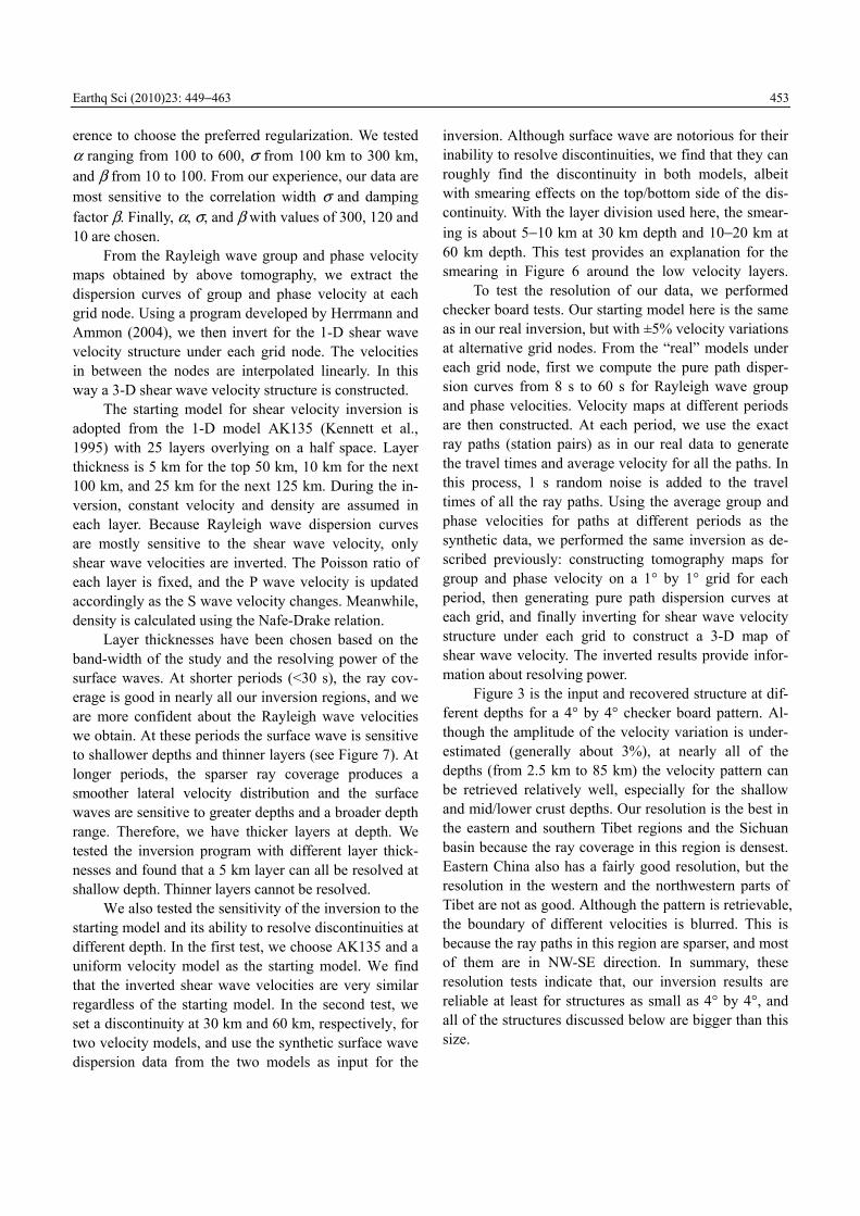
Figure 2 (a) Histograms of the number of dispersion meas-urements as a function of period for Rayleigh wave group (solid) and phase (dashed) velocities. (b) Ray path density at 20 s pe-riod. The ray density is the number of rays in each 1° by 1° cell. The coverage for shorter and longer periods deteriorates, but the spatial pattern remains similar.

whitening. We then do cross correlation on each day�’s seismograms between all possible stations, and stack all the correlations to get the EGF. An EGF is accepted if its signal to noise ratio (SNR) is greater than 10 and the inter-station distance is at least 3 times of wavelength at a given period. After this selection, about 30%!50% of the EGFs remain. Second, we use frequency-time analy-sis (FTAN) (Levshin and Ritzwoller, 2001) to measure the Rayleigh wave group and phase velocity dispersion curves between station pairs from the selected EGFs. Third, the group and phase velocity tomography maps in this region are then constructed (Barmin et al., 2001) on a 1° by 1° grid (Figure 4). Pure path dispersion curves at each grid node are obtained from the dispersion maps as a function of period. Finally, we invert for 1-D shear

wave velocity structure of the crust and upper mantle beneath each grid node and these profiles are combined to construct a 3-D shear wave velocity map.

The dispersion curves we use are from 8 s to 60 s. The total number of ray paths for each period maxi-mized at about 7 500 at 20 s period and minimizes around 3 300 at 60 s (Figure 2a). Figure 2b shows a ray density map at 20 s for the tomography. The best cover-age is centered in eastern Tibet and the Sichuan basin because of the location of the PASSCAL experiments in these regions. In the surrounding areas, the ray coverage deteriorates gradually.

In the surface wave tomography, we assume that the group and phase velocities are isotropic at different periods. Following Barmin et al. (2001), we minimize the following function to get the best model that fits the data.

T 1

2 2 2 2

( ( ) ) ( ( ) )|| ( ) || || ( ) ||F H$ %

!! ! ++

G m d C G m dm m

This equation is a combination of data misfit (first term), spatial smoothing (second term) and perturbation rela-tive to the reference model based on path density (third term).

The spatial smoothing is defined as

( ) ( ) ( , ) ( )d ,F s # # #= !m m r r r m r r

2

2

| |( , ) exp .2

s K&

#!# = ! r rr r

In these equations, $, &, % are damping parameter for smoothing, the smoothing width, and damping pa-rameter for the size of the perturbation, respectively. The choice of these numbers is somewhat arbitrary, and usu-ally needs tests based on different data subsets.

To ensure that the results are not affected signifi-cantly by outliers, tomography is performed in two steps. In the first step, we use a set of relatively large regulari-zation parameters to make an overly smoothed map. Based on the smooth maps, we calculate the predicted travel times for all the data and residuals falling outside of 2 standard deviations of all the residuals are then re-jected. Using the newly selected data, the second stage of tomography is performed. For this run we try differ-ent smoothing and damping factors (usually smaller than those of the first stage). The resulted images are then compared and we use the good correlations of the im-ages with major surface features at short periods as ref-

Earthq Sci (2010)23: 449!463 453

erence to choose the preferred regularization. We tested $ ranging from 100 to 600, & from 100 km to 300 km, and % from 10 to 100. From our experience, our data are most sensitive to the correlation width & and damping factor %. Finally, $, &, and % with values of 300, 120 and 10 are chosen.

From the Rayleigh wave group and phase velocity maps obtained by above tomography, we extract the dispersion curves of group and phase velocity at each grid node. Using a program developed by Herrmann and Ammon (2004), we then invert for the 1-D shear wave velocity structure under each grid node. The velocities in between the nodes are interpolated linearly. In this way a 3-D shear wave velocity structure is constructed.

The starting model for shear velocity inversion is adopted from the 1-D model AK135 (Kennett et al., 1995) with 25 layers overlying on a half space. Layer thickness is 5 km for the top 50 km, 10 km for the next 100 km, and 25 km for the next 125 km. During the in-version, constant velocity and density are assumed in each layer. Because Rayleigh wave dispersion curves are mostly sensitive to the shear wave velocity, only shear wave velocities are inverted. The Poisson ratio of each layer is fixed, and the P wave velocity is updated accordingly as the S wave velocity changes. Meanwhile, density is calculated using the Nafe-Drake relation.

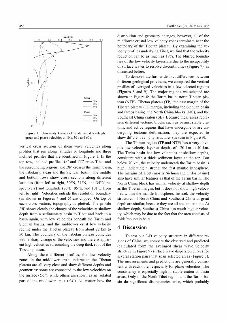
Layer thicknesses have been chosen based on the band-width of the study and the resolving power of the surface waves. At shorter periods (<30 s), the ray cov-erage is good in nearly all our inversion regions, and we are more confident about the Rayleigh wave velocities we obtain. At these periods the surface wave is sensitive to shallower depths and thinner layers (see Figure 7). At longer periods, the sparser ray coverage produces a smoother lateral velocity distribution and the surface waves are sensitive to greater depths and a broader depth range. Therefore, we have thicker layers at depth. We tested the inversion program with different layer thick-nesses and found that a 5 km layer can all be resolved at shallow depth. Thinner layers cannot be resolved.

We also tested the sensitivity of the inversion to the starting model and its ability to resolve discontinuities at different depth. In the first test, we choose AK135 and a uniform velocity model as the starting model. We find that the inverted shear wave velocities are very similar regardless of the starting model. In the second test, we set a discontinuity at 30 km and 60 km, respectively, for two velocity models, and use the synthetic surface wave dispersion data from the two models as input for the

inversion. Although surface wave are notorious for their inability to resolve discontinuities, we find that they can roughly find the discontinuity in both models, albeit with smearing effects on the top/bottom side of the dis-continuity. With the layer division used here, the smear-ing is about 5!10 km at 30 km depth and 10!20 km at 60 km depth. This test provides an explanation for the smearing in Figure 6 around the low velocity layers.

To test the resolution of our data, we performed checker board tests. Our starting model here is the same as in our real inversion, but with ±5% velocity variations at alternative grid nodes. From the �“real�” models under each grid node, first we compute the pure path disper-sion curves from 8 s to 60 s for Rayleigh wave group and phase velocities. Velocity maps at different periods are then constructed. At each period, we use the exact ray paths (station pairs) as in our real data to generate the travel times and average velocity for all the paths. In this process, 1 s random noise is added to the travel times of all the ray paths. Using the average group and phase velocities for paths at different periods as the synthetic data, we performed the same inversion as de-scribed previously: constructing tomography maps for group and phase velocity on a 1° by 1° grid for each period, then generating pure path dispersion curves at each grid, and finally inverting for shear wave velocity structure under each grid to construct a 3-D map of shear wave velocity. The inverted results provide infor-mation about resolving power.

Figure 3 is the input and recovered structure at dif-ferent depths for a 4° by 4° checker board pattern. Al-though the amplitude of the velocity variation is under-estimated (generally about 3%), at nearly all of the depths (from 2.5 km to 85 km) the velocity pattern can be retrieved relatively well, especially for the shallow and mid/lower crust depths. Our resolution is the best in the eastern and southern Tibet regions and the Sichuan basin because the ray coverage in this region is densest. Eastern China also has a fairly good resolution, but the resolution in the western and the northwestern parts of Tibet are not as good. Although the pattern is retrievable, the boundary of different velocities is blurred. This is because the ray paths in this region are sparser, and most of them are in NW-SE direction. In summary, these resolution tests indicate that, our inversion results are reliable at least for structures as small as 4° by 4°, and all of the structures discussed below are bigger than this size.

454 Earthq Sci (2010)23: 449!463

Figure 3 Checker board resolution tests of our surface wave inversion. The input model (upper left corner) has 4° by 4° checker, with ±5% velocity perturbation with respect to the AK135 model. Retrieved models at different depths (labeled on lower left corner) are also shown.

3 Results In this section, we first present dispersion maps for

Rayleigh wave group and phase velocities. The group velocity maps are updates to the earlier versions pre-sented by Zheng et al. (2008). We then present the re-sulting 3-D shear wave velocity structure inverted using the dispersion maps and discuss the major features of the 3-D structure. 3.1 Dispersion maps of Rayleigh group and phase velocities

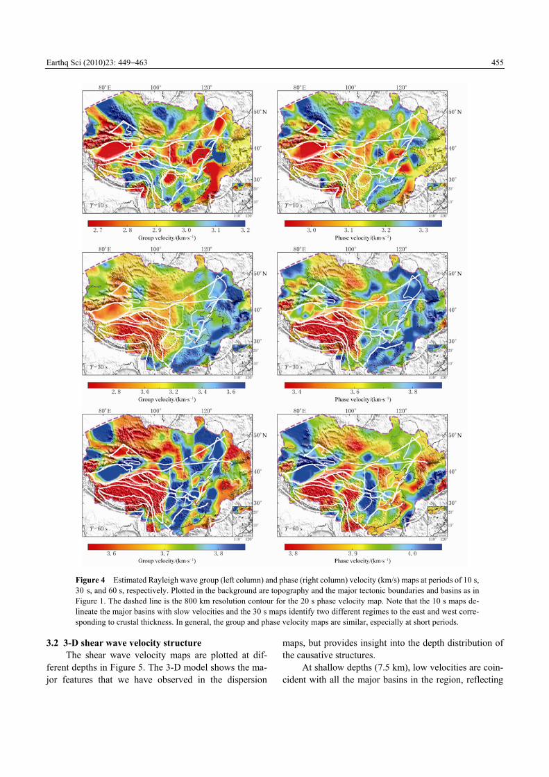
The ray coverage of our dispersion measurements is sufficient to invert for Rayleigh wave group and phase velocity maps at periods from 8 s to 60 s. Figure 4 shows tomography maps for Rayleigh group and phase velocity at periods of 10 s, 30 s, and 60 s, respectively. Because the surface wave velocities are sensitive to structures at different depths (with the most sensitive depth at about 1/3 of its wavelength), the tomography maps at different periods indicate the general features of 3-D structure at depth. In general, our group and phase velocity maps are quite similar in their major features, but they also show obvious differences at smaller scales, reflecting different sensitivities of group and phase ve-locities to velocity changes with depth (Figure 7).

The tomography results possess features that cor-relate with the large-scale geological structures of China. These features confirm earlier observations from group velocity dispersion with a smaller data set (Zheng et al., 2008). Major basins in China, including the Bohai-wan basin (North China basin), western part of the Ordos, Sichuan, Qaidam, Junggar, and Tarim basins, are clearly manifested by low velocities at short periods (10 s map) (Figure 4), which is consistent with thick sedimentary layers underlying these basins. At the same time, the stable Yangtze craton and South China block show clear high velocities, indicating a cool and strong upper crust. When the period increases to 30 s, the dichotomy of low and high velocity in the map corresponds well with the thicker crust in the west and the thinner crust in the east. The boundary between fast and slow velocities (around longitude 108°E) shows a NNE-SSW trend, coinciding with the sharp topographic change and the well-known gravity lineation. At 60 s, the Rayleigh wave velocities are influenced more by mantle lithosphere structure. The most striking feature here is a �“wall�” of high velocities in the north, northeast and east of the Tibetan plateau underneath the major basins (Tarim, Ordos, and Si-chuan). We will discuss this feature further below.

Earthq Sci (2010)23: 449!463 455

Figure 4 Estimated Rayleigh wave group (left column) and phase (right column) velocity (km/s) maps at periods of 10 s, 30 s, and 60 s, respectively. Plotted in the background are topography and the major tectonic boundaries and basins as in Figure 1. The dashed line is the 800 km resolution contour for the 20 s phase velocity map. Note that the 10 s maps de-lineate the major basins with slow velocities and the 30 s maps identify two different regimes to the east and west corre-sponding to crustal thickness. In general, the group and phase velocity maps are similar, especially at short periods.

3.2 3-D shear wave velocity structure The shear wave velocity maps are plotted at dif-

ferent depths in Figure 5. The 3-D model shows the ma-jor features that we have observed in the dispersion

maps, but provides insight into the depth distribution of the causative structures.

At shallow depths (7.5 km), low velocities are coin-cident with all the major basins in the region, reflecting

456 Earthq Sci (2010)23: 449!463

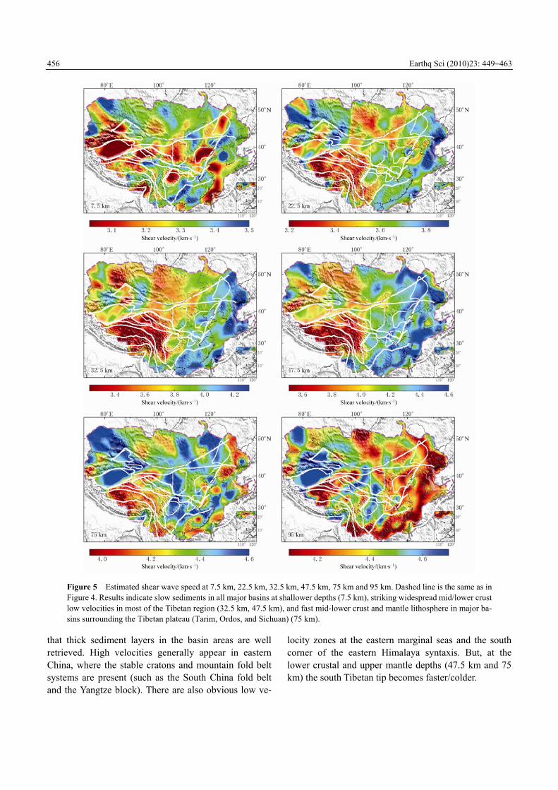
Figure 5 Estimated shear wave speed at 7.5 km, 22.5 km, 32.5 km, 47.5 km, 75 km and 95 km. Dashed line is the same as in Figure 4. Results indicate slow sediments in all major basins at shallower depths (7.5 km), striking widespread mid/lower crust low velocities in most of the Tibetan region (32.5 km, 47.5 km), and fast mid-lower crust and mantle lithosphere in major ba-sins surrounding the Tibetan plateau (Tarim, Ordos, and Sichuan) (75 km).

that thick sediment layers in the basin areas are well retrieved. High velocities generally appear in eastern China, where the stable cratons and mountain fold belt systems are present (such as the South China fold belt and the Yangtze block). There are also obvious low ve-

locity zones at the eastern marginal seas and the south corner of the eastern Himalaya syntaxis. But, at the lower crustal and upper mantle depths (47.5 km and 75 km) the south Tibetan tip becomes faster/colder.

Earthq Sci (2010)23: 449!463 457

At greater depths, around 30 km to 50 km, a strik-ing feature is the slow and fast velocity dichotomy be-tween west and east China, divided approximately at the 108° in the NE direction along the east Tibetan margin. The contrast is well correlated with the increase in to-pography from east to west. This is a vivid demonstra-tion of the thickened crust in the TP and the Tianshan from the India-Eurasia collision. As a result, at these depths, the eastern part of China is already in the mantle while the TP and the Tianshan are still in the crust.

Although most of the Tibetan plateau shows obvi-ously low velocities, the major basins surrounding Tibet and the Tianshan, including the Tarim, Junggar, Sichuan and Ordos basins, exhibit relatively high velocities. This high velocity forms a �“wall�” around the Tibetan plateau that persists to at least the uppermost mantle (around 75 km).

Another prominent feature at mid-lower crust depths is the low velocity regions in most of the central, eastern and southeastern part of Tibet. Figure 6 shows

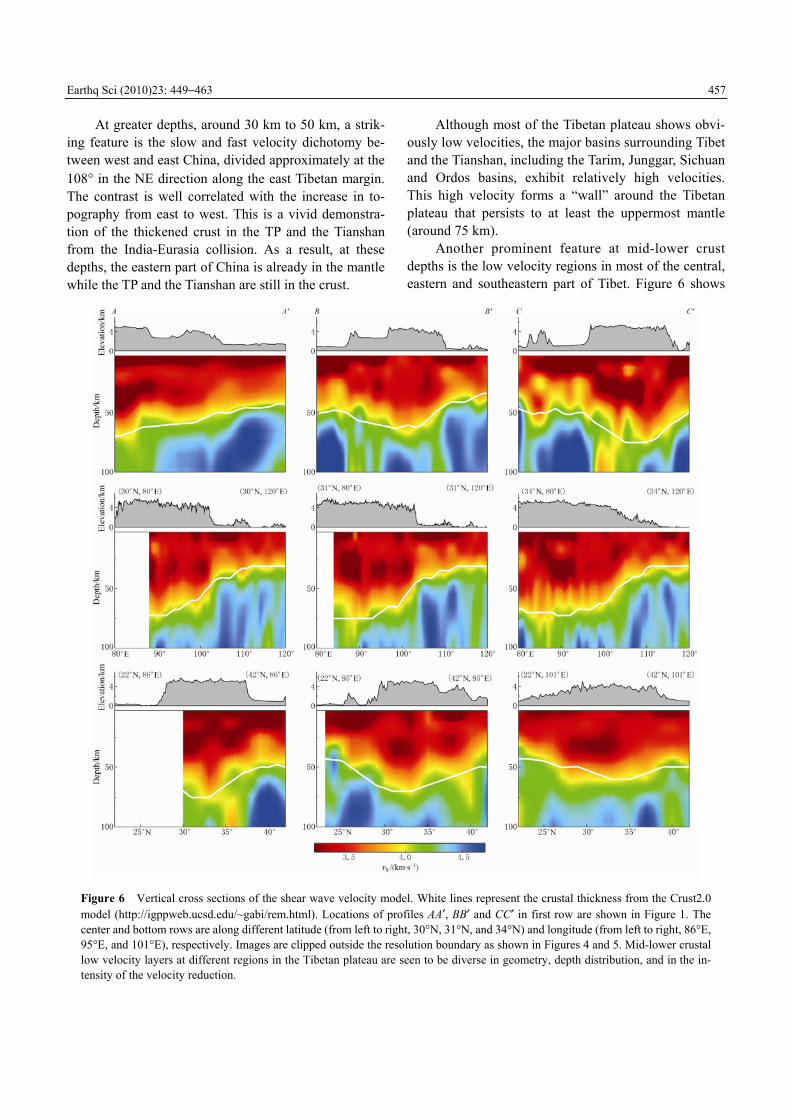
Figure 6 Vertical cross sections of the shear wave velocity model. White lines represent the crustal thickness from the Crust2.0 model (http://igppweb.ucsd.edu/~gabi/rem.html). Locations of profiles AA#, BB# and CC# in first row are shown in Figure 1. The center and bottom rows are along different latitude (from left to right, 30°N, 31°N, and 34°N) and longitude (from left to right, 86°E, 95°E, and 101°E), respectively. Images are clipped outside the resolution boundary as shown in Figures 4 and 5. Mid-lower crustal low velocity layers at different regions in the Tibetan plateau are seen to be diverse in geometry, depth distribution, and in the in-tensity of the velocity reduction.

458 Earthq Sci (2010)23: 449!463

Figure 7 Sensitivity kernels of fundamental Rayleigh group and phase velocities at 10 s, 30 s and 60 s.

vertical cross sections of shear wave velocities along profiles that run along latitudes or longitude and three inclined profiles that are identified in Figure 1. In the top row, inclined profiles AA# and CC# cross Tibet and the surrounding regions, and BB# crosses the Tarim basin, the Tibetan plateau and the Sichuan basin. The middle and bottom rows show cross sections along different latitudes (from left to right, 30°N, 31°N, and 34°N, re-spectively) and longitude (86°E, 95°E, and 101°E from left to right). Velocities outside the resolution boundary (as shown in Figures 4 and 5) are clipped. On top of each cross section, topography is plotted. The profile BB# shows clearly the change of the velocities at shallow depth from a sedimentary basin to Tibet and back to a basin again, with low velocities beneath the Tarim and Sichuan basins, and the mid/lower crust low velocity regime under the Tibetan plateau from about 22 km to 50 km. The boundary of the Tibetan plateau coincides with a sharp change of the velocities and there is appar-ent high velocities surrounding the deep thick root of the Tibetan plateau.

Along these different profiles, the low velocity zones in the mid/lower crust underneath the Tibetan plateau are all very clear and show different depths and geometries: some are connected to the low velocities on the surface (CC#); while others are shown as an isolated part of the mid/lower crust (AA#). No matter how the

distribution and geometry changes, however, all of the mid/lower crustal low velocity zones terminate near the boundary of the Tibetan plateau. By examining the ve-locity profiles underlying Tibet, we find that the velocity reduction can be as much as 19%. The blurred bounda-ries of the low velocity layers are due to the incapability of surface waves to resolve discontinuities (Figure 7), as discussed before.

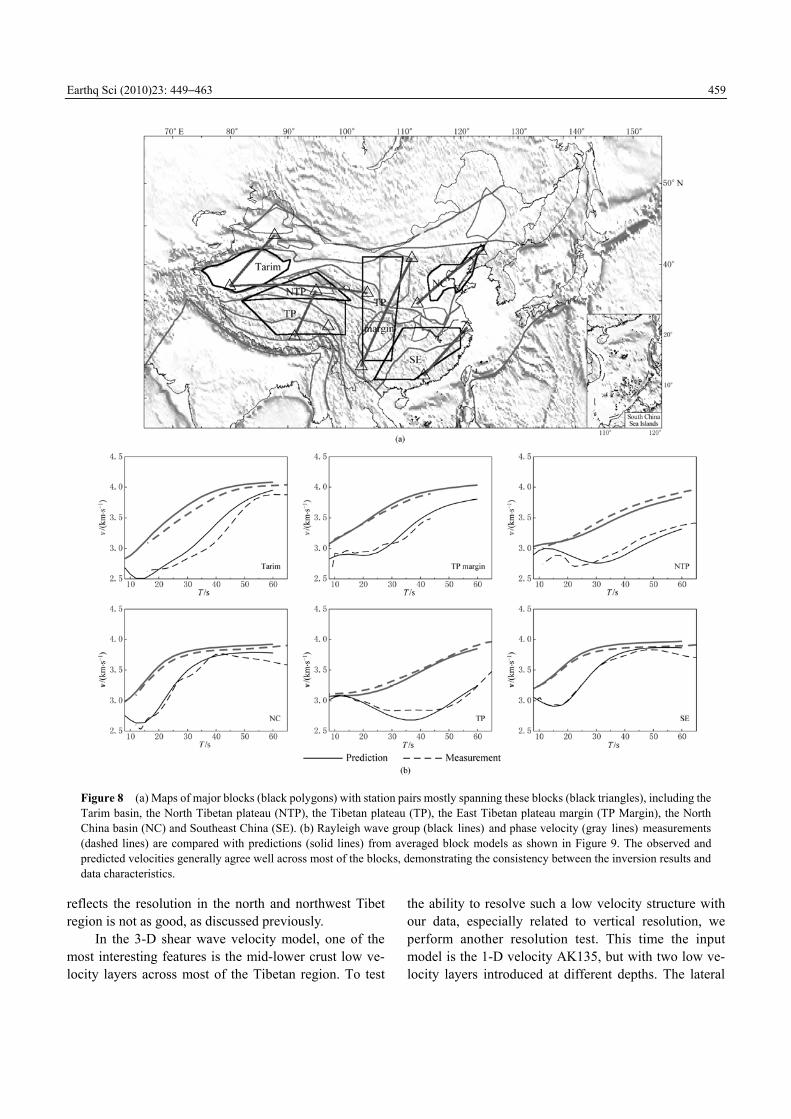
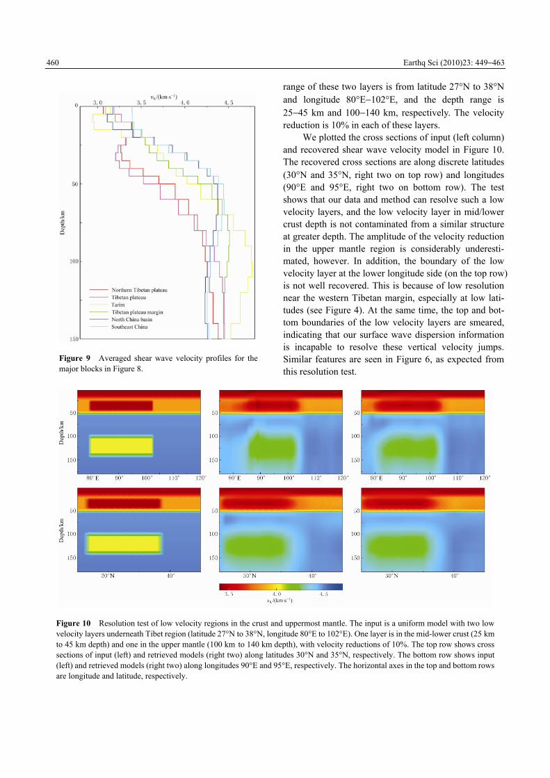
To demonstrate further distinct differences between different geological provinces, we compared the vertical profiles of averaged velocities in a few selected regions (Figures 8 and 9). The major regions we selected are shown in Figure 8: the Tarim basin, north Tibetan pla-teau (NTP), Tibetan plateau (TP), the east margin of the Tibetan plateau (TP margin, including the Sichuan basin and Ordos basin), the North China blocks (NC), and the Southeast China craton (SE). Because these areas repre-sent different tectonic blocks such as basins, stable cra-tons, and active regions that have undergone or are un-dergoing tectonic deformation, they are expected to show different velocity structures (as seen in Figure 9).

The Tibetan region (TP and NTP) has a very obvi-ous low velocity layer at depths of ~20 km to 40 km. The Tarim basin has low velocities at shallow depths, consistent with a thick sediment layer at the top. But below 70 km, the velocity underneath the Tarim basin is high, indicating a strong and fast mantle lithosphere. The margins of Tibet (mostly Sichuan and Ordos basins) also have similar features as that of the Tarim basin. The North China block has similar velocity at shallow depth as the Tibetan margin, but it does not show high veloci-ties within the mantle lithosphere. Instead, the velocity structures of North China and Southeast China at great depth are similar, because they are all ancient cratons. At shallow depth, Southeast China has much higher veloc-ity, which may be due to the fact that the area consists of folds/mountain belts.

4 Discussion To test our 3-D velocity structure in different re-

gions of China, we compare the observed and predicted (calculated from the averaged shear wave velocity structure in Figure 9) surface wave dispersion curves for several station pairs that span selected areas (Figure 8). The measurements and predictions are generally consis-tent with each other, especially for phase velocities. The consistency is especially high in stable craton or basin areas. Only in the North Tibet region and the Tarim ba-sin do significant discrepancies arise, which probably

Earthq Sci (2010)23: 449!463 459

Figure 8 (a) Maps of major blocks (black polygons) with station pairs mostly spanning these blocks (black triangles), including the Tarim basin, the North Tibetan plateau (NTP), the Tibetan plateau (TP), the East Tibetan plateau margin (TP Margin), the North China basin (NC) and Southeast China (SE). (b) Rayleigh wave group (black lines) and phase velocity (gray lines) measurements (dashed lines) are compared with predictions (solid lines) from averaged block models as shown in Figure 9. The observed and predicted velocities generally agree well across most of the blocks, demonstrating the consistency between the inversion results and data characteristics.

reflects the resolution in the north and northwest Tibet region is not as good, as discussed previously.

In the 3-D shear wave velocity model, one of the most interesting features is the mid-lower crust low ve-locity layers across most of the Tibetan region. To test

the ability to resolve such a low velocity structure with our data, especially related to vertical resolution, we perform another resolution test. This time the input model is the 1-D velocity AK135, but with two low ve-locity layers introduced at different depths. The lateral

460 Earthq Sci (2010)23: 449!463

Figure 9 Averaged shear wave velocity profiles for the major blocks in Figure 8.

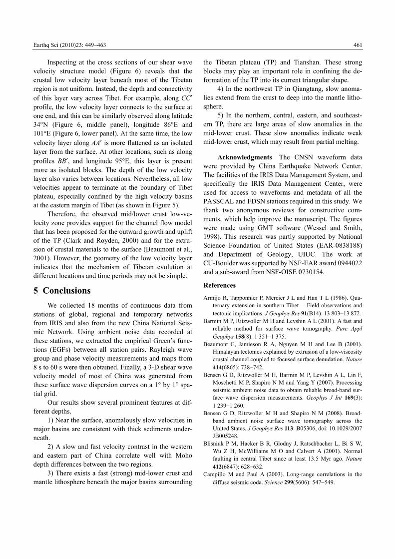
range of these two layers is from latitude 27°N to 38°N and longitude 80°E!102°E, and the depth range is 25!45 km and 100!140 km, respectively. The velocity reduction is 10% in each of these layers.

We plotted the cross sections of input (left column) and recovered shear wave velocity model in Figure 10. The recovered cross sections are along discrete latitudes (30°N and 35°N, right two on top row) and longitudes (90°E and 95°E, right two on bottom row). The test shows that our data and method can resolve such a low velocity layers, and the low velocity layer in mid/lower crust depth is not contaminated from a similar structure at greater depth. The amplitude of the velocity reduction in the upper mantle region is considerably underesti-mated, however. In addition, the boundary of the low velocity layer at the lower longitude side (on the top row) is not well recovered. This is because of low resolution near the western Tibetan margin, especially at low lati-tudes (see Figure 4). At the same time, the top and bot-tom boundaries of the low velocity layers are smeared, indicating that our surface wave dispersion information is incapable to resolve these vertical velocity jumps. Similar features are seen in Figure 6, as expected from this resolution test.

Figure 10 Resolution test of low velocity regions in the crust and uppermost mantle. The input is a uniform model with two low velocity layers underneath Tibet region (latitude 27°N to 38°N, longitude 80°E to 102°E). One layer is in the mid-lower crust (25 km to 45 km depth) and one in the upper mantle (100 km to 140 km depth), with velocity reductions of 10%. The top row shows cross sections of input (left) and retrieved models (right two) along latitudes 30°N and 35°N, respectively. The bottom row shows input (left) and retrieved models (right two) along longitudes 90°E and 95°E, respectively. The horizontal axes in the top and bottom rows are longitude and latitude, respectively.

Earthq Sci (2010)23: 449!463 461

Inspecting at the cross sections of our shear wave velocity structure model (Figure 6) reveals that the crustal low velocity layer beneath most of the Tibetan region is not uniform. Instead, the depth and connectivity of this layer vary across Tibet. For example, along CC# profile, the low velocity layer connects to the surface at one end, and this can be similarly observed along latitude 34°N (Figure 6, middle panel), longitude 86°E and 101°E (Figure 6, lower panel). At the same time, the low velocity layer along AA# is more flattened as an isolated layer from the surface. At other locations, such as along profiles BB#, and longitude 95°E, this layer is present more as isolated blocks. The depth of the low velocity layer also varies between locations. Nevertheless, all low velocities appear to terminate at the boundary of Tibet plateau, especially confined by the high velocity basins at the eastern margin of Tibet (as shown in Figure 5).

Therefore, the observed mid/lower crust low- ve-locity zone provides support for the channel flow model that has been proposed for the outward growth and uplift of the TP (Clark and Royden, 2000) and for the extru-sion of crustal materials to the surface (Beaumont et al., 2001). However, the geometry of the low velocity layer indicates that the mechanism of Tibetan evolution at different locations and time periods may not be simple.

5 Conclusions We collected 18 months of continuous data from

stations of global, regional and temporary networks from IRIS and also from the new China National Seis-mic Network. Using ambient noise data recorded at these stations, we extracted the empirical Green�’s func-tions (EGFs) between all station pairs. Rayleigh wave group and phase velocity measurements and maps from 8 s to 60 s were then obtained. Finally, a 3-D shear wave velocity model of most of China was generated from these surface wave dispersion curves on a 1° by 1° spa-tial grid.

Our results show several prominent features at dif-ferent depths.

1) Near the surface, anomalously slow velocities in major basins are consistent with thick sediments under-neath.

2) A slow and fast velocity contrast in the western and eastern part of China correlate well with Moho depth differences between the two regions.

3) There exists a fast (strong) mid-lower crust and mantle lithosphere beneath the major basins surrounding

the Tibetan plateau (TP) and Tianshan. These strong blocks may play an important role in confining the de-formation of the TP into its current triangular shape.

4) In the northwest TP in Qiangtang, slow anoma-lies extend from the crust to deep into the mantle litho-sphere.

5) In the northern, central, eastern, and southeast-ern TP, there are large areas of slow anomalies in the mid-lower crust. These slow anomalies indicate weak mid-lower crust, which may result from partial melting.

Acknowledgments The CNSN waveform data were provided by China Earthquake Network Center. The facilities of the IRIS Data Management System, and specifically the IRIS Data Management Center, were used for access to waveforms and metadata of all the PASSCAL and FDSN stations required in this study. We thank two anonymous reviews for constructive com-ments, which help improve the manuscript. The figures were made using GMT software (Wessel and Smith, 1998). This research was partly supported by National Science Foundation of United States (EAR-0838188) and Department of Geology, UIUC. The work at CU-Boulder was supported by NSF-EAR award 0944022 and a sub-award from NSF-OISE 0730154.

References

Armijo R, Tapponnier P, Mercier J L and Han T L (1986). Qua-ternary extension in southern Tibet �— Field observations and tectonic implications. J Geophys Res 91(B14): 13 803!13 872.

Barmin M P, Ritzwoller M H and Levshin A L (2001). A fast and reliable method for surface wave tomography. Pure Appl Geophys 158(8): 1 351!1 375.

Beaumont C, Jamieson R A, Nguyen M H and Lee B (2001). Himalayan tectonics explained by extrusion of a low-viscosity crustal channel coupled to focused surface denudation. Nature 414(6865): 738!742.

Bensen G D, Ritzwoller M H, Barmin M P, Levshin A L, Lin F, Moschetti M P, Shapiro N M and Yang Y (2007). Processing seismic ambient noise data to obtain reliable broad-band sur-face wave dispersion measurements. Geophys J Int 169(3): 1 239!1 260.

Bensen G D, Ritzwoller M H and Shapiro N M (2008). Broad-band ambient noise surface wave tomography across the United States. J Geophys Res 113: B05306, doi: 10.1029/2007 JB005248.

Blisniuk P M, Hacker B R, Glodny J, Ratschbacher L, Bi S W, Wu Z H, McWilliams M O and Calvert A (2001). Normal faulting in central Tibet since at least 13.5 Myr ago. Nature 412(6847): 628!632.

Campillo M and Paul A (2003). Long-range correlations in the diffuse seismic coda. Science 299(5606): 547!549.

462 Earthq Sci (2010)23: 449!463

Clark M K and Royden L H (2000). Topographic ooze: Building the eastern margin of Tibet by lower crustal flow. Geology 28(8): 703!706.

Friederich W (2003). The S-velocity structure of the East Asian mantle from inversion of shear and surface waveforms. Geo-phys J Int 153(1): 88!102.

Hauck M L, Nelson K D, Brown L D, Zhao W J and Ross A R (1998). Crustal structure of the Himalayan orogen at similar to 90 degrees east longitude from Project INDEPTH deep re-flection profiles. Tectonics 17(4): 481!500.

Herrmann R B and Ammon C J (2004) Surface waves receiver functions and crustal structure. Computer Programs in Seis-mology, Version 3.30. Saint Louis University, http://www.eas. slu.edu/ People/RBHerrmann/CPS330.html.

Huang Z X, Su W, Peng Y J, Zheng, Y J and Li H Y (2003). Rayleigh wave tomography of China and adjacent regions. J Geophys Res 108: 2073, doi:10.1029/2001JB001696.

Kennett B L N, Engdahl E R and Buland R (1995). Constraints on seismic velocities in the Earth from traveltimes. Geophys J Int 122: 108!124.

Levshin A L and Ritzwoller M H (2001). Automated detection, extraction, and measurement of regional surface waves. Pure Appl Geophys 158(8): 1 531!1 545.

Li C, van der Hilst R D and Toksöz A N (2006). Constraining P-wave velocity variations in the upper mantle beneath Southeast Asia. Phys Earth Planet Inter 154(2): 180!195.

Li H Y, Su W, Wang C Y and Huang Z X (2009). Ambient noise Rayleigh wave tomography in western Sichuan and eastern Tibet. Earth Planet Sci Lett 282(1-4): 201!211.

Liang C T and Song X D (2006). A low velocity belt beneath northern and eastern Tibetan Plateau from Pn tomography. Geophys Res Lett 33: L22306, doi: doi:10.1029/2006GL02792.

Liang C T, Song X D and Huang J L (2004). Tomographic inver-sion of Pn travel times in China. J Geophys Res 109: B11304, doi:10.1029/2003JB002789.

Lin F C, Moschetti M P and Ritzwoller M H (2008). Surface wave tomography of the western United States from ambient seismic noise: Rayleigh and Love wave phase velocity maps. Geophys J Int 173(1): 281!298.

Molnar P and Tapponnier P (1975). Cenozoic tectonics of Asia-effects of a continental collision. Science 189(4201): 419!426.

Moschetti M P, Ritzwoller M H and Shapiro N M (2007). Surface wave tomography of the western United States from ambient seismic noise: Rayleigh wave group velocity maps. Geochem Geophys Geosys 8: Q08010, doi:10.1029/2007GC001655.

Nabelek J, Chen W P and Ye H (1987). The Tangshan earthquake sequence and its implications for the evolution of the North China basin. J Geophys Res 92(B12): 12 615!12 628.

Nelson K D, Zhao W J, Brown L D, Kuo J, Che J K, Liu X W, Klemperer S L, Makovsky Y, Meissner R, Mechie J, Kind R, Wenzel F, Ni J, Nabelek J, Chen L S, Tan H D, Wei W B, Jones A G, Booker J, Unsworth M, Kidd W S F, Hauck M, Alsdorf D, Ross A, Cogan M, Wu C D, Sandvol E and Ed-wards M (1996). Partially molten middle crust beneath south-ern Tibet: Synthesis of project INDEPTH results. Science

274(5293): 1 684!1 688. Paul A, Campillo M, Margerin L, Larose E and Derode A (2005).

Empirical synthesis of time-asymmetrical Green functions from the correlation of coda waves. J Geophys Res 110: B08302, doi:10.1029/2004JB003521.

Ritzwoller M H, Levshin A L, Ratnikova L I and Egorkin A A (1998). Intermediate-period group-velocity maps across Cen-tral Asia western China and parts of the Middle East. Geophys J Int 134(2): 315!328.

Sabra K G, Gerstoft P, Roux P, Kuperman W A and Fehler M C (2005a). Extracting time-domain Green�’s function estimates from ambient seismic noise. Geophys Res Lett 32: L03310, doi:10.1029/2004GL021862.

Sabra K G, Gerstoft P, Roux P, Kuperman W A and Fehler M C (2005b). Surface wave tomography from microseisms in Southern California. Geophys Res Lett 32: L14311, doi:10.1029/2005GL023155.

Sabra K G, Roux P and Kuperman W A (2005c). Emergence rate of the time-domain Green�’s function from the ambient noise cross-correlation function. J Acoust Soc Am 118(6): 3 524! 3 531.

Sandvol E, Ni J, Kind R and Zhao W J (1997). Seismic anisotropy beneath the southern Himalayas-Tibet collision zone. J Geo-phys Res 102(B8): 17 813!17 823.

Shapiro N M and Campillo M (2004). Emergence of broadband Rayleigh waves from correlations of the ambient seismic noise. Geophys Res Lett 31: L07614, doi:10.1029/2004GL019491.

Shapiro N M, Campillo M, Stehly L and Ritzwoller M H (2005). High-resolution surface-wave tomography from ambient seismic noise. Science 307(5715): 1 615!1 618.

Shapiro N M, Ritzwoller M H, Molnar P and Levin V (2004). Thinning and flow of Tibetan crust constrained by seismic anisotropy. Science 305(5681): 233!236.

Sun Y S and Toksöz M N (2006). Crustal structure of China and surrounding regions from P wave traveltime tomography. J Geophys Res 111: B03310, doi:10.1029/2005JB003962.

Tilmann F and Ni J (2003). Seismic imaging of the downwelling Indian lithosphere beneath central Tibet. Science 300(5624): 1 424!1 427.

Tseng T L, Chen W P and Nowack R L (2009). Northward thin-ning of Tibetan crust revealed by virtual seismic profiles. Geophys Res Lett 36: L24304, doi:10.1029/2009GL040457.

Turner S, Arnaud N, Liu J, Rogers N, Hawkesworth C, Harris N, Kelley S, VanCalsteren P and Deng W (1996). Post-collision, shoshonitic volcanism on the Tibetan plateau: Implications for convective thinning of the lithosphere and the source of ocean island basalts. J Petrology 37(1): 45!71.

Villasenor A, Ritzwoller M H, Levshin A L, Barmin M P, Engdahl E R, Spakman W and Trampert J (2001). Shear velocity structure of Central Eurasia from inversion of surface wave velocities. Phys Earth Planet Int 123(2-4): 169!184.

Wessel P and Smith W H F (1998). New improved version of the Generic Mapping Tools released. EOS Trans AGU 79: 579.

Williams H, Turner S, Kelley S and Harris N (2001). Age and composition of dikes in Southern Tibet: New constraints on the timing of east-west extension and its relationship to post-

Earthq Sci (2010)23: 449!463 463

collisional volcanism. Geology 29(4): 339!342. Wu F T, Levshin A L and Kozhevnikov V M (1997). Rayleigh

wave group velocity tomography of Siberia, China and the vicinity. Pure Appl Geophys 149(3): 447!473.

Yang Y J, Ritzwoller M H, Levshin A L and Shapiro N M (2007). Ambient noise Rayleigh wave tomography across Europe. Geophys J Int 168(1): 259!274.

Yao H J, Beghein C and van der Hilst R D (2008). Surface wave array tomography in SE Tibet from ambient seismic noise and two-station analysis �– II. Crustal and upper-mantle structure. Geophys J Int 173(1): 205!219.

Yin A and Harrison T M (2000). Geologic evolution of the Hi-malayan-Tibetan orogen. Annu Rev Earth Planet Sci 28: 211! 280.

Ying J F, Zhang H F, Kita N, Morishita Y and Shimoda G (2006). Nature and evolution of late cretaceous lithospheric mantle

beneath the eastern North China Craton: Constraints from pe-trology and geochemistry of peridotitic xenoliths from Jünan, Shandong Province, China. Earth Planet Sci Lett 244(3-4): 622!638.

Zhang P Z, Shen Z, Wang M, Gan W J, Burgmann R and Molnar P (2004). Continuous deformation of the Tibetan Plateau from global positioning system data. Geology 32(9): 809!812.

Zhao W, Mechie J, Brown L D, Guo J, Haines S, Hearn T, Klem-perer S L, Ma Y S, Meissner R, Nelson K D, Ni J F, Pananont P, Rapine R, Ross A and Saul J (2001). Crustal structure of central Tibet as derived from project INDEPTH wide-angle seismic data. Geophys J Int 145(2): 486!498.

Zheng S H, Sun X L, Song X D, Yang Y J and Ritzwoller M H (2008). Surface wave tomography of China from ambient seismic noise correlation. Geochem Geophys Geosyst 9: Q05020, doi:10.1029/2008GC001981.