Three-Dimensional Projection Pursuit

By GUY NASON

Department of Mathematics, University of Bristol, University Walk, Bristol, BS8 1TW, UK

Email: G.P.Nason@bristol.ac.uk

SUMMARY

The development and usage of an approach to three-dimensional projection pursuit is discussed. The well-

established Jones and Sibson moments index is chosen as a computationally efficient projection index to

extend to 3D. The 3D index was initially developed to find interesting linear combinations of spectral bands

in a multispectral image. Computer algebraic methods are extensively employed to handle the complex

formulae that constitute the index and are explained in detail. A discussion of important practical issues

such as interpreting projection solutions, dealing with outliers and optimization techniques completes the

description of the index. An artificial tetrahedral data set is used to demonstrate how 3D projection pursuit

can produce better clusters than those obtained by principal components analysis. The main example

shows how 3D projection pursuit can successfully combine bands to discover alternative clusters to those

produced by, say, principal components.

Keywords: projection pursuit; multispectral images; clustering; computer algebra; varimax

rotation

1 Introduction

This article discusses various aspects of projection pursuit into three dimensions.

The aim of projection pursuit is to find interesting linear combinations of variables

in a multivariate data set. The precise definition of “interesting” is given later

but clusters and other forms of non-linear structure are interesting. One- and two-

dimensional projection pursuit have been dealt with extensively in the literature and

some excellent software implementations are available. The benefit of projection

into three-dimensions is that more complex structures can be identified than with

lower-dimensional projections. Projection pursuit into three dimensions is particularly

attractive for two further perceptual reasons. Firstly, colours naturally correspond

to 3-vectors, for example through the RGB representation. Secondly, point clouds

and other objects in three dimensions can be investigated on computer screens. For

example through spinning 3D plots, which are immediately comprehensible because

of our 3D intuition. These reasons are important when applying 3D projection pursuit

1

to multispectral images (colour) and multivariate data sets (intuition).

Section 2 briefly describes projection pursuit and includes details on projection

indices and the process of sphering. Section 3 explains that we have chosen to extend

Jones and Sibson’s (1987) well-known moments index into three dimensions because

of its computational efficiency. The formulae for the moments index were analytically

computed by the computer algebra package REDUCE (see Section 3.3). Section 3

also addresses the differentiation and optimization of the moments index, examines

how outliers can be treated to provide better projection solutions and discusses how

optimal projections can be rotated to give solutions that are more easily interpreted.

Section 4 gives two examples of projection pursuit in action. The first example

applies the pursuit to an artificial data set that has a three-dimensional structure

embedded within a noisy six-dimensional data set. No single one- or two-dimensional

projection will clearly show the structure and with these data the principal components

are contaminated with noise. The projection pursuit method clearly isolates the

three-dimensional structure and gives clearer definition to the clusters than principal

components analysis does. Many real multivariate data sets are of this type (for

example, the Lubischew (1962) beetle data).

The second example and the main reason for the development of three-dimensional

pursuit is discussed section 4.3. This example shows how projection pursuit may be

applied to some real multispectral image data to produce low-dimensional projections

that exhibit clustering. We argue that tighter clusters in variable-space result in better

contrasts between differing land use types and we give an example where this is so.

2 A brief description of projection pursuit

SupposeX is aK � N data matrix ofN observations onK variables. Define the

multivariate mean ofX by:

�X =X1NN

;

where1N is theN -dimensional vector consisting solely of ones. The centred data!

X

are obtained by subtracting the mean vector off each observation:

!

X= X ��X1TN :

2

The sample variance matrix ofX is obtained from the centred data by

SX =

!

X!

XT

N � 1:

The aim of classical principal components analysis (PCA) is to find linear

combinations of the original variables that have maximal sample variance. The linear

combinations can be thought of as projections onto a projection direction defined by a

unit vectora:

Z = aTX:

The sample variance of the projected data is

varX(a) = aTSa: (1)

The first principal componenta� is the vector that solves the following optimization

problem:

arg max varX(a) subject toaTa = 1: (2)

Thekth principal component (PC) is the vectorx that solves (2) with the additional

constraint of being orthogonal to the previousk�1 components. Thus PCAmaximizes

a functionof the projection vectora. The variance function is a quadratic form ina

and therefore an analytical solution exists. The PCs are the eigenvectors ofS and the

principal variances associated with each component are the eigenvalues ofS.

The aim of projection pursuit is different to that of PCA: projection pursuit

searches for projections that areinteresting rather than those that exhibit large

variation. Projection pursuit also maximizes a function ofa but the difference is that

the function (generally called a projectionindex) measures some criterion of interest

within the projected data. As a result the maximization problem usually becomes

analytically intractable and has to be solved using numerical methods. We denote a

generic projection index byI(a) and so for projection pursuit the optimization problem

becomes:

arg maxI(a) subject toaTa = 1: (3)

3

2.1 Projection indices

The choice of projection index is important in projection pursuit. The projected sample

variance (1) could be used as a projection index, but there would be little point because

there is an analytical solution.

Successful projection indices are designed to respond to interesting or clustered

variation — not just the large variation discovered by PCA. Early work by Friedman

and Tukey (1974) developed a projection index to search for non-linear structure.

Subsequently Huber (1985) and Jones and Sibson (1987) considered the population

rather than the sample case and assumed that the projected data,aTX, has a density,

fa(x). Their projection indices were based on measuring the departure offa(x) from

the standard normal density�(x). This is based on the heuristic that normality is the

least interesting density on the line. In practice departures can be measured by forming

a density estimatefa(x) of the projected data and comparing it to standard normality.

Huber (1985) and Jones and Sibson (1987) suggested a projection index based on the

Shannon entropy

IS(a) =

Z1

�1

fa(x) log fa(x) dx: (4)

The entropy index (4) is sometimes used in projection pursuit because it is uniquely

minimized by the standard normal density. There are several other possible choices for

a projection index (see Cooket al. (1993) for a list). Projection into two dimensions

is common and has been promoted extensively in the literature and in implementation.

An excellent implementation that exists for running two-dimensional pursuit is the

XGobi program described by Swayneet al. (1991; 1990).

2.2 Centring and sphering

A data set is sphered by using a linear transform to cause the transformed data to have

zero mean and identity variance matrix.

If a linear transformationQ is applied to the centred data!

X then the result

Y = Q!

X is also centred and has variance

SY =Y Y T

N � 1=Q!

X!

XT

QT

N � 1= QSXQ

T :

4

One convenient choice ofQ that ensures thatSY is the identity matrix isQ = S�

12

X

which may be computed from the principal components ofX.

The are two main reasons for sphering:

1. the variables ofY are uncorrelated. Any structure that projection pursuit

picks up will be independent of PCA. Indeed PCA investigates the covariance

structure of data so it would be wasteful for projection pursuit to do the same.

2. sphering simplifies the design of projection indices because the projections of

sphered data are themselves sphered.

A more detailed explanation for sphering in projection pursuit can be found in

Jones and Sibson (1987). A more general discussion of sphering may be found in

Tukey and Tukey (1981).

3 Three-dimensional projection pursuit

3.1 Introduction

The benefit of three-dimensional projection is that more complicated structures can be

observed than in one or two dimensions. For example, a torus or a sphere would be

difficult to determine from a single one- or two-dimensional projection.

We now describe a three-dimensional projection index and how it is computed

and optimized. We detail how outliers can affect the pursuit and what can be done to

reduce their influence. Lastly, we describe a way in which projections can be made

more interpretable in terms of original measurement variables.

3.2 A projection index for three dimensions

A projection index into three dimensions is a function of three projection vectors. The

optimization problem (3) becomes

arg maxI(a; b; c) subject toaTa = bT b = cT c = 1 andaT b = aT c = bT c = 0:

Again the projection vectors are of unit length but they are also forced to be orthogonal.

The orthogonality is a convenience mainly for computational reasons but also aids

5

interpretation of the final projection solution.

Many two-dimensional indices could be extended to a three-dimensional form.

We choose one in particular because it requires less computational effort than other

indices. The one-dimensional index was devised by Jones and Sibson (1987) and

is based on the following approximation of the difference between the Shannon

entropies (4) of the projected data density,f , and the standard normal density�:

Zf(x) log f(x) dx�

Z�(x) log �(x) dx �

��23 +

14�

24

�=12; (5)

where�3 and�4 are the third and fourth order cumulants of the projected sphered data.

(If we denote therth moment by�r then for sphered data we have�1 = 0, �2 = 1 and

�3 = �3 and�4 = �4 � 3). In practice the cumulant based quantity on the right-hand

side of (5) is estimated by a sample version computed on the projected data. We shall

discuss estimation in the next section.

Jones and Sibson’s two-dimensional moments index is derived using precisely the

same argument as for the one-dimensional case. The index is given in terms of two-

dimensional cumulants��� as:

(�230 + 3�221 + 3�212 + �203) +1

4(�240 + 4�231 + 6�222 + 4�213 + �204): (6)

Our extension of Jones and Sibson’s index to three dimensions in terms of three-

dimensional cumulants��� is:

X�+ � + = 3

�; �; = 0; : : : ; 3

C(3)�� �

2�� +

1

4

X�+ � + = 4

�; �; = 0; : : : ; 4

C(4)�� �

2�� : (7)

The three-dimensional index may be obtained by repeating Jones and Sibson’s (1987)

mathematical argument or by studying the final steps in the derivation of the two-

dimensional index. The coefficients of the bivariate cumulant��� in (6) are simply

the coefficients ofx�y� in the expansion of(x+y)r. SimilarlyC(r)�� is the coefficient

of x�y�z in the expansion of(x + y + z)r. Mardia (1987) noted the connection

between moments indices and formal tests for non-normality and also suggested an

alternative means of obtaining higher-dimensional projection indices.

6

One important property of moments indices of the type (6) and (7) is that they

are rotationally invariant with respect to any choice of axes for the projection space

(a; b; c). Another set of vectors(d; e; f) can be chosen that represent the same

projection space as(a; b; c) but differ by a rotation. We would want the index to

remain the same on(d; e; f) as on(a; b; c) since it is the projection space that matters

not the way in which wish to represent it. Surprisingly many indices do not have

this property (Friedman and Tukey (1974) and Friedman (1987)) although more recent

indices do (for example Morton (1989) and Cooket al. (1993)). The invariance is

important during the optimization sequence since optimizers can spend time changing

the representation when they should be changing the projection space. Also it is

sometimes useful to be able to rotate the representing axes to aid interpretability of the

projection solution without changing the projection index. We discuss this procedure

in Section 3.5.

Estimation of the projection index

Kendall et al. (1969) described a class of unbiased estimators for cumulants of any

order known ask-statistics. Thek-statistics are computed from the projected sphered

data and are dependent on the projection vectors. Therefore Jones and Sibson’s one-

dimensional sample index was obtained by replacing cumulants withk-statistics in

equation (5):

M1(a) = k23(a) +1

4k24(a); (8)

where thek-statistics were computed from the projected sphered dataYi by

k3(a) =N

(N � 1)(N � 2)

NXi=1

Y 3i (a); (9)

and

k4(a) =N

(N � 1)(N � 2)(N � 3)

((N + 1)

NXi=1

Y 4i (a)�

3(N � 1)3

N

): (10)

In the two-dimensional case the bivariate cumulants��� are replaced by bivariate

k-statisticsk�� and similarly for the three-dimensional index. The formulae fork3

andk4 were given by Kendallet al. (1969, page 280) and are modified for sphered

data in (9) and (10). Kendallet al. gave only a few of the formulae for trivariate

7

k-statistics, but they also gave an algorithm for deriving an arbitrary orderk-statistic

from the univariate ones.

Automating Kendall’s algorithm using computer algebra.

We repeat Kendall’s algorithm here because it is a good example of a procedure that

may be automated using computer algebra. Suppose that we wished to obtain the

bivariatek-statistick21. We would start with the formula ofk3 in terms of power

sums:

k3 =1

n[3](n2s3 � 3ns2s1 + 2s31);

wheren[k] is defined to be the descending factorialn(n � 1) : : : (n � k). First we

formalizethis equation by introducing a variabler:

k(r3) =1

n[3]

nn2s(r3)� 3ns(r2)s(r) + 2s(r)3

o: (11)

To produce the bivariate formula we must operate on (11) with the operatort @@r

and

obtain

3k(tr2) =1

n[3]

h3n2s(tr2)� 3n

n2s(rt) + s(t)s(r2)

o+ 6s(t)s(r)2

i:

Finally, replacing powers by subscripts and dividing both sides by three and obtain:

k21 =1

n[3]

�n2s21 � 2ns10s11 � ns20s01 + 2s210s01

�: (12)

This is precisely the formula fork21 as given by Kendallet al. (1969, page 308). We

could producek12 from (12) by applying the same operator as before. The trivariate

k111 would be obtained by using the operatoru @@r

on (12), which would introduce a

new variableu and differentiate ther2 and obtain the formula:

k111 =1

n[3]

nn2s111 � n (s011s100 + s001s110 + s101s010) + 2s101s010

o:

All the other trivariate formulae can be produced in this way and a complete list

necessary for the computation of the three-dimensional moments index (7) appeared

in Nason (1992).

The key operation above was the application of theu @@r

operator to the power sum

s(r3). In REDUCE this operation is programmed in as

8

FOR ALL U,R,N,KK LET OP(U,SF(KK*R**N),R)=N*SF(KK*U*R**(N-1));

This line says that for all instances of the variablesU,R,N,KK whenever the operator

OPis applied to argumentsU,SF(KK*R**N),R we get the result on the right-hand

side of the= sign. In this example we have effectively built our own differentiation

operator. REDUCE does have its own operator calledDIFF which we could have used

here. Although we believe that merely producing the trivariatek-statistics is enough

reason to use REDUCE there are other more compelling ones. REDUCE is able to

produce both typesetting instructions and FORTRAN code for the formulae making

incorporation into documents and computer programs easy and error free.

3.3 Computing the projection index

The algorithm that we use is that of Jones (1983) but modified for three-dimensions.

The logic of the algorithm is depicted in Figure 1. The rationale for computing the

k-statistics in this way originally stems from the way in which Kendallet al. (1969)

representk-statistics in terms of power sums, and power sums in terms of the data. Figure 1 here

First the third and fourth order product moment tensors are computed from the

sphered dataY by

Tpqr =NXi=1

YpiYqiYri (13)

Upqrs =NXi=1

YpiYqiYriYsi: (14)

All evaluations of the moments index and its derivatives are made using onlyT and

U . The link between the moments index andT; U is the basis of the moments index’s

computational efficiency and is discussed later in this section.

Next the power sums are computed from current projection using formulae such

as

s201 =KX

m=n=p=1

amancpTmnp (15)

s121 =KX

m=n=p=q=1

ambnbpcqUmnpq: (16)

The computation of the projection index requires 10 third order power sums and 15

fourth order sums. A complete list was presented by Nason (1992).

9

Finally, after thek-statistics have been computed the projection index and its

derivatives are computed with respect to the projection direction. The derivatives are

computed because they supply two useful pieces of information: they inform us of our

proximity to a local maximum and they indicate which direction should be followed

to increase the index.

Optimization

Most optimization methods find local optima and not the global optimum. This is

an advantage as a local optimum indicates some departure from normality and the

projection solution can be quickly examined for any possible structure. For projection

pursuit we believe that any reasonable optimizer is likely to be of use.

Many optimization methods have been used previously. For example: steepest

ascent (Jones and Sibson (1987)); genetic algorithms (Crawford (1991)); a coarse

stepping and Newton method hybrid (Friedman (1987)) and methods based on the

grand tour (Posse (1990)). We use the method of conjugate gradients and the

implementation supplied by the NetLib archive.

The projection pursuit optimization problem is constrained. Most of the optimizers

mentioned above are designed for unconstrained problems. To allow for this

Friedman (1987) maintained orthogonal projection vectors by modifying the derivative

of the projection index so that a step in the modified direction did not violate the

orthogonality constraints. We use the cruder method used by Jones and Sibson (1987)

which reorthogonalizes the projection vectors after an optimization step has been

taken.

Computing the derivatives

To optimize the projection index efficiently it is necessary to know the derivatives of

the projection index. Given the projection space(a; b; c) we need to find

@M3

@ar;@M3

@br;@M3

@cr;

for eachr = 1; : : : ;K. The indexM3 is composed of trivariatek-statistics which in

turn are composed of power sums. Differentiation ofM3 reduces to differentiation

10

of the power sums via the chain rule. Each power sum involved in the computation

must be differentiated with respect to each component of the three projection vectors.

For example, the power sums103 is a component of the projection index, and the

derivatives with respect to the projection vectors are:

@s103@ar

=X

cmcncpUmnpr � ars103 � 3crs202; (17)

@s103@br

= �3crs112; (18)

@s103@cr

= 3�X

amcncpUmnpr � ars202 � brs112 � crs103�: (19)

These derivatives look much more complicated than the form for power sums given

in (16). The original power sums are given for the orthonormalized versions of

the projection vectors. The derivatives are given in terms of the original projection

vectors that might not necessarily be orthogonal. This non-orthogonality may occur

temporarily after the optimizer had made a step in a particular direction and off

the manifold defined by the orthogonality condition. In all there are 30 individual

derivatives for the third order case and 45 for the fourth order case. The full results of

the differentiation can be found in Nason (1992).

Computational efficiency

The computation of the product moment tensors is anO(N) computation. Once these

have been computed all further evaluations of the moments index and its derivatives

are independent ofN . Indices such as those of Friedman (1987), Morton (1989),

Hall (1989) and Cooket al. (1993) require anO(N) computation foreveryevaluation

of the projection index during the optimization sequence. For small data sets the

difference in execution time is negligible. For large data sets, such as the image set in

Section 4.3, the moments index tends to find optimal solutions in about one tenth of

the time it takes other indices.

3.4 Treatment of outliers

A major criticism of the moments index is that it is sensitive to outliers and finds

outlyingprojections — that is projections that contain a few outliers and a single major

11

cluster. To alleviate the outlying projection problem we will either remove outliers or

trim them. Trimming involves shrinking outliers’ distancer to the centroid of the

set to a new distanceT (r). We implement two possible choices forT suggested by

Tukey (1987); they are

TL(r) = 1 + log(r); (20)

and

TS(r) = 3� 2r�12 : (21)

Tukey suggests that the data should be sphered first, then trimmed ifr > 1 and then

sphered again. The pursuit is then applied to the re-sphered data. Typically trimming

helps solve the problems caused by outliers, but not always.

3.5 Axes rotation

After performing projection pursuit we obtain an optimal projection(a; b; c) which

can be written in matrix form in terms of the original unsphered data asAX where

A = [a b c]T . Sometimes such a projection solution can be hard to interpret and it

would be useful to interpret what the projection vectors mean in terms of the original

variables. The three vectors define a particular space but not uniquely so. A3 � 3

rotation matrix can be applied to the projection without changing the projection index.

For example:

RA = [d e f ]T ;

where the rotated vectors(d; e; f) are also orthonormal. After a rotation the

configuration of the projected points does not change but the particular basis that they

are represented in does. However, performing a rotation may allow us to chooseR so

that(d; e; f) are easier to interpret than(a; b; c).

Choice of rotation and interpretability

What do we mean by interpretability? We consider the projection vector that has all

entries equal, or nearly so, to be hardest to interpret whereas vectors that have few

large and many small entries to be easiest. Working with this definition we need to

12

find the orthogonal matrixR that maximizes the criterion:

KXk=1

(dk �K�12 )2 + (ek �K�

12 )2 + (fk �K�

12 )2: (22)

In practice we implement the maximization in a varimax like way. Given two

projection vectors it is easy to compute the angle that maximizes the criterion for

those two only. A cycle of steps performs the pairwise maximization for all pairs

of projection vectors (in the three-dimensional case(d; e), (d; f) and(e; f)). Given

initial projection vectors(a; b; c) a number of cycles is performed until the maximum

absolute angle change within any step of a cycle is below some tolerance. The

procedure converges because the criterion (22) is bounded and each step within the

cycle increases the criterion.

Further details on varimax can be found in Kaiser (1958) and Friedman (1987). We

adopt a simpler approach to Friedman and just rotate the projection solution within its

own space after doing projection pursuit. However, for three-dimensional solutions we

adapt Kaiser’s iterative varimax algorithm to achieve the desired rotation.

4 Using three-dimensional projection pursuit

In this section we describe two examples. The first uses an artificial data set that shows

the ability of 3D projection pursuit to pull out structure that is not obtainable through

lower-dimensional pursuits or PCA. The second example describes an application of

three-dimensional projection pursuit to multispectral image data.

The code to compute the projection index and its derivatives is implemented in

FORTRAN77 and embedded within the statistical package S (Beckeret al. (1988)).

The code is freely available by electronic file transfer (Nason (1994)) or directly from

the author.

4.1 Using projection pursuit in S

The S functionpp3 performs projection pursuit on an S data matrix and returns a

complete record of the pursuit as a composite object. Some of the more interesting

items stored within the returned object are:

13

� the data projected onto the optimal projection plane (in both sphered and original

coordinate systems);

� a record of the projection index for each iteration;

� the number of iterations expended and the maximum possible;

� the sphered data;

� the sphering transformation matrix and its inverse;

� the modulus of the gradient of the projection index at termination and the

tolerance used to decide convergence

� the initial and final projection vectors.

4.2 A tetrahedral example

Although the data set described in this example is artificial it is similar to real

multivariate data in that there are loose clusters representing different populations and

other variables that do not discriminate between populations. For example, the well-

known Lubischew (1962) beetle data set is of this type, but its structure is usually clear

in one-dimension and not challenging enough for three-dimensional pursuit. We create

a 6-dimensional data set containing 400 observations and possessing a tetrahedral

structure in the first three and noise in the remaining three dimensions. There is no

single one- or two-dimensional projection that will give a complete idea of the true

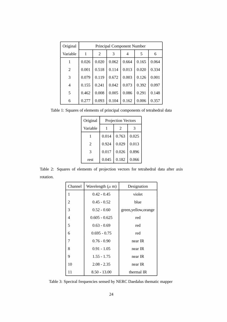
three-dimensional structure. The squares of the principal components of the tetrahedral

data appear in Table 1. The squares are shown to emphasize the contribution of

each element and consequently the sum of each column is 1. Each row of the table Table 1 here

corresponds to the variables that the tetrahedral data were originally recorded on. Even

knowing that the clustering is concentrated in the first three variables is no help here.

The only PCs that might be of some help in discerning the clusters are 2, 3 and 4

but even these contain some proportion of the noise variables. It is better to examine

the data with respect to these three PCs using a three-dimensional data viewer such

asbrush() in SPlus or XGobi. We obviously cannot show the three-dimensional

principal components picture here but the clustering is very difficult to see without

14

giving each point a group label (which defeats the aim of exploratory methods where

you may not know any structure but you are trying to find it).

Three-dimensional projection pursuit does much better. However, for this set

trimming was required to obtain a good solution. It is difficult to know when to trim

data and by how much. Generally Tukey’s advice from Section 3.3 is taken. That is,

the sphered data are trimmed if their distance to the centroid is larger than 1, although

this can sometimes be relaxed as in this example where points are trimmed ifr > 2:4.

The tetrahedral data were put into an S matrix calledtetra . Table 2 shows squares

of elements of the optimal projection solution arrived at after issuing the command:

> results <- pp3(tetra, trim.action="log", limit=2.4)

followed by the axes rotation procedure described in Section 3.5. It is patently clear in Table 2 here

Table 2 that the three-dimensional pursuit has extracted the tetrahedral structure. For

example, the first column in Table 2 has most of its weight associated with the second

original variable, the second column with the first original and the third column with

the third original variable. Once more it is impossible to properly show the three-

dimensional projection solution (since the paper only has 2 dimensions). Figure 2

shows the solution using the method of displaying two variables on a scatter plot and

coding the third as square size. The data in Figure 2 separate into four groups. The Figure 2 here

largest squares appear in the top-left hand portion and are overlaid with the smallest

squares which look like dots. These are two groups separated in the third dimension.

The other two groups are in the top-right hand portion (medium sized squares) and the

lower half of the plot (next smallest squares).

Finally, if three-dimensional projection pursuit is applied to the tetrahedral data

using the second, third and fourth PCs as a starting projection then the algorithm

converges to the projection pursuit solution shown here. The moments index was

initially 8.47 and increased to 9.73. The norm of the gradient was initially 0.81 and

decreased to0:00024. Some PCs often provide a reasonable starting projection space.

4.3 Analyzing multispectral data

The three-dimensional algorithm and software were developed primarily to apply

them to multispectral image data. Multispectral image data records the same image

15

scanned at many different frequencies. All the real images that we use to illustrate our

examples are images of Chew Valley Lake in Somerset, UK and have been scanned

by a Daedalus AADS 1268 thematic mapper from an aeroplane at a altitude of 2500

metres. The Daedalus scanned eleven frequencies and these are listed in Table 3. Each

image at each frequency consists of1254 � 715 pixels ( = 896610 pixels in all) and

the value of each pixel has a range from 0 to 255. The data can be thought of as Table 3 here

an image framework; that is there are 11 images each of dimension 1254 by 715 or

they can be thought of as a standard multivariate set with 11 dimensions and 896610

observations. We shall refer to these two aspects as “image-space” and “variable-

space”. Clustering can occur in both spaces. Usually spatial clusters in image-space

(fields, lakes, roads etc.) correspond to (parts of) clusters in variable-space. However,

clusters in variable space usually correspond to a collection of spatial features in

image-space. For example, in variable-space several wheat fields will occupy one

area but they could be spread as a patchwork across the landscape in image-space.

Two of the main objectives for the analysis of multispectral data are:

� the visual examination of the images;

� classification of pixels into land types.

Visual examination of the images can be carried out in several ways. Each frequency

in the image can be viewed separately as a grey scale image or three images may be

combined to form a colour image by assigning one scanner frequency to each of the

red, green and blue guns of a colour display. These two methods are analogous to

examining variables separately (as a density estimate perhaps) or as pairwise scatter

plots. Both are simple methods but their usefulness should not be underestimated.

Scanner frequencies may be combined in several ways to provide colour images.

There is the simple assignment mentioned above although withK scanner frequencies

there are

PK3 =

K!

(K � 3)!

ways of assigningK frequencies to 3 guns. In most cases expert knowledge will be

able to select the scanner frequencies of most use in a particular situation, but even

16

with K = 11 there are already 990 different assignments. Clearly with many more

scanners the problems quickly becomes severe.

One well-known approach to viewing image data involves displaying the data

with respect to their PCs. In this guise PCA is acting as a dimension reduction

technique. Dimension reduction is especially useful here because images from scanner

frequencies close in frequency are usually highly correlated. For example, Table 4

displays the correlation between some of the scanner frequencies for a small subsection

of the main Chew Valley image. Table 4 here

Clustering in the multidimensional space can and does appear when the data are

projected with respect to theiirr principal components. For viewing purposes tight

clustering in the variable-space corresponds to homogeneous colouring of areas of

land in image-space. What is required is not only a dimension reduction technique

but one that preserves or seeks out clustering in low dimensions. This is because if

clustering exists in higher dimensions we do not want to lose it through dimension

reduction, as that will cause loss of contrast in image-space. The other objective,

of classifying pixels, is aided by dimension reduction techniques that search out

clusters. Huber (1985) noted how the performance of various classification techniques

deteriorated in high dimensions and therefore good cluster-preserving dimension

reduction techniques are necessary.

Quite often large variation is due to separated clusters, but not always, as the

tetrahedral example showed in the previous section. As a result we propose three-

dimensional projection pursuit as a complement to PCA. We do not reject PCA because

it is a useful method, it is rapidly computed and widely understood. Finally, we

propose using the three-dimensional moments index because the image data sets are

large and require a computationally efficient index.

An example using the Chew Valley data

To illustrate and compare the methods a small100 � 100 pixel section of the Chew

Valley image is used. The image that we have selected is centred on the sailing club on

the lake. The image includes water, buildings, roads, trees and jetties! (Approximate

OS Map reference ST 568168). Colour images cannot be displayed here. However

17

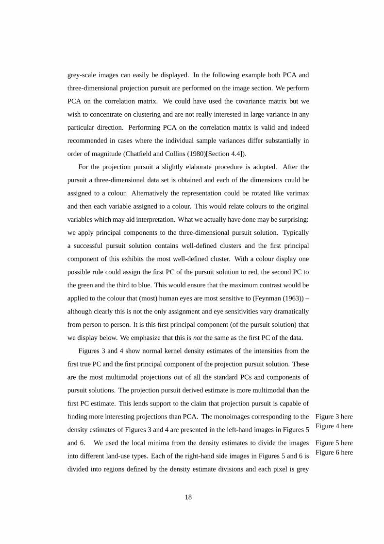
grey-scale images can easily be displayed. In the following example both PCA and

three-dimensional projection pursuit are performed on the image section. We perform

PCA on the correlation matrix. We could have used the covariance matrix but we

wish to concentrate on clustering and are not really interested in large variance in any

particular direction. Performing PCA on the correlation matrix is valid and indeed

recommended in cases where the individual sample variances differ substantially in

order of magnitude (Chatfield and Collins (1980)[Section 4.4]).

For the projection pursuit a slightly elaborate procedure is adopted. After the

pursuit a three-dimensional data set is obtained and each of the dimensions could be

assigned to a colour. Alternatively the representation could be rotated like varimax

and then each variable assigned to a colour. This would relate colours to the original

variables which may aid interpretation. What we actually have done may be surprising:

we apply principal components to the three-dimensional pursuit solution. Typically

a successful pursuit solution contains well-defined clusters and the first principal

component of this exhibits the most well-defined cluster. With a colour display one

possible rule could assign the first PC of the pursuit solution to red, the second PC to

the green and the third to blue. This would ensure that the maximum contrast would be

applied to the colour that (most) human eyes are most sensitive to (Feynman (1963)) –

although clearly this is not the only assignment and eye sensitivities vary dramatically

from person to person. It is this first principal component (of the pursuit solution) that

we display below. We emphasize that this isnot the same as the first PC of the data.

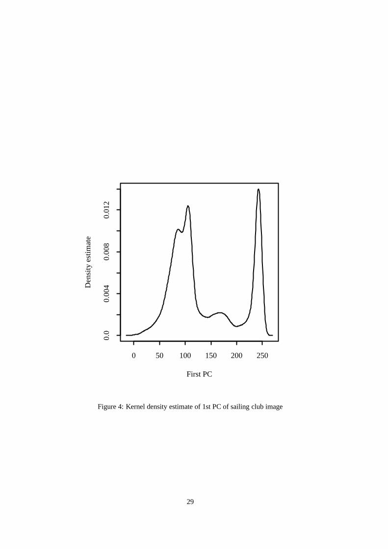
Figures 3 and 4 show normal kernel density estimates of the intensities from the

first true PC and the first principal component of the projection pursuit solution. These

are the most multimodal projections out of all the standard PCs and components of

pursuit solutions. The projection pursuit derived estimate is more multimodal than the

first PC estimate. This lends support to the claim that projection pursuit is capable of

finding more interesting projections than PCA. The monoimages corresponding to the Figure 3 hereFigure 4 heredensity estimates of Figures 3 and 4 are presented in the left-hand images in Figures 5

and 6. We used the local minima from the density estimates to divide the images Figure 5 hereFigure 6 hereinto different land-use types. Each of the right-hand side images in Figures 5 and 6 is

divided into regions defined by the density estimate divisions and each pixel is grey

18

shaded depending on its intensity in the pursuit or PCA solution. For example, the very

bright patches in Figure 5 correspond to the mode at the extreme right of the density

estimate in Figure 3.

As the projection pursuit solution has one more mode we can identify another type

of land with a new shade of grey. There are 5 grey shades on the projection pursuit

classification and 4 on the PCA picture. The differences between the classifications

can be most strikingly seen on the shore where projection pursuit has subdivided the

white area on the PCA picture into two groups and shaded them white and light grey

(right pictures in Figure 5 and 6). Indeed, no other PC makes this distinction. It is only

visible with the pursuit solution. What is even more fascinating is referring back to the

left-hand pictures in Figures 5 and 6. The areas that are differentiated by the extra grey

level do seem to correspond to different ground types. One grey level corresponds to

a grid-like network aligned with the jetties and the other to material in between. The

regularity of the network suggests that this is probably man-made and that projection

pursuit has discovered a real feature. However, projection pursuit can only fulfil an

exploratory role and a ground visit would be necessary to confirm the reality of such

features.

Naturally other PCs show interesting spectral band combinations that projection

pursuit does not find. We claim only that projection pursuit is an extra tool for finding

such combinations. The interest here lies in the greater multimodality of the pursuit

solution when compared to the first (or any) PC. Therefore projection pursuit would

be of value as an automatic band combination and selection tool because it is tuned for

clusters and not just large variation.

5 Conclusions and further work

This article shows the development and application of a three-dimensional projection

pursuit package based on a three-dimensional extension of the Jones and Sibson (1987)

moments index. The work involved in the development of the index was greatly

reduced by the use of computer algebra that permitted the arbitrary computation of

trivariatek-statistics. We have described how to use the pursuit within the statistical

19

package S using a freely available package. The potential of pursuit on real and

simulated data has been demonstrated and its performance compared to principal

components.

Further work will need to investigate the choice of outlier trimming and limit as

this sometimes determines the quality of the projection solutions.

Acknowledgments

The work reported here was supported partly by a grant from the UK Science and

Engineering Research Council (SERC). The author was a grateful recipient of a

SERC Research Studentship. The multispectral images described in Section 4.3 were

supplied by NERC Computer Services, UK. He is grateful to Robin Sibson for helpful

comments and advice, and to Merrilee Hurn and Bernard Silverman for many helpful

comments on an earlier version of this article.

References

Becker, R.A., Chambers, J. M. and Wilks, A. R. (1988).The New S Language. Pacific

Grove, CA: Wadsworth and Brooks/Cole.

Chatfield, C. and Collins, A. J. (1980).Introduction to Multivariate Analysis. London:

Chapman and Hall.

Cook, D., Buja, A. and Cabrera, J. (1993). Projection pursuit indices based on

expansions with orthonormal functions.J. Comput. Graph. Statist., 2, 225–250.

Crawford, S. L. (1991). Genetic optimization for exploratory projection pursuit.

In Computer Science and Statistics: Proc. 23rd Symp. Interface(ed. E. M.

Keramidas), pp. 318–321. Fairfax Station, VA: Interface Foundation.

Feynman, R. P. (1963).The Feynman Lectures on Physics. Vol. 1. Reading, Mass.:

Addison.

Friedman, J. H. (1987). Exploratory projection pursuit.J. Am. Statist. Ass., 82, 249–

266.

20

Friedman, J. H. and Tukey, J. W. (1974). A projection pursuit algorithm for exploratory

data analysis.IEEE Trans. Comput., 23, 881–890.

Hall, P. (1989). On polynomial-based projection indices for exploratory projection

pursuit.Ann. Statist., 17, 589–605.

Huber, P. J. (1985). Projection pursuit (with discussion).Ann. Statist., 13, 435–525.

Jones, M. C. (1983). The Projection Pursuit Algorithm for Exploratory Data Analysis.

PhD Thesis, University of Bath.

Jones, M. C. and Sibson, R. (1987). What is projection pursuit? (with discussion).J.

R. Statist. Soc. A, 150, 1–36.

Kaiser, H.F. (1958). The varimax criterion for analytic rotation in factor analysis.

Psychometrika, 23, 187–200.

Kendall, M. G. and Stuart, A. (1969).The Advanced Theory of Statistics. 3rd edn. Vol.

1. London: Griffin.

Lubischew, A. A. (1962). On the use of discriminant functions in taxonomy.

Biometrics, 18, 455–477.

Mardia, K. V. (1987). Discussion of the paper by Dr Jones and Professor Sibson.J. R.

Statist. Soc. A, 150, 22.

Morton, S. C. (1989). Interpretable Projection Pursuit.Technical Report 106.

Department of Statistics, Stanford University, Stanford, California.

Nason, G. P. (1992). Design and Choice of Projection Indices.PhD Thesis, University

of Bath.

Nason, G. P. (1994).PP3: Three-dimensional projection pursuit in S. Available

via anonymous FTP fromftp.stats.bris.ac.uk in the directory

/pub/software/pp3/ as the filepp3.shar.gz .

Posse, C. (1990). An effective two-dimensional projection pursuit algorithm.Comm.

Statist. Simul. Comput., 19, 1143–1164.

21

Swayne, D. F. and Cook, D. (1990).XGobi. Available from the StatLib archive.

Anonymous FTP fromlib.stat.cmu.edu .

Swayne, D. F., Cook, D. and Buja, A. (1991).User’s Manual for XGobi, a

dynamic graphics program for Data Analysis Implemented in the X Window

System (Release 2). Available from the StatLib archive. Anonymous FTP from

lib.stat.cmu.edu .

Tukey, J.W. (1987). Discussion of the paper by Dr Jones and Professor Sibson.J. R.

Statist. Soc. A, 150, 33.

Tukey, P. A. and Tukey, J. W. (1981). Preparation; prechosen sequences of views. In

Interpreting Multivariate Data(ed V. Barnett), pp. 189–213. Chichester: Wiley.

22

List of Figures

1 The projection pursuit algorithm. . . . . . . . . . . . . . . . . . . . 26

2 Projection pursuit solution from tetrahedral data. The data with

respect to the third projection direction is coded as the size of each

square.(Optimal projection index isM3 = 9:73) . . . . . . . . . . . . 27

3 Kernel density estimate of projection pursuit solution (1st PC) of

sailing club image .. . . . . . . . . . . . . . . . . . . . . . . . . . . 28

4 Kernel density estimate of 1st PC of sailing club image . . .. . . . . 29

5 Projection pursuit solution, first PC (left), classification from density

estimate (right) . . . . . . . . . . . . . . . . . . . . . . . . . . . . . 30

6 Real first PC (left), classification from density estimate (right). . . . 30

23

Original Principal Component Number

Variable 1 2 3 4 5 6

1 0.026 0.020 0.062 0.664 0.165 0.064

2 0.001 0.518 0.114 0.013 0.020 0.334

3 0.079 0.119 0.672 0.003 0.126 0.001

4 0.155 0.241 0.042 0.073 0.392 0.097

5 0.462 0.008 0.005 0.086 0.291 0.148

6 0.277 0.093 0.104 0.162 0.006 0.357

Table 1: Squares of elements of principal components of tetrahedral data

Original Projection Vectors

Variable 1 2 3

1 0.014 0.763 0.025

2 0.924 0.029 0.013

3 0.017 0.026 0.896

rest 0.045 0.182 0.066

Table 2: Squares of elements of projection vectors for tetrahedral data after axis

rotation.

Channel Wavelength (� m) Designation

1 0.42 - 0.45 violet

2 0.45 - 0.52 blue

3 0.52 - 0.60 green,yellow,orange

4 0.605 - 0.625 red

5 0.63 - 0.69 red

6 0.695 - 0.75 red

7 0.76 - 0.90 near IR

8 0.91 - 1.05 near IR

9 1.55 - 1.75 near IR

10 2.08 - 2.35 near IR

11 8.50 - 13.00 thermal IR

Table 3: Spectral frequencies sensed by NERC Daedalus thematic mapper

24

Channel 2 3 4 5 6 8 9 10 11

2 1

3 0.97 1

4 0.95 0.99 1

5 0.91 0.98 0.98 1

6 0.49 0.61 0.61 0.73 1

8 0.34 0.45 0.45 0.60 0.97 1

9 0.58 0.69 0.70 0.81 0.94 0.92 1

10 0.79 0.86 0.87 0.93 0.83 0.75 0.93 1

11 0.48 0.54 0.55 0.64 0.71 0.71 0.85 0.80 1

Table 4: Correlation matrix for section of multispectral image

25

Data, X

Sphered Data

Y

Product Moment

Tensors

T,U

Power Sumss

k-statistics

k

Projection index

and derivatives

Modify projection

directions

(a,b,c)

Initial projection

directions

(a,b,c)

Yes

projection

solution

optimality ?

No

Figure 1: The projection pursuit algorithm

26

Axis 2

Axi

s 3

-1 0 1 2

-2.0

-1.5

-1.0

-0.5

0.0

0.5

1.0

Figure 2: Projection pursuit solution from tetrahedral data. The data with respect to

the third projection direction is coded as the size of each square.(Optimal projection

index isM3 = 9:73) .

27

Projection pursuit: first PC

Den

sity

est

imat

e

0 50 100 150 200 250

0.0

0.00

50.

010

0.01

5

Figure 3: Kernel density estimate of projection pursuit solution (1st PC) of sailing club

image

28

First PC

Den

sity

est

imat

e

0 50 100 150 200 250

0.0

0.00

40.

008

0.01

2

Figure 4: Kernel density estimate of 1st PC of sailing club image

29

Figure 5: Projection pursuit solution, first PC (left), classification from density

estimate (right)

Figure 6: Real first PC (left), classification from density estimate (right)

30