three-dimensional multispectral stochastic image
TRANSCRIPT
THREE-DIMENSIONAL MULTISPECTRAL STOCHASTIC IMAGE
SEGMENTATION
By
Brian Gerard Johnston
B. Sc. (Computer Science) Memorial University of Newfoundland 1990
Ph. C. (Pharmacy) Cabot Institute of Technology 1982
A THESIS SUBMITTED IN PARTIAL FULFILLMENT OF
THE REQUIREMENTS FOR THE DEGREE OF
MASTER OF SCIENCE
in
THE FACULTY OF GRADUATE STUDIES
DEPARTMENT OF COMPUTER SCIENCE
We accept this thesis as conforming
to the required standard
January 1994
TUNIVERSIT BRITISH COLUMBIA
© Brian Gerard Johnston, 1994

In presenting this thesis in partial fulfillment of the requirements for an advanced degree at the
University of British Columbia, I agree that the Library shall make it freely available for refer
ence and study. I further agree that permission for extensive copying of this thesis for scholarly
purposes may be granted by the head of my department or by his or her representatives. It
is understood that copying or publication of this thesis for financial gain shall not be allowed
without my written permission.
Department of Computer Science
The University of British Columbia
2366 Main Mall
Vancouver, Canada
V6T 1Z4
Date:
i/’
(I
Abstract
Current methods of lesion localization and quantification from magnetic resonance imaging, and
other methods of computed tomography fall short of what is needed by clinicians to accurately
diagnose pathology and predict clinical outcome. We investigate a method of lesion aild tissue
segmentation which uses stochastic relaxation techniques in three dimensions, using images from
multiple image spectra, to assign partial tissue classification to individual voxels. The algorithm
is an extension of the concept of Iterated Conditional Modes first used to restore noisy and
corrupted images. Our algorithm requires a minimal learning phase and may incorporate prior
organ models to aid in the segmentatioll. The algorithm is based on local neighbourhoods and
can therefore be implemented in parallel to enhance its performance. Parallelism is achieved
through the use of a datafiow image processing development package which allows multiple
servers to execute in parallel.
11
Table of Contents
Abstract ii
Table of Contents iii
List of Tables vii
List of Figures viii
Acknowledgement x
1 introduction 1
1.1 Overview of Segmentation Methods 3
1.2 Overview of the Thesis o1.2.1 Chapter Summary 6
2 Computerized Tomographic Imaging 8
2.1 Introduction 8
2.2 Computed Tomography(CT) 9
2.2.1 Physical Principles 10
2.2.2 Practical Aspects 14
2.2.3 Conclusion 15
2.3 Magnetic Resonance Imaging(MRI) 15
2.3.1 Introduction 15
2.3.2 Physical Principles 16
2.3.3 Practical Aspects 19
2.3.4 Conclusion . 20
111
2.4 Emission Computed Tomography (PET and SPECT) 21
2.4.1 Introduction 21
2.4.2 Physical Principles 21
2.4.3 Practical Aspects 23
2.4.4 Conclusion 25
2.5 Combining Images 25
3 Basics of Image Segmentation 27
3.1 Introduction 27
3.2 Definitions 28
3.2.1 Techniques 30
3.3 Summary 33
4 Segmentation Applied to Medical Imaging 35
4.1 Difficulties with Medical Imaging 35
4.1.1 Partial Volume Effect 36
4.1.2 CT 36
4.1.3 MRI 37
4.1.4 PET/SPECT 38
4.2 Current Algorithms 39
4.2.1 Manual Tracing 39
4.2.2 Edge Detection 40
4.2.3 Thresholding and Cluster Analysis 40
4.2.4 Region Growing 42
4.3 Extensions to Fundamental Techniques 43
4.3.1 Mathematical Morphology 43
4.3.2 Pyramidal Techniques 45
4.4 Model-Based Approaches 46
iv
4.5 Markov Random Fields and the Gibbs Distribution 49
4.6 Iterated Conditional Modes 52
4.6.1 Segmentation Using Iterated Conditional Modes 53
5 3D Multispectral Stochastic Volume Segmentation 58
5.1 Returning to Basic Theory 58
5.2 Extensions to Iterated Conditional Modes 60
5.2.1 Neighbour Interaction Parameters 61
5.2.2 Neighbour Counts 62
5.2.3 Histogram Re-evaluation 62
5.2.4 Prior Organ Models 62
5.2.5 Convergence 63
5.2.6 Multispectral Approach 64
5.2.7 Parallelism 64
5.3 Implementation Platform 64
5.3.1 Dataflow Paradigm 65
5.3.2 WIT 66
5.3.3 Extensibility Using WIT 70
5.3.4 Parallelism Using Multiple Servers 71
5.3.5 Limitations of the Dataflow Approach 71
5.4 WIT Implementation of 1CM 74
6 Algorithm Testing and Results 81
6.1 Multiple Sclerosis 81
6.2 Results Analysis 83
6.2.1 Initial Histograms 85
6.2.2 Initial Neighbourhood Interaction Parameters 89
6.2.3 Recalculated Histograms 91
V

6.2.4 Recalculated Neighbourhood Interaction Parameters
6.3 Segmentation Results
6.3.1 Ti Segmentation
6.3.2 T2 Segmentation
6.3.3 Combining Ti and T2 Segmentations
6.3.4 Post-Processing of the Segmentation
6.3.5 Visualizing Partial Volumes
6.4 Lesion Volume Analysis
6.5 General Conclusions and Future Work
6.5.1 Future Work
94
95
96
96
99
99
101
105
108
109
Appendices
A 1CM Source Code Kernel
Bibliography
112
112
116
vi

List of Tables
6.1 Initial neighbourhood interaction parameters obtained from Ti image seqneuce. 89
6.2 Initial neighbourhood interaction parameters obtained from T2 image sequence. 89
6.3 Recalculated neighbourhood interaction parameters obtained from Ti image se
quence 94
6.4 Recalculated neighbourhood interaction parameters obtained from T2 image se
quence 95
VII
List of Figures
2.1 The 1-D projection g(8, ) of the 2-D function f(x, y) 12
2.2 The pulse sequence of a conventional MRI imaging system 18
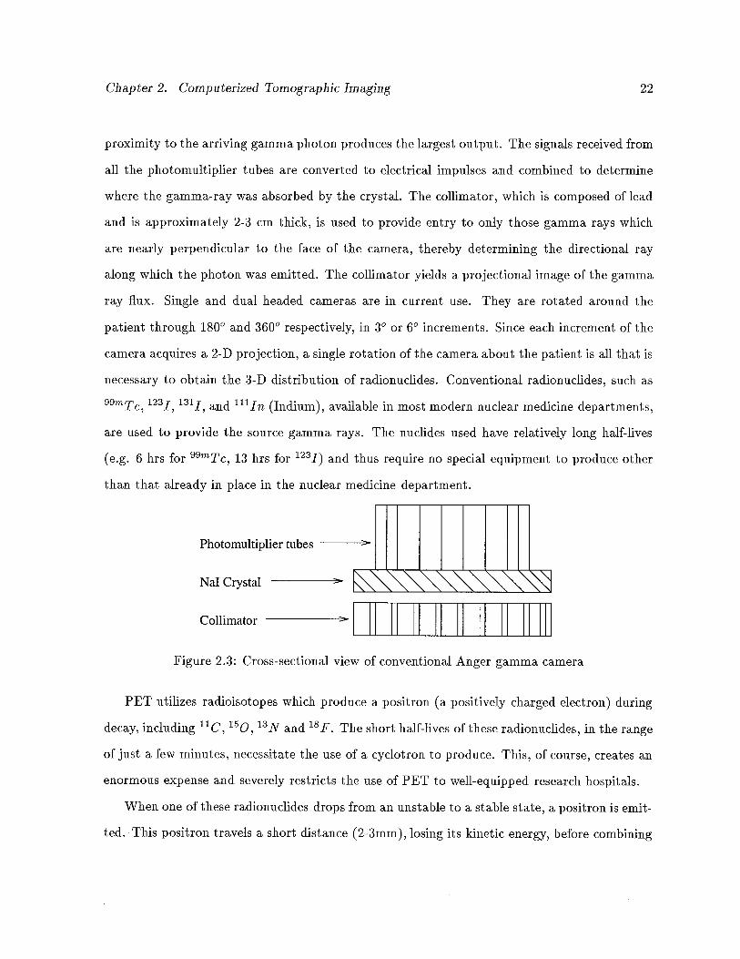
2.3 Cross-sectional view of conventional Anger gamma camera 22
4.4 Examples of morphological operations 44
4.5 Pyramid representation of a one-dimensional signal 45
4.6 Neighbourhood systems in 2D 50
4.7 Neighbourhood systems in 3D 51
5.8 Sample WIT screen 67
5.9 Hierarchical igraph in WIT 69
.5.10 Expanded hierarchical operator 69
5.11 Example of deadlock in a WIT Igraph 72
5.12 WIT igraph of 1CM algorithm 74
5.13 Expanded WIT igraph of icrnlnitialize operator 75
5.14 MRI Ti-Weighted data from which sample image is selected for ROl analysis. 76
5.15 Expanded WIT igraph of segmentation operator seg Volume 78
6.16 MS lesions on MRI 82
6.17 MRI series — Ti weighted 83
6.18 MRI series — T2 weighted 84
6.19 Histograms of Ti weighted MRI series 86
6.20 Histograms of T2 weighted MRI series 87
6.21 Recalculated histograms of Ti weighted MRI series 92
6.22 Recalculated histograms of T2 weighted MRI series 93
viii

6.23 Segmentation of Ti Echo Sequence 97
6.24 Segmentation of T2 Echo Sequence 98
6.25 Combined Segmentation of T1/T2 Echo Sequences 100
6.26 Manual Segmentation overlaid on combined T1/T2 Segmentation 101
6.27 Combined Lesion Segmentation of Ti/T2 Echo Sequences after post-processing. 102
6.28 Illustration of partial volume assignment using colour images (No post-processing
has been applied.) i03
6.29 Illustration of partial volume assignment using colour images (Post-processing
has been applied.) 103
6.30 Colour-map used to enhance partial volume characteristics of segmentation. . . . 104
6.3i Graphs of lesion volumes determined at all stages of the segmentation, including
manual segmentation 106
6.32 Expanded graphs of lesion volumes of final segmentation and manual segmentation. 107
ix
Acknowledgement
The contributions, both physical and moral, of the following people are gratefully acknowledged:
Dr. L.C.E. Phillips, my wife, without whose inspiration and support, this work could not
possibly have materialized;
Dr. M.S. Atkins of Simon Fraser University and Dr. K.S. Booth of University of British
Columbia, my co-supervisors in this project;
Torre Zuk, my student reader, with whom I collaborated and, at times, conspired;
Dr. James Little of University of British Columbia, the “third” reader of this thesis, whose
input with respect to this work and otherwise, is greatly appreciated;
The MS MRI Study Group at UBC Hospital, especially Andrew Riddehough and Dr. Guojun
Zhou, who supplied MRI scans and hand segmented the data for our analysis;
Dr. K. Poskitt, of Children’s Hospital in Vancouver, who supplied both motivation and patient
data to the project;
Terry Arden, the creator of WIT, the image processing platform on which the software portion
of this thesis is based.
Financial support for this project has been provided in part by the Natural Sciences and Engi
neering Research Council of Canada.
x
Chapter 1
Introduction
Since the advent of computer image processing, researchers have been seeking ways in which
to classify objects and the relationships between objects represented in these images. In the
field of medicine in particular, many attempts have been made to automatically classify and
quantify tissues, organs, and disease states from images obtained by various medical imaging
sources. It is the ease with which humans can so readily interpret these images that has been
the impetus for attempting to force computers to do the same.
Image segmentation is possibly the single most important area of image analysis research
being carried out today. Image segmentation can be considered the separation of an image into
different regions, each having a certain property, for example average gray level or texture. It is
usually the first step in a process leading to description, classification and interpretation of an
image by higher level processes. However, classificatioll and interpretation may form part of the
segmentation process itself. The applications of image segmentation are many and range from
pattern recognition in robot vision systems to innumerable medical uses including aiding in the
diagnosis, evaluation and treatment of disease. It is the application of image segmentation to
medical images which has motivated the development of this thesis.
For many years physicians have been producing and analyzing medical images, from X-rays
to ultrasound. Physicians usually employ computers and sophisticated hardware to produce
the images and rely on their medical expertise and knowledge to analyze the images visually.
There are many types of medical imaging techniques being employed in hospital settings today.
We shall be concerned only with a subset of those techniques, however, this subset forms a
substantial concentration of the total amount of medical imaging being carried out today. The
1
Chapter 1. Introduction 2
types of imaging which we shall encounter are each a category of what is termed tornographic
imaging. That is, the images obtained from each of these modalities are pictures of cross-
sectional slices of different areas of the human body. Multiple contiguous slices are combined
to provide a 3D volume represeuting selected organs of interest within the body.
When analysing tomographic images, the physician is most often attempting to identify and
quantify lesions, for example, cancerous tumours or cysts, which may be present in some organ
in the patient. Today the state of the art in quantifying lesions on medical scans is defined by
the manual outlining of the lesions on every slice in the scan, lesion by lesion, slice-by-slice. The
areas defined by the hand-drawn lesions are then summed slice-by-slice to determine the volumes
of the lesions. The measurement of volumes aids the physician in determining a diagnosis and
a prognosis with respect to the disease state of the patient. Lesions are also measured over
time, foliowing therapy, in order to assess the progress of the patient and determine the efficacy
of the treatment being applied. Most often, in the course of imaging a patient over time,
different medical personnel are responsible for the analysis of the medical scans obtained from
the patient on any one occasion. This can lead to bias and inconsistencies in the identification
and measurement of lesions, and consequently in the diagnosis and evaluation of the patient.
Accurate automatic lesion detection could provide a consistent, unbiased account of the disease
process under investigation.
Image segmentation, including medical image segmentation, has been studied extensively
in the literature and many algorithms have been developed in an attempt to solve the problem.
The efficacy and accuracy of many of these algorithms have not been clearly demonstrated. As
a result, the number of medical teams employing these algorithms in practise is quite small.
The reasons for the difficulties encountered in general medical image segmentation are many.
For example, the tremendous variation in the output of medical imaging devices makes it dif
ficult to design a segmentation algorithm which will be effective in more than one imaging
modality, so most researchers carry out their studies using a single modality. Another problem
is that no lighting or depth cues, generally available in other types of images, are observable
Chapter 1. Introduction 3
in medical images. There are no shadows from light sources, and often no discernible fore
ground/background contrast to aid in the analysis. A third complicating factor in medical
image segmentation is the fact that researchers involved in image segmentation work are gen
erally computer scientists and engineers, while the people who produce and analyse medical
images are physicians and medical technicians. It is difficult to merge the knowledge and ex
pertise of both fields to acquire the composite knowledge that is essential to a valid solution to
the problem. The requisite multidisciplinary nature of this work is another motivating factor in
this thesis. We have endeavoured to maintain an ongoing liaison with several medical imaging
centres during the development of the research.
One major obstacle which continues to complicate the segmentation of medical images is the
partial volume, or volume averaging problem. At surfaces between objects the corresponding
image elements (pixels in 2D or voxels in 3D) may be composed of more than one object,
for example, gray matter and white matter in the brain. Most segmentation techniques try to
classify each pixel in an image as belonging to one type of structure. If volume averaging occurs
at a significant rate, which it does in medical images due to inherently poor spatial resolution,
this will cause significant artifacts in the segmentation of these images.
1.1 Overview of Segmentation Methods
In general, image segmentation algorithms can be loosely categorized into thresholding methods,
edge detection, and region oriented techniques.
The simplest method of image segmentation involves thresholding. All pixels which have a
certain property such as falling into a given intensity range are classified as belonging to the
same group. All pixels outside the given range are not included in the object. Most thresholding
techniques involve a binarization of the image into foreground and background objects. This
limits the application of these techniques to images having few objects. Another drawback to
thresholdirig is the difficulty in the proper selection of the threshold value required to optimally
extract the desired objects. Many factors affect the observed intensity value of an object in an
Chapter 1. Introduction 4
image. For example, the characteristics of the imaged material, the proximity of an object to
nearby objects, and imaging conditions such as lighting and shadows ali combine to make it
difficult to obtain an optimal threshold value.
Edge detection methods of image segmentation involve locating significant intensity changes
in images which can most often be interpreted as edges between objects. Although many
improvements in edge detection have been demonstrated in recent years, the methods are stili
complicated by the difficulty of finding actual object boundaries as opposed to noise or artifacts.
Foliowing edge detection it is often the case that many gaps exist along the detected contours
of an object. The complexity of properly linking the fragmented edges which most often result
from the application of these techniques further detracts from their general usefulness.
The third general class of image segmentation techniques is defined by the region-oriented
methods. These techniques assume that objects are defined by individual, closed regions in
space. Region analysis techniques are further broken down into region growing methods and
region splitting and merging. In region growing, a pixel or pixels in the image are used as a
seed and an analysis is performed of the neighbours of the seed to determine inclusion into the
region. This analysis is iteratively applied until the object ceases to grow further. The split
and merge methods of region analysis work by iteratively splitting the image into smalier and
smalier regions until it is determined that the resulting regions have some uniform property.
The results of the image splitting are then merged with one another if it is determined that
the merged regions also satisfy the desired property. The difficulty of defining the uniformity
property and the complexity of applying these techniques detract from their general application.
Recently the above general segmentation techniques have been augmented by the incorpora
tion of mathematical morphology, pyramidal schemes, and model-based image segmentation. It
has been observed that accurate segmentation of many images, especialiy medical images, wili
require external knowledge about the object represented in the image. In order to incorporate
external knowledge many organ and tissue models have been applied to the segmentation of
Chapter 1. Introduction 5
medical scans with limited success. Most of these model-based techniques involve the acquisi
tion and analysis of many data sets in order to form the model. For this reason the success of
these methods to date has been marginal.
In this thesis we have extended a model-based approach which has been investigated in
the literature. The model used assumes the given image data represents a Markov random
field (MRF). Using MRFs, we exploit the fact that pixels (or in 3D, voxels) in a given local
neighbourhood of the image have similar intensity. The method we have implemented is iterative
and on each iteration an analysis is made of each voxel and its neighbours. Based on this
analysis the voxel is classified. At each iteration every voxel in the volume is assigned a set of
probabilities which represent the percentage of that voxel considered to be a particular tissue
type. In this manner, we present a solution to the partial volume problem. The classification
values for each voxel eventualiy converge if the MRF assumption is valid. The model used
requires a minimum of user interaction in order to train the algorithm.
The algorithm has been implemented in 3D using a visual datafiow programming environ
ment. The use of this development environment has enabled us to paralielize the computation,
which because of its 3D nature is relatively complex.
1.2 Overview of the Thesis
This thesis has been designed to be readable and understandable by persons with a moderate
Computer Science or Engineering background. Because of the extensive medical nature of
the thesis, an attempt has been made to include as much background material as possible,
relative to the medical aspects of the thesis. The segmentation solution presented, as weli as
the background literature leading up to the solution, employs a significant amount of statistics
and probability theory. However, readers with an introductory knowledge of these subjects
should have no difficulty with the material presented here.
This thesis, although essentialiy self-contained, is not meant to be read in isolation from the
vast literatnre available concerning medical image segmentation. Interested readers are strongly
Chapter 1. Introduction 6
encouraged to explore the extensive bibliography at the end of the thesis.
1.2.1 Chapter Summary
As mentioned previously, the thesis has been written with the intent of applying its results
to medical images. In light of this fact, we first introduce computerized medical imaging in
Chapter 2. Each of the commonly used methods of medical imaging including Computed
Tomography (CT), Magnetic Resonance Imaging (MRI) and Emission Computed Tomography
(ECT), is discussed in detail. For each imaging modality we present the physical principles
underlying the technique, its main applications and its limitations. A small discussion of how
researchers have combined the various techniques in order to enhance their diagnostic potential
is also presented. This chapter has been included to provide the reader with information
necessary to understand the medical terminology and references found in later chapters. As
well, it provides an indication of the difficulty which arises in analysis of the images obtained
from these techniques.
Chapter 3 introduces the problem of image segmentation. Some formal definitions and
notation are provided followed by a discussion of the fundamental techniques used to solve the
problem. The inherent advantages and disadvantages of each of these methods are also given.
Each of the imaging methods discussed in Chapter 2 has unique features which complicate
the segmentation problem and detract from the discovery of a general solution which will work
for all modalities. In Chapter 4 these features are presented, followed by a discussion of how
the general segmentation techniques of Chapter 3 have been extended to medical images. A
detailed discussion of model-based segmentation methods is then given. Special consideration is
given to the method of Iterated Conditional Modes, a model-based method employing Markov
random fields. This technique provides the basis upon which our solution is built.
We have extended and adapted the Iterated Conditional Modes method presented in Chap
ter 4 to incorporate 3D, partial volume features and this forms the bulk of the discussion
Chapter 1. Introduction 7
contained in Chapter 5. A multispectral approach is presented which combines the segmenta
tions obtained from independent image scans of the same organ. These scans are first aligned,
or registered, so that corresponding voxels from each set represent the same structure. In the
case of MRI, registered independent scans can often be acquired simultaneously so that physical
alignment of the images is not necessary. A discussion of how the algorithm has been designed
so that its implementation is easily parallelized is also included.
The algorithm presented in Chapter 5 has been implemented using a visual datafiow pro
gramming environment specially designed for image processing. The environment allows rapid
development of algorithms and provides explicit parallelism by distributing the computation
to multiple workstations. The visual programming environment and the implementation of the
algorithm using the environment are also discussed in Chapter 5.
The algorithm has been applied to multispectral MRI scans of the brains of Multiple Sclerosis
patients. Multiple Sclerosis causes lesions in the brain which are visible on MRI scans. The
segmentations obtained are evaluated visually and by a lesion volume comparison with hand
drawn lesions obtained over the entire image volumes. The results obtained by our algorithm
are presented in Chapter 6, and compare favourably with the hand drawn versions. Following
a discussion of the results of experiments using our algorithm, some future directions this work
may take in the coming months are also given. This will include further experimentation using
phantom or simulated data, improvements to the algorithm, and the development of an accurate
model of brain tissue and lesions.
Chapter 2
Computerized Tomographic Imaging
2.1 Introduction
A revolution has taken place over the last 20 years in diagnostic medical imaging, integrating
advances in the fields of medicine, physics, computer science and engineering. The result is a
vast array of tomographic medical imaging techniques designed to exploit the electro-magnetic
wave spectrum to the fullest. Tomographic imaging involves obtaining multiple projections
through each of many planes or slices through the body. These multiple projections are used
to create images of consecutive cross-sections of interest. Together, these cross-sections or
tornograrns form a 3D volume image of the organ(s) of interest. The manner in which these
projections are obtained defines the types of computerized tomographic imaging currently avail
able. The tomographic imaging repertoire now includes computed tomography (CT), magnetic
resonance imaging (MRI), and emission computed tomography (ECT) which is further broken
down into two classes, single photon emission computed tomography (SPECT) and positron
emission tomography (PET).
CT provides images of internal structures by measuring the attenuation of X-Ray beams
passed through body. Images are obtained with MRI using a combination of the inherent
resonance characteristics of atomic nuclei and the application of a strong magnetic field to the
patient. Varying tissue characteristics can be determined and the spatial locations of the atomic
nuclei can be discovered through gradient applications of further magnetic fields in orthogonal
directions.
ECT yields images of slices through the body by measuring the gamma ray flux emitted
by radiotracers, chemicals which are combined with radioactive nuclei and injected into the
8
Chapter 2. Computerized Tomographic Imaging 9
patient. Different radiotracers have affinity for different tissues and locate selectively in the
organ of interest. Depending on the method of creation of the gamma ray photons, ECT
has evolved into two separate imaging modalities; positron emission tomography (PET) and
single photon emission computed tomography (SPECT). Both of these methods are capable of
quantitatively measuring metabolic and physiological processes.
The results of each of the above imaging modalities can be used to develop 3D models of the
organs or tissues being imaged. Using advanced computer graphics techniques, the images can
be correlated and interpolated to compute the volumes and surfaces of the objects. These vol
umes can then be viewed from any desired angle and the usual post-processing techniques such
as thresholding, scaling, contrast enhancement, etc., previously applied to the two dimensional
views, can be applied to the 3D image.
The purpose of this chapter is to provide an introduction to each of the currently available
tomographic imaging techniques, to describe the fundamental aspects of the physics of each and
to establish a framework for the remainder of the thesis. It is not intended to be an exhaustive
survey. The interested reader is encouraged to explore the reference list at the end of the thesis
for further details on each technique.
The images obtained from each of these methods can also be combined or registered to yield
a composite view, consisting of both the structural information obtained from CT or MRI and
the functional information granted by SPECT and PET. The registration of multi-modality
images serves to enhance the diagnostic potential of any single technique. The final section in
this chapter discusses some of the methods and difficulties associated with image registration.
2.2 Computed Tomography(CT)
Since its conception in 1971, computed tomography, or computerized axial tomography (CAT),
has revolutionized the field of diagnostic imaging and provided the impetus for the development
of more advanced imaging modalities such as magnetic resonance imaging. Known more famil
iarly as CAT scanning, this technique provides images of the internal structures of organs by
Chapter 2. Computerized Tomographic Imaging 10
measuring the X-ray attenuation of underlying tissues in a slice through the body. A series of
1-D projections is obtained, from which tomographic reconstruction methods are used to obtain
a 2-D image of the slice. Because noise from over- and under-lying tissues, so detrimental iu
ordinary X-ray imaging, is substantialiy reduced, much better resolution and contrast between
tissues is obtained. A series of 2-D images of a given portion of the body under study can be
used to obtain volumetric images using either volume rendering or surface rendering techniques
provided by advanced computer graphics.
2.2.1 Physical Principles
Imaging of the body with computed tomography is accomplished by measuring the attenuation
of X-ray beams lying entirely within successive planes of the section being imaged. In order
to obtain the 1-D projections necessary to reconstruct the image accurately, the attenuations
must be measured at many different angles around the body. This results in a need for imaging
equipment which can be rotated at an angle which is transverse to the long axis of the body.
Hence, most of the images obtained in this manner are transaxial images.
When Geoffrey Hounsefield of EMI in Great Britain first experimented with CT in 1972,
the source/detector arrangement consisted of a single X-ray generator and a single detector
mechanism which would exist at opposing sides of the area to be imaged [123]. By translating
both the source and detector coincidentaliy, through the plane of interest, a single view was
obtained. The unit would then be rotated by 10 and the process repeated until 180 such views
were obtained. Each view required 160 translations thus culminating in 28,800 ray sums being
obtained. Each such slice would take approximately 4 minutes, creating considerable difficulties,
since many slices would have to be obtained to provide a worthwhile study.
This first generation CT scanner has been succeeded by three major design modifications
culminating in the modern fourth generation scanners available to day. In the fourth generation
design the X-ray is emanated in fan-beam fashion extending over the entire plane of interest.
The detectors, of which there are as many as 1200, are arranged in a static ring around the
Chapter 2. Computerized Tomographic Imaging 11
patient. Thus no translation of the source is necessary and a complete scan can be obtained
from a single rotation of the source/detector coupling through an arc of 180 degrees. The
detectors are composed of scintigraphic crystals with short afterglow, coupled to solid state
photo-iodes sensitive to scintillation photons. A single scan now takes 1.5 to 18 seconds instead
of 4 minutes. Each detector makes approximately 1024 measurements resulting in over 1.2
miffion samples per slice. Most modern third and fourth generation CT systems incorporate
variable scanning rates in order to accommodate the different requirements of imaging various
tissues and organs. As well, the diameter of the field of view can be adjusted to further reduce
the imaging times where appropriate.
Regardless of which generation scanning system is employed, the end result of any CT scan
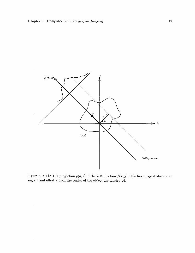
is a series of data in the form of g(8, .s), the line integral sum along angle of orientation 0 with
offset s from the center of the section. Figure 2.1 illustrates one such projection through an
image f(x, y). The problem then is to transform the data into a 2-D distribution in the spatial
domain from the set of line integrals so obtained, that is, to determine f(x, y) from g(O, s).
The function g(0, .s) is called the Radon transform of f(x, y), named after the mathematician
J. Radon who determined, in the late 19th century, how the transform could be achieved.
The basic property of X-ray absorption which is necessary for the evaluation is given in
Equation 2.1:
ln(j-) = —ctL (2.1)
where a = the absorption coefficient for a uniform absorbing material of length L.
I = transmitted intensity of the X-ray beam.
I = the detected intensity of the X-ray beam.
Human tissue is obviously not uniform along any given length so Equation 2.1 must be
modified to incorporate the integral of intensity along the length of the tissue. This is given by
Equation 2.2 below:
Iln(—)
- I a(z)dz (2.2)10 ft
Chapter 2. Computerized Tomographic Imaging 12
x
Figure 2.1: The 1-D projection g(O, s) of the 2-D function f(x, y). The line integral along t atangle 9 and offset s from the center of the object are illustrated.
g( 0,
f(x,y)
X-Ray source
Chapter 2. Computerized Tomographic Imaging 13
Solving for I we obtain:
I = Ioe1L (2.3)
In order to reconstruct f(x, y), the original data, we need to determine a(z). Several
methods of reconstruction have been developed to obtain the 2-D spatial intensity distribution
from the line integrals. The first method to be developed, which has largely been displaced by
the filtered back-projection technique, was the Arithmetic Reconstruction Technique (ART).
ART uses an iterative method to obtain successive approximations using a best fit strategy.
The filtered back-projection method is used extensively in CT, PET, SPECT and other
imaging modalities with minor variations across the imaging spectrum. One view of a section
of the body under consideration is defined as a set of parallel rays obtained at any given angle
0. All values of ray sums are back-projected such that each point intensity in this intermediate
image is equal to the sum of all the views contributing to it. Each point in the unfiltered back-
projection gives rise to artifactual densities proportional to 1/r, the distance from the point
density location. All points thus contribute to the blur of each other point. The transforma
tion so obtained is the Radon transform of the image and the result is the original function
blurred by the point spread function 1/z2 + y2. The original function can be restored by an
approximation of the 2-D inverse filter whose frequency response is given by:
F = + v2
where mm and v are the frequency domain counterparts of the z and y spatial coordinates,
respectively.
A series of filters have been designed and used to obtain the reconstructed image, and the
use of any particular one is determined by the preference of the radiologist using the equipment
and the characteristics of the hardware used to obtain the projections. It is beyond the scope
of this chapter to further explore the difficulties encountered and the techniques used in image
reconstruction from projections. The interested reader is encouraged to explore Herman [44]
and Jam [51].
Chapter 2. Computerized Tomographic Imaging 14
An enormous number of calculations is required to perform the reconstruction process and
thus specialized hardware is necessary to obtain reasonable results in a reasonable amount of
time. To facilitate the process, array processors and other parallel processing hardware and
software are employed in the reconstruction process.
Having obtained the approximation of the slice of the body under investigation, a great
many post-processing techniques are available to further extract information from the resulting
2-D image slices, using filtering, edge detection, thresholding, etc. As well, the 2-D images
can be manipulated to obtain 3-D views using the volume rendering and surface reconstruction
techniques of modern computer graphics installations. The reader is referred to Kaufman [61]
for an exhaustive survey and a comprehensive bibliography of volume visualization research.
2.2.2 Practical Aspects
Almost all CT scanners available today use some variation of the aforementioned methods of
signal generation, detection and image reconstruction from projections. Progress has been made
in all these areas over the last twenty years, resulting in complete examinations requiring as
little as 8-20 seconds. The actual display of the generated images can proceed in parallel, with
the 3-D reconstructions taking only seconds more. Thus a patient can be imaged in real-time
allowing maximum utilization of the available resources.
Recent innovations in CT research have led to thin-section imaging techniques obtaining
section thicknesses in the range of 1-2mm with scan times of 1-23 seconds per slice. The
resolution obtained is quite remarkable. The ultra-fast CT scanner can produce an image in
50msec and complete an examination of the heart in under a second [69].
The use of CT does have some problems and limitations and is not a panacea for all imaging
requirements. For example, one advantage of CT is not requiring invasive procedures. This
advantage is lost when cardiovascular and bowel viewing is considered. It then becomes neces
sary to use a contrast medium since the differential across tissue demarcations is not sufficiently
Chapter 2. Computerized Tomographic Imaging 15
pronounced. Another major drawback of CT is its inability to fully characterize tissue, espe
cially significant in distinguishing between malignant and benign lesions, a problem common to
all currently available imaging modalities. The only way to differentiate malignant tumors is
through multiple scans over a period of time sufficient to detect changes in the affected tissue.
CT costs about half the price of MRI, both for installation and maintenance, but is more than
10 times as expensive as readily available ultrasound imaging.
2.2.3 Conclusion
CT has revolutionized the diagnostic capabilities of modern medical science. Through the
development of low cost, versatile hardware, this tomographic imaging method has become a
reality for even the smallest of general hospitals. Though it has its disadvantages, CT promises
to be one of the leading methods of organ and tissue visualization for the next several decades.
2.3 Magnetic Resonance Imaging(MRI)
2.3.1 Introduction
No imaging modality has witnessed the explosion of growth and development that Magnetic
Resonance Imaging has over the past 10 years. Once labeled NMR, for Nuclear Magnetic Reso
nance imaging, the “Nuclear” term has recently been replaced due to its negative connotations
among the general public. Using a combination of the inherent magnetic resonance properties
of tissue and application of radio frequency pulses, MRI obtains images by measuring varying
tissue characteristics. The resulting frequency information is converted, using Fourier Trans
form techniques, to spatial intensity information of slices through the body. As with CT these
slices can be integrated using advanced computer graphics techniques to produce 3-D views of
the imaged tissues. Unlike CT, where the signal is generated by X-Ray beams, in MRI the
patient becomes the signal source.
Chapter 2. Computerized Tomographic Imaging 16
2.3.2 Physical Principles
Atomic nuclei of odd number exhibit a magnetic moment, somewhat as if the nuclei were
replaced by tiny magnets. In the absence of an applied magnetic field these magnetic moments
are arbitrary and random. Following the application of a large magnetic field, B0, on the
order of 0.3 to 2.0 Tesla, the magnetic moments of all the atomic nuclei align themselves in
the direction of B0. This results in a net magnetic moment, M, the vector sum of all the
individual magnetic moments of the charged nuclei, in the direction of B0. Currently, the most
prevalent entity for which measurements are taken is the ‘H nucleus. Other nuclei in the body
are suitable for measurement but the ‘H nucleus is the preferred entity, for two reasons. Firstly,
J[ is abundant throughout body tissues in the form of H20, and secondly the ‘H proton yields
the highest detectable signal of all the available atomic nuclei. Other nuclei such as ‘3C, ‘9F,
23Na, 31P, while less efficient, are finding increased use both in the research laboratory and in
established MRI installations in a limited number of hospital settings. The use of these nuclei
offers the advantage of exploring a large number of metabolic processes not possible using ‘H.
For the remainder of this discussion, however, we will assume that ‘H is the nuclei of reference.
When ‘H nuclei are placed in the magnetic field, B0, they precess or wobble at a character
istic frequency known as the Larmor frequency, proportional to the strength of B0, according
to the following equation:
= 7B1 (2.4)
where w = the Larmor frequency.
= the magnetogyric ratio of the atomic nuclei,
for 1H,7 = 42.6MHz/Tesla
B0 = the strength of the applied magnetic field in Tesla
Following the application of the magnetic field, a radio frequency (RF) pulse is applied
perpendicular to B0 at the Larmor frequency, c. This causes the induced magnetic moment,
M, to rotate or nutate away from B0. The extent of the nutation varies linearly with the
Chapter 2. Computerized Tomographic Imaging 17
amplitude and the duration of the RF pulse. In this manner the operator controls what is
imaged and how the imaging takes place. If we now cease the application of the RF pulse the
induced magnetic field, M, reverts to its original direction, namely that of B0. A signal is
produced in the RE coil wound around the inside of the magnet bore. Two relaxation times
are associated with the decay of the resonant signal; T,, which is a measure of the longitudinal
relaxation time, and T2, which is a measure of the transverse relaxation time.
The information obtained thus far is only a measure related to the concentration of ‘H
protons in the tissue being imaged. In order to spatially encode the frequency data received,
pulsed magnetic gradients in the x, y and z directions are imposed concurrently with the
primary magnetic field B0. If no gradients are applied then all locations in the magnetic
field precess at the same Larmor frequency. If a gradient is applied then the Larmor frequency
detected becomes a function of the position of the 1H proton which generated the signal. These
gradients are applied in a timed sequence known as a pulse sequence. The pulse sequence of
a conventional MRI imager is shown in Figure 2.2. An RF pulse, modulated by a sinc-like
function, is applied at the Larmor frequency, the amplitude of which determines the nutation
angle. Simultaneously a z-gradient is applied inducing a z-dependency in the Larmor frequency
of the object. This determines the slice to be imaged within the object. The negative lobe in
the z-gradient wave form, following the RF pulse, is used to rephase the spins within the excited
slice. The spins within the slice can then be encoded spatially in the x and y directions.
The first pulse in the x-gradient ensures that all spins in the resulting signal are in phase.
The second pulse is applied when the signal is to be measured, causing the Larmor frequency
to vary in the x direction.
The final gradient performs encoding in the y direction. It is applied such that the incre
mental phase accumulation corresponds to powers of complex exponential functions. The time
from application of the RF pulse to the end of the y-gradient application is called the repetition
time or TR of the cycle. The time from the centre of the RF pulse to the center of the signal
is the echo time or TE time.

Chapter 2. Computerized Tomographic Imaging 18
Detected MR Signal
RF
Z-Gradient
Y-Gradient
X-Gradient t
Figure 2.2: The pulse sequence of a conventional MRI imaging system.
Chapter 2. Computerized Tomographic Imaging 19
The data acquisition phase is terminated when many cycles of the pulse sequences illustrated
in Figure 2.2 have been applied. If the gradient fields are applied as shown in Figure 2.2 then a
transaxial slice is produced. Interchanging z, y, and z yields coronal and sagittal slices. Taking
linear combinations of x, y, and z waveforms can produce oblique views from any desired angle
in the section being imaged.
The relaxation times T1 and T are produced differently and have varying effects on the
resulting image [69]. If the TR and TE times are relatively short then T1 or spin-spin relaxation
times result, and the images obtained contain more detail. If the TR and TE times are long
then T2 relaxation times are produced resulting in more contrast between different tissues. The
operator has full control over the application of RF pulses and z, y, aud z gradients and thus
has control over the T1 and T2 images which result.
The ensuing frequency eucoded information can be decoded in several standard ways. The
filtered back-projection methods discussed in Section 2.2 apply equally to the reconstruction
of MRI data. This was the method of choice during the early development of MRI. Today,
however, the back-projection methods have largely been replaced by faster and more accurate
2-Dimensional Fourier Transform techniques [28]. Foliowing reconstruction, various geometric
and other compensatory techniques are applied to reduce artifactual contamination caused by
imperfections in the reconstruction process.
2.3.3 Practical Aspects
Magnetic resonance imaging has many advantages over computed tomography, but also suffers
from some distracting difficulties. Clinically, MRI is superior to CT in detecting demyelinatiug
lesions, such as those found in Multiple Sclerosis. Because MRI is relatively insensitive to bone
(due to the lack of “20 in bone) it can image regions abutting bone, such as the cerebral
cortex and the base of the brain, much more clearly. This imaging modality was previously
the slowest of all imaging techniques, requiring up to 8 minutes per slice and up to 45 minutes
for a single examination of a desired section. Recent research has resulted in producing images
Chapter 2. Computerized Tomographic Imaging 20
in breath-holding times by reducing the number of excitations required down to just one [28].
Most present day systems still suffer from the long examination times, however, which result
in imaging artifacts. These artifacts arise from physiological motions originating from patient
breathing, peristalsis, and even pulse beats. Patients for whom remaining still for long periods
is a problem create a serious difficulty for MRI, as the measurements are quite sensitive to even
the slightest motion. The MRI source/detector coupling is enclosed in a large doughnut shaped
structure which encloses the patient during examination. Many patients suffer claustrophobia
from being placed in the imaging area and as many as 15 per cent of patients refuse the
procedure on these grounds.
As well as patient-related difficulties, installation of MRI machines presents technical prob
lems. The requirement for exclusion of external RF interference means that specialized rooms
must be designed to keep out secondary radio frequency waves. This adds to the cost of the
already high price of MRI imaging equipment. Although no health related disorders have been
attributed to the application of strong magnetic fields and radio frequency pulses to date, the
long-term safety of magnetic resonance imaging has yet to be determined. There are other
safety factors to consider as well such as ensuring that no metallic prostheses or implants are
contained within the patient, since these may lead to serious injury when placed inside the large
magnetic field. Radio frequency waves also may lead to disruption of implanted pace-makers
within the heart.
2.3.4 Conclusion
MRI has provided a second revolution in medical imaging and is currently just in its infancy.
Future developments in reducing the scanning times and the costs to the patient, high speed
reconstruction methods, and the use of several other atomic nuclei will make MRI a leader in
diagnostic radiology in years to come. Research involving post-processing of MRI images using
3D graphics techniques is also ongoing, and offers broad opportunities for further development
of the technology.
Chapter 2. Computerized Tomographic Imaging 21
2.4 Emission Computed Tomography (PET and SPECT)
2.4.1 Introduction
Tomographic radiopharmaceutical imaging or emission computed tomography (ECT) is based
on the detection of gamma-rays emitted by radioisotopes such as 99mTc 1231, 15w, and ‘3C.
The images acquired in this manner contain physiological information as opposed to CT or
MRI which almost invariably yield structural or anatomical images. Organ and tissue specific
pharmaceuticals are labeled with the gamma-ray emitting radioisotopes and injected into the
patient, producing a set of 2-D projectional images of the distribution of the isotopes within the
tissue being investigated. These 2-D projections are used to obtain 3-D images of radionucide
distributions within the body. Reconstruction of these 2-D projections is accomplished using
the same reconstruction techniques used with CT, with corrections being made for attenuation
and scatter of gamma-rays within the affected organ or tissue.
Emission computed tomography (ECT) has developed along two fundamentally different but
complementary paths, the basic difference being how the direction of the emitted gamma-ray is
determined and the type of radioisotope used. Positron emission tomography (PET) relies on
the coincident detection of two collinear annihilation photons resulting from the combination
of both a positive charged electron (positron) and a negatively charged electron. Single photon
emission computed tomography (SPECT) determines the direction of the gamma-ray by the
single and sequential detection of collimated photons emitted by the radionucides.
2.4.2 Physical Principles
SPECT is achieved with the use of the traditional gamma camera first developed by 11.0 Anger
in 1957 [123]. The camera is composed of a large diameter (30-45cm) sodium iodide (Na])
scintillation crystal coupled to an array of photomultipier tubes. A cross-sectional view of the
gamma camera is shown in Figure 2.3. Gamma-rays interact with the Nal scintillation crystal
and the crystal in turn emits energy in the form of light. The photomultiplier tube in closest
Chapter 2. Computerized Tomographic Imaging 22
proximity to the arriving gamma photon produces the largest output. The signals received from
all the photomultiplier tubes are converted to electrical impulses and combined to determine
where the gamma-ray was absorbed by the crystal. The coffimator, which is composed of lead
and is approximately 2-3 cm thick, is used to provide entry to oniy those gamma rays which
are nearly perpendicular to the face of the camera, thereby determining the directional ray
along which the photon was emitted. The coffimator yields a projectional image of the gamma
ray flux. Single and dual headed cameras are in current use. They are rotated around the
patient through 180° and 360° respectively, in 30 or 6° increments. Since each increment of the
camera acquires a 2-D projection, a single rotation of the camera about the patient is all that is
necessary to obtain the 3-D distribution of radionudides. Conventional radionucides, such as
99mTc, 1231, 1311, and 1111n (Indium), available in most modern nuclear medicine departments,
are used to provide the source gamma rays. The nudides used have relatively long half-lives
(e.g. 6 hrs for 99mTc, 13 hrs for 1231) and thus require no special equipment to produce other
than that already in place in the nuclear medicine department.
Photomultiplier tubes
NaT Crystal >
Collimator
Figure 2.3: Cross-sectional view of conventional Anger gamma camera
PET utilizes radioisotopes which produce a positron (a positively charged electron) during
decay, including ‘1C, 15w, ‘3N and 18F. The short half-lives of these radionucides, in the range
of just a few minutes, necessitate the use of a cyclotron to produce. This, of course, creates an
enormous expense and severely restricts the use of PET to well-equipped research hospitals.
When one of these radionucides drops from an unstable to a stable state, a positron is emit
ted. This positron travels a short distance (2-3mm), losing its kinetic energy, before combining
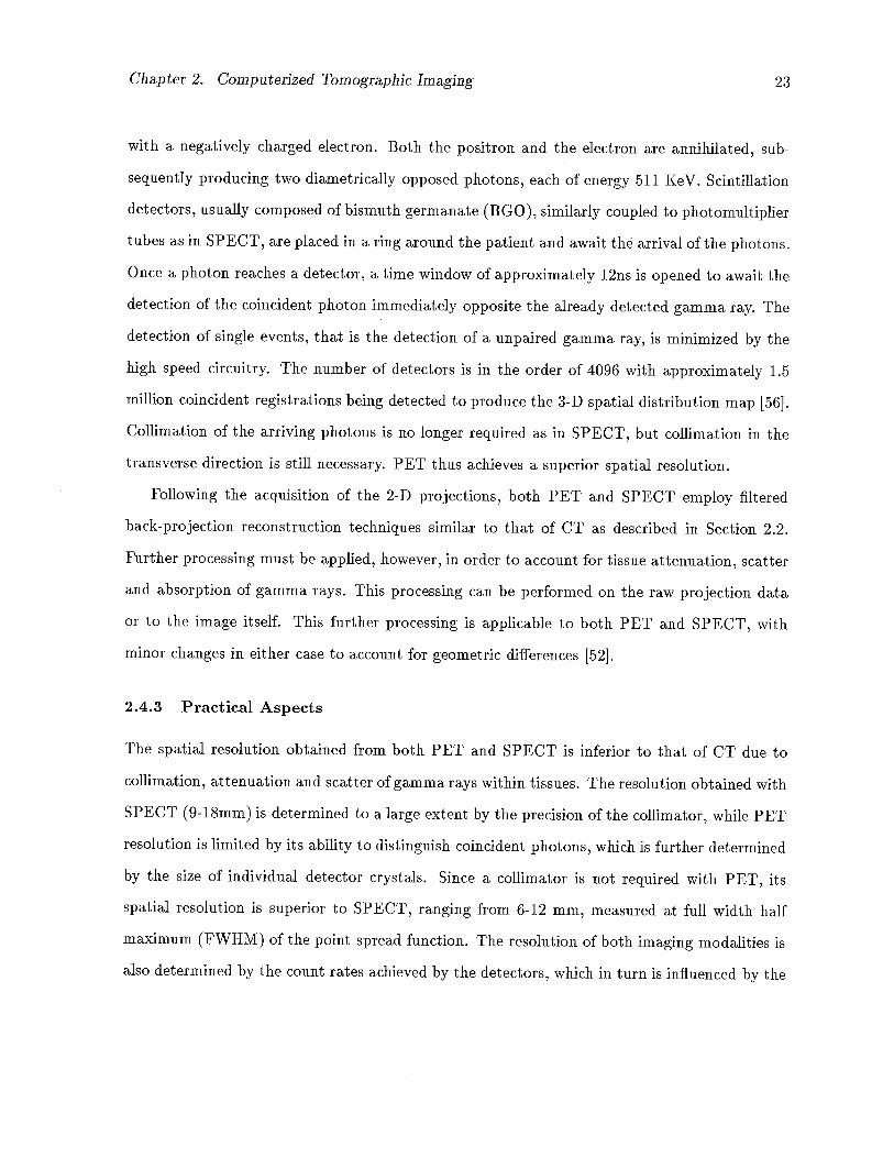
Chapter 2. Computerized Tornographic Imaging 23
with a negatively charged electron. Both the positron and the electron are annihilated, sub—
sequently producing two diametrically opposed photons, each of energy 511 KeV. Scintillation
detectors, usually composed of bismuth germanate (BGO), similarly coupled to photomultiplier
tubes as in SPECT, are placed in a ring around the patient and await the arrival of the photons.
Once a photon reaches a detector, a time window of approximately l2ns is opened to await the
detection of the coincident photon immediately opposite the already detected gamma ray. The
detection of single events, that is the detection of a unpaired gamma ray, is minimized by the
high speed circuitry. The number of detectors is in the order of 4096 with approximately 1.5
miffion coincident registrations being detected to produce the 3-D spatial distribution map [56].
Coffimation of the arriving photons is no longer required as in SPECT, but coffimation in the
transverse direction is still necessary. PET thus achieves a superior spatial resolution.
Following the acquisition of the 2-D projections, both PET and SPECT employ filtered
back-projection reconstruction techniques similar to that of CT as described in Section 2.2.
Further processing must be applied, however, in order to account for tissue attenuation, scatter
and absorption of gamma rays. This processing can be performed on the raw projection data
or to the image itself. This further processing is applicable to both PET and SPECT, with
minor changes in either case to account for geometric differences [52].
2.4.3 Practical Aspects
The spatial resolution obtained from both PET and SPECT is inferior to that of CT due to
coffimation, attenuation and scatter of gamma rays within tissues. The resolution obtained with
SPECT (918mm) is determined to a large extent by the precision of the coffimator, while PET
resolution is limited by its ability to distinguish coincident photons, which is further determined
by the size of individual detector crystals. Since a collimator is not required with PET, its
spatial resolution is superior to SPECT, ranging from 6-12 mm, measured at full width half
maximum (FWHM) of the point spread function. The resolution of both imaging modalities is
also determined by the count rates achieved by the detectors, which in turn is influenced by the
Chapter 2. Computerized Tornographic Imaging 24
affinity of the radiopharmaceuticals for the target organ, the half-life of the radionucides, the
dose given to the patient and the pharmacokinetics of the labeled pharmaceuticals. For all these
reasons it is usually necessary to calibrate the system using phantoms of known materials [52].
Both imaging methods are fundamentally limited in the spatial resolution achievable, which is
restricted by attenuation, scatter, and limited count statistics [56].
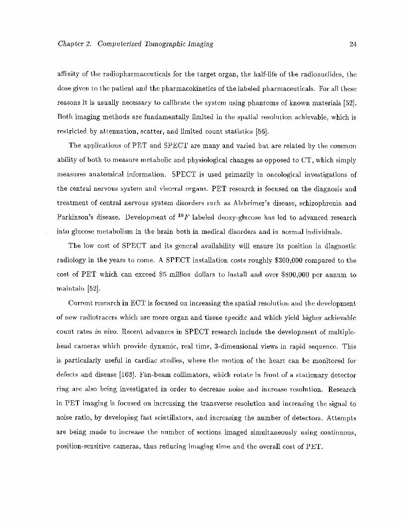
The applications of PET and SPECT are many and varied but are related by the common
ability of both to measure metabolic and physiological changes as opposed to CT, which simply
measures anatomical information. SPECT is used primarily in oncological investigations of
the central nervous system and visceral organs. PET research is focused on the diagnosis and
treatment of central nervous system disorders such as Alzheimer’s disease, schizophrenia and
Parkinson’s disease. Development of 18F labeled deoxy-glucose has led to advanced research
into glucose metabolism in the brain both in medical disorders and in normal individuals.
The low cost of SPECT and its general availability will ensure its position in diagnostic
radiology in the years to come. A SPECT installation costs roughly $300,000 compared to the
cost of PET which can exceed $5 miffion dollars to install and over $800,000 per annum to
maintain [52].
Current research in ECT is focused on increasing the spatial resolution and the development
of new radiotracers which are more organ and tissue specific and which yield higher achievable
count rates in vivo. Recent advances in SPECT research include the development of multiple-
head cameras which provide dynamic, real time, 3-dimensional views in rapid sequence. This
is particularly useful in cardiac studies, where the motion of the heart can be monitored for
defects and disease [103]. Fan-beam collimators, which rotate in front of a stationary detector
ring are also being investigated in order to decrease noise and increase resolution. Research
in PET imaging is focused 011 increasing the transverse resolution and increasing the signal to
noise ratio, by developing fast scintillators, and increasing the number of detectors. Attempts
are being made to increase the number of sections imaged simultaneously using continuous,
position-sensitive cameras, thus reducing imaging time and the overall cost of PET.
Chapter 2. Computerized Tomographic Imaging 25
2.4.4 Conclusion
Dramatic advancements in ECT in recent years, together with its unique characteristics and
abilities, ensure its position in medical imaging for the foreseeable future. Increased resolution
and detection efficiency, together with continually new uses for the technology make ECT an
invaluable tool in diagnostic medicine.
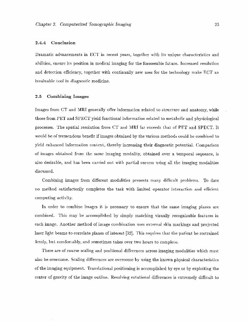
2.5 Combining Images
Images from CT and MRI generally offer information related to structure and anatomy, while
those from PET and SPECT yield functional information related to metabolic and physiological
processes. The spatial resolution from CT and MRI far exceeds that of PET and SPECT. It
would be of tremendous benefit if images obtained by the various methods could be combined to
yield enhanced information content, thereby increasing their diagnostic potential. Comparison
of images obtained from the same imaging modality, obtained over a temporal sequence, is
also desirable, and has been carried out with partial success using all the imaging modalities
discussed.
Combining images from different modalities presents many difficult problems. To date
no method satisfactorily completes the task with limited operator interaction and efficient
computing activity.
In order to combine images it is necessary to ensure that the same imaging planes are
combined. This may be accomplished by simply matching visually recognizable features in
each image. Another method of image combination uses external skin markings and projected
laser light beams to correlate planes of interest [32]. This requires that the patient be restrained
firmly, but comfortably, and sometimes takes over two hours to complete.
There are of course scaling and positional differences across imaging modalities which must
also be overcome. Scaling differences are overcome by using the known physical characteristics
of the imaging equipment. Translational positioning is accomplished by eye or by exploiting the
center of gravity of the image outline. Resolving rotational differences is extremely difficult to
Chapter 2. Computerized Tomographic Imaging 26
automate, but attempts have been made to solve the problem. Both rotational and translational
positioning can be achieved by physically attaching imaging markers to the patient’s body
which are sensitive to each of the imaging methods under investigation. This provides accurate
detection of the proper orientation of the patient during imaging and is adaptable to all areas
of the patient’s body.
Once corresponding imaging planes have been determined, comparison and registration
of the images presents further difficulties. Each imaging method possesses a different 2-D
spatial resolution, making comparison of small areas difficult. As well, the images have different
effective thicknesses in the third dimension. This difficulty may be overcome by combining
multiple slices of high resolution images such as CT or MRI to give the effective thickness of the
relatively low spatial definition images of PET or SPECT. Images can also be compared simply
by placing them side by side and using a dual tracker, which is mouse driven, to investigate
coincident regions of interest.
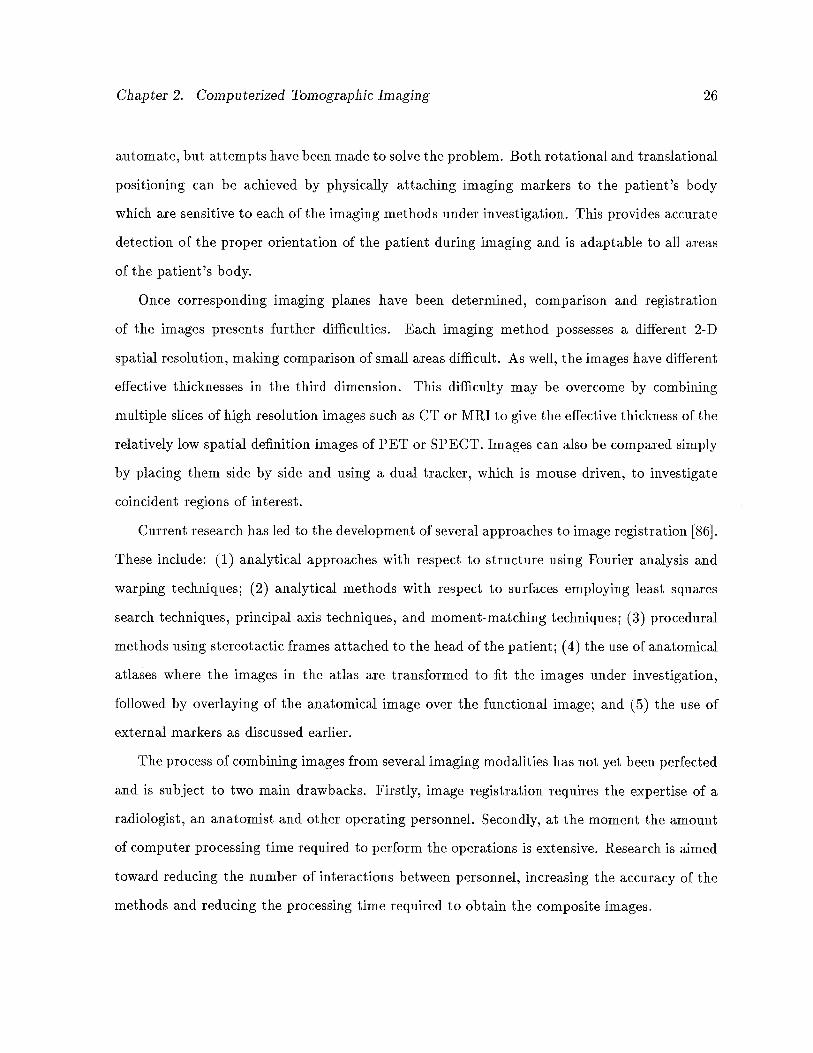
Current research has led to the development of several approaches to image registration [86].
These include: (1) analytical approaches with respect to structure using Fourier analysis and
warping techniques; (2) analytical methods with respect to surfaces employing least squares
search techniques, principal axis techniques, and moment-matching techniques; (3) procedural
methods using stereotactic frames attached to the head of the patient; (4) the use of anatomical
atlases where the images in the atlas are transformed to fit the images under investigation,
followed by overlaying of the anatomical image over the functional image; and (5) the use of
external markers as discussed earlier.
The process of combining images from several imaging modalities has not yet been perfected
and is subject to two main drawbacks. Firstly, image registration requires the expertise of a
radiologist, an anatomist and other operating personnel. Secondly, at the moment the amount
of computer processing time required to perform the operations is extensive. Research is aimed
toward reducing the number of interactions between personnel, increasing the accuracy of the
methods and reducing the processing time required to obtain the composite images.
Chapter 3
Basics of Image Segmentation
3.1 Introduction
One of the most difficult to solve problems and extensively researched areas in image analysis
over the past fifteen years has been the problem of image segmentation. Image segmentation can
be considered the division of an image into different regions, each having a certain property, for
example average gray level. It is the first step in a process leading to description, classification
and interpretation of an image, usually by higher level processes.
To date, no generalized segmentation algorithms exist which are suitable for all or even
many different types of images. Most currently available algorithms are ad hoc in nature. One
of the reasons for the difficulty encountered in segmenting images is the infinite number of
possibilities that an image can represent. A truly general image segmentation algorithm would
require the storage and retrieval of vast amounts of knowledge and data. Another problem arises
in the evaluation of segmentation algorithms. There is no adequate solution to the problem of
determining the validity or accuracy of a given segmentation algorithm. In many cases, various
mathematical and other assumptions are made with respect to the image under investigation.
Given these assumptions verification of the segmentation technique is possible to some degree.
However, it is generally the case that algorithms are validated for a specific and often small
number of images. Despite these difficulties, many hundreds of segmentation algorithms have
been published in the literature.
The applications of image segmentation are many and include but are not limited to such
areas as pattern recognition in computer vision systems and numerous biomedical uses including
automated tumour volume determination and 3-dimensional visualization. Before discussing
27

Chapter 3. Basics of Image Segmentation 28
any algorithms, it will be necessary to formally define image segmentation.
3.2 Definitions
There have been several definitions put forward for image segmentation but the one that is
generally accepted as the definition is as follows:
A segrnerLtation [35] of a 2D image grid, X, over a predicate P is a partition of X into N
non-empty, disjoint subsets X1,X2,. . . , Xj such that:
N
UX= (3.5)
X, i = 1,2,. . . , N is connected (3.6)
XflX=0,forallij (3.7)
P(X)= TRUE,fori= 1,2,...,N (3.8)
P(X U Xj) = FALSE, for i j where X and X3 are adjacent. (3.9)
Equation 3.5 above states that every picture point must be in a region. That is, no pixel
in the image can exist outside of some defined region Xi.’ Equation 3.6 says individual regions
must be connected; each X is composed of contiguous lattice points.2 Equation 3.7 indicates
that the intersection of two regions is empty; regions are disjoint.
The predicate P in Equation 3.8 implies that the region X must satisfy some property,
for example, uniform pixel intensity. Equation 3.9 states that if two regions X and Xj are
adjacent and disjoint then the predicate P cannot be true for the region defined by the union
of X and X3. That is, properties are different for adjacent regions. The predicate P discussed
in Equations 3.8 and 3.9 above is formally defined below:
‘In later discussions this requirement wifi be adapted to include the possibility that a given pixel may becomposed of more than one object class.
‘This condition can and is relaxed in many applications of image analysis, including medical image analysis,since it is quite possible to have disjoint regions of an image which belong to the same class. For example, incervical cancer smears, many nuclei may be affected but are disjoint, but all should be assigned to the same classlabeling.
Chapter 3. Basics of Image Segmentation 29
Let X denote the image sample points in the picture, i.e., the set of pairs
(i,j) i = 1,2,...,M, j = 1,2,. ..,N
where M and N are the number of pixels in the x and y directions respectively. Let
Y be a non-empty subset of X consisting of contiguous picture points. A uniformity
predicate F(Y) is one which (i) assigns the value true or false to Y depending only
on the properties related to the brightness matrix f(i, j) for the points of Y and (ii)
has the property that if a region Z is a subset of Y and P(Y) is true, then P(Z) is
also true.
The most basic form of uniformity predicate is based on the comparison of the mean pixel
intensity in a given region and the standard deviation from the mean. In general, a region, R,
is called uniform, i.e. P(R) = TRUE, if there exists a constant a such that:
max,I(f(i,j))-
aj <T
for some threshold value T.
Using the mean, ji and standard deviation, a, this means that:
max,(f(i,j))— ILl <ka
for some constant multiple, k, of a.
Other features used to determine region uniformity are based on a variety of properties
of the image including the co-occurrence matrix, texture, Fourier Transform and correlation
functions. The co-occurrence matrix is composed of values C(i, j), the number of pairs of pixels
having gray levels i and j which exist at a particular distance apart and at a fixed angle.
Properties of the co-occurrence matrix such as entropy and correlation are used to determine
textures of regions [143].

Chapter 3. Basics of Image Segmentation 30
3.2.1 Techniques
Segmeiltation methods can be loosely subdivided into three principal categories including (1)
characteristic feature thresholding or clustering, (2) edge detection methods and (3) region
oriented techniques.
Thresholding
The simplest method of image segmentation involves thresholding. All pixels which have a
certain property such as faffing into a given intensity range are classified as belonging to the
same group. In its most gelleral form thresholding can be described mathematically as:
S(i,j) = kifTkl <f(i,j)<Tkforkz’1,2,...,m
where (i,j) = the coordinates of a pixel in the x, y directions, respectively,
S(i, j) = the segmentation function,
f(i,j) = the characteristic feature (e.g. gray level) function
T0,. . . Tm the threshold values, and
m = the number of distinct labels to be applied to the image,
If rn = 1, the thresholding method is termed binary thresholding. If m> 1, these methods
are described as multi-modal thresholding techniques. Thresholding is best applied to images
of relatively few homogeneous areas which are contrasted against a uniform background. For
example, in the case of binary thresholding, a suitable applicatioll is extraction of text from a
printed page.
Well known histogram modification and manipulation techniques are applied in image
thresholding [38]. From the survey papers by Lee et al. [76] and Sahoo et al. [112] it ap
pears that a method of thresholding labeled moment preserving thresholding (MPT) [131] is
Chapter 3. Basics of Image Segmentation 31
the most suitable of the commonly used methods tested by those authors. In MPT the object
is to preserve the k’th moments of an image and to find the threshold values which maintain
the moments in the segmentation. The k’th moment of an image, mk, is defined to be:
.
fk(,)
mj=MN
Thus the zeroth moment of an image is 1, and the first moment is the average gray level present
in the image. These moments are also obtainable from the histogram of the image. Preservation
of moments is motivated by the assumption that the original image is simply a blurred version
of the true segmentation. Tsai et al. [131] use a value of k 3 in order to obtain segmentations
using 2, 3, and 4 different threshold levels. Extensions to higher dimensional thresholding are
possible but with substantial increases in computational load. The success of MPT methods
applied to medical image segmentation has not been validated, and is not likely to succeed as
most medical images do not contain few homogeneous areas.
The reader is encouraged to explore the survey papers by Lee et al. [76] and Sahoo et
al. [112] for detailed descriptions of MPT and other classic thresholding methods.
A multidimensional extension of thresholding, called feature clustering, segments the image
based on pixels clustered in a feature space and the properties of these clusters. Clusters are
generally formed using two or more characteristic features. The clusters need not be contiguous
in space.
Thresholding and clustering methods have the advantage of being fast and simple to im
plement. There are, however, inherent shortcomings present in all thresholding techniques.
Primarily, there is the problem of threshold selection, which usually requires some a priori
knowledge of the image being segmented. As well, valleys and peaks in the histograms used to
segment the images are often not well defined and are difficult to differentiate.
Edge Detection
Edge detection methods of image segmentation involve locating local discontinuities in pixel
intensities, followed by some method of connecting these fragmented edges to form longer,
Chapter 3. Basics of Image Segmentation 32
hopefully significant and complete boundaries. Most methods of edge detection involve the
application of a smoothing filter (e.g. Gaussian), followed by a first or second order gradient
operator. In the case of a first order gradient, local maxima signify the existence of an edge. If
a second derivative operator is applied then zero crossings in the result indicate the presence
of an edge. A thresholding operator is usually applied to the result to filter out insignificant
edges, or edges caused by noise which was not filtered in the smoothing process.
The biggest drawback to edge detection methods of image segmentation is the sensitivity to
the size and type of smoothing and derivative convolution masks applied to the original image.
In some cases these two masks are not parameterized and are therefore not under user control.
This limits the applicability of these algorithms to different types of images.
As well, most edge detection algorithms are very sensitive to noise and can yield edge
information that is not a boundary between regions in an image. Furthermore, edges that are
computed are often not linked where contiguity exists in the image. These edges must be joined
to be useful in successfully segmenting the image. Algorithms for edge linking are often at least
as complex as the edge detection algorithms used in the first place.
Region-oriented Segmentation
Regioll based methods of image segmentation can be further subdivided into two main categories
including (1) region growing and (2) region splitting and merging.
While thresholding and edge detection methods involve determining the differences in pixel
intensities or groups of intensities, region growing and region splitting and merging deal with
the similarities between pixels and groups of pixels.
Region growing methods start with one or more pixels as a seed and then make an analysis
of the neighbours of the seed pixel(s). If the neighbours of the seed have similar intensity or
some other property then those pixels become part of a region. This process continues with the
new region until no further expansion is possible.
One advantage of region growing is that little a priori information is necessary to segment
Chapter 3. Basics of Image Segmentation 33
the image. As well, isolated areas with similar features can be successfully segmented by seeding
these regions independently. For example, muscle and brain have similar gray levels on magnetic
resonance images, but can be differentiated by seeding each region individually. Difficulties are
encountered with choosing a seed point or region and with evaluation of inclusion criteria for
neighbouring pixels. The latter usually involves a common problem with all techniques, that
of threshold selection.
In contrast to the forms of image segmentation discussed so far, region splitting and merging
begins with an image subdivided into smaller regions. These regions are grouped together if the
pixel intensities meet some uniformity criteria, for example, similar average intensity level. The
regions are then examined for uniformity and are further split if they do not meet the uniformity
criterion. The order of splitting and merging is variable and dependent on the implementation
and data structures used. Relatively complex data structures are required to perform split and
merge techniques with corresponding complexity in maintaining these structures. Again, the
problem exists of determining a valid uniformity criterion and of determining a threshold at
which to assign the uniformity.
3.3 Summary
Image segmentation has been studied extensively to date and many algorithms have been de
veloped to solve the problem. These algorithms can be loosely categorized into characteristic
feature thresholding and cluster analysis, edge detection methods, and region oriented tech
niques.
Thresholding methods, although simple and fast, are suited to images of low numbers of
regions with highly contrasting backgrounds.
The problem with edge detection methods is that it is possible to detect an edge which
is not a boundary between regions. Detected edges often have gaps in them which involve
computationally expensive methods to eliminate.
Both thresholding and edge detection methods are sensitive to image noise. Again edges
Chapter 3. Basics of Image Segmentation 34
are detected which may not exist. Noise affects thresholding by altering the peaks and valleys
of the histograms used to determine the thresholds.
Region growing requires user input to determine a seed or seeds and requires threshold
determination for pixel inclusion as well. Region splitting and merging is computationally
complex and also requires threshold analysis.
The choice of any segmentation technique is highly application dependent. This chapter
has only just begun to explore the many and varied algorithms currently applied to image
segmentation. One point that general segmentation algorithms raise is the need for semantic
and a priori information to be incorporated into the segmentation process. The segmentation
of medical images is one area where semantic and a priori information is generally available.
However, due to relatively low signal to noise ratios and inherent artifacts generally present
in medical images, their segmentation is particularly difficult. The next chapter details the
intrinsic characteristics of medical imaging techniques, including CT, MRI, PET and SPECT,
which further complicate the segmentation task. A more detailed discussion of segmentation
methods applied to medical imaging is also presented.
Chapter 4
Segmentation Applied to Medical Imaging
The basic segmentation techniques discussed in Chapter 3 are all currently employed with
modifications and adaptations in the analysis of medical images. Section 4.1 deals with the
inherent difficulties encountered by each of the medical imaging modalities discussed in Chap
ter 2. Section 4.2 discusses the use of the basic methods of thresholding and clustering, edge
detection, and region analysis as applied to medical images. In addition, medical investigators
have developed several new methods for the segmentation of medical images. These include
the manual tracing of structures of interest using a mouse or other drawing tool, statistical
relaxation methods, morphological segmentation methods, and pyramidal techniques. These
new techniques are discussed in Section 4.3. Model-based or knowledge-guided techniques, dis
cussed in Section 4.4, exploit the a priori knowledge of the characteristics of how human tissues
react to the different imaging modalities. One such model-based technique called the method
of Iterated Conditional Modes [14] is described in detail beginning in Section 4.5. This method,
first developed to restore noisy and corrupted images, is based on the theory of Markov random
fields and Gibbs distributions from probability theory. Because this work forms an integral part
of the thesis a significant amount of this chapter is devoted to its discussion.
4.1 Difficulties with Medical Imaging
Medical images, including CT, MRI, PET and SPECT data, add new complications to the
problem of image segmentation. Each modality has particular characteristics that detract from
a straightforward solution. These difficulties range from the partial volume effects common to
all modalities to RF inhomogeneities experienced by MRI, beam hardening effects of CT and
35
Chapter 4. Segmentation Applied to Medical Imaging 36
scatter and attenuation problems common to PET and SPECT imaging. The following sections
describe in greater detail the characteristics of some of these inherent shortcomings.
4.1.1 Partial Volume Effect
All medical imaging modalities suffer from the partial volume effect to some extent. The
measured signal represents an average signal received through a section of tissue of specific
thickness. Voxels may intersect more than one tissue type, depending on the area and the slice
thickness realized. For example, a given voxel in a brain image obtained from a CT study
may represent the attenuation through a cubic volume of brain tissue measuring several cubic
miffimeters. This volume of tissue may contain 40% gray matter and 60% white matter. If gray
matter usually yields a CT value of 50 and white matter a CT value of 100 then the measured
value will be an average attenuation measurement representing the combined composition, i.e.
80, which is not an accurate representation of the underlying tissue. Spatial and tissue resolution
are thereby decreased.
The problem is of lesser but still significant importance in MET scans because the obtainable
tissue resolution of Mlii images is higher than that of CT. Since the spatial resolution in the
functional modalities (PET and SPECT) is much less than CT or MET, the partial volume
effect is especially pronounced in images obtained using these methods.
4.1.2 CT
Beam Hardening
In CT, a phenomenon known as beam hardening is another source of artifacts which reduces the
spatial resolution in certain image areas and forms dark streaks in the image. Beam hardening
occurs due to the polychromatic nature of the X-ray beam. Attenuation coefficients of individual
tissues vary with the energy level of incident X-ray photons. Because X-ray beams are made
up of a distribution of varying photon energies, as the X-ray beam passes through the patient,
low energy photons are more readily absorbed so that the average beam energy increases or
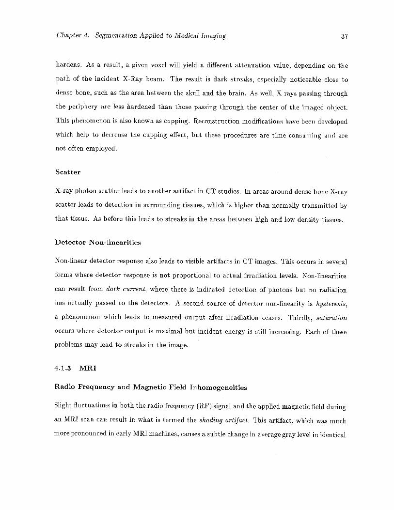
Chapter 4. Segmentation Applied to Medical Imaging 37
hardens. As a result, a given voxel will yield a different attenuation value, depending on the
path of the incident X-Ray beam. The result is dark streaks, especially noticeable close to
dense bone, such as the area between the skull and the brain. As well, X-rays passing through
the periphery are less hardened than those passing through the center of the imaged object.
This phenomenon is also known as cupping. Reconstruction modifications have been developed
which help to decrease the cupping effect, but these procedures are time consuming and are
not often employed.
Scatter
X-ray photon scatter leads to another artifact in CT studies. In areas around dense bone X-ray
scatter leads to detection in surrounding tissues, which is higher than normally transmitted by
that tissue. As before this leads to streaks in the areas between high and low density tissues.
Detector Non-linearities
Non-linear detector response also leads to visible artifacts in CT images. This occurs in several
forms where detector response is not proportional to actual irradiation levels. Non-linearities
can result from dark current, where there is indicated detection of photons but no radiation
has actually passed to the detectors. A second source of detector non-linearity is hysteresis,
a phenomenon which leads to measured output after irradiation ceases. Thirdly, saturation
occurs where detector output is maximal but rncident energy is still increasing. Each of these
problems may lead to streaks in the image.
4.1.3 MRI
Radio Frequency and Magnetic Field Inhomogeneities
Slight fluctuations in both the radio frequency (RF) signal and the applied magnetic field during
an MRI scan can result in what is termed the shading artifact. This artifact, which was much
more pronounced in early MRI machines, causes a subtle change in average gray level in identical
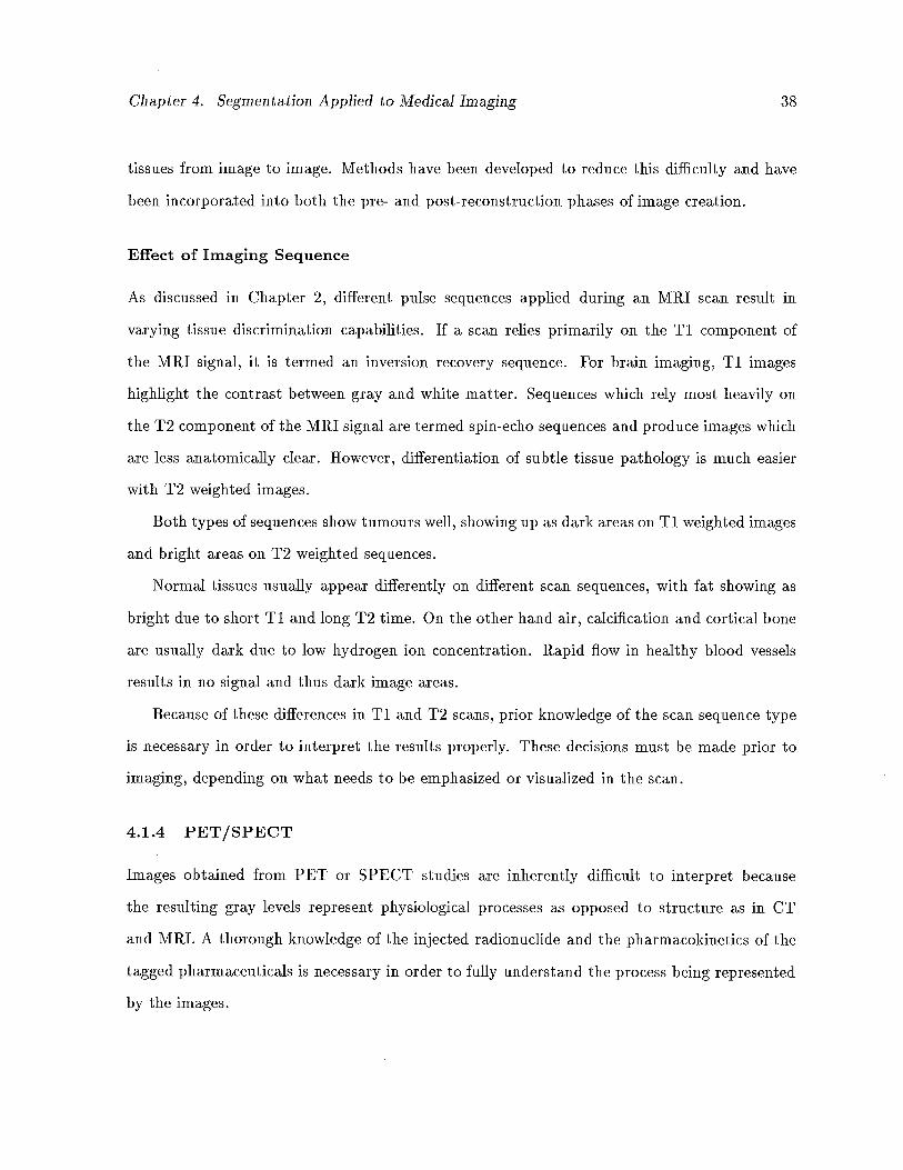
Chapter 4. Segmentation Applied to Medical Imaging 38
tissues from image to image. Methods have been developed to reduce this difficulty and have
been incorporated into both the pre- and post-reconstruction phases of image creation.
Effect of Imaging Sequence
As discussed in Chapter 2, different pulse sequences applied during an MRI scan result in
varying tissue discrimination capabilities. If a scan relies primarily on the Ti component of
the MRI signal, it is termed an inversion recovery sequence. For brain imaging, Ti images
highlight the contrast between gray and white matter. Sequences which rely most heavily on
the T2 component of the MRI signal are termed spin-echo sequences and produce images which
are less anatomically clear. However, differentiation of subtle tissue pathology is much easier
with T2 weighted images.
Both types of sequences show tumours well, showing up as dark areas on Ti weighted images
and bright areas on T2 weighted sequences.
Normal tissues usually appear differently on different scan sequences, with fat showing as
bright due to short Ti and long T2 time. On the other hand air, calcification and cortical bone
are usually dark due to low hydrogen ion concentration. Rapid flow in healthy blood vessels
results in no signal and thus dark image areas.
Because of these differences in Ti and T2 scans, prior knowledge of the scan sequence type
is necessary in order to interpret the results properly. These decisions must be made prior to
imaging, depending on what needs to be emphasized or visualized in the scan.
4.1.4 PET/SPECT
Images obtained from PET or SPECT studies are inherently difficult to interpret because
the resulting gray levels represent physiological processes as opposed to structure as in CT
and MRI. A thorough knowledge of the injected radionucide and the pharmacokinetics of the
tagged pharmaceuticals is necessary in order to fully understand the process being represented
by the images.
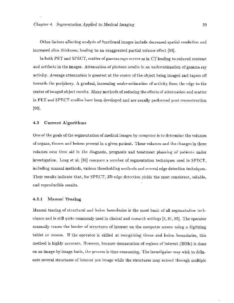
Chapter 4. Segmentation Applied to Medical Imaging 39
Other factors affecting analysis of functional images include decreased spatial resolution and
increased slice thickness, leading to an exaggerated partial volume effect [95].
In both PET and SPECT, scatter of gamma rays occurs as in CT leading to reduced contrast
and artifacts in the images. Attenuation of photons results in an underestimation of gamma ray
activity. Average attenuation is greatest at the center of the object being imaged and tapers off
towards the periphery. A gradual, increasing under-estimation of activity from the edge to the
center of imaged object results. Many methods of reducing the effects of attenuation and scatter
in PET and SPECT studies have been developed and are usually performed post-reconstruction
[90].
4.2 Current Algorithms
One of the goals of the segmentation of medical images by computer is to determine the volumes
of organs, tissues and lesions present in a given patient. These volumes and the changes in these
volumes over time aid in the diagnosis, prognosis and treatment planning of patients under
investigation. Long et al. [80] compare a number of segmentation techniques used in SPECT,
including manual methods, various thresholding methods and several edge detection techniques.
Their results indicate that, for SPECT, 3D edge detection yields the most consistent, reliable,
and reproducible results.
4.2,1 Manual Tracing
Manual tracing of structural and lesion boundaries is the most basic of all segmentation tech
niques and is still quite commonly used in clinical and research settings [4, 81, 85]. The operator
manually traces the border of structures of interest on the computer screen using a digitizing
tablet or mouse. If the operator is skilled at recognizing tissue and lesion boundaries, this
method is highly accurate. However, because demarcation of regions of interest (ROTs) is done
on an image-by-image basis, the process is time consuming. The investigator may wish to delin
eate several structures of interest per image while the structures may extend through multiple

Chapter 4. Segmentation Applied to Medical Imaging 40
images. This process becomes labour intensive, especially for radiologists whose expertise could
be better applied elsewhere. One of the main goals of automated segmentation techniques is
to free the operator from the tedium of outlining hundreds of structures per study, sometimes
costing hours per study to segment.
4.2.2 Edge Detection
Despite the disadvantages of edge detection methods, including the computational complexity
of defining incomplete edges and the inaccuracies of the technique when noise and artifacts
are present in an image, many researchers have adapted common methods of edge detection to
medical image segmentation.
Williams et al. [141] use a method based on detecting and linking local maximum gradients
in the image. First the images are smoothed using a Gaussian kernel and then a directional
derivative operator is applied to determine the gradient image. The gradient image is then
processed by an edge linking algorithm which sequentially links the edges locally, pixel by
pixel.
Udupa [132] uses dynamic programming to locate globally optimal boundary paths. Even
in two dimensions the algorithm is computationally complex and a clear, adequate definition
of optimal is not evident.
Other authors employ 3D gradient operators with further increases in computational load.
The 3D methods almost certainly are more accurate but at the cost of increased computational
complexity. Long et al. [79] compare the effectiveness of a 2D and a 3D edge operator applied to
the segmentation of SPECT images. The superiority of the 3D method is clearly demonstrated.
4.2.3 Thresholding and Cluster Analysis
One of the biggest difficulties encountered by the thresholding methods is the selection of a
proper threshold or several thresholds if multi-modal thresholding is necessary. Suzuki and
Toriwaki [127] have proposed a technique which involves a goodness measure to aid in the
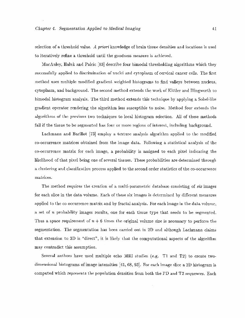
Chapter 4. Segmentation Applied to Medical Imaging 41
selection of a threshold value. A priori knowledge of brain tissue densities and locations is used
to iteratively refine a threshold until the goodness measure is achieved.
MacAuley, Haluk and Palcic [83] describe four bimodal thresholding algorithms which they
successfully applied to discrimination of nuclei and cytoplasm of cervical cancer cells. The first
method uses multiple modified gradient weighted histograms to find valleys between nucleus,
cytoplasm, and background. The second method extends the work of Kittler and lllingworth to
bimodal histogram analysis. The third method extends this technique by applying a Sobel-like
gradient operator rendering the algorithm less susceptible to noise. Method four extends the
algorithms of the previous two techniques to local histogram selection. All of these methods
fail if the tissue to be segmented has four or more regions of interest, including background.
Lachmann and Barillot [73] employ a texture analysis algorithm applied to the modified
co-occurrence matrices obtained from the image data. Following a statistical analysis of the
co-occurrence matrix for each image, a probability is assigned to each pixel indicating the
likelihood of that pixel being one of several tissues. These probabilities are determined through
a clustering and classification process applied to the second order statistics of the co-occurrence
matrices.
The method requires the creation of a multi-parametric database consisting of six images
for each slice in the data volume. Each of these six images is determined by different measures
applied to the co-occurrence matrix and by fractal analysis. For each image in the data volume,
a set of n probability images results, one for each tissue type that needs to be segmented.
Thus a space requirement of n + 6 times the original volume size is necessary to perform the
segmentation. The segmentation has been carried out in 2D and although Lachmann claims
that extension to 3D is “direct”, it is likely that the computational aspects of the algorithm
may contradict this assumption.
Several authors have used multiple echo MRI studies (e.g. Ti and T2) to create two
dimensional histograms of image intensities [41, 68, 93]. For each image slice a 2D histogram is
computed which represents the population densities from both the PD and T2 sequences. Each
Chapter 4. Segmentation Applied to Medical Imaging 42
axis represents the distribution of pixel intensities for one of the two measured pulse sequences.
The value at a given coordinate (x, y) in the histogram represents the number of pixels in the
image which yielded x in one sequence and y in another. The 2D histogram clearly shows
clusters which hopefully represent individual tissue and lesion types. The resulting clusters
of points are partitioned according to several commonly used methods of cluster analysis [68].
These methods are clearly superior to one-dimensional histogram analysis.
Handels and Tolxdorff [43] exploit the multispectral characteristics of the MRI signal to
create an n-dimensional clustering method which assigns pixels to one of n clusters (in this case
n = 6) interactively defined by the program. In this manner the operator can combine different
relaxation times with proton density characteristics together with partial volume to measure
different biochemical properties of the tissues. A multi-cluster colour image is generated to aid
in the visualization of different combinations of cluster membership. Extensive user interaction
is required on a slice-by-slice basis. No results (other than visual) were presented by the authors.
4.2.4 Region Growing
Sandor, Metcalf and Kim [117] use a modified region growing technique together with cor
rections for beam hardening and partial volume effects in the analysis of CT images. The
cupping effect induced by the polychromatic nature of the X-Ray beam, discussed in Section
4.1.2, is reduced by fitting the image surface with a bivariate spline function which resembles
the cup artifact. Following the reduction of the beam hardening artifacts, the brain tissue is
isolated from the skull contour. Seed pixels are then chosen using specific threshold values of
the histogram. These values have a high probability of being accurately assigned a particular
tissue/fluid classification. The remaining pixels are then classified using a nearest neighbour
region growing algorithm. Regions are grown from seed pixels depending on a combination of
pixel intensity, the number of surrounding pixels which have been classified as tissue or fluid,
the sum and difference of already classified pixels, the number of already classified pixels and
a polarization index calculated based on the histogram value for that particular pixel. This
Chapter 4. Segmentation Applied to Medical Imaging 43
defines an initial segmentation of brain tissue.
Lesions are segmented from the brain tissue by applying the algorithm to the result of the
initial segmentation. Again, extensive user interaction is required on a slice-by-slice basis and
the algorithm is highly specific to CT images of the head.
4.3 Extensions to Fundamental Techniques
The discussion of general segmentation algorithms discussed in Chapter 3 is by no means com
plete. Many other methods of image segmentation have been applied to medical images with
varying degrees of success. Some of the more widely publicized methods to be discussed fur
ther include mathematical morphology, pyramidal schemes, relaxation methods and techniques
which attempt to combine the best features of several methods.
4.3.1 Mathematical Morphology
The term morphology originally referred to the study of the form and structure of living organ
isms. In image processing, mathematical morphology means the study of the form and structure
of objects from images of those objects. The process is based on the concept of hitting an object
with a structuring element in order to reduce the object to a more recognizable and simplified
shape.
Two basic operations are applied in mathematical morphology, the processes of erosion and
dilation [51]. Given an object 0 with origin x and a structuring element 5, erosion amounts to
ANDing each element of 0 with S yielding a new object, 0’. That is, 0’ is defined as the set
of all points x such that S is included in 0. Dilation, an ORing operation, is defined similarly
as the set of all points x such that S hits 0, i.e. they have a non-empty intersection. Erosion
amounts to a shrinking operation while dilation corresponds to an enlargement. Figure 4.4
illustrates the application of erosion and dilation to a binary image of a black square on white
background with a square structuring element. The operations are carried out pixel by pixel by
centering the structuring element over each pixel and applying the operation. The application
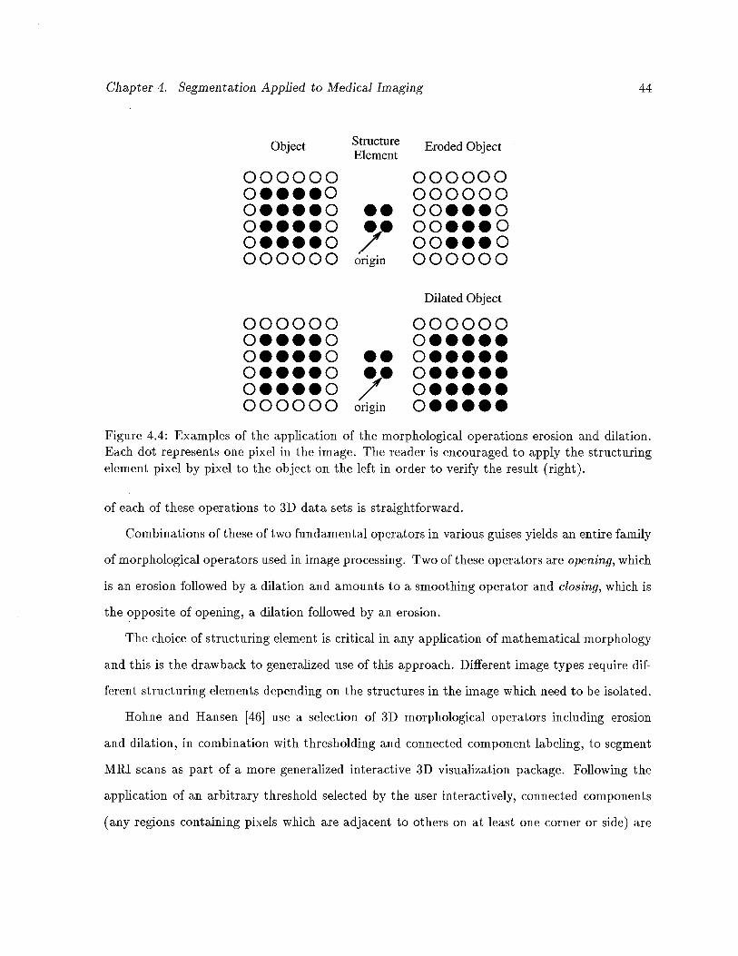
Chapter 4. Segmentation Applied to Medical Imaging 44
Object Structure Eroded ObjectElement
000000 000000000000
o....o •• oo...oo••••o •• oo•••oo••••o / oo•••o000000 origin 000000
Dilated Object
000000 000000o•••••
o••••o •• o•••••o....o •• o.....o....o / o.....000000 origin o•••••
Figure 4.4: Examples of the application of the morphological operations erosion and dilation.Each dot represents one pixel in the image. The reader is encouraged to apply the structuringelement pixel by pixel to the object on the left in order to verify the result (right).
of each of these operations to 3D data sets is straightforward.
Combinations of these of two fundamental operators in various guises yields an entire family
of morphological operators used in image processing. Two of these operators are opening, which
is an erosion followed by a dilation and amounts to a smoothing operator and closing, which is
the opposite of opening, a dilation followed by an erosion.
The choice of structuring element is critical in any application of mathematical morphology
and this is the drawback to generalized use of this approach. Different image types require dif
ferent structuring elements depending on the structures in the image which need to be isolated.
Hohne and Hansen [46] use a selection of 3D morphological operators including erosion
and dilation, in combination with thresholding and connected component labeling, to segment
MRI scans as part of a more generalized interactive 3D visualization package. Following the
application of an arbitrary threshold selected by the user interactively, connected components
(any regions containing pixels which are adjacent to others on at least one corner or side) are

Chapter 4. Segmentation Applied to Medical Imaging 45
automatically determined by the algorithm. Morphological operations are performed on the
connected components to isolate individual objects. This process is repeated iteratively on each
image until the operator is satisfied with the segmentation. The method requires extensive user
interaction and has not been validated except visually. One effect of the use of morphological
operators, iliustrated by Hohne, is that generalized opening and closing operations cause a
non-measurable loss (and gain) in pixels at region boundaries.
4.3.2 Pyramidal Techniques
Pyramidal segmentation schemes [88, 91, 109] rely on the creation of representations of an
image at progressively lower resolutions. These representations form a pyramid with the low
est resolution image being the top of the pyramid. Figure 4.5 represents progressively lower
resolutions of a one-dimensional signal, with the lowest resolution being at level 5.
Level 5 LI
Level4 LI LI
Level3 LI LI LI
Level2 U LI LI LI
Levell LI LI LI LI LI
LevelO LI LI LI LI LI LI
Figure 4.5: Pyramid representation of a one-dimensional signal at progressively lower resolutionsas the pyramid reaches the apex. Each square represents a discrete value in the signal. Level 0represents the highest resolution and Level 5, the lowest.
Each row in the pyramid represents the image at a different spatial scale, thus isolating
structures of different size and shape. Pixels in lower levels of the pyramid are classified by
linking to pixels in higher levels. This linking is performed by comparison of pixels between
any two levels with respect to nearest gray level and geometric proximity. Ultimately pixels in
the higher levels of the pyramid form roots of a tree. The roots of the tree are not linked to
Chapter 4. Segmentation Applied to Medical Imaging 46
any pixels in higher levels of the pyramid. The resulting tree forms a specific segment for that
image.
Mathieu et al. [91] apply a graph theoretic approach to pyramidal segmentation by rep
resenting the pixels as nodes in a graph. The links of the graph represent a neighbourhood
relationship between pixels. Through iterative application of graph contraction, using stan
dard algorithms, successive graph representations form the levels of a pyramid. The resulting
pyramid is called a stochastic pyramid because graph contraction is known to be a stochastic
process. Nodes in the pyramid graphs are linked using a variation on the method discussed
previously, ultimately forming a segmentation.
Most pyramid segmentation techniques have been proven to be shift-, rotation-, and scale-
variant [15] giving unreliable and unreproducible results. These methods have therefore not
been investigated further by the author.
4.4 Model-Based Approaches
A relatively recent development in medical image segmentation is the model-driven technique.
The purpose of using model-based approaches to medical image segmentation is to transfer the
low-level pixel/voxel information into high level semantic information, for example anatomy,
pathology, or physiology of tissues. Medical images lend themselves well to model-based meth
ods since much more a priori information is available compared to general object recognition as
applied in the artificial intelligence (AT) approach to vision. Medical images already contain 3D
data as opposed to a 2D projection of a 3D scene used in AT vision. In AT research perceptual
processes are usually modeled and care must be taken to allow for different views, illumination,
shadows, and hidden objects, etc.
Applying a model-based approach first involves the creation of a parameterized model,
allowing for modifications in shape, size, texture and other properties of objects. An attempt is
then made to match the available data to the computer model of the data. The model constrains
the possible interpretations of the data. Inconsistent interpretations are never considered, thus
Chapter 4. Segmentation Applied to Medical Imaging 47
drastically reducing the search space to valld, consistent solutions of the segmentation problem.
We have incorporated a material percentage model as part of this thesis (See Chapter 5) in
an attempt to assign a probabilistic classification to brain tissues. This method is an example
of a model-based approach to medical image segmentation. A solution to the partial volume
problem is offered, assigning a set of percentages to each voxel. These percentages can be
considered the probability of a certain voxel containing a particular tissue.
Arata et al. [8] use a composite image model to guide the segmentation of ventricles from
PD and T2 weighted MRT scans. The model provides ROT and boundary information, while
new data provides gray level information used to grow ventricular regions following registration
of the images with those of the model.
To create the model, four MRI data sets are first hand segmented and interpolated to give
uniform voxel dimensions of approximately T mm3. The segmented sets are then registered to a
standard position, orientation and size using centroids and principal axes. New scan data uses
a composite model to guide the segmentation of ventricles. The model slice which most closely
resembles the scan slice is “easily” identified [8]. The algorithm then uses a region growing
technique with ventricle regions seeded according to pixels that have been labeled ventricles in
the model.
Problems with this model are evident and iliustrate the difficulty in applying the model-
based technique. Firstly, the limited number of patients used to standardize the scans is inad
equate. Patients whose scans will be used in the model must therefore match the model with
respect to age, sex, gender and health, since there is tremendous variability in these param
eters in different patient groups. As well, the accuracy of the registration method used will
greatly affect the accuracy of the segmentation. Since no accurate, automatic method of image
registration exists to date, this can only adversely affect the results.
Kamber et al. [57] use a similar approach to segment multiple sclerosis (MS) lesions from
multi-dimensional MRT data. They developed a probabilistic model using MRT scans of twelve
healthy volunteers. Each of the original scans is mapped to a standardized 3D rectangular

Chapter 4. Segmentation Applied to Medical Imaging 48
coordinate space which they call Talairach space. The mapping is based on the 3D spatial
location of landmark anatomical features of the brain. Homomorphic filtering is then used to
reduce the RF inhomogeneity effect. Ventricular cerebrospinal fluid (CSF) is then manually
segmented from each study. A supervised Bayesian classifier is used to segment gray matter,
white matter and external CSF. The 12 scans are subsequently averaged to form the composite
probabilistic model. At each point in the Talairach space, five probability values are stored. The
values indicated the probability of gray, white, ventricular CSF, external CSF and background
at each point in the standardized space.
The model is used to provide geometric features using the probabilities assigned to the
voxels. It is also used to confine the search space for MS lesions to white matter areas of the
brain since 95% of MS lesions occur in white matter. The model is combined with a decision
tree classifier using 300 tissue samples to train the classifier. The nodes in the decision tree
represent some kind of test on a feature of a particular tissue, until ultimately reaching the
leaves of the tree which represented specific tissue classes.
The results obtained with the probabilistic model are compared to a manual segmentation
of the same patient data. The results obtained from experiments that confined the search
space using the model increased the accuracy of the segmentation by 3-5% relative to the non-
model-based approach. False positive lesions, indicating MS pathology where none existed,
were reduced by 50%.
Although the results reported are significant, the method illustrates again the inherent
problems of model-based segmentation, that of limited numbers of patients with which to form
the model and the registration of patient data to a standardized space. As well as requiring vast
amounts of patient data with which to form the model, training of the decision tree classifier
also requires excessive amounts of data storage, user and computational time.
Having converted the test data to the Talairach space and performed the segmentation,
the results are displayed in Talairach space as well. It is not evident from the paper that
the transformation process is invertible, so that the results can be converted back to “real”
Chapter 4. Segmentation Applied to Medical Imaging 49
space. Many radiologists, having been trained to analyze tomographic scans using real data,
will perhaps not be willing or able to extract from these images the information that would
otherwise be quite apparent.
4.5 Markov Random Fields and the Gibbs Distribution
A modeling method which has previously been applied to the restoration of corrupted im
ages [14, 37] has recently been adapted, with varying degrees of success, to the segmentation
problem [18, 23, 59, 122, 125]. Using this model, an image is assumed to represent a locally
dependent Markov Random Field (MRF), exploiting the assumption that pixels in a given lo
cal neighbourhood of the image have similar intensity. Before discussing this model, it will be
necessary to first define the notation to be used in the remainder of this section and later in
the thesis.
Consider the 3D cubic lattice of the image space as a set, S, of n voxels indexed in some
manner from i = 1,2,. . ., n. Let the observed data y represent one set of data values on
a particular realization of a random vector Y. The value y, denotes the observed record at
position i. A segmentation of y will be represented by a set z, a particular realization of a
random vector X. The value x denotes the segmentation value at pixel i. Let x* represent the
true segmentation of y. Throughout the remainder of this discussion two assumptions will be
made with respect to the observed record of intensities [14].
• Assumption 1: Each ‘r has the same known conditional density function, p(yjxj), which
is dependent oniy on x. So the conditional probability of the observed record y, given x,
is determined by:
p(yx)=
1h9(yIx)
• Assumption 2: The true segmentation x is a realization of a locally dependent MRF with
distribution p(x).
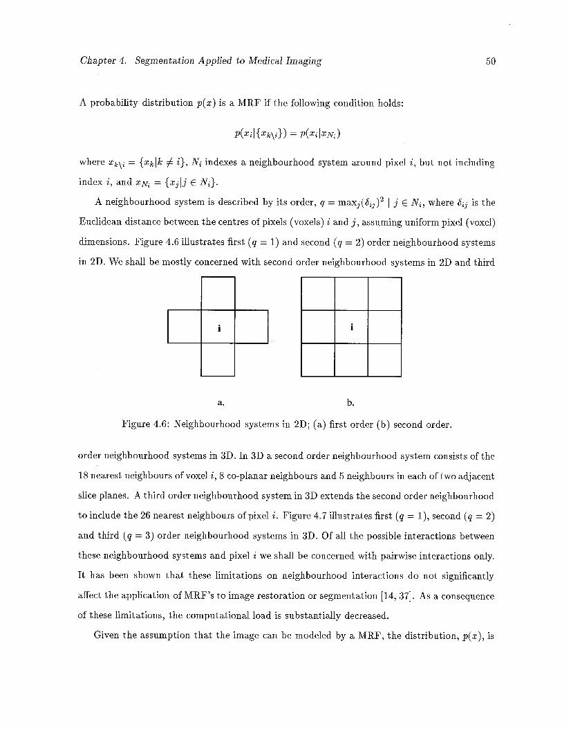
Chapter 4. Segmentation Applied to Medical Imaging 50
A probability distribution p(x) is a MRF if the following condition holds:
P(XiI{Xk\}) = p(xIxN)
where = {xkk i}, N indexes a neighbourhood system around pixel i, but not including
index i, and XN1 {xIi NJ.
A neighbourhood system is described by its order, q = maxj(j)2 I j e N, where 5jj is the
Eucidean distance between the centres of pixels (voxels) i and j, assuming uniform pixel (voxel)
dimensions. Figure 4.6 illustrates first (q = 1) and second (q = 2) order neighbourhood systems
in 2D. We shall be mostly concerned with second order neighbourhood systems in 2D and third
__
I
__
a.
1
b.
Figure 4.6: Neighbourhood systems in 2D; (a) first order (b) second order.
order neighbourhood systems in 3D. In 3D a second order neighbourhood system coilsists of the
18 nearest neighbours of voxel i, 8 co-planar neighbours and 5 neighbours in each of two adjacent
slice planes. A third order neighbourhood system in 3D extends the second order neighbourhood
to include the 26 nearest neighbours of pixel i. Figure 4.7 illustrates first (q = 1), second (q = 2)
and third (q = 3) order neighbourhood systems in 3D. Of all the possible interactions between
these neighbourhood systems and pixel i we shall be concerned with pairwise interactions only.
It has been shown that these limitations on neighbourhood interactions do not significantly
affect the application of MRF’s to image restoration or segmentation [14, 37]. As a consequence
of these limitations, the computational load is substantially decreased.
Given the assumption that the image can be modeled by a MRF, the distribution, p(x), is
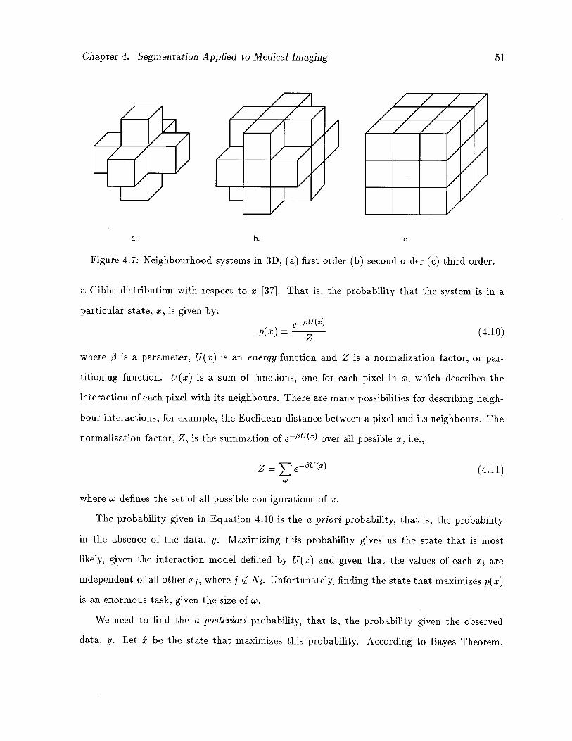
Chapter 4. Segmentation Applied to Medical Imaging 51
a.b.c.
Figure 4.7: Neighbourhood systems in 3D; (a) first order (b) second order (c) third order.
a Gibbs distribution with respect to x [37]. That is, the probability that the system is in a
particular state, x, is given by:e_(x)
=(4.10)
where i is a parameter, U(x) is an energy function and Z is a normalization factor, or par
titioning function. U(x) is a sum of functions, one for each pixel in x, which describes the
interaction of each pixel with its neighbours. There are many possibilities for describing neigh
bour interactions, for example, the Eucidean distance between a pixel and its neighbours. The
normalization factor, Z, is the summation of e(2) over all possible x, i.e.,
Z = (4.11)
where w defines the set of all possible configurations of x.
The probability given in Equation 4.10 is the a priori probability, that is, the probability
in the absence of the data, y. Maximizing this probability gives us the state that is most
likely, given the interaction model defined by U(x) and given that the values of each x are
independent of all other x3, where j 0 N. Unfortunately, finding the state that maximizes p(x)
is an enormous task, given the size of w.
We need to fluid the a posteriori probability, that is, the probability given the observed
data, y. Let be the state that maximizes this probability. According to Bayes Theorem,
Chapter 4. Segmentation Applied to Medical Imaging 52
maximizing this probability is equivalent to maximizing
p(xly) oc p(yIx)p(x) (4.12)
The state is the maximum a posteriori (MAP) estimate of the true segmentation x and is
the mode of the posterior distribution of x.
Given Assumptions 1 and 2 previously, maximizing p(xly) is equivalent to maximizing the
conditional probability of each x, given the record at i, y, and the current estimate of the
neighbours of x. That is, it is equivalent to maximizing, with respect to x,
p(xIy,N) (4.13)
at every pixel site, i, in the image. Through application of Bayes Theorem and simplifying,
this is equivalent to maximizing
p(yiIxi)p(xiIN) (4.14)
It turns out that this distribution is also Gibbs distributed with the U(X) term of Equation 4.10
expanded into a sum of two terms, one, as before, pertaining to the neighbourhood interaction
potential and one term describing the differences between the observed and predicted data.
4.6 Iterated Conditional Modes
Application of Equation 4.14 to each pixel in an image constitutes a single iteration of what
Besag has coined Iterated Conditional Modes (1CM) [14]. Convergence to a local maximum
of p(xjy) is achieved after approximately 6 to 10 iterations of 1CM. However, this depends on
the model used for the prior distribution of x and that used for the conditional distribution of
the record given the current estimation of x, i.e. p(yx). Besag originally used the method to
restore noisy and corrupted images, however, if we consider the true segmentation xK to be the
original image we wish to recover, the method is readily applied to the segmentation problem.
Chapter 4. Segmentation Applied to Medical Imaging 53
4.6.1 Segmentation Using Iterated Conditional Modes
Various simplifying assumptions have been proposed in order to reduce the computation neces
sary in the evaluation of the partition function Z. Choi et al. [23] have developed an algorithm
using a variation of Besag’s Iterated Conditional Modes to segment multichannel MRI images
of the brain. Choi uses a partial volume model of tissue segmentation and models the poste
rior distribution of y given x by an rn-dimensional Gaussian, where m is the number of MRI
channels present. In order to reduce the computational demands of determining the partition
function Z, it is assumed that the probability distribution of the energy function U(x) is also
Gaussian. This also aided in the determination of an optimal j3. Although the results reported
in [23] were encouraging, we believe the algorithm suffered from some important drawbacks.
Firstly, an assumption was made that the variance for pixels of pure tissue type is negligible,
ignoring the natural variations which exist due to biological inconsistencies throughout a tissue
(e.g. anatomy, physiology, metabolism). This will be especially pronounced in various tissue
pathologies, due to the variation in extent of disease in individual tissues. Another difficulty
that was raised in the paper was the following: in order to solve the matrix of equations that
resulted from the model used, the number of distinct tissues differentiable in the scan had to
be at most one less than the number of image channels available. Given that it is extremely
difficult to obtain more than two perfectly registered MRI data sets from a single scan [68],
this restriction raises doubts about the robustness of the method. Choi uses heuristics and a
rule based approach which must be adapted according to the number and types of tissues being
segmented in order to circumvent this restriction. As well as these deficiencies, the algorithm
is applied on a slice-by-slice basis, in 2D, and does not incorporate any 3D information.
Besag has shown [14] that given only pairwise neighbour interactions, and two estimates of
the segmentation that differ only at index i, the most general form of the probability that pixel
i belongs to class k, given the the neighbours of pixel i in the previous estimate, is
p(xj = kIN) o (4.15)
Chapter 4. Segmentation Applied to Medical Imaging 54
where (i) ce(k) is an external field parameter representing prior knowledge of the spatial dis
tribution of class k, (ii) 13k1 = 131k, which, when positive, gives a prize for neighbouring pixels
belonging to the same class, and (iii) u(l) counts the number of neighbours of pixel i belonging
to class 1. Since we are attempting to maximize 4.15, the normalization constant, Z, is not
necessary and has been dropped from the equation. It is also worth noting that the symmetry
of the /3 parameters is a necessary condition to conform to the MRF assumption [14, 60].
Karssemeijer [59] has adopted this approach in order to segment abdominal CT scans, ex
ploiting some important assumptions. In order to make an initial estimate of the segmentation,
Karssemeijer initializes all /3k1 to zero and thereby models the external field as 1n(p(x =
the prior log likelihood that pixel i belongs to class k. This maintains Bayes Theorem in Equa
tion 4.15. Considering these assumptions and combining Equations 4.14 and 4.15, the initial
segmentation estimate was reduced to the product
p(yjxj = lc)p(x = k) (4.16)
The prior probabilities, p(Xj), were obtained by “normalizing” a series of 18 CT scans of the
abdominal area and registering the new scans to the normalized data. The conditional proba
bilities p(yjjxj) were obtained by combining the record with the prior distributions.
In subsequent iterations of 1CM the interaction parameters were determined by trial and
error, with small values for tissue pairs which often occur together and a value of infinity
for tissue types which are never adjacent. Adjacent scan planes were also used to estimate
interaction with a single orthogonal neighbour in 3D. The o?s were maintained as 1n(p(x = k))
even though, as Karssemeijer pointed out, this no longer holds when /3k1 # 0.
Karssemeijer obtained good results for the data which was used in his experiments, how
ever, general application of the algorithm will require significant amounts of new training data
depending on the imaging technique and equipment used. As well, accuracy and extensibility
of the registration technique used to obtain the prior distributions has not been validated.
In an effort to more fully automate the method of Karssemeijer, Broekhuijsen et al. [18]
adapted the previous approach and applied it to the segmentation of myocardial CT scans.
Chapter 4. Segmentation Applied to Medical Imaging 55
Prior and conditional probabilities were obtained in a similar manner to that of Karssemeijer.
The interaction parameters were estimated from training data and calculated as = the
percentage of the total number of pixels labeled Ic which lie on the border of regions labeled 1.
As a result, the range of values of /3k1 are adjusted to 0.0 < [3ia K 1.0. However, the symmetry
condition is violated by allowing 13k1 !3lk The neighbour counts u(l), from Equation 4.15,
are further replaced by percentages of neighbouring pixels labeled 1. In order to normalize the
resulting expression to yield a value between zero and one, Broekhuijseu replaced the summation
term of Equation 4.15 with its reciprocal, yielding the new product
p(yjxj = k)p(x = k)e+ (4.17)
where
z = Z!3kluiQ) (4.18)lk
Since both the /3’s and the neighbour counts u(l) range from zero to unity, it is clear that
0.0 K Z K t, where t is the number of discrete possibilities for labeling voxels, resulting in
probability measures ranging from 0.0 to e ?. Broekhuijsen uses a heuristic to overcome this
significant inconsistency by arbitrarily assigning 0.5 to the highest resulting probability, 0.25
to the next highest, and so on, in an effort to normalize the resulting distributions. This
drawback, combined with the violation of not conforming to the symmetry condition imposed
by the assumed MRF nature of the data, precludes the use of this algorithm in a general setting.
Stringham, Barrett and Taylor [125] have extended the work of Broekhuijsen [18] and Karsse
meijer [59] by including region growing and edge information into the MRF context. Stringham
adds an edge probability term to the product of Equation 4.17 and eliminates the prior proba
bility measure altogether. The segmentation is initialized by seeding a series of representative
tissue samples from a single slice in the scan to be segmented. From these regions, normalized,
low pass filtered histograms are obtained representing the conditional probabilities. The neigh
bourhood interaction parameters are either obtained empiricaliy or initialized to 1 for the initial
segmentation. A gradient image is also obtained and is used to generate edge probabilities to be
Chapter 4. Segmentation Applied to Medical Imaging 56
incorporated into the 1CM equation. Following calculation of the conditional probabilities the
1CM equation is applied only to those pixels which border the seed regions obtained previously.
In this manner, region growing is incorporated into the algorithm. Following convergence of
the algorithm on the initial slice, the resulting segmentation is used as the seed segmentation
for adjacent slices. If necessary, neighbour interaction parameters and conditional probabilities
may be recalculated based on the final segmentation. The process continues until the entire
volume is segmented.
This approach suffers from some major drawbacks. The edge probability measure is used
to coerce region boundaries towards points of high gradient magnitude in the edge image. This
will only happen, however, if the region boundary and the detected edge in the gradient image
occur within the pixel width of the edge filter used to obtain the gradient image. As such, edge
information is utilized only after regions have grown sufficiently (and possibly erroneously) to
fall within the range of the edge filter used. This problem is alleviated somewhat (at least
for the initial segmentation) by seeding multiple disjoint regions according to the histograms
obtained during initial training, yielding a much more accurate initial segmentation than that
obtained by simply using the seed regions themselves. Since adjacent slices may contain new
structures and/or lose structures present in the previous slice, the problem is again present
when proceeding to adjacent image planes.
Secondly, the edge probability measure included in Stringham, Barrett and Taylor’s paper
depends heavily on the scale of the gradient magnitude image. For example, given discrete pixel
values of 0-255 in the image scans, the gradient magnitude image will have values in the same
range, 0-255. The edge probability associated with pixel x is calculated by the expression
E(x) = 0.5 + f * m (4.19)
where f is a proportionality factor (0.1 was used in Stringham [125]) and m is a minimum
(maximum) difference measure on the gradient magnitudes of pixel i and its neighbours, de
pending on the edge classes that have been assigned to pixel i and its neighbours. Thus
—255 m 255, and it follows that the edge probability measure will have values in the range
Chapter 4. Segmentation Applied to Medical Imaging 57
—25,0 < E(x) <26.0 for the value f = 0.1 used in the paper. The edge probability term will
almost certainly dominate the probability product.
These inherent difficulties draw into question the robustness of this algorithm. Little in the
way of results was given in the paper, making verification difficult as well. It is interesting to note
that no mention of MRF’s or Gibbs distributions is made in the Broekhuijsen or Stringham
papers. This in turn is likely the reason that the methods stray so significantly from the
theory and produce questionable results. In the next chapter we attempt to maintain the
MRF assumption, while almost eliminating the need for prior organ models. We examine a
3D, multichannel, partial volume solution to the segmentation problem based on MRF theory
which requires a minimum of user input. Our method also provides a high level of parallelism
to speed the computation.
Chapter 5
3D Multispectral Stochastic Volume Segmentation
In this chapter we describe a quasi-automatic solution to the segmentation problem using the
theory of MRF’s in 3D, resulting in partial membership of voxels in several tissue types. The
method is simple, requiring a minimum of user input and allowing a high degree of parallelism.
In Section 5.1 we revisit the theoretical basis for our solution. Section 5.2 describes the ex
tensions we have made to the Iterated Conditional Modes algorithm in order to incorporate
the available 3D information. In Sections 5.3 and 5.4 we describe the implementation of the
algorithm using a datafiow image processing environment, WIT. The benefits and limitations
of adopting the dataflow paradigm will also be presented.
5.1 Returning to Basic Theory
As is evident from the preceding discussion, the variations made to 1CM by Karssemeijer [59],
Broekhuijsen [18], and Stringham [125] are not always consistent with the theory of MRF’s and
may require extensive training and user interaction in order to perform properly. As well, none
of the authors exploits the 3D nature of the data to any appreciable extent. In the following
sections we describe how we perform the segmentation while at the same time maintaining the
MRF property. User intervention is kept at a minimum by training the algorithm using an
initial region of interest (ROl) selection on a single image from the volume to be segmented.
The ROT selection yields conditional probability profiles for each tissue to be segmented. We
fully utilize the third dimension by incorporating a 3rd order neighbourhood system in 3D. We
make the solution tractable by allowing extensive parallelism.
As the partial volume problem is still one of the major difficulties encountered in medical
58
Chapter 5. 3D Multispectral Stochastic Volume Segmentation 59
image segmentation, we have endeavoured to provide a solution which yields a probability
classification for each voxel, indicating the percentage composition of different tissues in that
voxel. Each x will now be considered a vector of values indexed from k = 1,2,. . . , t, where
t is the number of tissue types present in the data volume. The kth value of element x,
which we call its labeling, represents the probability that voxel i is of tissue type k. These
probabilities can be viewed as the partial volume contribution from each tissue type to voxel
x. As such, p(Xjk) = 1.0 must hold at each iteration of the algorithm. The basic
assumption introduced by Karssemeijer [59] is maintained here. That is, the external field, o
will still be modeled by ln(p(x = k)) in order to simplify the general form of the 1CM equation.
Now, on each iteration of 1CM, the probability that x belongs to a particular tissue type,
k, is given by
p(Xjk) = p(yiIxk) * p(ik)e_Z (5.20)
where
Z = /3iu(l)
and ( I xj) is the conditional probability of the record, given its labeling, obtained from the
initial histograms, p(ik) is the provisional estimate of the probability of pixel i belonging to
tissue type k, 13k1 is a measure of the interaction between tissues labeled k and 1, and is obtained
using partial memberships of voxels in a particular tissue class.
The energy term u(l), in Equation 5.20, is the number of neighbours of voxel x, having
label 1. It is likewise determined from partial volume memberships weighted by inter-voxel
distances. The total number of tissues considered to be present in the image volume, t, is
obtained implicitly from the initial regions of interest selected by the user.
A minimum of user intervention is required to train the algorithm by requiring the manual
outlining of regions of interest in a single image selected from the volume. Each of these possibly
disjoint regions represents the user’s belief that the voxels contained within the circumscribed
regions are pure voxels. Normalized, low pass-filtered histograms are obtained from each of
Chapter 5. 3D Multispectral Stochastic Volume Segmentation 60
these regions and used as input into the relaxation algorithm. These histograms provide the
initial estimate of the segmentation, which in turn provides the initial neighbour interaction
parameters and energy term of Equation 5.20. In order to obtain an initial estimate of the
segmentation which represents our prior knowledge of the tissue distribution, the probability
that voxel Ij is of tissue type k is initialized to
-‘ p(yiIxik)p(Xjk) =
(5.21)p(yIx)
which is simply a set of normalized probabilities based on the conditional probabilities obtained
from the histograms. In subsequent iterations of the algorithm, the i’s are assigned the value
which was obtained in the previous iteration.
Application of Equation 5.20 to each voxel in 3D constitutes one iteration of the algorithm.
After each iteration or a predetermined number of iterations, the histograms and neighbour
hood interaction parameters may be recalculated. Relaxation of the segmentation occurs after
approximately six to eight iterations. Following convergence, a partial volume estimation is
produced, indicating the probability that each candidate voxel is of a particular tissue type.
Segmentations obtained from multiple echo sequences may be determined independently
and then combined by forming the product of the probabilities of each tissue type for each
imaging spectrum. This combination is possible because the data sets are independent.
5.2 Extensions to Iterated Conditional Modes
In order to accommodate a partial volume solution some modifications have been adopted
to automatically calculate neighbour interactions and neighbour counts in 3D. In light of the
fact that voxels are rarely cubic, the neighbour interactions and neighbour counts are further
weighted by the intervoxel distances between pixel i and its 26 neighbours in 3D. That is, we use
a 3rd order neighbourhood system in 3D, believing that this is the minimum neighbourhood,
in 3D, having a significant influence on the central voxel.
Chapter 5. 3D Multispectral Stochastic Volume Segmentation 61
5.2.1 Neighbour Interaction Parameters
One of the difficulties encountered by previous authors was determination of neighbour in
teraction parameters. The parameters were estimated heuristically by Karssemeijer [59] and,
although automatically calculated by Broekjhuisen [18] and Stringham [125], resulted in a non-
symmetric matrix, contradicting a fundamental assumption of the theory of MRF’s. Broekjhuisen’s
calculation required a modification to the 1CM equation which introduced inconsistencies in the
resulting probabilities (see Section 4.6).
A simple, intuitive notion of tissue interaction may be used to solve this difficulty, without
requiring a priori information about the tissues which must be segmented. We have defined the
neighbour interaction parameters, 13k1, to be the inverse of the probability that tissues k and
1 are adjacent, as opposed to the notion of the probability that tissue k is adjacent to tissue
1. These adjacencies are weighted by the partial volume consistencies of each voxel and by the
relative distance from each voxel to its neighbours in 3-space.
The probabilities are determined from the tallied adjacencies for each tissue pair (k,l) in
the provisional estimate of the segmentation, . Let Tlkl represent the total number of weighted
adjacencies involving both tissues k and 1. Let Tlk and represent the number of weighted
adjacencies involving tissue k and 1 respectively. /3k1 is therefore defined as:
kl= ( k1
(5.22)71k + 7l
where
k1 = lk =
i=1 jeN
where n is the number of voxels in the image volume, N defines the neighbourhood system
surrounding voxel i, and is the distance measure from the centre of voxel i to the centre of
its neighbour voxel j. The accumulated adjacencies for each tissue type, r, may be defined as:
]kZ77kj

Chapter 5. 3D Multispectral Stochastic Volume Segmentation 62
where t is the number of tissues present in the segmentation. Matrix is therefore symmetric
with (1.0 < /3, < cc) for all 1 and k (lim,7ko/3k1 = cc). These neighbourhood interaction
parameters are determined from the initial segmentation estimate and may be updated after a
predetermined number of iterations, thereby refining the accuracy of the segmentation.
5.2.2 Neighbour Counts
The energy term u(l), in Equation 5.20, is the number of neighbours of voxel j, in the provi
sional estimate of the segmentation, having label 1. It is again determined from partial volume
memberships weighted by inter-voxel distances. The neighbour counts for tissue 1 in voxel x
are thus defined as:
u(l) =
jEN
5.2.3 Histogram Re-evaluation
As the segmentation proceeds the accuracy of assigned probabilities increases. Since the his
tograms used to initialize the segmentation were based on a limited number of voxels from the
volume, we have allowed for the re-calculation of histograms to be used in further iterations.
Thus histograms representing updated tissue profiles are computed as follows. The histogram
entry Hkg, associated with each tissue class k and each possible discrete gray level value g is
given by
= p(jk) V {i I 1(y3) = g} (5.23)
where I(y) is the intensity value of voxel y in the observed record. These histograms are of
course normalized and smoothed, as before, in order to eliminate sharp peaks which are likely
the result of noise in the observed record.
5.2.4 Prior Organ Models
The prior probabilities defined in Equation 5.21 may also be obtained as by other authors,
that. is, by analyzing multiple sets of image data, when available. The reality is, however, that
Chapter 5. 3D Multispectral Stochastic Volume Segmentation 63
construction of prior models is subject to the enormous variability between specific imaging
machines and imaging variables. For example, depending on the sequence of application of
RE pulses in the acquisition of MRI studies, significantly different tissue profiles will result.
The normalization of such scans is not a straightforward task, and is complicated by image
registration difficulties, not to mention the extra time and effort required to form the model.
Although the priors obtained here may not be as accurate as those obtained through model
creation, they do allow an accurate segmentation to be performed. The automatically generated
priors may be accumulated and used to form a more suitable model over time. This is one focus
of future work in the area.
5.2.5 Convergence
It has been discussed that the segmentation continues until convergence is achieved, usually
following six to eight iterations of the algorithm. A measure of convergence has not been
specified up to this point. There are a number of methods of measuring convergence of the
algorithm, usually done by placing a limit on the number of voxels which change from one
iteration to the next. With a partial volume solution to the problem, the number of voxels
which change between iterations is not readily measurable. However we have adopted a method
which tracks the change in p(Ijj) between iterations, resulting in a vector of values for each j,
indicating the change in each tissue. A scalar measure of the change in voxel i, on iteration m,
denoted kjmI is obtained by calculating the 2-Norm of this vector such that:
kjml (P(ik)m) P(ik) (rn_i))
The user may then assess changes between successive iterations and apply suitable threshold
criteria on the number of changes required per iteration, in order to allow convergence to be
achieved within six to eight iterations. This is a significant computational burden to bear on
each iteration, but is partially offset by the inherent parallelism borne by the algorithm.
Chapter 5. 3D Multispectral Stochastic Volume Segmentation 64
5.2.6 Multispectral Approach
When available, two or more independent sets of data may be used to drive the segmentation
algorithm. We have performed the segmentation on multiple echo MRI sequences, but other
combinations of data are just as valid, provided the data sets are independent and spatially
registered. For example, patient scans from PET analysis may be combined with MRI or
CT. Since the data sets are independently acquired, the resulting probabilities calculated by
the 1CM algorithm may be combined by multiplying corresponding values. The result of the
multiplication is again normalized such that p(Xjk) = 1.0. We have found that the results
obtained from using two or more data sets are consistently more accurate than those obtained
from using either of the data sets alone.
5.2.7 Parallelism
It is the elegance and simplicity of the MRF assumption that allows for high levels of parallelism
in the implementation of 1CM in 3D. Since, at each iteration, the new segmentation estimates are
entirely neighbourhood based, we could conceivably allow updating of each voxel to be carried
out by a separate processor. This would require the use of highly specialized hardware, such as
a transputer network. The parallelism that we have achieved is provided by the image process
development environment that we adopted as part of the implementation of this algorithm.
This is described in the next section.
5.3 Implementation Platform
In this section we introduce the image processing development platform used to implement the
3D 1CM algorithm on standard Sun Sparc workstations.
Following extensive evaluation of several imaging platforms and visualization tools, it was
decided that the implementation of 1CM would be developed using WIT®’, a state of the
‘The word WIT is derived from pronunciation of the acronym OOIT which stands for Object Oriented ImagingTechnology.
Chapter 5. 3D Multispectral Stochastic Volume Segmentation 65
art image processing development package based on the data flow paradigm of software de
velopment. WIT is highly interactive and allows the rapid prototyping of algorithms under
development.
5.3.1 Dataflow Paradigm
The concept of dataflow is based on the notion of processing data while it is in motion. A
dataflow network consists of a collection of nodes, or processing stations, linked together by
arcs, to allow the flow of data through the network. Each of these processing stations may have
multiple inputs and outputs. Loops may be formed from the arcs and nodes to allow repeated
processing of dynamically changing data. Thus, data processing is not sequential as it is with
traditional von Neumann architectures.
The notion of dataflow as described above is rather vague, and so we will concern ourselves
only with one particular type of dataflow, namely pipeline dataflow. Using the pipeline approach
implies that it is not possible for data on an arc of the network to overtake other data traveling
in the network. There are two basic principles associated with pipeline dataflow which provide
inherent parallelism. The first principle is that of asynchrony which allows a node to be executed
only when all inputs to that node are present. The second principle of execution of a pipeline
dataflow network is that of functionality. Each node in the network represents an atomic
functional unit, which accepts inputs and produces unique outputs based on those inputs.
There are no side effects, and therefore no global variables. These functional operations may
thus be carried out in any order or in parallel, provided the inputs to the node are present.
Parallelism is implicit in such a dataflow network, and therefore requires the existence of an
external scheduling mechanism which tracks the arrival and exit of all inputs and outputs. It
is the need to establish and maintain a scheduling conflict resolution mechanism which makes
dataflow programming difficult to implement, and not always appropriate.
Chapter 5. 3D Multispectral Stochastic Volume Segmentation 66
5.3.2 WIT
The image processing development environment adopted for implementation of this thesis,
WIT, employs the pipeline dataflow approach to programming. Interfacing with WIT is a
simple matter of selecting graphical icons from the multiple libraries of operators which are
available, and joining these icons together by simple mouse point and click operations. The
operators form the nodes of a dataflow network, which in WIT is termed an interactive graph,
or igraph. The inherent parallelism of the dataflow approach is exploited by the use of a Unix
client/server model of computation to distribute execution of operators across a network of
resources.
Along with the operator libraries which accompany WIT, the developer can easily incor
porate new operators when more functionality is required. These operators may be added to
custom designed libraries created by the developer or added to already existing libraries and
used in an equivalent manner to the operators already available. One of the advantages which
WIT enjoys over similar software products is its extensive control flow library which grants the
user significant powers of sequencing, iteration, and synchronization of operators in an igraph.
The package was written in the C language, running under OpenWindows® on the SIInTM
family of workstations and is currently being ported to other software and hardware platforms.
WIT is pseudo-object oriented in that it provides encapsulation of both data and function
ality. Polymorphism is achieved to some degree, by requiring all WIT data types to be some
form of Object. It is up to the developer of new operators in WIT to assure that any new func
tionality introduced is applicable to multiple data types. There is no concept of inheritance in
WIT and so it is not truly object oriented. WIT could have incorporated significantly more
object oriented features, with some loss of efficiency, if it had been written in C++.
The highly interactive nature of igraph formulation and editing can be exploited in order to
accurately trace execution of developed algorithms and to more readily analyze an algorithm
under investigation. Figure 5.8 is an example of a small WIT session, illustrating an elementary
igraph, together with the results of executing the igraph. We have used this igraph to simply
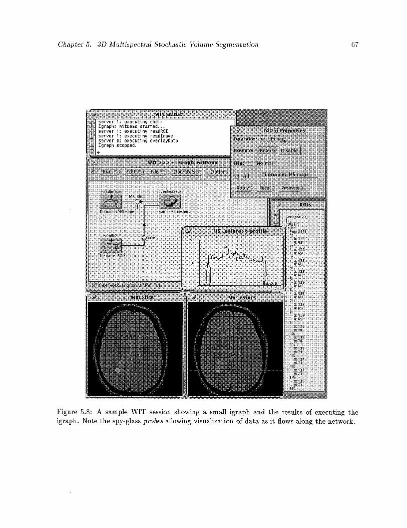
Chapter 5. 3D Multispectral Stochastic Volume Segmentation 67
Figure 5.8: A sample WIT session showing a small igraph and the results of executing theigraph. Note the spy-glass probes allowing visualization of data as it flows along the network.
Chapter 5. 3D Multispectral Stochastic Volume Segmentation 68
read in an MRI image and overlay a series of regions of interest (ROIs), which have been
previously obtained, indicating the presence of Multiple Sclerosis lesions in this area of the
brain.
The WIT Status window updates operator, igraph, and server status as the igraph executes.
The Operator property panel pops up when the user gives a mouse click over an operator icon
of interest. In Figure 5.8 the rdObj or read Object operator panel is shown. The rdObj operator
reads in any of the WIT Object data types from disk. The property panel allows the user to
edit the options pertaining to the operator, such as enabling or disabling its execution, and its
orientation or Flip mode on the igraph screen. As well, any parameters which are required to be
manually input to the operator can be modified through the property panel. These parameters
can be converted to inputs and thus provided to the operator by linkage from other operators.
There are two copies of the rdObj operator in the igraph, one labeled readlmage and the
other readROl. The readlrnage operator reads an image, in WIT format, while the readROl
operator reads a region of interest description, also in WIT format. The operator is able to
differentiate the type of Object which it reads. Data flows from these two operators down the
pipes (or links, as they are termed in WIT) and illto the next operator called overlayData.
Data flows in the direction of the arrows seen on the links. The overlayData operator is also
supplied in WIT and accepts the region of interest description and the WIT image as input and
overlays the ROI onto the image. The result of this overlay is displayed in the image labeled
MS Lesions.
Note the spy-glass shaped probes in Figure 5.8 which are visible on the links of the igraph.
These probes can be interactively placed on any link in an igraph in order to observe the data
as it flows through the network. The image slice labeled MRI Slice and the ROIs object are
displayed as a result of placement of these probes on the links.
Following the display of any image in WIT, the user may interactively examine the image by
altering its scale, zooming, panning, adapting the colour map used in display of the image, and
so on. In this example, an X-Profile, showing the profile of values across a selected horizontal
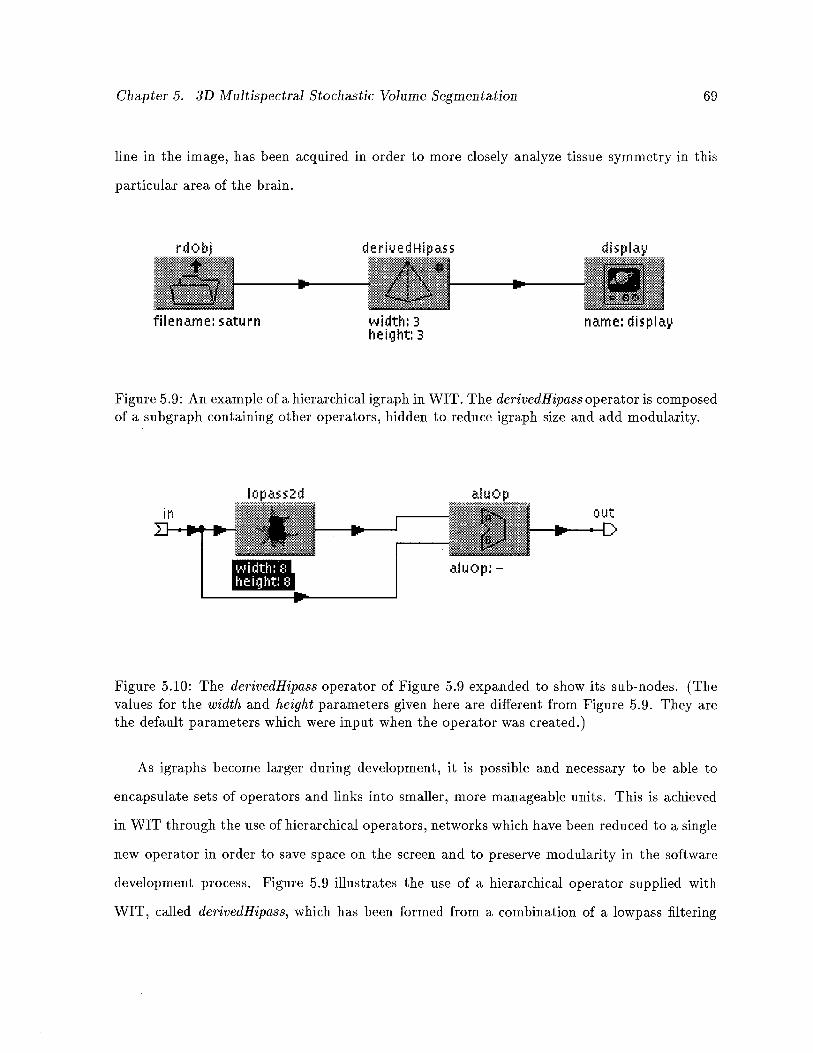
Chapter 5. 3D Multispectral Stochastic Volume Segmentation 69
line in the image, has been acquired in order to more closely analyze tissue symmetry in this
particular area of the brain.
Fass
name: dispIa
Figure 5.9: An example of a hierarchical igraph in WIT. The derivedHipass operator is composedof a subgraph containing other operators, hidden to reduce igrapli size and add modularity.
out
Figure 5.10: The derivedHipass operator of Figure 5.9 expanded to show its sub-nodes. (Thevalues for the width and height parameters given here are different from Figure 5.9. They arethe default parameters which were input when the operator was created.)
As igraphs become larger during development, it is possible and necessary to be able to
encapsulate sets of operators and links into smaller, more manageable units. This is achieved
in WIT through the use of hierarchical operators, networks which have been reduced to a single
new operator in order to save space on the screen and to preserve modularity in the software
development process. Figure 5.9 illustrates the use of a hierarchical operator supplied with
WIT, called derivedHipass, which has been formed from a combination of a lowpass filtering
filename: saturn width: 3height: 3
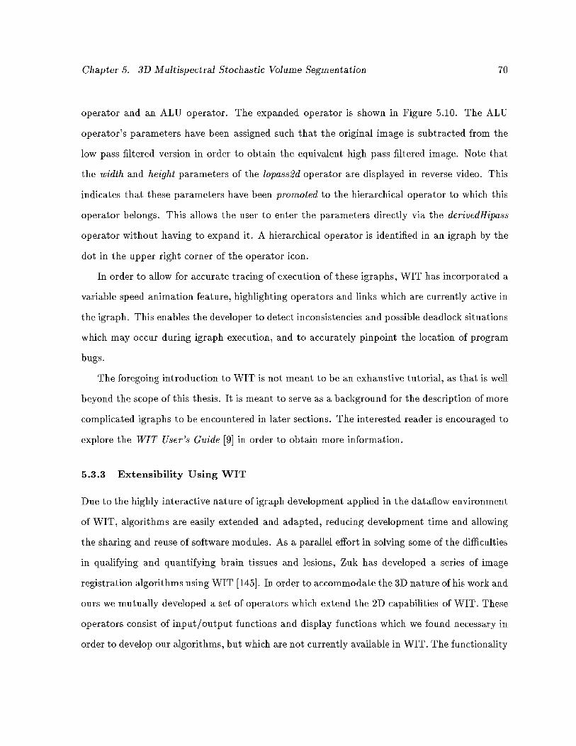
Chapter 5. 3D Multispectral Stochastic Volume Segmentation 70
operator and an ALU operator. The expanded operator is shown in Figure 5.10. The ALU
operator’s parameters have been assigned such that the original image is subtracted from the
low pass filtered version in order to obtain the equivalent high pass filtered image. Note that
the width and height parameters of the lopass2d operator are displayed in reverse video. This
indicates that these parameters have been promoted to the hierarchical operator to which this
operator belongs. This allows the user to enter the parameters directly via the derivedHipass
operator without having to expand it. A hierarchical operator is identified in an igraph by the
dot in the upper right corner of the operator icon.
In order to allow for accurate tracing of execution of these igraplis, WIT has incorporated a
variable speed animation feature, highlighting operators and links which are currently active in
the igraph. This enables the developer to detect inconsistencies and possible deadlock situations
which may occur during igraph execution, and to accurately pinpoint the location of program
bugs.
The foregoing introduction to WIT is not meant to be an exhaustive tutorial, as that is well
beyond the scope of this thesis. It is meant to serve as a background for the description of more
complicated igraphs to be encountered in later sections. The interested reader is encouraged to
explore the WIT User’s Guide [9] in order to obtain more information.
5.3.3 Extensibility Using WIT
Due to the highly interactive nature of igraph development applied in the dataflow environment
of WIT, algorithms are easily extended and adapted, reducing development time and allowing
the sharing and reuse of software modules. As a parallel effort in solving some of the difficulties
in qualifying and quantifying brain tissues and lesions, Zuk has developed a series of image
registration algorithms using WIT [145]. In order to accommodate the 3D nature of his work and
ours we mutually developed a set of operators which extend the 2D capabilities of WIT. These
operators consist of input/output functions and display functions which we found necessary in
order to develop our algorithms, but which are not currently available in WIT. The functionality
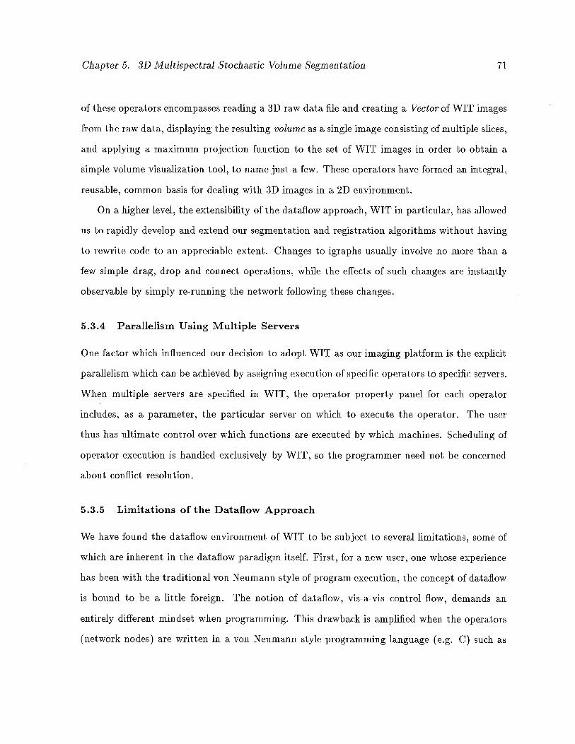
Chapter 5. 3D Multispectral Stochastic Volume Segmentation 71
of these operators encompasses reading a 3D raw data file and creating a Vector of WIT images
from the raw data, displaying the resulting volume as a single image consisting of multiple slices,
and applying a maximum projection function to the set of WIT images in order to obtain a
simple volume visualization tool, to name just a few. These operators have formed an integral,
reusable, common basis for dealing with 3D images in a 2D environment.
On a higher level, the extensibility of the dataflow approach, WIT in particular, has allowed
us to rapidly develop and extend our segmentation and registratioll algorithms without having
to rewrite code to an appreciable extent. Changes to igraphs usually involve no more than a
few simple drag, drop and connect operations, while the effects of such changes are instantly
observable by simply re-running the network following these changes.
5.3.4 Parallelism Using Multiple Servers
One factor which influenced our decision to adopt WIT as our imaging platform is the explicit
parallelism which can be achieved by assigning execution of specific operators to specific servers.
When multiple servers are specified in WIT, the operator property panel for each operator
includes, as a parameter, the particular server on which to execute the operator. The user
thus has ultimate control over which functions are executed by which machines. Scheduling of
operator execution is handled exclusively by WIT, so the programmer need not be concerned
about conflict resolution.
5.3.5 Limitations of the Dataflow Approach
We have found the datafiow environment of WIT to be subject to several limitations, some of
which are inherent in the dataflow paradigm itself. First, for a new user, one whose experience
has been with the traditional von Neumann style of program execution, the concept of datafiow
is bound to be a little foreign. The notion of datafiow, vis-a-vis control flow, demands an
entirely different mindset when programming. This drawback is amplified when the operators
(network nodes) are written in a von Neumann style programming language (e.g. C) such as
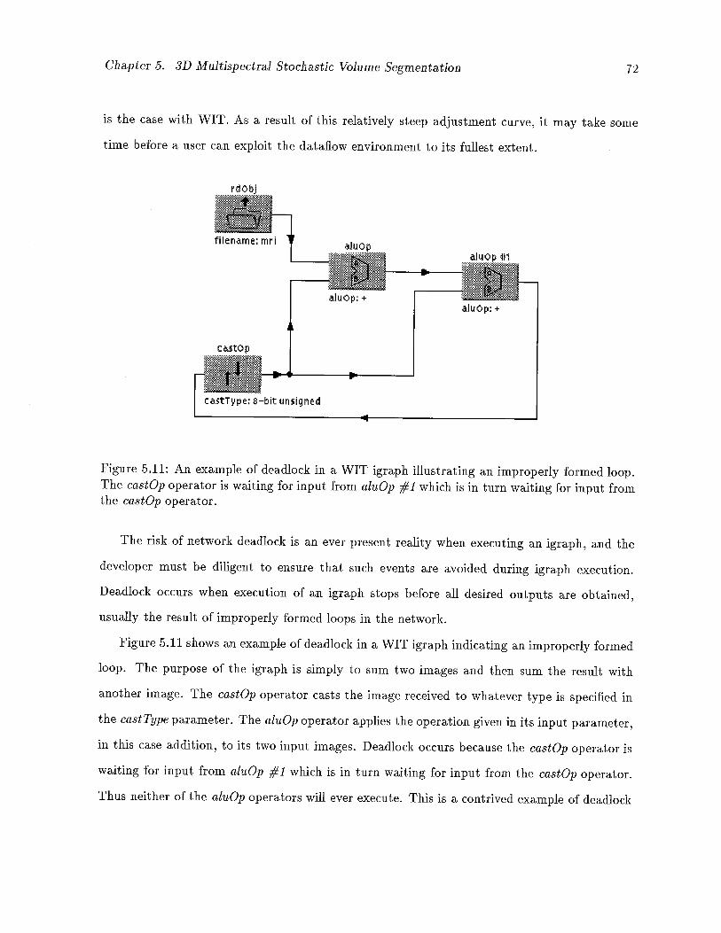
Chapter 5. 3D Multispectral Stochastic Volume Segmentation 72
is the case with WIT. As a result of this relatively steep adjustment curve, it may take some
time before a user can exploit the dataflow environment to its fullest extent.
filename:
Figure 5.11: An example of deadlock in a WIT igraph illustrating an improperly formed ioop.The castOp operator is waiting for input from aizzOp #1 which is in turn waiting for input fromthe castOp operator.
The risk of network deadlock is an ever present reality when executing an igraph, and the
developer must be diligent to ensure that such events are avoided during igraph execution.
Deadlock occurs when execution of an igraph stops before all desired outputs are obtained,
usually the result of improperly formed loops in the network.
Figure 5.11 shows an example of deadlock in a WIT igraph indicating an improperly formed
loop. The purpose of the igraph is simply to sum two images and then sum the result with
another image. The castOp operator casts the image received to whatever type is specified in
the cast Type parameter. The alnOp operator applies the operation given in its input parameter,
in this case addition, to its two input images. Deadlock occurs because the castOp operator is
waiting for input from al’aOp #1 which is in turn waiting for input from the castOp operator.
Thus neither of the aluOp operators will ever execute. This is a contrived example of deadlock
aluop: +
luOp 11
aIiAOp: +
castop
ca5tType: 8—bit unsigned
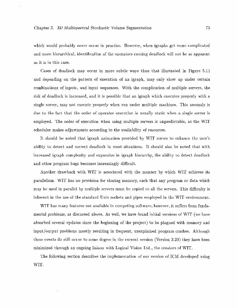
Chapter 5. 3D Multispectral Stochastic Volume Segmentation 73
which would probably never occur in practise. However, when igraphs get more complicated
and more hierarchical, identification of the operators causing deadlock will not be as apparent
as it is in this case.
Cases of deadlock may occur in more subtle ways than that illustrated in Figure 5.11
and depending on the pattern of execution of an igraph, may only show up under certain
combinations of inputs, and input sequences. With the complication of multiple servers, the
risk of deadlock is increased, and it is possible that an igraph which executes properly with a
single server, may not execute properly when run under multiple machines. This anomaly is
due to the fact that the order of operator execution is usually static when a single server is
employed. The order of execution when using multiple servers is unpredictable, as the WIT
scheduler makes adjustments according to the availability of resources.
It should be noted that igraph animation provided by WIT serves to enhance the user’s
ability to detect and correct deadlock in most situations. It should also be noted that with
increased igraph complexity and expansion in igraph hierarchy, the ability to detect deadlock
and other program bugs becomes increasingly difficult.
Another drawback with WIT is associated with the manner by which WIT achieves its
parallelism. WIT has no provision for sharing memory, such that any program or data which
may be used in parallel by multiple servers must be copied to all the servers. This difficulty is
inherent in the use of the standard Unix sockets and pipes employed in the WIT environment.
WIT has many features not available in competing software, however, it suffers from funda
mental problems, as discussed above. As well, we have found initial versions of WIT (we have
absorbed several updates since the beginning of the project) to be plagued with memory and
input/output problems mostly resulting in frequent, unexplained program crashes. Although
these events do still occur to some degree in the current version (Version 3.23) they have been
minimized through an ongoing liaison with Logical Vision Ltd., the creators of WIT.
The following section describes the implementation of our version of 1CM developed using
WIT.
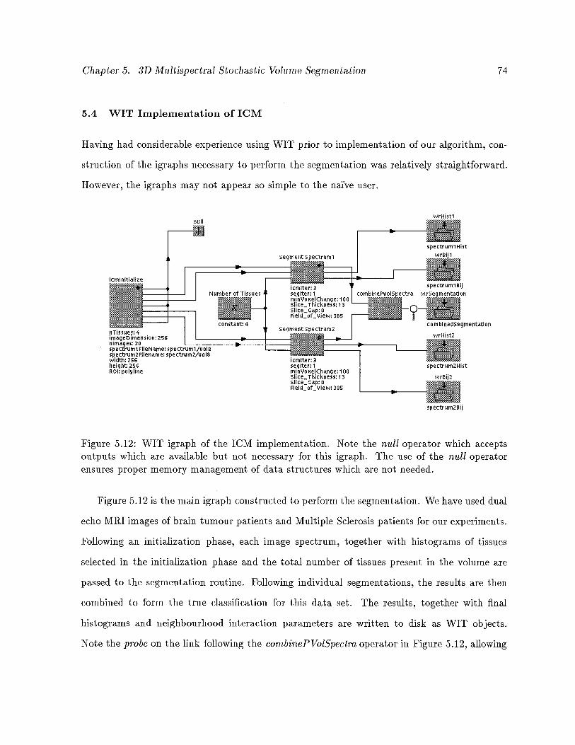
Chapter 5. 3D Multispectral Stochastic Volume Segmentation 74
5.4 WIT Implementation of 1CM
Having had considerable experience using WIT prior to implementation of our algorithm, con
struction of the igraphs necessary to perform the segmentation was relatively straightforward.
However, the igraphs may not appear so simple to the naive user.
Figure 5.12: WIT igraph of the 1CM implementation. Note the null operator which acceptsoutputs which are available but not necessary for this igraph. The use of the null operatorensures proper memory management of data structures which are not needed.
Figure 5.12 is the main igraph constructed to perform the segmentation. We have used dual
echo MRI images of brain tumour patients and Multiple Sclerosis patients for our experiments.
Following an initialization phase, each image spectrum, together with histograms of tissues
selected in the initialization phase and the total number of tissues present in the volume are
passed to the segmentation routine. Following individual segmentations, the results are then
combined to form the true classification for this data set. The results, together with final
histograms and neighbourhood interaction parameters are written to disk as WIT objects.
Note the probe on the link following the combinePVolSpectra operator in Figure 5.12, allowing
nufl
Segrn out Spectrurnl
iurrIutr
Ii
wrHistl
spectruml Hist
srBj 1
spectruml Bij
r5ernentathm
IILI,corn bi nedsegme ntation
icmlter: 3neglter: 1minvoeelChange: ionSlice_Thick000s: 13Slice_ Gap: 0FieILof_Vie: 385
spectrumzHist
epectrum2nij
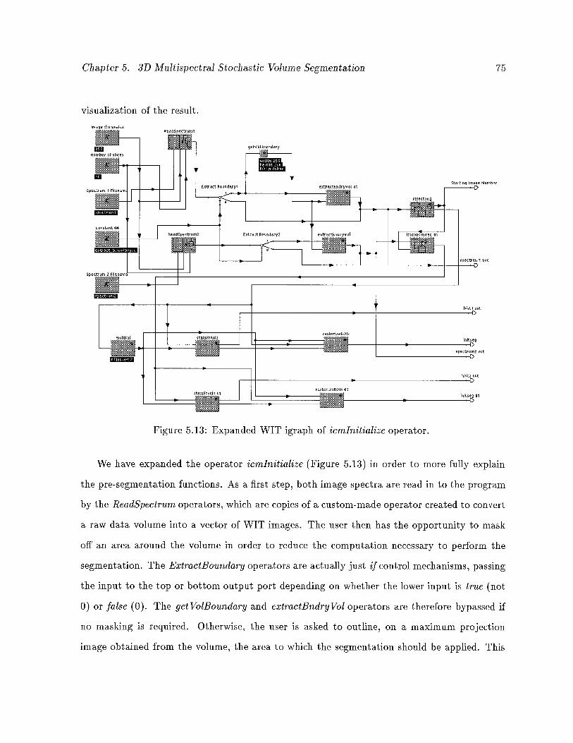
Chapter 5. 3D Multispectral Stochastic Volume Segmentation 75
visualization of the result.
We have expanded the operator icmlnitialize (Figure 5.13) in order to more fully explain
the pre-segmentation functions. As a first step, both image spectra are read in to the program
by the ReadSpectrum operators, which are copies of a custom-made operator created to convert
a raw data volume into a vector of WIT images. The user then has the opportunity to mask
off an area around the volume in order to reduce the computation necessary to perform the
segmentation. The ExtractBoundary operators are actually just if control mechanisms, passing
the input to the top or bottom output port depending on whether the lower input is true (not
0) or false (0). The get VolBo’undary and extractBndry Vol operators are therefore bypassed if
no masking is required. Otherwise, the user is asked to outline, on a maximum projection
image obtained from the volume, the area to which the segmentation should be applied. This
Figure 5.13: Expanded WIT igraph of icmlnitialize operator.
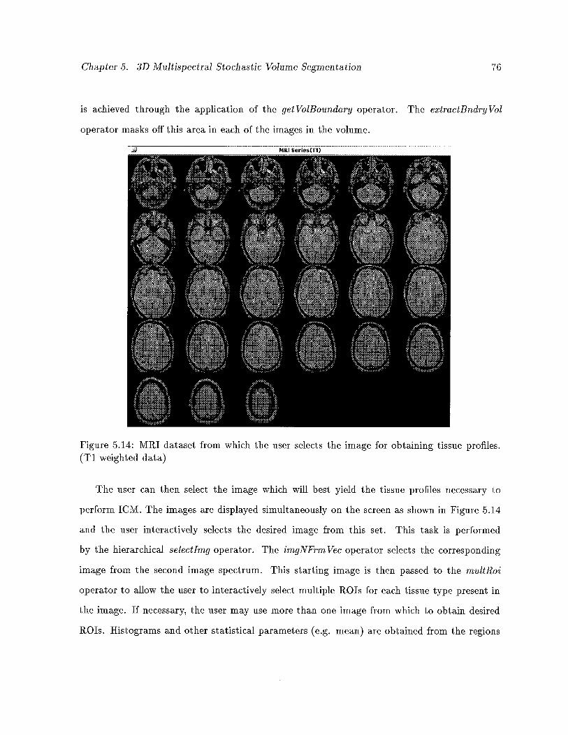
Chapter 5. 3D Multispectral Stochastic Volume Segmentation 76
is achieved through the application of the get VolBonndary operator. The extractBndry Vol
operator masks off this area in each of the images in the volume.
MRI (T1)
Figure 5.14: MRI dataset from which the user selects the image for obtaining tissue profiles.(Ti weighted data)
The user can then select the image which will best yield the tissue profiles necessary to
perform 1CM. The images are displayed simultaneously on the screen as shown in Figure 5.14
and the user interactively selects the desired image from this set. This task is performed
by the hierarchical selectlmg operator. The imgNFrm Vec operator selects the corresponding
image from the second image spectrum. This starting image is then passed to the rnultRoi
operator to allow the user to interactively select multiple ROTs for each tissue type present in
the image. If necessary, the user may use more than one image from which to obtain desired
ROTs. Histograms and other statistical parameters (e.g. mean) are obtained from the regions
Chapter 5. 3D Multispectral Stochastic Volume Segmentation 77
of interest by the statsFrRois operator, which also normalizes and smoothes the histograms so
obtained.
As an optional output the rasterizeROls operators colour the ROTs with the mean gray level
in each region for possible later viewing. The histograms, coloured ROTs and image spectra
(possibly masked) are then output to be processed by the segmentation operators.
Some points worth noting from the expanded igraph of Figure 5.13 are (i) the use of hierar
chical operators, some of which extend the hierarchy to even more levels; (ii) the potential for
parallelism in execution of this igraph; (iii) the input parameters seen in some operators such
as the constant (K) operators, which have been promoted to the next level in the hierarchy so
that they can be entered in the main igraph without ever having to expand the icmlnitialize
operator; and (iv) the rapid increase in the complexity of the igraphs which occurs during
development.
We can now move on to the segmentSpectr’um operators, one of which has been expanded
and is shown in Figure 5.15. This hierarchical operator forms the core of the segmentation
algorithm. The image volume and histograms obtained from the initialization phase are input
to the operator, as well as the number of tissues determined to be present in the volume. From
the histograms an initial segmentation is obtained, as explained in Section 4.14. The crcateP Vol
(create partial volume) operator is responsible for the computation of this initial segmentation.
The memory operator (brain icon) holds the image vector until the input is required by other
operators. Release of an input supplied to the top input port of the memory operator occurs
when any object is received at its bottom input port. This is necessary in order to allow
repeated access to this input, since all operators in WIT destroy their inputs upon releasing
their outputs.
In order to ensure that the creatPvol operator is bypassed in future iterations of the al
gorithm, the oneshot operator is used, shutting down further inputs once a single input has
passed. The initial segmentation output from the createPvol operator is passed to the icmSeg
operator. The for and if operators allow the user to control the exact number of iterations of
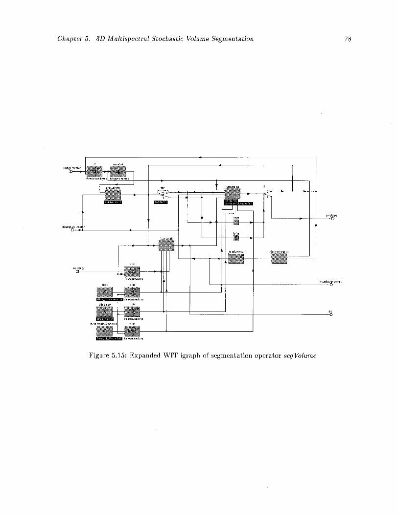
Chapter 5. 3D Multispectral Stochastic Volume Segmentation 78
Figure 5.15: Expanded WIT igraph of segmentation operator seg Volume
Chapter 5. 3D Multispectral Stochastic Volume Segmentation 79
1CM to be applied before recalculation of the neighbourhood interaction parameters and new
histograms.
The icrnSeg operator accepts the image vector, the initial segmentation, a collection of his
tograms describing tissue profiles, and a set of neighbourhood interaction parameters (the /3k1),
as inputs. From the input number of tissues, and the input parameters for slice thickness, slice
gap and field of view, we are able to compute the neighbourhood interaction parameter matrix,
as described by Equation 5.22 in Section 5.2.1. Operator icmGetBij is responsible for this
computation. Note how the input parameters are maintained in memory operators for future
iterations of the algorithm. The icrnSeg operator repeatedly applies the 1CM equation to each
voxel in the input volume until convergence is achieved or until the number of iterations of
the algorithm reaches the input parameter maximum, icrnlter. Convergence is determined to
have occurred when the number of voxels changing in a given iteration is less than the input
parameter minVoxelChange. (See Section 5.2.5 for a more detailed description of convergence.)
When convergence has occurred or the number of iterations of 1CM reaches icrnlter, the output
segmentation is passed to the if operator. If the number of segmentation iterations specified
by the seglter parameter of the for operator has been reached, the segmentation is output as
p VolSeg. Otherwise, a recalculation of neighbourhood interaction parameters and histograms
is performed by looping the output back to the icmGetBij and histFrom Vol operators. This
recalculation increases the accuracy of the segmentation. Equation 5.23 in Section 5.2.3 de
scribes how the histograms are recalculated. Following execution of these operators, the new
parameters are shunted back to the icmSeg operator, and the algorithm is repeated. Note how
the looping of the segmentation output to the memory operators triggers the release of the
parameters necessary to repeat execution of the segmentation.
The operator icmSeg forms the core of the segmentation algorithm. Although the algorithm
is fully described in Section 5.1 we have included the source code of the kernel of this algorithm
in Appendix A. We have duplicated the source code in the appendix in order to better convey
the complexity of dealing with 3D data in WIT and give some intuition for the significant time

Chapter 5. 3D Multispectral Stochastic Volume Segmentation 80
and space requirements of the operator.
Chapter 6
Algorithm Testing and Results
We have applied our version of the 1CM algorithm in 3D to MRI scans of the head obtained from
Multiple Sclerosis patients. In this chapter we first offer a short description of Multiple Sclerosis
in order to motivate the application of our algorithm in this area of research. The results of
applying our algorithm to the MS images in order to quantify the extent of Multiple Sclerosis
lesions are then discussed. The results are encouraging and serve to illustrate the difficulties
in solving the segmentation problem. The chapter concludes with some general observations
regarding the 1CM algorithm as implemented in this thesis followed by a description of future
work to be completed in the area.
6.1 Multiple Sclerosis
Multiple Sclerosis (MS) is a disease of the central nervous system (CNS), i.e. the braill and
spinal cord [110]. It is a debilitating and progressive disease which may result in a variety of
symptoms from blurred vision to severe muscle weakness and degradation, depending on the
area of the CNS which is affected. Multiple Sclerosis is caused by a breakdown in the myelin
sheath, a soft, white, fatty material which insulates the neurons of the CNS and provides for
the rapid transmission of nerve impulses along the nerve fibres of the brain and spinal cord. As
the myelin breaks down, it is replaced by scar tissue, and the speed and frequency of impulse
transmission along the nerve fibre is reduced and in some cases eliminated. The scar tissue
formed from demyelination results in the formation of characteristic plaques in the affected
area. These plaques can be readily observed by post-mortem dissection and by MRI scanning
of live patients.
81
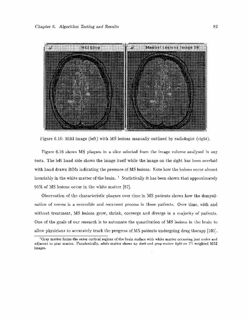
Chapter 6. Algorithm Testing and Results 82
Figure 6.16: MRI image (left) with MS lesions manually outlined by radiologist (right).
Figure 6.16 shows MS plaques in a slice selected from the image volume analysed in our
tests. The left hand side shows the image itself while the image on the right has been overlaid
with hand drawn ROTs indicating the presence of MS lesions. Note how the lesions occur almost
invariably in the white matter of the brain. 1 Statistically it has been shown that approximately
95% of MS lesions occur in the white matter [57].
Observation of the characteristic plaques over time in MS patients shows how the demyeli
nation of nerves is a reversible and recurrent process in these patients. Over time, with and
without treatment, MS lesions grow, shrink, converge and diverge in a majority of patients.
One of the goals of our research is to automate the quantitation of MS lesions in the brain to
allow physicians to accurately track the progress of MS patients undergoing drug therapy [101].
‘Gray matter forms the outer cortical regions of the brain surface with white matter occurring just under andadjacent to gray matter. Paradoxically, white matter shows up dark and gray matter light on Ti weighted MRIimages.
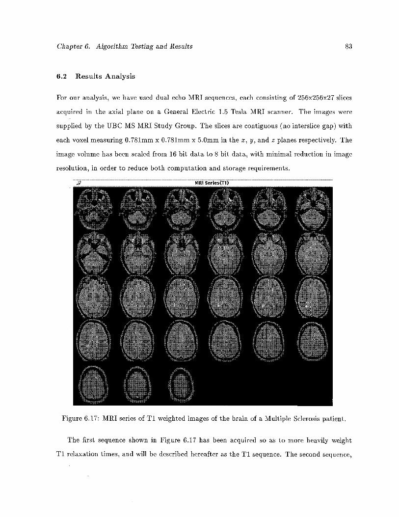
Chapter 6. Algorithm Testing and Results 83
6.2 Results Analysis
For our analysis, we have used dual echo MRI sequences, each consisting of 256x256x27 slices
acquired in the axial plane on a General Electric 1.5 Tesla MRI scanner. The images were
supplied by the UBC MS MRI Study Group. The slices are contiguous (no interslice gap) with
each voxel measuring 0.781mm x 0.781mm x 5.0mm in the x, y, and z planes respectively. The
image volume has been scaled from 16 bit data to 8 bit data, with minimal reduction in image
resolution, in order to reduce both computation and storage requirements.
MRlSeries(T1)
Figure 6.17: MRI series of Ti weighted images of the brain of a Multiple Sclerosis patient.
The first sequence shown in Figure 6.17 has been acquired so as to more heavily weight
Ti relaxation times, and will be described hereafter as the Ti sequence. The second sequence,
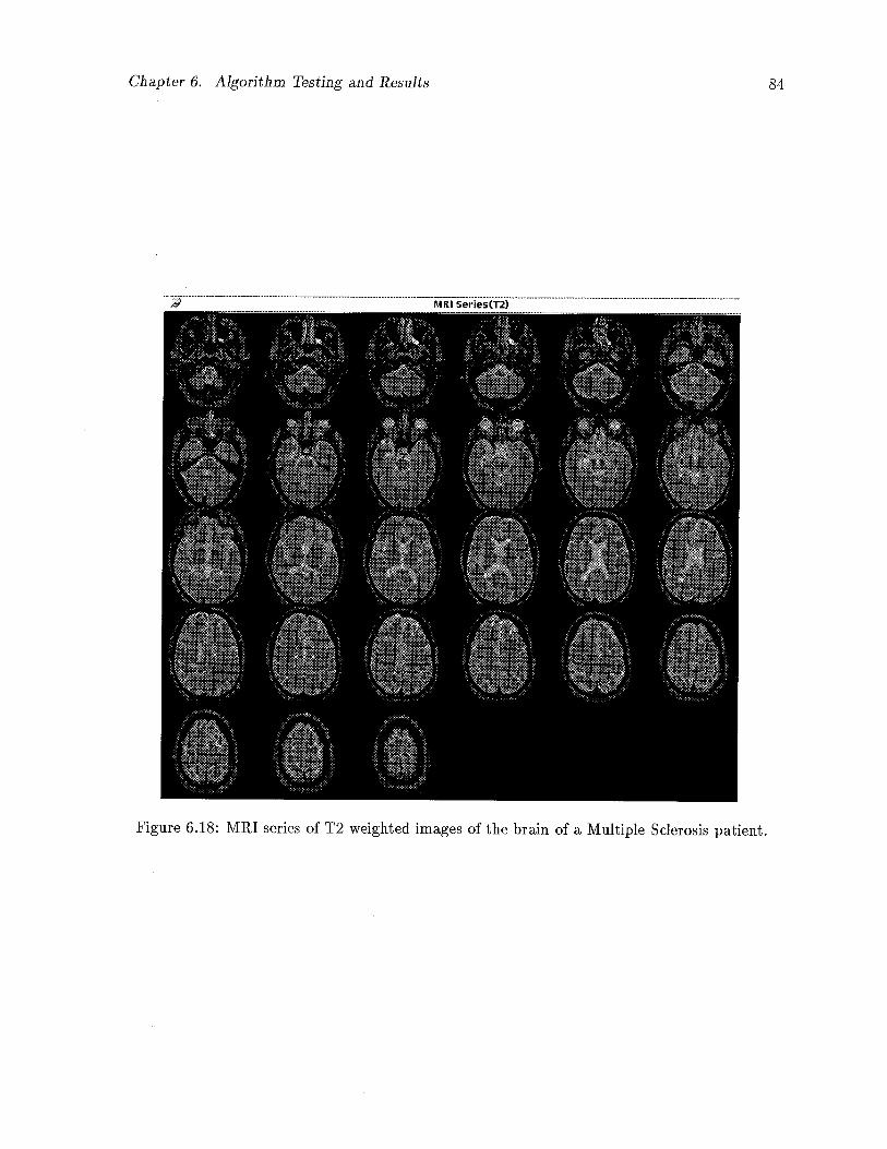
Chapter 6. Algorithm Testing and Results 84
MIII Series(T2)
Figure 6.18: MRI series of T2 weighted images of the brain of a Multiple Sclerosis patient.
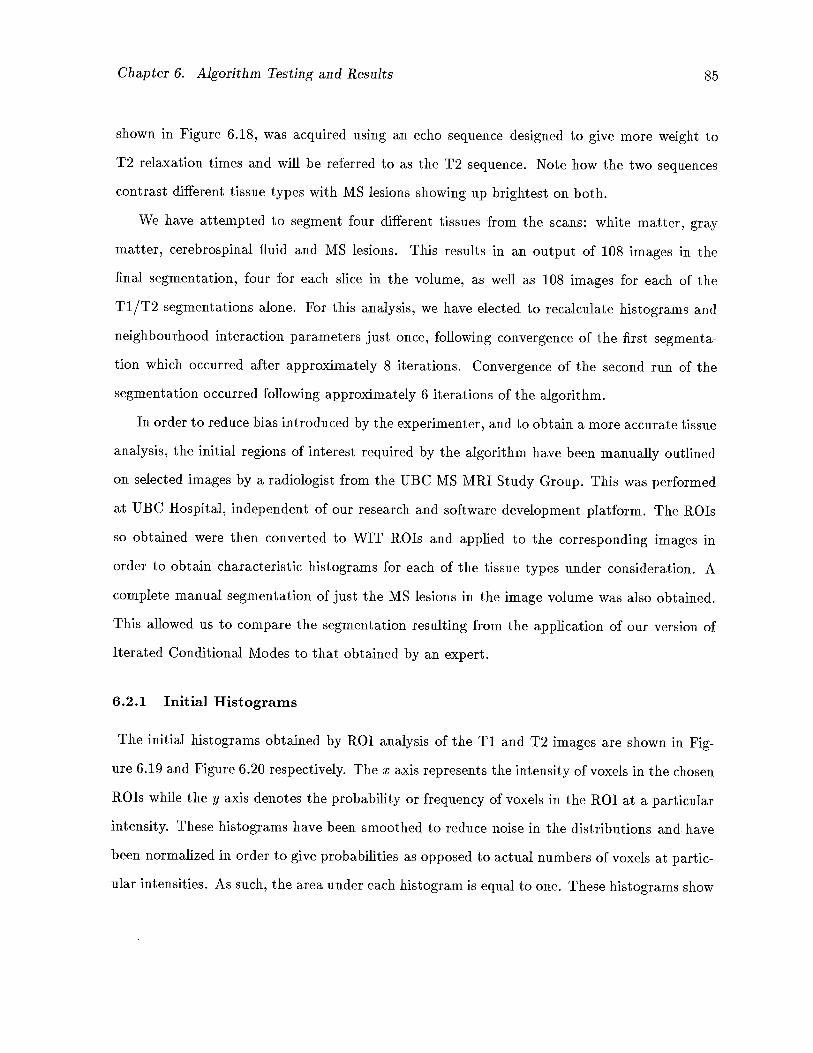
Chapter 6. Algorithm Testing and Results 85
shown in Figure 6.18, was acquired using an echo sequence designed to give more weight to
T2 relaxation times and will be referred to as the T2 sequence. Note how the two sequences
contrast different tissue types with MS lesions showing up brightest on both.
We have attempted to segment four different tissues from the scans: white matter, gray
matter, cerebrospinal fluid and MS lesions. This results in an output of 108 images in the
final segmentation, four for each slice in the volume, as well as 108 images for each of the
T1/T2 segmentations alone. For this analysis, we have elected to recalculate histograms and
neighbourhood interaction parameters just once, following convergence of the first segmenta
tion which occurred after approximately 8 iterations. Convergence of the second run of the
segmentation occurred following approximately 6 iterations of the algorithm.
In order to reduce bias introduced by the experimenter, and to obtain a more accurate tissue
analysis, the initial regions of interest required by the algorithm have been manually outlined
on selected images by a radiologist from the UBC MS MRI Study Group. This was performed
at UBC Hospital, independent of our research and software development platform. The ROTs
so obtained were then converted to WIT ROTs and applied to the corresponding images in
order to obtain characteristic histograms for each of the tissue types under consideration. A
complete manual segmentation of just the MS lesions in the image volume was also obtained.
This allowed us to compare the segmentation resulting from the application of our version of
Iterated Conditional Modes to that obtained by an expert.
6.2.1 Initial Histograms
The initial histograms obtained by ROT analysis of the Ti and T2 images are shown in Fig
ure 6.19 and Figure 6.20 respectively. The x axis represents the intensity of voxels in the chosen
ROIs while the y axis denotes the probability or frequency of voxels in the ROT at a particular
intensity. These histograms have been smoothed to reduce noise in the distributions and have
been normalized in order to give probabilities as opposed to actual numbers of voxels at partic
ular intensities. As such, the area under each histogram is equal to one. These histograms show
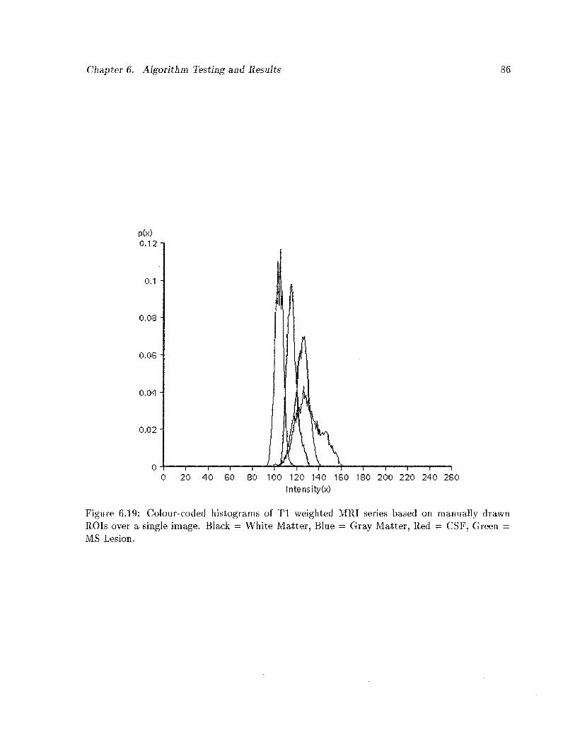
Chapter 6. Algorithm Testing and Results 86
p(x)0.12
0.1
0.09
0.06
0.04
0.02
0
intensity(x)
Figure 6.19: Co1ourcoded histograms of Ti weighted MRI series based on manually drawnROTs over a single image. Black = White Matter, Blue = Gray Matter, Red = CSF, Green =
MS Lesion.
0 20 40 60 80 100 120 140 160 180 200 220 240 260
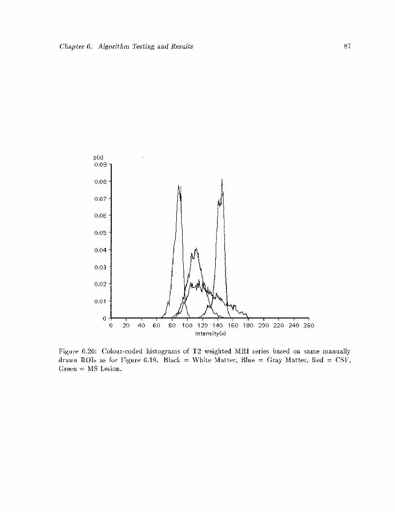
Chapter 6. Algorithm Testing and Results 87
p(x)0.08
0.08
0,07
0.08
0.05
0.04
0.03
0.02
0.01
00 20 40 80 80 100 120 140 180 180 200 220 240 280
Intensity(x)
Figure 6.20:drawn ROTsGreen = MS
Co1ourcoded histograms of 12 weighted MRI series based on same manuallyas for Figure 6.19. Black = White Matter, Blue = Gray Matter, Red = CSF,Lesion.
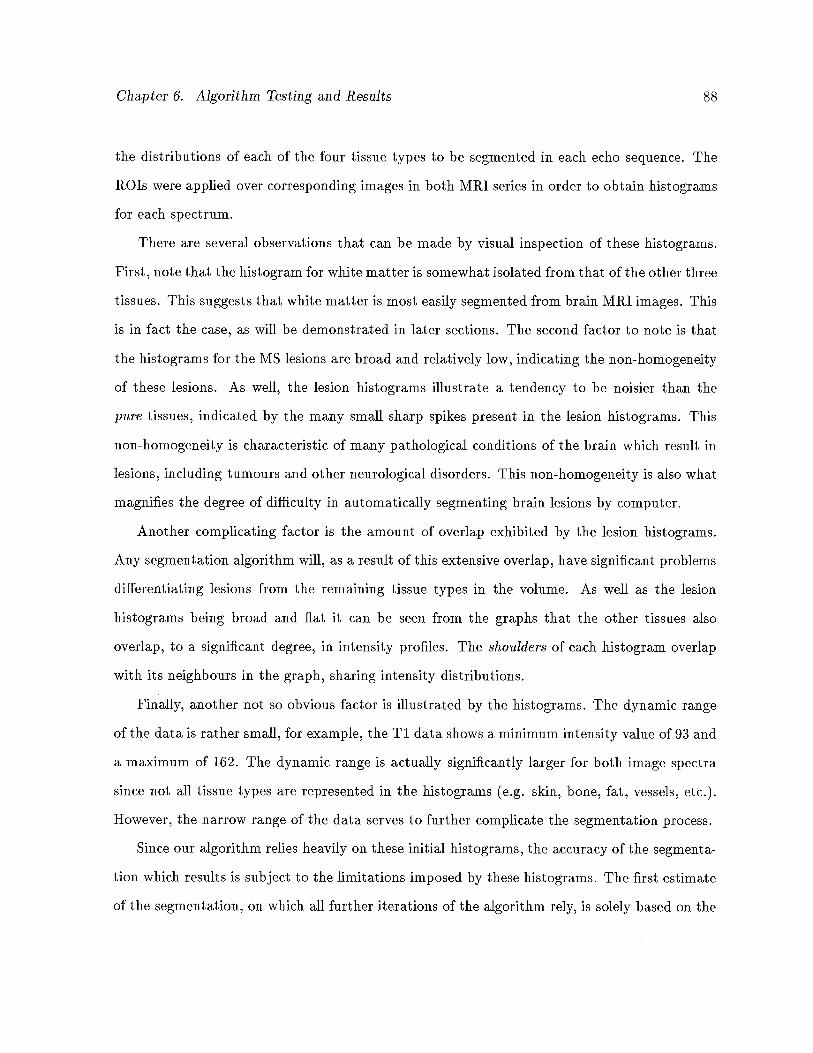
Chapter 6. Algorithm Testing and Results 88
the distributions of each of the four tissue types to be segmented in each echo sequence. The
ROTs were applied over corresponding images in both MRI series in order to obtain histograms
for each spectrum.
There are several observations that can be made by visual inspection of these histograms.
First, note that the histogram for white matter is somewhat isolated from that of the other three
tissues. This suggests that white matter is most easily segmented from brain MRI images. This
is in fact the case, as will be demonstrated in later sections. The second factor to note is that
the histograms for the MS lesions are broad and relatively low, indicating the non-homogeneity
of these lesions. As well, the lesion histograms illustrate a tendency to be noisier than the
pure tissues, indicated by the many small sharp spikes present in the lesion histograms. This
non-homogeneity is characteristic of many pathological conditions of the brain which result in
lesions, including tumours and other neurological disorders. This non-homogeneity is also what
magnifies the degree of difficulty in automatically segmenting brain lesions by computer.
Another complicating factor is the amount of overlap exhibited by the lesion histograms.
Any segmentation algorithm will, as a result of this extensive overlap, have significant problems
differentiating lesions from the remaining tissue types in the volume. As well as the lesion
histograms being broad and fiat it can be seen from the graphs that the other tissues also
overlap, to a significant degree, in intensity profiles. The shoulders of each histogram overlap
with its neighbours in the graph, sharing intensity distributions.
Finally, another not so obvious factor is illustrated by the histograms. The dynamic range
of the data is rather small, for example, the Ti data shows a minimum intensity value of 93 and
a maximum of 162. The dynamic range is actually significantly larger for both image spectra
since not all tissue types are represented in the histograms (e.g. skin, bone, fat, vessels, etc.).
However, the narrow range of the data serves to further complicate the segmentation process.
Since our algorithm relies heavily on these initial histograms, the accuracy of the segmenta
tion which results is subject to the limitations imposed by these histograms. The first estimate
of the segmentation, on which all further iterations of the algorithm rely, is solely based on the
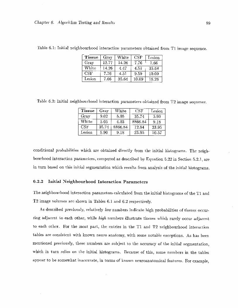
Chapter 6. Algorithm Testing and Results 89
Table 6.1: Initial neighbourhood interaction parameters obtained from Ti image sequence.
Tissue Gray White CSF LesionGray 12.77 14.26 7.76 7.66White 14.26 4.47 4.51 35.64CSF 7.76 4.51 9.59 10.09Lesion 7.66 35.64 10.09 18.28
Table 6.2: Initial neighbourhood interaction parameters obtained from T2 image sequence.
Tissue Gray White CSF LesionGray 9.02 5.05 35.74 5.90White 5.05 4.03 8866.84 9.18CSF 35.74 8866.84 12.84 23.95Lesion 5.90 9.18 23.95 10.57
conditional probabilities which are obtained directly from the initial histograms. The neigh
bourhood interaction parameters, computed as described by Equation 5.22 in Section 5.2.1, are
in turn based on this initial segmentation which results from analysis of the initial histograms.
6.2.2 Initial Neighbourhood Interaction Parameters
The neighbourhood interaction parameters calculated from the initial histograms of the Ti and
T2 image volumes are shown in Tables 6.1 and 6.2 respectively.
As described previously, relatively low numbers indicate high probabilities of tissues occur
ring adjacent to each other, while high numbers illustrate tissues which rarely occur adjacent
to each other. For the most part, the entries in the Ti and T2 neighbourhood interaction
tables are consistent with known neuro-anatomy, with some notable exceptions. As has been
mentioned previously, these numbers are subject to the accuracy of the initial segmentation,
which in turn relies on the initial histograms. Because of this, some numbers in the tables
appear to be somewhat inaccurate, in terms of known neuroanatomical features. For example,
Chapter 6. Algorithm Testing and Results 90
we have mentioned that MS lesions occur almost exclusively in the white matter of the brain.
However, the (white matter:lesion) adjacency measure given in Table 6.1 would suggest other
wise. But, if we keep in mind that the relative numbers of white matter (and other non-lesion)
voxels far exceeds the numbers of lesion voxels, then this number seems more realistic. In fact
the (white matter:lesion) interaction parameter actually increases when these parameters are
recalculated following the first convergence of the algorithm (See Table 6.3). Another reason
for the apparent contradiction in the (white matter:lesion) interaction probability is the nature
of the MS lesion itself. Although occurring in white matter almost exclusively, the lesions do
not have sharp transitions from lesion to white matter. It can be seen on analysis that the
intensity of MS lesions declines when measured from the centres of the lesions to the edges.
Because the decline is gradual and because white matter is dark and lesion is brightest on both
Ti and T2 images, the intensity proffle of the MS lesions passes through an area shared with
gray matter.2 This phenomenon is borne out by the histograms of Figures 6.19 and 6.20. This
results in a higher than expected value in the interaction table for the (white matter:lesion)
adjacency measure, and a lower than expected value for (gray:lesion).
Consider the diagonal elements of Table 6.1. These numbers can be considered self-adjacencies,
yielding measures of the relative quantities of different tissues and a measure of the convolut
edness of the tissue structure. White matter, for example, which constitutes most of the brain
matter, yields a very low number, while lesion, which occurs infrequently, and thus must share a
larger percentage of its total voxels with other tissues, exhibits a relatively large self adjacency
number. This pattern is repeated in Table 6.2.
When Table 6.1 is compared with Table 6.2, the corresponding entries are relatively consis
tent, but for a few notable exceptions. These differences are due to differences in the charac
teristics of the Ti and T2 imaging sequences of MRI, as well as the complex nature of tissue
interaction as measured by our algorithm. In particular the (CSF:white matter) interaction
2Because of the reduced reproduction capabilities from raster to laser printer this phenomenon cannot beadequately ifiustrated in the thesis.
Chapter 6. Algorithm Testing and Results91
parameter is highly contrasted between the two tables. This results from the poor differentiability of CSF in the Ti image volume, due to the nature of the nature of the imaging sequence.The high value given in Table 6.2 is more plausible than the low value of Table 6.1, as CSF andwhite matter do not occur adjacently in healthy brain tissue.
Following initial convergence of the 1CM algorithm, the histograms and neighbourhoodinteraction parameters are recalculated and used as input to the algorithm a second time. Thisrecalculation of parameters is performed in order to refine the segmentation, assuming thenew parameters are more accurate than those used initially. Since we are using intensity andsegmentation values from the entire volume in the second run of the algorithm, as opposed tojust a single slice, this assumption is realistic.
6.2.3 Recalculated Histograms
The new histograms are calculated as per Equation 5.23 in Section 5.2.3, using partial volumecontributions from each tissue to each voxel. Thus, the manner in which the histograms areobtained is fundamentally different than that which was used to obtain the initial histograms,i.e. manual segmentation. We would expect, theoretically, that the new histograms will be quitesimilar to the initial versions, and this expectation is fulfilled, despite the dramatically differentmanner in which the two sets of histograms are obtained. Figures 6.21 and 6.22 show theresults of reassessment of tissue profiles in the intermediate segmentation of the Ti and T2image sequences respectively. Note the similarities between these and the original histogramsof Figures 6.19 and 6.20. Again we notice the overlap in tissue distributions. Most notably, itis shown that the lesion intensity profiles are shared by several other tissues, especially graymatter and CSF. The white matter histogram is, again, less affected by other tissue profiles,though not to the same extent as with the original distributions.
What is different about these histograms is that the lesion profiles have become less distributed, that is taller and thinner, perhaps indicating the attempt of the first run of thesegmentation to isolate the lesions from the other tissues. As well as the difference in the shape
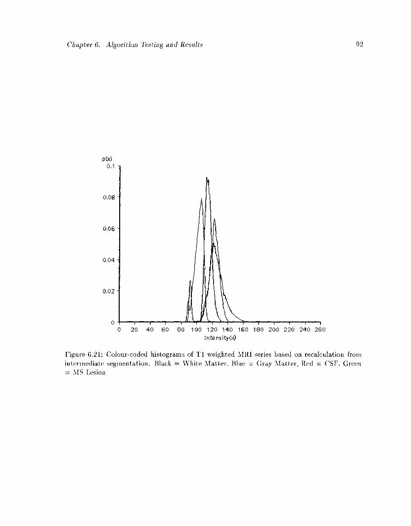
Chapter 6. Algorithm Testing and Results 92
1—'—f f 1 1 1 1 1
100 120 140 160 180 200 220 240 2G0 Intensity(x)
Figure 6.21: Colour-coded histograms of T l weighted MRI series based on recalculation from intermediate segmentation. Black = White Matter, Blue = Gray Matter, Red = CSF, Green = MS Lesion
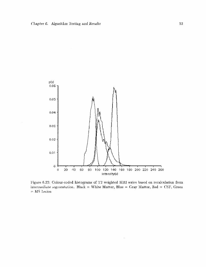
Chapter 6. Algorithm Testing and Results 93
ptx)0.06
0.05
0.04
003
0.02
0,01
00 20 40 60 60 100 120 140 160 180 200 220 240 260
Intensity(x)
Figure 6.22: Colour-coded histograms of T2 weighted MRI series based on recalculation fromintermediate segmentation. Black White Matter, Blue Gray Matter, Red = CSF, Green= MS Lesion
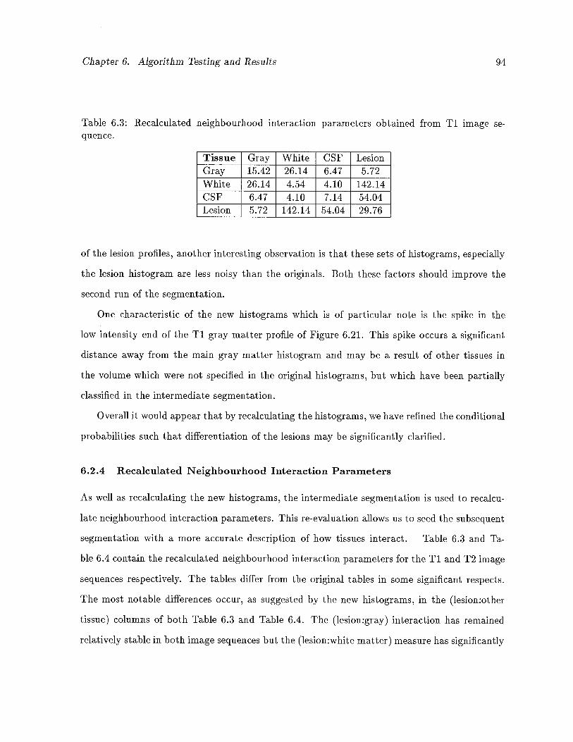
Chapter 6. Algorithm Testing and Results 94
Table 6.3: Recalculated neighbourhood interaction parameters obtained from Ti image sequence.
Tissue Gray White CSF LesionGray 15.42 26.14 6.47 5.72White 26.14 4.54 4.10 i42.i4CSF 6.47 4.10 7.14 54.04Lesion 5.72 142.i4 54.04 29.76
of the lesion profiles, another interesting observation is that these sets of histograms, especially
the lesion histogram are less noisy than the originals. Both these factors should improve the
second run of the segmentation.
One characteristic of the new histograms which is of particular note is the spike in the
low intensity end of the Ti gray matter profile of Figure 6.21. This spike occurs a significant
distance away from the main gray matter histogram and may be a result of other tissues in
the volume which were not specified in the original histograms, but which have been partially
classified in the intermediate segmentation.
Overall it would appear that by recalculating the histograms, we have refined the conditional
probabilities such that differentiation of the lesions may be significantly clarified.
6.2.4 Recalculated Neighbourhood Interaction Parameters
As well as recalculating the new histograms, the intermediate segmentation is used to recalcu
late neighbourhood interactioll parameters. This re-evaluation allows us to seed the subsequent
segmentation with a more accurate description of how tissues interact. Table 6.3 and Ta
ble 6.4 contain the recalculated neighbourhood interaction parameters for the Ti and T2 image
sequences respectively. The tables differ from the original tables in some significant respects.
The most notable differences occur, as suggested by the new histograms, in the (lesion:other
tissue) columns of both Table 6.3 and Table 6.4. The (lesion:gray) interaction has remained
relatively stable in both image sequences but the (lesion:white matter) measure has significantly
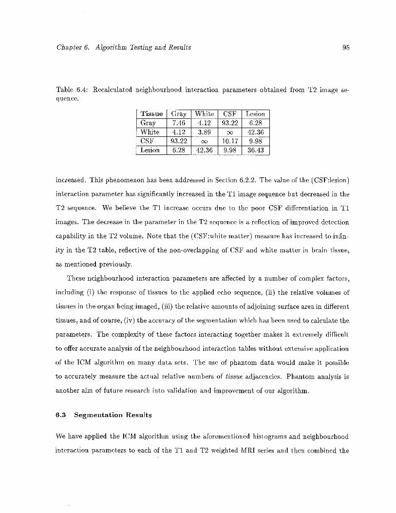
Chapter 6. Algorithm Testing and Results 95
Table 6.4: Recalculated neighbourhood interaction parameters obtained from T2 image sequence.
Tissue Gray White CSF LesionGray 7.46 4.12 93.22 6.28White 4.12 3.89 oo 42.36CSF 93.22 00 10.17 9.98Lesion 6.28 42.36 9.98 36.43
increased. This phenomenon has been addressed in Section 6.2.2. The value of the (CSF:lesion)
interaction parameter has significantly increased in the Ti image sequence but decreased in the
T2 sequence. We believe the Ti increase occurs due to the poor CSF differentiation in Ti
images. The decrease in the parameter in the T2 sequence is a reflection of improved detection
capability in the T2 volume. Note that the (CSF:white matter) measure has increased to infin
ity in the T2 table, reflective of the non-overlapping of CSF and white matter in brain tissue,
as mentioned previously.
These neighbourhood interaction parameters are affected by a number of complex factors,
including (i) the response of tissues to the applied echo sequence, (ii) the relative volumes of
tissues in the organ being imaged, (iii) the relative amollnts of adjoining surface area in different
tissues, and of course, (iv) the accuracy of the segmentation which has been used to calculate the
parameters. The complexity of these factors interacting together makes it extremely difficult
to offer accurate analysis of the neighbourhood interaction tables without extensive application
of the 1CM algorithm on many data sets. The use of phantom data would make it possible
to accurately measure the actual relative numbers of tissue adjacencies. Phantom analysis is
another aim of future research into validation and improvement of our algorithm.
6.3 Segmentation Results
We have applied the 1CM algorithm using the aforementioned histograms and neighbourhood
interaction parameters to each of the Ti and T2 weighted MRI series and then combined the
Chapter 6. Algorithm Testing and Results 96
results by multiplying and normalizing the respective probabilities for each tissue type. We are
able to do this because the two series have been acquired independently.
6.3.1 Ti Segmentation
We have selected from the segmentation results a single slice from the volume to iliustrate the
performance of the 1CM algorithm. Figure 6.23 shows the result of the segmentation on slice
number 18 (of 27) from the Ti weighted volume. The top four images show the segmentation of
CSF, gray matter, white matter and lesion, as labeled in the figure. The actual slice data, with
and without the manually segmented lesions overlaid on the slice, are given in the bottom two
images. The gray scale intensity of each of the four segmentation images is in direct proportion
to the probability obtained for that tissue in the image.
As anticipated, the results for white matter are by far the most impressive, whlie the algo
rithm had difficulty differentiating gray matter and CSF and gray matter and lesion. However,
the results for lesion segmentation are accurate when compared to the manual segmentation
and, when combined with the segmentation obtained from the T2 weighted sequence, produce
satisfactory results.
It is interesting to note that, as discussed in the Section 6.2.2, the edges of some MS lesions
whose intensities pass through the intensity distribution dominated by gray matter, have in
fact been incorrectly classified as gray matter in the Ti segmentation.
6.3.2 T2 Segmentation
Figure 6.24 shows the segmentation of the corresponding slice in the T2 weighted data set.
Again, the white matter segmentation is the most accurate of all the tissues due to the relative
isolation of its intensity profile in the histograms. There is considerable improvement in the
differentiation of CSF and gray matter, but again, the lesion/gray matter separation is bur
dened. As well, some CSF has been incorrectly classified as lesion. On the whole, however, the
segmentation is reasonably accurate.
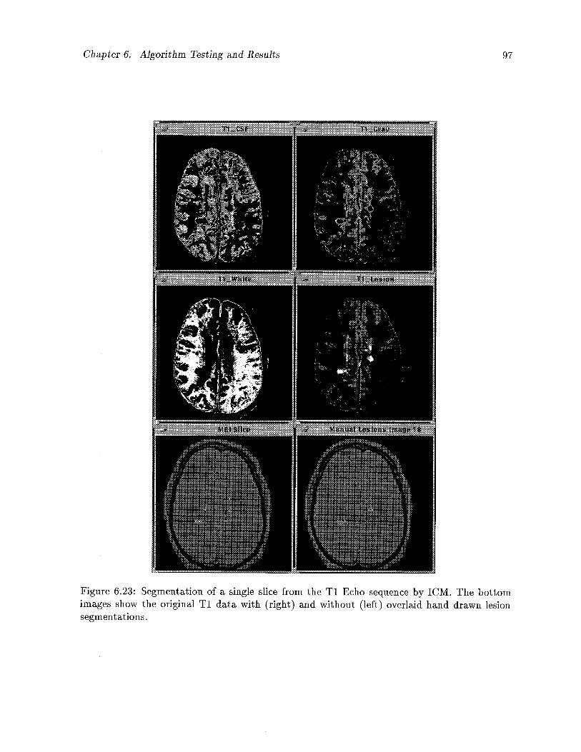
Chapter 6; Algorithm Testing and Results 97
Figure 6.23: Segmentation of a single slice from the Ti Echo sequence by 1CM. The bottomimages show the original Ti data with (right) and without (left) overlaid hand drawn lesionsegmentations.
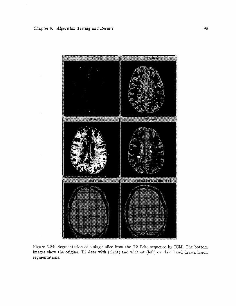
Chapter 6. Algorithm Testing and Results 98
Figure 6.24: Segmentation of a single slice from the T2 Echo sequence by 1CM. The bottomimages show the original T2 data with (right) and without (left) overlaid hand drawn lesionsegmentations.
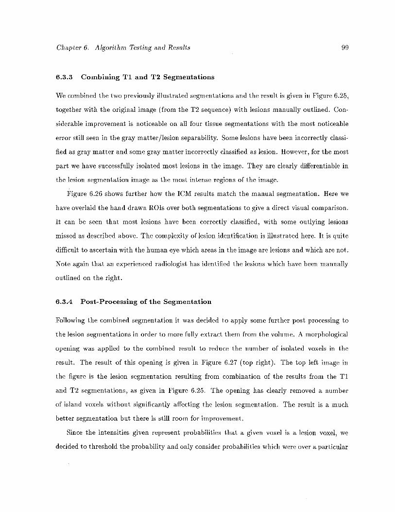
Chapter 6. Algorithm Testing and Results 99
6.3.3 Combining Ti and T2 Segmentations
We combined the two previously illustrated segmentations and the result is given in Figure 6.25,
together with the original image (from the T2 sequence) with lesions manually outlined. Con
siderable improvement is noticeable on all four tissue segmentations with the most noticeable
error still seen in the gray matter/lesion separability. Some lesions have been incorrectly classi
fied as gray matter and some gray matter incorrectly classified as lesion. However, for the most
part we have successfully isolated most lesions in the image. They are clearly differentiable in
the lesion segmentation image as the most intense regions of the image.
Figure 6.26 shows further how the 1CM results match the manual segmentation. Here we
have overlaid the hand drawn ROTs over both segmentations to give a direct visual comparison.
It can be seen that most lesions have been correctly classified, with some outlying lesions
missed as described above. The complexity of lesion identification is illustrated here. It is quite
difficult to ascertain with the human eye which areas in the image are lesions and which are not.
Note again that an experienced radiologist has identified the lesions which have been manually
outlined on the right.
6.3.4 Post-Processing of the Segmentation
Following the combined segmentation it was decided to apply some further post processing to
the lesion segmentations in order to more fully extract them from the volume. A morphological
opening was applied to the combined result to reduce the number of isolated voxels in the
result. The result of this opening is given in Figure 6.27 (top right). The top left image in
the figure is the lesion segmentation resulting from combination of the results from the Ti
and T2 segmentations, as given in Figure 6.25. The opening has clearly removed a number
of island voxels without significantly affecting the lesion segmentation. The result is a much
better segmentation but there is still room for improvement.
Since the intensities given represent probabilities that a given voxel is a lesion voxel, we
decided to threshold the probability and only consider probabilities which were over a particular
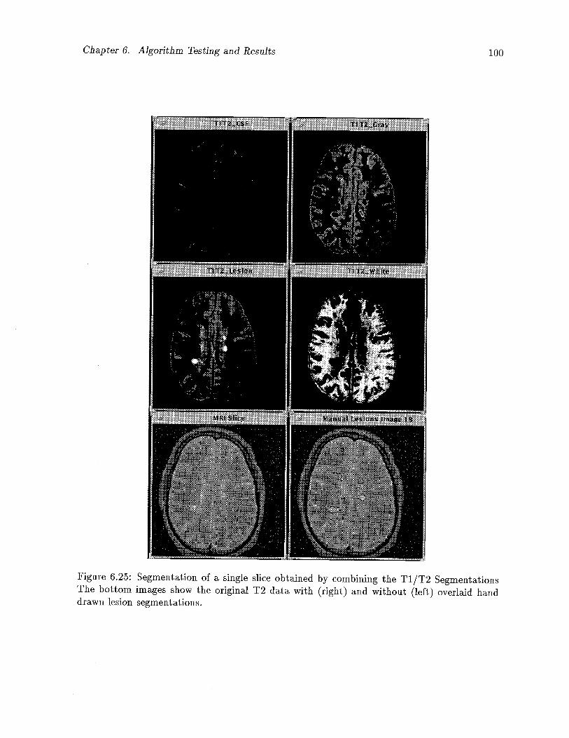
Chapter 6. Algorithm Testing and Results 100
Figure 6.25: Segmentation of a single slice obtained by combining the T1/T2 SegmentationsThe bottom images show the original T2 data with (right) and without (left) overlaid handdrawn lesion segmentations.
Chapter 6. Algorithm Testing and Results 101
Figure 6.26: Manual segmentation overlaid on combined T1/T2 Segmentation (left) and alsooverlaid on raw T2 image (right).
measure, in this case 0.4. This thresholding operation was applied to the morphologically
opened result obtained previously. Visually, this threshold gave the best result when compared
with the manual segmentation. The thresholded final segmentation is given in the bottom right
of Figure 6.27.
6.3.5 Visualizing Partial Volumes
Partial volume considerations are most significant near the borders of different tissue types,
but this has not been clearly demonstrated to this point. In order to more fully appreciate
the partial volume solution that we have given, the segmentations of white matter and lesion
(before and after post-processing) have been given in Figures 6.28 and 6.29 respectively.
The gray scales in the previous images have been mapped to particular colours according
to the colour map given in Figure 6.30, with bright red indicating the highest intensity, and
dark blue the lowest. These figures illustrate that voxels in the central areas of tissues have
much more definite composition, while there is less certainty about voxels nearer the borders
of tissue. This could not be properly appreciated in the grayscale versions of the segmentation.
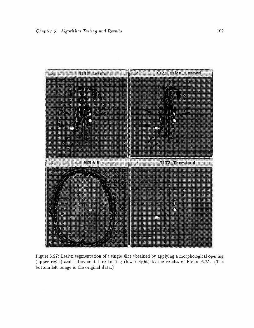
Chapter 6. Algorithm Testing and Results 102
Figure 6.27: Lesion segmentation of a single slice obtained by applying a morphological opening(upper right) and subsequent thresholding (lower right) to the results of Figure 6.25. (Thebottom left image is the original data.)
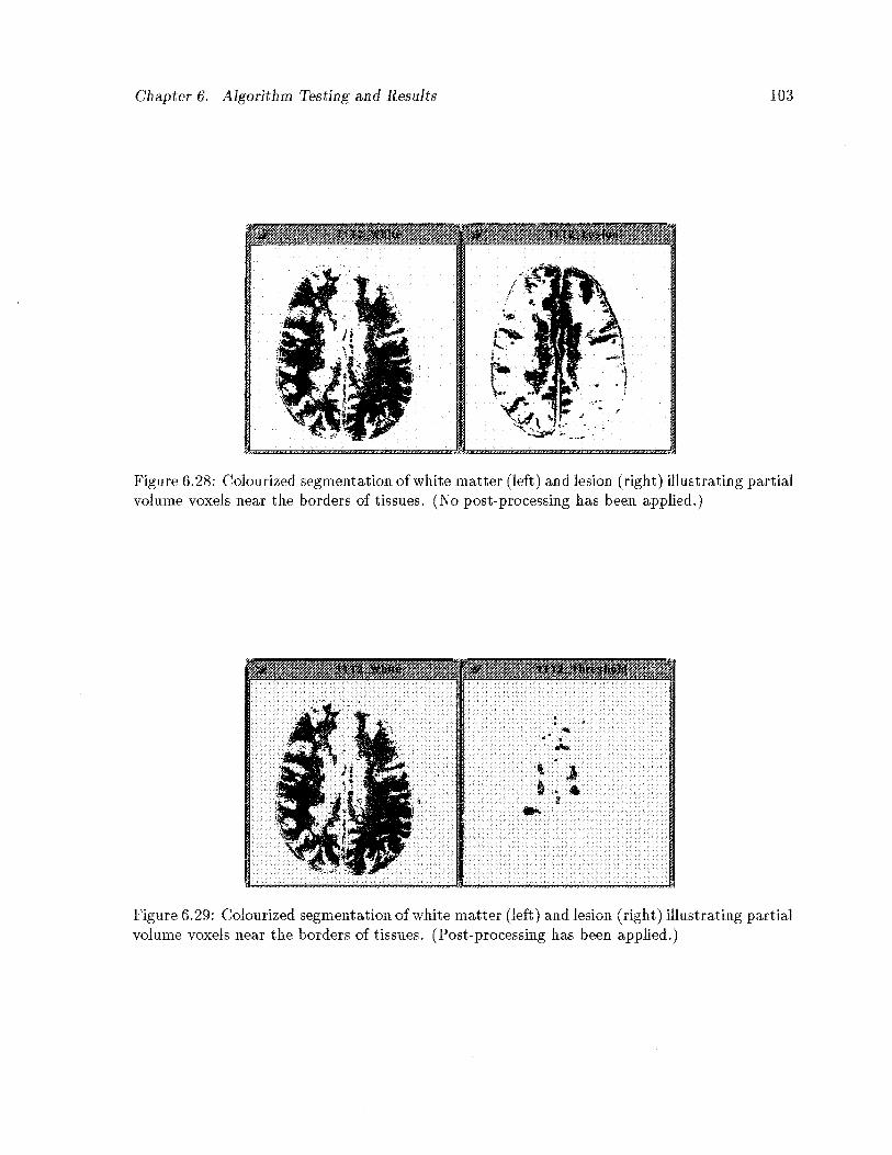
Chapter 6. Algorithm Testing and Results 103
Figure 6.28: Colourized segmentation of white matter (left) and lesion (right) illustrating partialvolume voxels near the borders of tissues. (No post-processing has been applied.)
Figure 6.29: Colourized segmeiltation of white matter (left) and lesion (right) illustrating partialvolume voxels near the borders of tissues. (Post-processing has been applied.)
I
r
lb

Chapter 6. Algorithm Testing and Results 104
Figure 6.30: WIT colour-map used to euhance partial volume characteristics of segmentationas sliowu iii Figures 6.28 and 6.29.
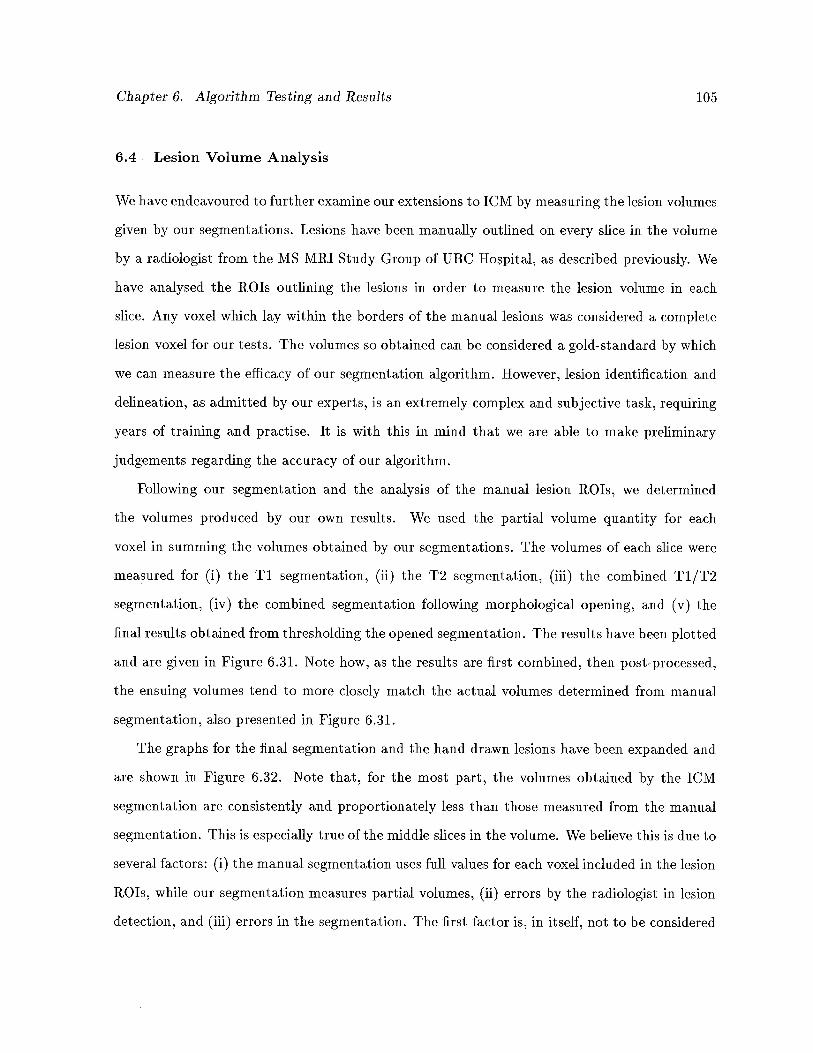
Chapter 6. Algorithm Testing and Results 105
6.4 Lesion Volume Analysis
We have endeavoured to further examine our extensions to 1CM by measuring the lesion volumes
given by our segmentations. Lesions have been manually outlined on every slice in the volume
by a radiologist from the MS MRI Study Group of UBC Hospital, as described previously. We
have analysed the ROTs outlining the lesions in order to measure the lesion volume in each
slice. Any voxel which lay within the borders of the manual lesions was considered a complete
lesion voxel for our tests. The volumes so obtained can be considered a gold-standard by which
we can measure the efficacy of our segmentation algorithm. However, lesion identification and
delineation, as admitted by our experts, is an extremely complex and subjective task, requiring
years of training and practise. It is with this in mind that we are able to make preliminary
judgements regarding the accuracy of our algorithm.
Following our segmentation and the analysis of the manual lesion ROTs, we determined
the volumes produced by our own results. We used the partial volume quantity for each
voxel in summing the volumes obtained by our segmentations. The volumes of each slice were
measured for (i) the Ti segmentation, (ii) the T2 segmentation, (iii) the combined T1/T2
segmentation, (iv) the combined segmentation following morphological opening, and (v) the
final results obtained from thresholding the opened segmentation. The results have been plotted
and are given in Figure 6.31. Note how, as the results are first combined, then post-processed,
the ensuing volumes tend to more closely match the actual volumes determined from manual
segmentation, also presented in Figure 6.3i.
The graphs for the final segmentation and the hand drawn lesions have been expanded and
are shown in Figure 6.32. Note that, for the most part, the volumes obtained by the 1CM
segmentation are consistently and proportionately less than those measured from the manual
segmentation. This is especially true of the middle slices in the volume. We believe this is due to
several factors: (i) the manual segmentation uses full values for each voxel included in the lesion
ROTs, while our segmentation measures partial volumes, (ii) errors by the radiologist in lesion
detection, and (iii) errors in the segmentation. The first factor is, in itself, not to be considered
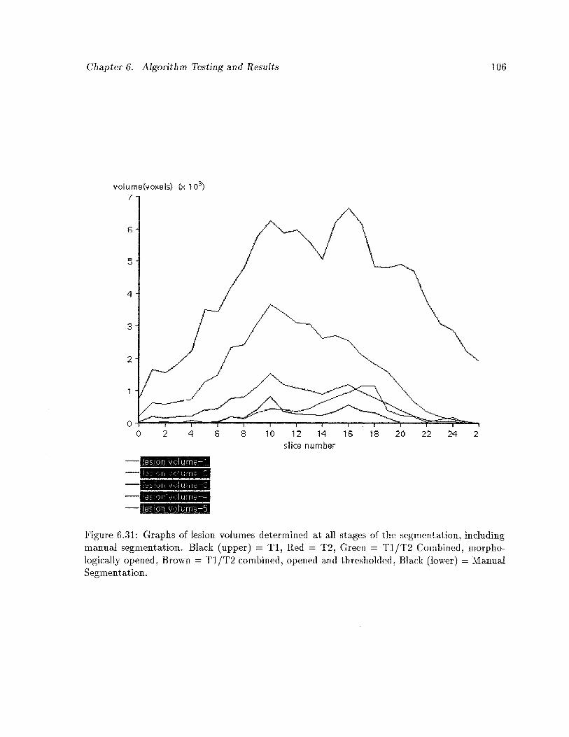
Chapter 6. Algorithm Testing and Results 106
volume(voxels) (x ‘iO)7.
6-
5.
4.
s’ice number
j:fl ‘.;;(:Furfle—-l
S)fl .urn-—3
Ie. c)ri.,.:::I_1 rri—5
Figure 6.31: Graphs of lesion volumes determined at all stages of the segmentation, includingmanual segmentation. Black (upper) = Ti, Red = T2, Green = T1/T2 Combined, morphologically opened, Brown = Ti/T2 combined, opened and thresholded, Black (lower) = ManualSegmentation.
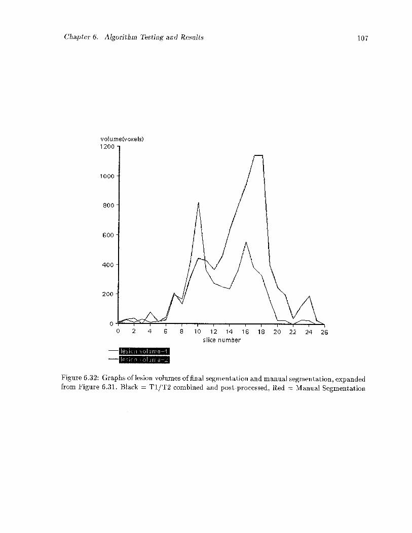
Chapter 6. Algorithm Testing and Results 107
1000
400
200
esi.::ri VC:hrflP—1
Figure 6.32: Graphs of lesion volumes of final segmentation and manual segmentation, expandedfrom Figure 6.31. Black = T1/T2 combined and post-processed, Red = Manual Segmentation
volu me(voxels)1200
800
800
00 2 4 8 8 10 12 14 16 18 20 22 24 26
silce number
Chapter 6. Algorithm Testing and Results 108
an error but perhaps an adjustment made by our program that is not possibly (or at least
not easily) accomplished by manual outlining of regions. The second factor is usually due to a
tendency by clinicians to consistently classify an area as lesion when in fact there is considerable
uncertainty as to the region’s composition. The third factor, errors in the segmentation, result
from inconsistencies in the histograms and neighbourhood interaction parameters as discussed
previously, and will be addressed in future work to be completed in this area.
6.5 General Conclusions and Future Work
We have seen that the problem of accurate segmentation of MRI and other medical images is
a complex, as yet unsolved problem in medical image analysis. We have endeavoured to offer a
reasonable, model-based solution using neighbourhood and histogram analysis. In so doing, an
attempt was made to build a model of the image on a case-by-case basis, and use this model
as a foundation on which to refine the segmentation. We have developed this algorithm in
3D using a datafiow-based visual programming environment which lends itself well to parallel
implementation. We have maintained a local neighbourhood analysis scheme throughout the
algorithm in order to preserve the potential for parallel computation.
Some conclusions emanating from this work arise out of the previous discussion on the
results of our preliminary experiments. It is evident that a more accurate model of brain tissue
characteristics may be necessary in order to more accurately obtain prior probabilities of the
tissue composition of voxels in the volume. This model can be used as the external field term in
the 1CM equation. The model should be developed from not just conditional tissue probabilities,
but must include spatial information as well. It is clear that the amount of knowledge required
for a human being, even an expert in the field, to identify tissues, structures, and pathology in
a medical image scan is enormous. As has been mentioned, models developed to date by other
researchers require vast amounts of data and accurate image registration techniques which have
not yet been validated.
In the absence of an accurate tissue model, the current algorithm may be improved in other
Chapter 6. Algorithm Testing and Results 109
ways. First, a general masking of tissues outside the area of interest (in this case, the brain)
would improve the results significantly. We have performed a trivial masking over the entire
volume but this does not accurately compensate for all non-interesting tissues. This masking
could be acquired through the development of a user friendly, 3D, interactive ROT analysis tool.
Second, an incremental compilation of tissue histograms and neighbourhood interaction
parameters, as more data is analyzed, should provide a more accurate solution. As the accuracy
of the segmentation relies ultimately on the accuracy of these histograms and neighbourhood
interaction parameters, improvement in this area is imperative.
Third, the T1/T2 sequences obtained for this study were not accurately matched to the
particular tissues which were under consideration. Further consultation with the MS MRI
Study Group and others is necessary in order to determine optimum echo sequences to be
applied to best contrast the tissues under study. Tt will also be of help to compensate for
MRI RF inhomogeneity prior to attempting a segmentation. This was not performed for our
analysis.
Another concern which arises from this work is the issue of time and space requirements.
Although a partial volume solution is vital to an accurate solution to lesion and tissue quail
titation, it does exact a heavy toll. The space required to store the resulting segmentation is
up to m x n times the original data size, where m is the number of image channels used (in
this case just 2) and n is the number of tissues being investigated. This is reduced to at least
n times the data size if only the final segmentation will be stored. As well, in order to incorpo
rate 3D information into the algorithm, the time required to perform the segmentation will be
prohibitive unless there are multiple workstations with which to parallelize the computation.
This is one of the reasons we have developed the algorithm using the datafiow environment of
WTT.
6.5.1 Future Work
The previous paragraphs identify innumerable areas for future development of our work.
Chapter 6. Algorithm Testing and Results 110
Phantom studies, whether obtained by imaging a manufactured phantom or by simulation
of phantom data, should be carried out immediately. A better understanding of these neigh
bourhood interaction parameters will be obtained by the application of our algorithm to known
phantoms. This will allow us to assign the parameters in future segmentations according to
expert knowledge about the imaging modality used, the organs and tissues under investigation,
and the pathology of the lesions being quantified. Phantom studies should also provide a more
accurate analysis of our algorithm and indicate further areas of improvement.
Assuming we can accurately register multiple imaging modalities, either by manual or au
tomatic registration techniques, it will be worthwhile to perform the segmentation using both
structural and functional images. In this manner we can determine the optimum combination
of techniques which yields the most accurate segmentation.
The manner in which the segmentations are combined can be improved as well. Instead of
doing independent segmentations based on histogram analysis and combing the segmentations
later, we can perform a cluster analysis on the combined histograms, and determine a single
segmentation based on these clusters. The neighbourhood analysis could also be performed on
the vector of neighbours present from multiple data sets, as opposed to just single neighbour
analysis performed independently. This may, however, result in increases in computational
complexity.
In cooperation with various imaging centres, an effort should be made to develop an accurate
model of tissue distribution which can be used as the external field in the 1CM equation. The MS
MRI Study Group is evaluating the efficacy of a new drug, interferon beta-ib, in the treatment
of Multiple Sclerosis. The group does not require an absolute quantitation of MS lesions in the
brain, but just what they describe as a “measure” of MS in these patients. We believe that
with some improvements the algorithm we have implemented can provide that “measure”. One
avenue of future work involves co-operating with the MS group and the developers of interferon
beta-lb in evaluating the drug’s efficacy in reducing and eliminating MS lesions over time.
The problem of accurately and automatically segmenting medical images using computers

Chapter 6. Algorithm Testing and Results 111
is an extremely complex and difficult task. It is hoped that through this thesis we may have
identified aspects of the problem that will aid in its solution. Through future research, maybe
sufficient knowledge can be obtained that will lead to a general solution. Perhaps, just perhaps,
no such solution exists.

Appendix A
1CM Source Code Kernel
The following source code forms the kernel of the 1CM algorithm. One iteration of the do ioop
constitutes one iteration of 1CM through the image volume.
do {
nChanges = 0; /* initialize and track voxel ‘‘changes’’ */
/* for each image */
for (z0; z<nlmages; z++) {
/* set pointer to first image voxel */
srcp[z] = (u_Pix8 *) (sI->data[z].data[O]);
/* for each voxel */
for (y = 0; y < xsize; y-’-+) {
for (x = 0; x < ysize; x++) {
/* initialize statistics vectors to zero
for (k=0; k < nTissues; k++) {
Pix[k] = 0.0;
/* condition probability pixel i is
tissue k given record,
obtained from histograms */
Nxrtk] = 0.0; /* the e term in the icm equation *1
Pxr[kJ = 0.0; /* prior probability */
delta[k] = 0.0; /* measure of voxel change */
}
112
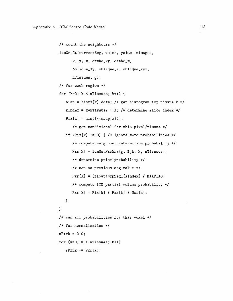
Appendix A. 1CM Source Code Kernel 113
/* count the neighbours *1
icmGetGx(currentSeg, xsize, ysize, nlmages,
x, y, z, ortho_xy, ortho_z,
oblique_xy, oblique_z, oblique_xyz,
nTissues, g);
1* for each region */
for (k0; k < nTissues; k++) {
hist = histV[kJ .data; 1* get histogram for tissue k *1
klndex = z*nTissues + k; 1* determine slice index */
Pix[k] = hist[*(srcp[z])];
1* get conditional for this pixel/tissue *1
if (Pix[k] 0) { 1* ignore zero probabilities */
/* compute neighbour interaction probability */
Nxr[kJ = icmGetNxrknx(g, Bjk, k, nTissues);
1* determine prior probability */
1* set to previous seg value */
Pxr[k] (float)*rpSegl[klndexj / MAXPIX8;
1* compute 1CM partial volume probability *1
Pxr [k] = Pix [k] * Pxr [k] * Nxr [k];
}
}
/* sum all probabilities for this voxel *1
/* for normalization *1
sPxrk = 0.0;
for (k0; k < nTissues; k++)
sPxrk += Pxr[k];
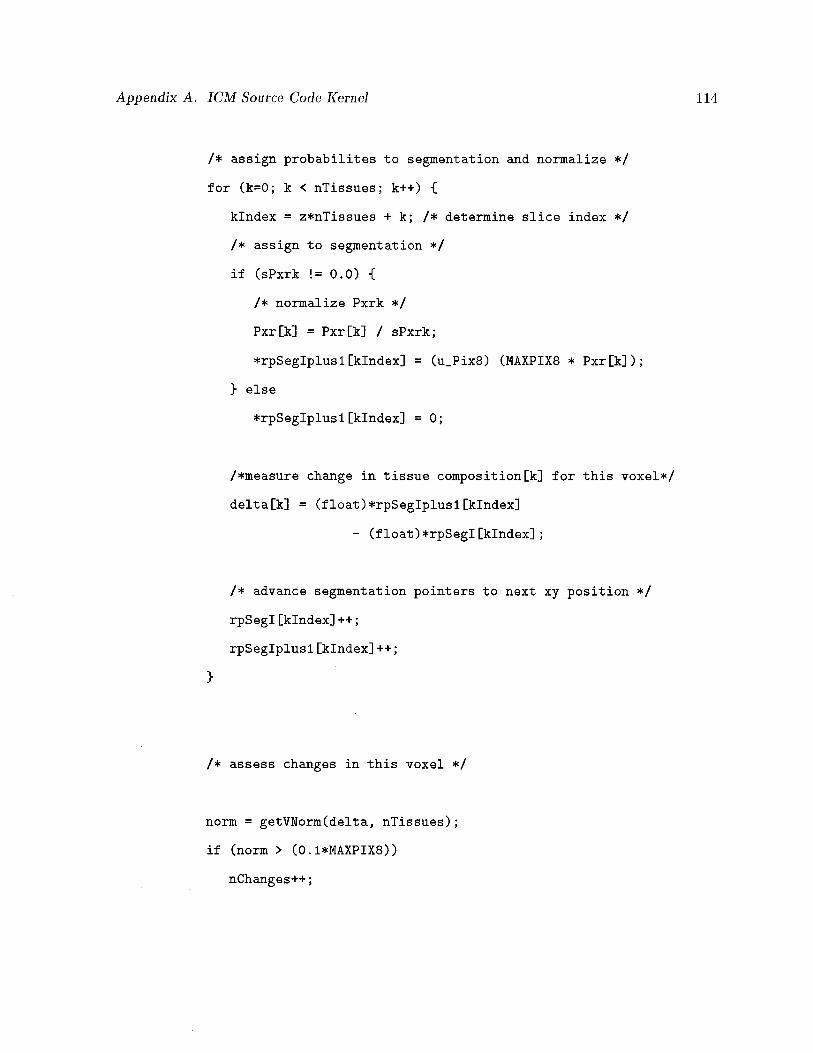
Appendix A. 1CM Source Code Kernel 114
/* assign probabilites to segmentation and normalize *1
for (k0; k < nTissues; k++) {
klndex = z*nTissues + k; /* determine slice index */
/* assign to segmentation *1
if (sPxrk 0.0) {
/* normalize Pxrk */
Pxr [k] = Pxr [k] / sPxrk;
*rpSeglplusl[klndex] = (u_Pix8) (MAXPIX8 * PxrLkJ);
} else
*rpSeglplusl[klndex] = 0;
/*measure change in tissue composition[k] for this voxel*/
delta[k] = (float) *rpSeglplusl [klndex]
- (float)*rpSegl[klndex];
1* advance segmentation pointers to next xy position *1
rpSegl [klndex] ++;
rpSeglplus 1 [klndex] ++;
}
1* assess changes in this voxel *1
norm = getVNorm(delta, nTissues);
if (norm > (O.1*MAXPIX8))
nChanges++;
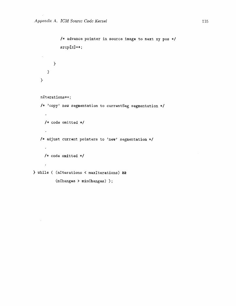
Appendix A. 1CM Source Code Kernel 115
1* advance pointer in source image to next xy pos *1
srcp [z] ++;
}
}
}
nIt erat ions++;
/* ‘copy’ new segmentation to currentSeg segmentation *1
/* code omitted */
/* adjust current pointers to ‘new’ segmentation */
/* code omitted */
} while ( (nlterations < maxlterations) &&
(nChanges > minChanges) );
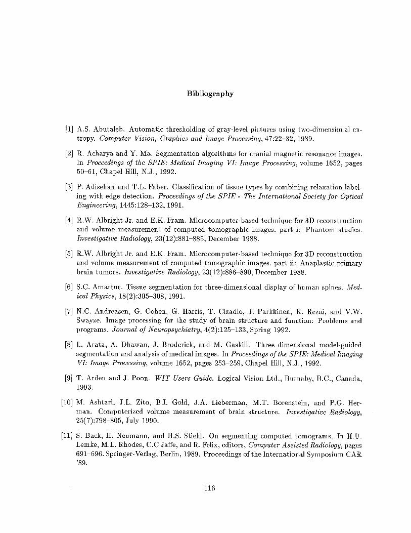
Bibliography
[1] A.S. Abutaleb. Automatic thresholding of gray-level pictures using two-dimensional entropy. Computer Vision, Graphics and Image Processing, 47:22—32, 1989.
[2] R. Acharya and Y. Ma. Segmentation algorithms for cranial magnetic resonance images.In Proceedings of the SPIE: Medical Imaging VI: Image Processing, volume 1652, pages50—61, Chapel Hill, N.J., 1992.
[3] P. Adisehan and T.L. Faber. Classification of tissue types by combining relaxation labeling with edge detection. Proceedings of the SPIE - The International Society for OpticalEngineering, 1445:128—132, 1991.
[4] R.W. Albright Jr. and E.K. Fram. Microcomputer-based technique for 3D reconstructionand volume measurement of computed tomographic images. part i: Phantom studies.Investigative Radiology, 23(12) :881—885, December 1988.
[5] R.W. Albright Jr. and E.K. Fram. Microcomputer-based technique for 3D reconstructionand volume measurement of computed tomographic images. part ii: Anaplastic primarybrain tumors. Investigative Radiology, 23(12):886—890, December 1988.
[6] S.C. Amartur. Tissue segmentation for three-dimensional display of human spines. Medical Physics, 18(2):305—308, 1991.
[7] N.C. Andreasen, G. Cohen, G. Harris, T. Cizadlo, J. Parkkinen, K. Rezai, and V.W.Swayze. Image processing for the study of brain structure and function: Problems andprograms. Journal of Neuropsychiatry, 4(2):125—133, Spring 1992.
[8] L. Arata, A. Dhawan, J. Broderick, and M. Gaskill. Three dimensional model-guidedsegmentation and analysis of medical images. In Proceedings of the SPIE: Medical ImagingVI: Image Processing, volume 1652, pages 253—259, Chapel Hill, N.J., 1992.
[9] T. Arden and J. Poon. WIT Users Guide. Logical Vision Ltd., Burnaby, B.C., Canada,1993.
[10] M. Ashtari, J.L. Zito, B.I. Gold, J.A. Lieberman, M.T. Borenstein, and P.G. Herman. Computerized volume measurement of brain structure. Investigative Radiology,25(7):798—805, July 1990.
[11] 5. Back, H. Neumann, and H.S. Stiehl. On segmenting computed tomograms. In H.U.Lemke, M.L. Rhodes, C.C Jaffe, and R. Felix, editors, Computer Assisted Radiology, pages691—696. Springer-Verlag, Berlin, 1989. Proceedings of the International Symposium CAR‘89.
116
Bibliography 117
[12] R.H.T. Bates, K.L. Garden, and T.M. Peters. Overview of computerized tomographywith emphasis on future developments. Proceedings of the IEEE, 71(3):356—372, March1983.
[13] M.D. Bentley and R.A. Karwoski. Estimation of tissue volume from serial tomographicsections: A statistical random marking method. Investigative Radiology, 23(10):742—747,October 1988.
[14] J. Besag. On the statistical analysis of dirty pictures. Journal of the Royal StatisticalSociety, 48(3):259—302, 1986.
[15] M. Bister, Y. Taeymans, and J. Cornelis. Automated segmentation of cardiac MR images. In Computers in Cardiology, pages 215—218, Long Beach, California, 1989. IEEEComputer Society.
[16] P. Bloch, R.E. Kenkinski, E.L. Buhle, R.H. Kendrix, M. Bryer, and W.G. McKenna. Theuse of t2 distribution to study tumor extent and heterogeneity in head and neck cancer.Magnetic Resonance Imaging, 9(2):205—211, 1991.
[17] J.Y. Boire, J.C. Cauvin, P. Cluzel, M. Lahellec, J. Maublant, M. Zanca, and A. Veyre.Segmentation methods for automatic kidney volume quantification in SPECT. Annual International Conference of the IEEE Engineering in Medicine and Biology Society,12(1):421—422, 1990.
[18] J.A. Broekhuijsen, S.C. Becker, and W. A. Barrett. Probabilistic segmentation of myocardial tissue by deterministic relaxation. In Computers in Cardiology, pages 99—102,Long Beach, California, 1989. IEEE Computer Society.
[19] E. Burghardt, H.M.H. Hofmann, G. Ebner, H. Haas, K. Tamussino, and E. Justich. Magnetic resonance imaging in cervical cancer: A basis for objective classification. GynecologicOncology, 33(1):61—67, April 1989.
[20] B. Chanda and D.D. Majumder. A note on the use of the gralevel co-occurrence matrixin threshold selection. Signal Processing, 15(2):149—167, September 1988.
[21] R. Chandra and H. Rusinek. Tissue volume determinations from brain MRI images, aphantom study. Proceedings of the SPIE - The International Society for Optical Engineering, 1445:133—143, 1991.
[22] P.C. Chen and T. Pavlidis. Image segmentation as an estimation problem. ComputerGraphics and Image Processing, 12:153—172, 1980.
[23] H.S. Choi, D.R. Haynor, and Y. Kim. Partial volume tissue classification of multichannel magnetic resonance images—a mixel model. IEEE Transaction on Medical Imaging,10(3):395—407, September 1991.
[24] R.P. Clark and M.R. Goff, editors. Recent Developmensts in Medical and PhysiologicalImaging. Taylor and Francis, London, 1986.
Bibliography 118
[25] H.E. Clime, W.E. Lorensen, R. Kikinis, and F. Jolesz. Three dimensional segmentation ofMR images of the head using probability and connectivity. Journal of Computer AssistedTomography, 14(6):1037—1045, 1990.
[26] H.E. Clime, W.E. Lorensen, S.F. Souza, F.A. Jolesz, R. Kikinis, G. Gerig, and T.E.Kennedy. 3D surface rendered MR images of the brain and its vasculature. Journal ofComputer Assisted Tomography, 15(2) :344—351, 1991.
[27] F.S. Cohen and D.B. Cooper. Simple parallel hierarchical and relaxation algorithms forsegmenting noncausal markovian random fields. IEEE Transactions on Pattern Analysisand Machine Intelligence, 9(22):195—219, March 1987.
[28] M.S. Cohen and R.M. Weisskoff. Ultra-fast imaging. Magnetic Resonance Imaging,9(1):1—37, 1991.
[29] D.L. Collins, T.M. Peters, W. Dai, and A.1C. Evans. Model based segmentation of individual brain structures from MRI data. In Proceedings of the SPIE: Visualization inBiomedical Computing 199, volume 1808, pages 10—23, Chapel Hill, N.J., 1992.
[30] S. Dellepiane, D.D. Giusto, C. Regazzoni, S.B. Serpico, and G. Vermazza. Interpretation oftomographic images via virtual-data fusion. In H.U. Lemke, M.L. Rhodes, C.C Jaffe, andR. Felix, editors, Computer Assisted Radiology, pages 697—701. Springer-Verlag, Berlin,1989. Proceedings of the International Symposium CAR ‘89.
[31] P.J. Ell. Single photon emission computed tomography of the brain. Journal of Neuroscience Methods, 34:207—217, 1990.
[32] N.T.S Evans. Combining imaging techniques. Clinical Physics and Physiological Measurement, 11(A):97—102, 1990.
[33] E.K. Fishman and et. al. Three-dimensional imaging. Radiology, 181:321—337, 1991.
[34] E.K. Fishman, D. Magid, D.R. Ney, J.E. Kuhlman, and A.F. Brooker. Three dimensionalimaging in orthopedics: State of the art 1988. Orthopedics, 11(7):1021—1026, July 1988.
[35] K.S. Fu and J.K. Mui. A survey on image segmentation. Pattern Recognition, 13:3—16,1981.
[36] E.S. Gelsema, H.F. Bao, A.W.M. Smeulders, and H.C. den Harink. Application of themethod of multiple thresholding to white blood cell classification. Computers in Biologyand Medicine, 18(2):65—74, 1988.
[37] S. Geman and D. Geman. Stochastic relaxation, gibbs distributions and the bayesianrestoration of images. IEEE Transactions on Pattern Analysis and Machine Intelligence,6(6):721—’741, November 1984.
[38] R. Gonzalez. Digital Image Processing. Addison-Wesley, Reading, MA, 2nd edition, 1987.
Bibliography 119
[39] W.M. Gregory, R.H. Reznek, M. Hallett, and M.L. Slevin. Using mathematical modelsto estimate drug resistance and treatment efficacy via CT scan measurements of tumourvolume. British Journal of Cancer, 62(4):671—675, October 1992.
[40] L.D. Griffin, A.C.F. Coichester, G.P. Robinson, and D.J. Hawkes. Structure-sensitivescale and the hierarchical segmentation of grey-level images. In Proceedings of the SPIE:Visualization in Biomedical Computing 199, volume 1808, pages 24—32, Chapel Hill,N.J., 1992.
[41] R.E. Gur, P.D. Mozley, S.M. Resnick, D. Shtasel, M. Kohn, R. Zimmerman, G. Herman, S. Atlas, Grossman R., R. Erwin, and R.C. Gur. Magnetic resonance imaging inschizophrenia: I. volumetric analysis of brain and cerebrospinal fluid. Archives of GeneralPsychiatry, 48:407—412, May 1991.
[42] R. Hallgren and N.P. Ta. Automated computation of cardiac ventricle volume fromtwo-dimensional MRI data. In TENCON ‘89: Fourth IEEE Region 10 InternationalConference 1989, pages 1015—1020, 1988.
[43] H. Handels and T. Tolxdorff. A new segmentation algorithm for knowledge acquisitionin tissue characterizing NMR-imaging. In H.U. Lemke, M.L. Rhodes, C.C Jaffe, andR. Felix, editors, Computer Assisted Radiology, pages 46—50. Springer-Verlag, Berlin,1989. Proceedings of the International Symposium CAR ‘89.
[44] Gabor T. Herman. Image Reconstruction From Projections: the Fundamentals of Computerized Tomography. Academic Press, San Fransisco, 1980.
[45] W.S. Hinshaw and A.H. Lent. An introduction to NMR imaging: from the bloch equationto the imaging equation. Proceedings of the IEEE, 71(3):338—350, March 1983.
[46] K.ll. Hohne and W. H. Hanson. Interactive 3D segmentation of MRI and CT volumesusing morphological operations. Journal of Computer assisted tomography, 16(2) :285—294,1992.
[47] S.L. Horowitz and T. Pavlidis. Picture segmentation by a tree traversal algorithm. Journal of the ACM, 23(2):368—388, 1976.
[48] S.L. Horowitz and T. Pavlidis. A graph theoretic approach to picture processing. Computer Graphics and Image Processing, 7:282—291, 1978.
[49] Robert A. Hummel and Steven W. Zucker. On the foundations of the relaxation labelingprocess. IEEE Transactions on Pattern Analysis and Machine Intelligence, 5:267—287,1983.
[50] C.R. Jack. Brain and cerebrospinal fluid volume: Measurement with MR imaging. Radiology, 178(1):22—24, January 1991.
[51] A.K. Jam. Fundamentals of Digital Image Processing. Prentice Hall, Englewood Cliffs,New Jersey, 1989.
Bibliography 120
[52] R.J. Jaszczak. Tomographic radiopharmaceutical imaging. Proceedings of the IEEE,76(9):1079—94, September 1988.
[53] T.L. Jernigan, S.L. Archibald, M.T. Berhow, E.R. Sowell, D.S. Foster, and J.R. Hesselink. Cerebral structure on MRI, part i: Localization of age-related changes. BiologicalPsychiatry, 29:55—67, 1991.
[54] T. Jiang and M.B. Merickel. Identification and boundary extraction of blobs in compleximagery. Computerized Medical Imaging and Graphics, 13(5):369—382, 1989.
[55] R.D. Jones and J.R. MacFall. Computers in magnetic resonance imaging. Computers inPhysics, 2(5):25—30, Sept-Oct 1988.
[56] T. Jones. Positron emission tomography. Clinical Physics and Physiological Measurement, 11(A):27—36, 1990.
[57] M. Kamber, D.L. Coffins, R. Shinghal, G.S. Francis, and A.C. Evans. Model-based 3Dsegmentation of multiple sclerosis lesions in dual-echo MRI data. In Proceedings of theSPIE: Visualization in Biomedical Computing 1992, volume 1808, pages 590—600, ChapelHill, N.J., 1992.
[58] J.N. Kaput, P.K. Sahoo, and A.K.C. Wong. A new method for gray-level picture thresholding using the entropy of the histogram. Computer Vision, Graphics and Image Processing, 29:273—285, 1985.
[59] N. Karssemeijer. Three dimensional stochastic organ models for segmentation in CTscans. In Proceedings of the SPIE: Biostereometrics ‘88—Fifth international meeting, volume 1030, pages 177—184, Chapel Hill, N.J., 1988.
[60] N. Karssemeijer, L.J.T.O. van Erning, and W.G.J. Eijkman. Recognition of organs inCT image sequences: A model guided approach. Computers and Biomedical Research,21:434—448, 1988.
[61] A. Kaufman, editor. Volume Visualization. IEEE Computer Society Press, New York,1991.
[62] G.J. Kavanagh, J.T. Kavanagh, B.K. Kavanagh, E. Irwin, A.C. Perkins, and L.A. Swanson. Automated volume determination of the liver and spleen from tc-99m colloid SPECTimaging: quantification of liver functional and nonfunctional tissue in disease. Clinical
• Nuclear Medicine, 15(7):495—500, 1990.
[63] P.J. Kelly. Computer assisted stereotactic biopsy and volumetric resection of pediatricbrain tumors. Neurologic Clinics, 9(2):317—336, May 1991.
[64] D.N. Kennedy, P.A. Filiped, and V.S. Caviness Jr. Anatomic segmentation and volumetric calculations in nuclear magnetic resonance imaging. IEEE Transactions on MedicalImaging, 8(1):1—7, March 1989.
Bibliography 121
[65] K.T. Kim, K.L. Black, D. Marciano, J.C. Mazziotta, B.H. Guze, S. Grafton, R.A.Hawkins, and D.P. Becker. Thaffium-201 SPECT imaging of brain tumours: Methodsand results. Journal of Nuclear Medicine, 31(6):965—968, June 1990.
[66] M.A. King, d.T. Long, and A.B. Brill. SPECT volume quantitation: influence of spatial resolution, source size and shape and voxel size. Medical Physics, 18(5):1016—1024,September—October 1991.
[67] G.F. Knoll. Single photon emission computed tomography. Proceedings of the IEEE,71(3):320—329, March 1983.
[68] M.I. Kohn, N.K. Tanna, G.T Herman, S.M. Resnick, P.D. Mosley, R.E. Gur, A. Alavi,R.A. Zimmerman, and R.C. Gur. Analysis of brain and cerebrospinal fluid volumes withMR imaging: Part i. methods, reliability and validation. Radiology, 178(1):115—122,January 1991.
[69] L. Kreel. Medical imaging. Postgraduate Medical Journal, 67:334—36, 1991.
[70] 0. Kubler and G. Gerig. Segmentation and analysis of multidimensional datasets inmedicine. In K.H. Hohne, H. Fuchs, and S. M. Pizer, editors, 3D Imaging in Medicine:Alogorithms, Systems, Applications, pages 63—82. Springer-Verlag, Berlin, 1990. NATOASI Series Volume 60.
[71] W.S. Kuklinski, G.S. Frost, and T. MacLaughlin. Adaptive textural segmentation ofmedical images. In Proceedings of the SPIE: Medical Imaging VI: Image Processing,volume 1652, pages 3 1—37, Chapel Hill, N.J., 1992.
[72] A. Kundu. Local segmentation of biomedical images. Computerized Medical Imaging andGraphics, 14(3):173—183, 1990.
[73] F. Lachmann and C. Barillot. Brain tissue classification from MRI data by means oftexture analysis. In Proceedings of the SPIE: Medical Imaging VI: Image Processing,volume 1652, pages 72—83, Chapel Hill, N.J., 1992.
[74] J.L. Lancaster and G.D. Fullerton. Physics and medicine: Imaging the body. Computersin Physics, 2(5):16—22, Sept-Oct 1988.
[75] K.H. Lee, H.T.H. Liu, D.C.P. Chen, M.E. Siegel, and S. Ballard. Volume calculationby means of SPECT: analysis of imaging acquisition and processing factors. Radiology,167(1):259—262, 1988.
[76] S.U. Lee and S.Y. Chung. A comparative performance study of several global thresholdingtechniques for segmentation. Computer Vision, Graphics and Image Processing, 52:171—190, 1990.
[77] Z. Liang, R. Jaszczak, and R. Coleman. Simultaneous reconstruction, segmentation andedge enhancement of relatively piecewise continuous images with intensity level information. Medical Physics, 18(3):394—401, May—June 1991.
Bibliography 122
[78] K.O. Lim and A. Phefferbaum. Segmentation of MR brain images into cerebrospinal fluidspaces, white and gray matter. Journal of Computer Assisted Tomography, 13(4):588—593,July/August 1989.
[79] D.T. Long, M.A. King, and B.C. Penney. 2D vs. 3D edge detection as a basis for volumequantitaion hi SPECT. In Information Processing in Medical Imaging, pages 457—471,1991.
[80] D.T. Long, M.A. King, and J. Sheehan. Comparative evaluation of image segmentationmethods for voluem quantitation in SPECT. Medical Physics, 19(2):483—489, March—April 1992.
[81] P. Lundin and G. Pedersen. Volume of pituitary macroadenomas: Assessment by MRI.Journal of Computer Assisted Tomography, 16(4):519—528, July/August 1992.
[82] C. MacAulay, T. Haluk, and B. Palcic. Adaptive color basis transformation: An aid inimage segmentation. Analytical and Quantitative Cytology and Histology, 11(1):53—58,1989.
[83] C. MacAulay and B. Palcic. A comparison of some quick and simple threshold selectionmethods for stained cells. Analytical and Quantitative Cytology and Histology, 10(2):134—138, 1988.
[84] C. MacAulay and B. Palcic. An edge relocation segmentation algorithm. Analytical andQuantitative Cytology and Histology, 12(3):165—171, 1990.
[85] P. Maeder, A. Wirsen, M Bajc, W. Schalen, H. Sjoholm, H. Skeidsvoll, S. Cronoqvist,and D. H. Ingvar. Volumes of chromis traumatic frontal brain lesions measured by MRimaging and CBF tomography. Acta Radiologica, 32:271—278, 1991.
[86] G.Q. Maguire, Jr., M.E. Noz, H. Rusinek, J. Jaeger, E.L. Kramer, J.J. Sanger, andG. Smith. Graphics applied to medical image registration. IEEE Computer Graphics andApplications, 11(2):20—8, March 1991.
[87] M.S. Mahaley, G.Y. Gillespie, and R. Hammett. Computerized tomography brain scantumor volume determinations: Sensitivity as an objective criterion of response to therapy.Journal of Neurosurgery, 72(6):872—878, June 1990.
[88] N.J. Mankivich, L.I. Rudin, G. Koepfler, J.M. Morel, and S. Osher. Application of a newpyramidal segmentation algorithm to medical images. In Proceedings of the SPIE: MedicalImaging VI: Image Processing, volume 1652, pages 23—30, Chapel Hill, N.J., 1992.
[89] Jose L. Marroquin. Deterministic Bayesian estimation of Markovian random fields withapplications to computational vision. London, England, June 1987. IEEE, Washington,DC.
[90] J. Mas, R.B. Younes, and R. Bidet. Improvement of quantification in SPECT studies byscatter and attenuation compensation. European Journal of Nuclear Medicine, 15:351—356, 1989.
Bibliography 123
[91] C. Mathieu, I.E. Magnin, and C. Baldy-Porcher. Optimal stochastic pyramid: Segmentation of MRI data. In Proceedings of the SPIE: Medical Imaging VI: Image Processing,volume 1652, pages 14—22, Chapel Hill, N.J., 1992.
[92] M.B. Merickel, J.W. Snell, T.R. Hackson, D.M Skyba, and W.K. Datz. Multispectraltissue identification in MR images. Annual International Conference of the IEEE Engineering in Medicine and Biology Society, 13(3):1323—1325, 1991.
[93] J.R. Mitchell, S.J. Karlik, D.H. Lee, and A. Fenster. Automated detection and quantification of multiple sclerosis lesions in MR volumes of the brain. hi Proceedings of theSPIE: Medical Imaging VI: Image Processing, volume 1652, pages 99—106, Chapel Hill,N.J., 1992.
[94] L. Mortelmans, J. Nuyts, G.V Pamel, V. van den Maegdenbergh, M. DeRoo, andP. Suetens. A new thresholding method for volume determination by SPECT. European Journal of Nuclear Medicine, 12:284—290, 1986.
[95] H.W. Muller-Gartner, J.M. Links, J.L. Prince, R.N. Bryan, E. McVeigh, J.P. Leal, C. Davatzikos, and J.J. Frost. Measurement of radiotracer concentration in brain gray matterusing positron emission tomography: MRI-based correction for partial volume effects.Journal of Cerebral Blood Flow and Metabolism, 12(4):571—583, 1992.
[96] K. Murase, S. Tanada, Y. Yasuliara, H. Mogami, A. flo, and K. Hamamoto. SPECTvolume measurement using an automatic threshold selection method combined with vfilter. European Journal of Nuclear Medicine, 54:21—25, 1989.
[97] J.A. Newell. Medical images and automated interpretation. Journal of Biomedical Engineering, 10:555—561, November 1988.
[98] R. Ohlander, K. Price, and D.R. Reddy. Picture segmentation using a region splittingmethod. Computer Graphics and Image Processing, 8:313—333, 1978.
[99] F. Pannizzo, M.J.B. Stallmeyer, J. Friedman, R.J. Jennis, J. Zabriskie, C. Pland, R. Zimmerman, J.P. Whalen, and P.T. Cahill. Quantitative MRI studies for assessment ofmultiple sclerosis. Magnetic Resonance in Medicine, 24:90—99, 1992.
[100] J. Parkkinen, G. Cohen, M. Sonka, and N. Andreasen. Segmentation of MR brain images. Annual International Conference of the IEEE Engineering in Medicine and BiologySociety, 13(1):71—72, 1991.
[101] D.W. Patey and D.K.B. Li. Interferon beta-lb is effective in relapsing-remitting multiplesclerosis. ii. MRI analysis results of a multicenter, randomized, double-blind, placebocontrolled trial. Neurology, 43:662—667, April 1993.
[102] T. Pavlidis. Algorithms for Graphics and Image Processing. Computer Science Press,Rockviile, MD, 1982.
Bibliography 124
[103] A.M. Peters. Recent advances and future projections in clinical radionudide imaging.The British Journal of Radiology, 63(750):411—429, June 1990.
[104] S.M. Pizer, T.J. Culup, and R.E. Fredericksen. Toward ineractive object definition in 3Dscalar images. In K.H. Hohne, H. Fuchs, and S. M. Pizer, editors, 3D Imaging in Medicine:Alogorithms, Systems, Applications, pages 83—106. Springer-Verlag, Berlin, 1990. NATOASI Series Volume 60.
[105] P. H. Pretorius, A. van Aswegen, C.P. Herbst, and M.G. Lotter. The effects of differentcorrection techniques on absolute volume determination with SPECT using a thresholdedge detection method. Medical Physics, 18(3):390—393, May—June 1991.
[106] S.S. Rajan, L. Tosa, J. Francisco, A. Muraki, M. Carvlin, and E. Tuturea. MRI characterization of 91 glioma in rat brain at 4.7 tesla. Magnetic Resonance Imaging, 8(2):185—90,1990.
[107] S.J. Riederer. Recent advances in magnetic resonance imaging. Proceedings of the IEEE,76(9):1095—1105, September 1989.
[108] R.A. Robb. Interactive display and analysis of 3D medical images. IEEE Transactionson Medical Imaging, 8(3):217—226, September 1989.
[109] A. Rosenfeld. Computer vision: A source of models for biological visual processes. IEEETransactions on Biomedical Engineering, 36(1):93—96, 1989.
[110] L.J. Rosner and S. Ross. Multiple Sclerosis. Simon and Schuster, New York, New York,1992.
[111] H. Rusinek, M.J. de Leon, A.E. George, L.A. Stylopoulos, R. Chandra, C. Smith, T. Rand,M. Mourino, and H. Kowaiski. Alzheimer disease: Measuring loss of cerebral gray matterwith MR imaging. Radiology, 178(1):109—114, January 1991.
[112] P.K. Sahoo, S. Soltani, and K.C. Wong. A survey of thresholding techniques. ComputerVision, Graphics, and Image Processing, 41:233—360, 1988.
[113] H. Samet. Region representation: Quadtrees from boundary codes. Communications ofthe ACM, 23(3):163—170, 1980.
[114] H. Samet. Neighbour finding techniques for images represented by quadtrees. ComputerGraphics and Image Processing, 18(1):37—57, 1982.
[115] H. Samet. The quadtree and related heirarchical data structures. Computing Surveys,16(2):187—235, 1984.
[116] H. Samet. Applications of Spatial Data Structures. Addison-Wesley, Reading, MA, 1990.
[117] T. Sandor, D. Metcalf, and Y. Kim. Segmentation of brain CT images using the conceptof region growing. International Journal of Biomedical Computing, 29:143—147, 1991.
Bibliography 125
[118] U. Schendel. Sparse Matrices—Numerical Aspects with Applications for Scientists andEngineers. Effis Horwood Limited, Chichester, 1989.
[119] M.E. Shenton, R. Kikinis, R.W. McCarley, D. Metcalf, J. Tieman, and F.A. Jolesz.Application of automated MRI volumetric measurement techniques to the ventricularsystem in schizophrenics and normal controls. Schizophrenic Research, 5:103—113, 1991.
[120] P.E. Shile, M.P. Chwialkowski, D. Pfeifer, R.W. Parkey, and R.M. Peshock. Atomatedidentification of the spine in magnetic resonance images: A reference point for automatedprocessing. In H.TJ. Lemke, M.L. Rhodes, C.C Jalfe, and R. Felix, editors, ComputerAssisted Radiology, pages 678—690. Springer-Verlag, Berlin, 1989. Proceedings of theInternational Symposium CAR ‘89.
[121] A. Simmons, S.R. Arridge, G.J. Barker, and P.S. Tofts. Segmentatin of neuroanatomyin magnetic resonance images. In Proceedings of the SPIE: Medical Imaging VI: ImageProcessing, volume 1652, pages 2—13, Chapel Hill, N.J., 1992.
[122] K.R. Smith and L.A. Kendrick. Bayesian computer vision methods for improved tumorlocalization and delineation. In Proceedings of the IEEE Medical Imaging Conference,pages 2140—2144, Santa Fe, 1991.
[123] R.A. Spangler. Computers in Medicine, chapter 6. Computer Science Press, Rockville,Md., 1987.
[124] P.G. Spetsieris, V. Dhawan, S. Takikawa, D. Margouleff, and D. Eidelberg. Imagingcerebral function. IEEE Computer Graphics and Applications, 13(1):15—26, January 1993.
[125] R.R. Stringham, W.A. Barrett, and D.C. Taylor. Probabilistic segmentation using edgedetection and region growing. In Proceedings of the SPIE: Visualization in BiomedicalComputing 1992, volume 1808, pages 40—51, Chapel Hill, N.J., 1992.
[126] M. R. Stytz, G. Frieder, and 0. Frieder. Three-dimensional medical imaging: Algorithmsand computer systems. ACM Computing Surveys, 23(4):421—499, 1991.
[127] H. Suzuki and J. Toriwaki. Automatic segmentation of head MRI images by knowledgeguided thresholding. Computerized Medical Imaging and Graphics, 15(4):233—240, Jul—Aug 1991.
[128] C.E. Swenberg and J.J. Conklin, editors. Imaging techniques in Biology and Medicine.Academic Press, San Diego, 1988.
[129] N.K. Tanna, M.I. Kohn, D.N. Horwich, P.R.Jolles, R.A. Zimmerman, W.M. Alves, andA. Alavi. Analysis of brain and cerebrospinal fluid volumes with MR imaging: Impacton PET data correction for atrophy: Partii. aging and alzheimer dementia. Radiology,178(1):123—130, January 1991.
[130] W.N. Tauxe, F. Soussaline, A. Todd-Pokropek, A. Cao, P. Collard, S. Richard, C. Raynaud, and T. Itti. Determination of organ volume by single photon emission tomography.Journal of Nuclear Medicine, 23(11):984—987, 1982.
Bibliography 126
[131] W. Tsai. Moment-preserving thresholding: A new approach. Computer Vision, Graphicsand Image Processing, 29:377—393, 1985.
[132] J.K. Udupa, S. Samarasekera, and W.A. Barrett. Boundary detection via dynamic programming. In Proceedings of the SPIE: Visualization in Biomedical Computing 1992,volume 1808, pages 33—39, Chapel Hill, N.J., 1992.
[133] P.E. Undrill. Computer Techniques in Clinical Medicine, chapter 8. Butterworth & Co.Ltd, London, 1985.
[134] M.W. Vannier. Computers in computer axial tomography. Computers in Physics,2(5):39—43, Sept-Oct 1988.
[135] K.L. Vincken, A.S.E. Koster, and M.A. Viergever. Probabilistic multiscale imagesegmentation—set-up and first results. In Proceedings of the SPIE: Visualization inBiomedical Computing 1992, volume 1808, pages 63—77, Chapel Hill, N.J., 1992.
[136] J.W. Wallis and T.R. Miller. Volume rendering in three-dimensional display of SPECTimages. Journal of Nuclear Medicine, 31(8):1421—1428, August 1990.
[137] J.W. Wallis and T.R. Miller. Three-dimensional display in nuclear medicine and radiology.The Journal of Nuclear Medicine, 32(3):534—546, March 1991.
[138] K. Wechsler-Jentzsen, J.H. Witt, C.R. Fitz, D.C. McCullough, and L.H. Harisiadis. Unresectable gliomas in children: Tumor-volume response to radiation therapy. Radiology,169(1):237—242, October 1988.
[139] H.K. Wijrdeman and C.J.G. Bakker. Multiple slice MR imaging as an aid in radiotherapy of carcinoma of the cervix uteri: A case report. Strahlentherapie und Onkologie,164(1):44—47, 1988.
[140] D.M. Wilbert, K.J. Klose, P. Alken, G.H. Jacobi, and R. Hohenfeilner. Tumor volume,CT scan, lymphography, sonography, intravenous pyelography, and tumor markers intestis tumors. Urologia Internationalis, 44(1): 15—19, 1989.
[141] D. Wiffiams, P. Bland, L.Liu, L. Farjo, I.R. Francis, and C.R. Meyer. Liver-tumourboundary detection: Human observer vs. computer edge detection. Investigative Radiology, 24(10):768—775, October 1989.
[142] J. Yla-Jaaski and 0. Kubler. Segmentation and analysis of 3D volume images. In Proceedings of the International Conference on Pattern Recognition 1988, pages 951—953,1988.
[143] T.Y. Young and K.S. Pu. Handbook of Pattern Recognition and Image Processing. Academic Press, Inc., Orlando, FL, 1986.
[144] S. Zucker, R. Hummel, and A. Rosenfeld. An application of relaxation labeling to lineand curve enhancement. IEEE Transactions on Computing, 26:394—403, 922—929, 1977.

Bibliography 127
[145] T.D. Zuk. The registration of multimodality medical scans. Master’s thesis, The University of British Columbia, Computer Science Department, Vancouver, B.C., October1993.