Three-dimensional instantaneous mantle flow induced by subduction

C. Piromallo(1), T.W. Becker(2), F. Funiciello(3) and C. Faccenna(3)

(1) Istituto Nazionale di Geofisica e Vulcanologia, Rome, Italy

(2) Dep. of Earth Sciences, University of Southern California, Los Angeles, USA

(3) Dip. Scienze Geologiche, Universita’ degli Studi “Roma TRE”, Rome, Italy

Abstract

We conduct three-dimensional subduction experiments using a finite element approach to study

flow around slabs, which are prescribed based on a transient stage of upper mantle subduction

from a laboratory model. Instantaneous velocity field solutions are examined with a particular

focus on the toroidal vs. poloidal components as a function of boundary conditions, plate width,

and viscosity contrast between slab and mantle. We show how the slab-to-mantle viscosity ratio

determines the strength of toroidal flow, and find that the toroidal flow component peaks for

slab/mantle viscosity ratios ~100, independent of slab width or geometry.

1. Introduction

Insight into subduction and related mantle circulation has been gained by comparison of natural

observables with predictions from analytical, numerical and laboratory models. Using two-

dimensional (2-D) models, corner flow theory [e.g. Tovish et al., 1978] evolved into models that

explore, e.g., the sensitivity of subduction and induced mantle flow to trench migration [e.g.

Garfunkel et al., 1986; Zhong and Gurnis, 1996; Christensen, 1996; Kincaid and Sacks, 1997;

Enns et al., 2005]. However, seismic anisotropy studies indicate that moving trench systems are

complex three-dimensional environments [e.g. Russo and Silver, 1984; Smith et al., 2001], where

a simple 2-D approximation fails. Full 3-D modelling is computationally challenging, and even

inherently 3-D laboratory models have long been intentionally constrained to quasi 2-D [e.g.

Kincaid and Olson, 1987; Guillou-Frottier et al., 1995]. More recent laboratory models allow for

fully 3-D, kinematically prescribed [Buttles and Olson, 1998; Kincaid and Griffiths, 2003, 2004],

or dynamically self-consistent [Funiciello et al., 2003, 2004a, 2006; Schellart, 2004; Bellahsen

et al., 2005] trench migration, representing a significant advance for a comprehensive study of

mantle circulation. These works highlight the importance of the toroidal vs. poloidal mantle flow

components during trench migration, but the intrinsic experimental limitations of a laboratory

model restrict quantitative analysis.

Thus, we model the 3-D instantaneous mantle velocity field induced by a free slab using the

finite element approach of Moresi and Solomatov [1995] and Zhong et al. [2000] and a

prescribed slab density and shape based on an intermediate stage of a laboratory subduction

model [Funiciello et al., 2006]. Numerical modelling of 3-D flow has previously addressed

several related issues, including the effect of lateral strength variation of slabs [Moresi and

Gurnis, 1996] and plates [Zhong and Davies, 1999] on geoid anomalies; the role of faults,

rheology and viscosity for plate generation [Zhong et al., 1998]; and the effects of lateral

variations in viscosity on deformation and flow in subduction zones [Billen and Gurnis, 2003;

Funiciello et al. 2004b; Stegman et al., in press]. Here we focus on the instantaneous mantle

flow induced by subduction, and explore the characteristic flow pattern of a 3-D versus a 2-D

setting, the role of boundary conditions, plate width, and viscosity contrasts between slab and

mantle.

2. Numerical method and model set up

The convection problem is solved using a regional version, regcitcom, of the 3-D finite

element code CitcomS [Moresi and Solomatov; 1995; Zhong et al., 2000; Tan et al., 2002].

CitcomS solves the conservation equations for mass, momentum and energy in the Boussinesq

approximation, assuming that the mantle is an incompressible viscous medium [see Zhong et al.,

2000, for details]. A slab shape with constant temperature contrast is assigned from a selected

transient stage of a reference laboratory model [Funiciello et al., 2006], in which the slab tip

reaches ~half the box depth. The numerical domain reproduces the one adopted in the laboratory

model and is 7.4×7.4×1 in x, y, z directions respectively, representing a box that is roughly 4900

km wide and 660 km deep. Therefore, one non-dimensional length unit scales to 660 km. The

slab thickness is 0.15, corresponding to ~100 km. Resolution is 384×384 elements in the

horizontal and 48 in the vertical direction; the convergence of the numerical solution was tested

by doubling the resolution, and velocity variations were less than 5%. We assign a constant

density contrast to the slab which scales absolute velocities along with the background viscosity

akin to a Stokes’ sinker. All viscosities are Newtonian and constant within the slab and mantle;

slab viscosities are chosen as 1, 10, 50, 102, 5·102, 103, and 104 times the mantle viscosity. In

nature, power-law rheologies and lateral viscosity contrasts will clearly change the details of

mantle flow [e.g. Billen and Hirth, 2005] but we expect the general insights into the dominant

controls on the velocity field to remain valid. We study the instantaneous flow field solution for

models with free-slip and no-slip boundary conditions (BCs) at lateral and bottom sides (the

surface is always free-slip), to explore both end-member cases and to be able to compare with

the laboratory setup, which is no-slip.

3. 2-D versus 3-D

We show here results for models with a viscosity contrast of η'=104 between slab and mantle,

directly comparable to the parameters of the laboratory models. We approximate the 2-D setting

by a slab extending laterally for the whole box width (‘laterally constrained’ configuration sensu

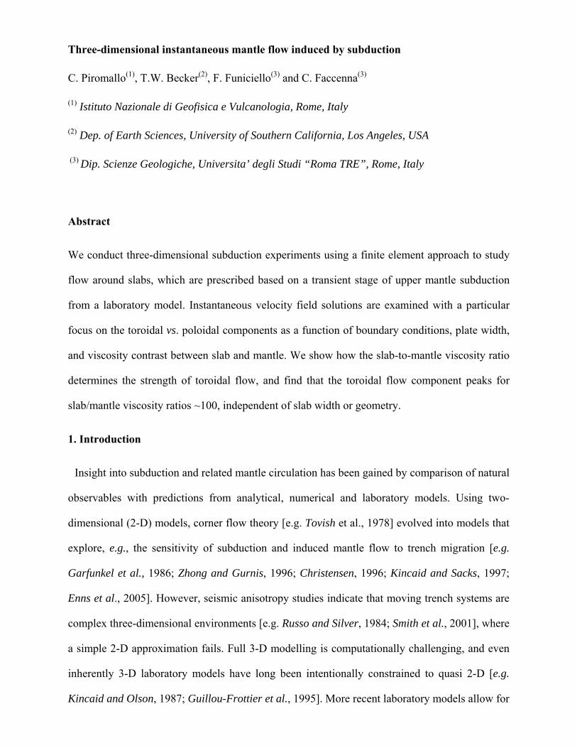
Funiciello et al., 2004a). In 2-D (Fig. 1a) the flow is obviously confined in the vertical plane

where we observe the characteristic subduction velocity pattern [cf. Garfunkel et al., 1986]; in

the case of retrograde slab migration, a poloidal cell of return flow exists beneath the slab tip.

“Trench suction” is responsible for back-arc motion towards trench, thus generating extension in

the back arc region, then upward flow in front of the slab.

In Fig. 1b-c we show a 3-D model with slab width w=1.85 (i.e. 0.25 the box width). Return

flow in the vertical plane along the slab centerline is again observed, but it is characterized by

less vigorous circulation under the slab tip (Fig.1b) with respect to the 2-D case (Fig.1a); the

return flow (vx component) below the slab tip is reduced by ~ 75%. This is due to the fact that

mantle material is now allowed to move around the slab lateral edges, in response to both

verticalization and roll-back of the free slab in this transient stage, as also observed in laboratory

models [e.g. Kincaid and Griffiths, 2003; Funiciello et al., 2006]. On a horizontal plane located

at sub-lithospheric depth (Fig. 1c), this toroidal flow component describes symmetrical cells at

the slab edges. In addition, we observe positive vertical velocities (red-upward directed), not

only in front of the slab, but also close to its lateral edges, due to the extrusion of mantle material

from below the inclined slab.

Overall velocity patterns match those of the corresponding laboratory models [Funiciello et

al., 2006], whose streamlines are superimposed on the velocity fields of Fig.b-c for an initial,

qualitative comparison. Note for example the good match of the return flow cell below the slab

tip and around its lateral edge, as well as the uplifted streamlines in the wedge. Discrepancies are

likely due to surface boundary conditions, which are free surface in the laboratory and free-slip

in the numerical models; they may also be caused by methodological difficulties in determining

the velocity field, such as in the case of the vortex underneath the slab. We consider the match

between lab and numerics encouraging, and quantitative comparisons will be the subject of a

future study.

4. Role of plate width

Fig. 2 shows profiles of horizontal velocities vx across the slab (profile BB’ on Fig. 1c) for different

slab width w (1/16<w<1/3 of the box width) and BCs. These profiles summarize the characteristics

of the horizontal return flow in terms of geometry. In front of the slab (y'<0, where y'=y-w/2) vx

increases with w up to w~1 and then decreases for larger slab widths. This is also the case for

maximum vertical velocities (not shown here), indicating that in this area, the velocity is controlled

by the box-height in the transient stage. Outside the slab (y'>0) vx increases with w showing that

larger slabs trigger horizontal return flow with larger velocities. The characteristic length-scale

associated with this arctan-like velocity increase is ~1/3 the box height for all free-slip cases.

No-slip BCs have an overall damping effect on the velocity, as expected (Fig. 2b). The return

flow transition-length, where vx=0 and flow changes opposite direction, depends on w. Moreover, the

return flow is more confined to the slab edge compared to the free-slip case.

5. Role of viscosity contrast

For no lateral viscosity variations, the slab induced flow is similar to that of a Stokes’ sinker;

increasing η' causes the mantle to flow around the slab edges with a toroidal pattern on a

horizontal plane (Fig. 1c). On a vertical plane through the slab centerline we also observe a

dominant component in the negative x-axis direction (Fig. 1b), which fades away when

decreasing the viscosity contrast η'. In order to quantify the flow characteristics we decompose

velocities into toroidal and poloidal components [e.g. Bercovici, 1993]. Following Tackley

[2000], the 2-D velocities on each individual horizontal layer are expressed as the sum of an

irrotational and a divergence-free field. We solve Poisson’s equation for the poloidal and toroidal

potentials and set their gradient or value to zero on the boundaries for free-slip or no-slip cases,

respectively. The vertical velocity component vz is added to the poloidal field. The rms of

poloidal and toroidal velocities, RMSvpol and RMSvtor, is computed for each layer, and then

summed over the layers for the total toroidal/poloidal ratio (TPR), given as

TPR=1 1

N N

tor poli i

RMSv RMSv= =∑ ∑ , where N is the number of layers.

Fig. 3a shows the TPR as a function of viscosity contrast η', for free-slip BCs and fixed

buoyancy contrast. Note that the TPR increases with η', ranging from ~0.2 (η'=10) to ~0.7

(η'=104), nearly independent of slab width. This trend is due to the combined effect of the

poloidal and toroidal components as the flow becomes more similar to that of a rigid sinking

body. The poloidal component, as well as absolute maximum velocities, decrease monotonically

for increasing η' (Fig. 3c), because stiffer slabs suffer from more viscous dissipation. The

toroidal component instead increases up to η'~102 and decreases for larger contrasts (Fig. 3b).

This peak in toroidal flow is likely due to the interplay between induced toroidal motion (which

becomes significant once viscosity contrasts are larger than ~10) and increased slab bending

resistance (which tends to inhibit motions, as also seen for the poloidal component). Although

the TPR is nearly independent of w, wider slabs have larger poloidal and toroidal terms due to

their higher negative buoyancy and ability to laterally displace material. No-slip cases show very

similar trends, though the maximum TPR is reduced to ~40% with respect to 70% for the free-

slip case.

To evaluate the role of transients in our models, we conducted similar experiments for a fully

developed, steady-state roll-back stage which shows similar, though more vigorous, horizontal

flow patterns, again in agreement with Funiciello et al. [2006]. While toroidal and poloidal flow

are stronger in amplitude for steady-state subduction, the toroidal strength shows a similar peak

around η'tmax ~102, and the TPR as a function of η' is within 10% of that of the transient stage

presented here.

6. Discussion and conclusions

From our 3-D modeling, we are able to quantify the importance of the large scale toroidal

flow component in the horizontal plane, triggered in the mantle by the motion of a stiff, free slab.

Since we focus on a transient subduction stage where the slab tip reaches halfway the box

bottom, the flow pattern we observe is the result of both slab verticalization and roll-back

motion. The presence of the toroidal component plays a key role in affecting the geometry of

circulation in the vertical plane, compared to the 2-D case. In particular, the 3-D approach shows

that the material resumed at the surface in the back-arc wedge by the return flow cell below the

slab tip is minimal with respect to 2-D models [Tovish et al., 1978], in agreement with

laboratory modeling [Funiciello et al., 2006]. Furthermore, we observe that circulation around

the slab is characterized by a non-negligible upward flow component close to its sides (Fig. 1c),

that could have important implications to interpret local tectonic structure at slab edges.

In our models of a transient subduction stage, the characteristic spatial length-scale influencing

the flow pattern is the box height. These models are closed at 660 km, rather than using a deeper box

with an increase in viscosity, which might have an effect on the poloidal circulation and

characteristic length-scales of the flow. Moreover, we show that BCs, besides the expected effect of

damping/enhancing the flow velocities, also affect the flow pattern. In particular, in proximity of the

slab the flow is similar for no- and free-slip BCs, while strong variations in the flow field exist

elsewhere, as expected for a Stokes problem. Therefore, laboratory models can only be

considered a good approximation to numerical models, which are typically free-slip, if we

restrict our observations close to the slab. In nature, of course neither no-, nor free-slip boundary

conditions apply, but the larger scale regional setting has to be considered.

By modelling different viscosity contrasts between slab and mantle, we show that significant

return flow around edges can only be obtained for stiff slabs. This is comparable with results by

Kincaid and Griffths [2003], who discussed return flow as a function of prescribed trench

rollback, for a rigid plate (the end member, η' =∞). Here, we obtain similar flow patterns for a

slab that sinks freely into the mantle. Moreover, we find that the strength of the TPR increases

with η', nearly independent of slab width. This relationship is affected by the lateral BCs and

might be modified for time-dependent subduction, where we expect a more prominent

dependence on w [Stegman et al., 2006]. We observe that for η'≥103 the toroidal flow

components make up ~60-70% of the poloidal ones, while we estimate ~40-50% for lower

viscosity contrasts (η'~102). We find that the toroidal component peaks for slab/mantle viscosity

ratios η'tmax of ~ 102 for our models, independent of slab w. This trend is found not only for

transient but also for steady-state, rollback subduction. Estimates for effective η' viscosity

contrasts in nature are comparable to, or somewhat higher than η'tmax [Conrad and Hager, 1999;

Becker et al., 1999]. We suggest that future modelling should explore regional settings where the

slab shape can be inferred (e.g. from tomography) and the toroidal flow estimated (e.g. from

shear wave splitting), in order to constrain the effective slab/mantle viscosity ratio from the TPR.

Numerical models can be easily quantitatively explored and compared with the velocity field

from laboratory models as analyzed by feature tracking [e.g. Funiciello et al., 2006]. Here, our

comparison has to remain qualitative, but future efforts will be useful to understand, in

particular, the role of mechanical surface boundary conditions for issues such as roll-back.

Acknowledgments. We thank all authors that contributed to the development of CitcomS,

GeoFramework.org for making the source code available, and B. Kaus, M. Moroni, D. Stegman

and an anonymous reviewer for valuable comments. Some figures were created using Generic

Mapping Tools [Wessel and Smith, 1998], and this study was partly funded by grants MIUR-

FIRB RBAU01JMT3 and NSF-EAR0409373. Some of the computation for the work described

in this paper was supported by the University of Southern California Center for High

Performance Computing and Communications (www.usc.edu/hpcc).

References

Becker, T. W., C. Faccenna, R. J. O’Connell, and D. Giardini, The development of slabs in the

upper mantle: Insights from numerical and laboratory experiments, J. Geophys. Res., 104(B7),

15,207–15,226, 1999.

Bercovici, D., A simple model of plate generation from mantle flow, Geophys. J. Int., 114, 635-

650, 1993.

Bellahsen, N., C. Faccenna, and F. Funiciello, Dynamics of subduction and plate motion in

laboratory experiments: insights into the "plate tectonics" behavior of the Earth, J. Geophys.

Res., 110 (B01401), doi:10.1029/2004JB002999, 2005.

Billen, M.I., M. Gurnis, and M. Simons, Multiscale dynamics of the Tonga-Kermadec

subduction zone, Geophys. J. Int., 153 (2), 359-388, 2003.

Billen, M. I. and Hirth, G., Newtonian verse non-Newtonian upper mantle viscosity: implications

for subduction initiation. Geophys. Res. Lett., 32, doi:10.1029/2005GL023457, 2005.

Buttles, J., and P. Olson, A laboratory model of subduction zone anisotropy, Earth Planet. Sci.

Lett., 164 (1-2), 245-262, 1998.

Conrad, C. P. and Hager, B. The effects of plate bending and fault strength at subduction zones

on plate dynamics, J. Geophys. Res., 104, 17,551 – 17,571, 1999.

Christensen, U.R.. The influence of trench migration on slab penetration into the lower mantle,

Earth Planet. Sci. Lett., 140, 27-39, 1996.

Enns, A., T.W. Becker, H. Schmeling, The dynamics of subduction and migration for viscosity

stratification, Geophys. J. Int.,160, 761-775, 2005.

Funiciello, F., C. Faccenna, D. Giardini, and K. Regenauer-Lieb, Dynamics of retreating slabs

(part 2): Insights from 3D laboratory experiments, J. Geophys. Res., 108 (B4), 2003.

Funiciello, F., C. Faccenna, and D. Giardini, Role of Lateral Mantle Flow in the Evolution of

Subduction System: Insights from 3-D Laboratory Experiments., Geophys. J. Int., 157, 1393-

1406, 2004a.

Funiciello, F., C. Piromallo, M. Moroni, Becker, T., Faccenna, C., Bui, H. A. and Cenedese, A.,

3-D Laboratory and Numerical Models of Mantle Flow in Subduction Zones, Eos Trans. AGU,

85(47), Fall Meet. Suppl., Abstract T21B-0527, 2004b.

Funiciello, F., M. Moroni, C. Piromallo, C. Faccenna, A. Cenedese, H.A. Bui, Mapping flow

during retreating subduction: laboratory models analyzed by Feature Tracking, J. Geophys.

Res., (in press), 2006.

Garfunkel, Z., D.L. Anderson, and G. Schubert, Mantle circulation and lateral migration of

subducting slabs, J. Geophys. Res., 91, 7205-7223, 1986.

Guillou-Frottier, L., J. Buttles, and P. Olson, Laboratory experiments on structure of subducted

lithosphere, Earth Planet. Sci. Lett., 133, 19-34, 1995.

Kincaid, C., and R.W. Griffiths, Laboratory models of the thermal evolution of the mantle during

rollback subduction, Nature, 425, 58-62, 2003.

Kincaid, C., and R. W. Griffiths, Variability in flow and temperatures within mantle subduction

zones, Geochem. Geophys. Geosyst., 5, Q06002, doi:10.1029/2003GC000666, 2004.

Kincaid, C., and P. Olson, An experimental study of subduction and slab migration, J. Geophys.

Res., 92, 13832-13840, 1987.

Kincaid, C., and I.S. Sacks, Thermal and dynamical evolution of the upper mantle in subduction

zones, J. Geophys. Res., 102 (B6), 12295-12315, 1997.

Moresi, L., and M. Gurnis, Constraints on the lateral strength of slabs from three-dimensional

dynamic flow models, Earth Planet. Sci. Lett., 138, 15-28, 1996.

Moresi, L., and V.S. Solomatov, Numerical investigation of 2D convection with extremely large

viscosity variation, Phys. Fluid., 7, 2154-2162, 1995.

Russo, R.M., and P.G. Silver, Trench-parallel flow beneath the Nazca plate from seismic

anisotropy, Science, 263 (5150), 1105-1111, 1994.

Schellart, W.P., Kinematics of subduction and subduction-induced flow in the upper mantle, J.

Geophys. Res., 109 (B7), B07401, 2004.

Smith, G.P., D.A. Wiens, K.M. Fischer, L.M. Dorman, S.C. Webb, and J.A. Hildebrand, A

complex pattern of mantle flow in the Lau backarc, Science, 292, 713-716, 2001.

Stegman, D.R., J. Freeman, W.P. Schellart, L. Moresi and D.A. May, Influence of trench width

on subduction hinge retreat rates in 3-D models of slab roll-back, G3, in press, 2006.

Tackley, P.J., Self-consistent generation of tectonic plates in time-dependent, three-dimensional

mantle convection simulations, 1, Pseudoplastic yielding, G3, 1 (20000GC000036), 2000.

Tan, E., M. Gurnis, and L. Han, Slabs in the lower mantle and their modulation of plume

formation, Geochem. Geophys. Geosyst., 3(11), 1067, doi:10.1029/2001GC000238, 2002.

Tovish, A., G. Schubert, and B.P. Luyendyk, Mantle flow pressure and the angle of subduction:

non-Newtonian corner flows, J. Geophys. Res., 83 (B12), 5892– 5898, 1978.

Wessel, P., and W.H.F. Smith, New, improved version of Generic Mapping Tools released

[version 3.1], Eos Trans. AGU 79, 1998.

Zhong, S., and M. Gurnis, Interaction of weak faults and non-Newtonian rheology produces

plate tectonics in a 3D model of mantle flow, Nature, 383, 245-247, 1996.

Zhong, S., M. Gurnis, and L. Moresi, Role of faults, nonlinear rheology, and viscosity structure

in generating plates from instantaneous mantle flow models, J. Geophys. Res., 103 (B7),

15255-15268, 1998.

Zhong, S., and G.F. Davies, Effects of plate an slab viscosities on the geoid, Earth. Planet. Sci.

Lett., 170, 487-496, 1999.

Zhong, S., M.T. Zuber, L.N. Moresi, and M. Gurnis, Role of temperature-dependent viscosity

and surface plates in spherical shell models of mantle convection, J. Geophys. Res., 105,

11,063-11,082, 2000.

Figure captions

Figure 1. Velocity for models with η'=104, no-slip BCs at lateral and bottom sides, free-slip at

surface. All dimensions are normalized to the box depth. Side view on a vertical plane through

the slab centerline in the a) 2-D case, and b) 3-D case, slab width w=1.85. Arrows represent

velocity vectors projected onto the y-z plane. c) Map view (3-D case) on a horizontal plane cross-

cutting at sub-lithospheric depth z = 0.21 (~1.5 times the slab thickness). Here we show only half

box, given the mirror symmetry of the models along the mid-plane perpendicular to the trench.

Grey-shaded rectangle is the plate at the surface, while the outlined rectangle is the slab

intersection with the horizontal plane at z = 0.21. Arrows represent velocity vectors projected

onto the x-y cutting plane, color plot gives the magnitude of the vertical component of velocity.

Arrows in the vertical plane are reduced by a factor of two with respect to those in the horizontal

plane for plotting reasons. Non-dimensional velocities need to be multiplied by a factor of ~ 0.17

cm/yr to get the corresponding values in nature, assuming 1021 Pa·s as reference viscosity.

Streamlines of the corresponding laboratory model [Funiciello et al., 2006] are represented on

both side and map views as dashed lines.

Figure 2. Velocity component vx along profile BB’, parallel to y-axis and centred at x=0, through

the horizontal layer of Fig. 1c. Curves are related to models with η' = 102 and different slab

width w, a) with free-slip and b) no-slip BCs. The y-coordinate is shifted by the slab half-width

(y’=y-w/2) to ease comparison of different models. Non-dimensional velocities need to be

multiplied by a factor of ~4.22 cm/yr to get the corresponding values in nature, assuming 1021

Pa·s as reference viscosity.

Figure 3. a) Total Toroidal/poloidal ratio (TPR), b) toroidal and c) poloidal components

computed following Tackley [2000] as a function of viscosity contrast η' (see text for details).

Each curve is related to a slab of different width w. Free-slip BC at side and bottom boundaries.

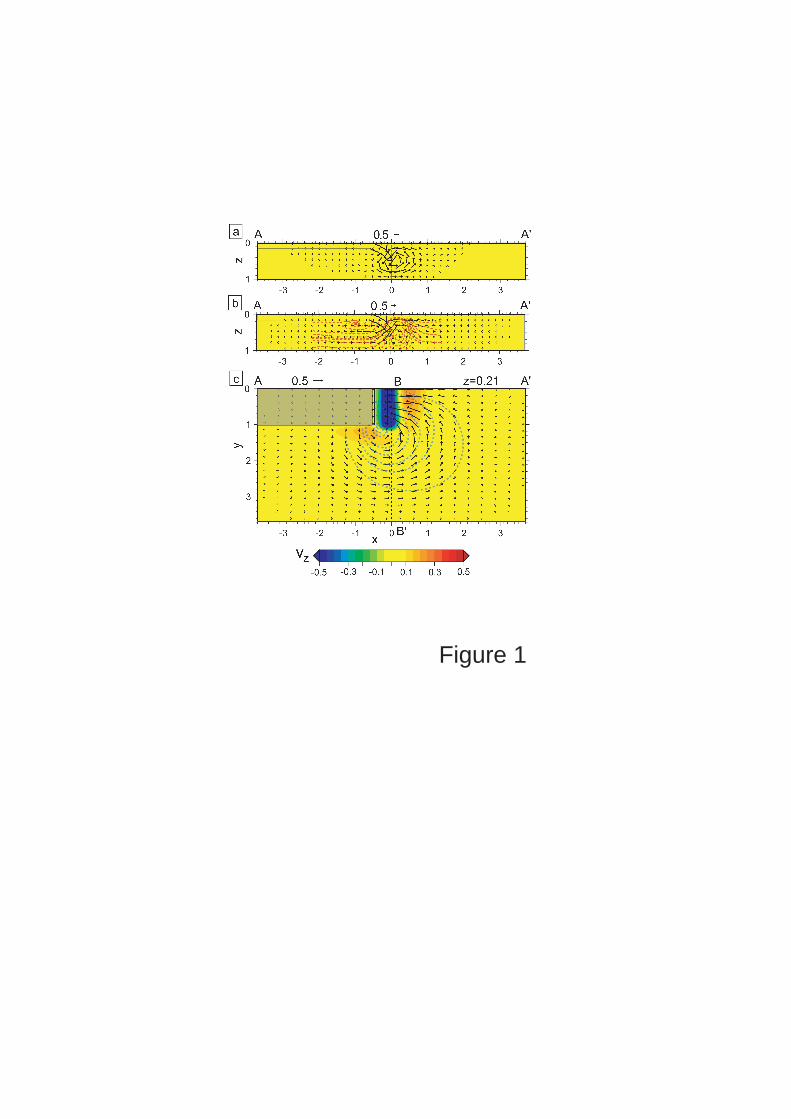
Figure 1

-0.8

-0.6

-0.4

-0.2

0

0.2

0.4

V x

y’=y-w/2

Free-slip η'=100

w=2.78w=1.85w=0.93w=0.46

-0.8

-0.6

-0.4

-0.2

0

0.2

0.4

y’=y-w/2

No-slip

Figure 2

η'=100a b

w=2.78w=1.85w=0.93w=0.46

-3 -2 -1 0 1 2 3 -3 -2 -1 0 1 2 3

Figure 3

0

0.2

0.4

0.6

0.8

1

1 10 100 1000 10000

TPR

w=0.46w=0.93w=1.85w=2.78

0

0.5

1

1.5

2

1 10 100 1000 10000

toro

idal

0

2

4

6

8

10

1 10 100 1000 10000

polo

idal

a

b

c

η'

w=0.46w=0.93w=1.85w=2.78

w=0.46w=0.93w=1.85w=2.78