Three-Dimensional Deconvolution of Wide FieldMicroscopy with Sparse Priors: Application to

Zebrafish ImageryBo Dong, Ling Shao

Department of Electronic andElectrical Engineering

The University of SheffieldEmail: bdong2@sheffield.ac.uk,

ling.shao@sheffield.ac.uk

Alejandro F FrangiDepartment of Mechanical Engineering

The University of SheffieldEmail: a.frangi@sheffield.ac.uk

Oliver Bandmann, Marc Da CostaDepartment of NeuroscienceThe University of Sheffield

Email: o.bandmann@sheffield.ac.uk,m.dacosta@sheffield.ac.uk

Abstract—Zebrafish, as a popular experimental model or-ganism, has been frequently used in biomedical research. Forobserving, analysing and recording labelled transparent featuresin zebrafish images, it is often efficient and convenient to adoptthe fluorescence microscopy. However, the acquired z-stack im-ages are always blurred, which makes deblurring/deconvolutioncritical for further image analysis. In this paper, we propose aBayesian Maximum a-Posteriori (MAP) method with the sparseimage priors to solve three-dimensional (3D) deconvolution prob-lem for Wide Field (WF) fluorescence microscopy images fromzebrafish embryos. The novel sparse image priors include a globalHyper-Laplacian model and a local smooth region mask. Thesetwo kinds of prior are deployed for preserving sharp edges andsuppressing ringing artifacts, respectively. Both synthetic and realWF fluorescent zebrafish embryo data are used for evaluation.Experimental results demonstrate the potential applicability ofthe proposed method for 3D fluorescence microscopy images,compared with state-of-the-art 3D deconvolution algorithms.

I. INTRODUCTION

Zebrafish has been used as an important model organismfor many kinds of disease research, such as cancer andParkinson’s disease. Zebrafish is extremely useful to scien-tists, because this kind of fish is vertebrate with an immunesystem highly similar to human beings. In addition, zebrafishembryos develop externally and are transparent providing anunparalleled opportunity to study the biology of the immuneresponse. Compared to image analysis of tissue samples fromother species, such as mice or humans, where slides withclearly orientated tissue samples of well-defined, standardizedthickness would typically form the basis of any subsequentimage acquisition and analysis, whole mount in situ stainingor immunohistochemistry of zebrafish embryos results in thechallenge of having to undertake image analysis in a tissuesample of ill-defined height and orientation.

Zebrafish embryos are observed using light Microscopy,which has been fundamental in advancing our understandingof the molecular and cellular biology of health and diseases.Particularly, WF Fluorescence Microscopy is conventional,and widely used for observing, analysing and imaging specificlabelled features of small living specimens. Compared with

the confocal microscopy, WF microscopy is much faster andmore convenient, which can also record the information ofthe whole specimen and make the high throughput imagingand large-scale image analysis possible. The current useful-ness of zebrafish for high throughput screens is limited dueto high variability in signal strength and signal distributionwithin particular regions of interest of the transparent zebrafishbody. These are at least partially due to technical problemswhilst embedding the zebrafish embryos for subsequent imageanalysis but also due to the specific nature of image acquisitionin zebrafish.

During the light illumination, both focus and out-of-focuslights are recorded by the Charge-Coupled Device (CCD)camera. To use recorded images for further research, (suchas feature detection, cell tracking and cell counting), the out-of-focus light in the z-stack images should be removed first.According to [1], the imaging process using WF or confocalfluorescence microscopy is assumed to be linear and shiftinvariant. Then, the whole imaging process can be seen as a3D convolution process. In this paper, we focus on the 3DWF fluorescent images. The 3D fluorescent information ofthe specimens will be recorded as a z-stack of images. Theinverse procedure, i.e., removing the out-of-focus light in z-stack images, is known as 3D deconvolution. The convolutionprocess can be formulated as:

g(x) = n(∑

k∈Ω⊂R3

h(k)f(x− k)), (1)

whereg : observed, blurred image,h : R3 → R–point spread function of the imaging system,f : R3 → R–latent image or ground truth image function,n : voxelwise noise function,Ω : Ω ⊂ R3 is the support in the specimen domain recordedby the imaging system,x : 3-tuple of discrete spatial coordinates.Equation (1) can be written in a short form:

g = n(h ∗ f), (2)

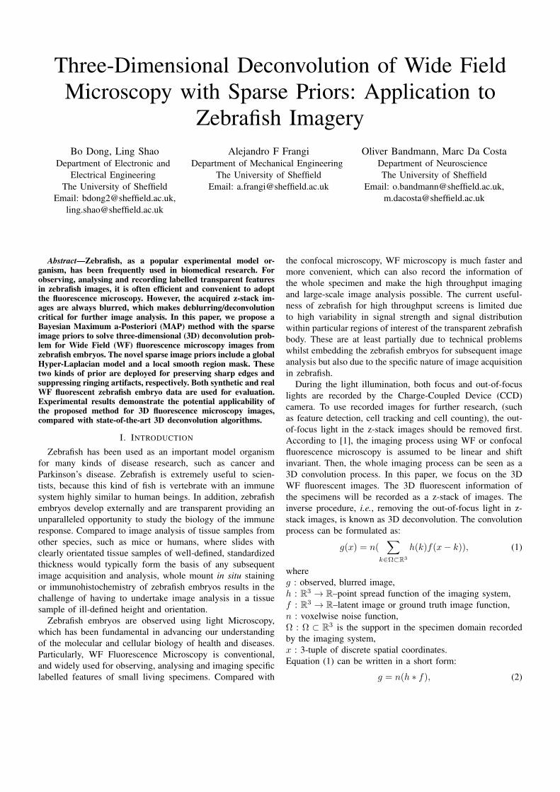
(a) One frame of the stack (b) log-gradient distribution

Fig. 1: (a) is one frame of a zebrafish embryo z-stack. (b): Theblue curve describes the gradient distribution (5xf ) of theimage. The Hyper-Laplacian with α = 1/3 is a more appro-priate model to describe the log-gradient distribution (blue),compared with the Gaussian (black), Laplacian (yellow) orHyper-Laplacian with α = 2/3 (green) log-distribution.

where ∗ is the 3D convolution operator.The convolution kernel h is called Point Spread Function

(PSF), which describes the blurring shape of one point lightthrough the light microscope [2]. In this paper, the PSF iscalculated using an analytical model if the true PSF is notgiven, which is called the Variable Refractive index Gibsonand Lanni (VRGL) model [3]. The final goal of the decon-volution method is to estimate the best latent image fromthe observed image with the given PSF. During the imagingprocess, the fluorescent data are influenced by photon noise,which can be described as a Poisson distribution [4]:

p(k) =λke−λ

k!, k = 0, 1, 2, ... (3)

In this paper, the MAP method with sparse image priors,including the Hyper-Laplacian prior and a local prior withmask, is presented to solve the 3D deconvolution problemfor WF Fluorescence Microscopy images. Then, the proposedmethod is tested on both synthetically generated microscopydata and real WF microscopy data from zebrafish. Comparedwith other regularization methods, the unique part of theproposed method is that we combine the Hyper-Laplacianmodel and a local mask together into the MAP frameworkfor 3D deconvolution.

The main contributions of our work include three aspects.Firstly, the MAP method with sparse priors is applied to3D deconvolution for Poisson noise WF microscopy images.Secondly, the Hyper-Laplacian distribution as a global prioris used in the deconvolution framework. The Hyper-Laplaciandistribution is a better model to describe the log-gradient dis-tribution of the image compared with other models, especiallyfor WF microscopy images. Finally, a local mask as the secondprior is applied to the 3D deconvolution problem for reducingringing artifacts.

The structure of this paper is as follows. In the next section,a brief review of relevant works is given. Section 3 explainshow sparse priors are designed in the MAP framework forPoisson noise WF images, and also describes the VRGL model

for generating PSF. Section 4 gives the experimental resultsusing three different datasets. In section 5, we conclude thepaper.

II. RELATED WORKS

Deconvolution is a typical area in image restoration [5], [6].Traditional methods such as inverse filtering [7], Tikhonov fil-tering [8], Weiner filtering [9], and Richardson-Lucy algorithm[10], [11] were proposed several decades ago for the inverseproblem. A non-linear iterative method, Maximum LikelihoodExpectation Maximization (MLEM), which is similar to theRichardson-Lucy algorithm, has been designed for solvingboth the blind and the non-blind Poisson image deconvolutionproblems [12], [13], [14], [15]. A machine learning methodmodelling the PSF based on MLEM was introduced for blinddeconvolution [15]. Most of the inverse problems are ill-posed, and the 3D deconvolution problem is also no exception.Therefore, the observed image (g) can be explained usinginfinite pairs of the PSF (h) and the ground truth image (f )[16]. Several methods using the Maximum a-Posteriori (MAP)estimation approach with the sparse image prior for solving thetwo-dimensional (2D) deconvolution problem were presented[16], [17], [18].

The MAP approach, as a non-linear iteration method, wasproved to be very efficient and accurate to recover the trueblur kernel of the 2D image, due to the movement of theobject or the shake of the camera [16]. The sparse derivativedistribution, as a kind of image prior knowledge, has beenused for solving many ill-posed problems, such as motiondeblurring [19], denoising [20], transparency separation [21]and super resolution [22].

In Fig. 1, the empirical distribution (blue) is the log-probability of the image gradient, and this heavy-tailed dis-tribution is known as the sparse image prior. State of theart estimation strategies for demonstrating the sparse priormodel were proposed, including using the Tikhonov-Millerregularizer [23] and the Total Variation (TV) regularization[13], [14], which will be used for comparison in this paper.Different penalty functions were introduced for the gradientfilter, such as f1(x) = | 5 x| for the TV regularizationmethod and f1(x) = ‖ 5 x‖2 for the TM regularizationmethod [13]. The Total variation regularization term wasapplied to 3D deconvolution for microscopy data [13]. In [14],the TV regularization term was presented for blind iterativedeconvolution by updating both the latent image function andthe PSF simultaneously.

The Hyper-Laplacian distribution has been applied to 2Dnon-blind deconvolution [24]. In [18], the Hyper-Laplaciandistribution was modified with the Gaussian noise model,and a lookup table (LUT) was developed for improving thecomputational speed. In [17], both global and local priors wereintroduced for solving the motion deblurring problem from asingle image. For the global prior, they presented two piece-wise continuous functions to fit the heavy-tailed distribution.The local prior was used for suppressing ringing artifacts. Ourlocal prior part is similar to the method in [17].

(a) Original frame (b) Zoom-in of the yel-low box in (a)

(c) The smooth regionsΨ are shown in blackand texture regions arehighlighted in green

Fig. 2: (a): One frame of an original zebrafish z-stack; (b):Zoom-in of the yellow box in (a); (c): After applying thetriangle threshold to the image gx. The green color indicatestexture regions of the image, and the remaining part is Ψ.

III. DECONVOLUTION FRAMEWORK

In this section, a Maximum a-Posterior algorithm withsparse priors is presented for estimating the best latent imagef given the blurred image g and the PSF h. According to theBayes Rule:

p (f |g, h) =p (g|f, h) p (f)

p (g)∝ p (g|f, h) p (f) , (4)

where p (f) is a prior about f , p (g|f, h) can be seen as aPoisson distribution with mean (f ∗ h)(x), and Equation (3)can be rewritten as:

p (g (x) |f, h) =(f ∗ h) (x)

g(x)e−(f∗h)(x)

g (x)!. (5)

The sparse image priors will be discussed in the followingsubsections.

A. Sparse Image Priors

In this paper, to simultaneously address the ill-posed natureof the problem and ringing artifacts reduction when restoringthe latent image f , the prior p(f) is decomposed into twocomponents, including a global prior pg (f) [18] and a localprior pl (f) [17]:

p (f) = pg (f) pl (f) . (6)

1) Global Prior pg (f): The heavy-tailed distribution ofthe gradient in the WF fluorescence microscopy z-stack isexplained well by the Hyper-Laplacian distribution [18]. InFig. 1, it can be seen that the best approximation for thelogarithmic image gradient distribution is the Hyper-Laplaciandistribution with α = 1/3. The global prior pg (f) is definedas:

pg (f) ∝∏

i∈Ω⊂R3

e−τ |5fi|α

, (0 < α < 1) , (7)

where τ is the positive rate parameter, and 5 is the 3D firstorder derivative filter.

2) Local Prior pl (f): Besides the global prior, a local priorwith mask is used for reducing ringing artifacts, which wasintroduced first in a motion deblurring problem [17]. In thispaper, we design a similar local prior for 3D deconvolution,but the difference is that we use a triangle threshold method[25] to determine the smooth region in the z-stack imagesautomatically. It is indicated in [17] that the smooth regionin the image should also be smooth after restoration, and thislocal prior can suppress ringing artifacts effectively in both thesmooth regions and the texture regions. Due to the inaccuratelygenerated PSF, some ringing artifacts will appear near theboundary and the edges after a number of iterations during therestoration in the frequency domain. Similar to [17], the errorof the gradient between the estimated image and the blurredimage in the smooth area is defined to follow the Normaldistribution with zero mean:

pl (f) =∏i∈Φ

N (Ofi − Ogi| 0, σ), (8)

where Φ denotes the smooth regions in each frame of the z-stack images, and the smooth regions Φ are shown in Fig. 2.Even though this local prior is only defined in the smoothregions, it can globally reduce ringing artifacts due to theeffect of the PSF during the restoration [17]. We define a maskfunction, M(x), to describe the smooth regions Ψ in the z-stack images. The triangle threshold algorithm [25] is appliedto determine the threshold automatically, and Ψ indicates theregions where M(x) = 1:

M(x) =

0, g ≥ Threshold1, else.

(9)

B. Optimization

After defining the two priors, Equation (4) becomes:

p (f |g, h) ∝ p (g|f, h) pg (f) pl (f) . (10)

Instead of maximizing the likelihood probability of Equation(10), the negative log-likelihood function, J(f), is mini-mized. In the function J(f), − log(p (g|f, h)) is defined asJMLEM (f).

J (f) =− log (p (f |g, h))

∝− log (p (g|f, h))− log (p (f))

=− log (p (g|f, h))− log (pg (f))− log (pl (f))

= JMLEM (f) +

∫x

λg|Of |αdx

+

∫Φ

λl‖Of(x)− Og(x)‖2dx,

(11)

where JMLEM (f) is redefined as:

JMLEM (f) =

∫x

(f ∗ h)(x)− g(x) log (f ∗ h) (x)

+ log (g(x)!) dx

∝∫x

(f ∗ h)(x)− g(x) log (f ∗ h) (x)dx.

(12)

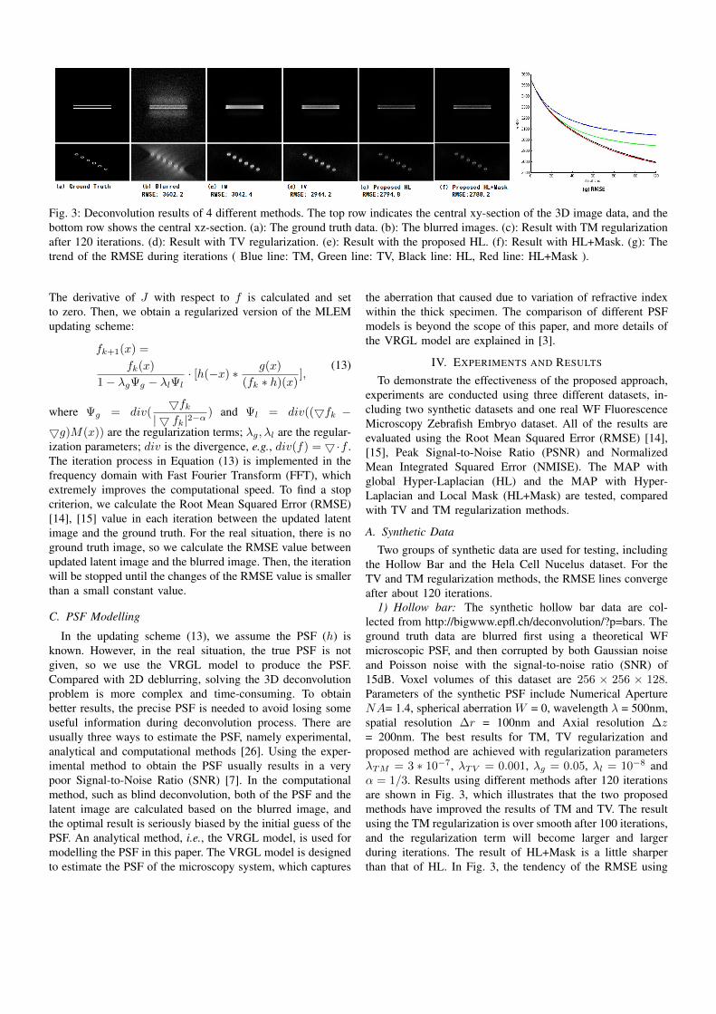
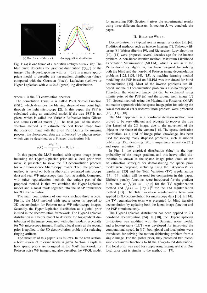
Fig. 3: Deconvolution results of 4 different methods. The top row indicates the central xy-section of the 3D image data, and thebottom row shows the central xz-section. (a): The ground truth data. (b): The blurred images. (c): Result with TM regularizationafter 120 iterations. (d): Result with TV regularization. (e): Result with the proposed HL. (f): Result with HL+Mask. (g): Thetrend of the RMSE during iterations ( Blue line: TM, Green line: TV, Black line: HL, Red line: HL+Mask ).

The derivative of J with respect to f is calculated and setto zero. Then, we obtain a regularized version of the MLEMupdating scheme:

fk+1(x) =

fk(x)

1− λgΨg − λlΨl· [h(−x) ∗ g(x)

(fk ∗ h)(x)],

(13)

where Ψg = div(5fk

| 5 fk|2−α) and Ψl = div((5fk −

5g)M(x)) are the regularization terms; λg, λl are the regular-ization parameters; div is the divergence, e.g., div(f) = 5·f .The iteration process in Equation (13) is implemented in thefrequency domain with Fast Fourier Transform (FFT), whichextremely improves the computational speed. To find a stopcriterion, we calculate the Root Mean Squared Error (RMSE)[14], [15] value in each iteration between the updated latentimage and the ground truth. For the real situation, there is noground truth image, so we calculate the RMSE value betweenupdated latent image and the blurred image. Then, the iterationwill be stopped until the changes of the RMSE value is smallerthan a small constant value.

C. PSF Modelling

In the updating scheme (13), we assume the PSF (h) isknown. However, in the real situation, the true PSF is notgiven, so we use the VRGL model to produce the PSF.Compared with 2D deblurring, solving the 3D deconvolutionproblem is more complex and time-consuming. To obtainbetter results, the precise PSF is needed to avoid losing someuseful information during deconvolution process. There areusually three ways to estimate the PSF, namely experimental,analytical and computational methods [26]. Using the exper-imental method to obtain the PSF usually results in a verypoor Signal-to-Noise Ratio (SNR) [7]. In the computationalmethod, such as blind deconvolution, both of the PSF and thelatent image are calculated based on the blurred image, andthe optimal result is seriously biased by the initial guess of thePSF. An analytical method, i.e., the VRGL model, is used formodelling the PSF in this paper. The VRGL model is designedto estimate the PSF of the microscopy system, which captures

the aberration that caused due to variation of refractive indexwithin the thick specimen. The comparison of different PSFmodels is beyond the scope of this paper, and more details ofthe VRGL model are explained in [3].

IV. EXPERIMENTS AND RESULTS

To demonstrate the effectiveness of the proposed approach,experiments are conducted using three different datasets, in-cluding two synthetic datasets and one real WF FluorescenceMicroscopy Zebrafish Embryo dataset. All of the results areevaluated using the Root Mean Squared Error (RMSE) [14],[15], Peak Signal-to-Noise Ratio (PSNR) and NormalizedMean Integrated Squared Error (NMISE). The MAP withglobal Hyper-Laplacian (HL) and the MAP with Hyper-Laplacian and Local Mask (HL+Mask) are tested, comparedwith TV and TM regularization methods.

A. Synthetic Data

Two groups of synthetic data are used for testing, includingthe Hollow Bar and the Hela Cell Nucelus dataset. For theTV and TM regularization methods, the RMSE lines convergeafter about 120 iterations.

1) Hollow bar: The synthetic hollow bar data are col-lected from http://bigwww.epfl.ch/deconvolution/?p=bars. Theground truth data are blurred first using a theoretical WFmicroscopic PSF, and then corrupted by both Gaussian noiseand Poisson noise with the signal-to-noise ratio (SNR) of15dB. Voxel volumes of this dataset are 256 × 256 × 128.Parameters of the synthetic PSF include Numerical ApertureNA= 1.4, spherical aberration W = 0, wavelength λ = 500nm,spatial resolution ∆r = 100nm and Axial resolution ∆z= 200nm. The best results for TM, TV regularization andproposed method are achieved with regularization parametersλTM = 3 ∗ 10−7, λTV = 0.001, λg = 0.05, λl = 10−8 andα = 1/3. Results using different methods after 120 iterationsare shown in Fig. 3, which illustrates that the two proposedmethods have improved the results of TM and TV. The resultusing the TM regularization is over smooth after 100 iterations,and the regularization term will become larger and largerduring iterations. The result of HL+Mask is a little sharperthan that of HL. In Fig. 3, the tendency of the RMSE using

(a) Ground Truth (b) BlurredRMSE:5907.4

(c) TMRMSE:4153.0

(d) TVRMSE:4081.7

(e) Proposed HLRMSE:4059.9

(f) Proposed HL+MaskRMSE:4052.0

Fig. 4: The HeLa cell dataset results using 4 different methodsafter 120 iterations.

4 different methods is shown. The TV and TM methods havealready converged after 100 iterations, and the RMSE lines ofthe two proposed methods are much lower than those of theother two methods after 50 iterations.

2) HeLa Cell Nucleus: The HeLa Cell Nucleus dataset wasfirst used in [14], and the ground truth data were generatedusing an online simulation tool [27]. The data are corruptedby a WF PSF without aberration, and then the Poisson noise isadded. The SNR of the final blurred data is 1.61. The PSF isgenerated with Numerical Aperture NA= 1.4, wavelength λ =530nm, spatial resolution ∆r = 64.5nm and Axial resolution∆z = 160nm. For this dataset, λTM = 10−5, λTV = 0.005,λg = 0.01 with α = 1/3, λl = 10−7 with α = 1/3 are chosenfor testing TM, TV, proposed HL and proposed HL+Maskmethods, respectively. After 120 iterations, the results and theRMSE are shown in Fig. 4.

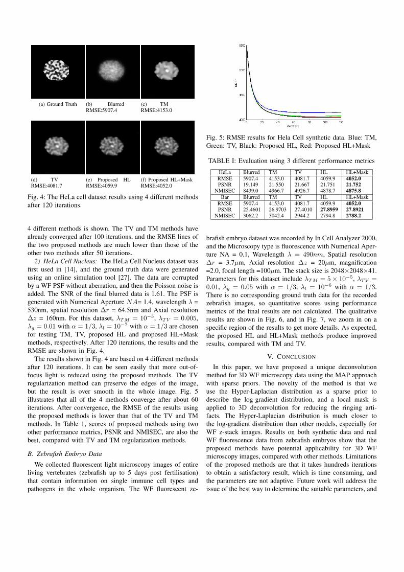
The results shown in Fig. 4 are based on 4 different methodsafter 120 iterations. It can be seen easily that more out-of-focus light is reduced using the proposed methods. The TVregularization method can preserve the edges of the image,but the result is over smooth in the whole image. Fig. 5illustrates that all of the 4 methods converge after about 60iterations. After convergence, the RMSE of the results usingthe proposed methods is lower than that of the TV and TMmethods. In Table 1, scores of proposed methods using twoother performance metrics, PSNR and NMISEC, are also thebest, compared with TV and TM regularization methods.

B. Zebrafish Embryo Data

We collected fluorescent light microscopy images of entireliving vertebrates (zebrafish up to 5 days post fertilisation)that contain information on single immune cell types andpathogens in the whole organism. The WF fluorescent ze-

Fig. 5: RMSE results for Hela Cell synthetic data. Blue: TM,Green: TV, Black: Proposed HL, Red: Proposed HL+Mask

TABLE I: Evaluation using 3 different performance metrics

HeLa Blurred TM TV HL HL+MaskRMSE 5907.4 4153.0 4081.7 4059.9 4052.0PSNR 19.149 21.550 21.667 21.751 21.752

NMISEC 8439.0 4966.7 4926.7 4878.7 4875.8Bar Blurred TM TV HL HL+Mask

RMSE 5907.4 4153.0 4081.7 4059.9 4052.0PSNR 25.4601 26.9703 27.4010 27.8959 27.8921

NMISEC 3062.2 3042.4 2944.2 2794.8 2788.2

brafish embryo dataset was recorded by In Cell Analyzer 2000,and the Microscopy type is fluorescence with Numerical Aper-ture NA = 0.1, Wavelength λ = 490nm, Spatial resolution∆r = 3.7µm, Axial resolution ∆z = 20µm, magnification=2.0, focal length =100µm. The stack size is 2048×2048×41.Parameters for this dataset include λTM = 5× 10−5, λTV =0.01, λg = 0.05 with α = 1/3, λl = 10−6 with α = 1/3.There is no corresponding ground truth data for the recordedzebrafish images, so quantitative scores using performancemetrics of the final results are not calculated. The qualitativeresults are shown in Fig. 6, and in Fig. 7, we zoom in on aspecific region of the results to get more details. As expected,the proposed HL and HL+Mask methods produce improvedresults, compared with TM and TV.

V. CONCLUSION

In this paper, we have proposed a unique deconvolutionmethod for 3D WF microscopy data using the MAP approachwith sparse priors. The novelty of the method is that weuse the Hyper-Laplacian distribution as a sparse prior todescribe the log-gradient distribution, and a local mask isapplied to 3D deconvolution for reducing the ringing arti-facts. The Hyper-Laplacian distribution is much closer tothe log-gradient distribution than other models, especially forWF z-stack images. Results on both synthetic data and realWF fluorescence data from zebrafish embryos show that theproposed methods have potential applicability for 3D WFmicroscopy images, compared with other methods. Limitationsof the proposed methods are that it takes hundreds iterationsto obtain a satisfactory result, which is time consuming, andthe parameters are not adaptive. Future work will address theissue of the best way to determine the suitable parameters, and

Fig. 6: The Zebrafish data results using 4 different methods.The central xy-section and central xz-section of the z-stackimages are shown in each block. (a): Central frame of theRecorded images. (b): TM. (c): TV. (d): Proposed HL. (e):Proposed HL+Mask.

Fig. 7: To observe the results in detail, we magnify the resultsshown in Fig. 6. (a): Central xy-section with a yellow square.(b): Zoom-in of the yellow square region. (c): TM. (d): TV.(e): Proposed HL. (f): Proposed HL+Mask.

also to improve the computational speed for high throughputimage analysis.

REFERENCES

[1] I. T. Young, “Image fidelity: characterizing the imaging transfer func-tion,” Methods Cell Biol, vol. 30, pp. 1–45, 1989.

[2] P. J. Shaw, “Comparison of widefield/deconvolution and confocal mi-croscopy for three-dimensional imaging,” in Handbook of BiologicalConfocal Microscopy. Springer, 2006, pp. 453–467.

[3] S. Hiware, P. Porwal, R. Velmurugan, and S. Chaudhuri, “Modeling ofPSF for refractive index variation in fluorescence microscopy,” in IEEEConference on Image Processing, 2011, pp. 2037–2040.

[4] M. Bertero, P. Boccacci, G. Desidera, and G. Vicidomini, “Imagedeblurring with poisson data: from cells to galaxies,” Inverse Problems,vol. 25, no. 12, p. 123006, 2009.

[5] L. Shao, R. Yan, X. Li, and Y. Liu, “From heuristic optimiza-tion to dictionary learning: A review and comprehensive comparisonof image denoising algorithms,” IEEE Transactions on Cybernetics,doi:10.1109/TCYB.2013.2278548.

[6] L. Shao, H. Zhang, and G. de Haan, “An overview and performanceevaluation of classification-based least squares trained filters,” IEEETransactions on Image Processing, vol. 17, no. 10, pp. 1772–1782, 2008.

[7] J. G. McNally, T. Karpova, J. Cooper, and J. A. Conchello, “Three-dimensional imaging by deconvolution microscopy,” Methods, vol. 19,no. 3, pp. 373–385, 1999.

[8] A. ı. N. Tikhonov, Numerical Methods for the Solution of Ill-posedProblems. Springer, 1995, vol. 328.

[9] T. Tommasi, A. Diaspro, and B. Bianco, “3D reconstruction in opticalmicroscopy by a frequency-domain approach,” IEEE Transactions onSignal Processing, vol. 32, no. 3, pp. 357–366, 1993.

[10] W. H. Richardson, “Bayesian-based iterative method of image restora-tion,” Journal of the Optical Society of America, vol. 62, no. 1, pp.55–59, 1972.

[11] L. Lucy, “An iterative technique for the rectification of observed distri-butions,” The Astronomical Journal, vol. 79, p. 745, 1974.

[12] L. A. Shepp and Y. Vardi, “Maximum likelihood reconstruction foremission tomography,” IEEE Transactions on Medical Imaging, vol. 1,no. 2, pp. 113–122, 1982.

[13] N. Dey, L. Blanc, Feraud, C. Zimmer, P. Roux, Z. Kam, M. Olivo,C. Jean, and J. Zerubia, “Richardson–Lucy algorithm with total variationregularization for 3D confocal microscope deconvolution,” MicroscopyResearch and Technique, vol. 69, no. 4, pp. 260–266, 2006.

[14] M. Keuper, T. Schmidt, M. Temerinac Ott, J. Padeken, P. Heun,O. Ronneberger, and T. Brox, “Blind deconvolution of widefield flu-orescence microscopic data by regularization of the optical transferfunction (OTF),” in IEEE Conference on Computer Vision and PatternRecognition, 2013.

[15] T. Kenig, Z. Kam, and A. Feuer, “Blind image deconvolution usingmachine learning for three-dimensional microscopy,” IEEE Transactionson Pattern Analysis and Machine Intelligence, vol. 32, no. 12, pp. 2191–2204, 2010.

[16] A. Levin, Y. Weiss, F. Durand, and W. T. Freeman, “Understandingand evaluating blind deconvolution algorithms,” in IEEE Conference onComputer Vision and Pattern Recognition, 2009, pp. 1964–1971.

[17] Q. Shan, J. Jia, and A. Agarwala, “High-quality motion deblurring froma single image,” ACM Transactions on Graphics, vol. 27, no. 3, p. 73,2008.

[18] D. Krishnan and R. Fergus, “Fast image deconvolution using hyper-laplacian priors,” in Advances in Neural Information Processing Systems,2009, pp. 1033–1041.

[19] H. Takeda and P. Milanfar, “Removing motion blur with space-timeprocessing,” IEEE Transactions on Image Processing, vol. 20, no. 10,pp. 2990–3000, 2011.

[20] J. Portilla, V. Strela, M. J. Wainwright, and E. P. Simoncelli, “Imagedenoising using scale mixtures of gaussians in the wavelet domain,”IEEE Transactions on Image Processing, vol. 12, no. 11, pp. 1338–1351, 2003.

[21] A. Levin and Y. Weiss, “User assisted separation of reflections froma single image using a sparsity prior,” IEEE Transactions on PatternAnalysis and Machine Intelligence, vol. 29, no. 9, pp. 1647–1654, 2007.

[22] M. F. Tappen, B. C. Russell, and W. T. Freeman, “Exploiting the sparsederivative prior for super-resolution and image demosaicing,” in IEEEWorkshop on Statistical and Computational Theories of Vision, 2003.

[23] N. Dey, L. Blanc-Feraud, C. Zimmer, Z. Kam, J.-C. Olivo-Marin, andJ. Zerubia, “A deconvolution method for confocal microscopy withtotal variation regularization,” in IEEE International Symposium onBiomedical Imaging, 2004, pp. 1223–1226.

[24] C. V. Stewart, “Robust parameter estimation in computer vision,” Societyfor Industrial and Applied Mathematics Review, vol. 41, no. 3, pp. 513–537, 1999.

[25] G. Zack, W. Rogers, and S. Latt, “Automatic measurement of sisterchromatid exchange frequency.” Journal of Histochemistry and Cyto-chemistry, vol. 25, no. 7, pp. 741–753, 1977.

[26] P. Sarder and A. Nehorai, “Deconvolution methods for 3D fluorescencemicroscopy images,” IEEE Signal Processing Magazine, vol. 23, no. 3,pp. 32–45, 2006.

[27] D. Svoboda, M. Kozubek, and S. Stejskal, “Generation of digitalphantoms of cell nuclei and simulation of image formation in 3D imagecytometry,” Cytometry, vol. 75A, no. 6, pp. 494–509, 2009.