three-dimensional cfd flygt mixer model and results
TRANSCRIPT

WSRC-TR-2000-00205
KEYWORDS:Mixer Model
CFD ApproachMixer Shroud Model
Propeller ModelAsymmetric Wall Jet Model
RETENTION - Permanent
Three-Dimensional CFD FLYGT Mixer Modeland Results
SAVANNAH RIVER TECHNOLOGY CENTER
Si Young Lee and Richard A. Dimenna
Publication Date: June, 2000
Westinghouse Savannah River CompanySavannah River SiteAiken, SC 29808
Prepared for the U.S. Department of Energy under Contract No. DE-AC09-96SR18500

This document was prepared in conjunction with work accomplished under Contract No.DE-AC09-96SR18500 with the U. S. Department of Energy.
DISCLAIMER
This report was prepared as an account of work sponsored by an agency of the United StatesGovernment. Neither the United States Government nor any agency thereof, nor any of theiremployees, makes any warranty, express or implied, or assumes any legal liability or responsibilityfor the accuracy, completeness, or usefulness of any information, apparatus, product or processdisclosed, or represents that its use would not infringe privately owned rights. Reference herein toany specific commercial product, process or service by trade name, trademark, manufacturer, orotherwise does not necessarily constitute or imply its endorsement, recommendation, or favoring bythe United States Government or any agency thereof. The views and opinions of authors expressedherein do not necessarily state or reflect those of the United States Government or any agencythereof.
This report has been reproduced directly from the best available copy.
Available for sale to the public, in paper, from: U.S. Department of Commerce, National TechnicalInformation Service, 5285 Port Royal Road, Springfield, VA 22161,phone: (800) 553-6847,fax: (703) 605-6900email: [email protected] ordering: http://www.ntis.gov/support/index.html
Available electronically at http://www.osti.gov/bridgeAvailable for a processing fee to U.S. Department of Energy and its contractors, in paper, from: U.S.Department of Energy, Office of Scientific and Technical Information, P.O. Box 62, Oak Ridge, TN37831-0062,phone: (865)576-8401,fax: (865)576-5728email: [email protected]

-ii-
(This Page Intentionally Left Blank)

-iii-
DOCUMENT: WSRC-TR-2000-00205TITLE: Three-Dimensional CFD FLYGT Mixer Model and Results
APPROVALS
____________________________________________ _Date:_____________Si Y. Lee, Author (EM&S Group/EDS/SRTC)
____________________________________________ _Date:_____________Richard A. Dimenna, Coauthor (EM&S Group/EDS/SRTC)
____________________________________________ _Date:_____________Glenn A. Taylor, Technical Reviewer (Process Engineering)
____________________________________________ _Date:_____________Cynthia P. Holding-Smith, Manager (EM&S Group/SRTC)
____________________________________________ _Date:_____________Martha A. Ebra, Manager (EDS/SRTC)
____________________________________________ _Date:_____________Brannen J. Adkins, Customer (Waste Removal Engineering)

-iv-
(This Page Intentionally Left Blank)
-v-
Table of Contents
Summary 1
1. Background and Objective 2
2. Model Descriptions and Solution Methods 3
3. Investigation of the Nominal Pump Operating Conditions 12
4. Results and Discussions 20
4.1 Steady-State Results ...................................................................................................204.2 Sensitivity Run Results ................................................................................................45
- Non-uniform Inlet Flow Condition ................................................................................45- Shroud Wall Roughness .............................................................................................47- Pump Rotational Speed ..............................................................................................49
4.3 Transient Flow Behavior of FLYGT Mixer Associated with Pump Cavitation ..............51
5. Conclusions 63
6. Recommendations 64
7. References 65

-vi-
(This Page Intentionally Left Blank)
-vii-
List of Figures
Figure 1. Analysis methodology for FLYGT mixer models ....................................................6
Figure 2. Modeling boundary for three-dimensional FLYGT mixer model .............................7
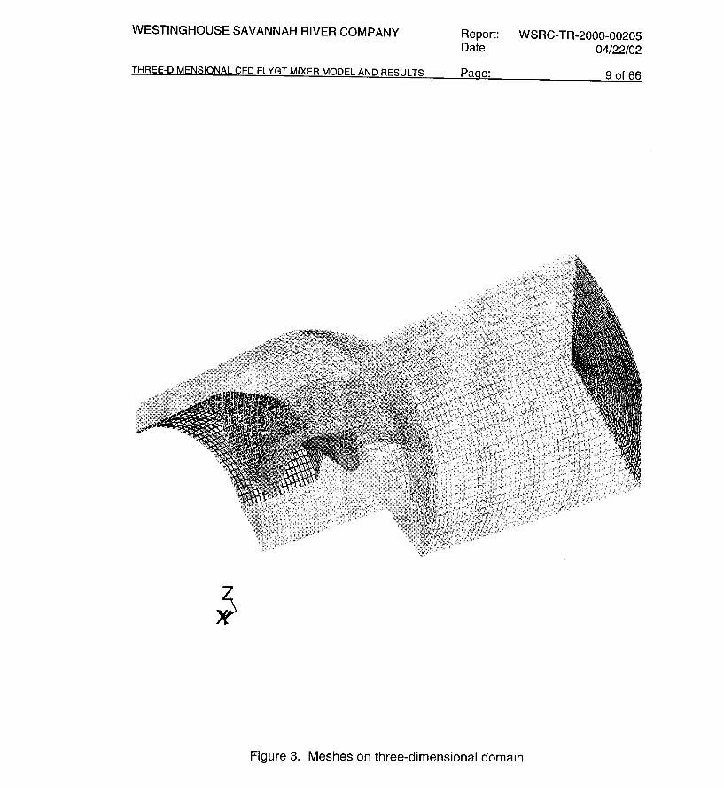
Figure 3. Meshes on three-dimensional domain....................................................................9
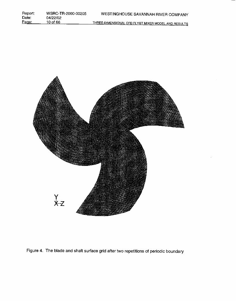
Figure 4. The blade and shaft surface grid after two repetitions of periodic boundary........10
Figure 5. Two-dimensional meshes at exit plane after two periodic repetitions of thepresent model .....................................................................................................11
Figure 6. Overview of segregated solution method for the present model..........................12
Figure 7. Comparison of predictions with test data .............................................................14
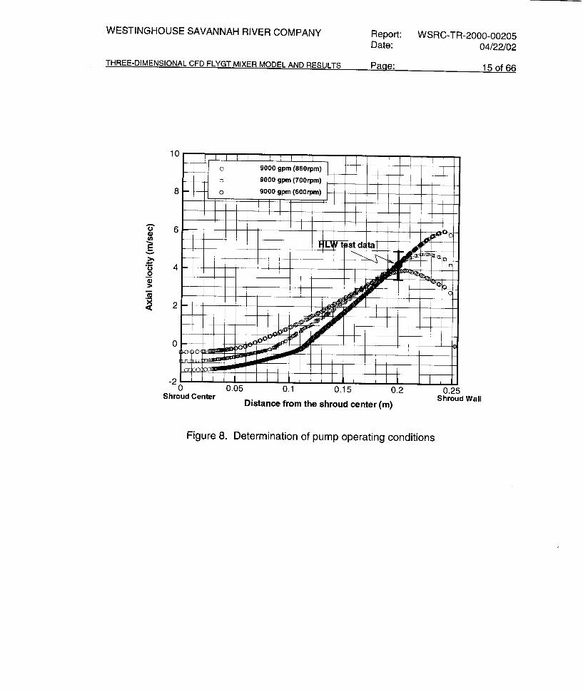
Figure 8. Determination of pump operating conditions ........................................................15
Figure 9. Axial velocity distribution as a function of liquid level at the 40ft distance fromthe shroud exit based on two-dimensional wall jet model (Lee and Dimenna,2000) for 9000 gpm pump flowrate. Inlet velocity is uniformly 45o skewedagainst the axial flow direction (θin = 45o in the figure). ......................................16
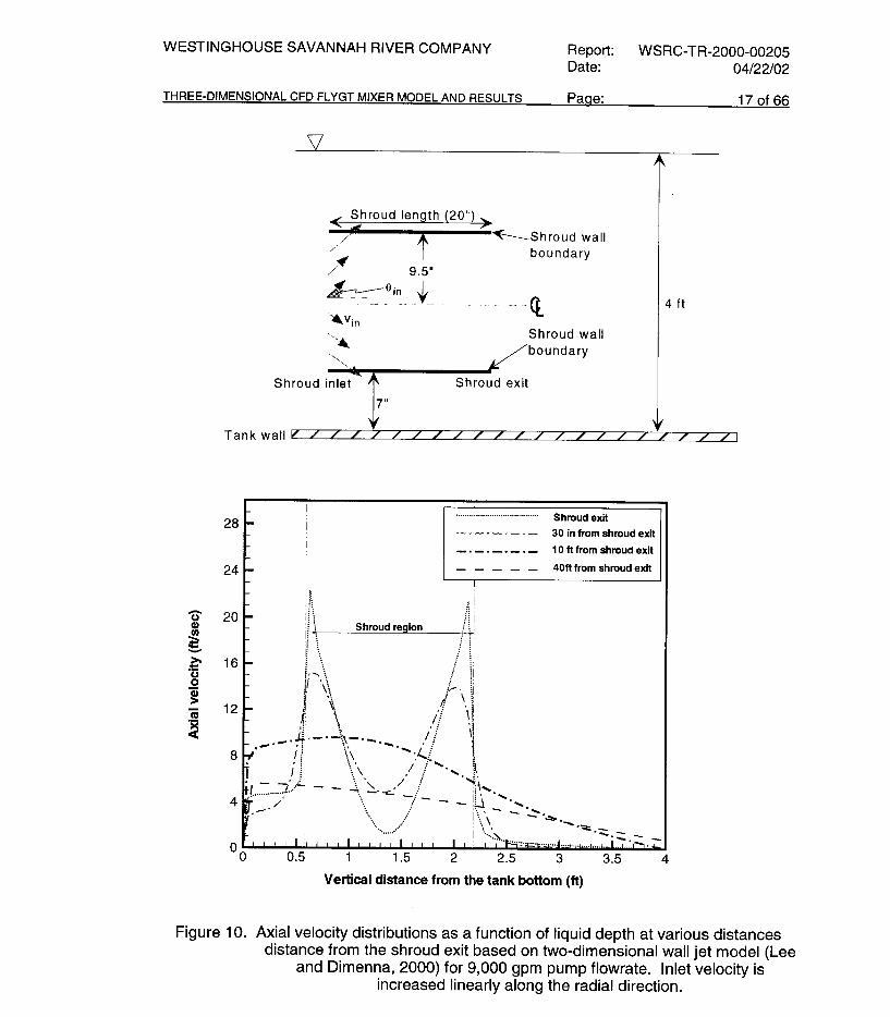
Figure 10. Axial velocity distributions as a function of liquid depth at various distancesdistance from the shroud exit based on two-dimensional wall jet model (Leeand Dimenna, 2000) for 9,000 gpm pump flowrate. Inlet velocity is increasedlinearly along the radial direction. ........................................................................17
Figure 11. Velocity vector plot near the shroud region predicted by the two-dimensionalwall jet model (Lee and Dimenna, 2000) for 9,000 gpm pump flowrate. Inletvelocity is increased linearly along the radial direction. ......................................18
Figure 12. Velocity distributions near the shroud region and over the whole computationaldomain predicted by two-dimensional wall jet model (Lee and Dimenna, 2000)for 9,000 gpm pump flowrate. Inlet velocity is increased linearly along theradial direction. ....................................................................................................19
Figure 13. Typical static pressure distribution at downstream and upstream regions nearthe leading-edge tip of single pump blade for 860rpm of pump rotational speedand 9,000 gpm flow condition (Propeller blade shown in the figure rotatesclockwise.). .........................................................................................................25
Figure 14. Typical fluid flow pattern and rotation profile at downstream and upstreamregions near the leading-edge tip of single pump blade for 860rpm of pump

-viii-
rotational speed and 9,000 gpm flow condition (Propeller blade shown in thefigure rotates clockwise.). ...................................................................................26
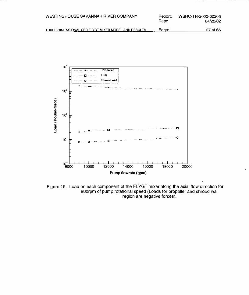
Figure 15. Load on each component of the FLYGT mixer along the axial flow direction for860rpm of pump rotational speed (Loads for propeller and shroud wall regionare negative forces). ...........................................................................................27
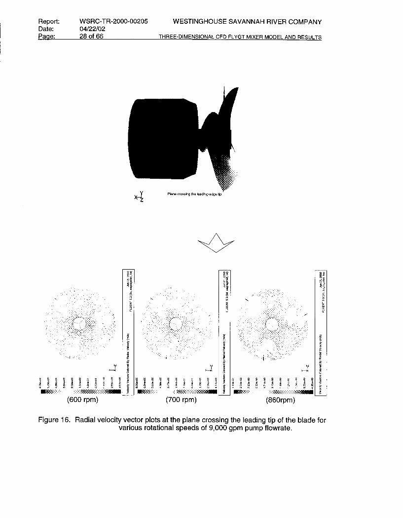
Figure 16. Radial velocity vector plots at the plane crossing the leading tip of the bladefor various rotational speeds of 9,000 gpm pump flowrate.................................28
Figure 17. Static pressure contour plots at the plane crossing the leading tip of the bladefor various rotational speeds of 9,000 gpm pump flowrate.................................29
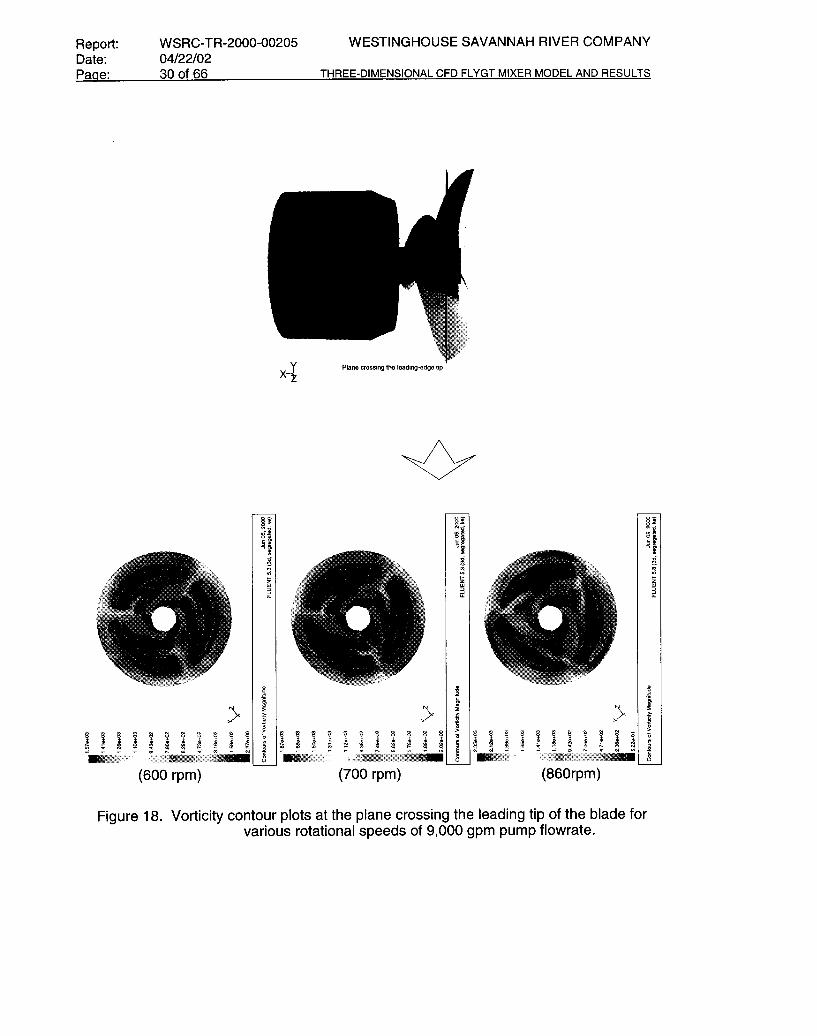
Figure 18. Vorticity contour plots at the plane crossing the leading tip of the blade forvarious rotational speeds of 9,000 gpm pump flowrate......................................30
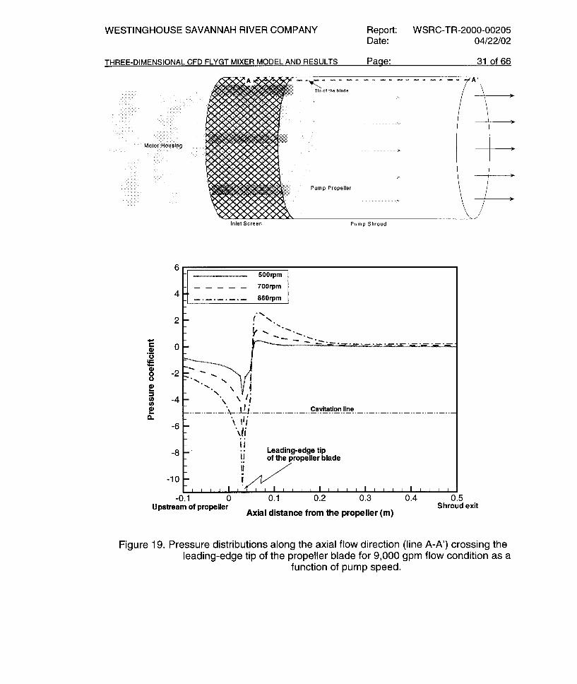
Figure 19. Pressure distributions along the axial flow direction (line A-A’) crossing theleading-edge tip of the propeller blade for 9,000 gpm flow condition as afunction of pump speed.......................................................................................31
Figure 20. Fluid vorticity distributions along the axial flow direction (line A-A’) crossing theleading-edge tip of the propeller blade for 9,000 gpm flow condition as afunction of pump speed e....................................................................................32
Figure 21. Turbulence intensity contour plots at the plane crossing the leading tip of theblade for various rotational speeds of 9,000 gpm pump flowrate.......................33
Figure 22. Static pressure contour plot on the propeller surface. .......................................34
Figure 23. Shear stress contour plot on the propeller surface. ...........................................35
Figure 24. Velocity contour plot near the pump propeller. ...................................................36
Figure 25. Vorticity contour plot at the pump propeller region (counterclockwise propellerdirection)..............................................................................................................37
Figure 26. Vorticity contour plot at the propeller hub region (counterclockwise propellerdirection)..............................................................................................................38
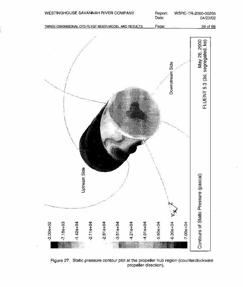
Figure 27. Static pressure contour plot at the propeller hub region (counterclockwisepropeller direction)...............................................................................................39
Figure 28. Shear stress contour plot at the propeller hub region (counterclockwisepropeller direction)...............................................................................................40
Figure 29. Static pressure contour plot at the shroud wall (counterclockwise propellerdirection)..............................................................................................................41
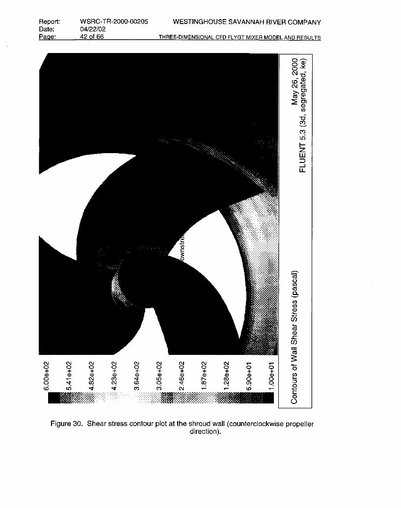
Figure 30. Shear stress contour plot at the shroud wall (counterclockwise propellerdirection)..............................................................................................................42

-ix-
Figure 31. Velocity distributions along the radial direction. ..................................................43
Figure 32. Velocity vector plot at the inlet and exit planes of shroud exit.............................44
Figure 33. Non-uniform and uniform flow conditions at the pump inlet for the sensitivityruns. ....................................................................................................................46
Figure 34. Sensitivity run results for axial flow velocities at shroud exit. .............................46
Figure 35. Velocity vector plot at the inlet and exit planes for non-uniform inlet flowcondition. .............................................................................................................48
Figure 36. Sensitivity run results for surface roughness effects of shroud wall on axialflow velocities at shroud exit (Roughness height of rough wall used in thisfigure was 0.01ft equivalent to concrete surface.)..............................................49
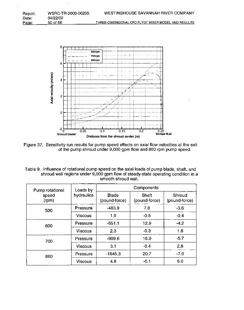
Figure 37. Sensitivity run results for pump speed effects on axial flow velocities at theexit of the pump shroud under 9,000 gpm flow and 860 rpm pump speed........50
Figure 38. Transient response of flow velocity along the radial direction of the shroud exitplane for 12,000 gpm and 860 rpm operating condition. ....................................53
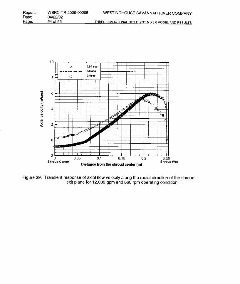
Figure 39. Transient response of axial flow velocity along the radial direction of theshroud exit plane for 12,000 gpm and 860 rpm operating condition...................54
Figure 40. Transient response of total pressure force for three propeller blades under12,000 gpm and 860 rpm operating condition. ...................................................55
Figure 41. Transient response of pressure force for hub under 12,000 gpm and 860 rpmoperating condition. .............................................................................................56
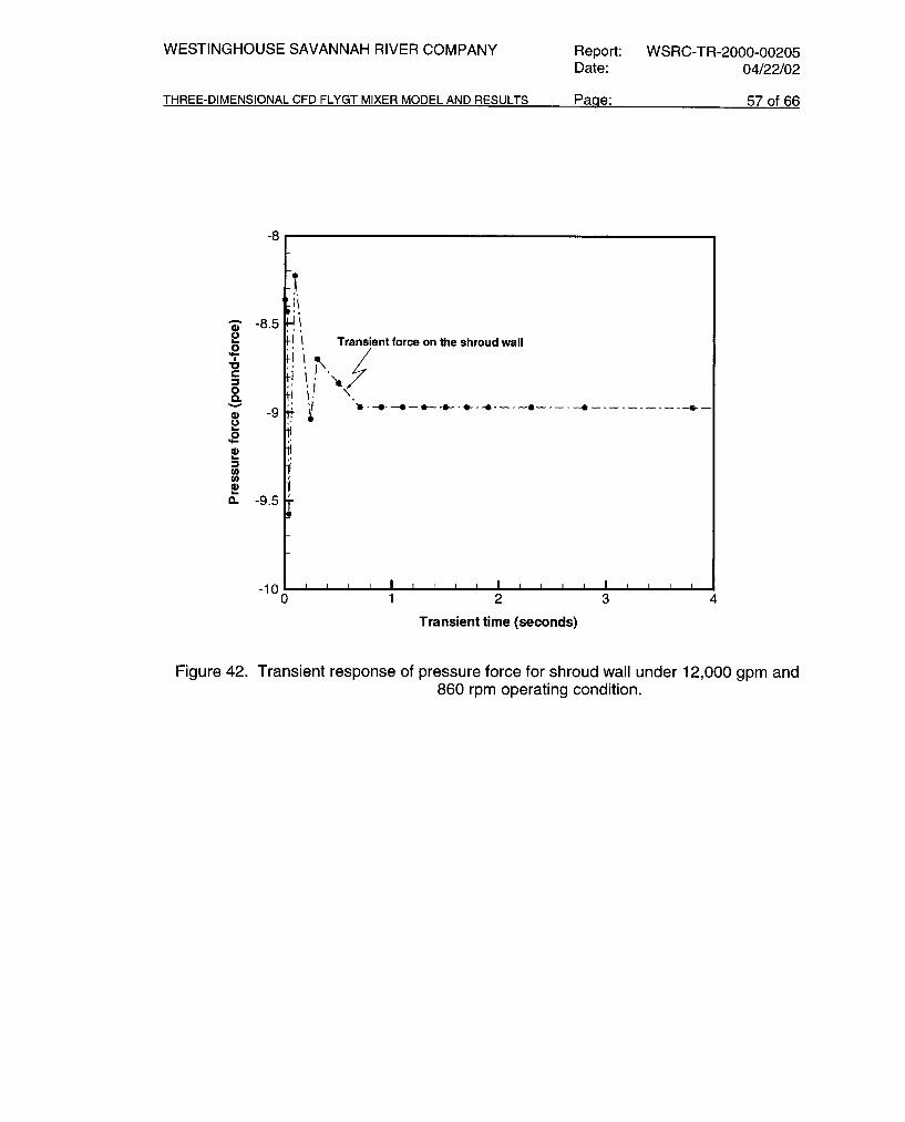
Figure 42. Transient response of pressure force for shroud wall under 12,000 gpm and860 rpm operating condition................................................................................57
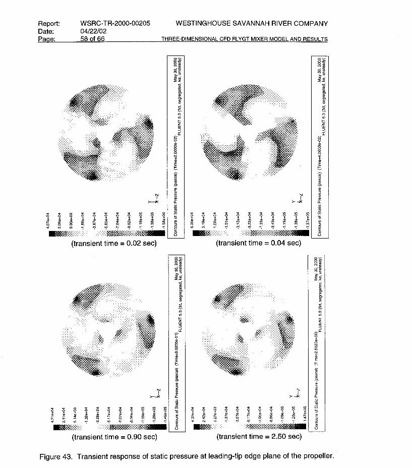
Figure 43. Transient response of static pressure at leading-tip edge plane of thepropeller...............................................................................................................58
Figure 44. Transient response of fluid density at leading edge plane of the propeller tip....59
Figure 45. Transient response of fluid velocity at leading edge plane of the propeller tip. ..60
Figure 46. Transient response of fluid vorticity at leading edge plane of the propeller tip. ..61
Figure 47. Transient velocity distributions at the exit of the shroud for 700 rpm pumpspeed and 12000 gpm flow condition.. ...............................................................62
Figure 48. Transient response of total pressure force for three propeller blades under12000 gpm flow with two pump speeds.. ...........................................................62

-x-

-xi-
(This Page Intentionally Left Blank)

-xii-
List of Tables
Table 1. Modeling purpose and descriptions for Tank 19 FLYGT mixer..............................35
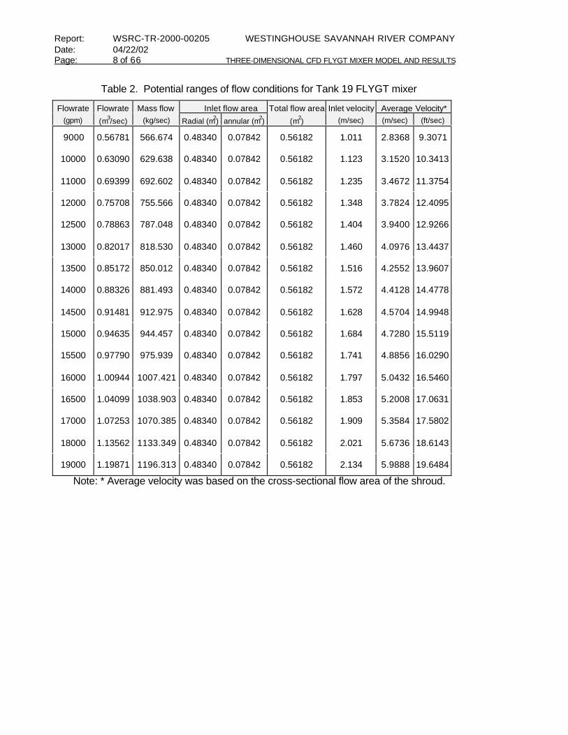
Table 2. Potential ranges of flow conditions for Tank 19 FLYGT mixer.................................8
Table 3. Absolute pressures near the leading-edge tip of the pump blade under 9,000gpm water flowrate of steady-state operating condition. .......................................21
Table 4. Maximum axial and radial velocities for various pump speeds at the leading-edgetip of the pump blade under 9,000 gpm flow constraint of steady-state operatingcondition. ................................................................................................................21
Table 5. Axial forces along the flow direction for propeller, hub, and shroud regions underwide range of steady-state pump operating conditions.........................................24
Table 6. Comparison of minimum pressure coefficients (Cp,min) for three differentadvance coefficients (J) corresponding to three rotational pump speeds.............24
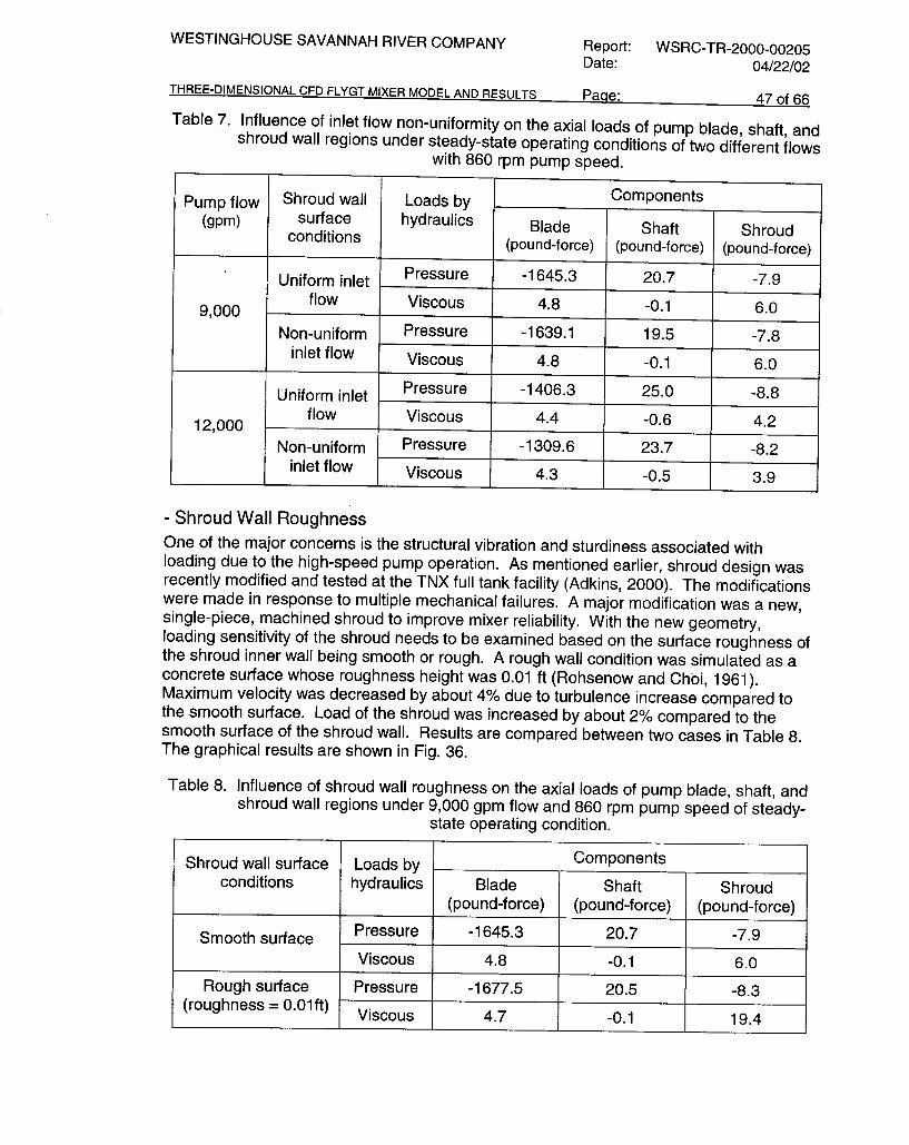
Table 7. Influence of inlet flow non-uniformity on the axial loads of pump blade, shaft, andshroud wall regions under steady-state operating conditions of two differentflows with 860 rpm pump speed............................................................................47
Table 8. Influence of shroud wall roughness on the axial loads of pump blade, shaft, andshroud wall regions under 9,000 gpm flow and 860 rpm pump speed of steady-state operating condition. .......................................................................................47
Table 9. Influence of rotational pump speed on the axial loads of pump blade, shaft, andshroud wall regions under 9,000 gpm flow of steady-state operating condition ina smooth shroud wall.............................................................................................50
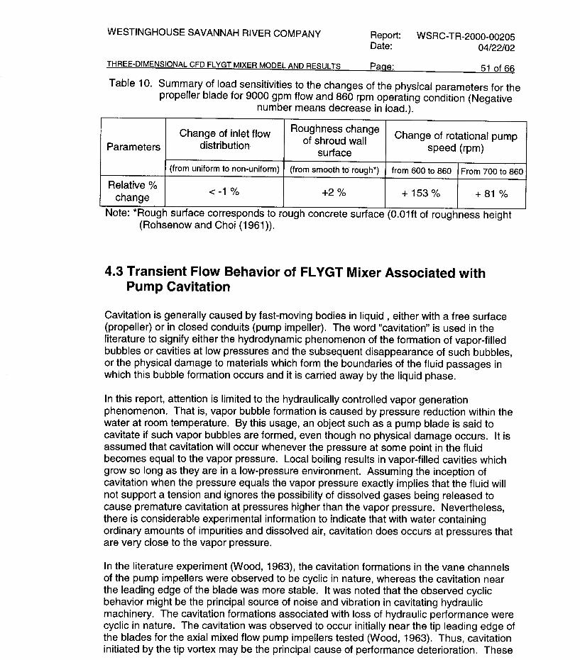
Table 10. Summary of load sensitivities to the changes of the physical parameters for thepropeller blade for 9,000 gpm flow and 860 rpm operating condition (Negativenumber means decrease in load.).........................................................................51

-xiii-
(This Page Intentionally Left Blank)

WESTINGHOUSE SAVANNAH RIVER COMPANY Report: WSRC-TR-2000-00205Date: 04/22/02
THREE-DIMENSIONAL CFD FLYGT MIXER MODEL AND RESULTS Page: 1 of 66
Summary
Since mid-February, the Engineering Development Section (EDS) has been assisting theHigh Level Waste (HLW) customer to assess the failure causes of the FLYGT mixer to beused to recover waste from Tank 19 and to redesign the mixer.
In support of this project, two Computational Fluid Dynamics (CFD) models have beendeveloped. They are a steady-state pump model and a transient model considering theeffects of vapor formation due to pump cavitation. The commercial CFD code, FLUENT, isused in the present analysis. The computations are performed for a three-dimensionalmodel of the FLYGT mixer with the prototypic propeller shape. In the models, thepropeller is assumed to be symmetrical and perfectly-balanced within a rigid andstationary shroud boundary under any operating condition. Both of the models include thepropeller region, the inlet region upstream of the propeller, and the downstream shroudregion as computational domain.
The areas of focus for the analysis presented here are the flow performance of themodified mixer under potential operating conditions and the loads on the propeller, shaft,and shroud regions of the mixer. Calculated physical parameters include velocity profilesof axial flow, cavitation locations, and loads on the shroud wall, propeller blade, and hub ofthe propeller for the operating flow conditions. As inlet boundary conditions of the model,uniform radial and axial velocities through the shroud inlet and around the motor housingare used assuming azimuthally symmetrical flow conditions.
An operating flow condition of 9,000 gpm is established by the comparison of the steady-state model predictions and HLW test data (Adkins, 2000) at the shroud exit. The resultsof the model show that the modified mixer has reasonable performance for 9,000 gpm flowand 500 rpm pump speed in terms of flow behavior and spread angle near the exit.
Sensitivity runs are performed for non-uniform inlet velocity along the axial flow direction,different surface roughness of the shroud inner wall, and different pump speeds. Fromthe model results, the non-uniform inlet velocity and wall roughness effects are found tohave a negligible effect on overall flow patterns at the inner and outlet regions of theshroud, loads on each pump component, and cavitation size near the tip of the blade aslong as liquid flow rate remains constant. The primary reason for these results is thatturbulent flow effect within the shroud is dominant due to the high-speed rotations of axialpropeller. Thus, it is noted that pump speed is the most sensitive one among the threeparameters in terms of flow performance and pump loading.
Transient model results show that transient flow behavior such as change of fluid densityand loadings of the mixer establish steady-state conditions within about 1 second,corresponding to about 40 cycles of the propeller blade, after the initiation of the pumpcavitation. In addition, a low density region is established near the peripheral regionadjacent to the shroud wall because all bubbles generated as a result of cavitation migrateto the high-velocity fluid region near the tip of the propeller blade.
Report: WSRC-TR-2000-00205 WESTINGHOUSE SAVANNAH RIVER COMPANYDate: 04/22/02Page: 2 of 66 THREE-DIMENSIONAL CFD FLYGT MIXER MODEL AND RESULTS
1. Background and Objective
The Engineering Modeling and Simulation Group (EMSG) was asked to perform ananalysis which could provide pertinent information in support of a modified High-LevelWaste (HLW) Tank 19 FLYGT mixer design. The modified FLYGT mixer will be used torecover waste from the Tank 19. Under normal operating conditions, the mixer will beoriented in a horizontal position above approximately 6 to 7 inches above the bottom of the85 ft diameter tank. In this situation, the discharge from the shroud exit is the driving forcefor liquid mixing and material suspension from the tank floor.
In previous work (Lee and Dimenna, 2000), two two-dimensional models were developedto determine the optimum shroud length for acceptable flow performance and to conductsensitivity analysis for a wide range of possible boundary conditions at the shroud inletdownstream of the pump propeller. One model was axisymmetric using the shroud alonewithout the pump propeller as a modeling boundary. The other model was a two-dimensional wall jet model to investigate asymmetric effects of the shroud discharge flow.
For the previous analysis (Ref. 8) and the present work, a Computational Fluid Dynamics(CFD) approach has been taken. In the present analysis, a three-dimensional steady-state pump model and a transient cavitation model have been developed to evaluatedetailed flow performance of the Tank 19 FLYGT mixer improved by the previous work.The commercial CFD preprocessor and solver, GAMBIT and FLUENT5.3, have been usedto model the mixer. The geometry files of the mixer models have been created with theintegrated CFD preprocessor GAMBIT based on the propeller model. At the beginning ofApril, Fluent Inc. was contracted to assist in the development of the propeller model basedon digital propeller shape data obtained from Michigan Wheel Company, whomanufactured the present propeller.
The present three-dimensional CFD models can identify a number of viscous flowphenomena in the propeller flow field confined in the shroud region, including blade andhub boundary layers, flow separation on the blade, hub and tip vortices, etc. Thus, themodels help estimate reasonable loading conditions for the optimum operatingperformance of the mixer. Parametric sensitivity studies with the models also help identifyoperation and design variations that may be used to improve the operational design of themixer from the aspect of pump flow performance. The main objectives of the present workare as follows:
1. To examine detailed flow performance of the Tank 19 FLYGT mixer improved by theprevious work,
2. To conduct sensitivity analysis for a wide range of possible boundary conditions, and
3. To investigate transient flow behavior and loading of the FLYGT mixer.
For the present study, a flow simulation method is developed to calculate the flow arounda marine-type propeller configuration of the FLYGT mixer. The flow characteristics of theblade boundary layer and tip vortex are investigated by the CFD method. Comparisonsbetween calculation results and experimental data are made to demonstrate the capabilityof the model to handle propeller flows. The analysis results for the mixer model provide

WESTINGHOUSE SAVANNAH RIVER COMPANY Report: WSRC-TR-2000-00205Date: 04/22/02
THREE-DIMENSIONAL CFD FLYGT MIXER MODEL AND RESULTS Page: 3 of 66
design guidance concerning the operation performance of a modified mixer, and thisestimated loading information would be used as input to assess the structural vibrationand stress analysis of the FLYGT mixer.
Table 1. Modeling purpose and descriptions for Tank 19 FLYGT mixer.
Model Brief description Primary purpose Status
Axisymmetric 2-Dmodel
Shroud model usingtwo-dimensional CFDapproach
To assess the impact of shroudlength on discharge flowbehavior for variousboundary conditions
Done(Ref. 8)
2-D wall jet model
Two-dimensional walljet model with thepump shroudsubmerged in 4ft tanklevel
To investigate asymmetriceffect of the liquid dischargefrom the optimum length ofshroud due to the presenceof the tank bottom
Done(Ref. 8)
Steady-statemodel
Detailed three-dimensional pumpmodel with prototypicpropeller blade shapeto exclude cavitationmodel
To assess pump flowperformance in detail and toevaluate load on propellerblade, hub, and pumpshroud in a steady-stateoperation
Presentanalysis
3-DFLYGTmixermodel
Transientmodel
Detailed three-dimensional pumpmodel with prototypicpropeller blade shapeto include cavitationmodel
To evaluate transient load onpropeller blade, hub, andpump shroud and toestimate transient time toreach steady-state mode
Presentanalysis
2. Model Descriptions and Solution Methods
Two CFD models have been developed to examine the flow performance of the modifiedTank 19 FLYGT mixer (Lee and Dimenna, 2000) and to conduct sensitivity analysis for awide range of possible boundary conditions. The modeling purpose and brief descriptionsfor the models are provided in Table 1. The methodology used for the models andanalysis of the FLYGT mixer are shown in Fig. 1. The computational domain for the mixermodel consists of three major regions, which are the propeller region, the inlet regionupstream of the propeller, and the shroud region downstream of the propeller. Thepresent modeling boundary is shown in Fig. 2.
For computational efficiency, a 120o sector of the mixer was used as a computationaldomain by using the following assumptions:
- The blades of the propeller are perfectly balanced and symmetrical.
Report: WSRC-TR-2000-00205 WESTINGHOUSE SAVANNAH RIVER COMPANYDate: 04/22/02Page: 4 of 66 THREE-DIMENSIONAL CFD FLYGT MIXER MODEL AND RESULTS
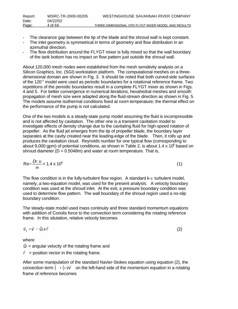
- The clearance gap between the tip of the blade and the shroud wall is kept constant.- The inlet geometry is symmetrical in terms of geometry and flow distribution in an
azimuthal direction.- The flow distribution around the FLYGT mixer is fully mixed so that the wall boundary
of the tank bottom has no impact on flow pattern just outside the shroud wall.
About 120,000 mesh nodes were established from the mesh sensitivity analysis on aSilicon Graphics, Inc. (SGI) workstation platform. The computational meshes on a three-dimensional domain are shown in Fig. 3. It should be noted that both curved-side surfacesof the 120 o model were used as periodic boundaries for a rotational reference frame. Tworepetitions of the periodic boundaries result in a complete FLYGT mixer as shown in Figs.4 and 5. For better convergence in numerical iterations, hexahedral meshes and smoothpropagation of mesh size were adapted along the fluid-stream direction as shown in Fig. 5.The models assume isothermal conditions fixed at room temperature; the thermal effect onthe performance of the pump is not calculated.
One of the two models is a steady-state pump model assuming the fluid is incompressibleand is not affected by cavitation. The other one is a transient cavitation model toinvestigate effects of density change due to the cavitating fluid for high-speed rotation ofpropeller. As the fluid jet emerges from the tip of propeller blade, the boundary layerseparates at the cavity created near the leading-edge of the blade. Then, it rolls up andproduces the cavitation cloud. Reynolds number for one typical flow (corresponding toabout 9,000 gpm) of potential conditions, as shown in Table 2, is about 1.4 x 10⁶ based onshroud diameter (D = 0.5048m) and water at room temperature. That is,
µρ uD=Re = 1.4 x 10⁶ (1)
The flow condition is in the fully-turbulent flow region. A standard k-ε turbulent model,namely, a two-equation model, was used for the present analysis. A velocity boundarycondition was used at the shroud inlet. At the exit, a pressure boundary condition wasused to determine flow pattern. The wall boundary of the shroud region used a no-slipboundary condition.
The steady-state model used mass continuity and three standard momentum equationswith addition of Coriolis force to the convection term considering the rotating referenceframe. In this situtation, relative velocity becomes
rxvv rrrrr
Ω−= (2)
whereΩr
= angular velocity of the rotating frame andrr
= position vector in the rotating frame.
After some manipulation of the standard Navier-Stokes equation using equation (2), theconvection term ( )( )vv
rrρ•∇ on the left-hand side of the momentum equation in a rotating
frame of reference becomes

WESTINGHOUSE SAVANNAH RIVER COMPANY Report: WSRC-TR-2000-00205Date: 04/22/02
THREE-DIMENSIONAL CFD FLYGT MIXER MODEL AND RESULTS Page: 5 of 66
( ) ( )rxxvxvv rrrrrrrrrr
ΩΩ+Ω+•∇ ρρρ 2 (3)
Equation (3) shows that two new terms, referred to as Coriolis force and centrifugal force,respectively, in the literature, are added to the standard convection term for the rotationaleffect.
The transient cavitation model relies on the volume fraction concept so that it allows thefluids to be interpenetrating. The volume fraction of vapor phase created from thecavitation can therefore be equal to any value between 0 and 1, depending on the spaceoccupied by vapor and liquid phases. The cavitation model allows mass to be transferredfrom one phase to another. This allows for modeling the formation of vapor from a liquidwhen fluid is cavitated. The model assumes no collapses of bubbles inside the shroudregion and no slip between the two phases of the fluid because bubble residence timewithin the shroud is very short and bubbly flow regime is assumed to be dominant in themodeling domain. Thus, FLUENT solves a single-phase momentum equation for bothphases and a volume fraction equation for the second phase. The volume fraction for thesecondary vapor phase is determined from the continuity relation with interphase masstransfer from liquid to vapor phases. To get interphase mass transfer term, the change inbubble radius can be computed by a simplified Rayleigh equation assuming that thepressure within the bubble remains nearly constant when cavitation bubbles form in aliquid at room temperature. The latent heat of vaporization is neglected in isothermalcavitating flow. Bubble growth due to inertia effects is assumed negligible compared tocaviation pressure. In this situation, bubble radius R at time t is determined by thefollowing equation (Kubota et al., 1992):
( ) 50
3
2.
−=
f
g pp
dtdR
ρ(4)
where pg is vapor pressure corresponding to fluid temperature and ρ f is the density of theliquid.
The total vapor mass (mg) can be written as
nRm gg
= 3
34πρ (5)
where n is the number of bubbles per unit volume.
Bubble number density (n) in eq. (5) was assumed to be constant. For the present work, nwas chosen as 1.0 x 10⁴ m-3 from the literature (Kubota el al. (1992)). After somealgebraic manipulation of eq. (5), rate of vapor formation due to cavitation can be written interms of void fraction (αg) as

Report: WSRC-TR-2000-00205 WESTINGHOUSE SAVANNAH RIVER COMPANYDate: 04/22/02Page: 6 of 66 THREE-DIMENSIONAL CFD FLYGT MIXER MODEL AND RESULTS
=
=
dtdR
R
dtdR
nR
Rdt
dm
gg
gg
αρ
πρ
3
343 3
(6)
Thus, an equation for the interphase mass transfer (mf g) due to cavitation can be obtainedfrom eqs. (4) and (6). That is,
( ) 50
3
23.
−
==
f
ggggfg
pp
Rdt
dmm
ρ
αρ(7)
Equation (7) is used in the continuity equation for the vapor phase, which is created fromthe cavitation phenomenon of the high-speed mixing pump.
Computations use the FLUENT rotating reference frame assumption in which the three-dimensional flow field rotates in a reference frame that is fixed on the propeller blade.When equations of motion are solved in the steady-rotating reference frame, the Coriolisforce term is added to the fluid acceleration term in the left-hand side of the Reynolds-Averaged Navier-Stokes equations derived in the inertial frame. The three-dimensionalincompressible Navier-Stokes flow solver developed by Fluent, Inc. is applied to computethe rotating propeller flow in Tank 19 FLYGT mixer. The FLUENT solver is based onsegregated solution method as shown in Fig. 6.
2 - D a x i s y m met r i c m o d e l
O p tim um s h ro ud le n g th
H L W t e s t d a ta
O p e ra t ing c o n d iti ons
f o r t he p re s e nt m o d el
F l ue n t p ro pe l le r m o d e lb as e d on d ig i ti z e d
p ro pe l ler s h a p e d a ta o f
T a n k 1 9 F L Y G T m ixe r
( inc l ud ing c a v i ta ti o n e ff e c t)
Detail ed 3-D F L YGT m ixer m o d e l
2 - D w al l je t m o d e l
A s s e s s m e n t o f
fl o w p e r fo r m a nc e in a 4 ft t a nk lev e l
Figure 1. Analysis methodology for FLYGT mixer models

WESTINGHOUSE SAVANNAH RIVER COMPANY Report: WSRC-TR-2000-00205Date: 04/22/02
THREE-DIMENSIONAL CFD FLYGT MIXER MODEL AND RESULTS Page: 7 of 66
Pr
es
en
t
Mo
de
li
ng
B
ou
nd
ar
y
Mo
to
r
H
ou
si
ng
In
le
t
Re
gi
on
Pu
mp
S
hro
ud
Pum
p Pr
opel
ler
3/16
" Gap
Cle
aran
ce
2" A
nnul
ar G
ap
Figure 2. Modeling boundary for three-dimensional FLYGT mixer model
Report: WSRC-TR-2000-00205 WESTINGHOUSE SAVANNAH RIVER COMPANYDate: 04/22/02Page: 8 of 66 THREE-DIMENSIONAL CFD FLYGT MIXER MODEL AND RESULTS
Table 2. Potential ranges of flow conditions for Tank 19 FLYGT mixer
Flowrate Flowrate Mass flow Inlet flow area Total flow area Inlet velocity Average Velocity*(gpm) (m3/sec) (kg/sec) Radial (m2) annular (m2) (m2) (m/sec) (m/sec) (ft/sec)
9000 0.56781 566.674 0.48340 0.07842 0.56182 1.011 2.8368 9.3071
10000 0.63090 629.638 0.48340 0.07842 0.56182 1.123 3.1520 10.3413
11000 0.69399 692.602 0.48340 0.07842 0.56182 1.235 3.4672 11.3754
12000 0.75708 755.566 0.48340 0.07842 0.56182 1.348 3.7824 12.4095
12500 0.78863 787.048 0.48340 0.07842 0.56182 1.404 3.9400 12.9266
13000 0.82017 818.530 0.48340 0.07842 0.56182 1.460 4.0976 13.4437
13500 0.85172 850.012 0.48340 0.07842 0.56182 1.516 4.2552 13.9607
14000 0.88326 881.493 0.48340 0.07842 0.56182 1.572 4.4128 14.4778
14500 0.91481 912.975 0.48340 0.07842 0.56182 1.628 4.5704 14.9948
15000 0.94635 944.457 0.48340 0.07842 0.56182 1.684 4.7280 15.5119
15500 0.97790 975.939 0.48340 0.07842 0.56182 1.741 4.8856 16.0290
16000 1.00944 1007.421 0.48340 0.07842 0.56182 1.797 5.0432 16.5460
16500 1.04099 1038.903 0.48340 0.07842 0.56182 1.853 5.2008 17.0631
17000 1.07253 1070.385 0.48340 0.07842 0.56182 1.909 5.3584 17.5802
18000 1.13562 1133.349 0.48340 0.07842 0.56182 2.021 5.6736 18.6143
19000 1.19871 1196.313 0.48340 0.07842 0.56182 2.134 5.9888 19.6484
Note: * Average velocity was based on the cross-sectional flow area of the shroud.


Report: WSRC-TR-2000-00205 WESTINGHOUSE SAVANNAH RIVER COMPANYDate: 04/22/02Page: 20 of 66 THREE-DIMENSIONAL CFD FLYGT MIXER MODEL AND RESULTS
4. Results and Discussions
The results characterizing the overall flow behavior seen in the present calculations usingthe detailed three-dimensional CFD model with a prototypic propeller shape show areasonably good representation of turbulent flow behavior. The three-dimensionalcomputational domain and boundary for the model is shown in Fig. 1. The standard k-εmodel was used to capture the turbulent flow behavior of the FLYGT mixer. The flowvelocity at the inlet of the mixer was about 3.3 ft/sec corresponding to 9,000 gpm flow asshown in Table 2. The inlet velocity was computed by assuming uniform flow distributionover the inlet geometry. The motor housing represents a flow blockage in the inlet region.Rotational effects of the pump propeller and hub regions were modeled by using themoving reference frame. The Reynolds number (Re) at the inlet is about 1.4 x 10⁶ forliquid water at room temperature, which corresponds to the fully-turbulent flow regime.Pressures shown in all contour plots of this report should be considered as gaugepressure with respect to one atmospheric pressure unless there is any description aboutthe pressure.
4.1 Steady-State Results
All steady-state calculations were performed for turbulent flow using 120-deg symmetryand an unstructured mesh under a rotating reference frame. The turbulence effect in themodel was represented by a two-equation model, standard κ-ε model. The calculationshave been performed under steady-state conditions to evaluate the loads on the propeller,hub, and shroud regions of the mixer under the operating flow conditions of 9,000 to19,000 gpm. In addition, the steady-state model has been used to examine how sensitivethe pump flow performance or cavitation phenomenon associated with deterioration of thepump performance is to a change of operating parameters or conditions. In this model,the density change due to pump cavitation was not considered. The main operatingparameters used in the present analysis are rotational speed of the propeller, pumpflowrate, flow profile entering the pump propeller, and surface roughness of shroud wall.
As mentioned earlier, the nominal operating flow condition was estimated by the steady-state CFD model using the HLW data (Adkins, 2000) measured at the shroud exit. Fromthe present analysis and the literature, it is noted that pump cavitation is closely related tothe pump performance in terms of performance deterioration and structural stability. Theresults showed that most cavitation occurred near the leading-edge tip of the pump bladeas shown in Fig. 13. As shown in the figure, the lowest pressure is in the upstream regionof the propeller blade causing the cavitation, while the highest pressure is in thedownstream region of the blade. Table 3 shows minimum and maximum pressuresaround the leading tip of the propeller blade. The pressure difference across the leading-edge tip of the blade was about 38 psi for 860 rpm rotational speed as shown in Table 3.This is consistent with the literature data on the blade tips of ships’ propellers. In theliterature, this type of cavitation is often referred to as tip cavitation. Thus, this cavitation iscaused by vorticity shed into the flow field just downstream of the blade tip. The results inTable 3 shows that cavitation doesn’t occur when pump speed is lower than 500 rpm.
Figure 14 shows typical flow pattern and vorticity distributions near the downstream andupstream regions of the leading tip of the propeller blade. Maximum radial velocity
WESTINGHOUSE SAVANNAH RIVER COMPANY Report: WSRC-TR-2000-00205Date: 04/22/02
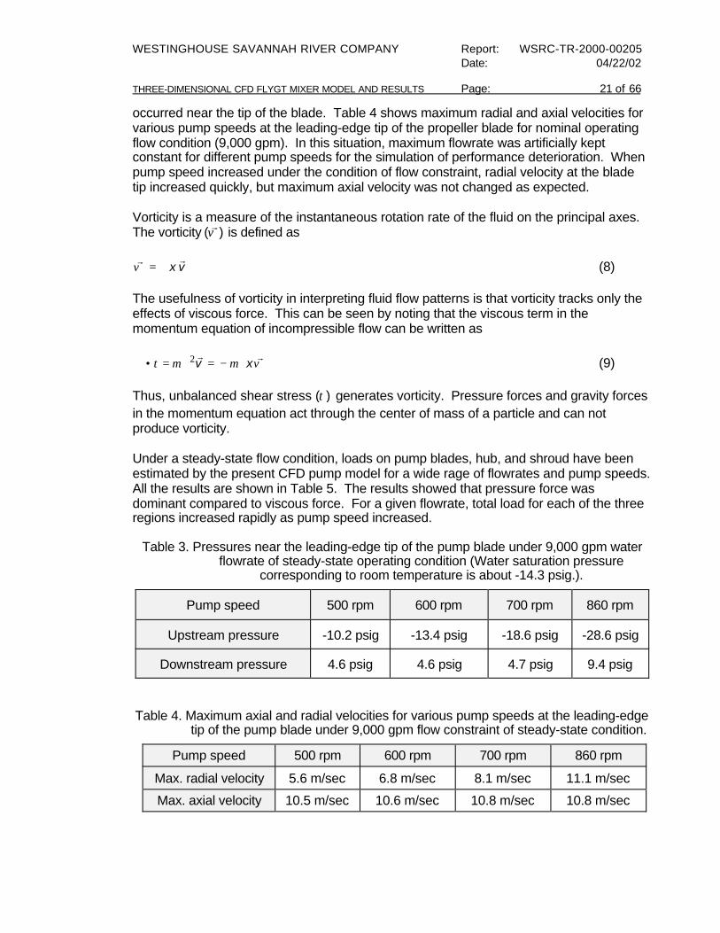
THREE-DIMENSIONAL CFD FLYGT MIXER MODEL AND RESULTS Page: 21 of 66
occurred near the tip of the blade. Table 4 shows maximum radial and axial velocities forvarious pump speeds at the leading-edge tip of the propeller blade for nominal operatingflow condition (9,000 gpm). In this situation, maximum flowrate was artificially keptconstant for different pump speeds for the simulation of performance deterioration. Whenpump speed increased under the condition of flow constraint, radial velocity at the bladetip increased quickly, but maximum axial velocity was not changed as expected.
Vorticity is a measure of the instantaneous rotation rate of the fluid on the principal axes.The vorticity )(ϖr is defined as
vxrr
∇=ϖ (8)
The usefulness of vorticity in interpreting fluid flow patterns is that vorticity tracks only theeffects of viscous force. This can be seen by noting that the viscous term in themomentum equation of incompressible flow can be written as
ϖµµτrr
xv ∇−=∇=•∇ 2 (9)
Thus, unbalanced shear stress )(τ generates vorticity. Pressure forces and gravity forcesin the momentum equation act through the center of mass of a particle and can notproduce vorticity.
Under a steady-state flow condition, loads on pump blades, hub, and shroud have beenestimated by the present CFD pump model for a wide rage of flowrates and pump speeds.All the results are shown in Table 5. The results showed that pressure force wasdominant compared to viscous force. For a given flowrate, total load for each of the threeregions increased rapidly as pump speed increased.
Table 3. Pressures near the leading-edge tip of the pump blade under 9,000 gpm waterflowrate of steady-state operating condition (Water saturation pressure
corresponding to room temperature is about -14.3 psig.).
Pump speed 500 rpm 600 rpm 700 rpm 860 rpm
Upstream pressure -10.2 psig -13.4 psig -18.6 psig -28.6 psig
Downstream pressure 4.6 psig 4.6 psig 4.7 psig 9.4 psig
Table 4. Maximum axial and radial velocities for various pump speeds at the leading-edgetip of the pump blade under 9,000 gpm flow constraint of steady-state condition.
Pump speed 500 rpm 600 rpm 700 rpm 860 rpm
Max. radial velocity 5.6 m/sec 6.8 m/sec 8.1 m/sec 11.1 m/sec
Max. axial velocity 10.5 m/sec 10.6 m/sec 10.8 m/sec 10.8 m/sec

Report: WSRC-TR-2000-00205 WESTINGHOUSE SAVANNAH RIVER COMPANYDate: 04/22/02Page: 22 of 66 THREE-DIMENSIONAL CFD FLYGT MIXER MODEL AND RESULTS
Changes in flowrate are harder to interpret because the flowrate was used a boundarycondition for the calculation. As the flowrate was decreased for a given pump speed, thepropeller became starved for flow. Cavitation increased and the pressure loads on themixer components increased. All of this indicated a deterioration in pump performancewith reduced flow.
As shown in Fig. 15, load for the propeller blade is the largest among the three regions. Itis noted that load for each component is not sensitive to the pump flowrate. Figure 16shows that radial velocity at the tip of the blade is very sensitive to the rotational speed ofthe mixer. When pump speed increased from 500 to 860 rpm, maximum radial speedincreased from 5.6 m/sec to 11.1 m/sec as shown in Table 4. Static pressure distributionscorresponding to the velocity distributions are quite different depending on rotationalspeed of the mixing pump as presented in Fig. 17. These pressure distributions inducethe load for each component of the mixer. As expected from our intuition, a large andlocalized vortex motion is generated near the leading-edge tip of the propeller blade. Thislarge vortex motion introduces the cavitation, referred to as vortex cavitation in theliterature (Knapp et al., 1970). Vorticity contour plots for the plane crossing the tip of theblade are shown in Fig. 18. The pressure coefficient along the axial flow direction crossingthe leading-edge tip of the blade, as shown in fig. 19, indicates that the location of theminimum pressure is very close to the tip of the blade. This implies that the vortexcavitation inception will occur near the tip of the blade. It is seen that the negativeminimum pressure coefficient (- Cp,min) increases as the pump speed increases and thecorresponding advance coefficient decreases, i.e., the propeller loading is increased.Comparisons of the numerical results for a wide range of non-dimensional pump speedsare summarized in Table 6. The advance coefficient J is a dimensionless numberassociated with the propeller design condition, which is the ratio of fluid average velocity(uavg) to the product of pump speed (n) and propeller diameter (Dprop), that is, J = uavg/(nDprop). These results are consistent with the literature data (Hsiao and Pauley, 1999). Thepressure coefficient (Cp) is a dimensionless parameter defined by the reference pressure(Pref) and the reference dynamic pressure (Qref ). That is,
( )ref
refp Q
PPC
−= (10)
In eq. (5), Qref is defined in terms of the reference velocity (Vref ).
250 reffref VQ ρ.= (11)
In Table 6 and Fig. 19, one atmospheric pressure and 6 m/sec flow conditions were usedas the reference values. The results shown in Fig. 19 indicate that cavitation occurs nearthe leading-edge tip of the blade for the 700 and 860 rpm pump speeds, but it does notoccur for the 500 rpm speed. The 600 rpm pump speed is the critical value for thecavitation to occur. Thus, pump speed should be decreased from 860 rpm to about 500rpm, which is close to the original design speed 440 rpm of the FLYGT mixer, if cavitationneeds to be avoided for the structural vibration or stability of the mixer. The cavitation lineshown in the figure is based on the saturation pressure of vapor corresponding to theroom temperature water, although real flow effects such as random turbulent fluctuationand water quality are known to influence cavitation inception. Figure 20 shows the
WESTINGHOUSE SAVANNAH RIVER COMPANY Report: WSRC-TR-2000-00205Date: 04/22/02
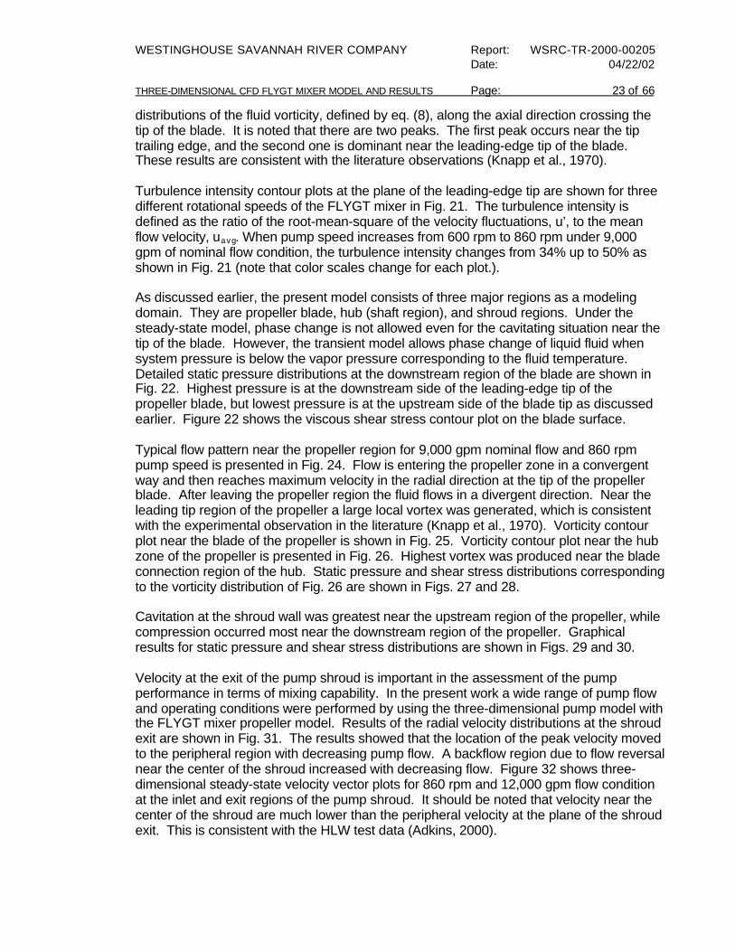
THREE-DIMENSIONAL CFD FLYGT MIXER MODEL AND RESULTS Page: 23 of 66
distributions of the fluid vorticity, defined by eq. (8), along the axial direction crossing thetip of the blade. It is noted that there are two peaks. The first peak occurs near the tiptrailing edge, and the second one is dominant near the leading-edge tip of the blade.These results are consistent with the literature observations (Knapp et al., 1970).
Turbulence intensity contour plots at the plane of the leading-edge tip are shown for threedifferent rotational speeds of the FLYGT mixer in Fig. 21. The turbulence intensity isdefined as the ratio of the root-mean-square of the velocity fluctuations, u’, to the meanflow velocity, uavg. When pump speed increases from 600 rpm to 860 rpm under 9,000gpm of nominal flow condition, the turbulence intensity changes from 34% up to 50% asshown in Fig. 21 (note that color scales change for each plot.).
As discussed earlier, the present model consists of three major regions as a modelingdomain. They are propeller blade, hub (shaft region), and shroud regions. Under thesteady-state model, phase change is not allowed even for the cavitating situation near thetip of the blade. However, the transient model allows phase change of liquid fluid whensystem pressure is below the vapor pressure corresponding to the fluid temperature.Detailed static pressure distributions at the downstream region of the blade are shown inFig. 22. Highest pressure is at the downstream side of the leading-edge tip of thepropeller blade, but lowest pressure is at the upstream side of the blade tip as discussedearlier. Figure 22 shows the viscous shear stress contour plot on the blade surface.
Typical flow pattern near the propeller region for 9,000 gpm nominal flow and 860 rpmpump speed is presented in Fig. 24. Flow is entering the propeller zone in a convergentway and then reaches maximum velocity in the radial direction at the tip of the propellerblade. After leaving the propeller region the fluid flows in a divergent direction. Near theleading tip region of the propeller a large local vortex was generated, which is consistentwith the experimental observation in the literature (Knapp et al., 1970). Vorticity contourplot near the blade of the propeller is shown in Fig. 25. Vorticity contour plot near the hubzone of the propeller is presented in Fig. 26. Highest vortex was produced near the bladeconnection region of the hub. Static pressure and shear stress distributions correspondingto the vorticity distribution of Fig. 26 are shown in Figs. 27 and 28.
Cavitation at the shroud wall was greatest near the upstream region of the propeller, whilecompression occurred most near the downstream region of the propeller. Graphicalresults for static pressure and shear stress distributions are shown in Figs. 29 and 30.
Velocity at the exit of the pump shroud is important in the assessment of the pumpperformance in terms of mixing capability. In the present work a wide range of pump flowand operating conditions were performed by using the three-dimensional pump model withthe FLYGT mixer propeller model. Results of the radial velocity distributions at the shroudexit are shown in Fig. 31. The results showed that the location of the peak velocity movedto the peripheral region with decreasing pump flow. A backflow region due to flow reversalnear the center of the shroud increased with decreasing flow. Figure 32 shows three-dimensional steady-state velocity vector plots for 860 rpm and 12,000 gpm flow conditionat the inlet and exit regions of the pump shroud. It should be noted that velocity near thecenter of the shroud are much lower than the peripheral velocity at the plane of the shroudexit. This is consistent with the HLW test data (Adkins, 2000).

Report: WSRC-TR-2000-00205 WESTINGHOUSE SAVANNAH RIVER COMPANYDate: 04/22/02Page: 24 of 66 THREE-DIMENSIONAL CFD FLYGT MIXER MODEL AND RESULTS
Table 5. Axial forces along the flow direction for propeller, hub, and shroud regions underwide range of steady-state pump operating conditions.
Pump operatingconditions Propeller region Hub region Shroud wall region
Pumpflowrate(gpm)
Pumpspeed(rpm)
Pressure(N)
Viscous(N)
Pressure(N)
Viscous(N)
Pressure(N)
Viscous(N)
500 -2152 8.5 35 -2.2 -16 -1.8
600 -2896 10.3 58 -1.5 -19 8.1
700 -4352 13.6 71 -1.3 -25 13.89,000
860 -7317 21.3 92 -0.3 -35 26.4
700 -4310 13.6 72 -1.9 -25 12.510,000
860 -6978 20.7 98 -0.7 -36 23.1
680 -4020 14.7 63 -3.9 -30 -2.1
700 -4290 15.3 69 -3.9 -30 -0.912,000
860 -6255 19.5 111 -2.7 -39 18.9
700 -4155 16.2 67 -4.8 -33 -4.813,000
860 -5941 20.0 118 -3.0 -39 15.1
700 -1614 23.1 189 -8.1 -39 -3.619,000
860 -5229 27.3 132 -9.9 -54 -11.7
(Note: Conversion factor 1 pound-force = 4.448N)
Table 6. Comparison of minimum pressure coefficients (Cp,min) for the advance coefficients(J) corresponding to various rotational pump speeds.
Pump speed(rpm)
J(---)
Reynolds number(---)
- Cp,min
(---)Total loading on the blades
(pound-force)
860 0.40 1.4 x 10⁶ 10.4 1645
700 0.49 1.4 x 10⁶ 7.2 978
600 0.57 1.4 x 10⁶ 5.3 651
500 0.68 1.4 x 10⁶ 3.9 484
440 0.78 1.4 x 10⁶ 3.0 342


WESTINGHOUSE SAVANNAH RIVER COMPANY Report: WSRC-TR-2000-00205Date: 04/22/02
THREE-DIMENSIONAL CFD FLYGT MIXER MODEL AND RESULTS Page: 45 of 66
4.2 Sensitivity Run Results
Sensitivity runs were performed by using the steady-state three-dimensional CFD model.The primary purpose is to investigate what physical parameters have the most impact onoperating performance and system stability of the FLYGT mixer. From the steady-statemodel results, physical parameters such as inlet flow conditions, shroud wall roughness,and rotational speed of pump were chosen for the sensitivity studies.
- Non-uniform Inlet Flow Condition
This situation was simulated to examine the impact on the shroud exit velocity of non-uniform inlet velocity for the flow blockage caused by the motor housing upstream of thepump propeller. Non-uniform velocity was tested with an assumption that velocity aroundmotor housing increased linearly along the flow direction toward the propeller region. Thatis,
∫= 2
1
1 A
A ravg dAxuA
u )(
( )∫==
+= inLx
xin
dxxL 0
1 βα (10)
Constants α and β in the above integral, eq. (10), were determined by using the boundarycondition 00 == )(xu r and the flow continuity Q(total volumetric flowrate) = Auavg .
uavg is area-averaged radial velocity at the inlet of the mixer. The area-averaged speedsfor potential flow conditions are shown in Table 2. Detailed flow direction and notationsused in the above equation are shown in Fig. 33. This non-uniform condition was basedon the assumption that azimuthal velocity gradients at both sides of the symmetry planesin 120o sector geometry of the mixer, as shown in Fig. 3, are zero. For these studies,typical operating conditions were chosen as two different operating flows (9,000 and12,000 gpm) with 860 rpm pump speed.
The results showed that at shroud exit radial flow distributions for non-uniform inletcondition is a little bit more uniform than those of uniform inlet flow condition. Thesensitivity results are shown in Fig. 34. Total loads for the three components of the mixerwith non-uniform inlet flow are about 7% lower than those of uniform inlet flow for theoperating conditions of 12,000 gpm flow with 860 rpm pump speed. Three-dimensionalvelocity flow pattern near the inlet and the shroud exit regions is shown in Fig. 35.However, for 9,000 gpm pump flow with 860 rpm pump speed, loads for non-uniform inletflow are close to those of uniform inlet flow. The detailed comparison of the two cases isshown in Table 7.


WESTINGHOUSE SAVANNAH RIVER COMPANY Report: WSRC-TR-2000-00205Date: 04/22/02
THREE-DIMENSIONAL CFD FLYGT MIXER MODEL AND RESULTS Page: 63 of 66
5. Conclusions
The present analysis took two modeling approaches with a Computational Fluid Dynamics(CFD) method. They are steady-state pump model and transient cavitation modelconsidering density change effect due to local cavitation. The computations wereperformed for a three-dimensional detailed model of the FLYGT mixer with the prototypicpropeller shape. The models mainly include propeller region, inlet region upstream of thepropeller, and downstream shroud region as a computational domain. The generalcharacteristics of the propeller flow including the blade-to-blade rotational flow, cavitationwith tip vortex, and flow pattern at shroud exit were well predicted by the present CFDmethod using computational domain of one-third FLYGT mixer for better computationalefficiency.
From the analysis results for the three-dimensional models of the Tank 19 FLYGT mixer,the following conclusions are drawn:
1. Nominal operating conditions were measured by the pitot-tube test data (Adkins,2000). Comparisons with calculated results showed that nominal pump flow conditionswere about 9000 gpm, and pump flow distribution was not sensitive to rotational speedof the mixer (600 to 860 rpm), which is consistent with the test data.
2. From the results of the present detailed model and the previous wall jet model, thepump with a 20” long modified shroud showed reasonable flow performance at the exitof the shroud in terms of backflow prevention and mixing capability.
3. The detailed steady-state model results showed that load for each of the three majorcomponent (propeller blade, hub and shroud) of the mixer increased as speed of themixer increased. It was noted that cavitation occurred near the leading-tip of the pumpblade and the degree of cavitation increased rapidly with pump speed increase.
4. The steady-state results show that cavitation doesn’t occur for 9,000 gpm flowratewhen the pump speed is lower than 500 rpm. This is consistent with the original bladedesign of the FLYGT mixer to avoid the cavitation. The original design speed was 440rpm.
5. From the sensitivity study, it was noted that the pump speed was a sensitive parameterfor the load for each pump component, but it was not sensitive for the pump flowperformance. The propeller blade has the largest load among the three components ofthe FLYGT mixer under a wide range of pump operating conditions.
6. The transient results showed that transient pump behaviors such as change of fluiddensity and loadings of mixer were developed to steady-state conditions within about 1second, corresponding to about 40 cycles of the propeller blade after the initiation ofthe pump cavitation. In addition, a low density region was established near theperipheral region adjacent to the shroud wall because all bubbles generated as a resultof cavitation migrated to the high-velocity fluid region near the tip of the blade.

Report: WSRC-TR-2000-00205 WESTINGHOUSE SAVANNAH RIVER COMPANYDate: 04/22/02Page: 64 of 66 THREE-DIMENSIONAL CFD FLYGT MIXER MODEL AND RESULTS
6. Recommendations
From the detailed model and the previous two-dimensional wall jet model, it was notedthat the pump speed could be decreased without reducing the flow performance of themixer under the current 20” single-piece machined shroud. From the present steady-stateresults, it is recommended that the pump speed decrease from 860 rpm down to about500 rpm when cavitation needs to be avoided for better pump performance.
The present model used azimuthal symmetrical assumption at the inlet region. One third ofthe mixer was modeled by using symmetrical planes at both-end sides of the model forcomputational efficiency. Thus, the present model can not predict non-uniform inlet flowcondition in an azimuthal direction. In reality, non-uniform water flow and air entrained bya vortex at the inlet region may cause periodical choking before entering the propellerregion.
It is recommended that the current 120o symmetry, single-blade model be extended to athree-blade mixer with the tank bottom and free liquid surface (about 4ft level) included inthe full three-dimensional computation domain. Thus, boundary conditions at the pumpinlet for the CFD model would be closer to the real situation, which is non-uniform flowdistribution at the screen inlet due to the flow blockage and due to the presence of the tankbottom. This change would allow us to:
1. Remove the fixed flow boundary condition at the pump inlet.2. Analyze pump performance as a function of operating speed.3. Determine the optimum operating point for the existing propeller shape.
This model could also simulate three-dimensional axial flow dissipation after the shroudexit above the tank bottom to assess mixing performance. The current two-dimensional jetmodel has been used to estimate this performance, but it can not capture the physics ofthree-dimensional swirling phenomena.

WESTINGHOUSE SAVANNAH RIVER COMPANY Report: WSRC-TR-2000-00205Date: 04/22/02
THREE-DIMENSIONAL CFD FLYGT MIXER MODEL AND RESULTS Page: 65 of 66
7. References
1. Adkins, B., “Flygt Mixer Design Optimization Test Summary”, WSRC Memorandum,HLW-STE-2000-00196, May 8, 2000.
2. Davis, M. R. and Winarto, H., “Jet Diffusion From a Circular Nozzle Above a SolidPlane”, Journal of Fluid Mechanics, Vol. 101, pp. 201 - 221, 1980.
3. FLUENT User’s Guide, V.5.0, Fluent Incorporated, Lebanon, NH, January 2000.
4. Hsiao, C. and Pauley, L. L., “Numerical Computation of Tip Vortex Flow Generated byMarine Propeller”, Transactions of the ASME, Journal of Fluid Engineering, Vol. 121,pp. 638-645, September 1999.
5. Knapp, R. T., Daily, J. W., and Hammitt, F. G., Cavitation, McGraw-Hill BookCompany, New York, 1970.
6. Kubota, A., Kato, H., and Yamaguchi, H., “A New Modeling of Cavitating Flows: ANumerical Study of Unsteady Cavitation on a Hydrofoil Section”, Journal of FluidMechanics, Vol. 240, pp. 59-96, 1992.
7. Lee, S. Y. and Dimenna, R. A., “Validation Analysis for a Computational FluidDynamics calculation of a Turbulent free Jet in water” Using CFDS-FLOW3D andFLUENT (U)”, WSRC-TR-95-0170, May 1995.
8. Lee, S. Y. and Dimenna, R. A., “Two-Dimensional FLYGT Mixer Shroud Model andResults”, WSRC-TR-2000-00106, May 2000.
9. Poirier, M. R. and Rodwell, P. O., “Phase C Flygt Mixer Test Results (U)”, WSRC-TR-99-00097, March 1999.
10. Personal communications with Brannen J. Adkins, March 2000.
11. Rajaratnam, N. and Pani, B. S., “Three-Dimensional Turbulent Wall Jets”, Journal ofThe Hydraulics Divison, Vol. 100, pp. 69 - 83, January, 1974.
12. Rohsenow, W. M. and Choi, H. Y., Heat, Mass, and Momentum transfer, Prentice-Hall,Inc., Englewood Cliff, New Jersey, 1961.
13. Schlichting, H., Boundary-Layer Theory, Translated by J. Kestin, McGraw-Hill BookCompany, New York, 1979.
14. Wood, G. M., “Visual Cavitation Studies of Mixed Flow Pump Impellers”, Transactionsof the ASME, Journal of Basic Engineering, pp. 17-28, March 1963.

Report: WSRC-TR-2000-00205 WESTINGHOUSE SAVANNAH RIVER COMPANYDate: 04/22/02Page: 66 of 66 THREE-DIMENSIONAL CFD FLYGT MIXER MODEL AND RESULTS
(This Page Intentionally Left Blank)