threads (ch.4) - upfrramirez/os/l03.pdf · silberschatz / os concepts / 6e - chapter 6 cpu...

Threads (Ch.4) !   Many software packages are multi-threaded

l  Web browser: one thread display images, another thread retrieves data from the network

l  Word processor: threads for displaying graphics, reading keystrokes from the user, performing spelling and grammar checking in the background

l  Web server: instead of creating a process when a request is received, which is time consuming and resource intensive, server creates a thread to service the request

!   A thread is sometimes called a lightweight process l  It is comprised over a thread ID, program counter, a register set and a

stack l  It shares with other threads belonging to the same process its code

section, data section and other OS resources (e.g., open files) l  A process that has multiples threads can do more than one task at a time

Benefits !   Responsiveness

l  One part of a program can continue running even if another part is blocked

!   Resource Sharing l  Threads of the same process share the same memory space and

resources !   Economy

l  Much less time consuming to create and manage threads than processes

l  Solaris 2: creating a process is 30 times slower than creating a thread, context switching is 5 times slower

!   Utilization of MP Architectures l  Each thread can run in parallel on a different processor

Many-to-One Model !   Many user-level threads mapped to single kernel thread.

l  Efficient - thread management done in user space l  Entire process will block if a thread makes a blocking system call l  Only one thread can access the kernel, no parallel processing in MP

environment

One-to-One !   Each user-level thread maps to kernel thread.

l  Another thread can run when one thread makes a blocking call l  Multiple threads an run in parallel on a MP machine l  Overhead of creating a kernel thread for each user thread l  Most implementations limit the number of threads supported

!   Examples - Windows - OS/2

- Linux

Many-to-Many Model !   Allows many user level threads to be mapped to smaller or equal

number of kernel threads. !   As many user threads as necessary can be created !   Corresponding kernel threads can run in parallel on a multiprocessor !   When a thread performs a blocking system call, the kernel can

schedule another thread for execution

!   Allows true concurrency in a MP environment and does not restrict number of threads that can be created

Java Threads !   Java threads may be created by extending the Thread class or implementing the

Runnable interface !   Java threads are managed by the JVM

l  support provided at the language level l  The JVM specification does not indicate how threads should be mapped to the

underlying OS l  Windows 95/98/NT/2000 use the one-to-one model (each Java thread maps to a

kernel thread) l  Solaris 2 used the many-to-many model

!   public MyThread extends Thread !   { !   public void run() !   {do_stuff();} !   } ! MyThread t = new MyThread(); ! t.start();

!   public MyRunnable implements Runnable

!   { !   public void run() !   {do_stuff();} !   } !   Thread t = new Thread(new

MyRunnable()); ! t.start();

Silberschatz / OS Concepts / 6e - Chapter 5 Threads Slide 7

Java Thread States

CPU Scheduling (Ch.5) !   Basic Concepts !   Scheduling Criteria !   Scheduling Algorithms !   Multiple-Processor Scheduling !   Real-Time Scheduling !   Algorithm Evaluation

Basic Concepts

!   Maximum CPU utilization obtained with multiprogramming

!   CPU–I/O Burst Cycle – Process execution consists of a cycle of CPU execution and I/O wait.

!   Scheduling is central to OS design l  CPU and almost all computer resources are scheduled

before use

Alternating Sequence of CPU And I/O Bursts

Histogram of CPU-burst Times

!   CPU bursts, though different by process and computer, tend to have a frequency curve as shown above !   Characterized by many short bursts and few long ones !   The distribution can help in the selection of an appropriate

scheduling algorithm

CPU Scheduler !   Selects from among the processes in memory that are ready to execute,

and allocates the CPU to one of them. !   CPU scheduling decisions may take place when a process:

1. Switches from running to waiting state. 2. Switches from running to ready state. 3. Switches from waiting to ready. 4. Terminates.

!   Scheduling under 1 and 4 is nonpreemptive – a new process must be selected for execution l  Once the CPU has been allocated to a process, the process keeps the

CPU until it releases the CPU either by terminating or switching to a waiting state

!   All other scheduling is preemptive.

Dispatcher !   Dispatcher module gives control of the CPU to the process

selected by the short-term scheduler; this involves: l  switching context l  switching to user mode l  jumping to the proper location in the user program to restart

that program

!   Dispatch latency – time it takes for the dispatcher to stop one process and start another running.

Scheduling Criteria !   CPU utilization – keep the CPU as busy as possible !   Throughput (tasa de procesamiento) – # of processes that

complete their execution per time unit !   Turnaround time (tiempo de ejecución)– amount of time to

execute a particular process l  waiting to get into memory + waiting in the ready queue +

executing on the CPU + I/O !   Waiting time – amount of time a process has been waiting in

the ready queue !   Response time – amount of time it takes from when a request

was submitted until the first response is produced, not output (for time-sharing environment)

Optimization Criteria !   Max CPU utilization !   Max throughput !   Min turnaround time !   Min waiting time !   Min response time

!   In most cases we optimize the average measure !   In some circumstances we want to optimize the min or max

values rather than the average – e.g., minimize the max response time so all users get good service

Silberschatz / OS Concepts / 6e - Chapter 6 CPU Scheduling Slide 16

Scheduling Algorithms First-Come, First-Served (FCFS)

Process Burst Time P1 24 P2 3 P3 3

!   Suppose that the processes arrive in the order: P1 , P2 , P3 The Gantt Chart for the schedule is:


Scheduling Algorithms First-Come, First-Served (FCFS)

Process Burst Time P1 24 P2 3 P3 3

!   Suppose that the processes arrive in the order: P1 , P2 , P3 The Gantt Chart for the schedule is:

!   Waiting time for P1 = 0; P2 = 24; P3 = 27 !   Average waiting time: (0 + 24 + 27)/3 = 17

P1! P2! P3!

24! 27! 30!0!


FCFS Scheduling (Cont.) Suppose that the processes arrive in the order P2 , P3 , P1 !   The Gantt chart for the schedule is:

!   Much better than previous case. !   Average waiting time is generally not minimal and may vary

substantially if the process CPU-burst times vary greatly


FCFS Scheduling (Cont.) Suppose that the processes arrive in the order P2 , P3 , P1 !   The Gantt chart for the schedule is:

!   Waiting time for P1 = 6; P2 = 0; P3 = 3 !   Average waiting time: (6 + 0 + 3)/3 = 3 !   Much better than previous case. !   Average waiting time is generally not minimal and may vary

substantially if the process CPU-burst times vary greatly

P1!P3!P2!

6!3! 30!0!


FCFS Scheduling (Cont.) !   FCFS is non-preemptive !   Not good for time sharing systems where where each user needs to

get a share of the CPU at regular intervals !   Convoy effect short process(I/O bound) wait for one long CPU-

bound process to complete a CPU burst before they get a turn l  lowers CPU and device utilization


Shortest-Job-First (SJR)Scheduling !   Associate with each process the length of its next CPU burst.

Use these lengths to schedule the process with the shortest time (on a tie use FCFS)

!   Two schemes: l  nonpreemptive – once CPU given to the process it cannot be

preempted until completes its CPU burst. l  preemptive – if a new process arrives with CPU burst length

less than remaining time of current executing process, preempt. This scheme is know as the Shortest-Remaining-Time-First (SRTF).

!   SJF is optimal – gives minimum average waiting time for a given set of processes.


Process Arrival Time Burst Time P1 0.0 7 P2 2.0 4 P3 4.0 1 P4 5.0 4

!   SJF (non-preemptive)

Example of Non-Preemptive SJF


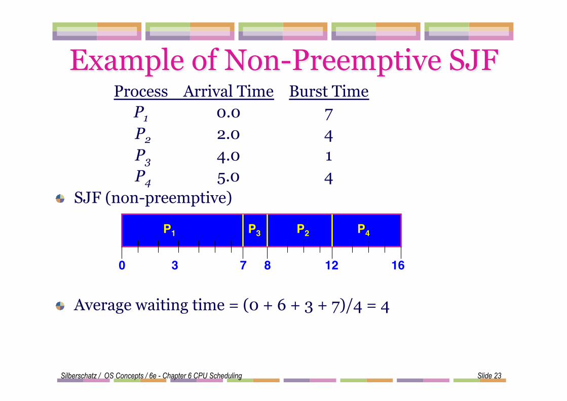
Process Arrival Time Burst Time P1 0.0 7 P2 2.0 4 P3 4.0 1 P4 5.0 4

!   SJF (non-preemptive)

!   Average waiting time = (0 + 6 + 3 + 7)/4 = 4

Example of Non-Preemptive SJF

P1! P3! P2!

7!3! 16!0!

P4!

8! 12!


Example of Preemptive SJF Process Arrival Time Burst Time P1 0.0 7 P2 2.0 4 P3 4.0 1 P4 5.0 4

!   SJF (preemptive)


Example of Preemptive SJF Process Arrival Time Burst Time P1 0.0 7 P2 2.0 4 P3 4.0 1 P4 5.0 4

!   SJF (preemptive)

!   Average waiting time = (9 + 1 + 0 +2)/4 = 3

P1! P3!P2!

4!2! 11!0!

P4!

5! 7!

P2! P1!

16!

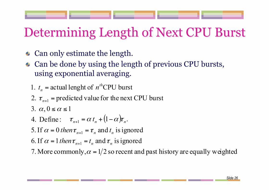
Determining Length of Next CPU Burst !   Can only estimate the length. !   Can be done by using the length of previous CPU bursts,

using exponential averaging.

ightedequally we arehistory past andrecent so 21 commonly, More 7.ignored is and 1 If 6.ignored is and 0 If 5.

:Define 4.10 , 3.

burst CPUnext for the valuepredicted 2.burst CPU oflenght actual 1.

1

1

1

=

==

==

≤≤

=

=

+

+

+

α

ττα

ττα

αα

τ

nnn

nnn

n

thn

tthentthen

nt

( ) .1 1 nnn t ταατ −+=+


Prediction of the Length of the Next CPU Burst

α= 1/2


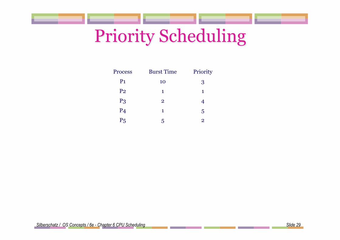
Priority Scheduling !   A priority number (integer) is associated with each process !   The CPU is allocated to the process with the highest priority

(smallest integer ≡ highest priority). l  Can be preemptive (compares priority of process that has

arrived at the ready queue with priority of currently running process) or nonpreemptive (put at the head of the ready queue)

!   SJF is a priority scheduling where priority is the predicted next CPU burst time.

!   Problem ≡ Starvation – low priority processes may never execute.

!   Solution ≡ Aging – as time progresses increase the priority of the process.


Priority Scheduling

Process Burst Time Priority

P1 10 3

P2 1 1

P3 2 4

P4 1 5

P5 5 2


Round Robin (RR) !   Each process gets a small unit of CPU time (time quantum),

usually 10-100 milliseconds. After this time has elapsed, the process is preempted and added to the end of the ready queue.

!   If there are n processes in the ready queue and the time quantum is q, then each process gets 1/n of the CPU time in chunks of at most q time units at once. No process waits more than (n-1)q time units.

!   Performance l  q large ⇒ FIFO l  q small ⇒ q must be large with respect to context switch,

otherwise overhead is too high.


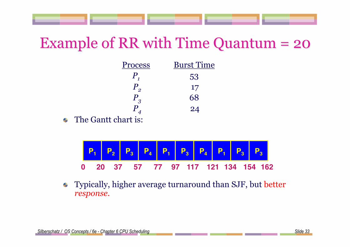
Example of RR with Time Quantum = 20 Process Burst Time P1 53 P2 17 P3 68 P4 24

!   The Gantt chart is:


Example of RR with Time Quantum = 20 Process Burst Time P1 53 P2 17 P3 68 P4 24

!   The Gantt chart is:

!   Typically, higher average turnaround than SJF, but better response.

P1! P2! P3! P4! P1! P3! P4! P1! P3! P3!

0! 20! 37! 57! 77! 97! 117! 121! 134! 154! 162!


Time Quantum and Context Switch Time

A smaller time quantum increase context switches


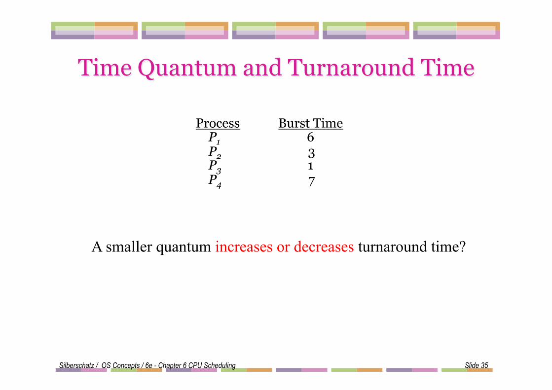
Time Quantum and Turnaround Time

Process Burst Time P1 6 P2 3 P3 1 P4 7

A smaller quantum increases or decreases turnaround time?


Turnaround Time Varies With The Time Quantum

!   The average turnaround time of a set of processes does not necessarily improve as the time quantum size increases

!   In general, it can be improved if most processes finish their next CPU burst in a single time quantum


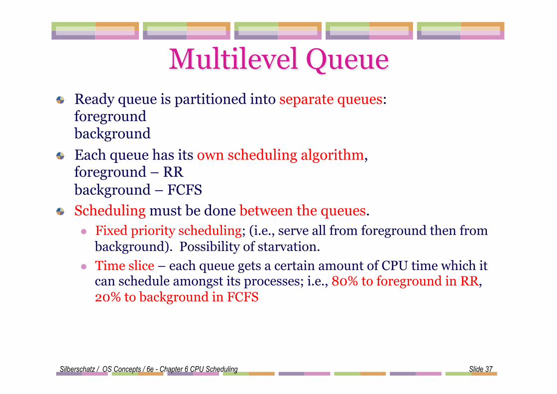
Multilevel Queue !   Ready queue is partitioned into separate queues:

foreground background

!   Each queue has its own scheduling algorithm, foreground – RR background – FCFS

!   Scheduling must be done between the queues. l  Fixed priority scheduling; (i.e., serve all from foreground then from

background). Possibility of starvation. l  Time slice – each queue gets a certain amount of CPU time which it

can schedule amongst its processes; i.e., 80% to foreground in RR, 20% to background in FCFS

Multilevel Queue



Foreground processes Background processes

foreground – RR (quantum=1) background – FCFS Time slice – 80% (8ms) to foreground in RR, 20% to background in FCFS


Multilevel Queue Scheduling

!   Each queue has absolute priority over lower priority queues

!   A lower priority process that is executing would be preempted if a higher priority process arrived


Multilevel Feedback Queue

!   A process can move between the various queues; aging can be implemented this way.

!   Multilevel-feedback-queue scheduler defined by the following parameters: l  number of queues l  scheduling algorithms for each queue l  method used to determine when to upgrade a process l  method used to determine when to demote a process l  method used to determine which queue a process will enter

when that process needs service


Example of Multilevel Feedback Queue

!   Three queues: l  Q0 – time quantum 8 milliseconds l  Q1 – time quantum 16 milliseconds l  Q2 – FCFS

!   Scheduling l  A new job enters queue Q0 which is served FCFS. When it gains

CPU, job receives 8 milliseconds. If it does not finish in 8 milliseconds, job is moved to queue Q1.

l  At Q1 job is again served FCFS and receives 16 additional milliseconds. If it still does not complete, it is preempted and moved to queue Q2.


Multilevel Feedback Queues

!   Processes with a CPU burst of 8 msec or less are given highest priority !   Those that need more than 8 but less than 24 msec are given next highest priority !   Anything longer sink to the bottom queue and are serviced only when the first two

queues are idle


Multilevel Feedback Queues

Process Burst Time P1 42 P2 6 P3 20 P4 12 P5 32 P6 30 P7 10 P8 5


Real-Time Scheduling !   Hard real-time systems – required to complete a critical task within

a guaranteed amount of time. l  Resource reservation – knows how much time it requires and will be

scheduled if it can be guaranteed that amount of time l  Requires special purpose software dedicated to their critical process

!   Soft real-time computing – requires that critical processes receive priority over less fortunate ones. l  System must have priority scheduling where real time processes are

given the highest priority (no aging to keep priorities constant) l  Dispatch latency must be small


Load balancing !   Load balancing attempts to keep the workload evenly

distributed across all processors in a MP system. !   load balancing is typically necessary only on systems where

each processor has its own private queue of eligible processes to execute.

!   There are two general approaches to load balancing: l  push migration l  pull migration

!   load balancing often counteracts the benefits of processor affinity, That is, the benefit of keeping a process running on the same processor (cache memory)


Algorithm Evaluation !   Deterministic modeling – takes a particular predetermined workload and

defines the performance of each algorithm for that workload. l  Requires too much exact knowledge, can not generalize

!   Queueing models l  Arrival and service distributions are often unrealistic

!   Simulation l  Distribution of jobs may not accurate; use trace tapes of real system activity l  Expensive to run, time consuming; writing and testing the simulator is a

major task !   Implementation – code the algorithm and actually evaluate it in the OS

l  Expensive to code and modify the OS; users unhappy with changing environment l  Users take advantage of knowledge of the scheduling algorithm and run different

types of programs (interactive or smaller programs given higher priority) !   Best would be to be able to change the parameters used by the scheduler to

reflect expected future use – separation of mechanism and policy – but not the common practice


Windows XP Priorities !   Priority based, !   preemptive scheduling algorithm; !   highest priority always runs !   Priorities are divided into two classes

l  Variable class – 1 through 15 and l  Real time class – 16 through 31

!   Priority is based on priority class it belongs to and the relative priority within each class l  When a threads quantum runs out the thread is interrupted. l  If it is in the variable priority class its priority is lowered l  Gives good response to interactive threads (mouse, windows) and

enables I/O-bound threads to keep the I/O devices busy while compute-bound use spare CPU cycles in the background


Linux Scheduling

!   Preemptive, priority based with two separate priority ranges l  Higher priority tasks have longer time quanta

threads (ch.4) - upfrramirez/os/l03.pdf · silberschatz / os concepts / 6e - chapter 6 cpu...

Documents