this work is licensed under a creative commons...

Copyright 2008, The Johns Hopkins University and Brian Caffo. All rights reserved. Use of these materials permitted only in accordance with license rights granted. Materials provided “AS IS”; no representations or warranties provided. User assumes all responsibility for use, and all liability related thereto, and must independently review all materials for accuracy and efficacy. May contain materials owned by others. User is responsible for obtaining permissions for use from third parties as needed.

This work is licensed under a Creative Commons Attribution-NonCommercial-ShareAlike License. Your use of this material constitutes acceptance of that license and the conditions of use of materials on this site.

http://creativecommons.org/licenses/by-nc-sa/2.5/

Lecture 18

Brian Caffo

Table ofcontents

Outline

The scorestatistic

Exact tests

Comparingtwo binomialproportions

Bayesian andlikelihoodanalysis of twoproportions

Lecture 18

Brian Caffo

Department of BiostatisticsJohns Hopkins Bloomberg School of Public Health

Johns Hopkins University

December 19, 2007

Lecture 18

Brian Caffo

Table ofcontents

Outline

The scorestatistic

Exact tests



Table of contents

1 Table of contents

2 Outline

3 The score statistic

4 Exact tests

5 Comparing two binomial proportions

6 Bayesian and likelihood analysis of two proportions

Lecture 18

Brian Caffo

Table ofcontents

Outline

The scorestatistic

Exact tests



Outline

1 Tests for a binomial proportion

2 Score test versus Wald

3 Exact binomial test

4 Tests for differences in binomial proportions

5 Intervals for differences in binomial proportions

Lecture 18

Brian Caffo

Table ofcontents

Outline

The scorestatistic

Exact tests



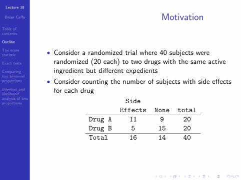
Motivation

• Consider a randomized trial where 40 subjects wererandomized (20 each) to two drugs with the same activeingredient but different expedients

• Consider counting the number of subjects with side effectsfor each drug

SideEffects None total

Drug A 11 9 20Drug B 5 15 20Total 16 14 40

Lecture 18

Brian Caffo

Table ofcontents

Outline

The scorestatistic

Exact tests



Hypothesis tests for binomialproportions

• Consider testing H0 : p = p0 for a binomial proportion

• The score test statistic

p − p0√p0(1− p0)/n

follows a Z distribution for large n

• This test performs better than the Wald test

p − p0√p(1− p)/n

Lecture 18

Brian Caffo

Table ofcontents

Outline

The scorestatistic

Exact tests



Inverting the two intervals

• Inverting the Wald test yields the Wald interval

p ± Z1−α/2

√p(1− p)/n

• Inverting the Score test yields the Score interval

p

(n

n+Z 21−α/2

)+ 1

2

(Z 2

1−α/2

n+Z 21−α/2

)

±Z1−α/2

√1

n+Z 21−α/2

[p(1− p)

(n

n+Z 21−α/2

)+ 1

4

(Z 2

1−α/2

n+Z 21−α/2

)]• Plugging in Zα/2 = 2 yields the Agresti/Coull interval

Lecture 18

Brian Caffo

Table ofcontents

Outline

The scorestatistic

Exact tests



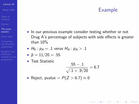
Example

• In our previous example consider testing whether or notDrug A’s percentage of subjects with side effects is greaterthan 10%

• H0 : pA = .1 verus HA : pA > .1

• p = 11/20 = .55

• Test Statistic.55− .1√.1× .9/20

= 6.7

• Reject, pvalue = P(Z > 6.7) ≈ 0

Lecture 18

Brian Caffo

Table ofcontents

Outline

The scorestatistic

Exact tests



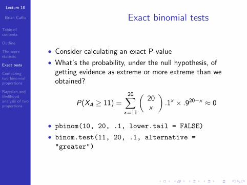
Exact binomial tests

• Consider calculating an exact P-value

• What’s the probability, under the null hypothesis, ofgetting evidence as extreme or more extreme than weobtained?

P(XA ≥ 11) =20∑

x=11

(20x

).1x × .920−x ≈ 0

• pbinom(10, 20, .1, lower.tail = FALSE)

• binom.test(11, 20, .1, alternative ="greater")

Lecture 18

Brian Caffo

Table ofcontents

Outline

The scorestatistic

Exact tests



Notes on exact binomial tests

• This test, unlike the asymptotic ones, guarantees the TypeI error rate is less than desired level; sometimes it is muchless

• Inverting the exact binomial test yields an exact binomialinterval for the true proprotion

• This interval (the Clopper/Pearson interval) has coveragegreater than 95%, though can be very conservative

• For two sided tests, calculate the two one sided P-valuesand double the smaller

Lecture 18

Brian Caffo

Table ofcontents

Outline

The scorestatistic

Exact tests



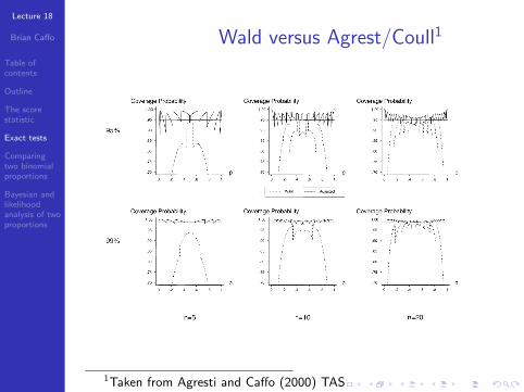
Wald versus Agrest/Coull1

1Taken from Agresti and Caffo (2000) TAS

Lecture 18

Brian Caffo

Table ofcontents

Outline

The scorestatistic

Exact tests



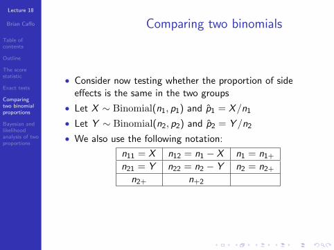
Comparing two binomials

• Consider now testing whether the proportion of sideeffects is the same in the two groups

• Let X ∼ Binomial(n1, p1) and p1 = X/n1

• Let Y ∼ Binomial(n2, p2) and p2 = Y /n2

• We also use the following notation:

n11 = X n12 = n1 − X n1 = n1+

n21 = Y n22 = n2 − Y n2 = n2+

n2+ n+2

Lecture 18

Brian Caffo

Table ofcontents

Outline

The scorestatistic

Exact tests



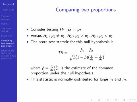
Comparing two proportions

• Consider testing H0 : p1 = p2

• Versus H1 : p1 6= p2, H2 : p1 > p2, H3 : p1 < p2

• The score test statstic for this null hypothesis is

TS =p1 − p2√

p(1− p)( 1n1

+ 1n2

)

where p = X+Yn1+n2

is the estimate of the commonproportion under the null hypothesis

• This statistic is normally distributed for large n1 and n2.

Lecture 18

Brian Caffo

Table ofcontents

Outline

The scorestatistic

Exact tests



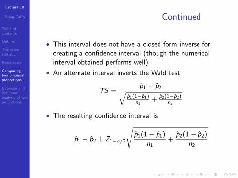
Continued

• This interval does not have a closed form inverse forcreating a confidence interval (though the numericalinterval obtained performs well)

• An alternate interval inverts the Wald test

TS =p1 − p2√

p1(1−p1)n1

+ p2(1−p2)n2

• The resulting confidence interval is

p1 − p2 ± Z1−α/2

√p1(1− p1)

n1+

p2(1− p2)

n2

Lecture 18

Brian Caffo

Table ofcontents

Outline

The scorestatistic

Exact tests



Continued

• As in the one sample case, the Wald iterval and testperforms poorly relative to the score interval and test

• For testing, always use the score test

• For intervals, inverting the score test is hard and notoffered in standard software

• A simple fix is the Agresti/Caffo interval which is obtainedby calculating p1 = x+1

n1+2 , n1 = n1 + 2, p2 = y+1n2+2 and

n2 = (n2 + 2)

• Using these, simply construct the Wald interval

• This interval does not approximate the score interval, butdoes perform better than the Wald interval

Lecture 18

Brian Caffo

Table ofcontents

Outline

The scorestatistic

Exact tests



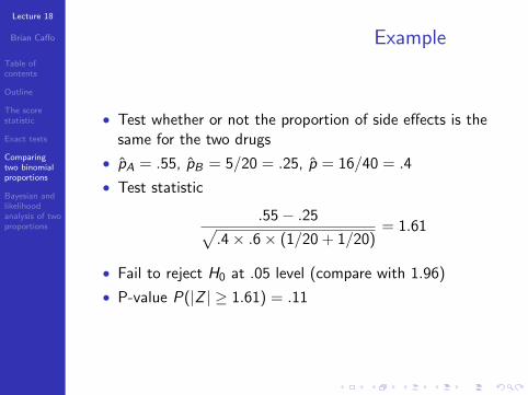
Example

• Test whether or not the proportion of side effects is thesame for the two drugs

• pA = .55, pB = 5/20 = .25, p = 16/40 = .4

• Test statistic

.55− .25√.4× .6× (1/20 + 1/20)

= 1.61

• Fail to reject H0 at .05 level (compare with 1.96)

• P-value P(|Z | ≥ 1.61) = .11

Lecture 18

Brian Caffo

Table ofcontents

Outline

The scorestatistic

Exact tests



Wald versus Agrest/Caffo2


Lecture 18

Brian Caffo

Table ofcontents

Outline

The scorestatistic

Exact tests



Wald versus Agrest/Caffo3


Lecture 18

Brian Caffo

Table ofcontents

Outline

The scorestatistic

Exact tests



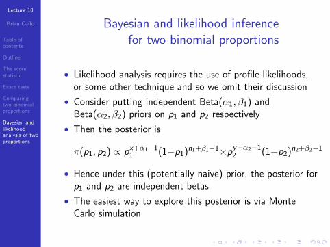
Bayesian and likelihood inferencefor two binomial proportions

• Likelihood analysis requires the use of profile likelihoods,or some other technique and so we omit their discussion

• Consider putting independent Beta(α1, β1) andBeta(α2, β2) priors on p1 and p2 respectively

• Then the posterior is

π(p1, p2) ∝ px+α1−11 (1−p1)n1+β1−1×py+α2−1

2 (1−p2)n2+β2−1

• Hence under this (potentially naive) prior, the posterior forp1 and p2 are independent betas

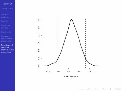
• The easiest way to explore this posterior is via MonteCarlo simulation

Lecture 18

Brian Caffo

Table ofcontents

Outline

The scorestatistic

Exact tests



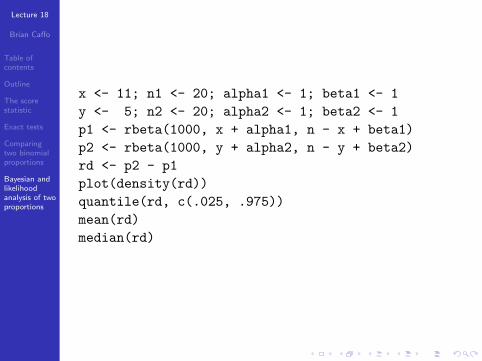
x <- 11; n1 <- 20; alpha1 <- 1; beta1 <- 1y <- 5; n2 <- 20; alpha2 <- 1; beta2 <- 1p1 <- rbeta(1000, x + alpha1, n - x + beta1)p2 <- rbeta(1000, y + alpha2, n - y + beta2)rd <- p2 - p1plot(density(rd))quantile(rd, c(.025, .975))mean(rd)median(rd)

Lecture 18

Brian Caffo

Table ofcontents

Outline

The scorestatistic

Exact tests



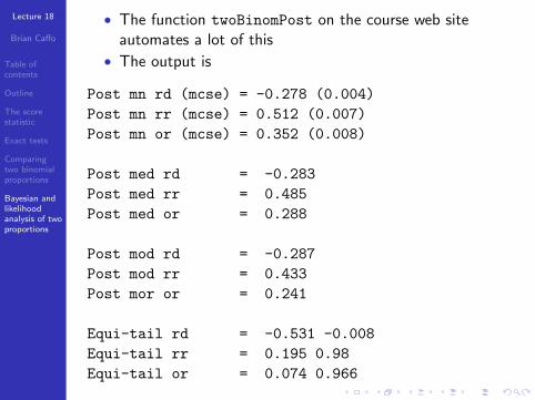
• The function twoBinomPost on the course web siteautomates a lot of this

• The output is

Post mn rd (mcse) = -0.278 (0.004)Post mn rr (mcse) = 0.512 (0.007)Post mn or (mcse) = 0.352 (0.008)

Post med rd = -0.283Post med rr = 0.485Post med or = 0.288

Post mod rd = -0.287Post mod rr = 0.433Post mor or = 0.241

Equi-tail rd = -0.531 -0.008Equi-tail rr = 0.195 0.98Equi-tail or = 0.074 0.966

Lecture 18

Brian Caffo

Table ofcontents

Outline

The scorestatistic

Exact tests



−0.2 0.0 0.2 0.4 0.6

0.0

0.5

1.0

1.5

2.0

2.5

3.0

Risk Difference

this work is licensed under a creative commons...

Documents