1

THE HEALTH BENEFITS OF CONTROLLING CARBON EMISSIONS IN CHINA1

by Richard F. GARBACCIO; Mun S. HO; and Dale W. JORGENSON

1. Introduction

Air pollution from rapid industrialization and the use of energy has been recognized to be a cause ofserious health problems in urban China. For example, the World Bank (1997) estimated that airpollution caused 178,000 premature deaths in urban China in 1995 and valued health damages atnearly 5% of GDP. The same study estimated that hospital admissions due to pollution-relatedrespiratory illness were 346,000 higher than if China had met its own air pollution standards, therewere 6.8 million additional emergency room visits, and 4.5 million additional person-years were lostbecause of illnesses associated with pollution levels that exceeded standards. Much of this damagehas been attributed to emissions of particulates and sulfur dioxide. Furthermore, this problem isexpected to grow in the near future as rapid growth outpaces efforts to reduce emissions.

While particulate and sulfur dioxide emissions from burning fossil fuel contributes to local pollution,the use of fossil fuels also produces carbon dioxide, a greenhouse gas thought to be a majorcontributor to global climate change. The issue of climate change has engaged policy makers for sometime now and is the focus of much current research.

As part of this research, in a previous paper, we examined the effects of limiting CO2 emissions inChina through the use of a carbon tax. In this paper we make a first attempt at estimating the localhealth benefits of such policies. Unlike many other efforts aimed at estimating health effects, whichfocus on specific technological policies to reduce pollution, here we examine broad based economicpolicies within a framework which includes all sectors of the economy. We present a preliminaryeffort, utilizing a number of simplifications, to illustrate the procedure. We plan to use moresophisticated air quality modelling techniques in future work.

1 This research is financially supported by the U.S. Department of Energy and the U.S. EnvironmentalProtection Agency. Gordon Hughes and Kseniya Lvovsky of the World Bank generously shared data andestimates from their work on the health costs of fuel use. Karen Fisher-Vanden and Gernot Wagner contributedto this project. The authors may be contacted at: mun_ho@harvard.edu and garbaccio.richard@epa.gov.

2

Our simple estimates, nevertheless, are instructive. We find that a policy which reduces carbonemissions by 5% every year from our base case will also reduce premature deaths by some 3.5 to4.5%. If we apply commonly used valuation methods, the health damage caused by air pollution inthe first year is about 5% of GDP. A policy to modestly reduce carbon emissions would thereforereduce local health losses by some 0.2% of GDP annually.

2. The economy-energy-health model

Our economic modeling framework is described in Garbaccio, Ho, and Jorgenson (1999). Wesummarize only key features of the model here. Instead, we describe in some detail the health aspectsof our model. Our approach is to first estimate the reduction in emissions of local pollutants due topolicies to reduce CO2 emissions. These changes in emissions are translated into changes inconcentrations of various pollutants in urban areas. Dose-response functions are then used to calculatethe effect of reductions in concentrations of pollutants on health outcomes. These include reducedpremature mortality, fewer cases of chronic bronchitis, and other health effects. Finally, we utilizecommonly used valuation methods to translate the reduced damages to health into yuan values whichmay be compared to the other costs and benefits of such policies.

2.1 The economic model

Our model is a standard multi-sector Solow growth (dynamic recursive) model that is modified torecognize the two-tier plan-market nature of the Chinese economy. The equations of the model aresummarized in Appendix A. As listed in Table 1, there are 29 sectors, including four energy sectors.Output is produced using constant returns to scale technology. Enterprises are given plan outputquotas and the government fixes prices for part of their output. They also receive some plan inputs atsubsidized prices. Marginal decisions, however, are made using the usual “price equals marginal cost”condition. Domestic output competes with imports, which are regarded as imperfect substitutes.

The household sector maximizes a utility function that has all 29 commodities as arguments. Incomeis derived from labor and capital and supplemented by transfers. As in the original Solow model, theprivate savings rate is set exogenously. Total national savings is made up of household savings andenterprise retained earnings. These savings, plus allocations from the central plan, finance nationalinvestment (and the exogenous government deficit and current account). This investment increasesthe stocks of both market and plan capital.

Labor is supplied inelastically by households and is mobile across sectors. The capital stock is partlyowned by households and partly by the government. The plan part of the stock is immobile in anygiven period, while the market part responds to relative returns. Over time, plan capital is depreciatedand the total stock becomes mobile across sectors.

The government imposes taxes on enterprise income, sales, and imports, and also derives revenuefrom a number of miscellaneous fees. On the expenditure side, it buys commodities, makes transfersto households, pays for plan investment, makes interest payments on the public debt, and providesvarious subsidies. The government deficit is set exogenously and projected for the duration of thesimulation period. This exogenous target is met by making government spending on goodsendogenous.

3

Finally, the rest-of-the-world supplies imports and demands exports. World relative prices are set tothe data in the last year of the sample period. The current account balance is set exogenously in thisone-country model. An endogenous terms of trade exchange rate clears this equation.

The level of technology is projected exogenously, i.e. we make a guess of how input requirements perunit output fall over time, including energy requirements. For the later, this is sometimes called theAEEI (autonomous energy efficiency improvement). In the model, there are separate sectors for coalmining, crude petroleum, petroleum refining, and electric power. Non-fossil fuels, includinghydropower and nuclear power, are included as part of the electric power sector.

Table 1. Sectoral characteristics for China, 1992

Gross Energy Use EmissionOutput (mil. tn. coal Height

Sector (bil. yuan) equivalent) Class

1 Agriculture 909 50 low2 Coal Mining 76 44 medium3 Crude Petroleum 69 22 medium4 Metal Ore Mining 24 6 medium5 Other Non-metallic Ore Mining 66 13 medium6 Food Manufacturing 408 36 medium7 Textiles 380 33 medium8 Apparel & Leather Products 149 5 medium9 Lumber & Furniture Manufacturing 50 20 medium

10 Paper, Cultural, & Educational Articles 176 19 medium11 Electric Power 115 49 high12 Petroleum Refining 108 32 medium13 Chemicals 473 138 medium14 Building Material 254 109 medium15 Primary Metals 321 119 medium16 Metal Products 141 23 medium17 Machinery 390 34 medium18 Transport Equipment 163 5 medium19 Electric Machinery & Instruments 155 9 medium20 Electronic & Communication Equipment 107 2 medium21 Instruments and Meters 24 1 medium22 Other Industry 75 7 medium23 Construction 520 14 low24 Transportation & Communications 267 51 low25 Commerce 635 14 low26 Public Utilities 205 17 low27 Culture, Education, Health, & Research 227 19 low28 Finance & Insurance 171 1 low29 Public Administration 191 7 low

Households lowGovernment -Totals 6,846 900

Source: Development Research Center Social Accounting Matrix for 1992; State Statistical Bureau; andauthor’s estimates.

4

A carbon tax is a tax on fossil fuels at a rate based on their carbon content. This tax is applied to theoutput of three industries – coal mining, crude petroleum, and petroleum refining. It is applied toimports while exports are excluded. In the base case this tax is zero. In the policy simulations thecarbon tax rate is set to achieve a desired reduction in carbon emissions. Since the application of thistax will raise revenues above those in the base case, to maintain comparability, we keep governmentspending and revenues the same by reducing other existing taxes.

2.2 The environment-health aspects

Emissions of local pollutants comes from two distinct sources, the first is due to the burning of fossilfuels (combustion emissions), the other from non-combustion processes (process emissions). A greatdeal of dust is produced in industries like cement production and building construction that is notrelated to the amount of fuel used. In this paper we concentrate on two pollutants, particulate matterless than 10 microns (PM-10) and sulfur dioxide (SO2). The analysis of the health effects of otherpollutants, such as nitrogen oxides and lead, are left for future work. PM-10 and SO2 both have theirorigins in combustion and non-combustion sources. Our specification of emissions, concentrations,and dose-response follows Lvovsky and Hughes (1997).2

Total emissions from industry j is the sum of process emissions and combustion emissions fromburning coal, oil, and gas. Let jxtEM denote the emissions of pollutant x from industry j in period t.

Then we have:

(1) ( )∑+=f

jftjxfjtjxjxt AFQIEM ψσ ,

where x = PM-10, SO2 , f = coal, oil, gas , j = 1,2, .. , 29, H, G .

jxσ is process emissions of pollutant x from a unit of sector j output and jxfψ is the emissions from

burning one unit of fuel f in sector j. jtQI is the quantity of output j and jftAF is the quantity of fuel f

(in tons of oil equivalent (toe)) consumed by sector j in period t. The model generates intermediateinputs, denoted ijtA , which are measured in constant yuan. For the cases where i is one of the fuels,

these ijtA ‘s are translated to jftAF which are in tons of oil equivalent of coal, oil, and natural gas.

The j index runs over the 29 production sectors and the non-production sectors (household andgovernment). For the two non-production sectors there are zero process emissions ( 0=jxσ ).

2 Lvovsky and Hughes (1997) discuss the choice of PM-10 rather than total suspended particulates (TSP). Thedata currently collected by the Chinese authorities are mostly in TSP. Health damage, however, is believed to bemainly due to finer particles. Lvovsky and Hughes make an estimate of the share of PM-10 in TSP and kept thatconstant. Improved data would obviously refine this and other analyses.

5

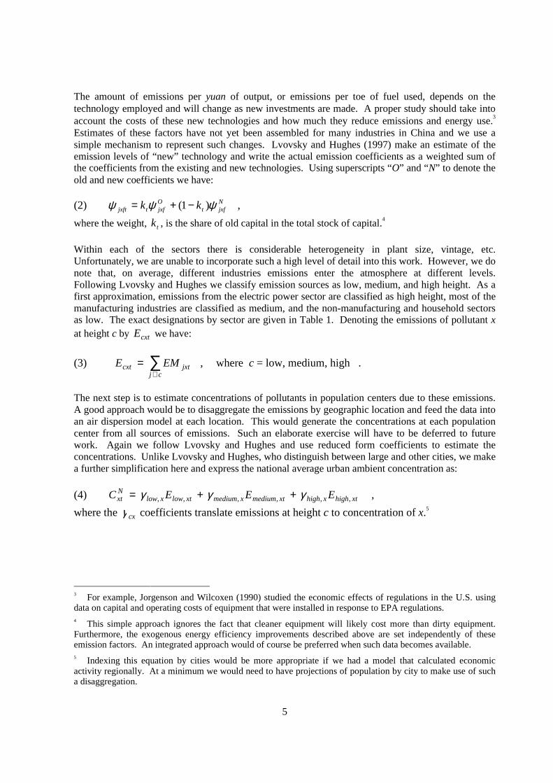
The amount of emissions per yuan of output, or emissions per toe of fuel used, depends on thetechnology employed and will change as new investments are made. A proper study should take intoaccount the costs of these new technologies and how much they reduce emissions and energy use.3

Estimates of these factors have not yet been assembled for many industries in China and we use asimple mechanism to represent such changes. Lvovsky and Hughes (1997) make an estimate of theemission levels of “new” technology and write the actual emission coefficients as a weighted sum ofthe coefficients from the existing and new technologies. Using superscripts “O” and “N” to denote theold and new coefficients we have:

(2) Njxft

Ojxftjxft kk ψψψ )1( −+= ,

where the weight, tk , is the share of old capital in the total stock of capital.4

Within each of the sectors there is considerable heterogeneity in plant size, vintage, etc.Unfortunately, we are unable to incorporate such a high level of detail into this work. However, we donote that, on average, different industries emissions enter the atmosphere at different levels.Following Lvovsky and Hughes we classify emission sources as low, medium, and high height. As afirst approximation, emissions from the electric power sector are classified as high height, most of themanufacturing industries are classified as medium, and the non-manufacturing and household sectorsas low. The exact designations by sector are given in Table 1. Denoting the emissions of pollutant xat height c by cxtE we have:

(3) ∑∈

=cj

jxtcxt EME , where c = low, medium, high .

The next step is to estimate concentrations of pollutants in population centers due to these emissions.A good approach would be to disaggregate the emissions by geographic location and feed the data intoan air dispersion model at each location. This would generate the concentrations at each populationcenter from all sources of emissions. Such an elaborate exercise will have to be deferred to futurework. Again we follow Lvovsky and Hughes and use reduced form coefficients to estimate theconcentrations. Unlike Lvovsky and Hughes, who distinguish between large and other cities, we makea further simplification here and express the national average urban ambient concentration as:

(4) xthighxhighxtmediumxmediumxtlowxlowNxt EEEC ,,,,,, γγγ ++= ,

where the cxγ coefficients translate emissions at height c to concentration of x.5

3 For example, Jorgenson and Wilcoxen (1990) studied the economic effects of regulations in the U.S. usingdata on capital and operating costs of equipment that were installed in response to EPA regulations.4 This simple approach ignores the fact that cleaner equipment will likely cost more than dirty equipment.Furthermore, the exogenous energy efficiency improvements described above are set independently of theseemission factors. An integrated approach would of course be preferred when such data becomes available.5 Indexing this equation by cities would be more appropriate if we had a model that calculated economicactivity regionally. At a minimum we would need to have projections of population by city to make use of sucha disaggregation.

6

The formulation described above is rather crude and so we now briefly discuss the effects ofmisspecification of different parts of the procedure. An error in the cxγ reduced form coefficients

has a first-order effect on the level of concentration, which as we describe next, will have afirst-order effect on the estimate of health damage. This has an important direct impact on theestimates of the absolute level of the value of damages. However, when we discuss the effects ofpolicy changes (e.g. what is the percentage reduction in mortality due to a particular policy?), thenan error in cxγ would have only a second-order effect. (In this model this parameter only enters

linearly, and with no feedback, so there are no second-order effects. However, in a more generalspecification, there will be.) This is illustrated numerically in section six below.

Much debate and research is ongoing about the magnitude of the effect a particular level ofconcentration of a pollutant has on human health and on how the effects of various pollutantsinteract. Since much of the existing research has been done in developed countries, questions havebeen raised as to how these dose-response relationships should be translated to countries like Chinawith very different pollution mixes and populations with different demographic and healthcharacteristics. This is discussed in Wang and Smith (1999b, Appendix E) who also cite a range of

estimates for mortality effects ranging from 0.04% to 0.30% for a one 3/ mgµ increase in PM-10(see their Table 5). In addition, there is the issue of differential age impacts of these pollutants andthe associated difficulty of measuring the “quality of life-years.”

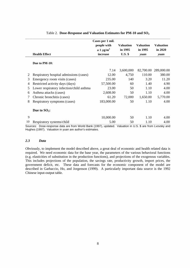
We will not be able to address these important issues here and choose only a simple formulation.In our base case we follow Lvovsky and Hughes (1997) who identify eight separate health effectsfor PM-10 and two for SO2. The most important of these effects are mortality and chronicbronchitis. These effects, indexed by h, are given in Table 2 together with the dose-responserelationship, hxDR . The 7.1 number for mortality is interpreted as the number of excess deaths per

million people due to an increase in the concentration of PM-10 of one 3/ mgµ . This isequivalent to a 0.1% mortality effect, which is also the central estimate in Wang and Smith (1999b,Table 5). We use an alternative estimate in our sensitivity analysis in section six.

With these dose-response relationships, the number of cases of health effect h in period t is thengiven by:

(5) ( )∑ −=x

utx

Nxthxht erPOPCDRHE )( α h = Mortality, RHA,...,

where xα is the WHO reference concentration, utPOP is the urban population (in millions), and

er is the exposure rate (the share of the urban population exposed to pollution of concentrationNxtC ).

7

Various approaches have been used to value these damages. We use the “willingness to pay”method. The valuation of these damages is a controversial and difficult exercise, with argumentsover the idea itself [Heinzerling (1999)], whether the “contingent valuation” method works[Hammit and Graham (1999)], and how to aggregate the willingness to pay [Pratt and Zeckhauser(1996)]. For this preliminary effort we again follow Lvovsky and Hughes (1997) and use estimatesfor willingness to pay in the U.S. and scale them by the ratio of per capita incomes in China and theU.S.6 Using this simple scaling means that we are assuming a linear income effect. The U.S.values associated with each health effect are given in the third column of numbers in Table 2. Thenext column gives the values scaled using per capita incomes in 1995.

Most studies of health damage valuation would use these estimates for all years of their analysis.However, China is experiencing rapid increases in real incomes. For example if income rises at anannual rate of 5%, it would have risen 3.4 times in 25 years. In the base case, our model projectsan average growth rate of 4-5% in per capita incomes over the next 40 years. Given this rate ofincrease, we have chosen a valuation method that changes every period in line with income growth,again assuming a linear income effect. The values for 2020 are given in the last column of Table 2.The national value of damage due to effect h is given by:

(6) ∑=x

hththt HEVDamage ,

where the valuations for 1995, 1995,hV , are in the third column of Table 2. The value of total

damages is simply the sum over all effects:

(7) ∑=h

htt DamageTD .

We should point out that these are the valuations of people who suffer the health effect. This is notthe same as calculating the medical costs, the cost of lost output of sick workers, the cost of parentstime to take care of sick babies, etc. The personal willingness-to-pay may, or may not, includethese costs, especially in a system of publicly provided medical care.

6 These estimates are from Chapter 2 of World Bank (1997), which also discusses the use of “willingness topay” valuation versus “human capital” valuation, the method most commonly used in China.

8

Table 2. Dose-Response and Valuation Estimates for PM-10 and SO2

Cases per 1 mil.people with Valuation Valuation Valuation

a 1 µg/m3 in 1995 in 1995 in 2020Health Effect increase U.S. $ yuan yuan

Due to PM-10:

7.14 3,600,000 82,700.00 289,000.002 Respiratory hospital admissions (cases) 12.00 4,750 110.00 380.003 Emergency room visits (cases) 235.00 140 3.20 11.204 Restricted activity days (days) 57,500.00 60 1.40 4.905 Lower respiratory infection/child asthma 23.00 50 1.10 4.006 Asthma attacks (cases) 2,608.00 50 1.10 4.007 Chronic bronchitis (cases) 61.20 72,000 1,650.00 5,770.008 Respiratory symptoms (cases) 183,000.00 50 1.10 4.00

Due to SO2:

9 10,000.00 50 1.10 4.0010 Respiratory systems/child 5.00 50 1.10 4.00

Sources: Dose-response data are from World Bank (1997), updated. Valuation in U.S. $ are from Lvovsky andHughes (1997). Valuation in yuan are author’s estimates.

2.3 Data

Obviously, to implement the model described above, a great deal of economic and health related data isrequired. We need economic data for the base year, the parameters of the various behavioral functions(e.g. elasticities of substitution in the production functions), and projections of the exogenous variables.This includes projections of the population, the savings rate, productivity growth, import prices, thegovernment deficit, etc. These data and forecasts for the economic component of the model aredescribed in Garbaccio, Ho, and Jorgenson (1999). A particularly important data source is the 1992Chinese input-output table.

9

For the health component described in section two above we obtained the output and energy use from the1992 input-output table and Sinton (1996). The process emissions coefficients are calculated from thesectoral non-combustion emissions data in Sinton (1996). The energy related emission coefficients( jxfψ ) are derived from those in Lvovsky and Hughes (1997) and scaled to equal the combustion

emissions data.7 Data is given in detail for the mining, manufacturing, and electric power sectors, withsummary estimates for the other sectors (agriculture, services, and final demand). We distribute the totalfor the other sectors in proportion to fuel use and scale Lvovsky and Hughes’ estimates of these jxσ and

jxfψ coefficients. Lvovsky and Hughes also provided separate estimates of Ojxfψ and N

jxfψ and for

process coefficients, Ojxσ and N

jxσ . The estimates for PM-10 for current and low-cost improved

technology are given in Table 3a for combustion emissions and in Table 3b for process emissions.

Lvovsky and Hughes (1997) give coefficients that transform emissions to concentrations separately foreach of 11 major cities. We use this information to calculate a national average set of cxγ ‘s. In the

1992 base year, with emissions calibrated to the data from Sinton (1996), the estimated urban

concentration averaged over the cities is 194 3/ mgµ .

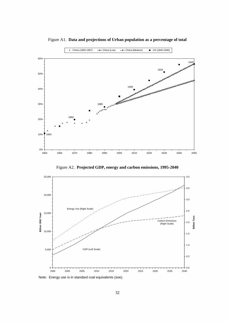
Estimating the number of people affected by air pollution involves estimating and projecting the sizeof the urban population. Both the future total population and the urbanized portion have to beprojected. We take total population projections the from World Bank (1995). The rate of urbanizationin China for 1950-97 is plotted in Figure A1. For comparison we also plot the rate of urbanization inthe U.S. over the period 1840-1940.8 The “medium” urbanization projection is produced by letting theurbanization rate rise at 0.5% per year, while in the “low” urbanization projection, the rate is assumedto be 0.3% per year. The medium projection is very close to U.S. historical rates. Lvovsky andHughes (1997) assume a rate of urbanization slightly higher than our medium projection.

2.4 The base case simulation

It is not the aim of this paper to provide estimates of the damage caused by urban air pollution, butrather the changes in the damage caused by some policy. It is only to give a clear idea of how ourapproach works that we describe our base case simulation, i.e. a simulation of the economy and healtheffects using current policy parameters.

7 Sinton (1996) provides a convenient English compilation from various Chinese sources including the ChinaEnvironmental Yearbook. Page 18 gives the energy conversion coefficients. Table VIII-4 gives the emissions bysector from both combustion and noncombustion sources.8 From U.S. Census Bureau publication CPH-2-1, at http://www.census.gov/population/censusdata/ur-def.htm.

10

We start the simulation in 1995 and so we initialize the economy to have the capital stocks that wereavailable at the start of 1995 and the working age population of 1995 supplying labor. The economicmodel described in the appendix calculates the output of all commodities, consumption by householdsand the government, exports, and the savings available for investment. This investment augments thecapital stock for the next period and we repeat the exercise. The level of output (specific commoditiesand total GDP) thus calculated depends on our projections of the population, savings behavior, changesin spending patterns as incomes rise, the ability to borrow from abroad, improvements in technology, etc.Our results are reported in Table 4 and Figure A2. The 5.9% growth rate of GDP over the next 25 yearsthat results from our assumptions is slightly less optimistic than the 6.7% growth rate projected recentlyfor China by the World Bank (1997), but still implies a very rapid growth in per capita income. Thepopulation is projected to rise at a 0.7% annual rate during these 25 years.

11

Table 3a. Combustion particulate emissions

Current Emissions

by Fuel

Emissions with Low Cost

Improvements by Fuel

Sector Coal OilNatural

Gas Coal OilNatural

Gas

1 Agriculture 42,560 160 27 21,280 160 272 Coal Mining 38,182 143 24 19,091 143 243 Crude Petroleum 38,182 143 24 19,091 143 244 Metal Ore Mining 38,182 143 24 19,091 143 245 Other Non-metallic Ore Mining 38,182 143 24 19,091 143 246 Food Manufacturing 32,983 124 21 16,492 124 217 Textiles 18,505 69 12 9,253 69 128 Apparel & Leather Products 7,678 29 5 3,839 29 59 Lumber & Furniture

Manufacturing25,629 949 27 10,990 949 27

10 Paper, Cultural, & EducationalArticles

25,629 949 27 10,990 949 27

11 Electric Power 32,642 544 0 10,881 544 012 Petroleum Refining 7,235 723 12 2,412 723 1213 Chemicals 17,898 1,790 30 5,966 1,790 3014 Building Material 13,454 1,345 22 4,485 1,345 2215 Primary Metals 6,379 638 11 2,126 638 1116 Metal Products 8,814 33 6 4,407 33 617 Machinery 11,970 45 7 5,985 45 718 Transport Equipment 11,970 45 7 5,985 45 719 Electric Machinery &

Instruments11,970 45 7 5,985 45 7

20 Electronic & CommunicationEquipment

11,970 45 7 5,985 45 7

21 Instruments and Meters 11,970 45 7 5,985 45 722 Other Industry 46,872 176 29 23,436 176 2923 Construction 42,560 160 27 21,280 160 2724 Transportation &

Communications42,560 5,320 27 21,280 2,660 27

25 Commerce 42,560 160 27 21,280 160 2726 Public Utilities 42,560 160 27 21,280 160 2727 Culture, Education, Health, &

Research42,560 160 27 21,280 160 27

28 Finance & Insurance 42,560 160 27 21,280 160 2729 Public Administration 42,560 160 27 21,280 160 27

Households 21,280 426 27 10,640 426 27

Note: Coefficients Ojxfψ and

Njxfψ in tons of PM-10 per million tons of oil equivalent (toe).

12

Table 3b. Process Particulate Emissions

EmissionsCurrent with Low

CostSector Emissions Improvement

s

1 Agriculture - -2 Coal Mining 0.81 0.163 Crude Petroleum 0.81 0.164 Metal Ore Mining 0.81 0.165 Other Non-metallic Ore Mining 0.81 0.166 Food Manufacturing 0.09 0.097 Textiles 0.04 0.048 Apparel & Leather Products -- --9 Lumber & Furniture Manufacturing 0.12 0.02

10 Paper, Cultural, & Educational Articles 0.12 0.0211 Electric Power 0.72 0.7212 Petroleum Refining 0.57 0.5713 Chemicals 0.71 0.7114 Building Material 14.92 2.9815 Primary Metals 3.17 0.6316 Metal Products 0.05 0.0517 Machinery 0.11 0.1118 Transport Equipment 0.11 0.1119 Electric Machinery & Instruments 0.11 0.1120 Electronic & Communication Equipment 0.11 0.1121 Instruments and Meters 0.11 0.1122 Other Industry 1.53 1.5323 Construction -- --24 Transportation & Communications -- --25 Commerce -- --26 Public Utilities -- --27 Culture, Education, Health, & Research -- --28 Finance & Insurance -- --29 Public Administration -- --

Households -- --

Note: Coefficients Ojxσ and

Njxσ in tons per million 1992 yuan.

13

Table 4. Selected Variables from Base Case Simulation

Variable 1995 2010 2030

Population (mil.) 1,200.00 1,348.00 1,500.00

GDP (bil. 1992 yuan) 3,560.00 10,200.00 18,600.00

Energy Use (mil. tons sce) 1,190.00 2,490.00 3,280.00

Coal Use (mil. tons) 1,270.00 2,580.00 3,090.00

Oil Use (mil. tons) 180.00 420.00 690.00

Carbon Emissions (mil. tons) 810.00 1,670.00 2,160.00

Particulate Emissions (mil. tons) 21.55 26.78 33.84

From High Height Sources 3.94 4.81 6.80

From Medium Height Sources 11.30 12.48 15.99

From Low Height Sources 6.32 9.49 11.05

SO2 Emissions (mil. tons) 21.80 42.40 57.90

Premature Deaths (1,000) 320.00 700.00 1,200.00

Health Damage (bil. yuan) 180.00 1,000.00 2,800.00

Health Damage/GDP 5.10% 9.80% 15.30%

The dashed line in Figure A2 shows the fossil fuel based energy use in standard coal equivalents (sce)on the right-hand axis. Our assumptions on energy use improvements are fairly optimistic andtogether with changes in the structure of the economy, result in an energy-GDP ratio in 2030 that isalmost half that in 1995. The carbon emissions from fossil fuels are also plotted using the right-handaxis. The rate of growth of carbon emissions is even slower than the growth in energy use. This ismainly due to our assumptions on the shift from coal to oil.

14

With the industry outputs and input requirements calculated for each period we use equations (1)-(7)to calculate total emission of pollutants, the urban concentration of pollutants, and the health effects ofthese pollutants. The growth of PM-10 emissions is much slower than the growth in energy use andcarbon emissions. This is due to the sharp difference in the assumed coefficients for new and oldcapital (see Table 3). All sources of PM-10 increase emissions, with the largest rise coming fromlow-height sources. Projected SO2 emissions rise much faster than particulates due to a less optimisticestimate of the improvement in the jxσ and jxfψ coefficients.9

In this base case we assume no increase in emission reduction efforts over time. This differs fromLvovsky and Hughes’ (1997) BAU case which assumes that the largest 11 cities will choose what theycall the “high investment” option. The result is that our estimate of current premature mortality ishigher, 320,000 versus 230,000. The growth rate of health effects from our simulations, however, arequite close. By 2020 our estimated excess deaths are 3.1 times the 1995 level, compared to the3.7 times calculated in Lvovsky and Hughes’ BAU case.

Of course the fact that our estimates are close does not mean that either estimate is “good.” We reportthe level estimates to explain our simulation procedure and to illustrate the magnitudes involved. Toreiterate, this is not a forecast of emissions, but rather a projection if no changes in policy are made.We expect both the government and private sectors to have policies and investments that are differentfrom today’s. The important issue is policy choices and the estimation of the effects of differentpolicies. This is where we turn next.

2.5 Health effects of a carbon tax

As described in the previous section, our projected growth of carbon emissions in the base case, whilelower than the growth of GDP, is still very high. The level of emissions doubles in 15 years. Anumber of policies have been suggested to reduce the growth of emissions of this global pollutant,ranging from specific, detailed policies like importing natural gas or shutting down small coal plants,to broader approaches, such as carbon taxes and emissions trading. In this paper we concentrate on thesimplest broad based policy by imposing a “carbon tax,” i.e. a tax on fossil fuels based on their carboncontent.10

The specifics of this tax, and the detailed economic effects, are discussed in Garbaccio, Ho, andJorgenson (1999). In our simulations we raise the price of crude petroleum and coal, both domesticand imported, by this carbon tax. In this paper, two carbon targets are examined, 5% and 10%reductions in annual carbon emissions. The level of the tax is calculated endogenously such thatemissions in each period are 5% or 10% less than in the base case. This is shown in Figure 1. Therevenues from this new tax are used to reduce other existing taxes. The amount of reduction is suchthat the public deficit (exogenous) and real government expenditures (endogenous) were kept the sameas the base case.

9 The emission coefficients for sulphur dioxide are not reported here but are available from the authors. Giventhe relatively minor role in human health (as shown in Table 2), we do not emphasize SO2 in this study. It is ofcourse an important cause of other damages, e.g. acid rain.10 In this study we ignore both other sources of carbon dioxide and other greenhouse gases.

15

The results of these carbon tax simulations are given in Table 5 and Figures 1-4. The amount ofcarbon tax needed to achieve these reductions is plotted in Figure 2. In the first year, a tax of 8.8 yuanper ton is required to achieve a 5% reduction in emissions.11 This is equivalent to a 6% increase in thefactory gate price of coal and a 1% increase in the price of crude petroleum. These higher energyprices reduce demand for fuels and raise the relative prices of energy intensive goods. We assume thatthe government does not compensate the household sector for the higher prices and so consumptionfalls in the short run. Because the labor supply is assumed fixed, real wages fall slightly. Thecompensating reduction in enterprise taxes, however, leaves firms with higher after-tax income, andgiven our specification, this leads to higher investment. Over time, this leads to a significantly highercapital stock, i.e., higher than in the base case, and thus higher GDP. This higher output allows a levelof consumption that exceeds that in the base case soon after the beginning of the simulation period.

As can be seen in Table 5, in the first year of the 5% carbon reduction case, the imposition of thecarbon tax leads to a reduction in total particulate emissions of 3.5%. This, however, is an averageover three different changes. High height emissions from the electric power sector fell by 5.6%,medium height emissions from manufacturing fell 2.7%, while low height emissions fell 3.7%.Sectoral emissions of sulfur dioxide fell by similar amounts. The electric power sector is the mostfossil fuel intensive and hence experiences the largest fall in output and emissions.

11 There are 0.518 tons of carbon emitted per ton of average coal. The average price of coal output in 1992,derived by dividing the value in the input-output table by the quantity of coal mined, is about 68 yuan per ton.This implies a tax on coal of about 7 percent.

16

Table 5. Effects of a Carbon Tax on Selected Variables(Percentage Change from Base Case)

Effect in 1st Year with: Effect in 15th Year with:5% CO2 10% CO2 5% CO2 10% CO2

Emissions Emissions Emissions EmissionsVariable Reduction Reduction Reduction Reduction

GDP -0.00% -0.00% 0.21% 0.42%

Primary Energy -4.72% -9.45% -4.68% -9.35%

Market Price of Coal 6.03% 12.80% 6.29% 13.40%

Market Price of Oil 0.95% 2.01% 0.71% 1.53%

Coal Output -5.93% -11.80% -6.14% -12.20%

Oil Output -0.81% -1.71% -0.59% -1.29%

Particulate Emissions -3.50% -6.97% -3.11% -6.20%

From High Height Sources -3.67% -7.37% -3.09% -6.21%

From Medium Height Sources -2.66% -5.29% -2.22% -4.40%

From Low Height Sources -5.59% -11.20% -5.44% -10.90%

Particulate Concentration -3.45% -6.92% -2.95% -5.92%

SO2 Concentration -3.43% -6.88% -2.78% -5.59%

Premature Deaths -4.52% -9.04% -3.55% -7.10%

Cases of Chronic Bronchitis -4.52% -9.04% -3.55% -7.10%

Value of Health Damages -4.52% -9.04% -3.55% -7.11%

17

Figure 1. Carbon emissions in base case and simulations

0.0

0.5

1.0

1.5

2.0

2.5

1995 2000 2005 2010 2015 2020 2025 2030 2035 2040

Bill

ion

To

ns

Base Case 5% Emissions Reduction 10% Emissions Reduction

Figure 2. Carbon taxes required to attain a given reduction in emissions

0

5

10

15

20

25

30

1995 2000 2005 2010 2015 2020 2025 2030 2035 2040

Yu

an p

er T

on

5% Emissions Reduction 10% Emissions Reduction

18

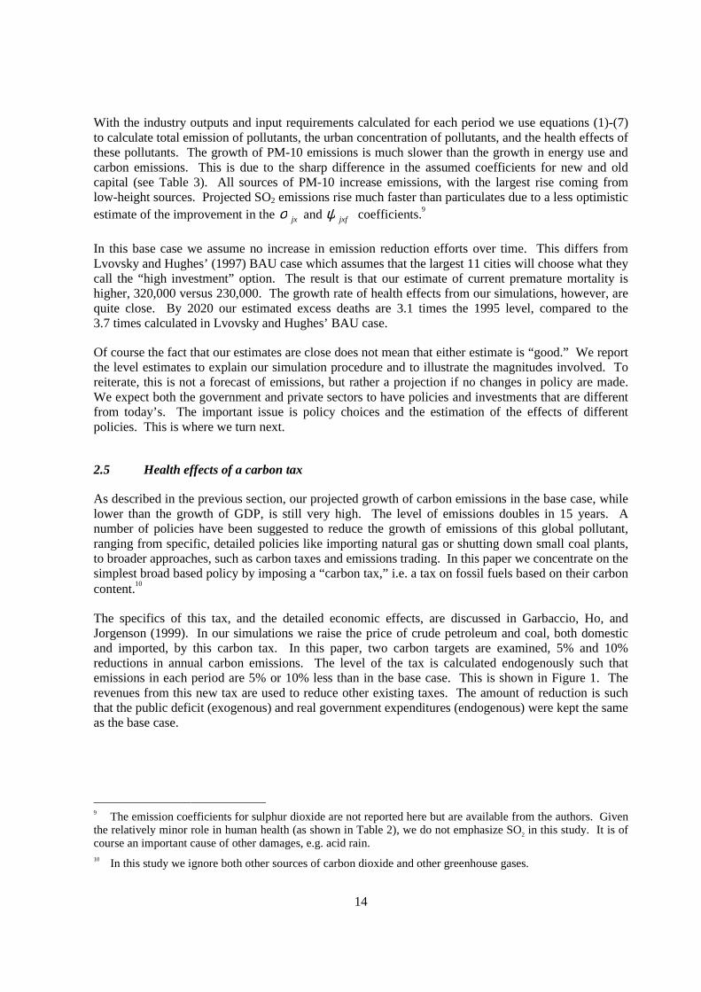
Figure 3. Reduction in PM-10 emissions and concentrations relative to base

-9

-8

-7

-6

-5

-4

-3

-2

-1

01995 2000 2005 2010 2015 2020 2025 2030 2035 2040

Per

cen

tag

e C

han

ge

10% CO2 Reduction Case - Emissions 10% CO2 Reduction Case - Concentration

5% CO2 Reduction Case - Emissions 5% CO2 Reduction Case - Concentration

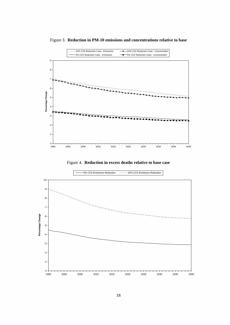
Figure 4. Reduction in excess deaths relative to base case

-10

-9

-8

-7

-6

-5

-4

-3

-2

-1

01995 2000 2005 2010 2015 2020 2025 2030 2035 2040

Per

cen

tag

e C

han

ge

5% CO2 Emissions Reduction 10% CO2 Emissions Reduction

19

This reduction in emissions results in a fall in the average urban concentration of PM-10 by 3.4%. Asa consequence, cases of various health effects fall by about 4.5% (i.e. the number of premature deaths,the number of cases of chronic bronchitis, etc.). The reduction in health effects is bigger than thechange in concentration due to the non-proportional nature of equation 5. If we apply these percentchanges to the base case estimates in Table 4, this translates to 14,000 fewer excess deaths, and126,000 fewer cases of chronic bronchitis. Since the valuations are simple multiples (see equation 6)the percent change in yuan values of this health damage is also -4.5%.

Over time, as the revenue raised through the carbon tax reduces the income tax burden on enterprises,higher investment leads to a larger capital stock and hence a higher level of GDP. The higher level ofoutput means greater demand for energy and hence requires a higher carbon tax rate to achieve the 5%reduction in carbon emissions. This is shown in the “15th year” column of Table 5 and in Figure 2.The lower tax on crude petroleum in the 15th year is due to our assumption on the price of world oil.If we had assumed no imports, the tax on crude petroleum would also have been higher. This twist infossil fuel prices results in a bigger fall in coal consumption compared to crude petroleumconsumption for an unchanged GDP. However, the higher demand has a bigger effect than this twistin fuel prices and hence the reduction in emissions in the 15th year is smaller than the initial reduction,3.1% versus 3.5%. The reduction in concentrations over time is correspondingly smaller, as shown inFigure 3.

Another feature of the results that should be pointed out is that the change in concentration is smallerthan the change in emissions in future years (see Figure 3). This is due to our classifying emissions byheight and that low level emissions are the biggest contributors to concentration (i.e. the biggest

cxγ ‘s). Different sectors of the economy are growing at different rates (sources of low height

emissions are growing the most rapidly), and respond differently to the imposition of the carbon tax.The most responsive sector (i.e. the one that shrinks the most) is electric power generation, whichproduces high height emissions with the lowest contribution to concentrations. Finally, this path ofconcentration changes leads to health effects that become smaller over time, from a 4.5% reduction inthe first year, to a 3.6% reduction in the 15th year, to 3.2% in the 25th year.

When we raise the targeted carbon emissions reductions from 5% to 10% of the base case the effectsare approximately linear. In the “15th year” column of Table 5 we see that the effects on coal pricesare less than doubled while the effects on oil prices are more than doubled. The end result onemissions, concentrations, and health effects is a simple doubling of the percentage change. Thisseeming linearity would not hold for larger changes.

2.6 Sensitivity analysis

In section three above we discuss first- and second-order effects of an error in a parameter. Toillustrate this we use an alternative assumption about an exogenous variable, the future urbanization

rate. This variable, utPOP , enters in equation 4. The base case plotted in Figure A1 has the urban

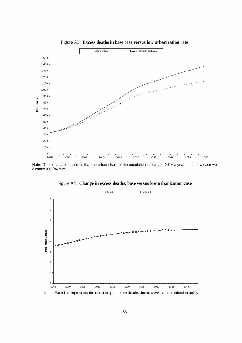
share of total population rising at 0.5% per year, the “low” case rises at 0.3% per year. We ran themodel again with this lower estimate of the exposed population. The number of premature deaths inboth the base case and in this alternative simulation are plotted in Figure A3. This is an example of afirst-order effect of an error in a parameter or exogenous variable.

20

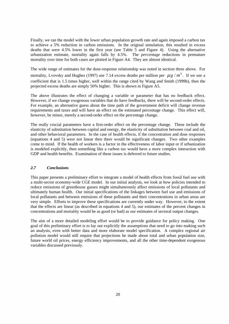
Finally, we ran the model with the lower urban population growth rate and again imposed a carbon taxto achieve a 5% reduction in carbon emissions. In the original simulation, this resulted in excessdeaths that were 4.5% lower in the first year (see Table 5 and Figure 4). Using the alternativeurbanization estimate, mortality again falls by 4.5%. The percentage reductions in prematuremortality over time for both cases are plotted in Figure A4. They are almost identical.

The wide range of estimates for the dose-response relationship was noted in section three above. For

mortality, Lvovsky and Hughes (1997) use 7.14 excess deaths per million per 3/ mgµ . If we use acoefficient that is 1.5 times higher, well within the range cited by Wang and Smith (1999b), then theprojected excess deaths are simply 50% higher. This is shown in Figure A5.

The above illustrates the effect of changing a variable or parameter that has no feedback effect.However, if we change exogenous variables that do have feedbacks, there will be second-order effects.For example, an alternative guess about the time path of the government deficit will change revenuerequirements and taxes and will have an effect on the estimated percentage change. This effect will,however, be minor, merely a second-order effect on the percentage change.

The really crucial parameters have a first-order effect on the percentage change. These include theelasticity of substitution between capital and energy, the elasticity of substitution between coal and oil,and other behavioral parameters. In the case of health effects, if the concentration and dose responses(equations 4 and 5) were not linear then there would be significant changes. Two other examplescome to mind. If the health of workers is a factor in the effectiveness of labor input or if urbanizationis modeled explicitly, then something like a carbon tax would have a more complex interaction withGDP and health benefits. Examination of these issues is deferred to future studies.

2.7 Conclusions

This paper presents a preliminary effort to integrate a model of health effects from fossil fuel use witha multi-sector economy-wide CGE model. In our initial analysis, we look at how policies intended toreduce emissions of greenhouse gasses might simultaneously affect emissions of local pollutants andultimately human health. Our initial specifications of the linkages between fuel use and emissions oflocal pollutants and between emissions of these pollutants and their concentrations in urban areas arevery simple. Efforts to improve these specifications are currently under way. However, to the extentthat the effects are linear (as described in equations 4 and 5), our estimates of the percent changes inconcentrations and mortality would be as good (or bad) as our estimates of sectoral output changes.

The aim of a more detailed modeling effort would be to provide guidance for policy making. Onegoal of this preliminary effort is to lay out explicitly the assumptions that need to go into making suchan analysis, even with better data and more elaborate model specification. A complex regional airpollution model would still require that projections be made about total and urban population size,future world oil prices, energy efficiency improvements, and all the other time-dependent exogenousvariables discussed previously.

21

Another goal of this preliminary modelling effort is to highlight in which areas improvements in datacollection and modelling would bring the greatest benefit to even a limited analysis. Issues beyondthose associated with the economic part of the model include: (i) Health damage from air pollution isbelieved to be due to very fine particles. Data on that would be important. (ii) Data on concentrationsin different urban areas and the modelling of these concentrations in a sample of cities would give asense of the range of the reduced form coefficients. (iii) We have crudely classified emissions by low,medium, and high heights for different industries. Having more refined data on industry emissionscharacteristics would improve the modelling in item (ii). (iv) Getting better dose-response functions isalready a recognized priority. We would urge consideration of including an age dimension in theresearch. This would be especially important in attempting to link worker’s health back to laborproductivity.

22

REFERENCES

Garbaccio, Richard F., Mun S. Ho and Dale W. Jorgenson. (1997). “A DynamicEconomy-Energy-Environment Model of China.” Unpublished Manuscript, Harvard University.

Garbaccio, Richard F., Mun S. Ho, and Dale W. Jorgenson (1999). “Controlling Carbon Emissions inChina.” Environment and Development Economics, 4(4), 493-518.

Hammitt, James K. and J. D. Graham (1999). “Willingness to Pay for Health Protection: InadequateSensitivity to Probability?” Journal of Risk and Uncertainty, 18(1), 33-62.

Heinzerling, Lisa (1999). “Discounting Life.” Yale Law Journal, 108, 1911-1915.

Jorgenson, Dale W. and Peter J. Wilcoxen (1990). “Environmental Regulation and U.S. EconomicGrowth.” Rand Journal of Economics, 21(2), 314-340.

Lvovsky, Kseniya and Gordon Hughes (1997). “An Approach to Projecting Ambient Concentrationsof SO2 and PM-10.” Unpublished Annex 3.2 to World Bank (1997).

Maddison, David, Kseniya Lvovsky, Gordon Hughes, and David Pearce (1998). “Air Pollution and theSocial Cost of Fuels.” Mimeo, World Bank, Washington, D.C.

Pratt, John W. and Richard J. Zeckhauser (1996). “Willingness to Pay and the Distribution of Risk andWealth.” Journal of Political Economy, 104(4), 747-763.

Sinton, Jonathan ed. (1996). China Energy Databook. Lawrence Berkeley National Laboratory,LBL-32822, Rev. 3.

Wang, Xiaodong and Kirk R. Smith (1999a). “Secondary Benefits of Greenhouse Gas Control: HealthImpacts in China.” Environmental Science and Technology, 33(18), 3056-3061.

Wang, Xiaodong and Kirk R. Smith (1999b). “Near-term Health Benefits of Greenhouse GasReductions.” World Health Organization, Geneva, WHO/SDE/PHE/99.1.

World Bank (1994). China: Issues and Options in Greenhouse Gas Emissions Control. Washington,D.C.

World Bank (1995). World Population Projections. Washington, D.C.

World Bank (1997). Clear Water, Blue Skies: China’s Environment in the New Century.Washington, D.C.

23

APPENDIX A: DESCRIPTION OF THE ECONOMIC MODEL

The main features of the model for China are discussed in this appendix, further details are given inGarbaccio, Ho, and Jorgenson (1997). We describe the modeling of each of the main agents in themodel in turn. Table A1 lists a number of parameters and variables which are referred to with somefrequently. In general, a bar above a symbol indicates that it is a plan parameter or variable while atilde indicates a market variable. Symbols without markings are total quantities or average prices. Toreduce unnecessary notation, whenever possible, we drop the time subscript, t, from our equations.

24

Table 1A. Selected Parameters and Variables in the Economic Model

Parameters

sie

export subsidy rate on good iti

c

carbon tax rate on good it k

tax rate on capital incomet L

tax rate on labor incometi

r

net import tariff rate on good iti

t

net indirect tax (output tax less subsidy) rate on good it x

unit tax per ton of carbon

Endogenous Variables

G_I interest on government bonds paid to households

G_INV investment through the government budget

G_IR interest on government bonds paid to the rest of the world

G_transfer government transfer payments to households

PiKD rental price of market capital by sector

PEi* export price in foreign currency for good i

PI i producer price of good i

PI it purchaser price of good i including taxes

PL average wage

PLi wage in sector i

PMi import price in domestic currency for good i

PMi* import price in foreign currency for good i

PSi supply price of good i

PTi rental price of land of type i

QI i total output for sector i

QSi total supply for sector i

r B( )* payments by enterprises to the rest of the world

R_transfer transfers to households from the rest of the world

25

A.1 Production

Each of the 29 industries is assumed to produce its output using a constant returns to scale technology.For each sector j this can be expressed as:

(A1) QI f KD LD TD A A tj j j j j nj= ( , , , , ... , , )1 ,

where KDj , LDj , TDj , and Aij are capital, labor, land, and intermediate inputs, respectively.12

In sectors for which both plan and market allocation exists, output is made up of two components,

the plan quota output ( QI j

−) and the output sold on the market ( QI j

~). The plan quota output is

sold at the state-set price ( PI j

−) while the output in excess of the quota is sold at the market price

( PI j

~).

A more detailed discussion of how this plan-market formulation is different from standard marketeconomy models is given in Garbaccio, Ho, and Jorgenson (1999). In summary, if the constraints arenot binding, then the “two-tier plan/market” economy operates at the margin as a market economywith lump sum transfers between agents. The return to the owners of fixed capital in sector j is:

(A2) profit PI QI PI QI P KD PL LD PT TDj j j j j jKD

j j j j j=− −

+ − − −~ ~ ~ ~

−− −

−∑ ∑PS A PS Ai iji

ii

ij

~ ~ .

For each industry, given the capital stock K j and prices, the first order conditions from maximizing

equation A2, subject to equation A1, determine the market and total input demands.

Given the lack of a consistent time-series data set, in this version of the model, we use Cobb-Douglasproduction functions. Equation A1 for the output of industry j at time t then becomes:

(A3) QI g t KD LD TD E Mjt jt jt jt jt jtKj Lj Tj Ej Mj= ( ) α α α α α , where

log logE Ajt kjE

kkjt= ∑α and k = coal, oil, electricity, and refined petroleum ,

log logM Ajt kjM

kkjt= ∑α and k = non-energy intermediate goods .

12 QIj denotes the quantity of industry j’s output. This is to distinguish it from, QCj, the quantity ofcommodity j. In the actual model each industry may produce more than one commodity and each commoditymay be produced by more than one industry. In the language of the input output tables, we make use of both theUSE and MAKE matrices. For ease of exposition we ignore this distinction here.

26

Here α Ej is the cost share of aggregate energy inputs in the production process and α kjE is the share of

energy of type k within the aggregate energy input. Similarly, α Mj is the cost share of aggregate

non-energy intermediate inputs and α kjM is the share of intermediate non-energy input of type k within

the aggregate non-energy intermediate input.

To allow for biased technical change, the α Ej coefficients are indexed by time and are updated

exogenously. We set α Ej to fall gradually over the next 40 years while the labor coefficient, α Lj ,

rises correspondingly. The composition of the aggregate energy input (i.e. the coefficients αkjE ) are

also allowed to change over time. These coefficients are adjusted gradually so that they come close toresembling the U.S. use patterns of 1992. The exception is that the Chinese coefficients for coal formost industries will not vanish as they have in the U.S.13 The coefficient g(t) in equation A3represents technical progress and the change in g(t) is determined through an exponential function( � ( ) exp( )g t A tj j j= −µ ). This implies technical change that is rapid initially, but gradually declines

toward zero. The price to buyers of this output includes the indirect tax on output and the carbon tax:

(A4) PI t PI tit

it

i ic= + +( )1 .

A.2 Households

The household sector derives utility from the consumption of commodities, is assumed to supply laborinelastically, and owns a share of the capital stock. It also receives income transfers and interest on itsholdings of public debt. Private income after taxes and the payment of various non-tax fees (FEE),

Y p , can then be written as:

(A5) Y YL DIV G I G transfer R transfer FEEp = + + + + −_ _ _ ,

where YL denotes labor income from supplying LS units of effective labor, less income taxes. YL isequal to:

(A6) YL t PL LSL= −( )1 .

13 We have chosen to use U.S. patterns in our projections of these exogenous parameters because they seem tobe a reasonable anchor. While it is unlikely that China’s economy in 2032 will mirror the U.S. economy of1992, it is also unlikely to closely resemble any other economy. Other projections, such as those by the WorldBank (1994), use the input-output tables of developed countries including the U.S. We have considered makingextrapolations based on recent Chinese input-output tables, but given the short sample period and magnitude ofthe changes in recent years, this did not seem sensible.

27

The relationship between labor demand and supply is given in equation A31 below. LS is a functionof the working age population, average annual hours, and an index of labor quality:

(A7) LS POP hr qt tw

t tL= .

Household income is allocated between consumption (VCCt ) and savings. In this version of the

model we use a simple Solow growth model formulation with an exogenous savings rate ( st ) to

determine private savings ( Stp ):

(A8) S s Y Y VCCtp

t tp

tp

t= = − .

Household utility is a function of the consumption of goods such that:

(A9) U U C C Ct t nt itC

iti

= = ∑( ,..., ) log1 α .

Assuming that the plan constraints are not binding, then as in the producer problem above, givenmarket prices and total expenditures, the first order conditions derived from equation A9 determine

household demand for commodities, Ci , where C C Ci i i= + ~. Here Ci and

~Ci are household

purchases of commodities at state-set and market prices. The household budget can be written as:

(A10) VCC PS C PS Ci

i i i i= +− −

∑ (~ ~

) .

We use a Cobb-Douglas utility function because we currently lack the disaggregated data to estimatean income elastic functional form. However, one would expect demand patterns to change with rising

incomes and this is implemented by allowing the α itC coefficients to change over time. These future

demand patterns are projected using the U.S. use patterns of 1992.

A.3 Government and taxes

In the model, the government has two major roles. First, it sets plan prices and output quotas andallocates investment funds. Second, it imposes taxes, purchases commodities, and redistributesresources. Public revenue comes from direct taxes on capital and labor, indirect taxes on output,tariffs on imports, the carbon tax, and other non-tax receipts:

(A11) Rev = − + + +∑ ∑ ∑ ∑t P KD D t PL LD t PI QI t PM MkjKD

j jj

Lj j

jjt

j jj

ir

i ii

( ) *

+ − + +∑ t QI X M FEEic

i i ii

( ) ,

28

where Dj is the depreciation allowance and X i and Mi are the exports and imports of good i. The

carbon tax per unit of fuel i is:

(A12) t tic x

i= θ ,

where t x is the unit carbon tax calculated per ton of carbon and θi is the emissions coefficient foreach fuel type i.

Total government expenditure is the sum of commodity purchases and other payments:

(A13) Expend VGG G INV s PI X G I G IR G transferie

i i= + + + + +∑_ _ _ _

Government purchases of specific commodities are allocated as shares of the total value ofgovernment expenditures, VGG. For good i:

(A14) PS G VGGi i iG= α .

We construct a price index for government purchases as log logPGG PSiG

i i= ∑ α . The real

quantity of government purchases is then:

(A15) GGVGG

PGG= .

The difference between revenue and expenditure is the deficit, ∆G , which is covered by increases in

the public debt, both domestic ( B ) and foreign ( BG* ):

(A16) ∆G Expendt t t= − Rev ,

(A17) B B B B Gt tG

t tG

t+ = + +− −* *

1 1 ∆ .

The deficit and interest payments are set exogenously and equation A16 is satisfied by making thelevel of total government expenditure on goods, VGG , endogenous.

A.4 Capital, investment, and the financial system

We model the structure of investment in a fairly simple manner. In the Chinese economy, somestate-owned enterprises receive investment funds directly from the state budget and are allocated crediton favorable terms through the state-owned banking system. Non-state enterprises get a negligibleshare of state investment funds and must borrow at what are close to competitive interest rates. Thereis also a small but growing stock market that provides an alternative channel for private savings. Weabstract from these features and define the capital stock in each sector j as the sum of two parts, whichwe call plan and market capital:

(A18) K K Kjt jt jt= + ~ .

29

The plan portion evolves with plan investment and depreciation:

(A19) K K Ijt jt jt= − +−( )1 1δ , t = 1, 2, …, T .

In this formulation, K j 0 is the capital stock in sector j at the beginning of the simulation. This portion

is assumed to be immobile across sectors. Over time, with depreciation and limited governmentinvestment, it will decline in importance. Each sector may also “rent” capital from the total stock of

market capital, ~Kt :

(A20)~ ~K Kt jtj

= ∑ , where ~K ji > 0 .

The allocation of market capital to individual sectors, ~K jt , is based on sectoral rates of return. As in

equation A2, the rental price of market capital by sector is ~Pj

KD . The supply of ~K jt , subject to

equation A20, is written as a translog function of all of the market capital rental prices,~

(~

, ... ,~

)K K P Pjt jKD

nKD= 1 .

In two sectors, agriculture and crude petroleum, “land” is a factor of production. We have assumedthat agricultural land and oil fields are supplied inelastically, abstracting from the complex propertyrights issues regarding land in China. After taxes, income derived from plan capital, market capital,and land is either kept as retained earnings by the enterprises, distributed as dividends, or paid toforeign owners:

(A21) profits P K PT T tax k RE DIV r Bjj

jKD

jj j j

j∑ ∑ ∑+ + = + + +~ ~

( ) ( )* ,

where tax k( ) is total direct taxes on capital (the first term on the right hand side of equation A11).14

As discussed below, total investment in the model is determined by savings. This total, VII, is then

distributed to the individual investment goods sectors through fixed shares, α itI :

(A22) PS I VIIit it itI

t= α .

Like the α itC coefficients in the consumption function, the investment coefficients are indexed by time

and projected using U.S. patterns for 1992. A portion of sectoral investment, It , is allocated directly

by the government, while the remainder, ~It , is allocated through other channels.15 The total, It , can

be written as:

14 In China, most of the “dividends” are actually income due to agricultural land.15 It should be noted that the industries in the Chinese accounts include many sectors that would be consideredpublic goods in other countries. Examples include local transit, education, and health.

30

(A23) I I I I I It t t t t nt

I InI

= + =~...1 2

1 1α α α .

As in equation A19 for the plan capital stock, the market capital stock, ~K jt , evolves with new market

investment:

(A24)~

( )~ ~

K K Ijt jt jt= − +−1 1δ .

A.5 The foreign sector

Trade flows are modeled using the method followed in most single-country models. Imports areconsidered to be imperfect substitutes for domestic commodities and exports face a downward slopingdemand curve. We write the total supply of commodity i as a CES function of the domestic ( QIi ) and

imported good ( Mi ):

(A25) [ ]QS A QI Mid

im

i= +0

1

α αρ ρ ρ ,

where PS QS PI QI PM Mi i it

i i i= + is the value of total supply. The purchaser’s price for domestic

goods, PIit , is discussed in the producer section above. The price of imports to buyers is the foreign

price plus tariffs (less export subsidies), multiplied by a world relative price, e:

(A26) PM e t PMi ir

i= +( ) *1 .

Exports are written as a simple function of the domestic price relative to world prices adjusted for

export subsidies ( site ):

(A27) X EXPI

e s PEit it

it

t ite

it

i

=+

~

*( )1

η

,

where EX it is base case exports that are projected exogenously.

The current account balance is equal to exports minus imports, less net factor payments, plus transfers:

(A28) CAPI X

sPM M r B G IR R transferi i

ie

ii i

i

=+

− − − +∑ ∑( )( ) _ _*

1 ,

Like the government deficits, the current account balances are set exogenously and accumulate into

stocks of net foreign debt, both private ( Bt* ) and public ( Bt

G* ):

31

(A29) B B B B CAt tG

t tG

t* * * *+ = + −− −1 1 .

A.6 Markets

The economy is in equilibrium in period t when the market prices clear the markets for the 29commodities and the two factors. The supply of commodity i must satisfy the total of intermediateand final demands:

(A30) QS A C I G Xi ijj

i i i i= + + + +∑ , i = 1, 2, …, 29.

For the labor market, we assume that labor is perfectly mobile across sectors so there is one averagemarket wage which balances supply and demand. As is standard in models of this type, we reconcile

this wage with the observed spread of sectoral wages using wage distribution coefficients, ψ jtL . Each

industry pays PL PLjt jtL

t= ψ for a unit of labor. The labor market equilibrium is then given as:

(A31) ψ jtL

jtj

tLD LS∑ = .

For the non-plan portion of the capital market, adjustments in the market price of capital, ~Pj

KD , clears

the market in sector j:

(A32) KD Kjt jtK

jt= ψ ,

where ψ jtK converts the units of capital stock into the units used in the production function. The rental

price PTj adjusts to clear the market for “land”:

(A33) TD Tj j= , where j = “agriculture” and “petroleum extraction.”

In this model without foresight, investment equals savings. There is no market where the supply ofsavings is equated to the demand for investment. The sum of savings by households, businesses (asretained earnings), and the government is equal to the total value of investment plus the budget deficitand net foreign investment:

(A34) S RE G INV VII G CAp + + = + +_ ∆ .

The budget deficit and current account balance are fixed exogenously in each period. The worldrelative price (e) adjusts to hold the current account balance at its exogenously determined level.

32

Figure A1. Data and projections of Urban population as a percentage of total

0%

10%

20%

30%

40%

50%

60%

1950 1960 1970 1980 1990 2000 2010 2020 2030 2040 2050

China (1950-1997) China (Low) China (Medium) US (1840-1940)

1840

1860

1880

1900

1920

1940

Figure A2. Projected GDP, energy and carbon emissions, 1995-2040

0

5,000

10,000

15,000

20,000

25,000

1995 2000 2005 2010 2015 2020 2025 2030 2035 2040

Bill

ion

199

2 Y

uan

0.0

0.5

1.0

1.5

2.0

2.5

3.0

3.5

4.0

Bill

ion

To

ns

GDP (Left Scale)

Energy Use (Right Scale)

Carbon Emissions (Right Scale)

Note: Energy use is in standard coal equivalents (soe).

33

Figure A3. Excess deaths in base case versus low urbanization rate

0

100

200

300

400

500

600

700

800

900

1,000

1,100

1,200

1,300

1,400

1,500

1995 2000 2005 2010 2015 2020 2025 2030 2035 2040

Th

ou

san

ds

Base Case Low Urbanization Rate

Note: The base case assumes that the urban share of the population is rising at 0.5% a year, in the low case weassume a 0.3% rate.

Figure A4. Change in excess deaths, base versus low urbanization case

-8

-7

-6

-5

-4

-3

-2

-1

0

1995 2000 2005 2010 2015 2020 2025 2030 2035 2040

Per

cen

tag

e C

han

ge

urb=0.5 urb=0.3

Note: Each line represents the effect on premature deaths due to a 5% carbon reduction policy.

34

Figure A5. Excess deaths in base case versus high dose-response case

0

200

400

600

800

1,000

1,200

1,400

1,600

1,800

2,000

1995 2000 2005 2010 2015 2020 2025 2030 2035 2040

Th

ou

san

ds

Base DR Base DR*1.5

Note: The base case uses the central estimate of the dose response to a 1 microgram/m3 increase inconcentration. In the high DR case the value is 1.5 times the base coefficient.