Copyright © 2008, 1997, 1984, 1973, 1963, 1950, 1941, 1934 by The McGraw-Hill Companies, Inc. All rights reserved. Manufactured in the UnitedStates of America. Except as permitted under the United States Copyright Act of 1976, no part of this publication may be reproduced or distributedin any form or by any means, or stored in a database or retrieval system, without the prior written permission of the publisher.

0-07-154211-6

The material in this eBook also appears in the print version of this title: 0-07-151127-X.

All trademarks are trademarks of their respective owners. Rather than put a trademark symbol after every occurrence of a trademarked name, we usenames in an editorial fashion only, and to the benefit of the trademark owner, with no intention of infringement of the trademark. Where such desig-nations appear in this book, they have been printed with initial caps.

McGraw-Hill eBooks are available at special quantity discounts to use as premiums and sales promotions, or for use in corporate training programs.For more information, please contact George Hoare, Special Sales, at george_hoare@mcgraw-hill.com or (212) 904-4069.

TERMS OF USE

This is a copyrighted work and The McGraw-Hill Companies, Inc. (“McGraw-Hill”) and its licensors reserve all rights in and to the work. Use of thiswork is subject to these terms. Except as permitted under the Copyright Act of 1976 and the right to store and retrieve one copy of the work, you maynot decompile, disassemble, reverse engineer, reproduce, modify, create derivative works based upon, transmit, distribute, disseminate, sell, publishor sublicense the work or any part of it without McGraw-Hill’s prior consent. You may use the work for your own noncommercial and personal use;any other use of the work is strictly prohibited. Your right to use the work may be terminated if you fail to comply with these terms.

THE WORK IS PROVIDED “AS IS.” McGRAW-HILL AND ITS LICENSORS MAKE NO GUARANTEES OR WARRANTIES AS TO THEACCURACY, ADEQUACY OR COMPLETENESS OF OR RESULTS TO BE OBTAINED FROM USING THE WORK, INCLUDING ANYINFORMATION THAT CAN BE ACCESSED THROUGH THE WORK VIA HYPERLINK OR OTHERWISE, AND EXPRESSLY DISCLAIMANY WARRANTY, EXPRESS OR IMPLIED, INCLUDING BUT NOT LIMITED TO IMPLIED WARRANTIES OF MERCHANTABILITY ORFITNESS FOR A PARTICULAR PURPOSE. McGraw-Hill and its licensors do not warrant or guarantee that the functions contained in the work willmeet your requirements or that its operation will be uninterrupted or error free. Neither McGraw-Hill nor its licensors shall be liable to you or anyone else for any inaccuracy, error or omission, regardless of cause, in the work or for any damages resulting therefrom. McGraw-Hill has noresponsibility for the content of any information accessed through the work. Under no circumstances shall McGraw-Hill and/or its licensors be liablefor any indirect, incidental, special, punitive, consequential or similar damages that result from the use of or inability to use the work, even if any ofthem has been advised of the possibility of such damages. This limitation of liability shall apply to any claim or cause whatsoever whether such claimor cause arises in contract, tort or otherwise.

DOI: 10.1036/007151127X

This page intentionally left blank

INTRODUCTIONPostulate 1. . . . . . . . . . . . . . . . . . . . . . . . . . . . . . . . . . . . . . . . . . . . . . . . . 4-4Postulate 2 (First Law of Thermodynamics) . . . . . . . . . . . . . . . . . . . . . . 4-4Postulate 3. . . . . . . . . . . . . . . . . . . . . . . . . . . . . . . . . . . . . . . . . . . . . . . . . 4-5Postulate 4 (Second Law of Thermodynamics) . . . . . . . . . . . . . . . . . . . . 4-5Postulate 5. . . . . . . . . . . . . . . . . . . . . . . . . . . . . . . . . . . . . . . . . . . . . . . . . 4-5

VARIABLES, DEFINITIONS, AND RELATIONSHIPSConstant-Composition Systems . . . . . . . . . . . . . . . . . . . . . . . . . . . . . . . . 4-6

U, H, and S as Functions of T and P or T and V . . . . . . . . . . . . . . . . . 4-6The Ideal Gas Model . . . . . . . . . . . . . . . . . . . . . . . . . . . . . . . . . . . . . . 4-7Residual Properties. . . . . . . . . . . . . . . . . . . . . . . . . . . . . . . . . . . . . . . . 4-7

PROPERTY CALCULATIONS FOR GASES AND VAPORSEvaluation of Enthalpy and Entropy in the Ideal Gas State . . . . . . . . . 4-8Residual Enthalpy and Entropy from PVT Correlations . . . . . . . . . . . . 4-9

Virial Equations of State. . . . . . . . . . . . . . . . . . . . . . . . . . . . . . . . . . . . 4-9Cubic Equations of State . . . . . . . . . . . . . . . . . . . . . . . . . . . . . . . . . . . 4-11Pitzer’s Generalized Correlations. . . . . . . . . . . . . . . . . . . . . . . . . . . . . 4-12

OTHER PROPERTY FORMULATIONSLiquid Phase . . . . . . . . . . . . . . . . . . . . . . . . . . . . . . . . . . . . . . . . . . . . . . . 4-13Liquid/Vapor Phase Transition. . . . . . . . . . . . . . . . . . . . . . . . . . . . . . . . . 4-13

THERMODYNAMICS OF FLOW PROCESSESMass, Energy, and Entropy Balances for Open Systems . . . . . . . . . . . . 4-14

Mass Balance for Open Systems . . . . . . . . . . . . . . . . . . . . . . . . . . . . . 4-14General Energy Balance. . . . . . . . . . . . . . . . . . . . . . . . . . . . . . . . . . . . 4-14Energy Balances for Steady-State Flow Processes . . . . . . . . . . . . . . . 4-14Entropy Balance for Open Systems . . . . . . . . . . . . . . . . . . . . . . . . . . . 4-14Summary of Equations of Balance for Open Systems . . . . . . . . . . . . 4-15

Applications to Flow Processes . . . . . . . . . . . . . . . . . . . . . . . . . . . . . . . . 4-15Duct Flow of Compressible Fluids . . . . . . . . . . . . . . . . . . . . . . . . . . . 4-15

Pipe Flow . . . . . . . . . . . . . . . . . . . . . . . . . . . . . . . . . . . . . . . . . . . . . . . 4-15Nozzles . . . . . . . . . . . . . . . . . . . . . . . . . . . . . . . . . . . . . . . . . . . . . . . . . 4-15Throttling Process. . . . . . . . . . . . . . . . . . . . . . . . . . . . . . . . . . . . . . . . . 4-16Turbines (Expanders) . . . . . . . . . . . . . . . . . . . . . . . . . . . . . . . . . . . . . . 4-16Compression Processes . . . . . . . . . . . . . . . . . . . . . . . . . . . . . . . . . . . . 4-16Example 1: LNG Vaporization and Compression . . . . . . . . . . . . . . . . 4-17

SYSTEMS OF VARIABLE COMPOSITIONPartial Molar Properties . . . . . . . . . . . . . . . . . . . . . . . . . . . . . . . . . . . . . . 4-17

Gibbs-Duhem Equation. . . . . . . . . . . . . . . . . . . . . . . . . . . . . . . . . . . . 4-18Partial Molar Equation-of-State Parameters . . . . . . . . . . . . . . . . . . . . 4-18Partial Molar Gibbs Energy . . . . . . . . . . . . . . . . . . . . . . . . . . . . . . . . . 4-19

Solution Thermodynamics . . . . . . . . . . . . . . . . . . . . . . . . . . . . . . . . . . . . 4-19Ideal Gas Mixture Model . . . . . . . . . . . . . . . . . . . . . . . . . . . . . . . . . . . 4-19Fugacity and Fugacity Coefficient . . . . . . . . . . . . . . . . . . . . . . . . . . . . 4-19Evaluation of Fugacity Coefficients. . . . . . . . . . . . . . . . . . . . . . . . . . . 4-20Ideal Solution Model . . . . . . . . . . . . . . . . . . . . . . . . . . . . . . . . . . . . . . 4-20Excess Properties . . . . . . . . . . . . . . . . . . . . . . . . . . . . . . . . . . . . . . . . . 4-21Property Changes of Mixing. . . . . . . . . . . . . . . . . . . . . . . . . . . . . . . . . 4-21

Fundamental Property Relations Based on the Gibbs Energy. . . . . . . . 4-21Fundamental Residual-Property Relation. . . . . . . . . . . . . . . . . . . . . . 4-21Fundamental Excess-Property Relation . . . . . . . . . . . . . . . . . . . . . . . 4-22

Models for the Excess Gibbs Energy. . . . . . . . . . . . . . . . . . . . . . . . . . . . 4-23Behavior of Binary Liquid Solutions . . . . . . . . . . . . . . . . . . . . . . . . . . 4-26

EQUILIBRIUMCriteria . . . . . . . . . . . . . . . . . . . . . . . . . . . . . . . . . . . . . . . . . . . . . . . . . . . 4-26Phase Rule. . . . . . . . . . . . . . . . . . . . . . . . . . . . . . . . . . . . . . . . . . . . . . . . . 4-27

Example 2: Application of the Phase Rule . . . . . . . . . . . . . . . . . . . . . 4-27Duhem’s Theorem . . . . . . . . . . . . . . . . . . . . . . . . . . . . . . . . . . . . . . . . 4-27

Vapor/Liquid Equilibrium . . . . . . . . . . . . . . . . . . . . . . . . . . . . . . . . . . . . 4-28Gamma/Phi Approach . . . . . . . . . . . . . . . . . . . . . . . . . . . . . . . . . . . . . 4-28Modified Raoult’s Law . . . . . . . . . . . . . . . . . . . . . . . . . . . . . . . . . . . . . 4-28Example 3: Dew and Bubble Point Calculations . . . . . . . . . . . . . . . . 4-29

4-1

Section 4

Thermodynamics

Hendrick C. Van Ness, D.Eng. Howard P. Isermann Department of Chemical and Bio-logical Engineering, Rensselaer Polytechnic Institute; Fellow, American Institute of ChemicalEngineers; Member, American Chemical Society (Section Coeditor)

Michael M. Abbott, Ph.D. Deceased; Professor Emeritus, Howard P. Isermann Depart-ment of Chemical and Biological Engineering, Rensselaer Polytechnic Institute (Section Coeditor)*

*Dr. Abbott died on May 31, 2006. This, his final contribution to the literature of chemical engineering, is deeply appreciated, as are his earlier contributions tothe handbook.

Copyright © 2008, 1997, 1984, 1973, 1963, 1950, 1941, 1934 by The McGraw-Hill Companies, Inc. Click here for terms of use.

Data Reduction. . . . . . . . . . . . . . . . . . . . . . . . . . . . . . . . . . . . . . . . . . . 4-30Solute/Solvent Systems. . . . . . . . . . . . . . . . . . . . . . . . . . . . . . . . . . . . . 4-31K Values, VLE, and Flash Calculations . . . . . . . . . . . . . . . . . . . . . . . . 4-31Example 4: Flash Calculation. . . . . . . . . . . . . . . . . . . . . . . . . . . . . . . . 4-32Equation-of-State Approach . . . . . . . . . . . . . . . . . . . . . . . . . . . . . . . . 4-32Extrapolation of Data with Temperature. . . . . . . . . . . . . . . . . . . . . . . 4-34Example 5: VLE at Several Temperatures . . . . . . . . . . . . . . . . . . . . . 4-34

Liquid/Liquid and Vapor/Liquid/Liquid Equilibria . . . . . . . . . . . . . . . . 4-35Chemical Reaction Stoichiometry . . . . . . . . . . . . . . . . . . . . . . . . . . . . . . 4-35Chemical Reaction Equilibria . . . . . . . . . . . . . . . . . . . . . . . . . . . . . . . . . 4-35

Standard Property Changes of Reaction . . . . . . . . . . . . . . . . . . . . . . . 4-35

Equilibrium Constants . . . . . . . . . . . . . . . . . . . . . . . . . . . . . . . . . . . . . 4-36Example 6: Single-Reaction Equilibrium . . . . . . . . . . . . . . . . . . . . . . 4-37Complex Chemical Reaction Equilibria . . . . . . . . . . . . . . . . . . . . . . . 4-38

THERMODYNAMIC ANALYSIS OF PROCESSESCalculation of Ideal Work. . . . . . . . . . . . . . . . . . . . . . . . . . . . . . . . . . . . . 4-38Lost Work . . . . . . . . . . . . . . . . . . . . . . . . . . . . . . . . . . . . . . . . . . . . . . . . . 4-39Analysis of Steady-State Steady-Flow Proceses. . . . . . . . . . . . . . . . . . . . 4-39

Example 7: Lost-Work Analysis . . . . . . . . . . . . . . . . . . . . . . . . . . . . . . 4-40

4-2 THERMODYNAMICS

A Molar (or unit-mass) J/mol [J/kg] Btu/lb molHelmholtz energy [Btu/lbm]

A Cross-sectional area in flow m2 ft2

âi Activity of species i Dimensionless Dimensionlessin solution

a⎯i Partial parameter, cubic equation of state

B 2d virial coefficient, cm3/mol cm3/moldensity expansion

B⎯

i Partial molar second cm3/mol cm3/molvirial coefficient

B Reduced second virialcoefficient

C 3d virial coefficient, density cm6/mol2 cm6/mol2

expansionC Reduced third virial coefficientD 4th virial coefficient, density cm9/mol3 cm9/mol3

expansionB′ 2d virial coefficient, pressure kPa−1 kPa−1

expansionC′ 3d virial coefficient, pressure kPa−2 kPa−2

expansionD′ 4th virial coefficient, kPa−3 kPa−3

pressure expansionBij Interaction 2d virial cm3/mol cm3/mol

coefficientCijk Interaction 3d virial cm6/mol2 cm6/mol2

coefficientCP Heat capacity at constant J/(mol·K) Btu/(lb·mol·R)

pressureCV Heat capacity at constant J/(mol·K) Btu/(lb·mol·R)

volumefi Fugacity of pure species i kPa psifi Fugacity of species i in solution kPa psiG Molar (or unit-mass) J/mol [J/kg] Btu/(lb·mol)

Gibbs energy [Btu/lbm]g Acceleration of gravity m/s2 ft/s2

g ≡ GE/RT Dimensionless DimensionlessH Molar (or unit-mass) enthalpy J/mol [J/kg] Btu/(lb·mol)

[Btu/lbm]Ki Equilibrium K value, yi /xi Dimensionless DimensionlessKj Equilibrium constant for Dimensionless Dimensionless

chemical reaction jk1 Henry’s constant for kPa psi

solute species 1M Molar or unit-mass solution

property (A, G, H, S, U, V)M Mach number Dimensionless DimensionlessMi Molar or unit-mass

pure-species property(Ai, Gi, Hi, Si, Ui, Vi)

M⎯

i Partial property of species iin solution(A

⎯i, G

⎯i, H

⎯i, S

⎯i, U

⎯i, V

⎯i)

MR Residual thermodynamic property(AR, GR, HR, SR, UR, VR)

ME Excess thermodynamic property(AE, GE, HE, SE, UE, VE)

M⎯

iE Partial molar excess thermodynamic

property∆M Property change of mixing

(∆A, ∆G, ∆H, ∆S, ∆U, ∆V)∆M°j Standard property change of reaction j

(∆Gj°, ∆Hj°, ∆CPj°)

m Mass kg lbmm⋅ Mass flow rate kg/s lbm/sn Number of molesn⋅ Molar flow rateni Number of moles of species iP Absolute pressure kPa psi

Pisat Saturation or vapor pressure kPa psi

of species iQ Heat J Btuq Volumetric flow rate m3/s ft3/sQ⋅ Rate of heat transfer J/s Btu/sR Universal gas constant J/(mol·K) Btu/(lb·mol·R)S Molar (or unit-mass) entropy J/(mol·K) Btu/(lb·mol·R)

[J/(kg·K)] [Btu/(lbm·R)]S⋅G Rate of entropy generation, J/(K·s) Btu/(R·s)

Eq. (4-151)T Absolute temperature K RTc Critical temperature K RU Molar (or unit-mass) J/mol [J/kg] Btu/(lb·mol)

internal energy [Btu/lbm]u Fluid velocity m/s ft/sV Molar (or unit-mass) volume m3/mol [m3/kg] ft3/(lb·mol)

[ft3/lbm]W Work J BtuWs Shaft work for flow process J BtuW⋅

s Shaft power for flow process J/s Btu/sxi Mole fraction in generalxi Mole fraction of species i in

liquid phaseyi Mole fraction of species i in

vapor phaseZ Compressibility factor Dimensionless Dimensionlessz Elevation above a datum level m ft

Superscripts

E Denotes excess thermodynamic propertyid Denotes value for an ideal solutionig Denotes value for an ideal gasl Denotes liquid phaselv Denotes phase transition, liquid to vaporR Denotes residual thermodynamic propertyt Denotes total value of propertyv Denotes vapor phase∞ Denotes value at infinite dilution

Subscripts

c Denotes value for the critical statecv Denotes the control volumefs Denotes flowing streamsn Denotes the normal boiling pointr Denotes a reduced valuerev Denotes a reversible process

Greek Letters

α, β As superscripts, identify phasesβ Volume expansivity K−1 °R−1

ε j Reaction coordinate for mol lb·molreaction j

Γi(T) Defined by Eq. (4-196) J/mol Btu/(lb·mol)γ Heat capacity ratio CP/CV Dimensionless Dimensionlessγi Activity coefficient of species i Dimensionless Dimensionless

in solutionκ Isothermal compressibility kPa−1 psi−1

µi Chemical potential of species i J/mol Btu/(lb·mol)νi,j Stoichiometric number Dimensionless Dimensionless

of species i in reaction jρ Molar density mol/m3 lb·mol/ft3

σ As subscript, denotes a heat reservoir

Φi Defined by Eq. (4-304) Dimensionless Dimensionlessφi Fugacity coefficient of Dimensionless Dimensionless

pure species iφ i Fugacity coefficient of Dimensionless Dimensionless

species i in solutionω Acentric factor Dimensionless Dimensionless

Nomenclature and UnitsCorrelation- and application-specific symbols are not shown.

U.S. Customary U.S. CustomarySymbol Definition SI units System units Symbol Definition SI units System units

THERMODYNAMICS 4-3

GENERAL REFERENCES: Abbott, M. M., and H. C. Van Ness, Schaum’s Out-line of Theory and Problems of Thermodynamics, 2d ed., McGraw-Hill, NewYork, 1989. Poling, B. E., J. M. Prausnitz, and J. P. O’Connell, The Propertiesof Gases and Liquids, 5th ed., McGraw-Hill, New York, 2001. Prausnitz, J. M.,R. N. Lichtenthaler, and E. G. de Azevedo, Molecular Thermodynamics ofFluid-Phase Equilibria, 3d ed., Prentice-Hall PTR, Upper Saddle River, N.J.,1999. Sandler, S. I., Chemical and Engineering Thermodynamics, 3d ed.,

Wiley, New York, 1999. Smith, J. M., H. C. Van Ness, and M. M. Abbott,Introduction to Chemical Engineering Thermodynamics, 7th ed., McGraw-Hill, New York, 2005. Tester, J. W., and M. Modell, Thermodynamics and ItsApplications, 3d ed., Prentice-Hall PTR, Upper Saddle River, N.J., 1997. VanNess, H. C., and M. M. Abbott, Classical Thermodynamics of NonelectrolyteSolutions: With Applications to Phase Equilibria, McGraw-Hill, New York,1982.

INTRODUCTION

Thermodynamics is the branch of science that lends substance to theprinciples of energy transformation in macroscopic systems. The gen-eral restrictions shown by experience to apply to all such transfor-mations are known as the laws of thermodynamics. These laws areprimitive; they cannot be derived from anything more basic.

The first law of thermodynamics states that energy is conserved,that although it can be altered in form and transferred from one placeto another, the total quantity remains constant. Thus the first law ofthermodynamics depends on the concept of energy, but converselyenergy is an essential thermodynamic function because it allows thefirst law to be formulated. This coupling is characteristic of the primi-tive concepts of thermodynamics.

The words system and surroundings are similarly coupled. A systemcan be an object, a quantity of matter, or a region of space, selected forstudy and set apart (mentally) from everything else, which is called thesurroundings. An envelope, imagined to enclose the system and toseparate it from its surroundings, is called the boundary of the system.

Attributed to this boundary are special properties which may serveeither to isolate the system from its surroundings or to provide forinteraction in specific ways between the system and surroundings. Anisolated system exchanges neither matter nor energy with its sur-roundings. If a system is not isolated, its boundaries may permitexchange of matter or energy or both with its surroundings. If theexchange of matter is allowed, the system is said to be open; if onlyenergy and not matter may be exchanged, the system is closed (but notisolated), and its mass is constant.

When a system is isolated, it cannot be affected by its surroundings.Nevertheless, changes may occur within the system that are detectablewith measuring instruments such as thermometers and pressure gauges.However, such changes cannot continue indefinitely, and the systemmust eventually reach a final static condition of internal equilibrium.

For a closed system which interacts with its surroundings, a finalstatic condition may likewise be reached such that the system is notonly internally at equilibrium but also in external equilibrium with itssurroundings.

The concept of equilibrium is central in thermodynamics, for asso-ciated with the condition of internal equilibrium is the concept ofstate. A system has an identifiable, reproducible state when all itsproperties, such as temperature T, pressure P, and molar volume V,are fixed. The concepts of state and property are again coupled. Onecan equally well say that the properties of a system are fixed by itsstate. Although the properties T, P, and V may be detected with mea-suring instruments, the existence of the primitive thermodynamicproperties (see postulates 1 and 3 following) is recognized much moreindirectly. The number of properties for which values must be speci-fied in order to fix the state of a system depends on the nature of thesystem, and is ultimately determined from experience.

When a system is displaced from an equilibrium state, it undergoesa process, a change of state, which continues until its properties attainnew equilibrium values. During such a process, the system may becaused to interact with its surroundings so as to interchange energy inthe forms of heat and work and so to produce in the system changesconsidered desirable for one reason or another. A process that pro-ceeds so that the system is never displaced more than differentiallyfrom an equilibrium state is said to be reversible, because such aprocess can be reversed at any point by an infinitesimal change inexternal conditions, causing it to retrace the initial path in the oppositedirection.

Thermodynamics finds its origin in experience and experiment,from which are formulated a few postulates that form the foundationof the subject. The first two deal with energy.

POSTULATE 1

There exists a form of energy, known as internal energy, which forsystems at internal equilibrium is an intrinsic property of the system,functionally related to the measurable coordinates that characterizethe system.

POSTULATE 2 (FIRST LAW OF THERMODYNAMICS)

The total energy of any system and its surroundings is conserved.Internal energy is quite distinct from such external forms as the

kinetic and potential energies of macroscopic bodies. Although it is amacroscopic property, characterized by the macroscopic coordinatesT and P, internal energy finds its origin in the kinetic and potentialenergies of molecules and submolecular particles. In applications ofthe first law of thermodynamics, all forms of energy must be consid-ered, including the internal energy. It is therefore clear that postulate2 depends on postulate 1. For an isolated system the first law requiresthat its energy be constant. For a closed (but not isolated) system, thefirst law requires that energy changes of the system be exactly com-pensated by energy changes in the surroundings. For such systemsenergy is exchanged between a system and its surroundings in twoforms: heat and work.

Heat is energy crossing the system boundary under the influence ofa temperature difference or gradient. A quantity of heat Q representsan amount of energy in transit between a system and its surroundings,and is not a property of the system. The convention with respect tosign makes numerical values of Q positive when heat is added to thesystem and negative when heat leaves the system.

Work is again energy in transit between a system and its surround-ings, but resulting from the displacement of an external force actingon the system. Like heat, a quantity of work W represents an amountof energy, and is not a property of the system. The sign convention,analogous to that for heat, makes numerical values of W positive whenwork is done on the system by the surroundings and negative whenwork is done on the surroundings by the system.

When applied to closed (constant-mass) systems in which onlyinternal-energy changes occur, the first law of thermodynamics isexpressed mathematically as

dUt = dQ + dW (4-1)

where Ut is the total internal energy of the system. Note that dQ anddW, differential quantities representing energy exchanges betweenthe system and its surroundings, serve to account for the energychange of the surroundings. On the other hand, dUt is directly thedifferential change in internal energy of the system. Integration of Eq.(4-1) gives for a finite process

∆Ut = Q + W (4-2)

where ∆Ut is the finite change given by the difference between thefinal and initial values of Ut. The heat Q and work W are finite quan-tities of heat and work; they are not properties of the system or func-tions of the thermodynamic coordinates that characterize thesystem.

4-4

POSTULATE 3

There exists a property called entropy, which for systems at internalequilibrium is an intrinsic property of the system, functionally relatedto the measurable coordinates that characterize the system. Forreversible processes, changes in this property may be calculated bythe equation

dSt = dQ

Trev (4-3)

where St is the total entropy of the system and T is the absolute tem-perature of the system.

POSTULATE 4 (SECOND LAW OF THERMODYNAMICS)

The entropy change of any system and its surroundings, consideredtogether, resulting from any real process is positive, approachingzero when the process approaches reversibility.

In the same way that the first law of thermodynamics cannot beformulated without the prior recognition of internal energy as a prop-erty, so also the second law can have no complete and quantitativeexpression without a prior assertion of the existence of entropy as aproperty.

The second law requires that the entropy of an isolated systemeither increase or, in the limit where the system has reached an equi-librium state, remain constant. For a closed (but not isolated) systemit requires that any entropy decrease in either the system or its sur-roundings be more than compensated by an entropy increase in theother part, or that in the limit where the process is reversible, the totalentropy of the system plus its surroundings be constant.

The fundamental thermodynamic properties that arise in connectionwith the first and second laws of thermodynamics are internal energyand entropy. These properties together with the two laws for which theyare essential apply to all types of systems. However, different types ofsystems are characterized by different sets of measurable coordinates orvariables. The type of system most commonly encountered in chemicaltechnology is one for which the primary characteristic variables are tem-perature T, pressure P, molar volume V, and composition, not all ofwhich are necessarily independent. Such systems are usually made upof fluids (liquid or gas) and are called PVT systems.

For closed systems of this kind the work of a reversible process mayalways be calculated from

dWrev = −PdVt (4-4)

where P is the absolute pressure and Vt is the total volume of the sys-tem. This equation follows directly from the definition of mechanicalwork.

POSTULATE 5

The macroscopic properties of homogeneous PVT systems at internalequilibrium can be expressed as functions of temperature, pressure,and composition only.

This postulate imposes an idealization, and is the basis for all subse-quent property relations for PVT systems. The PVT system serves as asatisfactory model in an enormous number of practical applications.In accepting this model one assumes that the effects of fields (e.g.,electric, magnetic, or gravitational) are negligible and that surface andviscous shear effects are unimportant.

Temperature, pressure, and composition are thermodynamic coor-dinates representing conditions imposed upon or exhibited by the sys-tem, and the functional dependence of the thermodynamic propertieson these conditions is determined by experiment. This is quite directfor molar or specific volume V, which can be measured, and leadsimmediately to the conclusion that there exists an equation of staterelating molar volume to temperature, pressure, and composition forany particular homogeneous PVT system. The equation of state is aprimary tool in applications of thermodynamics.

Postulate 5 affirms that the other molar or specific thermodynamicproperties of PVT systems, such as internal energy U and entropy S,are also functions of temperature, pressure, and composition. Thesemolar or unit-mass properties, represented by the plain symbols V, U,and S, are independent of system size and are called intensive. Tem-perature, pressure, and the composition variables, such as mole frac-tion, are also intensive. Total-system properties (Vt, Ut, St) do dependon system size and are extensive. For a system containing n mol offluid, Mt = nM, where M is a molar property.

Applications of the thermodynamic postulates necessarily involvethe abstract quantities of internal energy and entropy. The solution ofany problem in applied thermodynamics is therefore found throughthese quantities.

VARIABLES, DEFINITIONS, AND RELATIONSHIPS 4-5

Consider a single-phase closed system in which there are no chemicalreactions. Under these restrictions the composition is fixed. If such asystem undergoes a differential, reversible process, then by Eq. (4-1)

dUt = dQrev + dWrev

Substitution for dQrev and dWrev by Eqs. (4-3) and (4-4) gives

dUt= T dSt− P dVt

Although derived for a reversible process, this equation relates prop-erties only and is valid for any change between equilibrium states in aclosed system. It is equally well written as

d(nU) = T d(nS) − P d(nV) (4-5)

where n is the number of moles of fluid in the system and is constantfor the special case of a closed, nonreacting system. Note that

n n1 + n2 + n3 + … = i

ni

where i is an index identifying the chemical species present. When U,S, and V represent specific (unit-mass) properties, n is replaced by m.

Equation (4-5) shows that for a single-phase, nonreacting, closedsystem, nU = u(nS, nV).

Then d(nU) = nV,n

d(nS) + nS,n

d(nV)∂(nU)∂(nV)

∂(nU)∂(nS)

VARIABLES, DEFINITIONS, AND RELATIONSHIPS

where subscript n indicates that all mole numbers ni (and hence n)are held constant. Comparison with Eq. (4-5) shows that

∂∂((nnUS)

)

nV,n= T and ∂∂

((nn

UV)

)

nS,n= −P

For an open single-phase system, we assume that nU = U (nS, nV,n1, n2, n3, . . .). In consequence,

d(nU) = ∂∂((nnUS)

)

nV,nd(nS) + ∂∂

((nn

UV)

)

nS,nd(nV) +

i∂(

∂nnU

i

)

nS,nV,nj

dni

where the summation is over all species present in the system andsubscript nj indicates that all mole numbers are held constant exceptthe ith. Define

µi ∂(∂nnU

i

)

nS,nV,nj

The expressions for T and −P of the preceding paragraph and the def-inition of µi allow replacement of the partial differential coefficients inthe preceding equation by T, −P, and µi. The result is Eq. (4-6) ofTable 4-1, where important equations of this section are collected.Equation (4-6) is the fundamental property relation for single-phasePVT systems, from which all other equations connecting properties of

4-6 THERMODYNAMICS

TABLE 4-1 Mathematical Structure of Thermodynamic Property Relations

For homogeneous systems of Primary thermodynamic functions Fundamental property relations constant composition Maxwell equations

U = TS − PV + i

xiµi (4-7)

H U + PV (4-8)

A U − TS (4-9)

G H − TS (4-10)

d(nU) = T d(nS) − P d(nV) + i

µi dni (4-6)

d(nH) = T d(nS) + nV dP + i

µi dni (4-11)

d(nA) = − nS dT − P d(nV) + i

µi dni (4-12)

d(nG) = − nS dT + nV dP + i

µi dni (4-13)

dU = T dS − P dV (4-14)

dH = T dS + V dP (4-15)

dA = −S dT − P dV (4-16)

dG = −S dT + V dP (4-17)

∂∂VT

S= −

∂∂PS

V(4-18)

∂∂TP

S=

∂∂VS

P(4-19)

∂∂TP

V=

∂∂VS

T(4-20)

∂∂VT

P= −

∂∂PS

T(4-21)

U, H, and S as functions of T and P or T and V Partial derivatives Total derivatives

dH = ∂∂HT

PdT +

∂∂HP

TdP (4-22)

dS = ∂∂TS

PdT +

∂∂PS

TdP (4-23)

dU = ∂∂UT

VdT +

∂∂UV

TdV (4-24)

dS = ∂∂TS

VdT +

∂∂VS

TdV (4-25)

∂∂HT

P= T

∂∂TS

P= CP (4-28)

∂∂HP

T= T

∂∂PS

T+ V = V − T

∂∂VT

P(4-29)

∂∂UT

V= T

∂∂TS

V= CV (4-30)

∂∂UV

T= T

∂∂VS

T− P = T

∂∂TP

V− P (4-31)

dH = CP dT + V − T ∂∂VT

P dP (4-32)

dS = CT

P dT −

∂∂VT

PdP (4-33)

dU = CV dT + T ∂∂TP

V− P dV (4-34)

dS = CT

V dT +

∂∂TP

VdV (4-35)

such systems are derived. The quantity µ i is called the chemical poten-tial of species i, and it plays a vital role in the thermodynamics ofphase and chemical equilibria.

Additional property relations follow directly from Eq. (4-6).Because ni = xin, where xi is the mole fraction of species i, this equa-tion may be rewritten as

d(nU) − T d(nS) + P d(nV) − i

µi d(xin) = 0

Expansion of the differentials and collection of like terms yield

dU − T dS + P dV − i

µi dxin + U − TS + PV − i

xiµidn = 0

Because n and dn are independent and arbitrary, the terms in bracketsmust separately be zero. This provides two useful equations:

dU = T dS − P dV + i

µi dxi U = TS − PV + i

xiµi

The first is similar to Eq. (4-6). However, Eq. (4-6) applies to a sys-tem of n mol where n may vary. Here, however, n is unity and invari-ant. It is therefore subject to the constraints i xi = 1 and i dxi = 0.Mole fractions are not independent of one another, whereas the molenumbers in Eq. (4-6) are.

The second of the preceding equations dictates the possible com-binations of terms that may be defined as additional primary func-tions. Those in common use are shown in Table 4-1 as Eqs. (4-7)through (4-10). Additional thermodynamic properties are related tothese and arise by arbitrary definition.

Multiplication of Eq. (4-8) of Table 4-1 by n and differentiationyield the general expression

d(nH) = d(nU) + P d(nV) + nV dP

Substitution for d(nU) by Eq. (4-6) reduces this result to Eq. (4-11).The total differentials of nA and nG are obtained similarly and areexpressed by Eqs. (4-12) and (4-13). These equations and Eq. (4-6)are equivalent forms of the fundamental property relation, and appearunder that heading in Table 4-1. Each expresses a total property—nU,nH, nA, and nG—as a function of a particular set of independent

variables, called the canonical variables for the property. The choiceof which equation to use in a particular application is dictated by con-venience. However, the Gibbs energy G is special, because of its rela-tion to the canonical variables T, P, and ni, the variables of primaryinterest in chemical processing. Another set of equations results fromthe substitutions n = 1 and ni = xi. The resulting equations are ofcourse less general than their parents. Moreover, because the molefractions are not independent, mathematical operations requiringtheir independence are invalid.

CONSTANT-COMPOSITION SYSTEMS

For 1 mol of a homogeneous fluid of constant composition, Eqs. (4-6)and (4-11) through (4-13) simplify to Eqs. (4-14) through (4-17) ofTable 4-1. Because these equations are exact differential expressions,application of the reciprocity relation for such expressions producesthe common Maxwell relations as described in the subsection “Multi-variable Calculus Applied to Thermodynamics” in Sec. 3. These areEqs. (4-18) through (4-21) of Table 4-1, in which the partial deriva-tives are taken with composition held constant.

U, H, and S as Functions of T and P or T and V At constantcomposition, molar thermodynamic properties can be consideredfunctions of T and P (postulate 5). Alternatively, because V is relatedto T and P through an equation of state, V can serve rather than P asthe second independent variable. The useful equations for the totaldifferentials of U, H, and S that result are given in Table 4-1 by Eqs.(4-22) through (4-25). The obvious next step is substitution for thepartial differential coefficients in favor of measurable quantities. Thispurpose is served by definition of two heat capacities, one at constantpressure and the other at constant volume:

CP ∂∂HTP

(4-26)

CV ∂∂UTV

(4-27)

Both are properties of the material and functions of temperature,pressure, and composition.

U Internal energy; H enthalpy; A Helmoholtz energy; G Gibbs energy.

Equation (4-15) of Table 4-1 may be divided by dT and restrictedto constant P, yielding (∂H/∂T)P as given by the first equality of Eq.(4-28). Division of Eq. (4-15) by dP and restriction to constant T yield(∂H/∂P)T as given by the first equality of Eq. (4-29). Equation (4-28) iscompleted by Eq. (4-26), and Eq. (4-29) is completed by Eq. (4-21).Similarly, equations for (∂U/∂T)V and (∂U/∂V)T derive from Eq. (4-14),and these with Eqs. (4-27) and (4-20) yield Eqs. (4-30) and (4-31) ofTable 4-1.

Equations (4-22), (4-26), and (4-29) combine to yield Eq. (4-32);Eqs. (4-23), (4-28), and (4-21) to yield Eq. (4-33); Eqs. (4-24), (4-27),and (4-31) to yield Eq. (4-34); and Eqs. (4-25), (4-30), and (4-20) toyield Eq. (4-35).

Equations (4-32) and (4-33) are general expressions for the enthalpyand entropy of homogeneous fluids at constant composition as func-tions of T and P. Equations (4-34) and (4-35) are general expressionsfor the internal energy and entropy of homogeneous fluids at constantcomposition as functions of temperature and molar volume. The coef-ficients of dT, dP, and dV are all composed of measurable quantities.

The Ideal Gas Model An ideal gas is a model gas comprisingimaginary molecules of zero volume that do not interact. Its PVTbehavior is represented by the simplest of equations of state PVig = RT,where R is a universal constant, values of which are given in Table 1-9.The following partial derivatives, all taken at constant composition,are obtained from this equation:

V

= = P

= = T

= −

The first two of these relations when substituted appropriately intoEqs. (4-29) and (4-31) of Table 4-1 lead to very simple expressions forideal gases:

T

= T

= 0 T

= − T

=

Moreover, Eqs. (4-32) through (4-35) become

dHig = CPig dT dSig = dT − dP

dUig = CVig dT dSig = dT + dV

In these equations Vig, Uig, CigV, Hig, CP

ig, and Sig are ideal gas statevalues—the values that a PVT system would have were the ideal gasequation the true equation of state. They apply equally to pure speciesand to constant-composition mixtures, and they show that Uig, Cig

V, Hig,and CP

ig, are functions of temperature only, independent of P and V.The entropy, however, is a function of both T and P or of both T and V.Regardless of composition, the ideal gas volume is given by Vig = RT/P,and it provides the basis for comparison with true molar volumesthrough the compressibility factor Z. By definition,

Z = = (4-36)

The ideal gas state properties of mixtures are directly related to theideal gas state properties of the constituent pure species. For thoseproperties that are independent of P—Uig, Hig, Cig

V , and CigP —the mix-

ture property is the sum of the properties of the pure constituentspecies, each weighted by its mole fraction:

Mig = i

yiMiig (4-37)

where Mig can represent any of the properties listed. For the entropy,which is a function of both T and P, an additional term is required toaccount for the difference in partial pressure of a species between itspure state and its state in a mixture:

Sig = i

yiSiig − R

iyi ln yi (4-38)

PVRT

VRTP

VVig

RVig

CVig

T

RP

CPPig

T

RVig

∂Sig

∂V

RP

∂Sig

∂P

∂Hig

∂P

∂Uig

∂V

PVig

∂P∂V

Vig

T

RP

∂Vig

∂T

PT

RVig

∂P∂T

For the Gibbs energy, Gig = Hig − TSig; whence by Eqs. (4-37) and (4-38):

Gig = i

yiGiig + RT

iyi ln yi (4-39)

The ideal gas model may serve as a reasonable approximation to real-ity under conditions indicated by Fig. 4-1.

Residual Properties The differences between true and ideal gasstate properties are defined as residual properties MR:

MR M − Mig (4-40)

where M is the molar value of an extensive thermodynamic propertyof a fluid in its actual state and Mig is its corresponding ideal gasstate value at the same T, P, and composition. Residual propertiesdepend on interactions between molecules and not on characteristicsof individual molecules. Because the ideal gas state presumes theabsence of molecular interactions, residual properties reflect devia-tions from ideality. The most commonly used residual properties areas follows:

Residual volume VR V − Vig Residual enthalpy HR H − Hig

Residual entropy SR S − Sig Residual Gibbs energy GR G − Gig

Useful relations connecting these residual properties derive fromEq. (4-17), an alternative form of which follows from the mathemati-cal identity:

d dG − dTGRT 2

1RT

GRT

VARIABLES, DEFINITIONS, AND RELATIONSHIPS 4-7

FIG. 4-1 Region where Z lies between 0.98 and 1.02, and the ideal-gas equa-tion is a reasonable approximation. [Smith, Van Ness, and Abbott, Introductionto Chemical Engineering Thermodynamics, 7th ed., p. 104, McGraw-Hill, NewYork (2005).]

0 1 2 3 4

10

1

0.1

0.01

0.001

Pr

Tr

Z = 1.02

Z = 0.98

Substitution for dG by Eq. (4-17) and for G by Eq. (4-10) gives, afteralgebraic reduction,

d = dP − dT (4-41)

This equation may be written for the special case of an ideal gas andsubtracted from Eq. (4-41) itself, yielding

d = dP − dT (4-42)

As a consequence, = T

(4-43)

and = −T P

(4-44)

Equation (4-43) provides a direct link to PVT correlations throughthe compressibility factor Z as given by Eq. (4-36). Thus, with V =ZRT/P,

VR V − Vig = − = (Z − 1)

This equation in combination with a rearrangement of Eq. (4-43)yields

d = dP = (Z − 1) (constant T)

Integration from P = 0 to arbitrary pressure P gives

= P

0(Z − 1) (constant T) (4-45)

dPP

GR

RT

dPP

VR

RT

GR

RT

RTP

RTP

ZRT

P

∂(GRRT)

∂THR

RT

∂(GR/RT)

∂PVR

RT

HR

RT2

VR

RT

GR

RT

HRT2

VRT

GRT

Smith, Van Ness, and Abbott [Introduction to Chemical EngineeringThermodynamics, 7th ed., pp. 210–211, McGraw-Hill, New York(2005)] show that it is permissible here to set the lower limit of inte-gration (GR/RT)P=0 equal to zero. Note also that the integrand (Z − 1)/Premains finite as P → 0. Differentiation of Eq. (4-45) with respect toT in accord with Eq. (4-44) gives

= −TP

0 P

(constant T) (4-46)

Because G = H − TS and Gig = Hig − TSig, then by difference, GR =HR − TSR, and

= − (4-47)

Equations (4-45) through (4-47) provide the basis for calculation ofresidual properties from PVT correlations. They may be put into gen-eralized form by substitution of the relationships

P = PcPr T = TcTr

dP = Pc dPr dT = Tc dTr

The resulting equations are

= Pr

0(Z − 1) (4-48)

= −Tr2Pr

0 Pr

(4-49)

The terms on the right sides of these equations depend only on theupper limit Pr of the integrals and on the reduced temperature atwhich they are evaluated. Thus, values of GR/RT and HR/RTc may bedetermined once and for all at any reduced temperature and pressurefrom generalized compressibility factor data.

dPrPr

∂Z∂Tr

HR

RTc

dPrPr

GR

RT

GR

RT

HR

RT

SR

R

dPP

∂Z∂T

HR

RT

4-8 THERMODYNAMICS

PROPERTY CALCULATIONS FOR GASES AND VAPORS

The most satisfactory calculation procedure for the thermodynamicproperties of gases and vapors is based on ideal gas state heat capaci-ties and residual properties. Of primary interest are the enthalpy andentropy; these are given by rearrangement of the residual propertydefinitions:

H = Hig + HR and S = Sig + SR

These are simple sums of the ideal gas and residual properties, evalu-ated separately.

EVALUATION OF ENTHALPY AND ENTROPY IN THE IDEAL GAS STATE

For the ideal gas state at constant composition:

dHig = CPig dT and dSig = CP

ig − R

Integration from an initial ideal gas reference state at conditions T0

and P0 to the ideal gas state at T and P gives

Hig = H0ig + T

T0

CPig dT

Sig = S0ig + T

T0

CPig − R ln

Substitution into the equations for H and S yields

H = H0ig + T

T0

CPig dT + HR (4-50)

PP0

dTT

dPP

dTT

S = S0ig + T

T0

CPig − R ln + SR (4-51)

The reference state at T0 and P0 is arbitrarily selected, and the valuesassigned to H0

igand S0ig are also arbitrary. In practice, only changes in H

and S are of interest, and fixed reference state values ultimately can-cel in their calculation.

The ideal gas state heat capacity CigP is a function of T but not of P.

For a mixture the heat capacity is simply the molar average iyiCPi

ig.Empirical equations relating Cig

P to T are available for many puregases; a common form is

CR

igP = A + BT + CT 2 + DT −2 (4-52)

where A, B, C, and D are constants characteristic of the particular gas,and either C or D is zero. The ratio Cig

P /R is dimensionless; thus theunits of Cig

P are those of R. Data for ideal gas state heat capacities aregiven for many substances in Table 2-155.

Evaluation of the integrals ∫ CigP dT and ∫ (Cig

P /T) dT is accomplishedby substitution for Cig

P , followed by integration. For temperaturelimits of T0 and T and with τ T/T0, the equations that follow fromEq. (4-52) are

T

T0

CR

igP dT = AT0(τ − 1) + T2

0(τ 2 − 1) + T 30 (τ 3 − 1) + τ −τ

1

(4-53)

T

T0

RC

T

igP dT = A ln τ + BT0 + CT2

0 + (τ − 1) (4-54)τ + 1

2D

τ 2T2

0

DT0

C3

B2

PP0

dTT

Equations (4-50) and (4-51) may sometimes be advantageouslyexpressed in alternative form through use of mean heat capacities:

H = H0ig + ⟨CP

ig⟩H(T − T0) + HR (4-55)

S = S0ig + ⟨CP

ig⟩S ln − R ln + SR (4-56)

where ⟨CPig⟩H and ⟨CP

ig⟩S are mean heat capacities specific, respectively,for enthalpy and entropy calculations. They are given by the followingequations:

= A + T0(τ + 1) + T 20(τ 2 + τ + 1) + (4-57)

= A + BT0 + CT20 + (4-58)

RESIDUAL ENTHALPY AND ENTROPY FROM PVT CORRELATIONS

The residual properties of gases and vapors depend on their PVTbehavior. This is often expressed through correlations for the com-pressibility factor Z, defined by Eq. (4-36). Analytical expressions forZ as functions of T and P or T and V are known as equations of state.They may also be reformulated to give P as a function of T and V or Vas a function of T and P.

Virial Equations of State The virial equation in density is aninfinite series expansion of the compressibility factor Z in powers ofmolar density ρ (or reciprocal molar volume V−1) about the real gasstate at zero density (zero pressure):

Z = 1 + Bρ + Cρ2 + Dρ3 + · · · (4-59)

The density series virial coefficients B, C, D, . . . depend on tempera-ture and composition only. In practice, truncation is to two or threeterms. The composition dependencies of B and C are given by theexact mixing rules

B = i

jyi yj Bij (4-60)

C = ij

k

yi yj yk Cijk (4-61)

where yi, yj, and yk are mole fractions for a gas mixture and i, j, and kidentify species.

The coefficient Bij characterizes a bimolecular interaction betweenmolecules i and j, and therefore Bij = Bji. Two kinds of second virialcoefficient arise: Bii and Bjj, wherein the subscripts are the same (i = j),and Bij, wherein they are different (i ≠ j ). The first is a virial coefficientfor a pure species; the second is a mixture property, called a cross coef-ficient. Similarly for the third virial coefficients: Ciii, Cjjj, and Ckkk arefor the pure species, and Ciij = Ciji = Cjii, . . . are cross coefficients.

Although the virial equation itself is easily rationalized on empiricalgrounds, the mixing rules of Eqs. (4-60) and (4-61) follow rigorouslyfrom the methods of statistical mechanics. The temperature deriva-tives of B and C are given exactly by

= i

jyi yj (4-62)

= ij

k

yi yj yk (4-63)

An alternative form of the virial equation expresses Z as an expan-sion in powers of pressure about the real gas state at zero pressure(zero density):

Z = 1 + B′P + C′P2 + D′P3 + . . . (4-64)

Equation (4-64) is the virial equation in pressure, and B′, C′, D′, . . .are the pressure series virial coefficients. Again, truncation is to two

dCijk

dTdCdT

dBijdT

dBdT

τ − 1ln τ

τ + 1

2D

τ2T2

0

⟨CPig⟩S

R

DτT2

0

C3

B2

⟨CPig⟩H

R

PP0

TT0

or three terms, with B′ and C′ depending on temperature and compo-sition only. Moreover, the two sets of coefficients are related:

B′ = BRT (4-65)

C′ = (C − B2)(RT)2 (4-66)

Values can often be found for B, but not so often for C. Generalizedcorrelations for both B and C are given by Meng, Duan, and Li [FluidPhase Equilibria 226: 109–120 (2004)].

For pressures up to several bars, the two-term expansion in pres-sure, with B′ given by Eq. (4-65), is usually preferred:

Z = 1 + B′P = 1 + BPRT (4-67)

For supercritical temperatures, it is satisfactory to ever higher pres-sures as the temperature increases. For pressures above the rangewhere Eq. (4-67) is useful, but below the critical pressure, the virialexpansion in density truncated to three terms is usually suitable:

Z = 1 + Bρ + Cρ2 (4-68)

Equations for residual enthalpy and entropy may be developed fromeach of these expressions. Consider first Eq. (4-67), which is explicitin volume. Equations (4-45) and (4-46) are therefore applicable.Direct substitution for Z in Eq. (4-45) gives

RG

T

R

= RB

TP (4-69)

Differentiation of Eq. (4-67) yields

P

= − By Eq. (4-46),

= − (4-70)

and by Eq. (4-47),

= − (4-71)

An extensive set of three-parameter corresponding-states correla-tions has been developed by Pitzer and coworkers [Pitzer, Thermo-dynamics, 3d ed., App. 3, McGraw-Hill, New York (1995)].Particularly useful is the one for the second virial coefficient. Thebasic equation is

RB

TPc

c

= B0 + ωB1 (4-72)

with the acentric factor defined by Eq. (2-17). For pure chemicalspecies B0 and B1 are functions of reduced temperture only. Substitu-tion for B in Eq. (4-67) by this expression gives

Z = 1 + (B0 + ωB1)TPr

r

(4-73)

By differentiation,

Pr

= Pr − + ωPr − Upon substitution of these equations into Eqs. (4-48) and (4-49), inte-gration yields

= (B0 + ωB1) (4-74)

= Pr B0 − Tr + ωB1 − Tr (4-75)

The residual entropy follows from Eq. (4-47):

= − Pr + ω (4-76)dB1

dTr

dB0

dTr

SR

R

dB1

dTr

dB0

dTr

HR

RTc

PrTr

GR

RT

B1

Tr

2

dB1dTr

Tr

B0

Tr

2

dB0dTr

Tr

∂Z∂Tr

dBdT

PR

SR

R

dBdT

BT

PR

HR

RT

PRT

BT

dBdT

∂Z∂T

PROPERTY CALCULATIONS FOR GASES AND VAPORS 4-9

In these equations, B0 and B1 and their derivatives are well repre-sented by Abbott’s correlations [Smith and Van Ness, Introduction toChemical Engineering Thermodynamics, 3d ed., p. 87, McGraw-Hill,New York (1975)]:

B0 = 0.083 − (4-77)

B1 = 0.139 − (4-78)

= (4-79)

= (4-80)

Although limited to pressures where the two-term virial equation inpressure has approximate validity, these correlations are applicable formost chemical processing conditions. As with all generalized correla-tions, they are least accurate for polar and associating molecules.

Although developed for pure materials, these correlations can beextended to gas or vapor mixtures. Basic to this extension are the mix-ing rules for the second virial coefficient and its temperature deriva-tive as given by Eqs. (4-60) and (4-62). Values for the cross coefficientsBij, with i ≠ j, and their derivatives are provided by Eq. (4-72) writtenin extended form:

Bij = (B0 + ωij B1) (4-81)

where B0, B1, dB0 /dTr, and dB1/dTr are the same functions of Tr asgiven by Eqs. (4-77) through (4-80). Differentiation produces

= + ωij = + ωij (4-82)

where Trij = T/Tcij. The following combining rules for ωij, Tcij, and Pcij

are given by Prausnitz, Lichtenthaler, and de Azevedo [MolecularThermodynamics of Fluid-Phase Equilibria, 2d ed., pp. 132 and 162,Prentice-Hall, Englewood Cliffs, N.J. (1986)]:

ωij = (4-83)

Tcij = (TciTcj)12(1 − kij) (4-84)

Pcij = (4-85)

with Zcij = (4-86)

and Vcij = 3

(4-87)

In Eq. (4-84), kij is an empirical interaction parameter specific toan i − j molecular pair. When i = j and for chemically similar species,kij = 0. Otherwise, it is a small (usually) positive number evaluatedfrom minimal PVT data or, absence data, set equal to zero.

When i = j, all equations reduce to the appropriate values for a purespecies. When i ≠ j, these equations define a set of interaction para-meters without physical significance. For a mixture, values of Bij anddBij/dT from Eqs. (4-81) and (4-82) are substituted into Eqs. (4-60)and (4-62) to provide values of the mixture second virial coefficient

Vci13 + Vcj

13

2

Zci + Zcj

2

ZcijRTcij

Vcij

ωi + ωj

2

dB1

dTrij

dB0

dTrij

RPcij

dBijdT

dB1

dT

dB0

dT

RTcijPcij

dBijdT

RTcijPcij

0.722

Tr5.2

dB1

dTr

0.675

Tr2.6

dB0

dTr

0.172

Tr4.2

0.422Tr

1.6

B and its temperature derivative. Values of HR and SR are then givenby Eqs. (4-70) and (4-71).

A primary virtue of Abbott’s correlations for second virial coeffi-cients is simplicity. More complex correlations of somewhat widerapplicability include those by Tsonopoulos [AIChE J. 20: 263–272(1974); ibid., 21: 827–829 (1975); ibid., 24: 1112–1115 (1978); Adv. inChemistry Series 182, pp. 143–162 (1979)] and Hayden and O’Con-nell [Ind. Eng. Chem. Proc. Des. Dev. 14: 209–216 (1975)]. For aque-ous systems see Bishop and O’Connell [Ind. Eng. Chem. Res., 44:630–633 (2005)].

Because Eq. (4-68) is explicit in P, it is incompatible with Eqs. (4-45)and (4-46), and they must be transformed to make V (or molar den-sity ρ) the variable of integration. The resulting equations are given bySmith, Van Ness, and Abbott [Introduction to Chemical EngineeringThermodynamics, 7th ed., pp. 216–217, McGraw-Hill, New York (2005)]:

RG

T

R

= Z − 1 − ln Z + ρ0

(Z − 1) dρρ (4-88)

RH

T

R

= Z − 1 − Tρ0

ρdρρ (4-89)

By differentiation of Eq. (4-68),

ρ = ρ + ρ2

Substituting in Eqs. (4-88) and (4-89) for Z by Eq. (4-68) and in Eq.(4-89) for the derivative yields, upon integration and reduction,

= 2Bρ + Cρ2 − ln Z (4-90)

= B − T ρ + C − ρ2 (4-91)

The residual entropy is given by Eq. (4-47).In a process calculation, T and P, rather than T and ρ (or T and V),

are usually the favored independent variables. Applications of Eqs.(4-90) and (4-91) therefore require prior solution of Eq. (4-68) for Zor ρ. With Z = P/ρRT, Eq. (4-68) may be written in two equivalentforms:

Z 3 − Z 2 − Z − = 0 (4-92)

ρ3 + ρ2 + ρ − = 0 (4-93)

In the event that three real roots obtain for these equations, only thelargest Z (smallest ρ), appropriate for the vapor phase, has physicalsignificance, because the virial equations are suitable only for vaporsand gases.

Data for third virial coefficients are often lacking, but generalizedcorrelations are available. Equation (4-68) may be rewritten in reducedform as

Z = 1 + B + C 2

(4-94)

where B is the reduced second virial coefficient given by Eq. (4-72).Thus by definition,

B = B0 + ωB1 (4-95)

The reduced third virial coefficient C is defined as

C (4-96)

A Pitzer-type correlation for C is then written asC = C0 + ωC1 (4-97)

CPc2

R2Tc

2

BPcRTc

PrTrZ

PrTr Z

PCRT

1C

BC

CP2

(RT)2

BPRT

dCdT

T2

dBdT

HR

RT

32

GR

RT

dCdT

dBdT

∂Z∂T

∂Z∂T

4-10 THERMODYNAMICS

Correlations for C0 and C1 with reduced temperature are

C0 = 0.01407 + − (4-98)

C1 = − 0.02676 + − (4-99)

The first is given by, and the second is inspired by, Orbey and Vera[AIChE J. 29: 107–113 (1983)].

Equation (4-94) is cubic in Z; with Tr and Pr specified, solution forZ is by iteration. An initial guess of Z = 1 on the right side usually leadsto rapid convergence.

Another class of equations, known as extended virial equations, wasintroduced by Benedict, Webb, and Rubin [J. Chem. Phys. 8: 334–345(1940); 10: 747–758 (1942)]. This equation contains eight parameters,all functions of composition. It and its modifications, despite theircomplexity, find application in the petroleum and natural gas indus-tries for light hydrocarbons and a few other commonly encounteredgases [see Lee and Kesler, AIChE J., 21: 510–527 (1975)].

Cubic Equations of State The modern development of cubicequations of state started in 1949 with publication of the Redlich-Kwong (RK) equation [Chem. Rev., 44: 233–244 (1949)], and manyothers have since been proposed. An extensive review is given byValderrama [Ind. Eng. Chem. Res. 42: 1603–1618 (2003)]. Of theequations published more recently, the two most popular are theSoave-Redlich-Kwong (SRK) equation, a modification of the RKequation [Chem. Eng. Sci. 27: 1197–1203 (1972)] and the Peng-Robinson (PR) equation [Ind. Eng. Chem. Fundam. 15: 59–64(1976)]. All are encompased by a generic cubic equation of state,written as

P = VR−T

b −

(V + %ba)((TV)+ σb)

(4-100)

For a specific form of this equation, % and σ are pure numbers, thesame for all substances, whereas parameters a(T) and b are substance-dependent. Suitable estimates of the parameters in cubic equations ofstate are usually found from values for the critical constants Tc and Pc.The procedure is discussed by Smith, Van Ness, and Abbott[Introduction to Chemical Engineering Thermodynamics, 7th ed.,pp. 93–94, McGraw-Hill, New York (2005)], and for Eq. (4-100) theappropriate equations are given as

a(T) = ψ (4-101)

b = Ω (4-102)

Function α(Tr) is an empirical expression, specific to a particular formof the equation of state. In these equations ψ and Ω are pure num-bers, independent of substance and determined for a particular equa-tion of state from the values assigned to % and σ.

As an equation cubic in V, Eq. (4-100) has three volume roots, ofwhich two may be complex. Physically meaningful values of V arealways real, positive, and greater than parameter b. When T > Tc, solu-tion for V at any positive value of P yields only one real positive root.When T = Tc, this is also true, except at the critical pressure, wherethree roots exist, all equal to Vc. For T < Tc, only one real positive (liq-uidlike) root exists at high pressures, but for a range of lower pressuresthere are three. Here, the middle root is of no significance; the small-est root is a liquid or liquidlike volume, and the largest root is a vaporor vaporlike volume.

Equation (4-100) may be rearranged to facilitate its solution eitherfor a vapor or vaporlike volume or for a liquid or liquidlike volume.

Vapor: V = RPT + b −

(V + %

Vb)−(V

b+ σb)

(4-103a)

Liquid: V = b + (V + %b)(V + σb) (4-103b)RT − bP − VP

a(T)

a(T)

P

RTcPc

α(Tr)R2Tc2

Pc

0.00242

Tr10.5

0.05539

Tr2.7

0.00313

Tr10.5

0.02432

Tr

Solution for V is most convenient with the solve routine of a softwarepackage. An initial estimate for V in Eq. (4-103a) is the ideal gas valueRT/P; for Eq. (4-103b) it is V = b. In either case, iteration is initiatedby substituting the estimate on the right side. The resulting value of Von the left is returned to the right side, and the process continues untilthe change in V is suitably small.

Equations for Z equivalent to Eqs. (4-103) are obtained by substi-tuting V = ZRT/P.

Vapor: Z = 1 + β − qβ(Z + %

Zβ)−(Zβ+ σβ)

(4-104a)

Liquid: Z = β + (Z + %b)(Z + σb) (4-104b)

where by definition β (4-105)

and q (4-106)

These dimensionless quantities provide simplification, and whencombined with Eqs. (4-101) and (4-102), they yield

β = Ω (4-107)

q = (4-108)

In Eq. (4-104a) the initial estimate is Z = 1; in Eq. (4-104b) it is Z = β.Iteration follows the same pattern as for Eqs. (4-103). The final valueof Z yields the volume root through V = ZRT/P.

Equations of state, such as the Redlich-Kwong (RK) equation, whichexpresses Z as a function of Tr and Pr only, yield two-parameter corre-sponding-states correlations. The SRK equation and the PR equation,in which the acentric factor ω enters through function α(Tr; ω) as anadditional parameter, yield three-parameter corresponding-states cor-relations. The numerical assignments for parameters %, σ, Ω, and Ψare given in Table 4-2. Expressions are also given for α(Tr; ω) for theSRK and PR equations.

As shown by Smith, Van Ness, and Abbott [Introduction to Chemi-cal Engineering Thermodynamics, 7th ed., pp. 218–219, McGraw-Hill, New York (2005)], Eqs. (4-104) in conjunction with Eqs. (4-88),(4-89), and (4-47) lead to

= Z − 1 − ln(Z − β) − qI (4-109)

= Z − 1 + d dln

lnα

T(T

r

r) − 1 qI (4-110)

HR

RT

GR

RT

Ψα(Tr)ΩTr

PrTr

a(T)bRT

bPRT

1 + β − Z

qβ

PROPERTY CALCULATIONS FOR GASES AND VAPORS 4-11

TABLE 4-2 Parameter Assignments for Cubic Equations of State*

For use with Eqs. (4-104) through (4-106)

Eq. of state α(Tr) σ % Ω Ψ

RK (1949) Tr−1/2 1 0 0.08664 0.42748

SRK (1972) αSRK(Tr; ω)† 1 0 0.08664 0.42748PR (1976) αPR(Tr; ω)‡ 1 + 2 1 − 2 0.07780 0.45724

*Smith, Van Ness, and Abbott, Introduction to Chemical Engineering Ther-modynamics, 7th ed., p. 98, McGraw-Hill, New York (2005).

†αSRK(Tr; ω) = [1 + (0.480 + 1.574ω − 0.176ω 2) (1 − Tr1/2)]2

‡αPR(Tr; ω) = [1 + (0.37464 + 1.54226ω − 0.26992ω 2) (1 − Tr1/2)]2

= ln (Z − β) +d

dln

lnα(

TT

r

r) qI (4-111)

where I = ln (4-112)

Preliminary to application of these equations Z is found by solution ofeither Eq. (4-104a) or (4-104b).

Cubic equations of state may be applied to mixtures through expres-sions that give the parameters as functions of composition. No estab-lished theory prescribes the form of this dependence, and empiricalmixing rules are often used to relate mixture parameters to pure-species parameters. The simplest realistic expressions are a linear mix-ing rule for parameter b and a quadratic mixing rule for parameter a

b = i

xibi (4-113)

a = ij

xixjaij (4-114)

with aij = aji. The aij are of two types: pure-species parameters (likesubscripts) and interaction parameters (unlike subscripts). Parameterbi is for pure species i. The interaction parameter aij is often evaluatedfrom pure-species parameters by a geometric mean combining rule

aij = (aiaj)1/2 (4-115)

These traditional equations yield mixture parameters solely fromparameters for the pure constituent species. They are most likely to besatisfactory for mixtures comprised of simple and chemically similarmolecules.

Pitzer’s Generalized Correlations In addition to thecorresponding-states coorelation for the second virial coefficient,Pitzer and coworkers [Thermodynamics, 3d ed., App. 3, McGraw-Hill, New York (1995)] developed a full set of generalized correla-tions. They have as their basis an equation for the compressibilityfactor, as given by Eq. (2-63):

Z = Z0 + ωZ1 (2-63)

where Z0 and Z1 are each functions of reduced temperature Tr andreduced pressure Pr. Acentric factor ω is defined by Eq. (2-17). Cor-relations for Z appear in Sec. 2.

Generalized correlations are developed here for the residualenthalpy and residual entropy from Eqs. (4-48) and (4-49). Substitu-tion for Z by Eq. (2-63) puts Eq. (4-48) into generalized form:

= Pr

0(Z0 − 1) + ω Pr

0Z1 (4-116)

Differentiation of Eq. (2-63) yields

Pr

= Pr

+ ω Pr

Substitution for (∂Z∂Tr)Prin Eq. (4-49) gives

= − Tr2Pr

0 Pr

− ωTr2 Pr

0 Pr

(4-117)

By Eq. (4-47), = −Combination of Eqs. (4-116) and (4-117) leads to

= − Pr

0 Tr Pr

+ Z0 − 1 − ω Pr

0 Tr Pr

+ Z1If the first terms on the right sides of Eq. (4-117) and of this equation(including the minus signs) are represented by (HR)0/RTc and (SR)0/Rand if the second terms, excluding ω but including the minus signs,are represented by (HR)1/RTc and (SR)1/R, then

dPrPr

∂Z1

∂Tr

dPrPr

∂Z0

∂Tr

SR

R

GR

RT

HR

RTc

1Tr

SR

R

dPrPr

∂Z1

∂Tr

dPrPr

∂Z0

∂Tr

HR

RTc

∂Z1

∂Tr

∂Z0

∂Tr

∂Z∂Tr

dPrPr

dPrPr

GR

RT

Z + σβZ + %β

1σ − %

SR

R

= + ω (4-118)

= + ω (4-119)

Pitzer’s original correlations for Z and the derived quantities weredetermined graphically and presented in tabular form. Since then,analytical refinements to the tables have been developed, with extendedrange and accuracy. The most popular Pitzer-type correlation is that ofLee and Kesler [AIChE J. 21: 510–527 (1975); see also Smith, VanNess, and Abbott, Introduction to Chemical Engineering Thermody-namics, 5th, 6th, and 7th eds., App. E, McGraw-Hill, New York (1996,2001, 2005)]. These tables cover both the liquid and gas phases andspan the ranges 0.3 ≤ Tr ≤ 4.0 and 0.01 ≤ Pr ≤ 10.0. They list values ofZ0, Z1, (HR)0/RTc, (HR)1/RTc, (SR)0/R, and (SR)1/R.

Lee and Kesler also included a Pitzer-type correlation for vaporpressures:

ln Prsat(Tr) = ln Pr

0(Tr) + ω ln Pr1(Tr) (4-120)

where ln Pr0(Tr) = 5.92714 − − 1.28862 ln Tr + 0.169347Tr

6

(4-121)

and ln Pr1(Tr) = 15.2518 − − 13.4721 ln Tr + 0.43577Tr

6

(4-122)The value of ω to be used with Eq. (4-120) is found from the correla-tion by requiring that it reproduce the normal boiling point; that is, ωfor a particular substance is determined from

ω =ln Ps

l

a

n

trn−Pl

r

l(nT

P

rn)r0(Trn

) (4-123)

where Trnis the reduced normal boiling point and Prn

sat is the reducedvapor pressure corresponding to 1 standard atmosphere (1.01325 bar).

Although the tables representing the Pitzer correlations are basedon data for pure materials, they may also be used for the calculation ofmixture properties. A set of recipes is required relating the parametersTc, Pc, and ω for a mixture to the pure-species values and to composi-tion. One such set is given by Eqs. (2-80) through (2-82) in the SeventhEdition of Perry’s Chemical Engineers’ Handbook (1997). These equa-tions define pseudoparameters, so called because the defined values ofTpc, Ppc, and ω have no physical significance for the mixture.

The Lee-Kesler correlations provide reliable data for nonpolar andslightly polar gases; errors of less than 3 percent are likely. Larger errorscan be expected in applications to highly polar and associating gases.

The quantum gases (e.g., hydrogen, helium, and neon) do not con-form to the same corresponding-states behavior as do normal fluids.Prausnitz, Lichtenthaler, and de Azevedo [Molecular Thermodynam-ics of Fluid-Phase Equilibria, 3d ed., pp. 172–173, Prentice-Hall PTR,Upper Saddle River, N.J. (1999)] propose the use of temperature-dependent effective critical parameters. For hydrogen, the quantumgas most commonly found in chemical processing, the recommendedequations are

= (for H2) (4-124)

= (for H2) (4-125)

= (for H2) (4-126)

where T is absolute temperature in kelvins. Use of these effective criticalparameters for hydrogen requires the further specification that ω = 0.

51.51 − 9.91/2.016T

Vccm3mol−1

20.51 + 44.2/2.016T

Pcbar

43.61 + 21.8/2.016T

TcK

15.6875

Tr

6.09648

Tr

(SR)1

R

(SR)0

R

SR

R

(HR)1

RTc

(HR)0

RTc

HR

RTc

4-12 THERMODYNAMICS

LIQUID PHASE

Although residual properties have formal reality for liquids as well asfor gases, their advantageous use as small corrections to ideal gasstate properties is lost. Calculation of property changes for the liquidstate are usually based on alternative forms of Eqs. (4-32) through(4-35), shown in Table 4-1. Useful here are the definitons of twoliquid-phase properties—the volume expansivity β and the isother-mal compressibility κ:

β P

(4-127)

κ − T

(4-128)

For V = f (T, P), dV = P

dT + T

dP

This equation in combination with Eqs. (4-127) and (4-128) becomes

= β dT − κ dP (4-129)

If V is constant, V

= (4-130)

Because liquid-phase isotherms of P versus V are very steep andclosely spaced, both β and κ are small. Moreover (outside the criticalregion), they are weak functions of T and P and are often assumedconstant at average values. Integration of Eq. (4-129) then gives

ln = β(T2 − T1) − κ(P2 − P1) (4-131)

Substitution for the partial derivatives in Eqs. (4-32) through (4-35)by Eqs. (4-127) and (4-130) yields

dH = CP dT + (1 − βT)V dP (4-132)

dS = CP − βV dP (4-133)

dU = CV dT + T − PdV (4-134)

dS = dT + dV (4-135)

Integration of these equations is most common from the saturated-liquid state to the state of compressed liquid at constant T. For exam-ple, Eqs. (4-132) and (4-133) in integral form become

H = Hsat + P

Psat

(1 − βT)V dP (4-136)

S = Ssat − P

PsatβV dP (4-137)

Again, β and V are weak functions of pressure for liquids, and areoften assumed constant at the values for the saturated liquid at tem-perature T. An alternative treatment of V comes from Eq, (4-131),which for this application can be written

V = Vsatexp[−κ(P − Psat)]

LIQUID/VAPOR PHASE TRANSITION

The isothermal vaporization of a pure liquid results in a phase changefrom saturated liquid to saturated vapor at vapor pressure Psat. The

βκ

CVT

βκ

dTT

V2V1

βκ

∂P∂T

dVV

∂V∂P

∂V∂T

∂V∂P

1V

∂V∂T

1V

treatment of this transition is facilitated by definition of propertychanges of vaporization ∆Mlv:

∆Mlv Mv − Ml (4-138)

where Ml and Mv are molar properties for states of saturated liquidand saturated vapor. Some experimental values of the enthalpy changeof vaporization ∆Hlv, usually called the latent heat of vaporization, arelisted in Table 2-150.

The enthalpy change and entropy change of vaporization aredirectly related:

∆Hlv = T∆Slv (4-139)

This equation follows from Eq. (4-15), because vaporization at thevapor pressure Psat occurs at constant T.

As shown by Smith, Van Ness, and Abbott [Introduction to Chemi-cal Engineering Thermodynamics, 7th ed., p. 221, McGraw-Hill, NewYork (2005)] the heat of vaporization is directly related to the slope ofthe vapor-pressure curve.

∆Hlv = T∆Vlv (4-140)

Known as the Clapeyron equation, this exact thermodynamic relationprovides the connection between the properties of the liquid andvapor phases.

In application an empirical vapor pressure versus temperature rela-tion is required. The simplest such equation is

ln Psat = A − (4-141)

where A and B are constants for a given chemical species. This equa-tion approximates Psat over its entire temperature range from triplepoint to critical point. It is also a sound basis for interpolation betweenreasonably spaced values of T. More satisfactory for general use is theAntoine equation

ln Psat = A − (4-142)

The Wagner equation is useful for accurate representation of vaporpressure data over a wide temperature range. It expresses the reducedvapor pressure as a function of reduced temperature

ln Prsat = (4-143)

where τ 1 − Tr

and A, B, C, and D are constants. Values of the constants for either theWagner equation or the Antoine equation are given for many speciesby Poling, Prausnitz, and O’Connell [The Properties of Gases and Liq-uids, 5th ed., App. A, McGraw-Hill, New York (2001)].

Latent heats of vaporization are functions of temperature, andexperimental values at a particular temperture are often not available.Recourse is then made to approximate methods. Trouton’s rule of1884 provides a simple check on whether values calculated by othermethods are reasonable:

∼ 10

Here, Tn is the absolute temperature of the normal boiling point,and ∆Hn

lv is the latent heat at this temperature. The units of ∆Hnlv, R,

and Tn must be chosen so that ∆Hnlv/RTn is dimensionless.

A much more accurate equation is that of Riedel [Chem. Ing. Tech.26: 679–683 (1954)]:

= (4-144)1.092(ln Pc − 1.013)

0.930 − Trn

∆Hnlv

RTn

∆Hnlv

RTn

Aτ + Bτ1.5 + Cτ3 + Dτ6

1 − τ

BT + C

BT

dPsat

dT

OTHER PROPERTY FORMULATIONS 4-13

OTHER PROPERTY FORMULATIONS

where Pc is the critical pressure in bars and Trnis the reduced temper-

ature at Tn. This equation provides reasonable approximations; errorsrarely exceed 5 percent.

Estimates of the latent heat of vaporization of a pure liquid at anytemperature from the known value at a single temperature may bebased on an experimental value or on a value estimated by Eq. (4-144).

Watson’s equation [Ind. Eng. Chem. 35: 398–406 (1943)] has foundwide acceptance:

= 0.38

(4-145)

This equation is simple and fairly accurate.

1 − Tr21 − Tr1

∆H2lv

∆H1

lv

4-14 THERMODYNAMICS

THERMODYNAMICS OF FLOW PROCESSES

The thermodynamics of flow encompasses mass, energy, and entropybalances for open systems, i.e., for systems whose boundaries allowthe inflow and outflow of fluids. The common measures of flow are asfollows:

Mass flow rate m⋅ molar flow rate n⋅ volumetric flow rate q velocity u

Also m = Mn and q = uA

where M is molar mass. Mass flow rate is related to velocity by

m = uAρ (4-146)

where A is the cross-sectional area of a conduit and ρ is mass density. Ifρ is molar density, then this equation yields molar flow rate. Flow ratesm⋅, n⋅, and q measure quantity per unit of time. Although velocity u doesnot represent quantity of flow, it is an important design parameter.

MASS, ENERGY, AND ENTROPY BALANCES FOR OPEN SYSTEMS

Mass and energy balances for an open system are written with respectto a region of space known as a control volume, bounded by an imagi-nary control surface that separates it from the surroundings. This sur-face may follow fixed walls or be arbitrarily placed; it may be rigid orflexible.

Mass Balance for Open Systems Because mass is conserved,the time rate of change of mass within the control volume equals thenet rate of flow of mass into the control volume. The flow is positivewhen directed into the control volume and negative when directedout. The mass balance is expressed mathematically by

+ ∆(m)fs = 0 (4-147)

The operator ∆ signifies the difference between exit and entranceflows, and the subscript fs indicates that the term encompasses allflowing streams. When the mass flow rate m⋅ is given by Eq. (4-146),

+ ∆(ρuA)fs = 0 (4-148)

This form of the mass balance equation is often called the continuityequation. For the special case of steady-state flow, the control volumecontains a constant mass of fluid, and the first term of Eq. (4-148) is zero.

General Energy Balance Because energy, like mass, is con-served, the time rate of change of energy within the control volumeequals the net rate of energy transfer into the control volume. Streamsflowing into and out of the control volume have associated with themenergy in its internal, potential, and kinetic forms, and all contribute tothe energy change of the system. Energy may also flow across the con-trol surface as heat and work. Smith, Van Ness, and Abbott [Introduc-tion to Chemical Engineering Thermodynamics, 7th ed., pp. 47–48,McGraw-Hill, New York (2005)] show that the general energy balancefor flow processes is

+ ∆H + u2 + zg mfs= Q + W (4-149)

The work rate W⋅ may be of several forms. Most commonly there isshaft work W⋅ s. Work may be associated with expansion or contractionof the control volume, and there may be stirring work. The velocity uin the kinetic energy term is the bulk mean velocity as defined by the

12

d(mU)cv

dt

dmcv

dt

dmcv

dt

equation u = m ρA; z is elevation above a datum level, and g is thelocal acceleration of gravity.

Energy Balances for Steady-State Flow Processes Flowprocesses for which the first term of Eq. (4-149) is zero are said tooccur at steady state. As discussed with respect to the mass balance,this means that the mass of the system within the control volume isconstant; it also means that no changes occur with time in the proper-ties of the fluid within the control volume or at its entrances and exits.No expansion of the control volume is possible under these circum-stances. The only work of the process is shaft work, and the generalenergy balance, Eq. (4-149), becomes

∆H + u2 + zg m⋅ fs= Q⋅ + W⋅

s (4-150)

Entropy Balance for Open Systems An entropy balance differsfrom an energy balance in a very important way—entropy is not con-served. According to the second law, the entropy changes in the sys-tem and surroundings as the result of any process must be positive,with a limiting value of zero for a reversible process. Thus, the entropychanges resulting from the process sum not to zero, but to a positivequantity called the entropy generation term. The statement of bal-ance, expressed as rates, is therefore

+ + =

The equivalent equation of entropy balance is

∆(Sm⋅ )fs + + = S⋅G ≥ 0 (4-151)

where S⋅G is the entropy generation term. In accord with the secondlaw, it must be positive, with zero as a limiting value. This equation isthe general rate form of the entropy balance, applicable at any instant.The three terms on the left are the net rate of gain in entropy of theflowing streams, the time rate of change of the entropy of the fluidcontained within the control volume, and the time rate of change ofthe entropy of the surroundings.

The entropy change of the surroundings results from heat transferbetween system and surroundings. Let Q⋅ j represent the heat-transferrate at a particular location on the control surface associated witha surroundings temperature Tσ, j. In accord with Eq. (4-3), the rateof entropy change in the surroundings as a result of this transfer is − Q⋅ j Tσ,j. The minus sign converts Q⋅ j, defined with respect to the sys-tem, to a heat rate with respect to the surroundings. The third term inEq. (4-151) is therefore the sum of all such quantities, and Eq. (4-151)can be written

∆(Sm⋅ )fs + d(m

dtS)cv −

j= S⋅G ≥ 0 (4-152)

For any process, the two kinds of irreversibility are (1) those inter-nal to the control volume and (2) those resulting from heat transferacross finite temperature differences that may exist between the

Q⋅ jTσ, j

dStsurr

dt

d(mS)cv

dt

Total rateof entropygeneration

Time rate ofchange ofentropy in

surroundings

Time rate ofchange ofentropy

in controlvolume

Net rate ofchange inentropy of

flowing streams

12

system and surroundings. In the limiting case where S⋅G = 0, theprocess is completely reversible, implying that• The process is internally reversible within the control volume.• Heat transfer between the control volume and its surroundings is

reversible.Summary of Equations of Balance for Open Systems Only

the most general equations of mass, energy, and entropy balanceappear in the preceding sections. In each case important applicationsrequire less general versions. The most common restricted case is forsteady flow processes, wherein the mass and thermodynamic proper-ties of the fluid within the control volume are not time-dependent. Afurther simplification results when there is but one entrance and oneexit to the control volume. In this event, m⋅ is the same for bothstreams, and the equations may be divided through by this rate to putthem on the basis of a unit amount of fluid flowing through the con-trol volume. Summarized in Table 4-3 are the basic equations of bal-ance and their important restricted forms.

APPLICATIONS TO FLOW PROCESSES

Duct Flow of Compressible Fluids Thermodynamics providesequations interrelating pressure changes, velocity, duct cross-sectionalarea, enthalpy, entropy, and specific volume within a flowing stream.Considered here is the adiabatic, steady-state, one-dimensional flowof a compressible fluid in the absence of shaft work and changes inpotential energy. The appropriate energy balance is Eq. (4-155). WithQ, Ws, and ∆z all set equal to zero,

∆H + = 0

In differential form, dH = − u du (4-158)

The continuity equation given by Eq. (4-148) here becomes d(ρuA) =d(uA/V) = 0, whence

− − = 0 (4-159)

Smith, Abbott, and Van Ness [Introduction to Chemical Engineer-ing Thermodynamics, 7th ed., pp. 255–258, McGraw-Hill, New York(2005)] show that these basic equations in combination with Eq. (4-15)and other property relations yield two very general equations

V(1 − M2) + T1 + − = 0 (4-160)

u − T βu2

1/ C−

P

M+

2

M2

ddSx + 1 −

1M2

uA

2

ddAx = 0 (4-161)

Mach number M is the ratio of the speed of fluid in the duct to thespeed of sound in the fluid. The derivatives in these equations arerates of change with length as the fluid passes through a duct. Equa-tion (4-160) relates the pressure derivative, and Eq. (4-161), thevelocity derivative, to the entropy and area derivatives. According to

dudx

dAdx

u2

A

dSdx

βu2

CP

dPdx

dAA

duu

dVV

∆u2

2

the second law, the irreversibilities of fluid friction in adiabatic flowcause an entropy increase in the fluid in the direction of flow. In thelimit as the flow approaches reversibility, this increase approacheszero. In general, then, dS/dx ≥ 0.

Pipe Flow For a pipe of constant cross-sectional area, dA/dx = 0,and Eqs. (4-160) and (4-161) reduce to

= − u = Tβu2

1/C−

P

M+

2

M2

When flow is subsonic, M2 < 1; all terms on the right in these equa-tions are then positive, and dP/dx < 0 and du/dx > 0. Pressure there-fore decreases and velocity increases in the direction of flow. Thevelocity increase is, however, limited, because these inequalitieswould reverse if the velocity were to become supersonic. This is notpossible in a pipe of constant cross-sectional area, and the maximumfluid velocity obtainable is the speed of sound, reached at the exit ofthe pipe. Here, dS/dx reaches its limiting value of zero. For a dis-charge pressure low enough, the flow becomes sonic and lengtheningthe pipe does not alter this result; the mass rate of flow decreases sothat the sonic velocity is still obtained at the outlet of the lengthenedpipe.

According to the equations for supersonic pipe flow, pressureincreases and velocity decreases in the direction of flow. However, thisflow regime is unstable, and a supersonic stream entering a pipe ofconstant cross section undergoes a compression shock, the result ofwhich is an abrupt and finite increase in pressure and decrease invelocity to a subsonic value.

Nozzles Nozzle flow is quite different from pipe flow. In a prop-erly designed nozzle, its cross-sectional area changes with length insuch a way as to make the flow nearly frictionless. The limit isreversible flow, for which the rate of entropy increase is zero. In thisevent dS/dx = 0, and Eqs. (4-160) and (4-161) become

ddPx =

VuA

2

1 −1M2

ddAx

ddux = −

Au

1 −1M2

ddAx

The characteristics of flow depend on whether the flow is subsonic(M < 1) or supersonic (M > 1). The possibilities are summarized inTable 4-4. Thus, for subsonic flow in a converging nozzle, the velocityincreases and the pressure decreases as the cross-sectional area

dsdx

dudx

dsdx

1 + βu2/CP1 − M2

TV

dpdx

THERMODYNAMICS OF FLOW PROCESSES 4-15

TABLE 4-3 Equations of Balance

Balance equations for single-stream General equations of balance Balance equations for steady-flow processes steady-flow processes

+ ∆(m)fs = 0 (4-147) ∆(m)fs = 0 (4-153) m1 = m2 = m (4-154)

+ ∆H + u2 + zgmfs

= Q + W (4-149) ∆H + u2 + zgm⋅fs

= Q + Ws (4-150) ∆H + + g∆z = Q + Ws (4-155)

+ ∆(Sm)fs − j

TQ

σ

j, j

= SG ≥ 0 (4-152) ∆(Sm)fs − j

TQ

σ

j, j

= SG ≥ 0 (4-156) ∆S − j

= SG ≥ 0 (4-157)QjTσ, j

d(mS)cv

dt

∆u2

2

12

12

d(mU)cv

dt

dmcv

dt

TABLE 4-4 Nozzle Characteristics

Subsonic: M < 1 Supersonic: M > 1

Converging Diverging Converging Diverging

ddAx − + − +

ddPx − + + −

ddux + − − +

diminishes. The maximum possible fluid velocity is the speed ofsound, reached at the exit. A converging subsonic nozzle can thereforedeliver a constant flow rate into a region of variable pressure.

Supersonic velocities characterize the diverging section of a prop-erly designed converging/diverging nozzle. Sonic velocity is reached atthe throat, where dA/dx = 0, and a further increase in velocity anddecrease in pressure require a diverging cross-sectional area toaccommodate the increasing volume of flow. The pressure at thethroat must be low enough for the velocity to become sonic. If this isnot the case, the diverging section acts as a diffuser—the pressurerises and the velocity decreases in the conventional behavior of sub-sonic flow in a diverging section.

An analytical expression relating velocity to pressure in an isen-tropic nozzle is readily derived for an ideal gas with constant heatcapacities. Combination of Eqs. (4-15) and (4-159) for isentropic flowgives

u du = − V dP

Integration, with nozzle entrance and exit conditions denoted by 1and 2, yields

u22 − u2

1 = − 2P2

P1

V dP = 1 − (γ −1)/γ

(4-162)

where the final term is obtained upon elimination of V by PV γ = const,an equation valid for ideal gases with constant heat capacities. Here,γ CP/CV.

Throttling Process Fluid flowing through a restriction, such asan orifice, without appreciable change in kinetic or potential energyundergoes a finite pressure drop. This throttling process producesno shaft work, and in the absence of heat transfer, Eq. (4-155)reduces to ∆H = 0 or H2 = H1. The process therefore occurs at con-stant enthalpy.

The temperature of an ideal gas is not changed by a throttlingprocess, because its enthalpy depends on temperature only. For mostreal gases at moderate conditions of T and P, a reduction in pressureat constant enthalpy results in a decrease in temperature, although theeffect is usually small. Throttling of a wet vapor to a sufficiently lowpressure causes the liquid to evaporate and the vapor to becomesuperheated. This results in a considerable temperature drop becauseof the evaporation of liquid.

If a saturated liquid is throttled to a lower pressure, some of the liq-uid vaporizes or flashes, producing a mixture of saturated liquid andsaturated vapor at the lower pressure. Again, the large temperaturedrop results from evaporation of liquid.

Turbines (Expanders) High-velocity streams from nozzles imping-ing on blades attached to a rotating shaft form a turbine (or expander)through which vapor or gas flows in a steady-state expansion processwhich converts internal energy of a high-pressure stream into shaftwork. The motive force may be provided by steam (turbine) or by ahigh-pressure gas (expander).

In any properly designed turbine, heat transfer and changes inpotential and kinetic eneregy are negligible. Equation (4-155) there-fore reduces to

Ws = ∆H = H2 − H1 (4-163)

The rate form of this equation is

Ws = m∆H = m(H2 − H1) (4-164)

When inlet conditions T1 and P1 and discharge pressure P2 are known,the value of H1 is fixed. In Eq. (4-163) both H2 and Ws are unknown,and the energy balance alone does not allow their calculation. How-ever, if the fluid expands reversibly and adiabatically, i.e., isentropi-cally, in the turbine, then S2 = S1. This second equation establishes thefinal state of the fluid and allows calculation of H2. Equation (4-164)then gives the isentropic work:

Ws(isentropic) = (∆H)S (4-165)

The absolute value |Ws |(isentropic) is the maximum work that can beproduced by an adiabatic turbine with given inlet conditions and given

P2P1

2γP1V1γ − 1

discharge pressure. Because the actual expansion process is irre-versible, turbine efficiency is defined as

η

where Ws is the actual shaft work. By Eqs. (4-163) and (4-165),

η = (4-166)

Values of η usually range from 0.7 to 0.8.The HS diagram of Fig. 4-2 compares the path of an actual expan-

sion in a turbine with that of an isentropic expansion for the sameintake conditions and the same discharge pressure. The isentropicpath is the dashed vertical line from point 1 at intake pressure P1 topoint 2′ at P2. The irreversible path (solid line) starts at point 1 and ter-minates at point 2 on the isobar for P2. The process is adiabatic, andirreversibilities cause the path to be directed toward increasingentropy. The greater the irreversiblity, the farther point 2 lies to theright on the P2 isobar, and the lower the value of η.

Compression Processes Compressors, pumps, fans, blowers,and vacuum pumps are all devices designed to bring about pressureincreases. Their energy requirements for steady-state operation are ofinterest here. Compression of gases may be accomplished in rotatingequipment (high-volume flow) or for high pressures in cylinders withreciprocating pistons. The energy equations are the same; indeed,based on the same assumptions, they are the same as for turbines orexpanders. Thus, Eqs. (4-159) through (4-161) apply to adiabatic com-pression.

The isentropic work of compression, as given by Eq. (4-165), is theminimum shaft work required for compression of a gas from a giveninitial state to a given discharge pressure. A compressor efficiency isdefined as

η

In view of Eqs. (4-163) and (4-165), this becomes

η (4-167)

Compressor efficiencies are usually in the range of 0.7 to 0.8.The compression process is shown on an HS diagram in Fig. 4-3.

The vertical dashed line rising from point 1 to point 2′ represents thereversible adiabatic (isentropic) compression process from P1 to P2.

(∆H)S∆H

Ws(isentropic)

Ws

∆H(∆H)S

WsWs(isentropic)

4-16 THERMODYNAMICS

(H)S

H

SP2

P1

2

1

2

H

S

FIG. 4-2 Adiabatic expansion process in a turbine or expander. [Smith, VanNess, and Abbott, Introduction to Chemical Engineering Thermodynamics, 7thed., p. 269, McGraw-Hill, New York (2005).]

The actual irreversible compression process follows the solid linefrom point 1 upward and to the right in the direction of increasingentropy, terminating at point 2. The more irreversible the process, thefarther this point lies to the right on the P2 isobar, and the lower theefficiency η of the process.

Liquids are moved by pumps, usually by rotating equipment. Thesame equations apply to adiabatic pumps as to adiabatic compressors.Thus, Eqs. (4-163) through (4-165) and Eq. (4-167) are valid. How-ever, application of Eq. (4-163) requires values of the enthalpy ofcompressed (subcooled) liquids, and these are seldom available. Thefundamental property relation, Eq. (4-15), provides an alternative.For an isentropic process,

dH = V dP (constant S)

Combining this with Eq. (4-165) yields

Ws(isentropic) = (∆H)S = P2

P1

V dP

The usual assumption for liquids (at conditions well removed from thecritical point) is that V is independent of P. Integration then gives

Ws(isentropic) = (∆H)S = V(P2 − P1) (4-168)

Also useful are Eqs. (4-132) and (4-133). Because temperaturechanges in the pumped fluid are very small and because the propertiesof liquids are insensitive to pressure (again at conditions not close tothe critical point), these equations are usually integrated on theassumption that CP, V, and β are constant, usually at initial values.Thus, to a good approximation

∆H = CP ∆T + V(1 − βT)∆P (4-169)

∆S = CP ln − βV∆P (4-170)T2T1

Example 1: LNG Vaporization and Compression A port facilityfor unloading liquefied natural gas (LNG) is under consideration. The LNGarrives by ship, stored as saturated liquid at 115 K and 1.325 bar, and is unloadedat the rate of 450 kg s-1. It is proposed to vaporize the LNG with heat discardedfrom a heat engine operating between 300 K, the temperature of atmosphericair, and 115 K, the temperature of the vaporizing LNG. The saturated-vaporLNG so produced is compressed adiabatically to 20 bar, using the work pro-duced by the heat engine to supply part of the compression work. Estimate thework to be supplied from an external source.

For estimation purposes we need not be concerned with the design of theheat engine, but assume that a suitable engine can be built to deliver 30 percentof the work of a Carnot engine operating between the temperatures of 300 and115 K. The equations that apply to Carnot engines can be found in any thermo-dynamics text.

By the first law: W = QH − QC

By the second law: QQ

H

C

= TT

H

C

In combination: W = QC TT

H

C

− 1Here, |W| is the work produced by the Carnot engine; |QC| is the heat trans-ferred at the cold temperature, i.e., to vaporize the LNG; TH and TC are the hotand cold temperatures of the heat reservoirs between which the heat engineoperates, or 300 and 115 K, respectively. LNG is essentially pure methane, andenthalpy values from Table 2-281 of the Seventh Edition of Perry’s ChemicalEngineers’ Handbook provide its heat of vaporization:

∆Hlv = Hv − Hl = 802.5 − 297.7 = 504.8 kJ kg−1

For a flow rate of 450 kg s−1,

QC = (450)(504.8) = 227,160 kJ s−1

The equation for work gives

W = (227,160) − 1 = 3.654 × 105 kJ s−1 = 3.654 × 105 kW

This is the reversible work of a Carnot engine. The assumption is that the actualpower produced is 30 percent of this, or 1.096 × 105 kW.

The enthalpy and entropy of saturated vapor at 115 K and 1.325 bar are givenin Table 2-281 of the Seventh Edition of Perry’s as

Hv = 802.5 kJ kg−1 and Sv = 9.436 kJ kg−1 K−1

Isentropic compression of saturated vapor at 1.325 to 20 bar produces super-heated vapor with an entropy of 9.436 kJ kg−1 K−1. Interpolation in Table 2-282at 20 bar yields an enthalpy of H = 1026.2 kJ kg−1 at 234.65 K. The enthalpychange of isentropic compression is then

∆HS = 1026.2 − 802.5 = 223.7 kJ kg−1

For a compressor efficiency of 75 percent, the actual enthalpy change of com-pression is

∆H = = = 298.3 kJ kg−1

The actual enthalpy of superheated LNG at 20 bar is thenH = 802.5 + 298.3 = 1100.8 kJ kg−1

Interpolation in Table 2-282 of the Seventh Edition of Perry’s indicates an actualtemperature of 265.9 K for the compressed LNG, which is quite suitable for itsentry into the distribution system.

The work of compression isW = m∆H = (450 kg s−1)(298.3 kJ kg−1) = 1.342 × 105 kJ s−1 = 1.342 × 105 kW

The estimated power which must be supplied from an external source isW= 1.342 × 105 − 1.096 × 105 = 24,600 kW

223.70.75

∆HSη

300115

SYSTEMS OF VARIABLE COMPOSITION 4-17

H

S

P2

P1

1

2

2

S

H

(H)S

FIG. 4-3 Adiabatic compression process. [Smith, Van Ness, and Abbott, Intro-duction to Chemical Engineering Thermodynamics, 7th ed., p. 274, McGraw-Hill,New York (2005).]

SYSTEMS OF VARIABLE COMPOSITION

The composition of a system may vary because the system is open orbecause of chemical reactions even in a closed system. The equationsdeveloped here apply regardless of the cause of composition changes.

PARTIAL MOLAR PROPERTIES

For a homogeneous PVT system comprised of any number of chemicalspecies, let symbol M represent the molar (or unit-mass) value of an

extensive thermodynamic property, say, U, H, S, A, or G. A total-systemproperty is then nM, where n = Σini and i is the index identifying chem-ical species. One might expect the solution property M to be relatedsolely to the properties Mi of the pure chemical species which comprisethe solution. However, no such generally valid relation is known, and theconnection must be established experimentally for every specific system.

Although the chemical species which make up a solution do not havetheir own individual properties, a solution property may be arbitrarily

apportioned among the individual species. Once an apportioningrecipe is adopted, the assigned property values are quite logicallytreated as though they were indeed properties of the individual speciesin solution, and reasoning on this basis leads to valid conclusions.

For a homogeneous PVT system, postulate 5 requires that

nM = M (T, P, n1, n2, n3, …)

The total differential of nM is therefore

d(nM) = ∂(∂nTM)

P,ndT +

T,ndP +

i

T,P,nj

dni

where subscript n indicates that all mole numbers ni are held constant,and subscript nj signifies that all mole numbers are held constantexcept the ith. This equation may also be written

d(nM) = n P,x

dT + n T,x

dP + i

T,P,nj

dni

where subscript x indicates that all mole fractions are held constant.The derivatives in the summation are called partial molar properties.They are given the generic symbol M

⎯i and are defined by

M⎯

i T,P,nj

(4-171)

The basis for calculation of partial properties from solution propertiesis provided by this equation. Moreover,

d(nM) = n P,x

dT + n T,x

dP + i

M⎯

i dni (4-172)

This equation, valid for any equilibrium phase, either closed oropen, attributes changes in total property nM to changes in T and Pand to mole-number changes resulting from mass transfer or chem-ical reaction.

The following are mathematical identities:

d(nM) = n dM + M dn dni = d(xin) = xi dn + n dxi

Combining these expressions with Eq. (4-172) and collecting liketerms give

dM − P,x

dT − T,x

dP − i

M⎯

i dxin + M − i

M⎯

i xi dn = 0

Because n and dn are independent and arbitrary, the terms in brack-ets must separately be zero, whence

dM = P,x

dT + T,x

dP + i

M⎯

i dxi (4-173)

and

M = i

xi M⎯

i (4-174)

The first of these equations is merely a special case of Eq. (4-172);however, Eq. (4-174) is a vital new relation. Known as the summabil-ity equation, it provides for the calculation of solution properties frompartial properties, a purpose opposite to that of Eq. (4-171). Thus asolution property apportioned according to the recipe of Eq. (4-171)may be recovered simply by adding the properties attributed to theindividual species, each weighted by its mole fraction in solution. Theequations for partial molar properties are valid also for partial specificproperties, in which case m replaces n and xi are mass fractions.Equation (4-171) applied to the definitions of Eqs. (4-8) through (4-10)yields the partial-property relations

H⎯

i = U⎯

i + PV⎯

i A⎯

i = U⎯

i − TS⎯

i G⎯

i = H⎯

i − TS⎯

i

These equations illustrate the parallelism that exists between theequations for a constant-composition solution and those for the cor-responding partial properties. This parallelism exists whenever the

∂M∂P

∂M∂T

∂M∂P

∂M∂T

∂M∂P

∂M∂T

∂(nM)

∂ni

∂(nM)

∂ni

∂M∂P

∂M∂T

∂(nM)

∂ni

∂(nM)

∂P

solution properties in the parent equation are related linearly (in thealgebraic sense).

Gibbs-Duhem Equation Differentiation of Eq. (4-174) yields

dM = i

xi dM⎯

i + i

M⎯

i dxi

Because this equation and Eq. (4-173) are both valid in general, theirright sides can be equated, yielding

P,x

dT + T,x

dP − i

xi dM⎯

i = 0 (4-175)

This general result, the Gibbs-Duhem equation, imposes a constrainton how the partial properties of any phase may vary with temperature,pressure, and composition. For the special case where T and P areconstant,

i

xi dM⎯

i = 0 (constant T, P) (4-176)

Symbol M may represent the molar value of any extensive thermo-dynamic property, say, V, U, H, S, or G. When M H, the derivatives(∂H/∂H)P and (∂H/∂P)T are given by Eqs. (4-28) and (4-29), and Eqs.(4-173), (4-174), and (4-175) specialize to

dH = CP dT + V − T P,x dP +

iH⎯

i dxi (4-177)

H = i

xiH⎯

i (4-178)

CP dT + V − T P,x dP −

ixi dH

⎯i = 0 (4-179)

Similar equations are readily derived when M takes on other identities.Equation (4-171), which defines a partial molar property, provides

a general means by which partial-property values may be determined.However, for a binary solution an alternative method is useful. Equa-tion (4-174) for a binary solution is

M = x1M⎯

1 + x2M⎯

2

Moreover, the Gibbs-Duhem equation for a solution at given T and P,Eq. (4-176), becomes

x1 dM⎯

1 + x2 dM⎯

2 = 0

These two equations combine to yield

M⎯

1 = M + x2 (4-180a)

M⎯

2 = M − x1 (4-180b)

Thus for a binary solution, the partial properties are given directly asfunctions of composition for given T and P. For multicomponent solu-tions such calculations are complex, and direct use of Eq. (4-171) isappropriate.

Partial Molar Equation-of-State Parameters The parametersin equations of state as applied to mixtures are related to compositionby mixing rules. For the second virial coefficient

B = ij

yiyjBij (4-60)

The partial molar second virial coefficient is by definition

B⎯

i T,nj

(4-181)

Because B is independent of P, this is in accord with Eq. (4-171).These two equations lead through derivation to useful expressionsfor B

⎯i, as shown in detail by Van Ness and Abbott [Classical Thermo-

dynamics of Nonelectrolyte Solutions: With Applications to Phase

∂(nB)

∂ni

dMdx1

dMdx1

∂V∂T

∂V∂T

∂M∂P

∂M∂T

4-18 THERMODYNAMICS

Equilibria, pp. 137–140, McGraw-Hill, New York (1982)]. The sim-plest result is

B⎯

i = 2k

ykBki − B (4-182)

An analogous expression follows from Eq. (4-114) for parameter ain the generic cubic equation of state given by Eqs. (4-100), (4-103),and (4-104):

a⎯i = 2k

ykaki − a (4-183)

This expression is independent of the combining rule [e.g., Eq. (4-114)]used for aki. For the linear mixing rule of Eq. (4-113) for b, the resultof derivation is simply b

⎯i = bi.

Partial Molar Gibbs Energy Implicit in Eq. (4-13) is therelation

µi = T,P,nj

Comparison with Eq. (4-171) indicates the following identity:

µi = G⎯

i (4-184)

The reciprocity relation for an exact differential applied to Eq. (4-13)produces not only the Maxwell relation, Eq. (4-21), but also two otheruseful equations:

T,n

= T,P,nj

= V⎯

i (4-185)

P,n

= − T,P,nj

= − S⎯

i (4-186)

Because µ = f (T, P),

dµi dG⎯

i = P,n

dT + T,n

dP

and dG⎯

i = − S⎯

i dT + V⎯

i dP (4-187)

Similarly, in view of Eqs. (4-14), (4-15), and (4-16),

dU⎯

i = T dS⎯

i − P dV⎯

i (4-188)

dH⎯

i = T dS⎯

i + V⎯

i dP (4-189)

dA⎯

i = − S⎯

i dT − P dV⎯

i (4-190)

These equations again illustrate the fact that for every equation pro-viding a linear relation among the thermodynamic properties of aconstant-composition solution there exists a parallel relationship forthe partial properties of the species in solution.

The following equation is a mathematical identity:

d d(nG) − dT

Substitution for d(nG) by Eq. (4-13), with µi = G⎯

i, and for G byEq. (4-10) gives, after algebraic reduction,

d = dP − dT + i

dni (4-191)

This result is a useful alternative to the fundamental property relationgiven by Eq. (4-13). All terms in this equation have units of moles;moreover, the enthalpy rather than the entropy appears on the rightside.

SOLUTION THERMODYNAMICS

Ideal Gas Mixture Model The ideal gas mixture model is usefulbecause it is molecularly based, is analytically simple, is realistic in the

G⎯

iRT

nHRT2

nVRT

nGRT

nGRT2

1RT

nGRT

∂µi∂P

∂µi∂T

∂(nS)

∂ni

∂µi∂T

∂(nV)

∂ni

∂µi∂P

∂(nG)

∂ni

limit of zero pressure, and provides a conceptual basis upon which tobuild the structure of solution thermodynamics. Smith, Van Ness, andAbbott [Introduction to Chemical Engineering Thermodynamics, 7thed., pp. 391–394, McGraw-Hill, New York (2005)] develop the fol-lowing property relations for the ideal gas model.

V⎯

iig = V i

ig = (4-192)

Because the enthalpy is independent of pressure,

H⎯

iig = Hi

ig (4-193)

where Siig is evaluated at the mixture T and P. The entropy of an ideal

gas does depend on pressure, and here

S⎯

iig = Si

ig − R ln yi (4-194)

where Siig is evaluated at the mixture T and P.

From the definition of the Gibbs energy, G⎯

iig = H

⎯iig − TS

⎯iiig. In combi-

nation with Eqs. (4-193) and (4-194), this becomes

G⎯

iig = Hi

ig − TSiig + RT ln yi

or µiig G

⎯iig = Gi

ig + RT ln yi (4-195)

Elimination of Giig from this equation is accomplished through Eq.

(4-17), written for pure species i as an ideal gas:

dGiig = V i

ig dP = dP = RT d ln P (constant T)

Integration gives Giig = Γi(T) + RT ln P (4-196)

where integration constant Γi(T) is a function of temperature only.Equation (4-195) now becomes

µiig = G

⎯iig = Γi(T) + RT ln (yiP) (4-197)

By Eq. (4-172) Gid = i

yiΓi(T) + RTi

ln (yiP) (4-198)

A dimensional ambiguity is apparent with Eqs. (4-196) through (4-198)in that P has units, whereas ln P must be dimensionless. In practicethis is of no consequence, because only differences in Gibbs energyappear, along with ratios of the quantities with units of pressure in thearguments of the logarithm. Consistency in the units of pressure is, ofcourse, required.

Fugacity and Fugacity Coefficient The chemical potential µi

plays a vital role in both phase and chemical reaction equilibria. How-ever, the chemical potential exhibits certain unfortunate characteris-tics that discourage its use in the solution of practical problems. TheGibbs energy, and hence µi, is defined in relation to the internalenergy and entropy, both primitive quantities for which absolute val-ues are unknown. Moreover, µi approaches negative infinity wheneither P or yi approaches zero. While these characteristics do not pre-clude the use of chemical potentials, the application of equilibriumcriteria is facilitated by introduction of the fugacity, a quantity thattakes the place of µi but that does not exhibit its less desirable charac-teristics.

The origin of the fugacity concept resides in Eq. (4-196), an equa-tion valid only for pure species i in the ideal gas state. For a real fluid,an analogous equation is written as

Gi Γi(T) + RT ln fi (4-199)

in which a new property fi replaces the pressure P. This equationserves as a partial definition of the fugacity fi.

Subtraction of Eq. (4-196) from Eq. (4-199), both written for thesame temperature and pressure, gives

Gi − Giig = RT ln

fiP

RTP

RTP

SYSTEMS OF VARIABLE COMPOSITION 4-19

According to the definition of Eq. (4-40), Gi − Giig is the residual

Gibbs energy GRi . The dimensionless ratio fi /P is another new property

called the fugacity coefficient φi. Thus,

GiR = RT ln φi (4-200)

where φi (4-201)

The definition of fugacity is completed by setting the ideal gas statefugacity of pure species i equal to its pressure, fi

ig = P. Thus for thespecial case of an ideal gas, Gi

R = 0, φi = 1, and Eq. (4-196) is recoveredfrom Eq. (4-199).

The definition of the fugacity of a species in solution is parallel tothe definition of the pure-species fugacity. An equation analogous tothe ideal gas expression, Eq. (4-197), is written for species i in a fluidmixture

µi Γi(T) + RT ln fi (4-202)

where the partial pressure yiP is replaced by fi, the fugacity of speciesi in solution. Because it is not a partial property, it is identified by a cir-cumflex rather than an overbar.

Subtracting Eq. (4-197) from Eq. (4-202), both written for the sametemperature, pressure, and composition, yields

µi − µiig = RT ln

yf

i

ˆ

Pi

The residual Gibbs energy of a mixture is defined by GR G − Gig,and the analogous definition of a partial molar residual Gibbs energy isG⎯

iR G

⎯i − G

⎯iig = µi − µi

ig. Therefore

G⎯

iR = RT ln φi (4-203)

where by definition φi yf

i

ˆ

Pi (4-204)

The dimensionless ratio φi is called the fugacity coefficient of species iin solution.

Equation (4-203) is the analog of Eq. (4-200), which relates φi toGR

i . For an ideal gas, G⎯

iR is necessarily zero; therefore φi

ig = 1 andfi

ig = yiP. Thus the fugacity of species i in an ideal gas mixture is equalto its partial pressure.

Evaluation of Fugacity Coefficients Combining Eq. (4-200)with Eq. (4-45) gives

ln φ = = P

0(Z − 1) (4-205)

Subscript i is omitted, with the understanding that φ here is for apure species. Clearly, all correlations for GR/RT are also correlationsfor ln φ.

Equation (4-200) with Eqs. (4-48) and (4-73) yields

ln φ = Pr

0(Z − 1) = (B0 + ωB1) (4-206)

This equation, used in conjunction with Eqs. (4-77) and (4-78), pro-vides a useful generalized correlation for the fugacity coefficients ofpure species.

A more comprehensive generalized correlation results from Eqs.(4-200) and (4-116):

ln φ = Pr

0(Z0 − 1) + ω Pr

0Z1

An alternative form is ln φ = ln φ0 + ω ln φ1 (4-207)

where ln φ0 Pr

0(Z 0 − 1) and ln φ1 Pr

0Z1

By Eq. (4-207), φ = (φ0)(φ1)ω (4-208)

Correlations may therefore be presented for φ0 and φ1, as was done byLee and Kesler [AIChE J. 21: 510–527 (1975)].

dPrPr

dPrPr

dPrPr

dPrPr

PrTr

dPrPr

dPP

GR

RT

fiP

Ideal Solution Model The ideal gas model is useful as a stan-dard of comparison for real gas behavior. This is formalized throughresidual properties. The ideal solution is similarly useful as a standardto which real solution behavior may be compared.

The partial molar Gibbs energy or chemical potential of species i inan ideal gas mixture is given by Eq. (4-195), written as

µiig = G

⎯iig = Gi

ig(T, P) + RT ln yi

This equation takes on new meaning when Giig(T, P) is replaced by Gi

(T, P), the Gibbs energy of pure species i in its real physical state ofgas, liquid, or solid at the mixture T and P. The ideal solution is there-fore defined as one for which

µiid = G

⎯iid Gi(T, P) + RT ln xi (4-209)

where superscript id denotes an ideal solution property and xi repre-sents the mole fraction because application is usually to liquids.

This equation is the basis for development of expressions for all otherthermodynamic properties of an ideal solution. Equations (4-185)and (4-186), applied to an ideal solution with µi replaced by G⎯i, arewritten as

V⎯

iid =

T, x

and S⎯

iid = −

P,x

Differentiation of Eq. (4-209) yields

T,x

= T

and P,x

= P

+ R ln xi

Equation (4-17) implies that

T

= Vi and P

= −Si

In combination these sets of equations provide

V⎯

iid = Vi (4-210)

and S⎯

iid = Si − R ln xi (4-211)

Because H⎯

iid = G

⎯iid + TS

⎯iid, substitutions by Eqs. (4-209) and (4-211)

yield

H⎯

iid = Hi (4-212)

The summability relation, Eq. (4-174), written for the special caseof an ideal solution, may be applied to Eqs. (4-209) through (4-212):

Gid = i

xiGi + RTi

xi ln xi (4-213)

Vid = i

xiVi (4-214)

Sid = i

xiSi − Ri

xi ln xi (4-215)

Hid = i

xiHi (4-216)

A simple equation for the fugacity of a species in an ideal solutionfollows from Eq. (4-209). For the special case of species i in an idealsolution, Eq. (4-202) becomes

µidi = G

⎯iid = Γi(T) + RT ln f i

id

When this equation and Eq. (4-199) are combined with Eq. (4-209),Γi (T) is eliminated, and the resulting expression reduces to

fiid = xi fi (4-217)

This equation, known as the Lewis-Randall rule, shows that the fugac-ity of each species in an ideal solution is proportional to its mole frac-tion; the proportionality constant is the fugacity of pure species i in thesame physical state as the solution and at the same T and P. Division ofboth sides of Eq. (4-217) by xi P and substitution of φi

id for f iidxiP [Eq.

(4-204)] and of φi for fi/P [Eq. (4-201)] give the alternative form

φiid = φi (4-218)

∂Gi∂T

∂Gi∂P

∂Gi∂T

∂G⎯

iid

∂T

∂Gi∂P

∂G⎯

iid

∂P

∂G⎯

iid

∂T

∂G⎯

iid

∂P

4-20 THERMODYNAMICS

Thus the fugacity coefficient of species i in an ideal solution equals thefugacity coefficient of pure species i in the same physical state as thesolution and at the same T and P.

Ideal solution behavior is often approximated by solutions com-prised of molecules not too different in size and of the same chemicalnature. Thus, a mixture of isomers conforms very closely to ideal solu-tion behavior. So do mixtures of adjacent members of a homologousseries.

Excess Properties An excess property ME is defined as the dif-ference between the actual property value of a solution and the valueit would have as an ideal solution at the same T, P, and composition.Thus,

ME M − Mid (4-219)

where M represents the molar (or unit-mass) value of any extensivethermodynamic property (say, V, U, H, S, G). This definition is analo-gous to the definition of a residual property as given by Eq. (4-40).However, excess properties have no meaning for pure species,whereas residual properties exist for pure species as well as for mix-tures. Partial molar excess properties M

⎯iE are defined analogously:

M⎯

iE = M

⎯i − M

⎯iid (4-220)

Of particular interest is the partial molar excess Gibbs energy.Equation (4-202) may be written as

G⎯

i = Γi(T) + RT ln fi

In accord with Eq. (4-217) for an ideal solution, this becomes

G⎯

iid = Γi(T) + RT ln xi fi

By difference G⎯

i − G⎯

iid = RT ln

The left side is the partial excess Gibbs energy G⎯

iE; the dimensionless

ratio fixi fi on the right is the activity coefficient of species i in solution,given the symbol γi, and by definiton,

γi (4-221)

Thus, G⎯

iE = RT ln γi (4-222)

Comparison with Eq. (4-203) shows that Eq. (4-222) relates γi to G⎯

iE

exactly as Eq. (4-203) relates φi to G⎯

iR. For an ideal solution, G⎯i

E = 0,and therefore γi = 1.

Property Changes of Mixing A property change of mixing isdefined by

∆M M − i

xiMi (4-223)

where M represents a molar thermodynamic property of a homoge-neous solution and Mi is the molar property of pure species i at the Tand P of the solution and in the same physical state. Applications areusually to liquids.

Each of Eqs. (4-213) through (4-216) is an expression for an idealsolution property, and each may be combined with the defining equa-tion for an excess property [Eq. (4-219)], yielding the equations ofthe first column of Table 4-5. In view of Eq. (4-223) these may bewritten as shown in the second column of Table 4-5, where ∆G, ∆V,

fixifi

fixifi

∆S, and ∆H are the Gibbs energy change of mixing, the volumechange of mixing, the entropy change of mixing, and the enthalpychange of mixing. For an ideal solution, each excess property is zero,and for this special case the equations reduce to those shown in thethird column of Table 4-5.

Property changes of mixing and excess properties are easily calcu-lated one from the other. The most common property changes of mix-ing are the volume change of mixing ∆V and the enthalpy change ofmixing ∆H, commonly called the heat of mixing. These properties areidentical to the corresponding excess properties. Moreover, they aredirectly measurable, providing an experimental entry into the networkof equations of solution thermodynamics.

FUNDAMENTAL PROPERTY RELATIONS BASED ON THE GIBBS ENERGY

Of the four fundamental property relations shown in the second col-umn of Table 4-1, only Eq. (4-13) has as its special or canonical vari-ables T, P, and ni. It is therefore the basis for extension to severaluseful supplementary thermodynamic properties. Indeed an alterna-tive form has been developed as Eq. (4-191). These equations are thefirst two entries in the upper left quadrant of Table 4-6, which is nowto be filled out with important derived relationships.

Fundamental Residual-Property Relation Equation (4-191)is general and may be written for the special case of an ideal gas

d = dP − nRHT

i

2

g

dT + i

dni

Subtraction of this equation from Eq. (4-191) gives

d = dP − nRHT

R

2 dT +

idni (4-236)

where the definitions GR G − Gig and G⎯

iR G

⎯i − G

⎯iig have been

imposed. Equation (4-236) is the fundamental residual-property rela-tion. An alternative form follows by introduction of the fugacity coef-ficient given by Eq. (4-203). The result is listed as Eq. (4-237) in theupper left quadrant of Table 4-6.

Limited forms of this equation are particularly useful. Division bydP and restriction to constant T and composition lead to

= T, x

(4-238)

Similarly, the result of division by dT and restriction to constant P andcomposition is

= −T P,x

(4-239)

Also implicit in Eq. (4-237) is the relation

ln φi = T,P,nj

(4-240)

This equation demonstrates that ln φi is a partial property with respectto GR/RT. The summability relation therefore applies, and

= i

xi ln φi (4-241)GR

RT

∂(nGRRT)

∂ni

∂(GRRT)

∂THR

RT

∂(GRRT)

∂PVR

RT

G⎯

iR

RT

nVR

RT

nGR

RT

G⎯

iig

RT

nVig

RT

nGig

RT

SYSTEMS OF VARIABLE COMPOSITION 4-21

TABLE 4-5 Relations Connecting Property Changes of Mixing and Excess PropertiesME in relation to M ME in relation to ∆M Expressions for ∆Mid

GE = G − i

xiGi − RT i

xi ln xi (4-224) GE = ∆G − RT i

xi ln xi (4-228) ∆Gid = RT i

xi ln xi (4-232)

VE = V − i

xiVi (4-225) VE = ∆V (4-229) ∆Vid = 0 (4-233)

SE = S − i

xiSi + R i

xi ln xi (4-226) SE = ∆S + R i

xi ln xi (4-230) ∆Sid = − Ri

xi ln xi (4-234)

HE = H − i

xiHi (4-227) HE = ∆H (4-231) ∆Hid = 0 (4-235)

Application of Eq. (4-240) to an expression giving GR as a functionof composition yields an equation for ln φi. In the simplest case of a gasmixture for which the virial equation [Eq. (4-67)] is appropriate,Eq. (4-69) provides the relation

= (nB)

Differentiation in accord with Eqs. (4-240) and (4-181) yields

ln φi = B⎯

i (4-242)

where B⎯

i is given by Eq. (4-182). For a binary system these equationsreduce to

ln φ1 = (B11 + y22δ12) (4-243a)

ln φ2 = (B22 + y21δ12) (4-243b)

where δ12 2B12 − B11 − B22

For the special case of pure species i, these equations reduce to

ln φi = Bii (4-244)

For the generic cubic equation of state [Eqs. (4-104)], GR/RT isgiven by Eq. (4-109), which in view of Eq. (4-200) for a pure speciesbecomes

ln φi = Zi − 1 − ln(Zi − βi) − qiIi (4-245)

For species i in solution Smith, Van Ness, and Abbott [Introduction toChemical Engineering Thermodynamics, 7th ed., pp. 562–563,McGraw-Hill, New York (2005)] show that

ln φi = (Z − 1) − ln(Z − β) − q⎯iI (4-246)

Symbols without subscripts represent mixture properties, and I isgiven by Eq. (4-112).

b⎯

ib

PRT

PRT

PRT

PRT

PRT

nGR

RT

Fundamental Excess-Property Relation Equations for excessproperties are developed in much the same way as those for residualproperties. For the special case of an ideal solution, Eq. (4-191)becomes

d = nRVT

id

dP − dT + i

dni

Subtraction of this equation from Eq. (4-191) yields

d = nRVT

E

dP − dT + i

dni (4-247)

where the definitions GE G − Gid and G⎯

iE G

⎯i − G

⎯iid have been

imposed. Equation (4-247) is the fundamental excess-property rela-tion. An alternative form follows by introduction of the activity coeffi-cient as given by Eq. (4-222). This result is listed as Eq. (4-248) in theupper left quadrant of Table 4-6.

The following equations are in complete analogy to those for resid-ual properties.

= T, x

(4-249)

= −T P, x

(4-250)

ln γi = T, P,nj

(4-251)

This last equation demonstrates that ln γi is a partial property withrespect to GE/RT, implying also the validity of the summability relation

= i

xi ln γi (4-252)

The equations of the upper left quadrant of Table 4-6 reduce tothose of the upper right quadrant for n = 1 and dni = 0. Each equationin the upper left quadrant has a partial-property analog, as shown inthe lower left quadrant. Each equation of the upper left quadrant is aspecial case of Eq. (4-172) and therefore has associated with it aGibbs-Duhem equation of the form of Eq. (4-173). These are shownin the lower right quadrant. The equations of Table 4-6 store an enor-mous amount of information, but they are so general that their direct

GE

RT

∂(nGERT)

∂ni

∂(GERT)

∂THE

RT

∂(GERT)

∂PVE

RT

G⎯

iE

RT

nHE

RT 2

nGE

RT

G⎯

iid

RT

nHid

RT 2

nGid

RT

4-22 THERMODYNAMICS

TABLE 4-6 Fundamental Property Relations for the Gibbs Energy and Related Properties

General equations for an open system Equations for 1 mol (constant composition)

d(nG) = nV dP − nS dT + i

µi dni (4-13) dG = V dP − S dT (4-17)

d = dP − dT + i

dni (4-191) d = dP − dT (4-253)

d = dP − dT + i

ln φi dni (4-237) d = dP − dT (4-254)

d = dP − dT + i

ln γi dni (4-248) d = dP − dT (4-255)

Equations for partial molar properties (constant composition) Gibbs-Duhem equations

dG⎯

i = dµi = V⎯

i dP − S⎯

i dT (4-256) V dP − S dT = i

xi dµi (4-260)

d = d = dP − dT (4-257) dP − dT = i

xi d (4-261)

d = d ln φi = dP − dT (4-258) dP − dT = i

xi d ln φi (4-262)

d = d ln γi = dP − dT (4-259) dP − dT = i

xi d ln γi (4-263)HE

RT 2

VE

RT

H⎯

iE

RT2

V⎯

iE

RT

G⎯

iE

RT

HR

RT 2

VR

RT

H⎯

iR

RT 2

V⎯

iR

RT

G⎯

iR

RT

G⎯

iRT

HRT 2

VRT

H⎯

iRT 2

V⎯

iRT

µiRT

G⎯

iRT

HE

RT 2

VE

RT

GE

RT

nHE

RT 2

nVE

RT

nGE

RT

HR

RT 2

VR

RT

GR

RT

nHR

RT 2

nVR

RT

nGR

RT

HRT 2

VRT

GRT

G⎯

iRT

nHRT 2

nVRT

nGRT

application is seldom appropriate. However, by inspection one canwrite a vast array of relations valid for particular applications. Forexample, one sees immediately from Eqs. (4-258) and (4-259) that

∂ ∂lnPφi

T,x

= (4-264)

∂ ∂lnTφi

P,x

= − (4-265)

∂ ∂lnPγi

T,x

= (4-266)

∂ ∂lnTγi

P,x

= − (4-267)

MODELS FOR THE EXCESS GIBBS ENERGY

Excess properties find application in the treatment of liquid solutions.Of primary importance for engineering calculations is the excessGibbs energy GE, because its canonical variables are T, P, and compo-sition, the variables usually specified or sought in design calculations.Knowing GE as a function of T, P, and composition, one can in princi-ple compute from it all other excess properties.

The excess volume for liquid mixtures is usually small, and in accordwith Eq. (4-249) the pressure dependence of GE is usually ignored.Thus, engineering efforts to model GE center on representing its com-position and temperature dependence. For binary systems at constantT, GE becomes a function of just x1, and the quantity most conve-niently represented by an equation is GE/x1x2RT. The simplest proce-dure is to express this quantity as a power series in x1:

= a + bx1 + cx21 + · · · (constant T)

An equivalent power series with certain advantages is the Redlich-Kister expansion [Redlich, Kister, and Turnquist, Chem. Eng. Progr.Symp. Ser. No. 2, 48: 49–61 (1952)]:

= A + B(x1 − x2) + C(x1 − x2)2 + · · ·

In application, different truncations of this expansion are appropri-ate, and for each truncation specific expressions for ln γ1 and ln γ2

result from application of Eq. (4-251). When all parameters are zero,GE/RT = 0, and the solution is ideal. If B = C = . . . = 0, then

= A

where A is a constant for a given temperature. The correspondingequations for ln γ1 and ln γ2 are

ln γ1 = Ax22 (4-268a)

ln γ2 = Ax21 (4-268b)

The symmetric nature of these relations is evident. The infinite dilu-tion values of the activity coefficients are ln γ ∞

1 = ln γ ∞2 = A.

If C = · · · = 0, then

= A + B(x1 − x2) = A + B(2x1 − 1)

and in this case GE/x1x2RT is linear in x1. The substitutions A + B = A21

and A−B = A12 transform this expression to the Margules equation:

x1x

G

2R

E

T = A21x1 + A12x2 (4-269)

GE

x1x2RT

GE

x1x2RT

GE

x1x2RT

GE

x1x2RT

H⎯

iE

RT 2

V⎯

iE

RT

H⎯

iR

RT 2

V⎯

iR

RT

Application of Eq. (4-251) yields

ln γ1 = x22 [A12 + 2(A21 − A12) x1] (4-270a)

ln γ2 = x21 [A21 + 2(A12 − A21) x2] (4-270b)

When x1 = 0, ln γ ∞1 = A12; when x2 = 0, ln γ ∞

2 = A21.An alternative equation is obtained when the reciprocal quantity

x1x2RT/GE is expressed as a linear function of x1:

= A′ + B′(x1 − x2) = A′ + B′(2x1 − 1)

This may also be written as

= A′(x1 + x2) + B′(x1 − x2) = (A′ + B′)x1 + (A′ − B′) x2

The substitutions A′ + B′ = 1/A′21 and A′ − B′ = 1/A′12 ultimately produce

= (4-271)

The activity coefficients implied by this equation are given by

ln γ1 = A′121 + −2

(4-272a)

ln γ2 = A′211 + −2

(4-272b)

These are the van Laar equations. When x1 = 0, ln γ ∞1 = A′12; when x2 = 0,

ln γ ∞2 = A′21.

The Redlich-Kister expansion, the Margules equations, and the vanLaar equations are all special cases of a very general treatment basedon rational functions, i.e., on equations for GE given by ratios of poly-nomials [Van Ness and Abbott, Classical Thermodynamics of Nonelec-trolyte Solutions: With Applications to Phase Equilibria, Sec. 5-7,McGraw-Hill, New York (1982)]. Although providing great flexibilityin the fitting of VLE data for binary systems, they are without theo-retical foundation, with no basis in theory for their extension to multi-component systems. Nor do they incorporate an explicit temperaturedependence for the parameters.

Theoretical developments in the molecular thermodynamics of liq-uid solution behavior are often based on the concept of local composi-tion, presumed to account for the short-range order and nonrandommolecular orientations resulting from differences in molecular sizeand intermolecular forces. Introduced by G. M. Wilson [J. Am. Chem.Soc. 86: 127−130 (1964)] with the publication of a model for GE, thisconcept prompted the development of alternative local compositionmodels, most notably the NRTL (Non-Random Two-Liquid) equationof Renon and Prausnitz [AIChE J. 14: 135−144 (1968)] and the UNI-QUAC (UNIversal QUAsi-Chemical) equation of Abrams and Praus-nitz [AIChE J. 21: 116−128 (1975)].

The Wilson equation, like the Margules and van Laar equations,contains just two parameters for a binary system (Λ12 and Λ21) and iswritten as

= − x1 ln(x1 + x2Λ12) − x2 ln(x2 + x1Λ21) (4−273)

ln γ1 = − ln (x1 + x2Λ12) + x2 − (4-274a)

ln γ2 = − ln (x2 + x1Λ21) − x1 − (4-274b)

At infinite dilution,

ln γ 1∞ = −ln Λ12 + 1 − Λ21 ln γ 2

∞ = −ln Λ21 + 1 − Λ12

Both Λ12 and Λ21 must be positive numbers.

Λ21x2 + x1Λ21

Λ12x1 + x2Λ12

Λ21x2 + x1Λ21

Λ12x1 + x2Λ12

GE

RT

A′21x2A′12x1

A′12x1A′21x2

A′12 A′21A′12x1 + A′21x2

GE

x1x2RT

x1x2GE/RT

x1x2GE/RT

SYSTEMS OF VARIABLE COMPOSITION 4-23

The NRTL equation contains three parameters for a binary systemand is written as

= + (4-275)

ln γ1 = x22 τ21

2+ (4-276a)

ln γ2 = x21 τ12

2+ (4-276b)

Here G12 = exp(−ατ12) G21 = exp(−ατ21)

and τ12 = τ21 =

where α, b12, and b21, parameters specific to a particular pair ofspecies, are independent of composition and temperature. The infi-nite dilution values of the activity coefficients are

ln γ 1∞ = τ21 + τ12 exp (−ατ12) ln γ 2

∞ = τ12 + τ21 exp (−ατ21)

The local composition models have limited flexibility in the fittingof data, but they are adequate for most engineering purposes. More-over, they are implicitly generalizable to multicomponent systemswithout the introduction of any parameters beyond those required todescribe the constitutent binary systems. For example, the Wilsonequation for multicomponent systems is written as

= −i

xi ln j

xjΛij (4-277)GE

RT

b21RT

b12RT

G21τ21(x1 + x2G21)2

G12x2 + x1G12

G12τ12(x2 + x1G12)2

G21x1 + x2G21

G12τ12x2 + x1G12

G21τ21x1 + x2G21

GE

x1x2RT

and ln γi = 1 − ln j

xjΛij − k

(4-278)

where Λij = 1 for i = j, etc. All indices in these equations refer to thesame species, and all summations are over all species. For each ij pairthere are two parameters, because Λij ≠ Λji. For example, in a ternarysystem the three possible ij pairs are associated with the parametersΛ12, Λ21; Λ13, Λ31; and Λ23, Λ32.

The temperature dependence of the parameters is given by

Λij = exp i ≠ j (4-279)

where Vj and Vi are the molar volumes of pure liquids j and i and aij isa constant independent of composition and temperature. Molar vol-umes Vj and Vi, themselves weak functions of temperature, form ratiosthat in practice may be taken as independent of T, and are usuallyevaluated at or near 25°C.

The Wilson parameters Λij and NRTL parameters Gij inherit aBoltzmann-type T dependence from the origins of the expressions forGE, but it is only approximate. Computations of properties sensitive tothis dependence (e.g., heats of mixing and liquid/liquid solubility) arein general only qualitatively correct. However, all parameters arefound from data for binary (in contrast to multicomponent) systems,and this makes parameter determination for the local compositionmodels a task of manageable proportions.

The UNIQUAC equation treats g GERT as made up of two addi-tive parts, a combinatorial term gC, accounting for molecular size andshape differences, and a residual term gR (not a residual property),accounting for molecular interactions:

g = gC + gR (4-280)

−aijRT

VjVi

xkΛki

j

xjΛkj

4-24 THERMODYNAMICS

2000

1000

J m

ol

1 J

mo

l1

0 0

0

(a) (b) (c)

1x1

0

(d )

1x1

0

(e)

1x1

0

( f )

1x1

0 1x1

0 1x1

1000

1000

0 0

1000

J m

ol

1

1000

1000

0

J m

ol

1

1000

1000

2000

1000

J m

ol

1

10002000

1000

J m

ol

1

1000

0

TS TS

TS

H H

H

G GG

TS

TSTS

H

H

H

GG

G

FIG. 4-4 Property changes of mixing at 50!C for six binary liquid systems: (a) chloroform(1)/n-heptane(2); (b) acetone(1)/methanol(2); (c) acetone(1)/chloroform(2); (d) ethanol(1)/n-heptane(2); (e) ethanol(1)/chloroform(2); (f ) ethanol(1)/water(2).[Smith, Van Ness, and Abbott, Introduction to Chemical Engineering Thermodynamics, 7th ed., p. 455, McGraw-Hill, New York(2005).]

Function gC contains pure-species parameters only, whereas functiongR incorporates two binary parameters for each pair of molecules. Fora multicomponent system,

gC = i

xi ln + 5i

qi xi ln (4-281)

gR = −i

qixi ln jθjτji (4-282)

where Φi (4-283)

and θi (4-284)

Subscript i identifies species, and j is a dummy index; all summationsare over all species. Note that τji ≠ τij; however, when i = j, then τii =τjj = 1. In these equations ri (a relative molecular volume) and qi (a rel-ative molecular surface area) are pure-species parameters. The influ-ence of temperature on g enters through the interaction parameters τji

of Eq. (4-282), which are temperature-dependent:

τji = exp (4-285)

Parameters for the UNIQUAC equation are therefore values of uji − uii.

− (uji − uii)

RT

xiqi

j

xjqj

xiri

j

xjrj

θiΦi

Φixi

An expression for ln γ i is found by application of Eq. (4-251) to theUNIQUAC equation for g [Eqs. (4-280) through (4-282)]. The resultis given by the following equations:

ln γi = ln γiC + ln γ i

R (4-286)

ln γiC = 1 − Ji + ln Ji − 5qi1 − + ln (4-287)

ln γiR = qi1 − ln si −

jθj (4-288)

where in addition to Eqs. (4-284) and (4-285),

Ji = (4-289)

Li = (4-290)

si = lθ lτli (4-291)

Again subscript i identifies species, and j and l are dummy indices.Values for the parameters of the commonly used models for the

excess Gibbs energy are given by Gmehling, Onken, and Arlt [Vapor-Liquid Equilibrium Data Collection, Chemistry Data Series, vol. 1,parts 1–8, DECHEMA, Frankfurt/Main (1974–1990)].

qi

j

qjxj

ri

j

rjxj

τijsj

JiLi

JiLi

SYSTEMS OF VARIABLE COMPOSITION 4-25

FIG. 4-5 Excess properties at 50!C for six binary liquid systems: (a) chloroform(1)/n-heptane(2); (b) acetone(1)/methanol(2);(c) acetone(1)/chloroform(2); (d) ethanol(1)/n-heptane(2); (e) ethanol(1)/chloroform(2); (f ) ethanol(1)/water(2). [Smith, VanNess, and Abbott, Introduction to Chemical Engineering Thermodynamics, 7th ed., p. 420, McGraw-Hill, New York (2005).]

500

500

500

500500

0

0

0

0

0

0

1000

1000

0

( f )(e)(d )

(a)

TSE

TSE

TSE

TSE

HEHE

HE

HE

GE

GE

GE

GE

x1x1x1

x1

111

1

J m

ol

1J

mo

l1

500

0

(b)

TSE

HE

GE

x1

1

J m

ol

1J

mo

l1

0

1000

0

(c)

TSE

HE

GE

x1

1

J m

ol

1J

mo

l1

Behavior of Binary Liquid Solutions Property changes ofmixing and excess properties find greatest application in the descrip-tion of liquid mixtures at low reduced temperatures, i.e., at tempera-tures well below the critical temperature of each constituent species.The properties of interest to the chemical engineer are VE ( ∆V),HE ( ∆H), SE, ∆S, GE, and ∆G. The activity coefficient is also ofspecial importance because of its application in phase equilibriumcalculations.

The volume change of mixing (VE = ∆V), the heat of mixing(HE = ∆H), and the excess Gibbs energy GE are experimentally acces-sible, ∆V and ∆H by direct measurement and GE (or ln γ i ) indirectlyby reduction of vapor/liquid equilibrium data. Knowledge of HE and

GE allows calculation of SE by Eq. (4-10), written for excess proper-ties as

SE = (4-292)

with ∆S then given by Eq. (4-230).Figure 4-4 displays plots of ∆H, ∆S, and ∆G as functions of compo-

sition for six binary solutions at 50°C. The corresponding excess prop-erties are shown in Fig. 4-5; the activity coefficients, derived fromEq. (4-251), appear in Fig. 4-6. The properties shown here are insen-sitive to pressure and for practical purposes represent solution prop-erties at 50°C and low pressure (P ≈ 1 bar).

HE − GE

T

4-26 THERMODYNAMICS

FIG. 4-6 Activity coefficients at 50!C for six binary liquid systems: (a) chloroform(1)/n-heptane(2); (b)acetone(1)/methanol(2); (c) acetone(1)/chloroform(2); (d) ethanol(1)/n-heptane(2); (e) ethanol(1)/chloro-form(2); (f ) ethanol(1)/water(2). [Smith, Van Ness, and Abbott, Introduction to Chemical Engineering Ther-modynamics, 7th ed., p. 445, McGraw-Hill, New York (2005).]

0.6

0.4

In1

In2

0.2

0 1x1

(a)

3

2

1

0 1x1

(d )

In1In2

0.6

0.4

0.2

0 1x1

(b)

In1In2

1.5

1.0

0.5

0 1x1

(e)

In1

In2

0.6

0.8

0.4

0.2

0

0

1x1

(c)

In1

In2

1.5

1.0

0.5

0 1x1

( f )

In1In2

EQUILIBRIUM

CRITERIA

The equations developed in preceding sections are for PVT systems instates of internal equilibrium. The criteria for internal thermal andmechanical equilibrium simply require uniformity of temperature andpressure throughout the system. The criteria for phase and chemicalreaction equilibria are less obvious.

If a closed PVT system of uniform T and P, either homogeneous orheterogeneous, is in thermal and mechanical equilibrium with its sur-roundings, but is not at internal equilibrium with respect to masstransfer or chemical reaction, then changes in the system are irre-versible and necessarily bring the system closer to an equilibriumstate. The first and second laws written for the entire system are

dUt = dQ + dW dSt ≥ dTQ

Combination gives dUt − dW − TdSt ≤ 0

Because mechanical equilibrium is assumed, dW = −PdVt, whence

dUt + PdVt − TdSt ≤ 0

The inequality applies to all incremental changes toward the equilib-rium state, whereas the equality holds at the equilibrium state wherechange is reversible.

Constraints put on this expression produce alternative criteria forthe directions of irreversible processes and for the condition of equi-librium. For example, dUt

St,Vt ≤ 0. Particularly important is fixing T andP; this produces

d(Ut + PVt − TSt)T,P ≤ 0 or dGtT,P ≤ 0

This expression shows that all irreversible processes occurring atconstant T and P proceed in a direction such that the total Gibbsenergy of the system decreases. Thus the equilibrium state of a closedsystem is the state with the minimum total Gibbs energy attainable atthe given T and P. At the equilibrium state, differential variations mayoccur in the system at constant T and P without producing a change inGt. This is the meaning of the equilibrium criterion

dGtT,P = 0 (4-293)

This equation may be applied to a closed, nonreactive, two-phasesystem. Each phase taken separately is an open system, capable ofexchanging mass with the other; Eq. (4-13) is written for each phase:

d(nG)′ = −(nS)′ dT + (nV)′ dP + i

µ′i dni′

d(nG)″ = −(nS)″ dT + (nV)″ dP + i

µ″i dni″

where the primes and double primes denote the two phases; the pre-sumption is that T and P are uniform throughout the two phases. Thechange in the Gibbs energy of the two-phase system is the sum ofthese equations. When each total-system property is expressed by anequation of the form nM = (nM)′ + (nM)″, this sum is given by

d(nG) = (nV)dP − (nS)dT + i

µ′i dni′ + i

µ″i dni″

If the two-phase system is at equilibrium, then application of Eq. (4-293)yields

dGtT,P d(nG)T,P =

iµ′i dni′ +

iµi″dni″ = 0

The system is closed and without chemical reaction; material balancestherefore require that dn″i = −dn′i, reducing the preceding equation to

i

(µ′i − µi″)dn′i = 0

Because the dn′i are independent and arbitrary, it follows that µ′i = µ″i.This is the criterion of two-phase equilibrium. It is readily generalizedto multiple phases by successive application to pairs of phases. Thegeneral result is

µi′ = µi″ = µi″′ = · · · (4-294)

Substitution for each µi by Eq. (4-202) produces the equivalent result:

fi′ = f i

″ = f i″′ = · · · (4-295)

These are the criteria of phase equilibrium applied in the solution ofpractical problems.

For the case of equilibrium with respect to chemical reaction withina single-phase closed system, combination of Eqs. (4-13) and (4-293)leads immediately to

i

µi dni = 0 (4-296)

For a system in which both phase and chemical reaction equilibriumprevail, the criteria of Eqs. (4-295) and (4-296) are superimposed.

PHASE RULE

The intensive state of a PVT system is established when its tempera-ture and pressure and the compositions of all phases are fixed. How-ever, for equilibrium states not all these variables are independent,and fixing a limited number of them automatically establishes theothers. This number of independent variables is given by the phaserule, and it is called the number of degrees of freedom of the system. Itis the number of variables that may be arbitrarily specified and thatmust be so specified in order to fix the intensive state of a system atequilibrium. This number is the difference between the number ofvariables needed to characterize the system and the number of equa-tions that may be written connecting these variables.

For a system containing N chemical species distributed at equilib-rium among π phases, the phase rule variables are T and P, presumeduniform throughout the system, and N − 1 mole fractions in each

phase. The number of these variables is 2 + (N − 1)π. The masses ofthe phases are not phase rule variables, because they have nothing todo with the intensive state of the system.

The equilibrium equations that may be written express chemicalpotentials or fugacities as functions of T, P, and the phase composi-tions, the phase rule variables:

1. Equation (4-295) for each species, giving (π − 1)N phase equi-librium equations

2. Equation (4-296) for each independent chemical reaction, giv-ing r equations

The total number of independent equations is therefore (π − 1)N + r.Because the degrees of freedom of the system F is the differencebetween the number of variables and the number of equations,

F = 2 + (N − 1)π − (π − 1)N − r

or F = 2 − π + N − r (4-297)

The number of independent chemical reactions r can be determinedas follows:

1. Write formation reactions from the elements for each chemicalcompound present in the system.

2. Combine these reaction equations so as to eliminate from the setall elements not present as elements in the system. A systematic pro-cedure is to select one equation and combine it with each of the otherequations of the set so as to eliminate a particular element. This usu-ally reduces the set by one equation for each element eliminated,although two or more elements may be simultaneously eliminated.

The resulting set of r equations is a complete set of independentreactions. More than one such set is often possible, but all sets num-ber r and are equivalent.

Example 2: Application of the Phase Rulea. For a system of two miscible nonreacting species in vapor/liquid equilibrium,

F = 2 − π + N − r = 2 − 2 + 2 − 0 = 2

The 2 degrees of freedom for this system may be satisfied by setting T and P, orT and y1, or P and x1, or x1 and y1, etc., at fixed values. Thus for equilibrium at aparticular T and P, this state (if possible at all) exists only at one liquid and onevapor composition. Once the 2 degrees of freedom are used up, no further spec-ification is possible that would restrict the phase rule variables. For example,one cannot in addition require that the system form an azeotrope (assuming thisis possible), for this requires x1 = y1, an equation not taken into account in thederivation of the phase rule. Thus the requirement that the system form anazeotrope imposes a special constraint, making F = 1.

b. For a gaseous system consisting of CO, CO2, H2, H2O, and CH4 in chemi-cal reaction equilibrium,

F = 2 − π + N − r = 2 − 1 + 5 − 2 = 4

The value of r = 2 is found from the formation reactions:

C + 12O2 → CO C + O2 → CO2

H2 + 12O2 → H2O C + 2H2 → CH4

Systematic elimination of C and O2 from this set of chemical equationsreduces the set to two. Three possible pairs of equations may result, dependingon how the combination of equations is effected. Any pair of the followingthree equations represents a complete set of independent reactions, and allpairs are equivalent.

CH4 + H2O → CO + 3H2

CO + H2O → CO2 + H2

CH4 + 2H2O → CO2 + 4H2

The result, F = 4, means that one is free to specify, for example, T, P, and twomole fractions in an equilibrium mixture of these five chemical species, pro-vided nothing else is arbitrarily set. Thus it cannot simultaneously be requiredthat the system be prepared from specified amounts of particular constituentspecies.

Duhem’s Theorem Because the phase rule treats only the inten-sive state of a system, it applies to both closed and open systems.Duhem’s theorem, on the other hand, is a rule relating to closed sys-tems only: For any closed system formed initially from given masses ofprescribed chemical species, the equilibrium state is completely

EQUILIBRIUM 4-27

determined by any two properties of the system, provided only thatthe two properties are independently variable at the equilibrium state.The meaning of completely determined is that both the intensive andextensive states of the system are fixed; not only are T, P, and thephase compositions established, but so also are the masses of thephases.

VAPOR/LIQUID EQUILIBRIUM

Vapor/liquid equilibrium (VLE) relationships (as well as other inter-phase equilibrium relationships) are needed in the solution of manyengineering problems. The required data can be found by experi-ment, but measurements are seldom easy, even for binary systems,and they become ever more difficult as the number of speciesincreases. This is the incentive for application of thermodynamics tothe calculation of phase equilibrium relationships.

The general VLE problem treats a multicomponent system ofN constituent species for which the independent variables are T, P,N − 1 liquid-phase mole fractions, and N − 1 vapor-phase mole frac-tions. (Note that Σixi = 1 and Σiyi = 1, where xi and yi represent liquidand vapor mole fractions, respectively.) Thus there are 2N indepen-dent variables, and application of the phase rule shows that exactly Nof these variables must be fixed to establish the intensive state of thesystem. This means that once N variables have been specified, theremaining N variables can be determined by simultaneous solution ofthe N equilibrium relations

fil= fi

v i = 1, 2, . . . , N (4-298)

where superscripts l and v denote the liquid and vapor phases,respectively.

In practice, either T or P and either the liquid-phase or vapor-phasecomposition are specified, thus fixing 1 + (N − 1) = N independentvariables. The remaining N variables are then subject to calculation,provided that sufficient information is available to allow determina-tion of all necessary thermodynamic properties.

Gamma/Phi Approach For many VLE systems of interest, thepressure is low enough that a relatively simple equation of state, suchas the two-term virial equation, is satisfactory for the vapor phase. Liquid-phase behavior, on the other hand, is described by an equation for theexcess Gibbs energy, from which activity coefficients are derived. Thefugacity of species i in the liquid phase is given by Eq. (4-221), and thevapor-phase fugacity is given by Eq. (4-204). These are here written as

f il = γi xi fi and fi

v = φ ivyiP

By Eq. (4-298), γi xi fi = φiyiP i = 1, 2, . . . , N (4-299)

Identifying superscripts l and v are omitted here with the understand-ing that γi and fi are liquid-phase properties, whereas φi is a vapor-phase property. Applications of Eq. (4-299) represent what is knownas the gamma/phi approach to VLE calculations.

Evaluation of φi is usually by Eq. (4-243), based on the two-termvirial equation of state. The activity coefficient γi is ultimately based onEq. (4-251) applied to an expression for GE/RT, as described in thesection “Models for the Excess Gibbs Energy.”

The fugacity fi of pure compressed liquid i must be evaluated at theT and P of the equilibrium mixture. This is done in two steps. First,one calculates the fugacity coefficient of saturated vapor φi

v = φisat by an

integrated form of Eq. (4-205), most commonly by Eq. (4-242) evalu-ated for pure species i at temperature T and the corresponding vaporpressure P = Pi

sat. Equation (4-298) written for pure species i becomes

fiv = fi

l = fisat (4-300)

where fisat indicates the value both for saturated liquid and for saturated

vapor. Division by Pisat yields corresponding fugacity coefficients:

= =

or φiv = φ l

i = φ isat (4-301)

fil

Pi

sat

fiv

Pi

sat

fisat

Pi

sat

The second step is the evaluation of the change in fugacity of theliquid with a change in pressure to a value above or below Pi

sat. For thisisothermal change of state from saturated liquid at Pi

sat to liquid atpressure P, Eq. (4-17) is integrated to give

Gi − Gisat = P

Pisat

Vi dP

Equation (4-199) is then written twice: for Gi and for Gisat. Subtraction

provides another expression for Gi − Gisat:

Gi − Gisat = RT ln

Equating the two expressions for Gi − Gisat yields

ln = P

Pisat

Vi dP

Because Vi, the liquid-phase molar volume, is a very weak function ofP at temperatures well below Tc, an excellent approximation is usuallyobtained when evaluation of the integral is based on the assumptionthat Vi is constant at the value for saturated liquid Vi

l:

ln =

Substituting f isat = φ i

satPisat and solving for fi give

fi = φ isatPi

sat exp (4-302)

The exponential is known as the Poynting factor.Equation (4-299) may now be written as

yiPΦi = xi γi Pisat i = 1, 2, . . . , N (4-303)

where Φi = φφisa

i

t exp (4-304)

If evaluation of φisat and φi is by Eqs. (4-244) and (4-243), this reduces to

Φi = exp (4-305)

where B⎯

i is given by Eq. (4-182).The N equations represented by Eq. (4-303) in conjunction with

Eq. (4-305) may be solved for N unknown phase equilibrium vari-ables. For a multicomponent system the calculation is formidable, butwell suited to computer solution.

When Eq. (4-303) is applied to VLE for which the vapor phase is anideal gas and the liquid phase is an ideal solution, it reduces to a verysimple expression. For ideal gases, fugacity coefficients φi and φi

sat areunity, and the right side of Eq. (4-304) reduces to the Poynting factor.For the systems of interest here, this factor is always very close tounity, and for practical purposes Φi = 1. For ideal solutions, the activ-ity coefficients γi are also unity, and Eq. (4-303) reduces to

yiP = xiPisat i = 1, 2, . . . , N (4-306)

an equation which expresses Raoult’s law. It is the simplest possibleequation for VLE and as such fails to provide a realistic representationof real behavior for most systems. Nevertheless, it is useful as a stan-dard of comparison.

Modified Raoult’s Law Of the qualifications that lead toRaoult’s law, the one least often reasonable is the supposition of solu-tion ideality for the liquid phase. Real solution behavior is reflected byvalues of activity coefficients that differ from unity. When γi of Eq.(4-303) is retained in the equilibrium equation, the result is the mod-ified Raoult’s law:

yiP = xi γi Pisat i = 1, 2, . . . , N (4-307)

PB⎯

i − PisatBii − Vi

l(P − Pisat)

RT

−Vil(P − Pi

sat)

RT

Vil(P − Pi

sat)

RT

Vil(P − Pi

sat)

RTfi

f i

sat

1RT

fifi

sat

fifi

sat

4-28 THERMODYNAMICS

This equation is often adequate when applied to systems at low tomoderate pressures and is therefore widely used. Bubble point anddew point calculations are only a bit more complex than the same cal-culations with Raoult’s law.

Activity coefficients are functions of temperature and liquid-phasecomposition and are correlated through equations for the excessGibbs energy. When an appropriate correlating equation for GE is notavailable, suitable estimates of activity coefficients may often beobtained from a group contribution correlation. This is the “solutionof groups” approach, wherein activity coefficients are found as sums ofcontributions from the structural groups that make up the moleculesof a solution. The most widely applied such correlations are based onthe UNIQUAC equation, and they have their origin in the UNIFACmethod (UNIQUAC Functional-group Activity Coefficients), pro-posed by Fredenslund, Jones, and Prausnitz [AIChE J. 21: 1086–1099(1975)], and given detailed treatment by Fredenslund, Gmehling, andRasmussen [Vapor-Liquid Equilibrium Using UNIFAC, Elsevier,Amsterdam (1977)].

Subsequent development has led to a variety of applications,including liquid/liquid equilibria [Magnussen, Rasmussen, and Fre-denslund, Ind. Eng. Chem. Process Des. Dev. 20: 331–339 (1981)],solid/liquid equilibria [Anderson and Prausnitz, Ind. Eng. Chem. Fun-dam. 17: 269–273 (1978)], solvent activities in polymer solutions[Oishi and Prausnitz, Ind. Eng. Chem. Process Des. Dev. 17: 333–339(1978)], vapor pressures of pure species [Jensen, Fredenslund, andRasmussen, Ind. Eng. Chem. Fundam. 20: 239–246 (1981)], gas sol-ubilities [Sander, Skjold-Jørgensen, and Rasmussen, Fluid PhaseEquilib. 11: 105–126 (1983)], and excess enthalpies [Dang and Tas-sios, Ind. Eng. Chem. Process Des. Dev. 25: 22–31 (1986)].

The range of applicability of the original UNIFAC model has beengreatly extended and its reliability enhanced. Its most recent revisionand extension is treated by Wittig, Lohmann, and Gmehling [Ind.Eng. Chem. Res. 42: 183–188 (2003)], wherein are cited earlier perti-nent papers. Because it is based on temperature-independent para-meters, its application is largely restricted to 0 to 150°C.

Two modified versions of the UNIFAC model, based on temperature-dependent parameters, have come into use. Not only do they providea wide temperature range of applicability, but also they allow corre-lation of various kinds of property data, including phase equilibria,infinite dilution activity coefficients, and excess properties. The mostrecent revision and extension of the modified UNIFAC (Dortmund)model is provided by Gmehling et al. [Ind. Eng. Chem. Res. 41:1678–1688 (2002)]. An extended UNIFAC model called KT-UNI-FAC is described in detail by Kang et al. [Ind. Eng. Chem. Res. 41:3260–3273 (2003)]. Both papers contain extensive literature citations.

The UNIFAC model has also been combined with the predictiveSoave-Redlich-Kwong (PSRK) equation of state. The procedure ismost completely described (with background literature citations) byHorstmann et al. [Fluid Phase Equilibria 227: 157–164 (2005)].

Because Σiyi = 1, Eq. (4-307) may be summed over all species to yield

P = i

xi γi P isat (4-308)

Alternatively, Eq. (4-307) may be solved for xi, in which case summingover all species yields

P = (4-309)

Example 3: Dew and Bubble Point Calculations As indicated byExample 2a, a binary system in vapor/liquid equilibrium has 2 degrees of free-dom. Thus of the four phase rule variables T, P, x1, and y1, two must be fixed toallow calculation of the other two, regardless of the formulation of the equilib-rium equations. Modified Raoult’s law [Eq. (4-307)] may therefore be applied tothe calculation of any pair of phase rule variables, given the other two.

The necessary vapor pressures and activity coefficients are supplied by datacorrelations. For the system acetone(1)/n-hexane(2), vapor pressures are givenby Eq. (4-142), the Antoine equation:

ln Pisat/kPa = Ai − i = 1, 2 (A)

BiTK + Ci

1

i

yi /γiPisat

with parameters

i Ai Bi Ci

1 14.3145 2756.22 −45.0902 13.8193 2696.04 −48.833

Activity coefficients are given by Eq. (4-274), the Wilson equation:

ln γ1 = −ln(x1 + x2Λ12) + x2λ (B)

ln γ2 = −ln(x2 + x1Λ21) − x1λ (C)

where λ −

By Eq. (4-279) Λij = exp i ≠ j

with parameters [Gmehling et al., Vapor-Liquid Data Collection, ChemistryData Series, vol. 1, part 3, DECHEMA, Frankfurt/Main (1983)]

a12 a21 V1 V2

cal mol−1 cal mol−1 cm3 mol−1 cm3 mol−1

985.05 453.57 74.05 131.61

When T and x1 are given, the calculation is direct, with final values for vaporpressures and activity coefficients given immediately by Eqs. (A), (B), and (C).In all other cases either T or x1 or both are initially unknown, and calculationsrequire trial or iteration.

a. BUBL P calculation: Find y1 and P, given x1 and T. Calculation here isdirect. For x1 = 0.40 and T = 325.15 K (52!C), Eqs. (A), (B), and (C) yield thevalues listed in the table on the following page. Equations (4-308) and (4-307)then become

P = x1γ1P1sat + x2 γ2 P2

sat = (0.40)(1.8053)(87.616) + (0.60)(1.2869)(58.105)= 108.134 kPa

y1 = = = 0.5851

b. DEW P calculation: Find x1 and P, given y1 and T. With x1 an unknown, theactivity coefficients cannot be immediately calculated. However, an iterationscheme based on Eqs. (4-309) and (4-307) is readily devised, and is part ofany solve routine of a software package. Starting values result from setting eachγi = 1. For y1 = 0.4 and T = 325.15 K (52!C), results are listed in the accompany-ing table.

c. BUBL T calculation: Find y1 and T, given x1 and P. With T unknown, nei-ther the vapor pressures nor the activity coefficients can be initally calculated.An iteration scheme or a solve routine with starting values for the unknowns isrequired. Results for x1 = 0.32 and P = 80 kPa are listed in the accompanyingtable.

d. DEW T calculation: Find x1 and T, given y1 and P. Again, an iterationscheme or a solve routine with starting values for the unknowns is required. Fory1 = 0.60 and P = 101.33 kPa, results are listed in the accompanying table.

e. Azeotrope calculations: As noted in Example 1a, only a single degree offreedom exists for this special case. The most sensitive quantity for identifyingthe azeotropic state is the relative volatility, defined as

α12

Because yi = xi for the azeotropic state, α12 = 1. Substitution for the two ratios byEq. (4-307) provides an equation for calculation of α12 from the thermodynamicfunctions:

α12 =

Because α12 is a monotonic function of x1, the test of whether an azeotropeexists at a given T or P is provided by values of α12 in the limits of x1 = 0 and x1 = 1.If both values are either > 1 or < 1, no azeotrope exists. But if one value is < 1and the other > 1, an azeotrope necessarily exists at the given T or P. Given T,the azeotropic composition and pressure is found by seeking the value of P thatmakes x1 = y1 or that makes α12 = 1. Similarly, given P, one finds the azeotropiccomposition and temperature. Shown in the accompanying table are calculatedazeotropic states for a temperature of 46!C and for a pressure of 101.33 kPa. At46°C, the limiting values of α12 are 8.289 at x1 = 0 and 0.223 at x1 = 1.

γ1P1sat

γ 2P2

sat

y1/x1y2/x2

(0.40)(1.8053)(87.616)

108.134x1γ1P1

sat

P

− aijRT

VjVi

Λ21x2 + x1Λ21

Λ12x1 + x2Λ12

EQUILIBRIUM 4-29

T/K P1sat/ kPa P2

sat/ kPa γ1 γ2 x1 y1 P/kPa

a. 325.15 87.616 58.105 1.8053 1.2869 0.4000 0.5851 108.134b. 325.15 87.616 58.105 3.5535 1.0237 0.1130 0.4000 87.939c. 317.24 65.830 43.591 2.1286 1.1861 0.3200 0.5605 80.000d. 322.98 81.125 53.779 1.6473 1.3828 0.4550 0.6000 101.330e. 319.15 70.634 46.790 1.2700 1.9172 0.6445 = 0.6445 89.707f. 322.58 79.986 53.021 1.2669 1.9111 0.6454 = 0.6454 101.330

Given values are italic; calculated results are boldface.

Data Reduction Correlations for GE and the activity coefficientsare based on VLE data taken at low to moderate pressures. Group-contribution methods, such as UNIFAC, depend for validity on para-meters evaluated from a large base of such data. The process offinding a suitable analytic relation for g ( GERT) as a function of itsindependent variables T and x1, thus producing a correlation of VLEdata, is known as data reduction. Although g is in principle also a func-tion of P, the dependence is so weak as to be universally and properlyneglected. Given here is a brief description of the treatment of datataken for binary systems under isothermal conditions. A more com-prehensive development is given by Van Ness [J. Chem. Thermodyn.27: 113–134 (1995); Pure & Appl. Chem. 67: 859–872 (1995)].

Presumed in all that follows is the existence of an equation inher-ently capable of correlating values of GE for the liquid phase as a func-tion of x1:

g GE/RT = G(x1;α, β, . . .) (4-310)

where α, β, etc., represent adjustable parameters.The measured variables of binary VLE are x1, y1, T, and P. Experi-

mental values of the activity coefficient of species i in the liquid arerelated to these variables by Eq. (4-303), written as

γ i* = Φi i = 1, 2 (4-311)

where Φi is given by Eq. (4-305) and the asterisks denote experimen-tal values. A simple summability relation analogous to Eq. (4-252)defines an experimental value of g*:

g* x1 ln γ *1 + x2 ln γ*2 (4-312)

Moreover, Eq. (4-263), the Gibbs-Duhem equation, may be writtenfor experimental values in a binary system at constant T and P as

x1 d

dlnx1

γ*1 + x2

ddlnx1

γ*2 = 0 (4-313)

Because experimental measurements are subject to systematic error,sets of values of ln γ *1 and ln γ *2 may not satisfy, i.e., may not be consis-tent with, the Gibbs-Duhem equation. Thus Eq. (4-313) applied tosets of experimental values becomes a test of the thermodynamic con-sistency of the data, rather than a valid general relationship.

Values of g provided by the equation used to correlate the data, asrepresented by Eq. (4-310), are called derived values, and producederived values of the activity coefficients by Eqs. (4-180) with M g:

ln γ1 = g + x2 (4-314a)

ln γ2 = g − x1 (4-314b)

These two equations combine to yield

= ln (4-315)

This equation is valid for derived property values. The correspondingexperimental values are given by differentiation of Eq. (4-312):

= x1 d

dlnx1

γ *1 + ln γ *1 + x2

ddlnx1

γ *2 − ln γ *2

or = ln γγ

**1

2 + x1

ddlnx1

γ *1 + x2

ddlnx1

γ *2 (4-316)

dg*dx1

dg*dx1

γ1γ2

dgdx1

dgdx1

dgdx1

yi*P*xiPi

sat

Subtraction of Eq. (4-316) from Eq. (4-315) gives

− = ln − ln − x1 d

dlnx1

γ *1 + x2

ddlnx1

γ *2

The differences between like terms represent residuals betweenderived and experimental values. Defining these residuals as

δg g − g* and δ ln γγ

1

2 ln

γγ

1

2 − ln

γγ

**1

2

puts this equation into the form

= δ ln − x1 d

dlnx1

γ *1 + x2

ddlnx1

γ *2

If a data set is reduced so as to yield parameters—α, β, etc.—thatmake the δg residuals scatter about zero, then the derivative on theleft is effectively zero, and the preceding equation becomes

δ ln γγ

1

2 = x1

ddlnx1

γ *1 + x2

ddlnx1

γ *2 (4-317)

The right side of this equation is the quantity required by Eq. (4-313),the Gibbs-Duhem equation, to be zero for consistent data. The resid-ual on the left is therefore a direct measure of deviations from theGibbs-Duhem equation. The extent to which values of this residualfail to scatter about zero measures the departure of the data from con-sistency with respect to this equation.

The data reduction procedure just described provides parametersin the correlating equation for g that make the δg residuals scatterabout zero. This is usually accomplished by finding the parametersthat minimize the sum of squares of the residuals. Once these para-meters are found, they can be used for the calculation of derived val-ues of both the pressure P and the vapor composition y1. Equation(4-303) is solved for yi P and written for species 1 and for species 2.Adding the two equations gives

P = + (4-318)

whence by Eq. (4-303), y1 = (4-319)

These equations allow calculation of the primary residuals:

δP P − P* and δy1 y1 − y*1If the experimental values P* and y*1 are closely reproduced by the cor-relating equation for g, then these residuals, evaluated at the experi-mental values of x1, scatter about zero. This is the result obtained whenthe data approach thermodynamic consistency. When they do not,these residuals fail to scatter about zero and the correlation for g doesnot properly reproduce the experimental values P* and y*1.

Such a correlation is unnecessarily divergent. An alternative is tobase data reduction on just the P-x1 data subset; this is possiblebecause the full P-x1-y1 data set includes redundant information.Assuming that the correlating equation is appropriate to the data, onemerely searches for values of the parameters α, β, etc., that yield pres-sures by Eq. (4-318) that are as close as possible to the measured val-ues. The usual procedure is to minimize the sum of squares of theresiduals δP. Known as Barker’s method [Austral. J. Chem. 6: 207−210(1953)], it provides the best possible fit of the experimental pressures.When experimental y*1 values are not consistent with the P*-x1 data,Barker’s method cannot lead to calculated y1 values that closely matchthe experimental y*1 values. With experimental error usually concen-trated in the y*1 values, the calculated y1 values are likely to be morenearly correct. Because Barker’s method requires only the P*-x1 datasubset, the measurement of y*1 values is not usually worth the extraeffort, and the correlating parameters α, β, etc., are usually best deter-mined without them. Hence, many P*-x1 data subsets appear in theliterature; they are of course not subject to a test for consistency by theGibbs-Duhem equation.

x1γ1P1sat

Φ1P

x2γ2P2sat

Φ2

x1γ1P1sat

Φ1

γ1γ2

dδgdx1

γ *1γ *2

γ1γ2

dg*dx1

dgdx1

4-30 THERMODYNAMICS

The world’s store of VLE data has been compiled by Gmehling et al.[Vapor-Liquid Equilibrium Data Collection, Chemistry Data Series,vol. 1, parts 1–8, DECHEMA, Frankfurt am Main (1979–1990)].

Solute/Solvent Systems The gamma/phi approach to VLE cal-culations presumes knowledge of the vapor pressure of each species atthe temperature of interest. For certain binary systems species 1, des-ignated the solute, is either unstable at the system temperature or issupercritical (T > Tc). Its vapor pressure cannot be measured, and itsfugacity as a pure liquid at the system temperature f1 cannot be calcu-lated by Eq. (4-302).

Equations (4-303) and (4-304) are applicable to species 2, desig-nated the solvent, but not to the solute, for which an alternativeapproach is required. Figure 4-7 shows a typical plot of the liquid-phase fugacity of the solute f1 versus its mole fraction x1 at constanttemperature. Since the curve representing f1 does not extend all theway to x1 = 1, the location of f1, the liquid-phase fugacity of purespecies 1, is not established. The tangent line at the origin, represent-ing Henry’s law, provides alternative information. The slope of thetangent line is Henry’s constant, defined as

k1 limx1→0

(4-320)

This is the definition of k1 for temperature T and for a pressure equalto the vapor pressure of the pure solvent P2

sat.The activity coefficient of the solute at infinite dilution is

limx1→0

γ1 = limx1→0

= limx1→0

In view of Eq. (4-320), this becomes γ1∞ = k1f1, or

f1 = γk

1

1

∞ (4-321)

where γ1∞ represents the infinite dilution value of the activity coeffi-

cient of the solute. Because both k1 and γ1∞ are evaluated at P2

sat, thispressure also applies to f1. However, the effect of P on a liquid-phasefugacity, given by a Poynting factor, is very small and for practical pur-poses may usually be neglected. The activity coefficient of the solutethen becomes

γ1 = yx1

1

Pfφ1

1 =

y1Px1

φk

1

1

γ1∞

For the solute, this equation takes the place of Eqs. (4-303) and (4-304).Solution for y1 gives

y1 =x1(γ

φ1

ˆ

1

γP

1∞)k1 (4-322)

f1x1 f1

f1x1

1f1

f1x1 f1

f1x1

For the solvent, species 2, the analog of Eq. (4-319) is

y2 = (4-323)

Because y1 + y2 = 1, P = + x2γΦ

2P

2

2sat

(4-324)

The same correlation that provides for the evaluation of γ1 also allowsevaluation of γ 1

∞.There remains the problem of finding Henry’s constant from the

available VLE data.

For equilibrium f1 f l1 = f v

1 = y1Pφ1

Division by x1 gives = Pφ1

Henry’s constant is defined as the limit as x1→0 of the ratio on the left;therefore

k1 = P2sat φ1

∞ limx1→0

yx1

1

The limiting value of y1/x1 can be found by plotting y1/x1 versus x1 andextrapolating to zero.

K Values, VLE, and Flash Calculations A measure of the dis-tribution of a chemical species between liquid and vapor phases is theK value, defined as the equilibrium ratio:

Ki (4-325)

It has no thermodynamic content, but may make for computationalconvenience through elimination of one set of mole fractions in favorof the other. It does characterize “lightness” of a constituent species.A “light” species, with K > 1, tends to concentrate in the vapor phasewhereas a “heavy” species, with K < 1, tends to concentrate in the liq-uid phase.

The rigorous evaluation of a K value follows from Eq. (4-299):

Ki = (4-326)

When Raoult’s law applies, Eq. (4-326) reduces to Ki = PisatP. For

modified Raoult’s law, Ki = γiPisatP. With Ki = yi xi, these are alterna-

tive expressions of Raoult’s law and modified Raoult’s law. WereRaoult’s valid, K values could be correlated as functions of just T andP. However, Eq. (4-326) shows that they are in general functions of T,P, xi, and yi, making convenient and accurate correlation impossi-ble. Those correlations that do exist are approximate and severelylimited in application. The nomographs for K values of light hydrocar-bons as functions of T and P, prepared by DePriester [Chem. Eng.Progr. Symp. Ser. No. 7, 49: 1–43 (1953)], do allow for an averageeffect of composition, but their essential basis is Raoult’s law.

The defining equation for K can be rearranged as yi= Kixi. The sumΣiyi = 1 then yields

i

Kixi = 1 (4-327)

With the alternative rearrangement xi = yi/Ki, the sum Σi xi = 1 yields

i

= 1 (4-328)

Thus for bubble point calculations, where the xi are known, the prob-lem is to find the set of K values that satisfies Eq. (4-327), whereas fordew point calculations, where the yi are known, the problem is to findthe set of K values that satisfies Eq. (4-328).

The flash calculation is a very common application of VLE. Consid-ered here is the P, T flash, in which are calculated the quantities andcompositions of the vapor and liquid phases in equilibrium at knownT, P, and overall composition. This problem is determinate on thebasis of Duhem’s theorem: For any closed system formed initally from

yiKi

γi fiφiP

yixi

yixi

y1x1

f1x1

x1(γ1γ1∞)k1

φ1

x2γ2P2sat

Φ2P

EQUILIBRIUM 4-31

Henry’s law

f^1

f^1

x1

10

FIG. 4-7 Plot of solute fugacity f1 versus solute mole fraction. [Smith, VanNess, and Abbott, Introduction to Chemical Engineering Thermodynamics, 7thed., p. 555, McGraw-Hill, New York (2005).]

given masses of prescribed chemical species, the equilibrium state iscompletely determined when any two independent variables are fixed.The independent variables are here T and P, and systems are formedfrom given masses of nonreacting chemical species.

For 1 mol of a system with overall composition represented by theset of mole fractions zi, let L represent the molar fraction of the sys-tem that is liquid (mole fractions xi) and let V represent the molarfraction that is vapor (mole fractions yi). The material balance equa-tions are

L + V = 1 and zi = xiL + yiV i = 1, 2, . . . , N

Combining these equations to eliminate L gives

zi = xi(1 − V ) + yiV i = 1,2, . . . , N (4-329)

Substitute xi = yi/Ki and solve for yi:

yi = i = 1,2, . . . , N

Because Σiyi = 1, this equation, summed over all species, yields

i

= 1 (4-330)

The initial step in solving a P, T flash problem is to find the value of Vwhich satisfies this equation. Note that V = 1 is always a trivial solu-tion.

Example 4: Flash Calculation The system of Example 3 has theoverall composition z1 = 0.4000 at T = 325.15 K and P = 101.33 kPa. DetermineV, x1, and y1.

The BUBL P and DEW P calculations at T = 325.15 K of Example 3a and 3bshow that for x1 = z1, Pbubl = 108.134 kPa, and for y1 = z1, Pdew = 87.939 kPa.Because P here lies between these values, the system is in two-phase equilib-rium, and a flash calculation is appropriate.

The modified Raoult’s law K values are given by

K1 = and K2 =

Equation (4-329) may be solved for V : V =

Equation (4-330) here becomes

+ = 1

A trial calculation illustrates the nature of the solution. Vapor pressures aretaken from Example 3a or 3b; a trial value of x1 then allows calculation of γ1 andγ2 by Eqs. (B) and (C) of Example 3. The values of K1, K2, and V that result aresubstituted into the summation equation. In the unlikely event that the sum isindeed unity, the chosen value of x1 is correct. If not, then successive trials eas-ily lead to this value. Note that the trivial solution giving V = 1 must be avoided.More elegant solution procedures can of course be employed. The answers are

x1 = 0.2373 y1 = 0.5190 V = 0.5775with γ1 = 2.5297 γ2 = 1.0997 K1 = 2.1873 K2 = 0.6306

Equation-of-State Approach Although the gamma/phi approachto VLE is in principle generally applicable to systems comprised ofsubcritical species, in practice it has found use primarily where pres-sures are no more than a few bars. Moreover, it is most satisfactory forcorrelation of constant-temperature data. A temperature dependencefor the parameters in expressions for GE is included only for the localcomposition equations, and it is at best approximate.

A generally applicable alternative to the gamma/phi approachresults when both the liquid and vapor phases are described by thesame equation of state. The defining equation for the fugacity coeffi-cient, Eq. (4-204), may be applied to each phase:

Liquid: fil = φ l

i xiP Vapor: f iv = φ i

vyiP

By Eq. (4-298), xiφ li = yiφ i

v i = 1, 2, . . . , N (4-331)

This introduces compositions xi and yi into the equilibrium equations,but neither is explicit, because the φi are functions, not only of T and

(z2)(K2)

1 + V (K2 − 1)(z1)(K1)

1 + V (K1 − 1)

z1 − x1y1 − x1

(γ2)(P2sat)

P

(γ1)(P1sat)

P

ziKi1 + V (Ki − 1)

ziKi1 + V(Ki − 1)

P, but of composition. Thus, Eq. (4-331) represents N complex rela-tionships connecting T, P, xi, and yi.

Two widely used cubic equations of state appropriate for VLE calcu-lations, both special cases of Eq. (4-100) [with Eqs. (4-101) and (4-102)],are the Soave-Redlich-Kwong (SRK) equation and the Peng-Robinson(PR) equation. The present treatment is applicable to both. The purenumbers ε, σ, Ψ, and Ω and expressions for α(Tri

) specific to these equa-tions are listed in Table 4-2. The associated expression for φi is given byEq. (4-246).

The simplest application of equations of state in vapor/liquid equi-librium is to the calculation of vapor pressures Pi

sat of pure liquids.Vapor pressures can of course be measured, but values are alsoimplicit in cubic equations of state.

A subcritical PV isotherm, generated by a cubic equation of state, isshown in Fig. 4-8. Three segments are evident. The very steep one onthe left (rs) is characteristic of liquids. Note that as P → ∞,V → b,where b is a constant in the cubic equation. The gently sloping seg-ment on the right (tu) is characteristic of vapors; here P → 0 asV → ∞. The middle segment (st), with both a minimum (note P < 0)and a maximum, provides a transition from liquid to vapor, but has nophysical meaning. The actual transition occurs along a horizontal line,such as connects points M and W.

For pure species i, Eq. (4-331) reduces to φiv = φl

i, which may bewritten as

ln φiv = ln φl

i (4-332)

For given T, line MW lies at the vapor pressure Pisat if and only if the

fugacity coefficients for points M and W satisfy Eq. (4-332). Thesepoints then represent saturated liquid and vapor phases in equilib-rium at temperature T.

The fugacity coefficients in Eq. (4-332) are given by Eq. (4-245):

ln φip = Zi

p − 1 − ln(Zip − βi) − qiIi

p p = l, v (4-333)

Expressions for Ziv and Zi

l come from Eqs. (4-104):

Ziv = 1 + βi − qiβi (4-334)

Zli = βi + (Zl

i + %βi)(Zli + σβi) (4-335)

and Iip comes from Eq. (4-112):

Iip= ln p = l, v (4-336)

Zip + σβiZi

p + %βi

1σ − %

1 + βi − Zli

qiβi

Ziv − βi

(Zi

v+ %βi)(Ziv + σβi)

4-32 THERMODYNAMICS

FIG. 4-8 A subcritical isotherm on a PV diagram for a pure fluid. [Smith, VanNess, and Abbott, Introduction to Chemical Engineering Thermodynamics, 7thed., p. 557, McGraw-Hill, New York (2005).]

P

P

s

r

t

u

W

V

M

0

The equation-of-state parameters are independent of phase. As definedby Eq. (4-105), βi is a function of P and here becomes

βi (4-337)

The remaining equation-of-state parameters, given by Eqs. (4-101),(4-102), and (4-106), are functions of T only and are written here as

ai(T) = ψ (4-338)

bi = Ω (4-339)

qi (4-340)

The eight equations (4-332) through (4-337) may be solved for theeight unknowns Pi

sat, βi, Zil, Zi

v, Iil, Ii

v, ln φil, and ln φi

v.Perhaps more useful is the reverse calculation whereby an equation-

of-state parameter is evaluated from a known vapor pressure.Thus, Eqs. (4-332) and (4-333) may be combined and solved for qi,yielding

qi = (4-341)

Expressions for Zil, Zi

v, Iil, Ii

v, and βi are given by Eqs. (4-334) through(4-337). Because Zi

l and Ziv depend on qi, an iterative procedure is

indicated, with a starting value for qi from a generalized correlation asgiven by Eqs. (4-338), (4-339), and (4-340).

For mixtures the presumption is that the equation of state hasexactly the same form as when written for pure species. Equations(4-104) are therefore applicable, with parameters β and q given byEqs. (4-105) and (4-106). Here, these parameters, and thereforeb and a(T), are functions of composition. Liquid and vapor mixtures inequilibrium in general have different compositions. The PV isothermsgenerated by an equation of state for these different compositionsare represented in Fig. 4-9 by two similar lines: the solid line for theliquid-phase composition and the dashed line for the vapor-phasecomposition. They are displaced from each other because the equation-of-state parameters are different for the two compositions.

Ziv − Zl

i + ln [(Zli − βi)/(Zv

i − βi)]

Iiv − Il

i

ai(T)biRT

RTciPci

α(Tri)R2T2

ciPci

biPisat

RT

Each line includes three segments as described for the isotherm ofFig. 4-8: the leftmost segment representing a liquid phase and therightmost segment, a vapor phase, both with the same composition.Each left segment contains a bubble point (saturated liquid), and eachright segment contains a dew point (saturated vapor). Because thesepoints for a given line are for the same composition, they do not rep-resent phases in equilibrium and do not lie at the same pressure.Shown in Fig. 4-9 is a bubble point B on the solid line and a dew pointD on the dashed line. Because they lie at the same P, they representphases in equilibrium, and the lines are characterized by the liquidand vapor compositions.

For a BUBL P calculation, the temperature and the liquid composi-tion are known, and this fixes the location of the PV isotherm for thecomposition of the liquid phase (solid line). The problem then is tolocate a second (dashed) line for a vapor composition such that theline contains a dew point D on its vapor segment that lies at the pres-sure of the bubble point B on the liquid segment of the solid line. Thispressure is the phase equilibrium pressure, and the composition forthe dashed line is that of the equilibrium vapor. This equilibrium con-dition is shown by Fig. 4-9.

In the absence of a theory to prescribe the composition depen-dence of parameters for cubic equations of state, empirical mixingrules are used to relate mixture parameters to pure-species parame-ters. The simplest realistic expressions are a linear mixing rule forparameter b and a quadratic mixing rule for parameter a, as shown byEqs. (4-113) and (4-114). A common combining rule is given by Eq.(4-115). The general mole fraction variable xi is used here becauseapplication is to both liquid and vapor mixtures. These equations,known as van der Waals prescriptions, provide for the evaluation ofmixture parameters solely from parameters for the pure constituentspecies. They find application primarily for mixtures comprised ofsimple and chemically similar molecules.

Useful in the application of cubic equations of state to mixturesare partial equation-of-state parameters. For the parameters of thegeneric cubic, represented by Eqs. (4-104), (4-105), and (4-106), thedefinitions are

a⎯i T,nj

(4-342)

b⎯

i T,nj

(4-343)

q⎯i T,nj

(4-344)

These are general equations, valid regardless of the particular mix-ing or combining rules adopted for the composition dependence ofmixture parameters.

Parameter q is defined in relation to parameters a and b by Eq. (4-106).Thus,

nq =

whence q⎯i T,nj

= q1 + − (4-345)

Any two of the three partial parameters form an independent pair, andany one of them can be found from the other two. Because q, a, and bare not linearly related, q⎯i ≠ a⎯i b

⎯iRT.

Values of φ li and φ i

v as given by Eq. (4-246) are implicit in an equa-tion of state and with Eq. (4-331) allow calculation of mixture VLE.Although more complex, the same basic principle applies as forpure-species VLE. With φ l

i a function of T, P, and xi, and φ iV a func-

tion of T, P, and yi, Eq. (4-331) represents N relations among the2N variables: T, P, (N −1) xi s, and (N−1) yis. Thus, specification of Nof these variables, usually either T or P and either the liquid- or vapor-phase composition, allows solution for the remaining N variables byBUBL P, DEW P, BUBL T, and DEW T calculations.

b⎯

ib

a⎯ia

∂(nq)

∂ni

n(na)RT(nb)

∂(nq)

∂ni

∂(nb)

∂ni

∂(na)

∂ni

EQUILIBRIUM 4-33

P

V

B D

0

FIG. 4-9 Two PV isotherms at the same T for mixtures. The solid line is for aliquid-phase composition; the dashed line is for a vapor-phase composition.Point B represents a bubble point with the liquid-phase composition; point Drepresents a dew point with the vapor-phase composition. When these points lieat the same P (as shown), they represent phases in equilibrium. [Smith, VanNess, and Abbott, Introduction to Chemical Engineering Thermodynamics, 7thed., p. 560, McGraw-Hill, New York (2005).]

Because of limitations inherent in empirical mixing and combiningrules, such as those given by Eqs. (4-113) through (4-115), the equation-of-state approach has found primary application to systems exhibitingmodest deviations from ideal solution behavior in the liquid phase,e.g., to systems containing hydrocarbons and cryogenic fluids. How-ever, since 1990, extensive research has been devoted to developingmixing rules that incorporate the excess Gibbs energy or activity coef-ficient data available for many systems. The extensive literature onthis subject is reviewed by Valderrama [Ind. Eng. Chem. Res. 42:1603–1618 (2003)] and by Twu, Sim, and Tassone [Chem. Eng.Progress 98:(11): 58–65 (Nov. 2002)].

The idea here is to exploit the connection between fugacity coeffi-cients and activity coefficients provided by their definitions:

γi = = φφ

ˆ

i

i

Therefore, ln γi = ln φ i − ln φi (4-346)

Because γi is a liquid-phase property, this equation is written forthe liquid phase. Substituting for ln φ i and ln φi by Eqs. (4-245) andEq. (4-246) gives

ln γi = (Z − 1) − Zi + 1 − ln − q⎯iI + qiIi

Symbols without subscripts are mixture properties. Solution for q⎯i

yields

q⎯i = 1 − Zi + (Z − 1) − ln + qiIi − ln γi (4-347)

Because q⎯i is a partial property, the summability equation provides anexact mixing rule:

q = i

xi q⎯i (4-348)

Application of this equation in the solution of VLE problems is illus-trated by Smith, Van Ness, and Abbott [Introduction to ChemicalEngineering Thermodynamics, 7th ed., pp. 569–572, McGraw-Hill,New York (2005)].

Extrapolation of Data with Temperature Liquid-phase excess-property data for binary systems at near-ambient temperatures appearin the literature. They provide for the extrapolation of GE correlationswith temperature. The key relations are Eq. (4-250), written as

d = − dT constant P, x

and the excess-property analog of Eq. (4-26):

dHE = CPE dT constant P, x

Integration of the first equation from T0 to T gives

= T0

− T

T0

dT (4-349)

Integration of the second equation from T1 to T yields

HE = H1E + T

T1

CPEdT (4-350)

In addition, dCPE =

P, x

dT

Integrate from T2 to T: CPE = CE

P2+ T

T2 P, x

dT∂CP

E

∂T

∂CPE

∂T

HE

RT 2

GE

RT

GE

RT

HE

RT2

GE

RT

Z − βZi − βi

bib

1I

Z − βZi − βi

bib

fi/xiPfi/P

fixifi

Combining this equation with Eqs. (4-349) and (4-350) leads to

= T0

− T1

− 1− ln − − 1 − I (4-351)

where I T

T0

T

T1

T

T2

P, x

dT dT dT

This general equation employs excess Gibbs energy data at temper-ature T0, excess enthalpy (heat-of-mixing) data at T1, and excess heatcapacity data at T2. Integral I depends on the temperature depen-dence of CP

E. Excess heat capacity data are uncommon, and the Tdependence is rarely known. Assuming CP

E independent of T makesthe integral zero, and the closer T0 and T1 are to T, the less the influ-ence of this assumption. When no information is available for CP

E andexcess enthalpy data are available at only a single temperature, CP

E

must be assumed zero. In this case only the first two terms on the rightside of Eq. (4-351) are retained, and it more rapidly becomes impre-cise as T increases.

For application of Eq. (4-351) to binary systems at infinite dilutionof one of the constituent species, it is divided by the product x1x2.

= T0

− T1 − 1

− ln − − 1 The assumption here is that CP

E is independent of T, making I = 0. Asshown by Smith, Van Ness and Abbott [Introduction to ChemicalEngineering Thermodynamics, 7th ed., p. 437, McGraw-Hill, NewYork (2005)],

xi= 0

ln γ i∞

The preceding equation may therefore be written as

ln γ i∞ = (ln γ i

∞)T0−

T1, xi= 0 − 1

− xi= 0

ln − − 1 (4-352)

Example 5: VLE at Several Temperatures For the methanol(1)/acetone(2) system at a base temperature of T0 = 323.15 K (50!C), both VLE data[Van Ness and Abbott, Int. DATA Ser., Ser. A, Sel. Data Mixtures, 1978: 67(1978)] and excess enthalpy data [Morris et al., J. Chem. Eng. Data 20: 403–405(1975)] are available. The VLE data are well correlated by the Margules equa-tions. As noted in connection with Eq. (4-270), parameters A12 and A21 relatedirectly to infinite dilution values of the activity coefficients. Thus, we have fromthe VLE data at 323.15 K:

A12 = ln γ 1∞ = 0.6281 and A21 = ln γ 2

∞ = 0.6557

These values allow calculation of equilibrium pressures through Eqs. (4-270)and (4-308) for comparison with the measured pressures of the data set. Valuesof Pi

sat required in Eq. (4-308) are the measured values reported with the dataset. The root-mean-square (rms) value of the pressure differences is given inTable 4-7 as 0.08 kPa, thus confirming the suitability of the Margules equationfor this system. Vapor-phase mole fractions were not reported; hence no valuecan be given for rms δy1.

Experimental VLE data at 372.8 and 397.7 K are given by Wilsak et al. [FluidPhase Equilib. 28: 13–37 (1986)]. Values of ln γ i

∞ and hence of the Margulesparameters for these higher temperatures are found from Eq. (4-352) with CP

E = 0.The required excess enthalpy values at T0 are

T0, x1=0

= 1.3636 and T0, x2= 0

= 1.0362HE

x1x2RT

HE

x1x2RT

T1T

TT0

TT0

CPE

x1x2R

T1T

TT0

HE

x1x2RT

GE

x1x2RT

T1T

TT0

TT0

CPE

x1x2R

T1T

TT0

HE

x1x2RT

GE

x1x2RT

GE

x1x2RT

∂CPE

∂T

1RT 2

T1T

TT0

TT0

CEP2

R

T1T

TT0

HE

RT

GE

RT

GE

RT

4-34 THERMODYNAMICS

Results of calculations with the Margules equations are displayed as the pri-mary entries at each temperature in Table 4-7. The values in parentheses arefrom the gamma/phi approach as reported in the papers cited.

Results for the higher temperatures indicate the quality of predictions basedonly on vapor-pressure data for the pure species and on mixture data at 323.15 K.Extrapolations based on the same data to still higher temperatures can beexpected to become progressively less accurate.

Only the Wilson, NRTL, and UNIQUAC equations are suited tothe treatment of multicomponent systems. For such systems, theparameters are determined for pairs of species exactly as for a binarysystem.

LIQUID/LIQUID AND VAPOR/LIQUID/LIQUID EQUILIBRIA

Equation (4-295) is the basis for both liquid/liquid equilibria (LLE)and vapor/liquid/liquid equilibria (VLLE). Thus for LLE with super-scripts α and β denoting the two phases, Eq. (4-295) is written as

f iα = f i

β i = 1, 2, . . . , N (4-353)

Eliminating fugacities in favor of activity coefficients gives

xiαγ i

α = xiβγ i

β i = 1, 2, . . . , N (4-354)

For most LLE applications, the effect of pressure on the γi can beignored, and Eq. (4-354) then constitutes a set of N equations relatingequilibrium compositions to one another and to temperature. For agiven temperature, solution of these equations requires a singleexpression for the composition dependence of GE suitable for bothliquid phases. Not all expressions for GE suffice, even in principle,because some cannot represent liquid/liquid phase splitting. TheUNIQUAC equation is suitable, and therefore prediction is possibleby UNIFAC models. A special table of parameters for LLE calcula-tions is given by Magnussen et al. [Ind. Eng. Chem. Process Des. Dev.20: 331–339 (1981)].

A comprehensive treatment of LLE is given by Sorensen et al.[Fluid Phase Equilib.2: 297–309 (1979); 3: 47–82 (1979); 4: 151–163(1980)]. Data for LLE are collected in a three-part set compiled bySorensen and Arlt [Liquid-Liquid Equilibrium Data Collection,Chemistry Data Series, vol. 5, parts 1–3, DECHEMA, Frankfurt amMain (1979–1980)].

For vapor/liquid/liquid equilibria, Eq. (4-295) becomes

f iα = f i

β = f iv i = 1, 2 , . . . , N (4-355)

where α and β designate the two liquid phases. With activity coeffi-cients applied to the liquid phases and fugacity coefficients to thevapor phase, the 2N equilibrium equations for subcritical VLLE are

xiα γ i

α f iα = yiφ iP

xiβ γ i

β f iβ = yiφ iP

all i (4-356)

As for LLE, an expression for GE capable of representing liquid/liquidphase splitting is required; as for VLE, a vapor-phase equation of statefor computing the φ i is also needed.

CHEMICAL REACTION STOICHIOMETRY

For a phase in which a chemical reaction occurs according to theequation

ν1A1 + ν2A2 + · · · → ν3A3 + ν4A4 + · · ·

the νi are stoichiometric coefficients and the Ai stand for chemicalformulas. The νi themselves are called stoichiometric numbers, andassociated with them is a sign convention such that the value is posi-tive for a product and negative for a reactant. More generally, for asystem containing N chemical species, any or all of which can partici-pate in r chemical reactions, the reactions are represented by theequations

0 = iνi,jAi j = I, II, . . . , r (4-357)

− for a reactant specieswhere sign (νi, j) = + for a product species

If species i does not participate in reaction j, then vi,j = 0.The stoichiometric numbers provide relations among the changes

in mole numbers of chemical species which occur as the result ofchemical reaction. Thus, for reaction j

= = … = (4-358)

All these terms are equal, and they can be equated to the change in asingle quantity ε j, called the reaction coordinate for reaction j, therebygiving

i = 1, 2, . . . , N∆ni, j = νi, j∆ε j

j = I, II, . . . , r (4-359)

Because the total change in mole number ∆ni is just the sum of thechanges ∆ni,j resulting from the various reactions,

∆ni = j∆ni,j =

jνi,j∆ε j i = 1, 2, . . . , N (4-360)

If the initial number of moles of species i is ni0and if the convention is

adopted that εj = 0 for each reaction in this initial state, then

ni = ni0+

jνi,j ε j i = 1, 2, . . . , N (4-361)

Equation (4-361) is the basic expression of material balance for aclosed system in which r chemical reactions occur. It shows for areacting system that at most r mole-number-related quantities ε j arecapable of independent variation. It is not an equilibrium relation, butmerely an accounting scheme, valid for tracking the progress of thereactions to arbitrary levels of conversion. The reaction coordinate hasunits of moles. A change in ε j of 1 mol signifies a mole of reaction,meaning that reaction j has proceeded to such an extent that thechange in mole number of each reactant and product is equal to itsstoichiometric number.

CHEMICAL REACTION EQUILIBRIA

The general criterion of chemical reaction equilibria is given by Eq. (4-296). For a system in which just a single reaction occurrs, Eq. (4-361)becomes

ni = ni0+ νiε whence dni = νi dε

Substitution for dni in Eq. (4-296) leads to

iνiµi = 0 (4-362)

Generalization of this result to multiple reactions produces

iνi,jµi = 0 j = I, II, . . . , r (4-363)

Standard Property Changes of Reaction For the reaction

aA + bB → lL + mM

a standard property change is defined as the property change resultingwhen a mol of A and b mol of B in their standard states at temperature

∆nN, jνN, j

∆n2, jν2, j

∆n1, jν1, j

EQUILIBRIUM 4-35

TABLE 4-7 VLE Results for Methanol(1)/Acetone(2)

T, K A12 = ln γ 1∞ A21 = ln γ 2

∞ RMS δP/kPa RMS % δP RMS δy1

323.15 0.6281 0.6557 0.08 0.12372.8 0.4465 0.5177 0.85 0.22 0.004

(0.4607) (0.5271) (0.83) (0.006)397.7 0.3725 0.4615 2.46 0.32 0.014

(0.3764) (0.4640) (1.39) (0.013)

T react to form l mol of L and m mol of M in their standard states alsoat temperature T. A standard state of species i is its real or hypotheti-cal state as a pure species at temperature T and at a standard statepressure P°. The standard property change of reaction j is given thesymbol ∆M°j, and its general mathematical definition is

∆M°j iνi, jM°i (4-364)

For species present as gases in the actual reactive system, the standardstate is the pure ideal gas at pressure P°. For liquids and solids, it isusually the state of pure real liquid or solid at P°. The standard statepressure P° is fixed at 100 kPa. Note that the standard states may rep-resent different physical states for different species; any or all thespecies may be gases, liquids, or solids.

The most commonly used standard property changes of reaction are

∆G°j iνi,jG°i =

iνi,jµ°i (4-365)

∆H°j iνi,jH°i (4-366)

∆C°Pj

iνi,jC°Pi

(4-367)

The standard Gibbs energy change of reaction ∆G°j is used in the cal-culation of equilibrium compositions. The standard heat of reaction∆H°j is used in the calculation of the heat effects of chemical reaction,and the standard heat capacity change of reaction is used for extrapo-lating ∆H°j and ∆G°j with T. Numerical values for ∆H°j and ∆G°j are com-puted from tabulated formation data, and ∆C°Pj

is determined fromempirical expressions for the T dependence of the C°Pi

[see, e.g., Eq.(4-52)].

Equilibrium Constants For practical application, Eq. (4-363)must be reformulated. The initial step is elimination of the µi in favorof fugacities. Equation (4-199) for species i in its standard state issubtracted from Eq. (4-202) for species i in the equilibrium mixture,giving

µi = G°i + RT ln ai (4-368)

where by definition ai fi/f°i and is called an activity. Substitution ofthis equation into Eq. (4-364) yields, upon rearrangement,

i

[νi, j(G°i + RT ln ai)] = 0

or iνi, jG°i + RT

iln ai

νi,j = 0

or ln i

aiνi, j =

The right side of this equation is a function of temperature only forgiven reactions and given standard states. Convenience suggests set-ting it equal to ln Kj, whence

i

aiνi,j = Kj all j (4-369)

where, by definition, Kj exp (4-370)

Quantity Kj is the chemical reaction equilibrium constant for reactionj, and ∆G°j is the corresponding standard Gibbs energy change ofreaction [see Eq. (4-365)]. Although called a “constant,” Kj is a func-tion of T, but only of T.

The activities in Eq. (4-369) provide the connection between theequilibrium states of interest and the standard states of the con-stituent species, for which data are presumed available. The standardstates are always at the equilibrium temperature. Although the stan-dard state need not be the same for all species, for a particular speciesit must be the state represented by both G°i and the f°i upon whichactivity âi is based.

−∆G°j

RT

−iνi,jG°i

RT

The application of Eq. (4-369) requires explicit introduction ofcomposition variables. For gas-phase reactions this is accomplishedthrough the fugacity coefficient

ai ff

i°i =

yi

fφi°

iP

However, the standard state for gases is the ideal gas state at the stan-dard state pressure, for which f i° = P°. Therefore,

ai = yPiφ

°iP

and Eq. (4-369) becomes

i

(yiφi)νi,j νj

= Kj all j (4-371)

where νj Σiνi,j and P° is the standard state pressure of 100 kPa,expressed in the same units used for P. The yi’s may be eliminated infavor of equilibrium values of the reaction coordinates ε j (see Example6). Then, for fixed temperature Eqs. (4-371) relate the ε j to P. In prin-ciple, specification of the pressure allows solution for the ε j. However,the problem may be complicated by the dependence of the φi on com-position, i.e., on the ε j. If the equilibrium mixture is assumed an idealsolution, then [Eq. (4-218)] each φi becomes φi, the fugacity coeffi-cient of pure species i at the mixture T and P. This quantity does notdepend on composition and may be determined from experimentaldata, from a generalized correlation, or from an equation of state.

An important special case of Eq. (4-371) results for gas-phase reac-tions when the phase is assumed an ideal gas. In this event φi = 1, and

i

(yi)νi, j νj

= Kj all j (4-372)

In the general case the evaluation of the φi requires an iterativeprocess. An initial step is to set each φi equal to unity and to solve theproblem by Eq. (4-372). This provides a set of yi values, allowingevaluation of the φi by, for example, Eq. (4-243) or (4-246). Equation(4-371) can then be solved for a new set of yi values, with the processcontinued to convergence.

For liquid-phase reactions, Eq. (4-369) is modified by introductionof the activity coefficient γi = fixifi, where xi is the liquid-phase molefraction. The activity is then

ai = γixi Both fi and fi° represent fugacity of pure liquid i at temperature T, butat pressures P and P°, respectively. Except in the critical region, pres-sure has little effect on the properties of liquids, and the ratio fifi° isoften taken as unity. When this is not acceptable, this ratio is evaluatedby the equation

ln = P

P°Vi dP

When the ratio fi fi° is taken as unity, ai = γixi, and Eq. (4-369) becomes

i

(γi xi)νi,j = Kj all j (4-373)

Here the difficulty is to determine the γ i’s, which depend on the xi’s.This problem has not been solved for the general case. Two coursesare open: the first is experiment; the second, assumption of solutionideality. In the latter case, γi = 1, and Eq. (4-373) reduces to

i

(xi)νi,j = Kj all j (4-374)

the “law of mass action.” The significant feature of Eqs. (4-372) and(4-374), the simplest expressions for gas- and liquid-phase reaction

Vi(P − P°)

RT1

RT

fif°i

fifi°

fifi°

PP°

PP°

4-36 THERMODYNAMICS

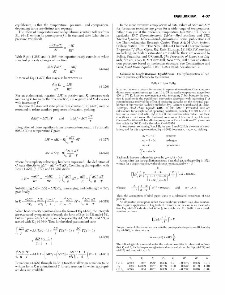
equilibrium, is that the temperature-, pressure-, and composition-dependent terms are distinct and separate.

The effect of temperature on the equilibrium constant follows fromEq. (4-41) written for pure species j in its standard state (wherein thepressure Po is fixed):

=

With Eqs. (4-365) and (4-366) this equation easily extends to relatestandard property changes of reaction:

= (4-375)

In view of Eq. (4-370) this may also be written as

= (4-376)

For an endothermic reaction, ∆Hj° is positive and Kj increases withincreasing T; for an exothermic reaction, it is negative and Kj decreaseswith increasing T.

Because the standard state pressure is constant, Eq. (4-28) may beextended to relate standard properties of reaction, yielding

d∆Hj° = ∆CPj° dT and d∆Sj° = ∆C°Pj

Integration of these equations from reference temperature T0 (usually298.15 K) to temperature T gives

∆H° = ∆H°0 + RT

T0

dT (4-377)

∆S° = ∆S°0 + RT

T0∆

RCP° (4-378)

where for simplicity subscript j has been supressed. The definition ofG leads directly to ∆G° = ∆H° − T ∆S°. Combining this equation withEqs. (4-370), (4-377), and (4-378) yields

ln K = = − T

T0∆

RCP° dT +

∆RS°0 + T

T0∆

RCP°

dTT

Substituting ∆S°0 = (∆G°0 − ∆H°0)/T0, rearranging, and defining τ TT0

give finally

ln K = −R∆

TG

0

°0 +

∆RHT

°00

τ −τ1

− T

T0∆C

R°P

dT + T

T0∆

RC°P

dTT (4-379)

When heat capacity equations have the form of Eq. (4-52), the integralsare evaluated by equations of exactly the form of Eqs. (4-53) and (4-54),but with parameters A, B, C, and D replaced by ∆A, ∆B, ∆C, and ∆D, inaccord with Eq. (4-364). Thus for the ideal gas standard state

T

T0∆RC°P dT = ∆A T0(τ − 1) + T2

0(τ 2 − 1) + T30(τ 3 − 1)

+ (4-380)

T

T0∆RC°P

dTT = ∆A lnτ + ∆BT0 + ∆CT2

0 + τ∆2TD

20

(τ − 1) (4-381)

Equations (4-379) through (4-381) together allow an equation to bewritten for lnK as a function of T for any reaction for which appropri-ate data are available.

τ + 1

2

τ − 1τ

∆DT0

∆C

3∆B

2

1T

1T

−∆H°0

RT−∆G°

RT

dTT

∆CP°

R

dTT

∆Hj°RT2

d ln Kj

dT

− ∆Hj°

RT2

d(∆Gj°RT)

dT

− Hj°RT2

d(Gj°/RT)

dT

In the more extensive compilations of data, values of ∆G° and ∆H°for formation reactions are given for a wide range of temperatures,rather than just at the reference temperature T0 = 298.15 K. [See inparticular TRC Thermodynamic Tables—Hydrocarbons and TRCThermodynamic Tables—Non-hydrocarbons, serial publications ofthe Thermodynamics Research Center, Texas A & M Univ. System,College Station, Tex.; “The NBS Tables of Chemical ThermodynamicProperties,” J. Phys. Chem. Ref. Data 11, supp. 2 (1982).] Where dataare lacking, methods of estimation are available; these are reviewed byPoling, Prausnitz, and O’Connell, The Properties of Gases and Liq-uids, 5th ed., chap. 6, McGraw-Hill, New York, 2000. For an estima-tion procedure based on molecular structure, see Constantinou andGani, Fluid Phase Equilib. 103: 11–22 (1995). See also Sec. 2.

Example 6: Single-Reaction Equilibrium The hydrogenation of ben-zene to produce cyclohexane by the reaction

C6H6 + 3H2 → C6H12

is carried out over a catalyst formulated to repress side reactions. Operating con-ditions cover a pressure range from 10 to 35 bar and a temperature range from450 to 670 K. Reaction rate increases with increasing T, but because the reac-tion is exothermic the equilibrium conversion decreases with increasing T. Acomprehensive study of the effect of operating variables on the chemical equi-librium of this reaction has been published by J. Carrero-Mantilla and M. Llano-Restrepo, Fluid Phase Equilib. 219: 181–193 (2004). Presented here arecalculations for a single set of operating conditions, namely, T = 600 K, P = 15bar, and a molar feed ratio H2/C6H6 = 3, the stoichiometric value. For theseconditions we determine the fractional conversion of benzene to cyclohexane.Carrero-Mantilla and Llano-Restrepo express ln K as a function of T by an equa-tion which for 600 K yields the value K = 0.02874.

A feed stream containing 3 mol H2 for each 1 mol C6H6 is the basis of calcu-lation, and for this single reaction, Eq. (4-361) becomes ni = ni0

+ νiε, yielding

nB = 1 − ε benzene

nH = 3 − 3ε hydrogen

nC = ε cyclohexane

i

ni = 4 − 3ε

Each mole fraction is therefore given by yi = ni(4 − 3ε).Assume first that the equilibrium mixture is an ideal gas, and apply Eq. (4-372),

written for a single reaction, with subscript j omitted and ν = − 3:

i

yiνi

ν=

−3= K = 0.02874

whence 3(15)−3 = 0.02874 and ε = 0.815

Thus, the assumption of ideal gases leads to a calculated conversion of 81.5percent.

An alternative assumption is that the equilibrium mixture is an ideal solution.This requires application of Eq. (4-371). However, in the case of an ideal solu-tion Eq. (4-218) indicates that φi

id = φi, in which case Eq. (4-371) for a singlereaction becomes

i

(yiφi)νi ν= K

For purposes of illustration we evaluate the pure-species fugacity coefficients byEq. (4-206), written here as

φi = exp(Bi0 + ωBi

1)

The following table shows values for the various quantities in this equation. Notethat Tc and Pc for hydrogen are effective values as calculated by Eqs. (4-124) and(4-125) and used with ω = 0.

Tc Tr Pc Pr ω B0 B1 φ

C6H6 562.2 1.067 48.98 0.306 0.21 − 0.2972 0.008 0.919H2 42.8 14.009 19.78 0.758 0.00 0.0768 0.139 1.004C6H12 553.6 1.084 40.73 0.368 0.21 − 0.2880 0.016 0.908

PriTri

PP°

4 − 3ε3 − 3ε

ε1 − ε

151

4 −

ε3ε

41−−

3εε

34−−

33εε

3

PP°

EQUILIBRIUM 4-37

The equilibrium equation now becomes:

i

(yiφi)νi ν=

−3= K = 0.02874

Solution yields ε = 0.816

This result is hardly different from that based on the ideal gas assumption. Thefugacity coefficients in the equilibrium equation clearly cancel one another. Thisis not uncommon in reaction equilibrium calculations, as there are always prod-ucts and reactions, making the ideal gas assumption far more useful than mightbe expected.

Carrero-Mantilla and Llano-Restrep present results for a wide range of con-ditions, both for the ideal gas assumption and for calculations wherein φi valuesare determined from the Soave-Redlich-Kwong equation of state. In no case arethese calculated conversions significantly divergent.

Complex Chemical Reaction Equilibria When the composi-tion of an equilibrium mixture is determined by a number of simulta-neous reactions, calculations based on equilibrium constants becomecomplex and tedious. A more direct procedure (and one suitable forgeneral computer solution) is based on minimization of the totalGibbs energy Gt in accord with Eq. (4-293). The treatment here islimited to gas-phase reactions for which the problem is to find theequilibrium composition for given T and P and for a given initial feed.

1. Formulate the constraining material-balance equations, basedon conservation of the total number of atoms of each element in a sys-tem comprised of w elements. Let subscript k identify a particularatom, and define Ak as the total number of atomic masses of the kthelement in the feed. Further, let aik be the number of atoms of the kthelement present in each molecule of chemical species i. The materialbalance for element k is then

i

niaik= Ak k = 1, 2 , . . . , w (4-382)

or i

niaik − Ak= 0 k = 1, 2, . . . , w

2. Multiply each element balance by λk, a Lagrange multiplier:

λki

niaik − Ak = 0 k = 1, 2, . . . , w

Summed over k, these equations give

k

λki

niaik − Ak = 0

3. Form a function F by addition of this sum to Gt:

F = Gt + k

λki

niaik − AkFunction F is identical with Gt, because the summation term is zero.However, the partial derivatives of F and Gt with respect to ni are dif-ferent, because function F incorporates the constraints of the materialbalances.

4. The minimum value of both F and Gt is found when the partialderivatives of F with respect to ni are set equal to zero:

T,P,nj

= T,P,nj

+ k

λkaik = 0∂Gt

∂ni

∂F∂ni

151

4 −

ε3ε 0.919

41−−

3εε

0.90834−−

33εε

1.0043

PP°

The first term on the right is the definition of the chemical potential;therefore,

µi + k

λkaik = 0 i = 1, 2, . . . , N (4-383)

However, the chemical potential is given by Eq. (4-368); for gas-phasereactions and standard states as the pure ideal gases at Po, this equa-tion becomes

µi = G°i + RT ln

If G°i is arbitrarily set equal to zero for all elements in their standardstates, then for compounds G°i = ∆G°f i, the standard Gibbs energy changeof formation of species i. In addition, the fugacity is eliminated—infavor of the fugacity coefficient by Eq. (4-204), fi = yiφiP. With thesesubstitutions, the equation for µi becomes

µi = ∆G°fi+ RT ln

yPiφ

°iP

Combination with Eq. (4-383) gives

∆G°fi+ RT ln

yPiφ

°iP +

kλkaik = 0 i = 1, 2, . . . , N (4-384)

If species i is an element, ∆G°f iis zero. There are N equilibrium equa-

tions [Eqs. (4-384)], one for each chemical species, and there are wmaterial balance equations [Eqs. (4-382)], one for each element—atotal of N + w equations. The unknowns in these equations are the ni’s(note that yi = ni/Σini), of which there are N, and the λk’s, of whichthere are w—a total of N + w unknowns. Thus the number of equa-tions is sufficient for the determination of all unknowns.

Equation (4-384) is derived on the presumption that the set φiis known. If the phase is an ideal gas, then each φi is unity. If the phaseis an ideal solution, each φi becomes φi and can at least be estimated.For real gases, each φi is a function of the set yi, the quantities beingcalculated. Thus an iterative procedure is indicated, initiated witheach φi set equal to unity. Solution of the equations then provides apreliminary set yi. For low pressures or high temperatures this resultis usually adequate. Where it is not satisfactory, an equation of statewith the preliminary set yi gives a new and more nearly correct setφi for use in Eq. (4-384). Then a new set yi is determined. Theprocess is repeated to convergence. All calculations are well suited tocomputer solution.

In this procedure, the question of what chemical reactions areinvolved never enters directly into any of the equations. However, thechoice of a set of species is entirely equivalent to the choice of a set ofindependent reactions among the species. In any event, a set ofspecies or an equivalent set of independent reactions must always beassumed, and different assumptions produce different results.

A detailed example of a complex gas-phase equilibrium calculationis given by Smith, Van Ness, and Abbott [Introduction to ChemicalEngineering Thermodynamics, 5th ed., Example 15.13, pp. 602–604;6th ed., Example 13.14, pp. 511–513; 7th ed., Example 13.14,pp. 527–528, McGraw-Hill, New York (1996, 2001, 2005)]. Generalapplication of the method to multicomponent, multiphase systems istreated by Iglesias-Silva et al. [Fluid Phase Equilib. 210: 229–245(2003)] and by Sotyan, Ghajar, and Gasem [Ind. Eng. Chem. Res. 42:3786–3801 (2003)].

fiP°

4-38 THERMODYNAMICS

THERMODYNAMIC ANALYSIS OF PROCESSES

Real irreversible processes can be subjected to thermodynamic analy-sis. The goal is to calculate the efficiency of energy use or productionand to show how wasted energy is apportioned among the steps of aprocess. The treatment here is limited to steady-state steady-flowprocesses, because of their predominance in chemical technology.

CALCULATION OF IDEAL WORK

In any steady-state steady-flow process requiring work, a minimumamount must be expended to bring about a specific change of state inthe flowing fluid. In a process producing work, a maximum amount is

attainable for a specific change of state in the flowing fluid. In eithercase, the limiting value obtains when the specific change of state isaccomplished completely reversibly. The implications of this require-ment are that

1. The process is internally reversible within the control volume.2. Heat transfer external to the control volume is reversible.The second item means that heat exchange between system and sur-

roundings must occur at the temperature of the surroundings, presumedto constitute a heat reservoir at a constant and uniform temperature Tσ .This may require Carnot engines or heat pumps internal to the systemthat provide for the reversible transfer of heat from the temperatures ofthe flowing fluid to that of the surroundings. Because Carnot enginesand heat pumps are cyclic, they undergo no net change of state.

These conditions are implicit in the entropy balance of Eq. (4-156)when SG = 0. If in addition there is but a single surroundings temper-ature Tσ, this equation becomes

∆(Sm)fs − TQ

σ = 0 (4-385)

The energy balance for a steady-state steady-flow process as givenby Eq. (4-150) is

∆H + u2 + zgmfs= Q + Ws (4-150)

Combining this equation with Eq. (4-385) to eliminate Q yields

∆H + u2 + zgmfs= Tσ ∆(Sm)fs + Ws(rev)

where Ws(rev) indicates that the shaft work is for a completelyreversible process. This work is called the ideal work Wideal. Thus

Wideal = ∆H + u2 + zgmfs− Tσ ∆(Sm)fs (4-386)

In most applications to chemical processes, the kinetic and poten-tial energy terms are negligible compared with the others; in thisevent Eq. (4-386) is written as

Wideal = ∆(Hm)fs − Tσ ∆(Sm)fs (4-387)

For the special case of a single stream flowing through the system, Eq.(4-387) becomes

Wideal = m(∆H − Tσ ∆S) (4-388)

Division by m puts this equation on a unit-mass basis:

Wideal = ∆H − Tσ ∆S (4-389)

A completely reversible process is hypothetical, devised solely tofind the ideal work associated with a given change of state. Its only con-nection with an actual process is that it brings about the same changeof state as the actual process, allowing comparison of the actual work ofa process with the work of the hypothetical reversible process.

Equations (4-386) through (4-389) give the work of a completelyreversible process associated with given property changes in the flow-ing streams. When the same property changes occur in an actualprocess, the actual work Ws (or Ws) is given by an energy balance, andcomparison can be made of the actual work with the ideal work. WhenWideal (or Wideal) is positive, it is the minimum work required to bringabout a given change in the properties of the flowing streams, and it issmaller than Ws. In this case a thermodynamic efficiency ηt is definedas the ratio of the ideal work to the actual work:

ηt(work required) = WW

id

s

eal (4-390)

When Wideal (or Wideal) is negative, Wideal is the maximum workobtainable from a given change in the properties of the flowingstreams, and it is larger than Ws. In this case, the thermodynamic effi-ciency is defined as the ratio of the actual work to the ideal work:

ηt(work produced) = (4-391)Ws

Wideal

12

12

12

LOST WORK

Work that is wasted as the result of irreversibilities in a process iscalled lost work Wlost, and it is defined as the difference between theactual work of a process and the ideal work for the process. Thus bydefinition,

Wlost Ws − Wideal (4-392)

The rate form is Wlost Ws − Wideal (4-393)

The actual work rate comes from Eq. (4-150):

Ws= ∆H + u2 + zgmfs− Q

Subtracting the ideal work rate as given by Eq. (4-386) yields

Wlost = Tσ ∆(Sm)fs − Q (4-394)

For the special case of a single stream flowing through the controlvolume,

Wlost = mTσ ∆S − Q (4-395)

Division of this equation by m gives

Wlost = Tσ ∆S − Q (4-396)

where the basis is now a unit amount of fluid flowing through the con-trol volume.

The total rate of entropy generation (in both system and surround-ings) as a result of a process is

SG = ∆(Sm)fs − (4-397)

Division by m provides an equation based on a unit amount of fluidflowing through the control volume:

SG = ∆S − (4-398)

Equations (4-397) and (4-398) are special cases of Eqs. (4-156) and(4-157).

Multiplication of Eq. (4-397) by Tσ gives

Tσ SG = Tσ ∆(Sm)fs − Q

Because the right sides of this equation and of Eq. (4-394) are identi-cal, it follows that

Wlost = Tσ SG (4-399)

For flow on the basis of a unit amount of fluid, this becomes

Wlost = TσSG (4-400)

Because the second law of thermodynamics requires

SG ≥ 0 and SG ≥ 0

therefore Wlost ≥ 0 and Wlost ≥ 0

When a process is completely reversible, the equality holds and thelost work is zero. For irreversible processes the inequality holds, andthe lost work, i.e., the energy that becomes unavailable for work, ispositive. The engineering significance of this result is clear: Thegreater the irreversibility of a process, the greater the rate of entropygeneration and the greater the amount of energy that becomesunavailable for work. Thus every irreversibility carries with it a price.

ANALYSIS OF STEADY-STATE STEADY-FLOW PROCESSES

Many processes consist of a number of steps, and lost-work calcula-tions are then made for each step separately. Writing Eq. (4-399) foreach step of the process and summing give

Wlost= Tσ SG

QTσ

QTσ

12

THERMODYNAMIC ANALYSIS OF PROCESSES 4-39

Dividing Eq. (4-399) by this result yields

W

Wlos

l

t

ost =

SG

S

G

Thus an analysis of the lost work, made by calculation of the fractionthat each individual lost-work term represents of the total lost work, isthe same as an analysis of the rate of entropy generation, made byexpressing each individual entropy generation term as a fraction of thesum of all entropy generation terms.

An alternative to the lost-work or entropy generation analysis is awork analysis. This is based on Eq. (4-393), written as

Wlost = Ws − Wideal (4-401)

For a work-requiring process, all these work quantities are positiveand Ws > Wideal. The preceding equation is then expressed as

Ws= Wideal + Wlost (4-402)

A work analysis then gives each of the individual work terms in thesummation on the right as a fraction of Ws.

For a work-producing process, Ws and Wideal are negative, andWideal > Ws. Equation (4-401) in this case is best written as

Wideal = Ws + Wlost (4-403)

A work analysis here expresses each of the individual work terms onthe right as a fraction of Wideal. A work analysis cannot be carried outin the case where a process is so inefficient that Wideal is negative, indi-cating that the process should produce work; but Ws is positive, indi-cating that the process in fact requires work. A lost-work or entropygeneration analysis is always possible.

Example 7: Lost-Work Analysis A work analysis follows for a simpleLinde system for the separation of air into gaseous oxygen and nitrogen, asdepicted in Fig. 4-10. Table 4-8 lists a set of operating conditions for the num-bered points of the diagram. Heat leaks into the column of 147 J/mol of enter-ing air and into the exchanger of 70 J/mol of entering air have been assumed.Take Tσ = 300 K.

The basis for analysis is 1 mol of entering air, assumed to contain 79 mol % N2

and 21 mol % O2. By a material balance on the nitrogen, 0.79 = 0.9148 x, whence

x = 0.8636 mol of nitrogen product1 − x = 0.1364 mol of oxygen product

Calculation of ideal work: If changes in kinetic and potential energies areneglected, Eq. (4-387) is applicable. From the tabulated data,

∆(Hm)fs = (13,460)(0.1364) + (12,074)(0.8636) − (12,407)(1) = −144 J∆(Sm)fs = (118.48)(0.1364) + (114.34)(0.8636) − (117.35)(1)= − 2.4453 JK

Thus, by Eq. (4-387),

Wideal= −144 − (300)(−2.4453) = 589.6 J

Calculation of actual work of compression: For simplicity, the work of com-pression is calculated by the equation for an ideal gas in a three-stage recipro-cating machine with complete intercooling and with isentropic compression ineach stage. The work so calculated is assumed to represent 80 percent of theactual work. The following equation may be found in any number of textbookson thermodynamics:

Ws = 0.

n8γ(γ

R−T1

1)

PP

2

1

(γ − 1)nγ − 1

where n = number of stages, here taken as 3γ = ratio of heat capacities, here taken as 1.4

T1 = initial absolute temperature, equal to 300 KP2/P1 = overall pressure ratio, equal to 54.5

R = universal gas constant, equal to 8.314 J/(mol·K)

The efficiency factor of 0.8 is already included in the equation. Substitution ofthe remaining values gives

Ws = (54.5)0.4(3)(1.4) − 1 = 15,171 J

The heat transferred to the surroundings during compression as a result of inter-cooling and aftercooling to 300 K is found from the first law:

Q = m(∆H) − Ws = (12,046 − 12,407) −15,171 = −15,532 J

Calculation of lost work: Equation (4-394) may be applied to each of themajor units of the process. For the compressor/cooler,

Wlost= (300)[(82.98)(1) − (117.35)(1)] − (−15,532)= 5221.0 J

For the exchanger,

Wlost = (300)[(118.48)(0.1364) + (114.34)(0.8636) + (52.08)(1)− (75.82)(0.8636) − (83.69)(0.1364) − (82.98)(1)] − 70

= 2063.4 J

Finally, for the rectifier,

Wlost = (300)[(75.82)(0.8636) + (83.69)(0.1364) − (52.08)(1)] − 147 = 7297.0 J

Work analysis: Because the process requires work, Eq. (4-402) is appropriatefor a work analysis. The various terms of this equation appear as entries in thefollowing table and are on the basis of 1 mol of entering air.

% of Ws

Wideal 589.6 J 3.9Wlost: Compressor/cooler 5,221.0 J 34.4Wlost: Exchanger 2,063.4 J 13.6Wlost: Rectifier 7,297.0 J 48.1Ws 15,171.0 J 100.0

The thermodynamic efficiency of this process as given by Eq. (4-390) is only3.9 percent. Significant inefficiencies reside with each of the primary units ofthe process.

(3)(1.4)(8.314)(300)

(0.8)(0.4)

4-40 THERMODYNAMICS

TABLE 4-8 States and Values of Properties for the Process ofFig. 4-10*

Point P, bar T, K Composition State H, J/mol S, J/(mol·K)

1 55.22 300 Air Superheated 12,046 82.982 1.01 295 Pure O2 Superheated 13,460 118.483 1.01 295 91.48% N2 Superheated 12,074 114.344 55.22 147.2 Air Superheated 5,850 52.085 1.01 79.4 91.48% N2 Saturated vapor 5,773 75.826 1.01 90 Pure O2 Saturated vapor 7,485 83.697 1.01 300 Air Superheated 12,407 117.35

*Properties on the basis of Miller and Sullivan, U.S. Bur. Mines Tech. Pap. 424(1928).

FIG. 4-10 Diagram of simple Linde system for air separation.