http://www.cambridge.org/9780521829601

This page intentionally left blank

This book provides an introduction to the major mathematical structures used in physicstoday. It covers the concepts and techniques needed for topics such as group theory, Liealgebras, topology, Hilbert spaces and differential geometry. Important theories of physicssuch as classical and quantum mechanics, thermodynamics, and special and general rela-tivity are also developed in detail, and presented in the appropriate mathematical language.

The book is suitable for advanced undergraduate and beginning graduate students inmathematical and theoretical physics. It includes numerous exercises and worked examplesto test the reader’s understanding of the various concepts, as well as extending the themescovered in the main text. The only prerequisites are elementary calculus and linear algebra.No prior knowledge of group theory, abstract vector spaces or topology is required.

Pe t e r Sz e k e r e s received his Ph.D. from King’s College London in 1964, in the areaof general relativity. He subsequently held research and teaching positions at CornellUniversity, King’s College and the University of Adelaide, where he stayed from 1971till his recent retirement. Currently he is a visiting research fellow at that institution. He iswell known internationally for his research in general relativity and cosmology, and has anexcellent reputation for his teaching and lecturing.

A Course in ModernMathematical PhysicsGroups, Hilbert Space and Differential Geometry

Peter SzekeresFormerly of University of Adelaide

cambridge university pressCambridge, New York, Melbourne, Madrid, Cape Town, Singapore, São Paulo

Cambridge University PressThe Edinburgh Building, Cambridge cb2 2ru, UK

First published in print format

isbn-13 978-0-521-82960-1

isbn-13 978-0-521-53645-5

isbn-13 978-0-511-26167-1

© P. Szekeres 2004

2004

Information on this title: www.cambridge.org/9780521829601

This publication is in copyright. Subject to statutory exception and to the provision ofrelevant collective licensing agreements, no reproduction of any part may take placewithout the written permission of Cambridge University Press.

isbn-10 0-511-26167-5

isbn-10 0-521-82960-7

isbn-10 0-521-53645-6

Cambridge University Press has no responsibility for the persistence or accuracy of urlsfor external or third-party internet websites referred to in this publication, and does notguarantee that any content on such websites is, or will remain, accurate or appropriate.

Published in the United States of America by Cambridge University Press, New York

www.cambridge.org

hardback

eBook (Adobe Reader)

eBook (Adobe Reader)

hardback

Contents

Preface page ixAcknowledgements xiii

1 Sets and structures 11.1 Sets and logic 21.2 Subsets, unions and intersections of sets 51.3 Cartesian products and relations 71.4 Mappings 101.5 Infinite sets 131.6 Structures 171.7 Category theory 23

2 Groups 272.1 Elements of group theory 272.2 Transformation and permutation groups 302.3 Matrix groups 352.4 Homomorphisms and isomorphisms 402.5 Normal subgroups and factor groups 452.6 Group actions 492.7 Symmetry groups 52

3 Vector spaces 593.1 Rings and fields 593.2 Vector spaces 603.3 Vector space homomorphisms 633.4 Vector subspaces and quotient spaces 663.5 Bases of a vector space 723.6 Summation convention and transformation of bases 813.7 Dual spaces 88

4 Linear operators and matrices 984.1 Eigenspaces and characteristic equations 994.2 Jordan canonical form 107

v

Contents

4.3 Linear ordinary differential equations 1164.4 Introduction to group representation theory 120

5 Inner product spaces 1265.1 Real inner product spaces 1265.2 Complex inner product spaces 1335.3 Representations of finite groups 141

6 Algebras 1496.1 Algebras and ideals 1496.2 Complex numbers and complex structures 1526.3 Quaternions and Clifford algebras 1576.4 Grassmann algebras 1606.5 Lie algebras and Lie groups 166

7 Tensors 1787.1 Free vector spaces and tensor spaces 1787.2 Multilinear maps and tensors 1867.3 Basis representation of tensors 1937.4 Operations on tensors 198

8 Exterior algebra 2048.1 r-Vectors and r-forms 2048.2 Basis representation of r-vectors 2068.3 Exterior product 2088.4 Interior product 2138.5 Oriented vector spaces 2158.6 The Hodge dual 220

9 Special relativity 2289.1 Minkowski space-time 2289.2 Relativistic kinematics 2359.3 Particle dynamics 2399.4 Electrodynamics 2449.5 Conservation laws and energy–stress tensors 251

10 Topology 25510.1 Euclidean topology 25510.2 General topological spaces 25710.3 Metric spaces 26410.4 Induced topologies 26510.5 Hausdorff spaces 26910.6 Compact spaces 271

vi

Contents

10.7 Connected spaces 27310.8 Topological groups 27610.9 Topological vector spaces 279

11 Measure theory and integration 28711.1 Measurable spaces and functions 28711.2 Measure spaces 29211.3 Lebesgue integration 301

12 Distributions 30812.1 Test functions and distributions 30912.2 Operations on distributions 31412.3 Fourier transforms 32012.4 Green’s functions 323

13 Hilbert spaces 33013.1 Definitions and examples 33013.2 Expansion theorems 33513.3 Linear functionals 34113.4 Bounded linear operators 34413.5 Spectral theory 35113.6 Unbounded operators 357

14 Quantum mechanics 36614.1 Basic concepts 36614.2 Quantum dynamics 37914.3 Symmetry transformations 38714.4 Quantum statistical mechanics 397

15 Differential geometry 41015.1 Differentiable manifolds 41115.2 Differentiable maps and curves 41515.3 Tangent, cotangent and tensor spaces 41715.4 Tangent map and submanifolds 42615.5 Commutators, flows and Lie derivatives 43215.6 Distributions and Frobenius theorem 440

16 Differentiable forms 44716.1 Differential forms and exterior derivative 44716.2 Properties of exterior derivative 45116.3 Frobenius theorem: dual form 45416.4 Thermodynamics 45716.5 Classical mechanics 464

vii

Contents

17 Integration on manifolds 48117.1 Partitions of unity 48217.2 Integration of n-forms 48417.3 Stokes’ theorem 48617.4 Homology and cohomology 49317.5 The Poincare lemma 500

18 Connections and curvature 50618.1 Linear connections and geodesics 50618.2 Covariant derivative of tensor fields 51018.3 Curvature and torsion 51218.4 Pseudo-Riemannian manifolds 51618.5 Equation of geodesic deviation 52218.6 The Riemann tensor and its symmetries 52418.7 Cartan formalism 52718.8 General relativity 53418.9 Cosmology 54818.10 Variation principles in space-time 553

19 Lie groups and Lie algebras 55919.1 Lie groups 55919.2 The exponential map 56419.3 Lie subgroups 56919.4 Lie groups of transformations 57219.5 Groups of isometries 578

Bibliography 587Index 589

viii

Preface

After some twenty years of teaching different topics in the Department of MathematicalPhysics at the University of Adelaide I conceived the rather foolhardy project of puttingall my undergraduate notes together in one single volume under the title MathematicalPhysics. This undertaking turned out to be considerably more ambitious than I had originallyexpected, and it was not until my recent retirement that I found the time to complete it.

Over the years I have sometimes found myself in the midst of a vigorous and at timesquite acrimonious debate on the difference between theoretical and mathematical physics.This book is symptomatic of the difference. I believe that mathematical physicists put themathematics first, while for theoretical physicists it is the physics which is uppermost. Thelatter seek out those areas of mathematics for the use they may be put to, while the formerhave a more unified view of the two disciplines. I don’t want to say one is better than theother – it is simply a different outlook. In the big scheme of things both have their placebut, as this book no doubt demonstrates, my personal preference is to view mathematicalphysics as a branch of mathematics.

The classical texts on mathematical physics which I was originally brought up on, suchas Morse and Feshbach [7], Courant and Hilbert [1], and Jeffreys and Jeffreys [6] are es-sentially books on differential equations and linear algebra. The flavour of the present bookis quite different. It follows much more the lines of Choquet-Bruhat, de Witt-Morette andDillard-Bleick [14] and Geroch [3], in which mathematical structures rather than mathemat-ical analysis is the main thrust. Of these two books, the former is possibly a little daunting asan introductory undergraduate text, while Geroch’s book, written in the author’s inimitablydelightful lecturing style, has occasional tendencies to overabstraction. I resolved thereforeto write a book which covers the material of these texts, assumes no more mathematicalknowledge than elementary calculus and linear algebra, and demonstrates clearly how theo-ries of modern physics fit into various mathematical structures. How well I have succeededmust be left to the reader to judge.

At times I have been caught by surprise at the natural development of ideas in this book.For example, how is it that quantum mechanics appears before classical mechanics? Thereason is certainly not on historical grounds. In the natural organization of mathematicalideas, algebraic structures appear before geometrical or topological structures, and linearstructures are evidently simpler than non-linear. From the point of view of mathematicalsimplicity quantum mechanics, being a purely linear theory in a quasi-algebraic space(Hilbert space), is more elementary than classical mechanics, which can be expressed in

ix

Preface

terms of non-linear dynamical systems in differential geometry. Yet, there is somethingof a paradox here, for as Niels Bohr remarked: ‘Anyone who is not shocked by quantummechanics does not understand it’. Quantum mechanics is not a difficult theory to expressmathematically, but it is almost impossible to make epistomological sense of it. I will noteven attempt to answer these sorts of questions, and the reader must look elsewhere for adiscussion of quantum measurement theory [5].

Every book has its limitations. At some point the author must call it a day, and theomissions in this book may prove a disappointment to some readers. Some of them area disappointment to me. Those wanting to go further might explore the theory of fibrebundles and gauge theories [2, 8, 13], as the stage is perfectly set for this subject by the endof the book. To many, the biggest omission may be the lack of any discussion of quantumfield theory. This, however, is an area that seems to have an entirely different flavour to therest of physics as its mathematics is difficult if nigh on impossible to make rigorous. Evenquantum mechanics has a ‘classical’ flavour by comparison. It is such a huge subject that Ifelt daunted to even begin it. The reader can only be directed to a number of suitable booksto introduce them to this field [10–14].

Structure of the book

This book is essentially in two parts, modern algebra and geometry (including topology).The early chapters begin with set theory, group theory and vector spaces, then move to moreadvanced topics such as Lie algebras, tensors and exterior algebra. Occasionally ideas fromgroup representation theory are discussed. If calculus appears in these chapters it is of anelementary kind. At the end of this algebraic part of the book, there is included a chapteron special relativity (Chapter 9), as it seems a nice example of much of the algebra that hasgone before while introducing some notions from topology and calculus to be developed inthe remaining chapters. I have treated it as a kind of crossroads: Minkowski space acts as alink between algebraic and geometric structures, while at the same time it is the first placewhere physics and mathematics are seen to interact in a significant way.

In the second part of the book, we discuss structures that are essentially geometricalin character, but generally have an algebraic component as well. Beginning with topology(Chapter 10), structures are created that combine both algebra and the concept of continuity.The first of these is Hilbert space (Chapter 13), which is followed by a chapter on quantummechanics. Chapters on measure theory (Chapter 11) and distribution theory (Chapter 12)precede these two. The final chapters (15–19) deal with differential geometry and examplesof physical theories using manifold theory as their setting – thermodynamics, classicalmechanics, general relativity and cosmology. A flow diagram showing roughly how thechapters interlink is given below.

Exercises and problems are interspersed throughout the text. The exercises are not de-signed to be difficult – their aim is either to test the reader’s understanding of a conceptjust defined or to complete a proof needing one or two more steps. The problems at endsof sections are more challenging. Frequently they are in many parts, taking up a thread

x

Preface

10

1

23

7 84 5 6 12 1311 14

15

16

17

18

19

9

of thought and running with it. This way most closely resembles true research, and is mypreferred way of presenting problems rather than the short one-liners often found in textbooks. Throughout the book, newly defined concepts are written in bold type. If a con-cept is written in italics, it has been introduced in name only and has yet to be definedproperly.

References

[1] R. Courant and D. Hilbert. Methods of Mathematical Physics, vols 1 and 2. New York,Interscience, 1953.

[2] T. Frankel. The Geometry of Physics. New York, Cambridge University Press, 1997.[3] R. Geroch. Mathematical Physics. Chicago, The University of Chicago Press, 1985.[4] J. Glimm and A. Jaffe. Quantum Physics: A Functional Integral Point of View. New

York, Springer-Verlag, 1981.[5] J. M. Jauch. Foundations of Quantum Mechanics. Reading, Mass., Addison-Wesley,

1968.[6] H. J. Jeffreys and B. S. Jeffreys. Methods of Mathematical Physics. Cambridge,

Cambridge University Press, 1946.[7] P. M. Morse and H. Feshbach. Methods of Theoretical Physics, vols 1 and 2. New York,

McGraw-Hill, 1953.[8] C. Nash and S. Sen. Topology and Geometry for Physicists. London, Academic Press,

1983.[9] P. Ramond. Field Theory: A Modern Primer. Reading, Mass., Benjamin/Cummings,

1981.[10] L. H. Ryder, Quantum Field Theory. Cambridge, Cambridge University Press, 1985.[11] S. S. Schweber. An Introduction to Relativistic Quantum Field Theory. New York,

Harper and Row, 1961.

xi

Preface

[12] R. F. Streater and A. S. Wightman. PCT, Spin and Statistics, and All That. New York,W. A. Benjamin, 1964.

[13] A. Trautman. Fibre bundles associated with space-time. Reports on MathematicalPhysics, 1:29–62, 1970.

[14] C. de Witt-Morette, Y. Choquet-Bruhat and M. Dillard-Bleick. Analysis, Manifoldsand Physics. Amsterdam, North-Holland, 1977.

xii

Acknowledgements

There are an enormous number of people I would like to express my gratitude to, but Iwill single out just a few of the most significant. Firstly, my father George Szekeres, whointroduced me at an early age to the wonderful world of mathematics and has continuedto challenge me throughout my life with his doubts and criticisms of the way physics(particularly quantum theory) is structured. My Ph.D. supervisor Felix Pirani was the first togive me an inkling of the importance of differential geometry in mathematical physics,whileothers who had an enormous influence on my education and outlook were Roger Penrose,Bob Geroch, Brandon Carter, Andrzej Trautman, Ray McLenaghan, George Ellis, BertGreen, Angas Hurst, Sue Scott, David Wiltshire, David Hartley, Paul Davies, Robin Tucker,Alan Carey, and Michael Eastwood. Finally, my wife Angela has not only been an endlesssource of encouragement and support, but often applied her much valued critical facultiesto my manner of expression. I would also like to pay a special tribute to Patrick Fitzhenryfor his invaluable assistance in preparing diagrams and guiding me through some of thenightmare that is today’s computer technology.

xiii

To my mother, Esther

1 Sets and structures

The object of mathematical physics is to describe the physical world in purely mathemat-ical terms. Although it had its origins in the science of ancient Greece, with the work ofArchimedes, Euclid and Aristotle, it was not until the discoveries of Galileo and Newton thatmathematical physics as we know it today had its true beginnings. Newton’s discovery ofthe calculus and its application to physics was undoubtedly the defining moment. This wasbuilt upon by generations of brilliant mathematicians such as Euler, Lagrange, Hamiltonand Gauss, who essentially formulated physical law in terms of differential equations. Withthe advent of new and unintuitive theories such as relativity and quantum mechanics in thetwentieth century, the reliance on mathematics moved to increasingly recondite areas suchas abstract algebra, topology, functional analysis and differential geometry. Even classicalareas such as the mechanics of Lagrange and Hamilton, as well as classical thermody-namics, can be lifted almost directly into the language of modern differential geometry.Today, the emphasis is often more structural than analytical, and it is commonly believedthat finding the right mathematical structure is the most important aspect of any physicaltheory. Analysis, or the consequences of theories, still has a part to play in mathematicalphysics – indeed, most research is of this nature – but it is possibly less fundamental in thetotal overview of the subject.

When we consider the significant achievements of mathematical physics, one cannot helpbut wonder why the workings of the universe are expressable at all by rigid mathematical‘laws’. Furthermore, how is it that purely human constructs, in the form of deep and subtlemathematical structures refined over centuries of thought, have any relevance at all? Thenineteenth century view of a clockwork universe regulated deterministically by differentialequations seems now to have been banished for ever, both through the fundamental appear-ance of probabilities in quantum mechanics and the indeterminism associated with chaoticsystems. These two aspects of physical law, the deterministic and indeterministic, seem tointerplay in some astonishing ways, the impact of which has yet to be fully appreciated. It isthis interplay, however, that almost certainly gives our world its richness and variety. Someof these questions and challenges may be fundamentally unanswerable, but the fact remainsthat mathematics seems to be the correct path to understanding the physical world.

The aim of this book is to present the basic mathematical structures used in our subject,and to express some of the most important theories of physics in their appropriate mathe-matical setting. It is a book designed chiefly for students of physics who have the need for amore rigorous mathematical education. A basic knowledge of calculus and linear algebra,including matrix theory, is assumed throughout, but little else. While different students will

1

Sets and structures

of course come to this book with different levels of mathematical sophistication, the readershould be able to determine exactly what they can skip and where they must take pause.Mathematicians, for example, may be interested only in the later chapters, where varioustheories of physics are expressed in mathematical terms. These theories will not, however,be developed at great length, and their consequences will only be dealt with by way of afew examples.

The most fundamental notion in mathematics is that of a set, or ‘collection of objects’.The subject of this chapter is set theory – the branch of mathematics devoted to the studyof sets as abstract objects in their own right. It turns out that every mathematical structureconsists of a collection of sets together with some defining relations. Furthermore, as weshall see in Section 1.3, such relations are themselves defined in terms of sets. It is thus acommonly adopted viewpoint that all of mathematics reduces essentially to statements inset theory, and this is the motivation for starting with a chapter on such a basic topic.

The idea of sets as collections of objects has a non-rigorous, or ‘naive’ quality, although itis the form in which most students are introduced to the subject [1–4]. Early in the twentiethcentury, it was discovered by Bertrand Russell that there are inherent self-contradictionsand paradoxes in overly simple versions of set theory. Although of concern to logicians andthose mathematicians demanding a totally rigorous basis to their subject, these paradoxesusually involve inordinately large self-referential sets – not the sort of constructs likely tooccur in physical contexts. Thus, while special models of set theory have been designedto avoid contradictions, they generally have somewhat artificial attributes and naive settheory should suffice for our purposes. The reader’s attention should be drawn, however,to the remarks at the end of Section 1.5 concerning the possible relevance of fundamentalproblems of set theory to physics. These problems, while not of overwhelming concern,may at least provide some food for thought.

While a basic familiarity with set theory will be assumed throughout this book, it never-theless seems worthwhile to go over the fundamentals, if only for the sake of completenessand to establish a few conventions. Many physicists do not have a good grounding in settheory, and should find this chapter a useful exercise in developing the kind of rigorousthinking needed for mathematical physics. For mathematicians this is all bread and butter,and if you feel the material of this chapter is well-worn ground, please feel free to pass onquickly.

1.1 Sets and logic

There are essentially two ways in which we can think of a set S. Firstly, it can be regardedas a collection of mathematical objects a, b, . . . , called constants, written

S = {a, b, . . . }.The constants a, b, . . . may themselves be sets and, indeed, some formulations of set theoryrequire them to be sets. Physicists in general prefer to avoid this formal nicety, and find itmuch more natural to allow for ‘atomic’ objects, as it is hard to think of quantities such astemperature or velocity as being ‘sets’. However, to think of sets as consisting of lists of

2

1.1 Sets and logic

objects is only suitable for finite or at most countably infinite sets. If we try putting the realnumbers into a list we encounter the Cantor diagonalization problem – see Theorems 1.4and 1.5 of Section 1.5.

The second approach to set theory is much more general in character. Let P(x) be alogical proposition involving a variable x . Any such proposition symbolically defines a set

S = {x | P(x)},

which can be thought of as symbolically representing the collection of all x for which theproposition P(x) is true. We will not attempt a full definition of the concept of logicalproposition here – this is the business of formal logic and is only of peripheral interest totheoretical physicists – but some comments are in order. Essentially, logical propositions arestatements made up from an alphabet of symbols, some of which are termed constants andsome of which are called variables, together with logical connectives such as not, and, orand implies, to be manipulated according to rules of standard logic. Instead of ‘P impliesQ’ we frequently use the words ‘if P then Q’ or the symbolic representation P ⇒ Q. Thestatement ‘P if and only if Q’, or ‘P iff Q’, symbolically written P ⇔ Q, is a shorthandfor

(P ⇒ Q) and (Q ⇒ P),

and signifies logical equivalence of the propositions P and Q. The two quantifiers ∀ and∃, said for all and there exists, respectively, make their appearance in the following way: ifP(x) is a proposition involving a variable x , then

∀x(P(x)) and ∃x(P(x))

are propositions.Mathematical theories such as set theory, group theory, etc. traditionally involve the

introduction of some new symbols with which to generate further logical propositions.The theory must be complemented by a collection of logical propositions called axioms forthe theory – statements that are taken to be automatically true in the theory. All other truestatements should in principle follow by the rules of logic.

Set theory involves the introduction of the new phrase is a set and new symbols{. . . | . . . } and ∈ defined by:

(Set1) If S is any constant or variable then ‘S is a set’ is a logical proposition.(Set2) If P(x) is a logical proposition involving a variable x then {x | P(x)} is a set.(Set3) If S is a set and a is any constant or variable then a ∈ S is a logical proposition,

for which we say a belongs to S or a is a member of S, or simply a is in S. Thenegative of this proposition is denoted a /∈ S – said a is not in S.

These statements say nothing about whether the various propositions are true or false – theymerely assert what are ‘grammatically correct’ propositions in set theory. They merely tellus how the new symbols and phrases are to be used in a grammatically correct fashion. Themain axiom of set theory is: if P(x) is any logical proposition depending on a variable x ,

3

Sets and structures

then for any constant or variable a

a ∈ {x | P(x)} ⇔ P(a).

Every mathematical theory uses the equality symbol = to express the identity of math-ematical objects in the theory. In some cases the concept of mathematical identity needs aseparate definition. For example equality of sets A = B is defined through the axiom ofextensionality:

Two sets A and B are equal if and only if they contain the same members. Expressedsymbolically,

A = B ⇔ ∀a(a ∈ A ⇔ a ∈ B).

A finite set A = {a1, a2, . . . , an} is equivalent to

A = {x | (x = a1) or (x = a2) or . . . or (x = an)}.A set consisting of just one element a is called a singleton and should be written as {a} todistinguish it from the element a which belongs to it: {a} = {x | x = a}.

As remarked above, sets can be members of other sets. A set whose elements are all setsthemselves will often be called a collection or family of sets. Such collections are oftendenoted by script letters such as A, U , etc. Frequently a family of sets U has its membersindexed by another set I , called the indexing set, and is written

U = {Ui | i ∈ I }.For a finite family we usually take the indexing set to be the first n natural numbers,I = {1, 2, . . . , n}. Strictly speaking, this set must also be given an axiomatic definitionsuch as Peano’s axioms. We refer the interested reader to texts such as [4] for a discussionof these matters.

Although the finer details of logic have been omitted here, essentially all concepts of settheory can be constructed from these basics. The implication is that all of mathematics canbe built out of an alphabet for constants and variables, parentheses (. . . ), logical connectivesand quantifiers together with the rules of propositional logic, and the symbols {. . . | . . . }and ∈. Since mathematical physics is an attempt to express physics in purely mathematicallanguage, we have the somewhat astonishing implication that all of physics should alsobe reducible to these simple terms. Eugene Wigner has expressed wonderment at this ideain a famous paper entitled The unreasonable effectiveness of mathematics in the naturalsciences [5].

The presentation of set theory given here should suffice for all practical purposes, but itis not without logical difficulties. The most famous is Russell’s paradox: consider the set ofall sets which are not members of themselves. According to the above rules this set can bewritten R = {A | A /∈ A}. Is R a member of itself? This question does not appear to havean answer. For, if R ∈ R then by definition R /∈ R, which is a contradiction. On the otherhand, if R /∈ R then it satisfies the criterion required for membership of R; that is, R ∈ R.

4

1.2 Subsets, unions and intersections of sets

To avoid such vicious arguments, logicians have been forced to reformulate the axioms ofset theory in a very careful way. The most frequently used system is the axiomatic schemeof Zermelo and Fraenkel – see, for example, [2] or the Appendix of [6]. We will adopt the‘naive’ position and simply assume that the sets dealt with in this book do not exhibit theself-contradictions of Russell’s monster.

1.2 Subsets, unions and intersections of sets

A set T is said to be a subset of S, or T is contained in S, if every member of T belongsto S. Symbolically, this is written T ⊆ S,

T ⊆ S iff a ∈ T ⇒ a ∈ S.

We may also say S is a superset of T and write S ⊃ T . Of particular importance is theempty set ∅, to which no object belongs,

∀a (a /∈ ∅).

The empty set is assumed to be a subset of any set whatsoever,

∀S(∅ ⊆ S).

This is the default position, consistent with the fact that a ∈ ∅ ⇒ a ∈ S, since there are noa such that a ∈ ∅ and the left-hand side of the implication is never true. We have here anexample of the logical dictum that ‘a false statement implies the truth of any statement’.

A common criterion for showing the equality of two sets, T = S, is to show that T ⊆ Sand S ⊆ T . The proof follows from the axiom of extensionality:

T = S ⇐⇒ (a ∈ T ⇔ a ∈ S)⇐⇒ (a ∈ T ⇒ a ∈ S) and (a ∈ S ⇒ a ∈ T )⇐⇒ (T ⊆ S) and (S ⊆ T ).

Exercise: Show that the empty set is unique; i.e., if ∅′ is an empty set then ∅′ = ∅.

The collection of all subsets of a set S forms a set in its own right, called the power setof S, denoted 2S .

Example 1.1 If S is a finite set consisting of n elements, then 2S consists of one emptyset ∅ having no elements, n singleton sets having just one member,

(n2

)sets having two

elements, etc. Hence the total number of sets belonging to 2S is, by the binomial theorem,

1+(

n

1

)+(

n

2

)+ · · · +

(n

n

)= (1+ 1)n = 2n.

This motivates the symbolic representation of the power set.

Unions and intersections

The union of two sets S and T , denoted S ∪ T , is defined as

S ∪ T = {x | x ∈ S or x ∈ T }.

5

Sets and structures

The intersection of two sets S and T , denoted S ∩ T , is defined as

S ∩ T = {x | x ∈ S and x ∈ T }.Two sets S and T are called disjoint if no element belongs simultaneously to both sets,S ∩ T = ∅. The difference of two sets S and T is defined as

S − T = {x | x ∈ S and x /∈ T }.

Exercise: If S and T are disjoint, show that S − T = S.

The union of an arbitrary (possibly infinite) family of sets A is defined as the set of allelements x that belong to some member of the family,⋃

A = {x | ∃S such that (S ∈ A) and (x ∈ S)}.Similarly we define the intersection of S to be the set of all elements that belong to everyset of the collection, ⋂

A = {x | x ∈ S for all S ∈ A}.When A consists of a family of sets Si indexed by a set I , the union and intersection arefrequently written ⋃

i∈I

{Si } and⋂i∈I

{Si }.

Problems

Problem 1.1 Show the distributive laws

A ∩ (B ∪ C) = (A ∩ B) ∪ (A ∩ C), A ∪ (B ∩ C) = (A ∪ B) ∩ (A ∪ C ).

Problem 1.2 If B = {Bi | i ∈ I } is any family of sets, show that

A ∩⋃

B =⋃{A ∩ Bi | i ∈ I }, A ∪

⋂B =

⋂{A ∪ Bi | i ∈ I }.

Problem 1.3 Let B be any set. Show that (A ∩ B) ∪ C = A ∩ (B ∪ C) if and only if C ⊆ A.

Problem 1.4 Show that

A − (B ∪ C) = (A − B) ∩ (A − C), A − (B ∩ C) = (A − B) ∪ (A − C).

Problem 1.5 If B = {Bi | i ∈ I } is any family of sets, show that

A −⋃

B =⋃{A − Bi | i ∈ I }.

Problem 1.6 If E and F are any sets, prove the identities

2E ∩ 2F = 2E∩F , 2E ∪ 2F ⊆ 2E∪F .

Problem 1.7 Show that if C is any family of sets then⋂X∈ C

2X = 2⋂ C,

⋃X∈ C

2X ⊆ 2⋃ C .

6

1.3 Cartesian products and relations

1.3 Cartesian products and relations

Ordered pairs and cartesian products

As it stands, there is no concept of order in a set consisting of two elements, since {a, b} ={b, a}. Frequently we wish to refer to an ordered pair (a, b). Essentially this is a set of twoelements {a, b} where we specify the order in which the two elements are to be written.A purely set-theoretical way of expressing this idea is to adjoin the element a that is tobe regarded as the ‘first’ member. An ordered pair (a, b) can thus be thought of as a setconsisting of {a, b} together with the element a singled out as being the first,

(a, b) = {{a, b}, a}. (1.1)

While this looks a little artificial at first, it does demonstrate how the concept of ‘order’ can bedefined in purely set-theoretical terms. Thankfully, we only give this definition for illustrativepurposes – there is essentially no need to refer again to the formal representation (1.1).

Exercise: From the definition (1.1) show that (a, b) = (a′, b′) iff a = a′ and b = b′.

Similarly, an ordered n-tuple (a1, a2, . . . , an) is a set in which the order of the elementsmust be specified. This can be defined inductively as

(a1, a2, . . . , an) = (a1, (a2, a3, . . . , an)).

Exercise: Write out the ordered triple (a, b, c) as a set.

The (cartesian) product of two sets, S × T , is the set of all ordered pairs (s, t) where sbelongs to S and t belongs to T ,

S × T = {(s, t) | s ∈ S and t ∈ T }.The product of n sets is defined as

S1 × S2 × · · · × Sn = {(s1, s2, . . . , sn) | s1 ∈ S1, s2 ∈ S2, . . . , sn ∈ Sn}.If the n sets are equal, S1 = S2 = · · · = Sn = S, then their product is denoted Sn .

Exercise: Show that S × T = ∅ iff S = ∅ or T = ∅.

Relations

Any subset of Sn is called an n-ary relation on a set S. For example,

unary relation ≡ 1-ary relation = subset of Sbinary relation ≡ 2-ary relation = subset of S2 = S × S

ternary relation ≡ 3-ary relation = subset of S3 = S × S × S, etc.

We will focus attention on binary relations as these are by far the most important. IfR ⊆ S × S is a binary relation on S, it is common to use the notation a Rb in place of(a, b) ∈ R.

7

Sets and structures

Some commonly used terms describing relations are the following:

R is said to be a reflexive relation if a Ra for all a ∈ S.R is called symmetric if a Rb ⇒ bRa for all a, b ∈ S.R is transitive if (a Rb and bRc) ⇒ a Rc for all a, b, c ∈ S.

Example 1.2 Let R be the set of all real numbers. The usual ordering of real numbers is arelation on R, denoted x ≤ y, which is both reflexive and transitive but not symmetric. Therelation of strict ordering x < y is transitive, but is neither reflexive nor symmetric. Similarstatements apply for the ordering on subsets of R, such as the integers or rational numbers.The notation x ≤ y is invariably used for this relation in place of the rather odd-looking(x, y) ∈≤ where ≤⊆ R2.

Equivalence relations

A relation that is reflexive, symmetric and transitive is called an equivalence relation. Forexample, equality a = b is always an equivalence relation. If R is an equivalence relation on aset S and a is an arbitrary element of S, then we define the equivalence class correspondingto a to be the subset

[a]R = {b ∈ S | a Rb}.The equivalence class is frequently denoted simply by [a] if the equivalence relation Ris understood. By the reflexive property a ∈ [a] – that is, equivalence classes ‘cover’ theset S in the sense that every element belongs to at least one class. Furthermore, if a Rbthen [a] = [b]. For, let c ∈ [a] so that a Rc. By symmetry, we have bRa, and the transitiveproperty implies that bRc. Hence c ∈ [b], showing that [a] ⊆ [b]. Similarly [b] ⊆ [a], fromwhich it follows that [a] = [b].

Furthermore, if [a] and [b] are any pair of equivalence classes having non-empty intersec-tion, [a] ∩ [b] �= ∅, then [a] = [b]. For, if c ∈ [a] ∩ [b] then a Rc and cRb. By transitivity,a Rb, or equivalently [a] = [b]. Thus any pair of equivalence classes are either disjoint,[a] ∩ [b] = ∅, or else they are equal, [a] = [b]. The equivalence relation R is therefore saidto partition the set S into disjoint equivalence classes.

It is sometimes useful to think of elements of S belonging to the same equivalence classas being ‘identified’ with each other through the equivalence relation R. The set whoseelements are the equivalence classes defined by the equivalence relation R is called thefactor space, denoted S/R,

S/R = {[a]R | a ∈ S} ≡ {x | x = [a]R, a ∈ S}.Example 1.3 Let p be a positive integer. On the set of all integers Z, define the equivalencerelation R by m Rn if and only if there exists k ∈ Z such that m − n = kp, denoted

m ≡ n (mod p).

This relation is easily seen to be an equivalence relation. For example, to show it is transitive,simply observe that if m − n = kp and n − j = lp then m − j = (k + l)p. The equivalenceclass [m] consists of the set of integers of the form m + kp, (k = 0,±1,±2, . . . ). It follows

8

1.3 Cartesian products and relations

that there are precisely p such equivalence classes, [0], [1], . . . , [p − 1], called the residueclasses modulo p. Their union spans all of Z.

Example 1.4 Let R2 = R× R be the cartesian plane and define an equivalence relation≡on R2 by

(x, y) ≡ (x ′, y′) iff ∃n,m ∈ Z such that x ′ = x + m, y′ = y + n.

Each equivalence class [(x, y)] has one representative such that 0 ≤ x < 1, 0 ≤ y < 1.The factor space

T 2 = R2/ ≡ = {[(x, y)] | 0 ≤ x, y < 1}is called the 2-torus. The geometrical motivation for this name will become apparent inChapter 10.

Order relations and posets

The characteristic features of an ‘order relation’ have been discussed in Example 1.2,specifically for the case of the real numbers. More generally, a relation R on a set S is saidto be a partial order on S if it is reflexive and transitive, and in place of the symmetricproperty it satisfies the ‘antisymmetric’ property

a Rb and bRa =⇒ a = b.

The ordering ≤ on real numbers has the further special property of being a total order,by which it is meant that for every pair of real numbers x and y, we have either x ≤ y ory ≤ x .

Example 1.5 The power set 2S of a set S is partially ordered by the relation of set in-clusion ⊆,

U ⊆ U for all U ∈ S,

U ⊆ V and V ⊆ W =⇒ U ⊆ W,

U ⊆ V and V ⊆ U =⇒ U = V .

Unlike the ordering of real numbers, this ordering is not in general a total order.

A set S together with a partial order ≤ is called a partially ordered set or more brieflya poset. This is an example of a structured set. The words ‘together with’ used here are arather casual type of mathspeak commonly used to describe a set with an imposed structure.Technically more correct is the definition of a poset as an ordered pair,

poset S ≡ (S,≤)

where ≤⊆ S × S satisfies the axioms of a partial order. The concept of a poset couldbe totally reduced to its set-theoretical elements by writing ordered pairs (s, t) as sets ofthe form {{s, t}, s}, etc., but this uninstructive task would only serve to demonstrate howsimple mathematical concepts can be made totally obscure by overzealous use of abstractdefinitions.

9

Sets and structures

Problems

Problem 1.8 Show the following identities:

(A ∪ B)× P = (A × P) ∪ (B × P),

(A ∩ B)× (P ∩ Q) = (A × P) ∩ (B × P),

(A − B)× P = (A × P)− (B × P).

Problem 1.9 If A = {Ai | i ∈ I } and B = {Bj | j ∈ J } are any two families of sets then⋃A×

⋃B =

⋃i∈I, j∈J

Ai × Bj ,⋂A×

⋂B =

⋂i∈I, j∈J

Ai × Bj .

Problem 1.10 Show that both the following two relations:

(a, b) ≤ (x, y) iff a < x or (a = x and b ≤ y)(a, b) � (x, y) iff a ≤ x and b ≤ y

are partial orders on R× R. For any pair of partial orders ≤ and � defined on an arbitrary set A, letus say that≤ is stronger than� if a ≤ b → a � b. Is≤ stronger than, weaker than or incomparablewith � ?

1.4 Mappings

Let X and Y be any two sets. A mapping ϕ from X to Y , often written ϕ : X → Y , is asubset of X × Y such that for every x ∈ X there is a unique y ∈ Y for which (x, y) ∈ ϕ.By unique we mean

(x, y) ∈ ϕ and (x, y′) ∈ ϕ =⇒ y = y′.

Mappings are also called functions or maps. It is most common to write y = ϕ(x) for(x, y) ∈ ϕ. Whenever y = ϕ(x) it is said that x is mapped to y, written ϕ : x �→ y.

In elementary mathematics it is common to refer to the subsetϕ ⊆ X × Y as representingthe graph of the function ϕ. Our definition essentially identifies a function with its graph.The set X is called the domain of the mapping ϕ, and the subset ϕ(X ) ⊆ Y defined by

ϕ(X ) = {y ∈ Y | y = ϕ(x), x ∈ X}is called its range.

Let U be any subset of Y . The inverse image of U is defined to be the set of all pointsof X that are mapped by ϕ into U , denoted

ϕ−1(U ) = {x ∈ X |ϕ(x) ∈ U }.This concept makes sense even when the inverse map ϕ−1 does not exist. The notationϕ−1(U ) is to be regarded as one entire symbol for the inverse image set, and should not bebroken into component parts.

10

1.4 Mappings

Example 1.6 Let sin : R → R be the standard sine function on the real numbers R. Theinverse image of 0 is sin−1(0) = {0,±π,±2π,±3π, . . . }, while the inverse image of 2 isthe empty set, sin−1(2) = ∅.

An n-ary function from X to Y is a function ϕ : Xn → Y . In this case we write y =ϕ(x1, x2, . . . , xn) for ((x1, x2, . . . , xn), y) ∈ ϕ and say that ϕ has n arguments in the set S,although strictly speaking it has just one argument from the product set Xn = X × · · · × X .

It is possible to generalize this concept even further and consider maps whose domainis a product of n possibly different sets,

ϕ : X1 × X2 × · · · × Xn → Y.

Important maps of this type are the projection maps

pri : X1 × X2 × · · · Xn → Xi

defined by

pri : (x1, x2, . . . , xn) �→ xi .

If ϕ : X → Y and ψ : Y → Z , the composition map ψ ◦ ϕ : X → Z is defined by

ψ ◦ ϕ (x) = ψ(ϕ(x)).

Composition of maps satisfies the associative law

α ◦ (ψ ◦ ϕ) = (α ◦ ψ) ◦ ϕwhere α : Z → W , since for any x ∈ X

α ◦ (ψ ◦ ϕ)(x) = α(ψ(ϕ(x))) = (α ◦ ψ)(ϕ(x)) = (α ◦ ψ) ◦ ϕ(x).

Hence, there is no ambiguity in writing α ◦ ψ ◦ ϕ for the composition of three maps.

Surjective, injective and bijective maps

A mapping ϕ : X → Y is said to be surjective or a surjection if its range is all of T . Moresimply, we say ϕ is a mapping of X onto Y if ϕ(X ) = Y . It is said to be one-to-one orinjective, or an injection, if for every y ∈ Y there is a unique x ∈ X such that y = ϕ(x);that is,

ϕ(x) = ϕ(x ′) =⇒ x = x ′.

A map ϕ that is injective and surjective, or equivalently one-to-one and onto, is calledbijective or a bijection. In this and only this case can one define the inverse map ϕ−1 :Y → X having the property

ϕ−1(ϕ(x)) = x, ∀x ∈ X.

Two sets X and Y are said to be in one-to-one correspondence with each other if thereexists a bijection ϕ : X → Y .

Exercise: Show that if ϕ : X → Y is a bijection, then so is ϕ−1, and that ϕ(ϕ−1(x)) = x, ∀x ∈ X .

11

Sets and structures

A bijective map ϕ : X → X from X onto itself is called a transformation of X . Themost trivial transformation of all is the identity map idX defined by

idX (x) = x, ∀x ∈ X.

Note that this map can also be described as having a ‘diagonal graph’,

idX = {(x, x) | x ∈ X} ⊆ X × X.

Exercise: Show that for any map ϕ : X → Y , idY ◦ ϕ = ϕ ◦ idX = ϕ.

When ϕ : X → Y is a bijection with inverse ϕ−1, then we can write

ϕ−1 ◦ ϕ = idX , ϕ ◦ ϕ−1 = idY .

If both ϕ and ψ are bijections then so is ψ ◦ ϕ, and its inverse is given by

(ψ ◦ ϕ)−1 = ϕ−1 ◦ ψ−1

since

ϕ−1 ◦ ψ−1 ◦ ψ ◦ ϕ = ϕ−1 ◦ idY ◦ ϕ = ϕ−1 ◦ ϕ = idX .

If U is any subset of X and ϕ : X → Y is any map having domain X , then we definethe restriction of ϕ to U as the map ϕ

∣∣U

: U → Y by ϕ∣∣U

(x) = ϕ(x) for all x ∈ U . Therestriction of the identity map

iU = idX

∣∣∣U

: U → X

is referred to as the inclusion map for the subset U . The restriction of an arbitrary map ϕto U is then its composition with the inclusion map,

ϕ∣∣U= ϕ ◦ iU .

Example 1.7 If U is a subset of X , define a function χU : X → {0, 1}, called thecharacteristic function of U , by

χU (x) ={

0 if x �∈ U,

1 if x ∈ U.

Any function ϕ : X → {0, 1} is evidently the characteristic function of the subset U ⊆ Xconsisting of those points that are mapped to the value 1,

ϕ = χU where U = ϕ−1({1}).Thus the power set 2X and the set of all maps ϕ : X → {0, 1} are in one-to-one correspon-dence.

Example 1.8 Let R be an equivalence relation on a set X . Define the canonical mapϕ : X → X/R from X onto the factor space by

ϕ(x) = [x]R, ∀x ∈ X.

It is easy to verify that this map is onto.

12

1.5 Infinite sets

More generally, any map ϕ : X → Y defines an equivalence relation R on X by a Rb iffϕ(a) = ϕ(b). The equivalence classes defined by R are precisely the inverse images of thesingleton subsets of Y ,

X/R = {ϕ−1({y}) | y ∈ T },and the mapψ : Y → X/R defined byψ(y) = ϕ−1({y}) is one-to-one, for ifψ(y) = ψ(y′)then y = y′ – pick any element x ∈ ψ(y) = ψ(y′) and we must have ϕ(x) = y = y′.

1.5 Infinite sets

A set S is said to be finite if there is a natural number n such that S is in one-to-onecorrespondence with the set N = {1, 2, 3, . . . , n} consisting of the first n natural numbers.We call n the cardinality of the set S, written n = Card(S).

Example 1.9 For any two sets S and T the set of all maps ϕ : S → T will be denotedby T S . Justification for this notation is provided by the fact that if S and T are both fi-nite and s = Card(S), t = Card(T ) then Card(T S) = t s . In Example 1.7 it was shown thatfor any set S, the power set 2S is in one-to-one correspondence with the set of charac-teristic functions on {1, 2}S . As shown in Example 1.1, for a finite set S both sets havecardinality 2s .

A set is said to be infinite if it is not finite. The concept of infinity is intuitively quitedifficult to grasp, but the mathematician Georg Cantor (1845–1918) showed that infinite setscould be dealt with in a completely rigorous manner. He even succeeded in defining different‘orders of infinity’ having a transfinite arithmetic that extended the ordinary arithmetic ofthe natural numbers.

Countable sets

The lowest order of infinity is that belonging to the natural numbers. Any set S that is inone-to-one correspondence with the set of natural numbers N = {1, 2, 3, . . . } is said to becountably infinite, or simply countable. The elements of S can then be displayed as asequence, s1, s2, s3, . . . on setting si = f −1(i).

Example 1.10 The set of all integers Z = {0,±1,±2, . . . } is countable, for the mapf : Z → N defined by f (0) = 1 and f (n) = 2n, f (−n) = 2n + 1 for all n > 0 is clearlya bijection,

f (0) = 1, f (1) = 2, f (−1) = 3, f (2) = 4, f (−2) = 5, . . .

Theorem 1.1 Every subset of a countable set is either finite or countable.

Proof : Let S be a countable set and f : S → N a bijection, such that f (s1) = 1, f (s2) =2, . . . Suppose S′ is an infinite subset of S. Let s ′1 be the first member of the sequences1, s2, . . . that belongs to S′. Set s ′2 to be the next member, etc. The map f ′ : S′ → N

13

Sets and structures

Figure 1.1 Product of two countable sets is countable

defined by

f ′(s ′1) = 1, f ′(s ′2) = 2, . . .

is a bijection from S′ to N. �

Theorem 1.2 The cartesian product of any pair of countable sets is countable.

Proof : Let S and T be countable sets. Arrange the ordered pairs (si , t j ) that make up theelements of S × T in an infinite rectangular array and then trace a path through the arrayas depicted in Fig. 1.1, converting it to a sequence that includes every ordered pair. �

Corollary 1.3 The rational numbers Q form a countable set.

Proof : A rational number is a fraction n/m where m is a natural number (positive integer)and n is an integer having no common factor with m. The rationals are therefore in one-to-one correspondence with a subset of the product set Z× N. By Example 1.10 and Theorem1.2, Z× N is a countable set. Hence the rational numbers Q are countable. �

In the set of real numbers ordered by the usual ≤, the rationals have the property thatfor any pair of real numbers x and y such that x < y, there exists a rational number q suchthat x < q < y. Any subset, such as the rationals Q, having this property is called a denseset in R. The real numbers thus have a countable dense subset; yet, as we will now show,the entire set of real numbers turns out to be uncountable.

Uncountable sets

A set is said to be uncountable if it is neither finite nor countable; that is, it cannot be setin one-to-one correspondence with any subset of the natural numbers.

14

1.5 Infinite sets

Theorem 1.4 The power set 2S of any countable set S is uncountable.

Proof : We use Cantor’s diagonal argument to demonstrate this theorem. Let the el-ements of S be arranged in a sequence S = {s1, s2, . . . }. Every subset U ⊆ S defines aunique sequence of 0’s and 1’s

x = {ε1, ε2, ε3, . . . }where

εi ={

0 if si �∈ U,

1 if si ∈ U.

The sequence x is essentially the characteristic function of the subset U , discussed inExample 1.7. If 2S is countable then its elements, the subsets of S, can be arranged insequential form, U1,U2,U3, . . . , and so can their set-defining sequences,

x1 = ε11, ε12, ε13, . . .

x2 = ε21, ε22, ε23, . . .

x3 = ε31, ε32, ε33, . . .

etc.

Let x ′ be the sequence of 0’s and 1’s defined by

x ′ = ε′1, ε′2, ε′3, . . .where

ε′i ={

0 if εi i = 1,

1 if εi i = 0.

The sequence x ′ cannot be equal to any of the sequences xi above since, by definition, itdiffers from xi in the i th place, ε′i �= εi i . Hence the set of all subsets of S cannot be arrangedin a sequence, since their characteristic sequences cannot be so arranged. The power set 2S

cannot, therefore, be countable. �

Theorem 1.5 The set of all real numbers R is uncountable.

Proof : Each real number in the interval [0, 1] can be expressed as a binary decimal

0.ε1ε2ε3 . . . where each εi = 0 or 1 (i = 1, 2, 3, . . . ).

The set [0, 1] is therefore uncountable since it is in one-to-one correspondence with thepower set 2N. Since this set is a subset of R, the theorem follows at once from Theorem 1.1.

�

Example 1.11 We have seen that the rational numbers form a countable dense subset ofthe set of real numbers. A set is called nowhere dense if it is not dense in any open interval(a, b). Surprisingly, there exists a nowhere dense subset of R called the Cantor set, whichis uncountable – the surprise lies in the fact that one would intuitively expect such a set to

15

Sets and structures

Figure 1.2 The Cantor set (after the four subdivisions)

be even sparser than the rationals. To define the Cantor set, express the real numbers in theinterval [0, 1] as ternary decimals, to the base 3,

x = 0.ε1ε2ε3 . . . where εi = 0, 1 or 2, ∀i.

Consider those real numbers whose ternary expansion contains only 0’s and 2’s. These areclearly in one-to-one correspondence with the real numbers expressed as binary expansionsby replacing every 2 with 1.

Geometrically one can picture this set in the following way. From the closed real interval[0, 1] remove the middle third (1/3, 2/3), then remove the middle thirds of the two piecesleft over, then of the four pieces left after doing that, and continue this process ad infinitum.The resulting set can be visualized in Fig. 1.2.

This set may appear to be little more than a mathematical curiosity, but sets displayinga similar structure to the Cantor set can arise quite naturally in non-linear maps relevant tophysics.

The continuum hypothesis and axiom of choice

All infinite subsets of R described above are either countable or in one-to-one correspon-dence with the real numbers themselves, of cardinality 2N. Cantor conjectured that this wastrue of all infinite subsets of the real numbers. This famous continuum hypothesis provedto be one of the most challenging problems ever postulated in mathematics. In 1938 the fa-mous logician Kurt Godel (1906–1978) showed that it would never be possible to prove theconverse of the continuum hypothesis – that is, no mathematical inconsistency could ariseby assuming Cantor’s hypothesis to be true. While not proving the continuum hypothesis,this meant that it could never be proved using the time-honoured method of reductio adabsurdum. The most definitive result concerning the continuum hypothesis was achieved byCohen [7], who demonstrated that it was a genuinely independent axiom, neither provable,nor demonstrably false.

In many mathematical arguments, it is assumed that from any family of sets it is alwayspossible to create a set consisting of a representative element from each set. To justify thisseemingly obvious procedure it is necessary to postulate the following proposition:

Axiom of choice Given a family of sets S = {Si | i ∈ I } labelled by an indexing set I ,there exists a choice function f : I →⋃S such that f (i) ∈ Si for all i ∈ I .

While correct for finite and countably infinite families of sets, the status of this axiom ismuch less clear for uncountable families. Cohen in fact showed that the axiom of choice was

16

1.6 Structures

an independent axiom and was independent of the continuum hypothesis. It thus appearsthat there are a variety of alternative set theories with differing axiom schemes, and the realnumbers have different properties in these alternative theories. Even though the real numbersare at the heart of most physical theories, no truly challenging problem for mathematicalphysics has arisen from these results. While the axiom of choice is certainly useful, itsavailability is probably not critical in physical applications. When used, it is often invokedin a slightly different form:

Theorem 1.6 (Zorn’s lemma) Let {P,≤} be a partially ordered set (poset) with the prop-erty that every totally ordered subset is bounded above. Then P has a maximal element.

Some words of explanation are in order here. Recall that a subset Q is totally ordered iffor every pair of elements x, y ∈ Q either x ≤ y or y ≤ x . A subset Q is said to be boundedabove if there exists an element x ∈ P such that y ≤ x for all y ∈ Q. A maximal elementof P is an element z such that there is no y �= z such that z ≤ y. The proof that Zorn’slemma is equivalent to the axiom of choice is technical though not difficult; the interestedreader is referred to Halmos [4] or Kelley [6].

Problems

Problem 1.11 There is a technical flaw in the proof of Theorem 1.5, since a decimal number endingin an endless sequence of 1’s is identified with a decimal number ending with a sequence of 0’s, forexample,

.011011111 . . . = .0111000000 . . .

Remove this hitch in the proof.

Problem 1.12 Prove the assertion that the Cantor set is nowhere dense.

Problem 1.13 Prove that the set of all real functions f : R→ R has a higher cardinality than thatof the real numbers by using a Cantor diagonal argument to show it cannot be put in one-to-onecorrespondence with R.

Problem 1.14 If f : [0, 1] → R is a non-decreasing function such that f (0) = 0, f (1) = 1, showthat the places at which f is not continuous form a countable subset of [0, 1].

1.6 Structures

Physical theories have two aspects, the static and the dynamic. The former refers to thegeneral background in which the theory is set. For example, special relativity takes placein Minkowski space while quantum mechanics is set in Hilbert space. These mathematicalstructures are, to use J. A. Wheeler’s term, the ‘arena’ in which a physical system evolves;they are of two basic kinds, algebraic and geometric.

In very broad terms, an algebraic structure is a set of binary relations imposed on a set,and ‘algebra’ consists of those results that can be achieved by formal manipulations usingthe rules of the given relations. By contrast, a geometric structure is postulated as a set of

17

Sets and structures

relations on the power set of a set. The objects in a geometric structure can in some sense be‘visualized’ as opposed to being formally manipulated. Although mathematicians frequentlydivide themselves into ‘algebraists’ and ‘geometers’, these two kinds of structure interrelatein all kinds of interesting ways, and the distinction is generally difficult to maintain.

Algebraic structures

A (binary) law of composition on a set S is a binary map

ϕ : S × S → S.

For any pair of elements a, b ∈ S there thus exists a new element ϕ(a, b) ∈ S called theirproduct. The product is often simply denoted by ab, while at other times symbols such asa · b, a ◦ b, a + b, a × b, a ∧ b, [a, b], etc. may be used, depending on the context.

Most algebraic structures consist of a set S together with one or more laws of compositiondefined on S. Sometimes more than one set is involved and the law of composition maytake a form such as ϕ : S × T → S. A typical example is the case of a vector space, wherethere are two sets involved consisting of vectors and scalars respectively, and the law ofcomposition is scalar multiplication (see Chapter 3). In principle we could allow laws ofcomposition that are n-ary maps (n > 2), but such laws can always be thought of as familiesof binary maps. For example, a ternary map φ : S3 → S is equivalent to an indexed familyof binary maps {φa | a ∈ S} where φa : S2 → S is defined by φa(b, c) = φ(a, b, c).

A law of composition is said to be commutative if ab = ba. This is always assumedto be true for a composition denoted by the symbol +; that is, a + b = b + a. The law ofcomposition is associative if a(bc) = (ab)c. This is true, for example, of matrix multipli-cation or functional composition f ◦ (g ◦ h) = ( f ◦ g) ◦ h, but is not true of vector producta× b in ordinary three-dimensional vector calculus,

a× (b× c) = (a.c)b− (a.b)c �= (a× b)× c.

Example 1.12 A semigroup is a set S with an associative law of composition defined onit. It is said to have an identity element if there exists an element e ∈ S such that

ea = ae = a, ∀a ∈ S.

Semigroups are one of the simplest possible examples of an algebraic structure. The theoryof semigroups is not particularly rich, and there is little written on their general theory, butparticular examples have proved interesting.

(1) The positive integers N form a commutative semigroup under the operation of addi-tion. If the number 0 is adjoined to this set it becomes a semigroup with identity e = 0,denoted N.

(2) A map f : S → S of a set S into itself is frequently called a discrete dynamical system.The successive iterates of the function f , namely F = { f, f 2, . . . , f n = f ◦ ( f n−1), . . . },form a commutative semigroup with functional iteration as the law of composition. If weinclude the identity map and set f 0 = idS , the semigroup is called the evolution semigroupgenerated by the function f , denoted E f .

18

1.6 Structures

The map φ : N → E f defined by φ(n) = f n preserves semigroup products,

φ(n + m) = f n+m .

Such a product-preserving map between two semigroups is called a homomorphism. Ifthe homomorphism is a one-to-one map it is called a semigroup isomorphism. Two semi-groups that have an isomorphism between them are called isomorphic; to all intents andpurposes they have the same semigroup structure. The map φ defined above need not be anisomorphism. For example on the set S = R− {2}, the real numbers excluding the number2, define the function f : S → S by

f (x) = 2x − 3

x − 2.

Simple algebra reveals that f ( f (x)) = x , so that f 2 = idS . In this case E f is isomorphicwith the residue class of integers modulo 2, defined in Example 1.3.

(3) All of mathematics can be expressed as a semigroup. For example, set theory is made upof finite strings of symbols such as {. . . | . . . }, and, not,∈,∀, etc. and a countable collectionof symbols for variables and constants, which may be denoted x1, x2, . . . Given two stringsσ1 and σ2 made up of these symbols, it is possible to construct a new string σ1σ2, formed byconcatenating the strings. The set of all possible such strings is a semigroup, where ‘product’is defined as string concatenation. Of course only some strings are logically meaningful,and are said to be well-formed. The rules for a well-formed string are straightforward to list,as are the rules for ‘universally valid statements’ and the rules of inference. Godel’s famousincompleteness theorem states that if we include statements of ordinary arithmetic in thesemigroup then there are propositions P such that neither P nor its negation, not P , can bereached from the axioms by any sequence of logically allowable operations. In a sense, thetruth of such statements is unknowable. Whether this remarkable theorem has any bearingon theoretical physics has still to be determined.

Geometric structures

In its broadest terms, a geometric structure defines certain classes of subsets of S as insome sense ‘acceptable’, together with rules concerning their intersections and unions.Alternatively, we can think of a geometric structure G on a set S as consisting of one ormore subsets of 2S , satisfying certain properties. In this section we briefly discuss twoexamples: Euclidean geometry and topology.

Example 1.13 Euclidean geometry concerns points (singletons), straight lines, triangles,circles, etc., all of which are subsets of the plane. There is a ‘visual’ quality of these concepts,even though they are idealizations of the ‘physical’ concepts of points and lines that musthave size or thickness to be visible. The original formulation of plane geometry as set outin Book 1 of Euclid’s Elements would hardly pass muster by today’s criteria as a rigorousaxiomatic system. For example, there is considerable confusion between definitions andundefined terms. Historically, however, it is the first systematic approach to an area ofmathematics that turns out to be both axiomatic and interesting.

19

Sets and structures

The undefined terms are point, line segment, line, angle, circle and relations such asincidence on, endpoint, length and congruence. Euclid’s five postulates are:

1. Every pair of points are on a unique line segment for which they are end points.2. Every line segment can be extended to a unique line.3. For every point A and positive number r there exists a unique circle having A as its

centre and radius r , such that the line connecting every other point on the circle to Ahas length r .

4. All right angles are equal to one another.5. Playfair’s axiom: given any line � and a point A not on �, there exists a unique line

through A that does not intersect � – said to be parallel to �.

The undefined terms can be defined as subsets of some basic set known as the Euclideanplane. Points are singletons, line segments and lines are subsets subject to Axioms 1 and2, while the relation incidence on is interpreted as the relation of set-membership ∈. Anangle would be defined as a set {A, �1, �2} consisting of a point and two lines on which itis incident. Postulates 1–3 and 5 seem fairly straightforward, but what are we to make ofPostulate 4? Such inadequacies were tidied up by Hilbert in 1921.

The least ‘obvious’ of Euclid’s axioms is Postulate 5, which is not manifestly independentof the other axioms. The challenge posed by this axiom was met in the nineteenth century bythe mathematicians Bolyai (1802–1860), Lobachevsky (1793–1856), Gauss (1777–1855)and Riemann (1826–1866). With their work arose the concept of non-Euclidean geometry,which was eventually to be of crucial importance in Einstein’s theory of gravitation knownas general relativity; see Chapter 18. Although often regarded as a product of pure thought,Euclidean geometry was in fact an attempt to classify logically the geometrical relationsin the world around us. It can be regarded as one of the earliest exercises in mathematicalphysics. Einstein’s general theory of relativity carried on this ancient tradition of unifyinggeometry and physics, a tradition that lives on today in other forms such as gauge theoriesand string theory.

The discovery of analytic geometry by Rene Descartes (1596–1650) converted Euclideangeometry into algebraic language. The cartesian method is simply to define the Euclideanplane as R2 = R× R with a distance function d : R2 × R2 → R given by the Pythagoreanformula

d((x, y), (u, v)) =√

(x − u)2 + (y − v)2. (1.2)

This theorem is central to the analytic version of Euclidean geometry – it underpins thewhole Euclidean edifice. The generalization of Euclidean geometry to a space of arbitrarydimensions Rn is immediate, by setting

d(x, y) =√√√√ n∑

i=1

(xi − yi )2 where x = (x1, x2, . . . , xn), etc.

The ramifications of Pythagoras’ theorem have revolutionized twentieth century physics inmany ways. For example, Minkowski discovered that Einstein’s special theory of relativitycould be represented by a four-dimensional pseudo-Euclidean geometry where time is

20

1.6 Structures

interpreted as the fourth dimension and a minus sign is introduced into Pythagoras’ law.When gravitation is present, Einstein proposed that Minkowski’s geometry must be ‘curved’,the pseudo-Euclidean structure holding only locally at each point. A complex vector spacehaving a natural generalization of the Pythagorean structure is known as a Hilbert spaceand forms the basis of quantum mechanics (see Chapters 13 and 14). It is remarkable tothink that the two pillars of twentieth century physics, relativity and quantum theory, bothhave their basis in mathematical structures based on a theorem formulated by an eccentricmathematician over two and a half thousand years ago.

Example 1.14 In Chapter 10 we will meet the concept of a topology on a set S, definedas a subset O of 2S whose elements (subsets of S) are called open sets. To qualify as atopology, the open sets must satisfy the following properties:

1. The empty set and the whole space are open sets, ∅ ∈ O and S ∈ O.2. If U ∈ O and V ∈ O then U ∩ V ∈ O.3. If U is any subset of O then

⋃U ∈ O.

The second axiom says that the intersection of any pair of open sets, and therefore of anyfinite collection of open sets, is open. The third axiom says that an arbitrary, possibly infinite,union of open sets is open. According to our criterion, a topology is clearly a geometricalstructure on S.

The basic view presented here is that the key feature distinguishing an algebraic structurefrom a geometric structure on a set S is

algebraic structure = a map S × S → S = a subset of S3,

while

geometric structure = a subset of 2S .

This may look to be a clean distinction, but it is only intended as a guide, for in realitymany structures exhibit both algebraic and geometric aspects. For example, Euclideangeometry as originally expressed in terms of relations between subsets of the plane such aspoints, lines and circles is the geometric or ‘visual’ approach. On the other hand, cartesiangeometry is the algebraic or analytic approach to plane geometry, in which points arerepresented as elements of R2. In the latter approach we have two basic maps: the differencemap− : R2 × R2 → R2 defined as (x, y)− (u, v) = (x − u, y − v), and the distance mapd : R2 × R2 → R defined by Eq. (1.2). The emphasis on maps places this method muchmore definitely in the algebraic camp, but the two representations of Euclidean geometryare essentially interchangeable and may indeed be used simultaneously to best understanda problem in plane geometry.

Dynamical systems

The evolution of a system with respect to its algebraic/geometric background invokes whatis commonly known as ‘laws of physics’. In most cases, particularly when describing

21

Sets and structures

a continuous evolution, these laws are expressed in the form of differential equations.Providing they have a well-posed initial value problem, such equations generally give riseto a unique evolution for the system, wherein lies the predictive power of physics. However,exact solutions of differential equations are only available in some very specific cases, andit is frequently necessary to resort to numerical methods designed for digital computerswith the time parameter appearing in discrete packets. Discrete time models can also serveas a useful technique for formulating ‘toy models’ exhibiting features similar to those of acontinuum theory, which may be too difficult to prove analytically.

There is an even more fundamental reason for considering discretely evolving systems.We have good reason to believe that on time scales less than the Planck time, given by

TPlanck =√

G�

c5,

the continuum fabric of space-time is probably invalid and a quantum theory of gravitybecomes operative. It is highly likely that differential equations have little or no physicalrelevance at or below the Planck scale.

As already discussed in Example 1.12, a discrete dynamical system is a set S togetherwith a map f : S → S. The map f : S → S is called a discrete dynamical structure on S.The complexities generated by such a simple structure on a single set S can be enormous.A well-known example is the logistic map f : [0, 1] → [0, 1] defined by

f (x) = Cx(1− x) where 0 < C ≤ 4,

and used to model population growth with limited resources or predator–prey systems inecology. Successive iterates give rise to the phenomena of chaos and strange attractors –limiting sets having a Cantor-like structure. The details of this and other maps such as theHenon map [8], f : R2 → R2 defined by

f (x, y) = (y + 1− ax2, bx)

can be found in several books on non-linear phenomena, such as [9].Discrete dynamical structures are often described on the set of states on a given set S,

where a state on S is a function φ : S → {0, 1}. As each state is the characteristic functionof some subset of S (see Example 1.7), the set of states on S can be identified with 2S . Adiscrete dynamical structure on the set of all states on S is called a cellular automatonon S.

Any discrete dynamical system (S, f ) induces a cellular automaton (2S, f ∗ : 2S → 2S),by setting f ∗ : φ �→ φ ◦ f for any stateφ : S → {0, 1}. This can be pictured in the followingway. Every state φ on S attaches a 1 or 0 to every point p on S. Assign to p the new valueφ( f (p)), which is the value 0 or 1 assigned by the original state φ to the mapped point f (p).This process is sometimes called a pullback – it carries state values ‘backwards’ rather thanforwards. We will frequently meet this idea that a mapping operates on functions, states inthis case, in the opposite direction to the mapping.

Not all dynamical structures defined on 2S , however, can be obtained in the way justdescribed. For example, if S has n elements, then the number of dynamical systems onS is nn . However, the number of discrete dynamical structures on 2S is the much larger

22

1.7 Category theory

number (2n)2n = 2n2n. Even for small initial sets this number is huge; for example, for

n = 4 it is 264 ≈ 2× 1019, while for slightly larger n it easily surpasses all numbers normallyencountered in physics. One of the most intriguing cellular automata is Conway’s game oflife, which exhibits complex behaviour such as the existence of stable structures with thecapacity for self-reproducibility, all from three simple rules (see [9, 10]). Graphical versionsfor personal computers are readily available for experimentation.

1.7 Category theory

Mathematical structures generally fall into ‘categories’, such as sets, semigroups, groups,vector spaces, topological spaces, differential manifolds, etc. The mathematical theorydevoted to this categorizing process can have enormous benefits in the hands of skilledpractioners of this abstract art. We will not be making extensive use of category theory, butin this section we provide a flavour of the subject. Those who find the subject too obscurefor their taste are urged to move quickly on, as little will be lost in understanding the restof this book.

A category consists of:

(Cat1) A class O whose elements are called objects. Note the use of the word ‘class’ ratherthan ‘set’ here. This is necessary since the objects to be considered are generallythemselves sets and the collection of all possible sets with a given type of structureis too vast to be considered as a set without getting into difficulties such as thosepresented by Russell’s paradox discussed in Section 1.1.

(Cat2) For each pair of objects A, B of O there is a set Mor(A, B) whose elements arecalled morphisms from A to B, usually denoted A

φ−→ B.

(Cat3) For any pair of morphisms Aφ−→ B, B

ψ−→ C there is a morphism Aψ◦φ−−→ C , called

the composition of φ and ψ such that

1. Composition is associative: for any three morphisms Aφ−→ B, B

ψ−→ C , Cρ−→ D,

(ρ ◦ ψ) ◦ φ = ρ ◦ (ψ ◦ φ).

2. For each object A there is a morphism AιA−→ A called the identity morphism

on A, such that for any morphism Aφ−→ B we have

φ ◦ ιA = φ,

and for any morphism Cψ−→ A we have

ιA ◦ ψ = ψ.Example 1.15 The simplest example of a category is the category of sets, in which theobjects are all possible sets, while morphisms are mappings from a set A to a set B. Inthis case the set Mor(A, B) consists of all possible mappings from A to B. Composi-tion of morphisms is simply composition of mappings, while the identity morphism on

23

Sets and structures

an object A is the identity map idA on A. Properties (Cat1) and (Cat2) were shown inSection 1.4.

Exercise: Show that the class of all semigroups, Example 1.12, forms a category, where morphismsare defined as semigroup homomorphisms.

The following are some other important examples of categories of structures to appearin later chapters:

Objects Morphisms Refer to

Groups Homomorphisms Chapter 2Vector spaces Linear maps Chapter 3Algebras Algebra homomorphisms Chapter 6Topological spaces Continuous maps Chapter 10Differential manifolds Differentiable maps Chapter 15Lie groups Lie group homomorphisms Chapter 19

Two important types of morphisms are defined as follows. A morphism Aϕ−→ B is

called a monomorphism if for any object X and morphisms Xα−→ A and X

α′−→ A we havethat

ϕ ◦ α = ϕ ◦ α′ =⇒ α = α′.

The morphism ϕ is called an epimorphism if for any object X and morphisms Bβ−→ Y and

Bβ ′−→ Y

β ◦ ϕ = β ′ ◦ ϕ =⇒ β = β ′.These requirements are often depicted in the form of commutative diagrams. For example,ϕ is a monomorphism if the morphism α is uniquely defined by the diagram shown inFig. 1.3. The word ‘commutative’ here means that chasing arrows results in composition ofmorphisms, ψ = (ϕ ◦ α).

Figure 1.3 Monomorphism ϕ

24

1.7 Category theory

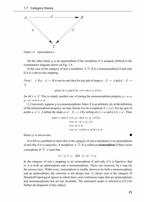
Figure 1.4 Epimorphism ϕ

On the other hand, ϕ is an epimorphism if the morphism β is uniquely defined in thecommutative diagram shown on Fig. 1.4.

In the case of the category of sets a morphism Aϕ−→ B is a monomorphism if and only

if it is a one-to-one mapping.

Proof : 1. If ϕ : A → B is one-to-one then for any pair of maps α : X → A and α′ : X →A,

ϕ(α(x)) = ϕ(α′(x)) =⇒ α(x) = α′(x)

for all x ∈ X . This is simply another way of stating the monomorphism property ϕ ◦ α =ϕ ◦ α′ =⇒ α = α′.

2. Conversely, suppose ϕ is a monomorphism. Since X is an arbitrary set, in the definitionof the monomorphism property, we may choose it to be a singleton X = {x}. For any pair ofpoints a, a′ ∈ A define the maps α, α′ : X → A by setting α(x) = a and α′(x) = a′. Then

ϕ(a) = ϕ(a′) =⇒ ϕ ◦ α(x) = ϕ ◦ α′(x)=⇒ ϕ ◦ α = ϕ ◦ α′=⇒ α = α′=⇒ a = α(x) = α′(x) = a′.

Hence ϕ is one-to-one. �

It is left as a problem to show that in the category of sets a morphism is an epimorphismif and only if it is surjective. A morphism A

ϕ−→ B is called an isomorphism if there exists

a morphism Bϕ′−→ A such that

ϕ′ ◦ ϕ = ιA and ϕ ◦ ϕ′ = ιB .In the category of sets a mapping is an isomorphism if and only if it is bijective; thatis, it is both an epimorphism and a monomorphism. There can, however, be a trap forthe unwary here. While every isomorphism is readily shown to be both a monomorphismand an epimorphism, the converse is not always true. A classic case is the category ofHausdorff topological spaces in which there exist continuous maps that are epimorphismsand monomorphisms but are not invertible. The interested reader is referred to [11] forfurther development of this subject.

25

Sets and structures

Problems

Problem 1.15 Show that in the category of sets a morphism is an epimorphism if and only if it isonto (surjective).

Problem 1.16 Show that every isomorphism is both a monomorphism and an epimorphism.

References

[1] T. Apostol. Mathematical Analysis. Reading, Mass., Addison-Wesley, 1957.[2] K. Devlin. The Joy of Sets. New York, Springer-Verlag, 1979.[3] N. B. Haaser and J. A. Sullivan. Real Analysis. New York, Van Nostrand Reinhold

Company, 1971.[4] P. R. Halmos. Naive Set Theory. New York, Springer-Verlag, 1960.[5] E. Wigner. The unreasonable effectiveness of mathematics in the natural sciences.

Communications in Pure and Applied Mathematics, 13:1–14, 1960.[6] J. Kelley. General Topology. New York, D. Van Nostrand Company, 1955.[7] P. J. Cohen. Set Theory and the Continuum Hypothesis. New York, W. A. Benjamin,

1966.[8] M. Henon. A two-dimensional map with a strange attractor. Communications in Math-

ematical Physics, 50:69–77, 1976.[9] M. Schroeder. Fractals, Chaos, Power Laws. New York, W. H. Freeman and Company,

1991.[10] W. Poundstone. The Recursive Universe. Oxford, Oxford University Press, 1987.[11] R. Geroch. Mathematical Physics. Chicago, The University of Chicago Press, 1985.

26

2 Groups

The cornerstone of modern algebra is the concept of a group. Groups are one of the simplestalgebraic structures to possess a rich and interesting theory, and they are found embeddedin almost all algebraic structures that occur in mathematics [1–3]. Furthermore, they areimportant for our understanding of some fundamental notions in mathematical physics,particularly those relating to symmetries [4].

The concept of a group has its origins in the work of Evariste Galois (1811–1832) andNiels Henrik Abel (1802–1829) on the solution of algebraic equations by radicals. Thelatter mathematician is honoured with the name of a special class of groups, known asabelian, which satisfy the commutative law. In more recent times, Emmy Noether (1888–1935) discovered that every group of symmetries of a set of equations arising from anaction principle gives rise to conserved quantities. For example, energy, momentum andangular momentum arise from the symmetries of time translations, spatial translations androtations, respectively. In elementary particle physics there are further conservation lawsrelated to exotic groups such as SU (3), and their understanding has led to the discoveryof new particles. This chapter presents the fundamental ideas of group theory and someexamples of how they arise in physical contexts.

2.1 Elements of group theory

A group is a set G together with a law of composition that assigns to any pair of ele-ments g, h ∈ G an element gh ∈ G, called their product, satisfying the following threeconditions:

(Gp1) The associative law holds: g(hk) = (gh)k, for all g, h, k ∈ G.(Gp2) There exists an identity element e ∈ G, such that

eg = ge = g for all g ∈ G.

(Gp3) Each element g ∈ G has an inverse g−1 ∈ G such that

g−1g = gg−1 = e.

More concisely, a group is a semigroup with identity in which every element has an inverse.Sometimes the fact that the product of two elements is another element of G is worth

noting as a separate condition, called the closure property. This is particularly relevant

27

Groups

when G is a subset of a larger set with a law of composition defined. In such cases it isalways necessary to verify that G is closed with respect to this law of composition; that is,for every pair g, h ∈ G, their product gh ∈ G. Examples will soon clarify this point.

Condition (Gp1) means that all parentheses in products may be omitted. For example,a((bc)d) = a(b(cd)) = (ab)(cd) = ((ab)c)d . It is a tedious but straightforward matter toshow that all possible ways of bracketing a product of any number of elements are equal.There is therefore no ambiguity in omitting all parentheses in expressions such as abcd .However, it is generally important to specify the order in which the elements appear in aproduct.

The identity element e is easily shown to be unique. For, if e′ is a second identity suchthat e′g = ge′ = g for all g ∈ G then, setting g = e, we have e = e′e = e′ by (Gp2).

Exercise: By a similar argument, show that every g ∈ G has a unique inverse g−1.

Exercise: Show that (gh)−1 = h−1g−1.

A group G is called abelian if the law of composition is commutative,

gh = hg for all g, h ∈ G.

The notation gh for the product of two elements is the default notation. Other possibilitiesare a · b, a × b, a + b, a ◦ b, etc. When the law of composition is written as an additiong + h, we will always assume that the commutative law holds, g + h = h + g. In this casethe identity element is usually written as 0, so that (Gp2) reads g + 0 = 0+ g = g. Theinverse is then written −g, with (Gp3) reading g + (−g) = 0 or, more simply, g − g = 0.Again, the associative law means we never have to worry about parentheses in expressionssuch as a + b + c + · · · + f .

A subgroup H of a group G is a subset that is a group in its own right. A subset H ⊆ Gis thus a subgroup if it contains the identity element of G and is closed under the operationsof taking products and inverses:

(a) h, k ∈ H ⇒ hk ∈ H (closure with respect to taking products);(b) the identity e ∈ H ;(c) h ∈ H ⇒ h−1 ∈ H (closure with respect to taking inverses).

It is not necessary to verify the associative law since H automatically inherits this propertyfrom the larger group G. Every group has two trivial subgroups {e} and G, consisting ofthe identity alone and the whole group respectively.

Example 2.1 The integers Z with addition as the law of composition form a group, calledthe additive group of integers. Strictly speaking one should write this group as (Z, +),but the law of composition is implied by the word ‘additive’. The identity element is theinteger 0, and the inverse of any integer n is −n. The even integers {0,±2,±4, . . . } forma subgroup of the additive group of integers.

Example 2.2 The real numbers R form a group with addition x + y as the law of com-position, called the additive group of reals. Again the identity is 0 and the inverse of x is−x . The additive group of integers is clearly a subgroup of R. The rational numbers Q are

28

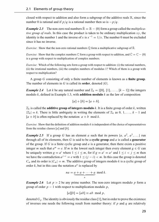
2.1 Elements of group theory

closed with respect to addition and also form a subgroup of the additive reals R, since thenumber 0 is rational and if p/q is a rational number then so is −p/q.

Example 2.3 The non-zero real numbers R = R− {0} form a group called the multiplica-tive group of reals. In this case the product is taken to be ordinary multiplication xy, theidentity is the number 1 and the inverse of x is x−1 = 1/x . The number 0 must be excludedsince it has no inverse.

Exercise: Show that the non-zero rational numbers Q form a multiplicative subgroup of R.

Exercise: Show that the complex numbers C form a group with respect to addition, and C = C− {0}is a group with respect to multiplication of complex numbers.

Exercise: Which of the following sets form a group with respect to addition: (i) the rational numbers,(ii) the irrational numbers, (iii) the complex numbers of modulus 1? Which of them is a group withrespect to multiplication?

A group G consisting of only a finite number of elements is known as a finite group.The number of elements in G is called its order, denoted |G|.Example 2.4 Let k be any natural number and Zk = {[0], [1], . . . , [k − 1]} the integersmodulo k, defined in Example 1.3, with addition modulo k as the law of composition

[a]+ [b] = [a + b].

Zk is called the additive group of integers modulo k. It is a finite group of order k, written|Zk | = k. There is little ambiguity in writing the elements of Zk as 0, 1, . . . , k − 1 and[a + b] is often replaced by the notation a + b mod k.

Exercise: Show that the definition of addition modulo k is independent of the choice of representativesfrom the residue classes [a] and [b].

Example 2.5 If a group G has an element a such that its powers {a, a2, a3, . . . } runthrough all of its elements, then G is said to be a cyclic group and a is called a generatorof the group. If G is a finite cyclic group and a is a generator, then there exists a positiveinteger m such that am = e. If m is the lowest such integer then every element g ∈ G canbe uniquely written g = ai where 1 ≤ i ≤ m, for if g = ai = a j and 1 ≤ i < j ≤ m thenwe have the contradiction a j−i = e with 1 ≤ ( j − i) < m. In this case the group is denotedCm and its order is |Cm | = m. The additive group of integers modulo k is a cyclic group oforder k, but in this case the notation an is replaced by

na = a + a + · · · + a︸ ︷︷ ︸n

mod k.

Example 2.6 Let p > 2 be any prime number. The non-zero integers modulo p form agroup of order p − 1 with respect to multiplication modulo p,

[a][b] = [ab] ≡ ab mod p,

denoted G p. The identity is obviously the residue class [1], but in order to prove the existenceof inverses one needs the following result from number theory: if p and q are relatively

29

Groups

prime numbers then there exist integers k and m such that kp + mq = 1. Since p is a primenumber, if [q] �= [0] then q is relatively prime to p and for some k and m

[m][q] = [1]− [k][p] = [1].

Hence [q] has an inverse [q]−1 = [m].

For finite groups of small order the law of composition may be displayed in the form ofa multiplication table, where the (i, j)th entry specifies the product of the i th element andthe j th element. For example, here is the multiplication table of G7:

G7 1 2 3 4 5 61 1 2 3 4 5 62 2 4 6 1 3 53 3 6 2 5 1 44 4 1 5 2 6 35 5 3 1 6 4 26 6 5 4 3 2 1

2.2 Transformation and permutation groups

All groups in the above examples are abelian. The most common examples of non-commutative groups are found in a class called transformation groups. We recall fromSection 1.4 that a transformation of a set X is a map g : X → X that is one-to-one andonto. The map g then has an inverse g−1 : X → X such that g−1 ◦ g = g ◦ g−1 = idX .Let the product of two transformations g and h be defined as their functional compositiongh = g ◦ h,

(gh)(x) = g ◦ h(x) = g(h(x)).

The set of all transformations of X forms a group, denoted Transf(X ):

Closure: if g and h are transformations of X then so is gh;Associative law: f (gh) = ( f g)h;Identity: e = idX ∈ Transf(X );Inverse: if g is a transformation of X then so is g−1.

Closure follows from the fact that the composition of two transformations (invertiblemaps) results in another invertible map, since ( f ◦ g)−1 = g−1 ◦ f −1. The associative lawholds automatically for composition of maps, while the identity and inverse are trivial. Bya transformation group of X is meant any subgroup of Transf(X ).

If X is a finite set of cardinality n then the transformations of X are called permutations ofthe elements of X . The group of permutations of X = {1, 2, . . . , n} is called the symmetricgroup of order n, denoted Sn . Any subgroup of Sn is called a permutation group. Apermutation π on n elements can be represented by the permutation symbol

π =(

1 2 . . . na1 a2 . . . an

)30

2.2 Transformation and permutation groups

where a1 = π (1), a2 = π (2), etc. The same permutation can also be written as

π =(

b1 b2 . . . bn

c1 c2 . . . cn

)where b1, b2, . . . , bn are the numbers 1, 2, . . . , n in an arbitrary order and c1 = π (b1), c2 =π (b2), . . . , cn = π (bn). For example, the permutation π that interchanges the elements 2and 4 from a four-element set can be written in several ways,

π =(

1 2 3 41 4 3 2

)=(

2 3 1 44 3 1 2

)=(

4 1 2 32 1 4 3

), etc.

In terms of permutation symbols, if

σ =(

1 2 . . . na1 a2 . . . an

)and π =

(a1 a2 . . . an

b1 b2 . . . bn

)then their product is the permutation πσ = π ◦ σ ,

πσ =(

1 2 . . . nb1 b2 . . . bn

).

Note that this product involves first performing the permutation σ followed by π , which isopposite to the order in which they are written; conventions can vary on this point. Sincethe product is a functional composition, the associative law is guaranteed. The identitypermutation is

idn =(

1 2 . . . n1 2 . . . n

),

while the inverse of any permutation is given by

π−1 =(

1 2 . . . na1 a2 . . . an

)−1

=(

a1 a2 . . . an

1 2 . . . n

).

The symmetric group Sn is a finite group of order n!, the total number of ways n objectsmay be permuted. It is not abelian in general. For example, in S3(

1 2 31 3 2

)(1 2 32 1 3

)=(

2 1 33 1 2

)(1 2 32 1 3

)=(

1 2 33 1 2

)while (

1 2 32 1 3

)(1 2 31 3 2

)=(

1 3 22 3 1

)(1 2 31 3 2

)=(

1 2 32 3 1

).

A more compact notation for permutations is the cyclic notation. Begin with any elementto be permuted, say a1. Let a2 be the result of applying the permutation π to a1, and leta3 be the result of applying it to a2, etc. Eventually the first element a1 must reappear, sayas am+1 = a1. This defines a cycle, written (a1 a2 . . . am). If m = n, then π is said to be acyclic permutation. If m < n then take any element b1 not appearing in the cycle generatedby a1 and create a new cycle (b1 b2 . . . bm) of successive images of b1 under π . Continue

31

Groups

until all the elements 1, 2, . . . , n are exhausted. The permutation π may be written as theproduct of its cycles; for example,(

1 2 3 4 5 6 74 5 3 7 2 1 6

)= (1 4 7 6)(2 5)(3).

Note that it does not matter which element of a cycle is chosen as the first member, so that(1 4 7 6) = (7 6 1 4) and (2 5) = (5 2).

Cycles of length 1 such as (3) merely signify that the permutation π leaves the element3 unchanged. Nothing is lost if we totally ignore such 1-cycles from the notation, writing

(1 4 7 6)(2 5)(3) = (1 4 7 6)(2 5).

The order in which cycles that have no common elements is written is also immaterial,

(1 4 7 6)(2 5) = (2 5)(1 4 7 6).

Products of permutations are easily carried out by following the effect of the cycles on eachelement in succession, taken in order from right to left. For example,

(1 3 7)(5 4 2)(1 2)(3 4 6 7)(1 4 6) = (1 6 5 4)(2 3)(7)

follows from 1 → 4 → 6, 6 → 1 → 2 → 5, 5 → 4, 4 → 6 → 7 → 1, etc.

Exercise: Express each permutation on {1, 2, 3} in cyclic notation and write out the 6× 6 multipli-cation table for S3.

Cycles of length 2 are called interchanges. Every cycle can be written as a product ofinterchanges,

(a1 a2 a3 . . . an) = (a2 a3)(a3 a4) . . . (an−1 an)(an a1),

and since every permutation π is a product of cycles, it is in turn a product of interchanges.The representation of a permutation as a product of interchanges is not in general unique,but the number of interchanges needed is either always odd or always even. To prove this,consider the homogeneous polynomial

f (x1, x2, . . . , xn) =∏i< j

(xi − x j )

= (x1 − x2)(x1 − x3) . . . (x1 − xn)(x2 − x3) . . . (xn−1 − xn).

If any pair of variables xi and x j are interchanged then the factor (xi − x j ) changes signand the factor (xi − xk) is interchanged with (x j − xk) for all k �= i, j . When k < i < j ori < j < k neither factor changes sign in the latter process, while if i < k < j each factorsuffers a sign change and again there is no overall sign change in the product of these twofactors. The net result of the interchange of xi and x j is a change of sign in the polynomialf (x1, x2, . . . , xn). Hence permutations may be called even or odd according to whether fis left unchanged, or changes its sign. In the first case they can be written as an even, and

32

2.2 Transformation and permutation groups

Figure 2.1 Symmetries of the square

only an even, number of interchanges, while in the second case they can only be written asan odd number. This quality is called the parity of the permutation and the quantity

(−1)π ={+1 if π is even,

−1 if π is odd,

is called the sign of the permutation. Sometimes it is denoted sign π .

Exercise: Show that

(−1)πσ = (−1)σπ = (−1)π (−1)σ . (2.1)

Example 2.7 In the Euclidean plane consider a square whose corners are labelled 1, 2, 3and 4. The group of symmetries of the square consists of four rotations (clockwise by0◦, 90◦, 180◦ and 270◦), denoted R0, R1, R2 and R3 respectively, and four reflectionsS1, S2, S3 and S4 about the axes in Fig. 2.1.

This group is not commutative since, for example, R1S1 = S4 �= S1 R1 = S3 – remember,the rightmost operation is performed first in any such product! A good way to do thesecalculations is to treat each of the transformations as a permutation of the vertices; forexample, in cyclic notation R1 = (1 2 3 4), R2 = (1 3)(2 4), S1 = (1 4)(2 3), S3 = (1 3),etc. Thus the symmetry group of the square is a subgroup of order 8 of the symmetric groupS4.

Exercise: Show that the whole group can be generated by repeated applications of R1 and S1.

Example 2.8 An important subgroup of Sn is the set of all even permutations, (−1)π = 1,known as the alternating group, denoted An . The closure property, that the product of two

33

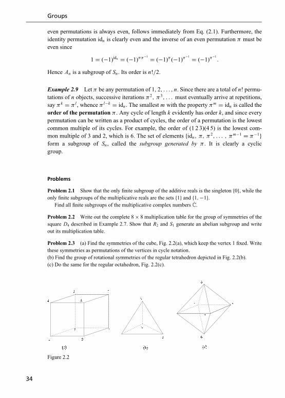
Groups

even permutations is always even, follows immediately from Eq. (2.1). Furthermore, theidentity permutation idn is clearly even and the inverse of an even permutation π must beeven since

1 = (−1)idn = (−1)ππ−1 = (−1)π (−1)π

−1 = (−1)π−1.

Hence An is a subgroup of Sn . Its order is n!/2.

Example 2.9 Let π be any permutation of 1, 2, . . . , n. Since there are a total of n! permu-tations of n objects, successive iterations π2, π3, . . . must eventually arrive at repetitions,say π k = π l , whence π l−k = idn . The smallest m with the property πm = idn is called theorder of the permutation π . Any cycle of length k evidently has order k, and since everypermutation can be written as a product of cycles, the order of a permutation is the lowestcommon multiple of its cycles. For example, the order of (1 2 3)(4 5) is the lowest com-mon multiple of 3 and 2, which is 6. The set of elements {idn, π, π

2, . . . , πm−1 = π−1}form a subgroup of Sn , called the subgroup generated by π . It is clearly a cyclicgroup.

Problems

Problem 2.1 Show that the only finite subgroup of the additive reals is the singleton {0}, while theonly finite subgroups of the multiplicative reals are the sets {1} and {1,−1}.

Find all finite subgroups of the multiplicative complex numbers C.

Problem 2.2 Write out the complete 8× 8 multiplication table for the group of symmetries of thesquare D4 described in Example 2.7. Show that R2 and S1 generate an abelian subgroup and writeout its multiplication table.

Problem 2.3 (a) Find the symmetries of the cube, Fig. 2.2(a), which keep the vertex 1 fixed. Writethese symmetries as permutations of the vertices in cycle notation.(b) Find the group of rotational symmetries of the regular tetrahedron depicted in Fig. 2.2(b).(c) Do the same for the regular octahedron, Fig. 2.2(c).

Figure 2.2

34

2.3 Matrix groups

Problem 2.4 Show that the multiplicative groups modulo a prime G7, G11, G17 and G23 are cyclic.In each case find a generator of the group.

Problem 2.5 Show that the order of any cyclic subgroup of Sn is a divisor of n!.

2.3 Matrix groups

Linear transformations

Let Rn be the space of n × 1 real column vectors

x =

⎛⎜⎜⎜⎝x1

x2...

xn

⎞⎟⎟⎟⎠ .A mapping A : Rn → Rn is said to be linear if

A(ax+ by) = a A(x)+ bA(y)

for all vectors x, y ∈ Rn and all real numbers a, b ∈ R. Writing

x =n∑

i=1

xi ei where e1 =

⎛⎜⎜⎜⎝10...0

⎞⎟⎟⎟⎠ , e2 =

⎛⎜⎜⎜⎝01...0

⎞⎟⎟⎟⎠ , . . . , en =

⎛⎜⎜⎜⎝00...1

⎞⎟⎟⎟⎠ ,we have

A(x) =n∑

i=1

xi A(ei ).

If we set

A(ei ) =n∑

j=1

a ji e j

the components xi of the vector x transform according to the formula

x �→ x′ = A(x) where x ′i =n∑

j=1

ai j x j (i = 1, . . . , n).

It is common to write this mapping in the form

x′ = Ax

35

Groups

where A = [ai j ] is the n × n array

A =

⎛⎜⎜⎝a11 a12 a13 . . . a1n

a21 a22 a23 . . . a2n

· · · · · · · · · · · · · · ·an1 an2 an3 . . . ann

⎞⎟⎟⎠ .A is called the matrix of the linear mapping A, and ai j are its components. The matrixAB of the product transformation AB is then given by the matrix multiplication rule,

(AB)i j =n∑

k=1

aikbk j .

Exercise: Prove this formula.

Linear maps on Rn and n × n matrices as essentially identical concepts, the latter beinglittle more than a notational device for the former. Be warned, however, when we come togeneral vector spaces in Chapter 3 such an identification cannot be made in a natural way.In later chapters we will often adopt a different notation for matrix components in order totake account of this difficulty, but for the time being it is possible to use standard matrixnotation as we are only concerned with the particular vector space Rn for the rest of thischapter.

A linear transformation A is a one-to-one linear mapping from Rn onto itself. Such amap is invertible, and its matrix A has non-zero determinant, det A �= 0. Such a matrix issaid to be non-singular and have an inverse matrix A−1 given by

(A−1)i j = A ji

det A,

where A ji is the ( j, i) cofactor of the matrix A, defined as the determinant of the submatrixof A formed by removing its j th row and i th column and multiplied by the factor (−1)i+ j .The inverse of a matrix acts as both right and left inverse:

AA−1 = A−1A = I, (2.2)

where I is the n × n unit matrix

I =

⎛⎜⎜⎜⎝1 0 . . . 00 1 . . . 0...

. . .

0 0 . . . 1

⎞⎟⎟⎟⎠ .The components of the unit matrix are frequently written as the Kronecker delta

δi j ={

1 if i = j,

0 if i �= j.(2.3)

The inverse of AB is given by the matrix identity

(AB)−1 = B−1A−1. (2.4)

36

2.3 Matrix groups

Matrix groups

The set of all n × n non-singular real matrices is a group, denoted GL(n,R). The key tothis result is the product law of determinants

det(AB) = det(A) det(B). (2.5)

Closure: this follows from the fact that det A �= 0 and det B �= 0 implies that det(AB) =det A det B �= 0.Associative law: (AB)C = A(BC) is true of all matrices, singular or not.Identity: the n × n unit matrix I is an identity element since IA = AI = A for all n × nmatrices A.Inverse: from Eq. (2.2) A−1 clearly acts as an inverse element to A. Equation (2.5) ensuresthat A−1 is non-singular and also belongs to GL(n,R), since

det A−1 = 1

det A.

A similar discussion shows that the set of n × n non-singular matrices with complexcomponents, denoted GL(n,C), also forms a group. Except for the case n = 1, these groupsare non-abelian since matrices do not in general commute, AB �= BA. The groups GL(n,R)and GL(n,C) are called the general linear groups of order n. Subgroups of these groups,whose elements are matrices with the law of composition being matrix multiplication, aregenerically called matrix groups [5].

In the following examples the associative law may be assumed, since the law of compo-sition is matrix multiplication. Frequent use will be made of the concept of the transposeAT of a matrix A, defined as the matrix formed by reflecting A about its diagonal,

(AT )i j = a ji where A = [ai j ].

The following identities can be found in many standard references such as Hildebrand [6],and should be known to the reader:

(AB)T = BT AT , (2.6)

det AT = det A, (2.7)

and if A is non-singular then the inverse of its transpose is the transpose of its inverse,

(A−1)T = (AT )−1. (2.8)

Example 2.10 The special linear group or unimodular group of degree n, denotedSL(n,R), is defined as the set of n × n unimodular matrices, real matrices having deter-minant 1. Closure with respect to matrix multiplication follows from Eq. (2.5),

det A = det B = 1 =⇒ det(AB) = det A det B = 1.

The identity I ∈ SL(n,R) since det I = 1, and closure with respect to inverses follows from

det A = 1 =⇒ det A−1 = 1

det A= 1.

37

Groups

Example 2.11 A matrix A is called orthogonal if its inverse is equal to its transpose,

AAT = AT A = I. (2.9)

The set of real orthogonal n × n matrices, denoted O(n), forms a group known as theorthogonal group of order n:Closure: if A and B are orthogonal matrices, AAT = BBT = I, then so is their product AB,

(AB)(AB)T = ABBT AT = AIAT = AAT = I.

Identity: the unit matrix I is clearly orthogonal since IT I = I2 = I.Inverse: if A is an orthogonal matrix then A−1 is also orthogonal for, using (2.8) and (2.4),

A−1(A−1)T = A−1(AT )−1 = (AT A)−1 = I−1 = I.

The determinant of an orthogonal matrix is always ±1 since

AAT = I =⇒ det A det AT = det(AAT ) = det I = 1.

Hence (det A)2 = 1 by (2.7) and the result det A = ±1 follows at once. The orthogonalmatrices with determinant 1 are called proper orthogonal matrices, while those withdeterminant −1 are called improper. The proper orthogonal matrices, denoted SO(n),form a group themselves called the proper orthogonal group of order n. This groupis often known as the rotation group in n dimensions – see Section 2.7. It is clearly asubgroup of the special linear group SL(n,R).

Example 2.12 Let p and q be non-negative integers such that p + q = n, and define Gp

to be the n × n matrix whose components Gp = [gi j ] are defined by

gi j =

⎧⎪⎪⎨⎪⎪⎩1 if i = j ≤ p,

−1 if i = j > p,

0 if i �= j.

We use O(p, q) to denote the set of matrices A such that

AT GpA = Gp. (2.10)

It follows from this equation that any matrix belonging to O(p, q) is non-singular, for ontaking determinants,

det AT det Gp det A = det Gp.

Since det Gp = ±1 �= 0 we have det AT det A = (det A)2 = 1, and consequently

det A = ±1.

The group properties of O(p, q) follow:

38

2.3 Matrix groups

Closure: if A and B both satisfy Eq. (2.10), then so does their product AB, for

(AB)T Gp(AB) = BT AT GpAB = BT GpB = Gp.

Identity: the unit matrix A = I clearly satisfies Eq. (2.10).Inverse: if Eq. (2.10) is multiplied on the right by A−1 and on the left by (A−1)T , we havefrom (2.8)

Gp = (A−1)T GpA−1.

Hence A−1 satisfies (2.10) and belongs to O(p, q).

The group O(p, q) is known as the pseudo-orthogonal group of type (p, q). The caseq = 0, p = n reduces to the orthogonal group O(n). As for the orthogonal group, thoseelements of O(p, q) having determinant 1 form a subgroup denoted SO(p, q).

Example 2.13 Let J be the 2n × 2n matrix

J =(

O I−I O

),

where O is the n × n zero matrix and I is the n × n unit matrix. A 2n × 2n matrix A is saidto be symplectic if it satisfies the equation

AT JA = J. (2.11)

The argument needed to show that these matrices form a group is essentially identical tothat just given for O(p, q). Again, since det J = 1, it follows immediately from (2.11) thatdet A = ±1, and A is non-singular. The group is denoted Sp(2n), called the symplecticgroup of order 2n.

Exercise: Show that the symplectic matrices of order 2 are precisely the unimodular matrices of order2. Hence for n = 2 all symplectic matrices have determinant 1. It turns out that symplectic matricesof any order have determinant 1, but the proof of this is more complicated.

Example 2.14 The general complex linear group, GL(n,C), is defined exactly as forthe reals. It is the set of non-singular complex n × n matrices, where the law of compositionis matrix product using multiplication of complex numbers. We define special subgroupsof this group the same way as for the reals:

SL(n,C) is the complex unimodular group of degree n, consisting of complex n × nmatrices having determinant 1;O(n,C) is the complex orthogonal group of degree n, whose elements are complex n × nmatrices A satisfying AT A = I;SO(n,C) is the complex proper orthogonal group, which is the intersection of the abovetwo groups.

There is no complex equivalent of the pseudo-orthogonal groups since these are all isomor-phic to O(n,C) – see Problem 2.7.

39

Groups

Example 2.15 The adjoint of a complex matrix A is defined as its complex conjugatetranspose A† = AT , whose components are a†

i j = a ji where a bar over a complex numberrefers to its complex conjugate. An n × n complex matrix U is called unitary if

UU† = I. (2.12)

It follows immediately that

det U det U = |det U|2 = 1,

and there exists a real number φ with 0 ≤ φ < 2π such that det U = eiφ . Hence all unitarymatrices are non-singular and the group properties are straightforward to verify. The groupof all n × n unitary matrices is called the unitary group of order n, denoted U (n). Thesubgroup of unitary matrices having det U = 1 is called the special unitary group of ordern, denoted SU (n).

Problems

Problem 2.6 Show that the following sets of matrices form groups with respect to addition ofmatrices, but that none of them is a group with respect to matrix multiplication: (i) real antisymmetricn × n matrices (AT = −A), (ii) real n × n matrices having vanishing trace (tr A =∑n

i=1 aii = 0),(iii) complex hermitian n × n matrices (H† = H).

Problem 2.7 Find a diagonal complex matrix S such that

I = ST GpS

where Gp is defined in Example 2.12. Show that:

(a) Every complex matrix A satisfying Eq. (2.10) can be written in the form

A = SBS−1

where B is a complex orthogonal matrix (i.e. a member of O(n,C)).(b) The complex versions of the pseudo-orthogonal groups, O(p, q,C), are all isomorphic to each

other if they have the same dimension,

O(p, q,C) ∼= O(n,C) where n = p + q.

Problem 2.8 Show that every element of SU (2) has the form

U =(

a bc d

)where a = d and b = −c.

2.4 Homomorphisms and isomorphisms

Homomorphisms

Let G and G ′ be groups. A homomorphism ϕ : G → G ′ is a map from G to G ′ thatpreserves products,

ϕ(ab) = ϕ(a)ϕ(b) for all a, b ∈ G.

40

2.4 Homomorphisms and isomorphisms

Theorem 2.1 Under a homomorphism ϕ : G → G ′ the identity e of G is mapped to theidentity e′ of G ′, and the inverse of any element g of G to the inverse of its image ϕ(g).

Proof : For any g ∈ G

ϕ(g) = ϕ(ge) = ϕ(g)ϕ(e).

Multiplying both sides of this equation on the left by (ϕ(g))−1 gives the desired result,

e′ = e′ϕ(e) = ϕ(e).

If g ∈ G then ϕ(g−1)ϕ(g) = ϕ(g−1g) = ϕ(e) = e′. Hence ϕ(g−1) = (ϕ(g))−1 as re-quired. �

Exercise: If ϕ : G → G ′ is a homomorphism, show that the image set

im(ϕ) = ϕ(G) = {g′ ∈ G ′ | g′ = ϕ(g), g ∈ G} (2.13)

is a subgroup of G ′.

Example 2.16 For any real number x ∈ R, define its integral part [x] to be the largestinteger that is less than or equal to x , and its fractional part to be (x) = x − [x]. Evidently0 ≤ (x) < 1. On the half-open interval [0, 1) of the real line define addition modulo 1 by

a + b mod 1 = (a + b) = fractional part of a + b.

This defines an abelian group, the group of real numbers modulo 1. To verify the groupaxioms we note that 0 is the identity element and the inverse of any a > 0 is 1− a. Theinverse of a = 0 is 0.

The map ϕ1 : R → [0, 1) from the additive group of real numbers to the group of realnumbers modulo 1 defined by ϕ1(x) = (x) is a homomorphism since (x)+ (y) = (x + y).

Exercise: Show that the circle map or phase map C : C→ [0, 2π ) defined by

C(z) = θ where z = |z|eiθ , 0 ≤ θ < 2π

is a homomorphism from the multiplicative group of complex numbers to the additive group of realsmodulo 2π , defined in a similar way to the reals modulo 1 in the previous example.

Example 2.17 Let sign : Sn → {+1,−1} be the map that assigns to every permutation πits parity,

sign(π) = (−1)π ={+1 if π is even,

−1 if π is odd.

From (2.1), sign is a homomorphism from Sn to the multiplicative group of reals

sign(πσ ) = sign(π )sign(σ ).

Exercise: From Eq. (2.5) show that the determinant map det : GL(n,R) → R from the general lineargroup of order n to the multiplicative group of reals is a homomorphism.

41

Groups

Isomorphisms

An isomorphism is a homomorphism that is one-to-one and onto. If an isomorphism existsbetween two groups G and G ′ they are said to be isomorphic, written G ∼= G ′. The twogroups are then essentially identical in all their group properties.

Exercise: Show that if ϕ : G → G ′ is an isomorphism, then so is the inverse map ϕ−1 : G ′ → G.

Exercise: If ϕ : G → G ′ and ψ : G ′ → G ′′ are isomorphisms then so is ψ ◦ ϕ : G → G ′′.

These two statements show that isomorphism is a symmetric and transitive relation onthe class of all groups. Hence it is an equivalence relation on the class of groups, since thereflexive property follows from the fact that the identity map idG : G → G is trivially anisomorphism. Note that the word ‘class’ must be used in this context because the ‘set ofall groups’ is too large to be acceptable. Group theory is the study of equivalence classesof isomorphic groups. Frequently it is good to single out a special representative of anequivalence class. Consider, for example, the following useful theorem for finite groups:

Theorem 2.2 (Cayley) Every finite group G of order n is isomorphic to a permutationgroup.

Proof : For every g ∈ G define the map Lg : G → G to be left multiplication by g,

Lg(x) = gx where x ∈ G.

This map is one-to-one and onto since

gx = gx ′ =⇒ x = x ′ and x = Lg(g−1x) for all x ∈ G.

The map Lg therefore permutes the elements of G = {g1 = e, g2, . . . , gn} and may beidentified with a member of Sn . It has the property Lg ◦ Lh = Lgh , since

Lg ◦ Lh(x) = g(hx) = (gh)x = Lgh(x), ∀x ∈ G.

Hence the map ϕ : G → Sn defined by ϕ(g) = Lg is a homomorphism,

ϕ(g)ϕ(h) = Lg ◦ Lh = Lgh = ϕ(gh).

Furthermore, ϕ is one-to-one, for if ϕ(g) = ϕ(h) then g = Lg(e) = Lh(e) = h. Thus G isisomorphic to the subgroup of ϕ(G) ⊆ Sn . �

From the abstract point of view there is nothing to distinguish two isomorphic groups,but different ‘concrete’ versions of the same group may have different applications. Theparticular concretization as linear groups of transformations or matrix groups is known asgroup representation theory and plays a major part in mathematical physics.

Automorphisms and conjugacy classes

An automorphism is an isomorphism ϕ : G → G of a group onto itself. A trivial exampleis the identity map idG : G → G. Since the composition of any pair of automorphisms is

42

2.4 Homomorphisms and isomorphisms

an automorphism and the inverse of any automorphism ϕ−1 is an automorphism, it followsthat the set of all automorphisms of a group G is itself a group, denoted Aut(G).

If g is an arbitrary element of G, the map Cg : G → G defined by

Cg(a) = gag−1 (2.14)

is called conjugation by the element g. This map is a homomorphism, for

Cg(ab) = gabg−1 = gag−1gbg−1 = Cg(a)Cg(b),

and Cg−1 is its inverse since

Cg−1 ◦ Cg(a) = g−1(gag−1)g = a, ∀a ∈ G.

Hence every conjugation Cg is an automorphism of G. Automorphisms that are a conjuga-tion by some element g of G are called inner automorphisms. The identity Cgh = Cg ◦ Ch

holds, since for any a ∈ G

Cgh(a) = gha(gh)−1 = ghah−1g−1 = Cg(Ch(a)).

Hence the map ψ : G → Aut(G), defined by ψ(g) = Cg , is a homomorphism. The innerautomorphisms, being the image of G underψ , form a subgroup of Aut(G). Two subgroupsH and H ′ of G that can be transformed to each other by an inner automorphism of G arecalled conjugate subgroups. In this case there exists an element g ∈ G such that

H ′ = gHg−1 = {ghg−1 | h ∈ H}.

Exercise: Show that conjugacy is an equivalence relation on the set of all subgroups of a group G.What is the equivalence class containing the trivial subgroup {e}?

Conjugation also induces an equivalence relation on the original group G by a ≡ b if andonly if there exists g ∈ G such that b = Cg(a). The three requirements for an equivalencerelation are easily verified: (i) reflexivity, a = Ce(a) for all a ∈ G; (ii) symmetry, if b =Cg(a) then a = Cg−1 (b); (iii) transitivity, if b = Cg(a) and c = Ch(b) then c = Chg(a). Theequivalence classes with respect to this relation are called conjugacy classes. The conjugacyclass of an element a ∈ G is denoted Ga . For example, the conjugacy class of the identityis always the singleton Ge = {e}, since Cge = geg−1 = e for all g ∈ G.

Exercise: What are the conjugacy classes of an abelian group?

Example 2.18 For a matrix group, matrices A and B in the same conjugacy class arerelated by a similarity transformation

B = SAS−1.

Matrices related by a similarity transformation have identical invariants such as determinant,trace (sum of the diagonal elements) and eigenvalues. To show determinant is an invariantuse Eq. (2.5),

det B = det S det A(det S)−1 = det A.

43

Groups

For the invariance of trace we need the identity

tr(AB) = tr(BA), (2.15)

which is proved by setting A = [ai j ] and B = [bi j ] and using the multiplication law ofmatrices,

tr(AB) =n∑

i=1

( n∑j=1

ai j b ji

)=

n∑j=1

( n∑i=1

b ji ai j

)= tr(BA).

Hence

tr B = tr(SAS−1) = tr(S−1SA) = tr(IA) = tr A,

as required. Finally, if λ is an eigenvalue of A corresponding to eigenvector v, then Sv is aneigenvector of B with the same eigenvalue,

Av = λv =⇒ B(Sv) = SAS−1Sv = SAv = λSv.

Example 2.19 The conjugacy classes of the permutation group S3 are, in cyclic notation,

{e}; {(1 2), (1 3), (2 3)}; and {(1 2 3), (1 3 2)}.These are easily checked by noting that (1 2)−1(1 2 3)(1 2) = (1 3 2) and

(1 2 3)−1(1 2)(1 2 3) = (1 3), etc.

It is a general feature of permutation groups that conjugacy classes consist of permutationshaving identical cycle structure (see Problem 2.11).

Problems

Problem 2.9 Show that Theorem 2.2 may be extended to infinite groups as well. That is, any groupG is isomorphic to a subgroup of Transf(G), the transformation group of the set G.

Problem 2.10 Find the group multiplication tables for all possible groups on four symbols e, a, band c, and show that any group of order 4 is either isomorphic to the cyclic group Z4 or the productgroup Z2 × Z2.

Problem 2.11 Show that every cyclic permutation (a1 a2 . . . an) has the property that for any per-mutation π ,

π(a1 a2 . . . an)π−1

is also a cycle of length n. [Hint: It is only necessary to show this for interchanges π = (b1 b2) asevery permutation is a product of such interchanges.]

(a) Show that the conjugacy classes of Sn consist of those permutations having the same cyclestructure, e.g. (1 2 3)(4 5) and (1 4 6)(2 3) belong to the same conjugacy class.

(b) Write out all conjugacy classes of S4 and calculate the number of elements in each class.

Problem 2.12 Show that the class of groups as objects with homomorphisms between groups asmorphisms forms a category – the category of groups (see Section 1.7). What are the monomorphisms,epimorphisms and isomorphisms of this category?

44

2.5 Normal subgroups and factor groups

2.5 Normal subgroups and factor groups

Cosets

For any pair of subsets A and B of a group G, define AB to be the set

AB = {ab | a ∈ A and b ∈ B}.

If H is a subgroup of G then H H = H .When A is a singleton set, say A = {a}, we usually write aB instead of {a}B. If H is a

subgroup of G, then each subset aH where a ∈ G is called a (left) coset of H . Two cosetsof a given subgroup H are either identical or non-intersecting. For, suppose there exists anelement g ∈ aH ∩ bH . Setting

g = ah1 = bh2 (h1, h2 ∈ H )

we have for any h ∈ H

ah = bh2h−11 h ∈ bH,

so that aH ⊆ bH . Equally, it can be argued that bH ⊆ aH , whence either aH ∩ bH = ∅or aH = bH . Since g = ge and e ∈ H , any element g ∈ G always belongs to the cosetgH . Thus the cosets of H form a family of disjoint subsets covering all of G. There isan alternative way of demonstrating this partitioning property. The relation a ≡ b on G,defined by

a ≡ b iff b−1a ∈ H,

is an equivalence relation since it is (i) reflexive, a−1a = e ∈ H ; (ii) symmetric, a−1b =(b−1a)−1 ∈ H if b−1a ∈ H ; and (iii) transitive, a−1b ∈ H , b−1c ∈ H implies a−1c =a−1bb−1c ∈ H . The equivalence classes defined by this relation are precisely the left cosetsof the subgroup H , for b ≡ a if and only if b ∈ aH .

Theorem 2.3 (Lagrange) If G is a finite group of order n, then the order of every subgroupH is a divisor of n.

Proof : Every coset gH is in one-to-one correspondence with H , for if gh1 = gh2 thenh1 = g−1gh2 = h2. Hence every coset gH must have exactly |H | elements, and since thecosets partition the group G it follows that n is a multiple of |H |. �

Corollary 2.4 The order of any element is a divisor of |G|.Proof : Let g be any element of G and let m be its order. As shown in Example 2.5 theelements {g, g2, . . . , gm = e} are then all unequal to each other and form a cyclic subgroupof order m. By Lagrange’s theorem m divides the order of the group, |G|. �

Exercise: If G has prime order p all subgroups are trivial – they are either the identity subgroup {e}or G itself. Show that G is a cyclic group.

45

Groups

Normal subgroups

The right cosets Hg of a subgroup H are defined in a completely analogous way to the leftcosets. While in general there is no obvious relationship between right and left cosets, thereis an important class of subgroups for which they coincide. A subgroup N of a group G iscalled normal if

gNg−1 = N , ∀g ∈ G.

Such subgroups are invariant under inner automorphisms; they are sometimes referred toas invariant or self-conjugate subgroups. The key feature of normal subgroups is that thesystems of left and right cosets are identical, for

gN = gNg−1g = Ng, ∀g ∈ G.

This argument may give the misleading impression that every element of N commutes withevery element of G, but what it actually demonstrates is that for every n ∈ N and everyg ∈ G there exists an element n′ ∈ N such that gn = n′g. There is no reason, in general,to expect that n′ = n.

For any group G the trivial subgroups {e} and G are always normal. A group is calledsimple if it has no normal subgroups other than these trivial subgroups.

Example 2.20 The centre Z of a group G is defined as the set of elements that commutewith all elements of G,

Z = {z ∈ G | zg = gz for all g ∈ G}.This set forms a subgroup of G since the three essential requirements hold:

Closure: if z, z′ ∈ Z then zz′ ∈ Z since

(zz′)g = z(z′g) = z(gz′) = (zg)z′ = (gz)z′ = g(zz′).

Identity: e ∈ Z , as eg = ge = g for all g ∈ G.

Inverse: if z ∈ Z then z−1 ∈ Z since

z−1g = z−1ge = z−1gzz−1 = z−1zgz−1 = gz−1.

This subgroup is clearly normal since gZ = Zg for all g ∈ G.

Factor groups

When we multiply left cosets of a subgroup H together, for example

gHg′H = {ghg′h′ | h, h′ ∈ H},the result is not in general another coset. On the other hand, the product of cosets of a normalsubgroup N is always another coset,

gNg′N = gg′N N = (gg′)N ,

46

2.5 Normal subgroups and factor groups

and satisfies the associative law,

(gNg′N )g′′N = (gg′g′′)N = gN (g′Ng′′N ).

Furthermore, the coset eN = N plays the role of an identity element, while every coset hasan inverse (gN )−1 = g−1 N . Hence the cosets of a normal subgroup N form a group calledthe factor group of G by N , denoted G/N .

Example 2.21 The even integers 2Z form a normal subgroup of the additive group ofintegers Z, since this is an abelian group. The factor group Z/2Z has just two cosets[0] = 0+ 2Z and [1] = 1+ 2Z, and is isomorphic to the additive group of integers modulo2, denoted by Z2 (see Example 2.4).

Kernel of a homomorphism

Let ϕ : G → G ′ be a homomorphism between two groups G and G ′. The kernel of ϕ,denoted ker(ϕ), is the subset of G consisting of those elements that map onto the identitye′ of G ′,

ker(ϕ) = ϕ−1(e′) = {k ∈ G |ϕ(k) = e′}.The kernel K = ker(ϕ) of any homomorphism ϕ is a subgroup of G:

Closure: if k1 and k2 belong to K then so does k1k2, since

ϕ(k1k2) = ϕ(k1)ϕ(k2) = e′e′ = e′.

Identity: e ∈ K as ϕ(e) = e′.Inverse: if k ∈ K then k−1 ∈ K , for

ϕ(k−1) = (ϕ(k))−1 = (e′)−1 = e′.

Furthermore, K is a normal subgroup since, for all k ∈ K and g ∈ G,

ϕ(gkg−1) = ϕ(g)ϕ(k)ϕ(g−1) = ϕ(g)e′(ϕ(g))−1 = e′.

The following theorem will show that the converse of this result also holds, namely thatevery normal subgroup is the kernel of a homomorphism.

Theorem 2.5 Let G be a group. Then the following two properties hold:

1. If N is a normal subgroup of G then there is a homomorphism μ : G → G/N.2. If ϕ : G → G ′ is a homomorphism then the factor group G/ ker(ϕ) is isomorphic with

the image subgroup im(ϕ) ⊆ G ′ defined in Eq. (2.13),

im(ϕ) ∼= G/ ker(ϕ).

Proof : 1. The map μ : G → G/N defined by μ(g) = gN is a homomorphism, since

μ(g)μ(h) = gNhN = ghN N = ghN = μ(gh).

2. Let K = ker(ϕ) and H ′ = im(ϕ). The map ϕ is constant on each coset gK , for

k ∈ K =⇒ ϕ(gk) = ϕ(g)ϕ(k) = ϕ(g)e′ = ϕ(g).

47

Groups

Hence the map ϕ defines a map ψ : G/K → H ′ by setting

ψ(gK ) = ϕ(g),

and this map is a homomorphism since

ψ(gK hK ) = ψ(ghK ) = ϕ(gh) = ϕ(g)ϕ(h) = ψ(gK )ψ(hK ).

Furthermore ψ is one-to-one, for

ψ(gK ) = ψ(hK ) =⇒ ϕ(g) = ϕ(h)=⇒ ϕ(gh−1) = ϕ(g)(ϕ(h))−1 = e′

=⇒ gh−1 ∈ K=⇒ g ∈ hK .

Since every element h′ of the image set H ′ is of the form h′ = ϕ(g) = ψ(gK ), the map ψis an isomorphism between the groups G/K and H ′. �

Example 2.22 Let G and H be two groups with respective identity elements eG and eH .A law of composition can be defined on the cartesian product G × H by

(g, h)(g′, h′) = (gg′, hh′).

This product clearly satisfies the associative law and has identity element (eG, eH ). Fur-thermore, every element has a unique inverse (g, h)−1 = (g−1, h−1). Hence, with this lawof composition, G × H is a group called the direct product of G and H . The group Gis clearly isomorphic to the subgroup (G, eH ) = {(g, eH ) | g ∈ G}. The latter is a normalsubgroup, since

(a, b)(G, eH )(a−1, b−1) = (aGa−1, beH b−1) = (G, eH ).

It is common to identify the subgroup of elements (G, eH ) with the group G. In a similarway H is identified with the normal subgroup (eG, H ).

Problems

Problem 2.13 (a) Show that if H and K are subgroups of G then their intersection H ∩ K is alwaysa subgroup of G.(b) Show that the product H K = {hk | h ∈ H, k ∈ K } is a subgroup if and only if H K = K H .

Problem 2.14 Find all the normal subgroups of the group of symmetries of the square D4 describedin Example 2.7.

Problem 2.15 The quaternion group G consists of eight elements denoted

{1, −1, i, −i, j, − j, k, −k},

48

2.6 Group actions

subject to the following law of composition:

1g = g1 = g, for all g ∈ Q,

−1g = −g, for g = i, j, k,

i2 = j2 = k2 = −1,

i j = k, jk = i, ki = j.

(a) Write down the full multiplication table for Q, justifying all products not included in the abovelist.

(b) Find all subgroups of Q and show that all subgroups of Q are normal.(c) Show that the subgroup consisting of {1, −1, i, −i} is the kernel of a homomorphism Q →

{1, −1}.(d) Find a subgroup H of S4, the symmetric group of order 4, such that there is a homomorphism

Q → H whose kernel is the subgroup {1, −1}.Problem 2.16 A Mobius transformation is a complex map,

z �→ z′ = az + b

cz + dwhere a, b, c, d ∈ C, ad − bc = 1.

(a) Show that these are one-to-one and onto transformations of the extended complex plane, whichincludes the point z = ∞, and write out the composition of an arbitrary pair of transformationsgiven by constants (a, b, c, d) and (a′, b′, c′, d ′).

(b) Show that they form a group, called the Mobius group.(c) Show that the map μ from SL(2,C) to the Mobius group, which takes the unimodular matrix(

a bc d

)to the above Mobius transformation, is a homomorphism, and that the kernel of this

homomorphism is {I,−I}; i.e. the Mobius group is isomorphic to SL(2,C)/Z2.

Problem 2.17 Assuming the identification of G with (G, eH ) and H with (eG, H ), show that G ∼=(G × H )/H and H ∼= (G × H )/G.

Problem 2.18 Show that the conjugacy classes of the direct product G × H of two groups G andH consist precisely of products of conjugacy classes from the groups

(Ci , D j ) = {(gi , h j ) | gi ∈ Ci , h j ∈ D j }where Ci is a conjugacy class of G and D j a conjugacy class of H .

2.6 Group actions

A left action of a group G on a set X is a homomorphism ϕ of G into the group oftransformations of X ,

ϕ : G → Transf(X ).

It is common to write ϕ(g)(x) simply as gx , a notation that makes it possible to write ghxin place of (gh)x , since

(gh)x = ϕ(gh)(x) = ϕ(g)ϕ(h)(x) = ϕ(g)(hx) = g(hx).

49

Groups

A left actionφ of G on Rn all of whose images are linear transformations is a homomorphism

φ : G → GL(n,R),

and is called an n-dimensional representation of G. Similarly, a homomorphism φ : G →GL(n,C) is called a complex n-dimensional representation of G.

An anti-homomorphism is defined as a map ρ : G → Transf(X ) with the property

ρ(gh) = ρ(h)ρ(g).

It can give rise to a right action xg = ρ(g)(x), a notation that is consistent with writingxgh in place of x(gh) = (xg)h.

Exercise: Ifϕ : G → H is a homomorphism show that the mapρ : G → H defined byρ(g) = ϕ(g−1)is an anti-homomorphism.

Let G be a group having a left action on X . The orbit Gx of a point x ∈ X is the set ofall points that can be reached from x by this action,

Gx = {gx | g ∈ G}.We say the action of G on X is transitive if the whole of X is the orbit of some point in

X ,

∃x ∈ X such that X = Gx .

In this case any pair of elements y, z ∈ X can be connected by the action of a group element,for if y = gx and z = hx then z = g′y where g′ = hg−1. Hence X = Gy for all y ∈ X .

If x is any point of X , define the isotropy group of x to be

Gx = {g | gx = x}.If gx = x =⇒ g = idX the action of G on X is said to be free. In this case the isotropygroup is trivial, Gx = {idX }, for every point x ∈ X .

Exercise: Show that Gx forms a subgroup of G.

If x ∈ X and h, h′ ∈ G then

hx = h′x =⇒ h−1h′ ∈ Gx =⇒ h′ ∈ hGx .

If G is a finite group, we denote the number of points in any subset S by |S|. Since hGx is aleft coset of the subgroup Gx and from the proof of Lagrange’s theorem 2.3 all cosets havethe same number of elements, there must be precisely |Gx | group elements that map x toany point y of its orbit Gx . Hence

|G| = |Gx | |Gx |. (2.16)

Example 2.23 The cyclic group of order 2, Z2 = {e, a} where a2 = e, acts on the realnumbers R by

ex = x, ax = −x .

50

2.6 Group actions

The orbit of any point x �= 0 is Z2x = {x, −x}, while Z20 = {0}. This action is not trans-itive. The isotropy group of the origin is the whole of Z2, while for any other point it is {e}.It is a simple matter to check (2.16) separately for x = 0 and x �= 0.

Example 2.24 The additive group of reals R acts on the complex plane C by

θ : z �→ zeiθ .

The orbit of any z �= 0 is the circle centred 0, radius r = |z|. The action is not transitivesince circles of different radius are disjoint. The isotropy group of any z �= 0 is the set ofreal numbers of the form θ = 2πn where n ∈ Z. Hence the isotropy group Rz for z �= 0 isisomorphic to Z, the additive group of integers. On the other hand the isotropy group ofz = 0 is all of R.

Example 2.25 A group G acts on itself by left translation

g : h �→ Lgh = gh.

This action is clearly transitive since any element g′ can be reached from any other g by aleft translation,

g′ = Lg′g−1 g.

Any subgroup H ⊆ G also acts on G by left translation. The orbit of any group element gunder this action is the right coset Hg containing g. Similarly, under the right action of Hon G defined by right translation Rh : g �→ gh, the orbits are the left cosets gH . Theseactions are not transitive in general.

Example 2.26 The process of conjugation by an element g, defined in Eq. (2.14), is a leftaction of the group G on itself since the map g �→ Cg is a homomorphism,

Cgha = (gh)a(gh)−1 = ghah−1g−1 = CgCha,

where we have written Cga for Cg(a). The orbits under the action of conjugation are preciselythe conjugacy classes. By Eq. (2.16) it follows that if G is a finite group then the numberof elements in any conjugacy class, being an orbit under an action of G, is a divisor of theorder of the group |G|.

If G has a left action on a set X and if x and y are any pair of points in X in the sameorbit, such that y = hx for some h ∈ G, then their isotropy groups are conjugate to eachother,

G y = Ghx = hGx h−1. (2.17)

For, let g ∈ G y , so that gy = y. Since y = hx it follows on applying h−1 that h−1ghx = x .Hence h−1gh ∈ Gx , or equivalently g ∈ hGx h−1. The converse, that hGx h−1 ⊆ G y , isstraightforward: for any g ∈ hGx h−1, we have that

gy = ghx = hg′h−1hx where g′ ∈ Gx ,

whence gy = hx = y and g ∈ G y . Thus the isotropy groups of x and y are isomorphicsince they are conjugate to each other, and are related by an inner automorphism. If the

51

Groups

action of G on X is transitive it follows that the isotropy groups of any pair of points x andy are isomorphic to each other.

Exercise: Under what circumstances is the action of conjugation by an element g on a group Gtransitive?

Problem

Problem 2.19 If H is any subgroup of a group G define the action of G on the set of left cosetsG/H by g : g′H �→ gg′H .

(a) Show that this is always a transitive action of H on G.(b) Let G have a transitive left action on a set X , and set H = Gx to be the isotropy group of any

point x . Show that the map i : G/H → X defined by i(gH ) = gx is well-defined, one-to-oneand onto.

(c) Show that the left action of G on X can be identified with the action of G on G/H definedin (a).

(d) Show that the group of proper orthogonal transformations SO(3) acts transitively on the 2-sphereS2,

S2 = {(x, y, z) | r 2 = x2 + y2 + z2 = 1} = {r | r 2 = rT r = 1},where r is a column vector having real components x, y, z. Show that the isotropy group of anypoint r is isomorphic to SO(2), and find a bijective correspondence between the factor spaceSO(3)/SO(2) and the 2-sphere S2 such that SO(3) has identical left action on these two spaces.

2.7 Symmetry groups

For physicists, the real interest in groups lies in their connection with the symmetries of aspace of interest or some important function such as the Lagrangian. Here the concept ofa space X will be taken in its broadest terms to mean a set X with a ‘structure’ imposedon it, as discussed in Section 1.6. The definitions of such spaces may involve combinationsof algebraic and geometric structures, but the key thing is that their definitions invariablyinvolve the specification of certain functions on the space. For example, algebraic struc-tures such as groups require laws of composition, which are functions defined on cartesianproducts of the underlying sets. Geometric structures such as topology usually involve aselection of subsets of X – this can also be defined as a characteristic function on the powerset of X . For the present purposes let us simply regard a space as being a set X togetherwith one or more functions F : X → Y to another set Y defined on it. This concept will begeneral enough to encapsulate the basic idea of a ‘space’.

If F is a Y -valued function on X , we say a transformation g : X → X leaves F invariantif

F(x) = F(gx) for all x ∈ X,

where, as in Section 2.6, we denote the left action by gx ≡ g(x).

Theorem 2.6 The set of all transformations of X leaving F invariant form a group.

52

2.7 Symmetry groups

Proof : We show the usual three things:

Closure: if g and h leave F invariant then F(x) = F(hx) for all x ∈ X and F(y) = F(gy)for all y ∈ X . Hence gh ≡ g ◦ h leaves F invariant since F(ghx) = F(g(hx)) = F(hx) =F(x).Identity: obviously F(x) = F(idX (x)); that is, idX leaves F invariant.Inverse: if g is a transformation then there exists an inverse map g−1 such that gg−1 = idX .The map g−1 leaves F invariant if g does, since

F(g−1x) = F(g(g−1x)) = F(x).�

It is a straightforward matter to extend the above theorem to an arbitrary setF of functionson X . The group of transformations leaving all functions F ∈ F invariant will be called theinvariance group or symmetry group of F . The following are some important examplesof symmetry groups in mathematical physics.

Example 2.27 The rotation group SO(3). As in Example 2.11, let R3 be the set of all3× 1 column vectors

r =⎛⎝x

yz

⎞⎠ such that x, y, z ∈ R.

Consider the set of all linear transformations r �→ r′ = Ar on R3, where A is a 3× 3 matrix,which leave the distance of points from the origin r = |r| =

√x2 + y2 + z2 invariant. Since

r2 = rT r, we have

r ′2 = r′T r′ = rT AT Ar = r2 = rT r,

which holds for arbitrary vectors r if and only if A is an orthogonal matrix, AAT = I.As shown in Example 2.11, orthogonal transformations all have determinant ±1. Thosewith determinant +1 are called rotations, while transformations of determinant −1 mustinvolve a reflection with respect to some plane; for example, the transformation x ′ = x, y′ =y, z′ = −z.

In a similar manner O(n) is the group of symmetries of the distance function in n-dimensions,

r =√

x 21 + x 2

2 + · · · + x 2n

and those with positive determinant are denoted SO(n), called the group of rotations inn-dimensions. There is no loss of generality in our assumption of linear transformationsfor this group since it can be shown that any transformation of Rn leaving r2 invariant mustbe linear (see Chapter 18).

Example 2.28 The Euclidean group. The Euclidean space E3 is defined as the cartesianspace R3 with a distance function between any pair of points given by

�s2 = (r2 − r1)2 = �rT�r.

53

Groups

A transformation of E3 that leaves the distance between any pair of points invariant will becalled a Euclidean transformation. As for the rotation group, a Euclidean transformationr → r′ has

�r′ = A�r, AAT = I.

For any pair of points r′2 − r′1 = A(r2 − r1), and if we set r1 = 0 to be the origin and0′ = a, then r′2 − a = Ar2. Since r2 is an arbitrary point in E3, the general Euclideantransformations have the form

r′ = Ar+ a where AT A = I, a = const. (2.18)

Transformations of this form are frequently called affine or inhomogeneous linear trans-formations.

Exercise: Check directly that these transformations form a group – do not use Theorem 2.6.

The group of Euclidean transformations, called the Euclidean group, can also be writtenas a matrix group by replacing r with the 4× 1 column matrix (x, y, z, 1)T and writing(

r′

1

)=(

A a0T 1

)(r1

)=(

Ar+ a1

).

This may seem an odd trick, but its value lies in demonstrating that the Euclidean group isisomorphic to a matrix group – the Euclidean transformations are affine, not linear, on R3,and thus cannot be written as 3× 3 matrices.

Example 2.29 The Galilean group. To find the set of transformations of space and timethat preserve the laws of Newtonian mechanics we follow the lead of special relativity(see Chapter 9) and define an event to be a point of R4 characterized by four coordinates(x, y, z, t). Define Galilean space G4 to be the space of events with a structure consistingof three elements:

1. Time intervals �t = t2 − t1.2. The spatial distance �s = |r2 − r1| between any pair of simultaneous events (events

having the same time coordinate, t1 = t2).3. Motions of inertial (free) particles, otherwise known as rectilinear motions,

r(t) = ut + r0, (2.19)

where u and r0 are arbitrary constant vectors.

Note that only the distance between simultaneous events is relevant. A simple exampleshould make this clear. Consider a train travelling with uniform velocity v between twostations A and B. In the frame of an observer who stays at A the distance between the(non-simultaneous) events E1 = ‘train leaving A’ and E2 = ‘train arriving at B’ is clearlyd = vt , where t is the time of the journey. However, in the rest frame of the train it hasn’tmoved at all and the distance between these two events is zero! Assuming no accelerations atthe start and end of the journey, both frames are equally valid Galilean frames of reference.

54

2.7 Symmetry groups

Note that �t is a function on all of G4 ×G4, while �s is a function on the subset ofG4 ×G4 consisting of simultaneous pairs of events, {((r, t), (r′, t ′)) |�t = t ′ − t = 0}. Wedefine a Galilean transformation as a transformation ϕ : G4 → G4 that preserves the threegiven structural elements. All Galilean transformations have the form

t ′ = t + a (a = const), (2.20)

r′ = Ar− vt + b (AT A = I, v, b = consts). (2.21)

Proof : From the time difference equation t ′ − 0′ = t − 0 we obtain (2.20) where a = 0′.Invariance of Property 2. gives, by a similar argument to that used to deduce Euclideantransformations,

r′ = A(t)r+ a(t), AT A = I (2.22)

where A(t) is a time-dependent orthogonal matrix and a(t) is an arbitrary vector functionof time. These transformations allow for rotating and accelerating frames of reference andare certainly too general to preserve Newton’s laws.

Property 3. is essentially the invariance of Newton’s first law of motion, or equivalentlyGalileo’s principle of inertia. Consider a particle in uniform motion given by Eq. (2.19).This equation must be transformed into an equation of the form r′(t) = u′t + r′0 under aGalilean transformation. From the transformation law (2.22)

u′t + r′0 = A(t)(ut + r0)+ a(t),

and taking twice time derivatives of both sides of this equation gives

0 = (At + 2A)u+ Ar0 + a.

Since u and r0 are arbitrary constant vectors it follows that

0 = A, 0 = At + 2A and 0 = a.

Hence A = 0, so that A is a constant orthogonal matrix, and a = −vt + b for some constantvectors v and b. �

Exercise: Exhibit the Galilean group as a matrix group, as was done for the Euclidean group in (2.18).

Example 2.30 The Lorentz group. The Galilean transformations do not preserve the lightcone at the origin

�x2 +�y2 +�z2 = c2�t2 (�x = x2 − x1, etc.).

The correct transformations that achieve this important property preserve the metric ofMinkowski space,

�s2 = �x2 +�y2 +�z2 − c2�t2

= �xT G�x,

55

Groups

where

x =

⎛⎜⎜⎝xyzct

⎞⎟⎟⎠ , �x =

⎛⎜⎜⎝�x�y�zc�t

⎞⎟⎟⎠ and G = [gμν] =

⎛⎜⎜⎝1 0 0 00 1 0 00 0 1 00 0 0 −1

⎞⎟⎟⎠ .The transformations in question must have the form

x′ = Lx+ a,

and the invariance law �s ′2 = �s2 implies

�x′T G�x′ = �xT LT GL�x = �xT G�x.

Since this equation holds for arbitrary �x, the 4× 4 matrix L must satisfy the equation

G = LT GL . (2.23)

The linear transformations, having a = 0, are called Lorentz transformations while thegeneral transformations with arbitrary a are called Poincare transformations. The cor-responding groups are called the Lorentz group and Poincare group, respectively. Theessence of the special theory of relativity is that all laws of physics are Poincare invariant.

Problems

Problem 2.20 The projective transformations of the line are defined by

x ′ = ax + b

cx + dwhere ad − bc = 1.

Show that projective transformations preserve the cross-ratio

(x1 − x2)(x3 − x4)

(x3 − x2)(x1 − x4)

between any four points x1, x2, x3 and x4. Is every analytic transformation that preserves the cross-ratio between any four points on the line necessarily a projective transformation? Do the projectivetransformations form a group?

Problem 2.21 Show that a matrix U is unitary, satisfying Eq. (2.12), if and only if it preserves the‘norm’

‖z‖2 =n∑

i=1

zi zi

defined on column vectors (z1, z2, . . . , zn)T in Cn . Verify that the set of n × n complex unitarymatrices U (n) forms a group.

Problem 2.22 Show that two rotations belong to the same conjugacy classes of the rotation groupSO(3) if and only if they have the same magnitude; that is, they have the same angle of rotation butpossibly a different axis of rotation.

Problem 2.23 The general Galilean transformation

t ′ = t + a, r′ = Ar− vt + b where AT A = I

56

2.7 Symmetry groups

may be denoted by the abstract symbol (a, v,b,A). Show that the result of performing two Galileantransformations

G1 = (a1, v1,b1,A1) and G2 = (a2, v2,b2,A2)

in succession is

G = G2G1 = (a, v,b,A)

where

a = a1 + a2, v = A2v1 + v2, b = b2 − a1v2 + A2b1 and A = A2A1.

Show from this rule of composition that the Galilean transformations form a group. In particularverify explicitly that the associative law holds.

Problem 2.24 (a) From the matrix relation defining a Lorentz transformation L,

G = LT GL,

where G is the 4× 4 diagonal matrix whose diagonal components are (1, 1, 1,−1); show that Lorentztransformations form a group.(b) Denote the Poincare transformation

x′ = Lx+ a

by (L, a), and show that two Poincare transformations (L1, a) and (L2, b) performed in succession isequivalent to the Poincare transformation

(L2L1,b+ L2a).

(c) From this law of composition show that the Poincare transformations form a group. As in theprevious problem the associative law should be shown explicitly.

Problem 2.25 Let V be an abelian group with law of composition +, and G any group with a leftaction on V , denoted as usual by g : v �→ gv. Assume further that this action is a homomorphism of V ,

g(v + w) = gv + gw .

(a) Show that G × V is a group with respect to the law of composition

(g, v)(g′, v′) = (gg′, v + gv′).

This group is known as the semi-direct product of G and V , and is denoted G�V .(b) Show that the elements of type (g, 0) form a subgroup of G�V that is isomorphic with G and

that V is isomorphic with the subgroup (e, V ). Show that the latter is a normal subgroup.(c) Show that every element of G�V has a unique decomposition of the form vg, where

g ≡ (g, 0) ∈ G and v ≡ (e, v) ∈ V .

Problem 2.26 The following provide examples of the concept of semi-direct product defined inProblem 2.25:

(a) Show that the Euclidean group is the semi-direct product of the rotation group SO(3,R) and R3,the space of column 3-vectors.

(b) Show that the Poincare group is the semi-direct product of the Lorentz group O(3, 1) and theabelian group of four-dimensional vectors R4 under vector addition (see Problem 2.24).

(c) Display the Galilean group as the semi-direct product of two groups.

57

Groups

Problem 2.27 The group A of affine transformations of the line consists of transformations of theform

x ′ = ax + b, a �= 0.

Show that these form a semi-direct product on R× R. Although the multiplicative group of reals Rand the additive group R are both abelian, demonstrate that their semi-direct product is not.

References

[1] G. Birkhoff and S. MacLane. A Survey of Modern Algebra. New York, MacMillan, 1953.[2] R. Geroch. Mathematical Physics. Chicago, The University of Chicago Press, 1985.[3] S. Lang. Algebra. Reading, Mass., Addison-Wesley, 1965.[4] M. Hammermesh. Group Theory and its Applications to Physical Problems. Reading,

Mass., Addison-Wesley, 1962.[5] C. Chevalley. Theory of Lie Groups. Princeton, N.J., Princeton University Press, 1946.[6] F. P. Hildebrand. Methods of Applied Mathematics. Englewood Cliffs, N. J., Prentice-

Hall, 1965.

58

3 Vector spaces

Some algebraic structures have more than one law of composition. These must be con-nected by some kind of distributive laws, else the separate laws of composition are simplyindependent structures on the same set. The most elementary algebraic structures of thiskind are known as rings and fields, and by combining fields and abelian groups we createvector spaces [1–7].

For the rest of this book, vector spaces will never be far away. For example, Hilbert spacesare structured vector spaces that form the basis of quantum mechanics. Even in non-lineartheories such as classical mechanics and general relativity there exist local vector spacesknown as the tangent space at each point, which are needed to formulate the dynamicalequations. It is hard to think of a branch of physics that does not use vector spaces in someaspect of its formulation.

3.1 Rings and fields

A ring R is a set with two laws of composition called addition and multiplication, denoteda + b and ab respectively. It is required that R is an abelian group with respect to +, withidentity element 0 and inverses denoted −a. With respect to multiplication R is to be acommutative semigroup, so that the identity and inverses are not necessarily present. Indetail, the requirements of a ring are:

(R1) Addition is associative, (a + b)+ c = a + (b + c).(R2) Addition is commutative, a + b = b + a.(R3) There is an element 0 such that a + 0 = a for all a ∈ R.(R4) For each a ∈ R there exists an element −a such that a − a ≡ a + (−a) = 0.(R5) Multiplication is associative, (ab)c = a(bc).(R6) Multiplication is commutative, ab = ba.(R7) The distributive law holds, a(b + c) = ab + ac. By (R6) this also implies

(a + b)c = ac + bc. It is the key relation linking the two laws of composition, additionand multiplication.

As shown in Chapter 2, the additive identity 0 is unique. From these axioms we also havethat 0a = 0 for all a ∈ R, for by (R1), R(3), (R4) and (R7)

0a = 0a + 0 = 0a + 0a − 0a = (0+ 0)a − 0a = 0a − 0a = 0.

59

Vector spaces

Example 3.1 The integers Z form a ring with respect to the usual operation of addition andmultiplication. This ring has a (multiplicative) identity 1, having the property 1a = a1 = afor all a ∈ Z. The set 2Z consisting of all even integers also forms a ring, but now there isno identity.

Example 3.2 The set Mn of all n × n real matrices forms a ring with addition of matricesA+ B and matrix product AB defined in the usual way. This is a ring with identity I, theunit matrix.

Example 3.3 The set of all real-valued functions on a set S, denoted F(S), forms a ringwith identity. Addition and multiplication of functions f + g, f g are defined in the usualway,

( f + g)(x) = f (x)+ g(x), ( f g)(x) = f (x)g(x).

The 0 element is the zero function whose value on every x ∈ S is the number zero, whilethe identity is the function having the value 1 at each x ∈ S.

These examples of rings all fail to be groups with respect to multiplication, for evenwhen they have a multiplicative identity 1, it is almost never true that the zero element 0has an inverse.

Exercise: Show that if 0−1 exists in a ring R with identity then 0 = 1 and R must be the trivial ringconsisting of just one element 0.

A field K is a ring with a multiplicative identity 1, in which every element a �= 0 has aninverse a−1 ∈ K such that aa−1 = 1. It not totally clear why the words ‘rings’ and ‘fields’are used to describe these algebraic entities. However, the word ‘field’ is a perhaps a littleunfortunate as it has nothing whatsoever to do with expressions such as ‘electromagneticfield’, commonly used in physics.

Example 3.4 The real numbers R and complex numbers C both form fields with respectto the usual rules of addition and multiplication. These are essentially the only fields ofinterest in this book. We will frequently use the symbol K to refer to a field which could beeither R or C.

Problems

Problem 3.1 Show that the integers modulo a prime number p form a finite field.

Problem 3.2 Show that the set of all real numbers of the form a + b√

2, where a and b are rationalnumbers, is a field. If a and b are restricted to the integers show that this set is a ring, but is not a field.

3.2 Vector spaces

A vector space (V,K) consists of an additive abelian group V whose elements u, v, . . .are called vectors together with a field K whose elements are termed scalars. The law of

60

3.2 Vector spaces

composition u + v defining the abelian group is called vector addition. There is also anoperation K× V → V called scalar multiplication, which assigns a vector au ∈ V to anypair a ∈ K, u ∈ V . The identity element 0 for vector addition, satisfying 0+ u = u forall vectors u, is termed the zero vector, and the inverse of any vector u is denoted −u.In principle there can be a minor confusion in the use of the same symbol + for vectoraddition and scalar addition, and the same symbol 0 both for the zero vector and the zeroscalar. It should, however, always be clear from the context which is being used. A similarremark applies to scalar multiplication au and field multiplication of scalars ab. The fulllist of axioms to be satisfied by a vector space is:

(VS1) For all u, v,w ∈ V and a, b, c ∈ K,

u+ (v+w) = (u+ v)+w a+ (b+ c) = (a+ b)+ c a(bc) = (ab)c

u+ v = v+ u a+ b = b+ a ab = ba

u+ 0 = 0+ u = u a+ 0 = 0+ a = a a1 = 1a = a

u+ (−u) = 0; a+ (−a) = 0; a(b+ c) = ab+ ac.

(VS2) a(u + v) = au + av.(VS3) (a + b)u = au + bu.(VS4) a(bv) = (ab)v.(VS5) 1v = v.

A vector space (V,K) is often referred to as a vector space V over a field K or simply avector space V when the field of scalars is implied by some introductory phrase such as ‘letV be a real vector space’, or ‘V is a complex vector space’.

Since v = (1+ 0)v = v + 0v it follows that 0v = 0 for any vector v ∈ V . Furthermore,(−1)v is the additive inverse of v since, by (VS3), (−1)v + v = (−1+ 1)v = 0v = 0. It isalso common to write u − v in place of u + (−v), so that u − u = 0. Vectors are often givendistinctive notations such as u, v, . . . or �u, �v, . . . , etc. to distinguish them from scalars, butwe will only adopt such notations in specific instances.

Example 3.5 The set Kn of all n-tuples x = (x1, x2, . . . , xn) where xi ∈ K is a vectorspace, with vector addition and scalar multiplication defined by

x+ y = (x1 + y1, x2 + y2, . . . , xn + yn),

ax = (ax1, ax2, . . . , axn).

Specific instances are Rn or Cn . Sometimes the vectors of Kn will be represented byn × 1 column matrices and there are some advantages in denoting the components bysuperscripts,

x =

⎛⎜⎜⎜⎝x1

x2

...xn

⎞⎟⎟⎟⎠ .61

Vector spaces

Scalar multiplication and addition of vectors is then

ax =

⎛⎜⎜⎜⎝ax1

ax2

...axn

⎞⎟⎟⎟⎠ , x+ y =

⎛⎜⎜⎜⎝x1 + y1

x2 + y2

...xn + yn

⎞⎟⎟⎟⎠ .

Exercise: Verify that all axioms of a vector space are satisfied by Kn .

Example 3.6 Let K∞ denote the set of all sequences u = (u1, u2, u3, . . . ) where ui ∈K. This is a vector space if vector addition and scalar multiplication are defined as inExample 3.5:

u + v = (u1 + v1, u2 + v2, u3 + v3, . . . ),

a u = (au1, au2, au3, . . . ).

Example 3.7 The set of all m × n matrices over the field K, denoted M (m,n)(K), is a vectorspace. In this case vectors are denoted by A = [ai j ] where i = 1, . . . ,m, j = 1, . . . , n andai j ∈ K. Addition and scalar multiplication are defined by:

A+ B = [ai j + bi j ], cA = [c ai j ].

Although it may seem a little strange to think of a matrix as a ‘vector’, this example isessentially no different from Example 3.5, except that the sequence of numbers from thefield K is arranged in a rectangular array rather than a row or column.

Example 3.8 Real-valued functions on Rn , denoted F(Rn), form a vector space over R.As described in Section 1.4, the vectors in this case can be thought of as functions of narguments,

f (x) = f (x1, x2, . . . , xn),

and vector addition f + g and scalar multiplication a f are defined in the obvious way,

( f + g)(x) = f (x)+ g(x), (a f )(x) = a f (x).

The verification of the axioms of a vector space is a straightforward exercise.More generally, if S is an arbitrary set, then the set F(S,K) of all K-valued functions

on S forms a vector space over K. For example, the set of complex-valued functions onRn , denoted F(Rn,C), is a complex vector space. We usually denote F(S,R) simply byF(S), taking the real numbers as the default field. If S is a finite set S = {1, 2, . . . , n}, thenF(S,K) is equivalent to the vector space Kn , setting ui = u(i) for any u ∈ F(S,K).

When the vectors can be uniquely specified by a finite number of scalars from the fieldK, as in Examples 3.5 and 3.7, the vector space is said to be finite dimensional. The numberof independent components needed to specify an arbitrary vector is called the dimension ofthe space; e.g., Kn has dimension n, while Mm,n(K) is of dimension mn. On the other hand,in Examples 3.6 and 3.8 it is clearly impossible to specify the vectors by a finite number of

62

3.3 Vector space homomorphisms

scalars and these vector spaces are said to be infinite dimensional. A rigorous definition ofthese terms will be given in Section 3.5.

Example 3.9 A set M is called a module over a ring R if it satisfies all the axioms (VS1)–(VS5) with R replacing the field K. Axiom (VS5) is only included if the ring has an identity.This concept is particularly useful when R is a ring of real or complex-valued functions ona set S such as the rings F(S) or F(S,C) in Example 3.8.

A typical example of a module is the following. Let C(Rn) be the ring of continuousreal-valued functions on Rn , sometimes called scalar fields, and let Vn be the set of alln-tuples of real-valued continuous functions on Rn . A typical element of Vn , called a vectorfield on Rn , can be written

v(x) = (v1(x), v2(x), . . . , vn(x))

where each vi (x) is a continuous real-valued function on Rn . Vector fields can be added inthe usual way and multiplied by scalar fields,

u+ v = (u1(x)+ v1(x), . . . , un(x)+ vn(x)),

f (x)v(x) = ( f (x)v1(x), f (x)v2(x), . . . , f (x)vn(x)).

The axioms (VS1)–(VS5) are easily verified, showing that Vn is a module over C(Rn).This module is finite dimensional in the sense that only a finite number of component scalarfields are needed to specify any vector field. Of course Vn also has the structure of a vectorspace over the field R, similar to the vector space F(Rn) in Example 3.8, but as a vectorspace it is infinite dimensional.

3.3 Vector space homomorphisms

If V and W are two vector spaces over the same field K, a map T : V → W is called linear,or a vector space homomorphism from V into W , if

T (au + bv) = aT u + bT v (3.1)

for all a, b ∈ K and all u, v ∈ V . The notation T u on the right-hand side is commonly usedin place of T (u). Vector space homomorphisms play a similar role to group homomorphismsin that they preserve the basic operations of vector addition and scalar multiplication thatdefine a vector space. They are the morphisms of the category of vector spaces.

Since T (u + 0) = T u = T u + T 0, it follows that the zero vector of V goes to thezero vector of W under a linear map, T 0 = 0. Note, however, that the zero vectors onthe two sides of this equation lie in different spaces and are, strictly speaking, differentvectors.

A linear map T : V → W that is one-to-one and onto is called a vector space isomor-phism. In this case the inverse map T−1 : W → V must also be linear, for if u, v ∈ W let

63

Vector spaces

u′ = T−1u, v′ = T−1v then

T−1(au + bv) = T−1(aT u′ + bT v′)= T−1(T (au′ + bv′))= idV (au′ + bv′)= au′ + bv′

= aT−1u + bT−1v.

Two vector spaces V and W are called isomorphic, written V ∼= W , if there exists a vectorspace isomorphism T : V → W . Two isomorphic vector spaces are essentially identical inall their properties.

Example 3.10 Consider the set Pn(x) of all real-valued polynomials of degree ≤ n,

f (x) = a0 + a1x + a2x2 + · · · + an xn.

Polynomials of degree ≤ n can be added and multiplied by scalars in the obvious way,

f (x)+ g(x) = (a0 + b0)+ (a1 + b1)x + (a2 + b2)x2 + · · · + (an + bn)xn,

c f (x) = ca0 + ca1x + ca2x2 + · · · + can xn,

making Pn(x) into a vector space. The map S : Pn(x) → Rn+1 defined by

S(a0 + a1x + a2x2 + · · · + an xn) = (a0, a1, a2, . . . , an)

is one-to-one and onto and clearly preserves basic vector space operations,

S( f (x)+ g(x)) = S( f (x))+ S(g(x)), S(a f (x)) = aS( f (x)).

Hence S is a vector space isomorphism, and Pn(x) ∼= Rn+1.The set R

∞of all sequences of real numbers (a0, a1, . . . ) having only a finite number

of non-zero members ai �= 0 is a vector space, using the same rules of vector addition andscalar multiplication given for R∞ in Example 3.6. The elements of R

∞are real sequences

of the form (a0, a1, . . . , am, 0, 0, 0, . . . ). LetP(x) be the set of all real polynomials,P(x) =P0(x) ∪ P1(x) ∪ P2(x) ∪ . . . This is clearly a vector space with respect to the standard rulesof addition of polynomials and scalar multiplication. The map S : R

∞ → P defined by

S : (a0, a1, . . . , am, 0, 0, . . . ) �→ a0 + a1x + · · · + am xm

is an isomorphism.It is simple to verify that the inclusion maps defined in Section 1.4,

i1 : R∞ → R∞ and i2 : Pn(x) → P(x)

are vector space homomorphisms.

Let L(V,W ) denote the set of all linear maps from V to W . If T, S are linear maps fromV to W , addition T + S and scalar multiplication aT are defined by

(T + S)(u) = T u + Su, (aT )u = a T u.

64

3.3 Vector space homomorphisms

The set L(V,W ) is a vector space with respect to these operations. Other common notationsfor this space are Hom(V,W ) and Lin(V,W ).

Exercise: Verify that L(V,W ) satisfies all the axioms of a vector space.

If T ∈ L(U, V ) and S ∈ L(V,W ), define their product to be the composition mapST = S ◦ T : U → W ,

(ST )u = S(T u).

This map is clearly linear since

ST (au + bv) = S(aT u + bT v) = aST u + bST v.

If S and T are invertible linear maps then so is their product ST , and (ST )−1 : W → Usatisfies

(ST )−1 = T−1S−1, (3.2)

since

T−1S−1ST = T−1idV T = T−1T = idU .

Linear maps S : V → V are called linear operators on V . They form the vector spaceL(V, V ). If S is an invertible linear operator on V it is called a linear transformation on V . Itmay be thought of as a vector space isomorphism of V onto itself, or an automorphism of V .The linear transformations of V form a group with respect to the product law of composition,called the general linear group on V and denoted GL(V ). The group properties are easilyproved:

Closure: if S and T are linear transformations of V then so is ST , since (a) it is a linearmap, and (b) it is invertible by Eq. (3.2).Associativity: this is true of all maps (see Section 1.4).Unit: the identity map idV is linear and invertible.Inverse: as shown above, the inverse T−1 of any vector space isomorphism T is linear.

Note, however, that GL(V ) is not a vector space, since the zero operator that sends everyvector in V to the zero vector 0 is not invertible and therefore does not belong to GL(V ).

Problems

Problem 3.3 Show that the infinite dimensional vector space R∞ is isomorphic with a proper sub-space of itself.

Problem 3.4 On the vector space P(x) of polynomials with real coefficients over a variable x , let xbe the operation of multiplying by the polynomial x , and let D be the operation of differentiation,

x : f (x) �→ x f (x), D : f (x) �→ d f (x)

dx.

Show that both of these are linear operators over P(x) and that Dx − x D = I , where I is the identityoperator.

65

Vector spaces

3.4 Vector subspaces and quotient spaces

A (vector) subspace W of a vector space V is a subset that is a vector space in its ownright, with respect to the operations of vector addition and scalar multiplication defined onV . There is a simple criterion for determining whether a subset is a subspace:

A subset W is a subspace of V if and only if u + av ∈ W for all a ∈ K andall u, v ∈ W .

For, setting a = 1 shows that W is closed under vector addition, while u = 0 impliesthat it is closed with respect to scalar multiplication. Closure with respect to these twooperations is sufficient to demonstrate that W is a vector subspace: the zero vector 0 ∈ Wsince 0 = 0v ∈ W for any v ∈ W ; the inverse vector −u = (−1)u ∈ W for every u ∈ W ,and the remaining vector space axioms (VS1)–(VS5) are all satisfied by W since they areinherited from V .

Example 3.11 Let U = {(u1, u2, . . . , um, 0, . . . , 0)} ⊆ Rn be the subset of n-vectorswhose last n − m components all vanish. U is a vector subspace of Rn , since

(u1, . . . , um, 0, . . . , 0)+ a(v1, . . . , vm, 0, . . . , 0)

= (u1 + av1, . . . , um + avm, 0, . . . , 0) ∈ U.

This subspace is isomorphic to Rm , through the isomorphism

T : (u1, . . . , um, 0, . . . , 0) �→ (u1, . . . , um).

Exercise: Show that Rn is isomorphic to a subspace of R∞ for every n > 0.

Example 3.12 Let V be a vector space over a field K, and u ∈ V any vector. The setU = {cu | c ∈ K} is a subspace of V , since for any pair of scalars c, c′ ∈ K,

cu + a(c′u) = cu + (ac′)u = (c + ac′)u ∈ U.

Exercise: Show that the set {(x, y, z) | x + 2y + 3z = 0} forms a subspace of R3, while the subset{(x, y, z) | x + 2y + 3z = 1} does not.

Example 3.13 The set of all continuous real-valued functions on Rn , denoted C(Rn), isa subspace of F(Rn) defined in Example 3.8, for if f and g are any pair of continuousfunctions on Rn then so is any linear combination f + ag where a ∈ R.

Exercise: Show that the vector space of all real polynomials P(x), defined in Example 3.10, is a vectorsubspace of C(R).

Given two subspaces U and W of a vector space V , their set-theoretical intersectionU ∩W forms a vector subspace of V , for if u,w ∈ U ∩W then any linear combinationu + aw belongs to each subspace U and W separately. This argument can easily be extendedto show that the intersection

⋂i∈I

Ui of any family of subspaces is a subspace of V .

66

3.4 Vector subspaces and quotient spaces

Complementary subspaces and quotient spaces

While the intersection of any pair of subspaces U and W is a vector subspace of V , this isnot true of their set-theoretical union U ∪ V – consider, for example, the union of the twosubspaces {(c, 0) | c ∈ R} and {(0, c) | c ∈ R} of R2. Instead, we can define the sum U +Wof any pair of subspaces to be the ‘smallest’ vector space that contains U ∪W ,

U +W = {u + w | u ∈ U, w ∈ W }.This is a vector subspace, for if u = u1 + w1 and v = u2 + w2 belong to U +W , then

u + av = (u1 + w1)+ a(u2 + w2) = (u1 + au2)+ (w1 + aw2) ∈ U +W.

Two subspaces U and W of V are said to be complementary if every vector v ∈ V has aunique decomposition v = u + w where u ∈ U and w ∈ W . V is then said to be the directsum of the subspaces U and W , written V = U ⊕W .

Theorem 3.1 U and W are complementary subspaces of V if and only if (i) V = U +Wand (ii) U ∩W = {0}.Proof : If U and W are complementary subspaces then (i) is obvious, and if there exists anon-zero vector u ∈ U ∩ V then the zero vector would have alternative decompositions 0 =0+ 0 and 0 = u + (−u). Conversely, if (i) and (ii) hold then the decomposition v = u + wis unique, for if v = u′ + w ′ then u − u′ = w − w ′ ∈ U ∩W . Hence u − u′ = w − w ′ = 0,so u = u′ and w = w ′. �

Example 3.14 Let R1 be the subspace of Rn consisting of vectors of the form{(x1, 0, 0, . . . , 0) | x1 ∈ R}, and S1 the subspace

S1 = {(0, x2, x3, . . . , xn) | (xi ∈ R)}.Then Rn = R1 ⊕ S1. Continuing in a similar way S1 may be written as a direct sum of R2 ={(0, x2, 0, . . . , 0)} and a subspace S2. We eventually arrive at the direct sum decomposition

Rn = R1 ⊕ R2 ⊕ · · · ⊕ Rn∼= R⊕ R⊕ · · · ⊕ R.

If U and W are arbitrary vector spaces it is possible to define their direct sum in aconstructive way, sometimes called their external direct sum, by setting

U ⊕W = U ×W = {(u,w) | u ∈ U,w ∈ W }with vector addition and scalar multiplication defined by

(u,w)+ (u′,w ′) = (u + u′,w + w ′), a(u,w) = (au, aw).

The map ϕ : U → U = {(u, 0) | u ∈ U } ⊂ U ⊕W defined by ϕ(u) = (u, 0) is clearly anisomorphism. Hence we may identify U with the subspace U , and similarly W is identifiablewith W = {(0,w) |w ∈ W }. With these identifications the constructive notion of direct sumis equivalent to the ‘internally defined’ version, since U ⊕W = U ⊕ W .

The real number system R can be regarded as a real vector space in which scalar multi-plication is simply multiplication of real numbers – vectors and scalars are indistinguishable

67

Vector spaces

in this instance. Since the subspaces Ri defined in Example 3.14 are clearly isomorphic toR for each i = 1, . . . , n, the decomposition given in that example can be written

Rn ∼= R⊕ R⊕ · · · ⊕ R︸ ︷︷ ︸n

.

For any given vector subspace there always exist complementary subspaces. We give theproof here as an illustration of the use of Zorn’s lemma, Theorem 1.6, but it is somewhattechnical and the reader will lose little continuity by moving on if they feel so inclined.

Theorem 3.2 Given a subspace W ⊆ V there always exists a complementary subspaceU ⊆ V such that V = U ⊕W .

Proof : Given a vector subspace W of V , let U be the collection of all vector subspacesU ⊆ V such that U ∩W = {0}. The set U can be partially ordered by set inclusion as inExample 1.5. Furthermore, if {Ui | i ∈ I } is any totally ordered subset of U such that forevery pair i, j ∈ I we have either Ui ⊆ U j or U j ⊆ Ui , then their union is bounded aboveby

U =⋃i∈I

Ui .

The set U is a vector subspace of V , for if u ∈ U and v ∈ U then there exists a member Ui

of the totally ordered family such that both vectors must belong to the same member Ui –if u ∈ U j and v ∈ Uk then set i = k if U j ⊆ Uk , else set i = j . Hence u + av ∈ Ui ⊆ Ufor all a ∈ K. By Zorn’s lemma we conclude that there exists a maximal subspace U ∈ U .

It remains to show that U is complementary to W . Suppose not; then there exists a vectorv′ ∈ V that cannot be expressed in the form v′ = u + w where u ∈ U, w ∈ W . Let U ′ bethe vector subspace defined by

U ′ = {av′ + u | u ∈ U } = {av′} ⊕U.

It belongs to the familyU , for if U ′ ∩W �= {0} then there would exist a non-zero vector w ′ =av′ + u belonging to W . This implies v′ = a−1(w ′ − u), in contradiction to the requirementthat v′ cannot be expressed as a sum of vectors from U and W . Hence we have strict inclusionU ⊂ U ′, contradicting the maximality of U . Thus U is a subspace complementary to W ,as required. �

This proof has a distinctly non-constructive feel to it, which is typical of proofs invokingZorn’s lemma. A more direct way to arrive at a vector space complementary to a givensubspace W is to define an equivalence relation ≡W on V by

u ≡W v iff u − v ∈ W.

Checking the equivalence properties is easy:

Reflexive: u − u = 0 ∈ W for all u ∈ V ,Symmetric: u − v ∈ W =⇒ v − u = −(u − v) ∈ W ,Transitive: u − v ∈ W and v − w ∈ W =⇒ u − w = (u − v)+ (v − w) ∈ W .

68

3.4 Vector subspaces and quotient spaces

The equivalence class to which u belongs is written u +W , where

u +W = {u + w |w ∈ W },and is called a coset of W . This definition is essentially identical to that given in Section2.5 for the case of an abelian group. It is possible to form the sum of cosets and multiplythem by scalars, by setting

(u +W )+ (v +W ) = (u + v)+W, a(u +W ) = (au)+W.

For consistency, it is necessary to show that these definitions are independent of the choiceof coset representative. For example, if u ≡W u′ and v ≡W v

′ then (u′ + v′) ≡W (u + v),for

(u′ + v′)− (u + v) = (u′ − u)+ (v′ − v) ∈ W.

Hence

(u′ +W )+ (v′ +W ) = (u′ + v′)+W = (u + v)+W = (u +W )+ (v +W ).

Similarly au′ ≡W au since au′ − au = a(u′ − u) ∈ W and

a(u′ +W ) = (au′)+W = (au)+W = a(u +W ).

The task of showing that the set of cosets is a vector space with respect to these operationsis tedious but undemanding. For example, the distributive law (VS2) follows from

a((u +W )+ (v +W )) = a((u + v)+W )

= a(u + v)+W

= (au + av)+W

= ((au)+W )+ ((av)+W )

= a(u +W )+ a(v +W ).

The rest of the axioms follow in like manner, and are left as exercises. The vector space ofcosets of W is called the quotient space of V by W , denoted V/W .

To picture a quotient space let U be any subspace of V that is complementary to W .Every element of V/W can be written uniquely as a coset u +W where u ∈ U . For, ifv +W is any coset, let v = u + w be the unique decomposition of v into vectors from Uand W respectively, and it follows that v +W = u +W since v ≡W u. The map T : U →V/W defined by T (u) = u +W describes an isomorphism between U and V/W . For, ifu +W = u′ +W where u, u′ ∈ U then u − u′ ∈ W ∩U , whence u = u′ since U and Ware complementary subspaces.

Exercise: Complete the details to show that the map T : U → V/W is linear, one-to-one and onto,so that U ∼= V/W .

This argument also shows that all complementary spaces to a given subspace W are iso-morphic to each other. The quotient space V/W is a method for constructing the ‘canonicalcomplement’ to W .

69

Vector spaces

Example 3.15 While V/W is in a sense complementary to W it is not a subspace of V and,indeed, there is no natural way of identifying it with any subspace complementary to W . Forexample, let W = {(x, y, 0) | x, y ∈ R} be the subspace z = 0 of R3. Its cosets are planesz = a, parallel to the x–y plane, and it is these planes that constitute the ‘vectors’ of V/W .The subspace U = {(0, 0, z) | z ∈ R} is clearly complementary to W and is isomorphic toV/W using the map

(0, 0, a) �→ (0, 0, a)+W = {(x, y, a) | x, y ∈ R}.However, there is no natural way of identifying V/W with a complementary subspace suchas U . For example, the space U ′ = {(0, 2z, z) | z ∈ R} is also complementary to W sinceU ′ ∩W = {0} and every vector (a, b, c) ∈ R3 has the decomposition

(a, b, c) = (a, b − 2c, 0)+ (0, 2c, c), (a, b − 2c, 0) ∈ W, (0, 2c, c) ∈ U ′.

Again, U ′ ∼= V/W , under the map

(0, 2c, c) �→ (0, 2c, c)+W = (0, 0, c)+W.

Note how the ‘W -component’ of (a, b, c) depends on the choice of complementary sub-space; (a, b, 0) with respect to U , and (a, b − 2c, 0) with respect to U ′.

Images and kernels of linear maps

The image of a linear map T : V → W is defined to be the set

im T = T (V ) = {w |w = T v} ⊆ W.

The set im T is a subspace of W , for if w,w ′ ∈ im T then

w + aw ′ = T v + aT v′ = T (v + av′) ∈ im T .

The kernel of the map T is defined as the set

ker T = T−1(0) = {v ∈ V | T v = 0} ⊆ V .

This is also a subspace of V , for if v, v′ ∈ ker T then T (v + av′) = T v + aT v′ =0+ 0 = 0. The two spaces are related by the identity

im T ∼= V/ ker T . (3.3)

Proof : Define the map T : V/ ker T → im T by

T (v + ker T ) = T v.

This map is well-defined since it is independent of the choice of coset representative v,

v + ker T = v′ + ker T =⇒ v − v′ ∈ ker T=⇒ T (v − v′) = 0=⇒ T v = T v′

70

3.4 Vector subspaces and quotient spaces

and is clearly linear. It is onto and one-to-one, for every element of im T is of the formT v = T (v + ker T ) and

T (v + ker T ) = T (v′ + ker T ) =⇒ T v = T v′

=⇒ v − v′ ∈ ker T=⇒ v + ker T = v′ + ker T .

Hence T is a vector space isomorphism, which proves Eq. (3.3). �

Example 3.16 Let V = R3 and W = R2, and define the map T : V → W by

T (x, y, z) = (x + y + z, 2x + 2y + 2z).

The subspace im T of R2 consists of the set of all vectors of the form (a, 2a), where a ∈ R,while ker T is the subset of all vectors (x, y, z) ∈ V such that x + y + z = 0 – check thatthese do form a subspace of V . If v = (x, y, z) and a = x + y + z, then v − ae ∈ ker Twhere e = (1, 0, 0) ∈ V , since

T (v − ae) = T (x, y, z)− T (x + y + z, 0, 0) = (0, 0).

Furthermore a is the unique value having this property, for if a′ �= a then v − a′e /∈ ker T .Hence every coset of ker T has a unique representative of the form ae and may be writtenuniquely in the form ae + ker T . The isomorphism T defined in the above proof is givenby

T (ae + ker T ) = (a, 2a) = a(1, 2).

Problems

Problem 3.5 If L , M and N are vector subspaces of V show that

L ∩ (M + (L ∩ N )) = L ∩ M + L ∩ N

but it is not true in general that

L ∩ (M + N ) = L ∩ M + L ∩ N .

Problem 3.6 Let V = U ⊕W , and let v = u + w be the unique decomposition of a vector v into asum of vectors from u ∈ U and w ∈ W . Define the projection operators PU : V → U and PW : V →W by

PU (v) = u, PW (v) = w .

Show that

(a) P2U = PU and P2

W = PW .(b) Show that if P : V → V is an operator satisfying P2 = P , said to be an idempotent operator, then

there exists a subspace U such that P = PU . [Hint: Set U = {u | Pu = u} and W = {w | Pw = 0}and show that these are complementary subspaces such that P = PU and PW = idV − P .]

71

Vector spaces

3.5 Bases of a vector space

Subspace spanned by a set

If A is any subset of a vector space V define the subspace spanned or generated by A,denoted L(A), as the set of all finite linear combinations of elements of A,

L(A) ={

n∑i=1

aivi |ai ∈ K, vi ∈ A, n = 1, 2, . . .

}.

The word ‘finite’ is emphasized here because no meaning can be attached to infinite sumsuntil we have available the concept of ‘limit’ (see Chapters 10 and 13). We may think of L(A)as the intersection of all subspaces of V that contain A – essentially, it is the ‘smallest’ vectorsubspace containing A. At first sight the notation whereby the indices on the coefficientsai of the linear combinations have been set in the superscript position may seem a littlepeculiar, but we will eventually see that judicious and systematic placements of indices canmake many expressions much easier to manipulate.

Exercise: If M and N are subspaces of V show that their sum M + N is identical with the span oftheir union, M + N = L(M ∪ N ).

The vector space V is said to be finite dimensional [7] if it can be spanned by a finiteset, V = L(A), where A = {v1, v2, . . . , vn}. Otherwise we say V is infinite dimensional.When V is finite dimensional its dimension, dim V , is defined to be the smallest number nsuch that V is spanned by a set consisting of just n vectors.

Example 3.17 Rn is finite dimensional, since it can be generated by the set of ‘unit vectors’,

A = {e1 = (1, 0, . . . , 0), e2 = (0, 1, . . . , 0), . . . , en = (0, 0, . . . , 1)}.Since any vector u can be written

u = (u1, u2, . . . , un) = u1e1 + u2e2 + · · · + unen,

these vectors span Rn , and dim Rn ≤ n. We will see directly that dim Rn = n, as to beexpected.

Example 3.18 R∞ is clearly infinite dimensional. It is not even possible to span this spacewith the set of vectors A = {e1, e2, . . . }, where

e1 = (1, 0, . . . ), e2 = (0, 1, . . . ), . . . .

The reason is that any finite linear combination of these vectors will only give rise to vectorshaving at most a finite number of non-zero components. The set of all those vectors thatare finite linear combinations of vectors from A does in fact form an infinite dimensionalsubspace of R∞, but it is certainly not the whole space. The space spanned by A is preciselythe subspace R

∞defined in Example 3.10.

Exercise: If V is a vector space and u ∈ V is any non-zero vector show that dim V = 1 if and onlyif every vector v ∈ V is proportional to u; i.e., v = au for some a ∈ K.

72

3.5 Bases of a vector space

Exercise: Show that the set of functions on the real line, F(R), is an infinite dimensional vectorspace.

Basis of a vector space

A set of vectors A is said to be linearly independent, often written ‘l.i.’, if every finitesubset of vectors {v1, v2, . . . , vk} ⊆ A has the property that

k∑i=1

aivi = 0 =⇒ a j = 0 for all j = 1, . . . , k.

In other words, the zero vector 0 cannot be written as a non-trivial linear combination ofthese vectors. The zero vector can never be a member of a l.i. set since a0 = 0 for anya ∈ K. If A is a finite set of vectors, A = {v1, v2, . . . , vn}, it is sufficient to set k = n in theabove definition. A subset E of a vector space V is called a basis if it is linearly independentand spans the whole of V . A set of vectors is said to be linearly dependent if it is not l.i.

Example 3.19 The set of vectors {e1 = (1, 0, . . . , 0), . . . , en = (0, 0, . . . 0, 1)} span Kn ,since every vector v = (v1, v2, . . . , vn) can be expressed as a linear combination

v = v1e1 + v2e2 + · · · + vnen.

They are linearly independent, for if v = 0 then we must have v1 = v2 = · · · vn = 0. Hencee1, . . . , en is a basis of Kn .

Exercise: Show that the vectors f1 = (1, 0, 0), f2 = (1, 1, −1) and f3 = (1, 1, 1) are l.i. and forma basis of R3.

It is perhaps surprising to learn that even infinite dimensional vector space such asR∞ always has a basis. Just try and construct a basis! The set A = {e1 = (1, 0, 0, . . . ),e2 = (0, 1, 0, . . . ), . . . } clearly won’t do, since any vector having an infinite number ofnon-zero components cannot be a finite linear combination of these vectors. We omit theproof as it is heavily dependent on Zorn’s lemma and such bases are only of limited use.For the rest of this section we only consider bases in finite dimensional spaces.

Theorem 3.3 Let V be a finite dimensional vector space of dimension n. A subset E ={e1, e2, . . . , en} spans V if and only if it is linearly independent.

Proof : Only if : Assume V = L(E), so that every vector v ∈ V is a linear combination

v =n∑

i=1

vi ei .

The set E is then linearly independent, for suppose there exists a vanishing linear combi-nation

n∑i=1

ai ei = 0 (ai ∈ K)

73

Vector spaces

where, say, a1 �= 0. Replacing e1 by e1 = b2e2 + · · · + bnen where bi = −ai/a1, we find

v =n∑

j=2

v j e j where v j = v j + b jv1.

Thus E ′ = E − {e1} spans V , contradicting the initial hypothesis that V cannot be spannedby a set of fewer than n vectors on account of dim V = n.

If : Assume E is linearly independent. Our aim is to show that it spans all of V . Sincedim V = n there must exist a set F = { f1, f2, . . . , fn} of exactly n vectors spanning V . Bythe above argument this set is l.i. Expand e1 in terms of the vectors from F ,

e1 = a1 f1 + a2 f2 + · · · + an fn, (3.4)

where, by a permutation of the vectors of the basis F , we may assume that a1 �= 0. The setF ′ = {e1, f2, . . . , fn} is a basis for V :

(a) F ′ is linearly independent, for if there were a vanishing linear combination

ce1 + c2 f2 + · · · + cn fn = 0,

then substituting (3.4) gives

ca1 f1 + (ca2 + c2) f2 + · · · + (can + cn) fn = 0.

By linear independence of { f1, . . . , fn} and a1 �= 0 it follows that c = 0, and subsequentlythat c2 = · · · = cn = 0.

(b) The set F ′ spans the vector space V since by Eq. (3.4)

f1 = 1

a1(e1 − a2 f2 − · · · − an fn),

and every v ∈ V must be a linear combination of {e1, f2, . . . , fn} since it is spanned by{ f1, . . . , fn}.

Continuing, e2 must be a unique linear combination

e2 = b1e1 + b2 f2,+ · · · + bn fn.

Since, by hypothesis, e1 and e2 are linearly independent, at least one of the coefficientsb2, . . . , bn must be non-zero, say b2 �= 0. Repeating the above argument we see that theset F ′′ = {e1, e2, f3, . . . , fn} is a basis for V . Continue the process n times to prove thatE = F (n) = {e1, e2, . . . , en} is a basis for V . �

Corollary 3.4 If E = {e1, e2, . . . , en} is a basis of the vector space V then dim V = n.

Proof : Suppose that dim V = m < n. The set of vectors E ′ = {e1, e2, . . . , em} is l.i.,since it is a subset of the l.i. set E . Hence, by Theorem 3.3 it spans V , since it consists ofexactly m = dim V vectors. But this is impossible since, for example, the vector en cannotbe a linear combination of the vectors in E ′. Hence we must have dim V ≥ n. However, bythe definition of dimension it is impossible to have dim V > n; hence dim V = n. �

Exercise: Show that if A = {v1, v2, . . . , vm} is an l.i. set of vectors then m ≤ n = dim V .

74

3.5 Bases of a vector space

Theorem 3.5 Let V be a finite dimensional vector space, n = dim V . If {e1, . . . , en} isa basis of V then each vector v ∈ V has a unique decomposition

v =n∑

i=1

vi ei , vi ∈ K. (3.5)

The n scalars vi ∈ K are called the components of the vector v with respect to this basis.

Proof : Since the ei span V , every vector v has a decomposition of the form (3.5). If therewere a second such decomposition,

v =n∑

i=1

vi ei =n∑

i=1

wi ei

thenn∑

i=1

(vi − wi )ei = 0.

Since the ei are linearly independent, each coefficient of this sum must vanish, vi − wi = 0.Hence vi = wi , and the decomposition is unique. �

Theorem 3.6 If V and W are finite dimensional then they are isomorphic if and only ifthey have the same dimension.

Proof : Suppose V and W have the same dimension n. Let {ei } be a basis of V and{ fi } a basis of W , where i = 1, 2, . . . , n. Set T : V → W to be the linear map definedby T e1 = f1, T e2 = f2, . . . , T en = fn . This map extends uniquely to all vectors in V bylinearity,

T

(n∑

i=1

vi ei

)=

n∑i=1

vi T ei =n∑

i=1

vi fi

and is clearly one-to-one and onto. Thus T is an isomorphism between V and W .Conversely suppose V and W are isomorphic vector spaces, and let T : V → W be a

linear map having inverse T−1 : W → V . If {e1, e2, . . . , en} is a basis of V , we show that{ fi = T ei } is a basis of W :

(a) The vectors { fi } are linearly independent, for suppose there exist scalars ai ∈ K suchthat

n∑i=1

ai fi = 0.

Then,

0 = T−1

(n∑

i=1

ai fi

)=

n∑i=1

ai T−1 fi =n∑

i=1

ai ei

and from the linear independence of {ei } it follows that a1 = a2 = · · · = an = 0.

(b) To show that the vectors { fi } span W let w be any vector in W and set v = T−1w ∈ V .

75

Vector spaces

Since {ei } spans V there exist scalars vi such that

v =n∑

i=1

vi ei .

Applying the map T to this equation results in

w =n∑

i=1

vi T ei =n∑

i=1

vi fi ,

which shows that the set { f1, . . . , fn} spans W .By Corollary 3.4 it follows that dim W = dim V = n since both vector spaces have a

basis consisting of n vectors. �

Example 3.20 By Corollary 3.4 the space Kn is n-dimensional since, as shown in Ex-ample 3.19, the set {ei = (0, 0, . . . , 0, 1, 0, . . . , 0)} is a basis. Using Theorem 3.6 everyn-dimensional vector space V over the field K is isomorphic to Kn , which may be thoughtof as the archetypical n-dimensional vector space over K. Every basis { f1, f2, . . . , fn} ofV establishes an isomorphism T : V → Kn defined by

T v = (v1, v2, . . . , vn) ∈ Kn where v =n∑

i=1

vi fi .

Example 3.20 may lead the reader to wonder why we bother at all with the abstractvector space machinery of Section 3.2, when all properties of a finite dimensional vectorspace V could be referred to the space Kn by simply picking a basis. This would, however,have some unfortunate consequences. Firstly, there are infinitely many bases of the vectorspace V , each of which gives rise to a different isomorphism between V and Kn . There isnothing natural in the correspondence between the two spaces, since there is no generalway of singling out a preferred basis for the vector space V . Furthermore, any vector spaceconcept should ideally be given a basis-independent definition, else we are always facedwith the task of showing that it is independent of the choice of basis. For these reasons wewill persevere with the ‘invariant’ approach to vector space theory.

Matrix of a linear operator

Let T : V → V be a linear operator on a finite dimensional vector space V . Given a basis{e1, e2, . . . , en} of V define the components T a

k of the linear operator T with respect tothis basis by setting

T e j =n∑

i=1

T ij ei . (3.6)

By Theorem 3.5 the components T ij are uniquely defined by these equations, and the square

n × n matrix T = [T ij ] is called the matrix of T with respect to the basis {ei }. It is usual

to take the superscript i as the ‘first’ index, labelling rows, while the subscript j labelsthe columns, and for this reason it is generally advisable to leave some horizontal spacingbetween these two indices. In Section 2.3 the components of a matrix were denoted by

76

3.5 Bases of a vector space

subscripted symbols such as A = [ai j ], but in general vector spaces it is a good idea todisplay the components of a matrix representing a linear operator T in this ‘mixed script’notation.

If v =∑nk=1 v

k ek is an arbitrary vector of V then its image vector v = T v =∑mj=1 w j e j

is given by

v = T v = T( n∑

j=1

v j e j

)=

n∑j=1

v j T e j =n∑

j=1

n∑i=1

v j T ij ei ,

and the components of v are given by

vi = (T v)i =n∑

j=1

T ij v

j . (3.7)

If we write the components of v and v as column vectors or n × 1 matrices, v and v,

v =

⎛⎜⎜⎜⎝v1

v2

...vn

⎞⎟⎟⎟⎠ , v =

⎛⎜⎜⎜⎝v1

v2

...vn

⎞⎟⎟⎟⎠ ,then Eq. (3.7) is the componentwise representation of the matrix equation

v = Tv. (3.8)

The matrix of the composition of two operators ST ≡ S ◦ T is given by

ST (ei ) =n∑

j=1

S(T ji e j )

=n∑

j=1

T ji Se j

=n∑

j=1

n∑k=1

T ji Sk

j ek

=n∑

k=1

(ST )ki ek

where

(ST )ki =

n∑j=1

Skj T

ji . (3.9)

This can be recognized as the componentwise formula for the matrix product ST.

Example 3.21 Care should be taken when reading off the components of the matrix Tfrom (3.6) as it is very easy to come up mistakenly with the ‘transpose’ array. For example,if a transformation T of a three-dimensional vector space is defined by its effect on a basis

77

Vector spaces

e1, e2, e3,

T e1 = e1 − e2 + e3

T e2 = e1 − e3

T e3 = e2 + 2e3,

then its matrix with respect to this basis is

T =⎛⎝ 1 1 0−1 0 11 −1 2

⎞⎠ .The result of applying T to a vector u = xe1 + ye2 + ze3 is

T u = xT e1 + yT e2 + zT e3 = (x + y)e1 + (−x + z)e2 + (x − y + 2z)e3,

which can also be obtained by multiplying the matrix T and the column vector u =(x, y, z)T ,

Tu =⎛⎝ 1 1 0−1 0 11 −1 2

⎞⎠⎛⎝ xyz

⎞⎠ =⎛⎝ x + y

−x + zx − y + 2z

⎞⎠ .If S is a transformation given by

Se1 = e1 + 2e3

Se2 = e2

Se3 = e1 − e2

whose matrix with respect to this basis is

S =⎛⎝1 0 1

0 1 −12 0 0

⎞⎠ ,the product of these two transformations is found from

ST e1 = Se1 − Se2 + Se3 = 2e1 − 2e2 + 2e3

ST e2 = Se1 − Se3 = e2 + 2e3

ST e3 = Se2 + 2Se3 = 2e1 − e2.

Thus the matrix of ST is the matrix product of S and T,

ST =⎛⎝ 2 0 2−2 1 −12 2 0

⎞⎠ =⎛⎝1 0 1

0 1 −12 0 0

⎞⎠⎛⎝ 1 1 0−1 0 11 −1 2

⎞⎠ .Exercise: In Example 3.21 compute TS by calculating T (Sei ) and also by evaluating the matrixproduct of T and S.

78

3.5 Bases of a vector space

Exercise: If V is a finite dimensional vector space, dim V = n, over the field K = R or C, show thatthe group GL(V ) of linear transformations of V is isomorphic to the matrix group of invertible n × nmatrices, GL(n,K).

Basis extension theorem

While specific bases should not be used in general definitions of vector space concepts if atall possible, there are specific instances when the singling out of a basis can prove of greatbenefit. The following theorem is often useful, in that it allows us to extend any l.i. set toa basis. In particular, it implies that if v ∈ V is any non-zero vector, one can always find abasis such that e1 = v.

Theorem 3.7 Let A = {v1, v2, . . . , vm} be any l.i. subset of V , where m ≤ n = dim V .Then there exists a basis E = {e1, e2, . . . , en} of V such that e1 = v1, e2 = v2, . . . , em =vm.

Proof : If m = n then by Theorem 3.3 the set E is a basis of V and there is nothing toshow. Assuming m < n, we set e1 = v1, e2 = v2, . . . , em = vm . By Corollary 3.4 the setA cannot span V since it consists of fewer than n elements, and there must exist a vectorem+1 ∈ V that is not a linear combination of e1, . . . , em . The set A′ = {e1, e2, . . . , em+1} isl.i., for if

a1e1 + · · · + amem + am+1em+1 = 0,

then we must have am+1 = 0, else em+1 would be a linear combination of e1, . . . , em . Thelinear independence of e1, . . . , em then implies that a1 = a2 = · · · = am = 0. If m + 1 < ncontinue adding vectors that are linearly independent of those going before, until we arriveat a set E = A(n−m), which is l.i. and has n elements. This set must be a basis and the processcan be continued no further. �

The following examples illustrate how useful this theorem can be in applications.

Example 3.22 Let W be a k-dimensional vector subspace of a vector space V of dimensionn. We will demonstrate that the dimension of the factor space V/W , known as the codimen-sion of W , is n − k. By Theorem 3.7 it is possible to find a basis {e1, e2, . . . , en}of V such thatthe first k vectors e1, . . . , ek are a basis of W . Then {ek+1 +W, ek+2 +W, . . . , en +W }forms a basis for V/W since every coset v +W can be written

v +W = vk+1(ek+1 +W )+ vk+2(ek+2 +W )+ · · · + vn(en +W )

where v =∑ni=1 v

i ei is the unique expansion given by Theorem 3.5. These cosets thereforespan V/W . They are also l.i., for if

0+W = ak+1(ek+1 +W )+ ak+2(ek+2 +W )+ · · · + an(en +W )

then ak+1ek+1 + ak+2ek+2 + · · · + anen ∈ W , which implies that there exist b1, . . . , bk suchthat

ak+1ek+1 + ak+2ek+2 + · · · + anen = b1e1 + · · · + bkek .

79

Vector spaces

By the linear independence of e1, . . . , en we have that ak+1 = ak+2 = · · · = an = 0. Thedesired result now follows,

codim W ≡ dim(V/W ) = n − k = dim V − dim W.

Example 3.23 Let A : V → V be a linear operator on a finite dimensional vector spaceV . Define its rank ρ(A) to be the dimension of its image im A, and its nullity ν(A) to bethe dimension of its kernel ker A,

ρ(A) = dim im A, ν(A) = dim ker A.

By Theorem 3.7 there exists a basis {e1, e2, . . . , en} of V such that the first ν vectorse1, . . . , eν form a basis of ker A such that Ae1 = Ae2 = · · · = Aeν = 0. For any vectoru =∑n

i=1 ui ei

Au =n∑

i=ν+1

ui Aei ,

and im A = L({Aeν+1, . . . , Aen}). Furthermore the vectors Aeν+1, . . . , Aen are l.i., for ifthere were a non-trivial linear combination

n∑i=ν+1

bi Aei = A( n∑

i=ν+1

bi ei

)= 0

then∑n

i=ν+1 bi ei ∈ ker A, which is only possible if all bi = 0. Hence dim im A = n −dim ker A, so that

ρ(A) = n − ν(A) where n = dim V . (3.10)

Problems

Problem 3.7 Show that the vectors (1, x) and (1, y) in R2 are linearly dependent iff x = y. In R3,show that the vectors (1, x, x2), (1, y, y2) and (1, z, z2) are linearly dependent iff x = y or y = z orx = z.

Generalize these statements to (n + 1) dimensions.

Problem 3.8 Let V and W be any vector spaces, which are possibly infinite dimensional, andT : V → W a linear map. Show that if M is a l.i. subset of W , then T−1(M) = {v ∈ V | T v ∈ M} isa linearly independent subset of V .

Problem 3.9 Let V and W be finite dimensional vector spaces of dimensions n and m respectively,and T : V → W a linear map. Given a basis {e1, e2, . . . , en} of V and a basis { f1, f2, . . . , fm} ofW , show that the equations

T ek =m∑

a=1

T ak fa (k = 1, 2, . . . , n)

serve to uniquely define the m × n matrix of components T = [T ak ] of the linear map T with respect

to these bases.

80

3.6 Summation convention and transformation of bases

If v =∑nk=1 v

k ek is an arbitrary vector of V show that the components of its image vector w = T vare given by

wa = (T v)a =∑nk=1T a

kvk .

Write this as a matrix equation.

Problem 3.10 Let V be a four-dimensional vector space and T : V → V a linear operator whoseeffect on a basis e1, . . . , e4 is

T e1 = 2e1 − e4

T e2 = −2e1 + e4

T e3 = −2e1 + e4

T e4 = e1.

Find a basis for ker T and im T and calculate the rank and nullity of T .

3.6 Summation convention and transformation of bases

Summation convention

In the above formulae summation over an index such as i or j invariably occurs on apair of equal indices that are oppositely placed in the superscript and subscript position.Of course it is not inconceivable to have a summation between indices on the same levelbut, as we shall see, it is unlikely to happen in a natural way. In fact, this phenomenonoccurs with such regularity that it is possible to drop the summation sign

∑ni=1 whenever

the same index i appears in opposing positions without running into any serious misun-derstandings, a convention first proposed by Albert Einstein (1879–1955) in the theory ofgeneral relativity, where multiple summation signs of this type arise repeatedly in the use oftensor calculus (see Chapter 18). The principal rule of Einstein’s summation conventionis:

If, in any expression, a superscript is equal to a subscript then it will be assumed that these indicesare summed over from 1 to n where n is the dimension of the space.

Repeated indices are called dummy or bound, while those appearing singly are calledfree. Free indices are assumed to take all values over their range, and we omit statementssuch as (i, j = 1, 2, . . . , n). For example, for any vector u and basis {ei } it is acceptable towrite

u = ui ei ≡n∑

i=1

ui ei .

The index i is a dummy index, and can be replaced by any other letter having the samerange,

u = ui ei = u j e j = ukek .

81

Vector spaces

For example, writing out Eqs. (3.6), (3.7) and (3.9) in this convention,

T e j = T ij ei , (3.11)

vi = (T v)i = T ij v

j , (3.12)

(ST )ki = Sk

j Tji . (3.13)

In more complicated expressions such as

T i jk Shi j ≡n∑

i=1

n∑j=1

T i jk Shi j (h, k = 1, . . . , n)

i and j are dummy indices and h and k are free. It is possible to replace the dummy indices

T ilk Shil or T mik Shmi , etc.

without in any way changing the meaning of the expression. In such replacements any letterof the alphabet other than one already used as a free index in that expression can be used,but you should always stay within a specified alphabet such as Roman, Greek, upper caseRoman, etc., and sometimes even within a particular range of letters.

Indices should not be repeated on the same level, and in particular no index should everappear more than twice in any expression. This would occur in V j Ti j if the dummy indexj were replaced by the already occurring free index i to give the non-permissible V i Tii .Although expressions such as Vj Ti j should not occur, there can be exceptions; for example,in cartesian tensors all indices occur in the subscript position and the summation conventionis often modified to apply to expressions such as Vj Ti j ≡

∑nj=1 Vj Ti j .

In an equation relating indexed expressions, a given free index should appear in thesame position, either as a superscript or subscript, on each expression of the equation. Forexample, the following are examples of equations that are not permissible unless there aremitigating explanations:

T i = Si , T j +U j F jk = S j , T kkk = Sk .

A free index in an equation can be changed to any symbol not already used as a dummyindex in any part of the equation. However, the change must be made simultaneously in allexpressions appearing in the equation. For example, the equation

Y j = T kj Xk

can be replaced by

Yi = T ji X j

without changing its meaning, as both equations are a shorthand for the n equations

Y1 = T 11 X1 + T 2

1 X2 + · · · + T n1 Xn

. . . = . . .Yn = T 1

n X1 + T 2n X2 + · · · + T n

n Xn.

82

3.6 Summation convention and transformation of bases

Among the most useful identities in the summation convention are those concerning theKronecker delta δi

j defined by

δij =

{1 if i = j,

0 if i �= j.(3.14)

These are the components of the unit matrix, I = [δij ]. This is the matrix of the identity

operator idV with respect to any basis {e1, . . . , en}. The Kronecker delta often acts as an‘index replacement operator’; for example,

T i jk δ

mi = T mj

k ,

T i jk δ

kl = T i j

l ,

T i jk δ

kj = T i j

j = T ikk .

To understand these rules, consider the first equation. On the left-hand side the index i isa dummy index, signifying summation from i = 1 to i = n. Whenever i �= m in this sumwe have no contribution since δm

i = 0, while the contribution from i = m results in theright-hand side. The remaining equations are proved similarly.

Care should be taken with the expression δii . If we momentarily suspend the summation

convention, then obviously δii = 1, but with the summation convention in operation the i is

a dummy index, so that

δii = δ1

1 + δ22 + · · · + δn

n = 1+ 1+ · · · + 1.

Hence

δii = n = dim V . (3.15)

In future, the summation convention will always be assumed to apply unless a rider like‘summation convention suspended’ is imposed for some reason.

Basis transformations

Consider a change of basis

E = {e1, e2, . . . , en} −→ E ′ = {e′1, e′2, . . . , e′n}.By Theorem 3.5 each of the original basis vectors ei has a unique linear expansion in termsof the new basis,

ei = A ji e′j , (3.16)

where A ji represents the j th component of the vector ei with respect to the basis E ′. Of

course, the summation convention has now been adopted.What happens to the components of a typical vector v under such a change of basis?

Substituting Eq. (3.16) into the component expansion of v results in

v = vi ei = vi A ji e′j = v′ j e′j ,

83

Vector spaces

where

v′ j = A jiv

i . (3.17)

This law of transformation of components of a vector v is sometimes called the con-travariant transformation law of components, a curious and somewhat old-fashionedterminology that possibly defies common sense. Equation (3.17) should be thought of as a‘passive’ transformation, since only the components of the vector change, not the physicalvector itself. On the other hand, a linear transformation S : V → V of the vector spacecan be thought of as moving actual vectors around, and for this reason is referred to as an‘active’ transformation.

Neverthless, it is still possible to think of (3.17) as a matrix equation if we represent thecomponents vi and v′ j of the vector v as column vectors

v =

⎛⎜⎜⎜⎝v1

v2

...vn

⎞⎟⎟⎟⎠ , v′ =

⎛⎜⎜⎜⎝v′1

v′2...v′n

⎞⎟⎟⎟⎠ ,and the transformation coefficients A j

i as an n × n matrix

A =

⎛⎜⎜⎜⎝A1

1 A12 . . . A1

n

A21 A2

2 . . . A2n

· · · · · · · · · · · ·An

1 An2 . . . An

n

⎞⎟⎟⎟⎠ .Equation (3.17) can then be written as a matrix equation

v′ = Av. (3.18)

Note, however, that A = [A ji ] is a matrix of coefficients representing the old basis {ei } in

terms of the new basis {e′j }. It is not the matrix of components of a linear operator.

Example 3.24 Let V be a three-dimensional vector space with basis {e1, e2, e3}. Vectorsbelonging to V can be set in correspondence with the 3× 1 column vectors by

v = v1e1 + v2e2 + v3e3 ←→ v =⎛⎝ v1

v2

v3

⎞⎠ .Let {e′i } be a new basis defined by

e′1 = e1, e′2 = e1 + e2 − e3, e′3 = e1 + e2 + e3.

Solving for ei in terms of the e′j gives

e1 = e′1e2 = −e′1 + 1

2 (e′2 + e′3)

e3 = 12 (−e′2 + e′3),

84

3.6 Summation convention and transformation of bases

and the components of the matrix A = [A ji ] can be read off using Eq. (3.16),

A =

⎛⎜⎝1 −1 0

0 12 − 1

2

0 12

12

⎞⎟⎠ .A general vector v is written in the e′i basis as

v = v1e1 + v2e2 + v3e3

= v1e′1 + v2(−e′1 + 1

2 (e′2 + e′3))+ v3 1

2 (−e′2 + e′3)

= (v1 − v2)e′1 + 12 (v2 − v3)e′2 + 1

2 (v2 + v3)e′3= v′1e′1 + v′2e′2 + v′3e′3,

where

v′ ≡

⎛⎜⎝ v′1

v′2

v′3

⎞⎟⎠ =⎛⎜⎝ v1 − v2

12 (v2 − v3)

12 (v2 + v3)

⎞⎟⎠ = Av.

We will denote the inverse matrix to A = [Aij ] by A′ = [A′ j

k] = A−1. Using the sum-mation convention, the inverse matrix relations

A′ A = I, A A′ = I

may be written componentwise as

A′kj A ji = δk

i , Aik A′kj = δi

j . (3.19)

From (3.16)

A′ikei = A′ik A ji e′j = δ j

ke′j = e′k,

which can be rewritten as

e′j = A′kj ek . (3.20)

Exercise: From Eq. (3.19) or Eq. (3.20) derive the inverse transformation law of vector compo-nents

vi = A′i jvj . (3.21)

We are now in a position to derive the transformation law of components of a linearoperator T : V → V . The matrix components of T with respect to the new basis, denotedT′ = [T ′ j

i ], are given by

T e′i = T ′ ji e′j ,

85

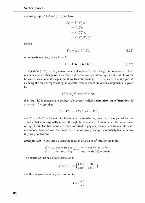
Vector spaces

and using Eqs. (3.16) and (3.20) we have

T e′i = T (A′ki ek)

= A′ki T ek

= A′ki Tmk em

= A′ki Tmk A j

m e′j .

Hence

T ′ ji = A j

m T mk A′ki , (3.22)

or in matrix notation, since A′ = A−1,

T′ = ATA′ = A T A−1. (3.23)

Equation (3.23) is the passive view – it represents the change in components of anoperator under a change of basis. With a different interpretation Eq. (3.23) could howeverbe viewed as an operator equation. If we treat the basis {e1, . . . , en} as fixed and regard Aas being the matrix representing an operator whose effect on vector components is givenby

v′i = Aijv

j ⇐⇒ v′ = Av,

then Eq. (3.23) represents a change of operator, called a similarity transformation. Ifx ′ = Ax, y′ = Ay, then

y′ = AT x = AT A−1 Ax = T ′x ′,

and T ′ = AT A−1 is the operator that relates the transforms, under A, of any pair of vectorsx and y that were originally related through the operator T . This is called the active viewof Eq. (3.23). The two views are often confused in physics, mainly because operators arecommonly identified with their matrices. The following example should help to clarify anylingering confusions.

Example 3.25 Consider a clockwise rotation of axes in R2 through an angle θ ,

e′1 = cos θe1 − sin θe2

e′2 = sin θe1 + cos θe2⇐⇒ e1 = cos θe′1 + sin θe′2

e2 = − sin θe′1 + cos θe′2.

The matrix of this basis transformation is

A = [Aij ] =

(cos θ − sin θsin θ cos θ

)and the components of any position vector

x =(

xy

)

86

3.6 Summation convention and transformation of bases

Figure 3.1 Active and passive views of a transformation

Figure 3.2 Active view of a similarity transformation

change by

x′ = Ax ⇐⇒ x ′ = cos θ x − sin θ yy′ = sin θ x + cos θ y.

This is the passive view. On the other hand, if we regard A as the matrix of componentsof an operator with respect to fixed axes e1, e2, then it represents a physical rotation of thespace by an angle θ in a counterclockwise direction, opposite to the rotation of the axesin the passive view. Figure 3.1 demonstrates the apparent equivalence of these two views,while Fig. 3.2 illustrates the active view of a similarity transformation T ′ = AT A−1 on alinear operator T : R2 → R2.

87

Vector spaces

Problems

Problem 3.11 Let {e1, e2, e3} be a basis of a three-dimensional vector space V . Show that the vectors{e′1, e′2, e′3} defined by

e′1 = e1 + e3

e′2 = 2e1 + e2

e′3 = 3e2 + e3

also form a basis of V .What are the elements of the matrix A = [A j

i ] in Eq. (3.16)? Calculate the components of thevector

v = e1 − e2 + e3

with respect to the basis {e′1, e′2, e′3}, and verify the column vector transformation v′ = Av.

Problem 3.12 Let T : V → W be a linear map between vector spaces V and W . If {ei | i = 1, . . . , n}is a basis of V and { fa | a = 1, . . . ,m} a basis of W , how does the matrix T , defined in Problem 3.9,transform under a transformation of bases

ei = A ji e′j , fa = Bb

a f ′b ?

Express your answer both in component and in matrix notation.

Problem 3.13 Let e1, e2, e3 be a basis for a three-dimensional vector space and e′1, e′2, e

′3 a second

basis given by

e′1 = e3,

e′2 = e2 + 2e3,

e′3 = e1 + 2e2 + 3e3.

(a) Express the ei in terms of the e′j , and write out the transformation matrices A = [Aij ] and

A′ = A−1 = [A′i j ].(b) If u = e1 + e2 + e3, compute its components in the e′i basis.(c) Let T be the linear transformation defined by

T e1 = e2 + e3, T e2 = e3 + e1, T e3 = e1 + e2.

What is the matrix of components of T with respect to the basis ei ?(d) By evaluating T e′1, etc. in terms of the e′j , write out the matrix of components of T with respect

to the e′j basis and verify the similarity transformation T′ = ATA−1.

3.7 Dual spaces

Linear functionals

A linear functional ϕ on a vector space V over a field K is a linear map ϕ : V → K, wherethe field of scalars K is regarded as a one-dimensional vector space, spanned by the element 1,

ϕ(au + bv) = aϕ(u)+ bϕ(v). (3.24)

88

3.7 Dual spaces

The use of the phrase linear functional in place of ‘linear function’ is largely adopted withinfinite dimensional spaces in mind. For example, if V is the space of continuous functionson the interval [0, 1] and K (x) is an integrable function on [0, 1], letϕK : V → K be definedby

ϕK ( f ) =∫ 1

0K (y) f (y) dy.

As the linear map ϕK is a function whose argument is another function, the terminology‘linear functional’ seems more appropriate. In this case it is common to write the action ofϕK on the function f as ϕK [ f ] in place of ϕK ( f ).

Theorem 3.8 If ϕ : V → K is any linear functional then its kernel kerϕ has codimension1. Conversely, any subspace W ⊂ V of codimension 1 defines a linear functional ϕ on Vuniquely up to a scalar factor, such that W = kerϕ.

Proof : The first part of the theorem follows from Example 3.22 and Eq. (3.3),

codim (kerϕ) = dim(V/(kerϕ)) = dim(imϕ) = dim K = 1.

To prove the converse, let u be any vector not belonging to W – if no such vector existsthen W = V and the codimension is 0. The set of cosets au +W = a(u +W ) where a ∈ Kform a one-dimensional vector space that must be identical with all of V/W . Every vectorv ∈ V therefore has a unique decomposition v = au + w where w ∈ W , since

v = a′u + w ′ =⇒ (a − a′)u = w − w ′ =⇒ a = a′ and w = w ′.

A linear functional ϕ having kernel W has ϕ(W ) = 0 and ϕ(u) = c �= 0, for if c = 0 then thekernel ofϕ is all of V . Furthermore, given any non-zero scalar c ∈ K, these two requirementsdefine a linear functional on V as its value on any vector v ∈ V is uniquely determinedby

ϕ(v) = ϕ(au + w) = ac.

If ϕ′ is any other such linear functional, having c′ = ϕ′(u) �= 0, then ϕ′ = (c′/c)ϕ sinceϕ′(v) = ac′ = (c′/c)ϕ(v). �

This proof even applies, as it stands, to infinite dimensional spaces, although in that caseit is usual to impose the added stipulation that linear functionals be continuous (see Section10.9 and Chapter 13).

Exercise: If ω and ρ are linear functionals on V , show that

kerω = ker ρ ⇐⇒ ω = aρ for some a ∈ K.

Example 3.26 Let V = Kn , where n is any integer ≥ 2 or possibly n = ∞. For conve-nience, we will take V to be the space of row vectors of length n here. Let W be the subspaceof vectors

W = {(x1, x2, . . . ) ∈ Kn | x1 + x2 = 0}.

89

Vector spaces

This is a subspace of codimension 1, for if we set u = (1, 0, 0, . . . ), then any vector v canbe written

v = (v1, v2, v3, . . . ) = au + w

where a = v1 + v2 and w = (−v2, v2, v3, . . . ). This decomposition is unique, for ifau + w = a′u + w ′ then (a − a′)u = w ′ − w ∈ W . Hence a = a′ and w = w ′, sinceu �∈ W . Every coset v +W can therefore be uniquely expressed as a(u +W ), and W hascodimension 1.

Let ϕ : V → K be the linear functional such that ϕ(W ) = 0 and ϕ(u) = 1. Then ϕ(v) =ϕ(au + w) = aϕ(u)+ ϕ(w) = a, so that

ϕ((x1, x2, x3, . . . )

) = x1 + x2.

The kernel of ϕ is evidently W , and every other linear functional ϕ′ having kernel W is ofthe form ϕ

((x1, x2, x3, . . . )

) = c(x1 + x2).

The dual space of a vector space

As for general linear maps, it is possible to add linear functionals and multiply them byscalars,

(ϕ + ω)(u) = ϕ(u)+ ω(u), (aω)(u) = aω(u).

With respect to these operations the set of linear functionals on V forms a vector space overK called the dual space of V , usually denoted V ∗. In keeping with earlier conventions, otherpossible notations for this space are L(V,K) or Hom(V,K). Frequently, linear functionalson V will be called covectors, and in later chapters we will have reason to refer to them as1-forms.

Let V be a finite dimensional vector space, dim V = n, and {e1, e2, . . . , en} any basisfor V . A linear functional ω on V is uniquely defined by assigning its values on the basisvectors,

w1 = ω(e1), w2 = ω(e2), . . . , wn = ω(en),

since the value on any vector u = ui ei ≡∑n

i=1 ui ei can be determined using linearity (3.24),

ω(u) = ω(ui ei ) = uiω(ei ) = wi ui ≡n∑

i=1

wi ui . (3.25)

Define n linear functionals ε1, ε2, . . . , εn by

εi (e j ) = δij (3.26)

where δij is the Kronecker delta defined in Eq. (3.14). Note that these equations uniquely

define each linear functional εi , since their values are assigned on each basis vector e j inturn.

Theorem 3.9 The n-linear functionals {ε1, ε2, . . . , εn} form a basis of V ∗, called the dualbasis to {e1, . . . , en}. Hence dim V ∗ = n = dim V .

90

3.7 Dual spaces

Proof : Firstly, suppose there are scalars ai ∈ K such that

aiεi = 0.

Applying the linear functional on the left-hand side of this equation to an arbitrary basisvector e j ,

0 = aiεi (e j ) = aiδ

ij = a j ,

shows that the linear functionals {ε1, . . . , εn} are linearly independent. Furthermore theselinear functions span V ∗ since every linear functional ω on V can be written

ω = wiεi where wi = ω(ei ). (3.27)

This follows from

wiεi (u) = wiε

i (u j e j )

= wi ujεi (e j )

= wi ujδi

j

= wi ui

= ω(u) by Eq. (3.25).

Thus ω and ω′ = wiεi have the same effect on every vector u = ui ei ; they are therefore

identical linear functionals. The proposition that dim V ∗ = n follows from Corollary 3.4.�

Exercise: Show that the expansion (3.27) is unique; i.e., if ω = w ′iε

i then w ′i = wi for each i =

1, . . . , n.

Given a basis E = {ei }, we will frequently refer to the n numbers wi = ω(ei ) as thecomponents of the linear functional ω in this basis. Alternatively, we can think of them asthe components ofωwith respect to the dual basis in V ∗. The formula (3.25) has a somewhatdeceptive ‘dot product’ feel about it. In Chapter 5 a dot product will be correctly defined asa product between vectors from the same vector space, while (3.25) is a product betweenvectors from different spaces V and V ∗. It is, in fact, better to think of the componentsui of a vector u from V as forming a column vector, while the components w j of a linearfunctional ω form a row vector. The above product then makes sense as a matrix productbetween a 1× n row matrix and an n × 1 column matrix. While a vector is often thought ofgeometrically as a directed line segment, often represented by an arrow, this is not a goodway to think of a covector. Perhaps the best way to visualize a linear functional is as a setof parallel planes of vectors determined by ω(v) = const. (see Fig. 3.3).

Dual of the dual

We may enquire whether this dualizing process can be continued to generate further vectorspaces such as the dual of the dual space V ∗∗, etc. For finite dimensional spaces the processessentially stops at the first dual, for there is a completely natural way in which V can be

91

Vector spaces

Figure 3.3 Geometrical picture of a linear functional

identified with V ∗∗. To understand how V itself can be regarded as the dual space of V ∗,define a linear map v : V ∗ → K corresponding to any vector v ∈ V by

v(ω) = ω(v) for all ω ∈ V ∗. (3.28)

The map v is a linear functional on V ∗, since

v(aω + bρ) = (aω + bρ)(v)

= aω(v)+ bρ(v)

= av(ω)+ bv(ρ).

The map β : V → V ∗∗ defined by β(v) = v is linear, since

β(au + bv)(ϕ) = au + bv(ϕ) (ϕ ∈ V ∗)

= ϕ(au + bv)

= aϕ(u)+ bϕ(v)

= au(ϕ)+ bv(ϕ)

= aβ(u)(ϕ)+ bβ(v)(ϕ).

As this holds for arbitrary covectors ϕ we have β(au + bv) = aβ(u)+ bβ(v). Furthermoreif e1, e2, . . . , en is a basis of V with dual basis ε1, ε2, . . . , εn , then

ei (εj ) = ε j (ei ) = δ j

i ,

and it follows from Theorem 3.9 that {β(ei ) = ei } is the basis of V ∗∗ dual to the basis {ε j }of V ∗. The map β : V → V ∗∗ is therefore onto since every f ∈ V ∗∗ can be written in theform

f = uiβ(ei ) = β(u) = u where u = ui ei .

92

3.7 Dual spaces

Since {β(ei )} is a basis, it follows from Theorem 3.5 that the components ui , and thereforethe vector u, are uniquely determined by f . The map β is thus a vector space isomorphism,as it is both onto and one-to-one.

We have shown that V ∼= V ∗∗. In itself this is to be expected since these spaces have thesame dimension, but the significant thing to note is that since the defining Eq. (3.28) makesno mention of any particular choice of basis, the correspondence between V and V ∗∗ istotally natural. There is therefore no ambiguity in identifying v with v, and rewriting (3.28)as

v(ω) = ω(v).

This reciprocity between the two spaces V and V ∗ lends itself to the following alternativenotations, which will be used interchangeably throughout this book:

〈ω, v〉 ≡ 〈v, ω〉 ≡ v(ω) ≡ ω(v). (3.29)

However, it should be pointed out that the identification of V and V ∗∗ will only workfor finite dimensional vector spaces. In infinite dimensional spaces, every vector may beregarded as a linear functional on V ∗ in a natural way, but the converse is not true – thereexist linear functionals on V ∗ that do not correspond to vectors from V .

Transformation law of covector components

By Theorem 3.9 the spaces V and V ∗ are in one-to-one correspondence since they have thesame dimension, but unlike that described above between V and V ∗∗ this correspondenceis not natural. For example, if v = vi ei is a vector in V let υ be the linear functional whosecomponents in the dual basis are exactly the same as the components of the original vector,υ = viεi . While the map v �→ υ is a vector space isomorphism, the same rule applied withrespect to a different basis {e′i } will generally lead to a different correspondence betweenvectors and covectors. Thus, given an arbitrary vector v ∈ V there is no basis-independentway of pointing to a covector partner in V ∗. Essentially this arises from the fact that the lawof transformation of components of a linear functional is different from the transformationlaw of components for a vector.

We have seen in Section 3.6 that the transformation of a basis can be written by Eqs.(3.16) and (3.20),

ei = A ji e′j , e′j = A′kj ek (3.30)

where [Aik] and [A′ik] are related through the inverse matrix equations (3.19). Let {εi } and

{ε′i } be the dual bases corresponding to the bases {e j } and {e′j } respectively of V ,

εi (e j ) = δij , ε′i (e′j ) = δi

j . (3.31)

93

Vector spaces

Set

εi = Bijε′ j ,

and substituting this and Eq. (3.30) into the first identity of (3.31) gives, after replacing theindex j by k,

δik = Bi

jε′ j (ek)

= Bijε′ j (Al

ke′l)

= Bij Al

kδjl

= Bij A j

k .

Hence Bij = A′i j and the transformation of the dual basis is

εi = A′i jε′ j . (3.32)

Exercise: Show the transform inverse to (3.32)

ε′ j = A jkε

k . (3.33)

If ω = wiεi is a linear functional having components wi with respect to the first basis,

then

ω = wiεi = wi A′ijε

′ j = w ′iε′i

where

w ′i = A′ j

i w j . (3.34)

This is known as the covariant vector transformation law of components. Its inverseis

w j = Akj w

′k . (3.35)

These equations are to be compared with the contravariant vector transformation law ofcomponents of a vector v = vi ei , given by Eqs. (3.17) and (3.21),

v′ j = A jiv

i , vi = A′i jvj . (3.36)

Exercise: Verify directly from (3.34) and (3.36) that Eq. (3.25) is basis-independent,

ω(u) = wi ui = w ′

j u′ j .

Exercise: Show that if the components of ω are displayed as a 1× n row matrix wT =(w1, w2, . . . , wn) then the transformation law (3.34) can be written as a matrix equation

w′T = wT A.

94

3.7 Dual spaces

Problems

Problem 3.14 Find the dual basis to the basis of R3 having column vector representation

e1 =

⎛⎜⎝ 111

⎞⎟⎠ , e2 =

⎛⎜⎝ 10−1

⎞⎟⎠ , e3 =

⎛⎜⎝ 0−11

⎞⎟⎠ .Problem 3.15 Let P(x) be the vector space of real polynomials f (x) = a0 + a1x + · · · + an xn .If (b0, b1, b2, . . . ) is any sequence of real numbers, show that the map β : P(x) → R givenby

β( f (x)) =n∑

i=0

bi ai

is a linear functional on P(x).

Show that every linear functional β on P(x) can be obtained in this way from such a sequence andhence that (R

∞)∗ = R∞.

Problem 3.16 Define the annihilator S⊥ of a subset S ⊆ V as the set of all linear functionals thatvanish on S,

S⊥ = {ω ∈ V ∗ |ω(u) = 0 ∀u ∈ S}.

(a) Show that for any subset S, S⊥ is a vector subspace of V ∗.(b) If T ⊆ S, show that S⊥ ⊆ T⊥.(c) If U is a vector subspace of V , show that (V/U )∗ ∼= U⊥. [Hint: For each ω in U⊥ define the

element ω ∈ (V/U )∗ by ω (v +U ) = ω (v).](d) Show that U ∗ ∼= V ∗/U⊥.(e) If V is finite dimensional with dim V = n and W is any subspace of V with dim W = m, show

that dim W⊥ = n − m. [Hint: Use a basis adapted to the subspace W by Theorem 3.7 and considerits dual basis in V ∗.]

(f ) Adopting the natural identification of V and V ∗∗, show that (W⊥)⊥ = W .

Problem 3.17 Let u be a vector in the vector space V of dimension n.

(a) If ω is a linear functional on V such that a = ω (u) �= 0, show that a basis e1, . . . , en can bechosen such that

u = e1 and ω = aε1

where {ε1, . . . , εn} is the dual basis. [Hint: Apply Theorem 3.7 to the vector u and try a furtherbasis transformation of the form e′1 = e1, e′2 = e2 + a2e1, . . . , e′n = en + ane1.

](b) If a = 0, show that the basis may be chosen such that

u = e1 and ω = ε2.

Problem 3.18 For the three-dimensional basis transformation of Problem 3.13 evaluate the ε′ j dualto e′i in terms of the dual basis ε j . What are the components of the linear functional ω = ε1 + ε2 + ε3

with respect to the new dual basis?

95

Vector spaces

Problem 3.19 If A : V → V is a linear operator, define its transpose to be the linear map A′ :V ∗ → V ∗ such that

A′ω(u) = ω(Au), ∀ u ∈ V, ω ∈ V ∗.

Show that this relation uniquely defines the linear operator A′ and that

O ′ = O, (idV )′ = idV ∗ , (aB + bA)′ = aB ′ + bA′, ∀a, b ∈ K.

(a) Show that (B A)′ = A′B ′.(b) If A is an invertible operator then show that (A′)−1 = (A−1)′.(c) If V is finite dimensional show that A′′ = A, if we make the natural identification of V ∗∗

and V .(d) Show that the matrix of components of the transpose map A′ with respect to the dual basis is the

transpose of the matrix of A, A′ = AT .(e) Using Problem 3.16 show that ker A′ = (im A)⊥.(f) Use (3.10) to show that the rank of A′ equals the rank of A.

Problem 3.20 The row rank of a matrix is defined as the maximum number of linearly independentrows, while its column rank is the maximum number of linearly independent columns.

(a) Show that the rank of a linear operator A on a finite dimensional vector space V is equal to thecolumn rank of its matrix A with respect to any basis of V .

(b) Use parts (d) and (f ) of Problem 3.19 to show that the row rank of a square matrix is equal to itscolumn rank.

Problem 3.21 Let S be a linear operator on a vector space V .

(a) Show that the rank of S is one, ρ(S) = 1, if and only if there exists a non-zero vector u and anon-zero linear functional α such that

S(v) = uα(v).

(b) With respect to any basis {ei } of V and its dual basis {ε j }, show that

Sij = ui a j where u = ui ei , α = a jε

j .

(c) Show that every linear operator A of rank r can be written as a sum of r linear operators of rankone.

(d) Show that the last statement is equivalent to the assertion that for every matrix A of rank r thereexist column vectors ui and ai (i = 1, . . . , r ) such that

S =r∑

i=1

ui aT

i .

References

[1] G. Birkhoff and S. MacLane. A Survey of Modern Algebra. New York, MacMillan,1953.

[2] N. B. Haaser and J. A. Sullivan. Real Analysis. New York, Van Nostrand ReinholdCompany, 1971.

[3] S. Hassani. Foundations of Mathematical Physics. Boston, Allyn and Bacon, 1991.

96

References

[4] R. Geroch. Mathematical Physics. Chicago, The University of Chicago Press, 1985.[5] S. Lang. Algebra. Reading, Mass., Addison-Wesley, 1965.[6] L. H. Loomis and S. Sternberg. Advanced Calculus. Reading, Mass., Addison-Wesley,

1968.[7] P. R. Halmos. Finite-dimensional Vector Spaces. New York, D. Van Nostrand Company,

1958.

97

4 Linear operators and matrices

Given a basis {e1, e2, . . . , en} of a finite dimensional vector space V , we recall from Section3.5 that the matrix of components T = [T i

j ] of a linear operator T : V → V with respectto this basis is defined by Eq. (3.6) as:

T e j = T ij ei , (4.1)

and under a transformation of basis,

ei = A ji e′j , e′i = A′ki ek, (4.2)

where

A′kj A ji = δk

i , Aik A′kj = δi

j , (4.3)

the components of any linear operator T transform by

T ′ ji = A j

m T mk A′ki . (4.4)

The matrices A = [A ji ] and A′ = [A′ki ] are inverse to each other, A′ = A−1, and (4.4) can

be written in matrix notation as a similarity transformation

T′ = A T A−1. (4.5)

The main task of this chapter will be to find a basis that provides a standard represen-tation of any given linear operator, called the Jordan canonical form. This representationis uniquely determined by the operator and encapsulates all its essential properties. Theproof given in Section 4.2 is rather technical and may be skipped on first reading. It would,however, be worthwhile to understand its appearance, summarized at the end of that section,as it has frequent applications in mathematical physics. Good references for linear operatorsand matrices in general are [1–3], while a detailed discussion of the Jordan canonical formcan be found in [4].

It is important to realize that we are dealing with linear operators on free vector spaces.This concept will be defined rigorously in Chapter 6, but essentially it means that thevector spaces have no further structure imposed on them. A number of concepts such as‘symmetric’, ‘hermitian’ and ‘unitary’, which often appear in matrix theory, have no placein free vector spaces. For example, the requirement that T be a symmetric matrix wouldread T i

j = T ji in components, an awkward-looking relation that violates the rules given

in Section 3.6. In Chapter 5 we will find a proper context for notions such as ‘symmetrictransformations’ and ‘hermitian transformations’.

98

4.1 Eigenspaces and characteristic equations

4.1 Eigenspaces and characteristic equations

Invariant subspaces

A subspace U of V is said to be invariant under a linear operator S : V → V if

SU = {Su | u ∈ U } ⊆ U.

In this case, the action of S restricted to the subspace U , S∣∣U

, gives rise to a linear operatoron U .

Example 4.1 Let V be a three-dimensional vector space with basis {e1, e2, e3}, and S theoperator defined by

Se1 = e2 + e3,

Se2 = e1 + e3,

Se3 = e1 + e2.

Let U be the subspace of all vectors of the form (a + b)e1 + be2 + (−a + b)e3, where aand b are arbitrary scalars. This subspace is spanned by f1 = e1 − e3 and f2 = e1 + e2 + e3

and is invariant under S, since

S f1 = − f1, S f2 = 2 f2 =⇒ S(a f1 + b f2) = −a f1 + 2b f2 ∈ U.

Exercise: Show that if both U and W are invariant subspaces of V under an operator S then so istheir intersection U ∩W and their sum U +W = {v = u + w | u ∈ U,w ∈ W }.

Suppose dim U = m < n = dim V and let {e1, . . . , em} be a basis of U . By Theorem3.7 this basis can be extended to a basis {e1, . . . , en} spanning all of V . The invariance ofU under S implies that the first m basis vectors are transformed among themselves,

Sea =m∑

b=1

Sbaeb (a ≤ m).

In such a basis, the components Ski of the operator S vanish for i ≤ m, k > m, and the n × n

matrix S = [Ski ] has the upper block diagonal form

S =(

S1 S3

O S2

).

The submatrix S1 is the m × m matrix of components of S|U expressed in the basis{e1, . . . , em}, while S3 and S2 are submatrices of orders m × p and p × p, respectively,where p = n − m, and O is the zero p × m matrix.

If V = U ⊕W is a decomposition with both U and W invariant under S, then choosea basis {e1, . . . , em, em+1, . . . , en} of V such that the first m vectors span U while the lastp = n − m vectors span W . Then Sk

i = 0 whenever i > m and k ≤ m, and the matrix ofthe operator S has block diagonal form

S =(

S1 OO S2

).

99

Linear operators and matrices

Example 4.2 In Example 4.1 set f3 = e3. The vectors f1, f2, f3 form a basis adapted tothe invariant subspace spanned by f1 and f2,

S f1 = − f1, S f2 = 2 f2, S f3 = f2 − f3,

and the matrix of S has the upper block diagonal form

S =⎛⎝ −1 0 0

0 2 10 0 −1

⎞⎠ .On the other hand, the one-dimensional subspace W spanned by f ′3 = e3 − 1

2 e1 − 12 e2 is

invariant since S f ′3 = − f ′3, and in the basis { f1, f2, f ′3} adapted to the invariant decompo-sition V = U ⊕W the matrix S takes on block diagonal form

S =⎛⎝ −1 0 0

0 2 10 0 −1

⎞⎠ .

Eigenvectors and eigenvalues

Given an operator S : V → V , a scalar λ ∈ K is said to be an eigenvalue of S if there existsa non-zero vector v such that

Sv = λv (v �= 0) (4.6)

and v is called an eigenvector of S corresponding to the eigenvalue λ. Eigenvectors arethose non-zero vectors that are ‘stretched’ by an amount λ on application of the operator S.It is important to stipulate v �= 0 since the equation (4.6) always holds for the zero vector,S0 = 0 = λ0.

For any scalar λ ∈ K, let

Vλ = {u | Su = λu}. (4.7)

The set Vλ is a vector subspace, for

Su = λu and Sv = λv =⇒ S(u + av) = Su + aSv=⇒ S(u + av) = λu + aλv = λ(u + av) for all a ∈ K.

For every λ, the subspace Vλ is invariant under S,

u ∈ Vλ =⇒ Su = λu =⇒ S(Su) = λSu =⇒ Su ∈ Vλ.

Vλ consists of the set of all eigenvectors having eigenvalue λ, supplemented with the zerovector {0}. If λ is not an eigenvalue of S, then Vλ = {0}.

100

4.1 Eigenspaces and characteristic equations

If {e1, e2, . . . , en} is any basis of the vector space V , and v = vi ei any vector of V , letv be the column vector of components

v =

⎛⎜⎜⎜⎝v1

v2

...vn

⎞⎟⎟⎟⎠ .By Eq. (3.8) the matrix equivalent of (4.6) is

Sv = λv, (4.8)

where S is the matrix of components of S. Under a change of basis (4.2) we have from Eqs.(3.18) and (4.5),

v′ = Av, S′ = ASA−1.

Hence, if v satisfies (4.8) then v′ is an eigenvector of S′ with the same eigenvalue λ,

S′v′ = ASA−1Av = ASv = λAv = λv′.

This result is not unexpected, since Eq. (4.8) and its primed version are simply representa-tions with respect to different bases of the same basis-independent equation (4.6).

Define the nth power Sn of an operator inductively, by setting S0 = idV and

Sn = S ◦ Sn−1 = SSn−1.

Thus S1 = S and S2 = SS, etc. If p(x) = a0 + a1x + a2x2 + · · · + an xn is any polynomialwith coefficients ai ∈ K, the operator polynomial p(S) is defined in the obvious way,

p(S) = a0 + a1S + a2S2 + · · · + an Sn.

If λ is an eigenvalue of S and v a corresponding eigenvector, then v is an eigenvector ofany power Sn corresponding to eigenvalue λn . For n = 0,

S0v = idV v = λ0v since λ0 = 1,

and the proof follows by induction: assume Sn−1v = λn−1v then by linearity

Snv = SSn−1v = Sλn−1v = λn−1Sv = λn−1λv = λnv.

For a polynomial p(x), it follows immediately that v is an eigenvector of the operator p(S)with eigenvalue p(λ),

p(S)v = p(λ)v. (4.9)

Characteristic equation

The matrix equation (4.8) can be written in the form

(S− λI)v = 0. (4.10)

101

Linear operators and matrices

A necessary and sufficient condition for this equation to have a non-trivial solution v �= 0is

f (λ) = det(S− λI) =

∣∣∣∣∣∣∣∣∣S1

1 − λ S12 . . . S1

n

S21 S2

2 − λ . . . S2n

......

...Sn

1 Sn2 . . . Sn

n − λ

∣∣∣∣∣∣∣∣∣ = 0, (4.11)

called the characteristic equation of S. The function f (λ) is a polynomial of degree n inλ,

f (λ) = (−1)n(λn − Sk

kλn−1 + · · · + (−1)n det S

), (4.12)

known as the characteristic polynomial of S.If the field of scalars is the complex numbers, K = C, then the fundamental theorem of

algebra implies that there exist complex numbers λ1, λ2, . . . , λn such that

f (λ) = (−1)n(λ− λ1)(λ− λ2) . . . (λ− λn).

As some of these roots of the characteristic equation may appear repeatedly, we can writethe characteristic polynomial in the form

f (z) = (−1)n(z − λ1)p1 (z − λ2)p2 . . . (z − λm)pm

where p1 + p2 + · · · + pm = n. (4.13)

Since for each λ = λi there exists a non-zero complex vector solution v to the lin-ear set of equations given by (4.10), the eigenvalues of S must all come from theset of roots {λ1, . . . , λm}. The positive integer pi is known as the multiplicity of theeigenvalue λi .

Example 4.3 When the field of scalars is the real numbers R there will not in generalbe real eigenvectors corresponding to complex roots of the characteristic equation. Forexample, let A be the operator on R2 defined by the following action on the standard basisvectors e1 = (1, 0) and e2 = (0, 1),

Ae1 = e2, Ae2 = −e1 =⇒ A =(

0 −11 0

).

The characteristic polynomial is

f (z) =∣∣∣∣−z − 1

1 − z

∣∣∣∣ = z2 + 1,

whose roots are z = ±i . The operator A thus has no real eigenvalues and eigenvectors.However, if we regard the field of scalars as being C and treat A as operating on C2, then ithas complex eigenvectors

u = e1 − ie2, Au = iu,v = e1 + ie2, Av = −iv.

102

4.1 Eigenspaces and characteristic equations

It is worth noting that, since A2e1,= Ae2 = −e1 and A2e2 = −Ae1 = −e2, the operator Asatisfies its own characteristic equation

A2 + idR2 = 0 =⇒ A2 + I = 0.

This is a simple example of the important Cayley–Hamilton theorem – see Theorem 4.3below.

Example 4.4 Let V be a three-dimensional complex vector space with basis e1, e2, e3,and S : V → V the operator whose matrix with respect to this basis is

S =⎛⎝1 1 0

0 1 00 0 2

⎞⎠ .The characteristic polynomial is

f (z) =∣∣∣∣∣∣1− z 1 0

0 1− z 00 0 2− z

∣∣∣∣∣∣ = −(z − 1)2(z − 2).

Hence the eigenvalues are 1 and 2, and it is trivial to check that the eigenvector correspondingto 2 is e3. Let u = xe1 + ye2 + ze3 be an eigenvector with eigenvalue 1,

Su = u where u =⎛⎝x

yz

⎞⎠ ,then

x + y = x, y = y, 2z = z.

Hence y = z = 0 and u = xe1. Thus, even though the eigenvalue λ = 1 has multiplicity 2,all corresponding eigenvectors are multiples of e1.

Note that while e2 is not an eigenvector, it is annihilated by (S − idV )2, for

Se2 = e1 + e2 =⇒ (S − idV )e2 = e1

=⇒ (S − idV )2e2 = (S − idV )e1 = 0.

Operators of the form S − λi idV and their powers (S − λidV )m , where λi are eigenvaluesof S, will make regular appearances in what follows. These operators evidently commutewith each other and there is no ambiguity in writing them as (S − λi )m .

Theorem 4.1 Any set of eigenvectors corresponding to distinct eigenvalues of an operatorS is linearly independent.

Proof : Let { f1, f2, . . . , fk} be a set of eigenvectors of S corresponding to eigenvaluesλ1, λ2, . . . , λk , no pair of which are equal,

S fi = λi fi (i = 1, . . . , k),

and let c1, c2, . . . , ck be scalars such that

c1 f1 + c2 f2 + · · · + ck fk = 0.

103

Linear operators and matrices

If we apply the polynomial P1(S) = (S − λ2)(S − λ3) . . . (S − λk) to this equation, then allterms except the first are annihilated, leaving

c1 P1(λ1) f1 = 0.

Hence

c1(λ1 − λ2)(λ1 − λ3) . . . (λ1 − λk) f1 = 0,

and since f1 �= 0 and all the factors (λ1 − λi ) �= 0 for i = 2, . . . , k, it follows that c1 = 0.Similarly, c2 = · · · = ck = 0, proving linear independence of f1, . . . , fk . �

If the operator S : V → V has n distinct eigenvalues λ1, . . . , λn where n = dim V , thenTheorem 4.1 shows the eigenvectors f1, f2, . . . , fn are l.i. and form a basis of V . Withrespect to this basis the matrix of S is diagonal and its eigenvalues lie along the diagonal,

S =

⎛⎜⎜⎜⎝λ1 0 . . . 00 λ2 . . . 0...

. . ....

0 0 . . . λn

⎞⎟⎟⎟⎠ .Conversely, any operator whose matrix is diagonalizable has a basis of eigenvectors (theeigenvalues need not be distinct for the converse). The more difficult task lies in the classi-fication of those cases such as Example 4.4, where an eigenvalue λ has multiplicity p > 1but there are less than p independent eigenvectors corresponding to it.

Minimal annihilating polynomial

The space of linear operators L(V, V ) is a vector space of dimension n2 since it can beput into one-to-one correspondence with the space of n × n matrices. Hence the first n2

powers I ≡ idV = S0, S = S1, S2, . . . , Sn2of any linear operator S on V cannot be linearly

independent since there are n2 + 1 operators in all. Thus S must satisfy a polynomialequation,

P(S) = c0 I + c1S + c2S2 + · · · + cn2 Sn2 = 0,

not all of whose coefficients c0, c1, . . . , cn vanish.

Exercise: Show that the matrix equivalent of any such polynomial equation is basis-independentby showing that any similarity transform S′ = ASA−1 of S satisfies the same polynomial equation,P(S′) = 0.

Let

�(S) = Sk + c1Sk−1 + · · · + ck I = 0

be the polynomial equation with leading coefficient 1 of lowest degree k ≤ n2, satisfied byS. The polynomial �(S) is unique, for if

�′(S) = Sk + c′1Sk−1 + · · · + c′k I = 0

104

4.1 Eigenspaces and characteristic equations

is another such polynomial equation, then on subtracting these two equations we have

(�−�′)(S) = (c1 − c′1)Sk−1 + (c2 − c′2)Sk−2 + · · · + (ck − c′k) = 0,

which is a polynomial equation of degree < k satisfied by S. Hence c1 = c′1, c2 =c′2, . . . , ck = c′k . The unique polynomial �(z) = zk + c1zk−1 + · · · + ck is called the min-imal annihilating polynomial of S.

Theorem 4.2 A scalar λ is an eigenvalue of an operator S over a vector space V if andonly if it is a root of the minimal annihilating polynomial �(z).

Proof : If λ is an eigenvalue of S, let u �= 0 be any corresponding eigenvector, Su = λu.Since 0 = �(S)u = �(λ)u it follows that �(λ) = 0.

Conversely, if λ is a root of �(z) = 0 then there exists a polynomial �′(z) such that

�(z) = (z − λ)�′(z),

and since �′(z) has lower degree than �(z) it cannot annihilate S,

�′(S) �= 0.

Therefore, there exists a vector u ∈ V such that �′(S)u = v �= 0, and

0 = �(S)u = (S − λ)�′(S)u = (S − λ)v.

Hence Sv = λv, and λ is an eigenvalue of S with eigenvector v. �

It follows from this theorem that the minimal annihilating polynomial of an operator Son a complex vector space can be written in the form

�(z) = (z − λ1)k1 (z − λ2)k2 . . . (z − λm)km (k1 + k2 + · · · + km = k) (4.14)

where λ1, λ2, . . . , λm run through all the distinct eigenvalues of S. The various factors(z − λi

)ki are called the elementary divisors of S. The following theorem shows that thecharacteristic polynomial is always divisible by the minimal annihilating polynomial; thatis, for each i = 1, 2, . . . ,m the coefficient ki ≤ pi where pi is the multiplicity of the i theigenvalue.

Theorem 4.3 (Cayley–Hamilton) Every linear operator S over a finite dimensional vec-tor space V satisfies its own characteristic equation

f (S) = (S − λ1)p1 (S − λ2)p2 . . . (S − λm)pm = 0.

Equivalently, every n × n matrix S satisfies its own characteristic equation

f (S) = (S− λ1I)p1 (S− λ2I)p2 . . . (S− λm I)pm = 0.

Proof : Let e1, e2, . . . , en be any basis of V , and let S = [Skj ] be the matrix of components

of S with respect to this basis,

Se j = Skj ek .

This equation can be written as

(Skj idV − δk

j S)ek = 0,

105

Linear operators and matrices

or alternatively as

T kj (S)ek = 0, (4.15)

where

T kj (z) = Sk

j − δkj z.

Set R(z) = [Rkj (z)] to be the matrix of cofactors of T(z) = [T k

j (z)], such that

R ji (z)T k

j (z) = δki det T(z) = δk

i f (z).

The components Rkj (z) are polynomials of degree ≤ (n − 1) in z, and multiplying both

sides of Eq. (4.15) by R ji (S) gives

R ji (S)T k

j (S)ek = δki f (S)ek = f (S)ei = 0.

Since the ei span V we have the desired result, f (S) = 0. The matrix version is simply thecomponent version of this equation. �

Example 4.5 Let A be the matrix operator on the space of complex 4× 1 column vectorsgiven by

A =

⎛⎜⎜⎝i α 0 00 i 0 00 0 i 00 0 0 −1

⎞⎟⎟⎠ .

Successive powers of A are

A2 =

⎛⎜⎜⎝−1 2iα 0 00 −1 0 00 0 −1 00 0 0 1

⎞⎟⎟⎠ , A3 =

⎛⎜⎜⎝−i −3α 0 00 −i 0 00 0 −i 00 0 0 −1

⎞⎟⎟⎠and it is straightforward to verify that the matrices I, A, A2 are linearly independent, while

A3 = (−1+ 2i )A2 + (1+ 2i )A+ I.

Hence the minimal annihilating polynomial of A is

�(z) = z3 + (1− 2i )z2 − (1+ 2i )z − 1 = (z + 1)(z − i )2.

The elementary divisors of A are thus z + 1 and (z − i )2 and the eigenvalues are−1 and i .Computation of the characteristic polynomial reveals that

f (z) = det(A− zI) = (z + 1)(z − i )3,

which is divisible by �(z) in agreement with Theorem 4.3.

106

4.2 Jordan canonical form

Problem

Problem 4.1 The trace of an n × n matrix T = [T ij ] is defined as the sum of its diagonal elements,

tr T = T ii = T 1

1 + T 22 + · · · + T n

n .

Show that

(a) tr(ST) = tr(TS).(b) tr(ATA−1) = tr T .(c) If T : V → V is any operator define its trace to be the trace of its matrix with respect to a basis

{ei }. Show that this definition is independent of the choice of basis, so that there is no ambiguityin writing tr T .

(d) If f (z) = a0 + a1z + a2z2 + · · · + (−1)nzn is the characteristic polynomial of the operator T ,show that tr T = (−1)n−1an−1.

(e) If T has eigenvalues λ1, . . . , λm with multiplicities p1, . . . , pm , show that

tr T =m∑

i=1

piλi .

4.2 Jordan canonical form

Block diagonal form

Let S be a linear operator over a complex vector space V , with characteristic polynomial andminimal annihilating polynomial given by (4.13) and (4.14), respectively. The restrictionto complex vector spaces ensures that all roots of the polynomials f (z) and �(z) areeigenvalues. A canonical form can also be derived for operators on real vector spaces, butit relies heavily on the complex version.

If (z − λi )ki is the i th elementary divisor of S, define the subspace

Vi = {u | (S − λi )ki u = 0}.

This subspace is invariant under S, for

u ∈ Vi =⇒ (S − λi )ki u = 0

=⇒ (S − λi )ki Su = S(S − λi )

ki u = 0=⇒ Su ∈ Vi .

Our first task will be to show that V is a direct sum of these invariant subspaces,

V = V1 ⊕ V2 ⊕ . . .Lemma 4.4 If (z − λi )

ki is an elementary divisor of the operator S and (S − λi )ki+r u = 0

for some r > 0, then (S − λi )ki u = 0.

Proof : There is clearly no loss of generality in setting i = 1 in the proof of this result.The proof proceeds by induction on r .

Case r = 1: Let u be any vector such that (S − λ1)k1+1u = 0 and set

v = (S − λ1)k1 u.

107

Linear operators and matrices

Since (S − λ1)v = 0, this vector satisfies the eigenvector equation, Sv = λ1v. If �(S) isthe minimal annihilating polynomial of S, then

0 = �(S)u = (S − λ2)k2 . . . (S − λm)kmv

= (λ1 − λ2)k2 . . . (λ1 − λm)kmv.

As all λi �= λ j for i �= j it follows that v = 0, which proves the case r = 1.

Case r > 1: Suppose the lemma has been proved for r − 1. Then

(S − λ1)k1+r u = 0 =⇒ (S − λ1)k1+r−1(S − λ1)u = 0

=⇒ (S − λ1)k1 (S − λ1)u = 0 by induction hypothesis

=⇒ (S − λ1)k1 u = 0 by the case r = 1,

which concludes the proof of the lemma. �

If dim(V1) = p let h1, . . . , h p be a basis of V1 and extend to a basis of V using Theorem3.7:

h1, h2, . . . , h p, h p+1, . . . , hn. (4.16)

Of course if (z − λ1)k1 is the only elementary divisor of S then p = n, since V1 = V asevery vector is annihilated by (S − λ1)k1 . If, however, p < n we will show that the vectors

h1, h2, . . . , h p, h1, h2, . . . , hn−p (4.17)

form a basis of V , where

ha = (S − λ1)k1 h p+a (a = 1, . . . , n − p). (4.18)

Since the vectors listed in (4.17) are n in number it is only necessary to show that theyare linearly independent. Suppose that for some constants c1, . . . , cp, c1, . . . , cn−p

p∑i=1

ci hi +n−p∑a=1

ca ha = 0. (4.19)

Apply (S − λ1)k1 to this equation. The first sum on the left is annihilated since it belongsto V1, resulting in

(S − λ1)k1

n−p∑a=1

ca ha = (S − λ1)2k1

n−p∑a=1

cah p+a = 0,

and since k1 > 0 we conclude from Lemma 4.4 that

(S − λ1)k1

n−p∑a=1

cah p+a = 0.

Hence∑n−p

a=1 cah p+a ∈ V1, and there exist constants d1, d2, . . . , d p such that

n−p∑a=1

cah p+a =p∑

i=1

di hi .

108

4.2 Jordan canonical form

As the set {h1, . . . , hn} is by definition a basis of V , these constants must vanish:ca = di = 0 for all a = 1, . . . , n − p and i = 1, . . . , p. Substituting into (4.19), it fol-lows from the linear independence of h1, . . . , h p that c1, . . . , cp all vanish as well. Thisproves the linear independence of the vectors in (4.17).

Let W1 = L( h1, h2, . . . , hn−p). By Eq. (4.18) every vector x ∈ W1 is of the form

x = (S − λ1)k1 y

since this is true of each of the vectors spanning W1. Conversely, suppose x = (S − λ1)k1 yand let {y1, . . . , yn} be the components of y with respect to the original basis (4.16);then

x = (S − λ1)k1

(∑i

yi hi +∑

a

y p+ah p+a

)=∑

a

y p+a ha ∈ W1.

Hence W1 consists precisely of all vectors of the form x = (S − λ1)k1 y where y is anarbitrary vector of V . Furthermore W1 is an invariant subspace of V , for if x ∈ W1

then

x = (S − λ1)k1 y =⇒ Sx = (S − λ1)k1 Sy =⇒ Sx ∈ W1.

Hence W1 and V1 are complementary invariant subspaces, V = V1 ⊕W1, and the matrix ofS with respect to the basis (4.17) has block diagonal form

S =(

S1 OO T1

)where S1 is the matrix of S1 = S

∣∣V1

and T1 is the matrix of T1 = S∣∣W1

.Now on the subspace V1 we have, by definition,

(S1 − λ1)k1 = (S − λ1)k1

∣∣∣V1

= 0.

Hence λ1 is the only eigenvalue of S1, for if u ∈ V1 is an eigenvector of S1 correspondingto an eigenvalue σ ,

S1u = σu,

then

(S1 − λ1)k1 u = (σ − λ1)k1 u = 0,

from which it follows that σ = λ1 since u �= 0. The characteristic equation of S1 is therefore

det(S1 − zI) = (−1)p(λ1 − z)p. (4.20)

Furthermore, the operator

(T1 − λ1)k1 = (S − λ1)k1

∣∣∣W1

: W1 → W1

is invertible. For, let x be an arbitrary vector in W1 and set x = (S − λ1)k1 y where y ∈ V .Let y = y1 + y2 be the unique decomposition such that y1 ∈ V1 and y2 ∈ W1; then

x = (S − λ1)k1 y2 = (T1 − λ1)k1 y2,

109

Linear operators and matrices

and since any surjective (onto) linear operator on a finite dimensional vector space is bijective(one-to-one), the map (T1 − λ1)k1 must be invertible on W1. Hence

det(T1 − λ1I) �= 0 (4.21)

and λ1 cannot be an eigenvalue of T1.The characteristic equation of S is

det(S− zI) = det(S1 − zI) det(T1 − zI)

and from (4.20) and (4.21) the only way the right-hand side can equal the expression inEq. (4.13) is if

p1 = p and det(T1 − zI) = (−1)n−p(z − λ2)p2 . . . (z − λm)pm .

Hence, the dimension pi of each space Vi is equal to the multiplicity of the eigenvalue λi

and from the Cayley–Hamilton Theorem 4.3 it follows that pi ≥ ki .Repeating this process on T1, and proceeding inductively, it follows that

V = V1 ⊕ V2 ⊕ · · · ⊕ Vm,

and setting

h11, h12, . . . , h1p1 , h21, . . . , h2p2 , . . . , hm1, . . . , hmpm

to be a basis adapted to this decomposition, the matrix of S has block diagonal form

S =

⎛⎜⎜⎝S1 0 . . . 00 S2 . . . 0. . . . . . . . . . . .

0 0 . . . Sm

⎞⎟⎟⎠ . (4.22)

The restricted operators Si = S∣∣Vi

each have a minimal polynomial equation of the form

(Si − λi )ki = 0,

so that

Si = λi idi + Ni where N kii = 0. (4.23)

Nilpotent operators

Any operator N satisfying an equation of the form N k = 0 is called a nilpotent operator.The matrix N of any nilpotent operator satisfies Nk = 0, and is called a nilpotent matrix.From Eq. (4.23), each pi × pi matrix Si in the decomposition (4.22) is a multiple of theunit matrix plus a nilpotent matrix Ni ,

Si = λi I+ Ni where (Ni )ki = 0.

We next find a basis that expresses the matrix of any nilpotent operator in a standard(canonical) form.

110

4.2 Jordan canonical form

Let U be a finite dimensional space, not necessarily complex, dim U = p, and N anilpotent operator on U . Set k to be the smallest positive integer such that N k = 0. Evidentlyk = 1 if N = 0, while if N �= 0 then k > 1 and N k−1 �= 0. Define the subspaces Xi ofU by

Xi = {x ∈ U | N i x = 0} (i = 0, 1, . . . , k).

These subspaces form an increasing sequence,

{0} = X0 ⊂ X1 ⊂ X2 ⊂ · · · ⊂ Xk = U

and all are invariant under N , for if u ∈ Xi then Nu also belongs to Xi sinceN i Nu = N N i u = N0 = 0. The set inclusions are strict inclusion in every case, forsuppose that Xi = Xi+1 for some i ≤ k − 1. Then for any vector x ∈ Xi+2 we have

N i+2x = N i+1 N x = 0 =⇒ N i N x = 0 =⇒ x ∈ Xi+1.

Hence Xi+1 = Xi+2, and continuing inductively we find that Xi = · · · = Xk−1 = Xk = U .This leads to the conclusion that N k−1x = 0 for all x ∈ U , which contradicts the assumptionthat N k−1 �= 0. Hence none of the subspaces Xi can be equal to each other.

We call a set of vectors v1, v2, . . . , vs belonging to Xi linearly independent with respectto Xi−1 if

a1v1 + · · · + asvs ∈ Xi−1 =⇒ a1 = · · · = as = 0.

Lemma 4.5 Set ri = dim Xi − dim Xi−1 > 0 so that p = r1 + r2 + · · · + rk . Then ri isthe maximum number of vectors in Xi that can form a set that is linearly independent withrespect to Xi−1.

Proof : Let dim Xi−1 = q, dim Xi = q ′ > q and let u1, . . . , uq be a basis of Xi−1. Sup-pose {v1, . . . , vr } is a maximal set of vectors l.i. with respect to Xi−1; that is, a set thatcannot be extended to a larger such set. Such a maximal set must exist since any set ofvectors that is l.i. with respect to Xi−1 is linearly independent and therefore cannot exceedq in number. We show that S = {u1, . . . , uq , v1, . . . , vr } is a basis of Xi :(a) S is a l.i. set since

q∑i=1

ai ui +r∑

a=1

bava = 0

implies firstly that all ba vanish by the requirement that the vectors va are l.i. with respectto Xi−1, and secondly all the ai = 0 because the ui are l.i.(b) S spans Xi else there would exist a vector x that cannot be expressed as a linearcombination of vectors of S, and S ∪ {x}would be linearly independent. In that case, the setof vectors {v1, . . . , vr , x} would be l.i. with respect to Xi−1, for if

∑ra=1 bava + bx ∈ Xi−1

then from the linear independence of S ∪ {x} all ba = 0 and b = 0. This contradicts themaximality of v1, . . . , vr , and S must span the whole of Xi .This proves the lemma. �

111

Linear operators and matrices

Let {h1, . . . , hrk } be a maximal set of vectors in Xk that is l.i. with respect to Xk−1. FromLemma 4.5 we have rk = dim Xk − dim Xk−1. The vectors

h′1 = Nh1, h′2 = Nh2, . . . , h′rk= Nhrk

all belong to Xk−1 and are l.i. with respect to Xk−2, for if

a1h′1 + a2h′2 + · · · + ark h′rk∈ Xk−2

then

N k−1(a1h1 + a2h2 + · · · + ark hrk ) = 0,

from which it follows that

a1h1 + a2h2 + · · · + ark hrk ∈ Xk−1.

Since {h1, . . . , hrk } are l.i. with respect to Xk−1 we must have

a1 = a2 = · · · = ark = 0.

Hence rk−1 ≥ rk . Applying the same argument to all other Xi gives

rk ≤ rk−1 ≤ · · · ≤ r2 ≤ r1. (4.24)

Now complete the set {h′1, . . . , h′rk} to a maximal system of vectors in Xk−1 that is l.i.

with respect to Xk−2,

h′1, . . . , h′rk, h′rk+1

, . . . , h′rk−1.

Similarly, define the vectors h′′i = Nh′i (i = 1, . . . , rk−1) and extend to a maximal system{h′′1, h′′2, . . . , h′′rk−2

} in Xk−2. Continuing in this way, form a series of r1 + r2 + · · · + rk =p = dim U vectors that are linearly independent and form a basis of U and may be displayedin the following scheme:

h1 . . . hrk

h′1 . . . h′rk. . . h′rk−1

h′′1 . . . h′′rk. . . h′′rk−1

. . . h′′rk−2

. . . . . . . . . . . . . . . . . . . . . . . .

h(k−1)1 . . . h(k−1)

rk . . . h(k−1)rk−1 . . . . . . . . . h(k−1)

r1 .

Let Ua be the subspace generated by the ath column where a = 1, . . . , r1. These sub-spaces are all invariant under N , since Nh( j)

a = h( j+1)a , and the bottom elements h(k−1)

a ∈ X1

are annihilated by N ,

Nh(k−1)a ∈ X0 = {0}.

Since the vectors h(i)a are linearly independent and form a basis for U , the subspaces Ua are

non-intersecting, and

U = U1 ⊕U2 ⊕ · · · ⊕Ur1 ,

112

4.2 Jordan canonical form

where the dimension d(a) = dim Ua of the ath subspace is given by height of the athcolumn. In particular, d(1) = k and

r1∑a=1

d(a) = p.

If a basis is chosen in Ua by proceeding up the ath column starting from the vector in thebottom row,

fa1 = h(k−1)a , fa2 = h(k−2)

a , . . . , fad(a) = h(k−d(a))a ,

then the matrix of Na = N∣∣Ua

has all components zero except for 1’s in the superdiagonal,

Na =

⎛⎜⎜⎜⎜⎜⎝0 1 0 . . .

0 0 1 . . .

. . .

0 0 . . . 10 0 . . . 0

⎞⎟⎟⎟⎟⎟⎠ . (4.25)

Exercise: Check this matrix representation by remembering that the components of the matrix of anoperator M with respect to a basis {ui } are given by

Mui = M ji u j .

Now set M = Na , u1 = fa1, u2 = fa2, . . . , ud(a) = fad(a) and note that Mu1 = 0, Mu2 = u1, etc.

Selecting a basis for U that runs through the subspaces U1, . . . ,Ur1 in order,

e1 = f11, e2 = f12, . . . , ek = f1k, ek+1 = f21, . . . , ep = fr1d(r1),

the matrix of N appears in block diagonal form

N =

⎛⎜⎜⎜⎝N1

N2

. . .

Nr1

⎞⎟⎟⎟⎠ (4.26)

where each submatrix Na has the form (4.25).

Jordan canonical form

Let V be a complex vector space and S : V → V a linear operator on V . To summarizethe above conclusions: there exists a basis of V such that the operator S has matrix Sin block diagonal form (4.22), and each Si has the form Si = λi I+ Ni , where Ni is anilpotent matrix. The basis can then be further specialized such that each nilpotent matrixis in turn decomposed into a block diagonal form (4.26) such that the submatrices alongthe diagonal all have the form (4.25). This is called the Jordan canonical form of thematrix S.

113

Linear operators and matrices

In other words, if S is an arbitrary n × n complex matrix, then there exists a non-singularcomplex matrix A such that ASA−1 is in Jordan form. The essential features of the matrixS can be summarized by the following Segre characteristics:

Eigenvalues λ1 . . . λm

Multiplicities p1 . . . pm

(d11 . . . d1r1 ) . . . (dm1 . . . dmrm )

where ri is the number of eigenvectors corresponding to the eigenvalue λi and

ri∑a=1

dia = pi ,

m∑i=1

pi = n = dim V .

The Segre characteristics are determined entirely by properties of the operator S such as itseigenvalues and its elementary divisors. It is important, however, to realize that the Jordancanonical form only applies in the context of a complex vector space since it dependscritically on the fundamental theorem of algebra. For a real matrix there is no guaranteethat a real similarity transformation will convert it to the Jordan form.

Example 4.6 Let S be a transformation on a four-dimensional vector space having matrixwith respect to a basis {e1, e2, e3, e4} whose components are

S =

⎛⎜⎜⎝1 1 −1 00 1 0 −11 0 1 10 1 0 1

⎞⎟⎟⎠ .The characteristic equation can be written in the form

det(S− λI) = ((λ− 1)2 + 1)2 = 0,

which has two roots λ = 1± i , both of which are repeated roots. Each root corresponds tojust a single eigenvector, written in column vector form as

f1 =

⎛⎜⎜⎝10−i0

⎞⎟⎟⎠ and f3 =

⎛⎜⎜⎝10i0

⎞⎟⎟⎠ ,satisfying

Sf1 = (1+ i )f1 and Sf3 = (1− i )f3.

Let f2 and f4 be the vectors

f2 =

⎛⎜⎜⎝010−i

⎞⎟⎟⎠ and f4 =

⎛⎜⎜⎝010i

⎞⎟⎟⎠ ,114

4.2 Jordan canonical form

and we find that

Sf2 = f1 + (1+ i )f2 and Sf4 = f3 + (1− i )f4.

Expressing these column vectors in terms of the original basis

f1 = e1 − ie3, f2 = e2 − ie4, f3 = e1 + ie3, f4 = e2 + ie4

provides a new basis with respect to which the matrix of operator S has block diagonalJordan form

S′ =

⎛⎜⎜⎝1+ i 1 0 0

0 1+ i 0 00 0 1− i 10 0 0 1− i

⎞⎟⎟⎠ .The matrix A needed to accomplish this form by the similarity transformation S′ = ASA−1

is found by solving for the ei in terms of the f j ,

e1 = 12 ( f1 + f3), e2 = 1

2 ( f2 + f4), e3 = 12 i ( f1 − f3), e4 = 1

2 i ( f2 − f4),

which can be written

e j = Aij fi where A = [Ai

j ] = 12

⎛⎜⎜⎝1 0 i 00 1 0 i1 0 −i 00 1 0 −i

⎞⎟⎟⎠ .The matrix S′ is summarized by the Segre characteristics:

1+ i 1− i2 2

(2) (2)

Exercise: Verify that S′ = ASA−1 in Example 4.6.

Problems

Problem 4.2 On a vector space V let S and T be two commuting operators, ST = T S.

(a) Show that if v is an eigenvector of T then so is Sv.(b) Show that a basis for V can be found such that the matrices of both S and T with respect to this

basis are in upper triangular form.

Problem 4.3 For the operator T : V → V on a four-dimensional vector space given in Problem3.10, show that no basis exists such that the matrix of T is diagonal. Find a basis in which the matrix

115

Linear operators and matrices

of T has the Jordan form ⎛⎜⎜⎜⎝0 0 0 00 0 0 00 0 λ 10 0 0 λ

⎞⎟⎟⎟⎠for some λ, and calculate the value of λ.

Problem 4.4 Let S be the matrix

S =

⎛⎜⎜⎜⎝i − 1 1 0 0−1 1+ i 0 0

−1− 2i 2i −i 12i − 1 1 0 −i

⎞⎟⎟⎟⎠ .Find the minimal annihilating polynomial and the characteristic polynomial of this matrix, its eigen-values and eigenvectors, and find a basis that reduces it to its Jordan canonical form.

4.3 Linear ordinary differential equations

While no techniques exist for solving general differential equations, systems of linearordinary differential equations with constant coefficients are completely solvable with thehelp of the Jordan form. Such systems can be written in the form

x ≡ dx

dt= Ax, (4.27)

where x(t) is an n × 1 column vector and A an n × n matrix of real constants. Initially itis best to consider this as an equation in complex variables x, even though we may only beseeking real solutions. Greater details of the following discussion, as well as applicationsto non-linear differential equations, can be found in [4, 5].

Try for a solution of (4.27) in exponential form

x(t) = eAt x0, (4.28)

where x0 is an arbitrary constant vector, and the exponential of a matrix is defined by theconvergent series

eS = I+ S+ S2

2!+ S3

3!+ . . . (4.29)

If S and T are two commuting matrices, ST = TS, it then follows just as for real or complexscalars that eST = eSeT.

The initial value at t = 0 of the solution given by Eq. (4.28) is clearly x(0) = x0. If P isany invertible n × n matrix, then y = Px satisfies the differential equation

y = A′y where A′ = PAP−1,

and gives rise to the solution

y = eA′t y0 where y0 = Px0.

116

4.3 Linear ordinary differential equations

If P is chosen such that A′ has the Jordan form

A′ =

⎛⎜⎝λ1I+ N11

. . .

λm I+ Nmrm

⎞⎟⎠where the Ni j are nilpotent matrices then, since λi I commutes with Ni j for every i, j , theexponential term has the form

eA′t =

⎛⎜⎝eλ1t eN11t

. . .

eλm t eNmrm t

⎞⎟⎠ .If N is a k × k Jordan matrix having 1’s along the superdiagonal as in (4.25), then N2 has1’s in the next diagonal out and each successive power of N pushes this diagonal of 1’s oneplace further until Nk vanishes altogether,

N2 =

⎛⎜⎜⎜⎝0 0 1 0 . . .

0 0 0 1 . . .

. . .

0 0 0 . . . 0

⎞⎟⎟⎟⎠ , . . . , Nk−1 =

⎛⎜⎜⎜⎝0 0 0 . . . 10 0 0 . . . 0

. . .

. . . 0

⎞⎟⎟⎟⎠ , Nk = O.

Hence

eNt =

⎛⎜⎜⎜⎜⎝1 t t2

2 . . . t k−1

(k−1)!

0 1 t . . .

. . .

0 0 . . . 1

⎞⎟⎟⎟⎟⎠ ,and the solution (4.28) can be expressed as a linear supposition of solutions of the form

xr (t) = wr (t)eλi t (4.30)

where

wr (t) = tr−1

(r − 1)!h1 + tr−2

(r − 2)!h2 + · · · + thr−1 + hr . (4.31)

If A is a real matrix then the matrices P and A′ are in general complex, but given realinitial values x0 the solution having these values at t = 0 is

x = P−1y = P−1eA′tPx0,

which must necessarily be real by the existence and uniqueness theorem of ordinary differ-ential equations. Alternatively, for A real, both the real and imaginary parts of any complexsolution x(t) are solutions of the linear differential equation (4.27), which may be separatedby the identity

eλt = cos λt + i sin λt.

117

Linear operators and matrices

Two-dimensional autonomous systems

Consider the special case of a planar (two-dimensional) system (4.27) having constantcoefficients, known as an autonomous system,

x = Ax where A =(

a11 a12

a21 a22

), x =

(x1

x2

).

Both the matrix A and vector x are assumed to be real. A critical point x0 refers to anyconstant solution x = x0 of (4.27). The analysis of autonomous systems breaks up into averitable zoo of cases and subcases. We consider the case where the matrix A is non-singular,for which the only critical point is x0 = 0. Both eigenvalues λ1 and λ2 are �= 0, and thefollowing possibilities arise.

(1)λ1 �= λ2 and both eigenvalues are real. In this case the eigenvectors h1 and h2 form abasis of R2 and the general solution is

x = c1 eλ1t h1 + c2 eλ2t h2.

(1a) If λ2 < λ1 < 0 the critical point is called a stable node.(1b) If λ2 > λ1 > 0 the critical point is called an unstable node.(1c) If λ2 < 0 < λ1 the critical point is called a saddle point.

These three cases are shown in Fig. 4.1, after the basis of the vector space axes has beentransformed to lie along the vectors hi .

(2)λ1 = λ, λ2 = λ where λ is complex. The eigenvectors are then complex conjugate toeach other since A is a real matrix,

Ah = λh ⇒ Ah = λh,

and the arbitrary real solution is

x = c eλt h+ c eλt h.

If we set

h = 12 (h1 − ih2), λ = μ+ iν, c = Reiα

where h1, h2, μ, ν, R > 0 and α are all real quantities, then the solution x has the form

x = R eμt(cos(νt + α)h1 + sin(νt + α)h2

).

(2a)μ < 0: This is a logarithmic spiral approaching the critical point x = 0 as t →∞, andis called a stable focus.

(2b)μ > 0: Again the solution is a logarithmic spiral but arising from the critical pointx = 0 as t →−∞, called an unstable focus.

(2c)μ = 0: With respect to the basis h1, h2, the solution is a set of circles about the origin.

When the original basis e1 =(

10

), e2 =

(01

)is used, the solutions are a set of ellipses

and the critical point is called a vortex point.

These solutions are depicted in Fig. 4.2.

118

4.3 Linear ordinary differential equations

Figure 4.1 (a) Stable node, (b) unstable node, (c) saddle point

Figure 4.2 (a) Stable focus, (b) unstable focus, (c) vortex point

119

Linear operators and matrices

Problems

Problem 4.5 Verify that (4.30), (4.31) is a solution of xr = Axr (t) provided

Ah1 = λi h1

Ah2 = λi h2 + h1

...

Ahr = λi hr + hr−1

where λi is an eigenvalue of A.

Problem 4.6 Discuss the remaining cases for two-dimensional autonomous systems: (a) λ1 = λ2 =λ �= 0 and (i) two distinct eigenvectors h1 and h2, (ii) only one eigenvector h1; (b) A a singular matrix.Sketch the solutions in all instances.

Problem 4.7 Classify all three-dimensional autonomous systems of linear differential equationshaving constant coefficients.

4.4 Introduction to group representation theory

Groups appear most frequently in physics through their actions on vector spaces, known asrepresentations. More specifically, a representation of any group G on a vector space V isa homomorphism T of G into the group of linear automorphisms of V ,

T : G → GL(V ).

For every group element g we then have a corresponding linear transformation T (g) : V →V such that

T (g)T (h)v = T (gh)v for all g, h ∈ G, v ∈ V .

Essentially, a representation of an abstract group is a way of providing a concrete model of theelements of the group as linear transformations of a vector space. The representation is said tobe faithful if it is one-to-one; that is, if ker T = {e}. While in principal V could be either a realor complex vector space, we will mostly consider representations on complex vector spaces.If V is finite-dimensional its dimension n is called the degree of the representation. We willrestrict attention almost entirely to representations of finite degree. Group representationtheory is developed in much greater detail in [6–8].

Exercise: Show that any representation T induces a faithful representation of the factor group G/ ker Ton V .

Two representations T1 : G → V1 and T2 : G → V2 are said to be equivalent, writtenT1 ∼ T2, if there exists a vector space isomorphism A : V1 → V2 such that

T2(g)A = AT1(g), for all g ∈ G. (4.32)

If V1 = V2 = V then T2(g) = AT1(g)A−1. For finite dimensional representations thematrices representing T2 are then derived from those representing T1 by a similarity

120

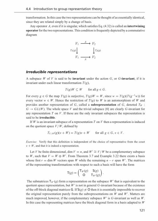
4.4 Introduction to group representation theory

transformation. In this case the two representations can be thought of as essentially identical,since they are related simply by a change of basis.

Any operator A, even if it is singular, which satisfies Eq. (4.32) is called an intertwiningoperator for the two representations. This condition is frequently depicted by a commutativediagram

A

T2(g)T1(g)

AV2

V2

V1

V1

Irreducible representations

A subspace W of V is said to be invariant under the action G, or G-invariant, if it isinvariant under each linear transformation T (g),

T (g)W ⊆ W for all g ∈ G.

For every g ∈ G the map T (g) is surjective, T (g)W = W , since w = T (g)(T (g−1w)) forevery vector w ∈ W . Hence the restriction of T (g) to W is an automorphism of W andprovides another representation of G, called a subrepresentation of G, denoted TW :G → GL(W ). The whole space V and the trivial subspace {0} are clearly G-invariant forany representation T on V . If these are the only invariant subspaces the representation issaid to be irreducible.

If W is an invariant subspace of a representation T on V then a representation is inducedon the quotient space V/W , defined by

TV/W (g)(v +W ) = T (g)v +W for all g ∈ G, v ∈ V .

Exercise: Verify that this definition is independent of the choice of representative from the cosetv +W , and that it is indeed a representation.

Let V be finite dimensional, dim V = n, and W ′ ∼= V/W be a complementary subspaceto W , such that V = W ⊕W ′. From Theorem 3.7 and Example 3.22 there exists a basiswhose first r = dim W vectors span W while the remaining n − r span W ′. The matricesof the representing transformations with respect to such a basis will have the form

T(g) =(

TW (g) S(g)O TW ′ (g)

).

The submatrices TW ′ (g) form a representation on the subspace W ′ that is equivalent to thequotient space representation, but W ′ is not in general G-invariant because of the existenceof the off-block diagonal matrices G. If S(g) �= O then it is essentially impossible to recoverthe original representation purely from the subrepresentations on W and W ′. Matters aremuch improved, however, if the complementary subspace W ′ is G-invariant as well as W .In this case the representing matrices have the block diagonal form in a basis adapted to W

121

Linear operators and matrices

and W ′,

T(g) =(

TW (g) OO TW ′ (g)

)and the representation is said to be completely reducible.

Example 4.7 Let the map T : R → GL(R2) be defined by

T : a �→ T(a) =(

1 a0 1

).

This is a representation since T(a)T(b) = T(a + b). The subspace of vectors of the form(x0

)is invariant, but there is no complementary invariant subspace – for example, vectors

of the form

(0y

)are not invariant under the matrices T(a). Equivalently, it follows from

the Jordan canonical form that no matrix A exists such that AT(1)A−1 is diagonal. Therepresentation T is thus an example of a representation that is reducible but not completelyreducible.

Example 4.8 The symmetric group of permutations on three objects, denoted S3, has arepresentation T on a three-dimensional vector space V spanned by vectors e1, e2 and e3,defined by

T (π)ei = eπ (i).

In this basis the matrix of the transformation T (π ) is T = [T ji (π )], where

T (π)ei = T ji (π )e j .

Using cyclic notation for permutations the elements of S3 are e = id, π1 = (1 2 3), π2 =(1 3 2), π3 = (1 2), π4 = (2 3), π5 = (1 3). Then T (e)ei = ei , so that T(e) is the identitymatrix I, while T (π1)e1 = e2, T (π1)e2 = e3, T (π1)e3 = e1, etc. The matrix representa-tions of all permutations of S3 are

T(e) =⎛⎝1 0 0

0 1 00 0 1

⎞⎠ , T(π1) =⎛⎝0 0 1

1 0 00 1 0

⎞⎠ , T(π2) =⎛⎝0 1 0

0 0 11 0 0

⎞⎠ ,

T(π3) =⎛⎝0 1 0

1 0 00 0 1

⎞⎠ , T(π4) =⎛⎝1 0 0

0 0 10 1 0

⎞⎠ , T(π5) =⎛⎝0 0 1

0 1 01 0 0

⎞⎠ .Let v = vi ei be any vector, then T (π)v = T j

i (π )vi e j and the action of the matrix T(π ) isleft multiplication on the column vector

v =⎛⎝v1

v2

v3

⎞⎠ .122

4.4 Introduction to group representation theory

We now find the invariant subspaces of this representation. In the first place any one-dimensional invariant subspace must be spanned by a vector v that is an eigenvector of eachoperator T (πi ). In matrices,

T(π1)v = αv =⇒ v1 = αv2, v2 = αv3, v3 = αv1,

whence

v1 = αv2 = α2v3 = α3v1.

Similarly v2 = α3v2 and v3 = α3v3, and since v �= 0 we must have thatα3 = 1. Sinceα �= 0it follows that all three components v1, v2 and v3 are non-vanishing. A similar argumentgives

T(π3)v = βv =⇒ v1 = βv2, v2 = βv1, v3 = βv3,

from whichβ2 = 1, andαβ = 1 since v1 = αv2 = αβv1. The only pair of complex numbersα and β satisfying these relations is α = β = 1. Hence v1 = v2 = v3 and the only one-dimensional invariant subspace is that spanned by v = e1 + e2 + e3.

We shall now show that this representation is completely reducible by choosing thebasis

f1 = e1 + e2 + e3, f2 = e1 − e2, f3 = e1 + e2 − 2e3.

The inverse transformation is

e1 = 1

3f1 + 1

2f2 + 1

6f3, e2 = 1

3f1 − 1

2f2 + 1

6f3, e3 = 1

3f1 − 1

3f3,

and the matrices representing the elements of S3 are found by calculating the effect of thevarious transformations on the basis elements fi . For example,

T (e) f1 = f1, T (e) f2 = f2, T (e) f3 = f3,

T (π1) f1 = T (π1)(e1 + e2 + e3)

= e2 + e3 + e1 = f1,

T (π1) f2 = T (π1)(e1 − e2)

= e2 − e3 = 1

2f2 + 1

2f3,

T (π1) f3 = T (π1)(e1 + e2 − 2e3)

= e2 + e3 − 2e1 = −3

2f2 − 1

2 f3, etc.

Continuing in this way for all T (πi ) we arrive at the following matrices:

T(e) =⎛⎝1 0 0

0 1 00 0 1

⎞⎠ , T(π1) =⎛⎝1 0 0

0 − 12 − 3

20 1

2 − 12

⎞⎠ , T(π2) =⎛⎝1 0 0

0 − 12

32

0 − 12 − 1

2

⎞⎠ ,T(π3) =

⎛⎝1 0 00 −1 00 0 1

⎞⎠ , T(π4) =⎛⎝1 0 0

0 12

32

0 12 − 1

2

⎞⎠ , T(π5) =⎛⎝1 0 0

0 12 − 3

20 − 1

2 − 12

⎞⎠ .123

Linear operators and matrices

The two-dimensional subspace spanned by f2 and f3 is thus invariant under the action ofS3 and the representation T is completely reducible.

Exercise: Show that the representation T restricted to the subspace spanned by f2 and f3 is irreducible,by showing that there is no invariant one-dimensional subspace spanned by f2 and f3.

Schur’s lemma

The following key result and its corollary are useful in the classification of irreduciblerepresentations of groups.

Theorem 4.6 (Schur’s lemma) Let T1 : G → GL(V1) and T2 : G → GL(V2) be two ir-reducible representations of a group G, and A : V1 → V2 an intertwining operator suchthat

T2(g)A = AT1(g) for all g ∈ G.

Then either A = 0 or A is an isomorphism, in which case the two representations areequivalent, T1 ∼ T2.

Proof : Let v ∈ ker A ⊆ V1. Then

AT1(g)v = T2(g)Av = 0

so that T1(g)v ∈ ker A. Hence ker A is an invariant subspace of the representation T1. AsT1 is an irreducible representation we have that either ker A = V1, in which case A = 0,or ker A = {0}. In the latter case A is one-to-one. To show it is an isomorphism it is onlynecessary to show that it is onto. This follows from the fact that im A ⊂ V2 is an invariantsubspace of the representation T2,

T2(g)(im A) = T2(g)A(V1) = AT1(g)(V1) ⊆ A(V1) = im A.

Since T2 is an irreducible representation we have either im A = {0} or im A = V2. In thefirst case A = 0, while in the second A is onto. Schur’s lemma is proved. �

Corollary 4.7 Let T : G → GL(V ) be a representation of a finite group G on a complexvector space V and A : V → V an operator that commutes with all T (g); that is, AT (g) =T (g)A for all g ∈ G. Then A = αidV for some complex scalar α.

Proof : Set V1 = V2 = V and T1 = T2 = T in Schur’s lemma. Since AT (g) = T (g)A wehave

(A − αidV )T (g) = T (g)(A − αidV )

since idV commutes with all linear operators on V . By Theorem 4.6 either A − αidV isinvertible or it is zero. Let α be an eigenvalue of A – for operators on a complex vectorspace this is always possible. The operator A − αidV is not invertible, for if it is applied to acorresponding eigenvector the result is the zero vector. Hence A − αidV = 0, which is thedesired result. �

124

References

It should be observed that the proof of this corollary only holds for complex representa-tions since real matrices do not necessarily have any real eigenvalues.

Example 4.9 If G is a finite abelian group then all its irreducible representations are one-dimensional. This follows from Corollary 4.7, for if T : G → GL(V ) is any representationof G then any T (h) (h ∈ G) commutes with all T (g) and is therefore a multiple of theidentity,

T (h) = α(h)idV .

Hence any vector v ∈ V is an eigenvector of T (h) for all h ∈ G and spans an invariant one-dimensional subspace of V . Thus, if dim V > 1 the representation T cannot be irreducible.

References

[1] P. R. Halmos. Finite-dimensional Vector Spaces. New York, D. Van Nostrand Company,1958.

[2] S. Hassani. Foundations of Mathematical Physics. Boston, Allyn and Bacon, 1991.[3] F. P. Hildebrand. Methods of Applied Mathematics. Englewood Cliffs, N. J., Prentice-

Hall, 1965.[4] L. S. Pontryagin. Ordinary Differential Equations. New York, Addison-Wesley, 1962.[5] D. A. Sanchez. Ordinary Differential Equations and Stability Theory: An Introduction.

San Francisco, W. H. Freeman and Co., 1968.[6] S. Lang. Algebra. Reading, Mass., Addison-Wesley, 1965.[7] M. Hammermesh. Group Theory and its Applications to Physical Problems. Reading,

Mass., Addison-Wesley, 1962.[8] S. Sternberg. Group Theory and Physics. Cambridge, Cambridge University Press, 1994.

125

5 Inner product spaces

In matrix theory it is common to say that a matrix is symmetric if it is equal to its transpose,ST = S. This concept does not however transfer meaningfully to the matrix of a linearoperator on a vector space unless some extra structure is imposed on that space. For example,let S : V → V be an operator whose matrix S = [Si

j ] is symmetric with respect to a specific

basis. Under a change of basis ei = A ji e′j the transformed matrix is S′ = ASA−1, while for

the transpose matrix

S′T = (ASA−1)T = (A−1)T SAT .

Hence S′T �= S′ in general. We should hardly be surprised by this conclusion for, as com-mented at the beginning of Chapter 4, the component equation Si

j = S ji violates the index

conventions of Section 3.6.

Exercise: Show that S′ is symmetric if and only if S commutes with AT A,

SAT A = AT AS.

Thus the concept of a ‘symmetric operator’ is not invariant under general basis transformations, butit is invariant with respect to orthogonal basis transformations, AT = A−1.

If V is a complex vector space it is similarly meaningless to talk of an operator H : V →V as being ‘hermitian’ if its matrix H with respect to some basis {ei } is hermitian, H = H†.

Exercise: Show that the hermitian property is not in general basis invariant, but is preserved underunitary transformations, ei = U j

i e′j where U−1 = U†.

In this chapter we shall see that symmetric and hermitian matrices play a different rolein vector space theory, in that they represent inner products instead of operators [1–3].Matrices representing inner products are best written with both indices on the subscriptlevel, G = GT = [gi j ] and H = H† = [hi j ]. The requirements of symmetry g ji = gi j andhermiticity hji = hi j are not then at odds with the index conventions.

5.1 Real inner product spaces

Let V be a real finite dimensional vector space with dim V = n. A real inner product,often referred to simply as an inner product when there is no danger of confusion, on the

126

5.1 Real inner product spaces

vector space V is a map V × V → R that assigns a real number u · v ∈ R to every pair ofvectors u, v ∈ V satisfying the following three conditions:

(RIP1) The map is symmetric in both arguments, u · v = v · u.(RIP2) The distributive law holds, u · (av + bw) = au · v + bu · w .(RIP3) If u · v = 0 for all v ∈ V then u = 0.

A real vector space V together with an inner product defined on it is called a real innerproduct space. The inner product is also distributive on the first argument for, by conditions(RIP1) and (RIP2),

(au + bv) · w = w · (au + bv) = aw · u + bw · v = au · w + bv · w .We often refer to this linearity in both arguments by saying that the inner product is bilinear.

As a consequence of property (RIP3) the inner product is said to be non-singular andis often referred to as pseudo-Euclidean. Sometimes (RIP3) is replaced by the strongercondition

(RIP3′) u · u > 0 for all vectors u �= 0.

In this case the inner product is said to be positive definite or Euclidean, and a vector spaceV with such an inner product defined on it is called a Euclidean vector space. Condition(RIP3′) implies condition (RIP3), for if there exists a non-zero vector u such that u · v = 0for all v ∈ V then u · u = 0 (on setting v = u), which violates (RIP3′). Positive definitenessis therefore a stronger requirement than non-singularity.

Example 5.1 The space of ordinary 3-vectors a,b, etc. is a Euclidean vector space, oftendenoted E3, with respect to the usual scalar product

a · b = a1b1 + a2b2 + a3b3 = |a| |b| cos θ

where |a| is the length or magnitude of the vector a and θ is the angle between a and b.Conditions (RIP1) and (RIP2) are simple to verify, while (RIP3′) follows from

a · a = a2 = (a1)2 + (a2)2 + (a3)2 > 0 if a �= 0.

This generalizes to a positive definite inner product on Rn ,

a · b = a1b1 + a2b2 + · · · + anbn =n∑

i=1

ai bi ,

the resulting Euclidean vector space denoted by En .

The magnitude of a vector w is defined as w · w . Note that in a pseudo-Euclidean spacethe magnitude of a non-vanishing vector may be negative or zero, but in a Euclidean spaceit is always a positive quantity. The length of a vector in a Euclidean space is defined to bethe square root of the magnitude.

Two vectors u and v are said to be orthogonal if u · v = 0. By requirement (RIP3) thereis no non-zero vector u that is orthogonal to every vector in V . A pseudo-Euclidean innerproduct may allow for the existence of self-orthogonal or null vectors u �= 0 having zeromagnitude u · u = 0, but this possibility is clearly ruled out in a Euclidean vector space.

127

Inner product spaces

In Chapter 9 we shall see that Einstein’s special theory of relativity postulates a pseudo-Euclidean structure for space-time known as Minkowski space, in which null vectors playa significant role.

Components of a real inner product

Given a basis {e1, . . . , en} of an inner product space V , set

gi j = ei · e j = g ji , (5.1)

called the components of the inner product with respect to the basis {ei }. The innerproduct is completely specified by the components of the symmetric matrix, for if u =ui ei , v = v j e j are any pair of vectors then, on using (RIP1) and (RIP2), we have

u · v = gi j ui v j . (5.2)

If we write the components of the inner product as a symmetric matrix

G = [gi j ] = [ei · e j ] = [e j · ei ] = [g ji ] = GT ,

and display the components of the vectors u and v in column form as u = [ui ] and v = [v j ],then the inner product can be written in matrix notation,

u · v = uT Gv.

Theorem 5.1 The matrix G is non-singular if and only if condition (RIP3) holds.

Proof : To prove the if part, assume that G is singular, det[gi j ] = 0. Then there exists anon-trivial solution u j to the linear system of equations

gi j uj ≡

n∑j=1

gi j uj = 0.

The vector u = u j e j is non-zero and orthogonal to all v = vi ei ,

u · v = g(u, v) = gi j uiv j = 0,

in contradiction to (RIP3).Conversely, assume the matrix G is non-singular and that there exists a vector u violating

(RIP3); u �= 0 and u · v = 0 for all v ∈ V . Then, by Eq. (5.2), we have

u jvj = 0 where u j = gi j u

i = g ji ui

for arbitrary values of v j . Hence u j = 0 for j = 1, . . . , n. However, this implies a non-trivialsolution to the set of linear equations g ji ui = 0, which is contrary to the non-singularityassumption, det[gi j ] �= 0. �

Orthonormal bases

Under a change of basis

ei = A ji e′j , e′j = A′kj ek, (5.3)

128

5.1 Real inner product spaces

the components gi j transform by

gi j = ei · e j = (Aki e′k) · (Al

j e′l)

= Aki g′kl Al

j ,(5.4)

where g′kl = e′k · e′l . In matrix notation this equation reads

G = AT G′ A. (5.5)

Using A′ = [A′ jk] = A−1, the transformed matrix G′ can be written

G′ = A′T G A′. (5.6)

An orthonormal basis {e1, e2, . . . , en}, for brevity written ‘o.n. basis’, consists ofvectors all of magnitude ±1 and orthogonal to each other in pairs,

gi j = ei · e j = ηiδi j where ηi = ±1, (5.7)

where the summation convention is temporarily suspended. We occasionally do this whena relation is referred to a specific class of bases.

Theorem 5.2 In any finite dimensional real inner product space (V, ·), with dim V = n,there exists an orthonormal basis {e1, e2, . . . , en} satisfying Eq. (5.7).

Proof : The method is by a procedure called Gram–Schmidt orthonormalization,an algorithmic process for constructing an o.n. basis starting from any arbitrary basis{u1, u2, . . . , un}. For Euclidean inner products the procedure is relatively straightforward,but the possibility of vectors having zero magnitudes in general pseudo-Euclidean spacesmakes for added complications.

Begin by choosing a vector u such that u · u �= 0. This is always possible because ifu · u = 0 for all u ∈ V , then for any pair of vectors u, v

0 = (u + v) · (u + v) = u · u + 2u · v + v · v = 2u · v,which contradicts the non-singularity condition (RIP3). For the first step of the Gram–Schmidt procedure we normalize this vector,

e1 = u√|u · u)| and η1 = e1 · e1 = ±1.

In the Euclidean case any non-zero vector u will do for this first step, and e1 · e1 = 1.Let V1 be the subspace of V consisting of vectors orthogonal to e1,

V1 = {w ∈ V |w · e1 = 0}.This is a vector subspace, for if w and w ′ are orthogonal to e1 then so is any linear combi-nation of the form w + aw ′,

(w + aw ′) · e1 = w · e1 + aw ′ · e1 = 0.

For any v ∈ V , the vector v′ = v − ae1 ∈ V1 where a = η1(v · e1), since v′ · e1 = v · e1 −(η1)2v · e1 = 0. Furthermore, the decomposition v = a e1 + v′ into a component parallel

129

Inner product spaces

to e1 and a vector orthogonal to e1 is unique, for if v = a′ e1 + v′′ where v′′ ∈ V1 then

(a′ − a)e1 = v′′ − v′.Taking the inner product of both sides with e1 gives firstly a′ = a, and consequently v′′ = v′.

The inner product restricted to V1, as a map V1 × V1 → R, is an inner product on thevector subspace V1. Conditions (RIP1) and (RIP2) are trivially satisfied if the vectors u,v and w are restricted to vectors belonging to V1. To show (RIP3), that this inner productis non-singular, let v′ ∈ V1 be a vector such that v′ · w ′ = 0 for all w ′ ∈ V1. Then v′ isorthogonal to every vector in w ∈ V for, by the decomposition

w = η1(w · e1)e1 + w ′,

we have v′ · w = 0. By condition (RIP3) for the inner product on V this implies v′ = 0, asrequired.

Repeating the above argument, there exists a vector u′ ∈ V1 such that u′ · u′ �= 0. Set

e2 = u′√|u′ · u′|and η2 = e2 · e2 = ±1. Clearly e2 · e1 = 0 since e2 ∈ V1. Defining the subspace V2 of vec-tors orthogonal to e1 and e2, the above argument can be used again to show that the re-striction of the inner product to V2 satisfies (RIP1)–(RIP3). Continue this procedure until northonormal vectors {e1, e2, . . . , en} have been produced. These vectors must be linearlyindependent, for if there were a vanishing linear combination ai ei = 0, then performing theinner product of this equation with any e j gives a j = 0. By Theorem 3.3 these vectors forma basis of V . At this stage of the orthonormalization process Vn = {0}, as there can be novector that is orthogonal to every e1, . . . , en , and the procedure comes to an end. �

The following theorem shows that for a fixed inner product space, apart from the orderin which they appear, the coefficients ηi are the same in all orthonormal frames.

Theorem 5.3 (Sylvester) The number of + and − signs among the ηi is independent ofthe choice of orthonormal basis.

Proof : Let {ei } and { f j } be two orthonormal bases such that

e1 · e1 = · · · = er · er = +1, er+1 · er+1 = · · · = en · en = −1,

f1 · f1 = · · · = fs · fs = +1, fs+1 · fs+1 = · · · = fn · fn = −1.

If s > r then the vectors f1, . . . , fs and er+1, . . . , en are a set of s + n − r > n = dim Vvectors and there must be a non-trivial linear relation between them,

a1 f1 + · · · + as fs + b1er+1 + · · · + bn−r en = 0.

The ai cannot all vanish since the ei form an l.i. set. Similarly, not all the b j will vanish.Setting

u = a1 f1 + · · · + as fs = −b1er+1 − · · · − bn−r en �= 0

130

5.1 Real inner product spaces

we have the contradiction

u · u =s∑

i=1

(ai )2 > 0 and u · u = −n−r∑j=1

(b j )2 < 0.

Hence r = s and the two bases must have exactly the same number of + and − signs. �

If r is the number of + signs and s the number of − signs then their difference r − sis called the index of the inner product. Sylvester’s theorem shows that it is an invariantof the inner product space, independent of the choice of o.n. basis. For a Euclidean innerproduct, r − s = n, although the word ‘Euclidean’ is also applied to the negative definitecase, r − s = −n. If r − s = ±(n − 2), the inner product is called Minkowskian.

Example 5.2 In a Euclidean space the Gram–Schmidt procedure is carried out as follows:

f1 = u1 e1 = f1√f1 · f1

η1 = e1 · e1 = 1,

f2 = u2 − (e1 · u2)e1 e2 = f2√f2 · f2

η2 = e2 · e2 = 1,

f3 = u3 − (e1 · u3)e1 − (e2 · u3)e2 e3 = f3√f3 · f3

η3 = e3 · e3 = 1, etc.

Since each vector has positive magnitude, all denominators√

fi · fi > 0, and each step iswell-defined. Each vector ei is a unit vector and is orthogonal to each previous e j ( j < i).

Example 5.3 Consider an inner product on a three-dimensional space having componentsin a basis u1, u2, u3

G = [gi j ] = [ui · u j ] =⎛⎝0 1 1

1 0 11 1 0

⎞⎠ .The procedure given in Example 5.2 obviously fails as each basis vector is a null vector,u1 · u1 = u2 · u2 = u3 · u3 = 0, and cannot be normalized to a unit vector.

Firstly, we find a vector u such that u · u �= 0. Any vector of the form u = u1 + au2 witha �= 0 will do, since

u · u = u1 · u1 + 2au1 · u2 + u2 · u2 = 2a.

Setting a = 1 gives u = u1 + u2 and u · u = 2. The first step in the orthonormalizationprocess is then

e1 = 1√2

(u1 + u2), η1 = e1 · e1 = 1.

There is of course a significant element of arbitrariness in this as the choice of u is by nomeans unique; for example, choosing a = 1

2 leads to e1 = u1 + 12 u2.

The subspace V1 of vectors orthogonal to e1 consists of vectors of the form v = au1 +bu2 + cu3 such that

v · e1 ∝ v · u = (au1 + bu2 + cu3) · (u1 + u2) = a + b + 2c = 0.

131

Inner product spaces

Setting, for example, c = 0 and a = −b = 1 results in v = u1 − u2. The magnitude of v isv · v = −2 and normalizing gives

e2 = 1√2

(u1 − u2), η2 = e2 · e2 = −1, e2 · e1 = 0.

Finally, we need a vector w = au1 + bu2 + cu3 that is orthogonal to both e1 and e2. Thesetwo requirements imply that a = b = −c, and setting c = 1 results in w = u1 + u2 − u3.Normalizing w results in

w · w = (u1 + u2 − u3) · (u1 + u2 − u3) = −2

=⇒ e3 = 1√2

(u1 + u2 − u3), η3 = e3 · e3 = −1.

The components of the inner product in this o.n. basis are therefore

G′ = [g′i j ] = [ei · e j ] =

⎛⎜⎝1 0 0

0 −1 00 0 −1

⎞⎟⎠ .The index of the inner product is 1− 2 = −1.

Any pair of orthonormal bases {ei } and {e′i } are connected by a basis transformation

ei = L ji e′j ,

such that

gi j = ei · e j = e′i · e′j = g′i j = diag(η1, . . . , ηn) .

From Eq. (5.4) we have

gi j = gkl Lki Ll

j , (5.8)

or its matrix equivalent

G = LT GL . (5.9)

For a Euclidean metric G = I, and L is an orthogonal transformation, while for aMinkoswkian metric with n = 4 the transformations are Lorentz transformations discussedin Section 2.7. As was shown in Chapter 2, these transformations form the groups O(n)and O(3, 1) respectively. The general pseudo-orthogonal inner product results in a groupO(p, q) of pseudo-orthogonal transformations of type (p, q).

Problems

Problem 5.1 Let (V, ·) be a real Euclidean inner product space and denote the length of a vectorx ∈ V by |x | = √x · x . Show that two vectors u and v are orthogonal iff |u + v|2 = |u|2 + |v|2.

132

5.2 Complex inner product spaces

Problem 5.2 Let

G = [gi j ] = [ui · u j ] =

⎛⎜⎝0 1 01 0 −10 −1 1

⎞⎟⎠be the components of a real inner product with respect to a basis u1, u2, u3. Use Gram–Schmidtorthogonalization to find an orthonormal basis e1, e2, e3, expressed in terms of the vectors ui , andfind the index of this inner product.

Problem 5.3 Let G be the symmetric matrix of components of a real inner product with respect toa basis u1, u2, u3,

G = [gi j ] = [ui · u j ] =

⎛⎜⎝1 0 10 −2 11 1 0

⎞⎟⎠ .Using Gram–Schmidt orthogonalization, find an orthonormal basis e1, e2, e3 expressed in terms ofthe vectors ui .

Problem 5.4 Define the concept of a ‘symmetric operator’ S : V → V as one that satisfies

(Su) · v = u · (Sv) for all u, v ∈ V .

Show that this results in the component equation

Ski gk j = gik Sk

j ,

equivalent to the matrix equation

ST G = GS.

Show that for an orthonormal basis in a Euclidean space this results in the usual notion of symmetry,but fails for pseudo-Euclidean spaces.

Problem 5.5 Let V be a Minkowskian vector space of dimension n with index n − 2 and let k �= 0be a null vector (k · k = 0) in V .

(a) Show that there is an orthonormal basis e1, . . . , en such that

k = e1 − en .

(b) Show that if u is a ‘timelike’ vector, defined as a vector with negative magnitude u · u < 0, thenu is not orthogonal to k.

(c) Show that if v is a null vector such that v · k = 0, then v ∝ k.(d) If n ≥ 4 which of these statements generalize to a space of index n − 4?

5.2 Complex inner product spaces

We now consider a complex vector space V , which in the first instance may be infinitedimensional. Vectors will continue to be denoted by lower case Roman letters such as u andv, but complex scalars will be denoted by Greek letters such as α, β, . . . from the early partof the alphabet. The word inner product, or scalar product, on a complex vector space

133

Inner product spaces

V will be reserved for a map V × V → C that assigns to every pair of vectors u, v ∈ V acomplex scalar 〈u |v〉 satisfying

(IP1) 〈u |v〉 = 〈v |u〉.(IP2) 〈u |αv + βw〉 = α〈u |v〉 + β〈u |w〉 for all complex numbers α, β.(IP3) 〈u |u〉 ≥ 0 and 〈u |u〉 = 0 iff u = 0.

The condition (IP1) implies 〈u |u〉 is always real, a necessary condition for (IP3) to makeany sense. From (IP1) and (IP2)

〈αv + βw |u〉 = 〈u |αv + βw〉= α〈u |v〉 + β〈u |w〉= α〈u |v〉 + β 〈w |v〉,

so that

〈αv + βw |u〉 = α〈v |u〉 + β〈w |u〉. (5.10)

This property is often described by saying that the inner product is antilinear with respectto the first argument.

A complex vector space with an inner product will simply be called an inner productspace. If V is finite dimensional it is often called a finite dimensional Hilbert space, butfor infinite dimensional spaces the term Hilbert space only applies if the space is complete(see Chapter 13).

Mathematicians more commonly adopt a notation (u, v) in place of our angular bracketnotation, and demand linearity in the first argument, with antilinearity in the second. Ourconventions follow that which is most popular with physicists and takes its origins in Dirac’s‘bra’ and ‘ket’ terminology for quantum mechanics (see Chapter 14).

Example 5.4 On Cn set

〈(α1, . . . , αn) | (β1, . . . , βn)〉 =n∑

i=1

αiβi .

Conditions (IP1)–(IP3) are easily verified. We shall see directly that this is the archetypalfinite dimensional inner product space. Every finite dimensional inner product space has abasis such that the inner product takes this form.

Example 5.5 A complex-valued function ϕ : [0, 1] → C is said to be continuous if boththe real and imaginary parts of the functionϕ(x) = f (x)+ ig(x) are continuous. Let C[0, 1]be the set of continuous complex-valued functions on the real line interval [0, 1], and definean inner product

〈ϕ |ψ〉 =∫ 1

0ϕ(x)ψ(x) dx.

Conditions (IP1) and (IP2) are simple to prove, but in order to show (IP3) it is necessary toshow that ∫ 1

0| f (x)|2 + |g(x)|2 dx = 0 =⇒ f (x) = g(x) = 0, ∀x ∈ [0, 1].

134

5.2 Complex inner product spaces

If f (a) �= 0 for some 0 ≤ a ≤ 1 then, by continuity, there exists an interval [a − ε, a] or aninterval [a, a + ε] on which | f (x)| > 1

2 | f (a)|. Then∫ 1

0|ϕ(x)|2 dx > 1

2ε| f (a)|2 +∫ 1

0|g(x)|2 dx > 0.

Hence f (x) = 0 for all x ∈ [0, 1]. The proof that g(x) = 0 is essentially identical.

Example 5.6 A complex-valued function on the real line, ϕ : R → C, is said to be squareintegrable if |ϕ|2 is an integrable function on any closed interval of R and

∫∞−∞ |ϕ(x)|2dx

<∞. The set L2(R) of square integrable complex-valued functions on the real line is acomplex vector space, for if α is a complex constant and ϕ and ψ are any pair of squareintegrable functions, then∫ ∞

−∞|ϕ(x)+ αψ(x)|2 dx ≤

∫ ∞

−∞|ϕ(x)|2 dx + |α|2

∫ ∞

−∞|ψ(x)|2 dx <∞.

On L2(R) define the inner product

〈ϕ |ψ〉 =∫ ∞

−∞ϕ(x)ψ(x) dx .

This is well-defined for any pair of square integrable functions ϕ and ψ for, after somealgebraic manipulation, we find that

ϕψ = 12

(|ϕ + ψ |2 − i |ϕ + iψ |2 − (1− i)(|ϕ|2 + |ψ |2)).

Hence the integral of the left-hand side is equal to a sum of integrals on the right-hand side,each of which has been shown to exist.

The properties (IP1) and (IP2) are trivial to show but the proof of (IP3) along the linesgiven in Example 5.5 will not suffice here since we do not stipulate continuity for thefunctions in L2(R). For example, the function f (x) defined by f (x) = 0 for all x �= 0 andf (0) = 1 is a positive non-zero function whose integral vanishes. The remedy is to ‘identify’any two real functions f and g having the property that

∫∞−∞ | f (x)− g(x)|2dx = 0. Such a

pair of functions will be said to be equal almost everywhere, and L2(R) must be interpretedas consisting of equivalence classes of complex-valued functions whose real and imaginaryparts are equal almost everywhere. A more complete discussion will be given in Chapter13, Example 13.4.

Exercise: Show that the relation f ≡ g iff∫∞−∞ | f (x)− g(x)|2dx = 0 is an equivalence relation on

L2(R).

Norm of a vector

The norm of a vector u in an inner product space, denoted ‖u‖, is defined to be the non-negative real number

‖u‖ =√〈u |u〉 ≥ 0. (5.11)

135

Inner product spaces

From (IP2) and Eq. (5.10) it follows immediately that

‖αu‖ = |α| ‖u‖. (5.12)

Theorem 5.4 (Cauchy–Schwarz inequality) For any pair of vectors u, v in an innerproduct space

|〈u |v〉| ≤ ‖u‖ ‖v‖. (5.13)

Proof : By (IP3), (IP2) and Eq. (5.10) we have for all λ ∈ C

0 ≤ 〈u + λv |u + λv〉= 〈u |u〉 + λ〈u |v〉 + λ〈v |u〉 + λλ〈v |v〉.

Substituting the particular value

λ = −〈v |u〉〈v |v〉gives the inequality

0 ≤ 〈u |u〉 − 〈v |u〉〈u |v〉〈v |v〉 − 〈v |u〉〈v |u〉〈v |v〉 + |〈v |u〉|2

〈v |v〉

= 〈u |u〉 − |〈v |u〉|2

〈v |v〉 .

Hence, from (IP1),

|〈u |v〉|2 = |〈v |u〉|2 ≥ 〈u |u〉〈v |v〉and the desired result follows from (5.11) on taking the square roots of both sides of thisinequality. �

Corollary 5.5 Equality in (5.13) can only result if u and v are proportional to each other,

|〈u |v〉| = ‖u‖ ‖v‖ ⇐⇒ u = αv, for some α ∈ C.

Proof : If u = αv then from (5.11) and (5.12) we have

|〈u |v〉| = |〈αv |v〉| = |α|〈v |v〉 = ‖αv‖‖v‖ = ‖u‖‖v‖.Conversely, if |〈u |v〉| = ‖u‖ ‖v‖ then,

|〈u |v〉|2 = ‖u‖2 ‖v‖2

and reversing the steps in the proof of Lemma 5.4 with inequalities replaced by equalitiesgives

〈u + λv |u + λv〉 = 0 where λ = −〈v |u〉〈v |v〉 .

By (IP3) we conclude that u = −λv and the proposition follows with α = −λ. �

136

5.2 Complex inner product spaces

Theorem 5.6 (Triangle inequality) For any pair of vectors u and v in an inner productspace,

‖u + v‖ ≤ ‖u‖ + ‖v‖. (5.14)

Proof :(‖u + v‖)2 = 〈u + v |u + v〉

= 〈u |u〉 + 〈v |v〉 + 〈v |u〉 + 〈u |v〉= ‖u‖2 + ‖v‖2 + 2Re(〈u |v〉)≤ ‖u‖2 + ‖v‖2 + 2|〈u |v〉|≤ ‖u‖2 + ‖v‖2 + 2‖u‖‖v‖ by Eq. (5.13)= (‖u‖ + ‖v‖)2 .

The triangle inequality (5.14) follows on taking square roots. �

Orthonormal bases

Let V be a finite dimensional inner product space with basis e1, e2, . . . , en . Define thecomponents of the inner product with respect to this basis to be

hi j = 〈ei |e j 〉 = 〈e j |ei 〉 = h ji . (5.15)

The matrix of components H = [hi j ] is clearly hermitian,

H = H† where H† = HT.

Under a change of basis (5.3) we have

〈ei |e j 〉 = Aki 〈e′k |e′m〉Am

j

and the components of the inner product transform as

hi j = Aki h′km Am

j . (5.16)

An identical argument can be used to express the primed components in terms of unprimedcomponents,

h′i j = 〈e′i |e′j 〉 = A′ki hkm A′mj . (5.17)

These equations have matrix equivalents,

H = A†H′A, H′ = A′†HA′, (5.18)

where A′ = A−1.

Exercise: Show that the hermitian nature of the matrix H is unchanged by a transformation (5.18).

Two vectors u and v are said to be orthogonal if 〈u |v〉 = 0. A basis e1, e2, . . . , en iscalled an orthonormal basis if the vectors all have unit norm and are orthogonal to each

137

Inner product spaces

other,

〈ei |e j 〉 = δi j ={

1 if i = j,

0 if i �= j.

Equivalently, a basis is orthonormal if the matrix of components of the inner product withrespect to the basis is the unit matrix, H = I.

Starting with an arbitrary basis {u1, u2, . . . , un}, it is always possible to construct anorthonormal basis by a process known as Schmidt orthonormalization, which closelymirrors the Gram–Schmidt process for Euclidean inner products, outlined in Example 5.2.Sequentially, the steps are:

1. Set f1 = u1, then e1 = f1

‖ f1‖ .

2. Set f2 = u2 − 〈e1 |u2〉e1, which is orthogonal to e1 since

〈e1 | f2〉 = 〈e1 |u2〉 − 〈e1 |u2〉‖e1‖ = 0.

Normalize f2 by setting e2 = f2/‖ f2‖.3. Set f3 = u3 − 〈e1 |u3〉e1 − 〈e2 |u3〉e2, which is orthogonal to both e1 and e2. Normalize

to give e3 = f3

‖ f3‖ .

4. Continue in this way until

fn = un −n−1∑i=1

〈ei |un〉ei and en = fn

‖ fn‖ .

Since each vector ei is a unit vector and is orthogonal to all the e j for j < i defined byprevious steps, they form an o.n. set. It is easily seen that any vector v = vi ui of V is alinear combination of the ei since each u j is a linear combination of e1, . . . , e j . Hence thevectors {ei } form a basis by Theorem 3.3 since they span V and are n in number.

With respect to an orthonormal basis the inner product of any pair of vectors u = ui ei

and v = v j e j is given by

〈u |v〉 = 〈ui ei |v j e j 〉 = uiv j 〈ei |e j 〉 = uiv jδi j .

Hence

〈u |v〉n∑

i=1

uivi = u1v1 + u2v2 + · · · + unvn,

which is equivalent to the standard inner product defined on Cn in Example 5.4.

Example 5.7 Let an inner product have the following components in a basis u1, u2, u3:

h11 = 〈u1 |u1〉 = 1 h12 = 〈u1 |u2〉 = 0 h13 = 〈u1 |u3〉 = 12 (1+ i)

h21 = 〈u2 |u1〉 = 0 h22 = 〈u2 |u2〉 = 2 h23 = 〈u2 |u3〉 = 0

h31 = 〈u3 |u1〉 = 12 (1− i) h32 = 〈u3 |u2〉 = 0 h33 = 〈u3 |u3〉 = 1.

Before proceeding it is important to realize that this inner product does in fact sat-isfy the positive definite condition (IP3). This would not be true, for example, if we had

138

5.2 Complex inner product spaces

given h13 = h31 = 1+ i , for then the vector v = u1 − 1− i√2

u3 would have negative norm

〈v |v〉 = 2(1−√2) < 0.In the above inner product, begin by setting e1 = f1 = u1. The next vector is

f2 = u2 − 〈e1 |u2〉e1 = u2, e2 = u2

‖u2‖ =1√2

u2.

The last step is to set

f3 = u3 − 〈e1 |u3〉e1 − 〈e2 |u3〉e2 = u3 − 12 (1+ i)u1

which has norm squared

(‖ f3‖)2 = 〈u3 |u3〉 − 12 (1− i)〈u1 |u3〉 − 1

2 (1+ i)〈u3 |u1〉 + 14 (1− i)(1+ i)〈u1 |u1〉

= 1− 14 (1− i)(1+ i)− 1

4 (1+ i)(1− i)+ 12 = 1

2 .

Hence e3 = f3/‖ f3‖ = √2(u3 − (1+ i)u1) completes the orthonormal basis.

The Schmidt orthonormalization procedure actually provides a good method for provingpositive definiteness, since the process breaks down at some stage, producing a vector withnon-positive norm if the inner product does not satisfy (IP3).

Exercise: Try to perform the Schmidt orthonormalization on the above inner product suggested withthe change h13 = h31 = 1+ i , and watch it break down!

Unitary transformations

A linear operator U : V → V on an inner product space is said to be unitary if it preservesinner products,

〈Uu |Uv〉 = 〈u |v〉, ∀ u, v ∈ V . (5.19)

Unitary operators clearly preserve the norm of any vector v,

‖Uv‖ =√〈Uv |Uv〉 =

√〈v |v〉 = ‖v‖.

In fact it can be shown that a linear operator U is unitary if and only if it is norm preserving(see Problem 5.7).

A unitary operator U transforms any orthonormal basis {ei } into another o.n. basise′i = Uei , since

〈e′i |e′j 〉 = 〈Uei |Ue j 〉 = 〈ei |e j 〉 = δi j . (5.20)

The set {e′1, . . . , e′n} is linearly independent, and is thus a basis, for if αi e′i = 0 then〈e′j |αi e′i 〉 = α j = 0. The map U is onto since every vector u = u′i e′i = U (u′i ei ), andone-to-one since Uv = 0 ⇒ vi e′i = 0 ⇒ v = vi ei = 0. Hence every unitary operator U isinvertible.

139

Inner product spaces

With respect to an orthonormal basis {ei } the components of the linear transformationU , defined by Uei = U k

i ek , form a unitary matrix U = [U ki ]:

δi j = 〈Uei |Ue j 〉 = U ki U

mj 〈ek |em〉

= U ki U

mj δkm =

n∑k=1

U ki U

kj ,

or, in terms of matrices,

I = U†U.

If {ei } and {e′j } are any pair of orthonormal bases, then the linear operator U defined bye′i = Uei is unitary since for any pair of vectors u = ui ei and v = v j e j

〈Uu |Uv〉 = uiv j 〈e′i |e′j 〉= uiv jδi j

= uiv j 〈ei |e j 〉 = 〈u |v〉.Thus all orthonormal bases are uniquely related by unitary transformations.

In the language of Section 3.6 this is the active view, wherein vectors are ‘physically’moved about in the inner product space by the unitary transformation. In the related passiveview, the change of basis is given by (5.3) – it is the components of vectors that are trans-formed, not the vectors themselves. If both bases are orthonormal the components of aninner product, given by Eq. (5.16), are hi j = h′i j = δi j , and setting Ak

i = U ki in Eq. (5.18)

implies the matrix U = [U ki ] is unitary,

I = H = U†H′U = U†IU = U†U.

Thus, from both the active and passive viewpoint, orthonormal bases are related by unitarymatrices.

Problems

Problem 5.6 Show that the norm defined by an inner product satisfies the parallelogram law

‖u + v‖2 + ‖u − v‖2 = 2‖u‖2 + 2‖v‖2.

Problem 5.7 On an inner product space show that

4〈u |v〉 = ‖u + v‖2 − ‖u − v‖2 − i‖u + iv‖2 + i‖u − iv‖2.

Hence show that a linear transformation U : V → V is unitary iff it is norm preserving,

〈Uu |Uv〉 = 〈u |v〉, ∀ u, v ∈ V ⇐⇒ ‖Uv‖ = ‖v‖, ∀ v ∈ V .

Problem 5.8 Show that a pair of vectors u and v in a complex inner product space are orthogonaliff

‖αu + βv‖2 = ‖αu‖2 + ‖βv‖2, ∀ α, β ∈ C.

Find a non-orthogonal pair of vectors u and v in a complex inner product space such that ‖u + v‖2 =‖u‖2 + ‖v‖2.

140

5.3 Representations of finite groups

Problem 5.9 Show that the formula

〈A |B〉 = tr(B A†)

defines an inner product on the vector space of m × n complex matrices M(m, n).

(a) Calculate ‖In‖ where In is the n × n identity matrix.(b) What characterizes matrices orthogonal to In?(c) Show that all unitary n × n matrices U have the same norm with respect to this inner product.

Problem 5.10 Let S and T be complex inner product spaces and let U : S → T be a linear mapsuch that ‖U x‖ = ‖x‖. Prove that

〈U x |U y〉 = 〈x | y〉 for all x, y ∈ S.

Problem 5.11 Let V be a complex vector space with an ‘indefinite inner product’, defined as aninner product that satisfies (IP1), (IP2) but with (IP3) replaced by the non-singularity condition

(IP3′) 〈u |v〉 = 0 for all v ∈ V implies that u = 0.

(a) Show that similar results to Theorems 5.2 and 5.3 can be proved for such an indefinite innerproduct.(b) If there are p +1’s along the diagonal and q −1’s, find the defining relations for the group oftransformations U (p, q) between orthonormal basis.

Problem 5.12 If V is an inner product space, an operator K : V → V is called self-adjoint if

〈u |Kv〉 = 〈K u |v〉

for any pair of vectors u, v ∈ V . Let {ei } be an arbitrary basis, having 〈ei |e j 〉 = hi j , and set K ek =K j

ke j . Show that if H = [hi j ] and K = [K kj ] then

HK = K†H = (HK)†.

If {ei } is an orthonormal basis, show that K is a hermitian matrix.

5.3 Representations of finite groups

If G is a finite group, it turns out that every finite dimensional representation is equivalent toa representation by unitary transformations on an inner product space – known as a unitaryrepresentation. For, let T be a representation on any finite dimensional vector space V ,and let {ei } be any basis of V . Define an inner product (u|v) on V by setting {ei } to be anorthonormal set,

(u|v) =n∑

i=1

uivi where u = ui ei , v = v j e j (ui , v j ∈ C). (5.21)

Of course there is no reason why the linear transformations T (g) should be unitary withrespect to this inner product, but they will be unitary with respect to the inner product 〈u |v〉

141

Inner product spaces

formed by ‘averaging over the group’,

〈u |v〉 = 1

|G|∑a∈G

(T (a)u|T (a)v), (5.22)

where |G| is the order of the group G (the number of elements in G). This follows from

〈T (g)u |T (g)v〉 = 1

|G|∑a∈G

(T (a)T (g)u|T (a)T (g)v)

= 1

|G|∑a∈G

(T (ag)u|T (ag)v)

= 1

|G|∑b∈G

(T (b)u|T (b)v)

= 〈u |v〉since, as a ranges over the group G, so does b = ag for any fixed g ∈ G.

Theorem 5.7 Any finite dimensional representation of a finite group G is completelyreducible into a direct sum of irreducible representations.

Proof : Using the above device we may assume that the representation is unitary on a finitedimensional Hilbert space V with inner product 〈· | ·〉. If W is a vector subspace of V , defineits orthogonal complement W⊥ to be the set of vectors orthogonal to W ,

W⊥ = {u | 〈u |w〉 = 0, ∀w ∈ W }.W⊥ is clearly a vector subspace, for if α is an arbitrary complex number then

u, v ∈ W⊥ =⇒ 〈u + αv |w〉 = 〈u |w〉 + α〈v |w〉 = 0 =⇒ u + αv ∈ W⊥.

By selecting an orthonormal basis such that the first dim W vectors belong to W , it followsthat the remaining vectors of the basis span W⊥. Hence W and W⊥ are orthogonal andcomplementary subspaces, H = W ⊕W⊥. If W is a G-invariant subspace, then W⊥ is alsoG-invariant, For, if u ∈ W⊥ then for any w ∈ W ,

0 = 〈T (g)u |w〉 = 〈T (g)u |T (g)T (g)−1w〉= 〈u |T (g−1)w〉 since T (g) is unitary

= 0

since T (g−1)w ∈ W by the G-invariance of W . Hence T (g)u ∈ W⊥.Now pick W to be the G-invariant subspace of V of smallest dimension, not counting the

trivial subspace {0}. The representation induced on W must be irreducible since it can haveno proper G-invariant subspaces, as they would need to have smaller dimension. If W = Vthen the representation T is irreducible. If W �= V its orthogonal complement W⊥ is eitherirreducible, in which case the proof is finished, or it has a non-trivial invariant subspace W ′.Again pick the invariant subspace of smallest dimension and continue in this fashion untilV is a direct sum of irreducible subspaces,

V = W ⊕W ′ ⊕W ′′ ⊕ · · ·The representation T decomposes into subrepresentations T

∣∣W (i) . �

142

5.3 Representations of finite groups

Orthogonality relations

The components of the matrices of irreducible group representatives satisfy a numberof important orthogonality relationships, which are the cornerstone of the classificationprocedure of group representations. We will give just a few of these relations; others canbe found in [4, 5].

Let T1 and T2 be irreducible representations of a finite group G on complex vector spacesV1 and V2 respectively. If {ei | i = 1, . . . , n1 = dim V1} and { fa | a = 1, . . . , n2 = dim V2}are bases of these two vector spaces, we will write the representative matrices as T1(g) =[T(1)

ji ] and T2(g) = [T(2)

ba] where

T1(g)ei = T(1)ji e j and T2(g) fa = T(2)

ba fb.

If A : V1 → V2 is any linear map, define its ‘group average’ A : V1 → V2 to be the linearmap

A = 1

|G|∑g∈G

T2(g)AT1(g−1).

Then if h is any element of the group G,

T2(h) AT1(h−1) = 1

|G|∑g∈G

T2(hg)AT1((hg)−1)

= 1

|G|∑g′∈G

T2(g′)AT1((g′)−1)

= A.

Hence A is an intertwining operator,

T2(h)A = AT1(h) for all h ∈ G,

and by Schur’s lemma, Theorem 4.6, if T1 � T2 then A = 0. On the other hand, from thecorollary to Schur’s lemma, 4.7, if V1 = V2 = V and T1 = T2 then A = c idV . The matrixversion of this equation with respect to any basis of V is A = c I, and taking the trace gives

c = 1

ntr A.

However

tr A = 1

|G| tr∑g∈G

T(g)AT−1(g)

= 1

|G|∑g∈G

tr(T−1(g)T(g)A)

= 1

|G|∑g∈G

tr A = tr A,

whence

c = 1

ntr A.

143

Inner product spaces

If T1 � T2, expressing A and A in terms of the bases e1 and fa ,

Aei = Aai fa and Aei = Aa

i fa

the above consequence of Schur’s lemma can be written

Aai =

1

|G|∑g∈G

T(2)ab(g)Ab

j T(1)ji (g

−1) = 0.

As A is an arbitrary operator the matrix elements Abj are arbitrary complex numbers, so

that

1

|G|∑g∈G

T(2)ab(g)T(1)

ji (g

−1) = 0. (5.23)

If T1 = T2 = T and n = dim V is the degree of the representation we have

A ji =

1

|G|∑g∈G

T jk (g)Ak

l Tli (g

−1) = 1

nAk

kδji .

As Akl are arbitrary,

1

|G|∑g∈G

T jk (g)T l

i (g−1) = 1

nδ

ji δ

lk . (5.24)

If 〈· | ·〉 is the invariant inner product defined by a representation T on a vector space Vby (5.22), and {ei } is any basis such that

〈ei |e j 〉 = δ j i ,

then the unitary condition 〈T (g)u |T (g)v〉 = 〈u |v〉 implies∑k

Tki (g)Tkj (g) = δi j ,

where indices on T are all lowered. In matrices

T†(g)T(g) = I,

whence

T(g−1) = (T(g))−1 = T†(g),

or equivalently

Tji (g−1) = Ti j (g). (5.25)

Substituting this relation for T1 in place of T into (5.23), with all indices now lowered, gives

1

|G|∑g∈G

T(1)i j (g)T(2)ab(g) = 0. (5.26)

Similarly if T1 = T2 = T , Eqs. (5.25) and (5.24) give

1

|G|∑g∈G

Ti j (g)Tkl(g) = 1

nδikδ jl . (5.27)

144

5.3 Representations of finite groups

The left-hand sides of Eqs. (5.26) and (5.27) have the appearance of an inner product,and this is in fact so. Let F(G) be the space of all complex-valued functions on G,

F(G) = {φ |φ : G → C}with inner product

(φ,ψ) = 1

|G|∑a∈G

φ(a)ψ(a). (5.28)

It is easy to verify that the requirements (IP1)–(IP3) hold for this inner product, namely

(φ,ψ) = (ψ, φ),(φ, αψ) = α(φ,ψ),

(φ, φ) ≥ 0 and (φ, φ) = 0 iff φ = 0.

The matrix components Tji of any representation with respect to an o.n. basis form a setof n2 complex-valued functions on G, and Eqs. (5.26) and (5.27) read

(T(1)i j , T(2)ab) = 0 if T1 � T2, (5.29)

and

(Ti j , Tkl) = 1

nδikδ jl . (5.30)

Example 5.8 Consider the group S3 with notation as in Example 4.8. The invariant innerproduct (5.22) on the space spanned by e1, e2 and e3 is given by

〈u |v〉 = 16

∑π

3∑i=1

(T (π)u)i (T (π )v)i

= 16

(u1v1 + u2v2 + u3v3 + u3v3 + u1v1 + u2v2 + . . . )

= u1v1 + u2v2 + u3v3.

Hence {ei } forms an orthonormal basis for this inner product,

hi j = 〈ei |e j 〉 = δi j .

It is only because S3 runs through all permutations that the averaging process gives thesame result as the inner product defined by (5.21). A similar conclusion would hold for theaction of Sn on an n-dimensional space spanned by {e1, . . . , en}, but these vectors would notin general be orthonormal with respect to the inner product (5.22) defined by an arbitrarysubgroup of Sn .

As seen in Example 4.8, the vector f1 = e1 + e2 + e3 spans an invariant subspace withrespect to this representation of S3. As in Example 4.8, the vectors f1, f2 = e1 − e2 andf3 = e1 + e2 − 2e3 are mutually orthogonal,

〈 f1 | f2〉 = 〈 f1 | f3〉 = 〈 f2 | f3〉 = 0.

Hence the subspace spanned by f2 and f3 is orthogonal to f1, and from the proofof Theorem 5.7, it is also invariant. Form an o.n. set by normalizing their lengths to

145

Inner product spaces

unity,

f ′1 =f1√3, f ′2 =

f2√2, f ′3 =

f3√6.

The representation T1 on the one-dimensional subspace spanned by f ′1 is clearly the trivialone, whereby every group element is mapped to the number 1,

T1(π ) = 1 for all π ∈ S3.

The matrices of the representation T2 on the invariant subspace spanned by h1 = f ′2 andh2 = f ′3 are easily found from the 2× 2 parts of the matrices given in Example 4.8 bytransforming to the renormalized basis,

T2(e) =(

1 00 1

), T2(π1) =

(− 12 −

√3

2√3

2 − 12

), T2(π2) =

( − 12

√3

2

−√

32 − 1

2

),

T2(π3) =(−1 0

0 1

), T2(π4) =

(12

√3

2√3

2 − 12

), T2(π5) =

(12 −

√3

2

−√

32 − 1

2

).

It is straightforward to verify (5.29):(T(1)11, T(2)11

) = 1

6

(1− 1

2− 1

2− 1+ 1

2+ 1

2

)= 0,(

T(1)11, T(2)12) = 1

6

(0−

√3

2+√

3

2+ 0+

√3

2−√

3

2

)= 0, etc.

From the exercise following Example 4.8 the representation T2 is an irreducible represen-tation with n = 2 and the relations (5.30) are verified as follows:(

T(2)11, T(2)11) = 1

6

(12 +

(−1

2

)2+(−1

2

)2+ (−1)2 + 1

2

2

+ 1

2

2)= 3

6= 1

2δ11δ11 = 1

2(T(2)12, T(2)12

) = 1

6

((−√

3

2

)2+(√3

2

)2+(√3

2

)2+(−√

3

2

)2)= 1

2= 1

2δ11δ22

(T(2)11, T(2)12

) = 1

6

(1 · 0− 1

2·(−√

3

2

)− 1

2·√

3

2− 1 · 0+ 1

2·√

3

2+ 1

2·(−√

3

2

))= 0 = 1

2δ11δ12, etc.

Theorem 5.8 There are a finite number N of inequivalent irreducible representations ofa finite group, and

N∑μ=1

(nμ)2 ≤ |G|, (5.31)

where nμ = dim Vμ are the degrees of the inequivalent representations.

Proof : Let T1 : G → GL(V1), T2 : G → GL(V2), . . . be inequivalent irreducible repre-sentations of G. If the basis on each vector space Vμ is chosen to be orthonormal withrespect to the inner product 〈· | ·〉 for each μ = 1, 2, . . . , then (5.29) and (5.30) may be

146

5.3 Representations of finite groups

summarized as the single equation

(T(μ)i j , T(ν)ab

) = 1

nμδμνδ

iaδ jb.

Hence for each μ the T(μ)i j consist of (nμ)2 mutually orthogonal functions in F(G) that areorthogonal to all T(ν)ab for ν �= μ. There cannot therefore be more than dimF(G) = |G| ofthese, giving the desired inequality (5.31). Clearly there are at most a finite number N ofsuch representations. �

It may in fact be shown that the inequality (5.31) can be replaced by equality, a veryuseful identity in the enumeration of irreducible representations of a finite group. Details ofthe proof as well as further orthogonality relations and applications of group representationtheory to physics may be found in [4, 5].

Problems

Problem 5.13 For a function φ : G → C, if we set gφ to be the function (gφ)(a) = φ(g−1a) showthat (gg′)φ = g(g′φ). Show that the inner product (5.28) is G-invariant, (gφ, gψ) = (φ,ψ) for allg ∈ G.

Problem 5.14 Let the character of a representation T of a group G on a vector space V be thefunction χ : G → C defined by

χ (g) = tr T (g) = T ii (g).

(a) Show that the character is independent of the choice of basis and is a member of F(G), and thatcharacters of equivalent representations are identical. Show that χ (e) = dim V .

(b) Any complex-valued function on G that is constant on conjugacy classes (see Section 2.4) is calleda central function. Show that characters are central functions.

(c) Show that with respect to the inner product (5.28), characters of any pair of inequivalent irre-ducible representations T1 � T2 are orthogonal to each other, (χ1, χ2) = 0, while the character of anyirreducible representation T has unit norm (χ, χ ) = 1.

(d) From Theorem 5.8 and Theorem 5.7 every unitary representation T can be decomposed into adirect sum of inequivalent irreducible unitary representations Tμ : G → GL(Vμ),

T ∼ m1T1 ⊕ m2T2 ⊕ · · · ⊕ m N TN (mμ ≥ 0).

Show that the multiplicities mμ of the representations Tμ are given by

mμ = (χ, χμ) = 1

|G|∑g∈G

χ (g)χμ(g)

and T is irreducible if and only if its character has unit magnitude, (χ, χ ) = 1. Show that T and T ′

have no irreducible representations in common in their decompositions if and only if their charactersare orthogonal.

147

Inner product spaces

References

[1] P. R. Halmos. Finite-dimensional Vector Spaces. New York, D. Van Nostrand Company,1958.

[2] P. R. Halmos. Introduction to Hilbert Space. New York, Chelsea Publishing Company,1951.

[3] L. H. Loomis and S. Sternberg. Advanced Calculus. Reading, Mass., Addison-Wesley,1968.

[4] M. Hammermesh. Group Theory and its Applications to Physical Problems. Reading,Mass., Addison-Wesley, 1962.

[5] S. Sternberg. Group Theory and Physics. Cambridge, Cambridge University Press, 1994.

148

6 Algebras

In this chapter we allow for yet another law of composition to be imposed on vector spaces,whereby the product of any two vectors results in another vector from the same vectorspace. Structures of this kind are generically called algebras and arise naturally in a varietyof contexts [1, 2].

6.1 Algebras and ideals

An algebra consists of a vector space A over a field K together with a law of compositionor product of vectors, A×A→ A, denoted

(A, B) �→ AB ∈ A (A, B ∈ A),

which satisfies a pair of distributive laws:

A(aB + bC) = a AB + bAC, (a A + bB)C = a AC + bBC (6.1)

for all scalars a, b ∈ K and vectors A, B and C . In the right-hand sides of Eq. (6.1) quantitiessuch as a AB are short for a(AB); this is permissible on setting b = 0, which gives theidentities a AB = (a A)B = A(aB). In Section 3.2 it was shown that 0A = A0 = O for allA ∈ A, taking careful note of the difference between the zero vector O and the zero scalar0. Hence

O A = (0A)A = 0(AA) = O, AO = A(0A) = 0AA = O.

We have used capital letters A, B, etc. to denote vectors because algebras most frequentlyarise in spaces of linear operators over a vector space V . There is, however, nothing inprinciple to prevent the more usual notation u, v, . . . for vectors and to write uv for theirproduct. The vector product has been denoted by a simple juxtaposition of vectors, but othernotations such as A × B, A ⊗ B, A ∧ B and [A, B] may arise, depending upon the context.The algebra is said to be associative if A(BC) = (AB)C for all A, B,C ∈ A. It is calledcommutative if AB = B A for all A, B ∈ A.

Example 6.1 On the vector space of ordinary three-dimensional vectors R3 define theusual vector product u× v by

(u× v)i =3∑

j=1

3∑k=1

εi jku jvk

149

Algebras

where

εi jk =

⎧⎪⎪⎨⎪⎪⎩0 if any pair of indices i, j, k are equal,

1 if i jk is an even permutation of 123,

−1 if i jk is an odd permutation of 123.

The vector space R3 with this law of composition is a non-commutative, non-associativealgebra. The product is non-commutative since

u× v = −v× u,

and it is non-associative as

(u× v)× w− u× (v× w) = (u · v)w− (v · w)u

does not vanish in general.

Example 6.2 The vector space L(V, V ) of linear operators on a vector space V forms anassociative algebra where the product AB is defined in the usual way,

(AB)u = A(Bu).

The distributive laws (6.1) follow trivially and the associative law A(BC) = (AB)C holdsfor all linear transformations. It is, however, non-commutative as AB �= B A in general.

Similarly the set of all n × n real matrices Mn forms an algebra with respect to matrixmultiplication, since it may be thought of as being identical with L(Rn,Rn) where Rn isthe vector space of n × 1 column vectors. If the field of scalars is the complex numbers, weuse Mn(C) to denote the algebra of n × n complex matrices.

If A is a finite dimensional algebra and E1, E2, . . . , En any basis, then let Cki j be a set

of scalars defined by

Ei E j = Cki j Ek . (6.2)

The scalars Cki j ∈ K, uniquely defined as the components of the vector Ei E j with respect

to the given basis, are called the structure constants of the algebra with respect to thebasis {Ei }. This is a common way of defining an algebra for, once the structure constantsare specified with respect to any basis, we can generate the product of any pair of vectorsA = ai Ei and B = b j E j by the distributive law (6.1),

AB = (ai Ei )(bj E j ) = ai b j Ei E j =

(ai b j Ck

i j

)Ek .

Exercise: Show that an algebra is commutative iff the structure constants are symmetric in the sub-scripts, Ck

i j = Ckji .

Let A and B be any pair of algebras. A linear map ϕ : A→ B is called an algebrahomomorphism if it preserves products, ϕ(AB) = ϕ(A)ϕ(B).

Exercise: Show that for any pair of scalars a, b and vectors A, B,C

ϕ(

A(aB + bC)) = aϕ(A)ϕ(B)+ bϕ(A)ϕ(C).

150

6.1 Algebras and ideals

A subalgebra B of A is a vector subspace that is closed under the law of composition,

A ∈ B, B ∈ B =⇒ AB ∈ B.

Exercise: Show that if ϕ : A→ B is an algebra homomorphism then the image set ϕ(A) ⊆ B is asubalgebra of B.

A homomorphism ϕ is called an algebra isomorphism if it is one-to-one and onto; thetwo algebras A and B are then said to be isomorphic.

Example 6.3 On the vector space R∞ define a law of multiplication

(a0, a1, a2, . . . )(b0, b1, b2, . . . ) = (c0, c1, c2, . . . )

where

cp = a0bp + a1bp−1 + · · · + apb0.

Setting A = (a0, a1, a2, . . . ), B = (b0, b1, b2, . . . ), it is straightforward to verify Eq.(6.1) and the commutative law AB = B A. Hence with this product law, R∞ is a commutativealgebra. Furthermore this algebra is associative,

(A(BC))p =p∑

i=0

ai (bc)p−i

=p∑

i=0

p−i∑j=0

ai b j cp−i− j

=∑

i+ j+k=p

ai b j ck

=p∑

j=0

p− j∑i=0

a j bp−i− j ci

= ((AB)C)p .

The infinite dimensional vector space of all real polynomialsP is also a commutative andassociative algebra, whereby the product of a polynomial f (x) = a0 + a1x + a2x2 + · · ·+an xn of degree n and g(x) = b0 + b1x + b2x2 + · · · + bm xm of degree m results in a poly-nomial f (x)g(x) of degree m + n in the usual way. On explicitly carrying out the multipli-cation of two such polynomials it follows that the map ϕ : P → R∞ defined by

ϕ( f (x)) = (a0, a1, a2, . . . , an, 0, 0, . . . )

is an algebra homomorphism. In Example 3.10 it was shown that the map ϕ (denoted S inthat example) establishes a vector space isomorphism between P and the vector space R

∞

of sequences having only finitely many non-zero terms. If A ∈ R∞

let us call its length thelargest natural number p such that ap �= 0. From the law of composition it follows that if

A has length p and B has length q then AB is a vector of length ≤ p + q. The space R∞

is a subalgebra of R∞, and is isomorphic to the algebra P .

151

Algebras

Ideals and factor algebras

A vector subspace B of A is a subalgebra if it is closed with respect to products, a propertythat may be written BB ⊆ B. A vector subspace L of A is called a left ideal if

L ∈ L, A ∈ A =⇒ AL ∈ L,

or, in the above notation, AL ⊆ L. Similarly a right ideal R is a subspace such that

RA ⊆ R.

A two-sided ideal or simply an ideal is a subspace I that is both a left and right-sided ideal.An ideal is always a subalgebra, but the converse is not true.

Ideals play a role in algebras parallel to that played by normal subgroups in grouptheory (see Section 2.5). To appreciate this correspondence let ϕ : A→ B be an algebrahomomorphism between any two algebras. As in Section 3.4, define the kernel kerϕ of thelinear map ϕ to be the vector subspace of A consisting of those vectors that are mapped tothe zero element O ′ of B, namely kerϕ = ϕ−1(O ′).

Theorem 6.1 The kernel of an algebra homomorphism ϕ : A→ B is an ideal of A.Conversely, if I is an ideal of A then there is a natural algebra structure defined onthe factor space A/I such that the map ϕ : A→ A/I whereby A �→ [A] ≡ A + I is ahomomorphism with kernel I.

Proof : The vector subspace kerϕ is a left ideal of A, for if B ∈ kerϕ and A ∈ A thenAB ∈ kerϕ, for

ϕ(AB) = ϕ(A)ϕ(B) = ϕ(A)O ′ = O ′.

Similarly kerϕ is a right ideal.If I is an ideal of A, denote the typical elements of A/I by the coset [A] = A + I and

define an algebra structure on A/I by setting [A][B] = [AB]. This product rule is ‘natural’in the sense that it is independent of the choice of representative from [A] and [B], for if[A′] = [A] and [B ′] = [B] then A′ ∈ A + I and B ′ ∈ B + I. Using the fact that I is botha left and right ideal, we have

A′B ′ ∈ (A + I)(B + I) = AB + AI + IB + II = AB + I.

Hence [A′][B ′] = [A′B ′] = [AB] = [A][B]. The map ϕ : A→ A/I defined by ϕ(A) =[A] is clearly a homomorphism, and its kernel is ϕ−1([O]) = I. �

6.2 Complex numbers and complex structures

The complex numbers C form a two-dimensional commutative and associative algebra overthe real numbers, with a basis {1, i} having the defining relations

12 = 11 = 1, i1 = 1i = i , i2 = ii = −1.

152

6.2 Complex numbers and complex structures

Setting E1 = 1, E2 = i the structure constants are

C111 = 1 C1

12 = C121 = 0 C1

22 = −1

C211 = 0 C2

12 = C221 = 1 C2

22 = 0.

It is common to write the typical element x E1 + yE2 = x1+ xi simply as x + i y and Eq.(6.1) gives the standard rule for complex multiplication,

(u + iv)(x + i y) = ux − vy + i (uy + vx).

Exercise: Verify that this algebra is commutative and associative.

Every non-zero complex number α = x + i y has an inverse α−1 with the propertyαα−1 = α−1α = 1. Explicitly,

α−1 = α

|α|2 ,

where

α = x − i y

and

|α| =√αα =

√x2 + y2

are the complex conjugate and modulus of α, respectively.Any algebra in which all non-zero vectors have an inverse is called a division algebra,

since for any pair of elements A, B (B �= O) it is possible to define A/B = AB−1. Thecomplex numbers are the only associative, commutative division algebra of dimension> 1over the real numbers R.

Exercise: Show that an associative, commutative division algebra is a field.

Example 6.4 There is a different, but occasionally useful representation of the complexnumbers as matrices. Let I and J be the matrices

I =(

1 00 1

), J =

(0 1−1 0

).

It is a trivial matter to verify that

JI = IJ = J, I2 = I, J2 = −I, (6.3)

and the subalgebra of M2 generated by these two matrices is isomorphic to the algebra ofcomplex numbers. The isomorphism can be displayed as

x + i y ←→ x I+ yJ =(

x y−y x

).

Exercise: Check that the above map is an isomorphism by verifying that

(u + iv)(x + i y) ←→ (uI+ vJ)(x I+ vJ).

153

Algebras

Complexification of a real vector space

Define the complexification V C of a real vector space V as the set of all ordered pairsw = (u, v) ∈ V × V with vector addition and scalar product by complex numbers definedas

(u, v)+ (u′, v′) = (u + u′, v + v′),(a + ib)(u, v) = (au − bv, bu + av),

for all u, u′, v, v′ ∈ V and a, b ∈ R. This process of transforming any real vector spaceinto a complex space is totally natural, independent of choice of basis.

Exercise: Verify that the axioms (VS1)–(VS6) in Section 3.2 are satisfied for V C with the complexnumbers C as the field of scalars. Most axioms are trivial, but (VS4) requires proof:

(c + id)((a + ib)(u, v)) = ((c + id)(a + ib))(u, v).

Essentially what we have done here is to ‘expand’ the original vector space by permittingmultiplication with complex scalars. There is no ambiguity in adopting the notation w =u + iv for w = (u, v), since

(a + ib)(u + iv) ≡ (a + ib)(u, v) = (au − bv, bu + av) ≡ au − bv + i (bu + av).

If V is finite dimensional and n = dim V then V C is also finite dimensional and has thesame dimension as V . For, let {ei | i = 1, . . . , n} be any basis of V . These vectors clearlyspan V C , for if u = u j e j and v = v j e j are any pair of vectors in V then

u + iv = (u j + iv j )e j .

Furthermore, the vectors {e j } are linearly independent over the field of complex numbers,for if (u j + iv j )e j = 0 then (u j e j , v

j e j ) = (0, 0). Hence u j e j = 0 and v j e j = 0, so thatu j = v j = 0 for all j = 1, . . . , n. Thus {e1, e2, . . . , en} also forms a basis for V C .

In the complexification V C of a real space V we can define complex conjugation by

w = u + iv = u − iv.

In an arbitrary complex vector space, however, there is no natural, basis-independent, wayof defining complex conjugation of vectors. For example, if we set the complex conjugateof a vector u = u j e j to be u = u j e j , this definition will give a different answer in the basis{ie j } since

u = (−iu j )(ie j ) =⇒ u = (iu j )(ie j ) = −u j e j .

Thus the concept of complex conjugation of vectors requires prior knowledge of the ‘realpart’ of a complex vector space. The complexification of a real space has precisely therequired extra structure needed to define complex conjugation of vectors, but there is nonatural way of reversing the complexification process to produce a real vector space of thesame dimension from any given complex vector space.

154

6.2 Complex numbers and complex structures

Complex structure on a vector space

One way of creating a real vector space V R from a complex vector space V is to forgetaltogether about the possibility of multiplying vectors by complex numbers and only allowscalar multiplication with real numbers. In this process a pair of vectors u and iu must beregarded as linearly independent vectors in V R for any non-zero vector u ∈ V . Thus if V isfinite dimensional and dim V = n, then V R is 2n-dimensional, for if {e1, . . . , en} is a basisof V then

e1, e2, . . . , en, ie1, ie2, . . . , ien

is readily shown to be a l.i. set of vectors spanning V R .To reverse this ‘realification’ of a complex vector space, observe firstly that the operator

J : V R → V R defined by Jv = iv satisfies the relation J 2 = −idV R . We now show thatgiven any operator on a real vector space having this property, it is possible to define a passageto a complex vector space. This process is not to be confused with the complexification ofa vector space, but there is a connection with it (see Problem 6.2).

If V is a real vector space, any operator J : V → V such that J 2 = −idV is called acomplex structure on V . A complex structure J can be used to convert V into a complexvector space VJ by defining addition of vectors u + v just as in the real space V , and scalarmultiplication of vectors by complex numbers through

(a + ib)v = av + bJv.

It remains to prove that VJ is a complex vector space; for example, to show axiom (VS4)of Section 3.2

(a + ib)((c + id)v) = a(cv + d Jv)+ bJ (cv + d Jv)= (ac − bd)v + (ad + bc)Jv= (ac − bd + i (ad + bc))v= ((a + ib)(c + id))v.

Most other axioms are trivial.A complex structure is always an invertible operator since

J J 3 = J 4 = (−idV )2 = idV =⇒ J−1 = J 3.

Furthermore if dim V = n and {e1, . . . , en} is any basis of V then the matrix J = [J ji ]

defined by Jei = J ji e j satisfies

J2 = −I.

Taking determinants gives

(det J)2 = det(−I) = (−1)n,

which is only possible for a real matrix J if n is an even number, n = 2m. Thus a real vectorspace can only have a complex structure if it is even dimensional.

As a set, the original real vector space V is identical to the complex space VJ , but scalarmultiplication is restricted to the reals. It is in fact the real space constructed from VJ by

155

Algebras

the above realification process,

V = (VJ )R .

Hence the dimension of the complex vector space VJ is half that of the real space fromwhich it comes, dim VJ = m = 1

2 dim V .

Problems

Problem 6.1 The following is an alternative method of defining the algebra of complex numbers.Let P be the associative algebra consisting of real polynomials on the variable x , defined in Example6.3. Set C to be the ideal of P generated by x2 + 1; i.e., the set of all polynomials of the formf (x)(x2 + 1)g(x). Show that the linear map φ : C→ P/C defined by

φ(i) = [x] = x + C, φ(1) = [1] = 1+ C

is an algebra isomorphism.Which complex number is identified with the polynomial class [1+ x + 3x2 + 5x3] ∈ P/C?

Problem 6.2 Let J be a complex structure on a real vector space V , and set

V (J ) = {v = u − i Ju | u ∈ V } ⊆ V C , V (J ) = {v = u + i Ju | u ∈ V }.

(a) Show that V (J ) and V (J ) are complex vector subspaces of V C .(b) Show that v ∈ V (J ) ⇒ Jv = iv and v ∈ V (J ) ⇒ Jv = −iv.(c) Prove that the complexification of V is the direct sum of V (J ) and V (J ),

V C = V (J )⊕ V (J ).

Problem 6.3 If V is a real vector space and U and U are complex conjugate subspaces of V C

such that V C = U ⊕ U , show that there exists a complex structure J for V such that U = V (J ) andU = V (J ), where V (J ) and V (J ) are defined in the previous problem.

Problem 6.4 Let J be a complex structure on a real vector space V of dimension n = 2m. Letu1, u2, . . . , um be a basis of the subspace V (J ) defined in Problem 6.2, and set

ua = ea − iem+a where ea, em+a ∈ V (a = 1, . . . ,m).

Show that the matrix J0 = [J ji ] of the complex structure, defined by Jei = J j

i e j where i =1, 2, . . . , n = 2m, has the form

J0 =(

O I−I O

).

Show that the matrix of any complex structure with respect to an arbitrary basis has the form

J = AJ0A−1.

156

6.3 Quaternions and Clifford algebras

6.3 Quaternions and Clifford algebras

Quaternions

In 1842 Hamilton showed that the next natural generalization to the complex numbers mustoccur in four dimensions. LetQ be the associative algebra over R generated by four elements{1, i, j, k} satisfying

i2 = j2 = k2 = −1,

i j = k, jk = i, ki = j,

12 = 1, 1i = i, 1 j = j, 1k = k. (6.4)

The element 1 may be regarded as being identical with the real number 1. From theserelations and the associative law it follows that

j i = −k, k j = −i, ik = − j.

To prove the first identity use the defining relation jk = i and the associative law,

j i = j( jk) = ( j j)k = j2k = (−1)k = −k.

The other identities follow in a similar way. The elements of this algebra are called quater-nions; they form a non-commutative algebra since i j − j i = 2k �= 0.

Exercise: Write out the structure constants of the quaternion algebra for the basis E1 = 1, E2 =i, E3 = j, E4 = k.

Every quaternion can be written as

Q = q01+ q1i + q2 j + q3k = q0 + q

where q0 is known as its scalar part and q = q1i + q2 j + q3k is its vector part. Definethe conjugate quaternion Q by

Q = q01− q1i − q2 j − q3k = q0 − q.

Pure quaternions are those of the form Q = q1i + q2 j + q3k = q, for which the scalarpart vanishes. If p and q are pure quaternions then

pq = −p · q+ p× q, (6.5)

a formula in which both the scalar product and cross product of ordinary 3-vectors makean appearance.

Exercise: Prove Eq. (6.5).

For full quaternions

P Q = (p0 + p)(q0 + q)

= p0q0 − p · q+ p0q+ q0p+ p× q. (6.6)

157

Algebras

Curiously, the scalar part of P Q is the four-dimensional Minkowskian scalar product ofspecial relativity

12 (P Q + P Q) = p0q0 − p1q1 − p2q2 − p3q3 = p0q0 − p · q.

To show that quaternions form a division algebra, define the magnitude |Q| of a quater-nion Q by

|Q|2 = Q Q = q 20 + q 2

1 + q 22 + q 2

3 .

The right-hand side is clearly a non-negative quantity that vanishes if and only if Q = 0.

Exercise: Show that∣∣Q∣∣ = |Q|.

The inverse of any non-zero quaternion Q is

Q−1 = Q

|Q|2 ,

since

Q−1 Q = Q Q−1 = Q Q

|Q|2 = 1.

Hence, as claimed, quaternions form a division algebra.

Clifford algebras

Let V be a real vector space with inner product u ·v, and e1, e2, . . . , en an orthonormalbasis,

gi j = ei · e j ={±1 if i = j,

0 if i �= j.

The Clifford algebra associated with this inner product space, denoted Cg , is defined as theassociative algebra generated by 1, e1, e2, . . . , en with the product rules

ei e j + e j ei = 2gi j 1, 1ei = ei 1 = ei . (6.7)

The case n = 1 and g11 = −1 gives rise to the complex numbers on setting i = e1. Thealgebra of quaternions arises on setting n = 2 and gi j = −δi j , and making the identifications

i ≡ e1, j ≡ e2, k ≡ e1e2 = −e2e1 .

Evidently k = i j = − j i , while other quaternionic identities in Eq. (6.4) are straightforwardto show. For example,

ki = e1e2e1 = −e1e1e2 = e2 = j, etc.

Thus Clifford algebras are a natural generalization of complex numbers and quaternions.They are not, however, division algebras – the only possible higher dimensional divisionalgebra turns out to be non-associative and is known as an octonian.

158

6.3 Quaternions and Clifford algebras

The Clifford algebra Cg is spanned by successive products of higher orders ei e j , ei e j ek ,etc. However, since any pair ei e j = −e j ei for i �= j , it is possible to keep commutingneighbouring elements of any product ei1 ei2 . . . eir until they are arranged in increasingorder i1 ≤ i2 ≤ · · · ≤ ir , with at most a change of sign occurring in the final expression.Furthermore, whenever an equal pair appear next to each other, ei ei , they can be replacedby gii = ±1, so there is no loss of generality in assuming i1 < i2 < · · · < ir . The wholealgebra is therefore spanned by

1, {ei | i = 1, . . . , n}, {ei e j | i < j}, {ei e j ek | i < j < k}, . . .{ei1 ei2 . . . eir | i1 < i2 < · · · < ir }, . . . , e1e2 . . . en.

Each basis element can be labelled eA where A is any subset of the integers {1, 2, . . . , n},the empty set corresponding to the unit scalar, e∅ ≡ 1. From Example 1.1 we have thedimension of Cg is 2n . The definition of Clifford algebras given here depends on the choiceof basis for V . It is possible to give a basis-independent definition but this involves theconcept of a free algebra (see Problem 7.5 of the next chapter).

The most important application of Clifford algebras in physics is the relativistic theoryof the spin 1

2 particles. In 1928, Paul Dirac (1902–1984) sought a linear first-order equationfor the electron,

γ μ∂μψ = −meψ where μ = 1, 2, 3, 4, ∂μ ≡ ∂

∂xμ.

In order that this equation imply the relativistic Klein–Gordon equation,

gμν∂μ∂νψ = −m 2e ψ

where

[gμν] = [gμν] =

⎛⎜⎜⎝1 0 0 00 1 0 00 0 1 00 0 0 −1

⎞⎟⎟⎠ ,it is required that the coefficients γ μ satisfy

γ μγ ν + γ νγ μ = 2gμν.

The elements γμ defined by ‘lowering the index’, γμ = gμργ ρ , must satisfy

γμγν + γνγμ = 2gμν

and can be used to generate a Clifford algebra with n = 4. Such a Clifford algebra has24 = 16 dimensions. If one attempts to represent this algebra by a set of matrices, thelowest possible order turns out to be 4× 4 matrices. The vectorial quantities ψ on whichthese matrices act are known as spinors; they have at least four components, a fact relatedto the concept of relativistic spin. The greatest test for Dirac’s theory was the prediction ofantiparticles known as positrons, shown to exist experimentally by Anderson in 1932.

159

Algebras

Problems

Problem 6.5 Show the ‘anticommutation law’ of conjugation,

P Q = Q P.

Hence prove

|P Q| = |P| |Q|.

Problem 6.6 Show that the set of 2× 2 matrices of the form(z w−w z

),

where z and w are complex numbers, forms an algebra of dimension 4 over the real numbers.

(a) Show that this algebra is isomorphic to the algebra of quaternions by using the bijection

Q = a + bi + cj + dk ←→(

a + ib c + id−c + id a − ib

).

(b) Using this matrix representation prove the identities given in Problem 6.5.

Problem 6.7 Find a quaternion Q such that

Q−1i Q = j, Q−1 j Q = k.

[Hint : Write the first equation as i Q = Q j .] For this Q calculate Q−1k Q.

Problem 6.8 Let eA and eB where A, B ⊆ {1, 2, . . . , n} be two basis elements of the Clifford algebraassociated with the Euclidean inner product space having gi j = δi j . Show that eAeB = ±eC whereC = A ∪ B − A ∩ B. Show that a plus sign appears in this rule if the number of pairs

{(ir , js) | ir ∈ A, js ∈ B, ir > js}

is even, while a minus sign occurs if this number of pairs is odd.

6.4 Grassmann algebras

Multivectors

Hermann Grassmann took a completely different direction to generalize Hamilton’s quater-nion algebra (1844), one in which there is no need for an inner product. Grassmann’s ideawas to regard entire subspaces of a vector space as single algebraic objects and to define amethod of multiplying them together. The resulting algebra has far-reaching applications,particularly in differential geometry and the theory of integration on manifolds (see Chapters16 and 17). In this chapter we present Grassmann algebras in a rather intuitive way, leavinga more formal presentation to Chapter 8.

Let V be any real vector space. For any pair of vectors u, v ∈ V define an abstractquantity u ∧ v, subject to the following identifications for all vectors u, v,w ∈ V and scalars

160

6.4 Grassmann algebras

a, b ∈ R:

(au + bv) ∧ w = au ∧ w + bv ∧ w, (6.8)

u ∧ v = −v ∧ u. (6.9)

Any quantity u ∧ v will be known as a simple 2-vector or bivector. Taking into accountthe identities (6.8) and (6.9), we denote by �2(V ) the vector space generated by the set ofall simple 2-vectors. Without fear of confusion, we denote vector addition in �2(V ) by thesame symbol + as for the vector space V . Every element A of �2(V ), generically knownas a 2-vector, can be written as a sum of bivectors,

A =r∑

i=1

ai ui ∧ vi = a1u1 ∧ v1 + a2u2 ∧ v2 + · · · + ar ur ∧ vr . (6.10)

From (6.8) and (6.9) the wedge operation is obviously linear in the second argument,

u ∧ (av + bw) = au ∧ v + bu ∧ w . (6.11)

Also, for any vector u,

u ∧ u = −u ∧ u =⇒ u ∧ u = 0.

As an intuitive aid it is useful to think of a simple 2-vector u ∧ v as representing thesubspace or ‘area element’ spanned by u and v. If u and v are proportional to each other,v = au, the area element collapses to a line and vanishes, in agreement with u ∧ v =au ∧ u = 0. No obvious geometrical picture presents itself for non-simple 2-vectors, anda sum of simple bivectors such as that in Eq. (6.10) must be thought of in a purely formalway.

If V has dimension n and {e1, . . . , en} is a basis of V then for any pair of vectorsu = ui ei , v = v j e j

u ∧ v = uiv j ei ∧ e j = −v j ui e j ∧ ei .

Setting

ei j = ei ∧ e j = −e ji (i, j = 1, 2, . . . , n)

it follows from Eqs. (6.10) and (6.8) that all elements of �2(V ) can be written as a linearcombination of the bivectors ei j

A = Ai j ei j .

Furthermore, since ei j = −e ji , each term in this sum can be converted to a sum of terms

A =∑i< j

(Ai j − A ji ) ei j ,

and the space of 2-vectors, �2(V ), is spanned by the set

E2 = {ei j | 1 ≤ i < j ≤ n}.As E2 consists of

(n2

)elements it follows that

dim(�2(V )) ≤(

n

2

)= n(n − 1)

2.

161

Algebras

In the tensorial approach of Chapter 8 it will emerge that the set E2 is linearly independent,whence

dim(�2(V )) =(

n

2

).

The space of r -vectors, �r (V ), is defined in an analogous way. For any set of r vectorsu1, u2, . . . , ur , let the simple r -vector spanned by these vectors be defined as the abstractobject u1 ∧ u2 ∧ · · · ∧ ur , and define a general r -vector to be a formal linear sum of simpler -vectors,

A =N∑

J=1

aJ u J1 ∧ u J2 ∧ · · · ∧ u Jr where aJ ∈ R, u Ji ∈ V .

In forming such sums we impose linearity in the first argument,

(au1 + bu′1) ∧ u2 ∧ · · · ∧ ur = au1 ∧ u2 ∧ · · · ∧ ur + bu′1 ∧ u2 ∧ · · · ∧ ur , (6.12)

and skew symmetry in any pair of vectors,

u1 ∧ · · · ∧ ui ∧ · · · ∧ u j ∧ · · · ∧ ur = −u1 ∧ · · · ∧ u j ∧ · · · ∧ ui ∧ · · · ∧ ur . (6.13)

As for 2-vectors, linearity holds on each argument separately

u1 ∧ · · · ∧ (aui+bu′i ) ∧ · · · ∧ ur = au1 ∧ · · · ∧ ui ∧ · · · ∧ ur+bu1 ∧ · · · ∧ u′i ∧ · · · ∧ ur ,

and for a general permutation π of 1, 2, . . . , r

u1 ∧ u2 ∧ · · · ∧ ur = (−1)πuπ (1) ∧ uπ(2) ∧ · · · ∧ uπ (r ). (6.14)

If any two vectors among u1, . . . , ur are equal then u1 ∧ u2 ∧ · · · ∧ ur vanishes,

u1 ∧ · · · ∧ ui ∧ · · · ∧ ui ∧ · · · ∧ ur = −u1 ∧ · · · ∧ ui ∧ · · · ∧ ui ∧ · · · ∧ ur = 0. (6.15)

Again, it is possible to think of a simple r -vector as having the geometrical interpretationof an r -dimensional subspace or volume element spanned by the vectors u1, . . . , ur . Thegeneral r -vector is a formal sum of such volume elements.

If V has dimension n and {e1, . . . , en} is a basis of V , it is convenient to define ther -vectors

ei1i2...ir = ei1 ∧ ei2 · · · ∧ eir .

For any permutation π of 1, 2, . . . , r Eq. (6.14) implies that

ei1i2...ir = (−1)πeiπ (1)iπ (2)...iπ (r ) ,

while if any pair of indices are equal, say ia = ib for some 1 ≤ a < b ≤ r , then ei1i2...ir = 0.For example

e123 = −e321 = e231, etc. e112 = e233 = 0, etc.

By a permutation of vectors e j the r -vector ei1i2...ir may be brought to a form in whichi1 < i2 < · · · < ir , to within a possible change of sign. Since the simple r -vector spanned

162

6.4 Grassmann algebras

by vectors u1 = u i1 ei , . . . , ur = u i

r ei is given by

u1 ∧ u2 ∧ · · · ∧ ur = u i11 u i2

2 . . . uirr ei1i2...ir ,

the vector space �r (V ) is spanned by the set

Er = {ei1i2...ir | 1 ≤ i1 < i2 < · · · < ir ≤ n}.As for the case r = 2, every r -vector A can be written, using the summation convention,

A = Ai1i2...ir ei1i2...ir , (6.16)

which can be recast in the form

A =∑

i1<i2<···<ir

Ai1i2...ir ei1i2...ir (6.17)

where

Ai1i2...ir =∑σ

(−1)σ Aiσ (1)iσ (2)...iσ (r ) .

When written in the second form, the components Ai1i2...ir are totally skew symmetric,

Ai1i2...ir = (−1)π Aiπ (1)iπ (2)...iπ (r )

for any permutationπ of (1, 2, . . . , r ). As there are no further algebraic relationships presentwith which to simplify the r -vectors in Er , we may again assume that the ei1i2...ir are linearlyindependent. The dimension of�r (V ) is then the number of ways in which r values can beselected from the n index values {1, 2, . . . , n}, i.e.

dim�r (V ) =(

n

r

)= n!

r !(n − r )!.

For r > n the dimension is zero, dim�r (V ) = 0, since each basis r -vector ei1i2...ir = ei1 ∧ei2 ∧ · · · ∧ eir must vanish by (6.15) since some pair of indices must be equal.

Exterior product

Setting the original vector space V to be�1(V ) and denoting the field of scalars by�0(V ) ≡R, we define the vector space

�(V ) = �0(V )⊕�1(V )⊕�2(V )⊕ · · · ⊕�n(V ).

The elements of �(V ), called multivectors, can be uniquely written in the form

A = A0 + A1 + A2 + · · · + An where Ar ∈ �r (V ).

The dimension of �(V ) is found by the binomial theorem,

dim(�(V )) =n∑

r=0

(n

r

)= (1+ 1)n = 2n. (6.18)

Define a law of composition A ∧ B for any pair of multivectors A and B, called exteriorproduct, satisfying the following rules:

163

Algebras

(EP1) If A = a ∈ R = �0(V ) and B ∈ �r (V ) the exterior product is defined as scalarmultiplication, a ∧ B = B ∧ a = aB.

(EP2) If A = u1 ∧ u2 ∧ · · · ∧ ur is a simple r -vector and B = v1 ∧ v2 ∧ · · · ∧ vs a simples-vector then their exterior product is defined as the simple (r + s)-vector

A ∧ B = u1 ∧ · · · ∧ ur ∧ v1 ∧ · · · ∧ vs .

(EP3) The exterior product A ∧ B is linear in both arguments,

(a A + bB) ∧ C = a A ∧ C + bB ∧ C,

A ∧ (aB + bC) = a A ∧ B + bA ∧ C.

Property (EP3) makes �(V ) into an algebra with respect to exterior product, called theGrassmann algebra or exterior algebra over V .

By (EP2), the product of a basis r -vector and basis s-vector is

ei1...ir ∧ e j1... js = ei1...ir j1... js , (6.19)

and since

ei1i2...ir ∧(e j1 j2... js ∧ ek1k2...kt

) = (ei1i2...ir ∧ e j1 j2... js

) ∧ ek1k2...kt

= ei1i2...ir j1 j2... js k1k2...kt

the associative law follows for all multivectors by the linearity condition (EP3),

A ∧ (B ∧ C) = (A ∧ B) ∧ C for all A, B,C ∈ �(V ).

Thus �(V ) is an associative algebra. The property that the product of an r -vector and ans-vector always results in an (r + s)-vector is characteristic of what is commonly called agraded algebra.

Example 6.5 General products of multivectors are straightforward to calculate from theexterior products of basis elements. Some simple examples are

ei ∧ e j = ei j = −e ji = −e j ∧ ei ,

ei ∧ ei = 0 for all i = 1, 2, . . . , n,

e1 ∧ e23 = e123 = −e132 = −e213 = −e2 ∧ e13,

e14 ∧ e23 = e1423 = −e1324 = −e13 ∧ e24 = e1234 = e12 ∧ e34,

e24 ∧ e14 = e2414 = 0,

(ae1 + be23) ∧ (a′ + b′e34) = aa′e1 + a′be23 + ab′e134.

Properties of exterior product

If A is an r -vector and B an s-vector, they satisfy the ‘anticommutation rule’

A ∧ B = (−1)rs B ∧ A. (6.20)

164

6.4 Grassmann algebras

Since every r -vector is by definition a linear combination of simple r -vectors it is onlynecessary to prove Eq. (6.20) for simple r -vectors and s-vectors

A = x1 ∧ x2 ∧ · · · ∧ xr , B = y1 ∧ y2 ∧ · · · ∧ ys .

Successively perform r interchanges of positions of each vector yi to bring it in front of x1,and we have

A ∧ B = x1 ∧ x2 ∧ · · · ∧ xr ∧ y1 ∧ y2 ∧ · · · ∧ ys

= (−1)r y1 ∧ x1 ∧ x2 ∧ · · · ∧ xr ∧ y2 ∧ · · · ∧ ys

= (−1)2r y1 ∧ y2 ∧ x1 ∧ x2 ∧ · · · ∧ xr ∧ y3 ∧ · · · ∧ ys

= . . .= (−1)sr y1 ∧ y2 ∧ · · · ∧ ys ∧ x1 ∧ x2 ∧ · · · ∧ xr

= (−1)rs B ∧ A,

as required. Hence an r -vector and an s-vector anticommute, A ∧ B = −B ∧ A, if both rand s are odd. They commute if either one of them has even degree.

The following theorem gives a particularly quick and useful method for deciding whetheror not a given set of vectors is linearly independent.

Theorem 6.2 Vectors u1, u2, . . . , ur are linearly dependent if and only if their wedgeproduct vanishes,

u1 ∧ u2 ∧ · · · ∧ ur = 0.

Proof : 1. If the vectors are linearly dependent then without loss of generality we mayassume that u1 is a linear combination of the others,

u1 = a2u2 + a3u3 + · · · + ar ur .

Hence

u1 ∧ u2 ∧ · · · ∧ ur =r∑

i=2

ai ui ∧ u2 ∧ · · · ∧ ur

=r∑

i=2

± ai u2 ∧ · · · ∧ ui ∧ ui ∧ · · · ∧ ur

= 0.

This proves the only if part of the theorem.2. Conversely, suppose u1, . . . , ur (r ≤ n) are linearly independent. By Theorem 3.7 thereexists a basis {e j } of V such that

e1 = u1, e2 = u2, . . . , er = ur .

Since e1 ∧ e2 ∧ · · · ∧ er is a basis vector of �r (V ) it cannot vanish. �

Example 6.6 If e1, e2 and e3 are three basis vectors of a vector space V then the vectorse1 + e3, e2 + e3, e1 + e2 are linearly independent, for

(e1 + e3) ∧ (e2 + e3) ∧ (e1 + e2) = (e12 + e13 + e32) ∧ (e1 + e2)= e132 + e321

= 2e132 �= 0.

165

Algebras

On the other hand, the vectors e1 − e3, e2 − e3, e1 − e2 are linearly dependent since

(e1 − e3) ∧ (e2 − e3) ∧ (e1 − e2) = (e12 − e13 − e32) ∧ (e1 − e2)= e132 − e321

= 0.

We return to the subject of exterior algebra in Chapter 8.

Problems

Problem 6.9 Let {e1, e2, . . . , en} be a basis of a vector space V of dimension n ≥ 5. By calculatingtheir wedge product, decide whether the following vectors are linearly dependent or independent:

e1 + e2 + e3, e2 + e3 + e4, e3 + e4 + e5, e1 + e3 + e5.

Can you find a linear relation among them?

Problem 6.10 Let W be a vector space of dimension 4 and {e1, e2, e3, e4} a basis. Let A be the2-vector on W ,

A = e2 ∧ e1 + ae1 ∧ e3 + e2 ∧ e3 + ce1 ∧ e4 + be2 ∧ e4.

Write out explicitly the equations A ∧ u = 0 where u = u1e1 + u2e2 + u3e3 + u4e4 and show thatthey have a non-trivial solution if and only if c = ab. In this case find two vectors u and v such thatA = u ∧ v.

Problem 6.11 Let U be a subspace of V spanned by linearly independent vectors {u1, u2, . . . , u p}.

(a) Show that the p-vector EU = u1 ∧ u2 ∧ · · · ∧ u p is defined uniquely up to a factor by the subspaceU in the sense that if {u′1, u′2, . . . , u′p} is any other linearly independent set spanning U then thep-vector E ′

U ≡ u′1 ∧ · · · ∧ u′p is proportional to EU ; i.e., E ′U = cEU for some scalar c.

(b) Let W be a q-dimensional subspace of V , with corresponding q-vector EW . Show that U ⊆ Wif and only if there exists a (q − p)-vector F such that EW = EU ∧ F .

(c) Show that if p > 0 and q > 0 then U ∩W = {0} if and only if EU ∧ EW �= 0.

6.5 Lie algebras and Lie groups

An important class of non-associative algebras is due to the Norwegian mathematicianSophus Lie (1842–1899). Lie’s work on transformations of surfaces (known as contacttransformations) gave rise to a class of continuous groups now known as Lie groups. Theseencompass essentially all the important groups that appear in mathematical physics, suchas the orthogonal, unitary and symplectic groups. This subject is primarily a branch ofdifferential geometry and a detailed discussion will appear in Chapter 19. Lie’s principaldiscovery was that Lie groups were related to a class of non-associative algebras that in turnare considerably easier to classify. These algebras have come to be known as Lie algebras.A more complete discussion of Lie algebra theory and, in particular, the Cartan–Dynkinclassification for semisimple Lie algebras can be found in [3–5].

166

6.5 Lie algebras and Lie groups

Lie algebras

A Lie algebra L is a real or complex vector space with a law of composition or bracketproduct [X, Y ] satisfying

(LA1) [X, Y ] = −[Y, X ] (antisymmetry).(LA2) [X, aY + bZ ] = a[X, Y ]+ b[X, Z ] (distributive law).(LA3) [X, [Y, Z ]]+ [Y, [Z , X ]]+ [Z , [X, Y ]] = 0 (Jacobi identity).

By (LA1) the bracket product is also distributive on the first argument,

[aX + bY, Z ] = −[Z , aX + bY ] = −a[Z , X ]− b[Z , Y ] = a[X, Z ]+ b[Y, Z ].

Lie algebras are therefore algebras in the general sense, since Eq. (6.1) holds for the bracketproduct. The Jacobi identity replaces the associative law.

Example 6.7 Any associative algebra, such as the algebraMn of n × n matrices discussedin Example 6.2, can be converted to a Lie algebra by defining the bracket product to be thecommutator of two elements

[X, Y ] = XY − Y X.

Conditions (LA1) and (LA2) are trivial to verify, while the Jacobi identity (LA3) is straight-forward:

[X, [Y, Z ]]+ [Y, [Z , X ]]+ [Z , [X, Y ]]= X (Y Z − ZY )− (Y Z − ZY )X + Y (Z X − X Z )− (Z X − X Z )Y + Z (XY − Y X )− (XY − Y X )Z= XY Z − X ZY − Y Z X + ZY X + Y Z X − Y X Z− Z XY + X ZY + Z XY − ZY X − XY Z + Y X Z= 0.

The connection between brackets and commutators motivates the terminology that if a Liealgebra L has all bracket products vanishing, [X, Y ] = 0 for all X, Y ∈ L, it is said to beabelian.

Given a basis X1, . . . , Xn of L, let Cki j = −Ck

ji be the structure constants with respectto this basis,

[Xi , X j ] = Cki j Xk . (6.21)

Given the structure constants, it is possible to calculate the bracket product of any pair ofvectors A = ai Xi and B = b j X j :

[A, B] = ai b j [Xi , X j ] = ai b j Cki j Xk . (6.22)

A Lie algebra is therefore abelian if and only if all its structure constants vanish. It isimportant to note that structure constants depend on the choice of basis and are generallydifferent in another basis X ′i = A′ j

i X j .

167

Algebras

Example 6.8 Consider the set T2 of real upper triangular 2× 2 matrices, having the form

A =(

a b0 c

).

Since [(a b0 c

),

(d e0 f

)]=(

0 ae + b f − bd − ce0 0

), (6.23)

these matrices form a Lie algebra with respect to the commutator product. The followingthree matrices form a basis of this Lie algebra:

X1 =(

0 10 0

), X2 =

(1 00 0

), X3 =

(0 00 1

),

having the commutator relations

[X1,X2] = −X1, [X1,X3] = X1, [X2,X3] = O.

The corresponding structure constants are

C112 = −C1

21 = −1, C113 = −C1

31 = 1, all other Cijk = 0.

Consider a change of basis to

X′1 = X2 + X3 =(

1 00 1

),

X′2 = X1 + X3 =(

0 10 1

),

X′3 = X1 + X2 =(

1 10 0

).

The commutation relations are

[X′1,X′2] = O, [X′1,X

′3] = O, [X′2,X

′3] = −2X1 = X′1 − X′2 − X′3,

with corresponding structure constants

C ′123 = −C ′2

23 = −C ′323 = 1, all other C ′i

jk = 0.

As before, an ideal I of a Lie algebra L is a subset such that [X, Y ] ∈ I for all X ∈ Land all Y ∈ I, a condition written more briefly as [L, I] ⊆ I. From (LA1) it is clear thatany right or left ideal must be two-sided. If I is an ideal of L it is possible to form a factorLie algebra on the space of cosets X + I, with bracket product defined by

[X + I, Y + I] = [X, Y ]+ I.

This product is independent of the choice of representative from the cosets X + I andY + I, since

[X + I, Y + I] = [X, Y ]+ [X, I]+ [I, Y ]+ [I, I] ⊆ [X, Y ]+ I.

168

6.5 Lie algebras and Lie groups

Example 6.9 In Example 6.8 let B be the subset of matrices of the form(0 x0 0

).

From the product rule (6.23) it follows that B forms an ideal of T2. Every coset X+ Bclearly has a diagonal representative

X =(

a 00 b

),

and since diagonal matrices always commute with each other, the factor algebra is abelian,

[X+ B,Y+ B] = O+ B.

The linear map ϕ : T2 → T2/B defined by

ϕ :

(a x0 b

)�−→

(a 00 b

)+ B

is a Lie algebra homomorphism, since by Eq. (6.23) it follows that [X,Y] ∈ B for any pairof upper triangular matrices X and Y, and

ϕ([X,Y]) = O+ B = [ϕ(X), ϕ(Y)].

The kernel of the homomorphism ϕ consists of those matrices having zero diagonal ele-ments,

kerϕ = B.

This example is an illustration of Theorem 6.1.

Matrix Lie groups

In Chapter 19 we will give a rigorous definition of a Lie group, but for the present purposewe may think of a Lie group as a group whose elements depend continuously on n realparameters λ1, λ2, . . . , λn . For simplicity we will assume the group to be a matrix group,whose elements can typically be written as

A = �(λ1, λ2, . . . , λn).

The identity is taken to be the element corresponding to the origin λ1 = λ2 = · · · = λn = 0:

I = �(0, 0, . . . , 0).

Example 6.10 The general member of the rotation group is an orthogonal 3× 3 matrixA that can be written in terms of three angles ψ, θ, φ,

A =⎛⎝ cosφ cosψ cosφ sinψ − sinφ

sin θ sinφ cosψ − cos θ sinψ sin θ sinφ sinψ + cos θ cosψ sin θ cosφcos θ sinφ cosψ + sin θ sinψ cos θ sinφ sinψ − sin θ cosψ cos θ cosφ

⎞⎠ .169

Algebras

As required, the identity element I corresponds to θ = φ = ψ = 0. These angles are similarbut not identical to the standard Euler angles of classical mechanics, which have an unfor-tunate degeneracy at the identity element. Group elements near the identity have the formA = I+ εX (ε ' 1), where

I = AAT = (I+ εX)(I+ εXT ) = I+ ε(X+ XT )+ O(ε2).

If we only keep terms to first order in this equation then X must be antisymmetric;X = −XT .

Although the product of two antisymmetric matrices is not in general antisymmetric,the set of n × n antisymmetric matrices is closed with respect to commutator products andforms a Lie algebra:

[X,Y]T = (XY− YX)T =YT XT − XT YT = (−Y)(−X)+ X(−Y) = YX− XY = −[X,Y].

The Lie algebra of 3× 3 antisymmetric matrices may be thought of as representing ‘in-finitesimal rotations’, or orthogonal matrices ‘near the identity’. Every 3× 3 antisymmetricmatrix X can be written in the form

X =⎛⎝ 0 x3 −x2

−x3 0 x1

x2 −x1 0

⎞⎠ = 3∑i=1

xi Xi

where

X1 =⎛⎝0 0 0

0 0 10 −1 0

⎞⎠ , X2 =⎛⎝0 0 −1

0 0 01 0 0

⎞⎠ , X3 =⎛⎝ 0 1 0−1 0 00 0 0

⎞⎠ . (6.24)

The basis elements Xi are called infinitesimal generators of the group and satisfy thefollowing commutation relations:

[X1, X2] = −X3, [X2, X3] = −X1, [X3, X1] = −X2. (6.25)

This example is typical of the procedure for creating a Lie algebra from the groupelements ‘near the identity’. More generally, if G is a matrix Lie group whose elementsdepend on n continuous parameters

A = �(λ1, λ2, . . . , λn) with I = �(0, 0, . . . , 0),

define the infinitesimal generators by

Xi = ∂�

∂λi

∣∣∣∣λ=0

(λ ≡ (λ1, λ2, . . . , λn)

), (6.26)

so that elements near the identity can be written

A = I+n∑

i=1

εai Xi + O(ε2).

The group structure of G implies the commutators of the Xi are always linear combinationsof the Xi , satisfying Eq. (6.21) for some structure constants Ck

ji = −Cki j . The proof will

be given in Chapter 19.

170

6.5 Lie algebras and Lie groups

One-parameter subgroups

A one-parameter subgroup of a Lie group G is the image ϕ(R) of a homomorphismϕ : R → G of the additive group of real numbers into G. Writing the elements of a one-parameter subgroup of a matrix Lie group simply as A(t) = �(a1(t), a2(t), . . . , an(t)

), the

homomorphism property requires that

A(t + s) = A(t)A(s). (6.27)

It can be shown that through every element g in a neighbourhood of the identity of a Liegroup there exists a one-parameter subgroup ϕ such that g = ϕ(1).

Applying the operationd

ds

∣∣∣∣s=0

to Eq. (6.27) results in

d

dsA(t + s)

∣∣∣∣s=0

= d

dtA(t + s)

∣∣∣∣s=0

= A(t)dA(s)

ds

∣∣∣∣s=0

.

Hence

d

dtA(t) = A(t)X (6.28)

where

X = dA(s)

ds

∣∣∣∣s=0

=∑

i

∂�(λ)

∂λi

∣∣∣∣λ=0

dai (s)

ds

∣∣∣∣s=0

=∑

i

dai

ds

∣∣∣∣s=0

Xi .

The unique solution of the differential equation (6.28) that satisfies the boundary conditionA(0) = I is A(t) = etX, where the exponential of the matrix tX is defined by the powerseries

etX = I+ tX+ 1

2!t2X2 + 1

3!t3X3 + . . .

The group property e(t+s)X = etXesX follows from the fact that if A and B are any pair ofcommuting matrices AB = BA then eAeB = eA+B.

In a neighbourhood of the identity consisting of group elements all connected to theidentity by one-parameter subgroups, it follows that any group element A1 can be writtenas the exponential of a Lie algebra element

A1 = A(1) = eX = I+ X+ 1

2!X2 + 1

3!X3 + . . . where X ∈ G.

Given a Lie algebra, say by specifying its structure constants, it is possible to reverse thisprocess and construct the connected neighbourhood of the identity of a unique Lie group.Since the structure constants are a finite set of numbers, as opposed to the complicated setof functions needed to specify the group products, it is generally much easier to classify Liegroups by their Lie algebras than by their group products.

171

Algebras

Example 6.11 In Example 6.10 the one-parameter group etX1 generated by the infinitesi-mal generator X1 is found by calculating the first few powers

X1 =⎛⎝0 0 0

0 0 10 −1 0

⎞⎠ , X12 =

⎛⎝0 0 00 −1 00 0 −1

⎞⎠ , X13 =

⎛⎝0 0 00 0 −10 1 0

⎞⎠ = −X1,

as all higher powers follow a simple rule

X14 = −X1

2, X15 = X1, X1

6 = X12, etc.

From the exponential expansion

etX1 = I+ tX1 + 1

2!t2X1

2 + 1

3!t3X1

3 + . . .it is possible to calculate all components(

etX1

)11= 1(

etX1

)22= 1− t2

2!+ t4

4!− . . . = cos t(

etX1

)23= 0+ t − t3

3!+ t5

5!− . . . = sin t, etc.

Hence

etX1 =⎛⎝1 0 0

0 cos t sin t0 − sin t cos t

⎞⎠ ,which represents a rotation by the angle t about the x-axis. It is straightforward to verifythe one-parameter group law

etX1 esX1 = e(t+s)X1 .

Exercise: Show that etX2 and etX3 represent rotations by angle t about the y-axis and z-axis respectively.

Complex Lie algebras

While most of the above discussion assumes real Lie algebras, it can apply equally tocomplex Lie algebras. As seen in Section 6.2, it is always possible to regard a complexvector space G as being a real space GR of twice the number of dimensions, by simplyrestricting the field of scalars to the real numbers. In this way any complex Lie algebraof dimension n can also be considered as being a real Lie algebra of dimension 2n. It isimportant to be aware of whether it is the real or complex version of a given Lie algebrathat is in question.

Example 6.12 In Example 2.15 of Chapter 2 it was seen that the 2× 2 unitary matricesform a group SU (2). For unitary matrices near the identity, U = I+ εA,

I = UU† = I+ ε(A+ A†)+ O(ε2).

172

6.5 Lie algebras and Lie groups

Hence A must be anti-hermitian,

A+ A† = O.

Special unitary matrices are required to have the further restriction that their determinantis 1,

det U =∣∣∣∣1+ εa11 εa12

εa12 1+ εa22

∣∣∣∣ = 1+ ε(a11 + a22)+ O(ε2),

and the matrix A must be trace-free as well as being anti-hermitian,

A =(

ic b + ia−b + ia −ic

)(a, b, c ∈ R).

Such matrices form a real Lie algebra, as they constitute a real vector space and are closedwith respect to commutator product,

[A,A′]=AA′ − A′A=(

2i (ba′ − ab′) 2(ac′ − ca′)+ 2i (cb′ − bc′)−2(ac′ − ca′)+ 2i (cb′ − bc′) −2i (ba′ − ab′)

).

Any trace-free anti-hermitian matrix may be cast in the form

A = iaσ1 + ibσ2 + icσ3

where σi are the Pauli matrices,

σ1 =(

0 11 0

), σ2 =

(0 −ii 0

), σ3 =

(1 00 −1

)(6.29)

whose commutation relations are easily calculated,

[σ1, σ2] = 2iσ3, [σ2, σ3] = 2iσ1, [σ3, σ1] = 2iσ2. (6.30)

Although this Lie algebra consists of complex matrices, note that it is not a complex Liealgebra since multiplying an anti-hermitian matrix by a complex number does not in generalresult in an anti-hermitian matrix. However multiplying by real scalars does retain the anti-hermitian property. A basis for this Lie algebra is

X1 = 12 iσ1, X2 = 1

2 iσ2, X3 = 12 iσ3,

and the general Lie algebra element A has the form

A = 2aX1 + 2bX2 + 2cX3 (a, b, c ∈ R).

By (6.30) the commutation relations between the Xk are

[X1, X2] = −X3, [X2, X3] = −X1, [X3, X1] = −X2,

which shows that this Lie algebra is in fact isomorphic to the Lie algebra of the groupof 3× 3 orthogonal matrices given in Example 6.10. Denoting these real Lie algebras bySU(2) and SO(3) respectively, we have

SU(2) ∼= SO(3).

173

Algebras

However, the underlying groups are not isomorphic in this case, although there does exista homomorphism ϕ : SU (2) → SO(3) whose kernel consists of just the two elements ±I.This is the so-called spinor representation of the rotation group. Strictly speaking it is nota representation of the rotation group – rather, it asserts that there is a representation ofSU (2) as the rotation group in R3.

Example 6.13 A genuinely complex Lie algebra is SL(2,C), the Lie algebra of the groupof 2× 2 complex unimodular matrices. As in the preceding example the condition ofunimodularity, or having determinant 1, implies that the infinitesimal generators are trace-free,

det(I+ εA) = 1 =⇒ tr A = a11 + a22 = 0.

The set of complex trace-free matrices form a complex Lie algebra since (a) it forms acomplex vector space, and (b) it is closed under commutator products by Eq. (2.15),

tr[A,B] = tr(AB)− tr(BA) = 0.

This complex Lie algebra is spanned by

Y1 = 12 iσ1 = 1

2

(0 ii 0

), Y2 = 1

2 iσ2 = 12

(0 1−1 0

), Y3 = 1

2 iσ3 = 12

(i 00 −i

),

for if A = [Ai j ] is trace-free then

A = αY1 + βY2 + γY3

where

α = −i (A12 + A21), β = A12 − A21, γ = −2i A11.

The Lie algebra SL(2,C) is isomorphic as a complex Lie algebra to the Lie algebraSO(3,C) of infinitesimal complex orthogonal transformations. The latter Lie algebra isspanned, as a complex vector space, by the same matrices Xi defined in Eq. (6.26) to forma basis of the real Lie algebra SO(3). Since, by (6.30), the commutation relations of the Yi

are

[Y1, Y2] = −Y3, [Y2, Y3] = −Y1, [Y3, Y1] = −Y2,

comparison with Eq. (6.25) shows that the linear map ϕ : SL(2,C) → SO(3,C) definedby ϕ(Yi ) = Xi is a Lie algebra isomorphism.

However, as a real Lie algebra the story is quite different since the matrices Y1, Y2 andY3 defined above are not sufficient to span SL(2,C)R . If we supplement them with thematrices

Z1 = 12σ1 = 1

2

(0 11 0

), Z2 = 1

2σ2 = 12

(0 −ii 0

), Z3 = 1

2σ3 = 12

(1 00 1

),

then every member of SO(3,C) can be written uniquely in the form

A = a1Y1 + a2Y2 + a3Y3 + b1Z1 + b2Z2 + b3Z3 (ai , bi ∈ R)

174

6.5 Lie algebras and Lie groups

where

b3 = A11 + A11,

a3 = −i (A11 − A11),

b1 = A12 + A21 + A12 + A21, etc.

Hence the Yi and Zi span SL(2,C) as a real vector space, which is a real Lie algebradetermined by the commutation relations

[Y1,Y2] = −Y3 [Y2,Y3] = −Y1 [Y3,Y1] = −Y2, (6.31)

[Z1,Z2] = Y3 [Z2,Z3] = Y1 [Z3,Z1] = Y2, (6.32)

[Y1,Z2] = −Z3 [Y2,Z3] = −Z1 [Y3,Z1] = −Z2, (6.33)

[Y1,Z3] = Z3 [Y2,Z1] = Z3 [Y3,Z2] = Z1, (6.34)

[Y1,Z1] = 0 [Y2,Z2] = 0 [Y3,Z3] = 0. (6.35)

Example 6.14 Lorentz transformations are defined in Section 2.7 by

x′ = Lx, G = LT GL

where

G =

⎛⎜⎜⎝1 0 0 00 1 0 00 0 1 00 0 0 −1

⎞⎟⎟⎠ .Hence infinitesimal Lorentz transformations L = I+ εA satisfy the equation

AT G+ GA = O,

which reads in components

Ai j + A ji = 0, A4i − Ai4 = 0, A44 = 0

where indices i, j range from 1 to 3. It follows that the Lie algebra of the Lorentz group isspanned by six matrices

Y1 =

⎛⎜⎜⎝0 0 0 00 0 1 00 −1 0 00 0 0 0

⎞⎟⎟⎠ , Y2 =

⎛⎜⎜⎝0 0 −1 00 0 0 01 0 0 00 0 0 0

⎞⎟⎟⎠ , Y3 =

⎛⎜⎜⎝0 1 0 01 0 0 00 0 0 00 0 0 0

⎞⎟⎟⎠ ,

Z1 =

⎛⎜⎜⎝0 0 0 10 0 0 00 0 0 01 0 0 0

⎞⎟⎟⎠ , Z2 =

⎛⎜⎜⎝0 0 0 00 0 0 10 0 0 00 1 0 0

⎞⎟⎟⎠ , Z3 =

⎛⎜⎜⎝0 0 0 00 0 0 00 0 0 10 0 1 0

⎞⎟⎟⎠ .These turn out to have exactly the same commutation relations (6.31)–(6.35) as the genera-tors ofSL(2,C) in the previous example. Hence the real Lie algebraSL(2,C) is isomorphicto the Lie algebra of the Lorentz group SO(3, 1). Since the complex Lie algebras SL(2,C)

175

Algebras

and SO(3,C) were shown to be isomorphic in Example 6.13, their real versions must alsobe isomorphic. We thus have the interesting sequence of isomorphisms of real Lie algebras,

SO(3, 1) ∼= SL(2,C) ∼= SO(3,C).

Problems

Problem 6.12 As in Example 6.12, n × n unitary matrices satisfy UU† = I and those near theidentity have the form

U = I+ εA (ε ' 1)

where A is anti-hermitian, A = −A†.

(a) Show that the set of anti-hermitian matrices form a Lie algebra with respect to the commutator[A,B] = AB− BA as bracket product.

(b) The four Pauli matrices σμ (μ = 0, 1, 2, 3) are defined by

σ0 =(

1 00 1

), σ1 =

(0 11 0

), σ2 =

(0 −i

i 0

), σ3 =

(1 00 −1

).

Show that Yμ = 12 i σμ form a basis of the Lie algebra of U (2) and calculate the structure constants.

(c) Show that the one-parameter subgroup generated by Y1 consists of matrices of the form

et Y1 =(

cos 12 t i sin 1

2 ti sin 1

2 t cos 12 t

).

Calculate the one-parameter subgroups generated by Y2, Y3 and Y0.

Problem 6.13 Let u be an n × 1 column vector. A non-singular matrix A is said to stretch u if it isan eigenvector of A,

Au = λu.

Show that the set of all non-singular matrices that stretch u forms a group with respect to matrixmultiplication, called the stretch group of u.

(a) Show that the 2× 2 matrices of the form(a a + c

b + c b

)(c �= 0, a + b + c �= 0)

form the stretch group of the 2× 1 column vector u =(

1−1

).

(b) Show that the Lie algebra of this group is spanned by the matrices

X1 =(

1 10 0

), X2 =

(0 01 1

), X3 =

(0 11 0

).

Calculate the structure constants for this basis.(c) Write down the matrices that form the one-parameter subgroups etX1 and etX3 .

Problem 6.14 Show that 2× 2 trace-free matrices, having tr A = A11 + A22 = 0, form a Lie algebrawith respect to bracket product [A,B] = AB− BA.

176

References

(a) Show that the following matrices form a basis of this Lie algebra:

X1 =(

1 00 −1

), X2 =

(0 10 0

), X3 =

(0 01 0

)and compute the structure constants for this basis.

(b) Compute the one-parameter subgroups etX1 , etX2 and etX3 .

Problem 6.15 Let L be the Lie algebra spanned by the three matrices

X1 =

⎛⎜⎝0 1 00 0 00 0 0

⎞⎟⎠ , X2 =

⎛⎜⎝0 0 00 0 10 0 0

⎞⎟⎠ , X3 =

⎛⎜⎝0 0 10 0 00 0 0

⎞⎟⎠ .Write out the structure constants for this basis, with respect to the usual matrix commutator bracketproduct.

Write out the three one-parameter subgroups etXi generated by these basis elements, and verify ineach case that they do in fact form a one-parameter group of matrices.

References

[1] R. Geroch. Mathematical Physics. Chicago, The University of Chicago Press, 1985.[2] S. Lang. Algebra. Reading, Mass., Addison-Wesley, 1965.[3] S. Helgason. Differential Geometry and Symmetric Spaces. New York, Academic Press,

1962.[4] N. Jacobson. Lie Algebras. New York, Interscience, 1962.[5] H. Samelson. Notes on Lie Algebras. New York, D. Van Nostrand Reinhold Company,

1969.

177

7 Tensors

In Chapter 3 we saw that any vector space V gives rise to other vector spaces such asthe dual space V ∗ = L(V,R) and the space L(V, V ) of all linear operators on V . In thischapter we will consider a more general class of spaces constructed from a vector spaceV , known as tensor spaces, of which these are particular cases. In keeping with modernmathematical practice, tensors and their basic operations will be defined invariantly, but wewill also relate it to the ‘old-fashioned’ multicomponented formulation that is often bettersuited to applications in physics [1].

There are two significantly different approaches to tensor theory. Firstly, the methodof Section 7.1 defines the tensor product of two vector spaces as a factor space of a freevector space [2]. While somewhat abstract in character, this is an essentially constructiveprocedure. In particular, it can be used to gain a deeper understanding of associative algebras,and supplements the material of Chapter 6. Furthermore, it applies to infinite dimensionalvector spaces. The second method defines tensors as multilinear maps [3–5]. Readers mayfind this second approach the easier to understand, and there will be no significant lossin comprehension if they move immediately to Section 7.2. For finite dimensional vectorspaces the two methods are equivalent [6].

7.1 Free vector spaces and tensor spaces

Free vector spaces

If S is an arbitrary set, the concept of a free vector space on S over a field K can be thoughtof intuitively as the set of all ‘formal finite sums’

a1s1 + a2s2 + · · · + ansn where n = 0, 1, 2, . . . ; ai ∈ K, si ∈ S.

The word ‘formal’ means that if S is an algebraic structure that already has a concept ofaddition or scalar multiplication defined on it, then the scalar product and summation in theformal sum bears no relation to these.

More rigorously, the free vector space F(S) on a set S is defined as the set of all functionsf : S → K that vanish at all but a finite number of elements of S. Clearly F(S) is a vectorspace with the usual definitions,

( f + g)(s) = f (s)+ g(s), (a f )(s) = a f (s).

178

7.1 Free vector spaces and tensor spaces

It is spanned by the characteristic functions χt ≡ χ{t} (see Example 1.7)

χt (s) ={

1 if s = t,

0 if s �= t,

since any function having non-zero values at just a finite number of places s1, s2, . . . , sn

can be written uniquely as

f = f (s1)χs1 + f (s2)χs2 + · · · + f (sn)χsn .

Evidently the elements of F(S) are in one-to-one correspondence with the ‘formal finitesums’ alluded to above.

Example 7.1 The vector space R∞

defined in Example 3.10 is isomorphic with the freevector space on any countably infinite set S = {s1, s2, s3, . . . }, since the map σ : R

∞ →F(S) defined by

σ (a1, a2, . . . , an, 0, 0, . . . ) =n∑

i=1

aiχsi

is linear, one-to-one and onto.

The tensor product V ⊗W

Let V and W be two vector spaces over a field K. Imagine forming a product v ⊗ w betweenelements of these two vector spaces, called their ‘tensor product’, subject to the rules

(av + bv′)⊗ w = av ⊗ w + bv′ ⊗ w, v ⊗ (aw + bw ′) = av ⊗ w + bv ⊗ w ′.

The main difficulty with this simple idea is that we have no idea of what space v ⊗ wbelongs to. The concept of a free vector space can be used to give a proper definition forthis product.

Let F(V ×W ) be the free vector space over V ×W . This vector space is, in a sense,much too ‘large’ since pairs such as a(v,w) and (av,w), or (v + v′,w) and (v,w)+ (v′,w),are totally unrelated in F(V ×W ). To reduce the vector space to sensible proportions, wedefine U to be the vector subspace of F(V ×W ) generated by all elements of the form

(av + bv′, w)− a(v,w)− b(v′,w) and (v, aw + bw ′)− a(v,w)− b(v,w ′)

where, for notational simplicity, we make no distinction between a pair (v,w) and itscharacteristic function χ(v,w) ∈ F(V ×W ). The subspace U contains essentially all vectorcombinations that are to be identified with the zero element. The tensor product of V andW is defined to be the factor space

V ⊗W = F(V ×W )/U.

The tensor product v ⊗ w of a pair of vectors v ∈ V and w ∈ W is defined as theequivalence class or coset in V ⊗W to which (v,w) belongs,

v ⊗ w = [(v,w)] = (v,w)+U.

179

Tensors

This product is bilinear,

(av + bv′)⊗ w = av ⊗ w + bv′ ⊗ w,

v ⊗ (aw + bw ′) = av ⊗ w + bv ⊗ w ′.

To show the first identity,

(av + bv′)⊗ w = (av + bv′, w)+U= (av + bv′, w)− ((av + bv′, w)− a(v,w)− b(v′,w))+U= a(v,w)+ b(v′,w)+U= av ⊗ w + bv′ ⊗ w,

and the second identity is similar.If V and W are both finite dimensional let {ei | i = 1, . . . , n} be a basis for V , and

{ fa | a = 1, . . . ,m} a basis of W . Every tensor product v ⊗ w can, through bilinearity, bewritten

v ⊗ w = (vi ei )⊗ (wa fa) = vi wa(ei ⊗ fa). (7.1)

We will use the term tensor to describe the general element of V ⊗W . Since every tensorA is a finite sum of elements of the form v ⊗ w it can, on substituting (7.1), be expressedin the form

A = Aiaei ⊗ fa . (7.2)

Hence the tensor product space V ⊗W is spanned by the nm tensors {ei ⊗ fa | i =1, . . . , n, a = 1, . . . ,m}.

Furthermore, these tensors form a basis of V ⊗W since they are linearly independent.To prove this statement, let (ρ, ϕ) be any ordered pair of linear functionals ρ ∈ V ∗, ϕ ∈ W ∗.Such a pair defines a linear functional on F(V ×W ) by setting

(ρ, ϕ)(v,w) = ρ(v)ϕ(w),

and extending to all of F(V ×W ) by linearity,

(ρ, ϕ)[∑

r

ar (vr ,wr )]=∑

r

arρ(vr )ϕ(wr ).

This linear functional vanishes on the subspace U and therefore ‘passes to’ the tensorproduct space V ⊗W by setting

(ρ, ϕ)[∑

r

arvr ⊗ wr

]=∑

r

ar (ρ, ϕ)((vr ,wr )).

Let εk , ϕb be the dual bases in V ∗ and W ∗ respectively; we then have

Aiaei ⊗ fa = 0 =⇒ (ε j , ϕb)(Aiaei ⊗ fa) = 0

=⇒ Aiaδji δ

ba = 0

=⇒ A jb = 0.

180

7.1 Free vector spaces and tensor spaces

Hence the tensors ei ⊗ fa are l.i. and form a basis of V ⊗W . The dimension of V ⊗W isgiven by

dim(V ⊗W ) = dim V dim W.

Setting V = W , the elements of V ⊗ V are called contravariant tensors of degree 2on V . If {ei } is a basis of V every contravariant tensor of degree 2 has a unique expansion

T = T i j ei ⊗ e j ,

and the real numbers T i j are called the components of the tensor with respect to this basis.Similarly each element S of V ∗ ⊗ V ∗ is called a covariant tensor of degree 2 on V andhas a unique expansion with respect to the dual basis εi ,

S = Si j εi ⊗ ε j .

Dual representation of tensor product

Given a pair of vector spaces V1 and V2 over a field K, a map T : V1 × V2 → K is said tobe bilinear if

T (av1 + bv′1, v2) = aT (v1, v2)+ bT (v′1, v2),

T (v1, av2 + bv′2, ) = aT (v1, v2)+ bT (v1, v′2),

for all v1, v′1 ∈ V1, v2, v

′2 ∈ V2, and a, b ∈ K. Bilinear maps can be added and multiplied

by scalars in a manner similar to that for linear functionals given in Section 3.7, and forma vector space that will be denoted (V1, V2)∗.

Every pair of vectors (v,w) where v ∈ V , w ∈ W defines a bilinear map V ∗ ×W ∗ → K,by setting

(v, w) : (ρ, ϕ) �→ ρ(v)ϕ(w).

We can extend this correspondence to all of F(V ×W ) in the obvious way by setting∑r

ar (vr , wr ) : (ρ, ϕ) �→∑

r

arρ(vr )ϕ(wr ),

and since the action of any generators of the subspace U , such as (av + bv′, w)− a(v,w)−b(v′,w), clearly vanishes on V ∗ ×W ∗, the correspondence passes in a unique way tothe tensor product space V ⊗W = F(V,W )/U . That is, every tensor A =∑r arvr ⊗ wr

defines a bilinear map V ∗ ×W ∗ → K, by setting

A(ρ, ϕ) =∑

r

arρ(vr )ϕ(wr ).

This linear mapping from V ⊗W into the space of bilinear maps on V ∗ ×W ∗ is alsoone-to-one in the case of finite dimensional vector spaces. For, suppose A(ρ, ϕ) = B(ρ, ϕ)for all ρ ∈ V ∗, ϕ ∈ W ∗. Let ei , fa be bases of V and W respectively, and ε j , ϕa be the dualbases. Writing A = Aiaei ⊗ fa = 0, B = Biaei ⊗ fa = 0, we have

Aiaρ(ei )ϕ( fa) = Biaρ(ei )ϕ( fa)

181

Tensors

for all linear functionals ρ ∈ V ∗, ϕ ∈ W ∗. If we set ρ = ε j , ϕ = ϕb then

Aiaδji δ

ba = Biaδ

ji δ

ba ,

resulting in A jb = B jb. Hence A = B, and for finite dimensional vector spaces V and W wehave shown that the linear correspondence between V ⊗W and (V ∗,W ∗)∗ is one-to-one,

V ⊗W ∼= (V ∗,W ∗)∗. (7.3)

This isomorphism does not hold for infinite dimensional spaces.A tedious but straightforward argument results in the associative law for tensor products

of three vectors

u ⊗ (v ⊗ w) = (u ⊗ v)⊗ w .

Hence the tensor product of three or more vector spaces is defined in a unique way,

U ⊗ V ⊗W = U ⊗ (V ⊗W ) = (U ⊗ V )⊗W.

For finite dimensional spaces it may be shown to be isomorphic with the space of mapsA : U ∗ × V ∗ ×W ∗ → K that are linear in each argument separately.

Free associative algebras

Let F(V ) be the infinite direct sum of vector spaces

F(V ) = V (0) ⊕ V (1) ⊕ V (2) ⊕ V (3) ⊕ . . .where K = V (0), V = V (1) and

V (r ) = V ⊗ V ⊗ · · · ⊗ V︸ ︷︷ ︸r

.

The typical member of this infinite direct sum can be written as a finite formal sum oftensors from the tensor spaces V (r ),

a + u + A2 + · · · + Ar .

To define a product rule on F(V ) set

u1 ⊗ u2 ⊗ · · · ⊗ ur︸ ︷︷ ︸∈V (r )

v1 ⊗ v2 ⊗ · · · ⊗ vs︸ ︷︷ ︸∈V (s)

= u1 ⊗ · · · ⊗ ur ⊗ v1 ⊗ · · · ⊗ vs︸ ︷︷ ︸∈V (r+s)

and extend to all of F(V ) by linearity. The distributive law (6.1) is automatically satisfied,making F(V ) with this product structure into an associative algebra. The algebra F(V ) hasin essence no ‘extra rules’ imposed on it other than simple juxtaposition of elements fromV and multiplication by scalars. It is therefore called the free associative algebra over V .All associative algebras can be constructed as a factor algebra of the free associative algebraover a vector space. The following example illustrates this point.

Example 7.2 If V is the one-dimensional free vector space over the reals on the singletonset S = {x} then the free associative algebra over F(V ) is in one-to-one correspondence

182

7.1 Free vector spaces and tensor spaces

with the algebra of real polynomials P , Example 6.3, by setting

a0 + a1x + a2x2 + · · · + an xn ≡ a0 + a1x + a2x ⊗ x + · · · + an x ⊗ x ⊗ · · · ⊗ x︸ ︷︷ ︸n

.

This correspondence is an algebra isomorphism since the product defined on F(V ) by theabove procedure will be identical with multiplication of polynomials. For example,

(ax + bx ⊗ x ⊗ x)(c + dx ⊗ x) = acx + (ad + bc)x ⊗ x ⊗ x + bdx ⊗ x ⊗ x ⊗ x ⊗ x

≡ acx + (ad + bc)x3 + bdx5

= (ax + bx3)(c + dx2), etc.

Set C to be the ideal of P generated by x2 + 1, consisting of all polynomials of the formf (x)(x2 + 1)g(x). By identifying i with the polynomial class [x] = x + C and real num-bers with the class of constant polynomials a → [a], the algebra of complex numbers isisomorphic with the factor algebra P/C, for

i2 ≡ [x]2 = [x2] = [x2 − (x2 + 1)] = [−1] ≡ −1.

Grassmann algebra as a factor algebra of free algebras

The definition of Grassmann algebra given in Section 6.4 is unsatisfactory in two keyaspects. Firstly, in the definition of exterior product it is by no means obvious that the rules(EP1)–(EP3) produce a well-defined and unique product on �(V ). Secondly, the matter oflinear independence of the basis vectors ei1i2...ir (i1 < i2 < · · · < ir ) had to be postulatedseparately in Section 6.4. The following discussion provides a more rigorous foundationfor Grassmann algebras, and should clarify these issues.

Let F(V ) be the free associative algebra over a real vector space V , and let S be the idealgenerated by all elements of F(V ) of the form u ⊗ T ⊗ v + v ⊗ T ⊗ u where u, v ∈ Vand T ∈ F(V ). The general element of S is

S ⊗ u ⊗ T ⊗ v ⊗U + S ⊗ v ⊗ T ⊗ u ⊗U

where u, v ∈ V and S, T,U ∈ F(V ). The ideal S essentially identifies those elements ofF(V ) that will vanish when the tensor product ⊗ is replaced by the wedge product ∧.

Exercise: Show that the ideal S is generated by all elements of the form w ⊗ T ⊗ w where w ∈ Vand T ∈ F(V ). [Hint: Set w = u + v.]

Define the Grassmann algebra �(V ) to be the factor algebra

�(V ) = F(V )/S, (7.4)

and denote the induced associative product by ∧,

[A] ∧ [B] = [A ⊗ B] (7.5)

where [A] ≡ A + S, [B] ≡ B + S. As in Section 6.4, the elements [A] of the factoralgebra are called multivectors. There is no ambiguity in dropping the square brackets,

183

Tensors

A ≡ [A] and writing A ∧ B for [A] ∧ [B]. The algebra�(V ) is the direct sum of subspacescorresponding to tensors of degree r ,

�(V ) = �0(V )⊕�1(V )⊕�2(V )⊕ . . . ,

where

�r (V ) = [V (r )] = {A + S | A ∈ V (r )}

whose elements are called r -vectors. If A is an r -vector and B an s-vector then A ∧ B isan (r + s)-vector.

Since, by definition, u ⊗ v + v ⊗ u is a member of S, we have

u ∧ v = [u ⊗ v] = [−v ⊗ u] = −v ∧ u,

for all u, v ∈ V . Hence u ∧ u = 0 for all u ∈ V .

Exercise: Prove that if A, B and C are any multivectors then for all u, v ∈ V

A ∧ u ∧ B ∧ v ∧ C + A ∧ v ∧ B ∧ u ∧ C = 0,

and A ∧ u ∧ B ∧ u ∧ C = 0.

Exercise: From the corresponding rules of tensor product show that exterior product is associativeand distributive.

From the associative law

(u1 ∧ u2 ∧ · · · ∧ ur ) ∧ (v1 ∧ v2,∧ · · · ∧ vs) = u1 ∧ · · · ∧ ur ∧ v1 ∧ · · · ∧ vs,

in agreement with (EP2) of Section 6.4. This provides a basis-independent definition forexterior product on any finite dimensional vector space V , having the desired properties(EP1)–(EP3). Since every r -vector is the sum of simple r -vectors, the space of r -vectors�r (V ) is spanned by

Er = {ei1i2...ir | i1 < i2 < · · · < ir },

where

ei1i2...ir = ei1 ∧ ei2 · · · ∧ eir ,

as shown in Section 6.4. It is left as an exercise to show that the set Er does indeed form abasis of the space of r -vectors (see Problem 7.6). Hence, as anticipated in Section 6.4, thedimension of the space of r -vectors is

dim�r (V ) =(

n

r

)= n!

r !(n − r )!,

and the dimension of the Grassmann algebra �(V ) is 2n .

184

7.1 Free vector spaces and tensor spaces

Problems

Problem 7.1 Show that the direct sum V ⊕W of two vector spaces can be defined from the freevector space as F(V ×W )/U where U is a subspace generated by all linear combinations of the form

(av + bv′, aw + bw ′)− a(v,w)− b(v′,w ′).

Problem 7.2 Prove the so-called universal property of free vector spaces. Let ϕ : S → F(S) be themap that assigns to any element s ∈ S its characteristic function χs ∈ F(S). If V is any vector spaceand α : S → V any map from S to V , then there exists a unique linear map T : F(S) → V such thatα = T ◦ ϕ, as depicted by the commutative diagram

α

ϕF(S)

T

V

S

Show that this process is reversible and may be used to define the free vector space on S as beingthe unique vector space F(S) for which the above commutative diagram holds.

Problem 7.3 Let F(V ) be the free associative algebra over a vector space V .

(a) Show that there exists a linear map I : V → F(V ) such that if A is any associative algebra overthe same field K and S : V → A a linear map, then there exists a unique algebra homomorphismα : F(V ) → A such that S = α ◦ I .

(b) Depict this property by a commutative diagram.(c) Show the converse: any algebraF for which there is a map I : V → F such that the commutative

diagram holds for an arbitrary linear map S is isomorphic with the free associative algebra over V .

Problem 7.4 Give a definition of quaternions as a factor algebra of the free algebra on a three-dimensional vector space.

Problem 7.5 The Clifford algebra Cg associated with an inner product space V with scalar productg(u, v) ≡ u · v can be defined in the following way. Let F(V ) be the free associative algebra on Vand C the two-sided ideal generated by all elements of the form

A ⊗ (u ⊗ v + v ⊗ u − 2g(u, v)1)⊗ B (A, B ∈ F(V )).

The Clifford algebra in question is now defined as the factor space F(V )/C. Verify that this algebra isisomorphic with the Clifford algebra as defined in Section 6.3, and could serve as a basis-independentdefinition for the Clifford algebra associated with a real inner product space.

Problem 7.6 Show that E2 is a basis of �2(V ). In outline: define the maps εkl : V 2 → R by

εkl (u, v) = εk(u)εl (v)− εl (u)εk(v) = ukvl − ulvk .

Extend by linearity to the tensor space V (2,0) and show there is a natural passage to the factor space,εkl : �2(V ) = V (2,0)/S2 → R. If a linear combination from E2 were to vanish,∑

i< j

Ai j ei ∧ e j = 0,

apply the map εkl to this equation, to show that all coefficients Ai j must vanish separately.

185

Tensors

Indicate how the argument may be extended to show that if r ≤ n = dim V then Er is a basis of�r (V ).

7.2 Multilinear maps and tensors

The dual representation of tensor product allows for an alternative definition of tensorspaces and products. Key to this approach is the observation in Section 3.7, that every finitedimensional vector space V has a natural isomorphism with V ∗∗ whereby a vector v actsas a linear functional on V ∗ through the identification

v(ω) = ω(v) = 〈v, ω〉 = 〈ω, v〉.

Multilinear maps and tensor spaces of type (r, s)

Let V1, V2, . . . , VN be vector spaces over the field R. A map

T : V1 × V2 × · · · × VN → R

is said to be multilinear if it is linear in each argument separately,

T (v1, . . . , vi−1, avi + bv′i , . . . , vN )= aT (v1, . . . , vi−1, vi , . . . , vN )+ bT (v1, . . . , vi−1, v

′i , . . . , vN ).

Multilinear maps can be added and multiplied by scalars in the usual fashion,

(aT + bS)(v1, v2, . . . , vs) = aT (v1, v2, . . . , vs)+ bS(v1, v2, . . . , vs),

and form a vector space, denoted

V ∗1 ⊗ V ∗

2 ⊗ · · · ⊗ V ∗N ,

called the tensor product of the dual spaces V ∗1 , V ∗

2 , . . . , V ∗N . When N = 1, the word

‘multilinear’ is simply replaced with the word ‘linear’ and the notation is consistent withthe concept of the dual space V ∗ defined in Section 3.7 as the set of linear functionals onV . If we identify every vector space Vi with its double dual V ∗∗

i , the tensor product of thevector spaces V1, V2, . . . , VN , denoted V1 ⊗ V2 ⊗ · · · ⊗ VN , is then the set of multilinearmaps from V ∗

1 × V ∗2 × · · · × V ∗

N to R.Let V be a vector space of dimension n over the field R. Setting

V1 = V2 = · · · = Vr = V ∗, Vr+1 = Vr+2 = · · · = Vr+s = V, where N = r + s,

we refer to any multilinear map

T : V ∗ × V ∗ × · · · × V ∗︸ ︷︷ ︸r

× V × V × · · · × V︸ ︷︷ ︸s

→ R

as a tensor of type (r, s) on V . The integer r ≥ 0 is called the contravariant degreeand s ≥ 0 the covariant degree of T . The vector space of tensors of type (r, s) is

186

7.2 Multilinear maps and tensors

denoted

V (r,s) = V ⊗ V ⊗ · · · ⊗ V︸ ︷︷ ︸r

⊗ V ∗ ⊗ V ∗ ⊗ · · · ⊗ V ∗︸ ︷︷ ︸s

.

This definition is essentially equivalent to the dual representation of the definition in Section7.1. Both definitions are totally ‘natural’ in that they do not require a choice of basis on thevector space V .

It is standard to set V (0,0) = R; that is, tensors of type (0, 0) will be identified as scalars.Tensors of type (0, 1) are linear functionals (covectors)

V (0,1) ≡ V ∗,

while tensors of type (1, 0) can be regarded as ordinary vectors

V (1,0) ≡ V ∗∗ ≡ V .

Covariant tensors of degree 2

A tensor of type (0, 2) is a bilinear map T : V × V → R. In keeping with the terminologyof Section 7.1, such a tensor may be referred to as a covariant tensor of degree 2 on V .Linearity in each argument reads

T (av + bw, u) = aT (v, u)+ bT (w, u) and T (v, au + bw) = aT (v, u)+ bT (v,w).

Ifω, ρ ∈ V ∗ are linear functionals over V , let their tensor productω ⊗ ρ be the covarianttensor of degree 2 defined by

ω ⊗ ρ (u, v) = ω(u) ρ(v).

Linearity in the first argument follows from

ω ⊗ ρ (au + bv,w) = ω(au + bv)ρ(w)

= (aω(u)+ bω(v))ρ(w)

= aω(u)ρ(w)+ bω(v)ρ(w)

= aω ⊗ ρ (u,w)+ bω ⊗ ρ (v,w).

A similar argument proves linearity in the second argument v.

Example 7.3 Tensor product is not a commutative operation since in general ω ⊗ ρ �=ρ ⊗ ω. For example, let e1, e2 be a basis of a two-dimensional vector space V , and let ε1,ε2 be the dual basis of V ∗. If

ω = 3ε1 + 2ε2, ρ = ε1 − ε2

then

ω ⊗ ρ (u, v) = ω(u1e1 + u2e2) ρ(v1e1 + v2e2)

= (3u1 + 2u2)(v1 − v2)

= 3u1v1 − 3u1v2 + 2u2v1 − 2u2v2

187

Tensors

and

ρ ⊗ ω (u, v) = (u1 − u2)(3v1 + 3v2)

= 3u1v1 + 2u1v2 − 3u2v1 − 2u2v2

�= ω ⊗ ρ (u, v).

More generally, let e1, . . . , en be a basis of the vector space V and ε1, . . . , εn its dualbasis, defined by

εi (e j ) = 〈εi , e j 〉 = δij (i, j = 1, . . . , n). (7.6)

Theorem 7.1 The tensor products

εi ⊗ ε j (i, j = 1, . . . , n)

form a basis of the vector space V (0,2), which therefore has dimension n2.

Proof : The tensors εi ⊗ ε j (i, j = 1, . . . , n) are linearly independent, for if

ai jεi ⊗ ε j ≡

n∑i=1

n∑j=1

ai jεi ⊗ ε j = 0,

then for each 1 ≤ k, l ≤ n,

0 = ai jεi ⊗ ε j (ek, el) = ai j δ

ik δ

jl = akl .

Furthermore, if T is any covariant tensor of degree 2 then

T = Ti jεi ⊗ ε j where Ti j = T (ei , e j ) (7.7)

since for any pair of vectors u = ui ei , v = v j e j in V ,

(T − Ti jεi ⊗ ε j )(u, v) = T (u, v)− Ti jε

i (u)ε j (v)

= T (ui ei , vj e j )− Ti j u

iv j

= uiv j Tei ,e j − Ti j uiv j

= uiv j Ti j − Ti j uiv j = 0.

Hence the n2 tensors εi ⊗ ε j are linearly independent and span V (0,2). They therefore forma basis of V (0,2). �

The coefficients Ti j in the expansion T = Ti jεi ⊗ ε j are uniquely given by the expression

on the right in Eq. (7.7), for if T = T ′i jεi ⊗ ε j then by linear independence of the εi ⊗ ε j

(T ′i j − Ti j )εi ⊗ ε j = 0 =⇒ T ′i j − Ti j = 0 =⇒ T ′i j = Ti j .

They are called the components of T with respect to the basis {ei }. For any vectorsu = ui ei , v = v j e j

T (u, v) = Ti j uiv j . (7.8)

Example 7.4 For the linear functional ω and ρ given in Example 7.3, we can write

ω ⊗ ρ = (3ε1 + 2ε2)⊗ (ε1 − ε2)= 3ε1 ⊗ ε1 − 3ε1 ⊗ ε2 + 2ε2 ⊗ ε1 − 2ε2 ⊗ ε2

188

7.2 Multilinear maps and tensors

and similarly

ρ ⊗ ω = 3ε1 ⊗ ε1 + 2ε1 ⊗ ε2 − 3ε2 ⊗ ε1 − 2ε2 ⊗ ε2.

Hence the components of the tensor products ω ⊗ ρ and ρ ⊗ ω with respect to the basistensors εi ⊗ ε j may be displayed as arrays,

[(ω ⊗ ρ)i j ] =(

3 −32 −2

), [(ρ ⊗ ω)i j ] =

(3 23 −2

).

Exercise: Using the components (ω ⊗ ρ)12, etc. in the preceding example verify the formula (7.8)for ω ⊗ ρ (u, v). Do the same for ρ ⊗ ω (u, v).

In general, if ω = wiεi and ρ = r jε

j then

ω ⊗ ρ = (wiεi )⊗ (r jε

j ) = wir jεi ⊗ ε j ,

and the components of ω ⊗ ρ are

(ω ⊗ ρ)i j = wir j . (7.9)

This n × n array of components is formed by taking all possible component-by-componentproducts of the two linear functionals.

Exercise: Prove Eq. (7.9) by evaluating (ω ⊗ ρ)i j = (ω ⊗ ρ)(ei , e j ).

Example 7.5 Let (V, ·) be a real inner product space, as in Section 5.1. The map g :V × V → R defined by

g(u, v) = u · vis obviously bilinear, and is a covariant tensor of degree 2 called the metric tensor ofthe inner product. The components gi j = ei · e j = g(ei , e j ) of the inner product are thecomponents of the metric tensor with respect to the basis {ei },

g = gi j εi ⊗ ε j ,

while the inner product of two vectors is

u · v = g(u, v) = gi j uiv j .

The metric tensor is symmetric,

g(u, v) = g(v, u).

Exercise: Show that a tensor T is symmetric if and only if its components form a symmetric array,

Ti j = Tji for all i, j = 1, . . . , n.

Example 7.6 Let T be a covariant tensor of degree 2. Define the map T : V → V ∗ by

〈T v, u〉 = T (u, v) for all u, v ∈ V . (7.10)

189

Tensors

Here T (v) has been denoted more simply by T v. The map T is clearly linear, T (au + bv) =aT u + bT v, since

〈T (au + bv),w〉 = T (w, au + bv) = aT (w, u)+ bT (w, v) = 〈aT u + bT v,w〉holds for all w ∈ V . Conversely, given a linear map T : V → V ∗, Eq. (7.10) defines a tensorT since T (u, v) so defined is linear both in u and v. Thus every covariant tensor of degree2 can be identified with an element of L(V, V ∗).

Exercise: In components, show that (T v)i = Ti jvj .

Contravariant tensors of degree 2

A contravariant tensor of degree 2 on V , or tensor of type (2, 0), is a bilinear real-valuedmap S over V ∗:

S : V ∗ × V ∗ → R.

Then, for all a, b ∈ R and all ω, ρ, θ ∈ V ∗

S(aω + bρ, θ ) = aS(ω, θ )+ bS(ρ, θ ) and S(ω, aρ + bθ ) = aS(ω, ρ)+ bS(ω, θ ).

If u and v are any two vectors in V , then their tensor product u ⊗ v is the contravarianttensor of degree 2 defined by

u ⊗ v (ω, ρ) = u(ω) v(ρ) = ω(u) ρ(v). (7.11)

If e1, . . . , en is a basis of the vector space V with dual basis {ε j } then, just as for V (0,2), thetensors ei ⊗ e j form a basis of the space V (2,0), and every contravariant tensor of degree 2has a unique expansion

S = Si j ei ⊗ e j where Si j = S(εi , ε j ).

The scalars Si j are called the components of the tensor S with respect to the basis {ei }.Exercise: Provide detailed proofs of these statements.

Exercise: Show that the components of the tensor product of two vectors is given by

(u ⊗ v)i j = uiv j .

Example 7.7 It is possible to identify contravariant tensors of degree 2 with linear mapsfrom V ∗ to V . If S is a tensor of type (0, 2) define a map S : V ∗ → V by

(Sρ)(ω) ≡ ω(Sρ) = S(ω, ρ) for all ω, ρ ∈ V ∗.

The proof that this correspondence is one-to-one is similar to that given in Example 7.6.

Example 7.8 Let (V, ·) be a real inner product space with metric tensor g as defined inExample 7.5. Let g : V → V ∗ be the map defined by g using Example 7.6,

〈gv, u〉 = g(u, v) = u · v for all u, v ∈ V . (7.12)

190

7.2 Multilinear maps and tensors

From the non-singularity condition (SP3) of Section 5.1 the kernel of this map is {0},from which it follows that it is one-to-one. Furthermore, because the dimensions of V andV ∗ are identical, g is onto and therefore invertible. As shown in Example 7.7 its inverseg−1 : V ∗ → V defines a tensor g−1 of type (2, 0) by

g−1(ω, ρ) = 〈ω, g−1ρ〉.

From the symmetry of the metric tensor g and the identities

gg−1 = idV ∗ , g−1g = idV

it follows that g−1 is also a symmetric tensor, g−1(ω, ρ) = g−1(ρ, ω):

g−1(ω, ρ) = 〈ω, g−1ρ〉= 〈gg−1ω, g−1ρ〉= g(g−1ρ, g−1ω)

= g(g−1ω, g−1ρ)

= 〈gg−1ρ, g−1ω〉= 〈ρ, g−1ω〉= g−1(ρ, ω).

It is usual to denote the components of the inverse metric tensor with respect to any basis{ei } by the symbol gi j , so that

g−1 = gi j ei ⊗ e j where gi j = g−1(εi , ε j ) = g ji . (7.13)

From Example 7.6 we have

〈gei , e j 〉 = g(e j , ei ) = g ji ,

whence

g(ei ) = g jiεj .

Similarly, from Example 7.7

〈g−1ε j , εk〉 = g−1(εk, ε j ) = gkj =⇒ g−1(ε j ) = gkj ek .

Hence

ei = g−1 ◦ g(ei ) = g−1(g jiεj ) = g ji g

k j ek .

Since {ei } is a basis of V , or from Eq. (7.6), we conclude that

gkj g ji = δki , (7.14)

and the matrices [gi j ] and [gi j ] are inverse to each other.

191

Tensors

Mixed tensors

A tensor R of covariant degree 1 and contravariant degree 1 is a bilinear map R : V ∗ × V →R:

R(aω + bρ, u) = a R(ω, u)+ bR(ρ, u)

R(ω, au + bv) = a R(ω, u)+ bR(ω, v),

sometimes referred to as a mixed tensor. Such tensors are of type (1, 1), belonging to thevector space V (1,1).

For a vector v ∈ V and covector ω ∈ V ∗, define their tensor product v ⊗ ω by

v ⊗ ω (ρ, u) = v(ρ)ω(u).

As in the preceding examples it is straightforward to show that ei ⊗ ε j form a basis ofV (1,1), and every mixed tensor R has a unique decomposition

R = Rij ei ⊗ ε j where Ri

j = R(εi , e j ).

Example 7.9 Every tensor R of type (1, 1) defines a map R : V → V by

〈Ru, ω〉 ≡ ω(Ru) = R(ω, u).

The proof that there is a one-to-one correspondence between such maps and tensors of type(1, 1) is similar to that given in Examples 7.6 and 7.7. Operators on V and tensors of type(1, 1) can be thought of as essentially identical, V (1,1) ∼= L(V, V ).

If {ei } is a basis of V then setting

Rei = R ji e j

we have

〈Re j , εi 〉 = R(εi , e j ) = Ri

j

and

〈Re j , εi 〉 = 〈Rk

j ek, εi 〉 = Rk

iδik = R j

i .

Hence Rki = Rk

i and it follows that

Rei = R ji e j .

On comparison with Eq. (3.6) it follows that the components of a mixed tensor R are thesame as the matrix components of the associated operator on V .

Exercise: Show that a tensor R of type (1, 1) defines a map R : V ∗ → V ∗.

Example 7.10 Define the map δ : V ∗ × V → R by

δ(ω, v) = ω(v) = v(ω) = 〈ω, v〉.

192

7.3 Basis representation of tensors

This map is clearly linear in both arguments and therefore constitutes a tensor of type (1, 1).If {ei } is any basis of V with dual basis {ε j }, then it is possible to set

δ = ei ⊗ εi ≡ e1 ⊗ ε1 + e2 ⊗ ε2 + · · · + en ⊗ εn

since

ei ⊗ εi (ω, v) = ei (ω) εi (v) = wivi = ω(v).

An alternative expression for δ is

δ = ei ⊗ εi = δij ei ⊗ ε j

from which the components of the mixed tensor δ are precisely the Kronecker delta δij . As

no specific choice of basis has been made in this discussion the components of the tensor δare ‘invariant’, in the sense that they do not change under basis transformations.

Exercise: Show that the map δ : V → V that corresponds to the tensor δ according to Example 7.9is the identity map

δ = idV .

Problems

Problem 7.7 Let T be the linear map defined by a covariant tensor T of degree 2 as in Example 7.6.If {ei } is a basis of V and {ε j } the dual basis, define the matrix of components of T with respect tothese bases as [T ji ] where

T (ei ) = T jiεj .

Show that the components of the tensor T in this basis are identical with the components as a map,Ti j = T i j .

Similarly if S is a contravariant tensor of degree 2 and S the linear map defined in Example 7.7,show that the components Si j are identical with the tensor components Si j .

Problem 7.8 Show that every tensor R of type (1, 1) defines a map R : V ∗ → V ∗ by

〈Rω, u〉 = R(ω, u)

and show that for a natural definition of components of this map, Rki = Rk

i .

Problem 7.9 Show that the definition of tensor product of two vectors u × v given in Eq. (7.11)agrees with that given in Section 7.1 after relating the two concepts of tensor by isomorphism.

7.3 Basis representation of tensors

We now construct a basis of V (r,s) from any given basis {ei } of V and its dual basis {ε j },and display tensors of type (r, s) with respect to this basis. While the expressions that ariseoften turn out to have a rather complicated appearance as multicomponented objects, this

193

Tensors

is simply a matter of becoming accustomed to the notation. It is still the represention oftensors most frequently used by physicists.

Tensor product

If T is a tensor of type (r, s) and S is a tensor of type (p, q) then define T ⊗ S, called theirtensor product, to be the tensor of type (r + p, s + q) defined by

(T ⊗ S)(ω1, . . . , ωr , ρ1, . . . , ρ p, u1, . . . , us, v1, . . . , vq )

= T (ω1, . . . , ωr , u1, . . . , us)S(ρ1, . . . , ρ p, v1, . . . , vq ). (7.15)

This product generalizes the definition of tensor products of vectors and covectors in theprevious secion. It is readily shown to be associative

T ⊗ (S ⊗ R) = (T ⊗ S)⊗ R,

so there is no ambiguity in writing expressions such as T ⊗ S ⊗ R.If e1, . . . , en is a basis for V and ε1, . . . , εn the dual basis of V ∗ then the tensors

ei1 ⊗ · · · ⊗ eir ⊗ ε j1 ⊗ · · · ⊗ ε js (i1, i2, . . . , j1, . . . , js = 1, 2, . . . , n)

form a basis of V (r,s), since every tensor T of type (r, s) has a unique expansion

T = T i1...irj1... js

ei1 ⊗ · · · ⊗ eir ⊗ ε j1 ⊗ · · · ⊗ ε js (7.16)

where

T i1...irj1... js

= T (εi1 , . . . , εir , e j1 , . . . , e js ) (7.17)

are called the components of the tensor T with respect to the basis {ei } of V .

Exercise: Prove these statements in full detail. Despite the apparent complexity of indices the proofis essentially identical to that given for the case of V (0,2) in Theorem 7.1.

The components of a linear combination of two tensors of the same type are given by

(T + aS)i j ...kl... = (T + aS)(εi , ε j , . . . , ek, el , . . . )= T (εi , ε j , . . . , ek, el , . . . )+ aS(εi , ε j , . . . , ek, el , . . . )

= T i j ...kl... + aSi j ...

kl... .

The components of the tensor product of two tensors T and S are given by

(T ⊗ S)i j ...pq...kl...mn... = T i j ...

kl... S pq...mn...

The proof follows from Eq. (7.15) on setting ω1 = εi , ω2 = ε j , . . . , ρ1 = εk, . . . , u1 = ep,u2 = eq , etc.

Exercise: Show that in components, a multilinear map T has the expression

T (ω, ρ, . . . , u, v, . . . ) = T i j ...kl... wir j . . . u

kvl . . . (7.18)

where ω = wiεi , ρ = r jε

j , u = ukek , etc.

194

7.3 Basis representation of tensors

Change of basis

Let {ei } and {e′j } be two bases of V related by

ei = A ji e′j , e′j = A′kj ek (7.19)

where the matrices [Aij ] and [A′i j ] are inverse to each other,

A′kj A ji = Ak

j A′ ji = δk

i . (7.20)

As shown in Chapter 3 the dual basis transforms by Eq. (3.32),

ε′ j = A jkε

k (7.21)

and under the transformation laws components of vectors v = vi ei and covectorsω = w jεj

are

v′ j = A jiv

i , w ′i = A′ j

i w j . (7.22)

The terminology ‘contravariant’ and ‘covariant’ transformation laws used in Chapter 3 ismotivated by the fact that vectors and covectors are tensors of contravariant degree 1 andcovariant degree 1 respectively.

If T = T i j ei ⊗ e j is a tensor of type (2, 0) then

T = T i j ei ⊗ e j

= T i j Aki e′k ⊗ Al

j e′l

= T ′kle′k ⊗ e′l

where

T ′kl = T i j Aki Al

j . (7.23)

Exercise: Alternatively, show this result from Eq. (7.21) and

T ′kl = T (ε′k, ε′l ).

Similarly the components of a covariant tensor T = Ti jεi ⊗ ε j of degree 2 transform as

T ′kl = Ti j A′ik A′ jl . (7.24)

Exercise: Show (7.24) (i) by transformation of εi using Eq. (7.21), and (ii) from T ′i j = T (ei , e j ) using

Eq. (7.19).

In the same way, the components of a mixed tensor T = T ij ei ⊗ ε j can be shown to have

the transformation law

T ′kl = T ij Ak

i A′ jl . (7.25)

Exercise: Show Eq. (7.25).

195

Tensors

Before giving the transformation law of components of a general tensor it is useful toestablish a convention known as the kernel index notation. In this notation we denote theindices on the transformed bases and dual bases by a primed index, {e′i ′ | i ′ = 1, . . . , n} and{ε′ j ′ | j ′ = 1, . . . , n}. The primes on the ‘kernel’ letters e and ε are essentially superfluousand little meaning is lost in dropping them, simply writing ei ′ and ε j ′ for the transformedbases. The convention may go even further and require that the primed indices range over anindexed set of natural numbers i ′ = 1′, . . . , n′. These practices may seem a little bizarre andpossibly confusing. Accordingly, we will only follow a ‘half-blown’ kernel index notation,with the key requirement that primed indices be used on transformed quantities. The mainadvantage of the kernel index notation is that it makes the transformation laws of tensorseasier to commit to memory.

Instead of Eq. (7.19) we now write the basis transformations as

ei = Ai ′i e′i ′ , e′j ′ = A′ j

j ′e j (7.26)

where the matrix array A = [A j ′i ] is always written with the primed index in the superscript

position, while its inverse A−1 = [A′kj ′ ] has the primed index as a subscript. The relations(7.20) between these are now written

A′kj ′ Aj ′i = δk

i , A j ′k A′ki ′ = δ j ′

i ′ , (7.27)

which take the place of (7.20).The dual basis satisfies

ε′i′(e′j ′ ) = δi ′

j ′

and is related to the original basis by Eq. (7.21), which reads

εi = A′ij ′ε′ j ′ , ε′i

′ = Ai ′jε

j . (7.28)

The transformation laws of vectors and covectors (7.22) are replaced by

v′i′ = Ai ′

jvj , w ′

j ′ = A′ij ′wi . (7.29)

Exercise: If e1 = e′1 + e′2, e2 = e′2 are a basis transformation on a two-dimensional vector spaceV , write out the matrices [Ai ′

j ] and [A′ij ′ ] and the transformation equation for the components of acontravariant vector vi and a covariant vector w j .

The tensor transformation laws (7.23), (7.24) and (7.25) can be replaced by

T ′i′ j ′ = Ai ′

i A j ′j T i j ,

T ′i ′ j ′ = A′ii ′ A′ j

j ′Ti j ,

T ′i′k ′ = Ai ′

i A′kk ′Tik .

When transformation laws are displayed in this notation the placement of the indices im-mediately determines whether Ai ′

i or A′ jj ′ is to be used, as only one of them will give rise

to a formula obeying the conventions of summation convention and kernel index notation.

196

7.3 Basis representation of tensors

Exercise: Show that the components of the tensor δ are the same in all bases by

(a) showing ei ⊗ εi = e′i ′ ⊗ ε′i′, and

(b) using the transformation law Eq. (7.25).

Now let T be a general tensor of type (r, s),

T = T i1...irj1... js ei1 ⊗ · · · ⊗ eir ⊗ ε j1 ⊗ · · · ⊗ ε js

where

T i1...irj1... js = T (εi1 , . . . , εir , e j1 , . . . e js ).

The separation in spacing between contravariant indices and covariant indices is not strictlynecessary but has been done partly for visual display and also to anticipate a further oper-ation called ‘raising and lowering indices’, which is available in inner product spaces. Thetransformation of the components of T is given by

T ′i′1,...,i

′rj ′1,..., j ′s = T (ε′i

′1 , . . . , ε′i

′r , e′j ′1 , . . . , e

′j ′s

)

= T (Ai ′ii1εi1 , . . . , A

i ′rirεir , A′ j1

j ′1e j1 , . . . , A′ js

j ′se js )

= Ai ′1i1. . . A

i ′rir

A′ j1j ′1. . . A′ js

j ′sT i1...ir

j1... js . (7.30)

The general tensor transformation law of components merely replicates the contravariantand covarient transformation law given in (7.29) for each contravariant and covariant indexseparately. The final formula (7.30) compactly expresses a multiple summation that canrepresent an enormous number of terms, even in quite simple cases. For example in fourdimensions a tensor of type (3, 2) has 43+2 = 1024 components. Its transformation lawtherefore consists of 1024 separate formulae, each of which has in it a sum of 1024 termsthat themselves are products of six indexed entities. Including all indices and primes onindices, the total number of symbols used would be that occurring in about 20 typicalbooks.

Problems

Problem 7.10 Let e1, e2 and e3 be a basis of a vector space V and e′i ′ a second basis given by

e′1 = e1 − e2,

e′2 = e3,

e′3 = e1 + e2.

(a) Display the transformation matrix A′ = [A′ii ′ ].(b) Express the original basis ei in terms of the e′i ′ and write out the transformation matrix A =

[A j ′j ].

(c) Write the old dual basis εi in terms of the new dual basis ε′i′

and conversely.(d) What are the components of the tensors T = e1 ⊗ e2 + e2 ⊗ e1 + e3 ⊗ e3 and S = e1 ⊗ ε1 +

3e1 ⊗ ε3 − 2e2 ⊗ ε3 − e3 ⊗ ε1 + 4e3 ⊗ ε2 in terms of the basis ei and its dual basis?(e) What are the components of these tensors in terms of the basis e′i ′ and its dual basis?

197

Tensors

Problem 7.11 Let V be a vector space of dimension 3, with basis e1, e2, e3. Let T be the contravarianttensor of rank 2 whose components in this basis are T i j = δi j , and let S be the covariant tensor ofrank 2 whose components are given by Si j = δi j in this basis. In a new basis e′1, e

′2, e

′3 defined by

e′1 = e1 + e3

e′2 = 2e1 + e2

e′3 = 3e2 + e3

calculate the components T ′i ′ j ′ and S′i ′ j ′ .

Problem 7.12 Let T : V → V be a linear operator on a vector space V . Show that its componentsT i

j given by Eq. (3.6) are those of the tensor T defined by

T (ω, v) = 〈ω, T v〉.

Prove that they are also the components with respect to the dual basis of a linear operator T ∗ : V ∗ → V ∗

defined by

〈T ∗ω, v〉 = 〈ω, T v〉.

Show that tensors of type (r, s) are in one-to-one correspondence with linear maps from V (s,0) toV (r,0), or equivalently from V (0,r ) to V (0,s).

Problem 7.13 Let T : V → V be a linear operator on a vector space V . Show that its componentsT i

j defined through Eq. (3.6) transform as those of a tensor of rank (1,1) under an arbitrary basistransformation.

Problem 7.14 Show directly from Eq. (7.14) and the transformation law of components gi j

g′j ′k′ = g jk A′ jj ′ A

′kk′ ,

that the components of an inverse metric tensor gi j transform as a contravariant tensor of degree 2,

g′i′k′ = Ai ′

l glk Ak′k .

7.4 Operations on tensors

Contraction

The process of tensor product (7.15) creates tensors of higher degree from those of lowerdegrees,

⊗ : V (r,s) × V (p,q) → V (r+p,s+q).

We now describe an operation that lowers the degree of tensor. Firstly, consider a mixedtensor T = T i

j ei ⊗ ε j of type (1, 1). Its contraction is defined to be a scalar denoted C11T ,

given by

C11T = T (εi , ei ) = T (ε1, e1)+ · · · + T (εn, en).

198

7.4 Operations on tensors

Although a basis of V and its dual basis have been used in this definition, it is independentof the choice of basis, for if e′i ′ = A′ii ′ei is any other basis then

T (ε′i′, e′i ′ ) = T (Ai ′

i εi , A′ki ′ek)

= Ai ′i A′ki ′T (εi , ek)

= δki T (εi , ek) using Eq. (7.27)

= T (εi , ei ).

In components, contraction is written

C11T = T i

i = T 11 + T 2

2 + · · · T nn.

This is a basis-independent expression since

T ′i′i ′ = T i

j Ai ′i A′ j

i ′ = T ijδ

ji = T i

i .

Exercise: If T = u ⊗ ω, show that its contraction is C11T = ω(u).

More generally, for a tensor T of type (r, s) with both r > 0 and s > 0 one can defineits (p, q)-contraction (1 ≤ p ≤ r, 1 ≤ q ≤ s) to be the tensor C p

q T of type (r − 1, s − 1)defined by

(C pq T )(ω1, . . . , ωr−1, v1, . . . , vs−1)

=∑nk=1T (ω1, . . . , ωp−1, εk, ωp+1, . . . , ωr−1,

v1, . . . , vq−1, ek, vq+1, . . . , vs−1). (7.31)

Exercise: Show that the definition of C pq T is independent of choice of basis. The proof is essentially

identical to that for the case r = s = 1.

On substitutingω1 = εi1 , . . . , v1 = e j1 , . . . , etc., we arrive at an expression for the (p, q)-contraction in terms of components,

(C pq T )i1...ir−1

j1... js−1 = T i1...i p−1ki p+1...ir−1j1... jq−1k jq+1... js−1 . (7.32)

Example 7.11 Let T be a tensor of type (2, 3) having components T i jklm . Set A = C1

2T ,B = C2

3T and D = C11T . In terms of the components of T ,

A jkm = T i j

kim,

Bikl = T i j

kl j ,

D jlm = T i j

ilm .

Typical contraction properties of the special mixed tensor δ defined in Example 7.10 areillustrated in the following formulae:

δij T

jkl = T i

kl ,

δij Slm

ik = Slmjk,

δii = 1+ 1+ · · · + 1︸ ︷︷ ︸

n

= n = dim V .

Exercise: Write these equations in C pq form.

199

Tensors

Raising and lowering indices

Let V be a real inner product space with metric tensor g = gi jεi ⊗ ε j such that

u · v = gi j uiv j = C1

1C22g ⊗ u ⊗ v.

By Theorem 5.1 the components gi j are a non-singular matrix, so that det[gi j ] �= 0. Asshown in Example 7.8 there is a tensor g−1 whose components, written gi j = g ji , form theinverse matrix G−1. Given a vector u = ui ei , the components of the covector C1

2(g ⊗ u)can be written

ui = gi j uj ,

a process that is called lowering the index. Conversely, given a covector ω = wiεi , the

vector C21g−1 ⊗ ω can be written in components

wi = gi j w j ,

and is called raising the index. Lowering and raising indices in succession, in either order,has no effect as

ui = δij u

j = gik gk j uj = gikuk .

This is important, for without this property, the convention of retaining the same kernelletter u in a raising or lowering operation would be quite untenable.

Exercise: Show that lowering the index on a vector u is equivalent to applying the map g in Example7.6 to u, while raising the index of a covector ω is equivalent to the map g−1 of Example 7.8.

The tensors g and g−1 can be used to raise and lower indices of tensors in general, forexample

Tij = gik T k j = g jk Tik = gik g jl T k

l , etc.

It is strongly advised to space out the upper and lower indices of mixed tensors for thisprocess, else it will not be clear which ‘slot’ an index should be raised or lowered into. Forexample

Sij

pm = Skjq

l gik gqpgml .

If no metric tensor is specified there is no distinction in the relative ordering of covariantand contravariant indices and they can simply be placed one above the other or, as oftendone above, the contravariant indices may be placed first followed by the covariant indices.Given the capability to raise and lower indices, however, it is important to space all indicescorrectly. Indeed, by lowering all superscripts every tensor can be displayed in a purelycovariant form. Alternatively, it can be displayed in a purely contravariant form by raisingevery subscript. However, unless the indices are correctly spaced we would not know wherethe different indices in either of these forms came from in the original ‘unlowered’ tensor.

Example 7.12 It is important to note that while δij are components of a mixed tensor the

symbol δi j does not represent components of a tensor of covariant degree 2. We thereforetry to avoid using this symbol in general tensor analysis. However, by Theorem 5.2, for a

200

7.4 Operations on tensors

Euclidean inner product space with positive definite metric tensor g it is always possible tofind an orthonormal basis {e1, e2, . . . , en} such that

ei · e j = gi j = δi j .

In this case a special restricted tensor theory called cartesian tensors is frequently employedin which only orthonormal bases are permitted and basis transformations are restrictedto orthogonal transformations. In this theory δi j can be treated as a tensor. The inversemetric tensor then also has the same components gi j = δi j and the lowered version of anycomponent index is identical with its raised version,

T...i ... = gi j T...j... = δi j T...

j... = T ...i....

Thus every cartesian tensor may be written with all its indices in the lower position, Ti jk...,since raising an index has no effect on the values of the components of the tensor.

In cartesian tensors it is common to adopt the summation convention for repeated indiceseven when they are both subscripts. For example in the standard vector theory of three-dimensional Euclidean space commonly used in mechanics and electromagnetism, oneadopts conventions such as

a · b = ai bi ≡ a1b1 + a2b2 + a3b3,

and

a× b = εi jka j bk ≡3∑

i=1

3∑j=1

εi jka j bk,

where the alternating symbol εi jk is defined by

εi jk =

⎧⎪⎪⎨⎪⎪⎩1 if i jk is an even permutation of 123,

−1 if it is an odd permutation of 123,

0 if any pair of i jk are equal.

.

It will be shown in Chapter 8 that with respect to proper orthogonal transformations εi jk isa cartesian tensor of type (0, 3).

Symmetries

A tensor S of type (0, 2) is called symmetric if S(u, v) = S(v, u) for all vectors u, v in V ,while a tensor A of type (0, 2) is called antisymmetric if A(u, v) = −A(v, u).

Exercise: In terms of components show that S is a symmetric tensor iff Si j = Sji and A is antisym-metric iff Ai j = −A ji .

Any tensor T of type (0, 2) can be decomposed into a symmetric and antisymmetric part,T = S(T )+A(T ), where

S(T )(u, v) = 12 (T (u, v)+ T (v, u)),

A(T )(u, v) = 12 (T (u, v)− T (v, u)).

201

Tensors

It is immediate that these tensors are symmetric and antisymmetric respectively. Settingu = ei , v = e j , this decomposition becomes

Ti j = T (ei , e j ) = T(i j) + T[i j],

where

T(i j) = S(T )i j = 12 (Ti j + Tji )

and

T[i j] = A(T )i j = 12 (Ti j − Tji ).

A similar discussion applies to tensors of type (2, 0), having components T i j , but one cannottalk of symmetries of a mixed tensor.

Exercise: Show that T ij = T j

i is not a tensor equation, since it is not invariant under basis transfor-mations.

If A is an antisymmetric tensor of type (0, 2) and S a symmetric tensor of type (2, 0)then their total contraction vanishes,

C11C2

2 A ⊗ S ≡ Ai j Si j = 0 (7.33)

since

Ai j Si j = −A ji S ji = −Ai j Si j .

Problems

Problem 7.15 Let gi j be the components of an inner product with respect to a basis u1, u2, u3

gi j = ui · u j =

⎛⎜⎝1 0 10 1 01 0 0

⎞⎟⎠ .(a) Find an orthonormal basis of the form e1 = u1, e2 = u2, e3 = au1 + bu2 + cu3 such that a > 0,

and find the index of this inner product.(b) If v = u1 + 1

2 u3 find its lowered components vi .(c) Express v in terms of the orthonormal basis found above, and write out its lowered components

with respect to that basis.

Problem 7.16 Let g be a metric tensor on a vector space V and define T to be the tensor

T = ag−1 ⊗ g + δ ⊗ u ⊗ ωwhere u is a non-zero vector of V and ω is a covector.

(a) Write out the components T i jkl of the tensor T .

(b) Evaluate the components of the following four contractions:

A = C11 T, B = C1

2 T, C = C21 T, D = C2

2 T

and show that B = C .(c) Show that D = 0 iff ω(u) = −a. Hence show that if T i j

kl ulu j = 0, then D = 0.(d) Show that if n = dim V > 1 then T i j

kl ulu j = 0 if and only if a = ω(u) = 0 or ui ui = 0.

202

References

Problem 7.17 On a vector space V of dimension n let T be a tensor of rank (1, 1), S a symmetrictensor of rank (0, 2) and δ the usual ‘invariant tensor’ of rank (1, 1). Write out the components Ri j

klmr

of the tensor

R = T ⊗ S ⊗ δ + S ⊗ δ ⊗ T + δ ⊗ T ⊗ S.

Perform the contraction of this tensor over i and k, using any available contraction properties of δij .

Perform a further contraction over the indices j and r .

Problem 7.18 Show that covariant symmetric tensors of rank 2, satisfying Ti j = Tji , over a vectorspace V of dimension n form a vector space of dimension n(n + 1)/2.

(a) A tensor S of type (0, r ) is called totally symmetric if Si1i2 ...ir is left unaltered by any interchangeof indices. What is the dimension of the vector space spanned by the totally symmetric tensorson V ?

(b) Find the dimension of the vector space of covariant tensors of rank 3 having the cyclic symmetry

T (u, v,w)+ T (v,w, u)+ T (w, u, v) = 0.

References

[1] J. L. Synge and A. Schild. Tensor Calculus. Toronto, University of Toronto Press, 1959.[2] R. Geroch. Mathematical Physics. Chicago, The University of Chicago Press, 1985.[3] S. Hassani. Foundations of Mathematical Physics. Boston, Allyn and Bacon, 1991.[4] E. Nelson. Tensor Analysis. Princeton, Princeton University Press, 1967.[5] L. H. Loomis and S. Sternberg. Advanced Calculus. Reading, Mass., Addison-Wesley,

1968.[6] S. Sternberg. Lectures on Differential Geometry. Englewood Cliffs, N.J., Prentice-Hall,

1964.

203

8 Exterior algebra

In Section 6.4 we gave an intuitive introduction to the concept of Grassmann algebra�(V )as an associative algebra of dimension 2n constructed from a vector space V of dimensionn. Certain difficulties, particularly those relating to the definition of exterior product, werecleared up by the more formal approach to the subject in Section 7.1. In this chapter wepropose a definition of Grassmann algebra entirely of tensors [1–5]. This presentation hasa more ‘concrete’constructive character, and to distinguish it from the previous treatmentswe will use the term exterior algebra over V to describe it from here on.

8.1 r-Vectors and r-forms

A tensor of type (r, 0) is said to be antisymmetric if, as a multilinear function, it changessign whenever any pair of its arguments are interchanged,

A(α1, . . . , αi , . . . , α j , . . . , αr ) = −A(α1, . . . , α j , . . . , αi , . . . , αr ). (8.1)

Equivalently, if π is any permutation of 1, . . . , r then

A(απ(1), απ(2), . . . , απ (r )) = (−1)π A(α1, α2, . . . , αr ).

To express these conditions in components, let {ei } be any basis of V and {ε j } its dualbasis. Setting α1 = εi1 , α2 = εi2 , . . . in (8.1), a tensor A is antisymmetric if it changes signwhenever any pair of component indices is interchanged,

Ai1... j ...k...ir = −Ai1...k... j ...ir .

For any permutation π of 1, . . . , r we have

Aiπ (1)...iπ (r ) = (−1)π Ai1...ir .

Antisymmetric tensors of type (r, 0) are also called r -vectors, forming a vector spacedenoted �r (V ). Ordinary vectors of V are 1-vectors and scalars will be called 0-vectors.

A similar treatment applies to antisymmetric tensors of type (0, r ), called r -forms. Theseare usually denoted by Greek letters α, β, etc., and satisfy

α(vπ (1), . . . , vπ (r )) = (−1)πα(v1, . . . , vr ),

204

8.1 r-Vectors and r-forms

or in terms of components

αiπ (1)...iπ (r ) = (−1)παi1...ir .

Linear functionals, or covectors, are called 1-forms and scalars are 0-forms. The vectorspace of r -forms is denoted �∗r (V ) ≡ �r (V ∗).

As shown in Eq. (7.33), the total contraction of a 2-form α and a symmetric tensor S oftype (2, 0) vanishes,

αi j Si j = 0.

The same holds true of more general contractions such as that between an r -form α and atensor S of type (s, 0) that is symmetric in any pair of indices; for example, if Sikl = Slki

then

αi jkl Sikl = 0.

The antisymmetrization operator ALet T be any totally contravariant tensor of degree r ; that is, of type (r, 0). Its antisymmetricpart is defined to be the tensor AT given by

AT(ω1, ω2, . . . , ωr

) = 1

r !

∑σ

(−1)σT(ωσ (1), ωσ (2), . . . , ωσ (r )

), (8.2)

where the summation on the right-hand side runs through all permutations σ of 1, 2, . . . , r .If π is any permutation of 1, 2, . . . , r then

AT(απ (1), απ (2), . . . , απ(r )

) = 1

r !

∑σ

(−1)σT(απσ (1), απσ (2), . . . , απσ (r )

)= 1

r !

∑σ ′

(−1)π (−1)σ′T(ασ

′(1), ασ′(2), . . . , ασ

′(r ))

= (−1)πAT(α1, α2, . . . , αr

),

since σ ′ = πσ runs through all permutations of 1, 2, . . . , r and (−1)σ′ = (−1)π (−1)σ .

Hence AT is an antisymmetric tensor.The antisymmetrization operator A : V (r,0) → �r (V ) ⊆ V (r,0) is clearly a linear op-

erator on V (r,0),

A(aT + bS) = aA(T )+ bA(S),

and since the antisymmetric part of an r -vector A is always A itself, it is idempotent

A2 = A.ThusA is a projection operator (see Problem 3.6). This property generalizes to the followinguseful theorem:

Theorem 8.1 If T is a tensor of type (r, 0) and S a tensor of type (s, 0), then

A(AT ⊗ S) = A(T ⊗ S), A(T ⊗AS) = A(T ⊗ S).

205

Exterior algebra

Proof : We will prove the first equation, the second being essentially identical. Letω1, ω2, . . . , ωr+s be any r + s covectors. Then

AT ⊗ S(ω1, ω2, . . . , ωr+s

) = 1

r !

∑σ

(−1)σT(ωσ (1), . . . , ωσ (r )

)S(ωr+1, . . . , ωr+s

).

Treating each permutation σ in this sum as a permutation σ ′ of 1, 2, . . . , r + s that leavesthe last s numbers unchanged, this equation can be written

AT ⊗ S(ω1, ω2, . . . , ωr+s

) = 1

r !

∑σ ′

(−1)σ′T(ωσ

′(1), . . . , ωσ′(r ))S

(ωσ

′(r+1), . . . , ωσ′(r+s)

).

Now for each permutation σ ′, as ρ ranges over all permutations of 1, 2, . . . , r + s, theproduct π = ρσ ′ also ranges over all such permutations, and (−1)π = (−1)ρ(−1)σ

′. Hence

A(AT ⊗ S)(ω1, ω2, . . . , ωr+s

)= 1

(r + s)!

∑ρ

(−1)ρ1

r !

∑σ ′

(−1)σ′T(ωρσ

′(1), . . . , ωρσ′(r ))S(ωρσ

′(r+1), . . . , ωρσ′(r+s)

)= 1

r !

∑σ ′

1

(r + s)!

∑π

(−1)πT(ωπ (1), . . . , ωπ(r )

)S(ωπ (r+1), . . . , ωπ (r+s)

),

since there are r ! permutations of type σ ′, each making an identical contribution. Hence

A(AT ⊗ S)(ω1, ω2, . . . , ωr+s

)= 1

(r + s)!

∑π

(−1)πT(ωπ(1), . . . , ωπ (r )

)S(ωπ(r+1), . . . , ωπ (r+s)

)= A(T ⊗ S)

(ω1, ω2, . . . , ωr+s

),

as required. �

The same symbol A can also be used to represent the projection operator A : V (0,r ) →�∗r defined by

AT (u1, u2, . . . , ur ) = 1

r !

∑σ

(−1)σT (uσ (1), uσ (2), . . . , uσ (r )).

Theorem 8.1 has a natural counterpart for tensors T of type (0, r ) and S of type (0, s).

8.2 Basis representation of r-vectors

Let {ei } be any basis of V with dual basis {ε j }, then settingω1 = εi1 , ω1 = εi1 , . . . , ωr = εir

in Eq. (8.2) results in an equation for the components of any tensor T of type (r, 0)

(AT )i1i2...ir = T [i1i2...ir ] ≡ 1

r !

∑σ

(−1)σT iσ (1)iσ (2)...iσ (r ) .

206

8.2 Basis representation of r-vectors

From the properties of the antisymmetrization operator, the square bracketing of any set ofindices satisfies

T [i1i2...ir ] = (−1)πT [iπ (1)iπ (2)...iπ (r )], for any permutation π

T [[i1i2...ir ]] = T [i1i2...ir ].

If A is an r -vector then AA = A, or in components,

Ai1i2...ir = A[i1i2...ir ].

Similar statements apply to tensors of covariant type, for example

T[i j] = 12 (Ti j − Tji ),

T[i jk] = 16 (Ti jk + Tjki + Tki j − Tik j − Tjik − Tkji ).

Theorem 8.1 can be expressed in components as

T [[i1i2...ir ]S jr+1 jr+2... jr+s ] = T [i1i2...ir S jr+1 jr+2... jr+s ],

or, with a slight generalization, square brackets occurring anywhere within square bracketsmay always be eliminated,

T [i1...[ik ...ik+l ]...ir ] = T [i1...ik ...ik+l ...ir ].

By the antisymmetry of its components every r -vector A can be written

A = Ai1i2...ir ei1 ⊗ ei2 ⊗ · · · ⊗ eir

= Ai1i2...ir ei1i2...ir

(8.3)

where

ei1i2...ir =1

r !

∑σ

(−1)σ eiσ (1) ⊗ eiσ (2)a ⊗ · · · ⊗ eiσ (r )a . (8.4)

For example

e12 = 12 (e1 ⊗ e2 − e2 ⊗ e1),

e123 = 16

(e1 ⊗ e2 ⊗ e3 − e1 ⊗ e3 ⊗ e2 + e2 ⊗ e3 ⊗ e1

− e2 ⊗ e1 ⊗ e3 + e3 ⊗ e1 ⊗ e2 − e3 ⊗ e2 ⊗ e1), etc.

The r -vectors ei1...ir have the property

ei1...ir ={

0 if any pair of indices are equal,

(−1)πeiπ (1)...iπ (r ) for any permutation π of 1, 2, . . . , r.(8.5)

Hence the expansion (8.3) can be reduced to one in which every term has i1 < i2 < · · · < ir ,

A = r !∑

· · ·∑︸ ︷︷ ︸

i1<i2<···<ir

Ai1i2...ir ei1i2...ir . (8.6)

Hence �r (V ) is spanned by the set

Er = {ei1i2...ir | i1 < i2 < · · · < ir }.

207

Exterior algebra

Furthermore this set is linearly independent, for if there were a linear relation

0 =∑

· · ·∑︸ ︷︷ ︸

i1<i2<···<ir

Bi1i2...ir ei1i2...ir ,

application of this multilinear function to arguments ε j1 , ε j2 , . . . , ε jr with j1 < j2 · · · < jrgives

0 =∑

· · ·∑︸ ︷︷ ︸

i1<i2<···<ir

Bi1i2...ir δj1i1δ

j2i2. . . δ

jrir= B j1 j2... jr .

Hence Er forms a basis of �r (V ).The dimension of the vector space �r (V ) is the number of subsets {i1 < i2 < · · · < ir }

occurring in the first n integers {1, 2, . . . , n},

dim�r (V ) =(

n

r

)= n!

r !(n − r )!.

In particular dim�n(V ) = 1, while dim�(n+k)(V ) = 0 for all k > 0. The latter followsfrom the fact that if r > n then all r -vectors ei1i2...ir vanish, since some pair of indices mustbe equal.

An analogous argument shows that the set of r -forms

Er = {εi1...ir | ii < · · · < ir }, (8.7)

where

εi1...ir = 1

r !

∑π

(−1)πεiπ (1) ⊗ εiπ (2) ⊗ · · · ⊗ εiπ (r ) , (8.8)

is a basis of �∗r (V ) and the dimension of the space of r -forms is also(n

r

).

8.3 Exterior product

The vector space �(V ) is defined to be the direct sum

�(V ) = �0(V )⊕�1(V )⊕�2(V )⊕ · · · ⊕�n(V ).

Elements of �(V ) are called multivectors, written

A = A0 + A1 + · · · + An where Ar ∈ �r (V ).

As shown in Section 6.4,

dim(�(V )) =n∑

r=0

(n

r

)= 2n.

For any r -vector A and s-vector B we define their exterior product or wedge productA ∧ B to be the (r + s)-vector

A ∧ B = A(A ⊗ B), (8.9)

208

8.3 Exterior product

and extend to all of �(V ) by linearity,

(a A + bB) ∧ C = a A ∧ C + bB ∧ C, A ∧ (aB + bC) = a A ∧ B + bA ∧ C.

The wedge product of a 0-vector, or scalar, a with an r -vector A is simply scalar multipli-cation, since

a ∧ A = A(a ⊗ A) = A(a A) = aAA = a A.

For general multivectors (∑

a Aa) and (∑

b Bb) we have(∑a

Aa

)∧(∑

b

Bb

)=∑

a

∑b

Aa ∧ Bb.

The associative law holds by Theorem 8.1 and the associative law for tensor products,

A ∧ (B ∧ C) = A(A ⊗A(B ⊗ C))

= A(A ⊗ (B ⊗ C))

= A((A ⊗ B)⊗ C)

= A(A(A ⊗ B)⊗ C)

= (A ∧ B) ∧ C.

The space�(V ) with wedge product∧ is therefore an associative algebra, called the exterioralgebra over V . There is no ambiguity in writing expressions such as A ∧ B ∧ C . Sincethe exterior product has the property

∧ : �r (V )×�s(V ) → �r+s(V ),

it is called a graded product and the exterior algebra �(V ) is called a graded algebra.

Example 8.1 If u and v are vectors then their exterior product has the property

(u ∧ v)(ω, ρ) = A(u ⊗ v)(ω, ρ)

= A(u ⊗ v)(ω, ρ)

= 12 (u(ω)v(ρ)− u(ρ)v(ω)),

whence

u ∧ v = 12 (u ⊗ v − v ⊗ u) = −v ∧ u. (8.10)

Obviously u ∧ u = 0. Setting ω = εi and ρ = ε j in the derivation of (8.10) gives

(u ∧ v)i j = 12 (uiv j − u jvi ).

In many textbooks exterior product A ∧ B is defined as(r + s)!

r !s!A(A ⊗ B), in which case

the factor 12 does not appear in these formulae.

The anticommutation property (8.10) is easily generalized to show that for any permu-tation π of 1, 2, . . . , r ,

uπ (1) ∧ uπ (2) ∧ · · · ∧ uπ (r ) = (−1)πu1 ∧ u2 ∧ · · · ∧ ur . (8.11)

209

Exterior algebra

The basis r -vectors ei1...ir defined in Eq. (8.4) can clearly be written

ei1i2...ir = ei1 ∧ ei2 ∧ · · · ∧ eir , (8.12)

and the permutation property (8.5) is equivalent to Eq. (8.11).For any pair of basis elements ei1...ir ∈ �r (V ) and e j1... js ∈ �s(V ) it follows immediately

from Eq. (8.12) that

ei1...ir ∧ e j1... js = ei1...ir j1... js . (8.13)

These expressions permit us to give a unique expression for the exterior products of arbitrarymultivectors, for if A is an r -vector and B an s-vector,

A = r !∑

· · ·∑︸ ︷︷ ︸

i1<i2<···<ir

Ai1...ir ei1...ir , B = s!∑

· · ·∑︸ ︷︷ ︸

j1< j2<···< js

B j1... js e j1... js ,

then

A ∧ B = r !s!∑

· · ·∑︸ ︷︷ ︸

i1<···<ir

∑· · ·∑︸ ︷︷ ︸

j1<···< js

Ai1...ir B j1... js ei1...ir j1... js . (8.14)

Alternatively, the formula for wedge product can be written

A ∧ B = Ai1i2...ir ei1i2...ir ∧ B j1 j2... js e j1 j2... js

= Ai1...ir B j1... js ei1...ir j1... js

= A[i1...ir B j1... js ] ei1 ⊗ · · · ⊗ eir ⊗ e j1 ⊗ · · · ⊗ e js

on using Eq. (8.4). The tensor components of A ∧ B are thus

(A ∧ B)i1...ir j1... js = A[i1...ir B j1... js ]. (8.15)

Example 8.2 If u and v are 1-vectors, then

(u ∧ v)i j = u[iv j] = 12 (uiv j − u jvi )

as in Example 8.1. For exterior product of a 1-vector u and a 2-vector A we find, using theskew symmetry A jk = −Akj ,

(u ∧ A)i jk = u[i A jk]

= 16

(ui A jk − ui Akj + u j Aki − u j Aik + uk Ai j − uk A ji

)= 1

3

(ui A jk + u j Aki + uk Ai j

).

The wedge product of three vectors is

u ∧ v ∧ w = 16 (u ⊗ v ⊗ w + v ⊗ w ⊗ u + w ⊗ u ⊗ v− u ⊗ w ⊗ v − w ⊗ v ⊗ u − v ⊗ u ⊗ w).

In components,

(u ∧ v ∧ w)i jk = u[iv j wk]

= 16

(uiv j wk − uivkw j + u jvkwi − u jvi wk + ukvi w j − ukv j wi

).

210

8.3 Exterior product

Continuing in this way, the wedge product of any r vectors u1, u2, . . . , ur results in ther -vector

u1 ∧ u2 ∧ · · · ∧ ur = 1

r !

∑π

(−1)πuπ(1) ⊗ uπ (2) ⊗ · · · ⊗ uπ (r )

which has components

(u1 ∧ u2 ∧ · · · ∧ ur )i1i2...ir = u1[i1 u2

i2 . . . urir ].

The anticommutation rule for vectors, u ∧ v = −v ∧ u, generalizes for an r -vector Aand s-vector B to

A ∧ B = (−1)rs B ∧ A. (8.16)

This result has been proved in Section 6.4, Eq. (6.20). It follows from

A ∧ B = Ai1...ir B j1... js ei1...ir j1... js

= (−1)rs B j1... js Ai1...ir e j1... js i1...ir

since rs interchanges are needed to bring the indices j1, . . . , jr in front of the indicesi1, . . . , is .

If r is even then A commutes with all multivectors, while a pair of odd degree multivectorsalways anticommute. For example if u is a 1-vector and A a 2-vector, then u ∧ A = A ∧ u,since

(u ∧ A)i jk = u[i A jk] = A[ jkui] = A[i j uk] = (A ∧ u)i jk .

The space of multiforms is defined in a totally analagous manner,

�∗(V ) = �(V ∗) = �∗0(V )⊕�∗1(V )⊕�∗2(V )⊕ · · · ⊕�∗n(V ),

with an exterior product

α ∧ β = A(α ⊗ β) (8.17)

having identical properties to the wedge product on multivectors,

α ∧ (β ∧ γ ) = (α ∧ β) ∧ γ and α ∧ β = (−1)rsβ ∧ α.The basis r -forms defined in Eq. (8.7) can be written as

εi1...ir = εi1 ∧ · · · ∧ εir ,

and the component expression for exterior product of a pair of forms is

(α ∧ β)i1...ir j1... js = α[i1...irβ j1... js ].

Simple p-vectors and subspaces

A simple p-vector is one that can be written as a wedge product of 1-vectors,

A = v1 ∧ v2 ∧ · · · ∧ vp, vi ∈ �1(V ) = V .

211

Exterior algebra

Similarly a simple p-form α is one that is decomposable into a wedge product of 1-forms,

α = α1 ∧ α2 ∧ · · · ∧ α p, αi ∈ �∗1(V ) = V ∗.

Let W be a p-dimensional subspace of V . For any basis e1, e2, . . . , ep of W , definethe p-vector EW = e1 ∧ e2 ∧ · · · ∧ ep. If e′1, e′2, . . . , e

′p is a second basis then for some

coefficients Bii ′

e′i ′ =p∑

i=1

Bii ′ei ,

and the p-vector corresponding to this basis is

E ′W = e′1 ∧ · · · ∧ e′p

=∑

i1

· · ·∑

i p

Bi11 Bi2

2 . . . Bi pp ei1 ∧ ei2 ∧ ei p

=∑π

(−1)π Biπ (1)1 Biπ (2)

2 . . . Biπ (p)p e1 ∧ e2 ∧ · · · ∧ ep

= det[Bij ′ ]EW .

Hence the subspace W corresponds uniquely, up to a multiplying factor, to a simple p-vectorEW .

Theorem 8.2 A vector u belongs to W if and only if u ∧ EW = 0.

Proof : This statement is an immediate corollary of Theorem 6.2. �

Problems

Problem 8.1 Express components of the exterior product of two 2-vectors A = Ai j ei j and B =Bklekl as a sum of six terms,

(A ∧ B)i jkl = 16 (Ai j Bkl + Aik Bl j + . . . ).

How many terms would be needed for a product of a 2-vector and a 4-vector? Show that in generalthe components of the exterior product of an r -vector and an s-vector can be expressed as a sum of(r + s)!

r !s!terms.

Problem 8.2 Let V be a four-dimensional vector space with basis {e1, e2, e3, e4}, and A a 2-vectoron V .

(a) Show that a vector u satisfies the equation

A ∧ u = 0

if and only if there exists a vector v such that

A = u ∧ v.[Hint: Pick a basis such that e1 = u.]

(b) If

A = e2 ∧ e1 + ae1 ∧ e3 + e2 ∧ e3 + ce1 ∧ e4 + be2 ∧ e4

212

8.4 Interior product

write out explicitly the equations A ∧ u = 0 where u = u1e1 + u2e2 + u3e3 + u4e4 and showthat they have a solution if and only if c = ab. In this case find two vectors u and v such thatA = u ∧ v.

(c) In general show that the 4-vector A ∧ A = 8αe1 ∧ e2 ∧ e3 ∧ e4 where

α = A12 A34 + A23 A14 + A31 A24,

and

det[Ai j ] = α2.

(d) Show that A is the wedge product of two vectors A = u ∧ v if and only if A ∧ A = 0.

Problem 8.3 Prove Cartan’s lemma, that if u1, u2, . . . , u p are linearly independent vectors andv1, . . . , vp are vectors such that

u1 ∧ v1 + u2 ∧ v2 + · · · + u p ∧ vp = 0,

then there exists a symmetric set of coefficients Ai j = A ji such that

vi =p∑

j=1

Ai ju j .

[Hint: Extend the ui to a basis for the whole vector space V .]

Problem 8.4 If V is an n-dimensional vector space and A a 2-vector, show that there exists a basise1, e2, . . . , en of V such that

A = e1 ∧ e2 + e3 ∧ e4 + . . . e2r−1 ∧ e2r ,

for some number 2r , called the rank of A.(a) Show that the rank only depends on the 2-vector A, not on the choice of basis, by showing thatAr �= 0 and Ar+1 = 0 where

Ap = A ∧ A ∧ · · · ∧ A︸ ︷︷ ︸p

.

(b) If f1, f2, . . . , fn is any basis of V and A = Ai j fi ⊗ f j where Ai j = −A ji , show that the rank ofthe matrix of components A = [Ai j ] coincides with the rank as defined above.

Problem 8.5 Let V be an n-dimensional space and A an arbitrary (n − 1)-vector.(a) Show that the subspace VA of vectors u such that u ∧ A = 0 has dimension n − 1.(b) Show that every (n − 1)-vector A is decomposable, A = v1 ∧ v2 ∧ · · · ∧ vn−1 for some vectorsv1, . . . , vn−1 ∈ V . [Hint: Take a basis for e1, . . . , en of V such that the first n − 1 vectors span thesubspace VA, which is always possible by Theorem 3.7, and expand A in terms of this basis.]

8.4 Interior product

Let u be a vector in V and α an r -form. We define the interior product iuα to be an(r − 1)-form defined by

(iuα)(u2, . . . , ur ) = rα(u, u2, . . . , ur ). (8.18)

213

Exterior algebra

The interior product of a vector with a scalar is assumed to vanish, iua = 0 for all a ∈�∗0(V ) ≡ R. The component expression with respect to any basis {ei } of the interior productof a vector with an r -form is given by

(iuα)i2...ir = (iuα)(ei2 , . . . , eir )

= rα(ui ei , ei2 , . . . , eir )

= ruiαi i2...ir .

Hence

iuα = rC11 (u ⊗ α),

where C11 is the (1, 1) contraction operator.

Performing the interior product with two vectors in succession on any r -form α has theproperty

iu(ivα) = −iv(iuα), (8.19)

for

(iu(ivα))(u3, . . . , ur ) = (r − 1)(ivα)(u, u3, . . . , ur )

= (r − 1)rα(v, u, u3, . . . , ur )

= −(r − 1)rα(u, v, u3, . . . , ur )

= −(iv(iuα))(u3, . . . , ur ).

It follows immediately that (iu)2 ≡ iu iu = 0.Another important identity, for an arbitrary r -form α and s-form β, is the antiderivation

law

iu(α ∧ β) = (iuα) ∧ β + (−1)rα ∧ (iuβ). (8.20)

Proof : Let u1, u2, . . . , ur+s be arbitrary vectors. By Eqs. (8.18) and (8.17)(iu1 (α ∧ β)

)(u2, . . . , ur+s) = (r + s)A(α ⊗ β)(u1, u2, . . . , ur+s)

= 1

(r + s − 1)!

∑σ

(−1)σα(uσ (1), . . . , uσ (r ))β(uσ (r+1), . . . , uσ (r+s)).

For each 1 ≤ a ≤ r + s let γa be the cyclic permutation (1 2 . . . a). If σ is any permutationsuch that σ (a) = 1 then σ = σ ′γa where σ ′(1) = σ (a) = 1. The signs of the permutationsσ and σ ′ are related by (−1)σ = (−1)σ

′(−1)a+1, and the sum of permutations in the above

equation may be written as

1

(r + s − 1)!

( r∑a=1

∑σ ′

(−1)σ′(−1)a+1α

(uσ ′(2), . . . , uσ ′(a), u1 . . . , uσ ′(r )

)× β(uσ ′(r+1), . . . , uσ ′(r+s)

)+ s∑b=1

∑σ ′

(−1)σ′(−1)r+b+1α

(uσ ′(2), . . . , uσ ′(r+1)

)× β(uσ ′(r+2), . . . , uσ ′(r+b), u1, . . . , uσ ′(r+s)

)).

214

8.5 Oriented vector spaces

By cyclic permutations u1 can be brought to the first argument of α and β respectively,introducing factors (−1)a+1 and (−1)b+1 in the two sums, to give

1

(r + s − 1)!

(r∑σ ′

(−1)σ′α(u1, uσ ′(2), . . . , uσ ′(a−1), uσ ′(a+1), . . . , uσ ′(r )

)× β(uσ ′(r+1), . . . , uσ ′(r+s)

)+ s(−1)r∑σ ′

(−1)σ′α(uσ ′(1), . . . , uσ ′(r )

)× β(u1, uσ ′(r+1), . . . , uσ ′(r+b−1), uσ ′(r+b+1), . . . , uσ ′(r+s)

)),

where σ ′ ranges over all permutations of (2, 3, . . . , r + s). Thus

iu1 (α ∧ β)(u2, . . . , ur+s) = A((iu1α)⊗ β + (−1)rα ⊗ (iu1β)

)(u2, . . . , ur+s

)= (iu1α

) ∧ β + (−1)rα ∧ (iu1β)(u2, . . . , ur+s).

Equation (8.20) follows on setting u = u1. �

8.5 Oriented vector spaces

n-Vectors and n-forms

Let V be a vector space of dimension n with basis {e1, . . . , en} and dual basis {ε1, . . . , εn}.Since the spaces �n(V ) and �∗n(V ) are both one-dimensional, the n-vector

E = e12...n = e1 ∧ e2 ∧ · · · ∧ en

forms a basis of �n(V ), while the n-form

� = ε12...n = ε1 ∧ · · · ∧ εn

is a basis of �∗n(V ). These will sometimes be referred to as volume elements associatedwith this basis.

Exercise: Show that every non-zero n-vector is the volume element associated with some basis of V .

Given a basis {e1, . . . , en}, every n-vector A has a unique expansion

A = aE = a e1 ∧ e2 ∧ · · · ∧ en

= a

n!

∑σ

(−1)σ eσ (1) ⊗ eσ (2) ⊗ · · · ⊗ eσ (n)

= a

n!εi1i2...in ei1 ⊗ ei2 ⊗ · · · ⊗ ein

where the ε-symbols, or Levi–Civita symbols, εi1i2...in and εi1i2...in are defined by

εi1i2...in = εi1i2...in =

⎧⎪⎪⎨⎪⎪⎩1 if i1 . . . in is an even permutation of 1, 2, . . . , n,

−1 if i1 . . . in is an odd permutation of 1, 2, . . . , n,

0 if any pair of indices are equal.

(8.21)

The ε-symbols are clearly antisymmetric in any pair of indices.

215

Exterior algebra

Exercise: Show that any n-form β has a unique expansion

β = b� = b

n!εi1 ...in ε

i1 ⊗ · · · ⊗ εin .

Every n-vector and n-form has tensor components proportional to the ε-symbols,

Ai1...in = a

n!εi1...in ,

βi1...in =b

n!εi1...in ,

and setting a = b = 1 we have

Ei1...in = 1

n!εi1...in , �i1...in =

1

n!εi1...in . (8.22)

Transformation laws of n-vectors and n-forms

The transformation matrix A = [Ai ′i ] appearing in Eq. (7.26) satisfies

Ai ′1i1

Ai ′2i2. . . A

i ′ninεi1i2...in = det[Ai ′

i ] εi ′1i ′2...i′n . (8.23)

Proof : If i ′1 = 1, i ′2 = 2, . . . , i ′n = n then the left-hand side is the usual expansion of thedeterminant of the matrix A as a sum of products of its elements taken from different rowsand columns with appropriate ± signs, while the right-hand side is det Aε12...n = det A.From the antisymmetry of the epsilon symbol in any pair of indices i and j we have

. . . Ai ′i . . . A j ′

j . . . ε...i ... j ... = − . . . Ai ′

j . . . A j ′i . . . ε

...i ... j ... = − . . . A j ′i . . . Ai ′

j . . . ε...i ... j ...,

and the whole expression is antismmetric in any pair of indices i ′, j ′. In particular, it van-ishes if i ′ = j ′. Hence if π is any permutation of (1, 2, . . . , n) such that i ′1 = π (1), i ′2 =π (2), . . . , i ′n = π(n) then both sides of Eq. (8.23) are multiplied by the sign of the permuta-tion (−1)π , while if any pair of indices i ′1 . . . i

′n are equal, both sides of the equation vanish.

�

If A = aE is any n-vector, then from the law of transformation of tensor components,Eq. (7.30),

Ai ′1...i′n = Ai1...in A

i ′1i1. . . A

i ′nin

= a

n!εi1...in A

i ′1i1. . . A

i ′nin

= det[A j ′i ]

a

n!εi ′1...i

′n .

Setting A = a′E ′, the factor a is seen to transform as

a′ = a det[Ai ′j ] = a det A. (8.24)

If a = 1 we arrive at the transformation law of volume elements,

E = det A E ′, E ′ = det A−1 E . (8.25)

216

8.5 Oriented vector spaces

A similar formula to Eq. (8.23) holds for the inverse matrix A′ = [A′ij ′ ],

Ai1

i ′1Ai2

i ′2. . . Ain

i ′nεi1i2...in = det[Ai

i ′ ] εi ′1i ′2...i ′n , (8.26)

and the transformation law for an n-form β = b� = bn!ε

12...n = b′�′ is

b′ = b det[A′ij ′ ] = b det A−1 that is b = b′ det A, (8.27)

� = det A−1 �′, �′ = det A�. (8.28)

Exercise: Prove Eqs. (8.26)–(8.28).

Note, from Eqs. (8.23) and (8.26), that the ε-symbols do not transform as componentsof tensors under general basis transformations. They do however transform as tensors withrespect to the restricted set of unimodular transformations, having det A = det[A j ′

i ] = 1. Inparticular, for cartesian tensors they transform as tensors provided only proper orthog-onal transformations, rotations, are permitted. The term ‘tensor density’ is sometimesused to refer to entities that include determinant factors like those in (8.23) and (8.26),while scalar quantities that transform like a or b in (8.24) and (8.27) are referred to as‘densities’.

Oriented vector spaces

Two bases {ei } and {e′i ′ } are said to have the same orientation if the transformation matrixA = [Ai ′

j ] in Eq. (7.26) has positive determinant, det A > 0; otherwise they are said to beoppositely oriented. Writing {ei }o{e′i ′ } iff {ei } and {e′i ′ } have the same orientation, it isstraightforward to show that o is an equivalence relation and divides the set of all baseson V into two equivalence classes, called orientations. A vector space V together with achoice of orientation is called an oriented vector space. Any basis belonging to the selectedorientation will be said to be positively oriented, while oppositely oriented bases will becalled negatively oriented.

Example 8.3 Euclidean three-dimensional space E3 together with choice of a right-handedorthonormal basis {i, j,k} is an oriented vector space. The orientation consists of the setof all bases related to {i, j,k} through a positive determinant transformation. A left-handedset of axes has opposite orientation since the basis transformation will involve a reflection,having negative determinant.

Example 8.4 Let V be an n-dimensional vector space. Denote the set of all volume ele-ments on V by �n(V ) and �∗n(V ). Two non-zero n-vectors A and B can be said to havethe same orientation if A = cB with c > 0. This clearly provides an equivalence relationon �n(V ), dividing it into two non-intersecting equivalence classes. A selection of one ofthese two classes is an alternative way of specifying an orientation on a vector space V ,for we may stipulate that a basis {ei } has positive orientation if A = aE with a > 0 forall volume elements A in the chosen class. By Eqs. (8.24) and (8.25), this is equivalent todividing the set of bases on V into two classes.

217

Exterior algebra

Now let V be an oriented n-dimensional real inner product space having index t =r − s where n = r + s. If {e1, e2, . . . , en} is any positively oriented orthonormal framesuch that

ei · e j = ηi j ={ηi = ±1 if i = j,

0 if i �= j,

then r is the number of+1’s and s the number of−1’s among the ηi . As pseudo-orthogonaltransformations all have determinant ±1, those relating positively oriented orthonormalframes must have det = 1. Hence, by Eq. (8.25), the volume element E = e1 ∧ e2 ∧ · · · ∧ en

is independent of the choice of positively oriented orthonormal basis and is entirely deter-mined by the inner product and the orientation on V .

By Eq. (8.22), the components of the volume element E with respect to any positivelyoriented orthonormal basis are

Ei1i2...in = 1

n!εi1i2...in .

With respect to an arbitrary positively oriented basis e′i , not necessarily orthonormal, thecomponents of E are, by Eqs. (7.30) and (8.23),

E ′i′1i ′2...i

′n = det[Ai ′

i ]1

n!εi ′1i ′2...i

′n . (8.29)

Take note that these are the components of the volume element E determined by the originalorthonormal basis expressed with respect to the new basis, not the components of thevolume element e′1 ∧ e′2 ∧ · · · ∧ e′n determined by the new basis. It is possible to arrive at aformula for the components on the right-hand side of Eq. (8.29) that is independent of thetransformation matrix A. Consider the transformation of components of the metric tensor,defined by u · v = gi j uiv j ,

g′i ′ j ′ = gi j A′ii ′ A′ jj ′ ,

which can be written in matrix form

G′ = (A−1)T G A−1 where G = [gi j ], G′ = [g′i ′ j ′ ].

On taking determinants

g′ = g(det A)−2 where g = det G = ±1, g′ = det G′,

and subsituting in (8.29) we have

E ′i′1i ′2...i

′n = 1

n!√|g′|ε

i ′1i ′2...i′n .

Eliminating the primes, it follows that the components of the volume element E defined bythe inner product can be written in an arbitrary positively oriented basis as

Ei1i2...in = 1

n!√|g|ε

i1i2...in . (8.30)

218

8.5 Oriented vector spaces

On lowering the indices of E we have

Ei1i2...in = gi1 j1 gi2 j2 . . . gin jn E j1 j2... jn

= 1

n!√|g|gi1 j1 gi2 j2 . . . gin jnε

j1 j2... jn

= 1

n!√|g|gεi1i2...in .

Since the sign of the determinant g is equal to (−1)s we have, in any positively orientedbasis,

Ei1i2...in = (−1)s

√|g|n!

εi1i2...in . (8.31)

Exercise: Show that the components of the n-form � = ε12...n defined by a positively oriented o.n.basis are

�i1i2 ...in =√|g|

n!εi1i2 ...in = (−1)s Ei1i2 ...in . (8.32)

ε-Symbol identities

The ε-symbols satisfy a number of fundamental identities, the most general of which is

εi1...inεj1... jn = δ j1... jn

i1...in, (8.33)

where the generalized δ-symbol is defined by

δj1... jri1...ir

=

⎧⎪⎪⎨⎪⎪⎩1 if j1 . . . jr is an even permutation of i1 . . . ir ,

−1 if j1 . . . jr is an odd permutation of i1 . . . ir ,

0 otherwise.

(8.34)

Total contraction of (8.33) over all indices gives

εi1...inεi1...in = n!. (8.35)

Contracting (8.33) over the first n − 1 indices gives

εi1...in−1 jεi1...in−1k = (n − 1)!δk

j , (8.36)

for if k �= j each term in the summation δi1...in−1ki1...in−1 j vanishes since in every summand either

one pair of superscripts or one pair of subscripts must be equal, while if k = j the expressionis a sum of (n − 1)! terms each of value +1.

The most general contraction identity arising from (8.34) is

εi1...in−r j1... jr εi1...in−r k1...kr = (n − r )!δk1...kr

j1... jr, (8.37)

where the δ-symbol on the right-hand side can be expressed in terms of Kronecker

219

Exterior algebra

deltas,

δk1...krj1... jr

=∑σ

(−1)σ δk1jσ (1)δ

k2jσ (2). . . δ

krjσ (r )

= δk1j1δ

k2j2. . . δ

krjr− δk1

j2δ

k2j1. . . δ

krjr+ . . . , (8.38)

a sum of r ! terms in which the ji indices run over every permutation of j1, j2, . . . , jr .

Example 8.5 In three dimensions we have

εi jkεlmn = δl

i δmj δ

nk − δl

i δnj δ

mk + δm

i δnj δ

lk − δm

i δljδ

nk + δn

i δljδ

mk − δn

i δmj δ

lk,

εi jkεimn = δm

j δnk − δm

k δnj ,

εi jkεi jn = 2δn

k ,

δi jkεi jk = 6.

The last three identities are particularly useful in cartesian tensors where the summationconvention is used on repeated subscripts, giving

εi jkεimn = δmjδnk − δmkδnj , εi jkεi jn = 2δnk, δi jkεi jk = 6.

For example, the vector product u× v of two vectors u = ui ei and v = vi ei is defined asthe vector whose components are given by

(u× v)k = εi jk(u ∧ v)i j = εki j uiv j .

The vector identity

u× (v× w) = (u · w)v− (u · v)w

follows from(u× (v× w)

)i= εi jku jεklmvlwm

= (δilδ jm−δimδ jl)u jvlwm= (u j w j )vi−(u jv j )wi=((u · w)v−(u · v)w

)i.

Exercise: Show the identity (u× v)2 = u2 v2 − (u · v)2.

8.6 The Hodge dual

Inner product of p-vectors

The coupling between linear functionals (1-forms) and vectors, denoted

〈u, ω〉 ≡ 〈ω, u〉 = ω(u) = ui wi ,

can be extended to define a product between p-vectors A and p-forms β,

〈A, β〉 = p!C11C2

2 . . .Cpp A ⊗ β = p!Ai1i2...i pβi1i2...i p . (8.39)

220

8.6 The Hodge dual

For each fixed p-form β the map A �→ 〈A, β〉 clearly defines a linear functional on thevector space �p(V ).

Exercise: Show that

〈u1 ∧ u2 ∧ · · · ∧ u p, β〉 = p!β(u1, u2, . . . , u p). (8.40)

Theorem 8.3 If A is a p-vector, β a (p + 1)-form and u an arbitrary vector, then

〈A, iuβ〉 = 〈u ∧ A, β〉. (8.41)

Proof : For a simple p-vector, A = u1 ∧ u2 ∧ · · · ∧ u p, using Eqs. (8.40) and (8.18),

〈u1 ∧ u2 ∧ · · · ∧ u p, iuβ〉 = p!(iuβ)(u1, u2, . . . , u p)

= (p + 1)!β(u, u1, . . . , u p)

= 〈u ∧ u1 ∧ · · · ∧ u p, β〉.Since every p-vector A is a sum of simple p-vectors, this generalizes to arbitrary p-vectorsby linearity. �

If V is an inner product space it is possible to define the inner product of two p-vectorsA and B to be

(A, B) = 〈A, β〉 (8.42)

where β is the tensor formed from B by lowering indices,

βi1i2...i p = Bi1i2...i p = gi1 j1 gi1 j2 . . . gi p jp B j1 j2... jp .

Lemma 8.4 Let X and Y be simple p-vectors, X = x1 ∧ x2 ∧ · · · ∧ x p and Y = y1 ∧y2 ∧ · · · ∧ yp, then

(X, Y ) = det[xi · y j ] . (8.43)

Proof : With respect to a basis {ei }(X, Y ) = p!x [i1

1 xi22 . . . x

i p]p gi1 j1 gi1 j2 . . . gi p jp y[ j1

1 y j22 . . . y

jp]p

= p!x [i1

1 xi22 . . . x

i p]p y1 i1 y2 i2 . . . yp i p

=∑σ

(−1)σ xiσ (1)

1 xiσ (2)

2 . . . xiσ (p)p y1 i1 y2 i2 . . . yp i p

= det[〈xi , γ j 〉] where γ j = y j kεk

= det[gkl xk

i y lj ]

= det[xi · y j ] . �

Theorem 8.5 The map A, B �→ (A, B) makes �p(V ) into a real inner product space.

Proof : From Eqs. (8.42) and (8.39)

(A, B) = p!Ai1i2...i p gi1 j1 gi1 j2 . . . gi p jp B j1 j2... jp = (B, A)

so that (A, B) is a symmetric bilinear function of A and B. It remains to show that (. , .) isnon-singular, satisfying (SP3) of Section 5.1.

221

Exterior algebra

Let e1, e2, . . . , en be an orthonormal basis,

ei · e j = ηiδi j , ηi = ±1,

and for any arbitrary increasing sequences of indices h = h1 < h2 < · · · < h p set eh to bethe basis p-vector

eh = eh1 ∧ eh2 ∧ · · · ∧ eh p .

If h = h1 < h2 < · · · < h p and k = k1 < k2 < · · · < kp are any pair of increasing se-quences of indices and hi /∈ {k1, k2, . . . , kp} for some i , then, by Lemma 8.4

(eh, ek) = det[ehi · ek j ] = 0

since the i th row of the determinant vanishes completely. On the other hand, if h = k wehave

(eh, eh) = ηh1ηh2 . . . ηh p .

In summary,

(eh, ek) = det[ehi · ek j ] ={

0 if h �= k,

ηh1ηh2 . . . ηh p if h = k,(8.44)

so E p = {eh | h1 < h2 < · · · < h p} forms an orthonormal basis with respect to the innerproduct on�p(V ). The matrix of the inner product is non-singular with respect to this basissince it is diagonal with ±1’s along the diagonal. �

Exercise: Show that (E, E) = (−1)s where E = e12...n and s is the number of − signs in gi j .

An inner product can of course be defined on �∗p(V ) in exactly the same way as for�p(V ),

(α, β) = 〈A, β〉 = p!Ai1i2...i pβi1i2...i p (8.45)

where A is the tensor formed from α by raising indices,

Ai1i2...i p = αi1i2...i p = gi1 j1 gi1 j2 . . . gi p jpα j1 j2... jp .

Exercise: Show that Theorem 8.3 can be expressed in the alternative form: for any p-form α, (p + 1)-form β and vector u

(α, iuβ) = (gu ∧ α, β) (8.46)

where gu is the 1-form defined in Example 7.8 by lowering the index of ui .

The Hodge star operator

Let V be an oriented inner product space and {e1, e2, . . . , en} be a positively orientedorthonormal basis, ei · e jδi jηi , with associated volume element E = e12...n = e1 ∧ e2 ∧

222

8.6 The Hodge dual

· · · ∧ en . For any A ∈ �p(V ) the map f A : �n−p(V ) → R defined by A ∧ B = f A(B)E islinear since

f A(B + aC)E = A ∧ (B + aC) = A ∧ B + a A ∧ C = ( f A(B)+ a f A(C))E .

Thus f A is a linear functional on �n−p(V ), and as the inner product (. , .) on �n−p(V )is non-singular there exists a unique (n − p)-vector ∗A such that f A(B) = (∗A, B). The(n − p)-vector ∗A is uniquely determined by this equation, and is frequently referred to asthe (Hodge) dual of A,

A ∧ B = (∗A, B)E for all B ∈ �(n−p)(V ). (8.47)

The one-to-one map ∗ : �p(V ) → �n−p(V ) is called the Hodge star operator; it assignsan (n − p)-vector to each p-vector, and vice versa. This reciprocity is only possible becausethe dimensions of these two vector spaces are identical,

dim�p(V ) = dim�n−p(V ) =(

n

p

)=(

n

n − p

)= n!

p!(n − p)!.

Since E is independent of the choice of positively oriented orthonormal basis, the Hodgedual is a basis-independent concept.

To calculate the components of the dual with respect to a positively oriented orthonormalbasis e1, . . . , en , set i = i1 < i2 < · · · < i p and j = j1 < j2 < · · · < jn−p. Since

ei ∧ ej = εi1i2...i p ji ... jn−p E,

we have from Eq. (8.47) that

(∗ei, ej) = εi1i2...i p ji ... jn−p ,

and Eq. (8.44) gives

∗ei = εi1i2...i p ji ... jn−p (ej, ej)ej (8.48)

where j = j1 < j2 < · · · < jn−p is the complementary set of indices to i1 < · · · < i p. Bya similar argument

∗ej = ε j1 j2... jn−pi1...i p (ei, ei)ei,

and, temporarily suspending the summation convention,

∗ ∗ ei = εi1i2...i p ji ... jn−pε j1 j2... jn−pi1...in−p (ei, ei)(ej, ej)ei

= (−1)p(n−p)ηi1ηi2 . . . ηi pη j1η j2 . . . η jn−p ei

= (−1)p(n−p)+sei

where s is the number of −1’s in gi j . The coefficient s can also be written as s = 12 (n − t)

where t is the index of the metric. As any p-vector A is a linear combination of the ei, wehave the identity

∗ ∗ A = (−1)p(n−p)+s A. (8.49)

223

Exterior algebra

Theorem 8.6 For any p-vectors A and B we also have the following identities:

A ∧ ∗B = B ∧ ∗A = (−1)s(A, B)E, (8.50)

and

(∗A, ∗B) = (−1)s(A, B). (8.51)

Proof : The first part of (8.50) follows from

A ∧ ∗B = (∗A, ∗B)E = (∗B, ∗A)E = B ∧ ∗A.

The second part of (8.50) follows on using Eqs. (8.16) and (8.49),

A ∧ ∗B = (−1)p(n−p) ∗ B ∧ A

= (−1)p(n−p) ∗ B ∧ A

= (−1)p(n−p)(∗ ∗ B, A)E

= (−1)s(A, B)E .

Using Eqs. (8.47) and (8.50) we have

(∗A, ∗B)E = A ∧ ∗B = (−1)s(A, B)E

and (8.51) follows at once since E �= 0. �

The component prescription for the Hodge dual in an o.n. basis is straightforward, andis left as an exercise

∗A j1... jn−p = (−1)s

(n − p)!εi1...i p j1... jn−p Ai1...i p . (8.52)

Writing this equation as the component form of the tensor equation,

∗A j1... jn−p = (−1)sn!

(n − p)!Ei1...i p j1... jn−p Ai1...i p ,

and using Eq. (8.30), we can express the Hodge dual in an arbitrary basis:

∗A j1... jn−p = (−1)s

(n − p)!√|g|ε

i1...i p j1... jn−p Ai1...i p . (8.53)

Exercise: Show that on lowering indices, (8.53) can be written

∗A j1 ... jn−p =√|g|

(n − p)!εi1 ...i p j1 ... jn−p Ai1 ...i p . (8.54)

Example 8.6 Treating 1 as the basis 0-vector, we obtain from (8.48) that

∗1 = ε12...n(E, E)E = (−1)s E .

Conversely the dual of the volume element E is 1,

∗E = ε12...n1 = 1.

These two formulae agree with the double star formula (8.49) on setting p = n or p = 0.

224

8.6 The Hodge dual

Example 8.7 In three-dimensional cartesian tensors, s = 0 and all indices are in the sub-script position:

(∗1)i jk = εi jk,

A = Ai ei =⇒ (∗A)i j = 12!εki j Ak = 1

2εi jk Ak,

A = Ai j ei ⊗ e j =⇒ (∗A)i = ε jki A jk = εi jk A jk,

∗E = 13!εi jkεi jk = 1.

The concept of vector product of any two vectors u× v is the dual of the wedge product,for

u ≡ u = ui ei , v ≡ v = v j e j =⇒ (u ∧ v)i j = 12 (uiv j − u jvi ),

whence

∗(u ∧ v)i = εi jk(u ∧ v) jk

= 12εi jk(u jvk − ukv j )

= εi jku jvk

= (u× v)i .

Example 8.8 In four-dimensional Minkowski space, with s = 1, the formulae for dualsof various p-vectors are

(∗1)i jkl = − 1

4!εi jkl = − 1

24εi jkl ,

A = Ai ei =⇒ (∗A)i jk = −1

3!εli jk Al = 1

6εi jkl Al ,

B = Bi jkei ⊗ e j ⊗ ek =⇒ (∗B)i = −ε jkli B jkl = εi jkl B jkl ,

F = Fi j ei ⊗ e j =⇒ (∗F)i j = −1

2!εkli j Fkl = −1

2εi jkl Fkl ,

∗E = −εi jkl−1

4!εi jkl = 4!

4!= 1.

Note that if the components Fi j are written out in the following ‘electromagnetic form’,the significance of which will become clear in Chapter 9,

[Fi j ] =

⎛⎜⎜⎝0 B3 −B2 −E1

−B3 0 B1 −E2

B2 −B1 0 −E3

E1 E2 E3 0

⎞⎟⎟⎠ =⇒ [Fi j ] =

⎛⎜⎜⎝0 B3 −B2 E1

−B3 0 B1 E2

B2 −B1 0 E3

−E1 −E2 −E3 0

⎞⎟⎟⎠then the dual tensor essentially permutes electric and magnetic fields, up to a sign change,

∗Fi j =

⎛⎜⎜⎝0 −E3 E2 −B1

E3 0 −E1 −B2

−E2 E1 0 −B3

B1 B2 B3 0

⎞⎟⎟⎠ .

225

Exterior algebra

The index lowering map g : V → V ∗ can be uniquely extended to a linear map fromp-vectors to p-forms,

g : �p(V ) → �∗p(V )

by requiring that

g(u ∧ v ∧ · · · ∧ w) = g(u) ∧ g(v) ∧ · · · ∧ g(w).

In components it has the expected effect

(g A)i1i2...i p = gi1 j1 gi2 j2 . . . gi p jp A j1 j2... jp

and from Eqs. (8.42) and (8.45) it follows that

(g(A), g(B)) = (A, B). (8.55)

If the Hodge star operator is defined on forms by requiring that it commutes with thelowering operator g,

∗g(A) = g(∗A) (8.56)

then we find the defining relation for the Hodge star of a p-form α in a form analogous toEq. (8.47),

α ∧ β = (−1)s(∗α, β)�. (8.57)

The factor (−1)s that enters this equation is essentially due to the fact that the ‘lowered’basis vectors g(ei ) have a different orientation to the dual basis εi if s is an odd number,while they have the same orientation when s is even.

Problems

Problem 8.6 Show that the quantity 〈A, β〉 defined in Eq. (8.39) vanishes for all p-vectors A if andonly if β = 0. Hence show that the correspondence between linear functionals on�(V ) and p-formsis one-to-one,

(�p(V ))∗ ∼= �∗p(V ).

Problem 8.7 Show that the interior product between basis vectors ei and εi1i2 ...ir is given by

iei εi1 ...ir =

{0 if i /∈ {i1, . . . ir },(−1)a−1εi1 ...ia−1ia+1 ...ir if i = ia .

Problem 8.8 Prove Eq. (8.52).

Problem 8.9 Every p-form α can be regarded as a linear functional on �p(V ) through the actionα(A) = 〈A, α〉. Show that the basis εi is dual to the basis ej where i = i1 < i2 < · · · < i p , j = j1 <j2 < · · · < jp ,

〈ej, εi〉 = δi

j ≡ δi1j1δ

i2j2. . . δ

i pjp.

Verify that ∑· · ·∑

i1<i2<···<i p

ei1i2 ...i pεi1i2 ...i p = dim�p(V ).

226

References

Problem 8.10 Show that if u, v and w are vectors in an n-dimensional real inner product spacethen

(a) (u ∧ v, u ∧ v) = (u · u)(v · v)− (u · v)2.

(b) u ∧ ∗(v ∧ w) = (u · w) ∗ v − (u · v) ∗ w .(c) Which identities do these equations reduce to in three-dimensional cartesian vectors?

Problem 8.11 Let gi j be the Minkowski metric on a four-dimensional space, having index 2 (so thatthere are three + signs and one − sign).

(a) By calculating the inner products (ei1i2 , e j1, j2 ), using (8.44) show that there are three +1’s −1’sin these inner products, and the index of the inner product defined on the six-dimensional spaceof bivectors �2(V ) is therefore 0.

(b) What is the index of the inner product on�2(V ) if V is n-dimensional and gi j has index t? [Ans.:12 (t2 − n).]

Problem 8.12 Show that in an arbitrary basis the component representation of the dual of a p-formα is

(∗α) j1 j2 ... jn−p =√|g|

(n − p)!εi1 ...i p j1 j2 ... jn−pα

i1 ...i p . (8.58)

Problem 8.13 If u is any vector, and α any p-form show that

iu ∗ α = ∗(α ∧ g(u)).

References

[1] R. W. R. Darling. Differential Forms and Connections. New York, Cambridge UniversityPress, 1994.

[2] H. Flanders. Differential Forms. New York, Dover Publications, 1989.[3] S. Hassani. Foundations of Mathematical Physics. Boston, Allyn and Bacon, 1991.[4] L. H. Loomis and S. Sternberg. Advanced Calculus. Reading, Mass., Addison-Wesley,

1968.[5] E. Nelson. Tensor Analysis. Princeton, Princeton University Press, 1967.

227

9 Special relativity

In Example 7.12 we saw that a Euclidean inner product space with positive definite metrictensor g gives rise to a restricted tensor theory called cartesian tensors, wherein all bases{ei } are required to be orthonormal and basis transformations ei = Ai ′

i ei ′ are restricted toorthogonal transformations. Cartesian tensors may be written with all their indices in thelower position, Ti jk... and it is common to adopt the summation convention for repeatedindices even though both are subscripts.

In a general pseudo-Euclidean inner product space we may also restrict ourselves toorthonormal bases wherein

gi j ={±1 if i = j,

0 if i �= j,

so that only pseudo-orthogonal transformation matrices A = [Ai ′i ] are allowed. The resulting

tensor theory is referred to as a restricted tensor theory. For example, in a four-dimensionalMinkowskian vector space the metric tensor in an orthonormal basis is

gi j =

⎛⎜⎜⎝1 0 0 00 1 0 00 0 1 00 0 0 −1

⎞⎟⎟⎠ ,and the associated restricted tensors are commonly called 4-tensors. In 4-tensor theorythere is a simple connection between covariant and contravariant indices, for example

U 1 = U1, U 2 = U2, U 3 = U3, U 4 = −U4,

but the distinction between the two types of indices must still be maintained. In thischapter we give some applications of 4-tensor theory in Einstein’s special theory of rel-ativity [1–3].

9.1 Minkowski space-time

In Newtonian mechanics an inertial frame is a one-to-one correspondence between phys-ical events and points of R4, each event being assigned coordinates (x, y, z, t) such thatthe motion of any free particle is represented by a rectilinear path r = ut + r0. This isNewton’s first law of motion. Coordinate transformations (x, y, z, t) → (x ′, y′, z′, t ′)

228

9.1 Minkowski space-time

between inertial frames are called Galilean transformations, shown in Example 2.29 tohave the form

t ′ = t + a, r′ = Ar− vt + b (9.1)

where a is a real constant, v and b are constant vectors, and A is a 3× 3 orthogonal matrix,AT A = I.

If there is no rotation, A = I in (9.1), then a rectilinear motion r = ut + r0 is trans-formed to

r′ = u′t ′ + r′0

where r′0 = r0 + b− a(u− v) and

u′ = u− v.

This is known as the law of transformation of velocities and its inverse form,

u = u′ + v

is called the Newtonian law of addition of velocities.In 1888 the famous Michelson–Morley experiment, using light beams oppositely directed

at different points of the Earth’s orbit, failed to detect any motion of the Earth relative toan ‘aether’ postulated to be an absolute rest frame for the propagation of electromagneticwaves. The apparent interpretation that the speed of light be constant under transformationsbetween inertial frames in relative motion is clearly at odds with Newton’s law of additionof velocities. Eventually the resolution of this problem came in the form of Einstein’sprinciple of relativity (1905). This is essentially an extension of Galileo’s and Newton’sideas on invariance of mechanics, made to include electromagnetic fields (of which lightis a particular manifestation). The geometrical interpretation due to Hermann Minkowski(1908) is the version we will discuss in this chapter.

Poincare and Lorentz transformations

In classical mechanics we assume that events (x, y, z, t) form a Galilean space-time, asdescribed in Example 2.29. In relativity the structure is somewhat different. Instead ofseparate spatial and temporal intervals there is a single interval defined between pairs ofevents, written

�s2 = �x2 +�y2 +�z2 − c2�t2

where c is the velocity of light (c ≈ 3× 108 m s−1). This singles out events connected by alight signal as satisfying�s2 = 0. Setting (x1 = x, x2 = y, x3 = z, x4 = ct), the intervalreads

�s2 = gμν�xμ�xν, (9.2)

229

Special relativity

where

G = [gμν] =

⎛⎜⎜⎝1 0 0 00 1 0 00 0 1 00 0 0 −1

⎞⎟⎟⎠ .Throughout this chapter, Greek indices μ, ν, etc. will range from 1 to 4 while indicesi, j, k . . . range from 1 to 3. The set R4 with this interval structure is called Minkowskispace-time, or simply Minkowski space. The geometrical version of the principle of rela-tivity says that the set of events forms a Minkowski space-time. The definition of Minkoswkispace as given here is not altogether satisfactory. We will give a more precise definitiondirectly, in terms of an affine space.

The restricted class of coordinate systems for which the space-time interval has the form(9.2) will be called inertial frames. We will make the assumption, as in Newtonian mechan-ics, that free particles have rectilinear paths with respect to inertial frames in Minkowskispace-time. As shown in Example 2.30, transformations preserving (9.2) are of the form

x ′μ′ = Lμ

′ν xν + aμ

′(9.3)

where the coefficients Lμ′ν satisfy

gρσ = gμ′ν ′Lμ′ρ Lν

′σ . (9.4)

Equation (9.3) is known as a Poincare transformation, while the linear transformationsx ′μ

′ = Lμ′ρ xρ that arise on setting aμ

′ = 0 are called Lorentz transformations.We define the light cone C p at an event p = (x, y, z, t) to be the set of points connected

to p by light signals,

C p = {p′ = (x ′, y′, z′, ct ′) |�x2 +�y2 +�z2 − c2�t2 = 0}where �x = x ′ − x , �y = y′ − y, etc. Events p′ on C p can be thought of either as areceiver of light signals from p, or as a transmitter of signals that arrive at p. Poincaretransformations clearly preserve the light cone C p at any event p.

As for Eq. (5.9), the matrix version of (9.4) is (see also Example 2.30)

G = LT GL, (9.5)

where G = [gμν] and L = [Lμ′ν ]. Taking determinants, we have det L = ±1. It is further

possible to subdivide Lorentz transformations into those having L4′4 ≥ 1 and those having

L4′4 ≤ −1 (see Problem 9.2). Those Lorentz tansformations for which both det L = +1 and

L4′4 ≥ 1 are called proper Lorentz transformations. They are analogous to rotations about

the origin in Euclidean space. All other Lorentz transformations are called improper.

Affine geometry

There is an important distinction to be made between Minkowski space and a Minkowskianvector space as defined in Section 5.1. Most significantly, Minkowski space is not a vectorspace since events do not combine linearly in any natural sense. For example, consider

230

9.1 Minkowski space-time

two events q and p, having coordinates qμ and pμ with respect to some inertial frame.If the linear combination q + bp is defined in the obvious way as being the event havingcoordinates (q + bp)μ = qμ + bpμ, then under a Poincare transformation (9.3)

q ′μ′ + bp′μ

′ = Lμ′ν (qν + bpν)+ (1+ b)aμ

′ �= Lμ′ν (q + bp)ν + aμ

′.

In particular, the origin qμ = 0 of Minkowski space has no invariant meaning since it istransformed to a non-zero point under a general Poincare transformation. The difference ofany pair of points, qμ − pμ, does however always undergo a linear transformation

q ′μ′ − p′μ

′ = Lμ′ν (qν − pν)

and can be made to form a genuine vector space. Loosely speaking, a structure in whichdifferences of points are defined and form a vector space is termed an affine space.

More precisely, we define an affine space to be a pair (M, V ) consisting of a set Mand a vector space V , such that V acts freely and transitively on M as an abelian group oftransformations. The operation of V on M is written + : M × V → M , and is required tosatisfy

p + (u + v) = (p + u)+ v, p + 0 = p

for all p ∈ M . There is then no ambiguity in writing expressions such as p + u + v. Recallfrom Section 2.6 that a free action means that if p + u = p (p ∈ M) then u = 0, while theaction is transitive if for any pair of points p, q ∈ M there exists a vector u ∈ V such thatq = p + u. The vector u in this equation is necessarily unique, for if q = p + u = p + u′

then p + u − u′ = p, and since the action is free it follows that u = u′.Let p0 be a fixed point of M . For any point p ∈ M let x(p) ∈ V be the unique vector such

that p = p0 + x(p). This establishes a one-to-one correspondence between the underlyingset M of an affine space and the vector space V acting on it. If ei is any basis for Vthen the real functions p �→ xi (p) where x(p) = xi (p)ei are said to be coordinates on Mdetermined by the basis ei and the origin p0.

As anticipated above, in an affine space it is always possible to define the differenceof any pair of points q − p. Given a fixed point p0 ∈ M let x(p) and x(q) be the uniquevectors in V such that p = p0 + x(p) and q = p0 + x(q), and define the difference of twopoints of M to be the vector q − p = x(q)− x(p) ∈ V . This definition is independent ofthe choice of fixed point p0, for if p′0 is a second fixed point such that p0 = p′0 + v then

p = p′0 + v + x(p) = p′0 + x ′(p),

q = p′0 + v + x(q) = p′0 + x ′(q),

and

x ′(q)− x ′(p) = v + x(q)− v − x(p) = x(q)− x(p) = q − p.

Minkowski space and 4-tensors

Minkowski space can now be defined as an affine space (M, V ) where V is a four-dimensional Minkowskian vector space having metric tensor g, acting freely and transitively

231

Special relativity

on the set M . If {e1, e2, e3, e4} is an orthonormal basis of V such that

gμν = g(eμ, eν) =

⎧⎪⎪⎨⎪⎪⎩1 if μ = ν < 4

−1 if μ = ν = 4

0 if μ �= νwe say an inertial frame is a choice of fixed point p0 ∈ M , called the origin, together withthe coordinates xμ(p) on M defined by

p = p0 + xμ(p)eμ (p ∈ M).

The interval between any two events q and p in M is defined by

�s2 = g(p − q, p − q).

This is independent of the choice of fixed point p0 or orthonormal frame eμ, since it dependsonly on the vector difference between p and q and the metric tensor g. In an inertial framethe interval may be expressed in terms of coordinates

�s2 = gμν�xμ�xν where �xμ = xμ(q)− xμ(p) = xμ(q − p). (9.6)

Under a Lorentz transformation eν = Lμ′ν e′μ′ and a change of origin p0 = p′0 + aμ

′e′μ′ we

have for an arbitrary point p

p = p0 + xν(p)eν

= p′0 + aμ′e′μ′ + xν(q)Lμ

′ν e′μ′

= p′0 + x ′μ′(p)e′μ′

where x ′μ′(p) is given by the Poincare transformation

x ′μ′(p) = Lμ

′ν xν(p)+ aμ

′. (9.7)

It is a simple matter to verify that the coordinate expression (9.6) for �s2 is invariant withrespect to Poincare transformations (9.7).

Elements v = vμeμ of V will be termed 4-vectors. With respect to a Poincare transfor-mation (9.7) the components vμ transform as

v′μ′ = Lμ

′ν vν,

where Lμ′ν satisfy (9.4). The inverse transformations are

vν = L ′νρ ′v′ρ ′ where L ′νρ ′L

ρ ′μ = δνμ.

Elements of V (r, s), defined in Chapter 7, are termed 4-tensors of type (r, s). Since werestrict attention to orthonormal bases of V , the components T στ ...μν... of a 4-tensor areonly required to transform as a tensor with respect to the Lorentz transformations,

T ′σ′ρ ′...

μ′ν ′... = T σρ...μν...L′σ ′σ L ′ρ

′ρ . . . L

μ

μ′Lνν ′ . . .

4-tensors of type (0, 1) are called 4-covectors, and 4-tensors of type (0, 0) will be termed4-scalars or simply scalars. The important thing about 4-tensors, as for general tensors,

232

9.1 Minkowski space-time

is that if a 4-tensor equation can be shown to hold in one particular frame it holds inall frames. This is an immediate consequence of the homogeneous transformation law ofcomponents.

By Eq. (9.4) g is a covariant 4-tensor of rank 2 since its components gμν transform as

g′μ′ν ′ = gμνL ′μμ′L′νν ′

where g′μ′ν ′ = gμ′ν ′ . The inverse metric gμν , defined by

gμρ gρν = δμν,

has identical components to gμν and is a contravariant tensor of rank 2,

g′μ′ν ′ = gμνLμ

′μLν

′ν, gμν = g′μ

′ν ′L ′μμ′L′νν ′ .

We will use gμν and gμν to raise and lower indices of 4-tensors; for example,

Uμ = gμνUν, Wμ = gμνW ν, Tμνρ = gμαgρβT ανβ .

Given two 4-vectors A = Aμeμ, B = Bνeν , define their inner product to be the scalar

g(A, B) = AμBμ = gμν AμBν = AμBμ = gμν AμBν .

We say the vectors are orthogonal if AμBμ = 0. The magnitude of a 4-vector Aμ is definedto be g(A, A) = AμAμ. A non-zero 4-vector Aμ is called

spacelike if g(A, A) = AμAμ > 0,timelike if g(A, A) = AμAμ < 0,null if g(A, A) = AμAμ = 0.

The set of all null 4-vectors is called the null cone. This is a subset of the vector space Vof 4-vectors. The concept of a light cone at p ∈ M , defined in Section 2.30, is the set ofpoints of M that are connected to p by a null vector, C p = {q | g(q − p, q − p) = 0} ⊂ M .Figure 9.1 shows how the null cone separates 4-vectors into the various classes. Timelike ornull vectors falling within or on the upper half of the null cone are called future-pointing,while those in the lower half are past-pointing.

Spacelike vectors, however, lie outside the null cone and form a continuously connectedregion of V , making it impossible to define invariantly the concept of a future-pointing orpast-pointing spacelike vector – see Problem 9.2.

Problems

Problem 9.1 Show that

[Lμ′ν ] =

⎛⎜⎜⎜⎝1 0 −α α

0 1 −β β

α β 1− γ γ

α β −γ 1+ γ

⎞⎟⎟⎟⎠ where γ = 12 (α2 + β2)

233

Special relativity

Figure 9.1 The null cone in Minkowski space

is a Lorentz transformation for all values of α and β. Find those 4-vectors V μ whose components areunchanged by all Lorentz transformations of this form.

Problem 9.2 Show that for any Lorentz transformation Lμ′ν one must have either

L44 ≥ 1 or L4

4 ≤ −1.

(a) Show that those transformations having L44 ≥ 1 have the property that they preserve the concept

of ‘before’ and ‘after’ for timelike separated events by demonstrating that they preserve the signof �x4.

(b) What is the effect of a Lorentz transformation having L44 ≤ −1?

(c) Is there any meaning, independent of the inertial frame, to the concepts of ‘before’ and ‘after’for spacelike separated events?

Problem 9.3 Show that (i) if T α is a timelike 4-vector it is always possible to find a Lorentztransformation such that T ′α′ will have components (0, 0, 0, a) and (ii) if N α is a null vector then itis always possible to find a Lorentz transformation such that N ′α′ has components (0, 0, 1, 1).

Let Uα and V α be 4-vectors. Show the following:

(a) If UαVα = 0 and Uα is timelike, then V α is spacelike.(b) If U αVα = 0 and Uα and V α are both null vectors, then they are proportional to each other.(c) If Uα and V α are both timelike future-pointing then UαV α < 0 and Uα + V α is timelike.(d) Find other statements similar to the previous assertions when Uα and V α are taken to be various

combinations of null, future-pointing null, timelike future-pointing, spacelike, etc.

Problem 9.4 If the 4-component of a 4-vector equation A4 = B4 is shown to hold in all inertialframes, show that all components are equal in all frames, Aμ = Bμ.

234

9.2 Relativistic kinematics

9.2 Relativistic kinematics

Special Lorentz transformations

From time to time we will call upon specific types of Lorentz transformations. The followingtwo examples present the most commonly used types.

Example 9.1 Time-preserving Lorentz transformations have t ′ = t , or equivalently x ′4 =x4. Such transformations have L4

4 = 1, L4i = 0 for i = 1, 2, 3, and substituting in Eq. (9.4)

with ρ = σ = 4 gives

3∑i ′=1

(Li ′

4

)2 − (L44

)2 = −1 =⇒3∑

i ′=1

(Li ′4)2 = 0.

This can only hold if Li ′4 = 0 for i ′ = 1, 2, 3. Hence

L = [Lμ′ν ] =

⎛⎜⎜⎝0

[ai j ] 00

0 0 0 1

⎞⎟⎟⎠ (i, j, · · · = 1, 2, 3) (9.8)

where A = [ai j ] is an orthogonal 3× 3 matrix, AT A = I, which follows on substituting L inEq. (9.5). If det L = det A = +1 these transformations are spatial rotations, while if det A =−1 they are space reflections.

Example 9.2 Lorentz transformations that leave the y and z coordinates unchanged areof the form

L = [Lμ′ν ] =

⎛⎜⎜⎝L1

1 0 0 L14

0 1 0 00 0 1 0

L41 0 0 L4

4

⎞⎟⎟⎠ .Substituting in Eq. (9.4) gives

L11L1

1 − L41L4

1 = g11 = 1, (9.9)

L11L1

4 − L41L4

4 = g14 = g41 = 0, (9.10)

L14L1

4 − L44L4

4 = g44 = −1. (9.11)

From (9.11), we have (L44)2 = 1+∑3

i=1(Li4)2 ≥ 1, and assuming L4

4 ≥ 1 it is possible to set

L44 = coshα for some real number α. Then L1

4 = ±√

cosh2 α − 1 = sinhα on choosingα with the appropriate sign. Similarly, (9.9) implies that L1

1 = coshβ, L41 = sinhβ and

(9.10) gives

0 = sinhα coshβ − coshα sinhβ = sinh(α − β) =⇒ α = β.Let v be the unique real number defined by

tanhα = −vc,

235

Special relativity

then trigonometric identities give that |v| < c and

coshα = γ, sinhα = −γ vc

where

γ = 1√1− v2/c2

. (9.12)

The resulting Lorentz transformations have the form

L = [Lμ′ν ] =

⎛⎜⎜⎝γ 0 0 −γ vc0 1 0 00 0 1 0

−γ vc 0 0 γ

⎞⎟⎟⎠ , (9.13)

and are known as boosts with velocity v in the x-direction. Written out explicitly in x, y, z, tcoordinates they read

x ′ = γ (x − vt), y′ = y, z′ = z, t ′ = γ(

t − v

c2x). (9.14)

The inverse transformation is obtained on replacing v by −vx = γ (x ′ + vt ′), y = y′, z = z′, t = γ

(t ′ + v

c2x ′). (9.15)

The parameter v plays the role of a relative velocity between the two frames since thespatial origin (x ′ = 0, y′ = 0, z′ = 0) in the primed frame satisfies the equation x = vt inthe unprimed frame. As the relative velocity v must always be less than c we have the firstindication that according to relativity theory, the velocity of light c is a limiting velocity formaterial particles.

Exercise: Verify that performing two Lorentz transformations with velocities v1 and v2 in the x-directions in succession is equivalent to a single Lorentz transformation with velocity

v = v1 + v2

1+ v1v2/c2.

Relativity of time, length and velocity

Two events p = (x1, y1, z1, ct1) and q = (x2, y2, z2, ct2) are called simultaneous withrespect to an inertial frame K if�t = t2 − t1 = 0. Consider a second frame K ′ related to Kby a boost, (9.14). These equations are linear and therefore apply to coordinate differences,

�x ′ = γ (�x − v�t), �t ′ = γ (�t − v

c2�x).

Hence,

�t = 0 =⇒ �t ′ = −γ vc2�x �= 0 if x1 �= x2,

demonstrating the effect known as relativity of simultaneity: simultaneity of spatiallyseparated points is not an absolute concept.

236

9.2 Relativistic kinematics

Consider now a clock at rest in K ′ marking off successive ‘ticks’ at events (x ′, y′, z′, ct ′1)and (x ′, y′, z′, ct ′2). The time difference according to K is given by (9.15),

�t = γ(�t ′ + v

c2�x ′

)= γ�t ′ if �x ′ = 0.

That is,

�t = �t ′√1− v2

c2

≥ �t ′, (9.16)

an effect known as time dilatation – a moving clock appears to slow down. Equivalently,a stationary clock in K appears to run slow according to the moving observer K ′.

Now consider a rod of length � = �x at rest in K . Again, using the inverse boosttransformation (9.15) we have

� = �x = γ (�x ′ + v�t ′) = γ�x ′ if �t ′ = 0.

The rod’s length with respect to K ′ is determined by considering simultaneous momentst ′1 = t ′2 at the end points,

�′ = �x ′ = �

γ=√

1− v2

c2� ≤ �. (9.17)

The common interpretation of this result is that the length of a rod is contracted whenviewed by a moving observer, an effect known as the Lorentz–Fitzgerald contraction. Byreversing the roles of K and K ′ it is similarly found that a moving rod is contracted in thedirection of its motion. The key to this effect is that, by the relativity of simultaneity, pairsof events on the histories of the ends of the rod that are simultaneous with respect to K ′

differ from simultaneous pairs in the frame K . Since there is no contraction perpendicularto the motion, a moving volume V will undergo a contraction

V ′ =√

1− v2

c2V . (9.18)

This is the most useful application of the Lorentz–Fitzgerald contraction.

Exercise: Give the reverse arguments to the above; that a clock at rest runs slow relative to a movingobserver, and that a moving rod appears contracted.

Let a particle have velocity u = (ux , uy, uz) with respect to K , and u′ = (u′x , u′y, u′z)with respect to K ′. Setting

ux = dx

dt, u′x =

dx ′

dt ′, uy = dy

dt, etc.

and using the Lorentz transformations (9.14), we have

u′x =ux − v

1− uxv/c2, u′y =

uy

γ (1− uxv/c2), u′z =

uz

γ (1− uxv/c2). (9.19)

Comparing with the Newtonian discussion at the beginning of this chapter it is naturalto call this the relativistic law of transformation of velocities. Similarly on using the

237

Special relativity

inverse Lorentz transformations (9.15), we arrive at the relativistic law of addition ofvelocities:

ux = u′x + v1+ u′xv/c2

, uy =u′y

γ (1+ u′xv/c2), uz = u′z

γ (1+ u′xv/c2). (9.20)

The same result can be obtained from (9.19) by replacing v by−v and interchanging primedand unprimed velocities.

For a particle moving in the x–y plane set ux = u cos θ , uy = u sin θ , uz = 0 and u′x =u′ cos θ ′, u′y = u′ sin θ ′, u′z = 0. If u′ = c it follows from Eq. (9.20) that u = c, and thevelocity of light is independent of the motion of the observer as required by Einstein’sprinciple of relativity. The second equation of (9.20) gives a relation between the θ and θ ′,the angles the light beam subtends with the x- and x ′-directions respectively:

sin θ = sin θ ′

1+ (v/c) cos θ ′

√1− v

2

c2. (9.21)

This formula is known as the relativistic aberration of light. Ifv

c' 1 then

δθ = θ − θ ′ ≈ −vc

sin θ ′,

a Newtonian formula for aberration of light, which follows simply from the triangle additionlaw of velocities and was used by the astronomer Bradley nearly 300 years ago to estimatethe velocity of light.

Problems

Problem 9.5 From the law of transformation of velocities, Eq. (9.19), show that the velocity of lightin an arbitrary direction is invariant under boosts.

Problem 9.6 If two intersecting light beams appear to be making a non-zero angle φ in one frameK , show that there always exists a frame K ′ whose motion relative to K is in the plane of the beamssuch that the beams appear to be directed in opposite directions.

Problem 9.7 A source of light emits photons uniformly in all directions in its own rest frame.

(a) If the source moves with velocity v with respect to an inertial frame K , show the ‘headlighteffect’: half the photons seem to be emitted in a forward cone whose semi-angle is given bycos θ = v/c.

(b) In films of the Star Wars genre, star fields are usually seen to be swept backwards around a rocketas it accelerates towards the speed of light. What would such a rocketeer really see as his velocityv→ c?

Problem 9.8 If two separate events occur at the same time in some inertial frame S, prove thatthere is no limit on the time separations assigned to these events in other frames, but that their spaceseparation varies from infinity to a minimum that is measured in S. With what speed must an observertravel in order that two simultaneous events at opposite ends of a 10-metre room appear to differ intime by 100 years?

238

9.3 Particle dynamics

Problem 9.9 A supernova is seen to explode on Andromeda galaxy, while it is on the westernhorizon. Observers A and B are walking past each other, A at 5 km/h towards the east, B at 5 km/htowards the west. Given that Andromeda is about a million light years away, calculate the differencein time attributed to the supernova event by A and B. Who says it happened earlier?

Problem 9.10 Twin A on the Earth and twin B who is in a rocketship moving away from him at aspeed of 1

2 c separate from each other at midday on their common birthday. They decide to each blowout candles exactly four years from B’s departure.

(a) What moment in B’s time corresponds to the event P that consists of A blowing his candle out?And what moment in A’s time corresponds to the event Q that consists of B blowing her candleout?

(b) According to A which happened earlier, P or Q? And according to B?(c) How long will A have to wait before he sees his twin blowing her candle out?

9.3 Particle dynamics

World-lines and proper time

Let I = [a, b] be any closed interval of the real line R. A continuous map σ : I → M iscalled a parametrized curve in Minkowski space (M, V ). In an inertial frame generatedby a basis eμ of V such a curve may be written as four real functions xμ ◦ σ : I → R. Wefrequently write these functions as xμ(λ) (a ≤ λ ≤ b) in place of xμ(σ (λ)), and generallyassume them to be differentiable.

If the parametrized curve σ passes through the event p having coordinates pμ, so thatpμ = xμ(λ0) ≡ xμ(σ (λ0)) for some λ0 ∈ I , define the tangent 4-vector to the curve at pto be the 4-vector U given by

U = Uμeμ ∈ V where Uμ = dxμ

dλ

∣∣∣∣λ=λ0

.

This definition is independent of the choice of orthonormal basis eμ on V , for if e′μ′ is a

second o.n. basis related by a Lorentz transformation eν = Lμ′ν e′μ′ , then

U ′ = U ′μ′e′μ′ =dx ′μ

′(λ)

dλ

∣∣∣∣λ=λ0

Lμμ′eμ =dxμ

dλ

∣∣∣∣λ=λ0

eμ = U.

The parametrized curve σ is called timelike, spacelike or null at p if its tangent 4-vector at p is timelike, spacelike or null, respectively. The path of a material particle willbe assumed to be timelike at all events through which it passes, and is frequently referredto as the particle’s world-line (see Fig. 9.2). This assumption amounts to the requirementthat the particle’s velocity is always less than c, for

0 > g(U (λ),U (λ)) = gμνdxμ(λ)

dλ

dxν(λ)

dλ=( dt

dλ

)2( 3∑

i=1

(dxi (t)

dt

)2− c2

),

239

Special relativity

Figure 9.2 World-line of a material particle

on setting t = x4/c = t(λ). Hence

v2 =3∑

i=1

(dxi

dt

)2< c2.

For two neighbouring events on the world-line, xμ(λ) and xμ(λ+�λ), set

�τ 2 = − 1

c2�s2 = − 1

c2gμν�xμ�xν > 0,

where

�xμ = xμ(λ+�λ)− xμ(λ).

In the limit �λ→ 0

�τ 2 →− 1

c2gμν

dxμ(λ)

dλ

dxν(λ)

dλ

(�λ)2 = − 1

c2(v2 − c2)

( dt

dλ

)2�λ2.

Hence

�τ →√

1− v2

c2�t = 1

γ�t. (9.22)

Since the velocity of the particle is everywhere less than c, the relativistic law of trans-formation of velocities (9.19) can be used to find a combination of rotation and boost, (9.8)and (9.14), which transforms the particle’s velocity to zero at any given point p = σ (λ0)on the particle’s path. Any such inertial frame in which the particle is momentarily at restis known as an instantaneous rest frame or i.r.f. at p. The i.r.f will of course vary frompoint to point on a world-line, unless the velocity is constant along it. Since v = 0 in ani.r.f. we have from (9.22) that�τ/�t → 1 as�t → 0. Thus�τ measures the time intervalregistered on an inertial clock instantaneously comoving with the particle. It is generallyinterpreted as the time measured on a clock carried by the particle from xμ to xμ +�xμ.

240

9.3 Particle dynamics

The factor 1/γ in Eq. (9.22) represents the time dilatation effect of Eq. (9.16) on such aclock due to its motion relative to the external inertial frame. The total time measured on aclock carried by the particle from event p to event q is given by

τpq =∫ q

pdτ =

∫ tq

tp

dt

γ,

and is called the proper time from p to q . If we fix the event p and let q vary along thecurve then proper time can be used as a parameter along the curve,

τ =∫ t

tp

dt

γ= τ (t). (9.23)

The tangent 4-vector V = V μeμ calculated with respect to this special parameter is calledthe 4-velocity of the particle,

V μ = dxμ

dτ= γ dxμ

dt= γ (v, c). (9.24)

Unlike coordinate time t , proper time τ is a true scalar parameter independent of inertialframe; hence the components of 4-velocity V μ transform as a contravariant 4-vector

V ′μ′ = Lμ′ν V ν .

From Eq. (9.24) the magnitude of the 4-velocity always has constant magnitude −c2,

g(V, V ) = V μVμ =(v2 − c2

)γ 2 = −c2. (9.25)

The 4-acceleration of a particle is defined to be the contravariant 4-vector A = Aμeμwith components

Aμ = dV μ

dτ= d2xμ(τ )

dτ 2. (9.26)

Expressing these components in terms of the coordinate time parameter t gives

Aμ = γ(

dγ

dtv+ γ dv

dt, c

dγ

dt

). (9.27)

The 4-vectors A and V are orthogonal to each other since

d

dτ

(g(V, V )

) = d

dτ

(−c2) = 0,

and expanding the left-hand side gives g(A, V )+ g(V, A) = 2g(A, V ), so that

g(A, V ) = AμVμ = 0. (9.28)

Exercise: Show that in an i.r.f. the components of 4-velocity and 4-acceleration are given by

V μ = (0, c), Aμ = (a, 0) where a = dv

dt,

and verify that the 4-vectors A and V are orthogonal to each other.

241

Special relativity

Relativistic particle dynamics

We assume each particle has a constant scalar m attached to it, called its rest mass. This maybe thought of as the Newtonian mass in an instantaneous rest frame of the particle, satisfyingNewton’s second law F = ma for any imposed force F in that frame. The 4-momentum ofthe particle is defined to be the 4-vector having components Pμ = mV μ where V = V μeμis the 4-velocity of the particle,

Pμ =(

p,E

c

)(9.29)

where

p = mγ v = mv√1− v2/c2

= momentum, (9.30)

E = mγ c2 = mc2√1− v2/c2

= energy. (9.31)

For v ' c the momentum reduces to the Newtonian formula p = mv and the energy can bewritten as E ≈ mc2 + 1

2 mv2 + . . . The energy contribution E = mc2, which arises evenwhen the particle is at rest, is called the particle’s rest-energy.

Exercise: Show the following identities:

g(P, P) = PμPμ = −m2c2, E =√

p2c2 + m2c2, p = Ev

c2. (9.32)

The relations (9.32) make sense even in the limit v→ c provided the particle has zerorest mass, m = 0. Such particles will be termed photons, and satisfy the relations

E = pc, p = E

cn where n · n = 1. (9.33)

Here n is called the direction of propagation of the photon. The 4-momentum of a photonhas the form

Pμ =(

p,E

c

)= E

c(n, 1),

and is clearly a null vector, PμPμ = 0.In analogy with Newton’s law F = ma, it is sometimes useful to define a 4-force F =

Fμeμ having components

Fμ = dPμ

dτ= m Aμ. (9.34)

By Eq. (9.28) the 4-force is always orthogonal to the 4-velocity. Defining 3-force f in theusual way by

f = dp

dt

242

9.3 Particle dynamics

and usingd

dτ= γ d

dtwe obtain

Fμ = γ(

f,1

c

dE

dt

). (9.35)

Problems

Problem 9.11 Using the fact that the 4-velocity V μ = γ (u)(ux , uy, uz, c) transforms as a 4-vector,show from the transformation equation for V ′4 that the transformation of u under boosts is

γ (u′)γ (u)

= γ (v)(

1− vux

c2

).

From the remaining transformation equations for V ′i ′ derive the law of transformation of velocities(9.19).

Problem 9.12 Let K ′ be a frame with velocity v relative to K in the x-direction.

(a) Show that for a particle having velocity u′, acceleration a′ in the x ′-direction relative to K ′, itsacceleration in K is

a = a′

[γ (1+ vu′/c2)]3.

(b) A rocketeer leaves Earth at t = 0 with constant acceleration g at every moment relative to hisinstantaneous rest frame. Show that his motion relative to the Earth is given by

x = c2

g

(√1+ g2

c2t2 − 1

).

(c) In terms of his own proper time τ show that

x = c2

g

(cosh

g

cτ − 1

).

(d) If he proceeds for 10 years of his life, decelerates with g = 9.80 m s−2 for another 10 years tocome to rest, and returns in the same way, taking 40 years in all, how much will people on Earthhave aged on his return? How far, in light years, will he have gone from Earth?

Problem 9.13 A particle is in hyperbolic motion along a world-line whose equation is given by

x2 − c2t2 = a2, y = z = 0.

Show that

γ =√

a2 + c2t2

a

and that the proper time starting from t = 0 along the path is given by

τ = a

ccosh−1 ct

a.

Evaluate the particle’s 4-velocity V μ and 4-acceleration Aμ. Show that Aμ has constant magnitude.

243

Special relativity

Problem 9.14 For a system of particles it is generally assumed that the conservation of total 4-momentum holds in any localized interaction,∑

a

Pμ(a) =∑

b

Qμ

(b).

Use Problem 9.4 to show that the law of conservation of 4-momentum holds for a given system providedthe law of energy conservation holds in all inertial frames. Also show that the law of conservation ofmomentum in all frames is sufficient to guarantee conservation of 4-momentum.

Problem 9.15 A particle has momentum p, energy E in a frame K .

(a) If K ′ is an inertial frame having velocity v relative to K , use the transformation law of the

momentum 4-vector Pμ =(

p,E

c

)to show that

E ′ = γ (E − v · p), p′⊥ = p⊥ and p′‖ = γ(

p‖ − E

c2v),

where p⊥ and p‖ are the components of p respectively perpendicular and parallel to v.(b) If the particle is a photon, use these transformations to derive the aberration formula

cos θ ′ = cos θ − v/c1− cos θ (v/c)

where θ is the angle between p and v.

Problem 9.16 Use FμVμ = 0 to show that

f · v = dE

dt.

Also show this directly from the definitions (9.30) and (9.31) of p, E .

9.4 Electrodynamics

4-Tensor fields

A 4-tensor field of type (r, s) consists of a map T : M → V (r,s). We can think of this asa 4-tensor assigned at each point of space-time. The components of a 4-tensor field arefunctions of space-time coordinates

T μν...ρσ ... = T μν...ρσ ...(xα).

Define the gradient of a 4-tensor field T to be the 4-tensor field of type (r, s + 1), havingcomponents

T μν...ρσ ...,τ = ∂

∂xτT μν...ρσ ....

244

9.4 Electrodynamics

This is a 4-tensor field since a Poincare transformation (9.7) induces the transformation

T μ′...ρ ′...,τ ′ = ∂

∂x ′τ ′(T α...β...L

μ′α . . . L

′βρ ′ . . .

)= ∂xγ

∂x ′τ ′∂

∂xγ(T α...β...L

μ′α . . . L

′βρ ′ . . .

)= T α...β...,γ L ′γτ ′L

μ′α . . . L

′βρ ′ . . .

For example, if f : M → R is a scalar field, its gradient is a 4-covector field,

f,μ = ∂ f (xα)

∂xμ.

Example 9.3 A 4-vector field, J = Jμ(xα)eμ, is said to be divergence-free if

Jμ,μ = 0.

Setting ji = J i (i = 1, 2, 3) and ρ = 1

cJ 4, the divergence-free condition reads

∂ρ

∂t+ ∇ · j = 0, (9.36)

known both in hydrodynamics and electromagnetism as the equation of continuity. In-terpreting ρ as the charge density or charge per unit volume, j is the current density. Thecharge per unit time crossing unit area normal to the unit vector n is given by j · n. Equation(9.36) implies conservation of charge – the rate of increase of charge in a volume V equalsthe flux of charge entering through the boundary surface S:

dq

dt=∫V

∂ρ

∂tdV = −

∫V∇ · j dV = −

∫S

j · dS.

Electromagnetism

As in Example 9.3, let there be a continuous distribution of electric charge present inMinkowski space-time, having charge density ρ(r, t) and charge flux density or currentdensity j = ρv, where v(r, t) is the velocity field of the fluid. The total charge of a systemis a scalar quantity – else an unionized gase would not generally be electrically neutral.Charge density in a local instantaneous rest frame of the fluid at any event p is denotedρ0(p) and is known as proper charge density. It may be assumed to be a scalar quantity,since it is defined in a specific inertial frame at p. On the other hand, the charge density ρis given by

ρ = lim�V→0

�q

�V

where, by the length–volume contraction effect (9.18),

�V = 1

γ�V0.

245

Special relativity

Since charge is a scalar quantity, �q = �q0, charge density and proper charge density arerelated by

ρ = lim�V0→0

�q0

V0/γ= γρ0.

If the charged fluid has a 4-velocity field V = V μ(xα)eμ, define the 4-current J to bethe 4-vector field having components

Jμ = ρ0V μ.

From Eq. (9.24) together with the above we have

Jμ = ( j, ρc),

and by Example 9.3, conservation of charge is equivalent to requiring the 4-current bedivergence-free,

Jμ,μ = 0 ⇐⇒ ∇ · j+ ∂ρ∂t= 0.

In electrodynamics we are given a 4-current field J = Jμeμ representing the chargedensity and current of the electric charges present, also known as the source field, and anantisymmetric 4-tensor field F = Fμν(xα)εμ ⊗ εν such that Fμν = −Fνμ, known as theelectromagnetc field, satisfying the Maxwell equations:

Fμν,ρ + Fνρ,μ + Fρμ,ν = 0, (9.37)

Fμν,ν = 4π

cJμ, (9.38)

where Fμν = gμαgνβFαβ . Units adopted here are the Gaussian units, which are convenientfor the formal presentation of the subject.

The first set (9.37) is known as the source-free Maxwell equations, while the secondset (9.38) relates electromagnetic field and sources. It is common to give explicit symbolsfor the components of the electromagnetic field tensor

Fμν =

⎛⎜⎜⎝0 B3 −B2 E1

−B3 0 B1 E2

B2 −B1 0 E3

−E1 −E2 −E3 0

⎞⎟⎟⎠ , i.e. set F12 = B3, etc. (9.39)

The 3-vector fields E = (E1, E2, E3) and B = (B1, B2, B3) are called the electric andmagnetic fields, respectively. The source-free Maxwell equations (9.37) give non-trivialequations only when all three indices μ, ν and ρ are unequal, giving four independentequations

(μ, ν, ρ) = (1, 2, 3) =⇒ ∇.B = 0, (9.40)

(μ, ν, ρ) = (2, 3, 4), etc. =⇒ ∇ × E+ 1

c

∂B

∂t= 0. (9.41)

246

9.4 Electrodynamics

The second set of Maxwell equations (9.38) imply charge conservation for, on commutingpartial derivatives and using the antisymmetry of Fμν , we have

Jμ,μ =c

4πFμν,νμ = c

8π(Fμν − Fνμ),μν = 0.

Using Fi4 = −F4i = Ei and Fi j = εi jk Bk , Eqs. (9.38) reduce to the vector form of Maxwellequations

∇ · E = 4πρ, (9.42)

−1

c

∂E

∂t+ ∇ × B = 4π

cj. (9.43)

Exercise: Show Eqs. (9.42) and (9.43).

There are essentially two independent invariants that can be constructed from an elec-tromagnetic field,

FμνFμν and ∗ FμνFμν

where the dual electromagnetic tensor ∗Fμν is given in Example 8.8. Substituting electricand magnetic field components we find

FμνFμν = 2(B2 − E2) and ∗ FμνFμν = −4E · B. (9.44)

Exercise: Show that the source-free Maxwell equations (9.37) can be written in the dual form

∗Fμν,ν = 0.

The equation of motion of a charged particle, charge q, is given by the Lorentz forceequation

d

dτPμ = q

cFμνV ν = Fμ (9.45)

where the 4-momentum Pμ has components (p, −E/c). Energy is written here as E so thatno confusion with the magnitude of electric field can arise. Using Eq. (9.34) for componentsof the 4-force Fμ we find that

f = dp

dt= q

(E+ 1

cv× B

)(9.46)

and taking ·v of this equation gives rise to the energy equation (see Problem 9.16)

dEdt= f · v = qE · v.

Potentials and gauge transformations

The source-free equations (9.37) are true if and only if in a neighbourhood of any eventthere exists a 4-covector field Aμ(xα), called the 4-potential, such that

Fμν = Aν,μ − Aμ,ν. (9.47)

247

Special relativity

The if part of this statement is simple, for (9.47) implies, on commuting partial derivatives,

Fμν,ρ + Fνρ,μ + Fρμ,ν = Aν,μρ − Aμ,νρ + Aρ,νμ − Aν,ρμ + Aμ,ρν − Aρ,μν = 0.

The converse will be postponed till Chapter 17, Theorem 17.5.

Exercise: Setting Aμ = (A1, A2, A3, −φ) = (A, −φ), show that Eq. (9.47) reads

B = ∇ × A, E = −∇φ − 1

c

∂A

∂t. (9.48)

A is known as the vector potential, and φ as the scalar potential.

If the 4-vector potential of an electromagnetic field is altered by addition of the gradientof a scalar field ψ

Aμ = Aμ + ψ,μ (9.49)

then the electromagnetic tensor Fμν remains unchanged

Fμν = Aν,μ − Aμ,ν = Aν,μ + ψ,νμ − Aμ,ν − ψ,μν = Fμν.

A transformation (9.49), which has no effect on the electromagnetic field, is called a gaugetransformation.

Exercise: Write the gauge transformation (9.49) in terms of the vector and scalar potential,

A = A+ ∇ψ, φ = φ − 1

c

∂ψ

∂t,

and check that E and B given by Eq. (9.48) are left unchanged by these transformations.

Under a gauge transformation, the divergence of Aμ transforms as

Aμ,μ = Aμ,μ +�ψ

where

�ψ = ψ,μμ = gμνψ,μν = ∇2ψ − 1

c2

∂2ψ

∂t2.

The operator � is called the wave operator or d’Alembertian. If we choose ψ to be anysolution of the inhomogeneous wave equation

�ψ = −Aμ,μ (9.50)

then Aμ,μ = 0. Ignoring the tilde over A, any choice of 4-potential Aμ that satisfies

Aμ,μ = ∇ · A+1

c

∂φ

∂t= 0 (9.51)

is called a Lorentz gauge. Since solutions of the inhomogeneous wave equation (9.50)are always locally available, we may always adopt a Lorentz gauge if we wish. It should,however, be pointed out that the 4-potential Aμ is not uniquely determined by the Lorentzgauge condition (9.51), for it is still possible to add a further gradient ψ,μ provided ψ is asolution of the wave equation, �ψ = 0. This is said to be the available gauge freedom inthe Lorentz gauge.

248

9.4 Electrodynamics

In terms of a 4-potential, the source-free part of the Maxwell equations (9.37) is auto-matically satisfied, while the source-related part (9.38) reads

Fμν,ν = Aν,μ,ν − Aμ,ν,ν = 4π

cJμ.

If Aμ is in a Lorentz gauge (9.51), then the first term in the central expression vanishes andthe Maxwell equations reduce to inhomogeneous wave equations,

�Aμ = −4π

cJμ, Aμ,μ = 0, (9.52)

or in terms of vector and scalar potentials

�A = −4π

cj, �φ = −4πρ, ∇ · A+ 1

c

∂φ

∂t= 0. (9.53)

In the case of a vacuum, ρ = 0 and j = 0, the Maxwell equations read

�A = 0, �φ = 0.

Problems

Problem 9.17 Show that with respect to a rotation (9.8) the electric and magnetic fields E and Btransform as 3-vectors,

E ′i = ai j E j , B ′i = ai j B j .

Problem 9.18 Under a boost (9.13) show that the 4-tensor transformation law for Fμν or Fμν givesrise to

E ′1 = F ′

14 = E1, E ′2 = γ

(E2 − v

cB3

), E ′

3 = γ(

E2 + vc

B2

),

B ′1 = F ′23 = B1, B ′2 = γ

(B2 + v

cE3

), B ′3 = γ

(B2 − v

cE2

).

Decomposing E and B into components parallel and perpendicular to v = (v, 0, 0), show that thesetransformations can be expressed in vector form:

E′‖ = E‖, E′⊥ = γ(

E⊥ + 1

cv× B

),

B′‖ = B‖, B′⊥ = γ(

B⊥ − 1

cv× E

).

Problem 9.19 It is possible to use transformation of E and B under boosts to find the field ofa uniformly moving charge. Consider a charge q travelling with velocity v, which without loss ofgenerality may be taken to be in the x-direction. Let R = (x − vt, y, z) be the vector connectingcharge to field point r = (x, y, z). In the rest frame of the charge, denoted by primes, suppose thefield is the coulomb field

E′ = qr′

r ′3, B′ = 0

where

r′ = (x ′, y′, z′) =(

x − vt√1− v2/c2

, y, z

).

249

Special relativity

Apply the transformation law for E and B derived in Problem 9.18 to show that

E = qR(1− v2/c2)

R3(1− (v2/c2) sin2 θ )3/2and B = 1

cv× E,

where θ is the angle between R and v. At a given distance R where is most of the electromagneticfield concentrated for highly relativistic velocities v ≈ c?

Problem 9.20 A particle of rest mass m, charge q is in motion in a uniform constant magnetic fieldB = (0, 0, B). Show from the Lorentz force equation that the energy E of the particle is constant, andits motion is a helix about a line parallel to B, with angular frequency

ω = qcB

E .

Problem 9.21 Let E and B be perpendicular constant electric and magnetic fields, E · B = 0.

(a) If B2 > E2 show that a transformation to a frame K ′ having velocity v = kE× B can be foundsuch that E′ vanishes.

(b) What is the magnitude of B′ after this transformation?(c) If E2 > B2 find a transformation that makes B′ vanish.(d) What happens if E2 = B2?(e) A particle of charge q is in motion in a crossed constant electric and magnetic field E · B = 0,

B2 > E2. From the solution of Problem 9.20 for a particle in a constant magnetic field, describeits motion.

Problem 9.22 An electromagnetic field Fμν is said to be of ‘electric type’ at an event p if thereexists a unit timelike 4-vector Uμ at p, UαUα = −1, and a spacelike 4-vector field Eμ orthogonal toUμ such that

Fμν = UμEν −UνEμ, EαUα = 0.

(a) Show that any purely electric field, i.e. one having B = 0, is of electric type.(b) If Fμν is of electric type at p, show that there is a velocity v such that

B = v

c× E (|v| < c).

Using Problem 9.18 show that there is a Lorentz transformation that transforms the electromag-netic field to one that is purely electric at p.

(c) If Fμν is of electric type everywhere with Uμ a constant vector field, and satisfies the Maxwellequations in vacuo, Jμ = 0, show that the vector field Eμ is divergence-free, Eν,ν = 0.

Problem 9.23 Use the gauge freedom �ψ = 0 in the Lorentz gauge to show that it is possible toset φ = 0 and ∇ · A = 0. This is called a radiation gauge.

(a) What gauge freedoms are still available to maintain the radiation gauge?(b) Suppose A is independent of coordinates x and y in the radiation gauge. Show that the Maxwell

equations have solutions of the form

E = (E1(u), E2(u), 0), B = (−E2(u), E1(u), 0)

where u = ct − z and Ei (u) are arbitrary differentiable functions.(c) Show that these solutions may be interpreted as right-travelling electromagnetic waves.

250

9.5 Conservation laws and energy–stress tensors

9.5 Conservation laws and energy–stress tensors

Conservation of charge

Consider a general four-dimensional region � of space-time with boundary 3-surface ∂�.The four-dimensional Gauss theorem (see Chapter 17) asserts that for any vector fieldAα ∫∫∫∫

�

Aα,α dx1 dx2 dx3 dx4 =∫∫∫∂�

AαdSα. (9.54)

If ∂� has the parametric form xα = xα(λ1, λ2, λ3), the vector 3-volume element dSα isdefined by

dSα = εαβγ δ ∂xβ

∂λ1

∂xγ

∂λ2

∂xδ

∂λ3dλ1 dλ2 dλ3,

with the four-dimensional epsilon symbol εαβγ δ defined by Eq. (8.21). Since the epsilonsymbol transforms as a tensor with respect to basis transformations having determinant 1,it is a 4-tensor if we restrict ourselves to proper Lorentz transformations, and it follows thatdSα is a 4-vector. Furthermore, dSα is orthogonal to the 3-surface ∂�, for any 4-vector Xα

tangent to the 3-surface has a linear decomposition

Xα =3∑

i=1

ci∂xδ

∂λi,

and by the total antisymmetry of εαβγ δ it follows that

dSαXα =3∑

i=1

ciεαβγ δ∂xα

∂λi

∂xβ

∂λ1

∂xγ

∂λ2

∂xδ

∂λ3= 0.

The four-dimensional Gauss theorem is a natural generalization of the well-known three-dimensional result. In Chapter 17, it will become clear that this theorem is independent ofthe choice of parametrization λi on ∂�.

A 3-surface S is called spacelike if its orthogonal 3-volume element dSα is a timelike4-covector. The reason for this terminology is that a 4-vector orthogonal to three linearlyindependent spacelike 4-vectors must be timelike. The archetypal spacelike 3-surface isgiven by the equation t = const. in a given inertial frame. Parametrically the surface maybe given by x = λ1, y = λ2, z = λ3 and its 3-volume element is

dSα = εα123 dx dy dz = (0, 0, 0, −dx dy dz).

Given a current 4-vector Jα = ( j, cρ), satisfying the divergence-free condition J α,α = 0, itis natural to define the ‘total charge’ over an arbitrary spacelike 3-surface S to be

Q = −1

c

∫∫∫S

J αdSα, (9.55)

as this gives the expected Q = ∫∫∫ ρ dx dy dz when S is a surface of type t = const.

251

Special relativity

Let� be a 4-volume enclosed by two spacelike surfaces S and S ′ having infinite extent.Using the four-dimensional Gauss theorem and the divergence-free condition Jα,α = 0 weobtain the law of conservation of charge,

Q′ − Q = 1

c

(∫∫∫S

J α dSα −∫∫∫S ′

Jα dSα)= 1

c

∫∫∫∫�

J α,α dx1 dx2 dx3 dx4 = 0

where the usual physical assumption is made that the 4-current J α vanishes at spatial infinity|r| → ∞. This implies that there are no contributions from the timelike ‘sides at infinity’to the 3-surface integral over ∂S. Note that in Minkowski space, dSα is required to be‘inwards-pointing’ on the spacelike parts of the boundary, S and S ′, as opposed to the moreusual outward pointing requirement in three-dimensional Euclidean space.

As seen in Example 9.3 and Section 9.4 there is a converse to this result: given a conservedquantity Q, generically called ‘charge’, then J α = ( j, cρ), where ρ is the charge density andj the charge flux density, form the components of a divergence-free 4-vector field, J α,α = 0.

Energy–stress tensors

Assume now that the total 4-momentum Pμ of a system is conserved. Treating its compo-nents as four separate conserved ‘charges’, we are led to propose the existence of a quantityT μν such that

T μν,ν = 0 (9.56)

and the total 4-momentum associated with any spacelike surface S is given by

Pμ = −1

c

∫∫∫S

T μν dSν . (9.57)

In order to ensure that Eq. (9.56) be a tensorial equation it is natural to postulate that T μν

is a 4-tensor field, called the energy–stress tensor of the system. This will also guaranteethat the quantity Pμ defined by (9.57) is a 4-vector. For a surface t = const. we have

Pμ =(

p,E

c

)= 1

c

∫t=const.

T μ4 d3x

and the physical interpretation of the components of the energy–stress tensor T μν are

T 44 = energy density,

T 4i = 1

c× energy flux density,

T i4 = c ×momentum density,T i j = j th component of flux of i th component of momentum = stress tensor.

It is usual to require that T μν are components of a symmetric tensor, T μν = T νμ. Theargument for this centres around the concept of angular 4-momentum, which for a con-tinuous distribution of matter is defined to be

Mμν =∫∫∫

Sxμ dPν − xν dPμ ≡ −1

c

∫∫∫S(xμT νρ − xνT μρ) dSρ = −Mνμ.

252

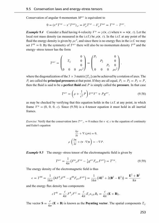
9.5 Conservation laws and energy–stress tensors

Conservation of angular 4-momentum Mμν is equivalent to

0 = (xμT νρ − xνT μρ),ρ = δμρT νρ − δνρT μρ = T νμ − T μν.

Example 9.4 Consider a fluid having 4-velocity V μ = γ (v, c) where v = v(r, t). Let thelocal rest mass density (as measured in the i.r.f.) be ρ(r, t). In the i.r.f. at any point of thefluid the energy density is given by ρc2, and since there is no energy flux in the i.r.f. we mayset T 4i = 0. By the symmetry of T μν there will also be no momentum density T i4 and theenergy–stress tensor has the form

T μν =

⎛⎜⎜⎝0

Ti j 00

0 0 0 ρc2

⎞⎟⎟⎠ =⎛⎜⎜⎝

P1 0P2 0

P3 00 0 0 ρc2

⎞⎟⎟⎠ ,where the diagonalization of the 3× 3 matrix [Ti j ] can be achieved by a rotation of axes. ThePi are called the principal pressures at that point. If they are all equal, P1 = P2 = P3 = P ,then the fluid is said to be a perfect fluid and P is simply called the pressure. In that case

T μν =(ρ + 1

c2P

)V μV ν + Pgμν, (9.58)

as may be checked by verifying that this equation holds in the i.r.f. at any point, in whichframe V μ = (0, 0, 0, c). Since (9.58) is a 4-tensor equation it must hold in all inertialframes.

Exercise: Verify that the conservation laws T μν,ν = 0 reduce for v ' c to the equation of continuity

and Euler’s equation

∂ρ

∂t+ ∇.(ρv) = 0,

ρ

(∂v

∂t+ (v · ∇)v

)= −∇P.

Example 9.5 The energy–stress tensor of the electromagnetic field is given by

T μν = 1

4π

(FμρFνρ − 1

4 gμνFρσ Fρσ) = T νμ. (9.59)

The energy density of the electromagnetic field is thus

ε = T 44 = 1

16π

(4F4

i F4i − g44 Fρσ Fρσ) = 1

16π

(4E2 + 2(B2 − E2)

) = E2 + B2

8π

and the energy flux density has components

cT 4i = c

4πF4

j Fi j = c

4πE jεi jk Bk = c

4π(E× B)i .

The vector S = c

4π(E× B) is known as the Poynting vector. The spatial components Ti j

253

Special relativity

are known as the Maxwell stress tensor

T i j = Ti j = 1

16π

(4(Fik Fj

k + Fi4 Fj4)− δi j 2(B2 − E2)

)= 1

4π

(−Ei E j − Bi B j + 12δi j (E

2 + B2)).

The total 4-momentum of an electromagnetic field over a spacelike surface S is calculatedfrom Eq. (9.57).

Exercise: Show that the average pressure P = 13

∑i

Tii of an electromagnetic field is equal to 13×

energy density. Show that this also follows from the fact that T μν is trace-free, T μμ = 0.

For further developments in relativistic classical field theory the reader is referred to [4, 5].

Problems

Problem 9.24 Show that as a consequence of the Maxwell equations,

T β

α,β = −1

cFαγ J γ

where T βα is the electromagnetic energy–stress tensor (9.59), and when no charges and currents are

present it satisfies Eq. (9.56). Show that the α = 4 component of this equation has the form

∂ε

∂t+ ∇ · S = −j · E

where ε = energy density and S = Poynting vector. Interpret this equation physically.

Problem 9.25 For a plane wave, Problem 9.23, show that

Tαβ = ε nα nβ

where ε = E2/4π and nα = (n, 1) is the null vector pointing in the direction of propagation of thewave. What pressure does the wave exert on a wall placed perpendicular to the path of the wave?

References

[1] W. Kopczynski and A. Trautman. Spacetime and Gravitation. Chichester, John Wiley &Sons, 1992.

[2] W. Rindler. Introduction to Special Relativity. Oxford, Oxford University Press, 1991.[3] R. K. Sachs and H. Wu. General Relativity for Mathematicians. New York, Springer-

Verlag, 1977.[4] L. D. Landau and E. M. Lifshitz. The Classical Theory of Fields. Reading, Mass.,

Addison-Wesley, 1971.[5] W. Thirring. A Course in Mathematical Physics, Vol. 2: Classical Field Theory. New

York, Springer-Verlag, 1979.

254

10 Topology

Up till now we have focused almost entirely on the role of algebraic structures in mathe-matical physics. Occasionally, as in the previous chapter, it has been necessary to use somedifferential calculus, but this has not been done in any systematic way. Concepts such ascontinuity and differentiability, central to the area of mathematics known as analysis, areessentially geometrical in nature and require the use of topology for their rigorous defini-tion. In broad terms, a topology is a structure imposed on a set to allow for the definitionof convergence and limits of sequences or subsets. A space with a topology defined on itwill be called a topological space, and a continuous map between topological spaces is onethat essentially preserves limit points of subsets. The most general approach to this subjectturns out to be through the concept of open sets.

Consider a two-dimensional surface S embedded in Euclidean three-dimensional spaceE3. In this case we have an intuitive understanding of a ‘continuous deformation’ of thesurface as being a transformation of the surface that does not involve any tearing or pasting.Topology deals basically with those properties that are invariant under continuous defor-mations of the surface. Metric properties are not essential to the concept of continuity, andsince operations such as ‘stretching’ are permissible, topology is sometimes called ‘rubbersheet geometry’. In this chapter we will also define the concept of a metric space. Such aspace always has a naturally defined topology associated with it, but the converse is not truein general – it is quite possible to define topology on a space without having a concept ofdistance defined on the space.

10.1 Euclidean topology

The archetypal model for a topological space is the real line and the Euclidean planeR2. On the real line R, an open interval is any set (a, b) = {x ∈ R | a < x < b}. A setU ⊆ R is called a neighbourhood of x ∈ R if there exists ε > 0 such that the open interval(x − ε, x + ε) is a subset of U . We say a sequence of real numbers {xn} converges tox ∈ R, written xn → x , if for every ε > 0 there exists an integer N > 0 such that |x −xn| < ε for all n > N ; that is, for sufficiently large n the sequence xn enters and staysin every neighbourhood U of x . The point x is then said to be the limit of the sequence{xn}.

Exercise: Show that the limit of a sequence is unique: if xn → x and xn → x ′ then x = x ′.

255

Topology

Figure 10.1 Points in an open set can be ‘thickened’ to an open ball within the set

Similar definitions apply to the Euclidean plane R2, where we set |y− x| =√(y1 − x1)2 + (y2 − x2)2. In this case, open intervals are replaced by open balls

Br (x) = {y ∈ R2 | |y− x| < r}and a set U ⊆ R2 is said to be a neighbourhood of x ∈ R2 if there exists a real numberε > 0 such that the open ball Bε(x) ⊆ U . A sequence of points {xn} converges to x ∈ R2,or x is the limit of the sequence {xn}, if for every ε > 0 there exists an integer N > 0 suchthat

xn ∈ Bε(x) for all n > N .

Again we write xn → x, and the definition is equivalent to the statement that for everyneighbourhood U of x there exists N > 0 such that xn ∈ U for all n > N .

An open set U in R or R2 is a set that is a neighbourhood of every point in it. Intuitively,U is open in R (resp. R2) if every point in U can be ‘thickened out’ to an open interval(resp. open ball) within U (see Fig. 10.1). For example, the unit ball B1(O) = {y | |y|2 < 1}is an open set since, for every point x ∈ B1(O) the open ball Bε(x) ⊆ B1(O) where ε =1− |x| > 0.

On the real line it may be shown that the most general open set consists of a union ofnon-intersecting open intervals,

. . . , (a−1, a0), (a1, a2), (a3, a4), (a5, a6), . . .

where . . . a−1 < a0 ≤ a1 < a2 ≤ a3 < a4 ≤ a5 < a6 ≤ . . . In R2 open sets cannot be sosimply categorized, for while every open set is a union of open balls, the union need not bedisjoint.

256

10.2 General topological spaces

In standard analyis, a function f : R → R is said to be continuous at x if for every ε > 0there exists δ > 0 such that

|y − x | < δ =⇒ | f (y)− f (x)| < ε.Hence, for every ε > 0, the inverse image set f −1( f (x)− ε, f (x)+ ε) is a neighbourhoodof x , since it includes an open interval (x − δ, x + δ) centred on x . As every neighbourhoodof f (x) contains an interval of the form ( f (x)− ε, f (x)+ ε) the function f is continuousat x if and only if the inverse image of every neighbourhood of f (x) is a neighbourhood of x .A function f : R → R is said to be continuous on R if it is continuous at every point x ∈ R.

Theorem 10.1 A function f : R → R is continuous on R if and only if the inverse imageV = f −1(U ) of every open set U ⊆ R is an open subset of R.

Proof : Let f be continuous on R. Since an open set U is a neighbourhood of every pointy ∈ U , its inverse image V = f −1(U ) must be a neighbourhood of every point x ∈ V .Hence V is an open set.

Conversely let f : R → R be any function having the property that V = f −1(U ) is openfor every open set U ⊆ R. Then for any x ∈ R and every ε > 0 the inverse image under fof the open interval ( f (x)− ε, f (x)+ ε) is an open set including x . It therefore containsan open interval of the form (x − δ, x + δ), so that f is continuous at x . Since x is anarbitrary point, the function f is continuous on R. �

In general topology this will be used as the defining characteristic of a continuous map.In R2 the treatment is almost identical. A function f : R2 → R2 is said to be continuous atx if for every ε > 0 there exists a real number δ > 0 such that

|y− x| < δ =⇒ | f (y)− f (x)| < ε.An essentially identical proof to that given in Theorem 10.1 shows that a function f iscontinuous on R2 if and only if the inverse image f −1(U ) of every open set U ⊆ R2 is anopen subset of R2. The same applies to real-valued functions f : R2 → R. Thus continuityof functions can be described entirely by their inverse action on open sets. For this reason,open sets are regarded as the key ingredients of a topological space. Experience fromEuclidean spaces and surfaces embedded in them has taught mathematicians that the mostimportant properties of open sets can be summarized in a few simple rules, which are setout in the next section (see also [1–8]).

10.2 General topological spaces

Given a set X , a topology on X consists of a family of subsets O, called open sets, whichsatisfy the following conditions:

(Top1) The empty set ∅ is open and the entire space X is open, {∅, X} ⊂ O.(Top2) If U and V are open sets then so is their intersection U ∩ V ,

U ∈ O and V ∈ O =⇒ U ∩ V ∈ O.(Top3) If {Vi | i ∈ I } is any family of open sets then their union

⋃i∈I

Vi is open.

257

Topology

Successive application of (Top2) implies that the intersection of any finite number ofopen sets is open, but O is not in general closed with respect to infinite intersections of opensets. On the other hand, O is closed with respect to arbitrary unions of open sets. The pair(X,O), where O is a topology on X , is called a topological space. We often refer simply toa topological space X when the topology O is understood. The elements of the underlyingspace X are normally referred to as points.

Example 10.1 Define O to be the collection of subsets U of the real line R having theproperty that for every x ∈ U there exists an open interval (x − ε, x + ε) ⊆ U for someε > 0. These sets agree with the definition of open sets given in Section 10.1. The emptyset is assumed to belong to O by default, while the whole line R is evidently open sinceevery point lies in an open interval. Thus (Top1) holds for the family O. To prove (Top2)let U and V be open sets such that U ∩ V �= ∅, the case where U ∩ V = ∅ being trivial.For any x ∈ U ∩ V there exist positive numbers ε1 and ε2 such that

(x − ε1, x + ε1) ⊆ U and (x − ε2, x + ε2) ⊆ V .

If ε = min(ε1, ε2) then (x − ε, x + ε) ⊆ U ∩ V , hence U ∩ V is an open set.For (Top3), let U be the union of an arbitrary collection of open sets {Ui | i ∈ I }. If x ∈ U ,

then x ∈ U j for some j ∈ I and there exists ε > 0 such that (x − ε, x + ε) ⊆ U j ⊆ U .Hence U is open and the family O forms a topology for R. It is often referred to as thestandard topology on R. Any open interval (a, b) where a < b is an open set, for ifx ∈ (a, b) then (x − ε, x + ε) ⊂ (a, b) for ε = 1

2 min(x − a, b − x). A similar argumentshows that the intervals may also be of semi-infinite extent, such as (−∞, a) or (b, ∞).Notice that infinite intersections of open sets do not generally result in an open set. Forexample, an isolated point {a} is not an open set since it contains no finite open interval,yet it is the intersection of an infinite sequence of open intervals such as

(a − 1, a + 1), (a − 12 , a + 1

2 ), (a − 13 , a + 1

3 ), (a − 14 , a + 1

4 ), . . .

Similar arguments can be used to show that the open sets defined on R2 in Section 10.1form a topology. Similarly, in Rn we define a topology where a set U is said to be open iffor every point x ∈ U there exists an open ball

Br (x) = {y ∈ R2 | |y− x| < r} ⊂ U,

where

|y− x| =√

(y1 − x1)2 + (y2 − x2)2 + · · · + (yn − xn)2.

This topology will again be termed the standard topology on Rn .

Example 10.2 Consider the familyO′ of all open intervals on R of the form (−a, b) wherea, b > 0, together with the empty set. All these intervals contain the origin 0. It is not hardto show that (Top1)–(Top3) hold for this family and that (X,O′) is a topological space. Thisspace is not very ‘nice’ in some of its properties. For example no two points x, y ∈ R lie innon-intersecting neighbourhoods. In a sense all points of the line are ‘arbitrarily close’ toeach other in this topology.

258

10.2 General topological spaces

Figure 10.2 Relative topology induced on a subset of a topological space

A subset V is called closed if its complement X − V is open. The empty set and thewhole space are clearly closed sets, since they are both open sets and are the complementsof each other. The intersection of an arbitrary family of closed sets is closed, as it is thecomplement of a union of open sets. However, only finite unions of closed sets are closedin general.

Example 10.3 Every closed interval [a, b] = {x | a ≤ x ≤ b} where−∞ < a ≤ b <∞is a closed set, as it is the complement of the open set (−∞, a) ∪ (b, ∞). Every singletonset consisting of an isolated point {a} ≡ [a, a] is closed. Closed intervals [a, b] are notopen sets since the end points a or b do not belong to any open interval included in [a, b].

If A is any subset of X the relative topology on A, or topology induced on A, is thetopology whose open sets are

OA = {A ∩U |U ∈ O}.Thus a set is open in the relative topology on A iff it is the intersection of A and an openset U in X (see Fig. 10.2). That these sets form a topology on A follows from the followingthree facts:

1. ∅ ∩ A = ∅, X ∩ A = A.2. (U ∩ A) ∩ (V ∩ A) = (U ∩ V ) ∩ A.

3.⋃i∈I

(Ui ∩ A

) = (⋃i∈I

Ui

)∩ A.

A subset A of X together with the relative topology OA induced on it is called a subspaceof (X,O).

Example 10.4 The relative topology on the half-open interval A = [0, 1) ⊂ R, inducedon A by the standard topology on R, is the union of half-open intervals of the form [0, a)

259

Topology

Figure 10.3 Accumulation point of a set

where 0 < a < 1, and all intervals of the form (a, b) where 0 < a < b ≤ 1. Evidently someof the open sets in this topology are not open in R.

Exercise: Show that if A ⊆ X is an open set then all open sets in the relative topology on A are openin X .

Exercise: If A is a closed set, show that every closed set in the induced topology on A is closed in X .

A point x is said to be an accumulation point of a set A if every open neighbourhoodU of x contains points of A other than x itself, as shown in Fig. 10.3. What this means isthat x may or may not lie in A, but points of A ‘cluster’ arbitrarily close to it (sometimesit is also called a cluster point of A). A related concept is commonly applied to sequencesof points xn ∈ X . We say that the sequence xn ∈ X converges to x ∈ X or that x is a limitpoint of {xn}, denoted xn → x , if for every open neighbourhood U of x there is an integerN such that xn ∈ U for all n ≥ N . This differs from an accumulation point in that we couldhave xn = x for all n > n0 for some n0.

The closure of any set A, denoted A, is the union of the set A and all its accumulationpoints. The interior of A is the union of all open sets U ⊆ A, denoted Ao. The differenceof these two sets, b(A) = A − Ao, is called the boundary of A.

Theorem 10.2 The closure of any set A is a closed set. The interior Ao is the largest openset included in A. The boundary b(A) is a closed set.

Proof : Let x be any point not in A. Since x is not in A and is not an accumulation pointof A, it has an open neighbourhood Ux not intersecting A. Furthermore, Ux cannot containany other accumulation point of A else it would be an open neighbourhood of that point notintersecting A. Hence the complement X − A of the closure of A is the union of the opensets Ux . It is therefore itself an open set and its complement A is a closed set.

260

10.2 General topological spaces

Since the interior Ao is a union of open sets, it is an open set by (Top3). If U is any openset such that U ⊆ A then, by definition, U ⊆ Ao. Thus Ao is the largest open subset of A.Its complement is closed and the boundary b(A) = A ∩ (X − Ao) is necessarily a closedset. �

Exercise: Show that a set A is closed if and only if it contains its boundary, A ⊇ b(A).

Exercise: A set A is open if and only if A ∩ b(A) = ∅.

Exercise: Show that all accumulation points of A lie in the boundary b(A).

Exercise: Show that a point x lies in the boundary of A iff every neighbourhood of x contains pointsboth in A and not in A.

Example 10.5 The closure of the open ball Ba(x) ⊂ Rn (see Example 10.1) is the closedball

Ba(x) = {y | |y− x| ≤ a}.Since every open ball is an open set, it is its own interior, Bo

a (x) = Ba(x) and its boundaryis the (n − 1)-sphere of radius a, centre x,

b(Ba(x)) = Sn−1a (x) = {y | |y− x| = a}.

Example 10.6 A set whose closure is the entire space X is said to be dense in X . Forexample, since every real number has rational numbers arbitrarily close to it, the rationalnumbers Q are a countable set that is dense in the set of real numbers. In higher dimensionsthe situation is similar. The set of points with rational coordinates Qn is a countable set thatis dense in Rn .

Exercise: Show that Q is neither an open or closed set in R.

Exercise: Show that Q0 = ∅ and b(Q) = R.

It is sometimes possible to compare different topologies O1 and O2 on a set X . We sayO1 is finer or stronger than O2 if O1 ⊇ O2. Essentially, O1 has more open sets than O2.In this case we also say that O2 is coarser or weaker than O1.

Example 10.7 All topologies on a set X lie somewhere between two extremes, the discreteand indiscrete topologies. The indiscrete or trivial topology consists simply of the emptyset and the whole space itself, O1 = {∅, X}. It is the coarsest possible topology on X –if O is any other topology then O1 ⊆ O by (Top1). The discrete topology consists of allsubsets of X , O2 = 2X . This topology is the finest possible topology on X , since it includesall other topologies O2 ⊇ O. For both topologies (Top1)–(Top3) are trivial to verify.

Given a set X , and an arbitrary collection of subsets U , we can ask for the weakesttopology O(U) containing U . This topology is the intersection of all topologies that contain

261

Topology

U and is called the topology generated by U . It is analogous to the concept of the vectorsubspace L(M) generated by an arbitrary subset M of a vector space V (see Section 3.5).

A contructive way of defining O(U) is the following. Firstly, adjoin the empty set ∅ andthe entire space X to U if they are not already in it. Next, extend U to a family U consistingof all finite intersections U1 ∩U2 ∩ · · · ∩Un of sets Ui ∈ U ∪ {∅, X}. Finally, the set O(U)consisting of arbitrary unions of sets from U forms a topology. To prove (Top2),

⋃i∈I

( ni⋂a=1

Uia

)∩⋃j∈J

( n j⋂b=1

Vjb

)=⋃i∈I

⋃j∈J

(Ui1 ∩ · · · ∩Uini ∩ Vj1 ∩ · · · ∩ Vjn j

).

Property (Top3) follows immediately from the contruction.

Example 10.8 On the real line R, the family U of all open intervals generates the standardtopology since every open set is a union of open sets of the form (x − ε, x + ε). Similarly,the standard topology on R2 is generated by the set of open balls

U = {Ba(r) | > 0, r = (x, y) ∈ R2}.To prove this statement we must show that every set that is an intersection of two openballs Ba(r) and Bb(r′) is a union of open balls from U . If x ∈ Ba(r), let ε < a be such thatBε(x) ⊂ Ba(r). Similarly if x ∈ Bb(r′), let ε′ < a be such that Bε′ (x) ⊂ Bb(r′). Hence, ifx ∈ Ba(r) ∩ Bb(r′) then Bε′′ (x) ⊂ Ba(r) ∩ Bb(r′) where ε′′ = min(ε, ε′). The proof easilygeneralizes to intersections of any finite number of open balls. Hence the standard topologyof R2 is generated by the set of all open balls. The extension to Rn is straightforward.

Exercise: Show that the discrete topology on X is generated by the family of all singleton sets {x}where x ∈ X .

A set A is said to be a neighbourhood of x ∈ X if there exists an open set U such thatx ∈ U ⊂ A. If A itself is open it is called an open neighbourhood of x . A topologicalspace X is said to be first countable if every point x ∈ X has a countable collectionU1(x),U2(x), . . . of open neighbourhoods of x such that every open neighbourhood U ofx includes one of these neighbourhoods U ⊃ Un(x). A stronger condition is the following:a topological space (X,O) is said to be second countable or separable if there exists acountable set U1, U2, U3, . . . that generates the topology of X .

Example 10.9 The standard topology of the Euclidean plane R2 is separable, since it isgenerated by the set of all rational open balls,

Brat = {Ba(r) | a > 0 ∈ Q, r = (x, y) s.t. x, y ∈ Q}.The set Brat is countable as it can be put in one-to-one correspondence with a subset of Q3.Since the rational numbers are dense in the real numbers, every point x of an open set U liesin a rational open ball. Thus every open set is a union of rational open balls. By a similarargument to that used in Example 10.8 it is straightforward to prove that the intersectionof two sets from Brat is a union of rational open balls. Hence R2 is separable. Similarly, allspaces Rn where n ≥ 1 are separable.

262

10.2 General topological spaces

Let X and Y be two topological spaces. Theorem 10.1 motivates the following definition:a function f : X → Y is said to be continuous if the inverse image f −1(U ) of every openset U in Y is open in X . If f is one-to-one and its inverse f −1 : Y → X is continuous, thefunction is called a homeomorphism and the topological spaces X and Y are said to behomeomorphic or topologically equivalent, written X ∼= Y . The main task of topology isto find topological invariants – properties that are preserved under homeomorphisms. Theymay be real numbers, algebraic structures such as groups or vector spaces constructed fromthe topological space, or specific properties such as compactness and connectedness. Theultimate goal is to find a set of topological invariants that characterize a topological space. Inthe language of category theory, Section 1.7, continuous functions are the morphisms of thecategory whose objects are topological spaces, and homeomorphisms are the isomorphismof this category.

Example 10.10 Let f : X → Y be a continuous function between topological spaces. Ifthe topology on X is discrete then every function f is continuous, for no matter what thetopology on Y , every inverse image set f −1(U ) is open in X . Similarly if the topology onY is indiscrete than the function f is always continuous since the only inverse images in Xof open sets are f −1(∅) = ∅ and f −1(Y ) = X , which are always open sets by (Top1).

Problems

Problem 10.1 Give an example in R2 of each of the following:

(a) A family of open sets whose intersection is a closed set that is not open.(b) A family of closed sets whose union is an open set that is not closed.(c) A set that is neither open nor closed.(d) A countable dense set.(e) A sequence of continuous functions fn : R2 → R whose limit is a discontinuous function.

Problem 10.2 If U generates the topology on X show that {A ∩U |U ∈ U} generates the relativetopology on A.

Problem 10.3 Let X be a topological space and A ⊂ B ⊂ X . If B is given the relative topology,show that the relative topology induced on A by B is identical to the relative topology induced on itby X .

Problem 10.4 Show that for any subsets U , V of a topological space U ∪ V = U ∪ V . Is it truethat U ∩ V = U ∩ V ? What corresponding statements hold for the interior and boundaries of unionsand intersections of sets?

Problem 10.5 If A is a dense set in a topological space X and U ⊆ X is open, show that U ⊆ A ∩U .

Problem 10.6 Show that a map f : X → Y between two topological spaces X and Y is continuous ifand only if f (U ) ⊆ f (U ) for all sets U ⊆ X . Show that f is a homeomorphism only if f (U ) = f (U )for all sets U ⊆ X .

Problem 10.7 Show the following:

(a) In the trivial topology, every sequence xn converges to every point of the space x ∈ X .

263

Topology

(b) In R2 the family of open sets consisting of all open balls centred on the origin Br (0) is a topology.Any sequence xn → x converges to all points on the circle of radius |x| centred on the origin.

(c) If C is a closed set of a topological space X it contains all limit points of sequences xn ∈ C .(d) Let f : X → Y be a continuous function between topological spaces X and Y . If xn → x is any

convergent sequence in X then f (xn) → f (x) in Y .

Problem 10.8 If W , X and Y are topological spaces and the functions f : W → X , g : X → Y areboth continuous, show that the function h = g ◦ f : W → Y is continuous.

10.3 Metric spaces

To generalize the idea of ‘distance’ as it appears in R and R2, we define a metric space [9]to be a set M with a distance function or metric d : M × M → R such that

(Met1) d(x, y) ≥ 0 for all x, y ∈ M .(Met2) d(x, y) = 0 if and only if x = y.(Met3) d(x, y) = d( y, x).(Met4) d(x, y)+ d( y, z) ≥ d(x, z).

Condition (Met4) is called the triangle inequality – the length of any side of a triangle xyzis less than the sum of the other two sides. For every x in a metric space (M, d) and positivereal number a > 0 we define the open ball Ba(x) = {y | d(x, y) < a}.

In n-dimensional Euclidean space Rn the distance function is given by

d(x, y) = |x− y| =√

(x1 − y1)2 + (x2 − y2)2 + · · · + (xn − yn)2,

but the following could also serve as acceptable metrics:

d1(x, y) = |x1 − y1| + |x2 − y2| + · · · + |xn − yn|,d2(x, y) = max

(|x1 − y1|, |x2 − y2|, . . . , |xn − yn|).

Exercise: Show that d(x, y), d1(x, y) and d2(x, y) satisfy the metric axioms (Met1)–(Met4).

Exercise: In R2 sketch the open balls B1((0, 0)) for the metrics d, d1 and d2.

If (M, d) is a metric space, then a subset U ⊂ M is said to be open if and only if for everyx ∈ U there exists an open ball Bε(x) ⊆ U . Just as for R2, this defines a natural topologyon M , called the metric topology. This topology is generated by the set of all open ballsBa(x) ⊂ M . The proof closely follows the argument in Example 10.8.

In a metric space (M, d), a sequence xn converges to a point x if and only if d(xn, x) → 0as n →∞. Equivalently, xn → x if and only if for every ε > 0 the sequence eventuallyenters and stays in the open ball Bε(x). In a metric space the limit point x of a sequencexn is unique, for if xn → x and xn → y then d(x, y) ≤ d(x, xn)+ d(xn, y) by the triangleinequality. By choosing n large enough we have d(x, y) < ε for any ε > 0. Hence d(x, y) =0, and x = y by (Met2). For this reason, the concept of convergent sequences is more usefulin metric spaces than in general topological spaces (see Problem 10.7).

264

10.4 Induced topologies

In a metric space (M, d) let xn be a sequence that converges to some point x ∈ M . Thenfor every ε > 0 there exists a positive integer N such that d(xn, xm) < ε for all n,m > N .For, let N be an integer such that d(xk, x) < 1

2ε for all k > N , then

d(xn, xm) ≤ d(xn, x)+ d(x, xm) < ε for all n, m > N .

A sequence having this property, d(xn, xm) → 0 as n,m →∞, is termed a Cauchysequence.

Example 10.11 Not every Cauchy sequence need converge to a point of M . For example,in the open interval (0, 1) with the usual metric topology, the sequence xn = 2−n is a Cauchysequence yet it does not converge to any point in the open interval. A metric space (M, d)is said to be complete if every Cauchy sequence x1, x2, . . . converges to a point x ∈ M .Completeness is not a topological property. For example the real line R is a complete metricspace, and the Cauchy sequence 2−n has the limit 0 in R. The topological spaces R and(0, 1) are homeomorphic, using the map ϕ : x �→ tan 1

2π (2x − 1). However one space iscomplete while the other is not with respect to the metrics generating their topologies.

Problems

Problem 10.9 Show that every metric space is first countable. Hence show that every subset of ametric space can be written as the intersection of a countable collection of open sets.

Problem 10.10 If U1 and U2 are two families of subsets of a set X , show that the topologiesgenerated by these families are homeomorphic if every member of U2 is a union of sets from U1 andvice versa. Use this property to show that the metric topologies on Rn defined by the metrics d, d1

and d2 are all homeomorphic.

Problem 10.11 A topological space X is called normal if for every pair of disjoint closed subsetsA and B there exist disjoint open sets U and V such that A ⊂ U and B ⊂ V . Show that every metricspace is normal.

10.4 Induced topologies

Induced topologies and topological products

Given a topological space (X,O) and a map f : Y → X from an arbitrary set Y into X ,we can ask for the weakest topology on Y for which this map is continuous – it is uselessto ask for the finest such topology since, as shown in Example 10.10, the discrete topologyon Y always achieves this end. This is known as the topology induced on Y by the map f .Let O f be the family of all inverse images of open sets of X ,

O f = { f −1(U ) |U ∈ O}.Since f is required to be continuous, all members of this collection must be open inthe induced topology. Furthermore, O f is a topology on Y since (i) property (Top1) istrivial, as ∅ = f −1(∅) and Y = f −1(X ); (ii) the axioms (Top2) and (Top3) follow from the

265

Topology

set-theoretical identities

f −1(U ∩ V ) = f −1(U ) ∩ f −1(V ) and⋃i∈I

f −1(Ui ) = f −1(⋃

i∈I

Ui

).

Hence O f is a topology on Y and is included in any other topology such that the map fis continuous. It must be the topology induced on Y by the map f since it is the coarsestpossible such topology.

Example 10.12 Let (X,O) be any topological space and A any subset of X . In the topologyinduced on A by the natural inclusion map iA : A → X defined by iA(x) = x for all x ∈ A, asubset B of A is open iff it is the intersection of A with an open set of X ; that is, B = A ∩Uwhere U is open in X . This is precisely the relative topology on A defined in Section 10.2.The relative topology is thus the coarsest topology on A for which the inclusion map iscontinuous.

More generally, for a collection of maps { fi : Y → Xi | i ∈ I } where Xi are topologicalspaces, the weakest topology on Y such that all these maps are continuous is said to bethe topology induced by these maps. To create this topology it is necessary to consider theset of all inverse images of open sets U = { f −1

i (Ui ) |Ui ∈ Oi }. This collection of sets isnot itself a topology in general, the topology generated by these sets will be the coarsesttopology on Y such that each function fi is continuous.

Given two topological spaces (X,OX ) and (Y,OY ), let pr1 : X × Y → X and pr2 : X ×Y → Y be the natural projection maps defined by

pr1(x, y) = x and pr2(x, y) = y.

The product topology on the set X × Y is defined as the topology induced by these twomaps. The space X × Y together with the product topology is called the topological productof X and Y . It is the coarsest topology such that the projection maps are continuous. Theinverse image under pr1 of an open set U in X is a ‘vertical strip’ U × Y , while the inverseimage of an open set V in Y under pr2 is a ‘horizontal strip’ X × V . The intersection ofany pair of these strips is a set of the form U × V where U and V are open sets from X andY respectively (see Fig. 10.4). Since the topology generated by the vertical and horizontalstrips consists of all possible unions of such intersections, it follows that in the producttopology a subset A ⊂ X × Y is open if for every point (x, y) ∈ A there exist open setsU ∈ OX and V ∈ OY such that (x, y) ∈ U × V ⊆ A.

Given an arbitrary collection of sets {Xi | i ∈ I }, their cartesian product P =∏i∈I Xi

is defined as the set of maps f : I →⋃i Xi such that f (i) ∈ Xi for each i ∈ I . For a

finite number of sets, taking I = {1, 2, . . . , n}, this concept is identical with the set of n-tuples from X1 × X2 × · · · × Xn . The product topology on P is the topology induced bythe projection maps pri : P → Xi defined by pri ( f ) = f (i). This topology is coarser thanthe topology generated by all sets of the form

∏i∈I Ui where Ui is an open subset of Xi .

Example 10.13 Let S1 be the unit circle in R2 defined by x2 + y2 = 1, with the relativetopology. The product space S1 × S1 is homeomorphic to the torus T 2 or ‘donut’, withtopology induced from its embedding as a subset of R3. This can be seen by embeddingS1 in the z = 0 plane of R3, and attaching a vertical unit circle facing outwards from each

266

10.4 Induced topologies

Figure 10.4 Product of two topological spaces

point on S1. As the vertical circles ‘sweep around’ the horizontal cirle the resulting circleis clearly a torus.

The following is an occasionally useful theorem.

Theorem 10.3 If X and Y are topological spaces then for each point x ∈ X the injectionmap ιx : Y → X × Y defined by ιx (y) = (x, y) is continuous. Similarly the map ι′y : X →X × Y defined by ι′y(x) = (x, y) is continuous.

Proof : Let U and V be open subsets of X and Y respectively. Then

(ιx )−1(U × V ) ={

V if x ∈ U,

∅ if x /∈ U.

Since every open subset of U × V in the product topology is a union of sets of type U × V ,it follows that the inverse image under ιx of every open set in X × Y is an open subset ofY . Hence the map ιx is continuous. Similarly for the map ι′y . �

Topology by identification

We may also reverse the above situation. Let (X,O) be a topological space, and f : X → Ya map from X onto an arbitrary set Y . In this case the topology on Y induced by f is definedto be the finest topology such that f is continuous. This topology consists of all subsetsU ⊆ Y such that f −1(U ) is open in X ; that is, OY = { f −1(U ) |U ∈ O}.Exercise: Show that OY is a topology on Y .

Exercise: Show that OY is the strongest topology such that f is continuous.

267

Topology

A

D

B

C

Figure 10.5 Construction of a torus by identification of opposite sides of a square

A common instance of this type of induced topology occurs when there is an equivalencerelation E defined on a topological space X . Let [x] = {y | yEx} be the equivalence classcontaining the point x ∈ X . In the factor space X/E = {[x] | x ∈ X} define the topologyobtained by identification from X to be the topology induced by the natural map iE :X → X/E associating each point x ∈ X with the equivalence class to which it belongs,iE (x) = [x]. In this topology a subset A is open iff its inverse image i−1

E (A) = {x ∈ X | [x] ∈A} =⋃[x]∈A[x] is an open subset of X . That is, a subset of equivalence classes A = {[x]}is open in the identification topology on X/E iff the union of the sets [x] that belong to Ais an open subset of X .

Exercise: Verify directly from the last statement that the axioms (Top1)–(Top3) are satisfied by thistopology on X/E .

Example 10.14 As in Example 1.4, we say two points (x, y) and (x ′, y′) in the plane R2

are equivalent if their coordinates differ by integral amounts,

(x, y) ≡ (x ′y′) iff x − x ′ = n, y − y′ = m (n,m ∈ Z).

The topology on the space R2/≡ obtained by identification can be pictured as the unit squarewith opposite sides identified (see Fig. 10.5). To understand that this is a representation ofthe torus T 2, consider a square rubber sheet. Identifying sides AD and BC is equivalentto joining these two sides together to form a cylinder. The identification of AB and C D isnow equivalent to identifying the circular edges at the top and bottom of the cylinder. Inthree-dimensions this involves bending the cylinder until top and bottom join up to formthe inner tube of a tyre – remember, distances or metric properties need not be preservedfor a topological transformation. The n-torus T n can similarly be defined as the topological

268

10.5 Hausdorff spaces

space obtained by identification from the corresponding equivalence relation on Rn , wherebypoints are equivalent if their coordinates differ by integers.

Example 10.15 Let R3 = R3 − {0} be the set of non-zero 3-triples of real numbers given

the relative topology in R3. Define an equivalence relation on R3

whereby (x, y, z) ≡(x ′, y′, z′) iff there exists a real number λ �= 0 such that x = λx ′, y = λy′ and z = λz′. The

factor space P2 = R3/≡ is known as the real projective plane.

Each equivalence class [(x, y, z)] is a straight line through the origin that meets the unit2-sphere S2 in two diametrically opposite points. Define an equivalence relation on S2 byidentifying diametrically opposite points, (x, y, z) ∼ (−x,−y,−z) where x2 + y2 + z2 =1. The topology on P2 obtained by identification from R

3is thus identical with that of the

2-sphere S2 with diametrically opposite points identified.

Generalizing, we define real projective n-space Pn to be Rn+1/≡ where

(x1, x2, . . . , xn+1) ≡ (x ′1, x ′2, . . . , x ′n+1) if and only if there exists λ �= 0 such that x1 = λx ′1,x2 = λx ′2, . . . , xn+1 = λx ′n+1. This space can be thought of as the set of all straight linesthrough the origin in Rn+1. The topology of Pn is homeomorphic with that of the n-sphereSn with opposite points identified.

Problems

Problem 10.12 If f : X → Y is a continuous map between topological spaces, we define its graphto be the set G = {(x, f (x)) | x ∈ X} ⊆ X × Y . Show that if G is given the relative topology inducedby the topological product X × Y then it is homeomorphic to the topological space X .

Problem 10.13 Let X and Y be topological spaces and f : X × Y → X a continuous map. For eachfixed a ∈ X show that the map fa : Y → X defined by fa(y) = f (a, y) is continuous.

10.5 Hausdorff spaces

In some topologies, for example the indiscrete topology, there are so few open sets thatdifferent points cannot be separated by non-intersecting neighbourhoods. To remedy thissituation, conditions known as separation axioms are sometimes imposed on topologicalspaces. One of the most common of these is the Hausdorff condition: for every pair ofpoints x, y ∈ X there exist open neighbourhoods U of x and V of y such that U ∩ V = ∅.A topological space satisfying this property is known as a Hausdorff space. In an intuitivesense, no pair of distinct points of a Hausdorff space are ‘arbitrarily close’ to each other.

A typical ‘nice’ property of Hausdorff spaces is the fact that the limit of any convergentsequence xn → x , defined in Problem 10.7, is unique. Suppose, for example, that xn → xand xn → x ′ in a Hausdorff space X . If x �= x ′ let U and U ′ be disjoint open neighbourhoodssuch that x ∈ U and x ′ ∈ U ′, and N an integer such that xn ∈ U for all n > N . Since xn /∈ U ′

for all n > N the sequence xn cannot converge to x ′. Hence x = x ′.In a Hausdorff space every singleton set {x} is a closed set, for let Y = X − {x} be

its complement. Every point y ∈ Y has an open neighbourhood Uy that does not intersect

269

Topology

some open neighbourhood of x . In particular x /∈ Uy . By (Top3) the union of all these openneighbourhoods, Y =⋃y∈Y Uy = X − {x}, is open. Hence {x} = X − Y is closed since itis the complement of an open set.

Exercise: Show that on a finite set X , the only Hausdorff topology is the discrete topology. For thisreason, finite topologies are of limited interest.

Theorem 10.4 Every metric space (X, d) is a Hausdorff space.

Proof : Let x, y ∈ X be any pair of unequal points and let ε = 14 d(x, y). The open balls

U = Bε(x) and V = Bε(y) are open neighbourhoods of x and y respectively. Their inter-section is empty, for if z ∈ U ∩ V then d(x, z) < ε and d(y, z) < ε, which contradicts thetriangle inequality (Met4),

d(x, y) ≤ d(x, z)+ d(z, y) ≤ 2ε < 12 d(x, y).

�

An immediate consequence of this theorem is that the standard topology on Rn is Haus-dorff for all n > 0.

Theorem 10.5 If X and Y are topological spaces and f : X → Y is a one-to-one con-tinuous mapping, then X is Hausdorff if Y is Hausdorff.

Proof : Let x and x ′ be any pair of distinct points in X and set y = f (x), y′ = f (x ′). Sincef is one-to-one these are distinct points of Y . If Y is Hausdorff there exist non-intersectingopen neighbourhoods Uy and Uy′ in Y of y and y′ respectively. The inverse images of thesesets under f are open neighbourhoods of x and x ′ respectively that are non-intersecting,since f −1(Uy) ∩ f −1(Uy′ ) = f −1(Uy ∩Uy′ ) = f −1(∅) = ∅. �

This shows that the Hausdorff condition is a genuine topological property, invariant undertopological transformations, for if f : X → Y is a homeomorphism then f −1 : Y → X iscontinuous and one-to-one.

Corollary 10.6 Any subspace of a Hausdorff space is Hausdorff in the relative topology.

Proof : Let A be any subset of a topological space X . In the relative topology the inclusionmap iA : A → X is continuous. Since it is one-to-one, Theorem 10.5 implies that A isHausdorff. �

Theorem 10.7 If X and Y are Hausdorff topological spaces then their topological productX × Y is Hausdorff.

Proof : Let (x, y) and (x ′, y′) be any distinct pair of points in X × Y , so that either x �= x ′

or y �= y′. Suppose that x �= x ′. There then exist open sets U and U ′ in X such that x ∈ U ,x ′ ∈ U ′ and U ∩U ′ = ∅. The sets U × Y and U ′ × Y are disjoint open neighbourhoods of(x, y) and (x ′, y′) respectively. Similarly, if y �= y′ a pair of disjoint neighbourhoods of theform X × V and X × V ′ can be found that separate the two points. �

270

10.6 Compact spaces

Problems

Problem 10.14 If Y is a Hausdorff topological space show that every continuous map f : X → Yfrom a topological space X with indiscrete topology into Y is a constant map; that is, a map of theform f (x) = y0 where y0 is a fixed element of Y .

Problem 10.15 Show that if f : X → Y and g : X → Y are continuous maps from a topologicalspace X into a Hausdorff space Y then the set of points A on which these maps agree, A = {x ∈X | f (x) = g(x)}, is closed. If A is a dense subset of X show that f = g.

10.6 Compact spaces

A collection of sets U = {Ui | i ∈ I } is said to be a covering of a subset A of a topologicalspace X if every point x ∈ A belongs to some member of the collection. If every member Uis an open set it is called an open covering. A subset of the covering, U ′ ⊆ U , which coversA is referred to as a subcovering. If U ′ consists of finitely many sets {U1, U2, . . . ,Un} it iscalled a finite subcovering.

A topological space (X,O) is said to be compact if every open covering of X containsa finite subcovering. The motivation for this definition lies in the following theorem, theproof of which can be found in standard books on analysis [10–12].

Theorem 10.8 (Heine–Borel) A subset A of Rn is closed and bounded (included in acentral ball, A ⊂ Ba(0) for some a > 0) if and only if every open covering U of A has afinite subcovering.

Theorem 10.9 Every closed subspace A of a compact space X is compact in the relativetopology.

Proof : Let U be any covering of A by sets that are open in the relative topology. Eachmember of this covering must be of the form U ∩ A, where U is open in Y . The sets {U }together with the open set X − A form an open covering of X that, by compactness of X ,must have a finite subcovering {U1, U2, . . . ,Un, X − A}. The sets {U1 ∩ A, . . . ,Un ∩ A}are thus a finite subfamily of the original open covering U of A. Hence A is compact in therelative topology. �

Theorem 10.10 If f : X → Y is a continuous map from a compact topological space Xinto a topological space Y , then the image set f (X ) ⊆ Y is compact in the relative topology.

Proof : Let U be any covering of f (X ) consisting entirely of open sets in the relativetopology. Each member of this covering is of the form U ∩ f (X ), where U is open in Y .Since f is continuous, the sets f −1(U ) form an open covering of X . By compactness of X ,a finite subfamily { f −1(Ui ) | i = 1, . . . , n} serves to cover X , and the corresponding setsUi ∩ f (X ) evidently form a finite subcovering of f (X ). �

Compactness is therefore a topological property, invariant under homeomorphisms.

Example 10.16 If E is an equivalence relation on a compact topological space X , the mapiE : X → X/E is continuous in the topology on X/E obtained by identification from X . By

271

Topology

Theorem 10.10 the topological space X/E is compact. For example, the torus T 2 formedby identifying opposite sides of the closed and compact unit square in R2 is a compactspace.

Theorem 10.11 The topological product X × Y is compact if and only if both X and Yare compact.

Proof : If X × Y is compact then X and Y are compact by Theorem 10.10 since boththe projection maps pr1 : X × Y → X and pr2 : X × Y → Y are continuous in the producttopology.

Conversely, suppose X and Y are compact. Let W = {Wi | i ∈ I } be an open coveringof X × Y . Since each set Wi is a union of such sets of the form U × V where U and Vare open sets of X and Y respectively, the family of all such sets U j × Vj ( j ∈ J ) that aresubsets of Wi for some i ∈ I is an open cover of X × Y . Given any point y ∈ Y , the setof all U j such that y ∈ Vj is an open cover of X , and since X is compact there exists afinite subcover {U j1 , U j2 , . . . ,U jn }. The set Ay = Vj1 ∩ Vj2 ∩ · · · ∩ Vjn is an open set in Yby condition (Top2), and y ∈ Ay since y ∈ Vjk for each k = 1, . . . , n. Thus the family ofsets {Ay | y ∈ Y } forms an open cover of Y . As Y is compact, there is a finite subcoveringAy1 , Ay2 , . . . , Aym . The totality of all the sets U jk × Vjk associated with these sets Aya formsa finite open covering of X × Y . For each such set select a corresponding member Wi ofthe original covering W of which it is a subset. The result is a finite subcovering of X × Y ,proving that X × Y is compact. �

Somewhat surprisingly, this statement extends to arbitrary infinite products (Tychonoff’stheorem). The interested reader is referred to [8] or [2] for a proof of this more difficultresult.

Theorem 10.12 Every infinite subset of a compact topological space has an accumulationpoint.

Proof : Suppose X is a compact topological space and A ⊂ X has no accumulation point.The aim is to show that A is a finite set. Since every point in x ∈ A − X has an open neigh-bourhood Ux such that Ux ∩ A = ∅ it follows that A ⊆ X is closed since its complementA − X =⋃x∈X−A Ux is open. Hence, by Theorem 10.9, A is compact. Since each pointa ∈ A is not an accumulation point, there exists an open neighbourhood Ua of a such thatUa ∩ A = {a}. Hence each singleton {a} is an open set in the relative topology inducedon A, and the relative topology on A is therefore the discrete topology. The singleton sets{a | a ∈ A} therefore form an open covering of A, and since A is compact there must be afinite subcovering {a1}, {a2}, . . . , {an}. Thus A = {a1, a2, . . . , an} is a finite set. �

Theorem 10.13 Every compact subspace of a Hausdorff space is closed.

Proof : Let X be a Hausdorff space and A a compact subspace in the relative topology. Ifa ∈ A and x ∈ X − A then there exist disjoint open sets Ua and Va such that a ∈ Ua andx ∈ Va . The family of open sets Ua ∩ A is an open covering of A in the relative topology.Since A is compact there is a finite subcovering {Ua1 ∩ A, . . . ,Uan ∩ A}. The intersection ofthe corresponding neighbourhoods W = Va1 ∩ · · · ∩ Van is an open set that contains x . As

272

10.7 Connected spaces

all its points lie outside every Uai ∩ A we have W ∩ A = ∅. Thus every point x ∈ X − Ahas an open neighbourhood with no points in A. Hence A includes all its accumulationpoints and must be a closed set. �

In a metric space (M, d) we will say a subset A is bounded if sup{d(x, y) | x, y ∈ A} <∞.

Theorem 10.14 Every compact subspace of a metric space is closed and bounded.

Proof : Let A be a compact subspace of a metric space (M, d). Since M is a Hausdorffspace by Theorem 10.4 it follows by the previous theorem that A is closed. Let U ={B1(a) ∩ A | a ∈ A} be the open covering of A consisting of intersections of A with unitopen balls centred on points of A. Since A is compact, a finite number of these open balls{B1(a1), B1(a2), . . . , B1(an)} can be selected to cover A. Let the greatest distance betweenany pair of these points be D = max d(ai , a j ). For any pair of points a, b ∈ A, if a ∈ B1(ak)and b ∈ B1(al) then by the triangle inequality

d(a, b) ≤ d(a, ai )+ d(ai , a j )+ · · · + d(a j , b) ≤ D + 2.

Thus A is a bounded set. �

Problems

Problem 10.16 Show that every compact Hausdorff space is normal (see Problem 10.11).

Problem 10.17 Show that every one-to-one continuous map f : X → Y from a compact space Xonto a Hausdorff space Y is a homeomorphism.

10.7 Connected spaces

Intuitively, we can think of a topological space X as being ‘disconnected’ if it can bedecomposed into two disjoint subsets X = A ∪ B without these sets having any boundarypoints in common. Since the boundary of a set is at the same time the boundary of thecomplement of that set, the only way such a decomposition can occur is if there exists aset A other than the empty set or the whole space X that has no boundary points at all.Since b(A) = A − Ao, the only way b(A) = ∅ can occur is if A = Ao. As A ⊆ A ⊆ Ao,the set A must equal both its closure and interior; in particular, it would need to be bothopen and closed at the same time. This motivates the following definition: a topologicalspace X is said to be connected if the only subsets that are both open and closed are theempty set and the space X itself. A space is said to be disconnected if it is not connected. Inother words, X is disconnected if X = A ∪ B where A and B are disjoint sets that are bothopen and closed. A subset A ⊂ X is said to be connected if it is connected in the relativetopology.

Example 10.17 The indiscrete topology on any set X is connected, since the only open setsare ∅ or X . The discrete topology on any set X having more than one point is disconnectedsince every non-empty subset is both open and closed.

273

Topology

Example 10.18 The real numbers R are connected in the standard topology. To show this,let A ⊂ R be both open and closed. If x ∈ A set y to be the least upper bound of thosereal numbers such that [x, y) ⊂ A. If y <∞ then y is an accumulation point of A, andtherefore y ∈ A since A is closed. However, since A is an open set there exists an interval(y − a, y + a) ⊂ A. Thus [x, y + a) ⊂ A, contradicting the stipulation that y is the leastupper bound. Hence y = ∞. Similarly (−∞, x] ⊂ A and the only possibility is that A = ∅or A = R.

Theorem 10.15 The closure of a connected set is connected.

Proof : Let A ⊂ X be a connected set. Suppose U is a subset of the closure A of A, whichis both open and closed in A, and let V = A −U be the complement of U in A. Since Ais connected and the sets U ∩ A and V ∩ A are both open and closed in A, one of themmust be the empty set, while the other is the whole set A. If, for example, V ∩ A = ∅then U ∩ A = A, so that A ⊂ U ⊆ A. Since U is closed in A we must have that U = Aand V = A −U = ∅. If U ∩ A = ∅ then U = ∅ by an identical argument. Hence A isconnected. �

The following theorem is used in many arguments to do with connectedness of topologicalspaces or their subspaces. Intuitively, it says that connectedness is retained if any numberof connected sets are ‘attached’ to a given connected set.

Theorem 10.16 Let A0 be any connected subset of a topological space X and {Ai | i ∈ I }any family of connected subsets of X such that A0 ∩ Ai �= ∅ for each member of the family.Then the set A = A0 ∪

(⋃i∈I Ai

)is a connected subset of X.

Proof : Suppose A = U ∪ V where U and V are disjoint open sets in the relative topologyon A. For all i ∈ I the sets U ∩ Ai and V ∩ Ai are disjoint open sets of Ai whose union is Ai .Since Ai is connected, either U ∩ Ai = ∅ or V ∩ Ai = ∅. This also holds for A0: either U ∩A0 = ∅ or V ∩ A0 = ∅, say the latter. Then U ∩ A0 = A0, so that A0 ⊆ U . Since A0 ∩ Ai �=∅ we have U ∩ Ai �= ∅ for all i ∈ I . Hence V ∩ Ai = ∅ and U ∩ Ai = Ai ; that is, Ai ⊆ Ufor all i ∈ I . Hence U = A and V = ∅, showing that A is a connected subset of X . �

A theorem similar to Theorem 10.10 is available for connectedness: the image of aconnected space under a continuous map is connected. This also shows that connectednessis a topological property, invariant under homeomorphisms.

Theorem 10.17 If f : X → Y is a continuous map from a connected topological spaceX into a topological space Y , its image set f (X ) is a connected subset of Y .

Proof : Let B be any non-empty subset of f (X ) that is both open and closed in therelative topology. This means there exists an open set U ⊆ Y and a closed set C ⊆ Ysuch that B = U ∩ f (X ) = C ∩ f (X ). Since f is a continuous map, the inverse image setf −1(B) = f −1(U ) = f −1(C) is both open and closed in X . As X is connected it followsthat B = f (X ); hence f (X ) is connected. �

A useful application of these theorems is to show the topological product of two connectedspaces is connected.

274

10.7 Connected spaces

Theorem 10.18 The topological product X × Y of two topological spaces is connected ifand only if both X and Y are connected spaces.

Proof : By Theorem 10.3, the maps ιx : Y → X × Y and ι′y : X → X × Y defined byιx (y) = ι′y(x) = (x, y) are both continuous. Suppose that both X and Y are connectedtopological spaces. Select a fixed point y0 ∈ Y . By Theorem 10.17 the set of pointsX × y0 = {(x, y0) | x ∈ X} = ι′y0

(X ) is a connected subset of X × Y . Similarly, the sets{x × Y = ιx (Y ) | x ∈ X} are connected subsets of X × Y , each of which intersects X × y0

in the point (x, y0). The union of these sets is clearly X × Y , which by Theorem 10.16 mustbe connected.

Conversely, suppose X × Y is connected. The spaces X and Y are both connected, byTheorem 10.17, since they are the images of the continuous projection maps pr1 : X × Y →X and pr2 : X × Y → Y, respectively. �

Example 10.19 The spaces Rn are connected by Example 10.18 and Theorem 10.18. Toshow that the 2-sphere S2 is connected consider the ‘punctured’ spheres S′ = S2 − {N =(0, 0, 1)} and S′′ = S2 − {S = (0, 0,−1)} by removing the north and south poles, respec-tively. The set S′ is connected since it is homeomorphic to the plane R2 under stereographicprojection (Fig. 10.6),

x ′ = x

1− z, y′ = y

1− zwhere z = ±

√1− x2 − y2, (10.1)

which has continuous inverse

x = 2x ′

r ′2 + 1, y = 2y′

r ′2 + 1, z = r ′2 − 1

r ′2 + 1

(r ′2 = x ′2 + y′2

). (10.2)

Similarly S′′ is connected since it is homeomorphic to R2. As S′ ∩ S′′ �= ∅ and S2 = S′ ∪ S′′

it follows from Theorem 10.16 that S2 is a connected subset of R3. A similar argument canbe used to show that the n-sphere Sn is a connected topological space for all n ≥ 1.

A connected component C of a topological space X is a maximal connected set; that is,C is a connected subset of X such that if C ′ ⊇ C is any connected superset of C then C ′ = C .A connected component of a subset A ⊂ X is a connected component with respect to therelative topology on A. By Theorem 10.15 it is immediate that any connected component isa closed set, since it implies that C = C . A topological space X is connected if and only ifthe whole space X is its only connected component. In the discrete topology the connectedcomponents consist of all singleton sets {x}.Exercise: Show that any two distinct components A and B are separated, in the sense that A ∩ B =A ∩ B = ∅.

Theorem 10.19 Each connected subset A of a topological space lies in a unique connectedcomponent.

Proof : Let C be the union of all connected subsets of X that contain the set A. Sincethese sets all intersect the connected subset A it follows from Theorem 10.16 that C is aconnected set. It is clearly maximal, for if there exists a connected set C1 such that C ⊆ C1,then C1 is in the family of sets of which C is the union, so that C ⊃ C1. Hence C = C1.

275

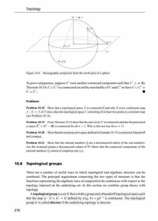
Topology

Figure 10.6 Stereographic projection from the north pole of a sphere

To prove uniqueness, suppose C ′ were another connected component such that C ′ ⊃ A. ByTheorem 10.16, C ∪ C ′ is a connected set and by maximality of C and C ′ we have C ∪ C ′ =C = C ′. �

Problems

Problem 10.18 Show that a topological space X is connected if and only if every continuous mapf : X → Y of X into a discrete topological space Y consisting of at least two points is a constant map(see Problem 10.14).

Problem 10.19 From Theorem 10.16 show that the unit circle S1 is connected, and that the puncturedn-space R

n = Rn − {0} is connected for all n > 1. Why is this not true for n = 1?

Problem 10.20 Show that the real projective space defined in Example 10.15 is connected, Hausdorffand compact.

Problem 10.21 Show that the rational numbers Q are a disconnected subset of the real numbers.Are the irrational points a disconnected subset of R? Show that the connected components of therational numbers Q consist of singleton sets {x}.

10.8 Topological groups

There are a number of useful ways in which topological and algebraic structure can becombined. The principal requirement connecting the two types of structure is that thefunctions representing the algebraic laws of composition be continuous with respect to thetopology imposed on the underlying set. In this section we combine group theory withtopology.

A topological group is a set G that is both a group and a Hausdorff topological space suchthat the map ψ : G × G → G defined by ψ(g, h) = gh−1 is continuous. The topologicalgroup G is called discrete if the underlying topology is discrete.

276

10.8 Topological groups

The maps φ : G → G and τ : G → G defined by φ(g, h) = gh and τ (g) = g−1 are bothcontinuous. For, by Theorem 10.3 the injection map i : G → G × G defined by i(h) =ιe(h) = (e, h) is continuous. The map τ is therefore continuous since it is a compositionof continuous maps, τ : ψ ◦ i . Since φ(g, h) = ψ(g, τ (h)) it follows immediately that φ isalso a continuous map.

Exercise: Show that τ is a homeomorphism of G.

Exercise: If φ and τ are continuous maps, show that ψ is continuous.

Example 10.20 The additive group Rn , where the ‘product’ is vector addition

φ(x, y) = (x1, . . . , xn)+ (y1, . . . , yn) = (x1 + y1, . . . , xn + yn)

and the inverse map is

τ (x) = −x = (−x1, . . . ,−xn),

is an abelian topological group with respect to the Euclidean topology on Rn . The n-torusT n = Rn/Zn is also an abelian topological group, where group composition is additionmodulo 1.

Example 10.21 The set Mn(R) of n × n real matrices has a topology homeomorphic to theEuclidean topology on Rn2

. The determinant map det : Mn(R) → R is clearly continuoussince det A is a polynomial function of the components of A. Hence the general lineargroup GL(n,R) is an open subset of Mn(R) since it is the inverse image of the open setR = R− {0} under the determinant map. If GL(n,R) is given the induced relative topologyin Mn(R) then the map ψ reads in components,

(ψ(A,B))i j =n∑

k=1

Aik

(B−1

)k j.

These are continuous functions since(B−1

)i j

are rational polynomial functions of thecomponents Bi j with non-vanishing denominator det B.

A subgroup H of G together with its relative topology is called a topological subgroupof G. To show that any subgroup H becomes a topological subgroup with respect to therelative topology, let U ′ = H ∩U where U is an arbitrary open subset of G. By continuityof the map φ, for any pair of points g, h ∈ H such that gh ∈ U ′ ⊂ U there exist open setsA and B of G such that A × B ⊂ φ−1(U ). It follows that φ(A′ × B ′) ⊂ H ∩U , whereA′ = A ∩ H , B ′ = B ∩ H , and the continuity of φ

∣∣H

is immediate. Similarly the inversemap τ is continuous when restricted to H . If H is a closed set in G, it is called a closedsubgroup of G.

For each g ∈ G let the left translation Lg : G → G be the map

Lg(h) ≡ Lgh = gh,

as defined in Example 2.25. The map Lg is continuous since it is the composition of twocontinuous maps, Lg = φ ◦ ιg , where ιg : G → G × G is the injection map ιg(h) = (g, h)

277

Topology

(see Theorem 10.3). It is clearly one-to-one, for gh = gh′ =⇒ h = g−1gh′ = h′, and itsinverse is the continuous map Lg−1. Hence Lg is a homeomorphism. Similarly, every righttranslation Rg : G → G defined by Rgh = hg is a homeomorphism of G, as is the innerautomorphism Cg : G → G defined by Cgh = ghg−1 = Lh ◦ Rh−1 (g).

Connected component of the identity

If G is a topological group we will denote by G0 the connected component containing theidentity element e, simply referred to as the component of the identity.

Theorem 10.20 Let G be a topological group, and G0 the component of the identity. ThenG0 is a closed normal subgroup of G.

Proof : By Theorem 10.17 the set G0g−1 is connected, since it is a continuous imageunder right translation by g−1 of a connected set. If g ∈ G0 then e = gg−1 ∈ G0g−1. HenceG0g−1 is a closed connected subset containing the identity e, and must therefore be a subsetof G0. We have therefore G0G−1

0 ⊆ G0, showing that G0 is a subgroup of G. Since it is aconnected component of G it is a closed set. Thus, G0 is a closed subgroup of G.

For any g ∈ G, the set gG0g−1 is connected as it is the image of G0 under the innerautomorphism h �→ Cg(h). Since this set contains the identity e, we have gG0g−1 ⊆ G0,and G0 is a normal subgroup. �

A topological space X is said to be locally connected if every neighbourhood of everypoint of X contains a connected open neighbourhood. A topological group G is locallyconnected if it is locally connected at the identity e, for if V is a connected open neigh-bourhood of e then gV = LgV is a connected open neighbourhood of any selected pointg ∈ G. If K is any subset of a group G, we call the smallest subgroup of G that con-tains K the subgroup generated by K . It is the intersection of all subgroups of G thatcontain K .

Theorem 10.21 In any locally connected group G the component of the identity G0 isgenerated by any connected neighbourhood of the identity e.

Proof : Let V be any connected neighbourhood of e, and H the subgroup generated byV . For any g ∈ H , the left coset gV = LgV ⊂ H is a neighbourhood of g since Lg is ahomeomorphism. Hence H is an open subset of G. On the other hand, if H is an opensubgroup of G it is also closed since it is the complement in G of the union of all cosets ofH that differ from H itself. Thus H is both open and closed. It is therefore the connectedcomponent of the identity, G0. �

Let H be a closed subgroup of a topological group G, we can give the factor spaceG/H the natural topology induced by the canonical projection map π : g �→ gH . This isthe finest topology on G/H such that π is a continuous map. In this topology a collectionof cosets U ⊆ G/H is open if and only if their union is an open subset of G. Clearly πis an open map with respect to this topology, meaning that π (V ) is open for all open setsV ⊆ G.

278

10.9 Topological vector spaces

Theorem 10.22 If G is a topological group and H a closed connected subgroup such thatthe factor space G/H is connected, then G is connected.

Proof : Suppose G is not connected. There then exist open sets U and V such that G =U ∪ V , with U ∩ V = ∅. Since π is an open map the sets π (U ) and π (V ) are open in G/Hand G/H = π(U ) ∪ π (V ). But G/H is connected, π (U ) ∩ π (V ) �= ∅, so there exists acoset gH ∈ π (U ) ∩ π (V ). As a subset of G this coset clearly meets both U and V , andgH = (gH ∩U ) ∪ (gH ∩ V ), contradicting the fact that gH is connected (since it is theimage under the continuous map Lg of a connected set H ). Hence G is connected. �

Example 10.22 The general linear group GL(n,R) is not connected since the determi-nant map det : GL(n,R) → R has image R = R− {0}, which is a disconnected set. Thecomponent G0 of the identity I is the set of n × n matrices with determinant > 0, and thegroup of components is discrete

GL(n,R)/G0∼= {1,−1} = Z2.

Note, however, that the complex general linear group GL(n,C) is connected, as may besurmised from the fact that the Jordan canonical form of any non-singular complex matrixcan be continuously deformed to the identity matrix I.

The special orthogonal groups SO(n) are all connected. This can be shown by inductionon the dimension n. Evidently SO(1) = {1} is connected. Assume that SO(n) is con-nected. It will be shown in Chapter 19, Example 19.10, that SO(n + 1)/SO(n) is home-omorphic to the n-sphere Sn . As this is a connected set (see Example 10.19) it followsfrom Theorem 10.22 that SO(n + 1) is connected. By induction, SO(n) is a connectedgroup for all n = 1, 2, . . . However the orthogonal groups O(n) are not connected, thecomponent of the identity being SO(n) while the remaining orthogonal matrices havedeterminant −1.

Similarly, SU (1) = {1} and SU (n + 1)/SU (n) ∼= S2n−1, from which it follows that allspecial unitary groups SU (n) are connected. By Theorem 10.22 the unitary groups U (n)are also all connected, since U (n)/SU (n) = S1 is connected.

Problem

Problem 10.22 If G0 is the component of the identity of a locally connected topological group G,the factor group G/G0 is called the group of components of G. Show that the group of componentsis a discrete topological group with respect to the topology induced by the natural projection mapπ : g �→ gG0.

10.9 Topological vector spaces

A topological vector space is a vector space V that has a Hausdorff topology definedon it, such that the operations of vector addition and scalar multiplication are continuous

279

Topology

functions on their respective domains with respect to this topology,

ψ : V × V → V defined by ψ(u, v) = u + v,τ : K× V → V defined by τ (λ, v) = λv.

We will always assume that the field of scalars is either the real or complex numbers, K = Ror K = C; in the latter case the topology is the standard topology in R2.

Recall from Section 10.3 that a sequence of vectors vn ∈ V is called convergent if thereexists a vector v ∈ V , called its limit, such that for every open neighbourhood U of v thereis an integer N such that vn ∈ U for all n ≥ N . We also say the sequence converges to v,denoted

vn → v or limn→∞ vn = v.

The following properties of convergent sequences are easily proved:

vn → v and vn → v′ =⇒ v = v′, (10.3)

vn = v for all n =⇒ vn → v, (10.4)

if {v′n} is a subsequence of vn → v then v′n → v, (10.5)

un → u, vn → v =⇒ un + λvn → u + λv, (10.6)

where λ ∈ K is any scalar. Also, if λn is a convergent sequence of scalars in K then

λn → λ =⇒ λnu → λu. (10.7)

Example 10.23 The vector spaces Rn are topological vector spaces with respect to theEuclidean topology. It is worth giving the full proof of this statement, as it sets the patternfor a number of other examples. A set U ⊂ Rn is open if and only if for every x ∈ U thereexists ε > 0 such that

Iε(x) = {y | |yi − xi | < ε, for all i = 1, . . . , n} ⊆ U.

To show that vector addition ψ is continuous, it is necessary to show that N = ψ−1(Iε(x))is an open subset of Rn × Rn for all x ∈ Rn , ε > 0. If ψ(u, v) = u+ v = x then for any(u′, v′) ∈ Iε/2(u)× Iε/2(v), we have for all i = 1, . . . , n∣∣(xi − (u′i + v′i )

)∣∣ = ∣∣((ui − u′i )+ (vi − v′i ))∣∣

≤ ∣∣((ui − u′i ))∣∣+ ∣∣((vi − v′i )

)∣∣ ≤ ε

2+ ε

2= ε.

Hence Iε/2(u)× Iε/2(v) ⊂ N , and continuity of ψ is proved.

280

10.9 Topological vector spaces

For continuity of the scalar multiplication function τ , let M = τ−1(Iε(x)) ⊂ R× Rn . Ifx = au, let v ∈ Iδ(u) and b ∈ Iδ′ (a). Then, setting A = maxi |ui |, we have

|bvi − aui | = |bvi − bui + bui − aui |≤ |b||vi − ui | + |b − a||ui |≤ (|a| + δ′)δ + δ′A≤ ε if δ′ = ε

2Aand δ = ε

2|a|A + ε .

A similar proof may be used to show that the complex vector space Cn is a topologicalvector space.

Example 10.24 The vector space R∞ consisting of all infinite sequences x = (x1, x2, . . . )is an infinite dimensional vector space. We give it the product topology as described, wherebya set U is open if for every point x ∈ U there is a finite sequence of integers i = (i1, i2, . . . , in)such that

Ii,ε(x) = {y | ∣∣yik − xik

∣∣ < ε for k = 1, . . . , n} ⊂ U.

This neighbourhood of x is an infinite product of intervals of which all but a finite numberconsist of all of R. To prove that ψ and τ are continuous functions, we again need onlyshow thatψ−1

(Ii,ε(x)

)and τ−1

(Ii,ε(x)

)are open sets. The argument follows along essentially

identical lines to that in Example 10.23. To prove continuity of the scalar product τ , we setA = maxi∈i |ui |, where x = au and continue as in the previous example.

Example 10.25 Let S be any set, and set F(S) to be the set of bounded real-valuedfunctions on S. This is obviously a vector space, with vector addition defined by ( f +g)(x) = f (x)+ g(x) and scalar multiplication by (a f )(x) = a f (x). A metric can be definedon this space by setting d( f, g) to be the least upper bound of | f (x)− g(x)| on S. Conditions(Met1)–(Met4) are easy to verify. The vector space F(S) is a topological vector spacewith respect to the metric topology generated by this distance function. For example, letf (x) = u(x)+ v(x), then if |u′(x)− u(x)| < ε/2 and |v′(x)− v(x)| < ε/2 it follows atonce that | f (x)− (u′(x)+ v′(x))| < ε. To prove continuity of scalar addition we againproceed as in Example 10.23. If f (x) = au(x), let |b − a| < ε/2A where A is an upperbound of u(x) in S and |v(x)− u(x)| < ε/(2|a|A + ε) for all x ∈ S; then

|bv(x)− f (x)| < ε for all x ∈ S.

Banach spaces

A norm on a vector space V is a map ‖·‖ : V → R, associating a real number ‖v‖ withevery vector v ∈ V , such that

(Norm1) ‖v‖ ≥ 0, and ‖v‖ = 0 if and only if v = 0.(Norm2) ‖λv‖ = |λ| ‖v‖.(Norm3) ‖u + v‖ ≤ ‖u‖ + ‖v‖.In most cases the field of scalars is taken to be the complex numbers, K = C, although

281

Topology

much of what we say also applies to real normed spaces. We have met this concept earlier,in the context of a complex inner product space (see Section 5.2).

A norm defines a distance function d : V × V → R by

d(u, v) = ‖u − v‖.The properties (Met1)–(Met3) are trivial to verify, while the triangle inequality

d(u, v) ≤ d(u,w)+ d(w, v) (10.8)

is an immediate consequence of (Norm3),

‖u − v‖ = ‖u − w + w − v‖ ≤ ‖u − w‖ + ‖w − v‖.We give V the standard metric topology generated by open balls Ba(v) = {u | d(u, v)

< a} as in Section 10.3. This makes it into a topological vector space. To show that thefunction (u, v) �→ u + v is continuous with respect to this topology,

‖u′ − u‖ < ε

2and ‖v′ − v‖ < ε

2=⇒ ‖u′ + v′ − (u + v)‖ < ε

on using the triangle inequality. The proof that (λ, v) �→ λv is continuous follows the linesof Example 10.23.

Exercise: Show that the ‘norm’ is a continuous function ‖·‖ : V → R.

Example 10.26 The vector spaceF(S) of bounded real-valued functions on a set S definedin Example 10.25 has a norm

‖ f ‖ = supx∈S| f (x)|,

giving rise to the distance function d( f, g) of Example 10.25. This is called the supremumnorm.

Convergence of sequences is defined on V by

un → u if d(un, u) = ‖un − u‖ → 0.

As in Section 10.3, every convergent sequence ui → u is a Cauchy sequence

‖ui − u j‖ ≤ ‖u − ui‖ + ‖u − u j‖ → 0 as i, j →∞,but the converse need not always hold. We say a normed vector space (V, ‖·‖) is complete,or is a Banach space, if every Cauchy sequence converges,

‖ui − u j‖ → 0 as i, j →∞ =⇒ ui → u for some u ∈ V .

Exercise: Give an example of a vector subspace of C∞ that is an incomplete normed vector space.

Example 10.27 On the vector space Cn define the standard norm

‖x‖ =√|x1|2 + |x2|2 + · · · + |xn|2.

282

10.9 Topological vector spaces

Conditions (Norm1) and (Norm2) are trivial, while (Norm3) follows from Theorem 5.6,since this norm is precisely that defined in Eq. (5.11) from the inner product 〈x |y〉 =∑n

i=1 xi yi . If ‖xn − xm‖ → 0 for a sequence of vectors xn , then each component is aCauchy sequence |xni − xmi | → 0, and therefore has a limit xni → xi . It is straightforwardto show that ‖xn − x‖ = 0 where x = (x1, x2, . . . , xn). Hence this normed vector space iscomplete.

Example 10.28 Let D([−1, 1]) be the vector space of bounded differentiable complex-valued functions on the closed interval [−1, 1]. As in Example 10.26 we adopt the supremumnorm ‖ f ‖ = supx∈[−1,1] | f (x)|. This normed vector space is not complete, for consider thesequence of functions

fn(x) = ∣∣x∣∣1+1/n(n = 1, 2, . . . ).

These functions are all differentiable on [−1, 1] and have zero derivative at x = 0 fromboth the left and the right. Since they approach the bounded function |x | as n →∞ thisis necessarily a Cauchy sequence. However, the limit function |x | is not differentiable atx = 0, and the norm is incomplete.

By a linear functional on a Banach space V we always mean a continuous linear mapϕ : V → C. The vector space of all linear functionals on V is called the dual space V ′

of V . If V is finite dimensional then V ′ and V ∗ coincide, since all linear functionals arecontinuous with respect to the norm

‖u‖ =√|u1|2 + · · · + |un|2,

but for infinite dimensional spaces it is important to stipulate the continuity requirement. Alinear map ϕ on a Banach space is said to be bounded if there exists M > 0 such that

|ϕ(x)| ≤ M‖x‖ for all x ∈ V .

The following theorem shows that the words ‘bounded’ and ‘continuous’ are interchangeablefor linear functionals on a Banach space.

Theorem 10.23 A linear functional ϕ : V → R on a Banach space V is continuous ifand only if it is bounded.

Proof : If ϕ is bounded, let M > 0 be such that |ϕ(x)| ≤ M‖x‖ for all x ∈ V . Then forany pair of vectors x, y ∈ V

|ϕ(x − y)| ≤ M‖x − y‖,and for any ε > 0 we have

‖x − y‖ < ε

M=⇒ |ϕ(x)− ϕ(y)| = |ϕ(x − y)| ≤ ε.

Hence ϕ is continuous.Conversely, suppose ϕ is continuous. In particular, it is continuous at the origin x = 0

and there exists δ > 0 such that

‖x‖ < δ =⇒ |ϕ(x)| < 1.

283

Topology

For any vector y ∈ V we have ∥∥∥ δy‖y‖∥∥∥ < δ

whence ∣∣∣ϕ( δy‖y‖)∣∣∣ < 1.

Thus

|ϕ(y)| < ‖y‖δ,

showing that ϕ is bounded. �

Example 10.29 Let �1 be the vector space of all complex infinite sequences x =(x1, x2, . . . ) that are absolutely convergent,

‖x‖ =∞∑

i=1

|xi | < ∞.

If c = (c1, c2, . . . ) is a bounded infinite sequence of complex numbers, |ci | ≤ C for alli = 1, 2, . . . , then

ϕc(x) = c1x1 + c2x2 + . . .

is a continuous linear functional on �1. Linearity is obvious as long as the series converges,and convergence and boundedness are proved in one step,

‖ϕc(x)‖ =∞∑

i=1

|ci xi | ≤ |C |∞∑

i=1

|xi | = |C | ‖x‖ <∞.

Hence ϕc is a continuous linear operator by Theorem 10.23.

Problems

Problem 10.23 Prove the properties (10.3)–(10.7).

Problem 10.24 Show that a linear map T : V → W between topological vector spaces is continuouseverywhere on V if and only if it is continuous at the origin 0 ∈ V .

Problem 10.25 Give an example of a linear map T : V → W between topological vector spaces Vand W that is not continuous.

Problem 10.26 Complete the proof that a normed vector space is a topological vector space withrespect to the metric topology induced by the norm.

Problem 10.27 Show that a real vector space V of dimension ≥ 1 is not a topological vector spacewith respect to either the discrete or indiscrete topology.

284

10.9 Topological vector spaces

Problem 10.28 Show that the following are all norms in the vector space R2:

‖u‖1 =√

(u1)2 + (u2)2,

‖u‖2 = max{|u1|, |u2|},‖u‖3 = |u1| + |u2|.

What are the shapes of the open balls Ba(u)? Show that the topologies generated by these norms arethe same.

Problem 10.29 Show that if xn → x in a normed vector space then

x1 + x2 + · · · + xn

n→ x .

Problem 10.30 Show that if xn is a sequence in a normed vector space V such that every subsequencehas a subsequence convergent to x , then xn → x .

Problem 10.31 Let V be a Banach space and W be a vector subspace of V . Define its closure Wto be the union of W and all limits of Cauchy sequences of elements of W . Show that W is a closedvector subspace of V in the sense that the limit points of all Cauchy sequences in W lie in W (notethat the Cauchy sequences may include the newly added limit points of W ).

Problem 10.32 Show that every space F(S) is complete with respect to the supremum norm ofExample 10.26. Hence show that the vector space �∞ of bounded infinite complex sequences is aBanach space with respect to the norm ‖x‖ = sup(xi ).

Problem 10.33 Show that the set V ′ consisting of bounded linear functionals on a Banach space Vis a normed vector space with respect to the norm

‖ϕ‖ = sup{M | |ϕ(x)| ≤ M‖x‖ for all x ∈ V }.Show that this norm is complete on V ′.

Problem 10.34 We say two norms ‖u‖1 and ‖u‖2 on a vector space V are equivalent if there existconstants A and B such that

‖u‖1 ≤ A‖u‖2 and ‖u‖2 ≤ B‖u‖1

for all u ∈ V . If two norms are equivalent then show the following:

(a) If un → u with respect to one norm then this is also true for the other norm.(b) Every linear functional that is continuous with respect to one norm is continuous with respect to

the other norm.(c) Let V = C[0, 1] be the vector space of continuous complex functions on the interval [0, 1]. By

considering the sequence of functions

fn(x) = n√π

e−n2x2

show that the norms

‖ f ‖1 =√∫ 1

0| f |2 dx and ‖ f ‖2 = max{| f (x)| | 0 ≤ x ≤ 1}

are not equivalent.

285

Topology

(d) Show that the linear functional defined by F( f ) = f (1) is continuous with respect to ‖·‖2 butnot with respect to ‖·‖1.

References

[1] R. Geroch. Mathematical Physics. Chicago, The University of Chicago Press, 1985.[2] J. Kelley. General Topology. New York, D. Van Nostrand Company, 1955.[3] M. Nakahara. Geometry, Topology and Physics. Bristol, Adam Hilger, 1990.[4] C. Nash and S. Sen. Topology and Geometry for Physicists. London, Academic Press,

1983.[5] J. G. Hocking and G. S. Young. Topology. Reading, Mass., Addison-Wesley, 1961.[6] D. W. Kahn. Topology. New York, Dover Publications, 1995.[7] E. M. Patterson. Topology. Edinburgh, Oliver and Boyd, 1959.[8] I. M. Singer and J. A. Thorpe. Lecture Notes on Elementary Topology and Geometry.

Glenview, Ill., Scott Foresman, 1967.[9] L. H. Loomis and S. Sternberg. Advanced Calculus. Reading, Mass., Addison-Wesley,

1968.[10] T. Apostol. Mathematical Analysis. Reading, Mass., Addison-Wesley, 1957.[11] L. Debnath and P. Mikusinski. Introduction to Hilbert Spaces with Applications. San

Diego, Academic Press, 1990.[12] N. B. Haaser and J. A. Sullivan. Real Analysis. New York, Van Nostrand Reinhold

Company, 1971.

286

11 Measure theory andintegration

Topology does not depend on the notion of ‘size’. We do not need to know the length,area or volume of subsets of a given set to understand the topological structure. Measuretheory is that area of mathematics concerned with the attribution of precisely these sortsof properties. The structure that tells us which subsets are measurable is called a measurespace. It is somewhat analogous with a topological structure, telling us which sets are open,and indeed there is a certain amount of interaction between measure theory and topology.A measure space requires firstly an algebraic structure known as a σ -algebra imposed onthe power set of the underlying space. A measure is a positive-valued real function on theσ -algebra that is countably additive, whereby the measure of a union of disjoint measurablesets is the sum of their measures. The measure of a set may well be zero or infinite. Fullintroductions to this subject are given in [1–5], while the flavour of the subject can be foundin [6–8].

It is important that measure be not just finitely additive, else it is not far-reaching enough,yet to allow it to be additive on arbitrary unions of disjoint sets would lead to certaincontradictions – either all sets would have to be assigned zero measure, or the measure of aset would not be well-defined. By general reckoning the broadest useful measure on the realline or its cartesian products is that due to Lebesgue (1875–1941), and Lebesgue’s theory ofintegration based on this theory is in most ways the best definition of integration available.

Use will frequently be made in this chapter of the extended real line R consisting ofR ∪ {∞} ∪ {−∞}, having rules of addition a +∞ =∞, a + (−∞) = −∞ for all a ∈ R,but no value is given to ∞+ (−∞). The natural order on the real line is supplemented bythe inequalities −∞ < a <∞ for all real numbers a. Multiplication can also be extendedin some cases, such as a∞ =∞ if a > 0, but it is best to avoid the product 0∞ unlessa clear convention can be adopted. The natural order topology on R, generated by openintervals (a, b) is readily extended to R.

Exercise: Show R is a compact topological space with respect to the order topology.

11.1 Measurable spaces and functions

Measurable spaces

Given a set X , aσ -algebraM on X consists of a collection of subsets, known as measurablesets, satisfying

287

Measure theory and integration

(Meas1) The empty set ∅ is a measurable set, ∅ ∈M.(Meas2) If A is measurable then so is its complement:

A ∈M =⇒ Ac = X − A ∈M.

(Meas3) M is closed under countable unions:

A1, A2, A3, . . . ∈M =⇒⋃

i

Ai ∈M.

The pair (X,M) is known as a measurable space. Although there are similarities betweenthese axioms and (Top1)–(Top3) for a topological space, (Meas2) is distinctly different inthat the complement of an open set is a closed set and is rarely open. It follows from (Meas1)and (Meas2) that the whole space X = ∅c is measurable. The intersection of any pair ofmeasurable sets is measurable, for

A ∩ B = (Ac ∪ Bc)c.

Also, M is closed with respect to taking differences,

A − B = A ∩ Bc = (Ac ∪ B)c.

Exercise: Show that any countable intersection of measurable sets is measurable.

Example 11.1 Given any set X , the collection M = {∅, X} is obviously a σ -algebra. Thisis the smallest σ -algebra possible. By contrast, the largest σ -algebra is the set of all subsets2X . All interesting examples fall somewhere between these two extremes.

It is trivial to see that the intersection of any two σ -algebras M ∩M′ is anotherσ -algebra – check that properties (Meas1)–(Meas3) are satisfied by the sets common tothe two σ -algebras. This statement extends to the intersection of an arbitrary family ofσ -algebras,

⋂i∈I Mi . Hence, given any collection of subsets A ⊂ 2X , there is a unique

‘smallest’ σ -algebra S ⊇ A. This is the intersection of all σ -algebras that contain A. It iscalled the σ -algebra generated by A. For a topological space X , the σ -algebra generatedby the open sets are called Borel sets on X . They include all open and all closed sets and,in general, many more that are neither open nor closed.

Example 11.2 In the standard topology on the real line R every open set is a countableunion of open intervals. Hence the Borel sets are generated by the set of all open inter-vals {(a, b) | a < b}. Infinite left-open intervals such as (a,∞) = (a, a + 1) ∪ (a, a + 2) ∪(a, a + 3) ∪ . . . are Borel sets by (Meas3), and similarly all intervals (−∞, a) are Borel.The complements of these sets are the infinite right or left-closed intervals (−∞, a] and[a,∞). Hence all closed intervals [a, b] = (−∞, b] ∩ [a,∞) are Borel sets.

Exercise: Prove that the σ -algebra of Borel sets on R is generated by (a) the infinite left-open intervals(a,∞), (b) the closed intervals [a, b].

Exercise: Prove that all singletons {a} are Borel sets on R.

288

11.1 Measurable spaces and functions

If (X,M) and (Y,N ) are two measurable spaces then we define the product measurablespace (X × Y,M⊗N ), by setting the σ -algebra M⊗N on X × Y to be the σ -algebragenerated by all sets of the form A × B where A ∈M and B ∈ N .

Measurable functions

Given two measurable spaces (X,M) and (Y,N ), a map f : X → Y is said to be a mea-surable function if the inverse image of every measurable set is measurable:

A ∈ N =⇒ f −1(A) ∈M.

This definition mirrors that for a continuous function in topological spaces.

Theorem 11.1 If X and Y are topological spaces and M and N are the σ -algebras ofBorel sets, then every continuous function f : X → Y is Borel measurable.

Proof : Let OX and OY be the families of open sets in X and Y respectively. We adopt thenotation f −1(A) ≡ { f −1(A) | A ∈ A} for any family of sets A ⊆ 2Y . Since f is continu-ous, f −1(OY ) ⊆ OX . The σ -algebras of Borel sets on the two spaces are M = S(OX )and N = S(OY ). To prove f is Borel measurable we must show that f −1(N ) ⊆M.Let

N ′ = {B ⊆ Y | f −1(B) ∈M} ⊂ 2Y .

This is a σ -algebra on Y , for f −1(∅) = ∅ and

f −1(Bc) = ( f −1(B)

)c, f −1

(⋃i

Bi

)=⋃

i

f −1(Bi

).

Hence N ′ ⊇ OY for f −1(OY ) ⊆ OX ⊂M. Since N is the σ -algebra generated by OY wemust have that N ′ ⊇ N . Hence f −1(N ) ⊆ f −1(N ′) ⊆M as required. �

Exercise: If f : X → Y and g : Y → Z are measurable functions between measure spaces, show thatthe composition g ◦ f : X → Z is a measurable function.

If f : X → R is a measurable real-valued function on a measurable space (X,M), whereR is assumed given the Borel structure of Example 11.2, it follows that the set

{x | f (x) > a} = f −1((a,∞)

)is measurable in X . Since the family of Borel sets B on the real line is generated by theintervals (a,∞) (see the exercise following Example 11.2), this can actually be used as acriterion for measurability: f : X → R is a measurable function iff for any a ∈ R the set{x | f (x) > a} is measurable.

Exercise: Prove the sufficiency of this condition [refer to the proof of Theorem 11.1].

289

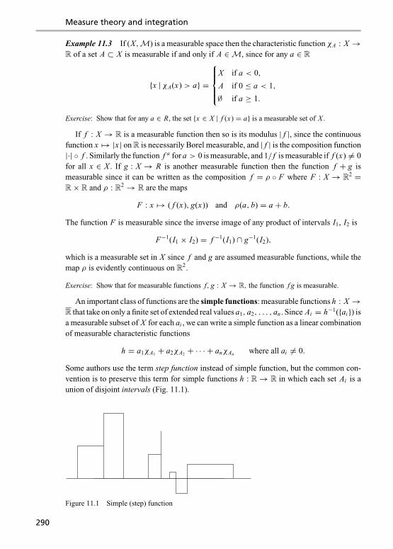
Measure theory and integration

Example 11.3 If (X,M) is a measurable space then the characteristic function χA : X →R of a set A ⊂ X is measurable if and only if A ∈M, since for any a ∈ R

{x |χA(x) > a} =

⎧⎪⎪⎨⎪⎪⎩X if a < 0,

A if 0 ≤ a < 1,

∅ if a ≥ 1.

Exercise: Show that for any a ∈ R, the set {x ∈ X | f (x) = a} is a measurable set of X .

If f : X → R is a measurable function then so is its modulus | f |, since the continuousfunction x �→ |x | on R is necessarily Borel measurable, and | f | is the composition function|·| ◦ f . Similarly the function f a for a > 0 is measurable, and 1/ f is measurable if f (x) �= 0for all x ∈ X . If g : X → R is another measurable function then the function f + g ismeasurable since it can be written as the composition f = ρ ◦ F where F : X → R2 =R× R and ρ : R2 → R are the maps

F : x �→ ( f (x), g(x)) and ρ(a, b) = a + b.

The function F is measurable since the inverse image of any product of intervals I1, I2 is

F−1(I1 × I2) = f −1(I1) ∩ g−1(I2),

which is a measurable set in X since f and g are assumed measurable functions, while themap ρ is evidently continuous on R2.

Exercise: Show that for measurable functions f, g : X → R, the function f g is measurable.

An important class of functions are the simple functions: measurable functions h : X →R that take on only a finite set of extended real values a1, a2, . . . , an . Since Ai = h−1({ai }) isa measurable subset of X for each ai , we can write a simple function as a linear combinationof measurable characteristic functions

h = a1χA1 + a2χA2 + · · · + anχAn where all ai �= 0.

Some authors use the term step function instead of simple function, but the common con-vention is to preserve this term for simple functions h : R → R in which each set Ai is aunion of disjoint intervals (Fig. 11.1).

Figure 11.1 Simple (step) function

290

11.1 Measurable spaces and functions

Let f and g be any pair of measurable functions from X into the extended reals R. Thefunction h = sup( f, g) defined by

h(x) ={

f (x) if f (x) ≥ g(x)

g(x) if g(x) > f (x)

is measurable, since

{x | h(x) > a} = {x | f (x) > a or g(x) > a} = {x | f (x) > a} ∪ {x | g(x) > a}is measurable. Similarly, inf( f, g) is a measurable function. In particular, if f is a measurablefunction, its positive and negative parts

f + = sup( f, 0) and f − = − inf( f, 0)

are measurable functions.

Exercise: Show that f = f + − f − and | f | = f + + f −.

A simple extension of the above argument shows that sup fn is a measurable function forany countable set of measurable functions f1, f2, f3, . . . with values in the extended realnumbers R. We define the lim sup as

lim sup fn(x) = infn≥1

Fn(x) where Fn(x) = supk≥n

fk(x).

The lim sup always exists since the functions Fn are everywhere monotone decreasing,

F1(x) ≥ F2(x) ≥ F3(x) ≥ . . .and therefore have a limit if they are bounded below or approach−∞ if unbounded below.Similarly we can define

lim inf fn(x) = supn≥1

Gn(x) where Gn(x) = infk≥n

fk(x).

It follows that if fn is a sequence of measurable functions then lim sup fn and lim inf fn

are also measurable. By standard arguments in analysis fn(x) is a convergent sequence ifand only if lim sup fn(x) = lim inf fn(x) = lim fn(x). Hence the limit of any convergentsequence of measurable functions fn(x) → f (x) is measurable. Note that the convergenceneed only be ‘pointwise convergence’, not uniform convergence as is required in manytheorems in Riemann integration.

Theorem 11.2 Any measurable function f : X → R is the limit of a sequence of simplefunctions. The sequence can be chosen to be monotone increasing at all positive values off , and monotone decreasing at negative values.

Proof : Suppose f is positive and bounded above, 0 ≤ f (x) ≤ M . For each integer n =1, 2, . . . let hn be the simple function

hn =n∑

k=0

k M

2nχAk

291

Measure theory and integration

where Ak is the measurable set

Ak ={

x∣∣∣ k M

2n≤ f (x) <

k + 1

2n

}.

These simple functions are increasing, 0 ≤ h1(x) ≤ h2(x) ≤ . . . and | f (x)− hn(x)| <M/2n . Hence hn(x) → f (x) for all x ∈ X as n →∞.

If f is any positive function, possibly unbounded, the functions gn = inf(hn, n) arepositive and bounded above. Hence for each n there exists a simple function h′n such that|gn − h′n| < 1/n. The sequence of simple functions h′n clearly converges everywhere tof (x). To obtain a monotone increasing sequence of simple functions that converge to f , set

fn = sup(h′1, h′2, . . . , h

′n).

If f is not positive, construct simple function sequences approaching the positive andnegative parts and use f = f + − f −. �

Problems

Problem 11.1 If (X,M) and (Y,N ) are measurable spaces, show that the projection maps pr1 : X ×Y → X and pr2 : X × Y → Y defined by pr1(x, y) = x and pr2(x, y) = y are measurable functions.

Problem 11.2 Find a step function s(x) that approximates f (x) = x2 uniformly to within ε > 0 on[0, 1], in the sense that | f (x)− s(x)| < ε everywhere in [0, 1].

Problem 11.3 Let f : X → R and g : X → R be measurable functions and E ⊂ X a measurableset. Show that

h(x) ={

f (x) if x ∈ E

g(x) if x /∈ E

is a measurable function on X .

Problem 11.4 If f, g : R→ R are Borel measurable real functions show that h(x, y) = f (x)g(y)is a measurable function h : R2 → R with respect to the product measure on R2.

11.2 Measure spaces

Given a measurable space (X,M), a measureμ on X is a functionμ : M→ R such that

(Meas4) μ(A) ≥ 0 for all measurable sets A, and μ(∅) = 0.(Meas5) If A1, A2, . . . ∈M is any mutually disjoint sequence (finite or countably infinite)

of measurable sets such that Ai ∩ A j = ∅ if i �= j , then

μ(A1 ∪ A2 ∪ A3 ∪ . . . ) =∑

i

μ(Ai ).

A functionμ satisfying property (Meas5) is often referred to as being countably additive. Ifthe series on the right-hand side is not convergent, it is given the value∞. A measure spaceis a triple (X,M, μ) consisting of a measurable space (X,M) together with a measure μ.

292

11.2 Measure spaces

Exercise: Show that if B ⊂ A are measurable sets, then μB ≤ μA.

Example 11.4 An occasionally useful measure on a σ -algebra M defined on a set X isthe Dirac measure. Let a be any fixed point of X , and set

δa(A) ={

1 if a ∈ A,

0 if a /∈ A.

(Meas4) holds trivially forμ = δa , and (Meas5) follows from the obvious fact that the unionof a disjoint family of sets {Ai } can contain a if and only if a ∈ A j for precisely one memberA j . This measure has applications in distribution theory, Chapter 12.

Example 11.5 The branch of mathematics known as probability theory is best expressed interms of measure theory. A probability space is a measure space (�,M, P), where P(�) =1. Sets A ∈ � are known as events and � is sometimes referred to as the universe. This‘universe’ is usually thought of as the set of all possible outcomes of a specific experiment.Note that events are not outcomes of the experiment, but sets of possible outcomes. Themeasure function P is known as the probability measure on�, and P(A) is the probabilityof the event A. All events have probability in the range 0 ≤ P(A) ≤ 1. The element ∅has probability 0, P(∅) = 0, and is called the impossible event. The entire space � hasprobability 1; it can be thought of as the certainty event.

The event A ∪ B is referred to as either A or B, while A ∩ B is A and B. Since Pis additive on disjoint sets and A ∪ B = (A − (A ∩ B)) ∪ (B − (A ∩ B)) ∪ (A ∩ B), theprobabilities are related by

P(A ∪ B) = P(A)+ P(B)− P(A ∩ B).

The two events are said to be independent if P(A ∩ B) = P(A)P(B). This is by no meansalways the case.

We think of the probability of event B after knowing that A has occurred as the condi-tional probability P(B|A), defined by

P(B|A) = P(A ∩ B)

P(A).

Events A and B are independent if and only if P(B|A) = P(B) – in other words, theprobability of B in no way depends on the occurrence of A.

For a finite or countably infinite set of disjoint events H1, H2, . . . partitioning� (some-times called a hypothesis), � =⋃i Hi , we have for any event B

B =∞⋃

i=1

(Hi ∩ B).

Since the sets in this countable union are mutually disjoint, the probability of B is

P(B) =∞∑

i=1

P(Hi ∩ B) =∞∑

i=1

P(B|Hi )P(Hi ).

293

Measure theory and integration

This leads to Bayes’ formula for the conditional probability of the hypothesis Hi given theoutcome event B,

P(Hi |B) = P(B ∩ Hi )

P(B)

= P(Hi )P(B|Hi )

P(B)

= P(Hi )P(B|Hi )∑∞k=1 P(B|Hk)P(Hk)

.

Theorem 11.3 Let E1, E2, . . . be a sequence of measurable sets, which is increasing inthe sense that En ⊂ En+1 for all n = 1, 2, . . . Then

E =∞⋃

n=1

En ∈M and μE = limn→∞μEn.

Proof : E is measurable by condition (Meas3). Set

F1 = E1, F2 = E2 − E1, . . . , Fn = En − En−1, . . . .

The sets Fn are all measurable and disjoint, Fn ∩ Fm = ∅ if n �= m. Since En = F1 ∪F2 ∪ · · · ∪ Fn we have by (Meas5)

limn→∞μEn =

∞∑i=1

μ(Fn) = μ( ∞⋃

k=1

Fk

)= μ(E).

�

Lebesgue measure

Every open set U on the real line is a countable union of disjoint open intervals. This followsfrom the fact that every rational point r ∈ U lies in a maximal open interval (a, b) ⊆ Uwhere a < r < b. These intervals must be disjoint, else they would not be maximal, andthere are countably many of them since the rational numbers are countably infinite. On thereal line R set μ(I ) = b − a for all open intervals I = (a, b). This extends uniquely bycountable additivity (Meas5) to all open sets of R. By finite additivityμmust take the valueb − a on all intervals, open, closed or half-open. For example, for any ε > 0

(a − ε, b) = (a − ε, a) ∪ [a, b),

and since the right-hand side is the union of two disjoint Borel sets we have

b − a + ε = a − a + ε + μ([a, b)).

Hence the measure of the left-closed interval [a, b) is

μ([a, b)

) = b − a.

Using

[a, b) = {a} ∪ (a, b)

294

11.2 Measure spaces

we see that every singleton has zero measure, μ({a}) = 0, and

(a, b] = (a, b) ∪ {b}, [a, b] = (a, b) ∪ {a} ∪ {b} =⇒ μ((a, b]

) = μ([a, b]) = b − a.

Exercise: Show that if A ⊂ R is a countable set, then μ(A) = 0.

Exercise: Show that the set of finite unions of left-closed intervals [a, b) is closed with respect to theoperation of taking differences of sets.

For any set A ⊂ R we define its outer measure

μ∗(A) = inf{μ(U ) |U is an open set in R and A ⊆ U }. (11.1)

While outer measure can be defined for arbitrary sets A of real numbers it is not really ameasure at all, for it does not satisfy the countably additive property (Meas5). The best wecan do is a property known as countable subadditivity: if A1, A2, . . . ∈ 2X is any mutuallydisjoint sequence of sets then

μ∗(⋃

i

Ai

)≤

∞∑i=1

μ∗(Ai ). (11.2)

Proof : Let ε > 0. For each n = 1, 2, . . . there exists an open set Un ⊇ An such that

μ(Un) ≤ μ∗(An)+ ε

2n.

Since U = U1 ∪U2 ∪ . . . covers A = A1 ∪ A2 ∪ . . . ,

μ∗(A) ≤ μ(U ) ≤ μ(U1)+ μ(U2)+ · · · ≤∞∑

i=1

μ∗(An)+ ε.

As this is true for arbitrary ε > 0, the inequality (11.2) follows immediately. �

Exercise: Show that outer measure satisfies (Meas4), μ∗(∅) = 0.

Exercise: For an open interval I = (a, b) show that μ∗(I ) = μ(I ) = b − a.

Exercise: Show that

A ⊆ B =⇒ μ∗(A) ≤ μ∗(B). (11.3)

Following Caratheodory, a set E is said to be Lebesgue measurable if for any openinterval I = (a, b)

μ(I ) = μ∗(I ∩ E)+ μ∗(I ∩ Ec). (11.4)

At first sight this may not seem a very intuitive notion.What it is saying is that when we try to cover the mutually disjoint sets I ∩ E and

I − E = I ∩ Ec with open intervals, the overlap of the two sets of intervals can be made‘arbitrarily small’ (see Fig. 11.2). From now on we will often refer to Lebesgue measurablesets simply as measurable.

295

Measure theory and integration

Figure 11.2 Lebesgue measurable set

Theorem 11.4 If E is measurable then for any set A, measurable or not,

μ∗(A) = μ∗(A ∩ E)+ μ∗(A ∩ Ec).

Proof : Given ε > 0, let U be an open set such that A ⊆ U and

μ(U ) < μ∗(A)+ ε. (11.5)

Since A = (A ∩ E) ∪ (A ∩ Ec) is a union of two disjoint sets, Eq. (11.2) gives

μ∗(A) ≤ μ∗(A ∩ E)+ μ∗(A ∩ Ec).

Setting U =⋃n In where In are a finite or countable collection of disjoint open intervals,we have by (11.3)

μ∗(A) ≤ μ∗(U ∩ E)+ μ∗(U ∩ Ec)

≤∑

n

μ∗(In ∩ E)+ μ∗(In ∩ Ec)

=∑

n

μ∗(In) since E is measurable.

Using the inequality (11.5)

μ∗(A) ≤ μ∗(U ∩ E)+ μ∗(U ∩ Ec) < μ∗(A)+ εfor arbitrary ε > 0. This proves the desired result. �

Corollary 11.5 If E1, E2, . . . , En is any family of disjoint measurable sets then

μ∗(E1 ∪ E2 ∪ · · · ∪ En) =n∑

i=1

μ∗(Ei ).

Proof : If E and F are disjoint measurable sets, setting A = E ∪ F in (11.4) gives

μ∗(E ∪ F) = μ∗((E ∪ F) ∩ E)+ μ∗((E ∪ F) ∩ Ec

) = μ∗(E)+ μ∗(F).

The result follows by induction on n. �

296

11.2 Measure spaces

Theorem 11.6 The set of all Lebesgue measurable sets L is a σ -algebra, and μ∗ is ameasure on L.

Proof : The empty set is Lebesgue measurable, since for any open interval I ,

μ∗(I ∩ ∅)+ μ∗(I ∩ R) = μ∗(∅)+ μ∗(I ) = μ∗(I ) = μ(I ).

If E is a measurable set then so is Ec, on substituting in Eq. (11.4) and using (Ec)c =E . Hence conditions (Meas1) and (Meas2) are satisfied. We prove (Meas3) in severalstages.

Firstly, if E and F are measurable sets then E ∪ F is measurable. For, I = (I ∩ (E ∪F)) ∪ (I ∩ (E ∪ F)c

)and using Eq. (11.2) gives

μ∗(I ) ≤ μ∗(I ∩ (E ∪ F))+ μ∗(I ∩ (E ∪ F)c

). (11.6)

The sets in the two arguments on the right-hand side can be decomposed as

I ∩ (E ∪ F) = ((I ∩ F) ∩ E) ∪ ((I ∩ F) ∩ Ec

) ∪ ((I ∩ Fc) ∩ E)

and

I ∩ (E ∪ F)c = I ∩ (Ec ∩ Fc) = (I ∩ Fc) ∩ Ec.

Again using Eq. (11.2) gives

μ∗(I ∩ (E ∪ F)

)+ μ∗(I ∩ (E ∪ F)c)

≤ μ∗((I ∩ F) ∩ E)+ μ∗((I ∩ F) ∩ Ec

)+ μ∗((I ∩ Fc) ∩ E)+ μ∗((I ∩ Fc) ∩ Ec

)On setting A = I ∩ F and A = I ∩ Fc respectively in Theorem 11.4 we have

μ∗(I ∩ (E ∪ F)

)+ μ∗(I ∩ (E ∪ F)c) ≤ μ∗(I ∩ F)+ μ∗(I ∩ Fc) = μ∗(I ),

since F is measurable. Combining this with the inequality (11.6) we conclude that for allintervals I

μ∗(I ∩ (E ∪ F)

)+ μ∗(I ∩ (E ∪ F)c) = μ∗(I ) = μ(I ),

which shows that E ∪ F is measurable. Incidentally it also follows that the intersectionE ∩ F = (Ec ∪ Fc)c and the difference F − E = F ∩ Ec is measurable. Simple inductionshows that any finite union of measurable sets E1 ∪ E2 ∪ · · · ∪ En is measurable.

Let E1, E2, . . . be any sequence of disjoint measurable sets. Set

Sn =n⋃

i=1

Ei and S =∞⋃

i=1

Ei .

By subadditivity (11.2),

μ∗(S) ≤∞∑

i=1

μ∗(Ei )

297

Measure theory and integration

and since S ⊃ Sn we have, using Corollary 11.5,

μ∗(S) ≥ μ∗(Sn) =n∑

i=1

μ∗(Ei ).

Since this holds for all integers n and the right-hand side is a monotone increasing series,

μ∗(S) =∞∑

i=1

μ∗(Ei ). (11.7)

If the series does not converge, the right-hand side is assigned the value∞.Since the Ei are disjoint sets, so are the sets I ∩ Ei . Furthermore by Corollary 11.5

n∑i=1

μ∗(I ∩ Ei ) = μ∗( n⋃

i=1

(I ∩ Ei ))= μ∗

(I ∩

n⋃i=1

Ei

)≤ μ∗(I ).

Hence the series∑∞

i=1 μ∗(I ∩ Ei ) is convergent and for any ε > 0 there exists an integer n

such that∞∑

i=n

μ∗(I ∩ Ei ) < ε.

Now since Sn ⊂ S,

I ∩ S = I ∩ (Sn ∪ (S − Sn)) = (I ∩ Sn) ∪ (I ∩ (S − Sn)

)and by subadditivity (11.2),

μ(I ) = μ∗((I ∩ S) ∪ (I ∩ Sc))

≤ μ∗(I ∩ S)+ μ∗(I ∩ Sc)

≤ μ∗((I ∩ Sn))+ μ∗(I ∩ (S − Sn)

)+ μ∗(I ∩ (Sn)c)

= μ(I )+ μ∗(

I ∩∞⋃

i=n+1

Ei

)= μ(I )+

∞∑i=n+1

μ∗(I ∩ Ei )

< μ(I )+ ε.Since ε > 0 is arbitrary

μ(I ) = μ∗(I ∩ S)+ μ∗(I ∩ Sc),

which proves that S is measurable.If E1, E2, . . . are a sequence of measurable sets, not necessarily disjoint, then set

F1 = E1, F2 = E2 − E1, . . . , Fn = En − (E1 ∪ E2 ∪ · · · ∪ En−1), . . .

These sets are all measurable and disjoint, and

∞⋃i=1

Ei =∞⋃

i=1

Fi .

298

11.2 Measure spaces

The union of any countable collection {En} of measurable sets is therefore measurable,proving that L is a σ -algebra. The outer measure μ∗ is a measure on L since it satisfiesμ∗(∅) = 0 and is countably additive by (11.7). �

Theorem 11.6 shows that (R,L, μ = μ∗∣∣L) is a measure space. The notation μ forLebesgue measure agrees with the earlier convention μ

((a, b)

) = b − a on open intervals.All open sets are measurable as they are disjoint unions of open intervals. Since the Borelsets form the σ -algebra generated by all open sets, they are included in L. Hence everyBorel set is Lebesgue measurable. It is not true however that every Lebesgue measurableset is a Borel set.

A property that holds everywhere except on a set of measure zero is said to hold almosteverywhere, often abbreviated to ‘a.e.’. For example, two functions f and g are said to beequal a.e. if the set of points where f (x) �= g(x) is a set of measure zero. It is sufficientfor the set to have outer measure zero, μ∗(A) = 0, in order for it to have measure zero (seeProblem 11.8).

Lebesgue measure is defined on cartesian product spaces Rn in a similar manner. Wegive the construction for n = 2. We have already seen that the σ -algebra of measurable setson the product space R2 = R× R is defined as that generated by products of measurablesets E × E ′ where E and E ′ are Lebesgue measurable on R. The outer measure of any setA ⊂ R2 is defined as

μ∗(A) = sup∑

i

μ(Ii )μ(I ′i )

where Ii and I ′i are any finite or countable family of open intervals of R such that theunion

⋃i Ii × I ′i covers A. The outer measure of any product of open intervals is clearly

the product of their measures, μ∗(I × I ′) = μ(I )μ(I ′). We say a set E ⊂ R2 is Lebesguemeasurable if, for any pair of open intervals I, I ′

μ(I )μ(I ′) = μ∗((I × I ′) ∩ E)+ μ∗((I × I ′) ∩ Ec

).

As for the real line, outer measure μ∗ is then a measure on R2. Lebesgue measure on higherdimensional products Rn is completely analogous. We sometimes denote this measureby μn .

Example 11.6 The Cantor set, Example 1.11, is a closed set since it is formed by takingthe complement of a sequence of open intervals. It is therefore a Borel set and is Lebesguemeasurable. The Cantor set is an uncountable set of measure 0 since the length remainingafter the nth step in its construction is

1− 13 − 2

(13

)2 − 22(

13

)3 − · · · − 2n−1(

13

)n = ( 23

)n → 0.

Its complement is an open subset of [0, 1] with measure 1 – that is, having ‘no gaps’ betweenits component open intervals.

Example 11.7 Not every set is Lebegue measurable, but the sets that fail are non-constructive in character and invariably make use of the axiom of choice. A classic exampleis the following. For any pair of real numbers x, y ∈ I = (0, 1) set x Qy if and only if x − y

299

Measure theory and integration

is a rational number. This is an equivalence relation on I and it partitions this set into dis-joint equivalence classes Qx = {y | y − x = r ∈ Q}where Q is the set of rational numbers.Assuming the axiom of choice, there exists a set T consisting of exactly one representativefrom each equivalence class Qx . Suppose it has Lebesgue measure μ(T ). For each rationalnumber r ∈ (−1, 1) let Tr = {x + r | x ∈ T }. Every real number y ∈ I belongs to some Tr

since it differs by a rational number r from some member of T . Hence, since |r | < 1 foreach such Tr , we must have

(−1, 2) ⊃⋃

r

Tr ⊃ (0, 1).

The sets Tr are mutually disjoint and all have measure equal toμ(T ). If the rational numbersare displayed as a sequence r1, r2, . . . then

3 ≥ μ(T1)+ μ(T2)+ · · · =∞∑

i=1

μ(T ) ≥ 1.

This yields a contradiction either for μ(T ) = 0 or μ(T ) > 0; in the first case the sum is 0,in the second it is∞.

Problems

Problem 11.5 Show that every countable subset of R is measurable and has Lebesgue measure zero.

Problem 11.6 Show that the union of a sequence of sets of measure zero is a set of Lebesgue measurezero.

Problem 11.7 If μ∗(N ) = 0 show that for any set E , μ∗(E ∪ N ) = μ∗(E − N ) = μ∗(E). Henceshow that E ∪ N and E − N are Lebesgue measurable if and only if E is measurable.

Problem 11.8 A measure is said to be complete if every subset of a set of measure zero is measurable.Show that if A ⊂ R is a set of outer measure zero, μ∗(A) = 0, then A is Lebesgue measurable andhas measure zero. Hence show that Lebesgue measure is complete.

Problem 11.9 Show that a subset E of R is measurable if for all ε > 0 there exists an open setU ⊃ E such that μ∗(U − E) < ε.

Problem 11.10 If E is bounded and there exists an interval I ⊃ E such that

μ∗(I ) = μ∗(I ∩ E)+ μ∗(I − E)

then this holds for all intervals, possibly even those overlapping E .

Problem 11.11 The inner measure μ∗(E) of a set E is defined as the least upper bound of themeasures of all measurable subsets of E . Show that μ∗(E) ≤ μ∗(E).

For any open set U ⊃ E , show that

μ(U ) = μ∗(U ∩ E)+ μ∗(U − E)

and that E is measurable with finite measure if and only if μ∗(E) = μ∗(E) <∞.

300

11.3 Lebesgue integration

11.3 Lebesgue integration

Let h be a simple function on a measure space (X,M, μ),

h =n∑

i=1

aiχAi (ai ∈ R)

where Ai = h−1(ai ) are measurable subsets of X . We define its integral to be∫h dμ =

n∑i=1

aiμ(Ai ).

This integral only gives a finite answer if the measure of all sets Ai is finite, and in somecases it may not have a sensible value at all. For example h : R → R defined by

h(x) ={

1 if x > 0

−1 if x < 0

has integral∞+ (−∞) which is not well-defined.If h : X → R is a simple function, then for any constant b we have∫

b f dμ = b

∫f dμ. (11.8)

If g =∑mj=1 b jχB j is another simple function then f + g is a simple function

f + g =n∑

i=1

m∑j=1

(ai + b j )χAi∩B j ,

and has integral ∫( f + g) dμ =

∫f dμ+

∫g dμ. (11.9)

It is best to omit any term from the double sum where ai + b j = 0, else we may face theawkward problem of assigning a value to the product 0∞.

Exercise: Prove (11.8).

For any pair of functions f, g : X → R we write f ≤ g to mean f (x) ≤ g(x) for allx ∈ X . If h and h′ are simple functions such that h ≤ h′ then∫

h dμ ≤∫

h′ dμ.

This follows immediately from the fact that h − h′ is a simple function that is non-negativeeverywhere, and therefore has an integral ≥ 0.

Taking the measure on R to be Lebesgue measure, the integral of a non-negativemeasurable function f : X → R is defined as∫

f dμ = sup∫

h dμ

301

Measure theory and integration

Figure 11.3 Integral of a non-negative measurable function

where the supremum is taken over all non-negative simple functions h : X → R such thath ≤ f (see Fig. 11.3). If E ⊂ X is a measurable set then f χE is a measurable function onX that vanishes outside E . We define the integral of f over E to be∫

Ef dμ =

∫f χE dμ.

Exercise: Show that for any pair of non-negative measurable functions f and g

f ≥ g =⇒∫

f dμ ≥∫

g dμ. (11.10)

The following theorem is often known as the monotone convergence theorem:

Theorem 11.7 (Beppo Levi) If fn is an increasing sequence of non-negative measurablereal-valued functions on X, fn+1 ≥ fn, such that fn(x) → f (x) for all x ∈ X then

limn→∞

∫fn dμ =

∫f dμ.

Proof : From the comments before Theorem 11.2 we know that f is a measurable function,as it is the limit of a sequence of measurable functions. If f has a finite integral then, bydefinition, for any ε > 0 there exists a simple function h : X → R such that 0 ≤ h ≤ f and∫

f dμ− ∫ h dμ < ε. For any real number 0 < c < 1 let

En = {x ∈ X | fn(x) ≥ ch(x)} = ( fn − ch)−1([0,∞)

),

clearly a measurable set for each positive integer n. Furthermore, since fn is an increasingsequence of functions we have

En ⊂ En+1 and X =∞⋃

n=1

En,

since every point x ∈ X lies in some En for n big enough. Hence∫f dμ ≥

∫fn dμ ≥ c

∫hχEn dμ.

If h =∑i aiχAi then∫hχEn dμ =

∫ ∑i

aiχAi∩En dμ =∑

i

aiμ(Ai ∩ En).

302

11.3 Lebesgue integration

Hence, by Theorem 11.3,

limn→∞

∫hχEn dμ =

∑i

aiμ(Ai ∩ X ) =∑

i

aiμ(Ai ) =∫

h dμ,

so that ∫f dμ ≥ lim

n→∞

∫fn dμ ≥ c

∫h dμ ≥ c

∫f dμ− cε.

Since c can be chosen arbitrarily close to 1 and ε arbitrarily close to 0, we have∫f dμ ≥ lim

n→∞

∫fn dμ ≥

∫f dμ,

which proves the required result. �

Exercise: How does this proof change if∫

f dμ = ∞?

Using the result from Theorem 11.2, that every positive measurable function is a limitof increasing simple functions, it follows from Theorem 11.7 that simple functions can bereplaced by arbitrary measurable functions in Eqs. (11.8) and (11.9).

Theorem 11.8 The integral of a non-negative measurable function f ≥ 0 vanishes if andonly if f (x) = 0 almost everywhere.

Proof : If f (x) = 0 a.e., let h =∑i aiχAi ≥ 0 be a simple function such that h ≤ f .Every set Ai must have measure zero, else f (x) > 0 on a set of positive measure. Hence∫

f dμ = sup∫

h dμ = 0.Conversely, suppose

∫f dμ = 0. Let En = {x | f (x) ≥ 1/n}. These are an increasing

sequence of measurable sets, En+1 ⊃ En , and

f ≥ 1

nχAn .

Hence ∫1

nχAn dμ = 1

nμ(An) ≤

∫f dμ = 0,

which is only possible if μ(An) = 0. By Theorem 11.3 it follows that

μ({x | f (x) > 0}) = μ( ∞⋃

n=1

An

)= lim

n→∞μ(An) = 0.

Hence f (x) = 0 almost everywhere. �

Integration may be extended to real-valued functions that take on positive or negativevalues. We say a measurable function f is integrable with respect to the measure μ ifboth its positive and negative parts, f + and f −, are integrable. The integral of f is thendefined as ∫

f dμ =∫

f + dμ−∫

f − dμ.

303

Measure theory and integration

If f is integrable then so is its modulus | f | = f + + f −, and∣∣∣∫ f dμ∣∣∣ ≤ ∣∣∣∫ f + dμ−

∫f − dμ

∣∣∣ ≤ ∣∣∣∫ f + dμ+∫

f − dμ∣∣∣ ≤ ∫ | f | dμ. (11.11)

Hence a measurable function f is integrable if and only if | f | is integrable.A function f : R → R is said to be Lebesgue integrable if it is measurable and integrable

with respect to the Lebesgue measure on R. As for Riemann integration it is common touse the notations ∫

f (x) dx =∫ ∞

−∞f (x) dx ≡

∫f dμ,

and for integration over an interval I = [a, b],∫ b

af (x) dx ≡

∫I

f dμ.

Riemann integrable functions on an interval [a, b] are Lebesgue integrable on that interval.A function f is Riemann integrable if for any ε > 0 there exist step functions h1 and h2 –simple functions that are constant on intervals – such that h1 ≤ f ≤ h2 and∫ b

ah2(x) dx −

∫ b

ah1(x) dx < ε.

By taking Hn = sup(hi1) for the sequence of functions (hi1, hi2) (i = 1, . . . , n) defined byε = 1, 1

2 , . . . ,1n , it is straightforward to show that the Hn are simple functions the supremum

of whose integrals is the Riemann integral of f . Hence f is Lebesgue integrable, and itsLebesgue integral is equal to its Riemann integral. The difference between the two conceptsof integration is that for Lebesgue integration the simple functions used to approximate afunction f need not be step functions, but can be constant on arbitrary measurable sets. Forexample, the function on [0, 1] defined by

f (x) ={

1 if x is irrational

0 if x is rational

is certainly Lebesgue integrable, and since f = 1 a.e. its Lebesgue integral is 1. It can-not, however, be approximated in the required way by step functions, and is not Riemannintegrable.

Exercise: Prove the last statement.

Theorem 11.9 If f and g are Lebesgue integrable real functions, then for any a, b ∈ Rthe function a f + bg is Lebesgue integrable and for any measurable set E∫

E(a f + bg) dμ = a

∫E

f dμ+ b

∫E

g dμ.

The proof is straightforward and is left as an exercise (see problems at end of chapter).

304

11.3 Lebesgue integration

Lebesgue’s dominated convergence theorem

One of the most important results of Lebesgue integration is that, under certain generalcircumstances, the limit of a sequence of integrable functions is integrable. First we need alemma, relating to the concept of lim sup of a sequence of functions, defined in the paragraphprior to Theorem 11.2.

Lemma 11.10 (Fatou) If ( fn) is any sequence of non-negative measurable functions de-fined on the measure space (X,M, μ), then∫

lim infn→∞ fn dμ ≤ lim inf

n→∞

∫fn dμ.

Proof : The functions Gn(x) = infk≥n fk(x) form an increasing sequence of non-negativemeasurable functions such that Gn ≤ fn for all n. Hence the lim inf of the sequence ( fn) isthe limit of the sequence Gn ,

lim infn→∞ fn = sup

nGn = lim

n→∞Gn.

By the monotone convergence theorem 11.7,

limn→∞

∫Gn dμ =

∫lim inf

n→∞ fn dμ

while the inequality Gn ≤ fn implies that∫Gn dμ ≤

∫fn dμ.

Hence ∫lim inf

n→∞ fn dμ = limn→∞

∫Gn dμ ≤ lim inf

n→∞

∫fn dμ.

�

Theorem 11.11 (Lebesgue) Let ( fn) be any sequence of real-valued measurable functionsdefined on the measure space (X,M, μ) that converges almost everywhere to a functionf . If there exists a positive integrable function g : X → R such that | fn| < g for all n then

limn→∞

∫fn dμ =

∫f dμ.

Proof : The function f is measurable since it is the limit a.e. of a sequence of measurablefunctions, and as | fn| < g all functions fn and f are integrable with respect to the measureμ. Apply Fatou’s lemma 11.10 to the sequence of positive measurable functions gn =2g − | fn − f | > 0,∫

lim infn→∞ (2g − | fn − f |) dμ ≤ lim inf

n→∞

∫(2g − | fn − f |) dμ.

Since∫

g dμ <∞ and lim inf | fn − f | = lim | fn − f | = 0, we have

0 ≤ lim infn→∞

∫−| fn − f | dμ = − lim sup

n→∞

∫| fn − f | dμ.

305

Measure theory and integration

Since | fn − f | > 0 this is only possible if

limn→∞

∫| fn − f | dμ = 0.

Hence ∣∣∣∫ ( fn − f ) dμ∣∣∣ ≤ ∫ | fn − f | dμ→ 0,

so that∫

fn dμ→ ∫f dμ, as required. �

The convergence in this theorem is said to be dominated convergence, g being thedominating function. An attractive feature of Lebesgue integration is that an integral overan unbounded set is defined exactly as for a bounded set. The same is true of unboundedintegrands. This contrasts sharply with Riemann integration where such integrals are notdefined directly, but must be defined as ‘improper integrals’ that are limits of boundedfunctions over a succession of bounded intervals. The concept of an improper integral isnot needed at all in Lebesgue theory. However, Lebesgue’s dominated convergence theoremcan be used to evaluate such integrals as limits of finite integrands over finite regions.

Example 11.8 The importance of a dominating function is shown by the following exam-ple. The sequence of functions (χ[n,n+1]) consists of a ‘unit hump’ drifting steadily to theright and clearly has the limit f (x) = 0 everywhere. However it has no dominating functionand the integrals do not converge∫

χ[n,n+1] dμ =∫ n+1

n1 dx = 1 �

∫0 dx = 0.

We mention, without proof, the following theorem relating Lebesgue integration onhigher dimensional Euclidean spaces to multiple integration.

Theorem 11.12 (Fubini) If f : R2 → R is a Lebesgue measurable function, then for eachx ∈ R the function fx (y) = f (x, y) is measurable. Similarly for each y ∈ R the functionf ′y(x) = f (x, y) is measurable on R. It is common to write∫

f (x, y) dy ≡∫

fx dμ and

∫f (x, y) dx ≡

∫f ′y dμ.

Then ∫ ∫f (x, y) dx dy ≡

∫f dμ2 =

∫ (∫f (x, y) dy

)dx

=∫ (∫

f (x, y) dx)

dy.

The result generalizes to a product of an arbitrary pair of measure spaces. For a proofsee, for example, [1, 2].

306

References

Problems

Problem 11.12 Show that if f and g are Lebesgue integrable on E ⊂ R and f ≥ g a.e., then∫E

f dμ ≥∫

Eg dμ.

Problem 11.13 Prove Theorem 11.9.

Problem 11.14 If f is a Lebesgue integrable function on E ⊂ R then show that the function ψdefined by

ψ(a) = μ({x ∈ E | | f (x)| > a}) = O(a−1) as a →∞.

References

[1] N. Boccara. Functional Analysis. San Diego, Academic Press, 1990.[2] B. D. Craven. Lebesgue Measure and Integral. Marshfield, Pitman Publishing Company,

1982.[3] L. Debnath and P. Mikusinski. Introduction to Hilbert Spaces with Applications. San

Diego, Academic Press, 1990.[4] N. B. Haaser and J. A. Sullivan. Real Analysis. New York, Van Nostrand Reinhold Com-

pany, 1971.[5] P. R. Halmos. Measure Theory. New York, Van Nostrand Reinhold Company, 1950.[6] R. Geroch. Mathematical Physics. Chicago, The University of Chicago Press, 1985.[7] C. de Witt-Morette, Y. Choquet-Bruhat and M. Dillard-Bleick. Analysis, Manifolds and

Physics. Amsterdam, North-Holland, 1977.[8] F. Riesz and B. Sz.-Nagy. Functional Analysis. New York, F. Ungar Publishing Company,

1955.

307

12 Distributions

In physics and some areas of engineering it has become common to make use of certain‘functions’ such as the Dirac delta function δ(x), having the property∫ ∞

−∞f (x)δ(x) dx = f (0)

for all continuous functions f (x). If we set f (x) to be a continuous function that is ev-erywhere zero except on a small interval (a − ε, a + ε) on which f > 0, it follows thatδ(a) = 0 for all a �= 0. However, setting f (x) = 1 implies

∫δ(x) dx = 1, so we must as-

sign an infinite value to δ(0),

δ(x) ={

0 if x �= 0,

∞ if x = 0.(12.1)

As it stands this really won’t do, since the δ-function vanishes a.e. and should therefore beassigned Lebesgue integral zero. Our aim in this chapter is to give a rigorous definition ofsuch ‘generalized functions’, which avoids these contradictions.

In an intuitive sense we might think of the Dirac delta function as being the ‘limit’ of asequence of functions (see Fig. 12.1) such as

ϕn(x) ={

2n if |x | ≤ 1/n

0 if |x | > 1/n

or of Gaussian functions

ψn(x) = 1

n√π

e−x2/n2.

Lebesgue’s dominated convergence theorem does not apply to these sequences, yet the limitof the integrals is clearly 1, and for any continuous function f (x) it is not difficult to showthat

limn→∞

∫ ∞

−∞f (x)ϕn(x) dx = lim

n→∞

∫ ∞

−∞f (x)ψn(x) dx = f (0).

However, we will not attempt to define Dirac-like functions as limiting functions in somesense. Rather, following Laurent Schwartz, we define them as continuous linear functionalson a suitably defined space of regular test functions. This method is called the theory ofdistributions [1–6].

308

12.1 Test functions and distributions

Figure 12.1 Dirac delta function as a limit of functions

12.1 Test functions and distributions

Spaces of test functions

The support of a function f : Rn → R is the closure of the region of Rn where f (x) �= 0.We will say a real-valued function f on Rn has compact support if the support is a closedbounded set; that is, there exists R > 0 such that f (x1, . . . , xn) = 0 for |x| ≥ R. A functionf is said to be Cm if all partial derivatives of order m,

Dm f = ∂m f

∂xm11 , . . . , ∂xmn

n,

exist and are continuous, where m = (m1, . . . ,mn) and m = |m| ≡∑ni=1 mi . We adopt the

convention that D(0,0,...,0) f = f . A function f is said to be C∞, or infinitely differentiable,if it is Cm to all orders m = 1, 2, . . . We setDm(Rn) to be the vector space of all Cm functionson R with compact support, called the space of test functions of order m.

Exercise: Show that Dm(Rn) is a real vector space.

The space of infinitely differentiable test functions, D∞(Rn), is often denoted simply asD(Rn) and is called the space of test functions,

D(Rn) =∞⋂

n=1

Dm(Rn).

To satisfy ourselves that this space is not empty, consider the function f : R → R definedby

f (x) ={

e−1/x if x > 0,

0 if x ≤ 0.

This function is infinitely differentiable everywhere, including the point x = 0 where allderivatives vanish both from the left and the right. Hence the function ϕ : R → R

ϕ(x) = f (−(x − a)) f (x + a) =⎧⎨⎩exp

(2a

x2−a2

)if |x | < a,

0 if |x | ≥ a,

309

Distributions

is everywhere differentiable and has compact support [−a, a]. There is a counterpartin Rn ,

ϕ(x) =⎧⎨⎩exp

(2a

|x|2−a2

)if |x| < a,

0 if |x| ≥ a,

where

|x| =√

(x1)2 + (x2)2 + · · · + (xn)2.

A sequence of functions ϕn ∈ D(Rn) is said to converge to order m to a functionϕ ∈ D(Rn) if the functions ϕn and ϕ all have supports within a common bounded setand

Dkϕn(x) → Dkϕ(x)

uniformly for all x, for all k of orders k = 0, 1, . . . ,m. If we have convergence to order mfor all m = 0, 1, 2, . . . then we simply say ϕn converges to ϕ, written ϕn → ϕ.

Example 12.1 Let ϕ : R → R be any differentiable function having compact support onK in R. The sequence of functions

ϕn(x) = 1

nϕ(x) sin nx

are all differentiable and have common compact support K . Since |ϕ(x) sin nx | < 1 it isevident that these functions approach the zero function uniformly as n →∞, but theirderivatives

ϕ′n(x) = 1

nϕ′(x) sin nx + ϕ(x) cos nx � 0.

This is an example of a sequence of functions that converge to order 0 to the zero function,but not to order 1.

To define this convergence topologically, we can proceed in the following manner. Forevery compact set K ⊂ Rn let Dm(K ) be the space of Cm functions of compact supportwithin K . This space is made into a topological space as in Example 10.25, by defining anorm

‖ f ‖K ,m = supx∈K

∑|k|≤m

∣∣Dk f (x)∣∣.

On Dm(Rn) we define a set U to be open if for every f ∈ U there exists a compact set Kand a real a > 0 such that f ∈ K and

{g ∈ K | ‖g − f ‖K ,m < a} ⊆ U.

It then follows that a sequence fk ∈ Dm(Rn) converges to order m to a function f ∈ Dm(Rn)

310

12.1 Test functions and distributions

if and only if fn → f with respect to this topology. A similar treatment gives a topologyon D(Rn) leading to convergence in all orders (see Problem 12.2).

Distributions

In this chapter, when we refer to ‘continuity’ of a functional S on a space such as D(Rn), wewill mean that whenever fn → f in some specified sense onD(Rn) we have S( fn) → S( f ).A distribution of order m on Rn is a linear functional T on D(Rn),

T (aϕ + bψ) = aT (ϕ)+ bT (ψ),

which is continuous to order m; that is, if ϕk → ϕ is any sequence of functions in D(Rn)convergent to order m then T (ϕk) → T (ϕ). A linear functional T on D(Rn) that is contin-uous with respect to sequences ϕi in D(Rn) that are convergent to all orders will simply bereferred to as a distribution on Rn . In this sense of continuity, the space of distributionsof order m on Rn is the dual space of Dm(Rn) (see Section 10.9), and the space of distri-butions is the dual space of D(Rn). Accordingly, these are denoted D′m(Rn) and D′(Rn)respectively.

Note that a distribution T of order m is also a distribution of order m ′ for all m ′ > m.For, if ϕi is a convergent sequence of functions in Dm ′

(Rn), then ϕi and all its derivativesup to order m ′ converge uniformly to a function ϕ ∈ Dm ′

(Rn). In particular, it is also asequence in Dm(Rn) converging to order m < m ′ to ϕ. Therefore a linear functional T oforder m, having the property T (ϕi ) → T (ϕ) for all convergent sequences ϕi in Dm(Rn),automatically has this property for all convergent sequences in Dm ′

(Rn). This is a curiousfeature, characteristic of dual spaces: given a function that is Cm we can only concludethat it is Cm ′

for m ′ ≤ m, yet given a distribution of order m we are guaranteed that it is adistribution of order m ′ for all m ′ ≥ m.

Regular distributions

A function f : Rn → R is said to be locally integrable if it is integrable on everycompact subset K ⊂ Rn . Set T f : D(Rn) → R to be the continuous linear functional definedby

T f (ϕ) =∫Rnϕ f dμn =

∫· · ·∫

Rn

ϕ(x) f (x) dx1 . . . dxn.

The integral always exists, since every test function ϕ vanishes outside some compact set.Linearity is straightforward by elementary properties of the integral operator,

T f (aϕ + bψ) = aT f (ϕ)+ bT f (ψ).

311

Distributions

Continuity of T f follows from the inequality (11.11) and Lebesgue’s dominated convergencetheorem 11.11, ∣∣T f (ϕi )− T f (ϕ)

∣∣ = ∣∣∣∫ · · ·∫

Rn

f (x)(ϕi (x)− ϕ(x)) dn x∣∣∣

≤∫· · ·∫

Rn

∣∣ f (x)(ϕi (x)− ϕ(x))∣∣ dn x

≤∫· · ·∫

Rn

| f (x)|∣∣(ϕi (x)− ϕ(x))∣∣ dn x

→ 0,

since the sequence of integrable functions f ϕi is dominated by the integrable function(supi |ϕi |

)| f |. Hence T f is a distribution and the function f is called its density. In fact T f

is a distribution of order 0, since only convergence to order 0 is needed in its definition.Two locally integrable functions f and g that are equal almost everywhere give rise to the

same distribution, T f = Tg . Conversely, if T f (ϕ) = Tg(ϕ) for all test functions ϕ then thedensity functions f and g are equal a.e. An outline proof is as follows: let I n be any productof closed intervals I n = I1 × I2 × · · · × In , and choose a test function ϕ arbitrarily close tothe unit step function χI n . Then

∫I n ( f − g) dμn = 0, which is impossible for all I n if f − g

has non-vanishing positive part, ( f − g)+ > 0, on a set of positive measure. This argumentmay readily be refined to show that f − g = 0 a.e. Hence the density f is uniquely deter-mined by T f except on a set of measure zero. By identifying f with T f , locally integrablefunctions can be thought of as distributions. Not all distributions, however, arise in this way;distributions having a density T = T f are sometimes referred to as regular distributions,while those not corresponding to any locally integrable function are called singular.

Example 12.2 Define the distribution δa on D(R) by

δa(ϕ) = ϕ(a).

In particular, we write δ for δ0, so that δ(ϕ) = ϕ(0). The map δa : D(R) → R is obviouslylinear, δa(bϕ + cψ) = bϕ(a)+ cψ(a) = bδa(ϕ)+ cδa(ψ), and is continuous since ϕn →ϕ =⇒ ϕn(a) → ϕ(a). Hence δa is a distribution, but by the reasoning at the beginning ofthis chapter it cannot correspond to any locally integrable function. It is therefore a singulardistribution. Nevertheless, physicists and engineers often maintain the density notation andwrite

δ(ϕ) ≡∫ ∞

−∞ϕ(x)δ(x) dx = ϕ(0). (12.2)

In writing such an equation, the distribution δ is imagined to have the form Tδ for a densityfunction δ(x) concentrated at the point x = 0 and having an infinite value there as inEq. (12.1), such that ∫ ∞

−∞δ(x) dx = 1.

312

12.1 Test functions and distributions

Using a similar convention, the distribution δa may be thought of as representing thedensity function δa(x) such that ∫ ∞

−∞ϕ(x)δa(x) dx = ϕ(a)

for all test functions ϕ. It is common to write δa(x) = δ(x − a), for on performing the‘change of variable’ x = y + a,∫ ∞

−∞ϕ(x) δ(x − a) dx =

∫ ∞

−∞ϕ(y + a)δ(y) dy = ϕ(a).

The n-dimensional delta function may be similarly defined by

δna (ϕ) = ϕ(a) = ϕ(a1, . . . , an)

and can be written

δna (ϕ) ≡ Tδn

a(ϕ) =

∫· · ·∫

Rn

ϕ(x)δn(x− a) dn x = ϕ(a)

where

δn(x− a) = δ(x1 − a1)δ(x2 − a2) . . . δ(xn − an).

Although it is not in general possible to define the product of distributions, no problemsarise in this instance because the delta functions on the right-hand side depend on separateand independent variables.

Problems

Problem 12.1 Construct a test function such that φ(x) = 1 for |x | ≤ 1 and φ(x) = 0 for |x | ≥ 2.

Problem 12.2 For every compact set K ⊂ Rn let D(K ) be the space of C∞ functions of compactsupport within K . Show that if all integer vectors k are set out in a sequence where N (k) denotes theposition of k in the sequence, then

‖ f ‖K = supx∈K

∑|k|

1

2N (k)

|Dk f (x)|1+ |Dk f (x)|

is a norm on D(K ). Let a set U be defined as open in D(Rn) if it is a union of open balls{g ∈ K | ‖g − f ‖K < a}. Show that this is a topology and sequence convergence with respect tothis topology is identical with convergence of sequences of functions of compact support to allorders.

Problem 12.3 Which of the following is a distribution?

(a) T (φ) =m∑

n=1

λnφ(n)(0) (λn ∈ R).

(b) T (φ) =m∑

n=1

λnφ(xn) (λn, xn ∈ R).

(c) T (φ) = (φ(0))2.

313

Distributions

(d) T (φ) = supφ.

(e) T (φ) =∫ ∞

−∞|φ(x)| dx .

Problem 12.4 We say a sequence of distributions Tn converges to a distribution T , written Tn → T ,if Tn(φ) → T (φ) for all test functions φ ∈ D (this is sometimes called weak convergence). If asequence of continuous functions fn converges uniformly to a function f (x) on every compact subsetof R, show that the associated regular distributions T fn → T f .

In the distributional sense, show that we have the following convergences:

fn(x) = n

π (1+ n2x2)→ δ(x),

gn(x) = n√π

e−n2x2 → δ(x).

12.2 Operations on distributions

If T and S are distributions of order m on Rn , then clearly T + S and aT are distributionsof this order for all a ∈ R. Thus D′m(Rn) is a vector space.

Exercise: Prove that T + S is linear and continuous. Similarly for aT .

The product ST of two distributions is not a distribution. For example, if we were todefine (ST )(ϕ) = S(ϕ)T (ϕ), this is not linear in ϕ. However, if α is a Cm function on Rn

and T is a distribution of order m then αT can be defined as a distribution of order m, bysetting

(αT )(ϕ) = T (αϕ),

since αϕ ∈ Dm(Rn) for all ϕ ∈ Dm(Rn). Note that α need not be a test function for thisconstruction – it works even if the function α does not have compact support.

If T is a regular distribution on Rn , T = T f , then αT f = Tα f . For

αT f (ϕ) = T f (αϕ)

=∫· · ·∫

Rn

ϕα f dn x

= Tα f (ϕ).

The operation of multiplying the regular distribution T f by α is equivalent to simply mul-tiplying the corresponding density function f by α. In this case α need only be a locallyintegrable function.

Example 12.3 The distribution δ defined in Example 12.2 is a distribution of order zero,since it is well-defined on the space of continuous test functions, D0(R). For any continuousfunction α(x) we have

αδ(ϕ) = δ(αϕ) = α(0)ϕ(0) = α(0)δ(ϕ).

314

12.2 Operations on distributions

Thus

αδ = α(0)δ. (12.3)

In terms of the ‘delta function’ this identity is commonly written as

α(x)δ(x) = α(0)δ(x),

since ∫ ∞

−∞α(x)δ(x)ϕ(x) dx = α(0)ϕ(0) =

∫ ∞

−∞α(0)δ(x)ϕ(x) dx .

For the delta function at an arbitrary point a, these identities are replaced by

αδa = α(a)δa, α(x)δ(x − a) = α(a)δ(x − a). (12.4)

Setting α(x) = x results in the useful identities

xδ = 0, xδ(x) = 0. (12.5)

Exercise: Extend these identities to the n-dimensional delta function,

αδa = α(a)δa, α(x)δn(x− a) = α(a)δ(x− a).

Differentiation of distributions

Let T f be a regular distribution where f is a differentiable function. Standard results in realanalysis ensure that the derivative f ′ = d f/dx is a locally integrable function. Let ϕ be anytest function from D1(R). Using integration by parts

T f ′ (ϕ) =∫ ∞

−∞ϕ(x)

d f

dxdx

=[ϕ f]∞−∞

−∫ ∞

−∞

dϕ

dxf (x) dx

= T f (−ϕ′),since ϕ(±∞) = 0. We can extend this identity to general distributions, by defining thederivative of a distribution T of order m ≥ 0 on R to be the distribution T ′ of order m + 1given by

T ′(ϕ) = T (−ϕ′) = −T (ϕ′). (12.6)

The derivative of a regular distribution then corresponds to taking the derivative of thedensity function. Note that the order of the distribution increases on differentiation, forϕ′ ∈ Dm(R) implies that ϕ ∈ Dm+1(R). In particular, if T is a distribution of order 0 thenT ′ is a distribution of order 1.

To prove that T ′ is continuous (linearity is obvious), we use the fact that in the definitionof convergence to order m + 1 of a sequence of functions ϕn → ϕ it is required that allderivatives up to and including order m + 1 converge uniformly on a compact subset K of

315

Distributions

R. In particular, ϕ′n(x) → ϕ′(x) for all x ∈ K , and

T ′(ϕn) = T (−ϕ′n) → T (−ϕ′) = T ′(ϕ).

It follows that every distribution of any order is infinitely differentiable.If T is a distribution of order greater or equal to 0 on Rn , we may define its partial

derivatives in a similar way,

∂T

∂xk(ϕ) = −T

( ∂ϕ∂xk

).

As for distributions on R, any such distribution is infinitely differentiable. For higher deriva-tives it follows that

Dm T (ϕ) = (−1)m T (Dmϕ) where m = |m| =∑i mi .

Exercise: Show that

∂2T

∂xi∂x j= ∂2T

∂x j∂x j.

Example 12.4 Set θ (x) to be the Heaviside step function

θ (x) ={

1 if x ≥ 0,

0 if x < 0.

This is evidently a locally integrable function, and generates a regular distribution Tθ . Forany test function ϕ ∈ D1(R)

Tθ ′ (ϕ) = Tθ (−ϕ′) = −∫ ∞

−∞ϕ′(x)θ (x) dx

= −∫ ∞

0

dϕ

dxdx

= ϕ(0) since ϕ(∞) = 0

= δ(ϕ).

Thus we have the distributional equation, valid only over D1(R),

T ′θ = δ.This is commonly written in terms of ‘functions’ as

δ(x) = θ ′(x) = dθ (x)

dx.

Intuitively, the step at x = 0 is ‘infinitely steep’.

Example 12.5 The derivative of the delta distribution is defined as the distribution δ′ oforder 1, which may be applied to any test function ϕ ∈ D1(R) :

δ′(ϕ) = δ(−ϕ′) = −ϕ′(0).

316

12.2 Operations on distributions

Expressed in terms of the delta function, this reads∫ ∞

−∞δ′(x)ϕ(x) dx = −ϕ′(0),

for an arbitrary function differentiable on a neighbourhood of the origin x = 0. Continuingto higher derivatives, we have

δ′′(ϕ) = ϕ′′(0)

or in Dirac’s notation ∫ ∞

−∞δ′′(x)ϕ(x) dx = ϕ′′(0).

For the mth derivative,

δ(m)(ϕ) = (−1)mϕ(m)(0),∫ ∞

−∞δ(m)(x)ϕ(x) dx = (−1)mϕ(m)(0).

For the product of a differentiable function α and a distribution T we obtain the usualLeibnitz rule,

(αT )′ = αT ′ + α′T,for

(αT )′(ϕ) = αT (−ϕ′)= T (−αϕ′)= T ((−αϕ)′ + α′ϕ)

= T ′(αϕ)+ α′T (ϕ)

= αT ′(ϕ)+ α′T (ϕ).

Example 12.6 From Examples 12.3 and 12.5 we have that

(xδ)′ = 0′ = 0

and

(xδ)′ = xδ′ + x ′δ = xδ′ + δ.Hence

xδ′ = −δ.We can also derive this equation by manipulating the delta function in natural ways,

xδ′(x) = (xδ(x))′ − x ′δ(x) = 0′ − 1.δ(x) = −δ(x).

Exercise: Verify the identity xδ′ = −δ by applying both sides as distributions to an arbitrary testfunction φ(x).

317

Distributions

Change of variable in δ-functions

In applications of the mathematics of delta functions it is common to consider ‘functions’such as δ( f (x)). While this is not an operation that generalizes to all distributions, there isa sense in which we can define this concept for the delta distribution for many functionsf . Firstly, if f : R → R is a continuous monotone increasing function such that f (±∞) =±∞ and we adopt Dirac’s notation then, assuming integrals can be manipulated by thestandard rules for change of variable,∫ ∞

−∞ϕ(x)δ

(f (x)

)dx =

∫ ∞

−∞ϕ(x)δ(y)

dy

f ′(x)where y = f (x)

=∫ ∞

−∞

ϕ(

f −1(y))

f ′(

f −1(y))δ(y) dy

= ϕ(a)

f ′(a)where f (a) = 0.

If f (x) is monotone decreasing then the range of integration is inverted to∫∞−∞ resulting in

a sign change. The general formula for a monotone function f of either direction, havinga unique zero at x = a, is ∫ ∞

−∞ϕ(x)δ

(f (x)

)dx = ϕ(a)

| f ′(a)| . (12.7)

Symbolically, we may write

δ(

f (x)) = 1

| f ′(a)|δ(x − a),

or in terms of distributions,

δ ◦ f = 1

| f ′(a)|δa . (12.8)

Essentially this equation can be taken as the definition of the distribution δ ◦ f . Settingf (x) = −x , it follows that δ(x) is an even function, δ(−x) = δ(x).

If two test functions ϕ and ψ agree on an arbitrary neighbourhood [−ε, ε] of the originx = 0 then

δ(ϕ) = δ(ψ) = ϕ(0) = ϕ(ψ).

Hence the distribution δ can be regarded as being a distribution on the space of functionsD([−ε, ε]), since essentially it only samples values of any test functionϕ in a neighbourhoodof the origin. Thus it is completely consistent to write

δ(ϕ) =∫ ε

−εϕ(x)δ(x) dx .

This just reiterates the idea that δ(x) = 0 for all x �= 0.If f (x) has zeros at x = a1, a2, . . . and f is a monotone function in the neighbourhood

of each ai , then a change of variable to y = f (x) gives, on restricting integration to a small

318

12.2 Operations on distributions

neighbourhood of each zero,∫ ∞

−∞ϕ(x)δ

(f (x)

)dx =

∑i

ϕ(ai )

| f ′(ai )| .

Hence

δ(

f (x)) =∑

i

1

| f ′(ai )|δ(x − ai ), (12.9)

or equivalently

δ ◦ f =∑

i

1

| f ′(ai )|δai .

Example 12.7 The function f = x2 − a2 = (x − a)(x + a) is locally monotone at bothits zeros x = ±a, provided a �= 0. In a small neighbourhood of x = a the function f maybe approximated by the monotone increasing function 2a(x − a), while in a neighbourhoodof x = −a it is monotone decreasing and approximated by −2a(x + a). Thus

δ(x2 − a2) = δ(2a(x − a))+ δ(−2a(x + a)

) = 1

2a

(δ(x − a)+ δ(x + a)

),

in agreement with Eq. (12.9).

Problems

Problem 12.5 In the sense of convergence defined in Problem 12.4 show that if Tn → T thenT ′

n → T ′.

In the distributional sense, show that we have the following convergences:

fn(x) = −2n3x√π

e−n2x2 → δ′(x).

Problem 12.6 Evaluate

(a)∫ ∞

−∞eat sin bt δ(n)(t) dt for n = 0, 1, 2.

(b)∫ ∞

−∞(cos t + sin t)δ(n)(t3 + t2 + t) dt for n = 0, 1.

Problem 12.7 Show the following identities:

(a) δ((x − a)(x − b)) = 1

b − a(δ(x − a)+ δ(x − b)).

(b)d

dxθ (x2 − 1) = δ(x − 1)− δ(x + 1) = 2xδ(x2 − 1).

(c)d

dxδ(x2 − 1) = 1

2 (δ′(x − 1)+ δ′(x + 1)).

(d) δ′(x2 − 1) = 14 (δ′(x − 1)− δ′(x + 1)+ δ(x − 1)+ δ(x + 1)).

Problem 12.8 Show that for a monotone function f (x) such that f (±∞) = ±∞ with f (a) = 0∫ ∞

−∞ϕ(x)δ′

(f (x)

)dx = − 1

f ′(x)

d

dx

( ϕ(x)

| f ′(x)|)∣∣∣

x=a.

319

Distributions

For a general function f (x) that is monotone on a neighbourhood of all its zeros, find a generalformula for the distribution δ′ ◦ f .

Problem 12.9 Show the identities

d

dx

(δ( f (x))

) = f ′(x)δ′(

f (x))

and

δ(

f (x))+ f (x)δ′

(f (x)

) = 0.

Hence show that φ(x, y) = δ(x2 − y2) is a solution of the partial differential equation

x∂φ

∂x+ y

∂φ

∂y+ 2φ(x, y) = 0.

12.3 Fourier transforms

For any function ϕ(x) its Fourier transform is the function Fϕ defined by

Fϕ(y) = 1√2π

∫ ∞

−∞e−ixyϕ(x) dx .

The inverse Fourier transform is defined by

F−1ϕ(y) = 1√2π

∫ ∞

−∞eixyϕ(x) dx .

Fourier’s integral theorem, applicable to all functions ϕ such that |ϕ| is integrable over[−∞,∞] and is of bounded variation, says that F−1Fϕ = ϕ, expressed in integral form as

ϕ(a) = 1

2π

∫ ∞

−∞dyeiay

∫ ∞

−∞e−i yxϕ(x) dx

= 1

2π

∫ ∞

−∞dx ϕ(x)

∫ ∞

−∞ei y(a−x) dy.

The proof of this theorem can be found in many books on real analysis. The reader is referredto [6, chap. 7] or [2, p. 88].

Applying standard rules of integrals applied to delta functions, we expect

δa(x) = δ(x − a) = 1

2π

∫ ∞

−∞ei y(a−x) dy, (12.10)

or, on setting a = 0 and using δ(x) = δ(−x),

δ(x) = 1

2π

∫ ∞

−∞e−i yx dy = 1

2π

∫ ∞

−∞ei yx dy. (12.11)

Similarly, the Fourier transform of the delta function should be

Fδ(y) = 1√2π

∫ ∞

−∞e−ixyδ(x) dx = 1√

2π(12.12)

320

12.3 Fourier transforms

and Eq. (12.11) agrees with

δ(x) = F−1 1√2π

= 1

2π

∫ ∞

−∞eixy dy. (12.13)

Mathematical consistency can be achieved by defining the Fourier transform of adistribution T to be the distribution FT given by

FT (ϕ) = T (Fϕ), (12.14)

for all test functions ϕ. For regular distributions we then have the desired result,

TF f (ϕ) = FT f (ϕ),

since

FT f (ϕ) = T f (Fϕ)

= 1√2π

∫ ∞

−∞

(∫ ∞

−∞e−i yxϕ(x) dx

)f (y) dy

= 1√2π

∫ ∞

−∞ϕ(x)

(∫ ∞

−∞e−i yx f (y) dy

)dx

=∫ ∞

−∞ϕ(x)F f (x) dx

= TF f (ϕ).

If the inverse Fourier transform is defined on distributions by F−1T (ϕ) = T (F−1ϕ), then

F−1FT = T,

for

F−1FT (ϕ) = FT (F−1ϕ) = T (FF−1ϕ) = T (ϕ).

There is, however, a serious problem with these definitions. If ϕ is a function of boundedsupport then Fϕ is generally an entire analytic function and cannot be of bounded support,since an entire function that vanishes on any open set must vanish everywhere. Hence theright-hand side of (12.14) is not in general well-defined. A way around this is to define a moregeneral space of test functions S(R) called the space of rapidly decreasing functions –functions that approach 0 as |x | → ∞ faster than any inverse power |x |−n ,

S(R) = {ϕ|supx∈R

|xmϕ(p)(x)| <∞ for all integers m, p > 0}.

Convergence in S(R) is defined by ϕn → ϕ if and only if

limn→∞ sup

x∈R

|xm(ϕ(p)(x)− ϕ(p))| = 0 for all integers m, p > 0.

The space of continuous linear functions on S(R) is denoted S ′(R), and they are called tem-pered distributions. Since every test function is obviously a rapidly decreasing function,D(R) ⊂ S(R). If T is a tempered distribution in Eq. (12.14), the Fourier transform FT iswell-defined, since the Fourier transform of any rapidly decreasing function may be shownto be a function of rapid decrease.

321

Distributions

Example 12.8 The Fourier transform of the delta distribution is defined by

Fδa(ϕ) = δa(Fϕ)

= Fϕ(a)

= 1√2π

∫ ∞

−∞e−iaxϕ(x) dx

= T(2π )−1/2eiax (ϕ).

Similarly

F−1Te−iax =√

2πδa .

The delta function versions of these distributional equations are

Fδa(y) = 1√2π

∫ ∞

−∞e−i yxδ(x − a) dx = e−iay

√2π

and

F−1e−iax = 1√2π

∫ ∞

−∞eixye−iax dx =

√2πδ(x − a),

in agreement with Eqs. (12.10)–(12.13) above.

Problems

Problem 12.10 Find the Fourier transforms of the functions

f (x) ={

1 if− a ≤ x ≤ a

0 otherwise

and

g(x) ={

1− |x |2 if− a ≤ x ≤ a

0 otherwise.

Problem 12.11 Show that

F(e−a2x2/2

) = 1

|a| e−k2/2a2

.

Problem 12.12 Evaluate Fourier transforms of the following distributional functions:

(a) δ(x − a).(b) δ′(x − a).(c) δ(n)(x − a).(d) δ(x2 − a2).(e) δ′(x2 − a2).

Problem 12.13 Prove that

xmδ(n)(x) = (−1)m n!

(n − m)!δ(n−m)(x) for n ≥ m.

322

12.4 Green’s functions

Hence show that the Fourier transform of the distribution

√2π

k!

(m + k)!xmδ(m+k)(−x) (m, k ≥ 0)

is (−i y)k .

Problem 12.14 Show that the Fourier transform of the distribution

δ0 + δa + δ2a + · · · + δ(2n−1)a

is a distribution with density

1√2π

sin(nay)

sin( 12 ay)

e−(n− 12 )iay .

Show that

F−1( f (y)eiby) = (F−1 f )(x + b).

Hence find the inverse Fourier transform of

g(y) = sin nay

sin( 12 ay)

.

12.4 Green’s functions

Distribution theory may often be used to find solutions of inhomogeneous linear partialdifferential equations by the technique of Green’s functions. We give here two importantstandard examples.

Poisson’s equation

To solve an inhomogeneous equation such as Poisson’s equation

∇2φ = −4πρ (12.15)

we seek a solution to the distributional equation

∇2G(x− x′) = δ3(x− x′) = δ(x − x ′)δ(y − y′)δ(z − z′). (12.16)

A solution of Poisson’s equation (12.15) is then

φ(x) = −∫∫∫

4πρ(x′)G(x− x′) d3x ′,

for

∇2φ = −∫∫∫

4πρ(x′)∇2G(x− x′) d3x ′

= −∫∫∫

4πρ(x′)δ3(x− x′) d3x ′

= −4πρ(x).

323

Distributions

To solve, set

g(k) = FG = 1

(2π )3/2

∫∫∫ ∞

−∞e−ik·yG(y) d3 y.

By Fourier’s theorem

G(y) = 1

(2π )3/2

∫∫∫ ∞

−∞eik·yg(k) d3k,

which implies that

∇2G(x− x′) = 1

(2π )3/2

∫∫∫ ∞

−∞−k2eik·(x−x′)g(k) d3k.

But

δ(y) = 1

(2π )3

∫ ∞

−∞eik1 y1 dk1

∫ ∞

−∞eik2 y2 dk2

∫ ∞

−∞eik3 y3 dk3

= 1

(2π )3

∫∫∫ ∞

−∞eik·y d3k,

so

δ3(x− x′) = 1

2π3

∫∫∫ ∞

−∞eik·(x−x′) d3k.

Substituting in Eq. (12.16) gives

g(k) = − 1

(2π )3/2k2,

and

G(x− x′) = − 1

(2π )3

∫∫∫ ∞

−∞

eik·y

k2d3k. (12.17)

The integration in k-space is best performed using polar coordinates (k, θ, φ) with thek3-axis pointing along the direction R = x− x′ (see Fig. 12.2). Then

k · (x− x′) = k R cos θ (k =√

k · k)

and

d3k = k2 sin θ dk dθ dφ.

324

12.4 Green’s functions

Figure 12.2 Change to polar coordinates in k-space.

This results in

G(R) = − 1

(2π )3

∫ ∞

0dk

∫ π

0dθ∫ 2π

0dφ

eik R cos θ

k2k2 sin θ

= − 2π

(2π )3

∫ ∞

0dk

∫ π

0dθ

d

dθ

(−eik R cos θ

ik R

)= − 1

(2π )2 R

∫ ∞

0dk

eik R − e−ik R

ik

= − 1

(2π )2 R

∫ ∞

0dk2

sin k R

k

= − 1

4πR,

on making use of the well-known definite integral∫ ∞

0

sin x

xdx = π

2.

Hence

G(x− x′) = − 1

4π |x− x′| , (12.18)

and a solution of Poisson’s equation (12.15) is

φ(x) =∫∫∫

ρ(x′)|x− x′| d3x ′,

where the integral is taken over all of the space, −∞ < x ′, y′, z′ <∞. For a point charge,ρ(x) = qδ3(x− a) the solution reduces to the standard coulomb solution

φ(x) = q

|x− a| .

325

Distributions

Green’s function for the wave equation

To solve the inhomogeneous wave equation

�ψ = − ∂2

c2∂t2ψ + ∇2ψ = f (x, t) (12.19)

it is best to adopt a relativistic 4-vector notation, setting x4 = ct . The wave equation canthen be written as in Section 9.4,

�ψ = gμν∂

∂xμ∂

∂xνψ = f (x)

where μ and ν range from 1 to 4, gμν is the diagonal metric tensor having diagonal com-ponents 1, 1, 1,−1 and the argument x in the last term is shorthand for (x, x4).Again we look for a solution of the equation

�G(x − x ′) = δ4(x − x ′) ≡ δ(x1 − x ′1)δ(x2 − x ′2)δ(x3 − x ′3)δ(x4 − x ′4). (12.20)

Every Green’s function G generates a solution ψG(x) of Eq. (12.19),

ψG(x) =∫∫∫∫

G(x − x ′) f (x ′) d4x ′

for

�ψG =∫∫∫∫

�G(x − x ′) f (x ′) d4x ′ =∫∫∫∫

δ4(x − x ′) f (x ′) d4x ′ = f (x).

Exercise: Show that the general solution of the inhomogeneous wave equation (12.19) has the formψG(x)+ φ(x) where �φ = 0.

Set

G(x − x ′) = 1

(2π )2

∫∫∫∫g(k) eik.(x−x ′) d4k

where k = (k1, k2, k3, k4), and

k.(x − x ′) = kμ(xμ − x ′μ) = k4(x4 − x ′4)+ k. · (x− x′)

and d4k = dk1 dk2 dk3 dk4. Writing the four-dimensional δ function as a Fourier transformwe have

�G(x − x ′) = 1

(2π )2

∫∫∫∫−k2g(k) eik.(x−x ′) d4k

= δ4(x − x ′) = 1

(2π)4

∫∫∫∫eik.(x−x ′) d4k,

whence

g(k) = − 1

4π2k2

326

12.4 Green’s functions

Figure 12.3 Green’s function for the three-dimensional wave equation

where k2 ≡ k.k = kμkμ. The Fourier transform expression of the Green’s function is thus

G(x − x ′) = − 1

(2π )4

∫∫∫∫eik.(x−x ′)

k2d4k. (12.21)

To evaluate this integral set

τ = x4 − x ′4, R = x− x′, K = |k| =√

k · k,whence k2 = K 2 − k 2

4 and

G(x − x ′) = 1

(2π )4

∫ ∞

−∞dk4

eik4τ

k 24 − K 2

∫∫∫d3k eik·R.

Deform the path in the complex k4-plane to avoid the pole singularities at k4 = ±K asshown in Fig. 12.3 – convince yourself, however, that this has no effect on G satisfyingEq. (12.20).

For τ > 0 the contour is completed in a counterclockwise sense by the upper half semi-circle and ∫ ∞

−∞

eik4τ

k 24 − K 2

dk4 = 2π i × sum of residues

= 2π i(eiK τ

2K− e−iK τ

2K

).

For τ < 0 we complete the contour with the lower semicircle in a clockwise direction; nopoles are enclosed and the integral vanishes. Hence∫ ∞

−∞

eik4τ

k 24 − K 2

dk4 = −2π

Kθ (τ ) sin K τ

where θ (τ ) is the Heaviside step function.

327

Distributions

This particular contour gives rise to a Green’s function that vanishes for τ < 0; that is, forx4 < x ′4. It is therefore called the outgoing wave condition or retarded Green’s function,for a source switched on at (x′, x ′4) only affects field points at later times. If the contour hadbeen chosen to lie above the poles, then the ingoing wave condition or advanced Green’sfunction would have resulted.

To complete the calculation of G, use polar coodinates in k-space with the k3-axis parallelto R. This gives

G(x − x ′) = − 1

(2π )3θ (τ )

∫ 2π

0dφ∫ ∞

0dK

∫ π

0dθ K 2 sin θeiKR cos θ sin K τ

K

= − θ(τ )

2π2 R

∫ ∞

0dK sin K τ sin K R

= − θ (τ )

2π2 R

∫ ∞

0dK

(eiK τ − e−iK τ )

2i

(eiK R − e−iK R)

2i

= θ (τ )

4πR

(δ(τ + R)− δ(τ − R)

)= −δ(τ − R)

4πR.

The last step follows because the whole expression vanishes for τ < 0 on account of theθ (τ ) factor, while for τ > 0 we have δ(τ + R) = 0. Hence the Green’s function may bewritten

G(x − x ′) = − 1

4π |x− x′|δ(x4 − x ′4 − |x− x′|), (12.22)

which is non-vanishing only on the future light cone of x ′.The solution of the inhomogeneous wave equation (12.19) generated by this Green’s

function is

ψ(x, t) =∫∫∫∫

G(x − x ′) f (x ′) d4x ′

= − 1

4π

∫∫∫[ f (x′, t ′)]ret

|x− x′| d3x ′(12.23)

where [ f (x′, t ′)]ret means f evaluated at the retarded time

t ′ = t − |x− x′|c

.

Problems

Problem 12.15 Show that the Green’s function for the time-independent Klein–Gordon equation

(∇2 − m2)φ = ρ(r)

can be expressed as the Fourier integral

G(x− x′) = − 1

(2π )3

∫ ∫ ∫d3k

eik.(x−x′)

k2 + m2.

328

References

Evaluate this integral and show that it results in

G(R) = − e−m R

4πRwhere R = x− x′, R = |R|.

Find the solution φ corresponding to a point source

ρ(r) = qδ3(r).

Problem 12.16 Show that the Green’s function for the one-dimensional diffusion equation,

∂2G(x, t)

∂x2− 1

κ

∂G(x, t)

∂t= δ(x − x ′)δ(t − t ′)

is given by

G(x − x ′, t − t ′) = −θ (t − t ′)√

κ

4π(t − t ′)e−(x−x ′)2/4κ(t−t ′),

and write out the corresponding solution of the inhomogeneous equation

∂2ψ(x, t)

∂x2− 1

κ

∂ψ(x, t)

∂t= F(x, t).

Do the same for the two- and three-dimensional diffusion equations

∇2G(x, t)− 1

κ

∂G(x, t)

∂t= δn(x− x′)δ(t − t ′) (n = 2, 3).

References

[1] J. Barros-Neto. An Introduction to the Theory of Distributions. New York, MarcelDekker, 1973.

[2] N. Boccara. Functional Analysis. San Diego, Academic Press, 1990.[3] R. Geroch. Mathematical Physics. Chicago, The University of Chicago Press, 1985.[4] R. F. Hoskins. Generalized Functions. Chichester, Ellis Horwood, 1979.[5] C. de Witt-Morette Y. Choquet-Bruhat and M. Dillard-Bleick. Analysis, Manifolds and

Physics. Amsterdam, North-Holland, 1977.[6] A. H. Zemanian. Distribution Theory and Transform Analysis. New York, Dover

Publications, 1965.

329

13 Hilbert spaces

13.1 Definitions and examples

Let V be a complex vector space with an inner product 〈· | ·〉 : V × V → C satisfying (IP1)–(IP3) of Section 5.2. Such a space is sometimes called a pre-Hilbert space. As in Eq. (5.11)define a norm on an inner product space by

‖u‖ =√〈u |u〉. (13.1)

The properties (Norm1)–(Norm3) of Section 10.9 hold for this choice of ‖·‖. Condition(Norm1) is equivalent to (IP3), and (Norm2) is an immediate consequence of (IP1) and(IP2), for

‖λv‖ =√〈λv |λv〉 =

√λλ〈v |v〉 = |λ| ‖v‖.

The triangle inequality (Norm3) is a consequence of Theorem 5.6. These properties holdequally in finite or infinite dimensional vector spaces. A Hilbert space (H, 〈· | ·〉) is an innerproduct space that is complete in the induced norm; that is, (H, ‖·‖) is a Banach space. Anintroduction to Hilbert spaces at the level of this chapter may be found in [1–6], while moreadvanced topics are dealt with in [7–11].

The parallelogram law

‖x + y‖2 + ‖x − y‖2 = 2‖x‖2 + 2‖y‖2 (13.2)

holds for all pairs of vectors x, y in an inner product spaceH. The proof is straightforward, bysubstituting ‖x + y‖2 = 〈x + y | x + y〉 = ‖x‖2 + ‖y‖2 + 2Re(〈x | y〉), etc. It immediatelygives rise to the inequality

‖x + y‖2 ≤ 2‖x‖2 + 2‖y‖2. (13.3)

For complex numbers (13.2) and (13.3) hold with norm replaced by modulus.

Example 13.1 The typical inner product defined on Cn in Example 5.4 by

〈(u1, . . . , un) | (v1, . . . , vn)〉 =n∑

i=1

uivi

makes it into a Hilbert space. The norm is

‖v‖ =√|v1|2 + |v2|2 + · · · + |vn|2,

330

13.1 Definitions and examples

which was shown to be complete in Example 10.27. In any finite dimensional inner productspace the Schmidt orthonormalization procedure creates an orthonormal basis for whichthe inner product takes this form (see Section 5.2). Thus every finite dimensional Hilbertspace is isomorphic to Cn with the above inner product. The only thing that distinguishesfinite dimensional Hilbert spaces is their dimension.

Example 13.2 Let �2 be the set of all complex sequences u = (u1, u2, . . . ) where ui ∈ Csuch that

∞∑i=1

|ui |2 <∞.

This space is a complex vector, for if u, v are any pair of sequences in �2, then u + v ∈ �2.For, using the complex number version of the inequality (13.3),

∞∑i=1

|ui + vi |2 ≤ 2∞∑

i=1

|ui |2 + 2∞∑

i=1

|vi |2 <∞.

It is trivial that u ∈ �2 implies λu ∈ �2 for any complex number λ.Let the inner product be defined by

〈u |v〉 =∞∑

i=1

uivi .

This is well-defined for any pair of sequences u, v ∈ �2, for∣∣∣ ∞∑i=1

uivi

∣∣∣ ≤ ∞∑i=1

∣∣uivi

∣∣≤ 1

2

∞∑i=1

(∣∣ui

∣∣2 + ∣∣vi

∣∣2) <∞.The last step follows from

2∣∣ab∣∣2 = 2|a|2|b|2 = |a|2 + |b|2 − (|a| − |b|)2 ≤ |a|2 + |b|2.

The norm defined by this inner product is

‖u‖ =√√√√ ∞∑

i=1

∣∣ui

∣∣2 ≤ ∞.For any integer M and n,m > N

M∑i=1

∣∣u(m)i − u(n)

i

∣∣2 ≤ ∞∑i=1

∣∣u(m)i − u(n)

i

∣∣2 = ‖u(m) − u(n)‖2 < ε2,

and taking the limit n →∞ we have

M∑i=1

∣∣u(m)i − ui

∣∣2 ≤ ε2.

331

Hilbert spaces

In the limit M →∞∞∑

i=1

∣∣u(m)i − ui

∣∣2 ≤ ε2

so that u(m) − u ∈ �2. Hence u = u(m) − (u(m) − u) belongs to �2 since it is the differenceof two vectors from �2 and it is the limit of the sequence u(m) since ‖u(m) − u‖ < ε forall m > N . It turns out, as we shall see, that �2 is isomorphic to most Hilbert spaces ofinterest – the so-called separable Hilbert spaces.

Example 13.3 On C[0, 1], the continuous complex functions on [0, 1], set

〈 f |g〉 =∫ 1

0f g dx .

This is a pre-Hilbert space, but fails to be a Hilbert space since a sequence of continuousfunctions may have a discontinuous limit.

Exercise: Find a sequence of functions in C[0, 1] that have a discontinuous step function as theirlimit.

Example 13.4 Let (X,M, μ) be a measure space, and L2(X ) be the set of all squareintegrable complex-valued functions f : X → C, such that∫

X| f |2 dμ <∞.

This space is a complex vector space, for if f and g are square integrable then∫X| f + λg|2 dμ ≤ 2

∫X| f |2 dμ+ 2|λ|2

∫X|g|2 dμ

by (13.3) applied to complex numbers.Write f ∼ f ′ iff f (x) = f ′(x) almost everywhere on X ; this is clearly an equivalence

relation on X . We set L2(X ) to be the factor space L2(X )/∼. Its elements are equivalenceclasses f of functions that differ at most on a set of measure zero. Define the inner productof two classes by

〈 f | g〉 =∫

Xf g dμ,

which is well-defined (see Example 5.6) and independent of the choice of representatives.For, if f ′ ∼ f and g′ ∼ g then let A f and Ag be the sets on which f (x) �= f ′(x) andg′(x) �= g(x), respectively. These sets have measure zero, μ(A f ) = μ(Ag) = 0. The set onwhich f ′(x)g′(x) �= f (x)g(x) is a subset of A f ∪ Ag and therefore must also have measurezero, so that

∫X f g dμ = ∫X f ′g′ dμ.

The inner product axioms (IP1) and (IP2) are trivial, and (IP3) follows from

‖ f ‖ = 0 =⇒∫

X| f |2 dμ = 0 =⇒ f = 0 a.e.

332

13.1 Definitions and examples

It is common to replace an equivalence class of functions f ∈ L2(X ) simply by a represen-tative function f when there is no danger of confusion.

It turns out that the inner product space L2(X ) is in fact a Hilbert space. The followingtheorem is needed in order to show completeness.

Theorem 13.1 (Riesz–Fischer) If f1, f2, . . . is a Cauchy sequence of functions inL2(X ),there exists a function f ∈ L2(X ) such that ‖ f − fn‖ → 0 as n →∞.

Proof : The Cauchy sequence condition ‖ fn − fm‖ → 0 implies that for any ε > 0 thereexists N such that ∫

X| fn − fm |2 dμ < ε for all m, n > N .

We may, with some relabelling, pick a subsequence such that f0 = 0 and

‖ fn − fn−1‖ < 2−n.

Setting

h(x) =∞∑

n=1

| fn(x)− fn−1(x)|

we have from (Norm3),

‖h‖ ≤∞∑

n=1

‖ fn − fn−1‖ <∞∑

n=1

2−n = 1.

The function x �→ h2(x) is thus a positive real integrable function on X , and the set ofpoints where its defining sequence diverges, E = {x | h(x) = ∞}, is a set of measure zero,μ(E) = 0. Let gn be the sequence of functions

gn(x) ={

fn − fn−1 if x /∈ E,

0 if x ∈ E .

Since gn = fn − fn−1 a.e. these functions are measurable and ‖gn‖ = ‖ fn − fn−1‖ < 2−n .The function

f (x) =∞∑

n=1

gn(x)

is defined almost everywhere, since the series is absolutely convergent to h(x) almosteverywhere. Furthermore it belongs to L2(X ), for

| f (x)|2 =∣∣∣∑ gn(x)

∣∣∣2 ≤ (∑|gn(x)|)2≤ (h(x)

)2.

Since

fn =n∑

k=1

( fk − fk−1) =n∑

k=1

gk a.e.

333

Hilbert spaces

it follows that

‖ f − fn‖ =∥∥∥ f −

n∑k=1

gk

∥∥∥=∥∥∥ ∞∑

k=n+1

gk

∥∥∥≤

∞∑k=n+1

‖gk‖

<

∞∑k=n+1

2−k = 2−n.

Hence ‖ f − fn‖ → 0 as n →∞ and the result is proved. �

Problems

Problem 13.1 Let E be a Banach space in which the norm satisfies the parallelogram law (13.2).Show that it is a Hilbert space with inner product given by

〈x | y〉 = 14

(‖x + y‖2 − ‖x − y‖2 + i‖x − i y‖2 − i‖x + i y‖2).

Problem 13.2 On the vector space F1[a, b] of complex continuous differentiable functions on theinterval [a, b], set

〈 f |g〉 =∫ b

af ′(x)g′(x) dx where f ′ = d f

dx, g′ = dg

dx.

Show that this is not an inner product, but becomes one if restricted to the space of functions f ∈F1[a, b] having f (c) = 0 for some fixed a ≤ c ≤ b. Is it a Hilbert space?

Give a similar analysis for the case a = −∞, b = ∞, and restricting functions to those of compactsupport.

Problem 13.3 In the space L2([0, 1]) which of the following sequences of functions (i) is a Cauchysequence, (ii) converges to 0, (iii) converges everywhere to 0, (iv) converges almost everywhere to 0,and (v) converges almost nowhere to 0?

(a) fn(x) = sinn(x), n = 1, 2, . . .

(b) fn(x) ={

0 for x < 1− 1n ,

nx + 1− n for 1− 1n ≤ x ≤ 1.

(c) fn(x) = sinn(nx).(d) fn(x) = χUn (x), the characteristic function of the set

Un =[

k

2m,

k + 1

2m

]where n = 2m + k, m = 0, 1, . . . and k = 0, . . . , 2m − 1.

334

13.2 Expansion theorems

13.2 Expansion theorems

Subspaces

A subspace V of a Hilbert space H is a vector subspace that is closed with respect to thenorm topology. For a vector subspace to be closed we require the limit of any sequence ofvectors in V to belong to V ,

u1, u2, . . .→ u and all un ∈ V =⇒ u ∈ V .

If V is any vector subspace of H, its closure V is the smallest subspace containing V . It isthe intersection of all subspaces containing V .

If K is any subset of H then, as in Chapter 3, the vector subspace generated by K is

L(K ) ={

n∑i=1

αi ui |αi ∈ C, ui ∈ K

},

but the subspace generated by K will always refer to the closed subspace L(K ) generatedby K . A Hilbert space H is called separable if there is a countable set K = {u1, u2, . . . }such that H is generated by K ,

H = L(K ) = L(u1, u2, . . . ).

Orthonormal bases

If the Hilbert space H is separable and is generated by {u1, u2, . . . }, we may use theSchmidt orthonormalization procedure (see Section 5.2) to produce an orthonormal set{e1, e2, . . . , en},

〈ei |e j 〉 = δi j ={

1 if i = j,

0 if i �= j.

The steps of the procedure are

f1 = u1 e1 = f1/‖ f1‖f2 = u2 − 〈e1 |u2〉e1 e2 = f2/‖ f2‖f3 = u3 − 〈e1 |u3〉e1 − 〈e2 |u3〉e2 e3 = f3/‖ f3‖, etc.

from which it can be seen that each un is a linear combination of {e1, e2, . . . , en}. HenceH = L({e1, e2, . . . }) and the set {en | n = 1, 2, . . . } is called a complete orthonormal setor orthonormal basis of H.

Theorem 13.2 If H is a separable Hilbert space and {e1, e2, . . . } is a complete orthonor-mal set, then any vector u ∈ H has a unique expansion

u =∞∑

n=1

cnen where cn = 〈en |u〉. (13.4)

335

Hilbert spaces

The meaning of the sum in this theorem is∥∥∥u −N∑

n=1

cnen

∥∥∥→ 0 as N →∞.

A critical part of the proof is Bessel’s inequality:

N∑n=1

∣∣〈en |u〉∣∣2 ≤ ‖u‖2. (13.5)

Proof : For any N > 1

0 ≤∥∥∥u −

N∑n=1

〈en |u〉 en

∥∥∥2

= 〈u −∑n〈en |u〉en |u −∑

m〈em |u〉em〉

= ‖u‖2 − 2N∑

n=1

〈en |u〉〈en |u〉 +N∑

n=1

N∑m=1

〈en |u〉δmn〈em |u〉

= ‖u‖2 −N∑

n=1

|〈en |u〉|2,

which gives the desired inequality. �

Taking the limit N →∞ in Bessel’s inequality (13.5) shows that the series

∞∑n=1

∣∣〈en |u〉∣∣2

is bounded above and therefore convergent since it consists entirely of non-negative terms.To prove the expansion theorem 13.2, we first show two lemmas.

Lemma 13.3 If vn → v in a Hilbert space H, then for all vectors u ∈ H

〈u |vn〉 → 〈u |v〉.Proof : By the Cauchy–Schwarz inequality (5.13)∣∣〈u |vn〉 − 〈u |v〉

∣∣ = ∣∣〈u |vn − v〉∣∣

≤ ‖u‖ ‖vn − v‖→ 0 �

Lemma 13.4 If {e1, e2, . . . } is a complete orthonormal set and 〈v |en〉 = 0 for n =1, 2, . . . then v = 0.

Proof : Since {en} is a complete o.n. set, every vector v ∈ H is the limit of a sequence ofvectors spanned by the vectors {e1, e2, . . . },

v = limn→∞ vn where vn =

N∑i=1

vni ei .

336

13.2 Expansion theorems

Setting u = v in Lemma 13.3, we have

‖v‖2 = 〈v |v〉 = limn→∞〈v |vn〉 = 0.

Hence v = 0 by the condition (Norm1). �

We now return to the proof of the expansion theorem.

Proof of Theorem 13.2: Set

uN =N∑

n=1

〈en |u〉 en.

This is a Cauchy sequence,

‖uN − uM‖2 =N∑

n=M

∣∣〈en |u〉∣∣2 → 0 as M, N →∞

since the series∑

n

∣∣〈en |u〉∣∣2 is absolutely convergent by Bessel’s inequality (13.5). By

completeness of the Hilbert space H, uN → u′ for some vector u′ ∈ H. But

〈ek |u − u′〉 = limN→∞

〈ek |u − uN 〉 = 〈ek |u〉 − eku = 0

since 〈ek |uN 〉 = 〈ek |u〉 for all N ≥ k. Hence, by Lemma 13.4,

u = u′ = limN→∞

uN ,

and Theorem 13.2 is proved. �

Exercise: Show that every separable Hilbert space is either a finite dimensional inner product space,or is isomorphic with �2.

Example 13.5 For any real numbers a < b the Hilbert space L2([a, b]) is separable. Thefollowing is an outline proof; details may be found in [1]. By Theorem 11.2 any posi-tive measurable function f ≥0 on [a, b] may be approximated by an increasing sequenceof positive simple functions 0 < sn(x) → f (x). If f ∈ L2([a, b]) then by the dominatedconvergence, Theorem 11.11, ‖ f − sn‖ → 0. By a straightforward, but slightly techni-cal, argument these simple functions may be approximated with continuous functions,and prove that for any ε > 0 there exists a positive continuous function h(x) such that‖ f − h‖ < ε. Using a famous theorem of Weierstrass that any continuous function on aclosed interval can be arbitrarily closely approximated by polynomials, it is possible to finda complex-valued polynomial p(x) such that ‖ f − p‖ < ε. Since all polynomials are of theform p(x) = c0 + c1x + c2x2 + · · · + cn xn where c ∈ C, the functions 1, x, x2, . . . form acountable sequence of functions on [a, b] that generate L2([a, b]). This proves separabilityof L2([a, b]).

Separability of L2(R) is proved by showing the restricted polynomial functions fn,N =xnχ[−N ,N ] are a countable set that generates L2(R).

337

Hilbert spaces

Example 13.6 On L2([−π, π ]) the functions

φn(x) = einx

√2π

form an orthonormal basis,

〈φm |φn〉 = 1

2π

∫ π

−πei(n−m)x dx = δmn

as is easily calculated for the two separate cases n �= m and n = m. These generate theFourier series of an arbitrary square integrable function f on [−π, π ]

f =∞∑

n=−∞cnφn a.e.

where cn are the Fourier coefficients

cn = 〈φn | f 〉 = 1√2π

∫ π

−πe−inx f (x) dx .

Example 13.7 The hermite polynomials Hn(x) (n = 0, 1, 2, . . . ) are defined by

Hn(x) = (−1)nex2 dne−x2

dxn.

The first few are

H0(x) = 1, H1(x) = 2x, H2(x)4x2 − 2, H3(x) = 8x3 − 12x, . . .

The nth polynomial is clearly of degree n with leading term (−2x)n . The functionsψn(x) =e−(1/2)x2

Hn(x) form an orthogonal system in L2(R):

〈ψm |ψn〉 = (−1)n+m∫ ∞

−∞ex2 dme−x2

dxm

dne−x2

dxndx

= (−1)n+m

([ex2 dme−x2

dxm

dn−1e−x2

dxn−1

]∞−∞

−∫ ∞

−∞

d

dx

(ex2 dme−x2

dxm

)dn−1e−x2

dxn−1dx

)on integration by parts. The first expression on the right-hand side of this equation vanishessince it involves terms of order e−x2

xk that approach 0 as x →±∞. We may repeat theintegration by parts on the remaining integral, until we arrive at

〈ψm |ψn〉 = (−1)m∫ ∞

−∞e−x2 dn

dxn

(ex2 dme−x2

dxm

)dx,

which vanishes if n > m since the expression in the brackets is a polynomial of degree m.A similar argument for n < m yields

〈ψm |ψn〉 = 0 for n �= m.

338

13.2 Expansion theorems

For n = m we have, from the leading term in the hermite polynomials,

‖ψn‖2 = 〈ψn |ψn〉 = (−1)n∫ ∞

−∞e−x2 dn

dxn

(ex2 dne−x2

dxn

)dx

= (−1)n∫ ∞

−∞e−x2 dn

dxn

((−2x)n

)dx

= 2nn!∫ ∞

−∞e−x2

dx

= 2nn!√π.

Thus the functions

φn(x) = e−(1/2)x2√2nn!

√π

Hn(x) (13.6)

form an orthonormal set. From Weierstrass’s theorem they form a complete o.n. basis forL2(R).

The following generalization of Lemma 13.3 is sometimes useful.

Lemma 13.5 If un → u and vn → v then 〈un |vn〉 → 〈u |v〉.

Proof : Using the Cauchy–Schwarz inequality (5.13)∣∣〈un |vn〉 − 〈u |v〉∣∣ = ∣∣〈un |vn〉 − 〈un |v〉 + 〈un |v〉 − 〈u |v〉

∣∣≤ ∣∣〈un |vn〉 − 〈un |v〉

∣∣+ ∣∣〈un |v〉 − 〈u |v〉∣∣

≤ ‖un‖ ‖vn − v‖ + ‖un − u‖ ‖v‖→ ‖u‖.0+ 0.‖v‖ → 0. �

Exercise: If un → u show that ‖un‖ → ‖u‖, used in the last step of the above proof.

The following identity has widespread application in quantum mechanics.

Theorem 13.6 (Parseval’s identity)

〈u |v〉 =∞∑

i=1

〈u |ei 〉〈ei |v〉. (13.7)

Proof : Set

un =n∑

i=1

〈ei |u〉 ei and vn =n∑

i=1

〈ei |v〉 ei .

339

Hilbert spaces

By Theorem 13.2, un → u and vn → v as n →∞. Now using Lemma 13.5,

〈u |v〉 = limn→∞〈un |vn〉

= limn→∞

n∑i=1

n∑j=1

〈ei |u〉〈e j |v〉〈ei |e j 〉

= limn→∞

n∑i=1

n∑j=1

〈u |ei 〉〈e j |v〉δi j

= limn→∞

n∑i=1

〈u |ei 〉〈ei |v〉.

=∞∑

i=1

〈u |ei 〉〈ei |v〉. �

For a function f (x) =∑∞n=−∞ cnφn on [−π, π ], where φn(x) are the standard Fourier

functions given in Example 13.6, Parseval’s identity becomes the well-known formula

‖ f ‖2 =∫ π

−π| f (x)|2 dx =

∞∑n=−∞

|cn|2.

Problems

Problem 13.4 Show that a vector subspace is a closed subset ofH with respect to the norm topologyiff the limit of every sequence of vectors in V belongs to V .

Problem 13.5 Let �0 be the subset of �2 consisting of sequences with only finitely many termsdifferent from zero. Show that �0 is a vector subspace of �2, but that it is not closed. What is itsclosure �0?

Problem 13.6 We say a sequence {xn} converges weakly to a point x in a Hilbert space H, writtenxn ⇀ x if 〈xn | y〉 → 〈x | y〉 for all y ∈ H. Show that every strongly convergent sequence, ‖xn − x‖ →0 is weakly convergent to x . In finite dimensional Hilbert spaces show that every weakly convergentsequence is strongly convergent.

Give an example where xn ⇀ x but ‖xn‖ �→ ‖x‖. Is it true in general that the weak limit of asequence is unique?

Show that if xn ⇀ x and ‖xn‖ �→ ‖x‖ then xn �→ x .

Problem 13.7 In the Hilbert space L2([−1, 1]) let { fn(x)} be the sequence of functions1, x, x2, . . . , fn(x) = xn, . . .

(a) Apply Schmidt orthonormalization to this sequence, writing down the first three polynomials soobtained.

(b) The nth Legendre polynomial Pn(x) is defined as

Pn(x) = 1

2nn!

dn

dxn

(x2 − 1

)n.

Prove that ∫ 1

−1Pm(x)Pn(x) dx = 2

2n + 1δmn .

(c) Show that the nth member of the o.n. sequence obtained in (a) is√

n + 12 Pn(x).

340

13.3 Linear functionals

Problem 13.8 Show that Schmidt orthonormalization in L2(R), applied to the sequence of functions

fn(x) = xne−x2/2,

leads to the normalized hermite functions (13.6) of Example 13.7.

Problem 13.9 Show that applying Schmidt orthonormalization in L2([0,∞]) to the sequence offunctions

fn(x) = xne−x/2

leads to a normalized sequence of functions involving the Laguerre polynomials

Ln(x) = ex dn

dxn

(xne−x

).

13.3 Linear functionals

Orthogonal subspaces

Two vectors u, v ∈ H are said to be orthogonal if 〈u|v〉 = 0, written u ⊥ v. If V is asubspace of H we denote its orthogonal complement by

V⊥ = {u | u ⊥ v for all v ∈ V }.Theorem 13.7 If V is a subspace of H then V⊥ is also a subspace.

Proof : V⊥ is clearly a vector subspace, for v, v′ ∈ V⊥ since

〈αv + βv′ |u〉 = α〈v |u〉 + β〈v′ |u〉 = 0

for all u ∈ V . The space V⊥ is closed, for if vn → v where vn ∈ V⊥, then

〈v |u〉 = limn→∞〈vn |u〉 = lim

n→∞ 0 = 0

for all u ∈ V . Hence v ∈ V . �

Theorem 13.8 If V is a subspace of a Hilbert space H then every u ∈ H has a uniquedecomposition

u = u′ + u′′ where u′ ∈ V, u′′ ∈ V⊥.

Proof : The idea behind the proof of this theorem is to find the element of V that is ‘nearest’to u. Just as in Euclidean space, this is the orthogonal projection of the vector u onto thesubspace V . Let

d = inf{‖u − v‖ | v ∈ V }and vn ∈ V a sequence of vectors such that ‖u − vn‖ → d. The sequence {vn} is Cauchy,for if we set x = u − 1

2 (vn + vm) and y = 12 (vn − vm) in the parallelogram law (13.2), then

‖vn − vm‖2 = 2‖u − vn‖2 + 2‖u − vm‖2 − 4‖u − 12 (vn + vm)‖2. (13.8)

341

Hilbert spaces

For any ε > 0 let N > 0 be such that for all k > N , ‖u − vk‖2 ≤ d2 + 14ε. Setting n,m

both > N in Eq. (13.8) we find ‖vn − vm‖2 ≤ ε. Hence vn is a Cauchy sequence.Since H is complete and V is a closed subspace, there exists a vector u′ ∈ V such that

vn → u′. Setting u′′ = u − u′, it follows from the exercise after Lemma 13.5 that

‖u′′‖ = limn→∞‖u − vn‖ = d.

For any v ∈ V set v0 = v/‖v‖, so that ‖v0‖ = 1. Then

d2 ≤ ‖u − (u′ + 〈v0 |u′′〉 v0)‖2

= ‖u′′ − 〈v0 |u′′〉v0‖2

= 〈u′′ − 〈v0 |u′′〉v0 |u′′ − 〈v0 |u′′〉v0〉= d2 − |〈v0 |u′′〉|2.

Hence 〈v0 |u′′〉 = 0, so that 〈v |u′′〉 = 0. Sincev is an arbitrary vector in V , we have u′′ ∈ V⊥.A subspace and its orthogonal complement can only have the zero vector in common,

V ∩ V⊥ = {0}, for if w ∈ V ∩ V⊥ then 〈w |w〉 = 0, which implies that w = 0. If u =u′ + u′′ = v′ + v′′, with u′, v′ ∈ V and u′′, v′′ ∈ V⊥, then the vector u′ − v′ ∈ V is equalto v′′ − u′′ ∈ V⊥. Hence u′ = v′ and u′′ = v′′, the decomposition is unique. �

Corollary 13.9 For any subspace V , V⊥⊥ = V .

Proof : V ⊆ V⊥⊥ for if v ∈ V then 〈v |u〉 = 0 for all u ∈ V⊥. Conversely, let v ∈ V⊥⊥.By Theorem 13.8 v has a unique decomposition v = v′ + v′′ where v′ ∈ V ⊆ V⊥⊥ andv′′ ∈ V⊥. Using Theorem 13.8 again but with V replaced by V⊥, it follows that v′′ = 0.Hence v = v′ ∈ V . �

Riesz representation theorem

For every v ∈ H the map ϕv : u �→ 〈v |u〉 is a linear functional on H. Linearity is obviousand continuity follows from Lemma 13.3. The following theorem shows that all (continuous)linear functionals on a Hilbert space are of this form, a result of considerable significancein quantum mechanics, as it motivates Dirac’s bra-ket notation.

Theorem 13.10 (Riesz representation theorem) If ϕ is a linear functional on a Hilbertspace H, then there is a unique vector v ∈ H such that

ϕ(u) = ϕv(u) = 〈v |u〉 for all u ∈ H.Proof : Since a linear functional ϕ : H→ C is required to be continuous, we always have

|ϕ(xn)− ϕ(x)| → 0 whenever ‖x − xn‖ → 0.

Let V be the null space of ϕ,

V = {x |ϕ(x) = 0}.This is a closed subspace, for if xn → x and ϕ(xn) = 0 for all n, then ϕ(x) = 0 by continuity.If V = H thenϕ vanishes onH and one can set v = 0. Assume therefore that V �= H, and let

342

13.3 Linear functionals

w be a non-zero vector such that w �∈ V . By Theorem 13.8, there is a unique decomposition

w = w ′ + w ′′ where w ′ ∈ V, w ′′ ∈ V⊥.

Then ϕ(w ′′) = ϕ(w)− ϕ(w ′) = ϕ(w) �= 0 since w �∈ V . For any u ∈ H we may write

u =(

u − ϕ(u)

ϕ(w ′′)w ′′)+ ϕ(u)

ϕ(w ′′)w ′′,

where the first term on the right-hand side belongs to V since the linear functional ϕ givesthe value 0 when applied to it, while the second term belongs to V⊥ as it is proportional tow ′′. For any v ∈ V⊥ we have then

〈v |u〉 = ϕ(u)

ϕ(w ′′)〈v |w ′′〉.

In particular, setting

v = ϕ(w ′′)‖w ′′‖2

w ′′ ∈ V⊥

gives

〈v |u〉 = ϕ(u)

ϕ(w ′′)ϕ(w ′′)‖w ′′‖2

〈w ′′ |w ′′〉 = ϕ(u).

Hence this v is the vector required for the theorem. It is the unique vector with this property,for if 〈v − v′ |u〉 = 0 for all u ∈ H then v = v′, on setting u = v − v′. �

Problems

Problem 13.10 If S is any subset of H, and V the closed subspace generated by S, V = L(S), showthat S⊥ = {u ∈ H | 〈u | x〉 = 0 for all x ∈ S} = V⊥.

Problem 13.11 Which of the following is a vector subspace of �2, and which are closed? In eachcase find the space of vectors orthogonal to the set.

(a) VN = {(x1, x2, . . . ) ∈ �2 | xi = 0 for i > N }.(b) V =

∞⋃N=1

VN = {(x1, x2, . . . ) ∈ �2 | xi = 0 for i > some N }.(c) U = {(x1, x2, . . . ) ∈ �2 | xi = 0 for i = 2n}.(d) W = {(x1, x2, . . . ) ∈ �2 | xi = 0 for some i}.

Problem 13.12 Show that the real Banach space R2 with the norm ‖(x, y)‖ = max{|x |, |y|} doesnot have the closest point property of Theorem 13.8. Namely for a given point x and one-dimensionalsubspace L , there does not in general exist a unique point in L that is closest to x.

Problem 13.13 If A : H→ H is an operator such that Au ⊥ u for all u ∈ H, show that A = 0.

343

Hilbert spaces

13.4 Bounded linear operators

Let V be any normed vector space. A linear operator A : V → V is said to be bounded if

‖Au‖ ≤ K‖u‖for some constant K ≥ 0 and all u ∈ V .

Theorem 13.11 A linear operator on a normed vector space is bounded if and only if itis continuous with respect to the norm topology.

Proof : If A is bounded then it is continuous, for if ε > 0 then for any pair of vectors u, vsuch that ‖u − v‖ < ε/K

‖Au − Av‖ = ‖A(u − v)‖ ≤ K‖u − v‖ < ε.Conversely, let A be a continuous operator on V . If A is not bounded, then for each

N > 0 there exists uN such that ‖AuN‖ ≥ N‖uN‖. Set

w N = uN

N‖uN‖ ,

so that

‖w N‖ = 1

N→ 0.

Hence w N → 0, but ‖Aw N‖ ≥ 1, so that Awn definitely does not → 0, contradicting theassumption that A is continuous. �

The norm of a bounded operator A is defined as

‖A‖ = sup{‖Au‖ | ‖u‖ ≤ 1}.By Theorem 13.11, A is continuous at x = 0. Hence there exists ε > 0 such that ‖Ax‖ ≤ 1for all ‖x‖ ≤ ε. For any u with ‖u‖ ≤ 1 let v = εu so that ‖v‖ ≤ ε and

‖Au‖ = 1

ε‖Av‖ ≤ 1

ε.

This shows ‖A‖ always exists for a bounded operator.

Example 13.8 On �2 define the two shift operators S and S′ by

S((x1, x2, x3, . . . )

) = (0, x1, x2, . . . )

and

S′((x1, x2, x3, . . . )

) = (x2, x3, . . . ).

These operators are clearly linear, and satisfy

‖Sx‖ = ‖x‖ and ‖S′x‖ ≤ ‖x‖.Hence the norm of the operator S is 1, while ‖S′‖ is also 1 since equality holds for x1 = 0.

344

13.4 Bounded linear operators

Example 13.9 Let α be any bounded measurable function on the Hilbert space L2(X )of square integrable functions on a measure space X . The multiplication operator Aα :L2(X ) → L2(X ) defined by Aα( f ) = α f is a bounded linear operator, for α f is measurablefor every f ∈ L2(X ), and it is square integrable since

|α f |2 ≤ M2| f |2 where M = supx∈X|α(x)|.

The multiplication operator is well-defined on L2(X ), for if f and f ′ are equal almosteverywhere, f ∼ f ′, then α f ∼ α f ′; thus there is no ambiguity in writing Aα f for Aα[ f ].Linearity is trivial, while boundedness follows from

‖Aα f ‖2 =∫

X|α f |2 dμ ≤ M2

∫X| f |2 dμ = M2‖ f ‖2.

Exercise: If A and B are bounded linear operators on a normed vector space, show that A + λB andAB are also bounded.

A bounded operator A : V → V is said to be invertible if there exists a bounded operatorA−1 : V → V such that AA−1 = A−1 A = I ≡ idV . A−1 is called the inverse of A. It isclearly unique, for if B A = C A then B = B I = B AA−1 = C AA−1 = C . It is importantthat we specify A−1 to be both a right and left inverse. For example, in �2, the shift operatorS defined in Example 13.8 has left inverse S′, since S′S = I , but it is not a right inverse forSS′(x1, x2, . . . ) = (0, x2, x3, . . . ). Thus S is not an invertible operator, despite the fact thatit is injective and an isometry, ‖Sx‖ = ‖x‖. For a finite dimensional space these conditionswould be enough to guarantee invertibility.

Theorem 13.12 If A is a bounded operator on a Banach space V , with ‖A‖ < 1, then theoperator I − A is invertible and

(I − A)−1 =∞∑

n=0

An.

Proof : Let x be any vector in V . Since ‖Ak x‖ ≤ ‖A‖(Ak−1x) it follows by simpleinduction that Ak is bounded and has norm ‖Ak‖ ≤ (‖A‖)k . The vectors un = (I + A +A2 + · · · + An)x form a Cauchy sequence, since

‖un − um‖ = ‖(Am+1 + · · · + An)x‖≤ (‖A‖m+1 + · · · + ‖A‖n

)‖x‖

≤ ‖A‖m+1

1− ‖A‖‖x‖

→ 0 as m →∞.Since V is a Banach space, um → u for some u ∈ V , so there is a linear operator T : V → Vsuch that u = T x . Furthermore, since T − (I + A + · · · + An) is a bounded linear operator,it follows that T is bounded. Writing T =∑∞

k=1 Ak , in the sense that

limm→∞

(T −

m∑k=1

Ak)

x = 0,

345

Hilbert spaces

it is straightforward to verify that (I − A)T x = T (I − A)x = x , which shows that T =(I − A)−1. �

Adjoint operators

Let A : H→ H be a bounded linear operator on a Hilbert space H. We define its adjointto be the operator A∗ : H→ H that has the property

〈u | Av〉 = 〈A∗u |v〉 for all u, v ∈ H. (13.9)

This operator is well-defined, linear and bounded.

Proof : For fixed u, the map ϕu : v �→ 〈u | Av〉 is clearly linear and continuous, on usingLemma 13.3. Hence ϕu is a linear functional, and by the Riesz representation theorem thereexists a unique element A ∗ u ∈ H such that

〈A∗u |v〉 = ϕu(v) = 〈u | Av〉.The map u �→ A ∗ u is linear, since for an arbitrary vector v

〈A∗(u + λw) |v〉 = 〈u + λw | Av〉= 〈u | Av〉 + λ〈w | Av〉= 〈A∗u + λA∗w |v〉.

To show that the linear operator A∗ is bounded, let u be any vector,

‖A∗u‖2 = |〈A∗u | A∗u〉|= |〈u | AA∗u〉|≤ ‖u‖ ‖AA∗u‖≤ ‖A‖ ‖u‖ ‖A∗u‖.

Hence, either A∗u = 0 or ‖A∗u‖ ≤ ‖A‖ ‖u‖. In either case ‖A∗u‖ ≤ ‖A‖ ‖u‖. �

Theorem 13.13 The adjoint satisfies the following properties:

(i) (A + B)∗ = A∗ + B∗,(ii) (λA)∗ = λA∗,

(iii) (AB)∗ = B∗A∗,(iv) A∗∗ = A,(v) if A is invertible then (A−1)∗ = (A∗)−1.

Proof : We provide proofs of (i) and (ii), leaving the others as exercises.

(i) For arbitrary u, v ∈ H

〈(A + B)∗u |v〉 = 〈u | (A + B)v〉 = 〈u | Av + Bv〉= 〈u | Av〉 + 〈u | Bv〉 = 〈A∗u |v〉 + 〈B∗u |v〉 = 〈A∗u + B∗u |v〉. (13.10)

As 〈w |v〉 = 〈w ′ |v〉 for all v ∈ H implies w = w ′, we have

(A + B)∗u = A∗u + B∗u.

346

13.4 Bounded linear operators

(ii) For any pair of vectors u, v ∈ H

〈(λA)∗u |v〉 = 〈u |λAv〉 = λ〈u | Av〉= λ〈A∗u |v〉 = 〈λA∗u |v〉. (13.11)

The proofs of (iii)–(v) are on similar lines.

Example 13.10 The right shift operator S on �2 (see Example 13.8) induces the innerproduct

〈x | Sy〉 = x1.0+ x2 y1 + x3 y2 + · · · = 〈S′x | y〉,where S′ is the left shift. Hence S∗ = S′. Similarly S′∗ = S, since

〈x | S′y〉 = x1 y2 + x2 y3 + · · · = 〈S′x | y〉.Example 13.11 Let α be a bounded measurable function on the Hilbert space L2(X )of square integrable functions on a measure space X , and Aα the multiplication operatordefined in Example 13.9. For any pair of functions f , g square integrable on X , the equation〈A∗α f |g〉 = 〈 f | Aαg〉 reads∫

XA∗α f g dμ =

∫X

f Aαg dμ =∫

Xf αg dμ.

Since g is an arbitrary function from L2(X ), we have A∗α f = α f a.e., and in terms of theequivalence classes of functions in L2(X ) the adjoint operator reads

A∗α[ f ] = [α f ].

The adjoint operator of a multiplication operator is the multiplication operator by the com-plex conjugate function.

We define the matrix element of the operator A between the vectors u and v in H tobe 〈u | Av〉. If the Hilbert space is separable and ei is an o.n. basis then, by Theorem 13.2,we may write

Ae j =∑

i

ai j ei where ai j = 〈ei | Ae j 〉.

Thus the matrix elements of the operator between the basis vectors are identical with thecomponents of the matrix of the operator with respect to this basis, A = [ai j ]. The adjointoperator has decomposition

A∗e j =∑

i

a∗i j ei where a∗i j = 〈ei | A∗e j 〉.

The relation between the matrix elements [a∗i j ] and [ai j ] is determined by

a∗i j = 〈ei | A∗e j 〉 = 〈Aei |e j 〉 = 〈e j | Aei 〉 = a ji ,

or, in matrix notation,

A∗ ≡ [a∗i j ] = [ a ji ] = AT = A†.

347

Hilbert spaces

In quantum mechanics it is common to use the conjugate transpose notation A† for the adjointoperator, but the equivalence with the complex adjoint matrix only holds for orthonormalbases.

Exercise: Show that in an o.n. basis Au =∑i u′i ei where u =∑i ui ei and u′i =∑

j ai j u j .

Hermitian operators

An operator A is called hermitian if A = A∗, so that

〈u | Av〉 = 〈A∗u |v〉 = 〈v | A∗u〉 = 〈Au |v〉.If H is separable and e1, e2, . . . a complete orthonormal set, then the matrix elements inthis basis, ai j = 〈ei | Ae j 〉, have the hermitian property

ai j = a ji .

In other words, a bounded operator A is hermitian if and only if its matrix with respect toany o.n. basis is hermitian,

A = [ai j ] = AT = A†.

These operators are sometimes referred to as self-adjoint, but in line with modern usage wewill use this term for a more general concept defined in Section 13.6.

Let M be a closed subspace of H then, by Theorem 13.8, any u ∈ H has a uniquedecomposition

u = u′ + u′′ where u′ ∈ M, u′′ ∈ M⊥.

We define the projection operator PM : H→ H by PM (u) = u′, which maps every vectorof H onto its orthogonal projection in the subspace M .

Theorem 13.14 For every subspace M, the projection operator PM is a bounded hermi-tian operator and satisfies P2

M = PM (called an idempotent operator). Conversely anyidempotent hermitian operator P is a projection operator into some subspace.

Proof : 1. PM is hermitian. For any two vectors from u, v ∈ H

〈u | PMv〉 = 〈u |v′〉 = 〈u′ + u′′ |v′〉 = 〈u′ |v′〉since 〈u′′ |v′〉 = 0. Similarly,

〈PM u |v〉 = 〈u′ |v〉 = 〈u′ |v′ + v′′〉 = 〈u′ |v′〉.Thus PM = P∗M .

2. PM is bounded, for ‖PM u‖2 ≤ ‖u‖2 since

‖u‖2 = 〈u |u〉 = 〈u′ + u′′ |u′ + u′′〉 = 〈u′ |u′〉 + 〈u′′ |u′′〉 ≥ ‖u′‖2.

3. PM is idempotent, for P2M u = PM u′ = u′ since u′ ∈ M . Hence P2

M = PM .

348

13.4 Bounded linear operators

4. Suppose P is hermitian and idempotent, P2 = P . The operator P is bounded and thereforecontinuous, for by the Cauchy–Schwarz inequality (5.13),

‖Pu‖2 = |〈Pu | Pu〉| = |〈u | P2u〉| = |〈u | Pu〉| ≤ ‖u‖ ‖Pu‖.Hence either ‖Pu‖ = 0 or ‖Pu‖ ≤ ‖u‖.

Let M = {u | u = Pu}. This is obviously a vector subspace ofH. It is closed by continuityof P , for if un → u and Pun = un , then Pun → Pu = limn→∞ un = u. Thus M is asubspace of H. For any vector v ∈ H, set v′ = Pv and v′′ = (I − P)v = v − v′. Thenv = v′ + v′′ and v′ ∈ M , v′′ ∈ M⊥, for

Pv′ = P(Pv) = P2v = Pv = v′,and for all w ∈ M

〈v′′ |w〉 = 〈(I−P)v |w〉 = 〈v |w〉−〈Pv |w〉 = 〈v |w〉−〈v | Pw〉 = 〈v |w〉−〈v |w〉 = 0.�

Unitary operators

An operator U : H→ H is called unitary if

〈Uu |Uv〉 = 〈u |v〉 for all u, v ∈ H.

Since this implies 〈U ∗Uu |v〉 = 〈u |v〉, an operator U is unitary if and only if U−1 = U ∗.Every unitary operator is isometric, ‖Uu‖ = ‖u‖ for all u ∈ H – it preserves the distanced(u, v) = ‖u − v‖ between any two vectors. Conversely, every isometric operator is unitary,for if U is isometric then

〈U (u + v) |U (u + v)〉 − i〈U (u + iv) |U (u + iv)〉 = 〈u + v |u + v〉 − i〈u + iv |u + iv〉.Expanding both sides and using 〈Uu |Uu〉 = 〈u |u〉 and 〈Uv |Uv〉 = 〈v |v〉, gives

2〈Uu |Uv〉 = 2〈u |v〉.If {e1, e2, . . . } is an orthonormal basis then so is

e′1 = Ue1, e′2 = Ue2, . . . ,

for

〈e′i |e′j 〉 = 〈Uei |Ue j 〉 = 〈U ∗Uei |e j 〉 = 〈ei |e j 〉 = δi j .

Conversely for any pair of complete orthonormal sets {e1, e2, . . . } and {e′1, e′2, . . . } theoperator defined by Uei = e′i is unitary, for if u is any vector then, by Theorem 13.2,

u =∑

i

ui ei where ui = 〈ei |u〉.

Hence

Uu =∑

i

uiUei =∑

i

ui e′i ,

349

Hilbert spaces

which gives

ui = 〈ei |u〉 = 〈e′i |Uu〉.Parseval’s identity (13.7) can be applied in the primed basis,

〈Uu |Uv〉 =∑

i

〈Uu |e′i 〉〈e′i |Uv〉

=∑

i

uivi

=∑

i

〈u |ei 〉〈ei |v〉

= 〈u |v〉,which shows that U is a unitary operator.

Exercise: Show that if U is a unitary operator then ‖U‖ = 1.

Exercise: Show that the multiplication operator Aα on L2(X ) is unitary iff |α(x)| = 1 for all x ∈ X .

Problems

Problem 13.14 The norm ‖φ‖ of a bounded linear operator φ : H→ C is defined as the greatestlower bound of all M such that |φ(u)| ≤ M‖u‖ for all u ∈ H. If φ(u) = 〈v |u〉 show that ‖φ‖ = ‖v‖.Hence show that the bounded linear functional norm satisfies the parallelogram law

‖φ + ψ‖2 + ‖φ − ψ‖2 = 2‖φ‖2 + 2‖ψ‖2.

Problem 13.15 If {en} is a complete o.n. set in a Hilbert space H, and αn a bounded sequenceof scalars, show that there exists a unique bounded operator A such that Aen = αnen . Find the normof A.

Problem 13.16 For bounded linear operators A, B on a normed vector space V show that

‖λA‖ = |λ| ‖A‖, ‖A + B‖ ≤ ‖A‖ + ‖B‖, ‖AB‖ ≤ ‖A‖ ‖B‖.Hence show that ‖A‖ is a genuine norm on the set of bounded linear operators on V .

Problem 13.17 Prove properties (iii)–(v) of Theorem 13.13. Show that ‖A∗‖ = ‖A‖.Problem 13.18 Let A be a bounded operator on a Hilbert space H with a one-dimensional range.

(a) Show that there exist vectors u, v such that Ax = 〈v | x〉u for all x ∈ H.(b) Show that A2 = λA for some scalar λ, and that ‖A‖ = ‖u‖‖v‖.(c) Prove that A is hermitian, A∗ = A, if and only if there exists a real number a such that v = au.

Problem 13.19 For every bounded operator A on a Hilbert space H show that the exponentialoperator

eA =∞∑

n=0

An

n!

350

13.5 Spectral theory

is well-defined and bounded on H. Show that

(a) e0 = I .(b) For all positive integers n, (eA)n = en A.(c) eA is invertible for all bounded operators A (even if A is not invertible) and e−A = (eA)−1.(d) If A and B are commuting operators then eA+B = eAeB .(e) If A is hermitian then ei A is unitary.

Problem 13.20 Show that the sum of two projection operators PM + PN is a projection operator iffPM PN = 0. Show that this condition is equivalent to M ⊥ N .

Problem 13.21 Verify that the operator on three-dimensional Hilbert space, having matrix repre-sentation in an o.n. basis ⎛⎜⎝ 1

2 0 i2

0 1 0− i

2 0 12

⎞⎟⎠is a projection operator, and find a basis of the subspace it projects onto.

Problem 13.22 Let ω = e2πi/3. Show that 1+ ω + ω2 = 0.

(a) In Hilbert space of three dimensions let V be the subspace spanned by the vectors (1, ω, ω2) and(1, ω2, ω). Find the vector u0 in this subspace that is closest to the vector u = (1,−1, 1).

(b) Verify that u − u0 is orthogonal to V .(c) Find the matrix representing the projection operator PV into the subspace V .

Problem 13.23 An operator A is called normal if it is bounded and commutes with its adjoint,A∗A = AA∗. Show that the operator

Aψ(x) = cψ(x)+ i

∫ b

aK (x, y)ψ(y) dy

on L2([a, b]), where c is a real number and K (x, y) = K (y, x), is normal.

(a) Show that an operator A is normal if and only if ‖Au‖ = ‖A∗u‖ for all vectors u ∈ H.

(b) Show that if A and B are commuting normal operators, AB and A + λB are normal forall λ ∈ C.

13.5 Spectral theory

Eigenvectors

As in Chapter 4 a complex number α is an eigenvalue of a bounded linear operator A :H→ H if there exists a non-zero vector u ∈ H such that

Au = αu.

u is called the eigenvector of A corresponding to the eigenvalue α.

Theorem 13.15 All eigenvalues of a hermitian operator A are real, and eigenvectorscorresponding to different eigenvalues are orthogonal.

351

Hilbert spaces

Proof : If Au = αu then

〈u | Au〉 = 〈u |αu〉 = α‖u‖2.

Since A is hermitian

〈u | Au〉 = 〈Au |u〉 = 〈αu |u〉 = α‖u‖2.

For a non-zero vector ‖u‖ �= 0, we have α = α; the eigenvalue α is real.If Av = βv then

〈u | Av〉 = 〈u |βv〉 = β〈u |v〉and

〈u | Av〉 = 〈Au |v〉 = 〈αu |v〉 = α〈u |v〉 = α〈u |v〉.If β �= α then 〈u |v〉 = 0. �

A hermitian operator is said to be complete if its eigenvectors form a complete o.n. set.

Example 13.12 The eigenvalues of a projection operator P are always 0 or 1, for

Pu = αu =⇒ P2u = P(αu) = αPu = α2u

and since P is idempotent,

P2u = Pu = αu.

Hence α2 = α, so that α = 0 or 1. If P = PM then the eigenvectors corresponding toeigenvalue 1 are the vectors belonging to the subspace M , while those having eigenvalue 0belong to its orthogonal complement M⊥. Combining Theorems 13.8 and 13.2, we see thatevery projection operator is complete.

Theorem 13.16 The eigenvalues of a unitary operator U are of the form α = eia where ais a real number, and eigenvectors corresponding to different eigenvalues are orthogonal.

Proof : Since U is an isometry, if Uu = αu where u �= 0, then

‖u‖2 = 〈u |u〉 = 〈Uu |Uu〉 = 〈αu |αu〉 = αα‖u‖2.

Hence αα = |α|2 = 1, and there exists a real a such that α = eia .If Uu = αu and Uv = βv, then

〈u |Uv〉 = βuv.

But U ∗U = I implies u = U ∗Uu = αU ∗u, so that

U ∗u = α−1u = αu since |α|2 = 1.

Therefore

〈u |Uv〉 = 〈U ∗u |v〉 = 〈αu |v〉 = α〈u |v〉.Hence (α − β)〈u |v〉 = 0. If α �= β then u and v are orthogonal, 〈u |v〉 = 0. �

352

13.5 Spectral theory

Spectrum of a bounded operator

In the case of a finite dimensional space, the set of eigenvalues of an operator is known asits spectrum. The spectrum is non-empty (see Chapter 4), and forms the diagonal elementsin the Jordan canonical form. In infinite dimensional spaces, however, operators may haveno eigenvalues at all.

Example 13.13 In �2, the right shift operator S has no eigenvalues, for suppose

S(x1, x2, . . . ) = (0, x1, x2, . . . ) = λ(x1, x2, . . . ).

If λ �= 0 then x1 = 0, x2 = 0, . . . , hence λ is not an eigenvalue. But λ = 0 also impliesx1 = x2 = · · · = 0, so this operator has no eigenvalues at all.

Exercise: Show that every λ such that |λ| < 1 is an eigenvalue of the left shift operator S′ = S∗. Notethat the spectrum of S and its adjoint S∗ may be unrelated in the infinite dimensional case.

Example 13.14 Let α(x) be a bounded integrable function on a measure space X , and letAα : g �→ αg be the multiplication operator defined in Example 13.9. There is no normal-izable function g ∈ L2(X ) such that α(x)g(x) = λg(x) unless α(x) has the constant valueλ on an interval E of non-zero measure. For example, if α(x) = x on X = [a, b], then f (x)is an eigenvector of Ax iff there exists λ ∈ C such that

x f (x) = λ f (x),

which is only possible through [a, b] if f (x) = 0. In quantum mechanics (see Chapter 14)this problem is sometimes overcome by treating the eigenvalue equation as a distributionalequation. Then the Dirac delta function δ(x − x0) acts as a distributional eigenfunction,with eigenvalue a < λ = x0 < b,

xδ(x − x0) = x0δ(x − x0).

Examples such as 13.14 lead us to consider a new definition for the spectrum of anoperator. Every operator A has a degeneracy at an eigenvalue λ, in that A − λI is not aninvertible operator. For, if (A − λI )−1 exists then Au �= λu, for if Au = λu then

u = (A − λI )−1(A − λI )u = (A − λI )−10 = 0.

We say a complex number λ is a regular value of a bounded operator A on a Hilbertspace H if A − λI is invertible – that is, (A − λI )−1 exists and is bounded. The spectrum�(A) of A is defined to be the set of λ ∈ C that are not regular values of A. If λ is aneigenvalue of A then, as shown above, it is in the spectrum of A but the converse is not true.The eigenvalues are often called the point spectrum. The other points of the spectrum arecalled the continuous spectrum. At such points it is conceivable that the inverse exists butis not bounded. More commonly, the inverse only exists on a dense domain of H and isunbounded on that domain. We will leave discussion of this to Section 13.6.

Example 13.15 Ifα(x) = x then the multiplication operator Aα on L2([0, 1]) has spectrumconsisting of all real numbers λ such that 0 ≤ λ ≤ 1. If λ > 1 or λ < 0 or has non-zero

353

Hilbert spaces

imaginary part then the function β = x − λ is clearly invertible and bounded on the interval[0, 1]. Hence all these are regular values of the operator Ax . The real values 0 ≤ λ ≤ 1 formthe spectrum of Ax . From Example 13.14 none of these numbers are eigenvalues, but theydo lie in the spectrum of Ax since the function β is not invertible. The operator Aβ is thendefined, but unbounded, on the dense set [0, 1]− {λ}.

Theorem 13.17 Let A be a bounded operator on a Hilbert space H.

(i) Every complex number λ ∈ �(A) has magnitude |λ| ≤ ‖A‖.(ii) The set of regular values of A is an open subset of C.

(iii) The spectrum of A is a compact subset of C.

Proof : (i) Let |λ| > ‖A‖. The operator A/λ then has norm < 1 and by Theorem 13.12the operator I − A/λ is invertible and

(A − λI )−1 = −λ−1

(I − A

λ

)−1

= −λ−1∞∑

n=0

( A

λ

)n.

Hence λ is a regular value. Spectral values must therefore have |λ| ≤ ‖A‖.(ii) If λ0 is a regular value, then for any other complex number λ

I − (A − λ0 I )−1(A − λI ) = (A − λ0 I )−1((A − λ0 I )− (A − λI )

)= (A − λ0 I )−1(λ− λ0).

Hence

‖I − (A − λ0 I )−1(A − λI )‖ = |λ− λ0| ‖(A − λ0 I )−1‖ < 1

if

|λ− λ0| < 1

‖(A − λ0 I )−1‖ .

By Theorem 13.12, for λ in a small enough neighbourhood of λ the operator I − (I − (A −λ0 I )−1(A − λ)

) = (A − λ0 I )−1(A − λI ) is invertible. If B is its inverse, then

B(A − λ0 I )−1(A − λ) = I

and A − λI is invertible with inverse B(A − λ0 I )−1. Hence the regular values form an openset.

(iii) The spectrum�(A) is a closed set since it is the complement of an open set (the regularvalues). By part (i), it is a subset of a bounded set |λ| ≤ ‖A‖, and is therefore a compactset. �

Spectral theory of hermitian operators

Of greatest interest is the spectral theory of hermitian operators. This theory can becomequite difficult, and we will only sketch some of the proofs.

354

13.5 Spectral theory

Theorem 13.18 The spectrum �(A) of a hermitian operator A consists entirely of realnumbers.

Proof : Suppose λ = a + ib is a complex number with b �= 0. Then ‖(A − λI )u‖2 =‖(A − aI )u‖2 + b2‖u‖2, and

‖u‖ ≤ 1

|b| ‖(A − λI )u‖. (13.12)

The operator A − λI is therefore one-to-one, for if (A − λI )u = 0 then u = 0.The set V = {(A − λI )u | u ∈ H} is a subspace of H. To show closure (the vector sub-

space property is trivial), let vn = (A − λI )un → v be a convergent sequence of vectors inV . From the fact that it is a Cauchy sequence and the inequality (13.12), it follows that un

is also a Cauchy sequence, having limit u. By continuity of the operator A − λI , it followsthat V is closed, for

(A − λI )u = limn→∞(A − λI )un = lim

n→∞ vn = v.

Finally, V = H, for if w ∈ V⊥, then 〈(A − λI )u |w〉 = 〈u | (A − λI )w〉 = 0 for all u ∈H. Setting u = (A − λI )w gives (A − λI )w = 0. Since A − λI is one-to-one, w = 0.Hence V⊥ = {0}, the subspace V = H and every vector u ∈ H can be written in the formu = (A − λI )v. Thus A − λI is invertible, and the inequality (13.12) can be used to showit is bounded. �

The full spectral theory of a hermitian operator involves reconstructing the operator fromits spectrum. In the finite dimensional case, the spectrum consists entirely of eigenvalues,making up the point spectrum. From Theorem 13.15 the eigenvalues may be written as anon-empty ordered set of real numbers λ1 < λ2 < · · · < λk . For each eigenvalue λi therecorresponds an eigenspace Mi of eigenvectors, and different spaces are orthogonal to eachother. A standard inductive argument can be used to show that every hermitian operator ona finite dimensional Hilbert space is complete, so the eigenspaces span the entire Hilbertspace. In terms of projection operators into these eigenspaces Pi = PMi , these statementscan be summarized as

A = λ1 P1 + λ2 P2 + · · · + λk Pk

where

P1 + P2 + · · · + Pk = I, Pi Pj = Pj Pi = δi j Pi .

Essentially, this is the familiar statement that a hermitian matrix can be ‘diagonalized’with its eigenvalues along the diagonal. If we write, for any two projection operators,PM ≤ PN iff M ⊆ N , we can replace the operators Pi with an increasing family of projectionoperators Ei = P1 + P2 + · · · + Pi . These are projection operators since they are clearlyhermitian and idempotent, (Ei )2 = Ei , and project into an increasing family of subspaces,Vi = L(M1 ∪ M2 ∪ · · · ∪ Mi ), having the property Vi ⊂ Vj if i < j . Since Pi = Ei − Ei−1,

355

Hilbert spaces

where E0 = 0, we can write the spectral theorem in the form

A =n∑

i=1

λi (Ei − Ei−1).

For infinite dimensional Hilbert spaces, the situation is considerably more complicated,but the projection operator language can again be used to effect. The full spectral theoremin arbitrary dimensions is as follows:

Theorem 13.19 Let A be a hermitian operator on a Hilbert spaceH, with spectrum�(A).By Theorem 13.17 this is a closed bounded subset of R. There exists an increasing familyof projection operators Eλ (λ ∈ R), with Eλ ≤ Pλ′ for λ ≤ λ′, such that

Eλ = 0 for λ < inf(�(A)), Eλ = I for λ > sup(�(A))

and

A =∫ ∞

−∞λ dEλ.

The integral in this theorem is defined in the Lebesgue–Stieltjes sense. Essentially itmeans that if f (x) is a measurable function, and g(x) is of the form

g(x) = c +∫ x

0h(x) dx

for some complex constant c and integrable function h(x), then∫ b

af (x) d(g(x)) =

∫ b

af (x)h(x) dx .

A function g of this form is said to be absolutely continuous; the function h is uniquelydefined almost everywhere by g and we may write it as a kind of derivative of g, h(x) = g′(x).For the finite dimensional case this theorem reduces to the statement above, on setting Eλto have discrete jumps by Pi at each of the eigenvalues λi . The proof of this result is noteasy. The interested reader is referred to [3, 6] for details.

Problems

Problem 13.24 Show that a non-zero vector u is an eigenvector of an operator A if and only if|〈u | Au〉| = ‖Au‖‖u‖.Problem 13.25 For any projection operator PM show that every value λ �= 0, 1 is a regular value,by showing that (PM − λI ) has a bounded inverse.

Problem 13.26 Show that every complex numberλ in the spectrum of a unitary operator has |λ| = 1.

Problem 13.27 Prove that every hermitian operator A on a finite dimensional Hilbert space can bewritten as

A =k∑

i=1

λi Pi wherek∑

i=1

Pi = I, Pi Pj = Pj Pi = δi j Pi .

356

13.6 Unbounded operators

Problem 13.28 For any pair of hermitian operators A and B on a Hilbert space H, define A ≤ B iff〈u | Au〉 ≤ 〈u | Bu〉 for all u ∈ H. Show that this is a partial order on the set of hermitian operators –pay particular attention to the symmetry property, A ≤ B and B ≤ A implies A = B.

(a) For multiplication operators on L2(X ) show that Aα ≤ Aβ iff α(x) ≤ β(x) a.e. on X .(b) For projection operators show that the definition given here reduces to that given in the text,

PM ≤ PN iff M ⊆ N .

13.6 Unbounded operators

A linear operator A on a Hilbert space H is unbounded if for any M > 0 there exists avector u such that ‖Au‖ ≥ M‖u‖. Very few interesting examples of unbounded operatorsare defined on all of H – for self-adjoint operators, there are none at all. It is thereforeusual to consider an unbounded operator A as not being necessarily defined over all of Hbut only on some vector subspace DA ⊆ H called the domain of A. Its range is definedas the set of vectors that are mapped onto, RA = A(DA). In general we will refer to a pair(A, DA), where DA is a vector subspace of H and A : DA → RA ⊆ H is a linear map, asbeing an operator in H. Often we will simply refer to the operator A when the domain DA

is understood.We say the domain DA is a dense subspace of H if for every vector u ∈ H and any

ε > 0 there exists a vector v ∈ DA such that ‖u − v‖ < ε. The operator A is then said tobe densely defined.

We say A is an extension of B, written B ⊆ A, if DB ⊆ DA and A∣∣

DB= B. Two operators

(A, DA) and (B, DB) in H are called equal if and only if they are extensions of each other –their domains are equal, DA = DB and Au = Bu for all u ∈ DA.

For any two operators in H we must be careful about simple operations such as additionA + B and multiplication AB. The former only exists on the domain DA+B = DA ∩ DB ,while the latter only exists on the set B−1(RB ∩ DA). Thus operators in H do not form avector space or algebra in any natural sense.

Example 13.16 In H = �2 let A : H→ H be the operator defined by

(Ax)n = 1

nxn.

This operator is bounded, hermitian and has domain DA = H since

∞∑n=1

|xn|2 <∞ =⇒∞∑

n=1

∣∣∣ xn

n

∣∣∣2 <∞.The range of this operator is

RA ={

y∣∣∣ ∞∑

n=1

n2|yn|2 <∞},

which is dense in �2 – since every x ∈ �2 can be approximated arbitrarily closely by, forexample, a finite sum

∑Nn=1 xnen where en are the standard basis vectors having components

357

Hilbert spaces

(en)m = δnm . The inverse operator A−1, defined on the dense domain DA−1 = RA, is un-bounded since

‖A−1en‖ = ‖nen‖ = n →∞.Example 13.17 In the Hilbert space L2(R) of equivalence classes of square integrablefunctions (see Example 13.4), set D to be the vector subspace of elements ϕ having arepresentative ϕ from the C∞ functions on R of compact support. This is essentially thespace of test functions D∞(R) defined in Chapter 12. An argument similar to that outlinedin Example 13.5 shows that D is a dense subspace of L2(R). We define the position operatorQ : D → D ⊂ L2(R) by Qϕ = xϕ. We may write this more informally as

(Qϕ)(x) = xϕ(x).

Similarly the momentum operator P : D → D is defined by

Pϕ(x) = −id

dxϕ(x).

Both these operators are evidently linear on their domains.

Exercise: Show that the position and momentum operators in L2(R) are unbounded.

If A is a bounded operator defined on a dense domain DA, it has a unique extension to allof H (see Problem 13.30). We may always assume then that a bounded operator is definedon all of H, and when we refer to a densely defined operator whose domain is a propersubspace of H we implicitly assume it to be an unbounded operator.

Self-adjoint and symmetric operators

Lemma 13.20 If DA is a dense domain and u a vector in H such that 〈u |v〉 = 0 for allv ∈ DA, then u = 0.

Proof : Let w be any vector inH and ε > 0. Since DA is dense there exists a vector v ∈ DA

such that ‖w − v‖ < ε. By the Cauchy–Schwarz inequality

|〈u |w〉| = |〈u |w − v〉| ≤ ‖u‖‖w − v‖ < ε‖u‖.Since ε is an arbitrary positive number, 〈u |w〉 = 0 for all w ∈ H; hence u = 0. �

If (A, DA) is an operator in H with dense domain DA, then let DA∗ be defined by

u ∈ DA∗ ⇐⇒ ∃u∗such that 〈u | Av〉 = 〈u∗ |v〉, ∀v ∈ DA.

If u ∈ DA∗ we set A∗u = u∗. This is uniquely defined, for if 〈u∗1 − u∗2 |v〉 = 0 for allv ∈ DA then u∗1 = u∗2 by Lemma 13.20. The operator (A∗, DA∗ ) is called the adjoint of(A, DA).

We say a densely defined operator (A, DA) in H is closed if for every sequence un ∈DA such that un → u and Aun → v it follows that u ∈ DA and Au = v. Another way ofexpressing this is to say that an operator is closed if and only if its graph G A = {(x, Ax) | x ∈DA} is a closed subset of the product set H×H. The notion of closedness is similar to

358

13.6 Unbounded operators

continuity, but differs in that we must assert the limit Aun → v, while for continuity it isdeduced. Clearly every continuous operator is closed, but the converse does not hold ingeneral.

Theorem 13.21 If A is a densely defined operator then its adjoint A∗ is closed.

Proof : Let yn be any sequence of vectors in DA∗ such that yn → y and A∗yn → z. Thenfor all x ∈ DA

〈y | Ax〉 = limn→∞〈yn | Ax〉 = lim

n→∞〈A∗yn | x〉 = 〈z | x〉.

Since DA is a dense domain, it follows from Lemma 13.20 that y ∈ DA∗ and A∗y = z. �

Example 13.18 Let H be a separable Hilbert space with complete orthonormal basis en

(n = 0, 1, 2, . . . ). Let the operators a and a∗ be defined by

a en =√

nen−1, a∗ en =√

n + 1en+1.

The effect on a typical vector x =∑∞n=0 xnen , where xn = 〈x |en〉, is

a x =∞∑

n=0

xn+1

√n + 1en, a∗ x =

∞∑n=1

xn−1√

nen.

The operator a∗ is the adjoint of a since

〈a∗y | x〉 = 〈y |ax〉 =∞∑

n=1

yn

√n + 1xn+1

and both operators have domain of definition

D = Da = Da∗ ={

y∣∣∣ ∑

n=1

|yn|2n <∞},

which is dense in H (see Example 13.16). In physics, H is the symmetric Fock space,in which en represents n identical (bosonic) particles in a given state, and a∗ and a areinterpreted as creation and annihilation operators, respectively.

Exercise: Show that N = a∗a is the particle number operator, Nen = nen , and the commutator is[a, a∗] = aa∗ − a∗a = I . What are the domains of validity of these equations?

Theorem 13.22 If (A, DA) and (B, DB) are densely defined operators in H then A ⊆B =⇒ B∗ ⊆ A∗.

Proof : If A ⊆ B then for any vectors u ∈ DA and v ∈ DB∗

〈v | Au〉 = 〈v | Bu〉 = 〈B∗v |u〉.Hence v ∈ DA∗ , so that DB∗ ⊆ DA∗ and

〈v | Au〉 = 〈A∗v |u〉 = 〈B∗v |u〉.By Lemma 13.20 A∗v = B∗v, hence B∗ ⊆ A∗. �

359

Hilbert spaces

An operator (A, DA) on a dense domain is said to be self-adjoint if A = A∗. This meansthat not only is Au = A∗u wherever both sides are defined, but also that the domains areequal, DA = DA∗ . By Theorem 13.21 every self-adjoint operator is closed. This is not theonly definition that generalizes the concept of a hermitian operator to unbounded operators.The following related definition is also useful. A densely defined operator (A, DA) in H iscalled a symmetric operator if 〈Au |v〉 = 〈u | Av〉 for all u, v ∈ DA.

Theorem 13.23 An operator (A, DA) on a dense domain in H is symmetric if and only ifA∗ is an extension of A, A ⊆ A∗.

Proof : If A ⊆ A∗ then for all u, v ∈ DA ⊆ DA∗

〈u | Av〉 = 〈A∗u |v〉.Furthermore, since A∗u = Au for all u ∈ DA, we have the symmetry condition 〈u | Av〉 =〈Au |v〉.

Conversely, if A is symmetric then

〈u | Av〉 = 〈Au |v〉 for all u, v ∈ DA.

On the other hand, the definition of adjoint gives

〈u | Av〉 = 〈A∗u |v〉 for all u ∈ DA∗ , v ∈ DA.

Hence if u ∈ DA then u ∈ DA∗ and Au = A∗u, which two conditions are equivalent toA ⊆ A∗. �

From this theorem it is immediate that every self-adjoint operator is symmetric, sinceA = A∗ =⇒ A ⊆ A∗.

Exercise: Show that the operators A and A−1 of Example 13.16 are both self-adjoint.

Example 13.19 In Example 13.17 we defined the position operator (Q, D) having domainD, the space of C∞ functions of compact support on R. This operator is symmetric in L2(R),since

〈ϕ |Qψ〉 =∫ ∞

−∞ϕ(x)xψ(x) dx =

∫ ∞

−∞xϕ(x)ψ(x) dx = 〈Qϕ |ψ〉

for all functions ϕ,ψ ∈ D. However it is not self-adjoint, since there are many functionsϕ �∈ D for which there exists a function ϕ∗ such that 〈ϕ |Qψ〉 = 〈ϕ∗ |ψ〉 for allψ ∈ D. Forexample, the function

ϕ(x) ={

1 for − 1 ≤ x ≤ 1

0 for |x | > 1

is not in D since it is not C∞, yet

〈ϕ |Qψ〉 = 〈ϕ∗ |ψ〉, ∀ψ ∈ D where ϕ∗(x) = xϕ(x).

Similarly, the function ϕ = 1/(1+ x2) does not have compact support, yet satisfies the sameequation. Thus the domain DQ∗ of the adjoint operator Q∗ is larger than the domain D, and(Q, D) is not self-adjoint.

360

13.6 Unbounded operators

To rectify the situation, let DQ be the subspace of L2(R) of functions ϕ such thatxϕ ∈ L2(R), ∫ ∞

−∞|xϕ(x)|2 dx <∞.

Functionsϕ andϕ′ are always to be identified, of course, if they are equal almost everywhere.The operator (Q, DQ) is symmetric since

〈ϕ |Qψ〉 =∫ ∞

−∞ϕ(x)xψ(x) dx = 〈Qϕ |ψ〉

for all ϕ,ψ ∈ DQ . The domain DQ is dense in L2(R), for if ϕ is any square integrablefunction then the sequence of functions

ϕn(x) ={ϕ(x) for − n ≤ x ≤ n

0 for |x | > n

all belong to DQ and ϕn → ϕ as n →∞ since

‖ϕ − ϕn‖2 =∫ −n

−∞|ϕ(x)|2 dx +

∫ ∞

n|ϕ(x)|2 dx → 0.

By Theorem 13.23, Q∗ is an extension of Q since the operator (Q, DQ) is symmetric. Itonly remains to show that DQ∗ ⊆ DQ . The domain DQ∗ is the set of functions ϕ ∈ L2(R)such that there exists a function ϕ∗ such that

〈ϕ |Qψ〉 = 〈ϕ∗ |ψ〉, ∀ψ ∈ DQ .

The function ϕ∗ has the property∫ ∞

−∞

(xϕ(x)− ϕ∗)ψ(x) dx = 0, ∀ψ ∈ DQ .

Since DQ is a dense domain this is only possible if ϕ∗(x) = xϕ(x) a.e. Since ϕ∗ ∈ L2(R) itmust be true that xϕ(x) ∈ L2(R), whence ϕ(x) ∈ DQ . This proves that DQ∗ ⊆ DQ . HenceDQ∗ = DQ , and since ϕ∗(x) = xϕ(x) a.e., we have ϕ∗ = Qϕ. The position operator istherefore self-adjoint, Q = Q∗.

Example 13.20 The momentum operator defined in Example 13.17 on the domain D ofdifferentiable functions of compact support is symmetric, for

〈ϕ | Pψ〉 =∫ ∞

−∞−iϕ(x)

dψ

dxdx

= [−iϕ(x)ψ(x)]∞−∞ +

∫ ∞

−∞i

dϕ(x)

dxψ(x) dx

=∫ ∞

−∞i

dϕ(x)

dxψ(x) dx

= 〈Pϕ |ψ〉for all ϕ,ψ ∈ D. Again, it is not hard to find functions ϕ outside D that satisfy this relationfor all ψ , so this operator is not self-adjoint. Extending the domain so that the momentum

361

Hilbert spaces

operator becomes self-adjoint is rather trickier than for the position operator. We only givethe result; details may be found in [3, 7]. Recall from the discussion following Theorem 13.19that a function ϕ : R → C is said to be absolutely continuous if there exists a measurablefunction ρ on R such that

ϕ(x) = c +∫ x

0ρ(x) dx .

We may then set Dϕ = ϕ′ = ρ. When ρ is a continuous function, ϕ(x) is differentiableand Dϕ = dϕ(x)/dx . Let DP consist of those absolutely continuous functions such that ϕand Dϕ are square integrable. It may be shown that DP is a dense vector subspace ofL2(R) and that the operator (P, DP ) where Pϕ = −i Dϕ is a self-adjoint extension of themomentum operator P defined in Example 13.17.

Spectral theory of unbounded operators

As for hermitian operators, the eigenvalues of a self-adjoint operator (A, DA) are real andeigenvectors corresponding to different eigenvalues are orthogonal. If Au = λu, then λ isreal since

λ = 〈u | Au〉‖u‖2

= 〈Au |u〉‖u‖2

= 〈u | Au〉‖u‖2

= λ.

If Au = λu and Av = μv, then

0 = 〈Au |v〉 − 〈u | Av〉 = (λ− μ)〈u |v〉whence 〈u |v〉 = 0 whenever λ �= μ.

For each complex number define �λ to be the domain of the resolvent operator(A − λI )−1,

�λ = D(A−λI )−1 = RA−λI .

The operator (A − λI )−1 is well-defined with domain �λ provided λ is not an eigenvalue.For, if λ is not an eigenvalue then ker(A − λI ) = {0} and for every y ∈ RA−λI there existsa unique x ∈ DA such that y = (A − λI )x .

Exercise: Show that for all complex numbers λ, the operator A − λI is closed.

As for bounded operators a complex number λ is said to be a regular value for A if�λ = H. The resolvent operator (A − λI )−1 can then be shown to be a bounded (continuous)operator. The set of complex numbers that are not regular are again known as the spectrumof A.

Theorem 13.24 λ is an eigenvalue of a self-adjoint operator (A, DA) if and only if theresolvent set �λ is not dense in H.

Proof : If Ax = λx where x �= 0, then

0 = 〈(A − λI )x |u〉 = 〈x | (A − λI )u〉

362

13.6 Unbounded operators

for all u ∈ DA. Hence 〈x |v〉 = 0 for all v ∈ �λ = RA−λI . If �λ is dense in H then, byLemma 13.20, this can only be true for x = 0, contrary to assumption.

Conversely if �λ is not dense then by Theorem 13.8 there exists a non-zero vectorx ∈ (�λ)⊥. This vector has the property

0 = 〈x | (A − λI )u〉 = 〈(A − λI )x |u〉for all u ∈ DA. Since DA is a dense domain, x must be an eigenvector, Ax = λx . �

It is natural to classify the spectrum into two parts – the point spectrum consisting ofeigenvalues, where the resolvent set �λ is not dense in H, and the continuous spectrumconsisting of those values λ for which �λ is not closed. Note that these are not mutuallyexclusive; it is possible to have eigenvalues λ for which the resolvent set is neither closed nordense. The entire spectrum of a self-adjoint operator can, however, be shown to consist ofreal numbers. The spectral theorem 13.19 generalizes for self-adjoint operators as follows:

Theorem 13.25 Let A be a self-adjoint operator on a Hilbert space H. There exists anincreasing family of projection operators Eλ (λ ∈ R), with Eλ ≤ Pλ′ for λ ≤ λ′, such that

E−∞ = 0 and E∞ = I

such that

A =∫ ∞

−∞λ dEλ,

where the integral is interpreted as the Lebesgue–Stieltjes integral

〈u | Au〉 =∫ ∞

−∞λ d〈u |Eλu〉

valid for all u ∈ DA

The proof is difficult and can be found in [7]. Its main use is that it permits us to definefunctions f (A) of a self-adjoint operator A for a very wide class of functions. For exampleif f : R → C is a Lebesgue integrable function then we set

f (A) =∫ ∞

−∞f (λ) dEλ.

This is shorthand for

〈u | f (A)v〉 =∫ ∞

−∞f (λ) d〈u |Eλv〉

for arbitrary vectors u ∈ H, v ∈ DA. One of the most useful of such functions is f = eix ,giving rise to a unitary transformation

U = ei A =∫ ∞

−∞eiλ dEλ.

This relation between unitary and self-adjoint operators has its main expression in Stone’stheorem, which generalizes the result for finite dimensional vector spaces, discussed inExample 6.12 and Problem 6.12.

363

Hilbert spaces

Theorem 13.26 Every one-parameter unitary group of transformations Ut on a Hilbertspace, such that UtUs = Ut+s , can be expressed in the form

Ut = ei At =∫ ∞

−∞eiλt dEλ.

Problems

Problem 13.29 For unbounded operators, show that

(a) (AB)C = A(BC).(b) (A + B)C = AC + BC .(c) AB + AC ⊆ A(B + C). Give an example where A(B + C) �= AB + AC .

Problem 13.30 Show that a densely defined bounded operator A in H has a unique extension to anoperator A defined on all of H. Show that ‖ A‖ = ‖A‖.Problem 13.31 If A is self-adjoint and B a bounded operator, show that B∗AB is self-adjoint.

Problem 13.32 Show that if (A, DA) and (B, DB) are operators on dense domains inH then B∗A∗ ⊆(AB)∗.

Problem 13.33 For unbounded operators, show that A∗ + B∗ ⊆ (A + B)∗.

Problem 13.34 If (A, DA) is a densely defined operator and DA∗ is dense in H, show that A ⊆ A∗∗.

Problem 13.35 If A is a symmetric operator, show that A∗ is symmetric if and only if it is self-adjoint,A∗ = A∗∗.

Problem 13.36 If A1, A2, . . . , An are operators on a dense domain such that

n∑i=1

A∗i Ai = 0,

show that A1 = A2 = · · · = An = 0.

Problem 13.37 If A is a self-adjoint operator show that

‖(A + i I )u‖2 = ‖Au‖2 + ‖u‖2

and that the operator A + i I is invertible. Show that the operator U = (A − i I )(A + i I )−1 is unitary(called the Cayley transform of A).

References

[1] N. Boccara. Functional Analysis. San Diego, Academic Press, 1990.[2] L. Debnath and P. Mikusinski. Introduction to Hilbert Spaces with Applications. San

Diego, Academic Press, 1990.[3] R. Geroch. Mathematical Physics. Chicago, The University of Chicago Press, 1985.[4] P. R. Halmos. Introduction to Hilbert Space. New York, Chelsea Publishing Company,

1951.

364

References

[5] J. M. Jauch. Foundations of Quantum Mechanics. Reading, Mass., Addison-Wesley,1968.

[6] J. von Neumann. Mathematical Foundations of Quantum Mechanics. Princeton, N. J.,Princeton University Press, 1955.

[7] N. I. Akhiezer and I. M. Glazman. Theory of Linear Operators in Hilbert Space. NewYork, F. Ungar Publishing Company, 1961.

[8] F. Riesz and B. Sz.-Nagy. Functional Analysis. New York, F. Ungar Publishing Com-pany, 1955.

[9] E. Zeidler. Applied Functional Analysis. New York, Springer-Verlag, 1995.[10] R. D. Richtmyer. Principles of Advanced Mathematical Physics, Vol. 1. New York,

Springer-Verlag, 1978.[11] M. Reed and B. Simon. Methods of Modern Mathematical Physics, Vol. I: Functional

Analysis. New York, Academic Press, 1972.

365

14 Quantum mechanics

Our purpose in this chapter is to present the key concepts of quantum mechanics in thelanguage of Hilbert spaces. The reader who has not previously met the physical ideas moti-vating quantum mechanics, and some of the more elementary applications of Schrodinger’sequation, is encouraged to read any of a number of excellent texts on the subject suchas [1–4]. Otherwise, the statements given here must to a large extent be taken on trust – notan altogether easy thing to do, since the basic assertions of quantum theory are frequentlycounterintuitive to anyone steeped in the classical view of physics. Quantum mechanics isfrequently presented in the form of several postulates, as though it were an axiomatic systemsuch as Euclidean geometry. As often presented, these postulates may not meet the standardsof mathematical rigour required for a strictly logical set of axioms, so that little is gained bysuch an approach. We will do things a little more informally here. For those only interestedin the mathematical aspects of quantum mechanics and the role of Hilbert space see [5–8].

Many of the standard applications, such as the hydrogen atom, will be omitted hereas they can be found in all standard textbooks, and we leave aside the enormous topicof measurement theory and interpretations of quantum mechanics. This is not to say thatwe need be totally comfortable with quantum theory as it stands. Undoubtedly, there aresome philosophically disquieting features in the theory, often expressed in the form of so-called paradoxes. However, to attempt an ‘interpretation’ of the theory in order to resolvethese apparent paradoxes assumes that there are natural metaphysical concepts. Suitableintroductions to this topic can be found in [3, chap. 11] or [4, chap. 5].

14.1 Basic concepts

Photon polarization experiments

To understand how quantum mechanics works, we look at the outcome of a number ofGedanken experiments involving polarized light beams. Typically, a monochromatic planewave solution or Maxwell equations (see Problem 9.23) has electric field

E ∝ Re (αex + βey)ei(kz−ωt)

where ex and ey are the unit vectors in the x- and y-directions and α and β are complexnumbers such that

|α|2 + |β|2 = 1.

366

14.1 Basic concepts

When α/β is real we have a linearly polarized wave, as for example

E ∝ 1√2

(ex + ey)ei(kz−ωt).

If b = ±ia = ±i/√

2 the wave is circularly polarized; the + sign is said to be right cir-cularly polarized, and the − sign is left circularly polarized. In all other cases it is saidto be elliptically polarized. If we pass a polarized beam through a polarizer with axis ofpolarization ex , then the beam is reduced in intensity by the factor |a|2 and the emergentbeam is ex -polarized. Thus, if the resultant beam is passed through another ex -polarizerit will be 100% transmitted, while if it is passed through an ey-polarizer it will be totallyabsorbed and nothing will come through. This is the classical situation.

As was discovered by Planck and Einstein at the turn of the twentieth century, lightbeams come in discrete packets called photons, having energy E = hν = �ω where h ≈6.625× 10−27g cm2 s−1 is Planck’s constant and � = h/2π . What happens if we send thebeams through the polarizers one photon at a time? Since the frequency of each photonis unchanged it emerges with the same energy, and since the intensity of the beam isrelated to the energy, it must mean that the number of photons is reduced. However, themost obvious conclusion that the beam consists of a mixture of photons consisting of afraction |α|2 polarized in the ex -direction and |β|2 in the ey-direction will not stand up toscrutiny. For, if a beam with α = β = 1/

√2 were passed through a polarizer designed to

only transmit waves linearly polarized in the (ex + ey)/√

2 direction, then it should be 100%transmitted. However, on the mixture hypothesis only half the ex -polarized photons shouldget through, and half the ey-polarized photons, leaving a total fraction 1

2 · 12 + 1

2 · 12 = 1

2being transmitted.

In quantum mechanics it is proposed that each photon is a ‘complex superposition’αex + βey of the two polarization states ex and ey . The probability of transmission by anex -polarizer is given by |α|2, while the probability of transmission by an ey-polarizer is |β|2.The effect of the ex -polarizer is essentially to ‘collapse’ the photon into an ex -polarizedstate. The polarizer can be regarded both as a measuring device or equally as a device forpreparing photons in an ex -polarized state. If used as a measuring device it returns the value1 if the photon is transmitted, or 0 if not – in either case the act of measurement has changedthe state of the photon being measured.

An interesting arrangement to illustrate the second point of view is shown in Fig. 14.1.Consider a beam of photons incident on an ex -polarizer, followed by an ey-polarizer; the netresult is that no photons come out of the second polarizer. Now introduce a polarizer for thedirection (1/

√2)(ex + ey) – in other words a device that should block some of the photons

between the two initial polarizers. If the mixture theory were correct, it is inconceivablethat this could increase transmission. Yet the reality is that half the photons emerge fromthis intermediary polarizer with polarization (1/

√2)(ex + ey), and a further half of these,

namely a quarter in all, are now transmitted by the ey-polarizer.How can we find the transmission probability of a polarized state A with respect to an

arbitrary polarization direction B? The following argument is designed to be motivationalrather than rigorous. Let A = αex + βey , where α and β are complex numbers subjectto |α|2 + |β|2 = 1. We write α = 〈ex |A〉, called the amplitude for ex -transmission of an

367

Quantum mechanics

Figure 14.1 Photon polarization experiment

A-polarized photon. It is a complex number having no obvious physical interpretation ofitself, but its magnitude square |α|2 is the probability of transmission by an ex -polarizer.Similarly β = 〈ey |A〉 is the amplitude for ey-transmission, and |β|2 the probability oftransmission by an ey-polarizer. What is the polarization A⊥ such that a polarizer of thistype allows for no transmission, 〈A⊥ |A〉 = 0? For linearly polarized waves with α andβ both real we expect it to be geometrically orthogonal, A⊥ = βex − αey . For circularlypolarized waves, the orthogonal ‘direction’ is the opposite circular sense. Hence

1√2

(ex ± iey)⊥ = 1√2

(ex ∓ iey) ≡ ∓ 1√2

(iex − ey)

since phase factors such as±i are irrelevant. In the general elliptical case we might guess thatA⊥ = βex − αey , since it reduces to the correct answer for linear and circular polarization.Solving for ex and ey we have

ex = αA+ βA⊥, ey = βA− αA⊥.

Let B = γ ex + δey be any other polarization, then substituting for ex and ey gives

B = (γα + δβ)A+ (γβ − αδ)A⊥.

Setting B = A gives the normalization condition |α|2 + |β|2 = 1. Hence, since 〈A |A〉 = 1(transmission probability of 1),

〈B |A〉 = (γα + δβ) = 〈A |B〉.

Other systems such as the Stern–Gerlach experiment, in which an electron of mag-netic moment μ is always deflected in a magnetic field H in just two directions, exhibita completely analogous formalism. The conclusion is that the quantum mechanical statesof a system form a complex vector space with inner product 〈φ |ψ〉 satisfying the usual

368

14.1 Basic concepts

conditions

〈φ |αψ1 + βψ2〉 = α〈φ |ψ1〉 + β〈φ |ψ2〉 and 〈φ |ψ〉 = 〈ψ |φ〉.The probability of obtaining a value corresponding to φ in a measurement is

P(φ,ψ) = |〈φ |ψ〉|2.As will be seen, states are in fact normalized to 〈ψ |ψ〉 = 1, so that only linear combinationsαψ1 + βψ2 with |α|2 + |β|2 = 1 are permitted.

The Hilbert space of states

We will now assume that every physical system corresponds to a separable Hilbert space H,representing all possible states of the system. The Hilbert space may be finite dimensional,as for example the states of polarization of a photon or electron, but often it is infinitedimensional. A state of the system is represented by a non-zero vector ψ ∈ H, but thiscorrespondence is not one-to-one, as any two vectorsψ andψ ′ that are proportional througha non-zero complex factor, ψ ′ = λψ where λ ∈ C, will be assumed to represent identicalstates. In other words, a state is an equivalence class or ray of vectors [ψ] all related byproportionality. A state may be represented by any vector from the class, and it is standardto select a representative having unit norm ‖ψ‖ = 1. Even this restriction does not uniquelydefine a vector to represent the state, as any other vector ψ ′ = λψ with |λ| = 1 will alsosatisfy the unit norm condition. The angular freedom, λ = eic, is sometimes referred toas the phase of the state vector. Phase is only significant in a relative sense; for example,ψ + eicφ is in general a different state to ψ + φ, but eic(ψ + φ) is not.

In this chapter we will adopt Dirac’s bra-ket notation which, though slightly quirky,has largely become the convention of choice among physicists. Vectors ψ ∈ H are writtenas kets |ψ〉 and one makes the identification |λψ〉 = λ|ψ〉. By the Riesz representationtheorem 13.10, to each linear functional f : H→ C there corresponds a unique vector φ ≡|φ〉 ∈ H such that f (ψ) = 〈φ |ψ〉. In Dirac’s terminology the linear functional is referredto as a bra, written 〈φ|. The relation between bras and kets is antilinear,

〈λψ + φ| = λ〈ψ | + 〈φ|.In Dirac’s notation it is common to think of a linear operator (A, DA) as acting to the lefton kets (vectors), while acting to the right on bras (linear functionals):

A|ψ〉 ≡ |Aψ〉,and if φ ∈ DA∗

〈φ|A ≡ 〈A∗φ|.The following notational usages for the matrix elements of an operator between two vectorsare all equivalent:

〈φ|A|ψ〉 ≡ 〈φ | Aψ〉 = 〈A∗φ |ψ〉 = 〈ψ | A∗φ〉 = 〈ψ |A∗|φ〉.

369

Quantum mechanics

If |ei 〉 is an o.n. basis of kets in a separable Hilbert space then we may write

A|e j 〉 =∑

i

ai j |ei 〉 where ai j = 〈ei |A|e j 〉.

Observables

In classical mechanics, physical observables refer to quantities such as position, momentum,energy or angular momentum, which are real numbers or real multicomponented objects.In quantum mechanics observables are represented by self-adjoint operators on the Hilbertspace of states. We first consider the case where A is a hermitian operator (bounded andcontinuous). Such an observable is said to be complete if the corresponding hermitianoperator A is complete, so that there is an orthonormal basis made up of eigenvectors|ψ1〉, |ψ2〉, . . . such that

A|ψn〉 = αn|ψn〉 where 〈ψm |ψn〉 = δmn. (14.1)

The result of measuring a complete observable is always one of the eigenvalues αn , and thefact that these are real numbers provides a connection with classical physics. By Theorem13.2 every state |ψ〉 can be written uniquely in the form

|ψ〉 =∞∑

n=1

cn|ψn〉 where cn = 〈ψn |ψ〉, (14.2)

or, since the vector |ψ〉 is arbitrary, we can write

I ≡ idH =∞∑

n=1

|ψn〉〈ψn|. (14.3)

Exercise: Show that the operator A can be written in the form

A =∞∑

n=1

αn|ψn〉〈ψn|.

The matrix element of the identity operator between two states |φ〉 and |ψ〉 is

〈φ |ψ〉 = 〈φ|I |ψ〉 =∞∑

n=1

〈φ |ψn〉〈ψn |ψ〉.

Its physical interpretation is that |〈φ |ψ〉|2 is the probability of realizing a state |ψ〉 whenthe system is in the state |φ〉. Since both state vectors are unit vectors, the Cauchy–Schwarzinequality ensures that the probability is less than one,

|〈φ |ψ〉|2 ≤ ‖φ‖2‖ψ‖2 = 1.

If A is a complete hermitian operator with eigenstates |ψn〉 satisfying Eq. (14.1) then,according to this assumption, the probability that the eigenstate |ψn〉 is realized when thesystem is in the state |ψ〉 is given by |cn|2 = |〈ψn |ψ〉|2 where the cn are the coefficients inthe expansion (14.2). Thus |cn|2 is the probability that the valueαn be obtained on measuring

370

14.1 Basic concepts

the observable A when the system is in the state |ψ〉. By Parseval’s identity (13.7) we have

∞∑n=1

|cn|2 = ‖ψ‖2 = 1,

and the expectation value of the observable A in a given state |ψ〉 is given by

〈A〉 ≡ 〈A〉ψ =∞∑

n=1

|cn|2αn = 〈ψ |A|ψ〉. (14.4)

The act of measuring the observable A ‘collapses’ the system into one of the eigenstates|ψn〉, with probability |cn|2 = |〈ψn |ψ〉|2. This feature of quantum mechanics, that theresult of a measurement can only be known to within a probability, and that the system is nolonger in the same state after a measurement as before, is one of the key differences betweenquantum and classical physics, where a measurement is always made delicately enough soas to minimally disturb the system. Quantum mechanics asserts that this is impossible, evenin principle.

The root mean square deviation �A of an observable A in a state |ψ〉 is defined by

�A =√〈(A − 〈A〉I )2〉.

The quantity under the square root is positive, for

〈(A − 〈A〉I )2〉 = 〈ψ | (A − 〈A〉I )2ψ〉 = ‖(A − 〈A〉I )ψ‖2 ≥ 0

since A is hermitian and 〈A〉 is real. A useful formula for the RMS deviation is

(�A)2 = 〈ψ |A2 − 2A〈A〉 + 〈A〉2 I |ψ〉= 〈A2〉 − 〈A〉2. (14.5)

Hence |ψ〉 is an eigenstate of A if and only if it is dispersion-free,�A = 0. For, by (14.5), ifA|ψ〉 = α|ψ〉 then 〈A〉 = α and 〈A2〉 = α2 immediately results in�A = 0, and converselyif�A = 0 then ‖(A − 〈A〉I )ψ‖2, which is only possible if A|ψ〉 = 〈A〉|ψ〉. Dispersion-freestates are sometimes referred to as pure states with respect to the observable A.

Theorem 14.1 (Heisenberg) Let A and B be two hermitian operators, then for any state|ψ〉

�A�B ≥ 12

∣∣〈[A, B]〉∣∣ (14.6)

where [A, B] = AB − B A is the commutator of the two operators.

Proof : Let

|ψ1〉 = (A − 〈A〉I )|ψ〉, |ψ2〉 = (B − 〈B〉I )|ψ〉,so that �A = ‖ψ1‖ and �B = ‖ψ2‖. Using the Cauchy–Schwarz inequality,

�A�B = ‖ψ1‖ ‖ψ2‖ ≥∣∣〈ψ1 |ψ2〉

∣∣≥ ∣∣Im 〈ψ1 |ψ2〉

∣∣=∣∣∣ 1

2i(〈ψ1 |ψ2〉 − 〈ψ2 |ψ1〉

)∣∣∣.371

Quantum mechanics

Now

〈ψ1 |ψ2〉 = 〈(A − 〈A〉I )ψ | (B − 〈B〉I )ψ〉= 〈ψ |AB|ψ〉 − 〈A〉〈B〉.

Hence

�A�B ≥ 12

∣∣〈ψ |AB − B A|ψ〉∣∣ = 12

∣∣〈[A, B]〉∣∣.�

Exercise: Show that for any two hermitian operators A and B, the operator i[A, B] is hermitian.

Exercise: Show that 〈[A, B]〉 = 0 for any state |ψ〉 that is an eigenvector of either A or B.

A particularly interesting case of Theorem 14.1 occurs when A and B satisfy the canon-ical commutation relations,

[A, B] = i�I, (14.7)

where � = h/2π is Planck’s constant divided by 2π . Such a pair of observables are said tobe complementary. With some restriction on admissible domains they hold for the positionoperator Q = Ax and the momentum operator P = −i�d/dx discussed in Examples 13.19and 13.20. For, let f be a function in the intersection of their domains, then

[Q, P] = x(−i�

d f

dx

)+ i�

d(x f )

dx= i� f,

whence

[Q, P] = i�I. (14.8)

Theorem 14.1 results in the classic Heisenberg uncertainty relation

�Q�P ≥ �

2.

Sometimes it is claimed that this relation has no effect at a macroscopic level becausePlanck’s constant h is so ‘small’ (h ≈ 6.625× 10−27g cm2 s−1). Little could be furtherfrom the truth. The fact that we are supported by a solid Earth, and not collapse in towardsits centre, can be traced to this and similar relations.

Exercise: Show that Eq. (14.7) cannot possibly hold in a finite dimensional space. [Hint : Take thetrace of both sides.]

Theorem 14.2 A pair of complete hermitian observables A and B commute, [A, B] = 0,if and only if there exists a complete set of common eigenvectors. Such observables are saidto be compatible.

Proof : If there exists a basis of common eigenvectors |ψ1〉, |ψ2〉, . . . such that

A|ψn〉 = αn|ψn〉, B|ψn〉 = βn|ψn〉,

372

14.1 Basic concepts

then AB|ψn〉 = αnβn|ψn〉 = B A|ψn〉 for each n. Hence for arbitrary vectors ψ we havefrom (14.2)

[A, B]|ψ〉 = (AB − B A)∑

n

|ψn〉〈ψn |ψ〉 = 0.

Conversely, suppose that A and B commute. Let α be an eigenvalue of A with eigenspaceMα = {|ψ〉 | A|ψ〉 = α|ψ〉}, and set Pα to be the projection operator into this subspace. If|ψ〉 ∈ Mα then B|ψ〉 ∈ Mα , since

AB|ψ〉 = B A|ψ〉 = Bα|ψ〉 = αB|ψ〉.For any |φ〉 ∈ H we therefore have B Pα|φ〉 ∈ Mα . Hence

PαB Pα|φ〉 = B Pα|φ〉and since |φ〉 is an arbitrary vector,

PαB Pα = B Pα.

Taking the adjoint of this equation, and using B∗ = B, Pα = P∗α , gives

PαB Pα = P∗α B∗P∗α = P∗α B∗ = PαB

and it follows that PαB = B Pα , the operator B commutes with all projection operators Pα .If β is any eigenvalue of B with projection map Pβ , then since Pα is a hermitian operator

that commutes with B the above argument shows that it commutes with Pβ ,

PαPβ = Pβ Pα.

Hence, the operator Pαβ = PαPβ is hermitian and idempotent, and using Theorem 13.14it is a projection operator. The space it projects into is Mαβ = Mα ∩ Mβ . Two such spacesMαβ and Mα′β ′ are clearly orthogonal unless α = α′ and β = β ′. Choose an orthonormalbasis for each Mαβ . The collection of these vectors is a complete o.n. set consisting entirelyof common eigenvectors to A and B. For, if |φ〉 �= 0 is any non-zero vector orthogonal toall Mαβ , then PαPβ |φ〉 �= 0 for all α, β. Since A is complete this implies Pβ |φ〉 = 0 for alleigenvalues β of B, and since B is complete we must have |φ〉 = 0. �

Example 14.1 Consider spin 12 electrons in a Stern–Gerlach device for measuring spin in

the z-direction. Let σz be the operator for the observable ‘spin in the z-direction’. It can onlytake on two values – up or down. This results in two eigenvalues ±1, and the eigenvectorsare written

σz|+z〉 = |+z〉, σz|−z〉 = −|−z〉.Thus

σz = |+z〉〈+z| − |−z〉〈−z|, I = |+z〉〈+z| + |−z〉〈−z|,and setting |e1〉 = |+z〉, |e2〉 = |−z〉 results in the matrix components

(σz)i j = 〈e1|σz |e j 〉 =(

1 00 −1

). (14.9)

373

Quantum mechanics

Every state of the system can be written

|ψ〉 = ψ1|+z〉 + ψ2|−z〉 where ψi = 〈ei |ψ〉.The operator σn representing spin in an arbitrary direction

n = cos θez + sin θ cosφex + sin θ sinφey

has expectation values in different directions given by the classical values

〈+z|σn|+z〉 = cos θ,

〈+x |σn|+x〉 = sin θ cosφ,

〈+y|σn|+y〉 = sin θ sinφ,

where |±x〉 refers to the pure states in the x direction, σx |±x〉 = ±|±x〉, etc.Since σn is hermitian with eigenvalues λi = ±1 its matrix with respect to any o.n. basis

has the form

(σn)i j =(α β

β δ

)where

α + δ = λ1 + λ2 = 0, αδ − ββ = λ1λ2 = −1.

Hence δ = −α and α2 = 1− |β|2. The expectation value of σn in the |+z〉 state is given by

〈+z|σn|+z〉 = (σn)11 = α = cos θ

so that β = sin θe−ic where c is a real number. For n = ex and n = ey we have cos θ = 0,

σx =(

0 e−ia

eia 0

), σy =

(0 e−ib

eib 0

). (14.10)

The states |±x〉 and |±y〉 are the eigenstates of σx and σy with normalized components

|±x〉 = 1√2

(e−ia

±1

), |±y〉 = 1√

2

(e−ib

±1

)and as the expection values of σx in the orthogonal states |±y〉 vanish,

〈+y|σx |+y〉 = 12

(ei(b−a) + ei(a−b)

) = cos(b − a) = 0.

Hence b = a + π/2. Applying the unitary operator U

U =(

eia 00 1

)results in a = 0, and the spin operators are given by the Pauli representation

σx = σ1 =(

0 11 0

), σy = σ2 =

(0 −ii 0

), σz = σ3 =

(1 00 −1

). (14.11)

374

14.1 Basic concepts

For a spin operator in an arbitrary direction the expectation values are 〈+x |σn|+ x〉 =sin θ cosφ, etc., from which it is straightforward to verify that

σn =(

cos θ sin θe−iφ

sin θeiφ − cos θ

)= sin θ cosφσx + sin θ sinφσy + cos θσz .

Exercise: Find the eigenstates |+n〉 and |−n〉 of σn.

Unbounded operators in quantum mechanics

An important part of the framework of quantum mechanics is the correspondence princi-ple, which asserts that to every classical dynamical variable there corresponds a quantummechanical observable. This is at best a sort of guide – for example, as there is no naturalway of defining general functions f (Q, P) for a pair of non-commuting operators such asQ and P , it is not clear what operators correspond to generalized position and momentumin classical canonical coordinates. For rectangular cartesian coordinates x, y, z and mo-menta px = mx , etc. experience has taught that the Hilbert space of states correspondingto a one-dimensional dynamical system is H = L2(R), and the position and momentumoperators are given by

Qψ(x) = xψ(x) and Pψ(x) = −i�dψ

dx.

These operators are unbounded operators and have been discussed in Examples 13.17, 13.19and 13.20 of Chapter 13.

As these operators are not defined on all of H it is most common to take domains

DQ ={ψ(x) ∈ L2(R)

∣∣∣ ∫ ∞

−∞x2|ψ(x)|2 dx <∞

},

DP ={ψ(x) ∈ L2(R)

∣∣∣ ψ(x) is differentiable and∫ ∞

−∞

∥∥∥dψ(x)

dx

∥∥∥2dx <∞

}.

These domains are dense in L2(R) since the basis of functions φn(x) constructed fromhermite polynomials in Example 13.7 (see Eq. (13.6)) belong to both of them. As shown inExample 13.19 the operator (Q, DQ) is self-adjoint, but (P, DP ) is a symmetric operatorthat is not self-adjoint (see Example 13.20). To make it self-adjoint it must be extended tothe domain of absolutely continuous functions.

Example 14.2 The position operator Q has no eigenvalues and eigenfunctions in L2(R)(see Example 13.14). For the momentum operator P the eigenvalue equation reads

dψ

dx= iλψ(x) =⇒ ψ(x) = eiλx ,

and even when λ is a real number the function ψ(x) does not belong to DP ,∫ ∞

−∞

∣∣eiλx∣∣2 dx =

∫ ∞

−∞1 dx = ∞.

375

Quantum mechanics

For each real number k set εk(x) = eikx , and

〈εk |ψ〉 =∫ ∞

−∞e−ikxψ(x) dx

is a linear functional on L2(R) – in fact, it is the Fourier transform of Section 12.3. This linearfunctional can be thought of as a tempered distribution 〈εk | on the space of test functionsof rapid decrease DP . It is a bra that corresponds to no ket vector |εk〉 (this does not violatethe Riesz representation theorem 13.10 since the domain DP is not a closed subspace ofL2(R)). In quantum theory it is common to write equations that may be interpreted as

〈εk |P = k〈εk |,which hold in the distributional sense,

〈εk |P |ψ〉 = k〈εk |ψ〉 for all ψ ∈ DP .

Its integral version holds if we permit integration by parts, as for distributions,∫ ∞

−∞e−ikx

(−i

dψ(x)

dx

)dx =

∫ ∞

−∞i

de−ikx

dxψ(x) dx = k

∫ ∞

−∞e−ikxψ(x) dx .

Similarly, for each real a define the linear functional 〈δa| by

〈δa |ψ〉 = ψ(a)

for all kets |ψ〉 ≡ ψ(x) ∈ DQ . These too can be thought of as distributions on a set of testfunctions of rapid decrease. They behave as ‘eigenbras’ of the position operator Q,

〈δa|Q = a〈δa|since

〈δa |Q|ψ〉 = 〈δa | xψ(x)〉= aψ(a) = a〈δa |ψ〉

for all |ψ〉 ∈ DQ . While there is no function δa(x) in L2(R) having 〈δa|, the Dirac deltafunction δa(x) = δ(x − a) can be thought of as fulfilling this role in a distributional sense(see Chapter 12).

For a self-adjoint operator A we may apply Theorem 13.25. Let Eλ be the spectral familyof increasing projection operators defined by A, such that

A =∫ ∞

−∞λ dEλ and I =

∫ ∞

−∞dEλ.

The latter relation follows from

1 = 〈ψ |ψ〉 =∫ ∞

−∞d〈ψ |Eλψ〉 (14.12)

for all ψ ∈ DA.

Exercise: Prove Eq. (14.12).

376

14.1 Basic concepts

If S is any measurable subset of R then the probability of the measured value of A lyingin S, when the system is in a state |ψ〉, is given by

PS(A) =∫

Sd〈ψ |Eλψ〉.

The expectation value and RMS deviation are given by

〈A〉 =∫ ∞

−∞λ d〈ψ |Eλψ〉

and

(�A)2 =∫ ∞

−∞(λ− 〈A〉)2d〈ψ |Eλψ〉.

Example 14.3 The spectral family for the position operator is defined as the ‘cut-off’operators

(Eλψ)(x) ={ψ(x) if x ≤ λ,0 if x > λ.

Firstly, these operators are projection operators since they are idempotent (E 2λ = Eλ) and

hermitian:

〈φ |Eλψ〉 =∫ λ

−∞φ(x)ψ(x) dx = 〈Eλφ |ψ〉

for all φ,ψ ∈ L2(R). They are an increasing family since the image spaces are clearlyincreasing, and E−∞ = O , E∞ = I . The function λ �→ 〈φ |Eλψ〉 is absolutely continuous,since

〈φ |Eλψ〉 =∫ λ

−∞φ(x)ψ(x) dx

and has generalized derivative ′ with respect to λ given by

〈φ |Eλψ〉′ = φ(λ)ψ(λ).

Hence

〈φ |Qψ〉 =∫ ∞

−∞φ(λ)λψ(λ) dλ =

∫ ∞

−∞λ d〈φ |Eλψ〉,

which is equivalent to the required spectral decomposition

Q =∫ ∞

−∞λ dEλ.

Exercise: Show that for any −∞ ≤ a < b ≤ ∞ for the spectral family of the previous example∫ b

ad〈ψ |Eλψ〉 =

∫ b

a|ψ(x)|2dx .

377

Quantum mechanics

Problems

Problem 14.1 Verify for each direction

n = sin θ cosφex + sin θ sinφey + cos θez

the spin operator

σn =(

cos θ sin θe−iφ

sin θeiφ − cos θ

)has eigenvalues ±1. Show that up to phase, the eigenvectors can be expressed as

|+n〉 =(

cos 12 θe−iφ

sin 12 θ

), |−n〉 =

(− sin 1

2 θe−iφ

cos 12 θ

)and compute the expectation values for spin in the direction of the various axes

〈σi 〉±n = 〈±n|σi |±n〉.For a beam of particles in a pure state |+n〉 show that after a measurement of spin in the+x directionthe probability that the spin is in this direction is 1

2 (1+ sin θ cosφ).

Problem 14.2 If A and B are vector observables that commute with the Pauli spin matrices,[σi , A j ] = [σi , Bj ] = 0 (but [Ai , Bj ] �= 0 in general) show that

(σ · A)(σ · B) = A · B+ i(A× B) · σwhere σ = (σ1, σ2, σ3).

Problem 14.3 Prove the following commutator identities:

[A, [B,C]]+ [B, [C, A]]+ [C, [A, B]] = 0 (Jacobi identity)

[AB,C] = A[B,C]+ [A,C]B

[A, BC] = [A, B]C + B[A,C]

Problem 14.4 Using the identities of Problem 14.3 show the following identities:

[Qn, P] = ni�Qn−1,

[Q, Pm] = mi�Pm−1,

[Qn, P2] = 2ni�Qn−1 P + n(n − 1)�2 Qn−2,

[Lm, Qk] = i�εmkj Q j , [Lm, Pk] = i�εmkj Pj ,

where Lm = εmi j Qi Pj are the angular momentum operators.

Problem 14.5 Consider a one-dimensional wave packet

ψ(x, t) = 1√2π�

∫ ∞

−∞ei (xp−p2t/2m)/� (p) dp

where

(p) ∝ e−(p−p0)2/2(�p)2.

Show that |ψ(x, t)|2 is a Gaussian normal distribution whose peak moves with velocity p/m andwhose spread �x increases with time, always satisfying �x�p ≥ �/

√2.

378

14.2 Quantum dynamics

If an electron (m = 9× 10−28 g) is initially within an atomic radius �x0 = 10−8 cm, after howlong will �x be (a) 2× 10−8 cm, (b) the size of the solar system (about 1014 cm)?

14.2 Quantum dynamics

The discussion of Section 14.1 refers only to quantum statics – the essential framework inwhich quantum descriptions are to be set. The dynamical evolution of quantum systems isdetermined by a hermitian operator H , possibly but not usually a function of time H = H (t),such that the time development of any state |ψ(t)〉 of the system is given by Schrodinger’sequation

i�d

dt|ψ〉 = H |ψ〉. (14.13)

The operator H is known as the Hamiltonian or energy operator. Equation (14.13) guar-antees that all inner products are preserved for, taking the adjoint gives

−i�d

dt〈ψ | = 〈ψ |H∗ = 〈ψ |H

and for any pair of states |ψ〉 and |φ〉,

i�d

dt〈ψ |φ〉 = i�

(( d

dt〈ψ |)|φ〉 + 〈ψ |

( d

dt|φ〉))

= −〈ψ |H |φ〉 + 〈ψ |H |φ〉 = 0.

In particular the normalization ‖ψ(t)‖ = ‖φ(t)‖ = 1 is preserved by Schrodinger’s equa-tion. Since

〈ψ(t) |φ(t)〉 = 〈ψ(0) |φ(0)〉for all pairs of states, there exists a unitary operator U (t) such that

|ψ(t)〉 = U (t)|ψ(0)〉. (14.14)

If H is independent of t then

U (t) = e(−i/�)Ht (14.15)

where the exponential function can be defined as in the comments prior to Theorem 13.26at the end of Chapter 13. If H is a complete hermitian operator H =∑n λn|ψn〉〈ψn| then

e(−i/�)Ht =∑

n

e(−i/�)λt |ψn〉〈ψn|

and for a self-adjoint operator

H =∫ ∞

−∞λ dEλ =⇒ e(−i/�)Ht =

∫ ∞

−∞e(−i/�)λt dEλ.

To prove Eq. (14.15) substitute (14.14) in Schrodinger’s equation

i�dU

dt|ψ(0)〉 = HU |ψ(0)〉,

379

Quantum mechanics

and since |ψ(0)〉 is an arbitrary initial state vector,

i�dU

dt= HU.

Setting U (t) = e(−i/�)Ht V (t) (always possible since the operator e(−i/�)Ht is invertible withinverse e(i/�)Ht ) we obtain

e(−i/�)Ht H V (t)+ i�e(−i/�)Ht dV (t)

dt= He(−i/�)Ht V (t).

As H and e(−i/�)Ht commute it follows that V (t) = const. = V (0) = I since U (0) = I onsetting t = 0 in Eq. (14.14).

The Heisenberg picture

The above description of the evolution of a quantum mechanical system is called theSchrodinger picture. There is an equivalent version called the Heisenberg picture inwhich the states are treated as constant, but observables undergo a dynamic evolution. Theidea is to perform a unitary transformation on H, simultaneously on states and operators:

|ψ〉 �→ |ψ ′〉 = U ∗|ψ〉 (|ψ〉 = U |ψ ′〉)A �→ A′ = U ∗AU,

where U is given by (14.15). This transformation has the effect of bringing every solutionof Schrodinger’s equation to rest, for if |ψ(t)〉 is a solution of Eq. (14.13) then

|ψ ′〉 = U ∗|ψ(t)〉 = U ∗U |ψ(0)〉 = |ψ(0)〉 =⇒ d

dt|ψ ′(t)〉 = 0.

It preserves all matrix elements, and in particular all expectation values:

〈A′〉ψ ′ = 〈ψ ′|A′|ψ ′〉 = 〈ψ |UU ∗AUU ∗|ψ〉 = 〈ψ |A|ψ〉 = 〈A〉ψ.Thus the states and observables are physically equivalent in the two pictures.

We derive a dynamical equation for the Heisenberg operator A′:

d

dtA′ = d

dt(U ∗AU )

= dU ∗

dtAU +U ∗ dA

dtU +U ∗A

dU

dt

= 1

−i�U ∗H AU +U ∗ dA

dtU + 1

i�U ∗AHU

since, by Eq. (14.15),

dU

dt= 1

i�HU,

dU ∗

dt= 1

−i�U ∗H∗ = 1

−i�U ∗H.

Hence

d

dtA′ = 1

i�[A′, H ′]+ ∂A′

∂t(14.16)

380

14.2 Quantum dynamics

where

∂A′

∂t= U ∗ dA

dtU =

(dA

dt

)′.

The motivation for this identification is the following: if |ψi 〉 is a rest basis of H in theSchrodinger picture, so that d|ψi 〉/dt = 0, and if |ψ ′i 〉 = U ∗|ψi 〉 is the ‘moving basis’obtained from it, then

〈ψ ′i |A′|ψ ′j 〉 = 〈ψi |A|ψ j 〉and

〈ψ ′i |∂A′

∂t|ψ ′j 〉 = 〈ψi |U ∂A′

∂tU ∗|ψ j 〉 = 〈ψi |dA

dt|ψ j 〉 = d

dt〈ψi |A|ψ j 〉.

Thus the matrix elements of ∂A′/∂t measure the explicit time rate of change of the matrixelements of the operator A in the Schrodinger representation.

If A is an operator having no explicit time dependence, so that ∂A′/∂t = 0, then A′ is aconstant of the motion if and only if it commutes with the Hamiltonian, [A′, H ′] = 0,

dA′

dt= 0 ⇐⇒ [A′H ′] = [A, H ] = 0.

In particular, since every operator commutes with itself, the Hamiltonian H ′ is a constantof the motion if and only if it is time independent, ∂H ′/∂t = 0.

Example 14.4 For an electron of charge e, mass m and spin 12 , notation as in Example

14.1, the Hamiltonian in a magnetic field B is given by

H = −e�

2mcσ · B.

If B is parallel to the z-axis then H = −(e�/2mc)σz B and setting |ψ〉 = ψ1(t)|+z〉 +ψ2(t)|−z〉, Schrodinger’s equation (14.13) can be written as the two differential equations

i� ˙dψ1 = − e�

2mcBψ1, i� ˙dψ2 = e�

2mcBψ2

with solutions

ψ1(t) = ψ10ei(ω/2)t , ψ2(t) = ψ20e−i(ω/2)t ,

where ω = eB/mc. Substituting in the expectation values

〈ψ(t)|σ |ψ(t)〉 =⎛⎝sin θ cosφ(t)

sin θ sinφ(t)cos θ (t)

⎞⎠results in θ (t) = θ0 = const. and

cosφ(t) = ei(φ0−ωt) + e−i(φ0−ωt)

2= cos(φ0 − ωt).

Hence φ(t) = φ0 − ωt , and the motion is a precession with angular velocity ω about thedirection of the magnetic field.

381

Quantum mechanics

In the Heisenberg picture, set σx = σx (t), etc., where σx (0) = σ1, σy(0) = σ2, σz(0) = σ3

are the Pauli values, (14.11). From the commutation relations

[σ1, σ2] = 2iσ3, [σ2, σ3] = 2iσ1, [σ3, σ1] = 2iσ2 (14.17)

and σx = U ∗σ1U , etc., it follows that

[σx , σy] = 2iσz, etc.

Heisenberg equations of motion are

σx = 1

i�[σx , H ] = ωσy,

σy = −ωσx ,

σz = 0.

Hence σx = ωσy = −ω2σx and the solution of Heisenberg’s equation is

σx = Aeiωt + Be−iωt , σy = 1

ωσx .

The 2× 2 matrices A, B are evaluated by initial values at t = 0, resulting in

σx (t) = cosωt σ1 + sinωt σ2,

σy(t) = − sinωt σ1 + cosωt σ2

σz = σ3 = const.

Correspondence with classical mechanics and wave mechanics

For readers familiar with Hamiltonian mechanics (see Section 16.5), the following corre-spondence can be set up between classical and quantum mechanics:

Quantum mechanics Classical mechanics

State space Hilbert space H Phase space �States Normalized kets |ψ〉 ∈ H Points (qi , p j ) ∈ �Observables Self-adjoint operators in H; Real functions f (qi , p j ) on

multiple values λbi in each phase space; one value forstate |ψ〉 with probability each stateP = 〈ψi |ψ〉2

Commutators Bracket commutators [A, B] Poisson brackets ( f, g)Dynamics 1. Schrodinger picture 1. Hamilton’s equations

i�d

dt|ψ〉 = H |ψ〉 qi = ∂H

∂pi, pi = −∂H

∂qi2. Heisenberg picture 2. Poisson bracket form

A = 1

i�[A, H ]+ ∂A

∂tf = ( f, H )+ ∂ f

∂t

If f and g are classical observables with quantum mechanical equivalents F and Gthen, from Heisenberg’s equation of motion, the proposal is that the commutator [F,G]

382

14.2 Quantum dynamics

corresponds to the i� times the Poisson bracket,

[F,G] ←→ i�( f, g) = i�( ∂ f

∂qi

∂g

∂pi− ∂ f

∂qi

∂g

∂qi

).

For example if Qi are position operators representing classical variable qi and Pi =−i�∂/∂qi the momentum operators, then the classical canonical commutation relationsimply

(qi , q j ) = 0 =⇒ [Qi , Q j ] = 0,

(pi , p j ) = 0 =⇒ [Pi , Pj ] = 0,

(qi , p j ) = δi j =⇒ [Qi , Pj ] = i�δi j I.

Generalizing from the one-dimensional case, we assume H is the set of differentiablefunctions in L2(Rn) such that xiψ(x1, . . . , xn) belongs to L2(Rn) for each xi . The abovecommutation relations are satisfied by the standard operators:

Qiψ(x1, . . . , xn) = xiψ(x1, . . . , xn), Piψ(x1, . . . , xn) = −i�∂ψ

∂xi.

For a particle in a potential V (x, y, z) the Hamiltonian is H = p2/2m + V (x, y, z),which corresponds to the quantum mechanical Schrodinger equation

i�∂ψ

∂t= − �2

2m∇2ψ + V (r)ψ. (14.18)

Exercise: Show that the probability density P(r, t) = ψψ satisfies the conservation equation

∂P

∂t= −∇J where J = i�

2m(ψ∇ψ − ψ∇ψ).

A trial solution of Eq. (14.18) by separation of variables, ψ = T (t)φ(x), results in

ψ = e−iωtφ(x)

where φ(x) satisfies the time-independent Schrodinger equation

Hφ(x) = − �2

2m∇2φ(x)+ V (r)φ(x) = Eφ(x)

where E is given by Planck’s relation, E = �ω = hν. From its classical analogue, theeigenvalue E of the Hamiltonian is interpreted as the energy of the system, and if theHamiltonian is a complete operator with discrete spectrum En then the general solution ofthe Schrodinger equation is given by

ψ(x, t) =∑

n

cnφn(x)e−iEnt/�

where

Hφn(x) = Enφn(x).

383

Quantum mechanics

Harmonic oscillator

The classical one-dimensional harmonic oscillator has Hamiltonian

Hcl = 1

2mp2 + k

2q2.

Its quantum mechanical equivalent should have energy operator

H = 1

2mP2 + k

2Q2 (14.19)

where

P = −i�d

dx, [Q, P] = i�I.

Set

A = 1√ω�

( 1√2m

P + i

√k

2Q)

where ω = √k/m and we find

H = ω�(N + 12 I ) (14.20)

where N is the self-adjoint operator N = AA∗ = N ∗.It is not hard to show that

[A, A∗] = AA∗ − A∗A = −I, (14.21)

and from the identities in Problem 14.3 it follows that

[N , A] = [AA∗, A] = A[A∗, A]+ [A, A]A∗ = A, (14.22)

[N , A∗] = [A, N ∗]∗ = −[N , A]∗ = −A∗. (14.23)

All eigenvalues of N are non-negative, n ≥ 0, for if N |ψn〉 = n|ψn〉 then

0 ≤ ‖A∗ψn‖2 = 〈ψn |AA∗|ψn〉 = 〈ψn |N |ψn〉 = n〈ψn |ψn〉. (14.24)

Let n0 ≥ 0 be the lowest eigenvalue. Using (14.23), the state A∗|ψn〉 is an eigenstate of Nwith eigenvalue (n − 1)

N A∗|ψn〉 = (A∗N − A∗)|ψn〉 = (n − 1)A∗|ψn〉.Hence A∗|ψn0〉 = 0, else n0 − 1 would be an eigenvalue, contradicting n0 being lowest,and setting n = n0 in Eq. (14.24) gives n0 = 0. Furthermore, if n is an eigenvalue thenA|ψn〉 �= 0 is an eigenstate with eigenvalue (n + 1) for, by Eqs. (14.22) and (14.21)

N A|ψn〉 = (AN + A)|ψn〉 = (n + 1)|ψn〉,‖A|ψn〉‖2 = 〈ψn |A∗A|ψn〉 = 〈ψn |AA∗ + I |ψn〉 = (n + 1)〈ψn |ψn〉 > 0.

The eigenvalues of N are therefore n = 0, 1, 2, 3, . . . and the eigenvalues of H are 12 �ω,

32 �ω, . . . , (n + 1

2 )�ω, . . .

384

14.2 Quantum dynamics

Angular momentum

A similar analysis can be used to find the eigenvalues of the angular momentum operatorsLi = εi jk Q j Pk . Using the identities in Problems 14.3 and 14.4 it is straightforward to derivethe commutation relations of angular momentum

[Li , L j ] = i�εi jk Lk (14.25)

and

[L2, Li ] = 0 (14.26)

where L2 = (L1)2 + (L2)2 + (L3)2 is the total angular momentum.

Exercise: Prove the identities (14.25) and (14.26).

Any set of three operators L1, L2, L3 satisfying the commutation relations (14.25) aresaid to be angular momentum operators. If they are of the form Li = εi jk Q j Pk then weterm them orbital angular momentum, else they are called spin angular momentum, ora combination thereof. If we set Ji = L1/� and J 2 = (J1)2 + (J2)2 + (J3)2 then

[Ji , Jj ] = iεi jk Jk, [J 2, Ji ] = 0

and since J3 and J 2 commute there exist, by Theorem 14.2, a common set of eigenvectors| j2m〉 such that

J 2| j2m〉 = j2| j2m〉, J3| j2m〉 = m| j2m〉.Thus

〈 j2m|J 2| j2m〉 =3∑

k=1

〈 j2m|(Jk)2| j2m〉 =3∑

k=1

‖Jk | j2m〉‖2 ≥ m2‖| j2m〉‖2.

Since the left-hand side is equal to j2‖| j2m〉‖2 we have j2 ≥ m2 ≥ 0, and there is an upperand lower bound to the eigenvalue m for any fixed j2. Let this upper bound be l.

If we set J± = J1 ± i J2, then it is simple to show the identities

[J3, J±] = ±J±, J± J∓ = J 2 − (J3)2 ± J3. (14.27)

Exercise: Prove the identities (14.27).

Hence J± are raising and lowering operators for the eigenvalues of J3,

J3 J±| j2m〉 = (J± J3 ± J±)| j2m〉 = (m ± 1)J±| j2m〉

while they leave the eigenvalue of J 2 alone,

J 2(J±| j2m〉) = J± J 2| j2m〉 = j2 J± J 2| j2m〉.

Since l is the maximum possible value of m, we must have J±| j2l〉 = 0 and using thesecond identity of (14.27) we have

J− J+| j2l〉 = (J 2 − (J3)2 − J3)| j2l〉 = ( j2 − l2 − l)| j2l〉 = 0,

385

Quantum mechanics

whence j2 = l(l + 1). Since for each integer n, (J−)n| j2l〉 is an eigenket of J3 with eigen-value (l − n) and the eigenvalues of J3 are bounded below, there exists an integer n suchthat (J−)n| j2l〉 �= 0 and (J−)n+1| j2l〉 = 0. Using (14.27) we deduce

0 = J+ J−(J−)n| j2l〉 = (J 2 − (J3)2 ± J3)(J−)n| j2l〉

= ( j2 − (l − n)2 + (l − n))(

J−)n| j2l〉so that

j2 = (l − n)(l − n − 1) = l2 + l

from which it follows that l = 12 n. Thus the eigenvalues of total angular momentum L2

are of the form l(l + 1)�2 where l has integral or half integral values. The eigenspacesare (2l + 1)-degenerate, and the simultaneous eigenstates of L3 have eigenvalues m� where−l ≤ m ≤ m. For orbital angular momentum it turns out that the value of l is always integral,but spin eigenstates may have all possible eigenvalues, l = 0, 1

2 , 1,32 , . . . depending on the

particle in question.

Problems

Problem 14.6 In the Heisenberg picture show that the time evolution of the expection value of anoperator A is given by

d

dt〈A′〉ψ ′ = 1

i�〈[A′, H ′]〉ψ ′ + 〈∂A′

∂t〉ψ ′ .

Convert this to an equation in the Schrodinger picture for the time evolution of 〈A〉ψ .

Problem 14.7 For a particle of spin half in a magnetic field with Hamiltonian given in Example14.4, show that in the Heisenberg picture

〈σx (t)〉n = sin θ cos(φ − ωt),

〈σy(t)〉n = sin θ sin(φ − ωt),

〈σz(t)〉n = cos θ.

Problem 14.8 A particle of mass m is confined by an infinite potential barrier to remain within abox 0 ≤ x, y, z ≤ a, so that the wave function vanishes on the boundary of the box. Show that theenergy levels are

E = 1

2m

π 2�2

a2

(n 2

1 + n 22 + n 2

3

),

where n1, n2, n3 are positive integers, and calculate the stationary wave functions ψE (x). Verify thatthe lowest energy state is non-degenerate, but the next highest is triply degenerate.

Problem 14.9 For a particle with Hamiltonian

H = p2

2m+ V (x)

show from the equation of motion in the Heisenberg picture that

d

dt〈r · p〉 =

⟨p2

m

⟩− 〈r · ∇V 〉.

386

14.3 Symmetry transformations

This is called the Virial theorem. For stationary states, show that

2〈T 〉 = 〈r · ∇V 〉where T is the kinetic energy. If V ∝ rn this reduces to the classical result 〈2T + nV 〉 = 0.

Problem 14.10 Show that the nth normalized eigenstate of the harmonic oscillator is given by

|ψn〉 = 1

(n!)1/2An|ψ0〉.

Show from A∗ψ0 = 0 that

ψ0 = ce−√

kmx2/2� where c =(mω

π�

)1/4

and the nth eigenfunction is

ψn(x) = in

(2nn!)1/2

(mω

π�

)1/4e−mωx2/2�Hn

(√mω

�x

),

where Hn(y) is the nth hermite polynomial (see Example 13.7).

Problem 14.11 For the two-dimensional harmonic oscillator define operators A1, A2 such that

[Ai , A j ] = [A∗i , A∗j ] = 0, [Ai , A∗j ] = −δi j , H = �ω(2N + I )

where i, j = 1, 2 and N is the number operator

N = 12 (A1 A∗1 + A2 A∗2).

Let J1, J2 and J3 be the operators

J1 = 12 (A2 A∗1 + A1 A∗2), J2 = 1

2 i(A2 A∗1 − A1 A∗2), J3 = 12 (A1 A∗1 − A2 A∗2),

and show that:

(a) The Ji satisfy the angular momentum commutation relations [J1, J2] = i J3, etc.(b) J 2 = J 2

1 + J 22 + J 2

3 = N (N + 1).(c) [J 2, N ] = 0, [J3, N ] = 0.

From the properties of angular momentum deduce the energy levels and their degeneracies for thetwo-dimensional harmonic oscillator.

Problem 14.12 Show that the eigenvalues of the three-dimensional harmonic oscillator have theform (n + 3

2 )�ω where n is a non-negative integer. Show that the degeneracy of the nth eigenvalue is12 (n2 + 3n + 2). Find the corresponding eigenfunctions.

14.3 Symmetry transformations

Consider two observers O and O ′ related by a symmetry transformation such as a translationx′ = x− a, or rotation x′ = Ax where AAT = I, etc. For any state corresponding to a ray[|ψ〉] according to O let O ′ assign the ray [|ψ ′〉], and for any observable assigned theself-adjoint operator A by O let O ′ assign the operator A′. Since the physical elementsare determined by the modulus squared of the matrix elements between states (being the

387

Quantum mechanics

probability of transition between states) and the expectation values of observables, thiscorrespondence is said to be a symmetry transformation if

|〈φ′ |ψ ′〉|2 = |〈φ |ψ〉|2 (14.28)

〈A′〉ψ ′ = 〈ψ ′|A′|ψ ′〉 = 〈A〉ψ = 〈ψ |A|ψ〉 (14.29)

for all states |ψ〉 and observables A.

Theorem 14.3 (Wigner) A ray correspondence that satisfies (14.28) for all rays is gen-erated up to a phase by a transformation U : H→ H that is either unitary or anti-unitary.

A unitary transformation was defined in Chapter 13 as a linear transformation, U (|ψ〉 +α|φ〉) = U |ψ〉 + αU |φ〉, which preserves inner products

〈Uψ |Uφ〉 = 〈ψ |φ〉 ⇐⇒ UU ∗ = U ∗U = I.

A transformation V is said to be antilinear if

V (|ψ〉 + α|φ〉) = V |ψ〉 + αV |φ〉.The adjoint V ∗ is defined by

〈V ∗ψ |φ〉 = 〈ψ |Vφ〉 = 〈Vφ |ψ〉,in order that it too will be antilinear (we pay no attention to domains here). An operator Vis called anti-unitary if it is antilinear and V ∗V = V V ∗ = I . In this case

〈Vψ |Vφ〉 = 〈ψ |φ〉 = 〈φ |ψ〉for all vectors |ψ〉 and |φ〉.

Outline proof of Theorem 14.3: We prove Wigner’s theorem in the case of a two-dimensional Hilbert space. The full proof is along similar lines. If |e1〉, |e2〉 is an orthonormalbasis then, up to phases, so is |e′1〉, |e′2〉,

δi j = |〈ei |e j 〉|2 = |〈e′i |e′j 〉|2.Let |ψ〉 = a1|e1〉 + a2|e2〉 be any unit vector, 〈ψ |ψ〉 = |a1|2 + |a2|2 = 1. Set

|ψ ′〉 = a′1|e′1〉 + a′2|e′2〉and we have, from Eq. (14.28),

|a′1|2 = |〈e′1 |ψ ′〉|2 = |〈e1 |ψ〉|2 = |a1|2,and similarly |a′2|2 = |a2|2. Hence we can set real angles α, θ , ϕ, etc. such that

a1 = cosαeiθ , a′1 = cosαeiθ ′ ,

a2 = sinαeiϕ, a′2 = sinαeiϕ′ .

Let |ψ1〉 and |ψ2〉 be an arbitrary pair of unit vectors,

|ψi 〉 = cosαi eiθ1 |e1〉 + sinαi e

iϕ1 |e2〉,

388

14.3 Symmetry transformations

then |〈ψ ′1 |ψ ′2〉|2 = |〈ψ1 |ψ2〉|2 implies

cos(θ ′2 − ϕ′2 − θ ′1 + ϕ′1) = cos(θ2 − ϕ2 − θ1 + ϕ1).

Hence

θ ′2 − ϕ′2 − (θ ′1 − ϕ′1) = ±(θ2 − ϕ2 − (θ1 − ϕ1)). (14.30)

Define an angle δ by

θ ′1 − ϕ′1 = δ ± (θ1 − ϕ1),

and it follows from (14.30) that

θ ′2 − ϕ′2 = δ ± (θ2 − ϕ2).

Hence for an arbitrary vector |ψ〉,θ ′ − ϕ′ = δ ± (θ − ϕ).

For the + sign this results in the transformation

|ψ〉 �→ |ψ ′〉 = ei(ϕ′−ϕ)(a1eiδ|e′1〉 + a2|e′2〉

)while for the − sign it is

|ψ〉 �→ |ψ ′〉 = ei(ϕ′+ϕ)(a1eiδ|e′1〉 + a2|e′2〉

).

These transformations are, up to a phase ei f , unitary and anti-unitary respectively. This isWigner’s theorem. �

Exercise: Show that the phase f = ϕ′ ± ϕ is independent of the state.

If U is a unitary transformation and A is an observable, then

〈A′〉ψ ′ = 〈ψ ′|A′|ψ ′〉 = 〈ψ |U ∗e−i f A′ei f U |ψ〉 = 〈U ∗A′U 〉ψand the requirement (14.29) implies that this holds for arbitrary vectors |ψ〉 if and only if

A′ = U AU ∗.

Performing two symmetries g and h in succession results in a symmetry transformationof H satisfying

U (g)U (h) = eiϕU (gh)

where the phase ϕ may depend on g and h. This is called a projective or ray representationof the group G on the Hilbert space H. It is not in general possible to choose the phases suchthat all eiϕ = 1, giving a genuine representation. For a continuous group (see Section 10.8),elements in the component of the identity G0 must be unitary since they are connectedcontinuously with the identity element, which is definitely unitary. Anti-unitary transfor-mations can only correspond to group elements in components that are not continuouslyconnected with the identity.

389

Quantum mechanics

Infinitesimal generators

If G is a Lie group, the elements of which are unitary transformations characterized as inSection 6.5 by a set of real parameters U = U (a1, . . . , an) such that U (0, . . . , 0) = I , wedefine the infinitesimal generators by

Sj = −i∂U

∂a j

∣∣∣a=0. (14.31)

These are self-adjoint operators since UU ∗ = I implies that

0 = ∂U

∂a j

∣∣∣a=0

+ ∂U ∗

∂a j

∣∣∣a=0

= i(Sj − S∗j

).

Note that self-adjoint operators do not form a Lie algebra, since their commutator is not ingeneral self-adjoint. However, as seen in Section 6.5, Problem 6.12, the operators i Sj doform a Lie algebra,

[i Si , i Sj ] =n∑

k=1

Cki j i Sk .

Exercise: Show that an operator S satisfies S∗ = −S iff it is of the form S = i A where A is self-adjoint. Show that the commutator product preserves this property.

Example 14.5 If S is a hermitian operator the set of unitary transformations U (a) = eiaS

where −∞ < a <∞ is a one-parameter group of unitary transformations,

U (a)U ∗(a) = eiaSe−iaS = I, U (a)U (b) = eiaSeibS = ei(a+b)S = U (a + b).

Its infinitesimal generator is

−i∂

∂aeiaS

∣∣∣a=0

= S.

Example 14.6 Let O and O ′ be two observers related by a displacement of the originthrough the vector a. Let the state vectors be related by

|ψ ′〉 = T (a)|ψ〉.If Q is the position operator then

q′ = 〈Q〉ψ ′ = 〈ψ ′|Q|ψ ′〉 = q− a = 〈ψ |Q|ψ〉 − a〈ψ |I |ψ〉,whence

T ∗(a)QT (a) = Q− aI. (14.32)

Taking the partial derivative with respect to ai at a = 0 we find

−i Si Q j + i Q j Si = −δi j where Sj = −i∂T

∂a j

∣∣∣a=0.

Hence [Si , Q j ] = −iδi j , and we may expect

Si = 1

�Pi

390

14.3 Symmetry transformations

where Pi are the momentum operators

Pi = −i�∂

∂qi, [Qi , Pj ] = i�δi j .

This is consistent with P′ = P, since

T ∗(a)Pi T (a) = Pi =⇒ [Sj , Pi ] ∝ [Pj , Pi ] = 0.

To find the translation operators T (a), we use the group property T (a)T (b) = T (a+ b),and take the derivative with respect to bi at b = 0:

iT (a)Si = T (a)∂T

∂bi

∣∣∣b=0

= ∂T

∂ai(a).

The solution of this operator equation may be written

T (a) = ei∑

i ai Si = eia·S

= eia·P/� = eia1 P1/�eia2 P2/�eia3 P3/�

since the Pi commute with each other. It is left as an exercise (Problem 14.14) to verify Eq.(14.32).

Example 14.7 Two observers related by a rotation through an angle θ about the z-axis

q ′1 = q1 cos θ + q2 sin θ, q ′2 = −q1 sin θ + q2 cos θ, q ′3 = q3

are related by a unitary operator R(θ ) such that

|ψ ′〉 = R(θ )|ψ〉, R∗(θ )R(θ ) = I.

In order to arrive at the correct transformation of expectation values we require that

R∗(θ )Q1 R(θ ) = Q1 cos θ + Q2 sin θ, (14.33)

R∗(θ )Q2 R(θ ) = −Q1 sin θ + Q2 cos θ, (14.34)

R∗(θ )Q3 R(θ ) = Q3. (14.35)

Setting

J = −idR

dθ

∣∣∣θ=0, J ∗ = J

we find on taking derivatives at θ = 0 of Eqs. (14.33)–(14.35)

[J, Q1] = i Q2, [J, Q2] = −i Q1, [J, Q3] = 0.

A solution is the z-component of angular momentum,

J = 1

�L3 = 1

�

(Q1 P2 − Q2 P1

),

since [J, Q1] = i Q2, etc. (see Problem 14.4).It is again easy to verify the group property R(θ1)R(θ2) = R(θ1 + θ2) and as in the

translational example above,

i R(θ )J = dR

dθ=⇒ Rθ = eiθ J = eiθL3/�.

391

Quantum mechanics

It is again left as an exercise to show that this operator satisfies Eqs. (14.33)–(14.35). For arotation of magnitude θ about an axis n the rotation operator is

R(n, θ) = eiθn·L/�

where L is the angular momentum operator having components Li = εi jk Q j Pk . Sincethese operators do not commute, satisfying the commutation relations (14.25), we have ingeneral

R(n, θ ) �= eiθ1 L1/�eiθ2 L2/�eiθ3 L3/�.

Exercise: Show that the transformation of momentum components under a rotation with infinitesimalgenerator J is

[J, P1] = i P2, [J, P2] = −i P1, [J, P3] = 0.

Example 14.8 Under a time translation t ′ = t − τ , we have |ψ ′(t ′)〉 = |ψ(t)〉, so that

|ψ ′(t)〉 = |ψ(t + τ )〉 = T (τ )|ψ(t)〉.Hence, by Schrodinger’s equation

i S|ψ(t)〉 = ∂T

∂τ

∣∣∣τ=0|ψ(t)〉 = d

dt|ψ(t)〉 = 1

i�H |ψ(t)〉.

The infinitesimal generator of the time translation is essentially the Hamiltonian, S =−H/�. If the Hamiltonian H is time-independent,

T (τ ) = e−iHτ/�. (14.36)

Conserved quantities

Under a time-dependent unitary transformation

|ψ ′〉 = U (t)|ψ〉.Schrodinger’s equation (14.13) results in

i�d

dt|ψ ′〉 = i�

∂U

∂t|ψ〉 + i�U (t)

d

dt|ψ〉

= H ′|ψ ′〉where

H ′ = U HU ∗ + i�∂U

∂tU ∗. (14.37)

Exercise: Show that under an anti-unitary transformation

H ′ = −U HU ∗ + i�∂U

∂tU ∗.

392

14.3 Symmetry transformations

U is called a Hamiltonian symmetry if H ′ = H . Then, multiplying Eq. (14.37) by Uon the right gives

[U, H ]+ i�∂U

∂t= 0. (14.38)

If U is independent of time then U commutes with the Hamiltonian, [U, H ] = 0.If G is an n-parameter Lie group of unitary Hamiltonian symmetries U (t, a1, a2, . . . , an),

having infinitesimal generators

Si (t) = −i∂U

∂ai

∣∣∣a=0,

then differentiating Eq. (14.38) with respect to ai gives

[Si , H ]+ i�∂Si

∂t= 0. (14.39)

Any hermitian operator S(t) satisfying this equation is said to be a constant of the motionor conserved quantity, for Schrodinger’s equation implies that its expection values areconstant:

d

dt〈S〉ψ = d

dt〈ψ |S|ψ〉 = 〈dψ

dt|S|ψ〉 + 〈ψ |S d

dt|ψ〉 + 〈ψ |∂S

∂t|ψ〉

= −1

i�〈ψ |H S|ψ〉 + 1

i�〈ψ |SH |ψ〉 + 〈ψ |∂S

∂t|ψ〉

= 1

i�〈ψ |[S, H ]+ i�

∂S

∂t|ψ〉 = 0.

Exercise: Show that in the Heisenberg picture, this is equivalent to

dSH

dt= 0 where SH = e−iHt/�SeiHt/�.

From Examples 14.6 and 14.7 it follows that invariance of the Hamiltonian under trans-lations and rotations is equivalent to conservation of momentum and angular momentumrespectively. In both cases the infinitesimal generators are time-independent. If the Hamilto-nian is invariant under time translations, having generator S = −H/� (see Example 14.8),then Eq. (14.39) reduces to

−1

�[H, H ]− i

∂H

∂t= 0,

which is true if and only if H has no explicit time dependence, ∂H/∂t = 0.

Discrete symmetries

There are a number of important symmetries of a more discrete nature, illustrated in thefollowing examples.

Example 14.9 Consider a spatial inversion r �→ r′ = −r, which can be thought of as arotation by 180◦ about the z-axis followed by a reflection x ′ = x, y′ = y, z′ = −z. Let!

393

Quantum mechanics

be the operator on H induced by such an inversion, satisfying

!∗Qi! = −Qi , !∗Pi! = −Pi .

By Wigner’s theorem,

!∗[Qi , Pj ]! = !∗i�δi j! ={i�δi j if ! is unitary,

−i�δi j if ! is anti-unitary.

It turns out that ! must be a unitary operator, for

!∗[Qi , Pj ]! = [!∗Qi!,!∗Pj!] = [−Qi ,−Pj ] = [Qi , Pj ] = i�δi j .

Note also that angular momentum operators are invariant under spatial reflections,

!∗Li! = Li where L = Q× P.

Since successive reflections result in the identity!2 = I , we have!∗ = !. Hence! isa hermitian operator, corresponding to an observable called parity, having eigenvalues±1.States of eigenvalue 1,!|ψ〉 = |ψ〉, are said to be of even parity, while those of eigenvalue−1 are called odd parity, !|ψ〉 = −|ψ〉. Every state can be decomposed as a sum of aneven and an odd parity state,

|ψ〉 = 12 (I +!)|ψ〉 + 1

2 (I −!)|ψ〉 = |ψ+〉 + |ψ−〉.

Exercise: Show that if [!, H ] = 0, the parity of any state is preserved throughout its motion, andeigenstates of H with non-degenerate eigenvalue have definite parity.

Example 14.10 In classical physics, if q(t) is a solution of Newton’s equations then sois the reverse motion qrev(t) = q(t) having opposite momentum prev(t) = −p(−t). If O ′ isan observer having time in the reversed direction t ′ = −t to that of an observer O , let thetime-reversed states be

|ψ ′〉 = "|ψ〉,where " is the time-reversal operator. Since we require

"∗Qi" = Qi , "∗Pi" = −Pi

a similar discussion to that in Example 14.9 gives

"∗[Q, P]" = "∗i�I" = ±i�I

= [Q,−P] = −i�I.

Hence time-reversal " is an anti-unitary operator.If the Hamiltonian H is invariant under time reversal, [H,"] = 0, then applying " to

Schrodinger’s equation (14.13) gives

−i�d

dt"|ψ(t)〉 = "i�

d

dt|ψ〉 = "H |ψ〉 = H"|ψ(t)〉.

394

14.3 Symmetry transformations

Changing the time variable t to −t ,

i�d

dt"|ψ(−t)〉 = H"|ψ(−t)〉.

It follows that |ψrev(t)〉 = "|ψ(−t)〉 is a solution of Schrodinger’s equation, which may bethought of as the time-reversed solution. In this sense, the dynamics of quantum mechanicsis time-reversable, but note that because of the anitilinear nature of the operator ", acomplex conjugation is required in addition to time inversion. For example in the positionrepresentation, ifψ(r, t) is a solution of Schrodinger’s wave equation (14.18), thenψ(r,−t)is not in general a solution. However, taking the complex conjugate shows that ψrev(t) =ψ(r,−t) is a solution of (14.18),

i�∂

∂tψ(r,−t) = −

(�2

2m∇2 + V (r)

)ψ(r,−t).

Identical particles

Consider a system consisting of N indistinguishable particles. If the Hilbert space of eachindividual particle is H we take the Hilbert space of the entire system to be the tensorproduct

HN = H⊗H⊗ · · · ⊗H.

As in Chapter 7 this may be regarded as the tensor space spanned by free formal products

|ψ1ψ2 . . . ψN 〉 ≡ |ψ1〉|ψ2〉 . . . |ψN 〉where each |ψi 〉 ∈ H, subject to identifications(

α|ψ1〉 + β|φ〉)|ψ2〉 · · · = α|ψ1〉|ψ2〉 · · · + β|φ〉|ψ2〉 . . . , etc.

The inner product on HN is defined by

〈ψ1ψ2 . . . ψN |φ1φ2 . . . φN 〉 = 〈ψ1 |φ1〉〈ψ2 |φ2〉 . . . 〈ψN |φN 〉.For each pair 1 ≤ i < j ≤ N define the permutation operator Pi j : HN → HN by

〈φ1 . . . φi . . . φ j . . . φN | Pi jψ〉 = 〈φ1 . . . φ j . . . φi . . . φN |ψ〉for all |φi 〉 ∈ H. This is a linear operator that ‘interchanges particles’ i and j ,

Pi j |ψ1 . . . ψi . . . ψ j . . . ψN 〉 = |ψ1 . . . ψ j . . . ψi . . . ψN 〉.If |ψa〉 (a = 1, 2, . . . ) is an o.n. basis of the Hilbert space H then the set of all vectors

|ψa1ψa2 . . . ψaN 〉 ≡ |ψa1〉|ψa2〉 . . . |ψaN 〉forms an o.n. basis of HN . Since Pi j transforms any such o.n. basis to an o.n. basis it mustbe a unitary operator. These statements extend to a general permutation P , since it can bewritten as a product of interchanges

P = Pi j Pkl . . .

395

Quantum mechanics

As there is no dynamical way of detecting an interchange of identical particles, the expectionvalues of the Hamiltonian must be invariant under permutations, 〈H〉Pψ = 〈H〉ψ , so that

〈ψ |P∗H P |ψ〉 = 〈ψ |H |ψ〉for all |ψ〉 ∈ H. Hence P∗H P = H and as P is unitary, P P∗ = I ,

[H, P] = 0.

This is yet another example of a discrete symmetry. In classical mechanics it is taken asgiven that all particles have an individuality and are in principle distinguishable. It is basicto the philosophy of quantum mechanics, however, that since no physical procedure existsfor ‘marking’ identical particles such as a pair of electrons in order to keep track of them,there can be no method even in principle of distinguishing between them.

All interchanges have the property (Pi j )2 = I , from which they are necessarily hermitian,Pi j = P∗i j . Every interchange therefore corresponds to an observable. It has eigenvaluesε ± 1 and, since Pi j is a constant of the motion, any eigenstate

Pi j |ψ〉 = ε|ψ〉remains an eigenstate corresponding to the same eigenvalue, for

ε = 〈ψ |Pi j |ψ〉 = 〈Pi j 〉ψ = const.

Since no physical observable can distinguish between states related by a permutation, asimilar argument to that used for the Hamiltonian shows that every observable A commuteswith all permutation operators,

[A, P] = 0.

Hence, if |ψ〉 is a non-degenerate eigenstate of A, it is an eigenstate of every permutationoperator P ,

A|ψ〉 = a|ψ〉 =⇒ AP|ψ〉 = P A|ψ〉 = a P|ψ〉=⇒ P|ψ〉 = p|ψ〉

for some factor p = ±1. If, as is commonly assumed, every state is representable as asum of non-degenerate common eigenvectors of a commuting set of complete observablesA, B, C, . . . we must then assume that every physical state |ψ〉 of the system is a commoneigenvector of all permutation operators. In particular, for all interchanges Pi j

Pi j |ψ〉 = pi j |ψ〉 where pi j = ±1.

All pi j are equal for the state |ψ〉, since for any pair k, l

Pi j |ψ〉 = Pki Pl j Pkl Pl j Pki |ψ〉,from which it follows that pi j = pkl since

pi j |ψ〉 =(

pki

)2(pl j

)2pkl |ψ〉 = pkl |ψ〉.

396

14.4 Quantum statistical mechanics

Thus for all permutations either P|ψ〉 = |ψ〉or P|ψ〉 = (−1)P |ψ〉. In the first case, pi j = 1,the state is said to be symmetrical and the particles are called bosons or to obey Bose–Einstein statistics. If pi j = −1 the state is antisymmetrical, the particles are said to befermions and obey Fermi–Dirac statistics. It turns out that bosons are always particles ofintegral spin such as photons or mesons, while fermions such as electrons or protons alwayshave half-integral spin. This is known as the spin-statistics theorem, but lies beyond thescope of this book (see, for example, [9]).

The celebrated Pauli exclusion principle asserts that two identical fermions cannotoccupy the same state, for if

|ψ〉 = |ψ1〉 . . . |ψi 〉 . . . |ψ j 〉 . . . |ψN 〉

and |ψi 〉 = |ψ j 〉 then

Pi j |ψ〉 = |ψ〉 = −|ψ〉

since every state has eigenvalue −1. Hence |ψ〉 = 0.

Problems

Problem 14.13 If the operator K is complex conjugation with respect to a complete o.n. set,

K(∑

i

α|ei 〉) =∑

i

αi |ei 〉,

show that every anti-unitary operator V can be written in the form V = U K , where U is a unitaryoperator.

Problem 14.14 For any pair of operators A and B show by induction on the coefficients that

eaB Ae−aB = A + a[B, A]+ a2

2![B, [B, A]]+ a3

3![B, [B, [B, A]]]+ . . .

Hence show the relation (14.32) holds for T (a) = eia·P/�.

Problem 14.15 Using the expansion in Problem 14.14 show that R(θ ) = eiθL3/� satisfies Eqs.(14.33)–(14.35).

Problem 14.16 Show that the time reversal of angular momentum L = Q× P is "∗Li" = −Li ,and that the commutation relations [Li , L j ] = i�εi jk Lk are only preserved if " is anti-unitary.

14.4 Quantum statistical mechanics

Statistical mechanics is the physics of large systems of particles, which are usually identical.The systems are generally so large that only averages of physical quantities can be accuratelydealt with. This section will give only the briefest introduction to this enormous and far-ranging subject.

397

Quantum mechanics

Density operator

Let a quantum system have a complete o.n. basis |ψi 〉. If we imagine the rest of the universe(taken in a somewhat restricted sense) to be spanned by an o.n. set |θa〉, then the generalstate of the combined system can be written

| 〉 =∑

i

∑a

cia|ψi 〉|θa〉.

An operator A acting on the system only acts on the vectors |ψi 〉, hence

〈A〉 = 〈 |A| 〉=∑

i

∑a

∑j

∑b

cia〈θa|〈ψi |A|ψ j 〉|θb〉c jb

=∑

i

∑a

∑j

∑b

Ai j ciac jbδab

=∑

i

∑j

Ai jρ j i

where

Ai j = 〈ψi |A|ψ j 〉, ρ j i =∑

a

c jacia .

The operator A can be written

A =∑

i

∑j

Ai j |ψi 〉〈ψ j |.

Exercise: Verify that for any |φ〉 ∈ H,

A|φ〉 =∑

i

∑j

Ai j |ψi 〉〈ψ j |φ〉.

Define the density operator ρ as that having components ρi j ,

ρ =∑

i

∑j

ρi j |ψi 〉〈ψ j |,

which is hermitian since

ρ j i =∑

a

ciac ja = ρi j .

A useful expression for the expectation value of A is

〈A〉 = tr(Aρ) = tr(ρA) (14.40)

where the trace of an operator is given by

tr B =∑

i

〈ψi |B|ψi 〉 =∑

i

Bii .

Exercise: Show that the trace of an operator is independent of the o.n. basis |ψi 〉.

398

14.4 Quantum statistical mechanics

Setting A = I we have

〈I 〉 = 〈 | 〉 = ‖ ‖2 = 1 =⇒ tr(ρ) = 1,

and setting A = |ψk〉〈ψk | gives

〈A〉 = 〈 |ψk〉〈ψk | 〉 = ‖〈 |ψk〉‖2 ≥ 0.

On the other hand

tr(Aρ) =∑

i

〈ψi |Aρ|ψi 〉 =∑

i

〈ψi |ψk〉〈ψk |ρ|ψi 〉

=∑

i

δik〈ψk |ρ|ψi 〉 = 〈ψk |ρ|ψk〉 = ρkk .

Hence all diagonal elements of the density matrix are positive, ρkk = 〈ψk |ρ|ψk〉 ≥ 0. As-suming ρ is a complete operator, select |ψi 〉 to be eigenvectors, ρ|ψi 〉 = wi |ψi 〉, so that ρis diagonalized

ρ =∑

i

wi |ψi 〉〈ψi |. (14.41)

We then have ∑i

wi = 1, wi ≥ 0.

The interpretation of the density operator ρ, or its related state | 〉, is as a mixed state ofthe system, with the i th eigenstate |ψi 〉 having probability wi . A pure state occurs whenthere exists k such that wk = 1 and wi = 0 for all i �= k. In this case ρ2 = ρ and the densityoperator is idempotent – it acts as a projection operator into the one-dimensional subspacespanned by the associated eigenstate ψk .

Exercise: Show the converse: if ρ2 = ρ then all wi = 1 or 0, and there exists k such that ρ = |ψk〉〈ψk |.

Exercise: Show that the probability of finding the system in a state |χ〉 is tr ρ|χ〉〈χ |.

Example 14.11 Consider a beam of photons in the z-direction. Let |ψ1〉 be the state ofa photon polarized in the x-direction, and |ψ2〉 be the state of a photon polarized in they-direction. The general state is a linear sum of these two,

|ψ〉 = a|ψ1〉 + b|ψ2〉 where |a|2 + |b|2 = 1.

The pure state represented by this vector has density operator ρ = |ψ〉〈ψ |, having compo-nents

ρi j = 〈ψi |ρ|ψ j 〉 = 〈ψi |ψ〉〈ψ j |ψ〉 =(

aa abba bb

).

For example, the pure states corresponding to 45◦-polarization(a = b = 1√

2

)and

399

Quantum mechanics

135◦-polarization(a = −b = − 1√

2

)have respective density operators

ρ =(

12

12

12

12

)and ρ =

(12 − 1

2

− 12

12

).

A half–half mixture of 45◦- and 135◦-polarized photons is indistinguishable from an equalmixture of x-polarized photons and y-polarized photons, since( 1√

2|ψ1〉+ 1√

2|ψ2〉

)( 1√2〈ψ1|+ 1√

2〈ψ2|

)+( 1√

2|ψ1〉 − 1√

2|ψ2〉

)( 1√2〈ψ1| − 1√

2〈ψ2|

)= 1

2 |ψ1〉〈ψ1|+ 12 |ψ2〉〈ψ2|.

From Schrodinger’s equation (14.13),

i�d

dt|ψi 〉 = H |ψi 〉, −i�

d

dt〈ψi | = 〈ψi |H.

It follows that the density operator satisfies the evolution equation

dρ

dt= −i

�[H, ρ]. (14.42)

From the solution (14.14), (14.15) of the Schrodinger equation, the solution of (14.42) is

ρ(t) = e(−i/�)Htρ(0)e(i/�)Ht . (14.43)

Hence for any function f (ρ) =∑i f (wi )|ψi 〉〈ψi | the trace is constant,

tr(

f (ρ)) = tr

(e(−i/�)Ht f (ρ(0))e(i/�)Ht

) = tr(

f (ρ(0))) = const.

A mixed state is said to be stationary if dρ/dt = 0. From Eq. (14.42) this implies[H, ρ] = 0, and for any pair of energy eigenvectors

H |E j 〉 = E j |E j 〉, H |Ek〉 = Ek |Ek〉

we have

0 = 〈E j |ρH − Hρ|Ek〉 = (Ek − E j )〈E j |ρ|Ek〉.

Hence, if E j �= Ek then 〈E j |ρ|Ek〉 = ρ jk = 0, and if H has no degenerate energy levelsthen

ρ =∑

i

wi |Ei 〉〈Ei |,

which is equivalent to the assertion that the density operator is a function of the Hamilto-nian, ρ = ρ(H ). If H has degenerate energy levels then ρ and H can be simultaneouslydiagonalized, and it is possible to treat this as a limiting case of non-degenerate levels. It isreasonable therefore to assume that ρ = ρ(H ) in all cases.

400

14.4 Quantum statistical mechanics

Ensembles

An ensemble of physical systems is another way of talking about the density operator.Essentially, we consider a large number of copies of the same system, within certain con-straints, to represent a statistical system of particles. Each member of the ensemble is apossible state of the system; it is an eigenstate of the Hamiltonian and the density operatortells us its probability within the ensemble.

One of the simplest examples is the microcanonical ensemble, where ρ is constant forenergy values in a narrow range, E < Ek < E +�E , and w j = 0 for all energy values E j

outside this range. For those energy values within the allowed range, we set wk = w = 1/swhere s is the number of energy values in the range (E, E +�E). Let j(E) be the numberof states with energy Ek < E , then

s = j(E +�E)− j(E) = �(E)�E,

where

�(E) = d j(E)

dE= the density of states.

For the microcanonical ensemble all wk = 0 for Ek ≤ E or Ek ≥ E +�E , while

wk = 1

�(E)�Eif E < Ek < E +�E .

The canonical ensemble can be thought of as a system embedded in a heat reservoirconsisting of the external world. Let H be the Hamiltonian of the system and HR that ofthe reservoir. The total Hamiltonian of the universe is HU = HR + H . Suppose the systemis in the eigenstate |ψm〉 of energy Em

H |ψm〉 = Em |ψm〉

and let | 〉 = |θ〉|ψm〉 be the total state of the universe. If we assume the universe to be ina microcanonical ensemble, then

HU | 〉 = EU | 〉 where E < EU < E +�E .

Using the decomposition HU = HR + H we have

HR|θ〉|ψm〉 + |θ〉Em |ψm〉 = EU |θ〉|ψm〉,

whence

HR|θ〉 = (EU − Em)|θ〉.

Thus |θ〉 is an eigenstate of HR with energy EU − Em . If�R(ER) is the density of states inthe reservoir, then

wm�U (EU )�E = �R(EU − Em)�E,

401

Quantum mechanics

whence

wm = �R(EU − Em)

�U (EU ).

For Em ' EU , as expected of a system in a much larger reservoir,

ln wm = const.− βEm,

most commonly written in the form

wm = 1

Ze−βEm where Z =

∞∑m=0

e−βEm , (14.44)

where the last identity follows from∑

m wm = 1. The density operator for the canonicalensemble is thus

ρ = 1

Ze−βH (14.45)

where, by the identity tr ρ = 1,

Z = tr e−βH =∞∑

m=0

e−βEm , (14.46)

known as the canonical partition function. The average energy is

U = 〈E〉 = tr(ρH ) = 1

Z

∑k

Eke−βEk = −∂ ln Z

∂β. (14.47)

Example 14.12 Consider a linear harmonic oscillator having Hamiltonian given by Eq.(14.19). The energy eigenvalues are

Em = 12 �ω + m�ω

and the partition function is

Z =∞∑

m=0

e−βEm

= e−12 β�ω

∞∑m=0

(e−β�ω

)m= eβ�ω/2

eβ�ω − 1.

.

From Eq. (14.47) the average energy is

U = −∂ ln Z

∂β

= 1

2�ω + �ω

eβ�ω − 1.

Asβ → 0 we have U ≈ β−1. This is the classical limit U = kT , where T is the temperature,

402

14.4 Quantum statistical mechanics

and is an indication of the identity β = 1/kT . As β →∞ we arrive at the low temperaturelimit,

U → 12 �ω + �ωe−β�ω ≈ 1

2 �ω.

The entropy is defined as

S = −k tr(ρ ln ρ) = −k∑

i

wi ln wi . (14.48)

For a pure state, wi = 1 or 0, we have S = 0. This is interpreted as a state of maximumorder. For a completely random state, wi = const. = 1/N where N is the total number ofstates in the ensemble (assumed finite here), the entropy is

S = k ln N .

This state of maximal disorder corresponds to a maximum value of S, as may be seen byusing the method of Lagrange multipliers: the maximum of S occurs where dS = 0 subjectto the constraint

∑i wi = 1,

dS = 0 =⇒ d∑

i

wi ln wi − λ∑

i

dwi = 0

=⇒∑

i

(1+ ln wi − λ) dwi = 0.

Since dwi is arbitrary the Lagrange multiplier is λ = 1+ ln wi , so that

w1 = w2 = · · · = eλ−1.

Exercise: Two systems may be said to be independent if their combined density operator is ρ = ρ1ρ2 =ρ2ρ1. Show that the entropy has the additive property for independent systems, S = S1 + S2.

If the Hamiltonian depends on a parameter a, we define ‘generalized force’ A conjugateto a by

A =⟨− ∂H

∂a

⟩= − tr

(ρ∂H

∂a

). (14.49)

For example, for a gas in a volume V , the pressure p is defined as

p =⟨− ∂H

∂V

⟩= − tr

(ρ∂H

∂V

).

If H |ψk〉 = Ek |ψk〉 where Ek = Ek(a) and |ψk〉 = |ψk(a)〉, then

∂H

∂a|ψk〉 + H

∂

∂a|ψk〉 = ∂Ek

∂a|ψk〉 + Ek

∂

∂a|ψk〉

403

Quantum mechanics

so that

A = −⟨∂H

∂a

⟩= − tr

(ρ∂H

∂a

)= −

∑k

wk〈ψk |∂H

∂a|ψk〉

= −∑

k

wk

(〈ψk |∂Ek

∂a|ψk〉 + 〈ψk |Ek − H | ∂

∂aψk〉)

= −∑

k

wk

(∂Ek

∂a‖ψk‖2 + 〈ψk |Ek − Ek | ∂

∂aψk〉)

= −∑

k

wk∂Ek

∂a.

The total work done under a change of parameter da is defined to be

dW = −dU = −∑

k

wk∂Ek

∂a= Ada.

For a change in volume this gives the classical formula dW = pdV .For the canonical ensemble we have, by Eq. (14.44),

A = −∑

k

wk∂Ek

∂a= 1

β

∂ ln Z

∂a, (14.50)

and as the entropy is given by

S = −k∑

k

wk ln wk = k∑

k

wk(ln Z + βEk) = k(ln Z + βU )

we have

dS = k(d ln Z + β dU ) = 1

T(dU + A da) (14.51)

where

β = 1

kT.

This relation forms the basic connection between statistical mechanics and thermodynamics(see Section 16.4); the quantity T is known as the temperature of the system.

Systems of identical particles

For a system of N identical particles, bosons or fermions, let h be the Hamiltonian of eachindividual particle, having eigenstates

h|ϕa〉 = εa|ϕa〉 (a = 0, 1, . . . ).

404

14.4 Quantum statistical mechanics

The Hamiltonian of the entire system is H : HN → HN given by

H = h1 + h2 + · · · + hN

where

hi |ψ1〉 . . . |ψi 〉 . . . |ψN 〉 = |ψ1〉 . . . h|ψi 〉 . . . |ψN 〉.The eigenstates of the total Hamiltonian,

H |#k〉 = Ek |#k〉,are linear combinations of state vectors

|ψ1〉|ψ2〉 . . . |ψN 〉such that

Ek = ε0 + ε1 + · · · + εN .

If n0 particles are in state |ϕ0〉, n1 particles in state |ϕ1〉, etc. then the energy eigenstates aredetermined by the set of occupation numbers (n0, n1, n2, . . . ) such that

Ek =∞∑

a=0

naεa .

If we are looking for eigenstates that are simultaneously eigenstates of the permutationoperators P , then they must be symmetric states P| k〉 = | k〉 for bosons, and antisym-metric states P| k〉 = (−1)P | k〉 in the case of fermions. Let S be the symmetrizationoperator and A the antisymmetrization operator

S = 1

N !

∑P

P, A = 1

N !

∑P

(−1)P P.

Both are hermitian and idempotent

S∗ = 1

N !

∑P

P∗ = 1

N !

∑P

P−1 = S, A∗ = A since (−1)P∗ = (−1)P

S2 = S, A2 = A, AS = S A = 0.

Thus S and A are orthogonal projection operators, and for any state | 〉P S| 〉 = S| 〉, P A| 〉 = (−1)P A| 〉

for all permutations P . For bosons the eigenstates are of the form S|ϕa1〉|ϕa2〉 . . . |ϕaN 〉, whilefor fermions they are A|ϕa1〉|ϕa2〉 . . . |ϕaN 〉. In either case the state of the system is completelydetermined by the occupation numbers n0, n1, . . . For bosons the occupation numbers runfrom 0 to N , while the Pauli exclusion principle implies that fermionic occupation numbersonly take on values 0 or 1. Thus, for the canonical distribution

w(n0, n1, . . . ) = 1

Ze−β

∑a naεa ,

∑a

na = N ,

405

Quantum mechanics

where

ZBose =N∑

n0=0

N∑n1=0

. . . e−β∑

a naεa ,

ZFermi =1∑

n0=0

1∑n1=0

. . . e−β∑

a naεa .

The constraint∑

a na = N makes these sums quite difficult to calculate directly.In the classical version where particles are distinguishable, all ways of realizing a con-

figuration are counted separately,

ZBoltzmann =N∑

n0=0

N∑n1=0

. . . e−β∑

a naεaN !

n0!n1! . . .

=(

e−βε0 + e−βε1 + . . .)N

= (Z1)N ,

where Z1 is the one-particle partition function

Z1 =∑

a

e−βεa .

The average energy is

U = 〈E〉 = −∂ ln Z

∂β= N

∑a εae−βεa∑a e−βεa

= N 〈ε〉.

It is generally accepted that ZBoltzmann should be divided by N !, discounting all possiblepermutations of particles, in order to avoid the Gibbs paradox.

In the quantum case, it is easier to consider an even larger distribution, wherein thenumber of particles is no longer fixed. Assuming an open system, allowing exchange ofparticles between the system and reservoir, an argument similar to that used to arrive at thecanonical ensemble gives

wm N = 1

ZgeαN−βEm ,

where

Zg =∞∑

N=0

∑m

eαN−βEm .

This is known as the partition function for the grand canonical ensemble. In terms of thedensity operator,

ρ = 1

Zge−βH+αN , Zg = tr e−βH+αN .

For a system of identical particles,

w(n0, n1, . . . ) = 1

Zeα∑

a na−β∑

a naεa ,

406

14.4 Quantum statistical mechanics

where∑

a na = N is no longer fixed. We can therefore write

ZBose =∞∑

n0=0

∞∑n1=0

. . . eα∑

a na−β∑

a naεa

=∞∑

n0=0

e(αn0−βε0)n0

∞∑n1=0

e(αn1−βε1)n1 . . .

= 1

1− eα−βε0

1

1− eα−βε1. . .

and

ln ZBose = −∞∑

a=0

ln(1− λe−βεa

), λ = eα.

Similarly

ZFermi =1∑

n0=0

1∑n1=0

. . . eα∑

a na−β∑

a naεa . . .

results in

ln ZFermi =∞∑

a=0

ln(1+ λe−βεa

), λ = eα.

Summarizing, we have

ln Z = ±∞∑

a=0

ln(1± λe−βεa

)(14.52)

where the + sign occurs for fermions, the − sign for bosons.The average occupation numbers are

〈na〉 =∑

n0

∑n1

. . . naw(n0, n1, . . . )

= 1

Z

∑n0

∑n1

. . . nae∑

a (α−βεa )na

= − 1

β

∂

∂εaln Z .

Using Eq. (14.52),

〈na〉 = − 1

β

∂

∂εa

(± ln

(1± λe−βεa

)) = 1

λ−1eβεa ± 1, (14.53)

where the + sign applies to Fermi particles, and the − to Bose. The parameter λ is oftenwritten λ = eβμ, where μ is known as the chemical potential. It can be shown, usingthe method of steepest descent (see [10]) that the formulae (14.53) are also valid for thecanonical ensemble. In this case the total particle number is fixed so that the chemicalpotential may be found from∑

a

〈na〉 = 1

Z

∑n0

∑n1

. . .(∑

a

na

)e∑

b(α−βεb)nb = N∑

n0

∑n1

. . .w(n0, n1, . . . ) = N .

407

Quantum mechanics

That is,

N =∑

a

1

eβ(εa−μ) ± 1

and

U = 〈E〉 = −∂Z

∂β=∑

a

εa

eβ(εa−μ) ± 1=∑

a

εa〈na〉.

Application to perfect gases, black body radiation and other systems may be found in anystandard book on statistical mechanics [1, 10–12].

Problems

Problem 14.17 Show that the correctly normalized fermion states are

1√N !

∑P

(−1)P P|ϕa1 〉|ϕa2 〉 . . . |ϕaN 〉

and normalized boson states are

1√N !√

n0!√

n1! . . .

∑P

P|ϕa1 〉|ϕa2 〉 . . . |ϕaN 〉.

Problem 14.18 Calculate the canonical partition function, mean energy U and entropy S, for asystem having just two energy levels 0 and E . If E = E(a) for a parameter a, calculate the force Aand verify the thermodynamic relation dS = 1

T (dU + A da).

Problem 14.19 let ρ = e−βH be the unnormalized canonical distribution. For a free particle ofmass m in one dimension show that its position representation form ρ(x, x ′;β) = 〈x |ρ|x ′〉 satisfiesthe diffusion equation

∂ρ(x, x ′;β)

∂β= �2

2m

∂2

∂x2ρ(x, x ′;β)

with ‘initial’ condition ρ(x, x ′; 0) = δ(x − x ′). Verify that the solution is

ρ(x, x ′;β) =( m

2π�2β

)1/2e−m(x−x ′)2/2�

2β .

Problem 14.20 A solid can be regarded as being made up of 3N independent quantum oscillatorsof angular frequency ω. Show that the canonical partition function is given by

Z =( e−β�ω/2

1− e−β�ω

)3N,

and the specific heat is given by

CV = dU

dT= 3Nk

(T0

T

)2 eT0/T

(eT0/T − 1)2where kT0 = �ω.

Show that the high temperature limit T , T0 is the classical value CV = 3Nk.

Problem 14.21 Show that the average occupation numbers for the classical distribution, ZBoltzmann

are given by

〈na〉 = − 1

β

∂

∂εaln ZBoltzmann = λe−βεa .

408

References

Hence show that

〈na〉Fermi < 〈na〉Boltzmann < 〈na〉Bose

and that all three types agree approximately for low occupation numbers 〈na〉 ' 1.

Problem 14.22 A spin system consists of N particles of magnetic moment μ in a magnetic fieldB. When n particles have spin up, N − n spin down, the energy is En = nμB − (N − n)μB =(2n − N )μB. Show that the canonical partition function is

Z = sinh((N + 1)βμB

)sinhβμB

.

Evaluate the mean energy U and entropy S, sketching their dependence on the variable x = βμB.

References

[1] R. H. Dicke and J. P. Wittke. Introduction to Quantum Mechanics. Reading, Mass.,Addison-Wesley, 1960.

[2] P. Dirac. The Principles of Quantum Mechanics. Oxford, Oxford University Press,1958.

[3] J. M. Jauch. Foundations of Quantum Mechanics. Reading, Mass., Addison-Wesley,1968.

[4] A. Sudbery. Quantum Mechanics and the Particles of Nature. Cambridge, CambridgeUniversity Press, 1986.

[5] R. D. Richtmyer. Principles of Advanced Mathematical Physics, Vol. 1. New York,Springer-Verlag, 1978.

[6] M. Schlechter. Operator Methods in Quantum Mechanics. New York, Elsevier-NorthHolland, 1981.

[7] J. von Neumann. Mathematical Foundations of Quantum Mechanics. Princeton, N.J.,Princeton University Press, 1955.

[8] E. Zeidler. Applied Functional Analysis. New York, Springer-Verlag, 1995.[9] R. F. Streater and A. S. Wightman. PCT, Spin and Statistics, and All That. New York,

W. A. Benjamin, 1964.[10] E. Schrodinger. Statistical Thermodynamics. Cambridge, Cambridge University Press,

1962.[11] L. D. Landau and E. M. Lifshitz. Statistical Physics. Oxford, Pergamon, 1980.[12] F. Reif. Statistical and Thermal Physics. New York, McGraw-Hill, 1965.

409

15 Differential geometry

For much of physics and mathematics the concept of a continuous map, provided by topology,is not sufficient. What is often required is a notion of differentiable or smooth maps betweenspaces. For this, our spaces will need a structure something like that of a surface in Euclideanspace Rn . The key ingredient is the concept of a differentiable manifold, which can be thoughtof as topological space that is ‘locally Euclidean’ at every point. Differential geometry isthe area of mathematics dealing with these structures. Of the many excellent books on thesubject, the reader is referred in particular to [1–14].

Think of the surface of the Earth. Since it is a sphere, it is neither metrically nor topolog-ically identical with the Euclidean plane R2. A typical atlas of the world consists of separatepages called charts, each representing different regions of the Earth. This representation isnot metrically correct since the curved surface of the Earth must be flattened out to conformwith a sheet of paper, but it is at least smoothly continuous. Each chart has regions whereit connects with other charts – a part of France may find itself on a map of Germany, forexample – and the correspondence between the charts in the overlapping regions shouldbe continuous and smooth. Some charts may even find themselves entirely inside others;for example, a map of Italy will reappear on a separate page devoted entirely to Europe.Ideally, the entire surface of the Earth should be covered by the different charts of the atlas,although this may not strictly be the case for a real atlas, since the north and south poles arenot always properly covered by some chart. We have here the archetype of a differentiablemanifold.

Points of Rn will usually be denoted from now on by superscripted coordinates, x =(x1, x2, . . . , xn). In Chapter 12 we defined a function f : Rn → R to be Cr if all its partialderivatives

∂s f (x1, x2, . . . , xn)

∂xi1 ∂xi2 . . . ∂xis

exist and are continuous for s = 1, 2, . . . , r . A C0 function is simply a continuous function,while a C∞ function is one that is Cr for all values of r = 0, 1, 2, . . . ; such a function willgenerally be referred to simply as a differentiable function. A differentiable function neednot be analytic (expandable as a power series in a neighbourhood of any point), as illustratedby the function

f (x) ={

0 if x ≤ 0,

e−1/x2if x > 0,

410

15.1 Differentiable manifolds

which is differentiable but not analytic at x = 0 since its power series would have allcoefficients zero at x = 0.

A map φ : Rn → Rm is said to be Cr if, when expressed in coordinates

yi = φi (x1, x2, . . . , xn) where φi = pri ◦φ (i = 1, 2, . . . ,m),

each of the real-valued functions φi : Rn → R is Cr . Similarly, the notion of differentiableand analytic functions can be extended to maps between Euclidean spaces of arbitrarydimensions.

15.1 Differentiable manifolds

A locally Euclidean space or topological manifold M of dimension n is a Hausdorfftopological space M in which every point x has a neighbourhood homeomorphic to anopen subset of Rn . If p is any point of M then a (coordinate) chart at p is a pair (U, φ)where U is an open subset of M , called the domain of the chart and φ : U → φ(U ) ⊂ Rn isa homeomorphism between U and its image φ(U ). The image φ(U ) is an open subset of Rn ,given the relative topology in Rn . It is also common to call U a coordinate neighbourhoodof p and φ a coordinate map. The functions xi = pri ◦ φ : U → R (i = 1, . . . , n), wherepri : Rn → R are the standard projection maps, are known as the coordinate functionsdetermined by this chart, and the real numbers xi (p) are called the coordinates of p in thischart (see Fig. 15.1). Sometimes, when we wish to emphasize the symbols to be used forthe coordinate functions, we denote the chart by (U, φ; xi ), or simply (U ; xi ). Occasionallythe term coordinate system at p is used for a chart whose domain U covers p. Theuse of superscripts rather than subscripts for coordinate functions is not universal, but itsadvantages will become apparent as the tensor formalism on manifolds is developed.

For any pair of coordinate charts (U, φ; xi ) and (U ′, φ′; x ′ j ) such that U ∩U ′ �= ∅, definethe transition functions

φ′ ◦ φ−1 :φ(U ∩U ′) → φ′(U ∩U ′),

φ ◦ φ′−1 :φ′(U ∩U ′) → φ(U ∩U ′),

Figure 15.1 Chart at a point p

411

Differential geometry

Figure 15.2 Transition functions on compatible charts

which are depicted in Fig. 15.2. The transition functions are often written

x ′ j = x ′ j (x1, x2, . . . , xn) and xi = xi (x ′1, x ′2, . . . , x ′n) (i, j = 1, . . . , n) (15.1)

which is an abbreviated form of the awkward, but technically correct,

x ′ j ( p) = pri ◦ φ′ ◦ φ−1(x1( p), x2( p), . . . , xn( p)),

xi ( p) = pri ◦ φ ◦ φ′−1(x ′1( p), x ′2( p), . . . , x ′n( p)).

The two charts are said to be Cr -compatible where r is a non-negative integer or∞, if allthe functions in (15.1) are Cr . For convenience we will generally assume that the charts areC∞-compatible.

An atlas on M is a family of charts A = {(Uα, φα) |α ∈ A} such that the coordinateneighbourhoods Uα cover M , and any pair of charts from the family are C∞-compatible. IfA and A′ are two atlases on M then so is their union A ∪A′.

Exercise: Prove this statement. [Hint: A differentiable function of a differentiable function is alwaysdifferentiable.]

Any atlas A may thus be extended to a maximal atlas by adding to it all charts thatare C∞-compatible with the charts of A. This maximal atlas is called a differentiablestructure on M . A pair (M,A), where M , is an n-dimensional topological manifold andA is a differentiable structure on M , is called a differentiable manifold; it is usually justdenoted M .

The Jacobian matrix J = [∂x ′k/∂x j ] is non-singular since its inverse is J−1 = [∂xi/∂x ′k],

J−1J =[ ∂xi

∂x ′k∂x ′k

∂x j

]=[ ∂xi

∂x j

]= [δi

j

] = I.

Similarly JJ−1 = I. Hence the Jacobian determinant is non-vanishing, det[∂x ′ j/∂xi ] �= 0.We are making a return here and in the rest of this book to the summation convention ofearlier chapters.

412

15.1 Differentiable manifolds

Example 15.1 Euclidean space Rn is trivially a manifold, since the single chart (U =Rn, φ = id) covers it and generates a unique atlas consisting of all charts that are compatiblewith it. For example, in R2 it is permissible to use polar coordinates (r , θ ) defined by

x = r cos θ, y = r sin θ,

which are compatible with (x, y) on the open set U = R2 − {(x, y) | x ≥ 0, y = 0}. Theinverse transformation is

r =√

x2 + y2, θ =⎧⎨⎩

arctan y/x if y > 0,π if y = 0, x < 0,π + arctan y/x if y < 0.

The image set φ(U ) in the (r, θ )-plane is a semi-infinite open strip r > 0, 0 < θ < 2π .

Example 15.2 Any open region U of Rn is a differentiable manifold formed by giving itthe relative topology and the differentiable structure generated by the single chart (U, idU :U → Rn). Every chart on U is the restriction of a coordinate neighbourhood and coordinatemap on Rn to the open region U and can be written (U ∩ V, ψ

∣∣U∩V

) where (V, ψ) is a charton Rn . Such a manifold is called an open submanifold of Rn .

Exercise: Describe the open region of R3 and the image set in the (r, θ, φ) on which spherical polarcoordinates are defined,

x = r sin θ cosφ, y = r sin θ sinφ, z = r cos θ. (15.2)

Example 15.3 The unit circle S1 ⊂ R2, defined by the equation x2 + y2 = 1, is a one-dimensional manifold. The coordinate x can be used on either the upper semicircle y > 0or the lower semicircle y < 0, but not on all of S1. Alternatively, setting r = 1 in polarcoordinates as defined in Example 15.1, a possible chart is (U, φ; θ ) where U = S1 −{(1, 0)} and φ : U → R is defined by φ((x, y)) = θ . The image set φ(U ) is the open interval(0, 2π ) ⊂ R. These charts are clearly compatible with each other. S1 is the only one-dimensional manifold that is not homeomorphic to the real line R.

Example 15.4 The 2-sphere S2 defined as the subset of points (x, y, z) of R3 satisfying

x2 + y2 + z2 = 1

is a two-dimensional differentiable manifold. Some possible charts on S2 are:

(i) Rectangular coordinates (x, y), defined on the upper and lower hemisphere, z > 0 andz < 0, separately. These two charts are non-intersecting and do not cover the sphere sincepoints on the central plane z = 0 are omitted.

(ii) Stereographic projection from the north pole, Eqs. (10.1) and (10.2), defines a chart(S2 − {(0, 0, 1)},StN ) where StN : (x, y, z) �→ (X, Y ) is given by

X = x

1− z, Y = y

1− z.

413

Differential geometry

These coordinates are not defined on the sphere’s north pole N = (0, 0, 1), but a similarprojection StS from the south pole S = (0, 0,−1) will cover N ,

X ′ = x

1+ z, Y ′ = y

1+ z.

Both of these charts are evidently compatible with the rectangular coordinate charts (i) andtherefore with each other in their region of overlap.

(iii) Spherical polar coordinates (θ , φ) defined by seting r = 1 in Eq. (15.2). Simple algebrashows that these are related to the stereographic coordinates (ii) by

X = cot 12θ cosφ, Y = cot 1

2θ sinφ,

and therefore form a compatible chart on their region of definition.In a similar way the n-sphere Sn ,

Sn = {x ∈ Rn+1

∣∣∣∣ (x1)2 + (x2

)2 + · · · + (xn+1)2 = 1

}is a differentiable manifold of dimension n. A set of charts providing an atlas is the set ofrectangular coordinates on all hemispheres, (U+

i , φ±i ) and (U−

i , φ±i ), where

U+i = {x ∈ Sn | xi > 0}, U−

i = {x ∈ Sn | xi < 0},and φ+i : U+

i → Rn and φ−i : U−i → Rn are both defined by

φ±i (x) = (x1, x2, . . . , xi−1, xi+1, . . . , xn+1).

Exercise: Prove that StN and StS are compatible, by showing they are related by

X ′ = X

X 2 + Y 2, Y ′ = Y

X 2 + Y 2.

Example 15.5 The set of n × n real matrices M(n,R) can be put in one-to-one corre-spondence with points of Rn2

, through the map φ : M(n,R) → Rn2defined by

φ(A = [ai j ]) =(a11, a12, . . . , a1n, a21, a22, . . . , ann

).

This provides M(n,R) with a Hausdorff topology inherited from Rn2in the obvious way.

The differentiable structure generated by the chart (M(n,R), φ) converts M(n,R) into adifferentiable manifold of dimension n2.

The group of n × n real non-singular matrices GL(n,R) consists of n × n real matriceshaving non-zero determinant. The determinant map det : GL(n,R) → R is continuoussince it is made up purely of polynomial operations, so that φ(GL(n,R)) = det−1(R− {0})is an open subset of Rn2

. Thus GL(n,R) is a differentiable manifold of dimension n2, as itis in one-to-one correspondence with an open submanifold of Rn2

.

From any two differentiable manifolds M and N of dimensions m and n respectively, itis possible to form their product M × N , which is the topological space defined in Section10.4. Let (Uα, φα) and (Vβ, ψβ) be any families of mutually compatible charts on M and

414

15.2 Differentiable maps and curves

N respectively, which generate the differentiable structures on these manifolds. The charts(Uα × Vβ, φα × ψβ), where φα × ψβ : Uα × Vβ → Rm × Rn = Rm+n defined by

φα × ψβ((p, q)) = (φα(p), ψβ(q)) = (x1(p), . . . , xm(p), y1(q), . . . , yn(q)),

manifestly cover M × N , and are clearly compatible in their overlaps. The maximal atlasgenerated by these charts is a differentiable structure on M × N making it into a differen-tiable manifold of dimension m + n.

Example 15.6 The topological 2-torus T 2 = S1 × S1 (see Example 10.13) can be givena differentiable structure as a product manifold in the obvious way from the manifoldstructure on S1. Similarly, one can define the n-torus to be the product of n circles, T n =S1 × S1 × · · · × S1 = (S1

)n.

Problems

Problem 15.1 Show that the group of unimodular matrices SL(n,R) = {A ∈ GL(n,R) | detA = 1} is a differentiable manifold.

Problem 15.2 On the n-sphere Sn find coordinates corresponding to (i) stereographic projection,(ii) spherical polars.

Problem 15.3 Show that the real projective n-space Pn defined in Example 10.15 as the set ofstraight lines through the origin in Rn+1 is a differentiable manifold of dimension n, by finding anatlas of compatible charts that cover it.

Problem 15.4 Define the complex projective n-space C Pn in a similar way to Example 10.15 aslines in Cn+1 of the form λ(z0, z1, . . . , zn) where λ, z0, . . . , zn ∈ C. Show that C Pn is a differentiable(real) manifold of dimension 2n.

15.2 Differentiable maps and curves

Let M be a differentiable manifold of dimension n. A map f : M → R is said to bedifferentiable at a point p ∈ M if for some coordinate chart (U, φ; xi ) at p the functionf = f ◦ φ−1 : φ(U ) → R is differentiable at φ(p) = x(p) = (x1(p), x2(p), . . . , xn(p)

).

This definition is independent of the choice of chart at p, for if (U ′, φ′) is a second chart atp that is compatible with (U, φ), then

f ′ = f ◦ φ′−1 = f ◦ φ ◦ φ′−1

is C∞ since it is a differentiable function of a differentiable function. We denote by Fp(M)the set of all real-valued functions on M that are differentiable at p ∈ M .

Given an open set V ⊆ M , a real-valued function f : M → R is said to be differentiableor smooth between manifolds on V if it is differentiable at every point p ∈ V . Clearly, thefunction need only be defined on the open subset V for this definition. We will denote the setof all real-valued functions on M that are differentiable on an open subset V by the symbolF(V ). Since the sum f + g and product f g of any pair of differentiable functions f and

415

Differential geometry

g are differentiable functions, F(V ) is a ring. Furthermore, F(V ) is closed with respect totaking linear combinations f + ag where a ∈ R and is therefore also a real vector spacethat at the same time is a commutative algebra with respect to multiplication of functionsf g. All functions in Fp(M) are differentiable on some open neighbourhood V of the pointp ∈ M .

Exercise: Show that Fp(M) is a real commutative algebra with respect to multiplication of functions.

If M and N are differentiable manifolds, dimensions m and n respectively, then a mapα : M → N is differentiable at p ∈ M if for any pair of coordinate charts (U, φ; xi ) and(V, ψ ; ya) covering p and α(p) respectively, its coordinate representation

α = ψ ◦ α ◦ φ−1 : φ(U ) → ψ(V )

is differentiable at φ(p). As for differentiable real-valued functions this definition is inde-pendent of the choice of charts. The map α is represented by n differentiable real-valuedfunctions

ya = αa(x1, x2, . . . , xm

)(a = 1, 2, . . . , n),

where αa = pra ◦ α.A diffeomorphism is a mapα : M → N that is one-to-one and bothα andα−1 : N → M

are differentiable. Two manifolds M and N are said to be diffeomorphic, written M ∼= N ,if there exists a diffeomorphism α : M → N ; the dimensions of the two manifolds must ofcourse be equal, m = n. It is a curious and difficult fact that there exist topological manifoldswith more than one inequivalent differentiable structure.

A smooth parametrized curve on an n-dimensional manifold M is a differentiablemap γ : (a, b) → M from an open interval (a, b) ⊆ R of the real line into M . The curve issaid to pass through p at t = t0 if γ (t0) = p, where a < t0 < b. Note that a parametrizedcurve consists of a map, not the image points γ (t) ∈ M . Changing the parameter from t tot ′ = f (t), where f : R → R is a monotone differentiable function and a′ = f (a) < t ′ <b′ = f (b), changes the parametrized curve to γ ′ = γ ◦ f , but has no effect on the imagepoints in M . Given a chart (U, φ; xi ) at p, the inverse image of the open set U is an opensubset γ−1(U ) ⊆ R. Let (a1, b1) be the connected component of this set that contains thereal number t0 such that p = γ (t0). The ‘coordinate representation’ of the parametrizedcurve γ induced by this chart is the smooth curve γ = φ ◦ γ : (a1, b1) → Rn , describedby n real-valued functions xi = γ i (t) where γ i = pri ◦ φ ◦ γ . We often write this simplyas xi = xi (t) when there is no danger of any misunderstanding (see Fig. 15.3). In anotherchart (U ′; x ′ j ) the n functions representing the curve change to x ′ j = γ ′ j (t) = x ′ j

(γ (t)

).

Assuming compatible charts, these new functions representing the curve are again smooth,although it is possible that the parameter range (a′, b′) is altered.

Problems

Problem 15.5 Let R′ be the manifold consisting of R with differentiable structure generated bythe chart (R; y = x3). Show that the identity map idR : R′ → R is a differentiable homeomorphism,which is not a diffeomorphism.

416

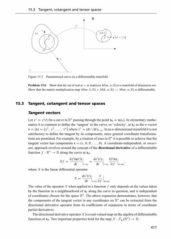
15.3 Tangent, cotangent and tensor spaces

Figure 15.3 Parametrized curve on a differentiable manifold

Problem 15.6 Show that the set of real m × m matrices M(m, n; R) is a manifold of dimension mn.Show that the matrix multiplication map M(m, k; R)× M(k, n; R) → M(m, n; R) is differentiable.

15.3 Tangent, cotangent and tensor spaces

Tangent vectors

Let xi = xi (t) be a curve in Rn passing through the point x0 = x(t0). In elementary mathe-matics it is common to define the ‘tangent’ to the curve, or ‘velocity’, at x0 as the n-vectorv = (x) = (x1, x2, . . . , x n

)where x i = (dxi/dt)t=t0 . In an n-dimensional manifold it is not

satisfactory to define the tangent by its components, since general coordinate transforma-tions are permitted. For example, by a rotation of axes in Rn it is possible to achieve that thetangent vector has components v = (v, 0, 0, . . . , 0). A coordinate-independent, or invari-ant, approach revolves around the concept of the directional derivative of a differentiablefunction f : Rn → R along the curve at x0,

X f = d f (x(t))

dt

∣∣∣t=t0

= dxi (t)

dt

∣∣∣t=t0

∂ f (x)

∂xi

∣∣∣x=x0

,

where X is the linear differential operator

X = dxi (t)

dt

∣∣∣t=t0

∂

∂xi

∣∣∣x=x0

.

The value of the operator X when applied to a function f only depends on the values takenby the function in a neighbourhood of x0 along the curve in question, and is independentof coordinates chosen for the space Rn . The above expansion demonstrates, however, thatthe components of the tangent vector in any coordinates on Rn can be extracted from thedirectional derivative operator from its coefficients of expansion in terms of coordinatepartial derivatives.

The directional derivative operator X is a real-valued map on the algebra of differentiablefunctions at x0. Two important properties hold for the map X : Fx0 (Rn) → R:

417

Differential geometry

(i) It is linear on the vector space Fx0 (Rn); that is, for any pair of functions f , g and realnumbers a, b we have X (a f + bg) = aX f + bXg.

(ii) The application of X on any product of functions f g in the algebraFx0 (Rn) is determinedby the Leibnitz rule, X ( f g) = f (x0)Xg + g(x0)X f .

These two properties completely characterize the class of directional derivative operators(see Theorem 15.1), and will be used to motivate the definition of a tangent vector at a pointof a general manifold.

A tangent vector X p at any point p of a differentiable manifold M is a linear map fromthe algebra of differentiable functions at p to the real numbers, X p : Fp(M) → R, whichsatisfies the Leibnitz rule for products:

X p(a f + bg) = aX p f + bX pg (linearity), (15.3)

X p( f g) = f (p)X pg + g(p)X p f (Leibnitz rule). (15.4)

The set of tangent vectors at p form a vector space Tp(M), since any linear combinationaX p + bYp of tangent vectors at p, defined by

(aX p + bYp) f = aX p f + bYp f,

is a tangent vector at p since it satisfies (15.3) and (15.4). It is called the tangent space atp. If (U, φ) is any chart at p with coordinate functions xi , define the operators(

∂xi

)p≡ ∂

∂xi

∣∣∣p

: Fp(M) → R

by

(∂xi

)p

f ≡ ∂

∂xi

∣∣∣p

f = ∂ f (x1, . . . , xn)

∂xi

∣∣∣x=φ(p)

, (15.5)

where f = f ◦ φ−1 : Rn → R. These operators are clearly tangent vectors since they satisfy(15.3) and (15.4). Thus any linear combination

X p = Xi ∂

∂xi

∣∣∣p≡

n∑i=1

Xi ∂

∂xi

∣∣∣p

where Xi ∈ R

is a tangent vector. The coefficients X j can be computed from the action of X on thecoordinate functions x j themselves:

X px j = Xi ∂x j

∂xi

∣∣∣x=φ(p)

= Xiδji = X j .

Theorem 15.1 If (U, φ; xi ) is a chart at p ∈ M, then the operators(∂xi

)p

defined by(15.5) form a basis of the tangent space Tp(M), and its dimension is n = dim M.

Proof : Let X p be a tangent vector at the given fixed point p. Firstly, it follows by theLeibnitz rule (15.4) that X p applied to a unit constant function f = 1 always results in zero,X p1 = 0, for

X p1 = X p(1.1) = 1.X p1+ 1.X p1 = 2X p1.

418

15.3 Tangent, cotangent and tensor spaces

By linearity, X p applied to any constant function f = c results in zero, Xc = X (c.1) =cX1 = 0.

Set the coordinates of p to be φ(p) = a = (a1, a2, . . . , an), and let y = φ(q) be anypoint in a neighbourhood ball Br (a) ⊆ φ(U ). The function f = f ◦ φ−1 can be written as

f (y1, y2, . . . , yn) = f (y1, y2, . . . , yn)− f (y1, . . . , yn−1, an)

+ f (y1, . . . , yn−1, an)− f (y1, . . . , yn−2, an−1, an)+ . . .+ f (y1, a2, . . . , an)− f (a1, a2, . . . , an)+ f (a1, a2, . . . , an)

= f (a1, a2, . . . , an)

+n∑

i=1

∫ 1

0

∂ f (y1, . . . , yi−1, ai + t(yi − ai ), ai+1, . . . , an)

∂tdt

= f (a)+n∑

i=1

∫ 1

0

∂ f

∂xi(y1, . . . , yi−1, ai + t(yi − ai ), ai+1, . . . , an)

× dt(yi − ai ).

Hence, in a neighbourhood of a = φ(p), any function f can be written in the form

f (y) = f (a)+ f i (y) (yi − ai ) (15.6)

where the functions f i (y1, y2, . . . , yn) are differentiable at a. Thus, in a neighbourhoodof p,

f (q) = f ◦ φ = f (p)+ fi (q)(xi (q)− ai

)where fi = f i ◦ φ ∈ Fp(M). Using the linear and Leibnitz properties of X p,

X p f = X p f (p)+ X p fi

(xi (p)− ai

)+ fi (p)(X pxi − X pai ) = fi (p)X pxi

since X pc = 0 for any constant c, and xi (p) = ai . Furthermore,

fi (p) = ∂ f

∂xi(a1, . . . , an)

∫ 1

0dt = ∂

∂xi

∣∣∣p

f,

and the tangent vectors(∂xi

)p

span the tangent space Tp(M),

X p = Xi ∂

∂xi

∣∣∣p= Xi

(∂xi

)p

where Xi = X pxi . (15.7)

To show that they form a basis, we need linear independence. Suppose

Ai ∂

∂xi

∣∣∣p= 0,

then the action on the coordinate functions f = x j gives

0 = Ai ∂

∂xi

∣∣∣px j = Ai ∂x j

∂xi

∣∣∣a= Aiδ

ji = A j

as required. �

419

Differential geometry

This proof shows that, for every tangent vector X p, the decomposition given byEq. (15.7) is unique. The coefficients Xi = X pxi are said to be the components of thetangent vector X p in the chart (U ; xi ).

How does this definition of tangent vector relate to that given earlier for a curve in Rn?Let γ : (a, b) → M be a smooth parametrized curve passing through the point p ∈ M att = t0. Define the tangent vector to the curve at p to be the operator γp defined by theaction on an arbitrary differentiable function f at p,

γp f = d f ◦ γ (t)

dt

∣∣∣t=t0.

It is straightforward to verify that the γp is a tangent vector at p, as it satisfies Eqs. (15.3)and (15.4). In a chart with coordinate functions xi at p, let the coordinate representation ofthe curve be γ = φ ◦ γ = (γ 1(t), . . . , γ n(t)

). Then

γp f = d f ◦ γ (t)

dt

∣∣∣t=t0

= ∂ f

∂xi

∣∣∣φ(p)

dγ i (t)

dt

∣∣∣t=t0

and

γp = γ i (t0)∂

∂xi

∣∣∣p

where γ i (t) = dγ i (t)

dt.

In the case M = Rn the operator γp is precisely the directional derivative of the curve.It is also true that every tangent vector is tangent to some curve. For example, the basis

vectors(∂xi

)p

are tangent to the ‘coordinate lines’ at p = φ−1(a),

γ i : t �→ φ−1((a1, a2, . . . , xi = ai + t − t0, . . . , an)

).

An arbitrary tangent vector X p = Xi(∂xi

)p

at p is tangent to the curve

γ : t �→ φ−1((a1 + X1(t − t0), . . . , xi = ai + Xi (t − t0), . . . , an + Xn(t − t0))

).

Example 15.7 The curves α, β and γ on R2 given respectively by

α1(t) = 1+ sin t cos t α2(t) = 1+ 3t cos 2t,

β1(t) = 1+ t β2(t) = 1+ 3te3t ,

γ 1(t) = et γ 2(t) = e3t ,

all pass through the point p = (1, 1) at t = 0 and are tangent to each other there,

αp = βp = γp =(∂x1

)p+ 3(∂x2

)p.

Cotangent and tensor spaces

The dual space T ∗p (M) associated with the tangent space at p ∈ M is called the cotangentspace at p. It consists of all linear functionals on Tp(M), also called covectors or 1-formsat p. The action of a covector ωp at p on a tangent vector X p will be denoted by ωp(X p),〈ωp, X p〉 or 〈X p, ωp〉. From Section 3.7 we have that dim T ∗p (M) = n = dim Tp(M) =dim M .

420

15.3 Tangent, cotangent and tensor spaces

If f is any function that is differentiable at p, we define its differential at p to be thecovector (d f )p whose action on any tangent vector X p at p is given by

〈(d f )p, X p〉 = X p f. (15.8)

This is a linear functional since, for any tangent vectors X p, Yp and scalars a, b ∈ R,

〈(d f )p, aX p + bYp〉= (aX p + bYp) f = aX p f + bYp f = a〈(d f )p, X p〉 + b〈(d f )p, Yp〉.Given a chart (U, φ; xi ) at p, the differentials of the coordinate functions have the

property

〈(dxi )p, X p〉 = X pxi = Xi

where Xi are the components of the tangent vector, X p = Xi(∂xi

)p. Applying (dxi )p to the

basis tangent vectors, we have

〈(dxi )p,(∂x j

)p〉 = ∂

∂x j

∣∣∣pxi = ∂xi

∂x j

∣∣∣φ(p)

= δij .

Hence the linear functionals (dx1)p, (dx2)p, . . . , (dxn)p are the dual basis, spanning thecotangent space, and every covector at p has a unique expansion

ωp = wi (dxi )p where wi = 〈ωp,(∂xi

)p〉.

The wi are called the components of the linear functional ωp in the chart (U ; xi ).The differential of any function at p has a coordinate expansion

(d f )p = fi (dxi )p

where

fi = 〈(d f )p,(∂xi

)p〉 = ∂

∂xi

∣∣∣p

f = ∂ f

∂xi

∣∣∣φ(p).

A common way of writing this is the ‘chain rule’

(d f )p = f,i (p)(dxi )p (15.9)

where

f,i = ∂ f

∂xi◦ φ.

These components are often referred to as the gradient of the function at p. Differentials havenever found a comfortable place in calculus as non-vanishing quantities that are ‘arbitrarilysmall’. The concept of differentials as linear functionals avoids these problems, yet has allthe desired properties such as the chain rule of multivariable calculus.

As in Chapter 7, a tensor of type (r, s) at p is a multilinear functional

Ap : T ∗p (M)× T ∗p (M)× · · · × T ∗p (M)︸ ︷︷ ︸r

×Tp(M)× · · · × Tp(M)︸ ︷︷ ︸s

→ R,

We denote the tensor space of type (r, s) at p by T (r,s)p (M). It is a vector space of dimension

nr+s .

421

Differential geometry

Vector and tensor fields

A vector field X is an assignment of a tangent vector X p at each point p ∈ M . In otherwords, X is a map from M to the set

⋃p∈M Tp(M) with the property that the image of

every point, X (p), belongs to the tangent space Tp(M) at p. We may thus write X p in placeof X (p). The vector field is said to be differentiable or smooth if for every differentiablefunction f ∈ F(M) the function X f defined by

(X f )(p) = X p f

is differentiable, X f ∈ F(M). The set of all differentiable vector fields on M is denotedT (M).

Exercise: Show that T (M) forms a module over the ring of functions F(M): if X and Y are vectorfields, and f ∈ F(M) then X + f Y is a vector field.

Every smooth vector field defines a map X : F(M) → F(M), which is linear

X (a f + bg) = aX f + bXg for all f, g ∈ F(M) and all a, b ∈ R,

and satisfies the Leibnitz rule for products

F( f g) = f Xg + gX f.

Conversely, any map X with these properties defines a smooth vector field, since for eachpoint p the map X p : Fp(M) → Fp(M) defined by X p f = (X f )(p) satisfies Eqs. (15.3)and (15.4) and is therefore a tangent vector at p.

We may also define vector fields on any open set U in a similar way as an assignment ofa tangent vector at every point of U such that X f ∈ F(U ) for all f ∈ F(U ). By the termlocal basis of vector fields at p we will mean an open neighbourhood U of p and a setof vector fields {e1, e2, . . . , en} on U such that the tangent vectors (ei )q span the tangentspace Tq (M) at each point q ∈ U . For any chart (U, φ; xi ), define the vector fields on thedomain U

∂xi ≡ ∂

∂xi: F(U ) → F(U )

by

∂xi f = ∂

∂xif = ∂ f ◦ φ−1

∂xi.

These vector fields assign the basis tangent vectors(∂xi

)p

at each point p ∈ U , and form alocal basis of vector fields at any point of U . When it is restricted to the coordinate domainU , every differentiable vector field X on M has a unique expansion in terms of these vectorfields

X∣∣U= Xi ∂

∂xi= Xi∂xi

where the components Xi : U ∈ R are differentiable functions on U . The local vector fields∂xi form a module basis on U , but they are not a vector space basis since as a vector spaceT (U ) is the direct sum of tangent spaces at all points p ∈ U , and is infinite dimensional.

422

15.3 Tangent, cotangent and tensor spaces

In a similar way we define a covector field or differentiable 1-form ω as an assignmentof a covectorωp at each point p ∈ M , such that the function 〈ω, X〉 defined by 〈ω, X〉(p) =〈ωp, X p〉 is differentiable for every smooth vector field X . The space of differentiable 1-forms will be denoted T ∗(M). Given any smooth function f , let d f be the differentiable1-form defined by assigning the differential d f p at each point p, so that

〈d f, X〉 = X f for all X ∈ T (M).

We refer to this covector field simply as the differential of f . A local module basis on anychart (U, φ; xi ) consists of the 1-forms dxi , which have the property

〈dxi , ∂x j 〉 = ∂xi

∂x j= δi

j .

Every differential can be expanded locally by the chain rule,

d f = f,i dxi where f,i = ∂

∂xif. (15.10)

Tensor fields are defined in a similar way, where the differentiable tensor field A of type(r, s) has a local expansion in any coordinate chart

A = Ai1i2...irj1... js

∂

∂xi1⊗ ∂

∂xi2⊗ · · · ⊗ ∂

∂xir⊗ dx j1 ⊗ · · · ⊗ dx js . (15.11)

The components are differentiable functions over the coordinate domain U given by

Ai1i2...irj1... js = A

(dxi1 , dxi2 , . . . , dxir ,

∂

∂x j1, . . . ,

∂

∂x js

).

Coordinate transformations

Let (U, φ; xi ) and (U ′, φ′; x ′ j ) be any two coordinate charts. From the chain rule of partialdifferentiation

∂

∂x ′ j= ∂xi

∂x ′ j

∂

∂xi,

∂

∂xi= ∂x ′ j

∂xi

∂

∂x ′ j. (15.12)

Exercise: Show these equations by applying both sides to an arbitrary differentiable function fon M .

Substituting the transformations (15.12) into the expression of a tangent vector withrespect to either of these bases

X = Xi ∂

∂xi= X ′ j ∂

∂x ′ j

gives the contravariant law of transformation of components

X ′ j = Xi ∂x ′ j

∂xi. (15.13)

The chain rule (15.10), written in coordinates x ′ j and setting f = xi , gives

dxi = ∂xi

∂x ′ jdx ′ j .

423

Differential geometry

Expressing a differentiable 1-form ω in both coordinate bases,

ω = wi dxi = w ′j dx ′ j ,

we obtain the covariant transformation law of components

w ′j =

∂xi

∂x ′ jwi . (15.14)

The component transformation laws (15.13) and (15.14) can be identified with similarformulae in Chapter 3 on setting

A ji =

∂x ′ j

∂xi, A′ik =

∂xi

∂x ′k.

The transformation law of a general tensor of type (r, s) follows from Eq. (7.30):

T ′i′1...i

′r

j ′1... j ′s = T i1...irj1... js

∂x ′i′1

∂xi1. . .∂x ′i

′r

∂xir

∂x j1

∂x ′ j ′1. . .

∂x js

∂x ′ j ′s. (15.15)

Tensor bundles

The tangent bundle T M on a manifold M consists of the set-theoretical union of all tangentspaces at all points

T M =⋃p∈M

Tp(M).

There is a natural projection mapπ : T M → M defined byπ (u) = p if u ∈ Tp(M), and foreach chart (U, φ; xi ) on M we can define a chart (π−1(U ), φ) on T M where the coordinatemap φ : π−1(U ) → R2n is defined by

φ(v) = (x1(p), . . . , xn(p), v1, . . . , vn)

where p = π (v) and v =n∑

i=1

vi ∂

∂xi

∣∣∣p.

The topology on T M is taken to be the coarsest topology such that all sets φ−1(A) are openwhenever A is an open subset of R2n . With this topology these charts generate a maximalatlas on the tangent bundle T M , making it into a differentiable manifold of dimension 2n.

Given an open subset U ⊆ M , a smooth map X : U → T M is said to be a smoothvector field on U if π ◦ X = id

∣∣U

. This agrees with our earlier notion, since it assignsexactly one tangent vector from the tangent space Tp(M) to the point p ∈ U . A similaridea may be used for a smooth vector field along a parametrized curve γ : (a, b) → M ,defined to be a smooth curve X : (a, b) → T M that lifts γ to the tangent bundle in thesense that π ◦ X = γ . Essentially, this defines a tangent vector at each point of the curve,not necessarily tangent to the curve, in a differentiable manner.

The cotangent bundle T ∗M is defined in an analogous way, as the union of all cotangentspaces T ∗p (M) at all points p ∈ M . The generating charts have the form (π−1(U ), φ) on

424

15.3 Tangent, cotangent and tensor spaces

T ∗M where the coordinate map φ : π−1(U ) → R2n is defined by

φ(ωp) = (x1(p), . . . , xn(p), w1, . . . , wn

)where p = π (ω) and ω =

n∑i=1

wi (dxi )p,

making T ∗M into a differentiable manifold of dimension 2n. This process may be extendedto produce the tensor bundle of type T (r,s) M , a differentiable manifold of dimension n +nr+s .

Problems

Problem 15.7 Let γ : R→ R2 be the curve x = 2t + 1, y = t2 − 3t . Show that at an arbitraryparameter value t the tangent vector to the curve is Xγ (t) = γ = 2∂x + (2t − 3)∂y = 2∂x + (x − 4)∂y .If f : R2 → R is the function f = x2 − y2, write f as a function of t along the curve and verify theidentities

Xγ (t) f = d f (t)

dt= 〈(d f )γ (t), Xγ (t)〉 = C1

1 (d f )γ (t) ⊗ Xγ (t).

Problem 15.8 Let x1 = x , x2 = y, x3 = z be ordinary rectangular cartesian coordinates in R3, andlet x ′1 = r , x ′2 = θ , x ′3 = φ be the usual transformation to polar coordinates.

(a) Calculate the Jacobian matrices [∂xi/∂x ′ j ] and [∂x ′i/∂x j ].

(b) In polar coordinates, work out the components of the covariant vector fields having componentsin rectangular coordinates (i) (0, 0, 1), (ii) (1, 0, 0), (iii) (x, y, z).

(c) In polar coordinates, what are the components of the contravariant vector fields whose componentsin rectangular coordinates are (i) (x, y, z), (ii) (0, 0, 1), (iii) (−y, x , 0).

(d) If gi j is the covariant tensor field whose components in rectangular coordinates are δi j , what areits components g′i j in polar coordinates?

Problem 15.9 Show that the curve

2x2 + 2y2 + 2xy = 1

can be converted by a rotation of axes to the standard form for an ellipse

x ′2 + 3y′2 = 1.

If x ′ = cosψ , y′ = 1√3

sinψ is used as a parametrization of this curve, show that

x = 1√2

(cosψ + 1√

3sinψ

), y = 1√

2

(− cosψ + 1√

3sinψ

).

Compute the components of the tangent vector

X = dx

dψ∂x + dy

dψ∂y .

Show that X ( f ) = (2/√

3)(x2 − y2

).

Problem 15.10 Show that the tangent space T(p,q)(M × N ) at any point (p, q) of a product manifoldM × N is naturally isomorphic to the direct sum of tangent spaces Tp(M)⊕ Tq (N ).

425

Differential geometry

Problem 15.11 On the unit 2-sphere express the vector fields ∂x and ∂y in terms of the polarcoordinate basis ∂θ and ∂φ . Again in polar coordinates, what are the dual forms to these vector fields?

Problem 15.12 Express the vector field ∂φ in polar coordinates (θ, φ) on the unit 2-sphere in termsof stereographic coordinates X and Y .

15.4 Tangent map and submanifolds

The tangent map and pullback of a map

Let α : M → N be a differentiable map between manifolds M and N , where dim M = m,dim N = n. This induces a map α∗ : Tp(M) → Tα(p)(N ), called the tangent map of α,whereby the tangent vector Yα(p) = α∗X p is defined by

Yα(p) f = (α∗X p) f = X p( f ◦ α)

for any function f ∈ Fα(p)(N ). This map is often called the differential of the map α, butthis may cause confusion with our earlier use of this term.

Let (U, φ; xi ) and (V, ψ ; ya) be charts at p and α(p), respectively. The map α hascoordinate representation α = ψ ◦ α ◦ φ−1 : φ(U ) → ψ(V ), written

ya = αa(x1, x2, . . . , xm) (a = 1, . . . , n).

To compute the components Y a of Yα(p) = α∗X p = Y a(∂ya

)α(p)

, we perform the followingsteps:

Yα(p) f = Y a ∂ f ◦ ψ−1

∂ya

∣∣∣α(p)

= Xi ∂

∂xi

∣∣∣p

f ◦ α

= Xi ∂ f ◦ α ◦ φ−1

∂xi

∣∣∣φ(p)

= Xi ∂ f ◦ ψ−1 ◦ α∂xi

∣∣∣φ(p)

= Xi ∂ f ◦ ψ−1(α1(x), α2(x), . . . , αn(x)

)∂xi

∣∣∣x=φ(p)

= Xi ∂ya

∂xi

∣∣∣φ(p)

∂ f ◦ ψ−1

∂ya

∣∣∣α(φ(p))

= Xi ∂ya

∂xi

∣∣∣φ(p)

∂

∂ya

∣∣∣α(p)

f.

Hence

Y a = Xi ∂ya

∂xi

∣∣∣φ(p). (15.16)

Exercise: If α : M → N and β : K → M are differentiable maps between manifolds, show that

(α ◦ β)∗ = α∗ ◦ β∗ . (15.17)

426

15.4 Tangent map and submanifolds

The map α : M → N also induces a map α∗ between cotangent spaces, but in this caseit acts in the reverse direction, called the pullback induced by α,

α∗ : T ∗α(p)(N ) → T ∗p (M) .

The pullback of a 1-form ωα(p) is defined by requiring

〈α∗ωα(p), X p〉 = 〈ωα(p), α∗X p〉 (15.18)

for arbitrary tangent vectors X p.

Exercise: Show that this definition uniquely defines the pullback α∗ωα(p).

Exercise: Show that the pullback of a functional composition of maps is given by

(α ◦ β)∗ = β∗ ◦ α∗ . (15.19)

The notion of tangent map or pullback of a map can be extended to totally contravariantor totally covariant tensors, such as r -vectors or r -forms, but is only available for mixedtensors if the map is a diffeomorphism (see Problem 15.13). The tangent map does notin general apply to vector fields, for if it is not one-to-one the tangent vector may not beuniquely defined at the image point α(p) (see Example 15.8 below). However, no suchambiguity in the value of the pullback α∗ω can ever arise at the inverse image point p,even if ω is a covector field, since its action on every tangent vector X p is well-defined byEq. (15.18). The pullback can therefore be applied to arbitrary differentiable 1-forms; themap α need not be either injective or surjective. This is one of the features that makescovector fields more attractive geometrical objects to deal with than vector fields. Thefollowing example should make this clear.

Example 15.8 Let α : R3 = R3 − {(0, 0, 0)} → R2 be the differentiable map

α : (x, y, z) �→ (u, v) where u = x + y + z, v =√

x2 + z2.

This map is neither surjective, since the whole lower half plane v < 0 is not mapped onto,nor injective, since, for example, the points p = (1, y, 0) and q = (0, y, 1) are both mappedto the point (y + 1, 1). Consider a vector field

X = Xi ∂

∂xi= X1 ∂

∂x+ X2 ∂

∂y+ X3 ∂

∂z

and the action of the tangent map α∗ at any point (x, y, z) is

α∗X = (X1 + X2 + X3) ∂∂u+(

X1 x√x2 + z2

+ X3 z√x2 + z2

) ∂∂v.

While this map is well-defined on the tangent space at any point x = (x, y, z), it does notin general map the vector field X to a vector field on R2. For example, no tangent vectorcan be assigned at u = α(p) = α(q) as we would need(

X1 + X2 + X3)(p)

∂

∂u

∣∣∣u+ X1(p)

∂

∂v

∣∣∣u= (X1 + X2 + X3

)(q)

∂

∂u

∣∣∣u+ X3(q)

∂

∂v

∣∣∣u.

There is no reason to expect these two tangent vectors at u to be identical.

427

Differential geometry

However, ifω = w1 du + w2 dv is a differentiable 1-form on R2 it induces a differentiable1-form on R

3, on substituting du = (∂u/∂x) dx + (∂u/∂y) dy + (∂u/∂z) dz, etc.

α∗ω =(

w1 + w2x√

x2 + z2

)dx + w1 dy +

(w1 + w2

z√x2 + z2

)dz,

which is uniquely determined at any point (x, y, z) �= (0, 0, 0) by the components w1(u, v)and w2(u, v) of the differentiable 1-form at (u, v) = α(x, y, z).

Example 15.9 If γ : R → M is a curve on M and p = γ (t0), the tangent vector to thecurve at p is the image under the tangent map induced by γ of the ordinary derivative onthe real line,

γp = γ∗ d

dt

∣∣∣t0,

for if f : M → R is any function differentiable at p then

γ∗d

dt

∣∣∣t0

( f ) = d f ◦ γdt

∣∣∣t0= γp( f ).

By a curve with endpoints we shall mean the restriction of a parametrized curve γ :(a, b) → M to a closed subinterval ofγ : [t1, t2] → M where a < t1 < t2 < b. The integralof a 1-form α on the curve with end points γ is defined as∫

γ

α =∫ t2

t1

α(γ ) dt.

In a coordinate representation xi = γ i (t) and α = αi dxi ,∫γ

α =∫ t2

t1

αi (x(t))dxi

dtdt.

Let γ ′ = γ ◦ f be the curve related to γ by a change of parametrization t ′ = f (t) wheref : R → R is a monotone function on the real line. Then∫

γ

α =∫γ ′α

for, by the standard change of variable formula for a definite integral,∫γ

α =∫ t2

t1

αi (x(t))dxi (t(t ′))

dt ′dt ′

dtdt

=∫ t ′2

t ′1

αi (x(t(t ′)))dx ′i (t ′)

dt ′dt ′

=∫γ ′α.

Hence the integral of a 1-form is independent of the parametrization on the curve γ .The integral of α along γ is zero if its pullback to the real line vanishes, γ ∗(α) = 0, for∫

γ

α =∫ t2

t1

〈α, γ∗ d

dt〉dt =

∫ t2

t1

〈γ ∗(α),d

dt〉dt = 0.

428

15.4 Tangent map and submanifolds

If α is the differential of a scalar field α = d f it is called an exact 1-form. The integralof an exact 1-form is independent of the curve connecting two points p1 = γ (t1) andp2 = γ (t2), for∫

γ

d f =∫ t2

t1

〈d f, γ 〉 dt =∫ t2

t1

d f (γ (t))

dtdt = f (γ (t2))− f (γ (t1)),

which only depends on the value of f at the end points. In particular, the integral of anexact 1-form vanishes on any closed circuit, since γ (t1) = γ (t2).

For general 1-forms, the integral is usually curve-dependent. For example, let α = xdyon the manifold R2 with coordinates (x, y). Consider the following two curves connectingp1 = (−1, 0) to p2 = (1, 0):

γ1 : x = t, y = 0 t1 = −1, t2 = 1,γ2 : x = cos t, y = sin t t1 = −π, t2 = 0.

The pullback of α to the first curve vanishes, γ ∗1 x dy = td0 = 0, while the pullback to γ2

is given by

γ ∗2 x dy = cos t d(y ◦ γ2(t)) = cos t d(sin t) = cos2 t dt.

Hence ∫γ2

x dy =∫ 0

−πcos2 t dt = π

2�=∫γ1

x dy = 0.

Submanifolds

Let α : M → N be a differentiable mapping where m = dim M ≤ n dim N . The map issaid to be an immersion if the tangent map α∗ : Tp(M) → Tα(p)(N ) is injective at everypoint p ∈ M ; i.e., α∗ is everywhere a non-degenerate linear map. From the inverse functiontheorem, it is straightforward to show that there exist charts at any point p and its imageα(p) such that the map α is represented as

yi = αi (x1, x2, . . . , xm) = xi for i = 1, . . . ,m,ya = αa(x1, x2, . . . , xm) = 0 for a > m.

A detailed proof may be found in [11].

Example 15.10 In general the image α(M) ⊂ N of an immersion is not a genuine ‘sub-manifold’, since there is nothing to prevent self-intersections. For example the mappingα : R → R2 defined by

x = α1(t) = t(t2 − 1), y = α2(t) = t2 − 1

is an immersion since its Jacobian matrix is everywhere non-degenerate,(∂x

∂t

∂y

∂t

)= (2t2 − 1 2t

) �= (0 0)

for all t ∈ R.

The subset α(R) ⊂ R2 does not, however, inherit the manifold structure of R since there isa self-intersection at t = ±1, as shown in Fig. 15.4.

429

Differential geometry

Figure 15.4 Immersion that is not a submanifold

In order to have a natural manifold structure on the subset α(M) we require that the mapα is itself injective as well as its tangent map α∗. The map is then called an embedding,and the pair (M, α) an embedded submanifold of N .

Example 15.11 Let A be any open subset of a manifold M . As in Example 15.2, it inheritsa manifold structure from M , whereby a chart is said to be admissible if it has the form(U ∩ A, φ

∣∣U∩A

) for some chart (U, φ) on M . With this differentiable structure, A is saidto be an open submanifold of M . It evidently has the same dimension as M . The pair(A, id

∣∣A) is an embedded submanifold of M .

Example 15.12 Let T 2 = S1 × S1 be the 2-torus (see Example 15.6). The space T 2 canalso be viewed as the factor space R2/mod 1, where (x, y) = (x ′, y′) mod 1 if there existintegers k and l such that x − x ′ = k and y − y′ = l. Denote equivalence classes mod 1 bythe symbol [(x, y)]. Consider the curve α : R → T 2 defined by α(t) = [(at, bt)]. This mapis an immersion unless a = b = 0. If a/b is a rational number it is not an embedding sincethe curve eventually passes through (1, 1) = (0, 0) for some t and α is not injective. For a/birrational the curve never passes through any point twice and is therefore an embedding.Figure 15.5 illustrates these properties. When a/b is rational the image C = α(R) has therelative topology in T 2 of a circle. Hence there is an embeddingβ : S1 → C , making (S1, β)an embedded submanifold of T 2. It is left to the reader to explicitly construct the map β.In this case the subset C = β(S1) ⊂ T 2 is closed.

The set α(R) is dense in T 2 when a/b is irrational, since the curve eventually passesarbitrarily close to any point of T 2, and cannot be a closed subset. Hence the relative topologyon α(R) induced on it as a subset of T 2 is much coarser than the topology it would obtainfrom R through the bijective map α. The embedding α is therefore not a homeomorphismfrom R to α(R) when the latter is given the relative topology.

In general, an embedding α : M → N that is also a homeomorphism from M to α(M)when the latter is given the relative topology in N is called a regular embedding. Anecessary and sufficient condition for this to hold is that there be a coordinate chart (U, φ; xi )

430

15.4 Tangent map and submanifolds

Figure 15.5 Submanifolds of the torus

at every point p ∈ α(M) such that α(M) ∩U is defined by the ‘coordinate slice’

xm+1 = xm+2 = · · · = xn = 0.

It also follows that the set α(M) must be a closed subset of N for this to occur. The proofsof these statements can be found in [11]. The above embedded submanifold (S1, β) is aregular embedding when a/b is rational.

Problems

Problem 15.13 Show that if ρp = ri (dxi )p = α∗ωα(p) then the components are given by

ri = ∂ya

∂xi

∣∣∣φ(p)

wa

where ωα(p) = wa(dya)α(p).If α is a diffeomorphism, define a map α∗ : T (1,1)

p (M) → T (1,1)α(p) (N ) by setting

α∗T(ωα(p), Xα(p)

) = T(α∗ωα(p), α

−1∗ Xα(p)

)and show that the components transform as

(α∗T )ab = T i

j∂ya

∂xi

∂x j

∂yb.

Problem 15.14 If γ : R→ M is a curve on M and p = γ (t0) and α : M → N is a differentiablemap show that

α∗γp = σα(p) where σ = α ◦ γ : R→ N .

Problem 15.15 Is the map α : R→ R2 given by x = sin t , y = sin 2t (i) an immersion, (ii) anembedded submanifold?

Problem 15.16 Show that the map α : R2 → R3 defined by

u = x2 + y2, v = 2xy, w = x2 − y2

is an immersion. Is it an embedded submanifold?

431

Differential geometry

Evaluate α∗(udu + vdv + wdw) and α∗(∂x )(a,b). Find a vector field X on R2

for which α∗X is nota well-defined vector field.

15.5 Commutators, flows and Lie derivatives

Commutators

Let X and Y be smooth vector fields on an open subset U of a differentiable manifold M .We define their commutator or Lie bracket [X, Y ] as the vector field on U defined by

[X, Y ] f = X (Y f )− Y (X f ) (15.20)

for all differentiable functions f on U . This is a vector field since (i) it is linear

[X, Y ](a f + bg) = a[X, Y ] f + b[x, y]g

for all f, g ∈ F(U ) and a, b ∈ R, and (ii) it satisfies the Leibnitz rule

[X, Y ]( f g) = f [X, Y ]g + g[X, Y ] f.

Linearity is trivial, while the Leibnitz rule follows from

[X, Y ]( f g) = X ( f Y g + gY f )− Y ( f Xg + gX f )= X f Y g + f X (Y g)+ Xg Y f + gX (Y f )− Y f Xg − f Y (Xg)− Y g X f − gY (X f )

= f [X, Y ]g + g[X, Y ] f.

A number of identities are easily verified for the Lie bracket:

[X, Y ] = −[Y, X ], (15.21)

[X, aY + bZ ] = a[X, Y ]+ b[X, Z ], (15.22)

[X, f Y ] = f [X, Y ]+ X f Y, (15.23)

[[X, Y ], Z ]+ [[Y, Z ], X ]+ [[Z , X ], Y ] = 0. (15.24)

Equations (15.21) and (15.22) are trivial, and (15.23) follows from

[X, f Y ]g = X ( f Y g)− f Y (Xg) = f X (Y g)+ X ( f )Y g − f Y (Xg)= f [X, Y ]g + X f Y g.

The Jacobi identity (15.24) is proved much as for commutators in matrix theory,Example 6.7.

Exercise: Show that for any functions f, g and vector fields X, Y

[ f X, gY ] = f g[X, Y ]+ f Xg Y − gY f X.

To find a coordinate formula for the Lie product, let X = Xi (x1, . . . , xn)∂xi , Y =Y i (x1, . . . , xn)∂xi . Then [X, Y ] = [X, Y ]k(x1, . . . , xn)∂xk , where

[X, Y ]k = [X, Y ](xk) = X (Y xk)− Y (X xk) = Xi ∂Y k

∂xi− Y i ∂Xk

∂xi,

432

15.5 Commutators, flows and Lie derivatives

or in the comma derivative notation

[X, Y ]k = Xi Y k,i − Y i Xk

,i . (15.25)

If we regard the vector field X as acting on the vector field Y by the Lie bracket to producea new vector field, X : Y �→ LX Y = [X, Y ], this action is remarkably ‘derivative-like’ inthat it is both linear

LX (aY + bZ ) = aLX Y + bLX Z

and has the property

LX ( f Y ) = X f Y + f LX Y. (15.26)

These properties follow immediately from (15.22) and (15.23). A geometrical interpretationof this derivative will appear in terms of the concept of a flow induced by a vector field.

Integral curves and flows

Let X be a smooth vector field on a manifold M . An integral curve of X is a parametrizedcurve σ : (a, b) → M whose tangent vector σ (t) at each point p = σ (t) on the curve isequal to the tangent vector X p assigned to p,

σ (t) = Xσ (t).

In a local coordinate chart (U ; xi ) at p where the curve can be written as n real functionsxi (t) = xi (σ (t)) and the vector field has the form X = Xi (x1, . . . , xn)∂xi , this requirementappears as n ordinary differential equations,

dxi

dt= Xi

(x1(t), . . . , xn(t)

). (15.27)

The existence and uniqueness theorem of ordinary differential equations asserts that througheach point p ∈ M there exists a unique maximal integral curve γp : (a, b) → M such thata = a(p) < 0 < b = b(p) and p = γp(0) [15, 16]. Uniqueness means that if σ : (c, d) →M is any other integral curve passing through p at t = 0 then a ≤ c < 0 < d ≤ b andσ = γp

∣∣(c,d)

.By a transformation of the manifold M is meant a diffeomorphism ϕ : M → M . A

one-parameter group of transformations of M , or on M , is a map σ : R× M → M suchthat:

(i) for each t ∈ R the map σt : M → M defined by σt (p) = σ (t, p) is a transformationof M ;

(ii) for all t, s ∈ R we have the abelian group property, σt+s = σt ◦ σs .

Since the maps σt are one-to-one and onto, every point p ∈ M is the image of a unique pointq ∈ M ; that is, we can write p = σt (q) where q = σ−1

t (p). Hence σ0 is the identity transfor-mation, σ0 = idM since σ0(p) = σ0 ◦ σt (q) = σt (q) = p for all p ∈ M . Furthermore, theinverse of each map σ−1

t is σ−t since σt ◦ σ−t = σ0 = idM .

433

Differential geometry

Figure 15.6 Streamlines representing the flow generated by a vector field

The curve γp : R → M defined by γp(t) = σt (p) clearly passes through p at t = 0. It iscalled the orbit of p under the flow σ and defines a tangent vector X p at p by

X p f = d f (γp(t))

dt

∣∣∣t=0= d f (σt (p))

dt

∣∣∣t=0.

Since p is an arbitrary point of M we have a vector field X on M , said to be the vectorfield induced by the flow σ . Any vector field X induced by a one-parameter group oftransformations of M is said to be complete. The one-parameter group σt can be thoughtof as ‘filling in’ the vector field X with a set of curves, which play the role of streamlinesfor a fluid whose velocity is everywhere given by X (see Fig. 15.6).

Not every vector field is complete, but there is a local concept that is always applicable. Alocal one-parameter group of transformations, or local flow, consists of an open subsetU ⊆ M and a real interval Iε = (−ε, ε), together with a map σ : Iε ×U → M such that:

(i′) for each t ∈ Iε the map σt : U → M defined by σt (p) = σ (t, p) is a diffeomorphismof U onto σt (U );

(ii′) if t, s and t + s ∈ Iε and p, σs(p) ∈ U then σt+s(p) = σt

(σs(p)

).

A local flow induces a vector field X on U in a similar way to that described above for aflow:

X p f = d f (σt (p))

dt

∣∣∣t=0

for all p ∈ U. (15.28)

It now turns out that every vector field X corresponds to a local one-parameter group oftransformations, which it may be said to generate.

434

15.5 Commutators, flows and Lie derivatives

Theorem 15.2 If X is a vector field on M, and p ∈ M then there exists an intervalI = (−ε, ε), a neighbourhood U of p, and a local flow σ : I ×U → M that induces thevector field X

∣∣U

restricted to U.

Proof : If (U, φ; xi ) is a coordinate chart at p we may set

X∣∣U= Xi ∂

∂xiwhere Xi : U → R.

The existence and uniqueness theorem of ordinary differential equations implies that forany x ∈ φ(U ) there exists a unique curve y = y(t ; x1, . . . , xn) on some interval I = (−ε, ε)such that

dyi (t ; x1, . . . , xn)

dt= Xi ◦ φ−1

(y1(t ; x), y2(t ; x), . . . , yn(t ; x)

)and

yi (0; x1, . . . , xn) = xi .

As the solutions of a family of differential equations depend smoothly on the initial coordi-nates [15, 16], the functions y(t ; x1, . . . , xn) are differentiable with respect to t and xi .

For fixed s and fixed x ∈ φ(U ) the curves t → zi (t, s; x) = yi (t ; y(s; x)) and t →z(t, s, x) = yi (t + s; x) satisfy the same differential equation

dzi (t, s; x1, . . . , xn)

dt= Xi

(z1(t, s; x), . . . , zn(t, s; x)

)and have the same initial conditions at t = 0,

yi (0; y(s; x)) = yi (s; x) = yi (0+ s; x).

These solutions are therefore identical and the map σ : I ×U → U defined by σ (t, p) =φ−1y

(t ;φ(p)

)satisfies the local one-parameter group condition

σ (t, σ (s, p)) = σ (t + s, p).�

A useful consequence of this theorem is the local existence of a coordinate system that‘straightens out’ any given vector field X so that its components point along the 1-axis,Xi = (1, 0, . . . , 0). The local flow σt generated by X is then simply a translation in the1-direction, σt (x1, x2, . . . , xn) = (x1 + t, x2, . . . , xn).

Theorem 15.3 If X is a vector field on a manifold M such that X p �= 0, then there existsa coordinate chart (U, φ; xi ) at p such that

X = ∂

∂x1. (15.29)

Outline proof : The idea behind the proof is not difficult. Pick any coordinate system(U, ψ ; yi ) at p such that yi (p) = 0, and X p =

(∂y1

)p. Let σ : Iε × A → M be a local

flow that induces X on the open set A. In a neighbourhood of p consider a small (n − 1)-dimensional ‘open ball’ of points through p that cuts across the flow, whose typical pointq has coordinates (0, y2, . . . , yn), and assign coordinates (x1 = t, x2 = y2, . . . , xn = yn)

435

Differential geometry

to points on the streamline σt (q) through q. The coordinates x2, . . . , xn are then constantalong the curves t → σt (q), and the vector field X , being tangent to the streamlines, hascoordinates (1, 0, . . . , 0) throughout a neighbourhood of p. A detailed proof may be foundin [11, theorem 4.3] or [4, p. 124]. �

Example 15.13 Let X be the differentiable vector field X = x2∂x on the real line manifoldR. To find a coordinate y = y(x) such that X = ∂y , we need to solve the differential equation

x2 ∂y

∂x= 1.

The solution is y = C − 1/x .The local one-parameter group generated by X is found by solving the ordinary differ-

ential equation,

dx

dt= x2.

The solution is

σt (x) = 1

x−1 − t= x

1− t x.

It is straightforward to verify the group property

σt

(σs(x)

) = x

1− (t + s)x= σt+s(x).

Example 15.14 If X and Y are vector fields on M generating flows φt andψt respectively,let σ be the curve through p ∈ M defined by

σ (t) = ψ−t ◦ φ−t ◦ ψt ◦ φt p.

Then σ (√

t) is a curve whose tangent vector is the commutator [X, Y ] at p. The proof is tolet f be any differentiable function at p and show that

[X, Y ]p f = limt→0

f[σ (√

t)]− f

[σ (0)

]t

.

Details may be found in [3, p. 130]. Some interesting geometrophysical applications of thisresult are discussed in [17].

Lie derivative

Let X be a smooth vector field on a manifold M , which generates a local one-parametergroup of transformations σt on M . If Y is any differentiable vector field on M , we defineits Lie derivative along X to be

LX Y = limt→0

Y − (σt )∗Yt

. (15.30)

Figure 15.7 illustrates the siutation. Essentially, the tangent map of the diffeomorphism σt

is used to ‘drag’ the vector field Y forward along the integral curves from a point σ−t (p)to p and the result is compared with original value Yp of the vector field. Equation (15.7)

436

15.5 Commutators, flows and Lie derivatives

Figure 15.7 Lie derivative of a vector field Y along a vector field X

performs this operation for neighbouring points and takes the limit on dividing by t . Wenow show that this derivative is identical with the ‘derivative-like’ operation of taking thecommutator of two vector fields.

Let f : M → R be a differentiable function, and p any point of M . From (15.30) wehave at p,

(LX Y )p f = limt→0

1

t

(Yp f − ((σt )∗Y )p f

)= lim

t→0

1

t

(Yp f − Yσ−t (p)( f ◦ σt )

)= lim

t→0

1

t

(Yp f − Yσ−t (p) f − Yσ−t (p)( f ◦ σt − f )

)= lim

t→0

1

t

((Y f − (Y f ) ◦ σ−t )(p)− Yσ−t (p)( f ◦ σt − f )

).

On setting s = −t in the first term and using Eq. (15.28), the right-hand side reduces toX (Y f )(p)− Y (X f )(p) = [X, Y ]p f , and we have the desired relation

LX Y = [X, Y ]. (15.31)

The concept of Lie derivative can be extended to all tensor fields. First, for any dif-feomorphism ϕ : M → M , we define the induced map ϕ : T (r,s)(M) → T (r,s)(M) in thefollowing way:

(i) for vector fields set ϕ = ϕ∗;(ii) for scalar fields f : M → R set ϕ f = f ◦ ϕ−1;

(iii) for covector fields set ϕ = (ϕ−1)∗

;

437

Differential geometry

(iv) the map ϕ is extended to all tensor fields by demanding linearity and

ϕ(T ⊗ S) = ϕT ⊗ ϕS

for arbitrary tensor fields T and S.

If ω and X are arbitrary covector and vector fields, then

〈ϕω, ϕX〉 = ϕ〈ω, X〉, (15.32)

since

〈ϕω, ϕX〉(p) = 〈(ϕ−1)∗ωϕ−1(p), ϕ∗Xϕ−1(p)〉= 〈ωϕ−1(p), Xϕ−1(p)〉 = 〈ω, X〉(ϕ−1(p)

).

Exercise: For arbitrary vector fields X show from (ii) that ϕX (ϕ f ) = ϕ(X ( f )).

Using Eq. (15.11), property (iv) provides a unique definition for the application of themap ϕ to all higher order tensors. Alternatively, as for covector fields, the following is acharacterization of the map ϕ:

(ϕT )(ϕω1, . . . , ϕωr , ϕX1, . . . , ϕXs

) = ϕ(T (ω1, . . . , ωr , X1, . . . , Xs))

for all vector fields X1, . . . Xs and covector fields ω1, . . . , ωr .The Lie derivative LX T of a smooth tensor field T with respect to the vector field X is

defined as

LX T = limt→0

1

t

(T − σt T

). (15.33)

Exercise: Show that for any tensor field T

LX T = −d σt T

dt

∣∣∣t=0

(15.34)

and prove the Leibnitz rule

LX (T ⊗ S) = T ⊗ (LX S)+ (LX T )⊗ S. (15.35)

When T is a scalar field f , we find, on changing the limit variable to s = −t ,(LX f

)p= d f ◦ σs(p)

ds

∣∣∣s=0

= X f (p),

and in a local coordinate chart (U ; xi )

LX f = X f = f,i X i . (15.36)

Since for any pair i, j

L∂xi

∂

∂x j=[ ∂∂xi,∂

∂x j

]= ∂2

∂xi∂x j− ∂2

∂x j∂xi= 0,

and LX Y = [X, Y ] = −[Y, X ] = −LY X for any pair of vector fields X, Y , we find

LX∂

∂x j= −L∂x j

(Xi ∂

∂xi

)= −Xi

, j∂

∂xi.

438

15.5 Commutators, flows and Lie derivatives

Applying the Leibnitz rule (15.35) results in

LX Y = LX

(Y i ∂

∂xi

)= Y i

, j X j ∂

∂xi− Y j Xi

, j∂

∂xi,

in agreement with the component formula for the Lie bracket in Eq. (15.25),(LX Y

)i = Y i, j X j − Y j Xi

, j . (15.37)

To find the component formula for the Lie derivative of a 1-form ω = wi dxi , we notethat for any pair of vector fields X, Y

LX 〈ω, Y 〉 = X〈ω, Y 〉 = 〈LXω, Y 〉 + 〈ω,LX Y 〉, (15.38)

which follows from Eqs. (15.32) and (15.34),

LX 〈ω, Y 〉 = X〈ω, Y 〉 = − d

dtσt 〈ω, Y 〉

∣∣∣t=0

= − d

dt〈σtω, σt Y 〉

∣∣∣t=0

= −〈 d

dtσtω, Y 〉

∣∣∣t=0− 〈ω, d

dtσt Y 〉

∣∣∣t=0

= 〈LXω, Y 〉 + 〈ω,LX Y 〉.If ω = wi dxi is a 1-form, then its Lie derivative LXω with respect to the vector field X hascomponents in a coordinate chart (U ; xi ) given by(

LXω)

j= 〈LXω,

∂

∂x j〉

= LX 〈ω, ∂∂x j

〉 − 〈ω,LX∂

∂x j〉

= LX w j + 〈ω, Xi, j∂

∂xi〉

= w j,i X i + wi Xi, j .

Extending this argument to a general tensor of type (r, s), we find(LX T

)i j ...kl... = T i j ...

kl...,m Xm − T mj ...kl...X

i,m − T im...

kl...Xj,m − · · ·

T i j ...ml...X

m,k + T i j ...

km...Xm,l + · · ·

(15.39)

Example 15.15 In local coordinates such that X = ∂x1 (see Theorem 15.3), all Xi, j = 0

since the components Xi = consts. and the components of the Lie derivative are simply thederivatives in the 1-direction, (

LX T)i j ...

kl... = T i j ...kl...,1.

Problems

Problem 15.17 Show that the components of the Lie product [X, Y ]k given by Eq. (15.25) transformas a contravariant vector field under a coordinate transformation x ′ j (xi ).

439

Differential geometry

Problem 15.18 Show that the Jacobi identity can be written

L[X,Y ] Z = LXLY Z − LYLX Z ,

and this property extends to all tensors T :

L[X,Y ]T = LXLY T − LYLX T .

Problem 15.19 Let α : M → N be a diffeomorphism between manifolds M and N and X a vectorfield on M that generates a local one-parameter group of transformations σt on M . Show that thevector field X ′ = α∗X on N generates the local flow σ ′t = α ◦ σt ◦ α−1.

Problem 15.20 For any real positive number n show that the vector field X = xn∂x is differentiableon the manifold R+ consisting of the positive real line {x ∈ R | x > 0}. Why is this not true in generalon the entire real line R? As done for the case n = 2 in Example 15.13, find the maximal one-parametersubgroup σt generated by this vector field at any point x > 0.

Problem 15.21 On the manifold R2 with coordinates (x, y), let X be the vector field X = −y∂x +x∂y . Determine the integral curve through any point (x, y), and the one-parameter group generatedby X . Find coordinates (x ′, y′) such that X = ∂x ′ .

Problem 15.22 Repeat the previous problem for the vector fields, X = y∂x + x∂y and X = x∂x +y∂y .

Problem 15.23 On a compact manifold show that every vector field X is complete. [Hint: Let σt

be a local flow generating X , and let ε be the least bound required on a finite open covering. Setσt = (σt/N )N for N large enough that |t | < εN .]

Problem 15.24 Show that the Lie derivative LX commutes with all operations of contraction Cij on

a tensor field T ,

LX Cij T = Ci

jLX T .

Problem 15.25 Prove the formula (15.39) for the Lie derivative of a general tensor.

15.6 Distributions and Frobenius theorem

A k-dimensional distribution Dk on a manifold M is an assignment of a k-dimensionalsubspace Dk(p) of the tangent space Tp(M) at every point p ∈ M . The distribution is saidto be C∞ or smooth if for all p ∈ M there is an open neighbourhood U and k smoothvector fields X1, . . . , Xk on U that span Dk(q) at each point q ∈ U . A vector field X onan open domain A is said to lie in or belong to the distribution Dk if X p ∈ Dk(p) at eachpoint p ∈ A. A one-dimensional distribution is equivalent to a vector field up to an arbitraryscalar factor at every point, and is sometimes called a direction field.

An integral manifold of a distribution Dk is a k-dimensional submanifold (K , ψ) of Msuch that all vector fields tangent to the submanifold belong to Dk ,

ψ∗(Tp(K )) = Dk(ψ(p)).

440

15.6 Distributions and Frobenius theorem

Every one-dimensional distribution has integral manifolds, for if X is any vector fieldthat spans a distribution D1 then any family of integral curves of X act as integral manifoldsof the distribution D1. We will see, however, that not every distribution of higher dimensionhas integral manifolds.

A distribution Dk is said to be involutive if for any pair of vector fields X , Y lying inDk , their Lie bracket [X, Y ] also belongs to Dk . If {e1, . . . , ek} is any local basis of vectorfields spanning an involutive Dk on an open neighbourhood U , then

[eα, eβ] =k∑γ=1

Cγ

αβeγ (α, β = 1, . . . , k) (15.40)

where Cγ

αβ = −Cγ

βα are C∞ functions on U . Conversely, if there exists a local basis {eα}satisfying (15.40) for some scalar structure fields Cγ

αβ , the distribution is involutive, for ifX = Xαeα and Y = Y βeβ then

[X, Y ] = [Xαeα, Y βeβ] = (X (Y γ )− Y (Xγ )+ XαY βCγ

αβ

)eγ ,

which belongs to Dk as required. For example, if there exists a coordinate chart (U ; xi ) suchthat the distribution Dk is spanned by the first k coordinate basis vector fields

e1 = ∂x1 , e2 = ∂x2 , . . . , ek = ∂xk

then Dk is involutive on U since all [eα, eβ] = 0, a trivial instance of the relation (15.40).In this case we can restrict the chart to a cubical neighbourhood U ′ = {p | − a < xi (p) <a}, and the ‘slices’ xa = const. (a = k + 1, . . . , n) are local integral manifolds of thedistribution Dk . The key result is the Frobenius theorem:

Theorem 15.4 A smooth k-dimensional distribution Dk on a manifold M is involutive ifand only if every point p ∈ M lies in a coordinate chart (U ; xi ) such that the coordinatevector fields ∂/∂xα for α = 1, . . . , k span Dk at each point of U.

Proof : The if part follows from the above remarks. The converse will be shown by induc-tion on the dimension k. The case k = 1 follows immediately from Theorem 15.3. Supposenow that the statement is true for all (k − 1)-dimensional distributions, and let Dk be ak-dimensional involutive distribution spanned at all points of an open set A by vector fields{X1, . . . , Xk}. At any point p ∈ A there exist coordinates (V ; yi ) such that Xk = ∂yk . Set

Yα = Xα − (Xα yk)Xk, Yk = Xk

where Greek indices α, β, . . . range from 1 to k − 1. The vector fields Y1, Y2, . . . , Yk

clearly span Dk on V , and

Yα yk = 0, Yk yk = 1 . (15.41)

Since Dk is an involutive we can write

[Yα, Yβ] = Cγ

αβYγ + aαβYk,

[Yα, Yk] = Cγα Yγ + aαYk .

441

Differential geometry

Applying both sides of these equations to the coordinate function yk and using (15.41), wefind aαβ = aα = 0, whence

[Yα, Yβ] = Cγ

αβYγ , (15.42)

[Yα, Yk] = Cγα Yγ . (15.43)

The distribution Dk−1 spanned by Y1, Y2, . . . , Yk−1 is therefore involutive on V , and by theinduction hypothesis there exists a coordinate chart (W ; zi ) such that Dk−1 is spanned by{∂z1 , . . . , ∂zk−1}. Set

∂

∂zα= AβαYβ

where [Aβα] is a non-singular matrix of functions on W . The original distribution Dk isspanned on W by the set of vector fields

{∂z1 , ∂z2 , . . . , ∂zk−1 , Yk}.It follows then from (15.43) that

[∂zα , Yk] = K βα∂zβ (15.44)

for some functions K βα . If we write

Yk =k−1∑α=1

ξα∂zα +n∑

a=k

ξ a∂za

and apply Eq. (15.44) to the coordinate functions za (a = k, . . . , n), we find

∂ξ a

∂zα= 0.

Hence ξ a = ξ a(zk, . . . , zn) for all a ≥ k. Since Yk is linearly independent of the vectors∂zα , the distribution Dk is spanned by the set of vectors {∂z1 , ∂z2 , . . . , ∂zk−1 , Z}, where

Z = Yk − ξα∂zα = ξ a(zk, . . . , zn)∂za .

By Theorem 15.3 there exists a coordinate transformation not involving the first (k − 1)coordinates,

xk = xk(zk, . . . , zn), xk+1 = xk+1(zk, . . . , zn), . . . , xn = xn(zk, . . . , zn)

such that Z = ∂xk . Setting x1 = z1, . . . , xk−1 = zk−1, we have coordinates (U ; xi ) in whichDk is spanned by {∂x1 , . . . , ∂xk−1 , ∂xk }. �

Theorem 15.5 A set of vector fields {X1, X2, . . . , Xk} is equal to the first k basis fields ofa local coordinate system, X1 = ∂x1 , . . . , Xk = ∂xk if and only if they commute with eachother, [Xα, Xβ] = 0.

Proof : The vanishing of all commutators is clearly a necessary condition for the vectorfields to be local basis fields of a coordinate system, for if Xα = ∂xα (α = 1, . . . , r ) then[Xα, Xβ] = [∂xα , ∂xβ ] = 0.

442

15.6 Distributions and Frobenius theorem

To prove sufficiency, we again use induction on k. The case k = 1 is essentially Theorem15.3. By the induction hypothesis, there exists local coordinates (U ; xi ) such that Xα = ∂xα

for α = 1, . . . , k − 1. Set Y = Xk = Y i (x1, . . . , xn)∂xi , and by Example 15.15 Y i,α = 0,

so that we may write

Y =k−1∑α=1

Y α(xk, . . . , xn)∂xα +n∑

a=k

Y a(xk, . . . , xn)∂xa .

Using Theorem 15.3 we may perform a coordinate transformation on the last n − k + 1coordinates such that

Y =k−1∑α=1

Y α(xk, . . . , xn)∂xα + ∂xk .

A coordinate transformation

x ′α = xα + f α(xk, . . . , xn) (α = 1, . . . , k − 1)x ′a = xa (a = k, . . . , n)

has the effect

Y =k−1∑β=1

(Y β + ∂ f β

∂xk

) ∂

∂x ′β+ ∂

∂x ′k.

Solving the differential equations

∂ f β

∂xk= −Y β(xk, . . . , xn)

by a straightforward integration leads to Y = ∂x ′k as required. �

Example 15.16 On R3 = R3 − {(0, 0, 0)} let X1, X2, X3 be the three vector fields

X1 = y∂z − z∂y, X2 = z∂x − x∂z, X3 = x∂y − y∂x .

These three vector fields generate a two-dimensional distribution D2, as they are not linearlyindependent

x X1 + yY2 + zX3 = 0.

The Lie bracket of any pair of these vector fields is easily calculated,

[X1, X2] f = [y∂z − z∂y, z∂x − x∂z] f

= yz[∂z, ∂x ] f + y f,x − yx[∂z, ∂z] f − z2[∂y, ∂x ] f + zx[∂y, ∂z] f − x f,y= (−x∂y + y∂x

)f = −X3 f.

There are similar identities for the other commutators,

[X1, X2] = −X3, [X2, X3] = −X1, [X3, X1] = −X2. (15.45)

443

Differential geometry

Hence the distribution D2 is involutive and by the Frobenius theorem it is possible to finda local transformation to coordinates y1, y2, y3 such that ∂y1 and ∂y2 span all three vectorfields X1, X2 and X3.

The vector field X = x∂x + y∂y + z∂z commutes with all Xi : for example,

[X3, X ] f = [x∂y − y∂x , x f,x + y f,y + z f,z] f

= x2[∂y, ∂x ] f − x∂y f + x∂y f + xy[∂y, ∂y] f − y2[∂x , ∂y] f

+ xz[∂y, ∂z] f − yz[∂x , ∂z] f

= 0 .

Hence the distribution E2 generated by the pair of vector fields {X3, X} is also involutive.Let us consider spherical polar coordinates, Eq. (15.2), having inverse transformations

r =√

x2 + y2 + z2, θ = cos−1( z

r

), φ = tan−1

( y

x

).

Express the basis vector fields in terms of these coordinates

∂x = ∂r

∂x∂r + ∂θ

∂x∂θ + ∂φ

∂x∂φ = sin θ cosφ∂r + cos θ cosφ

r∂θ − sinφ

r sin θ∂φ,

∂y = ∂r

∂y∂r + ∂θ

∂y∂θ + ∂φ

∂y∂φ = sin θ sinφ∂r + cos θ sinφ

r∂θ + cosφ

r sin θ∂φ,

∂z = ∂r

∂z∂r + ∂θ

∂z∂θ + ∂φ

∂z∂φ = cos θ∂r − sin θ

r∂θ ,

and a simple calculation gives

X1 = y∂z − z∂y = − sinφ∂θ − cot θ cosφ∂φ,

X2 = z∂x − x∂z = − cosφ∂θ − cot θ sinφ∂φ,

X3 = x∂y − y∂x = ∂φ,X = x∂x + y∂y + z∂z = r∂r = ∂r ′ where r ′ = ln r.

The distribution D2 is spanned by the basis vector fields ∂θ and ∂φ , while the distributionE2 is spanned by the vector fields ∂r and ∂φ in spherical polars.

Exercise: Find a chart, two of whose basis vector fields span the distribution generated by X1 and X .Do the same for the distribution generated by X2 and X .

Problems

Problem 15.26 Let Dk be an involutive distribution spanned locally by coordinate vector fieldseα = ∂/∂xα , where Greek indices α, β, etc. all range from 1 to k. If Xα = Aβαeβ is any local basisspanning a distribution Dk , show that the matrix of functions [Aβα] is non-singular everywhere on itsregion of definition, and that [Xα, Xβ ] = Cγ

αβXγ where

Cγ

αβ =(

AδαAηβ,δ − Aδβ Aηα,δ)(

A−1)γη.

444

References

Problem 15.27 There is a classical version of the Frobenius theorem stating that a system of partialdifferential equations of the form

∂ f β

∂x j= Aβj

(x1, . . . , xk, f 1(x), . . . , f r (x)

)where i, j = 1, . . . , k and α, β = 1, . . . , r has a unique local solution through any point(a1, . . . , ak, b1, . . . , br ) if and only if

∂Aβj∂xi

− ∂Aβi∂x j

+ Aαi∂Aβj∂yα

− Aαj∂Aβi∂yα

= 0

where Aβj = Aβj(x1, . . . , xk, y1, . . . , yr

). Show that this statement is equivalent to the version given

in Theorem 15.4. [Hint: On Rn where n = r + k consider the distribution spanned by vectors

Yi = ∂

∂xi+ Aβi

∂

∂yβ(i = 1, . . . , k)

and show that the integrability condition is precisely the involutive condition [Yi , Y j ] = 0, while thecondition for an integral submanifold of the form yβ = f β (x1, . . . , xk) is Aβj = f β, j .]

References

[1] L. Auslander and R. E. MacKenzie. Introduction to Differentiable Manifolds. NewYork, McGraw-Hill, 1963.

[2] R. W. R. Darling. Differential Forms and Connections. New York, Cambridge Univer-sity Press, 1994.

[3] T. Frankel. The Geometry of Physics. New York, Cambridge University Press, 1997.[4] N. J. Hicks. Notes on Differential Geometry. New York, D. Van Nostrand Company,

1965.[5] S. Kobayashi and K. Nomizu. Foundations of Differential Geometry. New York, Inter-

science Publishers, 1963.[6] L. H. Loomis and S. Sternberg. Advanced Calculus. Reading, Mass., Addison-Wesley,

1968.[7] M. Nakahara. Geometry, Topology and Physics. Bristol, Adam Hilger, 1990.[8] C. Nash and S. Sen. Topology and Geometry for Physicists. London, Academic Press,

1983.[9] I. M. Singer and J. A. Thorpe. Lecture Notes on Elementary Topology and Geometry.

Glenview, Ill., Scott Foresman, 1967.[10] M. Spivak. Differential Geometry, Vols. 1–5. Boston, Publish or Perish Inc., 1979.[11] W. H. Chen, S. S. Chern, and K. S. Lam. Lectures on Differential Geometry. Singapore,

World Scientific, 1999.[12] S. Sternberg. Lectures on Differential Geometry. Englewood Cliffs, N.J., Prentice-Hall,

1964.[13] F. W. Warner. Foundations of Differential Manifolds and Lie Groups. New York,

Springer-Verlag, 1983.

445

Differential geometry

[14] C. de Witt-Morette, Y. Choquet-Bruhat and M. Dillard-Bleick. Analysis, Manifoldsand Physics. Amsterdam, North-Holland, 1977.

[15] E. Coddington and N. Levinson. Theory of Ordinary Differential Equations. New York,McGraw-Hill, 1955.

[16] W. Hurewicz. Lectures on Ordinary Differential Equations. New York, John Wiley &Sons, 1958.

[17] E. Nelson. Tensor Analysis. Princeton, N.J., Princeton University Press, 1967.

446

16 Differentiable forms

16.1 Differential forms and exterior derivative

Let M be a differentiable manifold of dimension n. At any point p ∈ M let(�r

)p(M) ≡

�∗r (Tp(M)) be the space of totally antisymmetric tensors, or r -forms, generated by thetangent space Tp(M) (see Chapter 8). Denote the associated exterior algebra

�p(M) ≡ �∗(Tp(M)) = (�0

)p(M)⊕ (�1

)p(M)⊕ · · · ⊕ (�n

)p(M)

with graded exterior product ∧ :(�r

)p(M)× (�s

)p(M) → (

�r+s

)p(M).

A differential r -form α on an open subset U ⊆ M is an r -form field, or assignmentof an r -form αp at every point p ∈ U , such that the function α(X1, X2, . . . , Xr )(p) ≡αp((X1)p, (X2)p, . . . , (Xr )p) is differentiable for all smooth vector fields X1, X2, . . . , Xr

on U . The set of all differential r -forms on U is denoted�r (U ) and the differential exterioralgebra on U is the direct sum

�(U ) = �0(U )⊕�1(U )⊕ · · · ⊕�n(U )

with exterior product defined by (α ∧ β)p = αp ∧ βp. This product is linear, associativeand obeys the usual anticommutative rule:

α ∧ (β + γ ) = α ∧ β + α ∧ γα ∧ (β ∧ γ ) = (α ∧ β) ∧ γ

α ∧ β = (−1)rsβ ∧ α if α ∈ �r (U ), β ∈ �s(U ). (16.1)

Differential 0-forms are simply scalar fields, smooth real-valued functions f on U ,�0(U ) =F(U ).

In a coordinate chart (U, φ; xi ) a basis of �r (U ) is

d xi1 ∧ d xi2 ∧ · · · ∧ d xir = A(d xi1 ⊗ d xi2 ⊗ · · · ⊗ d xir

),

and every differential r -form on U has a unique expansion

α = αi1i2...ir d xi1 ∧ d xi2 ∧ · · · ∧ d xir (16.2)

where the components αi1i2...ir are smooth functions on U and are antisymmetric in allindices,

αi1i2...ir = α[i1i2...ir ].

447

Differentiable forms

If f is a scalar field then its gradient

f,i = ∂ f

∂xi

forms the components of a covariant vector field known as its differential d f (see Chapter15). This concept may be extended to a map on all differential forms, d : �(M) → �(M),called the exterior derivative, such that d�r (M) ⊆ �(r+1)(M) and satisfying the followingconditions:

(ED1) If f is a differential 0-form, then d f is its differential, defined by 〈d f, X〉 = X f forany smooth vector field X .

(ED2) For any pair of differential forms, α, β ∈ �(M), d(α + β) = dα + dβ.(ED3) If f is a differential 0-form then d2 f ≡ d(d f ) = 0.(ED4) For any r -form α, and any β ∈ �(M)

d(α ∧ β) = (dα) ∧ β + (−1)rα ∧ dβ. (16.3)

Condition (ED4) says that it is an anti-derivation (see Section 8.4, Eq. (8.18)), and (ED3)will be shown to hold for differential forms of all orders. The general theory of differentialforms and exterior derivative may be found in [1–9]. Our aim in the following discussionis to show that the operator d exists and is uniquely defined.

Lemma 16.1 Let U be an open subset of a differentiable manifold M. For any point p ∈ Uthere exist open sets W and W ′ where W has compact closure with p ∈ W ⊆ W ′ ⊆ U, anda smooth function h ≥ 0 such that h = 1 on W and h = 0 on M −W ′.

Proof : Let f : R → R be the smooth non-negative function, defined by

f (t) ={

e−1/t if t > 0,

0 if t ≤ 0.

For every a > 0 let ga : R → R be the non-negative smooth function

ga(t) = f (t)

f (t)+ f (a − t)=

⎧⎪⎪⎨⎪⎪⎩0 if t ≤ 0,

> 0 if 0 < t < a,

1 if t ≥ a.

If b > a the smooth function ha,b : R → R defined by

ha,b(t) = 1− gb−a(t − a)

has the value 1 for t ≤ a and is 0 for t ≥ b. On the open interval (a, b) it is positive with valuesbetween 0 and 1. Let (V, φ; xi ) be a coordinate chart at p such that xi (p) = 0 and V ⊆ U .Let b > 0 be any real number such that the open ball Bb(0) ⊂ φ(V ), and let 0 < a < b.Set W ′ = φ−1(Bb(0)) and W = φ−1(Ba(0)). The closure of W , being the homeomorphicimage of a compact set, is compact and W ⊂ W ′. Let h : Rn → R be the smooth map

h(x1, x2, . . . , xn) = ha,b(r ) where r =√

(x1)2 + (x2)2 + · · · + (xn)2,

448

16.1 Differential forms and exterior derivative

and the positive function h : M → R defined by

h(p) ={

h ◦ φ(p) for p ∈ W

0 for p ∈ M −W ′

has all the desired properties. �

If α is an r -form whose restriction to U vanishes, α∣∣U= 0, then hα = 0 on all of M

where h is the function defined in Lemma 16.1, and by property (ED4),

d(hα) = dh ∧ α + h dα = 0.

Restricting this equation to W we have dα∣∣W= 0, and in particular (dα)|p = 0. Since p is

an arbitrary point of U it follows that dα∣∣U= 0. Hence, if α and β are any pair of r -forms

such that α∣∣U= β∣∣

U, then (dα)

∣∣U= (dβ)

∣∣U

. Thus if d exists, satisfying (ED1)–(ED4), thenit has a local character and is uniquely defined everywhere.

To show the existence of the operator d, let (U ; xi ) be a coordinate chart at any point p.Expanding α according to Eq. (16.2) we have, using (ED1)–(ED4),

dα = dαi1...ir ∧ d xi1 ∧ · · · ∧ d xir + αi1...ir d2xi1 ∧ d xi2 ∧ · · · ∧ d xir

− αi1...ir dxi1 ∧ d2xi2 ∧ · · · ∧ d xir + · · ·= dαi1...ir d xi1 ∧ · · · ∧ d xir

= αi1...ir , j d x j ∧ d xi1 ∧ · · · ∧ d xir .

Performing a cyclic permutation of indices, and using the total antisymmetry of the wedgeproduct,

dα = (−1)rα[i1...ir ,ir+1] d xi1 ∧ · · · ∧ d xir ∧ d xir+1 . (16.4)

It still remains to verify that conditions (ED1)–(ED4) hold for (16.4). Firstly, this formulareduces to d f = f,i d xi in the case of a 0-form, consistent with (ED1). Condition (ED2)follows trivially. To verify (ED3),

d2 f = d( f,i d xi ) = f,i j d x j ∧ d xi = f,[i j] d x j ∧ d xi = 0

since

f,[i j] = 1

2

( ∂2 f

∂xi∂x j− ∂2 f

∂x j∂xi

)= 0.

Finally Eq. (16.4) implies (ED4):

d(α ∧ β) = d(αi1i2...irβ j1 j2... js d xi1 ∧ · · · ∧ d xir d x j1 ∧ · · · ∧ d x js

)= d(αi1i2...irβ j1 j2... js

) ∧ d xi1 ∧ · · · ∧ d xir d x j1 ∧ · · · ∧ d x js

= (dαi1i2...ir β j1 j2... js + αi1i2...ir dβ j1 j2... js

) ∧ d xi1 ∧ · · · ∧ d xir d x j1 ∧ · · · ∧ d x js

= (dα) ∧ β + (−1)rα ∧ dβ.

The last step follows on performing the r interchanges needed to bring the dβ j1 j2... js termbetween d xir and d x j1 . This shows the existence and uniqueness of the operator d on everycoordinate neighbourhood on M .

449

Differentiable forms

Exercise: For all differential forms α and β, and any pair of real numbers a and b, show that

d(aα + bβ) = ad(α)+ bd(β).

The property (ED3) extends to arbitrary differential forms

d2α = d(dα) = 0, (16.5)

for, applying the operator d to (16.2) and using (ED3) gives

d(dα) = (d2αi1...ir

) ∧ d xi1 ∧ · · · ∧ d xir = 0.

Example 16.1 Let x = x1, y = x2, z = x3 be coordinates on the three-dimensional man-ifold M = R3. The exterior derivative of any 0-form α = f is

d f = f,i d xi = ∂ f

∂xd x + ∂ f

∂ydy + ∂ f

∂zdz.

The three components are commonly known as the gradient of the scalar field f .If ω = wi d xi = A d x + B dy + Cdz is a differential 1-form then

dω =(∂C

∂y− ∂B

∂z

)dy ∧ dz +

(∂A

∂z− ∂C

∂x

)dz ∧ d x +

(∂B

∂x− ∂A

∂y

)d x ∧ dy.

The components of the exterior derivative are traditionally written as components of a vectorfield, known as the curl of the three-component vector field (A, B,C). Notice, however, thatthe tensor components of dω = −w[i, j] d xi ∧ d x j are half the curl components,

(dω)i j = −w[i, j] = 12

(w j,i − wi, j

).

If α = αi j d xi ∧ d x j = P dy ∧ dz + Q dz ∧ d x + R d x ∧ dy is a 2-form then

dα =(∂P

∂x+ ∂Q

∂y+ ∂R

∂z

)d x ∧ dy ∧ dz.

The single component of this 3-form is known as the divergence of the three-componentvector field (P, Q, R). Equation (16.5) applied to the 0-form f and 1-form ω gives thefollowing classical results:

d2 f = 0 =⇒ curl grad = 0,

d2ω = 0 =⇒ div curl = 0.

Exercise: If α = αi j d xi ∧ d x j is a 2-form on a manifold M , show that

(dα)i jk = 13

(αi j,k + α jk,i + αki, j

). (16.6)

More generally, lumping together the permutations of the first r indices in Eq. (16.4)we obtain the following formula for the tensor components of the exterior derivative of anr -form α:

(dα)i1...ir+1 =(−1)r

r + 1

∑cyclic π

(−1)παiπ (1)...iπ (r ),iπ (r+1) . (16.7)

450

16.2 Properties of exterior derivative

Problems

Problem 16.1 Let x1 = x , x2 = y, x3 = z be coordinates on the manifold R3. Write out the com-ponents αi j and (dα)i jk , etc. for each of the following 2-forms:

α = dy ∧ dz + d x ∧ dy,

β = x dz ∧ dy + y d x ∧ dz + z dy ∧ d x,

γ = d(r 2(x d x + y dy + z dz)) where r 2 = x2 + y2 + z2.

Problem 16.2 On the manifold Rn compute the exterior derivative d of the differential form

α =n∑

i=1

(−1)i−1xi d x1 ∧ · · · ∧ d xi−1 ∧ d xi+1 ∧ · · · ∧ d xn .

Do the same for β = r−nα where r 2 = (x1)2 + · · · + (xn)2.

Problem 16.3 Show that the right-hand side of Eq. (16.6) transforms as a tensor field of type (0, 3).Generalize this result to the right-hand side of Eq. (16.7), to show that this equation could be used asa local definition of exterior derivative independent of the choice of coordinate system.

16.2 Properties of exterior derivative

If ϕ : M → N is a smooth map between two differentiable manifolds M and N , we definethe induced map ϕ∗ : �r (N ) → �r (M) in a similar way to the pullback map, Eq. (15.18):

(ϕ∗α)p

((X1)p, (X2)p, . . . , (Xr )p

) = αϕ(p)(ϕ∗(X1)p, ϕ∗(X2)p, . . . , ϕ∗(Xr )p

).

As for covector fields, this map is well-defined on all differential r -forms, ϕ∗α. The pullbackof a 0-form f ∈ F(N ) = �0(N ) is defined byϕ∗ f = f ◦ ϕ, and it preserves wedge products

ϕ∗(α ∧ β) = ϕ∗α ∧ ϕ∗β,which follows immediately from the definition α ∧ β = A(α ⊗ β).

Exercise: Show that the composition of two maps ϕ and ψ results in a reverse composition ofpullbacks, as in Eq. (15.19), (ϕ ◦ ψ)∗ = ψ∗ ◦ ϕ∗.

Theorem 16.2 For any differential form α ∈ �(N ), the induced map ϕ∗ commutes withthe exterior derivative,

dϕ∗α = ϕ∗ dα.

Proof : For a 0-form, α = f : N → R, at any point p ∈ M and any tangent vector X p

〈(ϕ∗d f )p, X p〉 = 〈(d f )ϕ(p), ϕ∗X p〉= (ϕ∗X p) f= X p( f ◦ ϕ)

= 〈(d( f ◦ ϕ))

p, X p〉.

As this equation holds for all tangent vectors X p, we have

ϕ∗d f = d( f ◦ ϕ) = d(ϕ∗ f ).

451

Differentiable forms

For a general r -form, it is only necessary to prove the result in any local coordinate chart(U ; xi ). If α = αi1...ir d xi1 ∧ · · · ∧ d xir , then

ϕ∗dα = ϕ∗(dαi1...ir ∧ d xi1 ∧ . . . d xir )= d(ϕ∗αi1...ir ) ∧ d(ϕ∗xi1 ) ∧ · · · ∧ d(ϕ∗xir )= d(ϕ∗α). �

Applying the definition (15.33) of Lie derivative to the tensor field α and using σt =(σ−t

)∗, where σt is a local one-parameter group generating a vector field X , it follows from

Theorem 16.2 that the exterior derivative and Lie derivative commute,

LX dα = dLXα. (16.8)

For any vector field X define the interior product iX : �r (M) → �(r−1)(M) as in Section8.4,

iXα = rC11 (X ⊗ α), (16.9)

or equivalently, for arbitrary vector fields X1, X2, . . . , Xr

(iX1α)(X2, . . . , Xr ) = rα(X1, X2, . . . , Xr ). (16.10)

By Eq. (8.20) iX is an antiderivation – for any differential r -form α and arbitrary differentialform β

iX (α ∧ β) = (iXα) ∧ β + (−1)rα ∧ (iXβ). (16.11)

Exercise: Show that for any pair of vector fields X and Y , iX ◦ iY = −iY ◦ iX .

Theorem 16.3 (Cartan) If X and Y are smooth vector fields on a differentiable manifoldM and ω is a differential 1-form then

i[X,Y ] = LX ◦ iY − iY ◦ LX , (16.12)

LX = iX ◦ d+ d ◦ iX , (16.13)

dω(X, Y ) = 12

(X (〈Y, ω〉)− Y (〈X, ω〉)− 〈[X, Y ], ω〉). (16.14)

Proof : The first identity follows essentially from the fact that the Lie derivative LX com-mutes with contraction operators,LX Ci

j = CijLX (see Problem 15.24). Thus for an arbitrary

r -form α, using the Leibnitz rule (15.35) gives

LX (iYα) = rC11LX (Y ⊗ α)

= rC11

[(LX Y )⊗ α + Y ⊗ LXα

]= i[X,Y ]α + iY (LXα)

as required.To show (16.13) set K X to be the operator K X = iX ◦ d+ d ◦ iX : �r (M) → �r (M).

Using the fact that both iX and d are antiderivations, Eqs. (16.11) and (16.3), it is straight-forward to show that K X is a derivation,

K X (α ∧ β) = K Xα ∧ β + α ∧ K Xβ

452

16.2 Properties of exterior derivative

for all differential forms α and β. From d2 = 0 the operator K X commutes with d,

K X ◦ d = iX ◦ d2 + d ◦ iX ◦ d = d ◦ iX ◦ d = d ◦ K X .

If α is a 0-form α = f then iX f = 0 by definition, and

K X f = iX (d f )+ diX f = 〈d f, X〉 = X f = LX f.

Hence, since K X commutes both with d and LX ,

K X d f = dK X f = d(LX f ) = LX d f.

On applying the derivation property we obtain K X (g d f ) = LX (g d f ) and the requiredidentity holds for any 1-form ω, as it can be expressed locally in a coordinate chart at anypoint as ω = wi d xi . The argument may be generalized to higher order r -forms to showthat the operators LX and K X are identical on all of �r (M).

The final identity (16.14) is proved on applying (16.13) to a 1-form ω,

〈Y,LXω〉 = 〈Y, iX (dω)+ d(iXω)〉and using the Leibnitz rule for the Lie derivative,

LX

(〈Y, ω〉)− 〈LX Y, ω〉 = iX dω(Y )+ Y (iXω).

Setting r = 1 and α = ω in Eq. (16.10),

X(〈Y, ω〉)− 〈LX Y, ω〉 = 2 dω(X, Y )+ Y

(〈X, ω〉)from which (16.14) is immediate. �

If α is an r -form on M , a formula for α(X1, X2, . . . , Xr+1) that generalizes Eq. (16.14)is left to the reader (see Problem 16.5).

Problems

Problem 16.4 Let ϕ : R2 → R3 be the map

(x, y) → (u, v,w) where u = sin(xy), v = x + y, w = 2.

For the 1-form ω = w1du + w2dv + w3dw on R3 evaluate ϕ∗ω. For any function f : R3 → R verifyTheorem 16.2, that d(ϕ∗ f ) = ϕ∗d f .

Problem 16.5 If α is an r -form on a differentiable manifold M , show that for any vector fieldsX1, X2, . . . Xr+1

dα(X1, X2, . . . , Xr+1) = 1

r + 1

[ r+1∑i=1

(−1)i+1 Xiα(X1, X2, . . . , Xi , . . . , Xr+1)

+r∑

i=1

r+1∑j=i+1

(−1)i+ jα([Xi , X j ], . . . , Xi , . . . , X j , . . . , Xr+1)]

where X i signifies that the argument Xi is to be omitted. The case r = 0 simply asserts that d f (X ) =X f , while Eq. (16.14) is the case r = 1. Proceed by induction, assuming the identity is true for all(r − 1)-forms, and use the fact that any r -form can be written locally as a sum of tensors of the typeω ∧ β where ω is a 1-form and β an r -form.

453

Differentiable forms

Problem 16.6 Show that the Laplacian operator on R3 may be defined by

d ∗ dφ = ∇2φ d x ∧ dy ∧ dz =(∂2φ

∂x2+ ∂

2φ

∂y2+ ∂

2φ

∂z2

)d x ∧ dy ∧ dz

where ∗ is the Hodge star operator of Section 8.6.Use this to express the Laplacian operator in spherical polar coordinates (r , θ , φ).

16.3 Frobenius theorem: dual form

Let Dk be a k-dimensional distribution on a manifold M , assigning a k-dimensional subspaceDk(p) of the tangent space at each point p ∈ M . Its annihilator subspace (Dk)⊥(p) (seeProblem 3.16) consists of the set of covectors at p that vanish on Dk(p),

(Dk)⊥(p) = {ωp | 〈ωp, X p〉 = 0 for all X p ∈ Dk(p)}.Since the distribution Dk is required to be C∞, it follows from Theorem 3.7 that everypoint p has a neighbourhood U and a basis ei of smooth vector fields on U , such thater+1, . . . , en span Dk(q) at every point q ∈ U , where r = n − k. The dual basis of 1-formsωi defined by 〈ωi , e j 〉 = δi

j has the property that the first r 1-forms ω1, ω2, . . . , ωr arelinearly independent and span the annihilator subspace (Dk)⊥(q) at each q ∈ U .

The annihilator property is reciprocal: given r linearly independent 1-forms ωa (a =1, . . . , r ) on an open subset U of M , they span the annihilator subspace (Dk)⊥ of thek = (n − r )-dimensional distribution

Dk = {X ∈ T (U ) | 〈ωa, X〉 = 0}.As shown at the end of Section 8.3, the simple differential k-form

� = ω1 ∧ ω2 ∧ · · · ∧ ωk

is uniquely defined up to a scalar field factor by the subspace (Dk)⊥, and has the propertythat a 1-form ω belongs to (Dk)⊥ if and only if ω ∧� = 0.

Suppose the distribution Dk is involutive, so that X, Y ∈ Dk ⇒ [X, Y ] ∈ Dk . FromEq. (16.14)

dωa(X, Y ) = 12

(X (〈Y, ωa〉)− Y (〈X, ωa〉)− 〈[X, Y ], ωa〉) = 0

for any pair of vectors X, Y ∈ Dk . Conversely, if all ωa and dωa vanish when restrictedto the distribution Dk , then 〈[X, Y ], ωa〉 = 0 for all X, Y ∈ Dk . Thus, a necessary andsufficient condition for a distribution Dk to be involutive is that for all ωa ∈ (Dk)⊥ theexterior derivative dωa vanishes on Dk .

Let Aai j = −Aa

ji be scalar fields such that dωa = Aai jω

i ∧ ω j . If dωa(eα, eβ) = 0 for allα, β = r + 1, . . . , n, then Aa

αβ = 0 and

dωa = Aabcω

b ∧ ωc + Aabβω

b ∧ ωβ + Aaαcω

α ∧ ωc.

Thus, Dk is involutive if and only if for the 1-forms dωa there exist 1-forms θab such that

dωa = θab ∧ ωb.

454

16.3 Frobenius theorem: dual form

On the other hand, the Frobenius theorem 15.4 asserts that Dk is involutive if andonly if there exist local coordinates (U ; xi ) at any point p such that eα = Bβα ∂xβ for aninvertible matrix of scalar fields

[Bβα]

on U . In these coordinates, set ωa = Aab d xb +

W aα d xα , and using 〈ωa, eα〉 = 0, we have W a

α = 0. Hence an alternative necessary andsufficient condition for Dk to be involutive is the existence of coordinates (U ; xi ) such that

ωa = Aab d xb.

Theorem 16.4 Let ωa (a = 1, . . . , r) be a set of 1-forms on an open set U, linearlyindependent at every point p ∈ U. The following statements are all equivalent:

(i) There exist local coordinates (U ; xi ) at every point p ∈ U such that ωa = Aab d xb.

(ii) There exist 1-forms θab such that dωa = θa

b ∧ ωb.(iii) dωa ∧� = 0 where � = ω1 ∧ ω2 ∧ · · · ∧ ωr .(iv) d� ∧ ωa = 0.(v) There exists a 1-form θ such that d� = θ ∧�.

Proof : We have seen by the above remarks that (i)⇔ (ii) as both statements are equivalentto the statement that the distribution Dk that annihilates all ωa is involutive. Condition (ii)⇔ (iii) sinceωa ∧� = 0, while the converse follows on setting dωa = θa

b ∧ ωb + Aaαβω

α ∧ωβ , where ωi (i = 1, . . . , n) is any local basis of 1-forms completing the ωa .

The implication (iii)⇔ (iv) follows at once from Eq. (16.3), and (v)⇒ (iv) since

d� = θ ∧� =⇒ d� ∧ ωa = θ ∧� ∧ ωa = 0.

Finally, (ii)⇒ (v), for if dωa = θab ∧ ωb then

d� = dω1 ∧ ω2 ∧ · · · ∧ ωr − ω1 ∧ dω2 ∧ · · · ∧ ωr + . . .= θ1

1 ∧ ω1 ∧ ω2 ∧ · · · ∧ ωr − ω1 ∧ θ22 ∧ ω2 ∧ · · · ∧ ωr + . . .

= (θ11 + θ2

2 + · · · + θ rr ) ∧ ω1 ∧ ω2 ∧ · · · ∧ ωr

= θ ∧�where θ = θa

a . Hence (iv)⇒ (iii)⇒ (ii)⇒ (v) and the proof is completed. �A system of linearly independent 1-forms ω1, . . . , ωr on an open set U , satisfying any

of the conditions (i)–(v) of this theorem is said to be completely integrable . The equationsdefining the distribution Dk (k = n − r ) that annihilates these ωa is given by the equations〈ωa, X〉 = 0, often written as a Pfaffian system of equations

ωa = 0 (a = 1, . . . , r ).

Condition (i) says that locally there exist r functions ga(x1, . . . , xn) on U such that

ωa = f ab dgb

where the functions f ab form a non-singular r × r matrix at every point of U . The functions

ga are known as a first integral of the system. The r -dimensional submanifolds (Nc, ψc)defined by ga(x1, . . . , xn) = ca = const. have the property

ψ∗cωa = f a

b ◦ ψc dcb = 0,

and are known as integral submanifolds of the system.

455

Differentiable forms

Example 16.2 Consider a single Pfaffian equation in three dimensions,

ω = P(x, y, z) d x + Q(x, y, z) dy + R(x, y, z) dz = 0.

Ifω = f dg where f (0, 0, 0) �= 0, the function f (x, y, z) is said to be an integrating factor.It is immediate then that

dω = d f ∧ dg = d f ∧ 1

fω = θ ∧ ω

where θ = d(ln f ). This is equivalent to conditions (ii) and (v) of Theorem 16.4. Conditions(iii) and (iv) are identical since � = ω, and follow at once from

dω ∧ ω = θ ∧ ω ∧ ω = 0,

which reduces to Euler’s famous integrability condition for the existence of an integratingfactor,

P(∂R

∂y− ∂Q

∂z

)+ Q

(∂P

∂z− ∂R

∂x

)+ R

(∂Q

∂x− ∂P

∂y

)= 0.

For example, if ω = d x + z dy + dz there is no integrating factor, ω = f dg, since

dω ∧ ω = dz ∧ dy ∧ d x = −d x ∧ dy ∧ dz �= 0.

On the other hand, if ω = 2xz d x + 2yz dy + dz, then

dω ∧ ω = (2x dz ∧ d x + 2y dz ∧ dy) ∧ ω = 4xyz(dz ∧ d x ∧ dy + dz ∧ dy ∧ d x) = 0.

It should therefore be possible locally to express ω in the form f dg. The functions f and gare not unique, for if G(g) is an arbitrary function then ω = F dG where F = f/(dG/dg).To find an integrating factor f we solve a system of three differential equations

f∂g

∂x= 2xz, (a)

f∂g

∂y= 2yz, (b)

f∂g

∂z= 1. (c)

Eliminating f from (a) and (b) we have

1

x

∂g

∂x= 1

y

∂g

∂y,

which can be expressed as

∂g

∂x2= ∂g

∂y2.

This equation has a general solution g(z, u) where u = x2 + y2, and eliminating f from(b) and (c) results in

∂g

∂z= 2yz

∂g

∂y=⇒ ∂g

∂ ln z= ∂g

∂y2= ∂g

∂u.

456

16.4 Thermodynamics

Hence g = G(ln z + u), and since it is possible to pick an arbitrary function G we can setg = zex2+y2

. From (c) it follows that f = e−x2−y2, and it is easy to check that

ω = e−x2−y2d(zex2+y2) = 2xz d x + 2yz dy + dz.

Problems

Problem 16.7 Let ω = yz d x + xz + z2 dz. Show that the Pfaffian system ω = 0 has integral sur-faces g = z3exy = const., and express ω in the form f dg.

Problem 16.8 Given an r × r matrix of 1-forms �, show that the equation

dA = �A− A�

is soluble for an r × r matrix of functions A only if

"A = A"

where " = d�−� ∧�.If the equation has a solution for arbitrary initial values A = A0 at any point p ∈ M , show that

there exists a 2-form α such that " = αI and dα = 0.

16.4 Thermodynamics

Thermodynamics deals with the overall properties of systems such as a vessel of gas ormixture of gases, a block of ice, a magnetized iron bar, etc. While such systems may be im-possibly complex at the microscopic level, their thermodynamic behaviour is governed bya very few number of variables. For example, the state of a simple gas is determined by twovariables, its volume V and pressure p, while a mixture of gases also requires specificationof the molar concentrations n1, n2, . . . representing the relative number of particles of eachspecies of gas. An iron bar may need information from among variables such as its length�, cross-section A, tensile strength f and Young’s modulus Y , the magnetic field H, magne-tization μ, electric field E and conductivity σ . In any case, the number of variables neededfor a thermodynamic description of the system is tiny compared to the 1024 or so variablesrequired for a complete description of the microscopic state of the system (see Section 14.4).

The following treatment is similar to that given in [10]. Every thermodynamic systemwill be assumed to have a special class of states known as equilibrium states, formingan n-dimensional manifold K , and given locally by a set of thermodynamic variablesx = (x1, x2, . . . , xn). The dimension n is called the number of degrees of freedom of thethermodynamic system. Physically, we think of an equilibrium state as one in which thesystem remains when all external forces are removed. For a perfect gas there are two degreesof freedom, usually set to be x1 = p and x2 = V . The variable p is called an internal orthermal variable, characterized physically by the fact that no work is done on or by thesystem if we change p alone, leaving V unaltered. Variables such as volume V , a changein which results in work being done on the system, are called external or deformationvariables.

457

Differentiable forms

A quasi-static or reversible process, resulting in a transition from one equilibriumstate x1 to another x2, is a parametrized curve γ : [t1, t2] → K such that γ (t1) = x1 andγ (t2) = x2. Since the curve passes through a continuous succession of equilibrium states, itshould be thought of as occurring infinitely slowly, and its parameter t is not to be identifiedwith real time. For example, a gas in a cylinder with a piston attached will undergo a quasi-static transition if the piston is withdrawn so slowly that the effect on the gas is reversible.If the piston is withdrawn rapidly the action is irreversible, as non-equilibrium intermediatestates arise in which the gas swirls and eddies, creating regions of non-uniform pressureand density throughout the container. The same can be said of the action of a ‘stirrer’ ona gas or liquid in an adiabatic container – you can never ‘unstir’ the milk or sugar addedto a cup of tea. Irreversible transitions from one state of the system cannot be representedby parametrized curves in the manifold of equilibrium states K . Whether the transition bereversible or irreversible, we assume that there is always associated with it a well-definedquantity �W , known as the work done by the system. The work done on the system isdefined to be the negative of this quantity, −�W .

We will also think of thermodynamic systems as being confined to certain ‘enclosures’,to be thought of as closed regions of three-dimensional space. Most importantly, a systemK is said to be in an adiabatic enclosure if equilibrium states can only be disturbed bydoing work on the system through mechanical means (reversible or irreversible), such asthe movement of a piston or the rotation of a stirrer. In all cases, transitions between statesof a system in an adiabatic enclosure are called adiabatic processes.

The boundary of an adiabatic enclosure can be considered as being an insulating wallthrough which no ‘heat transfer’ is allowed; a precise meaning to the concept of heat willbe given directly. A diathermic wall within an adiabatic enclosure is one that permits heatto be transferred across it without any work being done. Two systems K A and K B are saidto be in thermal contact if both are enclosed in a common adiabatic enclosure, but areseparated by a diathermic wall. The states xA and xB of the two systems are then said to bein thermal equilibrium with each other.

Zeroth law of thermodynamics: temperature For every thermodynamic system K thereexists a function τ : K → R called empirical temperature such that two systems K A andK B are in equilibrium with each other if and only if τA(xA) = τB(xB).

This law serves as little more than a definition of empirical temperature, but the fact thata single function of state achieves the definition of equilibrium is significant. Any set ofstates {x | τ (x) = const.} is called an isotherm of a system K .

Example 16.3 For an ideal gas we find τ = pV is an empirical temperature, andthe isotherms are curves pV = const. Any monotone function τ ′ = ϕ ◦ τ will alsodo as empirical temperature. A system of ideal gases in equilibrium with each other,(p1, V1), (p2, V2), . . . , (pn, Vn) have common empirical temperature τ = Tg , called theabsolute gas temperature, given by

Tg = p1V1

n1 R= p2V2

n2 R= · · · = pn Vn

nn R

458

16.4 Thermodynamics

where ni are the relative molar quantities of the gases involved and R is the universal gasconstant. While an arbitrary function ϕ may still be applied to the absolute gas temperature,the same function must be applied equally to all component gases. In this example it ispossible to eliminate all pressures except one, and the total system can be described by asingle thermal variable, p1 say, and n external deformation variables V1, V2, . . . , Vn .

This example illustrates a common assumption made about thermodynamic systemsof n degrees of freedom, that it is possible to pick coordinates (x1, x2, . . . , xn) in a localneighbourhood of any point in K such that the first n − 1 coordinates are external variablesand xn is an internal variable. We call this the thermal variable assumption.

First law of thermodynamics: energy. For every thermodynamic system K there isa function U : K → R known as internal energy and a 1-form ω ∈ �1(K ) known as thework form such that the work done by the system in any reversible process γ : [t1, t2] → Kis given by

�W =∫γ

ω

(see Example 15.9 for the definition of integral of ω along the curve γ ). In every reversibleadiabatic process

γ ∗(ω + dU ) = 0.

From Example 15.9 the integral of ω + dU along the curve γ vanishes, since∫γ

ω + dU =∫ t2

t1

〈γ ∗(ω + dU ),d

dt〉dt = 0.

Furthermore, since ∫γ

dU =∫ t2

t1

dU

dtdt = U (t2)−U (t1) = �U

the conservation law of energy holds for any reversible adiabatic process,

�W +�U = 0.

Thus the change of internal energy is equal to the work done on the system, −�W . Thework done in any reversible adiabatic transition from one equilibrium state of a system Kto another is independent of the path. In particular, no work is done by the system in anycyclic adiabatic process, returning a system to its original state – commonly known as theimpossibility of a perpetual motion machine of the first kind.

The heat 1-form is defined to be θ = ω + dU , and we refer to �Q = ∫γθ as the heat

added to the system in any reversible process γ . The conservation of energy in the form

�Q = �W +�U

is often referred to in the literature as the first law of thermodynamics. Adiabatic transitionsare those with �Q = 0.

459

Differentiable forms

If the thermal variable assumption holds, then it is generally assumed that the work formis a linear expansion of the external variables alone,

ω =n−1∑k=1

Pk(x1, . . . , xn) d xk,

where the component function Pk is known as the kth generalized force. Since U is a thermalvariable, it is always possible to choose the nth coordinate as xn = U , in which case

θ =n−1∑k=1

Pk(x1, . . . , xn) d xk + dU =n−1∑k=1

Pk(x1, . . . , xn) d xk + d xn.

Second law of thermodynamics

Not every transition between equilibrium states is possible, even if conservation of energyholds. The second law of thermodynamics limits the possible transitions consistent withenergy conservation, and has a number of equivalent formulations. For example, the versiondue to Clausis asserts that no machine can perform work, or mechanical energy, while at thesame time having no other effect than to lower the temperature of a thermodynamic system.Such a machine is sometimes referred to as a perpetual motion machine of the second kind –if it were possible one could draw on the essentially infinite heat reservoir of the oceans toperform an unlimited amount of mechanical work.

An equivalent version is Kelvin’s principle: no cyclic quasi-static thermodynamic processpermits the conversion of heat entirely into mechanical energy. By this is meant that no quasi-static thermodynamic cycle γ exists, the first half of which consists of a quasi-static processγ1 purely of heat transfer in which no work is done, γ ∗1 ω = 0, while the second half γ2 isadiabatic and consists purely of mechanical work, γ ∗2 θ = 0. Since U is a function of stateit follows, on separating the cycle into its two parts, that

0 = �U =∮γ

dU = �1U +�2U = �1 Q −�2W.

Thus in any such cycle an amount of heat would be converted entirely into its mechanicalequivalent of work.

Consider a quasi-static process γ1 taking an equilibrium state x to another state x′ alonga curve of constant volume, xk = const. for k = 1, . . . , n − 1. Such a curve can be thoughtof as ‘cooling at constant volume’ and is achieved purely by heat transfer; no mechanicalwork is done,

γ ∗1 ω = γ ∗1n−1∑k=1

Pk d xk =n−1∑k=1

Pk d(xk ◦ γ1) = 0.

It then follows that no reversible adiabatic transition γ2 such that γ ∗2 θ = 0 exists betweenthese two states. Since processes such as γ1 may always be assumed to be locally possible, itfollows that every state x has equilibrium states in its neighbourhood that cannot be reachedby quasi-static adiabatic paths. This leads to Caratheodory’s more general version of thesecond law.

460

16.4 Thermodynamics

Second law of thermodynamics: entropy. In a thermodynamic system K , every neigh-bourhood U of an arbitrary equilibrium state x contains a state x′ that is inaccessible by aquasi-static adiabatic path from x.

Theorem 16.5 (Caratheodory) The heat 1-form θ is integrable, θ ∧ dθ = 0, if and onlyif every neighbourhood of any state x ∈ K contains a state x′ adiabatically inaccessiblefrom x.

Outline proof : If θ is integrable, then by Theorem 16.4 it is possible to find local co-ordinates (U ; yi ) of any state x such that θ

∣∣U= Qn dyn . Adiabatics satisfy γ ∗θ = 0, or

yn = const. Hence, if U ′ is an open neighbourhood of x such that U ′ ⊆ U , any state x′ ∈ U ′

such that y′n = yn(x′) �= yn(x) is adiabatically inaccessible from x.Conversely, if θ ∧ dθ �= 0, then the 1-form θ is not integrable on an open subset U of

every state x ∈ M . Hence the distribution Dn−1 such that θ ∈ (Dn−1)⊥ is not involutive onan open neighbourhood U ′ of x, so that [Dn−1, Dn−1] = T (U ′). Let X and Y be vectorfields in Dn−1 such that [X, Y ] is not in the distribution. It may then be shown that everystate x′ is accessible by a curve of the form

t �→ ψ−√t ◦ φ−√t ◦ ψ√t ◦ φ√t x

where ψt and φt are local flows generated by the vector field X and Y (see Example 15.14).�

For a reversible adiabatic process γ at constant volume we have γ ∗θ = 0 and

γ ∗ω =n−1∑k=1

Pkd xk(γ (t))

dtdt = 0.

Hence there is no change in internal energy for such processes, �U = 0. On the otherhand, for an irreversible adiabatic process at constant volume, such as stirring a gas in anadiabatic enclosure, there is always an increase in internal energy, U ′ > U . Hence all stateswith U ′ < U are adiabatically inaccessible by adiabatic processes at constant volume, bethey reversible or not. As remarked above, it is impossible to ‘unstir’ a gas. In general, forany two states x and x′ either (i) x is adiabatically inaccessible to x′, (ii) x′ is adiabaticallyinaccessible to x, or (iii) there exists a reversible quasi-static process from x and x′.

From Theorem 16.5 and Caratheodory’s statement of the second law, the heat form θ

can be expressed as

θ = f ds

where f and s are real-valued functions on K . Any function s(x1, . . . , xn−1,U ) for whichthis holds is known as an empirical entropy. A reversible adiabatic process γ : [a, b] → Kis clearly isentropic, s = const., since γ ∗θ = 0 along the process, and the hypersurfaces = const. through any state x represents the local boundary between adiabatically accessibleand inaccessible states from x.

For most thermodynamic systems the function s is globally defined by the identityθ = f ds. Since a path in K connecting adiabatically accessible states has dU/dt ≥ 0, wecan assume that s is a monotone increasing function of U for fixed volume coordinates

461

Differentiable forms

x1, . . . , xn−1. For any path γ with xk = const. for k = 1, . . . , n − 1, such that γ ∗ω = 0, itfollows that

dU

dt= 〈γ , θ〉 = f

ds

dt

and the function f must be everywhere positive.

Absolute entropy and temperature

Consider two systems A and B in an adiabatic enclosure and in equilibrium through mutualcontact with a diathermic wall. In place of variables x1, . . . , xn−1, UA for states of systemA let us use variables x1, . . . , xn−2, sA, τA where τA is the empirical temperature, and simi-larly use variables y1, . . . , ym−2, sB, τB = τA for states of system B. The combined systemthen has coordinates x1, . . . , xn−2, y1, . . . , ym−2, sA, sB, τ = τA = τB . Since work donein any reversible process is an additive quantity,�W = �WA +�WB , we may assume fromthe first law of thermodynamics that U is an additive function, U = UA +UB . Hence thework 1-form may be assumed to be additive, ω = ωA + ωB , and so is the heat 1-form

θ = ω + dU = ωA + ωB + dUA + dUB = θA + θB, (16.15)

which can be written

f ds = f A dsA + fB dsB, (16.16)

where f A = f A(x1, . . . , xn−2, sA, τ ) and fB = fB(y1, . . . , ym−2, sB, τ ). Since s is a func-tion of all variables s = s(x1, . . . , ym−2, sA, sB, τ ), it follows that s = s(sA, sB) and

f A

f= ∂s

∂sA,

fB

f= ∂s

∂sB. (16.17)

Hence f = f (sA, sB, τ ), f A = f A(sA, τ ), fB = fB(sB, τ ) and

∂ ln f A

∂τ= ∂ ln fB

∂τ= ∂ ln f

∂τ= g(τ )

for some function g. Setting T (τ ) = exp(∫

g(τ ) dτ),

f A = T (τ )FA(sA), fB = T (τ )FB(sB), f = T (τ )F(sA, sB),

and Eq. (16.16) results in

Fds = FA dsA + FB dsB . (16.18)

By setting SA =∫

FA(sA) dsA and SB =∫

FB(sB) dsB , we have

F ds = dSA + dSB = dS

where S = SA + SB . Hence

θA = f A dsA = T FA dsA = T dSA, θB = T dSB

and

θ = T F ds = T dS, (16.19)

462

16.4 Thermodynamics

which is consistent with the earlier requirement of additivity of heat forms, Eq. (16.15).The particular choice of empirical temperature T and entropy S such that (16.19) holds,and which has the additivity property S = SA + SB , is called absolute temperature andabsolute entropy. In the literature one often finds the formula dQ = T dS in place of (16.19)but this notation is not good, for the right-hand side is not an exact differential as dθ �= 0 ingeneral.

When dθ �= 0 the original variables τ and s are independent and only simple scalingfreedoms are available for absolute temperature and entropy. For example, if

θ = T dS = T ′ dS′

then

T ′(τ )

T (τ )= dS′(s)

dS(s)= a = const.,

where a > 0 if the rule�S > 0 for adiabatically accessible states is to be preserved. Hence

T ′ = aT, S′ = 1

aS + b.

Only a positive scaling may be applied to absolute temperature and there is an absolutezero of temperature; absolute entropy permits an affine transformation, consisting of botha rescaling and change of origin.

Example 16.4 An ideal or perfect gas is determined by two variables, volume V andabsolute temperature T . The heat 1-form is given by

θ = dU + p dV = T dS .

Using

d( θ

T

)= d2S = 0

we have

− 1

T 2dT ∧ dU + d

( p

T

)∧ dV = 0

and setting U = U (V, T ), p = p(V, T ) results in[− 1

T 2

(∂U

∂V

)T− p

T 2+ 1

T

( ∂p

∂T

)V

]dT ∧ dV = 0.

Hence

T( ∂p

∂T

)V=(∂U

∂V

)T+ p. (16.20)

For a gas in an adiabatic enclosure, classic experiments of Gay-Lussac and Joule have ledto the conclusion that U = U (T ). Substituting into (16.20) results in

∂ ln p

∂T= 1

T,

463

Differentiable forms

which integrates to give a function f (V ) such that

f (V )p = T .

Comparing with the discussion in Example 16.3, we have for a single mole of gas

V p = RTg,

and since T = T (Tg) it follows that after a suitable scaling of temperature we may setf (V ) = V and T = Tg . Thus for an ideal gas the absolute temperature is identical withabsolute gas temperature.

From θ = T dS = dU + p dV we have

dS = 1

TdU + R

VdV

and the formula for absolute entropy of an ideal gas is

S =∫

1

T

dU

dTdT + R ln V .

Problem

Problem 16.9 For a reversible process σ : T → K , using absolute temperature T as the parameter,set

σ ∗θ = c dT

where c is known as the specific heat for the process. For a perfect gas show that for a process atconstant volume, V = const., the specific heat is given by

cV =(∂U

∂T

)V.

For a process at constant pressure show that

cp = cV + R,

while for an adiabatic process, σ ∗θ = 0,

pV γ = const. where γ = cp

cV.

16.5 Classical mechanics

Classical analytic mechanics comes in two basic forms, Lagrangian or Hamiltonian. Bothhave natural formulations in the language of differential geometry, which we will outlinein this section. More details may be found in [2, 10–14] and [4, chap. 13].

Calculus of variations

The reader should have at least a rudimentary acquaintance with the calculus of variationsas found in standard texts on applied mathematics such as [15]. The following is a briefintroduction to the subject, as it applies to parametrized curves on manifolds.

464

16.5 Classical mechanics

Figure 16.1 Tangent bundle

Let M be any differential manifold and T M its tangent bundle (refer to Section 15.3;see Fig. 16.1). If γ : R → M is a smooth curve on M , define its lift to T M to be the curveγ : R → T M traced out by the tangent vector to the curve, so that γ (t) is the tangent vectorto the curve at γ (t) and π(γ (t)) = γ (t).

Exercise: Show that if X (t) is the tangent to the curve γ (t) then π∗X (t) = γ (t) ∈ Tγ (t)(M).

A function L : T M → R is called a Lagrangian function, and for any parametrizedcurve γ : [t0, t1] → M we define the corresponding action to be

S[γ ] =∫ t1

t0

L(γ (t)) dt. (16.21)

If (q1, . . . , qn) are local coordinates on M let the induced local coordinates on the tangentbundle T M be written (q1, . . . , qn, q1, . . . , qn). This notation may cause a little concern tothe reader, but it is much loved by physicists – the quantities q i are independent quantities,not to be thought of as ‘derivatives’ of qi unless a specific curve γ having coordinaterepresentation qi = qi (t) is given. In that case, and only then, we find q i (t) = dqi (t)/dtalong the lift γ (t) of the curve. Otherwise, the q i refer to all possible components of tangentvectors at that point of M having coordinates q j . A Lagrangian can be written as a functionof 2n variables, L(q1, . . . , qn, q1, . . . , qn).

By a variation of a given curve γ : [t0, t1] → M (see Fig. 16.2) is meant a one-parameterfamily of curves γ : [t0, t1]× [−a, a] → M such that for all λ ∈ [−a, a]

γ (t0, λ) = γ (t0) and γ (t1, λ) = γ (t1)

465

Differentiable forms

Figure 16.2 Variation of a curve

and the member of the family defined by λ = 0 is the given curve γ ,

γ (t, 0) = γ (t) for all t0 ≤ t ≤ t1.

For each t in the range [t0, t1] we define the connection curve γt : [−a, a] → M byγt (λ) = γ (t, λ). Its tangent vector along the curve λ = 0 is written δγ , whose value att ∈ [t0, t1] is determined by the action on an arbitrary function f : M → R,

δγt ( f ) = ∂ f (γt (λ))

∂λ

∣∣∣λ=0. (16.22)

This is referred to as the variation field along the curve. In traditional literature it is simplyreferred to as the ‘variation of the curve’. Since all curves of the family meet at the endpoints t = t0, t1, the quantity on the right-hand side of Eq. (16.22) vanishes,

δγt0 = δγt1 = 0. (16.23)

The lift of the variation field to the tangent bundle is a curve δγ : [t0, t1] → T M , whichstarts at the zero vector in the fibre above γ (t0) and ends at the zero vector in the fibre aboveγ (t1). In coordinates,

δγ (t) = (δq1(t), . . . , δqn(t), δq1(t), . . . , δqn(t))

where

δqi (t) = ∂qi (t, λ)

∂λ

∣∣∣λ=0, δq i (t) = ∂q i (t, λ)

∂λ

∣∣∣λ=0

= ∂δqi (t)

∂t.

Exercise: Justify the final identity in this equation.

466

16.5 Classical mechanics

The action S[γ ] becomes a function of λ if γ is replaced by its variation γλ. We say thata curve γ : [t0, t1] → M is an extremal if for every variation of the curve

δS ≡ dS

dλ

∣∣∣λ=0

=∫ t1

t0

δL dt = 0 (16.24)

where

δL ≡ ∂L(γλ)

∂λ

∣∣∣λ=0

= 〈dL |δγ 〉= ∂L

∂qiδqi + ∂L

∂ q iδq i .

Substituting in (16.24) and performing an integration by parts results in

0 = δS =∫ t1

t0

[∂L

∂qi− d

dt

( ∂L

∂ q i

)]dt + ∂L

∂q iδqi∣∣∣t1t0.

The final term vanishes on account of δqi = 0 at t = t0, t1, and since the δqi (t) are essentiallyarbitrary functions on the interval [t0, t1] subject to the end-point constraints it may be shownthat the term in the integrand must vanish,

∂L

∂qi− d

dt

( ∂L

∂q i

)= 0. (16.25)

These are known as the Euler–Lagrange equations.

Example 16.5 In the plane, the shortest curve between two fixed points is a straight line.To prove this, use the length as action

S =∫ t1

t0

√x2 + y2 dt.

Setting t = x and replacing˙ with ′ there is a single variable q1 = y and the Lagrangian isL =

√1+ (y′)2. The Euler–Lagrange equation reads

∂L

∂x− d

d x

( ∂L

∂y′)= d

d x

( y′√1+ (y′)2

)= 0

with solution

y′√1+ (y′)2

= const.

Hence y′ = a for some constant a, and the extremal curve is a straight line y = ax + b.

Lagrangian mechanics

In Newtonian mechanics a dynamical system of N particles is defined by positive realscalars m1, m2, . . . , m N called the masses of the particles, and parametrized curves t �→ra = ra(t) (a = 1, 2, . . . , N ) where each ra ∈ R3. The parameter t is interpreted as time.

467

Differentiable forms

The kinetic energy of the system is defined as

T = 1

2

N∑a=1

ma r 2a where ra = dra

dtand r 2

a = x 2a + y 2

a + z 2a .

We will also assume conservative systems in which Newton’s second law reads

ma ra = −∇aU ≡ −∂U (r1, r2, . . . , rN )

∂ra, (16.26)

where the given function U : R3N → r is known as the potential energy of the system.A constrained system consists of a Newtonian dynamical system together with a man-

ifold M of dimension n ≤ 3N , and a map C : M → R3N , called the constraint. In a localsystem of coordinates (V ; (q1, q2, . . . , qn)) on M , the constraint can be written as a set offunctions

ra = ra(q1, q2, . . . , qn)

and n is called the number of degrees of freedom of the constrained system. The coordinatesqi (i = 1, . . . , n) are commonly called generalized coordinates for the constrained system.They may be used even for an unconstrained system, in which n = 3N and V is an opensubmanifold of R3N ; in this case we are essentially expressing the original Newtoniandynamical system in terms of general coordinates. It will always be assumed that (M,C)is an embedded submanifold of R3N , so that the tangent map C∗ is injective everywhere.This implies that the matrix [∂ra/∂qi ] has rank n everywhere (no critical points).

Using the chain rule

ra = ∂ra

∂qiqi where q i = dqi

dt

the kinetic energy for a constrained system may be written

T = 12 gi j q

i q j (16.27)

where

gi j =N∑

a=1

ma∂ra

∂qi· ∂ra

∂q j. (16.28)

This is a tensor field of type (0, 2) over the coordinate neighbourhood V , since

g′i ′ j ′ =N∑

a=1

ma∂ra

∂q ′i ′· ∂ra

∂q ′ j ′ = gi j∂qi

∂q ′i ′∂q j

∂q ′ j ′ .

At each point of q ∈ M we can define an inner product on the tangent space Tq ,

g(u, v) ≡ u · v = gi j uiv j where u = ui ∂

∂qi, v = v j ∂

∂q j,

which is positive definite since

g(u, u) =N∑

a=1

ma

(∂ra

∂qiui)2≥ 0

468

16.5 Classical mechanics

and the value 0 is only possible if ui = 0 since the constraint map is an embedding and hasno critical points. A manifold M with a positive definite inner product defined everywhereis called a Riemannian manifold; further discussion of such manifolds will be found inChapter 18. The associated symmetric tensor field g = gi j dqi ⊗ dq j is called the metrictensor. These remarks serve as motivation for the following definition.

A Lagrangian mechanical system consists of an n-dimensional Riemannian manifold(M, g) called configuration space, together with a function L : T M → R called the La-grangian of the system. The Lagrangian will be assumed to have the form L = T −Uwhere, for any u = (qi , q j ) ∈ T M

T (u) = 12 g(u, u) = 1

2 gi j (q1, . . . , qn)q i q j

and

U (u) = U (π(u)) = U (q1, . . . , qn).

As for the calculus of variations it will be common to write L(q1, . . . , qn, q1, . . . , qn).The previous discussion shows that every constrained system can be considered as a

Lagrangian mechanical system with U (q1, . . . , qn) = U(r1(qi ), . . . , rN (qi )

). In place of

Newton’s law (16.26) we postulate Hamilton’s principle, that every motion t �→ γ (t) ≡qi (t) of the system is an extremal of the action determined by the Lagrangian L

δS =∫ t1

t0

δL dt = 0.

The equations of motion are then the second-order differential equations (16.25),

d

dt

( ∂L

∂q i

)− ∂L

∂qi= 0, L = T −U (16.29)

known as Lagrange’s equations.

Example 16.6 A Newtonian system of N unconstrained particles, ra = (xa, ya, za) canbe considered also as a Lagrangian system with 3N degrees of freedom if we set

q1 = x1, q2 = y1, q3 = z1, q4 = x2, . . . , q3N = zN .

The metric tensor is diagonal with g11 = m1, g22 = m1, . . . , g44 = m2, . . . , etc. La-grange’s equations (16.29) read, for i = 3a − 2 (a = 1, 2, . . . , N )

d

dt

( ∂L

∂ xa

)− ∂L

∂xa= d

dt

(ma xa

)+ ∂U

∂xa= 0,

that is,

ma xa = − ∂U

∂xa

and similarly

ma ya = − ∂U

∂ya, maza = − ∂U

∂za

in agreement with Eq. (16.26).

469

Differentiable forms

For a single particle, in spherical polar coordinates, q1 = r > 0, 0 < q2 = θ < π , 0 <q3 = φ < 2π ,

x = r sin θ cosφ, y = r sin θ sinφ, z = r cos θ

the kinetic energy is

T = m

2

(x2 + y2 + z2

) = m

2

(r2 + r2θ2 + r2 sin2 θφ2

).

Hence the metric tensor g has components

[gi j ] =⎛⎝mr2 0 0

0 mr2θ2 00 0 mr2 sin2 θφ2

⎞⎠and Lagrange’s equations for a central potential U = U (r ) read

mr − mr θ2 − mr sin2 θφ2 + dU

dr= 0,

md

dt

(r2θ)− mr2 sin θ cos θφ2 = 0,

md

dt

(r2 sin2 θφ

) = 0.

Exercise: Write out the equations of motion for a particle constrained to the plane z = 0 in polarcoordinates, x = r cos θ, y = r sin θ .

Example 16.7 The plane pendulum has configuration space M = S1, the one-dimensionalcircle, which can be covered with two charts, 0 < φ1 < 2π and −π < φ2 < π , such thaton the overlaps they are related by

θ2 = θ1 for 0 < θ1 ≤ πθ2 = θ1 − 2π for π ≤ θ1 < 2π

and constraint functions embedding this manifold in R3 are

x = 0, y = −a sin θ1, z = −a cos θ1;

x = 0, y = −a sin θ2, z = −a cos θ2.

For θ = θ1 or θ = θ2 we have

T = m

2a2θ2, U = mgz = −mga cos θ, L(θ, θ ) = T −U

and subsituting in Lagrange’s equations (16.29) with q1 = θ gives

d

dt

(∂L

∂θ

)− ∂L

∂θ= ma2θ + mga sin θ = 0.

For small values of θ , the pendulum hanging near vertical, the equation approximates thesimple harmonic oscillator equation

θ + g

aθ = 0

with period τ = 2π√

g/a.

470

16.5 Classical mechanics

Figure 16.3 Double pendulum

Example 16.8 The spherical pendulum is similar to the plane pendulum, but the config-uration manifold is the 2-sphere S2. In spherical polars the constraint is

x = a sin θ cosφ, y = a sin θ sinφ, z = −a cos θ

and as for Example 16.6 we find

T = m

2a2(θ2 + sin2 θφ2

), U = mgz = −mga cos θ.

Exercise: Write out Lagrange’s equations for the spherical pendulum.

Example 16.9 The double pendulum consists of two plane pendula, of lengths a, b andequal mass m, one suspended from the end of the other (see Fig. 16.3). The configurationmanifold is the 2-torus M = S1 × S1 = T 2, and constraint functions are

x1 = x2 = 0, y1 = −a sin θ1, z1 = −a cos θ1,

y2 = −a sin θ1 − b sin θ2, z2 = −a cos θ1 − b cos θ2.

The kinetic energy is

T = m

2

(y 2

1 + z 21 + y 2

2 + z 22

)= m

2

(2a2θ1

2 + b2θ22 + 2ab cos(θ1 − θ − 2)θ1θ2

)and the potential energy is U = −2mga cos θ1 − mgb cos θ2.

Exercise: Write out Lagrange’s equations for the double pendulum of this example.

Exercise: Write out the Lagrangian for a double pendulum with unequal masses, m1 and m2.

471

Differentiable forms

Figure 16.4 Degrees of freedom of a rigid body

Example 16.10 A rigid body is a system of particles subject to the constraint that alldistances between particles are constant, |ra − rb| = cab = const. These equations are notindependent since their number is considerably greater in general than the number of com-ponents in the ra . The number of degrees of freedom is in general six, as can be seen fromthe following argument. Fix a point in the object A, such as its centre of mass, and assignto it three rectangular coordinates R = (X, Y, Z ). Any other point B of the body is at afixed distance from A and therefore is constrained to move on a sphere about A. It canbe assigned two spherical angles θ, φ as for the spherical pendulum. The only remainingfreedom is a rotation by an angleψ , say, about the axis AB. Every point of the rigid body isnow determined once these three angles are specified (see Fig. 16.4). Thus the configurationmanifold of the rigid body is the six-dimensional manifold R3 × S2 × S1. Alternatively thefreedom of the body about the point A may be determined by a member of the rotationgroup SO(3), which can be specified by three Euler angles. These are the most commonlyused generalized coordinates for a rigid body. Details may be found in [12, chap. 6].

Given a tangent vector u = γ = q i∂qi , the momentum 1-form conjugate to u is definedby

〈ωu, v〉 = g(u, v) = gi j qiv j .

Setting ωu = pi dqi we see that

pi = gi j qj = ∂L

∂q i. (16.30)

472

16.5 Classical mechanics

The last step follows either by direct differentiation of L = 12 gi j q i q j −U (q) or by applying

Euler’s theorem on homogeneous functions to T (q j , λq i ) = λ2T (q j , q i ). The componentspi of the momentum 1-form, given by Eq. (16.30), are called the generalized momentaconjugate to the generalized coordinates qi .

Exercise: For a general Lagrangian L , not necessarily of the form T −U , show thatω = (∂L/∂q i ) dqi

is a well-defined 1-form on M .

Example 16.11 The generalized momentum for an unconstrained particle L = 12 mr2 −

U (r) given by

px = ∂L

∂ x= mx, py = ∂L

∂ y= my, pz = ∂L

∂ z= mz,

which are the components of standard momentum p = (px , py, pz) = mr.In spherical polar coordinates

L = m

2

(r2 + r2θ2 + r2 sin2 θφ2

)−U (r, θ, φ),

whence

pφ = ∂L

∂φ= mr2φ sin2 θ.

This can be identified with the z-component of angular momentum,

Lz = r× p · z = m(x y − yx) = mφr2 sin2 θ.

It is a general result that the momentum conjugate to an angular coordinate about a fixedaxis is the angular momentum about that axis.

Exercise: The angle θ in the previous example does not have a fixed axis of definition unlessφ = const.In this case show that pθ = L · (− cosφ, sinφ, 0) and interpret geometrically.

Example 16.12 If the Lagrangian has no explicit dependence on a particular generalizedcoordinate qk , so that ∂L/∂qk = 0, it is called an ignorable or cyclic coordinate, Thecorresponding generalized momentum pk is then a constant of the motion, for the kthLagrange’s equation reads

0 = d

dt

∂L

∂qk− ∂L

∂qk= dpk

dt.

This is a particular instance of a more general statement, known as Noether’s theorem.Let ϕs : M → M be a local one-parameter group of motions on M , generating the vector

field X by

Xq f = ∂ f(ϕs(q)

)∂s

∣∣∣s=0.

The tangent map ϕ∗s induces a local flow on the tangent bundle, since ϕ∗s ◦ ϕ∗t =(ϕs ◦

ϕt

)∗ = ϕ∗(s+t), and the Lagrangian is said to be invariant under this local one-parameter

group if L(ϕ∗su) = L(u) for all u ∈ T M . Noether’s theorem asserts that the quantity 〈ωu, X〉

473

Differentiable forms

is then a constant of the motion. The result is most easily proved in natural coordinates onT M .

Let qi (t) be any solution of Lagrange’s equations, and set q(s, t) = ϕsq(t). On differen-tiation with respect to t we have

q(s, t) = ϕs q(t) = ∂q(s, t)

∂t

and invariance of the Lagrangian implies, using Lagrange’s equations at s = 0,

0 = ∂L

∂s

∣∣∣s=0

= ∂

∂s

(L(q(s, t), q(s, t))

)∣∣∣s=0

=( ∂L

∂qi

∂qi

∂s+ ∂L

∂q i

∂q i

∂s

)∣∣∣s=0

=( ∂∂t

( ∂L

∂q i

)∂qi

∂s+ ∂L

∂q i

∂2qi

∂s∂t

)∣∣∣s=0

= ∂

∂t

( ∂L

∂q i

∂qi

∂s

)∣∣∣s=0

= ∂

∂t

(pi Xi

).

Hence, along any solution of Lagrange’s equations, we have an integral of the motion

〈ωu, X〉 = gi j qi X j = pi X j = const.

The one-parameter group is often called a symmetry group of the system, and Noether’stheorem exhibits the relation between symmetries and conservation laws.

If qk is an ignorable coordinate then the one-parameter group of motions

ϕs(q) = (q1, . . . , qk−1, qk + s, qk+1, . . . , qn)

is an invariance group of the Lagrangian. It generates the vector field Xi =∂(ϕs(q))i/∂s

∣∣s=0

= δik , and the associated constant of the motion is the generalized mo-

mentum pi Xi = piδik = pk conjugate to the ignorable coordinate.

Hamiltonian mechanics

A 2-form � is said to be non-degenerate at p ∈ M if

�p(X p, Yp) = 0 for all Yp ∈ Tp(M) =⇒ X p = 0.

As for the concept of non-singularity for inner products (Chapter 5), this is true if and onlyif

�p = Ai j (d xi )p ∧ (d x j )p where Ai j = −A ji , det[Ai j ] �= 0.

Exercise: Prove this statement.

474

16.5 Classical mechanics

The manifold M must necessarily be of even dimension m = 2n if there exists a non-degenerate 2-form, since det A = det AT = det(−A) = (−1)m det A. A symplectic struc-ture on a 2n-dimensional manifold M is a closed differentiable 2-form� that is everywherenon-degenerate. Recall that closed means that d� = 0 everywhere. An even-dimensionalmanifold M with a symplectic structure is called a symplectic manifold.

As in Examples 7.6 and 7.7, a symplectic form � induces an isomorphic map � :Tp(M) → T ∗p (M) where the covector X p = �X p is defined by

〈X p, Yp〉 ≡ 〈�X p, Yp〉 = �(X p, Yp). (16.31)

We may naturally extend this correspondence to one between vector fields and differential1-forms X ↔ X such that for any vector field Y

〈X , Y 〉 = �(X, Y ).

By Eq. (16.10), we find for any vector field

X = 12 iX�. (16.32)

In components Xi = A ji X j .We will write the vector field corresponding to a 1-form by the same notationω = �−1ω,

such that

〈ω, Y 〉 = �(ω, Y ) (16.33)

for all vector fields Y . A vector field X is said to be a Hamiltonian vector field if thereexists a function H on M such that X = dH , or equivalently X = dH . The function His called the Hamiltonian generating this vector field. A function f is said to be a firstintegral of the phase flow generated by the Hamiltonian vector field X = dH if X f = 0.The Hamiltonian H is a first integral of the phase flow, for

X (H ) = 〈dH, X〉 = 〈dH, dH〉 = �(dH , dH ) = 0

on setting ω = dH and Y = dH in Eq. (16.33) and using the antisymmetry of �.Any function f : M → R is known as a dynamical variable. For any dynamical variable

f we set X f = d f to be the Hamiltonian vector field generated by f . Then for any vectorfield Y ,

�(X f , Y ) = 〈X f , Y 〉 = 〈d f, Y 〉 = Y ( f ),

and we have the identity

iX f� = 2 d f.

Define the Poisson bracket of two dynamical variables f and g to be

( f, g) = �(X f , Xg), (16.34)

from which

( f, g) = 〈d f, Xg〉 = Xg f = −X f g = −( f, g).

475

Differentiable forms

In these and other conventions, different authors adopt almost random sign conventions –so beware of any discrepencies between formulae given here and those in other books!

From Eq. (16.13) we have that d� = 0 implies

LX� = iX d�+ d ◦ iX� = d(iX�),

whence the Lie derivative of the symplectic form in any Hamiltonian direction vanishes,

LX f� = 2 d(d f ) = 2 d2 f = 0.

Using Eq. (16.12) with X = X f and Y = Yg we obtain

i[X f ,Xg]� = LX f

(iXg�

).

By (16.8),

i[X f ,Xg]� = 2LX f dg = 2 dLX f g = 2 d(X f g) = iX (g, f )�,

whence

[X f , Xg] = X (g, f ) = −X ( f,g). (16.35)

From the Jacobi identity (15.24) it then follows that(( f, g), h

)+ ((g, h), f)+ ((h, f ), g

) = 0. (16.36)

Exercise: Prove Eq. (16.36).

Exercise: Show that ( f, g)+ ( f, h) = ( f, g + h) and ( f, gh) = g( f, h)+ h( f, g).

The rate of change of a dynamical variable f along a Hamiltonian flow is given by

f = d f

dt= X H f = ( f, H ). (16.37)

Thus f is a first integral of the phase flow generated by the Hamiltonian vector field X H ifand only if it ‘commutes’ with the Hamiltonian, in the sense that its Poisson bracket with Hvanishes, ( f, H ) = 0. The analogies with quantum mechanics (Chapter 14) are manifest.

Exercise: Show that if f and g are first integrals then so is ( f, g).

Example 16.13 Let M = R2n with coordinates labelled (q1, . . . , qn, p1, . . . , pn). The 2-form � = 2dqi ∧ dpi = dqi ⊗ dpi − dpi ⊗ dqi , having constant components

A =(

O I−I O

)is a symplectic structure, since det A = 1 (a simple exercise!) and it is closed,

d� = 2 d2qi ∧ dpi − dqi ∧ d2 pi = 0.

If X and Y are vector fields having components

X = ξ i ∂

∂qi+ ξ j

∂

∂p j, Y = ηi ∂

∂qi+ η j

∂

∂p j,

476

16.5 Classical mechanics

then

〈X , Y 〉 = �(X, Y ) = (dqi ⊗ dpi − dpi ⊗ dqi )(X, Y ) = ξ iηi − ξiηi

so that the 1-form X has components

X = −ξ j dq j + ξ i dpi .

A Hamiltonian vector field X has ξ j = −∂H/∂qi and ξ i = ∂H/∂pi , so that

X = dH = X H = ∂H

∂pi

∂

∂qi− ∂H

∂q j

∂

∂p j.

A curve γ : R → M is an integral curve of this vector field if the functions qi = qi (t),p j = p j (t) satisfy the differential equations known as Hamilton’s equations:

dqi

dt= ∂H

∂pi,

dp j

dt= − ∂H

∂q j. (16.38)

The Poisson bracket is given by

( f, g) = Xg f =( ∂g

∂pi

∂

∂qi− ∂g

∂q j

∂

∂p j

)f = ∂ f

∂qi

∂g

∂pi− ∂ f

∂p j

∂g

∂q j.

For any dynamical variable f it is straightforward to verify the Poisson bracket relations

(qi , f ) = ∂ f

∂pi, (pi , f ) = − ∂ f

∂qi, (16.39)

from which the canonical relations are immediate

(qi , q j ) = 0, (pi , p j ) = 0, (qi , p j ) = δij .

Connection between Lagrangian and Hamiltonian mechanics

If M is a manifold of any dimension n its cotangent bundle T ∗M , consisting of all covectorsat all points, is a 2n-dimensional manifold. If (U ; qi ) is any coordinate chart on M , a chartis generated on T ∗M by assigning coordinates (q1, . . . , qn, p1, . . . , pn) to any covectorωq = pi (dqi )q at q ∈ M . The natural projection map π : T ∗M → M has the effect ofsending any covector to its base point, π (ωq ) = q. The tangent map corresponding to thisprojection map, π∗ : Tωq (T ∗M) → Tq (M), maps every tangent vector Xωq ∈ Tωq (T ∗M) toa tangent vector π∗Xωq ∈ Tq (M). In canonical coordinates, set

Xωq = ξ i ∂

∂qi+ ξ j

∂

∂p j

and for any function f : M → R, written in coordinates as f (q1, . . . , qn), we have

(π∗Xωq ) f (q) = Xωq ( f ◦ π )(q,p) = ξ i ∂ f (q)

∂qi+ ξi

∂ f (q)

∂pi

so that

π∗Xωq = ξ i ∂

∂qi.

477

Differentiable forms

This defines a canonical 1-form θ on T ∗M by setting

θωq (Xωq ) ≡ 〈θωq , Xωq 〉 = 〈ωq , π∗Xωq 〉.Alternatively, we can think of θ as the pullback θωq = π∗ωq ∈ T ∗ωq (T ∗M), for

〈π∗ωq , Xωq 〉 = 〈ωq , π∗Xωq 〉 = θωq (Xωq )

for arbitrary Xωq ∈ Tωq (T ∗M). Writing ωq = pi dqi , we thus have 〈θωq , Xωq 〉 = piξi , so

that in any canonical chart (U × Rn; q1, . . . , qn, p1, . . . , pn)

θ = pi dqi . (16.40)

The 2-form

� = −2 dθ = 2 dqi ∧ dpi (16.41)

is of the same form as that in Example 16.13, and provides a natural symplectic structureon the cotangent bundle of any manifold M .

Given a Lagrangian system having configuration space (M, g) and Lagrangian functionL = T −U : T M → R where

T (q, q) = 12 gi j (q)q i q j , U = U (q)

the cotangent bundle T ∗M , consisting of momentum 1-forms on M , is known as the phasespace of the system. The coordinates pi and q j are related by Eq. (16.30), so that velocitycomponents can be expressed in terms of generalized momenta, q j = g jk pk where g jk gki =δ

ji , and Lagrange’s equations (16.29) can be written

pi = ∂L

∂qi.

Our first task is to find a Hamiltonian function H : T ∗M → R, written H (q1, . . . , qn,

p1, . . . , pn), such that the equations of motion of the system in phase space have the formof Hamiltonian equations (16.38) in Example 16.13. The Hamiltonian function H mustthen have exterior derivative

dH = ∂H

∂qidqi + H pi dpi

= − pi dqi + q i dpi

= − ∂L

∂qidqi + d(q i pi )− pi dq i

= d(q i pi )−( ∂L

∂qidqi + ∂L

∂q jdq j)

= d(q i pi − L)

whence, within an arbitrary constant

H = q i pi − L = gi j qi q j − L = 2T − (T −U ) = T +U = E .

The Hamiltonian is thus the energy of the system expressed in terms of canonical coordinateson T ∗M .

478

16.5 Classical mechanics

Apart from expressing the equations of mechanics as a first-order system of equations,one of the advantages of the Hamiltonian view is that coordinates in which the symplecticform takes the form given in Example 16.13 need not be restricted to the canonical coordi-nates generated by the tangent bundle construction. For example, let (qi , p j ) → (q i , p j ) beany coordinate transformation such that the canonical 1-forms θ = pi dqi and θ = pi dq i

generate the same symplectic form,

� = −2 dθ = � = −2 dθ

so that θ = θ − dF for some function F on T ∗M .

Exercise: Show that pi∂q i

∂p j= − ∂F

∂p j, pi

∂q i

∂q j= p j − ∂F

∂q j.

Since � = � the Hamiltonian vector fields generated by any dynamical variable f , areidentical for the two forms, X f = X f , since for any vector field Y on T ∗M ,

�(X f , Y ) = Y f = �(X f , Y ).

Hence, Poisson brackets are invariant with respect to this change of coordinates, for

( f, g)q, p = Xg f = Xg f = ( f, g)g,p.

This result is easy to prove directly by change of variables, as is done in some standardbooks on analytic mechanics. Using Eqs. (16.37) and (16.39) we have then

dq i

dt= (q i , H )q,p = (q i , H )q, p = ∂H

∂ pi,

d pi

dt= ( pi , H )q,p = ( pi , H )q, p = −∂H

∂q i,

and Hamilton’s equations are preserved under such transformations. These are called ho-mogeneous contact transformations.

More generally, let H (q1, . . . , qn, p1, . . . , pn, t) be a time-dependent Hamiltonian, de-fined on extended phase space T ∗M × R, where R represents the time variable t , and letλ be the contact 1-form,

λ = pi dqi − H dt.

If T ∗M → R is another extended phase of the same dimension with canonical coordinatesq i , pi and Hamiltonian H (q, p, t), then a diffeomorphism φ : T ∗M × R → T ∗M → R iscalled a contact transformation if φ∗ dλ = dλ. Since φ∗ ◦ d = d ◦ φ there exists a functionF on T ∗M × R in the neighbourhood of any point such that φ∗λ = λ− dF . If we write thefunction F as depending on the variables qi and q i , which is generally possible locally,

pi dq i − H dt = pi dqi − H dt − ∂F

∂qidqi − ∂F

∂q idq i − ∂F

∂tdt

and we arrive at the classical canonical transformation equations

pi = − ∂F

∂q i, pi = ∂F

∂qi, H = H + ∂F

∂t.

479

Differentiable forms

If H = 0 then the solution of the Hamilton equations trivially of the form q i = const., pi =const. To find the function F for a transformation to this system we seek the general solutionof the first-order partial differential equation known as the Hamilton–Jacobi equation,

∂S(q1, . . . , qn, c1, . . . , cn, t)

∂t+ H

(q1, . . . , qn,

∂S

∂q1, . . . ,

∂S

∂qn

)= 0, (16.42)

and set F(q1, . . . , qn, q1, . . . , qn) = S(q1, . . . , qn, q1, . . . , qn).

References

[1] R. W. R. Darling. Differential Forms and Connections. New York, Cambridge Univer-sity Press, 1994.

[2] H. Flanders. Differential Forms. New York, Dover Publications, 1989.[3] S. I. Goldberg. Curvature and Homology. New York, Academic Press, 1962.[4] L. H. Loomis and S. Sternberg. Advanced Calculus. Reading, Mass., Addison-Wesley,

1968.[5] M. Spivak. Calculus on Manifolds. New York, W. A. Benjamin, 1965.[6] W. H. Chen, S. S. Chern and K. S. Lam. Lectures on Differential Geometry. Singapore,

World Scientific, 1999.[7] S. Sternberg. Lectures on Differential Geometry. Englewood Cliffs, N.J., Prentice-Hall,

1964.[8] F. W. Warner. Foundations of Differential Manifolds and Lie Groups. New York,

Springer-Verlag, 1983.[9] C. de Witt-Morette, Y. Choquet-Bruhat and M. Dillard-Bleick. Analysis, Manifolds

and Physics. Amsterdam, North-Holland, 1977.[10] T. Frankel. The Geometry of Physics. New York, Cambridge University Press, 1997.[11] R. Abraham. Foundations of Mechanics. New York, W. A. Benjamin, 1967.[12] V. I. Arnold. Mathematical Methods of Classical Mechanics. New York, Springer-

Verlag, 1978.[13] G. W. Mackey. Mathematical Foundations of Quantum Mechanics. New York, W. J.

Benjamin, 1963.[14] W. Thirring. A Course in Mathematical Physics, Vol. 1: Classical Dynamical Systems.

New York, Springer-Verlag, 1978.[15] F. P. Hildebrand Methods of Applied Mathematics. Englewood Cliffs, N.J., Prentice-

Hall, 1965.

480

17 Integration on manifolds

The theory of integration over manifolds is only available for a restricted class known asoriented manifolds. The general theory can be found in [1–11]. An n-dimensional differen-tiable manifold M is called orientable if there exists a differential n-form ω that vanishesat no point p ∈ M . The n-form ω is called a volume element for M , and the pair (M, ω)is an oriented manifold. Since the space

(�n

)p(M) ≡ (�∗n

)p(M) is one-dimensional at

each p ∈ M , any two volume elements are proportional to each other, ω′ = f ω, wheref : M → R is a non-vanishing smooth function on M . If the manifold is a connected topo-logical space it has the same sign everywhere; if f (p) > 0 for all p ∈ M , the two n-formsωandω′ are said to assign the same orientation to M , otherwise they are oppositely oriented.Referring to Example 8.4, a manifold is orientable if each cotangent space T ∗p (M) (p ∈ M)is oriented by assigning a non-zero n-form � = ωp at p and the orientations are assignedin a smooth and continuous way over the manifold.

With respect to a coordinate chart (U, φ; xi ) the volume element ω can be written

ω = g(x1, . . . , xn) dx1 ∧ dx2 ∧ · · · ∧ dxn = g

n!εi1i2...in dxi1 ⊗ dxi2 ⊗ · · · ⊗ dxin .

If (U ′, φ′; x ′i′) is a second coordinate chart then, in the overlap region U ∩U ′,

ω = g′(x ′i1 , . . . , x ′in ) dx ′1 ∧ dx ′2 ∧ · · · ∧ dx ′n

where

g′(x′) = g(x) det[ ∂xi

∂x ′ j ′

].

The sign of the component function g thus remains unchanged if and only if the Jacobiandeterminant of the coordinate transformation is positive throughout U ∩ V , in which case thecharts are said to have the same orientation. A differentiable manifold is in fact orientableif and only if there exists an atlas of charts (Ui , φi ) covering M , such that any two charts(Ui , φi ) and (U j , φ j ) have the same orientation on their overlap Ui ∩U j , but the proofrequires the concept of a partition of unity.

Problems

Problem 17.1 Show that in spherical polar coordinates

dx ∧ dy ∧ dz = r 2 sin θ dr ∧ dθ ∧ dφ,

and that a2 sin θ dθ ∧ dφ is a volume element on the 2-sphere x2 + y2 + z2 = a2.

481

Integration on manifolds

Problem 17.2 Show that the 2-sphere x2 + y2 + z2 = 1 is an orientable manifold.

17.1 Partitions of unity

Given an open covering {Ui | i ∈ I } of a topological space S, an open covering {Va} of S iscalled a refinement of {Ui } if each Va ⊆ Ui for some i ∈ I . The refinement is said to belocally finite if every point p belongs to at most a finite number of Va’s. The topologicalspace S is said to be paracompact if for every open covering Ui (i ∈ I ) there exists alocally finite refinement. As it may be shown that every locally compact Hausdorff second-countable space is paracompact [12], we will from now on restrict attention to manifoldsthat are paracompact topological spaces.

Given a locally finite open covering {Va} of a manifold M , a partition of unity subor-dinate to the covering {Va} consists of a family of differentiable functions ga : M → Rsuch that

(1) 0 ≤ ga ≤ 1 on M for all α,

(2) ga(p) = 0 for all p /∈ Va ,

(3)∑

a

ga(p) = 1 for all p ∈ M .

It is important that the covering be locally finite, so that the sum in (3) reduces to a finitesum.

Theorem 17.1 For every locally finite covering {Va} of a paracompact manifold M thereexists a partition of unity {ga} subordinate to this refinement.

Proof : For each p ∈ M let Bp be an open neighbourhood of p such that its closure Bp

is compact and contained in some Va – for example, take Bp to be the inverse image ofa small coordinate ball in Rn . As the sets {Bp} form an open covering of M , they havea locally finite refinement {B ′α}. For each a let V ′

a be the union of all B ′α whose closureB ′α ⊂ Va . Since every B ′α ⊂ Bp ⊂ Va for some p and a, it follows that the sets V ′

a are anopen covering of M . For each a the closure of V ′

a is compact and, by the local finiteness ofthe covering {B ′α},

V ′a =

⋃B ′α ⊂ Va .

As seen in Lemma 16.1 for any point p ∈ V ′a it is possible to find a differentiable

function h p : M → R such that h p(p) = 1 and h p = 0 on M − Va . For each point p ∈ V ′a

let Up be the open neighbourhood {q ∈ Va | f p(q) > 12 }. Since V ′

a is compact, there exists afinite subcover {Up1 , . . . , Upk }. The function ha = h p1 + · · · + h pk has the following threeproperties: (i) ha ≥ 0 on M , (ii) h > 0 on V ′

a , and (iii) ha = 0 outside Va . As {Va} is a locallyfinite covering of M , the function h =∑a ha is well-defined, and positive everywhere onM . The functions ga = ha/h satisfy all requirements for a partition of unity subordinateto Va . �

482

17.1 Partitions of unity

We can now construct a non-vanishing n-form on a manifold M from any atlas ofcharts (Uα, φα; xi

α) having positive Jacobian determinants on all overlaps. Let {Va} be alocally finite refinement of {Uα} and ga a partition of unity subordinate to {Va}. The charts(Va, φa ; xi

a) where φa = φα∣∣Va

and xia = xi

α

∣∣Va

form an atlas on M , and

ω =∑

a

ga dx1a ∧ dx2

a ∧ · · · ∧ dxna

is a differential n-form on M that nowhere vanishes.

Example 17.1 The Mobius band can be thought of as a strip of paper with the twoends joined together after giving the strip a twist, as shown in Fig. 17.1. For exam-ple, let M = {(x, y) | − 2 ≤ x ≤ 2,−1 < y < 1} where the end edges are identified inopposing directions, (2, y) ≡ (−2,−y). This manifold can be covered by two charts

Figure 17.1 Mobius band

483

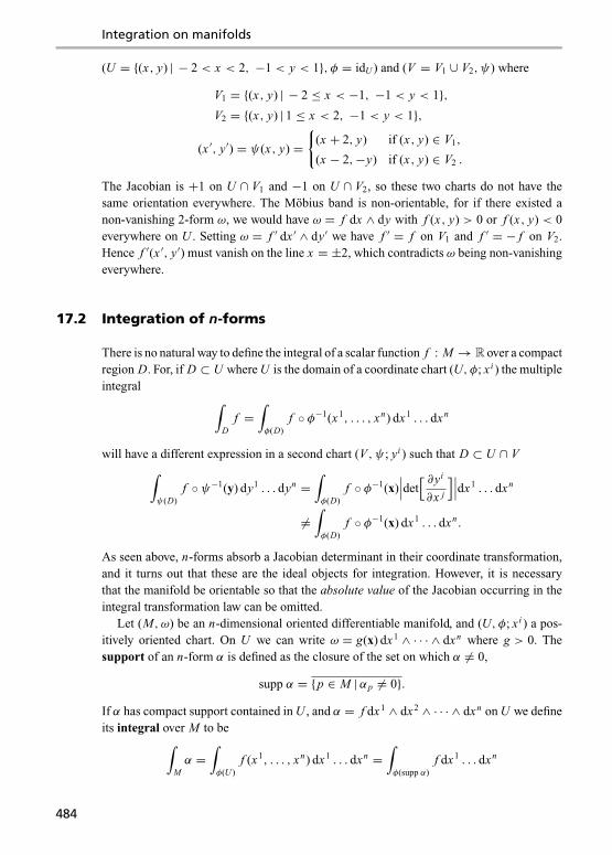
Integration on manifolds

(U = {(x, y) | − 2 < x < 2, −1 < y < 1}, φ = idU ) and (V = V1 ∪ V2, ψ) where

V1 = {(x, y) | − 2 ≤ x < −1, −1 < y < 1},V2 = {(x, y) | 1 ≤ x < 2, −1 < y < 1},

(x ′, y′) = ψ(x, y) ={

(x + 2, y) if (x, y) ∈ V1,

(x − 2,−y) if (x, y) ∈ V2 .

The Jacobian is +1 on U ∩ V1 and −1 on U ∩ V2, so these two charts do not have thesame orientation everywhere. The Mobius band is non-orientable, for if there existed anon-vanishing 2-form ω, we would have ω = f dx ∧ dy with f (x, y) > 0 or f (x, y) < 0everywhere on U . Setting ω = f ′ dx ′ ∧ dy′ we have f ′ = f on V1 and f ′ = − f on V2.Hence f ′(x ′, y′) must vanish on the line x = ±2, which contradicts ω being non-vanishingeverywhere.

17.2 Integration of n-forms

There is no natural way to define the integral of a scalar function f : M → R over a compactregion D. For, if D ⊂ U where U is the domain of a coordinate chart (U, φ; xi ) the multipleintegral ∫

Df =

∫φ(D)

f ◦ φ−1(x1, . . . , xn) dx1 . . . dxn

will have a different expression in a second chart (V, ψ ; yi ) such that D ⊂ U ∩ V∫ψ(D)

f ◦ ψ−1(y) dy1 . . . dyn =∫φ(D)

f ◦ φ−1(x)∣∣∣det[ ∂yi

∂x j

]∣∣∣dx1 . . . dxn

�=∫φ(D)

f ◦ φ−1(x) dx1 . . . dxn.

As seen above, n-forms absorb a Jacobian determinant in their coordinate transformation,and it turns out that these are the ideal objects for integration. However, it is necessarythat the manifold be orientable so that the absolute value of the Jacobian occurring in theintegral transformation law can be omitted.

Let (M, ω) be an n-dimensional oriented differentiable manifold, and (U, φ; xi ) a pos-itively oriented chart. On U we can write ω = g(x) dx1 ∧ · · · ∧ dxn where g > 0. Thesupport of an n-form α is defined as the closure of the set on which α �= 0,

supp α = {p ∈ M |αp �= 0}.If α has compact support contained in U , and α = f dx1 ∧ dx2 ∧ · · · ∧ dxn on U we defineits integral over M to be∫

Mα =

∫φ(U )

f (x1, . . . , xn) dx1 . . . dxn =∫φ(supp α)

f dx1 . . . dxn

484

17.2 Integration of n -forms

where f (x1, . . . , xn) is commonly written in place of f = f ◦ φ−1. If (V, ψ ; x ′i ) is a secondpositively oriented chart also containing the support of α and f ′(x ′1, . . . , x ′n) ≡ f ◦ ψ−1,we have by the change of variable formula in multiple integration∫

ψ(V )f ′(x ′1, . . . , x ′n) dx ′1 . . . dx ′n =

∫ψ(supp α)

f ′(x′) dx ′1 . . . dx ′n

=∫φ(supp α)

f ′(x′)∣∣∣det[∂x ′i

∂x j

]∣∣∣dx1 . . . dxn

=∫φ(U )

f (x) dx1 . . . dxn

since

α = f dx1 ∧ · · · ∧ dxn = f ′dx ′1 ∧ · · · ∧′ n where f = f ′ det[∂x ′i

∂x j

]and the Jacobian determinant is everywhere positive. The definition of the integral is there-fore independent of the coordinate chart, provided the support lies within the domain of thechart.

For an arbitrary n-form α with compact support and atlas (Ua, φa), assumed to be locallyfinite, let ga be a partition of unity subordinate to the open covering {Ua}. Evidently

α =∑

a

ga α

and each of the summands ga α has compact support contained in Ua . We define the integralof α over M to be ∫

Mα =

∑a

∫M

ga α. (17.1)

Exercise: Prove that∫

M is a linear operator,∫

M α + cβ = ∫M α + c∫

M β.

If α is a differential k-form with compact support on M and ϕ : N → M is a regularembedding of a k-dimensional manifold N in M (see Section 15.4), define the integral ofα on ϕ(N ) to be ∫

ϕ(N )α =

∫Nϕ∗α.

The right-hand side is well-defined since ϕ∗α is a differential k-form on N with compactsupport, since ϕ : M → N is a homeomorphism from N to ϕ(N ) in the relative topologywith respect to M .

Problems

Problem 17.3 Show that the definition of the integral of an n-form over a manifold M given in Eq.(17.1) is independent of the choice of partition of unity subordinate to {Ua}.

485

Integration on manifolds

17.3 Stokes’ theorem

Stokes’ theorem requires the concept of a submanifold with boundary. This is not an easynotion in general, but for most practical purposes it is sufficient to restrict ourselves toregions made up of ‘coordinate cubical regions’. Let �k be the standard unit k-cube,

�k = {x ∈ Rk | 0 ≤ xi ≤ 1 (i = 1, . . . , k)} ⊂ Rk .

The unit 0-cube is taken to be the singleton �0 = {0} ⊂ R. A k-cell in a manifold M is asmooth map σ : U → M where U is an open neighbourhood U of �k in Rk (see Fig. 17.2),and its support is defined as the image of the standard k-cube, σ (�k). A cubical k-chainin M consists of a formal sum

C = c1σ1 + c2σ2 + · · · + crσr where ci ∈ R, r a positive integer.

The set of all cubical k-chains is denoted Ck ; it forms an abelian group under addition of k-chains defined in the obvious way. It is also a vector space if we define scalar multiplicationas aC =∑i aciσi where a ∈ R.

For each i = 1, . . . , k and ε = 0, 1 define the maps ϕεi : �k−1 → �k by

ϕεi (y1, . . . , yk−1) = (y1, . . . , yi−1, ε, yi , . . . , yk−1).

These maps can be thought of as the (i, 0)-face and (i, 1)-face respectively of �k . If theinterior of the standard k-cube �k is oriented in the natural way, by assigning the k-formdx1 ∧ · · · ∧ dxk to be positively oriented over �k , then for each face map xi = 0 or 1the orientation on �k−1 is assigned according to the following rule: set the k-form dxi ∧dx1 ∧ · · · ∧ dxi−1 ∧ dxi+1 ∧ · · · ∧ dxk to be positively oriented if xi is increasing outwardsat the face, else it is negatively oriented. According to this rule the (k − 1)-form dy1 ∧dy2 ∧ · · · ∧ dyk−1 has orientation (−1)i on the (i, 0)-face, while on the (i, 1)-face it hasorientation (−1)i+1. This is sometimes called the outward normal rule – the orientation onthe boundary surface must be chosen such that at every point there exist local positivelyoriented coordinates such that the first coordinate x1 points outwards from the surface.

Exercise: On the two-dimensional square, verify that the outward normal rule implies that the di-rection of increasing x or y coordinate on each side proceeds in an anticlockwise fashion around thesquare.

Figure 17.2 k-Cell on a manifold M

486

17.3 Stokes’ theorem

This gives the rationale for the boundary map ∂ : Ck → (C)k−1, defined by:

(i) for a k-cell σ (k > 0), set

∂σ =k∑

i=1

(−1)i(σ ◦ ϕ0

i − σ ◦ ϕ1i

),

(ii) for a cubical k-chain C =∑ ciσi set

∂C =∑

i

ci∂σi .

An important identity is ∂2 = 0. For example if σ is a 2-cell, its boundary is given by

∂σ = −ϕ01 + ϕ1

1 + ϕ02 − ϕ1

2 .

The boundary of the face ϕ01(z) = (0, z) is ∂ϕ0

1 = −ρ01 + ρ00, where ρab : {0} → R is themap ρab(0) = (a, b). Hence

∂ ◦ ∂σ = −ρ01 + ρ00 + ρ11 − ρ10 + ρ10 − ρ00 − ρ11 + ρ01 = 0.

For a k-cell,

∂2σ =1∑ε=0

1∑ε′=0

[∑i

∑j<i

(−1)i+ε+ j+ε′σ ◦ ϕεε′i j +∑

i

∑j≥i

(−1)i+ε+ j+ε′+1σ ◦ ϕεε′i j

]where

ϕεε′

i j (z1, . . . , zk−2) ={

(z1, . . . , z j−1, ε′, z j , . . . , zi−1, ε, zi , . . . , zk−2) if j < i,

(z1, . . . , zi−1, ε, zi , . . . , z j−1, ε′, z j , . . . , zk−2) if j ≥ i.

It follows from this equation that all terms cancel in pairs, so that ∂2σ = 0. The identityextends by linearity to all k-chains.

Exercise: Write out ∂2σ for a 3-cube, and verify the cancellation property.

For a k-form α on M and a k-chain C =∑ ciσi we define the integral∫Cα =

∑ci∫σi

α =∑

ci∫�k

σ ∗i α.

Theorem 17.2 (Stokes’ theorem) For any (k + 1)-chain C, and differential k-form onM, ∫

Cdα =

∫∂Cα. (17.2)

Proof : By linearity, it is only necessary to prove the theorem for a (k + 1)-cell σ . Theleft-hand side of (17.2) can be written, using Theorem 16.2,∫

σ

dα =∫�k+1

σ ∗dα =∫�k+1

d(σ ∗α)

487

Integration on manifolds

while the right-hand side is∫∂σ

α =1∑ε=0

k+1∑i=1

(−1)i+ε∫σ◦ϕεi

α

=1∑ε=0

k+1∑i=1

(−1)i+ε∫�k

(ϕεi)∗ ◦ σ ∗α.

Since σ ∗α is a differential k-form on Rk+1 it can be written as

σ ∗α =k+1∑i=1

Ai dx1 ∧ · · · ∧ dxi−1 ∧ dxi+1 ∧ · · · ∧ dxk+1

where the Ai are differentiable functions Ai : V → R on an open neighbourhood V of�k+1.Hence

d(σ ∗α) =k+1∑i=1

k+1∑j=1

∂Ai

∂x jdx j ∧ dx1 ∧ · · · ∧ dxi−1 ∧ dxi+1 ∧ · · · ∧ dxk+1

=k+1∑i=1

(−1)i+1 ∂Ai

∂xidx1 ∧ · · · ∧ dx j ∧ · · · ∧ dxk+1.

Substituting in the left-hand integral of Eq. (17.2) we have∫�k+1

d(σ ∗α) =k+1∑i=1

(−1)i+1∫ 1

0

∫ 1

0· · ·∫ 1

0

∂Ai

∂xidx1 dx2 . . . dxk+1

=k+1∑i=1

(−1)i+1∫ 1

0

∫ 1

0· · ·∫ 1

0dx1 . . . dxi−1dxi+1 . . . dxk+1

× [Ai (x1, . . . , xi−1, 1, xi+1, . . . , xk+1)

− Ai (x1, . . . , xi−1, 0, xi+1, . . . , xk+1)

]=

1∑ε=0

k+1∑i=1

(−1)i+ε∫ 1

0· · ·∫ 1

0dx1 . . . dxi−1 dxi+1 . . .

dxk+1 Ai (x1, . . . , xi−1, ε, xi+1, . . . , xk+1)

=1∑ε=0

k+1∑i=1

(−1)i+ε∫�k

(ϕεi)∗ ◦ σ ∗α

=∫∂σ

α,

as required. �

Example 17.2 In Example 15.9 we defined the integral of a differential 1-form ω over acurve with end points γ : [t1, t2] → M to be∫

γ

ω =∫ t2

t1

〈ω, γ 〉dt =∫ t2

t1

〈γ ∗ω, d

dt〉dt.

A 1-cell σ : U → M is a curve with parameter range U = (−a, 1+ a) ⊃ �1 = [0, 1],and can be made to cover an arbitrary range [t1, t2] by a change of parameter t → t ′ =

488

17.3 Stokes’ theorem

t1 + (t2 − t1) t . The integral of ω = wi (x j ) dxi over the support of the 1-cell is∫σ

ω =∫�1

σ ∗ ω =∫ 1

0wi (x(t))

dxi

dtdt,

which agrees with the definition of the integral given in Example 15.9.The boundary of the 1-cell σ is

∂σ = σ ◦ ϕ11 − σ ◦ ϕ0

1

where the two terms on the right-hand side are the 0-cells �0 = {0} → σ (1) and �0 ={0} → σ (0), respectively. Settingω = d f where f is a differentiable function on M , Stokes’theorem gives ∫

σ

d f =∫∂σ

f = f (σ (1))− f (σ (0)).

If M = R and the 1-cell σ is defined by x = σ (t) = a + t(b − a), Stokes’ theorem reducesto the fundamental theorem of calculus,∫ b

a

d f

dxdx =

∫ 1

0

d f

dtdt =

∫σ

d f = f (b)− f (a).

Regular domains

In the above discussion, the only requirement made concerning the cell maps σ was thatthey be differentiable on a neighbourhood of the unit k-cube �k . For example, they could becompletely degenerate and map the entire set �k into a single point of M . For this reason,the chains are sometimes called singular. A fundamental n-chain on an n-dimensionalmanifold M has the form

C = σ1 + σ2 + · · · + σN

where each σi : U → σi (U ) is a diffeomorphism and the interiors of the supports σi (�k) ofdifferent cells are non-intersecting:

σi

((�n)o

) ∩ σ j

((�n)o

) = ∅ for i �= j.

A regular domain D ⊆ M is a closed set of the form

D =n⋃

i=1

σi (�n)

where σi are the n-cells of a fundamental chain C (see Fig. 17.3). We may think of aregular domain as subdivided into cubical cells or a region with boundary – the ‘boundary’consisting of boundary points of the chain that are not on the common faces of any pair ofcells.

Theorem 17.3 If D is a regular domain ‘cubulated’ in two different ways by fundamentalchains C = σi + · · · + σN and C ′ = τ1 + · · · + τM then

∫C ω =

∫C ′ ω for every differential

n-form ω.

489

Integration on manifolds

Figure 17.3 A regular domain on a manifold

Proof : Let Ai j = σi (�n) ∩ τ j (�n) and

Bi j = (σi )−1(Ai j ), Ci j = (τ j )

−1(Ai j ).

The maps τ−1j ◦ σi : Bi j → Ci j are all diffeomorphisms and∫

Bi j

σ ∗i ω =∫

Bi j

σ ∗i ◦ (τ−1j )∗ ◦ τ ∗j ω

=∫

Bi j

((τ−1

j ) ◦ σi

)∗ ◦ τ ∗j ω=∫

Ci j

τ ∗j ω .

Hence ∫Cω =

∑i

∫σi

ω =∑i, j

∫Bi j

σ ∗i ω =∑i, j

∫Ci j

τ ∗j ω =∫

C ′ω.

�

If α is a differential (n − 1)-form,∫∂Dα =

∫∂Cα =

N∑i=1

n∑j=1

1∑ε=0

∫�n−1

(ϕεj)∗ ◦ σ ∗i α.

Since the outward normals on common faces of adjoining cells are oppositely directed,the faces will be oppositely oriented and the integrals will cancel, leaving only an integralon the ‘free’ parts of the boundary of D. This results in Stokes’ theorem for a regulardomain ∫

Ddα =

∫∂Dα.

A regular k-domain Dk is defined as the image of a regular domain D ⊂ K of ak-dimensional manifold K under a regular embedding ϕ : K → M , and for any k-form

490

17.3 Stokes’ theorem

β and (k − 1)-form α we set ∫Dk

β =∫ϕ(D)

β =∫

Dϕ ∗ β∫

∂Dk

α =∫∂ϕ(D)

α =∫∂Dϕ ∗ α.

The general form of Stokes’ theorem asserts that for any (k − 1)-form α and regular k-domain Dk , ∫

Dk

dα =∫∂Dk

α. (17.3)

Example 17.3 In low dimensions, Stokes’ theorem reduces to a variety of familiar forms.For example, let D be a regular 2-domain in R2 bounded by a circuit C = ∂D havinginduced orientation according to the ‘right hand rule’. By this we mean that if the outwardnormal is taken locally in the direction of the first coordinate x1, and the tangent to C in thedirection x2, then dx1 ∧ dx2 is positively oriented. If α = P dx + Q dy, then

dα = ∂P

∂ydy ∧ dx + ∂Q

∂xdx ∧ dy =

(∂Q

∂x− ∂P

∂y

)dx ∧ dy,

and Stokes’ theorem is equivalent to Green’s theorem∫∫D

(∂Q

∂x− ∂P

∂y

)dx dy =

∮C

P dx + Q dy.

If D is a bounded region in R3 whose boundary is a surface S = ∂D, the inducedorientation is such that if (e, f ) are a correctly ordered pair of tangent vectors to S and nthe outward normal to S, then (n, e, f ) is a positively oriented basis of vectors in R3. Letα = A1 dy ∧ dz + A2 dz ∧ dx + A3 dx ∧ dz be a 2-form, then

dα = (A1,1 + A2,2 + A3,3)dx ∧ dy ∧ dz = ∇ · A dx ∧ dy ∧ dz

where A = (A1, A2, A3). Stokes’ theorem reads∫D

dα =∫∫∫

D

∇ · A dx dy dz =∫∂Dα =

∫∫S

A1 dy dz + A2 dz dx + A3 dx dz.

If the bounding surface is locally parametrized by two parameters, x = x(λ1, λ2), y =y(λ1, λ2), z = z(λ1, λ2), then we can write∫∫

S

α =∫∫

S

εi jk Ai∂x j

∂λ1

∂xk

∂λ2dλ1 ∧ dλ2

and it is common to write Stokes’ theorem in the standard Gauss theorem form∫∫∫D

∇ · A dx dy dz =∫∫

S

A · dS,

491

Integration on manifolds

where S is the vector area normal to S, having components

dSi = εi jk∂x j

∂λ1

∂xk

∂λ2dλ1 dλ2.

Let � be an oriented 2-surface in R3, with boundary an appropriately oriented circuitC = ∂�, and α a differential 1-form α = A1 dx + A2 dy + A3 dz = Ai dxi . Then∫

�

dα =∫�

Ai, j dx j ∧ dxi

=∫∫�

Ak, j

(∂x j

∂λ1

∂xk

∂λ2− ∂xk

∂λ1

∂x j

∂λ2

)dλ1 ∧ dλ2

=∫∫�

εi jk Ak, j dSi

and ∫∂�

α =∮

CAi dxi =

∮C

A1 dx + A2 dy + A3 dz.

This can be expressed in the familiar form of Stokes’ theorem∫∫�

(∇ × A) · dS =∮

CA · dr.

Exercise: Show that dSi is ‘normal’ to the surface S in the sense that dSi∂xi/∂λa = 0 for a = 1, 2.

Problems

Problem 17.4 Let α = y2 dx + x2 dy. If γ1 is the stretch of y-axis from (x = 0, y = −1) to (x =0, y = 1), and γ2 the unit right semicircle connecting these points, evaluate∫

γ1

α,

∫γ2

α and∫

S1α.

Verify Stokes’ theorem for the unit circle and the unit right semicircular region encompassed by γ1

and γ2.

Problem 17.5 If α = x dy ∧ dz + y dz ∧ dx + z dx ∧ dy compute∫∂�α where � is (i) the unit

cube, (ii) the unit ball in R3. In each case verify Stokes’ theorem,∫∂�

α =∫�

dα.

Problem 17.6 Let S be the surface of a cylinder of elliptical cross-section and height 2h given by

x = a cos θ, y = b sin θ (0 ≤ θ < 2π), −h ≤ z ≤ h.

(a) Compute∫

S α where α = x dy ∧ dz + y dz ∧ dx − 2z dx ∧ dy.(b) Show dα = 0, and find a 1-form ω such that α = dω.(c) Verify Stokes’ theorem

∫S α =

∫∂S ω.

492

17.4 Homology and cohomology

Problem 17.7 A torus in R3 may be represented parametrically by

x = cosφ(a + b cosψ), y = sinφ(a + b cosψ), z = b sinψ

where 0 ≤ φ < 2π , 0 ≤ ψ < 2π . If b is replaced by a variable ρ that ranges from 0 to b, show that

dx ∧ dy ∧ dz = ρ(a + ρ cosψ) dφ ∧ dψ ∧ dρ.

By integrating this 3-form over the region enclosed by the torus, show that the volume of the solidtorus is 2π2ab2. Can you see this by a simple geometrical argument?

Evaluate the volume by performing the integral of the 2-form α = x dy ∧ dz over the surface ofthe torus and using Stokes’ theorem.

Problem 17.8 Show that in n dimensions, if V is a regular n-domain with boundary S = ∂V , andwe set α to be an (n − 1)-form with components

α =n∑

i=1

(−1)i+1 Ai dx1 ∧ · · · ∧ dxi−1 ∧ dxi+1 ∧ · · · ∧ dxn,

Stokes’ theorem can be reduced to the n-dimensional Gauss theorem∫· · ·∫

V

Ai,i dx1 . . . dxn =

∫· · ·∫

S

Ai dSi

where dSi = dx1 . . . dxi−1 dxi+1 . . . dxn is a ‘vector volume element’ normal to S.

17.4 Homology and cohomology

In the previous section we considered regions that could be subdivided into ‘cubical’ parts.While this has practical advantages when it comes to integration, and makes the proofof Stokes’ theorem relatively straightforward, the subject of homology is more standardlybased on triangular cells. There is no essential difference in this change since any k-cube isreadily triangulated, as well as the converse. For example, a triangle in two dimensions iseasily divided into squares (see Fig. 17.4). Dividing a tetrahedron into four cubical regionsis harder to visualize, and is left as an excercise for the reader.

Ordered simplices and chains in Euclidean space

A set of points {x0, x1, . . . , xp} in Euclidean space Rn is said to be independent if the pvectors xi − x0 (i = 1, . . . , p) are linearly independent. The ordered p-simplex with thesepoints as vertices consists of their convex hull,

〈x0, x1, . . . , xp〉 ={

y =p∑

i=0

t i xi

∣∣∣∣∣ all t j ≥ 0 andp∑

i=0

t i = 1

},

together with a specific ordering (x0, x1, . . . , xp) of the vertex points. We will often denotean ordered r -simplex by a symbol such as � or �p. Two ordered p-simplices with the

493

Integration on manifolds

Figure 17.4 Dividing the triangular into ‘cubical’ cells

same set of vertices will be taken to be identical if the orderings are related by an evenpermutation, else they are given the opposite sign. For example,

〈x, y, z〉 = −〈x, z, y〉 = 〈y, z, x〉.

The standard n-simplex on Rn is �n = 〈0, e1, . . . , en〉 where ei is the i th basis vectorei = (0, 0, . . . , 1, . . . , 0), i.e.

�n = {(t1, t2, . . . , tn) |∑nj=1t j = 1 and 0 ≤ ti ≤ 1 (i = 1, . . . , n)} ⊂ Rn.

A 0-simplex 〈x0〉 is a single point x0 together with a plus or minus sign.A 1-simplex 〈x0, x1〉 is a closed directed line from x0 to x1.A 2-simplex 〈x0, x1, x2〉 is an oriented triangle, where the vertices are taken in a definite

order.A 3-simplex is a tetrahedron in which the vertices are again given a specific order up to

even permutations. These examples are depicted in Fig. 17.5.A p-chain is a formal sum C =∑M

μ=1 cμ�μ where aμ are real numbers and �μ arep-simplices in Rn . The set of all p-chains on Rn is obviously a vector space, denotedCp(Rn).

The i th face of a p-simplex � = 〈x0, x1, . . . , xp〉 is defined as the ordered (p − 1)-simplex

�i = (−1)i 〈x0, . . . , xi , . . . , xp〉 ≡ (−1)i 〈x0, x1, . . . , xi−1, xi+1, . . . , xp〉,

and the boundary of a p-simplex � is defined as the (p − 1)-chain

∂� =p∑

i=0

�i =p∑

i=0

(−1)i 〈x0, . . . , xi , . . . , xp〉,

494

17.4 Homology and cohomology

Figure 17.5 Standard low dimensional p-simplexes

and extends to all p-chains by linearity. For example,

∂〈x0, x1〉 = 〈x1〉 − 〈x0〉,∂〈x0, x1, x2〉 = 〈x1, x2〉 − 〈x0, x2〉 + 〈x0, x1〉,

∂〈x0, x1, x2, x3〉 = 〈x1, x2, x3〉 − 〈x0, x2, x3〉 + 〈x0, x1, x3〉 − 〈x0, x1, x2〉.

For each p = 0, . . . , n the boundary operator generates a linear map ∂ : Cp(Rn) →Cp−1(Rn) by setting

∂

(∑μ

cμ�μ

)=∑μ

cμ∂�μ.

If we set the boundary of any 0-form to be the zero chain, ∂〈x〉 = 0 it is trivial to seethat two successive applications of the boundary operator on any 1-simplex vanishes,

∂2〈x0, x1〉 = ∂(〈x1〉 − 〈x0〉) = 0− 0 = 0.

This identity generalizes to arbitrary p-simplices, for

∂∂〈x0, x1, . . . , xp〉 =p∑

i=0

∂(−1)i 〈x0, . . . , xi , . . . , xp〉

=p∑

i=0

(−1)i[∑

j<i

(−1) j 〈x0, . . . , x j , . . . , xi , . . . , xp〉

+∑j>i

(−1) j+1〈x0, . . . , xi , . . . , x j , . . . , xp〉]

= 0

since all terms cancel in pairs. The identity ∂2 = 0 follows from the linearity of the boundaryoperator ∂ on Cp(Rn).

495

Integration on manifolds

Exercise: Write out the cancellation of terms in this argument explicitly for a 2-simplex 〈x0, x1, x2〉and 3-simplex 〈x0, x1, x2, x3〉.

A p-chain C is said to be a cycle if it has no boundary, ∂C = 0. It is said to be a boundaryif there exists a (p + 1)-chain C ′ such that C = ∂C ′. Clearly every boundary is a p-chainsince ∂C = ∂2C ′ = 0, but the converse need not be true.

Simplicial homology on manifolds

Let M be an n-dimensional differentiable manifold. A (singular) p-simplex σp on Mis a smooth map φ : U → M where U is an open subset of Rp containing the standardp-simplex �p. A p-chain on M is a formal linear combination of p-simplices on M ,

C =M∑μ=1

cμσpμ (cμ ∈ R),

and let Cp(M) be the real vector space generated by all p-simplices on M .For each i = 1, 2, . . . , p − 1 denote by ϕi : Rp−1 → Rp the map that embeds Rp−1 into

the plane xi = 0 of Rp,

ϕi (x1, . . . , x p−1) = (x1, . . . , xi , 0, xi+1, . . . , x p−1),

and for i = 0 set

ϕ0(x1, . . . , x p−1) = (1−∑p−1i=1 xi , x1, . . . , x p−1

).

The maps ϕ0, ϕ1, . . . , ϕp−1 are (p − 1)-simplices in Rp, whose supports are the variousfaces of the standard p-simplex, �p,

ϕi (�p−1) = �pi (i = 0, 1, . . . , p − 1).

If σ is a p-simplex in M , define its i th face to be the (p − 1)-simplex

σi = σ ◦ ϕi : �p−1 → M,

and its boundary to be the (p − 1)-chain

∂pσ =p−1∑i=0

(−1)iσi .

Extend by linearity to all chains C ∈ Cp(M),

∂pC = ∂M∑μ=1

cμσpμ =M∑μ=1

cμ∂σpμ.

A p-boundary B is a singular p-cycle on M that is the boundary of a (p + 1)-chain,B = ∂p+1C . A p-cycle C is a singular p-chain on M whose boundary vanishes, ∂pC = 0.Since ∂2 = 0 it is clear that every p-boundary is a p-cycle.

496

17.4 Homology and cohomology

If we let Bp(M) be the set of all p-boundaries on M , and Z p(M) all p-cycles, these areboth vector subspaces of Cp(M):

Bp(M) = im ∂p+1,

Z p(M) = ker ∂p ⊇ Bp(M).

We define the pth homology space to be the factor space

Hp(M) = Z p(M)/Bp(M).

Commonly this is called the pth homology group, only the abelian group property beingrelevant. Two cycles C1 and C2 are said to be homologous if they belong to the samehomology class – that is, if there exists a chain C such that C1 − C2 = ∂C . The dimensionof the pth homology space is known as the pth Betti number,

bp = dim Hp(M),

and the quantity

χ (M) =n∑

p=0

(−1)pbp

is known as the Euler characteristic of the manifold M . A non-trivial result that we shallnot attempt to prove is that the Betti numbers are topological invariants – two manifolds thatare topologically homeomorphic have the same Betti numbers and Euler characteristic [13].

Example 17.4 Since ∂〈0〉 = 0 every 0-simplex in a manifold M has boundary 0. Henceevery 0-chain in M is a 0-cycle, and Z0(M) = C0(M). The zeroth homology space H0(M) =Z0(M)/B0(M) counts the number of 0-chains that are not boundaries of 1-chains. Since a1-simplex is essentially a smooth curve σ : [0, 1] → M it has boundary σ (1)− σ (0), wherewe represent the 0-simplex map 0 → p ∈ M simply by its image point p. Two 0-simplicesp and q are homologous if p − q is a boundary; that is, if they are the end points of asmooth curve connecting them. This is true if and only if they belong to the same connectedcomponent of M . Thus H0(M) is spanned by a set of simplices {p0, p1, . . . }, one from eachconnected component of M , and the zeroth Betti number β0 is the number of connectedcomponents of the topological space M .

De Rham cohomology groups and duality

Let Cr (M) = �r (M) be the real vector space consisting of all differential r -forms on M . Itselements are also known as r -cochains on M . The exterior derivative d is a linear operatord : Cr (M) → Cr+1(M) for each r = 0, 1, . . . , n, with the property d2 = 0. We write itsrestriction to Cr (M) as dr .

A differential r -form α is said to be closed if dα = 0, and it is said to be exact if thereexists an (r − 1)-form β such that α = dβ. Clearly every exact r -form is closed sinced2β = 0. In the language of cochains these definitions can be expressed as follows: an r -cochainα is called an r -cocycle if it is a closed differential form, while it is an r -coboundary

497

Integration on manifolds

if it is exact. We denoted the vector subspace of r -cocycles by Zr (M), and the subspace ofr -coboundaries by Br (M)

Zr (M) = {α ∈ Cr (M) | dα = 0} = ker dr ⊂ Cr (M)

Br (M) = {α ∈ Cr (M) |α = dβ, β ∈ Cr−1(M)} = im dr−1 ⊂ Zr (M).

The r th de Rham cohomology space (group) is defined as the factor space Hr (M) =Zr (M)/Br (M), and any two r -cocycles α and β are said to be cohomologous if theybelong to the same coset, α − β = dγ for some (r − 1)-cochain γ . The dimensions of thevector spaces Hr (M) are denoted br .

Example 17.5 Since there are no differential forms of degree−1 we always set B0(M) =0. Hence H 0(M) = Z0(M). A 0-form f is closed and belongs to Z0(M) if and only ifd f = 0. Hence f = const. on each connected component of M , and H 0(M) = R+R+ · · · + R, one contribution from each such component. Hence b0 = b0 is the number ofconnected components of M (see Example 17.4).

Example 17.6 If M = R, then from the previous example H 0(R) = R. A 1-form ω ∈C1(M) is closed if dω = 0. Setting ω = f (x) dx we can clearly always write

ω = d f = dF

xwhere F(x) =

∫ x

0f (y) dy.

Hence every closed 1-form is exact and H 1(R) = 0, b1 = 0. It is not difficult to verify thatthis is also the value of the Betti numbers, b1 = 0.

Define a bracket 〈 , 〉 : Cr (M)× Cr (M) → R by setting

〈C, α〉 =∫

Cα.

for every r -chain C ∈ Cr (M) and r -cochain α ∈ Cr (M) = �r (M). For every α the mapC �→ 〈C, α〉 is evidently linear on Cr (M) and for every C ∈ Cr (M) the map α �→ 〈C, α〉 islinear on Cr (M). By Stokes’ theorem the exterior derivative d is the adjoint of the boundaryoperator ∂ with respect to this bracket, in the sense that

〈C, dα〉 = 〈∂C, α〉.

The bracket induces a bracket 〈 , 〉 on Hr (M)× Hr (M) by setting

〈[C], [α]〉 = 〈C, α〉 =∫

Cα

for any pair [C] ∈ Hr (M) and [α] ∈ Hr (M). It is independent of the choice of representativefrom the homology and cohomology classes, for if C ′ = C + ∂C1 and α′ = α + dα1, where

498

17.4 Homology and cohomology

∂C = 0 and dα = 0, then

〈C ′, α′〉 =∫

C+∂C1

α + dα1

=∫

Cα +

∫∂C1

α +∫

Cdα1 +

∫∂C1

dα1

=∫

Cα +

∫C1

dα +∫∂Cα1 +

∫∂2C1

α1 by Stokes’ theorem

=∫

Cα = 〈C, α〉.

For any fixed r -cohomology class [α], the map f[α] : Hp(M) → R given by

f[α]([C]) = 〈[C], [α]〉is a well-defined linear functional on Hr (M). De Rham’s theorem asserts that this corre-spondence between linear functionals on Hr (M) and cohomology classes [α] ∈ Hr (M) isbijective.

Theorem 17.4 (de Rham) The bilinear map on Hr (M)× Hr (M) → R defined by([C], [α]) �→ 〈[C], [α]〉 is non-degenerate in both arguments. That is, every linear func-tional on Hr (M) has the form f[α] for a uniquely defined r-cohomology class [α].

The proof lies beyond the scope of this book, and may be found in [6, 10]. There are avariety of ways of expressing de Rham’s theorem. Essentially it says that the r th cohomologygroup is isomorphic with the dual space of the r th homology group,

Hr (M) ∼= (Hr (M))∗.

If the Betti numbers are finite then br = br .The integral of a closed r -form α over an r -cycle C

〈C, α〉 =∫

Cα

is sometimes called a period of α. By Stokes’ theorem all periods of α vanish if α is anexact form, and the period of any closed r -form vanishes over a boundary r -cycle C = ∂C ′.Let C1, . . . ,Ck be k = br linearly independent cycles in Zr (M), such that [Ci ] �= [C j ] fori �= j . De Rham’s theorem implies that an r -form α is exact if and only if all the periods∫

Ciα = 0. If α is exact then we have already remarked that all its periods vanish. The

converse follows from the fact that 〈[C], [α]〉 = 0 for every [C] ∈ Hr (M), since [C] can beexpanded to [C] =∑k

i=1[Ci ]. By non-degeneracy of the product 〈 , 〉we must have [α] = 0,so that α = dβ for some (r − 1)-form β.

Problems

Problem 17.9 Show that any tetrahedron may be divided into ‘cubical’ regions.Describe a procedure for achieving the same result for a general k-simplex.

499

Integration on manifolds

Problem 17.10 For any pair of subspaces H and K of the exterior algebra�∗(M), set H ∧ K to bethe vector subspace spanned by all α ∧ β where α ∈ H , β ∈ K . Show that

(a) Z p(M) ∧ Zq (M) ⊆ Z p+q (M),

(b) Z p(M) ∧ Bq (M) ⊆ B p+q (M),

(c) B p(M) ∧ Bq (M) ⊆ B p+q (M).

Problem 17.11 Show that for any set of real numbers a1, . . . , ak there exists a closed r -form α

whose periods∫

Ciα = ai .

Problem 17.12 If S1 is the unit circle, show that b0 = b1 = 1.

17.5 The Poincare lemma

The fact that every exact differential form is closed has a kind of local converse.

Theorem 17.5 (Poincare lemma) On any open set U ⊆ M homeomorphic to Rn, everyclosed differential form of degree k ≥ 1 is exact: if dα = 0 on U where α ∈ �k(U ), thenthere exists a (k − 1)-form β on U such that α = dβ.

Proof : We prove the theorem on Rn itself, with coordinates x1, . . . , xn , and set α =αi1i2...ik (x) dxi1 ∧ dxi2 ∧ · · · ∧ dxik . Let αt (0 ≤ t ≤ 1) be the one-parameter family of k-forms

αt = αi1...ik (tx) dxi1 ∧ · · · ∧ dxik .

The map hk : �k(Rn) → �k−1(Rn) defined by

hkα =∫ 1

0t k−1iXα

t dt where X = xi ∂

∂xi

satisfies the key identity

(d ◦ hk + hk+1 ◦ d)α = α (17.4)

for any k-form α on Rn . To prove (17.4) write out the left-hand side,

(d ◦ hk + hk+1 ◦ d)α =∫ 1

0t k−1diXα

t + t k iX (dα)t dt,

and

dαt = ∂αi1...ik (tx)

∂x jdx j ∧ dxi1 ∧ · · · ∧ dxik

= t(dα)t .

Using the Cartan identity, Eq. (16.13),

(d ◦ hk + hk+1 ◦ d)α =∫ 1

0t k−1

(d ◦ iX + iX ◦ d

)αt dt

=∫ 1

0t k−1LXα

t dt

500

17.5 The Poincare lemma

and from the component formula for the Lie derivative (15.39),(LXα

t)

i1...ik= ∂αi1...ik (tx)

∂x jx j + ∂x j

∂xi1α j i2...ik (tx)+ · · · + ∂x j

∂xikαi1... j (tx)

= t∂αi1...ik (tx)

∂t x j

dt x j

dt+ δ j

i1α j ...ik (tx)+ · · · + δ j

x ikαi1... j (tx)

= tdαi1...ik (tx)

dt+ kαi1...ik (tx).

Hence

LXαt = t

dαt

dt+ kαt ,

and Eq. (17.4) follows from

(d ◦ hk + hk+1 ◦ d)α =∫ 1

0t k dαt

dt+ ktk−1αt dt =

∫ 1

0

dt kαt

dtdt = α.

If dα = 0 we have α = dβ where β = hkα, and the theorem is proved. �

An immediate corollary of this theorem and de Rham’s theorem is that all homologygroups Hk(Rn) are trivial for k ≥ 1; that is, all Betti numbers for k ≥ 1 vanish in Euclideanspace, bk = bk = 0. Of course b0 = b0 = 1 since there is a single connected component.

Example 17.7 In R3 let α be the 1-form α = A1 dx1 + A2 dx2 + A3 dx3. Its exteriorderivative is

dα = (A2,1 − A1,2) dx1 ∧ dx2 + (A1,3 − A3,1) dx3 ∧ dx1 + (A3,2 − A2,3) dx2 ∧ dx3

and Poincare’s lemma asserts that dα = 0 if and only if there exists a function f on R3 suchthat α = d f . In components,

A2,1 − A1,2 = A1,3 − A3,1 = A3,2 − A2,3 = 0 ⇐⇒ A1 = f,1, A2 = f,2, A3 = f,3,

or in standard 3-vector language, with A = (A1, A2, A3),

∇ × A = 0 ⇐⇒ A = ∇ f.

If α is the differential 2-form α = A3 dx1 ∧ dx2 + A2 dx3 ∧ dx1 + A1 dx2 ∧ dx3, then

dα = (A1,1 + A2,2 + A3,3) dx1 ∧ dx2 ∧ dx3.

The Poincare lemma says

dα = 0 ⇐⇒ α = dβ where β = B1 dx1 + B2 dx2 + B3 dx3,

or in components

A1,1 + A2,2 + A3,3= 0 ⇐⇒ A1= B3,2 − B2,3, A2= B1,3 − B3,1, A3= B2,1 − B1,2,

which reduces to the familiar 3-vector statement

∇ · A = 0 ⇐⇒ there exists B such that A = ∇ × B.

501

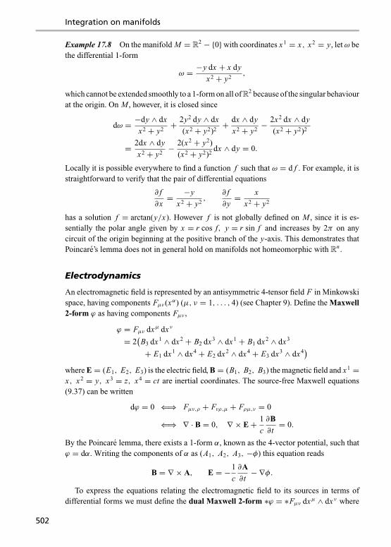
Integration on manifolds

Example 17.8 On the manifold M = R2 − {0}with coordinates x1 = x, x2 = y, letω bethe differential 1-form

ω = −y dx + x dy

x2 + y2,

which cannot be extended smoothly to a 1-form on all of R2 because of the singular behaviourat the origin. On M , however, it is closed since

dω = −dy ∧ dx

x2 + y2+ 2y2 dy ∧ dx

(x2 + y2)2+ dx ∧ dy

x2 + y2− 2x2 dx ∧ dy

(x2 + y2)2

= 2dx ∧ dy

x2 + y2− 2(x2 + y2)

(x2 + y2)2dx ∧ dy = 0.

Locally it is possible everywhere to find a function f such that ω = d f . For example, it isstraightforward to verify that the pair of differential equations

∂ f

∂x= −y

x2 + y2,

∂ f

∂y= x

x2 + y2

has a solution f = arctan(y/x). However f is not globally defined on M , since it is es-sentially the polar angle given by x = r cos f, y = r sin f and increases by 2π on anycircuit of the origin beginning at the positive branch of the y-axis. This demonstrates thatPoincare’s lemma does not in general hold on manifolds not homeomorphic with Rn .

Electrodynamics

An electromagnetic field is represented by an antisymmetric 4-tensor field F in Minkowskispace, having components Fμν(xα) (μ, ν = 1, . . . , 4) (see Chapter 9). Define the Maxwell2-form ϕ as having components Fμν ,

ϕ = Fμν dxμ dxν

= 2(B3 dx1 ∧ dx2 + B2 dx3 ∧ dx1 + B1 dx2 ∧ dx3

+ E1 dx1 ∧ dx4 + E2 dx2 ∧ dx4 + E3 dx3 ∧ dx4)

where E = (E1, E2, E3) is the electric field, B = (B1, B2, B3) the magnetic field and x1 =x, x2 = y, x3 = z, x4 = ct are inertial coordinates. The source-free Maxwell equations(9.37) can be written

dϕ = 0 ⇐⇒ Fμν,ρ + Fνρ,μ + Fρμ,ν = 0

⇐⇒ ∇ · B = 0, ∇ × E+ 1

c

∂B

∂t= 0.

By the Poincare lemma, there exists a 1-form α, known as the 4-vector potential, such thatϕ = dα. Writing the components of α as (A1, A2, A3, −φ) this equation reads

B = ∇ × A, E = −1

c

∂A

∂t− ∇φ.

To express the equations relating the electromagnetic field to its sources in terms ofdifferential forms we must define the dual Maxwell 2-form ∗ϕ = ∗Fμν dxμ ∧ dxν where

502

17.5 The Poincare lemma

∗Fμν is defined as in Example 8.8,

∗ϕ = 2(−E3 dx1 ∧ dx2 − E2 dx3 ∧ dx1 − E1 dx2 ∧ dx3

+ B1 dx1 ∧ dx4 + B2 dx2 ∧ dx4 + B3 dx3 ∧ dx4).

The distribution of electric charge present is represented by a 4-current vector field J =Jμeμ having components Jμ = (j, ρc) where ρ(r, t) is the charge density and j the chargeflux density (see Section 9.4).

ϑ = ∗Jμνρ dxμ ∧ dxν ∧ dxρ

= − 1

3!εμνρσ J σdxμ ∧ dxν ∧ dxρ

= −cρ dx1 ∧ dx2 ∧ dx3 + J 1dx2 ∧ dx3 ∧ dx4

+ J 2 dx3 ∧ dx1 ∧ dx4 + J 3dx1 ∧ dx2 ∧ dx4.

Equations (9.38) may then be written as

d ∗ ϕ = −ϑ ⇐⇒ ∇ · E = 4πρ, −1

c

∂E

∂t+ ∇ × B = 4π

cj.

Charge conservation follows from

dϑ = −d2 ∗ ϕ = 0 ⇐⇒ ∇ · j+ 1

c

∂ρ

∂t= 0.

Example 17.9 Although Maxwell’s vacuum equations take on the deceptively symmetricalform

dϕ = 0, d ∗ ϕ = 0

we cannot assume that ∗ϕ = dβ for a globally defined 1-form β. For example, the coulombfield

B = 0, E =(qx

r3,

qy

r3,

qz

r3

)corresponds to the Maxwell 2-form

ϕ = 2q

r3

(x dx ∧ dx4 + y dy ∧ dx4 + z dz ∧ dx4

) = 2q

r2dr ∧ dx4

where r2 = x2 + y2 + z2, with dual 2-form

∗ϕ = −2q

r3

(z dx ∧ dy + y dz ∧ dx + x dy ∧ dz

).

This 2-form is, however, only defined on the subspace M = R3 − {0}. A short calculationin spherical polar coordinates results in

∗ϕ = −2q sin θ dθ ∧ dφ = d(2q cos θ dφ) = d(2q(cos θ − 1) dφ).

Either of the choicesβ = 2q cos θ dφ orβ ′ = 2q(cos θ − 1)dφ will act as a potential 1-formfor ∗ϕ, but neither is defined on all of M since the angular coordinate φ is not well-definedon the z-axis where θ = 0 or π . The 1-form β is not well-defined on the entire z-axis, but thepotential 1-form β ′ vanishes on the positive z-axis and has a singularity along the negative

503

Integration on manifolds

z-axis. It is sometimes called a Dirac string – a term commonly reserved for solutionsrepresenting magnetic monopoles.

The impossibility of a global potential β can be seen by integrating ∗ϕ over the unit2-sphere ∫

S2

∗ϕ =∫ π

0

∫ 2π

0−2q sin θ dθ dφ = −8πq,

and using Stokes’ theorem (note that S2 has no boundary)∫S2

∗ϕ =∫

S2

dβ =∫∂S2

β = 0.

Problems

Problem 17.13 Let

α = xdy − ydx

x2 + y2.

Show that α is a closed 1-form on R2 − {0}. Compute its integral over the unit circle S1 and showthat it is not exact. What does this tell us of the de Rham cohomology of R2 − {0} and S1?

Problem 17.14 Prove that every closed 1-form on S2 is exact. Show that this statement does notextend to 2-forms by showing that the 2-form

α = r−3/2(x dy ∧ dz + y dz ∧ dx + z dx ∧ dy)

is closed, but has non-vanishing integral on S2.

Problem 17.15 Show that the Maxwell 2-form satisfies the identities

ϕ ∧ ∗ϕ = ∗ϕ ∧ ϕ = 4(B2 − E2)�

ϕ ∧ ϕ = − ∗ ϕ ∧ ∗ϕ = 8B · E�where � = dx1 ∧ dx2 ∧ dx3 ∧ dx4.

References

[1] R. W. R. Darling. Differential Forms and Connections. New York, Cambridge Univer-sity Press, 1994.

[2] S. I. Goldberg. Curvature and Homology. New York, Academic Press, 1962.[3] L. H. Loomis and S. Sternberg. Advanced Calculus. Reading, Mass., Addison-Wesley,

1968.[4] M. Nakahara. Geometry, Topology and Physics. Bristol, Adam Hilger, 1990.[5] C. Nash and S. Sen. Topology and Geometry for Physicists. London, Academic Press,

1983.[6] I. M. Singer and J. A. Thorpe. Lecture Notes on Elementary Topology and Geometry.

Glenview, Ill., Scott Foresman, 1967.[7] M. Spivak. Calculus on Manifolds. New York, W. A. Benjamin, 1965.

504

References

[8] W. H. Chen, S. S. Chern and K. S. Lam. Lectures on Differential Geometry. Singapore,World Scientific, 1999.

[9] S. Sternberg. Lectures on Differential Geometry. Englewood Cliffs, N.J., Prentice-Hall,1964.

[10] F. W. Warner. Foundations of Differential Manifolds and Lie Groups. New York,Springer-Verlag, 1983.

[11] C. de Witt-Morette, Y. Choquet-Bruhat and M. Dillard-Bleick. Analysis, Manifoldsand Physics. Amsterdam, North-Holland, 1977.

[12] J. Kelley. General Topology. New York, D. Van Nostrand Company, 1955.[13] J. G. Hocking and G. S. Young. Topology. Reading, Mass., Addison-Wesley, 1961.

505

18 Connections and curvature

18.1 Linear connections and geodesics

There is no natural way of comparing tangent vectors Yp and Yq at p and q, for if they hadidentical components in one coordinate system this will not generally be true in a differentcoordinate chart covering the two points. In a slightly different light, consider the partialderivatives Y i

, j = ∂Y i/∂xi of a vector field Y in a coordinate chart (U ; xi ). On performing

a transformation to coordinates (U ′; x ′i′), we have from Eq. (15.13)

Y ′i′, j ′ =

∂Y ′i′

∂x ′ j ′ =∂x j

∂x ′ j ′∂

∂x j

(Y i ∂x ′i

′

∂xi

),

whence

Y ′i′, j ′ =

∂x ′i′

∂xi

∂x j

∂x ′ j ′ Yi, j + Y i ∂x j

∂x ′ j ′∂2x ′i

′

∂xi∂x j. (18.1)

The first term on the right-hand side has the form of a tensor transformation term, as inEq. (15.15), but the second term is definitely not tensorial in character. Thus, if Y i hasconstant components in the chart (U ; xi ) (so that Y i

, j = 0) this will not be true in the chart

(U ′; x ′i′) unless the coordinate transformation functions are linear,

x ′i′ = Ai ′

j xj ⇐⇒ ∂2x ′i

′

∂xi∂x j= 0. (18.2)

Suppose we had a well-defined notion of ‘directional derivative’ of a vector field Y withrespect to a tangent vector X p at p, rather like the concept of directional derivative of afunction f with respect to X p. It would then be possible to define a ‘constant’ vector fieldY (t) along a parametrized curve γ connecting p and q by requiring that the directionalderivative with respect to the tangent vector γ to the curve be zero for all t in the parameterrange. The resulting tangent vector Yq at q may, however, be dependent on the choiceof connecting curve γ . If we write the action of a vector field X on a scalar field f asDX f ≡ X f , then for any real-valued function g

DgX f = gX f = gDX f. (18.3)

This property is essential for DX to be a local action, as the action of DgX at p only dependson the value g(p), not on the behaviour of the function g in an entire neighbourhood of p,(

DgX f)(p) = g(p)DX f (p).

506

18.1 Linear connections and geodesics

We may therefore write DX p f = (DX f )(p) without ambiguity, for if X p = Yp then(DX f )(p) = (DY f )(p).

Exercise: Show that the last assertion follows from Eq. (18.3).

Extending this idea to vector fields Y , we seek a derivative DX Y having the property

DgX Y = gDX Y

for any function g : M → R. We will show that the derivative of Y relative to a tangent vectorX p at p can then be defined by setting DX p Y = (DX Y )p – the result will be independentof the choice of vector field X reducing to X p at p.

The Lie derivative LX Y = [X, Y ] (see Section 15.5) is not a derivative in the senserequired here since, for a general function g ∈ F(M),

LgX Y = [gX, Y ] = g[X, Y ]− Y (g)X �= gLX Y.

To calculate the Lie derivative [X, Y ]p at a point p it is not sufficient to know the tangentvector X p at p – we must know the behaviour of the vector field X in an entire neighbourhoodof a point p.

A connection, also called a linear or affine connection, on a differentiable manifold Mis a map D : T (M)× T (M) → T (M), where T (M) is the module of differentiable vectorfields on M , such that the map DX : T (M) → T (M) defined by DX Y = D(X, Y ) satisfiesthe following conditions for arbitrary vector fields X , Y , Z and scalar fields f , g:

(Con1) DX+Y Z = DX Z + DY Z ,(Con2) DgX Y = gDX Y ,(Con3) DX (Y + Z ) = DX Y + DX Z ,(Con4) DX ( f Y ) = (X f )Y + f DX Y = (DX f )Y + f DX Y .

A linear connection is not inherent in the original manifold structure – it must be imposedas an extra structure on the manifold. Given a linear connection D on a manifold M , forevery vector field Y there exists a tensor field DY of type (1, 1) defined by

DY (ω, X ) = 〈ω, DX Y 〉 (18.4)

for every 1-form ω and vector field X . The tensor nature of DY follows from linearity inboth arguments. Linearity in ω is trivial, while linearity in X follows immediately from(Con1) and (Con2). The tensor field DY is called the covariant derivative of the vectorfield Y . The theory of connections as described here is called a Koszul connection [1–6],while the ‘old-fashioned’ coordinate version that will be deduced below appears in textssuch as [7, 8].

A connection can be restricted to any open submanifold U ⊂ M in a natural way. Forexample, if (U ; xi ) is a coordinate chart on M and ∂xi the associated local basis of vectorfields, we may set Dk = D∂xk . Expanding the vector fields Dk∂x j in terms of the local basis,

Dk∂x j = �ijk∂xi (18.5)

507

Connections and curvature

where �ijk are real-valued functions on U , known as the components of the connection D

with respect to the coordinates {xi }. Using (Con3) and (Con4) we can compute the covariantderivative of any vector field Y = Y i∂xi on U :

DkY = Dk

(Y j∂x j

) = (∂xk Y j)∂x j + Y j�i

jk∂xi

= Y i;k∂xi

where

Y i;k = Y i

,k + �ijkY j . (18.6)

The coefficients Y i;k are the components of the covariant derivative with respect to these

coordinates since, by Eq. (18.4),

(DY )ik = DY

(dxi , ∂xk

) = 〈dxi , DkY 〉= 〈dxi , Y j

;k〉∂x j

= Y j;kδ

ij = Y i

;k .

Thus

DY = Y i;k ∂xi ⊗ dxk

and the components of DX Y with respect to the coordinates xi are(DX Y

)i = DY (dxi , X ) = Y i;k Xk . (18.7)

As anticipated above, it is possible to define the covariant derivative of a vector field Ywith respect to a tangent vector X p at a point p as DX p Y = (DX Y

)p∈ Tp(M), where X is

any vector field that ‘reduces’ to X p at p. For this definition to make sense, we must showthat it is independent of the choice of vector field X . Suppose X ′ is a second vector fieldsuch that X ′p = X p. The vector field Z = X − X ′ vanishes at p, and we have(

DX Y)

p− (DX ′Y

)p= (DX−X ′Y

)p

= (DZ Y)

p

= Y i;k(p)(Z p)k ∂xi = 0 by Eq. (18.7).

The covariant derivative of a vector field Y along a curve γ : R → M is defined to be

DY

dt= DγY

where X = γ is the tangent vector to the curve. By (18.7), the components are

DY i

dt≡(DY

dt

)i= dxk

dt

(∂Y i

∂xk+ �i

jkY j)

= dY i (t)

dt+ �i

jkY j dxk

dt. (18.8)

We will say the vector field Y is parallel along the curve γ if DY (t)/dt = 0 for all t in thecurve’s parameter range. A curve will be called a geodesic if its tangent vector is everywhereparallel along the curve, Dγ γ = 0 – note that the expression on the right-hand side of

508

18.1 Linear connections and geodesics

Eq. (18.8) depends only on the values of the components Y i (t) ≡ Y i(γ (t)

)along the curve.

By (18.8) a geodesic can be written locally as a set of differential equations

D

dt

dxi

dt= d2xi

dt2+ �i

jk

dx j

dt

dxk

dt= 0. (18.9)

The above discussion can also be reversed. Let p be any point of M and γ : [a, b] → Ma curve such that p = γ (a). In local coordinates (U ; xi ) the equations for a vector field tobe parallel along the curve are a linear set of differential equations

dY i (t)

dt+ �i

jkY j (t)dxk

dt= 0. (18.10)

By the existence and uniqueness theorem of differential equations, for any tangent vectorYp at p there exists a unique vector field Y (t) parallel along γ ∩U such that Y (a) = Yp.The curve segment is a compact set and can be covered by a finite family of charts, sothat existence and uniqueness extends over the entire curve a ≤ t ≤ b. Furthermore, as thedifferential equations are linear the map Pt : Tp(M) → Tγ (t)(M) such that Pt (Yp) = Y (t) isa linear map, called parallel transport along γ from p = γ (a) to γ (t). Since the paralleltransport map can be reversed by changing the parameter to t ′ = −t , the map Pt is one-to-one and must be a linear isomorphism.

The uniqueness of a maximal solution to a set of differential equations also showsthat if p is any point of M there exists a unique maximal geodesic σ : [0, a) where a ≤∞ starting with any specified tangent vector σ (0) = X p at p = σ (0). The parameter tsuch that a geodesic satisfies Eq. (18.9) is called an affine parameter. Under a parametertransformation t ′ = f (t) the tangent vector becomes

σ ′ = dxi

dt ′∂xi = 1

f ′(t)dxi

dt∂xi

where f ′(t) = d f/dt and, using Eq. (18.9), we have

d2xi

dt ′2+ �i

jk

dx j

dt ′dxk

dt ′= 1

f ′(t)d

dt

( 1

f ′(t)

)dxi

dt

= − f ′′(t)( f ′(t))2

dxi

dt ′.

The new parameter t ′ is an affine parameter if and only if f ′′(t) = 0 – that is, an affinetransformation, t ′ = at + b. Herein lies the reason behind the term affine parameter.

Coordinate transformations

Consider a coordinate transformation from a chart (U ; xi ) to a chart (U ′; x ′i′). In the

overlap U ∩U ′ we have, using the transformations between coordinate bases given by

509

Connections and curvature

Eq. (15.12),

D∂x ′k′∂x ′ j ′ = ∂xk

∂x ′k ′Dk

( ∂x j

∂x ′ j ′ ∂x j

)= ∂xk

∂x ′k ′∂x j

∂x ′ j ′ �ijk

∂x ′i′

∂xi∂x ′ i ′ +

∂2x j

∂x ′k ′∂x ′ j ′ ∂x j

= �′i ′j ′k ′∂x ′ i ′

where

�′i′j ′k ′ =

∂xk

∂x ′k ′∂x j

∂x ′ j ′∂x ′i

′

∂xi�i

jk +∂2xi

∂x ′k ′∂x ′ j ′∂x ′i

′

∂xi. (18.11)

This is the law of transformation of components of a connection.The first term on the right-hand side of (18.11) is tensorial in nature, but the second

term adds a complication that only vanishes for linear transformations. It is precisely theexpression needed to counteract the non-tensorial part of the transformation of the derivativeof a vector field given in Eq. (18.1) – see Problem 18.1.

Problems

Problem 18.1 Show directly from the transformation laws (18.1) and (18.11) that the componentsof the covariant derivative (18.6) of a vector field transform as a tensor of type (1, 1).

Problem 18.2 Show that the transformation law (18.11) can be written in the form

�′i′j ′k′ =

∂xk

∂x ′k′∂x j

∂x ′ j ′∂x ′i

′

∂xi�i

jk −∂2x ′k

′

∂xi∂x j

∂xi

∂x ′i ′∂x j

∂x ′ j ′ .

18.2 Covariant derivative of tensor fields

For every vector field X we define a map DX : T (r,s)(M) → T (r,s)(M) that extends thecovariant derivative to general tensor fields by requiring:

(Cov1) For scalar fields, f ∈ F(M) = T (0,0)(M), we set DX f = X f .(Cov2) For 1-forms ω ∈ T (0,1)(M) assume a Leibnitz rule for 〈 , 〉,

DX 〈ω, Y 〉 = 〈DXω, Y 〉 + 〈ω, DX Y 〉.(Cov3) DX (T + S) = DX T + DX S for any pair of tensor fields T, S ∈ T (r,s)(M).(Cov4) The Leibnitz rule holds with respect to tensor products

DX (T ⊗ S) = (DX T )⊗ S + T ⊗ DX S.

These requirements define a unique tensor field DX T for any smooth tensor field T .Firstly, let ω = wi dxi be any 1-form defined on a coordinate chart (U ; xi ) covering p.Setting Y = ∂xi , condition (Cov1) gives DX 〈ω, ∂xi 〉 = DX (wi ) = Xkwi,k , while (Cov2)implies

DX 〈ω, ∂xi 〉 = 〈DXω, ∂xi 〉 + 〈ω, Xk Dk∂xi 〉.

510

18.2 Covariant derivative of tensor fields

Hence, using (18.5) and(DXω

)i= 〈DXω, ∂xi 〉, we find(

DXω)

i= wi ;k Xk (18.12)

where

wi ;k = wi,k − � jikw j . (18.13)

Exercise: Verify that Eq. (18.13) implies the coordinate expression for condition (Cov2),(wi Y

i),k

Xk = wi ;k XkY i + wi Yi;k Xk .

For a general tensor T , expand in terms of the basis consisting of tensor products of the∂xi and dx j and use (Cov3) and (Cov4). For example, if

T = T i j ...kl...∂xi ⊗ ∂x j ⊗ · · · ⊗ dxk ⊗ dxl ⊗ . . .

a straightforward calculation results in

DX T = T i j ...kl...;p X p∂xi ⊗ ∂x j ⊗ · · · ⊗ dxk ⊗ dxl ⊗ . . .

where

T i j ...kl...;p = T i j ...

kl...,p + �iapT aj ...

kl... + � japT ia...

kl... + . . .−�a

kpT i j ...al... − �a

lpT i j ...ka... − . . . (18.14)

This demonstrates that (Cov1)–(Cov4) can be used to compute the components of DX T atany point p ∈ M with respect to a coordinate chart (U ; xi ) covering p, and thus uniquelydefine the tensor field DXT throughout M .

For every tensor field T of type (r, s) its covariant derivative DT is the tensor field oftype (r, s + 1) defined by

DT (ω1, ω2, . . . , ωr , Y1, Y2, . . . , Ys, X ) = DX T (ω1, ω2, . . . , ωr , Y1, Y2, . . . , Ys).

Exercise: Show that, with respect to any local coordinates, the tensor field DT has componentsT i j ...

kl...;p defined by Eq. (18.14).

Exercise: Show that

δij ;k = 0. (18.15)

The covariant derivative commutes with all contractions on a tensor field

D(Ck

l T) = Ck

l DT . (18.16)

This relation is most easily shown in local coordinates, where it reads(T i1...a...ir

j1...a... js

);k= T i1...a...ir

j1...a... js ;k, (18.17)

the upper index a being in the kth position, the lower in the lth. If we expand the right-handside according to Eq. (18.14) the terms corresponding to these indices are

�abk T i1...b...ir

j1...a... js − �bak T i1...a...ir

j1...b... js = 0

511

Connections and curvature

and what remains reduces to the expression formed by expanding the left-hand side of(18.17).

A useful corollary of this property is the following relation:

X (T (ω1, . . . , ωr , Y1, . . . , Ys)) = DX T (ω1, . . . , ωr , Y1, . . . , Ys)

+ T (DXω1, . . . , ωr , Y1, . . . , Ys)+ · · · + T (ω1, . . . , DXω

r , Y1, . . . , Ys)

+ T (ω1, . . . , ωr , DX Y1, . . . , Ys)+ · · · + T (ω1, . . . , ωr , Y1, . . . , DX Ys). (18.18)

Problems

Problem 18.3 Show directly from (Cov1)–(Cov4) that D f X T = f DX T for all vector fields X ,tensor fields T and scalar functions f : M → R.

Problem 18.4 Verify from the coordinate transformation rule (18.11) for �ijk that the components

of the covariant derivative of an arbitrary tensor field, defined in Eq. (18.14), transform as componentsof a tensor field.

Problem 18.5 Show that the identity (18.18) follows from Eq. (18.16).

18.3 Curvature and torsion

Torsion tensor

In the transformation law of the components �ijk , Eq. (18.11), the term involving second

derivatives of the transformation functions is symmetric in the indices jk. It follows thatthe antisymmetrized quantity T i

jk = �ik j − �i

jk does transform as a tensor, since the non-tensorial parts of the transformation law (18.11) cancel out.

To express this idea in an invariant non-coordinate way, observe that for any vector fieldY the tensor field DY defined in Eq. (18.4) satisfies the identities

DY ( f ω, X ) = f DY (ω, X ), DY (ω, f X ) = f DY (ω, X )

for all functions f ∈ F(M). These are called F-linearity in the respective arguments. Onthe other hand, the map D′ : T ∗(M)× T (M)× T (M) → F(M) defined by

D′(ω, X, Y ) = 〈ω, DX Y 〉is not a tensor field of type (1, 2), since F-linearity fails for the third argument by (Con4),

D′(ω, X, f Y ) = 〈ω, DX ( f Y )〉 = 〈ω, (X f )Y + f DX Y 〉= (X f )〈ω, Y 〉 + f D′(ω, X, Y ) �= f D′(ω, X, Y ).

Exercise: Show that the ‘components’ of D′ are D′(dxi , ∂x j , ∂xk ) = �ijk .

Now let the torsion map τ : T (M)× T (M) → T (M) be defined by

τ (X, Y ) = DX Y − DY X − [X, Y ] = −τ (Y, X ). (18.19)

512

18.3 Curvature and torsion

This map is F-linear in the first argument,

τ ( f X, Y ) = D f X Y − DY ( f X )− [ f X, Y ]= f DX Y − (Y f )X − f DY X − f [X, Y ]+ (Y f )X= f τ (X, Y ),

and by antisymmetry it is also F-linear in the second argument Y . Hence τ gives rise to atensor field T of type (1, 2) by

T (ω, X, Y ) = 〈ω, τ (X, Y )〉, (18.20)

known as the torsion tensor of the connection D. In a local coordinate chart (U ; xi ) itscomponents are precisely the antisymmetrized connection components:

T ijk = �i

k j − �ijk . (18.21)

The proof follows from setting T ijk = 〈dxi , τ

(∂x j , ∂xk

)〉 and sustituting Eq. (18.19). We calla connection torsion-free or symmetric if its torsion tensor vanishes, T = 0; equivalently,its components are symmetric with respect to all coordinates, �i

jk = �ik j .

Exercise: Prove Eq. (18.21).

Curvature tensor

A similar problem occurs when commuting repeated covariant derivatives on a vector ortensor field. If X , Y and Z are any vector fields on M then DX DY Z − DY DX Z is obviouslya vector field, but the map P : T ∗(M)× T (M)× T (M)× T (M) → F(M) defined byP(ω, X, Y, Z ) = 〈ω, DX DY Z − DY DX Z〉 fails to be a tensor field of type (1, 3) as it is notF-linear in the three vector field arguments. The remedy is similar to that for creating thetorsion tensor.

For any pair of vector fields X and Y define the operator ρX,Y : T (M) → T (M) by

ρX,Y Z = DX DY Z − DY DX Z − D[X,Y ] Z = −ρY,X Z . (18.22)

This operator is F-linear with respect to X , and therefore Y , since

ρ f X,Y Z = D f X DY Z − DY D f X Z − D[ f X,Y ] Z

= f DX DY Z − (Y f )DX Z − f DY DX Z − f D[X,Y ] Z + (Y f )DX Z= fρX,Y Z .

F-linearity with respect to Z follows from

ρX,Y f Z = DX DY ( f Z )− DY DX ( f Z )− D[X,Y ]( f Z )

= DX

((Y f )Z + f DY Z

)− DY

((X f )Z + f DX Z

)− ([X, Y ] f )Z − f D[X,Y ] Z

= (Y f )DX Z + X (Y f )Z + (X f )DY Z + f DX DY Z − Y (X f )Z − (X f )DY Z

− (Y f )DX Z − f DY DX Z − ([X, Y ] f )Z − f D[X,Y ] Z= fρX,Y Z .

513

Connections and curvature

We can therefore define a tensor field R of type (1, 3), by setting

R(ω, Z , X, Y ) = 〈ω, ρX,Y Z〉 = −R(ω, Z , Y, X ), (18.23)

called the curvature tensor of the connection D.For a torsion-free connection, DX Y − DY X = [X, Y ], there is a cyclic identity:

ρX,Y Z + ρY,Z X + ρZ ,X Y = DX DY Z − DY DX Z − D[X,Y ] Z

+ DY DZ X − DZ DY X − D[Y,Z ] X + DZ DX Y

− DX DZ Y − D[Z ,X ]Y

= DX [Y, Z ]+ DY [Z , X ]+ DZ [X, Y ]− D[Y,Z ] X

− D[Z ,X ]Y − D[X,Y ] Z

= [X, [Y, Z ]]+ [Y, [Z , X ]]+ [Z , [X, Y ]] = 0

using τ (X, [Y, Z ]) = 0, etc. and the Jacobi identity (15.24). For T = 0 we thus have theso-called first Bianchi identity,

R(ω, Z , X, Y )+ R(ω, X, Y, Z )+ R(ω, Y, Z , X ) = 0. (18.24)

In a coordinate system (U ; xi ), using Eq. (18.5) and [∂xk , ∂xl ] = 0 for all k, l, the com-ponents of the curvature tensor are

Rijkl = R(dxi , ∂x j , ∂xk , ∂xl )

= 〈dxi , Dk Dl∂x j − Dl Dk∂x j − D[∂xk ,∂xl ]∂x j 〉= 〈dxi , Dk

(�m

jl∂xm

)− Dl

(�m

jk∂xm

)〉= 〈dxi , �m

jl,k∂xm + �mjl�

pmk∂x p − �m

jk,l∂xm − �mjk�

pml∂x p 〉

where �mjk,l = ∂�k

jk/∂xl . Hence

Rijkl = �i

jl,k − �ijk,l + �m

jl�imk − �m

jk�iml = −Ri

jlk . (18.25)

Setting ω = dxi , X = ∂xk , etc. in the first Bianchi identity (18.24) gives

Rijkl + Ri

kl j + Ril jk = 0. (18.26)

Another class of identities, known as Ricci identities, are sometimes used to define thetorsion and curvature tensors in a coordinate region (U ; xi ). For any smooth function f onU , set f;i j ≡ ( f;i ); j = ( f,i ); j . Then, by Eq. (18.13),

f;i j − f; j i = f,i j − �ki j f,k − f, j i + �k

ji f,k = T ki j f,k . (18.27)

Similarly, for a smooth vector field X = Xk∂xk , Eq. (18.25) gives rise to

Xk;i j − Xk

; j i = Xa Rkaji + T a

i j Xk;a, (18.28)

and for a 1-form ω = wi dxi ,

wk;i j − wk; j i = wa Raki j + T a

i j wk;a . (18.29)

514

18.3 Curvature and torsion

Problems

Problem 18.6 Let f be a smooth function, X = Xi∂xi a smooth vector field and ω = wi dxi adifferential 1-form. Show that

(D j Di − Di D j ) f = 0,

(D j Di − Di D j )X = Xa Rkaji∂xk ,

(D j Di − Di D j )ω = wa Rakji dxk .

Why does the torsion tensor not appear in these formulae, in contrast with the Ricci identities (18.27)–(18.29)?

Problem 18.7 Show that the coordinate expression for the Lie derivative of a vector field may bewritten

(LX Y )i = [X, Y ]i = Y i; j X j − Xi

; j Yj + T i

jk XkY j . (18.30)

For a torsion-free connection show that the Lie derivative (15.39) of a general tensor field S of type(r, s) may be expressed by(

LX S)i j ...

kl... = Si j ...kl...;m Xm − Smj ...

kl...Xi;m − Sim...

kl...Xj;m − . . .

+ Si j ...ml...X

m;k + Si j ...

km...Xm

;l + . . .(18.31)

Write down the full version of this equation for a general connection with torsion.

Problem 18.8 Prove the Ricci identities (18.28) and (18.29).

Problem 18.9 For a torsion-free connection prove the generalized Ricci identities

Skl...mn...;i j − Skl...

mn...; j i = Sal...mn...R

kaji + Ska...

mn...Rlaji + . . .

+ Skl...an...R

ami j + Skl...

ma...Ra

ni j + . . .How is this equation modified in the case of torsion?

Problem 18.10 For arbitrary vector fields Y , Z and W show that the operator �Y,Z ,W : T (M) →T (M) defined by

�Y,Z ,W X = DW

(ρY,Z X

)− ρZ ,[Y,W ] X − ρY,Z

(DW X

)has the cyclic symmetry

�Y,Z ,W X +�Z ,W,Y X +�W,Y,Z X = 0.

Express this equation in components with respect to a local coordinate chart and show that it isequivalent to the (second) Bianchi identity

Rijkl;m + Ri

jlm;k + Rijmk;l = Ri

jpk T pml + Ri

jpl Tp

km + Rijpm T p

lk . (18.32)

Problem 18.11 Let Y i (t) be a vector that is parallel propagated along a curve having coordinaterepresentation x j = 0

x j + A j t . Show that for t ' 1

Y i (t) =0Y i − 0

�ija

0Y j Aat + t2

2

( 0�i

ka

0�k

ja −0�

jja,b

)Aa Ab

0Y j + O(t3)

where0�i

jk = �ijk(

0xa) and

0Y i = Y i (0). From the point P , having coordinates

0xi , parallel transport

the tangent vector0Y i around a coordinate rectangle P Q RS P whose sides are each of parameter

515

Connections and curvature

length t and are along the a- and b-axes successively through these points. For example, the a-axis

through P is the curve x j = 0x j + δ j

a t . Show that to order t2, the final vector at P has components

Y i =0Y i + t2

0Ri

jba

0Y j

where0Ri

jba are the curvature tensor components at P .

18.4 Pseudo-Riemannian manifolds

A tensor field g of type (0, 2) on a manifold M is said to be non-singular if gp ∈ T (0,2)

is a non-singular tensor at every point p ∈ M . A pseudo-Riemannian manifold (M, g)consists of a differentiable manifold M together with a symmetric non-singular tensor fieldg of type (0, 2), called a metric tensor. This is equivalent to defining an inner productX p · Yp = gp(X p, Yp) on the tangent space Tp(M) at every point p ∈ M (see Chapters 5and 7). We will assume g is a differentiable tensor field, so that for every pair of smoothvector fields X, Y ∈ T (M) the inner product is a differentiable function,

g(X, Y ) = g(Y, X ) ∈ F(M).

In any coordinate chart (U ; xi ) we can write

g = gi j dxi ⊗ dx j where gi j = g ji = g(∂xi , ∂x j

),

and G = [gi j ] is a non-singular matrix at each point p ∈ M . As in Example 7.7 there existsa smooth inverse metric tensor g−1 on M , a symmetric tensor field of type (2, 0), such thatin any coordinate chart (U ; xi )

g−1 = gi j ∂

∂xi⊗ ∂

∂x jwhere gik gk j = δi

j .

It is always possible to find a set of orthonormal vector fields e1, . . . , en on a neighbour-hood of any given point p, spanning the tangent space at each point of the neighbourhood,such that

g(ei , e j ) = ηi j ={ηi if i = j

0 if i �= j

where ηi = ±1. At p one can set up coordinates such that ei (p) = (∂xi

)p, so that

gp = ηi j (dxi )p ⊗ (dx j )p,

but in general it is not possible to achieve that ei = ∂xi over an entire coordinate chartunless all Lie brackets of the orthonormal fields vanish, [ei , e j ] = 0. We say (M, g) is aRiemannian manifold if the metric tensor is everywhere positive definite,

gp(X p, X p) > 0 for all X p �= 0 ∈ Tp(M),

or equivalently, g(X, X ) ≥ 0 for all vector fields X ∈ T (M). In this case all ηi = 1 inthe above expansion. The word Riemannian is also applied to the negative definite case,

516

18.4 Pseudo-Riemannian manifolds

all ηi = −1. If the inner product defined by gp on every tangent space is Minkowskian, asdefined in Section 5.1, we say (M, g) is a Minkowskian or hyperbolic manifold. In this casethere exists a local orthonormal set of vector fields ei such that the associated coefficientsare η1 = ε, η2 = · · · = ηn = −ε where ε = ±1.

If γ : [a, b] → M is a parametrized curve on a Riemannian manifold, its length betweent0 and t is defined to be

s =∫ t

t0

√g(γ (u), γ (u)) du. (18.33)

If the curve is contained in a coordinate chart (U ; xi ) and is written xi = xi (t) we have

s =∫ t

t0

√gi j

dxi

du

dx j

udu.

Exercise: Verify that the length of the curve is independent of parametrization; i.e., s is unalteredunder a change of parameter u′ = f (u) in the integral on the right-hand side of (18.33).

Let the value of t0 in (18.33) be fixed. Then ds/dt = √g(γ (t), γ (t)), and(ds

dt

)2= gi j

dxi

dt

dx j

dt. (18.34)

If the parameter along the curve is set to be the distance parameter s, the tangent vector isa unit vector along the curve,

g(γ (s), γ (s)) = gi jdxi

ds

dx j

ds= 1. (18.35)

Sometimes Eq. (18.34) is written symbolically in the form

ds2 = gi j dxi dx j , (18.36)

commonly called the metric of the space. It is to be thought of as a symbolic expressionfor displaying the components of the metric tensor and replaces the more correct g =gi j dxi ⊗ dx j . This may be done even in the case of an indefinite metric where, strictlyspeaking, we can have ds2 < 0.

The Riemannian space Rn with metric

ds2 = (dx1)2 + (dx2

)2 + · · · + (dxn)2

is called Euclidean space and is denoted by the symbol En . Of course other coordinatessuch as polar coordinates may be used, but when we use the symbol En we shall usuallyassume that the rectilinear system is being adopted unless otherwise specified.

Example 18.1 If (M, ϕ : M → En) is any submanifold of En , it has a naturally inducedmetric tensor

g = ϕ∗(dx1 ⊗ dx1 + dx2 ⊗ dx2 + · · · + dxn ⊗ dxn).

Let M be the 2-sphere of radius a, x2 + y2 + z2 = a2, and adopt polar coordinates

x = a sin θ cosφ, y = a sin θ sinφ, z = a cos θ.

517

Connections and curvature

It is straightforward to evaluate the induced metric tensor on S2,

g = ϕ∗(dx ⊗ dx + dy ⊗ dy + dz ⊗ dz)= (cos θ cosφ dθ − sin θ sinφ dφ)⊗ (cos θ cosφ dθ − sin θ sinφ dφ)+ · · ·= a2(dθ ⊗ dθ + sin2 dφ ⊗ dφ).

Alternatively, let θ = θ (t), φ = φ(t) be any curve lying in M . The components of its tangentvector in E3 are

dx

dt= cos θ (t) cosφ(t)

dθ

dt− sin θ (t) sinφ(t)

dφ

dt, etc.

and the length of the curve in E3 is(ds

dt

)2=(dx

dt

)2+(dy

dt

)2+(dz

dt

)2= a2

((dθ

dt

)2+ sin2 θ

(dφ

dt

)2).

The metric induced on M from E3 may thus be written

ds2 = a2 dθ2 + a2 cos2 θ dφ2.

Riemannian connection

A pseudo-Riemannian manifold (M, g) has a natural connection D defined on it that issubject to the following two requirements:

(i) D is torsion-free.(ii) The covariant derivative of the metric tensor field vanishes, Dg = 0.

This connection is called the Riemannian connection defined by the metric tensor g. Aninteresting example of a physical theory that does not impose condition (i) is the Einstein–Cartan theory where torsion represents spin [9]. Condition (ii) has the following conse-quence. Let γ be a curve with tangent vector X (t) = γ (t), and let Y and Z be vector fieldsparallel transported along γ , so that DX Y = DX Z = 0. By Eq. (18.18) it follows that theirinner product g(Y, Z ) is constant along the curve:

d

dtg(Y, Z ) = D

dtg(Y, Z ) = DX (g(Y, Z ))

= (DX g)(Y, Z )+ g(DX Y, Z )+ g(Y, DX Z )

= Dg(Y, Z , X ) = 0.

In particular every vector field Y parallel transported along γ has constant magnitudeg(Y, Y ) along the curve, a condition that is in fact necessary and sufficient for condition (ii)to hold.

Exercise: Prove the last statement.

Conditions (i) and (ii) define a unique connection, for let (U ; xi ) be any local coordinatechart, and �i

jk = �ik j the components of the connection with respect to this chart. Condition

(ii) can be written using Eq. (18.14)

gi j ;k = gi j,k − �mik gmj − �m

jk gim = 0. (18.37)

518

18.4 Pseudo-Riemannian manifolds

Interchanging pairs of indices i, k and j, k results in

gkj ;i = gkj,i − �mki gmj − �m

ji gkm = 0, (18.38)

gik; j = gik, j − �mi j gmk − �m

kj gim = 0. (18.39)

The combination (18.37) + (18.38)− (18.39) gives, on using the symmetry of gi j and �mi j ,

gi j,k + gkj,i − gik, j = 2gmj�mik .

Multiply through by g jl and, after a change of indices, we have

�ijk = 1

2 gim(gmj,k + gmk, j − g jk,m

). (18.40)

These expressions are called Christoffel symbols; they are the explicit expression for thecomponents of the Riemannian connection in any coordinate system.

Exercise: Show that

gi j;k = 0. (18.41)

Let γ : R → M be a geodesic with affine parameter t . As the tangent vector X (t) = γis parallel propagated along the curve,

DX

dt= DX X = 0,

it has constant magnitude,

g(X, X ) = gi jdxi

dt

dx j

dt= const.

A scaling transformation can be applied to the affine parameter such that

g(X, X ) = gi jdxi

dt

dx j

dt= ±1 or 0.

In Minkowskian manifolds, the latter case is called a null geodesic. If (M, g) is a Riemannianspace and p = γ (0) then g(X, X ) = 1 and the affine parameter t is identical with the distanceparameter along the geodesic.

Exercise: Show directly from the geodesic equation (18.9) and the Christoffel symbols (18.40) that

d

dt

(gi j

dxi

dt

dx j

dt

)= 0.

Example 18.2 In a pseudo-Riemannian manifold the geodesic equations may be derivedfrom a variation principle (see Section 16.5). Geodesics can be thought of as curves ofstationary length,

δs = δ∫ t2

t1

√|g(γ (t), γ (t))| dt = 0.

Let γ : [t1, t2]× [−a, a] → M be a variation of the given curve γ : [t1, t2] → M , suchthat γ (t, 0) = γ (t) and the end points of all members of the variation are fixed, γ (t1, λ) =

519

Connections and curvature

γ (t1), γ (t1, λ) = γ (t1) for all λ ∈ [−a, a]. Set the Lagrangian L : T M → R to be L(X p) =√|g(X p, X p)|, and we follow the argument leading to the Euler–Lagrange equations (16.25):

0 = δs =∫ t2

t1

δL(γ (t)) dt

=∫ t2

t1

d

dλ

√|g(γ (t, λ), γ (t, λ))|

∣∣∣λ=0

dt

= ±∫ t2

t1

1

2L

(δgi j x

i x j + 2gi j xiδ x j

)dt

= ±∫ t2

t1

{ 1

2Lδgi j,k x i x jδxk − d

dt

(gik x i

L

)δxk}

dt +[gi j x i

Lδ x j]t2

t1

= ±∫ t2

t1

{ 1

2Lδgi j,k x i x j − d

dt

(gik x i

L

)}δxkdt

since δxk = 0 at the end points t = t1 and t = t2. Since δxk is arbitrary,

1

2Lδgi j,k x i x j − d

dt

(gik x i

L

)= 0

and expanding the second term on the left and multiplying the resulting equation by Lgkm ,we find

d2xm

dt2+ �m

i j

dxi

dt

dx j

dt= 1

L

dL

dt

dxm

dt, (18.42)

where �mi j are the Christoffel symbols given by Eq. (18.40). If we set t to be the distance

parameter t = s, then L = 1 so that dL/ds = 0 and Eq. (18.42) reduces to the standardgeodesic equation with affine parameter (18.9).

While we might think of this as telling us that geodesics are curves of ‘shortest distance’connecting any pair of points, this is by no means true in general. More usually there is acritical point along any geodesic emanating from a given point, past which the geodesicis ‘point of inflection’ with respect to distance along neighbouring curves. In pseudo-Riemannian manifolds some geodesics may even be curves of ‘longest length’. For timelikegeodesics in Minkowski space this is essentially the time dilatation effect – a clock carriedon an arbitrary path between two events will indicate less elapsed time than an inertial clockbetween the two events.

Geodesic coordinates

In cartesian coordinates for Euclidean space we have gi j = δi j and by Eq. (18.40) allcomponents of the Riemannian connection vanish, �i

jk = 0. It therefore follows fromEq. (18.25) that all components of the curvature tensor R vanish. Conversely, if all com-ponents of the connection vanish in a coordinate chart (U ; xi ), we have gi j,k = 0 byEq. (18.37) and the metric tensor components gi j are constant through the coordinate regionU .

In Section 18.7 we will show that a necessary and sufficent condition for �ijk = 0 in a

coordinate chart (V ; yi ) is that the curvature tensor vanish throughout an open region of

520

18.4 Pseudo-Riemannian manifolds

the manifold. However, as long as the torsion tensor vanishes, it is always possible to findcoordinates such that �i

jk(p) = 0 at any given point p ∈ M . For simplicity assume that phas coordinates xi (p) = 0. We attempt a local coordinate transformation of the form

xi = Bii ′ y

i ′ + Aij ′k ′ y

j ′ yk ′

where B = [Bii ′ ] and Ai

j ′k ′ = Aik ′ j ′ are constant coefficients. Since

∂xi

∂yi ′

∣∣∣p= Bi

i ′

the transformation is invertible in a neighbourhood of p only if B = [Bii ′ ] is a non-singular

matrix. The new coordinates of p are again zero, yi ′ (p) = 0, and using the transformationformula (18.11), we have

�′i′j ′k ′ (p) = B j

j ′ Bkk ′ (B−1)i ′

i �ijk(p)+ 2Ai

j ′k ′ (B−1)i ′i = 0

if we set

Aij ′k ′ = − 1

2 B jj ′ B

kk ′�

ijk(p).

Any such coordinates (V ; y j ′ ) are called geodesic coordinates, or normal coordinates,at p. Their effect is to make geodesics appear locally ‘straight’ in a vanishingly smallneighbourhood of p.

Exercise: Why does this procedure fail if the connection is not torsion free?

In the case of a pseudo-Riemannian manifold all derivatives of the metric tensor vanishin geodesic coordinates at p, gi j,k(p) = 0. The constant coefficients B j

j ′ in the above maybe chosen to send the metric tensor into standard diagonal form at p, such that g′i ′ j ′ (p) =gi j (p)Bi

i ′ Bjj ′ = ηi ′ j ′ has values ±1 along the diagonal. Higher than first derivatives of gi j

will not in general vanish at p. For example, in normal coordinates at p the componentsof the curvature tensor can be expressed, using (18.40) and (18.25), in terms of the secondderivatives gi j,kl(p):

Rijkl(p) = �i

jl,k(p)− �ijk,l(p)

= 12η

im(gml, jk + g jk,ml − gmk, jl − g jl,mk

)∣∣p.

(18.43)

Problems

Problem 18.12 (a) Show that in a pseudo-Riemannian space the action principle

δ

∫ t2

t1

L dt = 0

where L = gμν xμ xν gives rise to geodesic equations with affine parameter t .(b) For the sphere of radius a in polar coordinates,

ds2 = a2(dθ 2 + sin2 θ dφ2),

use this variation principle to write out the equations of geodesics, and read off from them theChristoffel symbols �μνρ .

521

Connections and curvature

(c) Verify by direct substitution in the geodesic equations that L = θ2 + sin2 θ φ2 is a constant alongthe geodesics and use this to show that the general solution of the geodesic equations is given by

b cot θ = − cos(φ − φ0) where b, φ0 = const.

(d) Show that these curves are great circles on the sphere.

Problem 18.13 Show directly from the tensor transformation laws of gi j and gi j that the Christoffelsymbols

�ijk = 1

2 gia(gaj,k + gak, j − g jk,a)

transform as components of an affine connection.

18.5 Equation of geodesic deviation

We now give a geometrical interpretation of the curvature tensor, which will subsequently beused in the measurement of the gravitational field (see Section 18.8). Let γ : I × J → M ,where I = [t1, t2] and J = [λ1, λ2] are closed intervals of the real line, be a one-parameterfamily of curves on M . We will assume that the restriction of the map γ to I ′ × J ′, whereI ′ and J ′ are the open intervals (t1, t2) and (λ1, λ2) respectively, is an embedded two-dimensional submanifold of M . We think of each map γλ : I → M defined by γλ(t) =γ (t, λ) as being the curve represented by λ = const. and t as the parameter along the curve.The one-parameter family of curves γ will be said to be from p to q if

p = γ (t1, λ), q = γ (t2, λ)

for all λ1 ≤ λ ≤ λ2.The tangent vectors to the curves of a one-parameter family constitute a vector field X

on the two-dimensional submanifold γ (I ′ × J ′). If the curves are all covered by a singlecoordinate chart (U ; xi ), then

X = ∂γ i (t, λ)

∂t

∂

∂xiwhere γ i (t, λ) = xi

(γ (t, λ)

).

The connection vector field Y defined by

Y = ∂γ i (t, λ)

∂λ

∂

∂xi

is the tangent vector field to the curves connecting points having the same parameter value,t = const. (see Fig. 18.1). The covariant derivative of the vector field Y along the curves γλis given by

DY i

∂t≡ ∂Y i

∂t+ �i

jkY j Xk

= ∂2γ i

∂t∂λ+ �i

jk

∂γ j

∂λ

∂γ k

∂t

= ∂2γ i

∂λ∂t+ �i

jk

∂γ k

∂t

∂γ j

∂λ.

522

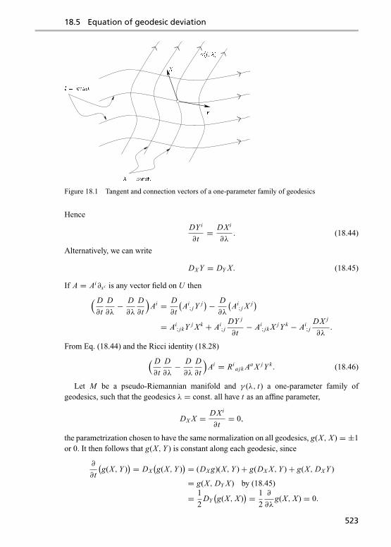
18.5 Equation of geodesic deviation

Figure 18.1 Tangent and connection vectors of a one-parameter family of geodesics

Hence

DY i

∂t= DXi

∂λ. (18.44)

Alternatively, we can write

DX Y = DY X. (18.45)

If A = Ai∂xi is any vector field on U then( D

∂t

D

∂λ− D

∂λ

D

∂t

)Ai = D

∂t

(Ai

; j Yj)− D

∂λ

(Ai

; j X j)

= Ai; jkY j Xk + Ai

; jDY j

∂t− Ai

; jk X j Y k − Ai; j

DX j

∂λ.

From Eq. (18.44) and the Ricci identity (18.28)( D

∂t

D

∂λ− D

∂λ

D

∂t

)Ai = Ri

ajk Aa X j Y k . (18.46)

Let M be a pseudo-Riemannian manifold and γ (λ, t) a one-parameter family ofgeodesics, such that the geodesics λ = const. all have t as an affine parameter,

DX X = DXi

∂t= 0,

the parametrization chosen to have the same normalization on all geodesics, g(X, X ) = ±1or 0. It then follows that g(X, Y ) is constant along each geodesic, since

∂

∂t

(g(X, Y )

) = DX

(g(X, Y )

) = (DX g)(X, Y )+ g(DX X, Y )+ g(X, DX Y )

= g(X, DY X ) by (18.45)

= 1

2DY

(g(X, X )

) = 1

2

∂

∂λg(X, X ) = 0.

523

Connections and curvature

Thus, if the tangent and connection vector are initially orthogonal on a geodesic of theone-parameter family, g(X p, Yp) = 0, then they are orthogonal all along the geodesic.

In Eq. (18.46) set Ai = Xi – this is possible since it is only necessary to have Ai definedin terms of t and λ (see Problem 18.14). With the help of Eq. (18.44) we have

D

∂t

DY i

∂t= Ri

ajk Xa X j Y k, (18.47)

known as the equation of geodesic deviation. For two geodesics, labelled by constants λand λ+ δλ, let δxi be the tangent vector

δxi ∂γi

∂λδλ = Y iδλ.

For vanishingly small �λ it is usual to think of δxi as an ‘infinitesimal separation vector’.Since δλ is constant along the geodesic we have

δ x i = Riajk Xa X jδxk (18.48)

where · ≡ D/∂t . Thus Rijkl measures the relative ‘acceleration’ between geodesics.

Problem

Problem 18.14 Equation (18.46) has strictly only been proved for a vector field A. Show that itholds equally for a vector field whose components Ai (t, λ) are only defined on the one-parameterfamily of curves γ .

18.6 The Riemann tensor and its symmetries

In a pseudo-Riemannian manifold (M, g) it is possible to lower the contravariant index ofthe curvature tensor to form a tensor R of type (0, 4),

R(W, Z , X, Y ) = R(ω, Z , X, Y ) where g(W, A) = 〈ω, A〉.This tensor will be referred to as the Riemann curvature tensor or simply the Riemanntensor. Setting W = ∂xi , Z = ∂x j , etc. then ω = gia dxa , whence

Ri jkl = gia Rajkl .

In line with the standard index lowering convention, we denote the components of R byRi jkl .

The following symmetries apply to the Riemann tensor:

Ri jkl = −Ri jlk, (18.49)

Ri jkl = −R jikl , (18.50)

Ri jkl + Rikl j + Ril jk = 0, (18.51)

Ri jkl = Rkli j . (18.52)

524

18.6 The Riemann tensor and its symmetries

Proof : Antisymmetry in the second pair of indices, Eq. (18.49), follows immediatelyfrom the definition of the curvature tensor (18.23) – it is not changed by the act of loweringthe first index. Similarly, (18.51) follows immediately from Eq. (18.26). The remainingsymmetries (18.50) and (18.52) may be proved by adopting geodesic coordinates at anygiven point p and using the expression (18.43) for the components of Ri

jkl :

Ri jkl(p) = 12

(gml, jk + g jk,ml − gmk, jl − g jl,mk

)∣∣p. (18.53)

A more ‘invariant’ proof of (18.50) is to apply the generalized Ricci identities, Problem18.9, to the metric tensor g,

0 = gi j ;kl − gi j ;lk = gaj Raikl + gia Ra

jkl = R jikl + Ri jkl .

The symmetry (18.52) is actually a consequence of the first three symmetries, as may beshown by performing cyclic permutations on all four indices of Eq. (18.51):

R jkli + R jlik + R jikl = 0, (18.51a)

Rkli j + Rki jl + Rkjli = 0, (18.51b)

Rli jk + Rl jki + Rlki j = 0. (18.51c)

The combination (18.51)− (18.51a)− (18.51b)+ (18.51c) gives, after several cancellationsusing the symmetries (18.49) and (18.50),

2Ri jkl − 2Rkli j = 0.

This is obviously equivalent to Eq. (18.52). �

Exercise: Prove from these symmetries that the cyclic symmetry also holds for any three indices; forexample

Ri jkl + R jkil + Rki jl = 0.

These symmetries permit us to count the number of independent components of theRiemann tensor. Since a skew symmetric tensor of type (0, 2) on an n-dimensional vec-tor space has 1

2 n(n − 1) independent components, a tensor of type (0, 4) subject to sym-metries (18.49) and (18.50) will have 1

4 n2(n − 1)2 independent components. For fixedi = 1, 2, . . . , n only unequal triples j �= k �= l need be considered in the symmetry (18.52),for if some pair are equal nothing new is added, by the cyclic identity: for example, ifk = l = 1 then Ri j11 + Ri11 j + Ri1 j1 = 0 merely reiterates the skew symmetry on the sec-ond pair of indices, Ri11 j = −Ri1 j1. For every triple j �= k �= l the total number of relationsgenerated by (18.52) that are independent of (18.49) and (18.50) is therefore the number ofsuch triples of numbers j �= k �= l in the range 1, . . . , n, namely n

(n3

) = n2(n − 1)(n − 2)/6.By the above proof we need not consider the symmetry (18.52), and the total number ofindependent components of the Riemann tensor is

N = n2(n − 1)2

4− n2(n − 1)(n − 2)

6

= n2(n2 − 1)

12. (18.54)

525

Connections and curvature

For low dimensions the number of independent components of the Riemann tensor is

n = 1: N = 0,

n = 2: N = 1,

n = 3: N = 6,

n = 4: N = 20.

A tensor of great interest in general relativity is the Ricci tensor, defined by

Ric = C12 R.

It is common to write the components of Ric(∂xi , ∂x j ) in any chart (U ; xi ) as Ri j :

Ri j = Raiaj = gab Raibj . (18.55)

This tensor is symmetric since, by symmetry (18.52),

Ri j = gab Raibj = gab Rbjai = Rajai = R ji .

Contracting again gives the quantity known as the Ricci scalar,

R = Rii = gi j Ri j . (18.56)

Bianchi identities

For a torsion-free connection we have, on setting T pkm = 0 in Eq. (18.32) of Problem 18.10,

the second Bianchi identity

Rijkl;m + Ri

jlm;k + Rijmk;l = 0. (18.57)

These are often referred to simply as the Bianchi identities. An alternative demonstrationis to use normal coordinates at any point p ∈ M , such that �i

jk(p) = 0. Making use of Eqs.(18.14) and (18.25) we have

Rijkl;m(p) = Ri

jkl,m(p)+ (�iam Ra

jkl − �ajm Ri

akl − �akm Ri

jal − �alm Ri

jka

)(p)

= Rijkl,m(p)

= �ijl,km(p)− �i

jk,lm(p)+ �ajl,m�

iak(p)+ �a

jl(p)�iak,m − �a

jk,m�ial(p)

− �ajk(p)�i

al,m

= �ijl,km(p)− �i

jk,lm(p).

If we substitute this expression in the left-hand side of (18.57) and use �ijk = �i

k j , all termscancel out.

Contracting Eq. (18.57) over i and m gives

Rijkl;i − R jl;k + R jk;l = 0. (18.58)

Contracting Eq. (18.58) again by multiplying through by g jl and using Eq. (18.41) we find

Rik;i − R;k + R j

k; j = 0,

526

18.7 Cartan formalism

or equivalently, the contracted Bianchi identities

R jk; j − 1

2 R,k = 0. (18.59)

A useful way of writing (18.59) is

G jk; j = 0, (18.60)

where Gij is the Einstein tensor,

Gij = Ri

j − 12 Rδi

j . (18.61)

This tensor is symmetric when its indices are lowered,

Gi j = giaGaj = Ri j − 1

2 Rgi j = G ji . (18.62)

18.7 Cartan formalism

Cartan’s approach to curvature is expressed entirely in terms of differential forms. Letei (i = 1, . . . , n) be a local basis of vector fields, spanning T (U ) over an open set U ⊆ Mand {εi } the dual basis of T ∗(U ), such that 〈ei , ε

j 〉 = δ ji . For example, in a coordinate

chart (U ; xi ) we may set ei = ∂xi and ε j = dx j , but such a coordinate system will existfor an arbitrary basis {ei } if and only if [ei , e j ] = 0 for all i, j = 1, . . . , n. We define theconnection 1-forms ωi

j : T (U ) → F(U ) by

DX e j = ωij (X )ei . (18.63)

These maps are differential 1-forms on U since they are clearly F-linear,

DX+ f Y e j = DX e j + f DY e j =⇒ ωij (X + f Y ) = ωi

j (X )+ f ωij (Y ).

If τ : T (U )× T (U ) → T (U ) is the torsion operator defined in Eq. (18.19), set

τ (X, Y ) = τ i (X, Y )ei .

The maps τ i : T (U )× T (U ) → F(U ) are F-linear in both arguments by the F-linearityof τ , and are antisymmetric τ i (X, Y ) = −τ i (Y, X ). They are therefore differential 2-formson U , known as the torsion 2-forms.

Exercise: Show that τ i = T ijkε

j ∧ εk where T ijk = 〈τ (e j , ek), εi 〉.

From the identity Z = 〈εi , Z〉ei for any vector field Z on U , we have

τ (X, Y ) = DX (〈εi , Y 〉ei )− DY (〈εi , X〉ei )− 〈εi , [X, Y ]〉ei

= X (〈εi , Y 〉)ei + 〈εi , Y 〉ωki (X )ek − Y (〈εi , X〉)ei − 〈εi , X〉ωk

i (X )ek

− 〈εi , [X, Y ]〉ei

= 2 dεi (X, Y )ei + 2ωki ∧ εi (X, Y )ek,

using the Cartan identity (16.14). Thus

τ i (X, Y )ei = 2(dεi (X, Y )+ 2ωi

k ∧ εk(X, Y ))ei ,

527

Connections and curvature

and by F-linear independence of the vector fields ei we have Cartan’s first structuralequation

dεi = −ωik ∧ εk + 1

2τi . (18.64)

Define the curvature 2-forms ρij by

ρX,Y e j = ρij (X, Y )ei , (18.65)

where ρX,Y : T (M) → T (M) is the curvature operator in Eq. (18.22).

Exercise: Show that the ρij are differential 2-forms on U ; namely, they are F-linear with respect to

X and Y and ρij (X, Y ) = −ρi

j (Y, X ).

Changing the dummy suffix on the right-hand side of Eq. (18.65) from i to k and applying〈εi , .〉 to both sides of the equation we have, with the help of Eq. (18.23),

ρij (X, Y ) = 〈εi , ρX,Y e j 〉

= R(εi , e j , X, Y )

= Rijkl XkY l where Ri

jkl = R(εi , e j , ek, el)

= 12 Ri

jkl(εk ⊗ εl − εl ⊗ εk)(X, Y ).

Hence

ρij = Ri

jklεk ∧ εl . (18.66)

A similar analysis to that for the torsion operator results in

ρX,Y e j = DX DY e j − DY DX e j − D[X,Y ]e j

= DX

(〈ωij , Y 〉ei

)− DY

(〈ωij , X〉ei

)− 〈ωij , [X, Y ]〉ei

= 2[dωi

j (X, Y )+ ωik ∧ ωk

j (X, Y )]ei ,

and Cartan’s second structural equation

dωij = −ωi

k ∧ ωkj + 1

2ρij . (18.67)

Example 18.3 With respect to a coordinate basis ei = ∂xi , the Cartan structural equationsreduce to formulae found earlier in this chapter. For any vector field X = Xk∂xk ,

DX∂x j = Xk Dk∂x j = Xk�ijk∂xi .

Hence, by Eq. (18.63), we have ωij (X ) = Xk�i

jk , so that

ωij = �i

jk dxk . (18.68)

Thus the components of the connection 1-forms with respect to a coordinate basis areprecisely the components of the connection.

Setting εi = dxi in Cartan’s first structural equation (18.64), we have

dεi = d2xi = 0 = −ωij ∧ dx j + 1

2τi .

528

18.7 Cartan formalism

Hence τ i = 2�ijk dxk ∧ dx j , and it follows that the components of the torsion 2-forms are

identical with those of the torsion tensor T in Eq. (18.21),

τ i = T ijk dx j ∧ dxk where T i

jk = �ik j − �i

jk . (18.69)

Finally, Cartan’s second structural equation (18.67) reduces in a coordinate basis to

d�ijk ∧ dxk = −�i

kl dxl ∧ �kjm dxm + 1

2ρij ,

whence, on using the decomposition (18.66),

Rijkl dxk ∧ dxl = 2�i

jk,l dxl ∧ dxk + 2�iml�

mjk dxl ∧ dxk .

We thus find, in agreement with Eq. (18.25),

Rijkl = �i

jl,k − �ijk,l + �m

jl�imk − �m

jk�iml = −Ri

jlk .

The big advantage of Cartan’s structural equations over these various coordinate expressionsis that they give expressions for torsion and curvature for arbitrary vector field bases.

Bianchi identities

Taking the exterior derivative of (18.64) gives, with the help of (18.67),

d2εi = 0 = −dωik ∧ εk + ωi

k ∧ dεk + 12 dτ i

= ωij ∧ ω j

k ∧ εk − 12ρ

ik ∧ εk − ωi

k ∧ ωkj ∧ ε j + 1

2ωik ∧ τ k + 1

2 dτ i

= 12

(−ρik ∧ εk + ωi

k ∧ τ k + dτ i).

Hence, we obtain the first Bianchi identity

dτ i = ρik ∧ εk − ωi

k ∧ τ k . (18.70)

Its relation to the earlier identity (18.24) is left as an exercise (see Problem 18.15).Similarly

d2ωij = 0 = −dωi

k ∧ ωkj + ωi

k ∧ dωkj + 1

2 dρij

= 12

(−ρik ∧ ωk

j + ωik ∧ ρk

j + dρij

),

resulting in the second Bianchi identity

dρij = ρi

k ∧ ωkj − ωi

k ∧ ρkj . (18.71)

Pseudo-Riemannian spaces in Cartan formalism

In a pseudo-Riemannian manifold with metric tensor g, set gi j = g(ei , e j ). Since gi j is ascalar field for each i, j = 1, . . . , n and DX g = 0, we have

〈X, dgi j 〉 = X (gi j) = DX

(g(ei , e j )

)= g(DX ei , e j )+ g(ei , DX e j )

= g(ωk

i (X )ek, ej)+ g

(ei , ω

kj (X )ek

)= gkjω

ki (X )+ gikω

kj (X )

= 〈X, ω j i 〉 + 〈X, ωi j 〉

529

Connections and curvature

where

ωi j = gkiωkj .

As X is an arbitrary vector field,

dgi j = ωi j + ω j i . (18.72)

For an orthonormal basis ei , such that gi j = ηi j , we have dgi j = 0 and

ωi j = −ω j i . (18.73)

In particular, all diagonals vanish, gii = 0 for i = 1, . . . , n.Lowering the first index on the curvature 2-forms ρi j = gikρ

kj , we have from the second

Cartan structural equation (18.67),

ρi j = 2(dωi j + ωik ∧ ωk

j

)= 2(−dω j i + ωk

j ∧ ωki

)= 2(−dω j i − ω jk ∧ ωk

i

),

whence

ρi j = −ρ j i . (18.74)

Exercise: Show that (18.74) is equivalent to the symmetry Ri jkl = −R jikl .

Example 18.4 The 3-sphere of radius a is the submanifold of R4,

S3(a) = {(x, y, z,w) | x2 + y2 + z2 + w2 = a2} ⊂ R4.

Spherical polar coordinates χ, θ, φ are defined by

x = a sinχ sin θ cosφ

y = a sinχ sin θ sinφ

z = a sinχ cos θ

w = a cosχ

where 0 < χ, θ < π and 0 < φ < 2π . These coordinates cover all of S3(a) apart from thepoints y = 0, x ≥ 0. The Euclidean metric on R4

ds2 = dx2 + dy2 + dz2 + dw2

induces a metric on S3(a) as for the 2-sphere in Example 18.1:

ds2 = a2[dχ2 + sin2 χ (dθ2 + sin2 θ dφ2)

].

An orthonormal frame is

e1 = 1

a

∂

∂χ, e2 = 1

a sinχ

∂

∂θ, e3 = 1

a sinχ sin θ

∂

∂φ

ε1 = a dχ, ε2 = a sinχ dθ, ε3 = a sinχ sin θ dφ

530

18.7 Cartan formalism

where

gi j = g(ei , e j ) = δi j , g = ε1 ⊗ ε1 + ε2 ⊗ ε2 + ε3 ⊗ ε3.

Since the metric connection is torsion-free, τ i = 0, the first structural equation reads

dεi = −ωik ∧ εk = −ωik ∧ εk

setting

ωi j = Ai jkεk

where Ai jk = −A jik . By interchanging dummy suffixes j and k we may also write

dεi = −Aik jεj ∧ εk = Aik jε

k ∧ ε j = Ai jkεj ∧ εk .

For i = 1, using A11k = 0,

dε1 = ad2χ = 0 = A121ε2 ∧ ε1 + A131ε

3 ∧ ε1 + (A123 − A132)ε2 ∧ ε3,

whence

A121 = A131 = 0, A123 = A132.

For i = 2,

dε2 = a cosχdχ ∧ dθ = a−1 cotχε1 ∧ ε2

= A212ε1 ∧ ε2 + A232ε

3 ∧ ε2 + (A213 − A231)ε1 ∧ ε3,

which implies

A212 = a−1 cotχ, A213 = A231, A232 = 0.

Similarly the i = 3 equation gives

A312 = A321, A313 = a−1 cotχ, A323 = a−1 cot θ

sinχ.

All coefficients having all three indices different, such as A123, must vanish since

A123 = A132 = −A312 = −A321 = A231 = A213 = −A123 =⇒ A123 = 0.

There is enough information now to write out the connection 1-forms:

ω12 = −ω21 = −a−1 cotχε2,

ω13 = −ω31 = −a−1 cotχε3,

ω23 = −ω32 = −a−1 cot θ

sinχε3.

The second structural relations (18.67) can now be used to calculate the curvature 2-forms:

ρ12 = 2(dω12 + ω1k ∧ ωk

2

)= 2(a−1cosec2 χdχ ∧ ε2 − a−1 cotχdε2 + ω13 ∧ ω32

)= 2a−2

(cosec2 χε1 ∧ ε2 − cot2 χε1 ∧ ε2

)= 2a−2ε1 ∧ ε2,

531

Connections and curvature

and similarly

ρ13 = 2(dω13 + ω12 ∧ ω23

) = 2a−2ε1 ∧ ε3,

ρ23 = 2(dω23 + ω21 ∧ ω13

) = 2a−2ε2 ∧ ε3.

The components of the Riemann curvature tensor can be read off using Eq. (18.66):

R1212 = R1313 = R2323 = a−2,

and all other components of the Riemann tensor are simply related to these components bysymmetries; for example, R2121 = −R1221 = a−2, R1223 = 0, etc. It is straightforward toverify the relation

Ri jkl = 1

a2(gik g jl − gil g jk).

For any Riemannian space (M, g) the sectional curvature of the vector 2-space spannedby a pair of tangent vectors X and Y at any point p is defined to be

K (X, Y ) = R(X, Y, X, Y )

A(X, Y )

where A(X, Y ) is the ‘area’ of the parallelogram spanned by X and Y ,

A(X, Y ) = g(X, Y )g(X, Y )− g(X, X )g(Y, Y ).

For the 3-sphere

K (X, Y ) = 1

a2

Xi Y i XkY k − Xi Xi YkY k

Xi Y i XkY k − Xi Xi YkY k= 1

a2

independent of the point p ∈ S3(a) and the choice of tangent vectors X, Y . For this reasonthe 3-sphere is said to be a space of constant curvature.

Locally flat spaces

A manifold M with affine connection is said to be locally flat if for every point p ∈ Mthere is a chart (U ; xi ) such that all components of the connection vanish throughout U .This implies of course that both torsion tensor and curvature tensor vanish throughout U ,but more interesting is that these conditions are both necessary and sufficient. This result ismost easily proved in Cartan’s formalism, and requires the transformation of the connection1-forms under a change of basis

ε′i = Aijε

j where Aij = Ai

j (x1, . . . , xn).

Evaluating dε′i , using Eq. (18.64), gives

dε′i = dAij ∧ ε j + Ai

j dε j = −ω′ik ∧ ε′k + 12τ′i

where τ ′i = Aijτ

j and

Akjω′i

k = dAij − Ai

kωkj . (18.75)

532

18.7 Cartan formalism

Exercise: Show from this equation and Eq. (18.67) that if a transformation exists such that ω′ik = 0then the curvature 2-forms vanish, ρk

j = 0.

Theorem 18.1 A manifold with symmetric connection is locally flat everywhere if andonly if the curvature 2-forms vanish, ρk

j = 0.

Proof : The only if part follows from the above comments. For the converse, we supposeτ i = ρi

j = 0 everywhere. If (U ; xi ) is any chart on M , let N = U × Rn2and denote coor-

dinates on Rn2by z j

k . Using the second structural formula (18.67) with ρij = 0, the 1-forms

αij = dzi

j − zikω

kj on N satisfy

dαij = −dzi

k ∧ ωkj − zi

k dωkj

= −(αik + zi

m dωmk

) ∧ ωkj + zi

kωkm ∧ ωm

j

= ωkj ∧ αi

k . (18.76)

By the Frobenius theorem 16.4, dαij = 0 is an integrable system on N , and has a local

integral submanifold through any point xi0, A j

0k where det[A j0k] �= 0, that may be assumed

to be of the form

z ji = A j

i (x1, . . . , xn) where A j

i (x10 , . . . , xn

0 ) = A j0i .

We may assume that det[A jk ] is non-singular in a neighbourhood of x0. Hence

αij = 0 =⇒ dAi

j − Aikω

kj = 0

and substituting in Eq. (18.75) results in

ω′ik = 0 if ε′i = Aijε

j .

Finally, the structural equation (18.64) gives dε′i = 0, and the Poincare lemma 17.5 impliesthat there exist local coordinates yi such that ε′i = dyi . �

In the case of a pseudo-Riemannian space, locally flat coordinates such that �ijk = 0

imply that gi j,k = 0 by Eq. (18.37). Hence gi j = const. throughout the coordinate region,and a linear transformation can be used to diagonalize the metric into standard diagonalform gi j = ηi j with ±1 along the diagonal.

Problems

Problem 18.15 Let ei = ∂xi be a coordinate basis.

(a) Show that the first Bianchi identity reads

Ri[ jkl] = T i

[ jk;l] − T a[ jk T i

l]a,

and reduces to the cyclic identity (18.26) in the case of a torsion-free connection.(b) Show that the second Bianchi identity becomes

Rij[kl;m] = Ri

ja[k T aml],

which is identical with Eq. (18.32) of Problem 18.10.

533

Connections and curvature

Problem 18.16 In a Riemannian manifold (M, g) show that the sectional curvature K (X, Y ) at apoint p, defined in Example 18.4, is independent of the choice of basis of the 2-space; i.e., K (X ′, Y ′) =K (X, Y ) if X ′ = aX + bY , Y ′ = cX + dY where ad − bc �= 0.

The space is said to be isotropic at p ∈ M if K (X, Y ) is independent of the choice of tangentvectors X and Y at p. If the space is isotropic at each point p show that

Ri jkl = f (gik g jl − gil g jk)

where f is a scalar field on M . If the dimension of the manifold is greater than 2, show Schur’s theorem:a Riemannian manifold that is everywhere isotropic is a space of constant curvature, f = const. [Hint :Use the contracted Bianchi identity (18.59).]

Problem 18.17 Show that a space is locally flat if and only if there exists a local basis of vectorfields {ei } that are absolutely parallel, Dei = 0.

Problem 18.18 Let (M, ϕ) be a surface of revolution defined as a submanifold of E3 of the form

x = g(u) cos θ, y = g(u) sin θ, z = h(u).

Show that the induced metric (see Example 18.1) is

ds2 = (g′(u)2 + h′(u)2)

du2 + g2(u) dθ2.

Picking the parameter u such that g′(u)2 + h′(u)2 = 1 (interpret this choice!), and setting the basis1-forms to be ε1 = du, ε2 = g dθ , calculate the connection 1-forms ωi

j , the curvature 1-forms ρij ,

and the curvature tensor component R1212.

Problem 18.19 For the ellipsoid

x2

a2+ y2

b2+ z2

c2= 1

show that the sectional curvature is given by

K =( x2bc

a3+ y2ac

b3+ z2ab

c3

)−2.

18.8 General relativity

The principle of equivalence

The Newtonian gravitational force on a particle of mass m is F = −m∇φ where the scalarpotential φ satisfies Poisson’s equation

∇2φ = 4πGρ. (18.77)

Here G = 6.672× 10−8 g−1 cm3 s−2 is Newton’s gravitational constant and ρ is the densityof matter present. While it is in principle possible to generalize this theory by postulatinga relativistically invariant equation such as

�φ = ∇2φ − ∂2

∂t2φ = 4πGρ,

534

18.8 General relativity

there are a number of problems with this theory, not least of which is that it does not accordwith observations.

Key to the formulation of a correct theory is the principle of equivalence that, in itssimplest version, states that all particles fall with equal acceleration in a gravitational field,a fact first attributed to Galileo in an improbable tale concerning the leaning tower of Pisa.While the derivation is by simple cancellation of m from both sides of the Newtonianequation of motion

mx = mg,

the masses appearing on the two sides of the equation could conceivably be different. Onthe left we really have inertial mass, mi , which measures the particle’s resistance to anyforce, while on the right the mass should be identified as gravitational mass, measuringthe particle’s response to gravitational fields – its ‘gravitational charge’ so to speak. Theprinciple of equivalence can be expressed as saying that the ratio of inertial to gravitationalmass will be the same for all bodies irrespective of the material from which they arecomposed. This was tested to one part in 108 for a vast variety of materials in 1890 byEotvos using a torsion balance, and repeated in the 1960s to one part in 1011 by Dicke usinga solar balancing mechanism (see C. M. Will’s article in [10]).

The principle of equivalence essentially says that it is impossible to distinguish inertialforces such as centrifugal or Coriolis forces from gravitational ones. A nice example of theequivalence of such forces is the Einstein elevator. An observer in an elevator at rest seesobjects fall to the ground with acceleration g. However if the elevator is set in free fall,objects around the observer will no longer appear to be subject to forces, much as if hewere in an inertial frame in outer space. It has in effect been possible to transform away thegravitational field by going to a freely falling laboratory. Conversely as all bodies ‘fall’ tothe floor in an accelerated rocket with the same acceleration, an observer will experiencean ‘apparent’ gravitational field.

The effect of a non-inertial frame in special relativity should be essentially indistinguish-able from the effects of gravity. The metric interval of Minkowski space (see Chapter 9) ina general coordinate system x ′μ

′ = x ′μ′(x1, x2, x3, x4), where xν are inertial coordinates,

becomes

ds2 = gμν dxμ dxν = g′μ′ν ′ dx ′μ′dx ′ν

′,

where

g′μ′ν ′ = gμν∂xμ

∂x ′μ′∂xν

∂x ′ν ′.

Expressed in general coordinates, the (geodesic) equations of motion of an inertial particle,d2xμ/ds2 = 0, are

d2x ′μ′

ds2+ �′μ′α′β ′

dx ′α′

ds

dx ′β′

ds= 0,

where

�′μ′α′β ′ = −

∂2x ′μ′

∂xμ∂xν∂xμ

∂x ′α′∂xν

∂x ′β ′.

535

Connections and curvature

Figure 18.2 Tidal effects in a freely falling laboratory

The principle of equivalence is a purely local idea, and only applies to vanishingly smalllaboratories. A real gravitational field such as that due to the Earth cannot be totally trans-formed away in general. For example, if the freely falling Einstein elevator has significantsize compared to the scale on which there is variation in the Earth’s gravitational field,then particles at different positions in the lift will undergo different accelerations. Particlesnear the floor of the elevator will have larger accelerations than particles released from theceiling, while particles released from the sides of the elevator will have a small horizontalacceleration relative to the central observer because the direction to the centre of the Earthis not everywhere parallel. These mutual accelerations or tidal forces can be measured inprinciple by connecting pairs of freely falling particles with springs (see Fig. 18.2).

Postulates of general relativity

The basic proposition of general relativity (Einstein, 1916) is the following: the world is afour-dimensional Minkowskian manifold (pseudo-Riemannian of index +2) called space-time. Its points are called events. The world-line, or space-time history of a materialparticle, is a parametrized curve γ : R → M whose tangent γ is everywhere timelike. Theproper time, or time as measured by a clock carried by the particle between parametervalues λ = λ1 and λ2, is given by

τ = 1

c

∫ λ2

λ1

√−g(γ , γ ) dλ = 1

c

∫ λ2

λ1

√−gμν

dxμ

dλ

dxν

dλdλ = 1

c

∫ s2

s1

ds. (18.78)

A test particle is a particle of very small mass compared to the major masses in its neigh-bourhood and ‘freely falling’ in the sense that it is subject to no external forces. Theworld-line of a test particle is assumed to be a timelike geodesic. The world-line of a photonof small energy is a null geodesic. Both satisfy equations

d2xμ

ds2+ �μνρ

dxν

ds

dxρ

ds= 0,

536

18.8 General relativity

where the Christoffel symbols �μνρ are given by Eq. (18.40) with Greek indices subsituted.The affine parameter s is determined by

gμνdxμ

ds

dxν

ds={−1 for test particles,

0 for photons.

An introduction to the theory of general relativity, together with many of its developments,can be found in [9, 11–16].

The principle of equivalence has a natural place in this postulate, since all particles havethe same geodesic motion independent of their mass. Also, at each event p, geodesic normalcoordinates may be found such that components of the metric tensor g = gμν dxμ ⊗ dxν

have the Minkowski values gμν(p) = ημν and the Christoffel symbols vanish,�μνρ(p) = 0. Insuch coordinates the space-time appears locally to be Minkowski space, and gravitationalforces have been locally transformed away since any geodesic at p reduces to a ‘localrectilinear motion’ d2xμ/ds2 = 0. When it is possible to find coordinates that transform themetric to constant values on an entire chart, the metric is locally flat and all gravitationalfields are ‘fictitious’ since they arise entirely from non-inertial effects. By Theorem 18.1such coordinate transformations are possible if and only if the curvature tensor vanishes.Hence it is natural to identify the ‘real’ gravitational field with the curvature tensor Rμνρσ .

The equations determining the gravitational field are Einstein’s field equations

Gμν = Rμν − 12 Rgμν = κTμν, (18.79)

where Gμν is the Einstein tensor defined above in Eqs. (18.61) and (18.62),

Rμν = Rαμαν and R = Rαα = gμνRμν,

and Tμν is the energy–stress tensor of all the matter fields present. The constant κ is knownas Einstein’s gravitational constant; we shall relate it to Newton’s gravitational constantdirectly. These equations have the property that for weak fields, gμν ≈ ημν , they reduceto the Poisson equation when appropriate identifications are made (see the discussion ofthe weak field approximation below), and by the contracted Bianchi identity (18.60) theyguarantee a ‘covariant’ version of the conservation identities

T μν;ν ≡ T μν,ν + �μανT αν + �νανT μα = 0.

Measurement of the curvature tensor

The equation of geodesic deviation (18.47) can be used to give a physical interpretation ofthe curvature tensor. Consider a one-parameter family of timelike geodesics γ (s, λ) withtangent vectors U = Uμ∂xμ when expressed in a coordinate chart (A; xμ), where

Uμ(s) = ∂xμ

∂s

∣∣∣λ=0, UμUμ = −1,

DUμ

∂s= 0.

Suppose the connection vector Y = Yμ∂xμ , where Yμ = ∂xμ/∂λ, is initially orthogonal toU at s = s0,

YμUμ∣∣s=s0

= g(U, Y )(s0) = 0.

537

Connections and curvature

Figure 18.3 Physical measurement of curvature tensor

We then have g(U, Y ) = 0 for all s, since g(U, Y ) is constant along each geodesic (seeSection 18.5). Thus if e1, e2, e3 are three mutually orthogonal spacelike vectors at s = s0

on the central geodesic λ = 0 that are orthogonal to U , and they are parallel propagatedalong this geodesic, Dei/∂s = 0, then they remain orthogonal to each other and U alongthis geodesic,

g(ei , e j ) = δi j , g(ei , u) = 0.

In summary, if we set e4 = U then the four vectors e1, . . . , e4 are an orthonormal tetrad ofvectors along λ = λ0,

g(eμ, eν) = ημν.

The situation is depicted in Fig. 18.3. Let λ = λ0 + δλ be any neighbouring geodesic fromthe family, then since we are assuming δxμ is orthogonal to Uμ, the equation of geodesicdeviation in the form (18.48) can be written

D2δxμ

ds2= δλD2Yμ

ds2= RμαρνU

αUρδxν . (18.80)

Expanding δxμ in terms of the basis eμ we have, adopting a cartesian tensor summationconvention,

δxμ = η j eμ

j ≡3∑

j=1

η j eμ

j ,

538

18.8 General relativity

where η j = η j (s), so that

Dδxμ

ds= dη j

dseμj + η j

eμids= dη j

dseμj ,

D2δxμ

ds2= d2η j

ds2eμj +

dη j

ds

eμids= d2η j

ds2eμj .

Substituting (18.80) results in

d2ηi

ds2= eiμ

D2δxμ

ds2= Rμαρνeiμeα4 eρ4 eνjη j ,

which reads in any local coordinates at any point on λ = λ0 such that eμα = δμα ,

d2ηi

ds2= −Ri4 j4η j . (18.81)

Thus Ri4 j4 ≡ Rμαρνeμ

i eα4 eρj eν4 measures the relative accelerations between neighbouringfreely falling particles in the gravitational field. Essentially these are what are termed tidalforces in Newtonian physics, and could be measured by the strain on a spring connectingthe two particles (see Fig. 18.2 and [17]).

The linearized approximation

Consider a one-parameter family of Minkowskian metrics having components gμν =gμν(xα, ε) such that ε = 0 reduces to flat Minkowski space, gμν(0) = ημν . Such a fam-ily is known as a linearized approximation of general relativity. If we set

hμν = ∂gμν∂ε

∣∣∣ε=0

(18.82)

then for |ε| ' 1 we have ‘weak gravitational fields’ in the sense that the metric is onlyslightly different from Minkowski space,

gμν ≈ ημν + εhμν.From gμρgρν = δμμ it follows by differentiating with respect to ε at ε = 0 that

∂gμρ

∂ε

∣∣∣ε=0ηρν + ημρhρν = 0,

whence

∂gμν

∂ε

∣∣∣ε=0

= −hμν ≡ −ημαηνβ. (18.83)

In this equation and throughout the present discussion indices are raised and lowered withrespect to the Minkowski metric, ημν, ημν . For ε ' 1 we evidently have gμν ≈ ημν − εhμν .

Assuming that partial derivatives with respect to xμ and ε commute, it is straightforwardto compute the linearization of the Christoffel symbols,

�μνρ ≡∂

∂ε�μνρ

∣∣∣ε=0

= − 12 hμα(ηαν,ρ + ηαρ,ν − ηνρ,α)+ 1

2ημα(hαν,ρ + hαρ,ν − hνρ,α)

= 12ημα(hαν,ρ + hαρ,ν − hνρ,α)

539

Connections and curvature

and

�μνρ,σ = 12ημα(hαν,ρσ + hαρ,νσ − hνρ,ασ ).

Thus, from the component expansion of the curvature tensor (18.25), we have

rμνρσ ≡ ∂

∂εRμνρσ

∣∣∣ε=0

= �μνσ,ρ − γ μνρ,σsince

∂

∂ε�ανσ�

μαρ

∣∣∣ε=0

= �ανσ�μαρ∣∣∣ε=0

+ �ανσ∣∣∣ε=0�μαρ = 0, etc.

since �ανσ∣∣ε=0

= 0. Thus

rμνρσ = 12ημα(hαν,σρ + hασ,νρ − hνσ,αρ − hαν,ρσ − hαρ,νσ + hνρ,ασ

)and for small values of the parameter ε the Riemann curvature tensor is

Rμνρσ ≈ εrμνρσ = ε

2

(hμσ,νρ + hνρ,μσ − hνσ,μρ − hμρ,νσ

). (18.84)

It is interesting to compare this equation with the expression in geodesic normal coordinates,Eq. (18.43).

The Newtonian tidal equation is derived by considering the motion of two neighbouringparticles

xi = −φ,i and xi + ηi = −φ,i (x+ η).

Since φ,i (x+ η) = φ,i (x)+ φi j (x)η j we have

ηi = −φ,i j (x)η j .

Compare with the equation of geodesic deviation (18.81) with s replaced by ct , which isapproximately correct for velocities |x| ' c,

ηi = −c2 Ri4 j4η j ,

and we should have, by Eq. (18.84),

Ri4 j4 = ε

2

(hi4,4 j + h4 j,i4 − hi j,44 − h44,i j

) = φ,i j

c2.

This equation can only hold in a general way if

εh44 ≈ −2φ

c2and hi4,4 j , hi j,44 ' h44,i j ,

and the Newtonian approximation implies that

g44 ≈ −1+ εh44 ≈ −1− 2φ

c2(φ ' c2). (18.85)

Note that the Newtonian potential φ has the dimensions of a velocity square – the weak fieldslow motion approximation of general relativity arises when this velocity is small comparedto the velocity of light c.

540

18.8 General relativity

Multiplying Eq. (18.79) through by gμν we find

R − 2R = −R = κT where T = T μμ = gμνTμν,

and Einstein’s field equations can be written in the ‘Ricci tensor form’

Rμν = κ(Tμν − 1

2 T gμν). (18.86)

Hence

R44 = Ri4i4 ≈ 1

c2∇2φ = κ(T44 + 1

2 T).

If we assume a perfect fluid, Example 9.4, for low velocities compared to c we have

Tμν =(ρ + P

c2

)VμVν + Pgμν where Vμ ≈ (v1, v2, v3, −c),

so that

T = −c2(ρ + P

c2

)+ 4P = −ρc2 + 3P ≈ −ρc2,

and

T44 ≈(ρ + P

c2

)c2 + P

(−1− φ

c2P)≈ ρc2.

Substituting in the Ricci form of Einstein’s equations we find

1

c2∇2φ ≈ 1

2κρc2,

which is in agreement with the Newtonian equation (18.77) provided Einstein’s gravitationalconstant has the form

κ = 8πG

c4. (18.87)

Exercise: Show that the contracted Bianchi identity (18.60) implies that in geodesic coordinates atany point representing a local freely falling frame, the conservation identities (9.56) hold, T μ

ν,μ = 0.

Exercise: Show that if we had assumed field equations of the form Rμν = λTμν , there would haveresulted the physically unsavoury result T = const.

Consider now the effect of a one-parameter family of coordinate transformations xμ =xμ(yα, ε) on a linearized approximation gμν = gμν(ε) and set

ξμ = ∂xμ

∂ε

∣∣∣ε=0.

The transformation of components of the metric tensor results in

gμν(x, ε) → g′μν(y, ε) = gαβ(x(y, ε), ε)∂xα

∂yμ∂xβ

∂yν

and taking ∂/∂ε at ε = 0 gives

h′μν(y) = hμν(y)+ ξμ,ν + ξν,μ. (18.88)

541

Connections and curvature

These may be thought of as ‘gauge transformations’ for the weak fields hμν , comparable withthe gauge transformations (9.49), A′μ = Aμ + ψ,μ, which leave the electromagnetic fieldFμν unchanged. In the present case, it is straightforward to verify that the transformations(18.88) leave the linearized Riemann tensor (18.84), or real gravitational field, invariant.

We define the quantities ϕμν by

ϕμν = hμν − hημν where h = hαα = ηαβhαβ.

The transformation of ϕνμ,ν under a gauge transformation is then

ϕ′νμ,ν = ϕνμ,ν + ξμ,νν = ϕνμ,ν +�ξμ,

where indices are raised and lowered with the Minkowski metric, ημν , ημν . Just as done forthe Lorentz gauge (9.51), it is possible (after dropping primes) to find ξ such that

ϕνμ,ν = 0. (18.89)

Such a gauge is commonly known as a harmonic gauge. There are still available gaugefreedoms ξμ subject to solutions of the wave equation �ξμ = 0.

A computation of the linearized Ricci tensor rμν = ηρσ rρμσν using Eq. (18.84) gives

rμν = 12

(−�hμν + ϕρν,ρμ + ϕρμ,ρν) = − 1

2�hμν

in a harmonic gauge. The Einstein tensor is thus Gμν ≈ −(ε/2)�ϕμν , and the linearizedEinstein equation is

ε�ϕμν = −κTμν = −16πG

c4Tμν,

having solution in terms of retarded Green’s functions (12.23)

εϕμν(x, t) = −4G

c4

∫∫∫[Tμν(x′, t ′)]ret

|x− x′| d3x ′.

In vacuo, Tμν , Einstein’s field equations can be written Rμν = 0, so that in the linearizedapproximation we have �hμν = 0; these solutions are known as gravitational waves (seeProblem 18.20 for further details).

The Schwarzschild solution

The vacuum Einstein field equations, Rμν = 0 are a non-linear set of 10 second-orderequations for 10 unknowns gμν that can only be solved in a handful of special cases. Themost important is that of spherical symmetry which, as we shall see in the next chapter,implies that the metric has the form in a set of coordinates x1 = r , x2 = θ , x3 = φ, x4 = ct ,

ds2 = eλ dr2 + r2(dθ2 + sin2 θ dφ2)− eνc2 dt2 (18.90)

where θ andφ take the normal ranges of polar coordinates (r does not necessarily range from0 to∞), and λ and ν are functions of r and t . We will assume for simplicity that the solutionsare static so that they are functions of the radial coordinate r alone, λ = λ(r ), ν = ν(r ). Aremarkable theorem of Birkhoff assures us that all spherically symmetric vacuum solutions

542

18.8 General relativity

are in fact static for an appropriate choice of the coordinate t ; a proof may be found inSynge [15].

We will perform calculations using Cartan’s formalism. Many books prefer to calculateChristoffel symbols and do all computations in the coordinate system of Eq. (18.90). Lete1, . . . , e4 be the orthonormal basis

e1 = e−12 λ∂r , e2 = 1

r∂θ , e3 = 1

r sin θ∂φ, e4 = e−

12 νc−1∂t

such that

gμν = g(eμ, eν) = η = diag(1, 1, 1,−1)

and let ε1, . . . , ε4 be the dual basis

ε1 = e12 λ dr, ε2 = r dθ, ε3 = r sin θ dφ, ε4 = e

12 νc dt = e

12 ν dx4.

We will write Cartan’s structural relations in terms of the ‘lowered’ connection forms ωμνsince, by Eq. (18.73), we have ωμν = −ωνμ. Thus (18.64) can be written

dεμ = −ωμν ∧ εν = −ημρωρνεν

and setting successively μ = 1, 2, 3, 4 we have, writing derivatives with respect to r by aprime ′,

dε1 = 12 e

12 λλ′ dr ∧ dr = 0 = −ω12 ∧ ε2 − ω13 ∧ ε3 − ω14 ∧ ε4, (18.91)

dε2 = r−1e−12 λε1 ∧ ε2 = ω12 ∧ ε1 − ω23 ∧ ε3 − ω24 ∧ ε4, (18.92)

dε3 = r−1e−12 λε1 ∧ ε3 + r−1 cot θε2 ∧ ε3 = ω13 ∧ ε1 + ω23 ∧ ε2 − ω34 ∧ ε4, (18.93)

dε4 = 12 e−

12 λν ′ε1 ∧ ε4 = −ω14 ∧ ε1 − ω24 ∧ ε2 − ω34 ∧ ε4. (18.94)

From (18.93) it follows at once that ω34 = �344ε4, and substituting in (18.94) we see that

�344 = 0 since it is the sole coefficient of the 2-form basis element ε3 ∧ ε4. Similarly, from(18.94), ω24 = �242ε

2 and

ω14 = 12 e−

12 λν ′ε4 + �141ε

1.

Continuing in this way we find the following values for the connection 1-forms:

ω12 = −r−1e−12 λε2, ω13 = −r−1e−

12 λε3, ω23 = −r−1 cot θε3,

ω14 = 12 e−

12 λν ′ε4, ω24 = 0, ω34 = 0. (18.95)

To obtain the curvature tensor it is now a simple matter of substituting these forms inthe second Cartan structural equation (18.67), with indices lowered

ρμν = −ρνμ = 2 dωμν + 2ωμρ ∧ ωσνηρσ . (18.96)

For example

ρ12 = 2(dω12 + ω13 ∧ ω32 + ω14 ∧ ω42

)= 2 d

(−r−1e−12 λε2

)since ω13 ∝ ω23 and ω42 = 0

= −2e−12 λ(r−1e−

12 λ)′ε1 ∧ ε2 − 2r−1e−

12 λ dε2.

543

Connections and curvature

Substituting for dε2 using Eq. (18.92) we find

ρ12 = r−1λ′e−λε1 ∧ ε2.

Similarly,

ρ13 = r−1λ′e−λε1 ∧ ε3, ρ23 = 2r−2(1− e−λ

)ε2 ∧ ε3,

ρ14 = e−λ(ν ′′ − 1

2λ′ν ′ + (ν ′)2

)ε1 ∧ ε4,

ρ24 = r−1ν ′e−λε2 ∧ ε4, ρ34 = r−1ν ′e−λε3 ∧ ε4.

The components of the Riemann tensor in this basis are given by

Rμνρσ = R(eμ, eν, eρ, eσ ) = ρμν(eρ, eσ ).

The non-vanishing components are

R1212 = R1313 = λ′

2re−λ,

R2323 = 1− e−λ

r2,

R1414 = 1

4e−λ(2ν ′′ − λ′ν ′ + (ν ′)2

),

R2424 = R3434 = ν ′

2re−λ. (18.97)

The Ricci tensor components

Rμν = ηρσ Rρμσν =3∑

i=1

Riμiν − R4μ4ν

are therefore

R11 = e−λ(−ν

′′

2+ λ

′ν ′

4− (ν ′)2

4+ λ

′

r

), (18.98)

R44 = e−λ(ν ′′

2− λ

′ν ′

4+ (ν ′)2

4+ ν

′

r

), (18.99)

R22 = R33 = e−λ(λ′ − ν ′

2r− 1

r2

)+ 1

r2. (18.100)

To solve Einstein’s vacuum equations Rμν = 0, we see by adding (18.98) and (18.99) thatλ′ + ν ′ = 0, whence

λ = −ν + C (C = const.)

A rescaling of the time coordinate, t → t ′ = eC/2t , has the effect of making C = 0, whichwe now assume. By Eq. (18.99), R44 = 0 reduces the second-order differential equation to

ν ′′ + (ν ′)2 + 2ν ′

r= 0

and the substitution α = eν results in (r2α′

)′ = 0,

544

18.8 General relativity

whence

α = eν = A − 2m

r(m, A = const.).

If we substitute this into R22 = 0 we have, by (18.100), (rα)′ = 1 so that A = 1. The mostgeneral spherically symmetric solution of Einstein’s vacuum equations is therefore

ds2 = 1

1− 2m/rdr2 + r2(dθ2 + sin2 θ dφ2)−

(1− 2m

r

)c2 dt2, (18.101)

known famously as the Schwarzschild solution. Converting the polar coordinates to equiv-alent cartesian coordinates x, y, z we have, as r →∞,

ds2 ≈ dx2 + dy2 + dz2 − c2 dt2 + 2m

r(c2 dt2 + · · · )

and gμν ≈ ημν + hμν where

h44 = 2m

r≈ −2φ

c2,

assuming the Newtonian approximation with potential φ is applicable in this limit. Sincethe potential of a Newtonian mass M is given by φ = G M/r , it is reasonable to make theidentification

m = G M

c2.

The constant m has dimensions of length and 2m = 2G M/c2, where the metric (18.101)exhibits singular behaviour, is commonly known as the Schwarzschild radius. For a solarmass, M. = 2× 1033 g, its value is about 3 km. However the Sun would need to collapseto approximately this size before strong corrections to Newtonian theory apply.

When paths of particles (timelike geodesics) and photons (null geodesics) are calculatedin this metric, the following deviations from Newtonian theory are found for the solarsystem:

1. There is a slowing of clocks at a lower gravitational potential. At the surface of theEarth this amounts to a redshift from a transmitter to a receiver at a height h above itof

z = G Meh

R 2e c2

.

This amounts to a redshift of about 10−15 m−1 and is measurable using the Mossbauereffect.

2. The perihelion of a planet in orbit around the Sun precesses by an amount

δϕ = 6πM.G

c2a(1− e2)per revolution.

For Mercury this comes out to 43 seconds of arc per century.

545

Connections and curvature

3. A beam of light passing the Sun at a closest distance r0 is deflected an amount

δϕ = 4G M.r0c2

.

For a beam grazing the rim of the Sun r0 = R. the deflection is 1.75 seconds of arc.

The limit r → 2m is of particular interest. Although it appears that the metric (18.101)is singular in this limit, this is really only a feature of the coordinates, not of the space-timeas such. A clue that this may be the case is found by calculating the curvature components(18.97) for the Schwarzschild solution,

R1212 = R1313 = R2424 = R3434 = −m

r3, R2424 = −R1414 = 2m

r3

all of which approach finite values as r → 2m.

Exercise: Verify these expressions for components of the Riemann tensor.

More specifically, let us make the coordinate transformation from t to v = ct + r +2m ln(r − 2m), sometimes referred to as advanced time since it can be shown to be constanton inward directed null geodesics, while leaving the spatial coordinates r, θ, φ unchanged.In these Eddington–Finkelstein coordinates the metric becomes

ds2 = −(

1− 2m

r

)dv2 + 2dr dv + r2(dθ2 + sin2 θ dφ2).

As r → 2m the metric shows no abnormality in these coordinates. Inward directed timelikegeodesics in the region r > 2m reach r = 2m in finite v-time (and also in finite propertime). However, after the geodesic particle crosses r = 2m no light signals can be sent outfrom it into r > 2m (see Fig. 18.4). The surface r = 2m acts as a one-way membrane forlight signals, called an event horizon. Observers with r > 2m can never see any eventsinside r = 2m, an effect commonly referred to as a black hole.

Figure 18.4 Schwarzschild solution in Eddington–Finkelstein coordinates

546

18.8 General relativity

Problems

Problem 18.20 A linearized plane gravitational wave is a solution of the linearized Einsteinequations �hμν = 0 of the form hμν = hμν(u) where u = x3 − x4 = z − ct . Show that the harmonicgauge condition (18.89) implies that, up to undefined constants,

h14 + h13 = h24 + h23 = h11 + h22 = 0, h34 = − 12 (h33 + h44).

Use the remaining gauge freedom ξμ = ξμ(u) to show that it is possible to transform hμν to the form

[hμν] =(

H OO O

)where H =

(h11 h12

h12 −h11

).

Setting h11 = α(u) and h12 = β(u), show that the equation of geodesic deviation has the form

η1 = ε

2c2(α′′η1 + β ′′η2

), η2 = ε

2c2(β ′′η1 − α′′η2

)and η3 = 0. Make a sketch of the distribution of neighbouring accelerations of freely falling parti-cles about a geodesic observer in the two cases β = 0 and α = 0. These results are central to theobservational search for gravity waves.

Problem 18.21 Show that every two-dimensional space-time metric (signature 0) can be expressedlocally in conformal coordinates

ds2 = e2φ(dx2 − dt2

)where φ = φ(x, t).

Calculate the Riemann curvature tensor component R1212, and write out the two-dimensional Einsteinvacuum equations Ri j = 0. What is their general solution?

Problem 18.22 (a) For a perfect fluid in general relativity,

Tμν = (ρc2 + P)UμUν + Pgμν (UμUμ = −1)

show that the conservation identities T μν;ν = 0 imply

ρ,νU ν + (ρc2 + P)U ν;ν,

(ρc2 + P)Uμ;νU

ν + P,ν(gμν +UμU ν

).

(b) For a pressure-free fluid show that the streamlines of the fluid (i.e. the curves xμ(s) satisfyingdxμ/ds = Uμ) are geodesics, and ρUμ is a covariant 4-current, (ρUμ),μ = 0.(c) In the Newtonian approximation where

Uμ =(vi

c,−1

)+ O(β2), P = O(β2)ρc2,

(β = v

c

)where |β| ' 1 and gμν = ημν + εhμν with ε ' 1, show that

h44 ≈ −2φ

c2, hi j ≈ −2φ

c2δi j where ∇2φ = 4πGρ

and hi4 = O(β)h44. Show in this approximation that the equations T μν;ν = 0 approximate to

∂ρ

∂t+ ∇ · (ρv) = 0, ρ

dv

dt= −∇P − ρ∇φ.

Problem 18.23 (a) Compute the components of the Ricci tensor Rμν for a space-time that has ametric of the form

ds2 = dx2 + dy2 − 2 du dv + 2H dv2 (H = H (x, y, u, v)).

547

Connections and curvature

(b) Show that the space-time is a vacuum if and only if H = α(x, y, v)+ f (v)u where f (v) is anarbitrary function and α satisfies the two-dimensional Laplace equation

∂2α

∂x2+ ∂

2α

∂y2= 0,

and show that it is possible to set f (v) = 0 by a coordinate transformation u′ = ug(v), v′ = h(v).(c) Show that Ri4 j4 = −H,i j for i, j = 1, 2.

Problem 18.24 Show that a coordinate transformation r = h(r ′) can be found such that theSchwarzschild solution has the form

ds2 = −eμ(r ′) dt2 + eν(r ′)(dr ′2 + r ′2(dθ 2 + sin2 θ dφ2)).

Evaluate the functions eμ and eν explicitly.

Problem 18.25 Consider an oscillator at r = r0 emitting a pulse of light (null geodesic) at t = t0.If this is received by an observer at r = r1 at t = t1, show that

t1 = t0 +∫ r1

r0

dr

c(1− 2m/r ).

By considering a signal emitted at t0 +�t0, received at t1 +�t1 (assuming the radial positions r0 andr1 to be constant), show that t0 = t1 and the gravitational redshift found by comparing proper timesat emission and reception is given by

1+ z = �τ1

�τ0=√

1− 2m/r1

1− 2m/r0.

Show that for two clocks at different heights h on the Earth’s surface, this reduces to

z ≈ 2G M

c2

h

R,

where M and R are the mass and radius of the Earth.

Problem 18.26 In the Schwarzschild solution show the only possible closed photon path is a circularorbit at r = 3m, and show that it is unstable.

Problem 18.27 (a) A particle falls radially inwards from rest at infinity in a Schwarzschild solution.Show that it will arrive at r = 2m in a finite proper time after crossing some fixed reference positionr0, but that coordinate time t →∞ as r → 2m.(b) On an infalling extended body compute the tidal force in a radial direction, by parallel propagatinga tetrad (only the radial spacelike unit vector need be considered) and calculating R1414.(c) Estimate the total tidal force on a person of height 1.8 m, weighing 70 kg, falling head-first into asolar mass black hole (M. = 2× 1030 kg), as he crosses r = 2m.

18.9 Cosmology

Cosmology is the study of the universe taken as a whole [18]. Generally it is assumed that onthe broadest scale of observation the universe is homogeneous and isotropic – no particularpositions or directions are singled out. Presuming that general relativity applies on this

548

18.9 Cosmology

overall scale, the metrics that have homogeneous and isotropic spatial sections are knownas flat Robertson–Walker models. The simplest of these are the so-called flat models

ds2 = a2(t)(dx2 + dy2 + dz2)− c2 dt2

= a2(t)(dr2 + r2(dθ2 + sin2 θ dφ2)

)− (dx4)2

(18.102)

where the word ‘flat’ refers to the 3-surfaces t = const., not to the entire metric. Setting

ε1 = a(t) dr, ε2 = a(t)r dθ, ε3 = a(t)r sin θ dφ, ε4 = c dt,

the first structural relations imply, much as in spherical symmetry,

ω12 = − 1

arε2, ω13 = − 1

arε3, ω23 = −cot θ

arε3

ω14 = a

caε1, ω24 = a

caε2, ω34 = a

caε3

and substitution in the second structural relations gives, as in the Schwarzschild case,

ρ12 = 2a2

c2a2ε1 ∧ ε2, ρ13 = 2a2

c2a2ε1 ∧ ε3, ρ23 = 2a2

c2a2ε2 ∧ ε3

ρ14 = − 2a

c2aε1 ∧ ε4, ρ24 = − 2a

c2aε2 ∧ ε4, ρ34 = − 2a

c2aε3 ∧ ε4.

Hence the only non-vanishing curvature tensor components are

R1212 = R1313 = R2323 = a2

c2a2, R1414 = R2424 = R3434 = − a

c2a.

The non-vanishing Ricci tensor components Rμν =∑

i=1 3Riμiν − R4μ4ν are

R11 = R22 = R33 = 1

c2

( a

a+ 2a2

a2

), R44 = − 3a

c2a2,

and the Einstein tensor is

G11 = G22 = G33 = − 1

c2

(2a

a+ a2

a2

), G44 = 3a2

c2a2.

The closed Robertson–Walker models are defined in a similar way, but the spatialsections t = const. are 3-spheres:

ds2 = a2(t)[dχ2 + sin2 χ (dθ2 + sin2 θ dφ2)

]− c2 dt2. (18.103)

Combining the analysis in Example 18.4 and that given above, we set

ε1 = a dx, ε2 = a sinχ dθ, ε3 = a sinχ sin θ dφ, ε4 = c dt.

549

Connections and curvature

The sections t = const. are compact spaces having volume

V (t) =∫ε1 ∧ ε2 ∧ ε3

=∫

a3(t) sin2 χ sin θ dχ ∧ dθ ∧ dφ

= a3(t)∫ π

0sin2 χ dχ

∫ π

0sin θ dθ

∫ 2π

0dφ

= 2π2a3(t). (18.104)

We find that ωi4 are as in the flat case, while

ω12 = −cotχ

aε2, ω13 = −cotχ

aε3, ω23 = − cot θ

a sinχε3.

The second structural relations result in the same ρi4 as for the flat case, while an additionalterm a2/c2a2 appears in the coefficients of the other curvature forms,

ρ12 =( a2

c2a2+ 2a2

c2a2

), etc.

Finally, the so-called open Robertson–Walker models, having the form

ds2 = a2(t)[dχ2 + sinh2 χ (dθ2 + sin2 θ dφ2)

]− c2 dt2, (18.105)

give rise to similar expressions for ωi j with hyperbolic functions replacing trigonometric,and

ρ12 =( a2

c2a2− 2a2

c2a2

), etc.

In summary, the non-vanishing curvature tensor components in the three models may bewritten

R1212 = R1313 = R2323 = a2

c2a2+ k

a2,

R1414 = R2424 = R3434 = − a

c2a,

where k = 0 refers to the flat model, k = 1 the closed and k = −1 the open model. TheEinstein tensor is thus

G11 = G22 = G33 = − 1

c2

(2a

a+ ka2

a2

), G44 = 3a2

c2a2,

and Einstein’s field equations Gμν = κTμν imply that the energy–stress tensor is that of aperfect fluid T = P(t)

∑3i=1 ε

i ⊗ εi + ρ(t)c2ε4 ⊗ ε4 (see Example 9.4), where

a2

a2= 8πG

3ρ − kc2

a2, (18.106)

a

a= −4πG

3

(ρ + 3

P

c2

). (18.107)

550

18.9 Cosmology

Taking the time derivative of (18.106) and substituting (18.107) gives

ρ + 3a

a

(ρ + P

c2

)= 0. (18.108)

Exercise: Show that (18.108) is equivalent to the Bianchi identity T 4ν;ν = 0.

If we set P = 0, a form of matter sometimes known as dust, then Eq. (18.108) impliesthat d(ρa3)/dt = 0, and the density has evolution

ρ(t) = ρ0a−3 (ρ0 = const.). (18.109)

This shows, using (18.104), that for a closed universe the total mass of the universe M =ρ(t)V (t) = ρ02π2 is finite and constant. Substituting (18.109) into Eq. (18.108) we havethe Friedmann equation

a2 = 8πGρ0

3a−1 − kc2. (18.110)

It is convenient to define rescaled variables

α = 3c2

8πGρ0a, y = 3c3

8πGρ0t

and Eq. (18.110) becomes (dα

dy

)2= 1

α− k. (18.111)

The solutions are as follows.

k = 0: It is straightforward to verify that, up to an arbitrary origin of the time coordinate,

α =(9

4

)1/3y2/3 =⇒ a(t) = (6πGρ0)1/3t2/3, ρ = 1

6πGt2.

This solution is known as the Einstein–de Sitter universe.

k = 1: Equation (18.111) is best solved in parametric form

α = sin2 η, y = η − sin η cos η

a cycloid in the α − η plane, which starts at α = 0, η = 0, rises to a maximum at η =π/2 then recollapses to zero at η = π . This behaviour is commonly referred to as anoscillating universe, but the term is not well chosen as there is no reason to expect that theuniverse can ‘bounce’ out of the singularity at a = 0 where the curvature and density areinfinite.

k = −1: The solution is parametrically α = sinh2 η, y = sinh η cosh η − η, which expandsindefinitely as η→∞.

Collectively these models are known as Friedmann models, the Einstein–de Sittermodel acting as a kind of critical case dividing closed from open models (see Fig. 18.5).

551

Connections and curvature

Figure 18.5 Friedmann cosmological models

Observational cosmology is still trying to decide which of these models is the closest rep-resentation of our actual universe, but most evidence favours the open model.

Problems

Problem 18.28 Show that for a closed Friedmann model of total mass M , the maximum radius isreached at t = 2G M/3c3 where its value is amax = 4G M/3πc2.

Problem 18.29 Show that the radiation filled universe, P = 13ρ has ρ ∝ a−4 and the time evolution

for k = 0 is given by a ∝ t1/2. Assuming the radiation is black body, ρ = aS T 4, where aS = 7.55×10−15erg cm−3 K−4, show that the temperature of the universe evolves with time as

T =( 3c2

32πGaS

)1/4t−1/2 = 1.52√

tK (t in seconds).

Problem 18.30 Consider two radial light signals (null geodesics) received at the spatial origin ofcoordinates at times t0 and t0 +�t0, emitted from χ = χ1 (or r = r1 in the case of the flat models) attime t = t1 < t0. By comparing proper times between reception and emission show that the observerexperiences a redshift in the case of an expanding universe (a(t) increasing) given by

1+ z = �t0

�t1= a(t0)

a(t1).

Problem 18.31 By considering light signals as in the previous problem, show that an observer atr = 0, in the Einstein–de Sitter universe can at time t = t0 see no events having radial coordinater > rH = 3ct0. Show that the mass contained within this radius, called the particle horizon, is givenby MH = 6c3t0/G.

552

18.10 Variation principles in space-time

18.10 Variation principles in space-time

We conclude this chapter with a description of the variation principle approach to field equa-tions, including an appropriate variational derivation of Einstein’s field equations [13, 19].Recall from Chapter 17 that for integration over an orientable four-dimensional space-time(M, g) we need a non-vanishing 4-form�. Let ε1, ε2, ε3, ε4 be any o.n. basis of differential1-forms, g−1(εμ, εn) = ημν . The volume element � = ε1 ∧ ε2 ∧ ε3 ∧ ε4 defined by thisbasis is independent of the choice of orthonormal basis, provided they are related by aproper Lorentz transformation. Following the discussion leading to Eq. (8.32), we have thatthe components of this 4-form in an arbitrary coordinate (U, φ; xμ) are

�μνρσ =√|g|

4!εμνρσ where g = det[gμν],

and we can write

� =√|g|

4!εμνρσ dxμ ⊗ dxν ⊗ dxρ ⊗ dxσ

= √−g dx1 ∧ dx2 ∧ dx3 ∧ dx4.

Every 4-form � can be written � = f� for some scalar function f on M , and for everyregular domain D contained in the coordinate domain U ,∫

D� =

∫φ(D)

f√−g d4x (d4x ≡ dx1 dx2 dx3 dx4).

If f√−g = Aμ,μ for some set of functions Aμ on M , then

� = Aμ,μ dx1 ∧ dx2 ∧ dx3 ∧ dx4

and a simple argument, such as suggested in Problem 17.8, leads to

� = dα where α = 1

3!εμνρσ Aμ dxν ∧ dxρ ∧ dxσ

and by Stokes’ theorem (17.3), ∫D� =

∫D

dα =∫∂Dα. (18.112)

Let #A(x) be any set of fields on a neighbourhood V of regular domain x ∈ D ⊂ M ,where the index A = 1, . . . , N refers to all possible components (scalar, vector, tensor,etc.) that may arise. By a variation of these fields is meant a one-parameter family of fields#A(x, λ) on D such that

1. #A(x, 0) = #A(x) for all x ∈ D.2. #A(x, λ) = #A(x) for all λ and all x ∈ V − D.

The second condition implies that the condition holds on the boundary ∂D and also allderivatives of the variation field components agree there, #A,μ(x, λ) = #A,μ(x) for allx ∈ ∂D. We define the variational derivatives

δ#A = ∂

∂λ#A(x, λ)

∣∣∣λ=0.

553

Connections and curvature

This vanishes on the boundary ∂D since #A is independent of λ there. A Lagrangian isa function L(#A,#A,μ) dependent on the fields and their derivatives. It defines a 4-form� = L� and an associated action

I =∫

D� =

∫D∩U

L√−g d4x .

Field equations arise by requiring that the action be stationary,

δ I = d

dλ

∫D�

∣∣∣λ=0

=∫

D∩Uδ(L√−g) d4x,

called a field action principle that, as for path actions, can be evaluated by

0 =∫

D∩U

∂L√−g

∂#Aδ#A + ∂L

√−g

∂#A,μδ#A,μ d4x

=∫

D∩U

∂L√−g

∂#Aδ#A + ∂

∂xμ

(∂L√−g

∂#A,μδ#A

)− ∂

∂xμ

(∂L√−g

∂#A,μ

)δ#A d4x .

Using the version of Stokes’ theorem given in (18.112), the middle term can be convertedto an integral over the boundary∫

∂D

1

3!εμνρσ

∂L

∂#A,μ

√−gδ#A dxν ∧ dxρ ∧ dxσ ,

which vanishes since δ#A = 0 on ∂D. Since δ#A are arbitrary functions (subject to thisboundary constraint) on D, we deduce the Euler–Lagrange field equations

δL√−g

δ#A≡ ∂L

√−g

∂#A− ∂

∂xμ

(∂L√−g

∂#A,μ

)= 0. (18.113)

It is best to include the term√−g within the derivatives since, as we shall see, the fields

may depend specifically on the metric tensor components gμν .

Hilbert action

Einstein’s field equations may be derived from a variation principle, by setting theLagrangian to be the Ricci scalar, L = R. This is known as the Hilbert Lagrangian.For independent variables it is possible to take either the metric tensor components gμν orthose of the inverse tensor gμν . We will adopt the latter, as it is slightly more convenient (thereader may try to adapt the analysis that follows for the variables#A = gμν . We cannot usethe Euler–Lagrange equations (18.113) as they stand since R is dependent on gμν and itsfirst and second derivatives. While the Euler–Lagrange analysis can be extended to includeLagrangians that depend on second derivatives of the fields (see Problem 18.32), this wouldbe a prohibitively complicated calculation. Proceeding directly, we have

δ IG = δ∫

DR� =

∫D∩U

δ(Rμνg

μν√−g

)d4x,

554

18.10 Variation principles in space-time

whence

δ IG =∫

D∩U

(δRμν gμν

√−g + Rμνδgμν√−g + Rδ

√−g)d4x . (18.114)

We pause at this stage to analyse the last term, δ√−g. Forgetting temporarily that gμν

is a symmetric tensor, and assuming that all components are independent, we see that thedeterminant is a homogeneous function of degree in the components,

δg = ∂g

∂gμνδgμν = Gμνδgμν

where Gμν is the cofactor of gμν . We may therefore write

δg = ggνμδgμν = ggμνδgμν (18.115)

since gμν = gνμ. The symmetry of gμν may be imposed at this stage, without in any wayaltering this result. From gμνgμν = δμμ = 4 it follows at once that we can write (18.115) as

δg = −ggμνδgμν. (18.116)

Hence

δ(√−g

) = 1

2√−g

δ(−g) = −√−g

2gμνδg

μν. (18.117)

A similar analysis gives (√−g),ρ= −

√−g

2gμνg

μν,ρ (18.118)

and from the formula (18.40) for Christoffel symbols,

�μρμ =1

2gμνgνμ,ρ = 1√−g

(√−g),ρ. (18.119)

This identity is particularly useful in providing an equation for the covariant divergence ofa vector field:

Aμ;μ = Aμ,μ + �μρμAρ = 1√−g

(Aμ√−g

),μ. (18.120)

We are now ready to continue with our evaluation of δ IG . Using (18.117) we can writeEq. (18.114) as

δ IG =∫

D∩U

(Rμν − 1

2 R)δgμν

√−g + δRμν gμν√−gd4x . (18.121)

To evaluate the last term, we write out the Ricci tensor components

Rμν = �ρμν,ρ − �ρμρ,ν + �αμν�ραρ − �αμρ�ραν.Since δ�ρμν is the limit as λ→ 0 of a difference of two connections, it is a tensor field andwe find

δRμν =(δ�ρμν

),ρ− (δ�ρμρ),ν ,

555

Connections and curvature

as may be checked either directly or, more simply, in geodesic normal coordinates. Hence,using gμν;ρ = 0,

δRμνgμν = W ρ

;ρ where W ρ = δ�ρμν gμν − δ�νμν gμρ

and from Eq. (18.120) we see that

δRμν gμν√−g = (W ρ

√−g),ρ.

Since W ρ depends on δgμν and δgμν,σ , it vanishes on the boundary ∂D, and the last term inEq. (18.121) is zero by Stokes’ theorem. Since δgμν is assumed arbitrary on D, the Hilbertaction gives rise to Einstein’s vacuum field equations,

Gμν = 0 ⇒ Rμν = 0.

Energy–stress tensor of fields

With other fields #A present we take the total Lagrangian to be

L = 1

2κ+ L F (#A,#A,μ, gμν) (18.122)

and we have

0 = δ I = δ∫

D∩U

( 1

2κR + L F

)√−g d4x

=∫

D∩U

( 1

2κGμνδg

μν√−g + ∂L F

√−g

∂gμνδgμν + δL F

√−g

δ#Aδ#A

)d4x .

Variations with respect to field variables#A give rise to the Euler–Lagrange field equations(18.113), while the coefficients of δgμν lead to the full Einstein’s field equations

Gμν = κTμν where Tμν = − 2√−g

∂L F√−g

∂gμν. (18.123)

Example 18.5 An interesting example of a variation principle is the Einstein–Maxwelltheory, where the field variables are taken to be components of a covector field Aμ –essentially the electromagnetic 4-potential given in Eq. (9.47) – and the field Lagrangian istaken to be

L F = − 1

16πFμνFμν = 1

16πFμνFρσ gμρgνσ (18.124)

where Fμν = Aν,μ − Aμ,ν . A straightforward way to compute the electromagnetic energy–stress tensor is to consider variations of gμν ,

Tμνδgμν = − 2√−g

δ(L F√−g

)= − 2√−g

[−1

8πFμνFρσ δg

μρgνσ√−g + L Fδ

(√−g)]

= 14π

(FμαFν

α − 14 FαβFαβgμν

), (18.125)

on using Eq. (18.117). This expression agrees with that proposed in Example 9.5, Eq. (9.59).

556

References

Variation of the field variables Aμ gives

δ

∫D

L F� = −1

4π

∫D∩U

δAν,μFμν√−g d4x

= −1

4π

∫D∩U

δAν;μFμν√−g d4x

= −1

4π

∫D∩U

(δAνFμν

);μ

√−g − δAνFμν;μ√−g d4x

= −1

4π

∫D∩U

(δAνFμν

√−g),μ− δAνFμν;μ

√−g d4x .

As the first term in the integrand is an ordinary divergence its integral vanishes, and wearrive at the charge-free covariant Maxwell equations

Fμν;μ = 0. (18.126)

The source-free equations follow automatically from Fμν = Aν,μ − Aμ,ν :

Fμν,ρ + Fνρ,μ + Fρμ,ν = 0 ⇐⇒ Fμν;ρ + Fνρ;μ + Fρμ;ν = 0. (18.127)

Problems

Problem 18.32 If a Lagrangian depends on second and higher order derivatives of the fields, L =L(#A, #A,μ, #A,μν, . . . ) derive the generalized Euler–Lagrange equations

δL√−g

δ#A≡ ∂L

√−g

∂#A− ∂

∂xμ

(∂L√−g

∂#A,μ

)+ ∂2

∂xμ∂xν

(∂L√−g

∂#A,μν

)− · · · = 0.

Problem 18.33 For a skew symmetric tensor Fμν show that

Fμν;ν = 1√−g

(√−gFμν),ν.

Problem 18.34 Compute the Euler–Lagrange equations and energy–stress tensor for a scalar fieldLagrangian in general relativity given by

L S = −ψ,μψ,νgμν − m2ψ2.

Verify T μν;ν = 0.

Problem 18.35 Prove the implication given in Eq. (18.127). Show that this equation and Eq. (18.126)imply T μν

;ν = 0 for the electromagnetic energy–stress tensor given in Eqn. (18.125).

References

[1] C. de Witt-Morette, Y. Choquet-Bruhat and M. Dillard-Bleick. Analysis, Manifoldsand Physics. Amsterdam, North-Holland, 1977.

[2] T. Frankel. The Geometry of Physics. New York, Cambridge University Press, 1997.[3] M. Nakahara. Geometry, Topology and Physics. Bristol, Adam Hilger, 1990.

557

Connections and curvature

[4] W. H. Chen, S. S. Chern and K. S. Lam. Lectures on Differential Geometry. Singapore,World Scientific, 1999.

[5] S. Kobayashi and K. Nomizu. Foundations of Differential Geometry. New York, Inter-science Publishers, 1963.

[6] E. Nelson. Tensor Analysis. Princeton, N.J., Princeton University Press, 1967.[7] J. A. Schouten. Ricci Calculus. Berlin, Springer-Verlag, 1954.[8] J. L. Synge and A. Schild. Tensor Calculus. Toronto, University of Toronto Press, 1959.[9] W. Kopczynski and A. Trautman. Spacetime and Gravitation. Chichester, John Wiley &

Sons, 1992.[10] S. Hawking and W. Israel. Three Hundred Years of Gravitation. Cambridge, Cambridge

University Press, 1987.[11] R. d’Inverno. Introducing Einstein’s Relativity. Oxford, Oxford University Press, 1993.[12] R. K. Sachs and H. Wu. General Relativity for Mathematicians. New York, Springer-

Verlag, 1977.[13] E. Schrodinger. Space-Time Structure. Cambridge, Cambridge University Press, 1960.[14] H. Stephani. General Relativity. Cambridge, Cambridge University Press, 1982.[15] J. L. Synge. Relativity: The General Theory. Amsterdam, North-Holland, 1960.[16] R. M. Wald. General Relativity. Chicago, The University of Chicago Press, 1984.[17] P. Szekeres. The gravitational compass. Journal of Mathematical Physics, 6:1387–91,

1965.[18] J. V. Narlikar. Introduction to Cosmology. Cambridge, Cambridge University Press,

1993.[19] W. Thirring. A Course in Mathematical Physics, Vol. 2: Classical Field Theory. New

York, Springer-Verlag, 1979.

558

19 Lie groups and Lie algebras

19.1 Lie groups

In Section 10.8 we defined a topological group as a group G that is also a topological spacesuch that the mapψ : (g, h) �→ gh−1 is continuous. If G has the structure of a differentiablemanifold and ψ is a smooth map it is said to be a Lie group. The arguments given inSection 10.8 to show that the maps φ : (g, h) �→ gh and τ : g �→ g−1 are both continuousare easily extended to show that both are differentiable in the case of a Lie group. The mapτ is clearly a diffeomorphism of G since τ−1 = τ . Details of proofs in Lie group theorycan sometimes become rather technical. We will often resort to outline proofs, when thefull proof is not overly instructive. Details can be found in a number of texts, such as [1–7].Warner [6] is particularly useful in this respect.

Example 19.1 The additive group Rn , described in Example 10.20, is an n-dimensionalabelian Lie group, as is the n-torus T n = Rn/Zn .

Example 19.2 The set Mn(R) of n × n real matrices is a differentiable manifold, diffeo-morphic to Rn2

, with global coordinates xij (A) = Ai

j , where A is the matrix [Aij ]. The

general linear group GL(n,R) is an n2-dimensional Lie group, which is an open submani-fold of Mn(R) and a Lie group since the function ψ is given by

xij (ψ(A,B)) = xi

k(A)xkj (B

−1),

which is differentiable since xkj (B

−1) are rational polynomial functions of the components

Bij with non-vanishing denominator on det−1(R). In a similar way, GL(n,C) is a Lie group,

since it is an open submanifold of Mn(C) ∼= Cn2 ∼= R2n2.

Left-invariant vector fields

If G is a Lie group, the operation of left translation Lg : G → G defined by Lgh ≡Lg(h) = gh is a diffeomorphism of G onto itself. Similarly, the operation of right trans-lation Rg : G → G defined by Rgh = hg is a diffeomorphism.

559

Lie groups and Lie algebras

A left translation Lg induces a map on the module of vector fields, Lg∗ : T (M) → T (M)by setting

(Lg∗X )a = Lg∗Xg−1a (19.1)

where X is any smooth vector field. On the right-hand side of Eq. (19.1) Lg∗ is the tangentmap at the point g−1a. A vector field X on G is said to be left-invariant if Lg∗X = X forall g ∈ G.

Given a tangent vector A at the identity, A ∈ Te(G), define the vector field X on G byXg = Lg∗A. This vector field is left-invariant for, by Eq. (15.17),

Lg∗Xh = Lg∗ ◦ Lh∗A = (Lg ◦ Lh)∗A = Lgh∗A = Xgh .

It is clearly the unique left-invariant vector field on G such that Xe = A. We must show,however, that X is a differentiable vector field. In a local coordinate chart (U, ϕ; xi ) atthe identity e let the composition law be represented by n differentiable functions ψ i :ϕ(U )× ϕ(U ) → ϕ(U ),

xi (gh−1) = ψ i (x1(g), . . . , xn(g), x1(h), . . . , xn(h)) where ψ i = xi ◦ ψ.For any smooth function f : G → R

X f = (Lg∗A) f = A( f ◦ Lg)

= Ai ∂ f ◦ Lg

∂xi

∣∣∣xi (e)

= Ai ∂

∂yif(ψ1(x1(g), . . . , xn(g), y), . . . , ψn(x1(g), . . . , xn(g), y)

)∣∣∣yi=xi (e)

where f = f ◦ ϕ−1. Hence X f is differentiable at e since it is differentiable on the neigh-bourhood U . If g is an arbitrary point of G then gU is an open neighbourhood of g andevery point h ∈ gU can be written h = gg′ where g′ ∈ U , so that

(X f )(h) = A( f ◦ Lh)

= A( f ◦ Lg ◦ Lg′ )

= X ( f ◦ Lg)(g′)

= X ( f ◦ Lg) ◦ Lg−1 (h).

Thus X f = X ( f ◦ Lg) ◦ Lg−1 on gU , and it follows that X f is differentiable at g.Hence X is the unique differentiable left-invariant vector field everywhere on G such

that Xe = A. Left-invariant vector fields on G are therefore in one-to-one correspondencewith tangent vectors at e, and form a vector space of dimension n, denoted G.

Lie algebra of a Lie group

Given a smooth map ϕ : M → N between manifolds M and M ′, we will say vector fieldsX on M and X ′ on M ′ are ϕ-related if ϕ∗X p = X ′ϕ(p) for every p ∈ M . In general theredoes not exist a vector field on M ′ that is ϕ-related to a given vector field X on M unless ϕis a diffeomorphism (see Section 15.4).

560

19.1 Lie groups

Lemma 19.1 If ϕ : M → M ′ is a smooth map and X and Y are two vector fields on M,ϕ-related respectively to X ′ and Y ′ on M ′, then their Lie brackets [X, Y ] and [X ′, Y ′] areϕ-related.

Proof : If f : M ′ → R is a smooth map on M ′ then for any p ∈ M

(X ′ f ) ◦ ϕ = X ( f ◦ ϕ)

since X ′ϕ(p) f = (ϕ∗X p) f = X p( f ◦ ϕ). Hence

[X ′, Y ′]ϕ(p) f = X ′ϕ(p)(Y′ f )− Y ′ϕ(p)(X ′ f )

= X p

((Y ′ f ) ◦ ϕ)− Yp

((X ′ f ) ◦ ϕ)

= X p

(Y ( f ◦ ϕ)

)− Yp

(X ( f ◦ ϕ)

)= [X, Y ]p( f ◦ ϕ)

= ϕ∗[X, Y ]p f,

as required. �

Exercise: Show that if X is a left-invariant vector field then (X f ) ◦ Lg = X ( f ◦ Lg).

If X and Y are left-invariant vector fields on a Lie group G it follows from Lemma 19.1that

Lg∗[X, Y ] = [X, Y ]. (19.2)

The vector space G therefore forms an n-dimensional Lie algebra called the Lie algebraof the Lie group G. Because of the one-to-one correspondence between G and Te(G) it ismeaningful to write [A, B] for any pair A, B ∈ Te(G), and the Lie algebra structure can bethought of as being imposed on the tangent space at the identity e.

Let A1, . . . , An be a basis of the tangent space at the identity Te(G), and X1, . . . , Xn theassociated set of left-invariant vector fields forming a basis of G. As in Section 6.5 definethe structure constants Ck

i j = −Ckji by

[Xi , X j ] = Cki j Xk .

Exercise: Show that the Jacobi identities (15.24) are equivalent to

Ckmi C

mjl + Ck

mj Cmli + Ck

mlCmi j = 0. (19.3)

Example 19.3 Let Rn be the additive abelian Lie group of Example 19.1. The vector fieldX generated by a tangent vector A = Ai

(∂xi

)e

has components

Xi (g) = (X xi )(g) = (Lg∗A)xi = A(xi ◦ Lg).

Now xi ◦ Lg = gi + xi where gi = xi (g), whence

Xi (g) = A j ∂

∂x j(gi + xi )

∣∣∣xi=0

= A jδij = Ai .

561

Lie groups and Lie algebras

If X = Ai∂xi and Y = B j∂x j are left-invariant vector fields, then for any function f

[X, Y ] f = Ai ∂

∂xi

(B j ∂ f

∂x j

)− B j ∂

∂x j

(Ai ∂ f

∂xi

)= Ai B j ( f, j i − f,i j ) = 0.

Hence [X, Y ] = 0 for all left-invariant vector fields. The Lie algebra of the abelian Liegroup Rn is commutative.

Example 19.4 Let A be a tangent vector at the identity element of GL(n,R),

A = Aij

( ∂

∂xij

)X=I.

The tangent space at e = I is thus isomorphic with the vector space of n × n real matricesMn(R). The left-invariant vector field X generated by this tangent vector is

X = Xij

∂

∂xij

with components

Xij (G) = (LG∗A)xi

j

= A(xi

j ◦ LG)

= Apq

∂

∂x pq

(Gi

k xkj

)∣∣∣X=I

where Gij = xi

j (G)

= Apq Gi

kδkpδ

qj

= xik(G)Ak

j .

Hence

X = xik Ak

j

∂

∂xij

.

If X and Y are left-invariant vector fields such that Xe = A and Ye = B, then their Liebracket has components

[X, Y ]ij = [X, Y ]xi

j = x pm Am

q

∂

∂x pq

(xi

k Bkj

)− x pm Bm

q

∂

∂x pq

(xi

k Akj

)= xi

m

(Am

k Bkj − Bm

k Akj

).

At the identity element e = I the components of [X, Y ] are therefore formed by taking thematrix commutator product AB− BA where A = [Ai

j ] and B = [Bij ], and the Lie algebra

of GL(n,R) is isomorphic to the Lie algebra formed by taking commutators of n × nmatrices from Mn(R), known as GL(n,R).

Maurer–Cartan relations

We say that a differential form α is left-invariant if L∗gα = α for all g ∈ G. Its exteriorderivative dα is also left-invariant, for L∗g dα = dL∗gα = dα. If ω is a left-invariant 1-form

562

19.1 Lie groups

and X a left-invariant vector field then 〈ω, X〉 is constant over G, for

〈ωg, Xg〉 = 〈ωg, Lg∗Xe〉 = 〈L∗gωg, Xe〉 = 〈ωe, Xe〉.By the Cartan identity, Eq. (16.14), we therefore have

dω(X, Y ) = 12

[X (〈Y, ω〉)− Y (〈X, ω〉)− 〈ω, [X, Y ]〉]

= − 12 〈ω, [X, Y ]〉. (19.4)

Let E1, . . . , En be a left-invariant set of vector fields, forming a basis of the Lie algebraG and ε1, . . . , εn the dual basis of differential 1-forms such that

〈εi , Ei 〉 = δij .

These 1-forms are left-invariant, for L∗gεi = εi for i = 1, . . . , n as

〈L∗gεi , E j 〉 = 〈εi , Lg∗E j 〉 = 〈εi , E j 〉 = δij .

Hence, by (19.4),

dεi (E j , Ek) = − 12 〈εi , [E j , Ek]〉 = − 1

2 〈εi ,Cljk El〉 = − 1

2 Cijk,

from which we can deduce the Maurer–Cartan relations

dεi = − 12 Ci

jkεj ∧ εk . (19.5)

Exercise: Show that the Jacobi identities (19.3) follow by taking the exterior derivative of the Maurer–Cartan relations.

Theorem 19.2 A Lie group G has vanishing structure constants if and only if it is iso-morphic to the abelian group Rn in some neighbourhood of the identity.

Proof : If there exists a coordinate neighbourhood of the identity such that (gh)i = gi + hi

then from Example 19.3 [X, Y ] = 0 throughout this neighbourhood. Thus Cijk = 0, since

the Lie algebra structure is only required in a neighbourhood of e.Conversely, if all structure constants vanish then the Maurer–Cartan relations imply

dεi = 0. By the Poincare lemma 17.5, there exist functions yi in a neighbourhood of theidentity such that εi = dyi . Using these as local coordinates at e, we may assume that theidentity is at the origin of these coordinates, yi (e) = 0. For any a, g in the domain of thesecoordinates

L∗g(εi )Lga = (εi )a = dai where ai = yi (a),

and

L∗g(εi )Lga = L∗g(dyi )ga =(d(yi ◦ Lg)

)ga.

Writing φ(g, h) = gh, we have for a fixed g

dai = d(yi ◦ φ(g, a)

) = ∂φi (g1, . . . , gn, a1, . . . , an)

∂a jda j

563

Lie groups and Lie algebras

where φi = yi ◦ φ. Thus

∂φi

∂a j= δi

j ,

equations that are easily integrated to give

φi (g1, . . . , gn, a1, . . . , an) = f i (g1, . . . , gn)+ ai .

If a = e, so that ai = 0, we have φi (g1, . . . , gn, 0, . . . , 0) = f i (g1, . . . , gn) = gi . The re-quired local isomorphism with Rn follows immediately,

φi (g1, . . . , gn, a1, . . . , an) = gi + ai .�

Problems

Problem 19.1 Let Eij be the matrix whose (i, j)th component is 1 and all other components vanish.

Show that these matrices form a basis of GL(n,R), and have the commutator relations

[Eij , Ek

l ] = δil Ek

j − δkj Ei

l .

Write out the structure constants with respect to this algebra in this basis.

Problem 19.2 Let Eij be the matrix defined as in the previous problem, and Fi

j = i Eij where

i = √−1. Show that these matrices form a basis of GL(n,C), and write all the commutator relationsbetween these generators of GL(n,C).

Problem 19.3 Define the Te(G)-valued 1-form θ on a Lie group G, by setting

θg(Xg) = Lg−1∗Xg

for any vector field X on G (not necessarily left-invariant). Show that θ is left-invariant, L∗aθg = θa−1g

for all a, g ∈ G.With respect to a basis Ei of left-invariant vector fields and its dual basis εi , show that

θ =n∑

i=1

(Ei

)eεi .

19.2 The exponential map

A Lie group homomorphism between two Lie groups G and H is a differentiable mapϕ : G → H that is a group homomorphism, ϕ(gh) = ϕ(g)ϕ(h) for all g, h ∈ G. In the casewhere it is a diffeomorphism ϕ is said to be a Lie group isomorphism.

Theorem 19.3 A Lie group homomorphism ϕ : G → H induces a Lie algebra homomor-phism ϕ∗ : G → H. If ϕ is an isomorphism, then ϕ∗ is a Lie algebra isomorphism.

Proof : The tangent map at the origin, ϕ∗ : Te(G) → Te(H ), defines a map between Liealgebras G and H. If X is a left-invariant vector field on G then the left-invariant vector

564

19.2 The exponential map

field ϕ∗X on H is defined by

(ϕ∗X )h = Lh∗ϕ∗Xe.

Since ϕ is a homomorphism

ϕ ◦ La(g) = ϕ(ag) = ϕ(a)ϕ(g) = Lϕ(a) ◦ ϕ(g)

for arbitrary g ∈ G. Thus the vector fields X and ϕ∗X are ϕ-related,

ϕ∗Xa = ϕ∗ ◦ La∗Xe

= Lϕ(a)∗ ◦ ϕ∗Xe

= (ϕ∗X )ϕ(a).

It follows by Theorem 19.1 that the Lie brackets [X, Y ] and [ϕ∗X, ϕ∗Y ] are ϕ-related,

[ϕ∗X, ϕ∗Y ] = ϕ∗[X, Y ],

so that ϕ∗ is a Lie algebra homomorphism. In the case where ϕ is an isomorphism, ϕ∗ isone-to-one and onto at Ge. �

A one-parameter subgroup of G is a homomorphism γ : R → G,

γ (t + s) = γ (t)γ (s).

Of necessity, γ (0) = e. The tangent vector at the origin generates a unique left-invariantvector field X such that Xe = γ (0), where we use the self-explanatory notation γ (t) forγγ (t). The vector field X is everywhere tangent to the curve, Xγ (t) = γ (t), for if f : G → Ris any differentiable function then

Xγ (t) f = (Lγ (t)∗γ (0))

f

= γ (0)( f ◦ Lγ (t))

= d

duf(γ (t)γ (u)

)∣∣∣u=0

= d

duf(γ (t + u)

)∣∣∣u=0

= d

dtf(γ (t)

) = γ (t) f.

Conversely, given any left-invariant vector field X , there is a unique one-parameter groupγ : R → G that generates it. The proof uses the result of Theorem 15.2 that there exists alocal one-parameter group of transformations σt on a neighbourhood U of the identity esuch that σt+s = σt ◦ σs for 0 ≤ |t |, |s|, |t + s| < ε, and for all h ∈ U and smooth functionsf on U

Xh f = d f(σt (h)

)dt

∣∣∣t=0.

565

Lie groups and Lie algebras

For all h, g ∈ U such that g−1h ∈ U we have

Xh f = X Lg(g−1h) f

= (Lg∗Xg−1h

)f

= Xg−1h

(f ◦ Lg

)= d f ◦ Lg ◦ σt (g−1h)

dt

∣∣∣t=0

= d f(σ ′t (h)

)dt

∣∣∣t=0

where

σ ′t = Lg ◦ σt ◦ Lg−1 .

The maps σ ′t form a local one-parameter group of transformations, since

σ ′t ◦ σ ′s = Lg ◦ σt ◦ σs ◦ Lg−1 = Lg ◦ σt+s ◦ Lg−1 = σ ′t+s,

and generate the same vector field X as generated by σt . Hence σ ′t = σt on a neighbourhoodU of e, so that

σt ◦ Lg = Lg ◦ σt . (19.6)

Setting γ (t) = σt (e), we have

σt (g) = gσt (e) = gγ (t)

for all g ∈ U , and the one-parameter group property follows for γ for 0 ≤ |t |, |s|, |t +s| < ε,

γ (t + s) = σt+s(e) = σt ◦ σs(e) = σt

(γ (s)

)= γ (s)σt (e) = γ (s)γ (t) = γ (t)γ (s).

The local one-parameter group may be extended to all values of t and s by setting

γ (t) = (γ (t/n))n

for n a positive integer chosen such that |t/n| < ε. The group property follows for all t, sfrom

γ (t + s) = (γ ((t + s)/n))n = (γ (t/n)γ (s/n)

)n = (γ (t/n))n(γ (s/n)

)n = γ (t)γ (s).

It is straightforward to verify that this one-parameter group is tangent to X for all valuesof t .

Exponential map

The exponential map exp : G → G is defined by

exp X ≡ exp(X ) = γ (1)

566

19.2 The exponential map

where γ : R → G, the one-parameter subgroup generated by the left-invariant vector fieldX . Then

γ (s) = exp s X. (19.7)

For, let α be the one-parameter subgroup defined by α(t) = γ (st),

α(t + t ′) = γ (s(t + t ′)) = γ (st)γ (st ′) = α(t)α(t ′).

If f is any smooth function on G, then

α(0) f = d

dtf(γ (st)

)∣∣∣t=0= s

d

duf(γ (u)

)∣∣∣u=0

= s Xe f.

Thus α is the one-parameter subgroup generated by the left-invariant vector field s X , andexp s X = α(1) = γ (s).

We further have that

(X f )(exp t X ) = Xγ (t) f = γ (t) f = d

dtf(γ (t)

)so that

(X f )(exp t X ) = d

dtf (exp t X ). (19.8)

The motivation for the name ‘exponential map’ lies in the identity

exp(s X ) exp(t X ) = γ (s)γ (t) = γ (s + t) = exp(s + t)X. (19.9)

Example 19.5 Let

X = xik Ak

j

∂

∂xij

be a left-invariant vector field on the general linear group GL(n,R). Setting f = xij we

have

X f = X xij = xi

k Akj

and substitution in Eq. (19.8) gives

Akj x

ik(exp t X ) = d

dtx i

j (exp t X ).

If yik = xi

k(exp t X ) are the components of the element exp(t X ), and the matrix Y = [yik]

satisfies the linear differential equation

dYdt= YA

with the initial condition Y(0) = I, having unique solution

Y(t) = etA = I+ tA+ t2A2

2!+ · · · ,

567

Lie groups and Lie algebras

then if Xe is identified with the matrix A ∈ G, the matrix of components of the elementexp(t Xe) ∈ GL(n,R) is etA.

For any left-invariant vector field X we have, by Eq. (19.8),

d

dtf(Lg(exp t X )

) = (X ( f ◦ Lg))(exp t X )

= (Lg∗X f )(exp t X )

= (X f )(g exp t X )

since Lg∗X = X . The curve t �→ Lg ◦ exp t X is therefore an integral curve of X throughg at t = 0. Since g is an arbitrary point of G, the maps σt : g → g exp t X = Rexp t X g forma one-parameter group of transformations that generate X , and we conclude that everyleft-invariant vector field is complete.

The exponential map is a diffeomorphism of a neighbourhood of the zero vector 0 ∈ Gonto a neighbourhood of the identity e ∈ G. The proof may be found in [6]. If ϕ : H → Gis a Lie group homomorphism then

ϕ ◦ exp = exp ◦ϕ∗ (19.10)

where ϕ∗ : G → H is the induced Lie group homomorphism of Theorem 19.3. For, letγ : R → G be the curve defined by γ (t) = ϕ(exp t X ). Since ϕ is a homomorphism, thiscurve is a one-parameter subgroup of G

γ (t)γ (s) = ϕ(exp t X exp s X ) = ϕ(exp(t + s)X ) = γ (t + s).

Its tangent vector at t = 0 is ϕ∗Xe since

γ (0) f = d f ◦ ϕ(exp t X )

dt

∣∣∣t=0= Xe( f ◦ ϕ) = (ϕ∗Xe) f,

and γ is the one-parameter subgroup generated by the left-invariant vector field ϕ∗X . Henceϕ(exp t X ) = exp tϕ∗X and Eq. (19.10) follows on setting t = 1.

Problems

Problem 19.4 A function f : G → R is said to be an analytic function on G if it can be expandedas a Taylor series at any point g ∈ G. Show that if X is a left-invariant vector field and f is an analyticfunction on G then

f (g exp t X ) = (et X f)(g)

where, for any vector field Y , we define

eY f = f + Y f + 1

2!Y 2 f + 1

3!Y 3 f + · · · =

∞∑i=0

Y n

n!f.

The operator Y n is defined inductively by Y n f = Y (Y n−1 f ).

Problem 19.5 Show that exp t X exp tY = exp t(X + Y )+ O(t2).

568

19.3 Lie subgroups

19.3 Lie subgroups

A Lie subgroup H of a Lie group G is a subgroup that is a Lie group, and such that the naturalinjection map i : H → G defined by i(g) = g makes it into an embedded submanifold ofG. It is called a closed subgroup if in addition H is a closed subset of G. In this case theembedding is regular and its topology is that induced by the topology of G (see Example15.12). The injection i induces a Lie algebra homomorphism i∗ : H→ (G), which is clearlyan isomorphism of H with a Lie subalgebra of G. We may therefore regard the Lie algebraof the Lie subgroup as being a Lie subalgebra of G.

Example 19.6 Let T 2 = S1 × S1 be the 2-torus, where S1 is the one-dimensional Liegroup where composition is addition modulo 1. This is evidently a Lie group whose elementscan be written as pairs of complex numbers (eiθ , eiφ), where

(eiθ , eiφ)(eiθ ′ , eiφ′ ) = (ei(θ+θ ′), ei(φ+φ′)).

The subset

H = {(eiat , eibt ) | −∞ < t <∞}is a Lie subgroup for arbitrary values of a and b. If a/b is rational it is isomorphic withS1, the embedding is regular and it is a closed submanifold. If a/b is irrational then thesubgroup winds around the torus an infinite number of times and is arbitrarily close to itselfeverywhere. In this case the embedding is not regular and the induced topology does notcorrespond to the submanifold topology. It is still referred to as a Lie subgroup. This is doneso that all Lie subalgebras correspond to Lie subgroups.

The following theorem shows that there is a one-to-one correspondence between Liesubgroups of G and Lie subalgebras of G. The details of the proof are a little technical andthe interested reader is referred to the cited literature for a complete proof.

Theorem 19.4 Let G be a Lie group with Lie algebra G. For every Lie subalgebra H ofG, there exists a unique connected Lie subgroup H ⊆ G with Lie algebra H.

Outline proof : The Lie subalgebra H defines a distribution Dk on G, by

Dk(g) = {Xg | X ∈ H}.Let the left-invariant vector fields E1, . . . , Ek be a basis of the Lie algebraH, so that a vectorfield X belongs to Dk if and only if it has the form X = Xi Ei where Xi are real-valuedfunctions on G. The distribution Dk is involutive, for if X and Y belong to Dk , then so doestheir Lie bracket [X, Y ]:

[X, Y ]g = Xi (g)Y j (g)Cki j Ek + Xi (g)Ei Y

j (g)E j − Y j (g)E j Xi (g)Ei .

By the Frobenius theorem 15.4, every point g ∈ G has an open neighbourhood U such thatevery h ∈ U lies in an embedded submanifold Nh of G whose tangent space spans H atall points h′ ∈ Nh . More specifically, it can be proved that through any point of G thereexists a unique maximal connected integral submanifold – see [2, p. 92] or [6, p. 48]. LetH be the maximal connected integral submanifold through the identity e ∈ G. Since Dk

569

Lie groups and Lie algebras

is invariant under left translations g−1 H = Lg−1 H is also an integral submanifold of Dk .By maximality, we must have g−1 ⊆ H . Hence, if g, h ∈ H then g−1h ∈ H , so that H isa subgroup of G. It remains to show that (g, h) �→ g−1h is a smooth function with respectto the differentiable structure on H , and that H is the unique subgroup having H as its Liealgebra. Further details may be found in [6, p. 94]. �

If the Lie subalgebra is set to be H = G, namely the Lie algebra of G itself, then theunique Lie subgroup corresponding to G is the connected component of the identity, oftendenoted G0.

Matrix Lie groups

All the groups discussed in Examples 2.10–2.15 of Section 2.3 are instances of matrix Liegroups; that is, they are all Lie subgroups of the general linear group GL(n,R). Their Liealgebras were discussed heuristically in Section 6.5.

Example 19.7 As seen in Example 19.4 the Lie algebra of GL(n,R) is isomorphic tothe Lie algebra of all n × n matrices with respect to commutator products [A,B] = AB−BA. The set of all trace-free matrices H = {A ∈ Mn(R) | tr A = 0} is a Lie subalgebra ofGL(n,R) since it is clearly a vector subspace of Mn(R),

tr A = 0, tr B = 0 =⇒ tr(A+ aB) = 0,

and is closed with respect to taking commutators,

tr[A,B] = tr(AB)− tr(BA) = 0.

It therefore generates a unique connected Lie subalgebra H ⊂ GL(n,R) (see Theorem19.4). To show that this Lie subgroup is the unimodular group SL(n,R), we use the well-known identity

det eA = etr A. (19.11)

Thus, for all A ∈ Hdet etA = et tr A = e0 = 1,

and by Example 19.5 the entire one-parameter subgroup exp(tA) lies in the unimodulargroup SL(n,R).

Since the map exp is a diffeomorphism from an open neighbourhood U of 0 in GL(n,R)onto exp(U ), every non-singular matrix X in a connected neighbourhood of I is uniquelyexpressible as an exponential, X = eA. Note the importance of connectedness here: theset of non-singular matrices has two connected components, being the inverse images ofthe two components of R under the continuous map det : GL(n,R) → R. The matricesof negative determinant clearly cannot be connected to the identity matrix by a smoothcurve in GL(n,R) since the determinant would need to vanish somewhere along such acurve. In particular the subgroup SL(n,R) is connected since it is the inverse image of theconnected set {1} under the determinant map. Every X ∈ SL(n,R) has det X = 1 and istherefore of the form X = eA where, by Eq. (19.11), A ∈ H. Let H be the unique connected

570

19.3 Lie subgroups

Lie subgroup H whose Lie algebra is H, according to Theorem 19.4. In a neighbourhoodof the identity every X = eA for some A ∈ H, and every matrix of the form eA belongsto H . Hence SL(n,R) = H is the connected Lie subgroup of GL(n,R) with Lie algebraSL(n,R) = H. Since a Lie group and its Lie algebra are of equal dimension, the Lie groupdim SL(n,R) = dimH = n2 − 1.

The Lie group GL(n,C) has Lie algebra isomorphic with Mn(C), with bracket [A,B]again the commutator of the complex matrices A and B. As discussed in Chapter 6 thiscomplex Lie algebra must be regarded as the complexification of a real Lie algebra byrestricting the field of scalars to the real numbers. In this way any complex Lie algebra ofdimension n can be considered as being a real Lie algebra of dimension 2n. As a real Liegroup GL(n,C) has dimension 2n2, as does its Lie algebra GL(n,C). A similar discussionto that above can be used to show that the unimodular group SL(n,C) of complex matricesof determinant 1 has Lie algebra consisting of trace-free complex n × n matrices. BothSL(n,C) and SL(n,C) have (real) dimension 2n2 − 2.

Example 19.8 The orthogonal group O(n) consists of real n × n matrices R such that

RRT = I.

A one-parameter group of orthogonal transformations has the form R(t) = exp(tA) = etA,whence

etA(etA)T = etAetAT = I.

Performing the derivative with respect to t of this matrix equation results in

AetAetAT + etAetATAT = A+ AT = O,

so that A is a skew-symmetric matrix.The set of skew-symmetric n × n matrices O(n) forms a Lie algebra since it is a vector

subspace of Mn(R) and is closed with respect to commutator products,

[A,B]T = (AB− BA)T

= BT AT − AT BT

= −[AT ,BT ] = −[A,B].

Since every matrix eA is orthogonal for a skew-symmetric matrix A,

A = −AT =⇒ eA(eA)T = eAeAT = eAe−A = I,

O(n) is the Lie algebra corresponding to the connected Lie subgroup SO(n) = O(n) ∩SL(n,R). The dimensions of this Lie group and Lie algebra are clearly 1

2 n(n − 1).Similar arguments show that the unitary group U (n) of complex matrices such that

UU† ≡ UUT = I

is a Lie group with Lie algebra U(n) consisting of skew-hermitian matrices, A = −A†. Thedimensions of U (n) and U(n) are both n2. The group SU (n) = U (n) ∩ SL(n,C) has Liealgebra consisting of trace-free skew-hermitian matrices and has dimension n2 − 1.

571

Lie groups and Lie algebras

Problems

Problem 19.6 For any n × n matrix A, show that

d

dtdet etA

∣∣∣t=0= tr A.

Problem 19.7 Prove Eq. (19.11). One method is to find a matrix S that transforms A to upper-triangular Jordan form by a similarity transformation as in Section 4.2, and use the fact that bothdeterminant and trace are invariant under such transformations.

Problem 19.8 Show that GL(n,C) and SL(n,C) are connected Lie groups. Is U (n) a connectedgroup?

Problem 19.9 Show that the groups SL(n,R) and SO(n) are closed subgroups of GL(N ,R), andthat U (n) and SU (n) are closed subgroups of GL(n,C). Show furthermore that SO(n) and U (n) arecompact Lie subgroups.

Problem 19.10 As in Example 2.13 let the symplectic group Sp(n) consist of 2n × 2n matrices Ssuch that

ST JS = J, J =(

O I−I O

),

where O is the n × n zero matrix and I is the n × n unit matrix. Show that the Lie algebra SP (n)consists of matrices A satisfying

AT J+ JA = O.

Verify that these matrices form a Lie algebra and generate the symplectic group. What is the dimensionof the symplectic group? Is it a closed subgroup of GL(2n,R)? Is it compact?

19.4 Lie groups of transformations

Let M be a differentiable manifold, and G a Lie group. By an action of G on M we meana differentiable map φ : G × M → M , often denoted φ(g, x) = gx such that

(i) ex = x for all x ∈ X , where e is the identity element in G,(ii) (gh)x = g(hx).

This agrees with the conventions of a left action as defined in Section 2.6 and we refer toG as a Lie group of transformations of M . We may, of course, also have right actions(g, x) �→ xg defined in the natural way.

Exercise: For any fixed g ∈ G show that the map φg : M → M defined by φg(x) = φ(g, x) = gx isa diffeomorphism of M .

The action of G on M is said to be effective if e leaves every point x ∈ M fixed,

gx = x for all x ∈ M =⇒ g = e.

As in Section 2.6 the orbit Gx of a point x ∈ M is the set Gx = {gx | g ∈ G}, and theaction of G on M is said to be transitive if the whole of M is the orbit of some point in

572

19.4 Lie groups of transformations

M . In this case M = Gy for all y ∈ M and it is commonly said that M is a homogeneousmanifold of G.

Example 19.9 Any Lie group G acts on itself by left translation Lg : G → G, in whichcase the map φ : G × G → G is defined by φ(g, h) = gh = Lgh. The action is both effec-tive and transitive. Similarly G acts on itself to the right with right translations Rg : G → G,where Rgh = hg.

Let H be a closed subgroup of a Lie group G, and π : G → G/H be the natural mapsending each element of g to the left coset to which it belongs, π (g) = gH . As in Section10.8 the factor space G/H is given the natural topology induced by π . Furthermore, G/Hhas a unique manifold structure such that π is C∞ and G is a transitive Lie transformationgroup of G/H under the action

φ(g, h H ) = g(h H ) = gh H.

A proof of this non-trivial theorem may be found in [6, p. 120]. The key result is the existenceeverywhere on G of local sections; every coset gH ∈ G/H has a neighbourhood W anda smooth map α : W → G with respect to the differentiable structure on G/H such thatπ ◦ α = id on α(W ).

Every homogeneous manifold can be cast in the form of a left action on a space of cosets.Let G act transitively to the left on the manifold M and for any point x ∈ M define the mapφx : G → M by φx (g) = gx . This map is smooth, as it is the composition of two smoothmaps φx = φ ◦ ix where ix : G → G × M is the injection defined by ix (g) = (g, x). Theisotropy group Gx of x , defined in Section 2.6 as Gx = {g | gx = x}, is therefore a closedsubgroup of G since it is the inverse image of a closed singleton set, Gx = φ−1

x ({x}). Letthe map ρ : G/Gx → M be defined by ρ(gGx ) = gx . This map is one-to-one, for

ρ(gGx) = ρ(g′Gx ) =⇒ gx = g′x=⇒ g−1g′ ∈ Gx

=⇒ g′ ∈ gGx

=⇒ g′Gx = gGx .

Furthermore, with respect to the differentiable structure induced on G/Gx , the map ρ isC∞ since for any local section α : W → G on a neighbourhood W of a given coset gGx wecan write ρ = π ◦ α, which is a composition of smooth functions. Since ρ(gK ) = g(ρ(K ))for all cosets K = hGx ∈ G/Gx , the group G has the ‘same action’ on G/Gx as it doeson M .

Exercise: Show that ρ is a continuous map with respect to the factor space topology induced onG/Gx .

Example 19.10 The orthogonal group O(n + 1) acts transitively on the unit n-sphere

Sn = {x ∈ Rn+1 | (x1)2 + (x2)2 + · · · + (xn+1)2 = 1} ⊂ Rn+1,

since for any x ∈ Sn there exists an orthogonal transformation A such that x = Ae wheree = (0, 0, . . . , 0, 1). In fact any orthogonal matrix with the last column having the same

573

Lie groups and Lie algebras

components as x, i.e. Ain+1 = xi , will do. Such an orthogonal matrix exists by a Schmidt

orthonormalization in which x is transformed to the (n + 1)th unit basis vector.Let H be the isotropy group of the point e, consisting of all matrices of the form⎛⎜⎜⎜⎝

0

[Bij ]

...0

. . . 0 1

⎞⎟⎟⎟⎠ where [Bij ] is n × n orthogonal.

Hence H ∼= O(n). The map O(n + 1)/H → Sn defined by AH �→ Ae is clearly one-to-one and continuous with respect to the induced topology on O(n + 1)/H . Furthermore,O(n + 1)/H is compact since it is obtained by identification from an equivalence relationon the compact space O(n + 1) (see Example 10.16). Hence the map O(n + 1)/H → Sn

is a homeomorphism since it is a continuous map from a compact Hausdorff space onto acompact space (see Problem 10.17). Smoothness follows from the general results outlinedabove. Thus O(n + 1)/O(n) is diffeomorphic to Sn , and similarly it can be shown thatSO(n + 1)/SO(n) ∼= Sn .

Example 19.11 The group of matrix transformations x′ = Lx leaving invariant the in-ner product x · y = x1 y1 + x2 y2 + x3 y3 − x4 y4 of Minkowski space is the Lorentz groupO(3, 1). The group of all transformations leaving this form invariant including translations,

x ′i = Lij x

j + b j ,

is the Poincare group P(4) (see Example 2.30 and Chapter 9). The isotropy group of theorigin is clearly O(3, 1). The factor space P4/O(3, 1) is diffeomorphic to R4, for twoPoincare transformations P and P ′ belong to the same coset if and only if their translationparts are identical,

P−1 P ′ ∈ O(3, 1) ⇐⇒ L−1(L′x+ b′)− L−1b = Kx for K ∈ O(3, 1)⇐⇒ b′ = b.

Normal subgroups

Theorem 19.5 Let H be a closed normal subgroup of a Lie group G. Then the factorgroup G/H is a Lie group.

Proof : The map : (aH, bH ) �→ ab−1 H from G/H × G/H → G/H is C∞ with re-spect to the natural differentiable structure on G/H . For, if (Ka, αa : Ka → G) and(Kb, αb : Kb → G) are any pair of local sections at a and b then on Ka × Kb

= π ◦ ψ ◦ (αa × αb)

where ψ : G × G → G is the map ψ(a, b) = ab−1. Hence is everywhere locally a com-position of smooth maps, and is therefore C∞. �

Now suppose ϕ : G → H is any Lie group homomorphism, and let N = ϕ−1({e′}) bethe kernel of the homomorphism, where e′ is the identity of the Lie group H . It is clearly

574

19.4 Lie groups of transformations

a closed subgroup of G. The tangent map ϕ∗ : G → H induced by the map ϕ is a Liealgebra homomorphism. Its kernel N = (ϕ∗)−1(0) is an ideal of G and is the Lie algebracorresponding to the Lie subgroup N , since

Z ∈ N ⇐⇒ ϕ∗Z = 0⇐⇒ exp tϕ∗Z = e′

⇐⇒ ϕ(exp t Z ) = e′ by Eq. (19.10)⇐⇒ exp t Z ∈ N .

Thus, if N is any closed normal subgroup of G then it is the kernel of the homomorphismπ : G → H = G/N , and its Lie algebra is the kernel of the Lie algebra homomorphismπ∗ : G → H. That is, H ∼= G/N .

Example 19.12 Let G be the additive abelian group G = Rn , and H the discrete subgroupconsisting of all points with integral coordinates. Evidently H is a closed normal subgroupof G, and its factor group

T n = Rn/H

is the n-dimensional torus (see Example 10.14). In the torus group two vectors are identifiedif they differ by integral coordinates, [x] = [y] in T n if and only if x− y = (k1, k2, . . . , kn)where ki are integers. The one-dimensional torus T = T 1 is diffeomorphic to the unitcircle in R2, and the n-dimensional torus group is the product of one-dimensional groupsT n = T × T × · · · × T . It is a compact group.

Induced vector fields

Let G be a Lie group of transformations of a manifold M with action to the right defined bya map ρ : G × M → M . We set ρ(p, g) = pg, with the stipulations pe = p and p(gh) =(pg)h. Every left-invariant vector field X on G induces a vector field X on M by setting

X p f = d

dtf (p exp t X )

∣∣∣t=0

(p ∈ M) (19.12)

for any smooth function f : M → R. This is called the vector field induced by the left-invariant vector field X .

Exercise: Show that X is a vector field on M by verifying linearity and the Leibnitz rule at each pointp ∈ M , Eqs. (15.3) and (15.4).

Theorem 19.6 Lie brackets of a pair of induced vector fields correspond to the Lie prod-ucts of the corresponding left-invariant vector fields,

[X, Y ] = [X , Y ]. (19.13)

Proof : Before proceeding with the main part of the proof, we need an expression for[X, Y ]e. Let σy be a local one-parameter group of transformations on G generated by thevector field X . By Eq. (19.6),

σt (g) = σt (ge) = gσt (e) = g exp t X = Rexp t X (g)

575

Lie groups and Lie algebras

where the operation Rh is right translation by h. Hence

[X, Y ]e = limt→0

1

t

[Ye −

(σt∗Y

)e

]= lim

t→0

1

t

[Ye −

(Rexp(t X )∗Y

)e

]. (19.14)

Define the maps ρp : G → M and ρg : M → M for any p ∈ M , g ∈ G by

ρp(g) = ρg(p) = ρ(p, g) = pg.

Then

X p = ρp∗Xe (19.15)

for if f is any smooth function on M then, on making use of (19.8), we have

ρp∗Xe f = Xe( f ◦ ρp) = d

dt

(f ◦ ρp(exp t X )

)∣∣∣t=0

= d

dt

(f (p exp t X )

)∣∣∣t=0= X p f.

The maps σt : M → M defined by

σt (p) = p exp t X = ρexp t X (p)

form a one-parameter group of transformations of M since, using Eq. (19.9),

σt+s(p) = σt ◦ σt (p)

for all t and s. By (19.12) they induce the vector field X , whence

[X , Y ]p = limt→0

1

t

[Yp −

(σt∗Y

)p

]. (19.16)

Applying the definition of σt we have(σt∗Y

)p= (ρexp(t X )∗Y

)p

= ρexp(t X )∗ρp exp(−t X )∗Ye

= (ρexp t X ◦ ρp exp(−t X ))∗Ye.

The map in the brackets can be written

ρexp t X ◦ ρp exp(−t X ) = ρp ◦ Rexp t X ◦ Lexp(−t X )

since

ρexp t X ◦ ρp exp(−t X )(g) = p exp(−t X )g exp t X = ρp ◦ Rexp t X ◦ Lexp(−t X )(g).

Hence, since Y is left-invariant(σt∗Y

)p= ρp∗ ◦ Rexp(t X )∗ ◦ Lexp(−t X )∗Ye

= ρp∗ ◦ Rexp(t X )∗(Yexp(−t X )

)= ρp∗

(Rexp(t X )∗Yexp(−t X )

)e.

576

19.4 Lie groups of transformations

Since Yp = ρp∗Ye by Eq. (19.15), substitution in Eq. (19.16) and using Eq. (19.14) gives

[X , Y ]p = ρp∗(

limt→0

1

t

[Ye −

(Rexp(t X )∗Y

)e

])= ρp∗[X, Y ]e = [X, Y ]p,

which proves Eq. (19.13). �

Problems

Problem 19.11 Show that a group G acts effectively on G/H if and only if H contains no normalsubgroup of G. [Hint : The set of elements leaving all points of G/H fixed is

⋂a∈G aHa−1.]

Problem 19.12 Show that the special orthogonal group SO(n), the pseudo-orthogonal groupsO(p, q) and the symplectic group Sp(n) are all closed subgroups of GL(n,R).

(a) Show that the complex groups SL(n,C), O(n,C), U (n), SU (n) are closed subgroups ofGL(n,C).

(b) Show that the unitary groups U (n) and SU (n) are compact groups.

Problem 19.13 Show that the centre Z of a Lie group G, consisting of all elements that commutewith every element g ∈ G, is a closed normal subgroup of G.

Show that the general complex linear group GL(n + 1,C) acts transitively but not effectively oncomplex projective n-space C Pn defined in Problem 15.4. Show that the centre of GL(n + 1,C)is isomorphic to GL(1,C) and GL(n + 1,C)/GL(1,C) is a Lie group that acts effectively andtransitively on C Pn .

Problem 19.14 Show that SU (n + 1) acts transitively on C Pn and the isotropy group of a typicalpoint, taken for convenience to be the point whose equivalence class contains (0, 0, . . . , 0, 1), is U (n).Hence show that the factor space SU (n + 1)/U (n) is homeomorphic to C Pn . Show similarly, that

(a) SO(n + 1)/O(n) is homeomorphic to real projective space Pn .(b) U (n + 1)/U (n) ∼= SU (n + 1)/SU (n) is homeomorphic to S2n+1.

Problem 19.15 As in Problem 9.2 every Lorentz transformation L = [Lij ] has det L = ±1 and either

L44 ≥ 1 or L4

4 ≤ −1. Hence show that the Lorentz group G = O(3, 1) has four connected components,

G0 = G++ : det L = 1, L44 ≥ 1 G+− : det L = 1, L4

4 ≤ −1

G−+ : det L = −1, L44 ≥ 1 G−− : det L = −1, L4

4 ≤ −1.

Show that the group of components G/G0 is isomorphic with the discrete abelian group Z2 × Z2.

Problem 19.16 Show that the component of the identity G0 of a locally connected group G isgenerated by any connected neighbourhood of the identity e: that is, every element of G0 can bewritten as a product of elements from such a neighbourhood.

Hence show that every discrete normal subgroup N of a connected group G is contained in thecentre Z of G.

Find an example of a discrete normal subgroup of the disconnected group O(3) that is not in thecentre of O(3).

Problem 19.17 Let A be a Lie algebra, and X any element of A.

(a) Show that the linear operator adX : A→ A defined by adX (Y ) = [X, Y ] is a Lie algebra homo-morphism of A into GL(A) (called the adjoint representation).

577

Lie groups and Lie algebras

(b) For any Lie group G show that each inner automorphism Cg : G → G defined by Cg(a) = gag−1

(see Section 2.4) is a Lie group automorphism, and the map Ad : G → GL(G) defined byAd(g) = Cg∗ is a Lie group homomorphism.

(c) Show that Ad∗ = ad.

Problem 19.18 (a) Show that the group of all Lie algebra automorphisms of a Lie algebra A forma Lie subgroup of Aut(A) ⊆ GL(A).(b) A linear operator D : A→ A is called a derivation on A if D[X, Y ] = [DX, Y ]+ [X, DY ].Prove that the set of all derivations of A form a Lie algebra, ∂(A), which is the Lie algebra of Aut(A).

19.5 Groups of isometries

Let (M, g) be a pseudo-Riemannian manifold. An isometry of M is a transformationϕ : M → M such that ϕg = g, where ϕ is the map induced on tensor fields as defined inSection 15.5. This condition amounts to requiring

gϕ(p)(ϕ∗X p, ϕ∗Yp

)= gp

(X p, Yp

)for all X p, Yp ∈ Tp(M).

Let G be a Lie group of isometries of (M, g), and G its Lie algebra of left-invariantvector fields. If A ∈ G is a left-invariant vector field then the induced vector field X = A iscalled a Killing vector on M . If σt is the one-parameter group of isometries generated byA then, by Eq. (15.33), we have

LX g = limt→0

1

t

(g − σt g

) = 0.

In any coordinate chart (U ; xi ) let X = ξ i∂xi and, by Eq. (15.39), this equation becomes

LX gi j = gi j,kξk + ξ k

,i gk j + ξ k, j gik = 0, (19.17)

known as Killing’s equations. In a local chart such that ξ i = (1, 0, . . . , 0) (see Theorem15.3), Eq. (19.17) reads

gi j,1 = ∂gi j

∂x1= 0

and the components of g are independent of the coordinate x1, gi j = gi j (x2, . . . , xn). Bydirect computation from the Christoffel symbols or by considering the equation in geodesiccoordinates, ordinary derivatives may be replaced by covariant derivatives in Eq. (19.17)

gi j ;kξk + ξ k

;i gk j + ξ k; j gik = 0,

and since gi j ;k = 0 Killing’s equations may be written in the covariant form:

ξi ; j + ξ j ;i = 0. (19.18)

By Theorem 19.6, if X = A and Y = B then [X, Y ] = [A, B]. We also conclude fromProblem 15.18 that if X and Y satisfy Killing’s equations then so does [X, Y ]. In fact, there

578

19.5 Groups of isometries

can be at most a finite number of linearly independent Killing vectors. For, from (19.18)and the Ricci identities (18.29), ξk;i j − ξk; j i = ξa Ra

ki j (no torsion), we have

ξk;i j + ξ j ;ki = ξa Raki j .

From the cyclic first Bianchi identity (18.26), Rijkl + Ri

kl j + Ril jk = 0, we have ξi ; jk +

ξ j ;ki + ξk;i j = 0, whence

ξi ; jk = −ξ j ;ki − ξk;i j = −ξa Raki j = ξa Ra

k ji . (19.19)

Thus if we know the components ξi and ξi ; j in a given pseudo-Riemannian space, allcovariant derivatives of second order of ξi may be calculated from Eq. (19.19). All higherorders may then be found by successively forming higher order covariant derivatives of thisequation. Assuming that ξi can be expanded in a power series in a neighbourhood of anypoint of M (this is not actually an additional assumption as it turns out), we only need toknow ξi and ξi ; j = −ξ j ;i at a specified point p to define the entire Killing vector field in aneighbourhood of p. As there are n + (n2) = n(n + 1)/2 linearly independent initial valuesat p, the maximum number of linearly independent Killing vectors in any neighbourhoodof M is n(n + 1)/2. In general of course there are fewer than these, say r , and the generalKilling vector is expressible as a linear combination of r Killing vectors X1, . . . , Xr ,

X =r∑

i=1

ai Xi , (ai = const.)

generating a Lie algebra of dimension r with structure constants Cki j = −Ck

ji ,

[Xi , X j ] = Cki j Xk .

Maximal symmetries and cosmology

A pseudo-Riemannian space is said to have maximal symmetry if it has the maximumnumber n(n + 1)/2 of Killing vectors. Taking a covariant derivative of Eq. (19.19),

ξi ; jkl = ξa;l Rak ji + ξa Ra

k ji ;l ,

and using the generalized Ricci identities given in Problem 18.9,

ξi ; jkl − ξi : jlk = ξa; j Raikl + ξi ;a Ra

jkl

= ξa; j Raikl − ξa;i Ra

jkl ,

we have

ξa

(Ra

kji ;l − Ral ji ;k) = ξa;b

(Ra

iklδbj − Ra

jklδbi − Ra

kjiδbl + Ra

l jiδbk

).

Since for maximal symmetry ξa and ξa;b = −ξb;a are arbitrary at any point, the antisymmet-ric part with respect to a and b of the term in parentheses on the right-hand side vanishes,

Raiklδ

bj − Ra

jklδbi − Ra

kjiδbl + Ra

l jiδbk = Rb

iklδaj − Rb

jklδai − Rb

kjiδal + Rb

l jiδak .

579

Lie groups and Lie algebras

Contracting this equation with respect to indices b and l, we find on using the cyclicsymmetry (18.26),

(n − 1)Rakji = Rikδ

aj − R jkδ

ai .

Another contraction with respect to k and i gives n Raj = Rδa

j and substituting back in theexpression for Ra

kji , we find on lowering the index and making a simple permutation ofindex symbols

Ri jkl = R

n(n − 1)(gik g jl − gil g jk). (19.20)

The contracted Bianchi identity (18.60) implies that the Ricci scalar is constant for n > 2since

Raj ;a = 1

2 R, j =⇒ n R, j = 12 R, j =⇒ R, j = 0.

Spaces whose Riemann tensor has this form are known as spaces of constant curvature.Example 18.4 provides another motivation for this nomenclature and shows that the 3-sphereof radius a is a space of constant curvature, with R = 6/a2. The converse is in fact true –every space of constant curvature has maximal symmetry. We give a few instances of thisstatement in the following examples.

Example 19.13 Euclidean 3-space ds2 = δi j dxi dx j of constant curvature zero. To findits Killing vectors, we must find all solutions of Killing’s equations (19.18),

ξi, j + ξ j,i = 0.

Since this implies ξ1,1 = ξ2,2 = ξ3,3 = 0 we have

ξi,11 = −ξ1,1i = 0, ξi,22 = ξi,33 = 0,

whence there exist constants ai j = −a ji and bi such that

ξi = ai j xj + bi .

Setting ai j = −εi jkak and bk = bk we can express the general Killing vector in the form

X = a1 X1 + a2 X2 + a3 X3 + b1Y1 + b2Y2 + b3Y3

where X1 = x2∂3 − x2∂3, X2 = x3∂1 − x1∂3, X3 = x1∂2 − x2∂1 and Y1 = ∂1, Y2 = ∂2,Y3 = ∂3. As these are six independent Killing vectors, the space has maximal symmetry.Their Lie algebra commutators are

[X1, X2] = −X3, [X2, X3] = −X1, [X3, X1] = −X2,

[Y1, Y2] = [Y1, Y3] = [Y2, Y3] = 0,

[X1, Y1] = 0, [X2, Y1] = Y3, [X3, Y1] = −Y2,

[X1, Y2] = −Y3, [X2, Y2] = 0, [X3, Y2] = Y1,

[X1, Y3] = Y2, [X2, Y3] = −Y1, [X3, Y3] = 0.

This is known as the Lie algebra of the Euclidean group.

580

19.5 Groups of isometries

Example 19.14 The 3-sphere of Example 18.4,

ds2 = a2(dχ2 + sin2 χ (dθ2 + sin2 θ dφ2)),

has Killing’s equations

ξ1,1 = 0, (19.21)

ξ1,2 + ξ2,1 − 2 cotχ ξ2 = 0, (19.22)

ξ1,3 + ξ3,1 − 2 cotχ ξ3 = 0, (19.23)

ξ2,2 + sinχ cosχ ξ1 = 0, (19.24)

ξ2,3 + ξ3,2 − 2 cotχ ξ3 = 0, (19.25)

ξ3,3 + sinχ cosχ sin2 θ ξ1 + sin θ cos θ ξ2 = 0. (19.26)

From (19.21) we have ξ1 = F(θ, φ) and differentiating (19.22) with respect to x1 = χ wehave a differential equation for ξ2,

ξ2,11 − 2 cotχ ξ2,1 + 2 cosec2χ ξ2 = 0.

The general solution of this linear differential equation is not hard to find:

ξ2 = − sinχ cosχ f (θ, φ)+ sin2 χ G(θ, φ).

Substituting back into (19.22) we find f = −F,2 where x2 = θ . Similarly,

ξ3 = F,3 sinχ cosχ + H (θ, φ) sin2 χ.

Substituting these expressions in the remaining equations results in the following gen-eral solution of Killing’s equations dependent on six arbitrary constants a1, a2, a3, b1,

b2, b3:

X = ξ i∂i = ai Xi + b j Y j

where ξ 1 = ξ1, ξ 2 = ξ2/ sin2 χ , ξ 3 = ξ3/ sin2 χ sin2 θ , and

X1 = cosφ ∂θ − cot θ sinφ ∂φ,

X2 = sinφ ∂θ + cot θ cosφ ∂φ,

X3 = ∂φ,Y1 = sin θ sinφ ∂χ + cotχ cos θ sinφ ∂θ + cotχ

sin θcosφ ∂φ,

Y2 = − sin θ cosφ ∂χ − cotχ cos θ cosφ ∂θ + cotχ

sin θsinφ ∂φ,

Y3 = cos θ ∂χ − sin θ cotχ ∂θ .

The Lie algebra brackets are tedious to calculate compared with those in the previous

581

Lie groups and Lie algebras

example, but the results have similarities to those of the Euclidean group:

[X1, X2] = −X3, [X2, X3] = −X1, [X3, X1] = −X2,

[Y1, Y2] = −X3, [Y2, Y3] = −X1, [Y3, Y1] = −X2,

[X1, Y1] = 0, [X1, Y2] = −Y3, [X1, Y3] = Y2,

[X2, Y1] = Y3, [X2, Y2] = 0, [X2, Y3] = −Y1,

[X3, Y1] = −Y2, [X3, Y2] = Y1, [X3, Y3] = 0.

Not surprisingly this Lie algebra is isomorphic to the Lie algebra of the four-dimensionalrotation group, SO(4).

The Robertson–Walker cosmologies of Section 18.9 all have maximally symmetric spa-tial sections. The sections t = const. of the open model (18.105) are 3-spaces of con-stant negative curvature, called pseudo-spheres. These models are called homogeneous andisotropic. It is not hard to see that these space-times have the same number of independentKilling vectors as their spatial sections. In general they have six Killing vectors, but somespecial cases may have more. Of particular interest is the de Sitter universe, which is amaximally symmetric space-time, having 10 independent Killing vectors:

ds2 = −dt2 + a2 cosh2(t/a)[dχ2 + sin2 χ (dθ2 + sin2 θ dφ2)

].

This is a space-time of constant curvature, which may be thought of as a hyperboloidembedded in five-dimensional space,

x2 + y2 + z2 + w2 − v2 = a2.

Since it is a space of constant curvature, Rμν = 14 Rgμν , the Einstein tensor is

Gμν = Rμν − 1

2Rgμν = −1

4Rgμν = 3

a2gμν.

This can be thought of in two ways. It can be interpreted as a solution of Einstein’s fieldequations Gμν = κTμν with a perfect fluid Tμν ∝ gμν having negative pressure P = −ρc2.However it is more common to interpret it as a vacuum solution Tμν = 0 of the modifiedEinstein field equations with cosmological constant �,

Gμν = κTμν −�gμν (� = 3a−2).

This model is currently popular with advocates of the inflationary cosmology. Interestingaspects of its geometry are described in [8, 9].

Sometimes cosmologists focus on cosmologies having fewer symmetries. A commontechnique is to look for homogeneous models that are not necessarily isotropic, equivalentto relaxing the Lie algebra of Killing vectors from six to three, and assuming the orbitsare three-dimensional subspaces of space-time. All three-dimensional Lie algebras maybe categorized into one of nine Bianchi types, usually labelled by Roman numerals. Adetailed discussion may be found in [10]. The Robertson–Walker models all fall into thisclassification, the flat model being of Bianchi type I, the closed model of type IX, and theopen model of type V. To see how such a relaxation of symmetry gives rise to more general

582

19.5 Groups of isometries

models, consider type I, which is the commutative Lie algebra

[X1, X2] = [X2, X3] = [X1, X3] = 0.

It is not hard to show locally that a metric having these symmetries must have the form

ds2 = e2α1(t)(dx1)2 + e2α2(t)(dx2)2 + e2α3(t)(dx3)2 − c2dt2.

The vacuum solutions of this metric are (see [11])

αi (t) = ai ln t (a1 + a2 + a3 = a 21 + a 2

2 + a 23 = 1),

called Kasner solutions. The pressure-free dust cosmologies of this type are calledHeckmann–Schucking solutions (see the article by E. Heckmann and O. Schucking in [12])and have the form

αi = ai ln(t − t1)+ bi ln(t − t2)(bi = 2

3 − ai ,∑3

i=1ai =∑3

i=1(ai )2 = 1

).

It is not hard to show that∑3

i=1bi =∑3

i=1(bi )2 = 1. The density in these solutionsevolves as

ρ = 1

6πG(t − t1)(t − t2).

The flat Friedmann model arises as the limit t1 = t2 of this model.

Spherical symmetry

A space-time is said to be spherically symmetric if it has three spacelike Killing vectorsX1, X2, X3 such that they span a Lie algebra isomorphic with SO(3),

[Xi , X j ] = −εi jk Xk (i, j, k ∈ {1, 2, 3})and such that the orbits of all points are two-dimensional surfaces, or possibly isolatedpoints. The idea is that the orbits generated by the group of transformations are in general2-spheres that could be represented as r = const. in appropriate coordinates. There shouldtherefore be coordinates x = r, x2 = θ, x3 = φ such that the Xi are spanned by ∂θ and ∂φ ,and using Theorem 15.3 it should be locally possible to choose these coordinates such that

X3 = ∂φ, X1 = ξ 1∂θ + ξ 2∂φ, X2 = η1∂θ + η2∂φ.

We then have

[X3, X1] = −X2 =⇒ η1 = −ξ 1,φ, η

2 = −ξ 2,φ

[X3, X2] = X1 =⇒ ξ 1 = η1,φ, ξ 2 = η2

,φ

whence ξ i,φφ = −ξ i (i = 1, 2), so that

ξ 1 = f sinφ + g cosφ, ξ 2 = h sinφ + k cosφ

η1 = − f cosφ + g sinφ, η2 = −h cosφ + k sinφ

583

Lie groups and Lie algebras

where the functions f, g, h, k are arbitrary functions of θ , r and t . The remaining commu-tation relation [X1, X2] = −X3 implies, after some simplification,

f gθ − g fθ + gk + f h = 0 (19.27)

f kθ − ghθ + h2 + k2 = −1 (19.28)

where gθ ≡ ∂g/∂θ , etc. A coordinate transformation φ′ = φ + F(θ, r, t), θ = G(θ, r, t)has the effect

∂φ = ∂φ′ , ∂θ = Fθ ∂φ′ + Gθ ∂θ ′

and therefore

X1 = ξ 1Gθ ∂θ ′ +(ξ 1 Fθ + ξ 2

)∂φ′ .

Hence, using addition of angle identities for the functions sin and cos,

(ξ 1)′ = ξ 1Gθ =(

f sin(φ′ − F)+ g cos(φ′ − F))

Gθ

= ( f cos F + g sin F) Gθ sinφ′ + (− f sin F + g cos F) Gθ cosφ′.

Choosing

tan F = − f

gand Gθ = 1

g cos F − f sin F

we have (ξ 1)′ = cosφ′. We have thus arrived at the possibility of selecting coordinates θand φ such that f = 0, g = 1. Substituting in Eqs. (19.27) and (19.28) gives k = 0 andh = − cot(θ − θ0(r, t)). Making a final coordinate transformation θ → θ − θ0(r, t), whichhas no effect on ξ 1, we have

X1 = cosφ ∂θ − cot θ sinφ ∂φ, X2 = sinφ ∂θ + cot θ cosφ ∂φ, X3 = ∂φ.From Killing’s equations (19.17) with X = X3 we have gμν = gμν(r, θ, t) and for X = X2,X3, we find that these equations have the form

ξ 2∂θgμν + ξ 2,μg2ν + ξ 3

,μg3ν + ξ 2,νg2μ + ξ 3

,νg3μ = 0

and successively setting μν = 11, 12, . . . we obtain

g11 = g11(r, t), g14 = g14(r, t), g44 = g44(r, t),

g12 = g13 = g42 = g43 = g23 = 0,

g22 = f (r, t), g33 = f (r, t) sin2 θ.

As there is still an arbitrary coordinate freedom in the radial and time coordinate,

r ′ = F(r, t), t ′ = G(r, t)

it is possible to choose the new radial coordinate to be such that f = r ′2 and the timecoordinate may then be found so that g′14 = 0. The resulting form of the metric is that

584

References

postulated in Eq. (18.90),

ds2 = g11(r, t) dr2 + r2(dθ2 + sin2 θ dφ2)− |g44(r, t)|c2 dt2.

If g11 and g44 are independent of the time coordinate then the vector X = ∂t is a Killingvector. Any space-time having a timelike Killing vector is called stationary. For the caseconsidered here the Killing vector has the special property that it is orthogonal to the 3-surfaces t = const., and is called a static space-time. The condition for a space-time to bestatic is that the covariant version of the Killing vector be proportional to a gradient ξμ =gμνξν = λ f,μ for some functions λ and f . Equivalently, if ξ is the 1-form ξ = ξμ dxμ, thenξ = λ d f which, by the Frobenius theorem 16.4, can hold if and only if dξ ∧ ξ = 0. For thespherically symmetric metric above, ξ = g44c dt and dξ ∧ ξ = dg44 ∧ c dt ∧ g44c dt = 0,as required. An important example of a metric that is stationary but not static is the Kerrsolution, representing a rotating body in general relativity. More details can be found in[8, 13].

Problem

Problem 19.19 Show that the non-translational Killing vectors of pseudo-Euclidean space withmetric tensor gi j = ηi j are of the form

X = A jk x j∂xk where Akl = Ak

jη jl = −Alk .

Hence, with reference to Example 19.3, show that the Lie algebra of SO(p, q) is generated by matricesIi j with i < j , having matrix elements (Ii j )a

b = ηiaδbj − δ b

i η ja . Show that the commutators of thesegenerators can be written (setting Ii j = −I ji if i > j)

[Ii j , Ikl ] = Iilη jk + I jkηil − Iikη jl − I jlηik .

References

[1] L. Auslander and R. E. MacKenzie. Introduction to Differentiable Manifolds. NewYork, McGraw-Hill, 1963.

[2] C. Chevalley. Theory of Lie Groups. Princeton, N.J., Princeton University Press, 1946.[3] T. Frankel. The Geometry of Physics. New York, Cambridge University Press, 1997.[4] S. Helgason. Differential Geometry and Symmetric Spaces. New York, Academic Press,

1962.[5] W. H. Chen, S. S. Chern and K. S. Lam. Lectures on Differential Geometry. Singapore,

World Scientific, 1999.[6] F. W. Warner. Foundations of Differential Manifolds and Lie Groups. New York,

Springer-Verlag, 1983.[7] C. de Witt-Morette, Y. Choquet-Bruhat and M. Dillard-Bleick. Analysis, Manifolds

and Physics. Amsterdam, North-Holland, 1977.[8] S. Hawking and G. F. R. Ellis. The Large-Scale Structure of Space-Time. Cambridge,

Cambridge University Press, 1973.

585

Lie groups and Lie algebras

[9] E. Schrodinger. Expanding Universes. Cambridge, Cambridge University Press, 1956.[10] M. P. Ryan and L. C. Shepley. Homogeneous Relativistic Cosmologies. Princeton, N.J.,

Princeton University Press, 1975.[11] L. D. Landau and E. M. Lifshitz. The Classical Theory of Fields. Reading, Mass.,

Addison-Wesley, 1971.[12] L. Witten (ed.). Gravitation: An Introduction to Current Research. New York, John

Wiley & Sons, 1962.[13] R. d’Inverno. Introducing Einstein’s Relativity. Oxford, Oxford University Press, 1993.

586

Bibliography

The following is a list of books that the reader may find of general interest. None coversthe entire contents of this book, but all relate to significant portions of the book, and somego significantly beyond.

V. I. Arnold. Mathematical Methods of Classical Mechanics. New York, Springer-Verlag,1978.

N. Boccara. Functional Analysis. San Diego, Academic Press, 1990.

R. Courant and D. Hilbert. Methods of Mathematical Physics, Vols. 1 and 2. New York,Interscience, 1953.

R. W. R. Darling. Differential Forms and Connections. New York, Cambridge UniversityPress, 1994.

L. Debnath and P. Mikusinski. Introduction to Hilbert Spaces with Applications. San Diego,Academic Press, 1990.

H. Flanders. Differential Forms. New York, Dover Publications, 1989.

T. Frankel. The Geometry of Physics. New York, Cambridge University Press, 1997.

R. Geroch. Mathematical Physics. Chicago, The University of Chicago Press, 1985.

S. Hassani. Foundations of Mathematical Physics. Boston, Allyn and Bacon, 1991.

S. Hawking and G. F. R. Ellis. The Large-Scale Structure of Space–Time. Cambridge,Cambridge University Press, 1973.

F. P. Hildebrand. Methods of Applied Mathematics. Englewood Cliffs, N.J., Prentice-Hall,1965.

J. M. Jauch. Foundations of Quantum Mechanics. Reading, Mass., Addison-Wesley, 1968.

S. Lang. Algebra. Reading, Mass., Addison-Wesley, 1965.

L. H. Loomis and S. Sternberg. Advanced Calculus. Reading, Mass., Addison-Wesley,1968.

M. Nakahara. Geometry, Topology and Physics. Bristol, Adam Hilger, 1990.

C. Nash and S. Sen. Topology and Geometry for Physicists. London, Academic Press, 1983.

I. M. Singer and J. A. Thorpe. Lecture Notes on Elementary Topology and Geometry.Glenview, Ill., Scott Foresman, 1967.

587

Bibliography

M. Spivak. Differential Geometry, Vols. 1–5. Boston, Publish or Perish Inc., 1979.

W. H. Chen, S. S. Chern and K. S. Lam. Lectures on Differential Geometry. Singapore,World Scientific, 1999.

F. W. Warner. Foundations of Differential Manifolds and Lie Groups. New York, Springer-Verlag, 1983.

Y. Choquet-Bruhat, C. de Witt-Morette and M. Dillard-Bleick. Analysis, Manifolds andPhysics. Amsterdam, North-Holland, 1977.

588

Index

ε-symbol, 215σ -algebra, 287

generated, 288ϕ-related vector fields, 560k-cell, 486

support of, 486k-dimensional distribution, 440

integral manifold, 440involutive, 441smooth, 440vector field belongs to, 440vector field lies in, 440

n-ary function, 11arguments, 11

n-ary relation on a set, 7nth power of a linear operator, 101p-boundary on a manifold, 496p-chain, 494p-chain on a manifold, 496

boundary of, 496p-cycle on a manifold, 496r -forms, 204

simple, 212r -vector, 162, 184, 204

simple, 162, 2111-form, 90, 420

components of, 421exact, 428

2-torus, 92-vector, 161

simple, 1613-force, 2423-sphere, 5304-acceleration, 2414-current, 2464-force, 2424-momentum, 2424-scalar, 2324-tensor, 228

4-covector, 232of type (r, s), 232

4-tensor field, 2444-vector, 232

future-pointing, 233magnitude of, 233null, 233past-pointing, 233spacelike, 233timelike, 233

4-velocity, 241

aberration of light, 238absolute continuity, 356absolute entropy, 463absolute gas temperature, 458absolute temperature, 463absolute zero of temperature, 463accumulation point, 260action, 465, 554action of Lie group on a manifold, 572action principle, 554addition modulo an integer, 29addition of velocities

Newtonian, 229relativistic, 238

additive group of integers modulo an integer,29

adiabatic enclosure, 458adiabatic processes, 458adjoint representation of a Lie algebra,

577advanced time, 546affine connection, see connectionaffine space, 231

coordinates, 231difference of points in, 231origin, 231

affine transformation, 54, 58algebra, 149

associative, 149commutative, 149

algebra homomorphism, 150algebra isomorphism, 151almost everywhere, 135, 299alternating group, 33angular 4-momentum, 252

589

Index

angular momentum, 378orbital, 385spin, 385

angular momentum operator, 392annihilator of a subset, 95annihilator subspace, 454antiderivation, 214, 448anti-homomorphism, 50antilinear, 134antilinear transformation, 388antisymmetrical state, 397antisymmetrization operator, 205, 405anti-unitary transformation, 388associative law, 11, 27atlas, 412

maximal, 412automorphism

inner, 278of groups, 42

autonomous system, 118axiom of extensionality, 4

Banach space, 282basis, 73Bayes’ formula, 294Bessel’s inequality, 336Betti numbers, 497Bianchi identities, see Bianchi identity, secondBianchi identity

first, 514, 529second, 515, 526, 529

Bianchi types, 582bijection, 11bijective map, 11bilinear, 127, 181binary relation, 7bivector, 161block diagonal form, 107boost, 236Borel sets, 288Bose–Einstein statistics, 397boson, 397boundary, 496boundary map, 487boundary of a p-chain, 495boundary of a set, 260bounded above, 17bounded linear map, 283bounded set, 273bra, 369bra-ket notation, 342, 369bracket product, 167

canonical 1-form, 478canonical commutation relations, 372canonical map, 12

Cantor set, 15, 299Cantor’s continuum hypothesis, 16Cantor’s diagonal argument, 15Caratheodory, 460cardinality of a set, 13Cartan formalism, 527–34Cartan’s first structural equation, 528Cartan’s lemma, 213Cartan’s second structural equation, 528cartesian product, 266cartesian product of two sets, 7cartesian tensors, 201, 228category, 23category of sets, 23Cauchy sequence, 265Cauchy–Schwartz inequality, 136, 336Cayley–Hamilton theorem, 105cellular automaton, 22centre of a group, 46certainty event, 293character of a representation, 147characteristic equation, 102characteristic function, 12characteristic polynomial, 102charge density, 245

proper, 245charge flux density, 245charts having same orientation, 481chemical potential, 407Christoffel symbols, 519Clifford algebra, 158closed set, 259closed subgroup, 277closed subgroup of a Lie group, 569closure

of vector subspace, 335closure of a set, 260closure property, 27coarser topology, 261coboundary, 497cochains, 497cocycle, 497codimension, 79cohomologous cocycles, 498collection of sets, 4commutator, 167

of observables, 371of vector fields, 432

compact support, 309compatible charts, 412complementary subspaces, 67complete orthonormal set, see orthonormal

basiscompletely integrable, 455complex number, 152

conjugate of, 153

590

Index

inverse of, 153modulus of, 153

complex structure on a vector space, 155complexification of a vector space, 154component of the identity, 278components of a linear operator, 76components of a vector, 75composition of maps, 11conditional probability, 293configuration space, 469conjugacy class, 43conjugation by group element, 43connected component, 275connected set, 273connection, 507

Riemannian, 518symmetric, see connection, torsion-freetorsion-free, 513

connection 1-forms, 527connection vector field, 522conservation of charge, 252conservation of total 4-momentum, 244conservative system, 468conserved quantity, 393constant of the motion, 393constants, 2constrained system, 468constraint, 468contact 1-form, 479contact transformation

homogeneous, 479continuous function, 257, 262continuous spectrum, 363contracted Bianchi identities, 527contravariant degree, 186contravariant transformation law of components, 84convergence to order m, 310convergent sequence, 255, 256, 260, 280Conway’s game of life, 23coordinate chart, 411coordinate functions, 411coordinate map, 411coordinate neighbourhood, 411coordinate system at a point, 411coordinates of point in a manifold, 411correspondence between classical and quantum

mechanics, 382correspondence principle, 375coset

left, 45right, 46

coset of a vector subspace, 69cosmological constant, 582cosmology, 548cotangent bundle, 424cotangent space, 420

countable set, 13countably infinite set, 13countably subadditive, 295covariant degree, 186covariant derivative, 507

components of, 508of a tensor field, 510of a vector field, 507of a vector field along a curve, 508

covariant vector transformation law of components,94

covector at a point, 420covector field, 423covectors, 90covering, 271

open, 271critical point, 118cubical k-chain, 486current density, 245curvature 2-forms, 528curvature tensor, 513, 516

physical interpretation, 537–539Riemann curvature tensor, 524

number of independent components, 526symmetries of, 524

curvedirectional derivative of a function, 417passes through a point, 416smooth parametrized, 416

curves, one parameter family of, 522cycle, 496

d’Alembertian, 248de Rham cohomology spaces (groups), 498de Rham’s theorem, 499de Sitter universe, 582delta distribution, 312

derivative of, 316dense set, 261dense set in R, 14density operator, 398diathermic wall, 458diffeomorphic, 416diffeomorphism, 416difference of two sets, 6differentiable 1-form, 423differentiable manifold, 412differentiable structure, 412differentiable vector field, 422differential r -form, 447

closed, 497exact, 497

differential exterior algebra, 447differential of a function, 423differential of a function at a point, 421dimension of vector space, 72

591

Index

Dirac delta function, 308, 353change of variable, 318Fourier transform, 320

Dirac measure, 293Dirac string, 504direct product

of groups, 48direct sum of vector spaces, 67discrete dynamical structure, 22discrete dynamical system, 18discrete symmetries, 393discrete topology, 261disjoint sets, 6displacement of the origin, 390distribution, 311–5

density, 312derivative of, 315Fourier transform of, 321inverse Fourier transform of, 321of order m, 311regular, 311singular, 312tempered, 321

distributive law, 59, 149divergence-free 4-vector field, 245division algebra, 153domain

of a chart, 411of an operator, 357of a mapping, 10

dominated convergence, 306double pendulum, 471dual electromagnetic tensor, 247dual Maxwell 2-form, 502dual space, 90, 283dummy indices, 81dust, 551dynamical variable, 475

Eddington–Finkelstein coordinates, 546effective action, 572eigenvalue, 100, 351

multiplicity, 102eigenvector, 100, 351Einstein elevator, 535Einstein tensor, 527Einstein’s field equations, 537Einstein’s gravitational constant, 537Einstein’s principle of relativity, 229Einstein–Cartan theory, 518electric field, 246electrodynamics, 246electromagnetc field, 246electromagnetic 4-potential, 247electron spin, 373elementary divisors, 105

embedded submanifold, 429embedding, 429empirical entropy, 461empirical temperature, 458empty set, 5energy operator, 379energy–stress tensor, 252

of electromagnetic field, 253ensemble, 401

canonical, 401grand canonical, 406microcanonical, 401

entropy, 403Eotvos experiment, 535equal operators, 357equality of sets, 4equation of continuity, 245equivalence class, 8equivalence relation, 8Euclidean geometry, 19Euclidean group, 580Euclidean space, 53Euclidean transformation, 54Euclidean vector space, 127Euler characteristic, 497Euler–Lagrange equations, 467even parity, 394event, 54, 230, 536event horizon, 546exponential map, 566exponential operator, 350extended real line, 287exterior algebra, 164, 209exterior derivative, 448exterior product, 163, 208external direct sum, 67extremal curve, 467

factor group, 47factor space, 8family of sets, 4Fermi–Dirac statistics, 397fermion, 397field, 60finer topology, 261finite set, 4, 13flow, 433focus

stable, 118unstable, 118

four-dimensional Gauss theorem, 251Fourier series, 338Fourier transform, 320

inverse, 320Fourier’s integral theorem, 320free action, 50

592

Index

free associative algebra, 182free indices, 81free vector space, 178Friedmann equation, 551Frobenius theorem, 441

expressed in differential forms, 455Fubini’s theorem, 306function, 10

analytic, 410differentiable, 410real differentiable, 415

fundamental n-chain, 489

Galilean group, 54Galilean space, 54Galilean transformation, 55, 229gauge transformation, 248, 542Gauss theorem, 491general linear group on a vector space, 65general linear groups, 37

complex, 39general relativity, 536–552generalized coordinates, 468generalized momentum, 473generalized thermal force, 460geodesic, 508

affine parameter along, 509null, 536timelike, 536

geodesic coordinates, 520–22geodesic deviation, equation of, 522–24geodesics

curves of stationary length, 519graded algebra, 164gradient

of 4-tensor field, 244Gram–Schmidt orthonormalization, 129graph of a map, 269Grassmann algebra, 160, 166gravitational redshift, 548Green’s theorem, 491group, 27

abelian, 28cyclic, 29

generator of, 29finite, 29order of, 29simple, 46

group of components, 279

Henon map, 22Hamilton’s equations, 477Hamilton’s principle, 469Hamilton–Jacobi equation, 480Hamiltonian, 475Hamiltonian operator, 379

Hamiltonian symmetry, 393Hamiltonian vector field, 475harmonic gauge, 542harmonic oscillator

quantum, 384, 402heat 1-form, 459heat added to a system, 459Heaviside step function, 316Heckmann–Schucking solutions, 583Heisenberg picture, 380Heisenberg uncertainty relation, 372hermite polynomials, 338hermitian operator

complete, 352eigenvalues, 351eigenvectors, 351spectrum, 355

Hilbert Lagrangian, 554Hilbert space, 330–34

finite dimensional, 134of states, 369separable, 332, 335

Hodge dual, 220–27Hodge star operator, 223homeomorphic, 263homeomorphism, 263homogeneous manifold, 573homologous cycles, 497homology spaces (groups), 497homomorphism

of groups, 40

idealleft, 152right, 152two-sided, 152

ideal gas, 458idempotent, 205identity element, 27identity map, 12ignorable coordinate, 473image of a linear map, 70immersion, 429impossible event, 293inclusion map, 12independent events, 293independent set of points in R

n , 493indexing set, 4indiscrete topology, 261indistinguishable particles, 395induced, 267induced topology, 259induced vector field, 575inertial frame, 228, 230, 232infinite set, 13infinitesimal generator, 170, 390

593

Index

injection, 11, 267injective map, 11inner automorphism, 43inner measure, 300inner product, 330

complexcomponents of, 137

components of, 128Euclidean, 127index of inner product, 131Minkowskian, 131non-singular, 127of p-vectors, 221on complex spaces, 133positive definite, 127real, 126

inner product spacecomplex, 134

instantaneous rest frame, 240integral curve of a vector field, 433integral of n-form with compact support,

484integral of a 1-form on the curve, 428interior of a set, 260interior product, 213, 452internal energy, 459intersection of sets, 6intertwining operator, 121invariance group of a set of functions, 53invariance of function under group action, 52invariance of Lagrangian under local flow, 474invariant subspace, 99, 121invariants of electromagnetic field, 247inverse element, 27inverse image of a set under a mapping, 10inverse map, 11is a member of, 3isentropic, 461isometry, 578isomorphic

groups, 42isomorphic algebras, 151isomorphic vector spaces, 64isomorphism

of groups, 42isotherm, 458isotropic space, 534isotropy group, 50

Jacobi identity, 167, 432Jordan canonical form, 113

Kasner solutions, 583kernel index notation, 196kernel of a linear map, 70kernel of an algebra homomorphism, 152kernel of homomorphism, 47

ket, 369Killing vector, 578Killing’s equations, 578kinetic energy, 468Kronecker delta, 36, 83

Lagrange’s equations, 469Lagrangian, 469, 554Lagrangian function, 465Lagrangian mechanical system, 469law of composition, 18

associative, 18commutative, 18

Lebesgue integrable function, 304Lebesgue integral

non-negative measurable function, 301over measurable set, 302simple functions, 301

Lebesgue measure, 295–300non-measurable set, 299

Lebesgue–Stieltjes inetgral, 356left action of group on a set, 49left translation, 51, 277, 559left-invariant differential form, 562left-invariant vector field, 560Leibnitz rule, 418Levi–Civita symbols, 215Lie algebra, 166–77

commutative, 167factor algebra, 168ideal, 168

Lie algebra of a Lie group, 561Lie bracket, 432Lie derivative, 507

components of, 439of a tensor field, 438of a vector field, 436

Lie group, 559Lie group homomorphism, 564Lie group isomorphism, 564Lie group of transformations, 572Lie subgroup, 569lift of a curve

to tangent bundle, 424, 465light cone, 230light cone at a point, 233lim inf, 291lim sup, 291limit, 255, 256, 280limit point, 260linear connection, see connectionlinear functional, 88

components of, 91on Banach space, 283

linear map, 63linear mapping, 35

matrix of, 36

594

Index

linear operator, 65bounded, 344continuous, 344

linear ordinary differential equations, 116linear transformation, 36, 65linearized approximation, 539linearly dependent set of vectors, 73linearly independent vectors, 73local basis of vector fields, 422local flow, 434local one-parameter group of transformations, 434

generated by a vector field, 434locally Euclidean space, 411

dimension, 411locally flat space, 532–34locally integrable function, 311logical connectives, 3logical propositions, 3logistic map, 22Lorentz force equation, 247Lorentz gauge, 248

gauge freedom, 248Lorentz group, 56Lorentz transformation, 56

improper, 230proper, 230

Lorentz–Fitzgerald contraction, 237lowering an index, 200

magnetic field, 246magnitude of a vector, 127map, 10

differentiable at a point, 416differentiable between manifolds, 415

mapping, 10mass of particle, 467matrix

adjoint, 40components of, 36improper orthogonal, 38non-singular, 36orthogonal, 38proper orthogonal, 38symplectic, 39unimodular, 37unitary, 40

matrix element of an operator, 347matrix group, 37matrix Lie groups, 169–72, 570matrix of components, 98matrix of linear operator, 76Maurer–Cartan relations, 563maximal element, 17maximal symmetry, 579Maxwell 2-form, 502Maxwell equations, 246

source-free, 246

measurable function, 289–92measurable set, 287measurable space, 288measure, 292

complete, 300measure space, 287, 292metric, 264metric space, 264

complete, 265metric tensor, 189, 469, 516

inverse, 516metric topology, 264Michelson–Morley experiment, 229minimal annihilating polynomial, 105Minkowski space, 55, 230, 231, 535

inner product, 233interval between events, 232

Minkowski space–time, 230mixed state, 399

stationary, 400module, 63momentum 1-form conjugate to generalized velocity,

472momentum operator, 361, 375monotone convergence theorem, 302morphism, 23

composition of, 23epimorphism, 24identity morphism, 23isomorphism, 25monomorphism, 24

multilinear map, 186multiplication operator, 345, 347, 350, 353multiplicities of representation, 147multivector, 183, 208multivectors, 163

natural numbers, 4negatively oriented, 217neighbourhood, 255, 256, 262Newtonian tidal equation, 540nilpotent matrix, 110nilpotent operator, 110node

stable, 118unstable, 118

Noether’s theorem, 473non-degenerate 2-form, 474norm

bounded linear operator, 350of linear operator, 344

norm of a vector, 135normal coordinates, see geodesic coordinatesnormed space

complete, 282null cone, 233null vector, 127

595

Index

nullity of a linear operator, 80number of degrees of freedom of constrained system,

468

objects, 23observable, 370

compatible, 372complementary, 372complete, 370expectation value of, 371root mean square deviation of, 371

occupation numbers, 405octonians, 158odd parity, 394one-parameter group of transformations, 433one-parameter group of unitary transformations, 390one-parameter subgroup, 171one-parameter subgroup of a Lie group, 565one-to-one correspondence between sets, 11one-to-one map, 11onto map, 11open ball, 256, 264open interval, 255open map, 278open neighbourhood, 262open set, 256, 257open submanifold, 413, 430operator

adjoint, 346–8closed, 358densely defined, 357extension of, 357hermitian, 348–349idempotent, 348in Hilbert space, 357invertible, 345isometric, 349normal, 351projection, 348self-adjoint, 360symmetric, 360unbounded, 357unitary, 349

opposite orientation on a manifold, 481oppositely oriented, 217orbit, 50orbit of a point under a Lie group action, 572orbit of point

under a flow, 433ordered n-tuple, 7ordered p-simplex, 493

vertices, 493ordered pair, 7orientable manifold, 481orientation, 217orientation on a manifold, 481

oriented manifold, 481oriented vector space, 217orthogonal 4-vectors, 233orthogonal complement, 341–42orthogonal complement of a vector subspace, 142orthogonal groups, 38

complex, 39proper, 38

orthogonal projection, 341orthogonal vectors, 127, 137, 341orthonormal basis, 129, 137, 335, 370outer measure, 295

paracompact topological space, 482parallel transport, 509parallelogram law, 140, 330parametrized curve

in Minkowski space, 239length of, 517null, 239spacelike, 239timelike, 239

parity observable, 394Parseval’s identity, 339partial order, 9partially ordered set, 9particle horizon, 552particle number operator, 359partition function

canonical, 402grand canonical, 406one-particle, 406

partition of a set, 8partition of unity subordinate to the covering,

482Pauli exclusion principle, 397Pauli matrices, 173Peano’s axioms, 4perfect fluid, 253

pressure, 253periods of an r -form, 499permutation, 30

cycle, 31cyclic, 31cyclic notation, 31even, 32interchange, 32odd, 32order of, 34parity, 33sign of, 33

permutation group, 30permutation operator, 395Pfaffian system of equations, 455

first integral, 455integral submanifolds, 456

596

Index

phase space, 478extended, 479

photon, 242, 367direction of propagation, 242

plane gravitational waves, 547plane pendulum, 470plane waves, 366Poincare group, 56Poincare transformation, 56, 230point spectrum, 363Poisson bracket, 383, 475Poisson’s equation, 323, 534

Green’s function, 323–25polarization

circular, 367elliptical, 367linear, 367

poset, 9position operator, 360, 375positively oriented, 217potential energy, 468power set of a set, 5Poynting vector, 253pre-Hilbert space, 330principal pressures, 253principle of equivalence, 534–37probability measure, 293probability of an event, 293probability space, 293product, 18

of elements of a group, 27of manifolds, 414of vectors, 149

product of linear maps, 65product topology, 266projection map, 11

tangent bundle, 424projection operator, 352projective representation, 389proper time, 241, 536pseudo-orthogonal groups, 39pseudo-orthogonal transformations, 132pseudo-Riemannian manifold, 516–22,

529hyperbolic manifold, 517Minkowskian manifold, 517Riemannian manifold, 516

pseudo-sphere, 582pullback, 426pure state, 399

quantifiers, 3quasi-static process, 458quaternion, 157

conjugate, 157inverse, 158

magnitude, 158pure, 157scalar part, 157vector part, 157

quaternions, 157–58quotient vector space, 69

raising an index, 200range

of an operator, 357of a mapping, 10

rank of a linear operator, 80rational numbers, 14ray, 369ray representation, see projective representationreal inner product space, 127real projective n-space, 269real projective plane, 269real structure of a complex vector space, 155rectilinear motion, 54refinement of an open covering, 482

locally finite, 482reflexive relation, 8regular k-domain, 490regular domain, 489regular embedding, 430regular value, 353, 362relative topology, 259representation, 120

completely reducible, 122degree of, 120equivalent, 120faithful, 120irreducible, 121unitary, 141

representation of a group, 50complex, 50

residue classes modulo an integer, 8resolvent operator, 362rest mass, 242rest-energy, 242restriction of map to a subset, 12reversible process, 458Ricci identities, 514

general, 515Ricci scalar, 526Ricci tensor, 526Riemann tensor, see curvature tensor, Riemann

curvature tensorRiemannian manifold, 469Riesz representation theorem, 342, 369Riesz–Fischer theorem, 333right action, 50right translation, 51, 278, 559rigid body, 472ring, 59

597

Index

Robertson–Walker models, 549, 582closed, 549flat, 549open, 550

rotation, 53rotation group, 38, 53

spinor representation, 174rotation operator, 392

saddle point, 118scalar, 60scalar multiplication, 61scalar potential, 248scalar product, 133Schmidt orthonormalization, 138, 335Schrodinger equation, 379

time-independent, 383Schrodinger picture, 380Schur’s lemma, 124Schwarzschild radius, 545Schwarzschild solution, 545sectional curvature, 532Segre characteristics, 114self-adjoint, 348self-adjoint operator, 141semi-direct product, 57semigroup, 18

homomorphism, 19identity element, 18isomorphism, 19

separation axioms, 269sequence, 13set, 2set theory, 3shift operators, 344, 347, 353similarity transformation, 43, 86simple function, 290simultaneity, 236simultaneous events, 54singleton, 4singular p-simplex, 496singular chains, 489smooth vector field, 422

along a parametrized curve, 424on open set, 424

source field, 246space of constant curvature, 532, 534, 580space–time, 536spacelike 3-surface, 251spatial inversion, 393special linear group, 37specific heat, 464spectral theorem

hermitian operators, 356self-adoint operaotrs, 363

spectral theoryunbounded operators, 362–64

spectrumbounded operator, 353–57continuous spectrum, 353point spectrum, 353unbounded operator, 362

spherical pendulum, 471spherical symmetry, 542, 583spin-statistics theorem, 397standard n-simplex, 494state, 369

dispersion-free, 371static metric, 585stationary metric, 585step function, 290stereographic projection, 413Stern–Gerlach experiment, 368Stokes’ theorem, 487, 491strange attractors, 22stronger topology, 261structure constants, 150structured set, 9subalgebra, 151subcovering, 271subgroup, 28

conjugate, 43generated by a subset, 278normal, 46trivial, 28

subrepresentation, 121subset, 5subspace

dense, 357generated by a subset, 72, 335Hilbert, 335spanned by a subset, 72

sum of vector subspaces, 67summation convention, 81superposition

of polarization states, 367superset, 5support of a function, 309support of an n-form, 484surface of revolution, 534surjection, 11surjective map, 11Sylvester’s theorem, 130symmetric group, 30symmetric relation, 8symmetrical state, 397symmetrization operator, 405symmetry group of a set of functions, 53symmetry group of Lagrangian system, 474symmetry transformation

between observers, 387symplectic groups, 39symplectic manifold, 475symplectic structure, 475

598

Index

tangent 4-vector, 239tangent bundle, 424tangent map, 426tangent space at a point, 418tangent vector

components, 420to a curve at a point, 420

tangent vector at point in a manifold,418

temperature, 404tensor, 180

antisymmetric, 201, 204antisymmetric part, 205components of, 188, 190, 194contraction, 198contravariant of degree 2, 181, 190covariant of degree 2, 181, 187mixed, 192symmetric, 189, 201

tensor of type (r, s), 186at a point, 421

tensor product, 194of covectors, 187of vectors, 190

tensor product of dual spaces, 186tensor product of two vector spaces,

179tensor product of two vectors, 179tensor product of vector spaces, 186test functions, 309

of order m, 309test particle, 536thermal contact, 458thermal equilibrium, 458thermal variable assumption, 459thermodynamic system

equilibrium states of, 457internal variables, 457number of degrees of freedom, 457thermal variables, 457

thermodynamic variables, 457tidal forces, 536, 539time dilatation, 237time translation, 392time-reversal operator, 394topological group, 277

discrete, 277topological invariant, 263topological manifold, 411topological product, 266topological space, 258

compact, 271connected, 273disconnected, 273first countable, 262Hausdorff, 269locally connected, 278

normal, 265second countable, 262separable, 262

topological subgroup, 277topological subspace, 259topological vector space, 279topologically equivalent, 263topology, 21, 257

by identification, 268generated by a collection of sets,

261induced, 265, 266

torsion 2-forms, 527torsion map, 512torsion tensor, 512–13torus

n-torus, 415total angular momentum, 385total order, 9trace, 107transformation

of a manifold, 433of a set, 12

transformation group, 30transformation of velocities

Newtonian, 229relativistic, 237

transition functions, 411transitive action, 50, 572transitive relation, 8translation operators, 391transmission probability, 367transpose, 37transpose of a linear operator, 96triangle inequality, 137, 264, 330trivial topology, 261

unary relation, 7uncountable set, 14unimodular group, 37

complex, 39union of sets, 5unit matrix, 36unitary group, 40

special, 40unitary operator

eigenvalues, 352eigenvectors, 352

unitary transformation, 139

variables, 3variation

of a curve, 465of fields, 553

variation field, 466variational derivative, 553vector, 60

599

Index

vector addition, 61vector field

complete, 434parallel along a curve, 508

vector field on a manifold, 422vector product, 220vector space, 60

finite dimensional, 72infinite dimensional, 72

vector space homomorphism, 63vector space isomorphism, 63vector subspace, 66volume element, 215volume element on a manifold,

481vortex point, 118

wave equationGreen’s function, 326–28inhomogeneous, 326

wave operator, 248weak field approximation, 537weaker topology, 261wedge product, 208Weierstrass approximation theorem, 337Wigner’s theorem, 388work done by system, 458work done on system, 458work form, 459world-line, 239, 536

zero vector, 61zeroth law of thermodynamics, 458

600