DEPARTMENT OF ECONOMICS OxCarre Oxford Centre for the Analysis of Resource Rich Economies

Manor Road Building, Manor Road, Oxford OX1 3UQ Tel: +44(0)1865 281281 Fax: +44(0)1865 271094

oxcarre@economics.ox.ac.uk www.oxcarre.ox.ac.uk

Direct tel: +44(0) 1865 281281 E-mail: oxcarre@economics.ox.ac.uk

_

OxCarre Research Paper 141

This Mine is Mine!

How minerals fuel conflicts in Africa

Nicolas Berman

Graduate Institute, Geneva

Mathieu Couttenier, Dominic

Rohner*, Mathias Thoenig

University of Lausanne

*OxCarre External Research Associate

This mine is mine!

How minerals fuel conflicts in Africa∗

Nicolas Berman† Mathieu Couttenier‡ Dominic Rohner§ Mathias Thoenig¶

Abstract. This paper studies empirically the impact of mining on conflicts in Africa.Using novel data, we combine geo-referenced information over the 1997-2010 period on thelocation and characteristics of violent events and mining extraction of 27 minerals. Workingwith a grid covering all African countries at a spatial resolution of 0.5 × 0.5 degree, wefind a sizeable impact of mining activity on the probability/intensity of conflict at the locallevel. This is both true for low-level violence (riots, protests), as well as for organizedviolence (battles). Our main identification strategy exploits exogenous variations in theminerals’ world prices; however the results are robust to various alternative strategies,both in the cross-section and panel dimensions. Our estimates suggest that the historicalrise in mineral prices observed over the period has contributed to up to 21 percent of theaverage country-level violence in Africa. The second part of the paper investigates whetherminerals, by increasing the financial capacities of fighting groups, contribute to diffuseviolence over time and space, therefore affecting the intensity and duration of wars. We finddirect evidence that the appropriation of a mining area by a group increases the probabilitythat this group perpetrates future violence elsewhere. This is consistent with “feasibility”theories of conflict. We also find that secessionist insurgencies are more likely in miningareas, which is in line with recent theories of secessionist conflict.

JEL classification: C23, D74, Q34Keywords: Minerals, Mines, Conflict, Natural Resources, Rebellion

∗We thank Gani Aldashev, Paola Conconi, Hannes Mueller and seminar and conference audiences in Montpel-lier, Oxford (OxCarre), Aix-Marseille, and IEA World Congress Jordan for very useful discussions and comments.Andre Python, Quentin Gallea, Jingjing Xia and Nathan Zorzi provided excellent research assistance. MathieuCouttenier and Mathias Thoenig acknowledge financial support from the ERC Starting Grant GRIEVANCES-313327.†Department of International Economics, Graduate Institute of International and Development Studies, and

CEPR. E-mail: nicolas.berman@graduateinstitute.ch.‡Department of Economics, University of Lausanne. E-mail: mathieu.couttenier@unil.ch§Department of Economics, University of Lausanne. E-mail: dominic.rohner@unil.ch.¶Department of Economics, University of Lausanne and CEPR. E-mail: mathias.thoenig@unil.ch.

1 Introduction

Natural riches such as valuable minerals have often been accused of fueling armed fighting. A

typical case that recently made the headlines is the heavy fighting that broke out between the

Rizeigat and Bani Hussein, two Arab tribes, over the Jebel Amer gold mine near Kabkabiya in

Sudan’s North Darfur region, killing more than 800 people and displaced some 150,000 others

since January 2013. Fighters from the “Sudan Liberation Army” (SLA) have operated their own

illicit gold mine in Hashaba to the east of Jebel Amer to finance their fighting.1 Other prominent

examples of rebels sustaining their fighting efforts with the cash from running mines include for

example rebels groups operating in Sierra Leone and Liberia such as the “Revolutionary United

Front” (RUF) that financed weaponry with “blood diamonds” (cf. Campbell, 2002), Angola’s

rebels from “Uniao Nacional para a Independencia Total de Angola” (UNITA) that financed

their armed struggle with diamond money (cf. Dietrich, 2000) or the case of several mines in

Democratic Republic of Congo’s Lunga region that are directly run by Mayi Mayi militias.2

The present paper investigates the impact of mining on conflict by using geolocalized data

on conflict events and mining extraction of 27 minerals for all African countries over the 1997-

2010 period. Our results show that mining activity increases conflicts at the local level and

then spreads violence across territory and time by enhancing the financial capacities of fighting

groups. Our empirical analysis is based on the combination of an original dataset, Raw Mate-

rial Data (RMD), documenting the location and the types of mines and minerals, and Armed

Conflict Location Events Data (ACLED) that provides information on the location and type of

conflict events and the involved actors. The units of analysis are cells of 0.5 × 0.5 degree latitude

and longitude (approx. 55km × 55km) covering all Africa. The use of geo-referenced informa-

tion enables causal identification: Including country×year fixed-effects and cell fixed-effects,

we exploit in most of our econometric specifications the within-mining area panel variations in

violence due to changes in the world price of the main mineral extracted in the area.

In the first stage of our analysis, we estimate the extent of mining-induced violence at the

local level. We find a positive effect of mining activity on conflict probability: (i) in the cross-

section, this probability is higher in cells with active mines; in the panel (within cells), it increases

when mines start to produce; (ii) a spike of mineral prices increases conflict risk in cells producing

these commodities. These results are robust to a variety of consistency checks. We also perform

several quantification exercises to gauge the magnitude of the effect: A one-standard deviation

increase in the price of minerals translates into an increase in probability of violence in mining

areas from the benchmark 16.5% to a counterfactual 20.3%. When aggregated at the country

level, the effect remains sizeable. Our estimates suggest that the contribution of the historical

rise in mineral prices between 1997 and 2010 to the average violence observed across African

countries over the period lies between 13 and 21%.

1Cf. Reuters, 8 October 2013, “Special Report: The Darfur conflict’s deadly gold rush”. Another typicalexample is the Marikana Mine Massacre, where in a wildcat strike at a platinum mine owned by Lonmin in theMarikana area, close to Rustenburg, South Africa in 2012 several dozens of people were shot.Cf. BBC, 5 October2012, “South African mine owner Amplats fires 12,000 workers”.

2In addition, often armed groups control mines without directly managing them. For example in the DRC,the “plundering of mining communities – taking the form of brief visits to demand cash, goods or minerals withviolence or the threat of violence – is a well-documented phenomenon, perpetrated by soldiers of all sides sinceduring the recent conflict in the DRC” (De Koning, 2010: 13).

In a second stage we take a more global view and investigate the diffusion over space and

time of mining-induced violence, a question of central importance for understanding how local

conflicts escalate to regional or national wars. Looking at the nature of violent events, we

first find that, beyond riots and protests, mining-induced violence is also composed of battles

perpetrated by fighting groups, a form of organized violence that can lead to a change of territory.

Then, we make use of the information contained in our data on the winners and losers of

particular battle events. We show that the appropriation of a mining area by a fighting group

increases the probability that this group perpetrates violence elsewhere in the rest of the country

in the following years. We interpret this result as the fact that mines spread conflicts across

space and time by making rebellions financially feasible. Finally, we use an additional dataset

on the political exclusion of ethnic groups to study whether the effects of resource rents are

particularly strong in regions with secessionist potential. We find indeed a particularly sizeable

conflict potential in mineral-rich homelands of discriminated groups located in remote areas.

Related literature. In the last ten years there has been an increasing interest of the empirical

literature in linking natural resource abundance to civil conflict and other forms of violence.3

Most existing papers have run pooled cross-country regressions finding that civil war onset and

incidence correlate positively with natural resources, generally focusing on oil, diamonds or

narcotics.4 The main shortcoming of this “first generation” of papers is that resource-rich and

resource-poor countries typically also differ on various geographic, demographic, political and

economic dimensions, and the risk of omitted variable bias and unobserved heterogeneity makes

it hard to give a causal interpretation to such cross-country correlations.

A more recent literature tries to take into account this issue through the use of panel data

and the inclusion of country fixed effects, focusing on variations in prices or resource discoveries

as an identification device. This has led to contradictory results: While Lei and Michaels (2011)

find a positive effect of oil discoveries on conflict, Cotet and Tsui (2013) find that oil discoveries

do not have an effect on conflict anymore when controlling for country fixed effects. Commodity

price shocks also have an unclear effect on conflict, and are found in particular to be unrelated to

conflict onsets (Bazzi and Blattman, 2013).5 One of the reasons for these contradictory results

could be that having as unit of observation the country-year level is just too aggregate, as in

many countries conflicts are concentrated in particular regions (i.e. think e.g. of the Niger delta

in Nigeria or the Kurdish part of Turkey). Given this within-country heterogeneity, aggregating

information into a country-year panel may lead to noisy estimates and hence attenuation bias.

Recently, some papers have used disaggregated data on natural resources and conflict for one

particular country, such as Dube and Vargas (2013) on oil in Colombia; Aragon and Rud (2013)

on a gold mine in Peru; and De Luca et al. (2013) on minerals in the DRC. However, there does

3Natural resources have also been found to empirically matter for homicides (Couttenier, Grosjean and Sang-nier, 2014), for organized crime (Buonanno et al., 2012), for interstate wars (Caselli, Morelli and Rohner, 2013)and for mass killings of civilians (Esteban, Morelli and Rohner, 2013).

4See De Soysa (2002), Fearon and Laitin (2003), Ross (2004, 2006), Fearon (2005), Humphreys (2005) in thecase of oil; Lujala, Gleditsch and Gilmore (2005), Humphreys (2005), Ross, (2006) and Lujala (2010) focusing ondiamonds; Angrist and Kugler (2008) and Lujala (2009) on narcotics. Collier and Hoeffler (2004) provide evidencemore generally related to primary commodities. This cross-country literature has also found that lootable resources(e.g. alluvial gemstones, narcotics) prolong conflicts (Fearon, 2004; Ross, 2004, 2006; Lujala, 2010).

5Morelli and Rohner (2013) find – running fixed effects regressions with both a country and an ethnic grouppanel – that natural resource inequality is a major trigger of civil conflicts.

2

not exist so far a study of the nexus between natural resources and conflict with a panel of very

disaggregated cells covering a whole continent, as we use in the current paper. In terms of the

methodology, our paper is also related to the recent papers on conflict that exploit exogenous

shocks and the geographical location of fighting events to identify the causes and consequences

of violence, including Berman and Couttenier (2014), Cassar, Grosjean, and Whitt (2013),

Michalopoulos and Papaioannou (2013), Rohner, Thoenig, and Zilibotti (2013b), Besley and

Reynal-Querol (2013), and La Ferrara and Harari (2012).

The main drawback of the existing empirical literature is that it has typically been unable

to distinguish between different mechanisms or channels of why natural resource abundance

matters.6 Theoretically, there are various reasons to expect natural resource abundance to fuel

conflict. The first is that resources increase the “prize” that can be seized through the capture

of the state – which has been referred to as “greed” or “rent-seeking”.7 A second possibility is

that natural resources make rebellion feasible, i.e. relax credit constraints and make it easier to

set up and sustain a rebel movement (Fearon, 2004; Collier, Hoeffler and Rohner, 2009; Nunn

and Qian, 2014; Dube and Naidu, 2014). A third channel, recently emphasized by Morelli and

Rohner (2013), predicts that natural resources create incentives for separatism when they are

unevenly spread in the country, as they provide perspectives of economically viable independence

to resource rich regions with ethnic minorities. The other mechanisms that have been mentioned

by the literature relate to state capacity (rentier states can rely on resource rents and do not build

up enough state capacity, which makes them eventually more instable)8 and grievances (natural

resources can exacerbate grievances, due to frustrations from environmental degradation, or

banned access to lucrative mining jobs)9.

In a nutshell, the novelty of our current paper is manifold: First, this is the first paper

assessing systematically the impact on conflict of all major minerals. Second, it is the first

study of resource abundance and conflict i) using data at a high spatial resolution, ii) covering

all Africa and iii) going beyond pooled panel regressions. Third, it is the first study to provide

direct, large-scale evidence of how capturing a mining area affects the diffusion of conflict over

space and time. This yields findings that are in line with the view that resource rents can fuel

diffusion of fighting by making it feasible to sustain rebellion.

The paper is organized as follows: Section 2 presents the data. Section 3 displays the

empirical analysis related to the local impact of mining activity on violence. In section 4 we

study the diffusion over time and space of mining-induced violence. Section 5 concludes.

6A notable exception is Humphreys (2005) who uses among others the distinction between production andreserves to distinguish between different channels, running pooled cross-country regressions.

7See for instance Reuveny and Maxwell (2001), Grossman and Mendoza (2003), Hodler (2006), van der Ploegand Rohner (2012), Rohner, Thoenig and Zilibotti (2013), and Caselli and Coleman (2013).

8Fearon (2005), Besley and Persson (2011) and Bell and Wolford (2014).9Le Billon (2001), Ross (2004), and Humphreys (2005).

3

2 Data

2.1 Data description

The structure of the dataset is a full grid of Africa divided in sub-national units of 0.5×0.5

degrees latitude and longitude (which means around 55×55 kilometers at the equator). We use

this level of aggregation rather than administrative boundaries to ensure that our unit of obser-

vation is not endogenous to conflict events.10 Our unit of observation is therefore a cell-year in

the rest of the paper, i.e. we study how mineral resources affect the probability that a conflict

takes place in a given cell, during a given year.

Conflict data. We use the Armed Conflict Location and Event dataset11 (acled) (ACLED,

2013) which contains information on the geo-location of conflict events in all African countries

over the period 1997-2010. We have information about the date (precise day most of the time),

longitude and latitude of conflicts events within each country. These events are obtained from

various sources, including press accounts from regional and local news, humanitarian agencies or

research publications. acled records all political violence, including violence against civilians,

rioting and protesting within and outside a civil conflict, without specifying a battle-related

deaths threshold. A unique feature of the acled dataset is that it contains information on the

type of events, as well as the characteristics of the actors on both sides of the conflicts. We

know in particular if the event was a battle, the names of the groups involved, and who won the

battle.12 We shall make use of this information when testing for the channels of transmission.

The latitude and longitude associated with each event define a geographical “location”.

acled contains information on the precision of the geo-referencing of the events. The geo-

precision is at least the municipality level in more than 95% of the cases, and is even finer

(village) for more than 80% of the observations. For each data source, we aggregate the data

by year and 0.5×0.5 degree cell. We construct a dummy variable which equals one if at least

one conflict happened in the cell during the year, which we interpret as cell-specific conflict

incidence, as well as a variable containing the number of events observed in the cell during the

year, which we label conflict intensity. These are our main dependent variables in the rest of

the paper. We also show that our results are robust to modeling cell-specific conflict onset and

ending separately.

While the geo-coding of the events is cross-checked in the acled dataset, it is not immune

from potential biases and measurement errors. We cannot rule out the possibility that the

reporting of conflicts is biased towards certain types of countries, regions or events, as some re-

gions might in particular have better media coverage. An event dataset such as acled cannot,

by definition, be exhaustive. Our empirical methodology makes it however unlikely that this

10See e.g. La Ferrara and Harari (2013), Besley and Reynal-Querol (2013) or Berman and Couttenier (2014)for papers using similar grid-cell level data.

11See e.g. La Ferrara and Harari (2012), Michalopoulos and Papaioannou (2013), Rohner, Thoenig, and Zilibotti(2013b), Besley and Reynal-Querol (2013) and Berman and Couttenier (2014) for recent contributions using acleddata.

12Eight different types of events are included in acled: battle with no changes in territory; battle with territorygains for rebels; battle with territory gains for the government; establishment of an headquarter ; non violentactivity by rebels; rioting; violence against civilians; non violent acquisition of territory. Actors are classifiedaccording to the following typology: government or mutinous force; rebel force; political militia; ethnic militia;rioters; protesters; civilians; outside / external force (e.g. UN).

4

affects our results, as structural differences in media coverage or more generally in the reporting

of events will be captured by cell and country-year fixed-effects.

Mines data. To each cell-year, we merge information on mines from Raw Material Data

(RMD).13 The data contain information on the location of mining companies around the world

since 1980. We focus on the 1997-2010 period, which overlaps with acled. For each year, we

know whether the mine is active or not, the specific minerals produced14 and the total production

for each of them. We use this data to identify active mining areas, and the type of minerals they

produce. For each cell k, we compute Mkt, a dummy variable which equals one if a least one

active mine is recorded in the cell during year t. As an alternative measure we also compute the

number of mines. For cells with no active mines - the vast majority - we compute the distance

between the cell’s centroid and the closest mine. We also identify the main mineral produced

in the cell or by the closest mine, defined as the mineral with the highest production over the

period.

The RMD dataset collects information mostly for large-scale mines, usually operated by

multinationals or the country’s government. Hence small-scale mines, and those that are il-

legally operated, are not included in our sample. While these measurement errors could lead

to some attenuation bias in our estimates, we believe that this concern is limited in practice,

given our empirical strategy. Firstly, our baseline specification is based on exogenous mineral

price variations within cells with a permanently active RMD-registered mine; in other words,

the measurement errors are unlikely to attenuate our estimates given the inclusion of cell fixed

effects. Secondly, our unit of analysis being an area (i.e. a 0.5 × 0.5 degree cell) where a mine

is active, we interpret our key explanatory variable Mkt as a proxy for the extraction area of a

given mineral rather than as coding for a specific RMD-referenced mine. If minerals are spatially

clustered, these mining areas will include all mines, including small ones. Note that we run a

number of robustness exercises to ensure that our results are not sensitive to changes in the

definition of a mining area. In particular, we include the surrounding cells (first and second

degrees), use 1×1 degree cells instead of 0.5×0.5, or use the distance to the closest active mine.

As shown later, results are consistent across specifications.

Other data. Our final dataset contains a number of additional variables. The appendix con-

tains more details on the data construction and sources. We complement the conflict data with

geo-localized data on massacres from the “Political Instability Task Force Worldwide Atroci-

ties Event Data” (PITF, 2013) and with country-level information on conflict incidence from

UCDP/PRIO Armed Conflict Dataset. We use data on mineral prices from the World Bank

Commodities prices dataset. Finally, we include a number of cell-specific information, includ-

ing the distance between the cell’s centroid and international borders and to capital city (from

prio-grid), GDP and population (included in prio-grid but originally from G-econ), and

satellite nighttime lights from the National Oceanic and Atmospheric Administration (2010) as

time-varying proxy for the level of economic activity (Henderson et al., 2012).

13This dataset comes from IntierraRMG (2013): http://www.intierrarmg.com/Homepage.aspx1427 minerals are included for African mines: Antimony, Bauxite, Chromite, Coal, Cobalt, Copper, Diamond,

Gold, Iron, Lead, Lithium, Manganese, Nickel, Niobium, PGMs, Palladium, Phosphate, Platinum, Rhodium,Silver, Tantalum, Tin, Tungsten, Uranium oxide, Vanadium, Zinc, Zirconium.

5

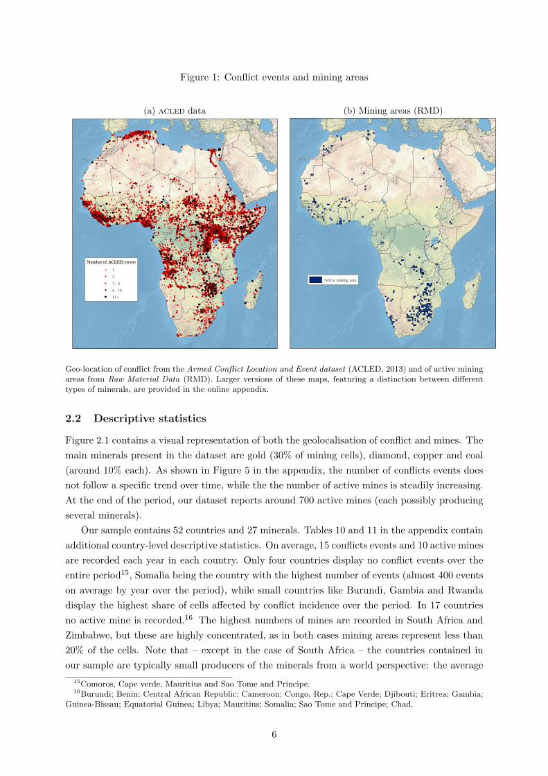
Figure 1: Conflict events and mining areas

(a) acled data (b) Mining areas (RMD)

!!! !!!!!!!!! !! !! !!!! !!!!!!! !! ! !!!!!!!!!!! !! !! !!! ! !! !!!!!! ! !!

! !! !! !! !!! !! !!

!!!! ! !!!! !!!! !! !!!!!!!!!!!!! !! !! ! !!!! !!! !!! !! !! ! !!! !! !! ! !! !!!! ! !!!!! ! !!!!! ! !!! ! !!!

! !!! !!! !!! !! !!!! !! !! !! !! !! ! !! !! !!!!! !! !!!!! !!! !!! !!!!! !!! !!!!!!! !!!!!!! ! !! ! !!! !!!!!! !! !! !!!! ! !! !!!!! !! !! !!! !! !! !! !! !! !!! ! !!!! ! ! !!! ! ! !!!! !! !! !! ! !! !!! ! !! !!! !! !! ! !!!!! !!!! ! !! !!! ! !! !!!!!! !

!!! ! !! !!! !!! !!!! !!!! !!! ! !! !!! !!! ! !!!! !! ! !!! !!!!!!! !! !!!! !!!!!!!! !!!!! ! !! !!! !!! !!!!! ! !! !! !!! !!!! !!!! !! ! !! !! !! ! !!! !!!! !! !!! !!!! !!! ! !!! !! !!!!!! !!! ! ! !!! ! !!!! ! !!! ! !!! !!! !! !!!! ! ! !! !!!!! ! !!!! !! !! !!! !! !! !! !!!!!!! ! !!!!! ! !!!! !!! !! ! !!!! !!!!! !!!!!!! !!! ! !!! !!! !!! !!!!!!!! ! !!!!!!!!!!! ! ! ! !!! !! !!!!! !!! ! !! ! !!!! ! ! !!! !!!!! !! !!! ! !!! ! ! !! !!! !!! !! !!! ! ! !! !! ! ! !!! !! !!! !!! ! ! !!! !!!! ! !! !!!!!!!! ! !!! !!! ! !!! ! !! !!!!! !! !!! !! ! ! !!!! !!! !! !!!!!! !!!! ! ! !!! !! ! !! !! !! ! !! !! ! ! !! !! !!!! !! !! !! !!!!! !!! !! !! ! !! !! !! !!! !!!! ! ! ! !! !!! ! !!!! ! !!! !!!! ! ! !! !!!! !!! ! ! ! !! !! !! !! !! !! !!! !!! !! ! ! !! !! !! ! !! !! !! !! ! !!!! !!!! !! ! ! ! !!! ! !!!! !!!!!!!! !!!! ! !!! !!! !!! !! !!!! !! ! !! !!!!!! !! !! !!! !! !!! ! !! ! !! !!! !!! ! ! !!! !!! ! !! ! !!! !! !!!! !!! !!!! !!!! !! ! ! !! !! !! !!! ! !!! ! !! !! ! !! !!!! ! !! !! !! ! !! !! ! !! ! ! !!! !! !! !!!! ! ! !!! !! ! ! !!! !!!! ! !! !!! ! !! !! !! ! !!! !! !! ! !!!! ! !!! !! !! ! ! !!!!! !!! ! !!!! ! !! ! ! !! ! !!! !! ! ! !!!!!!!!! !!!!!!!! ! !! ! !!!! ! !!!! !! ! ! !!! !! !! ! !! ! !!! !! ! !! ! !! !!!!!! ! !! !! !! !! !! ! !!!! !!! ! !!! !! ! !! !! ! !!! !!! ! !! ! ! !!!! ! !!! ! !! ! !! ! ! !! ! !!!! !!! !! !!! ! !! ! !! !! !! !! !! !! !!! !!! !!!!! ! !! !! ! !!! !! ! ! !!! !!! ! !!!!!! !!! ! ! ! !! !! !! ! !! ! !! ! ! ! !!! !! !! ! ! ! !! !!!!! !! !! ! !! !! !!!!! ! ! !!! !! !!! !!! !! !! !! ! !! ! !! !!!!!!! !!!! ! !!! !!! ! ! ! !! ! ! !!!! ! ! ! !!!! ! ! !!! ! ! !!! !!!! ! !!!!! ! ! ! !! ! !!! ! !! !!! ! !! ! !! !!!! !!! !!! ! !! !!! !! ! !! !! !! !!! !!!! ! !! ! !!! !!! ! !! !!!!! !! !!! !! ! !! !! !!!! ! !!! !! !! ! !!! ! !! ! !! !!!! ! ! ! !!! !!!!!! !! !! !! !!!! ! !!!!! !! !!!! !! !! !! !!! !! ! ! !!!!!! !!!!!!!! !!!! ! !! ! !!! !! !! ! !! !!!! !! !!!!!!! !!!! !! !!! !!!! !! !! ! !! !!!!! !!! !!! !! !!! !! !! !!!! ! !!! !! !!!!!!!! !!!!!!!!! ! !!!! ! !!!!!!!!!!! !!!!!!!!!! !!!! !!!!! ! !!!!! !!! !!!!!!!!!!!! !!!!!!! !!!! !! !!!!!!!!!!! !!!!!!!!!!!!!!!!! ! !!!! !!! !!!! !! !!!! !! !! !! !!!!!!!!!! ! !!!!! !! !!!!! !!!!!!!!!! ! !! ! !!!!!!!!!!! !!! !!!!!! !!!!! !!! !!!!!!! !! !!!!!!!!!!!! ! !!!!!!!!!! !!!!!! !!! !! !!!!!!!!!! !!!!! !!!! !!!!!! !!! !!!!!!!! !!!!!!!!!!!! !!! !!!! !! ! !!!!!!! !!!!!!!!!! ! !!!!!! ! !! ! !!!! !!!! !!!!!! ! !!!!!!!!!!!!!!!!! !!!!!!!!!!!!!!!!!! !!!!! !!! !! !!!! !!!!!!!! !! !!!!! !!! ! !! !! !! !!!!! !!!!!!!!!!! !!!!!!! ! !!!!! !! ! !!!!!!! !!!! !!! !! !!!!!!!!!!!! !! !!! !! !!!!!!! !! !!! !!!! !! !!!!!!!! !!! !!!!! ! !!!!!! !!!!!!!!!! ! !!!!! !!!!! !!!! !!! !!!!! !! ! !! ! ! !!!!!! ! !!!! ! !! !!! !!!! !!!!!! !!! ! !!!!!!!! !!!!!!! !!!!!!!! ! !!!!! !!! !!! !!!! !!! !!!!!!!!! !!!! ! !!! !!! !!!! !!! !!! !! !!! !! !! ! ! !! !!!! !!!! !!! !!!! !! !!! !!! !! !! ! !! !!!!!! !!!!! !!!! !!! ! ! !!! !! ! !! !!! !!!!!!! !!!! !! ! !!!!!! ! ! ! !!!!! !! !!!!! ! !!! !! !!!! !!! !! ! !!!!! !!!! ! !!!! !! !!!! !! !!!!!!!!! !!!!! !! !!!! !!!!!! !!!!! !! !! !!! !!!! !! !! !!!!! !!!!! ! !!! !!!!!!!!!! !! !! !!!! ! !!!!!!!!!!!!!!!!! !! !!!!! !! !!!!!!! !!!! ! ! !! !!! !! !!! !!!! ! !! !!! ! ! !!! !!! !!!!!! !! ! ! ! !!!! ! !! !!! ! !!!!! !! ! !! !!! !!! !! ! !! !! !!!!!!!!!!!!!!! ! !!!!!! !!!!! !!!!!!!!! !! ! ! !!!!!!!! ! !!!! !!!!!!!!! ! !!!!! ! ! !!!! !!! !!!! !! !!!! !! ! !!!!! !!! !!! !!!! !!! ! !!!! ! ! !!! !!!!! !!!!! ! !! !!! !! !!!! ! ! ! !!!! ! !! ! !!!! !! ! !!! !! !! !!! ! !! ! !! !!! ! !!! !!! !!!!!! !! !!! ! !! !!! ! ! !!!! !!! ! ! !! !!! !! ! ! !! !! ! ! !!! ! !! ! !!! !! ! !! !! !!!! ! ! !!! ! ! !!!! !! ! ! !!! !!!! !!!!! !!! ! !! !!!! ! !! ! !!!! ! !! !!! !! !! ! ! !!! !!!! !! ! !! ! !! ! ! !! !! !! !! !! !! !!!! !!!!!!! ! ! !! !! !! ! ! ! !! !! ! !! !! ! !!! !!! !! !!! ! ! !!!!! !! !! !! !! !! !! ! ! !!!! !!!! !! !! ! ! !!! !! !!! !! ! !! !!! ! ! ! !!! !!! ! !! ! !!! ! ! !! ! !! !! ! !!!! ! ! !!!! !!! !! ! !!! ! !!!! !!!! !!!! ! !!! !! !! !!!!!! ! !!!!!! !! !!!!!!! !! ! !!! ! !! !!! !! ! !! !! ! !!! ! !!!! ! !!! ! !!!!! ! ! ! !! !!! !!! !!!! ! !!! !! !! ! !!!! !! !!! !!!! ! !! !! ! !! !!!! ! !!!!! !!! ! !! !!!! ! !!!!!! ! !!!!! ! ! !! !!!! !! !!! !! !!! !!! ! !!!! !!!!! !! !! !!!! !!!! ! ! !! !! !! !!! !!! ! ! !! !!!!! !! !!! !! !! !! !! !!! ! ! !! !! !! !! !! !!!! ! !!! !!!! ! !! !!!!! !!! !! ! !! !! !! ! ! ! !!!! !!!! !!!! !! ! !! ! !! ! !!!!!! !!! !! !! ! !! !! !! !! !!! !!! ! ! !!! !! !!!! !! !!!!! ! ! ! !! ! ! !!! !! ! !! ! ! !!! !!!!! ! !! !!! !! !!! !!! !!!!! !!!!!! !!!! !! !!!! !! ! !!! !! ! !!!! ! ! ! !!!! !! ! ! !!!!! ! !! !! !!!! !! !! !! ! ! !!! !!! ! !!! !!!! !! !!!!!! ! !! !! ! !! !!!! !! !!! !!! !!!! !!!!!!!!!! !!!! !! ! ! !!!!!! ! !!!! !!!!!! !!! ! !!!!! ! !!! !! !!! ! ! !! !! !!! ! !!!! ! ! !! !! ! !!!! !! ! !! !! !! ! ! !!!! ! ! !! ! ! !! !! ! !!! !! ! !! ! !! ! !! !! !! ! !!!! !! !!!!! !!!!!!! ! !! !!! !! ! !! !! !!! ! !! ! !! ! !! ! ! ! !! ! !!! !!! !!!! !!!! !!! !!!! !!! ! !!! ! !!! !!! !!! !!! !!! ! !! !! !! ! !! !!!!! !!! !! ! !! ! !! !! !! ! ! ! !! !!! !! !!!! !! !! !!!! !! !!! ! ! !! !!!!! !! ! ! !!!!!! ! !! !! !!! ! ! !!!! !!!! !!!! ! ! ! ! ! !!! !!! !! !!! ! !! ! !!! ! ! ! !! !!! ! ! ! !!!!! ! !! ! !! !!!!!! ! ! ! !! ! !! ! !! ! !!!! !! !!!! ! !! !!! ! !! ! ! !! !! !!!!!! ! ! ! !! ! !!!! !!! !!!!! !! !! ! ! !!!! ! ! ! !!! !! !!!! !! ! !! !!! !!! !!!! ! ! ! !!!!!! !!!! ! ! !!! !!! !! !! !!!! !! ! !! !!! ! !!! !!! !!!! ! ! !! !! !! !! !! ! !! !! ! ! !!!!!! !!! !!! !! !!!! ! !!! !! !! ! !! !! !! ! ! !!!! !!! !! !!!!!! ! !! !! !!!! !! !!!! !!!!! !!! ! ! !!! !! !! !! !!! !! ! !!!!!! !!!! ! !! ! !! ! !!!! !!! !!!!! ! !!! ! !! ! !! !!! ! !! !! ! !! !!! !! ! !! !! !!!! ! !! !! !!! !! !! !!!!!! ! !! ! !!!!!!!! ! !! !! !! ! ! !! !! ! !! ! !!!! !! !!! !! ! !! !!!! !! !! ! !! !!!! ! ! !!! !!! ! !! !!!! !!! !! !! !!!!! ! ! !!!! !!! !! !!! !!!! !! !! !!! ! !!!! !!!! !!!!!! ! ! ! !! !! ! ! !!!!!! !!! !!! ! ! ! ! !!!! ! !! !! !! !!! ! !!! !! ! !!!! !! !! !! ! !!! !! ! !! !! ! ! !!! !!! !! ! ! !! ! !!! !! ! ! !! ! ! ! !! !!! ! !! ! ! !! !!! !!! ! !!! !! !! ! !! ! !!!! !! !!!! ! !!! ! !! ! ! !! ! ! ! !!!! !!! !! ! ! !!! !!!!! !!! ! ! ! !!!! ! !!!!! !! !! !!!! ! ! !!! !! !! !! !! !! !!!! ! ! ! !!!! !!!! !! ! !! !! !!!!!! ! !! ! !!!! ! !!!!! !!!! !! !! !!! !! !!! !! !!!!! !! !!! ! !! !! ! !! !! ! !!! !! ! !!! ! !!!! !! !! ! !!!!! !! !! ! !! !!!!! ! !! ! !!! !! !! ! !!! !!! ! ! !! !!!! ! !!! !! !!! !! ! !! !!! ! ! !!! !! !! ! !! !! !!!! ! !! ! !! !!!!! !!!!!! ! !!!! !! !! !!!! !! ! ! ! !!!! ! ! !!!! !! ! ! !! ! !! !!!! ! ! !! ! !!!! !! ! !! !!! ! !!! !! ! ! !! !! !! ! !! ! !!! ! ! ! ! ! !!!! !!!! !! !! !!!! ! !!!!!!!! !!! !! !!! ! ! !!!! ! !! ! !!! ! ! ! ! !! ! !! ! !! !! !! !!!!! !!!! !! !! !!!! !! !! ! !! !!!! !! ! ! !!!!!!! !!!! !!! ! ! !!!! !! !!!!! !!!!! !! ! ! ! !! ! !!! ! !!! !! !! ! !!! !!!! ! !! !! ! !! !! ! !! !!! !!!! !!!! !! !! !!!! ! !!! ! !! ! ! !! !!! !!! ! !!!! !! ! !! !! ! ! !! !! !!! ! ! ! ! ! ! ! !!! !! !! ! !! !!! ! !!! !!! ! !!! ! !!! !! !! !! ! !!! ! !! !!! !! ! !!! !! ! !! !! ! !! !!!! ! ! ! !! ! !!!! !! !!! ! !! ! !!!!! ! !! ! !! !! ! !!! !!! !!!! ! ! !! ! !! !! !! !!!! ! !! !!! !!! !! ! !! ! ! ! !! ! ! !!!!!! !! ! !! !! ! ! ! !!!! !!! !!! !!!! !! !!! !!! !!! !! !!!! !!! ! ! ! !!! !! ! !!! ! !! ! !! !! ! !! !!! !! ! !!! ! ! !!! ! !!!!!! ! ! ! !! ! !! !!! ! ! !!!! ! ! !!!! ! ! !!! !! ! ! ! !!! !!!! !! !! ! ! !!! ! !! ! !!!! !! !!!! ! !!! ! ! ! ! ! !!!! !! ! !! ! !! !!!! !! ! ! !! !! ! !!! !! !! !!! !! ! !! ! ! ! ! !!! !! ! !! !! ! !! ! !! ! ! !! ! ! ! !! !! !! !! !!!! ! !! !! ! ! ! !! !! ! !!! !!! !! !! !!! !!! !!!!!! !!!!!!! !!!! !!! ! !!! ! ! ! ! !!!!!!! !! ! ! !!! !! !! !!!! ! !!! !!! !!! !!! !!! ! ! ! ! !!!! !!!! ! !! !!! ! !! !!!!!! ! !!!!!!!! ! !! !!!! ! !! !! ! !! ! !! !!! ! !! !! ! ! !!!! !! ! ! !!!! !! !! !! ! !!! ! ! ! ! ! !!! !! !! !!! !!! ! !! !!! !!! ! ! !! !!! !! !! !! ! !! ! !!! ! !! ! !! !!! ! ! !! !! ! ! !! ! ! !!! ! ! !! !! ! !! ! !!!! !! !!! ! !! !!!!! ! ! !! ! !!!!!! !! ! ! !! !!! ! ! !!! ! ! ! !!!!! !!! ! ! ! !!!! ! ! ! ! !!! !! !!! ! ! ! !!!! !! ! ! !! !! !! !!! ! !!! !! ! !!! !! ! ! ! ! !! !! !! !!! !! !! ! ! !! ! ! !! !!! !!! !! ! ! ! ! !! !!! ! ! !!! ! ! !! !! ! ! ! !!!! !! ! ! ! !! ! ! ! ! ! !!!!!! !!! ! ! ! !! ! !!!!! !!! !!! !! !! ! !! !!!! ! !!!! !! !!! ! !!! ! ! !! ! ! !! !! !! ! !!!! ! ! ! ! ! ! !!! ! !!! !! ! !! !!! ! !! ! !!! ! !!! !! ! ! !! !! ! !! !!!!! ! ! ! !!!! !! ! !! !! !! ! !! ! ! !! !! ! !! !!!! !! !! ! !! ! ! ! !! ! !! !!! ! !!! ! !! !! ! !! !! !! ! !! !! ! !! ! !! ! !! !! ! ! !!! ! !!! ! !! !! !! ! !! !! ! !! ! !!! ! !!!!! ! !!! ! !! ! !!! ! !! ! !!! !! ! ! !!! !! ! ! ! !! !! ! !!!! !! !! ! !! ! !! !! !! !! !! !!! !! !!! ! ! !!! !!!! !! ! !! ! ! ! !! ! !!! !! !!! !! !!! ! !!!! !! ! !!! !! !! !! !! !!! ! ! !! !! !! !!!! ! ! !!! !!! !!!! ! !! ! !! ! !! !!! ! !! ! !! ! !! !!!! !! ! !! !! !! ! !! ! !! ! !! !! !!!!! !! ! !! ! !!!! !!! !! !!! ! ! !! !! !! !! ! ! ! ! !! ! !! !! ! !! ! !! !!! ! ! ! ! !!! !! ! !! !! !!! !! ! !! ! !! ! !! ! !! !! !!! !!!! ! !! ! ! ! !!!! !!! ! ! !! !! ! ! ! !! ! !! !! !! ! ! ! !! ! ! ! ! ! ! ! !! ! !! !! !! ! !!! !!!! !! !!!! !! ! !!! ! ! ! !! ! ! !!! !! !!! !!! ! !!! !! !! !! !! !!! !!!!!! !!!! !! !!!! ! !! !!!!!! ! !!!!! ! !! !! !! !!! ! !!!! !!! !!!!! ! ! !! ! !!!!!!!! !!!!!! ! !!! !! !!! !!!! !! !! !!! !!! ! ! !!! ! ! !!!! ! !!!! ! !! !!!!! !! ! !! !! ! !! !!! ! !! ! !!! !! ! !!!!! !!! !!!! !! ! !! !!! ! !! !!! !!! ! !! ! !! ! !!! !! !!! ! !! ! ! ! ! ! !! !!! ! ! ! !! !!! ! ! ! ! ! !! ! !!!!! ! !!!! !! !!!! ! !! !! ! ! ! !!! !! ! ! ! !!!! !! !!!!! !!!! ! !!!! !! ! !!! !!!!! !! !!! !!!! ! !! ! ! ! !! ! !! ! !! !! !! ! ! !! ! ! !!!! ! !!! !!! !! !! !!! ! !!!! !! !! !!! ! !! ! !! !!!!! ! !! !! !! ! !! ! !! ! !! !! !! !! ! !! ! !! !!! ! !!! !!!!! !! ! !!! !!! ! !!! !! !!!!! !! !!!! ! ! !!! !! !!! !! !! ! !! !!!!!! ! !!! !!! ! !!!! !! ! !!!! !! !!! ! !! !!! ! ! !! ! ! !! !!!! !!!! !!! !! ! ! !! !!!! ! !! ! !! !! !!!!!! !! ! !! !!! !! !! ! ! !! !!! !! ! !!! ! ! !!! ! ! !!!!! ! ! !! !!! !! ! ! ! !!!!! ! !!! !! ! !!! ! !! ! !! ! ! !!! ! ! !!! !! !! !! !!! ! !!! ! !!! ! !!! ! ! !!! ! !!! !! !! !! ! ! !!! !! ! ! !! !

!!! !!! !!! ! ! !! !!! ! !!! !! !!!!

!!!!! !!!!! ! !! ! !! !!

!! !!!!

! !!! !!!

!!!

!!!

! !!!!! !!!! ! ! !

!! !! !! !!! !! !!!!

!!!!!!! !! ! !!!!

! !!! !!! !! !!!!!!!!!!!!!!!!!!! !!!! !! !!!!!!!!! !! !!! !! !!! !!! !!! !!!!! ! ! ! !!! ! !!!!!! !!

! !! !! !!! !!! !!! !!! !! !!!!! ! !!! !! !!! ! !!!! !! !!! ! !!! ! !! !! !!! ! !! !!! ! !! !! !!!! !!!! !!!! ! !! !!!! !! ! !! !! !! ! !!! ! !! ! !!!! !!!! !!!! !! !! !!! ! !! ! !! !! ! ! !!!! !!!! !!!! ! !!! ! !!! !! !!!!!!!!! ! ! !!! !!! !!! !!!!!! !! !! !!!! !!! !! ! !!! !! !!!! !! !! !!! !! ! !! ! !! !!! !!! !! !! !!!!!! !!!! ! !! ! !!! !!!!! !! !! ! !! !! !!! !!! !!! !!! !!! ! !!!!! !! ! !!! !! ! !!! !! !!!! ! !! !! !!! !! !! !!!!! !! !! ! !!!!!!! !!!!! !! !!! !! ! !!!!! !! ! !!! !! !!!!! !!! !!!!! !! !!!! !!! !!!! !! ! !!! !!! !! !! !! !!! !!!!! !! ! !!! !!! !!! !! !!!! !! !!!!!! !!! !! !!! ! !!!! !! !!!! !!!! !!! !!! !! !!!!!!! !!!! !!!!!!! !! !!! !!! !! !! !! !! !!!!!!!!! !!!! !!! !!!! !! !!!!!!!! !! ! !!!! !!! ! !!!! ! !! !!!!! !! !!!!!!!! !!!! !!! !! !! !!! !! !!!!!!! !! ! ! !! !! !!! !!! !!!! !!!!!! ! !!! !!!!!!!! ! !!!! !!! !! !!!!!!

Number of ACLED events! 1! 2! 3 - 5! 6 - 10! 11+

Active mining area

Geo-location of conflict from the Armed Conflict Location and Event dataset (ACLED, 2013) and of active miningareas from Raw Material Data (RMD). Larger versions of these maps, featuring a distinction between differenttypes of minerals, are provided in the online appendix.

2.2 Descriptive statistics

Figure 2.1 contains a visual representation of both the geolocalisation of conflict and mines. The

main minerals present in the dataset are gold (30% of mining cells), diamond, copper and coal

(around 10% each). As shown in Figure 5 in the appendix, the number of conflicts events does

not follow a specific trend over time, while the the number of active mines is steadily increasing.

At the end of the period, our dataset reports around 700 active mines (each possibly producing

several minerals).

Our sample contains 52 countries and 27 minerals. Tables 10 and 11 in the appendix contain

additional country-level descriptive statistics. On average, 15 conflicts events and 10 active mines

are recorded each year in each country. Only four countries display no conflict events over the

entire period15, Somalia being the country with the highest number of events (almost 400 events

on average by year over the period), while small countries like Burundi, Gambia and Rwanda

display the highest share of cells affected by conflict incidence over the period. In 17 countries

no active mine is recorded.16 The highest numbers of mines are recorded in South Africa and

Zimbabwe, but these are highly concentrated, as in both cases mining areas represent less than

20% of the cells. Note that – except in the case of South Africa – the countries contained in

our sample are typically small producers of the minerals from a world perspective: the average

15Comoros, Cape verde, Mauritius and Sao Tome and Principe.16Burundi; Benin; Central African Republic; Cameroon; Congo, Rep.; Cape Verde; Djibouti; Eritrea; Gambia;

Guinea-Bissau; Equatorial Guinea; Libya; Mauritius; Somalia; Sao Tome and Principe; Chad.

6

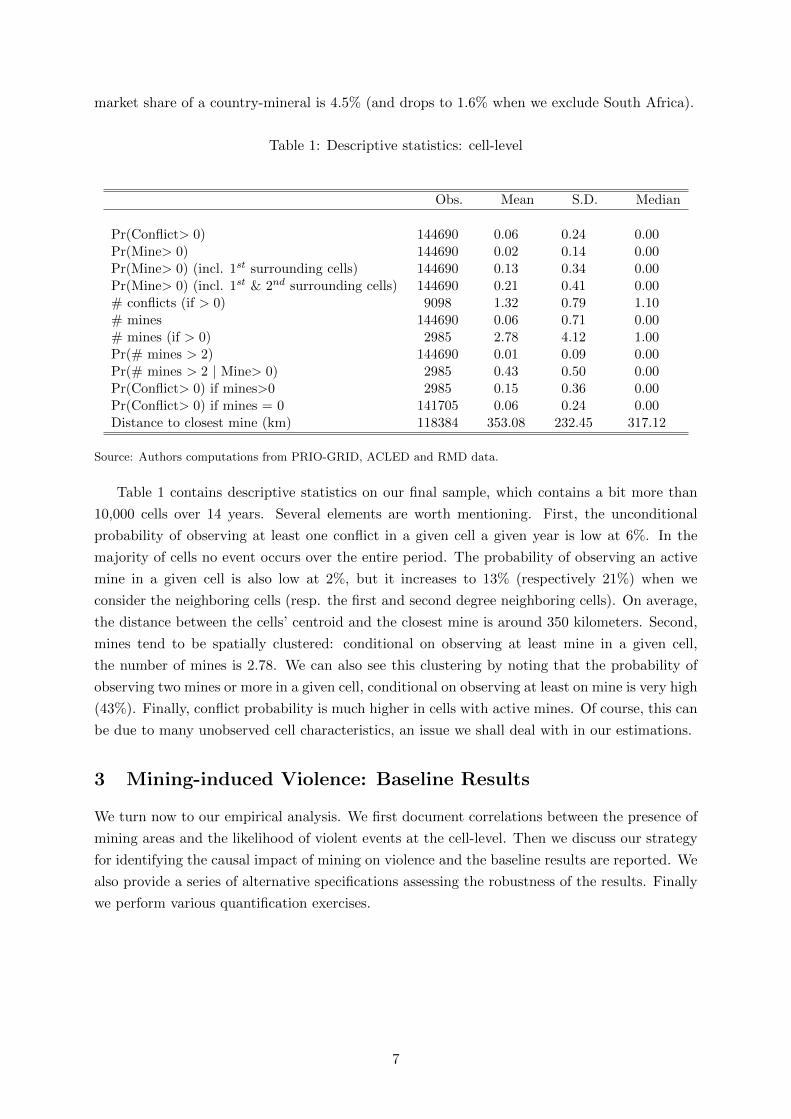
market share of a country-mineral is 4.5% (and drops to 1.6% when we exclude South Africa).

Table 1: Descriptive statistics: cell-level

Obs. Mean S.D. Median

Pr(Conflict> 0) 144690 0.06 0.24 0.00Pr(Mine> 0) 144690 0.02 0.14 0.00Pr(Mine> 0) (incl. 1st surrounding cells) 144690 0.13 0.34 0.00Pr(Mine> 0) (incl. 1st & 2nd surrounding cells) 144690 0.21 0.41 0.00# conflicts (if > 0) 9098 1.32 0.79 1.10# mines 144690 0.06 0.71 0.00# mines (if > 0) 2985 2.78 4.12 1.00Pr(# mines > 2) 144690 0.01 0.09 0.00Pr(# mines > 2 | Mine> 0) 2985 0.43 0.50 0.00Pr(Conflict> 0) if mines>0 2985 0.15 0.36 0.00Pr(Conflict> 0) if mines = 0 141705 0.06 0.24 0.00Distance to closest mine (km) 118384 353.08 232.45 317.12

Source: Authors computations from PRIO-GRID, ACLED and RMD data.

Table 1 contains descriptive statistics on our final sample, which contains a bit more than

10,000 cells over 14 years. Several elements are worth mentioning. First, the unconditional

probability of observing at least one conflict in a given cell a given year is low at 6%. In the

majority of cells no event occurs over the entire period. The probability of observing an active

mine in a given cell is also low at 2%, but it increases to 13% (respectively 21%) when we

consider the neighboring cells (resp. the first and second degree neighboring cells). On average,

the distance between the cells’ centroid and the closest mine is around 350 kilometers. Second,

mines tend to be spatially clustered: conditional on observing at least mine in a given cell,

the number of mines is 2.78. We can also see this clustering by noting that the probability of

observing two mines or more in a given cell, conditional on observing at least on mine is very high

(43%). Finally, conflict probability is much higher in cells with active mines. Of course, this can

be due to many unobserved cell characteristics, an issue we shall deal with in our estimations.

3 Mining-induced Violence: Baseline Results

We turn now to our empirical analysis. We first document correlations between the presence of

mining areas and the likelihood of violent events at the cell-level. Then we discuss our strategy

for identifying the causal impact of mining on violence and the baseline results are reported. We

also provide a series of alternative specifications assessing the robustness of the results. Finally

we perform various quantification exercises.

7

3.1 Correlations

The correlation between mining and cell-level violence is estimated in various ways, all based on

the following specification:

conflictkt = α×Mkt + FEit + εkt (1)

where (k, t, i) denote respectively cell, time and country. The dependent variable, conflictkt,

corresponds to the observation of violent events at the cell-year level where violence is measured

either in term of intensity (i.e. number of events) or in term of incidence (i.e. a binary variable

coding for non-zero events). Information on violent events is retrieved from the acled dataset

on civil conflicts or alternatively from data on massacres from the Political Instability Task

Force (PITF). The main explanatory variable, Mkt, measures mining activity at the cell-year

level with two possible coding options: a discrete variable equal to the number of active mines,

or a binary variable coding for the presence of at least one active mine. Finally, the vector FEit

corresponds to a set of country×year fixed effects that filter out all countrywide time-varying

characteristics affecting violence and activity of mines – e.g. a war-induced collapse of central

state and property rights.

In our baseline specifications, equation (1) is estimated with OLS or LPM in the case of a

binary dependent variable. Our results are robust to alternative non-linear estimators such as

a conditional logit or a PPML estimator (Tables A.2 and A.3 in the online appendix). In all

specifications (here and in other sections of the paper as well), standard errors are clustered

at the country-level (note that all our results are robust to less demanding levels of clustering

such as country × year or cell). We also check that our main results are robust to a non-

parametric estimation of the standard errors allowing for both cross-sectional spatial correlation

and location-specific serial correlation (Conley, 1999; Hsiang, Meng and Cane, 2011) (see Table

A.11).

Results are displayed in Table 2. Columns (1) and (2) show that our two measures of mining

activity (presence and number) correlate positively and significantly (at the 1 percent level)

with the incidence of acled conflict events at the cell-level. The presence of one or more mines

is associated with a 8.5 percentage points increase in conflict probability. Given the similarity

of the results, in the rest of our empirical analysis, we report the results mostly for the binary

version of mining activity (i.e. presence) estimated with LPM. Columns (3) to (6) consider

several alternatives for the dependent variable with violence being measured, respectively, by

the number of acled events, by the violence-induced fatalities (as reported in acled), by

the incidence of massacres and by the massacre-induced fatalities. Our point estimates are

systematically positive and, except in the last specification, statistically significant at the 5

percent threshold.17

The main source of identification in specification (1) corresponds to the between-cell varia-

tions in mining activity and violence, for a given country in a given year. Part of the correlation

could be spuriously driven by omitted time-invariant cell-specific characteristics such as the local

17In the online appendix we consider pure cross-sectional specifications that replicate Table 2 with all variablesbeing averaged in the time dimension (see Table A.1).

8

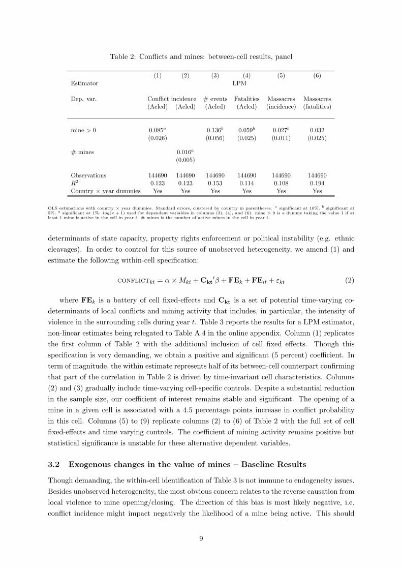
Table 2: Conflicts and mines: between-cell results, panel

(1) (2) (3) (4) (5) (6)Estimator LPM

Dep. var. Conflict incidence # events Fatalities Massacres Massacres(Acled) (Acled) (Acled) (Acled) (incidence) (fatalities)

mine > 0 0.085a 0.136b 0.059b 0.027b 0.032(0.026) (0.056) (0.025) (0.011) (0.025)

# mines 0.016a

(0.005)

Observations 144690 144690 144690 144690 144690 144690R2 0.123 0.123 0.153 0.114 0.108 0.194Country × year dummies Yes Yes Yes Yes Yes Yes

OLS estimations with country × year dummies. Standard errors, clustered by country in parentheses. c significant at 10%; b significant at5%; a significant at 1%. log(x + 1) used for dependent variables in columns (3), (4), and (6). mine > 0 is a dummy taking the value 1 if atleast 1 mine is active in the cell in year t. # mines is the number of active mines in the cell in year t.

determinants of state capacity, property rights enforcement or political instability (e.g. ethnic

cleavages). In order to control for this source of unobserved heterogeneity, we amend (1) and

estimate the following within-cell specification:

conflictkt = α×Mkt + Ckt′β + FEk + FEit + εkt (2)

where FEk is a battery of cell fixed-effects and Ckt is a set of potential time-varying co-

determinants of local conflicts and mining activity that includes, in particular, the intensity of

violence in the surrounding cells during year t. Table 3 reports the results for a LPM estimator,

non-linear estimates being relegated to Table A.4 in the online appendix. Column (1) replicates

the first column of Table 2 with the additional inclusion of cell fixed effects. Though this

specification is very demanding, we obtain a positive and significant (5 percent) coefficient. In

term of magnitude, the within estimate represents half of its between-cell counterpart confirming

that part of the correlation in Table 2 is driven by time-invariant cell characteristics. Columns

(2) and (3) gradually include time-varying cell-specific controls. Despite a substantial reduction

in the sample size, our coefficient of interest remains stable and significant. The opening of a

mine in a given cell is associated with a 4.5 percentage points increase in conflict probability

in this cell. Columns (5) to (9) replicate columns (2) to (6) of Table 2 with the full set of cell

fixed-effects and time varying controls. The coefficient of mining activity remains positive but

statistical significance is unstable for these alternative dependent variables.

3.2 Exogenous changes in the value of mines – Baseline Results

Though demanding, the within-cell identification of Table 3 is not immune to endogeneity issues.

Besides unobserved heterogeneity, the most obvious concern relates to the reverse causation from

local violence to mine opening/closing. The direction of this bias is most likely negative, i.e.

conflict incidence might impact negatively the likelihood of a mine being active. This should

9

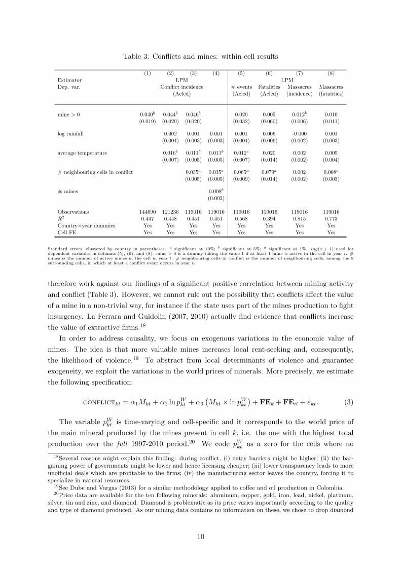
Table 3: Conflicts and mines: within-cell results

(1) (2) (3) (4) (5) (6) (7) (8)Estimator LPM LPMDep. var. Conflict incidence # events Fatalities Massacres Massacres

(Acled) (Acled) (Acled) (incidence) (fatalities)

mine > 0 0.040b 0.044b 0.046b 0.020 0.005 0.012b 0.010(0.019) (0.020) (0.020) (0.032) (0.060) (0.006) (0.011)

log rainfall 0.002 0.001 0.001 0.001 0.006 -0.000 0.001(0.004) (0.003) (0.003) (0.004) (0.006) (0.002) (0.003)

average temperature 0.016b 0.011b 0.011b 0.012c 0.020 0.002 0.005(0.007) (0.005) (0.005) (0.007) (0.014) (0.002) (0.004)

# neighbouring cells in conflict 0.035a 0.035a 0.065a 0.079a 0.002 0.008a

(0.005) (0.005) (0.009) (0.014) (0.002) (0.003)

# mines 0.008b

(0.003)

Observations 144690 121236 119016 119016 119016 119016 119016 119016R2 0.447 0.448 0.451 0.451 0.568 0.394 0.815 0.773Country×year dummies Yes Yes Yes Yes Yes Yes Yes YesCell FE Yes Yes Yes Yes Yes Yes Yes Yes

Standard errors, clustered by country in parentheses. c significant at 10%; b significant at 5%; a significant at 1%. log(x + 1) used fordependent variables in columns (5), (6), and (8). mine > 0 is a dummy taking the value 1 if at least 1 mine is active in the cell in year t. #mines is the number of active mines in the cell in year t. # neighbouring cells in conflict is the number of neighbouring cells, among the 8surrounding cells, in which at least a conflict event occurs in year t.

therefore work against our findings of a significant positive correlation between mining activity

and conflict (Table 3). However, we cannot rule out the possibility that conflicts affect the value

of a mine in a non-trivial way, for instance if the state uses part of the mines production to fight

insurgency. La Ferrara and Guidolin (2007, 2010) actually find evidence that conflicts increase

the value of extractive firms.18

In order to address causality, we focus on exogenous variations in the economic value of

mines. The idea is that more valuable mines increases local rent-seeking and, consequently,

the likelihood of violence.19 To abstract from local determinants of violence and guarantee

exogeneity, we exploit the variations in the world prices of minerals. More precisely, we estimate

the following specification:

conflictkt = α1Mkt + α2 ln pWkt + α3

(Mkt × ln pWkt

)+ FEk + FEit + εkt. (3)

The variable pWkt is time-varying and cell-specific and it corresponds to the world price of

the main mineral produced by the mines present in cell k, i.e. the one with the highest total

production over the full 1997-2010 period.20 We code pWkt as a zero for the cells where no

18Several reasons might explain this finding: during conflict, (i) entry barriers might be higher; (ii) the bar-gaining power of governments might be lower and hence licensing cheaper; (iii) lower transparency leads to moreunofficial deals which are profitable to the firms; (iv) the manufacturing sector leaves the country, forcing it tospecialize in natural resources.

19See Dube and Vargas (2013) for a similar methodology applied to coffee and oil production in Colombia.20Price data are available for the ten following minerals: aluminum, copper, gold, iron, lead, nickel, platinum,

silver, tin and zinc, and diamond. Diamond is problematic as its price varies importantly according to the qualityand type of diamond produced. As our mining data contains no information on these, we chose to drop diamond

10

active mine ever produces over the period; by contrast, it is non-zero for cells with a mine that

is inactive only temporary. This coding strategy being non neutral, we check below that our

estimates are robust when restricted to the sub-sample of cells with only permanently active

mine.21 Note that we do not include the controls Ckt in our baseline estimations as they reduce

significantly the sample size without affecting the estimate of our coefficient of interest, as shown

later in the robustness section.

We are primarily interested in α3, the coefficient of the interaction term between the world

price and the dummy for mining activity. This coefficient captures the impact on local violence

of an exogenous increase in the world price of a given mineral, in cells where mining extraction

of this mineral takes place. Given the fact that we include country ×year fixed-effects in all

specifications, our identification strategy relies on the exogeneity of the interaction term, Mkt×ln pWkt , with respect to the local determinants of conflict. We discuss hereafter this identification

assumption.

a/ Exogeneity of Prices – This seems a reasonable assumption for the world price of

minerals, pWkt , as mentioned earlier. Still, one might argue that some mines are large

enough to affect world prices, in which case the occurrence of conflict in these cells might

also affect these prices. Although our sample contains only few countries with potentially

large market power on the mineral market, we nevertheless test whether our results are

robust to excluding from the sample all cells located in countries belonging to the top ten

world producers of a specific mineral (see subsection 3.3.1).

b/ Exogeneity of mining activity – As discussed above, potential reverse causation

from conflicts to mining opening/closing is a severe concern. As a consequence, our coeffi-

cient of interest, α3, could be partly identified through conflict-induced shift in the binary

variable Mkt. To account for this issue, we can restrict the estimate of equation (3) to the

sub-sample of cells without opening/closing of mine over the period (i.e. Var(Mkt) = 0

for a given k). Given that Mkt = 0 or Mkt = 1 for all years, this variable is now absorbed

by the cell fixed effects and the covariates ln pWkt and (Mkt × ln pWkt ) become identical; we

accordingly include only the interaction term and the specification takes the following

simpler expression:

conflictkt = α3

(Mkt × ln pWkt

)+ FEk + FEit + εkt (4)

This specification ensures that our coefficient of interest, α3, is identified within cells

through the changes in world commodity prices conditional on having a permanent active

mine (i.e. Mkt = 1 for all t), and not through the potentially endogenous opening/closing of

mines. Note also that including country×year dummies is crucial, as they absorb common

shocks (or trends) on world prices and country-level conflicts. However, from a data

perspective, estimating this set of 935 dummies is very demanding. With this respect,

from our baseline estimations. We however show that our results are robust to the inclusion of this mineral (seeTable A.6).

21We also run robustness checks where instead of replacing pWkt by zero for cells with no active mine ever, wereplace it by a price index representing the average price level of the minerals in country i, during year t, weightedby the relative frequency of each mineral in each country over the period. As discussed in subsection 3.3.4, theresults are very similar.

11

keeping in the sample not only cells with a permanent mine opening but also the large

amount of cells with no mines (Mkt = 0 for all t) conveys information which is decisive for

estimating these dummies. This is why we favor, in our baseline estimations, specifications

using the full sample of cells without opening/closing. Alternatively, in the robustness, we

report the estimates when the sample is restricted to cells with a permanent active mine

(see subsection 3.3.4).

Table 4 reports the baseline results for various sample compositions and definitions of the

variables. The dependent variable is conflict incidence, except in columns (3) and (4) where we

consider the number of events. Mines activity is coded as a dummy variable except in columns

(5) and (6) where it is measured by the number of active mines. Columns (1), (3) and (5) are

estimated on the full sample (specification 3); while columns (2), (4) and (6) are restricted on the

subsample of cells without mine opening/closing (specification 4). We see that in all columns,

our coefficient of interest is positive and significant at the 1 percent level. Columns (2) and (4)

are our preferred regressions.

Table 4: Conflicts and mineral prices

(1) (2) (3) (4) (5) (6)Estimator LPM LPM LPMDep. var. Conflict incidence # conflicts Conflict incidenceSample All Var(Mkt) = 0 All Var(Mkt) = 0 All Var(Mkt) = 0

mine > 0 0.055 0.043(0.094) (0.111)

ln price main mineral -0.029 -0.045c 0.010(0.019) (0.024) (0.012)

ln price × mines > 0 0.093a 0.073a 0.148a 0.099a

(0.027) (0.020) (0.035) (0.033)

# mines 0.036b

(0.015)

ln price × # mines 0.017a 0.004a

(0.004) (0.001)

Observations 142817 141890 142817 141890 142926 141568R2 0.445 0.445 0.562 0.563 0.447 0.446Country×year dummies Yes Yes Yes Yes Yes YesCell FE Yes Yes Yes Yes Yes Yes

Standard errors, clustered by country, in parentheses. c significant at 10%; b significant at 5%; a significant at 1%. Var(Mkt) = 0 means thatwe consider only cells in which the mine variable takes always the same value over the period. mine > 0 is a dummy taking the value 1 if atleast 1 mine is active in the cell in year t. log(x + 1) used for dependent variable in columns (3) and (4). # mines is the number of activemines in the cell in year t. ln price main mineral is the world price of the mineral with the highest average production in the cell over theperiod.

3.3 Robustness

Our results shown in Table 4 are robust to a battery of sensitivity checks. We present below

several types of robustness exercises. First, we address further concerns with reversed causality,

12

and second, further concerns with omitted variable bias. Third, we consider alternative cell

sizes, and fourth, a variety of further robustness checks.

3.3.1 Reversed causality

Reversed causality is a potential concern. In particular, it could be conceivable that mining

prices do not affect conflict, but that on the contrary the occurrence or the anticipation of a

conflict in a major producer country leads to an increase in the mineral prices. To address this

concern, we include additional interaction terms between world prices of minerals and a dummy

which equals 1 if the country belongs to the top-10 world producer in the mineral produced by

the cell, and therefore could influence world prices (Table 12 in the appendix). Our result still

holds for the rest of the cells, and we cannot find robust evidence of market power influencing

our results (the interaction terms with the large producer dummy is insignificant or negative

in all but one specification). Alternatively, we drop all country-minerals which belong to the

top-10 world producers (Table A.5 of the online appendix). The results are again similar.

3.3.2 Population/economic size and time-varying controls

We want to rule out the fact that our baseline estimates are driven by an increase in population

size resulting from more intense mining activity (induced by raising mineral prices). To this

purpose, we control in Table 13 (see appendix) for economic size, proxied by night light satellite

data, and, more importantly, for the interaction of luminosity and mineral prices. The results

are unchanged. Similarly, Table 14 of the appendix goes further and includes a number of

alternative cell-specific, time-varying controls which might be correlated with commodity price

variations (climate variables) or mining activity (number of conflicts in the surrounding cells, or

number of conflicts observed in the cell since the start of the period). In all cases, our coefficients

of interest remain stable and highly significant.

3.3.3 Alternative cell sizes

In this subsection we enquire robustness to alternative sizes of the units of observation. As

discussed in Section 2, the RMD dataset does not survey small-scale (potentially illegally oper-

ated) mines. Because of spatial clustering of mineral deposits, our main explanatory variable,

Mkt, must be interpreted as a proxy for the extraction area of a given mineral rather than as

coding for a specific RMD-referenced mine. Imagine now for example that mining areas could

on average be larger than our cells of a spatial resolution of 0.5 × 0.5 degree. In this case,

focusing on the impact of mines on the conflict likelihood in its surrounding cell of 0.5 × 0.5

degree may underestimate the real impact of being in a mining area. Hence, in what follows we

broaden the scope of a mining area.

In Table 5 below we study the impact on conflict of mineral price shocks in neighboring cells

(of degrees 1 and 2) of a cell containing a RMD-referenced mine. As shown by the coefficient

of the second interaction term, we detect in all specifications a positive and significant impact,

which is consistent with the view that some mining areas are indeed larger than our 0.5 × 0.5

degree cells. Note however that the effect is much lower than for the cell itself (i.e. the first

interaction term).

13

Table 5: Conflicts and mineral prices, including neighboring cells

(1) (2) (3) (4)Estimator LPM LPMDep. var. Conflict incidence # conflictsSample All Var(Mkt) = 0 All Var(Mkt) = 0

mine > 0 0.056 0.040(0.096) (0.113)

ln price main mineral -0.041b -0.065b

(0.019) (0.026)

ln price × mines > 0 0.094a 0.059b 0.152a 0.087c

(0.028) (0.026) (0.034) (0.048)

mine > 0 (neighboring cells) -0.023 -0.037(0.016) (0.026)

ln price × mine > 0 (neighbouring cells) 0.024a 0.028a 0.041b 0.052a

(0.008) (0.010) (0.016) (0.019)

Observations 134899 123466 134899 123466R2 0.442 0.440 0.554 0.557Country×year dummies Yes Yes Yes YesCell FE Yes Yes Yes Yes

Standard errors, clustered by country, in parentheses. c significant at 10%; b significant at 5%; a significant at 1%. Var(Mkt) = 0 means thatwe consider only cells in which the mine variables (including the one for surrounding cells) take always the same value over the period. mine> 0 is a dummy taking the value 1 if at least 1 mine is active in the cell in year t. log(x + 1) used for dependent variable in columns (3) and(4). ln price main mineral is the world price of the mineral with the highest average production in the cell over the period. Neighboring cellsinclude the first degree neighboring cells (8 cells) as well as the second degree (16 cells).

Alternatively, in Table 16 in the appendix we reproduce our baseline table for a grid of cells

at a larger resolution (1 degree × 1 degree). In all columns, the coefficient of interest has the

expected positive sign and is often statistically significant at the 5 or 1 percent level. The slightly

weaker results for the 1 × 1 resolution than in the baseline table may indicate that many mining

zones are of relatively limited size and that the baseline resolution of 0.5 × 0.5 is indeed the

appropriate level of disaggregation.

A further sensitivity test relates to taking into account actual distances from the closest

mines. As mentioned above, the observation of a mine acts as a proxy for the existence of a

wider mining area, given that some smaller non-industrial mines are unobserved. However, the

spatial extension of the extraction areas may clearly vary across minerals and across deposits,

an issue that we ignore in our baseline estimates where the grid scaling imposes all mining areas

to be limited to a 0.5 × 0.5 degree cell. We consequently adopt a more flexible approach here

by using information on the precise location of mines to compute the distance between each cell

and the closest mine. We consequently estimate:

conflictkt = β1 lnDkt + β2 lnDkt × ln pWkt + ln pWkt × γi + FEk + FEit + εkt (5)

where Dkt is the distance in kilometers between the centroid of the cell and the closest active

mine in the country during year t. pWkt is the world price of the mineral produced by the closest

mine. We include a set of interaction terms between the price variable and country dummies

14

to control for country-specific heterogeneity such as country size, which can be correlated with

conflicts and affect the value of Dkt. If mining fuels conflicts, we expect both β1 and β2 to be

negative. The results are provided in the appendix, in Table 17. In column (1), we include only

the log of distance to the closest mine.22 In column (2) we add the interaction with mineral

prices. Column (3) restricts the sample to the cell in which distance to mines is fixed over

the period. Finally, in column (4) we include additional interactions with cell-specific variables

which could be correlated with the distance to the closest mine: distance to the capital city

and to the nearest international border. The results are consistent with our baseline estimates:

cells located further away from opening mines have a significantly lower conflict probability in

column (1), and variations in mineral prices have a significantly lower effect in cells located away

from mines (columns (2) to (4)).

3.3.4 Other robustness checks

Placebo – We perform a placebo test with the idea of testing the consistency of our empirical

strategy that is based on exogenous variations in mineral prices. In particular, we want to

exclude the fact that comovements in the World price of minerals could drive our results. The

logic is to replace the price of the mineral produced in the cell by the price of a mineral that is

not produced in the cell. More precisely, we randomly assign a mineral to each of the mining

cells and run specification (2) of Table 4 with this fake Mkt × ln pWkt variable. We repeat the

procedure in 1,000 draws. Figure A.1 in the online appendix displays the results. Reassuringly,

the Monte Carlo coefficients are distributed far from our baseline estimate (0.073) and are

massively insignificant.

Alternative price data – An important variable in our analysis are the mineral prices. We

hence investigate robustness to alternative definition of prices (Table A.9 in the appendix). In

particular, we use second-differences in prices instead of levels in columns (1) and (2), real prices

instead of nominal prices in columns (3) and (4), and replace the price variables by a country-

specific index when no mine is ever recorded in the cell in columns (5) and (6). In all columns

the coefficient of interest is still highly significant.

Sample restrictions – Another issue that arises for our interaction with mineral prices is how

to treat cells that do not have any mines. In Table 15 we report the estimates when the sample is

restricted to cells with a permanent active mine. Column (1) reports our preferred specification

on the full sample. Column (2) replicates this specification on the subsample of cells with

permanent active mines. The coefficient of interest remains positive but much less accurately

estimated, the reason being a massive sample size reduction (925 observations) with a set of

country×year dummies remaining large (221). In column (4), we consequently exclude those

dummies and this restores statistical significance. In column (3), for the sake of comparison, we

replicate column (4) on the full sample of cells.

Subset of metals – Are our results driven by a particular subset of minerals? We respectively

include diamonds in our estimations or exclude gold, silver and diamond mines from our set

22This coefficient can be identified despite the cell fixed effects as distance can vary over time when mines openor close in the country.

15

of minerals (Tables A.6 and A.7 of the online appendix).23 Our coefficient of interest keeps its

positive sign and is highly significant in all columns, indicating that our results generalize to a

broad category of minerals, and that they are not driven by the most precious minerals only.

Conflict onset and ending – In all tables we focus on conflict incidence, which reflects our

interest in explaining the general presence of conflict. A higher conflict incidence can of course

be due to either more conflicts breaking out or due to existing conflicts lasting longer. Hence, in

the civil war literature, a number of papers focus on civil war beginnings (onsets) and endings

separately. In Table A.8 of the online appendix, we study cell-specific conflict onsets and endings

of conflict separately. We find that our variable of interest, the interaction of mining dummy

times price, both significantly increases the risk of conflict onset, and significantly reduces the

likelihood of conflict ending. This implies that the higher conflict incidence due to mines is both

due to more conflicts breaking out and to existing conflicts lasting longer.

Alternative estimators – Table A.10 of the online appendix reproduces our baseline re-

sults using estimators specifically designed for binary dependent variables and count data, i.e.

fixed effects logit (whenever the dependent variable is conflict incidence) or a Poisson pseudo-

maximum-likelihood (PPML, whenever the dependent variable is the number of conflict events).

With the exception of column (4) where the coefficient on the interaction term between the world

price and the dummy for mining activity is marginally insignificant, our results are very similar

to our baseline estimates. The LPM is however our preferred estimator as it allows for a more

straightforward interpretation of the coefficients and does not suffer from certain econometric

problems due to the inclusion of both cell and country×year fixed effects.24

Statistical inference – Another econometric issue to consider is statistical inference. As

mentioned, in all tables standard errors are clustered at the country-level. Alternatively, we

allow for various levels of cross-sectional spatial correlation and cell-specific serial correlation,

applying the method developed by Hsiang (2010). We display the standard errors for our six

main specifications when allowing for spatial correlation of 100 or 1000 kilometers, and for a

serial correlation over 1 or 5 years (Table A.11 of the online appendix). For all combinations

of spatial and serial correlation considered, the standard errors are such that our coefficients of

interest are still statistically significant.

3.4 Quantification

How large is the effect of mineral price variations on the conflict probability? In our preferred

specification (Table 4, column (2)) a standard-deviation increase in the price of all minerals

from their mean translates into an increase in probability of violence from 0.165 to 0.203. This

is of non negligible magnitude, but of course concerns only the cells where active mining takes

23There is large heterogeneity in diamond quality in different mines and price shocks for different categories ofdiamonds can go in different directions. As we do not have information of the type of diamonds produced by eachcell, we ignore this heterogeneity, which might add statistical noise and lead to attenuation bias; this is why ourpreferred estimations do not consider diamond mines.

24The estimations shown in Table A.10 include year dummies instead of country×year dummies for two reasons;first, because the logit and PPML estimator fail to reach convergence when including country×year dummies;second, because the inclusion of two dimensions of fixed effects in logit and Poisson models might lead to anincidental parameter problem (Charbonneau, 2012).

16

place. When we also consider the surrounding cells (Table 5, column (2)), conflict probability

rises from 0.169 to 0.212.

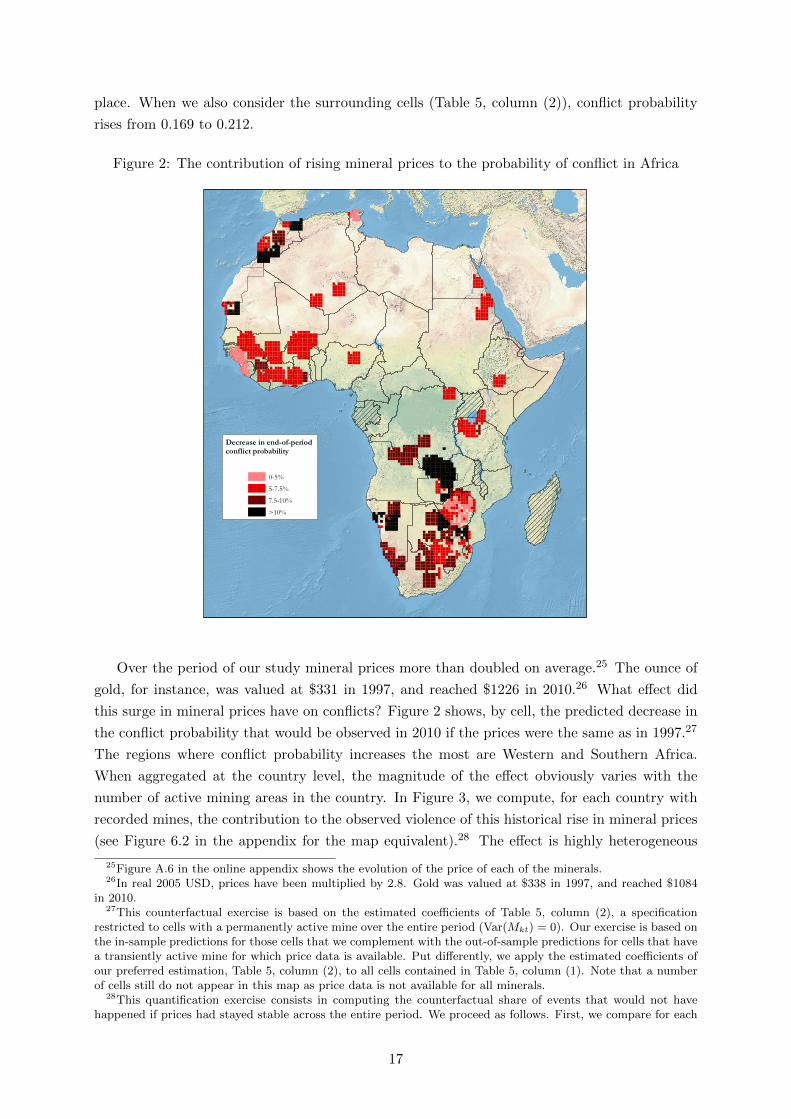
Figure 2: The contribution of rising mineral prices to the probability of conflict in Africa

Decrease in end-of-period conflict probability

0-5%5-7.5%7.5-10%>10%

Over the period of our study mineral prices more than doubled on average.25 The ounce of

gold, for instance, was valued at $331 in 1997, and reached $1226 in 2010.26 What effect did

this surge in mineral prices have on conflicts? Figure 2 shows, by cell, the predicted decrease in

the conflict probability that would be observed in 2010 if the prices were the same as in 1997.27

The regions where conflict probability increases the most are Western and Southern Africa.

When aggregated at the country level, the magnitude of the effect obviously varies with the

number of active mining areas in the country. In Figure 3, we compute, for each country with

recorded mines, the contribution to the observed violence of this historical rise in mineral prices

(see Figure 6.2 in the appendix for the map equivalent).28 The effect is highly heterogeneous

25Figure A.6 in the online appendix shows the evolution of the price of each of the minerals.26In real 2005 USD, prices have been multiplied by 2.8. Gold was valued at $338 in 1997, and reached $1084

in 2010.27This counterfactual exercise is based on the estimated coefficients of Table 5, column (2), a specification

restricted to cells with a permanently active mine over the entire period (Var(Mkt) = 0). Our exercise is based onthe in-sample predictions for those cells that we complement with the out-of-sample predictions for cells that havea transiently active mine for which price data is available. Put differently, we apply the estimated coefficients ofour preferred estimation, Table 5, column (2), to all cells contained in Table 5, column (1). Note that a numberof cells still do not appear in this map as price data is not available for all minerals.

28This quantification exercise consists in computing the counterfactual share of events that would not havehappened if prices had stayed stable across the entire period. We proceed as follows. First, we compare for each

17

across countries. Averaging across all countries with at least one recorded mine, we find that

the historical rise in mineral prices contributed on average to 21% of the observed country-level

violence. As is apparent in Figure 3, this number is however inflated by countries, such as Ghana

or Mauritania, in which only few conflict events are recorded (see Table 11). When we adopt

a more conservative approach and consider only countries with more than 50 events observed

over the period, we find that the observed rise in mineral prices contributed to a 13.6% of the

observed violence.29 In the online appendix (Figures 4.a and 4.b) we consider a more extreme

thought experiment where we quantify the impact on violence of a closing of all mines in Africa.

As expected, the effects are even larger: the number of conflicts falls by as much as 60-80%

in Ghana or Zimbabwe; and in most countries, the number of conflicts decreases by more than

20%.

Figure 3: The contribution of rising mineral prices to violence in Africa

0 .2 .4 .6 .8 1Share of events explained by increase in mineral prices

MRTGHABWA

MLIBFATZA

NAMZAF

MARLSOMOZTGOCIVGIN

ZMBSENZWENERTUNSWZDZAEGYLBRCODSDNETHNGARWAKENAGOGNBBDISLE

We have several reasons to believe that these numbers are conservative estimates. First,

our dataset is not exhaustive: only two percent of the cells contain active mines; we consider

year and cell the predicted number of events for the observed prices with the counterfactual prediction when pricesare set at their 1997 level. These predictions are based on column (4) of Table 5, which considers the numberof conflict events as a dependent variable. Then, we sum events across cells and years for each country. Finally,we take the ratio of these counterfactual “prevented” events over the total number of events observed in thecountry during the 1998-2010 period. We consider both in and and out of sample predictions. For quantificationsrestricted to the cells present in column (4) of Table 5, see online appendix, Figure A.3.a. Also in the onlineappendix, Figure A.3.b contains a similar quantification but based on column (2) of Table 4, i.e. it does not takeinto account the mines active in surrounding cells. As expected, the effects are smaller.

29Alternatively we can aggregate violence at the continental level. In that case the contribution of mineralprices to violence is 4.6%, reflecting the fact that increases in prices have a relatively small effect on the countriesin which the lion’s share of conflict events are recorded (Angola, Democratic Republic of Congo).

18

surrounding cells as well, but many small-scale mines are not included, although they may have

a significant impact on violence, adding up to the one we identify here; further, not all minerals

are taken into account in these estimations. Therefore, Figure 2 is probably a lower bound of

what would be predicted if the same estimations were run on an exhaustive dataset. Second

and more importantly, our results only deal so far with the local and contemporaneous impact

of mining on violence. In the next section, we emphasize how mining can diffuse violence over

space and time, by improving the financial means of armed groups.

4 The diffusion of mining-induced violence over space and time

So far our empirical analysis has been performed at the local level: Our baseline results show

that mining areas generate violence. In this section we take a more global view by investigating

the diffusion over space and time of mining-induced violence. The idea is to understand whether

mining activity is a factor of escalation from local violence to large-scale conflict. This would

be the case if mineral rents finance rebellions, i.e. make rebel movements easier to set up and

sustain, or, put differently, make conflict feasible. The main objective of this section is to test for

this mechanism by exploiting the various dimensions of our data – time-series, geolocalization,

information on the outcome of the violent events, their type, and the identity of the perpetrators.

4.1 The nature of mining-induced violence

Uncovering the nature of mining-induced violence is crucial for understanding whether it can

escalate from the local level to the global scale. From the Wild West to South Africa, there is an

abundance of narratives about how dangerous and lawless the mining areas are. They attract a

selected subsample of the population, mainly composed of young and uneducated males; labor

regulation is often lenient, not to say absent; property rights enforcement is a challenge and this

weak institutional environment makes them particularly crime-prone (see Couttenier, Grosjean,

and Sangnier 2014 for statistical evidence on homicide rates in US mining areas). Such violence,

rooted in riots and protests, is driven by the characteristics of the mining areas that are local

and immobile. By contrast, battles between fighting groups over the control of mines can spread

over the space as appropriation relaxes the financing constraints of future fighting capacity.

In Table 6 we replicate our baseline specifications (columns (2) and (4) of Table 4) for each

of the three categories of violent events covered by the acled dataset: battles between fighting

groups, protests/riots, and violence against civilians.30 As expected, we find that an increase in

mineral prices leads to more riots and protests (columns (5) and (6)) and more violence against

civilians, though with a less significant coefficient (columns (3) and (4)). More importantly,

however, the occurrence of battles is also significantly affected by changes in the value of mines,

as shown in columns (1) and (2) confirming that the appropriation of mines is a key driver of

violence.31

30The data also contains non violent events. We do not consider them in this section.31We have also reproduced our baseline estimations excluding all events that involved civilians, protesters or

rioters. These results are very similar to our baseline estimates (Table 18).

19

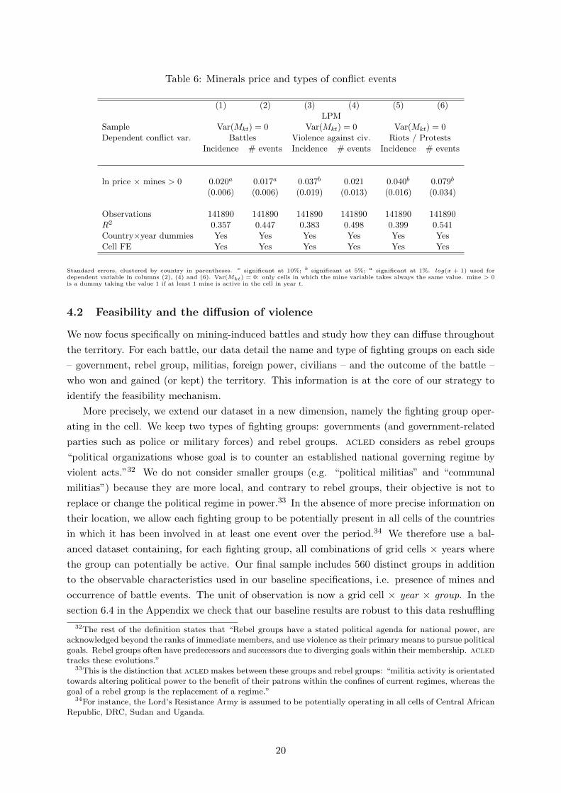
Table 6: Minerals price and types of conflict events

(1) (2) (3) (4) (5) (6)LPM

Sample Var(Mkt) = 0 Var(Mkt) = 0 Var(Mkt) = 0Dependent conflict var. Battles Violence against civ. Riots / Protests

Incidence # events Incidence # events Incidence # events

ln price × mines > 0 0.020a 0.017a 0.037b 0.021 0.040b 0.079b

(0.006) (0.006) (0.019) (0.013) (0.016) (0.034)

Observations 141890 141890 141890 141890 141890 141890R2 0.357 0.447 0.383 0.498 0.399 0.541Country×year dummies Yes Yes Yes Yes Yes YesCell FE Yes Yes Yes Yes Yes Yes

Standard errors, clustered by country in parentheses. c significant at 10%; b significant at 5%; a significant at 1%. log(x + 1) used fordependent variable in columns (2), (4) and (6). Var(Mkt) = 0: only cells in which the mine variable takes always the same value. mine > 0is a dummy taking the value 1 if at least 1 mine is active in the cell in year t.

4.2 Feasibility and the diffusion of violence

We now focus specifically on mining-induced battles and study how they can diffuse throughout

the territory. For each battle, our data detail the name and type of fighting groups on each side

– government, rebel group, militias, foreign power, civilians – and the outcome of the battle –

who won and gained (or kept) the territory. This information is at the core of our strategy to

identify the feasibility mechanism.

More precisely, we extend our dataset in a new dimension, namely the fighting group oper-

ating in the cell. We keep two types of fighting groups: governments (and government-related

parties such as police or military forces) and rebel groups. acled considers as rebel groups

“political organizations whose goal is to counter an established national governing regime by

violent acts.”32 We do not consider smaller groups (e.g. “political militias” and “communal

militias”) because they are more local, and contrary to rebel groups, their objective is not to

replace or change the political regime in power.33 In the absence of more precise information on

their location, we allow each fighting group to be potentially present in all cells of the countries

in which it has been involved in at least one event over the period.34 We therefore use a bal-

anced dataset containing, for each fighting group, all combinations of grid cells × years where

the group can potentially be active. Our final sample includes 560 distinct groups in addition

to the observable characteristics used in our baseline specifications, i.e. presence of mines and

occurrence of battle events. The unit of observation is now a grid cell × year × group. In the

section 6.4 in the Appendix we check that our baseline results are robust to this data reshuffling

32The rest of the definition states that “Rebel groups have a stated political agenda for national power, areacknowledged beyond the ranks of immediate members, and use violence as their primary means to pursue politicalgoals. Rebel groups often have predecessors and successors due to diverging goals within their membership. acledtracks these evolutions.”

33This is the distinction that acled makes between these groups and rebel groups: “militia activity is orientatedtowards altering political power to the benefit of their patrons within the confines of current regimes, whereas thegoal of a rebel group is the replacement of a regime.”

34For instance, the Lord’s Resistance Army is assumed to be potentially operating in all cells of Central AfricanRepublic, DRC, Sudan and Uganda.

20

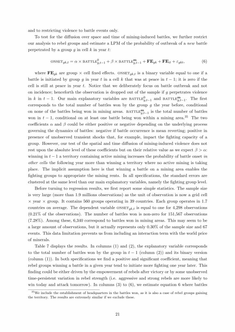
and to restricting violence to battle events only.

To test for the diffusion over space and time of mining-induced battles, we further restrict

our analysis to rebel groups and estimate a LPM of the probability of outbreak of a new battle

perpetrated by a group g in cell k in year t:

onsetgk,t = α× battle0g,t−1 + β × battlemg,t−1 + FEgk + FEit + εgkt, (6)

where FEgk are group × cell fixed effects. onsetgk,t is a binary variable equal to one if a

battle is initiated by group g in year t in a cell k that was at peace in t − 1; it is zero if the

cell is still at peace in year t. Notice that we deliberately focus on battle outbreak and not

on incidence; henceforth the observation is dropped out of the sample if g perpetrates violence

in k in t − 1. Our main explanatory variables are battle0g,t−1 and battlemg,t−1. The first

corresponds to the total number of battles won by the group g the year before, conditional

on none of the battles being won in mining areas. battlemg,t−1 is the total number of battles

won in t − 1, conditional on at least one battle being won within a mining area.35 The two

coefficients α and β could be either positive or negative depending on the underlying process

governing the dynamics of battles: negative if battle occurrence is mean reverting; positive in

presence of unobserved transient shocks that, for example, impact the fighting capacity of a

group. However, our test of the spatial and time diffusion of mining-induced violence does not

rest upon the absolute level of these coefficients but on their relative value as we expect β > α:

winning in t− 1 a territory containing active mining increases the probability of battle onset in

other cells the following year more than winning a territory where no active mining is taking

place. The implicit assumption here is that winning a battle on a mining area enables the

fighting groups to appropriate the mining rents. In all specifications, the standard errors are

clustered at the same level than our main explanatory variables, namely the fighting group level.

Before turning to regression results, we first report some simple statistics. The sample size

is very large (more than 1.9 millions observations) as the unit of observation is now a grid cell

× year × group. It contains 560 groups operating in 39 countries. Each group operates in 1.7

countries on average. The dependent variable onsetgk,t is equal to one for 4,298 observations

(0.21% of the observations). The number of battles won is non-zero for 151,567 observations

(7.28%). Among these, 6,340 correspond to battles won in mining areas. This may seem to be

a large amount of observations, but it actually represents only 0.30% of the sample size and 67

events. This data limitation prevents us from including an interaction term with the world price

of minerals.

Table 7 displays the results. In columns (1) and (2), the explanatory variable corresponds

to the total number of battles won by the group in t − 1 (column (2)) and its binary version

(column (1)). In both specifications we find a positive and significant coefficient, meaning that

rebel groups winning a battle in a given year tend to initiate more fighting one year later. This

finding could be either driven by the empowerment of rebels after victory or by some unobserved

time-persistent variation in rebel strength (i.e. aggressive and strong rebels are more likely to

win today and attack tomorrow). In columns (3) to (6), we estimate equation 6 where battles

35We include the establishment of headquarters in the battles won, as it is also a case of rebel groups gainingthe territory. The results are extremely similar if we exclude these.

21

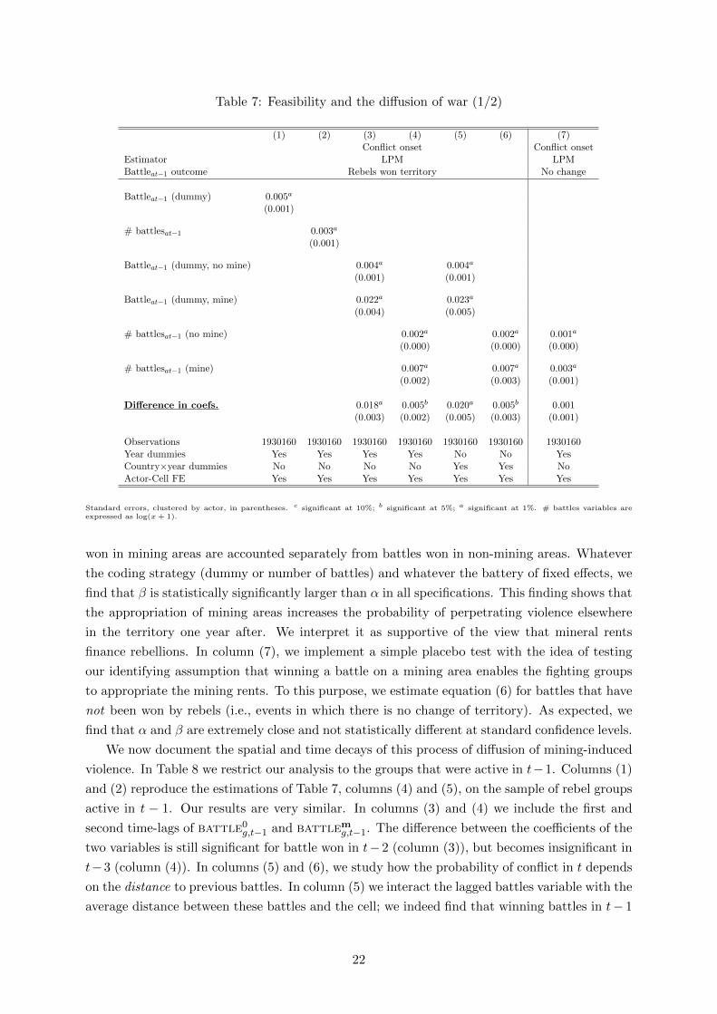
Table 7: Feasibility and the diffusion of war (1/2)

(1) (2) (3) (4) (5) (6) (7)Conflict onset Conflict onset

Estimator LPM LPMBattleat−1 outcome Rebels won territory No change

Battleat−1 (dummy) 0.005a

(0.001)

# battlesat−1 0.003a

(0.001)

Battleat−1 (dummy, no mine) 0.004a 0.004a

(0.001) (0.001)

Battleat−1 (dummy, mine) 0.022a 0.023a

(0.004) (0.005)

# battlesat−1 (no mine) 0.002a 0.002a 0.001a

(0.000) (0.000) (0.000)

# battlesat−1 (mine) 0.007a 0.007a 0.003a

(0.002) (0.003) (0.001)

Difference in coefs. 0.018a 0.005b 0.020a 0.005b 0.001(0.003) (0.002) (0.005) (0.003) (0.001)

Observations 1930160 1930160 1930160 1930160 1930160 1930160 1930160Year dummies Yes Yes Yes Yes No No YesCountry×year dummies No No No No Yes Yes NoActor-Cell FE Yes Yes Yes Yes Yes Yes Yes

Standard errors, clustered by actor, in parentheses. c significant at 10%; b significant at 5%; a significant at 1%. # battles variables areexpressed as log(x + 1).

won in mining areas are accounted separately from battles won in non-mining areas. Whatever

the coding strategy (dummy or number of battles) and whatever the battery of fixed effects, we

find that β is statistically significantly larger than α in all specifications. This finding shows that

the appropriation of mining areas increases the probability of perpetrating violence elsewhere

in the territory one year after. We interpret it as supportive of the view that mineral rents

finance rebellions. In column (7), we implement a simple placebo test with the idea of testing

our identifying assumption that winning a battle on a mining area enables the fighting groups

to appropriate the mining rents. To this purpose, we estimate equation (6) for battles that have

not been won by rebels (i.e., events in which there is no change of territory). As expected, we

find that α and β are extremely close and not statistically different at standard confidence levels.

We now document the spatial and time decays of this process of diffusion of mining-induced

violence. In Table 8 we restrict our analysis to the groups that were active in t−1. Columns (1)

and (2) reproduce the estimations of Table 7, columns (4) and (5), on the sample of rebel groups

active in t − 1. Our results are very similar. In columns (3) and (4) we include the first and

second time-lags of battle0g,t−1 and battlemg,t−1. The difference between the coefficients of the

two variables is still significant for battle won in t− 2 (column (3)), but becomes insignificant in

t−3 (column (4)). In columns (5) and (6), we study how the probability of conflict in t depends

on the distance to previous battles. In column (5) we interact the lagged battles variable with the

average distance between these battles and the cell; we indeed find that winning battles in t− 1

22

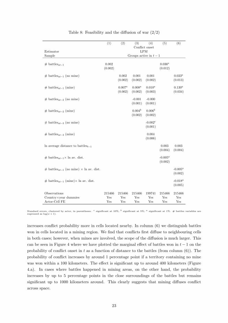
Table 8: Feasibility and the diffusion of war (2/2)

(1) (2) (3) (4) (5) (6)Conflict onset

Estimator LPMSample Groups active in t− 1

# battlesat−1 0.002 0.036a

(0.002) (0.012)

# battlesat−1 (no mine) 0.002 0.001 0.001 0.033a

(0.002) (0.002) (0.002) (0.013)

# battlesat−1 (mine) 0.007a 0.008a 0.010a 0.130a

(0.002) (0.002) (0.003) (0.034)

# battlesat−2 (no mine) -0.001 -0.000(0.001) (0.001)

# battlesat−2 (mine) 0.004b 0.006b

(0.002) (0.002)

# battlesat−3 (no mine) -0.002c

(0.001)

# battlesat−3 (mine) 0.004(0.006)

ln average distance to battlest−1 0.003 0.003(0.004) (0.004)

# battlesat−1× ln av. dist. -0.005a

(0.002)

# battlesat−1 (no mine) × ln av. dist. -0.005a

(0.002)

# battlesat−1 (mine)× ln av. dist. -0.018a

(0.005)

Observations 215466 215466 215466 199741 215466 215466Country×year dummies Yes Yes Yes Yes Yes YesActor-Cell FE Yes Yes Yes Yes Yes Yes

Standard errors, clustered by actor, in parentheses. c significant at 10%; b significant at 5%; a significant at 1%. # battles variables areexpressed as log(x + 1).

increases conflict probability more in cells located nearby. In column (6) we distinguish battles

won in cells located in a mining region. We find that conflicts first diffuse to neighbouring cells

in both cases; however, when mines are involved, the scope of the diffusion is much larger. This

can be seen in Figure 4 where we have plotted the marginal effect of battles won in t− 1 on the

probability of conflict onset in t as a function of distance to the battles (from column (6)). The

probability of conflict increases by around 1 percentage point if a territory containing no mine

was won within a 100 kilometers. The effect is significant up to around 400 kilometers (Figure

4.a). In cases where battles happened in mining areas, on the other hand, the probability

increases by up to 5 percentage points in the close surroundings of the battles but remains

significant up to 1000 kilometers around. This clearly suggests that mining diffuses conflict

across space.

23

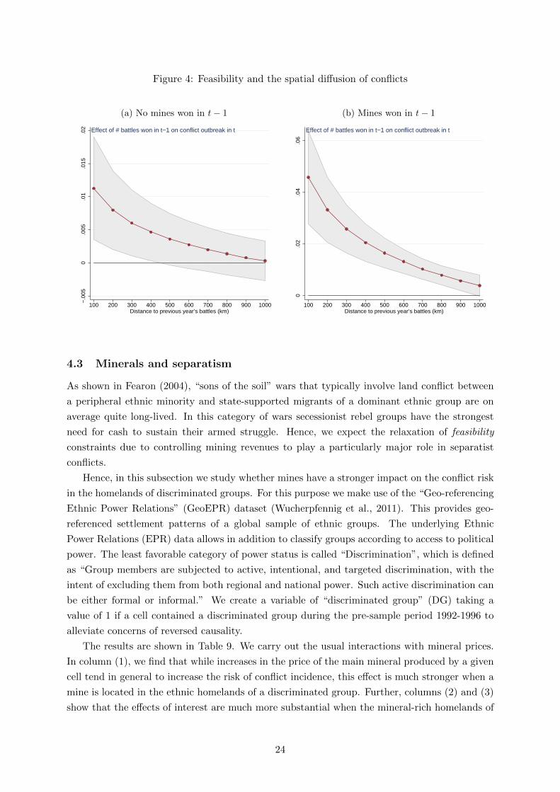
Figure 4: Feasibility and the spatial diffusion of conflicts

(a) No mines won in t− 1 (b) Mines won in t− 1

−.0

050

.005

.01

.015

.02

100 200 300 400 500 600 700 800 900 1000Distance to previous year’s battles (km)

Effect of # battles won in t−1 on conflict outbreak in t

0.0

2.0

4.0

6

100 200 300 400 500 600 700 800 900 1000Distance to previous year’s battles (km)

Effect of # battles won in t−1 on conflict outbreak in t

4.3 Minerals and separatism

As shown in Fearon (2004), “sons of the soil” wars that typically involve land conflict between

a peripheral ethnic minority and state-supported migrants of a dominant ethnic group are on

average quite long-lived. In this category of wars secessionist rebel groups have the strongest

need for cash to sustain their armed struggle. Hence, we expect the relaxation of feasibility

constraints due to controlling mining revenues to play a particularly major role in separatist

conflicts.

Hence, in this subsection we study whether mines have a stronger impact on the conflict risk

in the homelands of discriminated groups. For this purpose we make use of the “Geo-referencing

Ethnic Power Relations” (GeoEPR) dataset (Wucherpfennig et al., 2011). This provides geo-

referenced settlement patterns of a global sample of ethnic groups. The underlying Ethnic

Power Relations (EPR) data allows in addition to classify groups according to access to political

power. The least favorable category of power status is called “Discrimination”, which is defined

as “Group members are subjected to active, intentional, and targeted discrimination, with the

intent of excluding them from both regional and national power. Such active discrimination can

be either formal or informal.” We create a variable of “discriminated group” (DG) taking a

value of 1 if a cell contained a discriminated group during the pre-sample period 1992-1996 to

alleviate concerns of reversed causality.

The results are shown in Table 9. We carry out the usual interactions with mineral prices.

In column (1), we find that while increases in the price of the main mineral produced by a given

cell tend in general to increase the risk of conflict incidence, this effect is much stronger when a

mine is located in the ethnic homelands of a discriminated group. Further, columns (2) and (3)

show that the effects of interest are much more substantial when the mineral-rich homelands of

24

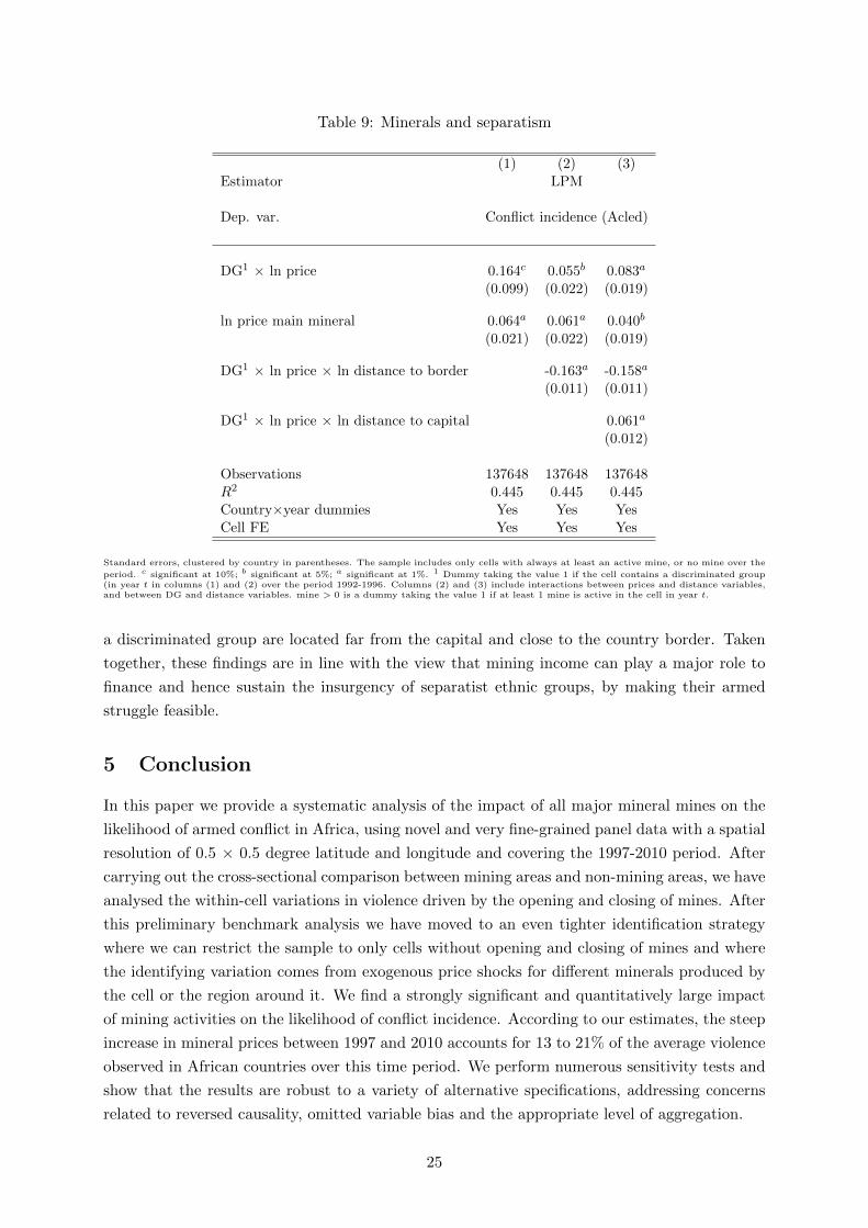
Table 9: Minerals and separatism

(1) (2) (3)Estimator LPM

Dep. var. Conflict incidence (Acled)

DG1 × ln price 0.164c 0.055b 0.083a

(0.099) (0.022) (0.019)

ln price main mineral 0.064a 0.061a 0.040b

(0.021) (0.022) (0.019)

DG1 × ln price × ln distance to border -0.163a -0.158a

(0.011) (0.011)

DG1 × ln price × ln distance to capital 0.061a

(0.012)

Observations 137648 137648 137648R2 0.445 0.445 0.445Country×year dummies Yes Yes YesCell FE Yes Yes Yes

Standard errors, clustered by country in parentheses. The sample includes only cells with always at least an active mine, or no mine over the

period. c significant at 10%; b significant at 5%; a significant at 1%. 1 Dummy taking the value 1 if the cell contains a discriminated group(in year t in columns (1) and (2) over the period 1992-1996. Columns (2) and (3) include interactions between prices and distance variables,and between DG and distance variables. mine > 0 is a dummy taking the value 1 if at least 1 mine is active in the cell in year t.

a discriminated group are located far from the capital and close to the country border. Taken

together, these findings are in line with the view that mining income can play a major role to

finance and hence sustain the insurgency of separatist ethnic groups, by making their armed

struggle feasible.

5 Conclusion

In this paper we provide a systematic analysis of the impact of all major mineral mines on the

likelihood of armed conflict in Africa, using novel and very fine-grained panel data with a spatial

resolution of 0.5 × 0.5 degree latitude and longitude and covering the 1997-2010 period. After

carrying out the cross-sectional comparison between mining areas and non-mining areas, we have

analysed the within-cell variations in violence driven by the opening and closing of mines. After

this preliminary benchmark analysis we have moved to an even tighter identification strategy

where we can restrict the sample to only cells without opening and closing of mines and where

the identifying variation comes from exogenous price shocks for different minerals produced by

the cell or the region around it. We find a strongly significant and quantitatively large impact

of mining activities on the likelihood of conflict incidence. According to our estimates, the steep

increase in mineral prices between 1997 and 2010 accounts for 13 to 21% of the average violence

observed in African countries over this time period. We perform numerous sensitivity tests and

show that the results are robust to a variety of alternative specifications, addressing concerns

related to reversed causality, omitted variable bias and the appropriate level of aggregation.

25

This first systematic disaggregate study of the causal impact of minerals on fighting has

the virtue of closing a gap in the literature on conflict. Maybe even more importantly, our

fine-grained data also allow us to carry out an in-depth analysis of possible mechanisms through

which mineral rents could fuel fighting efforts and lead to the diffusion of violence over space

and time. In particular, we have found that mining activity does not only increase the scope for

localised protests and riots, but that it also systematically fuels larger-scale battles. Importantly,

we have been able to show that winning a battle involving a mine empowers rebel groups and

leads them to intensify and spread their fighting activity in the successive periods, while winning

a battle outside a mining area does not have such a conflict diffusion effect. Our findings are

consistent with the view that rents from looted minerals can make it financially feasible for the

rebels to sustain insurgency over a longer period, which can result in longer-lasting wars. We

also find that the presence of mines has the strongest conflict inducing effect in the homelands of

discriminated ethnic groups being located in peripheral areas of the country, which is consistent

with recent theories of separatist warfare.

In future work, we plan to extend the approach in this paper to the study of how multinational

mining companies adapt to the conflict risk in mining areas. Other interesting research questions

include the impact of trade embargoes on particular mineral types (e.g. “blood diamonds”) and

the impact of the (public or private) ownership of mines on the conflict risk.

26

References

[1] ACLED (2013): “Armed Conflict Location Events Data”, dataset.

http://www.acleddata.com/.

[2] Angrist, Joshua and Adriana Kugler (2008): “Rural Windfall or a New Resource Curse?

Coca, Income, and Civil Conflict in Colombia”, Review of Economics and Statistics 90:

191-215.

[3] Aragon, Fernando, and Juan Pablo Rud (2013): “Natural Resources and Local Communi-

ties: Evidence from a Peruvian Gold Mine”, American Economic Journal: Economic Policy

5: 1-25.

[4] Bazzi, Samuel, and Chris Blattman (2013): “Economic Shocks and Conflict: The Evidence

from Commodity Prices”, forthcoming in American Economic Journal: Macroeconomics.

[5] Bell, Curtis, and Scott Wolford (2014): “Oil Discoveries, Shifting Power, and Civil Con-

flict,” forthcoming in International Studies Quarterly.

[6] Berman, Nicolas, and Mathieu Couttenier (2014): “External Shocks, Internal Shots: The

Geography of Civil Conflicts”, CEPR Discussion Paper No. 9895.

[7] Besley, Timothy, and Torsten Persson (2011): “The Logic of Political Violence”, Quarterly

Journal of Economics 126: 1411-1445.

[8] Besley, Timothy, and Marta Reynal-Querol (2013): “The Legacy of Historical Conflict:

Evidence from Africa”, forthcoming in American Political Science Review.

[9] Buonanno, Paolo, Ruben Durante, Giovanni Prarolo, and Paolo Vanin (2013): “Poor In-

stitutions, Rich Mines: Resource Curse and the Origins of the Sicilian Mafia ”, mimeo,

University of Bergamo, Sciences Po Paris, University of Bologna.

[10] Campbell, Greg (2002): Blood Diamonds: Tracing the Deadly Path of the World’s Most

Precious Stones, Boulder, Colorado: Westview Press.

[11] Caselli, Francesco and Wilbur John Coleman II (2013): “On the Theory of Ethnic Conflict,”

Journal of the European Economic Association 11: 161-192.

[12] Caselli, Francesco, Massimo Morelli, and Dominic Rohner (2013): “The Geography of Inter

State Resource Wars,” NBER working paper no. 18978.

[13] Cassar, Alessandra, Pauline Grosjean, and Sam Whitt (2013): “Legacies of violence: trust

and market development.” Journal of Economic Growth 18: 285-318.

[14] Charbonneau, Karyne (2012): “Multiple fixed effects in nonlinear panel data models: theory

and evidence ”, unpublished manuscript, Princeton University.

[15] Collier, Paul and Anke Hoeffler (2004): “Greed and Grievance in Civil War”, Oxford Eco-

nomic Papers 56: 563-95.

27

[16] Collier, Paul, Anke Hoeffler, and Dominic Rohner (2009): “Beyond Greed and Grievance:

Feasibility and Civil War”, Oxford Economic Papers 61: 1-27.

[17] Conley, Timothy G. (1999): “GMM Estimation with Cross Sectional Dependence”, Journal

of Econometrics 92: 1-45.

[18] Cotet, Anca M., and Kevin K. Tsui (2013): “Oil and Conflict: What Does the Cross

Country Evidence Really Show?”, American Economic Journal: Macroeconomics 5: 49-80.

[19] Couttenier, Mathieu, Pauline Grosjean, and Marc Sangnier (2014): “The Wild West is

Wild: The Homicide Resource Curse”, 2014, mimeo, University of Lausanne

[20] Dal Bo, Ernesto, and Pedro Dal Bo (2011): “Workers, Warriors, and Criminals: Social

Conflict in General Equilibrium”, Journal of European Economic Association 9: 646-677.

[21] De Koning, Ruben, (2010). “Demilitarizing Mining Areas in the Democratic Republic of the

Congo: The Case of Northern Katanga Province”, SIPRI Insights on Peace and Security

No. 2010/1.

[22] De Soysa, Indra (2002): “Paradise Is a Bazaar? Greed, Creed and Governance in Civil

War, 1989-99,” Journal of Peace Research 39: 395-416.

[23] Dietrich, Christian (2000): “Power struggles in the diamond fields” in Jakkie Cilliers and

Christian Dietrich (editors), Angola’s War Economy: The Role of Oil and Diamonds, Pre-

toria: Institute for Security Studies (ISS).

[24] Dube, Oendrila, and Suresh Naidu (2014): “Bases, Bullets and Ballots: the Effect of U.S.

Military Aid on Political Conflict in Colombia”, NBER Working Paper 20213.

[25] Dube, Oendrila, and Juan Vargas (2013): “Commodity Price Shocks and Civil Conflict:

Evidence from Colombia”, Review of Economics Studies 80: 1384–1421.

[26] Esteban, Joan, Massimo Morelli, and Dominic Rohner (2013): “Strategic Mass Killings,”

mimeo, IAE, Columbia University, and University of Zurich.

[27] Fearon, James (2004): “Why Do Some Civil Wars Last So Much Longer than Others?”

Journal of Peace Research 41: 275-301.

[28] Fearon, James (2005): “Primary Commodity Exports and Civil War,” Journal of Conflict

Resolution 49: 483-507.

[29] Fearon, James and David Laitin (2003): “Ethnicity, Insurgency, and Civil War,” American

Political Science Review 97: 75-90.

[30] Grossman, Herschel and Juan Mendoza (2003): “Scarcity and appropriative competition,”

European Journal of Political Economy 19: 747-58.

[31] Guidolin, Massimo, and Eliana La Ferrara (2007): “Diamonds Are Forever, Wars Are Not.

Is Conflict Bad for Private Firms?”, American Economic Review 97: 1978-93.

28

[32] Guidolin, Massimo, and Eliana La Ferrara (2010): “The Economic Effects of Violent Con-

flict: Evidence from Asset Market Reactions” Journal of Peace Research 47: 671-84.

[33] Henderson, Vernon, Adam Storeygard and David N. Weil (2012): “Measuring Economic

Growth from Outer Space”, American Economic Review 102: 994-1028.

[34] Hodler, Roland (2006): “The curse of natural resources in fractionalized countries,” Euro-

pean Economic Review 50: 1367-86.

[35] Hsiang, Solomon (2010): “Temperatures and cyclones strongly associated with economic

production in the Caribbean and Central America” Proceedings of the National Academy

of Sciences, 107: 15367-15372.

[36] Hsiang, Solomon, Kyle Meng, and Mark Cane (2011): “Civil Conflicts are Associated with

the Global Climate”, Nature 476: 438-441.

[37] Humphreys, Macartan (2005): “Natural Resources, Conflict, and Conflict Resolution: Un-

covering the Mechanisms,” Journal of Conflict Resolution 49: 508-37.

[38] La Ferrara, Eliana, and Mariaflavia Harari (2012): “Conflict, Climate and Cells: A Disag-

gregated Analysis”, IGIER Working Paper n. 461, 2012.

[39] Le Billon, Philippe (2001): “The political ecology of war: natural resources and armed

conflicts,” Political Geography 20: 561-584.

[40] Lei, Yu-Hsiang, and Guy Michaels (2011): “Do Giant Oil Field Discoveries Fuel Internal

Armed Conflicts?”, mimeo, LSE.

[41] Lujala, Paivi (2009): “Deadly Combat over Natural Resources: Gems, Petroleum, Drugs,

and the Severity of Armed Civil Conflict”, Journal of Conflict Resolution 53: 50-71.

[42] Lujala, Paivi (2010): “The Spoils of Nature: Armed Civil Conflict and Rebel Access to

Natural Resources,” Journal of Peace Research 47: 15-28.

[43] Lujala, Paivi, Nils Petter Gleditsch and Elisabeth Gilmore (2005): “A Diamond Curse?

Civil War and a Lootable Resource,” Journal of Conflict Resolution 49: 538-62.

[44] Maystadt, Jean-Francois, Giacomo De Luca, Petros G. Sekeris, and John Ulimwengu (2013):

“Mineral resources and conflicts in DRC: a case of ecological fallacy?”, forthcoming in

Oxford Economic Papers.

[45] Michalopoulos, Stelios, and Elias Papaioannou (2013): “The Long-Run effects of the Scram-

ble for Africa”, mimeo, Brown University.

[46] Morelli, Massimo, and Dominic Rohner (2013): “Resource Concentration and Civil Wars”,

mimeo, Columbia University and University of Lausanne.

[47] National Oceanic and Atmospheric Administration (2010): “Version 4 DMSP-OLS Night-

time Lights Time Series.” dataset.

http://www.ngdc.noaa.gov/dmsp/downloadV4composites.html#AXP.

29

[48] Nordhaus, William D (2006): “Geography and macroeconomics: New data and new find-

ings”, Proceedings of the National Academy of Sciences of the USA 103: 3510-3517. Data

available under http://gecon.yale.edu/.

[49] Nunn, Nathan, and Nancy Qian (2014): “U.S. Food Aid and Civil Conflict”, forthcoming,

American Economic Review.

[50] PITF (2013): “Political Instability Task Force Worldwide Atrocities Event Data”, dataset,

http://web.ku.edu/keds/data.dir/atrocities.html.

[51] Ploeg, Frederick van der and Dominic Rohner (2012): “War and Natural Resource Ex-

ploitation,” European Economic Review 56: 1714-1729.

[52] PRIO (2013): PRIO-GRID, dataset, http://www.prio.no/Data/PRIO-GRID/.

[53] Reuveny, Rafael and John Maxwell (2001): “Conflict and Renewable Resources,” Journal

of Conflict Resolution 45: 719-42.

[54] Rohner, Dominic, Mathias Thoenig, and Fabrizio Zilibotti (2013): “War Signals: A Theory

of Trade, Trust and Conflict”, Review of Economic Studies 80: 1114-1147.

[55] Rohner, Dominic, Mathias Thoenig, and Fabrizio Zilibotti (2013b): “Seeds of Distrust?

Conflict in Uganda”, Journal of Economic Growth 18: 217-252.

[56] Ross, Michael (2004): “What Do We Know About Natural Resources and Civil War?”

Journal of Peace Research 41: 337-56.

[57] Ross, Michael (2006): “A closer look at oil, diamonds, and civil war”, Annual Review of

Political Science 9: 265–300.

[58] Wucherpfennig, Julian, Nils B. Weidmann, Luc Girardin, Lars-Erik Cederman, and Andreas

Wimmer (2011): “Politically Relevant Ethnic Groups across Space and Time: Introducing

the GeoEPR Dataset”, Conflict Management and Peace Science 28: 423-437. Data available

under http://www.icr.ethz.ch/data/growup/geoepr-eth.

[59] IntierraRMG (2013): “SNL Metals & Mining”, dataset.

http://www.intierrarmg.com/Homepage.aspx.

30

6 Appendix

6.1 Additional data information

Massacre data: We rely on the “Political Instability Task Force Worldwide Atrocities Event

Data” (PITF, 2013), put together by the “Political Instability Task Force”, which has under

the direction of Barbara Harff provided the most widely used datasets on mass killings. PITF’s

Atrocities Event Data contains information on geo-referenced events of atrocities committed,

where “atrocities” are defined as “as implicitly or explicitly political, direct, and deliberate

violent action resulting in the death of noncombatant civilians”.

The Ethnic Power Relations Dataset : Further, we use the “Geo-referencing Ethnic Power

Relations” (GeoEPR) dataset (Wucherpfennig et al., 2011). This provides geo-referenced set-

tlement patterns of a global sample of ethnic groups. The underlying Ethnic Power Relations

(EPR) data allows in addition to classify groups according to access to political power. The

least favorable category of power status is called “Discrimination”, which is defined as “Group

members are subjected to active, intentional, and targeted discrimination, with the intent of

excluding them from both regional and national power. Such active discrimination can be either

formal or informal.” We create a variable of “discriminated group” (DG) taking a value of 1 if

a cell contains a discriminated group.

Country level conflict data: We use also information from the UCDP/PRIO Armed Conflict

Dataset (v4-2013) to measure the incidence of conflict at the country level. We use the civil

war incidence dummy variable, which is equal to 1 for years with a number of battle deaths

greater than 1000, and 0 otherwise; and civil conflict dummy which is equal to 1 for years with

a number of battle deaths greater than 25, and 0 otherwise.

Other location-specific data. Distance between the cell’s centroid and international borders

and to capital city are taken directly from prio-grid. Cell-specific GDP and population data

are also available in prio-grid, and originally come from G-econ 4.0 data (Nordhaus, 2006).

We proxy the level of economic activity with data on Satellite nightlight. This data comes from

the National Oceanic and Atmospheric Administration (2010). We use their data on Average

Visible, Stable Light & Cloud Free Coverages. In particular, we use their “cleaned” and “filtered”

version of the data, which “contains the lights from cities, towns, and other sites with persistent

lighting, including gas flares. Ephemeral events, such as fires have been discarded. Then the

background noise was identified and replaced with values of zero. Data values range from 1-63.”

Using ArcGIS we generate the average at cell-year level.

Price data. The data on mineral prices comes from the World Bank Commodity Prices

dataset. Data is available for the ten following minerals: aluminum, copper, diamond, gold,

iron, lead, nickel, platinum, silver, tin and zinc.

31

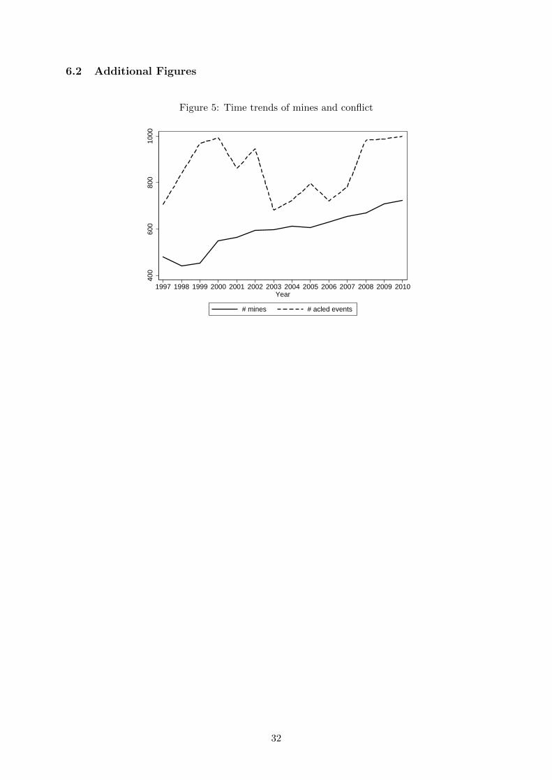
6.2 Additional Figures

Figure 5: Time trends of mines and conflict

400

600

800

1000

1997 1998 1999 2000 2001 2002 2003 2004 2005 2006 2007 2008 2009 2010Year

# mines # acled events

32

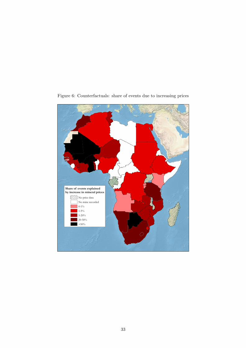
Figure 6: Counterfactuals: share of events due to increasing prices

Share of events explained by increase in mineral prices

No price dataNo mine recorded0-1%1-5%5-20%20-50%>50%

33

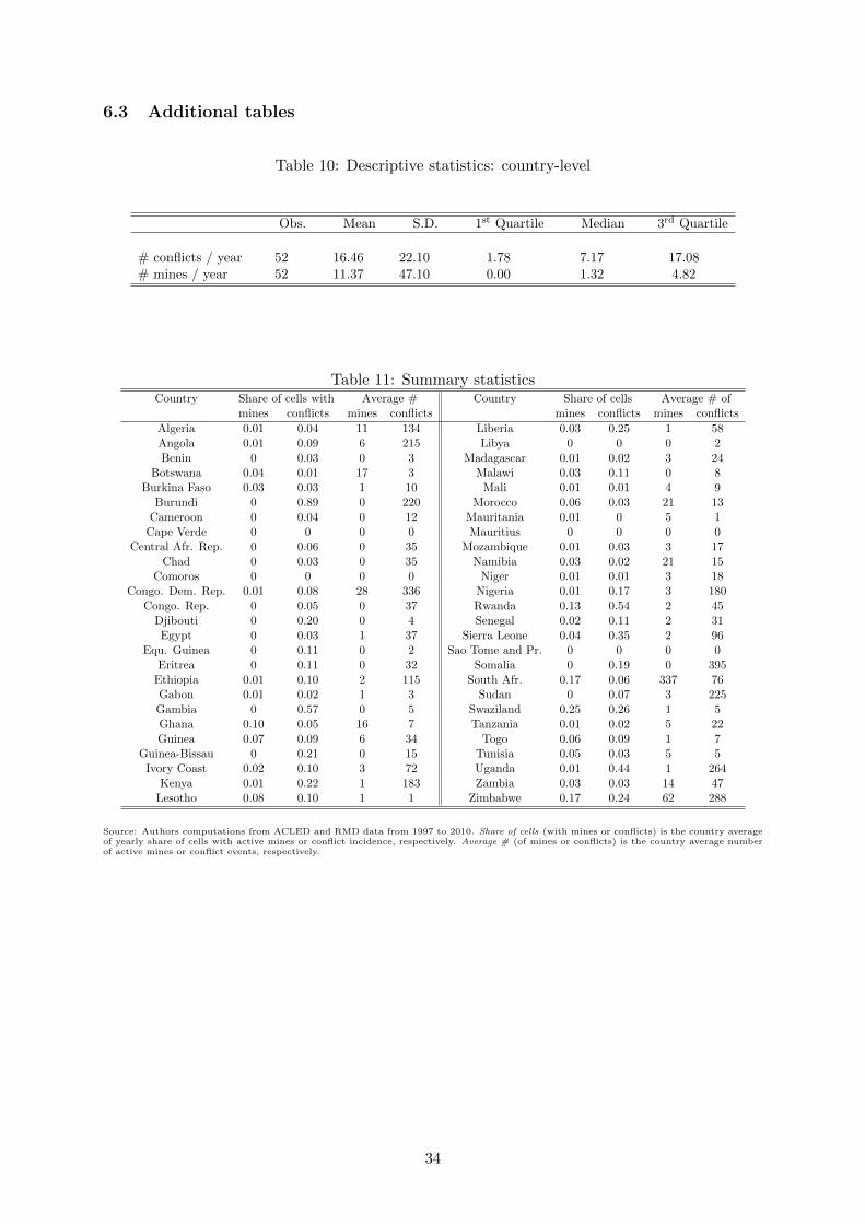
6.3 Additional tables

Table 10: Descriptive statistics: country-level

Obs. Mean S.D. 1st Quartile Median 3rd Quartile

# conflicts / year 52 16.46 22.10 1.78 7.17 17.08# mines / year 52 11.37 47.10 0.00 1.32 4.82

Table 11: Summary statisticsCountry Share of cells with Average # Country Share of cells Average # of

mines conflicts mines conflicts mines conflicts mines conflicts

Algeria 0.01 0.04 11 134 Liberia 0.03 0.25 1 58Angola 0.01 0.09 6 215 Libya 0 0 0 2Benin 0 0.03 0 3 Madagascar 0.01 0.02 3 24

Botswana 0.04 0.01 17 3 Malawi 0.03 0.11 0 8Burkina Faso 0.03 0.03 1 10 Mali 0.01 0.01 4 9

Burundi 0 0.89 0 220 Morocco 0.06 0.03 21 13Cameroon 0 0.04 0 12 Mauritania 0.01 0 5 1

Cape Verde 0 0 0 0 Mauritius 0 0 0 0Central Afr. Rep. 0 0.06 0 35 Mozambique 0.01 0.03 3 17

Chad 0 0.03 0 35 Namibia 0.03 0.02 21 15Comoros 0 0 0 0 Niger 0.01 0.01 3 18

Congo. Dem. Rep. 0.01 0.08 28 336 Nigeria 0.01 0.17 3 180Congo. Rep. 0 0.05 0 37 Rwanda 0.13 0.54 2 45

Djibouti 0 0.20 0 4 Senegal 0.02 0.11 2 31Egypt 0 0.03 1 37 Sierra Leone 0.04 0.35 2 96

Equ. Guinea 0 0.11 0 2 Sao Tome and Pr. 0 0 0 0Eritrea 0 0.11 0 32 Somalia 0 0.19 0 395

Ethiopia 0.01 0.10 2 115 South Afr. 0.17 0.06 337 76Gabon 0.01 0.02 1 3 Sudan 0 0.07 3 225Gambia 0 0.57 0 5 Swaziland 0.25 0.26 1 5Ghana 0.10 0.05 16 7 Tanzania 0.01 0.02 5 22Guinea 0.07 0.09 6 34 Togo 0.06 0.09 1 7

Guinea-Bissau 0 0.21 0 15 Tunisia 0.05 0.03 5 5Ivory Coast 0.02 0.10 3 72 Uganda 0.01 0.44 1 264

Kenya 0.01 0.22 1 183 Zambia 0.03 0.03 14 47Lesotho 0.08 0.10 1 1 Zimbabwe 0.17 0.24 62 288

Source: Authors computations from ACLED and RMD data from 1997 to 2010. Share of cells (with mines or conflicts) is the country averageof yearly share of cells with active mines or conflict incidence, respectively. Average # (of mines or conflicts) is the country average numberof active mines or conflict events, respectively.

34

Table 12: Conflicts and mineral prices: robustness (controlling for large players)

(1) (2) (3) (4) (5) (6)Estimator LPM LPM LPMSample All Var(Mkt) = 0 All Var(Mkt) = 0 All Var(Mkt) = 0

Dep. var. Conflict incidence # conflicts Conflict incidence

mine > 0 0.060 0.050(0.095) (0.115)

ln price main mineral -0.026 -0.042c 0.013(0.018) (0.025) (0.012)

ln price × mines > 0 0.091a 0.058b 0.144a 0.048a

(0.028) (0.023) (0.036) (0.017)

ln price × mines > 0 × large player 0.004 0.053 0.006 0.178b

(0.004) (0.040) (0.004) (0.084)

# mines 0.045b

(0.019)

ln price × # mines 0.016a 0.004a

(0.003) (0.001)

ln price × # mines × large player 0.001 -0.034a

(0.002) (0.010)

Observations 142817 141890 142817 141890 142926 141568R2 0.445 0.445 0.562 0.563 0.447 0.446Country×year dummies Yes Yes Yes Yes Yes YesCell FE Yes Yes Yes Yes Yes Yes

Standard errors, clustered by country, in parentheses. c significant at 10%; b significant at 5%; a significant at 1%. This table is the sameas Table 4, except that cells producing minerals for which the country is among the top 10 of world producers are removed from the sample.Var(Mkt) = 0: only cells in which the mine variable takes always the same value over the period. All estimations include controls for theaverage level of mineral world price interacted with the mines variables. mine > 0 is a dummy taking the value 1 if at least 1 mine is activein the cell in year t. # mines is the number of active mines in the cell in year t. log(x + 1) used for dependent variable in columns (3) and(4). ln price main mineral is the world price of the mineral with the highest average production in the cell over the period.

35

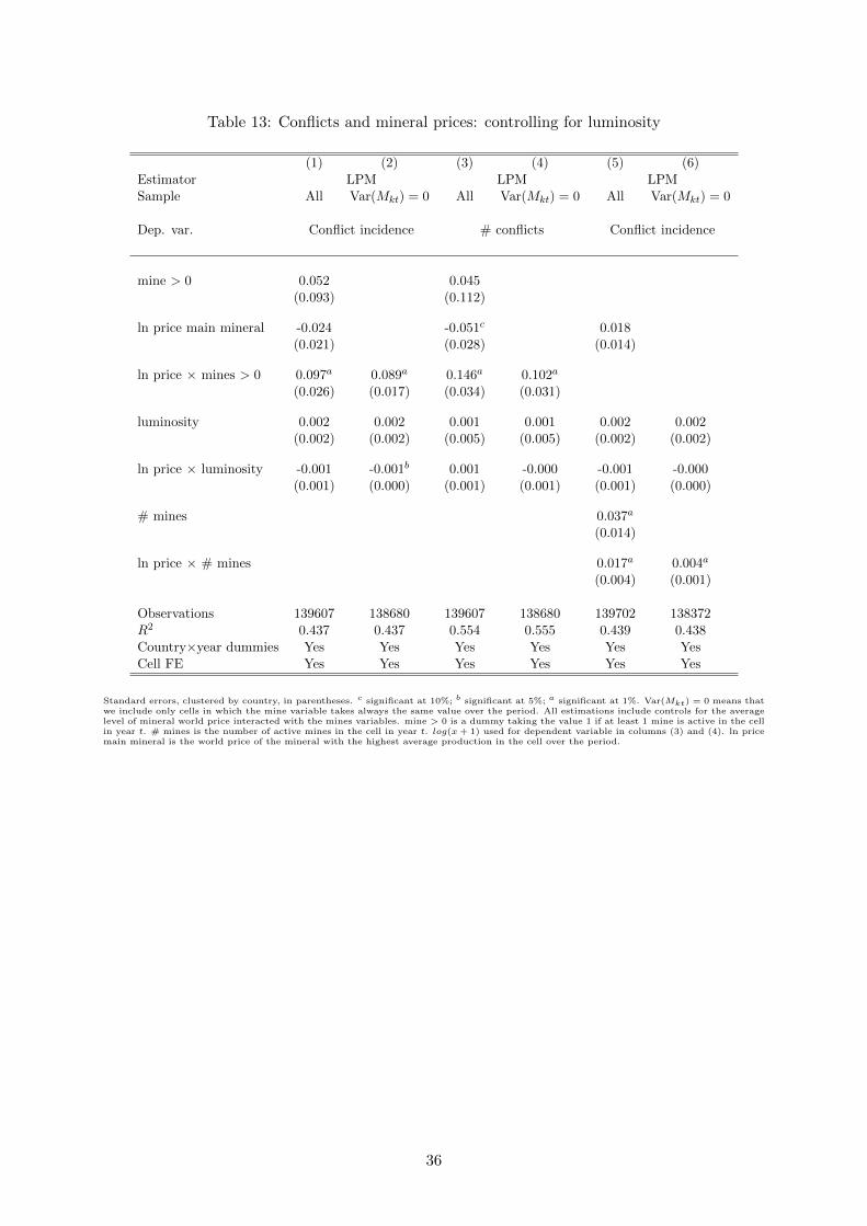
Table 13: Conflicts and mineral prices: controlling for luminosity

(1) (2) (3) (4) (5) (6)Estimator LPM LPM LPMSample All Var(Mkt) = 0 All Var(Mkt) = 0 All Var(Mkt) = 0

Dep. var. Conflict incidence # conflicts Conflict incidence

mine > 0 0.052 0.045(0.093) (0.112)

ln price main mineral -0.024 -0.051c 0.018(0.021) (0.028) (0.014)

ln price × mines > 0 0.097a 0.089a 0.146a 0.102a

(0.026) (0.017) (0.034) (0.031)

luminosity 0.002 0.002 0.001 0.001 0.002 0.002(0.002) (0.002) (0.005) (0.005) (0.002) (0.002)

ln price × luminosity -0.001 -0.001b 0.001 -0.000 -0.001 -0.000(0.001) (0.000) (0.001) (0.001) (0.001) (0.000)

# mines 0.037a

(0.014)

ln price × # mines 0.017a 0.004a

(0.004) (0.001)

Observations 139607 138680 139607 138680 139702 138372R2 0.437 0.437 0.554 0.555 0.439 0.438Country×year dummies Yes Yes Yes Yes Yes YesCell FE Yes Yes Yes Yes Yes Yes

Standard errors, clustered by country, in parentheses. c significant at 10%; b significant at 5%; a significant at 1%. Var(Mkt) = 0 means thatwe include only cells in which the mine variable takes always the same value over the period. All estimations include controls for the averagelevel of mineral world price interacted with the mines variables. mine > 0 is a dummy taking the value 1 if at least 1 mine is active in the cellin year t. # mines is the number of active mines in the cell in year t. log(x + 1) used for dependent variable in columns (3) and (4). ln pricemain mineral is the world price of the mineral with the highest average production in the cell over the period.

36

Table 14: Conflicts and mineral prices: additional controls

(1) (2) (3) (4) (5) (6) (7) (8) (9)Estimator LPM LPM LPMSample Var(Mkt) = 0 Var(Mkt) = 0 Var(Mkt) = 0

Dep. var. Incidence # conflicts Incidence Incidence # conflicts Incidence Incidence # conflicts Incidence

ln price × mines > 0 0.105a 0.151a 0.064a 0.067b 0.071a 0.084b

(0.022) (0.047) (0.020) (0.034) (0.022) (0.034)

ln price × # mines 0.005a 0.004a 0.004a

(0.001) (0.001) (0.001)

temperature × mines > 0 0.028 0.027 0.024(0.018) (0.035) (0.015)

rainfall × mines > 0 -0.014 -0.141 -0.056(0.066) (0.163) (0.040)

ln price × # neighb. cells in conflict 0.000 0.004b -0.001(0.001) (0.002) (0.001)

ln price × # past conflicts in cell 0.004 0.019b 0.004a

(0.003) (0.008) (0.001)

Observations 118884 118884 118608 137900 137900 137578 141890 141890 141568R2 0.446 0.567 0.446 0.448 0.563 0.448 0.445 0.563 0.446Country×year dummies Yes Yes Yes Yes Yes Yes Yes Yes YesCell FE Yes Yes Yes Yes Yes Yes Yes Yes Yes

Standard errors, clustered by country, in parentheses. c significant at 10%; b significant at 5%; a significant at 1%. Var(Mkt) = 0 means thatwe include only cells in which the mine variable takes always the same value over the period. All estimations include controls for the averagelevel of mineral world price interacted with the mines variables. mine > 0 is a dummy taking the value 1 if at least 1 mine is active in the cellin year t. # mines is the number of active mines in the cell in year t. log(x + 1) used for dependent variable in columns (2) and (5) and (8).ln price main mineral is the world price of the mineral with the highest average production in the cell over the period.

37

Table 15: Conflicts and mineral prices: cells with permanent active mine(s)

(1) (2) (3) (4)Estimator LPM LPM

Conflict incidenceSample Var(Mkt) = 0 Permanent active mine(s) Var(Mkt) = 0 Permanent active mine(s)

ln price × mines > 0 0.073a 0.049 0.082a 0.082a

(0.020) (0.102) (0.025) (0.026)

Observations 141890 952 141890 952Country×year dummies Yes Yes No NoCell FE Yes Yes Yes Yes

Standard errors, clustered by country, in parentheses. c significant at 10%; b significant at 5%; a significant at 1%. Var(Mkt) = 0: only cellsin which the mine variable takes always the same value over the period. All estimations include controls for the average level of mineral worldprice interacted with the mines variables. mine > 0 is a dummy taking the value 1 if at least 1 mine is active in the cell in year t. ln pricemain mineral is the world price of the mineral with the highest average production in the cell over the period.

38

Table 16: Mineral and price: 1×1 degrees cells

(1) (2) (3) (4) (5) (6)Estimator LPM LPM LPMDep. var. Conflict incidence # conflicts Conflict incidenceSample All Var(Mkt) = 0 All Var(Mkt) = 0 All Var(Mkt) = 0

mine > 0 -0.027 -0.035(0.089) (0.157)

ln price main mineral -0.003 0.027 0.042b

(0.032) (0.081) (0.019)

ln price × mines > 0 0.089b 0.098a 0.105 0.122b

(0.043) (0.032) (0.096) (0.057)

# mines 0.043b

(0.019)

ln price × # mines 0.009a 0.002(0.003) (0.002)

Observations 36515 35826 36515 35826 36624 35672R2 0.522 0.521 0.639 0.639 0.525 0.525Country×year dummies Yes Yes Yes Yes Yes YesCell FE Yes Yes Yes Yes Yes Yes

Standard errors, clustered by country, in parentheses. c significant at 10%; b significant at 5%; a significant at 1%. Var(Mkt) = 0: only cellsin which the mine variable takes always the same value over the period. mine > 0 is a dummy taking the value 1 if at least 1 mine is activein the cell in year t. log(x + 1) used for dependent variable in columns (3) and (4). # mines is the number of active mines in the cell in yeart. ln price main mineral is the world price of the mineral with the highest average production in the cell over the period.

39

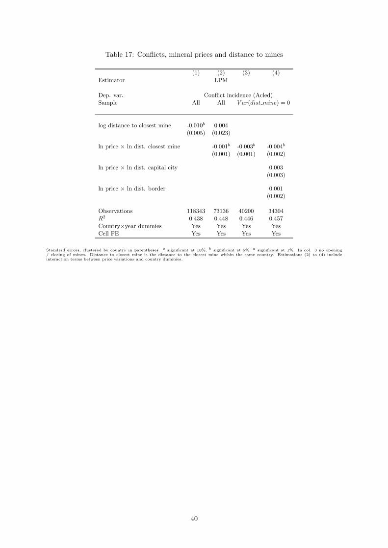
Table 17: Conflicts, mineral prices and distance to mines

(1) (2) (3) (4)Estimator LPM

Dep. var. Conflict incidence (Acled)Sample All All V ar(dist mine) = 0

log distance to closest mine -0.010b 0.004(0.005) (0.023)

ln price × ln dist. closest mine -0.001b -0.003b -0.004b

(0.001) (0.001) (0.002)

ln price × ln dist. capital city 0.003(0.003)

ln price × ln dist. border 0.001(0.002)

Observations 118343 73136 40200 34304R2 0.438 0.448 0.446 0.457Country×year dummies Yes Yes Yes YesCell FE Yes Yes Yes Yes

Standard errors, clustered by country in parentheses. c significant at 10%; b significant at 5%; a significant at 1%. In col. 3 no opening/ closing of mines. Distance to closest mine is the distance to the closest mine within the same country. Estimations (2) to (4) includeinteraction terms between price variations and country dummies.

40

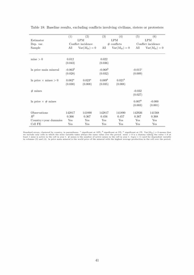
Table 18: Baseline results, excluding conflicts involving civilians, rioters or protesters

(1) (2) (3) (4) (5) (6)Estimator LPM LPM LPMDep. var. Conflict incidence # conflicts Conflict incidenceSample All Var(Mkt) = 0 All Var(Mkt) = 0 All Var(Mkt) = 0

mine > 0 0.012 0.022(0.043) (0.036)

ln price main mineral -0.063b -0.068b -0.015c

(0.028) (0.032) (0.009)

ln price × mines > 0 0.082a 0.023a 0.089b 0.021b

(0.030) (0.008) (0.035) (0.008)

# mines -0.032(0.027)

ln price × # mines 0.007b -0.000(0.003) (0.001)

Observations 142817 141890 142817 141890 142926 141568R2 0.366 0.367 0.456 0.457 0.367 0.368Country×year dummies Yes Yes Yes Yes Yes YesCell FE Yes Yes Yes Yes Yes Yes

Standard errors, clustered by country, in parentheses. c significant at 10%; b significant at 5%; a significant at 1%. Var(Mkt) = 0 means thatwe include only cells in which the mine variable takes always the same value over the period. mine > 0 is a dummy taking the value 1 if atleast 1 mine is active in the cell in year t. # mines is the number of active mines in the cell in year t. log(x + 1) used for dependent variablein columns (3) and (4). ln price main mineral is the world price of the mineral with the highest average production in the cell over the period.

41

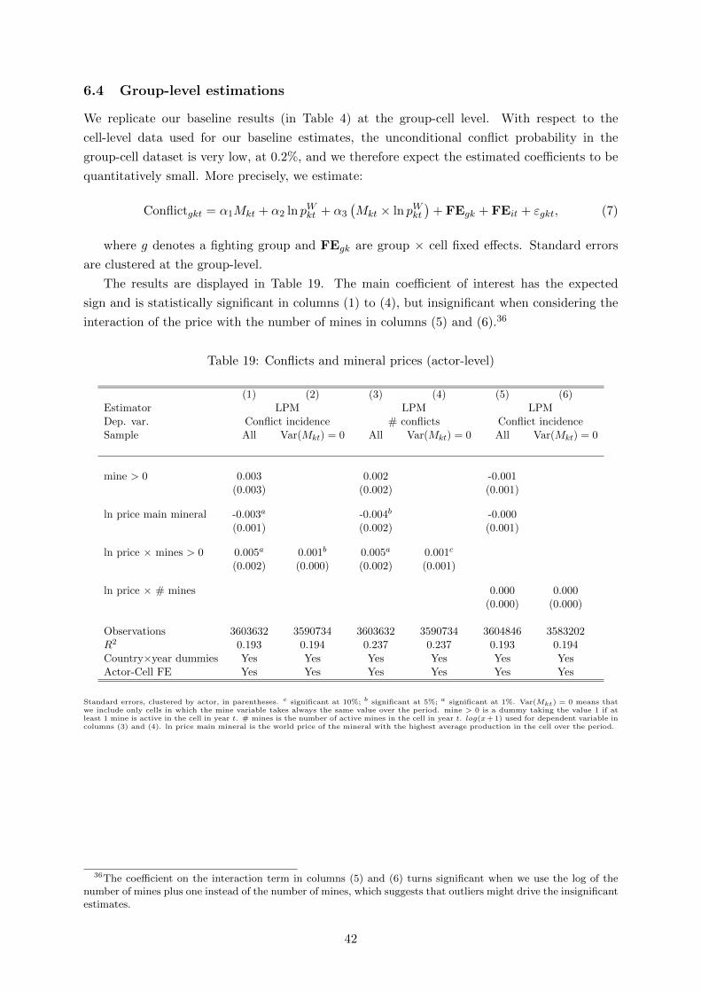
6.4 Group-level estimations

We replicate our baseline results (in Table 4) at the group-cell level. With respect to the

cell-level data used for our baseline estimates, the unconditional conflict probability in the

group-cell dataset is very low, at 0.2%, and we therefore expect the estimated coefficients to be

quantitatively small. More precisely, we estimate:

Conflictgkt = α1Mkt + α2 ln pWkt + α3

(Mkt × ln pWkt

)+ FEgk + FEit + εgkt, (7)

where g denotes a fighting group and FEgk are group × cell fixed effects. Standard errors

are clustered at the group-level.

The results are displayed in Table 19. The main coefficient of interest has the expected

sign and is statistically significant in columns (1) to (4), but insignificant when considering the

interaction of the price with the number of mines in columns (5) and (6).36

Table 19: Conflicts and mineral prices (actor-level)

(1) (2) (3) (4) (5) (6)Estimator LPM LPM LPMDep. var. Conflict incidence # conflicts Conflict incidenceSample All Var(Mkt) = 0 All Var(Mkt) = 0 All Var(Mkt) = 0

mine > 0 0.003 0.002 -0.001(0.003) (0.002) (0.001)

ln price main mineral -0.003a -0.004b -0.000(0.001) (0.002) (0.001)

ln price × mines > 0 0.005a 0.001b 0.005a 0.001c

(0.002) (0.000) (0.002) (0.001)

ln price × # mines 0.000 0.000(0.000) (0.000)

Observations 3603632 3590734 3603632 3590734 3604846 3583202R2 0.193 0.194 0.237 0.237 0.193 0.194Country×year dummies Yes Yes Yes Yes Yes YesActor-Cell FE Yes Yes Yes Yes Yes Yes

Standard errors, clustered by actor, in parentheses. c significant at 10%; b significant at 5%; a significant at 1%. Var(Mkt) = 0 means thatwe include only cells in which the mine variable takes always the same value over the period. mine > 0 is a dummy taking the value 1 if atleast 1 mine is active in the cell in year t. # mines is the number of active mines in the cell in year t. log(x+1) used for dependent variable incolumns (3) and (4). ln price main mineral is the world price of the mineral with the highest average production in the cell over the period.

36The coefficient on the interaction term in columns (5) and (6) turns significant when we use the log of thenumber of mines plus one instead of the number of mines, which suggests that outliers might drive the insignificantestimates.

42

This mine is mine!

How minerals fuel conflicts in Africa

Online Appendix

Nicolas Berman∗ Mathieu Couttenier† Dominic Rohner‡ Mathias Thoenig§

July 23, 2014

∗Graduate Institute of International and Development Studies and CEPR. E-mail: nico-las.berman@graduateinstitute.ch.†Department of Economics, University of Lausanne. E-mail: mathieu.couttenier@unil.ch‡Department of Economics, University of Lausanne. E-mail: dominic.rohner@unil.ch.§Department of Economics, University of Lausanne and CEPR. E-mail: mathias.thoenig@unil.ch.

Contents

1 Minerals and conflict: more correlations ii

2 Conflicts, minerals and prices: further robustness iv

3 Additional quantifications xii

4 Maps xiii

5 Mineral prices xvi

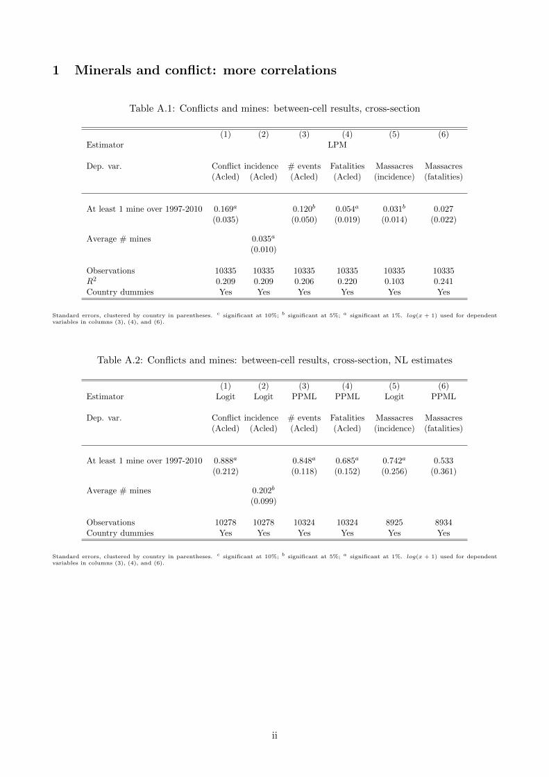
1 Minerals and conflict: more correlations

Table A.1: Conflicts and mines: between-cell results, cross-section

(1) (2) (3) (4) (5) (6)Estimator LPM

Dep. var. Conflict incidence # events Fatalities Massacres Massacres(Acled) (Acled) (Acled) (Acled) (incidence) (fatalities)

At least 1 mine over 1997-2010 0.169a 0.120b 0.054a 0.031b 0.027(0.035) (0.050) (0.019) (0.014) (0.022)

Average # mines 0.035a

(0.010)

Observations 10335 10335 10335 10335 10335 10335R2 0.209 0.209 0.206 0.220 0.103 0.241Country dummies Yes Yes Yes Yes Yes Yes

Standard errors, clustered by country in parentheses. c significant at 10%; b significant at 5%; a significant at 1%. log(x + 1) used for dependentvariables in columns (3), (4), and (6).

Table A.2: Conflicts and mines: between-cell results, cross-section, NL estimates

(1) (2) (3) (4) (5) (6)Estimator Logit Logit PPML PPML Logit PPML

Dep. var. Conflict incidence # events Fatalities Massacres Massacres(Acled) (Acled) (Acled) (Acled) (incidence) (fatalities)

At least 1 mine over 1997-2010 0.888a 0.848a 0.685a 0.742a 0.533(0.212) (0.118) (0.152) (0.256) (0.361)

Average # mines 0.202b

(0.099)

Observations 10278 10278 10324 10324 8925 8934Country dummies Yes Yes Yes Yes Yes Yes

Standard errors, clustered by country in parentheses. c significant at 10%; b significant at 5%; a significant at 1%. log(x + 1) used for dependentvariables in columns (3), (4), and (6).

ii

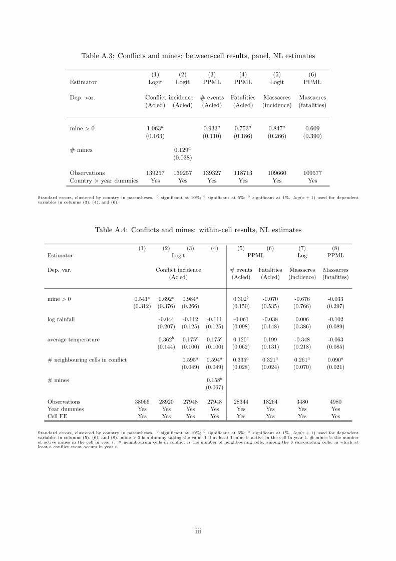
Table A.3: Conflicts and mines: between-cell results, panel, NL estimates

(1) (2) (3) (4) (5) (6)Estimator Logit Logit PPML PPML Logit PPML

Dep. var. Conflict incidence # events Fatalities Massacres Massacres(Acled) (Acled) (Acled) (Acled) (incidence) (fatalities)

mine > 0 1.063a 0.933a 0.753a 0.847a 0.609(0.163) (0.110) (0.186) (0.266) (0.390)

# mines 0.129a

(0.038)

Observations 139257 139257 139327 118713 109660 109577Country × year dummies Yes Yes Yes Yes Yes Yes

Standard errors, clustered by country in parentheses. c significant at 10%; b significant at 5%; a significant at 1%. log(x + 1) used for dependentvariables in columns (3), (4), and (6).

Table A.4: Conflicts and mines: within-cell results, NL estimates

(1) (2) (3) (4) (5) (6) (7) (8)Estimator Logit PPML Log PPML

Dep. var. Conflict incidence # events Fatalities Massacres Massacres(Acled) (Acled) (Acled) (incidence) (fatalities)

mine > 0 0.541c 0.692c 0.984a 0.302b -0.070 -0.676 -0.033(0.312) (0.376) (0.266) (0.150) (0.535) (0.766) (0.297)

log rainfall -0.044 -0.112 -0.111 -0.061 -0.038 0.006 -0.102(0.207) (0.125) (0.125) (0.098) (0.148) (0.386) (0.089)

average temperature 0.362b 0.175c 0.175c 0.120c 0.199 -0.348 -0.063(0.144) (0.100) (0.100) (0.062) (0.131) (0.218) (0.085)

# neighbouring cells in conflict 0.595a 0.594a 0.335a 0.321a 0.261a 0.090a

(0.049) (0.049) (0.028) (0.024) (0.070) (0.021)

# mines 0.158b

(0.067)

Observations 38066 28920 27948 27948 28344 18264 3480 4980Year dummies Yes Yes Yes Yes Yes Yes Yes YesCell FE Yes Yes Yes Yes Yes Yes Yes Yes

Standard errors, clustered by country in parentheses. c significant at 10%; b significant at 5%; a significant at 1%. log(x + 1) used for dependentvariables in columns (5), (6), and (8). mine > 0 is a dummy taking the value 1 if at least 1 mine is active in the cell in year t. # mines is the numberof active mines in the cell in year t. # neighbouring cells in conflict is the number of neighbouring cells, among the 8 surrounding cells, in which atleast a conflict event occurs in year t.

iii

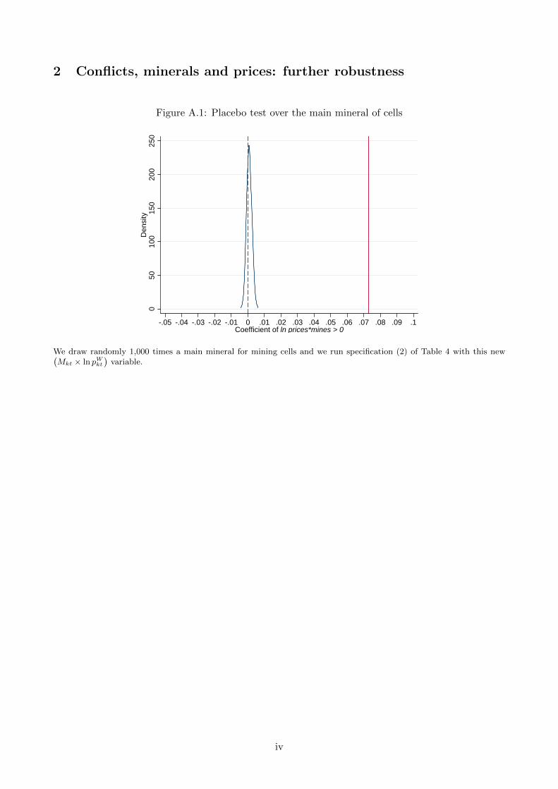
2 Conflicts, minerals and prices: further robustness

Figure A.1: Placebo test over the main mineral of cells

050

100

150

200

250

Den

sity

-.05 -.04 -.03 -.02 -.01 0 .01 .02 .03 .04 .05 .06 .07 .08 .09 .1Coefficient of ln prices*mines > 0

We draw randomly 1,000 times a main mineral for mining cells and we run specification (2) of Table 4 with this new(Mkt × ln pWkt

)variable.

iv

Table A.5: Conflicts and mineral prices: robustness (dropping large players)

(1) (2) (3) (4) (5) (6)Estimator LPM LPM LPMSample All Var(Mkt) = 0 All Var(Mkt) = 0 All Var(Mkt) = 0

Dep. var. Conflict incidence # conflicts Conflict incidence

mine > 0 0.090 0.076(0.111) (0.134)

ln price main mineral -0.042b -0.054c 0.002(0.018) (0.028) (0.015)

ln price × mines > 0 0.097a 0.058b 0.127a 0.049a

(0.033) (0.023) (0.043) (0.017)

# mines 0.034c

(0.019)

ln price × # mines 0.019c 0.004a

(0.010) (0.001)

Observations 142355 141610 142355 141610 142464 141498R2 0.444 0.444 0.561 0.561 0.446 0.446Country×year dummies Yes Yes Yes Yes Yes YesCell FE Yes Yes Yes Yes Yes Yes

Standard errors, clustered by country, in parentheses. This table is the same as Table 4, except that cells producing minerals for which the country is

among the top 10 of world producers are removed from the sample. c significant at 10%; b significant at 5%; a significant at 1%. Var(Mkt) = 0 meansthat we include only cells in which the mine variable takes always the same value over the period. All estimations include controls for the average levelof mineral world price interacted with the mines variables. mine > 0 is a dummy taking the value 1 if at least 1 mine is active in the cell in year t. #mines is the number of active mines in the cell in year t. log(x + 1) used for dependent variable in columns (3) and (4). ln price main mineral is theworld price of the mineral with the highest average production in the cell over the period.

v

Table A.6: Conflicts and mineral prices: robustness (adding diamonds)

(1) (2) (3) (4) (5) (6)Estimator LPM LPM LPMSample All Var(Mkt) = 0 All Var(Mkt) = 0 All Var(Mkt) = 0

Dep. var. Conflict incidence # conflicts Conflict incidence

mine > 0 -0.013 -0.057(0.061) (0.105)

ln price main mineral -0.029 -0.046c 0.002(0.019) (0.025) (0.013)

ln price × mines > 0 0.084a 0.062a 0.132a 0.081b

(0.030) (0.022) (0.039) (0.036)

# mines 0.024(0.016)

ln price × # mines 0.017a 0.004a

(0.004) (0.001)

Observations 143349 142254 143349 142254 143458 141848R2 0.445 0.445 0.561 0.562 0.446 0.445Country×year dummies Yes Yes Yes Yes Yes YesCell FE Yes Yes Yes Yes Yes Yes

Standard errors, clustered by country, in parentheses. c significant at 10%; b significant at 5%; a significant at 1%. Var(Mkt) = 0 means that weinclude only cells in which the mine variable takes always the same value over the period. All estimations include controls for the average level ofmineral world price interacted with the mines variables. mine > 0 is a dummy taking the value 1 if at least 1 mine is active in the cell in year t. #mines is the number of active mines in the cell in year t. log(x + 1) used for dependent variable in columns (3) and (4). ln price main mineral is theworld price of the mineral with the highest average production in the cell over the period.

vi

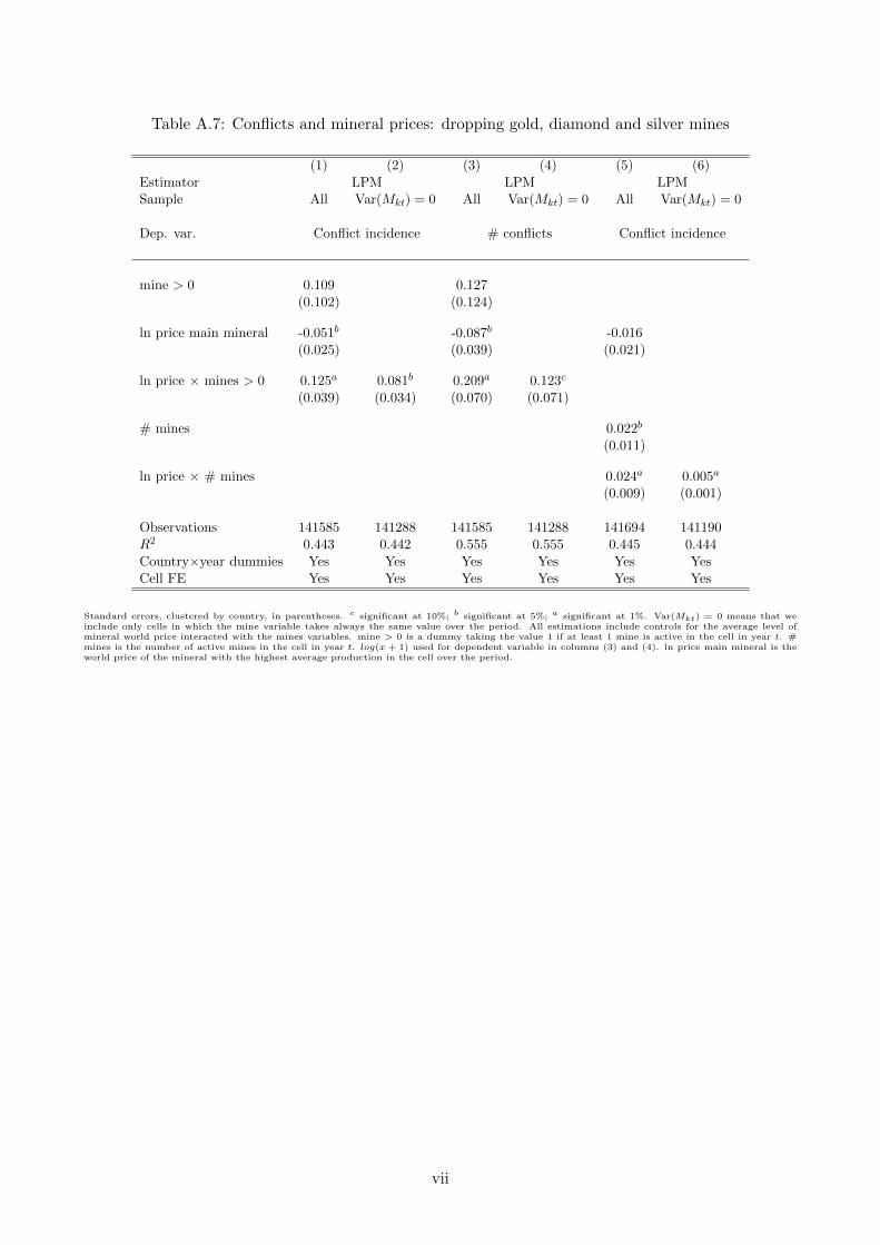
Table A.7: Conflicts and mineral prices: dropping gold, diamond and silver mines

(1) (2) (3) (4) (5) (6)Estimator LPM LPM LPMSample All Var(Mkt) = 0 All Var(Mkt) = 0 All Var(Mkt) = 0

Dep. var. Conflict incidence # conflicts Conflict incidence

mine > 0 0.109 0.127(0.102) (0.124)

ln price main mineral -0.051b -0.087b -0.016(0.025) (0.039) (0.021)

ln price × mines > 0 0.125a 0.081b 0.209a 0.123c

(0.039) (0.034) (0.070) (0.071)

# mines 0.022b

(0.011)

ln price × # mines 0.024a 0.005a

(0.009) (0.001)

Observations 141585 141288 141585 141288 141694 141190R2 0.443 0.442 0.555 0.555 0.445 0.444Country×year dummies Yes Yes Yes Yes Yes YesCell FE Yes Yes Yes Yes Yes Yes

Standard errors, clustered by country, in parentheses. c significant at 10%; b significant at 5%; a significant at 1%. Var(Mkt) = 0 means that weinclude only cells in which the mine variable takes always the same value over the period. All estimations include controls for the average level ofmineral world price interacted with the mines variables. mine > 0 is a dummy taking the value 1 if at least 1 mine is active in the cell in year t. #mines is the number of active mines in the cell in year t. log(x + 1) used for dependent variable in columns (3) and (4). ln price main mineral is theworld price of the mineral with the highest average production in the cell over the period.

vii

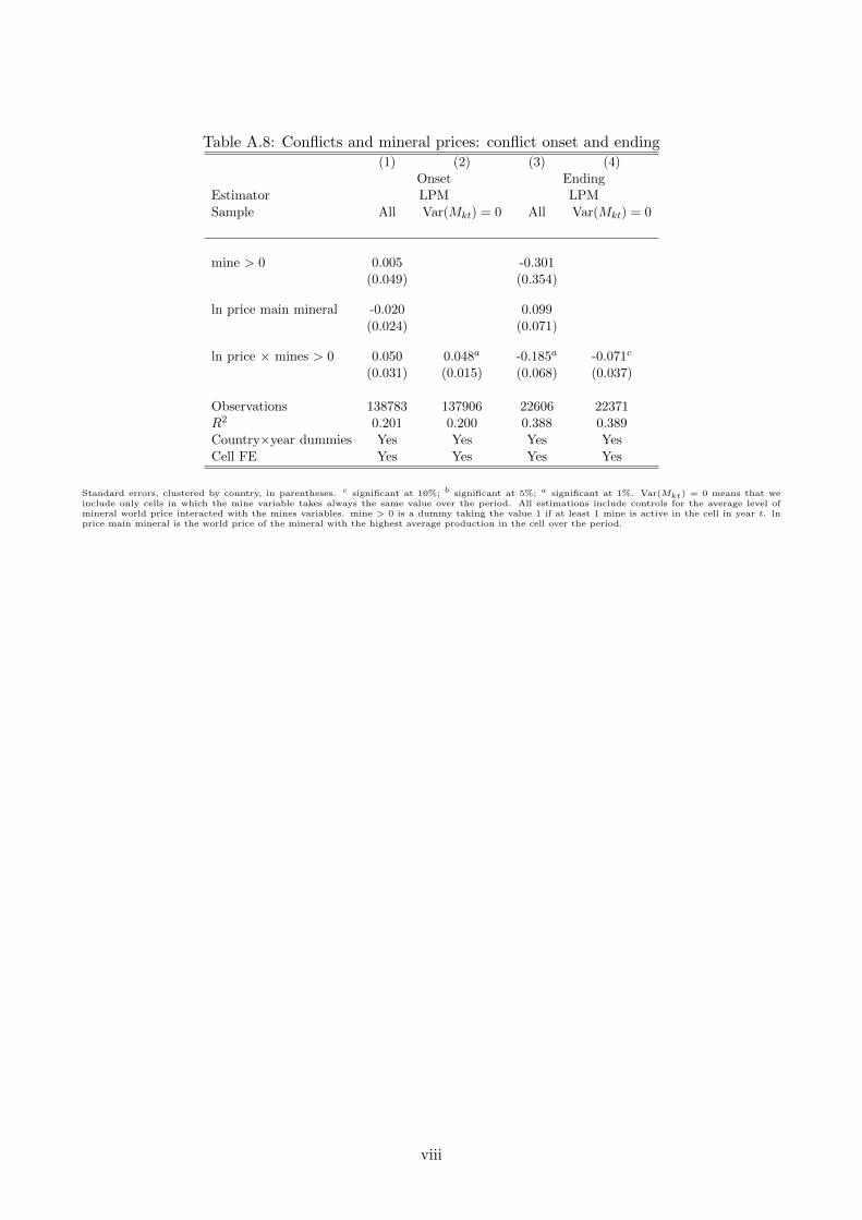
Table A.8: Conflicts and mineral prices: conflict onset and ending(1) (2) (3) (4)

Onset EndingEstimator LPM LPMSample All Var(Mkt) = 0 All Var(Mkt) = 0

mine > 0 0.005 -0.301(0.049) (0.354)

ln price main mineral -0.020 0.099(0.024) (0.071)

ln price × mines > 0 0.050 0.048a -0.185a -0.071c

(0.031) (0.015) (0.068) (0.037)

Observations 138783 137906 22606 22371R2 0.201 0.200 0.388 0.389Country×year dummies Yes Yes Yes YesCell FE Yes Yes Yes Yes

Standard errors, clustered by country, in parentheses. c significant at 10%; b significant at 5%; a significant at 1%. Var(Mkt) = 0 means that weinclude only cells in which the mine variable takes always the same value over the period. All estimations include controls for the average level ofmineral world price interacted with the mines variables. mine > 0 is a dummy taking the value 1 if at least 1 mine is active in the cell in year t. lnprice main mineral is the world price of the mineral with the highest average production in the cell over the period.

viii

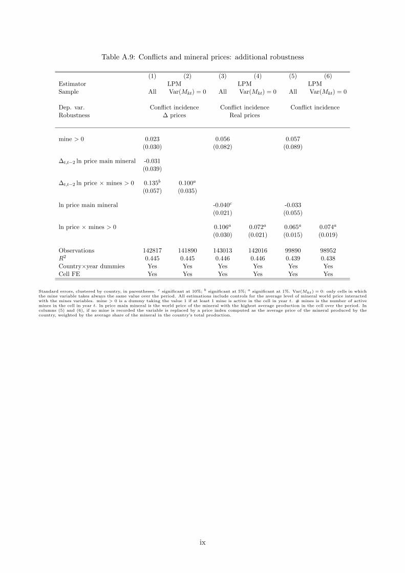
Table A.9: Conflicts and mineral prices: additional robustness

(1) (2) (3) (4) (5) (6)Estimator LPM LPM LPMSample All Var(Mkt) = 0 All Var(Mkt) = 0 All Var(Mkt) = 0

Dep. var. Conflict incidence Conflict incidence Conflict incidenceRobustness ∆ prices Real prices

mine > 0 0.023 0.056 0.057(0.030) (0.082) (0.089)

∆t,t−2 ln price main mineral -0.031(0.039)

∆t,t−2 ln price × mines > 0 0.135b 0.100a

(0.057) (0.035)

ln price main mineral -0.040c -0.033(0.021) (0.055)

ln price × mines > 0 0.106a 0.072a 0.065a 0.074a

(0.030) (0.021) (0.015) (0.019)

Observations 142817 141890 143013 142016 99890 98952R2 0.445 0.445 0.446 0.446 0.439 0.438Country×year dummies Yes Yes Yes Yes Yes YesCell FE Yes Yes Yes Yes Yes Yes

Standard errors, clustered by country, in parentheses. c significant at 10%; b significant at 5%; a significant at 1%. Var(Mkt) = 0: only cells in whichthe mine variable takes always the same value over the period. All estimations include controls for the average level of mineral world price interactedwith the mines variables. mine > 0 is a dummy taking the value 1 if at least 1 mine is active in the cell in year t. # mines is the number of activemines in the cell in year t. ln price main mineral is the world price of the mineral with the highest average production in the cell over the period. Incolumns (5) and (6), if no mine is recorded the variable is replaced by a price index computed as the average price of the mineral produced by thecountry, weighted by the average share of the mineral in the country’s total production.

ix

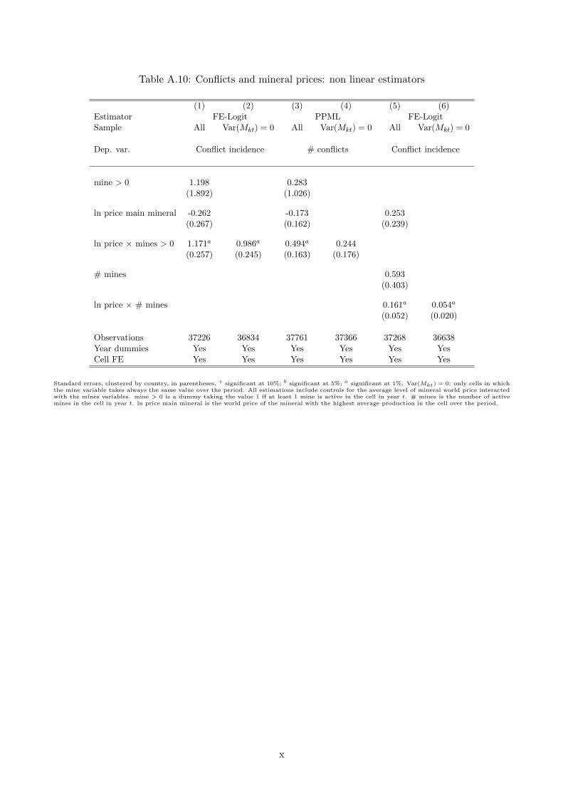
Table A.10: Conflicts and mineral prices: non linear estimators

(1) (2) (3) (4) (5) (6)Estimator FE-Logit PPML FE-LogitSample All Var(Mkt) = 0 All Var(Mkt) = 0 All Var(Mkt) = 0

Dep. var. Conflict incidence # conflicts Conflict incidence

mine > 0 1.198 0.283(1.892) (1.026)

ln price main mineral -0.262 -0.173 0.253(0.267) (0.162) (0.239)

ln price × mines > 0 1.171a 0.986a 0.494a 0.244(0.257) (0.245) (0.163) (0.176)

# mines 0.593(0.403)

ln price × # mines 0.161a 0.054a

(0.052) (0.020)

Observations 37226 36834 37761 37366 37268 36638Year dummies Yes Yes Yes Yes Yes YesCell FE Yes Yes Yes Yes Yes Yes

Standard errors, clustered by country, in parentheses. c significant at 10%; b significant at 5%; a significant at 1%. Var(Mkt) = 0: only cells in whichthe mine variable takes always the same value over the period. All estimations include controls for the average level of mineral world price interactedwith the mines variables. mine > 0 is a dummy taking the value 1 if at least 1 mine is active in the cell in year t. # mines is the number of activemines in the cell in year t. ln price main mineral is the world price of the mineral with the highest average production in the cell over the period.

x

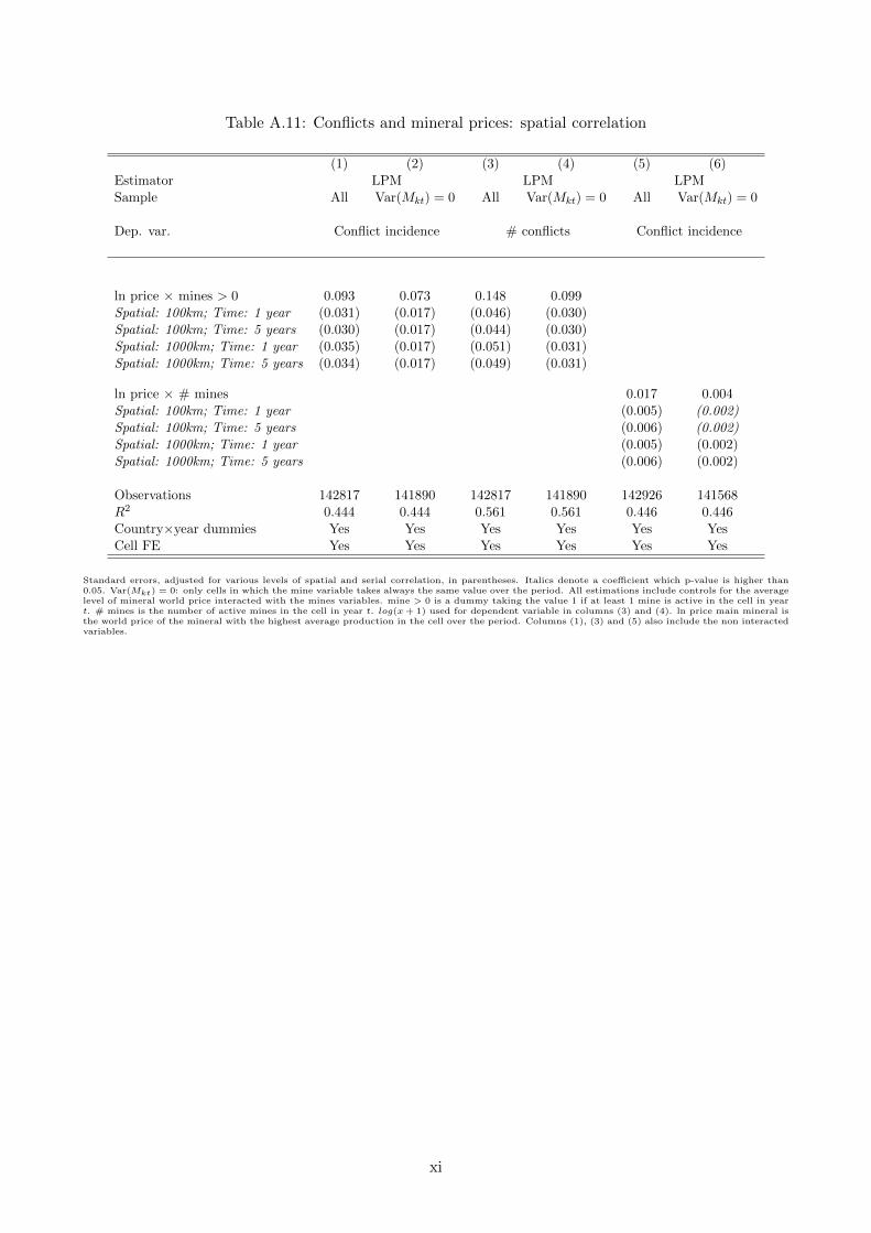
Table A.11: Conflicts and mineral prices: spatial correlation

(1) (2) (3) (4) (5) (6)Estimator LPM LPM LPMSample All Var(Mkt) = 0 All Var(Mkt) = 0 All Var(Mkt) = 0

Dep. var. Conflict incidence # conflicts Conflict incidence

ln price × mines > 0 0.093 0.073 0.148 0.099Spatial: 100km; Time: 1 year (0.031) (0.017) (0.046) (0.030)Spatial: 100km; Time: 5 years (0.030) (0.017) (0.044) (0.030)Spatial: 1000km; Time: 1 year (0.035) (0.017) (0.051) (0.031)Spatial: 1000km; Time: 5 years (0.034) (0.017) (0.049) (0.031)

ln price × # mines 0.017 0.004Spatial: 100km; Time: 1 year (0.005) (0.002)Spatial: 100km; Time: 5 years (0.006) (0.002)Spatial: 1000km; Time: 1 year (0.005) (0.002)Spatial: 1000km; Time: 5 years (0.006) (0.002)

Observations 142817 141890 142817 141890 142926 141568R2 0.444 0.444 0.561 0.561 0.446 0.446Country×year dummies Yes Yes Yes Yes Yes YesCell FE Yes Yes Yes Yes Yes Yes

Standard errors, adjusted for various levels of spatial and serial correlation, in parentheses. Italics denote a coefficient which p-value is higher than0.05. Var(Mkt) = 0: only cells in which the mine variable takes always the same value over the period. All estimations include controls for the averagelevel of mineral world price interacted with the mines variables. mine > 0 is a dummy taking the value 1 if at least 1 mine is active in the cell in yeart. # mines is the number of active mines in the cell in year t. log(x + 1) used for dependent variable in columns (3) and (4). ln price main mineral isthe world price of the mineral with the highest average production in the cell over the period. Columns (1), (3) and (5) also include the non interactedvariables.

xi

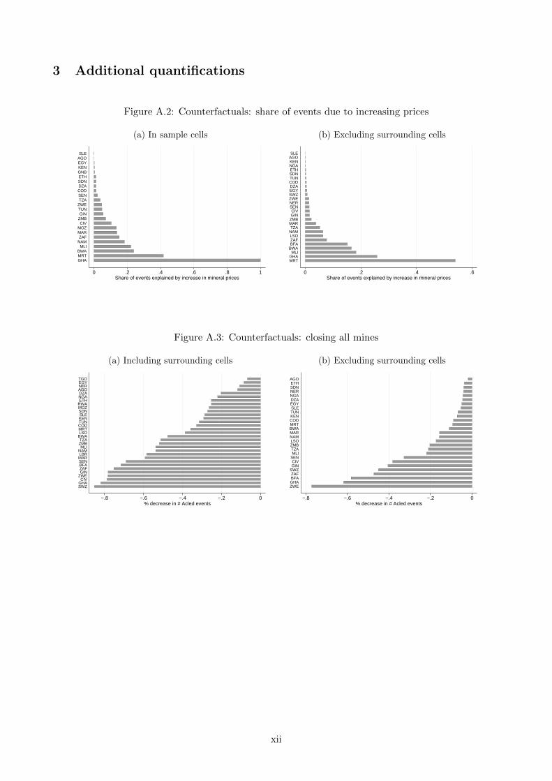
3 Additional quantifications

Figure A.2: Counterfactuals: share of events due to increasing prices

(a) In sample cells (b) Excluding surrounding cells

0 .2 .4 .6 .8 1Share of events explained by increase in mineral prices

GHAMRTBWA

MLINAMZAF

MARMOZCIV

ZMBGINTUNZWETZASENCODDZASDNETHGNBKENEGYAGOSLE

0 .2 .4 .6Share of events explained by increase in mineral prices

MRTGHAMLI

BWABFAZAFLSONAMTZA

MARZMBGINCIV

SENNERZWESWZEGYDZACODTUNSDNETHNGAKENAGOSLE

Figure A.3: Counterfactuals: closing all mines

(a) Including surrounding cells (b) Excluding surrounding cells

−.8 −.6 −.4 −.2 0% decrease in # Acled events

SWZGHACIV

ZWEGINZAFBFASENMARLBRNAMMLI

ZMBTZA

BWALSOMRTCODTUNKENSLESDNMOZRWAETHNGADZAAGONEREGYTGO

−.8 −.6 −.4 −.2 0% decrease in # Acled events

ZWEGHABFAZAF

SWZGINCIV

SENMLITZAZMBLSONAMMARBWAMRTCODKENTUNSLEEGYDZANGANERSDNETHAGO

xii

4 Maps

xiii

Figure A.4: Conflict events

!!! !!!!!!!!! !! !! !!!! !!!!!!! !! ! !!!!!!!!!!! !! !! !!! ! !! !!!!!! ! !!

! !! !! !! !!! !! !!

!!!! ! !!!! !!!! !! !!!!!!!!!!!!! !! !! ! !!!! !!! !!! !! !! ! !!! !! !! ! !! !!!! ! !!!!! ! !!!!! ! !!! ! !!!

! !!! !!! !!! !! !!!! !! !! !! !! !! ! !! !! !!!!! !! !!!!! !!! !!! !!!!! !!! !!!!!!! !!!!!!! ! !! ! !!! !!!!!! !! !! !!!! ! !! !!!!! !! !! !!! !! !! !! !! !! !!! ! !!!! ! ! !!! ! ! !!!! !! !! !! ! !! !!! ! !! !!! !! !! ! !!!!! !!!! ! !! !!! ! !! !!!!!! !

!!! ! !! !!! !!! !!!! !!!! !!! ! !! !!! !!! ! !!!! !! ! !!! !!!!!!! !! !!!! !!!!!!!! !!!!! ! !! !!! !!! !!!!! ! !! !! !!! !!!! !!!! !! ! !! !! !! ! !!! !!!! !! !!! !!!! !!! ! !!! !! !!!!!! !!! ! ! !!! ! !!!! ! !!! ! !!! !!! !! !!!! ! ! !! !!!!! ! !!!! !! !! !!! !! !! !! !!!!!!! ! !!!!! ! !!!! !!! !! ! !!!! !!!!! !!!!!!! !!! ! !!! !!! !!! !!!!!!!! ! !!!!!!!!!!! ! ! ! !!! !! !!!!! !!! ! !! ! !!!! ! ! !!! !!!!! !! !!! ! !!! ! ! !! !!! !!! !! !!! ! ! !! !! ! ! !!! !! !!! !!! ! ! !!! !!!! ! !! !!!!!!!! ! !!! !!! ! !!! ! !! !!!!! !! !!! !! ! ! !!!! !!! !! !!!!!! !!!! ! ! !!! !! ! !! !! !! ! !! !! ! ! !! !! !!!! !! !! !! !!!!! !!! !! !! ! !! !! !! !!! !!!! ! ! ! !! !!! ! !!!! ! !!! !!!! ! ! !! !!!! !!! ! ! ! !! !! !! !! !! !! !!! !!! !! ! ! !! !! !! ! !! !! !! !! ! !!!! !!!! !! ! ! ! !!! ! !!!! !!!!!!!! !!!! ! !!! !!! !!! !! !!!! !! ! !! !!!!!! !! !! !!! !! !!! ! !! ! !! !!! !!! ! ! !!! !!! ! !! ! !!! !! !!!! !!! !!!! !!!! !! ! ! !! !! !! !!! ! !!! ! !! !! ! !! !!!! ! !! !! !! ! !! !! ! !! ! ! !!! !! !! !!!! ! ! !!! !! ! ! !!! !!!! ! !! !!! ! !! !! !! ! !!! !! !! ! !!!! ! !!! !! !! ! ! !!!!! !!! ! !!!! ! !! ! ! !! ! !!! !! ! ! !!!!!!!!! !!!!!!!! ! !! ! !!!! ! !!!! !! ! ! !!! !! !! ! !! ! !!! !! ! !! ! !! !!!!!! ! !! !! !! !! !! ! !!!! !!! ! !!! !! ! !! !! ! !!! !!! ! !! ! ! !!!! ! !!! ! !! ! !! ! ! !! ! !!!! !!! !! !!! ! !! ! !! !! !! !! !! !! !!! !!! !!!!! ! !! !! ! !!! !! ! ! !!! !!! ! !!!!!! !!! ! ! ! !! !! !! ! !! ! !! ! ! ! !!! !! !! ! ! ! !! !!!!! !! !! ! !! !! !!!!! ! ! !!! !! !!! !!! !! !! !! ! !! ! !! !!!!!!! !!!! ! !!! !!! ! ! ! !! ! ! !!!! ! ! ! !!!! ! ! !!! ! ! !!! !!!! ! !!!!! ! ! ! !! ! !!! ! !! !!! ! !! ! !! !!!! !!! !!! ! !! !!! !! ! !! !! !! !!! !!!! ! !! ! !!! !!! ! !! !!!!! !! !!! !! ! !! !! !!!! ! !!! !! !! ! !!! ! !! ! !! !!!! ! ! ! !!! !!!!!! !! !! !! !!!! ! !!!!! !! !!!! !! !! !! !!! !! ! ! !!!!!! !!!!!!!! !!!! ! !! ! !!! !! !! ! !! !!!! !! !!!!!!! !!!! !! !!! !!!! !! !! ! !! !!!!! !!! !!! !! !!! !! !! !!!! ! !!! !! !!!!!!!! !!!!!!!!! ! !!!! ! !!!!!!!!!!! !!!!!!!!!! !!!! !!!!! ! !!!!! !!! !!!!!!!!!!!! !!!!!!! !!!! !! !!!!!!!!!!! !!!!!!!!!!!!!!!!! ! !!!! !!! !!!! !! !!!! !! !! !! !!!!!!!!!! ! !!!!! !! !!!!! !!!!!!!!!! ! !! ! !!!!!!!!!!! !!! !!!!!! !!!!! !!! !!!!!!! !! !!!!!!!!!!!! ! !!!!!!!!!! !!!!!! !!! !! !!!!!!!!!! !!!!! !!!! !!!!!! !!! !!!!!!!! !!!!!!!!!!!! !!! !!!! !! ! !!!!!!! !!!!!!!!!! ! !!!!!! ! !! ! !!!! !!!! !!!!!! ! !!!!!!!!!!!!!!!!! !!!!!!!!!!!!!!!!!! !!!!! !!! !! !!!! !!!!!!!! !! !!!!! !!! ! !! !! !! !!!!! !!!!!!!!!!! !!!!!!! ! !!!!! !! ! !!!!!!! !!!! !!! !! !!!!!!!!!!!! !! !!! !! !!!!!!! !! !!! !!!! !! !!!!!!!! !!! !!!!! ! !!!!!! !!!!!!!!!! ! !!!!! !!!!! !!!! !!! !!!!! !! ! !! ! ! !!!!!! ! !!!! ! !! !!! !!!! !!!!!! !!! ! !!!!!!!! !!!!!!! !!!!!!!! ! !!!!! !!! !!! !!!! !!! !!!!!!!!! !!!! ! !!! !!! !!!! !!! !!! !! !!! !! !! ! ! !! !!!! !!!! !!! !!!! !! !!! !!! !! !! ! !! !!!!!! !!!!! !!!! !!! ! ! !!! !! ! !! !!! !!!!!!! !!!! !! ! !!!!!! ! ! ! !!!!! !! !!!!! ! !!! !! !!!! !!! !! ! !!!!! !!!! ! !!!! !! !!!! !! !!!!!!!!! !!!!! !! !!!! !!!!!! !!!!! !! !! !!! !!!! !! !! !!!!! !!!!! ! !!! !!!!!!!!!! !! !! !!!! ! !!!!!!!!!!!!!!!!! !! !!!!! !! !!!!!!! !!!! ! ! !! !!! !! !!! !!!! ! !! !!! ! ! !!! !!! !!!!!! !! ! ! ! !!!! ! !! !!! ! !!!!! !! ! !! !!! !!! !! ! !! !! !!!!!!!!!!!!!!! ! !!!!!! !!!!! !!!!!!!!! !! ! ! !!!!!!!! ! !!!! !!!!!!!!! ! !!!!! ! ! !!!! !!! !!!! !! !!!! !! ! !!!!! !!! !!! !!!! !!! ! !!!! ! ! !!! !!!!! !!!!! ! !! !!! !! !!!! ! ! ! !!!! ! !! ! !!!! !! ! !!! !! !! !!! ! !! ! !! !!! ! !!! !!! !!!!!! !! !!! ! !! !!! ! ! !!!! !!! ! ! !! !!! !! ! ! !! !! ! ! !!! ! !! ! !!! !! ! !! !! !!!! ! ! !!! ! ! !!!! !! ! ! !!! !!!! !!!!! !!! ! !! !!!! ! !! ! !!!! ! !! !!! !! !! ! ! !!! !!!! !! ! !! ! !! ! ! !! !! !! !! !! !! !!!! !!!!!!! ! ! !! !! !! ! ! ! !! !! ! !! !! ! !!! !!! !! !!! ! ! !!!!! !! !! !! !! !! !! ! ! !!!! !!!! !! !! ! ! !!! !! !!! !! ! !! !!! ! ! ! !!! !!! ! !! ! !!! ! ! !! ! !! !! ! !!!! ! ! !!!! !!! !! ! !!! ! !!!! !!!! !!!! ! !!! !! !! !!!!!! ! !!!!!! !! !!!!!!! !! ! !!! ! !! !!! !! ! !! !! ! !!! ! !!!! ! !!! ! !!!!! ! ! ! !! !!! !!! !!!! ! !!! !! !! ! !!!! !! !!! !!!! ! !! !! ! !! !!!! ! !!!!! !!! ! !! !!!! ! !!!!!! ! !!!!! ! ! !! !!!! !! !!! !! !!! !!! ! !!!! !!!!! !! !! !!!! !!!! ! ! !! !! !! !!! !!! ! ! !! !!!!! !! !!! !! !! !! !! !!! ! ! !! !! !! !! !! !!!! ! !!! !!!! ! !! !!!!! !!! !! ! !! !! !! ! ! ! !!!! !!!! !!!! !! ! !! ! !! ! !!!!!! !!! !! !! ! !! !! !! !! !!! !!! ! ! !!! !! !!!! !! !!!!! ! ! ! !! ! ! !!! !! ! !! ! ! !!! !!!!! ! !! !!! !! !!! !!! !!!!! !!!!!! !!!! !! !!!! !! ! !!! !! ! !!!! ! ! ! !!!! !! ! ! !!!!! ! !! !! !!!! !! !! !! ! ! !!! !!! ! !!! !!!! !! !!!!!! ! !! !! ! !! !!!! !! !!! !!! !!!! !!!!!!!!!! !!!! !! ! ! !!!!!! ! !!!! !!!!!! !!! ! !!!!! ! !!! !! !!! ! ! !! !! !!! ! !!!! ! ! !! !! ! !!!! !! ! !! !! !! ! ! !!!! ! ! !! ! ! !! !! ! !!! !! ! !! ! !! ! !! !! !! ! !!!! !! !!!!! !!!!!!! ! !! !!! !! ! !! !! !!! ! !! ! !! ! !! ! ! ! !! ! !!! !!! !!!! !!!! !!! !!!! !!! ! !!! ! !!! !!! !!! !!! !!! ! !! !! !! ! !! !!!!! !!! !! ! !! ! !! !! !! ! ! ! !! !!! !! !!!! !! !! !!!! !! !!! ! ! !! !!!!! !! ! ! !!!!!! ! !! !! !!! ! ! !!!! !!!! !!!! ! ! ! ! ! !!! !!! !! !!! ! !! ! !!! ! ! ! !! !!! ! ! ! !!!!! ! !! ! !! !!!!!! ! ! ! !! ! !! ! !! ! !!!! !! !!!! ! !! !!! ! !! ! ! !! !! !!!!!! ! ! ! !! ! !!!! !!! !!!!! !! !! ! ! !!!! ! ! ! !!! !! !!!! !! ! !! !!! !!! !!!! ! ! ! !!!!!! !!!! ! ! !!! !!! !! !! !!!! !! ! !! !!! ! !!! !!! !!!! ! ! !! !! !! !! !! ! !! !! ! ! !!!!!! !!! !!! !! !!!! ! !!! !! !! ! !! !! !! ! ! !!!! !!! !! !!!!!! ! !! !! !!!! !! !!!! !!!!! !!! ! ! !!! !! !! !! !!! !! ! !!!!!! !!!! ! !! ! !! ! !!!! !!! !!!!! ! !!! ! !! ! !! !!! ! !! !! ! !! !!! !! ! !! !! !!!! ! !! !! !!! !! !! !!!!!! ! !! ! !!!!!!!! ! !! !! !! ! ! !! !! ! !! ! !!!! !! !!! !! ! !! !!!! !! !! ! !! !!!! ! ! !!! !!! ! !! !!!! !!! !! !! !!!!! ! ! !!!! !!! !! !!! !!!! !! !! !!! ! !!!! !!!! !!!!!! ! ! ! !! !! ! ! !!!!!! !!! !!! ! ! ! ! !!!! ! !! !! !! !!! ! !!! !! ! !!!! !! !! !! ! !!! !! ! !! !! ! ! !!! !!! !! ! ! !! ! !!! !! ! ! !! ! ! ! !! !!! ! !! ! ! !! !!! !!! ! !!! !! !! ! !! ! !!!! !! !!!! ! !!! ! !! ! ! !! ! ! ! !!!! !!! !! ! ! !!! !!!!! !!! ! ! ! !!!! ! !!!!! !! !! !!!! ! ! !!! !! !! !! !! !! !!!! ! ! ! !!!! !!!! !! ! !! !! !!!!!! ! !! ! !!!! ! !!!!! !!!! !! !! !!! !! !!! !! !!!!! !! !!! ! !! !! ! !! !! ! !!! !! ! !!! ! !!!! !! !! ! !!!!! !! !! ! !! !!!!! ! !! ! !!! !! !! ! !!! !!! ! ! !! !!!! ! !!! !! !!! !! ! !! !!! ! ! !!! !! !! ! !! !! !!!! ! !! ! !! !!!!! !!!!!! ! !!!! !! !! !!!! !! ! ! ! !!!! ! ! !!!! !! ! ! !! ! !! !!!! ! ! !! ! !!!! !! ! !! !!! ! !!! !! ! ! !! !! !! ! !! ! !!! ! ! ! ! ! !!!! !!!! !! !! !!!! ! !!!!!!!! !!! !! !!! ! ! !!!! ! !! ! !!! ! ! ! ! !! ! !! ! !! !! !! !!!!! !!!! !! !! !!!! !! !! ! !! !!!! !! ! ! !!!!!!! !!!! !!! ! ! !!!! !! !!!!! !!!!! !! ! ! ! !! ! !!! ! !!! !! !! ! !!! !!!! ! !! !! ! !! !! ! !! !!! !!!! !!!! !! !! !!!! ! !!! ! !! ! ! !! !!! !!! ! !!!! !! ! !! !! ! ! !! !! !!! ! ! ! ! ! ! ! !!! !! !! ! !! !!! ! !!! !!! ! !!! ! !!! !! !! !! ! !!! ! !! !!! !! ! !!! !! ! !! !! ! !! !!!! ! ! ! !! ! !!!! !! !!! ! !! ! !!!!! ! !! ! !! !! ! !!! !!! !!!! ! ! !! ! !! !! !! !!!! ! !! !!! !!! !! ! !! ! ! ! !! ! ! !!!!!! !! ! !! !! ! ! ! !!!! !!! !!! !!!! !! !!! !!! !!! !! !!!! !!! ! ! ! !!! !! ! !!! ! !! ! !! !! ! !! !!! !! ! !!! ! ! !!! ! !!!!!! ! ! ! !! ! !! !!! ! ! !!!! ! ! !!!! ! ! !!! !! ! ! ! !!! !!!! !! !! ! ! !!! ! !! ! !!!! !! !!!! ! !!! ! ! ! ! ! !!!! !! ! !! ! !! !!!! !! ! ! !! !! ! !!! !! !! !!! !! ! !! ! ! ! ! !!! !! ! !! !! ! !! ! !! ! ! !! ! ! ! !! !! !! !! !!!! ! !! !! ! ! ! !! !! ! !!! !!! !! !! !!! !!! !!!!!! !!!!!!! !!!! !!! ! !!! ! ! ! ! !!!!!!! !! ! ! !!! !! !! !!!! ! !!! !!! !!! !!! !!! ! ! ! ! !!!! !!!! ! !! !!! ! !! !!!!!! ! !!!!!!!! ! !! !!!! ! !! !! ! !! ! !! !!! ! !! !! ! ! !!!! !! ! ! !!!! !! !! !! ! !!! ! ! ! ! ! !!! !! !! !!! !!! ! !! !!! !!! ! ! !! !!! !! !! !! ! !! ! !!! ! !! ! !! !!! ! ! !! !! ! ! !! ! ! !!! ! ! !! !! ! !! ! !!!! !! !!! ! !! !!!!! ! ! !! ! !!!!!! !! ! ! !! !!! ! ! !!! ! ! ! !!!!! !!! ! ! ! !!!! ! ! ! ! !!! !! !!! ! ! ! !!!! !! ! ! !! !! !! !!! ! !!! !! ! !!! !! ! ! ! ! !! !! !! !!! !! !! ! ! !! ! ! !! !!! !!! !! ! ! ! ! !! !!! ! ! !!! ! ! !! !! ! ! ! !!!! !! ! ! ! !! ! ! ! ! ! !!!!!! !!! ! ! ! !! ! !!!!! !!! !!! !! !! ! !! !!!! ! !!!! !! !!! ! !!! ! ! !! ! ! !! !! !! ! !!!! ! ! ! ! ! ! !!! ! !!! !! ! !! !!! ! !! ! !!! ! !!! !! ! ! !! !! ! !! !!!!! ! ! ! !!!! !! ! !! !! !! ! !! ! ! !! !! ! !! !!!! !! !! ! !! ! ! ! !! ! !! !!! ! !!! ! !! !! ! !! !! !! ! !! !! ! !! ! !! ! !! !! ! ! !!! ! !!! ! !! !! !! ! !! !! ! !! ! !!! ! !!!!! ! !!! ! !! ! !!! ! !! ! !!! !! ! ! !!! !! ! ! ! !! !! ! !!!! !! !! ! !! ! !! !! !! !! !! !!! !! !!! ! ! !!! !!!! !! ! !! ! ! ! !! ! !!! !! !!! !! !!! ! !!!! !! ! !!! !! !! !! !! !!! ! ! !! !! !! !!!! ! ! !!! !!! !!!! ! !! ! !! ! !! !!! ! !! ! !! ! !! !!!! !! ! !! !! !! ! !! ! !! ! !! !! !!!!! !! ! !! ! !!!! !!! !! !!! ! ! !! !! !! !! ! ! ! ! !! ! !! !! ! !! ! !! !!! ! ! ! ! !!! !! ! !! !! !!! !! ! !! ! !! ! !! ! !! !! !!! !!!! ! !! ! ! ! !!!! !!! ! ! !! !! ! ! ! !! ! !! !! !! ! ! ! !! ! ! ! ! ! ! ! !! ! !! !! !! ! !!! !!!! !! !!!! !! ! !!! ! ! ! !! ! ! !!! !! !!! !!! ! !!! !! !! !! !! !!! !!!!!! !!!! !! !!!! ! !! !!!!!! ! !!!!! ! !! !! !! !!! ! !!!! !!! !!!!! ! ! !! ! !!!!!!!! !!!!!! ! !!! !! !!! !!!! !! !! !!! !!! ! ! !!! ! ! !!!! ! !!!! ! !! !!!!! !! ! !! !! ! !! !!! ! !! ! !!! !! ! !!!!! !!! !!!! !! ! !! !!! ! !! !!! !!! ! !! ! !! ! !!! !! !!! ! !! ! ! ! ! ! !! !!! ! ! ! !! !!! ! ! ! ! ! !! ! !!!!! ! !!!! !! !!!! ! !! !! ! ! ! !!! !! ! ! ! !!!! !! !!!!! !!!! ! !!!! !! ! !!! !!!!! !! !!! !!!! ! !! ! ! ! !! ! !! ! !! !! !! ! ! !! ! ! !!!! ! !!! !!! !! !! !!! ! !!!! !! !! !!! ! !! ! !! !!!!! ! !! !! !! ! !! ! !! ! !! !! !! !! ! !! ! !! !!! ! !!! !!!!! !! ! !!! !!! ! !!! !! !!!!! !! !!!! ! ! !!! !! !!! !! !! ! !! !!!!!! ! !!! !!! ! !!!! !! ! !!!! !! !!! ! !! !!! ! ! !! ! ! !! !!!! !!!! !!! !! ! ! !! !!!! ! !! ! !! !! !!!!!! !! ! !! !!! !! !! ! ! !! !!! !! ! !!! ! ! !!! ! ! !!!!! ! ! !! !!! !! ! ! ! !!!!! ! !!! !! ! !!! ! !! ! !! ! ! !!! ! ! !!! !! !! !! !!! ! !!! ! !!! ! !!! ! ! !!! ! !!! !! !! !! ! ! !!! !! ! ! !! !

!!! !!! !!! ! ! !! !!! ! !!! !! !!!!

!!!!! !!!!! ! !! ! !! !!

!! !!!!

! !!! !!!

!!!

!!!

! !!!!! !!!! ! ! !

!! !! !! !!! !! !!!!

!!!!!!! !! ! !!!!

! !!! !!! !! !!!!!!!!!!!!!!!!!!! !!!! !! !!!!!!!!! !! !!! !! !!! !!! !!! !!!!! ! ! ! !!! ! !!!!!! !!

! !! !! !!! !!! !!! !!! !! !!!!! ! !!! !! !!! ! !!!! !! !!! ! !!! ! !! !! !!! ! !! !!! ! !! !! !!!! !!!! !!!! ! !! !!!! !! ! !! !! !! ! !!! ! !! ! !!!! !!!! !!!! !! !! !!! ! !! ! !! !! ! ! !!!! !!!! !!!! ! !!! ! !!! !! !!!!!!!!! ! ! !!! !!! !!! !!!!!! !! !! !!!! !!! !! ! !!! !! !!!! !! !! !!! !! ! !! ! !! !!! !!! !! !! !!!!!! !!!! ! !! ! !!! !!!!! !! !! ! !! !! !!! !!! !!! !!! !!! ! !!!!! !! ! !!! !! ! !!! !! !!!! ! !! !! !!! !! !! !!!!! !! !! ! !!!!!!! !!!!! !! !!! !! ! !!!!! !! ! !!! !! !!!!! !!! !!!!! !! !!!! !!! !!!! !! ! !!! !!! !! !! !! !!! !!!!! !! ! !!! !!! !!! !! !!!! !! !!!!!! !!! !! !!! ! !!!! !! !!!! !!!! !!! !!! !! !!!!!!! !!!! !!!!!!! !! !!! !!! !! !! !! !! !!!!!!!!! !!!! !!! !!!! !! !!!!!!!! !! ! !!!! !!! ! !!!! ! !! !!!!! !! !!!!!!!! !!!! !!! !! !! !!! !! !!!!!!! !! ! ! !! !! !!! !!! !!!! !!!!!! ! !!! !!!!!!!! ! !!!! !!! !! !!!!!!

Number of ACLED events! 1! 2! 3 - 5! 6 - 10! 11+

Geo-location of conflict from the Armed Conflict Location and Event dataset (ACLED, 2013).

xiv

Figure A.5: Mining areas

Active mining areas GoldDiamondOther minerals

Geo-location of active mining areas from Raw Material Data.

xv

5 Mineral prices

xvi

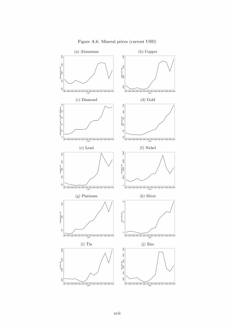
Figure A.6: Mineral prices (current USD)

(a) Aluminum (b) Copper

1000

1500

2000

2500

3000

alum

inum

pric

e, $

/t

1997 1998 1999 2000 2001 2002 2003 2004 2005 2006 2007 2008 2009 2010year

2000

4000

6000

8000

copp

er p

rice,

$/t

1997 1998 1999 2000 2001 2002 2003 2004 2005 2006 2007 2008 2009 2010year

(c) Diamond (d) Gold

7080

9010

011

012

0di

amon

d pr

ice

(1 c

arat

, F−

VV

S2)

, 100

$/ca

rat

1997 1998 1999 2000 2001 2002 2003 2004 2005 2006 2007 2008 2009 2010year

200

400

600

800

1000

1200

gold

pric

e, $

/t

1997 1998 1999 2000 2001 2002 2003 2004 2005 2006 2007 2008 2009 2010year

(e) Lead (f) Nickel

500

1000

1500

2000

2500

lead

pric

e, $

/t

1997 1998 1999 2000 2001 2002 2003 2004 2005 2006 2007 2008 2009 2010year

010

000

2000

030

000

4000

0ni

ckel

pric

e, $

/t

1997 1998 1999 2000 2001 2002 2003 2004 2005 2006 2007 2008 2009 2010year

(g) Platinum (h) Silver

500

1000

1500

plat

inum

pric

e, $

/t

1997 1998 1999 2000 2001 2002 2003 2004 2005 2006 2007 2008 2009 2010year

510

1520

silv

er p

rice,

$/t

1997 1998 1999 2000 2001 2002 2003 2004 2005 2006 2007 2008 2009 2010year

(i) Tin (j) Zinc

5000

1000

015

000

2000

0tin

pric

e, $

/t

1997 1998 1999 2000 2001 2002 2003 2004 2005 2006 2007 2008 2009 2010year

1000

1500

2000

2500

3000

3500

zinc

pric

e, $

/t

1997 1998 1999 2000 2001 2002 2003 2004 2005 2006 2007 2008 2009 2010year

xvii