Let’s start by modeling the movement

of the points D, C and the oscillation

of the table.

O

CDG

AB

(Writing

table)

A physical implementation of a harmonograph by Karl Sims

http://www.karlsims.com/harmonograph/index.html

x1

x2

x

y1

y2

y

B

A

E

D

C

F

G

O

R

R

H

1

Modeling a Three-Pendulum Harmonograph - Part #1 – by George Lungu

This first part of the presentation deals with

the movement equations of the three pendu-

lums.

<excelunusual.com>

<excelunusual.com>

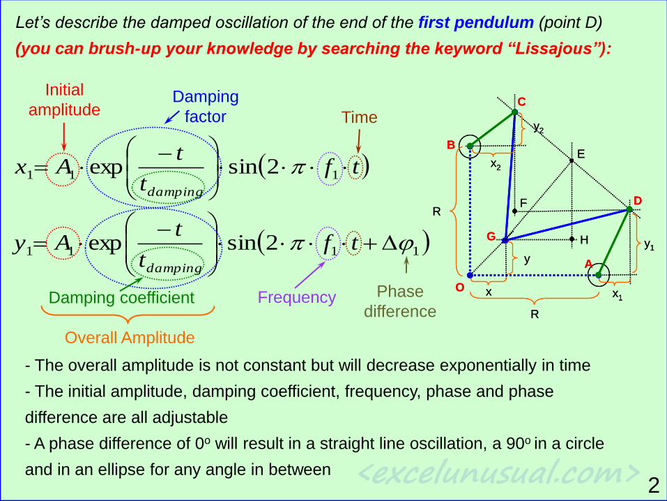
Let’s describe the damped oscillation of the end of the first pendulum (point D)

(you can brush-up your knowledge by searching the keyword “Lissajous”):

tft

tAx

damping

111 2sinexp

x1

x2

x

y1

y2

y

B

A

E

D

C

F

G

O

R

R

H

x1

x2

x

y1

y2

y

B

A

E

D

C

F

G

O

R

R

H 1111 2sinexp

tf

t

tAy

damping

Initial

amplitudeDamping

factor

Damping coefficient Frequency

Time

Phase

difference

2

Overall Amplitude

- The overall amplitude is not constant but will decrease exponentially in time

- The initial amplitude, damping coefficient, frequency, phase and phase

difference are all adjustable

- A phase difference of 0o will result in a straight line oscillation, a 90o in a circle

and in an ellipse for any angle in between

<excelunusual.com>3

Modeling rigid pendulum 2-D oscillations:

- Let’s see some examples of how the trajectories might look like. Below there are the

oscillation equations of the first pendulum

tft

tAx

damping

111 2sinexp

1111 2sinexp

tf

t

tAy

damping

Initial

amplitudeDamping

factor

Damping coefficient Frequency

Time

Overall Amplitude

- Insert a worksheet named “Pendulum_Equations” and create a table of data: X(t) and

Y(t). After that, we save several parametric plots of data to see the effect of the oscillation

parameters on the shape of the pendulum trajectories.

<excelunusual.com>4

- Let’s see several examples of effects of pendulum parameters on pendulum end trajectories:

-1.3

-0.8

-0.3

0.2

0.7

1.2

1.7

-1.5 -1 -0.5 0 0.5 1 1.5

X

YInit. Amplitude=1.2, Frequency=5, Phase Diff.=0, Damping Time=2sec.

-1.5

-1

-0.5

0

0.5

1

1.5

0 0.5 1 1.5 2 2.5 3 3.5 4 4.5 5

Time [s]

Dis

pla

cem

ent

X(t)

Y(t)

-1.3

-0.8

-0.3

0.2

0.7

1.2

1.7

-1.5 -1 -0.5 0 0.5 1 1.5

X

Y

Init. Amplitude=0.3, Frequency=5, Phase Diff.=0, Damping Time=2sec.

-1.5

-1

-0.5

0

0.5

1

1.5

0 0.5 1 1.5 2 2.5 3 3.5 4 4.5 5

Time [s]

Dis

pla

cem

ent

X(t)

Y(t)

Pendulum Parameter Effects:

Amplitude change

<excelunusual.com>5

Pendulum Parameter Effects:

-1.3

-0.8

-0.3

0.2

0.7

1.2

1.7

-1.5 -1 -0.5 0 0.5 1 1.5

X

YInit. Amplitude=1.2, Frequency=5, Phase Diff.=0, Damping Time=2sec.

-1.5

-1

-0.5

0

0.5

1

1.5

0 0.5 1 1.5 2 2.5 3 3.5 4 4.5 5

Time [s]

Dis

pla

cem

ent

X(t)

Y(t)

-1.3

-0.8

-0.3

0.2

0.7

1.2

1.7

-1.5 -1 -0.5 0 0.5 1 1.5

X

Y

Init. Amplitude=1.2, Frequency=10, Phase Diff.=0, Damping Time=2sec.

-1.5

-1

-0.5

0

0.5

1

1.5

0 0.5 1 1.5 2 2.5 3 3.5 4 4.5 5

Time [s]

Dis

pla

cem

ent

X(t)

Y(t)

Frequency change

<excelunusual.com>6

Pendulum Parameter Effects:

-1.3

-0.8

-0.3

0.2

0.7

1.2

1.7

-1.5 -1 -0.5 0 0.5 1 1.5

X

YInit. Amplitude=1.2, Frequency=5, Phase Diff.=0, Damping Time=2sec.

-1.5

-1

-0.5

0

0.5

1

1.5

0 0.5 1 1.5 2 2.5 3 3.5 4 4.5 5

Time [s]

Dis

pla

cem

ent

X(t)

Y(t)

-1.3

-0.8

-0.3

0.2

0.7

1.2

1.7

-1.5 -1 -0.5 0 0.5 1 1.5

X

Y

Init. Amplitude=1.2, Frequency=10, Phase Diff.=60, Damping Time=2sec.

-1.5

-1

-0.5

0

0.5

1

1.5

0 0.5 1 1.5 2 2.5 3 3.5 4 4.5 5

Time [s]

Dis

pla

cem

ent

X(t)

Y(t)

Phase Difference change

<excelunusual.com>7

Pendulum Parameter Effects:

-1.3

-0.8

-0.3

0.2

0.7

1.2

1.7

-1.5 -1 -0.5 0 0.5 1 1.5

X

YInit. Amplitude=1.2, Frequency=5, Phase Diff.=0, Damping Time=2sec.

-1.5

-1

-0.5

0

0.5

1

1.5

0 0.5 1 1.5 2 2.5 3 3.5 4 4.5 5

Time [s]

Dis

pla

cem

ent

X(t)

Y(t)

-1.3

-0.8

-0.3

0.2

0.7

1.2

1.7

-1.5 -1 -0.5 0 0.5 1 1.5

X

Y

Init. Amplitude=1.2, Frequency=10, Phase Diff.=90, Damping Time=2sec.

-1.5

-1

-0.5

0

0.5

1

1.5

0 0.5 1 1.5 2 2.5 3 3.5 4 4.5 5

Time [s]

Dis

pla

cem

ent

X(t)

Y(t)

Phase Difference change

<excelunusual.com>8

Pendulum Parameter Effects:

-1.3

-0.8

-0.3

0.2

0.7

1.2

1.7

-1.5 -1 -0.5 0 0.5 1 1.5

X

YInit. Amplitude=1.2, Frequency=5, Phase Diff.=0, Damping Time=2sec.

-1.5

-1

-0.5

0

0.5

1

1.5

0 0.5 1 1.5 2 2.5 3 3.5 4 4.5 5

Time [s]

Dis

pla

cem

ent

X(t)

Y(t)

-1.3

-0.8

-0.3

0.2

0.7

1.2

1.7

-1.5 -1 -0.5 0 0.5 1 1.5

X

Y

Init. Amplitude=1.2, Frequency=10, Phase Diff.=135, Damping

Time=2sec.

-1.5

-1

-0.5

0

0.5

1

1.5

0 0.5 1 1.5 2 2.5 3 3.5 4 4.5 5

Time [s]

Dis

pla

cem

ent

X(t)

Y(t)

Phase Difference change

<excelunusual.com>9

Pendulum Parameter Effects:

-1.3

-0.8

-0.3

0.2

0.7

1.2

1.7

-1.5 -1 -0.5 0 0.5 1 1.5

X

YInit. Amplitude=1.2, Frequency=5, Phase Diff.=0, Damping Time=2sec.

-1.5

-1

-0.5

0

0.5

1

1.5

0 0.5 1 1.5 2 2.5 3 3.5 4 4.5 5

Time [s]

Dis

pla

cem

ent

X(t)

Y(t)

Phase Difference change

-1.3

-0.8

-0.3

0.2

0.7

1.2

1.7

-1.5 -1 -0.5 0 0.5 1 1.5

X

Y

Init. Amplitude=1.2, Frequency=10, Phase Diff.=180, Damping

Time=2sec.

-1.5

-1

-0.5

0

0.5

1

1.5

0 0.5 1 1.5 2 2.5 3 3.5 4 4.5 5

Time [s]

Dis

pla

cem

ent

X(t)

Y(t)

<excelunusual.com>10

Pendulum Parameter Effects:

-1.3

-0.8

-0.3

0.2

0.7

1.2

1.7

-1.5 -1 -0.5 0 0.5 1 1.5

X

Y

Init. Amplitude=1.2, Frequency=10, Phase Diff.=90, Damping Time=2sec.

-1.5

-1

-0.5

0

0.5

1

1.5

0 0.5 1 1.5 2 2.5 3 3.5 4 4.5 5

Time [s]

Dis

pla

cem

ent

X(t)

Y(t)

-1.3

-0.8

-0.3

0.2

0.7

1.2

1.7

-1.5 -1 -0.5 0 0.5 1 1.5

X

Y

Init. Amplitude=1.2, Frequency=10, Phase Diff.=90, Damping

Time=0.3sec.

-1.5

-1

-0.5

0

0.5

1

1.5

0 0.5 1 1.5 2 2.5 3 3.5 4 4.5 5

Time [s]

Dis

pla

cem

ent

X(t)

Y(t)

Damping Time change

<excelunusual.com>

2222 2sinexp

tf

t

tAx

damping

22222 2sinexp

tf

t

tAy

damping

x1

x2

x

y1

y2

y

B

A

E

D

C

F

G

O

R

R

H

x1

x2

x

y1

y2

y

B

A

E

D

C

F

G

O

R

R

H

Initial

amplitude

Damping

factor

Damping

coefficient

Frequency

Time

Phase difference

between the second

and the first pendulum

11

- The overall amplitude is not constant but will decrease exponentially in time

- The initial amplitude, damping coefficient, frequency, phase and phase

difference are all adjustable

- A phase difference of 0o will result in a straight line oscillation, a 90o in a circle

and in an ellipse for any angle in between

Overall Amplitude

Phase difference

between x and y

Coming back to the second pendulum, (point C) we can

write the oscillation equations:

<excelunusual.com>

3333 2sinexp

tf

t

tAx

damping

33333 2sinexp

tf

t

tAy

damping

For the third pendulum (the table) we can write the oscillation

equations:

x1

x2

x

y1

y2

y

B

A

E

D

C

F

G

O

R

R

H

x1

x2

x

y1

y2

y

B

A

E

D

C

F

G

O

R

R

H

Initial

amplitude

Damping

factor

Damping

coefficient

Frequency

Time

Phase difference

between the third and

the first pendulum

12

- The overall amplitude is not constant but will decrease exponentially in time

- The initial amplitude, damping coefficient, frequency, phase and phase

difference are all adjustable

- A phase difference of 0o will result in a straight line oscillation, a 90o in a circle

and in an ellipse for any angle in between

Overall Amplitude

Phase difference

between x and y