This example analyzes an air-launched missile that uses a wing to provide lift and a fixed thruster engine that does not gimbal or throttle. The missile is controlled by three control surfaces located in the tail section: a vertical rudder mainly for yaw control and two horizontal rotating fins for pitch and roll control, see Figure (1.1). There are no control surfaces on the wing. Since the engine is not gimbaling the wing provides the necessary lift for the vehicle to climb at high altitudes using the elevon surfaces. The vehicle attitude, rate, and acceleration are measured by an Inertial Measurements Unit (IMU) located in the front section. There is also an air-data probe for measuring the angles of attack and sideslip which is located at the nose of the missile. We are going to model and analyze one of the most critical flight conditions. That is, when the missile is flying at 2.5 Mach, at 10 degrees of angle of attack, and the dynamic pressure is high, at 1220 psf.

1. Flight Control System Stability and Performance Analysis

In this section we will use the Flixan program to create the missile dynamic model. We will split it in two subsystems, a longitudinal and a lateral model and analyze them separately. We will analyze various flight control laws for classical stability (phase and gain margins) and simulate the missile response to flight direction commands and also to wind gusts. In section 2 we will demonstrate how to design pitch and lateral control laws using the Linear Quadratic Regulator (LQR) method. In section 3 we will demonstrate how to use Flixan and Matlab programs to analyze the flight control system (FCS) robustness to parameter uncertainties and sensitivity to gusts by using µ-analysis methods.

Figure 1.1 Missile configuration showing the control surfaces, CG, and sensor locations.

1.1 Creating the vehicle model

The files used in the flight control analysis are in folder "C:\Flixan\Examples\Missile with Wing\(a) Classical Analysis". There are two subfolders where the Matlab analysis is performed: "Pitch" and "Lateral". The vehicle input data are in file "Wing_Missile.Inp". The vehicle input data title is "Missile with Wing". The flags line (located below the title and comments) indicates that the output rates are body rates, and attitudes are defined to be Euler angles, because the

commands are referenced in Euler angles. The gust disturbance is applied perpendicular to the body x-axis, and at 45° in azimuth, that is, between the +z and the +y axes exciting both: pitch and lateral. This vehicle uses three control surfaces: an elevon, an aileron, and a rudder, which are defined in Fig. (1.1). Since this is a top level analysis we have the control surfaces tail-wag-dog option turned off "No TWD". The deflection rate aero-derivatives are all zero. There are two accelerometers defined in the input data: a normal and a lateral accelerometer located at the IMU. There is no need to define gyros because the vehicle model is rigid (zero flex modes) and the rigid rotations are always included in the outputs. There is also an air-data (vane) sensor included which is located in front of the vehicle. The vehicle modeling program processes this data-set and creates a state-space model of the missile in file "Wing-Missile.Qdr". The system title is the same "Missile with Wing" and it includes both pitch and lateral dynamics. There are two system reduction or extraction data sets below the vehicle data and they separate the coupled "Missile with Wing" model in two uncoupled pitch and lateral subsystems. The first set generates the subsystem "Missile with Wing Pitch Model" which consists only of longitudinal states, inputs, and outputs. The second set generates the subsystem "Missile with Wing Lateral Model" which consists only of lateral states, inputs, and outputs. The pitch and lateral subsystems are also saved in systems file "Wing_Missile.Qdr", and from there they are converted to Matlab functions "vehi_pitch.m" and "vehi_later.m".

Start the Flixan program and go to directory "C:\Flixan\Examples\Missile with Wing\(a) Classical Analysis". Then go to "Analysis Tools", "Flight Vehicle/ Spacecraft Modeling Tools", and "Flight Vehicle State-Space".

Fast Processing of the Input Data

The method we just described for processing the input data is an interactive step-by-step method which is used in the initial phase of modeling and it is time consuming. When the process has been debugged and the system is checked-out and you simply want to modify a few parameters, there is no need to repeat this lengthy process for a second time but you can re-run it in batch mode. The batch is faster because it does not run interactively. To run it in batch mode you need to create a batch data-set which is usually placed on the top of the input data file. A batch set is already created in file: "Wing_Missile.Inp" which automates the previously described process. In order to process the data in batch mode, from the Flixan menu bar, go to "Edit", "Manage Input Files", and "Process Input Data", and select filename "Wing-Missile.Inp". From the right hand side menu select the top title which is the batch set and click on "Execute/ View Data" button to process the batch. When the program completes the data processing click on the "Exit" button.

1.2 Pitch Axis Analysis

In this section we will only analyze the pitch flight control system FCS. In section 2 we will show how to design the gains using the Linear Quadratic Regulator (LQR) method. Since the control law requires an angle of attack feedback which is not directly measured, the alpha feedback will be implemented using two approaches: an alpha feedback from the air data probe (which has some errors due to vehicle rotation and offset from vehicle CG), and an estimated alpha feedback that uses the lateral accelerometer signal. Both approaches stabilize the system.

Pitch Flight Control System

The pitch axis flight control system is a state-feedback gain matrix, shown in Figure (1.2). It consists of 4 gains from the 4 pitch states: pitch rate (q), angle of attack (α), α-integral, and the elevon actuator position (δe). The output is the elevon actuator command. The extra state-feedback from the elevon actuator output provides some additional phase-lead for stabilization. The angle of attack (α) is not directly measurable. It is either measured from an air-data probe that is located at the nose of the missile, or it is estimated from the normal accelerometer, located approximately 20 feet in front of the CG. In either case the α-measurements are slightly corrupted.

Figure 1.2 State-Feedback Controller for the Pitch Axis

Pitch Axis Simulations

In folder "C:\Flixan\Examples\Missile with Wing\(a) Classical Analysis\Pitch" we have two very similar simulation models that use the same Flight Control System (FCS). Their difference is in the α-measurement. In file "Pitch_Sim1.mdl", shown in Figure (1.3), we use the measurement from the air-data probe, and in file "Pitch_Sim2.mdl", shown in Figure (1.4), we are using an estimator to estimate (α) from the normal accelerometer and the actuator measurements. The outer flight control loop controls the flight path angle (γ). The γ-error passes through a PI compensator and becomes an α-command to the inner FCS loop. Therefore, we indirectly control the flight path trajectory by commanding alpha. The elevon deflection command passes through a second order actuator model, of 5.5 Hz bandwidth, which drives the elevon deflection input in the missile dynamic model.

1delv_cmd

1/s

int

delta

add

-K-

Kq

-K-

Kalf

-K-

Kaint delev

Del_Elev-K-

3.11/34.5

3d-elev

2q

1alfa

Figure 1.3 Pitch Simulation model "Pitch_Sim1.mdl" using alpha-measurement from the air-data probe

Figure 1.4 Pitch Simulation model "Pitch_Sim2.mdl" using an estimated alpha from the accelerometer and actuator measurements

Flight Path Angle Gamma Comd

Flight Path Angle (Gamma) gam_cmd

2.5s+0.12

s+0.005

compens

alf a

q

d-elev

delv _cmd

State-FeedbackController

elev

gamma

alpha_sens

q

Pitch Dynamics

1190

s +27.6s+11902

Actuator

alpha_cmd

Flight Path Angle Gamma Comd

Flight Path Angle (Gamma)

gam_cmd

2.5s+0.12

s+0.005

compens

Nz

d-elev

alf _est

alfa estimat

alf a

q

d-elev

delv _cmd

State-FeedbackController

elev

gamma

q

Nz

Pitch Dynamics

1190

s +27.6s+11902

Actuator

alpha_cmd

Pitch Axis Stability Analysis

The Simulink model "Open_Loop2.mdl", shown in Figure (1.9), is used to generate the frequency response of the open-loop system and to calculate the pitch control system phase and gain margins. The control loop is broken at the elevon actuator output. The real angle of attack is replaced by the alpha estimator which is included in the control loop.

Figure 1.9 Simulink Model "Open_Loop2.mdl" Used for Stability Analysis

1elev

2.5s+0.12

s+0.005

compens

Nz

d-elev

alf _est

alfa estimat

alf a

q

d-elev

delv _cmd

State-FeedbackController

elev

gamma

q

alpha_sens

Nz

Pitch Dynamics

1190

s +27.6s+11902

Actuator

-K-

-1

1elev

alpha_cmd

Figure 1.10(a) Pitch Axis Open-Loop System Frequency Response Showing the Short-Period Resonance

Figure 1.10(b) Pitch Axis Nichols Chart Showing the Phase and Gain Margins

1.3 Lateral Axes Analysis

In the lateral axes we will analyze two flight control system designs. The first design was derived using classical control methods and the second one was designed by using the Linear Quadratic Regulator (LQR) method. We are going to analyze and compare the two designs by means of simulations and perform stability analysis in the frequency domain.

1.3.1 Lateral Flight Control System (Classical Approach)

In the classical FCS design the input to the flight control system is a flight direction command (Xi_cmd) which is compared with the estimated flight direction (Xi) and the flight direction error drives the aileron actuator command. The estimated (Xi) is equal to the yaw attitude (ψ) plus the estimated beta (βest). The measured roll and yaw attitudes are Euler angles. The beta estimate is equal to the estimated lateral velocity divided by the nominal speed (vy/V0). The lateral velocity estimate mainly controls the rudder but it also cross-couples into the aileron for better coordination. The lateral FCS block diagram is shown in Figure (1.11). The aileron and rudder actuators are also included. The part of the control system on the left side attempts to estimate the lateral velocity (vy). It uses the body rates the gravity component [g.cos(Θ)φ], and the lateral accelerometer measurement. The aileron and rudder surface deflections outputs are also used in the estimation of the lateral velocity.

Lateral Axes Simulation Model (Classical FCS)

The lateral Simulink model "Closed_Sim_Classic.mdl" is in folder "C:\Flixan\Examples\Missile with Wing\(a) Classical Analysis\Lateral", shown in Figure (1.12).

Figure 1.12 Roll and Yaw axes Simulation model "Closed_Sim_Classic.mdl" using the Classical FCS Design

The input to the simulation model is flight direction command (Xi-command) in (deg) and wind-gust velocity in (ft/sec). The missile dynamic model is in Figure (1.13). The aileron and rudder actuator outputs drive the aileron and rudder deflection inputs in the missile model. A filter is used to smooth out the gust pulse. The missile lateral dynamics are implemented as a state-space system from file "vehi_later.m" which was generated by Flixan. Its title is "Missile with Wing Lateral Model". The vehicle outputs are: roll and yaw attitudes and rates, lateral accelerometer measurement (Ny), cross range velocity (Vcr), beta, and beta measurement at the air-data probe. The flight direction (Xi) output is equal to beta + psi.

1Xi

1

Xi_cmd

dail

drud

p

phi

Xi

r

psi

Ny

Lateral Missile

p

phi

Xi_cmd

r

psi

Ny m

d-ailer

d-ruddr

Flight Control Systemand Actuators

phiphi

Lateral Stability Analysis (Classical Design)

The Simulink model "Open_Loop_Classic.mdl" uses the classical FCS design and the vehicle model used in the previous simulation model. It is used for frequency domain stability analysis. The loops are opened at the aileron and rudder actuator outputs, one at a time. The configuration shown in Figure (1.16) is for stability analysis at the rudder. The aileron loop is closed and the rudder loop is opened. For aileron stability analysis we must close the rudder loop and open the aileron loop. The Matlab file "freq.m" loads the lateral vehicle dynamics and calculates the frequency response. Figures (1.17 a & b) show the aileron and rudder loops phase and gain margins.

Figure 1.16 Simulink Model "Open_Loop_Classic.mdl" used for Lateral Stability Analysis. Configuration shown is for Rudder loop stability analysis

1out

dail

drud

p

phi

r

psi

Ny

Lateral Missile

p

phi

r

psi

Ny m

d-ailer

d-ruddr

Lateral Flight Control System with Actuators

-K-

-1

1in

phi

Figure 1.17(a) Rudder Loop Stability Analysis Showing Phase and Gain Margins

Figure 1.18(b) Aileron Loop Stability Analysis Showing Phase and Gain Margins

1.3.2 Lateral Flight Control System (LQR Design)

The lateral LQR design has a totally different structure in comparison with the classical design. The control system is a (2x9) state-feedback matrix Kpr that converts the 9 signals from the rigid-body state-vector to aileron and rudder deflection commands. In Section 2 we will describe the LQR design methodology in both pitch and lateral. The 9 lateral system states are: roll and yaw attitude errors (φ,ψ), body rates (p,r), integrals of attitude errors, angle of sideslip (β), and aileron and rudder control surface deflections (δ-aileron, δ-rudder). The actuator feedback provides some additional phase-lead for improving stability. The flight direction (Xi-error) is converted by means of a PI filter to roll and yaw attitude commands. Yaw attitude command is needed in addition to the roll command to reduce beta and subsequently lateral loading. This is because a 10 (deg) alpha is considerably high and a pure roll induces a sideslip beta. A coordinated roll and yaw command reduces beta and hence the lateral loading.

Figure 1.19 LQR Lateral Control System Simulation Model "Closed_Sim_LQR.mdl"

phippsirbetaphi_intpsi_intd-ailerd-ruddr

Flight Direction Comd (deg)

9States-Vector

x(i)

Aileron & RudderSurface Deflections (rad)

Actuator Outputs (rad)

Coordinated roll and yaw commands to minimize beta

(2x9) State-Feedback Matrix Kpr

1/s

int

1/s

int

Ny

d-rud

d-ail

beta

beta estimat

1*d2r

Xi_cmd

ailer

rudd

Xi

phi

p

psi

r

beta

dail

drud

Ny

Missile Lateral Dynamics

K*u

Kpr

s+2.2

s

Compens

-K- roll

cmd

y awcomd

beta_estim

Lateral Axes Simulation Model (LQR Controller)

The LQR lateral simulation model is "Closed_Sim_LQR.mdl", shown in Figure (1.19), and it is located in folder "C:\Flixan\ Examples\ Missile with Wing\ (a) Classical Analysis\Lateral". Notice, that the state (β) is not measurable directly. A beta estimator is used to estimate the sideslip angle by solving the following approximate equation. The beta estimator block is shown in detail in Figure (1.20). It requires knowledge of the vehicle mass, dynamic pressure, reference area and aero coefficients. The quality of the estimate obviously depends on the knowledge of those parameters.

( )ailerailYruddruddYYrefYV CCCSQNM δδβ δδβ ++=

Figure 1.20 Beta Estimator Block

The missile lateral dynamics are implemented as a state-space system from file "vehi_later.m" which was generated by Flixan. Its title is "Missile with Wing Lateral Model". The vehicle dynamics block is shown in Figure (1.21). A second order actuator dynamics (yellow) block is also included. The vehicle outputs are: roll and yaw attitudes and rates, lateral accelerometer measurement (Ny), cross range velocity (Vcr), beta, and beta measurement at the air-data probe. The actuator states are also included among the outputs. The flight direction (Xi) output is created by adding beta + psi.

Angle of Sideslip (beta) Estimator

1beta

-K-

d2r

beta_vn

beta_estim

add

-K-

Qb*Sr*Cydrudd

-K-

Qb*Sr*Cydail

-K-

Qb*Sr*Cyb

-K-

Mv

1

0.05s+1

LP

0.2

s

Int

beta_est

3d-ail

2d-rud

1Ny

Lateral Stability Analysis (LQR Design)

The Simulink model "Open_Loop_LQR.mdl" is used for frequency domain stability analysis of the lateral LQR flight controller. It consists of the same subsystems as in the simulation model "Closed_Sim_LQR.mdl". The loops are opened at the aileron and rudder actuator outputs, one at a time. The configuration shown in Figure (1.24) is for stability analysis at the aileron. The rudder loop is closed and the aileron loop is opened. For rudder stability analysis we must close the aileron loop and open the rudder loop. The Matlab file "freq.m" loads the lateral vehicle dynamics, linearized this system, and calculates its frequency response. Figures (1.25 a & b) show the aileron and rudder loops phase and gain margins.

Figure 1.24 Lateral LQR System Open Loop Analysis Model "Open_Loop_LQR.mdl "

phippsirbetaphi_intpsi_intd-ailerd-ruddr

9States-Vector

x(i)

Actuator Outputs (rad)

Coordinated roll and yaw commands to minimize beta

(2x9) State-Feedback Matrix Kpr

1out

1/s

int

1/s

int

Ny

d-rud

d-ail

beta

beta estimat

ailer

rudd

Xi

phi

p

psi

r

beta

dail

drud

Ny

Missile Lateral Dynamics

K*u

Kpr

s+2.2

s

Compens

K--1

-K-

1in

rollcmd

y awcomd

beta_estim

Figure 1.25(a) Aileron Loop Stability Analysis Showing Phase and Gain Margins

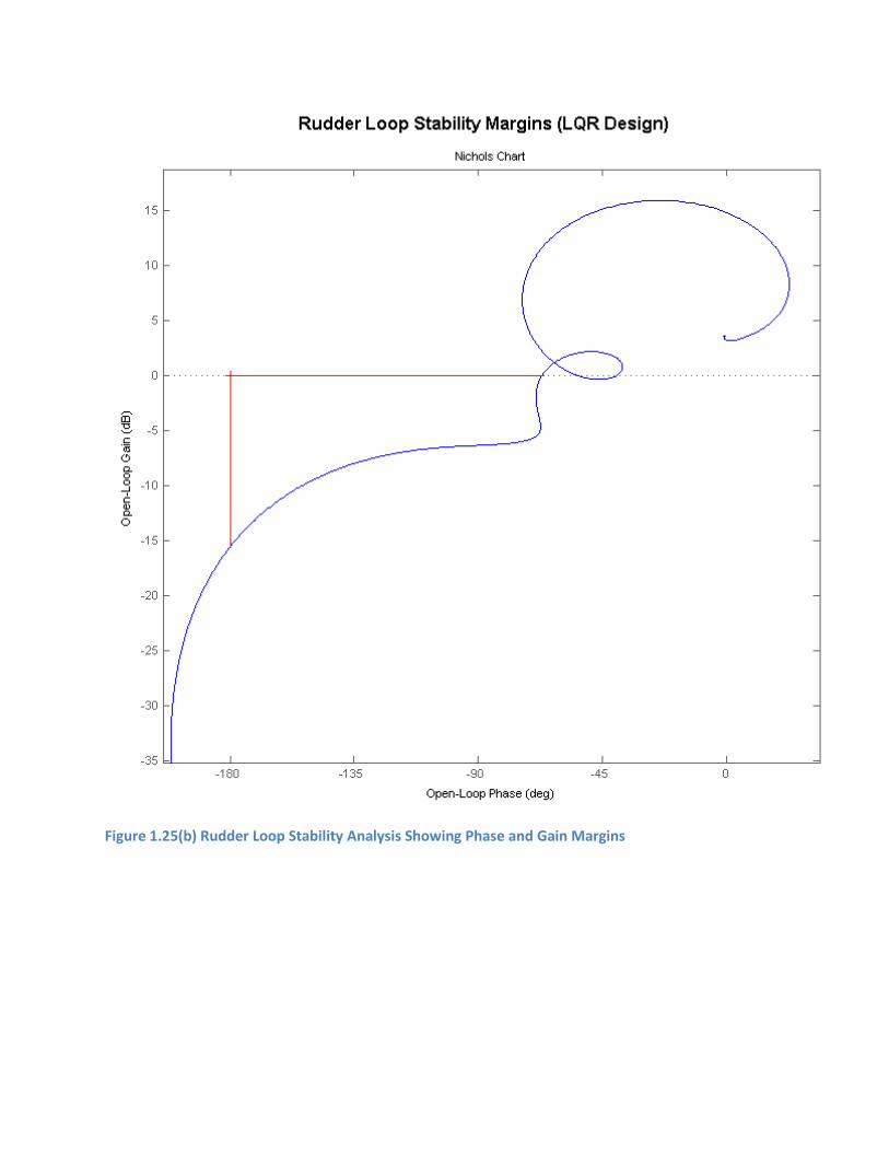
Figure 1.25(b) Rudder Loop Stability Analysis Showing Phase and Gain Margins

2. LQR Control Design

In this section we will demonstrate how to use the Linear Quadratic Regulator (LQR) method to design simple state-feedback control laws for this missile. We have chosen the LQR method because it is simple to apply and it can be automated for multiple flight conditions. The Flight Vehicle Modeling program is used to create Design Model (DM) plants of the missile at multiple flight conditions. The outputs of the DM are equal to the state-vector. In a typical design the analyst prepares Matlab scripts for designing state-feedback gains at each flight condition, where he chooses two diagonal matrices Q and R that trade performance versus control authority or control bandwidth. The choice of Q and R may be different at each flight condition. The design script reads the DM and calculates the gains based on the vehicle DM and the Q and R matrices. In this example, however, we will design gains at a single flight condition: Mach 2.5, Qbar=1220 (psf), α=10 (deg). The pitch and lateral flight control gains are designed separately in separate folders. We create a pitch design model and design script in folder "... \(b) LQR Design\Pitch LQR", and a lateral DM and script in folder "... \(b) LQR Design\Lateral LQR". The LQR gains are based on rigid-body models without tail-wag-dog and flex dynamics, and assuming that all states are directly available for feedback. They are great as "initial guesses" but they are frequently adjusted as needed in order to accommodate high order dynamics which were missing in the design plant.

2.1 Creating the Design Models

The pitch and lateral design models are created by processing the vehicle input data file "LQR_Design.Inp" in folder "C:\Flixan\Examples\Missile with Wing\(b) LQR Design". This input data file is slightly different from the one used in the previous section to create the analysis models. The missile data title is: "Missile with Wing LQR Design Model" and it is missing the accelerometer and air-data sensors because the outputs are equal to the state vector. The coupled axes system is separated, using the systems modification utility, in two simple design models: (a) "Missile with Wing Pitch Design Model", and (b) "Missile with Wing Lateral Design Model", which are also converted to Matlab system function files "pitch_lqr.m" and "later_lqr.m" respectively. This data processing is automated by a batch data-set located on the top of file "LQR_Design.Inp". In order to run the batch, process the data-sets, and to create the design plants, start the Flixan program, select the subdirectory "\LQR Design\Pitch Robust", and from the top menu select: "Edit", "Manage Input Files (*.inp)", and "Process/ Edit Input Data".

The following dialog appears, and initially only the menu on the left hand side is filled with the input data filenames containing the vehicle data. Choose the only filename "LQR_Design.Inp" and click on "Select Input Data".

The menu on the right hand side shows the titles of all the data sets included in file "LQR_Design.Inp" to be processed by the Flixan program. Each title is processed by a Flixan utility program shown on the left side of the title. Select the top title which is the batch set that will process all the other data sets, and click "Execute/ View Input Data". The program will ask you if it is okay to replace the systems which have already been created in systems file "LQR_Design.Qdr". Say "Yes", and the program will process all the data in that file to create the pitch plants. A display list appears highlighting each data set while it is executing and it disappears when the batch execution is complete. The batch also creates the two Matlab system function files "pitch_lqr.m" and "later_lqr.m" which contain the pitch and lateral design plants which will be processed by the LQR algorithm in Matlab. Click "Exit" to close Flixan and go to Matlab. The system matrices for the pitch and lateral design models are shown in color coded form in Figure (2.1). Notice that in both cases, the matrix C is equal to the identity matrix, and matrix D=0. The inputs are elevon, aileron and rudder control surface deflections and the outputs are equal to the state-vectors.

2.2 Pitch LQR Design

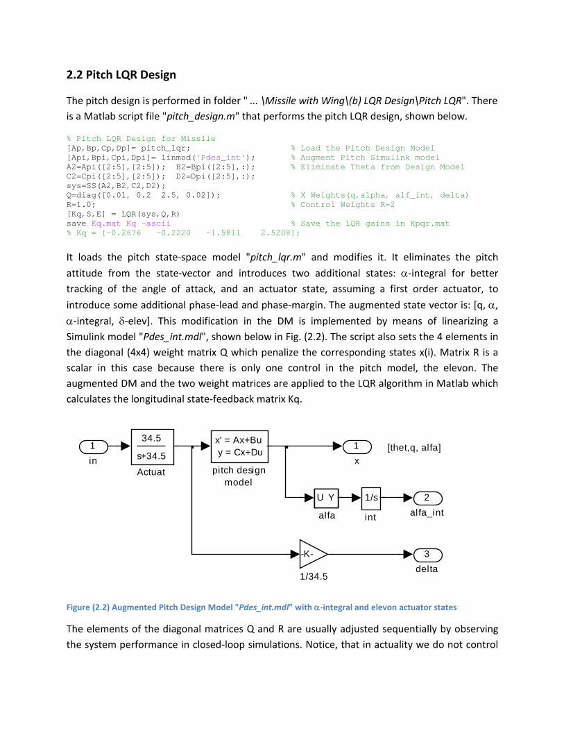
The pitch design is performed in folder " ... \Missile with Wing\(b) LQR Design\Pitch LQR". There is a Matlab script file "pitch_design.m" that performs the pitch LQR design, shown below.

% Pitch LQR Design for Missile [Ap,Bp,Cp,Dp]= pitch_lqr; % Load the Pitch Design Model [Api,Bpi,Cpi,Dpi]= linmod('Pdes_int'); % Augment Pitch Simulink model A2=Api([2:5],[2:5]); B2=Bpi([2:5],:); % Eliminate Theta from Design Model C2=Cpi([2:5],[2:5]); D2=Dpi([2:5],:); sys=SS(A2,B2,C2,D2); Q=diag([0.01, 0.2 2.5, 0.02]); % X Weights(q,alpha, alf_int, delta) R=1.0; % Control Weights R=2 [Kq,S,E] = LQR(sys,Q,R) save Kq.mat Kq -ascii % Save the LQR gains in Kpqr.mat % Kq = [-0.2676 -0.2220 -1.5811 2.5208];

It loads the pitch state-space model "pitch_lqr.m" and modifies it. It eliminates the pitch attitude from the state-vector and introduces two additional states: α-integral for better tracking of the angle of attack, and an actuator state, assuming a first order actuator, to introduce some additional phase-lead and phase-margin. The augmented state vector is: [q, α, α-integral, δ-elev]. This modification in the DM is implemented by means of linearizing a Simulink model "Pdes_int.mdl", shown below in Fig. (2.2). The script also sets the 4 elements in the diagonal (4x4) weight matrix Q which penalize the corresponding states x(i). Matrix R is a scalar in this case because there is only one control in the pitch model, the elevon. The augmented DM and the two weight matrices are applied to the LQR algorithm in Matlab which calculates the longitudinal state-feedback matrix Kq.

Figure (2.2) Augmented Pitch Design Model "Pdes_int.mdl" with α-integral and elevon actuator states

The elements of the diagonal matrices Q and R are usually adjusted sequentially by observing the system performance in closed-loop simulations. Notice, that in actuality we do not control

[thet,q, alfa]

3delta

2alfa_int

1x

x' = Ax+Bu y = Cx+Du

pitch designmodel

1/s

int

34.5

s+34.5

Actuat

-K-

1/34.5

U Y

alfa

1in

directly (α), but the state-feedback controller is only the inner-loop of a bigger control system that controls the flight-path angle (γ). The Simulink model "Panal.mdl", in Fig. (2.3), is used to evaluate the controller gain Kq obtained from the LQR algorithm and to adjust the elements of the weight matrices Q and R for a good trade-off between performance and control bandwidth. In Figure (2.3) the flight path angle error passes through a PI compensator and becomes an α-command to the inner-loop LQR controller. In simple terms, we control gamma indirectly by commanding alpha. It takes a few iterations between LQR design and simulations to converge to a set of Q and R matrices that provide a satisfactory performance and control bandwidth characteristics.

Figure (2.3) Augmented Pitch Analysis Model for Evaluating the Pitch LQR Design

theta, q, alfa

Flight Path Angle Gamma Comd

U Y

theta

thet

q1

U Y

q

x' = Ax+Bu y = Cx+Du

pitch designmodel 1/s

int

gam_cmd

elev

2.2s+0.12

s+0.005

compens

alfa

K*u

Kq

34.5

s+34.5

Actuator

-K-

1/34.5

U Y

alfa

Gamma

alpha_cmd

qalf aalf _intdelta

2.3 Lateral LQR Design

The lateral design is performed in folder " ... \Missile with Wing\(b) LQR Design\Lataeral LQR". There is a Matlab script file "Later_design.m" that performs the lateral LQR design, shown below.

% LQR Lateral Design for Missile [Al,Bl,Cl,Dl]= later_lqr; % Load the Lateral Design Model [Ali,Bli,Cli,Dli]= linmod('Lat_des'); % Linearize Lateral Simulink model sys=SS(Ali,Bli,Cli,Dli); % states: phi, p, psi, r, beta, phi_int,psi_int, ailr,rudd Q=diag([ 0.8,0.1, 0.001,0.02, 0.05, 0.3, 0.1e-9, 0.001,0.001]); R=diag([20 20])*2; % Control Weights [Kpr,S,E] = LQR(sys,Q,R) save Kpr.mat Kpr -ascii % Save the LQR gains in Kpqr.mat

The above design script loads the lateral state-space model "later_lqr.m" and augments it by introducing four additional states: integrals of roll and yaw attitude (φ and ψ), and aileron and rudder actuator states, assuming first order actuators of 5.5 (Hz) bandwidths. Including the actuator states in the LQR state-feedback introduces some additional phase-lead and phase-margin. The augmented state vector consists of 9 states: [φ, p, ψ, r, β, φ-int, ψ-int, δ-ailer, δ-rudd].

φ

ψ

β

r

ψcomm

φcomm

-

-

+

+

1/s

VehicleDynamics

Aileron

Rudder

pAileronActuator

RudderActuator

1/s

(2x9) LQR State-FeedbackMatrix Kpr

Lateral State-Feedback Control System

3. Robustness Analysis

A control system is robust when it can tolerate a certain amount of uncertainty in vehicle parameters before it becomes unstable. Parameter uncertainties can be seen as imprecise knowledge of the plant model parameters, such as: the mass properties, moments of inertia, aerodynamic coefficients, center of gravity, etc. The uncertainties of the flight vehicle are specified in terms of variations in the actual plant parameters, above or below their nominal values. The Flixan program generates the uncertain vehicle model by creating an additional input/ output pair for every parameter uncertainty in the model. Each parameter variation is “pulled out” of the plant model and it is placed inside a diagonal block ∆ that contains only the uncertainties, while the remaining plant is assumed to be known (best guess). The uncertainty block ∆ is attached to the known plant M(s) by means of (n) input/ output “wires”, where (n) is the number of the uncertainties, as shown in Figure (3.1). In essence we create (n) additional inputs and outputs in the plant that connect to the uncertainties block ∆, which is a block diagonal matrix ∆= diag(δ1,δ2,δ3,...δn). The individual perturbation elements δi may be scalars or matrices and each represents a real uncertainty in the plant. They may be aerodynamic coefficient variations from nominal values, moment of inertia variations, thrust variations, etc. The magnitude of each element represents the maximum possible variation of the parameter above or below its nominal value. M(s) represents the known dynamics consisting of the plant model with the control system included in closed-loop form.

Figure 3.1 Robustness analysis model, where M(s) is the Nominal Closed-Loop system connected with n uncertainties

The closed-loop system M(s) is used to perform robustness analysis using µ-methods. The system in this configuration is considered to be robust, assuming that M(s) is stable, if it remains stable despite all possible variations in the ∆ block as long as the magnitude of the individual variations are bounded below δ(i). The structured singular value (µ) is used for analyzing the system robustness in the frequency domain. To make things easier the diagonal block ∆ is normalized so that each individual element is allowed to vary between +1 and -1. We do this by normalizing the plant M(s), by scaling its I/O elements as needed to connect with the normalized ∆ whose elements are now bounded to within (±1). The value of 1/µ(M) represents the magnitude of the smallest perturbation that will destabilize the normalized system M(s). According to the small gain theorem, the closed-loop system is robust as long as µ(M) across the normalized block ∆ is less than one at all frequencies.

Robust Performance

Now, in addition to being robust against parameter variations, a system is said to have a "Robust Performance" when it can also satisfies nominal performance requirements in addition to robustness requirements in the presence of parameter variations.

Figure 3.2 Robust Performance Analysis Model

Consider the closed-loop system configuration in Figure (3.2), where the normalized parameter uncertainties block ∆ is pulled out of the plant as it was described earlier. P(s) is the open-loop plant dynamics and K(s) is the control system wrapped around the plant, and we assume that

the closed-loop system without the block ∆ is stable. The plant is connected to the uncertainty block ∆ by means of the inputs and outputs wp and zp. It is also connected to the controller K(s) by means of the inputs and outputs uc and ym. The input (w) is a disturbance input, such as, a wind-gust velocity. The output (z) is a performance criterion that should be kept within certain limits. For example, an angle of attack or sideslip, which should not be allowed to exceed a certain value in order to minimize structural loads. According to the previous definition the system is robust when the µ of the transfer function between (wp and zp) is less than 1 at all frequencies. Nominal performance, that is, performance without uncertainties means that the wind disturbance (w) does not violate the max (α) criterion in output (z). This happens when the µ of the transfer function between the disturbance inputs (w) and the performance criteria (z) is less than 1 at all frequencies. The transfer path of P(s) between (w) and (z) is assumed to be normalized to unity. For example, if we know that the maximum disturbance (w) is let's say 30 (ft/sec) we include a gain of 30 at the plant input (w), and if we know that the maximum acceptable angle of attack is, let's say 4 (deg), we include a gain of (1/4) at the plant output (z). After including the scaling gains within the plant we specify the performance requirement, which is: the magnitude of the scaled P(s) between (w) and (z) should be less than 1 at all frequencies. When the plant P(s) satisfies this requirement then we can say that we have achieved "Nominal Performance". We can go one step further and define "Robust Performance". This happens when we satisfy both: robustness and performance simultaneously, meaning that not only the uncertainties will not drive the system to instability but at the same time they will not violate the performance requirement between w and z. This happens, when the µ of the transfer function between the combined input vector [wp, w] and the output vector [zp, z] of the scaled plant P(s) is less than 1 at all frequencies.

Creating Robustness Analysis Models

Now that we have covered the background information for robustness analysis our next challenge is to generate the missile robustness analysis plants P(s) for both pitch and lateral and to analyze them separately. We are going to define 24 parameter uncertainties for the combined pitch and lateral coupled model, 8 of them are longitudinal and 16 are lateral. The coupled vehicle model with uncertainties will be separated in two systems: a pitch system with 8 uncertainty I/Os, and a lateral system with 16 uncertainty I/Os.

3.1 Pitch System Robustness Analysis

The longitudinal system robustness analysis is performed in directory "C:\Flixan\ Examples\ Missile with Wing\(c) Robustness Analysis\Pitch Robust". The missile input data is in file "WM_Pitch_Robust.Inp". The title of the vehicle model is "Missile with Wing with 24 Uncertainties". The nominal vehicle parameters are the same as the parameters used for

Figure 3.4 Pitch System Robustness and Robust Performance Results

For demo purposes and also for checking things out, we have created the same closed-loop system by combining smaller subsystems using Simulink. This new version is implemented in Simulink model "Closed_Robust_M2.mdl", shown in Fig. (3.5). The green block in Fig. (3.5) is the missile pitch dynamics which includes also the 8 uncertainties. The pink block is the pitch FCS which closes the loop around the vehicle. The FCS block is shown in detail in Figure (3.6). It consists of the LQR gains, the alpha estimator, and includes also the elevon actuator.

Figure 3.5 Simulink Model "Closed_Robust_M2.mdl" for analyzing Pitch Robust Performance

Figure 3.6 State-Feedback Pitch LQR Controller

Figure (3.7) shows the vehicle pitch dynamics with the 8 uncertainty I/Os included. It uses the missile state-space model "Missile with Wing Pitch Model with 8 Uncertainties" which is loaded

DeltaBlock

1unc-out

gamerr

q

Nz

d-elev

Pitch FCSunc-in

elev

unc-out

gamma

q

Nz

Pitch Dynamics

1unc-in

Angle of Attack Estimator

1d-elev

-K-

d2r

2.5s+0.12

s+0.005

compens

add1

add

-K-

Qb*Sr*Czde

-K-

Qb*Sr*Cza

-K-

Mv

-K-

Kq

-K-

Kalf

-K-

Kaint

1/s

Int3

0.1

sInt2

1190

s +27.6s+11902

Actuator

-K-

2.52/34.5

3Nz

2q1

gamerralpha_cmd

alf a_estim

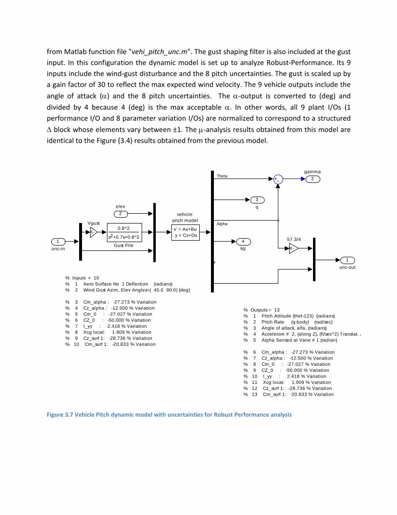
from Matlab function file "vehi_pitch_unc.m". The gust shaping filter is also included at the gust input. In this configuration the dynamic model is set up to analyze Robust-Performance. Its 9 inputs include the wind-gust disturbance and the 8 pitch uncertainties. The gust is scaled up by a gain factor of 30 to reflect the max expected wind velocity. The 9 vehicle outputs include the angle of attack (α) and the 8 pitch uncertainties. The α-output is converted to (deg) and divided by 4 because 4 (deg) is the max acceptable α. In other words, all 9 plant I/Os (1 performance I/O and 8 parameter variation I/Os) are normalized to correspond to a structured ∆ block whose elements vary between ±1. The µ-analysis results obtained from this model are identical to the Figure (3.4) results obtained from the previous model.

Figure 3.7 Vehicle Pitch dynamic model with uncertainties for Robust Performance analysis

% Inputs = 10% 1 Aero Surface No 1 Deflection (radians) % 2 Wind Gust Azim, Elev Angles=( 45.0 90.0) (deg)

% 3 Cm_alpha : -27.273 % Variation % 4 Cz_alpha : -12.500 % Variation % 5 Cm_0 : -27.027 % Variation % 6 CZ_0 : -50.000 % Variation % 7 I_yy : 2.418 % Variation % 8 Xcg locat: 1.909 % Variation % 9 Cz_surf 1: -28.736 % Variation % 10 Cm_surf 1: -20.833 % Variation

% Outputs = 13% 1 Pitch Attitude (thet-123) (radians) % 2 Pitch Rate (q-body) (rad/sec) % 3 Angle of attack, alfa, (radians) % 4 Accelerom # 2, (along Z), (ft/sec^2) Translat. A% 5 Alpha Sensed at Vane # 1 (radian)

% 6 Cm_alpha : -27.273 % Variation % 7 Cz_alpha : -12.500 % Variation % 8 Cm_0 : -27.027 % Variation % 9 CZ_0 : -50.000 % Variation % 10 I_yy : 2.418 % Variation % 11 Xcg locat: 1.909 % Variation % 12 Cz_surf 1: -28.736 % Variation % 13 Cm_surf 1: -20.833 % Variation

4Nz

3q

2gamma

1unc-out

x' = Ax+Bu y = Cx+Du

vehicle pitch model

-K-

Vgust0.8^2

s +0.7s+0.8^22

Gust Filtr -K-

57.3/4

2elev

1unc-in

Theta

Alpha

Robustness/ Sensitivity to Disturbance Analysis (Classical Design)

The robustness analysis model that uses the classical FCS design is shown in Fig. (3.8-a). The missile lateral dynamics is in the green block which is shown in detail in Fig. (3.8-b). The FCS block closes the loop between the plant outputs and the aileron and rudder deflection inputs, and we already know that the nominal closed-loop system is stable (must be). This system is set up to analyze robust performance in the lateral axes. There are 17 input-output pairs which are normalized to correspond to a 17 element diagonal ∆ block. Meaning, that it is normalized and its diagonal elements can vary up to ±1. There are 16 parameter uncertainty I/Os and one I/O for sensitivity analysis to lateral wind-gust disturbances. The gust is scaled up by a gain factor of 30 to reflect the max expected wind velocity. A gust shaping filter is used to capture the gust bandwidth characteristics. The plant outputs, in addition to the 16 uncertainties, include also the angle of sideslip (β). The β-output is converted to (deg) and divided by 4 because 4 (deg) is the max acceptable β.

Figure 3.8 Lateral Classical Flight Control Robustness Analysis model "Robust_Classic.mdl"

DeltaBlock

1unc_out

1

Xi_cmd

unc-in

dail

drud

unc_out

p

phi

r

psi

Ny

Lateral Missile

p

phi

r

psi

Ny m

Xi_Cmd

d-ailer

d-ruddr

Flight Control Systemand Actuators

1unc_in

Figure 3.9 The Classical Lateral FCS Design Satisfies Robust Performance Requirements