thin bed interpretation

57

technical article

© 2012 EAGE www.firstbreak.org

first break volume 30, December 2012

1 ffA, Northpoint, Suite E3, Exploration Drive, Aberdeen, AB23 8HZ, UK.2 Norwegian Energy Company ASA, Verksgata 1a, 4003 Stavanger, Norway.* Corresponding author, E-mail: [email protected]

AbstractRGB colour blending is a powerful technique of co-visualization of different band-limited magnitude volumes created by frequency decomposition. The aims of this study were to investigate the impact of changes in geometry and acoustic imped-ance on what we observe in a blend of frequency magnitude volumes, and to examine how sensitive different methods of frequency decomposition are to these variations. We present a comparison of frequency decomposition methods applied to the Hermod Member submarine fan system, a well understood fan system from the Northern North Sea, and to simple synthetic models. Observations made from RGB imaging are compared to equivalent results from synthetic models created using well measurements and systematic variations in reservoir parameters. We show that thickness variations between events are the dominant factor controlling RGB colour response and that subtle lithological changes, presented as differ-ences in acoustic impedance, are a second order effect. Furthermore, when the source frequency and decomposition bands of a synthetic wedge model are matched to a real dataset, we can relate colour values directly to thicknesses. In doing so we extend the classical tuning wedge for use as a calibration tool for frequency decomposition colour blends.

Understanding seismic thin-bed responses using frequency decomposition and RGB blending

N.J. McArdle1* and M.A. Ackers2

IntroductionThe use of frequency decomposition colour blending has become commonplace in the analysis of stratigraphic forma-tions from 3D seismic data (Partyka et al., 1999; Henderson et al., 2007, 2008). Red-green-blue (RGB) colour blending is a particularly effective way of displaying multiple frequency decomposition responses. The interference between different frequency bands can reveal startling detail within the colour blend, and can highlight very subtle features of sub-seismic resolution. The colour and intensity apparent in the RGB blend is dependent on a number of variables related to the fre-quency and amplitude of the signal, which in turn depend on the geometry and rock properties of the subsurface. Although the clarity of geological features imaged using RGB blending can be stark, isolating the overriding influence on the seismic signal that produces the differences in response, and hence the colours and intensity seen within an RGB blend, is com-plicated. Even though, through prior knowledge, we are able to recognize specific geometries, structures, and geological features within RGB blends, previously it has been difficult to predict exactly what a particular colour or intensity relates to, and this uncertainty makes quantitative seismic interpretation based on the multi-channel frequency response a complex and ambiguous task. Here we attempt to address that problem.

The aims of this study were to generate frequency decom-position responses for a number of simple synthetic geological models, and to relate the findings to the results obtained from

applying the same techniques to real 3D seismic data. We generated a complex 3D synthetic model of a well studied sub-surface example for which spectral decomposition has proved useful in imaging depositional patterns. We then re-applied the spectral decomposition in order to understand (1) the geo-logical controls on colour changes within RGB blends; (2) the limits on vertical sensitivity in RGB colour blends; and (3) the relative advantages of three different frequency decomposition methods. Understanding how different frequency decomposi-tion methods are influenced by frequency, change in thickness, and impedance, and also by the sub-surface setting will enable us to design frequency decomposition experiments with more efficiency and to analyse the results with greater effectiveness.

Methodology: synthetic modelling of wedges, thin beds and structural closuresTo provide a foundation for the interpretation of spectral decomposition colour blends on real data, an investigation has been carried out using various simple two-layer synthetic models:n Wedge models that account for variation in thickness.n Constant thickness thin-bed models with variable acoustic

impedance to accommodate variation in rock properties.n A structural closure model, with flat spots, created to

simulate the presence of hydrocarbon accumulations in order to demonstrate the manifestation of oil and gas in spectral decomposition RGB space.

technical article first break volume 30, December 2012

www.firstbreak.org © 2012 EAGE58

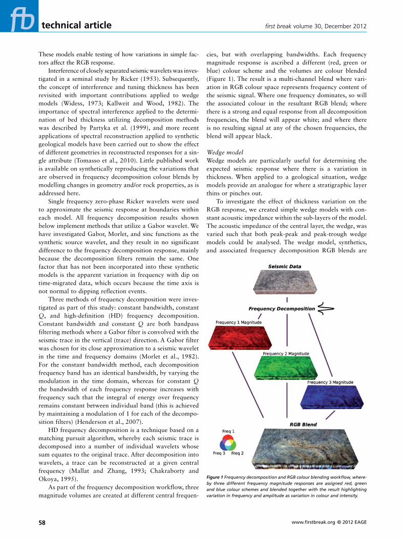
cies, but with overlapping bandwidths. Each frequency magnitude response is ascribed a different (red, green or blue) colour scheme and the volumes are colour blended (Figure 1). The result is a multi-channel blend where vari-ation in RGB colour space represents frequency content of the seismic signal. Where one frequency dominates, so will the associated colour in the resultant RGB blend; where there is a strong and equal response from all decomposition frequencies, the blend will appear white; and where there is no resulting signal at any of the chosen frequencies, the blend will appear black.

Wedge modelWedge models are particularly useful for determining the expected seismic response where there is a variation in thickness. When applied to a geological situation, wedge models provide an analogue for where a stratigraphic layer thins or pinches out.

To investigate the effect of thickness variation on the RGB response, we created simple wedge models with con-stant acoustic impedance within the sub-layers of the model. The acoustic impedance of the central layer, the wedge, was varied such that both peak-peak and peak-trough wedge models could be analysed. The wedge model, synthetics, and associated frequency decomposition RGB blends are

These models enable testing of how variations in simple fac-tors affect the RGB response.

Interference of closely separated seismic wavelets was inves-tigated in a seminal study by Ricker (1953). Subsequently, the concept of interference and tuning thickness has been revisited with important contributions applied to wedge models (Widess, 1973; Kallweit and Wood, 1982). The importance of spectral interference applied to the determi-nation of bed thickness utilizing decomposition methods was described by Partyka et al. (1999), and more recent applications of spectral reconstruction applied to synthetic geological models have been carried out to show the effect of different geometries in reconstructed responses for a sin-gle attribute (Tomasso et al., 2010). Little published work is available on synthetically reproducing the variations that are observed in frequency decomposition colour blends by modelling changes in geometry and/or rock properties, as is addressed here.

Single frequency zero-phase Ricker wavelets were used to approximate the seismic response at boundaries within each model. All frequency decomposition results shown below implement methods that utilize a Gabor wavelet. We have investigated Gabor, Morlet, and sinc functions as the synthetic source wavelet, and they result in no significant difference to the frequency decomposition response, mainly because the decomposition filters remain the same. One factor that has not been incorporated into these synthetic models is the apparent variation in frequency with dip on time-migrated data, which occurs because the time axis is not normal to dipping reflection events.

Three methods of frequency decomposition were inves-tigated as part of this study: constant bandwidth, constant Q, and high-definition (HD) frequency decomposition. Constant bandwidth and constant Q are both bandpass filtering methods where a Gabor filter is convolved with the seismic trace in the vertical (trace) direction. A Gabor filter was chosen for its close approximation to a seismic wavelet in the time and frequency domains (Morlet et al., 1982). For the constant bandwidth method, each decomposition frequency band has an identical bandwidth, by varying the modulation in the time domain, whereas for constant Q the bandwidth of each frequency response increases with frequency such that the integral of energy over frequency remains constant between individual band (this is achieved by maintaining a modulation of 1 for each of the decompo-sition filters) (Henderson et al., 2007).

HD frequency decomposition is a technique based on a matching pursuit algorithm, whereby each seismic trace is decomposed into a number of individual wavelets whose sum equates to the original trace. After decomposition into wavelets, a trace can be reconstructed at a given central frequency (Mallat and Zhang, 1993; Chakraborty and Okoya, 1995).

As part of the frequency decomposition workflow, three magnitude volumes are created at different central frequen-

Figure 1 Frequency decomposition and RGB colour blending workflow, where-by three different frequency magnitude responses are assigned red, green and blue colour schemes and blended together with the result highlighting variation in frequency and amplitude as variation in colour and intensity.

technical articlefirst break volume 30, December 2012

© 2012 EAGE www.firstbreak.org 59

For the peak-trough model (high impedance wedge), the RGB response has peak ‘brightness’ at the tuning thickness. For the peak-peak model, interference patterns also occur, but the blend is brightest at the pinchout and dimmest at the tuning thickness.

The interference effect is seen to vary between frequency decomposition methods. The constant bandwidth method shows the most separation of frequency, but has the lowest vertical resolution, whereas HD frequency decomposi-tion has the greatest vertical localization but does not show the same frequency separation through its RGB interference pattern. This trade-off between frequency and temporal localization is well documented within the field of time–frequency conversion, and understanding the relative advantages of each methodology within the context of RGB blending allows the best technique to be chosen for a given interpretation objective.

The wedge-model frequency response provides an informative way of examining the advantages and sensitivi-ties of each decomposition method. When the decomposi-tion and source frequencies are carefully matched to those used in a real subsurface example, it can provide a method of calibrating the colour response to thickness, and a wedge model is used in the next section to aid the interpretation of the Hermod fan system using RGB blends. It should be noted that the interference colours within a wedge are shown to repeat, and so colour itself cannot be used as a unique indicator of thickness.

shown in Figure 2. In this example, events were created at the upper and lower boundary of the wedge, using a Ricker wavelet of 15 Hz central frequency. Decomposition bands were chosen centred at frequencies of 10 Hz, 15 Hz, and 20 Hz, with overlapping bandwidths. These responses, when combined, are sensitive to a range of frequencies that cover the spectrum of the synthetic wavelet and the tuning frequencies between the upper and lower boundaries.

The resulting blends share several features. At the thickest part of the wedge, where there is no interference between neighbouring events, the reflectors are resolved as a uniform boundary of constant grey colour, which equates to an equal and intermediate contribution from each frequency band. As the reflectors converge, interfer-ence occurs and manifests as a distinct colour within the RGB blend, focused in between the upper and lower reflectors. Reducing thickness in the wedge causes a change in colour in the blend. This is due to variation in frequency caused by cycles of constructive and destruc-tive interference and results in a spectral interference pattern along the wedge.

Interference and the resulting colour separation in RGB space starts to occur at a thickness greater than the tuning thickness for the 15 Hz synthetic waveform, and the RGB amplitude response follows that of the standard tuning curve. The tuning thickness in time for a Ricker wavelet is1/2.57 f

0, where f0 is the central frequency (Chung and Lawton, 1995).

Figure 2 (a) Three-layer wedge model, where acoustic impedances of the upper, mid and lower layers are denoted Z1, Z2 and Z3, respectively. (b) RGB blends using the three magnitude volumes with a 15 Hz Ricker wavelet for a peak-trough model with Z1 < Z2 > Z3. RGB blends using the three magnitude volumes with a 15 Hz Ricker wavelet for a peak-peak model with Z1 < Z2 < Z3.



question from interpreters of RGB colour blends, ‘Where can I find the hydrocarbons?’ Firstly, a single low-impedance gas leg is introduced to an antiform structure. The resulting RGB response is a complex interference pattern composed of dif-ferent frequency and amplitude responses across the flat spot, due to interference of the gas-water contact with the layers above and below (Figure 4a). When an oil leg is introduced below the gas, the interference response is complicated fur-ther (Figure 4b), and using conventional bandpass methods of frequency decomposition, the two events are difficult to separate within RGB space. There are, however, distinguish-ing characteristics, particularly at the edges of the flat spots, where the presence of the second flat spot is noticeable by a ‘kick’ and unique high frequency response in the RGB blend at the outer boundary of the oil leg.

These models show that in areas with complicated and non-conformable geometry, one must try to identify and interpret interference patterns rather than simply look for layers with a constant RGB response. In fact, the models here are an extension of the wedge model, so interpretation of the interference patterns in relation to tuning and thinning towards the ‘pinchout’ is still valid. In both the gas and the gas/oil examples, HD frequency decomposition gives the most distinct temporal localization of the flat events, which is particularly important where the oil leg is thin and the second flat spot reflector is dim.

Application to Hermod Member submarine fan systemThe second part of the study involved relating observations made from the above synthetic examples to the interpreta-

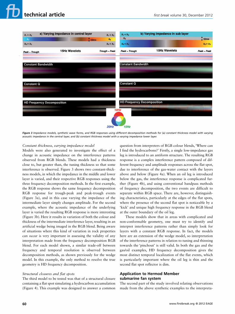
Constant thickness, varying impedance modelModels were also generated to investigate the effect of a change in acoustic impedance on the interference patterns observed from RGB blends. These models had a thickness close to, but greater than, the tuning thickness so that some interference is observed. Figure 3 shows two constant-thick-ness models, in which the impedance in the middle and lower layer is varied, and their respective RGB responses using the three frequency decomposition methods. In the first example, the RGB response shows the same frequency decomposition RGB response for trough-peak and peak-trough events (Figure 3a), and in this case varying the impedance of the intermediate layer simply changes amplitude. For the second example, where the acoustic impedance of the underlying layer is varied the resulting RGB response is more interesting (Figure 3b). Here it results in variation of both the colour and thickness of the intermediate interference layer, resulting in an artificial wedge being imaged in the RGB blend. Being aware of situations where this kind of variation in rock properties can occur is very important in assessing the validity of any interpretation made from the frequency decomposition RGB blend. For each model shown, a similar trade-off between frequency and temporal resolution is observed between decomposition methods, as shown previously for the wedge model. In this example, the only method to resolve the true geometry is HD frequency decomposition.

Structural closures and flat spotsThe third model to be tested was that of a structural closure containing a flat spot simulating a hydrocarbon accumulation (Figure 4). This example was designed to answer a common

Figure 3 Impedance models, synthetic wave forms, and RGB responses using different decomposition methods for (a) constant thickness model with varying acoustic impedance in the central layer, and (b) constant thickness model with a varying impedance lower layer.



fan system is very well documented by several scholars (Hadler-Jacobsen et al., 2005); and (3) rock property information is available from several wells that have pen-etrated the system. Figure 5 compares an example RGB blend showing the geometry of this splay with a side-scan sonar image of a modern submarine fan system from the Mississippi Delta.

Comparison of frequency decomposition techniques applied to Hermod Member submarine fan systemThe three methods of frequency decomposition applied to the Hermod dataset are, as described for the simple synthetic

tion of a real-world dataset. The subsurface example used is part of the Hermod Member submarine fan system, of Palaeocene age, in the Viking Graben area of the Northern North Sea. The easternmost splay of this system has been interpreted as a frontal splay complex overlain by a leveed channel, with little erosion of the surrounding Sele Formation shale, and we investigated it using the seismic response in cross-section, isochron maps, and an RGB blend of 10, 11, and 13 Hz. This dataset lends itself perfectly to the analysis performed here because: (1) it has been comprehensively imaged using spectral decomposi-tion (Bryn and Ackers, 2013); (2) the sedimentology of the

Figure 4 Impedance models, synthetic waveforms, and RGB responses using different decomposition methods for (a) structural closure with gas accumulation flat spot, and (b) structural closure with both gas and oil accumulation and associated flats spots.

Figure 5 Comparison of (a) RGB blend of the Hermod Member submarine fan system, and (b) side-scan sonar imaging of a modern Mississippian submarine fan system (image from USGS).



blending. This is necessary to produce a blend which displays a range in colour and intensity. The high vertical resolution means that the edges and small-scale internal geometries of the fan system are successfully imaged, and so this is the only method that provides full separation of neighbouring layers in section.

Application of synthetic modelling to Hermod Member submarine fan systemAlthough observations have been made about the colour and intensity variations that occur with distance from the channel axis within the RGB blends, there are two known and quantifiable variables that could be responsible for these vari-ations: bed thickness and acoustic impedance. The sequence is thickest at the channel centre and the depositional model predicts that bed thickness reduces towards the periphery of the splays where it abruptly terminates. Accompanying this thickness change is an expected variation in acoustic impedance, whereby more coarse-grained sands within the channel have high acoustic impedance and as the grain size reduces towards the edge of the fans, so does the acoustic impedance. In order to investigate the predominant cause of the colour and intensity variations, two synthetic models have been created to explore the effects of variable thickness and a combination of variable thickness and acoustic impedance.

The geometry of the sand fairway is defined by horizons picked near the top and base of the Sele Formation. The thickness of the Hermod Member was obtained by subtract-ing a constant shale thickness, derived from offset well data, from the mapped isochron. Acoustic impedance values from

modelling, constant bandwidth, constant Q, and HD fre-quency decomposition. A comparison of these methods for a reservoir horizon slice through the fan system is shown in Figure 6. All methods are successful in highlighting the edge of the fan system. Constant bandwidth and constant Q are particularly successful at highlighting the thickest part of the sequence at the channel core, which appears as the most ‘colourful’ part of the blend. Away from the channel centre, as the depositional system evolves into levees and splays, the blend brightens due to the amplitude of all the frequency magnitude responses increasing. Towards the most distal parts of the system, the bed thins and the amplitude response decreases, resulting in a dimming of the blend. Also notice-able within thin layers is a ‘sandwiching’ effect, an apparent coloured layer caused by interference of the responses of the upper and lower reflectors. The colour of this intermediate interference layer is seen to vary with thickness in an identi-cal manner to interference patterns observed for the wedge models described earlier.

Although constant bandwidth and constant Q methods produce similar results when the same central frequencies are blended, subtle differences are apparent. In particular, constant Q decomposition resolves sharper edges due to the increased vertical sensitivity accompanying the increased bandwidth, but at the expense of reduced frequency localiza-tion. As a result, constant Q blends often appear less colour-ful than constant bandwidth blends. The HD frequency decomposition blend has the highest vertical resolution, and because of the large bandwidths of each response, recon-struction frequencies are chosen at greater intervals prior to

Figure 6 Comparison of RGB blends of the Hermod Member submarine fan system mapped onto a horizon 46 ms below the top Sele reflector, generated using (a) constant bandwidth, (b) constant Q, and (c) HD frequency decomposition.



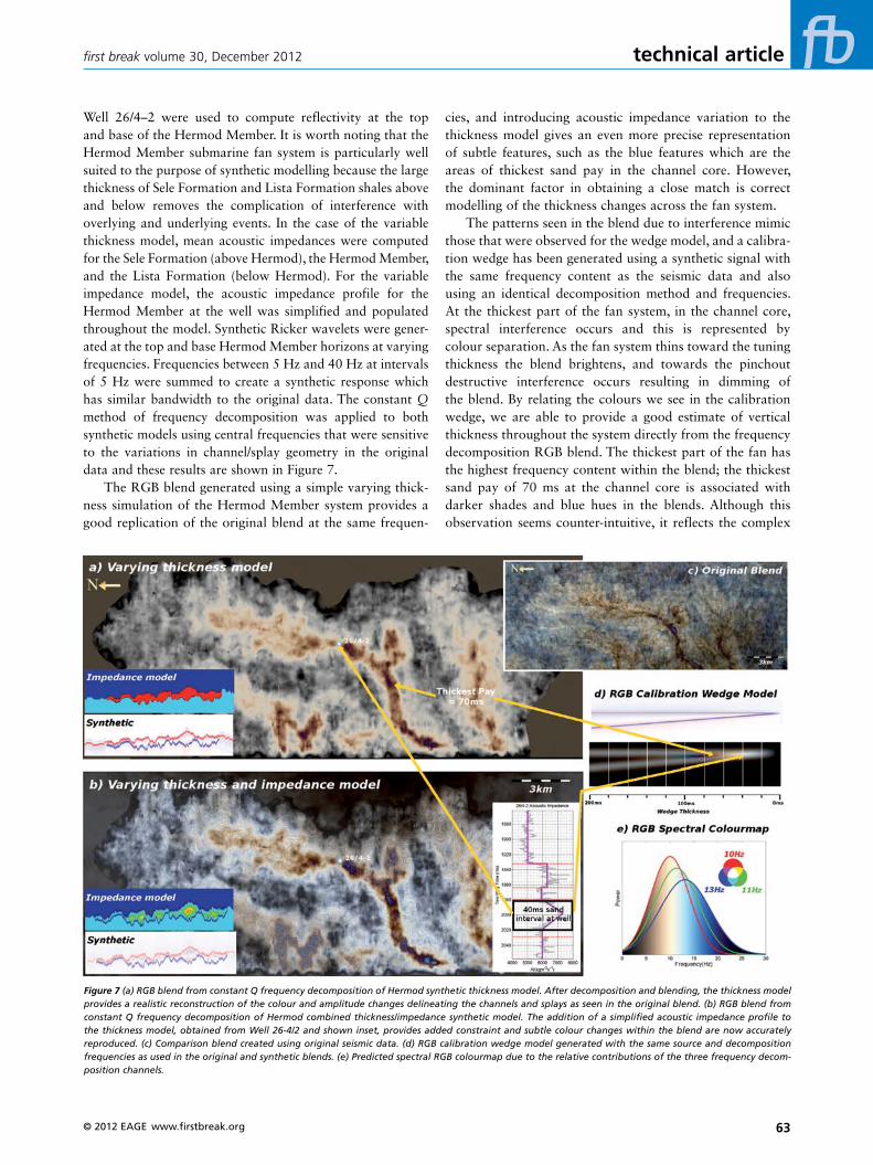
cies, and introducing acoustic impedance variation to the thickness model gives an even more precise representation of subtle features, such as the blue features which are the areas of thickest sand pay in the channel core. However, the dominant factor in obtaining a close match is correct modelling of the thickness changes across the fan system.

The patterns seen in the blend due to interference mimic those that were observed for the wedge model, and a calibra-tion wedge has been generated using a synthetic signal with the same frequency content as the seismic data and also using an identical decomposition method and frequencies. At the thickest part of the fan system, in the channel core, spectral interference occurs and this is represented by colour separation. As the fan system thins toward the tuning thickness the blend brightens, and towards the pinchout destructive interference occurs resulting in dimming of the blend. By relating the colours we see in the calibration wedge, we are able to provide a good estimate of vertical thickness throughout the system directly from the frequency decomposition RGB blend. The thickest part of the fan has the highest frequency content within the blend; the thickest sand pay of 70 ms at the channel core is associated with darker shades and blue hues in the blends. Although this observation seems counter-intuitive, it reflects the complex

Well 26/4–2 were used to compute reflectivity at the top and base of the Hermod Member. It is worth noting that the Hermod Member submarine fan system is particularly well suited to the purpose of synthetic modelling because the large thickness of Sele Formation and Lista Formation shales above and below removes the complication of interference with overlying and underlying events. In the case of the variable thickness model, mean acoustic impedances were computed for the Sele Formation (above Hermod), the Hermod Member, and the Lista Formation (below Hermod). For the variable impedance model, the acoustic impedance profile for the Hermod Member at the well was simplified and populated throughout the model. Synthetic Ricker wavelets were gener-ated at the top and base Hermod Member horizons at varying frequencies. Frequencies between 5 Hz and 40 Hz at intervals of 5 Hz were summed to create a synthetic response which has similar bandwidth to the original data. The constant Q method of frequency decomposition was applied to both synthetic models using central frequencies that were sensitive to the variations in channel/splay geometry in the original data and these results are shown in Figure 7.

The RGB blend generated using a simple varying thick-ness simulation of the Hermod Member system provides a good replication of the original blend at the same frequen-

Figure 7 (a) RGB blend from constant Q frequency decomposition of Hermod synthetic thickness model. After decomposition and blending, the thickness model provides a realistic reconstruction of the colour and amplitude changes delineating the channels and splays as seen in the original blend. (b) RGB blend from constant Q frequency decomposition of Hermod combined thickness/impedance synthetic model. The addition of a simplified acoustic impedance profile to the thickness model, obtained from Well 26-4/2 and shown inset, provides added constraint and subtle colour changes within the blend are now accurately reproduced. (c) Comparison blend created using original seismic data. (d) RGB calibration wedge model generated with the same source and decomposition frequencies as used in the original and synthetic blends. (e) Predicted spectral RGB colourmap due to the relative contributions of the three frequency decom-position channels.



and non-linear spectral interference pattern associated with tuning and, to a lesser degree, the effect of acoustic imped-ance variations within the sand fairway.

ConclusionsThis study presents an overview of the physical characteristics that affect the imaging results obtained using frequency decomposition colour blending. Complex interference pat-terns occur in RGB blends which can be related to thickness and impedance variations. This spectral interference causes complications when interpreting blends, but through calibra-tion can provide a means for quantifying thickness variation. We have also shown the impact of the trade-off in resolution in time and in frequency associated with different frequency decomposition methods.

A synthetic model of the Hermod Member submarine fan system was created which, when resolved using standard frequency decomposition, successfully reproduced the main aspects of the RGB blend generated from the original seismic data. The model combines sand thickness and acoustic impedance estimates predicted from well data intersecting the package. The dominant effect on the colour blend is variation in bed thickness and the RGB blend of this model closely reproduces the overall structure observed in the original blend. Large impedance contrasts are necessary to produce high intensity within the blend, and because acoustic impedance changes are gradual within the Hermod Member, they have a lesser effect on the blend. However, to more accurately reproduce subtle and localized changes in colour and intensity, the inclusion of acoustic impedance data is necessary. The observations relating bed thickness and

impedance changes to frequency decomposition colour blends were also verified using thin bed and wedge models. This calibration process aids interpretation and allows thickness to be estimated directly from the RGB blend. Figure 8 relates the observations from the frequency decomposition colour blending of the Hermod Member to variations in thickness and acoustic impedance.

The basic approach of frequency decomposition applied to simple synthetic wedge models and subsurface examples has proven to be an excellent approach for understanding the underlying causes of colour variation within RGB blends. It has revealed the complexities behind what we observe in these blends and the applicability of different methods for a given task.

For simple geometries, where interference between more than two layers is unlikely, careful matching of RGB responses in a comparable wedge provides a useful method of calibration. Future improvements to this approach might include automated classification and calibration. The simple modelling approach used here is appropriate for the relatively simple geological setting of the Sele Formation in this area; however, extending the approach to more complex systems will require more robust synthetic models.

Although the approach presented here has the potential to greatly improve the interpretability of RGB blends, there remain certain fundamental limitations to any frequency decomposition method. Due to the fundamental trade-off between temporal and frequency resolution of the different methods, careful consideration must be made as to which decomposition method is most appropriate for the particular example and given goals. Additionally, secondary effects,

Figure 8 Simplified explanation relating observations made from frequency decomposition colour blending of the Hermod Member submarine fan system to variations in thickness and impedance. (a) Channel core and levees - above tuning thickness. The colours that appear in the blend at this thickest part of the channel are due to interference effects from the top and bottom layer and are a consequence of the decomposition method. Subtle and localized increases in amplitude can be attributed to the high acoustic impedance sands in the channel centre. (b) Proximal splay - close to tuning thickness. High amplitudes occur in all frequencies due to constructive interference between the top and bottom events which results in brightening in the blend. (c) Distal splay - below tuning thickness. Dimming occurs in the blend due to destructive interference between upper and lower events, with also a small reduction in amplitude caused by the lower acoustic impedance of the finer-grained sediment at the periphery.



including aliasing due to sampling thresholds and harmonics, both of which can give erroneous responses, can introduce non-uniqueness to the frequency decomposition response and are not explored in this study.

ReferencesBryn, B. and Ackers, M. [2013] Unravelling the nature of deep-marine

sandstones through the linkage of seismic geomorphologies to

sedimentary facies – the Hermod Fan, Norwegian North Sea.

In: Martinius, A.W., Ravnås, R., Howell, J, Olsen, T., Steel, R.J.

and Wonham, J. (Ed.) From Depositional Systems to Sedimentary

Successions on the Norwegian Continental Margin. IAS Special

Publication 46, Wiley, Chichester, in press.

Chakraborty, A. and Okoya, D. [1995] Frequency-time decomposi-

tion of seismic data using wavelet-based methods. Geophysics, 60,

1906–1916.

Chung, H. and Lawton, D.C. [1995] Frequency characteristics of seis-

mic reflections from thin beds. Canadian Journal of Exploration

Geophysics, 31, 32–37.

Hadler-Jacobsen, F., Johannessen, E., Ashton, N., Henriksen, S., Johnson,

S. and Kristensen, J. [2005] Submarine fan morphology and lithol-

ogy distribution: a predictable function of sediment delivery, gross

shelf-to-basin relief, slope gradient and basin topography. In: Doré,

A.G. and Vining, B.A. (Eds.) Petroleum Geology: North-West Europe

and Global Perspectives—Proceedings of the 6th Petroleum Geology

Conference. Geological Society, London, 1121–1145.

Henderson, J., Purves, S.J. and Leppard, C. [2007] Automated delineation

of geological elements from 3D seismic data through analysis of

multichannel, volumetric spectral decomposition data. First Break,

25(3), 87–93.

Henderson, J., Purves, S.J., Fisher, G. and Leppard, C. [2008] Delineation

of geological elements from RGB color blending of seismic attribute

volumes. The Leading Edge, 27, 342–350.

Kallweit, R.S. and Wood, L.C. [1982] The limits of resolution of zero-

phase wavelets. Geophysics, 47, 1035–1046.

Mallat, S. and Zhang, Z. [1993] Matching pursuit with time-frequency

dictionaries. IEEE Transactions on Signal Processing, 41, 3397–3415.

Morlet, J., Arens, G., Fourgeau, E. and Giard, D. [1982] Wave propaga-

tion and sampling theory – Part I: Complex signal and scattering in

multilayered media. Geophysics,47, 203–221.

Partyka, G., Gridley, J. and Lopez, J. [1999] Interpretational applications

of spectral decomposition in reservoir characterization. The Leading

Edge, 18, 353–360.

Ricker, N. [1953] Wavelet contraction, wavelet expansion and the control

of seismic resolution. Geophysics, 18, 769–792.

Tomasso, M., Bouroullec, R. and Pyles, D. [2010] The use of spectral

recomposition in tailored forward seismic modeling of outcrop

analogs. Geohorizons, 94, 457–474.

Widess, M.B. [1973] How thin is a thin bed? Geophysics, 38, 1176–1180.

Received 22 September 2012; accepted 15 October 2012.

doi: 10.3997/1365-2397.2012022

75th EAGE Conference & Exhibition incorporating SPE EUROPEC 2013 | 10-13 June 2013 | ExCeL London

Changing Frontierswww.eage.org

Call for papers deadline 15 January 2013

LON13-V*H.indd 2 24-08-12 12:24

thin bed interpretation

Documents

rgb colour response

source frequency

different frequency

blue rgb colour blending

rgb blends

decomposition bands

colour values

particular colour