thesisproposal: scalable,activeandflexible
TRANSCRIPT

Thesis Proposal:Scalable, Active and FlexibleLearning on Distributions
Dougal J. Sutherland
November 17, 2015
School of Computer ScienceCarnegie Mellon University
Pittsburgh, PA 15213
Thesis Committee:Jeff Schneider (Chair)Maria-Florina BalcanBarnabás Póczos
Arthur Gretton (UCL)
Submitted in partial fulfillment of the requirementsfor the degree of Doctor of Philosophy.
Copyright © 2015 Dougal J. Sutherland

ii
AbstractA wide range of machine learning problems, including astronomical inference
about galaxy clusters, natural image scene classification, parametric statistical infer-ence, and predictions of public opinion, can be well-modeled as learning a functionon (samples from) distributions. This thesis explores problems in learning suchfunctions via kernel methods.
The first challenge is one of computational efficiency when learning from largenumbers of distributions: the computation of typicalmethods scales between quadrat-ically and cubically, and so they are not amenable to large datasets. We investigate theapproach of approximate embeddings into Euclidean spaces such that inner productsin the embedding space approximate kernel values between the source distributions.We present a new embedding for a class of information-theoretic distribution dis-tances, and evaluate it and existing embeddings on several real-world applications.We also propose the integration of these techniques with deep learning models so asto allow the simultaneous extraction of rich representations for inputs with the use ofexpressive distributional classifiers.
In a related problem setting, common to astrophysical observations, autonomoussensing, and electoral polling, we have the following challenge: when observingsamples is expensive, but we can choose where we would like to do so, how do wepick where to observe? We propose the development of a method to do so in thedistributional learning setting (which has a natural application to astrophysics), aswell as giving a method for a closely related problem where we search for instancesof patterns by making point observations.
Our final challenge is that the choice of kernel is important for getting goodpractical performance, but how to choose a good kernel for a given problem is notobvious. We propose to adapt recent kernel learning techniques to the distributionalsetting, allowing the automatic selection of good kernels for the task at hand. In-tegration with deep networks, as previously mentioned, may also allow for learningthe distributional distance itself.
Throughout, we combine theoretical results with extensive empirical evaluationsto increase our understanding of the methods.
Contents
1 Introduction 11.1 Summary of contributions . . . . . . . . . . . . . . . . . . . . . . . . . . . . . 21.2 The gestalt-learn package . . . . . . . . . . . . . . . . . . . . . . . . . . . 3
2 Learning on distributions 52.1 Distances on distributions . . . . . . . . . . . . . . . . . . . . . . . . . . . . . . 52.2 Estimators of distributional distances . . . . . . . . . . . . . . . . . . . . . . . . 92.3 Kernels on distributions . . . . . . . . . . . . . . . . . . . . . . . . . . . . . . . 112.4 Kernels on sample sets . . . . . . . . . . . . . . . . . . . . . . . . . . . . . . . 12
2.4.1 Handling indefinite kernel matrices . . . . . . . . . . . . . . . . . . . . 12
3 Scalable distribution learning with approximate kernel embeddings 153.1 Random Fourier features . . . . . . . . . . . . . . . . . . . . . . . . . . . . . . 15
3.1.1 Reconstruction variance . . . . . . . . . . . . . . . . . . . . . . . . . . 163.1.2 Convergence bounds . . . . . . . . . . . . . . . . . . . . . . . . . . . . 18
3.2 Mean map kernels . . . . . . . . . . . . . . . . . . . . . . . . . . . . . . . . . . 193.3 L2 distances . . . . . . . . . . . . . . . . . . . . . . . . . . . . . . . . . . . . . 20
3.3.1 Direct random Fourier features with Gaussian processes . . . . . . . . . 213.4 Information-theoretic distances . . . . . . . . . . . . . . . . . . . . . . . . . . . 22
4 Applications of distribution learning 254.1 Mixture estimation . . . . . . . . . . . . . . . . . . . . . . . . . . . . . . . . . 254.2 Scene recognition . . . . . . . . . . . . . . . . . . . . . . . . . . . . . . . . . . 26
4.2.1 sift features . . . . . . . . . . . . . . . . . . . . . . . . . . . . . . . . . 274.2.2 Deep features . . . . . . . . . . . . . . . . . . . . . . . . . . . . . . . . 28
4.3 Dark matter halo mass prediction . . . . . . . . . . . . . . . . . . . . . . . . . . 29
5 Active search for patterns 315.1 Related Work . . . . . . . . . . . . . . . . . . . . . . . . . . . . . . . . . . . . 325.2 Problem Formulation . . . . . . . . . . . . . . . . . . . . . . . . . . . . . . . . 325.3 Method . . . . . . . . . . . . . . . . . . . . . . . . . . . . . . . . . . . . . . . 34
5.3.1 Analytic Expected Utility for Functional Probit Models . . . . . . . . . . 355.3.2 Analysis for Independent Regions . . . . . . . . . . . . . . . . . . . . . 35
5.4 Empirical Evaluation . . . . . . . . . . . . . . . . . . . . . . . . . . . . . . . . 36
i

6 Proposed work 396.1 Integration with deep computer vision models . . . . . . . . . . . . . . . . . . . 396.2 Word embeddings as distributions . . . . . . . . . . . . . . . . . . . . . . . . . 396.3 Kernel learning for distribution embeddings . . . . . . . . . . . . . . . . . . . . 416.4 Embeddings for other kernels . . . . . . . . . . . . . . . . . . . . . . . . . . . . 426.5 Active learning on distributions . . . . . . . . . . . . . . . . . . . . . . . . . . . 426.6 Timeline . . . . . . . . . . . . . . . . . . . . . . . . . . . . . . . . . . . . . . . 43
Bibliography 45
ii

Chapter 1
Introduction
Traditional machine learning approaches focus on learning problems defined on vectors, mappingwhatever kind of object we wish to model to a fixed number of real-valued attributes. Thoughthis approach has been very successful in a variety of application areas, choosing natural andeffective representations can be quite difficult.
In many settings, we wish to perform machine learning tasks on objects that can be viewed asa collection of lower-level objects or more directly as samples from a distribution. For example:
• Images can be thought of as a collection of local patches (Section 4.2); similarly, videosare collections of frames.
• The total mass of a galaxy cluster can be predicted based on the positions and velocities ofindividual galaxies (Section 4.3).
• Support for a political candidate among various demographic groups can be estimated bylearning a regression model from electoral districts of individual voters to district-levelsupport for political candidates (Flaxman et al. 2015).
• Documents are made of sentences, which are themselves composed of words, which them-selves can be seen as being represented by sets of the contexts in which they appear(Section 6.2).
• Parametric statistical inference problems learn a function from sample sets to model pa-rameters (Section 4.1).
• Expectation propagation techniques relay on maps from sample sets to messages normallycomputed via expensive numerical integration (Jitkrittum et al. 2015).
• Causal arrows between distributions can be estimated from samples (Lopez-Paz et al. 2015).In order to use traditional techniques on these collective objects, we must create a single
vector that represents the entire set. Though there are various ways to summarize a set as a vector,we can often discard less information and require less effort in feature engineering by operatingdirectly on sets of feature vectors.
One method for machine learning on sets is to consider them as samples from some unknownunderlying probability distribution over feature vectors. Each example then has its own distribu-tion: if we are classifying images as sets of patches, each image is defined as a distribution overpatch features, and each class of clusters is a set of patch-level feature distributions. We can then
1
define a kernel based on statistical estimates of a distance between probability distributions. Let-ting X ⊆ Rd denote the set of possible feature vectors, we thus define a kernel k : 2X × 2X → R.This lets us perform classification, regression, anomaly detection, clustering, low-dimensionalembedding, and any of many other applications with the well-developed suite of kernel methods.Chapter 2 discusses various such kernels and their estimators; Chapter 4 gives empirical resultson several problems.
When used for a learning problem with N training items, however, typical kernel methodsrequire operating on an N × N kernel matrix, which requires far too much computation toscale to datasets with a large number of instances. Chapter 3 discusses one way to avoid thisproblem: approximate embeddings z : X → RD, à la Rahimi and Recht (2007), such thatz(x)Tz(y) ≈ k (x, y). These embeddings are available for several distributional kernels, and arealso evaluated empirically in Chapter 4.
Chapter 5 addresses the application of this type of complex functional classifier to an activesearch problem. Consider finding polluted areas in a body of water, based on point measurements.We wish to, given an observation budget, adaptively choose where we should make these obser-vations in order to maximize the number of regions we can be confident are polluted. If our notionof “pollution” is defined simply by a threshold on the mean value of a univariate measurement,Ma, Garnett, et al. (2014) give a natural selection algorithm based on Gaussian process inference.If, instead, our sensors measure the concentrations of several chemicals, the vector flow of watercurrent, or other such more complicated data, we can instead apply a classifier to a region andconsider the problem of finding regions that the classifier marks as relevant.
One area of proposed work, discussed in Section 6.5, bridges the problems of learning ondistributions in Chapters 2 to 4 with that of active pattern search in Chapter 5. Specifically,we would like to consider the problem of active learning on distributions. There are severalpossible avenues of incorporating active selection into distribution learning: given a noisyunderstanding of a distribution, which points should be selected for more careful measurement?Which distributions should be measured in order to best accomplish our objectives? This problemis intimately related to the setting of Chapter 5 when regions are independent of one another.
Other areas of future work, discussed in Chapter 6, propose integrating the distributionalembeddings of Chapter 3 with deep learning models (Section 6.1) and kernel learning techniques(Section 6.3), applying them to word embeddings in natural language processing (Section 6.2),and developing scalable embeddings for other forms of distributional kernel (Section 6.4).
1.1 Summary of contributions• Section 3.1 improves the theoretical understanding of the randomFourier features of Rahimiand Recht (2007). (Based on Sutherland and Schneider 2015.)
• Section 3.3.1 provides a method to scale the L2 embedding of J. B. Oliva, Neiswanger,et al. (2014) to higher dimensions in some situations.
• Section 3.4 gives an approximate embedding for a new class of distributional distances.(Based on Sutherland, J. B. Oliva, et al. 2015.)
• Chapter 4 provides three empirical studies for the application of distributional distances to
2

practical problems. (Based on Póczos, Xiong, Sutherland, et al. 2012; Ntampaka, Trac,Sutherland, Battaglia, et al. 2014; Sutherland, J. B. Oliva, et al. 2015.)
• Chapter 5 presents and analyzes amethod for the novel problem setting of active pointillisticpattern search. (Based on Ma, Sutherland, et al. 2015.)
Chapter 6 proposes further work related to these areas.
1.2 The gestalt-learn packageEfficient implementations of many of the methods for learning on distributions discussed inthis thesis are available in the Python package gestalt-learn1, and more will be availablesoon. This package integrates with the standard Python numerical ecosystem and presents an apicompatible with that of scikit-learn (Pedregosa et al. 2011).
1Currently https://github.com/dougalsutherland/skl-groups, soon to be renamed to https://github.com/dougalsutherland/gestalt-learn.
3

4
Chapter 2
Learning on distributions
As discussed in Chapter 1, we consider the problem of learning on probability distributions.Specifically: let X ⊆ Rd be the set of observable feature vectors, and P the set of probability dis-tributions under consideration. We then perform machine learning on samples from distributionsby:
1. Choosing a distance ρ : P × P → R.2. Defining a Mercer kernel k : P × P → R based on ρ.3. Estimating k based on the observed samples as k : 2X × 2X → R, which should itself be a
kernel on 2X .4. Using k in a standard kernel method, such as an svm or a Gaussian Process, to perform
classification, regression, collective anomaly detection, or other machine learning tasks.
Certainly, this is not the only approach to learning on distributions. Some distributionallearning methods do not directly compare sample sets to one another, but rather compare theirelements to a class-level distribution (Boiman et al. 2008). Given a distance ρ, one can naturallyuse k-nearest neighbor models (Póczos, Xiong, and Schneider 2011; Kusner et al. 2015), orNadaraya-Watson–type local regression models (J. B. Oliva, Póczos, et al. 2013; Póczos, Rinaldo,et al. 2013) with respect to that distance. In this thesis, however, we focus on kernel methods as awell-studied, flexible, and empirically effective approach to a broad variety of learning problems.
We typically assume that every distribution in P is absolutely continuous with respect tothe Lebesgue measure, and slightly abuse notation by using distributions and their densitiesinterchangeably.
2.1 Distances on distributions
We will define kernels on distributions by first defining distances between them. We first presentfour general frameworks for such distances:
5
Lr metrics One natural way to compute distances between distributions is the Lr metric betweentheir densities, for order r ≥ 1:
Lr (p, q) B(∫X
|p(x) − q(x) |r dx)1/r
.
Note that the limit r = ∞ yields the distance L∞(p, q) = supx∈X |p(x) − q(x) |.
f -divergences For any convex function f with f (1) = 0, the f -divergence of P to Q is
D f (P‖Q) B∫X
f(
p(x)q(x)
)q(x) dx.
This class is sometimes called “Csiszár f -divergences”, after Csiszár (1963). Sometimes therequirement of convexity or that f (1) = 0 is dropped. Note that these functions are not in generalsymmetric or respecting of the triangle inequality. They do, however, satisfy D f (P‖P) = 0,D f (P‖Q) ≥ 0, and are jointly convex:
D f (λP + (1 − λ)P′‖λQ + (1 − λ)Q′) ≤ λD f (P‖Q) + (1 − λ)D f (P′‖Q′).
In fact, the only metric f -divergences are multiples of the total variation distance, discussedshortly (Khosravifard et al. 2007) — though e.g. the Hellinger distance is the square of a metric.For an overview, see e.g. Liese and Vajda (2006).
α-β divergences The following somewhat less-standard divergence family, defined e.g. byPóczos, Xiong, Sutherland, et al. (2012) generalizing the α-divergence of Amari (1985), is alsouseful. Given two real parameters α, β, Dα,β is defined as
Dα,β (P‖Q) B∫
pα (x) q β (x) p(x) dx.
Dα,β (P‖Q) ≥ 0 for any α, β; Dα,−α (P‖P) = 0. Note also that Dα,−α has the form of anf -divergence with t 7→ tα+1, though this does not satisfy f (1) = 0 and is convex only ifα < (−1, 0).
Integral probability metrics Many useful metrics can be expressed as integral probabilitymetrics (ipms, Müller 1997):
ρF(P,Q) B supf ∈F
∫f dP −
∫f dQ
,
where F is some family of functions f : X → R. Note that ρF satisfies ρF(P, P) = 0,ρF(P,Q) = ρF(Q, P), and ρF(P,Q) ≤ ρF(P, R) + ρF(R,Q) for any F; the only metric propertywhich depends on F is (ρF(P,Q) = 0) =⇒ (P = Q). Sriperumbudur et al. (2009) give anoverview.
6

The various distributional distances below can often be represented in one or more of theseframeworks.
L2 distance The L2 distance is one of the most common metrics used on distributions. It canalso be represented as D1,0 − 2D0,1 + D−1,2.
Kullback-Leibler divergence The Kullback-Leibler (kl) divergence is defined as
kl(P‖Q) B∫X
p(x) logp(x)q(x)
dx.
For discrete distributions, the kl divergence bears a natural information theoretic interpretationas the expected excess code length required to send a message for P via the optimal code for Q. Itis nonnegative, and zero iff P = Q almost everywhere; however, kl(P‖Q) , kl(Q‖P) in general.Note also that if there is any point with p(x) > 0 and q(x) = 0, kl(P‖Q) = ∞.
Applications often use a symmetrization by averaging with the dual:
skl(P,Q) B 12 (kl(P‖Q) + kl(Q‖P)) .
skl, however, still does not satisfy the triangle inequality. It is also sometimes called Jeffrey’sdivergence, though that name is also sometimes used to refer to the Jensen-Shannon divergence(below), so we avoid it.
kl can be viewed as a f divergence, with one direction corresponding to t 7→ t log t and theother to t 7→ − log t; skl is thus an f divergence with t 7→ 1
2 (t − 1) log t.
Jensen-Shannon divergence The Jensen-Shannon divergence is based on kl:
js(P,Q) B 12 kl
(P
P +Q
2
)+ 1
2 kl(Q
P +Q
2
),
where P+Q2 denotes an equal mixture between P and Q. js is clearly symmetric, and in fact
√js
satisfies the triangle inequality. Note also that 0 ≤ js(P,Q) ≤ log 2. It gets its name from thefact that it can be written as the Jensen difference of the Shannon entropy:
js(P,Q) = H[
P +Q2
]−
H[P] + H[Q]2
,
a view which allows a natural generalization to more than two distributions. Non-equal mixturesare also natural, but of course asymmetric. For more details, see e.g. Martins et al. (2009).
Rényi-α divergence The Rényi-α divergence generalizes kl as
rα (P‖Q) B1
α − 1log
∫p(x)αq(x)1−α dx;
7
note that limα→1 rα (P‖Q) = kl(P‖Q). Like kl, r is asymmetric; we similarly define a sym-metrization
srα (P,Q) B 12 (rα (P‖Q) + rα (Q‖P)) .
srα does not satisfy the triangle inequality.rα can be represented based on an α-β divergence: r(P‖Q) = 1
α−1 log Dα−1,1−α (P‖Q).A Jensen-Rényi divergence, defined by replacing kl with rα in the definition of js, has also
been studied (Martins et al. 2009), but we will not consider it here.
Total variation distance The total variation distance (tv) is such an important distance that itis sometimes referred to simply as “the stastitical distance.” It can be defined as
tv(P,Q) = supA|P(A) −Q(A) |,
where A ranges over every event in the underlying sigma-algebra. It can also be represented as12 L1(P,Q), as an f -divergence with t 7→ |t − 1|, and as an ipm with F = f : ‖ f ‖∞ ≤ 1. (Recallthat ‖ f ‖∞ = supx∈X | f (x) |.) Note that tv is a metric, and 0 ≤ tv(P,Q) ≤ 1.
The total variation distance is closely related to the “intersection distance”, most commonlyused on histograms (Cha and Srihari 2002):∫
X
min(p(x), q(x)) dx =∫X
12(p(x) + q(x) − |p(x) − q(x) |
)dx = 1 − tv(P,Q).
Hellinger distance The square of the Hellinger distance h is defined as
h2(P,Q) B 12
∫ (√p(x) −
√q(x)
)2dx = 1 −
∫ √p(x) q(x) dx.
h2 can be expressed as an f -divergence with either t 7→ 12 (√
t − 1)2 or t 7→ 1 −√
t; it is alsoclosely related to an α-β divergence as h2(P,Q) = 1 − D−1/2,1/2. h is a metric, and is boundedin [0, 1]. It is proportional to the L2 difference between √p and √q, which yields the boundsh2(P,Q) ≤ tv(P,Q) ≤
√2 h(P,Q).
Earth mover’s distance The earth mover’s distance (emdρ) is defined for a metric ρ as
emdρ(P,Q) B infR∈Γ(P,Q)
E(X,Y )∼R[ρ(X,Y )
],
where Γ(P,Q) is the set of joint distributions with marginals P and Q. It is also calledthe first Wasserstein distance, or the Mallows distance. When (X, ρ) is separable, it is alsoequal to the Kantorovich metric, which is the ipm with F = f : ‖ f ‖L ≤ 1, where ‖ f ‖L Bsup | f (x) − f (y) |/ρ(x, y) | x , y ∈ X is the Lipschitz semi-norm.
For discrete distributions, emd can be computed via linear programming, and is popular inthe computer vision community.
8
Maximummean discrepancy The maximum mean discrepancy (mmd, Sriperumbudur, Gret-ton, et al. 2010; Gretton, Borgwardt, et al. 2012) is defined by embedding distributions intoa reproducing kernel Hilbert space (rkhs; for an overview see Berlinet and Thomas-Agnan2004). Let k be the kernel associated with some rkhs H with feature map ϕ : X → H ,such that 〈ϕ(x), ϕ(y)〉 = k (x, y). We can then map a distribution P to its mean embeddingµ(P) B EX∼P
[ϕ(X )
], and define the distance between distributions as the distance between
their mean embeddings:mmdk (P,Q) B ‖µ(P) − µ(Q)‖.
mmdk can also be viewed as an ipm with F = f ∈ H | ‖ f ‖H ≤ 1, where ‖ f ‖H is thenorm in H . (If f ∈ H , f (·) =
∑∞i=1 αi k (xi, ·) for some points xi ∈ X and weights αi ∈ R;
‖ f ‖2H=
∑∞i=1 αi f (xi).)
The mean embedding always exists when the base kernel k is bounded; ρ is metric for when itis characteristic. See Sriperumbudur, Gretton, et al. (2010) and Gretton, Borgwardt, et al. (2012)for details.
Szabó et al. (2014) proved learning-theoretic bounds on the use of ridge regression with mmd.
2.2 Estimators of distributional distancesWe now discuss methods for estimating different distributional distances ρ.
The most obvious estimator of most distributional distances is perhaps to first perform densityestimation, and then compute distances between the density estimates: the plug-in approach.These approaches suffer from the problem that the density is in some sense a nuisance parameterfor the problem of distance estimation, and density estimation is quite difficult, particularly inhigher dimensions.
Some of the methods below are plug-in methods; others correct a plug-in estimate, or useinconsistent density estimates in such a way that the overall divergence estimate is consistent.
Parametric models Closed forms of some distances are available for certain distributions:• For members of the same exponential family, closed forms of the Bhattacharyya kernel(corresponding to Hellinger distance), and certain other kernels of the form Dα−1,α werecomputed by Jebara et al. (2004). Nielsen and Nock (2011) give closed forms for allDα−1,1−α, allowing the computation of r, kl, and related divergences in addition to h.
• For Gaussian distributions, Muandet, Schölkopf, et al. (2012) compute the closed form ofmmd for a few base kernels. The Euclidean emd is also available.1
• Formixture distributions, L2 andmmd can be computed based on the inner products betweenthe components by simple linearity arguments. For mixtures specifically of Gaussians, F.Wang et al. (2009) obtain the quadratic (r2) entropy, which allows the computation ofJensen-Rényi divergences for α = 2.
For cases when a closed form does not exist, numerical integration may be necessary, oftenobviating the computational advantages of this approach.
1http://stats.stackexchange.com/a/144896/9964
9
It is thus possible to fit a parametric model to each distribution and compute distances betweenthe fits; this is done for machine learning applications by e.g. Jebara et al. (2004) and Morenoet al. (2004). In practice, however, we rarely know that a given parametric family is appropriate,and so the use of parametric models introduces unavoidable approximation error and bias.
Histograms One common method for representing distributions is the use of histograms; manydistances ρ are then simple to compute. The prominent exception to that is emd, which requiresO(m3 log m) time for exact computation with m-bin histograms, though in some settings O(m)approximations are available (Shirdhonkar and Jacobs 2008). mmd also requires approximatelyO(m2) computation for typical histograms.
The main disadvantages of histograms are their poor performance in even moderate dimen-sions, and the fact that (for most ρs) choosing the right bin size is both quite important and quitedifficult, since nearby bins do not affect one another.
Vector quantization An improvement over histograms popular in computer vision is to insteadquantize distributions to group points by their nearest codeword from a dictionary, often learnedvia k-means or a similar algorithm. This method is known as the bag of words (bow) approachand was popularized by Leung and Malik (2001). This method scales to much higher dimensionsthan the histogram approach, but suffers from similar problems related to the hard assignment ofsample points to bins.
Grauman and Darrell (2007) uses multiple resolutions of histograms to compute distances,helping somewhat with the issue of choosing bin sizes.
Kernel density estimation Probably the most popular form of general-purpose nonparametricdensity estimation is kernel density estimation (kde). kde results in a mixture distribution, whichallow O(n2) exact computation of plug-in mmd and L2 for certain density kernels.
Singh and Póczos (2014) show exponential concentration for a particular plug-in estimator fora broad class of functionals including Lp, α-β and f -divergences as well as js, though they don’tdiscuss computational issues of the estimator, which in general requires numerical integration.
Krishnamurthy et al. (2014) correct a plug-in estimator for L2 andrα divergences by estimatinghigher order terms in the vonMises expansion; one of their estimators is computationally attractiveand optimal for smooth distributions, while another is optimal for a broader range of distributionsbut requires numerical integration.
k-nn density estimator The k-nn density estimator provides the basis for another family ofestimators. These estimators typically require k-nearest neighbor distances within and betweenthe sample sets; much research has been put into data structures for approximate nearest neighborcomputation (e.g. Beygelzimer et al. 2006; Muja and Lowe 2009; Andoni and Razenshteyn 2015),though in high dimensions the problem is quite difficult and brute-force pairwise computationmay be the most efficient method. Plug-in methods require k to grow with sample size forconsistency, which makes computation more difficult.
Q. Wang et al. (2009) give a simple, consistent k-nn kl divergence estimator. Póczos andSchneider (2011) give a similar estimator for Dα−1,1−α and show consistency; Póczos, Xiong,
10
Sutherland, et al. (2012) generalize to Dα,β. This family of estimators is consistent with a fixedk, though convergence rates are not known.
Moon and Hero (2014a,b) propose an f -divergence estimator based on ensembles of plug-in estimators, and show the distribution is asymptotically Gaussian. (Their estimator requiresneither convex f nor f (1) = 0.)
Mean map estimators A natural estimator of mmk is simply the mean of the pairwise kernelevaluations between the two sets; this corresponds to estimating the mean embedding by theempirical mean of the embedding for each point (Gretton, Borgwardt, et al. 2012). More recently,Muandet, Fukumizu, et al. (2014) proposed biased estimators with smaller variance via the ideaof Stein shrinkage (1956). Ramdas and Wehbe (2014) showed the efficacy of this approach forindependence testing.
Other approaches Nguyen et al. (2010) provide an estimator for f -divergences (requiringconvex f but not f (1) = 0) by solving a convex program. When an rkhs structure is imposed, itrequires solving a general convex program with dimensionality equal to the number of samples,so the estimator is quite computationally expensive.
Sriperumbudur et al. (2012) estimate the L1-emd via a linear program.K. Yang et al. (2014) estimate f - and rα divergences by adaptively partitioning both distribu-
tions simultaneously. Their Bayesian approach requires mcmc and is computationally expensive,though it does provide a posterior over the divergence value which can be useful in some settings.
2.3 Kernels on distributionsWeconsider twomethods for defining kernels based on distributional distances ρ. Proposition 1 ofHaasdonk and Bahlmann (2004) shows that both methods always create positive definite kernelsiff ρ is isometric to an L2 norm, i.e. there exist a Hilbert space H and a mapping Φ : X → Hsuch that ρ(P,Q) = ‖Φ(P) − Φ(Q)‖. Such metrics are also called Hilbertian.2
For distances that do not satisfy this property, we will instead construct an indefinite kernelas below and then “correct” it, as discussed in Section 2.4.1.
The first method is to create a “linear kernel” k such that ρ(P,Q) = k (P, P)2 + k (Q,Q)2 −
2k (P,Q), so that the rkhs with inner product k has metric ρ. Note that, while distances aretranslation-invariant, inner products are not; we must thus first choose some origin O. Then
k (O)lin (P,Q) B 1
2
(ρ2(P, 0) + ρ2(Q,O) − ρ2(P,Q)
)(2.1)
is a valid kernel for any O iff ρ is Hilbertian. If ρ is defined for the zero measure, it is often mostnatural to use that as the origin.
We can also use ρ in a generalized rbf kernel: for a bandwidth parameter σ > 0,
k (σ)rbf (x, y) B exp
(−
12σ2 ρ
2(p, q)). (2.2)
2Note that if ρ is Hilbertian, Proposition 1 (ii) of Haasdonk and Bahlmann (2004) shows that−ρ2β is conditionallypositive definite for any 0 ≤ β ≤ 1; by a classic result of Schoenberg (1938), this implies that ρβ is also Hilbertian.We will use this fact later.
11
The L2 distance is clearly Hilbertian; k (0)lin (P,Q) =
∫p(x)q(x) dx.
Fuglede (2005) shows that√
js, tv, and h are Hilbertian.• For
√js, k (O)
lin (P,Q) = 12
(H
[P+O
2
]+ H
[Q+O
2
]− H
[P+Q
2
]− H[O]
).
• For tv, k (0)lin (P,Q) = 1
4 (1 − tv(P,Q)).
• For h, k (0)lin (P,Q) = 1 − 1
2 h2(P,Q) = 12 +
∫ √p(x) q(x)dx, but the halved Bhattacharyya
affinity k (P,Q) = 12
∫ √p(x) q(x)dx is more natural.
Gardner et al. (2015) shows that emd is Hilbertian for the 0-1 distance (an unusual choiceof ground metric for emd). emd is probably not Hilbertian in most cases for Euclidean basedistance: Naor and Schechtman (2007) show that emd on distributions supported on a grid in R2
does not embed in L1, which since L2 embeds into L1 (Bretagnolle et al. 1966) means that emdon that grid does not embed in L2. It is likely, though the details remain to be checked, that thisalso implies L1-emd on continuous distributions over Rd for d ≥ 2 is not Hilbertian. The mostcommon kernel based on emd, however, is actually exp
(−γ emd(P,Q)
). Whether that kernel
is positive definite seems to remain an open question, defined by whether√
emd is Hilbertian;studies that have used it in practice have not reported finding any instance of an indefinite kernelmatrix (Zhang et al. 2006).
The mmd is Hilbertian by definition. The natural associated linear kernel is k (0)lin (P,Q) =
〈µ(P), µ(Q)〉, which we term the mean map kernel (mmk). (We can easily verify that this is avalid kernel inducing mmd despite some technical issues with considering it as k (0)
lin .)
2.4 Kernels on sample setsAs discussed previously, in practice we rarely directly observe a probability distribution; rather,we observe samples from those distributions. We will instead construct a kernel on sample sets,based on an estimate of a kernel on distributions using an estimate of the base distance ρ.
We wish to estimate a kernel on N distributions PiNi=1 based on an iid sample from each
distribution X (i)Ni=1, where X (i) = X (i)j
nij=1, X (i)
j ∈ Rd . Given an estimator ρ(X (i), X ( j)) ofρ(Pi, Pj ), we estimate k (Pi, Pj ) with k (X (i), X ( j)) by substituting ρ(X (i), X ( j)) for ρ(Pi, Pj ) in(2.1) or (2.2). We thus obtain an estimate K of the true kernelmatrix K , where Ki, j = k (X (i), X ( j)).
2.4.1 Handling indefinite kernel matricesSection 2.3 established that K is positive semidefinite for many distributional distances ρ, but forsome, particularly skl and sr, K is indefinite. Even if K is psd, however, depending on the formof the estimator K is likely to be indefinite.
In this case, formany downstream learning taskswemustmodify K to be positive semidefinite.Chen et al. (2009) study this setting, presenting four methods to make K psd:
• Spectrum clip: Set any negative eigenvalues in the spectrum of K to zero. This yields thenearest psd matrix to K in Frobenius norm, and corresponds to the view where negativeeigenvalues are simply noise.
• Spectrum flip: Replace any negative eigenvalues in the spectrum with their absolute value.
12
• Spectrum shift: Increase each eigenvalue in the spectrum by the magnitude of the smallesteigenvalue, by taking K + |λmin |I. When |λmin | is small, this is computationally simpler – itis easier to find λmin than to find all negative eigenvalues, and requires modifying only thediagonal elements — but can change K more drastically.
• Spectrum square: Square the eigenvalues, by using K KT . This is equivalent to using thekernel estimates as features.
We denote this operation by Π.When test values are available at training time, i.e. in a transductive setting, it is best to
perform these operations on the full kernel matrix containing both training and test points: that
is, to use Π( [
Ktrain Ktrain,testKtest,train Ktest
]). (Note that Ktest is not actually used by e.g. an svm.) If the
changes are performed only on the training matrix, i.e. using
Π(Ktrain
)Ktrain,test
Ktest,train Ktest
, which is
necessary in the typical inductive setting, the resulting full kernel matrix may not be psd, and thekernel estimates may be treated inconsistently between training and test points. This is more ofan issue for a truly-indefinite kernel, e.g. one based on kl or r, where the changes due to Π maybe larger.
When the test values are not available, Chen et al. (2009) propose a heuristic to account forthe effect of Π: they find the linear transformation which maps Ktrain to ΠKtrain, based on theeigendecomposition of Ktrain, and apply it to Ktest,train. We compare this method to the transductivemethod as well as the method where test evaluations are unaltered in experiments. In general,the transductive method is better than the heuristic approach, which is better than ignoring theproblem, but the size of these gaps is problem-specific: for some problems, the gap is substantial,but for others it matters little.
When performing bandwidth selection for a generalized Gaussian rbf kernel, this approachrequires separately eigendecomposing each Ktrain. Xiong (2013, Chapter 6) considers a differ-ent solution: rank-penalized metric multidimensional scaling according to ρ, so that standardGaussian rbf kernels may be applied to the embedded points. That work does not consider theinductive setting, though an approach similar to that of Bengio et al. (2004) is probably applicable.
13

14
Chapter 3
Scalable distribution learning with approx-imate kernel embeddings
The kernel methods of Chapter 2 share a common drawback: solving learning problems with Ndistributions typically requires computing all or most of the N×N kernel matrix; further, many ofthe methods of Section 2.4.1 to deal with indefinite kernels require O(N3) eigendecompositions.For large N , this quickly becomes impractical.
Rahimi and Recht (2007) spurred recent interest in a method to avoid this: approximateembeddings z : X → RD such that k (x, y) ≈ z(x)Tz(y). Learning primal models in RD using thez features can then usually be accomplished in time linear in n, with themodels on z approximatingthe models on k.
This chapter first reviews the method of Rahimi and Recht (2007), providing some additionaltheoretical understanding, and then shows how to find embeddings z for various distributionalkernels.
3.1 Random Fourier features
Rahimi and Recht (2007) considered continuous shift-invariant kernels on Rd , i.e. those that canbe written k (x, y) = k (∆), where we will use ∆ B x − y throughout. In this case, Bochner’stheorem (1959) guarantees that the Fourier transform Ω(·) of k will be a nonnegative measure; ifk (0) = 1, it will be properly normalized. Thus if we define
z(x) :=√
2D
[sin(ωT
1 x) cos(ωT1 x) . . . sin(ωT
D/2x) cos(ωTD/2x)
]T, ωi
D/2i=1 ∼ Ω
D/2
and let s(x, y) B z(x)T z(y), we have that
s(x, y) =2D
D/2∑i=1
sin(ωTi x) sin(ωT
i y) + cos(ωTi x) cos(ωT
i y) =1
D/2
D/2∑i=1
cos(ωTi ∆).
Noting that E cos(ωT∆) =∫<eω
T∆idΩ(ω) = <k (∆), we therefore have E s(x, y) = k (x, y).
15
Note that k is the characteristic function of Ω, and s the empirical characteristic functioncorresponding to the samples ωi.
Rahimi and Recht (2007) alternatively proposed
z(x) :=√
2D
[cos(ωT
1 x + b1) . . . cos(ωTD x + bD)
]T, ωi
Di=1 ∼ Ω
D, biDi=1
iid∼ UnifD
[0,2π] .
Letting s(x, y) B z(x)T z(y), we have
s(x, y) =1D
D∑i=1
cos(ωTi x + bi) cos(ωT
i y + bi) =1D
D∑i=1
cos(ωTi (x − y)) + cos(ωT
i (x + y) + 2bi).
Let t B x + y throughout. Since E cos(ωTt + 2b) = Eω[Eb cos(ωTt + 2b)
]= 0, we also have
E s(x, y) = k (x, y).Thus, in expectation, both z and z work; they are each the average of bounded, independent
terms with the correct mean. For a given embedding dimension, z has half as many terms asz, but each of those terms has lower variance; which embedding is superior is, therefore, notobvious. We will answer this question, as well as giving uniform convergence bounds for eachembedding.1
3.1.1 Reconstruction varianceWe can in fact find the covariance of the reconstructions:
Cov(s(∆), s(∆′)
)=
2D
Cov(cos(ωT
∆), cos(ωT∆′))
=1D
[E
[cos
(ωT(∆ − ∆′)
)+ cos
(ωT(∆ + ∆′)
)]− 2E
[cos
(ωT∆)]E
[cos
(ωT∆)] ]
=1D
[k (∆ − ∆′) + k (∆ + ∆′) − 2k (∆)k (∆′)
],
so thatVar s(∆) =
1D
[1 + k (2∆) − 2k (∆)2
].
Similarly,
Cov(s(x, y), s(x′, y′)
)=
1D
Cov(cos(ωT
∆) + cos(ωTt + 2b), cos(ωT∆′) + cos(ωTt′ + 2b)
)=
1D
[Cov
(cos(ωT
∆), cos(ωT∆′))+ Cov
(cos(ωTt + 2b), cos(ωTt′ + 2b)
)+Cov
(cos(ωT
∆), cos(ωTt′ + 2b))︸ ︷︷ ︸
0
+Cov(cos(ωTt + 2b), cos(ωT
∆′))︸ ︷︷ ︸
0
=1D
[12 k (∆ − ∆′) + 1
2 k (∆ + ∆′) − k (∆)k (∆′) + 12 k (t − t′)
],
1Most of the remainder of Section 3.1 is based on Sutherland and Schneider (2015).
16
and soVar s(x, y) =
1D
[1 + 1
2 k (2∆) − k (∆)2].
Thus s has lower variance than s when k (2∆) < 2k (∆)2, i.e.
Var cos(ωT∆) =
12+
12
k (2∆) − k (∆)2 ≤12.
Exponentiated norms Consider a kernel of the form k (∆) = exp(−γ‖∆‖ β) for any norm andsome β ≥ 1. For example, the Gaussian kernel uses ‖·‖2 and β = 2, and the Laplacian kerneluses ‖·‖1 and β = 1. Then
2k (∆)2 − k (2∆) = 2 exp(−γ‖∆‖ β
)2− exp
(−γ‖2∆‖ β
)= 2 exp
(−2γ‖∆‖ β
)− exp
(−2βγ‖∆‖ β
)≥ 2 exp
(−2γ‖∆‖ β
)− exp
(−2γ‖∆‖ β
)= exp
(−2γ‖∆‖ β
)> 0.
Matérn kernel TheMatérn kernel for half-integer orders also yields s uniformly lower-variancethan s. The kernel has two hyperparameters, a length-scale ` and an order ν. If we let r B 1
` ‖∆‖
and ν = η+ 12 for η a nonnegative integer; then the kernel can be written (Rasmussen andWilliams
2006, equation 4.16):
k (r) = exp(−√
2η + 1r) η∑
i=0
η! (2η − i)!(2η)! i! (η − i)!
(2√
2η + 1) i
︸ ︷︷ ︸ai
r i .
Then we have
2k (r)2 − k (2r) = 2 exp(−√
2η + 1r)2
η∑i=0
η∑j=0
aia jr i+ j − exp(−2
√2η + 1r
) η∑i=0
ai (2r)i
= exp(−2
√2η + 1r
) *.,2
2η∑m=0
m∑i=0
aiam−irm −
η∑m=0
2mamrm+/-
≥ exp(−2
√2η + 1r
) η∑m=0
*,2
m∑i=0
aiam−i
am− 2m+
-amrm.
Now,m∑
i=0
aiam−i
am=
m∑i=0
m!i! (m − i)!
η!(η − i)!
(η − m)!(η − m + i)!
(2η − m + i)!(2η − m)!
(2η − i)!(2η)!
=
m∑i=0
(mi
) i∏j=1
η − i + jη − m + j
2η − m + j2η − i + j
≥
m∑i=0
(mi
)= 2m
because, since η − i+ j ≥ η −m+ j, each factor in the product is at least 1. Thus 2k (r)2 > k (2r).
17
3.1.2 Convergence bounds
Let f (x, y) B s(x, y) − k (x, y), and f (x, y) B s(x, y) − k (x, y). We know that E f (x, y) = 0and have a closed form for Var f (x, y), but to better understand the error behavior across inputs,we wish to bound ‖ f ‖ for various norms.
L2 bound If µ is a finite measure on X × X (µ(X2) < ∞), the L2(X2, µ) norm of f is
‖ f ‖2µ B∫X2
f (x, y)2 dµ(x, y).
We know (via Tonelli’s theorem) that
E‖ f ‖2µ =∫X2E f (x, y)2 dµ(x, y)
=1D
∫X2
[1 + k (2x, 2y) − 2k (x, y)2
]dµ(x, y)
E‖ f ‖2µ =1D
∫X2
[1 + 1
2 k (2x, 2y) − k (x, y)2]
dµ(x, y)
so that, for the kernels considered above, the expected L2(µ) error for z is less than that of z.Note that if µ = µX × µY is a joint distribution of independent variables, then
E‖ f ‖2µ =1D
[1 + mmkk (µ2X, µ2Y ) − 2 mmkk2 (µX, µy)
]
E‖ f ‖2µ =1D
[1 + 1
2 mmkk (µ2X, µ2Y ) − mmkk2 (µX, µy)].
Propositions 7 and 8 of Sutherland and Schneider (2015) further bound the deviation fromthis expectation via McDiarmid’s inequality:
Pr(‖ f ‖2µ − E‖ f ‖2µ
≥ ε)≤ 2 exp
(−D3ε2
8(4D + 1)2µ(X2)2
)≤ 2 exp
(−Dε2
200µ(X2)2
)Pr
(‖ f ‖2µ − E‖ f ‖2µ ≥ ε
)≤ 2 exp
(−D3ε2
512(D + 1)2µ(X2)2
)≤ 2 exp
(−Dε2
2048µ(X2)2
).
Sriperumbudur and Szabó (2015) independently bounded the deviation of f in the Lr normfor any r ∈ [1,∞) but only for µ the Lebesgue measure.
Uniform bound Rahimi and Recht (2007) showed a uniform convergence bound for s. Proposi-tions 1 and 2 of Sutherland and Schneider (2015) tightened that bound, and showed an analogousone for s, which we reproduce here.
When ∇2k (0) exists and X ⊂ Rd is compact with diameter `, let σ2ΩB EΩ‖ω‖
2 and
αε B min *,1, sup
x,y∈X
12 +
12 k (2x, 2y) − k (x, y)2 + 1
3ε+-, βd B
((d2
)− dd+2 +
(d2
) 2d+2
)2
6d+2d+2 .
18
Then, assuming only for the second statement that ε ≤ σp`,
Pr(‖ f ‖∞ ≥ ε
)≤ βd
(σp`
ε
) 21+ 2
d exp(−
Dε2
8(d + 2)αε
)≤ 66
(σp`
ε
)2exp
(−
Dε2
8(d + 2)
).
For f , define
α′ε B min *,1, sup
x,y∈X
14 +
18 k (2x, 2y) − 1
4 k (x, y)2 + 16ε
+-, β′d B
(d−
dd+1 + d
1d+1
)2
5d+1d+1 3
dd+1 .
Then, again assuming only for the second statement that ε ≤ σp`,
Pr(‖ f ‖∞ ≥ ε
)≤ β′d
(σp`
ε
) 21+ 1
d exp(−
Dε2
32(d + 1)α′ε
)≤ 98
(σp`
ε
)2exp
(−
Dε2
32(d + 1)
).
For the kernels for which k (2∆) < 2k (∆)2, note that αε ≤ 12 +
13ε and α
′ε ≤
14 +
16ε.
Propositions 3–4 of Sutherland and Schneider (2015) give an upper bound on E‖ f ‖∞, andPropositions 5–6 bound Pr
(‖ f ‖∞ − E‖ f ‖∞ ≥ ε
). The former bound is quite loose in practice;
the latter, when used with the true value of the expectation, is sometimes tighter than the previousbounds and sometimes not.
Sriperumbudur and Szabó (2015) later proved a rate-optimal OP(n−1/2) bound on ‖ f ‖∞; inpractice, the constants are often worse than the non-optimal bound above.
3.2 Mean map kernels
Armed with an approximate embedding for shift-invariant kernels on Rd , we now develop ourfirst embedding for a distributional kernel, mmk. Recall that, given samples Xi
ni=1 ∼ Pn and
Yj mj=1 ∼ Qm, mmk(P,Q) can be estimated as
mmk(X,Y ) =1
nm
n∑i=1
m∑j=1
k (Xi,Yj ).
Simply plugging in an approximate embedding z(x)Tz(y) ≈ k (x, y) yields
mmk(X,Y ) ≈1
nm
n∑i=1
m∑j=1
z(Xi)Tz(Yj ) =
1n
n∑i=1
z(Xi)
T
1m
m∑j=1
z(Yj )= z(X )T z(Y ),
where we defined z(X ) B 1n∑n
i=1 z(Xi). This additionally has a natural interpretation as thedirect estimate of mmd in the Hilbert space induced by the feature map z, which approximatesthe Hilbert space associated with k.
Note that e−γ mmd2 can be approximately embedded with z( z(·)).This natural approximation, or its equivalents, have been consideredmany times quite recently
(Mehta and Gray 2010; Li and Tsang 2011; Zhao and Meng 2014; Chwialkowski et al. 2015;Flaxman et al. 2015; Jitkrittum et al. 2015; Lopez-Paz et al. 2015; Sutherland, J. B. Oliva, et al.2015; Sutherland and Schneider 2015).
19
3.3 L2 distances
J. B. Oliva, Neiswanger, et al. (2014) gave an embedding for e−γL22 , by first embedding L2 with
orthonormal projections and then applying random Fourier features.Suppose that X ⊆ [0, 1]d . Let ϕii∈Z be an orthonormal basis for L2([0, 1]). Then, we
can construct an orthonormal basis for L2([0, 1]d) by the tensor product: letting ϕα (x) B∏di=1 ϕαi (xi), ϕαα∈Zd is an orthonormal basis, and any function f ∈ L2([0, 1]) can be repre-
sented as f (x) =∑α∈Zd aα ( f )ϕα (x), where aα ( f ) = 〈ϕα, f 〉 =
∫[0,1]d ϕα (t) f (t) dt. Thus for any
f , g ∈ L2([0, 1]d),
〈 f , g〉 =⟨ ∑α∈Zd
aα ( f )ϕα,∑β∈Zd
aβ (g)ϕβ
⟩=
∑α∈Zd
∑β∈Zd
aα ( f )aβ (g)〈ϕα, ϕβ〉
=∑α∈Zd
aα ( f )aα (g)
Let V ⊂ Zd be an appropriately chosen finite set of indices α1, . . . , α |V |. Define ~a( f ) =(aα1 ( f ), . . . , aα |V | ( f ))T ∈ R|V |. If f and g are smooth with respect to V , i.e. they have only smallcontributions from basis functions not in V , we have
〈 f , g〉 =∑α∈Zd
aα ( f ) aα (g) ≈∑α∈V
aα ( f ) aα (g) = ~a( f )T ~a(g).
Now, given a sample X = X1, . . . , Xn ∼ Pn, let P(x) = 1n∑n
i=1 δ(Xi − x) be the empiricaldistribution of X . J. B. Oliva, Neiswanger, et al. (2014) estimate the density p as
p(x) =∑α∈V
aα (P) ϕα (x) where aα (P) =∫
[0,1]dϕα (t) dP(t) =
1n
n∑i=1
ϕα (t).
Note that technically this is an extension of aα to a broader domain than L2([0, 1]). Assumingthe distributions lie in a certain Sobolev ellipsiod with respect to V , we thus have that
〈p, q〉 ≈ 〈p, q〉 ≈ ~a(P)T ~a(Q)
and so
z(~a(P))Tz(~a(Q)) ≈ exp(−
12σ2 ‖P −Q‖22
).
For the Sobolev assumption to hold on a fairly general class of distributions, however, weneed |V | to be Ω(T d) for some constant T . Thus this method is limited in practice to fairly lowdimensions d.
20
3.3.1 Direct random Fourier features with Gaussian processes
When we apply z(~a( f )) for the Gaussian kernel with bandwidth σ, we draw ωiid∼ N
(0, σ−2I
)and then take trigonometric functions of multiples of
ωT~a( f ) =∑α
ωαaα ( f ) =⟨∑α
ωαϕα (·),∑β
α β ( f )ϕβ (·)⟩= 〈g, f 〉 ,
where g(·) B∑α ωαϕα (·) is a random function distributed according to a process G. G is in fact
a Gaussian process: any m points have the distribution
G(x1)...
G(xm)
=
ϕ1(x1) · · · ϕ|V | (x1)...
. . ....
ϕ1(xm) · · · ϕ|V | (xm)
ω ∼ N
*.,0,
1σ2
∑α
ϕα (xi)ϕα (x j ) i j
+/-.
Thus, we can avoid explicitly computing ~a( f ) — which typically grows exponentially ind — if we can otherwise compute 〈g, f 〉. When f = p as above, this is simply 1
n∑n
i=1 g(Xi).Thus for each dimension of z, we need to sample from a gp at every point contained in any of thesamples X .
Doing so with the standard gp machinery requires quadratic storage and cubic computationin the total number of points contained in any sample, which is typically unacceptable in oursetting: the only case in which it would be reasonable is if the distributions are defined only overa relatively small number of distinct points, in which case we should probably be using histogramtechniques anyway. If the set of observed points happen to lie on a d-dimensional lattice, wecould use the fast Kronecker inference techniques of Saatçi (2011); however, as these techniquesrequire a full grid, it is more practical than simply computing ~a( f ) only in very special cases.
Suppose, however, there exists some ψ : X → RB such that ψ(x)Tψ(y) ≈ Cov(G(x),G(y)),and let Ψ =
[ψ(x1) · · · ψ(xm)
]∈ RB×m. Then we can just sample b ∼ N (0, IB) and use
[G(x1) · · · G(xm)
]T= ΨTb ∼ N (0,ΨTΨ), which can be computed on-demand as G(x) =
ψ(x)Tb. Not counting the evaluation of ψ, this takes O(A) storage and O(mA) time. Regressionwith this technique is known as sparse spectrum Gaussian process regression (Lázaro-Gredillaet al. 2010).
Suppose that V = 1, . . . ,T d . Then
Cov(G(x),G(y)) = σ−2∑
α∈1,...,T d
d∏i=1
ϕαi (xi)ϕαi (yi) = σ−2d∏
i=1
T∑j=1
ϕ j (xi)ϕ j (yi).
Further suppose that ϕi is the trigonometric basis for L2([0, 1]):
ϕ1(x) = 1 ϕ2m(x) =√
2 cos(2π m x) ϕ2m+1(x) =√
2 sin(2π m x)
and that T is odd. Then κ(xi, yi) B∑T
j=1 ϕ j (xi)ϕ j (yi) =sin(Tπ(xi−yi ))sin(π(xi−yi )) is known as the Dirichlet
kernel and can be evaluated in O(1). It also has a simple spectral representation: 1T κ(0) = 1, and
1T κ has Fourier transform
ξ ∼ Unif (−π(T − 1),−π(T − 3), . . . , π(T − 3), π(T − 1)) . (3.1)
21
Ψ is thus obtained via randomFourier features with each dimension of ξ independently distributedas (3.1).
If the approximation viaΨ is sufficient with A T d , this allows us to scale the L2 embeddingto higher dimensions.
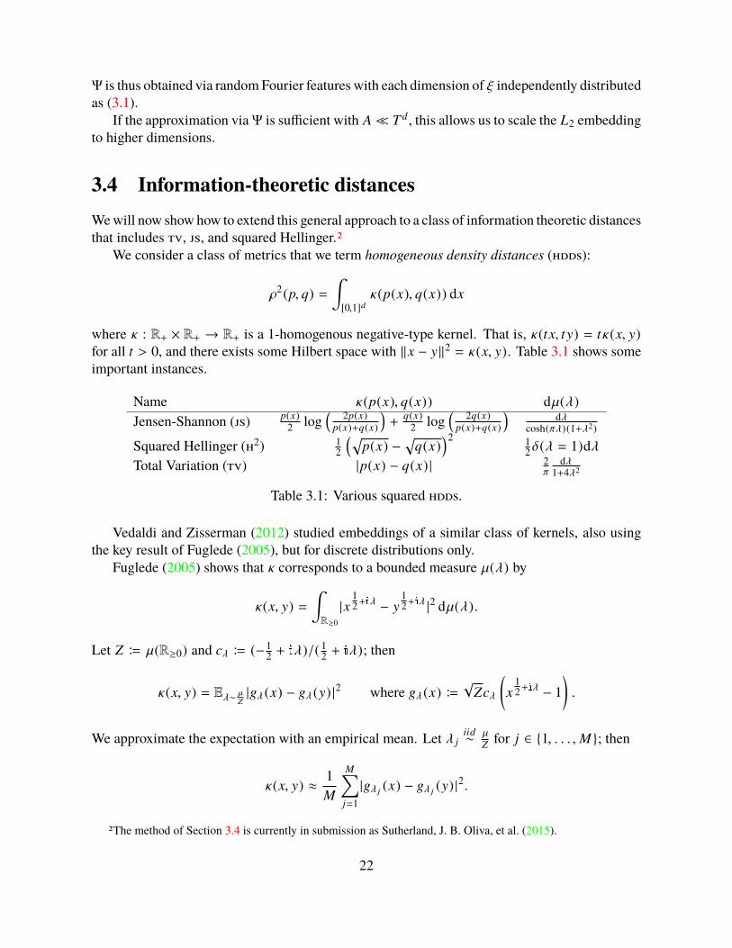
3.4 Information-theoretic distancesWewill now show how to extend this general approach to a class of information theoretic distancesthat includes tv, js, and squared Hellinger.2
We consider a class of metrics that we term homogeneous density distances (hdds):
ρ2(p, q) =∫
[0,1]dκ(p(x), q(x)) dx
where κ : R+ × R+ → R+ is a 1-homogenous negative-type kernel. That is, κ(t x, ty) = tκ(x, y)for all t > 0, and there exists some Hilbert space with ‖x − y‖2 = κ(x, y). Table 3.1 shows someimportant instances.
Name κ(p(x), q(x)) dµ(λ)Jensen-Shannon (js) p(x)
2 log( 2p(x)
p(x)+q(x)
)+
q(x)2 log
( 2q(x)p(x)+q(x)
)dλ
cosh(πλ)(1+λ2)
Squared Hellinger (h2) 12
(√p(x) −
√q(x)
)2 12δ(λ = 1)dλ
Total Variation (tv) |p(x) − q(x) | 2π
dλ1+4λ2
Table 3.1: Various squared hdds.
Vedaldi and Zisserman (2012) studied embeddings of a similar class of kernels, also usingthe key result of Fuglede (2005), but for discrete distributions only.
Fuglede (2005) shows that κ corresponds to a bounded measure µ(λ) by
κ(x, y) =∫R≥0
|x12+iλ − y
12+iλ |2 dµ(λ).
Let Z B µ(R≥0) and cλ B (−12 + iλ)/( 1
2 + iλ); then
κ(x, y) = Eλ∼ µZ|gλ (x) − gλ (y) |2 where gλ (x) B
√Zcλ
(x
12+iλ − 1
).
We approximate the expectation with an empirical mean. Let λ jiid∼
µZ for j ∈ 1, . . . , M ; then
κ(x, y) ≈1M
M∑j=1|gλ j (x) − gλ j (y) |2.
2The method of Section 3.4 is currently in submission as Sutherland, J. B. Oliva, et al. (2015).
22
Hence, the squared hdd is, letting R,I denote the real and imaginary parts:
ρ2(p, q) =∫
[0,1]dκ(p(x), q(x)) dx
=
∫[0,1]dEλ∼ µ
Z|gλ (p(x)) − gλ (q(x)) |2 dx
≈1M
M∑j=1
∫[0,1]d
((R(gλ j (p(x))) − R(gλ j (q(x)))
)2+
(I(gλ j (p(x))) − I(gλ j (q(x)))
)2)dx
=1M
M∑j=1‖pR
λ j− qR
λ j‖2 + ‖pI
λ j− qI
λ j‖2,
wherepRλ (x) B R(gλ (p(x))), pI
λ (x) B I(gλ (p(x))).
Each pλ function is in L2([0, 1]d), so we can approximate e−γρ2(p,q) as in Section 3.3: let
A(P) B1√
M
(~a(pR
λ1)T, ~a(pI
λ1)T, . . . , ~a(pR
λM)T, ~a(pI
λM)T
)T
so that the kernel is estimated by z(A(P)).However, the projection coefficients of the pλ functions do not have simple forms as before;
instead, we directly estimate the density as p using a technique such as kernel density estimation(kde), and then estimate ~a(pλ ) for each λ with numerical integration. Denote the estimatedfeatures as A(p).
For small d, simple Monte Carlo integration is sufficient.In higher dimensions, three problems arise: (i) the embedding dimension increases exponen-
tially, (ii) density estimation becomes statistically difficult, and (iii) accurate numerical integrationbecomes expensive. We can attempt to address (i) with the approach of Section 3.3.1, (ii) withsparse nonparametric graphical models (Lafferty et al. 2012), and (iii) with mcmc integration.High-dimensional multimodal integrals remain particularly challenging to current mcmc tech-niques, though some progress is being made (Betancourt 2015; Lan et al. 2014 give a heuristicalgorithm).
Sutherland, J. B. Oliva, et al. (2015) bound the error probability for this estimator for a pairof distributions P, Q satisfying certain smoothness properties.
23

24
Chapter 4
Applications of distribution learning
We now turn to case studies of the application of distributional kernels to real machine learningtasks.
4.1 Mixture estimationStatistical inference procedures can be viewed as functions from distributions to the reals; wecan therefore consider learning such procedures. Jitkrittum et al. (2015) trained mmd-based gpregression for the messages computed by numerical integration in an expectation propagationsystem, and saw substantial speedups by doing so. We, inspired by J. B. Oliva, Neiswanger, et al.(2014), consider a problem where we not only obtain speedups over traditional algorithms, butactually see far superior results.1 Specifically, we consider predicting the number of componentsin a Gaussian mixture. We generate mixtures as follows:
1. Draw the number of components Yi for the ith distribution as Yi ∼ Unif1, . . . , 10.2. For each component, select a mean µ(i)
k ∼ Unif[−5, 5]2 and covariance Σ(i)k = a(i)
k A(i)k A(i)T
k +
B(i)k , where a ∼ Unif[1, 4], A(i)
k (u, v) ∼ Unif[−1, 1], and B(i)k is a diagonal 2×2 matrix with
B(i)k (u, u) ∼ Unif[0, 1].
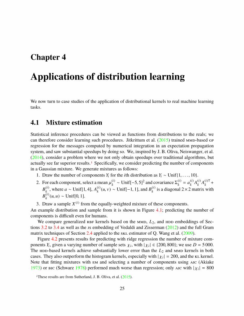
3. Draw a sample X (i) from the equally-weighted mixture of these components.An example distribution and sample from it is shown in Figure 4.1; predicting the number ofcomponents is difficult even for humans.
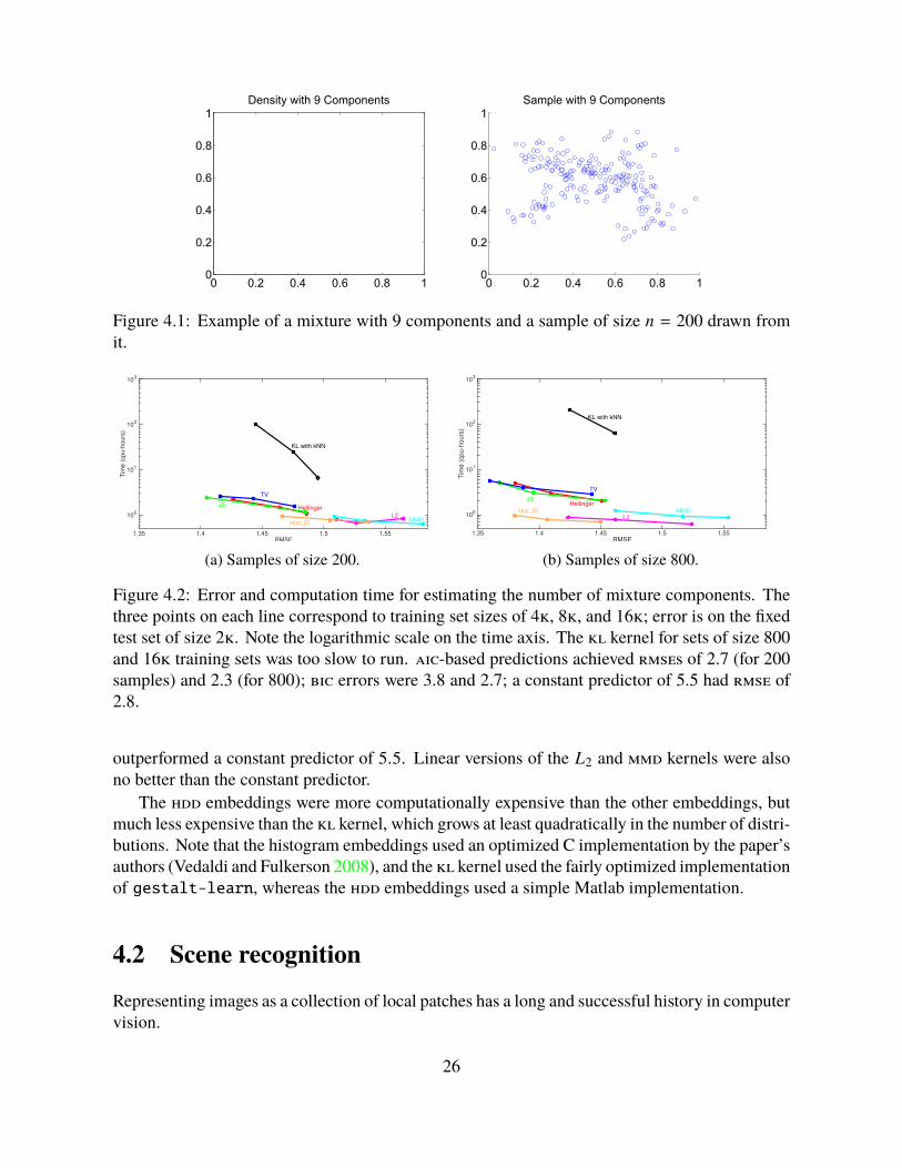
We compare generalized rbf kernels based on the mmd, L2, and hdd embeddings of Sec-tions 3.2 to 3.4 as well as the js embedding of Vedaldi and Zisserman (2012) and the full Grammatrix techniques of Section 2.4 applied to the skl estimator of Q. Wang et al. (2009).
Figure 4.2 presents results for predicting with ridge regression the number of mixture com-ponents Yi, given a varying number of sample sets χi, with | χi | ∈ 200, 800; we use D = 5 000.The hdd-based kernels achieve substantially lower error than the L2 and mmd kernels in bothcases. They also outperform the histogram kernels, especially with | χi | = 200, and the kl kernel.Note that fitting mixtures with em and selecting a number of components using aic (Akiake1973) or bic (Schwarz 1978) performed much worse than regression; only aic with | χi | = 800
1These results are from Sutherland, J. B. Oliva, et al. (2015).
25
Density with 9 Components
0 0.2 0.4 0.6 0.8 10
0.2
0.4
0.6
0.8
1
0 0.2 0.4 0.6 0.8 10
0.2
0.4
0.6
0.8
1Sample with 9 Components
Figure 4.1: Example of a mixture with 9 components and a sample of size n = 200 drawn fromit.
RMSE1.35 1.4 1.45 1.5 1.55
Tim
e (
cpu-h
ours
)
100
101
102
103
HellingerJS
TV
L2MMD
KL with kNN
Hist JS
(a) Samples of size 200.RMSE
1.35 1.4 1.45 1.5 1.55
Tim
e (
cp
u-h
ou
rs)
100
101
102
103
HellingerJS
TV
L2MMD
KL with kNN
Hist JS
(b) Samples of size 800.
Figure 4.2: Error and computation time for estimating the number of mixture components. Thethree points on each line correspond to training set sizes of 4k, 8k, and 16k; error is on the fixedtest set of size 2k. Note the logarithmic scale on the time axis. The kl kernel for sets of size 800and 16k training sets was too slow to run. aic-based predictions achieved rmses of 2.7 (for 200samples) and 2.3 (for 800); bic errors were 3.8 and 2.7; a constant predictor of 5.5 had rmse of2.8.
outperformed a constant predictor of 5.5. Linear versions of the L2 and mmd kernels were alsono better than the constant predictor.
The hdd embeddings were more computationally expensive than the other embeddings, butmuch less expensive than the kl kernel, which grows at least quadratically in the number of distri-butions. Note that the histogram embeddings used an optimized C implementation by the paper’sauthors (Vedaldi and Fulkerson 2008), and the kl kernel used the fairly optimized implementationof gestalt-learn, whereas the hdd embeddings used a simple Matlab implementation.
4.2 Scene recognition
Representing images as a collection of local patches has a long and successful history in computervision.
26
4.2.1 sift featuresThe traditional approach selects a grid of patches, computes a hand-designed feature vector suchas sift (Lowe 2004) for each patch, possibly appends information about the location of the patch,and then uses the bow representation for this set of features. We will first consider the use ofdistributional distance kernels for this feature representation.2
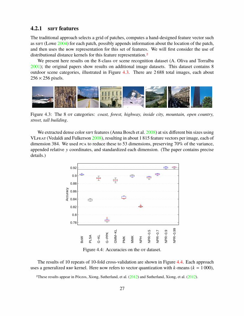
We present here results on the 8-class ot scene recognition dataset (A. Oliva and Torralba2001); the original papers show results on additional image datasets. This dataset contains 8outdoor scene categories, illustrated in Figure 4.3. There are 2 688 total images, each about256 × 256 pixels.
Figure 4.3: The 8 ot categories: coast, forest, highway, inside city, mountain, open country,street, tall building.
We extracted dense color sift features (Anna Bosch et al. 2008) at six different bin sizes usingVLfeat (Vedaldi and Fulkerson 2008), resulting in about 1 815 feature vectors per image, each ofdimension 384. We used pca to reduce these to 53 dimensions, preserving 70% of the variance,appended relative y coordinates, and standardized each dimension. (The paper contains precisedetails.)
0.78
0.8
0.82
0.84
0.86
0.88
0.9
0.92
BoW
PLS
A
G−
KL
G−
PP
K
GM
M−
KL
PM
K
MM
K
NP
H
NP
R−
0.5
NP
R−
0.7
NP
R−
0.9
NP
R−
0.99
Acc
urac
y
Figure 4.4: Accuracies on the ot dataset.
The results of 10 repeats of 10-fold cross-validation are shown in Figure 4.4. Each approachuses a generalized rbf kernel. Here bow refers to vector quantization with k-means (k = 1 000),
2These results appear in Póczos, Xiong, Sutherland, et al. (2012) and Sutherland, Xiong, et al. (2012).
27
plsa to the approach of A. Bosch et al. (2006), g-kl and g-ppk to the kl and Hellinger divergencesbetween Gaussians fit to the data, gmm-kl to the kl between Gaussian mixtures (computing viaMonte Carlo), pmk to the pyramid matching kernel of Grauman and Darrell (2007), mmk tothe mmk with a Gaussian base kernel, nph to the nonparametric Hellinger estimate of Póczos,Xiong, Sutherland, et al. (2012), and npr- to the rα estimates. The horizontal line shows the bestpreviously reported result (Qin and Yung 2010), though others have since slightly surpassed ourresults here.
4.2.2 Deep featuresFor the last several years, however, modern computer vision has become overwhelmingly basedon deep neural networks. Image classification networks typically broadly follow the architectureof Krizhevsky et al. (2012), i.e. several convolutional and pooling layers to extract complexfeatures of input images followed by one or two fully-connected layers to classify the images.
The activations are of shape n× h×w, where n is the number of filters; each unit correspondsto an overlapping patch of the original image. We can therefore treat the activations as a sampleof size hw from an n-dimensional distribution. Wu et al. (2015) set accuracy records on severalscene classification datasets with a particular method of extracting features from distributions.That method, however, resorts to ad-hoc statistics; we compare to our more principled alternativeshere.3
87%
88%
89%
90%
91%
92%
93%
D3 L2 HDDsJS TV Hel
MMD
12σ σ 2σ
Hist JS
10 25 50
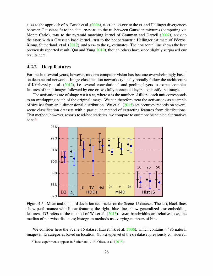
Figure 4.5: Mean and standard deviation accuracies on the Scene-15 dataset. The left, black linesshow performance with linear features; the right, blue lines show generalized rbf embeddingfeatures. D3 refers to the method of Wu et al. (2015). mmd bandwidths are relative to σ, themedian of pairwise distances; histogram methods use varying numbers of bins.
We consider here the Scene-15 dataset (Lazebnik et al. 2006), which contains 4 485 naturalimages in 15 categories based on location. (It is a superset of the ot dataset previously considered,
3These experiments appear in Sutherland, J. B. Oliva, et al. (2015).
28
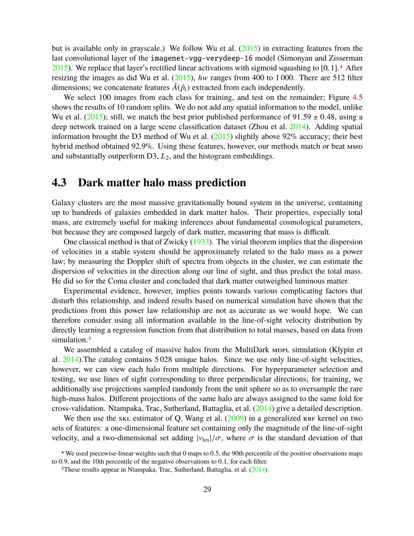
but is available only in grayscale.) We follow Wu et al. (2015) in extracting features from thelast convolutional layer of the imagenet-vgg-verydeep-16 model (Simonyan and Zisserman2015). We replace that layer’s rectified linear activations with sigmoid squashing to [0, 1].4 Afterresizing the images as did Wu et al. (2015), hw ranges from 400 to 1 000. There are 512 filterdimensions; we concatenate features A(pi) extracted from each independently.
We select 100 images from each class for training, and test on the remainder; Figure 4.5shows the results of 10 random splits. We do not add any spatial information to the model, unlikeWu et al. (2015); still, we match the best prior published performance of 91.59 ± 0.48, using adeep network trained on a large scene classification dataset (Zhou et al. 2014). Adding spatialinformation brought the D3 method of Wu et al. (2015) slightly above 92% accuracy; their besthybrid method obtained 92.9%. Using these features, however, our methods match or beat mmdand substantially outperform D3, L2, and the histogram embeddings.
4.3 Dark matter halo mass predictionGalaxy clusters are the most massive gravitationally bound system in the universe, containingup to hundreds of galaxies embedded in dark matter halos. Their properties, especially totalmass, are extremely useful for making inferences about fundamental cosmological parameters,but because they are composed largely of dark matter, measuring that mass is difficult.
One classical method is that of Zwicky (1933). The virial theorem implies that the dispersionof velocities in a stable system should be approximately related to the halo mass as a powerlaw; by measuring the Doppler shift of spectra from objects in the cluster, we can estimate thedispersion of velocities in the direction along our line of sight, and thus predict the total mass.He did so for the Coma cluster and concluded that dark matter outweighed luminous matter.
Experimental evidence, however, implies points towards various complicating factors thatdisturb this relationship, and indeed results based on numerical simulation have shown that thepredictions from this power law relationship are not as accurate as we would hope. We cantherefore consider using all information available in the line-of-sight velocity distribution bydirectly learning a regression function from that distribution to total masses, based on data fromsimulation.5
We assembled a catalog of massive halos from the MultiDark mdpl simulation (Klypin etal. 2014).The catalog contains 5 028 unique halos. Since we use only line-of-sight velocities,however, we can view each halo from multiple directions. For hyperparameter selection andtesting, we use lines of sight corresponding to three perpendicular directions; for training, weadditionally use projections sampled randomly from the unit sphere so as to oversample the rarehigh-mass halos. Different projections of the same halo are always assigned to the same fold forcross-validation. Ntampaka, Trac, Sutherland, Battaglia, et al. (2014) give a detailed description.
We then use the skl estimator of Q. Wang et al. (2009) in a generalized rbf kernel on twosets of features: a one-dimensional feature set containing only the magnitude of the line-of-sightvelocity, and a two-dimensional set adding |vlos |/σ, where σ is the standard deviation of that
4 We used piecewise-linear weights such that 0 maps to 0.5, the 90th percentile of the positive observations mapsto 0.9, and the 10th percentile of the negative observations to 0.1, for each filter.
5These results appear in Ntampaka, Trac, Sutherland, Battaglia, et al. (2014).
29
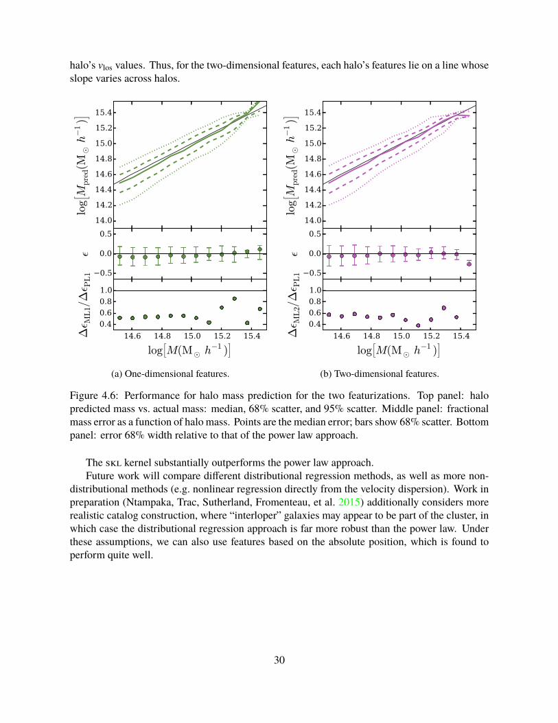
halo’s vlos values. Thus, for the two-dimensional features, each halo’s features lie on a line whoseslope varies across halos.
14.0
14.2
14.4
14.6
14.8
15.0
15.2
15.4
log[ M p
red(M
¯h−
1)]
0.5
0.0
0.5
ε
14.6 14.8 15.0 15.2 15.4
log[M(M¯ h
−1 )]
0.4
0.6
0.8
1.0
∆ε M
L1/∆ε P
L1
(a) One-dimensional features.
14.0
14.2
14.4
14.6
14.8
15.0
15.2
15.4
log[ M p
red(M
¯h−
1)]
0.5
0.0
0.5
ε
14.6 14.8 15.0 15.2 15.4
log[M(M¯ h
−1 )]
0.4
0.6
0.8
1.0∆ε M
L2/∆ε P
L1
(b) Two-dimensional features.
Figure 4.6: Performance for halo mass prediction for the two featurizations. Top panel: halopredicted mass vs. actual mass: median, 68% scatter, and 95% scatter. Middle panel: fractionalmass error as a function of halo mass. Points are the median error; bars show 68% scatter. Bottompanel: error 68% width relative to that of the power law approach.
The skl kernel substantially outperforms the power law approach.Future work will compare different distributional regression methods, as well as more non-
distributional methods (e.g. nonlinear regression directly from the velocity dispersion). Work inpreparation (Ntampaka, Trac, Sutherland, Fromenteau, et al. 2015) additionally considers morerealistic catalog construction, where “interloper” galaxies may appear to be part of the cluster, inwhich case the distributional regression approach is far more robust than the power law. Underthese assumptions, we can also use features based on the absolute position, which is found toperform quite well.
30
Chapter 5
Active search for patterns
We will now change focuses slightly, and consider another problem setting in which collectionsof data play a key role.1
Consider a function containing interesting patterns that are defined only over a region ofspace. For example, if you view the direction of wind as a function of geographical location,it defines fronts, vortices, and other weather patterns, but those patterns are defined only in theaggregate. If we can only measure the direction and strength of the wind at point locations, wethen need to infer the presence of patterns over broader spatial regions.
Many other real applications also share this feature. For example, an autonomous environ-mental monitoring vehicle with limited onboard sensors needs to strategically plan routes aroundan area to detect harmful plume patterns on a global scale (Valada et al. 2012). In astronomy,projects like the Sloan Digital Sky Survey (Eisenstein et al. 2011) search the sky for large-scaleobjects such as galaxy clusters. Biologists investigating rare species of animals must find theranges where they are located and their migration patterns (Brown et al. 2014). We aim to useactive learning to search for such global patterns using as few local measurements as possible.
This bears some resemblance to the artistic technique known as pointillism, where the paintercreates small and distinct dots each of a single color, but when viewed as a whole they reveala scene. Pointillist paintings typically use a denser covering of the canvas, but in our setting,“observing a dot” is expensive. Where should we make these observations in order to uncoverinteresting regions as quickly as possible?
We propose a probabilistic solution to this problem, known as active pointillistic patternsearch (apps). We assume we are given a predefined list of candidate regions and a classifierthat estimates the probability that a given region fits the desired pattern. Our goal is then tofind as many regions that are highly likely to match the pattern as we can. We accomplish thisby sequentially selecting point locations to observe so as to approximately maximize expectedreward.
1This chapter was previously published in longer form as Ma, Sutherland, et al. 2015.
31
5.1 Related WorkOur concept of active pattern search falls under the broad category of active learning (Settles2012), where we seek to sequentially build a training set to achieve some goal as fast as possible.Our focus solely on finding positive (“interesting”) regions, rather than attempting to learn todiscriminate accurately between positives and negatives, is similar to the problem previouslydescribed as active search (Garnett et al. 2012). In previous work on active search, however, ithas been assumed that the labels of interest can be revealed directly. In active pattern search, onthe other hand, the labels are never revealed but must be inferred via a provided classifier. Thisindirection increases the difficulty of the search task considerably.
In Bayesian optimization (Osborne et al. 2009; Brochu et al. 2010), we seek to find the globaloptimum of an expensive black-box function. Bayesian optimization provides a model-basedapproach where a Gaussian process (gp) prior is placed on the objective function, from which asimpler acquisition function is derived and optimized to drive the selection procedure. Tesch et al.(2013) extend this idea to optimizing a latent function from binary observations. Our proposedactive pattern search also uses a Gaussian process prior tomodel the unknown underlying functionand derives an acquisition function from it, but differs in that we seek to identify entire regionsof interest, rather than finding a single optimal value.
Another intimately related problem setup is that of multi-arm bandits (Auer et al. 2002), withmore focus on analysis of the cumulative reward over all function evaluations. Originally, thegoal was to maximize the expectation of a random function on a discrete set; a variant considersthe optimization in continuous domains (Kroemer et al. 2010; Niranjan et al. 2010). However,like Bayesian optimization, multi-arm bandit problems usually do not consider discriminating aregional pattern.
Level set estimation (Low et al. 2012; Gotovos et al. 2013), rather than finding optima of afunction, seeks to select observations so as to best discriminate the portions of a function aboveand below a given threshold. This goal, though related to ours, aims to directly map a portion ofthe function on the input space rather than seeking out instances of patterns. lse algorithms canbe used to attempt to find some simple types of patterns, e.g. areas with high mean.
apps can be viewed as a generalization of active area search (aas) (Ma, Garnett, et al. 2014),which is a considerably simpler version of active search for region-based labels. In aas, the labelof a region is only determined by whether its mean value exceeds some threshold. apps allows forarbitrary classifiers rather than simple thresholds, and in some cases its expected reward can stillbe computed analytically. This extends the usefulness of this class of algorithms considerably.
5.2 Problem FormulationThere are three key components of the apps framework: a function f which maps input covariatesto data observations, a predetermined set of regions wherein instances of function patterns areexpected, and a classifier that evaluates the salience of the pattern of function values in eachregion. We define f : Rm → R to be the function of interest,2 which can be observed at any
2For clarity, in this and the next sectionswewill focus on scalar-valued functions f . The extension to vector-valuedfunctions is straightforward; we consider such a case in the experiments.
32
location x ∈ Rm to reveal a noisy observation z. We assume the observation model z = f (x) + ε,where ε iid
∼ N (0, σ2). We suppose that a set of regions where matching patterns might be foundis predefined, and will denote these g1, . . . , gk ; gi ⊂ R
m. Finally, for each region g, we assume aclassifier hg which evaluates f on g and returns the probability that it matches the target pattern,which we call salience: hg ( f ) = h( f ; g) ∈ [0, 1], where the mathematical interpretation of hg issimilar to a functional of f . Classifier forms are typically the same for all regions with differentparameters.
Unfortunately, in general, we will have little knowledge about f other than the limitedobservations made at our selected set of points. Classifiers which take functional inputs (such asour assumed hg) generally do not account for uncertainty in their inputs, which should be inverselyrelated to the number of observed data points. We thus consider the probability that hg ( f ) ishigh enough, marginalized across the range of functions f that might match our observations.As is common in nonparametric Bayesian modeling, we model f with a Gaussian process (gp)prior; we assume that hyperparameters, including prior mean and covariance functions, are setby domain experts. Given a dataset D = (X, z), we define
f ∼ GP (µ, κ); f | D ∼ GP (µ f |D, κ f |D ),
to be a given gp prior and its posterior conditioned onD, respectively. Thus, since f is a randomvariable, we can obtain the marginal probability that g is salient,
Tg (D) = E f[hg ( f ) | D
]. (5.1)
We then define a matching region as one whose marginal probability passes a given threshold θ.Unit reward is assigned to each matching region g:
rg (D) B 1Tg (D) > θ
.
We make two assumptions regarding the interactive procedure. The first is that once a regionis flagged as potentially matching (i.e., its marginal probability exceeds θ), it will be immediatelyflagged for further review and no longer considered during the run. The second is that the dataresulting from this investigation will not be made immediately available during the course of thealgorithm; rather the classifiers hg will be trained offline. We consider both of these assumptionsto be reasonable when the cost of investigation is relatively high and the investigation collectsdifferent types of data. For example, if the algorithm is being used to run autonomous sensorsand scientists collect separate data to follow up on a matching region, these assumptions allow theautonomous sensors to continue in parallel with the human intervention, and avoid the substantialcomplexity of incorporating a completely different modality of data into the modeling process.
Garnett et al. (2012) attempt to maximize their reward at the end of a fixed number of queries.Directly optimizing that goal involves an exponential lookahead process. However, this canbe approximated by a greedy search like the one we perform. Similarly, one could attempt tomaximize the area under the recall curve through the search process. This also requires anintractable amount of computation which is often replaced with a greedy search.
We now write down the greedy criterion our algorithm seeks to optimize. DefineDt to be thealready collected (noisy) observations of f before time step t and Gt = g : Tg (Dτ) ≤ θ,∀τ ≤ t
33
to be the set of remaining search subjects; we aim to greedily maximize the sum of rewards overall the regions in Gt in expectation,
maxx∗E
∑g∈Gt
rg (D∗)
x∗,Dt
, (5.2)
where D∗ is the (random) dataset augmented with x∗.This criterion satisfies a desirable property: when the regions are uncoupled and the classifier
hg is probit-linear, the point that maximizes (5.2) in each region also minimizes the variance ofthat region’s label (Section 5.3.2).
5.3 MethodFor the aim of maximizing the greedy expected reward of finding matching patterns (5.2), a morecareful examination of the gp model can yield a straightforward sampling method. This method,in the following, turns out to be quite useful in apps problems with rather complex classifiers.Section 5.3.1 introduces an analytical solution in an important special case.
At each step, given Dt = (X, z) as the set of any already collected (noisy) observations of fand x∗ as any potential input location, we can assume the distribution of possible observations z∗as
z∗ | x∗,Dt ∼ N(µ f |Dt (x∗), κ f |Dt (x∗, x∗) + σ2) . (5.3)
Conditioned on an observation value z∗, we can update our gp model to include the new observa-tion (x∗, z∗), which further affects the marginal distribution of region classifier outputs and thusthe probability this region is matching. WithD∗ = Dt ∪
(x∗, z∗)
as the updated dataset, we use
rg (D∗) to be the updated reward of region g. The utility of this proposed location x∗ for regiong is thus measured by the expected reward function, marginalizing out the unknown observationvalue z∗:
ug (x∗,Dt ) B Ez∗[rg (D∗) | x∗,Dt
](5.4)
= PrTg (D∗) > θ | x∗,Dt
. (5.5)
Finally, in active pointillistic pattern search, we select the next observation location x∗ by consid-ering its expected reward over the remaining regions:
x∗ = argmaxx
u(x,Dt ) = argmaxx
∑g∈Gt
ug (x,Dt ). (5.6)
For the most general definition of the region classifier hg, the basic algorithm is to compute(5.4) and thus (5.6) via sampling at two stages:
1. Sample the outer variable z∗ in (5.4) according to (5.3).2. For every draw of z∗, sample enough of ( f | D∗) to compute the marginal reward Tg (D∗)
in (5.1), in order to obtain one draw for the expectation in (5.4).To speed up the process, we can evaluate (5.6) for a subset of possible x∗ values, as long as a
good action is likely to be contained in the set.
34
5.3.1 Analytic Expected Utility for Functional Probit ModelsFor a broad family of classifiers, we can compute both (5.1) and (5.5) analytically, allowing usto efficiently perform exact searches for potentially complex patterns. This family is formed by aprobit link function of any affine functional of f .
Suppose we have observed data D, yielding the posterior p( f | D) = GP ( f ; µ f |D, κ f |D ).Let Lg be a linear functional, Lg : f 7→ Lg f ∈ R, associated with region g. The family ofclassifiers is:
hg ( f ) = Φ(Lg f + bg),
where Φ is the cumulative distribution function of the standard normal and b ∈ R is an offset.Two examples of such functionals are:
• Lg f : f 7→ c|g |
∫g
f (x)dx, where |g | is the volume of region g ⊂ Rm. Here Lg f is the meanvalue of f on g, scaled by an arbitrary c ∈ R. When |c | → ∞ the model becomes quitesimilar to that of Ma, Garnett, et al. (2014).
• Lg f : f 7→ wT f (Ξ), where Ξ is a finite set of fixed points ξi|Ξ|
i=1, and w ∈ R|Ξ| is anarbitrary vector. This mapping applies a linear classifier to a fixed, discrete set of valuesfrom f .
Section 3.1 of Ma, Sutherland, et al. (2015) shows that the expected reward is:
ug (x∗,D) = Φ*..,
Lgµ f |D + b −√
1 + L2gκ f |D∗ Φ
−1(θ)√V−1∗|D
Lg[κ f |D (·, x∗)
]2
+//-
(5.7)
where L2g is the bilinear form L2
gκ : κ 7→ L[Lκ(x, ·)] = L[Lκ(·, x′)].
5.3.2 Analysis for Independent RegionsThe analytical solution to (5.5) by (5.7) enables us to further study the theory behind the explo-ration/exploitation tradeoff of apps in one nontrivial case: when all regions are approximatelyindependent. This assumption allows us to ignore the effect a data point has on regions otherthan its own. We will answer two questions in this case: which region will apps explore next,and what location will be queried for that region.
Define
ρg (x∗) B
√V−1∗|D
Lg
[κ f |D (·, x∗)
]2√1 + L2
gκ f |D
=Corr
(z∗, Lg f + b + ε1
x∗,D) ,
where ε1 ∼ N (0, 1) is independent noise, denote how informative the point z∗ is to the label ofits region g. Also define how close g is to receiving a reward by
Rg BΦ−1(Tg (D))Φ−1(θ)
.
Section 3.2 ofMa, Sutherland, et al. (2015) shows that for regions not currently carrying a reward:
35
1. For any region g, ug (x,D) is maximized by choosing the x that yields ρ∗g B maxx ρg (x).2. If two regions g and g′ can be equally explored (ρ∗g = ρ∗g′), then the region with more
probability of matching R will be selected.3. If two regions are equally likely tomatch the desired pattern (Rg = Rg′), themore explorable
region (that with a larger ρ∗) will be selected.
4. In general, apps will trade off the two factors by maximizing(Rg −
√1 − (ρ∗g)2
)/ρ∗g.
5.4 Empirical EvaluationMa, Sutherland, et al. (2015) evaluates the framework in three different settings, with threedifferent classifiers. We reproduce only one of these evaluations here. The others are based onreal environmental monitoring data and electoral prediction data, using the analytical results ofSection 5.3.1.
The problem we consider here requires more complex pattern classifiers. We study the taskof identifying vortices in a vector field based on limited observations of flow vectors. Linearclassifiers are insufficient for this problem,3 so we will demonstrate the flexibility of our approachwith a black-box classifier.
To illustrate this setting, we consider the results of a large-scale simulation of a turbulent fluidin three dimensions over time in the Johns Hopkins Turbulence Databases4 (Perlman et al. 2007).Following Sutherland, Xiong, et al. (2012), we aim to recognize vortices in two-dimensionalslices of the data at a single timestep, based on the same small training set of 11 vortices and 20non-vortices, partially shown in Figure 5.1.
Recall that hg assigns probability estimates to the entire function class F confined to regiong. We can consider the average flow across sectors (angular slices from the center) of our regionas building blocks in detecting vortices. We count how many sectors have clockwise/counter-clockwise flows to give a classification result, in three steps:
1. First, we divide a region into K sectors. In each sector, we take the integral of the innerproduct between the actual flow vectors and a template. The template is an “ideal” vortex,but with larger weights in the center than the periphery. This produces a K-dimensionalsummary statistic Lg ( f ) for each region.
2. Next, we improve robustness against different flow speeds in the data by scaling Lg ( f ) tohave maximum entry 1, and flip its sign if its mean is negative. Call the result Lg ( f ).
3. Finally, we feed the normalized Lg ( f ) vector through a 2-layer neural network of the form
hg ( f ) = σ *,wout
K∑i=1
σ(win Lg ( f )i + bin
)+ bout+
-,
where σ is the logistic sigmoid function.
3The set of vortices is not convex: consider the midpoint between a clockwise vortex and its identical counter-clockwise case.
4http://turbulence.pha.jhu.edu
36
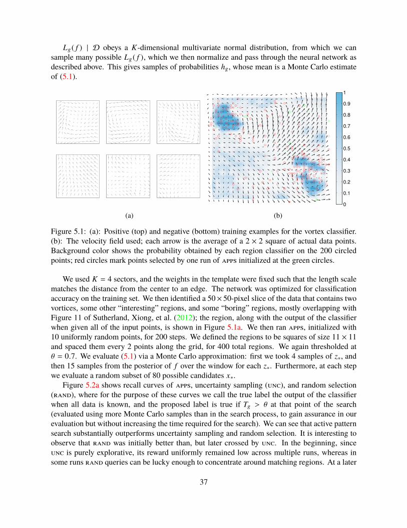
Lg ( f ) | D obeys a K-dimensional multivariate normal distribution, from which we cansample many possible Lg ( f ), which we then normalize and pass through the neural network asdescribed above. This gives samples of probabilities hg, whose mean is a Monte Carlo estimateof (5.1).
(a)
0
0.1
0.2
0.3
0.4
0.5
0.6
0.7
0.8
0.9
1
(b)
Figure 5.1: (a): Positive (top) and negative (bottom) training examples for the vortex classifier.(b): The velocity field used; each arrow is the average of a 2 × 2 square of actual data points.Background color shows the probability obtained by each region classifier on the 200 circledpoints; red circles mark points selected by one run of apps initialized at the green circles.
We used K = 4 sectors, and the weights in the template were fixed such that the length scalematches the distance from the center to an edge. The network was optimized for classificationaccuracy on the training set. We then identified a 50× 50-pixel slice of the data that contains twovortices, some other “interesting” regions, and some “boring” regions, mostly overlapping withFigure 11 of Sutherland, Xiong, et al. (2012); the region, along with the output of the classifierwhen given all of the input points, is shown in Figure 5.1a. We then ran apps, initialized with10 uniformly random points, for 200 steps. We defined the regions to be squares of size 11 × 11and spaced them every 2 points along the grid, for 400 total regions. We again thresholded atθ = 0.7. We evaluate (5.1) via a Monte Carlo approximation: first we took 4 samples of z∗, andthen 15 samples from the posterior of f over the window for each z∗. Furthermore, at each stepwe evaluate a random subset of 80 possible candidates x∗.
Figure 5.2a shows recall curves of apps, uncertainty sampling (unc), and random selection(rand), where for the purpose of these curves we call the true label the output of the classifierwhen all data is known, and the proposed label is true if Tg > θ at that point of the search(evaluated using more Monte Carlo samples than in the search process, to gain assurance in ourevaluation but without increasing the time required for the search). We can see that active patternsearch substantially outperforms uncertainty sampling and random selection. It is interesting toobserve that rand was initially better than, but later crossed by unc. In the beginning, sinceunc is purely explorative, its reward uniformly remained low across multiple runs, whereas insome runs rand queries can be lucky enough to concentrate around matching regions. At a later
37
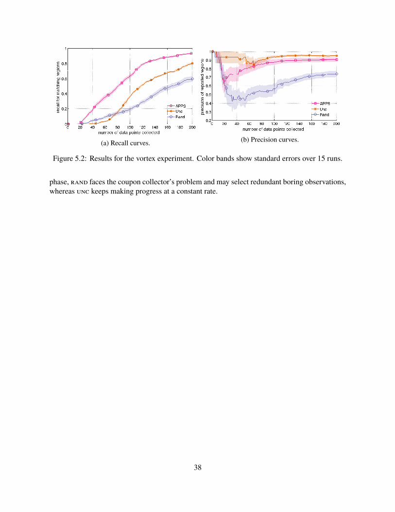
(a) Recall curves. (b) Precision curves.
Figure 5.2: Results for the vortex experiment. Color bands show standard errors over 15 runs.
phase, rand faces the coupon collector’s problem and may select redundant boring observations,whereas unc keeps making progress at a constant rate.
38

Chapter 6
Proposed work
6.1 Integration with deep computer vision models
In Section 4.2, we considered using the features learned by a standard convolutional deep networkas samples from an image-level distribution of local features, and classified images based on thosesets of features. Here features are trained using fully-connected final layers as the learning model,but then used in a separate distributional kernel model.
We can instead make a coherent model which combines feature extraction with a learningmodel based on a distributional kernel, by treating the approximate distributional embedding asa layer in the network. With the mean map-based embedding, gradients propagate through thislayer easily, and so standard stochastic gradient algorithms can be used either to fine-tune featurestrained on a different task or to learn features well-suited to distributional kernel models from thestart.
In fact, we can also consider using distributional embeddings in intermediate layers of thenet; gradients propagate in the same way. This could help in learning more complex filters insidethe net with fewer training examples.
I propose to:1. Implement the necessary components to add approximate distribution embedding layers to
standard deep learning software such as Caffe or Torch.2. Evaluate the use of fine-tuning features for scene recognition models using distributional
classifiers in the last layers.3. Experiment with image recognition using distributional filters in earlier layers.
6.2 Word embeddings as distributions
Until recently, much work in natural language processing treated words as unique symbols, e.g.with “one-hot” vectors, where the ith word from a vocabulary of size V is represented as avector with ith component 1 and all other components 0. It has recently become widely acceptedthat applications can benefit from richer word embeddings which take into account the similaritybetween distinct words, andmuchwork has been done on denseword embeddings so that distances
39

or inner products betweenword embeddings represent word similarity in someway (e.g. Collobertand Weston 2008; Turian et al. 2010; Mikolov et al. 2013). These embeddings can be learned invarious ways, but often involve optimizing the representation’s performance in some supervisedlearning task.
Document representations First, it is worth noting that although this breaks the traditional“bag of words” text model (where documents can be represented simply by the sum of the words’one-hot encodings), we can represent documents by viewing them as sample sets of word vectors.
Kusner et al. (2015) recently adopted this model, using kNN classifiers based on the emdbetween documents, and obtained excellent empirical results. emd, however, is expensive tocompute even for each pair of documents when the vocabulary is large, and additionally must becomputed pairwise between documents; an approximate embedding in the style of Chapter 3 isnot known.
Yoshikawa et al. (2014), in their empirical results, considered this model with mmd-basedkernels (but computing pairwise kernel values rather than approximate embeddings). Theirmain contribution, however, is to optimize the word embedding vectors for final classificationperformance; by doing so with random initializations, they saw mild performance improvementsover mmd kernels using substantially less training data for the embeddings but at much highercomputational cost. Yoshikawa et al. (2015) extend the approach to Gaussian process regressionmodels, but do not compare to separately-learned word embeddings.
I propose to:4. Empirically compare these embedding methods, particularly on larger datasets, to establish
the best method for bag-of-words document representation.5. Fine-tune word embeddings learned on a standard dataset simultaneously with learning the
model for a particular application, as is common in deep learning models for computervision, using techniques similar to those of Section 6.1.
Richer word representation Embedding words as a single vector does not allow for as richa word representation as we might wish. Vilnis and McCallum (2015) embed words instead asGaussian distributions, and use the kl divergence between word embeddings to measure asym-metric hypernym relationships: for example, their embedding for the word Bach is “included” intheir embeddings for famous and man, and mostly included in composer. Gaussian distributions,of course, are still fairly limiting; for example, a multimodal embedding might be able to captureword sense ambiguity, whereas a Gaussian embedding would be forced to attempt to combineboth senses in a single broad embedding.
We can thus consider richer, nonparametric classes of word embeddings: perhaps by rep-resenting a word as a (possibly weighted) set of latent vectors. Comparisons could then beperformed either with an mmd-based kernel, when symmetry is desired, or with kl estimators (orsimilar) when not.
One approach would be to choose these vectors arbitrarily, optimizing them for the output ofsome learning problem: this would be implemantionally similar to the approach of Yoshikawaet al. (2014, 2015) for mmd distances, or somewhat like that of Vilnis and McCallum (2015) butwith greater computational cost, and greater flexibility, for kl distances.
40
Another approach is inspired by the classic distributional hypothesis of Harris (1954), that thesemantics of words are characterized by the contexts in which it appears. Many word embeddingapproaches can be viewed as matrix factorizations of a matrix M with rows corresponding towords, columns to some notion of context, and entries containing some measure of associationbetween the two; the factorization M = WCT then typically discards the matrix C and usesthe rows of W as word vectors. This approach is sometimes taken explicitly; interestingly, thepopular method of Mikolov et al. (2013) can be seen as approximating this form as well (Levyand Goldberg 2014). This view inspires a natural alternative: treat each word as the sampleset of contexts in which it appears, representing each context via the learned context vectors.This is perhaps the most direct instantiation of the distributional hypothesis: compare words bycomparing the distribution of contexts in which they appear.
I propose to:6. Develop efficient methods for learning nonparametric distributional word embeddings for
asymmetric divergences.7. Empirically evaluate nonparametric distribution-based word embeddings, based both on
arbitrary embeddings and context features, both on analogy tasks and downstreamdocumentclassification tasks.
6.3 Kernel learning for distribution embeddings
Mean map methods rely on having a good base kernel in order to make good comparisonsbetween distributions, whether for kernels in learning problems or for two sample tests. The mostcommon technique is to choose a simple family of kernels, perhaps the Gaussian kernel withvarious bandwidths selected as multiples of the median inter-point distance, and then pick thekernel that performs best on a validation set — as with typical hyperparameter optimization. Fortwo-sample tests, Sriperumbudur, Fukumizu, Gretton, Lanckriet, et al. (2009) propose insteadusing the kernel that yields the maximum distance between distributions over certain families ofdistributions. Gretton, Sriperumbudur, et al. (2012) find the optimal positive linear combinationof kernels for (linear variants of) a two-sample test. Neither technique, however, seems to havebeen thoroughly evaluated outside the context of two-sample testing.
We can also consider more complex kernel learning frameworks thanmultiple kernel learning.Z. Yang et al. (2015) recently proposed a spectral kernel learning method capable of learningricher kernels than simple linear combinations or bandwidth selection; integrating that methodinto the mean map kernel, for two-sample testing as well as for machine learning models, couldprove fruitful in increasing the power and reducing the amount of human intervention needed inusing these models.
For distances being used within a deep network, as in Section 6.1, allowing the network toadapt the embedding may also provide an effective technique for learning the base kernel.
I propose to:8. Adapt the spectral kernel method of Z. Yang et al. (2015) to mean map methods, in
both classification or regression settings and in the two-sample test setting (as in Gretton,Sriperumbudur, et al. 2012).
41
9. Evaluate kernel learning for mmd kernel embeddings in deep networks.
6.4 Embeddings for other kernels
Despite the advantages of mean-map approaches, it may be that in some settings, other distancessuch as emd may induce more useful kernels. If this holds true experimentally, it may make senseto attempt to develop approximate embeddings for other kernels.
Given the close relation between mmd and other integral probability metrics (Müller 1997), asdiscussed in Chapter 2, the question of finding base kernels such that mmd approximates relateddistances is also quite interesting.
In fact, Sriperumbudur, Gretton, et al. (2010, Theorem 21) show the following: Let k bea measurable kernel with supx∈X k (x, x) ≤ C < ∞, and define ρ(x, y) = ‖k (·, x) − k (·, y)‖H .Then mmdk (P,Q) ≤
√C tv(P,Q), and if (X, ρ) is separable then mmdk (P,Q) ≤ emdρ(P,Q) ≤√
mmdk (P,Q)2 + 4C.The first statement implies that choosing k to maximize mmdk (from a family with fixed C),
similar to Sriperumbudur, Fukumizu, Gretton, Lanckriet, et al. (2009), makes mmd approximatetv more closely. But how close is this approximation? For certain classes of distributions, canwe find a kernel that closely approximates tv?
When k is the linear kernel (so ρ(x, y) = ‖x − y‖2) and X ⊆ x ∈ Rd : ‖x‖ ≤ R (soC = R2), mmd approximates the Euclidean emd, but the bounds are quite loose — note thatthe linear-kernel mmd is simply the distance between the means of the distributions. Can wechoose a kernel k such that mmdk more closely approximates the Euclidean emd? (Since mmd isHilbertian and emd is not, some distortion is unavoidable.)
I propose to:10. Look intowhether, for certain classes of distributions, kernels can be obtained such thatmmd
approximates emd or tv — particularly kernels admitting a good approximate embedding.11. Investigate emperically if areas where emd or tv are in common usage cannot be handled
more simply by more efficient mmd kernels, particularly with the kernel learning methodsof Section 6.3.
6.5 Active learning on distributions
Suppose we have a collection of distributions, but initially we have very few samples fromeach distribution. We can choose to take additional iid observations, but doing so is relativelyexpensive; perhaps it requires real-world expenditure of time or resources to collect samples,or perhaps these distributions are available only through computationally intensive numericalsimulations. We may wish to learn a classification or regression function mapping from thesedistributions to some label (similar to traditional active learning settings), to locate distributionswhich follow some prespecified pattern (similar to the setting of Chapter 5 with independentregions), or to find the distribution which is “best” in some sense (as in pure-exploration banditproblems, Bubeck et al. 2010). In any of these cases, we need to choose some selection criterion
42

that will appropriately consider the utility of selecting points from distributions, a problem thatis related to but certainly distinct from typical fully-observed active learning models.
In the dark matter prediction experiments of Section 4.3, we assumed that each observedgalaxy has a well-known line-of-sight velocity estimated via redshift. In practice, good velocityestimates are available only through relatively-expensive spectroscopic imaging; cheaper few-color imaging techniques give extremely uncertain velocity estimates. We could simply ignorethe imaging estimates and apply the previous model, selecting a random galaxy from each haloto perform spectroscopy upon. It would probably be more effective, however, to consider activelearning methods that begin with visual imaging, and then identify which objects will be usefulfor spectroscopy in order to best identify the masses of their dark matter halos. One modelingoption would be to take a probability distribution over the sample set, and then identify theresulting distribution of the mean map embedding and therefore its predicted label under alearned predictor; we would then identify objects to observe that most reduce uncertainty in thepredicted label. This could be conducted either for a single halo, where the objective is to bestlearn its mass, or across multiple halos, where the objective is either to find themost massive halos(active search) or to reduce some form of overall uncertainty in all of the halo mass predictions(active learning).
I propose to:12. Develop and evaluate efficient active learning selection criteria for each of the problem
settings discussed here.
6.6 TimelineMy rough plan for the proposed work is as follows:
September – December 2015: Integration with deep networks; experiments in computervision and document representation. Conference submission. (Partially complete.)
October – December 2015: Investigate embeddings for other kernels. If successful, experi-ments in various domains and possible conference submission.
December 2015 – February 2016: Kernel learning for distribution embeddings. Conferencesubmission.
March – April 2016: Word embeddings. Possible conference submission.April – July 2016: Active learning on distributions, with astronomical application. Submis-
sion to a machine learning conference and/or an astrophysics venue.August 2016: Thesis writing.September 2016: Thesis defense.
43

44

Bibliography
Akiake, Hirotugu (1973). “Information theory and an extension of the maximum likelihood principle”. In:2nd International Symposium on Information Theory (page 25).
Amari, Shun-ichi (1985). Differential-Geometrical Methods in Statistics. Lecture Notes in Statistics 28.Springer (page 6).
Andoni, Alexandr and Ilya Razenshteyn (2015). “Optimal Data-Dependent Hashing for Approximate NearNeighbors”. In: ACM Symposium on Theory of Computing. arXiv: 1501.01062 (page 10).
Auer, Peter, Nicoló Cesa-Bianchi, and Paul Fischer (2002). “Finite-time Analysis of theMultiarmed BanditProblem”. In: Machine Learning 47, pages 235–256 (page 32).
Bengio, Yoshua, Jean-François Paiement, Pascal Vincent, Olivier Delalleau, Nicolas Le Roux, and MarieOuimet (2004). “Out-of-Sample Extensions for LLE, Isomap, MDS, Eigenmaps, and Spectral Clus-tering”. In: Advances in Neural Information Processing Systems. NIPS (page 13).
Berlinet, Alain and Christine Thomas-Agnan (2004). Reproducing kernel Hilbert spaces in Probabilityand Statistics. Kluwer Academic Publishers (page 9).
Betancourt, Michael (2015). “Adiabatic Monte Carlo”. Version 5. In: arXiv: 1405.3489v5 (page 23).Beygelzimer, Alina, Sham Kakade, and John Langford (2006). “Cover trees for nearest neighbor”. In:
International Conference on Machine Learning, pages 97–104 (page 10).Bochner, Salomon (1959). Lectures on Fourier integrals. Princeton University Press (page 15).Boiman, Oren, Eli Shechtman, and Michal Irani (2008). “In defense of nearest-neighbor based image
classification”. In: Computer Vision and Pattern Recognition (page 5).Bosch, A., A. Zisserman, and X. Muñoz (2006). “Scene classification via pLSA”. In: ECCV (page 28).Bosch, Anna, Andrew Zisserman, and Xavier Munoz (2008). “Scene Classification Using a Hybrid Gen-
erative/Discriminative Approach”. In: IEEE Trans. PAMI 30.4 (page 27).Bretagnolle, Jean, Didier Dacunha Castelle, and Jean-Louis Krivine (1966). “Lois stables et espaces LP”.
French. In: Annales de l’institut Henri Poincaré (B) Probabilités et Statistiques 2 (3), pages 231–259(page 12).
Brochu, Eric, Vlad M Cora, and Nando de Freitas (2010). A tutorial on Bayesian optimization of expensivecost functions, with application to active usermodeling and hierarchical reinforcement learning. arXiv:1012.2599 (page 32).
Brown, JasonL,AlisonCameron,AnneDYoder, andMiguelVences (2014). “Anecessarily complexmodelto explain the biogeography of the amphibians and reptiles ofMadagascar.” In:Nature communications5, page 5046 (page 31).
Bubeck, Sébastien, Rémi Munos, and Gilles Stoltz (2010). “Pure exploration in multi-armed banditsproblems”. In: Algorithmic Learning Theory, pages 23–37. arXiv: 0802.2655 (page 42).
Cha, Sung Hyuk and Sargur N. Srihari (2002). “On measuring the distance between histograms”. In:Pattern Recognition 35.6, pages 1355–1370 (page 8).
45
Chen, Yihua, Eric K Garcia, Maya R Gupta, Ali Rahimi, and Luca Cazzanti (2009). “Similarity-basedclassification: Concepts and algorithms”. In: Journal of Machine Learning Research 10, pages 747–776 (pages 12, 13).
Chwialkowski, Kacper, Aaditya Ramdas, Dino Sejdinovic, and Arthur Gretton (2015). “Fast Two-SampleTesting with Analytic Representations of Probability Measures”. In: arXiv: 1506.04725 (page 19).
Collobert, Ronan and Jason Weston (2008). “A Unified Architecture for Natural Language Processing:Deep Neural Networks with Multitask Learning”. In: ICML (page 40).
Csiszár, I. (1963). “Eine informationstheoretische Ungleichung und ihre Anwendung auf den Beweis derErgodizitat von Markoffschen Ketten”. German. In: Magyar. Tud. Akad. Mat. Kutato Int. Kozl 8,pages 85–108 (page 6).
Eisenstein, Daniel J., David H. Weinberg, Eric Agol, et al. (2011). “SDSS-III: Massive Spectroscopic Sur-veys of the Distant Universe, theMilkyWay, and Extra-Solar Planetary Systems”. In: The AstronomicalJournal 142, 72, page 72. arXiv: 1101.1529 (page 31).
Flaxman, Seth R., Yu-xiang Wang, and Alexander J. Smola (2015). “Who Supported Obama in 2012?Ecological Inference through Distribution Regression”. In: Proceedings of the 21th ACM SIGKDD In-ternational Conference on Knowledge Discovery and Data Mining - KDD ’15. ACM Press, pages 289–298 (pages 1, 19).
Fuglede,Bent (2005). “Spirals inHilbert space:With an application in information theory”. In:ExpositionesMathematicae 23.1, pages 23–45 (pages 12, 22).
Gardner, Andrew, Christian a. Duncan, Jinko Kanno, and Rastko R. Selmic (2015). “Earth Mover’sDistance Yields Positive Definite Kernels For Certain Ground Distances”. In: arXiv: 1510.02833.url: http://arxiv.org/abs/1510.02833 (page 12).
Garnett, Roman, Yamuna Krishnamurthy, Xuehan Xiong, Jeff Schneider, and Richard P Mann (2012).“BayesianOptimalActive Search and Surveying”. In:Proceedings of the 29th International Conferenceon Machine Learning (ICML 2012) (pages 32, 33).
Gotovos, Alkis, Nathalie Casati, Gregory Hitz, and Andreas Krause (2013). “Active Learning for LevelSet Estimation”. In: Proceedings of the 23rd International Joint Conference on Artificial Intelligence(IJCAI 2013) (page 32).
Grauman, Kristen and Trevor Darrell (2007). “The Pyramid Match Kernel: Efficient Learning with Sets ofFeatures”. In: JMLR 8, pages 725–760 (pages 10, 28).
Gretton, Arthur, Karsten M Borgwardt, Malte J Rasch, Bernhard Schölkopf, and Alex J Smola (2012). “AKernel Two-Sample Test”. In: The Journal of Machine Learning Research 13 (pages 9, 11).
Gretton, Arthur, Bharath K. Sriperumbudur, Dino Sejdinovic, Heiko Strathmann, and Massimiliano Pontil(2012). “Optimal kernel choice for large-scale two-sample tests”. In: Advances in Neural InformationProcessing Systems. Volume 25, pages 1214–1222 (page 41).
Haasdonk, Bernard and Claus Bahlmann (2004). “Learning with Distance Substitution Kernels”. In:Pattern Recognition: 26th DAGM Symposium, pages 220–227 (page 11).
Harris, Z. (1954). “Distributional structure”. In: Word 10.23, pages 146–162 (page 41).Jebara, T., R. Kondor, A. Howard, K. Bennett, and N. Cesa-bianchi (2004). “Probability product kernels”.
In: JMLR 5, pages 819–844 (pages 9, 10).Jitkrittum, Wittawat, Arthur Gretton, Nicolas Heess, S M Ali Eslami, Balaji Lakshminarayanan, Dino
Sejdinovic, and Zoltán Szabó (2015). “Kernel-Based Just-In-Time Learning for Passing ExpectationPropagation Messages”. In: Uncertainty in Artificial Intelligence (pages 1, 19, 25).
Khosravifard, Mohammadali, Dariush Fooladivanda, and T. Aaron Gulliver (2007). “Confliction of theConvexity and Metric Properties in f-Divergences”. In: IEICE Transactions on Fundamentals ofElectronics, Communications, and Computer Sciences E90-A.9, pages 1848–1853 (page 6).
46
Klypin, Anatoly, Gustavo Yepes, Stefan Gottlober, Francisco Prada, and Steffen Hess (2014). “MultiDarksimulations: the story of dark matter halo concentrations and density profiles”. In: arXiv: 1411.4001(page 29).
Krishnamurthy, Akshay, Kirthevasan Kandasamy, Barnabás Póczos, and Larry Wasserman (2014). “Non-parametric Estimation of Rényi Divergence and Friends”. In: International Conference on MachineLearning. arXiv: 1402.2966 (page 10).
Krizhevsky, Alex, Ilya Sutskever, and Geoffrey E Hinton (2012). “ImageNet Classification with DeepConvolutional Neural Networks”. In: Advances In Neural Information Processing Systems. arXiv:1102.0183 (page 28).
Kroemer, O. B., R. Detry, J. Piater, and J. Peters (2010). “Combining active learning and reactive controlfor robot grasping”. In: Robotics and Autonomous Systems 58.9, pages 1105–1116 (page 32).
Kusner, Matt, Yu Sun, Nicholas Kolkin, and Kilian Weinberger (2015). “From Word Embeddings ToDocument Distances”. In: Proceedings of The 32nd International Conference on Machine Learning,pages 957–966 (pages 5, 40).
Lafferty, John, Han Liu, and Larry Wasserman (2012). “Sparse Nonparametric Graphical Models”. In:Statistical Science 27.4, pages 519–537. arXiv: 1201.0794 (page 23).
Lan, Shiwei, Jeffrey Streets, and Babak Shahbaba (2014). “Wormhole Hamiltonian Monte Carlo”. In:AAAI. arXiv: 1306.0063 (page 23).
Lázaro-Gredilla, Miguel, Joaquin Quiñonero-Candela, Carl Edward Rasmussen, and Aníbal R. Figueiras-Vidal (2010). “Sparse Spectrum Gaussian Process Regression”. In: Journal of Machine LearningResearch 11, pages 1865–1881 (page 21).
Lazebnik, Svetlana, Cordelia Schmid, and Jean Ponce (2006). “Beyond bags of features: Spatial pyramidmatching for recognizing natural scene categories”. In: CVPR (page 28).
Leung, Thomas and Jitendra Malik (2001). “Representing and Recognizing the Visual Appearance ofMaterials using Three-dimensional Textons”. In: IJCV 43, pages 29–44 (page 10).
Levy, Omer and Yoav Goldberg (2014). “Neural Word Embedding as Implicit Matrix Factorization”. In:Advances in Neural Information Processing Systems, pages 2177–2185 (page 41).
Li, Shukai and Ivor W Tsang (2011). “Learning to Locate Relative Outliers”. In: Asian Conference onMachine Learning. Volume 20. JMLR:Workshop andConference Proceedings, pages 47–62 (page 19).
Liese, Friedrich and Igor Vajda (2006). “On divergences and informations in statistics and informationtheory”. In: IEEE Transactions on Information Theory 52.10, pages 4394–4412 (page 6).
Lopez-Paz, David, Krikamol Muandet, Bernhard Schölkopf, and Ilya Tolstikhin (2015). “Towards a Learn-ing Theory of Cause-Effect Inference”. In: ICML. arXiv: 1502.02398 (pages 1, 19).
Low, Kian Hsiang, Jie Chen, John M. Dolan, Steve Chien, and David R. Thompson (2012). “Decentral-ized Active Robotic Exploration and Mapping for Probabilistic Field Classification in EnvironmentalSensing”. In: Proceedings of the 11th International Conference on Autonomous Agents and MultiagentSystems - Volume 1. AAMAS ’12. Valencia, Spain, pages 105–112 (page 32).
Lowe, David G. (2004). “Distinctive Image Features from Scale-Invariant Keypoints”. In: InternationalJournal of Computer Vision 60.2, pages 91–110 (page 27).
Ma, Yifei, Roman Garnett, and Jeff Schneider (2014). “Active Area Search via Bayesian Quadrature”. In:Seventeenth International Conference on Artificial Intelligence and Statistics. AISTATS (pages 2, 32,35).
Ma, Yifei, Dougal J. Sutherland, Roman Garnett, and Jeff Schneider (2015). “Active Pointillistic PatternSearch”. In: Eighteenth International Conference on Artificial Intelligence and Statistics. AISTATS(pages 3, 31, 35, 36).
47

Martins, André F. T., Noah A. Smith, Eric P. Xing, PedroM. Q. Aguiar, andMário A. T. Figueiredo (2009).“Nonextensive Information Theoretic Kernels on Measures”. In: The Journal of Machine LearningResearch 10 (pages 7, 8).
Mehta, Nishant A. and Alexander G. Gray (2010). “Generative and Latent Mean Map Kernels”. In: arXiv:1005.0188 (page 19).
Mikolov, Tomas, Ilya Sutskever, Kai Chen, Greg Corrado, and Jeffrey Dean (2013). “Distributed Rep-resentations of Words and Phrases and their Compositionality”. In: Advances in Neural InformationProcessing Systems (pages 40, 41).
Moon, Kevin R. and Alfred O. Hero (2014a). “Ensemble estimation of multivariate f-divergence”. In: 2014IEEE International Symposium on Information Theory. IEEE, pages 356–360. arXiv: 1404.6230(page 11).
— (2014b). “Multivariate f-divergence EstimationWith Confidence”. In: Advances in Neural InformationProcessing Systems, pages 2420–2428 (page 11).
Moreno, Pedro J., Purdy P. Ho, and Nuno Vasconcelos (2004). “A Kullback-Leibler Divergence BasedKernel for SVM Classification in Multimedia Applications”. In: NIPS (page 10).
Muandet, Krikamol, Kenji Fukumizu, Bharath K Sriperumbudur, Arthur Gretton, and Bernhard Schölkopf(2014). “Kernel Mean Estimation and Stein’s Effect”. In: International Conference on Machine Learn-ing. arXiv: arXiv:1306.0842v2 (page 11).
Muandet, Krikamol, Bernhard Schölkopf, Kenji Fukumizu, and Francesco Dinuzzo (2012). “Learningfrom Distributions via Support Measure Machines”. In: Advances in Neural Information ProcessingSystems. arXiv: arXiv:1202.6504v2 (page 9).
Muja,Marius andDavidG. Lowe (2009). “Fast Approximate Nearest Neighbors with Automatic AlgorithmConfiguration”. In: International Conference on Computer Vision Theory and Applications (VISAPP’09) (page 10).
Müller, Alfred (1997). “Integral Probability Metrics and their Generating Classes of Functions”. In:Advances in Applied Probability 29.2, pages 429–443 (pages 6, 42).
Naor, Assaf and Gideon Schechtman (2007). “Planar Earthmover is not in L1”. In: SIAM Journal onComputing 37.3, pages 804–826 (page 12).
Nguyen,Xuanlong,Martin J.Wainwright, andMichael I. Jordan (2010). “Estimating divergence functionalsand the likelihood ratio by convex risk minimization”. In: IEEE Transactions on Information Theory56.11, pages 5847–5861. arXiv: 0809.0853 (page 11).
Nielsen, Frank and Richard Nock (2011). “On Rényi and Tsallis entropies and divergences for exponentialfamilies”. In: arXiv: 1105.3259 (page 9).
Niranjan, Srinivas, Andreas Krause, Sham Kakade, and Matthias Seeger (2010). “Gaussian Process Op-timization in the Bandit Setting: No Regret and Experimental Design”. In: Proceedings of the 27thInternational Conference on Machine Learning (ICML 2010) (page 32).
Ntampaka,Michelle, Hy Trac, Dougal J. Sutherland, Nicholas Battaglia, Barnabás Póczos, and Jeff Schnei-der (2014). “A Machine Learning Approach for Dynamical Mass Measurements of Galaxy Clusters”.In: The Astrophysical Journal 803.2, page 50. arXiv: 1410.0686 (pages 3, 29).
Ntampaka, Michelle, Hy Trac, Dougal J. Sutherland, Sebastian Fromenteau, Barnabás Póczos, and JeffSchneider (2015). “Dynamical Mass Measurements of Contaminated Galaxy Clusters Using MachineLearning”. In: arXiv: 1509.05409 (page 30).
Oliva, Aude and Antonio Torralba (2001). “Modeling the shape of the scene: a holistic representation ofthe spatial envelope”. In: International Journal of Computer Vision 42.3 (page 27).
48
Oliva, Junier B., Willie Neiswanger, Barnabás Póczos, Jeff Schneider, and Eric Xing (2014). “Fast Dis-tribution To Real Regression”. In: Proceedings of the 17th International Conference on ArtificialIntelligence and Statistics (AISTATS). arXiv: 1311.2236 (pages 2, 20, 25).
Oliva, Junier B., Barnabás Póczos, and Jeff Schneider (2013). “Distribution to distribution regression”. In:Proceedings of The 30th International Conference on Machine Learning (page 5).
Osborne, Michael A., Roman Garnett, and Stephen J. Roberts (2009). “Gaussian Processes for GlobalOptimization”. In: Proceedings of the 3rd Learning and Intelligent Optimization Conference (LION 3)(page 32).
Pedregosa, F., G. Varoquaux, A. Gramfort, et al. (2011). “Scikit-learn: Machine Learning in Python”. In:Journal of Machine Learning Research 12, pages 2825–2830 (page 3).
Perlman, Eric, Randal Burns, Yi Li, and Charles Meneveau (2007). “Data Exploration of TurbulenceSimulations using a Database Cluster”. In: Proceedings of the 2007 ACM/IEEE Conference on Super-comupting (page 36).
Póczos, Barnabás, Alessandro Rinaldo, Aarti Singh, and Larry Wasserman (2013). “Distribution-FreeDistribution Regression”. In: Artificial Intelligence and Statistics. AISTATS. arXiv: 1302 . 0082(page 5).
Póczos, Barnabás and Jeff Schneider (2011). “On the Estimation of α-Divergences”. In: InternationalConference on Artificial Intelligence and Statistics (page 10).
Póczos, Barnabás, Liang Xiong, and Jeff Schneider (2011). “Nonparametric Divergence Estimation withApplications to Machine Learning on Distributions”. In:Uncertainty in Artificial Intelligence (page 5).
Póczos, Barnabás, Liang Xiong, Dougal J. Sutherland, and Jeff Schneider (2012). “Nonparametric kernelestimators for image classification”. In: Computer Vision and Pattern Recognition (CVPR), 2012 IEEEConference on, pages 2989–2996 (pages 3, 6, 10, 27, 28).
Qin, Jianzhao and Nelson H.C. Yung (2010). “SIFT and color feature fusion using localized maximum-margin learning for scene classfication”. In: International Conference on Machine Vision (page 28).
Rahimi, Ali and Benjamin Recht (2007). “Random Features for Large-Scale Kernel Machines”. In: Ad-vances in Neural Information Processing Systems. MIT Press (pages 2, 15, 16, 18).
Ramdas, Aaditya and LeilaWehbe (2014). “Nonparametric Independence Testing for Small Sample Sizes”.In: arXiv: 1406.1922 (page 11).
Rasmussen,Carl Edward andChristopherK. I.Williams (2006).GaussianProcesses forMachineLearning.MIT Press (page 17).
Saatçi, Yunus (2011). “Scalable Inference for Structured Gaussian ProcessModels”. PhD thesis. Universityof Cambridge (page 21).
Schoenberg, I. J. (1938). “Metric spaces and positive definite functions”. In: Transactions of the AmericanMathematical Society 44.3, pages 522–536 (page 11).
Schwarz, Gideon (1978). “Estimating the Dimension of a Model”. In: Ann. Statist. 6.2, pages 461–464(page 25).
Settles, Burr (2012). Active Learning. Morgan & Claypool (page 32).Shirdhonkar, Sameer and David W. Jacobs (2008). “Approximate earth mover’s distance in linear time”.
In: 2008 IEEE Conference on Computer Vision and Pattern Recognition, pages 1–8 (page 10).Simonyan, Karen and Andrew Zisserman (2015). “Very Deep Convolutional Networks for Large-Scale
Image Recognition”. In: ICLR. arXiv: 1409.1556 (page 29).Singh, Shashank and Barnabás Póczos (2014). “Exponential Concentration of a Density Functional Esti-
mator”. In: Advances in Neural Information Processing Systems, pages 3032–3040 (page 10).Sriperumbudur, Bharath K., Kenji Fukumizu, Arthur Gretton, Gert R. G. Lanckriet, and Bernhard
Schölkopf (2009). “Kernel choice and classifiability for RKHS embeddings of probability distribu-
49
tions”. In: Advances in Neural Information Processing Systems. Volume 22. MIT Press, pages 1750–1758 (pages 41, 42).
Sriperumbudur, Bharath K., Kenji Fukumizu, Arthur Gretton, Bernhard Schölkopf, and Gert R. G. Lanck-riet (2009). “On integral probability metrics, φ-divergences and binary classification”. In: arXiv:0901.2698 (page 6).
— (2012). “On the empirical estimation of integral probabilitymetrics”. In:Electronic Journal of Statistics6, pages 1550–1599 (page 11).
Sriperumbudur, Bharath K., Arthur Gretton, Kenji Fukumizu, Bernhard Schölkopf, and Gert R. G. Lanck-riet (2010). “Hilbert space embeddings and metrics on probability measures”. In: Journal of MachineLearning Research 11, pages 1517–1561. arXiv: 0907.5309 (pages 9, 42).
Sriperumbudur, Bharath K. and Zoltán Szabó (2015). “Optimal Rates for Random Fourier Features”. In:arXiv: 1506.02155 (pages 18, 19).
Stein, Charles (1956). “Inadmissibility of the Usual Estimator for the Mean of a Multi-Variate NormalDistribution”. In: Proc. Third Berkeley Symp. Math. Statist. Prob 1.4, pages 197–206 (page 11).
Sutherland, Dougal J., Junier B. Oliva, Barnabás Póczos, and Jeff Schneider (2015). Linear-Time Learningon Distributions with Approximate Kernel Embeddings. arXiv: 1509.07553 (pages 2, 3, 19, 22, 23,25, 28).
Sutherland, Dougal J. and Jeff Schneider (2015). “On the Error of Random Fourier Features”. In: Uncer-tainty in Artificial Intelligence. arXiv: 1506.02785 (pages 2, 16, 18, 19).
Sutherland, Dougal J., Liang Xiong, Barnabás Póczos, and Jeff Schneider (2012). “Kernels on SampleSets via Nonparametric Divergence Estimates”. In: arXiv: 1202.0302 (pages 27, 36, 37).
Szabó, Zoltán, Bharath Sriperumbudur, Barnabás Póczos, and Arthur Gretton (2014). “Learning Theoryfor Distribution Regression”. In: Artificial Intelligence and Statistics. AISTATS. arXiv: 1411.2066(page 9).
Tesch, Matthew, Jeff Schneider, and Howie Choset (2013). “Expensive function optimization with stochas-tic binary outcomes”. In: Proceedings of the 30th International Conference on Machine Learning(ICML 2013) (page 32).
Turian, Joseph, Lev Ratinov, and Yoshua Bengio (2010). “Word representations: A simple and generalmethod for semi-supervised learning”. In: Proceedings of the 48th Annual Meeting of the Associationfor Computational Linguistics (page 40).
Valada, Abhinav, Christopher Tomaszewski, Balajee Kannan, Prasanna Velagapudi, George Kantor, andPaul Scerri (2012). “An Intelligent Approach to Hysteresis Compensation while Sampling Using aFleet of Autonomous Watercraft”. In: Intelligent Robotics and Applications. Volume 7507. LectureNotes in Computer Science (page 31).
Vedaldi, Andrea and Brian Fulkerson (2008). VLFeat: An Open and Portable Library of Computer VisionAlgorithms. http://www.vlfeat.org/ (pages 26, 27).
Vedaldi, Andrea and Andrew Zisserman (2012). “Efficient additive kernels via explicit feature maps”. In:IEEE transactions on pattern analysis and machine intelligence 34.3, pages 480–92 (pages 22, 25).
Vilnis, Luke and Andrew McCallum (2015). “Word Representations via Gaussian Embedding”. In: Inter-national Conference on Learning Representations. arXiv: 1412.6623 (page 40).
Wang, Fei, Tanveer Syeda-Mahmood, Baba C. Vemuri, David Beymer, and Anand Rangarajan (2009).“Closed-Form Jensen-Renyi Divergence for Mixture of Gaussians and Applications to Group-WiseShape Registration”. In: Med Image Comput Comput Assist Interv. 12.1, pages 648–655 (page 9).
Wang, Qing, Sanjeev R Kulkarni, and Sergio Verdú (2009). “Divergence Estimation for MultidimensionalDensities Via k-Nearest-Neighbor Distances”. In: IEEE Transactions on Information Theory 55.5,pages 2392–2405 (pages 10, 25, 29).
50
Wu, Jianxin, Bin-Bin Gao, and Guoqing Liu (2015). “Visual Recognition Using Directional DistributionDistance”. In: arXiv: 1504.04792 (pages 28, 29).
Xiong, Liang (2013). “On Learning from Collective Data”. PhD thesis. Carnegie Mellon University(page 13).
Yang, Kun, Hao Su, andWing HungWong (2014). “co-BPM: a BayesianModel for Estimating Divergenceand Distance of Distributions”. In: arXiv: 1410.0726 (page 11).
Yang, Zichao, Alexander J Smola, and Andrew Gordon Wilson (2015). “A la Carte — Learning FastKernels”. In: AISTATS (page 41).
Yoshikawa, Yuya, Tomoharu Iwata, and Hiroshi Sawada (2014). “Latent Support Measure Machinesfor Bag-of-Words Data Classification”. In: Advances in Neural Information Processing Systems,pages 1961–1969 (page 40).
— (2015). “Non-Linear Regression for Bag-of-Words Data via Gaussian Process Latent Variable SetModel”. In: AAAI, pages 3129–3135 (page 40).
Zhang, J, M Marszałek, S Lazebnik, and C Schmid (2006). “Local Features and Kernels for Classificationof Texture and Object Categories: A Comprehensive Study”. In: International Journal of ComputerVision 73.2, pages 213–238 (page 12).
Zhao, Ji and Deyu Meng (2014). “FastMMD: Ensemble of Circular Discrepancy for Efficient Two-SampleTest”. In: arXiv: 1405.2664 (page 19).
Zhou, Bolei, Agata Lapedriza, Jianxiong Xiao, Antonio Torralba, and Aude Oliva (2014). “Learning DeepFeatures for Scene Recognition using Places Database”. In: NIPS (page 29).
Zwicky, Fritz (1933). “Die Rotverschiebung von extragalaktischenNebeln”. German. In:Helvetica PhysicaActa 6, pages 110–127 (page 29).
51