thesis title - centre for quantum technologies · thesis title: black box state estimation...

THESIS TITLE:

BLACK BOX STATE ESTIMATION

SUBMITTED BY:

CHARLES LIM CI WEN

SUPERVISOR:

Associate Professor Scarani, Valerio

DEPARTMENT OF PHYSICS

SCIENCE FACULTY

A honours year project report

presented to

National University of Singapore

in partial fulfillment of the requirements for the

Bachelor of Science (Hons) in Physics

April 2010

Name : Charles Lim Ci Wen

Degree : Bachelor of Science, Honours

Department : Physics

Thesis Title : Black Box State estimation:

using Bell inequalities and quantum resources

Abstract

This research work was motivated by the work of Bardyn et al [3] which they proposed

Bell’s inequalities as a tool to estimate the quality of a black box “entangled pair” source.

In the paper, under the restriction of pure states, they derived a lower bound for the

Mayers & Yao fidelity based on the observed CHSH violation. We conducted numerical

studies in C4⊗C4 to investigate Mayers & Yao fidelity and trace distance and compared

the results with the analytical bounds given by [3]. It was found that the numerical pure

states saturates the two qubits analytical bound instead of the qudits bound. In addition,

we showed an example where the closest ideal states can be infinitely many. The later

part of the research was shifted to black box teleportation, certain black box teleportation

schemes were proposed and how to distinguish between black box teleportation and

genuine quantum teleportation.

Keywords:

Entanglement, Quantum State Estimation, Bell’s Inequalities, Quantum Teleportation

Acknowledgements

The research leading to this thesis was carried out under the supervision of Associate

Professor Valerio Scarani. I would like to thank him for his encouragement and guidance

in the field of quantum information science. It is his clear and intuitive mind that often

inspires me to explore and to solve difficult problems from different perspectives. Outside

physics, he also provides advice and always makes time for my concerns in graduation

studies and personal dilemmas. This I appreciate greatly.

In addition there are also many great friends in the group of Valerio, mainly Melvyn

Ho and Daniel Cavalcanti. They provided immerse amount of time and efforts in this

research work. This I cannot ask for more. There also exist friendly cameo collaborators

like Lana Sheridan, Le Phuc Thinh, Wang Yimin, Evon Tan, Colin Teo, Haw Jing Yan,

Luigi Laurel and Tomasz Paterek.

I would also like to thank Associate Professor Christian Kurtsiefer and his experimental

group in the previous year-long internship. This internship gave me vast insights into

physics and experimental techniques, that were essential in my formation as a young

scientist.

Lastly, I thank the physics department of National University of Singapore and Centre

for Quantum Technologies for providing prompt logistic support and for making this

thesis research possible.

iii

Contents

Acknowledgements iii

List of Figures vii

1 Introduction 1

1.1 Quantum physics and state estimation . . . . . . . . . . . . . . . . . . . . 1

1.2 Objective of honours research . . . . . . . . . . . . . . . . . . . . . . . . . 4

1.3 Organization of thesis . . . . . . . . . . . . . . . . . . . . . . . . . . . . . 4

2 Preliminaries 6

2.1 Quantum states and density matrix . . . . . . . . . . . . . . . . . . . . . . 6

2.1.1 Dynamics of (isolated) quantum states . . . . . . . . . . . . . . . . 8

2.1.2 Measurement on quantum systems . . . . . . . . . . . . . . . . . . 9

2.2 Composite systems and tensor product structure . . . . . . . . . . . . . . 11

2.2.1 Subsystems . . . . . . . . . . . . . . . . . . . . . . . . . . . . . . . 11

2.2.2 Product Operators . . . . . . . . . . . . . . . . . . . . . . . . . . . 12

2.2.3 Non-signaling . . . . . . . . . . . . . . . . . . . . . . . . . . . . . . 12

2.3 States distinguishability measures . . . . . . . . . . . . . . . . . . . . . . . 13

iv

Contents v

2.3.1 Distinguishability and Errors . . . . . . . . . . . . . . . . . . . . . 14

2.3.2 Distinguishing probability distributions: Kolmogorov measure . . . 15

2.3.3 Quantum generalization of Kolomogov measures . . . . . . . . . . 16

2.3.4 Fidelity as an alternative distinguishability measure . . . . . . . . 18

2.4 Quantum correlations . . . . . . . . . . . . . . . . . . . . . . . . . . . . . 19

2.4.1 Bell’s inequalities . . . . . . . . . . . . . . . . . . . . . . . . . . . . 19

2.4.2 Clauser, Horne, Shimony and Holt inequality . . . . . . . . . . . . 21

2.4.3 Entanglement as a communication resource . . . . . . . . . . . . . 26

2.4.4 Quantum Teleporation with qubits . . . . . . . . . . . . . . . . . . 27

3 State estimation with Bell inequalities:CHSH 30

3.1 Description of problem and composite black box systems . . . . . . . . . . 30

3.1.1 Figure of merits . . . . . . . . . . . . . . . . . . . . . . . . . . . . 33

3.1.2 Under the assumption of two qubits . . . . . . . . . . . . . . . . . 34

3.1.3 Gisin-Peres’s CHSH pure states conjecture . . . . . . . . . . . . . 36

3.1.4 Definition of idea states, S . . . . . . . . . . . . . . . . . . . . . . 37

3.2 C4 ⊗ C4 system numerical studies . . . . . . . . . . . . . . . . . . . . . . . 39

3.2.1 Conjectured family of ideal states . . . . . . . . . . . . . . . . . . . 39

3.2.2 Analytical extension of Horodecki’s CHSH condition for certain

bipartite mixed states . . . . . . . . . . . . . . . . . . . . . . . . . 41

3.2.3 Numerical studies for FMY and DMY under the restriction of C4⊗C4 43

3.2.4 Numerical search for closest ideal states . . . . . . . . . . . . . . . 45

3.2.5 Comments on numerical studies . . . . . . . . . . . . . . . . . . . . 48

4 Teleportation channel 50

4.1 Introduction . . . . . . . . . . . . . . . . . . . . . . . . . . . . . . . . . . . 50

4.2 Figure of merit for quantum teleportation channel . . . . . . . . . . . . . 51

4.2.1 Considering quantum integrity of the teleportation channel . . . . 53

Contents vi

4.3 A simple classical protocol . . . . . . . . . . . . . . . . . . . . . . . . . . . 55

4.4 An elaborated classical protocol . . . . . . . . . . . . . . . . . . . . . . . . 58

4.4.1 Comments on Black box teleportation . . . . . . . . . . . . . . . . 61

5 Discussion 63

5.1 Black box state estimation with CHSH . . . . . . . . . . . . . . . . . . . . 63

5.2 Black box state estimation with teleportation performance . . . . . . . . . 64

5.3 Results and original works . . . . . . . . . . . . . . . . . . . . . . . . . . . 65

5.3.1 State estimation . . . . . . . . . . . . . . . . . . . . . . . . . . . . 65

5.3.2 Black box teleportation . . . . . . . . . . . . . . . . . . . . . . . . 65

5.4 Future work . . . . . . . . . . . . . . . . . . . . . . . . . . . . . . . . . . . 66

Bibliography 68

List of Figures

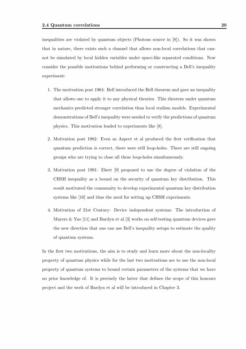
2.1 An abstract illustration of a simple black box computer. The user is given the

specfication of the black box computer and a black box device that supposely

perform accordingly to the specification. In this illustration, a user has to enter

binary values to n inputs and will locally receive a real valued outcome. . . . . 22

2.2 A schematic of the teleportation protocol: Alice receives an unknown quantum

state |φ(?)〉 and perform a Bell state measurement on both |φ(?)〉 and her qubit

(Entangled pair). The outcome is then communicated to Bob via the classical

channel and Bob does the corresponding unitary operations, e.g., σZ corresponds

to 00 from Alice. . . . . . . . . . . . . . . . . . . . . . . . . . . . . . . . . 28

3.1 An abstract illustration of composite black box system:Three black boxes are

defined in this figure, (1) black box source which is specified to produce entangled

pairs (2) Alice’s black box that is specifed to perform projective measurement on

her side of the entangled pair (3) Bob’s black box that has the same specification

as Alice’s black box. . . . . . . . . . . . . . . . . . . . . . . . . . . . . . . . 31

3.2 An illustration of how the family of ideal states looks like for a C6 ⊗ C6 space.

Note that the weights, λk are omitted for simplicity of illustration. . . . . . . . 40

vii

List of Figures viii

3.3 The (1) red coloured line indicates the theoretical bound eqn. (3.26) computed

by Bardyn et al for pure states, qudits. (2) the black theoretical line indicate the

Mayers & Yao fidelity for qubits eqn. (3.18). (3)The blue scatter plots refer to

numerical simulation of random pure states of eqn. (3.41) and (3) green scatter

plots indicate the numerical simulation of noisy states, eqn. (3.59) . . . . . . . 44

3.4 The (1) red coloured line indicates the theoretical bound eqn. (3.26) computed

by Bardyn et al for pure states. (2) the black theoretical line indicate the Mayers

& Yao fidelity for qubits eqn. (3.18). (3) The blue scatter plots indicate the

numerical simulation of random pure states of eqn. (3.41) and (4) cyan scatter

plots indicate the numerical simulation of noisy states, eqn. (3.59) . . . . . . . 45

3.5 The axes are given by the classical distribution of |Φ+0 〉 for Phi01 axis, |Φ+

1 〉 for

Phi23 axis, |Φ+θ 〉 for Phi1234 axis while the colour chart on the right side represent

the value of cos(θ). The data points plotted on the graph satisfy eqn. (3.27) and

δMY and they all define the same trace distance. . . . . . . . . . . . . . . . . 47

4.1 A pedagogical illustration of the average teleportation fidelities that can be achieved

by black box classical teleportation. . . . . . . . . . . . . . . . . . . . . . . . 52

4.2 A space-time diagram of how to prevent the black boxes to communicate with each

other, so as to rule out the black boxes attempt to simulate quantum correlations

with aid of classical communication. . . . . . . . . . . . . . . . . . . . . . . 54

4.3 An illustration of a black box teleportation setup. . . . . . . . . . . . . . . . 55

4.4 A 2D illustration of the simple classical protocol. (a) shows a situation where

Alice keys in a ~mA such that it is in the positive hemisphere of ~V cl. Then the

black box at Bob’s lab does nothing or just 180 degrees rotation about z axis.

(b) shows that Alice keys in a ~mA in the negative hemisphere and the 2 bits

communicated to Bob who will perform a 180 degrees rotation around x

or y axis. . . . . . . . . . . . . . . . . . . . . . . . . . . . . . . . . . . . . 56

4.5 A 3D scatter plot of the statistics: The red plots are defined for PY |~b,~V (+) > 0.95

and blue plots are defined for 0.95 ≥ PY |~b,~V (+) ≥ 0.9. . . . . . . . . . . . . . . 62

List of Figures ix

5.1 An illustration of black box swapping: In this scenario, one has already character-

ized the two independent black box sources with the same black box measurement

devices. . . . . . . . . . . . . . . . . . . . . . . . . . . . . . . . . . . . . . . 66

Chapter 1Introduction

1.1 Quantum physics and state estimation

The development of quantum mechanics since the early twentieth century has been fast

and vast. The very first revolution of quantum physics comes from the property of wave-

particle duality that concluded with inventions like transistors and lasers. However this

wave-particle duality is a single particle interference. With two quantum particles, en-

tanglement appears. Einstein, Podolsky and Rosen [1] in 1935 pointed out that quantum

mechanics predicts strong correlations between measurements on two space-like sepa-

rated systems. However the attempt to interpret quantum correlations in the view of

a realist demands that quantum mechanics must be complemented with an additional

classical variables that are hidden from the observers. This in short implies local realism,

which reads as results of measurements on a localized system are fully deterministic and

cannot be influenced by any other distant event. Later in 1964, John Bell [2] came with

a mathematical theorem called Bell theorem that defines a limit on correlations for any

local realism models. Then it seems that one should either drop locality or realism or

even drop both! It is intuitively correct to say that any physical entity always has some

information that exist regardless of measurements, e.g., a sealed container that contains

a basketball will always contain the basketball regardless whether one opens it or not.

However, experiments have shown that if one uses quantum entities (photons, electrons,

etc) for the experiments, then statistics from the experiments show that Bell theorem

1

1.1 Quantum physics and state estimation 2

is violated by quantum physics. If we assume locality then we have to accept that the

measurement outcomes do not exists before the measurement, it lacks intuition but it

is a fact that was tested and verified by many scientific groups around the world. It

is also well known that these non-local correlations can be achieved from incompatible

measurements on entangled particles that are distributed among space-like separated

parties.

However, the fundamental relationship between entanglement and non-local correlations

is indeed not that obvious. It was initially thought that entanglement and non-local

nature of any quantum state goes in the same direction and they are very much identical

to each other as quantum information processing resources. But it was shown that for

some Bell inequalities, the quantum state that achieve the maximal violation is not a

maximally entangled state. Nevertheless, one can still invoke Bell’s inequalities to detect

for non-local quantum states and these non-local quantum states imply entanglement.

It is also interesting to ask if some non-local correlations are observed, (e.g., experiment

statistics violates Bell’s inequality) can one learn something about the possible state of

the entangled system? Well, this sounds like a problem of quantum state estimation

already.

In principle, quantum state estimation is a method that provides the complete description

of a system, or equivalently to achieve the possible maximal knowledge of the state. It

is clear that in classical regime, one can always fully recover the characteristics of an

unknown classical object as one can always copy many copies of the original system.

However in quantum physics, there is a fundamental limit on our knowledge of a quantum

state. That is, if one is only given a single copy of an unknown quantum system then

one cannot learn the complete description of it. This principle is given by the quantum

no-cloning theorem. The demonstration of quantum no-cloning theorem requires only

the linearity of quantum dynamics: Suppose one has an unknown quantum state in the

following two levels system representation where the basis is given as {|0〉, |1〉}

|φ〉 = α|0〉+ β|1〉 (1.1)

1.1 Quantum physics and state estimation 3

There exists a quantum cloning machine such that it will produce an exact copy of the

unknown state:

|0〉 ⊗ |R〉 → |0〉 ⊗ |0〉 (1.2)

|1〉 ⊗ |R〉 → |1〉 ⊗ |1〉 (1.3)

now let the unknown state |φ〉 = α|0〉+ β|1〉 be processed with such a cloning machine

|φ〉 ⊗ |R〉 → α|00〉+ β|11〉 (1.4)

and this obviously is not a exact clone of the initial unknown state! Because if cloning is

possible, then the end state should be

|φ〉 ⊗ |φ〉 = α2|00〉+ αβ|01〉+ βα|10〉+ β2|11〉 (1.5)

We have demonstrated that quantum no-cloning theorem doesn’t allows one to clone an

unknown quantum state and it is evident that quantum state estimation demands many

copies of identical states. In addition, it seems that to characterize an unknown quan-

tum state requires the prior knowledge of its physical properties. For example, photon

does not interact with magnetic fields hence one cannot learn more about a photon with

a Stern-Gerlach apparatus (okay, you learn that the unknown particle has no charge.).

So that is to say, If one does not have the prior knowledge of physical properties(spins,

polarization, etc) of the quantum object, then it seems that it is impossible to perform

state tomography. However in quantum systems, there is a subtle property that allows

composite quantum systems to have more as a whole than just a summation of its sub-

systems. It is also precisely this exclusive nature of quantum systems that one can use

it to estimate the state of a black box that promise to generate entangled pairs.

1.2 Objective of honours research 4

1.2 Objective of honours research

The objective of the honours research is to develop new mathematical tools or approaches

that allows one to estimate an entangled black box source via Bell inequalities. The pri-

mary aim for the honours is to extend the work of Bardyn et al [3] Device independent

state estimation based on Bell’s inequalities to arbitrary bipartite quantum states. How-

ever, it is also the aim of the project to conduct numerical studies to gain some intuitions

about solutions. In addition to this work, we also explored the possibility of using tele-

portation dependency on entanglement to estimate the bound on the average fidelity that

differentiate between quantum black boxes and classical black boxes.

1.3 Organization of thesis

The organization of the thesis is as follows:

1. Chapter 2: The preliminaries aims to introduce to unfamiliar readers the basic tools

and techniques required to follow the research work in the thesis. In particular, the

distance measures and CHSH inequality are the main constructs of the research

work.

2. Chapter 3: §(3.1) of this chapter introduces the work of Bardyn et al [3], figure of

merits and formulation of problem. §3.2 are ordered as such

(a) The proposed family of ideal states that can give 2√

2 CHSH violation for

C4 ⊗ C4.

(b) The extension of Horodecki et al necessary and sufficient condition for C2⊗C2

to certain higher even dimension systems. The results were compared with

the generalized CHSH operator.

(c) The numerical studies of Mayers & Yao fidelity and trace distance. The results

were compared with the theoretical results by [3].

(d) An counter example of state that has infinitely many ideal states was presented

and implications are discussed.

1.3 Organization of thesis 5

3. Chapter 4: This chapter takes a different direction in the approach of black box

state estimation and instead of using Bell’s inequalities we use teleportation scheme

to distinguish between black box classical and quantum teleportation schemes.

(a) Two models of classical teleportation scheme were adapted to black box sce-

narios.

(b) Proposed a protocol to distinguish black box teleportation and genuine quan-

tum teleportation.

4. Chapter 5: The discussions and results are highlighted and discussed in depth.

Future work details the approach on how to conduct quantum apparatus estimation.

Chapter 2Preliminaries

2.1 Quantum states and density matrix

In quantum physics, any quantum system can be described by a representative space

called the Hilbert space(generally infinite dimension) and the Hilbert space is a complex

vector space with Hermitian inner product by mathematical framework. The dimension

of the representation space is then fully determined by the degree of freedom of the

specified property possessed by the physical system. For example, for a spin 12 particle

the internal degree of freedom (spin) can be described by a C2 Hilbert space. Here one

can ascribe the spin states as kets {|0〉 , |1〉} in the Dirac notation and these states are

perfectly distinguishable and correspond to the spin outcomes {+12 ,−1

2}. Any pure state

of a two-level system can be written as |Ψ〉 = α |0〉 + β |1〉 where α, β ∈ C characterize

the quantum state in the spin state basis. In general, quantum systems are microscopic

systems such that one can only use indirect observation to obtain information about it.

In precise definition, the state of knowledge(of the specified property) of the quantum

state is fully characterized by the state vector residing inside the Hilbert space. This

in turn implies that the Quantum-Hilbert space formalism is simply a mathematical

platform for one to express the state of knowledge with respect to the eigenstates of the

measurement apparatus. Often the observer’s knowledge of the system is incomplete

even if one carefully prepares the quantum system. For example instead of the intended

preparation of all spin +12 states, there may exists some mixture of spin −1

2 states.

6

2.1 Quantum states and density matrix 7

It is then obvious that representation in terms of kets can only be used to describe

superposition of states and not statistical mixtures of pure states.

Density operators

In order to represent any statistical mixtures of pure states, we introduce the definition

of density operator of a pure state |ψ〉 as

ρ := |ψ〉〈ψ| (2.1)

This is also called the density matrix of a pure quantum states and it has the follow

properties:

1. It is positive and thus implies Hermitian, ρ ≥ 0

2. The trace of the density matrix is always equal to unity, tr(ρ) = 1 and this implies

normalization.

It is easy to see that given any density matrix, one can always diagonalize the matrix in

some basis such that the matrix can be (spectral) decomposed into its eigenvectors

ρ =∑

x

PX(x)|φx〉〈φx| (2.2)

where the eigenvalues PX(x) is the probability of getting pure state |φx〉. The density

operator assumes pure state if and only if one of the eigenvalues of ρ is 1, tr(ρ2) = 1. In

the language of density operators, a distinct advantage is that one can also describe a

classical system that in the Hilbert space. We define these classical states as

ρclassical =∑

x

PX(x)σclassicalx (2.3)

whereby σclassicalx represents the x state of the classical system, e.g., head or tail of

the coin. In general these classical states are perfectly distinguishable (orthogonal in

Hilbert Space), which later one can see that quantum theory of information is actually a

mathematical generalization of the classical information theory.


2.1.1 Dynamics of (isolated) quantum states

Now that we have defined quantum states and their properties, one may ask what can we

do with these quantum states? As discussed above, a quantum state is nothing more than

a mathematical representation of our perceived knowledge of the physical system one is

interested in. Strictly speaking, one is only using quantum physics to predict measurable

properties of the system and not to fully describe the system. These described systems

are not directly observed (naked eye but see [4]) but are measured through machines So

it leaves only two possible paths:

1. Quantum Dynamics: Time evolution of quantum systems

2. Quantum Measurement: To obtain information about properties of the described

system, e.g., particle’s spin, photon’s polarization, etc

So in principle, how does one describe the evolution of a quantum system? The answer

can be clued from classical physics, Liouville dynamics. The classical Liouville equation

is a linear operation that describes the time evolution of phase space distribution function

from time ti to tf and is defined as

dρ

dt=∂ρ

∂t+

d∑

i=1

(∂ρ

∂qi

∂H

∂pi− ∂H

∂qi

∂ρ

∂pi

)= 0 (2.4)

∂ρ

∂t= −

d∑

i=1

(∂ρ

∂qi

∂H

∂pi− ∂H

∂qi

∂ρ

∂pi

)= 0 (2.5)

where the RHS of eqn. (2.5) is the Poisson bracket and is closely related to the commu-

tator in Quantum mechanics and H(q, p, t) is the classical Hamiltonian.

Koopman’s theorem

The Koopman’s theorem states that the phase space density distribution does not change

under Lioville dynamics, i.e., given two phase space distributions, the fidelity or inner

product of these two distributions is invariant under Liouville dynamics:

d〈ρ(q, p, t)|σ(q, p, t)〉dt

=d

dt

∫ρ(q, p, t)σ(q, p, t)dqdp = 0 (2.6)


Isolated Quantum evolution

In quantum physics, the time development of quantum states is given by the Schrodinger’s

equation for time evolution operator [5]

i~∂

∂tU(t, t0) = HU(t, t0) (2.7)

solving the equation for time independent Hamiltonian yields

U(t, t0) = exp

(− i~H(t− t0)

)(2.8)

so in fact, the unitary U(t, t0) operator encodes the full information of the evolution and

is deterministic and reversible, i.e., given any initial condition |ψ, t0〉

U(t, t0〉|ψ, t0〉 = |ψ, t〉 (2.9)

U †(t, t0)U(t, t0) = I (2.10)

Hence the inner product of the quantum state under the quantum evolution is conserved

similarly to the classical anagloue.

〈ψ, t0|ψ, t0〉 = 〈ψ, t|ψ, t〉 = 〈ψ, t0|U †(t, t0)U(t, t0)|ψ, t0〉 = 1 (2.11)

2.1.2 Measurement on quantum systems

Consider a quantum state that was prepared by some process in the past and given as ρ

in the present. A generalized operation is an operation that takes the present state ρ to

some other future state ρ′.

Λ : ρ→ ρ′ (2.12)

and this operation in general can have m distinguishable outcomes given as λm and

each outcomes has a corresponding density operator or quantum state ρm. As defined in


Quantum formalism, the probability of random variable X = λm outcome is defined as:

PX|ρ(λm) := tr(ρΠm) (2.13)

where usually the elements Πm are usually called positive operator valued measure

(POVMs) but I will denote them here as generalized observables. Naturally, the proba-

bility of an event is always real and ranges between 0 ≤ PX ≤ 1. The first property of

a probability implies that the operators Πm must be Hermitian. Another constraint on

the generalized observables is the normalization of the probabilities,∑

m PX|ρ(λm) = 1

implies that the summation of all operators must be equal to identity, I.

∑

m

PX|ρ(λm) =∑

m

tr(ρΠm) = tr(ρI) = 1 (2.14)

These two conditions are the only conditions for any generalized observables that takes

a quantum state to another quantum state with the corresponding probability. However

in the situation of quantum state discrimination where one tries to distinguish between

quantum states, only the probability distributions matters in the evaluation. This will

be discussed in detail in the section of trace distance measure. Now suppose that one

can write the generalized observables in the form of

Am = UmΠ12m (2.15)

where Um is any unitary operator and hence satisfy reversibility U †mUm = I, hence the

generalized observables can be written as

Πm = A†mAm (2.16)

and eqn. (2.13) now reads

PX|ρ(λm) := tr(AmρA†m) (2.17)

2.2 Composite systems and tensor product structure 11

and the post-measurement normalized quantum state that corresponds to outcome λm is

ρ′λm =AmρA

†m

tr(AmρA†m)

(2.18)

2.2 Composite systems and tensor product structure

So far, we have only discussed about single quantum system state description and gener-

alized measurements. But in reality, there is a more bizarre quantum phenomena called

entanglement that doesn’t has a direct classical analogue (but see [6]) to it. The descrip-

tion of composite quantum systems requires the treatment of tensor product structures

and later we will show that non-signaling can be derived from it.

2.2.1 Subsystems

The product Hilbert space HA⊗B of two subsystems HA, HB (in general, the dimensions

of the Hilbert spaces need no be the same) is defined to be the tensor product of the two

subsystems (Hilbert spaces)

HA⊗B = HA ⊗HB (2.19)

Also for each vectors |φA〉 ∈ HA, |φB〉 ∈ HB, the product vector |φA⊗B〉 ∈ HA⊗B can be

written as

|φA⊗B〉 := |φA〉 ⊗ |φB〉 (2.20)

Now, considering bipartite systems (HnA⊗HmB ), one can make use of the Schmidt decom-

position defined as

|φA⊗B〉 :=k∑

i=1

√λi|uiA〉 ⊗ |viB〉 (2.21)

Where k ≤ min(n,m) and |uiA〉, |viA〉 are bi-orthonormal eigenvectors of reduced density

operator ρA = tr(ρA⊗B) and ρB = tr(ρA⊗B) respectively.

2.2 Composite systems and tensor product structure 12

2.2.2 Product Operators

Let OA be a linear operator defined on the Hilbert Space of system A HA and QB be a

linear operator on HB, then the product of the operators is defined as

RA⊗B := OA ⊗QB (2.22)

This definition of bi-local operator acts only locally on the subsystems and given a product

state

RA⊗B|φA⊗B〉 := (OA ⊗QB)(|φA〉 ⊗ |φB〉) = OA|φA〉 ⊗QB|φB〉 (2.23)

and the bi-local operator can be equivalently written as

RA⊗B = (OA ⊗ IB)(IA ⊗QB) (2.24)

One point to emphasis is that given a bi-local operator and a product quantum state,

one can always factorize the joint expectation of the bi-local operator into expectation

into local expectation values.

〈φA⊗B|RA⊗B|φA⊗B〉 = 〈φA|OA|φA〉〈φB|QB|φB〉 (2.25)

However, if the given quantum state is not a product state (Schmidt number > 1) then

eqn (2.25) is no longer valid.

2.2.3 Non-signaling

A conditional probability distribution PXY |ab(x, y) is defined to be non-signaling if for

all inputs a, b

PX|ab = PX|a (2.26)

PY |ab = PY |b (2.27)

2.3 States distinguishability measures 13

where PX|ab and PY |ab are marginals of PXY |ab. The interpretation behind this condition

is that the choice of input at Alice(Bob)’s laboratories cannot influence the outcomes of

Bob(Alice)’s measurements. This is essentially the mathematical statement which states

that no information can be communicated instantaneously. In quantum mechanics frame-

work, let Alice and Bob’s measurements by represented by generalized measurements

{Πax}x and {Γby}y where a, b are the possible inputs. These generalized measurements

satisfy normalization,∑

x Πax = IA and

∑y Γby = IB. Given ρAB, the joint probability of

getting outcomes x, y that is conditioned on the inputs a, b is

PXY |ab,ρAB(x, y) = tr(Πa

x ⊗ ΓbyρAB) (2.28)

the marginal of X reads

∑

y

PXY |ab,ρAB(x, y) = PX|ab,ρAB

=∑

y

tr(Πax ⊗ ΓbyρAB)

PX|ab,ρAB= tr(Πa

x ⊗ IBρAB) = PX|a,ρAB(2.29)

where the probability distribution of Alice is independent of Bob’s choice of inputs which

satisfy eqn. (2.27). This also holds for the marginal of Y .

2.3 States distinguishability measures

This topic of state distinguishability measures is a little misleading but is befitting to

the objective of differentiating quantum states under the context of experiments. It

is misleading in a sense that the only meaningful information one can get from the

experiments are the frequencies of each outcomes and total number of outcomes and

not the abstract density operators. With these information, one can then define the

probability of observing any particular outcome within the measurement context. Hence

to distinguish quantum states one needs to perform some measurements and compare

the probability distributions for the given outcomes. The simplest case of distinguishing

two probability distributions that are not identical (if the distributions are identical then

the probability of guessing it correctly will be just 12 and this isn’t that interesting in our


formulation) will be the starting point of our discussion. In which, we introduce the idea

of distinguishability via error probability and show that the classical Kolmogorov trace

distance is closely related to it. In the following subsections will be the introduction of

the quantum trace distance measure and we will show that the quantum trace distance

and fidelity measures are the generalization of the classical distance measures.

2.3.1 Distinguishability and Errors

In order to discuss the notion of distinguishability of probability distributions, one can

consider a simple classical probability game [7]. The game is defined as such:

Guess the correct distribution game

Given two probability distributions, PX(x) and QX(x) where x = 1, ..., n, a player sam-

ples blindly once from either PX(x) or QX(x) without knowing the identities of the

distributions. If the player guesses the correct distribution then he wins, if not he loses

the game. In order to make the game more attractive, the player is allowed to know the

probability of the distribution which he is sampling, σP and σQ = 1− σP respectively. It

is obvious that if the two probability distributions are distinct then the player may gain

some meaningful information about the identity of the sampled distribution. In such a

game, the player has only the information of probability of getting either distributions

prior to the sample and may try to say something about the probability of error in his

single guess.

Probability of error

First lets define the guess/decision function as

δ : {1, ..., n} → {0, 1} (2.30)

that is the method of guessing the the correct distribution. So the probability of guessing

it wrongly will be

Perror(δ) = σPP(δ = 1|0) + σQP(δ = 0|1) (2.31)


where P(δ = 0|1) is the probability that the guess/decision is PX(x) but the correct

distribution is QX(x) and the converse is given as P(δ = 1|0). It can be shown [7] that

the probability of error is

Perror(δ) =

n∑

x=1

(PX(x) + QX(x))(1−max(P(0|x),P(1|x)) (2.32)

Perror(δ) =

n∑

x=1

min(σPPX(x), σQQX(x)) (2.33)

2.3.2 Distinguishing probability distributions: Kolmogorov measure

Given that the probability of error in choosing the distributions is given by eqn. (2.33),

one can let σQ, σP = 1/2 which is the most pessimistic situation for the player. The

probability of error now reads

Perror(δ) =1

2

n∑

x=1

min(PX(x),QX(x)) (2.34)

on another hand, one can write the probability of success as PSuccess = 1 − Perror and

obtains

PSuccess = 1− 1

2

n∑

x=1

min(PX(x),QX(x)) (2.35)

which can be rewritten as

PSuccess =1

2+

1

2

[1−

n∑

x=1

min(PX(x),QX(x))

](2.36)

The probability of distinguishability of two probability distributions is given by the Kol-

mogorov distance which gives the geometric interpretation of distance between two prob-

ability distributions.

D(P(x),Q(x)) =1

2

n∑

x=1

|P(x)−Q(x)| (2.37)

or equivalently given by the R.H.S square bracket of eqn. (2.36)

D(P(x),Q(x)) = 1−n∑

x=1

min(P(x),Q(x)) (2.38)


The trace distance then satisfy the following properties

1. It is symmetric and 0 ≤ D(P(x),Q(x)) ≤ 1

2. Positive and is zero if and only if P(x) = Q(x)

3. It satisfy the triangle inequality, D(P(x),Q(x)) ≤ D(P(x),R(x)) +D(R(x),Q(x))

4. D(P(x),Q(x)) = 1 if and only if P(x) and Q(x) have distinct support.

Another important property of the trace distance is that it can only decrease under the

operation of taking the marginals.

D(PXY (x, y),QXY (x, y)) =1

2

∑

x,y

|P(x, y)−Q(x, y)|

1

2

∑

x,y

|P(x, y)−Q(x, y)| ≥ 1

2

∑

x

|∑

y

P(x, y)−Q(x, y)|

=1

2

∑

x

|P(x)−Q(x)| (2.39)

2.3.3 Quantum generalization of Kolomogov measures

The main mathematical tool behind the black box state estimation work is the use of

trace distance between quantum states. That is given two quantum states ρ, σ ∈ H, the

trace distance between the two quantum states is defined as

DQM(ρ, σ) :=1

2‖ρ− σ‖1 (2.40)

where the trace norm of an operator A is defined as

‖A‖1 := tr√A∗A (2.41)

the quantum trace distance eqn. (2.40) carries the same properties as the classical Kol-

mogorov trace distance and is essentially a metric defined on the space of the density

operators. Also, it has the property that it is invariant under unitary operations that

is similar to the fidelity measures for classical phase space distributions eqn (2.6). Now

one can notice that given two density operators ρclassical, σclassical (cf. eqn. (2.3)) that are


characterized by only classical distributions PX(x) and QX(x) respectively, the quantum

trace distance reduces to the classical trace distance.

DQM(ρclassical, σclassical) =1

2‖ρclassical − σclassical‖1

1

2‖ρclassical − σclassical‖1 =

1

2‖∑

x

PX(x)Iclassical −∑

x

QX(x)Iclassical‖1

=1

2

∑

x

|PX(x)−QX(x)| (2.42)

one also must be careful to note that quantum trace distance depends not only on the

density operators ρ, σ but also on the generalized measurements (k inputs and m out-

comes)∑m

x=1 Πkx = I involved in the evaluation, i.e.,

PX|Πkx,ρ

(x) = tr(ρΠkx) (2.43)

QX|Πkx,σ

(x) = tr(σΠkx) (2.44)

The evalution of eqn. (2.40) will be then to maximize the classical trace distance between

PX|Πkx,ρ

(x) and QX|Πkx,σ

(x) over all possible generalized measurements.

1

2‖ρ− σ‖1 = max

Π

1

2

∑

x

|PX|Πkx,ρ

(x)−QX|Πkx,σ

(x)| (2.45)

Therefore the quantum trace distance between two quantum states can be interpreted

as the maximum distinguishing probability, i.e., the maximum probability that one can

detect a difference between ρ and σ. Hence given two quantum states, one can obtain

an upper bound on the probability that these two states can be distinguished and this

clearly has a strong operational definition, i.e., the state distinguishability game. Suppose

that Alice prepares two quantum states and distributes them statistically, 12ρ+ 1

2σ. Now

Bob has to make a guess with some generalized measurements to distinguish between the

two quantum states. As we have shown in §2.3.2, Bob’s probability of success is then

12 + 1

2DQM. So if the quantum states are perfectly distinguishable then Bob can win the

game with probability of success equal 1. However if the quantum states are identical

in the measurement context, his probability of success is 12 . Furthermore, trace distance


has a geometrical interpretation as well as it is a metric defined on the operator space

and is symmetric in terms of density operators. This geometrical picture is obvious if

one considers two-level systems (qubits) that has a corresponding R3 representation via

the Bloch Sphere.

2.3.4 Fidelity as an alternative distinguishability measure

An alternative to trace distance is another useful distance measure called fidelity measure.

The fidelity measure has a vague operational definition as compared to the trace distance

eqn. (2.40) but is often easier to compute. The quantum fidelity measure is very similar

to the classical fidelity (inner product) and reads

FQM(ρ, σ) := ‖ρ 12σ

12 ‖21 (2.46)

Now if one of the states is a pure state,e.g., σ = |ψ〉〈ψ| then fidelity reduces to the

expectation value of ρ given state σ

FQM(ρ, σ) = tr(

√σ

12 ρσ

12 )2 =

√〈ψ|ρ|ψ〉2 = 〈ψ|ρ|ψ〉 (2.47)

and if both quantum states are pure,

FQM(ρ, σ) = 〈ψ|φ〉〈φ|ψ〉 = |〈ψ|φ〉|2 (2.48)

Thus the fidelity between two pure quantum states is simply the probability of transition

between |ψ〉 and |φ〉. As one can see, the fidelity is unity if and only if the quantum

states are identical and is zero if the quantum states are on orthogonal subspaces.

The quantum trace distance eqn. (2.40) and quantum fidelity measure has a direct

relation given as

DQM(ρ, σ) ≤√

1− FQM(ρ, σ) (2.49)

Where the equality is satisfied for only pure quantum states.

2.4 Quantum correlations 19

2.4 Quantum correlations

As mentioned in the introduction, classical physics allows one to predict any measure-

ment outcomes with unity probability if and only if all influences (forces, fields, etc) and

specifications of measurements are taken into account. However, within the framework

of quantum formalization one can only make probabilistic predictions of any observa-

tions. That is the uncertainty in one’s measurement of a quantum system is intrinsic and

fundamental as oppose to the uncertainty of classical observations. This fundamental

uncertainty is called the Heisenberg’s uncertainty relation and it is the catalysis that

lifted determinism from our quantum experiments. It is also this relationship between

non-commuting physical properties or incompatible measurements that give rise to Ein-

stein, Podolsky and Rosen’s 1935 famous paper [1] that questioned the completeness

of quantum mechanics. The basic argument is that any individual (local measurements)

outcomes may depend on an additional parameter that is famously called the classical lo-

cal hidden variables or in modern language shared randomness. Theories involving shared

randomness are generally deterministic and probabilities exist because of the users lack

of knowledge (which is the hidden variables). Now, if one believes that no meaningful

information can be communicated faster than speed of light (non-signaling), then there

are no consistent ways to predict experimental results by using local hidden variables

models.

2.4.1 Bell’s inequalities

John Bell in 1964 [2] derived a theorem (an inequality) that can be interpreted as: “Phys-

ical theories compatible with special relativity and outcomes of measurements are fun-

damentally deterministic satisfy the inequality”. In short, if one believes in local realism

then his/her prediction of experiment’s results should not violate the Bell’s inequality.

However if one is to do the computation under the framework of quantum physics, then

one can achieve violation of Bell’s inequalities. In 1982, Alain Aspect et al [8] conducted

the CHSH experiment and showed that the statistics from the experiments violated the

CHSH Bell’s inequality by five standard deviations, this crucial result proved that Bell’s


inequalities are violated by quantum objects (Photons source in [8]). So it was shown

that in nature, there exists such a channel that allows non-local correlations that can-

not be simulated by local hidden variables under space-like separated conditions. Now

consider the possible motivations behind performing or constructing a Bell’s inequality

experiment:

1. The motivation post 1964: Bell introduced the Bell theorem and gave an inequality

that allows one to apply it to any physical theories. This theorem under quantum

mechanics predicted stronger correlation than local realism models. Experimental

demonstrations of Bell’s inequality were needed to verify the predictions of quantum

physics. This motivation leaded to experiments like [8].

2. Motivation post 1982: Even as Aspect et al produced the first verification that

quantum prediction is correct, there were still loop-holes. There are still ongoing

groups who are trying to close all these loop-holes simultaneously.

3. Motivation post 1991: Ekert [9] proposed to use the degree of violation of the

CHSH inequality as a bound on the security of quantum key distribution. This

result motivated the community to develop experimental quantum key distribution

systems like [10] and thus the need for setting up CHSH experiments.

4. Motivation of 21st Century: Device independent systems: The introduction of

Mayers & Yao [11] and Bardyn et al [3] works on self-testing quantum devices gave

the new direction that one can use Bell’s inequality setups to estimate the quality

of quantum systems.

In the first two motivations, the aim is to study and learn more about the non-locality

property of quantum physics while for the last two motivations are to use the non-local

property of quantum systems to bound certain parameters of the systems that we have

no prior knowledge of. It is precisely the latter that defines the scope of this honours

project and the work of Bardyn et al will be introduced in Chapter 3.


Bipartite Bell’s inequalities

In general, Bell’s inequalities are constraints on some functions of correlators of measure-

ment’s results and they are satisfied by all separable states i.e., ρ =∑

i PiρAi ⊗ ρBi and

∑i Pi = 1. Here, the definition of a bipartite bell’s inequality [12] is given as

B(c) ≥n∑

i=1

m∑

j=1

c(i, j)E(i, j) (2.50)

c(i, j) are some real coefficients, E(i, j) is the correlation function of the product of the

observables and B(c) is the maximal possible value of R.H.S of eqn. (2.50). As all Bell’s

inequalities are satisfied by shared randomness, one can without loss of generality define

the correlation functions as

E(i, j) =

∫dλρ(λ)A(i, λ)B(j, λ) (2.51)

where A(i, λ), B(j, λ) are deterministic and local functions (alternative notation: local

response functions) that given λ and i, j always output a specific result. So in the

correlation functions, what is not known or rather hidden is just the local deterministic

strategy distribution ρ(λ) and this is what give rise to probabilities in LHV theories.

2.4.2 Clauser, Horne, Shimony and Holt inequality

Since Bell introduction of Bell’s inequality, there has been many versions and variations

of inequalities that are adapted to nA, nB settings and mA, mB outcomes each settings.

For nA = nB = 2 and mA = mb = 2, there is only one tight inequality [13]: Clauser,

Horne, Shimony and Holt inequality [14].

− 2 ≤ EXY |~a,~b + E

XY |~a,~b′ + EXY |~a′,~b − EXY |~a′,~b′ ≤ 2 (2.52)

where each measurement device has binary input and binary output, {~a,~a′} for Alice and

{~b,~b′} for Bob. The correlator reads

EXY |~a,~b = P

XY |~a,~b(+,+) + PXY |~a,~b(−,−)− P

XY |~a,~b(−,+)− PXY |~a,~b(+,−) (2.53)


Entangled Source

Alice Bob

{�a,�a�} {�b,�b�}

X ∈ {+,−} Y ∈ {+,−}Figure 2.1: An abstract illustration of a simple black box computer. The user is given thespecfication of the black box computer and a black box device that supposely perform accordinglyto the specification. In this illustration, a user has to enter binary values to n inputs and willlocally receive a real valued outcome.

Local bound of CHSH and Cirel’son’s bound

Using a pre-established agreement (LHV), one can describe the eqn. (2.52) with eqn.

(2.51) and rewrite the CHSH as

∫dλρ(λ)[A(~a, λ)(B(~b, λ) +B(~b′, λ)) +A(~a′, λ)(B(~b, λ)−B(~b′, λ))] (2.54)

and A(i, λ), B(j, λ) = ±1 implies that the CHSH inequality for any specific λ is bounded

by

− 2 ≤ [A(~a, λ)(B(~b, λ) +B(~b′, λ)) +A(~a′, λ)(B(~b, λ)−B(~b′, λ))] ≤ 2 (2.55)

which is exactly eqn. (2.52). Now if one uses quantum states or explicitly the Bell states,

|Φ±〉 :=1√2

(|e0〉 ⊗ |f0〉 ± |e1〉 ⊗ |f1〉) (2.56)

|Ψ±〉 :=1√2

(|e0〉 ⊗ |f1〉 ± |e1〉 ⊗ |f0〉) (2.57)

where {|e0〉, |e1〉} ∈ HA and {|f0〉, |f1〉} ∈ Hb are bi-orthonormal states. Next define the

quantum measurement operators as Hermitian operators

A(~n) = ~n · ~σ (2.58)


with ±1 eigenvalues and ~n ∈ R3, and one can get the following relation with the local

identity operations

A(~a)2 = A(~a′)2 = IA

B(~b)2 = B(~b′)2 = IB (2.59)

Next the Bell operator is defined [15] as

B = A(~a)⊗ [B(~b) +B(~b′)] +A(~a′)⊗ [B(~b)−B(~b′)] (2.60)

B2 = 4IA ⊗ IB − [A(~a), A(~a′)][B(~b), B(~b′)] (2.61)

here, one can take the sup norm of eqn (2.48) and with ‖A+B‖sup ≤ ‖A‖sup + ‖B‖sup,

one gets

‖B2‖sup = ‖4IA ⊗ IB − [A(~a), A(~a′)][B(~b), B(~b′)]‖sup

≤ ‖4IA ⊗ IB‖sup + ‖[A(~a), A(~a′)][B(~b), B(~b′)]‖sup

= 4 + 4‖[A(~a)‖sup · ‖[A(~a)′‖sup · ‖[B(~b)‖sup · ‖[B(~b)′‖sup

= 8 (2.62)

as the Bell operator B is a Hermitian operator, i.e., A†A = AA = A2

‖B2‖sup = ‖B‖2sup ≤ 8 (2.63)

and since the sup norm of B is the maximum eigenvalue of√B†B = B, one can conclude

that the maximum eigenvalue of B is bounded by 2√

2, which is the Cirel’son’s bound [16]

for the CHSH inequality. This bound is valid for any arbitrary dimension systems as long

as the quantum measurements satisfy eqn. (2.59), i.e., the observables have eigenvalues

±1.


Optimization of CHSH inequality

Now that we have introduced the CHSH inequality, one in general can interpret it as a

function that takes a density operators ρAB ∈ HA⊗B to R

SCHSH : ρAB → s ∈ [−2√

2, 2√

2] (2.64)

where in principle the mapping is given by SCHSH(ρAB) := tr(BρAB) = s and is dependent

on following parameters

1. The choice of measurement settings, {~a,~a′,~b,~b′},

2. The choice of measurement bases, e.g., σ3 = |e0〉〈e0| − |e1〉〈e1|

3. The entanglement factor of ρAB, e.g., singlet fraction, negativity, etc .

Now one can notice that even if the CHSH experiment involves a maximally entangled

states (Bell states), this doesn’t guarantee that the mapping brings it to the maximal

violation of CHSH inequality, ±2√

2. It means that in order to achieve maximal violation,

one can either fix the quantum state ρAB to find the optimal measurement settings or one

can fix the settings and find the optimal quantum states. The latter is less interesting

as we are now more interested in estimating how non-local a quantum state is under

the context of CHSH inequality. In the following demonstration, one can invoke the

Horodecki et al [17] necessary and sufficient condition for violation of CHSH inequality

for a given arbitrary C2 ⊗ C2 quantum composite system.

Necessary and sufficient condition for violating CHSH inequality by arbitrary

two qubits

Given two qubits that have interacted in the past and are now deposited or transmitted

to Alice and Bob laboratories, one can describe the composite state as

ρAB =1

2(IA + ~n · ~σA)⊗ 1

2(IB + ~m · ~σB)

=1

4

IA ⊗ IB + ~n · ~σA ⊗ IB + IA ⊗ ~m · ~σB +

3∑

i,j=1

tijσi ⊗ σj

(2.65)


where tij = tr(ρABσi⊗σj). Now lets define a matrix U(ρAB) := T TT which is symmetric

and hence is diagonal in some bases. It was shown by [17] that the information that is

encoded into the T real matrix is related to the maximal violation of the CHSH inequality:

maxB|S(ρAB)CHSH| = 2

√M(ρAB) (2.66)

where M(ρAB) := λ1 + λ2 such that λ1 ≥ λ2 ≥ λ3 are the ordered positive eigenvalues

of matrix U(ρAB). In fact, the T matrix encodes the quantum correlations given by the

quantum state ρAB and its explicit form is given as

T := 2

Re(a~d+ b~c) Im(a~d− b~c) Re(a~c+ b~d)

Im(a~d+ b~c) Re(−a~d+ b~c) Im(a~c− b~d)

Re(a~b− c~d) Im(a~b− c~d) 12(|a|2 + |d|2 − |b|2 − |c|2)

(2.67)

where |φ〉 = a|e0, f0〉 + b|e0, f1〉 + c|e1, f0〉 + d|e1, f1〉 and {a, b, c, d} ∈ C. Now as an

example, we consider the Werner state [18]

ρW = P|Φ+〉〈Φ+|+ (1− P)I4

(2.68)

As the Bell operator is traceless, i.e., tr(B) = 0, the necessary and sufficient condition

for the Werner state to be non-local is P > 1√2. Next, consider a mixture of local states

and a maximally entangled state,

ρ = P|Φ+〉〈Φ+|+ (1− P)|e0, f0〉〈e0, f0| (2.69)

The T matrix is then the convex combination of T (|Φ+〉) and T (|e0, f0〉)

T (|Φ+〉) = diag(+,−,+) (2.70)

T (|e0, f0〉) = diag(0, 0,+) (2.71)

T (ρ) = Pdiag(+,−,+) + (1− P)diag(0, 0,+) (2.72)


where now M(ρ) = 1 + P2 implies the maximal violation of the CHSH inequality with

eqn. (2.66) is 2√

1 + P2.

2.4.3 Entanglement as a communication resource

As we have seen in the earlier section, we used Bell’s inequalities as a mathematical

measure to estimate the amount of non-locality for some given quantum states. How-

ever, there also exist other types of non-local measures that detect the non-locality of

states. One famous example is the Hardy non-locality test [19]. Now one can ask a very

relevant question,“is entanglement the same as non-locality in terms of resource?” As

an example, one performs an CHSH experiment in space-like separated laboratories and

achieve a violation of ' 2.422 for ρ1 and ' 2.622 for ρ2, can one say that ρ2 is much more

entangled than ρ1? In general, this is true only for two qubits systems and not true for

anything more complicated than that [20]. In [20], the authors gave an example in the

next simplest case of two qutrits: using the Collins, Gisin, Linden, Massar and Popescu

(CGLMP) inequality for a maximally entangled qutrits pair, they obtained a violation

of 2.873. However, they pointed out that Acin et al [21] found a higher violation with

a non-maximally entangled state (with the same settings as the maximally entangled

states, but this settings and non-maximally entangled state were checked to be optimal).

This implies that non-locality and entanglement are in general different resources. Nev-

ertheless, entanglement [22] has been essential in achieving communication feats that

classical communication cannot achieve, to list some:

1. Quantum teleportation

2. Quantum dense coding

3. Entanglement swapping

4. Quantum Key Distributions

Here, I will introduce the concept of quantum teleportation only as it is one of the

on-going work on black box state estimation.


2.4.4 Quantum Teleporation with qubits

For ages, people have been fascinated by the possibility of teleportation of beings from one

place to another space-like separated location instantaneously, this fascination is evident

as block buster movies like Star-Trek use ”teleportation” frequently. Now teleportation

is possible in nature as predicted by quantum mechanics and it respects special relativity,

i.e., the teleportation cannot be completed faster than speed of light. If that is the case,

what is so fantastic about quantum teleportation if it is still bounded by speed of light?

Well, it transmits partial information of the ”to be teleported” particle via a channel

of nature that is well described by quantum mechanics. Unfortunately, for every single

use of the channel requires us to sacrifice a well distributed entangled pair. That is, we

need to pay to use this channel. Also, the above statement sort of trivializes the hassle

in performing such an experimental, because one still needs to have perfect quantum

apparatus like the Bell state measurement, unitary operations, minimum distribution

losses, etc. Nevertheless, it is still a wonderful application of quantum physics! so lets

review the standard quantum teleportation protocol which was discovered by Bennett,

Brassard, Crepeau, Jozsa, Peres and Wootters in 1993 [23]:

Quantum teleportation protocol

Objective: Alice wants to ”teleport” an unknown state to Bob.

1. Alice receives an unknown quantum state |φ(?)〉 = α|0〉+ β|1〉 where α, β ∈ C

2. Alice does a joint measurement (Bell state measurement) on both |φ(?)〉 and her

qubit of the entangled pair |Φ+〉. This measurement is essentially a generalized

measurement with four outcomes {00, 01, 10, 11}.

3. Via the classical channel (e.g., telephone, GSM, etc) she informs Bob about the

outcome of her Bell state measurement.

4. Bob then does the correct unitary rotation that corresponds to the outcome ob-

tained by Alice. This of course requires that Alice and Bob has some pre-established

agreement that will give the correct interpretation of the outcomes of the Bell state


Bell statemeasurement

Unitary Operation

Alice Bob{0, 1}2

Classical Channel

Quantum Channel

|φ(?)� |φ(?)�Source|Φ+�

Figure 2.2: A schematic of the teleportation protocol: Alice receives an unknown quantum state|φ(?)〉 and perform a Bell state measurement on both |φ(?)〉 and her qubit (Entangled pair). Theoutcome is then communicated to Bob via the classical channel and Bob does the correspondingunitary operations, e.g., σZ corresponds to 00 from Alice.

measurement.

5. After the unitary operation, Bob will then exactly receives |φ(?)〉.

To be able to achieve faithful teleportation depends on a few crucial components. They

are mainly perfect quantum apparatus, source distributes maximally entangled states

and users have knowledge of the entangled source. One can view the teleportation as

a well-coordinated perfect transmission of 2 real numbers, i.e., α and β with just two

classical bits. This is indeed very amazing! because if one wishes to represent any two

real numbers, in principle will require infinite amount of classical bits, for example try

to represent π in terms of bits. Another astonishing feat that is a direct consequence of

teleportation is the Entanglement swapping protocol [24], whereby after the execution of

the swapping protocol, two quantum objects that never interacted can be entangled!

Comments on preliminaries

In writing the preliminaries, I hope that unfamiliar readers can follow the later chapters

in which I introduce the main idea of black box (device independent) state estimation

by Bardyn et al and the original research studies that I have conducted. In addition to


this preliminaries, it is highly recommended that unfamiliar readers also explore the rich

amount of literatures of quantum information science.

Chapter 3State estimation with Bell

inequalities:CHSH

3.1 Description of problem and composite black box sys-

tems

In the previous section, we see that entanglement is a property of quantum systems that

has no direct classical analog (however see [25] where the authors defined a interesting

classical substitute for entanglement correlation called secret correlation.). Also, it is

essentially an information processing resource that allows one to perform communication

tasks like QKD, teleportation, dense coding, etc that classical communication technolo-

gies cannot achieve. Now imagine in the situation whereby the human race has advanced

towards quantum technologies saturation such that every current technologies now in-

volved quantum physics (classical computer involves quantum physics as well; electrical

transistors. In particular a single black box cannot tell you much about the quantum

physics as we seen in the introduction chapter. However the situation changes if one

considers composite black boxes systems. Because in classical physics, composite sys-

tems are nothing more than summation of individual systems dynamics and their mutual

interactions, while quantum composite systems as we have seen can have entanglement

between subsystems! This is totally absence in classical physics! because in classical

30

3.1 Description of problem and composite black box systems 31

physics if one gains complete knowledge about the subsystems then one can fully de-

scribe the system as a whole, however with entangled systems the information is only

accessible if the composite system is considered. It is precisely this property that makes

composite black box physics as the next approach to distinguish between specification

and statistics of the black boxes.

In this chapter, the work was mainly motivated by the recent publication by Bardyn,

Liew, Massar, McKague and Scarani [3] where they proposed Bell’s inequalities as an

approach to estimate the quality of a black box source that is specified to produce en-

tangled pairs. The observed violation of CHSH, Sobs is then used to bound the trace

distance between the ideal entangled source and the observed black box source. However,

the authors did not managed to obtain a general bound for arbitrary bipartite states(for

arbitrary pure states, they did) but suggested a few possible figure of merits that may

be meaningful in the black box context. In §(3.1), I introduce the work of Bardyn et

al, §(3.2) the numerical studies for arbitrary two four levels system C4 ⊗ C4 that I have

done.

Formulation of problem

???

Black Box Source

Black box measurement


Specification: Produce entangled pairs

Specification: Perform quantum measurements

Specification: Perform quantum measurements

X ∈ {+,−} Y ∈ {+,−}

A ∈ {0, 1} B ∈ {0, 1}

Figure 3.1: An abstract illustration of composite black box system:Three black boxes are definedin this figure, (1) black box source which is specified to produce entangled pairs (2) Alice’s blackbox that is specifed to perform projective measurement on her side of the entangled pair (3) Bob’sblack box that has the same specification as Alice’s black box. .


In preliminaries §§(2.4), one of the way to check for quantum correlations is the Bell’s

inequalities. In such a measure, there is a dependency on measurement settings, bases

and amount of entanglement of the source. Now consider the composite black box setup

in fig. (3.1), where there are three black boxes, the source and two measurement boxes.

I define the assumptions of black box physics as:

1. The dynamics of a black box are completely unknown to the users

2. A black box is assumed to be isolated and hence there is no interaction with the

environment but under the composite black box system, the black boxes may have

some form of non-signalling communications between black boxes that are unknown

to the users.

3. The physics inside the black box can be described by the physics outside the black

box.

4. The availability of free will to the users is defined as the black box boundary.

In this setup, the amount of information that Alice and Bob (now the users) can obtain

are only the choice of measurements {0, 1} and PX|A(±), PX|B(±) and PXY |AB(±,±).

With these information, they are suppose to estimate the quality of the source, .i.e., to

quantitatively distinguish the observed black box source and the specifications.

The main goal of this section is to formulate a quantitative measure between the ideal

states and observed black box source based on the CHSH violation observed. Here, ideal

states is defined as states that belongs to a set S of states that can achieve absolute

maximum violation of the CHSH inequality

{ρideal ∈ S|SCHSH : ρideal 7→ tr (Bρideal) ≤ 2

√2}

(3.1)

For pure states that achieve the above condition are fully characterized [26,27] and it is

in the form

|Φ〉 =∑

i

ci |Ψi〉 (3.2)

|Ψi〉 =1√2

(|2i− 1, 2i− 1〉+ |2i, 2i〉) (3.3)


where |Ψi〉 are two qubit maximally entangled state in C ⊗ C subspace. Also, in general

the source can also produce mixed states due to imperfection of the black box or losses

between black boxes. One can then invoke the results from Mayers and Yao [11]. It

states that if the source and measuring apparatus are imperfect, then the real system is

essentially identical to the ideal specifications up to a local change of basis on each party.

Therefore the most general state from the set S will be of the form

ρideal = UA ⊗ UB

(Φ+ ⊗ σ

)U †A ⊗ U

†B (3.4)

and Φ+ is defined as 1√2

(|00〉+ |11〉)

3.1.1 Figure of merits

Given an abitrary state from the black box, one can define the geometric distance between

it and the closest ideal state ρideal by the trace distance eqn. (2.40)

δMY (ρ) := minρideal

1

2‖ρ− ρideal‖1 (3.5)

where the Mayer and Yao trace distance is minimized over the set S. This gives the

maximal distinguishing probability that the actual source will differ from the ideal source

as shown in [3], the authors set to find an upper bound to the eqn. (3.5) as a function of

the observed CHSH operation,

δMY (ρ) ≤ DMY (Sobs) (3.6)

This upper bound can then be computed by optimizing the CHSH operation with some

optimal measurement settings

δMY (ρ) ≤ maxρ:Smax(ρ)≥Sobs

{minρideal

1

2‖ρ− ρideal‖1

}(3.7)

Alternatively, the problem can be formulated in terms of fidelity and one can then max-

imize the fidelity over the set S


FMY (ρ) := maxρideal

(∥∥∥∥ρ12 ρ

12ideal

∥∥∥∥1

)2

(3.8)

FMY (ρ) ≥ FMY (Sobs) (3.9)

where the problem is now formulated equivalently in terms of fidelity.

3.1.2 Under the assumption of two qubits

In principle, how does one go ahead and compute the R.H.S of eqn (3.7)? As Bardyn et

al shown in [3], one can gain some intuitions by restricting the black box source to two

qubits space and then try to extend the solutions to higher dimensions. In their example

of two qubits black box source, they used the spectral decomposition [28] of the CHSH

Bell operator eqn. (2.60):

B :=

4∑

k=1

λk|Φk〉〈Φk| (3.10)

where the eigenvalues of the CHSH Bell operator are {λ1.λ2, λ3 = −λ2, λ4 = −λ1} and

the eigenvalues satisfy the following condition

λ21 + λ2

2 = 8 (3.11)

and {|Φk〉} are the Bell states eqn. (2.57) or eigenkets of the Bell operators. Let the

black box source be ρ and with eqn. (3.10)

tr(Bρ) =4∑

k=1

λk〈Φk|ρ|Φk〉 (3.12)

let λ1, λ2 ≥ 0 and now in order to maximize S(ρ), let |Φ1〉 satisfy the condition such that

|Φ1〉 is the closest Bell state to ρ. This implies that

Smax(ρ) ≤ λ1〈Φ1|ρ|Φ1〉+ λ2〈Φ2|ρ|Φ2〉 (3.13)

Now one can recognize that 〈Φ1|ρ|Φ1〉 = FMY (ρ)


Smax(ρ) ≤ λ1FMY (ρ) + λ2(1− FMY (ρ)) (3.14)

here one can maximize the Bell operator’s settings by using the following inequality:

Acos(θ) +Bsin(θ) ≤√A2 +B2 (3.15)

from condition of eqn.(3.11), one can rewrite the λ1 = 2√

2cos(θ) and λ2 = 2√

2sin(θ)

and this implies that one can perform the following maximization

Smax(ρ) ≤ λ1FMY (ρ) + λ2(1− FMY (ρ)) ≤ 2√

2

√FMY (ρ)2 + (1− FMY (ρ))2 − 1 (3.16)

2FMY (ρ)2 − 2FMY (ρ) + (1− Smax(ρ)

4

2

) ≥ 0 (3.17)

solving for FMY (ρ) yields

FMY (ρ) ≥ 1

2

1 +

√Sobs

4

2

− 1

(3.18)

this equation gives the lower bound to the Mayers & Yao Fidelity eqn. (3.9) in terms

of the observed violation of CHSH computed from the experiment statistics. Now if the

black box source is restricted to just two qubits subspaces then the problem has been

solved by Bardyn et al, however in higher dimensions the quantum states that saturate

the Tirel’son bound are not just the Bell states eqn. (2.57) but states of the form eqn.

(3.2). It was also shown by Braunstein et al [29] that any mixtures of eigenkets of the Bell

operator for arbitrary dimensions can give maximal violation. Now before we move on to

arbitrary dimension black box source, we will introduce a paper by Gisin and Peres [30]

whose conjecture was that if a pure state is in their Schmidt basis and their phases are

ordered and real positive, the optimal CHSH observables are given as block diagonals.


3.1.3 Gisin-Peres’s CHSH pure states conjecture

Let a bipartite pure states be

|Φ〉AB =d∑

i=1

ci|ei〉A ⊗ |fi〉B (3.19)

where c1 ≥ c2 ≥ c3 ≥ · · · ≥ cd ≥ 0 ∈ R, and define Γz and Γx as block diagonal matrices,

i.e.,

Γz := ⊕d/2i=1σz (3.20)

Γx := ⊕d/2i=1σx (3.21)

with Alice and Bob’s observables with eigenvalues of ±1 defined as

A(α) := Γzcos(α) + Γxsin(α) + Π (3.22)

B(β) := Γzcos(β) + Γxsin(β) + Π (3.23)

where the matrix Π is defined as [Π]dd = (d mod 2). Now if one uses these observables

for the CHSH operator eqn. (2.60),

B = A(α)⊗ [B(β) +B(β′)] +A(α′)⊗ [B(β)−B(β′)] (3.24)

and set α = 0, α′ = π/2 and β = −β′, one obtains the optimal CHSH bound:

〈Φ|B|Φ〉AB ≤ 2√

(1− γ)2 + 4(c1c2 + c3c4 + · · · )2 + 2γ (3.25)

where γ is given as c2d(d mod 2). Now as one can notice for d = 2, the measurement

scheme eqn. (3.23) is consistent with results obtain by Horodecki et al [17] eqn. (2.66)

and Popescu & Rorhlich [31]. Unfortunately this measurement scheme is yet to be

analytically proven to be the optimal for states of eqn. (3.19), however numerical results

by Liang & Doherty [32] suggested that for arbitrary pure bipartite states, the optimal

measurement scheme of CHSH operator was always given by eqn. (3.23). Using the

CHSH bound eqn. (3.25) but block-wise, Bardyn et al showed that if one relaxes the


restriction of two qubits to two qudits pure states, the Mayers & Yao’s fidelity is lower

bounded by

FMY (ρ) ≥ 1

4(√

2− 1)[Sobs + 2

√2− 4] (3.26)

Which in principle, if one could show that the FMY (ρ) for any arbitrary bipartite quan-

tum state is always lower bounded by the F pureMY (ρ) for pure state, then the problem is

essentially solved, i.e., the user just employ the bound for bipartite pure states for any

observed CHSH violation Sobs and use that bound to estimate the quality of the black

box.

3.1.4 Definition of idea states, S

In §4.1, the definition of ideal states reads

{ρideal ∈ S|SCHSH : ρideal 7→ tr (Bρideal) ≤ 2

√2}

(3.27)

In C2⊗C2 Hilbert space, only the Bell states satisfy the above definition and are unique

up to local unitaries, i.e, one can always transform one of the Bell basis to another Bell

basis via local unitaries, e.g., IA ⊗ UB. So a natural question one can ask is: “can any

mixture of the Bell states still saturate the Cirel’son bound?” Your intuition may have

hinted you that since all the Bell states can achieve 2√

2 violation under some settings,

then surely a mixture of these Bell states can also saturate the Cirel’son’ son bound.

However, recall that the mapping eqn. (2.64) depends on more than just the choice of

density operators and involves a careful selection of measurements as well. Hence for

two qubits subspace the answer is no but surprisingly for higher dimensions the answer is

yes [29]. Now lets examine why in the two qubits subspace, one cannot achieve maximum

violation of 2√

2 with mixtures of Bell states eqn. (2.57)


Now consider the Bell states in terms of the correlation matrix T eqn. (2.67)

T (Φ+) := diag(+,−,+) (3.28)

T (Φ−) := diag(−,+,+) (3.29)

T (Ψ+) := diag(+,+,−) (3.30)

T (Ψ−) := diag(−,−,−) (3.31)

where they form a tetrahedron in the correlators space. Hence one can see that the

T matrices gives the correlators function in terms of {~a,~a′,~b,~b′} and recall that the

correlator for |Ψ−〉 is given as −~a ·~b which saturate the Cirel’son bound for settings

~a = z, ~a′ = x, ~b =z + x√

2, ~b′ =

z − x√2

(3.32)

and |S| = |−2√

2| = 2√

2 is achieved. But for |Ψ+〉 state, the settings that achieve −2√

2

violation are just the relabelling of Bob’s measurement settings:

~a = z, ~a′ = x, ~b =z − x√

2, ~b′ =

z + x√2

(3.33)

This implies that these two states do not share the same optimal settings that can achieve

maximal violation of |S| = 2√

2. As a check, one can consider the necessary and sufficient

condition eqn. (2.66) with ρ = P|Ψ+〉〈Ψ+|+ (1− P)|Ψ−〉〈Ψ−|,

T (ρ) = diag(2P− 1, 2P− 1,−1) (3.34)

maxB|S(ρ)CHSH| = 2

√1 + (2P− 1)2 (3.35)

which gives a CHSH value of 2 → 2√

2 as P goes from 0.5 → 1. Hence any mixtures

of the Bell states in the two qubits subspace can never saturate the Cirel’son bound.

But if the quantum state is in a mixture of orthogonal block-wise generalized singlets

eqn. (3.3), one can use the block-wise measurement scheme eqn. (3.23) to obtain 2√

2

violation.

3.2 C4 ⊗ C4 system numerical studies 39

3.2 C4 ⊗ C4 system numerical studies

As shown in above examples, if one restricts the black box source to just two qubits sub-

space, the ideal states that can achieve maximal violation are the Bell states, {|Φ±〉 , |Ψ±〉}.

Also note that these Bell states do not form a convex set due to the fact that the Bell

states are unique up to local unitaries. However, upon considering higher dimensions

systems, there exists mixtures of generalized singlets that reside in orthogonal subspaces

that can leads to a violation of 2√

2. This has indeed poise an impasse in estimating the

source with reference to ideal states. Because it is the clear definition of idea states in the

two qubits subspace that enables one to solve eqn. (3.6) and eqn. (3.9) by using spectral

decomposition of Bell operator for qubits. Now it seems that the trace distance between

the observed system and the closest ideal state may now be operationally blurred, i.e.,

It is not clear if there exists a mixture of generalized singlet that may give a better trace

distance. It is also not known that for any given observed state, what are the quantum

states that satisfy eqn. (3.6) or eqn. (3.9), as we seen in the restriction under two qubits

studies, the closest ideal state is only one of the Bell states.

3.2.1 Conjectured family of ideal states

In general, let the states of both sub-systems Alice and Bob be represented by a set of

local orthonormal bases {|a〉i} and {|b〉i} respectively. Hence the representation space of

the composite system, any pure states can be represented by the Schmidt decomposition

as

|Ψ〉 =3∑

i=0

ci |a〉i ⊗ |b〉i (3.36)

It then possible to arrange the Schmidt coefficients such that they are real, positive and

in descending order, c0 ≥ c1 ≥ c2 ≥ c3 ≥ 0. Following from the formulation of the

problem, one can then try to define or determine the complete set of ideal states that

satisfy the condition eqn. (3.27). Here the family of idea states for Cd ⊗Cd is suggested


to be of the form

Φideal :=

d/2−1∑

k=0

λk|Φ+k 〉〈Φ+

k |+ λd/2|Φ+{θ0,θ1,··· ,θd/4−1}

〉〈Φ+{θ0,θ1,··· ,θd/4−1}

| (3.37)

where∑d/2

k=0 λk = 1 and

|Φ+{θ0,θ1,··· ,θd/4−1}

〉 :=

d/4−1∑

m=0

[cos(θm)|Φ+

m〉+ sin(θm)|Φ+m+1〉

](3.38)

with |Φ+m〉 given as the generalized singlet

|Φ+m〉 =

1√2

(|2m, 2m〉+ |2m+ 1, 2m+ 1〉) (3.39)

Fig. (3.2) is an illustration of a C6 ⊗ C6 subspace where one can observe that the family

of ideal states is just a convex combination of orthogonal subspace singlets of C2 ⊗ C2

with an additional full rank maximally entangled state.

⊕ ⊕

|Φ+01� =

1√2

(|00� + |11�) |Φ+23� =

1√2

(|22� + |33�) |Φ+45� =

1√2

(|44� + |55�) |Φ+012345� =

1√6

5�

i=0

|ii�

+

Figure 3.2: An illustration of how the family of ideal states looks like for a C6 ⊗ C6 space. Notethat the weights, λk are omitted for simplicity of illustration.

Now that we have defined the suggested family of ideal states for arbitrary bipartite

states, one gets the following family under the restriction of C4 ⊗ C4 subspace,

Φ4⊗4ideal = λ0|Φ+

0 〉〈Φ+0 |+ λ1|Φ+

1 〉〈Φ+1 |+ λ2|Φ+

θ 〉〈Φ+θ | (3.40)

Next define the computation basis for both HA and HB as {|0〉 , |1〉 , |2〉 , |3〉} s.t

|Ψ〉 = a |00〉+ b |11〉+ c |22〉+ d |33〉 (3.41)


where a ≥ b ≥ c ≥ d ≥ 0 and the pure ideal states are

∣∣Φ+0

⟩:=

1√2

(|00〉+ |11〉) ,∣∣Φ+

1

⟩:=

1√2

(|22〉+ |33〉) (3.42)

Also note that the following pure states also satisfy the condition eqn. (3.27)

∣∣Ψ+0

⟩:=

1√2

(|01〉+ |10〉) ,∣∣Ψ+

1

⟩:=

1√2

(|23〉+ |32〉) (3.43)

however, if one defines the observed state to be in the form of eqn. (3.41) then the closest

reference states are always of the form of {|Φ+0 〉, |Φ+

1 〉}.

Using eqn. (2.40), one gets a quantum trace distance operator function that is dependent

on the 8 parameters {a, b, c, d, λ0, λ1, λ2, θ} and these 8 parameters are further reduced

to 6 independent parameters upon invoking normalization conditions. Hence for a given

quantum state {a, b, c} the Mayers & Yao trace distance reads

δMY(|Ψ〉) = minλ0,λ1,θ

1

2‖|Ψ〉〈Ψ| − Φidea4⊗4‖1 (3.44)

3.2.2 Analytical extension of Horodecki’s CHSH condition for certain

bipartite mixed states

Next we need to compute the maximal possible violation achievable by |Ψ〉 and the

only known solution is numerical optimization for maximal violation for any arbitrary

bipartite states. If we consider only pure states, then eqn. (3.25) can be invoked as in

the case of Bardyn et al [3]. Here, we provide an analytical solution for arbitrary even

dimension bipartite state of the form:

ρ =∑

k

Pk|Ψk〉〈Ψk| (3.45)

where |Ψk〉 are pure states of ordered form, eqn. (3.19). One can generalize the Gisin-

Peres conjecture eqn. (3.23) and define the measurement scheme with the following


observables:

A(a) := axΓx + ayΓy + azΓz (3.46)

A(a′) := a′xΓx + a′yΓy + a′zΓz (3.47)

B(b) := bxΓx + byΓy + bzΓz (3.48)

B(b′) := b′xΓx + b′yΓy + b′zΓz (3.49)

the CHSH operator is then defined with the following unit vectors {a, a′, b, b′}. Here we

analytically optimize the CHSH operator with the given observables and ρ:

max{a,a′,b,b′}

tr(Bρ) = max{a,a′,b,b′}

(tr[ρ(a · ~Γ⊗ (b+ b′) · ~Γ)] + tr[ρ(a · ~Γ⊗ (b− b′) · ~Γ)]) (3.50)

let the unit vectors of Bob be related [26] by

b+ b′ := 2cos(θ)c (3.51)

b− b′ := 2sin(θ)c′ (3.52)

such that c and c′ are orthogonal vectors.

max{a,a′,c,c′,θ}

tr(Bρ) = max{a,a′,c,c′,θ}

2(

tr[ρ(a · ~Γ⊗ c · ~Γ)]cos(θ) + tr[ρ(a′ · ~Γ⊗ c′ · ~Γ)]sin(θ))

(3.53)

Here, one can optimize the Bell operator with respect to θ by using the bound eqn. (3.15)

max{a,a′,c,c′}

tr(Bρ) = max{a,a′,c,c′}

2

√tr[ρ(a · ~Γ⊗ c · ~Γ)]2 + tr[ρ(a′ · ~Γ⊗ c′ · ~Γ)]2 (3.54)

Similar in the formulation of maximal CHSH violation for two qubits by Horodecki et

al [17], we let kij := tr(ρ~Γi ⊗ ~Γj) be the quantum correlation matrix, K. Hence we can

maximize the operator by letting c and c′ be the eigenvectors of KTK and choosing a

and a′ to be unit vectors that is in the direction of Kc and Kc′ respectively. Hence we

obtain the maximal CHSH violation for arbitrary even dimension bipartite system by


defining L(ρ) := max{c,c′}

(|Kc|2 + |Kc′|2), hence

max{c,c′}

tr(Bρ) = max{c,c′}

2√L(ρ). (3.55)

From the extension of the Horodecki [17] work to bipartite systems of eqn. (3.45), we

could also recover the conjecture eqn. (3.25) given by Gisin & Peres [27]

K(|Ψ〉) = diag(2ab+ 2cd,−2ab− 2cd, 1) (3.56)

L(|Ψ〉) = diag((2ab+ 2cd)2, (2ab+ 2cd)2, 1) (3.57)

max〈Ψ|B|Ψ〉 = 2√

1 + 4(ab+ cd)2 (3.58)

The analytical result for states of eqn. (3.45) was compared with the general optimization

of CHSH operator and was found to have difference of 10−4 on the average.

3.2.3 Numerical studies for FMY and DMY under the restriction of C4⊗C4

In addition to considering pure states, we also considered the noisy pure states given as

ρnoisy := x|Ψ〉〈Ψ|+ (1− x)I

16(3.59)

The Mayers & Yao trace distance, fideliy and maximal CHSH violation for 10000 random

pure states and 30000 noisy states were computed simultaneously and data were loaded

into a matrix that produced fig. (3.3) and fig. (3.4)

Fidelity distance measure for pure states and noisy states

One can see that the theoretical bound eqn. (3.26) is respected by the numerical results

of both pure and noisy states and fig. (3.3) implies that noisy states under numerical

verification cannot be a worse bound than the simulations(blue scatter plots) by the pure

states. This is indeed interesting as it seems that with white noise, the fidelity can be

improved. Another interesting point is that numerical fidelity for pure states is given by

the two qubits result eqn. (3.18) (the black line) and the bound given by [3] eqn. (3.26)


Fide

lity

(MY)

CHSH violation (Observed)

Figure 3.3: The (1) red coloured line indicates the theoretical bound eqn. (3.26) computed byBardyn et al for pure states, qudits. (2) the black theoretical line indicate the Mayers & Yaofidelity for qubits eqn. (3.18). (3)The blue scatter plots refer to numerical simulation of randompure states of eqn. (3.41) and (3) green scatter plots indicate the numerical simulation of noisystates, eqn. (3.59)

appears to be not tight under this numerical studies. This result is indeed interesting as

the numerical results suggest that the tighter bound is given by the qubits bound.

Trace distance measure for pure states and noisy states

Here, we compute the trace distance measure independently of the relation eqn. (2.49),

but use the inequality between trace distance and fidelity eqn. (2.49) so that one can

compare the theoretical bound with the numerical results: The analytical trace distance

can be obtained after one does a direct substitution of eqn. (3.26) into eqn. (2.49):

δMY ≤√

1− 1

4(√

2− 1)[Sobs + 2

√2− 4] (3.60)

which gives the red colour bound in fig. (3.4) and for two qubits is given by the black

line in fig. (3.4)

δMY ≤

√√√√1−√S2

obs/4− 1

2(3.61)


Fide

lity

(MY)

CHSH violation (Observed)

Figure 3.4: The (1) red coloured line indicates the theoretical bound eqn. (3.26) computed byBardyn et al for pure states. (2) the black theoretical line indicate the Mayers & Yao fidelity forqubits eqn. (3.18). (3) The blue scatter plots indicate the numerical simulation of random purestates of eqn. (3.41) and (4) cyan scatter plots indicate the numerical simulation of noisy states,eqn. (3.59)

Here it appears that the computed bound (blue scatter plots) fig. (3.4) for trace distance

of pure states is again given by eqn. (3.61). It was initially thought that the fidelity

and trace distance measures may not have the same family of ideal states, but from this

result it seems that they share the same family in C4 ⊗ C4. It is also noted that the

noisy states are bounded by the pure states, which is consistent with the result from

the fidelity measure. The trace distance numerical results also agree with the results

from fidelity measure that the two qubits bound may be a tighter bound than the one

suggested by [3].

3.2.4 Numerical search for closest ideal states

The numerical studies for C4 ⊗ C4 suggested that the Mayers & Yao fidelity by Bardyn

et al for pure states is not a tight bound and now it appears that one only need to prove


that for any arbitrary states, the bound eqn. (3.26) given by [Bardyn] is the lowest

bound. Another interesting question is that given a density matrix with some observed

violation of Sobs, what are the states that satisfy the δMY? i.e., ideal states that can

give the minimum trace distance. It was found out that under the restriction of pure

states, the closest ideal states can be mixed or pure and the converse is also true. In the

following demonstration, instead of pure states we use a noisy maximally entangled state

as an example.

ρ =1

2|Φ+〉〈Φ+|+ 1

2

I16

(3.62)

and again we use the family of ideal states as

Φ4⊗4ideal = λ0|Φ+

0 〉〈Φ+0 |+ λ1|Φ+

1 〉〈Φ+1 |+ λ2|Φ+

θ 〉〈Φ+θ | (3.63)

now it seems that under the optimization (minimization) of δMY, there seems to be

infinitely number of closest reference states! fig. (3.5) is a collection of all points that

satisfy eqn. (3.27) and δMY but with different optimization points, i.e., different values

of θ, λ0 and λ1. This result is amusing in the sense that if one considers only two

qubits subspace, there is only one closest idea state but if one moves above two qubits

dimensions, then one can get infinitely many ideal states. To get an idea on how this

may affect the estimation, we consider the entanglement measure of the ideal states.

Negativity of ideal states

We introduce negativity measure by Vidal and Werner [33], which is a measure of entan-

glement for an arbitrary bipartite state ρ:

N (ρ) :=‖ρTA‖1 − 1

2(3.64)


Figure 3.5: The axes are given by the classical distribution of |Φ+0 〉 for Phi01 axis, |Φ+

1 〉 forPhi23 axis, |Φ+

θ 〉 for Phi1234 axis while the colour chart on the right side represent the value ofcos(θ). The data points plotted on the graph satisfy eqn. (3.27) and δMY and they all define thesame trace distance.

which can be computed for the states corresponding to the axis of fig. (3.5).

N (|Φ+0123〉) = | − 0.25× 6| = 1.5

N (|Φ+01〉) = | − 0.5× 1| = 0.5

N (|Φ+23〉) = | − 0.5× 1| = 0.5 (3.65)


where

|Φ+0123〉 =

1√4

(|00〉+ |11〉+ |22〉+ |33〉)

|Φ+01〉 =

1√2

(|00〉+ |11〉)

|Φ+23〉 =

1√2

(|22〉+ |33〉) (3.66)

now it is obvious that the entanglement measure, negativity of the ideal states that are

closest to the observed state via the statistics can range from 0.5 to 1.5. It is must be

emphasised that such an entanglement measure scale with the rank of the density opera-

tor, i.e., if the higher the dimension of a maximally entangled quantum state, the higher

the negativity is as the negativity is the summation of negative eigenvalues, |∑i µi|. The

demonstration of the above example hinted the implication of having many closest ideal

states instead of just an unique closest state. What this entails is that as much as one

tries to estimate the quality of the entanglement of the black box source, the minimum

amount of knowledge (specifications) one has prior to the estimation is sufficient to detect

entanglement but this may result in a weak bound as the dimension scales higher. Can

more be known via just the statistics? Yes, one can indeed put a lower bound on the

dimension of the unknown system [34].

3.2.5 Comments on numerical studies

It appears that much numerical studies are needed to gain better idea of how the ideal

states can be characterized. In the current work of the project, it was found that family

of ideal states suggested in eqn. (3.37) is the optimal one in the studies of C4 ⊗ C4

subspace. It was also this family that suggested that there are infinitely many closest

ideal states which again demonstrated the difficulty of working in higher dimensions. But

nevertheless, one can always adapt the proof by Bardyn et al and try to prove that the

lower bound given by the them is the lowest bound under arbitrary bipartite states. It

also appears that the bound computed for C4 ⊗ C4 gives the same bound as the one for

two qubits in fig. (3.3) and fig. (3.4). One could further try to find the numerical bounds

for C>4 ⊗ C>4 and try to check if indeed the bound given by the two qubits case is the


tightest bound for arbitrary bipartite states.

Chapter 4Teleportation channel

4.1 Introduction

In §(2.4.4), we introduce the quantum teleportation protocol that allows one to send

an unknown state (at Alice laboratory) to another location (Bob laboratory) in a single

run of the protocol. This single run requires a distributed entangled pair and 2 classical

bits of communication. It is also emphasized that the communication required during

the protocol is just 2 classical bits and no qubits are communicated. It seems that the

presence of an entangled pair that is distributed between Alice and Bob laboratories

complements the rest of the information in a successful teleportation. So one in general

can view the teleportation protocol as a channel that receives an unknown state and

exactly output the unknown state between two locations. It is also worth noting that the

distance between the laboratories has no bearings on the communication requirements.

In this chapter, I introduce the idea which all the quantum apparatus involved in a stan-

dard quantum teleportation protocol now are black boxes. §4.2 introduces the notion of

average fidelity which will be a figure of merit for the teleportation channel performance,

in §4.3 the quantum teleportation black box statement and protocols will be defined and

lastly §4.4 summarizes the current research progess in this direction.

50

4.2 Figure of merit for quantum teleportation channel 51

4.2 Figure of merit for quantum teleportation channel

Before the teleportation is conducted, the mathematical description of the state of the

composite system is given by

|Ψ〉ABC = |φ〉A ⊗ |Φres〉BC (4.1)

where system A, B and C refer to unknown state, Alice side of entangled pair and

Bob side of entangled pair respectively. After a single run of the teleportation protocol,

Bob will have the state |φ〉 exactly in his laboratory and the entangled pair |Φres〉BCwill no longer be distributed between the both parties, i.e., they lose their quantum

teleportation resource. In general, to distribute a perfect maximally entangled state

is not that simple as one has to face with transmission losses, imperfect generators,

human mistakes, etc. Suppose that one has finally m copies of maximally entangled

states and wishes to conduct teleportation m times, what is the accuracy of these runs

of teleportation? This is indeed a very valid question as one has to have some form of

estimation to quantify how accurate this teleportation channel is.

Average teleportation fidelity

A natural measure of a teleportation channel is the fidelity of the output state with

respect to the input state. This definition is given as [35–37]

FT =

∫dφρ(φ)

∑

k

Pk〈φ|ρBob,k|φ〉 (4.2)

where Pk is the probability of getting k outcome from the BSM measurement and ρBob,k is

the final density matrice after Bob does his unitary operation conditioned on the outcome

k. The Pk is given by

Pk = tr [(Pk ⊗ I)(|φ〉〈φ|A ⊗ |Φres〉〈Φres|BC ] (4.3)


It is then obvious that the average fidelity is 1 for perfect quantum teleportation, i.e.,

perfect Bell state measurements, entangled source, unitary operations and pre-established

protocol based on the resource (the knowledge of the resource is essential). Interestingly,

Gisin [36] 1995 showed an example of a classical teleportation protocol (not shown to be

the optimal scheme) that can achieve an average teleportation fidelity of ∼ 0.87. In 1999,

Cerf, Massar and Gisin [38] showed that with a more elaborated classical scheme, one

can achieve an average teleportation fidelity of ∼ 0.95 and Toner & Bacon [39] in 2003

showed that one can simulate quantum correlation of a modified teleportation scenario

with a local hidden variables model and communication of 2 classical bits. However it is

important to emphasize that if one is restricted to only quantum teleportation systems,

[37,40] showed that with just local quantum states, the average fidelity is upper bounded

by 23 and 2

d+1 for qubits and pure qudits states respectively. In fig. (4.1), only results from

Average teleportation Fidelty

2/3 1

Toner & Bacon (2003)

Standard Quantum Teleportation

Local Quantum states,Popescu (1994), Horodecki et al (1996)

Gisin, (1996) Cerf, Gisin & Massar(1999)

~0.87 ~0.95

Classical

Quantum

Figure 4.1: A pedagogical illustration of the average teleportation fidelities that can be achievedby black box classical teleportation.

2/3 is considered as the main ideal is to detect the entanglement involved in quantum

teleportation channel. However, note that in this scale all the results of the classical

teleportation schemes are assumed to be adapted to black box scenarios. That is the users

of the black box teleportation cannot know anything more than just the basic instructions

to perform the teleportation. That is to say, Alice will key in a description of the

”teleported” state into the black box in her laboratory instead of feeding in an unknown

quantum state. However as one can notice in fig. (4.1) that the Toner & Bacon model

is indistinguishable from the standard quantum teleportation results. So it seems that if

one just uses the average fidelity alone as the figure of merit to estimate the black box


teleportation scenario, it is impossible to distinguish between the classical and quantum

schemes. How one has to bear in mind that in quantum teleportation, entangled pairs are

involved and these quantum states have quantum correlations that cannot be simulated

by classical resources, i.e., Bell’s inequalities are non-local correlations witnesses. In

the following section, black box teleportation will be introduced and a simple model of

classical teleportation that can achieve fidelity of 0.75 will be demonstrated.

4.2.1 Considering quantum integrity of the teleportation channel

In most of the above pioneering works, Bob always receives the 2 classical bits and

conducts the the necessary operations to achieve the stated average fidelity. However

in a black box scenario, this part of the protocol will be discarded, that is Bob is to

measure the supposedly teleported state in some basis, ~b. Toner & Bacon showed that

even if Bob instead of performing unitary operations does a projective measurement on

his side of ”quantum” resource, it is possible to simulate the quantum correlation with

two classical bits and a local hidden variable model. Now if one denies the black boxes

to communicate, then one may be able to distinguish between quantum and classical

teleportation systems. So in principle, assume the black boxes are non-signaling and

conduct Alice and Bob’s laboratories at space-like separated locations. This will in

general prevent all communications between the two black boxes. For each run of the

teleportation, Alice and Bob will perform their measurement before the black boxes can

communicate and meet up at the end of the experiment to compute certain conditional

probabilities that will reveal certain classical models. But before we move on to the

details on how to reveal classical models, it is important to mention that the knowledge

of the specification of the black box source is assumed and the entire scenario is based

on two level systems, qubits.

Distribution and specifications of black boxes

Let Alice and Bob be distributed with three black boxes as described in fig. (4.3):

1. Alice’s laboratory: Allows the input description of a qubit by ~mA (supposedly to


ct

x

Light Cone of distributed LHV

Alice Lab Bob Lab

xBobxAlice xBB source

Black b

ox co

mmunica

tionBlack box communication

Alice and Bob are to conductmeasurements before these events

Measurement by Bob

Measurement by Alice

Figure 4.2: A space-time diagram of how to prevent the black boxes to communicate with eachother, so as to rule out the black boxes attempt to simulate quantum correlations with aid ofclassical communication.

be teleported) and Bell state measurement that gives four outcomes k ∈ {0, 1, 2, 3}

2. Bob’s laboratory: A black box that accepts a measurement vector ~b and upon

measurement gives two outcomes, {+,−}.

3. Source: A black box that supposedly admits pairs of entangled pairs.

4. Instruction manual: to perform quantum teleportation, one requires a reference

table that translate the two bits received from Alice via the classical channel to the

appropriate unitary operations to recover the teleportated state.

In addition to the specification, assume that the rotation matrices are given to Alice

and Bob. The black box vendor could in general not provide Alice and Bob with the

4.3 A simple classical protocol 55

???

Black Box Source



Specification: Produce entangled pairs

Specification: Perform quantum BSM and creation of pure states according to description of input state

Specification: Perform quantum

projective measurements

Y ∈ {+,−}X ∈ {0, 1}2

�mA �bDescription of input

state to be teleported

Figure 4.3: An illustration of a black box teleportation setup.

information of the rotation matrices, and the lack of this information may lead to the user

being unable to distinguish between the black box teleportation statistics and quantum

teleportation statistics. However, all hope is not lost as one could check for the non-

locality of the channel and in general apply bounds [37] for quantum systems if non-

locality is detected. Nevertheless, we now present an example of how can one with the

knowledge of the rotation can estimate the presence of a classical model that gives average

fidelity of 0.75.

4.3 A simple classical protocol

Suppose a (young and inexperienced) vendor design a black box source such that it only

produces a classical vector, ~V cl := z and wish to use this black box source to simulate

quantum teleportation with two other black boxes as in fig. (4.3). He then revealed his

classical protocol to his investors and try to convince them that he can achieve average

teleportation fidelity that is better than local quantum states and he doesn’t require any

entangled states as a resource. Of course, he makes all of the potential investors sign the

non-disclosure forms for commercial reasons. The young vendor defines his protocol in

the following:

1. The black box will always produce ~V cl := z and distribute them to Alice and Bob’s

black boxes.

2. Alice’s black box will then receive Alice’s description of her input state, ~mA and


computes the scalar product between the ~V cl and ~mA. This function is defined as

the local response function of the black box. The function will output only the sign

of the result and is given as q = sgn(~V cl · ~mA). If q ≥ 0 then Alice black box will

output 00⇒ I or 01⇒ σz, else q < 0 output 10⇒ σx or 11⇒ σy. See fig. (4.4)

3. Now Bob receives the 2 classical bits from Alice, and perform the flip operation

that takes ~V cl to the hemisphere that ~mA is residing in.

Alice' s black box outputs 00 or 01

Bob black box performs no rotation

or 180 degrees rotation around z axis

z z

z z

Alice' s black box outputs 10 or 11

Bob black box performs 180

degrees rotation around x or y axis

(a)

(b)

Figure 4.4: A 2D illustration of the simple classical protocol. (a) shows a situation where Alice

keys in a ~mA such that it is in the positive hemisphere of ~V cl. Then the black box at Bob’s labdoes nothing or just 180 degrees rotation about z axis. (b) shows that Alice keys in a ~mA inthe negative hemisphere and the 2 bits communicated to Bob who will perform a 180 degreesrotation around x or y axis.

So at the end of each protocol, Bob will have a vector ~mb = qz which forms a hemisphere

that contains ~mA. The average teleportation fidelity can be computed as

FT =1

2

[1 +

∫dρ(~mA)~mA · ~mB

](4.4)


with dρ(~mA) the uniform measure. In spherical coordinates, ~mA = sin θ cosϕx+sin θ sinϕy+

cos θz. Therefore the average fidelity reads

FT =1

2

[1 +

1

4π

∫ π/2

0dθ sin θ

∫ 2π

0dϕ cos θ

+1

4π

∫ π

π/2dθ sin θ

∫ 2π

0dϕ (− cos θ)

](4.5)

which gives

FT = 0.75 (4.6)

Now the young vendor highlighted that in quantum teleportation if one uses local quan-

tum states, the FT ≤ 2/3 and hence his idea is amazing and buyers of the teleportation

system will not suspect that his system is totally classical. Unfortunately, one of his

investors is a principal investigator(in entanglement theory) of Centre of Quantum Tech-

nologies in Singapore and he doesn’t believe in the young vendor’s claims that it is

foolproof, in addition this principal investigator claims that he can even estimate the

vendor choice of ~V cl if the knowledge of rotation is revealed to him. Here is the principal

investigator solution:

1. Now after the teleportation, Alice and Bob meet up and compare the statistics they

obtained from the experiment. Bob can then filter his ± outcomes according to the

rotations and the choice of Alice’s ~mA.

2. Bob will then notice that for every ~mA that is specified in the upper hemisphere,

the rotation are always given as identity rotation or π rotation about z while in

the lower hemisphere, the rotations given by Alice are always π rotation about x

or y. Hence after a number of runs of the teleportation, one can indeed observed

that the black box has a fixed classical vector in the z direction.

The young vendor appears shell-shocked and decided to come back with another proposal

to convince the investors and the smart principal investigator that he has a way of doing

classical teleportation without entanglement as a resource.

4.4 An elaborated classical protocol 58

4.4 An elaborated classical protocol

After much discussions with experts (people who don’t like quantum information science)

and refinement of his protocol, he comes before the investors once again and claims that

he found a much better protocol [36] that can achieve average fidelity of ∼ 0.87.

Here, the black box source instead of emitting maximally entangled state |Φ+〉 = 1√2(|00〉+

|11〉) now distributes a set of vectors with some distribution (for simplicity, the distribu-

tion of the vectors is uniform).

~Vk k ∈ {0, 1, 2, 3} (4.7)

where the set of vectors is defined as

~V0 =

(1√3,

1√3,

1√3

)(4.8)

~V1 =

(1√3,− 1√

3,− 1√

3

)(4.9)

~V2 =

(− 1√

3,

1√3,− 1√

3

)(4.10)

~V3 =

(− 1√

3,− 1√

3,

1√3

)(4.11)

One can then check that the scalar product between any two vectors ~Vi · ~Vj = −1/3 for

∀ i 6= j. So the source for any single run will distribute any pairs of the vectors to both

Alice and Bob with uniform probabilities, i.e., 1/4 of the time will be {~V A0 ,

~V B0 }.

Inside Alice’s laboratory, Alice can enter her input state ~mA = cosφAsinθAx+sinφAsinθAy+

cosθAz. The Bell state measurement black box will then receive the ~mA and as such an

information is classical, the machine may then store the data in a memory and then

perform the following computation:

~Vmax = maxk

(~mA · ~Vk) (4.12)


Where the maximum of the inner product is given by the optimal classical vector. The

BSM black box will then do a comparison check to see which rotation operation will

bring the given ~Vj to the ~Vmax. The rotation operations are then given by:

R0(π) = diag(+,+,+) (4.13)

R1(π) = diag(+,−,−) (4.14)

R2(π) = diag(−,+,−) (4.15)

R3(π) = diag(−,−,+) (4.16)

For example, if the given ~Vj is the same as the ~Vmax then the suitable operation will

be R0. Hence Alice will recording the set of ~mA and r for every single run of the

teleportation. This set of information will then be used to compute the average fidelity

of the teleportation channel at the end of the experiment.

It is then shown by [36] that the average fidelity of such a protocol is given by:

FT =1

2+

√3

2

arctan√

2

π' 0.87 (4.17)

Now it is the principal investigator turn to be surprised that one can achieve an average

teleportation fidelity of such value. The young vendor now appears very happy that the

investors seems absolutely convinced that his classical protocol is an excellent business

venture.

Principal investigator has the last laugh

Among the midst of laughters and congratulatory comments, the principle investigator

raises up his hand and claims that one can still find a loop-hole in such a protocol and may

estimate if the teleportation system uses a fixed distribution of classical vectors. Here is

how it goes: Instead of Bob doing rotation operations, Bob will now do a measurement

on his side of the supposedly entangled pair as shown in fig. (4.2). Bob will input

a measurement vector ~b that will produce two outcomes {+,−} with some probability


distribution conditioned on ~b and ~Vj for every run of the system. The distinct difference

from the standard quantum teleportation scheme here is that Bob instead of a unitary

operation conditioned on the 2 classical bits from Alice, he performs measurement without

any information from Alice now. This in principle will leave the state in the eigenstate

of the measurement device under the quantum setting, given by

ρBob =1

2

(I2⊗2 ±~b · ~σ

)(4.18)

while in the classical protocol, he will get the vector

~m′b = ~Vj (4.19)

and the black box at Bob’s laboratory can be defined by a local response function that

takes in ~b, ~Vj only and produce some distributions P(±|~b, ~Vj).

After Alice’s list of 2 classical bits and vectors ~mA

Now usually Alice sends Bob the 2 classical bits of information that corresponds to

the necessary rotation R to recover the orignal state. However, Bob does not apply

the rotation as in the standard quantum teleportation scheme but makes use of these

information with his list of ~b vectors to compute the probability distributions pertaining

to the supposedly quantum settings.

P(±|~b, ~mA, R) =1

2

(1±~b ·R~mA

)(4.20)

Next, Bob will compute the trace distance between these two set of probability distribu-

tions to ascertain the distinguishibility of the ideal and current teleportation channel.

D(ΛQ,ΛC) =1

2

∫dρ(~mA)

∫dρ′(~b) [|P(+|~b, ~mA, R)− P(+|~b, ~Vj)

+ |P(−|~b, ~mA, R)− P(−|~b, ~Vj)|] (4.21)


D(ΛQ,ΛC) =1

2

∫dρ(~mA)

∫dρ′(~b) |~b ·R~mA − g(~b, ~Vj)| (4.22)

Where g(~b, ~Vj) is the local response function of Bob’s black box measurement that seeks

to give the best (minimum) trace distance between the ideal teleportation channel and

the classically simulated teleportation channel. In general, these family of local response

functions can be of any form but only need to maps to the real interval [−1, 1]: −1 ≤

g(~b, ~Vj) ≤ 1 . As an example, a simple choice will be the scalar product function between

the vectors

g(~b, ~Vj) = ~b · ~Vj (4.23)

If the young vendor uses the above local response function eqn. (4.23) then the trace

distance between the two channels is ∼ 0.375. However Alice and Bob can go one more

step further and try to estimate the classical distributions. That is, Bob filters out the

rotation R and ~mA for a given ~b, he will observe the following distribution fig. (4.5),

This method of distinguishing classical black box teleportation from the actual quantum

teleportation is possible if the rotation matrix is given to the user to verify their statistics.

Now it seems that if the vendor refuse to reveal the rotation matrix information, one can

in general not buy the system since one cannot have the minimum information to verify

the quantum integrity of the teleportation channel. However, one could in general derive

an teleportation inequality [41] for the teleportation channel and determine if the system

involves non-locality.

4.4.1 Comments on Black box teleportation

Under the full black box scenario whereby the users are not given the information of

the rotation matrix, it is totally impossible to distinguish between the statistics of the

black box teleportation and quantum teleportation. However if the rotation matrix is

provided, one could reveal the classical model behind the source as shown in the two

examples. Another approach that can reveal information about the black box source

is the use of Bell’s inequalities. Zukowski [41] derived an inequality that measures the

non-locality part of the teleportation channel and this in principle is different from the


Figure 4.5: A 3D scatter plot of the statistics: The red plots are defined for PY |~b,~V (+) > 0.95

and blue plots are defined for 0.95 ≥ PY |~b,~V (+) ≥ 0.9.

standard approach of Bell’s inequalities. However, this model is yet to be studied in

detail and work is ongoing to reformulate it to CHSH equivalence.

Chapter 5Discussion

5.1 Black box state estimation with CHSH

In chapter 3, we use quantum correlation, an unique property of quantum systems to put

a bound of how far the observed black box (or explicity the experimental statistics) is

from the ideal states. In true nature, one is not trying to do a full quantum tomography

here but rather is to give an estimation on the distinguishability between the statistics of

an unknown black box setup and a genuine quantum entangled source. In doing so, one

has to have the knowledge of the families of ideal states eqn. (3.27) so that meaningful

estimation can be stated. To see why consider the following situation:

Suppose the observed CHSH violation is ∼ 2.2, then one can compute lower bound the

Mayers & Yao fidelity with this number and obtains ∼ 0.62. But in general, this bound

is valid but is no longer tight if the closet ideal state is a mixture of Bell states. In the

analytical bound given by eqn. (3.26) under the restriction of pure states, assumes that

the closest ideal state is always pure and this is yet to be proved to be true. However, in

our numerical studies of C4 ⊗ C4 we found that the closest ideal state can be both pure

or mixed. For mixed states, we showed an example in fig. (3.5). So it seems that it is

still reasonably safe to assume that the closest ideal states under the restriction of pure

states are pure, at least in C4 ⊗ C4. But one should prove this or even find an counter

example that for a given pure state, the closest ideal state is exclusively a mixed state.

In addition, we derive an analytical result for the optimization of CHSH inequality for

63

5.2 Black box state estimation with teleportation performance 64

arbitrary bipartite states of even dimensions. This result is able to recover the Gisin &

Peres conjecture eqn. 3.23 and eqn. 3.25 and it seems to lifted the requirement that the

pure states are to be given in form of eqn. (3.19). However, much numerical studies must

be done to justify these claims.

The numerical results also suggested that the bound given by eqn. (3.26) is not tight

and the suggested analytical bound is the bound achieved by two qubits. This could be

due to the fact that in the optimization we were considering a much larger family of ideal

states than the authors in [3]. However bear in mind that the pure states are equally as

close as to the mixed states in C4 ⊗C4 and one in general should be able to improve on

the bound given by [3] and conduct higher dimensions studies.

5.2 Black box state estimation with teleportation perfor-

mance

In the problem of black box state estimation, we tried to shift the figure of merit to average

teleportation fidelity and to gain some insights into black box teleportation scenario. It

is well known that to transmit two real numbers, one needs an entangled pair and two

classical bits of communication. This protocol is achieved by the quantum teleportation

channel [23]. So how faithfully can one communicates the two real numbers to another

space-like separated laboratory? This measure is given by the average teleportation

fidelity, eqn. (4.2). However as much as we wanted to use the average teleportation

fidelity to estimate the channel dependency on the entangled quantum resource, it seems

that this figure of merit is saturated by the Toner & Bacon model [39] under the black box

context. In their paper, they gave an example of a classical hidden variable model aided

with two bits of classical communication can simulate the quantum correlations or more

precisely the average teleportation fidelity. Bear in mind that under this assumption of

black boxes, the information of rotations is not revealed to the users. Thus this is indeed

a full black box situation. Nevertheless, we proceeded with the assumptions that the

vendor will provide the users with the knowledge of the rotation matrix and indeed we

showed two examples whereby one can use their statistics to estimate the classical hidden

5.3 Results and original works 65

variable model.

5.3 Results and original works

Here are the list of original works and results from the eight months long research work.

5.3.1 State estimation

1. Conduct numerical studies of Mayers & Yao distances measures: fig. (3.4) and fig.

(3.5) (1) suggested that the theoretical bound given by Bardyn et al [3] is not tight

but is still the lowest bound for fidelity and uppermost bound for trace distance

. (2) The numerical simulation of pure states are always given by the two qubits

theoretical bound even under independent distance optimization (fidelity and trace

distances are computed independently). (3)

2. Extension of Horodecki et al [17] conditions for two qubits to certain even dimen-

sions bipartite states, eqn. (3.45). Comparison with general optimization of CHSH

operators showed that the difference between the numerical optimization and ana-

lytical solution is ∼ 10−4.

3. Numerical search for closest ideal states revealed that the closest ideal states can

be infinitely many. This is in contrast with the two qubits result. An example was

shown in fig. (3.5)

5.3.2 Black box teleportation

1. Proposed a protocol to discriminate between black box teleportation and true quan-

tum teleportation. This protocol requires the full knowledge of the rotation matrix.

With respect to Gisin’s model [36], we applied the protocol and numerically obtain

an average of ∼ 0.375 for the trace distance between the Gisin’s model and the gen-

uine teleportation channel. In addition, our protocol allows the user to estimate

the distributions of the classical local hidden variables as seen in fig. (4.5).

5.4 Future work 66

5.4 Future work

In the context of black box physics as we have seen in chapter 3, one can estimate the

quality of the entangled source with just the observed CHSH violation. In doing so the

errors of the measurement apparatus are basically channeled to the black box source.

This is an assumption imposed by the formulation of the problem. That is to say we

assume the measurement devices are optimal and error free, so that we can formulate

black box in the worse case scenario. This method of state estimation does not ends with

just the targeted black box source but it may be extended to other quantum apparatus

as well.

Example of quantum apparatus estimation

For example, consider the entanglement swapping scenario fig. (5.1): There are two

independent black box sources which has been characterized with the Bardyn et al ap-

proach. That is to say, the black box measurements are optimal/perfect measurement

schemes for the black box sources. As a start, consider the tensor product of the two

pure non-maximally entangled source:

? ?

???

Black Box Source 1Specification: Produce entangled pairs

???

Black Box Source 2Specification: Produce entangled pairs

BSM

Specification: Perform quantum BSM

X ∈ {0, 1}2

X ∈ {+,−} Y ∈ {+,−}

A ∈ {0, 1} B ∈ {0, 1}

Figure 5.1: An illustration of black box swapping: In this scenario, one has already characterizedthe two independent black box sources with the same black box measurement devices.

|Ψ〉ABCD = [cos(α)|00〉+ sin(α)|11〉]AB ⊗ [cos(β)|00〉+ sin(β)|11〉]CD (5.1)

5.4 Future work 67

and now Bell state measurements (perfect) are made on the side B,C and the qubits

A,D are projected onto the corresponding states:

|Φ〉±AD =cos(α)cos(β)|00〉 ± sin(α)sin(β)|11〉√

cos(α)2cos(β)2 + sin(α)2sin(β)2(5.2)

|Ψ〉±AD =cos(α)sin(β)|01〉 ± sin(α)cos(β)|10〉√

cos(α)2sin(β)2 + sin(α)2cos(β)2(5.3)

Note that the entangled pair between A and D can never have a higher CHSH violation

more than the lesser of the two independent sources. That is to say, the CHSH violation

for the particles that never interacted is bounded by the SADobs ≤ min(SABobs , SCDobs ). So in

principle, if the measurement apparatus and bell state measurement are perfect, then the

observed CHSH violation of the final pair satisfy the equality, SADobs = min(SABobs , SCDobs ).

This gives the hint that one can employ such an inequality as a bound for the dis-

tinguishability between a perfect bell state measurement and the black box bell state

measurement.

Bibliography

[1] A. Einstein, B. Podolsky, and N. Rosen. Can quantum-mechanical description of

physical reality be considered complete? Phys. Rev, 47:777–780, 1935.

[2] J. S. Bell. On the einstein-podolsky-rosen paradox. Physics, 1:195–200, 1964.

[3] C. E. Bardyn, T. C. H. Liew, S. Massar, M. McKague, and V. Scarani. Device-

independent state estimation based on bellOs inequalities. Phys. Rev. A, 80:062327,

2009.

[4] N. Brunner, C. Branciard, and N Gisin. Possible entanglement detection with the

naked eye. Phys. Rev. A, 78:05, 052110, 2008.

[5] J. J. Sakurai. Modern Quantum Mechanics (Revised Edition). Addison Wesley,

1993.

[6] D. Collins and Popescu. S. Classical analog of entanglement. Phys. Rev. A,

65:032321, 2002.

[7] C.A Fuch. Distinguishability and accessible information in quantum theory. Ph.D.

Thesis, Departement IRO, Universite de Montreal, quant-ph/9601020, 1996.

68

Bibliography 69

[8] A. Aspect, P. Grangier, and G. Roger. Experimental realization of einstein-podolsky-

rosen-bohm gedankenexperiment: A new violation of bell’s inequalities. Phys. Rev.

Lett., 49(2):91–94, 1982.

[9] A. K. Ekert. Quantum cryptography based on bell’s theorem. Phys. Rev. Lett.,

67(6):661–663, 1991.

[10] A Ling, M. P. Peloso, I. Marcikic, V. Scarani, A. Lamas-Linares, and C. Kurt-

siefer. Experimental quantum key distribution based on a bell test. Phys. Rev. A,

78(2):020301, 2008.

[11] D. Mayers and A. Yao. Self testing quantum apparatus. Quantum Inform. Compu.,

4:273–286, 2004.

[12] M. Zukowski. Separability of quantum states vs. original bell (1964) inequalities.

Foundations of Physics, Springer, 36:541–545, 2006.

[13] N Gisin. Bell inequalities: Many questions, a few answers. Quantum Reality, Rela-

tivistic Causality, and Closing the Epistemic Circle, Springer, 73:125–138, 2009.

[14] J. F. Clauser, M. A. Horne, A. Shimony, and R. A. Holt. Proposed experiment to

test local hidden-variable theories. Phys. Rev. Lett, 23:880–884, 1969.

[15] S. L. Landau. On the violation of bell’s inequality in quantum theory. Phys. Lett.

A, 120:54, 1987.

[16] B. S. Cirel’son. Quantum generalizations of bell’s inequality. Lett. Math. Phys, 4:93,

1980.

[17] R. Horodecki, P. Horodecki, and M. Horodecki. Violating bell inequality by mixed

spin 1/2 states: necessary and sufficient condition. Phys. Lett. A, 200:340–344, 1995.

[18] R. F. Werner. Quantum states with einstein-podolsky-rosen correlations admitting

a hidden-variable model. Phys. Rev. A, 40:4277–4281, 1989.

[19] L. Hardy. Nonlocality for 2 particles without inequalities for almost all entangled

states. Phys. Rev. Lett, 71:1665–1668, 1993.

Bibliography 70

[20] A. A. Methot and V. Scarani. An anomaly of non-locality. Quantum Information

and Computation, 7:157–170, 2007.

[21] A. Acin, T. Durt, N. Gisin, and J. I. Latorre. Quantum nonlocality in two three-level

systems. Phys. Rev. A, 65:052325, 2002.

[22] R. Horodecki, P. Horodecki, M. Horodecki, and K. Horodecki. Quantum entangle-

ment. Rev. Mod. Phys, 81:865–942, 2009.

[23] C. H. Bennett, G. Brassard, C. Crepeau, R. Jozsa, A. Peres, and W. k. Wootters.

Teleporting an unknown quantum state via dual classical and einstein-podolsky-

rosen channels. Phys. Rev. Lett, 70:1895–1899, 1993.

[24] M. Zukowski, A. Zeilinger, M. A. Horne, and A. K. Ekert. OOevent-ready-

detectorsOO bell experiment via entanglement swapping. Phys. Rev. Lett, 71:4287–

4290, 1993.

[25] D. Collins and S Popescu. Classical analog of entanglement. Phys. Rev. A, 65:032321,

2002.

[26] S. Popescu and D Rohrlich. Which states violate bell’s inequality maximally? Phys.

Lett. A, 169:411–414, 1992.

[27] N. Gisin. Bell’s inequality holds for all non-product states. Phys. Lett. A, 154:201–

202, 1991.

[28] V. Scarani and N. Gisin. Spectral decomposition of bell’s operators for qubits.

J.Phys. A, 34:6043–6053, 2001.

[29] S. L. Braunstein, A. L. Mann, and M. Revzen. Maximal violation of bell inequalities

for mixed states. Phys. Rev. Lett, 68:3259–3261, 1992.

[30] N. Gisin and A. Peres. Maximal violation of bell’s inequality for arbitrarily large

spin. Phys. Lett. A, 162:15–17, 1992.

[31] S. Popescu and D. Rohrlich. Generic quantum nonlocality. Phys. Lett. A, 166:293–

297, 1992.

Bibliography 71

[32] Y. C. Liang and A. C. Doherty. Better bell inequality violation by collective mea-

surements. Phys. Rev. A, 73:052116, 2006.

[33] G. Vidal and R. F. Werner. Computable measure of entanglement. Phys. Rev. A,

65:0323314, 2002.

[34] N. Brunner, S. Pironio, A. Acin, N. Gisin, A. A. Methot, and V. Scarani. Testing

the dimension of hilbert spaces. Phys. Rev. Lett, 100:210503, 2008.

[35] S Popescu. Bell’s inequalities versus teleportation: What is non-locality? Phys.

Rev. Lett, 72:797–799, 1994.

[36] N. Gisin. Nonlocality criteria for quantum teleportation. Phys. Lett. A, 210:157–159,

1996.

[37] R. Horodecki, P. Horodecki, and M. Horodecki. Teleportation, bell’s inequalities and

inseparability. Phys. Lett. A, 222:21–25, 1996.

[38] N. J. Cerf, N. Gisin, and S. Massar. Classical teleportation of a quantum bit. Phys.

Rev. Lett, 84:2521–2524, 2000.

[39] B. F. Toner and D. Bacon. Communication cost of simulating bell correlations.

Phys. Rev. Lett, 91:187904, 2003.

[40] K. Banaszek. Optimal quantum teleportation with an arbitrary pure state. Phys.

Rev. A, 62:024301, 2000.

[41] M. Zukowski. Bell theorem for the nonclassical part of the quantum teleportation

process. Phys. Rev. A, 62(3):032101, 2000.

BLACK BOX STATE ESTIMATION

CHARLES LIM CI WEN

DEPARTMENT OF

PHYSICS

NATIONAL UNIVERSITY OF SINGAPORE

2010

thesis title - centre for quantum technologies · thesis title: black box state estimation...

Documents