Thesis proposal: robotic origami folding

Devin J. BalkcomCarnegie Mellon Robotics Institute

Pittsburgh, PA 15213devin@ri.cmu.edu

November 15, 2002

CommitteeMatthew T. Mason (Chair)

James KuffnerDoug James

Jeff Trinkle (Sandia National Labs)

Abstract

I will present origami folding as an exciting challenge problem for the field ofrobotic manipulation. The problem is familiar, but also challenging – an origamidesign can be described as a flexible closed chain with a large number of degreesof freedom. Through an exploration of origami folding, my thesis will give insightand provide a partial solution to some very hard manipulation problems.

Contents

1 Introduction 4

2 Problem statement and scope of the thesis 4

3 Related work 53.1 The geometry of paper . . . . . . . . . . . . . . . . . . . . . . . . . 6

3.1.1 Developable surfaces . . . . . . . . . . . . . . . . . . . . . . 63.1.2 Geometry of creases . . . . . . . . . . . . . . . . . . . . . . 83.1.3 Modelling paper with natural creases . . . . . . . . . . . . . 103.1.4 Origami mathematics and simulation . . . . . . . . . . . . . 10

3.2 Models and simulation of flexible objects . . . . . . . . . . . . . . . 113.2.1 Rigid multibody dynamic simulation . . . . . . . . . . . . . 113.2.2 Cloth simulation . . . . . . . . . . . . . . . . . . . . . . . . 123.2.3 Haptic simulation . . . . . . . . . . . . . . . . . . . . . . . . 133.2.4 Fourier models . . . . . . . . . . . . . . . . . . . . . . . . . 143.2.5 Continuum models . . . . . . . . . . . . . . . . . . . . . . . 15

3.3 Planning . . . . . . . . . . . . . . . . . . . . . . . . . . . . . . . . . 163.3.1 Planning for flexible objects . . . . . . . . . . . . . . . . . . 163.3.2 Planning for closed chains . . . . . . . . . . . . . . . . . . . 17

3.4 Applications and control . . . . . . . . . . . . . . . . . . . . . . . . 193.4.1 Rope handling . . . . . . . . . . . . . . . . . . . . . . . . . 193.4.2 Wire bending and insertion . . . . . . . . . . . . . . . . . . . 203.4.3 Manipulation of fabric . . . . . . . . . . . . . . . . . . . . . 203.4.4 Grasping of flexible objects . . . . . . . . . . . . . . . . . . 203.4.5 Sheet metal bending . . . . . . . . . . . . . . . . . . . . . . 203.4.6 Box folding . . . . . . . . . . . . . . . . . . . . . . . . . . . 21

4 Overview of completed work 23

5 Experimental work 235.1 Tool design . . . . . . . . . . . . . . . . . . . . . . . . . . . . . . . 245.2 Folding the paper . . . . . . . . . . . . . . . . . . . . . . . . . . . . 245.3 Bending the paper . . . . . . . . . . . . . . . . . . . . . . . . . . . . 265.4 Placing shallow creases . . . . . . . . . . . . . . . . . . . . . . . . . 285.5 Folding creased paper . . . . . . . . . . . . . . . . . . . . . . . . . . 285.6 Folding an envelope . . . . . . . . . . . . . . . . . . . . . . . . . . . 295.7 Evaluation . . . . . . . . . . . . . . . . . . . . . . . . . . . . . . . . 29

5.7.1 Manipulation primitives . . . . . . . . . . . . . . . . . . . . 295.8 Proposed thesis work . . . . . . . . . . . . . . . . . . . . . . . . . . 35

5.8.1 Design of a new folding mechanism . . . . . . . . . . . . . . 355.8.2 Grasping origami . . . . . . . . . . . . . . . . . . . . . . . . 36

6 Modelling one-dimensional paper 366.1 Formulation of the model . . . . . . . . . . . . . . . . . . . . . . . . 376.2 Potential energy functions . . . . . . . . . . . . . . . . . . . . . . . 396.3 Differential kinematics . . . . . . . . . . . . . . . . . . . . . . . . . 396.4 Kinetic energy and dynamics . . . . . . . . . . . . . . . . . . . . . . 416.5 Force control . . . . . . . . . . . . . . . . . . . . . . . . . . . . . . 426.6 Evaluation . . . . . . . . . . . . . . . . . . . . . . . . . . . . . . . . 43

7 Rigid origami 437.1 Origami with struts . . . . . . . . . . . . . . . . . . . . . . . . . . . 45

7.1.1 The minimum number of struts to make a facet rigid . . . . . 467.1.2 Grubler, for origami . . . . . . . . . . . . . . . . . . . . . . 47

7.2 Topology of the configuration space . . . . . . . . . . . . . . . . . . 487.3 Evaluation . . . . . . . . . . . . . . . . . . . . . . . . . . . . . . . . 527.4 Proposed thesis work . . . . . . . . . . . . . . . . . . . . . . . . . . 52

8 Simulation and planning 538.1 Formulation . . . . . . . . . . . . . . . . . . . . . . . . . . . . . . . 548.2 Moving on the surface . . . . . . . . . . . . . . . . . . . . . . . . . 54

8.2.1 Euler steps . . . . . . . . . . . . . . . . . . . . . . . . . . . 548.2.2 Normal steps . . . . . . . . . . . . . . . . . . . . . . . . . . 558.2.3 Efficient calculation . . . . . . . . . . . . . . . . . . . . . . 55

8.3 Planner implementation . . . . . . . . . . . . . . . . . . . . . . . . . 558.3.1 Joint limits . . . . . . . . . . . . . . . . . . . . . . . . . . . 568.3.2 Facet collisions . . . . . . . . . . . . . . . . . . . . . . . . . 578.3.3 Pruning using a hash table . . . . . . . . . . . . . . . . . . . 57

8.4 Evaluation . . . . . . . . . . . . . . . . . . . . . . . . . . . . . . . . 588.4.1 Limitations of struts . . . . . . . . . . . . . . . . . . . . . . 588.4.2 Keyholes . . . . . . . . . . . . . . . . . . . . . . . . . . . . 588.4.3 Step sizes and a heuristic . . . . . . . . . . . . . . . . . . . . 59

8.5 Proposed thesis work . . . . . . . . . . . . . . . . . . . . . . . . . . 59

9 Summary of proposed thesis work, and timeline 59

10 Conclusion 62

11 Acknowledgments 62

1 Introduction

The goal of my thesis is to explore the manipulation of flexible objects, particlarlypaper. The problem of manipulating flexible objects has been largely ignored by therobotics community. Putting on a shirt, reading the newspaper, and tying shoes areeveryday tasks far beyond the capabilities of most robots. Origami will provide a focusand a motivating problem for the new field of robotic manipulation of flexible objects.

There are two reasons that folding origami is a good focal problem. The first is thecomplexity and richness of the behavior of paper. Origami paper is flexible, and storesenergy like a spring. A good model might have a large or infinite number of degrees offreedom. Paper also has some interesting geometric properties. For example, it is notpossible to perfectly wrap a piece of paper around a globe without stretching the paper.Creased paper behaves differently than uncreased paper. We might model the creasesas joints, and the uncreased regions as rigid bodies. If the creases cross, it turns outthat the modelled mechanism is a closed kinematic chain.

Origami therefore provides motivation to consider some important problems inrobotic manipulation that are not well understood. How do we plan foldings motionsfor a complicated closed chain? How many ‘hands’ are needed to manipulate a closedchain, and how should it be grasped? What if the links are flexible, and springy?

The second reason that origami makes a good focal problem is that it is familiar andeasily described: fold a flat piece of paper into a given shape. Origami books providethousands of origami designs. Origami instructions also describe the order in whichcreases and folds should be made. Human ‘origamists’ provide a standard by which tojudge success, and their techniques may provide inspiration and intuition.

Understanding origami will also lead to a better understanding of tasks for whichrobots are already used. For example, one of the biggest sources of error in auto-mated sheet-metal bending is the unmodelled ‘droop’ of the metal. Understandingwhen origami paper can be treated as an articulated rigid body, and when the flexibilitymust be modelled, may lead to a better understanding of how to solve this problem.

2 Problem statement and scope of the thesis

This section summarizes the work that I plan to complete as part of the thesis. Thedetails and methodology will be discussed in later sections.

Statement of intent: I will explore the problem of origami folding from the perspec-tive of robotic manipulation.

In my preliminary work, I have identified some ‘manipulation primitives’: basicskills which a robot must have in order to fold origami. Some of the primitives includepositioning, folding, and flipping paper. These primitives are sufficient to fold a class oforigami. More complicated origami requires more sophisticated skills. Folding a cranerequires simultaneously folding along multiple creases, and folding a balloon typicallyinvolves bending the paper. Typically, origami foldings that include pre-creasing stepswill require more complicated manipulation skills than simple folding and flipping of

4

the paper.The nature of my thesis will be exploratory. The exploration will have three com-

ponents, and will be guided by the manipulation primitives. The experimental compo-nent will focus on the implementation of simple primitives: positioning, folding, andflipping. The analytical and planning compononents will focus on more complicatedskills.

• Experiments. I will design and build a mechanism to fold simple origami shapes.I have used an Adept arm to fold a simple envelope in the lab; I will build amechanism to fold slightly more complicated shapes more accurately.

• Analysis. I will focus on a model that considers origami to be an articulated rigidbody. As will be discussed below, folding a crane requires manipulating links ofa closed chain. The primary goal of this component of the exploration will be tounderstand the skills required to manipulate the closed chains that arise in rigidorigami. In my preliminary work, I have analyzed the topology of the configura-tion space of the simplest origami design involving closed chains. The thesis willexplore the topology of more complicated origami designs. A secondary goal ofthe work will be to find ways of classifying origami by manipulation complex-ity. How many hands are needed to fold an origami design? What manipulationskills are needed?

• Planning. I will design and implement a planner that can find continuous fold-ings of a pre-creased piece of origami paper. My preliminary work shows thatmost plans require that the origami go through singular configurations. There-fore, understanding the topology of the configuration space will be importantin the design of the planner. Although it may turn out to be difficult to enumer-ate important singularities automatically, instructions for folding origami includesequence information which may provide some hint about necessary via pointsin the trajectory. Because of the computational complexity of the problem, thecomplexity of origami shapes for which the planner is applicable will be verylimited, probably on the order of five to ten creases.

In order to provide a bridge between the theoretical and experimental work, I willalso consider the problem of grasping origami. I will design an algorithm that will placefingers to quasistatically immobilize rigid origami. I will evaluate the effectiveness ofthe generated grasps experimentally.

3 Related work

I have chosen to focus on related work in a few areas: the geometry of paper, someexamples of simulation of flexible systems, manipulation of flexible objects, and ma-nipulation involving folding or bending.

5

3.1 The geometry of paper

3.1.1 Developable surfaces

Paper stretches much less than materials like cloth or sheet metal, and assuming thatit does not stretch at all may be a useful approximation. If paper does not stretch,the class of shapes it can assume without creasing is restricted – wrapping an initiallyflat piece of paper onto the surface of a sphere is impossible. The possible shapes arecalled developable surfaces. We will need some concepts from differential geometryto describe the characteristics of developable surfaces; Thorpe [51] is my reference forbasic differential geometry, and Hilbert and Cohn-Vossen [20] has an extensive sectionon the properties of developable surfaces.

An isometry between two surfaces is defined as a continuous bijective mapping thatpreserves dot products of tangent vectors. Since lengths of paths and areas of regionson a surface are defined in terms of dot products of tangent vectors, isometries preservelength and area.

The simplest isometries are rigid body transforms (rotations and translations), butthere are more complicated isometries. If an initially flat paper cannot stretch, thenthere must be an isometry between the flat paper and any uncreased configuration ofthe paper. A path drawn on the flat piece of paper will have the same length along thebent piece of paper, and a rectangle will have the same area.

Even if there is an isometry between two surfaces, it may not be possible to smoothlytransform one surface into the other. A bending between two surfaces is a one-parameterfamily of isometries that continuously deforms one surface into the other. Consider aknotted piece of string. Glue the ends together to form a knotted loop. Although thereis an isometry between the knotted loop and an unknotted loop, there is no bendingbetween the two configurations that avoids self-intersection – the knot cannot be re-moved.

A property of a surface is said to be intrinsic if it is preserved under isometries.Geodesics are curves on a surface that have no component of acceleration tangent tothe surface. The shortest paths on a surface are geodesics; on a flat piece of paper thegeodesics are straight lines. Since isometries preserve length, it is not surprising thatgeodesics are intrinsic. So, the curves created by drawing straight lines on a flat pieceof paper and then bending the paper are geodesics on the bent paper.

The Gauss map takes all of the (unit) normal vectors of a surface to the origin.Since all the normal vectors are of unit length, the image of a surface under the Gaussmap must fall on a unit sphere centered on the origin. This unit sphere is called theGaussian sphere. The image is called the spherical indicatrix.

If we draw a triangle around a point p on a surface, the triangle encloses some areaon the surface; call this area a. The image of the region within the triangle under theGauss map has an area on the Gaussian sphere; call this area g. We define the Gaussiancurvature G at p to be the limit of the ratio of these two areas as the area of the trianglegoes to zero.

G(p) = lima→0

g

a(1)

There is another way to find the Gaussian curvature. If we take the intersection

6

of a surface with a plane that includes the normal at p, we get a plane curve whichwe call a normal section (or slice) at p. Define the principle curvatures at p to bethe maximum and minimum curvatures of the normal sections, evaluated at p. TheGaussian curvature at p is the product of the two principle curvatures at p.

Surprisingly, Gaussian curvature is an intrinsic property of a surface. (Gauss’ The-orem Egregium [15].) The Gaussian curvature of a plane is zero, since both principlecurvatures are zero, and since the Gauss map takes the entire surface to a single pointof zero area on the sphere. Since there is a local isometry between any developablesurface and the plane, the Gaussian curvature of a developable must also be zero ev-erywhere. For example, a piece of paper can be folded into a circular cone. At anypoint on the paper, one principle curvature is zero (along the line from that point to thevertex), and the other is equal to the curvature of the great circle on the cone containingthe point. Since one principle curvature is zero, the product must be zero; Gaussiancurvature is preserved.

If the Gaussian curvature is zero, then at least one of the principle curvatures mustalso always be zero. From this it is possible to show that developable surfaces are ruledsurfaces; through any point in the surface there is a line segment (a ruling) containedin the surface and extending to the boundaries of the surface. However, not all ruledsurfaces are developables: a developable may be defined as a ruled surface for whichthe tangent plane is the same at any point along a line embedded in the surface. Thisgives an additional way to describe developable surfaces – as the envelope of a one-parameter family of tangent planes.

A number of authors have used the geometric properties discussed to derive rep-resentations of developable surfaces. Redont [44] used the zero-curvature property aswell as the fact that geodesics are intrinsic in order to show that a developable canbe described by a parameterized path on the Gaussian sphere. Since the path on theGaussian sphere gives the normals to the surface, the formulation is in terms of an ordi-nary differential equation, together with an initial condition. Although the differentialequations usually cannot be solved analytically, Redont points out that if the trajectoryon the Gaussian sphere is a circular arc, then the developable is a segment of a circu-lar cone. Redont therefore proposes a method of approximating developable surfacesusing C1-connected circular arcs on the Gaussian sphere. Thus, the class of surfacesconsidered are composed of segments of right circular cones.

Sun and Fiume [49] used a representation similar to Redont’s to build a geometricmodelling program. The authors used their software to create models of a hangingscarf and of a bow made out of ribbon. Leopoldseder and Pottmann [31] have alsoexplored the problem of approximating developable surfaces by right circular cones.They point out that one difference between their work and Redont’s is that they areconcerned primarily with approximating local properties of the general developablesurface, whereas Redont’s algorithm is global in nature.

Pottmann and Wallner [43] also propose an alternate representation of developablesurfaces, based on the definition of a developable surface as the envelope of a oneparameter family of tangent planes. Since four numbers can be used to represent aplane using homogenous coordinates, there is a duality between developable surfacesand trajectories in projective Cartesian space. The authors present metrics in the dualspace, and use this to derive a method for approximating a set of tangent planes with

7

developable surfaces of a certain class.Weiss and Furtner [60] considered the problem of finding a developable surface

that connects two space curves. The rulings of the developable are used to connect thecurves. However, arbitrarily connecting the two curves by rulings will yield a ruledsurface, but not necessarily a developable; the additional constraint is that the tangentplane to the surface must be the same at each point along the ruling. The authorspropose a metric measuring the extent to which the four endpoints of two adjacentrulings are co-planar. An iterative algorithm generates appropriate rulings, and thus apolyhedral approximation of a developable surface connecting the two curves.

Aumann [4] presents an important extension of Weiss and Furtner’s work. Twogeneral curves cannot always be connected by a developable – bending the edges ofa pieces of paper into certain shapes will lead to crinkling and creasing of the paper.Aumann considers the special case where the two curves to be connected are Beziercurves, and determines necessary and sufficient conditions for the interpolating devel-opable patches to exist and be free of singularities.

3.1.2 Geometry of creases

The work on developable surfaces presents a detailed picture of the shapes a piece ofpaper can be bent into without creasing. But what happens if we crease the paper?Huffman studied this problem in [23], also from a geometric perspective. Huffman’smotivating application was scene analysis. One goal of the work was to extend thegenerality of the models that could be considered in computer vision. Huffman wrote,

Objects bounded by planes were reasonable ones upon which to do initialresearch in scene analysis... No two neighboring points on an arbitrarysurface need have the same tangent plane. By contrast, all points on aplane surface have the same tangent plane. On a developable...all pointson a given line embedded in the surface have the same tangent plane... [A]paper surface offers a complexity that is, therefore, in a very real senseexactly midway between that of a completely general surface and that ofa plane surface. Consequently, paper surfaces constitute a class that maybe ideally suited to be both richer than that of plane surfaces and moretractable analytically than that of totally arbitrary surfaces.

Huffman first examined the simpler problem of polyhedral vertices. Consider thevertex of the cube shown in the upper left of figure 1. The Gauss map takes each ofthe three faces to a point on the Gaussian sphere. We may consider the dihedral anglesof the cube to correspond to edges connecting these points. Thus the Gauss map ofthe area of the surface enclosed by a small loop around the vertex is a triangle on theGaussian sphere, shown in the upper right of figure 1. As the area of the loop shrinks tozero, the triangle on the Gaussian sphere is constant. Therefore, the Gaussian curvatureat a vertex of a cube is infinite.

If we assign a direction to the loop around the vertex, we can associate a directionwith each edge of the triangle on the Gaussian sphere. We consider the area of thetriangle to be positive, since the area is enclosed in a clockwise fashion. (Area enclosedin a counterclockwise fashion would be considered to be negative.) The area of the

8

Figure 1: Polyhedral vertices on the Gaussian sphere. Re-drawn from [23].

triangle is +π/2. If the cube were cut along an edge and laid flat, the ‘missing angle’would also be +π/2. In fact, a similar observation is true for all polyhedral vertices –the area of the region enclosed on the Gaussian sphere is equal to the ‘missing’ angle(positive area ) or ‘excess’ angle (negative area) if a cut were made from the vertexalong an edge and the facets were laid flat.

If we form a vertex by creasing paper, there will be no missing or excess angle.Huffman analyzed the simplest interesting example of a case where the area on theGaussian sphere is zero; this example is shown in the bottom of figure 1. Since threecreases intersecting at a point will always lead to a triangle on the Gaussian sphere(with non-zero area), the simplest example must have four creases. Furthermore, theconfiguration must be such that either three of the creases are convex, and one concave,or vice versa.

The above discussion assumes that the faces of the polyhedron are rigid. However,if the faces are actually parts of the paper where there are no creases, the faces shouldbe permitted to bend. For example, if a pieces of paper contains only three creaseswhich intersect at a point, then any non-flat configuration of the paper will require thatthe uncreased portions bend. In this case, each facet is a developable surface, and canbe represented by a curve on the Gaussian sphere. Finally, Huffman considered thecase of curved creases. The shape of the curve places a restriction on the orientationsof the nearby tangent planes.

9

3.1.3 Modelling paper with natural creases

Sometimes paper is creased intentionally, and sometimes creases occur because thereare constraints applied that are inconsistent with the paper remaining a smooth devel-opable surface. We will call creasing of the second type natural creasing. Kergosienet al [27] (Bending and Creasing Virtual Paper) is the only work that I know of thatcombines the work on developable surfaces with a model of natural creasing.

In spirit, the work is most similar to that of Weiss and Furtner [60] and Aumann [4].The location of rulings was used to describe the uncreased sections of paper; the loca-tions of rulings were parameterized along a trajectory around the edge of each section.The locations were discretized and all bending was assumed to occur along rulings.It was shown that there is a linear constraint between the positions of the rulings andthe ‘developability’ of the surface (the extent to which rulings share a common tangentplane at each endpoint). The authors implemented a graphical interface that allowedthe user to apply spring forces to the surface. The forces typically deformed the objectin a way that violated the constraint that the surface was developable. A constraintprojection step was then used to ensure developability.

When the rulings of the paper began to cross, a creasing model was triggered. Thus,the paper was described by a data structure containing both developable patches andcreased regions. The authors point out that the creasing patterns that may be used arenon-unique; they studied both point creases and short line creases. The specific choiceof crease type was heuristic; placing the creases was posed as an optimization problemand solved using sequential quadratic programming.

3.1.4 Origami mathematics and simulation

There is a rich field of work on the mathematics of origami design. Demaine et al. [12]is a good survey. According to [12], the field “essentially began with Robert Lang’swork on algorithmic origami design, starting around 1993.” Given a desired origamibase (an origami silhouette from a restricted class of shapes) Robert Lang’s TreeMakersoftware (described in [28]) finds a crease pattern allowing the paper to be folded intothe base.

Demaine et al. [12] classifies work in computational origami as universality results,efficient decision algorithms, and computational intractability results. As an exampleof universality results, the authors state that “any tree-shaped origami base, any polyg-onal surface, and any polyhedral surface can be folded out of a large enough piece ofpaper”. As an example of an efficient decision algorithm, “there is a polynomial timealgorithm to decide whether a ... grid of creases marked mountain and valley can befolded by a sequence of simple folds.” Intractability results include that the problem ofdetermining whether a crease pattern can be folded flat is NP-hard, and that “given acrease pattern... finding the overlap order of a flat folded state is NP-hard”.

Miyazaki et al. [39] describes software that allows the folding of “virtual” origamiby the user. The origami is treated as a collection of rigid facets connected by hingejoints. Two basic primitives are designed: folding and tucking in. During folding,facets rotate around a single hinge joint. During tucking, a pair of facets connected bya hinge joint is reflected through a plane perpendicular to the facets. The authors were

10

able to use their system to virtually fold a crane and a paper airplane.

3.2 Models and simulation of flexible objects

The work on developable surfaces and creasing is concerned with what shapes paper(or other developables) might take, assuming that paper does not stretch. If there areenough additional constraints, this may be sufficient to determine the shape of the paperkinematically – for the purposes of high level motion planning, we could treat a pieceof paper stretched tightly over a drumhead as a rigid body. Typically, however, theconfiguration of paper is determined by internal spring forces as well as external forcesand constraints.

The simplest way of modelling these internal forces is to attach discrete springsto various parts of the flexible body. Another possibility is to use a constitutive lawdescribing the potential energy as an integral of a continuous function representing theshape of the flexible object.

3.2.1 Rigid multibody dynamic simulation

Many of the most successful methods for simulating flexible objects treat the flexibleobject as a collection of a large number of rigid bodies. Therefore it is appropriate tobriefly discuss efficient simulation of high-DOF rigid body systems.

The simulation techniques may be broadly classified as two types: those with im-plicit constraints (joint space, or generalized coordinates), and those with explicit con-straints. The former techniques may make use either of Lagrangian or Newton-Eulerformulations of the dynamic equations; the latter introduce Lagrange multiplier forcesto maintain the constraints.

Craig [11] points out that the first algorithms used to simulate the dynamics ofrobot arms used a straightforwards Lagrangian formulation. The approach relied oncalculating and inverting the (dense) mass matrix, and was O(n4) in the number oflinks. The first efficient (O(n)) algorithms were based on recursive Newton-Euler for-mulations of the dynamics, and efficient Lagrangian formulations were also eventuallydeveloped [11].

Lagrangian representations with implicit constraints typically consider dynamicsequations of the form

Mq = f (2)

where M is the mass matrix, q is the configuration of the system, and f is the vectorof external and velocity-dependent forces. The structures of M and f depend on thechoice of coordinates for q, and the choice of coordinates ensures that the constraintsare always satisfied.

Unfortunately, it may be difficult to determine appropriate generalized coordinatesto represent the constraints. Another difficulty with these approaches is that somechoices of generalized coordinates lead to a system which is difficult to simulate ef-ficiently. Fortunately, efficient dynamic simulation techniques that allow explicit con-straints have also been demonstrated. In this case, the system consists of an equation

11

similar to that of equation 2, together with a constraint equation of the form

g(q) = 0 (3)

Since the constraint equation is satisfied at each time, the time derivative is also 0:

d

dtg(q) = J(q)q = 0 (4)

where J is the matrix of partials known as the constraint Jacobian. Simulation tech-niques which allow explicit constraints typically involve writing a matrix equation in-volving the external forces, the mass matrix, the constraint Jacobian, and the Lagrangemultipliers (constraint forces). Since the mass matrix and the constraint Jacobian aresparse, sparse matrix methods can be used to efficiently solve for the Lagrange multipli-ers. Gleicher [16] used a conjugate gradient method; Baraff [6] presents an algorithmwhich is O(n + m3), where n is the number of links and m is the number of closedloops – the method is linear if their are no closed loops.

Baraff’s algorithm is linear in the number of links, but cubic in the number ofclosed loops. Ascher and Lin [3] present an algorithm which is linear even if thereare a large number of closed loops. The algorithm breaks each closed loop to forman open chain. At each time step, the open chain is simulated using a method similarto that used by Baraff [6] and others. An iterative method is used to satsify the loopclosure constraints. It is shown that the number of iterations is independent of thenumber of links, although it is dependent on the topology of the configuration space.The algorithm was applied to simulate the dynamics of a four-connected mesh with upto 1000 links (25×20). In each case only two constraint satisfaction iterations per timestep were required. Simulations were conducted with a time step of .2 seconds, for asimulation time of a few seconds. No information on run-time was provided.

It is interesting that in addition to models that approximate flexible systems by highdegree of freedom systems of rigid bodies, there are also examples of approximatingdiscrete high degree of freedom rigid body systems by continuous models – for exam-ple, Minksy’s elephant trunk arm [38] and Chirikjian’s work on the inverse kinematicsof high-DOF binary manipulators [9].

3.2.2 Cloth simulation

Impressive dynamic simulations of cloth have been achieved by modelling the cloth asa high-DOF system of rigid bodies. Some of the most notable recent techniques arepresented by Choi and Ko [10], and by Bridson et al [8]; these papers also present amore complete survey of previous cloth simulation work than is possible here. [10]focuses on the internal dynamics of the cloth, and [8] concerns itself primarily withproblems of contact and friction.

Most cloth simulation algorithms do not place hard constraints on the relative mo-tion of particles or small facet elements; rather, stiff springs are used to keep the clothfrom stretching very much. As an example, figure 2 shows the configurations of springsand particles used by Choi and Ko [10]. Typically, these stiff springs introduce insta-bility into the dynamic simulation. The usual solution, proposed first by Baraff and

12

Figure 2: Connections between a central particle and its neighbors used by Choi andKo [10]. Top view (left) and side view (right). Re-drawn from [10].

Witkin [7], is to use implicit integration techniques. Implicit integration formulationsmay also ameliorate problems related to stiffness in the differential equations due tocontact and friction; for example, see Stewart and Trinkle [47]. (For a discussion ofimplicit integration methods, see the referenced papers.)

Since there are no constraints, and since the only direct interactions between par-ticles of the cloth are local, the mass matrix is sparse. Iterative sparse matrix methods(e.g., conjugate gradient) are therefore used to solve the dynamic equations efficiently.External contact forces due to collisions, friction, and self-intersection are usually han-dled by attaching virtual springs at contact points.

3.2.3 Haptic simulation

Cloth simulations do not typically run in real-time; even the most efficient algorithmsrequire minutes or hours to create a realistic-seeming dynamic simulation. Therefore,motion planning or control of flexible objects using these algorithms is problematic.

A different perspective on simulation of flexible objects is provided by a numberof papers on haptic simulation; James and Pai [25] provides a good survey. Unlike thecloth simulation algorithms, haptic simulation algorithms typically use a quasistaticmodel. That is, it is assumed (or proven) that if forces are applied to a flexible object,then it will eventually reach an equilibrium configuration. Green’s functions relatedisplacements of the material to forces applied.

James and Pai represent the surface of a flexible object by a set of discrete points,or nodes. Each node is either fixed in space, or has forces applied to it. The set ofnodes which are fixed describes the problem type. (Typically, the base of a flexibleobject might be fixed, while the remainder of the nodes would be free. Poking at theobject with a finger would introduce a new spatial constraint, and change the type.)

The authors consider linear models; models for which (by definition) there is alinear relationship between displacements and applied forces. If the model is linear,there is a linear basis for the Green’s functions. This basis can be computed off-line.Once the basis has been computed, simulation can be carried out quickly by simplematrix multiplication.

The linear model also allows efficient re-use of computation if the type of the prob-lem changes slightly (for example, if a finger pokes the object). Computing the re-sponse of the system to a set of forces or constraints requires a matrix inversion. If the

13

type of the problem is known, this inversion can be done off-line. If the type changesslightly, capacitance matrix algorithms can be used to efficiently update the inverse.

3.2.4 Fourier models

Hirai et al [22] modelled the shape of a cross section of a piece of bent (but not creased)paper. Fourier coefficients were used to describe the shape of the paper. (This techniqueis described in more detail in section 6.) The model was used to find equilibriumconfigurations of the paper under a set of geometric constraints. The authors write anequation for the potential energy in terms of the Fourier basis coefficients, and use non-linear optimization software to minimize the energy. They used five coefficients, anddemonstrated experimentally that the model predicted the behavior of a piece of copypaper reasonably well, for some simple examples. In [54] a similar approach was usedto model yarn in a knitted piece of fabric.

One difficulty of the method described is the problem of bifurcation. There may betwo or more possible configurations of the paper consistent with a given set of geomet-ric constraints. Non-uniqueness of solutions is a familiar problem in physical simula-tion algorithms. For example, it is well-known that the problem of determining the ac-celerations of two contacting rigid bodies under the Coulomb friction assumption mayhave no solutions, one solution, or many solutions (see Painleve [42], Lotstedt [32],Erdmann [13], and Stewart [48]).

There are various approaches to dealing with the problem of non-uniqueness ofsolutions for the purposes of simulation. The simplest is to modify the assumptions sothat the solutions are unique; this is the approach taken by Lotstedt [32], and Anitescuand Potra [1] in designing their rigid-body simulation algorithms. For the purposesof planning, analysis of the model to determine when the solutions are non-unique ornon-existent may allow plans to be generated that are guaranteed to work in spite ofthe uncertainty; for the rigid body contact planning problem, this is the approach takenby Erdmann [13], Trinkle et al. [53], and Balkcom and Trinkle [5].

Wada et al. [57] extended the Fourier model developed in Hirai et al [22] to thecase of a rod in three dimensions, and considered dealing with the bifurcation problemby using an optimizer that tends to find local rather than global potential energy min-ima. This approach is not really satisfactory, since it is not clear what metric should beused to decide which minima are ‘close’ and which are ‘far’; I expect that some mod-elling of dynamics is necessary to determine which of several local minima the systemeventually reaches.

Wakamatsu et al. [59] considered the problem of simulating the dynamics of rod-like objects. If the system is conservative, then the trajectories it follows must minimizethe integral of the difference between kinetic and potential energies, subject to the con-straints. The authors wrote equations for the kinetic and potential energies as functionsof Fourier basis coefficients that were used to approximate the rod’s configuration andvelocity. They then used non-linear optimization software to solve for the accelerationsat each discretized time step.

There is an interesting connection between the problem of finding minimum energyconfigurations of a rod and finding optimal (or near-optimal) trajectories for robots.Although the application is much different, the algorithm proposed by Hirai et al. [22]

14

appears to be identical to that used by Fernandes, Gurvits, and Li in A VariationalApproach to Optimal Nonholonomic Motion Planning [14].

The Fourier model just discussed uses a finite number of variables to approximatethe configuration of a flexible rod. This method is similar to classical techniques usedto analyse vibration. Symon’s Mechanics [50] describes the configuration of a vibrat-ing string by an infinite Fourier series. In this case, the series describes the x and ycoordinates of each particle, rather than the angle of the tangent. As a result, there isno implicit arc length constraint, and the string can stretch. The dynamics are modelled,and the frequency of vibration is determined analytically.

3.2.5 Continuum models

There is a vast field of research on elasticity and the mechanics of continua. Only thebriefest summary is possible here; Antman [2] provides a good survey. Typically, theconfiguration of the flexible object is represented by a parameterized function. Consti-tutive laws are formulated to describe the local behavior of the material. Potential andkinetic energy are described as functionals. Various techniques are then used to ana-lyze the behavior. For example, minima of the potential energy functional correspondto equilibrium states; variational approaches attempt to solve for the equilibria directly,or, when that is not possible (the usual case), used to find properties of the equilibria(e.g. bifurcations points, geometric properties, etc.).

The method of Lagrangian dynamics can also be extended to objects whose con-figurations are described by continous functions. Chapter 13 of Classical Mechanicsby Goldstein et al. [17] describes this technique in detail. It turns out that Lagrange’sequations yield partial differential equations describing the dynamics, rather than ordi-nary differential equations.

What if the flexible object is thin, like paper or string? Pai [41] considered theproblem of simulating thin elastic solids that both bend and twist. Pai points out that“modelling these [objects] as 3D elastic solids requires very fine FEM meshes to cor-rectly capture the global twisting behavior. . . models using meshes of mass particlesand springs have similar problems since they require a large number of particles andsprings. . . ”

Pai uses a Cosserat model to describe the behavior of a thin elastic rod that cantwist – a strand. The configuration is described by the trajectory of a frame of threedirectors. One of the directors is the tangent vector to the strand; the other two describethe twisting. If the trajectory is of constant speed, then the strand may bend but doesnot stretch. Pai formulates (ordinary) differential equations describing equilibria forthe case where one end is fixed and force is applied at the other end. He discretizes theequations, and presents a linear-time algorithm to solve the discretized equations.

Cosserat models also exist for shells and points, as well as for rods (strands).Antman [2] and Rubin [45] are standard sources. Rubin points out that an advantage ofmodelling flexible objects using thin, directed media is that thinness may simplify theform of the dynamic equations. In tabular form,

15

Model Dynamic equationsCosserat point ODE in time

Cosserat rod PDE in time, and in one spatial coordinateCosserat shells PDE in time, and in two spatial coordinates

3D elastic PDE in time, and in three spatial coordinates

Since ODEs are easier to solve than PDEs, Rubin also presents a number of meth-ods to numerically simulate Cosserat rods, shells, and general 3D elastic materialsusing a collection of points.

3.3 Planning

3.3.1 Planning for flexible objects

Most work involving flexible objects has focused on dynamic simulation and control offlexible objects; there is relatively little work on the problem of manipulation planningfor flexible objects among obstacles. The lack of work in this area may be due tothe difficulties inherent in applying traditional planning techniques to flexible systems.Some of the problems involve:

1. Dimensionality: Models of flexible and continuously deformable objects typi-cally use a large number of variables to approximate the possible configurationsof the system. The combinatorics of search algorithms makes planning in high-dimensional spaces infeasible without strong heuristics.

2. Predictability and Repeatability: Modelling flexible objects is difficult in it-self, and most models do not adequately capture all aspects of the system. Overshort time intervals, flaws in the model may not become apparent, and closed-loop control can ensure that the model is synchronized with the world. However,planning is intrinsically an open-loop process.

3. Underactuation: Ultimately, only a few controls will be available to manipulatea flexible object. How should a flexible object be grasped? Should the plan-ner operate in the lower-dimensional control space, or in the higher-dimensionalconfiguration space? If the planner operates in the control space, there is an ad-ditional difficulty: the configuration may be dependent not only on the currentgrasp configuration, but on the entire history of grasp configurations.

Kavraki et al [26] explored the problem of planning the motions of a thin, rectan-gular, elastic plate among obstacles. The plate was modelled as a Bezier surface withcontrol points. A potential energy function was defined over the location of the controlpoints. The plate was assumed to be grasped by two opposite edges. Once the con-figurations of the edges had been determined, a conjugate gradient method was usedto find a minimum of the energy function. A table of minimum-energy configurationswas precomputed.

The planner was a probabalistic roadmap planner. Each random configuration wasgenerated by fixing an edge, randomly selecting the configuration for the other grasped

16

edge, finding a minimum-energy configuration from the pre-computed table, and ran-domly selecting a rigid transformation to apply to the body.

The approach was tested using two hundred pre-computed minimum-energy con-figurations. A problem involving moving the plate through a triangular hole was solvedwith an average running time of about three minutes.

An alternate method was also explored, in which it was assumed that the Beziercontrol points could be directly manipulated to determine a configuration; the potentialenergy function was used only to exclude ‘unreasonable’ configurations. In this case,the problem was of much higher dimensionality (26 DOF). The planner took about fivehours to explore the space of solutions for a problem involving bending the plate andmoving it through a U-shaped hole.

3.3.2 Planning for closed chains

Most origami designs involve creases that cross. When creases cross, the mechanismcontains closed chains. The problem of motion planning for closed chains is difficult;no complete and general algorithms have been implemented. In this section I will dis-cuss some promising approaches that have been applied to a limited class of problems.

One of the first successful applications of randomized path planning techniques toproblems involving closed chains is described by LaValle et al. [29]. Planar mecha-nisms with multiple closed chains were considered; the environment was assumed tocontain planar static obstacles. The goal was to move some subset of the links to atarget configuration.

Each kinematic loop was broken to form an open chain. Explicit equality con-straints were used to describe the closure condition. During execution of the algorithm,random configurations of the open chain were generated. A randomized descent func-tion used a configuration of the open chain as a starting point, and attempted to find anew configuration satisfying the equality constraints. Once a number of configurationsof the closed chain had been generated, a randomized local planar was used to connectnearby nodes. The algorithm was applied to a ten-link chain containing one loop, andto a seven-link chain with two loops.

Han and Amato [19] presents another application of probablistic techniques toclosed chains. The authors cite two primary differences between this work and thework of [29]. Closed chains are broken to form pairs of open chains. However, ratherthan writing explicit equality constraints, some of the chains were designated as ac-tive, and others were designated as passive. The configurations of the system weredescribed by the configurations of the active chains, and inverse kinematics were usedto find compliant configurations of the passive chains. The second difference is that atwo-stage approach was used. The environment was first disregarded, and a roadmapdescribing the configurations of the mechanism alone was built. During the secondphase, collision detection was performed on the roadmap. The authors report that thesedifferences led to significant improvements in running time. The planner was appliedto planar problems involving up to fifteen links, and three-dimensional problems in-volving up to eleven links.

Although the results achieved by [29] and [19] were good, there are some issues thatthe randomized planners described do not address. Choosing random configurations

17

for the open chain and then minimizing the error to find a closed chain configurationis problematic. As the authors point out, the probability that a generated configurationsatisfies the equality constraint is zero. If there are a large number of connected closedloops, the local optimization algorithm is not likely to converge. In [19], these problemsare dealt with by using inverse kinematics rather than optimization to find compliantconfigurations; the same problem seems likely to occur if there are a large number oflinks or closed chains.

Probably the most significant problem is the fact that the topology of the configura-tion space may be very complicated. For many closed chains, the configuration spacemay consist of a number of manifolds of a certain dimension, connected by manifoldsof lower dimension. The probability of finding these lower dimensional ‘keyholes’ us-ing random sampling is zero. It is also unclear which joints should be removed to formopen chains. Even for a simple four-bar mechanism, there may be situations whereno single pair of driving links can be found, since each pair of links may have to gothrough a singular configuration to reach the goal.

There are efficient algorithms that do not exhibit these problems in the case wherethere are no obstacles (or self-intersections) and there is a single closed chain. Theseapproaches are based on global topological properties of the configuration space. Lenhartand Whitesides’ [30] O(n) algorithm determines a sequence of moves that transformsany planar closed loop into a triangle. The algorithm is applied to both the start andgoal configurations. Then a sequence of moves is used to tranform one triangle into theother.

One difficulty with extending Lenhart and Whitesides’ method to planning prob-lems with obstacles is the requirement of an intermediate triangular configuration. Ifthere are are obstacles, joint limits, or self-intersections, it might not be possible toachieve this configuration.

An alternate approach is suggested by Milgram and Trinkle [37, 52]. The algorithmfirst checks if the configuration space has one or two disconnected components. (Theseare the only two possibilities.) If there are two, it turns out that planning is easy; asubset of the links can be chosen as the driving links, and linear interpolation can beused to monotonically drive the system to the goal. If there is only one component,planning is more difficult. Two or more links are chosen, and driven to their finalrelative angle, while the remaining links comply. The relative angle between the chosenlinks is then fixed (a linkage reduction). This procedure is applied iteratively. It isshown that the algorithm is guaranteed to terminate, either when it is determined thatthe start and the goal are in disconnected components of the configuration space, oronce the mechanism has been reduced to a four-bar linkage. In the second case, acomplete four-bar planner is used to plan the trajectories of the final links. Topologicalproperties of the configuration space were derived and used to prove that this planner iscomplete; some details of the methodology are discussed in more detail in section 7.2.

The planner described in Milgram and Trinkle [37, 52] is less efficient than thatdescribed by Lenhart and Whitesides (O(n3) vs. O(n)), but the planner was able tofind plans for chains of one class with 500 links (in sixteen hours), and chains of theother class with 10, 000 links. The resulting plans do not require a fixed intermediateconfiguration. Therefore, although the authors do not consider self-intersections, jointlimits, or obstacles, implementing a more general planner based on their method might

18

Figure 3: One of the first examples of robotic manipulation of a flexible object, re-drawn from [24].

be feasible.

3.4 Applications and control

3.4.1 Rope handling

Inoue and Inaba’s paper, Hand-Eye Coordination in Rope Handling [24], describes anexperiment in robotic manipulation of rope. Figure 3 shows the task. The rope wasfed from a horizontally positioned hollow tube. The robot grasped the rope, and pulleda length of it from the tube. The robot re-grasped the rope closer to the tube, pulledout more rope, and dropped the dangling endpoint through a wire loop. The robot thenreleased the rope, and regrasped a point on the rope below the wire loop. It then pulledmore of the rope through the loop, and laid the endpoint over the feeder tube.

Inoue and Inaba’s system comprised a six degree of freedom arm, a stereo visionsystem, tactile sensors in the fingers, an arm controller, and a micro-computer runningcustom software. Although this paper appears to be the first published work describinga robot manipulating a flexible object, the focus is actually the design and architectureof this system – the rope handling was seen as a virtuoso demonstration of capabilitiesof the robot.

This focus on the system architecture defines the perspective with which the authorsview the manipulation task. Surprisingly, visual servoing was seen as the only feasibleapproach.

The task of rope handling seems simple. But it inherently requires in-tensive machine vision. So far, robots have handled only solid objects...aflexible object like a rope does not keep its initial shape and it changes dur-ing motion. Therefore, visual feedback is essential in order to manipulateflexible objects successfully.

How should we classify the model of flexible objects used in this work? Basedon the visual servoing approach, the model of the system appears to have a dimensionof nine: three numbers for the position of the rope endpoint, and six numbers for theconfiguration of the gripper. After each move, the robot waited for the dangling ropeto reach equilibrium; thus the model is essentially quasistatic. Constraints were notconsidered in the paper; the plan was hand-crafted, and reasoning about the motion ofthe rope through the ring was made by the researchers, not the robot.

19

3.4.2 Wire bending and insertion

Nakagaki et al [40] considered the task of inserting a flexible wire into a hole. Whenforce acts on the tip of the wire, some deformation occurs; if the deformation is entirelyelastic, the wire returns to its original shape when the force is removed. There may alsobe some plastic deformation; once the wire is released, it may not return to its originalshape. These authors use a Fourier basis model similar to that described above, togetherwith a vision system and a force sensor at the wire tip to determine how much of thedeformation is plastic, and how much is elastic. A gripper is used to remove the plasticdeformation and straighten the wire. Visual servoing is then used to insert the wire intoa hole.

3.4.3 Manipulation of fabric

If we grab the edges of a piece of paper and move them around, we expect to be ableto indirectly control other points on the paper. This is an implicit assumption in mostvisual servoing approaches to the manipulation of flexible objects. Wada et al. [56, 55]explores this approach for the problem of manipulating a piece of fabric during auto-matic stitching. The authors model the cloth using a simple mass-spring system, andshow that a small number of interior points can be controlled by moving a few cornersof the cloth. They also show that if deformations are small, their visual servoing con-troller will still converge even without a model of the cloth. Hirai et al. [21] describesa similar technique for manipulating a grasped sponge.

3.4.4 Grasping of flexible objects

Wakamatsu et al. [58] considers the problem of grasping deformable objects. Theauthors point out that the principle of force closure is not really approprate for flexibleobjects. They propose that grasps of flexible objects can be evaluated using the idea ofbounded force closure – can the current grasp resist a force of bounded magnitude inan arbitrary direction? The authors conducted some simulations involving the graspingof a thin rod.

3.4.5 Sheet metal bending

The problem of sheet metal bending has been studied by a number of authors. Possiblythe most complete and practical system is that described by Gupta et al [18]. Theirsystem consists of a high level planner that determines the sequence of bends, togetherwith a number of low level planners. The low level planners provide ‘primitive’ actions,including:

• selecting appropriate bending tools and configuration

• inserting the part into the station

• removing positional error by gaging

• creating a bend

20

• removing the part from the station

• using a second gripper to allow re-grasping of the part

The hardware consisted of a robot arm (used to position the sheet metal), a gripperthat was used for re-grasping, and a press brake that used a die and punch to create thebends. In fact, there are a large number of specialized tools which are used for sheetmetal bending. The punch and die selection planner attempted to recognize featuresfrom the intermediate part shape, and used these features to select appropriate toolsfrom a large database. A wide variety of grippers is also available; the system chosefrom a library of fifty different designs.

Each of the planners relied on kinematic models of the sheet metal and the pressbrake system. Most of the planners considered the sheet metal to be a single rigidbody; the exception is the grip location planner, which also considered the fact thatthe gripped portion of the sheet metal may move during bending in the brake. Sincethe angle of the bends were chosen by a human designer, and all bends occured atomi-cally, the top level planner needed to determine only the order of the bends, a discreteplanning problem.

3.4.6 Box folding

Lu and Akella ([34],[35]) describes a planner which enumerates all collision free se-quences to fold a carton blank into a carton. The carton blank is a flat piece of card-board with creases separating the panels. The carton was modelled as a collection ofjoints (the creases) and links (the panels). The possibility that bends are not atomic wasconsidered, so the configuration space was continous rather than discrete.

The model of the cartons was kinematic, and the number of degrees of freedomwas equal to the number of creases; typically between five and nine for the problemsconsidered. The model included both explicit constraints (self-intersection collisions)and implicit constraints (the configuration of the carton was described in joint space.)

The configuration space was represented by a recursive tree representation based onthat used by Lozano-Perez [33] to model serial arms; some modification was necessaryto take into the account the possibly branching sequences of links. Since creases inthe cartons do not typically cross, the authors do not consider the possibility that thestructure is a closed chain.

The intended use of the planner was to enumerate possible fold sequences to help ahuman design a carton-folding fixture. The authors applied the planner to a number oftypes of carton blanks, and designed a single fixture to fold two similar types of blank.They used a five-joint Adept arm to move the carton blanks through the fixture, andachieved good results – success rates were nine out of ten and nine out of sixteen forthe two types. Figure 4 shows an example.

A similar problem was also explored by Song and Amato [46]. Because cartonsmay have many flaps, the dimensionality of the configuration space may be very high.Fully exploring the configuration space therefore may be prohibitively expensive. Theauthors designed and implemented a probabalistic roadmap planner, and applied it tothe problem of folding a carton with twelve creases. The planner was also successfullyapplied to the problem of folding protein molecules with about one hundred degrees of

21

θ( )2

θ( )3

F1

Carton Blank

θ

θθ

θθ θ

θ θ( )1 4

θ θ( )5 7

1θ2

3 45

67

Figure 4: Folding a box using a fixture. Reprinted from [34] by permission.

22

freedom, and to a paper folding problem with eleven degrees of freedom. The problemsconsidered involved only open chains.

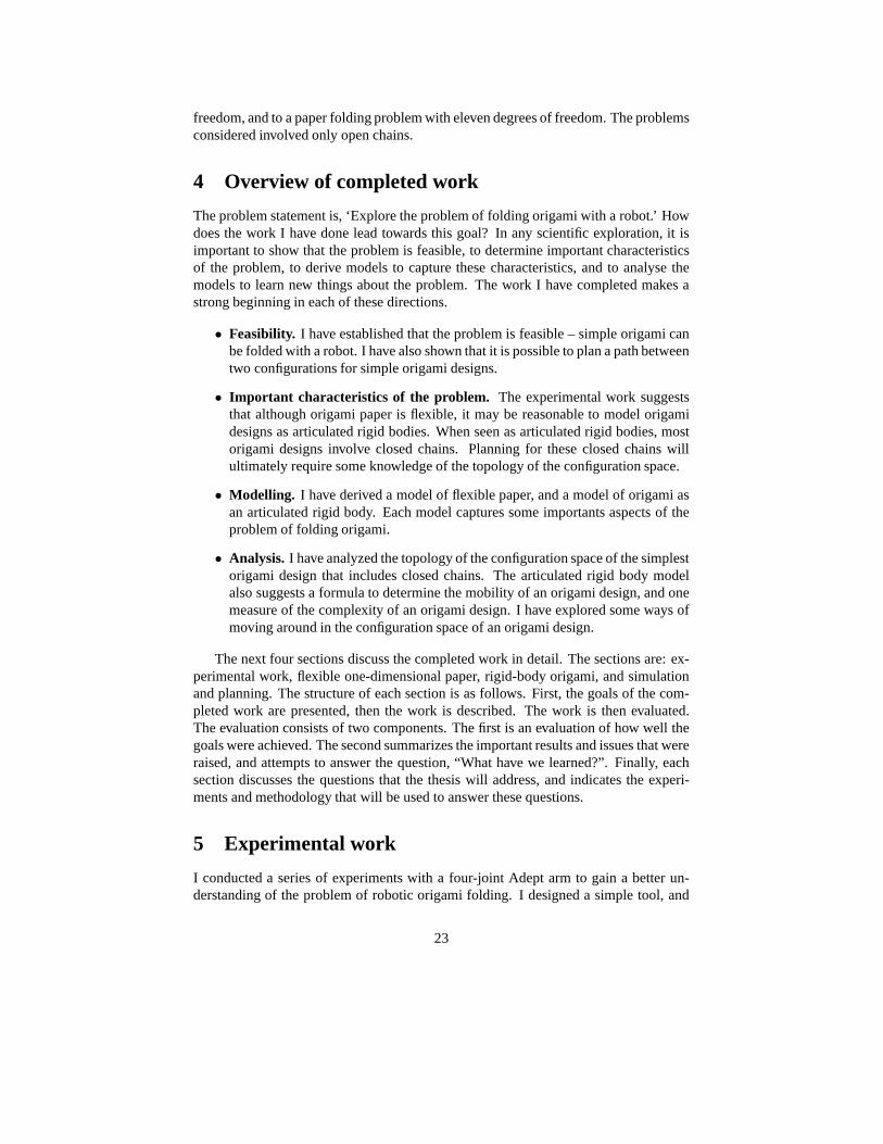
4 Overview of completed work

The problem statement is, ‘Explore the problem of folding origami with a robot.’ Howdoes the work I have done lead towards this goal? In any scientific exploration, it isimportant to show that the problem is feasible, to determine important characteristicsof the problem, to derive models to capture these characteristics, and to analyse themodels to learn new things about the problem. The work I have completed makes astrong beginning in each of these directions.

• Feasibility. I have established that the problem is feasible – simple origami canbe folded with a robot. I have also shown that it is possible to plan a path betweentwo configurations for simple origami designs.

• Important characteristics of the problem. The experimental work suggeststhat although origami paper is flexible, it may be reasonable to model origamidesigns as articulated rigid bodies. When seen as articulated rigid bodies, mostorigami designs involve closed chains. Planning for these closed chains willultimately require some knowledge of the topology of the configuration space.

• Modelling. I have derived a model of flexible paper, and a model of origami asan articulated rigid body. Each model captures some importants aspects of theproblem of folding origami.

• Analysis. I have analyzed the topology of the configuration space of the simplestorigami design that includes closed chains. The articulated rigid body modelalso suggests a formula to determine the mobility of an origami design, and onemeasure of the complexity of an origami design. I have explored some ways ofmoving around in the configuration space of an origami design.

The next four sections discuss the completed work in detail. The sections are: ex-perimental work, flexible one-dimensional paper, rigid-body origami, and simulationand planning. The structure of each section is as follows. First, the goals of the com-pleted work are presented, then the work is described. The work is then evaluated.The evaluation consists of two components. The first is an evaluation of how well thegoals were achieved. The second summarizes the important results and issues that wereraised, and attempts to answer the question, “What have we learned?”. Finally, eachsection discusses the questions that the thesis will address, and indicates the experi-ments and methodology that will be used to answer these questions.

5 Experimental work

I conducted a series of experiments with a four-joint Adept arm to gain a better un-derstanding of the problem of robotic origami folding. I designed a simple tool, and

23

Figure 5: Tool design for making simple folds.

programmed the Adept using hand-selected ‘via’ points. A primary goal was to demon-strate the feasibility of folding origami with an Adept arm. This goal was achieved. Inthe last few experiments, the robot did crease and fold a square piece of origami into asimple envelope.

Another important goal of the work was to determine a set of ‘manipulation prim-itives’ that could be combined to fold simple origami. I have designed some primitiveactions based on an analysis of a few origami designs of medium complexity (a samuraihat, a paper airplane, and partial foldings of a crane and a balloon.) The current me-chanical design can execute some of the primitives (placing the paper, simple folds),but not others (separating flaps and tucking, for example.)

5.1 Tool design

The design of the tool I used is shown in figure 5. A vacuum pad (suction cup) wasused to pick up the paper; a pneumatic vacuum generator supplied the vaccum. Inkbrayers are usually used to roll ink onto rubber stamps. They are available in sizesfrom about 8 cm in length to about 15 cm in length, and are made from a variety ofmaterials including foam, soft rubber, hard rubber, and acryllic. A 15 cm long softrubber ink brayer was attached to the tool to allow the robot to ‘roll out’ creases in thepaper. A pneumatically powered linear actuator moved the vacuum pad out of the waywhile the brayer was being used. I also built a wooden table to act as a workspace; formany of the experiments, the table played the role of a second hand.

5.2 Folding the paper

The first experiments I conducted were motivated by the observation that humans oftenplace precise creases by aligning two edges or corners, and then ‘rolling out’ the cur-

24

Figure 6: Placing a simple crease.

25

Figure 7: Creasing as a reflection.

vature until the paper is creased. The alignment of the edges or corners determines thelocation of the crease – a person who has difficulty drawing a straight line free-handcan still fold a straight crease.

Figure 6 shows the experiment I designed to explore this technique. The operationrequires two hands. As a substitute for the second hand, I taped one edge of the paperto the table. The robot grasped the other end of the paper with the vacuum pad, andpressed it down into contact with the table (1, 2). Once the brayer was firmly holdingthe paper against the table, the vacuum pad was removed (3). The robot then rolled thebrayer forwards (4), rolling out the curvature and eventually creasing the paper (5).

One interesting observation is that not all paper configurations can be ‘rolled out’ inthis way. When the taped edge and the grasped edge were precisely aligned, this simpleoperation was fairly repeatable, and the accuracy of the crease placement appeared tobe within a few millimeters. Occasionally, the paper tore along endpoints of the crease,typically when I had not place the paper carefully before the gripper grasped the topedge. When I intentionally rotated the gripper ten degrees before placing the top edge,the paper crumpled badly as the brayer rolled across it.

If there is only a single crease in a piece of paper, it acts as a line of reflection.If there is no line of reflection consistent with the placement of the two edges, thenwe should not expect the formation of a single crease. Figure 7 shows an example. Ifthe upper right corner of the paper is dragged in either direction along the dotted linewithout rotation, there will be no single crease consistent with the relative position ofthe upper and lower facets of the paper. Although it seems likely that most relativeplacements of the edges can be achieved with three creases, the ‘rolling out’ actiondoes not appear to permit the formation of more than one crease.

5.3 Bending the paper

The Adept arm I used has only four degrees of freedom; we can describe the configu-ration of the tool by the coordinates x, y, z, and θ, the rotation about the z axis. Thismeans that there is no way to flip a rigid body while grasping it from the top. If thepaper is grasped, the grasped point cannot be flipped over to create a 180 degree bend.In my second experiment, I investigated the possibility of using the flexiblity of thepaper to create a bend. Figure 8 shows the motion of the gripper and paper during theexperiment.

The robot first gripped the paper, and dragged it off of the table. It allowed thepaper to droop, and then swept the paper back onto the table. During this phase, the

26

Figure 8: Bending the paper.

edge of the table caused the paper to bend.I was surprised by the fact that the paper did not always droop once it was dragged

off the edge of the table. This may have been because the paper crinkled slightly whengripped by the vacuum pad. When support was removed from the paper it remained inan essentially horizontal configuration. This is an interesting example of paper behav-ing like a rigid body.

When people hold a newspaper up to read it, it is important that the top edge notdroop down. However, for this experiment, some droop was necessary. I implementeda strategy to ensure that the rigidity was broken. After moving the paper off of the edgeof the table, the robot moved the (ungrasped) edge of the paper underneath the tableedge. The arm then lifted the paper, using the table edge to break the rigidity. The armthen swept the paper across the table edge and back onto the table to place the desiredbend.

The flexibility of the paper also allows it to be flipped with one hand. If the vaccuumpad releases the paper once the bend has been placed, the paper slides off, and usuallyends up upside down. Unfortunately, the springiness of the paper makes this motiondynamic and very unpredictable!

Although the dynamic aspect could be ameliorated by grasping the bottom edgewith a simple gripper before releasing the top edge, a larger problem is that the motionof the bottom edge and shape of the bend are difficult to predict. Typically, some twistdevelops between the top and bottom edges. Also, if the robot drags the paper from leftto right starting in the final position shown in figure 8, the bottom edge will eventuallymove, trailing behind the robot. However, if the robot moves the gripper from right toleft, the bottom edge does not move until it eventually flips over. This would probablymake it hard to control the position of the bottom edge even with a feedback controllaw.

27

Figure 9: Placing a shallow crease using a blade.

Figure 10: Folding pre-creased paper.

5.4 Placing shallow creases

Although bending and flipping the paper using the edge of the table turned out to beunpredictable, the method is more successful if there is already a crease in the paper. Ifthere is already a crease, the deformation of the paper tends to occur along that creaseduring the bending phase. I explored pre-creasing the paper in the experiment outlinedby figure 9.

I attached the blade of a long paint scraper to the table. The robot placed the paperabove the blade. The brayer then rolled across the paper along the blade, forming acrease along the line of the blade. The process is analogous to bending sheet metal ina brake – the blade acted as the punch and the soft rubber brayer acted as the die.

The accuracy and repeatability of this procedure were not very good. As the brayermoved across the blade, the paper tended to be dragged along a few millimeters by thebrayer. Increasing the accuracy is a problem for a future mechanical design.

5.5 Folding creased paper

The method just described places a very shallow crease in the paper. However, even ashallow crease may be useful, since creased paper behaves differently from uncreasedpaper. Once there is a crease, applying forces to the edges of the paper tends to causemore bending along the crease than elsewhere in the paper. I used this observation tofold the paper once a shallow crease had been placed. Figure 10 outlines the experi-ment.

The motions of the paper for this experiment were the same as the motions shownin figures 6 and 8. The paper was grasped from above, near the crease. The paperwas then oriented so that the crease was parallel to the edge of the table. The robot

28

Figure 11: An ‘envelope’ origami shape. The four corner flaps are folded into thecenter of the square.

dragged the paper off the table, and used the edge of the table to break any rigidityand bend the paper. The robot then dragged the paper along the table while squeezingdownwards; most of the bending of the paper occurred along the crease. Once thepaper was essentially flat on the table, the robot released the vacuum grip and rolledthe brayer across the paper to sharpen the crease. It is interesting that in addition toallowing the fold to be made precisely, pre-creasing also allows the paper to be flipped:part of the paper is upside down after the motion, and positioned in a known location.

5.6 Folding an envelope

The experiments discussed to this point developed a series of primitives. These primi-tives can be combined to fold the simple origami shown in figure 11. Figure 12 showsthe strategy. First, one crease was placed in the paper using the method described insection 5.4. The robot then dragged the paper off the table, and used the table edgeto ‘fold under’ the flap formed by the crease. The fold was made along the crease bysqueezing the paper against the table while dragging the paper to the right. The brayerrolled over the paper to sharpen the crease. At the end of the procedure, one corner ofthe paper was folded under. The process was repeated for each of the three remainingflaps, folding the paper into the desired envelope shape.

5.7 Evaluation

“How well did it work?”. The robot was able to repeatably place all four creases, andfold the flaps to form the envelope. The error in the pose of the first crease was small– on the order of a few milimeters and a few degrees. However, error accumulated,and the pose error of the last crease was typically nearly a centimeter, and about tendegrees. The primary source of error seemed to be the slip of the paper on the tableas the brayer rolled over it to place a crease. Reducing this error will require that thepaper be grasped during creasing, probably on both sides of the crease. Some simplesensing of paper edges could be used to reduce the problem of error accumulation.

5.7.1 Manipulation primitives

“Can the method be extended to other origami designs?” Currently, the accumulation oferror means that four creases is probably about the maximum possible. If the accuracy

29

Figure 12: Folding the envelope.

30

Figure 13: Partial folding of a paper airplane, using just two manipulation primitives,positioning and folding down.

could be increased, then there is a class of origami that the primitives available could beused to fold. We will say that a manipulation task is feasible if the available primitiveswould be sufficient to complete the task, if all primitives were executed with perfectaccuracy. The feasibility class is the set of tasks that can be completed given some setof primitives.

Consider the partial folding of a paper airplane shown in figure 13. The manipu-lation primitives used are positioning of the paper, and folding down. Positioning ofthe paper requires that the robot be able to move a flat piece of a paper rigidly to anew configuration, and is indicated by a pair of arrows arranged in a circle. Foldingdown is indicated by a horizontal dashed line. A successful execution of the foldingdown primitive involves folding the section of paper above the line down (towards thereader) across the crease line, creating what is often called a ‘valley fold’. Both of theseprimitives can be executed by the current system to some degree.

The envelope and the paper airplane should probably not be placed in the samefeasibility class. Each of the creases in the envelope is only one layer thick; in the air-plane, multiple layers of paper are simultaneously folded. The current implementationof the folding down primitive first creases the paper and then uses the edge of the tableto execute the fold; this is much more likely to fail if there are multiple layers. In orderto fold the airplane, the implementation of the primitives must be able to successfullydeal with the case where there are multiple layers.

What other primitives should be available? Consider the folding of the samuraihat shown in figure 14. Two additional primitives are introduced. The first is flipping,denoted by a looping arrow; the meaning of this primitive is obvious. The combinationof flipping, folding down, and positioning primitives allows both ‘valley folds’ and‘mountain folds’ to be formed. The second primitive introduced is separating, shown

31

Figure 14: Folding a samurai hat with four primitives.

by the hollow arrow first introduced in step eight. Sometimes it is necessary to folddown only one of two flaps. Whereas the primitives introduced so far may be thoughtof as verbs in a manipulation sentence, the separating primitive should be considered tobe a modifier or adverb. Separating is always performed in combination with anotherprimitive, and implies that some number of flaps should be separated before applyingthe action primitive. Although separation of flaps was not necessary until step eight, itis interesting that all but one of the remaining folds require it.

The partial crane folding shown in figure 15 introduces another simple primitive,unfolding, which is denoted by an upwards-pointing arrow. When combined with fold-ing down, unfolding permits pre-creasing the paper.

As was discussed briefly in the introduction, a rigid body model of origami withcrossing creases contains closed chains. If we unfold the envelope or the airplane, wefind that no creases cross. This is not the case with the samurai hat, but the sequentialnature of the folds means that the crossing creases never become an issue.

The crane folding shown in figure 15 does require manipulation of closed chains.Step 6 requires a complicated simultaneous manipulation of multiple facets. The ar-rows denote folding the designated creases to a single line. If each facet is considered tobe a rigid link, and each crease a hinge joint, then the eight-link mechanism is a closedchain with a single loop. We might call the primitive required to fold this origamiclosed chain manipulation. (For the simple case where there are two colinear creases,Miyazaki et al. [39] refers to this operation as tucking. )

What about more complicated primitives? Figure 16 shows a partial folding of aballoon. There are only two crease lines; all four creases are valley creases. Huffman’s

32

Figure 15: Partial folding of the crane.

Figure 16: Partial folding of an origami balloon.

33

results tell us that there cannot be four valley creases and no mountain creases if thefacets are planar. Step 3 requires bending the two side facets. So we might define anadditional primitive, flex, that could be used to modify other primitives.

Once the shape shown in step 4 has been squeezed flat, two additional creases areintroduced. So it would be possible to avoid bending the side facets by precreasingthe paper. (In fact, the partial balloon folding and the partial crane folding are then thesame, up to a rotation of the paper before creasing.) An interesting question is whetherpre-creasing can always be used to avoid bending. If so, is it ever necessary to addadditional creases that will not be found in the final origami?

This collection of primitives is not complete, particularly since the primitives closedchain manipulation and flex are too general to be implemented. In fact, the software,Origami, the Secret Life of Paper, states that each of the traditional origami designs en-tails a good move – that is, a move that is ‘both surprising and satisfying’. It is also hardto see how simple primitives can be used to describe the folding of complicated three-dimensional designs. However, the basic primitives discussed (positioning, flipping,folding down, unfolding, separating) seem sufficient to fold a rich class of origami.This class will be the focus of the experimental portion of the thesis.

The primitives allow a comparison not only between types of origami, but betweenorigami and other folding manipulation. The following table lists some skills that arerequired to fold simple origami (for example, the samurai hat), flat origami (the crane),modular origami (many simple components), origami sculpture (state-of-the-art, oftenwith a human or animal subject), sheet metal, and cartons.

Simple Flat Modular Sculpture Sheet metal Carton2D position X X X X X X

Flip X X X X X X

3D position X X X X X

Simple fold X X X X X X

Fold to angle X X X X

Flex X X

Curved creases X

Separate X X X

Grasp section X X X

Pre-creasing X X X X

Closed chain X X

Flap insertion X X X X

Large forces X

The skills for each class should be interpreted loosely as the minimum require-ments to fold some representative examples of the class. The definition of each skillalso depends on the material. For example, ‘pre-creasing’ of sheet metal refers to thepractice of cutting out a wedge of material before making a bend; this greatly reducesthe amount of force that needs to be applied, and reduces warping of the metal.

34

5.8 Proposed thesis work

“What have we learned?” The experimental work and the above discussion suggest anumber of important characteristics of the problem.

• A large class of origami can be folded with just a few manipulation primitives.Although the samurai hat requires a large number of folds, and although thecreases cross in the unfolded hat, no complicated primitives are necessary.

• Certain origami designs require complicated manipulation to fold. Examplesinclude the crane and the balloon.

• Two hands may be needed. Paper is flexible, and grasping it at just a single pointcan make manipulation difficult. How many hands are needed? The experimentsshowed that if the paper is pre-creased, one grasping hand may be enough. (Thetable was used as a second, non-grasping hand.) If the design requires compli-cated manipulation of closed chains, more hands may be necessary. Are thereorigami designs that cannot be folded by a human being?

• Creased paper and uncreased paper behave differently. The experiments showedthat it may be relatively easy to fold with one hand once a crease has been placed.

• Error accumulates each time the paper is released. This problem was com-pounded by the fact that the paper was not grasped in any way while the creaseswere placed.

The thesis will explore and address each of these issues. The primary goal ofexperimental work is to design a system that implements a few manipulation primitives,and is somewhat more accurate than the current system. I will focus on three primitives:positioning, flipping, and folding down. I will also partially address the problem ofimplementing the primitives unfolding and separating.

5.8.1 Design of a new folding mechanism

Figure 17 shows a possible design for the folding mechanism. A vacuum pad wouldbe used to grip the paper, and the Adept arm would position the paper over the two‘palms’ shown in the figure. The right palm is in fact just the table. The left palm isactuated, and uses vacuum to grip the paper.

Folding down would be accomplished by the procedure shown in the figure. Oncethe paper was positioned, the vacuum in the left palm would grip the paper. The vacuumpad would be removed by the Adept, and be replaced by a sharp wedge. The left palmwould then rotate about the center joint, creating an initial fold. The wedge wouldbe removed, and folding would be completed. Flipping could be accomplished by asimilar procedure.

The advantages of the new design over the old include the fact that the paper wouldalways be gripped by either the left palm or the vacuum pad. This should significantlyreduce the accumulation of error. Folding and creasing also would occur simultane-ously, so the paper could be treated as a single rigid body. If the right palm were

35

Figure 17: Possible folding mechanism design

designed to tilt somewhat to the left, it would be possible to remove error by releas-ing the vacuum grip while the paper was being flipped. Gravity would then cause thepaper to slide to the bottom of the ‘V’, removing rotational and positional error alongone axis. Tilting both palms forwards would allow error to be removed along the otheraxis. In either case, some vibration of the palms might be necessary to break friction.

5.8.2 Grasping origami

I will also analyze the problem of grasping origami. Although this component of thethesis will be primarily theoretical, some experimental verification of results will benecessary as well. I will consider the problem of grasping the partial balloon folding,and the partial paper crane folding. The proposed theoretical work will be described inmore detail in a later section.

6 Modelling one-dimensional paper

Creased and uncreased paper behave differently. The work discussed in this sectionexplores the behavior of paper that is bent but not creased. A primary goal of the workwas to extend principles used in the manipulation of rigid bodies to a model of flexiblepaper.

The experimental work suggests that a one-dimensional model of paper that con-siders the paper ‘viewed from the side’ may be a good simplification. This model isapplicable when the rulings of the paper are approximately parallel in R3. Althoughthis was not an explicit goal of the experimental design, a number of factors led tothis being the case during most of the experiments. In the experiments described byfigures 6 and 8, all motion of the paper was made in a direction perpendicular to thedesired direction of the rulings. The robot also grasped the paper at the center of the

36

Figure 18: One-dimensional paper as the limit of a planar revolute arm.

desired rulings, so that bending would be more symmetric. In the experiments de-scribed by figures 9, 10,and 12, the creases were placed parallel to the desired directionof rulings.

In order to better understand the behavior of bending paper, I implemented a methoddescribed by Hirai et al. [22] to find likely configurations of paper subject to a set ofgeometric constraints. The model used by [22] describes the configuration of the pa-per using a set of Fourier basis coefficients. I used the model to extend some analysistechniques typically used for rigid bodies to the flexible paper. I determined a formuladescribing the forwards kinematics of the paper. The principle of virtual work can alsobe applied to the model. I derived the dynamic equations that are implied by the model,and considered the problem of force control of the paper.

Although I achieved some interesting results with this model, I do not anticipatethat this work will be a primary focus of future thesis work, for reasons discussedbelow (section 6.6). The derivations in the remainder of the section are provided forcompleteness, but may be skipped by the impatient reader.

6.1 Formulation of the model

One way to model paper is to describe the configuration by a function that gives theangle of the tangent at each point on the curve

θ(s) : [0, 1] 7→ [0, 2π) (5)

and an initial condition (x0, y0) which describes the location of a particle on an edgeof the paper. Figure 18 shows an example. The location of each particle is then givenby

x(x0, θ(·), s) = x0 +

∫ s

0

cos θ(τ) dτ (6)

y(y0, θ(·), s) = y0 +

∫ s

0

sin θ(τ) dτ (7)

The tangent vector to the parameterized curve described by equations 6 and 7 isalways of unit length; the paper was assumed not to stretch. Since θ is a continous

37

function of one variable, it can be approximated by a finite Fourier series. The Fouriercoefficients then give a finite-dimensional representation for the configuration of thepaper. Hirai used this method to find equilibrium points of model of copy paper heldat two opposite edges.

If the Fourier coefficients are collected in a vector p then the state of the paper q isgiven by

q =

x0

y0

p

(8)

If we define the vector b(s) containing two leading zeros followed by the Fourierbasis functions,

b(s) =

001

sin 2πscos 2πssin 4πscos 4πs

...

(9)

then we may write θ, x, and y as functions of q and s:

θ(q, s) = qT b(s) (10)

x(q, s) = x0 +

∫ s

0

cos qT b(τ) dτ (11)

y(q, s) = y0 +

∫ s

0

sin qT b(τ) dτ (12)

We may describe trajectories of the paper by allowing q to be a function of time.Hirai et al. [22] used this formulation together with non-linear programming soft-

ware to find configurations of the paper that minimize potential energy due to someconstraints. I implemented this algorithm. One difficulty with the algorithm is thatthere may be multiple local minima of the potential energy function. In order to betterunderstand how the paper actually behaves, I used the Fourier basis representation tofind the Lagrangian dynamics of the system. I will also briefly discuss the problemof controlling some control points or a subset of the degrees of freedom of the paperby applying forces at specified points along the paper. Although the dynamics of thismodel were also considered by [59], their algorithm involved numerically minimizingthe difference between kinetic and potential energy at each time step; my derivation isanalytical.

38

6.2 Potential energy functions

Hirai used the following formula to calculate the potential energy due to gravity

Vg(q) = ρ

∫ 1

0

y ds = ρy0 + ρ

∫ 1

0

∫ s

0

sin qT b(τ) dτ ds (13)

where ρ is the mass of the paper per unit length, assumed constant over the paper forsimplicity. The multiple integral can actually be simplified to a single integral:

Vg(q) = ρy0 + ρ

∫ 1

0

(1 − τ) sin qT b(τ) dτ (14)

Hirai used a constitutive law to model the spring energy of the paper

Vs = k

∫ 1

0

θ′2 ds, (15)

where k is a spring constant determined experimentally. Hirai calculated the energynumerically for a given configuration using the Fourier basis representation:

Vs(q) = k

∫ 1

0

(qT b′)2 ds (16)

Actually, the integral can be found analytically. If we define a diagonal matrix Kwith ki as the ith diagonal element of K

ki =

0 if i = 1k(i − 2)2π3 if i is even, i ≥ 2k(i − 3)2π3 if i is odd, i ≥ 3

(17)

(18)

it turns out that the spring energy can be written as a simple weighted sum ofsquares:

Vs(q) = qT Kq (19)

6.3 Differential kinematics

In a typical manipulation task, we might want to be able to determine the motion ofa number of points of interest on the paper, due to a change in the configuration ofthe paper as a whole. For example, the points of interest might be the set of points ofcontact between the paper and a manipulator. We can describe the points of interest bya vector of parameters:

s =

s1

s2

...

(20)

39

The location of the points is given by the vector

x(q, s) =

x(q, s1)x(q, s2)

...y(q, s1)y(q, s2)

...

(21)

We first consider how the x coordinate of a single point changes as a single basisfunction coefficient is varied.

∂x(q, s)

∂q1

=∂x(q, s)

∂x0

= 1 (22)

∂x(q, s)

∂q2

=∂x(q, s)

∂y0

= 0 (23)

For i ≥ 3,∂x(q, s)

∂qi

=∂

∂qi

∫ s

0

cos (qT b(τ)) dτ (24)

Since everything is continuous, we can exchange differentiation and integration:

∂x(q, s)

∂qi

=

∫ s

0

∂

∂qi

cos (qT b(τ)) dτ = −

∫ s

0

bi(τ) sin (qT b(τ)) dτ (25)

We may calculate the partials of y(s) similarly. For i ≥ 3,

∂y(q, s)

∂qi

=

∫ s

0

∂

∂qi

sin (qT b(τ)) dτ =

∫ s

0

bi(τ) cos (qT b(τ)) dτ (26)

Define the vector functions xq(q, s) and yq(q, s) which contain the partial deriva-tives of x and y with respect to q. Then define the 2m× n Jacobian matrix:

J(q, s) =

xq(q, s1)T

xq(q, s2)T

...yq(q, s1)

T

yq(q, s2)T

...

(27)

Thenx(q, s) = J(q, s)q (28)

40

6.4 Kinetic energy and dynamics

In order to find the kinetic energy of the system, we first consider the velocity of eachparticle. By the multivariable chain rule:

x = xTq q (29)

y = yTq q (30)

The square of the velocity of the particle at position s is

v2(q, q, s) = x2 + y2 (31)

= qT (xqxTq + yqy

Tq )q (32)

We define ρ to be the mass of the paper per unit length; we assume ρ is constantover the paper. Then the kinetic energy is

T =ρ

2

∫ 1

0

v2(q, q, s) ds (33)

T =ρ

2

∫ 1

0

qT (xqxTq + yqy

Tq )q ds (34)

T =1

2qT

(

ρ

∫ 1

0

xqxTq + yqy

Tq ds

)

q (35)

We define the mass matrix

M(q) = ρ

∫ 1

0

yqyTq + xqx

Tq ds (36)

The kinetic energy is

T (q, q) =1

2qT M(q)q (37)

Once the kinetic energy and mass matrix have been defined, we can derive thedynamical equations. The details of the derivation are ommited, but it turns out that theequations can be written in a familiar form:

Mq + Mq = Tq − Vq + JT f (38)

One use of the dynamic equations is simulation. We could truncate the Fourierseries, invert M to solve for q, and numerically integrate q to find the trajectory q(t).Since the mass matrix is symmetric, we could increase the numerical stability of thesimulation by using a Cholesky decomposition at each time step, rather than invertingM directly.

The dynamic equations also contain information about the static case. If q = q = 0,then

Vq = JT f (39)

41

6.5 Force control

f2

f1

f3

f4

What if we can control forces at some specified points? Let J1 be the Jacobian thatrelates the motion of the points where forces are applied to the generalized velocity q.Then write the dynamic equations.

q = M−1(Tq − Vq − M q) + M−1JT1 f (40)

Let s be the vector of parameters describing the points we want to control. Thenx(s) will be the Cartesian location of these points. Let J2 be the Jacobian relating qand x.

x(q, s) = J2(q, s)q (41)

Differentiate with respect to time.

x = J2q + J2q (42)

J2q = x − J2q (43)

Premultiply equation 40 by J2:

J2q = J2M−1(Tq − Vq + −Mq) + J2M

−1JT1 f (44)

Substitute:

x = J2M−1(Tq − Vq − M q) + J2q + J2M

−1JT1 f (45)

which has the form

x = d(q, q) + C(q)f (46)

C is square, and non-singular as long as both J1 and J2 have full row rank. (Thenumber of Fourier coefficients chosen to represent the system should be large comparedto the number of control points.) We can choose x as we like, and solve for f .

f = C−1(x − d) (47)

42

6.6 Evaluation

“What have we learned?” One observation is that directly simulating the system usingthe dynamics equations derived requires the mass matrix to be computed and factored ateach time step. Since the mass matrix is dense, this is computationally expensive. Theinverse dynamics method of force control described suffers from the same problem.The result is that only a few Fourier coefficients can be used if numerical simulationor control is the goal. Much better results could probably be achieved by modellingthe paper as a serial chain, and using efficient simulation techniques such as thosedescribed in [6].

On the other hand, the model derived may be useful from the perspective of analy-sis. It is particularly interesting that under the Fourier basis representation, the springenergy of the system is a simple weighted sum of squares. Another possible benefit isthe smoothness of the model; derivatives are defined everywhere along the curve. (Thiswould not be the case if the paper were modelled as a serial chain.)

The completed work suggests some interesting questions and approaches to con-trolling flexible paper. However, when compared to other aspects of folding origami,the problem of controlling flexible objects using models similar to that derived has beenrelatively well-addressed in the literature. Therefore, extending this work will not be afocus of the thesis.

7 Rigid origami

We return to two observations made in section 5:

• A large class of origami can be folded with just a few manipulation primitives.Although the samurai hat requires a large number of folds, and although thecreases cross in the unfolded hat, it seems that no complicated primitives arenecessary.

• Certain origami designs require complicated manipulation to fold. Examplesinclude the crane and the balloon.

The experimental work focusses on the first of these issues: developing simpleprimitives that can be used to fold a variety of origami shapes. The goal of the workdescribed in this section is an analysis of some more complicated cases. We focus onone specific problem: that of folding a pre-creased closed chain.

The partial crane folding shown in figure 15 requires pre-creasing, and then simul-taneously folding along multiple crease lines to form the base. Typical instructions forthe balloon base require that some of the facets be bent, while simultaneously fold-ing along multiple crease lines. Figure 19 shows how two additional creases can beintroduced to avoid bending of the facets. How bad can it get? Figure 20 shows thepre-creasing required to fold the stellated octohedron. There are eighty-eight creases.Fortunately, not all of the creases are folded simultaneously to create the final design.

If we fold an origami shape, and then unfold it, the paper will be creased. Sincecreases are typically made along straight lines in origami, the uncreased regions willbe polygonal facets. When the origami is folded flat, the facets will be planar. We will

43

Figure 19: Folding the balloon base using pre-creasing.

Figure 20: Complicated pre-creasing required to fold the stellated octohedron.

44

Figure 21: Rigid origami.

define creases as the edges of the facets. Creases may be colinear; we will call a linecontaining multiple creases a crease line.

The simplest way to model pre-creased origami is to consider each facet as a rigidlink and each crease as a hinge joint; this model is similar to those used by Huff-man [23] (geometry of creases), Lu and Akella [34] (carton folding), and Gupta etal [18] (sheet metal bending). Even for this simple model of origami, the kinematicstructure may be quite complicated. If crease lines cross, then the structure includesclosed chains.

Configuration spaces of closed chains are often difficult to parameterize, and formost closed chains no smooth one-to-one global parameterization exists. Since con-straints may be dependent, it is often difficult to even determine the number of degreesof freedom. In this section, I will discuss some of the interesting features of the rigidorigami model, including the number of degrees of freedom, and the topology of theconfiguration space of the simplest closed-chain rigid origami.

7.1 Origami with struts

In order to analyze rigid origami, it is often convenient to consider an equivalent mech-anism made up of struts and ball joints. Consider the origami shown at the top offigure 21. There are six facets and six creases. The mechanism shown at the bottom ofthe figure has twelve struts and seven ball joints; the struts are placed around the borderof each facet, and the ball joints are placed wherever struts meet. Since each facet istriangular, the struts ensure that each facet remains rigid. Folding is possible along anycrease, but along no other line.

45

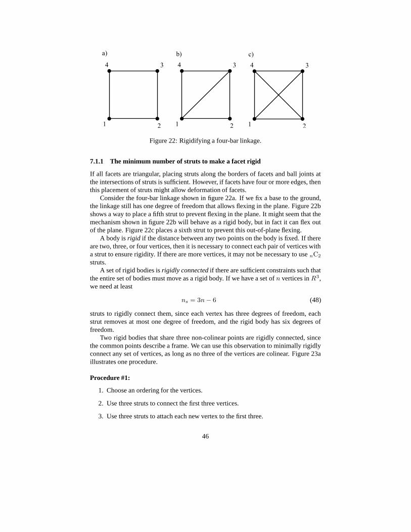
Figure 22: Rigidifying a four-bar linkage.

7.1.1 The minimum number of struts to make a facet rigid

If all facets are triangular, placing struts along the borders of facets and ball joints atthe intersections of struts is sufficient. However, if facets have four or more edges, thenthis placement of struts might allow deformation of facets.

Consider the four-bar linkage shown in figure 22a. If we fix a base to the ground,the linkage still has one degree of freedom that allows flexing in the plane. Figure 22bshows a way to place a fifth strut to prevent flexing in the plane. It might seem that themechanism shown in figure 22b will behave as a rigid body, but in fact it can flex outof the plane. Figure 22c places a sixth strut to prevent this out-of-plane flexing.

A body is rigid if the distance between any two points on the body is fixed. If thereare two, three, or four vertices, then it is necessary to connect each pair of vertices witha strut to ensure rigidity. If there are more vertices, it may not be necessary to use nC2

struts.A set of rigid bodies is rigidly connected if there are sufficient constraints such that

the entire set of bodies must move as a rigid body. If we have a set of n vertices in R3,we need at least

ns = 3n− 6 (48)

struts to rigidly connect them, since each vertex has three degrees of freedom, eachstrut removes at most one degree of freedom, and the rigid body has six degrees offreedom.

Two rigid bodies that share three non-colinear points are rigidly connected, sincethe common points describe a frame. We can use this observation to minimally rigidlyconnect any set of vertices, as long as no three of the vertices are colinear. Figure 23aillustrates one procedure.

Procedure #1:

1. Choose an ordering for the vertices.

2. Use three struts to connect the first three vertices.

3. Use three struts to attach each new vertex to the first three.

46

Figure 23: Two ways of rigidly connecting six points.

This procedure is simple, but has a disadvantage. All of the vertices of an origamifacet lie in a plane; the facet is a polygon. In order to minimize the number of strutsused to form the entire origami mechanism, the number of struts interior to each facetmust be minimized. Figure 23b illustrates a procedure that rigidly connects the vertices,while ensuring that a strut is placed along each edge.

Procedure #2 (rigidly connecting a polygon):

1. Choose a polygonal ordering of the vertices from 1 to n.

2. Use three struts to connect the first three vertices.

3. Connect each of vertices 4 . . .n − 1 to its three predecessors.

4. Connect vertex n to vertices n − 2, n − 1, and 1.

Since each new vertex is rigidly connected to a rigid body, each procedure rigidlyconnects the vertices. Since each procedure places a single strut for each of the firstthree vertices, and three struts for each additional vertex, 3n−6 struts are placed, whichis minimal.

7.1.2 Grubler, for origami

The origami shown in figure 21 has six facets and six creases. If we model the facetsas rigid bodies and the creases as hinge joints, the mechanism is a closed chain. Whatis the mobility of the mechanism in a generic position, if we fix a base? Grubler’sformula for the mobility of spatial closed chains is M = 6f−6, where f is the numberof freedoms for each joint. Each hinge joint has one freedom, so Grubler would tell usthat the mobility is zero. However, we know that the mechanism has some degrees offreedom. The problem is that the constraints are not independent.

It turns out that the mobility is three. How do we arrive at this number? Theconstruction using struts and ball joints gives a solution. For the strutted version, weexpect the constraints (the lengths of the struts) to be independent unless two facets areco-planar. Therefore, we should be able to count the number of vertices and struts to

47

Figure 24: An origami design with crossing creases.

find the number of degrees of freedom. If all facets are triangular, M ≥ 3n − ns − 6.(Equality occurs whenever constraints are independent.) The mechanism in figure 21dhas seven vertices and twelve struts, so M ≥ 21 − 12− 6 = 3.

If there are non-triangular vertices, we must rigidly connect the vertices of eachfacet. If pi is the number of facets with i vertices, then the formula is:

M ≥ 3n − ns − 6 −

n∑

i=4

pi(2i − 6) (49)

7.2 Topology of the configuration space

When constraints are not dependent, equation 49 gives a way of counting the freedomsof rigid origami. What happens when constraints are dependent? Figure 24 showsan origami design. There are four facets and four creases, but only two crease lines.There are five vertices and eight struts, so equation 49 tells us that we should expect themobility to be one. In fact, once a fold is made along the first crease, it is not possibleto fold along the other crease until the paper has been folded flat.

The joint angles of at least three creases are necessary to determine the configura-tion of the paper. Two crease angles are enough to describe trajectories of the paperfrom any initial configuration. Figure 25 shows the topology of the configuration space,parameterized by the angles of the two creases labeled ‘1’ and ‘2’ in figure 24. Filledcircles on the graph indicate nodes where transitions are possible, and unfilled circlesindicate nodes where a transition between two edges would involve self-intersection.The numbers and origami diagrams show a possible trajectory to fold the paper into atriangle.

As can be seen from the figure, the configuration space of this simple origami isnot a manifold, but rather a union of manifolds. Figure 25 was derived by consideringeach of the possible folded configurations of the paper. This will be difficult for morecomplicated origami shapes.

Milgram and Trinkle [37, 52] suggest a method for finding the topology of simpleclosed chains, if we ignore the possibility of self-intersections. The procedure is:

1. Break the loop by removing a single link.

2. Consider the n−1 bar open chain. Fix the first link, and designate a point on thelast link as an end-effector.

48

Figure 25: Topology of the configuration space of a simple origami design.

3. Determine the topology of the workspace of the end-effector. Where is the map-ping from joint space to workspace one-to-one? Two-to-one? Many-to-one?

4. Intersect this workspace with the (simple) workspace of the two-bar linkage con-taining the fixed link and the removed link.

5. The configuration space is the image of these workspace points under the inversekinematic mapping.

Milgram and Trinkle show how this procedure can be used to completely deter-mine the topology of the configuration space for planar four- and five-bar closed loops.Although the procedure becomes very difficult for mechanisms with more links, theauthors show that the analysis can be applied recursively to describe the topology of ann-bar linkage.

In a discussion and personal communication [36] with the author, James Milgramdemonstrated how the procedure may be used to determine the topology of the origamishown in figure 24 in a methodical way. Figure 26 shows the results. Figure 26a showsthe origami design. We will label the joints counter-clockwise from one to four, startingfrom the rightmost joint, and the facets by the index of the joint they follow. Facet one(in the first quadrant) is fixed. We remove facet four, and consider the workspaceof a point on the third facet (26b). If we spin the third facet about joint three, theselected point describes a circle. If we spin this circle about joint two, we find that theworkspace is a sphere. As the circle spins, the sphere is covered twice, except at thepoles, which are covered an infinite number of times. So the mapping from joint anglesto workspace is two-to-one, except at the poles, where it is many-to-one.

49

Figure 26: The configuration space of origami with two perpendicular crease lines,ignoring self-intersections. Due to Milgram [36].

We now consider the linkage containing only facets one and four (figure 26d). Weconsider the workspace of the point on facet four that is initially the same as the pointwe’ve already considered. The workspace of the point is a circle. We then intersectthe two workspaces ( 26e, 26f). This gives the workspace of the point for the originalclosed chain mechanism. The configuration space of the mechanism is the image ofthis set under the inverse of the mapping from joint angles to workspace. In figure 26f,the numbers 1 and 2 show the points where the mapping was many-to-one (the poles).Along the arcs, the mapping was two-to-one. So the topology of the configurationspace is four circles, connected circularly. This can be represented by the graph shownin 26g.

I have applied the method to some variations of the origami design with four inter-secting creases. Figures 27 and 28 show the results. The workspace of the open chainshown in figure 27b is a segment sphere cut by a plane perpendicular to the line con-necting the poles. The mapping from joint space to workspace is one-to-one at points1 and 3 in figure 27f, many-to-one at point 2, and two-to-one everywhere else. Thetopology of the configuration space can therefore be represented by three connectedcircles, or the graph shown in figure 27g.

The analysis depicted in figure 28 is similar, but the mapping is one-to-one at point3 in figure 28f. The topology of the c-space is a figure-eight. Physically, if we pickan angle for a single crease, there are two possible configurations for the rest of thecreases (‘elbow up’ and ‘elbow down’). To get from one configuration to the other,

50

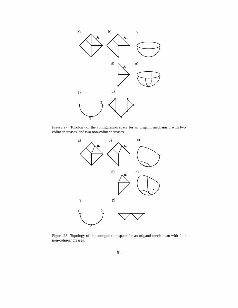
Figure 27: Topology of the configuration space for an origami mechanism with twocolinear creases, and two non-colinear creases.

Figure 28: Topology of the configuration space for an origami mechanism with fournon-colinear creases.

51

the mechanism must go through the flat configuration (the intersection point of the twocircles in the figure-eight).

It is also interesting that the designs shown in figures 26, 27, and 28 are in theclass studied by Huffman (described in section 3.1.2). One of Huffman’s results for amechanism with four non-colinear creases, like that shown in 28, is that at any timethree of the creases must be convex, and the remaining concave, or vice versa. If thecrease for which we determine the angle is concave, either the other three must beconvex, or exactly one of the others must be convex. Since the configuration spaceonly contains two components (the figure-eight), which crease is convex must fullydetermined by the origami design.

7.3 Evaluation

“What have we learned?” I proposed two different ways of representing the rigidorigami model. The first uses struts and ball joints to create facets and creases, andthe second uses rigid body facets and hinge joints at the creases. There are advantagesto each of the representations.

If creases do not cross, the hinge joint mechanism is more useful, since it willcontain no closed chains. There is therefore a one-to-one mapping between joint anglesand mechanism configurations, and we have a familiar joint-space representation. It isnot hard to analyze the topology of the simplest origami with crossing creases usingthis representation. Also, only a few numbers are needed to represent the configuration:the angles at each joint.

Even if creases do not cross, the ball joint mechanism will contain at least one(immobile) closed chain for each facet. Many variables are also needed to representeach configuration. However, the usefulness of the mechanism is that the constraintsare local, and typically independent. This makes it much easier to count freedoms ofthe mechanism, particularly if there are multiple closed chains in the origami. Thestructure of the constraints is also very uniform: each constraint involves on the dis-tance between two vertices. This means that the constraint Jacobian (discussed below),though large, is sparse and has a simple structure. (In fact, the constraint Jacobian islinear in configuration q.)

We have also learned that the topology of the configuration space for simple closedchains can be relatively complicated. A planner that does not take the topology intoaccount is likely to be unable to plan paths between arbitrary points in the c-space.

The singularities of the open chain formed by removing links determine the c-space topology. This suggests that different nodes of the c-space are separated byconfigurations where facets (not necessarily adjacent) are co-planar. This conjectureneeds to be generalized and proved, but might be a useful way of encoding the topologyfor use by a planner.

7.4 Proposed thesis work

The goal of this section was to explore a complicated manipulation primitive usedin folding origami: simultaneous folding of creases in pre-creased paper. I have de-

52

termined the structure of the configuration space for the simplest case where creasescross.

The thesis work will explore the topology of the configuration space for more com-plicated designs involving more than four links. It will be difficult to directly applyMilgram and Trinkle’s methodology to cases where there are more links or multipleloops, but it may be possible to prove some useful results. An interesting questionthat was raised by the completed work is whether the ball joint mechanism can alsobe used to find the topology of the configuration space. It seems likely that zeroes andsign changes of the eigenvalues of the constraint Jacobian correspond to regions of thec-space. (The constraint Jacobian, and some of its limitations, are discussed in the nextsection.)

8 Simulation and planning

The goal of the work described in this section is the same as that in the last: explorationof folding pre-creased origami. I considered the problem of planning local motions ofthe ball joint mechanism described in the previous section. I implemented a planner,and applied it to the simplest case, with good results.

Mechanical systems typically involve a set of constraints. Baraff [6] writes

...ultimately, we are faced with a basic choice. Either we model constraintsby reducing the number of coordinates needed to describe the system’sstate, or we introduce additional forces into the system to maintain theconstraints.

The constraints are implicit if generalized coordinates are used to parameterize thepossible configurations, and explicit if the constraints are described by a number ofauxiliary equations.

It is often difficult to find a joint space (or reduced coordinate) representation fororigami and other complicated closed chains. One common solution is to break thechain. Motion is then planned for the first segment (now an open chain), and inversekinematics are used to enforce compliance of the second segment. The primary diffi-culty lies in choosing where to break the chain, particularly if there are many closedloops. If the second segment is too short, compliance will not be possible. If it is toolong, arbitrary choices must be made in the inverse kinematics solution.

Path planners for serial arms and mobile robots typically assume a reduced coordi-nate system. Explicit inequality constraints are used to express the fact that collisionsshould be avoided. However, I am not aware of any practical, general path planningalgorithms that permit explicit equality constraints. This is surprising, given the suc-cess and ease of implentation of efficent dynamic simulation algorithms using explicitequality constraints (for example, see [6]).

In this section, I will discuss my preliminary work on planning for origami us-ing explicit equality constraints. The formulation is similar to that used in non-linearprogramming and other optimization problems.

53

8.1 Formulation

The strutted origami construction allows a simple description of the configuration spaceof rigid origami mechanisms. We will describe the configuration of the origami by avector listing the locations of the vertices. If there are n vertices,

qT = (x1, y1, z1, . . . , xn, yn, zn) (50)

Assume there are m struts. Then there are m distance constraints:

f(q) =

‖e1‖2 − l21

‖e2‖2 − l22...

‖en‖2 − l2n

=

00...0

(51)

where ei is the vector between the two vertices contained in edge i, and li is the (initial)length of edge i. The constraints described by equation 51 describe the configurationspace of the rigid origami. Locally, we expect the configuration space to be a surfaceembedded in R3n. The mobility at a configuration is the dimension of the tangentspace to the surface, if the tangent space is defined. The planning problem may bestated: given two configurations satisfying equation 51, find a continuous connectingpath that satisfies equation 51 at every point.

The formulation described will allow rigid body motions of the origami mecha-nism. The easiest way to deal with this problem would be to introduce additionalconstraints fixing the locations of key vertices. For reasons of efficiency and numericalstability, it is better to factor fixed vertices out of the configuration q.

8.2 Moving on the surface

In this section, I will discuss a simple continuation method for moving on a part of thesurface that is not too near any singularity.

8.2.1 Euler steps

Since equation 51 must hold at all time, f(q) = 0. Apply the multi-variable chain ruleto calculate f in terms of q.

f(q) = J(q)q = 0 (52)

The matrix J(q) is the m×n constraint Jacobian whose columns are formed by takingpartials of f with respect to each configuration variable (x1, . . . , zn).

Equation 52 means that the tangent to any trajectory of the system must be in thenull space of the constraint Jacobian. This suggests a way of moving around on thesurface: given an initial configuration, calculate the null space of the constraint Jaco-bian, N . Choose q to be a linear combination of columns of N . Pick some time step∆t, and use an Euler integration step to find a new q.

q(t + ∆t) = q(t) + ∆tq (53)

54

8.2.2 Normal steps

Each time we apply the first-order integration step described by equation 53, we expectthe new value for q to be slightly off the surface. That is, if f(q(t)) = 0, then we expectf(q(t+∆t)) 6= 0. The larger the ∆t, the worse we expect the method to perform. Aftera number of time steps, the divergence may be large. Following a sequence of Eulersteps by a constraint satisfaction step that moves in a direction normal to the surfacecan ameliorate the problem.

We can estimate the change in the error function f using the first-order Taylorapproximation:

f(t + ∆t) = f(t) + ∆tf (54)

We can write this in terms of q using equation 52:

f(t + ∆t) = f(t) + ∆tJq (55)

If there is some error (f 6= 0), then one approach is to pick q to attempt to remove theerror in one time step. We want to choose q to satisfy

f(t + ∆t) = 0 = f(t) + ∆tJq (56)

We can solve for ∆tq

∆tq = −J+f(t) (57)

where J+ is the pseudoinverse of J . Substituting into the Euler step equation (53), wederive a normal step equation:

q(t + ∆t) = q(t) − J+f(t) (58)

8.2.3 Efficient calculation

Taking an Euler step requires that we find a basis for the null space of the constraintJacobian at each time step. There are many ways to accomplish this. To take advantageof the sparsity of J , the best choice seems to be to apply a sparse QR decompositionto JT .

Sparsity should also be taken advantage of in the calculation of J+f(t) when takinga normal step. Since J is not square or symmetric, either a sparse QR decompostionor an iterative method would be good choices to solve equation 56.

8.3 Planner implementation

I used the methods of moving on the surface to design a simple graph search planner.Nodes in the graph correspond to configurations of the system. We begin by choosingsome configuration as the root node. To take Euler steps, an orthogonal null space basisfor the constraint Jacobian is calculated. The Euler step is then chosen from the nullspace. It seems reasonable to choose the vectors of the null space basis as primitiveactions for the search. The outline of the search algorithm is as follows:

55

Figure 29: An automatically generated plan to fold origami with two creases.

1. Choose a starting configuration to be the root node.

2. Add the root node to a priority queue with priority zero.

3. Pop a node from the priority queue.

4. Check if the node reached the goal.

5. Expand the node by calculating the null space of J and taking steps in eachdirection.

6. Take normal steps to bring each child node back to the surface.

7. Check a hash table to see if the child nodes are near previously generated con-figurations and prune.

8. Add the child node to a hash table used for pruning.

9. Check each child node for collisions.

10. Add each collision-free child node to the priority queue, with priority equal toone plus the parent node’s priority.

11. If the priority queue is not empty, go to step 3.

12. Backchain to find the path from start to goal.

The next sections will discuss the details of the implementation. I implemented theplanner in C, and applied it to the simple problem described in figure 29. The goal wasto make one two 180 degree folds to fold the origami under a single facet. The planshown was found after searching about a thousand nodes.

8.3.1 Joint limits

A collision occurs if two adjacent facets attempt to pass through each other. If eachcrease is viewed as a hinge joint, collisions of this type may be prevented by imple-menting simple joint limits. Given two nearby configurations q1 and q2, calculate eachcrease angle; choose a convention so that the angles fall in [−π, π]. (The maximum

56

distance between q1 and q2 should be chosen to be small relative to the length of theshortest strut.) If the crease angle changes by a large amount (> π, for example), thenany motion between the two configurations must violate the joint limit.

8.3.2 Facet collisions

Non-adjacent facets may also collide. I segment each facet into triangles and use asimple ray-triangle intersection test to check for collisions of facets. Currently, I do notcheck for intersections along a path segment, but only at single configurations.

8.3.3 Pruning using a hash table

During planning, it is useful to be able to answer the question of whether a new con-figuration is identical or near to a configuration that has already been generated. Sincethe configuration space is a surface, configurations are sparse in the embedding space.A hashtable is therefore a efficent way to store the set of visited configurations, andallows queries to be answered quickly.

The hash table must be designed so that two configurations which are nearby mapto the same bucket. One method is to discretize the embedding space into small hyper-cubes. In order to store a configuration q, convert each coordinate into an index intothe discretized space, yielding a vector of integers, which we will call qd. We can thenuse a simple hash function to hash the qd.

Define ph to be the expected size of the hash table. ph should be a prime not toonear a power of 2. Define pd to be the number of hypercubes per dimension; pd shouldalso be prime. For one example problem, I chose ph = 30011. I expected each vertexto fall in a cube with sides of length two. I chose pd = 47, so that the sides of eachhypercube were slightly larger than 2/47 ≈ .04.

I used the following hash function:

h(qd) =

(

3n−1∑

i=1

dipi−1

d

)

mod ph (59)

where di are the elements of qd. In order to implement the hash function, variableprecision arithmetic was necessary; I used the GMP library version 4.1 (available fromhttp://www.swox.com/gmp/ at the time of writing).

Multiple configurations are stored in each hash bucket by chaining. To answer thequestion of whether a configuration is close to a previously visited configuration, thehash value is computed and the configuration is compared to each configuration in thelinked list at the corresponding hash bucket. If the Euclidean distance between twonodes is small, the node is assumed to have been visited.

One problem with this method is illustrated by each of the four (really eight!) cor-ner nodes in figure 25. There may be no trajectory between configurations that arenearby as measured by a Euclidean metric. A partial solution would involve checkingfor collisions along a short path segment between nearby configurations. If there werea collision, both configurations would be kept.

57

Figure 30: Three facets of a flattened cube.

8.4 Evaluation

I have only applied the planner to very simple problems. However, some interestingissues and questions have already been raised.

8.4.1 Limitations of struts

If a facet has more than three sides, the submatrix formed by taking the correspondingrows in the constraint Jacobian will not have full row rank. Physically, this correspondsto the fact that the (planar) edge lengths constraints in each facet only constrain the ver-tices to remain in the plane in a second-order fashion. This means that Euler steps tendto violate the planarity of facets with four vertices. Although normal steps cause theconstraint to be satisfied, the generation of spurious nodes greatly increases the com-putation required to find plans. This also suggests that using the constraint Jacobianto determine the topology of the configuration space will be difficult if there are facetswith more than three edges. Adding an additional, out-of-plane vertex for each facetmight solve the problem.

Another difficulty with the struts is the fact that making a 180 degree fold betweentwo facets and making a −180 fold lead to physically different configurations of thepaper. It is possible to detect transitions between these cases collision detection, but forthe purposes of pruning the planner currently treats these configurations as identical.

8.4.2 Keyholes

The work on the topology of the configuration space suggests that plans will need to beable to find narrow passages (or keyholes) from one section of the c-space to another. Insome cases, the planner described gets lucky: the plan shown in figure 29 does involvea keyhole of this type. For this problem, the second fold cannot be made until the firstfold has been completed. Since the dimension of the null space basis is determinednumerically, it is not necessary that the critical configuration be reached exactly.

Relying on numerical instability in the null space computation to find keyholes doesnot seem like a good long term solution! For the problem considered, the topologicalstructure of the configuration space has already been determined; this should makeplanning easy, since the planner should only need to plan between the enumerated sin-gular configurations. For more complicated problems, determining some topologicalproperties of the configuration space will be necessary.

58

In addition to topological keyholes, there may be keyholes created by the geometryof the design. To find the plan shown above, it was necessary to disable collisiondetection. Consider the problem folding up both flaps of figure 30 to create a flatsquare. Once the first fold has been folded to 90 degrees, the second fold cannot bemade past 90 degrees until the first fold has been completed. Completing the secondfold at all relies on the thin-ness of the paper. One possible solution would involving‘melding’ facets once they become co-planar.

8.4.3 Step sizes and a heuristic

Exploring the configuration spaces of more complicated designs will require largerstep sizes and possibly a heuristic. Currently, the distance between nodes on the searchgraph is limited by the distance over which an Euler step remains close to the surface.The number of nodes in the graph is further increased by the fact that the combinationof Euler and normal steps generates configurations that are near the surface, but almostnever on it.

8.5 Proposed thesis work

The thesis work will address some of the issues raised. I will implement a planner thatcan find foldings of the six- and eight-link closed chains involved in folding the craneand the balloon. The planner will incorporate some information about the topology ofthe configuration space.

The planner described finds foldings of simple origami, but it is hard to see howto implement the plans on a robot. In order to connect the planning work with theexperimental work, I will also consider the problem of grasp analysis. Where can aset of fingers be placed to immobilize the origami? The constraint Jacobian suggests amethodical way of approaching the problem. If we add sufficient constraints such thatthe constraint Jacobian is square and has full rank (or has more rows than columns, andhas full column rank), then the rigid origami will be immobilized.

I will consider placing fingers to add the additional constraints. Since the fingerswill apply unilateral forces, the constraints cannot be directly appended to the con-straint Jacobian. However, as long as all motions in the null space of the constraintJacobian would violate the unilateral constraints, the rigid origami will still be immo-bilized.

Once I have found a grasping algorithm, I will conduct experiments to determineits applicability to real (flexible) origami. I will build fixtures to hold the origami, andapply some set of external forces to determine if the grasp is reliable.

9 Summary of proposed thesis work, and timeline

What skills must a robot possess in order to fold origami? I analyzed the foldingprocedure for each of the origami shown in figure 31. Each of the designs shown canbe folded using seven primitives: position, fold down, flip, separate, unfold, closedchain manipulation, and flex. One way to classify the difficulty of an origami design is

59

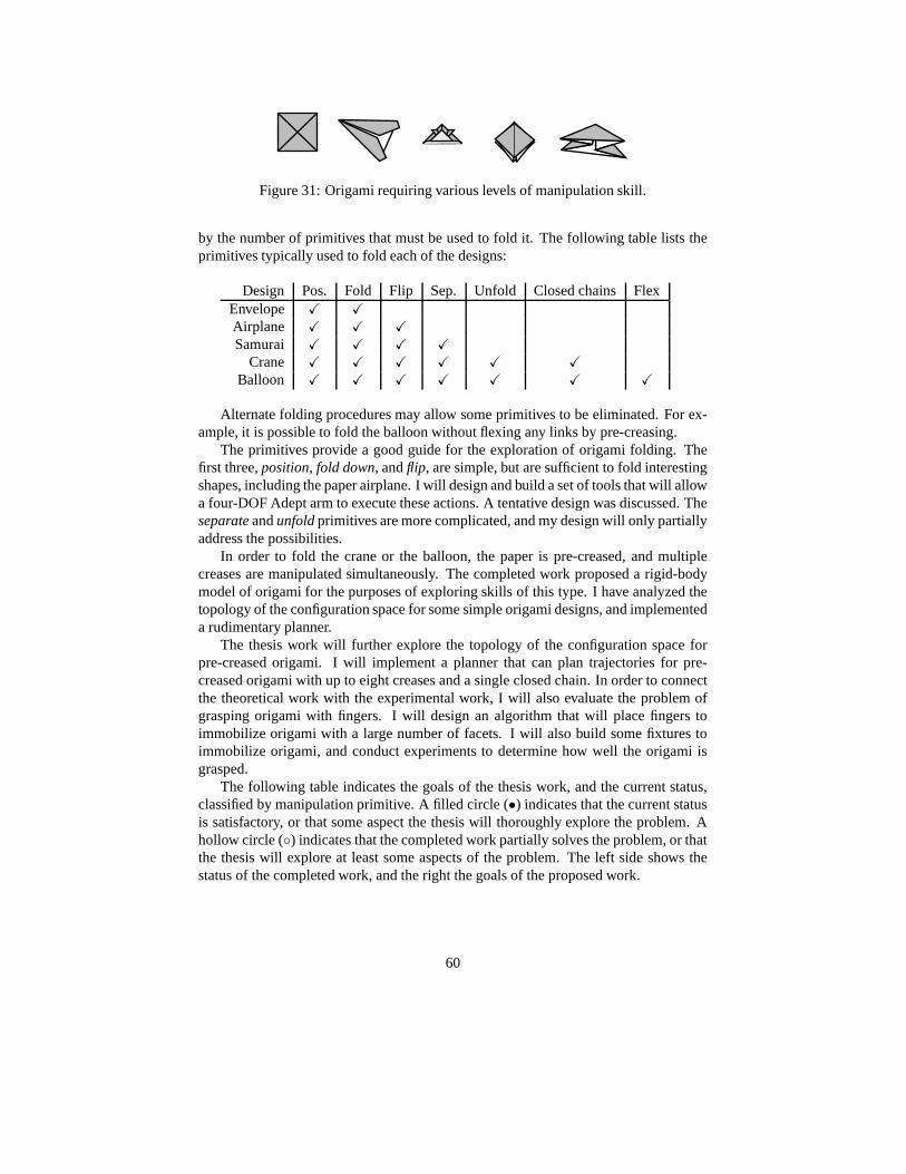
Figure 31: Origami requiring various levels of manipulation skill.

by the number of primitives that must be used to fold it. The following table lists theprimitives typically used to fold each of the designs:

Design Pos. Fold Flip Sep. Unfold Closed chains FlexEnvelope X X

Airplane X X X

Samurai X X X X

Crane X X X X X X

Balloon X X X X X X X

Alternate folding procedures may allow some primitives to be eliminated. For ex-ample, it is possible to fold the balloon without flexing any links by pre-creasing.

The primitives provide a good guide for the exploration of origami folding. Thefirst three, position, fold down, and flip, are simple, but are sufficient to fold interestingshapes, including the paper airplane. I will design and build a set of tools that will allowa four-DOF Adept arm to execute these actions. A tentative design was discussed. Theseparate and unfold primitives are more complicated, and my design will only partiallyaddress the possibilities.

In order to fold the crane or the balloon, the paper is pre-creased, and multiplecreases are manipulated simultaneously. The completed work proposed a rigid-bodymodel of origami for the purposes of exploring skills of this type. I have analyzed thetopology of the configuration space for some simple origami designs, and implementeda rudimentary planner.

The thesis work will further explore the topology of the configuration space forpre-creased origami. I will implement a planner that can plan trajectories for pre-creased origami with up to eight creases and a single closed chain. In order to connectthe theoretical work with the experimental work, I will also evaluate the problem ofgrasping origami with fingers. I will design an algorithm that will place fingers toimmobilize origami with a large number of facets. I will also build some fixtures toimmobilize origami, and conduct experiments to determine how well the origami isgrasped.

The following table indicates the goals of the thesis work, and the current status,classified by manipulation primitive. A filled circle (•) indicates that the current statusis satisfactory, or that some aspect the thesis will thoroughly explore the problem. Ahollow circle (◦) indicates that the completed work partially solves the problem, or thatthe thesis will explore at least some aspects of the problem. The left side shows thestatus of the completed work, and the right the goals of the proposed work.

60

Primitives Exp. 1D bend. Topol. Plan Exp. Topol. Plan GraspPosition • •

Fold down ◦ •Flip ◦ •

Separate ◦Unfold ◦

Closed chains ◦ ◦ ◦ • • •Flex links ◦ ◦ ◦

I expect to complete the thesis by August, 2004. My tentative research plan in-cludes the following components:

• Writing 1. The dissertation.

• Writing 2. The dissertation and the defense.

• Grasp analysis 1. Develop an algorithm for static grasping of simple rigidorigami.

• Grasp analysis 2. Explore the problem of time-varying grasps, and the problemof flexible links.

• Topology 1. Prove some things about the topology of the c-space of rigid origamiwith up to six links and a single closed loop, ignoring joint limits and self-intersection.

• Topology 2. Explore the implications of joint limits and multiple loops. Con-sider the problem of representing topology for a planning problem.

• Planning 0. Apply the planner already developed to more complicated problemsby adding heuristics.

• Planning 1. Develop a planner that either encodes some knowledge of the topol-ogy of the configuration space of closed chains, or automatically determinessome topological properties. Plan for mechanisms with five to six links, and asingle closed loop.

• Planning 2. Plan for mechanisms with six to eight links, and a single closedloop.

• Experiments and Engineering 1. Implement the proposed design, or an alter-nate design that allows positioning, folding down, and flipping of the paper, to ahigher degree of accuracy than the current system.

• Experiments and Engineering 2. Refine the implemented design, and applythe system to a simple origami test suite.

• Experiments and Engineering 3. Design and conduct experiments to test theresults of the grasping work.

61

• Experiments and Engineering 4. Refine all experimental designs, collect finaldata, and collate video documentation of experiments.

My expected schedule is:

Winter 2002 March 1 Planning 0 Grasping 1Spring 2003 June 1 Topology 1 Experiments 1

Summer 2003 September 1 Grasping 2 Experiments 2Fall 2003 December 1 Planning 1 Experiments 3

Winter 2003 March 1 Topology 2 Experiments 4Spring 2004 June 1 Planning 2 Writing 1

Summer 2004 September 1 Writing 2 Writing 2

10 Conclusion

My thesis will present origami folding as an exciting challenge problem for the fieldof robotic manipulation. Folding origami involves manipulating flexible closed chainswith a large number of degrees of freedom. However, we know that origami can befolded. Through an exploration of origami folding, my thesis will give insight andprovide partial solutions to some very hard manipulation problems.

11 Acknowledgments

My work has been supported by a Department of Energy Computational SciencesGraduate Fellowship. Thanks to my advisor, Matthew T. Mason, for all the usual, anda lot more. Thanks to my committee (Doug James, James Kuffner, and Jeff Trinkle)for their time and insight. Thanks to Vandi Verma and Siddhartha Srinivasa for theircomments on proposal drafts. Meetings and discussions with James Milgram, AlfredRizzi, David Bourne, Katsu Yamane, Jessica Hodgins, Jeff Schneider, Chris Atkeson,Srinivas Akella, David Hershberger, Kiran Bhat, Gabe Brisson, and Apostolos Lerioshave also been a great help. Thanks!

62

References

[1] M. Anitescu and F. Potra. Formulating multi-rigid-body contact problems withfriction as solvable linear complementarity problems. ASME Journal of Nonlin-ear Dynamics, 14:231–247, 1997.

[2] S. S. Antman. Nonlinear Problems of Elasticity. Number 107 in Applied Mathe-matical Sciences. Springer-Verlag, 1995.

[3] U. Ascher and P. Lin. Sequential regularization methods for simulating mechan-ical systems with many closed loops. SIAM Journal on Scientific Computing,21(4):1244–1262, 1999.

[4] G. Aumann. Interpolation with developable Bezier patches. Computer AidedGeometric Design, 8:409–420, 1991.

[5] D. J. Balkcom, E. Gottlieb, and J. Trinkle. A sensorless insertion strategy forrigid planar parts. In Proceedings, IEEE International Conference on Roboticsand Automation, 2002.

[6] D. Baraff. Linear-time dynamics using Lagrange multipliers. In SIGGRAPH,pages 137–146, Aug. 1996.

[7] D. Baraff and A. Witkin. Large steps in cloth simulation. In SIGGRAPH, pages43–54, July 1998.

[8] R. Bridson, R. Fedkiw, and J. Anderson. Robust treatment of collisions, contact,and friction for cloth animation. In SIGGRAPH, 2002.

[9] G. Chirikjian. Inverse kinematics of binary manipulators using a continuummodel. Journal of Intelligent and Robotic Systems, 19:5–22, 1997.

[10] K.-J. Choi and H.-S. Ko. Stable but responsive cloth. In SIGGRAPH, 2002.

[11] J. J. Craig. Introduction to Robotics: Mechanics and Control. Addison-Wesley,second edition, 1989.

[12] E. D. Demaine and M. L. Demaine. Recent results in computational origami.In Proceedings of the 3rd International Meeting of Origami Science, Math, andEducation, 2001.

[13] M. A. Erdmann. On motion planning with uncertainty. Master’s thesis, Mas-sachusetts Institute of Technology, Aug. 1984.

[14] C. Fernandes, L. Gurvits, and Z. Li. A variational approach to optimal nonholo-nomic motion planning. In Proceedings of the IEEE International Conference onRobotics and Automation, pages 680–685, Apr. 1991.

[15] C. Gauss. Disquisitiones generales circa superficies curvas. Gottingen: Di-eterich, 1828. (English translation by A. Hiltebietel and J. Morehead: Hewlett,NY, Raven Press, 1965.).

63

[16] M. Gleicher. A Differential Approach to Graphical Manipulation. PhD thesis,Carnegie Mellon University, 1994.

[17] H. Goldstein, C. Poole, and J. Safko. Classical Mechanics. Addison-Wesley,third edition, 2002.

[18] S. Gupta, D. Bourne, K. K. Kim, and S. S. Krishnan. Automated process planningfor robotic sheet metal bending operations. Journal of Manufacturing Systems,September 1998.

[19] L. Han and N. M. Amato. A kinematics-based probabalistic roadmap method forclosed chain systems. In Workshop on the Algorithmic Foundations of Robotics,pages 233–246, May 2000.

[20] D. Hilbert and S. Cohn-vossen. Geometry and the Imagination. Chelsea, 1952.

[21] S. Hirai, T. Tsuboi, and T. Wada. Robust grasping manipulation of deformableobjects. In Proceedings of the IEEE Symposium on Assembly and Task Planning,pages 411–416, May 2001.

[22] S. Hirai, H. Wakamatsu, and K. Iwata. Modeling of deformable thin parts for theirmanipulation. In Proceedings of the IEEE International Conference on Roboticsand Automation, pages 2955–2960, 1994.

[23] D. Huffman. Curvature and creases: A primer on paper. IEEE Transactions onComputers, C-25(10):1010–1019, Oct. 1976.

[24] H. Inoue and M. Inaba. Hand-eye coordination in rope handling. In RoboticsResearch: The First International Symposium, pages 163–174, 1985.

[25] D. L. James and D. K. Pai. A unified treatment of elastostatic contact simulationfor real time haptics. Haptics-e, the Electronic Journal of Haptics Research, 2(1),September 2001. http://www.haptics-e.org.

[26] L. E. Kavraki, F. Lamiraux, and C. Holleman. Towards planning for elastic ob-jects. In Workshop on the Algorithmic Foundations of Robotics, pages 313–326,1998.

[27] Y. L. Kergosien, H. Gotoda, and T. L. Kunii. Bending and creasing virtual paper.In IEEE Computer Graphics and Applications, pages 40–48, Jan. 1994.

[28] R. Lang. Trees and circles: an efficient algorithm for origami design. In Proceed-ings of the 3rd International Meeting of Origami Science, Math, and Education,2001.

[29] S. M. LaValle, J. H. Yakey, and L. E. Kavraki. A probabalistic roadmap approachfor systems with closed kinematic chains. In Proceedings of the IEEE Interna-tional Conference on Robotics and Automation, 1999.

[30] W. Lenhart and S. Whitesides. Reconfiguring simple polygons. Discrete andComputational Geometry, 1994.

64

[31] S. Leopoldseder and H. Pottmann. Approximation of developable surfaces withcone spline surfaces. Computer Aided Design, 30:571–582, 1998.

[32] P. Lotstedt. Coulomb friction in two-dimensional rigid-body systems. Zeitschriftfur Angewandte Mathematik und Mechanik, 61:605–615, 1981.

[33] T. Lozano-Perez. A simple motion-planning algorithm for general robot manipu-lators. IEEE Journal of Robotics and Automation, RA-3(3):224–238, June 1987.

[34] L. Lu and S. Akella. Folding cartons with fixtures: A motion planning approach.In Proceedings of the IEEE International Conference on Robotics and Automa-tion, May 1999.

[35] L. Lu and S. Akella. Folding cartons with fixtures: A motion planning approach.IEEE Transactions on Robotics and Automation, 16(4):346–356, Aug. 2000.

[36] R. J. Milgram. personal communication, Nov. 2002.

[37] R. J. Milgram and J. Trinkle. The geometry of configurations spaces for closedchains in two and three dimensions. Submitted to Homology, Homotopy, andApplications, forthcoming.

[38] M. Minsky. Manipulator design vignettes. Technical report, Massachusetts Insti-tute of Technology, Artificial Intelligence Laboratory, 1972.

[39] S. Miyazaki, T. Yasuda, S. Yokoi, and J. Toriwaki. An interactive simulationsystem of origami based on virtual space manipulation. In Proceedings of theIEEE International Workshop on Robot and Human Communication, pages 210–215, 1992.

[40] H. Nakagaki, K. Kitagaki, T. Ogasawara, and H. Tsukune. Study of deformationand insertion tasks of a flexible wire. In Proceedings of the IEEE InternationalConference on Robotics and Automation, pages 2397–2402, Apr. 1997.

[41] D. K. Pai. STRANDS: Interactive simulation of thin solids using cosserat models.In Eurographics, 2002.

[42] P. Painleve. Sur les lois du frottemont de glissement. C. R. Acad. Sci., 121:112–115, 1895.

[43] H. Pottmann and J. Wallner. Approximation algorithms for developable surfaces.Computer Aided Geometric Design, 16:539–556, 1999.

[44] P. Redont. Representation and deformation of developable surfaces. ComputerAided Design, 21(1):13–20, 1989.

[45] M. Rubin. Cosserat Theories: Shells, Rods, and Points. Kluwer Academic Pub-lishers, 2000.

[46] G. Song and N. M. Amato. A motion planning approach to folding: From papercraft to protein folding. In Proceedings of the IEEE International Conference onRobotics and Automation, pages 948–953, May 2001.

65

[47] D. Stewart and J. Trinkle. An implicit time-stepping scheme for rigid body dy-namics with inelastic collisions and coulomb friction. International Journal ofNumerical Methods in Engineering, 39:2673–2691, 1996.

[48] D. E. Stewart. Existence of solutions to rigid body dynamics and the paradoxesof Painleve. Comptes Rendus de l’Acad. Sci., Ser. I, 1997. To appear.

[49] M. Sun and E. Fiume. A technique for constructing developable surfaces. InGraphics Interface, pages 176–185, May 1996.

[50] K. R. Symon. Mechanics. Addison-Wesley, third edition, 1971.

[51] J. Thorpe. Elementary Topics in Differential Geometry. Springer-Verlag, 1979.

[52] J. Trinkle and R. J. Milgram. Motion planning for planar n-bar mechanisms withrevolute joints. Submitted to the International Journal of Robotics Research,forthcoming.

[53] J. Trinkle, J. Pang, S. Sudarsky, and G. Lo. On dynamic multi-rigid-body con-tact problems with coulomb friction. Zeitschrift fur Angewandte Mathematik undMechanik, 77(4):267–279, 1997.

[54] T. Wada, S. Hirai, T. Hirano, and S. Kawamura. Modeling of plain knitted fabricsfor their deformation control. In Graphics Interface, pages 176–185, May 1996.

[55] T. Wada, S. Hirai, S. Kawamura, N. Kamiji, and K. Tsukamoto. Robust manip-ulation of deformable objects by a simple pid feedback. In Proceedings of theIEEE International Conference on Robotics and Automation, pages 85–90, May2001.

[56] T. Wada, S. Hirai, S. Kawamura, N. Kamiji, and K. Tsukamoto. Robust manip-ulation of deformable objects by a simple position feedback. In 3rd Asia-EuropeCongress on Mechatronics, pages 112–117, Oct. 2001.

[57] T. Wada, B. J. McCarragher, H. Wakamatsu, and S. Hirai. Modeling of shape bi-furcation phenomena in manipulations of deformable string objects. InternationalJournal of Robotics Research, 15(8):833–846, 2001.

[58] H. Wakamatsu, S. Hirai, and K. Iwata. Static analysis of deformable object grasp-ing based on bounded force closure. In Proceedings of the IEEE InternationalConference on Robotics and Automation, pages 3324–3329, 1996.

[59] H. Wakamatsu, T. Matsumura, S. Hirai, and E. Arai. Dynamic analysis of rod-like object deformation towards their dynamic manipulation. In Proceedings ofthe 1997 IEEE/RSJ International Conference on Intelligent Robots and Systems,pages 196–201, 1997.

[60] G. Weiss and P. Furtner. Computer-aided treatment of developable surfaces. Com-puters and Graphics, 12(1):39–51, 1988.

66