thesis a cost-benefit analysis of preventative management …
TRANSCRIPT
THESIS
A COST-BENEFIT ANALYSIS OF PREVENTATIVE MANAGEMENT FOR ZEBRA AND
QUAGGA MUSSELS IN THE COLORADO-BIG THOMPSON SYSTEM
Submitted by
Catherine M. Thomas
Department of Agricultural and Resource Economics
In partial fulfillment of the requirements
For the Degree of Master of Science
Colorado State University
Fort Collins, Colorado
Summer 2010

ii
COLORADO STATE UNIVERSITY
July 12, 2010
WE HEREBY RECOMMEND THAT THE THESIS PREPARED UNDER OUR
SUPERVISION BY CATHERINE M. THOMAS ENTITLED A COST-BENEFIT ANALYSIS
OF PREVENTATIVE MANAGEMENT FOR ZEBRA AND QUAGGA MUSSELS IN THE
COLORADO-BIG THOMPSON SYSTEM BE ACCEPTED AS FULFILLING IN PART
REQUIREMENTS FOR THE DEGREE OF MASTER OF SCIENCE.
Committee on Graduate Work
Patricia A. Champ
Reagan M. Waskom
Advisor: Craig A. Bond
Co-Advisor: Christopher G. Goemans
Department Chair: Stephen P. Davies

iii
ABSTRACT OF THESIS
A COST-BENEFIT ANALYSIS OF PREVENTATIVE MANAGEMENT FOR ZEBRA AND
QUAGGA MUSSELS IN THE COLORADO-BIG THOMPSON SYSTEM
The introduction of zebra mussels (Dreissena polymorpha) and quagga
mussels (D. bugensis) to the western U.S. has water managers considering strategies
to prevent or slow their spread. In Colorado, the Department of Wildlife (CDOW)
has implemented a statewide mandatory boat inspection program. This study
builds a bioeconomic model to simulate a mussel invasion and associated control
costs for a connected Colorado water system, and compares the costs of the CDOW
boat inspection program to the expected reduction in control costs to infrastructure.
Results suggest that preventative management is effective at reducing the
probability that mussels invade, but the costs may exceed the benefits of reduced
control costs to infrastructure. The risk of invasion, the spatial layout of a system,
the type of infrastructure, and the level of control costs associated with a system are
key variables in determining net benefits of preventative management.
Catherine M. Thomas Department of Agricultural
And Resource Economics Colorado State University
Fort Collins, CO 80525 Summer 2010

iv
ACKNOWLEDGMENTS
Many people came together to make this project possible, and I am very
grateful for their gracious help. I am especially grateful for my wonderful mentors,
Craig Bond, Chris Goemans, Dawn Thilmany McFadden, and Josh Goldstein, who
have provided me tremendous support, inspiration and practical advice. I am also
grateful to my committee members Patty Champ and Reagan Waskom for their
participation and valuable feedback. I would also like to thank Elizabeth Brown
with the Colorado Department of Wildlife, Brad Wind, Dennis Miller, Greg Silkensen,
and Jennifer Stephenson with the Northern Colorado Water Conservancy District,
and Fred Nibling and Curtis Brown with the Bureau of Reclamation for their help in
understanding the issues and providing data and feedback. I am also grateful to the
many Northern Colorado municipalities that helped me gather data. Finally, I have
great thanks and appreciation for Ruddy Bartz and Daniel Deisenroth for their
enthusiastic help and friendship, and for my wonderful, loving and supportive
family.
v
TABLE OF CONTENTS
Introduction .............................................................................................................................................. 1
Chapter 1: Background Information ............................................................................................... 5
1.1 History of the Invasion .............................................................................................................. 5
1.2 The Invasion in Colorado ......................................................................................................... 8
1.3 Managing for Mussels in Colorado ....................................................................................... 9
1.4 Overview of the Colorado-Big Thompson System....................................................... 11
1.4 Dreissena Dispersal Models ................................................................................................. 14
1.4.1 Environmental Factors Affecting Mussel Spread ................................................. 14
1.4.2 Boater Movement Models ............................................................................................. 15
1.4.3 Combining Boater Movement Models with Environmental Factors
Affecting Mussel Spread ........................................................................................................... 18
1.4.4 Downstream Flow Models ............................................................................................ 19
1.5 Economic Studies ..................................................................................................................... 21
1.5.1 Control Cost Surveys ....................................................................................................... 21
1.5.2 Control Cost Forecasts ................................................................................................... 23
1.5.3 Bioeconomic Models ....................................................................................................... 24

vi
1.6 An Overview of the Costs and Benefits of Preventative Management in the
Colorado-Big Thompson System ............................................................................................... 27
1.6.1 Benefits of Preventative Management ..................................................................... 27
1.6.2 Costs of Preventative Management ........................................................................... 30
Chapter 2: Methodological Approach and Data ....................................................................... 32
2.1 Cost-Benefit Model .................................................................................................................. 34
2.1.1 Net Present Value of Expected Control Costs ........................................................ 35
2.1.2 Net Present Value of Program Costs ......................................................................... 36
2.2 Mussel Dispersal Component of the Simulation Model............................................. 36
2.2.1 Environmental Suitability of the Colorado-Big Thompson Reservoirs for
Mussel Colonization and the Probability of Invasibility .............................................. 38
2.2.2 Pathways of Invasion and the Probability of Establishment........................... 43
2.2.3 Combining the Probability of Invasibility and the Probability of
Establishment: The Joint Probability of Colonization ................................................... 67
2.3 Control Costs Component of the Simulation Model .................................................... 69
2.3.1 Simulating Net Benefits ................................................................................................. 70
2.3.2 Capital Expenditures and Variable Costs ................................................................ 72
2.3.3 Control Cost Schedules .................................................................................................. 73
vii
Water Treatment Facilities ..................................................................................................... 75
Hydropower Facilities ............................................................................................................... 83
Dams ................................................................................................................................................ 88
Pump Plants .................................................................................................................................. 90
Other Infrastructure .................................................................................................................. 91
Other Affected Industries ......................................................................................................... 91
2.4 Colorado-Big Thompson Zebra and Quagga Mussel Dispersal and Damage Cost
Simulation Model ............................................................................................................................. 93
2.5 Boat Inspection Program Costs .......................................................................................... 96
2.5.1 Direct Costs of the Boat Inspection Program ........................................................ 96
2.5.2 Indirect Costs of the Boat Inspection Program..................................................... 99
Chapter 3: Results .............................................................................................................................. 105
3.1 Model Results using Base Parameter Values............................................................... 109
3.1.1 Baseline Establishment Patterns ............................................................................. 109
3.1.2 Cost-Benefit Results ...................................................................................................... 116
3.2 Sensitivity Analysis ............................................................................................................... 121
3.2.1 Environmental Parameters ........................................................................................ 122
3.2.2 Boat Pressure Parameters .......................................................................................... 123

viii
3.2.3 Flow Parameters ............................................................................................................ 125
3.2.4 Program Parameters ..................................................................................................... 128
3.2.5 Economic Parameters .................................................................................................. 129
3.3 Results for a Highly Invasible System ............................................................................ 131
3.4 Benefit-Cost Ratios ................................................................................................................ 134
Chapter 4: Summary and Conclusions ....................................................................................... 135
Chapter 5: Discussion and Limitations ...................................................................................... 140
Comparison to Other Cost-Benefit Studies .......................................................................... 140
Limitations ....................................................................................................................................... 142
Omitted Benefits ........................................................................................................................ 142
External Benefits ....................................................................................................................... 143
Model Limitations ..................................................................................................................... 144
Areas for Future Research ......................................................................................................... 145
Works Cited .......................................................................................................................................... 146
Appendix A: Variables and Parameter Values ........................................................................ 151
Cost-Benefit Model: Variables .................................................................................................. 151
Dispersal Model: Variables and Parameter Estimates .................................................... 152

ix
Control Cost Model: Variables and Parameter Estimates .............................................. 157
Indirect Program Costs: Variables and Parameter Estimates ...................................... 159
Appendix B: Major Structures and Facilities in the Colorado-Big Thompson System
................................................................................................................................................................... 161
Appendix C: Base Parameter Values .......................................................................................... 163
Dispersal Model Base Parameter Values .............................................................................. 163
Damage Cost Model Base Parameter Values ...................................................................... 164
Program Cost Base Parameter Values ................................................................................... 165
Appendix D: Visual Basic Code ..................................................................................................... 166

1
INTRODUCTION
Zebra and quagga mussels are fresh water invaders that have the potential to
cause severe ecological and economic damage. It is estimated that mussels cause $1
billion dollars per year in damages to water infrastructure and industries in the
United States (Pimentel et al., 2004). Following their introduction to the Great
Lakes in the late 1980s, mussels spread rapidly throughout the Mississippi River
Basin and the Eastern U.S. The mussel invasion in the West is young. Mussels were
first identified in Nevada in 2007, and have since been identified in California,
Arizona, Colorado, Utah, and Texas.
Western water systems are very different from those found in the East. The
rapid spread of mussels through the eastern system was facilitated by connected
and navigable waterways. Western water systems are less connected and are
characterized by man-made reservoirs and canals. The main vector of spread for
mussels in the West is overland on recreational boats (Bossenbroek et al., 2001). In
response to the invasion, many western water managers have implemented
preventative management programs to slow the overland spread of mussels on
recreational boats. In Colorado, the Colorado Department of Wildlife (CDOW) has
implemented a mandatory boat inspection program that requires all trailered boats
to be inspected before launching in any Colorado water body. The objective of this
study is to analyze the costs and benefits of the CDOW boat inspection program in

2
Colorado, and to identify variables that affect the net benefits of preventative
management.
Predicting the potential economic benefits of slowing the spread of mussels
requires integrating information about mussel dispersal potential with estimates of
control costs (Keller et al., 2009). Uncertainty surrounding the probabilities of
establishment, the timing of invasions, and the damage costs associated with an
invasion make a simulation model an excellent tool for addressing "what if"
scenarios and shedding light on the net benefits of preventative management
strategies. This study builds a bioeconomic simulation model to predict and
compare the expected economic costs of the CDOW boat inspection program to the
benefits of reduced expected control costs to water conveyance systems,
hydropower generation stations, and municipal water treatment facilities. The
model is based on a case study water delivery and storage system, the Colorado-Big
Thompson system. The Colorado-Big Thompson system is an excellent example of
water systems in the Rocky Mountain West. The system is nearly entirely man-
made, with all of its reservoirs and delivery points connected via pipelines, tunnels,
and canals. The structures and hydropower systems of the Colorado-Big Thompson
system are common to other western water storage and delivery systems, making
the methods and insight developed from this case study transferable to other
western systems.
The model developed in this study contributes to the bioeconomic literature
in several ways. Foremost, the model predicts the spread of dreissena mussels and

3
associated damage costs for a connected water system in the Rocky Mountain West.
Very few zebra mussel studies have focused on western water systems. Another
distinguishing factor is the simultaneous consideration of spread from propagules
introduced by boats and by flows. Most zebra mussel dispersal models consider
boater movement patterns combined with limnological characteristics as predictors
of spread. A separate set of studies have addressed mussel spread via downstream
flows. To the author's knowledge, this is the first study that builds a zebra mussel
spread model that specifically accounts for propagule pressure from boat
introductions and from downstream flow introductions. By modeling an entire
connected system, the study highlights how the spatial layout of a system, the type
of infrastructure and level of control costs associated with a system, and the risk of
invasion within a system affect the benefits of preventative management.
This report is presented in five chapters. The first chapter provides
background information including a history of the zebra mussel invasion in the U.S.
and in the West, and details about the Colorado preventative management program
and the Colorado-Big Thompson system. The chapter also includes a literature
review of mussel dispersal models and economic studies that address control costs
and preventative management for aquatic invasive species. Chapter 2 presents the
methodological approach used to analyze the costs and benefits of preventative
management in the Colorado-Big Thompson system and provides details of the
bioeconomic simulation model used to predict invasion patterns and the net
benefits of preventative management. Results of the analysis and sensitivity testing
of model parameters are presented in Chapter 3. Chapter 4 provides a summary of

4
the analysis and conclusions. A discussion of the limitations of the model and areas
for future research is presented in Chapter 5.

5
CHAPTER 1: BACKGROUND INFORMATION
1.1 History of the Invasion
Zebra mussels (Dreissena polymorpha) and quagga mussels (Dreissena bugensis)
are invasive mollusks native to an area in the Ukraine and Russia near the Black and
Caspian Seas. The species is believed to have been introduced to U.S. waters in the
late 1980s through ballast water discharged from transatlantic freighters. Zebra
mussels were first identified in Lake St. Clair and Lake Erie in 1988, and quagga
mussels were discovered in 1991 (Ohio Sea Grant, 1997). Following their
introduction to the Great Lakes in the late 1980s, zebra mussels rapidly expanded
their North American range. By 1991, only 3 years after the discovery of zebra
mussels in Lake Saint Claire, the invader had already spread throughout the Great
Lakes and through much of the Mississippi River Basin.
The rapid spread of dreissena mussels is attributed to their prolific reproduction
and their ability to disperse. Both species reproduce rapidly and are very successful
invaders. A mature female mussel can produce as many as one million eggs per
season. Eggs are fertilized in the water column and develop into young mussels
within a few days. Young mussels, called veligers, are microscopic and invisible to
the naked eye. In this floating larval stage, veligers can be carried by water currents,
spreading to adjacent waterways. Veligers can also be carried overland in the
ballast water of recreational boats or on foliage entangled in boat motors. Mature

6
mussels generate a tuft of fibers called byssal threads that they use to attach to hard
surfaces. Dreissena can attach to any non-toxic hard surface including boats and
trailers, and are able to live out of water for several days (Ohio Sea Grant, 1997).
Thus, zebra and quagga mussels can spread downstream to adjacent waterways in
their veliger stage and can hitchhike to inland waters via transport on boats and
boat trailers in their adult or veliger stages.
Since their introduction in the late 1980s, zebra and quagga mussels have spread
through much of North America. However, their expansion has mostly been limited
to the connected waters of the Midwest and Northeast; see Figure 1 (USGS, 2009).
The spread of mussels to inland lakes and the Western U.S. has been much slower
(Kraft & Johnson, 2000).

7
Figure 1: U.S. mussel distribution as of November 2009, USGS
Dreissena invasions can cause severe economic and ecological damage.
Adult mussels attach to all types of structures and form dense mats up to one foot
thick (USGS, 2000). These mats can clog water pipes and damage hydrologic
infrastructure. Water-delivery structures, dams, power plants, and water treatment
facilities can all incur large costs either from removing mussels from their systems
or from suffering lost output (Deng, 1996). It is estimated that invasive mollusks
cost the nation about $1 billion per year, mostly in damages and control costs
associated with electric power plants and water supply facilities (Pimentel et al.,
2004). Dreissena also affect natural ecosystems through their feeding behavior;
they are filter feeders and process up to one gallon of water per mussel per day.
8
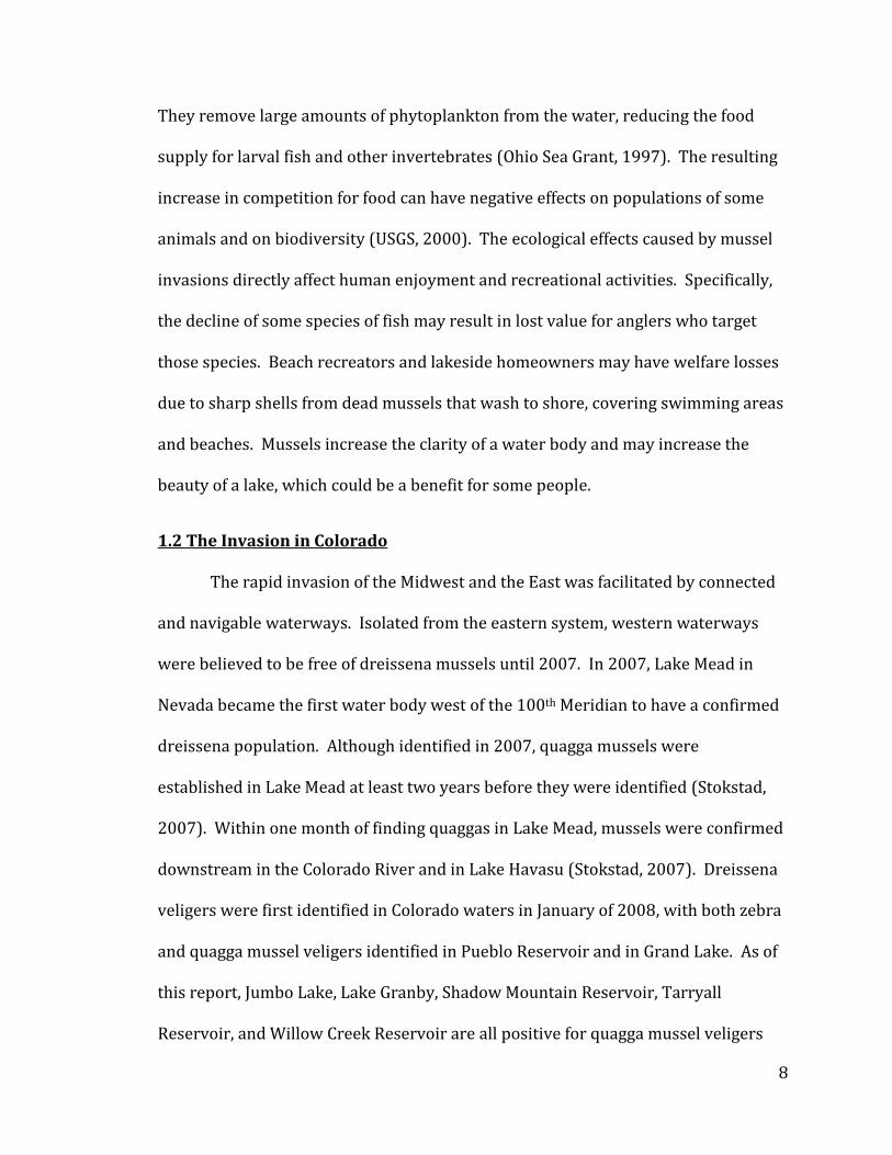
They remove large amounts of phytoplankton from the water, reducing the food
supply for larval fish and other invertebrates (Ohio Sea Grant, 1997). The resulting
increase in competition for food can have negative effects on populations of some
animals and on biodiversity (USGS, 2000). The ecological effects caused by mussel
invasions directly affect human enjoyment and recreational activities. Specifically,
the decline of some species of fish may result in lost value for anglers who target
those species. Beach recreators and lakeside homeowners may have welfare losses
due to sharp shells from dead mussels that wash to shore, covering swimming areas
and beaches. Mussels increase the clarity of a water body and may increase the
beauty of a lake, which could be a benefit for some people.
1.2 The Invasion in Colorado
The rapid invasion of the Midwest and the East was facilitated by connected
and navigable waterways. Isolated from the eastern system, western waterways
were believed to be free of dreissena mussels until 2007. In 2007, Lake Mead in
Nevada became the first water body west of the 100th Meridian to have a confirmed
dreissena population. Although identified in 2007, quagga mussels were
established in Lake Mead at least two years before they were identified (Stokstad,
2007). Within one month of finding quaggas in Lake Mead, mussels were confirmed
downstream in the Colorado River and in Lake Havasu (Stokstad, 2007). Dreissena
veligers were first identified in Colorado waters in January of 2008, with both zebra
and quagga mussel veligers identified in Pueblo Reservoir and in Grand Lake. As of
this report, Jumbo Lake, Lake Granby, Shadow Mountain Reservoir, Tarryall
Reservoir, and Willow Creek Reservoir are all positive for quagga mussel veligers

9
(USGS, 2009). To date, no adult mussels have been identified in the state. Figure 2
shows the progression of the mussel invasion in the West (USGS, 2009).
Figure 2: Western distribution of zebra and quagga mussels, USGS 2009.
1.3 Managing for Mussels in Colorado
In response to the identification of zebra and quagga mussels in the state, the
Colorado Department of Wildlife (CDOW) implemented the Colorado Zebra/Quagga
Mussel Management Plan (ZQM Plan) in 2009. The ZQM Plan is "a statewide
collaborative effort to detect, contain, and substantially reduce the risk of spread
and further infestation by zebra/quagga mussels in Colorado" (Colorado Division of
10
Wildlife, 2009). The ZQM Plan focuses on early detection and rapid response,
containment, prevention and education/outreach. The primary component of the
plan is a mandatory watercraft inspection and decontamination program to prevent
the spread of mussels overland on recreational watercraft.
As of 2009, boat inspections are required prior to launch in most reservoirs
and lakes in the state. Resident boaters must pass a state-certified boat inspection if
they plan to launch on a reservoir where inspections are required or if they have
traveled outside of the state or have launched on any of the Colorado lakes or
reservoirs where mussels have been detected. Out-of-state boaters are required to
pass a state-certified boat inspection before launching in any Colorado waterway.
As part of the standard boat inspection, boaters are asked what state they are from
and where and when they last boated. Boats that have been used out-of-state or in
infested waters within the last 30 days or are dirty are considered high-risk, and are
required to undergo a high-risk inspection and may be required to undergo a
decontamination process. In addition to pre-launch inspections, the program also
requires boats exiting dreissena positive waters to be cleaned, drained, and dried
upon leaving the water.
Watercraft inspections are based on the Pacific Marine Fisheries Commission
standardized watercraft inspection and decontamination training. All watercraft
inspectors are required to attend a state certification course in which they learn
about mussel biology, vectors of spread, methods for detecting mussels, and
methods for decontaminating boats. The goal of the CDOW boat inspection program
11
is to reduce the number of potentially infested boats that enter Colorado water
bodies, thus reducing the risk of spread in the state.
1.4 Overview of the Colorado-Big Thompson System
The Colorado-Big Thompson system is a prime case study for investigating
the possible implications of a mussel invasion and the effects of preventative
management in Colorado. The system consists of five headwater reservoirs on the
Western Slope of Colorado: Windy Gap Reservoir, Willow Creek Reservoir, Lake
Granby, Shadow Mountain Reservoir, and Grand Lake. With the exception of Windy
Gap Reservoir, all of these reservoirs have tested positive for dreissena veligers.
Although no adult mussels have been found in any of the reservoirs, managers of the
project and stakeholders that use Colorado-Big Thompson water are concerned
about the implications of mussels in the system. The Colorado-Big Thompson
system is comprised of the reservoirs and infrastructure that make up the Colorado-
Big Thompson Project and the Windy Gap Project, and the municipal water
treatment facilities that use Colorado-Big Thompson and Windy Gap water.
The Colorado-Big Thompson Project is the largest transmountain water
diversion project in Colorado. Water from Colorado's Western Slope is conveyed
through a series of 12 reservoirs and 5 hydropower plants on its journey across the
Continental Divide. The system provides supplemental water to 30 cities and towns
and over 600,000 acres of agricultural land on the Eastern Slope of the state
(Northern Colorado Water Conservancy District, 2010). The Windy Gap Project
pumps water from Windy Gap Reservoir to Lake Granby, where it is stored and
12
delivered through the Colorado-Big Thompson Project reservoirs and
infrastructure. The Bureau of Reclamation and the Northern Colorado Water
Conservancy District each own portions of the infrastructure and jointly manage the
system. Figure 3 shows a diagram of the Colorado-Big Thompson system, and
highlights the major infrastructure and municipal delivery points in the system.

13
Figure 3: Schematic of the Colorado-Big Thompson system
14
1.4 Dreissena Dispersal Models
The large economic and ecological costs resulting from zebra mussel
invasions have spurred a large field of research on the environmental limits and
potential distribution of mussels. Models that predict the spread of mussels do so
based on a combination of the biological and environmental requirements of
dreissena and on potential vectors of spread.
1.4.1 Environmental Factors Affecting Mussel Spread
Levels of calcium, pH, alkalinity, temperature, dissolved oxygen, Secchi depth,
nutrients, and available substrate have all been found to be important predictors of
dreissena habitat suitability (Ramcharan et al., 1992; Mellina & Rasmussen, 1994;
Cohen & Weinstein, 2001; Drake & Bossenbroek, 2004; Whittier et al., 2008; Claudi
& Prescott, 2009). Several studies address the possible spread of dreissena based
solely on environmental factors.
In 2004, Drake and Bossenbroek developed a model to predict the potential
distribution of zebra mussels in the United States using biological and geological
variables including average annual temperature, bedrock geology, elevation, flow
accumulation, frost frequency, max and min temperatures, precipitation, slope, solar
radiation, and surface geology. Of particular interest to this study are Drake and
Bossenbroek's predictions for the Rocky Mountain region. Two of the three models
developed by Drake and Bossenbroek (2004) predict that zebra mussels will not
spread to the Rocky Mountain region. The third model, which includes all of the
listed variables with the exception of the elevation variable, predicts the Eastern
15
Plains of Colorado to be at high risk of mussel infestation, but still predicts the
mountainous regions of the state to have very low probabilities of infestation. At
the time these models were developed, the third model was deemed the least
reliable of the three, and the consensus was that the Rocky Mountain States were
very unlikely candidates for mussel infestation.
Whittier et al. (2008 ) use calcium concentrations to assess the risk of dreissena
invasions for ecoregions across the contiguous U.S. Using calcium concentration
data from over 3000 stream and river sites across the nation, they define risk of
dreissena invasion based on calcium concentration. Ecoregions with average
calcium concentrations below 12 mg/L are defined as very low risk, 12-20 mg/L as
low risk, 20-28 mg/L as moderate risk, and greater than 28 mg/L as high risk. In
their assessment, the Eastern Plains of Colorado have a high risk of dreissena
invasion based on calcium concentration, and the risks to the mountainous regions
of the state are highly variable.
Overall, many environmental variables affect the risk of dreissena spread, and
there is mixed evidence on the risk of a dreissena invasion in Colorado. Based on
calcium concentrations alone, Whittier et al. (2008) find that much of the state is
considered to be at high risk of a dreissena invasion. However, the study by Drake
and Bossenbroek (2004) suggests that Colorado has a very low chance of invasion.
1.4.2 Boater Movement Models
Regardless of environmental suitability, in order for mussels to invade, they
must first be transported to new locations. In the early years of the North American

16
invasion, mussels were primarily transported through navigable waterways. The
connected system of waterways in the Midwestern and Eastern U.S. were quickly
inhabited, but the spread of mussels to inland waters and the Western U.S. has been
slower and is still ongoing (Kraft & Johnson, 2000).
Overland transportation of mussels on recreational boats is believed to be the
primary vector for zebra mussel dispersion into inland lakes and across large
distances. A substantial number of studies attempt to predict mussel dispersal
through boater movement patterns (Padilla et al., 1996; Bossenbroek et al., 2001;
Leung et al., 2006; Bossenbroek et al., 2007; Leung & Mandrak, 2007; Timar &
Phaneuf, 2009). Two types of boater movement models are used to predict mussel
dispersal: gravity models, and random utility models (RUM models). Gravity models
predict the flow of individuals that move from an origin to a destination based on
the distance between the origin and the destination and the attractiveness of the
destination. RUM models predict boater movement based on a boater's utility
maximizing choice of one lake from a set of many lakes. Models to predict the
movement of recreational boaters can be paired with biological models for habitat
suitability to forecast where invasions are likely to occur (Leung et al., 2006).
Bossenbroek et al. (2001) develop a gravity model to forecast zebra mussel
dispersal to inland lakes in Illinois, Indiana, Michigan, and Wisconsin. They assume
that boat pressure at each lake is a function of the number of registered boaters in a
county, the distance between the county and the lake, and the surface area of the
lake. Their model estimates the potential for colonization based on three factors:

17
the probability of a boat traveling to an infested lake, the probability of that same
boat traveling to an uninfested lake on a subsequent trip, and the probability that
zebra mussels become established in a water body once they have been introduced.
They determine that a single infested boat has a probability of 0.0000411 of
establishing a zebra mussel colony, which translates to a 3.5% chance that a water
body becomes established when visited by 850 infested boats. Spatially, they find
that zebra mussel spread is characterized by long distance jumps and subsequent
isolated centers of distribution.
Differing from the majority of gravity based boater movement models, Timar
and Phaneuf (2009) use a random utility model (RUM model) to forecast boater
behavior and resulting mussel spread based on utility theory. With their RUM
model, Timar and Phaneuf are able to address how boaters behave, and thus how
boater movement patterns change in the face of policies designed to limit the spread
of aquatic invasive species. They find that explicitly accounting for behavioral
responses has a dramatic effect on the predicted effectiveness of polices intended to
reduce invasion threats. Overall, their findings suggest that behavioral adjustments
to preventative management policies change the relative risks of invasion in a
region. Boaters faced with inspections or fees may substitute to nearby water
bodies that do not require inspections, thus increasing the risk of infestation of
those water bodies. The boat inspection program in Colorado is statewide;
therefore, boaters have very little opportunity to substitute away from lakes that
require inspections. Unlike the finding by Timar and Phaneuf, behavioral

18
adjustments are not expected to have a significant impact on the effectiveness of the
CDOW boat inspection program in Colorado.
Most spread models based on boater movement use data from the Midwest.
There are currently no boater movement models that predict movement within
Colorado. Developing such a model is beyond the scope of this project; thus, the
spread model developed for the Colorado-Big Thompson system does not
specifically address boater movement patterns. Reservoirs in the system are
assumed to have constant visits over time, and the percent of infested boats visiting
each reservoir is assumed to be equal throughout the system. The simplifying
assumptions made about boat pressure are expected to be relatively accurate, but
the model could be improved by explicitly accounting for boater movement patterns
with a gravity model or a RUM model.
1.4.3 Combining Boater Movement Models with Environmental Factors Affecting Mussel Spread
To predict mussel spread, boater movement models generally incorporate
environmental variables that limit dreissena colonization. Dichotomous
classifications of the habitability of lakes are common among models to predict the
dispersal of mussels. For example, Bossenbroek et al. (2001) use calcium and pH
data to determine if a lake is suitable for mussels. They develop a suitability score
for each lake based on the model developed by Ramcharan et al. (1992), and deem
lakes with scores below a threshold as uninhabitable.

19
Leung and Mandrake (2007) take a different approach and treat the habitability
of a lake as a probability. Similar to Bossenbroek et al, Leung and Mandrake use a
gravity model to predict boater movement from infested to uninfested lakes to
develop probabilities that uninfested lakes become established. They combine
these probabilities with the probability that a lake is habitable to develop joint
probabilities of infestation. Leung and Mandrake's approach to modeling
invasibility as a probability rather than a dichotomous choice is utilized in the
model developed for the Colorado-Big Thompson system. In a dichotomous choice
model, such as that used in Bossenbroek et al. (2001), many of the reservoirs in the
Colorado-Big Thompson would be omitted from the set of invasible lakes based on
low calcium levels. Modeling invasibility as a probability allows for a positive
probability of infestation in the Colorado-Big Thompson reservoirs.
1.4.4 Downstream Flow Models
Several studies address dispersal through connected waterways. In a study of
coupled lake-stream systems, Bobeldke et al. (2005) found that lakes downstream
from invaded lakes were more likely to be infested than lakes downstream from
non-invaded lakes and that the probability of a downstream lake becoming invaded
decreases with the distance between the lakes. Specifically, they found that
downstream lakes connected by streams to an upstream invaded lake were more
likely to be invaded with zebra mussels (79%) than lakes upstream from an invaded
lake (32%) or lakes that were not connected to an invaded lake (7%).
20
Bobeldke et al. (2005) also determine that a source-sink spread model is the best
type of model to predict downstream spread of dreissena. Source-sink models
assume that the probability of spread to a downstream lake depends on the
population size in an upstream source and the likelihood of survival during transit.
Source-sink dynamics also assume that mussels can settle in a stream but cannot
reproduce and develop self-sustaining populations in a stream. Consistent with the
source-sink model of lake-stream spread, Horvath et al. (1996) also find that mussel
populations in streams are not self-sustaining and rely on an upstream source of
propagules. This is an important consideration in modeling mussel movement
between water bodies. Assuming source-sink dynamics, in order for mussels to
invade a downstream water body, a substantial number of propagules must survive
the complete journey from an upstream infested water body to a downstream
uninfested water body.
Several studies address veliger mortality in transit. Horvath and Lamberti
(1999) find that the percent of veligers surviving downstream passage declines
exponentially with distance. Overall, findings suggest that distance downstream,
turbulence, and the presence of wetlands and vegetation all affect veliger transport
and mortality (Horvath & Lamberti, 1999; Rehmann et al., 2003; AMEC Earth and
Environment, 2009). The spread model developed for the Colorado-Big Thompson
allows for spread through flows and assumes a source-sink model of spread and
exponential decay with distance traveled downstream.
21
1.5 Economic Studies
Relatively few studies focus on the economic implications of dreissena
invasions. Many of the available economic studies are retrospective in nature,
assessing the control costs that water users have incurred in the past (Hushek et al.,
1995; Deng, 1996; O'Neill, 1997; Park & Hushak, 1999; Connelly et al., 2007).
Several studies use available cost data to forecast potential control costs for areas
that have not been invaded but may become so in the future (Rossi et al., 2004;
Phillips et al., 2005). An emerging literature has taken predictive studies a step
further by combining historic cost data with spread models to develop bioeconomic
models to predict future economic costs and ramifications of policy alternatives
(Leung et al., 2002; Lee et al., 2007; Keller et al., 2008; Warziniack et al., Draft). The
model developed for the Colorado-Big Thompson system is an example of a
bioeconomic model, and utilizes data from control cost surveys to intertemporally
predict expected control costs based on simulated spread.
1.5.1 Control Cost Surveys
In 1995, a nationwide study of the costs to raw water dependent
infrastructure was undertaken by the New York Sea Grant and the National Zebra
Mussel Information Clearinghouse to estimate the economic impact of zebra
mussels to North America (O'Neill, 1997). The Clearinghouse study is one of the
most referenced sources of zebra mussel damage costs. Of the survey respondents,
339 facilities reported zebra mussel expenditures totaling $69,070,780 over the
period 1989 through 1995, with average per facility expenditures of $205,570 for
the 6-year period. Expenditures varied dramatically between and within industry
22
categories, with expenditures on nuclear power plants accounting for over a quarter
of total expenditures across all industries.
In 2004, Connelly et al. administered a follow up survey to the 1995
Clearinghouse survey (Connelly et al., 2007). This second survey focuses on the two
industries known to incur the greatest zebra mussel expenses: drinking water
treatment facilities and electric power generation facilities. Data on the costs of
implementing zebra mussel control or prevention measures was collected via a mail
survey of all identifiable electric generation and drinking water treatment
companies in the U.S. and Canada within the range where zebra mussels were
known to be present. Forty-six percent of respondents had some zebra mussel
related expenditures between 1989 and 2004, with the percentage lower for electric
power generation facilities (32%) than for drinking water facilities (49%). Connelly
et al. estimate total economic costs for electric generation and water treatment
facilities through 2004 at $267 million with a 95% confidence interval of $161
million to $467 million. On average, per facility costs remained at about $30,000 per
facility per year in the latter years, down from $44,000 per facility per year in the
early years. The authors hypothesize that the decline in expenditures is likely due
to increased knowledge about zebra mussels and an increased tendency to be
proactive. Overall, the results of the study indicate that early predictions of the
economic damages from zebra mussels were overestimates.
A 1994 survey of raw water users conducted by Deng and the Ohio Sea Grant
is another oft-referenced source of zebra mussel expenditure data (Deng, 1996).

23
Raw water users were asked to report any costs incurred due to the presence of
zebra mussels for the six-year period between 1989 and 1994. Costs include
monitoring, treatment and maintenance costs, and production and revenue losses.
Respondents include private utilities, public utilities, municipal water facilities, and
other industries using raw water for cooling. Average reported expenditures per
facility for the five-year period were $21,031 for private utilities, $13,023 for public
utilities, $17,542 for municipal water treatment facilities, and $9183 for other
industries.
1.5.2 Control Cost Forecasts
Rossi et al. (2004) use data from the 1995 Clearinghouse study and the 1994
Deng study to estimate the potential costs of a hypothetical zebra mussel invasion in
Florida. Using data from each survey, they calculate two estimates of economic
impacts to water users in Florida. The first estimate uses average zebra mussel
control costs calculated from total expenditures reported in the Clearinghouse
study, and the second estimate uses volume based variable and total cost values
calculated by Deng. To generate a forecast of possible costs to the state, Rossi et al.
multiply cost estimates for facilities by the number of facilities in the area. This
assumption implies that all vulnerable facilities in the state would incur costs, and is
thus an upper bound of potential control costs.
Phillip's et al. (2005) use available cost data from infested hydropower
facilities to forecast the potential control costs of a hypothetical mussel invasion in a
system of thirteen hydropower facilities in the Columbia River Basin. Their

24
research finds that the costs of installing zebra mussel control systems at
hydroelectric facilities vary greatly from facility to facility. Phillips et al. (2005) base
their estimates of cost on the assumption that hydroelectric facilities will install
NaOCl (bleach) injectors and will paint their trash racks with anti-fouling paint.
They estimate the average cost of installing a bleach injection system at $62,599 per
generator, and the average cost of antifouling paint at $81,000 per generator.
Overall, they estimate that a full invasion of the system of 13 hydropower plants in
the Columbia River Basin would cost $23,621,000.
In their forecasts of control costs for a hypothetical invasion, Rossi et al.
(2004) and Phillips et al. (2005) estimate costs to a region based on a full invasion of
mussels. Mussel invasion are not likely to be uniform and complete across a region;
thus, forecasts such as those made by Rossi and Phillips are likely to overestimate
potential damage costs.
1.5.3 Bioeconomic Models
Bioeconomic models combine potential expenditure data with biological
models of spread. These models are far more complex and require the
interdisciplinary efforts of biologists, ecologists, economists, and mathematicians;
however, expenditure forecasts developed by bioeconomic models provide a more
complete picture of the possible implications of an invasion. Several current studies
use a bioeconomic framework to predict possible expenditures for hypothetical
mussel invasions.

25
Leung et al. (2002) use a bioeconomic model to assess the costs and benefits
of preventative management for zebra mussels. Using a stochastic dynamic
programming model, they incorporate biological variables and economic variables
to quantify invasion risk and associated control costs of preventative management
and reactive control. They conclude that it is optimal to spend up to $324,000 per
year to prevent invasions in a single lake with a power plant.
Lee et al. (2007) develop a probabilistic bioeconomic simulation model to
estimate the potential impact of zebra mussels to consumptive water users on a
single lake in Florida. They characterize the lake as being in one of four possible
states of nature (1) no mussels, (2) mussels introduced, (3) mussels propagating,
and (4) mussels at critical mass, and assign probabilities to each of the states. Using
a Markov approach, Lee et al. assess the net present values of impacts to water
supply, water recreation, and wetland ecosystem services based on four
management scenarios. Their results suggest that the benefits of preventative
management far outweigh the costs, with an expenditure of $2.5 million on
prevention over a 20-year horizon resulting in over $170 million in benefits.
Keller et al. (2008) develop a simulation model to predict the spread of rusty
crayfish (Orconectes rusticus) through lakes in Vilas County, Wisconsin. They build
their model based on data available in 1975, the initial year of the rusty crayfish
invasion, and simulate the costs and benefits that varying levels of preventative
management would have had in the county if a preventative management program
had been in place in 1975. Rusty crayfish is an aquatic invasive species that has
26
negative effects on native panfish populations. They are spread by anglers dumping
water from bait buckets, and it is assumed that the spread of rusty crayfish can be
prevented by stationing rangers on boat docks. The costs of preventative
management are assumed to be equal to staffing costs for boat docks and are set at
$6897 per lake per year. The benefits of preventative management are assumed to
equal prevented reductions in expenditures by anglers targeting panfish and are
estimated at $232.16 per hectare of lake surface area. Keller et al. assign an
invasion-prediction score between 0 and 1 to each lake based on lake suitability and
fishing pressure, with 0 representing a lake that is not invasible and 1 representing
a lake that is very invasible. To simulate the costs and benefits of targeted
preventative management, lakes with scores above a threshold are assumed to be
protected and lakes with scores below the threshold are not. They find that it would
have been optimal to protect lakes with invasion-prediction scores greater than 0.1
to 0.2. For the 30-year period between 1975 and 2005, an optimally targeted
preventative management program could have saved $37 million in lost fishing
value at a cost of $4.3 million.
Warziniack et al. (Draft) examine the potential economic impacts of a zebra
mussel invasion into the Columbia River Basin. They develop a computable general
equilibrium model (CGE model) combined with a biological model of mussel spread
to estimate potential direct and indirect costs of damages and the timing of
damages. Damages to irrigated agriculture, independent power producers,
municipal and industrial water users, federal power generation facilities, and state
and municipal power generation facilities are considered. The influence on industry
27
costs by zebra mussels is modeled as factor productivity shocks where, following an
invasion, industries respond by installing mitigation equipment and hiring
additional labor to monitor and control the effects. Their results suggest that the
electric generation and agricultural industries will incur significant damage costs,
but that per capita market impacts will be relatively small.
1.6 An Overview of the Costs and Benefits of Preventative Management in the Colorado-Big Thompson System
1.6.1 Benefits of Preventative Management
Transport by recreational boats is considered the most important vector of
spread in the West (Bossenbroek, Johnson, Peters, & Lodge, 2007). The primary
benefit of the CDOW boat inspection program is a reduction in the probability that
mussels will be transported overland on recreational boats. The tangible benefits of
a reduced probability of introduction by boats is a decrease in the expected value of
damages caused by a mussel invasion.
Mussel invasions have caused a host of damages in affected areas. These
damages include ecological damages and damages to water conveyance and
hydropower systems, municipal water treatment plants, water recreation, and
industries and irrigators who use raw surface water (Ohio Sea Grant, 1997). This
study considers damages to water conveyance systems, hydropower generation
facilities, and municipal water treatment facilities. Values are not assigned to
ecological damages, damages to industries and irrigators using raw surface water,
28
or damages to water recreationists. These damages are likely to be substantial, and
thus the net-benefits of the boat inspection program will be underestimated.
Furthermore, this assessment only considers the effect of CDOW boat inspections
within the Colorado-Big Thompson system. Reductions in the net present value of
expected damage costs for facilities and structures within the Colorado-Big
Thompson system are weighed against the costs of implementing the boat
inspection program on reservoirs within the system. Thus, this analysis does not
capture costs and benefits of the CDOW boat inspection program that are external to
the system. The program is statewide, and boaters move throughout the state, thus
there are interactions between Colorado-Big Thompson waters and waters
throughout the rest of the state that are not captured by the model. Furthermore, by
reducing the probability that Colorado waters harbor mussels, the CDOW boat
inspection program provides external benefits to other western states by potentially
reducing mussel sources. These external benefits are not included in this study,
thus resulting in a further underestimate of the benefits of the program. In addition
to slowing the spread of zebra and quagga mussels, the CDOW boat inspection
program also serves to slow the spread of other aquatic nuisance species, providing
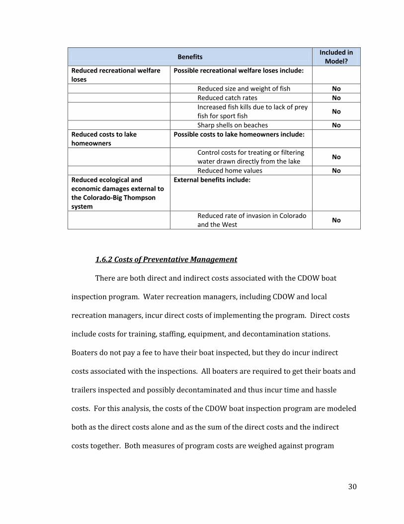
additional program benefits. Table 1 provides a summary of the benefits of the
CDOW boat inspection program and indicates which benefits are included in this
analysis.

29
Table 1: Benefits of preventative management for zebra and quagga mussels in the Colorado-Big Thompson System
Benefits of Preventative Management for Zebra and Quagga Mussels in the Colorado-Big Thompson System
Benefits Included in
Model?
Reduced costs to infrastructure Possible costs to infrastructure include:
Costs to hydropower facilities, water treatment facilities, dams, and pump plants
Yes
Costs to manually clean pipelines, tunnels and canals in the Colorado-Big Thompson system
No
Reduced control costs to industrial users
Industrial users that could be affected include:
Fossil-fuel fired power plants No
Any industry using raw water as an input to production
No
Reduced control costs to irrigators
Affected irrigators include:
Farmers using sub-irrigation or overhead sprinkler irrigation
No
Parks and golf courses using raw water
No
Reduced ecological damages Possible ecological damages include:
Food chain depletion No
Long term negative effects to fisheries
No
Severe reduction in populations of native mussels
No
Noxious weed growth and associated control costs
No
Algal blooms and associated control costs
No
Reduced human and animal health concerns
Human and animal health concerns include:
Accumulation of organic pollutants that are passed up through the food chain
No
Foul tastes in drinking water and associated costs to mitigate this in drinking water supplies
No
30
Benefits Included in
Model?
Reduced recreational welfare loses
Possible recreational welfare loses include:
Reduced size and weight of fish No
Reduced catch rates No
Increased fish kills due to lack of prey fish for sport fish
No
Sharp shells on beaches No
Reduced costs to lake homeowners
Possible costs to lake homeowners include:
Control costs for treating or filtering water drawn directly from the lake
No
Reduced home values No
Reduced ecological and economic damages external to the Colorado-Big Thompson system
External benefits include:
Reduced rate of invasion in Colorado and the West
No
1.6.2 Costs of Preventative Management
There are both direct and indirect costs associated with the CDOW boat
inspection program. Water recreation managers, including CDOW and local
recreation managers, incur direct costs of implementing the program. Direct costs
include costs for training, staffing, equipment, and decontamination stations.
Boaters do not pay a fee to have their boat inspected, but they do incur indirect
costs associated with the inspections. All boaters are required to get their boats and
trailers inspected and possibly decontaminated and thus incur time and hassle
costs. For this analysis, the costs of the CDOW boat inspection program are modeled
both as the direct costs alone and as the sum of the direct costs and the indirect
costs together. Both measures of program costs are weighed against program

31
benefits of reduced control costs to hydropower facilities, municipal water
treatment plants, and conveyance systems.
32
CHAPTER 2: METHODOLOGICAL APPROACH AND DATA
The bioeconomic model developed for this study simulates a mussel invasion
in the reservoirs of the Colorado-Big Thompson system over ten, thirty and fifty-
year time horizons. Included in the simulation are the timing and magnitude of
control costs accumulated to water conveyance structures, hydropower generation
stations, and municipal water treatment facilities that draw or convey water from
the Colorado-Big Thompson reservoirs. Simulations are run for two management
scenarios, a base-case scenario of no preventative management, and the CDOW boat
inspection preventative management scenario. The model outputs establishment
patterns and the associated distributions of control costs for each scenario. Benefits
of the preventative management program are measured as the difference in the net
present value of control costs for the two scenarios. Net benefits of the program are
measured as program benefits less program costs. Results are presented in Chapter
3 and include sensitivity analysis and "what-if" analysis to determine how sensitive
results are to changes in parameter values and to determine which conditions yield
benefits greater than costs.
This chapter describes the methodological approach and the data used to
analyze the costs and benefits of the CDOW boat inspection program. Section 2.1
develops the cost-benefit model used to analyze the program. The cost-benefit
model consists of three components: the probability of invasion, infrastructure

33
control costs, and project costs. Infrastructure control costs are incurred only if a
reservoir becomes invaded. To calculate the expected value of control costs, a
simulation model is developed to predict a mussel invasion in the system and
intertemporally match control costs to invaded reservoirs. The simulation model is
broken into two components, a mussel dispersal component and a control costs
component. Section 2.2 develops the mussel dispersal component of the simulation
model and Section 2.3 develops the control costs component of the simulation
model. Section 2.4 describes how the mussel dispersal component and the control
cost component are combined to simulate program benefits. Project costs are
assumed constant across time, and are described in Section 2.5. Each section
includes an explanation of model components and a description of the data used to
develop parameter values.
For all equations presented in the paper, superscripts denote differences in
values for the different scenarios, with the zero superscript representing the base-
case scenario of no preventative mussel management and the prime superscript
representing the preventive management scenario. Many of the equations include
values that vary between reservoirs and over time. For all equations presented in
the paper, the subscript represent reservoirs , and the subscript
represent time periods , with a time period equal to one year. Appendix A
includes a table of equations including names, descriptions, and parameter values
for all of the variables used in the model.

34
2.1 Cost-Benefit Model
The overall objective of this project is to compare the costs and benefits of
preventative management for zebra and quagga mussels in the Colorado-Big
Thompson system. The net benefits of the CDOW boat inspection program are
modeled as the reduction in the net present value of the expected damages to
conveyance, hydropower, and municipal water structures and facilities in the
Colorado-Big Thompson system, less the direct and indirect costs of implementing
the program on the reservoirs within the system. Water conveyance systems,
hydropower generation facilities, and municipal water treatment facilities are
assumed to incur control costs if the reservoir directly above them has an
established mussel population. The expected costs to structures and facilities is
equal to the probability that the reservoir directly upstream has an established
population of mussels multiplied by downstream facility control costs. The net
present value of the net benefits of the CDOW boat inspection program is given in
equation (1), and is equal to program benefits less direct and indirect program
costs:
(1)
where and are the net present values of the expected damages from mussels
over the time horizon for the base-case and preventative management scenarios,
and and are the net present values of the direct and indirect program costs.
The following subsections describe each of the components of the net benefits
equation.
35
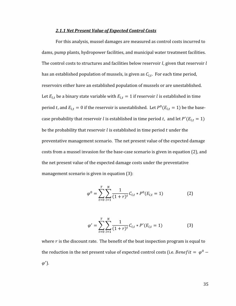
2.1.1 Net Present Value of Expected Control Costs
For this analysis, mussel damages are measured as control costs incurred to
dams, pump plants, hydropower facilities, and municipal water treatment facilities.
The control costs to structures and facilities below reservoir , given that reservoir
has an established population of mussels, is given as . For each time period,
reservoirs either have an established population of mussels or are unestablished.
Let be a binary state variable with if reservoir is established in time
period , and if the reservoir is unestablished. Let be the base-
case probability that reservoir is established in time period , and let
be the probability that reservoir is established in time period under the
preventative management scenario. The net present value of the expected damage
costs from a mussel invasion for the base-case scenario is given in equation (2), and
the net present value of the expected damage costs under the preventative
management scenario is given in equation (3):
(2)
(3)
where is the discount rate. The benefit of the boat inspection program is equal to
the reduction in the net present value of expected control costs (i.e.
).

36
2.1.2 Net Present Value of Program Costs
The costs of the CDOW boat inspection program are equal to the sum of the
direct costs to water recreation managers and the indirect costs incurred by
recreational boaters. The direct costs of implementing the boat inspection program
on reservoir in time period are given as . The net present value of the direct
costs of implementing the program for the whole system is denoted and is given
in equation (4):
(4)
The boat inspection program requires boaters to have their boats inspected
prior to launch. Thus, boaters incur time and hassle costs associated with the boat
inspection program. To model the indirect costs to boaters, welfare losses are
measured based on the increased time boaters must spend waiting for boat
inspections. Let represent lost welfare to boaters on reservoir in time period .
The net present value of the indirect costs of the boat inspection program is denoted
and is given in equation (5):
(5)
2.2 Mussel Dispersal Component of the Simulation Model
A mussel dispersal model is built to simulate values for and
. This section describes the mussel dispersal component of the

37
bioeconomic simulation model and culminates with the probability that reservoir
becomes colonized by time period .
Understanding the potential dispersal patterns of mussels is an essential
first step in estimating the expected damages that mussels may cause to a system
over time. Further, understanding how preventative management programs, like
the CDOW boat inspection program, change the dispersal patterns and timings of
invasions is an important key to estimating the benefits of such programs. Two
factors drive the probability of an invasion by an invasive species: (1) the suitability
of the receiving environment, and (2) the ability of the species to reach the receiving
environment (Bossenbroek et al., 2001; Leung & Mandrak, 2007). Dreissena
mussels can be transported to new environments on boats or via downstream flows.
The number of invaders that reach a new location via these pathways determines
propagule pressure, which is an important predictor of invasion success (Leung et
al., 2004; Keller et al., 2009). However, propagule pressure alone is not enough to
predict an invasion; once veligers are introduced to a new environment, their ability
to persist depends on the suitability of the new environment for survival. Thus,
simulating an invasion in the Colorado-Big Thompson system requires knowledge of
the pathways by which mussels can enter the system, the environmental qualities of
the habitat that the system provides, and the associated probabilities of
colonization. Leung and Mandrak describe an environment as invasible if a species
can survive and reproduce at that site, and suggest that the probability of
colonization is jointly determined by propagule pressure and invasibility (Leung &
Mandrak, 2007). They derive the joint probability of colonization as the product of

38
the probability that a location is invasible and the risk due to propagule pressure.
The joint probability of colonization is the key component in the mussel dispersal
model, and determines the likelihood of invasion for each reservoir in each time
period.
The mussel dispersal model has three main components: the probability that
a reservoir is invasible, the probability of establishment given invasibility, and the
joint probability of colonization. Section 2.2.1 describes the environmental
suitability of the Colorado-Big Thompson reservoirs for mussel colonization and
develops the probability of invasibility; Section 2.2.2 describes measures of
propagule pressure from boats and from flows in the Colorado-Big Thompson
system and relates propagule pressure to the probability of establishment; and
Section 2.2.3 describes the joint probability of colonization.
2.2.1 Environmental Suitability of the Colorado-Big Thompson Reservoirs for Mussel Colonization and the Probability of Invasibility
In order for an environment to be invasible, the environmental conditions of
the location must be such that introduced propagules can successfully reproduce
and form an established colony (Bossenbroek et al., 2001; Leung & Mandrak, 2007).
A number of water quality and limnological characteristics have been found to be
correlated with mussel survival and density. The most common parameters used to
assess mussel habitat suitability, in order from most predictive to least predictive,
are calcium content, alkalinity, pH, nutrients, Secchi depth, dissolved oxygen, mean
annual temperature, and conductivity (Claudi & Prescott, 2009). Calcium is a key
39
indicator. Dreissena need calcium to form their shells, and without sufficient
calcium, all of the other parameters become insignificant (Claudi & Prescott, 2009).
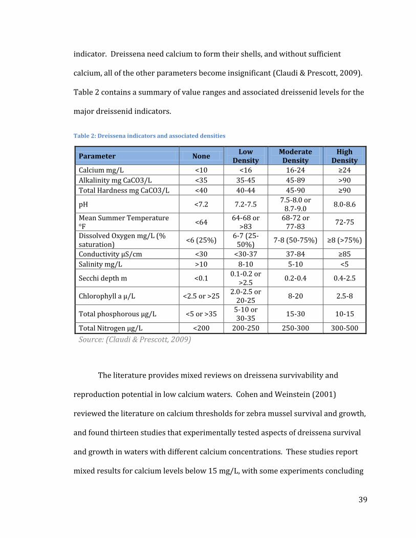
Table 2 contains a summary of value ranges and associated dreissenid levels for the
major dreissenid indicators.
Table 2: Dreissena indicators and associated densities
Parameter None Low
Density Moderate
Density High
Density Calcium mg/L <10 <16 16-24 ≥24 Alkalinity mg CaCO3/L <35 35-45 45-89 >90 Total Hardness mg CaCO3/L <40 40-44 45-90 ≥90
pH <7.2 7.2-7.5 7.5-8.0 or
8.7-9.0 8.0-8.6
Mean Summer Temperature °F
<64 64-68 or
>83 68-72 or
77-83 72-75
Dissolved Oxygen mg/L (% saturation)
<6 (25%) 6-7 (25-
50%) 7-8 (50-75%) ≥8 (>75%)
Conductivity μS/cm <30 <30-37 37-84 ≥85 Salinity mg/L >10 8-10 5-10 <5
Secchi depth m <0.1 0.1-0.2 or
>2.5 0.2-0.4 0.4-2.5
Chlorophyll a μ/L <2.5 or >25 2.0-2.5 or
20-25 8-20 2.5-8
Total phosphorous μg/L <5 or >35 5-10 or 30-35
15-30 10-15
Total Nitrogen μg/L <200 200-250 250-300 300-500
Source: (Claudi & Prescott, 2009)
The literature provides mixed reviews on dreissena survivability and
reproduction potential in low calcium waters. Cohen and Weinstein (2001)
reviewed the literature on calcium thresholds for zebra mussel survival and growth,
and found thirteen studies that experimentally tested aspects of dreissena survival
and growth in waters with different calcium concentrations. These studies report
mixed results for calcium levels below 15 mg/L, with some experiments concluding

40
that adult mussels can survive in waters with calcium levels as low as 4 mg/L;
however, most studies found poor reproduction at low calcium levels. Mussels have
been reported in Lake Champlain which has a calcium concentration of 13-14 mg/L,
and have also been reported in four inland lakes with mean calcium levels between
4 and 11 mg/L; however, it is not clear if these are established populations. There is
very little research on dreissena survival in waters with calcium levels between 15
and 20 mg/L. Experiments indicate that calcium concentrations greater than 20
mg/L can support good adult survival and reproduction, and calcium levels greater
than 28 mg/L can support abundant populations (Cohen & Weinstein, 2001). There
is mixed evidence and a general lack of research on zebra and quagga mussel
marginal habitats in the West (Claudi & Prescott, 2009).
In a series of reports prepared for the Bureau of Reclamation, RNT
Consultants deem the calcium levels in the Colorado-Big Thompson reservoirs to be
below those likely needed to support dreissenid survival, and conclude that there is
a very low risk of mussels establishing reproducing populations in the calcium-poor
reservoirs of the system (Claudi & Prescott, 2009). Many experts would agree with
this assessment, and most mussel dispersal models would exclude the possibility of
mussels establishing populations in the Colorado-Big Thompson waters. Mussel
have, however, been identified in the low calcium headwaters of the system. In
2008, multiple samples tested by multiple agencies positively identified dreissena
veligers in Willow Creek Reservoir, Lake Granby, Shadow Mountain Reservoir, and
Grand Lake. However, no evidence of veligers was found in any of these reservoirs
in 2009. This data spurs several questions: Were these reservoirs supporting a

41
small population of reproducing veligers that went extinct? Are the reservoirs
currently supporting reproducing populations that were missed in 2009 sampling
efforts? Were the veligers that were found in the reservoirs isolated individuals,
independent of a reproducing population? The answers to these questions are
uncertain.
Table 3 contains the available calcium data for the reservoirs in the
Colorado-Big Thompson system. Reservoirs are classified as having very low, low,
moderate, or high levels of risk based on classifications suggested by Whittier et al.
(2008 ). Reservoirs with average calcium levels less than 12 mg/L are classified as
very low risk, between 12 and 20 mg/L as low risk, between 20 and 28 mg/L as
moderate risk, and greater than 28 mg/L as high risk. Based on available calcium
data, Boulder Reservoir is the only reservoir in the system that is at high risk of a
dreissena invasion. Windy Gap Reservoir, Willow Creek Reservoir, Lake Granby,
Shadow Mountain Reservoir, Grand Lake, Horsetooth Reservoir and Carter Lake all
have calcium levels in the low or very low ranges. Two sources of calcium data for
Mary's Lake give conflicting evidence of the calcium levels in the lake. Samples
taken by the Northern Colorado Water Conservancy District of discharge water from
Mary's Lake indicate that calcium levels in the lake are very low, whereas sampling
by the Town of Estes water quality lab suggests that calcium levels in Mary's Lake
fall in the moderate range. There is no calcium data available for East Portal
Reservoir, Lake Estes, Pinewood Reservoir, or Flatiron Reservoir. As part of the
sensitivity testing of the model, calcium levels in these reservoirs and in Mary's Lake
are modeled as very low, low and moderate.
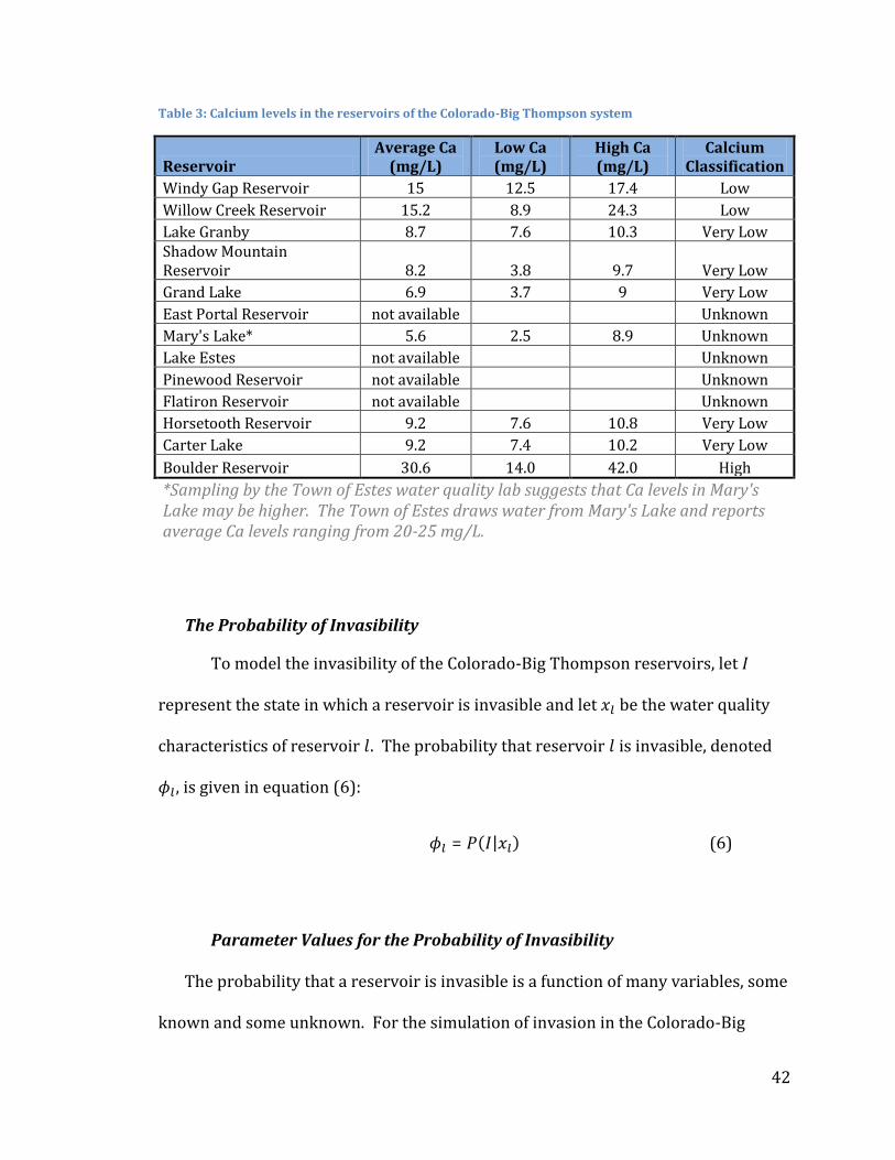
42
Table 3: Calcium levels in the reservoirs of the Colorado-Big Thompson system
Reservoir Average Ca
(mg/L) Low Ca (mg/L)
High Ca (mg/L)
Calcium Classification
Windy Gap Reservoir 15 12.5 17.4 Low Willow Creek Reservoir 15.2 8.9 24.3 Low Lake Granby 8.7 7.6 10.3 Very Low Shadow Mountain Reservoir 8.2 3.8 9.7 Very Low Grand Lake 6.9 3.7 9 Very Low East Portal Reservoir not available
Unknown
Mary's Lake* 5.6 2.5 8.9 Unknown Lake Estes not available Unknown Pinewood Reservoir not available Unknown Flatiron Reservoir not available Unknown Horsetooth Reservoir 9.2 7.6 10.8 Very Low Carter Lake 9.2 7.4 10.2 Very Low
Boulder Reservoir 30.6 14.0 42.0 High
*Sampling by the Town of Estes water quality lab suggests that Ca levels in Mary's Lake may be higher. The Town of Estes draws water from Mary's Lake and reports average Ca levels ranging from 20-25 mg/L.
The Probability of Invasibility
To model the invasibility of the Colorado-Big Thompson reservoirs, let
represent the state in which a reservoir is invasible and let be the water quality
characteristics of reservoir . The probability that reservoir is invasible, denoted
, is given in equation (6):
(6)
Parameter Values for the Probability of Invasibility
The probability that a reservoir is invasible is a function of many variables, some
known and some unknown. For the simulation of invasion in the Colorado-Big

43
Thompson system, parameter estimates for the probability of invasibility are
assigned based on the calcium risk level for each reservoir. The assumption made in
this study is that is small but greater than zero for all of the reservoirs in the
system. Although may be zero in the calcium-poor reservoirs of the Colorado-Big
Thompson Project, it is reasonable to assume that the probability of invasibility is
likely to be small but non-zero for the reservoirs in the very low and low calcium
categories. Available literature assigns risk qualitatively, which makes assigning
quantitative parameter values challenging. The chosen parameter values are
subjective, making this an important variable to consider as part of the sensitivity
analysis. The table presented in Appendix A gives the range of values for used in
simulating invasions in the Colorado-Big Thompson reservoirs.
2.2.2 Pathways of Invasion and the Probability of Establishment
The introduction of mussels to an environmentally suitable lake does not
guarantee that mussels will colonize the lake. In fact, it is likely that introductions
by multiple boats will be necessary for successful colonization of a water body
(Bossenbroek et al., 2001). Likewise, lakes downstream from infested water bodies
are not guaranteed to become infested. The distance downstream and the level of
turbulence in the stream have both been found to affect the mortality of mussel
veligers and their likelihood of establishing downstream colonies (Horvath &
Lamberti, 1999; Rehmann et al., 2003). Propagule pressure, a measure of the
number of propagules released into a region, is a key determinant of the probability
that an environmentally suitable water body becomes established (Keller et al.,

44
2009). In this section, measures of propagule pressure from boats and from
downstream flows are developed and related to the probability of establishment.
2.2.2(a) Propagule Pressure from Boats
In order to estimate the probability that a reservoir develops an established
colony of mussels from propagules introduced by boats, an estimate of the
propagule pressure from boats is required. Propagule pressure from boats is
assumed to be well estimated by the number of potentially infested boats visiting
each reservoir each year (Leung & Mandrak, 2007). The model developed in this
study assumes that the number of potentially infested boats visiting each reservoir
in the system is equal to a percent of total boat visits to each reservoir and is equal
across reservoirs. The number of invaded lakes and reservoirs in the western states
is expected to increase each year as the western invasion progresses. Consequently,
as the number of mussel sources increase, the percent of potentially infested boats
visiting the Colorado-Big Thompson reservoirs is also expected to increase. Thus,
propagule pressure from boats is expected to increase over time.
Boat Visits to the Colorado-Big Thompson Reservoirs
The first step in estimating propagule pressure from boats is to estimate the
total number of boat visits to each reservoir. Seven of the twelve reservoirs in the
Colorado-Big Thompson system allow motorized boating, including Lake Granby,
Shadow Mountain Reservoir, Grand Lake, Lake Estes, Horsetooth Reservoir, Carter
Lake, and Boulder Reservoir. Reservoirs that allow motorized boating are

45
highlighted in Figure 3 on page 13 with doubled borders1. CDOW inspection data
from the 2009 boating season is used to approximate the average annual number of
boat visits to each reservoir (CDOW, 2009)2. There is no dedicated monitoring
station for Lake Estes. Boats at Lake Estes are monitored by roving patrol; thus,
inspection data for Lake Estes does not provide valid estimates of seasonal boat
visits. Annual trailered boat visits to Lake Estes are estimated by the Estes Valley
Parks and Recreation marina based on daily permit sales (Estes Valley Parks and
Recreation, 2010).
To model total boat visits, let represent average yearly trailered boat
trips to reservoir in time period for the base-case scenario, and let represent
average yearly trailered boat trips for the preventative management scenario.
Values for are set equal to the number of boat inspections on reservoir in 2009.
Total boat visits may differ between scenarios. Although there is no fee for boat
inspections, the time and effort that boaters must spend to get their boats inspected
represents a time cost. The requirement of boat inspections may cause some
boaters to reduce the number of trips taken within the system. Boaters may
substitute out of the system and boat on non-Colorado waters, or they may simply
take fewer boat trips. Let represent the percent decline in the number of boat
1 Motorized boating was previously allowed in Willow Creek Reservoir, but the reservoir has been closed to motorized boating as part of the Colorado ZQM Plan. The reservoir may re-open to boating. This scenario is not considered in the model, but would be an easy adaptation. 2 The 2009 data may provide under estimates of average yearly boat visits, as the 2009 boating season was exceptionally rainy. Despite this concern, the 2009 boat inspection data is the best available data for estimating yearly boat visits to each reservoir.
46
visits attributable to the boat inspection program. Values for are estimated by
backing out 2009 inspection numbers as in equation (7) :
(7)
Parameter Values for the Percent Decline in Boat Visits
A survey conducted by CDOW in 2008 provides some idea of how boaters
may behave when faced with mandatory boat inspections. The survey was
conducted prior to the mandatory boat inspection program, and asks boaters:
Q12: In 2007, about how many days did you use your boat in
Colorado?
Q27: The average time for an aquatic nuisance species (ANS) boat
inspection is 3 minutes. There is currently no fee for an ANS
inspection in Colorado. If an inspection found or suspected an ANS
attached to your boat, you would have to go through the
decontamination process before putting in at that water body.
Decontamination would depend on the size of your boat but may take
20 minutes. After reading the text above, how likely would you be to
avoid water bodies which require the inspection process?
A major limit to using question 27 to address boater behavior when faced with the
CDOW boat inspection program, is that question 27 asks what a boater would do if
their favorite water body required inspections. Thus, question 27 implies that
boaters could substitute away from inspections by boating at other Colorado water
47
bodies. The CDOW boat inspection program is statewide, which greatly reduces
substitute options. Boater behavior when faced with statewide inspections may
differ from that reported in question 27. For the purpose of this analysis, it is
assumed that boaters who answered "very likely" or "likely" to question 27 may
reduce the number of boat trips they take within Colorado. A total of 1811
respondents answered both questions 12 and 27. Of those respondents, a total of
30,631 Colorado boat trips were reported. Questions 12 and 27 are used to
estimate a low, base, and high percent reduction in the number of Colorado boat
trips. The high estimate of assumes that respondents who answered "very likely"
to question 27 and respondents who answered "likely" will reduce their Colorado
trips by 20% and 10%, respectively. This assumption results in a 3% reduction in
the number of boat trips taken in the state. To estimate the base value of , a 10%
reduction in Colorado trips is assumed for respondents who answered "very likely",
with a 0% reduction in trips for all other respondents. This assumption results in a
1% reduction in the number of boat trips taken in the state. The low estimate of
assumes perfectly inelastic demand for recreational boating, resulting in a 0%
reduction in boat trips.

48
Total Boat Visits to the Colorado-Big Thompson Reservoirs Under the Base-Case Scenario and the Preventative Management Scenario
Table 4 gives average yearly boat visit values used in the simulation model.
Values for are given for the low, base, and high parameter values for .
Table 4: Total number of trailered boat visits by reservoir
Reservoir
, ,
,
Windy Gap Reservoir 0 0 0 0 Willow Creek Reservoir 0 0 0 0 Lake Granby 7404 7404 7479 7633 Shadow Mountain Reservoir
3562 3562 3598 3672
Grand Lake 3263 3263 3296 3364 East Portal Reservoir 0 0 0 0 Mary's Lake 0 0 0 0 Lake Estes 420 420 424 433 Pinewood Reservoir 0 0 0 0 Flatiron Reservoir 0 0 0 0 Horsetooth Reservoir 48,518 48,518 49,008 50,019 Carter Lake 7982 7982 8063 8229 Boulder Reservoir 1700 1700 1717 1753
The Percent of Potentially Infested Boats
The previous section considered the total number of boats visiting the
system for the base-case and preventative management scenarios. The next step in
estimating propagule pressure from boats is to estimate the percent of those boats
that are potentially infested with mussels. The percent of potentially infested boats
is expected to increase over time as a greater number of water bodies become
mussel sources. An increasing random-walk method, similar to that used by Leung
et al. (2004), is utilized to model an increasing percent of potentially infested boats
over time. Each year, the percent of potentially infested boats increases by a
49
random value, , where is chosen from a uniform distribution bounded by 0 and
. Let be the percent of visiting boats that are potentially infested in year 0
(i.e. 2009), and let represent the maximum rate at which the percent of
potentially infested boats can increase in each period. The percent of potentially
infested boats will be limited by the extent of the mussel infestation in the region.
Thus, is bounded by a maximum value, . Equation (8) gives the percent of
potentially infested boats in period for the base-case scenario:
(8)
The difference between the percent of potentially infested boats that enter
Colorado-Big Thompson waters for the preventative management scenario versus
the base-case scenario captures the main effect of the CDOW boat inspection
program. The boat inspection program affects the percent of potentially infested
boats in two ways: (1) it will slow the rate of invasion in the region, and (2)
inspectors will catch and clean a percent of potentially infested boats that visit the
system. Let be the percent reduction in the rate of invasion attributable to the
boat inspection program. Equation (9) gives the percent of potentially infested
boats entering the system in year for the preventative management scenario:
(9)
50
The percent of boats caught and cleaned by boat inspections is assumed to be
constant over time and across reservoirs, and is denoted . Equation (10) gives ,
the percent of potentially infested boats entering Colorado-Big Thompson waters
after being inspected (i.e. the percent of potentially infested boats that are missed
by boat inspectors):
(10)
Propagule Pressure from Boats
Propagule pressure from boats is derived by multiplying total boat visits
with the percent of potentially infested boats. Propagule pressure from boat
introductions in reservoir in time period for the base-case scenario is denoted
and is given in equation (11):
(11)
Propagule pressure from boat introductions for the preventative management
scenario is denoted
and is given in equation (12):
(12)
Parameter Values for the Percent of Potentially Infested Boats
Mussel veligers and adult mussels can be difficult to find, so boat inspectors
cannot be sure of the reliability of their inspections. Thus, the value of is
unknown. Parameter estimates of are set to range between .8 and 1, with

51
representing perfect efficacy of boat inspections. The value of is also unknown.
Parameter estimates of are set to range between .25 and .75.
CDOW inspection data is used to develop a range of values for the parameter
. A total of 305,622 entrance inspections were conducted in the state in 2009. Of
these, 5647 inspections were high-risk inspections, and 3364 resulted in
decontamination. Boats that have traveled from reservoirs that are known to be
infested or from high-risk states are subjected to a high-risk inspection or
decontamination; thus, the percent of inspections that were high-risk or resulted in
decontamination should be a good proxy for the percent of potentially infested
boats. To model the initial percent of potentially infested boats, the base value of
0 is set equal to 1.8%, the percent of high-risk inspections conducted in 2009. The
low value is set equal to 1.1%, the percent of decontaminations, and the high value
is set equal to 2.9%, the percent of entrance inspections that were high risk or
resulted in decontamination.
The parameter range for is based on the possible rate of infestation for
the region. The rate by which the mussel invasion in the West will occur is
unknown, but is likely to be slower than the initial U.S. invasion in the Midwest and
Northeast (Bossenbroek et al., 2007). To allow for differing rates of invasion, a
range of values for are tested in the model. Parameter values for are
based on two studies of mussel infestation rates. Kraft and Johnson (2000)
investigate zebra mussel colonization rates in a four-state region adjacent to the
Great Lakes from 1995 to 1997. They tested for the presence of zebra mussel

52
veligers each year from a sample of environmentally suitable lakes. For the period
1995-1996, the annual infestation rate was 4.6%. For the period 1996-1997, the
annual infestation rate increased to 5.6%, with annual infestation rates higher in
Indiana (11-12%) and Michigan (5-12%) than in Wisconsin (0%). These results
suggest that rates of inland colonization vary by region. Regional differences may
be attributed to differences in habitat suitability between regions or to differences
in the patterns and efficiency of dispersal vectors. Evidence from a 2004 study by
Johnson et al. (2006) suggest that the invasion of inland lakes is occurring slowly,
thus lower estimates of seem most appropriate. Using the infestation rates
found by Kraft and Johnson (2000), values for are set to range between 0%
and 5.6%; however, the base value of is set low (.5%) to reflect the finding by
Johnson et al (2006) that the invasion of inland lakes is happening very slowly.
Parameter values for are chosen based on national risk assessments
provided by Whittier et al. (2008 ). Using regional water calcium levels, Whittier et
al. classify 58.9% of U.S. ecoregions as being at high risk of dreissena invasion, and
an additional 19.8% as having highly variable risk. Evidence from the ongoing U.S.
invasion suggests that only a small portion of water bodies that are suitable habitat
for dreissena will become invaded. As of 2004, only in Michigan and Indiana were
more than 10% of suitable lakes invaded (Johnson et al., 2006). To reflect this, the
low value of is set at 2.95%, five percent of the percent of high-risk ecoregions,
and the base value is set at 5.89%, ten percent of the percent of high-risk ecoregions.
The high value is set at 58.9%. There is much uncertainty in the values for and
making sensitivity analysis of these parameters important.
53
3.2.2 (b) Propagule Pressure from Flows
To model the invasion in the Colorado-Big Thompson reservoirs, source-sink
dynamics are assumed. There are two main criteria for a downstream sink to
become colonized from an upstream source: (1) the population in the upstream
source must be sufficiently large, and (2) a sufficiently large percentage of veligers
must survive transport (Bobeldke et al., 2005). To account for both of these criteria,
propagule pressure from flows is modeled as the density of veligers who survive
downstream transport.
Density of the Upstream Reservoir
Estimating the potential densities of mussels in the reservoirs of the
Colorado-Big Thompson system is beyond the scope of this project; however,
mussel density is an important component in the simulation. In the model, the
probability of establishment from downstream flows is a function of mussel density
in the upstream reservoir and distance downstream. Upstream population densities
are dependent on a number of factors including water chemistry and other
limnological characteristics. Population densities can also change over time.
Ramcharan et al. (1992) develop models to predict the occurrence and
density of dreissena mussels in lakes based on limnological characteristics. They
find that both occurrence and average density of mussels are highly correlated with
the water chemistry of a lake. In their data set (a total of 278 European lakes), no
mussels were found in lakes with average pH values below 7.3 or calcium
concentrations below 28.3 mg/L. The variables pH and Ca were found to be
54
important for distinguishing lakes without dreissena from those with low densities,
and the variables PO4 and NO3 were found important for distinguishing lakes with
low densities from lakes with high densities. Overall, Ramcharan et al. (1992) find
that calcium and pH levels are important indicators of the presence or absence of
dreissena, but that other variables are more important for predicting the density of
mussels in an established water body.
Mellina and Rasmussen (1994) also find that calcium levels set a threshold
for the presence of zebra mussels, but are a poor predictor of abundance. They find
that the size distribution of the available substrate (i.e. boulders, gravel, sand, mud)
is a better determinate of mussel density, with larger substrates supporting denser
populations. Burlakove et al. (2006) find the major factors affecting the size of a
mussel population are the time since initial colonization, the relative abundance of
substrates for mussels to attach to, and limnological characteristics.
Overall, the density of zebra mussels in an established water body can vary
dramatically. In their study of mussel densities in European lakes, Ramcharan et al.
(1992) found densities ranging from a low of 22 individuals/m2 to a high of 7500
individuals/m2, with mean densities of just over 800 individuals/m2. Reported
densities of zebra mussels in the United States range from a low of 55
individuals/m2 in the Tennessee River to a high of 250,000 individuals/m2 in Lake
Michigan (Bossenbroek et al., 2007).
Casagrandi et al. (2007) model temporal patterns in mussel density based
on lifecycle and reproductive characteristics of zebra mussels and on predation.
55
They find that the density of zebra mussel populations can be described by a boom-
bust cycle of high densities followed by low densities, and that equilibrium
population densities can only be reached if veliger survival is very low. In contrast,
Burlakova et al. (2006) track population densities and biomass for three lakes in
Belarus over a 12-year period following initial colonization, and find that mussel
populations remain constant after reaching a maximum density.
For this model, it is assumed that population densities increase over an initial
period and then remain constant over time. It is further assumed that upstream
reservoirs only become potential sources for downstream infestation after reaching
their maximum population density following a lag time of years. Consequently,
reservoirs that are colonized at time become sources of propagules at time .
Mussel Density Parameter Values
The density of an established and homogeneous population of mussels in
reservoir is denoted , with parameter values of set at 22, 800, and 7500
individuals/m2, as described in Ramcharan et al. (1992). Although calcium is a
relatively poor predictor of population density, it is the only data available to
calibrate the base densities for the reservoirs in the Colorado-Big Thompson system.
Base parameter values are set at 22 individuals/m2 for very low and low calcium
reservoirs, 800 individuals/m2 for moderate calcium reservoirs, and 7500
individuals/m2 for high calcium reservoirs. The effects of different levels of mussel
densities in the system are tested as part of the sensitivity analysis.

56
It is difficult to determine the exact timing of an invasion, so most estimates
of lag time are based on the time from initial detection. A substantial difference may
exist between the time of initial introduction and the time of detection. When
populations grow exponentially or logistically, there is an initial period were growth
is very slow. This period may last for several years (Ricciardi, 2003). Data from
Europe and North America suggest that zebra mussels reach maximum density
about 2-3 years after detection. Burlakova et al. (2006) estimate that it takes 7-12
years for zebra mussels to reach maximum population density after the time of
initial invasion (2006). The time following initial invasion is the most appropriate
for this model. The estimates by Burlakova et al. (2006) seem on the high end, so
low, base, and high parameter values of are set equal to 6, 8, and 10 years,
respectively.
Veliger Survival in Downstream Transport
The density of veligers that survive downstream transport is also a function
of veliger survival in transit. Distance downstream, turbulence, and the presence of
wetlands and vegetation all affect veliger transport and mortality (AMEC Earth and
Environment, 2009). The Colorado-Big Thompson Project is nearly entirely
connected via pipelines, tunnels, and canals, with no wetlands or vegetation present
to slow or hinder veliger transport. Therefore, the possibility of veliger transport
between reservoirs comes down to the ability of veligers to survive the distances
and turbulence encountered in the system. Little is currently know about how
veligers will fair passage through the man-made conduits and the turbulent

57
hydropower plants of the Colorado-Big Thompson Project. Unlike natural rivers,
the canals and pipelines in the project are operated at hydraulic velocities that are
more conducive to transport of viable veligers; the conduits also provide an ideal
surface for settlement and growth (Claudi & Prescott, 2009; Clark, 2010). This
suggests that veligers may be able to travel further in the Colorado-Big Thompson
conduits than is suggested by studies of veliger mortality conducted in natural
rivers. Aside from a smoother ride in the pipelines and canals, in many stretches of
the system, veligers will be subject to a trip through a turbulent hydroelectric power
plant. These confounding characteristics provide added uncertainty to the viable
transport of mussels from upstream sources to downstream sinks in the Colorado-
Big Thompson system. Despite these unique and confounding characteristics,
information gathered from other systems is the best information available to
understand how mussel veligers may pass through the Colorado-Big Thompson
system.
In their study of connected lake-stream systems in the St. Joseph River Basin
in Michigan, Bobeldke et al. (2005) found that lakes greater than 20 km from an
upstream source had a lower chance of being invaded. The longest connections in
the Colorado-Big Thompson system are between Carter Lake and Boulder Reservoir
(36.7 km), between Grand Lake and East Portal Reservoir (21.1 km), and between
Flatiron Reservoir and Horsetooth Reservoir (21.3 km); see Figure 3 on page 13.
The remaining conduits in the system are all less than 20 km in length.

58
Horvath and Lamberti (1999) found that the percent of veligers that survive
downstream transport declines exponentially with distance traveled downstream
(1999). For the stretch of river tested, the percent of veligers that survived
downstream transport was found to be well estimated by the equation:
, where is the distance downstream, measured in
kilometers. The stretch of river used in their study is considered turbulent, and the
authors' findings suggest that exposure to turbulence or shear during transport
negatively affects veliger survival.
Incorporating turbulence, among other variables, AMEC Earth and
Environment (2009) built a particle tracking simulation model to assess the
possible transport of mussel veligers between two Colorado reservoirs connected
by over 50 km of natural river. Results of their model indicate that turbulence plays
a very large role in the fate of veligers in the system, with all simulations resulting in
100% veliger mortality within a short distance downstream from the upstream
reservoir.
In laboratory experiments, Rehmann et al. (2003) test the effects of
turbulence on the mortality of zebra mussel veligers. They conclude that turbulence
in streams can increase mortality rates, but the magnitude of the effect depends on
the size distribution of veligers and the relative importance of acute and chronic
exposure to turbulence. Their experiment was motivated by the possibility of using
bubbler barriers as a preventative control to block the passage of mussel veligers in
streams. They conclude that bubble barriers could be affective if mortality is a
59
result of acute exposure to turbulence, but would be impractical if veliger mortality
is a result of chronic exposure to turbulence. This finding is useful in evaluating the
potential mortality of mussels passing through hydropower plants. If mortality is a
result of acute effects caused by damage during short periods of high turbulence,
then it is reasonable to assume that veligers will not survive passage though
hydropower plants. However, if mortality is a result of chronic exposure to
turbulence, mussel veligers may have a greater chance of surviving passage through
hydropower penstocks and turbines.
Evidence from the Hoover Dam suggests that mussels can successfully pass
through hydropower facilities. In 2007, shortly after the discovery of mussels in
Lake Mead, Bureau of Reclamation divers identified quagga mussels on the intake
tower upstream of Hoover Dam and on the spillway outlet below the dam, indicating
that mussels had successfully passed through the hydroelectric facility (Bureau of
Reclamation, 2007).
In 2010, the Bureau of Reclamation began work on a project to assess the
viability of mussel veligers in Bureau of Reclamation conveyance structures. With
the exception of the Bureau of Reclamation study, there are currently no studies that
specifically address how mussel veligers will survive in a system like the Colorado-
Big Thompson Project; however, findings from other systems suggest that it is likely
that mussels can survive transport through the conduits and hydropower facilities
of the project.

60
In order to estimate propagule pressure from propagules introduced via
downstream flows, several assumptions are made about how veliger densities are
impacted by passage through the Colorado-Big Thompson system. It is assumed
that veliger densities will decline exponentially with distance traveled, as found by
Horvath and Lamberti (1999). It is also assumed that the presence of a hydropower
facility along a stretch does not affect the overall percentage of veligers that survive
passage. In order to make this assumption, the underlying assumption is that
veliger mortality is more dependent on chronic exposure to turbulence than on
acute exposure.
To model propagule pressure from downstream flows from infested
upstream sources, maximum upstream population densities are multiplied by the
percent of veligers that survive downstream passage. Propagule pressure from
flows that reach reservoir in time period are denoted , and are given in
equation (13):
(13)
where is the maximum population density in the reservoir directly upstream
from reservoir , is an intercept parameter, is a decay parameter, and is the
distance between reservoir and the upstream infested reservoir.
Parameter Values for Propagule Pressure From Flows
The intercept value of found in the Horvath and Lamberti (1999)
study is unlikely to differ across systems. This value represents the percent of
veligers that survive without passing any distance. The value for estimated in the
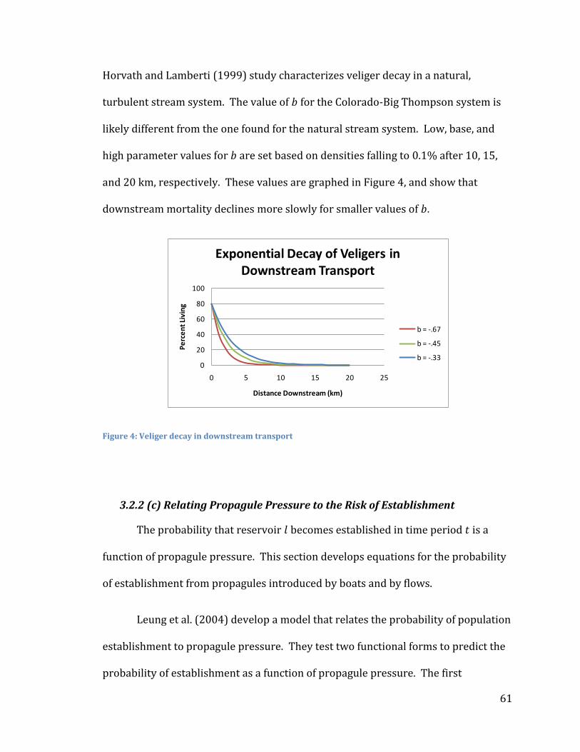
61
Horvath and Lamberti (1999) study characterizes veliger decay in a natural,
turbulent stream system. The value of for the Colorado-Big Thompson system is
likely different from the one found for the natural stream system. Low, base, and
high parameter values for are set based on densities falling to 0.1% after 10, 15,
and 20 km, respectively. These values are graphed in Figure 4, and show that
downstream mortality declines more slowly for smaller values of .
Figure 4: Veliger decay in downstream transport
3.2.2 (c) Relating Propagule Pressure to the Risk of Establishment
The probability that reservoir becomes established in time period is a
function of propagule pressure. This section develops equations for the probability
of establishment from propagules introduced by boats and by flows.
Leung et al. (2004) develop a model that relates the probability of population
establishment to propagule pressure. They test two functional forms to predict the
probability of establishment as a function of propagule pressure. The first
0
20
40
60
80
100
0 5 10 15 20 25
Pe
rce
nt
Livi
ng
Distance Downstream (km)
Exponential Decay of Veligers in Downstream Transport
b = -.67
b = -.45
b = -.33
62
functional form assumes that each propagule has an independent chance of
establishment, and the second assumes the presence of an Allee effect. An Allee
effect describes population reproduction for small populations were the
reproduction and survival rates of individual propagules increases with population
density. With an Allee effect, the probability of propagules successfully reproducing
and forming an established colony is disproportionately small for propagule
numbers below a threshold, and then grows with larger numbers of propagules
(Leung et al., 2004). For the case of independence, the probability of establishment
is the complement of the probability that no propagules successfully establish. For
this case, the probability of establishment as a function of propagule pressure is
given as: , where is the probability of a
single propagule establishing a colony, is the number of propagules arriving at
location at time , and is a shape coefficient. The second functional form
accounts for an Allee effect. In this form, the curve contains an inflection point.
Below the inflection point threshold, the probability of establishment is
disproportionately smaller. The function is similar to the one used for the
independent case, but includes an additional shape parameter, :
. Values of greater than one indicate the presence of an Allee effect,
whereas equal to one indicates independence. Leung et al. (2004) use boater
registration data and zebra mussel presence/absence data from Michigan to
develop estimates of propagule pressure and to fit parameter values to the models.
They assume recreational boat movement is the primary vector for zebra mussel
dispersal, and do not consider propagule pressure from upstream sources. They

63
estimate propagule pressure using a production constrained gravity model, as in
Bossenbroek et al. (2001), where is the number of potentially infested boats
that visit location in time period . To consider changes to propagule pressure
over time, Leung et al. (2004) assume that as the invasion progresses and more
locations become invaded, propagule pressure will increase over time. They
incorporate this into their model using the formula, where R is
randomly chosen from a uniform distribution between 0 and 10. Using observed
invasion data from Michigan lakes, Leung et al. (2004) estimate values for the model
parameters α and and find a significant Allee effect ( is found to be statistically
significantly larger than one). For the Allee model, the estimated parameter values
are and .
For the Colorado-Big Thompson dispersal model, the methods developed by
Leung et al. (2004) are used to establish relationships between the probability of
establishment and propagule pressure from boats and flows. Using the Allee effect
functional form developed by Leung et al. (2004), measures of propagule pressure
from boats and from upstream flows for the Colorado-Big Thompson system are
converted to probabilities of establishment. For the following equations, the
superscripts and subscripts and represent differences in equations for
propagules introduced by boats and by flows, respectively.
Probability of Establishment from Boats
Propagule pressure from boats for reservoir in time period for the base-
case scenario is denoted
and is measured as the number of potentially infested
64
boats visiting reservoir in time period . The formula for
is given in equation
(11), and the associated probability of establishment is given in equation (14):
(14)
For the preventative management scenario, propagule pressure from boats for
reservoir in time period is denoted
and is measured as the number of
potentially infested boats visiting reservoir in the time period that are still
infested after being inspected. The formula for
is given in equation (12), and
the associated probability of establishment is given in equation (15):
(15)
Parameter Values for the Probability of Establishment by Boats
Values for the parameters and are equal in equations (14) and (15),
because propagules introduced by boats face the same biological conditions
regardless of the CDOW boat inspection program. Parameter values for and in
equations (14) and (15) are assumed to be similar to those estimated for and in
the Leung et al. (2004) study, because the same measure of propagule pressure is
used. Figure 5 shows a graph of the probability of establishment as a function of the
number of potentially infested boats, with , as found in Leung et al. (2004),
and ranging between low, base, and high values of .00005, .000103, and .0005.
The base value for is equal to the value found by Leung et al. (2004), and the
low and high values are chosen subjectively.

65
Figure 5: The probability of establishment as a function of the number of potentially infested boats
Probability of Establishment from Flows
Propagule pressure from downstream flows for reservoir in time period is
measured as the density of propagules surviving downstream passage and is given
in equation (13). Upstream reservoirs become a source of propagules following a
lag time of years; thus, the probability of establishment from flows is a step-wise
function with the probability equal to zero prior to the completion of the lag time,
and a function of following the lag time. The probability of establishment from
propagules introduced from downstream flows is given in equation (16):
(16)
where is the time period in which the reservoir directly upstream from
reservoir becomes established.
0
0.2
0.4
0.6
0.8
1
0 5000 10000 15000 20000Pro
bab
ility
of
Esta
blis
hm
en
t
Number of Potentially Infested Boats
Probability of Establishment from Boats
α = .00005
α = .000103
α = .0005

66
Parameter Values for the Probability of Establishment from Flows
Values for the parameters and are expected to be substantially
different from those estimated in the Leung et al. (2004) study, because the measure
of propagule pressure is different. There is very little information available about
how veligers will survive in conveyance structures like those in the Colorado-Big
Thompson Project; thus, there is little data available to calibrate the and
parameter values. Figure 6 demonstrates how different values of and and
upstream densities affect the probability of establishment from downstream flows
as a function of distance downstream. The base decay rate of is used for
all of the graphs. In general, the probability of establishment from flows increases
with upstream density and with . The parameter affects how quickly the
probability of establishment drops off with distance downstream. For , the
probability of establishment remains close to 100% for short distances and then
quickly drops to 0%; whereas for , the probability of establishment drops
more gradually as the distance downstream increases.

67
Lo
w D
en
sity
Mo
de
rate
De
nsi
ty
Hig
h D
en
sity
Figure 6: The probability of establishment from flows
2.2.3 Combining the Probability of Invasibility and the Probability of Establishment: The Joint Probability of Colonization
This section combines the probability of establishment with the probability
of invasibility to develop the joint probability that reservoir becomes colonized by
time period . Joint probabilities of colonization are developed for propagules
0.00
0.10
0.20
0.30
0.40
0.50
0.60
0.70
0.80
0.90
1.00
0 5 10 15 20 25
Pro
bab
ility
of
Esta
blis
hm
en
t
Distance Downstream (km)
Probability of Establishment from Flows(Upstream Density = 20 individuals/m2; c=1.86;b=-.45)
α = .005
α = .05
α = .2
0.00
0.10
0.20
0.30
0.40
0.50
0.60
0.70
0.80
0.90
1.00
0 5 10 15 20 25
Pro
bab
ility
of
Esta
blis
hm
en
t
Distance Downstream (km)
Probability of Establishment from Flows(Upstream Density = 20 individuals/m2; c=1.00;b=-.45)
α = .005
α = .05
α = .2
0.00
0.10
0.20
0.30
0.40
0.50
0.60
0.70
0.80
0.90
1.00
0 5 10 15 20 25
Pro
bab
ility
of
Esta
blis
hm
en
t
Distance Downstream (km)
Probability of Establishment from Flows(Upstream Density = 800 individuals/m2; c=1.86;b=-.45)
α = .005
α = .05
α = .2
0.000.100.200.300.400.500.600.700.800.901.00
0 5 10 15 20 25P
rob
abili
ty o
f Es
tab
lish
me
nt
Distance Downstream (km)
Probability of Establishment from Flows(Upstream Density = 800 individuals/m2; c=1.00;r=-.45)
α = .005
α = .05
α = .2
0.00
0.10
0.20
0.30
0.40
0.50
0.60
0.70
0.80
0.90
1.00
0 5 10 15 20 25
Pro
bab
ility
of
ESta
blis
hm
en
t
Distance Downstream (km)
Probability of Establishment from Flows(Upstream Density = 7500 individuals/m2; c=1.86;b=-.45)
α = .005
α = .05
α = .2
0.00
0.10
0.20
0.30
0.40
0.50
0.60
0.70
0.80
0.90
1.00
0 5 10 15 20 25
Pro
bab
ility
of
ESta
blis
hm
en
t
Distance Downstream (km)
Probability of Establishment from Flows(Upstream Density = 7500 individuals/m2; c=1.00;b=-.45)
α = .005
α = .05
α = .2
68
introduced by boats and propagules introduced by flows. These probabilities are
the key components that determine establishment in the simulation model.
Leung and Mandrak (2007) derive the joint probability of colonization as the
product of the probability that a location is invasible and the probability of
establishment as a function of propagule pressure over time. Given that a reservoir
is invasible, the probability that reservoir becomes established in year can be
described by a binomial distribution. Let be the probability that reservoir
becomes established in year , given propagule pressure in reservoir in year .
Then the probability that reservoir remains unestablished in year is equal to
. The overall probability that reservoir remains unestablished by
year is the product of the probabilities that the reservoir remains unestablished in
each year up to year . The probability that reservoir is established by year ,
denoted , is the compliment of the probability that it is not established by year
and is given in equation (17):
(17)
Multiplying the probability of invasibility from equation (6) with the probability of
establishment from equation (17) gives the joint probability of colonization. The
joint probability that reservoir becomes established by year , denoted , is
given in equation (18):

69
(18)
Let
and represent the joint probabilities of colonization in reservoir
by time period from propagules introduced by boats in the base-case scenario and
the preventative management scenario, respectively. Let represent the joint
probability of colonization in reservoir by time period from propagules
introduced from an upstream infested reservoir.
2.3 Control Costs Component of the Simulation Model
The previous section described the derivation of the joint probability of
colonization from boats and from flows. These probabilities are used to simulate a
mussel invasion in the Colorado-Big Thompson system. Following the colonization
of a reservoir, structures directly downstream from that reservoir become
vulnerable to mussel biofouling and may incur mussel control costs. This section
describes the development of control cost schedules for the structures and facilities
in the Colorado-Big Thompson system and explains how control costs are spatially
and intertemporally matched to invasion patterns. Section 2.3.1 explains how
control cost schedules are matched to establishment patterns to simulate benefits of
the preventative management program; Section 2.3.2 explains how capital
expenditures and variable costs are handled in the model; and Section 2.3.3
describes the data used to develop control cost schedules.

70
2.3.1 Simulating Net Benefits
As described in the mussel dispersal component of the model, population
densities in newly established reservoirs are very small, and it can take as many as 6
to 12 years before a newly established colony grows to its maximum density
(Burlakova et al., 2006). To model damage costs to facilities and structures, it is
assumed that all structures directly downstream from an invaded water body will
incur control costs after a lag time of years following the establishment of the
source reservoir. Low, base, and high parameter values of are set equal to 6, 8,
and 10 years, respectively (Burlakova et al., 2006). To match control costs to
establishment patterns, control costs for facilities directly below an infested
reservoir are scheduled to begin years following the establishment of the
reservoir. Once facility control cost schedules are matched to colonized reservoirs,
control costs for the entire system are summed across time and discounted. Let
be an index for control cost schedules, where represents costs
incurred in the first year mussels settle in a facility. Let and
be the control
costs incurred by facilities under reservoir in time period for each scenario.
Equations (20) and (21) give incurred control costs for the base-case and
preventative management scenarios, respectively:
(19)
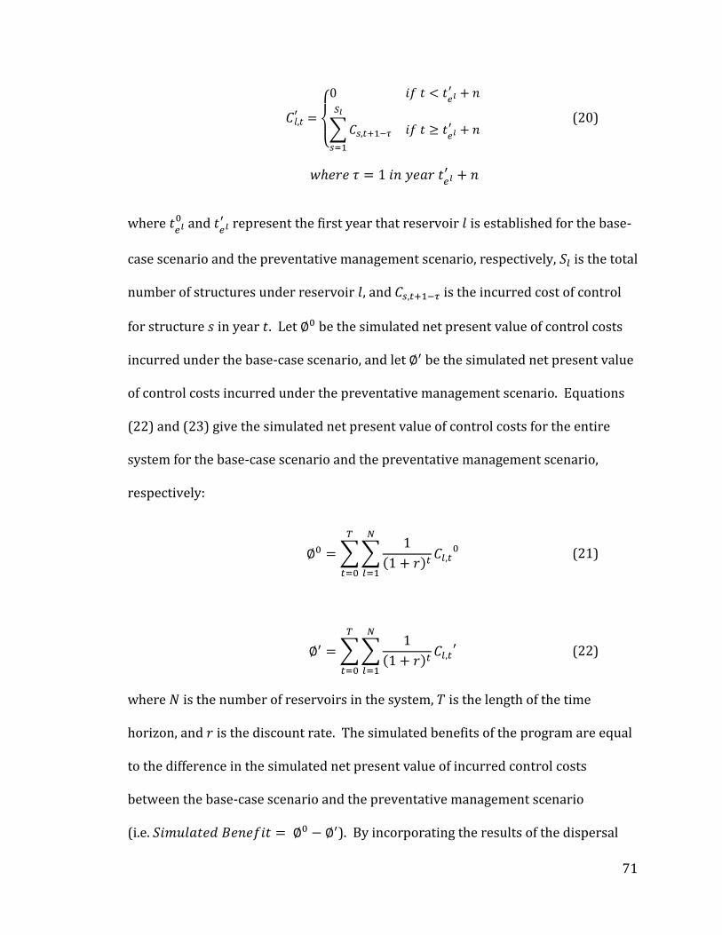
71
(20)
where and
represent the first year that reservoir is established for the base-
case scenario and the preventative management scenario, respectively, is the total
number of structures under reservoir , and is the incurred cost of control
for structure in year . Let be the simulated net present value of control costs
incurred under the base-case scenario, and let be the simulated net present value
of control costs incurred under the preventative management scenario. Equations
(22) and (23) give the simulated net present value of control costs for the entire
system for the base-case scenario and the preventative management scenario,
respectively:
(21)
(22)
where is the number of reservoirs in the system, is the length of the time
horizon, and is the discount rate. The simulated benefits of the program are equal
to the difference in the simulated net present value of incurred control costs
between the base-case scenario and the preventative management scenario
(i.e. ). By incorporating the results of the dispersal

72
model, and integrate the probability of establishment and the costs of control.
These simulated expected control costs are analogous to equations (2) and (3) in the
cost-benefit model.
Choosing the Discount Rate
Choosing an appropriate discount rate for the case of preventing or slowing a
dreissena invasion involves discounting benefits that may happen far in the future.
Furthermore, the event of a dreissena invasion is irreversible and may cause
irreversible damages such as loss of biodiversity. Discount rates for social projects
are generally based on a discount factor of .95 to .99, which corresponds to discount
rates between .01 and .053. Weitzman (1998) argues that the lowest discount rate
possible should be used for discounting the far distant future in long-term
environmental projects. Discount rates between 0 and .053 are tested as part of the
sensitivity analysis to determine how sensitive results are to discounting.
2.3.2 Capital Expenditures and Variable Costs
Appendix B includes a list of all major structures and facilities associated
with the Colorado-Big Thompson system. For each structure type, damage costs are
split into capital expenditures and yearly variable costs. It is assumed that funds for
capital expenditures are borrowed, and that funds for yearly variable costs are
incorporated into yearly budgets. Control costs schedules are constructed by
summing yearly variable costs with principal and interest payments for the capital

73
expenditure loan. Principal and interest payments are calculated using the
amortization formula given in equation (23):
(23)
where is the principal and interest payment, is the amount of the loan, is the
interest rate, and is the term length of the loan, in years.
Parameter Values for Capital Expenditure Loans
Low, base, and high interest rate values ranging between 4% and 5% are
chosen based on the median and quartiles of a sample of 100 bond trades posted on
the EMMA (Electronic Municipal Market Access) website in June of 2010 (MSRB,
2010). Low, base, and high loan term lengths are set at 15, 20, and 30 years,
respectively.
2.3.3 Control Cost Schedules
This section details the data and methods used to develop control costs
schedules for the major structures and facilities in the Colorado-Big Thompson
system. Forecasting specific control costs for water systems and facilities prior to
an invasion is difficult, because control costs depend on the severity of the invasion
and can vary drastically from facility to facility. Control cost schedules are
estimated for the major infrastructure in the Colorado-Big Thompson system using
the best data available. It is important to warn that the data available to make these
estimates is sparse and in many cases dated. In addition, some of the infrastructure
in the system is unique, resulting in a lack of transferable cost data. Control cost
schedules only account for mussel related costs incurred by facilities experiencing

74
settling mussels, and facility costs are assumed to be zero prior to settling. Some
facilities may monitor for mussels before mussels begin to settle in their facility.
Proactive monitoring costs are not included in this analysis for two reasons: (1)
conversations with municipalities in the Colorado-Big Thompson system suggest
that the majority of municipalities in the system are not proactively monitoring for
mussels, and (2) this analysis is focused on the reduction in control costs
attributable to the CDOW boat inspection program. If facilities are proactively
monitoring for mussels then they would likely do so with or without the presence of
the boat inspection program, making the reduction in proactive monitoring costs a
wash. All dollar values have been converted to 2009 dollars using the Bureau of
Labor Statistics Consumer Price Index inflation calculator (Bureau of Labor
Statistics).
A vulnerability report prepared by RNT Consultants (2009) for the Bureau of
Reclamation assesses the vulnerability of Colorado-Big Thompson infrastructure,
and finds that mussels could foul gauging stations, intake structures such as trash
racks, screens, grates, and intake towers, and water conveyance structures such as
piping, siphons, and parts of canals. Fouling of these structures could reduce
performance and additional cleaning and inspection may be necessary. RNT also
identifies minor risks to system pumping plants and power plants (Claudi &
Prescott, 2009). Municipal water treatment facilities that use Colorado-Big
Thompson water are also at risk of mussel fouling.
75
The Colorado-Big Thompson system contains 5 hydroelectric power plants, 4
pump plants, 14 dams, 24 water treatment plants, and nearly 400 km of pipelines,
tunnels, and canals. Appendix B lists all of the facilities and structures considered in
this analysis and their location in the system. Control cost schedules are developed
for all of the water treatment plants, hydropower facilities, dams and pump plants in
the system. Other system infrastructure such as pipelines, tunnels, canals, and
gauging stations are also likely to incur minor damage costs if mussels are present.
A description of the possible damages to these structures is included in the report;
however, due to a lack of data, damage costs for these structures are not included in
the analysis.
Water Treatment Facilities
Chlorine treatment is the most commonly used method for controlling
mussels in water treatment facilities. Most water treatment facilities already use
chlorine as part of their normal operations, so the main control costs for water
treatment facilities are for retrofitting facilities to move chlorine injectors to the
water intake (Deng, 1996). In general, the pattern for water treatment facilities
suggests that facilities have relatively constant yearly expenditures on monitoring
and control costs, and incur the greatest costs in a one-time retrofit of their facility.
Three zebra mussel control cost surveys provide data on zebra mussel
related costs to water treatment facilities: the 1994 survey of raw surface water
users drawing Great Lakes water conducted by Deng (1996), the 1995 National
Zebra Mussel Clearinghouse survey conducted by O'Neill (1997), and the 2004

76
Clearinghouse follow-up survey conducted by Connelly et al. (2007). The Connelly
survey is used to develop cost schedules for the water treatment facilities in the
Colorado-Big Thompson system, because it provides the most recent data on zebra
mussels control costs in water treatment facilities.
A fourth study by the City of Westminster provides an alternative estimate of
control costs to water treatment facilities. In preparation for the possibility of an
invasion in their source reservoir, the City of Westminster, near Denver Colorado,
hired HDR consultants to develop a zebra and quagga mussel management plan
(City of Westminster, 2010). The plan assesses the vulnerability of the City's source
reservoir, Standley Lake, and develops options for controlling mussels if Standley
Lake becomes infested. The control cost estimates developed in the City of
Westminster report are much larger than those reported in the Connelly et al.
(2007) study. This adds additional uncertainty to the potential control costs in the
Colorado-Big Thompson system. To account for the possibility of larger control
costs to municipalities, the model developed for the Colorado-Big Thompson system
gives the option of using control cost values from the Connelly et al. (2007) study, or
a combination of control cost values from the Connelly et al. (2007) study and the
City of Westminster (2010) study.
Water Treatment Control Cost Estimates Based on Values from Connelly et al. (2007)
Connelly et al. (2007) find that expenditures are correlated with facility
capacity, and provide summary statistics for expenditures split by capacity. Table 5
shows average per facility expenditures for the period 1989 to 2004, split by facility

77
capacity, and Table 6 gives capacities of the water treatment facilities in the
Colorado-Big Thompson system, measured in millions of gallons per day (MGD).
Table 5: Average expenditures per facility per period for the period 1989-2004; data from Connelly et al, 2007
Average Expenditures per facility per period
Expenditure Category ≤ 1 MGD 2-10 MGD ≥ 11 MGD
Prevention efforts $17,078 $59,144 $152,468 Lost production and revenues $0 $1,453 $0 Chemical treatment $26,618 $21,981 $64,736
Planning, design, and engineering $17,429 $13,140 $85,934
Retrofit and/or reconstruction $20,989 $30,283 $53,916 Filtration or other mechanical exclusion $2,893 $2,906 $47,352 Monitoring and inspection $17,615 $11,387 $27,388 Mechanical removal $2,956 $4,567 $19,179
Nonchemical treatment $211 $0 $0 Research and development $11 $0 $8,173 Personnel training $911 $1,780 $3,036 Customer education $3,571 $94 $3,443 Other $0 $0 $39,836
Total $110,282 $146,735 $505,461 Dollar values are listed as reported in Connelly et al. (2007), and are not adjusted for inflation. MGD=Millions of Gallons per Day

78
Table 6: Water treatment facility capacities in the Colorado-Big Thompson system
Water Treatment Facility
Capacity (MGD)
Town of Estes 4 Mary's Lake (Town) 2 Newell Warnock <1 City of Loveland 30 Emissaries of Divine Light <1 Eden Valley <1 Spring Canyon 0.25 Fort Collins 87 Soldier Canyon 50 Greeley 21 Carter Lake Filter Plant 1 20 Carter Lake Filter Plant 2 20 Town of Berthoud 4 City of Longmont 1 32 City of Longmont 2 15 Louisville 1 8 Superior 5.5 Town of Erie 12.3 Broomfield 20 City of Fort Lupton 5 City of Fort Morgan 10 City of Boulder 16 City of Lafayette 13 Louisville 2 5
Several of the categories listed in Table 5 represent one-time capital
expenditures, whereas other expenditure categories represent yearly costs. It is
assumed that planning, design, engineering, and retrofit/reconstruction
expenditures are one-time capital expenditures that must be paid in the first year
mussels start settling in the facility. The remainder of the expenditure categories,
with the exception of prevention efforts, are assumed to be ongoing yearly expenses.
Expenses for prevention efforts are omitted. Table 7 breaks expenditures into

79
capital expenditures and average yearly variable costs. The values reported for the
Connelly survey are aggregated over the period 1989 to 2004, thus it is difficult to
adjust these values for inflation. The values in Table 7 have been adjusted to 2009
dollars based on a base year of 1997 (the mid-point between 1989 and 2004).
Table 7: Capital expenditures and yearly variable costs for water treatment facilities; based on data from Connelly et al, 2007
Average Expenditures per facility
≤ 1 MGD 2-10 MGD ≥ 11 MGD
Capital Expenditures Planning, design, and engineering $23,297 $17,564 $114,866 Retrofit and/or reconstruction $28,056 $40,479 $72,068 Total Capital Expenditures $51,353 $58,043 $186,934
Yearly Principal and Interest Payment* $4034 $4559 $14,684
Variable Costs (average yearly values) Lost production and revenues $0 $121 $0 Chemical treatment $2,224 $1,837 $5,408 Filtration or other mechanical exclusion $242 $243 $3,957 Monitoring and inspection $1,472 $952 $2,288 Mechanical removal $247 $381 $1,603
Nonchemical treatment $17 $0 $0
Research and development $1 $0 $683 Personnel training $76 $148 $254
Customer education $298 $8 $287 Other $0 $0 $3,328
Total Average Yearly Variable Costs $4,577 $3,690 $17,808 Dollar values have been adjusted to 2009 dollars using a base year of 1997. *Based on the base interest rate of 4.75% and loan term length of 20 years.
Based on these values, with a base interest rate of 4.75% and a term length of
20 years for capital expenditure loans, control costs for water treatment facilities
with capacities less than 1 MGD are projected to be $8611 for , and $4577
for . Control costs for water treatment facilities with capacities between 2 and

80
10 MGD are projected to be $8249 for , and $3690 for ; and for
facilities with capacities greater than or equal to 11 MGD, control costs are projected
to be $32,492 for , and $17,808 for .
Water Treatment Control Cost Estimates Based on a combination of values from Connelly et al. (2007) and the City of Westminster (2010)
Standley Lake is the source of drinking water for four water providers: the
cities of Westminster, Thornton, and Northglenn, and the Farmers Reservoir and
Irrigation Company (FRICO). From an intake at Standley Lake, water is delivered to
the four entities via a system of pipelines totaling over 30 km in length. This type of
delivery system is common along the Front Range of Colorado. In the Colorado-Big
Thompson system, water is piped from Boulder Reservoir, Horsetooth Reservoir,
and Carter Lake to two, three, and ten water treatment facilities, respectively. These
piping systems are at risk of becoming clogged and could require expensive cleaning
methods such as pigging. Although some of the municipalities in the Connelly et al.
(2007) study may have incurred similar costs, it is not known if these costs are
explicitly accounted for in the Connelly expenditure values. One of the options
developed by the City of Westminster (2010) is to install a chlorine injection system
at the intake from Standley Reservoir. This method of control would chlorinate the
water in the pipelines and would prevent mussels from surviving and settling in the
pipelines. A similar control strategy could be implemented at Boulder Reservoir,
Horsetooth Reservoir, and Carter Lake in the Colorado-Big Thompson system.
To account for the possibility of higher costs to the cities below Boulder
Reservoir, Horsetooth Reservoir, and Carter Lake, the estimated control costs
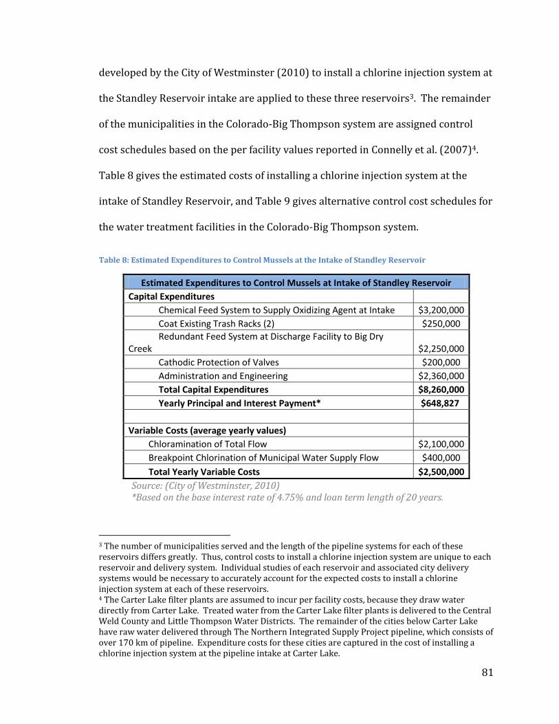
81
developed by the City of Westminster (2010) to install a chlorine injection system at
the Standley Reservoir intake are applied to these three reservoirs3. The remainder
of the municipalities in the Colorado-Big Thompson system are assigned control
cost schedules based on the per facility values reported in Connelly et al. (2007)4.
Table 8 gives the estimated costs of installing a chlorine injection system at the
intake of Standley Reservoir, and Table 9 gives alternative control cost schedules for
the water treatment facilities in the Colorado-Big Thompson system.
Table 8: Estimated Expenditures to Control Mussels at the Intake of Standley Reservoir
Estimated Expenditures to Control Mussels at Intake of Standley Reservoir Capital Expenditures
Chemical Feed System to Supply Oxidizing Agent at Intake $3,200,000 Coat Existing Trash Racks (2) $250,000 Redundant Feed System at Discharge Facility to Big Dry
Creek $2,250,000 Cathodic Protection of Valves $200,000 Administration and Engineering $2,360,000 Total Capital Expenditures $8,260,000 Yearly Principal and Interest Payment* $648,827
Variable Costs (average yearly values)
Chloramination of Total Flow $2,100,000 Breakpoint Chlorination of Municipal Water Supply Flow $400,000
Total Yearly Variable Costs $2,500,000
Source: (City of Westminster, 2010) *Based on the base interest rate of 4.75% and loan term length of 20 years.
3 The number of municipalities served and the length of the pipeline systems for each of these reservoirs differs greatly. Thus, control costs to install a chlorine injection system are unique to each reservoir and delivery system. Individual studies of each reservoir and associated city delivery systems would be necessary to accurately account for the expected costs to install a chlorine injection system at each of these reservoirs. 4 The Carter Lake filter plants are assumed to incur per facility costs, because they draw water directly from Carter Lake. Treated water from the Carter Lake filter plants is delivered to the Central Weld County and Little Thompson Water Districts. The remainder of the cities below Carter Lake have raw water delivered through The Northern Integrated Supply Project pipeline, which consists of over 170 km of pipeline. Expenditure costs for these cities are captured in the cost of installing a chlorine injection system at the pipeline intake at Carter Lake.
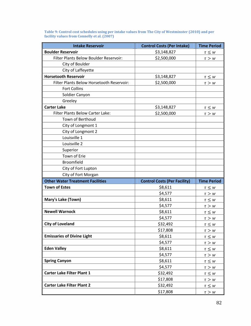
82
Table 9: Control cost schedules using per intake values from The City of Westminster (2010) and per facility values from Connelly et al. (2007)
Intake Reservoir Control Costs (Per Intake) Time Period Boulder Reservoir $3,148,827
Filter Plants Below Boulder Reservoir: $2,500,000 City of Boulder City of Laffeyette
Horsetooth Reservoir $3,148,827 Filter Plants Below Horsetooth Reservoir: $2,500,000
Fort Collins Soldier Canyon Greeley
Carter Lake $3,148,827 Filter Plants Below Carter Lake: $2,500,000
Town of Berthoud City of Longmont 1 City of Longmont 2 Louisville 1 Louisville 2 Superior Town of Erie Broomfield City of Fort Lupton City of Fort Morgan
Other Water Treatment Facilities Control Costs (Per Facility) Time Period Town of Estes $8,611 $4,577 Mary's Lake (Town) $8,611 $4,577 Newell Warnock $8,611 $4,577 City of Loveland $32,492 $17,808 Emissaries of Divine Light $8,611 $4,577 Eden Valley $8,611 $4,577 Spring Canyon $8,611 $4,577 Carter Lake Filter Plant 1 $32,492 $17,808 Carter Lake Filter Plant 2 $32,492 $17,808
83
Hydropower Facilities
Retrofit and control costs for hydropower facilities can vary dramatically, as
each facility is unique. Three sources provide estimates of mussel related control
costs for hydropower facilities: the 1995 National Zebra Mussel Clearinghouse
survey by O'Neill (1997), an estimation study conducted by Phillips et al. (2005),
and an estimate by Leonard Willett, the quagga mussel cordinator for the Hoover
Dam (2010).
Twenty-three hydropower facilities responded to the 1995 National Zebra
Mussel Clearinghouse survey and reported spending a total of $1,759,000 over the
period from 1989-1995, with a mean expenditure of $79,950 per facility. Thirteen
of the twenty-three facilities were infested with zebra mussels at the time of the
survey. Infested facilities had a mean expenditure of $122,154 for the period and
non-infested facilities had a mean expenditure of $17,100 for the period. The
largest hydropower expense was for chemical control, with an average expenditure
of $34,380 per facility. The second greatest expense was for planning and
engineering, with a mean expenditure of $17,865 per facility (O'Neill, 1997).
Philips et al. (2005) estimate the costs of a hypothetical zebra mussel
invasion to thirteen Federal hydropower facilities in the Columbia River Basin. To
develop their estimates, they use actual expenditure data from five invaded eastern
hydroelectric facilities. Based on controls implemented at these facilities, they
assume that the Columbia River Basin facilities will adopt NaOCL (bleach) injection
and anti-fouling paint mitigation strategies. Philips et al. (2005) estimate the cost of

84
a NaOCL injection system to be $62,599 per generator, and the cost of anti-fouling
paint for trash racks to be $81,000 per generator.
Using information from industry sources, Leonard Willett (2010), the quagga
mussel coordinator for the Hoover Dam, estimates that retrofit costs at dams with
hydropower plants can range between $1,000 and $2,000 per megawatt of
generation capacity. Retrofit costs include costs to purchase and install equipment
or modify systems to protect the various generator cooling water, fire water,
domestic water supply, turbine seal water, and transformer cooling water functions.
Willett also estimates annual operation and maintenance costs will increase by $50
to $100 per megawatt of generation capacity. These costs do not include impacts to
the dams themselves.
Table 10 lists the five hydropower facilities in the Colorado-Big Thompson
Project, along with number of generators and megawatts of generation capacity for
each facility. Table 11 gives capital expenditure and yearly variable cost estimates
for each facility based on the three available sources. All values in Table 11 are in
2009 dollars.
Table 10: Hydropower facilities in the Colorado-Big Thompson Project
Hydropower Facility Number of Generators
Megawatts of Generation
Mary's Lake Hydropower Plant 1 8.1 Estes Hydropower Plant 3 45 Pole Hill Hydropower Plant 1 38.2 Flatiron Hydropower Plant 2 94.5 Big Thompson Hydropower Plant 1 4.5

85
Table 11: Capital expenditure and yearly control cost estimates for hydropower facilities in the Colorado-Big Thompson Project
O'Neill Phillips Willett*
Mary's Lake Hydropower Plant Capital expenditures $25,149 $157,743 $12,150 Increase in annual operating
expenditures $8,066 $608 Estes Hydropower Plant
Capital expenditures $25,149 $473,230 $67,500 Increase in annual operating
expenditures $8,066 $3,375 Pole Hill Hydropower Plant
Capital expenditures $25,149 $157,743 $57,300 Increase in annual operating
expenditures $8,066 $2,865 Flatiron Hydropower Plant
Capital expenditures $25,149 $315,487 $141,750 Increase in annual operating
expenditures $8,066 $7,088 Big Thompson Hydropower Plant
Capital expenditures $25,149 $157,743 $6,750 Increase in annual operating
expenditures $8,066 $338 *Per megawatt values are set at the mean value provided by Willet (2010): capital costs=$1500 per megawatt of generation, yearly costs=$150 per megawatt of generation.
The Willett (2010) estimates are chosen to develop control cost schedules for
the Colorado-Big Thompson hydropower facilities based on two factors. The first is
the relative magnitude of the estimates. The vulnerability report prepared by RNT
Consultants states that the hydropower plants in the Colorado-Big Thompson
system are expected to only face minor damages (Claudi & Prescott, 2009). The cost
estimates developed by Phillips et al. (2005) are much larger than those estimated
from the other studies, and thus seem unrealistic for the Colorado-Big Thompson
hydropower facilities. The Willett (2010) estimates and the O'Neill (1997)
estimates are similar in magnitude, but the Willett estimates offer greater

86
differentiation between large and small power plants. The second factor that
supports using the Willett (2010) estimates is that the other two estimates are
based on facilities using chemical controls, whereas the Willett estimates are more
general. RNT consultants comment on the potential control methods that may be
used to treat mussels in affected hydropower facilities in the Colorado-Big
Thompson system. Although chemical treatments are among the most commonly
used control methods for zebra mussels, RNT does not believe that chemical
treatment methods to protect hydropower facilities in the Colorado-Big Thompson
will be acceptable due to sport fishing activities in the area. They suggest small-
pore self-cleaning filters or UV systems as possible alternatives. The cost estimates
produced by Phillips et al. (2005) are based on bleach injection systems, and the
major control methods for the hydropower facilities surveyed in the O'Neill (1997)
study are chemical controls.
Control cost schedules based on the Willett estimates are listed in Table 12.
Per megawatt values are set at the mean value provided by Willet (2010), with
capital costs set at $1500 per megawatt of generation and yearly increases in annual
operating expenditure set at $150 per megawatt of generation.
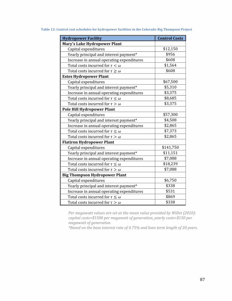
87
Table 12: Control cost schedules for hydropower facilities in the Colorado-Big Thompson Project
Hydropower Facility Control Costs Mary's Lake Hydropower Plant Capital expenditures $12,150 Yearly principal and interest payment* $956 Increase in annual operating expenditures $608 Total costs incurred for $1,564 Total costs incurred for $608 Estes Hydropower Plant
Capital expenditures $67,500 Yearly principal and interest payment* $5,310 Increase in annual operating expenditures $3,375 Total costs incurred for $8,685 Total costs incurred for $3,375
Pole Hill Hydropower Plant Capital expenditures $57,300
Yearly principal and interest payment* $4,508 Increase in annual operating expenditures $2,865 Total costs incurred for $7,373
Total costs incurred for $2,865 Flatiron Hydropower Plant
Capital expenditures $141,750 Yearly principal and interest payment* $11,151 Increase in annual operating expenditures $7,088 Total costs incurred for $18,239 Total costs incurred for $7,088 Big Thompson Hydropower Plant
Capital expenditures $6,750 Yearly principal and interest payment* $338
Increase in annual operating expenditures $531 Total costs incurred for $869 Total costs incurred for $338
Per megawatt values are set at the mean value provided by Willet (2010): capital costs=$1500 per megawatt of generation, yearly costs=$150 per megawatt of generation. *Based on the base interest rate of 4.75% and loan term length of 20 years.

88
Dams
The only specific data available for dams is from the 1995 Clearinghouse
study (O'Neill, 1997). Nine impoundments and reservoirs responded to the survey,
but none of these facilities were infested at the time of the survey. They reported
combined monitoring costs of $27,100 from 1991 through 1995, with a mean
expenditure per facility of $3,010, a minimum expenditure of $1000, and a
maximum expenditure of $17,500. This data is not appropriate for this study,
because cost schedules in this study are based on control costs for infested facilities.
In assessing the vulnerability of dams in the Colorado-Big Thompson Project,
RNT Consultants (Claudi & Prescott, 2009) find that dam trash racks are especially
at risk of biofouling. In the case of infestation, RNT recommends that the inspection
cycle for trash racks be increased from once every 5-years to quarterly. They also
suggest that trash racks can be painted with anti-fouling paint if frequent cleaning is
required. Beyond the potential for trash rack fouling, each of the dams in the system
have unique issues that could result from a mussel infestation. Some may have
issues with pitting corrosion of metal gates, spillway fouling, or pipe fouling. In
general, the potential damages to dams reported by RNT appear to range from none
to moderate. The potential for biofouling of trash racks is common across many of
the dams in the system, and data is available from Phillips et al. (2005) about the
costs of painting trash racks with anti-fouling paint. Using this information, control
cost schedules for dams are based on the cost of painting dam trash racks with anti-
fouling paint. Information from the Phillips et al. (2005) study suggests that the cost
of painting trash racks with anti-fouling paint is about $13.73 per square foot, and

89
the average surface area of a trash rack is about 416 square feet. Table 13 gives the
number of trash racks for each of the dams in the Colorado-Big Thompson Project.
Table 13: Dams in the Colorado-Big Thompson Project
Dams Number of Trash Racks
Willow Creek Dam 1 Granby Dam 1 Shadow Mountain Dam 0 East Portal Reservoir 1 Olympus Dam 1 Rattlesnake Dam 1 Flatiron Dam 1 Horsetooth Dam 1 Soldier Dam 1 Dixon Dam 0 Spring Canyon Dam 0 Carter Lake Dam 1 1 Carter Lake Dam 2 0 Carter Lake Dam 3 0
Control costs schedules for dams are built based on a 5-year useful life of
paint. Thus, costs for dams are equal to $0 in every year for dams with no trash
racks, and equal to $5712 every fifth year for dams that have one trash rack.
The Adams Tunnel also has trash racks that are vulnerable to mussel fouling
(Claudi & Prescott, 2009). The trash racks at the intake to the Adams Tunnel are
large, and it is assumed that the cost to paint the Adams Tunnel trash racks are
twice the cost of painting dam trash racks.

90
Pump Plants
No information was found on the control costs for pump plants. According to
the RNT vulnerability assessment, pump plants that are dry for more than one
month each year should have very few mussel related issues. Any settled mussels
would die of desiccation over the winter when the pump plant was dry, and summer
growth would result in little to no effect on the piping, flow capacity, or pump
systems (Claudi & Prescott, 2009). Table 14 lists all of the pump plants in the
system and shows if they are dry for at least one month each year. Control costs for
pump plants that are dry for at least one month each year are assumed to be zero.
Table 14: Pump plants in the Colorado-Big Thompson Project
Pump Plants Dry for at least one month?
Windy Gap Pump Plant no Willow Creek Pump Plant yes Farr Pumping Plant no Flatiron Reversible Pump yes West Longmont Pumping Plant
no
Louisville/Superior Pumping Plant
no
For lack of better information, the remainder of the pump plants are assumed to
incur costs similar to a mid-sized hydropower facility. Capital expenditures and
yearly variable costs for the Windy Gap, Farr, West Longmont, and
Louisville/Superior pump plants are set equal to those for the Estes Hydropower
Plant.
91
Other Infrastructure
According to the RNT vulnerability report (Claudi & Prescott, 2009), gauging
stations, intake towers, and conveyance structures such as piping, siphons, and
parts of canals are vulnerable to mussel fouling. Fouling of these structures could
reduce performance and additional cleaning and inspection may be necessary. No
cost information was found on control costs for these structures, and potential costs
to these structures have not been included in the analysis. In a conversation with
Fred Nibling of the of the Bureau of Reclamation, he explained that costs for cleaning
and inspecting these types of infrastructure are already incurred and that it is often
difficult to separate costs of other maintenance activities from those resulting from
mussel fouling (Nibling, May 14, 2010). Difficulty in separating mussel related costs
was also reported in the Phillips and Connelly studies (Phillips et al., 2005; Connelly
et al., 2007). The addition of mussels to the Colorado-Big Thompson system would
likely increase the frequency and possible duration of regular maintenance and
inspections, but this value is difficult to quantify. Thus, estimates for control costs in
the system should be considered a lower bound.
Other Affected Industries
Industrial facilities and fossil fuel-fired electric generating facilities that use
raw water as part of their operations have been found to incur large damage costs
from zebra mussel infestations (O'Neill, 1997; Deng, 1996). The extent of these
types of industrial activities using raw Colorado-Big Thompson water is unknown,
but believed to be small. Colorado-Big Thompson water is managed and sold by the

92
Northern Colorado Water Conservancy District, and almost all of their clients are
municipalities and irrigators. Therefore, unless municipalities sell raw Colorado-Big
Thompson water to industrial users, industries using Colorado-Big Thompson water
are not likely to incur mussel control costs.
The Platte River Power Authority (PRPA) is a Windy Gap client (Emsley, June
28, 2010). PRPA cools their fossil-fuel fired power plant with raw water from
Hamilton Reservoir. The majority of the water used to fill Hamilton Reservoir is
effluent from the City of Fort Collins Waste Water Treatment Plant. A small portion
of the water in the reservoir comes from Horsetooth Reservoir. Therefore, if
Horsetooth were to become infested, PRPA would likely incur control costs. The
PRPA power plant is not included in the analysis.
Raw water is often used to irrigate parks and golf courses. In the case of a
mussel infestation, these users would either need to install filtration systems or
switch to purchasing treated water. The cost of filtration systems can be large, and
it is expected that these users would likely switch to purchasing treated water.
Increased water costs to park and golf course irrigators are not included in the
analysis.
If faced with a mussel infestation, irrigators using micro-irrigation systems
and overhead systems may encounter problems. Both irrigation systems involve
pipes that may become clogged by mussels. For these irrigators, sand filters or
mechanical filters at the surface water source may be the best option for controlling
mussels. However, these filtration systems are very expensive, which could lead

93
farmers to substitute away from sprinkler irrigation (Michigan Sea Grant College
Program, 1993). Potential control costs to irrigators are not included in the
analysis.
2.4 Colorado-Big Thompson Zebra and Quagga Mussel Dispersal and Damage Cost Simulation Model
This section describes the bioeconomic simulation model developed for the
Colorado-Big Thompson system, and explains how the dispersal component of the
model is paired with the control cost component of the model to simulate the net
benefits of the preventative management program. The Colorado-Big Thompson
zebra and quagga mussel dispersal and damage cost simulation model is developed
in Microsoft Excel 2007 using Visual Basic 6.5. The Visual Basic code used to run the
model is reproduced in Appendix D. The model simulates a mussel invasion in the
Colorado-Big Thompson system starting with a base year of 2009 and extending for
a ten, thirty, or fifty year time horizon. The base-case scenario and the preventative
management scenario are run simultaneously for 1000 iterations, and the model
outputs a distribution of establishment patterns and associated control costs for
each scenario. An Excel-based interface allows users to easily change parameter
values to test how parameters affect establishment patterns and control costs in the
system.
To develop establishment patterns, the joint probability of colonization from
propagules introduced by boats and the joint probability of colonization from
propagules introduced by downstream flows are calculated for each reservoir in
each year for each scenario. Joint probabilities are functions of propagule pressure
94
from boats and from flows, the invasibility of the reservoir, and the state of the
environment in previous years.
The probability of establishment from downstream flows is dependent on
upstream relationships and flow distances, so the probability of colonization from
downstream flows requires information about how the reservoirs in the system are
connected. Figure 3 on page 13 shows directions of flow and distances between
reservoirs. Windy Gap Reservoir and Willow Creek Reservoir are at the head of the
system, and are considered to have no upstream water bodies. This implies that
these reservoirs are not vulnerable to establishment from upstream water bodies,
which makes the strong assumption that the system cannot receive veligers flowing
from waters outside of the Colorado-Big Thompson system. Flow between Flatiron
Reservoir and Carter Lake is reversible, making each of these reservoirs potentially
upstream from one another. The majority of the reservoirs in the system have one
upstream water body. Lake Granby, Flatiron Reservoir, and Carter Lake all have
two upstream water bodies. To accommodate for the possibility of two upstream
water bodies, two values for propagule pressure from an upstream water body are
calculated for each reservoir. Let
and
be the joint probabilities of
colonization from propagules introduced by flows from upstream water body 1 and
upstream water body 2, respectively, and let
, and
be the joint probabilities
of colonization from propagules introduced by boats under the base case scenario
and under the preventative management scenario, respectively.

95
Using the joint probabilities of colonization, establishment patterns are
determined through a series of Bernoulli trials. In each year and for each scenario,
three Bernouill trials are conducted for each water body (Bossenbroek et al., 2001).
The first trial is based on the joint probability of colonization from propagules
introduced by boats (
for the base-case scenario, and
for the preventative
management scenario), the second trial is based on the joint probability of
colonization from propagules introduced from upstream water body 1, , and the
third is based on the joint probability of colonization from propagules introduced
from upstream water body 2, . A water body is deemed established if at least
one of the Bernoulli Trials results in establishment5. Established upstream water
bodies become possible sources of invasion years after establishment, and once a
water body is established, it remains established in all subsequent years.
To simulate total control costs in the system, structures and facilities directly
downstream from invaded reservoirs are assumed to incur control costs years
after the reservoir directly upstream becomes established. Let be the first year
that reservoir becomes established. Control cost schedules for each of the
structures directly below reservoir are matched in time such that in year
. Control costs are summed over all reservoirs and all years and then
discounted to find the net present value of incurred costs. The model outputs the
5 A shortcoming of this method is that it does not allow for a mix in propagule pressure from boat introductions and from flow introductions. The units used to measure propagule pressure from boats and propagule pressure from downstream flows are not compatible; however, it is possible that propagules introduced by boats could interact with propagules introduced by flows to increase the overall propagule pressure in a reservoir. This would serve to increase the probability that propagules establish a colony.

96
net present value of incurred costs for each scenario and the difference in costs
between each scenario to provide a distribution of benefits of the preventative
management program. Net benefits are calculated as program benefits less
program costs.
2.5 Boat Inspection Program Costs
The costs of the CDOW boat inspection program are equal to the sum of the
direct costs to water recreation managers and the indirect costs incurred by
recreational boaters. Water recreation managers, including CDOW and local
recreation managers, incur direct costs of implementing the boat inspection
program. These direct costs include inspector training costs, administrative costs,
and costs to build and service inspection stations. Boaters do not pay a fee to have
their boats inspected, but they do incur indirect costs associated with the
inspections. All boaters are required to get their boats and trailers inspected and
possibly decontaminated and thus incur time and hassle costs.
2.5.1 Direct Costs of the Boat Inspection Program
The direct costs of the CDOW boat inspection program are estimated using
2009 and 2010 budgets and expenditure information. The largest costs of the
program are for staffing, followed by decontamination units, equipment and
materials, and training. Costs of capital are interest free and are calculated using
straight-line depreciation. The life of the asset is assumed to be equal to the term
length of capital expenditure loans. Total yearly variable costs for implementing the
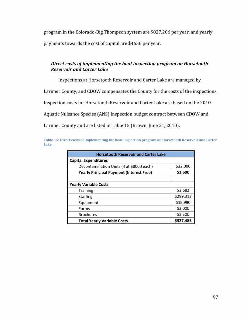
97
program in the Colorado-Big Thompson system are $827,206 per year, and yearly
payments towards the cost of capital are $4656 per year.
Direct costs of implementing the boat inspection program on Horsetooth Reservoir and Carter Lake
Inspections at Horsetooth Reservoir and Carter Lake are managed by
Larimer County, and CDOW compensates the County for the costs of the inspections.
Inspection costs for Horsetooth Reservoir and Carter Lake are based on the 2010
Aquatic Nuisance Species (ANS) Inspection budget contract between CDOW and
Larimer County and are listed in Table 15 (Brown, June 21, 2010).
Table 15: Direct costs of implementing the boat inspection program on Horsetooth Reservoir and Carter Lake
Horsetooth Reservoir and Carter Lake Capital Expenditures
Decontamination Units (4 at $8000 each) $32,000
Yearly Principal Payment (Interest Free) $1,600
Yearly Variable Costs
Training $3,682
Staffing $299,313
Equipment $18,990
Forms $3,000
Brochures $2,500
Total Yearly Variable Costs $327,485

98
Direct costs of implementing the boat inspection program on the Grand County Reservoirs
CDOW manages inspections at the Grand County Reservoirs (Lake Grandby,
Shadow Mountain Reservoir, and Grand Lake). Inspection costs for the Grand
County reservoirs are based on the 2009 CDOW ANS Inspection budget and are
listed in Table 16 (Brown, June 21, 2010).
Table 16: Direct costs of implementing the boat inspection program on the Grand County reservoirs
Grand County Reservoirs Capital Expenditures
Decontamination Units (6 at $6500 each) $39,000
Equipment $22,118
Yearly Principal Payment (Interest Free) $3,056
Yearly Variable Costs
Training $1,458
Staffing $370,400 Operating Expenditures (including brochures, signs, equipment, supplies, travel, per diem, equipment repair, building materials, road materials, equipment repair and maintenance, uniforms, training materials, gas, etc)
$22,118
Vehicle Lease ($1400/month x 5 months) $7,000
Travel and Mileage (1000 miles/month x 5 months x $.45/mile)
$2,250
Total Yearly Variable Costs $403,226
Direct costs of implementing the boat inspection program on Boulder Reservoir
The City of Boulder owns and manages Boulder Reservoir, and is responsible
for boat inspections on the reservoir. Inspection costs for Boulder Reservoir are
based on 2009 expenditures. In 2009, inspections were only conducted for three-
quarters of the boating season. To project full season costs for inspection on
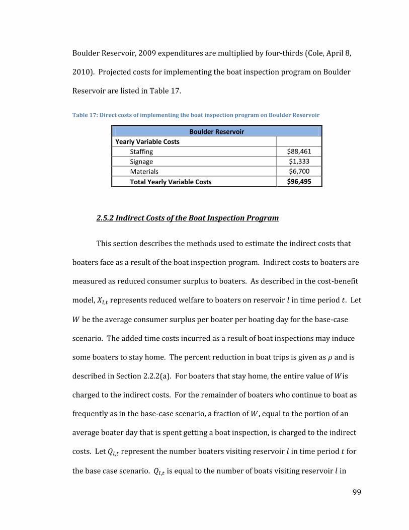
99
Boulder Reservoir, 2009 expenditures are multiplied by four-thirds (Cole, April 8,
2010). Projected costs for implementing the boat inspection program on Boulder
Reservoir are listed in Table 17.
Table 17: Direct costs of implementing the boat inspection program on Boulder Reservoir
Boulder Reservoir Yearly Variable Costs
Staffing $88,461
Signage $1,333
Materials $6,700
Total Yearly Variable Costs $96,495
2.5.2 Indirect Costs of the Boat Inspection Program
This section describes the methods used to estimate the indirect costs that
boaters face as a result of the boat inspection program. Indirect costs to boaters are
measured as reduced consumer surplus to boaters. As described in the cost-benefit
model, represents reduced welfare to boaters on reservoir in time period . Let
be the average consumer surplus per boater per boating day for the base-case
scenario. The added time costs incurred as a result of boat inspections may induce
some boaters to stay home. The percent reduction in boat trips is given as and is
described in Section 2.2.2(a). For boaters that stay home, the entire value of is
charged to the indirect costs. For the remainder of boaters who continue to boat as
frequently as in the base-case scenario, a fraction of , equal to the portion of an
average boater day that is spent getting a boat inspection, is charged to the indirect
costs. Let represent the number boaters visiting reservoir in time period for
the base case scenario. is equal to the number of boats visiting reservoir in
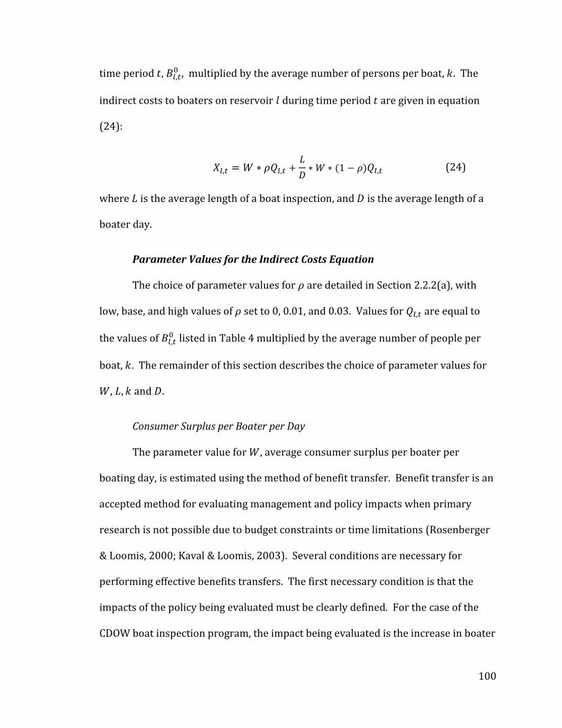
100
time period , , multiplied by the average number of persons per boat, . The
indirect costs to boaters on reservoir during time period are given in equation
(24):
(24)
where is the average length of a boat inspection, and is the average length of a
boater day.
Parameter Values for the Indirect Costs Equation
The choice of parameter values for are detailed in Section 2.2.2(a), with
low, base, and high values of set to 0, 0.01, and 0.03. Values for are equal to
the values of listed in Table 4 multiplied by the average number of people per
boat, . The remainder of this section describes the choice of parameter values for
, and .
Consumer Surplus per Boater per Day
The parameter value for , average consumer surplus per boater per
boating day, is estimated using the method of benefit transfer. Benefit transfer is an
accepted method for evaluating management and policy impacts when primary
research is not possible due to budget constraints or time limitations (Rosenberger
& Loomis, 2000; Kaval & Loomis, 2003). Several conditions are necessary for
performing effective benefits transfers. The first necessary condition is that the
impacts of the policy being evaluated must be clearly defined. For the case of the
CDOW boat inspection program, the impact being evaluated is the increase in boater
101
costs incurred due to wait times for boat inspections. Specifically, this analysis is
concerned with increased costs to recreationists using trailered boats on one of the
seven boatable reservoirs of the Colorado-Big Thompson system. Another
necessary condition is that the markets for and conditions of the study site and the
policy site are similar.
In 2003, Kaval and Loomis (2003) compiled a comprehensive database of all
studies that estimate outdoor recreation use values published between 1967 and
2003. Their database contains fifteen studies that estimate consumer surplus per
person per day for motor boating. Within these studies, a total of 32 boater
consumer surplus measures were estimated. Consumer surplus per boater per day
estimates ranged between $4.31 and $232.01, with a mean of $52.72 and a standard
error of $8.46 (all values are converted to 2009 dollars using the Bureau of Labor
Statistics inflation calculator). Kaval and Loomis separate studies by region, to
provide region specific consumer surplus estimates. Seven of the fifteen motorboat
studies were within the Intermountain Region. Consumer surplus per boater per
day values for the Intermountain Region studies range between $6.03 and $232.01,
with a mean of $61.16, a standard error of $21.61, and a standard deviation of
$57.17. The base value for is set at the average value for the Intermountain
Region. Low and high values of are set at two standard errors below and above
the average.
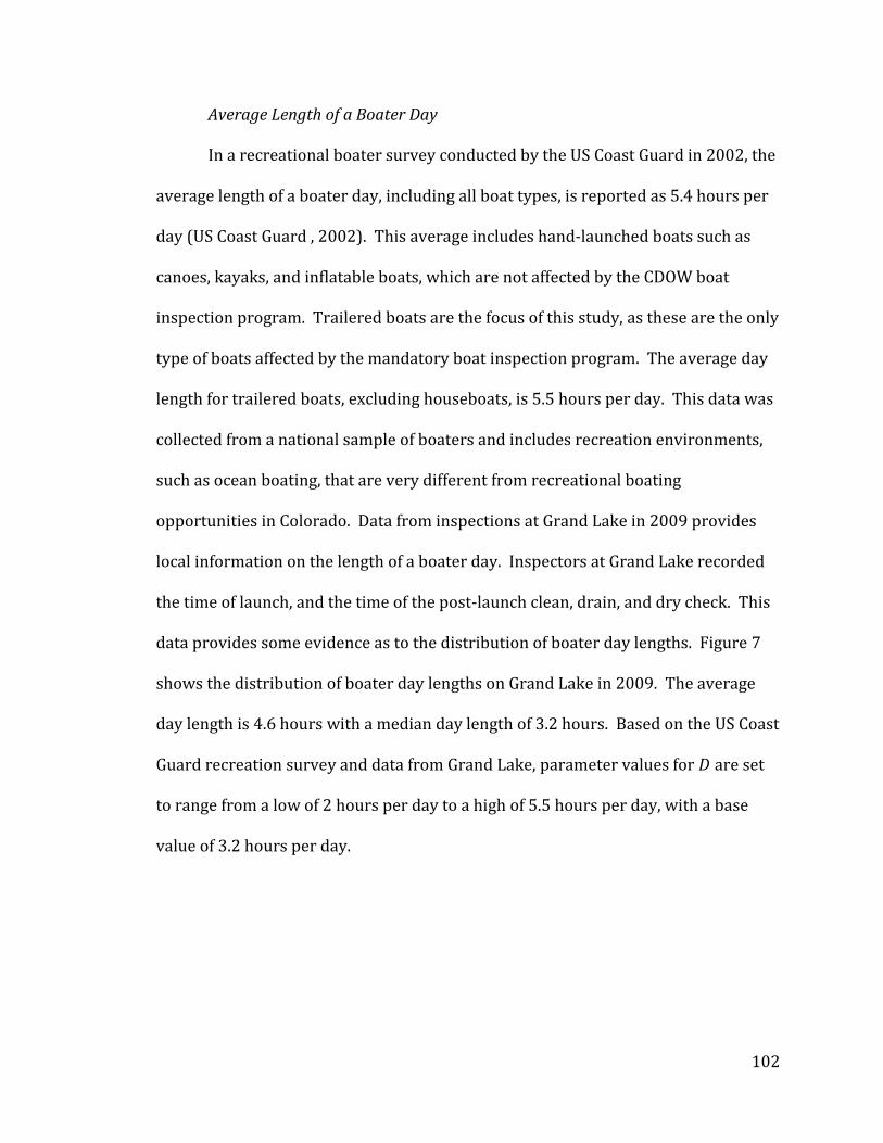
102
Average Length of a Boater Day
In a recreational boater survey conducted by the US Coast Guard in 2002, the
average length of a boater day, including all boat types, is reported as 5.4 hours per
day (US Coast Guard , 2002). This average includes hand-launched boats such as
canoes, kayaks, and inflatable boats, which are not affected by the CDOW boat
inspection program. Trailered boats are the focus of this study, as these are the only
type of boats affected by the mandatory boat inspection program. The average day
length for trailered boats, excluding houseboats, is 5.5 hours per day. This data was
collected from a national sample of boaters and includes recreation environments,
such as ocean boating, that are very different from recreational boating
opportunities in Colorado. Data from inspections at Grand Lake in 2009 provides
local information on the length of a boater day. Inspectors at Grand Lake recorded
the time of launch, and the time of the post-launch clean, drain, and dry check. This
data provides some evidence as to the distribution of boater day lengths. Figure 7
shows the distribution of boater day lengths on Grand Lake in 2009. The average
day length is 4.6 hours with a median day length of 3.2 hours. Based on the US Coast
Guard recreation survey and data from Grand Lake, parameter values for are set
to range from a low of 2 hours per day to a high of 5.5 hours per day, with a base
value of 3.2 hours per day.
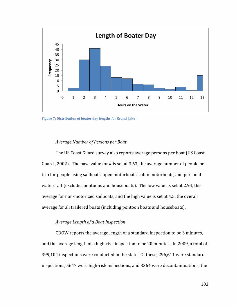
103
Figure 7: Distribution of boater day lengths for Grand Lake
Average Number of Persons per Boat
The US Coast Guard survey also reports average persons per boat (US Coast
Guard , 2002). The base value for is set at 3.63, the average number of people per
trip for people using sailboats, open motorboats, cabin motorboats, and personal
watercraft (excludes pontoons and houseboats). The low value is set at 2.94, the
average for non-motorized sailboats, and the high value is set at 4.5, the overall
average for all trailered boats (including pontoon boats and houseboats).
Average Length of a Boat Inspection
CDOW reports the average length of a standard inspection to be 3 minutes,
and the average length of a high-risk inspection to be 20 minutes. In 2009, a total of
399,104 inspections were conducted in the state. Of these, 296,611 were standard
inspections, 5647 were high-risk inspections, and 3364 were decontaminations; the
0
5
10
15
20
25
30
35
40
45
0 1 2 3 4 5 6 7 8 9 10 11 12 13
Fre
qu
en
cy
Hours on the Water
Length of Boater Day
104
remaining inspections were clean, drain, and dry checks. CDOW reports that, on
average, standard inspections take 3 minutes and high-risk inspections and
decontaminations take 20 minutes (CDOW, 2009). Assuming that clean, drain, and
dry checks take the same amount of time as standard inspections, the weighted
average overall inspection time for all inspections is 3.4 minutes, or .06 hours. In
addition to the time it takes to actually be inspected, boaters may have to wait in a
line to get their inspection or travel out of their way to go to an inspection station.
Based on wait/travel times of 0 minutes, 10 minutes, and 20 minutes, respectively,
the inspection time parameter, , is assigned a low value of .06 hours, a base value of
.22 hours, and a high value of .39 hours.
105
CHAPTER 3: RESULTS
This chapter highlights results of the bioeconomic simulation of the costs and
benefits of preventative management in the Colorado-Big Thompson system. The
focus is on how the preventative management program affects establishment
patterns and associated control costs in the system. Special attention is paid to the
spatial and intertemporal distribution of mussel establishment and associated
control costs.
Based on trends in establishment patterns and control costs, the reservoirs
in the system naturally break into three groups: the Grand County reservoirs
(Willow Creek Reservoir, Lake Grandby, Shadow Mountain Reservoir, and Grand
Lake), the central reservoirs (East Portal Reservoir, Mary's Lake, Lake Estes and
Pinewood Reservoir), and the Front Range reservoirs (Horsetooth Reservoir,
Flatiron Reservoir, Carter Lake, and Boulder Reservoir); see Figure 3, which is
reproduced on page 107. Windy Gap Reservoir is omitted from the discussion,
because it remains unestablished in all model runs.
Model results are generated by running the simulation with each of the
model parameters set at their base values. A description of each of the variables
used in the model is included in Appendix A, and a table of base parameter values is
included in Appendix C. To test the sensitivity of results to parameter values, each
variable is tested by holding all variables at their base values and varying one
106
variable at a time. In some cases, combinations of non-base parameter values are
tested to see how different levels of variables interact to affect the results. To
account for uncertainty in the initial state of the system, the model is run both with
the assumption that the Grand County reservoirs are established in 2009 and with
the assumption that the Grand County reservoirs are unestablished in 2009. To
account for uncertainty in the magnitude of control costs, the model is run using the
low estimates of control costs to water treatment facilities developed from the
Connelly et al. (2007) study, and with the high estimates developed from the City of
Westminster (2010) study.
Section 3.1 describes program costs, establishment patterns and associated
control costs using the base parameter values, and highlights differences in results
based on the initial state of the Grand County reservoirs and on the level of water
treatment control costs used. The section is broken into two subsections: the first
describes establishment patterns in the system and highlights differences between
the three groups of reservoirs, and the second provides results of the cost-benefit
analysis. Section 3.2 describes the results of the sensitivity analysis. To test result
sensitivity to parameter levels, the model variables are broken into five subsections,
each describing a different aspect of the simulation. The parameter groups tested
include environmental parameters, boat pressure parameters, flow parameters,
program parameters, and economic parameters. To account for the fact that the
Colorado-Big Thompson system has an overall low probability of invasibility,
Section 3.3 considers how results would change for a similar system with very high

107
probabilities of invasibility. In Section 3.4, conditions and parameter values that
result in benefit-cost ratios greater than 1 are identified.
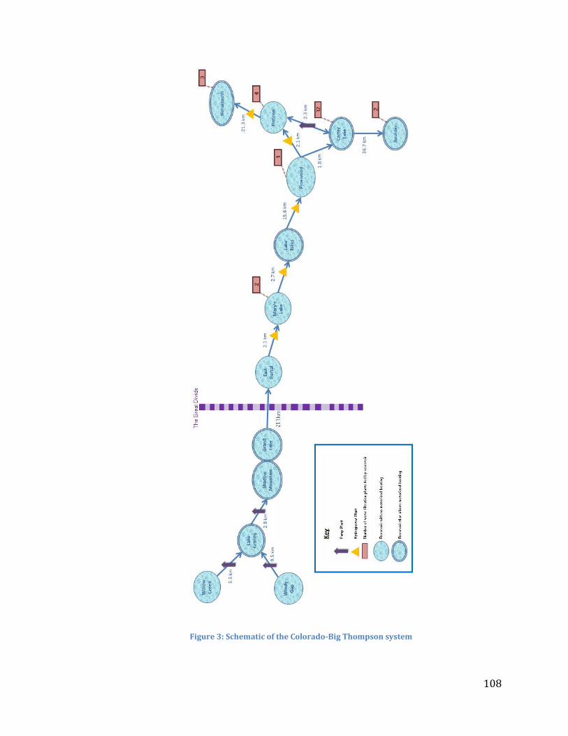
108
Figure 3: Schematic of the Colorado-Big Thompson system
109
3.1 Model Results using Base Parameter Values
This section describes results of the bioeconomic simulation of the costs and
benefits of preventative management in the Colorado-Big Thompson system using
the set of base parameter values. Overall, the results suggest that the preventative
management program is very effective at reducing the probability that reservoirs in
the system become established; however, program benefits, measured as reduced
control costs to dams, pump plants, hydroelectric facilities, and water treatment
facilities, are substantially smaller than program costs. The spatial layout of the
system, the environmental characteristics of the reservoirs, the level and location of
recreational boating activity, and the type of infrastructure in the system play a key
role in determining colonization frequency and timing and the associated benefits of
the preventative management program.
Section 3.1.1 describes establishment patterns and timing of establishment in
the system and details the factors affecting establishment patterns and control costs
across the three groups of reservoirs. Section 3.1.2 provides results of the cost-
benefit analysis and discusses the factors that drive the results.
3.1.1 Baseline Establishment Patterns
Figures 8 through 11 show the simulated establishment patterns and timings
of establishment in the system over a 50-year horizon. Figures 8 and 9 show results
when the Grand County reservoirs are assumed established in 2009, and Figures 10
and 11 show results when the Grand County reservoirs are assumed unestablished
in 2009. For most of the reservoirs in the system, the preventative management
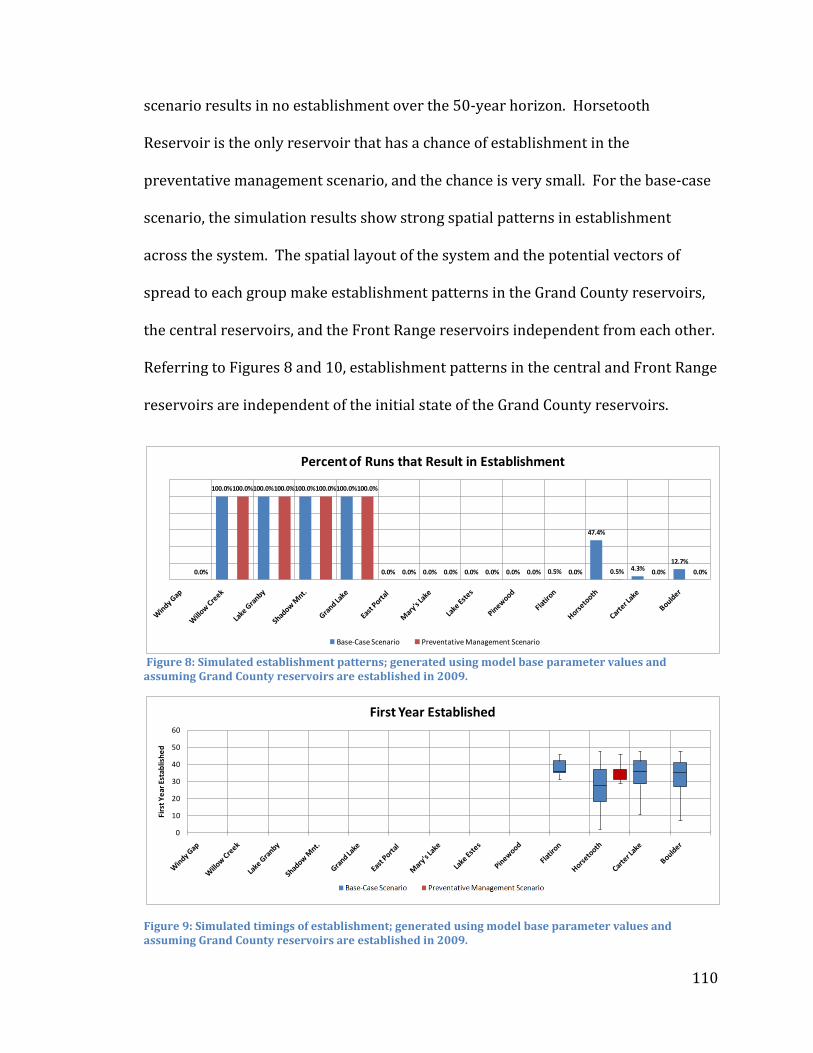
110
scenario results in no establishment over the 50-year horizon. Horsetooth
Reservoir is the only reservoir that has a chance of establishment in the
preventative management scenario, and the chance is very small. For the base-case
scenario, the simulation results show strong spatial patterns in establishment
across the system. The spatial layout of the system and the potential vectors of
spread to each group make establishment patterns in the Grand County reservoirs,
the central reservoirs, and the Front Range reservoirs independent from each other.
Referring to Figures 8 and 10, establishment patterns in the central and Front Range
reservoirs are independent of the initial state of the Grand County reservoirs.
Figure 8: Simulated establishment patterns; generated using model base parameter values and assuming Grand County reservoirs are established in 2009.
Figure 9: Simulated timings of establishment; generated using model base parameter values and assuming Grand County reservoirs are established in 2009.
100.0% 100.0% 100.0% 100.0%
0.0% 0.0% 0.0% 0.0% 0.5%
47.4%
4.3%12.7%
0.0%
100.0% 100.0% 100.0% 100.0%
0.0% 0.0% 0.0% 0.0% 0.0% 0.5% 0.0% 0.0%
Percent of Runs that Result in Establishment
Base-Case Scenario Preventative Management Scenario
0
10
20
30
40
50
60
Firs
t Y
ear
Est
ablis
he
d
Axis Title
First Year Established

111
Figure 10: Simulated establishment patterns; generated using model base parameters and assuming Grand County reservoirs are unestablished in 2009.
Figure 11: Simulated timings of establishment; generated using model base parameter values and assuming the Grand County reservoirs are unestablished in 2009.
Establishment is stochastically determined by the joint probability of
colonization, which is a function of the environmental suitability of the reservoirs,
propagule pressure from boats, and propagule pressure from flows. The
importance of each of these factors differs between the reservoir groups. Figure 12
shows propagule pressure from boats, Figure 13 shows the joint probability of
colonization from boats, and Figure 14 shows the joint probability of colonization
from flows. For all reservoirs, the joint probabilities of colonization from boats
remain below 0.02 for the entire horizon, and the joint probabilities of colonization
0.0%4.3% 2.5% 0.9% 0.0% 0.0% 0.0% 0.0% 0.5%
47.4%
4.3%
12.7%
0.0% 0.0% 0.0% 0.0% 0.0% 0.0% 0.0% 0.0% 0.0% 0.0% 0.5% 0.0% 0.0%
Percent of Runs that Result in Establishment
Base-Case Scenario Preventative Management Scenario
0
10
20
30
40
50
60
Firs
t Y
ear
Est
ablis
he
d
Axis Title
First Year Established

112
from flows remain below 0.0007 for the entire horizon. The very low probabilities
of establishment from flows result in flows making very little contribution to the
establishment of reservoirs in the system. The relatively low probabilities of
colonization from boats result in a low frequency of establishment throughout the
entire system.
Figure 12: Simulated average propagule pressure from boats; generated using model base parameter values.
0
500
1000
1500
2000
2500
3000
3500
0 5 10 15 20 25 30 35 40 45
Nu
mb
er
of P
ote
nti
ally
Infe
ste
d B
oat
s(a
vera
ged
ove
r al
l ru
ns)
Year
Average Propagule Pressure from Boats over Time
BASE-CASE SCENARIO:
Lake Granby
Shadow Mountain Reservoir
Grand Lake
Lake Estes
Horsetooth Reservoir
Carter Lake
Boulder Reservoir
PREVENTATIVE MANAGEMENT SCENARIO:
Lake Granby
Shadow Mountain Reservoir
Grand Lake
Lake Estes
Horsetooth Reservoir
Carter Lake
Boulder Reservoir

113
Figure 13: Simulated average joint probability of colonization from boats; generated using model base parameter values.
Figure 14: Simulated average joint probability of colonization from flows; generated using model base parameter values.
0
0.005
0.01
0.015
0.02
0.025
0 5 10 15 20 25 30 35 40 45
Join
t Pro
babi
lity
of C
olon
izat
ion
(Ave
rage
d ov
er a
ll ru
ns)
Year
Average Joint Probability of Colonization from Boats
BASE-CASE SCENARIO:
Lake Granby
Shadow Mountain Reservoir
Grand Lake
Lake Estes
Horsetooth Reservoir
Carter Lake
Boulder Reservoir
PREVENTATIVE MANAGEMENT SCENARIO:
Lake Granby
Shadow Mountain Reservoir
Grand Lake
Lake Estes
Horsetooth Reservoir
Carter Lake
Boulder Reservoir
0
0.0001
0.0002
0.0003
0.0004
0.0005
0.0006
0.0007
0 5 10 15 20 25 30 35 40 45 50
Ave
rage
Jo
int
Pro
bab
ility
of C
olo
niz
atio
n fr
om
Flo
ws
Year
Average Joint Probability of Colonization by Flows
BASE-CASE SCENARIO:
To Lake Granby From Windy Gap
To Shadow Mountain From Lake Granby
To Grand Lake From Shadow Mountain
To East Portal From Grand Lake
To Mary's Lake from East Portal
To Lake Estes from East Portal
To Pinewood From Lake Estes
To Flatiron From Pinewood
To Horsetooth From Flatiron
To Carter Lake from Pinewood
To Boulder From Carter Lake
To Lake Granby From Willow Creek
To Flatiron From Carter Lake
To Carter Lake from Flatiron

114
Establishment Patterns in the Grand County Reservoirs
The Grand County reservoirs have moderate boat pressure and are all very
close to each other. They are therefore susceptible to establishment from boats or
from flows. However, the reservoirs in this group all have very low probabilities of
invasibility based on low calcium concentrations. The combination of very low
probabilities of invasibility and moderate boat pressure result in overall low joint
probabilities of colonization for the Grand County reservoirs (see figures 13 and
14)6.
Establishment Patterns in the Central Reservoirs
Colonization of the central reservoirs is almost entirely dependent on
propagule pressure from flows. Apart from a small number of trailered boat visits
to Lake Estes, propagules traveling by flows from Grand Lake are the main source of
vulnerability for the central reservoirs. East Portal Reservoir is at the head of the
central reservoirs and is separated from Grand Lake by the 21.1 km Adams Tunnel.
The probability of establishment from flows is a function of the distance between
the source reservoir and the receiving reservoir, and the density of mussels in the
source reservoir. Grand Lake has a very low calcium concentration and is therefore
modeled as supporting a very low density of mussels. The low density of mussels in
Grand Lake combined with the long distance between Grand Lake and East Portal
Reservoir result in very low probabilities of establishment in the central reservoirs.
6 The fact that these reservoirs may already be established suggests that the joint probability of colonization for these reservoirs may be underestimated. This could indicate that the probability of invasibility in these reservoirs is underestimated or that the probability of establishment from boats is underestimated. Section 3.2.1 in the sensitivity analysis addresses the issue of invasibility, and Section 3.2.2 addresses the probability of establishment from boats.

115
These low probabilities of establishment combine with low probabilities of
invasibility to make the joint probabilities of colonization from flows for the central
reservoirs approximately zero (see Figure 14).
Establishment Patterns in the Front Range Reservoirs
The Front Range reservoirs have the greatest probability of establishment.
Among these reservoirs, Horsetooth Reservoir and Boulder reservoir are the most
vulnerable, but their vulnerability is driven by different factors. Horsetooth
Reservoir has very high boat pressure, with nearly 50,000 boat visits each year (see
Figure 12). The boat pressure in Horsetooth Reservoir is so large that the
probability of establishment from boats approaches 1 near the end of the 50-year
horizon. The joint probability of colonization for Horsetooth Reservoir is limited by
the reservoir's very low probability of invasibility, and asymptotically reaches a
maximum of .02 (see Figure 13). Even with this relatively low probability of
colonization, Horsetooth Reservoir becomes established in nearly half of the
simulations (see Figures 8 and 10).
Boulder Reservoir is the only reservoir in the system with a high probability
of invasibility. Boats are the main source of propagules to Boulder Reservoir, and
boat pressure in the reservoir is relatively low (see Figure 12). Despite low boat
pressure, Boulder Reservoir's high probability of invasibility results in a steadily
increasing joint probability of colonization over time (see Figure 13).

116
Timing of Establishment
On average, reservoirs become established between 30 and 40 years into the
future (see Figure 11). Low joint probabilities of colonization in the system result in
low rates of colonization in early years of the horizon. The joint probabilities of
colonization are increasing over time. As the horizon approaches infinity, the joint
probability of colonization approaches the probability of invasibility. Boat pressure
is also increasing over time, which increases the rate at which the joint probability
of colonization approaches its asymptote. The combination of a slow rate of
increase in the percent of potentially infested boats and low probabilities of
invasibility push possible invasions well into the future.
3.1.2 Cost-Benefit Results
This section details the simulated costs and benefits of the boat inspection
program. Benefits are simulated using the base parameter values and with the
assumptions of the Grand County reservoirs established in 2009 and unestablished
in 2009, and with the low water treatment facility control costs based on Connelly et
al. (2007) and the high water treatment facility control costs based on the City of
Westminster (2010). Section 3.2.1 (a) provides a summary of program costs, and
Section 3.2.1 (b) provides a summary of simulated control costs and associated
benefits of the program. There is a gap between program costs and benefits. This
gap is addressed in Section 3.2.1 (c). Table 18 at the end of this section provides a
summary of program costs and benefits.

117
3.2.1 (a) Program Costs
Program costs are comprised of the direct costs of the inspection program
and the indirect costs to boaters. Direct program costs are detailed in Section 2.5.1
and are assumed to be constant over the entire horizon. In total, it costs about $830
thousand dollars per year to implement the boat inspection program on the
reservoirs in the Colorado-Big Thompson system. The net present value (NPV) of
the cost of running the program for 50 years is about $23.5 million dollars. Indirect
costs of the boat inspection program are measured as reduced welfare for boaters
who have to spend time waiting for boat inspections. Section 2.5.2 provides details
about the boater welfare calculation. In total, reductions in boater welfare are
expected to amount to about $1.3 million dollars per year. Assuming welfare losses
are constant over time, the NPV of welfare losses over the 50-year horizon is about
$36 million dollars.
3.2.1 (b) Program Benefits
Program benefits are measured as the reduction in control costs to the dams,
pump plants, hydropower plants, and water treatment plants in the system. The
boat inspection program is very successful at reducing the probability that
reservoirs in the system become established; however, this does not translate into
large program benefits. There are several factors driving this result. The main
factors are the relatively low establishment rates and the late timing of
establishment in the system. For the base-case scenario, only Horsetooth Reservoir
and Boulder Reservoir become established in a substantial number of runs, with

118
Horsetooth Reservoir becoming established in about 46% of runs and Boulder
Reservoir becoming established in about 13% of runs. In the runs where these
reservoirs become established, the timing of establishment is on average 30 to 40
years into the horizon. Furthermore, control costs to facilities below an established
reservoir are scheduled to start eight years after the reservoir is established. So, for
most of the facilities in the system, no control costs are incurred over the horizon,
and for those that do experience control costs, they are not experienced until the
last few years of the simulation.
Almost all of the control costs in the system are experienced by water treatment
facilities below Horsetooth Reservoir, Boulder Reservoir, and Carter Lake. In the
case where the Grand County Reservoirs are assumed established in 2009, the dams
and pump plants associated with the Grand County reservoirs incur control costs
starting in year 2009. These costs increase the NPV of control costs for both the
base-case scenario and the preventative management scenario, so they are not
included in program benefits. All of the hydropower facilities are located in the
central reservoirs. The central reservoirs never become established, so no control
costs are incurred by hydropower facilities.
The expected NPV of control costs to the system are sensitive to the assumed
level of control costs to water treatment facilities. Using the Connelly et al. (2007)
control cost values, the total NPV of control costs to the system are about $560
thousand. Using the City of Westminster (2010) values, the NPV of control costs
increase to about $10 million dollars. The two estimates produce very different

119
benefit-cost ratios. For the Connelly case, the benefits to direct costs ratio is 0.013.
This value increases to 0.423 when the Westminster control cost estimates are used.
If the true control costs in the system are similar to the Connelly et al. (2007)
estimates, then benefits of reduced control costs will never exceed the costs of the
program. However, if the true control costs in the system are similar to the
Westminster (2010) estimates, then parameter values that either increase the
frequency of invasion or make the invasion happen earlier could easily push the
benefits of reduced control costs greater than the costs of the program.

120
3.2.1 (c) Cost-Benefit Gap
Using the model base parameter values, the NPV of the costs of the
inspection program exceed the simulated NPV of the program benefits of reduced
control costs to dams, pump plants, hydropower plants, and water treatment
facilities. The gap between direct program costs and program benefits is about $13
million dollars when the City of Westminster (2010) water treatment facility cost
estimates are used, and about $23 million dollars when the Connelly et al. (2007)
values are used. The simulated cost-benefit gap is driven by three factors: (1) the
probability of establishment in the system is low, (2) once established, facility
control costs in the system are relatively low compared to program costs, and (3)
program costs are incurred in every year whereas program benefits are realized 30
to 40 years in the future. As measured in this analysis, benefits only include reduced
control costs to infrastructure and facilities in the system. Non-market benefits such
as the prevention of ecosystem disruption, reductions in ecosystem services, and
diminished recreational opportunities are not included in the benefit calculation.
Also omitted from program benefits are reductions in control costs to irrigators and
industries using raw Colorado-Big Thompson water. The boat inspection program
is cost-effective if all of the omitted program benefits exceed the cost-benefit gap.
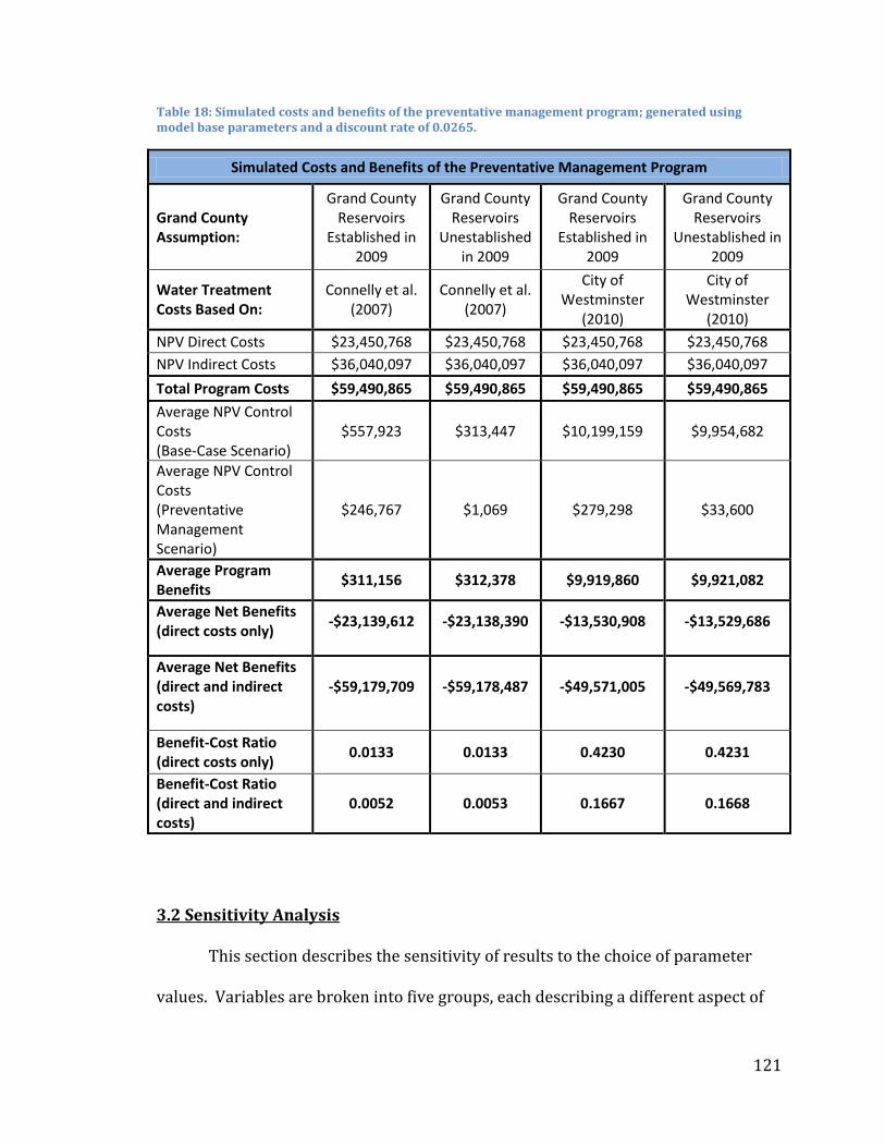
121
Table 18: Simulated costs and benefits of the preventative management program; generated using model base parameters and a discount rate of 0.0265.
Simulated Costs and Benefits of the Preventative Management Program
Grand County Assumption:
Grand County Reservoirs
Established in 2009
Grand County Reservoirs
Unestablished in 2009
Grand County Reservoirs
Established in 2009
Grand County Reservoirs
Unestablished in 2009
Water Treatment Costs Based On:
Connelly et al. (2007)
Connelly et al. (2007)
City of Westminster
(2010)
City of Westminster
(2010)
NPV Direct Costs $23,450,768 $23,450,768 $23,450,768 $23,450,768
NPV Indirect Costs $36,040,097 $36,040,097 $36,040,097 $36,040,097
Total Program Costs $59,490,865 $59,490,865 $59,490,865 $59,490,865
Average NPV Control Costs (Base-Case Scenario)
$557,923 $313,447 $10,199,159 $9,954,682
Average NPV Control Costs (Preventative Management Scenario)
$246,767 $1,069 $279,298 $33,600
Average Program Benefits
$311,156 $312,378 $9,919,860 $9,921,082
Average Net Benefits (direct costs only)
-$23,139,612 -$23,138,390 -$13,530,908 -$13,529,686
Average Net Benefits (direct and indirect costs)
-$59,179,709 -$59,178,487 -$49,571,005 -$49,569,783
Benefit-Cost Ratio (direct costs only)
0.0133 0.0133 0.4230 0.4231
Benefit-Cost Ratio (direct and indirect costs)
0.0052 0.0053 0.1667 0.1668
3.2 Sensitivity Analysis
This section describes the sensitivity of results to the choice of parameter
values. Variables are broken into five groups, each describing a different aspect of
122
the simulation. The parameter groups tested include environmental parameters,
boat pressure parameters, flow parameters, program parameters, and economic
parameters. Appendix A provides a description of each of the variables in the model
and gives a low, base, and high parameter value for each variable.
3.2.1 Environmental Parameters
The probability of invasibility, is an important and uncertain component
in the model. Values for are chosen subjectively based on calcium
concentrations. The low values of set the probability of invasibility for very low
and low calcium reservoirs equal to zero. If probabilities of invasibility are this low
in the system, only Boulder Reservoir is at risk of colonization. At base values of ,
the Grand County reservoirs, Carter Lake, and Horsetooth Reservoir become
vulnerable to infestation, but the central reservoirs remain free of mussels. The
same reservoirs are vulnerable at the high values of , but become established at
higher frequencies and in earlier years. This is especially true for Horsetooth
Reservoir, which on average becomes established 10 years earlier than with the
base values of and becomes established in over 80% of runs.
The parameter values chosen for the probability of invasibility have a
substantial effect on the average NPV of control costs and on program benefits.
Using the Connelly et al. (2007) control values for water treatment facilities, the
NPV of control costs in the system increase from about $16 thousand dollars for the
low values of to about $2.7 million dollars for the high values of . This
translates to a $2.5 million dollar increase in program benefits, but has little effect
123
on the benefit-cost ratio. Using the City of Westminster (2010) control values for
water treatment facilities, the NPV of control costs in the system increase from
about $1.1 million dollars for the low values of to about $19.9 million dollars for
the high values of . This translates to an $18.6 million dollar increase in program
benefits and increases the benefits to direct costs ratio from .038 to .831.
Probabilities of invasibility are assigned to reservoirs based on their calcium
concentrations. Calcium concentrations in the central reservoirs are unknown and
could range from very low to moderate. If the Grand County reservoirs are assumed
unestablished in 2009, then the calcium levels in the central reservoirs make no
difference in the probability of establishment for these reservoirs. If the Grand
County reservoirs are assumed established in 2009, then the calcium levels in the
central reservoirs have a slight effect on establishment patterns in the system. With
very low calcium levels, the central reservoirs do not become established. With low
and moderate calcium levels, there is a very small chance that East Portal Reservoir
may become established by flows from Grand Lake. Overall, the calcium levels in
the central reservoirs make very little difference on establishment patterns and the
expected control costs in the system.
3.2.2 Boat Pressure Parameters
This section considers how parameters levels for the variables that affect
boat pressure affect simulation results. The variables considered in this section
include , the shape parameter in the probability of establishment from boats
function, and , the random walk variables that affect the rate at which the

124
percent of potentially infested boats increases over time and , the percent by
which the boat inspection program slows the rate of increase in the percent of
potentially infested boats.
Average NPVs of control costs and program benefits are sensitive to the
shape parameter. The same reservoirs are susceptible to colonization for all
levels of , but the chance that these reservoirs become established increases as
increases. Reservoirs also become established earlier for larger values of .
Benefit-cost ratios remain low for all levels of when the water treatment cost
values based on Connelly et al. (2007) are used; however, using the City of
Westminster (2010) estimates and the high value for , the benefits to direct costs
ratio increases to 1.4. This suggests that results of the cost-benefit analysis are
highly dependent on the probability of establishment from boats and estimates of
control costs in the system.
Values of , and reflect how quickly the invasion is happening. In
general, the faster the invasion, the greater the benefits of preventative
management. If the invasion is not progressing (i.e. ), then only
Horsetooth Reservoir is at risk of colonization. This is due to the very large boat
pressure at Horsetooth Reservoir. As the rate of invasion increases and a greater
percent of boats become possible sources of propagules, the chance of invasion in
Boulder Reservoir and Carter Lake increases, thus increasing control costs to the
Front Range water treatment facilities. Overall, the rate of invasion has a very small
effect on the expected NPV of control costs in the system and on program benefits.
125
The parameter represents the percent by which the boat inspection
program slows the rate of increase in the percent of potentially infested boats. The
level of has very little effect on establishment patterns in the preventative
management scenario. This is largely due to the high efficacy of the boat inspection
program. At its base parameter setting, the program catches and cleans 95% of the
potentially infested boats that enter the system. At this level of efficacy, the rate at
which the percent of potentially infested boats is growing makes no difference on
establishment patterns in the preventative management scenario. At lower levels of
program efficacy, has a small effect on the probability of establishment in
Horsetooth Reservoir.
3.2.3 Flow Parameters
Five variables affect the probability of establishment from flows: the density
of the upstream water body ( ), the lag time between when an upstream
reservoir becomes established and when it becomes a source of propagules to
downstream reservoirs ( , the rate at which veligers decay ( ), and the alpha and
c shape parameters in the probability of establishment by flows function ( and
). When the model is run with the base parameters and the Grand County
reservoirs are assumed unestablished in 2009, none of these variables have a
substantial effect on establishment patterns in the system.
To test how flows could affect establishment in the system under more
favorable flow conditions, the model is run with the Grand County reservoirs
assumed established in 2009, set at its highest value, and , , and set at their
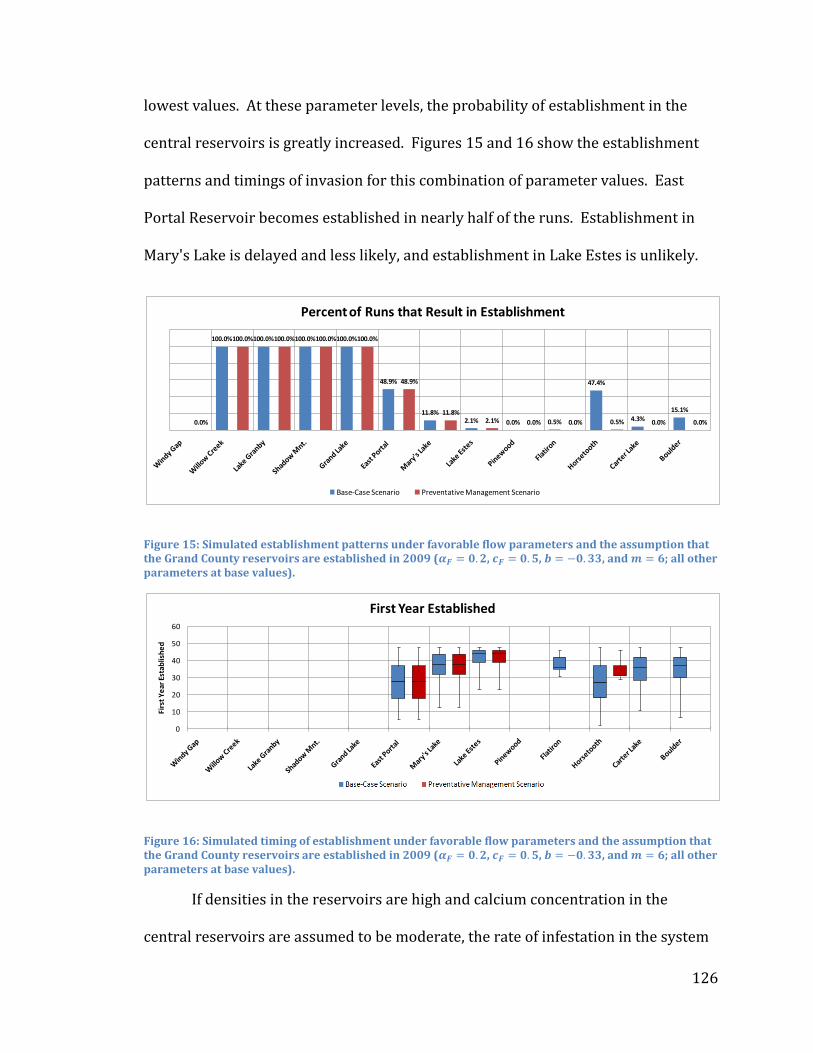
126
lowest values. At these parameter levels, the probability of establishment in the
central reservoirs is greatly increased. Figures 15 and 16 show the establishment
patterns and timings of invasion for this combination of parameter values. East
Portal Reservoir becomes established in nearly half of the runs. Establishment in
Mary's Lake is delayed and less likely, and establishment in Lake Estes is unlikely.
Figure 15: Simulated establishment patterns under favorable flow parameters and the assumption that the Grand County reservoirs are established in 2009 ( , , , and ; all other parameters at base values).
Figure 16: Simulated timing of establishment under favorable flow parameters and the assumption that the Grand County reservoirs are established in 2009 ( , , , and ; all other parameters at base values).
If densities in the reservoirs are high and calcium concentration in the
central reservoirs are assumed to be moderate, the rate of infestation in the system
100.0% 100.0% 100.0% 100.0%
48.9%
11.8%2.1% 0.0% 0.5%
47.4%
4.3%15.1%
0.0%
100.0% 100.0% 100.0% 100.0%
48.9%
11.8%2.1% 0.0% 0.0% 0.5% 0.0% 0.0%
Percent of Runs that Result in Establishment
Base-Case Scenario Preventative Management Scenario
0
10
20
30
40
50
60
Firs
t Y
ear
Est
ablis
he
d
Axis Title
First Year Established

127
increases dramatically and infestation occurs earlier. Figures 17 and 18 show
model results under high density conditions when the Grand County reservoirs are
assumed established in 2009, is set at its highest value, and , , and are set at
their lowest values. Under these conditions, establishment by flows becomes an
important driver in the system.
Figure 17: Simulated establishment patterns under favorable flow conditions, high densities, and the assumption that the Grand County reservoirs are established in 2009 ( individuals per m2 for all reservoirs in the system, calcium levels in the central reservoirs are assumed to be moderate, , , and ; all other parameters at base values).
Figure 18: Simulated timing of establishment under favorable flow conditions, high densities, and the assumption that the Grand County reservoirs are established in 2009 ( individuals per m2 for all reservoirs in the system, calcium levels in the central reservoirs are assumed to be moderate, , , and ; all other parameters at base values).
100.0% 100.0% 100.0% 100.0% 100.0% 100.0% 99.6%94.6%
72.4%
49.7%
16.3% 19.9%
0.0%
100.0% 100.0% 100.0% 100.0% 100.0% 100.0% 99.6%94.6%
71.6%
3.9%12.8%
5.4%
Percent of Runs that Result in Establishment
Base-Case Scenario Preventative Management Scenario
0
10
20
30
40
50
60
Firs
t Y
ear
Est
ablis
he
d
Axis Title
First Year Established
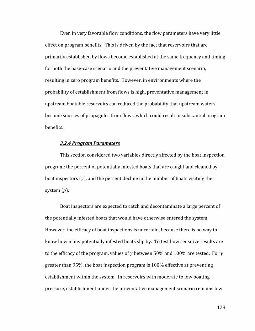
128
Even in very favorable flow conditions, the flow parameters have very little
effect on program benefits. This is driven by the fact that reservoirs that are
primarily established by flows become established at the same frequency and timing
for both the base-case scenario and the preventative management scenario,
resulting in zero program benefits. However, in environments where the
probability of establishment from flows is high, preventative management in
upstream boatable reservoirs can reduced the probability that upstream waters
become sources of propagules from flows, which could result in substantial program
benefits.
3.2.4 Program Parameters
This section considered two variables directly affected by the boat inspection
program: the percent of potentially infested boats that are caught and cleaned by
boat inspectors ( ), and the percent decline in the number of boats visiting the
system ( ).
Boat inspectors are expected to catch and decontaminate a large percent of
the potentially infested boats that would have otherwise entered the system.
However, the efficacy of boat inspections is uncertain, because there is no way to
know how many potentially infested boats slip by. To test how sensitive results are
to the efficacy of the program, values of between 50% and 100% are tested. For
greater than 95%, the boat inspection program is 100% effective at preventing
establishment within the system. In reservoirs with moderate to low boating
pressure, establishment under the preventative management scenario remains low

129
even at a level of 50%. Establishment in Horsetooth Reservoir, which has very
high boat pressure, is more sensitive to . This suggests that the quality of boat
inspections at reservoirs with high boat pressure is paramount to the overall
effectiveness of the program.
The boat inspection program may induce some boaters to reduce the number
of boating trips they take in a year. Overall, demand for boating is expected to be
inelastic, and values of between 0 and .03 are tested in the model. Over this range
of values, boater behavior has very little effect on establishment patterns or control
costs in the system. The level of does have a substantial effect on the indirect
costs of the boat inspection program. With no decline in boat visits (i.e. perfectly
inelastic demand), the NPV of the indirect costs of the program are about $55
million. With a 3% decline in boat visits, the NPV of the indirect costs of the
program increase to about $69 million.
3.2.5 Economic Parameters
This section addresses the effect of parameter levels for variables directly
associated with the net present value calculations, control cost calculations, and
program cost calculations.
Net Present Value Parameters
The discount rate ( ) and the time horizon are the main variables driving the
net present value calculations. With respect to the discount rate, the benefit-cost
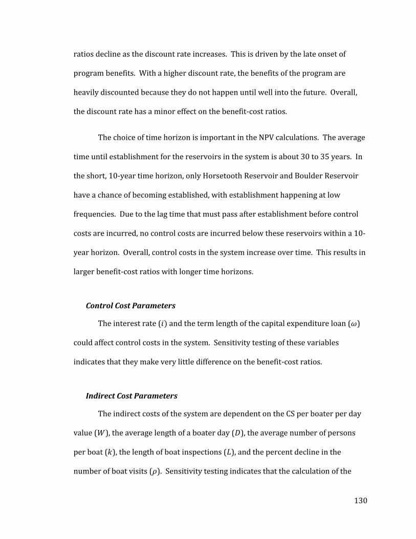
130
ratios decline as the discount rate increases. This is driven by the late onset of
program benefits. With a higher discount rate, the benefits of the program are
heavily discounted because they do not happen until well into the future. Overall,
the discount rate has a minor effect on the benefit-cost ratios.
The choice of time horizon is important in the NPV calculations. The average
time until establishment for the reservoirs in the system is about 30 to 35 years. In
the short, 10-year time horizon, only Horsetooth Reservoir and Boulder Reservoir
have a chance of becoming established, with establishment happening at low
frequencies. Due to the lag time that must pass after establishment before control
costs are incurred, no control costs are incurred below these reservoirs within a 10-
year horizon. Overall, control costs in the system increase over time. This results in
larger benefit-cost ratios with longer time horizons.
Control Cost Parameters
The interest rate ( and the term length of the capital expenditure loan ( )
could affect control costs in the system. Sensitivity testing of these variables
indicates that they make very little difference on the benefit-cost ratios.
Indirect Cost Parameters
The indirect costs of the system are dependent on the CS per boater per day
value ( ), the average length of a boater day ( ), the average number of persons
per boat ( ), the length of boat inspections ( ), and the percent decline in the
number of boat visits ( ). Sensitivity testing indicates that the calculation of the

131
reduction in boater welfare is very sensitive to all of these variables. To give an idea
of the possible range of values, lowest and highest scenarios are presented. Welfare
losses are lowest when the average length of a boater day is set at its highest value,
and the number of persons per boat, the length of a boat inspection, and the percent
decline in the number of boat visits are all set at their lowest values. Holding at
its base value, the lowest estimate of the direct costs of the boat inspection program
is $143 thousand dollars per year. To calculate the high estimate of direct costs, the
length of a boater day is set at its lowest value, and the number of persons per boat,
the length of a boat inspection, and the percent decline in the number of boat visits
are all set at their highest values. This results in a high estimate of $4 million dollars
per year. Thus, there is much uncertainty in the value of welfare losses to boaters,
and this could be an important area for further research.
3.3 Results for a Highly Invasible System
The majority of the reservoirs in the Colorado-Big Thompson system have
very low calcium levels, which results in low probabilities of invasibility. The CDOW
boat inspection program is a statewide mandate, and could have different effects in
other water bodies in the state that have higher probabilities of invasibility. To
consider the costs and benefits of preventative management to a similar but highly
invasible system, probabilities of invasibility are set to 0.8 and population densities
are set to 7500 individuals/m2 for all of the reservoirs in the system.
Figures 19 and 20 show establishment patterns in the reservoirs under these
conditions. For the base-case scenario, the probability of establishment in the
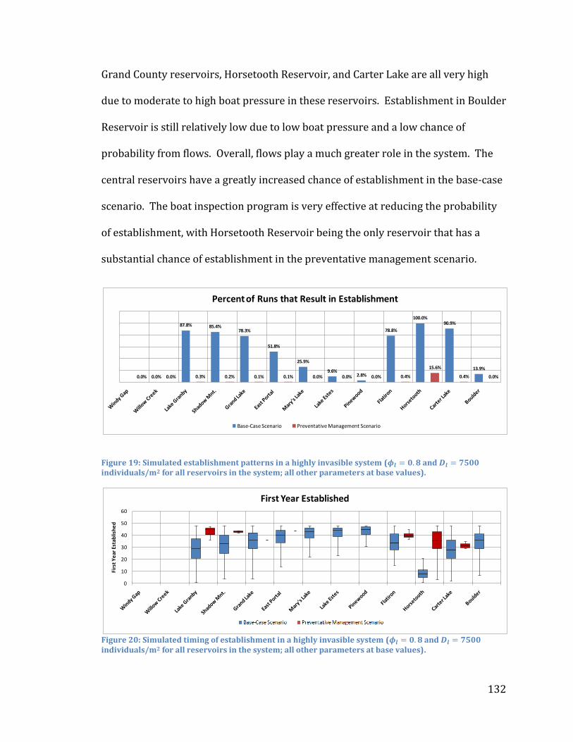
132
Grand County reservoirs, Horsetooth Reservoir, and Carter Lake are all very high
due to moderate to high boat pressure in these reservoirs. Establishment in Boulder
Reservoir is still relatively low due to low boat pressure and a low chance of
probability from flows. Overall, flows play a much greater role in the system. The
central reservoirs have a greatly increased chance of establishment in the base-case
scenario. The boat inspection program is very effective at reducing the probability
of establishment, with Horsetooth Reservoir being the only reservoir that has a
substantial chance of establishment in the preventative management scenario.
Figure 19: Simulated establishment patterns in a highly invasible system ( and individuals/m2 for all reservoirs in the system; all other parameters at base values).
Figure 20: Simulated timing of establishment in a highly invasible system ( and individuals/m2 for all reservoirs in the system; all other parameters at base values).
0.0%
87.8% 85.4%78.3%
51.8%
25.9%
9.6%2.8%
78.8%
100.0%90.9%
13.9%
0.0% 0.0% 0.3% 0.2% 0.1% 0.1% 0.0% 0.0% 0.0% 0.4%
15.6%
0.4% 0.0%
Percent of Runs that Result in Establishment
Base-Case Scenario Preventative Management Scenario
0
10
20
30
40
50
60
Firs
t Y
ear
Est
ablis
he
d
Axis Title
First Year Established
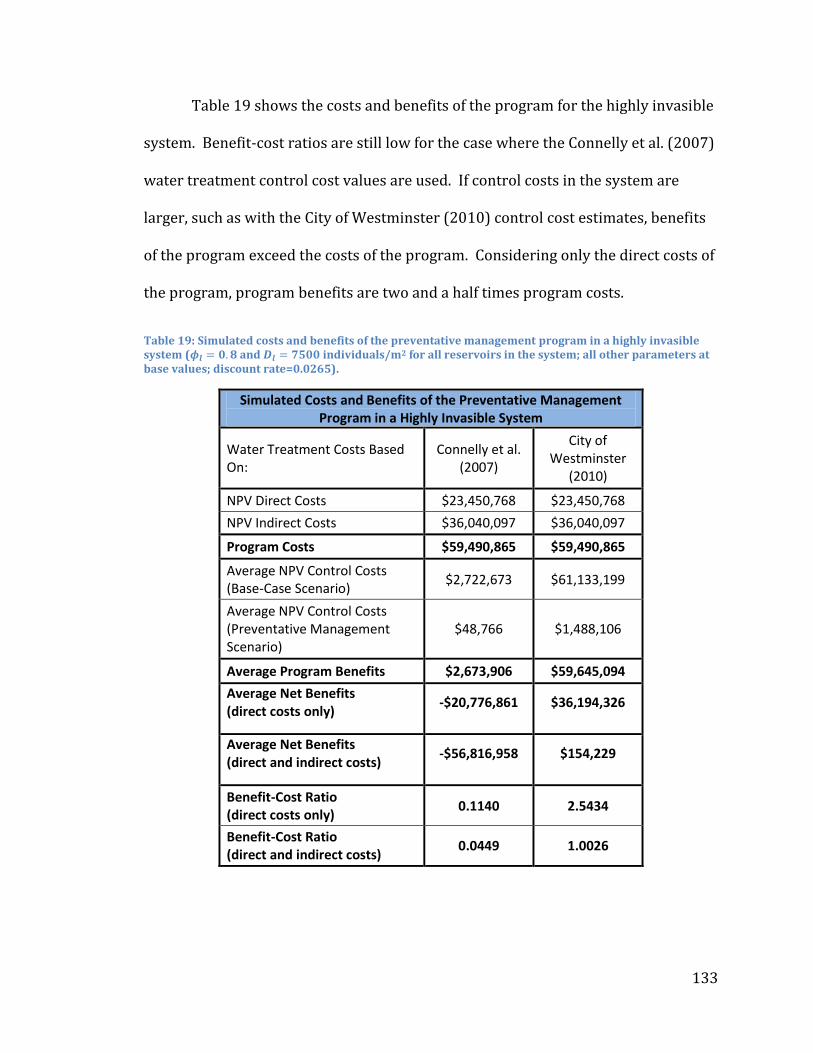
133
Table 19 shows the costs and benefits of the program for the highly invasible
system. Benefit-cost ratios are still low for the case where the Connelly et al. (2007)
water treatment control cost values are used. If control costs in the system are
larger, such as with the City of Westminster (2010) control cost estimates, benefits
of the program exceed the costs of the program. Considering only the direct costs of
the program, program benefits are two and a half times program costs.
Table 19: Simulated costs and benefits of the preventative management program in a highly invasible system ( and individuals/m2 for all reservoirs in the system; all other parameters at base values; discount rate=0.0265).
Simulated Costs and Benefits of the Preventative Management Program in a Highly Invasible System
Water Treatment Costs Based On:
Connelly et al. (2007)
City of Westminster
(2010)
NPV Direct Costs $23,450,768 $23,450,768
NPV Indirect Costs $36,040,097 $36,040,097
Program Costs $59,490,865 $59,490,865
Average NPV Control Costs (Base-Case Scenario)
$2,722,673 $61,133,199
Average NPV Control Costs (Preventative Management Scenario)
$48,766 $1,488,106
Average Program Benefits $2,673,906 $59,645,094
Average Net Benefits (direct costs only)
-$20,776,861 $36,194,326
Average Net Benefits (direct and indirect costs)
-$56,816,958 $154,229
Benefit-Cost Ratio (direct costs only)
0.1140 2.5434
Benefit-Cost Ratio (direct and indirect costs)
0.0449 1.0026

134
3.4 Benefit-Cost Ratios
Results suggest that benefit-cost ratios are sensitive to the probability of
establishment from boats, the invasibility of the system, and the level of control
costs facilities expect to incur if infested. If control costs for water treatment
facilities are as low as the Connelly et al. (2007) study suggests, then benefits of
reduced control costs will never exceed direct program costs. If control costs are
higher, like those estimated in the City of Westminster (2010) study, then the gap
between the benefits of reduced control and the direct cost of the boat inspection
program is much smaller. At higher control costs, increasing the probability of
invasibility in the system or increasing the probability of establishment from boats
both result in benefit-cost ratios greater than 1. In the case of a highly invasible
system, it would be reasonable to spend as much as $2.1 million dollars per year to
reduce control costs in the system.

135
CHAPTER 4: SUMMARY AND CONCLUSIONS
Colorado is expected to spend about $2.3 million dollars per year to slow or
prevent the spread of aquatic nuisance species in the state (Colorado Division of
Wildlife and Colorado State Parks, 2010). Of those expenditures, about one-third is
budgeted for boat inspections in the reservoirs of the Colorado-Big Thompson
system. This study provides information about how the boat inspection program
affects the potential spread of mussels in the Colorado-Big Thompson system, and
subsequently, how the program affects control costs for facilities and infrastructure
in the system. The objective of this analysis is to compare the costs of boat
inspections on the reservoirs of the Colorado-Big Thompson system to the benefits
of reduced control costs to the dams, pump plants, hydropower facilities, and
municipal water treatment facilities associated with the system.
A bioeconomic simulation model is developed to intertemporally predict
mussel spread in the reservoirs of the Colorado-Big Thompson system over a 50-
year horizon. Joint probabilities of colonization are estimated for each reservoir in
each year based on three factors: (1) the probability that the reservoir is invasible,
(2) the probability that the reservoir becomes established by propagules introduced
by boats, and (3) the probability that the reservoir becomes established by
propagules introduced by flows from an infested upstream reservoir. In each year,
reservoirs are subjected to a Bernoulli trail based on their joint probabilities of
colonization and either become infested or remain uninfested.

136
The simulation model predicts spread in the system under a base-case
scenario of no preventative management, and under an alternative scenario in
which the boat inspection program is in place. The key difference between the two
scenarios is the probability that reservoirs become established by propagules
introduced by boats. By slowing the rate of invasion and by catching and cleaning a
large percent of boats that are potentially carrying mussels, the boat inspection
program reduces the probability that a reservoir becomes established by
propagules introduced by boats and thus reduces the joint probability of
colonization.
Control cost schedules are developed for all of the dams, pump plants,
hydropower facilities, and municipal water treatment facilities in the Colorado-Big
Thompson system, and expected control costs in the system are assessed by
intertemporally matching results of the simulated invasion to control cost
schedules. Program benefits are measured as the difference in the net present value
of expected control costs for the base-case scenario and for the preventative
management scenario, and program costs are measured as the sum of the net
present values of the direct costs of implementing the program and the indirect
costs of reduced boater welfare. Net program benefits are equal to program
benefits less program costs.
Results of the simulation suggest that the boat inspection program is very
effective at reducing the probability that reservoirs in the system become
established, and almost entirely eliminates the possibility of invasion in the system

137
over the 50-year horizon. However, the benefits of reduced control costs to
infrastructure are not likely to exceed the costs of the boat inspection program. The
main factor driving this result is that the probability of invasion in the system is
likely to be low even without the boat inspection program, thus leading to low
expected control costs for the base-case scenario. The majority of the reservoirs in
the Colorado-Big Thompson system have low or very low probabilities of
invasibility based on low calcium concentrations. These low probabilities of
invasibility result in low joint probabilities of colonization and overall low
frequencies of invasion and late timings of invasion in the simulation. The spatial
layout of the system also plays a role in the cost-benefit results. All of the
hydropower facilities in the system are located between East Portal Reservoir and
Flatiron Reservoir. With the exception of Lake Estes, which has a very small number
of trailered boat visits each year, the reservoirs in this central stretch are closed to
trailered boats. Thus, probabilities of colonization in the central reservoirs are
almost entirely driven by flows. Simulation results suggest that the probability that
these reservoirs become established by flows is close to zero, which results in zero
control costs to hydropower facilities.
Within the system, Horsetooth Reservoir and Boulder Reservoir have the
greatest risk of establishment. Horsetooth Reservoir has nearly 50,000 boat visits
each year, making its probability of establishment by boats very high. The
probability of invasibility in Horsetooth Reservoir is low and limits its joint
probability of colonization; despite its low probability of invasibility, very large boat
pressure leads to Horsetooth Reservoir becoming established in nearly half of all

138
model runs. Boulder Reservoir has relatively low boat pressure, with about 1500
boat visits each year, but has a high probability of invasibility and becomes
established in about 13% of model runs. The majority of the control costs incurred
in the system are incurred by facilities below these reservoirs.
This study highlights several key differences between the eastern zebra
mussel invasion and the invasion of the West. In the East, mussels were introduced,
developed established colonies, and clogged infrastructure before people knew
what they were dealing with. As witnesses of the eastern invasion, Colorado and
other western states have the opportunity to try to stop an invasion before it
happens. This proactive approach is a valuable option for dealing with an
irreversible invasion that has the potential to cause severe ecological and economic
damages; however, the costs of proactively slowing the invasion are large. This
analysis suggests that the invasion and associated control costs are likely to be less
severe in the West than they were in the East, which may make the benefits of
slowing an invasion smaller than anticipated. This is driven by two major
differences between the East and the West. The first difference is that water
systems in the East are characterized by connected and navigable waterways, which
greatly increases the probability that mussels spread. Water systems in the West
are far less connected and thus have lower probabilities of colonization. The second
major difference is the type and quantity of industries and facilities using raw water.
Midwestern and eastern states are generally more industrial than western states,
and have a large number industrial facilities located on the shores of large lakes and
river systems. Many of these industries use raw lake water and are responsible for
139
a large portion of the reported mussel related control expenditures. Lacking a large
industrial presence, the West is expected to incur lower control costs than were
experienced in the East.

140
CHAPTER 5: DISCUSSION AND LIMITATIONS
The results of this analysis bring into question the cost-effectiveness of
preventative management for zebra and quagga mussels in the Colorado-Big
Thompson system. This is contrary to other similar studies, which have all found
that the benefits of preventative management far exceed the costs (Leung et al.,
2002; Lee et al., 2007; Keller et al., 2009). This chapter addresses the major
differences between this study and other similar studies, and explains the main
drivers of the contrary results. This analysis does not provide conclusive evidence
that the costs of the boat inspection program exceed the benefits. There are several
important limitations to consider when interpreting the results of this analysis.
Most importantly, this is not a complete cost-benefit analysis. There are many
benefits that are omitted from the analysis, resulting in an underestimate of
program benefits. Another limitation is the scope of the analysis, which is limited to
the costs and benefits of preventative management within the Colorado-Big
Thompson system. Inspecting boats on the reservoirs of the Colorado-Big
Thompson system has external benefits that are not captured by this analysis. A
further limitation is the uncertainty inherent in the bioeconomic model. This
chapter details these limitations and gives suggestions for future research.
Comparison to Other Cost-Benefit Studies
Several studies consider the costs and benefits of preventative management
for aquatic nuisance species, and they all find that preventative management is cost

141
effective (Leung et al., 2002; Lee et al., 2007; Keller et al., 2009). To place this study
in the context of these studies, it is important to highlight several key differences.
The Lee et al. (2007) study and the Keller et al. (2009) study both consider
non-market benefits in their analysis. Non-market benefits of the CDOW boat
inspection program are not included in this analysis, but are likely to be large.
Another difference between this study and the Keller et al. (2009) study is
the magnitude of the costs of preventative management. In Keller et al. (2009), the
cost per year of protecting a lake from invasion is $7000 dollars. Costs of the CDOW
boat inspection program range from $100,000 per lake per year to $165,000 per
lake per year.
Leung et al. (2002) conclude that it is optimal to spend up to $324,000 per
year to prevent invasions in a single lake with a power plant. There are two major
differences between this study and the Leung et al. (2002) study that drive the
discrepancy in results. First, Leung et al. (2002) consider costs to a fossil fuel-fired
power plant, which are known to have large control costs. The control cost
estimates for the facilities considered in the Colorado-Big Thompson system are
generally smaller, thus leading to lower benefits of preventative management. A
further distinguishing factor is the likelihood that a water body becomes
established. Leung et al. (2002) model their lake as having a 0.7% chance of
becoming infested each month. This is significantly greater than the probabilities of
colonization derived for the reservoirs in the Colorado-Big Thompson system.
When the Colorado-Big Thompson system is modeled as a highly invasible system

142
with higher control costs, model results are more in line with those found by Leung
et al. (2002). With high probabilities of invasibility and high control costs, the
benefits of preventative management are large and suggest that it would be
reasonable to spend as much as $2.1 million dollars per year to reduce control costs
in a highly invasible system similar to the Colorado-Big Thompson system.
Limitations
Omitted Benefits
This is not a complete cost-benefit analysis. The simulated benefits of the
CDOW boat inspection program only include reduced control costs to hydropower
plants, water treatment facilities, and water conveyance structures directly
associated with the Colorado-Big Thompson system. Reduced control costs to
irrigators and industries that use raw water from the Colorado-Big Thompson
system are not included, nor are the vast ecological benefits of reduced
establishment. Beyond ecological benefits, benefits to human recreation and natural
resource dependent industries such as fishing and aquiculture are not included in
this analysis. Thus, the accounting stance for this cost-benefit analysis is restricted
to a comparison of money spent on boat inspections and money saved by
stakeholders directly associated with the Colorado-Big Thompson system (see page
29 for a complete list of the benefits of the preventative management program).
Simulation results using model base parameter values suggest that the gap
between the NPV of the direct costs of the program and the NPV of the benefits of
reduced control costs is between $13 million and $23 million dollars. This suggests

143
that total program benefits will exceed program costs if all of the omitted benefits of
the program exceed these values. To put this in perspective, consider the value of
sport fishing in the state. Dreissena mussels can profoundly change the food web in
lake systems, which can affect the abundance and quality of sport fishing (Higgens &
Vander Zanden, 2010). Based on a meta-analysis of valuation studies, the value of
sport fishing in the intermountain states is on average $66.55 per angler day for
cold water species, and $48.47 per angler day for warm water species (Loomis et al.,
2008)7. In 2008, over 450 thousand anglers purchased Colorado fishing liscenses
and averaged 23 angler days per permit, resulting in a total of nearly 11 million
angler days (Holsman, 2010). Sixty percty of Colorado anglers target cold water
species and 10 percent target warm water species (Holsman, 2010). Assuming that
the remaining anglers target a combination of cold and warm water species, the
total value of sport fishing in the state is about $650 million per year. Therefore, if
mussels cause even small declines in angler welfare, the overall impact could be
large. If the sum of the benefits to sport fishing and the other omitted benefits is
greater than the cost-benefit gap indentified in this analysis, then the program is
cost-effective.
External Benefits
This analysis only looks at one system within the state. The CDOW boat
inspection program is statewide, and program benefits will be unique from system
to system. Net benefits for other systems in the state are expected to differ based on
the layout of the system, the type of infrastructure and level of control costs
7 Values converted to 2009 dollars using the BLS inflation calculator.
144
associated with the system, and the risk of invasion within the system. Thus, the net
benefits of preventative management within other systems in the state are expected
to differ from those found for the Colorado-Big Thompson system, which may result
in a larger statewide benefit-cost ratio.
Positive externalities between systems are also expected to increase the
statewide benefit-cost ratio. Boat inspections on the Colorado-Big Thompson
reservoirs have positive external benefits to the rest of the state. If the Grand
County reservoirs are already established, then expenditures on boat inspections in
these reservoirs have low local benefits. However, by inspecting all boats that leave
these infested reservoirs, the boat inspection program reduces the number of
infested boats traveling to other reservoirs. Thus, the benefits of expenditures at
the Grand County reservoirs are realized as reduced damage costs at other locations
in the state. These positive externalities are not captured in this analysis; thus,
statewide benefit-cost ratios are expected to be larger than those calculated for the
Colorado-Big Thompson system.
Model Limitations
There is uncertainty inherent in the model developed for this analysis. The
biological components of the model are simple, and the parameter estimates used in
the simulations are subjective approximations based on values from the literature
and best judgment. Most dispersal models are calibrated using invasion history;
such data was not available for this study. The dreissena invasion of Colorado and
the West is extremely young, and the Colorado-Big Thompson system represents a
145
very different kind of water system than those previously studied. In the dispersal
component of the model, the probability of invasibility and the parameters affecting
downstream flows are the most uncertain parameters, and their values could have a
major effect on establishment patterns and the associated benefits of the boat
inspection program. There is also uncertainty about the magnitude of control costs
in the system, which is an important driver in the cost-benefit results.
Areas for Future Research
The results of this study identify several areas for future research. To fully
address the costs and benefits of preventative management for mussels in Colorado,
valuation of the non-market benefits of the program is needed. The analysis of
welfare loses to boaters conducted in this study is inconclusive, and it is suggested
that a primary analysis be conducted to better estimate the indirect costs of the boat
inspection program. Overall, the probability of invasibility and the magnitude of
control costs in the system are important drivers in the cost-benefit analysis, and
further research on these values is needed. The results suggest that targeted
management may be a cost-effective alternative, and an optimal control study would
be a logical extension of this work.
146
WORKS CITED
AMEC Earth and Environment. (2009). Zebra/Quagga Mussel Veliger Transport Model: Taryall Reservoir to Cheesman Reservoir. Prepared for Denver Water by AMEC Earth and Environmental.
AMEC Earth and Environment. (2009). Zebra/Quagga Mussel Veliger Transport Model: Taryall Reservoir to Cheesman Reservoir. Prepared for Denver Water by AMEC Earth and Environmental.
Anderson, C., Britton, D., Claudi, R., Culver, M., & Frisher, M. (2008). Zebra/Quagga Mussel Early Detection and Rapid Response: Blue Ribbon Recommendations for the Colorado Division of Wildlife. U.S. Fish and Wildlife Service.
Bobeldke, A. M., Bossenbroek, J. M., Evans-White, M. A., Lodge, D. M., & Lamberti, G. A. (2005). Secondary spread of zebra mussels (Dreissena polymorpha) in coupled lake-stream systems. Ecoscience 12 (3) , 339-346.
Bossenbroek, J. M., Johnson, L. E., Peters, B., & Lodge, D. M. (2007). Forecasting the Expansion of Zebra Mussels in the United States. Conservation Biology , 800-810.
Bossenbroek, J. M., Kraft, C. E., & Nekola, J. C. (2001). Prediction of Long-Distance Dispersal Using Gravity Models: Zebra Mussel Invasion of Inland Lakes. Ecological Applications 11(6) , 1778-1788.
Brown, E. (June 21, 2010). Personal Correspondence.
Bureau of Labor Statistics. (n.d.). Inflation Calculator. Retrieved from http://data.bls.gov/cgi-bin/cpicalc.pl
Bureau of Reclamation. (2007, January 27). Quagga Mussels Found on Hoover Dam Intake Tower and in River Below Dam. Retrieved April 14, 2010, from http://www.usbr.gov/newsroom/newsrelease/detail.cfm?RecordID=15301
Burlakova, L. E., Karatayev, A. Y., & Padilla, D. K. (2006). Changes in the distribution and abundance of Dreissena polymorpha within lakes through time. Hydrobiologia , 113-146.
Casagrandi, R., Mari, L., & Gatto, M. (2007). Modeling the local dynamics of the zebra mussel (Dreissena polymorpha). Freshwater Biology (52) , 1223-1238.
CDOW. (2009). Unpublished boat inspection data.
City of Westminster. (2010). Quagga/Zebra Mussel Risk Assessment and Treatment Study. Denver, CO: HDR Engineering.
147
Clark, S. C. (2010). Quagga/Zebra Mussel Risk Assessment and Treatment Study: City of Westminster. Denver, CO: HDR Engineering.
Claudi, R., & Prescott, T. (2009). Assessment of the Potential Impact of Invasive Mussels to Water and Power System Facilities and Structures and Recommendations for Control-Willow Creek Reservoir, Granby Reservoir, Shadow Mountain Reservoir, Grand Lake, and Lake Estes, C-BT. Ontario, Canada: RNT Consulting Inc.
Claudi, R., & Prescott, T. (2009). Assessment of the Potential Impact of Invasive Mussels to Water and Power System Facilities and Structures for the following Facilities: East Portal Reservoir, Mary's Lake and Powerplant, Pole Hill Afterbay and Powerplant, Pinewood Reservoir, Flatiron Res. Picton, Ontario: RNT Consulting Inc.
Cohen, A. N., & Weinstein, A. (2001). Zebra Mussel's Calcium Threshold and Implications for its Potential Distribution in North America. Richmond, CA: San Francisco Estuary Institute.
Cole, S. (April 8, 2010). Personal Correspondence.
Colorado Division of Wildlife and Colorado State Parks. (2010). State Aquatic Nuisance Species (ANS) Program Summary for Colorado Legislators per SB 08-226.
Colorado Division of Wildlife. (2009). State of Colorado Zebra and Quagga Mussel Management Plan.
Connelly, N. A., O'Neill, C. R., Knuth, B. A., & Brown, T. L. (2007). Economic Impacts of Zebra Mussels on Drinking Water Treatment and Electric Power Generation Facilities. Environmental Management , 105-112.
Deng, Y. (1996). Present and Expected Economic Costs of Zebra Mussel Damages to Water Users with Great Lakes Water Intakes. Dissertation, Ohio State University.
Drake, J. M., & Bossenbroek, J. M. (2004). The Potential Distribution of Zebra Mussels in the United States. BioScience 54(10) , 931-941.
Emsley, B. (June 28, 2010). Personal correspondence.
Estes Valley Parks and Recreation. (2010, June 21). Personal correspondence.
Hansen, A., Nierzwicki-Bauer, S., & Frisher, M. (1998). Presence, Growth and Survival of Zebra Mussels in Lake George. New York Eighth International Conference on Zebra Mussels and Other Aquatic Nuisance Species.
Higgens, S., & Vander Zanden, M. (2010). What a difference a species makes: a meta-analysis of dreissenid mussel impacts on freshwater ecosystems. Ecological Monographs , 179-196.
Holsman, R. H. (2010). Results from the 2008 Colorado Angler Survey. Denver, CO: Colorado Division of Wildlife.
148
Horvath, T. G., & Lamberti, G. A. (1999). Mortality of zebra mussel, Dreissena polymorpha, veligers during downstream transport. Freshwater Biology 42 , 69-76.
Horvath, T. G., Lamberti, G. A., Lodge, D. M., & Perry, W. L. (1996). Zebra Mussel Dispersal in Lake-Stream systems: Source-Sink Dynamics? Journal of the North American Benthological Society 15(4) , 564-575.
Hushek, L., Deng, Y., & Bisian, M. (1995). Water User Expenditure on Zebra Mussel Monitoring and Control. Ohio Sea Grant College Program.
Johnson, L. E., Bossenbroek, J. M., & Kraft, C. E. (2006). Patterns and pathways in the post-establishment spread of non-indigenous aquatic species: the slowing invasion of North American inland lakes by the zebra mussel. Biological Invasions (8) , 475-489.
Kaval, P., & Loomis, J. (2003). Updated Outdoor Recreation Use Values with Emphasis on National Park Recreation. Fort Collins, CO: Colorado State University.
Keller, R. P., Lodge, D. M., Lewis, M. A., & Shogren, J. F. (2009). Bioeconomics of Invasive Species. New York, NY: Oxford University Press.
Kraft, C. E., & Johnson, L. E. (2000). Regional differences in rates and patterns of North American inland lake invasions by zebra mussels (Dreissena polymorpha). Canadian Journal of Fisheries and Aquatic Science , 993-1001.
Lee, D. J., Adams, D. C., & Rossi, F. (2007). Optimal Management of a Potential Invader: The Case of Zebra Mussels in Florida. Journal of Agricultural and Applied Economics , 69-81.
Leung, B., & Mandrak, N. E. (2007). The risk of establishment of aquatic invasive species: joining invasibility and propagule pressure. Proceedings of the Royal Society B 274 , 2603-2609.
Leung, B., Bossenbroek, J. M., & Lodge, D. M. (2006). Boats, pathways, and aquatic biological invasions: estimating dispersal potential with gravity models. Biological Invasions , 241-254.
Leung, B., Drake, J. M., & Lodge, D. M. (2004). Predicting Invasions: Propagule Pressure and the Gravity of Allee Effects. Ecology 85 (6) , 1651-1660.
Leung, B., Lodge, D. M., Finnoff, D., Shogren, J. F., Lewis, M. A., & Lamberti, G. (2002). An ounce of prevention or a pound of cure: bioeconomic risk analysis of invasive species. Proceedings of the The Royal Society B 269 , 2407-2413.
Loomis, J., Kroeger, T., Richardson, L., & Casey, F. (2008). The Benefit Transfer and Use Estimating Model Toolkit. Retrieved July 1, 2010, from Department of Agricultural and Resource Economics: http://dare.colostate.edu/tools/benefittransfer.aspx
Ludyanskiy, M., McDonald, D., & MacNeill, D. (1993). Impact of the zebra mussel, a bivalve invader. BioScience 43 , 533-544.
149
Mellina, E., & Rasmussen, J. B. (1994). Patterns in the Distribution and Abundance of Zebra Mussel (Dreissena polymorpha) in Rivers and Lakes in Relation to Substrate and Other Physicochemical Factors. Canadian Journal of Fisheries and Aquatic Science , 1024-1036.
Michigan Sea Grant College Program. New Conserns Emerge as Zebra Mussel Spreads. Ann Arbor, Michigan: Fact Sheet MICHU-SG-92-702.
Michigan Sea Grant College Program. (1993). Zebra Mussels May Clog Irrigation Systems. Ann Arbor, Michigan: Fact Sheet MICHU-SG-701.
MSRB. (2010, June 8). Market Activity. Retrieved June 8, 2010, from EMMA-Electronic Municipal Market Access: http://emma.msrb.org/marketactivity/recenttrades.aspx
Nibling, F. (May 14, 2010). Personal Correspondence.
Northern Colorado Water Conservancy District. (2010). Colorado-Big Thompson Project. Retrieved May 4, 2010, from http://www.ncwcd.org/project_features/cbt_main.asp
Ohio Sea Grant. (1997). Zebra mussels in North America: The invasion and its implications. Columbus, OH: Fact Sheet OHSU-FS-045.
O'Neill, C. R. (1997). Economic Impact of Zebra Mussels: The 1995 National Zebra Mussel Information Clearinghouse Study. Great Lakes Research Review, Vol. 3, No. 1 , 35-42.
Padilla, D. k., Chotkowski, M. A., & Buchan, L. A. (1996). Predicting the Spread of Zebra Mussels (Dreissena polymorpha) to Inland Waters Using Boater Movement Patterns. Global Ecology and Biogeography Letters , 353-359.
Park, J., & Hushak, L. (1999). Zebra Mussel Control Costs in Surface Water Using Facilities. Ohio Sea Grant College Program, Technical Summary OHSU-TS-028.
Phillips, S., Darland, T., & Sytsma, M. (2005). Potential economic impacts of zebra mussels on the hydropower facilities in the Columbia River Basin. Portland, Oregon: Pacific States Marine Fisheries Commission.
Pimentel, D., Lach, L., Zuniga, R., & Morrison, D. (2000). Environmental and Economic Costs of Nonindigenous Species in the United States. BioScience 50(1) , 53-65.
Pimentel, D., Zuniga, R., & Morrison, D. (2004). Update on the environmental and economic costs associated with alien-invasive species in the United States. Ecological Economics , 273-288.
Ramcharan, C., Padilla, D., & Dodson, S. (1992). Models to Predict Potential Occurrence and Density of the Zebra Mussel, Dreissena polymorpha. Canadian Journal of Fisheries and Aquatic Sciences 49(2) , 2611-2620.
Rehmann, C., Stoeckel, J., & Schneider, D. (2003). Effect of turbulence on the mortality of zebra mussel veligers. Canadian Journal of Zoology 81 , 1063-1069.
150
Ricciardi, A. (2003). Predicting the impacts of an introduced species from its invasion history: an empirical approach applied to zebra mussel invasions. Freshwater Biology (48) , 972-981.
Rosenberger, R. S., & Loomis, J. B. (2000). Benefit Transfer of Outdoor Recreation Use Values. USDA Forest Service.
Rossi, F., Adams, D. C., & Lee, D. J. (2004). The Use of Cost-Transfer Analysis to Estimate the Economic Impacts of a Potential Zebra Mussel Infestation in Florida. Selected Paper at the Southern Agricultural Economics Association Annual Meeting. Tulsa, Oklahoma.
Stokstad, E. (2007). Feared Quagga Mussel Turns Up in Western United States. Science .
Timar, L., & Phaneuf, D. J. (2009). Modeling the human-induced spread of an aquatic invasive: The case of the zebra mussel. Ecological Economics , 3060-3071.
US Coast Guard . (2002). 2002 National Recreational Boating Survey Report. Columbus, OH: Strategic Research Group.
USGS. (2009). Zebra and Quagga Mussel Information Resource Page. Retrieved December 1, 2009, from http://nas.er.usgs.gov/taxgroup/mollusks/zebramussel/
USGS. (2000). Zebra Mussels Cause Economic and Ecological Damage in the Great Lakes. GLSC Fact Sheet 2000-6.
Warziniack, T. W., Finnoff, D. C., & Shogren, J. F. (Draft). Evaluating the 100th Meridian Initiative: Assessing the Impacts of Zebra Mussel Invasion on the Columbia River Basin.
Weitzman, M. L. (1998). Why the Far-Distant Future Should Be Discounted at Its Lowest Possible Rate. Journal of Environmental Economics and Management , 201-208.
Whittier, T. R., Ringold, P. L., Herlihy, A. T., & Pierson, S. M. (2008 ). A calcium-based invasion risk assessment for zebra and quagga mussels (Dreissena spp). Frontiers in Ecology and the Environment (6) , 180-184.
Willett, L. (May 14, 2010, May 14). Personal Correspondence. .
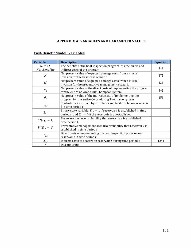
151
APPENDIX A: VARIABLES AND PARAMETER VALUES
Cost-Benefit Model: Variables
Variable Description Equation
The benefits of the boat inspection program less the direct and indirect costs of the program
(1)
Net present value of expected damage costs from a mussel invasion for the base-case scenario
(2)
Net present value of expected damage costs from a mussel invasion for the preventative management scenario
(3)
Net present value of the direct costs of implementing the program for the entire Colorado-Big Thompson system
(4)
Net present value of the indirect costs of implementing the program for the entire Colorado-Big Thompson system
(5)
Control costs incurred by structures and facilities below reservoir in time period
Binary state variable: if reservoir is established in time
period , and if the reservoir is unestablished
Base-case scenario probability that reservoir is established in time period
Preventative management scenario probability that reservoir is established in time period
Direct costs of implementing the boat inspection program on reservoir in time period
Indirect costs to boaters on reservoir during time period (24) Discount rate
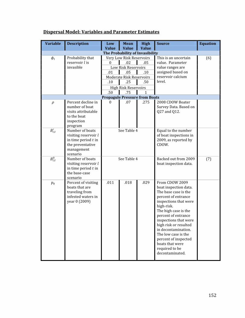
152
Dispersal Model: Variables and Parameter Estimates
Variable Description Low Value
Mean Value
High Value
Source Equation
The Probability of Invasibility Probability that
reservoir is invasible
Very Low Risk Reservoirs This is an uncertain value. Parameter value ranges are assigned based on reservoir calcium level.
(6) 0 .02 .05 Low Risk Reservoirs
.01 .05 .10 Moderate Risk Reservoirs .10
.25
.50
High Risk Reservoirs .50 .75 1
Propagule Pressure from Boats Percent decline in
number of boat visits attributable to the boat inspection program
0 .07 .275 2008 CDOW Boater Survey Data. Based on Q27 and Q12.
Number of boats
visiting reservoir in time period in the preventative management scenario
See Table 4 Equal to the number of boat inspections in 2009, as reported by CDOW.
Number of boats
visiting reservoir in time period in the base-case scenario
See Table 4 Backed out from 2009 boat inspection data.
(7)
Percent of visiting boats that are traveling from infested waters in year 0 (2009)
.011 .018 .029 From CDOW 2009 boat inspection data. The base case is the percent of entrance inspections that were high-risk. The high case is the percent of entrance inspections that were high risk or resulted in decontamination. The low case is the percent of inspected boats that were required to be decontaminated.

153
Variable Description Low Value
Mean Value
High Value
Source Equation
Increase in percent of infested boats over time, max value for the random walk
0.00 .005 .056 Kraft2000. The base value is set low to reflect a slow invasion, Johnson2006.
Max percent infested boats
.002945
.0589 .589 Whittier2008. The high value is the percent of ecoregions that are at high risk of invasion based on calcium concentrations. The low value is 5% of this value. The base value is set at 10% of high-risk ecoregions.
Base-case
scenario percent of potentially infested boats in period
(8)
Percent reduction in the maximum percent increase in infested boats per year, preventative management scenario
.25 .5 .75 This is an uncertain value.
Preventative
management scenario percent of potentially infested boats entering the system in period t
(9)
Percent of infested boats that are caught by inspection and get cleaned
.9 .95 1 This is an uncertain value.
Percent of
potentially infested boats that are missed by boat inspections
(10)

154
Variable Description Low Value
Mean Value
High Value
Source Equation
Propagule pressure from boats in reservoir in time period for the base-case scenario
(12)
Propagule pressure from boats in reservoir in time period for the preventative management scenario
(13)
Density of Veligers that Survive Downstream Transport Y-intercept for
veliger transport exponential decay function
80.1 Horvath1999.
Decay rate for veliger transport exponential decay function
-.67 -.45
-.33 Horvath1999. Based on density falling to 0.1% after 10, 15 and 20 km, respectively. From Bobeldke2005, lakes greater than 20km downstream had a lower chance of being invaded. Horvath1996 found isolated veligers 12km downstream. The smaller is, the lower mortality is.
Distance between reservoir and the reservoir directly upstream
See Figure 3 on page 13 for distances between
reservoirs
Distance data provided by Northern Water.
Maximum population density in the reservoir directly upstream from reservoir (individuals/m2)
20 800 7500 Ramcharan1992. These are the min, mean, and max densities of mussels in European Lakes.
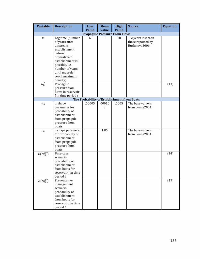
155
Variable Description Low Value
Mean Value
High Value
Source Equation
Propagule Pressure From Flows Lag time (number
of years after upstream establishment before downstream establishment is possible, i.e. number of years until mussels reach maximum density)
6 8 10 1-2 years less than those reported by Burlakova2006.
Propagule
pressure from flows in reservoir in time period
(13)
The Probability of Establishment from Boats shape
parameter for probability of establishment from propagule pressure from boats
.00005 .000103
.0005 The base value is from Leung2004.
shape parameter for probability of establishment from propagule pressure from boats
1.86 The base value is from Leung2004.
Base-case
scenario probability of establishment from boats for reservoir in time period
(14)
Preventative
management scenario probability of establishment from boats for reservoir in time period
(15)

156
Variable Description Low Value
Mean Value
High Value
Source Equation
The Probability of Establishment From Flows shape
parameter for probability of establishment from propagule pressure downstream flows (percent living veligers)
.005 .05 .2 This is an uncertain value, as there is much uncertainty in how veligers survive and are transported through conveyance systems. The larger is, the greater the probability of downstream establishment.
shape parameter for probability of establishment from propagule pressure from downstream flows (percent living veligers)
.5 1 1.86 The high value is from Leung2004; however, this value was used for boat pressure, not stream pressure. This parameter concerns the presence or absence of an Allee effect, and it is assumed that the value is the same for pressure from flows as it is for pressure from boats. The larger is, the quicker the probability of establishment falls from 1 to 0.
Probability of
establishment from flows for reservoir in time period
(16)
The Joint Probability of Colonization Probability that
reservoir is colonized by period , given reservoir is invasible
(17)
Joint Probability that reservoir is colonized by period
(18)

157
Control Cost Model: Variables and Parameter Estimates
Variable Description Low Value
Mean Value
High Value
Source Equation
Lag time (number of years post establishment when damages are first incurred for downstream structures)
6 8
2
10 1-2 years less than those reported by Burlakova2006 (following initial colonization). Westminster2010 (following detection).
Interest rate for capital expenditure loan
4 4.75 5 MSRB EMMA website. Based on a sample of 100 bond trades from 6/8/2010. Low, base, and high values are Q1, median, and Q3, respectively.
Tem length for capital expenditure loan
15 20 30
Capital expenditure loan value
Varies by facility type See section 2.3.3
Principal and interest payment on capital expenditure loan
(19)
Index for control cost schedules ( represents costs incurred in the first year mussels settle in a facility)
First year
reservoir is established for the base-case scenario
Simulated value
First year
reservoir is established for the preventative management scenario
Simulated value
Number of structures under reservoir
See Appendix B for a list of structures
and upstream sources
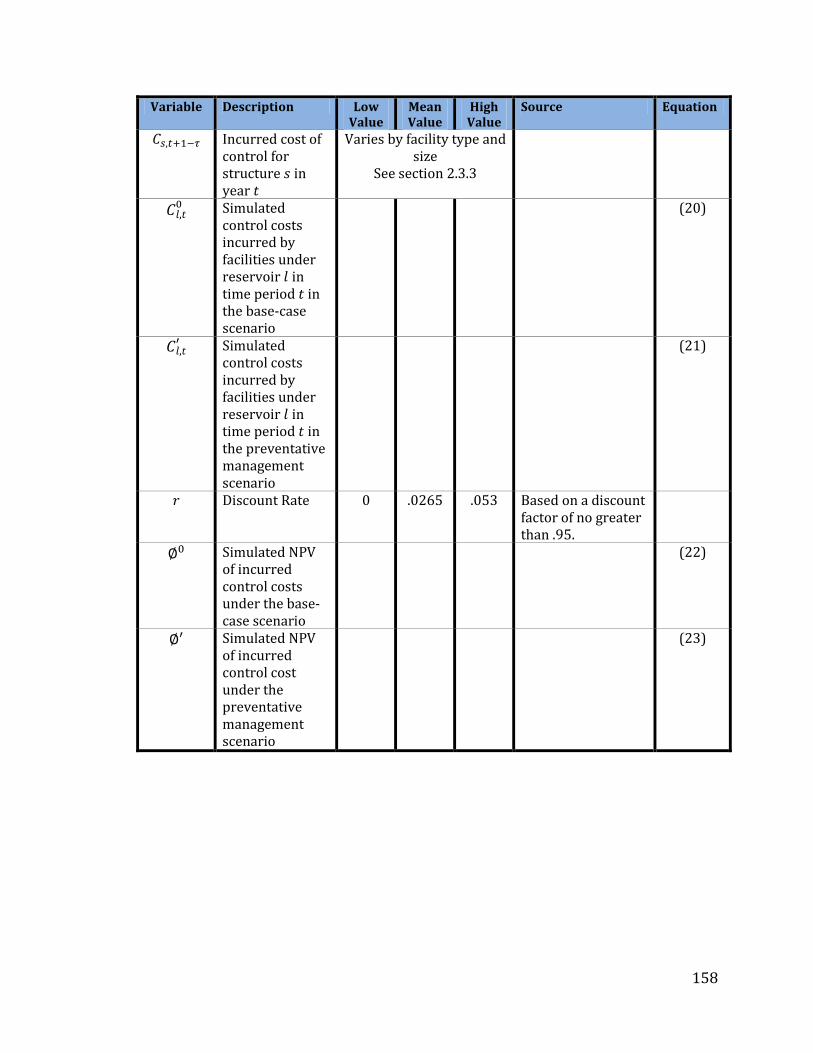
158
Variable Description Low Value
Mean Value
High Value
Source Equation
Incurred cost of control for structure in year
Varies by facility type and size
See section 2.3.3
Simulated control costs incurred by facilities under reservoir in time period in the base-case scenario
(20)
Simulated control costs incurred by facilities under reservoir in time period in the preventative management scenario
(21)
Discount Rate 0 .0265 .053 Based on a discount factor of no greater than .95.
Simulated NPV of incurred control costs under the base-case scenario
(22)
Simulated NPV of incurred control cost under the preventative management scenario
(23)
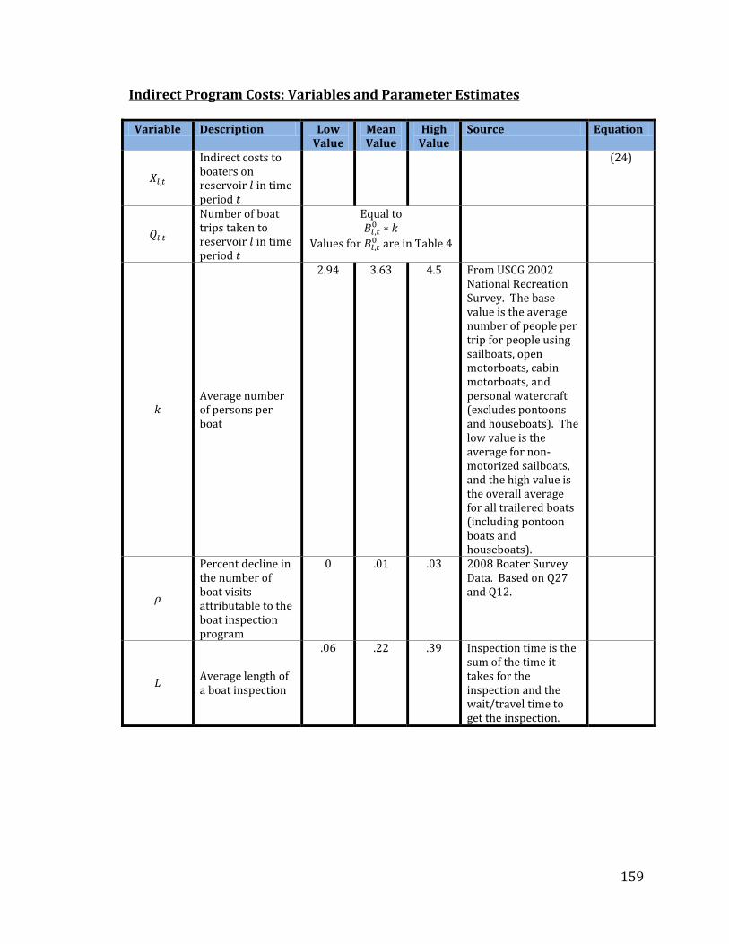
159
Indirect Program Costs: Variables and Parameter Estimates
Variable Description Low Value
Mean Value
High Value
Source Equation
Indirect costs to boaters on reservoir in time period
(24)
Number of boat trips taken to reservoir in time period
Equal to
Values for are in Table 4
Average number of persons per boat
2.94 3.63 4.5 From USCG 2002 National Recreation Survey. The base value is the average number of people per trip for people using sailboats, open motorboats, cabin motorboats, and personal watercraft (excludes pontoons and houseboats). The low value is the average for non-motorized sailboats, and the high value is the overall average for all trailered boats (including pontoon boats and houseboats).
Percent decline in the number of boat visits attributable to the boat inspection program
0 .01 .03 2008 Boater Survey Data. Based on Q27 and Q12.
Average length of a boat inspection
.06 .22 .39 Inspection time is the sum of the time it takes for the inspection and the wait/travel time to get the inspection.

160
Variable Description Low Value
Mean Value
High Value
Source Equation
Average length of a boater day
2 3.2 5.5 From Grand Lake Boater Survey Data: mean=4.6 hours, median=3.2 hours, min=1 hour, max=13 hours, n=161, distributions is positively skewed. From USCG National Recreation Survey, the average for sailboats, open motorboats, cabin motorboats and personal watercraft is 5.54.
Average consumer surplus per boater per boating day for the base-case scenario
17.94 61.16 104.38 Kaval and Loomis 2003. Base is average WTP taken from 7 studies in the Intermountain Region. The low is 2 standard errors below the average and the high is 2 standard errors about the average.

161
APPENDIX B: MAJOR STRUCTURES AND FACILITIES IN THE COLORADO-BIG THOMPSON SYSTEM
Structure/Facility Name Structure/Facility
Classification Upstream Water Body
Windy Gap Pump Plant pump plant Windy Gap Reservoir
Windy Gap Pipeline Pipeline Windy Gap Reservoir
Willow Creek Dam Dam Willow Creek Reservoir
Willow Creek Pump Canal Canal Willow Creek Reservoir
Willow Creek Pump Plant pump plant Willow Creek Reservoir
Granby Dam Dam Lake Granby
Farr Pumping Plant pump plant Lake Granby
Grandby Pump Canal Canal Lake Granby
Shadow Mountain Dam Dam Shadow Mountain
Reservoir
Adams Tunnel Tunnel Grand Lake
East Portal Reservoir Dam East Portal Reservoir
Rams Horn Tunnel Tunnel East Portal Reservoir
Mary's Lake Hydropower Plant Hydropower East Portal Reservoir
Prospect Mountain Tunnel Tunnel Mary's Lake
Estes Hydropower Plant Hydropower Mary's Lake
Town of Estes water filter plant Mary's Lake
Mary's Lake (Town) water filter plant Mary's Lake
Olympus Dam Dam Lake Estes
Olympus Tunnel Tunnel Lake Estes
Pole Hill Tunnel Tunnel Lake Estes
Pole Hill Hydropower Plant Hydropower Lake Estes
Rattlesnake Tunnel Tunnel Lake Estes
Rattlesnake Dam Dam Pinewood Reservoir
Bald Mountain Tunnel Tunnel Pinewood Reservoir
Flatiron Hydropower Plant Hydropower Pinewood Reservoir
Newell Warnock water filter plant Pinewood Reservoir
Flatiron Reversible Pump pump plant Flatiron Reservoir
Flatiron Dam Dam Flatiron Reservoir
Carter Lake Pressure Tunnel Tunnel Flatiron Reservoir
Big Thompson Hydropower Plant Hydropower Flatiron Reservoir
Hansen Feeder Canal Canal Flatiron Reservoir
City of Loveland water filter plant Flatiron Reservoir
Emissaries of Divine Light water filter plant Flatiron Reservoir
Eden Valley water filter plant Flatiron Reservoir
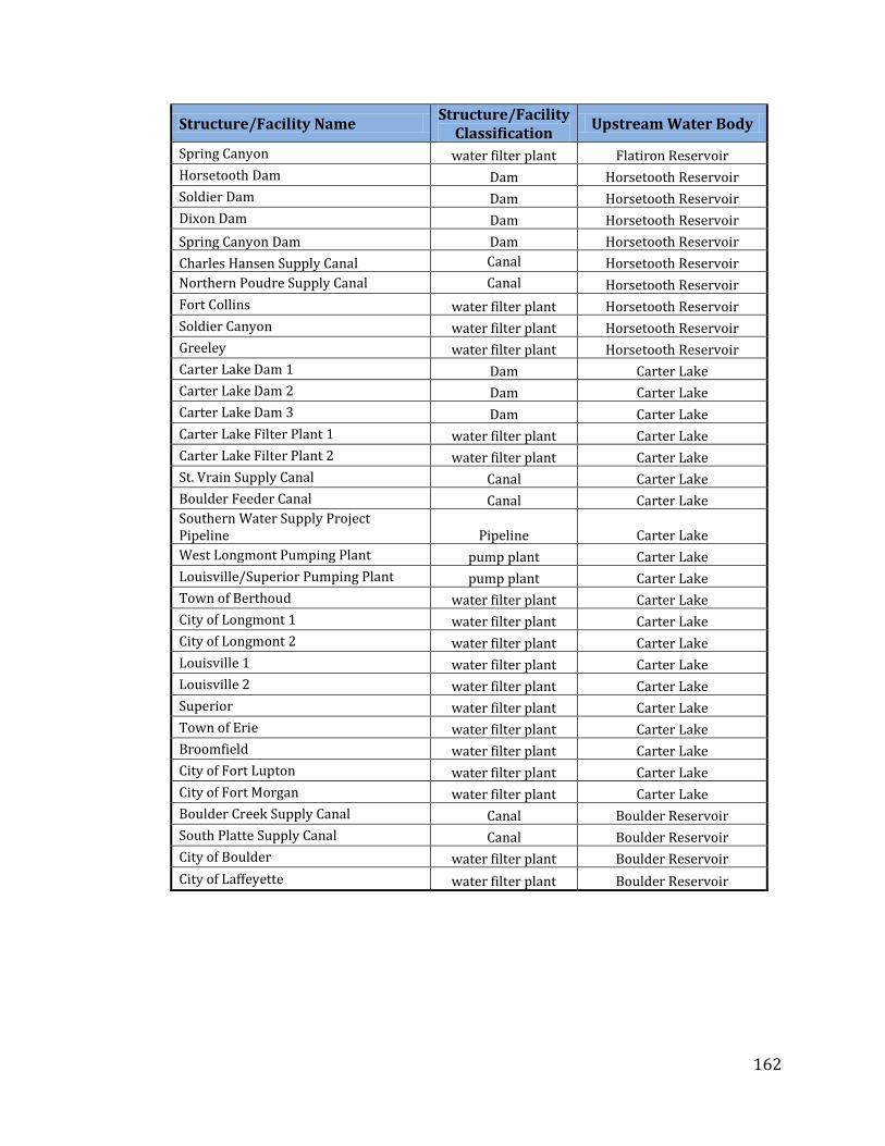
162
Structure/Facility Name Structure/Facility
Classification Upstream Water Body
Spring Canyon water filter plant Flatiron Reservoir
Horsetooth Dam Dam Horsetooth Reservoir
Soldier Dam Dam Horsetooth Reservoir
Dixon Dam Dam Horsetooth Reservoir
Spring Canyon Dam Dam Horsetooth Reservoir
Charles Hansen Supply Canal Canal Horsetooth Reservoir
Northern Poudre Supply Canal Canal Horsetooth Reservoir
Fort Collins water filter plant Horsetooth Reservoir
Soldier Canyon water filter plant Horsetooth Reservoir
Greeley water filter plant Horsetooth Reservoir
Carter Lake Dam 1 Dam Carter Lake
Carter Lake Dam 2 Dam Carter Lake
Carter Lake Dam 3 Dam Carter Lake
Carter Lake Filter Plant 1 water filter plant Carter Lake
Carter Lake Filter Plant 2 water filter plant Carter Lake
St. Vrain Supply Canal Canal Carter Lake
Boulder Feeder Canal Canal Carter Lake Southern Water Supply Project Pipeline Pipeline Carter Lake
West Longmont Pumping Plant pump plant Carter Lake
Louisville/Superior Pumping Plant pump plant Carter Lake
Town of Berthoud water filter plant Carter Lake
City of Longmont 1 water filter plant Carter Lake
City of Longmont 2 water filter plant Carter Lake
Louisville 1 water filter plant Carter Lake
Louisville 2 water filter plant Carter Lake
Superior water filter plant Carter Lake
Town of Erie water filter plant Carter Lake
Broomfield water filter plant Carter Lake
City of Fort Lupton water filter plant Carter Lake
City of Fort Morgan water filter plant Carter Lake
Boulder Creek Supply Canal Canal Boulder Reservoir
South Platte Supply Canal Canal Boulder Reservoir
City of Boulder water filter plant Boulder Reservoir
City of Laffeyette water filter plant Boulder Reservoir
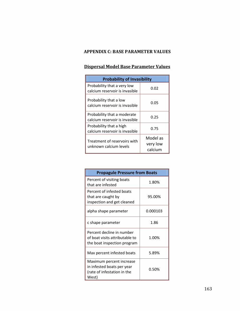
163
APPENDIX C: BASE PARAMETER VALUES
Dispersal Model Base Parameter Values
Probability of Invasibility
Probability that a very low calcium reservoir is invasible
0.02
Probability that a low calcium reservoir is invasible
0.05
Probability that a moderate calcium reservoir is invasible
0.25
Probability that a high calcium reservoir is invasible
0.75
Treatment of reservoirs with unknown calcium levels
Model as very low calcium
Propagule Pressure from Boats
Percent of visiting boats that are infested
1.80%
Percent of infested boats that are caught by inspection and get cleaned
95.00%
alpha shape parameter 0.000103
c shape parameter 1.86
Percent decline in number of boat visits attributable to the boat inspection program
1.00%
Max percent infested boats 5.89%
Maximum percent increase in infested boats per year (rate of infestation in the West)
0.50%

164
Propagule Pressure from Flows
y-intercept parameter 0.801
Decay rate -0.45
Lag time (m) 8
alpha shape parameter 0.05
c shape parameter 1
Mussel density for a very low calcium reservoir
22
Mussel density for a low calcium reservoir
22
Mussel density for a moderate calcium reservoir
800
Mussel density for a high calcium reservoir
7500
Damage Cost Model Base Parameter Values
Time Horizon 50
Lag Time (n) 8
Discount Rate 0.0265
Interest Rate 0.0475
Loan term length for capital expenditures (years)
20

165
Program Cost Base Parameter Values
Yearly Direct Costs: Variable Costs ($/year)
$827206
Yearly Direct Costs: Principal on Capital Expenditures ($/year)
$4656
CS per boater per day ($/boater/day)
61.16
Length of an Average Boater Day (hours)
3.2
Average Number of Boaters per Boat (persons/boat)
3.63
Inspection Length (hours) 0.22
Are indirect costs of the program included in the analysis?
Yes

166
APPENDIX D: VISUAL BASIC CODE
Sub Mussels() 'Random number arrays (to be imported from MUSSELS_random.xlsm) Dim RandomWalkLow(999, 49, 1) As Double 'RandomWalkLow(run, year,scenario) Dim RandomWalkBase(999, 49, 1) As Double 'RandomWalkBase(run, year,scenario) Dim RandomWalkHigh(999, 49, 1) As Double 'RandomWalkHigh(run, year,scenario) Dim RandomWalkUser(999, 49, 1) As Double 'RandomWalkUser(run, year,scenario) Dim RandomBoats(12999, 49) As Double 'RandomBoats(mix of run and reservoir, year) Dim RandomUpstream1(12999, 49) As Double 'RandomUpstream1(mix of run and reservoir, year) Dim RandomUpstream2(12999, 49) As Double 'RandomUpstream2(mix of run and reservoir, year) 'Constant Inputs (to be imported from sheet "Model Input") Dim Invasibility(12) As Double ' Invasibility(reservoirs) Dim per_infest_0 As Double Dim per_cleaned As Double Dim a_boat As Double Dim c_boat As Double Dim per_decline As Double Dim BoatVisits_0(12) As Long 'BoatVisits_0(reservoirs) Dim BoatVisits_1(12) As Long 'BoatVisits_1(reservoirs) Dim per_max As Double Dim R_max As Integer Dim B As Double Dim horizon As Integer Dim m As Integer Dim a_stream As Double Dim c_stream As Double Dim UpConnect1(12) As Integer 'UpConnect1(reservoir) Dim UpConnect2(12) As Integer 'UpConnect2(reservoir) Dim DensityAlive1(12) As Double ' DensityAlive1(reservoir) Dim DensityAlive2(12) As Double ' DensityAlive2(reservoir) Dim n As Integer Dim d_rate As Double Dim UpConnectStructure(67) As Integer 'UpConnectStructure(structure) Dim StructureType(67) As String 'StructureType(structure) Dim direct_costs_variable As Double Dim direct_costs_PI As Double Dim indirect_costs As Double Dim term_length As Integer 'Arrays to be populated Dim PerInfest(999, 49, 1) As Double ' PerInfest(run, year, scenario) Dim PerInfest_cleaned(999, 49) As Double 'PerInfest_cleaned(run, year) Dim RandomWalk(999, 49, 1) As Double 'RandomWalk(run,year,scenario) Dim NumInfest(999, 49, 12, 1) As Long 'NumInfest(run, year, reservoir, scenario) Dim AvgNumInfest(49, 12, 1) As Double 'AvgNumInfest(year, reservoir, scenario) Dim ProbEstab_Boats(999, 49, 12, 1) As Double ' ProbEstab_Boats(run, year, reservoir, scenario) Dim product_Boats(999, 49, 12, 1) As Double ' product_Boats(run, year, reservoir, scenario) Dim JointProb_Boats(999, 49, 12, 1) As Double ' JointProb_Boats(run, year, reservoir, scenario) Dim AvgJointProb_Boats(49, 12, 1) As Double 'AvgJointProb_Boats(year,reservoir,scenario) Dim ProbEstab_Up1(999, 49, 12, 1) As Double ' ProbEstab_Up1(run, year, reservoir, scenario) Dim ProbEstab_Up2(999, 49, 12, 1) As Double ' ProbEstab_Up2(run, year, reservoir, scenario) Dim JointProb_Up1(999, 49, 12, 1) As Double ' JointProb_Up1(run, year, reservoir, scenario) Dim JointProb_Up2(999, 49, 12, 1) As Double ' JointProb_Up2(run, year, reservoir, scenario) Dim Bernoulli_Boats(999, 49, 12, 1) As Boolean ' Bernoulli_Boats(run,year,reservoir,scenario)

167
Dim Bernoulli_Up1(999, 49, 12, 1) As Boolean ' Bernoulli_Up1(run,year,reservoir,scenario) Dim Bernoulli_Up2(999, 49, 12, 1) As Boolean ' Bernoulli_Up2(run,year,reservoir,scenario) Dim invasionrecord(999, 49, 12, 1) As Boolean 'InvasionRecord(run,year,reservoir,scenario) Dim FirstYearEstab(999, 12, 1) As Integer 'FirstYearEstab(run, reservoir, scenario) Dim ControlCostSchedules(49, 67) As Double 'ControlCostSchedules(year,structure) Dim IncurredControlCosts(999, 49, 67, 1) As Double 'IncurredControlCosts(run,year,structure,scenario) Dim DiscControlCosts(999, 49, 67, 1) As Double 'DiscControlCosts(run,year,structure,scenario) Dim NPVControlCosts(999, 1) As Double 'NPVControlCosts(run, scenario) Dim Benefits(999) As Double 'Benefits(run) Dim DirectCosts(49) As Double 'DirectCosts(year) Dim DiscDirectCosts(49) As Double 'DiscDirectCosts(year) Dim NPVDirectCosts As Double Dim IndirectCosts(49) As Double 'IndirectCosts(Year) Dim DiscIndirectCosts(49) As Double 'DiscIndirectCosts(Year) Dim NPVIndirectCosts As Double Dim TotalCosts(49) As Double 'TotalCosts(Year) Dim DiscTotalCosts(49) As Double 'DiscTotalCosts(year) Dim NPVTotalCosts As Double Dim NetBenefits(999) 'NetBenefits(Run) Dim NPVResControlCosts(999, 12, 1) As Double 'ResControlCosts(run, reservoir, scenario) Dim StrucControlCosts(999, 6, 1) As Double 'StrucControlCosts(run, structure type, scenario) Dim Cause(999, 12, 1) As String 'Cause(run, reservoir, scenario) Dim AvgJointProb_Up1(49, 12, 1) As Double 'avgJointProb_Up1(year,reservoir,scenario) Dim AvgJointProb_Up2(49, 12, 1) As Double 'avgJointProb_Up2(year,reservoir,scenario) 'Functional Variables Dim startrow As Integer Dim startcol As Integer Dim Count As Integer Dim Years As Integer Dim Runs As Integer Dim i As Integer Dim j As Integer Dim k As Integer Dim s As Integer Dim z As Integer Dim Candidate1 As Integer Dim Candidate2 As Integer Dim indicator As Boolean Dim Source As Integer Dim Start As Integer Dim sum As Double Dim term As Double Dim BoolArray(49) As Boolean 'BoolArray(year) Dim StringArray(999) As String 'StringArray(year or run) Dim DoubArray(999) As Double 'DoubArray(year or run) Dim cumsum(999, 49, 12, 1) As Integer 'CumSum(run,year,reservoir, scenario) Dim cumsum1(999, 49, 12, 1) As Integer 'CumSum1(run,year,reservoir, scenario) Dim cumsum2(999, 49, 12, 1) As Integer 'CumSum2(run,year,reservoir, scenario) Load Userform1 Userform1.Show Userform1.Label1.Caption = "Running Simulation." Userform1.Repaint 'Set number of iterations Runs = 1000 Userform1.Label1.Caption = "Running Simulation.." Userform1.Repaint 'Import inputs from "Model Input" sheet Worksheets("Model Input").Activate ' Invasibility(reservoirs) startrow = Range("Invasibility").Row startcol = Range("Invasibility").Column

168
For k = 0 To 12 Invasibility(k) = Cells(startrow + k, startcol).Value Next k per_infest_0 = Range("per_infest_0").Value per_cleaned = Range("per_cleaned").Value a_boat = Range("a_boat").Value c_boat = Range("c_boat").Value per_decline = Range("per_decline").Value 'BoatVisits_0(reservoirs) startrow = Range("BoatVisits_0").Row startcol = Range("BoatVisits_0").Column For k = 0 To 12 BoatVisits_0(k) = Cells(startrow + k, startcol).Value Next k 'BoatVisits_1(reservoirs) startrow = Range("BoatVisits_1").Row startcol = Range("BoatVisits_1").Column For k = 0 To 12 BoatVisits_1(k) = Cells(startrow + k, startcol).Value Next k per_max = Range("per_max").Value R_max = Range("R_max").Value B = Range("B_").Value horizon = Range("horizon").Value m = Range("m_").Value a_stream = Range("a_stream").Value c_stream = Range("c_stream").Value 'UpConnect1(reservoir) startrow = Range("UpConnect1").Row startcol = Range("UpConnect1").Column For k = 0 To 12 UpConnect1(k) = Cells(startrow + k, startcol).Value Next k 'UpConnect2(reservoir) startrow = Range("UpConnect2").Row startcol = Range("UpConnect2").Column For k = 0 To 12 UpConnect2(k) = Cells(startrow + k, startcol).Value Next k 'DensityAlive1(reservoir) startrow = Range("DensityAlive1").Row startcol = Range("DensityAlive1").Column For k = 0 To 12 DensityAlive1(k) = Cells(startrow + k, startcol).Value Next k 'DensityAlive2(reservoir) startrow = Range("DensityAlive2").Row startcol = Range("DensityAlive2").Column For k = 0 To 12 DensityAlive2(k) = Cells(startrow + k, startcol).Value Next k
169
n = Range("n_").Value d_rate = Range("d_rate").Value 'UpConnectStructure(structure) startrow = Range("UpConnectStructure").Row startcol = Range("UpConnectStructure").Column For s = 0 To 67 UpConnectStructure(s) = Cells(startrow + s, startcol).Value Next s 'StructureType(structure) startrow = Range("StructureType").Row startcol = Range("StructureType").Column For s = 0 To 67 StructureType(s) = Cells(startrow + s, startcol).Value Next s direct_costs_variable = Range("direct_costs_variable").Value direct_costs_PI = Range("direct_costs_PI").Value indirect_costs = Range("indirect_costs").Value 'ControlCostSchedules(structure, Year) startrow = Range("ControlCostSchedules").Row startcol = Range("ControlCostSchedules").Column For j = 0 To horizon - 1 For s = 0 To 67 ControlCostSchedules(j, s) = Cells(startrow + s, startcol + j).Value Next s Next j term_length = Range("term_length").Value 'Generate random number arrays Rnd (-1) Randomize (Range("Seed").Value) Years = 50 Count = 1000 Limit = Range("R_max_low").Value For j = 0 To Years - 1 For i = 0 To Count - 1 RandomWalkLow(i, j, 0) = Rng_Number(0, Limit) / 10000 RandomWalkLow(i, j, 1) = Rng_Number(0, Limit - B * Limit) / 10000 Next i Next j Limit = Range("R_max_base").Value For j = 0 To Years - 1 For i = 0 To Count - 1 RandomWalkBase(i, j, 0) = Rng_Number(0, Limit) / 10000 RandomWalkBase(i, j, 1) = Rng_Number(0, Limit - B * Limit) / 10000 Next i Next j Limit = Range("R_max_high").Value For j = 0 To Years - 1 For i = 0 To Count - 1 RandomWalkHigh(i, j, 0) = Rng_Number(0, Limit) / 10000 RandomWalkHigh(i, j, 1) = Rng_Number(0, Limit - B * Limit) / 10000 Next i Next j Years = 50 Count = 1000 Limit = Range("R_max_userdefined").Value For j = 0 To Years - 1
170
For i = 0 To Count - 1 RandomWalkUser(i, j, 0) = Rng_Number(0, Limit) / 10000 RandomWalkUser(i, j, 1) = Rng_Number(0, Limit - B * Limit) / 10000 Next i Next j Count = 13000 For j = 0 To Years - 1 For i = 0 To Count - 1 RandomBoats(i, j) = Rnd Next i Next j For j = 0 To Years - 1 For i = 0 To Count - 1 RandomUpstream1(i, j) = Rnd Next i Next j For j = 0 To Years - 1 For i = 0 To Count - 1 RandomUpstream2(i, j) = Rnd Next i Next j Userform1.Label1.Caption = "Running Simulation..." Userform1.Repaint 'Simulate Number of infested boats 'Assign RandomWalk(run, year,scenario) array based on R_max Select Case R_max Case 1 For i = 0 To Runs - 1 For j = 0 To horizon - 1 RandomWalk(i, j, 0) = RandomWalkLow(i, j, 0) RandomWalk(i, j, 1) = RandomWalkLow(i, j, 1) Next j Next i Case 2 For i = 0 To Runs - 1 For j = 0 To horizon - 1 RandomWalk(i, j, 0) = RandomWalkBase(i, j, 0) RandomWalk(i, j, 1) = RandomWalkBase(i, j, 1) Next j Next i Case 3 For i = 0 To Runs - 1 For j = 0 To horizon - 1 RandomWalk(i, j, 0) = RandomWalkHigh(i, j, 0) RandomWalk(i, j, 1) = RandomWalkHigh(i, j, 1) Next j Next i Case 4 For i = 0 To Runs - 1 For j = 0 To horizon - 1 RandomWalk(i, j, 0) = RandomWalkUser(i, j, 0) RandomWalk(i, j, 1) = RandomWalkUser(i, j, 1) Next j Next i End Select 'Populate PerInfest(run, year, scenario) in year 0 For i = 0 To Runs - 1 PerInfest(i, 0, 0) = per_infest_0 PerInfest(i, 0, 1) = per_infest_0 PerInfest_cleaned(i, 0) = per_infest_0 * (1 - per_cleaned) Next i 'Populate PerInfest(run, year, scenario) for all remaining years

171
For i = 0 To Runs - 1 For j = 1 To horizon - 1 If PerInfest(i, j - 1, 0) + RandomWalk(i, j, 0) <= per_max Then PerInfest(i, j, 0) = PerInfest(i, j - 1, 0) + RandomWalk(i, j, 0) Else: PerInfest(i, j, 0) = per_max End If If PerInfest(i, j - 1, 1) + RandomWalk(i, j, 1) <= per_max Then PerInfest(i, j, 1) = (PerInfest(i, j - 1, 1) + RandomWalk(i, j, 1)) Else: PerInfest(i, j, 1) = per_max End If PerInfest_cleaned(i, j) = PerInfest(i, j, 1) * (1 - per_cleaned) Next j Next i 'Propagule Pressure and Probabilities (Boats) 'Populate NumInfest(run, year, reservoir, scenario) For i = 0 To Runs - 1 For j = 0 To horizon - 1 For k = 0 To 12 NumInfest(i, j, k, 0) = BoatVisits_0(k) * PerInfest(i, j, 0) NumInfest(i, j, k, 1) = BoatVisits_1(k) * PerInfest_cleaned(i, j) Next k Next j Next i 'Populate ProbEstab_Boats(run, year, reservoir, scenario) For i = 0 To Runs - 1 For j = 0 To horizon - 1 For k = 0 To 12 ProbEstab_Boats(i, j, k, 0) = 1 - Exp(-1 * (a_boat * NumInfest(i, j, k, 0)) ^ c_boat) ProbEstab_Boats(i, j, k, 1) = 1 - Exp(-1 * (a_boat * NumInfest(i, j, k, 1)) ^ c_boat) Next k Next j Next i 'Populate year 0 of product_Boats(run, year, reservoir, scenario) 'Note:The product variable is a building block of the joint probability variable For i = 0 To Runs - 1 For k = 0 To 12 product_Boats(i, 0, k, 0) = 1 - ProbEstab_Boats(i, 0, k, 0) product_Boats(i, 0, k, 1) = 1 - ProbEstab_Boats(i, 0, k, 1) Next k Next i 'Populate remaining years of product_Boats(run, year, reservoir, scenario) For i = 0 To Runs - 1 For j = 1 To horizon - 1 For k = 0 To 12 product_Boats(i, j, k, 0) = product_Boats(i, j - 1, k, 0) * (1 - ProbEstab_Boats(i, j, k, 0)) product_Boats(i, j, k, 1) = product_Boats(i, j - 1, k, 1) * (1 - ProbEstab_Boats(i, j, k, 1)) Next k Next j Next i 'Populate JointProb_Boats(run, year, reservoir, scenario) For i = 0 To Runs - 1 For j = 0 To horizon - 1 For k = 0 To 12 JointProb_Boats(i, j, k, 0) = Invasibility(k) * (1 - product_Boats(i, j, k, 0)) JointProb_Boats(i, j, k, 1) = Invasibility(k) * (1 - product_Boats(i, j, k, 1)) Next k Next j Next i 'Bernoulli Trials 'Populate Bernoulli_Boats(run,year,reservoir,scenario)for all years

172
For i = 0 To Runs - 1 For j = 1 To horizon - 1 For k = 0 To 12 If RandomBoats(i * 12 + k, j) <= JointProb_Boats(i, j, k, 0) Then Bernoulli_Boats(i, j, k, 0) = 1 Else: Bernoulli_Boats(i, j, k, 0) = 0 End If If RandomBoats(i * 12 + k, j) <= JointProb_Boats(i, j, k, 1) Then Bernoulli_Boats(i, j, k, 1) = 1 Else: Bernoulli_Boats(i, j, k, 1) = 0 End If Next k Next j Next i Userform1.Label1.Caption = "Running Simulation...." Userform1.Repaint 'Populating Bernoulli_Up1 and Bernoulli_Up2 is a little trickier, because the trial in 'year j is dependent on the invasion record of year j-m. Therefore, InvasionRecord and 'Bernoulli_Up1 and Bernoulli_Up2 will have to be populated iteratively. The first m-1 'years must be populated before the iterative process can start, because the code will ask 'to look up the invasion record of upstream connections m years ago. 'Note: All of the upstream trials in years 0 through m-1 will be false because the lag time 'has not yet passed. Year j=m is the first year that upstream infested water bodies become 'candidates for downstream infestation. 'Populate years 0 through m-1 of Bernoulli_Up1(run,year,reservoir,scenario) 'and Bernoulli_Up2(run,year,reservoir,scenario) as false 'Populate ProbEstab_Up1(run,year,reservoir,scenario),ProbEstab_Up2(run,year,reservoir,scenario) 'and JointProb_Up1(run,year,reservoir,scenario), and JointProb_Up2(run,year,reservoir,scenario) as 0 For i = 0 To Runs - 1 For j = 0 To m - 1 For k = 0 To 12 Bernoulli_Up1(i, j, k, 0) = 0 Bernoulli_Up2(i, j, k, 0) = 0 Bernoulli_Up1(i, j, k, 1) = 0 Bernoulli_Up2(i, j, k, 1) = 0 ProbEstab_Up1(i, j, k, 0) = 0 ProbEstab_Up2(i, j, k, 0) = 0 JointProb_Up1(i, j, k, 0) = 0 JointProb_Up2(i, j, k, 0) = 0 ProbEstab_Up1(i, j, k, 1) = 0 ProbEstab_Up2(i, j, k, 1) = 0 JointProb_Up1(i, j, k, 1) = 0 JointProb_Up2(i, j, k, 1) = 0 Next k Next j Next i 'Populated InvasionRecord(run,year,reservoir,scenario) for year 0; imported from input sheet startrow = Range("InvasionRecord_0").Row startcol = Range("InvasionRecord_0").Column For i = 0 To Runs - 1 For k = 0 To 12 invasionrecord(i, 0, k, 0) = Cells(startrow + k, startcol).Value invasionrecord(i, 0, k, 1) = Cells(startrow + k, startcol).Value Next k Next i 'As of this point: Bernoulli_Boats is populated for all years; 'Bernoulli_Up1 and Bernoulli_Up2 are populated through year m-1 'Populate InvasionRecord(run,year,reservoir,scenario) 'for all reservoirs for years 1 through m-2 For i = 0 To Runs - 1 For j = 1 To m - 2 For k = 0 To 12

173
If invasionrecord(i, j - 1, k, 0) = True Then invasionrecord(i, j, k, 0) = 1 ElseIf Bernoulli_Boats(i, j, k, 0) = True Or Bernoulli_Up1(i, j, k, 0) = True Or Bernoulli_Up2(i, j, k, 0) = True Then invasionrecord(i, j, k, 0) = 1 Else: invasionrecord(i, j, k, 0) = 0 End If If invasionrecord(i, j - 1, k, 1) = True Then invasionrecord(i, j, k, 1) = 1 ElseIf Bernoulli_Boats(i, j, k, 1) = True Or Bernoulli_Up1(i, j, k, 1) = True Or Bernoulli_Up2(i, j, k, 1) = True Then invasionrecord(i, j, k, 1) = 1 Else: invasionrecord(i, j, k, 1) = 0 End If Next k Next j Next i 'As of this point: Bernoulli_Boats is populated for all years; 'Bernoulli_Up1 and Bernoulli_Up2 are populated through year m-1; 'InvasionRecord is populated through year m-2 'Populate first year of cumsum1 and cumsum2 For i = 0 To Runs - 1 For k = 0 To 12 Candidate1 = UpConnect1(k) If Candidate1 = -999 Then cumsum1(i, 0, k, 0) = 0 cumsum1(i, 0, k, 1) = 0 Else cumsum1(i, 0, k, 0) = invasionrecord(i, 0, Candidate1, 0) cumsum1(i, 0, k, 1) = invasionrecord(i, 0, Candidate1, 1) End If Next k Next i For i = 0 To Runs - 1 For k = 0 To 12 Candidate2 = UpConnect2(k) If Candidate2 = -999 Then cumsum2(i, 0, k, 0) = 0 cumsum2(i, 0, k, 1) = 0 Else cumsum2(i, 0, k, 0) = invasionrecord(i, 0, Candidate2, 0) cumsum2(i, 0, k, 1) = invasionrecord(i, 0, Candidate2, 1) End If Next k Next i 'Populate cumsum1 and cumsum2 through year m-2 For i = 0 To Runs - 1 For j = 1 To m - 2 For k = 0 To 12 Candidate1 = UpConnect1(k) If Candidate1 = -999 Then cumsum1(i, j, k, 0) = 0 cumsum1(i, j, k, 1) = 0 Else cumsum1(i, j, k, 0) = cumsum1(i, j - 1, k, 0) + invasionrecord(i, j, Candidate1, 0) cumsum1(i, j, k, 1) = cumsum1(i, j - 1, k, 1) + invasionrecord(i, j, Candidate1, 1) End If Next k Next j Next i For i = 0 To m - 2 For j = 1 To horizon - 1 For k = 0 To 12 Candidate2 = UpConnect2(k) If Candidate2 = -999 Then cumsum2(i, j, k, 0) = 0
174
cumsum2(i, j, k, 1) = 0 Else cumsum2(i, j, k, 0) = cumsum2(i, j - 1, k, 0) + invasionrecord(i, j, Candidate2, 0) cumsum2(i, j, k, 1) = cumsum2(i, j - 1, k, 1) + invasionrecord(i, j, Candidate2, 1) End If Next k Next j Next i 'This next loop iteratively populates InvasionRecord in year j 'and then Bernoulli_Up1, Bernoulli_Up2, ProbEstab_Up1, ProbEstab_up2, 'JointProb_Up1, and JointProb_Up2 in year j+1 for years m-1 to horizon-2 For i = 0 To Runs - 1 For j = m - 1 To horizon - 2 'Populate InvasionRecord(run,year,reservoir,scenario) in year j for all reservoirs For k = 0 To 12 If invasionrecord(i, j - 1, k, 0) = True Then invasionrecord(i, j, k, 0) = 1 ElseIf Bernoulli_Boats(i, j, k, 0) = True Or Bernoulli_Up1(i, j, k, 0) = True Or Bernoulli_Up2(i, j, k, 0) = True Then invasionrecord(i, j, k, 0) = 1 Else: invasionrecord(i, j, k, 0) = 0 End If If invasionrecord(i, j - 1, k, 1) = True Then invasionrecord(i, j, k, 1) = 1 ElseIf Bernoulli_Boats(i, j, k, 1) = True Or Bernoulli_Up1(i, j, k, 1) = True Or Bernoulli_Up2(i, j, k, 1) = True Then invasionrecord(i, j, k, 1) = 1 Else: invasionrecord(i, j, k, 1) = 0 End If Next k 'Populate ProbEstab_Up1, ProbEstab_Up2, JointProbEstab_Up1 and JointProbEstab_Up2 'in year j+1 for all reservoirs For k = 0 To 12 Candidate1 = UpConnect1(k) If Candidate1 = -999 Then cumsum1(i, j, k, 0) = 0 cumsum1(i, j, k, 1) = 0 Else cumsum1(i, j, k, 0) = cumsum1(i, j - 1, k, 0) + invasionrecord(i, j, Candidate1, 0) cumsum1(i, j, k, 1) = cumsum1(i, j - 1, k, 1) + invasionrecord(i, j, Candidate1, 1) End If Candidate2 = UpConnect2(k) If Candidate2 = -999 Then cumsum2(i, j, k, 0) = 0 cumsum2(i, j, k, 1) = 0 Else cumsum2(i, j, k, 0) = cumsum2(i, j - 1, k, 0) + invasionrecord(i, j, Candidate2, 0) cumsum2(i, j, k, 1) = cumsum2(i, j - 1, k, 1) + invasionrecord(i, j, Candidate2, 1) End If 'Note: When you sum boolean values, False=0 and True=-1 (i.e.True+True=-2) If Candidate1 = -999 Then ProbEstab_Up1(i, j + 1, k, 0) = 0 ElseIf cumsum1(i, j, k, 0) < -1 * m + 1 Then ProbEstab_Up1(i, j + 1, k, 0) = 1 - Exp(-1 * (a_stream * DensityAlive1(k)) ^ c_stream) Else: ProbEstab_Up1(i, j + 1, k, 0) = 0 End If JointProb_Up1(i, j + 1, k, 0) = Invasibility(k) * (1 - (1 - ProbEstab_Up1(i, j + 1, k, 0)) ^ (j + 2)) If Candidate2 = -999 Then ProbEstab_Up2(i, j + 1, k, 0) = 0 ElseIf cumsum2(i, j, k, 0) < -1 * m + 1 Then ProbEstab_Up2(i, j + 1, k, 0) = 1 - Exp(-1 * (a_stream * DensityAlive2(k)) ^ c_stream) Else: ProbEstab_Up2(i, j + 1, k, 0) = 0 End If JointProb_Up2(i, j + 1, k, 0) = Invasibility(k) * (1 - (1 - ProbEstab_Up2(i, j + 1, k, 0)) ^ (j + 2))

175
If Candidate1 = -999 Then ProbEstab_Up1(i, j + 1, k, 1) = 0 ElseIf cumsum1(i, j, k, 1) < -1 * m + 1 Then ProbEstab_Up1(i, j + 1, k, 1) = 1 - Exp(-1 * (a_stream * DensityAlive1(k)) ^ c_stream) Else: ProbEstab_Up1(i, j + 1, k, 1) = 0 End If JointProb_Up1(i, j + 1, k, 1) = Invasibility(k) * (1 - (1 - ProbEstab_Up1(i, j + 1, k, 1)) ^ (j + 2)) If Candidate2 = -999 Then ProbEstab_Up2(i, j + 1, k, 1) = 0 ElseIf cumsum2(i, j, k, 1) < -1 * m + 1 Then ProbEstab_Up2(i, j + 1, k, 1) = 1 - Exp(-1 * (a_stream * DensityAlive2(k)) ^ c_stream) Else: ProbEstab_Up2(i, j + 1, k, 1) = 0 End If JointProb_Up2(i, j + 1, k, 1) = Invasibility(k) * (1 - (1 - ProbEstab_Up2(i, j + 1, k, 1)) ^ (j + 2)) Next k 'Populate Bernoulli_Up1(run,year,reservoir,scenario) and 'Bernoulli_Up2(run,year,reservoir,scenario) in year j+1 for all reservoirs For k = 0 To 12 Candidate1 = UpConnect1(k) Candidate2 = UpConnect2(k) If Candidate1 = -999 Then Bernoulli_Up1(i, j + 1, k, 0) = 0 ElseIf invasionrecord(i, j + 1 - m, Candidate1, 0) = True And RandomUpstream1(i * 12 + k, j + 1) <= JointProb_Up1(i, j + 1, k, 0) Then Bernoulli_Up1(i, j + 1, k, 0) = 1 Else: Bernoulli_Up1(i, j + 1, k, 0) = 0 End If If Candidate2 = -999 Then Bernoulli_Up2(i, j + 1, k, 0) = 0 ElseIf invasionrecord(i, j + 1 - m, Candidate2, 0) = True And RandomUpstream1(i * 12 + k, j + 1) <= JointProb_Up2(i, j + 1, k, 0) Then Bernoulli_Up2(i, j + 1, k, 0) = 1 Else: Bernoulli_Up2(i, j + 1, k, 0) = 0 End If If Candidate1 = -999 Then Bernoulli_Up1(i, j + 1, k, 1) = 0 ElseIf invasionrecord(i, j + 1 - m, Candidate1, 1) = True And RandomUpstream1(i * 12 + k, j + 1) <= JointProb_Up1(i, j + 1, k, 1) Then Bernoulli_Up1(i, j + 1, k, 1) = 1 Else: Bernoulli_Up1(i, j + 1, k, 1) = 0 End If If Candidate2 = -999 Then Bernoulli_Up2(i, j + 1, k, 1) = 0 ElseIf invasionrecord(i, j + 1 - m, Candidate2, 1) = True And RandomUpstream1(i * 12 + k, j + 1) <= JointProb_Up2(i, j + 1, k, 1) Then Bernoulli_Up2(i, j + 1, k, 1) = 1 Else: Bernoulli_Up2(i, j + 1, k, 1) = 0 End If Next k Next j Next i 'Populate the last year of InvasionRecord(run,year,reservoir,scenario) For i = 0 To Runs - 1 For k = 0 To 12 If invasionrecord(i, horizon - 2, k, 0) = True Then invasionrecord(i, horizon - 1, k, 0) = 1 ElseIf Bernoulli_Boats(i, horizon - 1, k, 0) = True Or Bernoulli_Up1(i, horizon - 1, k, 0) = True Or Bernoulli_Up2(i, horizon - 1, k, 0) = True Then Bernoulli_Up2(i, horizon - 1, k, 0) = 1 Else: invasionrecord(i, horizon - 1, k, 0) = 0 End If If invasionrecord(i, horizon - 2, k, 1) = True Then invasionrecord(i, horizon - 1, k, 1) = 1 ElseIf Bernoulli_Boats(i, horizon - 1, k, 1) = True Or Bernoulli_Up1(i, horizon - 1, k, 1) = True Or Bernoulli_Up2(i, horizon - 1, k, 1) = True Then

176
Bernoulli_Up2(i, horizon - 1, k, 1) = 1 Else: invasionrecord(i, horizon - 1, k, 1) = 0 End If Next k Next i 'Populate FirstYearEstab(run, reservoir, scenario) 'Populate first year of CumSum(year) For i = 0 To Runs - 1 For k = 0 To 12 cumsum(i, 0, k, 0) = invasionrecord(i, 0, k, 0) cumsum(i, 0, k, 1) = invasionrecord(i, 0, k, 1) Next k Next i 'Populate remaining years of CumSum(year) For i = 0 To Runs - 1 For j = 1 To horizon - 1 For k = 0 To 12 cumsum(i, j, k, 0) = cumsum(i, j - 1, k, 0) + invasionrecord(i, j, k, 0) cumsum(i, j, k, 1) = cumsum(i, j - 1, k, 1) + invasionrecord(i, j, k, 1) Next k Next j Next i Userform1.Label1.Caption = "Running Simulation....." Userform1.Repaint 'Determine the first year of establishment For i = 0 To Runs - 1 For k = 0 To 12 j = 0 indicator = 0 Do If cumsum(i, j, k, 0) <> 0 Then indicator = 1 j = j + 1 Loop Until indicator = True Or j = horizon If j = horizon Then FirstYearEstab(i, k, 0) = -999 Else: FirstYearEstab(i, k, 0) = j - 1 End If j = 0 indicator = 0 Do If cumsum(i, j, k, 1) <> 0 Then indicator = 1 j = j + 1 Loop Until indicator = True Or j = horizon If j = horizon Then FirstYearEstab(i, k, 1) = -999 Else: FirstYearEstab(i, k, 1) = j - 1 End If Next k Next i 'Populate IncurredControlCosts(run,year,structure,scenario) For i = 0 To Runs - 1 For s = 0 To 67 Source = UpConnectStructure(s) indicator = 0 If FirstYearEstab(i, Source, 0) = -999 Then indicator = 1 End If If indicator = 0 And FirstYearEstab(i, Source, 0) + n < horizon Then Start = FirstYearEstab(i, Source, 0) + n For j = 0 To Start - 1 IncurredControlCosts(i, j, s, 0) = 0

177
Next j For j = Start To horizon - 1 IncurredControlCosts(i, j, s, 0) = ControlCostSchedules(j - Start, s) Next j Else: For j = 0 To horizon - 1 IncurredControlCosts(i, j, s, 0) = 0 Next j End If indicator = 0 If FirstYearEstab(i, Source, 1) = -999 Then indicator = 1 End If If indicator = 0 And FirstYearEstab(i, Source, 1) + n < horizon Then Start = FirstYearEstab(i, Source, 1) + n For j = 0 To Start - 1 IncurredControlCosts(i, j, s, 1) = 0 Next j For j = Start To horizon - 1 IncurredControlCosts(i, j, s, 1) = ControlCostSchedules(j - Start, s) Next j Else: For j = 0 To horizon - 1 IncurredControlCosts(i, j, s, 1) = 0 Next j End If Next s Next i 'Populate DiscControlCosts(run,year,structure,scenario) For i = 0 To Runs - 1 For j = 0 To horizon - 1 For s = 0 To 67 DiscControlCosts(i, j, s, 0) = (1 / (1 + d_rate)) ^ j * IncurredControlCosts(i, j, s, 0) DiscControlCosts(i, j, s, 1) = (1 / (1 + d_rate)) ^ j * IncurredControlCosts(i, j, s, 1) Next s Next j Next i 'Populate NPVControlCosts(run, scenario) For i = 0 To Runs - 1 sum = 0 For j = 0 To horizon - 1 For s = 0 To 67 term = (DiscControlCosts(i, j, s, 0)) sum = sum + term Next s Next j NPVControlCosts(i, 0) = sum sum = 0 For j = 0 To horizon - 1 For s = 0 To 67 term = (DiscControlCosts(i, j, s, 1)) sum = sum + term Next s Next j NPVControlCosts(i, 1) = sum Next i 'Populate Benefits(run) For i = 0 To Runs - 1 Benefits(i) = NPVControlCosts(i, 0) - NPVControlCosts(i, 1) Next i 'Populate DirectCosts(year) For j = 0 To term_length - 1 DirectCosts(j) = direct_costs_variable + direct_costs_PI Next j For j = term_length To horizon - 1
178
DirectCosts(j) = direct_costs_variable Next j 'Populate DiscDirectCosts(year) For j = 0 To horizon - 1 DiscDirectCosts(j) = (1 / (1 + d_rate)) ^ j * DirectCosts(j) Next j 'Populate NPVDirectCosts NPVDirectCosts = WorksheetFunction.sum(DiscDirectCosts) 'Populate IndirectCosts(year) For j = 0 To horizon - 1 IndirectCosts(j) = indirect_costs Next j 'Populate DiscIndirectCosts(year) For j = 0 To horizon - 1 DiscIndirectCosts(j) = (1 / (1 + d_rate)) ^ j * IndirectCosts(j) Next j 'Populate NPVIndirectCosts NPVIndirectCosts = WorksheetFunction.sum(DiscIndirectCosts) 'Populate TotalCosts(year) For j = 0 To horizon - 1 TotalCosts(j) = DirectCosts(j) + IndirectCosts(j) Next j 'Populate DiscTotalCosts(year) For j = 0 To horizon - 1 DiscTotalCosts(j) = (1 / (1 + d_rate)) ^ j * TotalCosts(j) Next j 'Populate NPVTotalCosts NPVTotalCosts = WorksheetFunction.sum(DiscTotalCosts) 'Populate NetBenefits(run) For i = 0 To Runs - 1 NetBenefits(i) = Benefits(i) - NPVTotalCosts Next i 'Populate NPVResControlCosts(run, reservoir, scenario) For i = 0 To Runs - 1 For k = 0 To 12 sum = 0 For j = 0 To horizon - 1 For s = 0 To 67 If UpConnectStructure(s) = k Then sum = sum + DiscControlCosts(i, j, s, 0) End If Next s Next j NPVResControlCosts(i, k, 0) = sum Next k Next i For i = 0 To Runs - 1 For k = 0 To 12 sum = 0 For j = 0 To horizon - 1 For s = 0 To 67 If UpConnectStructure(s) = k Then sum = sum + DiscControlCosts(i, j, s, 1) End If Next s Next j NPVResControlCosts(i, k, 1) = sum Next k
179
Next i 'Populate Cause(run, reservoir, scenario) For i = 0 To Runs - 1 For k = 0 To 12 z = FirstYearEstab(i, k, 0) If z = -999 Then Cause(i, k, 0) = "not established" ElseIf Bernoulli_Boats(i, z, k, 0) = True And Bernoulli_Up1(i, z, k, 0) = True Then Cause(i, k, 0) = "both" ElseIf Bernoulli_Boats(i, z, k, 0) = True And Bernoulli_Up2(i, z, k, 0) = True Then Cause(i, k, 0) = "both" ElseIf Bernoulli_Boats(i, z, k, 0) = True Then Cause(i, k, 0) = "boats" ElseIf Bernoulli_Up1(i, z, k, 0) = True Then Cause(i, k, 0) = "flows" ElseIf Bernoulli_Up2(i, z, k, 0) = True Then Cause(i, k, 0) = "flows" Else: Cause(i, k, 0) = "error" End If Next k Next i For i = 0 To Runs - 1 For k = 0 To 12 z = FirstYearEstab(i, k, 1) If z = -999 Then Cause(i, k, 1) = "not established" ElseIf Bernoulli_Boats(i, z, k, 1) = True And Bernoulli_Up1(i, z, k, 1) = True Then Cause(i, k, 1) = "both" ElseIf Bernoulli_Boats(i, z, k, 1) = True And Bernoulli_Up2(i, z, k, 1) = True Then Cause(i, k, 1) = "both" ElseIf Bernoulli_Boats(i, z, k, 1) = True Then Cause(i, k, 1) = "boats" ElseIf Bernoulli_Up1(i, z, k, 1) = True Then Cause(i, k, 1) = "flows" ElseIf Bernoulli_Up2(i, z, k, 1) = True Then Cause(i, k, 1) = "flows" Else: Cause(i, k, 1) = "error" End If Next k Next i 'Populate AvgNumInfest(year, reservoir, scenario) For j = 0 To horizon - 1 For k = 0 To 12 sum = 0 For i = 0 To Runs - 1 sum = sum + NumInfest(i, j, k, 0) Next i AvgNumInfest(j, k, 0) = sum / (Runs - 1) Next k Next j For j = 0 To horizon - 1 For k = 0 To 12 sum = 0 For i = 0 To Runs - 1 sum = sum + NumInfest(i, j, k, 1) Next i AvgNumInfest(j, k, 1) = sum / (Runs - 1) Next k Next j 'Populate AvgJointProb_Boats(year, reservoir, scenario) For j = 0 To horizon - 1 For k = 0 To 12 sum = 0 For i = 0 To Runs - 1

180
sum = sum + JointProb_Boats(i, j, k, 0) Next i AvgJointProb_Boats(j, k, 0) = sum / (Runs - 1) Next k Next j For j = 0 To horizon - 1 For k = 0 To 12 sum = 0 For i = 0 To Runs - 1 sum = sum + JointProb_Boats(i, j, k, 1) Next i AvgJointProb_Boats(j, k, 1) = sum / (Runs - 1) Next k Next j 'Populate AvgJointProb_Up1(year, reservoir, scenario) For j = 0 To horizon - 1 For k = 0 To 12 sum = 0 For i = 0 To Runs - 1 sum = sum + JointProb_Up1(i, j, k, 0) Next i AvgJointProb_Up1(j, k, 0) = sum / (Runs - 1) Next k Next j For j = 0 To horizon - 1 For k = 0 To 12 sum = 0 For i = 0 To Runs - 1 sum = sum + JointProb_Up1(i, j, k, 1) Next i AvgJointProb_Up1(j, k, 1) = sum / (Runs - 1) Next k Next j 'Populate AvgJointProb_Up2(year, reservoir, scenario) For j = 0 To horizon - 1 For k = 0 To 12 sum = 0 For i = 0 To Runs - 1 sum = sum + JointProb_Up2(i, j, k, 0) Next i AvgJointProb_Up2(j, k, 0) = sum / (Runs - 1) Next k Next j For j = 0 To horizon - 1 For k = 0 To 12 sum = 0 For i = 0 To Runs - 1 sum = sum + JointProb_Up2(i, j, k, 1) Next i AvgJointProb_Up2(j, k, 1) = sum / (Runs - 1) Next k Next j Userform1.Label1.Caption = "Running Simulation......" Userform1.Repaint 'Print Output to "Output" sheet Worksheets("Output").Activate 'Print NPVControlCosts(run, scenario) startrow = Range("output_npvcontrol_0").Row startcol = Range("output_npvcontrol_0").Column For i = 0 To Runs - 1 DoubArray(i) = NPVControlCosts(i, 0) Next i

181
ActiveSheet.Range(Cells(startrow, startcol), Cells(startrow, startcol + Runs - 1)).Value = (DoubArray) startrow = Range("output_npvcontrol_1").Row startcol = Range("output_npvcontrol_1").Column For i = 0 To Runs - 1 DoubArray(i) = NPVControlCosts(i, 1) Next i ActiveSheet.Range(Cells(startrow, startcol), Cells(startrow, startcol + Runs - 1)).Value = (DoubArray) 'Print Benefits(run) startrow = Range("output_benefits").Row startcol = Range("output_benefits").Column ActiveSheet.Range(Cells(startrow, startcol), Cells(startrow, startcol + Runs - 1)).Value = (Benefits) 'Print NPVDirectCosts ActiveSheet.Range("output_npvdirect") = NPVDirectCosts 'Print NPVIndirectCosts ActiveSheet.Range("output_npvindirect") = NPVIndirectCosts 'Print NPVTotalCosts ActiveSheet.Range("output_npvtotal") = NPVTotalCosts 'Print NetBenefits(run) startrow = Range("output_netben").Row startcol = Range("output_netben").Column ActiveSheet.Range(Cells(startrow, startcol), Cells(startrow, startcol + Runs - 1)).Value = (NetBenefits) Userform1.Label1.Caption = "Running Simulation......." Userform1.Repaint 'Print FirstYearEstab(run, reservoir, scenario) 'Print for scenario=0 startrow = Range("output_estab_0").Row startcol = Range("output_estab_0").Column For k = 0 To 12 For i = 0 To Runs - 1 DoubArray(i) = FirstYearEstab(i, k, 0) Next i ActiveSheet.Range(Cells(startrow + k, startcol), Cells(startrow + k, startcol + Runs - 1)).Value = (DoubArray) Next k 'Print for scenario=1 startrow = Range("output_estab_1").Row startcol = Range("output_estab_1").Column For k = 0 To 12 For i = 0 To Runs - 1 DoubArray(i) = FirstYearEstab(i, k, 1) Next i ActiveSheet.Range(Cells(startrow + k, startcol), Cells(startrow + k, startcol + Runs - 1)).Value = (DoubArray) Next k 'Print NPVResControlCosts(run, reservoir, scenario) 'Print for scenario=0 startrow = Range("output_ResControl_0").Row startcol = Range("output_ResControl_0").Column For k = 0 To 12 For i = 0 To Runs - 1 DoubArray(i) = NPVResControlCosts(i, k, 0) Next i ActiveSheet.Range(Cells(startrow + k, startcol), Cells(startrow + k, startcol + Runs - 1)).Value = (DoubArray) Next k 'Print for scenario=1 startrow = Range("output_ResControl_1").Row startcol = Range("output_ResControl_1").Column For k = 0 To 12
182
For i = 0 To Runs - 1 DoubArray(i) = NPVResControlCosts(i, k, 1) Next i ActiveSheet.Range(Cells(startrow + k, startcol), Cells(startrow + k, startcol + Runs - 1)).Value = (DoubArray) Next k 'Print Cause(run, reservoir, scenario) 'Print for scenario=0 startrow = Range("output_cause_0").Row startcol = Range("output_cause_0").Column For k = 0 To 12 For i = 0 To Runs - 1 StringArray(i) = Cause(i, k, 0) Next i ActiveSheet.Range(Cells(startrow + k, startcol), Cells(startrow + k, startcol + Runs - 1)).Value = (StringArray) Next k 'Print for scenario=1 startrow = Range("output_cause_1").Row startcol = Range("output_cause_1").Column For k = 0 To 12 For i = 0 To Runs - 1 StringArray(i) = Cause(i, k, 1) Next i ActiveSheet.Range(Cells(startrow + k, startcol), Cells(startrow + k, startcol + Runs - 1)).Value = (StringArray) Next k 'Print AvgNumInfest 'Print for scenario=0 startrow = Range("output_avgnuminfest_0").Row startcol = Range("output_avgnuminfest_0").Column For k = 0 To 12 For j = 0 To horizon - 1 DoubArray(j) = AvgNumInfest(j, k, 0) Next j ActiveSheet.Range(Cells(startrow + k, startcol), Cells(startrow + k, startcol + Runs - 1)).Value = (DoubArray) Next k 'Print for scenario=1 startrow = Range("output_avgnuminfest_1").Row startcol = Range("output_avgnuminfest_1").Column For k = 0 To 12 For j = 0 To horizon - 1 DoubArray(j) = AvgNumInfest(j, k, 1) Next j ActiveSheet.Range(Cells(startrow + k, startcol), Cells(startrow + k, startcol + Runs - 1)).Value = (DoubArray) Next k 'Print AvgJointProb_Boats 'Print for scenario=0 startrow = Range("output_avgjointprobboat_0").Row startcol = Range("output_avgjointprobboat_0").Column For k = 0 To 12 For j = 0 To horizon - 1 DoubArray(j) = AvgJointProb_Boats(j, k, 0) Next j ActiveSheet.Range(Cells(startrow + k, startcol), Cells(startrow + k, startcol + Runs - 1)).Value = (DoubArray) Next k 'Print for scenario=1 startrow = Range("output_avgjointprobboat_1").Row startcol = Range("output_avgjointprobboat_1").Column For k = 0 To 12 For j = 0 To horizon - 1 DoubArray(j) = AvgJointProb_Boats(j, k, 1) Next j
183
ActiveSheet.Range(Cells(startrow + k, startcol), Cells(startrow + k, startcol + Runs - 1)).Value = (DoubArray) Next k 'Print AvgJointProb_Up1(year,reservoir,scenario) startrow = Range("output_jointprob_up1_0").Row startcol = Range("output_jointprob_up1_0").Column For k = 0 To 12 For j = 0 To horizon - 1 DoubArray(j) = AvgJointProb_Up1(j, k, 0) Next j ActiveSheet.Range(Cells(startrow + k, startcol), Cells(startrow + k, startcol + Runs - 1)).Value = (DoubArray) Next k startrow = Range("output_jointprob_up1_1").Row startcol = Range("output_jointprob_up1_1").Column For k = 0 To 12 For j = 0 To horizon - 1 DoubArray(j) = AvgJointProb_Up1(j, k, 1) Next j ActiveSheet.Range(Cells(startrow + k, startcol), Cells(startrow + k, startcol + Runs - 1)).Value = (DoubArray) Next k 'Print AvgJointProb_Up2(year,reservoir,scenario) startrow = Range("output_jointprob_up2_0").Row startcol = Range("output_jointprob_up2_0").Column For k = 0 To 12 For j = 0 To horizon - 1 DoubArray(j) = AvgJointProb_Up2(j, k, 0) Next j ActiveSheet.Range(Cells(startrow + k, startcol), Cells(startrow + k, startcol + Runs - 1)).Value = (DoubArray) Next k startrow = Range("output_jointprob_up2_1").Row startcol = Range("output_jointprob_up2_1").Column For k = 0 To 12 For j = 0 To horizon - 1 DoubArray(j) = AvgJointProb_Up2(j, k, 1) Next j ActiveSheet.Range(Cells(startrow + k, startcol), Cells(startrow + k, startcol + Runs - 1)).Value = (DoubArray) Next k Userform1.Label1.Caption = "Running Simulation......." Userform1.Repaint Userform1.Hide Unload Userform1 Worksheets("Simulation Results").Activate End Sub Public Function Rng_Number(ByVal Lower, ByVal Upper) 'This function is just like Randbetween. It will return a random 'number between the passed in upper and lower bounds. Dim Random_Num As Integer ' Randomize Random_Num = Int((Upper - Lower + 1) * Rnd + Lower) Rng_Number = Random_Num End Function