thesis
TRANSCRIPT

ABHELSINKI UNIVERSITY OF TECHNOLOGYFaculty of Information and Natural ScienceDepartment of Information and Computer Science
Luis Gabriel De Alba Rivera
Modeling and profiling people’s way of living:
A data mining approach to a health survey
Master’s Thesis submitted in partial fulfillment of the requirements for the degreeof Master of Science in Technology.
Espoo, November 25, 2009
Supervisor: Professor Erkki OjaInstructor: Jaakko Hollmen, D.Sc. (Tech.)

HELSINKI UNIVERSITY ABSTRACT OF THEOF TECHNOLOGY MASTER’S THESIS
Author: Luis Gabriel De Alba Rivera
Name of the Thesis: Modeling and Profiling people’s way of living:
A data mining approach to a health survey
Date: November 25, 2009 Number of pages: ix + 84
Department: Department of Information and Computer Science
Professorship: T-61 Computer and Information Science
Supervisor: Professor Erkki Oja
Instructor: Jaakko Hollmen, D.Sc. (Tech.)
In this work a data set consisting of several variables and hundreds of thousands ofrecords is analyzed using different methodologies. The data is the result of a surveythat valuates different areas and characteristics that affect directly or indirectly thehealth and life styles of the Finnish population. The survey was organized by variousinstitutions from Finland.
Firstly, the data set is analyzed, parsed and organized in an effective structure. Thisprocess consists in recovering the valid answers from the survey, cleaning the data,removing outliers and filling up the database. The database is structured in a way thatfacilitates access and analysis of complex queries.
Secondly, the following step consists on a data exploratory analysis where the datais studied by means of graphical visualization and basic statistics. During this processthe variables are analyzed, alone and combined, finding relevant information in them.Depending on the involved variables specific plots are generated. Restrictive queriesare used to extract significant information of relevant parameters.
Thirdly, after the exploratory analysis the variables are modeled using different ap-proaches. The objective is to come up with the best set of regression parameters torepresent each independent variable. Simple linear and polynomial regression, variableselection algorithms as SISAL, neural network structures and principal componentstransformations are used for this purpose. The attributes of the models are comparedto mean predictors of all variables to confirm improvements. Special attention is puton variables with the most missing points.
In conclusion, the exploratory analysis shows how fast and simple it is to extractrelevant information from a data set if it is structured correctly; interesting facts arediscovered by this approach. The regression analysis is an appropriate methodologyto model the variables. The models show a considerable improvement over the meanpredictor; for some variable notably simple setups are sufficient. Results for all methodsare displayed in easy to follow tables. Strategies for future work are also presented.
Keywords: modeling, profiling, data mining, exploratory analysis, visualization, ma-chine learning, regression, variable selection, healthcare study, life style, survey.
ii

Acknowledgments
My Master’s thesis research project has been carried out in the Parsimonious Mod-elling group from the Helsinki Institute of Information Technology at TKK. Morethan everything it has been a learning experience. I want to thank my lab partnersMika, Mikko, Janne and Miguel for their willingness to help. Big thanks also go tomy instructor Jaakko Hollmen for trusting in me for this project. His dedication,simple solutions and interesting comments made the work more fun.
Professor Erkki Oja and post-doc Tapani Raiko were always supportive, providinginformation, signing papers and helping me with the burdens of my scholarship.Each one of the professors and teachers that instructed me during this two years inthe MACADAMIA program I thank you. I may not be able to see further than thegiants but I am able to see a piece of what the giants see and that’s amazing.
Special thanks also go to my master degree mates Laszlo, Dusan and Stevan, forall the ideas, experiences and code we shared. The new generation guys Li, Premand Agha because the best way to learn something is by explaining it; I reallyenjoyed that you trusted me in so many things.
Finland, the great country I have the opportunity to study at. I learned a lotabout its high standards always aiming for equality and prosperity.
My gratitude also goes to my two families, my mom Lucero, dad Luis and mynew mom and dad Noemi and Armando. My brother Pepe, sisters Lucy, Luluand Martha; because you all make the journey easier. Although your addiction toFinnish chocolate is impossible to maintain.
Finally, I would like from my hearth to thank my wife Aime who has alwayssupported me with belief and love. Walking always together under the sun, underthe moon; all this is for you.
Espoo, November 25th 2009
Luis Gabriel De Alba Rivera
iii

Solo es digno de la felicidad quien todos los dıas se esfuerza por conquistarla.Daniel El Viejo
Luis Gabriel De Alba Rivera was supported by the Programme
AlBan, the European Union Programme of High Level Scholarships
for Latin America, scholarship No. E07M402627MX
iv

Contents
Abbreviations and Notations vii
List of Figures viii
List of Tables ix
1 Introduction 11.1 Outline . . . . . . . . . . . . . . . . . . . . . . . . . . . . . . . . . . 3
2 Background 42.1 Elama Pelissa : The test . . . . . . . . . . . . . . . . . . . . . . . . . 52.2 Elama Pelissa : Life expectancy prediction . . . . . . . . . . . . . . . 52.3 Elama Pelissa : Related research . . . . . . . . . . . . . . . . . . . . 7
3 Data pre-processing 113.1 The dataset . . . . . . . . . . . . . . . . . . . . . . . . . . . . . . . . 113.2 Parsing the data . . . . . . . . . . . . . . . . . . . . . . . . . . . . . 12
3.2.1 Data clean-up . . . . . . . . . . . . . . . . . . . . . . . . . . . 133.2.2 SQLite database . . . . . . . . . . . . . . . . . . . . . . . . . 153.2.3 Outliers . . . . . . . . . . . . . . . . . . . . . . . . . . . . . . 163.2.4 Grouping and Sampling . . . . . . . . . . . . . . . . . . . . . 20
4 Data exploration 224.1 Single plots . . . . . . . . . . . . . . . . . . . . . . . . . . . . . . . . 224.2 Discrete variables . . . . . . . . . . . . . . . . . . . . . . . . . . . . . 234.3 Continuous variables . . . . . . . . . . . . . . . . . . . . . . . . . . . 244.4 Mixed variables . . . . . . . . . . . . . . . . . . . . . . . . . . . . . . 274.5 Specific consults . . . . . . . . . . . . . . . . . . . . . . . . . . . . . 29
5 Regression models 385.1 Introduction . . . . . . . . . . . . . . . . . . . . . . . . . . . . . . . . 385.2 Single predictor . . . . . . . . . . . . . . . . . . . . . . . . . . . . . . 405.3 Feature selection . . . . . . . . . . . . . . . . . . . . . . . . . . . . . 43
5.3.1 Forward stepwise selection . . . . . . . . . . . . . . . . . . . . 445.3.2 SISAL . . . . . . . . . . . . . . . . . . . . . . . . . . . . . . . 45
v

5.4 Regression improvement . . . . . . . . . . . . . . . . . . . . . . . . . 475.4.1 Artificial neural networks . . . . . . . . . . . . . . . . . . . . 475.4.2 Regression on principal components . . . . . . . . . . . . . . 48
6 Summary and conclusions 506.1 Future research . . . . . . . . . . . . . . . . . . . . . . . . . . . . . . 51
Bibliography 54
A Elama Pelissa test 55
B Outliers search & labeling 58
C Selection of samples 61
D Data exploration findings 64
E Regression tables 75
vi

Abbreviations and Notations
AI Artificial IntelligenceANN Artificial Neural NetworkBMI Body Mass IndexDEA Data Exploratory AnalysisDM Data MiningML Machine LearningMSE Mean Squared ErrorPCA Principal Component AnalysisRSS Residual Sum of SquaresSISAL Sequential Input Selection AlgorithmSQL Structured Query LanguageSSE Sum of Squared ErrorsTHL Terveyden ja Hyvinvoinnin Laitos
(National Institute for Health and Welfare)mmHg Millimeters of Mercury (to measure blood pressure)mmol/L Millimoles per Liter (to measure elements in blood)X N × d input data matrixy N × 1 output data matrixβ Regression coefficients of a single response linear modelx Vector of observations of d variables x = [x1, . . . , xd]y An observation of an output variabley An estimate of the observation y
ε Random error
vii

List of Figures
3.1 Number of outliers against Number of records . . . . . . . . . . . . . 183.2 Comparison of statistics for different datasets . . . . . . . . . . . . . 21
4.1 Discrete variable Milk . . . . . . . . . . . . . . . . . . . . . . . . . . 234.2 Continuous variables BMI . . . . . . . . . . . . . . . . . . . . . . . . 244.3 Economic situations and Life satisfaction . . . . . . . . . . . . . . . 254.4 Smoking now and Stress . . . . . . . . . . . . . . . . . . . . . . . . . 264.5 Age and Education . . . . . . . . . . . . . . . . . . . . . . . . . . . . 274.6 Education and Wine consumption . . . . . . . . . . . . . . . . . . . 284.7 Economic situation and Education . . . . . . . . . . . . . . . . . . . 304.8 Issues with children and Sleeping time . . . . . . . . . . . . . . . . . 314.9 Kind of milk and Age . . . . . . . . . . . . . . . . . . . . . . . . . . 324.10 Beer consumption for males 20-40 years old . . . . . . . . . . . . . . 334.11 Income of people with high stress and a worse economic situation . . 344.12 Life satisfaction of females with/without minors . . . . . . . . . . . . 354.13 Cholesterol levels for males that do/don’t smoke . . . . . . . . . . . 36
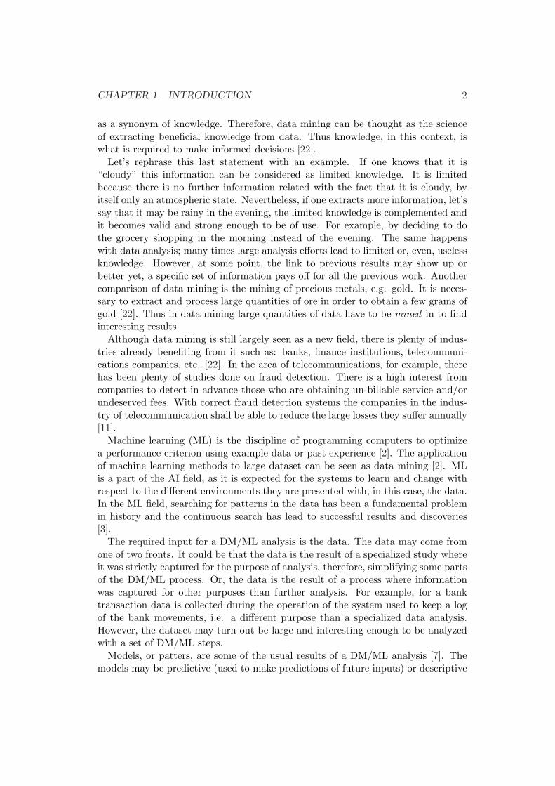
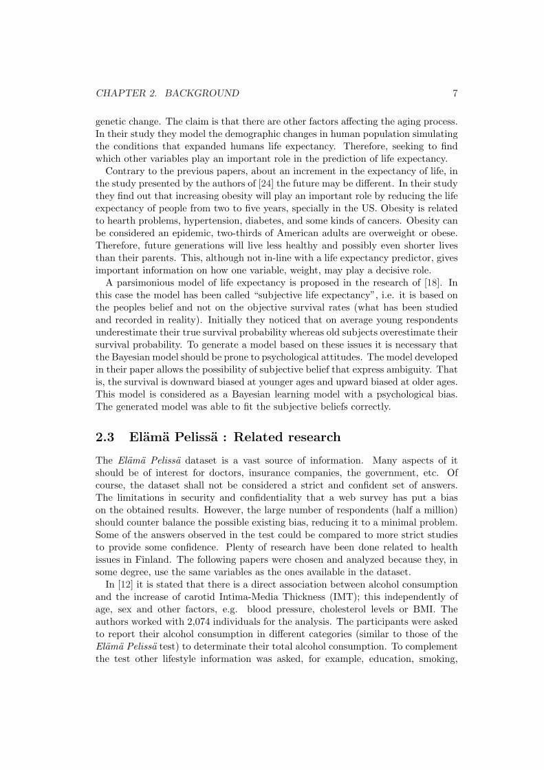
5.1 Variance of error depending on the number of samples . . . . . . . . 415.2 Linear model of variable Weight by means of Height . . . . . . . . . 425.3 Polynomial model of variable Weight by means of Height . . . . . . 445.4 Feature filter approach . . . . . . . . . . . . . . . . . . . . . . . . . . 44
viii

List of Tables
2.1 Life expectancy in Finland . . . . . . . . . . . . . . . . . . . . . . . . 6
3.1 Sub-questions in the Elama Pelissa test . . . . . . . . . . . . . . . . 133.2 Variable Age before and after filtering . . . . . . . . . . . . . . . . . 173.3 Proportion of valid, missing and outlier records in the database . . . 20
5.1 Numerical value of discrete . . . . . . . . . . . . . . . . . . . . . . . 40
A.1 Questions asked in the Elama Pelissa test . . . . . . . . . . . . . . . 55
B.1 Filtering out outliers from original database . . . . . . . . . . . . . . 58
C.1 Statistics from the sampled databases . . . . . . . . . . . . . . . . . 61
D.1 Single variable exploration findings . . . . . . . . . . . . . . . . . . . 64D.2 Discrete vs Discrete exploration findings . . . . . . . . . . . . . . . . 66D.3 Continuous vs Continuous exploration findings . . . . . . . . . . . . 68D.4 Discrete vs Continuous exploration findings . . . . . . . . . . . . . . 69
E.1 Mean predictors for continuous variables . . . . . . . . . . . . . . . . 75E.2 Regression with a single predictor . . . . . . . . . . . . . . . . . . . . 76E.3 Polynomial regression with extra variables Sex and Age . . . . . . . 77E.4 Polynomial regression with extra variables Sex and Age (Cont.) . . . 78E.5 Regression with the Forward stepwise selection algorithm . . . . . . 79E.6 Regression with the Forward stepwise selection algorithm (Cont.) . . 80E.7 Regression with the SISAL algorithm . . . . . . . . . . . . . . . . . . 81E.8 Regression with the SISAL algorithm (Cont.) . . . . . . . . . . . . . 82E.9 Neural network with Forward selection algorithm . . . . . . . . . . . 83E.10 Neural network with SISAL algorithm . . . . . . . . . . . . . . . . . 83E.11 PCA regression with Forward selection algorithm . . . . . . . . . . . 84E.12 PCA regression with SISAL algorithm . . . . . . . . . . . . . . . . . 84
ix

Chapter 1
Introduction
Nowadays it is known that data is everywhere; not only bits of data but really largeamounts of it. Nevertheless, the majority of the data observed today has always beenthere but we, as humans, were not able to collect it or realize it existed. Lately,however, the recollection systems have improved and we are observing, handlingand working with these immense piles of information. Today we are able to recordincredible amounts of data in just a few second, e.g. the new Synoptic SurveyTelescope being constructed in northern Chile will be generating 340MB of data persecond by 20151; and saving the data in continuously-improving smaller and moresecure devices as, e.g. flash memories, is even more possible.
Furthermore, in the industry, commerce, medical centers, etc., there are advancedmachines with precise measurement equipment updating databases constantly. For along time those measurements, or data, have been saved and used for many business-related purposes. But just recently has a further approach been taken with largedatasets, a decision to further collect and analyze the extracted valuable informationhiding behind the original purpose of the data. From astronomy to psychology thereare new and bast datasets waiting to be analyzed. However, the old approachesare not good enough and new methodologies are needed. Each dataset is, at someaspects, different to others, and traditional technology and approaches are not good,fast or even viable enough.
Data mining is a new research discipline that took off just a few years ago withthe aim of solving these problems. Data Mining (DM) is defined in [7] as:
“The science of extracting useful information from large datasets ordatabases”
DM combines Computer Science, Statistics, Artificial Intelligence (AI) and more.From the given definition it is important to notice the concept of useful information.On the one hand there is the term useful, defined as “Having the character or qualityto be of use or utility; suitable for use; advantageous, profitable, beneficial”2. Onthe other hand, the term information has been lately used, with some limitations,
1Large Synoptic Survey Telescope will generate 30TB of data per night, see [17].2useful at Oxford English Dictionary, see [23].
1
CHAPTER 1. INTRODUCTION 2
as a synonym of knowledge. Therefore, data mining can be thought as the scienceof extracting beneficial knowledge from data. Thus knowledge, in this context, iswhat is required to make informed decisions [22].
Let’s rephrase this last statement with an example. If one knows that it is“cloudy” this information can be considered as limited knowledge. It is limitedbecause there is no further information related with the fact that it is cloudy, byitself only an atmospheric state. Nevertheless, if one extracts more information, let’ssay that it may be rainy in the evening, the limited knowledge is complemented andit becomes valid and strong enough to be of use. For example, by deciding to dothe grocery shopping in the morning instead of the evening. The same happenswith data analysis; many times large analysis efforts lead to limited or, even, uselessknowledge. However, at some point, the link to previous results may show up orbetter yet, a specific set of information pays off for all the previous work. Anothercomparison of data mining is the mining of precious metals, e.g. gold. It is neces-sary to extract and process large quantities of ore in order to obtain a few grams ofgold [22]. Thus in data mining large quantities of data have to be mined in to findinteresting results.
Although data mining is still largely seen as a new field, there is plenty of indus-tries already benefiting from it such as: banks, finance institutions, telecommuni-cations companies, etc. [22]. In the area of telecommunications, for example, therehas been plenty of studies done on fraud detection. There is a high interest fromcompanies to detect in advance those who are obtaining un-billable service and/orundeserved fees. With correct fraud detection systems the companies in the indus-try of telecommunication shall be able to reduce the large losses they suffer annually[11].
Machine learning (ML) is the discipline of programming computers to optimizea performance criterion using example data or past experience [2]. The applicationof machine learning methods to large dataset can be seen as data mining [2]. MLis a part of the AI field, as it is expected for the systems to learn and change withrespect to the different environments they are presented with, in this case, the data.In the ML field, searching for patterns in the data has been a fundamental problemin history and the continuous search has lead to successful results and discoveries[3].
The required input for a DM/ML analysis is the data. The data may come fromone of two fronts. It could be that the data is the result of a specialized study whereit was strictly captured for the purpose of analysis, therefore, simplifying some partsof the DM/ML process. Or, the data is the result of a process where informationwas captured for other purposes than further analysis. For example, for a banktransaction data is collected during the operation of the system used to keep a logof the bank movements, i.e. a different purpose than a specialized data analysis.However, the dataset may turn out be large and interesting enough to be analyzedwith a set of DM/ML steps.
Models, or patters, are some of the usual results of a DM/ML analysis [7]. Themodels may be predictive (used to make predictions of future inputs) or descriptive

CHAPTER 1. INTRODUCTION 3
(to gain knowledge from the data) or both [2].This thesis is the result of a data mining and machine learning approach to a large
dataset of life styles in the Finnish population. The project included many, if notall, necessary steps to accomplish a small-scale but complete data mining analysiswhere interesting and useful results were obtained. Collaterally to the data miningwork the recovering of missing variables using the presence of others by means oflinear regression was also studied.
R, see [27], has been used as the de facto software tool for all the data analysiswithin the thesis. Perl has been an auxiliary language mainly used for scripting, e.g.pre-processing, data parsing, simplifying the creation of consults, etc. All the dataits being handled in a SQLite, see [10], database with a defined structure based onthree tables.
1.1 Outline
The work done for this thesis followed a similar approach as the one stated in [7],consisting on multiple steps. Initially, the dataset was understood, reviewed, thedifferent variables were selected and defined; afterwards the parsing process wasestablished. The data-processing step continued with the parsing and clean-up ofthe data, generating a valid dataset in an easy-to-understand and fast-to-accessformat.
With a structured dataset the data mining analysis was performed. The initialstep consisted in an exploratory visualization analysis of the data; some relationshipswere set and some findings were done. The exploratory analysis was followed by amodeling and regression analysis used to establish basic relationships between miss-ing and available variables. The regression was used for all variables but focusedon those with the most missing elements. The methods used were mean predic-tor, forward stepwise selection, SISAL, neural networks and principal componentanalysis.
The study concludes with the analysis of the different findings during the datamining approach, the visual exploratory analysis, the recovering of the missing vari-ables and the quality and usefulness of the results.

Chapter 2
Background
In this thesis a dataset is analyzed the later being the result of a web test preparedby various institutions from Finland. The dataset contains information regardingthe life styles or life’s risk the Finnish population has at present time. The originaltest was presented as an interactive part of a television show called Elama Pelissa 1.The television show was used as an incentive mechanism for the population to goand answer the web test form where important factors were captured. The webtest was answered by approximately half a million Finns. Although this is a largenumber, the test does not assure the independence of answers, i.e. one person couldhave answered the test several times. Nevertheless, half a million people account foralmost 10% of the total Finnish population. The television show was a part of theFinnish broadcasting company YLE during the year 2007. It was created by YLEwith the support of Duodecim and the Finnish National Institute for Health andWelfare (THL in Finnish).
Duodecim is a Finnish medical society playing an important role in the Finnishnational health care they have cooperation with different organization and officials[4]. Duodecim has supported this research by providing the author of the thesiswith the original dataset.
Another participant supporting the research is THL. A research unit inside THLhas been doing the FINRISK study since 1972, this study takes place every 5 years.The study is based on a survey on risk factors of chronic noncommunicable diseases.It uses random and representative population samples from all Finland. Datasetsresulting of the FINRISK surveys are used for a number of different research projectsand for national health monitoring needs [29]. Besides the contribution of THLto the development of the on-line test they also contributed with the algorithmthat calculates the life expectancy of a person given a set of input variables. TheFINRISK life expectancy algorithm is based on 37+ inputs, i.e. answers to differentquestions. Thus the users filling up the Elama Pelissa test are able to predict theirlife expectancy.
1Elama Pelissa can be roughly translated in English as: Life at stake.
4

CHAPTER 2. BACKGROUND 5
2.1 Elama Pelissa : The test
In Finland the life expectancy 100 years ago was just above 40 years; now thatexpectancy has almost doubled [14]. Individuals are free to take their own decisionand select their own choices on how their health and life expectancy is affected.Most of the Finnish people already know, or think that they know, how to improvetheir life and avoid health problems. However, many things that are consideredimportant are not that important or have not been proved important, e.g. eat morevegetables instead of stop smoking [14].
The Elama Pelissa test consists of 39 questions regarding the individual’s livingconditions, lifestyle, social relationships and experiences in different areas. Accu-rate answers to these questions will facilitate the prediction of “How long will theindividual live?”. The test can be taken as many times as wished; this openness iswith the sole purpose of showing the individuals what changes in his/her actual lifestyle could improve or worsen his/her health [14].
The test consists of 39 question considered key life factors. Of course the existenceof more factors that could affect the prediction is known, e.g. hereditary diseases orgenetic issues. Nevertheless, to keep the test accurate and at the same time simpleto an average public, specific or personal factors were not taken into account. Theimpact these factors may play, regarding the length of a life is limited, additionallyindividuals do not have enough information at hand [14]. For example cancer, insome cases is hereditary while in other cases not; therefore asking a question relatedto this disease is irrelevant. Other cases, e.g. glucose or sodium content in theblood, are difficult questions to ask as the answers are hardly known by individualsand could not be calculated by them without a laboratory study.
A descriptive list of the questions is in Appendix A. More information about thequestions and importance of each one is available in [14].
2.2 Elama Pelissa : Life expectancy prediction
As previously noticed the Elama Pelissa test is used to do a life forecast, i.e. predicthow long a person is going to live according to the given input (answer to ques-tions). The forecast takes into account a large number of factors. The test providesaccurate forecasts of life for people between 25 and 74 years of age that do not haveany hard illness affecting them, e.g. cancer or heart problems [14]. The forecast iscalculated based on the average figure of similar responses based on health monitor-ing. However, the use of the average, although complete and simple, discards thewell known individual variations. In general, the individual variations are consid-ered insignificant compared to the majority of the cases; therefore, affecting littlethe results. It is worth mentioning that the major impact factors are Smoking andAlcohol consumption. Nevertheless, all the factors, even simple ones, contribute tothe prediction.
The base average of life expectancy is reported each year by Statistics Finland2.2Statistics Finland is a Finnish government agency dedicated to produce statistics and informa-

CHAPTER 2. BACKGROUND 6
Life expectancyCurrent age Women Men
0 82 7620 83 7640 83 7760 85 8080 89 87100 102 102
Table 2.1: Life expectancy for men and women in Finland, according to [14].
The life expectancy works so that the older a person is the older he is expected tolive. Table 2.1 exhibits the life expectancy for men and women.
When gathering the information it is normal that some input variables are mis-taken or omitted. This is due to typo mistakes or respondents lack of knowledge,e.g. it is not common for people to know their diastole pressure in mmHg. The al-gorithm will use the population average (mean predictor) or if possible some relatedquestions to predict the erroneous/missing variable.
The problem of missing variables will be one of the topics later explored within thisthesis. In the following chapters there are studies on how to do better than the meanpredictor by means of other known variables. The mean predictor although simpleand in many cases good enough is not the best approach to solve the missing variableproblem, specially when a lot of information is available and DM/ML methods couldbe used. Replacing the missing data with the mean is known to produce biasedestimates, see [1], especially if the replaced variable is important for the estimation;therefore, this method shall be avoided if other approaches are available.
A similar project predicting for how long one is going to live has been developedby the University of Pennsylvania in [5]. They proposed a short and a long versionof what they call life calculator. The data and predictions are focused to Americans(USA); therefore, they claim, the forecast may not be accurate for other national-ities. A similar behavior shall be expected for the Elama Pelissa predictor, i.e. itwill work better with Finns than other nationalities. The questions used by thelife calculator are similar to those in the Elama Pelissa test. For example, theyask about education, smoking behavior, occupation activities and blood pressure.However, they have a complete different section where they ask questions related topossible hereditary diseases; like heart problems and colorectal cancer, for example.
Another interesting study has been done in [16]. Initially they comment thatduring the last century the average live expectancy has increased dramatically in theindustrialized countries; they claim that in America (USA) the increase has been ofalmost four fold. This drastic change however, is not an evolutionary change becausethe number of generations coexisting in a century is too small to have pushed a
tion services for the needs of society http://www.stat.fi
CHAPTER 2. BACKGROUND 7
genetic change. The claim is that there are other factors affecting the aging process.In their study they model the demographic changes in human population simulatingthe conditions that expanded humans life expectancy. Therefore, seeking to findwhich other variables play an important role in the prediction of life expectancy.
Contrary to the previous papers, about an increment in the expectancy of life, inthe study presented by the authors of [24] the future may be different. In their studythey find out that increasing obesity will play an important role by reducing the lifeexpectancy of people from two to five years, specially in the US. Obesity is relatedto hearth problems, hypertension, diabetes, and some kinds of cancers. Obesity canbe considered an epidemic, two-thirds of American adults are overweight or obese.Therefore, future generations will live less healthy and possibly even shorter livesthan their parents. This, although not in-line with a life expectancy predictor, givesimportant information on how one variable, weight, may play a decisive role.
A parsimonious model of life expectancy is proposed in the research of [18]. Inthis case the model has been called “subjective life expectancy”, i.e. it is based onthe peoples belief and not on the objective survival rates (what has been studiedand recorded in reality). Initially they noticed that on average young respondentsunderestimate their true survival probability whereas old subjects overestimate theirsurvival probability. To generate a model based on these issues it is necessary thatthe Bayesian model should be prone to psychological attitudes. The model developedin their paper allows the possibility of subjective belief that express ambiguity. Thatis, the survival is downward biased at younger ages and upward biased at older ages.This model is considered as a Bayesian learning model with a psychological bias.The generated model was able to fit the subjective beliefs correctly.
2.3 Elama Pelissa : Related research
The Elama Pelissa dataset is a vast source of information. Many aspects of itshould be of interest for doctors, insurance companies, the government, etc. Ofcourse, the dataset shall not be considered a strict and confident set of answers.The limitations in security and confidentiality that a web survey has put a biason the obtained results. However, the large number of respondents (half a million)should counter balance the possible existing bias, reducing it to a minimal problem.Some of the answers observed in the test could be compared to more strict studiesto provide some confidence. Plenty of research have been done related to healthissues in Finland. The following papers were chosen and analyzed because they, insome degree, use the same variables as the ones available in the dataset.
In [12] it is stated that there is a direct association between alcohol consumptionand the increase of carotid Intima-Media Thickness (IMT); this independently ofage, sex and other factors, e.g. blood pressure, cholesterol levels or BMI. Theauthors worked with 2,074 individuals for the analysis. The participants were askedto report their alcohol consumption in different categories (similar to those of theElama Pelissa test) to determinate their total alcohol consumption. To complementthe test other lifestyle information was asked, for example, education, smoking,

CHAPTER 2. BACKGROUND 8
physical activity, etc. Therefore, the questionnaire used was very similar to theone analyzed in this thesis. The correlations between the different risk factors andIMT were calculated using a stepwise linear regression model. In their findings theyobserve that for heavy drinkers a significant increase of arterial augmentation isnoticeable; supporting the statement that increased alcohol consumption is relatedto vascular damage in young adults especially among men. Other findings includethat the frequency of wine consumption was directly correlated with carotid IMT,independent of age, sex and other cardiovascular risk factors. Nevertheless, theyconclude their study was limited due to the small number of subjects drinking winedaily, hence, limiting the previous conclusion.
In another study by the authors of [21] the connection between alcohol-relatedmortality to age and sex is analyzed. The study estimates the impact of excessivealcohol use on life expectancy by sex. The study assumes that the mortality riskto alcohol-related causes is independent of all other mortality risks. The studywas done with the data available from the official death register maintained byStatistics Finland. Findings state that four out of ten alcohol-related deaths weredirectly attributable to alcohol; another four were accidental and violent deathswith alcohol-related contribution to the cause of death; the remaining two weredeaths from disease related to alcohol consumption. Deaths from disease with analcohol-related contribution were eight times more common among men than women.Alcohol-related accidental and violent deaths were almost 9 times more commonamong men. An interesting impact of alcohol found by the study is that alcoholreduced the life expectancy in women by 0.4 years and by 2.0 years in men. However,smoking reduces the life expectancy, at age 15, by 2.6 years among men and 0.3 yearsamong women, making smoking a more important cause of life reduction in men anda similar cause in women.
The paper of [9] reports on how smoking affects the quality of life of men andwomen in Finland. Previous studies have shown that tobacco consumption has adirect impact on the quality of life. The study divided the population into fourcategories depending on their smoking behavior: daily, occasional, ex-smoker andnever-a-smoker. The previous classification question was complemented by askingthe individuals an estimation of their quality of life by rating how good their presentlife has been. Fifteen additional questions related to discomforts were also asked,the answers ranged from 0 to 1. The study was performed separately for menand women. The influential variables used were age, marital status, education andincome. The findings show that compared to never-smokers daily smokers wereassociated with lower scores, i.e. worst feelings; in 9 of the 15 variables testedamong men, for example sleeping distress and vitality. Smoking women showed alsolow values. Consequently, daily smokers have a lower quality of live compared tonever smokers among both, men and women. However, the paper concludes thatthe numerical differences, although existent, are too small to consider smoking as avalid influence on the quality of life.
In the area of physical activities the paper of [28] is a study about physical activityamong the Finnish youth. The study initially states that the increase of obesity and

CHAPTER 2. BACKGROUND 9
the decrease in cardiorespiratory fitness among young people can be attributed tothe large amount of time spent watching TV (or computer screens or playing videogames). The study comprises 7,344 children from the northern regions of Finland(Lapland and Oulu). The subjects were asked about their daily physical activities,in ranges of 20 minutes; from 0 minutes to at least 1 hour per day. Corresponding totheir sedentary behavior they were asked about the amount spent on watching TV,reading books, at the computer and/or playing video games. The results showedthat boys are more physically active than girls; approximately 20% of the subjectsparticipate in moderate to vigorous physical activities. On the contrary, 50% of thesubjects do watch TV for more than 2 hours per day. However, the assumption thatTV incites inactivity showed some contradiction; in some individuals (43% of boys,23% of girls) watching 4 or more hours TV also included high levels of physicalactivities.
Related to diet and food intake there is the study of [25]. In the study it is analyzedthe consumption of polyphenols 3 in Finnish adults. The polyphenols are known ofhaving a beneficial effect on human health and they also provides protection againstchronic and cardiovascular diseases. The study was done to 2,007 adults between25 and 64 years of age. The daily mean intake of polyphenos is 863mg/d with ahigher intake by men than women. It was noticed that in the list of 20 foods withthe highest total polyphenol concentrations 16 were berries; in beverages the highestconcentrations was found in coffee (Finnish diet is well known for high consumptionof berries and coffee).
In the area of work and stress there is the study of [15] where they analyze the re-lation between Body Mass Index (BMI) and stress at work. Obesity is known to berelated to an interaction between biological and environmental factors. Therefore,the claim that the increasing proportion of obese people and the increase in stressrelated to a working life could be connected. The study covered more than 45,000employees; besides weight, height and age other variables were studied. These vari-ables included marital status, smoking status, alcohol consumption and physicalactivity. These variables were used as predictors of the BMI. In the results it wasnoticed that the BMI value was higher for men than for women; that the BMI meanincreased with age and that the BMI was highly related to socioeconomic status aswell as a lower job demand.
These formal studies have two things in common. Firstly, all of them wereperformed in Finland and among Finnish people. Secondly, the questions usedto extract information are very similar within them and in comparison with theElama Pelissa test, e.g. age, weight, stress, blood pressure, etc. Nevertheless, eachstudy focused on a different area like physical activity or smoking behavior. Theinterest of these studies, regarding the Elama Pelissa dataset, is that they weremainly limited in the number of participants. With the large data available it maybe probable to find new tendencies and/or complement the presented ones. Thework of finding multidimensional profiles could be improved by the localization of
3Polyphenols are a group of chemical substances mainly found in fruits like berries and vegetableslike cocoa or coffee.

CHAPTER 2. BACKGROUND 10
individual but important factors as, e.g. alcohol or smoking behavior.The study of this thesis will be, of course, not based in any scientific medical
terms, but more in the machine learning data mining science of extracting usefuland important information from a large dataset. Of what could be or should beinterpreted from the analysis results will depend on the specialists that take a lookat them. Some results are expected to be easily interpretable and some may requiremore specialization.

Chapter 3
Data pre-processing
A dataset is the resulting representation of the measurements taken from the envi-ronment or a given process [7]. This collection of measurements can be seen as an × p matrix, where n represents the number of objects from where the measure-ments were taken and where p represents the different measurements recorded. Theset of recorded variables describe the underlying process that generated them. Inthe case of the Elama Pelissa dataset the variables represent the life style of thedifferent people that answered the test. Usually datasets are captured for purposeother than data mining. Data mining is, in many cases, a secondary step; where thedataset is used to extract new and interesting information hiding behind.
3.1 The dataset
The purpose of the Elama Pelissa test is to invite people to play the life predictiongame, get to know their health status, life expectancy and act in consequence. All“plays” that have took place have been stored. The data was saved as it wasserved without any specification. The test transactions have been saved as URLs1
including the transaction variables2. The test consist on 17 forms (web pages) andas each page is sent to be processed it is saved as a unique URL, carrying with it thepreviously recorded variables and the ones given in the actual page. Therefore, it isexpected that in one play all saved URLs but the last one are incomplete becausenot all values from all variables have been given until the end. Besides the normalvariables in the test extra control variables are used. These control variables indicateif the test is complete and/or if it is a replay.
The knowledge on how the dataset has been structured and how it shall be readis not a strict part of the DM/ML approach. However, it is a part of the completedata analysis process strategy. One section in the process is called “Collection of
1URL stands for Uniform Resource Locator. URLs are commonly known as web page addresses.2Symbols & and = are used to separate and give variables an individual value, e.g.
?var1=3&var2=5. This approach is used to send and retrieve variables in scripting languagesunder GET transmission format. Therefore the variables are visible in the URL, contrary to POSTformat where the variables are send by other methods.
11

CHAPTER 3. DATA PRE-PROCESSING 12
data”. The collection of data includes the How is it going to be collected and How isit going to be saved. Moreover, this section can be extended to cover all the requiredpre-processing just before starting the strict analysis.
Duodecim provided 16 gzipped files. These files are from 8 servers which savedthe test transactions for two months, September and October of 2007. The serversshared the load, therefore all files have similar number of transactions. For Septem-ber, the initial month when the test was put on-line, each server saved 1,980,000transactions approximately. For October there were only 70,000 transaction in eachserver. The uncompressed dataset uses more than 24GB and has more than 16million transactions.
3.2 Parsing the data
One of the features that differentiates data mining from other types of data analysisis the large amounts of data to process [7]. With 24GB of information it is necessaryto organize the data in an efficient way. There are two alternating phases in a datamining approach. In the first phase it is necessary to get the data from the datasource and in the second phase it is necessary to run analysis algorithms on theextracted data. Because of the continuous switching between these two phases thecorrect organization of the data will play an important role on the speed with witchthe data is analyzed.
As previously stated not all transactions in the provided dataset are completetransaction; actually only a small percentage are complete, therefore valid. Hence,a filtering is necessary. The dataset was parsed using a Perl script programmedfor this purpose. The parsing program followed 8 steps to handle the data as bestpossible;
1. A transaction is selected only if it is a full transaction and if it represents thefirst play of the game, replays are discarded.
2. The valid transaction is broken into its different variables.
3. The date, UNIX epoch, of the transaction is calculated according to the avail-able information.
4. A reference to the input file and the row where the transaction is coming fromis extracted.
5. The recovered variables are cleaned-up, see sub section 3.2.1.
6. Extra informative variables Body Mass Index (BMI) and Total Alcohol Con-sumption are calculated.
7. A log of cleaned-up variables is kept as reference.
8. The variables of the transaction, the date, references and log are saved into aSQLite database, see sub section 3.2.2.

CHAPTER 3. DATA PRE-PROCESSING 13
Question Sub questions
7. Household size 7.1 Adults (18+ years)7.2 Minors (<18 years)
9. Cholesterol levels 9.1 Total cholesterol9.2 HDL cholesterol
10. Blood pressure 10.1 At systole10.2 At diastole
14. Alcohol use 14.1 Beer III, IV (bottle 1/3L)14.2 Long drink (bottle 1/3L)14.3 Concentrated alcohol (shot 4cl)14.4 Wine (glass 12cl)14.5 Light wine (glass 12cl)
Table 3.1: Variable expansion; questions 7, 9, 10 and 14 represent 11 variables.
3.2.1 Data clean-up
The on-line test includes some data protection, e.g. limitation of the number ofcharacters per input variable. Nevertheless, the web forms of the test do not handleall the possible inputs that may be introduced. As in any massive survey it isexpected that the subjects answering commit mistakes. The most obvious and easyto detect errors are typos, extra information or mixed answers. Errors appear due topoorly structured questions or laziness from the users to read and answer carefully.
For the data analysis it is necessary to keep the data as clean and coherent as pos-sible. Each URL contains 47 variables; there are 40 basic questions (as described inAppendix A) but some questions divide in sub-questions and each sub-question hasto be saved as an independent variable, see Table 3.1. That is why the total numberof variables is 47 and not the number of questions. All variables are quantitative,i.e. they represent a number. There are 18 continuous (nominal) variables and 29discrete (categorical) variables. Discrete variables are represented by integers whilecontinuous are represented by floats.
In the test it is possible to leave answers empty. If an answer is empty this usuallymeans that the user did not know the answer or he/she did not want to provide it.
During the data clean-up four issues were handled;
1. All URL encoding were converted to normal ASCII characters, e.g. %30 to 0.
2. Categorical question in the test are limited in the web form by means of radiobuttons. Each radio button is related to a unique integer value. However,it was noticed that because the variables were moved from web-form to web-form using the URL to carry them some hacking took place; some values werealtered and set outside their valid range. Incorrect answers out of the validrange were set to an empty value.

CHAPTER 3. DATA PRE-PROCESSING 14
3. For continuous variables non-numerical values are not valid answers. However,the web-forms do not prevent the users from introducing strings. Handling thisproblem was a big challenge, in many cases the given strings complementedthe answer, e.g. 78k in the question “How much do you weigh?”. Therefore,deleting these answers would have lead to a massive loss of information (on whyit is not good to just eliminate problematic records, see [1] second chapter).To overpass this problem the script was programmed to look for ordinarystrings and remove them. For example, the characters k(kilos), c(centimeters),t(hours), v(years)3 were removed.
Alcohol related sub questions (question No. 14) had plenty of unacceptableanswers. The test asks for the number of bottles or glasses, being drunk perweek; however, the questions and how to answer them is confusing. Someanswers were given in litters, others in centiliters, others in bottles, etc. Theseproblems were noticed because the strings users attached to their answers, e.g.25p. The script is programmed to handle the majority of the cases and if notable it will ask for help. The script will learn the provided help and use it asa reference for similar problems.
4. Another important issue observed in the dataset is the shifting of variables.Questions 37 and 38 are not included in the URL if their answers are leftempty, contrary to the rest of the questions that are included even if empty.The missing of such space holders shifts the order of the variables. Althoughnot a serious issue it has to be considered and handled correctly in order notto save answers of one question in another question’s section.
Informative variables BMI and Total Alcohol Consumption are calculated whileparsing each valid transaction. The variable BMI is calculated as the weight of aperson divided by his/her squared height, Equation 3.1. Total Alcohol Consumptionvariable is calculated as the sum of all the different alcohol consumption references,Beer, Long drink, Concentrated alcohol, Wine and Light wine. Although differentbeverages, it is possible to sum them together if they are registered in quantitiescontaining similar amounts of pure alcohol. That is why the questions ask for dosesin 1/3 of a liter, 4 centiliters and 12 centiliters. A similar approach was used in [12].
BMI =weight(kg)height2(m2)
(3.1)
In total there are 49 variables being processed, 47 original from the test and2 calculated ones. To these 49 variables 3 reference variables are added: time oftransaction, file transaction identifier and the row number where the transactionwas found. These reference variables though not of use in the DM/ML analysis willserve to backtrack errors to the original sources. The variables are all handled asnumbers; this approach will provide an optimized database with a small footprint.
3The t and v are for the Finnish words Tuntia (hours) and Vuotta (years).

CHAPTER 3. DATA PRE-PROCESSING 15
3.2.2 SQLite database
To perform the different phases of a DM/ML analysis it is necessary to have access toparticular sub-sets of the original dataset and, with the retrieved data, compute therequired analysis. One way to improve the access to the dataset is by organizing it ina structure that simplifies the burden of finding relevant points in it, i.e. be able tosearch for points quickly. Using a relational database that can be accessed by meansof the Structured Query Language (SQL) is a convenient way. SQL is a super setimplementation of what is known as relational algebra. The language is simple andintuitive, simplifying the access to sub-datasets. The strength of databases is thatthey provide fast execution for most of the queries; this is useful when the queriesare not known in advance and are formulated as the DM/ML project progress [7].
To save and organize the Elama Pelissa dataset the SQLite database engine isused [10]. This engine is based on extremely efficient R*Tree structures and thetotal engine size is less than 500 kilobytes; it also has a small memory footprint.Another benefit of using SQLite is the available plug-ins for Perl and R that permitinteracting with the database directly from these programs. Three tables werecreated for the dataset:
vars It is the main table where all the collected variables are saved. It has 55numerical fields plus the primary key. Each record has a key pointing to files.
info It is an informative table where original data, i.e. before processing, aboutAlcohol variables and Sleeping time is kept. This table can be considered asa log from the parsing script that processes the data. Each record has a keypointing to vars.
files This table contains information regarding the parsed files. Number of trans-action processed and number of valid transactions.
The parsing process for the 16 input files lasted no more than 30 minutes. A totalof 16,085,351 transactions were analyzed (15,555,584 for September and 529,767 forOctober) from those transaction only 457,097 were found as valid ones (445,278 forSeptember and 11,819 for October). Hence, from the provided dataset less than 1in 32 URLs was useful, only 3.29% of the recorded transactions. Moreover, a recordwas eliminated, setting the final number of transactions to 457,096. This recordwas reported by the logging mechanism as a “record with incomplete number ofvariables”. An in depth analysis to row: 1,082,747 of file: access log lahna syysshowed a damaged record; the URL has garbage in many of the variables.
The parsing also generated 4,937 records for the info table, i.e. there were around5,000 transactions (1% of the total) where the alcohol values or sleeping time infor-mation was detected as invalid and needed post processing by the parsing algorithm.
The process finished successfully with a completely populated database, in aneasy to access format and with a size of just 65MB, a radical improvement from theoriginal 24GB of data.

CHAPTER 3. DATA PRE-PROCESSING 16
3.2.3 Outliers
Outliers are points that come outside the main body of the data. These points havethe property of affecting the generation of data models. After parsing the data andhaving it loaded into the database the following step is to detect the outliers in it.Outliers have two possible sources; first, people made mistakes when answering thequestions, e.g. giving a height of 17 meters instead of 1.7 meters. Second, peopleintentionally played with the system giving invalid values, e.g. in the dataset someage values are set to 299,830 years.
The categorical variables are limited to only accept a restricted number of answers,incorrect answers are set to empty as it was explained in the previous section. There-fore, no more processing is needed. However, for continuous variables it is necessaryto calculate some basic statistics and limit their range accordingly. Initially thevariables are limited to what could be called an “educated guess”; thereafter with asimple statistical analysis the variables are limited to a range of 3σ, i.e. 3 standarddeviations from the mean. This approach considers 99.7% of the cases. This simpleprocess is done to each continuous variables; including the calculated ones BMI andTotal alcohol consumption.
The variables outside the statistical determined ranges are set to a -2 value in thedatabase4, also the counter kept at column outlierValue is increased. Otherwisethe record as a whole is not altered. This technique was performed manually toeach continuous variable in the dataset.
An example with variable Age is observable in Table 3.2. Initially the range ofvalues was wide open, up to 300,000 years with an extremely large variance. Thefirst filter, educated guess, was set to be < 500. This filter limited the age to gofrom 0 to 495 and normalized the original statistics values. However, the range ofage is still not usable, 495 is still to much for a human being; therefore a new filteris established setting the maximum of years to three standard deviations above themean. With this last filter the last column is obtained. Where the range of Agegoes from 1 to 88, a realistic value for human beings. During the filtering processthe mean had a small change, it went from 45 to 43 years. However, the variancechanged drastically, from more than half a million to 217. The filtering did not affecteither the Median (44 years) nor the Mode (50 years). A total of 801 Age variableswere set as outliers (64 from the first filter, 737 from the second). A similar processwas performed to all the continuous variables. Lets notice that not all variableswent through a two-step filtering, a second filter was applied only if required, e.g.the range of values with only one filter was still too large. The complete results forall variables can be observed in Appendix B.
If a record has few variables as outliers, e.g. two or three, it may imply that sometypos occurred while the user played the game. However, a record with multipleoutliers may imply that somebody introduced the errors on purpose; hence, the fullrecord shall be marked as an outlier, it should be discarded at once and its valuesnot used. With the numbers registered at the column outlierValue it is possible
4In the table vars two numerical codes are used to know why a value is not present or valid. A-1 means it is a missing value. A -2 means the value is an outlier.

CHAPTER 3. DATA PRE-PROCESSING 17
Age
Initial FinalMin 0 0 1Max 299830 495 88Mean 45.35 43.25 43.15Variance 594993.9 226.37 217.24Std Dev 771.36 15.05 14.74Median 44 44 44Filter < 500 µ < 3σ
Outliers 64 737 801
Table 3.2: Variable Age; before and after applying the different filtering rules.
to know the number of outlier fields in each record. The table vars also includesa column called outlier; this field is set to 1 when the record is an outlier and iskept as 0 when the record is valid.
Figure 3.1 depicts the number of outliers against the number of variables. It canbe seen that mistakes are common, there are 74,437 records with 1 to 4 outliers, i.e.16.28% of the answers in the test have a problem in up to 4 variables. In the figureis observable a breaking point at 5 variables. Therefore, five was decided as thenumber of outliers to separate valid records from invalid ones. Each record having5 or more outliers will be discarded, i.e. set to 1 in the outlier column. With thisdivision 2,668, 0.58%, records were marked as outliers.
In brief; two kinds of outliers were pinpointed in the data: the variables aloneand the complete records. When a variable is set as an outlier it is no longer usable;however, the record it belongs to is. On the other hand, when a record is tagged asan outlier none of its variables are usable, not even the few valid ones it may have.
The elements with values outside the valid ranges were labeled as outliers, ele-ments with missing values were not changed. Table 3.3 presents the proportions ofmissing, outlier and valid elements for each column in the database.
From the table it is noticeable that the discrete variables do not have outliers, dueto their limited set of answers. The only discrete variables outside this restrictionare House size adults and House size minors. These questions are open questions,i.e. the domain of the answer is the positive integers, however some outliers werefound and therefore the range was restricted. For any other case these two variablesare treated as discrete during the analysis.
The variables with the most missing values are Cholesterol total, Cholesterol HDL,Blood pressure diastole and Blood pressure systole. The high missingness of thesevariables is expected because of the difficulty the questions impose; knowing thecorrect answers beforehand is improbable. Other variables with high missingnessare House size minors and Number of cigarettes smoked per day. Although there ispeople with no children and people that does not smoke it is necessary to confirm

CHAPTER 3. DATA PRE-PROCESSING 18
Number of variables set as outlier
Num
ber
of r
ecor
ds (
thou
sand
s)
2 4 5 6 8 10 12 14 16 18 20 22
02
46
810
12
74,437 2,668
Figure 3.1: Plot showing the number of outliers against the number of records. Thebreaking point was set at 5. The arrows show the number of records in each set, lessthan 5 (Left) and 5 or more outliers (Right). The plot excluded the records withonly 1 outlier due to their large number (56,351).
this by giving a zero value in the answer. An empty answer is not automaticallytranslated to a zero-value answer. Therefore if the answers are not given the variablesare treated as missing ones. On the contrary, for the Alcohol-related variables emptyanswers will be translated to a zero-value, meaning that if a variable is left blankits value will be set to zero automatically. This modification is done accordingly tothe documentation of the test, see [14].
Regarding the outliers, the highest percentage are observable in the followingquestions: Until what age will you live? and When is the best age to live?. Althoughthese were simple questions the high number of outliers found was not expected.More difficult questions, e.g. Blood pressure diastole, did not show as many outlieras these two variables.
RecordsColumn Type Valid Missing OutlierSex D 453412(99.19%) 3684(0.81%) –Age C 452584(99.01%) 3711(0.81%) 801(0.18%)Height C 449834(98.41%) 5779(1.26%) 1483(0.32%)Weight C 448692(98.16%) 4037(0.88%) 4367(0.96%)Education C 448173(98.05%) 5648(1.24%) 3275(0.72%)Economic situation D 452154(98.92%) 4942(1.08%) –

CHAPTER 3. DATA PRE-PROCESSING 19
Income C 422703(92.48%) 27726(6.07%) 6667(1.46%)House size adults D 451762(98.83%) 4102(0.90%) 1232(0.27%)House size minors D 211093(46.18%) 244341(53.46%) 1662(0.36%)Cholesterol total C 243651(53.30%) 210739(46.10%) 2706(0.59%)Cholesterol HDL C 149737(32.76%) 304937(66.71%) 2422(0.53%)Blood pressure systole C 315379(69.00%) 135993(29.75%) 5724(1.25%)Blood pressure diastole C 311925(68.24%) 136960(29.96%) 8211(1.80%)Diabetes status D 448081(98.03%) 9015(1.97%) –Father infarct D 449151(98.26%) 7945(1.74%) –Mother infarct D 450130(98.48%) 6966(1.52%) –Alcohol beer C 448281(98.07%) 0(0.00%) 8815(1.93%)Alcohol drink C 453227(99.15%) 0(0.00%) 3869(0.85%)Alcohol concentrated C 450223(98.50%) 0(0.00%) 6873(1.50%)Alcohol wine C 450368(98.53%) 0(0.00%) 6728(1.47%)Alcohol light wine C 449763(98.40%) 0(0.00%) 7333(1.60%)Get drunk D 404024(88.39%) 53072(11.61%) –Vegetables D 451714(98.82%) 5382(1.18%) –Fruits and berries D 451564(98.79%) 5532(1.21%) –Kind of butter D 451699(98.82%) 5397(1.18%) –Kind of cooking oil D 450683(98.60%) 6413(1.40%) –Kind of milk D 448674(98.16%) 8422(1.84%) –Smoker for a year D 451063(98.68%) 6033(1.32%) –Smoking now D 448052(98.02%) 9044(1.98%) –Number of cigarettes C 199507(43.65%) 253868(55.54%) 3721(0.81%)Seat belt D 451189(98.71%) 5907(1.29%) –Sleeping time C 447291(97.85%) 4433(0.97%) 5372(1.18%)Sports activities D 451907(98.86%) 5189(1.14%) –Association activities D 448925(98.21%) 8171(1.79%) –Movies and theater D 451329(98.74%) 5767(1.26%) –Religious events D 448256(98.07%) 8840(1.93%) –Reading and music D 451765(98.83%) 5331(1.17%) –Hobbies D 451118(98.69%) 5978(1.31%) –Issues with spouse D 447882(97.98%) 9214(2.02%) –Issues with children D 448002(98.01%) 9094(1.99%) –Stress D 451709(98.82%) 5387(1.18%) –Life satisfaction D 451930(98.87%) 5166(1.13%) –Work study load D 448011(98.01%) 9085(1.99%) –Dreams impossible D 450634(98.59%) 6462(1.41%) –Do not have good friends D 450958(98.66%) 6138(1.34%) –What age will live C 431032(94.30%) 15585(3.41%) 10479(2.29%)

CHAPTER 3. DATA PRE-PROCESSING 20
Best time to live C 406536(88.94%) 35884(7.85%) 14676(3.21%)BMI C 441894(96.67%) 6201(1.36%) 9001(1.97%)Total alcohol consumption C 448323(98.08%) 0(0.00%) 8773(1.92%)
Table 3.3: Table of variables with the proportion of recordsthat are Valid, Missing or Outlier. The second column indi-cates if the variable is discrete (D) or continuous (C).
3.2.4 Grouping and Sampling
The database includes a total of 457,096 records. There are only 18,654 (4.08%)complete records, i.e. records where all the variables have a valid value. The com-plete records were grouped into identical ones to see if a basic profile could beidentified. However, 18,489 independent groups were found, the largest one with 7records; a really small number to call it a profile.
When using the original database 448,230 groups were found. The largest grouphas 1,835 records in it; nevertheless, instead of being an informative group, as theexpected profile, the group resulted to be the one with the records where all thevariables were left empty, i.e. no questions were answered. The next largest groupshave only 62 and 61 records hence, they are really small. The difference with thefirst group is that in these ones the Sex value is given, the rest of the variables arestill empty.
A database with complete valid records was generated. It has 18,489 records, itsbasic statistics were calculated and are observable in Appendix C. Because its sizethis database is easy and fast to handle and may be useful to speed up some analysis.However, a complete record may indicate two things; first, that it was answered bya person that knows him/herself really well and is willing to share the informationor, second; that it was answered by a person that knows his/her numbers becausehe/she has some problem and has to be cheeking them constantly. The later willrepresent a problem for further analysis because the data will be biased.
Another approach is to create samples of the original database based on all thevalid records. Nine databases were generated using random sampling selection fromthe original database. Only valid records, i.e. not outliers, were used; the pool tochoose from had 454,428 elements. The databases were filled in sets of three; with10,000 (2.2%), 50,000 (11.0%) and 200,000 (44.0%) records respectively. The basicstatistics of each group were also calculated, see Appendix C. The observed valuesare, as expected, close to those of the original data. However as it will be explainedin the next chapters the more records used the better results can be obtained.
Figure 3.2 illustrates a plot where different statistical information is comparedbetween the databases: Original, Complete records and samples 10k, 50k, 200k.Two variables are used for comparison Education and Blood pressure systole. Itis observable that all databases present similar basic statistics values. The largest

CHAPTER 3. DATA PRE-PROCESSING 21
Edu
catio
n
All Complete 10k 50k 200k
010
2030
MinMaxMeanVarianceStd. Dev.
Blo
od p
ress
ure
syst
ole
All Complete 10k 50k 200k
1060
110
160
MinMaxMeanVarianceStd. Dev.
Figure 3.2: Plot where the distributions for variables Education and Blood pres-sure systole for the sampled, complete and original databases are presented. Firstcolumn, all, shows the values for the original dataset. Column complete showsthe corresponding values for the dataset with only full records. Remaining columns10k 50k 200k show the statistics for the sampled datasets.
deviation is seen at the complete records dataset, where the variance is smaller. Thisdifference may correspond to some of the issues stated in the previous paragraphs.
The generation of the smaller databases will be of use when analyzing the dataand modeling the variables. Their size and completeness makes them easy to useand fast to analyze. The original database, however, has not been discarded. In thefollowing section a data exploratory analysis is performed. The different variablesare plotted in different ways and some interesting relations are found.

Chapter 4
Data exploration
When a new dataset is ready to be analyzed; one of the best, easiest and lesscostly ways of doing it is by performing a Data Exploratory Analysis (DEA). Dataexploratory analysis represent the set of techniques used for displaying a collectionof data so that the information within the data is easily available [19]. The datashall be displayed in a form that is simple, helpful and easy to interpret. Visualmethods are important because the human brain’s capability of analyzing imagesin a fast and accurate way. Correct visualization and careful analysis are ideal forfinding unexpected relationships in the dataset [7]. The exploratory analysis willprovide a way to check assumptions and reveal additional information that mayhave not been expected. Nevertheless, the limitations of the exploratory analysisare due to the high dimensionality of the data; how to display enough variables atonce to make the visualization valid, reliable and useful is a challenge. The basicprinciples on how to display data for accurate and effective analysis were followedas recommend in [32].
The Elama Pelissa dataset has 20 continuous and 29 discrete variables. Initiallyeach variable is analyzed independently. Then discrete variables are analyzed againsteach other and continuous variables are done so too. Finally, discrete variables areanalyzed against continuous variables.
4.1 Single plots
The Mean and Median are simple but interesting data summaries. Both are mea-sures of location [7]. The specific values for each variable were calculated in theprevious chapter for all continuous variables (see Appendix B and C). In the singleplots these measurements will be easy to visualize. For each single variable a plotand a histogram is calculated. Histograms are simple tools useful for displaying thefrequency distribution of a dataset. They could be used to observe data followingdifferent distribution, e.g. normal distribution. In a histogram the height of eachrectangle is dependent on the number of observations that lay on the width of thesame rectangle [19].
A total of 49 plots were generated, all graphics are available as a part of the
22

CHAPTER 4. DATA EXPLORATION 23
Milk
Fre
quen
cy
050
000
1000
0015
0000
2000
00
Whole Semi 1% Free Not
5963
7793
113
8899
1975
16
6 78 26 198 139
050
000
1000
0015
0000
Figure 4.1: Single plot of discrete variable Milk. “Fat free milk” and “Do notdrink milk” are the most common answers. With 197,516 (43%) and 138,899 (30%)respondents respectively.
research; however only some figures have been included in this thesis. For discretevariables Figure 4.1 illustrates the variable Milk. For continuous variables Figure4.2 illustrates the BMI of the population. All 49 plots were visually analyzed, someinteresting discoveries/observations are presented in Table D.1 in Appendix D. It isimportant to notice that these results come from a visual analysis therefore providednumerical values are not exact. Some plots returned valuable information, otherspresented obvious results and some few ones no information at all.
4.2 Discrete variables
The Elama Pelissa dataset has 29 discrete variables. Each variable was plottedagainst each other in a matrix-like figure. The size of the matrix corresponds to thenumber of different option combinations between the two evaluated discrete vari-ables. For example, there are five possible answers for Economic situation (Muchbetter, Better, Equal, Worse, Much worse) and there are four answers for Life satis-faction (Very pleased, Pleased, Somehow, Dissatisfied). Thus when these variablesare plotted together the resulting matrix will have 20 squares or options; each squarewill be labeled with the probability of the two answers shown together in the dataset.
A number and a color are associated to each square, the sum of all the numbers inthe matrix is 1000. The smaller the number is the smaller the chance of having suchcase in the data, contrary to what a large number represents. The colors go frompale yellow to dark green, where the pale yellow is associated with low probabilities

CHAPTER 4. DATA EXPLORATION 24
BMI (kg m2)
Fre
quen
cy
010
000
2000
030
000
4000
0
10 15 20 25 30 35 40
556
7412
094
2019
927
203
3387
341
039
020
000
4000
060
000
8000
0
10 15 20 25 30 35 40
Figure 4.2: Single plot of continuous variable BMI. The plot resembles a normaldistribution with a mean at 25.
and dark green with high probabilities. On the third and fourth axis of the plotthere are two histograms showing the number of corresponding answers for eachindividual option.
Depending on the resulting plot some interpretation can be done. With Economicsituation and Life satisfaction a possible linear relation is observed, i.e. a pooreconomic situation is related to a dissatisfied life. Figure 4.3 portrays the plot ofEconomic situation and Life satisfaction. Smoking and Stress are also correlatedvariables, Figure 4.4 depicts them.
With 29 discrete variables 406 combinations are possible; all combinations wereplotted and saved as part of the research. Some interesting discoveries are describedin Table D.2 in Appendix D. Not all plots showed important information but allcases were studied. The given percentages correspond to the pair of selected variablesfrom the amount of respondents found in the total number of records available. Nofilters have been used, e.g. dividing the respondents by sex or age groups; meaningthat the dataset was used as a whole.
4.3 Continuous variables
The Elama Pelissa dataset has 18 continuous variables plus two calculated ones.Each one of the variables has been plotted against each other in a contour-like plot.The contour has different colors for each surface which depends on the number ofelements it represents. Higher number of elements in the area are represented witha dark green color, while lower or none elements are drawn in pale gray.

CHAPTER 4. DATA EXPLORATION 25
Economic situation compared to the past
Life
sat
isfa
ctio
n
92
129
54
5
53
172
117
11
31
110
101
14
7
28
39
9
2
6
12
9
+B Better Eq Worse −W
AB
CD
280 353 256 83 29
185
445
323
48
Figure 4.3: Mixed plot of discrete variables: Economic situation and Life satis-faction. The plot shows a possible linear relation between the two variables; verypleased people will have a much better economic situation contrary to dissatisfiedpeople having a much worse economic situation.Code: A very pleased; B pleased; C somewhat satisfied; D dissatisfied.

CHAPTER 4. DATA EXPLORATION 26
Smoking now
Str
ess
10
39
99
24
2
16
50
11
13
119
469
149
Yes Random No
AB
CD
172 79 750
2517
461
818
4
Figure 4.4: Mixed plot of discrete variables: Smoking now and Stress. The plotshows that smokers are somewhat or more stressed; around 15% of the records failin these categories.Code: A yes, life its hard; B more than people in general; C somewhat; D no.

CHAPTER 4. DATA EXPLORATION 27
0
500
1000
1500
2000
10 20 30 40 50 60 70 80
4
6
8
10
12
14
16
18
20
22
24
Age
Yea
rs o
f edu
catio
n
Figure 4.5: Contour plot of continuous variables Age and Education. The educationlevel is limited by age, i.e. younger people do not have higher education levels. Itis also observable older generations are less prepared, e.g. 40-50 years old peopleconcentrate in 12 to 16 years of education while 50 to 60 years old people concentratein 8 to 14 years of education.
The number of elements available for the plot depends on the selected variables,e.g. for Age and Education there are 445,281 (97.4%) elements. Figure 4.5 illustratesa person’s years of education along with the age. Figure 4.6 depicts the consumptionof wine depending on the years of education. For this later plot there are 440,817(97.0%) elements. It is noticeable how educated people drink more wine, speciallywith 14 to 18 years of education.
With 20 continuous variables 190 different plots were generated. All plots weresaved as part of the research. Some interesting discoveries are described in TableD.3 in Appendix D. Only few plots showed important information but all cases werestudied. No filters were used during the generation of the plots.
4.4 Mixed variables
When working with discrete and continuous variables it is important to decide howto visualize pairs that come from both sources, i.e. how to have continuous anddiscrete variables on the same plot. For the analysis of the Elama Pelissa datasetthe discrete variables are set in the x -axis with their corresponding number of limited

CHAPTER 4. DATA EXPLORATION 28
0
10000
20000
30000
40000
4 6 8 10 12 14 16 18 20 22 24
0
2
4
6
8
10
12
14
16
Years of education
Gla
sses
of w
ine
(12c
l)
Figure 4.6: Contour plot of continuous variables Education and Wine consumptionper day in glasses. The years of education go from 6 to 21. The number of glasses ofwine have a peak at four when education is between 14 and 16 years. The majorityof the population drink less than one glass of wine per day; however, people withan education ranging between 12 to 18 years are the ones drinking more wine.

CHAPTER 4. DATA EXPLORATION 29
options; the continuous variables are set in the y-axis with their full range of values.The query applied to the database selects all the valid elements corresponding tothe pair of variables being processed. With the resulting dataset a matrix-likestructure is generated where the columns are normalized. Each column representsthe various options of the selected discrete variable. The normalization is done withthe objective of better observing how the continuous variables are distributed overthe discrete variables in each one of their different options. At the third axis thenumber of respondents per column is indicated. A color palette is added at thefourth axis, to facilitate the interpretation. The colors go from pale white to darkred; where pale white indicates low proportion of elements and dark red a highproportion. Let’s not forget that in these plots the values are given in proportionsand not in number of elements.
Figure 4.7 illustrates the plot of Economic situation and Education. The fivedifferent columns in the figure correspond to each one of the five different optionsto select from Economic situation. For all the columns dark red colors are observedbetween 12 and 16 years, specially 12 years. This means that independent of theeconomic situation a high proportion of people study for 12 years at least.
Figure 4.8 depicts the plot of Issues with children and Sleeping time; an interestingvariation is observable when problematic children show up. Another example isFigure 4.9 where variables Type of milk and Age are portrayed.
With a total of 49 variables (29 discrete and 20 continuous) the number of differentplots is 580. Some interesting discoveries are described in Table D.4 in AppendixD. Only few plots showed important information but all cases were studied. As inthe previous cases no filters were used during the generation of the plots.
4.5 Specific consults
In the previous sections the Elama Pelissa dataset has been analyzed using a visualexploratory approach; different kinds of plots were used depending on the type ofvariables. However, for all cases the full dataset has been used, i.e. all available andvalid records were used without filtering. A filter is a mechanism used to generatea valid subset of the full valid dataset. A filter can be used to select records limitedto the male or female gender, records that have w weight or y age, for example.With a filter correctly applied in a DEA it is possible to find interesting relationsinside subsets of data. The filter, or filters, can be as simple or complex as required.Initially some basic but useful filters are applied, e.g. sex, age group, etc. Morein-depth analysis may require a more advanced filter or sequence of filters.
To facilitate the filtering, plotting and analysis a Perl script was programmed.The script simplifies the generation of the SQL queries and it generates an R fileused to plot the resulting figure (if stated the script will handle the plotting also).The script can be run in batch mode or using a cgi web interface. However, the webinterface is not fully polished; the selection of variables and the setting of rangeshave to be done manually making it error prone.
The following four queries have been generated with the help of the script. The

CHAPTER 4. DATA EXPLORATION 30
Economic situation compared to the past
Yea
rs o
f edu
catio
n
Much better Better Equal Worse Much worse
124624 157122 113988 36943 12632
46
810
1214
1618
2022
24
(values are column normalized)
Low
High
Figure 4.7: Plot of discrete and continuous variables: Economic situation and Yearsof education. A step is observable at the different columns showing a possiblerelationship between the two variables. The people with a “Much better” economicsituation have an education level between 14-18 years; the people with a “Muchworse” economic situation have an education level between 8 and 14 years. Whilenot conclusive, it is noticeable that the education level directly affects the actualeconomic situation.

CHAPTER 4. DATA EXPLORATION 31
Issues with children
Sle
epin
g tim
e (h
ours
)
No ava. All the time Often Sometimes Rarely Never
146300 3703 13892 54583 120077 102842
56
78
910
(values are column normalized)
Low
High
Figure 4.8: Plot of discrete and continuous variables: Issues with children andSleeping time. The number sleeping hours for the population in general concentratebetween 7 to 8. The variation of hours of sleeping is similar in all the options ofvariable Issues with children; however at option “Issues all the time” a difference isnoticeable. For this case the sleeping time range goes down to 6 to 7 hours per dayand, in some cases, to 5 hours. Therefore, its a fact that problematic children doaffect the resting time of the parents.

CHAPTER 4. DATA EXPLORATION 32
Kind of milk
Age
(ye
ars)
Whole Semi 1 Fat free Do not drink
5855 77643 25657 196963 138549
1020
3040
5060
7080
(values are column normalized)
Low
High
Figure 4.9: Plot of discrete and continuous variables: Kind of milk and Age. Twointeresting patters can be observed in this plot. Firstly; it is observed that the agerange of people not consuming milk goes from 40 to 60 years. Secondly; whole milkis consumed in all the range of ages, but it is specifically consumed by older peoplebetween 60 to 80 years. This can be explained with the fact that some time agoonly the natural form of milk existed. The new milk categories are of recent times;therefore, old generations seem to be consuming what they grew up with.

CHAPTER 4. DATA EXPLORATION 33
0
200
400
600
800
1000
1200
0 2 4 6 8 10 12 14 16 18 20 22 24 26
20
22
24
26
28
30
32
34
36
38
40
Beer bottles per week
Age
(ye
ars)
Figure 4.10: Beer consumption per week for males between 20 to 40 years old; 68,694records (15.0%) found in this category. The gross of the population concentratesbetween 0 to 6 beers per week. The consumption is higher for people older than 25years. There is a visible consumption, 200 to 300 people, at 10, 12 and 15 beers perweek. Between 20 to 25 beers per week the visibility is less and a smaller populationof around only 100 people exists. Therefore, in average, it is highly probable that amale between 20 to 40 years old drinks one beer a day.
combination of filters that could be applied to the Elama Pelissa dataset is ex-tremely large (if not infinite); therefore, the analysis was limited to four consultsonly. The questions shown below are the result of the literature review and mypersonal interest.
1. What is the beer consumption per week for males between 20-40 years? Figure4.10.
2. What is the average income for people, male and females, with high stresslevels and a worse economic situation than the past? Figure 4.11.
3. What are the different life satisfaction levels for females that do normal tohard sports and have one or more minors living at home? and for those nothaving minors? Figure 4.12.
4. What are the cholesterol total levels for males that sleep seven or more hours,do not practice sports and are smokers? and for those doing sports and notsmoking? Figure 4.13.

CHAPTER 4. DATA EXPLORATION 34
Stress level
Inco
me
(tho
usan
ds o
f Eur
os p
er y
ear)
Yes its a hard life More than normal
3934 12311
020
4060
8010
012
0
Values are column normalized
Low
High
Figure 4.11: Income per year for people with high levels of stress and a “Worse”or “Much worse” economic situation that in the past; 16,456 records (3.6%) foundin this category. The results show a population earning mainly between 0 to 60thousands Euros per year. The highest levels of stress are seen at 30 thousandEuros. It is also noticeable that very stressed people, “Yes, its a hard life”, havein average a lower income than people stressed “More than normal”. However, theformer has only 3,987 elements, compared to 12,469 elements of the later, a ratioof almost 1:3. As could have been expected, the economic situation plays an inimportant role in people’s stress level.

CHAPTER 4. DATA EXPLORATION 35
Life Satisfaction
Sex 6511−27% 11830−48% 5697−23% 374−2%
Very pleased Pleased Somehow satisfied Dissatisfied
Fem
ale
A
(Internal labels Elements−Proportion)
Life Satisfaction
Sex 1415−20% 3295−46% 2240−31% 245−3%
Very pleased Pleased Somehow satisfied Dissatisfied
Fem
ale
B
(Internal labels Elements−Proportion)
Figure 4.12: Life Satisfaction of females that do heavy and normal sports having oneor more minor (A) or no minors (B) at home. In this plot it is noticeable how muchchildren influence the life satisfaction of females. While the proportion of answersfor “Pleased” and “Dissatisfied” do not change between plots, “Somehow satisfied”and “Very pleased” are switched. In plot A the really satisfied people represent27% of the population and 23% represent the quite satisfied. When children are notpresent there is a reduction in the really satisfied people proportion to 20% and anincrease in the quite satisfied people to 31%. Therefore, females with children aremore satisfied with their lives, hence, children play an importance role in female lifesatisfaction.

CHAPTER 4. DATA EXPLORATION 36
0
200
400
600
800
2 3 4 5 6 7 8
7
8
9
10
Level of total cholesterol (mmol/L)
Sle
epin
g tim
e (h
ours
per
day
)
A
0
200
400
600
800
2 3 4 5 6 7 8
7
8
9
10
Level of total cholesterol (mmol/L)
Sle
epin
g tim
e (h
ours
per
day
)
B
Figure 4.13: Cholesterol total levels for males sleeping seven or more hours thatsmoke and do not practice sports at all (A) and when not smoking and doing hardsports (B). Initially, it is observable that the mean level of cholesterol is at 5 mmol/Land that the average sleeping time variates from 7 (A) to 8 (B) hours. This variationmay be due to the hard sports performed. Another observable issue is that thecholesterol contour levels are higher in plot A than in plot B. In the first one thereare noticeable peaks (yellow-green) above 6 mmol/L while in the second one thelevels go below 4 mmol/L. Therefore, there is an indication that a sedentary lifecomplemented with smoking increases the levels of cholesterol. The desirable levelof total cholesterol is below 5.2 mmol/L according to [20]. Cholesterol total is oneof the variables that will be studied in the following chapter due to its high level ofmissingness.

CHAPTER 4. DATA EXPLORATION 37
The majority of the results obtained during the exploratory analysis could beconsidered new, interesting or reaffirmation of previous knowledge. In some casesthe results are exotic, e.g. the infarct of father increasing the BMI of a person.Some questions that may arise after the analysis as: why, how and who, shall bestudied by professionals from different fields as doctors, economist, sociologist, etc.Notwithstanding, this was the result of a data exploratory analysis; everything thatwas considered interesting has been pointed out throughout this thesis.
The exploratory data analysis showed the importance of an initial visualizationstage of the data and its basic features. Different types of plots used with differentpairs of variables showed important information within the data; without the needof an in-depth analysis. The filtering options and visualization tools facilitated theburden of preparing the queries and generating the plots, thus speeding up theexploratory process. Nevertheless, the analysis was delimited. The vast amountof available data and the different aspects of it would have required a full projectfocused to visualization and exploratory analysis; only to extract all the availableinformation.

Chapter 5
Regression models
5.1 Introduction
The analyzed dataset contains 47 variables of which 29 are discrete and 18 arecontinuous. As explained before, the dataset is the result of a questionnaire answeredby a large population. The application of a questionnaire to a large population hasconsequences; on the positive side the number of responses is very high, this gives awide range of different answers and enough correct responses to minimize the effectof possible errors. On the negative side large datasets are difficult to handle andusually require pre-processing; computational expensive tasks turn tricky to apply.
The dataset’s size also contributes to its porosity, i.e. there are unanswered ques-tions. The variables with missing values, as well as the outliers were previouslymarked in the pre-processing of the data. The percentage of availability of the vari-ables can be seen in Table 3.3. The missingness of each variable is highly relatedand dependent on the difficulty of the question related to it. If the respondent doesnot know the exact answer he/she may try to give the most used value, i.e. “thevalue everybody says is the correct one”. For example, in the case of Blood pressurelevels, people who had it checked a few days before answering the questionnairemay know the correct value, the same for people who have to check it constantly.However, the rest of the population may just try an average value or leave the fieldempty.
With enough information the missing variables could be recovered by means ofother available variables, one approach is the use of regression methods. In a linearregression problem the objective is to estimate the response variable y by a linearcombination of the input variables x = [x1, . . . , xd] [31]. The regression model isgiven by
y = Xβ + ε , (5.1)
where y is a N ×1 vector of responses and X is a N ×d matrix of input values. Theregression coefficients are given by β = [β1, . . . , βd]T and are unknown. The noisy
38

CHAPTER 5. REGRESSION MODELS 39
elements ε = [ε1, . . . , εd]T are independent and normally distributed with zero meanand a given variance εn ∼ N(0, σ2) [31].
The linear regression model given in [8] is
f(X) = β0 +p∑
j=1
Xjβj , (5.2)
the only major difference is in how the formula is represented. The term β0 is theintercept coefficient of the regression model.
To measure the quality of the regression model the Residual Sum of Squares (RSS)[8] also known as Sum of Squared Errors (SSE) [31] could be used. However, duringthis thesis the Mean Squared Error (MSE) is used. The sole difference is that theerror produced by the whole model is averaged by the number of elements used.The Root Mean Squared Error (RMSE) is the root of the MSE; by extracting theroot the measurement of the error is in the exact same units as the variable beingestimated.
RSS =N∑
i=1
(yi − f(xi))2 (5.3)
MSE =1N
N∑
i=1
(yi − f(xi))2 (5.4)
For the regression methods it is common to work only with continuous variables.Nevertheless, the idea of discarding all the discrete variables and only using thecontinuous ones did not seem correct. Specially, when more than half of the variablesbelong to this category; some useful information may be lying within them. It wasdecided to use the 7 most available discrete variables. They were transformed intoa valid continuous domain to be used in the regression problem. These selectedvariables and their numerical transformation are shown in Table 5.1.
Various regression methodologies were applied for this thesis. First, a regressionmodel was generated for each variable using its best predictor with a single vari-able. Then the previous approach was improved using a polynomial regression. Thethird and forth approaches included multiple input variables, in both cases differentalgorithms were used to select a relevant subset of predictor variables.
From previous analysis 5 variables were detected as the most missing ones, witha missingness between 30% to more than 50%. Four of these variables are related totopics which a given person has a high probability of not knowing the answer; thevariables are Blood pressure for diastole and systole, Cholesterol total and HDL.The fifth variable is Number of cigarettes being smoked per day; although, it is aneasy to know answer, the response is only available for 43% of the records. Themissing answers could just mean zeroes, i.e. not smoking anything or people hidingtheir smoking habits, thus affecting the result of the test. In an effort to improve

CHAPTER 5. REGRESSION MODELS 40
Variable Options (numerical value)
Sex Male(-1) Female(+1)Economic situation Much better(+2) Better(+1) Equal(0)
Worse(-1) Much Worse(-2)House size adults 1(1) 2(2) . . .Smoker for a year No(0) Yes(1)Smoking now No(0) Randomly(1) Yes(2)Stress Yes life is hard(3) More than average people(2)
Somewhat(1) No(0)Life satisfaction Very pleased(+3) Pleased(+2) Somewhat(+1)
Dissatisfied(-1)
Table 5.1: Discrete variable used for regression. The different options of each vari-able were transformed to an appropriate numerical value.
the regression of these variables a group of artificial neural networks were trainedand a PCA regression approach applied.
It has been stated many times before the size of the dataset. However, the questionof how many elements to use for regression is still open. As stated in [3] increasingthe size of the data reduces the over-fitting problem, this is observed in Figure 5.1.The number of points used affect the variance of the error for training and testing;the more points are used the more stable is the model. Therefore, it was decidedthat for all the regression approaches all the available points were going to be used.In the case of k-fold cross-validation only 20,000 elements are used because theapproach is always repeated, at least 100 times, to increase the reliability of theresults.
For each method studied in this thesis all the continuous variables were modeledusing the previously mentioned discrete variables, plus all the remaining continuousvariables with an availability of at least 95% and both calculated variables, BMI andTotal Alcohol Consumption. As a baseline to measure each one of the regressionmodels the errors given by the Mean predictor were used. The Mean predictor isbased on the mean, or most common answer, for each variable; an improvement overthe mean predictor can be considered a gain, or learning, by the model. The TableE.1 in Appendix E has the mean predictor for all the variables. Each variable has adifferent measure unit. To facilitate comparison and detection of importance withinvariables they were normalized to have a zero mean and unit variance.
5.2 Single predictor
In a linear regression model it is assumed that the regression function is linear in theinputs, or that the generated model is a good approximation [8]. By convention, inany model, linear or not, the x-variables has the role of explanatory variable while

CHAPTER 5. REGRESSION MODELS 41
Training setPoints used (thousands)
RM
SE
Wei
ght (
kilo
s)
0.9 45 90 135 180 225 270 315 360 405
13.1
13.3
13.5
13.3
0742
0
Testing setPoints used (thousands)
RM
SE
Wei
ght (
kilo
s)
0.1 5 10 15 20 25 30 35 40 45
12.8
13.2
13.6
13.3
0630
4
Figure 5.1: Variance of error in the Training and Testing phases depending on thenumber of samples used.
the y-variable is the response or result [19]. A linear regression model has the form
y = α + βx + ε , (5.5)
where the noise ε is independently and identically distributed with mean zero andvariance σ2. The coefficient x may come from different sources as its explained in[8]. It can be a quantitative input, a transformation of the quantitative input, anexpansion of the input (e.g. X2 = X2
1 ), etc. The estimation of the variable y is doneas
y = a + bx , (5.6)
where a is the intercept value, b is the slope and x the explanatory variable.For this thesis two linear approaches were followed. In the first approach the best
linear fitting variables are found, i.e. input variables are used, one by one, to findthe explanatory variable x that best fits the response variable y.
This first approach was performed as follows; for each pair of different variables,where one is the explanatory and the other one is the response, the complete validdataset was retrieved. With 90% of the retrieved dataset the linear model wasgenerated, the remaining 10% was used for testing the model. The variable thatpresented the smallest testing MSE was the selected explanatory variable of theactual variable.

CHAPTER 5. REGRESSION MODELS 42
Height (centimeters)
Wei
ght (
kilo
s)
130 140 150 160 170 180 190 200
2040
6080
100
120
Regression with 444K points(only 10K points in plot)MSE 177.1126RMSE 13.3084
Figure 5.2: Plot showing the linear model of variable Weight when using Height asexplanatory variable.
With the selected variable a 10-fold cross-validation was repeated 100 times andused to estimate the coefficients α and β as in Equation 5.6. The regression processreturned different results with interesting information. The results and error reduc-tion compared against the mean predictor are available in Table E.2 in AppendixE. As an example is the Height of a person; by using Sex as a explanatory variablethe MSE was reduced by 50% compared to the mean predictor, see Equation 5.7.For Weight a reduction of 30% is achieved when using Height as the explanatoryvariable, see Equation 5.8. Figure 5.2 shows the regression of variable Weight bymeans of Height.
H = 171.75− 6.76S (5.7)W = −88.12 + 0.96 H (5.8)
Not all models improved over the mean predictor, e.g. Alcohol Light Wine; in thiscase the error increased by 1%. In other cases the gain was too small, for exampleCholesterol Total and HDL had a gain below 5%.
In the second approach the models were set to have two fixed variables Sex and Ageplus a third one selected as the best explanatory variable. Moreover, the model wastrained with different polynomial degrees of the explanatory variable; the degreeswent from 1 to 5. All the different polynomials degrees were trained with all variablesand the best polynomial with the best explanatory variable was selected. From therefollowed a 10-fold cross-validation repeated 100 times to estimate the coefficients α

CHAPTER 5. REGRESSION MODELS 43
and [β1 . . . βd] where d is the degree of the selected polynomial.Sex and Age are selected as basic variables and they both have a linear influence
on the regression. The selection of these specific variables is because they can beseen as discriminants for the data, i.e. a way to cluster the data in a “natural” form(separation by sex and age groups). It is expected that, for example, height, weight,habits, stress levels, etc. differ between males and females. The same happenswith Age, factors vary over time and affect different, e.g. 60 year old people havedifferent habits than 30 year olds’. In many of the studies presented in Section 2.3this separation is noticed and used; therefore, this same regression approach is alsoused.
Sex and Age played an important role for the regression. For example, Agecontributed with more than 20% of the regression coefficient for Education, Income,Cholesterol total, Sleeping time and Best time to live; for this last one having morethan 80% contribution. Sex influenced the Alcohol concentrated and Light wine,with a participation of more than 10%; the same for Education and Blood pressuresystole but not diastole. The use of a polynomial regression model also contributedto an improvement compared to the previous single variable approach. There wereimprovements on the prediction of almost all variables; Height went from 51% to63%, Education from 0.02% to 0.05%, Number of cigarettes from 66% to 71%. Thedifficult variables: Blood pressure systole and diastole from 0.09% to 0.17% and0.09% to 0.13% respectively. The complete results can be seen in Tables E.3 andE.4 in Appendix E.
Figure 5.3 shows the regression of variable Weight using Height, the algorithmselected a polynomial of degree 5 as the best predictor. Height prediction improvedby 5 points, from 31% to 36%, using this approach. The regression formula can beseen at Equation 5.9 where S is Sex, A is Age and H is Height.
W = 35301.200− 1.239S + 0.213A− 1105.050H1 + 13.734H2
−0.085H3 + 0.0003H4 − 3.2E−7 H5 (5.9)
5.3 Feature selection
When there are plenty of variables available for regression it may seem wise to useall of them at once to predict the missing variable y. However, when solving thelinear models it is normal that all the input factors turn out to have coefficientsdifferent from zero regardless of its real importance [31]. Hence the problem ofselecting a relevant subset of features upon which to focus attention. Machinelearning algorithms including decision trees are known to degrade in performance,i.e. accuracy; when given as input features that are not necessary for predictingthe required output [13]. A feature X can be considered strongly relevant if theremoval of X alone will result in a deterioration of the classifier [13]. An approachto filter different features independently can be observed in Figure 5.4. All the set
CHAPTER 5. REGRESSION MODELS 44
Height (centimeters)
Wei
ght (
kilo
s)
140 160 180 200
2040
6080
100
120
MaleFemale
Regression with 442K points(only 10K points in plot)MSE 165.6593RMSE 12.8709
Figure 5.3: Plot showing the model of variable Weight when using Height in a poly-nomial form as explanatory variable. Sex was separated to appreciate the differentcurves for males and females. Variable Age, was kept fixed to its mean value.
featuresInput Feature
subset selectionInductionAlgorithm
Figure 5.4: Feature filter approach according to [13].
of features are given as initial inputs then a subset is selected based on a selectionalgorithm (Backward Selection, Forward Selection, SISAL, etc.) this selected subsetis later used as an input baseline for any Induction Algorithm, e.g. Linear regression,Neural networks, etc.
For feature selection the Stepwise selection methods are well known strategiesused to obtain candidate subsets from a set of input variables [31]. For this thesistwo methodologies are investigated, Forward Stepwise Selection and SISAL [30].Both methodologies were used as a way to select the best subset of features thatprovide the best regression in a parsimonious model.
5.3.1 Forward stepwise selection
The Forward Stepwise Selection algorithm starts with an empty set of inputs andadds the input that most decreases the RSS (or most improves the fit) in eachsubsequent step. The improvement in fit is often based on the F -statistics, Equation5.10, where β is the model with k features, β is the model with k+1 features and N is

CHAPTER 5. REGRESSION MODELS 45
the number of elements in the dataset. The algorithm sequentially adds the predictorproducing the largest value of F ; the forward selection algorithm is stopped whenthe F ratio is not greater than the 95th percentile of the F(1,N−k−2) distribution[8, 31].
F =RSS(β)−RSS(β)
RSS(β)/(N − k − 2)(5.10)
Each variable ran the forward selection algorithm in order to select the bestset of features that models the variable being analyzed. When the best featureswere selected a 10-fold cross-validation repeated 100 times was run to calculate thecoefficients of the selected features.
The use of forward selection resulted in improvements against the mean predictorat almost all variables but Alcohol Drink. The variables with the largest improve-ments were Number of cigarettes, Height, Weight, Best time to live and Incomewith a 67%, 61%, 35%, 28% and 18% improvement respectively. The most im-portant factors and their weights for these variables were Smoking now (0.83), Sex(0.51), Height (0.64), Age (0.94) and House size adults (0.25). The number of se-lected factors per variable was 5/15, 6/14, 4/14, 2/15 and 7/15; neither Height norWeight can be used for modeling themselves. Let’s notice that variable Number ofcigarettes is one of the five most missing variables.
The forward selection algorithm selected less than 50% of the number of featuresavailable for each variable; moreover, the few selected variables contributed to asignificant improvement in the prediction.
For the four remaining most missing variables the gains were as follows: Choles-terol Total 4%; Cholesterol HDL 3%; Blood pressure systole 15%; Blood pressurediastole 12%. The number of features selected was 4, 1, 3, 3 of 14 possible. Oneinteresting thing to notice is that the algorithm selected Age and Weight as themost important variables for Blood pressure diastole and systole. For Cholesteroltotal the variable with the most influence was Age. The complete set of results forthe forward selection algorithm can be seen in Tables E.5 and E.6 in Appendix E.
5.3.2 SISAL
Sequential Input Selection Algorithm (SISAL) is a simple and efficient backwardelimination algorithm proposed by [30]. In SISAL the removal of features is based onthe median and an empirically estimated width of parameter distributions sampledwith a cross-validation re-sampling process [30]. Initially all features are used in thealgorithm. The regression coefficient βi of each feature is sampled by a k-fold cross-validation repeated M times, i.e. a total of Mk coefficients are generated for eachfeature i. The median mβi
is calculated for each feature using the Mk estimates.The width of the sampled distribution is calculated by

CHAPTER 5. REGRESSION MODELS 46
∆βi= βhigh
i − βlowi , (5.11)
where βhighi and βlow
i are the Mk(1 − q) th and Mkq th values in the ordered listof the Mk estimates of βi. The variable q is a constant with a predefined value ofq = 0.165. Using the median and the width the least significant feature is removedfrom the input set. This is done by using the ratio |mβi
|/∆βi; the feature with
the smallest ratio is dropped from the set of inputs [30]. This sequence, of cross-validation and pruning, is repeated until there are no more features to remove. Theoutput is a number of models equal as the number of features available, due to thefact that only one feature is removed at a time. The model with the minimumvalidation error is selected and returned as the best model.
Each variable ran the SISAL algorithm to select the best model that representsit. A 10-fold cross-validation repeated 100 times was used to select the best featuresand models. The best results were obtained for variables Number of cigarettes,Height, Weight, Best time to live and Income, with respective improvements of 69%61% 37% 29% and 22% against the mean predictor. As can be seen, the samebest variables were observed while using the Forward stepwise selection algorithm;therefore, these variables may be easily predicted with a linear model. The mostimportant factors for these variables were Smoking now (0.68), Sex (0.49), Height(0.51), Age (0.66) and House size adults (0.19). Similar to those selected by forwardselection; however, the weight of the variables variates because SISAL selected, ingeneral, more features for each model. The number of selected features per variablewas 12/15, 9/14, 11/14, 12/15 and 13/15; neither Height nor Weight can be used formodeling themselves. As in forward selection variable Number of cigarettes showsup in the list of the best modeled variables.
The relatively high number of selected features provided a better regression com-pared to the single variable regression and a slightly improvement over forwardselection. However, the use of more than 80% of the available features per variablemay not be considered a simple and parsimonious model.
For the most missing variables the improvement was as follows: Cholesterol Total7%; Cholesterol HDL 4%; Blood pressure systole 19%; Blood pressure diastole 15%.The number of selected features were 9, 7, 4, 11 of 14 respectively. A noticeableimprovement in the regression can be observed, specially for Cholesterol HDL withan improvement of 4%. For all these four variables Age has a high influence onthe prediction, specially in Blood pressure diastole and systole. Another importantfactor selected by SISAL and with a relative high influence in the regression is TotalAlcohol Consumption, a calculated variable; it specially plays an important role forCholesterol HDL. The complete set of results for the SISAL algorithm can be seenin Tables E.7 and E.8 in Appendix E.

CHAPTER 5. REGRESSION MODELS 47
5.4 Regression improvement
The results of the previous methods show that some variables are easily defined bya linear model while others do not show an improvement over the mean predictor.If the gain is minute and/or it requires plenty of calculations to obtain it, it mayturn infeasible to use the model, specially if the mean predictor is so simple. Fromthe five most missing variables only one presented an improvement of more than50%, this was Number of cigarettes. For both Blood pressures the improvement wasabove 15% and for both Cholesterol levels it was below 10%. For the later the gainlevels by means of forward selection and SISAL can be considered small.
It is well known that the linear models are easy to interpret and fast to calculate;unfortunately they are not accurate enough for some problems [30]. The depen-dencies between variables may not be linear, therefore a non-linear model wouldexplain them better. It may also be that the features may work better if they aretransformed before the linear modeling is done. Two different methodologies areinvestigated; firstly, a feed-forward neural network is used for non-linear models.Secondly, regression on Principal Components (PCA) is analyzed.
The five most missing variables are used in this section; the available features aredetermined by the results of the previously executed forward selection and SISALalgorithms, i.e. the variables selected by these methods are used as input for theneural network and PCA approaches in the first run of experiments.
The importance of a variable in a model is given by how substantial is its coefficientin the regression model. Because all variables are mean centered and have unitvariance it is possible to compare them with each other. Neural networks and PCAare run, in a second set of experiments, using only enough features to represent atleast 80% of the weight available. These TOP features are also selected from theresults of the forward selection and SISAL algorithms.
5.4.1 Artificial neural networks
The artificial neural networks (ANN) are powerful processing systems originallyinspired by biological neurons [3]. The ANN are used because of its highly adaptivenonlinear models and high capability of adaptation based on the data. They havebeen used to solve many different problems, e.g. financial and biochemical systems[31]. Feed-forward ANN provide an adaptable way to generalize linear regressionfunctions, therefore the purpose of using them in this thesis. Generally a neuralnetwork consist of an input layer, a hidden layer and an output layer which are fullyconnected, i.e. each node in any layer is connected to all the nodes in the previouslayer. For how a ANN works, its variations and applications refer to [3, 8, 33].
The configurable neural network model available in R will be used for this thesis.The function is based on the one presented in [33]; the feed-forward neural networkis of generic form with a single hidden layer. For the purpose of modeling the givenvariables, the ANN are set to have a linear output instead of a logical one andthe number of hidden neurons varies according to the number of input features.The number of neurons in the hidden layer is changed from a minimum of half the

CHAPTER 5. REGRESSION MODELS 48
number of input features to twice plus one the number of input features, e.g. if thereare 5 input features the number of hidden neurons will vary from 3 to 11. Withthe network configured a 10-fold cross-validation process is repeated 100 times toincrease the reliability of the results. From the resulting networks the one with thesmallest error is selected.
In Table E.9, Appendix E, the results for the ANN when using the forward selec-tion features ALL and TOP can be observed. Compared to the results obtained byonly using forward selection a small positive improvement in the prediction is ob-served for both cases. Therefore, in the case of TOP, the model can be constrictedto only the most important variables without affecting the results when using theANN approach. Besides these facts the most difficult variable, Cholesterol HDL,did not present any improvement in the prediction.
In Table E.10, Appendix E, the results for the ANN when using SISAL are pre-sented. No improvement is visible in the predictions compared to the use of SISALalone. The only variable that presented a considerable gain is Number of cigarettes.This variable went from a 69% gain to 75% in the ALL variables test and to 73%in the TOP test.
The use of Neural Networks proved beneficial when using the features given byforward selection; nevertheless the gain was minute compared to the burden oftraining, testing and analyzing the ANN models. Neural Networks have proved tobe beneficial in an extensive number of different areas, however they are not thebest approach in all cases.
5.4.2 Regression on principal components
Methods for dimensionality reduction can be applied in the context of regression anddata analysis [19]. It may be useful to transform the set of explanatory variablesin a way that better suits the regression approach. Principal Component Analysis(PCA) is an orthogonal linear transformation that positions the data in a newcoordinate system. Each component in PCA represents a share of the variance;the first component has the largest sample variance; the second component has thesecond largest variance and so on [8]. The PCA transformation is based on thedecomposition of the data in its eigenvectors and eigenvalues, where each resultingvectors is orthogonal to each other. Further explanations and applications can befound in [2, 7, 8].
PCA is applied to the features selected by forward selection and SISAL. The datais used “raw”, i.e. there is no previous normalization, because the provided functionperforms this step. After calculating the PCA, enough components are selected torepresent at least 95% of the variance. In some cases only one variable was available,nevertheless the method was applied although no effect could be expected; this wasdone because the test ran systematically.
In Table E.11, Appendix E, the results for regression on principal components forthe features selected by forward selection are observable. Compared to the resultswhen only using forward selection no improvement is observed nor an importantdecrease noticed either. The only variable with a noticeable change is Number of

CHAPTER 5. REGRESSION MODELS 49
cigarettes; when using ALL the features it goes down to an improvement of only12%, on the other hand when using only the TOP features the gain goes up to 66%,matching that of the original prediction by forward selection.
In Table E.12, Appendix E, one can observe the results when using the SISALfeatures with PCA. Compared to the use of SISAL alone a reduction on the gain bythe predictor is noticeable; the most affected variables are Cholesterol HDL, Bloodpressure systole and Number of cigarettes. The tendency of no gain is also observedwhen using the TOP variables. Hence, the regression on principal components didnot improve the models while using the SISAL features as input.
PCA, although a well known methodology, did not show any gain on the qualityof the models. A future approach may include an in-depth study of the selectedvariables and their relations, as well as the visualization of the different componentsto observe, e.g. clusters.
When modeling the most missing variables, Cholesterol levels, Pressure levels andNumber of cigarettes it was noticed that nonlinear models, as feed-forward neuralnetworks, did not improve the quality of the prediction over other methods. In fact,the results were similar to those of simpler linear models and, in some cases, theresults were even worse. Similar results were observed while using regression onprincipal components, no improvements were seen at all. Moreover, some variableshave a noticeable reduction in the regression quality compared to the simpler models,e.g. Number of cigarettes. The results observed on Number of cigarettes provide astrong confidence of the linear model representation, as it could be calculated withan improvement of more than 60%, against the mean predictor, with a linear modelwith as few as 3 explanatory variables.
Chapter 6
Summary and conclusions
This thesis consisted on three parts. In the first part the dataset, Elama Pelissa,was presented and studied. The data was cleaned, pre-processed and inserted intoa custom-made database structure. All this with the purpose of facilitating theexploratory analysis and prediction of health related variables based on individuals’profile values. During this phase the basic statistics of each variable were calculatedand outlier elements were removed. The result of this phase facilitated an OnlineAnalytical Processing (OLAP), i.e. an approach to answer analytical queries in afast and reliable way.
For the second part a data exploratory analysis was performed. It was basedmainly on the basic statistics of the data and the visualization of the information indifferent plots. The information extracted during the exploratory analysis presentan interesting baseline for further analysis. All the variables were analyzed withdifferent approaches. An advanced script able to work with specific queries andplots was programmed with the sole purpose of finding interesting features thatmay not be easily visible.
In the third part of the thesis a data modeling approach was performed. Variousmethodologies were used for regression. The dataset has various elements as emptyfields, i.e. missing information. The objective behind the regression methods wereto create a model robust enough to predict these missing variables by using theavailable ones. Different configuration of linear models were tested; to complementthem Forward stepwise selection and SISAL algorithms were used. The informationobtained by these methodologies was fed into different multilayer perceptron net-works; another test consisted on doing regression by means of principal componentdiscriminant scores. The employment of fixed variables Sex and Age did improve theregression for single variable predictor models. Sex and Age showed to be relevantdiscriminant variables that shall be kept in mind for further analysis.
When using the variable selection algorithms, Forward stepwise and SISAL, inter-esting things were found. Both methodologies aim to reduce the number of necessaryvariables as much as possible while improving the quality of the model, i.e they followa parsimonious approach. SISAL demonstrated to be better than Forward stepwiseselection, the improvement difference is noticeable for some of the variables. How-
50

CHAPTER 6. SUMMARY AND CONCLUSIONS 51
ever, SISAL was more dense in the number of variables selected, therefore providinga more complex model. The algorithms’ different selection mechanism may be thecause of this difference. Forward stepwise increases the number of variables as again in the fit of the data while SISAL, on the other hand, reduces the number ofvariables based on the least significant variable.
In general, the work done provided large quantities of information and hints thatmay require further and deeper analysis. As consequence the work provided a struc-tured baseline in which future work could be done over the dataset. The datasetprovided detailed information that may not be available in smaller-scale question-naires. The findings, related to the Finnish way of living and its population, maybe of interest to the involved entities Duodecim and THL; they may provide furtherhints to focus the research. This thesis presented the initial round of findings andcould be easily extended into more in-depth areas as required. On the technicalside this thesis presented a complete data mining approach to a real life dataset,including detailed information on how to work and what to do with the data at eachphase.
6.1 Future research
The research done for this thesis had a limited scope. In the regression analysis onlycontinuous variables were used, for example. The analysis of discrete variables couldbe part of future research. Different approaches could be used for this purpose, e.g.Classification and Regression Trees (CART) for regression purpose [8]. Continuousvariables could be integrated in the regression if correctly discretized. Within theavailable discretization methods the one investigated was Histogram Analysis, inwhich the histogram distribution of the corresponding variable is used as a way todiscretize it [6].
A large dataset, as the one used for this thesis, could return interesting informationif it is clustered correctly. Because of the data content there are some variablesthat could be used for “natural” clustering, i.e. dividing the dataset in differentsubsets using only the different categories of the selected variables. Sex and Ageare important variables to keep in mind for this case; they played an importantrole when fixed for the regression models for single variable predictor as well as thepolynomial approach. More advanced clustering methods could be useful to finddifferent groups of people with similar profiles characteristics. The use of k-meansand x-means could be an efficient way to find these clusters [26]. Mixture modelsand Bayesian networks could also be used as methodologies for the analysis of thedata.

Bibliography
[1] Paul Allison. Missing Data. Quantitative Applications in the Social Sciences.Sage University Publications, 1st edition, 2001.
[2] Ethem Alpaydin. Introduction to Machine Learning. The MIT Press, 1st edi-tion, 2004.
[3] Christopher M. Bishop. Pattern Recognition and Machine Learning. Springer,1st edition, 2006.
[4] The finnish medical society duodecim. Internet: http://www.duodecim.fi,2009. Accessed July 17th, 2009.
[5] Dean P. Foster, Choong Tze Chua, and Lyle H. Ungar. How long will you live?http://gosset.wharton.upenn.edu/mortality.
[6] Jiawei Han and Micheline Kamber. Data Mining: Concepts and Techniques.Morgan Kaufmann, 1st edition, 2000.
[7] David Hand, Heikki Mannila, and Padhraic Smyth. Principles of Data Mining.The MIT Press, 1st edition, 2001.
[8] Trevor Hastie, Robert Tibshirani, and Jerome Friedman. The Elements ofStatistical Learning — Data Mining, Inference and Prediction. Springer Seriesin Statistics. Springer, 2001.
[9] H. Heikkinen, P. Jallinoja, S. Saarni, and K. Patja. The impact of smokingon health-related and overall quality of life: A general population survey infinland. Nicotine and Tobacco Research, 10(7):1199–1207, 2008.
[10] Richard Hipp et al. Sqlite. http://www.sqlite.org, 2009.
[11] Jaakko Hollmen. User Profiling and Classification for Fraud Detection in Mo-bile Communications Networks. PhD thesis, Helsinki University of Technology,2000.
[12] M. Juonala, J.S.A. Viikari, M. Kahonen, T. Laitinen, L. Taittonen, B.-M. Loo,A. Jula, J. Marniemi, L. Rasanen, T. Ronnemaa, and O.T. Raitakari. Alco-hol consumption is directly associated with carotid intima-media thickness infinnish young adults. the cardiovascular risk in young finns study. Atheroscle-rosis, 204(2):e93–e98, 2009.
52

BIBLIOGRAPHY 53
[13] R. Kohavi and G. H. John. Wrappers for feature subset selection. ArtificialIntelligence, 97(1-2):273–324, 1997.
[14] Seppo Koskinen, Tommi Harkanen, Pekka Jousilahti, Kari Kuulasmaa, Tu-ija Martelin, Ari-Pekka Sihvonen, and Ninni Vanhalakka. Pelataan elamanpelia. Internet: http://elamapelissa.yle.fi/sites/elamapelissa.yle.fi/pelataan elaman pelia.pdf, 2007. In Finnish.
[15] A. Kouvonen, M. Kivimaki, S.J. Cox, T. Cox, and J. Vahtera. Relationshipbetween work stress and body mass index among 45,810 female and male em-ployees. Psychosomatic Medicine, 67(4):577–583, 2005.
[16] A. Laszkiewicz, Sz. Szymczak, and S. Cebrat. Prediction of the human lifeexpectancy. http://arxiv.org/abs/cond-mat/0305277, 2003.
[17] Large synoptic survey telescope. Internet: http://www.lsst.org/lsst/about/technology, 2009. Accessed July 15th, 2009.
[18] Alexander Ludwig and Alexander Zimper. A parsimonious model of subjectivelife expectancy. http://ideas.repec.org/p/mea/meawpa/07154.html, 2007.
[19] John Maindonald and John Braun. Data Analysis and Graphics using R. TheCambridge University Press, 2nd edition, 2007.
[20] Mayo Clinic. Cholesterol levels: What numbers should you aim for?http://www.mayoclinic.com/health/cholesterol-levels/CL00001, 2009.Accessed September 1st, 2009.
[21] Pia Makela. Alcohol-related mortality by age and sex and its impact on lifeexpectancy: Estimates based on the finnish death register. European Journalof Public Health, 8(1):43–51, 1998.
[22] Michael Negnevitsky. Artificial Intelligence. Addison Wesley, 1st edition, 2002.
[23] Oxford english dictionary. Internet: http://dictionary.oed.com, 2009.
[24] S.J. Olshansky et al. Will obesity dramatically lower life expectancy inthe united states? Internet: http://healthfullife.umdnj.edu/archives/obesity archive.htm, 2005. Accessed July 27th, 2009.
[25] M.-L. Ovaskainen, R. Torronen, J.M. Koponen, H. Sinkko, J. Hellstrom,H. Reinivuo, and P. Mattila. Dietary intake and major food sources of polyphe-nols in finnish adults. Journal of Nutrition, 138(3):562–566, 2008.
[26] Dan Pelleg and Andrew Moore. X-means: Extending k-means with efficient es-timation of the number of clusters. Proceedings of the Seventeenth InternationalConference on Machine Learning, pages 727–734, 2000.

BIBLIOGRAPHY 54
[27] R Development Core Team. R: A Language and Environment for StatisticalComputing. R Foundation for Statistical Computing, Vienna, Austria, 2008.http://www.R-project.org.
[28] T. Tammelin, U. Ekelund, J. Remes, and S. Nayha. Physical activity andsedentary behaviors among finnish youth. Medicine and Science in Sports andExercise, 39(7):1067–1074, 2007.
[29] Terveyden ja hyvinvoinnin laitos. Internet: http://www.thl.fi, 2009. Ac-cessed July 17th, 2009.
[30] J. Tikka and J. Hollmen. Sequential input selection algorithm for long-termprediction of time series. Neurocomputing, 71(13-15):2604–2615, 2008.
[31] Jarkko Tikka. Input Variable Selection Methods for Construction of Inter-pretable Regression Models. PhD thesis, Helsinki University of Technology,2008.
[32] Edward Tufte. The visual display of quantitative information. Graphics Press,2nd edition, 2001.
[33] W.N. Venables and B.D. Ripley. Modern applied Statistics with S-PLUS.Springer, 2001.

Appendix A
Elama Pelissa test
The following table describes the questions asked in the Elama Pelissa test [14].Discrete answers are marked as [ ]. Continuous answers are marked as . Question40 is only available in the test on the web.
Table A.1: Questions asked in the Elama Pelissa test.
Variables Question givenPossible answer options
1. Gender What is your sex?[ ]Male [ ]Female
2. Age How old are you?Years
3. Length How tall are you?Centimeters
4. Weight How much do you weigh?Kilos
5. Education For how many years have you gone to school?Years
6. Income What was your total income last year (after taxes)?Thousands of euros
7. Household size Number of people living in your house (including yourself)Adults (18+ years)Minors (<18 years)
8. Economic situation How is your actual financial status compared to the past?[ ]Much better [ ]Slightly better [ ]The same[ ]Slightly worse [ ]Much worse
9. Cholesterol levels What is your cholesterol level (mmol/L) for ?Total CholesterolHDL Cholesterol
10. Blood pressure What is your blood pressure (mmHg)?At SystoleAt Diastole
55

APPENDIX A. ELAMA PELISSA TEST 56
Variables Question givenPossible answer options
11. Diabetes status Do you have diabetes?[ ]No [ ]Yes, Treatment is diet[ ]Yes, Treatment is medicine/insulin
12. Father infarct Has your father have a myocardial infarct?[ ]Yes [ ]No
13. Mother infarct Has your mother have a myocardial infarct?[ ]Yes [ ]No
14. Alcohol use How many glasses or bottles do you drink in a week of?Beer III, IV (bottle 1/3 l)Long drink (bottle 1/3 l)Concentrated alcohol (shot 4cl)Wine (glass 12cl)Light wine (glass 12cl)
15. Drunkenness How often do you drink so that you get drunk?[ ]2+/Week [ ]1+/Week [ ]1+/Month [ ]<1/Month
16. Fresh vegetables How often do you eat fresh vegetables?[ ]<1/Week [ ]1-2/Week [ ]3-5/Week [ ]Daily
17. Fruits and berries How often do you eat fresh fruits or berries?[ ]<1/Week [ ]1-2/Week [ ]3-5/Week [ ]Daily
18. Butter type What do you use as fat for bread?[ ]Butter [ ]Margarine [ ]Nothing
19. Cooking oil What kind of cooking oil do you use?[ ]Vegetable oil [ ]No fats oil [ ]Butter/Margarine
20. Milk What kind of milk do you drink?[ ]Whole [ ]Semi-skimmed [ ]Number one[ ]Skimmed [ ]Do not drink
21. Smoking Have you ever smoked daily for at least one year?[ ]Yes [ ]No
22. Smoking now Do you smoke now?[ ]Yes [ ]Randomly [ ]No
23. Number of cigarettes How many cigarettes do you smoke daily?Cigarettes
24. Sports How much physical activity do you do per week?[ ]Nothing hard (house chores)[ ]Light activities (walking)[ ]Normal activities (jogging)[ ]Hard activities (competition)
25. Seat belt Do you use a seat belt while traveling in a car?[ ]Yes [ ]No
26. Sleeping How many hours in average do you sleep per day?Hours
27. Association activities How often you go to a club or association?[ ]1+/Week [ ]1+/Mont [ ]1+/Year [ ]Almost never
28. Theater and movies How often do you go to the theater or movies?

APPENDIX A. ELAMA PELISSA TEST 57
Variables Question givenPossible answer options[ ]1+/Week [ ]1+/Mont [ ]1+/Year [ ]Almost never
29. Religious events How often do you assist to church or religious events?[ ]1+/Week [ ]1+/Mont [ ]1+/Year [ ]Almost never
30. Reading and music How often do you read books or listen to music?[ ]1+/Week [ ]1+/Mont [ ]1+/Year [ ]Almost never
31. Hobbies How often do you engage in hobbies-like activities?[ ]1+/Week [ ]1+/Mont [ ]1+/Year [ ]Almost never
32. Spouse Do you have issues with your spouse?[ ]Not married [ ]Almost all the time[ ]Sometimes [ ]Never
33. Children Do you have issues with your children?[ ]Not have children [ ]Almost all the time[ ]Quite often [ ]Sometimes [ ]Rarely [ ]Never
34. Stress Have you felt stressed the last months?[ ]Yes, life is unbearable [ ]Yes, more than average people[ ]Yes, somewhat [ ]Not at all
35. Satisfaction How satisfied are you with your achievements in your life?[ ]Very pleased [ ]Pleased [ ]Somewhat satisfied[ ]Dissatisfied
36. Work and study load Do you feel your work and/or study load is high?[ ]Do not have paid work [ ]All the time [ ]Quite often[ ]Sometimes [ ]Rarely
37. Dreams What do you think about:“It seem to me impossible to achieve dreams”[ ]Agree [ ]Somewhat agree [ ]Hard to say[ ]Slightly disagree [ ]Disagree
38. Friends What do you think about:“I do not have any good friend”[ ]Agree [ ]Disagree
39. Age to live Until what age will live?( )Years
40. Best age to live When is the best age to be alive?( )Years

Appendix B
Outliers search & labeling
The following table depicts the summary information of the continuous variablesduring the filtering process in the Elama Pelissa data base.† Stands for a filter that covers the elements from 0 to µ < +3σ‡ Stands for a filter that covers the elements within the range −3σ < µ < +3σ
Table B.1: Filtering out outliers from original database.
Age HeightInitial Temp. Final Initial Temp. Final
Min 0 0 1 0 130Max 299830 495 88 999 211Mean 45.35 43.25 43.15 170.5 170.67Variance 594993.9 226.37 217.24 186.86 88.93Std Dev 771.36 15.05 14.74 13.67 9.43Median 44 44 44 170 170Filter x < 500 † ‡Outliers 64 737 801 1483 1483
Weight EducationMin 0 0 22 0 0 2.5Max 999 499 130 999 89 25Mean 76.24 76 75.31 14.05 13.97 13.93Variance 523.01 332.95 260.16 69.66 15.58 13.1Std Dev 22.87 18.25 16.13 8.35 3.95 3.62Median 74 74 74 14 14 14Filter x < 500 ‡ x < 90 ‡Outliers 144 4223 4367 134 3141 3275
BMI IncomeMin 0 10 11.34 0 0Max 9.99x108 50 40.35 5472 278Mean 4905.44 25.85 25.6 55.93 48.53Variance 4.43x10¹² 23.45 19.18 5494.75 1202.75Std Dev 2105225 4.84 4.38 74.13 34.68
58

APPENDIX B. OUTLIERS SEARCH & LABELING 59
Median 25.1 25.06 25 45 45Filter 10 ≤ x ≤ 50 ‡ †Outliers 2765 6236 9001 6667 6667
Cholesterol total Cholesterol HDLMin 0 0 2 0 0 0Max 999 19 8 999 19 4.5Mean 5.67 5 4.98 2.52 1.8 1.73Variance 424.97 1.03 0.85 531.64 0.84 0.44Std Dev 20.61 1.02 0.92 23.06 0.92 0.66Median 5 5 5 1.6 1.6 1.5Filter x < 20 ‡ x < 20 †Outliers 670 2036 2706 342 2080 2422
Blood pressure systole Blood pressure diastoleMin 0 43 90 0 41 54Max 999 179 168 999 99 99Mean 129.79 129.1 128.92 79.98 79.08 79.18Variance 441.44 174.46 157.33 368.8 72.93 70.34Std Dev 21.01 13.21 12.54 19.2 8.54 8.39Median 130 130 130 80 80 80Filter 40 < x < 180 ‡ 40 < x < 100 ‡Outliers 2798 2926 5724 7211 1000 8211
Alcohol beer Alcohol long drinkMin 0 0 0 0 0 0Max 999 140 27 999 140 9Mean 4.08 3.69 2.89 0.79 0.42 0.24Variance 382.03 64.19 23.48 331.62 9.54 0.82Std Dev 19.55 8.01 4.85 18.21 3.09 0.9Median 1 1 1 0 0 0Filter x ≤ 140 † x ≤ 140 †Outliers 320 8495 8815 268 3601 3869
Alcohol concentrated Alcohol wineMin 0 0 0 0 0 0Max 999 140 17 999 140 17Mean 1.71 1.29 0.81 2.18 1.8 1.36Variance 368.27 29.02 5.04 342.31 26.04 6.89Std Dev 19.19 5.39 2.24 18.5 5.1 2.62Median 0 0 0 0 0 0Filter x ≤ 140 † x ≤ 140 †Outliers 351 6522 6873 322 6406 6728
Alcohol light wine Alcohol totalMin 0 0 0 0 0 0Max 999 14 1.5 4495 250 42Mean 0.49 0.07 0.01 9.26 7.03 5.95Variance 312.93 0.36 0.01 7842.6 137.93 58.8Std Dev 17.69 0.6 0.11 88.56 11.74 7.67

APPENDIX B. OUTLIERS SEARCH & LABELING 60
Median 0 0 0 3 3 3Filter x ≤ 140 † x ≤ 200 †Outliers 1066 6267 7333 810 7963 8773
Cigarettes per day Sleeping hoursMin 0 0 0 0 0.1 4.5Max 999 150 38 999 23 10Mean 8.21 6.52 5.74 7.52 7.48 7.48Variance 1532.05 110.82 67.07 30.01 1.14 0.9Std Dev 39.14 10.53 8.19 5.48 1.07 0.95Median 0 0 0 0 7.5 7.5Filter x ≤ 150 † 0 < x < 24 ‡Outliers 494 3227 3721 320 5052 5372
Age to live Best time to liveMin 0 1.6 57 0 1.5 1.5Max 999 119 111 3050 89 78Mean 86.89 84.41 84.89 36.75 37.48 37.43Variance 1742.21 84.37 60.97 516.48 189.95 187.7Std Dev 41.74 9.19 7.81 22.73 13.78 13.71Median 85 85 85 38 40 40Filter 1 < x < 120 ‡ 1 < x < 90 †Outliers 5249 5230 10479 14221 455 14676
Household size adults Household size minorsMin 0 0 0 0 0 0Max 9787 50 4 999 50 5Mean 1.83 1.68 1.66 1.77 1.44 1.38Variance 313.47 0.68 0.38 276.34 1.81 1.12Std Dev 17.71 0.82 0.61 16.62 1.35 1.06Median 2 2 2 1 1 1Filter x ≤ 50 † x ≤ 50 †Outliers 125 1107 1232 143 1519 1662

Appendix C
Selection of samples
Based on the original database ten smaller databases were generated. The first one,called Complete (C), includes only the complete records, i.e., the records where allthe variables have a value. The other nine databases are divided into three sets ofthree. Each set has a similar number of elements per database, 10k, 50k and 200krecords; i.e., there are three databases with 10k elements, three with 50k and threewith 200k. These databases were populated with random records selected from theoriginal database. Only valid records, not outliers, where available to be selected.The random selection was without repetition.
The sampling was done with the purpose of showing that there is not a com-pulsory necessity of using the full database; a large enough sample presents similarcharacteristics. This characteristic is mainly used during the regression analysis. Inthe k-fold cross-validation approach repeated M times a sample of only 20k elementsis used at each iteration. The reduction of the number of elements speeds-up theprocess without a significant influence in the result.
The following table depicts the statistics of the artificially generated databases;the average of values of each set of three is the one used. These values are, ingeneral, really close to the ones observed at Appendix B (last column, Final).
Table C.1: Statistics from the sampled databases.
Age HeightC 10k 50k 200k C 10k 50k 200k
Min 5 5 1 1 135 130 130 130Max 87 87.33 88 88 202 204 210 211Mean 45.36 43.16 43.27 43.21 172.4 170.67 170.68 170.67Variance 127.37 215.96 215.55 215.71 85.69 88.43 88.15 88.01Std Dev 11.29 14.7 14.68 14.69 9.26 9.4 9.39 9.38Median 45 44 44 44 172 170 170 170
Weight EducationMin 24 25.33 22.33 22 3 3 2.5 2.5Max 130 130 130 130 25 25 25 25Mean 77.83 74.12 75.26 75.24 14.75 13.96 13.95 13.96
61

APPENDIX C. SELECTION OF SAMPLES 62
Variance 230.59 256.21 257.3 257.23 11.98 13 13.04 12.99Std Dev 15.19 16.01 16.04 16.04 3.46 3.61 3.61 3.6Median 77 73.67 74 74 15 14 14 14
BMI IncomeMin 12.6 12 11.57 11.37 0 0 0 0Max 40.35 40.34 40.35 40.35 277 276.33 277.33 277.67Mean 26.06 25.57 25.6 25.59 58.99 48.48 48.72 48.73Variance 16.81 17.73 19.13 19.06 1333.41 1176.64 1204.11 1200.75Std Dev 4.1 4.37 4.37 4.37 36.52 34.44 34.7 34.65Median 25.47 24.97 24.99 24.98 55 45 45 45
Cholesterol total Cholesterol HDLMin 2 2 2 2 0 0 0 0Max 8 8 8 8 4.5 4.5 4.5 4.5Mean 4.91 4.96 4.98 4.98 1.68 1.72 1.72 1.73Variance 0.84 0.84 0.84 0.84 0.43 0.43 0.43 0.43Std Dev 0.92 0.92 0.92 0.92 0.66 0.65 0.65 0.66Median 5 5 5 5 1.5 1.5 1.5 1.5
Blood pressure systole Blood pressure diastoleMin 90 90 90 90 54 54 54 54Max 168 168 168 168 99 99 99 99Mean 128.7 128.77 128.94 128.88 79.41 79.09 79.16 79.16Variance 139.48 152.87 155.98 156.43 66.3 70.24 69.94 70.19Std Dev 11.81 12.36 12.49 12.51 8.14 8.38 8.36 8.38Median 130 130 130 130 80 80 80 80
Alcohol beer Alcohol long drinkMin 0 0 0 0 0 0 0 0Max 27 26.33 27 27 9 8.67 9 9Mean 3.34 2.86 2.86 2.86 0.24 0.23 0.23 0.24Variance 24.34 23.19 23.25 23.19 0.76 0.76 0.78 0.79Std Dev 4.93 4.82 4.82 4.82 0.87 0.87 0.88 0.89Median 1 0.67 1 1 0 0 0 0
Alcohol concentrated Alcohol wineMin 0 0 0 0 0 0 0 0Max 17 17 17 17 17 16.67 17 17Mean 1.01 0.76 0.78 0.79 1.72 1.34 1.35 1.35Variance 6.23 4.63 4.82 4.9 7.89 6.76 6.82 6.81Std Dev 2.5 2.15 2.2 2.21 2.81 2.6 2.61 2.61Median 0 0 0 0 0 0 0 0
Alcohol light wine Alcohol totalMin 0 0 0 0 0 0 0 0Max 1 1 1 1.33 42 42 42 42Mean 0.02 0.01 0.01 0.01 6.32 5.91 5.92 5.94Variance 0.02 0.05 0.01 0.01 46.09 58.73 58.14 58.47Std Dev 0.12 0.11 0.1 0.11 6.79 7.66 7.63 7.65Median 0 0 0 0 4 3 3 3

APPENDIX C. SELECTION OF SAMPLES 63
Cigarettes per day Sleeping hoursMin 0 0 0 0 4.5 4.67 4.5 4.5Max 35 36.33 37.67 38 10 10 10 10Mean 3.27 5.78 5.66 5.69 7.42 7.48 7.48 7.48Variance 42.58 66.81 66.18 66.08 0.77 0.89 0.89 0.89Std Dev 6.53 8.17 8.14 8.13 0.88 0.95 0.95 0.94Median 0 0 0 0 7 7.5 7.5 7.5
Age to live Best time to liveMin 57 57.33 57 57 2 2 1.83 1.5Max 111 110.67 111 111 77 75.67 77.67 78Mean 85.06 84.92 84.91 84.88 38.65 37.43 37.52 37.47Variance 57.14 60.39 60.19 60.62 164.74 186.91 186.44 187.15Std Dev 7.56 7.77 7.76 7.79 12.84 13.67 13.65 13.68Median 85 85 85 85 40 40 40 40
Household size adults Household size minorsMin 0 0 0 0 0 0 0 0Max 4 4 4 4 5 5 5 5Mean 1.7 1.66 1.66 1.66 1.15 1.38 1.38 1.38Variance 0.34 0.37 0.38 0.37 1.13 1.13 1.12 1.11Std Dev 0.59 0.61 0.62 0.61 1.06 1.06 1.06 1.06Median 2 2 2 2 1 1 1 1

Appendix D
Data exploration findings
The following tables depict the most interesting findings during the data explorationanalysis. The exploration consisted on simple queries used for displaying interestinginformation that is easily available. The variables were analyzed alone and mixed;discrete vs discrete, continuous vs continuous and discrete vs continuous. The letterk is used to indicate thousands, e.g., 40k equals 40,000.
Table D.1: Single variable exploration findings.
AgeThere are two possible normal distributions with means around 25 and 45 years.
Alcohol, beerOne to five bottles per week is what the majority (29%) of the people drinks.
Alcohol, light wineFew people drinks light wine (1%).
Alcohol, wineBetween 20k to 40k respondents drink 1 to 4 glasses per week.
Alcohol, drink to get drunk22k (5%) respondents get drunk more than once a week.
Association activitiesAround 241k (50%) respondents almost never participates.
Blood pressure diastoleAlmost everybody (70%) between 75 and 90 as expected.
Blood pressure systoleAlmost everybody (71%) between 120 and 140 as expected.
BMINormal distribution with mean at 25.
Cholesterol HDLHighest proportion of respondents with levels at 1 and 2 mmol/L.
Cholesterol totalNormal distribution with mean at 5 mmol/L.
Cooking oilVegetable oil is the most used one with 282k (62%) respondents using it.
64

APPENDIX D. DATA EXPLORATION FINDINGS 65
Diabetes21k cases of diabetes (4.5%), 14k (4%) are treated with insulin.
Do not have good friends52k (11%) respondents claim not having good friends.
Economic situationBetter and Much better situations are the most answered (63%) options.
EducationDependent on the age of the people with a peak at 12 years.
HeightNormal distribution with mean at 170 cms.
HobbiesMore than once a week has 167k (37%) respondents.
Infarct fatherAround 84k (18.8%) respondents with a Yes answer.
Infarct motherAround 37k (8.3%) respondents with a Yes answer.
IncomeResembles a Poisson distribution. The higher point at 50k euros.
Issues children147k (33%) respondents do not have children.
Issues spouseSometimes answer is the highest with 216k (48%);
91k respondants (20%) are single.
Milk138k (30%) respondents do not consume milk, the highest proportion
consume fat free 197k (43%).
Seat beltThere are 13k (2.8%) respondents that does not use seat belt.
SexThere are 70k more woman than man in the data set.
Size of the house adultsOne and two account for the majority of the answers (94%).
Sleeping time7 and 8 hours are the average, as expected.
Smoking cigarettes per dayThere is a tendency to round the answers, 10, 15 and 20.
Twenty being the most common answer.
Smoking daily for a year197k (43%) respondents have been smokers for a year.
Smoking now76k (17%) respondents are smoking now and 35k (8%) respondents
tend to smoke randomly.
Stress277k (61%) respondents are somehow stressed.
Weight

APPENDIX D. DATA EXPLORATION FINDINGS 66
Normal distribution with mean at 70kg.
What age will liveIncreased age to 91 years when respondants are between 80 to 90 years old.
Work and study load56k (12%) respondents do not have a paid job.
Table D.2: Discrete vs Discrete exploration findings.
Association activities Do not have good friendsNumber of answers of not having good friends increase when the association
activities occur almost never.
Association activities Religious eventsHighly correlated, 35% respondents have a Never answer in both.
Economic situation Association activitiesA better economic situation equals higher association activities.
Economic situation Dreams impossibleWith a worse economic situation it is more difficult to achieve dreams.
Economic situation Life satisfactionThere is linear correlation, good economic situation equals to a
satisfaction with life.
Economic situation Movies and theaterA better economic situation means people assist more often to these events.
Economic situation StressIn a worse economic situation people is more stressed.
Father infarct Mother infarct3.0% respondents have both as Yes.
Get Drunk Smoking nowPeople that get drunk is no more propense to be a smoker,
there are a similar number of smokers (4-6%) in all drinking categories.
Get Drunk Sports activitiesPeople that like to get drunk less is more sporty.
House size adults Dot not have good friendsThe proportion of not having good friends is high, 6%, when there are only
two adults in the house.
House size adults Get drunkIn cases of 1 or 2 adults the same drinking patterns are observed.
As if couples are going out together.
House size adults HobbiesIn cases of 1 or 2 adults the same hobbies responses are observed.
House size adults House size minorsThere is a high presence of minors when there are 2 adults; 1 minor 19%, 2 minors 21%.
House size minors Life satisfactionThe presence of one or more minor have a positive effect in life satisfaction.

APPENDIX D. DATA EXPLORATION FINDINGS 67
Life satisfaction Dreams impossibleDissatisfied people tends to agree with the impossibility of achieving dreams.
Religious events Dreams impossiblePeople that go to religious events tend to be more positive about achieving dreams.
Sex Diabetes statusMales have a higher probability of having diabetes 6.1% vs 4.2% of females.
Sex Economic situationWorse economic situation answer occurs more with females, 12.3%, than males, 9.4%.
Sex Fruits and berriesMales eat fruit in an uniformly distributed way, 24% fore each option.
42% of females tend to eat fruits and berries daily.
Sex Get drunkFemales are less propense to get drunk, males get drunk more often.
Once per week answered by 20% of males vs 9% of females.
Sex Kind of milk44% of the consumed milk is fat free and females intake 61% of it.
Sex Seat beltOf those not wearing a seat belt 70% are males and 30% females.
Sex Vegetables32% or respondents are females eating vegetables daily.
Smoking now StressThere is a tendency for smokers to consider themselves as stressed,
15% of the respondents fall in this category.
Sport activities Dreams impossiblePeople doing light and normal sports usually agree that achieving dreams is possible.
Sport activities Life satisfactionPeople that do sports is usually satisfied with their lives.
Sport activities StressStress can be related to people doing no sports at all.
Doing nothing and having more than normal stress levels account for 6% of respondents.
Stress Dreams impossibleNo stressed people agreeing with the possibility of achieving dreams accounts for 9.8%
of the respondents.
Vegetables Fruits and berriesEating Vegetables implies the consumption of fruits and berries.
Similar consumption patterns account for 51% of the answers.
Vegetables Sports activitiesBoth activities seem to be associated. Daily consumption is related with
light and normal sports activities for 38.5% of respondents.

APPENDIX D. DATA EXPLORATION FINDINGS 68
Table D.3: Continuous vs Continuous exploration findings.
Age Best time to livePeople tend to answer with their own age.
Age Blood pressure diastole/systoleOlder people have a tendency for a higher blood pressure.
Age BMIOlder people have a tendency for a higher BMI.
Age Cholesterol Total/HDLOlder people have a tendency for a higher cholesterol level.
Age EducationThe majority of the people starts education at age 6 and continues up to age 24,
new generations are more educated than older ones.
Age Total alcohol consumptionA noticeable increase in consumption after the age 18.
Blood pressure diastole/systole Total alcohol consumptionHigh pressure seems to be correlated with heavy alcohol consumption.
Cholesterol HDL Blood pressure diastole/systoleWhen the HDL is lower the blood pressure is slightly higher.
Cholesterol HDL BMIIt is noticeable that for lower levels of HDL the BMI is higher.
Education Alcohol beerLess educated people tend to drink more beer.
Education Alcohol wineMore educated people tend to drink wine.
Education Total alcohol consumptionLess educated people drink more alcohol.
Education IncomeHighly educated people have a better income, the average income in Finland
is seen between 40k to 60k euros.
Height Cigarettes per dayTaller people seems to smoke more.
Height WeightVariables are correlated. Taller people weights more, as expected.
Income Total alcohol consumptionWith an income of more than 20k the alcohol consumption increases to 5 or more
doses per week. Between 20k to 60k euros the consumption can be more than 10 doses.
Number of cigarettes What age will liveHeavy smokers (20+ cigarettes per day) reduce the number of years they will
live by 5 to 10 years compared to the average.
Weight Blood pressure diastoleHeavier people have a higher blood pressure, as expected.
Weight Cholesterol HDLHeavier people have a lower level of HDL.
Weight Number of cigarettesHeavier people seems to smoke more (as taller people do).

APPENDIX D. DATA EXPLORATION FINDINGS 69
Table D.4: Discrete vs Continuous exploration findings.
Diabetes status AgePeople with diabetes controlled by diet have an age range between 50-65 years,
people using insulin have an age range between 55-70 years.
Diabetes status Blood pressure diastolePeople with diabetes show higher levels of blood pressure.
Diabetes BMIPeople without diabetes have a range between 20-30, while diabetics have a range between 23-35.
Diabetes EducationPeople with diabetes have a lower number of years of education.
Diabetes WeightDiabetics tend to be heavier, with a range between 70-100 kilos.
Dreams impossible EducationPeople with higher education disagree less with the impossibility of
achieving dreams compared to people with less education.
Economic situation AgeThe Much better economic situation shows between 50-70 years.
The Much worse shows from 40-60 years and Worse shows in old people 60+ years.
Economic situation EducationEducated people have a much better situation that less educated people.
Economic situation Sleeping timeA much worse economic situation has people sleeping less than 6.5 or more than 9.5 hours.
Economic situation What age will livePeople with much worse economic situation expect to live less.
Father infarct AgeIt occurs when one is between 40-60 years old.
Father infarct BMIWith a father infarct people have a higher BMI.
Father infarct EducationA father infarct is related, strangely, to a lower level of education.
Fruits and berries AgeDaily consumption concentrates between people 50-60 years old.
Fruits and berries Blood pressure diastolePeople with a daily consumption have a slightly lower lever of blood pressure.
Fruits and berries EducationPeople with a higher education level consumes fruits and berries more often.
Get drunk Alcohol, beerGetting drunk more than once per week is correlated to high levels of beer consumption.
Get drunk AgePeople getting drunk more than once per week are, mainly, between 40-60 years old.
Get drunk EducationEducated people tends to get drunk less often.
House size minors Age

APPENDIX D. DATA EXPLORATION FINDINGS 70
Minors usually cohabitate with parents when parents are between 30-50 years old.
Issues children AgeThe conflicts usually occur when parents are between 40-60 years old, specially at theirs 50’s.
Issues children BMIWhen there are issues all the time the BMI range is higher, 24-32; (the average is 23-28),
with not children the BMI is below 20-25.
Issues children Cholesterol totalWhen there are issues all the time the cholesterol level range is higher (5-7mmol/L)
compared to the average of (5mmol/L).
Issues children EducationWhen there are issues all the time the parents’ education level is
below average compared to other groups.
Issues children IncomeNot having children is related to a lower income.
Issues children Number of cigarettesHeavy smokers have a tendency for issues all the time.
Issues children Sleeping timeWith issues all time the sleeping time is lower, 5-7 hours; than the average of 7-8 hours.
Issues children Total alcohol consumptionIssues all the time is related to heavy alcohol consumption.
Issues children WeightIssues all the time is related to heavier people.
Issues spouse Blood pressure diastoleHigher levels of blood pressure is observed when there are issues all the time.
Issues spouse Number of cigarettesConsumption of 20 to 30 cigarettes is related to issues all the time with spouse.
Issues spouse Total alcohol consumptionIssues all the time is related to high levels of alcohol consumption.
Cooking oil Total cholesterolHigher levels of cholesterol are present when using butter/margarine.
Cooking oil EducationMore educated people use vegetable oil, less educated people use butter/margarine.
Kind of milk AgeOlder people (60-90 years) drink whole milk, people not drinking milk is between 40-60 years.
Kind of milk Alcohol, beerWhole milk drinkers tend to drink more beers than the average.
Kind of milk Blood pressure diastole/systoleWhole milk drinkers have higher levels of pressure.
Kind of milk BMIWhole and semi milk drinkers have a lower BMI, 20-27; compared to the average of 23-27.
Kind of milk Cholesterol totalWhole milk drinkers have a higher level of cholesterol.
Kind of milk EducationWhole milk drinkers have a lower level of education.
Kind of milk Income

APPENDIX D. DATA EXPLORATION FINDINGS 71
Whole milk drinkers have a lower income.
Kind of milk Cigarettes per dayWhole milk drinkers smoke more than the average.
Life satisfaction Alcohol, beerDissatisfied people drink more beer.
Life satisfaction AgeDissatisfied people cover all the range of ages, from 20 to 60 years old.
Life satisfaction Best time to liveDissatisfied people set the best time to live around 20-30 (young ages).
Life satisfaction Blood pressure diastoleDissatisfied people have a higher pressure level.
Life satisfaction EducationVery pleased people are more educated compared to dissatisfied people.
Life Satisfaction HeightTaller people is slightly more dissatisfied than average-height people.
Life Satisfaction IncomeSatisfaction is highly correlated with the income.
Life Satisfaction Number of cigarettesDissatisfied people tend to smoke more.
Life Satisfaction What age will liveDissatisfied people have a lower expectancy, 60-80 years; compared to the average of 80-90 years.
Mother infarct AgeIt occurs when people is between 45-65 years.
Mother infarct BMIWith a mother infarct people have a higher BMI.
Mother infarct EducationA mother infarct is related, strangely, to a lower level of education.
Movies and theater AgeYounger people, 20-30 years, go more often, 1+/month, to these events.
Movies and theater EducationMore educated people go more often, 1+/month, to these events compared to
less educated people that goes almost never.
Movies and theater IncomeWith a higher income people assist more often to these events.
Movies and theater Cigarettes per dayHeavy smokers Almost never go to movies/theater.
Reading and music Alcohol beerHeavy beer drinkers Almost never read or listen to music.
Reading and music EducationReading and listening to music is positively correlated to the education level.
Reading and music Cigarettes per dayHeavy smokers almost never read or listen to music.
Reading and music Total alcohol consumptionHigh alcohol consumption is related to no reading nor listening to music.
Religious events Age

APPENDIX D. DATA EXPLORATION FINDINGS 72
Assistance of 1+/month shows a higher level between 50-70 years old people,
1+/week shows a high level between 50-60 years and 25-30 years.
Religious events Total alcohol consumptionThere is a decrease in alcohol consumption as the assistance to religious events increases.
Seat belt Alcohol, beer and concentratedHigher beer/alcohol concentrated consumption is related to no using seat belt.
Seat belt AgeYounger people, 20-40 years, are the ones less likely to use the seat belt.
Seat belt EducationLess educated people tend to use the seat belt less.
Seat belt IncomeLower income is related to not using the seat belt (Is due to public transportation?).
Seat belt Total alcohol consumptionHigher levels of alcohol are related to not using the seat belt.
Seat belt What age will livePeople not using the seat belt gave a lower range, 70-90 years; compared to the average of 80-90 years.
Sex Alcohol, beerMales have a higher maximum of beer consumption with 25 bottles per week compared to
10 bottles per week by females.
Sex AgeThe range of ages for both sexes is similar, 25-60 years.
Sex Blood pressure diastole/systoleHigher pressure levels show more in males than females.
Sex BMIMales have a range between 23-30 while female have a range between 20-27.
Sex EducationFemales are more educated, 12-18 years, compared to the 9-18 years of males.
Sex HeightThe range for males is between 170-190cm, for female the range is between 155-170cm.
Sex Number of cigarettesMales smoke more; 25 and 30 cigarettes per day is mainly done by males.
Sex Total alcohol consumptionMales have a higher maximum level of alcohol consumption, 35 doses vs 20 of females.
Sex WeightThe average of males is between 70-100kg, for females the average is between 50-80kg.
Smoker for a year Alcohol, beerSmokers are related to higher levels of beer consumption.
Smoker for a year BMISmokers have a higher BMI.
Smoker for a year EducationSmokers have a lower education level.
Smoker for a year Total alcohol consumptionHigh consumption of alcohol is related to a Yes in smoking for a year.
Smoker for a year WeightHeavier people tend to have been smokers for a year.

APPENDIX D. DATA EXPLORATION FINDINGS 73
Smoking now Alcohol, beerA Yes answer is related to heavy beer consumption, no smokers are related
to lower beer consumption.
Smoking now AgeRandom smokers are between 20-30 years old.
Smoking now EducationSmokers tend to have a lower level of education.
Smoking now Number of cigarettesHigh presence at 10, 15, 20 (up to 30) cigarettes per day, random smokers are between
1-5 cigarettes per day.
Smoking now Total alcohol consumptionFollow the same tendency as beer consumption.
Smoking now What age will liveSmokers tend to have a lower life expectancy, 70-90 years, compared to the average of 80-90 years.
Sports activities AgeHard sports are being done by people between 15-30 years.
Sports activities Blood pressure diastole/systoleThe blood pressure is lower for people doing hard sports.
Sports activities BMIPeople not doing sports have a higher BMI, 23-27, compared to the BMI of people doing
hard sports, 20-25.
Sports activities Sleeping timePeople doing hard sports tend to sleep more, 7-10 hours, than the average of 7-8 hours.
Sports activities WeightPeople doing nothing is heavier than people doing some kind of sports. There is abundance of
people weighting 90+ kilos.
Stress AgeThe majority of the people with no stress at all are between 55-65 years old (28%).
Stress Blood pressure diastole/systoleWhen answer is Yes it’s a hard life people have a higher pressure level.
Stress IncomeThe answer Yes it’s a hard life is related to a lower income.
Stress Sleeping timeStressed people sleep less, or more, than the average (5-10 hours).
No stressed people sleeps more, 7-10 hours.
Stress What age will liveStressed people responded with a lower life expectancy, 60-90 years, than the average of 80-90 years.
Vegetables AgePeople eating less than once per week are between 20-30 years,
people with daily consumption are between 40-60 years.
Vegetables EducationLess educated people tend to consume less vegetables.
Vegetables IncomeA higher income is related to daily consumption of vegetables.
Vegetables Number of cigarettes per day

APPENDIX D. DATA EXPLORATION FINDINGS 74
Heavy smokers tend to eat vegetables more sporadically.
Work/Study load AgeNot paid work is usually present within people between 60-70 years old.
Work/Study load Best time to livePeople with not paid work set an older best time to live range 40-60 years,
compared to the average of 30-50 years.
Work/Study load Blood pressure diastolePeople with an answer of Always show a higher pressure level.
Work/Study load EducationNot paid work is related to lower education level.
Work/Study load Sleeping timeHigh load is related to shorter sleeping time, 5-8 hours, while not paid work and
rarely load have a longer sleeping time 7-10 hours.

Appendix E
Regression tables
The following tables depict the different regression strategies used for this thesis.Depending on the approach the tables also show the selected variables, their corre-spondent coefficient the Mean Squared Errors for the training and testing sets. Allstrategies were compared to the Mean predictor at Table E.1, using this last one asbaseline. The improvement is also depicted in the tables at the last two columns.Long tables were divided in two; the first section shows the regression parametersand values, the second section shows the errors and improvements.
Variables Y Mean predictor MSE RMSE
age 43.2196 215.7516 14.6885height 170.6765 88.1681 9.3898weight 75.2627 257.8829 16.0587education 13.9488 13.0000 3.6055income 48.6815 1197.5406 34.6055cholesterolTotal 4.9799 0.8375 0.9152cholesterolHDL 1.7279 0.4342 0.6590bloodPressureSystole 128.8930 156.4849 12.5094bloodPressureDiastole 79.1710 70.1752 8.3771alcoholBeer 2.8687 23.1699 4.8135alcoholDrink 0.2362 0.7912 0.8895alcoholConcentrated 0.7914 4.9086 2.2155alcoholWine 1.3528 6.8010 2.6079alcoholLightWine 0.0113 0.0111 0.1055numberOfCigarettes 5.6978 66.2813 8.1413sleepingTime 7.4834 0.8906 0.9437whatAgeWillLive 84.8797 60.5785 7.7832bestTimeToLive 37.4743 186.9253 13.6721BMI 25.5954 19.0848 4.3686totalAlcoholConsumption 5.9380 58.4402 7.6446
Table E.1: Mean predictors for continuous variables.
75

APPENDIX E. REGRESSION TABLES 76
Vari
able
sY
Pre
dic
tor
XIn
terc
ept
Slo
pe
MSE
MSE
Impro
vem
ent
Impro
vem
ent
train
ing
test
ing
train
ing
test
ing
age
alc
oholW
ine
41.6
643
1.0
531
208.4
756
208.4
796
0.0
30.0
3
hei
ght
sex
171.7
531
-6.7
647
43.5
831
43.5
841
0.5
10.5
1
wei
ght
hei
ght
-88.1
171
0.9
576
177.2
027
177.2
066
0.3
10.3
1
educa
tion
alc
oholW
ine
13.6
960
0.1
776
12.7
673
12.7
676
0.0
20.0
2
inco
me
econom
icSit
uati
on
41.5
295
9.1
205
1108.3
357
1108.3
588
0.0
70.0
7
alc
oholB
eer
sex
3.1
394
-1.4
752
21.1
359
21.1
364
0.0
90.0
9
alc
oholD
rink
slee
pin
gT
ime
0.4
336
-0.0
263
0.7
879
0.7
879
0.0
00.0
0
alc
oholC
once
ntr
ate
dalc
oholB
eer
0.5
072
0.0
962
4.5
860
4.5
862
0.0
70.0
7
alc
oholW
ine
age
-0.0
736
0.0
333
6.5
961
6.5
963
0.0
30.0
3
alc
oholL
ightW
ine
alc
oholW
ine
0.0
131
-0.0
013
0.0
112
0.0
112
-0.0
1-0
.01
slee
pin
gT
ime
stre
ss7.7
120
-0.2
215
0.8
675
0.8
676
0.0
30.0
3
whatA
geW
illL
ive
life
Sati
sfact
ion
82.2
874
1.4
929
58.7
030
58.7
045
0.0
30.0
3
bes
tTim
eToLiv
eage
16.1
769
0.4
940
134.5
867
134.5
901
0.2
80.2
8
chole
ster
olT
ota
lage
4.3
413
0.0
129
0.8
127
0.8
128
0.0
30.0
3
chole
ster
olH
DL
wei
ght
2.1
231
-0.0
051
0.4
275
0.4
275
0.0
20.0
2
blo
odP
ress
ure
Syst
ole
wei
ght
110.7
684
0.2
372
142.0
263
142.0
389
0.0
90.0
9
blo
odP
ress
ure
Dia
stole
wei
ght
66.9
990
0.1
595
63.8
639
63.8
696
0.0
90.0
9
num
ber
OfC
igare
ttes
smokin
gN
ow
-0.4
573
7.1
280
22.2
687
22.2
710
0.6
60.6
6
Tab
leE
.2:
Reg
ress
ion
wit
ha
sing
lepr
edic
tor.

APPENDIX E. REGRESSION TABLES 77
Vari
able
sY
Pre
dic
tor
XIn
terc
ept
Sex
Age
X1
X2
X3
X4
X5
hei
ght
wei
ght
0.0
6994
-0.5
6846
-0.1
3737
0.2
8045
-0.0
3010
0.0
3187
-0.0
2252
0.0
0360
wei
ght
hei
ght
-0.0
2820
-0.0
7411
0.1
9492
0.4
8191
0.0
4013
0.0
1739
-0.0
0507
-0.0
0138
educa
tion
hei
ght
0.0
2059
0.2
1028
-0.0
6333
0.1
8610
-0.0
0404
0.0
2665
-0.0
0744
-0.0
0118
inco
me
house
Siz
eAdult
s0.0
6133
-0.0
6043
0.1
3944
0.2
8243
-0.0
7002
-0.0
1128
0.0
0417
–
alc
oholB
eer
smokin
gN
ow
0.0
5284
-0.2
8839
-0.0
3349
0.2
9764
-0.0
5284
––
–
alc
oholD
rink
stre
ss-0
.00446
-0.0
3148
-0.0
7110
0.0
1809
0.0
0167
0.0
0638
––
alc
oholC
once
ntr
ate
dalc
oholB
eer
0.0
1822
-0.1
7771
0.0
8990
0.3
8770
0.0
9320
-0.2
1520
0.0
7343
-0.0
0749
alc
oholW
ine
econom
icSit
uati
on
-0.0
1754
0.0
2635
0.1
8520
0.1
1005
0.0
2790
-0.0
2641
-0.0
0929
–
alc
oholL
ightW
ine
slee
pin
gT
ime
-0.0
0428
0.0
3192
0.0
1840
0.0
0598
0.0
0598
-0.0
0531
-0.0
0054
0.0
0061
slee
pin
gT
ime
stre
ss-0
.01682
0.0
6533
-0.1
5721
-0.1
8479
0.0
1682
––
–
whatA
geW
illL
ive
life
Sati
sfact
ion
-0.0
1459
0.0
6966
-0.0
0946
0.1
8267
0.0
1531
0.0
0087
––
bes
tTim
eToLiv
eed
uca
tion
0.0
1718
0.0
5188
0.5
2700
-0.0
3711
-0.0
1775
0.0
0795
––
chole
ster
olT
ota
lalc
oholB
eer
0.0
15992
0.0
28146
0.1
84171
0.1
16005
-0.0
19072
-0.0
01036
0.0
00572
–
chole
ster
olH
DL
wei
ght
-0.0
25641
0.0
63274
0.0
36840
-0.1
32331
0.0
31040
0.0
11866
-0.0
03826
–
blo
odP
ress
ure
Syst
ole
BM
I0.0
34368
-0.1
78180
0.2
12861
0.2
61529
-0.0
44149
-0.0
06727
0.0
06189
-0.0
01128
blo
odP
ress
ure
Dia
stole
BM
I0.0
28733
-0.1
40312
0.1
39877
0.2
95540
-0.0
31146
-0.0
15967
0.0
04042
–
num
ber
OfC
igare
ttes
smokin
gN
ow
-0.5
31695
-0.0
80528
0.0
35459
0.6
73183
0.5
31724
––
–
Tab
leE
.3:
Pol
ynom
ialre
gres
sion
wit
hex
tra
vari
able
sSe
xan
dA
ge.

APPENDIX E. REGRESSION TABLES 78
Vari
able
sY
Pre
dic
tor
XM
SE
MSE
Impro
vem
ent
Impro
vem
ent
train
ing
test
ing
train
ing
test
ing
hei
ght
wei
ght
0.3
763
0.3
838
0.6
20.6
2
wei
ght
hei
ght
0.6
450
0.6
488
0.3
60.3
5
educa
tion
hei
ght
0.9
524
0.9
577
0.0
50.0
4
inco
me
house
Siz
eAdult
s0.9
057
0.8
910
0.0
90.1
1
alc
oholB
eer
smokin
gN
ow
0.8
558
0.8
437
0.1
40.1
6
alc
oholD
rink
stre
ss0.9
911
1.0
101
0.0
1-0
.01
alc
oholC
once
ntr
ate
dalc
oholB
eer
0.9
090
0.9
241
0.0
90.0
8
alc
oholW
ine
econom
icSit
uati
on
0.9
593
0.9
917
0.0
40.0
1
alc
oholL
ightW
ine
slee
pin
gT
ime
0.9
981
1.0
179
0.0
0-0
.02
slee
pin
gT
ime
stre
ss0.9
465
0.9
453
0.0
50.0
5
whatA
geW
illL
ive
life
Sati
sfact
ion
0.9
637
0.9
846
0.0
40.0
2
bes
tTim
eToLiv
eed
uca
tion
0.7
166
0.7
169
0.2
80.2
8
chole
ster
olT
ota
lalc
oholB
eer
0.9
633
0.9
506
0.0
40.0
5
chole
ster
olH
DL
wei
ght
0.9
783
0.9
570
0.0
20.0
4
blo
odP
ress
ure
Syst
ole
BM
I0.8
367
0.8
229
0.1
60.1
8
blo
odP
ress
ure
Dia
stole
BM
I0.8
743
0.8
641
0.1
30.1
4
num
ber
OfC
igare
ttes
smokin
gN
ow
0.2
898
0.2
937
0.7
10.7
1
Tab
leE
.4:
Mea
nsq
uare
der
rors
and
impr
ovem
ents
for
the
trai
ning
and
test
ing
data
sets
used
inPol
ynom
ial
regr
essi
onw
ith
extr
ava
riab
les
Sex
and
Age
.

APPENDIX E. REGRESSION TABLES 79
Vari
able
sY
sex
age
height
weight
education
economicSituation
houseSizeAdults
alcoholBeer
alcoholWine
smokerForAYear
smokingNow
sleepingTime
stress
lifeSatisfaction
totalAlcoholConsumption
age
––
-0.1
859
0.2
571
-0.0
776
––
-0.0
578
0.1
849
0.1
589
-0.2
065
-0.1
419
-0.1
223
––
heig
ht
-0.5
810
-0.1
007
–0.3
164
0.1
110
––
–0.0
182
–0.0
084
––
––
weig
ht
–0.2
032
0.5
544
––
––
0.0
494
––
––
–-0
.0515
–
educati
on
––
––
––
––
0.1
326
-0.1
001
-0.0
456
––
––
incom
e–
0.1
658
––
0.2
022
0.2
319
0.2
324
0.0
337
–-0
.0074
-0.0
278
––
––
alc
oholB
eer
-0.2
832
––
––
––
–0.0
476
0.0
791
0.1
878
––
––
alc
oholD
rink
––
–0.0
373
––
–0.0
354
––
––
––
–
alc
oholC
oncent.
––
0.1
399
–-0
.0766
––
0.1
754
––
––
––
–
alc
oholW
ine
–0.1
903
––
––
––
––
0.0
082
––
––
alc
oholL
ightW
ine
––
––
–0.0
031
––
-0.0
318
––
––
––
sleepin
gT
ime
–-0
.1532
–-0
.0650
––
––
-0.0
107
–-0
.0627
–-0
.1664
––
whatA
geW
illL
ive
–-0
.0230
–-0
.0806
––
–-0
.0659
0.0
083
–-0
.1427
––
0.1
476
–
best
Tim
eToLiv
e–
0.5
290
––
––
–-0
.0291
––
––
––
–
chole
stero
lTota
l–
0.1
683
––
––
–0.0
606
0.0
371
––
––
-0.0
688
–
chole
stero
lHD
L–
––
-0.1
200
––
––
––
-0.0
095
––
––
blo
odPre
ssure
Syst
ole
–0.2
461
–0.2
198
––
–0.0
879
––
––
––
–
blo
odPre
ssure
Dia
stole
–0.1
626
–0.2
576
––
––
––
––
––
0.1
072
num
berO
fCig
are
ttes
––
0.0
004
0.0
542
––
–0.0
415
––
0.8
024
––
––
Tab
leE
.5:
Var
iabl
esan
dth
eirco
effici
ents
sele
cted
whi
leus
ing
the
Forw
ard
step
wis
ese
lect
ion
algo
rith
mfo
rre
gres
sion
.In
terc
ept
for
allva
riab
les
isze
rodu
eto
the
norm
aliz
atio
nof
data
.

APPENDIX E. REGRESSION TABLES 80
Vari
able
sY
MSE
MSE
Impro
vem
ent
Impro
vem
ent
train
ing
test
ing
train
ing
test
ing
age
0.8
248
0.8
294
0.1
80.1
7
hei
ght
0.3
931
0.3
871
0.6
10.6
1
wei
ght
0.6
445
0.6
534
0.3
60.3
5
educa
tion
0.9
665
0.9
645
0.0
30.0
4
inco
me
0.8
087
0.8
211
0.1
90.1
8
alc
oholB
eer
0.8
494
0.8
892
0.1
50.1
1
alc
oholD
rink
0.9
967
1.0
273
0.0
0-0
.03
alc
oholC
once
ntr
ate
d0.9
336
0.9
196
0.0
70.0
8
alc
oholW
ine
0.9
640
0.9
613
0.0
40.0
4
alc
oholL
ightW
ine
0.9
989
0.9
624
0.0
00.0
4
slee
pin
gT
ime
0.9
415
0.9
467
0.0
60.0
5
whatA
geW
illL
ive
0.9
321
0.9
321
0.0
70.0
7
bes
tTim
eToLiv
e0.7
170
0.7
187
0.2
80.2
8
chole
ster
olT
ota
l0.9
533
0.9
555
0.0
50.0
4
chole
ster
olH
DL
0.9
853
0.9
657
0.0
10.0
3
blo
odP
ress
ure
Syst
ole
0.8
456
0.8
488
0.1
50.1
5
blo
odP
ress
ure
Dia
stole
0.8
750
0.8
775
0.1
30.1
2
num
ber
OfC
igare
ttes
0.3
292
0.3
290
0.6
70.6
7
Tab
leE
.6:
Mea
nsq
uare
der
rors
and
impr
ovem
ents
for
the
trai
ning
and
test
ing
data
sets
whi
leus
ing
Forw
ard
step
wis
ese
lect
ion
algo
rith
m.
Inth
isca
seth
eba
selin
eva
lues
toco
mpa
reth
ere
sult
agai
nst
isno
tth
eM
ean
pred
icto
rbu
tva
lue
1.0,
this
isdu
eto
the
norm
aliz
atio
nof
the
data
.

APPENDIX E. REGRESSION TABLES 81
Vari
able
sY
sex
age
height
weight
education
economicSituation
houseSizeAdults
alcoholBeer
alcoholWine
smokerForAYear
smokingNow
sleepingTime
stress
lifeSatisfaction
totalAlcoholConsumption
age
––
-0.1
868
0.2
561
-0.0
774
––
-0.0
575
0.1
843
0.1
611
-0.2
065
-0.1
422
-0.1
218
––
heig
ht
-0.5
816
-0.1
018
–0.3
165
0.1
055
0.0
150
––
0.0
177
-0.0
118
0.0
166
––
0.0
155
–
weig
ht
-0.0
568
0.1
957
0.5
167
–-0
.0108
-0.0
088
–0.0
302
-0.0
267
0.0
660
-0.0
186
-0.0
251
0.0
388
-0.0
271
–
educati
on
0.2
028
-0.0
912
0.2
245
––
0.0
963
-0.0
728
–0.1
331
-0.0
838
-0.0
701
-0.0
228
0.0
684
0.0
546
–
incom
e-0
.0152
0.1
459
0.0
664
–0.1
748
0.1
921
0.2
262
0.0
114
0.1
214
-0.0
169
-0.0
220
-0.0
250
0.0
330
0.1
090
–
alc
oholB
eer
-0.2
640
-0.0
653
0.0
095
0.0
416
0.0
146
–-0
.0217
–0.0
560
0.0
863
0.1
664
-0.0
163
0.0
303
-0.0
428
–
alc
oholD
rink
–-0
.0873
–0.0
487
-0.0
398
––
–0.0
412
–0.0
548
-0.0
239
0.0
189
-0.0
211
–
alc
oholC
oncentr
ate
d-0
.1585
0.0
850
–0.0
771
––
–0.1
263
––
0.0
961
––
––
alc
oholW
ine
0.0
528
0.2
094
0.0
433
-0.0
381
0.1
380
0.0
411
0.0
178
0.0
618
–0.0
490
––
0.0
194
0.0
272
–
alc
oholL
ightW
ine
0.0
182
0.0
291
–-0
.0072
0.0
075
0.0
047
-0.0
050
-0.0
240
-0.0
382
-0.0
200
––
0.0
067
0.0
031
–
sleepin
gT
ime
–-0
.1447
–-0
.0686
––
––
––
––
-0.1
707
––
whatA
geW
illL
ive
––
–-0
.0814
0.0
546
0.0
224
–-0
.0604
–-0
.0345
-0.1
122
0.0
260
-0.0
628
0.1
159
–
best
Tim
eToLiv
e0.0
477
0.5
137
-0.0
331
0.0
515
-0.0
181
0.0
223
0.0
022
-0.0
164
-0.0
045
0.0
187
––
0.0
015
0.0
396
–
chole
stero
lTota
l–
0.1
641
-0.1
582
0.2
031
-0.0
267
––
––
-0.0
118
–-0
.0261
0.0
502
-0.0
422
0.0
927
chole
stero
lHD
L0.1
031
0.0
380
-0.0
322
––
––
–0.0
171
–-0
.0191
–0.0
219
–0.0
673
blo
odPre
ssure
Syst
ole
-0.1
624
0.2
202
––
––
––
––
––
–-0
.0554
0.0
773
blo
odPre
ssure
Dia
stole
-0.1
017
0.1
568
–0.0
565
––
-0.0
136
–0.0
076
-0.0
362
0.0
136
-0.0
260
0.0
521
-0.0
407
0.0
931
num
berO
fCig
are
ttes
-0.0
436
0.0
584
-0.0
448
0.0
938
-0.0
626
-0.0
177
––
-0.0
626
–0.7
879
-0.0
237
0.0
178
-0.0
114
0.0
656
Tab
leE
.7:
Var
iabl
esan
dth
eir
coeffi
cien
tsse
lect
edw
hile
usin
gth
eSI
SAL
algo
rith
mfo
rre
gres
sion
.In
terc
ept
for
allv
aria
bles
isze
rodu
eto
the
norm
aliz
atio
nof
data
.
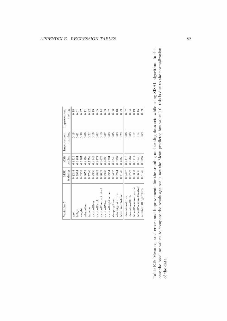
APPENDIX E. REGRESSION TABLES 82
Vari
able
sY
MSE
MSE
Impro
vem
ent
Impro
vem
ent
train
ing
test
ing
train
ing
test
ing
age
0.8
248
0.8
212
0.1
80.1
8
hei
ght
0.3
914
0.3
881
0.6
10.6
1
wei
ght
0.6
369
0.6
267
0.3
60.3
7
educa
tion
0.9
053
0.8
908
0.0
90.1
1
inco
me
0.7
780
0.7
752
0.2
20.2
2
alc
oholB
eer
0.8
360
0.8
144
0.1
60.1
9
alc
oholD
rink
0.9
823
0.9
477
0.0
20.0
5
alc
oholC
once
ntr
ate
d0.9
032
0.8
624
0.1
00.1
4
alc
oholW
ine
0.9
320
0.9
090
0.0
70.0
9
alc
oholL
ightW
ine
0.9
954
0.9
281
0.0
00.0
7
slee
pin
gT
ime
0.9
467
0.9
240
0.0
50.0
8
whatA
geW
illL
ive
0.9
244
0.8
987
0.0
80.1
0
bes
tTim
eToLiv
e0.7
120
0.7
058
0.2
90.2
9
chole
ster
olT
ota
l0.9
447
0.9
315
0.0
60.0
7
chole
ster
olH
DL
0.9
722
0.9
567
0.0
30.0
4
blo
odP
ress
ure
Syst
ole
0.8
303
0.8
114
0.1
70.1
9
blo
odP
ress
ure
Dia
stole
0.8
606
0.8
543
0.1
40.1
5
num
ber
OfC
igare
ttes
0.3
126
0.3
087
0.6
90.6
9
Tab
leE
.8:
Mea
nsq
uare
der
rors
and
impr
ovem
ents
for
the
trai
ning
and
test
ing
data
sets
whi
leus
ing
SISA
Lal
gori
thm
.In
this
case
the
base
line
valu
esto
com
pare
the
resu
ltag
ains
tis
not
the
Mea
npr
edic
tor
but
valu
e1.
0,th
isis
due
toth
eno
rmal
izat
ion
ofth
eda
ta.

APPENDIX E. REGRESSION TABLES 83
Variables Y NN size MSE MSE Improvement Improvementtraining testing training testing
Forward stepwise selection ALLcholesterolTotal 4-9-1 0.9454 0.9462 0.0546 0.0538cholesterolHDL 2-4-1 0.9823 0.9825 0.0177 0.0175bloodPressureSystole 3-7-1 0.8355 0.8357 0.1645 0.1643bloodPressureDiastole 3-7-1 0.8586 0.8589 0.1414 0.1411numberOfCigarettes 4-8-1 0.2748 0.2751 0.7252 0.7249
Forward stepwise selection TOPcholesterolTotal 3-6-1 0.9470 0.9475 0.0530 0.0525cholesterolHDL 1-3-1 0.9829 0.9830 0.0171 0.0170bloodPressureSystole 2-5-1 0.8437 0.8438 0.1563 0.1562bloodPressureDiastole 2-5-1 0.8668 0.8670 0.1332 0.1330numberOfCigarettes 1-2-1 0.2971 0.2972 0.7029 0.7028
Table E.9: Neural network models using parameters from the Forward selectionalgorithm. The first table shows the results when using all the selected parameters.The second table shows the results when using only the most important parametersfrom the selected ones (higher weight). Enough parameters are selected to have atleast 80% of the total weight represented.
Variables Y NN size MSE MSE Improvement Improvementtraining testing training testing
SISAL ALLcholesterolTotal 11-19-1 0.9212 0.9253 0.0788 0.0747cholesterolHDL 7-6-1 0.9767 0.9779 0.0233 0.0221bloodPressureSystole 4-8-1 0.8614 0.8618 0.1386 0.1382bloodPressureDiastole 11-15-1 0.8475 0.8497 0.1525 0.1503numberOfCigarettes 12-16-1 0.2440 0.2461 0.7560 0.7539
SISAL TOPcholesterolTotal 5-11-1 0.9278 0.9288 0.0722 0.0712cholesterolHDL 4-8-1 0.9775 0.9785 0.0225 0.0215bloodPressureSystole 3-7-1 0.8661 0.8663 0.1339 0.1337bloodPressureDiastole 7-12-1 0.8493 0.8504 0.1507 0.1496numberOfCigarettes 5-11-1 0.2600 0.2606 0.7400 0.7394
Table E.10: Neural network models using parameters from the SISAL algorithm.The first table shows the results when using all the selected parameters. The secondtable shows the results when using only the most important parameters from theselected ones (higher weight). Enough parameters are selected to have at least 80%of the total weight represented.

APPENDIX E. REGRESSION TABLES 84
Variables Y Selected MSE MSE Improvement Improvementcomponents training testing training testing
Forward stepwise selection ALLcholesterolTotal 1,2 0.8020 0.8023 0.0424 0.0421cholesterolHDL 1 0.4270 0.4271 0.0167 0.0165bloodPressureSystole 1,2 132.5606 132.6229 0.1529 0.1525bloodPressureDiastole 1,2,3 61.1725 61.2060 0.1283 0.1278numberOfCigarettes 1,2,3 58.0981 58.1301 0.1235 0.1230
Forward stepwise selection TOPcholesterolTotal 1,2 0.8029 0.8032 0.0414 0.0410cholesterolHDL 1 0.4283 0.4284 0.0136 0.0134bloodPressureSystole 1,2 132.9796 133.0368 0.1502 0.1498bloodPressureDiastole 1,2 62.0634 62.0887 0.1156 0.1152numberOfCigarettes 1 22.3077 22.3368 0.6634 0.6630
Table E.11: Regression on principal components using the parameters selected bythe Forward selection algorithm. The first table shows the results when using allthe selected parameters. The second table shows the results when using only themost important components. Enough components were selected to have at least a95% of the variance represented.
Variables Y Selected MSE MSE Improvement Improvementcomponents training testing training testing
SISAL ALLcholesterolTotal 1,2,3,4 0.7889 0.7894 0.0581 0.0575cholesterolHDL 1,2,3 0.4272 0.4274 0.0163 0.0158bloodPressureSystole 1,2 140.9091 140.9658 0.0995 0.0992bloodPressureDiastole 1,2,3 61.1734 61.2064 0.1283 0.1278numberOfCigarettes 1,2,3,4 57.3314 57.3707 0.1350 0.1344
SISAL TOPcholesterolTotal 1,2,3,4 0.7928 0.7932 0.0535 0.0529cholesterolHDL 1,2,3 0.4271 0.4273 0.0165 0.0160bloodPressureSystole 1,2 141.0715 141.1307 0.0985 0.0981bloodPressureDiastole 1,2,3 61.0889 61.1229 0.1295 0.1290numberOfCigarettes 1,2,3 55.5672 55.5992 0.1616 0.1612
Table E.12: Regression on principal components using parameters from the SISALselection algorithm. The first table shows the results when using all the selectedparameters. The second table shows the results when using only the most importantcomponents. Enough components were selected to have at least a 95% of the variancerepresented.