Thermodynamics of the BMN matrix model at strong coupling

Miguel S. Costa

Faculdade de Ciências da Universidade do Porto

Crete Center for Theoretical Physics - Heraklion, May 2014

Works with L. Greenspan, J. Penedones and J. Santos

Motivation

• Would like example where computations in both sides are within reachTest and understand the gauge/gravity duality with observables that are not protected by SUSY or can be computed using integrability.

How does gravitation phenomena, like black holes, emerge from gauge theory side?

Idea: Study thermodynamics of black holes dual to Matrix Quantum Mechanics that can be simulated on a computer using Monte-Carlo methods.

• Gauge/gravity duality as definition of quantum gravity in AdSDual CFT is renormalizable and unitary. Problem: how to decode the hologram?

Unfortunately field theory very difficult in region of interest for quantum gravity (strong coupled; classical gravity , expansion loop expansion).⌘N ! 1 1/N

The case of D0-branes

• Closed strings interact with D0-branes in flat spaceD0-brane

Open stringClosed string

• Closed strings interact with geometry produced by D0-branes

Closed string D0-brane geometry

,[Itzhaki, Maldacena, Sonnenschein, Yankielowicz ´98]

D0-branes: field theoretic description (matrix quantum mechanics)

SD0 =N

2�

ZdtTr

(DtX

i)2 + ↵Dt ↵ +

1

2

⇥Xi, Xj

⇤2+ i ↵�j

↵� [ � , Xj ]

�

Xi ⌘ SU(N) bosonic matrices (i = 1, . . . , 9)

⌘ SU(N) fermionic matrices (16 real components)

Dt = @t � i[A, ] ⌘ covariant derivative

�i ⌘ SO(9) gamma matrices��

�i, �j = 2�ij

�SO(9) global symmetry

• ‘t Hooft coupling is dimensionfull (relevant)

� = g2YMN =gsN

(2⇡)2l3s⌘ mass3 �eff =

�

E3

E ! 1 (UV ) ⌘ weak coupling

E ! 0 (IR) ⌘ strong coupling

• Dual 10D gravitational coupling16⇡GN l�8

s = (2⇡)11(�l3s)

2

N2

• Theory on Euclidean time circle with periodicity � = 1/T

Dimensionless temperature ⌧ =

T

�1/3 Low temperatures is strong coupling

SD0 =N

2�

Z �

0dt Tr

· · ·

�

• Can put theory on a computer using Monte Carlo simulations, accessing in particular strong coupled region.

Dimensionless mean energy

✏

N2=

E

N2�1/3

[Catterall, Wiseman ´07,´08,´09; Anagnostopoulos et al ´07; Hanada et al ´08,´13]

D0-branes: gravitational description

• 11D SUGRA solution (near horizon geometry of non-extremal D0-brane)

ds2 =dr2

f(r)+ r2d⌦2

8 +

✓R

r

◆7

dz2 + f(r)dt

✓2dz �

⇣r0R

⌘7dt

◆

f(r) = 1�⇣r0r

⌘7,

✓R

`s

◆7

= 60⇡3gsN ,

✓r0`s

◆5

=120⇡2

49(2⇡gsN)

53 ⌧2

• Classical gravity domain (at horizon)

1N� 1021N� 5

9N� 56

IIA 11D SUGRAG-L instability

Horizon at scalelP

Horizon at scalels l2sR(r0) ⌧ 1 ) ⌧ ⌧ 1

gse�(r0) ⌧ 1 ) ⌧ � N� 10

21

⌧ = T/�1/3

⌧

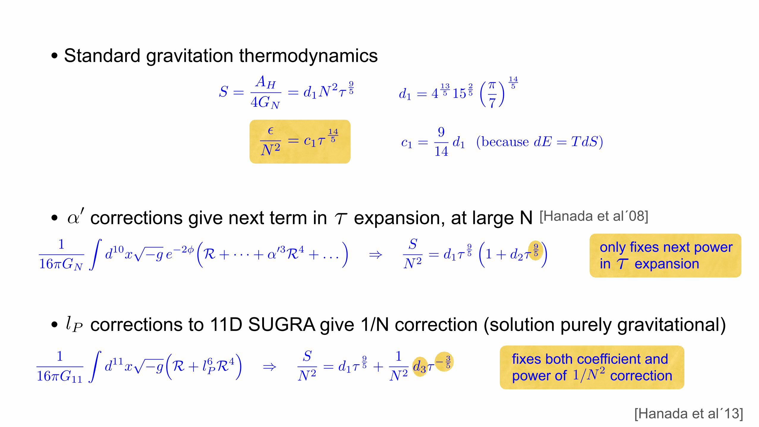
• Standard gravitation thermodynamics

✏

N2= c1⌧

145

S =AH

4GN= d1N

2⌧95 d1 = 4

135 15

25

⇣⇡7

⌘ 145

c1 =9

14d1 (because dE = TdS)

only fixes next power in expansion⌧

fixes both coefficient and power of correction1/N2

• corrections give next term in expansion, at large N↵0 ⌧1

16⇡GN

Zd

10x

p�g e

�2�⇣R+ · · ·+ ↵

03R4 + . . .

⌘) S

N

2= d1⌧

95

⇣1 + d2⌧

95

⌘[Hanada et al´08]

• corrections to 11D SUGRA give 1/N correction (solution purely gravitational)lP

1

16⇡G11

Zd

11x

p�g

⇣R+ l

6PR4

⌘) S

N

2= d1⌧

95 +

1

N

2d3⌧

� 35

[Hanada et al´13]

checked

predicted

negligible

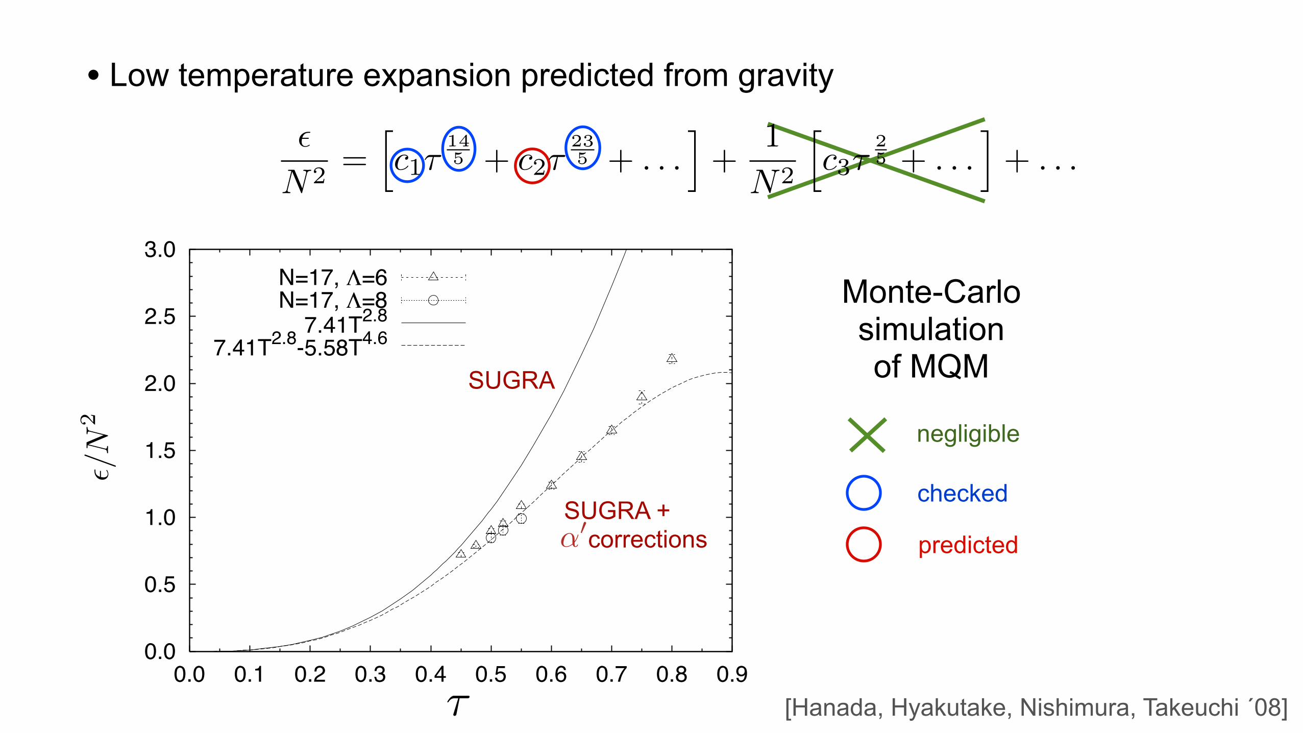
• Low temperature expansion predicted from gravity

✏

N2=

hc1⌧

145 + c2⌧

235 + . . .

i+

1

N2

hc3⌧

25 + . . .

i+ . . .

[Hanada, Hyakutake, Nishimura, Takeuchi ´08]

4

If we instead make a one-parameter fit with p = 4.6 fixed,we obtain C = 5.58(1). This value, in turn, provides aprediction for the α′ corrections on the gravity side.

-4

-3

-2

-1

0

1

2

3

4

-1.0 -0.5 0.0 0.5

ln (7

.41T

2.8 -E

/N2 )

ln T

N=14, !=4N=17, !=6N=17, !=8

FIG. 1: The deviation of the internal energy 1

N2 E from the

leading term 7.41 T14

5 is plotted against the temperature inthe log-log scale for λ = 1. The solid line represents a fitto a straight line with the slope 4.6 predicted from the α

′

corrections on the gravity side.

0.0

0.5

1.0

1.5

2.0

2.5

3.0

0.0 0.1 0.2 0.3 0.4 0.5 0.6 0.7 0.8 0.9

E/N

2

T

N=17, !=6N=17, !=8

7.41T2.8

7.41T2.8-5.58T4.6

FIG. 2: The internal energy 1

N2 E is plotted against T forλ = 1. The solid line represents the leading asymptotic be-havior at small T predicted by the gauge-gravity duality. Thedashed line represents a fit to the behavior (1) including thesubleading term with C = 5.58.

Summary.— We have discussed the α′ corrections tothe black hole thermodynamics, which enable us to de-termine the power of the sub-leading term in (1). Thispower is then found to be reproduced precisely by MonteCarlo data in gauge theory. Let us emphasize that thesubleading term is crucial for the precision test of thegauge-gravity duality. It is intriguing that our results ingauge theory can tell us the absence of O(α′) and O(α′2)

corrections to the supergravity action.

Recently [20] Monte Carlo data for the Wilson loopare also shown to reproduce a prediction obtained by es-timating the disk amplitude in the dual geometry. Unlikethe present case, α′ corrections to that quantity start atO(α′) due to the fluctuation of the string worldsheet andits coupling to the background dilaton field.

While it is certainly motivated to obtain the coefficientC of the subleading term from gravity, our results alreadyprovide a strong evidence that the gauge-gravity dualityholds including α′ corrections. This, in particular, im-plies that we can understand the microscopic origin ofthe black hole thermodynamics including α′ correctionsin terms of the open strings attached to the D0-branes.

Acknowledgments.— The authors would like to thankO. Aharony, K.N. Anagnostopoulos and A. Miwa for dis-cussions. The computations were carried out on super-computers (SR11000 at KEK) as well as on PC clustersat KEK and Yukawa Institute. The work of J.N. andY.H. is supported in part by Grant-in-Aid for ScientificResearch (Nos. 19340066, 20540286 and 19740141).

∗ Electronic address: masanori.hanada@weizmann.ac.il† Electronic address: hyakutake@cep.osaka-u.ac.jp‡ Electronic address: jnishi@post.kek.jp§ Electronic address: shingo@apctp.org

[1] T. Banks, W. Fischler, S. H. Shenker and L. Susskind,Phys. Rev. D 55, 5112 (1997).

[2] N. Ishibashi, H. Kawai, Y. Kitazawa and A. Tsuchiya,Nucl. Phys. B 498, 467 (1997).

[3] J. M. Maldacena, Adv. Theor. Math. Phys. 2, 231 (1998).[4] N. Itzhaki, J. M. Maldacena, J. Sonnenschein and

S. Yankielowicz, Phys. Rev. D 58, 046004 (1998).[5] E. Witten, Nucl. Phys. B 443, 85 (1995).[6] K. N. Anagnostopoulos, M. Hanada, J. Nishimura and

S. Takeuchi, Phys. Rev. Lett. 100 (2008) 021601.[7] M. Hanada, J. Nishimura and S. Takeuchi, Phys. Rev.

Lett. 99, 161602 (2007).[8] N. Kawahara, J. Nishimura and S. Takeuchi, JHEP 0712

103, (2007).[9] S. Catterall and T. Wiseman, Phys. Rev. D 78, 041502

(2008); JHEP 0712, 104 (2007).[10] D. Kabat, G. Lifschytz and D. A. Lowe, Phys. Rev. Lett.

86, 1426 (2001); Phys. Rev. D 64, 124015 (2001).[11] I.R. Klebanov and A.A. Tseytlin, Nucl. Phys. B 475, 164

(1996).[12] D.J. Gross and E. Witten, Nucl. Phys. B 277, 1 (1986).[13] A.A. Tseytlin, Nucl. Phys. B 584, 233 (2000).[14] Y. Hyakutake and S. Ogushi, JHEP 0602, 068 (2006).[15] D.J. Gross and J.H. Sloan, Nucl. Phys. B 291, 41 (1987).[16] Y. Hyakutake, Prog. Theor. Phys. 118, 109 (2007).[17] G. Policastro and D. Tsimpis, Class. Quant. Grav. 23,

4753 (2006).[18] R.M. Wald, Phys. Rev. D 48 R3427 (1993).[19] V. Iyer and R.M. Wald, Phys. Rev. D 50 846 (1994).[20] M. Hanada, A. Miwa, J. Nishimura and S. Takeuchi,

arXiv:0811.2081.

SUGRA

SUGRA + corrections

Monte-Carlo simulation of MQM

✏/N

2

⌧

↵0

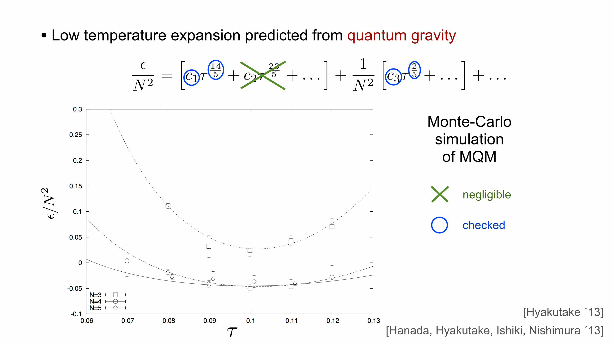
• Low temperature expansion predicted from quantum gravity

✏

N2=

hc1⌧

145 + c2⌧

235 + . . .

i+

1

N2

hc3⌧

25 + . . .

i+ . . .

checked

negligible

[Hanada, Hyakutake, Ishiki, Nishimura ´13][Hyakutake ´13]

Monte-Carlo simulation of MQM

In Fig. 3 we plot our results for the e⇥ective internal energy in the continuum limit asa function of T for N = 3, 4, 5. (In the small box we show the extrapolation to � = ⇤for N = 4 and T = 0.10 as an example.) The curves represent the fits to the behaviorsexpected from the gravity side, which shall be explained later. We find that the internalenergy increases as temperature decreases, which implies that the specific heat is negative.Such a behavior is possible since we are measuring the energy of the metastable boundstates.

Figure 3: The e�ective internal energy Egauge/N2 obtained for the metastablebound states in the continuum limit as a function of T . Results for N = 3 (squares),N = 4 (circles) and N = 5 (diamonds) are shown. The curves represent the fits to thebehaviors expected from the gravity side, which shall be explained later. The data pointsand the fitting curve for N = 5 are slightly shifted along the horizontal axis so that thedata points and the error bars for N = 4 and N = 5 do not overlap. In the small box, weshow an extrapolation to � = ⇤ for N = 4 and T = 0.10.

Testing the gauge/gravity duality

Now we can test the gauge/gravity duality by comparing the results on the gauge theoryside shown in Fig. 3 with the results on the gravity side represented by eq. (4). In thetemperature regime 0.07 � T � 0.12 investigated here, the terms with the coe⌅cients aand b, which represent the �� corrections, can be neglected unless |a| ⇥ 700 and |b| ⇥ 500.

9

✏/N

2

⌧

Today’s talk is not about D0-brane matrix model

• Instability corresponds to Hawking radiation of D0-branes. At large N this is suppressed and black hole is stable (positive specific heat).

• Today’s talk is about BMN matrix model

Mass deformation resolves IR divergence - canonical ensemble well defined.

Much richer thermodynamics with a 1st order phase transition(at large N there are two dimensionless parameters).

[Berenstein, Maldacena, Nastase ´02]

• Caveat: canonical ensemble ill defined - IR divergences from flat directions in D0-brane moduli space. This is suppressed at large N (metastable state), but it is a source of tension in Monte Carlo simulations

F (T, r)

N2⇠ Ffinite(T ) +

9

Nln r

[Catterall, Wiseman ´09]

BMN matrix model

Canonical ensemble is well defined. Still “easy” to simulate on a computer.

In large N ‘t Hooft limit dimensionless coupling constant � =g2YMN

µ3

S = SD0 �N

2�

ZdtTr

µ2

32(Xi)2 +

µ2

62(Xa)2 +

µ

4 ↵

��123

�↵� � + i

2µ

3✏ijkX

iXjXk

�

Massive deformation of D0-brane MQM. Preserves SUSY but breaks SO(9) ! SO(6)⇥ SO(3)a = 4, . . . , 9 i = 1, 2, 3

Many vacua Xa = 0 Xi =µ

3J i

[J i, Jj ] = i�ijkJk

N = mn M5�brane vacua ⌘ m ! 1, n fixed

Xi ⇠

0

BB@

n⇥ n 0 . . . 00 n⇥ n . . . 0. . . . . . . . . . . .0 0 . . . n⇥ n

1

CCA

9>>=

>>;m times

D2�brane vacua ⌘ n ! 1, m fixed (decoupled)

Focus on trivial vacuum (single M5-brane) that is SO(9) invariant Xi = Xa = 0

Exponential growth of spectrum with energy Hagedorn transition!Tc

µ=

1

12 log 3

1 +

2

65

3

4�� c�2

+O(�3)

�⇥ 0.076 +O(�)First-order phase transition at

[Hadizadeh, Ramadanovic, Semenoff, Young ’04]

N ! 1• Thermodynamics ( )Dimensionless temperature ⌘ T

µ

Dimensionless coupling ⌘ � =

g2YMN

µ3

T

µ

TH

µ

� =g2YMN

µ3

Confined phase

Deconfined phaseF = O(N2)

F = O(N0)

?WEAK

COUPLING

STRONG

COUPLING

Starthere

Today: strongly coupled limit

Dual geometry is SO(9) invariant non-extremal D0-brane with deformation turned on

µ ! 0 ,T

µfixed and large

Gravitational dual

• At strong coupling, for large temperature, dual geometry is SO(9) invariant and is approximately the non-extremal D0-brane solution

ds2 =dr2

f(r)+ r2d⌦2

8 +R7

r7dz2 + f(r)dt

✓2dz � r70

R7dt

◆

dC = µdt ^ dx

1 ^ dx

2 ^ dx

3

Need back-reaction to decrease temperature and study phase transition at strong coupling. In particular,

SO(9) ! SO(6)⇥ SO(3)

Non-normalizable mode responsible for massive deformation

• The different vacua of BMN matrix model correspond to the Lin-Maldacena geometries and asymptote to the M-theory plane wave solution

ds

2 = dx

idx

i + dx

adx

a + 2dtdz �✓µ

2

32x

ix

i +µ

2

62x

ax

a

◆dt

2

dC = µdt ^ dx

1 ^ dx

2 ^ dx

3

ds2 = �A(1� y7)

y7d⌘2 + T4 y

7

d⇣ + ⌦

(1� y7)d⌘

y7

�2

+1

y

2

"B

(dy + Fdx)2

(1� y

7)y2+ T1

4dx2

2� x

2+ T2 x

2(2� x

2)d⌦22 + T3 (1� x

2)2d⌦25

#

C = (M d⌘ + Ld⇣) ^ d2⌦2

Tailored to numerical implementation(domain of unknown is the unit square; everything dimensionless) y10

Horizon1

S2

S5

collapses

collapses

1

x

| {z }d�2

8 if T1=T2=T3=1

is a angular coordinate on compact 8-dimensional space with topology x S8

x = 1

x = 0S2

S5

pole

equator

are functions of and A,B, F, T1, T2, T3, T4,⌦,M,L x y

y is a radial coordinate from boundary ( ) to horizon ( ) y = 0 y = 1

y = 0 y = 1

S8 ⇥ S1 ⇥ S1 S8 ⇥ S1

boundary horizon

• Ansatz for 11D SUGRA

⇣ ⇠ ⇣ + 2⇡M-theory circle

| {z }d�2

8 if T1=T2=T3=1

ds2 = �A(1� y7)

y7d⌘2 + T4 y

7

d⇣ + ⌦

(1� y7)d⌘

y7

�2

+1

y

2

"B

(dy + Fdx)2

(1� y

7)y2+ T1

4dx2

2� x

2+ T2 x

2(2� x

2)d⌦22 + T3 (1� x

2)2d⌦25

#

C = (M d⌘ + Ld⇣) ^ d2⌦2

x = 1

x = 0S2

S5

pole

equator

y = 0 y = 1

S8 ⇥ S1 ⇥ S1 S8 ⇥ S1

boundary horizon

• Ansatz for 11D SUGRA

Non-extremal D0-brane solution corresponds to

A = B = T1 = T2 = T3 = T4 = ⌦ = 1 , F = M = L = 0 , � =4⇡

7(Euclidean time circle)

This scaling symmetry will be important later...

and need to use scaling symmetry of 11D SUGRA action

with⇣ ⇠ ⇣ + 2⇡ ! ⇣ ⇠ ⇣ + 2⇡s0 ) I ! s0I

gµ⌫ ! s2gµ⌫ , Cµ⌫⇢ ! s3Cµ⌫⇢ ) I ! s9I

s0 =

✓R

r0

◆ 72 gs`s

r0

s = r0

invariant tensor hamonicSO(6)⇥ SO(3)

• Boundary conditions

y10

Horizon1

S2

S5

collapses

collapses

1

x

y = 0At infinity ( ): A,B, T1, T2, T3, T4,⌦ ! 1 , F ! 0

M ! µ

x

3(2� x

2)32

y

3, L ! 3

2µ y

4x

3(2� x

2)32 Recall that C = (M d⌘ + Ld⇣) ^ d2⌦2

µ =7

12�

µ

T

To obtain physical solution do again above scalings, then geometry has same asymptotics of non-extremal D0-brane with temperature T and mass deformation turned on. The only parameter is

This important to thermodynamics, because we just learned that

I =s9s0

16⇡GNI⇣ µ

T

⌘=

15

28

✓15

142⇡8

◆ 25

N2

✓T

�13

◆ 95

I⇣ µ

T

⌘S =

s9s0

4GNS⇣µ

T

⌘=

15⇡

7

✓15

142⇡8

◆ 25

N2

✓T

�13

◆ 95

S⇣ µ

T

⌘

Regularity at the axis of symmetry:horizon ( ), pole ( ) and equator ( ).y = 1 x = 0

x = 1S2 S5

(� = 4⇡/7)

Einstein-DeTurck equations

�µ = g�⇥⇣�µ�⇥ � �µ

�⇥

⌘DeTurck term that makes Einstein equations elliptic

Connection of reference metric

Rµ⌅ �r(µ�⌅) =1

12

✓Fµ�⇥⇤F

�⇥⇤µ � 1

12gµ⌅F

2

◆d(�F ) +

1

2F ^ F = 0 F = dC

Our reference metric is the non-extremal D0-brane solution.

With appropriate boundary conditions on the numerical solution so solution also solves Einstein equations.

⇠µ = 0

[Headrick, Kitchen, Wiseman ’09]

A Smarr formula (good to check numerics)

• Integrate over surface of constant time with d⇣?Kv

⌘= 0 y1 < y < y2

0 =

Z

⌃12

d⇣?Kv

⌘=

Z

@⌃12

?Kv =

Z

H

?Kv �Z

y!0?Kv

• Let (time translations generator), then Smarr formula relates horizonv =@

@⌘area to boundary data

7

2S =

Z

y!0?Kv

• Let be a killing vector. From field equations it follows that

is a conserved antisymmetric tensor, i.e.

vµ

d⇣?Kv

⌘= 0

(Kv)µ⌫ = rµv⌫ +

1

3Fµ⌫↵�v�C↵�� +

1

6v[µF ⌫]↵��C↵��

The solution

Q1 = 1 + y4q1 , Q2 = 1 + y4q2 , Q3 = y5q3 , Q4 = 1 + y4q4 , Q5 = 1 + y4q5 , Q6 = 1 + y4q6 ,

Q7 = 1 + y4q7 , Q8 = 1 + y4q8 , Q9 = µ(1 + y + y2 + y3 + y4) + y4q9 , Q10 = µ+ yq10

• Horizon area and shape

0.0 0.5 1.0 1.5 2.0

120

140

160

180

m

S`

Horizon area

0.0 0.5 1.0 1.5 2.00.4

0.5

0.6

0.7

0.8

0.9

1.0

m

R2êR

5

Ratio of maximal radius of to S2 S5

S =15⇡

7

✓15

142⇡8

◆ 25

N2

✓T

�13

◆ 95

S⇣µ

T

⌘After scaling symmetry to obtain physical metric:

Ri = ai

✓T

�13

◆ 25

Ri

⇣ µ

T

⌘

Reproduces scalings predicted from strongly coupled low energy moduli estimate in [Wiseman ’13]

�N =

����1�AreaN

AreaN+1

����

log�N ⇡ �2.5� 0.75N

25 30 35 40 45 5010!34

10!30

10!26

10!22

10!18

!

"N

log� ⇡ �17.5� 0.75N

� = max

p⇠⌫⇠⌫

25 30 35 40 45 5010!24

10!22

10!20

10!18

10!16

!

Χ

Numerical convergence

Discretize PDEs using a Chebyshev grid with N x N points.

Derivatives are estimated using polynomial approximations that involve all points in the grid - spectral methods.

requires regularization easy to measure

Black hole thermodynamics

• From scaling symmetry we saw thatF (T, µ) = �c0 T

145 I

⇣ µ

T

⌘, S(T, µ) = c0

14

5T

95 S

⇣ µ

T

⌘

Therefore ratio of free energies and entropiesF (T, µ)

F (T, 0)=

I� µT

�

I(0)⌘ f

⇣ µ

T

⌘,

S(T, µ)

S(T, 0)=

S� µT

�

S(0)⌘ s

⇣µ

T

⌘

✓�F

�T

◆

µ

= �S

F (T, 0) = �c1T145

First law

Free energy

✓1� 5

14µ

@

@µ

◆f(µ) = s(µ)

)

)

Analyticity ) s(µ) =1X

n=0

sn µn , f(µ) =

1X

n=0

14sn14� 5n

µn

Critical temperature

T < Tc

[Lin, Maldacena ’05]• Phase transition occurs when free energy changes sign, since for geometry without horizon is favoured F ⇠ O�

N0�

Tc

µ=

7

12�µc⇡ 0.091

Similar to Hawking-Page phase transition in AdS

0.0 0.5 1.0 1.5 2.00.0

0.2

0.4

0.6

0.8

1.0

m

f

= �c1T145 f(µ)

F (T, µ) = F (T, 0)f(µ)

• Note that BH is thermodynamically stable c = T

✓@S

@T

◆

µ) c

S=

9

5

� µ@

@µlog s(µ) > 0

Phase diagram at large N

T

µ

� =g2YMN

µ3

Confined phase

Deconfined phaseF = O(N2)

F = O(N0)

?WEAK

COUPLING

STRONG

COUPLING

0.076

0.091

Very similar to SYM on a 3-sphere (µ ⌘ 1/R)[Aharony, Marsano, Minwalla, Papadodimas, van Raamsdonk ’03]

To preserve depends on ratio of radii E6

E3

Xi

Xa

✓

sin ✓ =R5

R2=

✓XaXa

XiXi

◆1/2

SO(6)⇥ SO(3)

Boundary data (preliminary)

• The 10 functions admit expansion near the boundary (y = 0)

Qi(x, y)

Qi(x, y) =X

j

y

jQ

ji (x)

SO(9)• Boundary metric has symmetry, so are harmonic functions on . Thus we can classify the invariant perturbations according tospin. This helps to establish bulk field / operator correspondence.

SO(9) S8

SO(6)⇥ SO(3)Q

ji (x)

µÊ

Ê

Ê

‡

‡

‡

‡

‡

1 3 5 7 9

0

2

4

6

1 3 5 7 9

0

2

4

6

⇢2

⇢4

⇢6

spin l

n(l)

vector mode

v(x, y) =

X

l

⇣⇢l y

n(l)+ µl y

n(l)⌘vl(x) + back reaction

↵5

↵6

�1

�2�3

zero modes�7, �7

Ê

Ê

Ê

Ê

Ê

‡

‡

‡

‡

‡

0 2 4 6 8 10

0

2

4

6

0 2 4 6 8 10

0

2

4

6

↵4

spin l

n(l)

scalar mode

s(x, y) =

X

l

⇣↵l y

n(l)+ �l y

n(l)⌘sl(x) + back reaction

normalizable

non-normalizable

O ⇠ Tr ([Xi, Xj ]XA1 . . . XAl) , l � 1 oddO ⇠ Tr (XA1 . . . XAl) , l � 2 even

0.0 0.5 1.0 1.5 2.0

-0.4

-0.3

-0.2

-0.1

0.0

m

a2

0.0 0.5 1.0 1.5 2.00.0

0.2

0.4

0.6

0.8

1.0

1.2

1.4

m

a5

0.0 0.5 1.0 1.5 2.0

-0.35

-0.30

-0.25

-0.20

-0.15

-0.10

-0.05

0.00

m

g7

0.0 0.5 1.0 1.5 2.0

-2.5

-2.0

-1.5

-1.0

-0.5

0.0

m

d7

• We got for ⇢2,↵5, �7, �7

⇢2

Numerics pass highly non-trival check! Smarr formula OK:

7

2S =

16⇡5

735(98 + 280�7 + 63�7 � 276↵2µ)

•Confirm phase diagram with Monte-Carlo simulations of PWMM

•Study other observables (expectation values) - holographic renormalization

•Study dynamical stability of our BH

•Construct BH duals of other vacua (different horizon topology) (caveat: we really only determined upper limit on critical temperature)

•Deeper question: What makes the PWMM special? What are the minimal ingredients of a quantum mechanical system such that it gives rise to classical gravity in the limit of many degrees of freedom?

Future work

THANK YOU