thermodynamics of chemical systems.pdf
TRANSCRIPT

8/11/2019 Thermodynamics of Chemical Systems.pdf
http://slidepdf.com/reader/full/thermodynamics-of-chemical-systemspdf 1/456
Thermodynamics of chemical systems

8/11/2019 Thermodynamics of Chemical Systems.pdf
http://slidepdf.com/reader/full/thermodynamics-of-chemical-systemspdf 2/456
8/11/2019 Thermodynamics of Chemical Systems.pdf
http://slidepdf.com/reader/full/thermodynamics-of-chemical-systemspdf 3/456
Thermodynamics
of
CHEMICAL SYSTEMS
SCOTT
E.
W O O D
Professor Emeritus
of
Chemistry, Illinois Institute
of
Technology
RUBIN BATTINO
Professor
of
Chemistry, Wright State University
The right of t he
University of Cambridge
to print and sell
all manner
oj
books
was granted
by
Henry VIII in 1534.
The University has printed
and published continuously
since 1584.
CAMBRIDGE UNIVERSITY PRESS
Cambridge
New York Port Chester Melbourne Sydney

8/11/2019 Thermodynamics of Chemical Systems.pdf
http://slidepdf.com/reader/full/thermodynamics-of-chemical-systemspdf 4/456
Published by the Press Syndicate of the University of Cambridge
The Pitt Building, Trumpington Street, Cambridge CB2 1RP
40 West 20th Street, New York NY 10011, USA
10 Stamford Road, Oakleigh, Melbourne 3166, Australia
© Cambridge University Press 1990
First published 1990
Library of Congress Cataloging in Publication Data
Wood, Scott E. (Scott Emerson), 1910-
Thermodynamics of chemical systems / Scott E. Wood, Rubin Battino.
p. cm.
Includes index.
ISBN 0-521-33041-6
1. The rmo dyna mics. I. Battino , Rub in. II. Title.
QD 504.W 66 1989 89-32580
541.3'69^dc20 CIP
British Library Cataloguing in Publication Data
Wood, Scott E.
Thermodynamics of chemical systems.
1.
Chemical react ions. Thermodynamics
I. Title II. Battino , Rubin
541.3'69
ISBN 0-521-33041-6 hard covers
Transferred to digital printing 2004

8/11/2019 Thermodynamics of Chemical Systems.pdf
http://slidepdf.com/reader/full/thermodynamics-of-chemical-systemspdf 5/456
To Our Sons
Edward S. Wood
David Rubin Battino
Benjamin Sadik Battino

8/11/2019 Thermodynamics of Chemical Systems.pdf
http://slidepdf.com/reader/full/thermodynamics-of-chemical-systemspdf 6/456

8/11/2019 Thermodynamics of Chemical Systems.pdf
http://slidepdf.com/reader/full/thermodynamics-of-chemical-systemspdf 7/456
Contents
Preface xiii
Notation xvi
1. Introduction 1
1.1 The langua ge of therm ody nam ics 2
1.2 Th erm ody nam ic prope rties of systems 4
1.3 N ota tio n 5
2. Tem perature, heat, work, energy, and enthalpy
6
2.1 Tem perature 6
2.2 He at and heat capacity 7
2.3 W ork 9
2.4 Qu asistatic processes 14
2.5 Ot her 'wo rk' interaction s 15
2.6 Th e first law of the rm od yn am ics : the energy function 16
2.7 The enthalp y function 19
2.8 The ideal gas and the first law of therm odyn am ics 20
2.9 Re prese ntation of changes of state 22
3. The second law of therm odynamics: the entropy function
24
3.1 He at and work reservoirs 24
3.2 He at engines 25
3.3 Reve rsible an d irreversible processe s 25
3.4 Th e reversible transfer of hea t 30
3.5 The C arn ot cycle 30
3.6 The thermod ynam ic tempe rature scale 32
3.7 The identity of the Kelvin and ideal gas tem pera ture scales 34
3.8 Th e efficiency of reversible heat engines: two statem ents of the
second law of thermod ynam ics 36
3.9 C ar no t's the or em : the m axim um efficiency of reversible hea t engines 38
3.10 The entrop y function 40

8/11/2019 Thermodynamics of Chemical Systems.pdf
http://slidepdf.com/reader/full/thermodynamics-of-chemical-systemspdf 8/456
viii Contents
3.11 The change in the value of the entropy function of an
isolated system along a reversible pa th 41
3.12 The change in the value of the entropy function of an
isolated system along an irreversible path 43
3.13 A third stateme nt of the second law of therm odyn am ics 45
3.14 The depende nce of the entro py on tem pera ture 45
3.15 The chang e of entro py for a change of state of aggregation 46
4. Gibbs and Helm holtz energy functions and open systems
47
4.1 The Helm holtz energy 47
4.2 Th e Gib bs energy 49
4.3 Op en systems 50
4.4 Resum e 52
4.5 Dep enden ce of the therm ody nam ic functions on the indepen dent
variables 55
4.6 The Maxw ell relations and other relations 57
4.7 Dev elopm ent of other relations 58
4.8 The energy as a function of the tem pera ture and volum e, and the
enthalpy as a function of the tem pera ture and pressure 61
4.9 The integration of Eq ua tion (4.74) 62
5. Conditions of equilibrium and stability: the phase rule
64
5.1 G ibb s' stateme nt conce rning equilibrium 64
5.2 Proo f of G ibb s' criterion for equilibrium 67
5.3 Co ndition s of equilibrium for heterog enou s systems 67
5.4 Co ndition s of equilibrium for chemical reactions 70
5.5 Co nditio ns of equilibrium for heterog enou s systems with
various restrictions 73
5.6 O ther cond itions of equilibrium 74
5.7 The chemical poten tial 75
5.8 The Gib bs-D uhe m equation 76
5.9 Ap plication of Eule r's theorem to othe r functions 77
5.10 The Gib bs phas e rule 78
5.11 Th e variab les requ ired to define the state of an isolated system 79
5.12 Applications of the Gib bs-D uhe m equation and the Gibbs phase rule 82
5.13 Indifferent state s 85
5.14 The Gib bs-K ono valo w theorems 88
5.15 Co nd ition s of stability 89
5.16 Critical phe nom ena 98
5.17 Gra phic al repre sentatio n 105
6. Partial molar quantities
119
6.1 Definition of pa rtial m ola r qua ntities 119
6.2 Relations concern ing partia l mo lar quan tities 120
6.3 Algebraic deter min ation of partial mo lar quan tities 122
6.4 Ap pare nt mo lar quan tities 129

8/11/2019 Thermodynamics of Chemical Systems.pdf
http://slidepdf.com/reader/full/thermodynamics-of-chemical-systemspdf 9/456
Contents
ix
6.5 Gr aph ical determ ination of the partial molar volumes of binary
systems 131
6.6 Int eg ratio n of Eq ua tion (6.12) for a bina ry system 132
7. Ideal gases and real gases 135
7.1 Th e ideal gas 135
7.2 Pu re real gases 137
7.3 M ixture s of real gases an d co m bin atio ns of coefficients 140
7.4 Th e Jou le effect 143
7.5 Th e Jo ul e- Th om so n effect 143
7.6 Th erm od yn am ic functions for ideal gases 146
7.7 The changes of the therm ody nam ic functions on mixing of ideal gases 148
7.8 Th e the rm od yn am ic functions of real gases 149
7.9 Th e chan ges of the the rm od yn am ic functions on mixing of real gases 152
7.10 The equilibrium pressure 153
7.11 Th e fugacity an d fugacity coefficient 153
7.12 The integration constant, g
k
{T ) 156
8. Liquids and solids : reference and standard states
159
8.1 Single-phase, one-c om ponen t systems 160
8.2 Cha nges of the state of aggregation in one-c om pone nt systems 164
8.3 Tw o-ph ase, one-c om pone nt systems 165
8.4 Thre e-pha se, one-c om pone nt systems 170
8.5 Solu tions 171
8.6 Th e ideal solutio n 173
8.7 Real sol utio ns: reference and sta nd ard states 175
8.8 Definitions based on mole fractions 178
8.9 Definitions based on molalities 182
8.10 Definitions based on mo larities 188
8.11 Th e osm otic coefficient 190
8.12 The dependence of the activity and the activity coefficient on
temperature 191
8.13 The dependence of the activity and the activity coefficient on
pressure 192
8.14 Co nve rsion from one reference state to an oth er 193
8.15 Reference an d sta nd ard states for species 197
8.16 So lutions of stron g electrolytes 201
8.17 So lutions of weak electrolytes 204
8.18 M ixture s of mo lten salts 205
9. Thermochemistry
209
9.1 Basic con cep ts of calo rime try 210
9.2 M olar heat capacities of satura ted phases 212
9.3 He at capa cities of m ultip has e, closed systems 214
9.4 Ch ang es of enth alpy for chan ges of state involving solution s 217
9.5 Ch ang es of enth alpy for chan ges of state involving chemical
reactions 223

8/11/2019 Thermodynamics of Chemical Systems.pdf
http://slidepdf.com/reader/full/thermodynamics-of-chemical-systemspdf 10/456

8/11/2019 Thermodynamics of Chemical Systems.pdf
http://slidepdf.com/reader/full/thermodynamics-of-chemical-systemspdf 11/456
Contents xi
11.2 The experimental determ ination of equilibrium con stants 296
11.3 The effect of tem pe ratu re on the equilibriu m co nsta nt 297
11.4 Th e effect of press ure on the equilibrium con stan t 299
11.5 The stan dar d Gib bs energy of formation 300
11.6 The stand ard Gib bs energy of formation of ions in solution 301
11.7 C onv entio ns conc erning solvated species 302
11.8 Ionization con stants of weak acids 308
11.9 Aq ueou s solution s of sulfuric acid 309
11.10 No nstoich iome tric solid solutions or com pou nds 311
11.11 Association and complex formation in condensed phases 312
11.12 Ph ase equilibria in term s of species 322
11.13 Use of the Gib bs-D uhe m equations 325
11.14 Equ ilibria between pu re solids an d liquids 327
11.15 The change of the Gibbs energy for a chemical change of
state under arbitra ry cond itions 329
12. Equilibria in electrochem ical systems 330
12.1 Electrically charged phases and phases of identical com position 330
12.2 Co ndition s of equilibrium 331
12.3 Differences in electrical po ten tials 331
12.4 An electroch emica l cell 334
12.5 Th e con ven tion of signs for a galvan ic cell 337
12.6 C on ditio ns of reversibility 338
12.7 Th e sta nd ard electro mo tive force of a cell 339
12.8 Th e tem pe ratu re dep end ence of the emf of a cell 340
12.9 Th e pres sure dep ende nce of the emf of a cell 346
12.10 Half-cell po ten tial s 347
12.11 Som e galvan ic cells with ou t liquid jun ctio n 349
12.12 G alva nic cells with liquid jun ctio n 351
12.13 M em bra ne equilibrium 355
12.14 Som e final com me nts 358
13.
Surface effects 359
13.1 Surface ph en om en a related to the system 359
13.2 Surface ph en om en a related to a defined surface 363
13.3 Th e surface tensio n and surface con cen tratio ns 368
13.4 Cu rved surfaces 373
14. Equilibrium conditions in the presence of an external field
376
The gravitational and centrifugal field
376
14.1 The grav itational and centrifugal poten tial 376
14.2 The fundam ental equa tions 377
14.3 Co ndition s of equilibrium 380
14.4 De pende nce of pressure on the poten tial 381
14.5 De pende nce of com position on the poten tial 382
14.6 The G ibbs -D uh em equation and the phase rule 384

8/11/2019 Thermodynamics of Chemical Systems.pdf
http://slidepdf.com/reader/full/thermodynamics-of-chemical-systemspdf 12/456
xii
Contents
14.7 Th e definition of the state of the system 384
Systems in an electrostatic field
387
14.8 The conde nser in emp ty space 387
14.9 The conden ser in a dielectric med ium 387
14.10 W ork assoc iated with elec trostatic fields 388
14.11 The rmo dyna mic s of the total system 389
14.12 The rmo dyna mic s of the dielectric medium 391
Systems in a magnetic field
394
14.13 The solenoid in em pty space 394
14.14 Th e solenoid filled with isotro pic m atte r 395
14.15 W ork assoc iated with ma gne tic effects 396
14.16 The rmo dyn am ics of the total system 396
14.17 The rmo dyn am ics of a dia- or para ma gne tic substance 397
15. The third law of thermodynam ics 399
15.1 The preliminary concepts of the third law 400
15.2 Expe rimental determ ination of absolute entropies 401
15.3 Co nfirm ation of the third law 403
15.4 U nde rstan ding the third law 403
15.5 Prac tical basis for absolu te values of the entrop y 409
15.6 The rm ody nam ic functions based on the third law 410
15.7 Uses of the therm ody nam ic functions 412
Appendices
A.
SI units and fundam ental con stants 415
A -l. Base SI units 415
A-2. Si-derived units 415
A-3. 1986 recommended values of the fundamental physical
constants 416
B. M olar heat capacities at con stant pressure for selected substances 417
C. Thermody namic data 418
C -l. Entha lpies and Gib bs energies of formation at 298.15 K 418
C-2. Abso lute entropies at 298.15 K 419
C-3.
En thalpy increment function 420
C-4. Gib bs energy increment function 421
D .
Sta nda rd reduc tion poten tials in aqu eou s solutions 422
Cited references and selected biblio gra phy 423
Subject index 431
8/11/2019 Thermodynamics of Chemical Systems.pdf
http://slidepdf.com/reader/full/thermodynamics-of-chemical-systemspdf 13/456
Preface
The systems to which thermodynamics have been applied have
become more and more complex. The analysis and understanding of these
systems requires a knowledge and understanding of the methods of applying
thermodynamics to multiphase, multicomponent systems. This book is an
attempt to fill the need for a monograph in this area.
The concept for this book was developed during several years of teaching
a one-year advanced graduate course in chemical thermodynamics at the
Illinois Institute of Technology. Students who took the course were studying
chemistry, chemical engineering, gas technology, or biochemistry. During
those years we came to believe that the major difficulty that students have
is not with the numerical solution of a problem; the difficulty is with the
development of the pertinent relations in terms of experimentally determinable
qua ntities. M oreo ver, du ring the initial writing of the boo k, it becam e evident
that chemical thermodynamics was being applied in many new fields and to
systems having more than two or three components. These new fields are
so num erous th at any attem pt to i l lustrate the application of thermody nam ics
to each of them would make this book much too long. Therefore, the aim of
the book is to develop in a general way the concepts and relations that are
pertinent to the solution of many thermodynamic problems encountered in
multiphase, multicomponent systems. The emphasis is on obtaining exact
expressions in terms of experimentally determinable quantities. Simplifying
assumptions can be made as necessary after the exact expression has been
obtained. It is expected that users of this book have some knowledge of
physical chemistry and elementary thermodynamics. It is hoped that, once
these basic concepts have been developed, the users will be able to apply
chemical thermodynamics to any specific problem in their particular field.
The m ethods of Gibb s are used throu gho ut w ith emphasis on the chemical
potential. The material is presented in a rigorous and mathematical manner.
Several topics that are presented briefly or omitted entirely in more-
elementary texts are introduced. Among these topics are: the requirements

8/11/2019 Thermodynamics of Chemical Systems.pdf
http://slidepdf.com/reader/full/thermodynamics-of-chemical-systemspdf 14/456
xiv Preface
that must be satisfied to define the state of a thermodynamic system,
particularly indifferent systems; the use of the Gib bs -D uh em equ ation in the
solution of problems associated not only with simple phase equilibria, but
also with phase equilibria in which chemical reactions may occur in one or
more phases; the conditions of stability for single-phase, multicomponent
systems; and the graphical representation of the thermodynamic functions.
Because of the importance of reference states and standard states, special
attention is given to their definition and use.
The subject matter is divided into two parts. The first part is devoted to
defining the thermodynamic functions and to developing the fundamental
relations relevant to chemical systems at equilibrium. The second part is
devoted to the application of these relations to real systems and the methods
that can be used to obtain additional relations.
The introductory material (Chapters 1-4) is treated briefly. The basic
concepts, which are always so difficult to define, are approached from an
operational viewpoint and in the classical manner. No attempt is made to
use a more general approach.
A bibliography is given after the appendices. The first section lists those
books to which reference is made in the text and a few of the more recent
and relevant advanced texts in chemical thermodynamics. The other sections
give references to data compilations and sources. An abbreviated set of
thermodynamic data are given in the appendices for quick reference.
The notation and symbolism used in this text are a combination of those
recommended by IUPAC and variations chosen by us for ease and clarity
of use. We have chosen the tilde over a symbol, such as V
l9
to represent the
mo lar volume of com ponen t 1, rather than the more cumbersome IU PA C
notation of V
ml
for the same qu antity . Similarly, althou gh the IU P A C
notation elegantly represents a partial molar volume, for example, as V
u
we
chose the redundant but unambiguous notation of placing a bar over a
symbol to indicate this quantity:
V
t
.
IU PA C recommends the phrase 'amount
of sub stanc e' for n which is commonly called the number of
m oles.
We chose
to describe n as the 'mole number,' for ease of writing, even though we (and
our readers) know that n refers to a quantity or amount of substance. In
any case, we have been consistent in our usage, and a list of our notation
is given after this Preface.
In concluding this Preface, we wish to make some separate and some
joint acknowledgments. First, SEW wishes to express his appreciation to
those who were influential in stimulating his interest in thermodynamics,
and to others w ho helped in the developm ent of this bo ok : first, to Professors
George Scatchard, James A. Beattie, and Louis J. Gillespie, for developing
his interest in thermodynamics and for introducing him to the work of
J. Willard Gibbs; second, to his many colleagues, but, particularly Dr.
Russell K. Edwards, Professor Harry E. Gunning, and Professor Ralph J.

8/11/2019 Thermodynamics of Chemical Systems.pdf
http://slidepdf.com/reader/full/thermodynamics-of-chemical-systemspdf 15/456
Preface xv
Tykodi, for many long, arduous, and helpful discussions; and third, to the
many students who took his course and taught him while they were being
taught. RB wishes to express his appreciation to his teachers of thermo-
dynamics: Professors Mark W. Zemansky and John H. Saylor, and to the
senior author, Professor Scott E. Wood. We thank Henry E. Sostman for
helpful comments and Dr. Thomas W. Listerman for carefully reading
Ch apte r 14. We both express our indebtedness to D r. Stanley W eissman,
who read and critiqued most of the book, and to the secretaries who typed
it: Alice Ca pp , Claudia Hillard, and M ary A lspaugh. Some of the book was
written while the senior author was a Senior Fulbright Scholar at the
Department of Chemistry at University College, Dublin. Finally, we wish
to thank our wives for the patience and encouragement that they showed
during the writing of this book.
Scott E. Wood
El Paso, Texas
Rubin Battino
Dayton, Ohio
September 1989

8/11/2019 Thermodynamics of Chemical Systems.pdf
http://slidepdf.com/reader/full/thermodynamics-of-chemical-systemspdf 16/456
Notation
a area
a
activity
A
area
A
Helmholtz energy
B magnetic induction
B
1 mole of an unspecified substance
c
molarity
c
specific heat capacity
C number of components
C heat capacity
C
P
heat capacity at constant pressure
C
v
heat capacity at con stant volume
d inexact differential
D electric displacement
E energy
E electric field strength
$
electro m otive force (emf)
/ fugacity
F force, generalized force
F
e
external force
£F Faraday constant
g gaseous state
g acceleration due to gravity
G Gibbs energy
h height
H
enthalpy
H magnetic field strength
i current
/ integration constant

8/11/2019 Thermodynamics of Chemical Systems.pdf
http://slidepdf.com/reader/full/thermodynamics-of-chemical-systemspdf 17/456
Notation xvii
k Henry's law constant
k distribution coefficient
K
equilibrium constant
/ length
/ liquid state
L liter
L length
m
mass
m number of units of mass
m molality
m magnetic moment per unit volume
M
molecular mass
M tota l magnet ic moment
n a m oun t of substance/mole num bers
niA magnet ic moment
p polarization of the medium per unit volume
P pressure
P number of phases
P
k
partial pressure of component k
P total polarization ( = K
c
p)
Q
heat
Q electrical charge
r distance
r radius
R
gas constant
R nu m ber of indep ende nt chemical reactions
s solid state
s displacement
S entropy
S
number of species
t time
t temperature
t transference number
T Kelvin or therm odyn am ic temperature
Tj inversion temperature (Joule-Thomson)
v velocity
v specific volume
V
volume
V
num ber of variances or num ber of degrees of freedom
W
work
x mole fraction
X
i
generalized coordinate
X
t
molar proper ty

8/11/2019 Thermodynamics of Chemical Systems.pdf
http://slidepdf.com/reader/full/thermodynamics-of-chemical-systemspdf 18/456
xviii Notation
X
t
partial mo lar property
y mole fraction, gas phase
z mole fraction, solid phase
z electrical charge on ion
Z compressibility factor
Greek
a deviations of the real gas or gas mix ture from ideal beha vior
y activity coefficient
y surface tension o r interfacial tension
y fugacity coefficient
F surface concentration
s permitt ivity
e
0
permitt ivity of empty space
s/s
0
d ie lec t r ic con sta n t
r\ efficiency
of a
hea t engine
9
arbitrary temperature
\i chemical potential
\x permeabili ty
fi
0
permeabili ty of vacuum
lbi/fi
0
re la t ive permeabi l i ty
ju
JT
Jou le -Thomson coe f f i c i en t
v stoichiometr ic coeff icient
n
osmotic pressure
p density
T arbitrary temperature
< / > e lec t r ica l po ten t ia l
0 function
of T , P ,
fi
l9
n
2
,. . .
(j) os mo tic coeff icient
(f)X
apparent molar quantity
O gravitational potential, centrifugal potential
Q > electrostatic potential
X
M
ma gne t ic suscept ib i l i ty
X
e
electr ic susceptibi l i ty
if/ e lec t r ica l po ten t ia l
o) angular ve loc i ty
co acentric factor
Superscripts
E excess change on mixing
M mixture or mixing
P planar
o defined surface

8/11/2019 Thermodynamics of Chemical Systems.pdf
http://slidepdf.com/reader/full/thermodynamics-of-chemical-systemspdf 19/456
Notation
e
•
*
0 0
Subscripts
1,2,3, . . .
b
c
c
D
E
f
m p
mix
M
r
7
s
sat
tr
standard state
pure component
molar proper ty
partial molar property
reference state
infinite dilution
c o m po n en t 1, 2 , 3 , . . .
boiling point
condenser
critical property
dimer
excess
formation
melting point
for the mixing process
monomer
reduced property, as in T
r
= T/T
c
mixed solvent (pseudobinary system)
space
saturated
transit ion
XIX

8/11/2019 Thermodynamics of Chemical Systems.pdf
http://slidepdf.com/reader/full/thermodynamics-of-chemical-systemspdf 20/456

8/11/2019 Thermodynamics of Chemical Systems.pdf
http://slidepdf.com/reader/full/thermodynamics-of-chemical-systemspdf 21/456
1
Introduction
With thermodynamics, one can calculate almost everything crudely; with
kinetic theory, one can calculate fewer things, but m ore accurately; and with
statistical mechanics, one can calculate almost nothing exactly.
Eugene Wigner
The range and scope of thermodynamics is implied in Wigner's
epigrammatic quote above, except for the fact that there are a great many
phenomena for which thermodynamics can provide quite accurate calcula-
tions. Chemical engineering is to a large extent based on thermodynamic
calculations applied to practical systems. The phase rule is indispensable to
metallurgists, geologists, geochemists, crystallographers, mineralogists, and
chemical engineers. Although students sometimes come away with the notion
that thermodynamics is remote and abstract, it is actually the most practical
of subjects. Part of what we endeavor to do in this book is to illustrate that
practicality, the tie to everyday life and utility.
Thermodynamics comprises a field of knowledge that is fundamental and
applicable to a vast area of hu m an experience. It is a study of the interactions
between two or more bodies, the interactions being described in terms of
the basic concepts of heat and work. These concepts are deduced from
experience, and it is this experience that leads to statements of the first and
second laws of thermodynamics. The first law leads to the definition of the
energy function, and the second law leads to the definition of the entropy
function. W ith the experim ental establishmen t of these laws, therm ody nam ics
gives an elegant and exact m etho d of studying an d determ ining the pro perties
of natural systems.
The branch of thermodynamics known as the thermodynamics of
reversible processes is actually a study of thermodynamic systems at
equilibrium, and it is this branch that is so important in the application of
thermodynamics to chemical systems. Starting from the fundamental con-
ditions of equilibrium based on the second law, more-practical conditions,

8/11/2019 Thermodynamics of Chemical Systems.pdf
http://slidepdf.com/reader/full/thermodynamics-of-chemical-systemspdf 22/456
2 Introduction
expressed in terms of experimentally measurable quantities, have been
developed. The application of the thermodynamics of chemical systems thus
leads to the determination of the equilibrium properties of macroscopic
systems as observed in nature (regardless of the complexity of the systems),
to possible limitations, and to the determination of the dependence of the
equilibrium properties with changes of the values of various independent
variables, such as pressure, temperature, or composit ion.
Since thermodynamics deals with systems at equilibrium, time is not a
thermo dyna mic coord inate. On e can calculate, for example, that if benze ne(/)
were in equilibrium with hydrogen(g) and carbon(s) at 298.15 K, then there
would be very little benzene present since the equilibrium constant for the
form ation of benz ene is 1.67 x
1 0 ~
2 2
.
The equilibrium constant for the
formation of diamond(s) from carbon(s, graphite) at 298.15 K is 0.310; that
is , graphite is more stable than diamond. As a final example, the equilibrium
constant for the following reaction at 298.15 K is 2.24 x 1 0 "
3 7
:
2C(s,gr) + H
2
(g) = C
2
H
2
(g )
People do not give away their diamonds or worry about benzene or ethyne
spontaneously decomposing, since these substances are
not
in equilibrium
with their starting materials. A specific catalyst or infinite time might be
required to attain equilibrium conditions.
After the appendices we provide a selected bibliography of general
references and data compilations. All cited references appear in the list of
general references.
1.1 The language of thermodynamics
In thermodynamics terms mean exactly what we define them to mean.
The exact use of language is particularly important in this subject, since
calculations a nd interp retation s a re directly tied to precisely defined changes
of state
and
the way in which those changes of state occur. So, in this
introductory chapter the language of thermodynamics is presented.
First, we speak of a system and its surroundings. The system is any region
of matter that we wish to discuss or investigate. The surroundings comprise
all other matter in the world or universe that can have an effect on or interact
with the system. Th erm ody nam ics, then , is a study of the interaction between
a system and its surroundings. These definitions are very broad and allow
a great deal of choice concerning the system and its surroundings. The
important point is that for any thermodynamic problem we must rigorously
define the system with which we are dealing and apply any limitations to
the surroundings that appear to be necessary. What we shall consider to be
the system and the surroundings is our choice, but it is imperative that we
consciously make this choice. As an example, we may be interested in the
chemical substances taking part in a chemical reaction. These substances

8/11/2019 Thermodynamics of Chemical Systems.pdf
http://slidepdf.com/reader/full/thermodynamics-of-chemical-systemspdf 23/456
1.1 The language of thermo dynamics
3
would have to be in a container of some kind. Certainly, the substances
taking part in the reaction would comprise at least part of the system, but
it is our choice whether we consider the container to be part of the system
or part of the surrou nd ings. Althou gh the surro und ings w ere defined generally
as all other matter in the world or universe, in all practical cases they are
limited in extent. Those parts of the universe that have no or only an
insignificant effect on the system are excluded, and only those of the
surroundings that actually interact with the system need to be considered.
In many experimental studies the surroundings that interact with the system
are actually designed for the purpose of controlling the system and making
measurements on i t .
For any thermodynamic system there is always a
boundary,
sometimes
called an
envelope,
which separates the system and the surroundings. The
only interactions considered in thermodynamics between a system and its
surroundings are those that occur across this boundary. Because of this, it
is as important to define the boundary and its properties as it is to define
the system and the surroundings themselves. The boundary may be real or
hypothetical, but it is considered to have certain properties. It may be
rigid, so tha t the volume of the system rem ains con stan t, or it may be no nrigid,
so that the volume of the system can change. Similarly, the boundary may
be adiabatic or diathermic. The boundary may be semipermeable, under
which condition it would be permeable to certain substances but not
permeable to others. In actual cases the properties of the boundary are
determined by the properties of the system and by our design of the
surroundings. In simplified, idealized cases we may endow the boundary
with whatever properties we choose. A clear definition of the system and of
the boundary that separates the system from its surroundings is extremely
important in the solution of many thermodynamic problems.
In addition to the general concept of a system, we define different types
of systems. An
isolated system
is one that is surrounded by an envelope
of such nature that no interaction whatsoever can take place between the
system and the surroundings. The system is completely isolated from the
surroundings. A closed system is one in which no matter is allowed to transfer
across the boundary; that is, no matter can enter or leave the system. In
contrast to a closed system we have an open system, in which matter can be
transferred across the boundary, so that the mass of a system may be varied.
(Flow systems are also open systems, but are excluded in this definition
because only equilibrium systems are considered in this book.)
The
state
of the system is defined in terms of certain state variables. The
state of the system is then fixed by assigning definite values to sufficient
variables, chosen to be independent, so that the values of all other variables
are fixed. The number of independent variables depends in general upon the
problem at hand and upon the system with which we are dealing. The

8/11/2019 Thermodynamics of Chemical Systems.pdf
http://slidepdf.com/reader/full/thermodynamics-of-chemical-systemspdf 24/456
4 Introduction
determination of this number and the type of variables required for the
definition of the state of the system is discussed in Chapter 5. When the
values of the independent variables that define the state of the system are
chang ed, we speak of a change of state of the system. Here we are concerned
with the values of the dep ende nt variables, as well as those of the indepen dent
variables, at the initial and final states of the system, and not with the way
in which the values of the independent variables are changed between the
two states. When it is necessary to consider the way in which the values of
the independent variables are changed, we speak of the path. In a graphical
representation the path is any line connecting the two points that depict the
two states. The term process encompasses both the change of state and the
pa th .
1.2 Thermodynam ic properties of systems
We have implied in Section 1.1 that certain properties of a
thermodynamic system can be used as mathematical variables. Several
independent and different classifications of these variables may be made. In
the first place there are ma ny v ariables that can be evaluated by experimental
measurement. Such quantit ies are the temperature, pressure, volume, the
amount of substance of the components (i.e., the mole numbers), and the
position of the system in some potential field. There are other properties or
variables of a thermodynamic system that can be evaluated only by means
of mathematical calculations in terms of the measurable variables. Such
quan tities may be called derived qua ntities. Of the many variables, those that
can be measured experimentally as well as those that must be calculated,
some will be considered as independent and the others are dependent. The
choice of which variables are independent for a given thermodynamic
problem is rather arbitrary and a matter of convenience, dictated somewhat
by the system
itself.
Finally, the thermodynamic properties of a system considered as variables
may be classified as either intensive or extensive variables. The distinction
between these two types of variables is best understood in terms of an
operation. We consider a system in some fixed state and divide this system
into two or more parts without changing any other properties of the system.
Those variables whose value remains the same in this operation are called
intensive variables. Such variables are the temperature, pressure, concentration
variables, and specific and molar quantities. Those variables whose values
are changed because of the operation are known as extensive variables. Such
variables are the volume and the amount of substance (number of moles) of
the components forming the system.
8/11/2019 Thermodynamics of Chemical Systems.pdf
http://slidepdf.com/reader/full/thermodynamics-of-chemical-systemspdf 25/456
1.2 Thermodyn amic properties of systems 5
1.3 Notation
In this book we use SI units and IUPAC symbolism and terminology
as far as possible. The complete set of notation used in this book is given
before this chapter. For clarity and consistency we have made some choices
of notation that differ from IUPAC recommendations. Notation is defined
where first introduced. Amongst other exceptions is the use of the phrase
'amount of substance' for the variable n, which has been traditionally called
the 'nu m ber of m oles' or, as we mo st frequently call it, the 'mo le num be rs.'
Some basic reference tables are given in the appendices.

8/11/2019 Thermodynamics of Chemical Systems.pdf
http://slidepdf.com/reader/full/thermodynamics-of-chemical-systemspdf 26/456
Temperature, heat, work, energy,
and enthalpy
In this chapter we briefly review the ideas and equations relating to
the important concepts of temperature, heat, work, energy, and enthalpy.
2.1 Temperature
The concept of temperature can be defined operationally; that is, in
terms of a set of operations or conditions that define the concept. To define
a temperature scale operationally we need: (1) one particular pure or defined
sub stanc e; (2) a specific p rop erty of tha t sub stance th at chang es with a naive
sense of 'degree of hotness' (i.e., temperature); (3) an equation relating
temperature to the specific property; (4) a sufficient number of fixed points
(defined as reproducible temperatures) to evaluate the constants in the
equation in (3); and (5) the assignment of numerical values to the fixed
points. Historically, many different choices have been made with respect
to the five conditions listed above, and this, of course, has resulted in many
temperature scales.
The ideal gas temperature scale is of especial interest, since it can be
directly related to the thermodynamic temperature scale (see Sect. 3.7). The
typical constant-volume gas thermometer conforms to the thermodynamic
temperature scale within about 0.01 K or less at agreed fixed points such as
the triple point of oxygen and the freezing points of metals such as silver
and g old. Th e therm ody nam ic tem pera ture scale requires only one fixed
point and is independent of the nature of the substance used in the defining
Carnot cycle. This is the triple point of water, which has an assigned value
of 273.16 K with the use of a gas therm om eter as the instrum ent of
measurement .
The International Practical Temperature Scale of 1968 (IPTS-68) is
currently the internationally accepted method of measuring temperature
reproducibly. A standard platinum resistance thermometer is the transfer
medium that is used over most of the range of practical thermometry.

8/11/2019 Thermodynamics of Chemical Systems.pdf
http://slidepdf.com/reader/full/thermodynamics-of-chemical-systemspdf 27/456
2.2 Heat and heat capacity 1
Interpolation formulas and a defined set of fixed points are used to establish
the scale. IPTS-68 is due to be replaced in 1990 or 1991.
The
zeroth law of thermodynamics is
in essence the basis of all the rmo m etric
measurements. It states that, if a body
A
has the same temperature as the
bodies B and C, then the temperature of B and C must be the same. One
way of doing this is to calibrate a given thermometer against a standard
thermometer. The given thermometer may then be used to determine the
temperature of some system of interest. The conclusion is made that the
temperature of the system of interest is the same as that of any other system
with the same reading as the standard thermometer. Since a thermometer
in effect measures only its own temperature, great care must be used in
assuring thermal equilibrium between the thermometer and the system to
be measured.
2.2 Heat and heat capacity
It is observed ex perimentally t ha t, when two bod ies having different
temperatures are brought into contact with each other for a sufficient length
of t ime, the temperature s of the two bodies appro ach each other. M oreover,
when we form the contact between the two bodies by means of walls
constructed of different materials and otherwise isolate the bodies from the
surroundings, the rate at which the two temperatures approach each other
depends upon the material used as the wall. Walls that permit a rather rapid
rate of temperature change are called diathermic walls, and those that permit
only a very slow rate are called adiabatic walls. The rate would be zero for
an ideal adiabatic wall. In thermodynamics we make use of the concept of
ideal adiabatic walls, although no such walls actually exist.
We describe the phenomenon that the temperatures of the two bodies
placed in diathermic contact with each other approach the same value by
saying that 'heat' has transferred from one body to another. This is the only
concept of heat that is used in this book.
It is based on the observation
of a particular phenomenon, the behavior of two bodies having different
temperatures when they are placed in thermal contact with each other.
One way to obtain a quantitative definition of a unit of heat is to choose
a particular substance as a standard substance and define a quantity of heat
in terms of the temperature change of a definite quantity of the substance.
Thus ,
we can define a quantity of heat, Q, by the equation
Q = C(t
2
-t
x
) (2.1)
where
t
2
is the final temperature and
t
l
is the initial temperature. The
proportionality constant, C, is called the heat capacity of the particular
quantity of the substance. For the present we will disregard the dependence
of C on pressure and volume. Experimental studies have shown that C is an
extensive quantity, so that it may be written as me, where m represents the

8/11/2019 Thermodynamics of Chemical Systems.pdf
http://slidepdf.com/reader/full/thermodynamics-of-chemical-systemspdf 28/456
8
Temperature, heat, work, energy, and enthalpy
number of units of mass of the standard substance used and c represents the
specific heat cap acity. Th e unit of hea t is then defined b y assigning an arb itrary
value to
c.
A positive value is assigned to c so that the quantity of heat
absorbed during an increase of temperature is positive.
The calorie was originally based on 1 g of water. For the purposes of a
m ore exact definition it has been sup erseded by the jou le, so tha t
cal = cal
th
= 4.184 jou les = 4.184 J
by international con vention. I t is called the ' thermo dyn am ic' calorie. (M any
authors omit the subscript 'th.')
Measurements of the heat capacity of all substances have shown that the
heat capacity is actually a function of tem pera ture. Therefore, Eq uatio n (2.1)
must be given as
f'
2
f'
2
= CdT = m cdT
(2.2)
where t
2
represents the final temperature and t
x
the initial temperature. If
the numerical value of Q is positive, then heat is absorbed by the substance;
if it is negative, then heat is emitted by the substance.
The quantity of heat absorbed or emitted by a system for a given change
of state depends not only upon the change of temperature, but also upon
changes in the values of other inde pend ent variables. Here we consider closed
systems (those of constant mass) and only either changes in the values of
the temperature and pressure or changes in the values of temperature and
volume. Differential expressions for the quantity of heat can be written either
as
&Q = M(T, P) dT + N(T
9
P) dP (2.3)
or
dQ = K(T, V) dT + L(T, V)dV (2.4)
where M(T, P) and N(T, P) represent functions of the temperature and
pressure, and K(T, V) and L(T, V) represent functions of the temperature
and volume. Experiment shows that these differential expressions for the
heat effect are inexact. The symbol d is used to distinguish between inexact
(d) and exact (d) differential quantities. The quantity of heat absorbed by the
system for a given change of state thus depends upon the path that is followed
from the initial state to the final state.
The symbol
Q
represents a quantity
of heat, taken as positive for heat absorbed by the system from the
surroundings. It may be measured experimentally or determined from the
line integral of appropriate inexact differential expressions represented by
the symbol dQ, such as Equation (2.3) or (2.4).
8/11/2019 Thermodynamics of Chemical Systems.pdf
http://slidepdf.com/reader/full/thermodynamics-of-chemical-systemspdf 29/456
2.3 Work 9
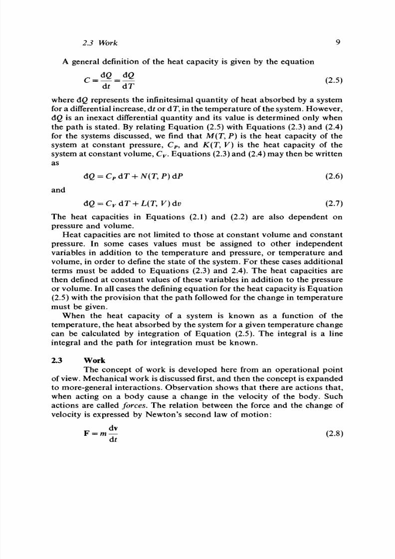
A general definition of the heat capacity is given by the equation
C = ^ = ^
(2.5)
dt dT
V ;
where dQ represents the infinitesimal quantity of heat absorbed by a system
for a differential increase, dt or dT , in the temp eratu re of the system. H owev er,
dQ is an inexact differential quantity and its value is determined only when
the path is stated. By relating Equation (2.5) with Equations (2.3) and (2.4)
for the systems discussed, we find that M(T, P ) is the heat capacity of the
system at constant pressure, C
P
, and K(T, V) is the heat capacity of the
system at constant volume, C
v
. Eq uatio ns (2.3) and (2.4) may then be w ritten
as
dQ =
C
P
dT
+ N(T
9
P) dP (2.6)
and
T, V)dv (2.7)
The heat capacities in Equations (2.1) and (2.2) are also dependent on
pressure and volume.
Heat capacities are not limited to those at constant volume and constant
pressure. In some cases values must be assigned to other independent
variables in addition to the temperature and pressure, or temperature and
volume, in order to define the state of the system. For these cases additional
terms must be added to Equations (2.3) and 2.4). The heat capacities are
then defined at constant values of these variables in addition to the pressure
or volum e. In all cases the defining eq uatio n for the heat cap acity is E qua tion
(2.5) with the provision that the path followed for the change in temperature
must be given.
When the heat capacity of a system is known as a function of the
temperature, the heat absorbed by the system for a given temperature change
can be calculated by integration of Equation (2.5). The integral is a line
integral and the path for integration must be known.
2.3 Work
The concept of work is developed here from an operational point
of view. M echan ical w ork is discussed first, and then the concep t is expanded
to more-general interactions. Observation shows that there are actions that,
when acting on a body cause a change in the velocity of the body. Such
actions are called
forces.
The relation between the force and the change of
velocity is expressed by Newton's second law of motion:
F = m — (2.8)
dt

8/11/2019 Thermodynamics of Chemical Systems.pdf
http://slidepdf.com/reader/full/thermodynamics-of-chemical-systemspdf 30/456
10
Temperature, heat, work, energy, and enthalpy
for nonrelativistic velocities, where F represents the force and m the mass of
the body. Here t refers to time. The unit of force, the newton (N), is defined
in terms of this relation for which
m
is one kilogram and dv/df is one meter
per secon d. The differential qu antity of wo rk dW, do ne by a force in op erating
on a body over a differential displacement, ds, is given by the scalar product
of the force and the differential of the displacement, so
dW = F cosocds
(2.9)
The symbols F and s here refer to scalar rather than vector quantities, and
a is the angle between the direction of the force and the direction of the
displacement. The unit of work is the joule.
This basic mechan ical concept of wo rk m ust be extended w hen it is applied
in thermodynamics. We are concerned with the interaction of a system and
its surroundings across the boundary that separates them. Both the system
and the surroundings may exert forces on the boundary, and it is the action
of these forces resulting in a displacement of the boundary that constitutes
work. The language used to describe the interaction in terms of work must
be developed and used with great care.
Because the change of the volume of a system is so important in the
application of thermodynamics to chemical systems, the expansion of a gas
is used as an example. Consider a known quantity of gas confined in a
frictionless piston-a nd-cy linder, as illustrated in Figu re 2 .1. Th e cylinder is
fixed in position relative to the Earth. The piston has a mass m and can
move in the direction of the gravitational field of the Earth. There is also a
known external force, F
e
, exerted on the upper surface of the piston. We
Figure 2.1. Piston-and-cylinder arrangement.

8/11/2019 Thermodynamics of Chemical Systems.pdf
http://slidepdf.com/reader/full/thermodynamics-of-chemical-systemspdf 31/456
2.3 Work 11
define
the system to be the gas contained in the volume within the
piston-and-cylinder. The surroundings are the cylinder, piston, and all of the
substances and devices that exert the external force on the piston. The
boundary is the internal wall of the cylinder and the lower surface of the
piston, and it is assumed to be diathermic. The piston is originally clamped
in position so that the lower surface of the piston is at the position labeled
h
x
. The gas exerts a force, F, on this surface. We now assume that, when
the clamps holding the piston in position are removed, the gas expands,
forcing the piston to move in the upward direction. We also assume that
the velocity of the piston can be measured when the lower surface of the
piston is at
h
2
.
Whether the process is adiabatic or isothermal is not important
for the present discussion.
We can analyze the process by the application of Newton's second law
of motion. The net force acting on the boundary, defined as the lower surface
of the piston, is F —mg —F
e
, where g represents the acceleration due to
gravity. Equation (2.9) for this case becomes
m-^ = F - m g - F
e
(2.10)
dt
When we multiply Equation (2.10) by dt and use the relations
dv = (^)dt (2.11)
and
dt =
(l/\)dh (2.12)
we obtain
my
dv = (F - mg - F
e
)
dh
(2.13)
On integrating between the limits 0 and v for the velocity and h
x
and h
2
for
the distance,
i m v
2
= f
h
2
-h,)- ¥
e
dh (2.14)
Finally, we place terms relating to the system on the left-hand side of the
equation and terms relating to the surroundings on the right-hand side so
that Equation (2.14) becomes
%
h
2
rh
2
Fd/i=
¥
e
dh-\-mg(h
2
—h
1
)-\-^m\
2
(2.15)
hi
Jhi
The term on the left-hand side represents the quantity of work done by the
system and associated with the force F. The right-hand side represents the

8/11/2019 Thermodynamics of Chemical Systems.pdf
http://slidepdf.com/reader/full/thermodynamics-of-chemical-systemspdf 32/456
12
Temperature, heat, work, energy, and enthalpy
effect of this quantity of work on the surroundings. Work has been done
against the force F
e
in raising the piston in the gravitational field of the
Earth against the force mg, and in imparting kinetic energy to the piston.
The force exerted by the gas on the lower surface of the piston cannot be
expressed in terms of the properties of the gas. As soon as the piston has
any velocity, pressure and temperature gradients appear in the gas, with the
result that the force is something less than the product of the equilibrium
pressure of the gas and the area of the piston. The surroundings are therefore
devised so that the changes that take place in the surroundings can be
measured. The right-hand side of Equation (2.15) represents the
quantity of
work done by the system as measured by changes in the surroundings.
It is informative to consider the same process and the same system and
surroundings with the exception that the piston is made a part of the system.
Part of the boundary is now defined as the upper surface of the piston rather
than the lower surface. Equation (2.15) takes the form
r
2
¥dh~mg(h
2
-h
1
)-^m\
2
= F
e
dh (2.16)
under these conditions. The force exerted by the system on the boundary is
(F
—
mg),
but the integral of this force does not represent the work done by
the system on the boundary. The only effect in the surroundings
is
represented
by the integral on the righ t-hand side of Equation (2.16). This integral gives
the quantity of work done by the system as determined by changes in the
surroundings or against the force F
e
. This is the only interaction between
the system and the surroundings. The raising of the piston in the gravitational
field of the Earth and the imparting of kinetic energy to the piston has no
relevance to the interaction of the system and the surroundings.
Further insight into the concept of work, the language used to define
work, and the importance of clearly defining the system, surroundings, and
boundary is obtained by introducing frictional effects. We consider the same
gas and frictionless piston-and-cylinder arrangement as in the previous
discussion, but insert a device in the cylinder so that the piston is stopped
instantly when the lower surface of the piston reaches the position h
2
. We
assume that the piston, cylinder, and device are not deformed or stressed by
the collision. For the purposes of discussion, we imagine that the piston and
cylinder, containing the gas, are separated from the surroundings which exert
the external force F
e
by an adiabatic wall. When we compare the result of
the expansion in which the piston is stopped and thermal equilibrium is
attained, with the result in which the piston
is
allowed to m aintain its velocity
at the position h
2
, we find that the temperature of the piston, cylinder, and
gas is greater for the former case than for the latter. (We assume here that
the temperature of the piston, cylinder, and gas can be measured while the

8/11/2019 Thermodynamics of Chemical Systems.pdf
http://slidepdf.com/reader/full/thermodynamics-of-chemical-systemspdf 33/456
2.3 Work 13
piston is moving and is determined when the lower surface of the piston
reaches the position /i
2
.) We can compare the two processes by bringing a
body of water into contact with the cylinder by the use of a diathermic wall.
The temperature of the piston, cylinder, and gas can now be changed to the
temperature when the piston is not stopped by allowing heat to flow into
the body of water. The quantity of heat removed is measured by the
temperature change of the water. In our idealized experiments we find that
the quantity of heat removed is equal to the kinetic energy of the piston at
the position h
2
, when expressed in the same units. It is only in this ope ration al
concep t that w e can speak of heat resulting from the performance of w ork.
We can now analyze the quantity of work done by the system associated
with the force F as measured by changes in the surroundings. A quantity of
work has been done against the external force F
e
and in raising the piston
in the gravitational field when the boundary is taken to be the lower surface
of the piston. In addition, a change of temperature has occurred in the piston
and cylinder, and the quantity of heat that would be required to cause the
temperature change must be considered as an effect of the work done by the
system. The temperature change of the gas itself is not included in the
consideration of the interaction between the system and the surroundings.
If the gas is separated from the piston and cylinder by an adiabatic wall,
then all effects of the collision appear in the change of the temperature of
the piston and cylinder, and the quantity of heat required to cause the
temperature change is considered to be the result of the work done by the
system. The analysis is simplified if we choose the gas, piston, and cylinder
to be the system. Then all of the effects of the collision are contained within
the system and the work done by the system is done only against the external
force. In the general case when the effects of friction must be considered, it
is convenient to define the system and the envelope in such a way that all
frictional effects are included within the system and therefore do not enter
into the interaction of the system and its surroundings.
We must recall that the process or processes that we have been discussing
have not been completely defined; that is, we have not stated whether the
process is adiabatic or isothermal, or whether any specific quantity of heat
has been added to or removed from the system during the process. Although
we have essentially defined the initial state of the system , we have n ot defined
its final state, neither have we defined the path that we choose to connect
the two states. When we do so,
we find by experience that the quantity of
work done by the system depends upon the path
and, therefore, the differential
quantity of work,
dW,
is an inexact differential quantity.
The basic concept of work is defined by Equation (2.9). However, in
thermodynamics this basic concept must be extended, because we are
interested in the interaction between a system and its surroundings. We wish
to emphasize that the work done by the system is associated with the force

8/11/2019 Thermodynamics of Chemical Systems.pdf
http://slidepdf.com/reader/full/thermodynamics-of-chemical-systemspdf 34/456
14 Temperature, heat, work, energy, and enthalpy
exerted by the system on the boundary separating the system from the
surroundings and is measured in general by appropriate changes that take place
in the surroundings.
The quantity of work,
W
9
which is the integral of
dW,
also depends up on the pa th. In this boo k the symbol W represents a quantity
of work, taken as negative for work done by the system on the boundary.
When work is done on the system by use of the surroundings, the numerical
value of W is positive. (Some books use a reverse convention for the sign of
work effects—e careful )
2.4 Quasistatic processes
The force exerted by the system on the lower surface of the piston
is not related directly to the equilibrium pressure of the material within the
cylinder when the piston is moving. However, there are many times when
it is adv antag eou s to ap pro xim ate this force by the produ ct of the equilibrium
pressure and the area of the piston. In so doing we can relate the force to
the equilibrium properties of the substance contained within the cylinder.
Imagine an idealized process, approximating a real process, in which the
movement of the piston is controlled so that it never attains an appreciable
velocity. The control is obtained by means of friction between the piston
and cylinder, or, more simply, by some device that permits a frictionless
piston to move only an infinitesimal distance before it is stopped by collision
with the device. Figure 2.2 depicts one such possible process. As the steps
become smaller, so the incremental increase in volume becomes smaller. The
process can be controlled by the size of the steps. Once the p iston is stopp ed,
the substance within the cylinder is allowed to attain equilibrium before the
piston is permitted to move again. The change of state that takes place in
the substance within the cylinder is thus accomplished by a succession of a
large number of equilibrium states, each state differing infinitesimally from
the previous state. Such processes are called quasistatic processes.
The force exerted by the substance within the cylinder on the lower force
of the piston under these conditions is the product of the pressure exerted
by the substance on the surface of the piston and the area of the piston.
Moreover, the product of the area and the differential displacement of the
piston is equal to the differential change of volume. The integral J^ F dh is
then equal to j£* P dV. This relation is the only change that is made in
Eq ua tion (2.15) or a similar equa tion for qu asistatic processes. The frictional
effects or the collisions result in a temperature increase either of the
surroundings, or of both the system and surroundings as the case may be,
or the effects may be interpreted in terms of heat, as discussed above.
Th e differential of wo rk related to volum e chang es is inexact for qua sistatic
processes. First, for quasistatic processes,
= P(T, V)dV

8/11/2019 Thermodynamics of Chemical Systems.pdf
http://slidepdf.com/reader/full/thermodynamics-of-chemical-systemspdf 35/456
2.4 Quasistatic processes
15
where P is the pressure of the system. How ever, we kno w that P is a function
of not only the volume, but also the temperature, and therefore we must
specify how the temperature of the system is to be changed for a given change
of volume. We thus define a path. Second, the volume of a closed system
may be taken to be a function of the temperature and pressure, so
(2.17)
When this equation is substituted for dV in Equation (2.16), the inexact
differential expression
(2.18)
dTj
PtH
d p J
T t m
is obtained.
2.5 Other 'work' interactions
We have discussed only two types of interactions between a system
and its surroundings. There are many other types, and we must determine
Figure 2.2. The quasistatic process.

8/11/2019 Thermodynamics of Chemical Systems.pdf
http://slidepdf.com/reader/full/thermodynamics-of-chemical-systemspdf 36/456
16 Temperature, heat, work, energy, and enthalpy
how these interactions may be included in a general concept of work. In
order to do so, the concept of generalized coordinates and conjugate
generalized forces
must be developed.
There are certain properties of a system whose values change when
interactions take place across the boundary between the system and its
surroundings. The analysis of the interaction would be extremely difficult if
the values of several properties changed for one specific interaction. We seek
a set of ind ep end ent variab les or prop ertie s so th at , for one specific intera ction
and isolation of the system from all othe r interac tions, the value of only one
variable is changed while all others remain constant. Such variables or
properties are called generalized coordinates, for which we use the symbol
X
t
in this book. Examples of these coordinates in addition to the volume
are : position in a gravitation al o r centrifugal field, surface a rea, m agnetization
in a magnetic field, and polarization in an electrostatic field.
For each generalized coordinate there is a conjugate generalized force.
These qua ntities are the specific pro perties of the system a nd the surrou nding s
that cause the interaction and that determine the direction of the change of
the value of the conjugate coordinate of the system. The forces of the system
and of the surroundings act on the boundary separating the system and its
surroundings. The unit of measurement of a force must be defined in terms
of the specific phenomenon that is observed. Then the measurement of the
force requires a comparison of the force to the unit of measurement. For the
mea sureme nt, the force being me asured
must be in equilibrium
with the force
exerted by the mea suring instrumen t. (The requirement for the m easurement
of a force, that forces can only be measured under conditions of equilibrium,
has been suggested as a definition of a force.) Examples of these forces are
the gravitational or centrifugal forces, the magnetic force, and the voltage
in an electrostatic field.
The differential quantity of work done by a specific force is defined as the
product of the force and the differential change of the conjugate coordinate.
The differential quantity of work done by the system on the surroundings
is expressed as
&W
i
=-F
i
dX
i
(2.19)
where F
t
represents the force exerted by the system at the boundary between
the system and the surroundings. (When we consider a force acting on a
unit volume of the system as in a magnetic field, the expression for work is
complex and an integral over the volume of the system is required (see Ch.
14)). The sign of
&W
t
is taken to be positive for work done
on
the system.
2.6 The first law of thermodynam ics: the energy function
The first law of thermodynamics states that all experience has shown

8/11/2019 Thermodynamics of Chemical Systems.pdf
http://slidepdf.com/reader/full/thermodynamics-of-chemical-systemspdf 37/456
2.6 The first law of thermodynamics: the energy function
17
that, for any cyclic process taking place in a closed system,
O
(2.20)
Because all experience to date h as show n this relation to be true , it is assumed
that it is true for all possible thermodynamic systems. There is no further
proof of such a statement beyond the experiential one.
From mathematics we recognize that the quantity (dg + AW) is an exact
differential, becau se its cyclic integral is zero for all path s. Th en , some function
of the variables that describe the state of the system exists. This function is
called the energy function, or more loosely the energy. We therefore have
the definition
dE = dQ + AW
(2.21)
which may be regarded as ano ther m athem atical statem ent of the first law .
1
The energy function is a function of the state of a system. The change in the
value of the energy function in going from one state to an oth er state dep ends
only
upon the two states and not at all upon the path that is used in going
from the one state to the other. Its differential is
exact.
The absolute value
of the energy function of a system in a given state is not known, however.
The absolute value might be given by the integral
• -
AE =
d £ + J (2.22)
where / is the integration constant, but the value of / is neither known or
determinable (at least at present). However, we can always determine the
difference
in the values of the energy function betwe en tw o states by u sing
a definite integral, so that
: =
E
2
-E
1=
P
JE i
AE =
E
2
-E
1
=
AE
(2.23)
In order to avoid chaos in reported data, it is convenient to choose some
state of a system, which is called the standard state, as the initial state, and
then to report the difference between the value of the function in any final
state and that in the standard state.
Additional understanding of the first law may be obtained from the
integration of Equation (2.21) between two states of a system, to obtain
AE = Q
+
W
(2.24)
1
Some texts use the symbol U for the energy, and some texts call it the internal energy. Also,
one should be aware that some texts define the energy function as being equal to (dQ —dW).
This depends upon the sign convention used for work.

8/11/2019 Thermodynamics of Chemical Systems.pdf
http://slidepdf.com/reader/full/thermodynamics-of-chemical-systemspdf 38/456
18
Temperature, heat, work, energy, and enthalpy
which implies that both
Q
and
W
can be determined experimentally. If the
system is isolated, both
Q
and
W
must be zero, and thus A£ must be zero.
Therefore,
the
value
of the
energy function
of an
isolated system
is constant.
The change in the value of the energy function for a cyclic process taking
place in a system that is not isolated must be zero. Therefore, under these
conditions Q must be equal to —W. This statement is equivalent to the denial
of a perpetual-motion machine of the first kind, which states that
no
machine
can be constructed which
,
operating in
cycles,
will perform work without the
absorption of an equivalent quantity of heat.
The symbols
dW
and
W
have been used to represent the sum of all work
terms. It is convenient to express the work term associated with a change
of volume separately from other work terms. Equation (2.21) may then be
written as
dE = dQ- (F/A) dV
+
dW
(2.25)
where F is the force exerted by the system on the boundary for a given
quasistatic process and
A
is the area of that portion of the boundary of the
system that is moved to cause a change in the volume;
W
represents the
sum of all other work terms. Equation (2.25) may be written as
d£ =
dQ - P dV
+
dW
(2.26)
where
P
is the pressure of the system.
One use of Equations (2.25) and (2.26) becomes apparent if we consider
calorimetric measurements at constant volume. In this case dV and dW are
both zero and, consequently,
(2.27)
for an infinitesimal change of state and
for a finite change of state. This equation is equivalent to the statement that
the change in the value of the energy function for a change of state that takes
place in a constant-volume calorimeter is equal to the heat absorbed by the
system from the calorimeter.
We can write the differential of the energy function in terms of the
differentials of the independent variables that we choose to define the state.
We will find in Chapter 5 that only two independent variables need to be
used if the system is closed and only the work of expansion is involved. The
two most convenient variables to use here are the temperature and volume.
The differential of the energy function in terms of T and V is given by
(
dE\ IdE\
— dT+ — dV (2.28)

8/11/2019 Thermodynamics of Chemical Systems.pdf
http://slidepdf.com/reader/full/thermodynamics-of-chemical-systemspdf 39/456
2.7 The enthalpy function
19
where the subscript n is used to denote that the system is closed. The
calculation of the change of the value of the energy function for some change
of state then involves the integration of this equation after the coefficients
have been evaluated. The discussion of the integration is postponed until
Chapter 4, when we will be able to evaluate (dE/dV)
Ttn
. With the use of
Equations (2.5) and (2.28), we find that
.
= c
-
a 2 9 )
Thus, the derivative of the energy with respect to the temperature of a closed
system at constant volume is equal to the heat capacity of the system at
constant volume.
2.7 The enthalpy function
The volume appears as an independent variable in the differential
expression of the energy function in Equation (2.26). However, the experi-
mental use of the volume as an independent variable is rather inconvenient,
whereas the use of the pressure is more convenient for most experimental
work. It is thus desirable to change the independent variable from the volume
to the pressure. In so doing we define a new function in terms of its differential,
di/, based on Equation (2.26) as
AH =
d(£ +
PV) =
&Q +
V dP
+
dW
(2.30)
Furthermore, as we are defining a new function, we can assign the value
zero to the integration constant involved in the integration of Equation
(2.30), and thus define
H = E + PV (2.31)
This function is called the
enthalpy
function, or more loosely the enthalpy.
2
By its definition the enthalpy function is a function of the state of the system.
The change in the values of this function in going from one state to another
depends only upon the two states, and not at all upon the path. Its differential
is exact. Its absolute value for any system in any particular state is not
known, because the absolute value of the energy is not known.
We may illustrate one use of Equation (2.30) by considering a change of
state taking place under constant pressure and involving no other work.
Such a change would take place in an open or constant-pressure calorimeter.
2
When the pressure of the system is not
uniform,
as in a gravitational
field,
the system may
be divided into parts in which the pressure is
uniform.
Then
H =
£
(E
+
PV) = E
+ £
{PV),
the
sum being taken over the individual parts . If the volumes of the regions are
infinitesimal,
then
Y,(PV)
m a v
be substituted by J
P dV.
The integral is taken over the entire volume of the
system.

8/11/2019 Thermodynamics of Chemical Systems.pdf
http://slidepdf.com/reader/full/thermodynamics-of-chemical-systemspdf 40/456
20
Temperature, heat, work, energy, and enthalpy
Both
dP
and
dW
would be zero, and consequently
dH = [dQ\
P
(2.32)
for an infinitesimal change and
(2.33)
for a finite change. Thus, for a change of state taking place under conditions
of constant pressure with no other work involved, the change in the value
of the enthalpy function is equal to the heat absorbed by the system from
the surroundings. This relation is basic to all calorimetric experiments taking
place at constant pressure.
As with the energy, we are often interested in determining the change in
the value of the enthalpy function of a closed system for some change of
state without having to measure the heat absorbed and without being
confined to constant-pressure processes. We choose the temperature and
pressure as the two convenient independent variables to use, and write the
differential of the enthalpy as
d
JL) dP ( 2 . 34 )
The calculation of the change in the value of the enthalpy function for some
change of state would then involve the integration of this equation after the
coefficients have been evaluated in terms of experimentally determined
quantit ies. Again, we cannot evaluate (dH/dP)
Tn
until Ch apte r 4, but we
can evaluate (dH/dT)
Pn
in the same way tha t we did for the energy, obtaining
The derivative of the enthalpy with respect to the temperature of a closed
system at constant pressure is equal to the heat capacity of the system at
constant pressure.
2.8 The ideal gas and the first law of thermodynamics
The concept of the ideal gas can be used to illustrate the relations
developed in this chapter. The ideal gas is defined by the two relations
PV = nRT
(2.36)
and
(dE/dV)
TtH
= 0 (2.37)
The first of these equations is the familiar ideal gas law, which expresses the
relation between the pressure, tem perature , volume, and am oun t of substance
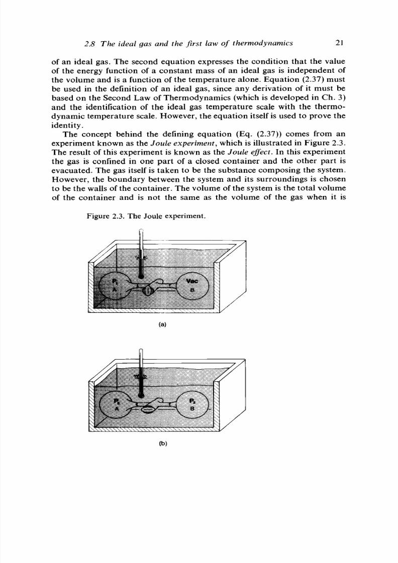
8/11/2019 Thermodynamics of Chemical Systems.pdf
http://slidepdf.com/reader/full/thermodynamics-of-chemical-systemspdf 41/456

8/11/2019 Thermodynamics of Chemical Systems.pdf
http://slidepdf.com/reader/full/thermodynamics-of-chemical-systemspdf 42/456
22
Temperature, heat, work, energy, and enthalpy
confined in one part of the container. The gas is allowed to expand
adiabatically into the evacuated part of the vessel, and the temperature of
the
gas
is
observed before
and
after
the
expansion.
No
work
is
done
by the
gas on the surroundings, because the walls are rigid and the volume of the
vessel
is
therefore constant. Also,
no
heat
is
absorbed or evolved
by the gas.
Consequently, the energy of
the gas
is constant. From Equation (2.28) we
obtain that
fdE\
— dF = O
\dv)
T
,n
, ,
d T + i
- '
d K
- °
(238)
We are concerned with the three variables E, T, and
V.
We know that
(dE\ (dr\ (ev\
=
_
{
\dTj
VtH
\dvJ
EtH
\dEj
TtH
or
fdT\ (dE/dV)
T
,
n
_ (dE/dV)
T
,
n
) (dE/dT)
v
,
n
The quantity (dT/dV)
Eytl
is called the Joule coefficient.
The results of early experiments showed that the temperature did not
change on the expansion of the gas, and consequently the value of the Joule
coefficient was zero. The heat capacity of the gas is finite and nonzero.
Therefore, it was concluded that (dE/dV)
TfH
was zero. Later and more-precise
experiments have shown that the Joule coefficient is not zero for real gases,
and therefore
(8E/dV)
Ttn
is not zero. The concept that
(dE/dV)
Ttn
is zero for
an ideal gas thus becomes a definition of an ideal
gas.
This definition is
consistent with
our
present theoretical concepts of
the
ideal
gas.
For an ideal
gas
Equation (2.28) reduces to
d£
=
(dE/dT)
v
,
n
dT=C
v
dT
(2.40)
which upon substitution into Equation (2.21) yields
&Q
=
C
v
dT-dW
(2.41)
Thus, the total heat absorbed by an ideal gas when the change of state
involves the performance of work as well as a change of temperature is equal
to the heat absorbed when the temperature is changed at constant volume
plus the work done by the system.
2.9 Representation
of
changes
of
state
The state of a chemical system can be defined in terms of the
substance or substances that comprise the system, the quantity of each,
the states of aggregation, and two of the four state functions: energy,

8/11/2019 Thermodynamics of Chemical Systems.pdf
http://slidepdf.com/reader/full/thermodynamics-of-chemical-systemspdf 43/456
2.9 Representation of changes of state 23
volume, temperature, and pressure. It will usually be convenient to use the
temperature and pressure, but it is not necessary to do so. Thus, the symbol
2 H
2
O [ / , 300 K,
1
ba r] w ould indicate a system co ntaining 2 mole of liquid
water at 300 K an d 1 bar. For solutions we might use 0.1NaCl[m, 100° C, 2 ba r]
to indicate a solution containing 0.1 mole of sodium chloride at the molality
m, 100° C, and 2 bar. W hether the solution is aqueou s or n ot w ould be
understood, but if any question exists, then the solvent must be specified.
An alternate symbolism is 0.1NaCl-200H
2
O|Y, 25° C, 1 ba r ] , where
0 .1NaCl-200H
2
O represents an aq ueo us so lution con taining 0.1 mole of
sodium chloride at a concentration of 1 mole of NaCl dissolved in 200 mole
of water. Some changes of state would be explicitly characterized by the
following:
0 . 1 H
2
O [ / , 25 ° C ,1 bar ] = 0 .1H
2
O[g , 150° C, 0 .5 bar]
0 .2NaOH • 200H
2
O|Y, 25° C ,1 bar] +
0.2HC1
• 300H
2
O|Y, 25° C ,1 bar ]
= 0.2NaCl-501H
2
O[Y, 30° C , 1 ba r ]
Many choices of independent variables such as the energy, volume,
temperature, or pressure (and others still to be defined) may be used.
However, only a certain number may be independent. For example, the
pressure, volume, temperature, and amount of substance are all variables of
a single-phase system. However, there is one equation expressing the value
of one of these variables in terms of the other three, and consequently only
three of the four variables are independent. Such an equation is called a
condition equation. The general case involves the Gibbs phase rule, which is
discussed in Chapter 5.
8/11/2019 Thermodynamics of Chemical Systems.pdf
http://slidepdf.com/reader/full/thermodynamics-of-chemical-systemspdf 44/456
The second law of thermodynamics:
the entropy function
In the development of the second law and the definition of the
entropy function, we use the phenomenological approach as we did for the
first law. First, the concept of reversible and irreversible processes is
developed. T he C arn ot cycle is used as an exam ple of a reversible heat engine,
and the results obtained from the study of the Carnot cycle are generalized
and shown to be the same for all reversible heat engines. The relations
obtain ed perm it the definition of a therm ody nam ic tem pera ture scale. Finally,
the entropy function is defined and its properties are discussed.
3.1 Heat and work reservoirs
We define a heat reservoir as any body, used as part of the
surroundings of a particular system, whose only interaction with the system
is across a diathermic boundary. A heat reservoir is then used to transfer
heat to or from a thermodynamic system and to measure these quantities
of heat. It may consist of one or more substances in one or more states of
aggregation. In most cases a heat reservoir must be of such a nature that
the addition of any finite amount of heat to the system or the removal of
any finite amount of heat from the system causes only an infinitesimal change
in the temperature of the reservoir.
A work reservoir is similarly defined as any bod y o r com binatio n of bod ies,
used as part of the surroundings, whose only interaction with the system is
one that may be described in terms of work. We may have a different type
of reservoir for each mode of interaction other than thermal interaction. A
work reservoir then is used to perform work across the boundary separating
the reservoir and the thermodynamic system and to measure these quantities
of work. In the following we are, in order to simplify the discussion, primarily
concerned with mechanical work, but this limitation does not alter or limit
the basic concepts. A reservoir for mechanical work may be a set of weights
and pulleys in a gravitational field, an idealized spring, or a compressible
fluid in a piston-and-cylinder arrangement. In any case the reservoir must

8/11/2019 Thermodynamics of Chemical Systems.pdf
http://slidepdf.com/reader/full/thermodynamics-of-chemical-systemspdf 45/456
3.3 Reversible an d irreversible processes
25
be designed so that the work done by it or on it can be measured by changes
tha t tak e place in the reservoir. It is actually incorrect to consider an y storage
of heat or work as such, but the concept of a reservoir is introduced for
convenience and for lack of a better term.
3.2 Heat engines
A heat engine is any device that is operated in cycles and that
performs work on its surroundings. The cyclic operation is required because
no system has been designed that can operate continuously in one direction.
It is found in Section 3.5 that, in the cyclic operation of a heat engine, a
quantity of heat is absorbed by the engine from a heat reservoir at some
higher temperature, and a smaller quantity of heat is transferred from the
engine to a reservoir at some lower temperature. In chemistry the importance
of the study of heat engines lies primarily in the understanding of the relations
between heat and work, reversible and irreversible processes, and the
definition of the thermodynamic temperature scale. We confine our study to
a simple idealized heat engine represented by the Carnot cycle. This cycle is
discussed in Section 3.5.
3.3 Reversible and irreversible processes
We know from experience that any isolated system left to itself will
change tow ard some final state tha t we call a state of equilibrium. W e further
know that this direction cannot be reversed without the use of some other
system ex ternal to the original system. F ro m all experience this cha racteristic
of systems progressing toward an equilibrium state seems to be universal,
and we call the process of such a change an irreversible process. In order to
characterize an irreversible process further, we use one specific example and
then discuss the general case. In doing so we always use a cyclic process.
We return to the piston-and-cylinder arrangement discussed in Section
2.3.
In that discussion we did not completely describe the process because
we were interested only in developing the concept of wo rk. He re, to com plete
the description, we choose an isothermal process and a gas to be the fluid.
We then have a gas confined in the piston-and-cylinder arrangement. A work
reservoir is used to exert the external force, F
e
, on the piston; this reservoir
can have work done on it by the expansion of the gas or it can do work by
compressing the gas. A heat reservoir is used to make the process isothermal.
The piston is considered as part of the surroundings, so the lower surface
of the piston constitutes part of the boundary between the system and its
surro und ings . Th us , the piston, the cylinder, and the two reservoirs co nstitute
the surroundings.
We now consider the isothermal, quasistatic expansion and compression
of the gas for several processes. The curve AE in Figure 3.1 represents a
pressure-volume isotherm of an ideal gas at a given temperature. The

8/11/2019 Thermodynamics of Chemical Systems.pdf
http://slidepdf.com/reader/full/thermodynamics-of-chemical-systemspdf 46/456
26
The entropy function
expansion of the gas is carried out from the volum e V
1
to the volume V
2
,
and the compression from V
2
to F
x
. The initial pressure of the gas is P± a nd
the pressure after expansion
is P
2
.
W e first exp and
the gas
under
the
conditions that the work reservoir exerts the constant pressure P
2
(equal to
F
e
A) against the piston. The work done on the gas and associated with the
pressure of the gas is given by
W
- r
Vi
PdV=-P
2
(V
2
-V
1
)-mg(h
2
-h
1
)-\ (3.1)
according to Equation (2.15). The work done by the gas is represented by
the area ACDE. The work done on the work reservoir is ^2(^2 ~~ ^i)>
represented by the area
BCDE.
The work done on the piston is
mg(h
2
—
/i
x
).
Finally \Q'\ is the abso lute value of the heat th at m ust be transferred to the
heat reservoir from the surroundings in order to keep the temp erature of
the piston and cylinder constant because of the frictional or collisional
processes. The area ABE represents the work done on the piston and the
quantity of heat transferred to the reservoir. Som e heat mu st also be
transferred to the gas in order to keep the temperature constant.
The gas is compressed under the conditions that the work reservoir exerts
the pressure
P
l
on
the piston. T he w ork don e
on
the gas an d associated
with the pressure of the gas
is
W=-
PdV=-P
1
(V
1
-V
2
)-mg(h
1
-h
2
)-\Q \ (3.2)
Jv
2
where \Q"\ represents the ab solute value of the quan tity of heat that must
Figure 3.1. Illustration of an irreversible cycle.

8/11/2019 Thermodynamics of Chemical Systems.pdf
http://slidepdf.com/reader/full/thermodynamics-of-chemical-systemspdf 47/456
3.3 Reversible and irreversible processes
27
be transferred to the heat reservoir in order to keep the temperature of the
piston and cylinder constant. The work done by the work reservoir is
| ^ i ( ^ i
~~ Vi%
represented by the area
ACDF,
and the work done by the gas
is again represented by the area ACDE. The area AEF represents the
difference between |Q"| and nig^ —h^. He re, in orde r to keep the
temperature of the gas constant, a quantity of heat must be transferred to
the heat reservoir.
For the cyclic process, the gas and the piston and cylinder are returned
to their original state. The net work done by the gas on the work reservoir
is (P
2
—
P
1
){V
2
—Vt), which is a negative quantity. Therefore, the work
reservoir has actually performed this quantity of work, which is represented
by the area
ABEF.
The work done by the gas on expansion is equal to the
work done on the gas on compression; moreover, the heat transferred to
the gas on expansion is equal to the heat transferred from the gas on
compression. Thus, the quantity of heat actually transferred to the heat
reservoir in the cyclic process is the sum of
\Q'\
and |g" |. If we consider the
gas, the piston and cylinder, and the two reservoirs as an isolated system,
then the cyclic process has resulted in the work reservoir doing some work
and the heat reservoir absorbing some heat, and the isolated system has not
been returned to its original state. The question is whether the heat may be
removed from the heat reservoir and used in some way to cause work to be
done on the work reservoir to bring the two reservoirs back to their original
state without causing changes in some other system or systems external to
the isolated system. Experience has shown that this is not possible.
If the expan sion is carried o ut stepwise, first against the c ons tant pressure
P
3
,
then against the constant pressure P
4
, and finally against the constant
pressure
P
2
,
as illustrated in Figure 3.2, then the amount of work done on
Figure 3.2. The work done by the expansion of a fluid for different conditions.

8/11/2019 Thermodynamics of Chemical Systems.pdf
http://slidepdf.com/reader/full/thermodynamics-of-chemical-systemspdf 48/456
28
The entropy function
the work reservoir is larger than in the single-step expansion. Also, the total
am ou nt of heat rem oved from the heat reservoir is larger by the same a m ou nt.
As the number of steps is increased indefinitely, both the work done on the
work reservoir and the amount of heat removed from the heat reservoir
approach a maximum value equal to the area ACDE under the curve.
Similarly, if the compression is carried out stepwise (Fig. 3.3), first at the
constant pressure P
5
, then at the constant pressure P
6
, and finally at the
constant pressure P
l9
then the amount of work done by the work reservoir
is less than in the single-step compression. Also, the total amount of heat
added to the heat reservoir is less by the same amount. As the number of
steps is increased indefinitely, the work done by the work reservoir and the
heat added to the heat reservoir approach a minimum value, both equal to
the area ACDE. We observe than in the limit of expansion and compression
along the curve AE the quantity of work done on the work reservoir on
expansion is equal to the quantity of work done by the work reservoir on
compression, and that the heat removed from the heat reservoir on expansion
is equal to the heat given to the heat reservoir on compression because both
\Q'\ an d |<2"| beco m e e qua l to zer o. It is only in this limit that both the work
and heat reservoirs are brought b ack to their original state, as w ell as the ga s.
In this limit the force exerted on the piston by the gas is always equal to
the sum of the forces exerted on the lower surface of the piston; that is,
the forces that are operating on the boundary between the system and its
surroundings are always in balance. Moreover, in the limit no kinetic energy
will be imparted to the piston.
In the general case we consider any system that is capable of being used
Figure 3.3. The work done by the compression of a fluid for different
conditions.

8/11/2019 Thermodynamics of Chemical Systems.pdf
http://slidepdf.com/reader/full/thermodynamics-of-chemical-systemspdf 49/456
3.3 Reversible and irreversible processes 29
as a heat engine as a part of an isolated system. The other parts are
appropriate heat and work reservoirs. These reservoirs interact with the
system and are used to measure the heat absorbed by the system from the
heat reservoirs and the work done by the system on the work reservoirs for
any process that takes place within the isolated system. We start with the
system, used as the heat engine, in a given state and carry out a cyclic process.
In all actual cases we find that we can return the system to its original state,
but always at least one work reservoir has done work on the system and an
equivalent amount of heat has been added to at least one heat reservoir.
No
method has been found by which the heat can be removed from the heat reservoir
and cause work to be done on the work reservoir so that all systems within the
isolated system can be returned to their original state without causing changes
in systems external to the isolated system. We could, of course, use a heat
reservoir external to the isolated system to return the heat reservoir to its
original state and use an external work reservoir to perform work on the
work reservoir to return it to its original state. However, such operations
do not help, since we would then need to include the external reservoirs
within the isolated system and the same situation would prevail. We could
also use the heat to operate an external heat engine to do some work on the
work reservoir within the system. However, changes occur in such external
systems so that they cannot be returned to
their
original state. All processes
that occur within an isolated system and produce this result for a cyclic
process are called irreversible. W e find further by experim ent t ha t only in
the limit in which all forces acting on the envelope between the system and
the reservoirs are balanced can we return the entire isolated system to its
original state. Processes that occur under these limiting conditions and that
produce this result for cyclic processes are called reversible processes.
Therefore, a reversible process is one in which all of the forces involved are
balanced by equal and opposite forces; i.e., the process takes place under
equilibrium conditions. The direction of the process can be reversed by an
infinitesimal change in these forces. In an irreversible process none of the
conditions hold. The forces are not balanced, the direction of the process
cannot be changed by an infinitesimal change in the forces, and the entire
isolated systems cannot be brought back to its original state. All natural
processes are irreversible. If any one step in a process is irreversible, then the
entire process is irreversible even if all other steps are reversible.
We then come to a general conclusion based on experience. No isolated
system can be returned to its original state when a natural cyclic process takes
place in the system.
This statement may be considered as one statement of
the Second Law of Thermodynamics. Although there is no rigorous proof
of such a statement, all experience in thermodynamics attests to its validity.
O ne concludes, then, tha t there m ust be some mon otonica lly varying function
that is related to this concept of reversibility. The value of this function for

8/11/2019 Thermodynamics of Chemical Systems.pdf
http://slidepdf.com/reader/full/thermodynamics-of-chemical-systemspdf 50/456
30 The entropy function
an isolated system can change only in one direction for any cyclic irreversible
process and would not change for any cyclic reversible process. This function
is the
entropy,
b ut we cons ider the Ca rn ot cycle before defining the function.
3.4 The reversible transfer of heat
The transfer of heat between two bodies requires a difference in their
temperatures. The reversible transfer of heat between two bodies would
require their temperatures to be the same. The question then arises of how
we may reversibly add a quantity of heat to or remove a quantity of heat
from a system over a temperature range. In order to do so we assume that
we have an infinitely large number of heat reservoirs whose temperatures
differ infinitesimally. Then, by bringing the system into thermal contact with
these reservoirs successively an d allowing th erm al equilibrium to be o btained
in each step, we approach a reversible process.
3.5 The Carnot cycle
The Carnot cycle is only one of many cycles that could be used to
illustrate the o pera tion of an ide al, reversible heat engine; however, it is one
of the simplest. In a Carnot cycle a heat engine is operated between two
heat reservoirs at different temperatures in such a way that all the heat
absorbed by the engine is absorbed reversibly from the hotter reservoir and
all of the heat that is rejected by the engine is given reversibly to the cooler
reservoir. Any type of work (mechanical, electrical, magnetic, etc.) may be
involved, bu t for simplicity an d the pu rposes of illustration we are concerned
solely with the wo rk assoc iated w ith the expan sion a nd co mp ression of a fluid.
We therefore consider a given quantity of a fluid contained in a frictionless
piston-an d-cylind er arran gem ent. Since the cycle is to be reversible, the force
exerted on the lower surface of the piston by this fluid must be opposed by
an eq ual force, wh ich is the sum of the forces exerted by so me w ork reservoir.
The cycle consists of four steps and is illustrated in Figure 3.4, which is
drawn for an ideal gas, but the results of the Carnot cycle analysis are
independent of the substance used or the state of aggregation. The four steps
are discussed separately.
1. We start at the state A and carry out an isothermal, reversible
expansion at the higher temperature 6
2
to the state B. The symbol
6 represents a general temperature without reference to any scale.
A quantity of work W
l9
equal to the area ABV
2
V
1
, is done on the
system, and to be consistent with our sign conventions this work
would have a negative value. In order to keep the system isothermal
during the expansion, the heat reservoir having the temperature 6
2
has to be in thermal contact with the cylinder and a quantity of
heat, Q
2
, is transferred from the heat reservoir to the fluid.

8/11/2019 Thermodynamics of Chemical Systems.pdf
http://slidepdf.com/reader/full/thermodynamics-of-chemical-systemspdf 51/456
3.5 The Carnot cycle 31
2. We next carry out an adiabatic reversible expansion from B to C
in which the additional quantity of work, W
2
, represented by the
area
BCV
3
V
2
is done on the system (a negative value). During this
expan sion th e cylinder is enclosed by an adia batic envelop e. N o heat
is transferred to the fluid, and its temperature decreases to 6
1
.
3. We now compress the fluid isothermally and reversibly from C to
D
at the tempera ture
6
1
.ln
this com pression the cylinder is in thermal
contact with the heat reservoir having this temperature. A quantity
of work equal to the area CDV
A
V
3
is done and a quantity of heat
is transferred from the fluid to the heat reservoir. However, because
of our original definition of the symbols
W
and Q, we state that the
work ,
W
3
,
is done by the surroundings on the fluid (a positive
quantity) and the quantity of heat, Q
1?
is transferred from the heat
reservoir to the fluid (a negative qu an tity). The po int D or V
4
is not
independent. The adiabatic AD is determined by the point A and
the isotherm CD is determined by the point C. Point D is the
intersection of the two curves.
4. Finally, we compress the fluid adiabatically and reversibly from D
to A, thus completing the cycle. In this compression the work, W
4
,
is done by the surroundings on the fluid (a positive quantity) and
no heat is transferred from or to the system.
Figure 3.4. Carnot cycle with an ideal gas.
V
2
V
4
V

8/11/2019 Thermodynamics of Chemical Systems.pdf
http://slidepdf.com/reader/full/thermodynamics-of-chemical-systemspdf 52/456
32
The entropy function
The net work,
W,
done on the heat engine by the work reservoir
is equal to the sum of the work done in each of the steps (a negative
quantity); the area
ABCD
represents this net work. The net heat absorbed
by the system is the sum (Q
2
+ 61). The result of the cycle is illustrated in
Figure 3.5, in which the squares represent the heat reservoirs and the circle
represents the heat engine. A quantity of heat, Q
2
, is absorbed by the fluid
from the heat reservoir at the higher temperature, a smaller quantity of heat,
— Q
l9
is rejected by the fluid to the heat reservoir at the lower temperature,
and some work, W , is done by the work reservoir. The efficiency of a heat
engine, n, is defined as
ri=-W/Q' (3.3)
where
Q'
is the sum of all of the qu antitie s of heat tha t are ac tually transferred
from the surroundings to the fluid. The change of energy of the heat engine
is zero, because the fluid and the piston and cylinder are returned to their
original states in the cyclic operation; then —
W = Q
2
+ 6
X
. Note that this
equation is a consequence of the first law, which has AE = 0 for a cycle.
Thus, the efficiency of the reversible cycle is expressed as
= (Q
2
+ Q
1
)/Q
2
(3.4)
It is important to remember that the numerical value of
Q
1
is negative.
3.6 The thermodynam ic temp erature scale
The temperature scales that have been discussed earlier are quite
arbitrary and depend upon the properties of a particular substance. Kelvin
was the first to ob serve th at the efficiency of a reversible hea t engine op eratin g
between two tem peratures is dependent only upo n the two temperatures and
not at all upon the working substance. Therefore, a temperature scale could
be defined that is independent of the properties of any substance.
The second law is independent of the first law. Historically, the second
law was generally accepted and understood before acceptance of the first
law. Therefore, we base the discussion on the efficiency of a reversible heat
engine used in a Carnot cycle. If the efficiency of a reversible heat engine
Figure 3.5. Block representation of the result of the operation of a Carnot
cycle.
e,
e
2
w

8/11/2019 Thermodynamics of Chemical Systems.pdf
http://slidepdf.com/reader/full/thermodynamics-of-chemical-systemspdf 53/456
3.6 The thermodynamic temperature scale 33
operating between
two
temperatures
in a
Carnot cycle
is
depen dent only
upon the two temp eratures, then it may be expressed as
ri=-W/Q
2
=
F(0
29
0
1
) (3.5)
where F (6
2
, #i) is some function of the two temperatures. When the difference
between the two tem peratu res is very small, Eq uatio n (3.5) may be written as
9
(3.6)
6(0)
or
-dW=Q(6)F(6)d6
(3.7)
because d W m ust become zero when d9 is zero (refer to Fig . 3.4). Th e function
F(6)
is called
Carnofs function.
For a reversible cycle operating between the
same two adiabatics, dW is an exact differential and consequently Q(9) F(6)
is
the
derivative
of
some function Q(9). Then
J_d0(^
^
V }
F(6) dO
K }
Temperature scales
can be
defined
by
assigning specific functions
to
F(0)
and the derivatives. Many scales could be defined, but the choice of a suitable
scale
has
depen ded up on utility
and
past history. O nly
the
functions used
in defining
the
present thermo dynam ic
or
Kelvin scale
are
discussed here.
The value of the derivative is assigned
a
constant value, k, an d F(9) is defined
as 1/9. Then
Q = k9
(3.9)
which states that
the
heat abso rbed along
an
isothermal p ath between
two
adiabatics
is
proport ional
to the
temperature .
The
integration
of
Equat ion
(3.7) between
two
tem peratu res yields
-W = k(9
2
-9
1
) (3.10)
so that
the
efficiency
is
given
by
= (0
2
-0
1
)/0
2
(3.11)
The ratio
of
the
two
tem peratures
is
related
to the
efficiency
and the
ratio
of the heats absorbed along
the
isotherms
by
9
2
/9, = 1/(1-r,) (3.12)
and
O
2
/0i = \Q
2
\/\Qi\ (3.13)
8/11/2019 Thermodynamics of Chemical Systems.pdf
http://slidepdf.com/reader/full/thermodynamics-of-chemical-systemspdf 54/456
34 The entropy function
We assume that the efficiency of a Carnot cycle operating between the
two temperatures 0
X
and 0
2
can be measured, or we assume that the absolute
values of the quantities of heat which are ab sorbed by the working substance
can be measured along the isotherms between two adiabatics. Equations
(3.12) and (3.13) give one relation between two qu antities. O ne m ore relation
is needed to fix the value of the two quantities. Since 1954 the definition of
the K elvin scale is comp leted by assignin g the v alue of 273.16 K to the
temperature of the triple point of water. This assignment determines the
value of the proportionality constant in Equation (3.9). Again, we can
determ ine the value of any other tem pera ture by opera ting a reversible C arn ot
cycle between the unknown temperature and the triple point of water. From
Equation (3.12)
0 = 27 3.1 6(1 -*/) (3.14)
if the unknown temperature is below the triple point of water and
0 = 27 3.1 6/( l - iy ) (3 .15)
if it is above. From Equation (3.13) we have
0 = 2 7 3 . 1 6 ^ (3.16)
iai
where Q
e
and Q
t
are the heat absorbed by the working substance in
the isothermal steps at the unknown temperature and the tr iple point,
respectively.
The Kelvin scale is thus defined in terms of an ideal reversible heat engine.
At first such a scale does not appear to be practical, because all natural
processes are irreversible. In a few cases, particularly a t very low tem peratu res,
a reversible process can be approximated and a temperature actually
measured. However, in most cases this method of measuring temperatures
is extremely inconve nient. F ortu nat ely , as is proved in Section 3.7, the Kelvin
scale is identical to the ideal gas temperature scale. In actual practice we use
the International Practical Temperature Scale, which is defined to be as
identical as possible to the ideal gas scale. Thus, the thermodynamic scale,
the ideal gas scale, and the International Practical Temperature Scale are
all consistent scales. Henceforth, we use the symbol
T
for each of these three
scales and reserve the symbol
6
for any other thermodynamic scale.
3.7 The identity of the Kelvin and ideal gas temperature scales
We prove the identity of the Kelvin scale and the ideal gas scale by
using an ideal gas as the fluid in a reversible heat engine operating in a
Carnot cycle between the temperatures T
2
and 7\. An ideal gas has been
defined by Equations (2.36) and (2.37). Then the energy of an ideal gas
depends upon the temperature alone, and is independent of the volume.

8/11/2019 Thermodynamics of Chemical Systems.pdf
http://slidepdf.com/reader/full/thermodynamics-of-chemical-systemspdf 55/456
3.7 The identity
of
the Kelvin and ideal gas temperature scales
35
Conseq uently, the energy of the gas is constant for the isothermal reversible
expansion or compression and, according to the first law of thermodynamics,
the work done
on
the gas
m ust therefore
be
equal
but
opposite
in
sign
to
the heat absorbed by the gas from the surrounding s. Fo r a reversible p rocess
the pressure must be the pressure of th e gas itself. Therefore, we have for
the isothermal reversible expansion of n moles of an ideal gas between the
volumes V and
V
-W=
PdV
(3.17)
ivv
Jv
-W=nRT
dV/V
(3.18)
Jv
where we have substituted the ideal gas law for P, and finally
-W=nRTln(V'/V) (3.19)
Consequently, along the path AB (Fig. 3.4) for the isothermal reversible
expansion
-W
1
=
Q
2
=
nRT
2
MVJV,)
(3.20)
and along
the
pa th CD
for the
isotherm al reversible co mp ression
V,) (3.21)
(The numerical value of W
3
is positive and that of Q
1
is negative, because
V
4
is smaller than K
3
.) We note that in Equations (3.20) and (3.21) the heat
absorbed by the gas from the surroundings is prop ortion al to the tem perature,
provided the ratio of the two volumes is always the same. We know that
the work done by the gas
in
the com plete cycle
is
the sum
of
the heats
absorbed, and therefore
- W=
nRT
2
HVJV,) + nRT, ln(VJV
3
) (3.22)
We complete
the
proof by considering
the
adiabatic reversible expansion
of
an
ideal gas. In this case we know tha t
dE=-PdV (3.23)
from
the
first
law of
thermodynamics, because
the
process is adiabatic.
We
also know that
dE =
C
v
dT
(3.24)
because (dE/dV)
T9 n
has been defined t o be zero for an ideal
gas.
We then have
C
v
dT=-PdV (3.25)

8/11/2019 Thermodynamics of Chemical Systems.pdf
http://slidepdf.com/reader/full/thermodynamics-of-chemical-systemspdf 56/456
36
The entropy function
and
for the
reversible expansion
or
compression
of an
ideal
gas
nR T
C
v
dT=
dV
(3.26)
We divide this equation
by
T and integrate between the limits T and T'
for
the temperature
and
V and V
for the
volume, because
the
heat capacity
of
an ideal
gas is a
function
of
the temperature alone. Thus,
for an
adiabatic
reversible expansion
of an
ideal
gas
C
^
=
- \
V
n R ^ (3.27)
T
I T /
Jv
*
JT
We then have along
the
path
BC
in
the
Carnot cycle
—dT = - nR ln(7
3
/7
2
) (3.28)
T
2
T
and along the path
DA
•r
2
r
—
dT=-nR\n{VJV
A
)
(3.29)
The left-hand side
of
these two equations are equal
but
opposite
in
sign, and
therefore
V
3
/V
2
= VJV
X
(3.30)
or
VJV VJV^
(3.31)
When we substitute this equation into Equation (3.22) we obtain
-W=(T
2
-
TJnR ln(7
2
/7 )
(3.32)
The efficiency
of
this cycle using
an
ideal gas
is
therefore
n
= —
=
Tl
~
Tl
(3.33)
n T
This equation is identical to Equation (3.11). Therefore, the Kelvin thermo-
dynamic scale and the ideal gas scale become identical when the temperature
of the triple point of water is assigned the value of 273.16 K.
3.8 The efficiency of reversible heat engines: two statements of the second
law of thermodynamics
We now discuss the efficiency of a reversible heat engine operating
in a Carnot cycle. The efficiency depends upon the difference between the
two temperatures. The greater the difference for a fixed
T
2
is, the greater the

8/11/2019 Thermodynamics of Chemical Systems.pdf
http://slidepdf.com/reader/full/thermodynamics-of-chemical-systemspdf 57/456
3.8 The efficiency of reversible heat engines
37
efficiency. However, the efficiency is always less than unity except in the
special case where 7\ is zero on the Kelvin scale. Indeed, this relation defines
absolute zero macroscopically as the temperature on the Kelvin scale that
the cooler heat reservoir used in a Carnot cycle must have for the efficiency
of the heat engine to be unity. A more important conclusion is that, if the
two temperatures are equal, the efficiency is zero and no work is done by
the heat engine on the surroundings. This is exactly the result that we found
for the cyclic isoth erm al exp ansio n a nd c om press ion of a fluid in Section 3.3.
This conclusion leads to the Kelvin-Planck statement of the second law:
It is impossible to co nstruct a heat engine w hich operating in cycles will do
work on the surroundings at the expense of heat obtained from a single heat
reservoir.
This is the denial of the possibility of a perpetual-motion of the
second kind. The difference between the first and second laws of thermo-
dynamics is evident. According to the first law a heat engine operating in
cycles must absorb from some heat reservoir a quantity of heat that is equal
to the work done by the engine on the surroundings, but it does not state
how this is done. The second law states that in the cyclic operation the heat
engine must absorb from a heat reservoir a quantity of heat greater than the
amount of work done on the surroundings, and must give the excess quantity
of heat to a heat reservoir at a lower temperature.
A second statement of the second law of thermodynamics can be obtained
by considering the operation of the Carnot cycle in the opposite direction;
that is, along the path ADCB. In this cycle the system in the heat engine
absorbs Q
x
units of heat from the heat reservoir at 7\ and absorbs Q
2
units
of heat (a negative quan tity) from the heat reservoir at the higher tem pera ture
T
2
. A quantity of work, W, has been done by the work reservoir on the
system. This cycle is the refrigeration cycle in which heat is removed from a
heat reservoir at a lower temperature and given to another heat reservoir at
a higher temperature by doing work on the heat engine. According to the
first law, the amount of work done on the system must be equal to the sum
of the heats absorbed by the system. Hence,
-W=Q
2
+ Q
1
or - 6 2 = ^ + 61 (3.34)
That is, the amount of heat given to the heat reservoir at the higher
temperature is equal to the sum of the heat removed from the heat reservoir
at the lower temp erature plus the am oun t of work d one by the su rroundings
on the heat engine. The coefficient of performance for a refrigeration cycle is
defined as
(3.35)
W -Q
2
-Q
1
T
2
-T
t
Here the numerical value of Q
2
is negative, which yields a positive value for

8/11/2019 Thermodynamics of Chemical Systems.pdf
http://slidepdf.com/reader/full/thermodynamics-of-chemical-systemspdf 58/456
38 The entropy function
T
2
. This equation may be written as
T T
(3.36)
Moreover, if Q
x
is always positive and nonzero, W must be positive and
nonzero except in the case when the two temperatures are equal. This
observation results in the Clausius statement of the second law of thermo-
dynamics: Heat of itself will not flow from a heat reservoir at a lower
temperature to one at a higher temperature. It is in no way possible for this
to occur without the agency of some system operating as a heat engine in
which work is done by the surroundings on the system.
3.9 Carnot's theorem: the maximum efficiency of reversible heat engines
The previous discussion an d the conclusions that have been obtaine d
are based on the reversible C arn ot cycle. Althoug h the results are indep enden t
of the fluid used and of the type of work, we must compare the efficiency of
a reversible heat engine operating in a Carnot cycle with that of any other
engine, reversible or irreversible, operated in such a cycle that its interactions
with the surroundings are those of a Carnot cycle. We consider two engines
A and B and two thermal reservoirs, one at the temperature T
2
and the
other at the temperature
T
l9
as shown in Figure 3.6. We assume that
A,
the
reversible or irreversible eng ine, has a gre ater efficiency th an B, the reversible
engine operated in a Carno t cycle. W hen A is operated in a cycle to produce
a quantity of work \W
A
\, \Q
2
\ joules of heat are absorbed from the reservoir
at T
2
and \Q
X
\ jou les of hea t ar e given to the reservoir at T
x
. Then,
Figure 3.6. The relative efficiency of two heat engines.
W
A

8/11/2019 Thermodynamics of Chemical Systems.pdf
http://slidepdf.com/reader/full/thermodynamics-of-chemical-systemspdf 59/456
3.9 Carnofs theorem 39
\W
A
\ = \Q
2
\ —\Qi\ and the efficiency is I Wj/|Q
2
|. We now restore the reservoir
at
T
2
to its original state by operating the heat engine
B
in the refrigeration
cycle and add \Q
2
\ joules to the reservoir. In so doing \Q\\ joules are transferred
from the heat reservoir at 7\ to the heat engine B and a quantity of work | W
B
\
is done on the heat engine. Then \W
B
\ = \Q
2
\ —\Q[\. The efficiency of B
operating to produce work is |WBI/|Q
2
I- We ^ave assumed that
WAW
A
>
\Qi\ \Qi\
and consequently
\W
A
\ > \W
B
\ (3.38)
The net result is that work is done by the heat engines on the surroundings.
When we express this relation in terms of the heats involved, we obtain
(3.39)
and, therefore,
-iGii>-ie;i (3.40)
or
that is, the amount of heat added to the heat reservoir at the temperature
T
x
during the work cycle is less than the amount of heat removed from this
reservoir during the refrigeration cycle. In this cyclic operation, work is done
at the expense of heat obtained from a reservoir at a single temperature.
This is contrary to the Kelvin-Planck statement of the second law of
thermodynamics. We conclude that no heat engine operating in cycles
between two temperatures can have an efficiency greater than that of a
reversible engine operating in a Carnot cycle between the same two
temperatures. This statement comprises
Carnofs theorem.
Mathematically,
we state
1A<1B (3-42)
On the basis of Carnot s theorem, we can further prove that two reversible
engines operating between the same two temperatures must have the same
efficiency. We consider two reversible heat engines
B
and
C
operated in a
Carnot cycle. When we operate
B
in a work cycle to drive
C
in a refrigeration
cycle, we have from Equation (3.42) that rj
B
^rj
c
. When C is used in the
work cycle to drive
B
in the refrigeration cycle, we have rj
B
^
r\
c
.
However,
the quantities of work and heat merely change in sign when the direction of
a reversible cycle is changed. Therefore, the two efficiencies must be equal.
Moreover, the efficiency of a reversible engine operating in a Carnot cycle

8/11/2019 Thermodynamics of Chemical Systems.pdf
http://slidepdf.com/reader/full/thermodynamics-of-chemical-systemspdf 60/456
40 The entropy function
between two temperatures must be the maximum efficiency obtainable for
any engine operating in a cycle between the same two temperatures.
3.10 The entropy function
In Section 3.3 we concluded that an isolated system can be returned
to its original state only when all processes that take place within the system
are reversible; otherwise, in attempting a cyclic process, at least one work
reservoir within the isolated system will have done work and some heat
reservoir, also within the isolated system, will have absorbed a quantity of
hea t. We sought a mo noton ically va rying function tha t describes these results.
The reversible Carnot cycle was introduced to investigate the properties of
reversible cycles, and the generality of the results has been shown in the
preceding sections. We now introduce the entropy function.
We continue with a reversible heat engine operating in a Carnot cycle,
but center our attention on the working substance rather than on the entire
system consisting of the heat engine, the work reservoir, and the two heat
reservoirs. For such a cycle we can write
^ + ^ = 0 (3.43)
T
2
T
x
when the absolute values are not used. This equation shows that a certain
quantity is zero in the reversible cyclic process; that is, the value of a cyclic
integral is zero. From Figure 3.4 we see that, for the steps involving the
isothermal expansion and compression of the system,
-= (3.44)
li JA T
and
that is, the line integral of
dQ/T
along the isotherm al path s is equal to the
heat absorbed by the system from the surroundings during the expansion
or compression divided by the temperature at which the heat is absorbed.
Similarly, the line integrals along the adiabatic paths are
— = 0 (3.46)
and
= 0 (3.47)
f
J
L

8/11/2019 Thermodynamics of Chemical Systems.pdf
http://slidepdf.com/reader/full/thermodynamics-of-chemical-systemspdf 61/456

8/11/2019 Thermodynamics of Chemical Systems.pdf
http://slidepdf.com/reader/full/thermodynamics-of-chemical-systemspdf 62/456
42 The entropy function
expansion of a fluid along the path AB in Figure 3.4. The fluid confined in
the piston-and-cylinder arrangement is at the temperature T
2
an d the cylinder
is in thermal contact with the heat reservoir at the same temperature. The
piston-and-cylinder arrangement, including the fluid, the heat reservoir, and
the work reservoir constitute an isolated system. The transfer of heat takes
place only between the fluid and the heat reservoir. For any infinitesimal
step along the path AB, dQ jou les of hea t are transferred from the he at
reservoir to the fluid. The differential change in the value of the entropy
function of the fluid is dQ/T
2
and that of the heat reservoir is —Q/T
2
. Thus ,
the total change in the value of the entropy function of the isolated system
is zero. For the entire path from A to B, Q
2
joules of heat are transferred
from the heat reservoir to the fluid, and the entropy change of the fluid is
Q
2
/T
2
and that of the heat reservoir is —Q
2
/T
2
. Thus, the total entropy
change of the isolated system along the entire path is also zero. By the same
arguments we find that the change in the value of the entropy function of
the isolated system for the isothermal reversible compression along the path
CD
is zero. For the adiabatic reversible expansion or compression along the
paths
BC
and
DA
the isolated system consists of the fluid in the piston-and-
cylinder arrangement and the work reservoir, separated from heat reservoirs
by an adiabatic envelope. Then, no heat is transferred from any part of the
isolated system to any o ther p art. Th e total entrop y chang e for these processes
is zero. For an isothermal reversible expansion or compression taking place
in an isolated system o r for an ad iabatic reversible expansion or com pression
taking place in an isolated system, the change in the value of the entropy
function is zero.
Consider any number of systems that may do work on each other and
also transfer heat from one to another by reversible processes. The changes
of state may be of any nature, and any type of work may be involved. This
collection of systems is isolated from the surroundings by a rigid, adiabatic
envelope. We assume first that the temperatures of all the systems between
which heat is transferred are the same, because of the requirements for the
reversible transfer of heat. For any infinitesimal change that takes place
within the isolated system, the change in the value of the entropy function
for the ith system is
dQJT,
where Q
{
is the heat a bsorb ed by the ith system.
The total entropy change is the sum of such quantities over all of the
subsystems in the isolated system, so
dS = £ AQJT = (1/T) X dQ
t
= 0 (3.50)
i i
The temperature can be factored from the sum, because it has the same value
for all sytems. How ever, £ d (2 i = 0 because the total system is isolated.
Co nseq uently, th e change in the value of the entrop y function of the isolated
system is zero. The change for a finite process is simply the sum of the
8/11/2019 Thermodynamics of Chemical Systems.pdf
http://slidepdf.com/reader/full/thermodynamics-of-chemical-systemspdf 63/456
3.12 The change in the value of the entropy function 43
changes for all of the infinitesimal changes and, therefore, the change in the
value of the entropy function for a finite process is also zero.
If several of the systems within the isolated system have different
temperatures, we must separate by adiabatic envelopes those systems that
have the same temperature from all other systems that have different
temperatures. Only in this way can we maintain the reversible transfer of
hea t. The isolated system is then co mp osed of several regions, each containin g
those systems that have the same temperature. The separate regions are not
isolated from each other, though, because work can still be done by a system
in one region on a system in another region. The change in the value of the
entropy function of any region is zero for any reversible process taking place
by Equation (3.50). The total entropy change for all regions is also zero. We
conclude that the change in the value of the entropy function in any isolated
system is zero for any reversible process that takes place within the system.
This is not to say that the value of the entropy function of each system within
the isolated system is constant, but only that the increase in the value of the
function for some systems is equal to the decrease in the value for other
systems.
3.12 The change in the value of the entropy function of an isolated system
along an irreversible path
Because the entropy function is defined in terms of a reversible
process, the change in the value of this function along an irreversible path
cannot be measured directly. We can determine it for any given system that
is not necessarily isolated, provided we know the final state as well as the
initial state, by devising a reversible path between the two states. However,
in many cases the final state of a system undergoing an irreversible process
is neither known nor predictable. In order to determine the change of entropy
of an isolated system for the general case, we must allow the irreversible
process to tak e place in the system. We then restore the system to its original
state by reversible processes. In so doing, the isolation of the system must
be removed and at least one extra heat reservoir must be used. The change
in the value of the entropy function of the system in the cyclic process must
be zero, because the entropy function is a function of the state of the system.
Consequently, the entropy change of the system for the irreversible process
must be equal and opposite to its entropy change for the reversible process,
so
AS=-AS
T
(3.51)
where AS is the change of the value of the entropy function of the system
for the irreversible process and AS
T
is that for the reversible process. Since
the process restoring the original system to its initial state is reversible, the
change of the value of the entropy function for the system must be equal

8/11/2019 Thermodynamics of Chemical Systems.pdf
http://slidepdf.com/reader/full/thermodynamics-of-chemical-systemspdf 64/456
44 The entropy function
and opp osite to tha t of the heat reservoirs used in the reversible process, so
AS
T
=-AS
h
(3.52)
where AS
h
is the change for the heat reservoirs. Therefore, the change in the
value of the entr op y function of the isolated system in the original irreversible
process must be equal to that of the heat reservoirs used in the reversible
process.
The expansion of an ideal gas in the
Joule experiment
will be used as a
simple example. Consider a quantity of an ideal gas confined in a flask at a
given temperature and pressure. This flask is connected through a valve to
another flask, which is evacuated. The two flasks are surrounded by an
adiabatic envelope and, because the walls of the flasks are rigid, the system
is isolated. We now allow the gas to expand irreversibly into the evacuated
flask. Fo r an ideal gas the tem per ature rema ins the same. Th us, the expansion
is isothermal as well as adiabatic. We can return the system to its original
state by carrying out an isothermal reversible compression. Here we use a
work reservoir to compress the gas and a heat reservoir to remove heat from
the gas. As we have seen before, a quantity of heat equal to the work done
on the gas must be transferred from the gas to the heat reservoir. In so
doing, the value of the entropy function of the heat reservoir is increased.
Consequently, the value of the entropy function of the gas increased during
the adiabatic irreversible expansion of gas.
We have already stated that an isolated system cannot be returned to its
original state whenever an irreversible process has taken place within it, and
that there is always at least one work reservoir that has done work and one
heat reservoir that has absorbed heat. To restore the isolated system to its
original state, the isolation must be broken. The work reservoir can be
returned to its original state by the use of a work reservoir that is external
to the originally isolated system. However, the performance of work on the
w ork rese rvoir doe s not alter the value of the entro py function of the originally
isolated system. The one or more heat reservoirs that have absorbed heat
can be returned to their original state by the use of heat reservoirs that are
external to the originally isolated system. The reversible transfer of heat from
those reservoirs originally within the system to the reservoirs originally
external to the system reduces the value of the entropy function of the
originally isolated system. Thus, the value of the entropy function of the
isolated system increased for the irreversible processes.
The results obtained in the previous two sections are expressed by the
differential expression
dS ^ 0 (isolated system) (3.53)
called the inequality of Clausius. This inequality refers to an isolated system
for w hich the differential cha ng e of the en tro py fun ction is zero for a reversible

8/11/2019 Thermodynamics of Chemical Systems.pdf
http://slidepdf.com/reader/full/thermodynamics-of-chemical-systemspdf 65/456
3.14 The dependence of the entropy on temperature 45
process and is greater than zero for an irreversible process that may take
place in the isolated system. It is impor tan t to emphasize that this statement
applies
to an
isolated system.
The
value
of
the entropy function
of a
system
tha t is not isolated m ay increase or decrease w ith changes of
state.
However,
in carrying out the changes of state, other systems would have to be used
as work or heat reservoirs. Equation (3.53) applies to the isolated systems,
which includes the necessary w ork and heat reservoirs.
3.13
A
third statement
of
the second
law of
thermodynamics
A third statement
of the
second
law is
based
on the
entropy.
In
reversible systems all forces must be opposed by equal and opposite forces.
Consequently,
in an
isolated system
any
change
of
state
by
reversible
processes must take place under equilibrium conditions. Changes of state
that occur in an isolated system by irreversible processes must of necessity
be spontaneous or natural processes. For all such processes in an isolated
system, the entropy increases. Clausius expressed the second law as:
The
entropy
of the
universe
is
always increasing
to a
maximum. Planck has given
a more general statement of the second law: Every physical
and
chemical
process
in
nature takes place
in
such
a way as to
increase
the sum of the
entropies
of all
bodies taking
any
part
in the
process.
In the
limit,
i.e., for
reversible processes,
the
sum
of the
entropies remains un changed.
3.14 The dependence
of
the entropy
on
temperature
The entropy of a system is a function of the independ ent variables
that are used to define the state of the system. For a closed system in which
no work other than that of expansion and com pression is involved, we need
two variables to define the state. These are usually the temperature and
volume or the temp erature and pressure. The dependence of the en tropy on
the volume and the pressure is developed in Chapte r 4, but its dependence
on
the
temperature
can be
obtained with
the
information that
we now
have.
By definition
dS = dQJT
(3.54)
At constant volume we may write
dS
as
dS=(dS/dT)
Vfn
dT (3.55)
Also, at constant volume dg
r
is an exact differential, and consequently
dQ
T
=
(dQ
r
/dT)
v
,
n
dT (3.56)
Therefore, on substituting Eq uatio ns (3.55) and (3.56) into Eq uatio n (3.49),
U) (3.57)

8/11/2019 Thermodynamics of Chemical Systems.pdf
http://slidepdf.com/reader/full/thermodynamics-of-chemical-systemspdf 66/456
46 The entropy function
However, the heat capacity in general is dQ/dT, and (dg
r
/ d T )
K
„ is thus the
heat capacity of the system at constant volume. We therefore obtain
= ^ (3.58)
T
where C
v
is the heat capacity of the system at constant volume. By a similar
argument we obtain, at constant pressure,
where C
P
is the heat capacity of the system at constant pressure.
3.15 The change of entropy for a change of state of aggregation
A reversible chang e of state of aggregation of a pu re sub stance takes
place under the equilibrium conditions of constant temperature and pressure.
We can therefore use Equation (3.49) to determine the change of entropy of
such a change of state. From this equation,
2
r
(3.60)
since the temperature is constant. The integral of dQ is Q, the heat abso rbed
by the systems during the change of state. Moreover, from Equation (2.33)
we know that Q = AH, the change of enthalpy for the particular change of
state, because the pressure is held constant. Consequently, we find that the
change of entropy for a change of state of aggregation of a pure substance
is given by
AS = AH/T
(change of state of agg rega tion) (3.61)

8/11/2019 Thermodynamics of Chemical Systems.pdf
http://slidepdf.com/reader/full/thermodynamics-of-chemical-systemspdf 67/456
Gibbs
and
Helmholtz energy functions
and open systems
The only two functions actually required in thermodynamics are the
energy function, obtained from the first law of thermodynamics, and the
entropy function, obtained from the second law of thermodynamics.
However, these functions are not necessarily the most convenient functions.
The enthalpy function was defined in order to make the pressure the
independent variable, rather than the volume. When the first and second
laws are combined, as is done in this chapter, the entropy function appears
as an independent variable. It then becomes convenient to define two other
functions, the Gibbs and Helmholtz energy functions, for which the
temperature is the independent variable, rather than the entropy. These two
functions are defined and discussed in the first part of this chapter.
Only closed systems have so far been considered. However, mass can be
varied and is an important variable for all thermodynamic functions. The
introduction of mass as an independent variable into the basic differential
expressions for the thermodynamic functions yields the equations that Gibbs
called 'fundamental'. It is on these equations that much of the development
of the applications of thermodynamics to chemical systems is based.
Many of the problems that are met in applications require the evaluation
of various derivatives and the integration of differential quantities that involve
the derivatives. To be of use, the derivatives must be expressed in terms of
experimentally determinable quantities. Because the number of derivatives
that can occur is extremely large, it is advantageous to be able to derive the
necessary relations. Methods to do this are discussed and several examples
given in the last part of this chapter.
4.1 The Helm holtz energy
One differential expression for the energy of a system is given by
Equation (2.26):
dE = dQ-PdV + dW

8/11/2019 Thermodynamics of Chemical Systems.pdf
http://slidepdf.com/reader/full/thermodynamics-of-chemical-systemspdf 68/456
48 Gibbs and Helmholtz energy functions
for which the process is quasistatic with respect to the work of expansion
or compression. This equation may be used when we are interested in the
heat absorbed by the system for some change of state for
a
specified process.
However , if the process is reversible, then dQ becomes dg
r
, which equals
T dS by the definition of the entropy. The equation
dE=TdS-PdV + dW'
T
(4.1)
is obtained when this limitation
is
ado pted and the substi tution ma de.
In
this equation P
is
the pressure
of
the system and dW'
r
is
the sum
of
all
of
the work done
on the
system, excluding
the
work
of
expansion
or
compression, along
a
reversible path. The integration
of
Eq uatio n (4.1)
to
determine the difference
in
energy between two states mu st
be
carried ou t
along
a
reversible path. The energy
is
still
a
function
of
the state
of
th e
system, and consequently this difference of energy is independent of the path.
It is the dete rm ination of this difference tha t m ust be m ade alon g
a
reversible
path when Equation (4.1) is used. No such limitation is placed on Equation
(2.26).
Although Equation (4.1)
is
useful, partic ularly
for
isentropic changes
of
state for which dS = 0, the entropy appears as an independent variable. This
circumstance
is
incon venie nt from
an
experimental point
of
view, because
no meters
or
devices exist that m easure entro py.
A
new function
in
which
the tem per ature is an indepen dent variable rather th an the entrop y is obtained
by subtracting
d(TS)=TdS + SdT
(4.2)
from Eq uatio n (4.1). W e then o btain
d(E
-TS)=-SdT-PdV
+ dW'
T
(4.3)
The new function is defined first
in
terms of its differential,
so
dA =
d(E-TS)
(4.4)
and then define the integration constant resulting from the integration
of
Equation (4.4)
to be
zero. This
is
justified becau se
we do not
know
the
absolute value of either the energy or the entropy and, consequently, cannot
kno w the abs olute value of the new function. Fu rth erm ore , as we are defining
a new function, we may define
it in
any way th at we please. Therefore, we
choose to make the integration constant zero. After the integration, we have
the definition
1
A =
E-TS (4.5)
1
If the product TS is not uniform throughout the system, the system can be divided into parts
in which
TS
is uniform. Then £
TS,
the sum being taken over the individual parts of the system,
may be substituted for T S. If the volumes in which TS is uniform are infinitesimal, the £
TS
may be substituted by J (TS/V) dV, the integral being tak en over the entire volum e of the system.

8/11/2019 Thermodynamics of Chemical Systems.pdf
http://slidepdf.com/reader/full/thermodynamics-of-chemical-systemspdf 69/456
4.2 The Gibbs energy
49
The new function A is called the Helmholtz energy.
2
Since £, T, and S are
functions of the state of the system, A is also a function of the state of the
system, and its differential is exact. The change in the value of the Helmholtz
energy in going from some initial state to some final state is independent of
the path. However, the determination of this change must be obtained by
the integration of Equation (4.3) along any reversible path between the two
states.
Any physical interpretation of the Helmholtz energy must be based on
interpreting Equation (4.3). Thus, for an isothermal change of state, the
equation becomes
dA=-PdV
+
Th e algebraic sum of the terms P dV and d W'
t
is the total work d one reversibly
by the system for a differential change of state. Hence, dA is the negative of
the maximum work that the system can do on the surroundings for an
isothermal differential change of state.
4.2 The Gibbs energy
The differential expression for the enthalpy is
dH = dQ + V dP + dW (2.30)
for quasistatic processes with respect to the work of expansion and
compression. If we limit the differential path to reversible processes, we may
substitute T dS for dQ and obtain
dH = T dS + V dP + dW'
T
(4.6)
Although the integration of this equation is limited to reversible paths, the
change of enthalpy in going from one state to another is still independent
of the path.
He re, again , the entrop y ap pea rs as an indep end ent v ariable. It is therefore
convenient to define another function so that the temperature appears as an
independent variable. This is done by subtracting Equation (4.2) from
Equation (4.6):
d(H - TS) = -S dT + V dP + dW'
r
(4.7)
We define the new function, G, by setting
dG =
d(H-TS)
(4.8)
2
Gibbs used
\j/
for this function; G. N. Lewis called it the work function, with the symbol A;
and in many European countries it was called the Helmholtz free energy, with the symbol F.
By international agreement the accepted name is the Helmholtz energy and the symbol is A.

8/11/2019 Thermodynamics of Chemical Systems.pdf
http://slidepdf.com/reader/full/thermodynamics-of-chemical-systemspdf 70/456

8/11/2019 Thermodynamics of Chemical Systems.pdf
http://slidepdf.com/reader/full/thermodynamics-of-chemical-systemspdf 71/456
4.3 Open systems 51
volume, num ber of moles of each com pon ent, an d the generalized coordinates
associated with the work terms other than the work of expansion or
compression, so that
E = E {S,V,
ni
,n
2t
n
3
,...,X) (4.10)
where X represents the generalized coordinates.
4
Th e differential of the energy
function is then
dV
S,ni,ti2,n3,...,X
(dE\
J
(dE\
+
1
—
1 dtti+l
—
1
dn
2
-+Y
i
F
j
dX
j
(4.11)
In this equation Fj represents the conjugate generalized forces and the sum is
taken over all of the generalized coordinates. The equation must reduce to
Eq ua tion (4.1) when the num ber of moles of each com pon ent is held co nstan t.
Comparison of these two equations shows that (dE/dS)
v ninin3f x
= T and
(dE/dV)
SVnun2n3 x
= —P. W hen we use the symbol /i
x
for (dE/dn^sy^^
x
,
etc.,
Equation (4.11) can be written as
d£ = T dS - P dV + £ ft dn
t
+ £ Fj dX
}
(4.12)
i j
where the subscript i represents any component in general and the sum is
taken over all components. Differential expressions for dH, dA, and dG for
open systems are obtained by the same methods that were used to obtain
them for closed systems. We thus have
dH = T dS + V dP + X Mi dn* + X
F
j
dX
j (
4
-
13
)
i j
dA = - S dT - P dV + X ft dn
{
+ £ F
j
dX
}
(4.14)
i j
dG = - S dT + V dP + X lit dn
t
+ X Fj dXj (4.15)
i j
The derivatives of the energy with respect to the number of moles of
4
Gibbs used mass in his development of thermodynamics, and any unit of mass may be used.
Th e nu m ber of moles of a subs tance is a mu ltiple of a specific unit of mas s tha t is different for
each substance: the molecular mass. If there is any question of the molecular mass of the
substance, the assumed molecular mass or the assumed chemical formula of the substance must
be given; e.g., A1C1
3
or
A1
2
C1
6
.

8/11/2019 Thermodynamics of Chemical Systems.pdf
http://slidepdf.com/reader/full/thermodynamics-of-chemical-systemspdf 72/456
52 Gibbs and Helmholtz energy functions
a component, keeping all other independent variables constant, are so
important in thermodynamics that they have been given the separate symbol
\i
and are called the 'chemical potentials.' They are the rates of change of
the energy of the system as the number of moles of a component in the
system is increased at constant entropy, volume, and number of moles of all
other components, with no work being involved. The problem of keeping
the entropy and volume constant as material is added to the system presents
no difficulties conceptually, because the temperature and pressure, which are
dependent variables according to E quation (4.12), will change as the material
is added under the given conditions. Other equivalent conditions of the
chemical potential are given in Section 4.5.
In many problems of thermodynamics we are concerned with both open
and closed systems simultaneously. As an example we may consider a
heterogenous system composed of several phases. The whole system is closed.
However, we can consider each phase as a system, and these phases are open
because material can be transferred from one phase to another.
4.4 Resume
We have now defined the five thermodynamic functions: energy
entropy, enthalpy, Helmholtz energy, and Gibbs energy. The energy and
entropy are defined in terms of the differentials such that dE = dQ + dW and
dS = dQJT. The others are defined as H = E + PV, A = E-TS and G =
H-TS = E + PV-TS. Each of these five functions is a function of the state
of the system, and consequently their differentials are exact. They are assumed
to be continuous functions of the independent variables between certain
easily recognized limits; at these limits some of the functions may be still
continuous, but others will be discontinuous. These limits are the points
where first- or second-order transitions occur. First-order transitions are
those in which the Gibbs energy is continuous, but its first and higher
derivatives are d iscontinuous. Such transitions are changes of phase (change
of state of aggregation) or of crystal structure. Second-order transitions are
those in which the first derivative is also continuous, but the second- and
higher-order derivatives are discontinuous. Such transitions occur at the
lambda point of helium, at the Curie point of a ferromagnetic material, or
at the temperature at which an 'order-disorder' transition takes place in
certain alloys and some chemical compounds. Finally, all five functions are
homogenous functions of the first degree in the mole numbers (number of
moles of each component).
Under the conditions that the system is closed and that we are concerned
only with the first law of thermodynamics, we have the two equations
(4.16)

8/11/2019 Thermodynamics of Chemical Systems.pdf
http://slidepdf.com/reader/full/thermodynamics-of-chemical-systemspdf 73/456
4.4 Resume 53
and
dH = AQ + V dP + dW (4.17)
Equation (4.17) is applicable to quasistatic processes for the work of
expansion an d com pression. On the introduction of the second law we have
four equations for closed systems
(4.18)
£ =
dH
=
dA =
TdS-
TdS
+
-SdT
PdV
VdP
+
+
IV
j
j
+
Fj
dX j
dX j
Fj
dXj
and
dG = - S dT + V dP + X Fj dX
}
(4.21)
j
The more general equations for open systems are
dE = T dS - P dV + X & dn
{
+ £
F,-
d ^ - (4.22)
Y
J
H
i
d«, + X F
;
d X
;
(4.23)
i J
dA = -S dT - P dV + X to
dn
i + Z
F
J
d x
i (
4
-
24
)
and
dG = -
S
dT +
K
dP + ][>,• (in* + £ F,- dX,-
(4.25)
* j
The integration of Equations (4.18)-(4.25) is limited to a reversible path
between some initial and some final state, but the change in the values of
the functions so determined is independent of the path.
W e see from these equ ation s th at we deal with a large num ber of variables
in thermodynamics. These variables are £, S, if , A, G, P, V, T, each n
h
and
two variables for each additional work term. In any given thermodynamic
problem only some of these variables are independent, and the rest are
dependent. The question of how many independent variables are necessary
to define completely the state of a system is discussed in Chapter 5. For the
present we take the number of moles of each component, the generalized
coordinate associated with each additional work term, and two of the four
variables S, T, P, and V as the independent variables. Moreover, not all of

8/11/2019 Thermodynamics of Chemical Systems.pdf
http://slidepdf.com/reader/full/thermodynamics-of-chemical-systemspdf 74/456
= E(S,
H = H(S,
= A(T
9
G = G(T,
V
9
n
l9
P,n
l9
V
9
n
l9
P,"i
n
2
,n
n
2
,n
n
2
,n
n
2
t
3>
[
3>
3»
••;X
l9
. . . ,
X i,
X
2
,....
x
2
x
2
,...)
, ^ - 2 ' • • •
Gibbs and Helmholtz energy functions
the four functions E,
if,
A,
and G are
applicable
to all
problems.
The
choice
of which function
to use may be
dictated somewhat
by the
problem,
or it
m ay
be a
mat ter
of
individual preference. From Eq uatio ns (4.22)-(4.25)
we
have
(4.26)
(4.27)
(4.28)
and
(4.29)
Thus , of the
four variables, S, V,
T, and P, if
S
and
V
are the
independent
ones
we
would
use the
energy,
if
S
and
P
are the
independent variables
we
would
use the
enthalpy,
if
T
and
V
are the
independent variables
we
would
use
the
Helmholtz energy,
and if
T
and
P
are the
independent variables
we
would
use the
Gibbs energy. This
is not to say
that
we are
limited
to
these
combinat ions.
We
could
set £ as a
function
of
T
and
V,
of T and
<S,
of
T
and
P, of
S
and P, or of P and
V. However,
if we do so, the
differential
expression
for d£
is much mo re complicated.
The
other three functions
(//,
A,
and
G)
could also
be
expressed
as
functions
of the
same combinations
of
the variables,
but
again more-complicated expressions
are
obtained
for the
differentials.
The two
most im porta nt com binations other tha n those given
in Equations (4.22)-(4.25) are to make the energy a function of T and V,
and the enthalpy a function of T and P, in addition to the mole numbers
and the work variables. These functions are discussed in Section 4.8.
In Equations (4.22)-(4.25) the energy, enthalpy, Gibbs energy, and
Helmholtz energy have been taken as dependent variables. However, any of
the four equations may be solved for any of the other differentials in that
equation. That particular variable would then become dependent
and the
energy, enthalpy, the Gibbs energy or the Helmholtz energy, as the case
m ay be, would become independent. For example, Equation (4.22) may be
written
as
d £ P d F I / F j d X , . ' Y
f
dn
t
T T T T
in which case
the
energy
is an
independent variable
and the
entropy
is
dependent .
In this section we have now given all of the basic equations in chemical
thermodynamics .
Any
other relation
can be
derived from
one or
more
of
these.
We
have also outlined
the
wide choice
of
independent variables that
m ay be used. Fortun ately, because of the limitation of being able to measure

8/11/2019 Thermodynamics of Chemical Systems.pdf
http://slidepdf.com/reader/full/thermodynamics-of-chemical-systemspdf 75/456
4.5 Dependence of functions on independent variables
55
experimentally only the pressure, temperature, volume, mass, and the other
work variables, the number of choices is much more limited than is at first
apparen t .
In the remainder of this book we consider all work terms other than the
wo rk of expansion and com pression to be zero , except in those specific cases
where such terms are definitely considered. This means that the generalized
coo rdina tes th at a pp ear as differentials in the expression for such wo rk terms
are all considered to be constant.
4.5 Dependence of the thermodynamic functions on the
independent variables
Each of Equations (4.22)-(4.25) is a differential expression for a
certain function written in terms of a num ber of indep enden t variables. F rom
m athem atics we ma y immed iately o btain the partial derivative of the function
with respect to each of the independent variables. Thus, from Equation
(4.22),
5
and
( w )
=
~
p (4
*
32)
In this case both the temperature and pressure are dependent variables and
are functions of the entropy , volume, and mole num bers of the com pone nts.
From Equation (4.23),
and
( —I =V (4.34)
Here the temperature and volume are dependent variables and are functions
of the entropy, pressure, and mole numbers of the components. From
5
In order to save space, the subscript
n
in a derivative indicates that the number of moles of
all com pon ents are kept co nstant except in the case when the variation is one of the com pon ents.
In that case it indicates that the number of moles of all of the components are kept constant
except the one that is being varied. Also, it must be remembered that all work terms other than
the work of expansion or compression are zero, even though the notation is not m ade in general
practice.

8/11/2019 Thermodynamics of Chemical Systems.pdf
http://slidepdf.com/reader/full/thermodynamics-of-chemical-systemspdf 76/456
56
Gibbs and Helmholtz energy functions
Equation (4.24),
and
-_ , .
=S
(4.35)
dTj
v
,
n
8
4) =~P ( 4 - 3 6 )
The entropy and pressure are dependent variables and are functions of the
volume, temperature, and the mole numbers of the components. Finally,
from Equation (4.25),
and
) =V (4.38)
In this case the entropy and volume are dependent variables and are functions
of the temperature, pressure, and mole numbers of the components. In
addition, we have four derivatives that are all equal to the chemical potential,
one from each of the four equations, so
) ( * > ) ,4.39,
_(«) . « _(£) _(*>)
\^i/s,v,n \dni/s,p,n \Sni/
TtVtn
\dnJ
Throughout this book we use the subscript i to refer to any component in
general. When it is necessary to specify a specific component, we use other
subscripts such as
j ,
fc, /, etc.
Two other important derivatives of the Gibbs and Helmholtz energies
with respect to the temperature can be derived from these simpler relations.
From the definition of the Gibbs energy and Equation (4.37) we obtain
However, the left-hand side of this equation equals - T
2
(d(G/T)/dT)
P
^ and
consequently
\ dT J
P
,
n
T
2
This equation may also be written as
=H (4.42)

8/11/2019 Thermodynamics of Chemical Systems.pdf
http://slidepdf.com/reader/full/thermodynamics-of-chemical-systemspdf 77/456
4.6 The Maxwell relations and other relations 57
b e c a u s e d ( l / T ) = —T/T
2
. Eq ua tion (4.41) is sometimes called the Gibbs-
Helmholtz equation. Similarly, for the Helmholtz energy, we obtain
V
dT J
Kn
T
2
or
(tyil) -E (4.44)
4.6 The Maxw ell relations and other relations
As stated previously, Equations (4.22)-(4.25) are differential expres-
sions of certain functions. Consequently, the differentials are exact and the
conditions of exactness must be satisfied. We can immediately write
m
(4.45)
(4.46)
S,n
(4.47)
(4.48)
Equations (4.45) and (4.46) may be inverted to read
\8f)s.n
and
( /
=
( /
( 4
'
5 0 )
These four relations are known as the Maxwell relations, and are useful in
terms of conve rting one set of variables to a no ther . They are limited to closed
systems, as indicated by the constancy of the mole numbers of the
components .
Additional relations can be written when we allow the mole numbers of
the components to be varied. Thus, from Equation (4.22),
) ( ) (4.51)
dSJ
Vn
\dJ

8/11/2019 Thermodynamics of Chemical Systems.pdf
http://slidepdf.com/reader/full/thermodynamics-of-chemical-systemspdf 78/456
58 Gibbs and Helmholtz energy functions
and
or, from Equation (4.25),
and
(4-54)
4.7 Development of other relations
One of the problems of thermodynamics is to obtain expressions for
various derivatives in terms of qua ntities tha t can be observed experimentally.
The total number of first partial derivatives is exceedingly large and it is
useless to attempt to memorize the relations between them. Fortunately,
there is only a relatively sm all num ber of such relations th at are of im po rtanc e,
and some of the simpler ones are easily learned through use. However, it is
still important to be able to obtain or derive such relations when they are
needed. Some systematic methods have already been developed; of these,
probably those most used are by Bridgman [1], and by Shaw [2], who
used the methods of Jacobians. The purpose of this section is to illustrate
various methods. The discussion is not necessarily complete or systematic,
but it does afford training in the use of properties of differentials and
derivatives to derive many thermodynamic relations between partial deriv-
atives. It should be remembered that thermodynamics is redundant, in that
the enthalpy and the Gibbs and Helmholtz energies have been defined for
convenience. Tho se functions are not absolutely necessary. As a result, there
is no single way to obtain a given relation.
(a) Any variable in thermodynamics can always be set as a function of
two other variables by keeping all other variables constant. We may be
interested in the relation between the three derivatives involving the three
variables. As an example, we may be interested in the isentropic change of
the volume with respect to the temperature. We may set
S = S(V, T)
at
constant n. Then
) ( i )
(4
-
55)
8/11/2019 Thermodynamics of Chemical Systems.pdf
http://slidepdf.com/reader/full/thermodynamics-of-chemical-systemspdf 79/456
dT
/s
,
n
4.7 Development of other relations
59
However, V may be considered as a function of S, T, and n, so
(4.56)
Substituting this equation into Equation (4.55) and setting [dS]
n
= 0,
(4.57)
The coefficient must be zero because [dT]
M
need not be zero. Therefore
™ +(*) =0 (4.58)
or
(4.59)
T{dP/dT)
v< n
recalling Equation (4.47). Another form of Equation (4.58) is
('I) pJ) . _ ,
,4.60)
I
..\dT)
,,\Ss)
r
,
(b) A nu m ber of derivatives may be obta ined from Eq uatio ns (4.22)-(4.25).
In these derivatives a new variable, different from the independent variables
of the basic eq ua tion , is introd uce d. As an exam ple consider the d eterm ination
of (dE/dV)
Tn
. Fro m Eq uation (4.22),
dE=TdS-PdV + Y
i
l*t dn
(
(4.22)
i
Because we are interested in the independent variables
T
and
V,
we may set
£ as a function of
T
and
V
at constant mole numbers of the components,
from which
. (4-61)
W e also need to express S as a function of T and V at constant mole numbers
of the components, to obtain
T
,
n
= ( ^ ) [ d F ]
r
,
n
(4.62)
Equation (4.22) becomes
(^) (4.63)

8/11/2019 Thermodynamics of Chemical Systems.pdf
http://slidepdf.com/reader/full/thermodynamics-of-chemical-systemspdf 80/456
60 Gibbs and Helmholtz energy functions
when we substitute Equations (4.61) and (4.62) for AE and AS, respectively.
We then divide by AV, so
-P (4.64)
Finally, from Eq ua tion (4.47), we kn ow that (8S/dV)
T
,
n
= (dP/dT)
v? n
and ,
consequently,
^ ) =T(
dP
) -P (4.65)
dv) \dTj
(c) Let us determine
(dE/dn^
P
„ ,
where the two variables
T
and
P
are
introduced. We may again start with Equation (4.22):
AE = T AS - P dV + X to
dn
i (
4
-
22
)
i
The functions £, S, and V can all be expressed as functions of T, P, and all
ns. At co nsta nt T, P , and all rcs except n,,
d E
= \ — )
dn
j
4
-
66
)
Anj (4.67)
and
( ) dn
;
(4.68)
Substitution of these three equations into Equation (4.22) and division by
dn, yields
(A) So far we have no t discussed second de rivatives. Of course, the
various relations discussed in (a), (b), and (c) above are applicable to
the first derivatives, as these are also functions of the same sets of
independent variables, as are the original functions. However, in addition,
for z = z(x, y) the equality of the two se cond -order derivatives [d(dz/dx)
y
ldy]
x
and
[_d(dzldy)Jdx]
y
is of importance. As an example, consider the evaluation
of (dC
v
/dV)
Ttn
. Since C
v
= (dE/dT)
Vtn
, we can write
(3CA J
±
(3E\
1
\dVj
T
* LdV\dTj
v
J
Tin

8/11/2019 Thermodynamics of Chemical Systems.pdf
http://slidepdf.com/reader/full/thermodynamics-of-chemical-systemspdf 81/456
4.8 Energy and enthalpy as functions 61
and then interchange the order
of
differentiation,
so
W e
now
carry
out the
indica ted differentiation with
the use of
Equat ion
(4.65). The result
is
(4.72)
dT
2
/Vin
4.8 The energy
as
a
function
of
the temperature and volume, and
the enthalpy
as a
function
of
the temperature and pressure
Because of the exp erim ental difficulties of using
the
entropy as an
independent variable, it is convenient to use the energy as a function of th e
temperature , volume, and mole numbers . Thus, for
E
— E(T, V,
n),
6EJ™
6T
+
(
d
J) dK +
z W dn
;
(4.73)
\dTj \dV) rW
With the use of Eq ua tion s (2.29) and (4.65), we o btain
) dn
t
(4.74)
Vttt
J i \dnJ
TtVt
n
A similar expression can
be
derived
for
the enthalpy
as a
function
of
the
temperature, pressure, and mole numbers. If we
set
H = H(T, P, n),
« dn, (4.75)
With the use of Eq uatio ns (4.19) and (4.48), we find that
,4.76,
SPj
r
,,
\iT)
r
,
and consequently, with Equation (2.33),
d H =
C
P
dT+\v-T(~)
idP
+
l f ^ ) dn,
(4.77)
Although Equations (4.74) and (4.77) are not as simple as Equat ions
(4.22) and (4.23), they are more important from an experime ntal viewpoint.
This importance arises from the fact that the temperature is the independent
variable in these equations, rather than the entrop y.
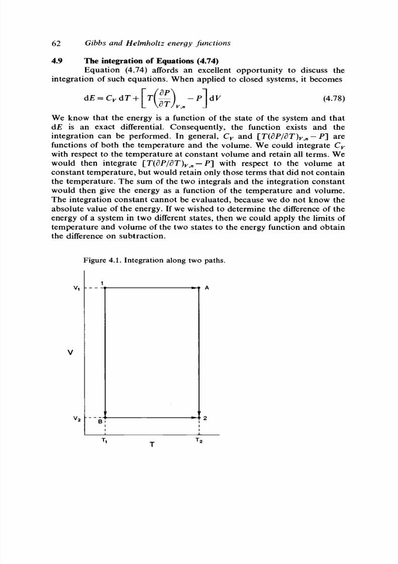
8/11/2019 Thermodynamics of Chemical Systems.pdf
http://slidepdf.com/reader/full/thermodynamics-of-chemical-systemspdf 82/456
62
Gibbs and Helmholtz energy functions
4.9 The integration of Equations (4.74)
Equation (4.74) affords an excellent opportunity to discuss the
integration of such equations. When applied to closed systems, it becomes
= CydT+\T[ — \
-P\dV (4.78)
We know that the energy is a function of the state of the system and that
dE is an exact differential. Consequently, the function exists and the
integration can be performed. In general, C
v
and [T(dP/dT)
v n
—P] are
functions of both the temperature and the volume. We could integrate C
v
with respect to the temperature at constant volume and retain all terms. We
would then integrate
[T(dPldT)
Vn
—P~\
with respect to the v olume at
constant tem perature, but w ould retain only those terms that did not contain
the temperature. The sum of the two integrals and the integration constant
would then give the energy as a function of the temperature and volume.
The integration constant cannot be evaluated, because we do not know the
absolute value of the energy. If we wished to determine the difference of the
energy of a system in two different states, then we could apply the limits of
temperature and volume of the two states to the energy function and obtain
the difference on subtraction.
Figure 4.1. Integration along two paths.

8/11/2019 Thermodynamics of Chemical Systems.pdf
http://slidepdf.com/reader/full/thermodynamics-of-chemical-systemspdf 83/456
4.9 The integration of Equations (4.74) 63
In such an integration [T(dP/dT)
v n
—
P ] w ould need to be know n as a
function of the temperature and volume. Such information can be obtained
from an equ ation of state giving the pressure as a function of the tem pera ture
and volume at constant mole numbers of the components. Also, C
v
would
need to be known as a function of the volume and temperature. With our
present knowledge of thermodynamic data, this quantity might be known
as a function of the tem pera ture at som e fixed volum e. If this were the case,
then we could still determ ine C
v
as a function of the volume by the integration
of Equation (4.72) with respect to the volume at constant temperature when
an equation of state is known. The integration constant would be determined
by our knowledge of C
v
as a function of the tem pera ture a t the fixed volum e.
Again, for this integration an equation of state would be needed.
Even when a limited amount of data is available, we may still be able to
perform the integration between two states, (V
l9
7\) and (V
2
, T
2
). Here we
m ake use of the pro per ty of functions; th at th e change of the energy in going
from some initial state to a final state is independent of the path. Consider
Figure 4.1. We wish to determine the change in the energy of a closed system
in going from state 1 to state 2. We may follow either pa th 1A2 or path
1B2. If we choose the first path, we may integrate first along the path I A,
thus changing the temperature from T
x
to T
2
at the constant volume V
x
.
For this change of state
AE, = (C
v
)
Vl
dT (4.79)
in which C
v
is evaluated a t F
x
. We may then integrate from A to 2 at the
constant temperature T
2
between the volumes V
x
and V
2
. Here the change
of energy is
in which [T(dP/dT)
Vn
-P ] is evaluated at the tem pera ture T
2
. The total
change of the energy is the sum of these two changes.
If we choose the path 1B2, we first integrate along the path IB , using
Equation (4.80), but in this case [T(dP/dT)
Vn
- P ] is evaluated at 7 \ . Then
we integrate from B to 2, using Equation (4.79); here C
v
is evaluated at V
2
.
The total energy change along the two pa ths, 1A2 and 1B2, mu st of necessity
be equal.

8/11/2019 Thermodynamics of Chemical Systems.pdf
http://slidepdf.com/reader/full/thermodynamics-of-chemical-systemspdf 84/456
Conditions of equilibrium and stability:
the phase rule
Reversible processes are those processes that take place under
conditions of equilibrium; that is, the forces operating within the system are
balan ced. Therefore, the therm ody nam ics associated with reversible processes
are closely related to equilibrium conditions. In this chapter we investigate
those conditions that must be satisfied when a system is in equilibrium. In
particular, we are interested in the relations that must exist between the
various thermodynamic functions for both phase and chemical equilibrium.
We are also interested in the conditions that must be satisfied when a system
is stable.
After the conditions of equilibrium have been determined, we can derive
the phase rule and determine the number and type of variables that are
necessary to define completely the state of a system. The concepts developed
in this chapter are illustrated by means of graphical representation of the
thermodynamic functions.
5.1 Gibbs
9
statement concerning equilibrium
Gibbs based his entire treatment of heterogenous equilibrium on the
following statement [3].
The criterion of equilibrium of a material system which is isolated from all
external influences may be expressed in either of the following entirely
equivalent forms:
1. For equilibrium of any isolated system it is necessary and sufficient that
in all possible variations of the state of the system which do not alter its
energy, the variations of its entropy shall either vanish or be negative.
2.
For equilibrium of any isolated system it is necessary and sufficient that
in all possible variations in the state of the system which do not alter its
entropy, the variation of its energy shall either vanish or be positive.
The first statement corresponds to the equation
^0 (5.1)

8/11/2019 Thermodynamics of Chemical Systems.pdf
http://slidepdf.com/reader/full/thermodynamics-of-chemical-systemspdf 85/456
5.7
Gibbs' statemen t concerning equilibrium
65
and the second statement corresponds to the equation
(SE)
s
>0 (5.2)
We find in Section 5.3 that the equality sign is applicable when all variations
of the system can be carried out in either direction. When any variation of
the system can be carried out in only one direction, the inequality sign is
applicable.
If the system is isolated and already at equilibrium, then any variation in
the state of the system cannot increase the entropy if the energy is kept
constant, and cannot decrease the energy if the entropy is kept constant.
In other words, for an isolated system at equilibrium, the entropy must have
the largest possible value consistent with the energy of the system, and the
energy must have the smallest possible value consistent with the entropy of
the system. There may be many states of the system that are equilibrium
states, bu t these con ditions m ust be applicable to each such equilibrium state.
The equivalence of the two statements is rather easily proved. Assume
tha t, contra ry to E qu ation (5.1), there is a variatio n tha t increases the entrop y
of the isolated system. W e can then decrease the entrop y of the varied system
to the original value by removing heat from it reversibly. However, in so
doing we also decrease the energy. Then, in this new state the energy has
been decreased at constant entropy. This is contrary to Equation (5.2).
Similarly, assume that, contrary to Equation (5.2), there is a variation that
decreases the energy of the system while the entropy is kept constant. We
may then increase the energy of the varied system to its original value by
adding heat to the system reversibly. However, in so doing we increase its
entropy. This is contrary to Equation (5.1). Thus, if the first statement is
not satisfied for some possible variation of the system, then there is also a
varied state for which the second statement is not satisfied, and if the second
statement is not satisfied for some possible variation of the system, then there
is a varied state for which the first statement is not satisfied. Therefore, the
two statements are equivalent.
The meaning and also the limitation of the term possible variations must
be considered. For the purposes of discussion, we center our attention on
Equation (5.2) and consider a heterogenous, multicomponent system. The
independent variables that are used to define the state are the entropy,
volume, and mole numbers (i.e., amount of substance or number of moles)
of the components. The statements of the condition of equilibrium require
these to be con stant because of the isolation of the system. Possible v ariations
are then the change of the entropy of two or more of the phases subject to
the condition that the entropy of the whole system remains constant, the
change of the volume of two or more phases subject to the condition that
the volume of the whole system remains constant, or the transfer of matter
from one phase to another subject to the condition that the mass of the
whole system remains constant. Such variations are virtual or hypothetical,

8/11/2019 Thermodynamics of Chemical Systems.pdf
http://slidepdf.com/reader/full/thermodynamics-of-chemical-systemspdf 86/456
66 Conditions of equilibrium and stability: the phase rule
and are not necessarily real variations. If we choose to make the varied
system real, then it would be necessary to insert adiabatic walls, rigid walls,
or semipermeable walls into the system. There are other variations that are
excluded. We do not consider any variation in which the system as a whole
is moved through space or in which it acquires kinetic energy. All parts of
the system between which matter is transferred must be in contact, and we
do not consider the transfer of matter between parts of the system that are
separated. We do not consider any change of restrictions placed on the
system. As an example, if one part of the system is separated from other
parts by means of an adiabatic me mb rane, then the removal of this mem brane
is not considered as a possible variable.
Finally, we must consider what Gibbs called
passive resistance.
From
experience we recognize many systems that over short time intervals appear
to be in equilibrium. However, over long time intervals it is obvious that
they are not in equilibrium. As a mechanical example, consider a glass rod
supported at its ends with a weight suspended from its center. Over short
time intervals such a system appears to be in equilibrium. However, when
such a system is observed over a long period, it is apparent that the weight
gradually drops in the gravitational field and that the rod becomes curved.
For chemical systems we might consider potassium chlorate, ammonium
nitrate, or a mixture of hydrogen and oxygen at ordinary temperatures. In
each of these cases the system is unstab le tow ard certain pro du cts. Potas sium
chlorate is unstable with respect to potassium chloride and oxygen;
ammonium nitrate is unstable with respect to i ts decomposition products;
and the mixture of hydrogen and oxygen is unstable with respect to water.
Yet each of these systems is capable of existing under suitable conditions
apparently at equilibrium for long periods without any reaction taking place.
Operating in each of these systems is some 'resistance' to change, which may
be called a passive resistance. In our consideration of equilibrium, we do not
consider any variation of the system that alters these passive resistances as
a possible variation. Thus, if no change takes place in a system in some
arbitrary time interval, then we consider the system to be in equilibrium,
even though it may be obvious that the system is not in equilibrium when
it is studied over long time intervals.
We have pointed out that the possible variations are virtual, and not
necessarily real. The symbol S is used in the mathematical relations to
emphasize this character of the variations. Moreover, in Equations (5.1) and
(5.2) only first-order terms are considered. When second- and higher-order
terms are con sidered, the sym bol A is used to indicate the increment of the
value of the function rather than the differential quantity.
1
Under these
1
The same symbol is used to indicate a finite, rather than an infinitesimal, change of the value
of a function for some change of state. The difference in the meaning of the symbol will be clear
from the context.

8/11/2019 Thermodynamics of Chemical Systems.pdf
http://slidepdf.com/reader/full/thermodynamics-of-chemical-systemspdf 87/456
5.3 Conditions of equilibrium for heterogenous systems 67
conditions Equations (5.1) and (5.2) become
(AS)
E
<0 (5.3)
and
( A £ )
s
> ° (5.4)
respectively; that is, the variation of the value of the entropy function can
only be negative for all possible variations of the system at constant energy,
and the variation of the value of the energy function can only be positive
for all possible variations of the system at constant entropy. The conditions
of stability, discussed in Section 5.14, are based on these two equations.
5.2 Proof of Gibbs' criterion for equilibrium [4 ]
It is a general observation that any system that is not in equilibrium
will approach equilibrium when left to itself. Such changes of state that take
place in an isolated system do so by irreversible processes. However, when
a change of state occurs in an isolated system by an irreversible process, the
entropy change is always positive (i.e., the entropy increases). Consequently,
as the system ap pro ach es equilibrium , the entro py increases and will continue
to do so until it obtains the largest value consistent with the energy of the
system. Thus, if the system is already at equilibrium, the entropy of the
system can only decrease or remain unchanged for any possible variation as
discussed in Section 5.1.
We may obtain further insight into the conditions by considering the
equat ion
d £ = T dS - P dV + X M dWi + dW'
T
i
At constant entropy, volume, and mass,
dE=+dW'
T
If the system is at equilibrium, it is incapable of doing work. If there is a
possible variation of the system that would decrease the value of the energy
at constant entropy, then the system would be capable of doing work. (The
numerical work of dW'
T
would be negative.) However, this is not possible
and therefore the energy can only increase or remain constant.
5.3 Conditions of equilibrium for heterogenous system s
Equations (5.1) and (5.2) give the basic criteria of equilibrium, but
it is advantageous to obtain more-useful conditions from them. We first
consider an isolated heterogenous system composed of any number of phases
and containing any number of components at equilibrium. These phases are
in thermal contact with each other, and there are no walls separating them.

8/11/2019 Thermodynamics of Chemical Systems.pdf
http://slidepdf.com/reader/full/thermodynamics-of-chemical-systemspdf 88/456
68 Conditions of equilibrium and stability: the phase rule
Each phase may be considered as an open, nonisolated system. The variation
of the energy of each phase is given by
SE = T'dS' - P' S V + £ /il Sri
t
i
SE" = T" SS" - P" SV" + X & Sri; (5.5)
i
5E' = T" SS' - P" SV" + X V7 Sri; '
i
etc.
In these equ ation s the primes refer to the phase s. Fo r the cond ition of
equilibrium of the entire system we use Equation (5.2), so
(5.6)
under the conditions that
5S = 0 (5.7)
SV = 0
(5.8)
3^=0 (5.9)
Sn
2
=0
(5.10)
Sn
3
= 0
(5.11)
Sn
t
= 0 (5.12
etc. , for all com pon ents. How ever,
SE
= SE' + SE" + SE" +•- (5.13)
SS
= 3S
f
+
SS"
+
SS'"
+ ••• (5.14)
SV = SV' + SV" + S V ' +
••• (5.15)
Sn
1
= Sn\ + Sri[ + Sri'i +
• • •
(5.16)
S n
2
=
Sr i
2
+
Sri'
2
+
Sri'i + • -
(5.17)
etc. , for every com po nen t. O n substituting Equ ation s (5.5) and (5.13) into
Equation (5.6),
r SS' + T" SS" + T" SS"' + P' SV -P" SV"
- p" dv
1
" +& Sn\
+
fi'[ sri[
+
n ; Sn
n
; +
• • •
+ H
f
2
Sri
2
+ \i '
2
Sri
2
+ fi
2
Sri
2
+
• • •
^ 0 (5.18)
The overall variations of the entropy, volume, and number of moles of each

8/11/2019 Thermodynamics of Chemical Systems.pdf
http://slidepdf.com/reader/full/thermodynamics-of-chemical-systemspdf 89/456
5.3 Conditions of equilibrium for heterogenous systems 69
component are independent, and we may separate Equation (5.18) into i ts
several parts. Thus,
T SS'
+
T" SS"
+
T" SS"'
+
• • •
^ 0 (5.19)
-P' SV - P" SV" - P'" SV" ^ 0 (5.20)
fi\ Sn[ + n\ Sn\ + HX
Sn {
+ • • ^ 0 (5.21)
t*'
2
$"2
+
1 * 2 M i
+
1 * 2 $
n
2 + - - > 0
(5.22)
etc.
At first consider only Eq ua tion (5.19). Of all the v ariation s,
SS', SS", SS'",
etc., one is dep ende nt an d the others are indepen dent because of the co ndition
expressed in Equation (5.7) and the relation given in Equation (5.14).
If we choose to eliminate
SS',
we have
3S'=-6S (5.23)
On substitution of this into Equation (5.19),
(T" - T) 5S" + (T'" - T) 5S"' + • • • ^ 0 (5.24)
in which each variation of entropy is independent. Consequently, we can
consider each term separa tely; so, if we take the first term in Eq uatio n (5.24),
we require that
(T "
- T) 6S" ^ 0
The en tropy of the double-prim ed p hase may be either increased or decreased,
so
SS"
may be either positive or negative. When we consider the equality
sign only, we see that
T" —
T" mu st be zero, and consequently T" must equal
T'.
When we consider the inequality sign, (T" —
T')
must be negative if
SS"
is negative, and consequently T" would have to be less than T". However,
if
SS"
is positive,
(T" -
T ) m ust also be positive and
T"
would have to be
greater than T". Also, each phase in the system at equilibrium must have a
fixed temperature, and the temperature cannot depend upon the possible
variation that we choose. Consequently, a contradiction arises and the
inequality sign can have no meaning. The other terms of Equation (5.24)
can be studied in exactly the same way. We then co nclude th at w hen a system
is in equilibrium, the temperatures of all of the phases must be identical.
This condition is equivalent to the zeroth law, as indicated in Section 2.1.
Eq ua tion (5.20) m ay be treated in the same way, with the use of Eq uatio ns
(5.8) and (5.15). Thu s, we find tha t the pressu re of each pha se m ust be identical
at equilibrium.
The argument becomes slightly different when we consider variations in
the mole numbers. In some systems not every component is present in every
phase. Under such circumstances the variation of the mole number of a

8/11/2019 Thermodynamics of Chemical Systems.pdf
http://slidepdf.com/reader/full/thermodynamics-of-chemical-systemspdf 90/456
70
Conditions of equilibrium and stability: the phase rule
component in a phase in which the component does not exist can only be
positive. When the variation of the mole number of a component can be
both positive
and
negative,
the
argument
is
identical
to the
previous
arguments . Thus, we find that the chemical potential of a component must
be the same in each phase of the system in which it exists at equilibrium, by
th e use of Equations (5.21), (5.22), etc., comb ined with E qua tions (5.9),
(5.10), etc., and Equations (5.16), (5.17), etc. For the second case we select
the term
with the condition that the first component does not exist in the double-
primed phase.
If the
equality conditions
are
valid, then
the two
chemical
potentials must have the same value. However, there is no contradiction
when we consider the inequality sign. The v ariation of n'[ can only be positive,
and therefore the value of \i[ can be greater tha n
fi\
under such circumstances.
Gibbs expresses these conclusions as follows [5].
The potential for each of the component substances must have a constant
value in all parts of the given mass of which that substance is an actual
component, and have a value not less than this in all parts of which it is a
possible component.
As
we see
below, this inequality does
not
lead
to any
difficulty.
In review, the conditions of equilibrium for the system described at the
beginning of this section, omitting the inequality sign, are
T' = T"=T'"=T""= ••• (5.25)
p
f
=
P"
=
P'"
=
p = . . . (5.26)
V'I = tfl = tfl = Hi' = '" (5-27)
V2
= l*2
= tf =
l*7='- (5.28)
& = &=--
(5-29)
&=-- (5.30)
The conditions concerning the temperature and pressure are rather obvious.
Those concerning the chemical potential are not so obvious, but they are
extremely imp ortan t. It is these cond itions that lead to all the thermod ynam ic
relations between different phases at equilibrium.
5.4 Conditions
of
equilibrium
for
chemical reactions
When a chemical reaction takes place in a system, new mo lecular
entities, other than the original components, are formed. The components
are the substances, a minimum number , that are used to form the system.
The term 'species'
is
used
to
refer
to all of the
molecular entities present
in

8/11/2019 Thermodynamics of Chemical Systems.pdf
http://slidepdf.com/reader/full/thermodynamics-of-chemical-systemspdf 91/456
5.4 Conditions of equilibrium for chemical reactions 71
the system, including the original components. In all of the equations that
have been developed for open systems, we have used the ns to indicate the
mole numbers (amount of substance) of the components. They can equally
be used to represent the mole numbers of species with the condition that
not all of the ns are independent, because of the conditions of mass balance.
The condition of equilibrium for a chemical reaction is obtained when we
use the ns to represent species.
The argument is again based on the concept that the system is isolated
an d, conseque ntly, the ma ss of the system is con stan t. Rath er th an considering
the general case, we choose a two-phase system containing the com pone nts,
B
l9
B
2
, #
4
, and B
5
. Here each B represents the molecular formula for a
substance. We further assume that the reaction
v
x
B
x
+ v
2
B
2
= v
3
B
3
takes place in the system. In this equation v
l9
v
2
, and v
3
represent the
stoichiometric coefficients of the substances that enter into the reaction
according to the usual balanced chemical equation. Finally, we assume that
all of the species are present in each phase. Then, for equilibrium,
T ' SS' + T" 6S" - F 5V - P" 5V" + n\ dn[ + ft 5n'[
n'
2
dri
2
+
fi
2
Sn
2
+
/z'
3
Sri
3
+
^ Sri^
+ /x
4
<5n
4
n'i
+ fjL
f
s
dri
5
+
ii"
5
5n"
5
= 0 (5.31)
must be satisfied. This equation is obtained by the same methods that were
used to obtain Equation (5.18). The equality sign is used in this equation
since all of the variations can take place in either direction. The conditions
that must be satisfied are
3S = 0 (5.32)
SV = 0
(5.33)
(5n? = 0 (5.34)
Sn°
2
=0 (5.35)
d n < i
= 0 (5.36)
and
Sn°
5
=0 (5.37)
Each
n°
represents the original number of moles of each component used
to form the system. By use of the condition equation (Eq. (5.32)) we find
that the temperature of the two phases must be the same and, according
to Equation (5.33), we find that the pressure of each phase must also be
the same . According to E qu ation s (5.36) and (5.37), we find tha t the chem ical

8/11/2019 Thermodynamics of Chemical Systems.pdf
http://slidepdf.com/reader/full/thermodynamics-of-chemical-systemspdf 92/456
72
Conditions of equilibrium and stability: the phase rule
potential of B
4
must be the same in both phases, and that the chemical
potential of B
5
must be the same in both phases. The remaining relation
that must be satisfied is
fi\ Sn[
+
jx'[
8ri[
+
ix'
2
Sn'
2
+ ^
bri^
+
M '
3
bri
3
+
M
3
<5n'
3
= 0 (5.38)
subject to the conditions of Equations (5.34) and (5.35). According to the
chemical equation and an atomic balance,
and
w ? =
n \
+
n \
+ —w '
3
+ —
n"
2
+ —n'
3
+ —
and therefore
5wi + bri[ + —Sn'
3
+ —bnl = 0 (5.39)
v
3
v
3
a n d
^n'
2
+ bnl + —5n'
3
+ —bri^ = 0 (5.40)
v
3
v
3
with the use of Eq ua t io ns (5 .34) an d (5 .35) . W e ma y no w so lve for bn\ a n d
dn
2
an d s ubs t i t u t e i n t o Eq ua t i on (5 .38) t o ob t a i n
- —M i
(5.41)
where each
5n
is now independent. Therefore, the conditions that must be
satisfied are
Mi=Mi (5.42)
M2
= M2
(5 .43)
^ = ^ (5.44)
and
0 (5.45)
We see that the chemical potential of a substance must be the same in all
phases in which it exists, wh ether this substanc e is considered as a co m pon ent

8/11/2019 Thermodynamics of Chemical Systems.pdf
http://slidepdf.com/reader/full/thermodynamics-of-chemical-systemspdf 93/456
5.5 Conditions of equilibrium for heterogenous systems 73
or a species. Furthermore, the new condition that must be satisfied in each
phase for chemical equilibrium is
=
V
3 J
U
3
for the chemical equation
v
1
B
1
+v
2
B
2
= v
3
B
3
This relation may be generalized, so
I v ^ = 0 (5.46)
i
for the chemical equation
E v A = 0 (5.47)
i
where the v
t
s are taken as positive for products and negative for reagents.
We have used a homogenous reaction in this proof, but the same relation
must also hold for a heterogenous reaction.
5.5 Conditions of equilibrium for heterogenous systems with
various restrictions
The conditions of equilibrium for heterogenous systems in which
there were no restrictions involving the transfer of heat between the phases,
the changes of volume of the phases, or the transfer of mass between the
phases are developed in Section 5.3. Here we consider the conditions of
equilibrium in a heterogenous system in which restrictions are introduced.
We consider the various phases in the heterogenous system to be separated
into a number of groups. Each phase within a group is in contact with the
other phases in the group without restrictions. However, each group is
separated from the other groups by an envelope or a wall that has certain
properties. The envelopes may be adiabatic, so that no heat can transfer
from one group to another group; rigid, so that the volumes of the groups
are consta nt; or semipermeable, so that at least one of the comp onents canno t
transfer from one group to another.
Consider a heterogenous system composed on P phases. The phases are
designated by the number of primes following a symbol, but we indicate this
number by the superscript P for simplicity. Thus, P may have any value
from 1 to
P.
We separate the phases into two groups, one group being
designated by the superscripts 1,.. .,/c and the other by the superscripts
k + 1 , . . ., P . Th e two groups are separated by some envelope. The condition
of equilibrium expressed by Equation (5.18) must still be satisfied subject to
the conditions given by Equations (5.7)—5.12).

8/11/2019 Thermodynamics of Chemical Systems.pdf
http://slidepdf.com/reader/full/thermodynamics-of-chemical-systemspdf 94/456
74
Con ditions of equilibrium and stability: the phase rule
If the envelope is adiabatic, then Equation (5.7) must be written as
8S=
£
5S
P
+
£
6S
p
= 0 (5.48)
P = l P=k+1
where the one sum is independent of the other. Consequently, each sum
must be zero and the two condition equations
k
X SS
P
= O (5.49)
p= i
and
£ 3S
p
= 0 (5.50)
p=k+i
must be satisfied. By using the same methods used in Section 5.3, we find
that the temperature of every phase within a group must be the same, but
the temperatures of the two groups of phases are independent of each other
and need not be equal.
If the envelope is rigid, then we find the pressure of each phase within a
group must be the same, but the pressures of the two groups are independent
and need not be equal.
When the envelope is permeable to a component, then the chemical
poten tial of the com pon ent m ust be the same in each phase in which it exists.
If the envelope is not permeable to a component, then for each group, the
chemical potential of that component must be the same in each phase in
which it exists. However, the chemical potential of that component need not
be the same in the groups. These conditions apply to species as well as to
components .
5.6 Other conditions of equilibrium
The most important conditions of equilibrium are those concerning
the temperature, pressure, and chemical potential given in the preceding
sections. However, other equivalent conditions are also useful, and it is well
to develop them here.
We may be interested in the sign of the change of enthalpy for variations
of a system that is already at equilibrium. We do have the knowledge that
the pressure is uniform throughout the system. We may use Equation (4.23),
from which
Using the same arguments as in Section 5.3, we find that
(6H)
StPtH
>0 (5.51)

8/11/2019 Thermodynamics of Chemical Systems.pdf
http://slidepdf.com/reader/full/thermodynamics-of-chemical-systemspdf 95/456
5.7 The chem ical potential 75
Similarly, by the use of Equation (4.24) and the knowledge that the
temperature of the system is uniform,
, ^
(5.52)
and finally, by Equation (4.25),
(5.53)
Equation (5.53) is of more importance for practical applications than
Equations (5.51) and (5.52). One interpretation of this equation is that the
Gibbs energy of a system in equilibrium has the smallest possible value
consistent with the given temperature and pressure of the system and with
the number of moles of each component contained in the system. Moreover,
if a change of state can take place within a system under equilibrium or
reversible conditions at constant temperature, pressure, and mole numbers
of the components, then AG must be zero for the change of state. If AG is
negative for some possible change of state within a system at constant
temperature, pressure, and mole numbers, then the change of state will take
place unless prevented by passive resistances, because the value of the Gib bs
energy of the system in the given state is not the smallest possible value for
the given temperature, pressure, and mole numbers. Finally, by the same
argument, if AG is positive for a possible change of state within a system at
constant temperature, pressure, and mole numbers, the change of state will
not take place. The inequality sign in these equations has the same limited
use as that observed in Section 5.3. In general, the inequality sign will be
omitted.
5.7 The chemical potential
We have seen in the preceding sections that the chemical potentials
are extremely important functions for the determination of equilibrium
relations. Indeed, all of the relations pertaining to the colligative properties
of solutions are readily obtain ed from the cond itions of equilibrium involving
the chemical potentials. In many of the relations developed in the remainder
of this chapter the chemical potentials appear as independent variables. It
would therefore be extremely convenient if their values could be determined
by direct experimental means. Unfortunately, this is not the case and we
must consider them as functions of other variables.
From their definitions (Eq. (4.39)) based on the energy, the enthalpy, and
the Gibbs and Helmholtz energies, we may set the chemical potentials to be
functions of other variables, as follows:
& = Hi(S, V, n
u
n
29
• . . ) = ^(S, P, n
l9
n
2
, • . •)
= ii
t
(T
9
V, n
u
n
2
, ...) = n
t
(T, P, n
l9
n
2
,
. . .) (5.54)
In the majority of applications we use the last relation, because the

8/11/2019 Thermodynamics of Chemical Systems.pdf
http://slidepdf.com/reader/full/thermodynamics-of-chemical-systemspdf 96/456
76
Conditions
of
equilibrium and stability:
the
phase rule
temperature and pressure are usually the most convenient experimental
variables. Therefore, we write
) ^ ) dn
;
(5.55)
for the differential of the chemical potential of the feth component. Here the
sum is taken over all of the components or species, as the case may be.
Moreover, we know that the energy, enthalpy, and the Gibbs and Helmholtz
energies are all homogenous functions of first degree in the mole numbers.
Therefore, the chemical potentials are hom ogenous functions of zeroth degree
in
th e
mole numbers; that
is ,
they
are
functions
of the
composition
and are
intensive variables. We may use
any
composition variable,
bu t for
the present
we primarily use the mole fraction. We can then express the differential of
the chemical potential as
p)
dx,
(5.56)
as an alternative to Equation (5.55). In Equation (5.56) the sum is taken
over
all but one of the
components
or
species, because
the sum of the
mole
fractions must
be
unity.
The use of the
chemical potentials
as
independent
variables thus introduce the composition variables as independent variables.
5.8 The Gibbs-D uhem equation
The energy of a single-phase system is a homogenous function of
the first degree in the entropy, volume, and the number of moles of each
component. Thus, by Euler's theorem
2
dSj
v
,
n
». (5.57)
On evaluating the pa rtia l differentials, we obtain
Y,w
l
(5.58)
i
If we differentiate this equation,
2
Euler's theo rem is stated here w ithout
proof.
The statement is that if w is a homogenous
function of degree n in the variables x, y, and z, so that
w
= w(x, y, z), then nw = x(dw/dx)
yf2
+

8/11/2019 Thermodynamics of Chemical Systems.pdf
http://slidepdf.com/reader/full/thermodynamics-of-chemical-systemspdf 97/456
5.9 Application of Euler's theorem to other functions 11
and by comparison with Equation (4.22), we find that
S &T - V dP
+ X
n
{
Alii =
0 (5.59)
i
This equa tion is extremely im portan t (see Section 5.12 for some applications).
It is known as the
Gibbs-Duhem
equation, and such equations as the
Duhem-Margules equation may be derived from it. Since no limitation
has been put on the type of
system
considered in the derivation, this equation
must be satisfied for every phase in a heterogenous system. We recognize
that the convenient independent variables for this equation are the intensive
variables: the temperature, the pressure, and the chemical potentials.
5.9 Application of Euler's theorem to other functions
We have seen that for open systems
E = E(S
9
V
9
n
l9
n
29
...)
H = H(S,P
9
n
l9
n
29
...)
A = A(T
9
V
9
n
l9
n
29
.
. .)
a n d
The entropy and volume are extensive properties, as are the num ber of moles
of each component, but the temperature and pressure are not. Consequently,
we may set H as a homogenous function of the first degree in the entropy
and mole num bers if the pressure is kept constant. Then, by Euler's theorem,
W (5.60)
i
Similarly, we find at constant temperature that
(5.61)
and at constant temperature and pressure that
G = 5 > ^ (5.62)
i
From mathematics we know that if
w
is a homogenous function of the
nth degree in x, y
9
and z, then (dw/dx)
ytZ9
(dw/dy)
Xt Z
, and (dw/dz)
Xt y
are
homogenous functions of degree ( n—1) in x, y , and z. Therefore, many other
relations can be obtained, some of which are useful, by the application of
Euler's theorem to the various partial derivatives of £, if, A, and G.

8/11/2019 Thermodynamics of Chemical Systems.pdf
http://slidepdf.com/reader/full/thermodynamics-of-chemical-systemspdf 98/456
78 Conditions of equilibrium and stability: the phase rule
5.10 The Gibbs phase rule
Th e derivation of the phase rule is based u po n an elem entary theorem
of algebra . This theore m states tha t the num ber of variables to which arbitrary
values can be assigned for any set of variables related by a set of sim ultaneo us,
independent equations is equal to the difference between the number of
variables and the number of equations. Consider a heterogenous system
having P phases and composed of C com ponents. We have one G ibbs-D uhem
equation of each phase, so we have the set of equations
S"
d T " -
V" dP" +
X
ri?
dn' =
0 (5.63)
i
S>»
dT'" - V"
&P'"
+ £ nj" d///' = 0
i
etc., for P phases. For the present we let the mole numbers refer to the
co m po nen ts. In each equ ation there are (C + 2) intensive variables, and
therefore there a re a to tal of (C + 2)P intensive variables. However, there
are (C 4- 2)(P — 1) relations between these variables according to Eq uatio ns
(5.25)-(5.29). In ad dition , there are the P equations given by Equation (5.63).
The difference, V, between the nu m ber of variables and the n um ber of
condition equations relating them is
- P (5 .64)
This is the usual relation given for the phase rule. The difference
V
is called
the number of variances or the number of degrees of freedom. (Note that
some texts use
F = C — P
+ 2, where
F
is the same as
V.)
These are the
number of intensive variables to which values may be assigned arbitrarily
but within the limits of the condition that the original number of P phases
exist. It is eviden t from E qu atio ns (5.63) an d (5.56) th at the intensive v ariables
are the temperature, pressure, and mole fractions or other composition
variables in one or more phases. Note that the Gibbs phase rule applies to
intensive variables and is not concerned with the amount of each component
in each phase.
In this development we have assumed that all of the components are
present in each phase. When this is not so, the number of variables present
in Equation (5.63) are reduced by one for each instance in which a com-
ponent is not present in a phase. However, the number of condition
equations obtained from Equations (5.25)-(5.29) is also reduced by one, and
consequently the phase rule remains the same.
8/11/2019 Thermodynamics of Chemical Systems.pdf
http://slidepdf.com/reader/full/thermodynamics-of-chemical-systemspdf 99/456
5.11 Variab les to define the state of an isolated system
79
The mole numbers in Equation (5.63) could represent the species present
in the system, rather than the components. However, in such a case they are
not all independent. For each independent chemical reaction taking place
within the system, a relation given by Equation (5.46) must be satisfied.
There would thus be (S — R ) independent mole numbers for the system if S
is the number of species and R is the number of independent chemical
reactions. In fact, this relation may be used to define the number of
com pon ents in the system [6 ]. If the species are ions, an eq uatio n expressing
the electroneutrality of the system is another condition equation relating the
mole numbers of the species. The total number of components in this case
is C = S-R-1.
Modifications of the phase rule are required when restrictions are placed
on the system. The changes are obtained from the conditions of equilibrium
expressed in Equ ation s (5.25)-(5.29). W hen th ere are several groups of phases
separated by adiabatic membranes, Equation (5.25) is valid for the phases
in each group; however, an additional set of equations must be written for
each group. We then find that the number of condition equations is decreased
by one and the number of degrees of freedom is increased by one for each
adiabatic membrane introduced into the system. The same arguments are
applicable to Equations (5.26)-(5.29). We thus observe that the number of
degrees of freedom is increased by one for each restriction that is introduced
into the system.
The phase rule, as expressed by Equation (5.64) or modifications of it,
has proved to be of great practical usefulness. However, more information
can often be obtained by the use of the set of equations given in Equation
(5.63) togethe r with the con dition e qua tions as given in Eq uatio ns (5.25)-(5.29)
or appropriate modifications of them. The method is the solution of the set
of simultaneou s, independent equations by elimination of as many differential
quantities as possible to obtain one equation. The final equation gives one
relation between a number of differential quantities; one differential quantity
is then dependent and all of the others are independent. The number of
indep end ent variables equals the n um ber of degrees of freedom. If the system
is univariant, then the final equation yields a derivative of one dependent
variable with respect to the one independent variable. Simple examples of
this calculation are given in Section 5.12, and a more complete discussion
is given in Chapters 10 and 11.
5.11 The variables required to define the state of an isolated system
We are now in a position to determine the type and number of
variables that are required to define the state of the system. The definition
of a state of a system demands that values be assigned to a sufficient number
of independent variables so that the values of all of the other variables may

8/11/2019 Thermodynamics of Chemical Systems.pdf
http://slidepdf.com/reader/full/thermodynamics-of-chemical-systemspdf 100/456
80 Conditions of equilibrium and stability: the phase rule
be determined. The energy of each phase is given in differential form by
d F =
T
dS '
- P' dV
+
Yu Vi
dn
'i
(
5
-
65
)
i
where the primes are used to emphasize the application to a phase. The
differential of the energy of the complete heterogenous system is then given
by the sum of such equations. When no restrictions are placed on the system
and the conditions of equilibrium are applied, the differential of the energy
of the entire system is
d £ = T dS - P dV + £ ft dn
t
(5.66)
because the differential quantities of the energy, entropy, volume, and mole
numbers are all additive. The mole numbers, as used here, represent the
number of moles of components, because we are interested in the number
of independent variables, and the mole numbers in terms of species are not
all independent. It is also well to recall that the temperature, pressure, and
chemical potentials are derived functions of the energy, and are functions of
the entropy, volum e, and m ole numbe rs of the com pone nts. Therefore, these
variables are not independent. We thus find that, according to Equation
(5.66),
the entropy, volume, and the mole numbers of the components are
independent. These quantities are all extensive variables. If there are C
components in the system, then the number of independent variables is
(C + 2). Thus, in order to define the state of the system we must assign values
to (C + 2) extensive variables; C of these variables are the number of moles
of each component taken to form the system, and the other two are any two
of the three variables energy, entropy, and volume.
3
When restrictions are placed on a system, values must be assigned to an
additional number of extensive variables in order to define the state of a
system. If an isolated system is divided into two parts by an adiabatic wall,
then the values of the entrop y of the two pa rts are indepe nden t of each other.
The term T dS in Equation (5.66) would have to be replaced by two terms,
T' dS' and T" dS", where the primes now refer to the separate parts. We see
that values must be assigned to the entropy of the two parts or to the entropy
of the whole system and one of the parts. Similar arguments pertain to rigid
walls and semiperm eable w alls. Th e value of one addition al extensive v ariable
must be assigned for each restriction that is placed on the system.
We must emphasize that this derivation requires that the variables be
extensive. W e illustrate the necessity of this by considering a one-c om pon ent
system at its triple point. In this case there are no degrees of freedom, and
3
This statement is similar to Duhem's theorem, which states that values must be assigned to
only two independent variables in order to define the state of a closed system for which the
original number of moles of each component is known.

8/11/2019 Thermodynamics of Chemical Systems.pdf
http://slidepdf.com/reader/full/thermodynamics-of-chemical-systemspdf 101/456
5.11 Variab les to define the state of an isolated system
81
the temperature and pressure of the system are fixed. However, the state of
the system is no t defined even w hen we kno w the mass of the system, because
we have no information concerning its volume, its entropy, or its energy
relative to some fixed state. Only when we assign values to two of the
va riab les—vo lum e, ene rgy , or ent ro py —do we define the sta te of the system .
However, in some cases we know that intensive variables may be used to
define the state of a system. As an example, if we have a one-phase system
and know the number of moles of each component in the system, then we
may define its state by assigning values to the temperature and pressure.
The Gibbs phase rule provides the necessary information to determine
when intensive variables may be used in place of extensive variables. We
consider the extensive variables to be the entropy, the volume, and the mole
numbers, and the intensive variables to be the temperature, the pressure,
and the chemical potentials. Each of the intensive variables is a function of
the extensive variables based on Equation (5.66). We may then write (on
these equations and all similar ones we use n to denote all of the mole
numbers)
T = T(S
9
V, n
l 9
n
29
...)= T( S
9
V, n) (5.67)
P = P(S
9
V, n)
(5.68)
and
/i
t
= ^i(S
9
V
9
n) (5.69)
If we have one degree of freedom, then we may assign values to one of the
intensive variables within limits. W hen we use the tem pera ture as an exam ple,
we can use Equation (5.67) to solve for one of the extensive variables in
terms of the temperature and the other extensive variables. Thus, the value
of the entropy is determined in principle from the known values of the
tem peratu re, the volum e, and the m ole num bers. If the system h as two degrees
of freedom, then two of Equations (5.67)-(5.69) may be used to solve for
two of the extensive variables in terms of two intensive variables and the
remaining extensive variables. We thus find that for each degree of freedom
that the system has, we may substitute one intensive variable for one extensive
variable. This means that, in addition to substi tuting the temperature and
pressure for the entropy and v olum e, we may s ubstitute the chemical potential
of a com pon ent for its mo le num ber. T his is seldom necessary experimen tally,
because the determination of the number of moles of each component usually
presents no problem. The arguments and results are identical for systems on
which restrictions have been placed.
States of closed systems for which it is necessary to assign values to at
least one extensive variable in addition to the mole numbers are called
indifferent states.
Thus, all nonvariant and univariant states are indifferent
states. These states are discussed in greater detail in Section 5.13.

8/11/2019 Thermodynamics of Chemical Systems.pdf
http://slidepdf.com/reader/full/thermodynamics-of-chemical-systemspdf 102/456
82 Conditions of equilibrium and stability: the phase rule
5.12 Applications of the Gibbs-Duhem equation and the
Gibbs phase rule
The Gibbs-Duhem equation is applicable to each phase in any
heterogenous system. Thus, if the system has P phases, the P equations of
Gibbs-Duhem form a set of simultaneous, independent equations in terms
of the temperature, the pressure, and the chemical potentials. The number
of degrees of freedom available for the particular systems, no matter how
complicated, can be determined by the same methods used to derive the
phase rule. However, in addition, a large amount of information can be
obtained by the solution of the set of simultaneous equations.
A one-component system may have a maximum of three phases in
equilibrium. Therefore, the three possible Gibbs-Duhem equations are
S'dT-V'dP
+ n'dii =
O (5.70)
S" dT- V" dP
+
n" dfi =
0 (5.71)
and
S'" dT - V" dP + ri" dfi = 0 (5.72)
when the conditions of equilibrium have been applied. When only one phase
is presen t, the one e qu ation gives the chemical pote ntial as a function of the
temperature and pressure, the temperature as a function of the pressure and
chemical potential, or the pressure as a function of the temperature and
chemical potential . W hen two phases are present, two of the three eq uations
are applicable. We can then eliminate the chemical potential from Equations
(5.70) and (5.71), and obtain
(5.73)
dT V" - V
This equation is the well-known Clapeyron equation, and expresses the
pressure of the two-ph ase equilibrium system as a function of the tem pera ture.
Alternatively, we could obtain dfi/dT or dfi/dP. When three phases are
present, solution of the three equations gives the result that dT, dP, and d^u
are all zero. Thus, we find that the temperature, pressure, and chemical
potential are all fixed at a triple point of a one-component system.
Similarly, a two-component system may have a maximum of four phases
in equilibrium. The four Gibbs-Duhem equations are
S' dT - V dP + n\ dfi
x
+
n'
2
d\i
2
= 0 (5.74)
S" dT - V" dP + n\ d\x
x
+
n"
2
dfi
2
= 0 (5.75)
S'" dT - V" dP + n"i d^ + ri% d[i
2
= 0 (5.76)

8/11/2019 Thermodynamics of Chemical Systems.pdf
http://slidepdf.com/reader/full/thermodynamics-of-chemical-systemspdf 103/456
5.12 Gibbs-Duhem equation and Gibbs phase rule 83
and
S"" dT - V"" dP + nT dfi, + n
2
dfi
2
= 0 (5.77)
If one phase is present, the one equation will give either dT, dP, djU
x
, or d//
2
in terms of the other three. We thus have three degrees of freedom. When
there are two phases present, the solution of two equations after elimination
of
dfi
2
is
IA ) - (K'/v.'
2
) ( V' /x'Z) - (V'/x'
2
j
x
x'J- \x" " "
(5
'
7 8 )
X
2
X
2 / \
X
2
We thus see that there is one relation between three variables, and hence
two of these variables are independent. Of course, we could have eliminated
d T , dP , o r
dfi
l
instead of d//
2
. When three phases are present, two of the
variables may be eliminated, leaving one equation expressing a relation
between the remaining two variables. If dju
x
and
d\i
2
are eliminated, the
solution becomes
d T
A
, - (5.79)
( x J x
2
) -
(x'Jx
f
2
) ( x j ' / x ? )
-
(x\lx'
2
)J
which gives the dependence of the pressure of the three-phase system with
temp erature. Finally, when four phaes are present, dT, dP , d/^, and dfi
2
are
all zero.
In the previous examples we have assumed that all comonents are present
in all of the phases, and we have not introduced any chemical reactions or
restrictions. When a component does not exist in a phase, the mole number
of that component is zero in that phase and its chemical potential does not
appear in the corresponding Gibbs-Duhem equation. As an example,
consider a two-component, three-phase system in which two of the phases
are pure and the third is a solution. The Gib bs- D uh em equations are then
S' d T - V dP + n\ d^ + r i
2
dju
2
= 0 (5.80)
S" d T - V" dP + n\ d^ = 0 (5.81)
and
S' » dT- V" dP + n' 2 dfi
2
= 0 (5.82)
From these equations we see that we have four variables and three equations,
and hence one degree of freedom. Moreover, two of the variables can be
eliminated from the three equations, leaving one equation relating the two
rema ining variab les. Again, if we eliminate d/^ and d/i
2
, the resultant

8/11/2019 Thermodynamics of Chemical Systems.pdf
http://slidepdf.com/reader/full/thermodynamics-of-chemical-systemspdf 104/456
84 Conditions of equilibrium and stability: the phase rule
equation is
(S'
- x'iS" - x'
2
S'")
dT-(V'
- x\V" - x'
2
V'") dP = 0 (5.83)
which gives the pressure as a function of temperature.
If one or more chemical reactions are at equilibrium within the system,
we can still set up the set of Gibbs-Duhem equations in terms of the
components. On the other hand, we can write them in terms of the species
present in each phase. In this case the mole numbers of the species are not
all independent, but are subject to the condition of mass balance and to the
condition that £
f
v
t
/ij must be equal to zero for each independent chemical
reaction. When these conditions are substituted into the Gibbs-Duhem
equations in terms of species, the resultant equations are the Gibbs-
Duhem equations in terms of components. Again, from a study of such sets of
equations we can easily determine the number of degrees of freedom and
can determine the mathematical relationships between these degrees of
freedom.
Finally, consider a two-phase, two-component system in which the two
phases are separated by an adiabatic membrane that is permeable only to
the first component. In this case we know that the temperatures of the two
phases are not necessarily the same, and that the chemical potential of the
second component is not the same in the two phases. The two Gibbs-Duhem
equations for this system are
S' AT' - V dP + n\ d^i + ri
2
d^'
2
= 0 (5.84)
and
S" dT" - V" d? + ri[ d/i
x
+ n"
2
d^
=
0 (5.85)
In this set there are six variables and two equations, and consequently four
degrees of freedom. Either d/i
x
or dP may be eliminated from these two
equations. When
d^
x
is eliminated the resultant equation is
P + d / i i - ^ d ^ = 0 (5.86)
x\ x'[
This equation shows the dependence of one of the remaining variables on
the other four. If three of the five independent variables were held constan t,
the system would be univariant. In this particular case it is also apparent
that, if the second component did not appear in one of the phases, then the
number of degrees of freedom would be reduced by one.
From this discussion it is apparent that the number of degrees of freedom
for any particular case can be determined rather easily by examination of
the set of Gibbs-Duehm equations that apply to the case. Moreover, the
solution of this set of simultaneous independent equations yields much more
information than the mere determination of the number of degrees of freedom.

8/11/2019 Thermodynamics of Chemical Systems.pdf
http://slidepdf.com/reader/full/thermodynamics-of-chemical-systemspdf 105/456
5.13 Indifferent states
85
5.13 Indifferent states [7 ]
The concept of indifferent states of systems is introduced in Section
5.11.
There we define indifferent states as those states that required the
assignment of a value to at least one extensive variable in addition to the
nu m ber of moles of the com po nen ts in order to define the state . Such systems
are considered in more detail in this section.
Consider a definite number of moles of a pure component at the triple
point for which the solid, liquid, and vapor states are in equilibrium. This
is a nonvariant system and, consequently, the temperature and pressure of
the system are fixed. One state of such a system may be that in which most
of the substance is in the solid phase, with only insignificant amounts of the
vapor and liquid phases being present. Now we may add heat to the system
and change its volume, taking care always to have the three phases present.
The changes of state that take place are the melting of the solid to the liquid
or the sublimation of the solid to the vapor under the conditions that the
temperature, pressure, and total mass remain constant. We may consider
such changes of state to be the transfer of matter from one phase to another.
With the addition of heat to the system and the change of volume, the
entropy and the energy of the system change. Therefore, we must assign
values of two extensive variables in order to define completely the state of
the system.
W hen we consider a one-com ponen t, two-phase system, of constant mass,
we find similar relations. Such two-phase systems are those in which a
solid-solid, solid-liquid, solid-vapor, or l iquid-vapor equilibrium exists.
These systems are all univariant. Thus, the temperature is a function of the
pressure, or the pressure is a function of the temperature. As a specific
examp le, consider a vapor-liqu id equilibrium at some fixed tem perature and
in a state in which most of the material is in the liquid state and only an
insignificant amount in the vapor state. The pressure is fixed, and thus the
volume is fixed from a knowledge of an equation of state. If we now add
heat to the system under the condition that the temperature (and hence the
pressure) is kept constant, the liquid will evaporate but the volume must
increase as the number of moles in the vapor phase increases. Similarly, if
the volume is increased, heat must be added to the system in order to keep
the temperature constant. The change of state that takes place is simply a
transfer of matter from one phase to another under conditions of constant
temperature and pressure. We also see that only one extensive variable—he
entropy, the energy, or the volume—s necessary to define completely the
state of the system.
Univariant systems containing two components are exemplified by the
equilibrium at a eutectic or peritectic. In each case a liquid phase is in
equilibrium with two solid phases. Since such systems are univariant, the
temperature is a function of the pressure, or the pressure is a function of

8/11/2019 Thermodynamics of Chemical Systems.pdf
http://slidepdf.com/reader/full/thermodynamics-of-chemical-systemspdf 106/456
86
Con ditions of equilibrium and stability: the phase rule
the temperature. Thus, if the pressure is fixed, so is the temperature. Now
consider the cooling of a system of such composition that the eutectic or
peritectic equilibrium will be observed. Just as the eutectic or peritectic
temperature is reached, the system will consist in general of a liquid phase
and a solid phase with only an insignificant quantity of the second solid
pha se. As we contin ue to rem ove heat from the system at the chosen pressure,
the temperature remains constant but the relative amounts of the three phases
change. The volume will not remain constant, but it will always be known.
Again we have a transfer of matter between phases, but in such a manner
that the compositions of all three phases remain constant. Moreover, one
extensive variable, presumably the entropy or energy, is required to fix the
state of the system.
Multivariant systems may also become indifferent under special con-
ditions. In all considerations the systems are to be thought of as closed
systems with known mole numbers of each component. We consider here
only divariant systems of two components. The system is thus a two-phase
system. The two Gibbs-Duhem equations applicable to such a system are
S' dT - V' dP + x i d/a, + x'
2
dfi
2
= 0 (5.87)
and
5"
d T -
V" d?
+
x\
d/i +
x"
2
d\i
2
=
0 (5.88)
where each equation has been divided by the total number of moles in the
corresponding phase, so that the mole fractions rather than moles appear
in the equations. When we eliminate dju
2
from these equations, we obtain
Equation (5.78). This equation shows the divariant nature of this system.
However, under the special condition that the mole fractions of the two
phases become identical , the equation becomes
f —- — d T - ( — - — d P = 0 (5.89)
\X
2
X
f
2
J
\X
2
x'J
which is univariant. Such conditions are found in azeotropic systems and in
systems in which the two phases are a liquid and a solid solution and which
exhibit a maximum or minimum in the freezing-point curves. At the
composition of the azeotrope or the maximum or minimum of the freezing
point, matter may be transferred from one phase to another without change
of the composition of either phase. In order to do so, heat must be rmoved
from or added to the system, and at the same time the volume of the system
will change. Thus, again we see that we must assign values so at least one
extensive variable in order to define the state of the system at the indifferent
composition.
Other divariant systems composed of two phases and containing two
components that become univariant and hence indifferent under special

8/11/2019 Thermodynamics of Chemical Systems.pdf
http://slidepdf.com/reader/full/thermodynamics-of-chemical-systemspdf 107/456
5.13 Indifferent states 87
conditions are those in which a compound in one phase is in equilibrium
with another phase in which the compound is partially or completely
dissociated. Such situations are frequently met in the freezing-point diagrams
of binary systems. As an example we assume that a compound, designated
by the subscript C, is formed in the solid phase from the two components,
designated by the subscripts 1 and 2. W e assume for simplicity th at th e m ole
ratio of the components in this compound is 1:1. We know that such a
compound has a definite melting point, and at this point the solid phase is
in equilibrium with one liquid phase. We assume further that the compound
is partially dissociated into its two com pon ents in the liquid ph ase; the result
is the same whether th e com po un d is only partially o r completely dissociated
in the l iquid phase. The two Gibbs-Duhem equations applicable to such a
system, when expressed in terms of species, are
S' dT - V dP + n\ d^ + r i
2
d fx
2
+ n'
c
d/i
c
= 0 (5.90)
and
S" d T - V" dP +
n"
c
d\x
c
= 0 (5.91)
The chemical potentials are subject to the further condition that dfi
c
=
dfi
1
-\-dfi
2
. W hen we eliminate d/i
c
from these equations, the resultant
equations become
S' dT - V dP
+ (ni +
ri
c
) d^
+ (n'
2
+
n'
c
)
d/z
2
= 0 (5.92)
and
S" d T - V" dP + n"
c
&n
x
+ n"
c
dfi
2
= 0 (5.93)
O n a mo lar basis these equ ation s are the same as Eq uatio ns (5.87) and (5.88).
However, for the specific case that we have postulated, xi = x'[ and x'
2
= x
2
,
and therefore
(5" - S') dT - {V" - V') dP =
0 (5.94)
The system is thus univariant at this composit ion, and the temperature is a
function of the pressure alone. At a fixed pressure we can transfer matter
from one phase to another at constant temperature without changing the
com position of the two phases. In doing so , heat m ust be added to or removed
from the system, thus changing the entropy and energy of the system. The
volume is determined from equations of state at the fixed temperature and
pressure. We find that in such a case we again have to assign values to at
least one extensive variable in order to define the state of such a system.
In every example that we have discussed, we have pointed out that it is
possible to transfer matter at constant pressure and temperature between
the phases present without causing any change in the composition of any
phase. This observation permits another definition of an indifferent state of

8/11/2019 Thermodynamics of Chemical Systems.pdf
http://slidepdf.com/reader/full/thermodynamics-of-chemical-systemspdf 108/456
88 Conditions of equilibrium and stability: the phase rule
a system: an indifferent state is a state in which it is possible to tran sfer matter
between the phases present at a constant temperature and pressure without
changing the composition of any phase.
For such systems it is obviously
necessary, according to the previous definition of indifferent states, to assign
values to at least one extensive variable in addition to the mole numbers of
the components in order to define the state of the system.
In this discussion of indifferent states we have always used the entropy,
energy, and volume as the possible extensive variables that must be used, in
addition to the mole numbers of the components, to define the state of the
system. The enthalpy or the Helmholtz energy may also be used to define
the state of the system, but the Gibbs energy cannot. Each of the systems
that we have considered has been a closed system in which it was possible
to transfer matter between the phases at constant temperature and pressure.
The differentials of the enthalpy and the H elmh oltz and Gib bs energies un der
these conditions are
dH=TdS dA = -PdV and dG = 0
Thus, the enthalpy is a function of the entropy and the Helmholtz energy is
a function of the volume, and each function may be used in place of the
other variable. How ever, the Gib bs energy is a con stant for any closed system
at constant temperature and pressure, and therefore its value is invariant
with the transfer of matter within the closed system.
5.14 The Gibbs-Konovalow theorems
Eq ua tion (5.78) is applicable to the systems th at hav e been described
in the imm ediate ne ighb orh ood of the indifferent state. It shows the divarian t
character of these systems. If the pressure is held constant, this equation
becomes
dT
Then, at the composition of the system at which it becomes indifferent, the
derivative becomes zero and thus the temperature has either a minimum or
maximum value at this composition. Similar arguments show that the value
of the pressure of such systems at constant temperature passes through either
a maximum or a minimum at the composition of the indifferent state of the
system. These observations, which have been obtained for divariant systems,
are specific cases of two more-general theorems that are known as the Gibbs-
Konovalow theorems [8]. These theorems are applicable to all systems that
have two or more degrees of freedom. One theorem states that if the system
passes throu gh an indifferent state when its com position is varied at co nstan t
temperature, the pressure passes through an extreme value. The second
theorem states that if the system passes through an indifferent state when

8/11/2019 Thermodynamics of Chemical Systems.pdf
http://slidepdf.com/reader/full/thermodynamics-of-chemical-systemspdf 109/456
5.75 Conditions of stability 89
its composition is varied at constant pressure, then the temperature passes
through an extreme value. The converse of these theorems is also true.
5.15 Conditions of stability
We have established the conditions that must be satisfied at
equilibrium, but we have not discussed the conditions that determine whether
a single-phase system is stable, metastable, or unstable. In order to do so,
we consider the incremental variation of the energy of a system, A£, rather
than the differential variation of the energy, SE, for continuous virtual
variations of the system. Higher-order terms must then be included. The
condition of stability is that
( A £ )
s
>0 (5.4)
for all virtual variations of the system.
We consider an isolated, homogenous system, and imagine that a part of
the single phase is separated from the rest of the phase by a diathermal,
nonrigid, permeable wall. By this device we can consider variations of the
entropy, volume, and mole numbers of the two parts of the system subject
to the conditions of constant entropy, volume, and mole numbers of the
entire system. The condition of stability then becomes
A£ ' + A £ " > 0 (5 .96 )
subject to the conditions
SS' + 5S" = 0 (5.97)
5V' + 6V" = 0 (5.98)
dn\+dn
f
[=0 (5.99)
dn'
2
+ 5n% = 0 (5.100)
dn '
3
+ 8nl = 0
(5.101)
5n
f
c
+ dn'i = 0 (5.102)
when there are
C
components. The primes are used to designate the two
parts. The increments of the energy of the two parts for continuous variation
can be expanded in a Taylor's series so that, for the primed part
A£ ' =
SE'
+
8
2
E
f
+
5
3
E'
+ • • • (5.103)
where
J
d
*)
t
8
^) SV+£( *-*) Sn'
t
(5.104)

8/11/2019 Thermodynamics of Chemical Systems.pdf
http://slidepdf.com/reader/full/thermodynamics-of-chemical-systemspdf 110/456
90 Conditions of equilibrium and stability: the phase rule
+ 2
[ w' {S ) ]
3S
'
dv
'
+ 2 X | — ( — )
(5.105)
1
',n'Js',n'
Identical equations can be written for the double-primed part. The combi-
nation of Equation (5.103) and the similar equation for the double-primed
part with Equation (5.96) results in the condition that
(SE
f
4-
&E")
+ (S
2
E' +
5
2
E")
+ (<5
3
F +
5
3
E")
+ • • • > 0 (5.107)
To satisfy this condition the first term in the series that is not zero must be
greater than zero. The conditions of equilibrium require that
(3E
f
+
6E")
must
be
taken
as
zero. Therefore,
we
must examine
the
conditions based
on
Equation (5.105) that make
((5
2
F + <5
2
£") > 0 (5.108)
The use of the conditions expressed by Equations (5.97)-(5.102) and the fact
that each second partial derivative in Equation (5.105) is identical to the
same derivative for the double-prime part shows that 5
2
E
r
=
S
2
E",
and
therefore Equation (5.108) can be w ritten as
2(S
2
E')>0 (5.109)
The primes are omitted in the rest of the discussion, because no distinction
need be made between the two parts.
The condition expressed in Equation (5.109) requires that the sum of
terms in Equation (5.105) must be, in mathematical terms, positive-definite.

8/11/2019 Thermodynamics of Chemical Systems.pdf
http://slidepdf.com/reader/full/thermodynamics-of-chemical-systemspdf 111/456
5.75 Conditions of stability
91
The specific requirements are determined more easily when the quadrat ic
form of Equation (5.105) is changed to a sum of squared terms by a suitable
change
of
variables.
The
general method
is to
introduce,
in
turn,
a new
independent variable
in
terms
of the old
independent variables.
The
coefficients in the resultant equations are simplified in terms of the new
variables by a standard mathematical method. First , the entropy is eliminated
by taking
the
temperature
as a
function
of the
entropy, volume,
and
mole
numbers , so
() i ( ) fin. (5.110)
or,
in
terms
of the
energy
(5.111)
Upon squaring Equation (5.111) and substituting the result for (<5S)
2
in
Equation (5.105), we obtain
Js^\
{3V)
2
2
)^
\\dV
2
J
[A(m[£
\-(-) 1
l-(-)
1
I3n
t
\dSjyJ
SiV
XSnj
\dSj
y
J
s
,
v
,
n
dS
2
V,n
(5.112)

8/11/2019 Thermodynamics of Chemical Systems.pdf
http://slidepdf.com/reader/full/thermodynamics-of-chemical-systemspdf 112/456
92
Conditions of equilibrium and stability: the phase rule
All terms involving the variation of the entropy have been eliminated and
one term involving (ST)
2
has been introduced.
Every coefficient in Eq ua tio n (5.112) except th at of
{ST)
2
can be expressed
more simply as a second derivative of the Helmholtz energy. We take only
the coefficient of (5V)
2
as an example. Both (dE/dV)
Stn
and (dA/dV)
T> n
are
equal to —P. The differential of (dE/dV)
Stn
is expressed in terms of the
entropy, volume, and mole numbers and the differential of (dA/dV)
TtK
is
expressed in terms of the temperature, volume, and mole numbers, so that
at constant mole numbers
d— = -
dV
S,n-JS,n
and, at constant temperature and mole numbers,
dV\8
However,
dV
= ( —) dV
(5.113)
(5.114)
(5.115)
at constant temperature and mole numbers. When Equation (5.115) is
substituted into Equation (5.113) and Equations (5.113) and (5.114) are
equated we obtain
dV\d
We find from Equation (5.111) that
d fdE\
Jsj,
+
IBS \dv)
s
J
v
\dv)
T
,
n
fdS
T,n
V,,
d fdE
(5.116)
(5.117)
Therefore, the coefficient is equal to (d
2
A/dV
2
)
T
„ . All other coefficients can
be converted by similar methods and Equation (5.112) written as
2(S
2
E) =
1
(ST)
2
(d
2
E/dS
2
)
v
,
+2
y i—
i
—
d
2
A
5V5n,
c c f d (BA\ 1
(5.118)

8/11/2019 Thermodynamics of Chemical Systems.pdf
http://slidepdf.com/reader/full/thermodynamics-of-chemical-systemspdf 113/456
5.15 Conditions of stability 93
In order to eliminate all terms containing bV, the pressure is taken as a
function of the volume and mole numbers at constant temperature, so
or
\dVj
Ttn
t=i\dn,/T.v*
When Equation (5.120) is squared and substitution is made for {SV)
2
,
2{3
2
E) = ,
l
, {ST)
2
+ ——— {SP)
2
{d
2
E/8S
2
)
Vtn
y
{d
2
A/8V
2
)
Tin
K
I
c c
() 1
drij
\dnJ
TtVtn
]
TtVtn
\
(5.121)
is obtained. The coefficients contained in the brackets are expressible as
second derivatives of the Gibbs energy, so that Equation (5.121) can be
written as
)
* * . , (5.122,
i/T,P,nJT,P,n
The method used is similar to that discussed in the previous paragraph.
The next step is to eliminate all terms containing Sn
1
. In order to do so
we use the chemical potential of the first component as a function of the
mole numbers at constant temperature and pressure. Then
(5-123)

8/11/2019 Thermodynamics of Chemical Systems.pdf
http://slidepdf.com/reader/full/thermodynamics-of-chemical-systemspdf 114/456
94 Conditions of equilibrium and
stability:
the phase rule
or
i * 1
The substitution of (5/* for dn
(
in Equation (5.122) yields
2(5
2
E) = ,
1
, —(<5r)
2
+ —— ——
(<5P)
2
+
(d
2
E/dS
2
)^ (8
2
A/8V
2
)/ (
+
IjJtsKsLL
^ l
» # 1
dn
2
T
,p,n
(5.125)
Again, the coefficients of the terms within the brackets can be written as
appropriate second derivatives of another function, but in this case the
function is a new function for which the independent variables are the
temperature, the pressure, the chemical potential of the first component, and
the mole numbers of all components except the first. If this new function
function is given the symbol </>, then
(5.126)
(5.127)
(5.128)
E-TS
+
PV-
c
= 1
and
d ( / > = - S d T + F d P - n
1
d
i
u
1
+
(5.129)
(5.130)
In order to change the coefficients in the brackets in Equation (5.125), we
note that
- *
( 5
-
1 3 1 )

8/11/2019 Thermodynamics of Chemical Systems.pdf
http://slidepdf.com/reader/full/thermodynamics-of-chemical-systemspdf 115/456
5.75 Conditions of stability
95
where the subscript n on the derivative of 0 refers to all mole numbers except
n
t
and n
x
. By using similar methods to those that have been used before, we
can obtain
1
(d
2
E/8S
2
)
Vin
(6T)
2
+
(8
2
A/dV
2
)
T
,
n
(5.132)
All terms containing 6n
2
can be eliminated by use of
which yields
(ST)
2
+
i = 3
iV 1
1
(3
2
A/dV
2
)
T
,
n
(SP)
2
+
c c
•I I
j = 3 i = 3
( )
d n
2
j
T t P t f l u
I
dn
t
dnj
(5.134)
The substitution that has been made here results in another new function
tha t is now a function of the tem per ature , the pressure , the chemical poten tials
of the first and second components, and the mole numbers of the other
components. The process can be continued for (C — 1) components, after
which the quadratic expression given in Equation (5.105) consists of a sum
of squared terms.
W e can now c onsider the cond itions of stability for pure subs tances, binary
systems, and terna ry systems based o n E qua tion s (5.122), (5.132), and (5.134),
respectively. In order to satisfy the conditions, the coefficient of each term
(except the last term in each applicable equation, which is zero) must be
positive. If any one of the terms is negative for a hypothetical homogenous
system, that system is unstable and cannot exist.

8/11/2019 Thermodynamics of Chemical Systems.pdf
http://slidepdf.com/reader/full/thermodynamics-of-chemical-systemspdf 116/456

8/11/2019 Thermodynamics of Chemical Systems.pdf
http://slidepdf.com/reader/full/thermodynamics-of-chemical-systemspdf 117/456
5.75 Conditions of stability
97
and, therefore,
(™
J*L) J>»
(5
.
143)
\dx\J
TtP
\dxJ
TtP
\dxJ
TP
However, from the Gibbs-Duhem equation
(5.144)
\dxJ
TyP
x
2
\dxJ
TtP
so
) (5.145,
J
TtP
For ternary systems the conditions of stability in addition to those given
by Equations (5.135) and (5.136) are
> 0 (5.146)
d
n
l/T,P,n
2
,n
3
and
> 0 (5.147)
The inequality given
in
Equation (5.147) can
be
written
in
two alternate
forms.
The first is based on Equation (5.130) and
is
P) >0 ( 5 . 1 4 8 )
The second is obtained from this equation by changing from constant fi
1
to
constant
n
x
.
At
constant
T, P, and
/ i
3
,
\i
2
is
a
function
of
n
x
and n
2
, so
dUlx
'
' ^
2 l
(5 .149)
H o w e v e r ,
— J = _ ^
1
/
n
2)r,p,n
1
,n
3
(5 .150)
and , t he re fo re ,
(5.151)

8/11/2019 Thermodynamics of Chemical Systems.pdf
http://slidepdf.com/reader/full/thermodynamics-of-chemical-systemspdf 118/456

8/11/2019 Thermodynamics of Chemical Systems.pdf
http://slidepdf.com/reader/full/thermodynamics-of-chemical-systemspdf 119/456

8/11/2019 Thermodynamics of Chemical Systems.pdf
http://slidepdf.com/reader/full/thermodynamics-of-chemical-systemspdf 120/456
100 Con ditions of equilibrium and stability: the phase rule
a continuous curve as represented by the broken curve. Along this portion
of the curve,
(dP/dV)
T
>
0 and hence the states of the system along the curve
are unstable. The loci of points
C
and
D
for other isotherms form the
boundary between stable and unstable states. Such curves are indicated by
the broken curves labeled a in the figure. The loci of points B and E for
various temperatures represent the boundary between metastable and stable
states. These curves are represented by the bro ken curves labeled b. The area
between the curves a and b represents a region of metastable states, and the
area within the curve marked a represents a region of unstable states. As
the temperature is increased toward the critical temperature (curve III), the
four points B, C, D, and E approach each other and become identical at the
critical point. Moreover, the point of inflection along curves C and
D
also
coincides with the four points a t the critical point. Th e critical isotherm thus
has a horizontal point of inflection, for which both (dP/dV)
T
and (d
2
P/dV
2
)
T
are equal to zero, at the critical point. Moreover, at this point the boundary
between stable and unstable states terminates. The phase at this point is
called the critical phase.
The stability of the critical phase can be discussed most easily in terms
of the Helmholtz energy and the condition expressed in Equation (5.154).
By use of the method used in Section 5.15, the second-order variation at
constant temperature is expressed as
2(8
2
A) =
l ^ \ (SV)
2
+ 2
- ( —) SVSn
+
r-^j (Sn)
2
(5.156)
The chemical potential is constant at constant temperature and volume, and
therefore (d
2
A/dn
2
)
T v
= 0. Fo r the critical pha se, (d
2
A/dV
2
)
T>fI
= 0 because
{dP/dV)
Tn
= 0. Tha t L(d/dn)(dA/dV)
Tn
]
TV
= 0 may be argued in two ways.
First, if the phase is stable, d
2
A cann ot be negative. How ever, by app ropriate
choices of
dV
and
dn
the term may be negative if the coefficient is not zero,
and therefore the coefficient must be zero. Second, we have
dn
\dv)
Ttn
]
TtV
\dn)
TV
\dvJ
Tn
\dnJ
TP
and the term is zero because
(dP/dV)
Tn
= 0
at the critical point. Here we
have shown that for the critical phase S
2
A = 0 .
The third-order term at constant temperature is
1(^\
1
(SVfSn
d\dV
2
)J
K
'T,V
8/11/2019 Thermodynamics of Chemical Systems.pdf
http://slidepdf.com/reader/full/thermodynamics-of-chemical-systemspdf 121/456
5.16 Critical phenomena
101
Because of the odd order of the variations, the term could have negative
values for appropriately chosen variations of the volume and mole number.
However, according to the condition of stability, negative values of AA
cannot occur and therefore the third-order term must be zero. The coefficient
(d
3
A/dn
3
)
T v
is zero because of the chemical potential. The other coefficients
become zero when (d
2
P/dV
2
)
Tn
and (dP/dV)
TtH
are zero. This condition is
consistent with the horizontal points of inflection at the critical point.
We finally have to consider the fourth-order term, which is
r,v
(5.158)
For this term to be positive,
{d
3
P/dV
3
)
Tn
must be negative. If
(d
3
P/dV
3
)
Tn
=
0,
the entire term becomes zero. Under such circumstances the fifth-order term
must be zero and the sixth-order term would have to be studied for its
positive character. Thus, the conditions of stability of the critical phase in a
one-component system must be
r)
3
A
s
1
=0 (5.159a)
and
The conditions
(— = (—J =0 (5.160a)
and
fd
3
P\
— ^0 (5.160b)
\SV /T,n
are,
of course, equivalent.
Other conditions at the critical point of a single-component system can
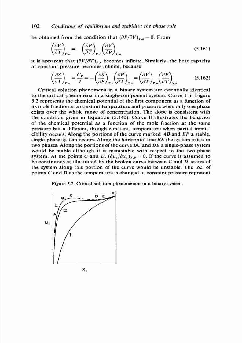
8/11/2019 Thermodynamics of Chemical Systems.pdf
http://slidepdf.com/reader/full/thermodynamics-of-chemical-systemspdf 122/456
102 Conditions of equilibrium and stability: the phase rule
be obtained from the condition that (dP/dV)
Tn
= 0 . F rom
f
dV\ (dP\ fdV^
(5.161)
it is apparent that
{dV/dT)
Py K
becomes infinite. Similarly, the heat capacity
at constant pressure becomes infinite, because
8S
df
P,n
dS dP
dV dP
(5.162)
Critical solution phenomena in a binary system are essentially identical
to the critical phenomena in a single-component system. Curve I in Figure
5.2 represents the chemical potential of the first component as a function of
its mole fraction at a constant temperature and pressure when only one phase
exists over the whole range of concentration. The slope is consistent with
the condition given in Equation (5.140). Curve II illustrates the behavior
of the chemical potential as a function of the mole fraction at the same
pressure but a different, though constant, temperature when partial immis-
cibility occurs. Along the portions of the curve marked AB and EF a stable,
single-phase system occurs. Along the horizontal line BE the system exists in
two ph ases. Along the portio ns of the curve B C and DE a single-phase system
would be stable although it is metastable with respect to the two-phase
system. At the points C and D, (dixjdx^j^ = 0. If the curv e is assum ed to
be continuous as illustrated by the broken curve between C and D, states of
the system along this portion of the curve would be unstable. The loci of
points C and D as the temperature is changed at constant pressure represent
Figure 5.2. Critical solution phenomenon in a binary system.

8/11/2019 Thermodynamics of Chemical Systems.pdf
http://slidepdf.com/reader/full/thermodynamics-of-chemical-systemspdf 123/456

8/11/2019 Thermodynamics of Chemical Systems.pdf
http://slidepdf.com/reader/full/thermodynamics-of-chemical-systemspdf 124/456
104 Con ditions of equilibrium and stability: the phase rule
The inequality
'd
2
A\ (d
2
A\ [_d_
. /
x
~ . / .
\ ~ ,
i > 0 (5 .166)
3x
2
J
TtV
\dV
2
J
TtX
ld
Xl
\3Vj
T
J
T
,
v
is equivalent to (d
2
G/dx
2
1
)
TP
>0. W e see th at, if (d
2
A/dV
2
)
Tx
= 0 , th e
expression in Equation (5.166) is already negative. We conclude that this
expression becomes zero and hence determines the boundary between stable
and unstable phases while (d
2
A/dV
2
)
T x
is still positive. This latter quantity
plays no role in determining the boundary between stable and unstable
systems. The conditions of stability of the critical phases can be obtained by
the requirem ent tha t the third-o rder term m ust be zero when the secon d-order
term is zero. The conditions thus obtained are
= 0 (5.167)
3x
2
J
TtP
= 0
(5.168)
c
l / T,P
and
>0
(5.169)
Equivalent conditions are
= 0 (5.170)
= 0 (5.171)
and
/r)
3
//
\
.0 (5.172)
i J
TtP
Problems concerning the conditions of stability of homogenous systems
for critical phases in ternary systems are very similar to those for the
gas-liquid phenomena in binary systems, because of two independent
variables at constant temperature and pressure. The conditions for stability
are
(d
2
G/dn
2
l
)
TJ J
^
n3
> 0 a nd
(d
2
(l)/dn
2
2
)
TiP
^
un 3
> 0 , given by Equat ions
(5.146) and (5.147), respectively. Inspection of the condition equivalent to
Eq uat ion (5.148) given by Equ ation (5.152) shows that
(S
2
( j)/dnl)
T P
^
n3
must
go to zero before
{< 3
2
G/dn\)
TPri2
^
an d, therefore, it is the con dition expressed
by Equation (5.147) or (5.150) that determines the boundary between stable

8/11/2019 Thermodynamics of Chemical Systems.pdf
http://slidepdf.com/reader/full/thermodynamics-of-chemical-systemspdf 125/456
5.17 Graphical representation 105
and unstable hom ogeno us systems. By the same argum ents used previously,
the conditions of stability of the critical phases are
d
n
2/T,P,m,n
3
^ ) = 0 (5.173a)
= 0 (5.173b)
and
(p£) >0 (5.173c)
or the equivalent conditions
^ ) = 0 (5.174a)
8
n
2 /T
t
P,n,n
3
^ = 0 (5.174b)
,
dn
2
and
/P 3
f
, \
(5.174c)
dn
5.17 Graphical representation
Many of the concepts developed in this chapter can be illustrated
by graphical representations of the thermodynamic functions, and further
insight into these concepts may be obtained from such graphs. We consider
here: (a) the surface in three-dimensional space representing the energy
function of a one-co m pon ent system as a function of the entropy and volum e;
(b) the molar Gibbs energy of a one-component system as a function of the
pressure and temperature; and (c) the molar Gibbs energy of a binary system
as a function of the temperature and mole fraction at constant pressure.
The energy-entropy-volume surface
For the energy surface we consider a closed system having only one
component. The energy is then a function of the entropy and volume alone,
and the differential of the energy is given by
dE=TdS-PdV
We then consider a set of rectilinear coordinates representing the energy,
entropy, and volume; we take the vertical axis to represent the energy.
Experience has shown that the thermodynamic functions are single-valued.

8/11/2019 Thermodynamics of Chemical Systems.pdf
http://slidepdf.com/reader/full/thermodynamics-of-chemical-systemspdf 126/456
106
Con ditions of equilibrium and stability: the phase rule
Thus ,
for each set of values assigned to the entropy and volume, there is
one value for the energy. Such points, when plotted, map out a surface in
the three-dimensional space. Our problem is to investigate the properties of
this surface.
First consider a single-phase system, for which there is a single surface.
The properties of this surface are obtained by determining the shape of the
curve formed by the intersection of the surface an d planes draw n perpen dicular
to the volume axis and to the entropy axis. We consider first the energy-
entropy curve at constant volume. We know that both (dE/dS)
v
and
(d
2
E/dS
2
)
v
m ust be positive, so the slope of the tangent at any one poin t on
the curve must be positive, and the slopes must become more positive as the
entropy is increased. These two conditions require the curve to be concave
up w ard as shown by the heavy curve in Figu re 5.3. The lighter line illustrates
the tange nt. Whe n we consider the energy-volume curve at constant entropy,
we are concerned with the sign of (dE/dV)
s
and (d
2
E/dV
2
)
s
. Th e first
derivative must be negative because the pressure is positive, and the second
derivative must be positive from the condition of stability. These two
conditions show that the curve must also be concave upward, but that the
slope of a tangent to the curve must be negative. The curve is illustrated by
the heavier line and the tangent by the lighter line in Figure 5.4.
The entire surface must then be concave upward. A plane, tangent to the
surface at any point must lie wholly below the surface. The slope of the line
obtained by the intersection of the tangent plane and a plane drawn
perpendicular to the volume axis represents the temperature. The slope of
Figure 5.3. The energy as a function of the entropy at constant volume.

8/11/2019 Thermodynamics of Chemical Systems.pdf
http://slidepdf.com/reader/full/thermodynamics-of-chemical-systemspdf 127/456
5.17 Graphical representation
107
the line obtained by the intersection of the tangent plane and a plane drawn
perpendicular to the entropy axis represents the negative of the pressure.
Th us, a po int on th e energy surface is fixed by assigning values to the en tropy
and volume of the system. The temperature and the negative of the pressure
of the system for these values of the entropy and volume are determined
from the principal slopes of the plane drawn tangent to the surface at the
given point. Such a surface must exist for each phase of the one-component
system. Gibbs called the entire surface represented by these surfaces the
primitive surface.
Next consider the triple point of the single-component system at which
the solid, liquid, and vapor phases are at equilibrium. The description of the
surfaces and tangent planes at this point are applicable to any triple point
of the system. At the triple point we have three surfaces, one for each phase.
For each surface there is a plane tangent to the surface at the point where
the entire system exists in that phase but at the temperature and pressure of
the triple point. There would thus seem to be three tangent planes. The
principal slopes of these planes are identical, because the temperatures of
the three phases and the pressures of the three phases must be the same at
equilibrium. The three planes are then parallel. The last condition of
equilibrium requires that the chemical potential of the component must be
the same in all three phases. At each point of tangency all of the component
must be in that phase. Consequently, the condition
nfx{g) = (5.175)
Figure 5.4. The energy as a function of the volume at constant entropy.

8/11/2019 Thermodynamics of Chemical Systems.pdf
http://slidepdf.com/reader/full/thermodynamics-of-chemical-systemspdf 128/456
108 Conditions of equilibrium and stability: the phase rule
where n represents the number of moles of the component in the system,
must be satisfied. According to Equation (5.58),
(5.176)
and, consequently,
E(g) - TS(g) + PK (g) = E(t) - TS(t) + PV(t) = E(s) - TS(s) + PV(s)
(5.177)
Equation (5.176) is the equation of a plane in three-dimensional space and
Eq ua tion (5.177) shows tha t the three equation s are identical. Th us, the three
possible planes are actually the same plane, which is tangent to all three
surfaces at the triple point. The principal slopes of this single plane give the
temperature and pressure of the system at the triple point. It is helpful in
further discussion to consider the projection of this plane on the entropy-
volume plane, as illustrated in Figure 5.5. The three points of tangency are
designated s, /, and v for the solid, liquid, and vapor states, respectively. It
is assumed that the molar volume of the liquid is greater than the molar
volum e of the solid. The m olar en trop y of the liquid is greater th an the m olar
entropy of the solid, and the molar entropy of the vapor is greater than the
molar entropies of both the liquid and the solid. Consider a system whose
state is determined by designating its entropy and volume so that the point
lies within the triangular area slv. The energy of this system is given by the
value of the energy on the tangent plane at this point. As the entropy and
volume of the system are changed within the triangular area, so the energy
of the system changes along the tangent plane. Thus, the surface of the
tangent plane within the three points of tangency represents the equilibrium
Figure 5.5. The projection of the equilibrium energy surface on the
entropy-volume plane.
8/11/2019 Thermodynamics of Chemical Systems.pdf
http://slidepdf.com/reader/full/thermodynamics-of-chemical-systemspdf 129/456
5.17 Graphical representation
109
states of the system at its triple point. Gibbs called such a portion of the
equilibrium surface a derived surface.
This graphical representation of the thermodynamic properties of a
single-component system at a triple point gives an excellent illustration of
the concept of an indifferent state of a system. The value of the energy of a
system at the given triple point must lie on the surface of the tangent plane
and within the triangular area determined by the three points of tangency.
However, a knowledge of only the temperature and pressure at the triple
point and the total number of moles of the component contained in the
system is not sufficient to determine its state. The values of the energy,
entropy, and volume of the system and of the number of moles of the
component in each phase of the system are unknown. It is evident that an
infinite number of states of the system lie in the triangular area. Only by
assigning values to the entropy and volume of the system do we determine
the point on the tangent plane that represents the energy of the system.
The conditions of stability may also be discussed in terms of this graphical
representation. Even though the assigned values of the entropy and volume
are such that the point lies within the triangular area slv, the value of the
energy might be such that the point lies on one of the primary surfaces
instead of the tangent plane. The system would then exist in a single phase.
According to the conditions of stability, such a system would be stable if the
primary surface were concave upward. However, the primary surface lies
wholly above the tang ent p lane. Thu s, the energy of the system on the prim ary
surface is greater than the energy of the three-phase system that lies on the
tangent plane. The condition of equilibrium requires the energy to have its
smallest possible value for a given entrop y a nd volum e. Th us, the single-phase
system, although stable with respect to the conditions of stability, is
metastable with respect to the three-phase system.
Of the three possible two-phase equilibria of a single-component system,
we discuss only the solid-liquid equilibrium and the liquid-vap or equilibrium;
the principles of the solid-vapor equilibrium are identical in all respects to
the solid-liquid equilibrium. For the liquid-vapor equilibrium we start with
a plane tangent to the three primary surfaces at the triple point. We then
move the plane so that it ceases to be tangent to the primary surface
representing the solid phase, but remains tangent to the two surfaces
representing the liquid and gas phases. That such a surface, tangent to two
primary surfaces, is possible may be proved in the same manner that the
three possible planes tangent to the three possible planes tangent to the three
primary surfaces at the triple point were proved to be identical. At any one
state of the vapor-liquid equilibrium there is a plane tangent to each surface,
but the conditions that the temperature and pressure of the phases and the
chemical potential of the component in each phase must be the same requires
that the two planes be identical. As the plane is rolled a long th e two surfaces,

8/11/2019 Thermodynamics of Chemical Systems.pdf
http://slidepdf.com/reader/full/thermodynamics-of-chemical-systemspdf 130/456
110 Conditions of equilibrium and stability: the phase rule
the points of tangency approach each other and become identical at the
critical point. The loci of the points of tangency are then a continuous curve,
the projection of which on the entropy-volume plane is represented by the
curve lev in Figure 5.5. A ruled surface can be generated if a line is drawn
between the two points of tangency at each position of the plane. The
projection of this ruled surface on the entropy-volume plane is represented
by the shaded area lev in Figure 5.5. This ruled surface must lie wholly below
the primary surfaces, as does the tangent plane. Therefore, this surface
represents the equilibrium surface for all possible states of the vapor-liquid
equilibria in the one-component system. Again, this surface is called a derived
surface.
The state of the system in the two-phase vapor-liquid equilibrium may
be determined in two ways. If values are assigned to the entropy and volume
of the system such that the point lies in the area lev, the energy of the system
is represented by the corresponding point on the derived surface. Only one
plane can pass thro ug h this poin t and be tangen t to the two prim ary surfaces.
Th us, this plane determines the poin ts of tangency an d the point representing
the energy of the system must lie on the line connecting the two points of
tangency. The principal slopes of this one tangent plane are equal to the
temperature and the negative of the pressure of the system. With knowledge
of the equation of state for the two phases, the values of all of the
thermodynamic functions and the number of moles of the component in each
phase can be determined. In the second method we might choose either the
temperature or the pressure of the system. This choice would fix one of the
principal slopes of the plane, and there can be only one plane with this slope
that is tangent to the two surfaces. Consequently, the other principal slope
is determ ined. How ever, the energy of the system is represented by any poin t
lying on the line connecting the two points of tangency. The assignment of
a value to either the entropy or the volume of the system determines a point
on this line. Thus, the state of the system is completely defined. Such a
two-phase system is again an example of an indifferent system. In this case
values must be assigned to at least one extensive variable in addition to the
mole number in order to define the state of the system completely.
The conditions of stability for the two-phase system can be discussed by
reference to the interse ction of the energy surface with a plane passing thro ug h
the l ine connecting two po ints of tangency and p erpendicular to the en tro py -
volume plane. Such an intersection is illustrated in Figure 5.6. The
intersection of this plane with the plane tangent to the two surfaces is
represented by the line tangent to the curve at the points
a
and
b.
Experimental studies do not determine whether the two primary surfaces
intersect as shown by the dotted lines, or whether the surface itself as well
as its first derivatives are continuous as shown by the solid line. Continuous
first derivatives are usually obtained from theoretical studies. If these

8/11/2019 Thermodynamics of Chemical Systems.pdf
http://slidepdf.com/reader/full/thermodynamics-of-chemical-systemspdf 131/456
5.17 Graphical representation
111
derivatives are continuous, then a portion of the energy surface must be
concave do w nw ard. Tw o points of inflection, represented by c and d in Figure
5.6, separate that part of the curve which is concave upward from that which
is concave downward. Then, according to the conditions of stability, any
system whose value of the energy lies on that portion of a primary surface
lying between the po ints
a
and
b
is concave u pw ard is m etastable w ith respect
to the two-phase system whose energy lies on the tangent line. However, the
con ditions of stability are not obeyed a long the por tion of the primary surface
between
c
and d, and hence this portion represents states that are inherently
unstable. Thus, if the energy surface and its first derivatives are continuous,
points
c
and
d
represent the limits of stable states of the one-phase system.
Throughout this discussion we have considered the gas or vapor phase
and the liquid phase to be distinct phases, and that for each phase there is
a primary energy surface. Because of the existence of the critical point, the
entire surface whose projection on the entropy-volume plane is represented
by the area above the lines alevd in Figure 5.5 is actually one surface. Any
plane can be tangent to only one point at a time on this entire surface. The
two phases can be distinguished only at the triple point or in the two-phase
region. It therefore seems more correct to speak of a single fluid phase when
one phase is present.
The characteristics of the primary surfaces and the derived surface for the
solid-liquid equilibria and the solid-vapor equilibria are identical to those
for the liquid-vapor equilibria with the exception that no critical phenomena
have ever been observed in these two equilibria. Thus, a plane, tangent to
the solid and liquid surfaces, may be rolled along these surfaces. The
projections of the loci of the points of tangency are represented by the lines
al and bs in Figure 5.5. If the points of tangency are connected by a straight
line lying in the plane at any position of the plane, a ruled surface is derived
Figure 5.6. Energy relations for the vapor-liquid equilibrium.

8/11/2019 Thermodynamics of Chemical Systems.pdf
http://slidepdf.com/reader/full/thermodynamics-of-chemical-systemspdf 132/456
112
Conditions of equilibrium and stability: the phase rule
as the plane rolls along the surfaces. This ruled surface then represents all
the equilibrium states of the two-p hase system. The p rima ry surfaces between
the points of tangency lie wholly above this ruled surface. The conditions of
stability are identical, although there is essentially no evidence to show
whether the primary surface is cont inuous or discontinuous in its first
derivatives. If it is continuous, there must be a region where the prima ry
surface is concave dow nw ard, and hence a region wh ere the system is
essentially unstable. Similarly, the projections of the points of tangency of
the rolling tangent plane for the solid-vapor equilibrium are represented by
the lines vd and sc in Figure 5.5. The ruled surface formed by connecting
the points of tangency represents all of the equilibrium states of th e
solid-vapor system. The primary surfaces lie wholly above the derived, ruled
surface, and represent the metastable and unstable states of the system, as
the case may be.
In summary, we refer to Figure 5.5, which m ay be considered as the
projection of the entire equilibrium surface on the entropy-volume plane.
All of the equilibrium states of the system when it exists in the single-phase
fluid state lie in the area above the curves
alevd.
All of the equilibrium states
of the system when
it
exists in th e sing le-phase solid state lie in the area
bounded by the lines bs and sc . These areas are the projections of the prim ary
surfaces. The two-phase systems are represented by the shaded areas
alsb,
lev, and
csvd.
These areas are the projections of the derived surfaces for these
states.
Finally, the triangular area slv represents the projection of the tan gent
plane at the triple point, and represents all possible states of the system at
the triple point. This area also is
a
projec tion of a derived surface.
The Gibbs energy-temperature-pressure surface
The Gibbs energy for a closed system m ay be represented by
dG=-SdT+VdP
(5.178)
In this discussion we consider only a single-comp onent system. It is evident
from Equation (5.178) that the Gibbs energy may also be represented as a
surface in a three-dim ension al co ord inate system, in which the rectangu lar
coordinates represent the Gibbs energy, the temperature, and the pressure.
The characteristics of the surface for a single-phase system are determined
as before from the first and second derivatives of the Gibbs energy with
respect to the temperature at con stan t p ressure, and the first and second
derivatives with respect to the pressure at constant temperature. Thus, the
slope of the curve formed by the intersection of the surface with
a
plane
drawn perpendicular to the p ressure axis must be negative, because the
entropy is always positive. Fu rth erm or e, this slope must decrease with
increasing temperature, because both the heat capacity and the temperature
are always positive. The curve in Figure 5.7 represents such an intersection,
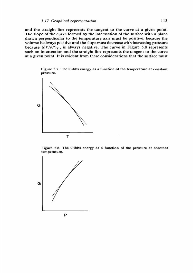
8/11/2019 Thermodynamics of Chemical Systems.pdf
http://slidepdf.com/reader/full/thermodynamics-of-chemical-systemspdf 133/456
5.17 Graphical representation
113
and the straight line represents the tangent to the curve at a given point.
The slope of the curve formed by the intersection of the surface with a plane
drawn perpendicular to the temperature axis must be positive, because the
volum e is always positive and the slope must decrease with increasing pressure
because (dV/dP)
Tn
is always negative. Th e curve in Figu re 5.8 represents
such an intersection and the straight line represents the tangent to the curve
at a given point. It is evident from these considerations that the surface must
Figure 5.7. The Gibbs energy as a function of the temperature at constant
pressure.
Figure 5.8. The Gibbs energy as a function of the pressure at constant
temperature.
G

8/11/2019 Thermodynamics of Chemical Systems.pdf
http://slidepdf.com/reader/full/thermodynamics-of-chemical-systemspdf 134/456
114
Conditions of equilibrium and stability: the phase rule
be everywhere concave downward. If the points of tangency in Figures 5.7
and 5.8 are the same point, then the tangent lines represent the principal
slopes of a plane tangent to the surface at this point. Thus, the surface in
the neighborhood of a given point lies wholly below the plane tangent to
the surface at the point. The point representing the Gibbs energy of the
single-phase system at a given temperature and pressure must therefore lie
on the surface for this phase. The principal slopes of the plane tangent to
the surface at the po int represen ts the volume an d the negative of the en tropy
of the system at this point.
Tw o such surfaces mu st be considered when two ph ases are in equ ilibrium .
From the conditions of equilibrium we know that the temperature of the
two phases must be the same and that the pressure of the two phases must
be the same. Moreover, from the phase rule, a choice of the temperature
determines the pressure. We then choose a temperature at which the
two-phase system is at equilibrium. Such a choice determines a point on
the pressure-temperature plane, and the Gibbs energy of the system must
lie on the line drawn perpendicular to this plane at the given point. The
third condition of equilibrium requires that the chemical potential of the
component in each phase must be the same. We point out in Section 5.13
that this con dition requires the Gibb s energy for a one-c om pon ent, two-ph ase
system to be constant at a given temperature and pressure, and independent
of the distribution of the component between the two phases. Consequently,
the point representing the Gibbs energy of the system must lie on both
surfaces at the given temperature and pressure, and the two surfaces must
intersect at the equilibrium point. Figure 5.9 represents the curves formed
by the intersection of the two surfaces and a plane perpendicular to the
Figure 5.9. Representation of the Gibbs energy at constant pressure for a
two-phase equilibrium.

8/11/2019 Thermodynamics of Chemical Systems.pdf
http://slidepdf.com/reader/full/thermodynamics-of-chemical-systemspdf 135/456
5.17 Graphical representation
115
pressure axis through an equilibrium point, and Figure 5.10 represents the
curves formed by the intersection of the surfaces with a plane drawn
perpendicular to the temperature axis. The point of intersection on each
figure represents the point at which the two phases are at equilibrium at the
given temperature and pressure.
The same problem of discussing the gas phase and liquid phase as two
separate phases or as different manifestations of the same phase arises with
the Gibbs energy surface as it did for the energy surface. The intersection of
the surfaces for the gas and liquid phases, as we have discussed them here,
stops at the critical point. At higher temperatures there is no intersection of
two surfaces, and indeed there is only one surface with no discontinuities.
We could refer to a single fluid phase except along the line where two fluid
phases—he gas and liquid phases—re in equilibrium. The Gibbs energy
surface for the fluid phase would then be a continuous single surface with
continuous first derivatives except along the vapor pressure curve. Along
this curve the surface would still be continuous, but the first derivatives
would be discontinuous up to the critical temperature.
In the three-dimensional diagram, the curve formed by the intersection
of the two surfaces represents all of the equilibrium points of the two-phase
system. Such a curve is obtained for each type of a two-phase equilibrium
existing in a single-component system. At any triple point of the system three
such curves meet at a po int, giving the tem pera ture and pressure of the triple
point .
The projection of the three-dimensional surface on the pressure-
temperature plane gives the familiar pressure-temperature diagram of a one
com pon ent system. The projection for only the solid, liquid, and vap or phases
Figure 5.10. Representation of the Gibbs energy at constant temperature
for a two-phase equilibrium.
G

8/11/2019 Thermodynamics of Chemical Systems.pdf
http://slidepdf.com/reader/full/thermodynamics-of-chemical-systemspdf 136/456
116 Con ditions of equilibrium and stability: the phase rule
is illustrated in Figure 5.11. In this diagram we have assumed that the slope
of the me lting-p oint line is positive . Each line on this diagra m is the projection
of the intersection of two of the three surfaces. The areas between the lines
are the projections of the surfaces for each phase. The triple point is the
projection of the intersection of the three lines as well as the intersection of
the three surfaces.
The stability of a system may be discussed in terms of Figures 5.9 and
5.10. Acco rding to Eq ua tion (5.53) the G ibb s energy of a system at eq uilibrium
must have the smallest possible value at a given temperature and pressure.
There fore, the lower curves on either side of the poin t of intersectio n represen t
the stable states of a one-phase system, and the upper curves represent
metastable states. For any essentially unstable state the surface would have
to be concave upward. The cut of this surface and the plane perpendicular
to the appropriate axis is shown by the broken line in Figures 5.9 and 5.10.
These curves are obtained when it is assumed that the equation of state and
its derivatives are continuous as shown in Figure 5.1.
The G ibbs energy-mole fraction diagrams
W hen we introduce com posit ion variables, we have more th an three
variables and consequently must apply certain restrictions in order to
illustrate the behavior of the Gibbs energy in two- or three-dimensional
graphs. Here we consider only binary systems at constant pressure. The three
variables that we use are the molar Gibbs energy, the temperature, and the
mole fraction of one of the components. We also limit the discussion to
systems having a single phase or two phases in equilibrium.
First consider a system at constant temperature. According to Equation
Figure 5.11. Projection of the Gibbs energy surface on the pressure-
temperature plane.

8/11/2019 Thermodynamics of Chemical Systems.pdf
http://slidepdf.com/reader/full/thermodynamics-of-chemical-systemspdf 137/456
5.17 Graphical representation
117
(5.14) (d
2
G/xl)
T P
must be positive, and consequently the curve of the molar
Gibbs energy as a function of the mole fraction for a single phase must be
concave upward as illustrated by the solid curve in Figure 5.12. There may
be another phase, metastable with respect to the stable phase, that would
have a higher Gibbs energy at this temperature. The molar Gibbs energy of
such a phase is illustrated by the dotted curve in the same figure. At another
tem pera ture these two curves may intersect or combine as illustrated in Figure
5.13.
In this case a line ma y be draw n tan gen t to the tw o curves at the p oints
Figure 5.12. Representation of phase equilibria of a binary system in terms
of the Gibbs energy at constant temperature and pressure.
Figure 5.13. Representation of phase equilibria of a binary system in terms
of the Gibbs energy at constant temperature and pressure: two-phase
equilibrium.

8/11/2019 Thermodynamics of Chemical Systems.pdf
http://slidepdf.com/reader/full/thermodynamics-of-chemical-systemspdf 138/456
118
Conditions of equilibrium and stability: the phase rule
a a nd b. This line lies wholly below the two curves. However, for equilibrium
the Gibbs energy must have the smallest possible value consistent with the
given temperature, pressure, and mole fraction. It is evident from the figure
that between the points a and b the G ibb s energy of the system o n the tangen t
line is less than that on either of the curves. In this case the system exists in
two phases, one phase having the composition represented by the point a
and the other phase having the composition represented by the point b. The
shape of the curve between the two points of tangency is uncertain. If the
two curves intersect as indicated by the dotted extensions of the two curves,
then a po int o n either of the two curves represents a system th at is metas table
with respect to the two-ph ase system. O n th e othe r h an d, if the first derivatives
of the curves are continuous, then a portion of the curve must be concave
dow nw ard. T his portio n of the curve lies between the two p oints of inflection
c and d. A point on this portion of the curve represents a system that is
unstable. If we again change the temperature, the two curves may no longer
intersect or com bine and the phase tha t was stable at the original tem peratu re
may now be metastable with respect to the second phase, as shown in Figure
5.14. We point out that these three figures are actually cuts at different
temperatures of the Gibbs energy surface drawn as a function of the
temperature and mole fraction. The projection on the temperature-mole
fraction plane of the loci of the points of tangency obtained at different
temperatures gives the usual temperature-mole fraction phase diagram for
the two phases.
Figure 5.14. Representation of phase equilibria of a binary system in terms
of the Gibbs energy at constant pressure and temperature.
\
8/11/2019 Thermodynamics of Chemical Systems.pdf
http://slidepdf.com/reader/full/thermodynamics-of-chemical-systemspdf 139/456
6
Partial molar quantities
The subject of partial molar quantities needs to be developed and
understood before considering the application of thermodynamics to actual
systems. Partial molar quantities apply to any extensive property of a
single-phase system such as the volume o r the Gibb s energy. These p roperties
are important in the study of the dependence of the extensive property on
the composition of the phase at constant temperature and pressure; e.g.,
what effect does changing the composition have on the Helmholtz energy?
In this chapter partial molar quantities are defined, the mathematical
relations that exist between them are derived, and their experimental
determination is discussed.
6.1 Definition of partial molar quantities
We let X represent any extensive property of a single phase, and
consider it to be a function of the temperature, pressure, and the mole
numbers of the components, so that X = X(T, P , n). The differential of X is
thus
) d T
+
f ^ d P
+
£ ( ) dn
f
(6.1)
j
P
,
n
\ d P j
T
,
n
tASJ
The quantity (dX/dn^j
P n
is defined as the partial molar quantity of the ith
component. It occurs so frequently in the thermodynamics of solutions that
it is given a separate symbol,
X
t
.
Consequent ly ,
partial molar quantities are
defined by the relation
where n refers to all of the other components present. Two important points
are to be noted in this definition: (1) the differentiation is always made at
constant temperature and pressure; and (2) it is an extensive quantity that

8/11/2019 Thermodynamics of Chemical Systems.pdf
http://slidepdf.com/reader/full/thermodynamics-of-chemical-systemspdf 140/456
120 Partial molar quan tities
is differentiated, and not a specific quantity. As an example of this second
point we differentiate the volume of a solution that contains n
l 5
n
2
, n
3
, etc.,
moles of components rather than the molar volume or the specific volume.
Although these quantities have been defined in terms of components, they
can also be defined in terms of the species present in the solution. In such
a case the mole numbers of all species rather than components must be held
constant except the one that is used in the differentiation; the change of the
mole numbers of the reacting species caused by an accompanying shift of
equilibrium is not considered.
Any physical interpretation of a partial molar quantity must be consistent
with its definition. It is simply the change of the property of the phase with
a change of the num ber of moles of one compo nent keeping the mole num bers
of all the other components constant, in addition to the temperature and
pressure. It is a property of the phase and not of the particular component.
One physical concept of a partial molar quantities may be obtained by
considering an infinite quantity of the phase. Then, the finite change of the
property on the addition of 1 mo le of the particu lar co m pon ent of this infinite
quantity of solution at constant temperature and pressure is numerically
equa l to the partial m olar value of the prope rty with respect to the co m pon ent.
6.2 Relations concerning partial molar quantities
The extensive quantities are functions of the temperature, pressure,
and mole numbers, and, consequently, so are the partial molar quantit ies,
so that X
k
= X
k
(T, P, n). The differential is then written directly as
where the sum is taken over all of the components. The partial molar
quantities are derivatives themselves, and therefore the order of differentiation
of the derivatives expressed in Equation (6.3) may be interchanged. Thus,
(6.5)
and
(«•) JUf) 1 .(« ) ,6 .6 ,
\ ^ / r,p,
w
L ^
k
Konjjp^
n
j
TtPtn
\on
k
/
TtPtn
Various expressions for the differential of the partial molar quantities can
be obtained by the use of these expressions.

8/11/2019 Thermodynamics of Chemical Systems.pdf
http://slidepdf.com/reader/full/thermodynamics-of-chemical-systemspdf 141/456
6.2 Relations
concerning
partial molar quantities 121
The extensive properties are homogenous functions of the first degree in
the mole numbers at constant temperature and pressure. Then, the partial
molar quantities are homogenous functions of zeroth degree in the mole
numbers at constant temperature and pressure; that is, they are functions
of the composition. We use the mole fractions here, but we could use the
molality, mole ratio, or any other composition variable that is zeroth degree
in the mole numbers. For mole fractions,
X
k
= X
k
(T,
P,
x)
and the differential
of
X
k
may be written as
,6.7,
The sum in the last term of this equation is taken over all of the components
of the system except one. The sum of the mole fractions must be unity, and
consequently for
C
components in the system there are (C —1) independent
mole fractions; or for
S
species, there are
(S —
1) independent mole fractions
in terms of the species. The proof of the identity of Equations (6.3) and (6.7)
is not difficult.
One of the most important applications of Equation (6.7) is to the chemical
potentials. From their definition in terms of the Gibbs energy we know that
they are functions of the temperature, pressure, and the mole fractions. The
differential of the chemical potential of the /cth component is then given by
(|) f ) dx ,6.8)
PiX
\dP/
T
,
x
< = i \dxJ
TtPtX
By the combination of Equations (4.37), (4.38),
(6.4),
and (6.5)
we find
hat
(dti
k
/dT)
P
,
n
=-S
k
and
(dfi
k
/dP)
T
,
n
=V
k
and therefore
dfi
k
= ~S
k
AT
+
V
k
dP
+ X - ^
d
Xi
(6.9)
This equation then gives the differential of the chemical potential of
a component in terms of the experimentally determined variables: the
temperature, pressure, and mole fractions. It is this equation that is used to
introduce the mole fraction into the Gibbs-Duhem equation as independent
variables, rather than the chemical potentials. The problem of expressing
the chemical potentials as functions of the composition variables, and
consequently the determination of (dfi
k
/dxi)
T
PtX9
is discussed in Chapters 7
and 8.
We have already said that the extensive quantities are homogenous
functions of the first degree in the mole numbers, and consequently the partial
molar quantities are homogenous functions of zeroth degree in the mole

8/11/2019 Thermodynamics of Chemical Systems.pdf
http://slidepdf.com/reader/full/thermodynamics-of-chemical-systemspdf 142/456
122 Partial molar quan tities
numbers, at both constant temperature and constant pressure. We may then
make use of Euler's theorem to obtain additional relations. For the extensive
quantities Euler's theorem gives
* = £
rttX,
(6.10)
i = l
or
X=l *iXi (6.H)
at constant temperature and pressure, where X is the
molar
quantity or the
value of the quantity per mole of solution. (For ease of interpretation we
use the tilde to represent a molar quantity.) We see from these relations that
any extensive quantity is additive in the partial molar quantities of the
components. For the partial molar quantities, Euler's theorem gives, at
constant temperature and pressure,
) = 0 , 6 , 2 ,
This equation is very similar to the Gibbs-Duhem equation under the
condition that the temperature and pressure are constant. A more general
relation can be obtained by differentiating Equation (6.10) and comparing
the result with E quation (6.1). The differentiation of Equation (6.10) gives
c _ c _
dX= X n
I
-dX
f
+ X Xidrii (6.13)
f = l i = 1
Comparison with Equation (6.1) yields
The similarity to the Gibbs-Duhem equation is quite apparent, and indeed
this equation is the Gibbs-D uhem equation if X refers to the Gibbs energy.
We should note that the differential
dX
i9
the differential that appears in
Equations (6.13) and (6.14), depends upon the differential quantities of the
temperature, the pressure, and the mole fractions as expressed in Equation
(6.7). At constant tem perature and pressure Equation
(6.12)
becomes a special
case of Equation (6.14).
6.3 Algebraic determination of partial molar quantities
As stated in the introduction to this chapter, the methods used and
the equations developed in the previous sections are formally applicable to
all extensive properties. However, there are two classes of properties: those

8/11/2019 Thermodynamics of Chemical Systems.pdf
http://slidepdf.com/reader/full/thermodynamics-of-chemical-systemspdf 143/456

8/11/2019 Thermodynamics of Chemical Systems.pdf
http://slidepdf.com/reader/full/thermodynamics-of-chemical-systemspdf 144/456
124
Partial molar quantities
differentiation is performed first, to obtain
(6.18)
The molar volume is a function of (C —1) independent mole fractions and
its differential at constant temperature and pressure is
c-i
(6.19)
where the sum is taken over the
(C —
1) components. Then, the derivatives
in Equation (6.18) are given by
dV
' T,P,n
Substitution into Equation (6.18) gives
(6.21)
When each
(dXi/dn
k
)
n
is evaluated, the expression for V
k
becomes
c-i
(6.22)
P,x
if the mole fraction of the /cth component is the dependent mole fraction.
When the mole fraction of one of the components other than the /cth
component is dependent, the expression becomes
dV\
c
^
2
(dV\
H - 4^)
(6
-
23)
(B) Let the specific volume be given as a function of the molality (m) of
the solutes, so
v = v( m
2
, m
3
, m
4
,. . .) (6.24)
at a constant temperature and pressure. (An italic m will be used for m olality.)
We use the subscript 1 to designate the solvent. If there are C components
in the solution, there are (C—1) independent molalities, the molalities of
the solutes. In order to convert the specific volume to the extensive variable
we must multiply by the mass of a solution containing
n
t
moles of the
components, so
V= v X n
{
Mi (6.25)

8/11/2019 Thermodynamics of Chemical Systems.pdf
http://slidepdf.com/reader/full/thermodynamics-of-chemical-systemspdf 145/456

8/11/2019 Thermodynamics of Chemical Systems.pdf
http://slidepdf.com/reader/full/thermodynamics-of-chemical-systemspdf 146/456
126 Partial molar quantities
(C) As a third example, assume that the density, p, of the solution is given
as
a
function
of
the mo larity
(c) of
a ll
the
solutes,
so
that
p
=
p ( c
2
, c
3
, c
4
, . . . ) (6 .33)
at constant temperature and pressure. H ere the units of p and c
i
are mass
per volume of solution and moles per liter of solution, respectively. The
volume
of
the solution
is
given
by
where, again,
the
sum
is
taken over all
of
the compo nents. The partial m olar
volume
of
the
/cth
component
is
then given
by
-^
=
pM
k
- g fL
x
nt
P
2
If we center our attention on the second m ethod, the problem becomes one
of expressing the par tial derivatives of the density with respect to the mole
numbers in terms of the p artial derivatives of the density with respect to the
molarity. The differential of the density is
at constant temperature
and
pres sure , from which
(¥) -i(
d
/) (P) 6-36)
\onj
T,p,
n
t = 2 \dCiJ
TfPfC
\cnj
TtP
,
n
As in part B, we must m ake a distinction between the solutes and the solvent.
We first consider that the subscript
k
refers to one of the solutes. M oreov er,
since
c ^ l O O O ^ p / X
n.Mi
(6.37)
when p is expressed in g c m ~
3
and c
t
in m o l d m "
3
or m o l L "
1
, we must
make a distinction between c
t
and c
k
in order to determ ine the sum expressed
in Equation (6.37). Thus, if i k, then
^ \
=
cJeA _ CM^
(638)
p ,
n
P
\d n
k
/
TfPtn
U=
and
if
i
=
fc, hen
p ,
n
"k P
\dn
k
y
r
,
P
,
n
c
k
M
k

8/11/2019 Thermodynamics of Chemical Systems.pdf
http://slidepdf.com/reader/full/thermodynamics-of-chemical-systemspdf 147/456
6.3 Algebraic determination
of
partial molar quantities 111
W hen E qua tion s (6.38) and (6.39) are substituted into E qu ation (6.36), we
obtain
- - c ~ ~ * — £
Cl
' ( / (
6
'
4 0)
from which
c
k(dp\ M
k
£ fSp\
)
—
—
I
^
XJ
CA
—
I
=
t W
f'''
2 V c
'
/ r
^ (6.41)
P i = 2 \5Ci/r,p,c
When this equation is substituted into Equation (6.34), we have
=
M
fc
1 0 0 0 p ( g p / a c
f c
)
r
,
P > c
- M
f c
X f
=
2
c
P P
2
which, on rearrangement, becomes
M
k
-10QQ(dp/dc
k
)
TtPie
If the subscript
k
refers
to
the solvent, then
_ , M
t ( 6 4 4 )
When Equation (6.44) is substituted into Eq ua tion (6.36), we have
\dni/T,P ,n P \^
n
i/T,P ,n i
=
2 \ ^i / T,P,c
Z?=iniM
ii
= 2
\dcJ
TtPtC
which on rearrangement becomes
(6.45)
r,p,« 1
_ i
V
c/—
c
i\
(6.46)
c / ^
' M o /
2 \OCi/T,P,c

8/11/2019 Thermodynamics of Chemical Systems.pdf
http://slidepdf.com/reader/full/thermodynamics-of-chemical-systemspdf 148/456
128 Partial molar quan tities
Finally, when E qu atio n (6.46) is substituted into E qu ation (6.34), we obtain
]
P
2
[ l
which, on rearrangem ent, becomes
(D) Experimental results are frequently rep orte d in terms of deviation
functions. The usefulness of these functions arises from the fact m any
properties of various systems obey approximate laws. Thus, we speak of the
deviations from ideal gas beha vior o r deviations from the ideal solution laws.
The advantage of such deviation functions is tha t their values are usually
much smaller than the whole value, and consequently greater accuracy can
be obtained with simpler calculations, either graphically or algebraically. As
an example, the m olar volume of a mixture of liquids is approximately
additive in the mole fractions, so tha t we m ay write
V=t x
t
V;+AV
M
(6.49)
where V\ is the molar volume of the pure ith component and AV
M
is the
change of the molar volume of the system on mixing the liquid components
at constant temperature and pressure. (The superscript dot is used to denote
a pure com pon ent.) In ord er to obta in the extensive variable we mu st m ultiply
by the total number of moles, so
V=Y
j
n
i
V;+AV™f
j
n) (6.50)
» = i \;=i /
From this equation we then obtain
1\
(6.51)
for the partial molar volume of the kth com pone nt. Th us, the partial mo lar
volume of this com ponent is given by the sum of its m olar volume and the
value of the d erivative expressed in Eq uat ion (6.51). The ev aluation of this
derivative requires the same m etho ds th at hav e been discussed in this section.
We have limited the discussion here to three different quantities each with
a different composition variable. Of course, there are oth er intensive
quantities, such as the volume of a solution containing a fixed quantity of
solvent, tha t could be used to express the same data . M oreo ver, each intensive

8/11/2019 Thermodynamics of Chemical Systems.pdf
http://slidepdf.com/reader/full/thermodynamics-of-chemical-systemspdf 149/456
6.4 Apparent molar quantities 129
quantity can be expressed as a function of any of the composition variables.
Th us, there are ma ny different relations capab le of expressing the same d ata ,
but for any specific case the same general methods given in this section are
used to calculate the partial molar quantities
6.4 Apparent molar quantities
Apparent molar quantit ies (sometimes called apparent molal quan-
tities) are used primarily for binary systems, and are usually expressed as
functions of the molality. These quantities are used because in many cases
their values are readily obtained by experiment. The general apparent molar
qu an tit y, 0AT, is defined as
for a binary system. (No te that <\>X is used as a single symbol and is not a
product. When seen together <\>X is the symbol for the apparent molar value
of the property X.) It is thus the difference in the value of the quantity for
the solution and that for the
pure
solvent per mole of solute. For the volume
of a binary system we have
v-
ni
vi
( 6 53 )
n
2
and, from this definition,
V =
nJ/\
+n
2
cj)V
(6.54)
The partial molar volumes of the two components can then be obtained by
differentiation, and are given by
f)
(6.55)
l /T,P,n
and
(
d
^
V
-) (6.56)
The a pp aren t m olar volum e is given as a function of one of the c om position
variables. The methods of evaluating the partial derivatives in Equat ions
(6.55) and (6.56) are identical to those discussed in Section 6.3. The final
expressions for the partial molar volumes of the two components in terms
of the molality are
1 0 0 0 V 8 m J
T
,
P

8/11/2019 Thermodynamics of Chemical Systems.pdf
http://slidepdf.com/reader/full/thermodynamics-of-chemical-systemspdf 150/456
130 Partial molar quan tities
and
dm )
(6.58)
TP
Figure 6.1 illustrates the concept of the apparent molar volume. AB is the
portion of the total volume AC for n
2
moles of solute that is attributed to
the pure solvent. Then, the volume BC is apparently due to the solute. The
slope of the line passing through point C and V[ is the apparent molar
volume. The slope of the curve of the total volume at point C is the partial
molar volume of component 2. Indeed, the slope of the total volume curve
at any point is the partial molar volume of com ponen t 2 at that concen tration.
It is obvious that partial molar properties and apparent molar properties
are both functions of concentration.
Ap parent m olar quantit ies for multicompo nent systems, other than binary
systems, have been used to only a limited extent because of the difficulty of
dealing with more than two mole numbers. Actually, there is no single
definition of an apparent molar quantity for such systems. If we limit the
discussion to the volume and refer to the definition of the apparent molar
volume of the binary system (Eq. 6.53)), then we see tha t for m ulticom pon ent
systems we must consider the difference between the volume of the solution
and some other volum e, and the meaning of the
molar
quan tity. There ap pear
to be two possible cases for these definitions. In the first case we could choo se
Figure 6.1. The apparent molar quantity illustrated.
Portion of total volume
apparently due to
solute
Portion of total volume
attributed to
solvent
n
2

8/11/2019 Thermodynamics of Chemical Systems.pdf
http://slidepdf.com/reader/full/thermodynamics-of-chemical-systemspdf 151/456
6.5 Partial molar volumes of binary systems 131
the other volume to be the volume of the pure solvent. We would then have
to use the total n um ber of moles of all solutes to determine the m olar qua ntity.
The apparent molar volume of all solutes would then be defined by
In the second case we might choose a solu tion of fixed m ole r atio s of the
components and consider the change in the volume of the solution as another
solute is added to it. The apparent molar volume of the added solute would
then be defined by
V-
V
<j)V
k
=
(6.60)
where V is the volum e of the original solution and
n
k
is the nu m ber of moles
of the /cth solute in the solution. In either case the apparent molar volumes
are functions of all of the composition variables needed
to
describe the
solution. For C compon ents there are (C —1) such v ariables. The calculation
of the partial molar volumes of the components from these relations follow
the same methods discussed in this section and Section 6.3.
6.5 Graphical determination of the partial molar volumes of
binary systems
In many instances
it is
possible
to
determine the p artial mo lar
volumes of binary systems by graphical means. Some cases simply require
the application of calculus to the equations developed. As an example we
consider Equations (6.57) and (6.58). We plot (j)V against m, determine the
slope of the curve at a given m, and then determine V
1
and V
2
by means of
these equations.
A different method is obtained if the molar volume is given as a function
of the mole fraction. Equation (6.22) may be written as
~ - fdV\
V=V
2
+ x
1
—
(6.61)
and as
( ) (6.62)
However, since dx
2
=
—
dx
l9
Eq ua tion (6.62) ma y also be written as
/dV\
V=V
1
-(l-x
1
) — (6.63)
\dxJ
TtP

8/11/2019 Thermodynamics of Chemical Systems.pdf
http://slidepdf.com/reader/full/thermodynamics-of-chemical-systemspdf 152/456
132 Partial molar quantities
If
we
plot V against x
x
as in
Figure
6.2, we see
that
the
equation
for the
tangent
to the
curve
at a
given value
of x
x
is
given
by
both Equations (6.62)
and (6.63).
It is
evident then that
V
2
is the
intercept
of
this tangent
on the
zero axis,
and
V
1
is the
intercept
of the
tangent
on the
unit axis.
If
we start
at
x
x
= 0 and
roll
the
tangent
on the
curve,
we see
that V
2
starts
at
V
2
and
steadily increases, whereas V
x
starts
at
some quantity greater than V[
and
decreases to this quantity.
By similar considerations we may plot
AV
M
defined by Equation (6.49)
against the mole fraction and determine the difference between V
2
and V
2
and between V
x
and V[ at a given mole fraction from the intercepts of the
tangent to the curve at this mole fraction.
6.6
Integration of Equation (6.12) for a binary system
Equation (6.12) may be written as
dV
x
\ fdV
2
\
dxJ
TP
9
(6.64)
for a binary system when it is applied to volumes. If either
V
x
or
V
2
is known
as a function of the mole fraction, then the other may be determined by
integration. Equation (6.64) may be written in either of the two forms
or
dV,=
2
r,p
dx
1
(6.65)
(6.66)
T,P
Figure 6.2. Graphical determination of partial molar volumes in a binary
system.
V

8/11/2019 Thermodynamics of Chemical Systems.pdf
http://slidepdf.com/reader/full/thermodynamics-of-chemical-systemspdf 153/456
6.6 Integration of E quations (6 .12) for a binary system
133
However, in order to obtain the integral, the integration constant or the
values of the lower limits must be known.
No difficulty exists for gases and for liquid and solid solutions that have
no region of immiscibility or limited solubility. In this case {SVJdx^j^ (Eq.
(6.65)) or (dVJdx^jp (Eq. (6.66)) can be determ ined over the whole range
of composition. The lower limit of integration of Equation (6.65) is x
x
= 1,
for which V
1
= V[
9
and the lower limit of integration of Equation (6.66) is
x
t
= 0, for which V
2
= V
2
.
In the case of limited solubility, for examp le an aqu eou s so lution of sucrose,
no difficulty arises in the use of Equation (6.65), if we use the subscript 1 to
refer to the solvent and the subscript 2 to refer to the solute. Here V
2
could
be determined as a function of the mole fraction from the very dilute solution
(pure solvent) to the saturation point. The lower limit of integration would
then be V[ when x
1
= 1. W ith E quatio n (6.66), V
x
could be determined as a
function of the mole fraction from the very dilute solution to the saturation
point. However, in order to determine the value of the integration constant,
V
2
would have to be known at some mole fraction. This is usually not the
case, and so the integration cannot be completed. This problem is clarified
by reference to Figu re 6.3, where the m olar volum e of a system having limited
solubility is plotted as a function of the mole fraction of the solvent. The
value of the mole fraction at the saturation point is indicated by the vertical
broken l ine; V
1
is indicated by the solid curve from the saturation value to
the pu re solvent. Th e form of the curve of V
2
can be obtained by integration
of Equation (6.66), but its absolute value cannot be determined. The broken
curves represent a family of curves that differ by a constant value. All of
Figure 6.3. Integration of Equation (6.12) for a binary system.

8/11/2019 Thermodynamics of Chemical Systems.pdf
http://slidepdf.com/reader/full/thermodynamics-of-chemical-systemspdf 154/456
134
Partial molar quan tities
these curves could represent
V
2
,
but the particular curve that actually gives
V
2
is unknown.
The problem discussed here is common to all partial molar quantities. It
is for this an d similar reason s, which we have already ind icated, th at reference
and standard states are defined (see Chapter 8).

8/11/2019 Thermodynamics of Chemical Systems.pdf
http://slidepdf.com/reader/full/thermodynamics-of-chemical-systemspdf 155/456
7
Ideal gases and real gases
The conditions of equilibrium expressed by Equations (5.25)-(5.29)
and (5.46) involve the temperature, pressure, and chemical potentials of the
components or species. The chemical potentials are functions of the
temperature, pressure or volume, and composition, according to Equations
(5.54) and (5.56). In order to study the equilibrium properties of systems in
terms of these experimentally observable variables, expressions for the
chemical poten tials in terms of these variables must be o btaine d. This p roblem
is considered in this chapter and in Chapter 8.
The thermodynamic functions for the gas phase are more easily developed
than for the l iquid or solid phases, because the tem perature-p ressure-v olum e
relations can be expressed, at least for low pre ssures, by an algebraic equ ation
of state. For this reason the thermodynamic functions for the gas phase are
developed in this chapter before discussing those for the liquid and solid
phases in Chapter 8. First the equation of state for pure ideal gases and for
mixtures of ideal gases is discussed. Then various equations of state for real
gases, both pure and mixed, are outlined. Finally, the more general
thermodynamic functions for the gas phase are developed in terms of the
experimentally observable quantities: the pressure, the volume, the tem-
perature, and the mole numbers. Emphasis is placed on the virial equation
of state accurate to the second virial coefficient. However, the methods used
are applicable to any equation of state, and the development of the
thermodynamic functions for any given equation of state should present no
difficulty.
7.1 The ideal gas
An ideal gas is defined as one whose properties are given by the two
equations (Sect. 2.8)
PV = nRT
(7.1)

8/11/2019 Thermodynamics of Chemical Systems.pdf
http://slidepdf.com/reader/full/thermodynamics-of-chemical-systemspdf 156/456
136 Ideal gases and real gases
and
**)
= 0 (7.2)
These two equations are applicable to mixtures of ideal gases as well as
to pure gases, provided n is taken to be the total number of moles of gas.
However, we must consider how the properties of the gas mixture depend
upon the composition of the gas mixture and upon the properties of the pure
gases. In particular, we must define the Dalton's pressures, the partial
pressures, and the Amagat volumes. Dalton's law states that each individual
gas in a mixture of ideal gases at a given temperature and volume acts as if
it were alone in the same volume and at the same temperature. Thus, from
Equation (7.1) we have
P nftT/V
(7.3)
where
P
t
is the pressure exerted by
n
x
moles of the /th gas at the volume
V
and temperature T. The quantity
P
l
is called the Dalton's pressure. The
addition of such equations for a mixture of gases yields
and, by comparison with Equation (7.1), we see that
P=£p
f
(7.5)
i = i
Thus, the total pressure of a mixture of ideal gases is the sum of the Dalton
pressures.
The partial pressure of a gas in a gas mixture, whether such a mixture is
ideal or real, is defined by
Pi = yf (7.6)
where y represents the mole fraction in the gas phase. The sum of the partial
pressures must always equal the total pressure, because the sum of the mole
fractions must always be equal to unity. By the combination of Equations
(7.3)-(7.5), we see that the partial pressure and Dalton's pressure of a
component in a mixture of ideal gases are identical. This statement is not
true in general for mixtures of real gases.
Amagat's law is very similar to Dalton's law, but deals with the additivity
of the volumes of the individual components or species of the gas mixture
when mixed at constant temperature and pressure. The Amagat volume may
be defined as the volume that n
z
moles of the pure /th gas occupies when

8/11/2019 Thermodynamics of Chemical Systems.pdf
http://slidepdf.com/reader/full/thermodynamics-of-chemical-systemspdf 157/456
7.2 Pure real gases
measured at the temperature
T
and pressure P, so
and
/ = I
/
"
137
(7.7)
(7.8)
Thus, the volume of a mixture of ideal gases is the sum of the volumes of
the individual gases when measured at the same pressure and temperature.
7.2 Pure real gases
No actual gas follows the ideal gas equation exactly. Only at low
pressures are the differences between the properties of a real gas and those
of an ideal gas sufficiently small that they can be neglected. For precision
wo rk the differences s hou ld never be neglected. Even at pressu res near 1 ba r
these differences may amount to several percent. Probably the best way to
illustrate the deviations of real gases from the ideal gas law is to consider
how the quantity PV/RT, called the compressibility factor, Z, for 1 mole of
gas depends upon the pressure at various temperatures. This is shown in
Figure 7.1, where the abscissa is actually the reduced pressure an d the curves
are for various reduced temperatures [9]. The behavior of the ideal gas is
represented by the line where PV/RT = 1. F o r real gases at sufficiently low
temperatures, the PV product is less than ideal at low pressures and, as the
pressure increases, passes through a minimum, and finally becomes greater
than ideal. At one temperature, called the Boyle temperature, this minimum
Figure 7.1. Deviations of real gases from ideal gas behavior.
P/P
r

8/11/2019 Thermodynamics of Chemical Systems.pdf
http://slidepdf.com/reader/full/thermodynamics-of-chemical-systemspdf 158/456
138 Ideal gases and real gases
occurs at zero pressure. The Boyle temperature is therefore defined as the
temperature at which
l
J
r
,
n
= 0
(7.9)
Above the Boyle temperature the deviations from ideal behavior are always
positive and increase with the pressure. The initial slope of the PV curves
at which P = 0 is negative at low tem pera tures, passes thro ug h zero at the
Boyle temperature, and then becomes positive. A maximum in the initial
slope as a function of temperature has been observed for both hydrogen and
helium, and it is presumed that all gases would exhibit such a maximum if
heated to sufficiently high temperatures. This behavior of the initial slope
with temperature is illustrated in Figure 7.2 [10].
M any equ ations have been suggested to express the behavior of real gases.
In general, there are those equations that express the pressure as a function
of the volume and temperature, and those that express the volume as a
function of the pressure and temperature. These cannot usually be converted
from one into the other without obtaining an infinite series. The most
convenient thermodynamic function to use for those in which the volume
and temp erature are the independen t variables is the Helm holtz energy. The
Figure 7.2. The second virial coefficient of carbon dioxide.
0
T
-40
CO
o
^
80
-120
/
/
(
200
t/° C
400 600

8/11/2019 Thermodynamics of Chemical Systems.pdf
http://slidepdf.com/reader/full/thermodynamics-of-chemical-systemspdf 159/456
7.2 Pure real gases 139
Gibbs energy is the most convenient function to use for those in which the
pressure and temperature are the independent variables.
The virial equation of state, first suggested by Kammerlingh-Ohnes, is
probably one of the most convenient equations to use, and is used in this
chapter to i l lustrate the development of the thermodynamic equations that
are consistent with the given equation of state. The methods used here can
be applied to any equation of state.
The virial equation gives the pressure as a power series of the molar
density, so that either
(7.10)
L
\v /
\yJ
\y /
J
or
(7.11)
The volume may also be expressed as a power series of the pressure, so
V
=
— ( 1 +
p'P
+
y ' P
2
+
8'P
3
+--)
(7.12)
or
/RT \
V=n(— + P + yP + dP
2
+--\ (7.13)
\P )
The quantit ies B, B\ /?, an d /?' are ca lled s econ d virial coefficients; C, C", y,
and y' third virial coefficients; and D, D', <5, an d 5 ' fou rth virial coefficients.
These coefficients are functions of the temperature and are characteristic
of the individual gas. These equations reproduce the pressure-volume-
temperature relations of gases accurately only for low pressures or small
densities.
The relationships between
B
and
B\ C
a n d C ,
D
and
D\
/? an d
ft', y
and
y', and
3
and
8'
are quite obvious from the defining equations. The two sets
of virial coefficients, however, are not independent, and the relations between
these sets are
P
= B (7.14)
y =
(C-B
2
)/RT (7.15)
and
8 = (D - 3BC
+
2B
3
)/(RT)
2
(7.16)
In general the dependence of the virial coefficients upon the temperature

8/11/2019 Thermodynamics of Chemical Systems.pdf
http://slidepdf.com/reader/full/thermodynamics-of-chemical-systemspdf 160/456
140 Ideal gases and real gases
m ust be determine d e xperimen tally. The tem pera ture dependen ce of j8 is
illustrated in Figu re 7.2 becau se, accord ing to Eq ua tio n (7.13), /? is the
limiting slope of the
PV
isotherms as the pressure goes to zero.
Dymond and Smith [11] give an excellent compilation of virial coefficients
of gases and mixtures. Cholinski
et al.
[12] provide second virial coefficient
data for individual organic compounds and binary systems. The latter book
also discusses various correlational methods for calculating second virial
coefficients. Mason and Spurling [13] have written an informative monograph
on the virial equation of state.
The search for better equations of state continues apace, since computers
make the computational part relatively easy. Stryjek and Vera [14], for
exam ple, have developed a complex eq uatio n of state based on that of Redlich
and Kwong, but which is suitable for representing the P-V-T behav ior of
liquid and gas phases over a wide range of temperature and pressure for
pure nonpolar compounds.
7.3 Mixtures of real gases and combinations of coefficients
1
The virial equation of state discussed in Section 7.2 is applicable to
gas mixtures with the condition that n represents the total moles of the gas
mixture; that is , w = £f=i n
t
. The constants and coefficients then become
functions of the mole fractions. These functions can be determined experi-
mentally, and actually the pressure-volume-temperature properties of some
binary mixtures and a few ternary mixtures have been studied. However,
sometimes it is necessary to estimate the properties of gas mixtures from
those of the pure gases. This is accomplished through the combination of
constants .
Experimental measurements and statistical mechanics both show that the
dep end ence of the virial coefficients on the mo le fractions m ay be expressed by
« = £
£
y
t
yjBv
(7-i7)
c = £
E £
y,yjy
t
c
tJk
(7.18)
i = l
j = l k = l
etc., where the summations are taken over all of the components or species
in the gas mixture for each index. The summations in Equations (7.17) and
1
In this section we give, for completeness, the combination of virial coefficients higher than
the second order. However, for the purposes of illustration, we go up to only the second virial
coefficient. The references cited at the end of Section 7.2 can be consulted for more-detailed
information.

8/11/2019 Thermodynamics of Chemical Systems.pdf
http://slidepdf.com/reader/full/thermodynamics-of-chemical-systemspdf 161/456
7.3 M ixtures of real gases and combinations of coefficients 141
(7.18) for a ternary system, for example, are
B = ylB
lx
+
y\B
22
+
y\B
33
+ 2
yi
y
2
B
12
+ 2
yi
y
3
B
13
+ 2y
2
y
3
B
23
(7.20)
and
C = ylC
xll
+ y \C
22 2
+
y\C
333
+
3y
2
y
2
C
11 2
+
3y
iy
2
2
C
12 2
+
6
yi
y
2
y
3
C
123
(7.21)
The assumption is made in these equations that the coefficients having
different combinations of the same indices are identical, thus C
1 1 2
= C
1 2 1
=
C
2 1 1
. With the omission of the coefficients, the expansion of these sums are
the square, cube, etc., of the sum of the mole fractions of the components
or species. With these expressions, the problem of the combination of
constants becomes one of expressing the coefficients having unlike indices
in terms of those having like indices.
Three methods have been used for the combination of these constants.
1.
Linear combination. In this method the coefficients having unlike
indices are assumed to be the arithmetical mean of those having like
indices. If a represents any of these coefficients, then
a
ij
= ±(a
ii
+ a
jj
) (7.22)
fly* = stem +
a
m +
a
kkk)
(7-23)
flyw = U^uH + ajj j j +
a
kkkk
+ a
m
) (7.24)
etc.
With these relations,
c c c
Z
Z w k / = Z
y&i
(
7
-
25
)
i =
1
j
= 1
i =
1
c c c c
Z Z Z
ytyjyifiijk =
Z
y&m
(
7
-
26
)
C C C C C
Z Z Z Z yiyjykyi<*iju = Z 3w ,« (7.27)
i = l j = l k = l 1 = 1 i = l
2.
Quadratic combination. This method assumes that the coefficients
having unlike indices are the geometric means of those having like
indices, thus
fly=(fl -)
1/2
(7.28)
(7.29)

8/11/2019 Thermodynamics of Chemical Systems.pdf
http://slidepdf.com/reader/full/thermodynamics-of-chemical-systemspdf 162/456
142 Ideal gases and real gases
<*iju = ( iii jjjfikkkk iu i)
1/4r
(7.30)
e t c . With these relations,
£ £ W . 7 = ( l3 W/
2
Y (7.31)
i = l j = l \ i= l /
£
£ £ W*«u*
= ( £
rfY
7-32)
i = l j = l f c = l \ i = l /
£ £ £ £ w*3w
7
*< = ( £
m ^ Y (7.33)
e t c .
3 . Lore ntz com bina tion. This m etho d is defined by
fly = i ( 4
/ 3
+ flJ[/
3
)
3
(7.34)
a
iJk
= U a } l? + a ) lJ + a \ fi )* (7.35)
and
«yu = MaUf +
fljjg
+ < ^ + < 4
3
)
3
(7-36)
e t c . Then ,
£ £ y ^ = ' £
£
y , y A° h'
+
<*jJ
3
)
3
(
7
-
3 7
)
i = l j = l
o i = lj =\
c
c c i c c c
I I I
y i y j y i f l i j k
= ~ I I I
y t y ^ k
i = l j = i f c = i Z / i = i j = i
f c
= i
x ( 4 (
3
+ a) if + a
fc
1
j
(
3
)
3
(7.38)
and
c
c c c
I E E E
i = l j = l k = l / = l
1
c
= ^ E
c
E
J = I
c
E
fc=i
c
E
f = i
+ a
ytyy.
1/3 ,
/cfckfc '- ai m
\ 3
(7
.39)
e t c .
Two further crude approximations have been used for the virial equation
of state. The first
is
th at the virial coefficients com bine linearly. T his
combination of constants results in an equation of state that is additive in
the properties of the p ure compo nents . In such a mixture D alton 's and
Amagat's laws still hold, and the mixture may be called an ideal mixture of
real gases. The assumption is probably the crudest that can be used and is
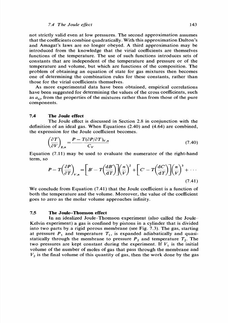
8/11/2019 Thermodynamics of Chemical Systems.pdf
http://slidepdf.com/reader/full/thermodynamics-of-chemical-systemspdf 163/456
7.4 The Joule effect 143
not strictly valid even at low pressures. The second approximation assumes
tha t the coefficients co mb ine qua dratically. With this app rox im ation D alto n's
and Amagat 's laws are no longer obeyed. A third approximation may be
introduced from the knowledge that the virial coefficients are themselves
functions of the temperature. The use of such functions introduces sets of
constants that are independent of the temperature and pressure or of the
temperature and volume, but which are functions of the composition. The
problem of obtaining an equation of state for gas mixtures then becomes
one of determining the combination rules for these constants, rather than
those for the virial coefficients themselves.
As more experimental data have been obtained, empirical correlations
have been suggested for determining the values of the cross coefficients, such
as
a
ij9
from the properties of the mixtures rather than from those of the pure
components .
7.4 The Joule effect
The Joule effect is discussed in Section 2.8 in conjunction with the
definition of an ideal gas. When Equations (2.40) and (4.64) are combined,
the expression for the Joule coefficient becomes.
dT
Cy
Equation (7.11) may be used to evaluate the numerator of the right-hand
term, so
3
- I +
(7.41)
We conclude from Equation (7.41) that the Joule coefficient is a function of
both the temperature and the volume. Moreover, the value of the coefficient
goes to zero as the molar volume approaches infinity.
7.5 The Joule-Thomson effect
In an idealized Joule-Thomson experiment (also called the Joule-
Kelvin experiment) a gas is confined by pistons in a cylinder that is divided
into tw o pa rts by, a rigid po rou s m em bran e (see Fig. 7.3). The g as, starting
at pressure
P
1
and temperature
T
u
is expan ded adiabatically and quasi-
statically through the membrane to pressure P
2
and temperature T
2
. The
two pressures are kept constant during the experiment. If V
x
is the initial
volume of the number of moles of gas that pass through the membrane and
V
2
is the final volume of this quantity of gas, then the work done by the gas

8/11/2019 Thermodynamics of Chemical Systems.pdf
http://slidepdf.com/reader/full/thermodynamics-of-chemical-systemspdf 164/456
144 Ideal gases and real gases
is
P
2
V
2
-PiVi. Th e chang e in energy is E
2
- E
x
and is equal to the work.
Consequently, we find that E
2
+P
2
Vi =
E
i+
p
i
v
i>
a n d
therefore the
enthalpy of the gas is constant. We are interested then in the quantity
(dT/dP)
Hn
,
the Joule-Thomson coefficient (also given the symbol ju
JT
), which
is given by
dT
T(dV/dT)
P
,
n
-V
(7.42)
For an ideal gas this quantity is zero. The Joule-Thomson process is
isenthalpic. When Equation (7.13) is used for the equation of state, the
numerator of the right-hand term becomes
— ) -V =
[ T
— - # )
+
( T — -y)P +
. . . (7.43)
K
dT j
P
,
n
V dT V V dT
We conclude that the Joule-Thomson coefficient is a function of both the
temperature and the pressure, but, unlike the Joule coefficient, it does not
go to zero as the pressure goes to zero. The inversion temperature, the
temperature at which
fi
JT
=
0, is also a function of the p ressu re. The value
usually reported in the literature is the limiting value as the pressure goes
to zero.
Joule-Thomson experiments can yield quite practical information. The
experim ents (see Fig. 7.3) involve starting a t a fixed tem pera ture and pressure
(T
h
P
t
) and me asuring the final temp eratu re for a series of pressures less than
P
t
. This results in an isenthalp for each set of starting pressures and
temperatures as shown in Figure 7.4. The heavy line in Figure 7.4 is drawn
through the points of zero slope of the individual isenthalps. At those points
fijj = 0 and the slope changes from positive (cooling) to negative (heating).
Figure 7.3. The Joule-Thomson experiment.
Direction \
of gas flow /
Throttling Device

8/11/2019 Thermodynamics of Chemical Systems.pdf
http://slidepdf.com/reader/full/thermodynamics-of-chemical-systemspdf 165/456
7.4 The Joule effect
145
The temperatures on the envelope where /x
JT
= 0 are called inversion
temperatures, T
t
. At any given pressure, up to a maximum pressure, a given
gas exhibits two inversion temperatures. The Joule-Thomson effect is
important in refrigeration and in the liquefaction of gases. Modern refrigeration
uses the larger effect of the evaporation of working fluids such as the
chlorofluorocarbons.
Some useful relationships may be derived involving the Joule-Thomson
coefficient. Let us start with
H
=
H(T, P),
to get
Mr- ^
For dH = 0 we can rearrange this to
(8T\
\3PJH
and this is just
(-)
Ti \STjp
(7.44)
(7.45)
(7.46)
Equation (7.46) permits us to evaluate the derivative
(8H/dP)
T
for real gases
(it is zero for an ideal gas) from experimentally determinable properties.
Upon substituting the definition of the enthalpy
(H = E + PV)
in Equation
(7.46), we get
c
P
IA
dE
~ d P
(7.47)
CD
7
6
5
4
3
2
Figure 7.4. Isenthalps for nitrogen and the Joule-Thomson effect.
H
1-
Nitrogen
"Cooling
X
Heating
Vapor-liquid equilibrium curve
Critical point I I
0 10 20 30 40 50
Pressure/MPa
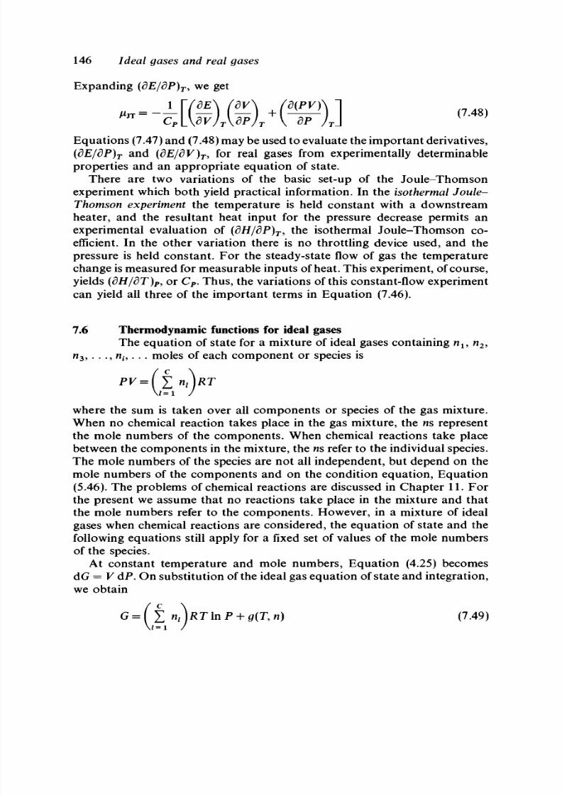
8/11/2019 Thermodynamics of Chemical Systems.pdf
http://slidepdf.com/reader/full/thermodynamics-of-chemical-systemspdf 166/456
146 Ideal gases and real gases
Expanding (dE/dP)
T
, we get
«f^l
7
. 4 8 )
C
P
l\dv)
T
\dp)
T
V dP
Eq uatio ns (7.47) and (7.48) ma y be used to evaluate the imp orta nt derivatives,
(dE/dP)
T
and (dE/dV)
T
, for real gases from experim entally de term inab le
properties and an appropriate equation of state.
There are two variations of the basic set-up of the Joule-Thomson
experiment which both yield practical information. In the isothermal Joule-
Thomson experiment the temperature is held constant with a downstream
heater, and the resultant heat input for the pressure decrease permits an
experimental evaluation of
(dH/dP)
T
,
the isothermal Joule-Thomson co-
efficient. In the other variation there is no throttling device used, and the
pressure is held constant. For the steady-state flow of gas the temperature
change is measured for measurable inputs of heat. This experimen t, of course,
yields
(dH/dT)
P
,
or
C
P
.
Th us, the variation s of this constant-flow experiment
can yield all three of the important terms in Equation (7.46).
7.6 Thermodynam ic functions for ideal gases
The equation of state for a mixture of ideal gases containing
n
u
n
2
,
n
3
, . . . , n
i9
...
moles of each com pon ent or species is
where the sum is taken over all components or species of the gas mixture.
When no chemical reaction takes place in the gas mixture, the ns represent
the mole numbers of the components. When chemical reactions take place
between the comp onen ts in the mixture, the ns refer to the individual species.
The mole numbers of the species are not all independent, but depend on the
mole numbers of the components and on the condition equation, Equation
(5.46). The problems of chemical reactions are discussed in Chapter 11. For
the present we assume that no reactions take place in the mixture and that
the mole numbers refer to the components. However, in a mixture of ideal
gases when chemical reactions are considered, the equation of state and the
following equations still apply for a fixed set of values of the mole numbers
of the species.
At constant temperature and mole numbers, Equation (4.25) becomes
dG =
V dP.
O n sub stitution of the ideal gas equ ation of state and in tegration ,
we obtain
In P + 0( T ,n) (7.49)

8/11/2019 Thermodynamics of Chemical Systems.pdf
http://slidepdf.com/reader/full/thermodynamics-of-chemical-systemspdf 167/456
7.6 Thermodyna mic functions for ideal gases 147
where g(T, n) represents a function of the temp eratur e an d the mole num bers.
The first term of this equation is additive in the mole numbers, and it is
necessary to investigate the dependence of the second term on the mole
numbers. According to Dalton's law, each gas in a gas mixture confined in
a given volume at a temperature T acts as if it were there alone. The Gibbs
energy of a pure gas under these conditions is
G
k
= n
k
[_RT\nP
k
+ g
k
{T)-] (7.50)
where g
k
(T) is now a molar quantity, a function of the temperature alone,
and characteristic of the individual /cth substance. The Gibbs energy of the
gas mixture is the sum of the Gibbs energies of the individual gases, since
each gas acts independently. Therefore,
(7.51)
1=1 1=1
This equation is consistent with the concept that the Gibbs energy is a
homogenous function of the first degree in the mole numbers. Comparison
of this equation with Equation (7.49) together with the relation that
P
t
= Py
t
shows that
g(T,
«) = £ n, [R T In
y , +
ffl
(T)] (7.52)
1= 1
The function g
t
(T) is essentially an unk no wn function and , consequen tly,
only the differences in the Gibbs energy of two different states at the same
temperature can be determined, for under such conditions these functions
cancel.
2
We discuss the form of these functions in Section 7.12. In order to
obtain consistency in reporting the differences in the Gibbs energies of two
states,
it is adv anta geo us to define on e state at each temp erature as a stan dard
state to which all measurements are referred. From Equation (7.50) we see
that
g
k
(T)
is the mo lar G ibb s energy of the pure /cth gas at 1 bar pressure
and temperature
T.
We use either of the symbols,
G^(T)
or / /P (T ), in place
of
g
t
(T)
in Equation (7.51) and write
3
G[T, P,
ri] =
£
n
t
{RT ]n(Py
t
)
+ iif[T
9
1 bar ,
y
t
=
1]) (7.53)
i= i
Other thermodynamic functions can be derived from this equation. With
2
Th e third law of therm odyn am ics, by which abso lute values of the entropy can be determ ined,
permits the calculation of the change of values of the Gibbs and Helmholtz energies with
temperature. This subject is discussed in Chapter 15.
3
In order to keep clearly in mind the states to which the symbols refer, it is advantageous to
indicate the states specifically. Brackets are used throughout this book to indicate states, and
parentheses are used to indicate the independent variables of a function.

8/11/2019 Thermodynamics of Chemical Systems.pdf
http://slidepdf.com/reader/full/thermodynamics-of-chemical-systemspdf 168/456
148 Ideal gases and real gases
the use of the ideal equation of state and the relation between the Helmholtz
and the Gibbs energies, the expression for the Helmholtz energy is
A\T
9
V, n\ = £ n
t
(RT ln(n</K) +
fl|
[T]) (7.54)
1= 1
w he re ^ [ T ] = g
t
(T) - RT + RTln(RT). The quan tity, a^T), may be inter-
preted as the molar Helmholtz energy of the pure /th component at unit
molar volume and temperature T. Differentiation of Equation (7.53) with
respect to the temperature at constant pressure and mole numbers yields
SIT, P , n] = - £ n
t
(R ln(P
yi
) -
S?\T
9
1
bar , y
t
= 1]) (7.55)
i= i
The expression for the enthalpy may be obtained from the relation
G = H-TS,
and is
(7-56)
i= i
Similarly, the equation for the energy is
(7.57)
In Equations (7.56) and (7.57) the indication of the pressure or volume is
unnecessary because both the energy and enthalpy for an ideal gas are
indep ende nt of these variables. F inally, the chem ical poten tial of the fcth
component or species is
T, P,
y-]
= RT \n(Py
k
) + ii?\T
9
1 bar , y
k
= 1] (7.58)
7.7 The changes of the thermodynamic functions on mixing
of ideal gases
In this section we consider the changes of the values of the
therm ody nam ic functions for the change of state in which an ideal gas mixture
in a given state is the final state and the pure ideal gases in given states
comprise the initial state. Of the large number of possible changes of state,
two —both of which are isotherm al—re p roba bly the most im po rtan t. The
first change of state is the one used in Section 7.6, in which the pure gases
each occupy the same volume and are mixed to give a mixture at the same
volume. This change of state may be expressed as
M i i X P ] +
n
2
B
2
[T
9
F ] =
(n,
+ n
2
)M[T, F ] (7.59)
for a binary mixture, where B
x
and B
2
represent the two components and
M the gas mixture. The fact that the Gibbs energy of the mixture is additive
in the Gibbs energies of the pure components was used in Section 7.6 (Eq.

8/11/2019 Thermodynamics of Chemical Systems.pdf
http://slidepdf.com/reader/full/thermodynamics-of-chemical-systemspdf 169/456
7.8 The thermodynamic functions of real gases 149
(7.51)). This is equivalent to the statement that the change of the Gibbs
energy for this change of state is zero. The changes for all of the other
thermodynamic functions may be shown to be zero by means of the relations
between these functions and the Gibbs energy.
For the second change of state, the initial state consists of the individual
pure gases all at the same pressure P and the same temperature T, and the
final state is the gas mixture at the same pressure and temperature. This
change of state may be expressed as
n.B.lZ F] + M
2
[T, P] = (n
x
+ n
2
)M[T, P] (7.60)
for a binary mixture. The Gibbs energy for the gas mixture is given by
Equation (7.53); from the same equation the expression for the Gibbs energy
for a pure gas is
+ P[T, lbar ,y
I
=l ] ) (7.61)
Therefore, the change of the Gibbs energy, AG
mix
, for this change of state is
AG
mix
=
G
- X G/ = Z
n
t
RT
In
y
t
(7.62)
Z = l
1 = 1
The change of the Helmholtz energy, A A
mix9
is the same as that for the Gibbs
energy. The change of the entropy,
AS
mix
,
is given by
A S
m i x
= S - £ S, = - £ n,R In
y
t
(7. 63)
i = i i = i
The change of both the energy, A£
mix
, and the enthalpy, Aif
mix
, is zero.
Finally, the change in the chemical potential,
Afi
k
>mix
, is
,
P,
y,] -ii
k
\T,
P,y
k
=ll=RT\n
y
k
(7.64)
7.8 The
thermodynamic functions
of
real gases
The equation of state
l=l
is used to illustrate the method of obtaining expressions for the thermo-
dynamic functions of real gases. In this equation the sums are taken over
all components or species in the gas mixture for each index. As was done
for the case of ideal gases, we assume for the present that no chemical
reactions take place in the mixture and that the indices refer to the
components of the mixture.
The Gibbs energy of the gas mixture is again obtained by integrating
Equation (4.25) under conditions of constant temperature and constant mole

8/11/2019 Thermodynamics of Chemical Systems.pdf
http://slidepdf.com/reader/full/thermodynamics-of-chemical-systemspdf 170/456
150 Ideal gases and real gases
numbers . Thus,
£
Y P + £
l = l
where
g(T
9
n)
again represents the integration constant and is a function of
the temperature and the m ole num bers. The same question of the dependence
of this function on the mole num bers ag ain arises. How ever, we know that the
behavior of real gases approaches that of ideal gases as the pressure
approaches zero. Consequently, Equation (7.65) must approach Equation
(7.51) as the pressure approaches zero, and thus
G[T,P,y] = £ n
l
[RT\n(Py
l
)+ £ £ y^^P
+
Gl
{T)\ (7.66)
The chem ical pote ntial of the fcth component can be obtained by differentiating
this equation with respect to n
k
at constant temperature, pressure, and all
other mole numbers, and is
, P , y-] = RT \n(Py
k
) + £ £ (2jJ
tt
- fi^y^P + g
k
(T) (7.67)
The differentiation of the term containing the second virial coefficient may
present some difficulty. In a specific case the summation could be expanded
and then the differentiation carried o ut. In the general case we mu st evaluate
' T,P,n
We can multiply through by the single summation and obtain
'
T,P,n
In the differentiation, three groups of similar terms may be considered. The
first is obtained on setting both
i
and
j
not equal to
k.
Then
% J
0Y l
k /T,P,n
The second group is obtained by letting
i = h
but
j
#
/c,
from which
'
T,P,n j^k
The third group is obtained by letting i ^ k but j = k. The result is similar

8/11/2019 Thermodynamics of Chemical Systems.pdf
http://slidepdf.com/reader/full/thermodynamics-of-chemical-systemspdf 171/456
7.8 The thermodynamic functions of real gases 151
to that of the second group:
c-i
i = k
One term for which both i and j are equal to k remains. In this case
= (2y
k
-y
2
k)Pkk
These four groups can now be recombined to give
where the indices i and j again refer to all components of the system. Each
term in the single summation may be multiplied by Yj= 1 yp which is equal
to unity. Thus, we finally obtain
The quantity g
k
(T) in Equation (7.67) is again a molar quantity,
characteristic of the individual gas, and a function of the temperature . It can
be related to the molar Gibbs energy of the /cth substance by the use of
Equation (7.67). The first two terms on the right-hand side of this equation
are zero when the gas is pure and ideal and the pressure is 1 bar. Then g
k
(T)
is the chemical potential or molar Gibbs energy for the pure /cth substance
in the ideal gas state at 1 bar pressure. We define this state to be the standard
state of the /cth substance and use the symbol
iif[T,
1 bar, y
k
= 1] for the
chemical potential of the substance in this state. Then Equation (7.66) may
be written as
c
/
c c
+ T T yty^ifP
+ /*P[T, 1 bar, ^ = 1 ] ) (7.68)
and Equation (7.67) as
T , l b a r , y
k
= l ] (7.69)
The standard state defined in terms of the ideal gas presents no difficulty.
In order to go from the ideal gas to the real gas at the same temperature,

8/11/2019 Thermodynamics of Chemical Systems.pdf
http://slidepdf.com/reader/full/thermodynamics-of-chemical-systemspdf 172/456
152 Ideal gases and real gases
we may consider two changes of state. For the first change of state the
pressure of the gas is changed from 1 bar to zero with the use of the ideal
equ ation of state, and for the second the pressure of the gas is changed from
zero to an y finite press ure w ith the use of an eq ua tion of state for the real gas.
7.9 The changes of the thermodynamic functions on mixing of real gases
We consider the changes of various thermodynamic functions only
for the change of state in which the initial state is that of the unmixed gases
each at pressure P and temperature T and the final state in the gas mixture
at the same pressure and temperature. The Gibbs energy of the final state
is given by Equation (7.68), and that of the initial state is
£
G,
= £
n^RT
In
P
+
fi
u
P
+
^ [ T ,
1
bar, y,
=
1]) (7.70)
i = i i = i
according to the same equation. Then, the change of the Gibbs energy for
this change of state is
AG
mix
= £
n\RT In y
t
+
(
£ £
y ^ - fi^P
1 (7.71)
This equation may be written in the form
m ix
= £ n\RTIn y
t
+ £ £ ytyjiPij-M
L
AG
mix
= £ n\RTIn y
t
+ £ £ ytyjiPij-Mp]
(7.72)
1= 1
L
i=lj=l
J
because £f
=1
Yj=i ^ i X /
=
1- W hen Eq uatio ns (7.71) and (7.72) are exp anded
for specific cases, that part of the resultant expressions which pertain to the
non ideality of the gases con sists of term s of the gen eral form (2/?^ —
f}
H
— fi
n
).
Consequently, if each /?
0
is the algebraic mean of f}
u
and P
jp
such terms
become zero and the change of the Gibbs energy becomes that of an ideal
gas.
Such a m ixture of gases migh t be called an
ideal mixture of real gases.
The change of the entropy for the change of state is obtained by
differentiating Equation (7.72) with respect to the temperature, and is
From the definition of the Gibbs energy or appropriate differentiation of
Equation (7.72), the change of enthalpy for the change of state is
£ £ U*^) (
di
^
T)
)]\ (7.74)
\ d ( i / r )
Finally, the change of the chemical potential of the
feth
component is
y
k
+
£ £
) ^ P ( 2 j 8
w
-
p
tj
- P
kk
) (7.75)

8/11/2019 Thermodynamics of Chemical Systems.pdf
http://slidepdf.com/reader/full/thermodynamics-of-chemical-systemspdf 173/456

8/11/2019 Thermodynamics of Chemical Systems.pdf
http://slidepdf.com/reader/full/thermodynamics-of-chemical-systemspdf 174/456
154 Ideal gases and real gases
gas in terms of the fugacity is defined in such a way that g
k
(T) is the chemical
potential of the gas in its standa rd state. Th us, the fugacity of the gas in its
standard state
is
unity.
This standard state
is
again
the
state
of
the
pure
substance as an ideal gas at 1 bar pressure and the temperature T.
The value of the fugacity of a gas in a given state must be calculated by
me ans of an eq uatio n of state, either algebraic or graph ic; it is not determined
directly by experimental m eans. An expression for the fugacity
of
the fcth
substance
in a
gas mixture can
be
obtained
by
comparison
of
Equat ions
(7.67) and (7.77). The se eq ua tion s give two different ways of expressing the
chemical potential , and consequently the two expressions m ust
be
equal .
Thus ,
RT In
f
k
=
RT
\n(Py
k
)
+ £ |
(2jJ
tt
-
fl^yf (7.78)
F or a pure gas this equ ation becomes
RT In
f
k
= RT In P + j5
kk
P (7.79)
The virial coefficients can be determ ined from studies of the pre ssu re-v olu m e-
temperature relations of gases. A graphical me thod for determining the
fugacity may be illustrated by the use of the e quation of state
v
= i l
n
< ) h r
+ a
)
(7
-
80)
where a is a function of the temperature, pressure, and com posit ion of th e
gas mixture. The q uantity a represents the dev iations of the real gas mixture
from ideal behavior. The change of the chemical poten tial of the /cth
component with pressure at constant composit ion and temperature is given
by
dix
k
=V
k
dP
Therefore,
\P ,
yk
] = RT\n(Py
k
)+
<x +
MT
n
t
- ^
\dP + g
k
(T)
and
RT In f
k
= R T l n ( P y
k
)+ j T * + ( £
n
< ) ( ^ ) ]
dP (781)
F or a pur e gas Eq uat ion (7.81) reduces to
RT\nf=RT\nP+ ocdP
(7.82)
J o
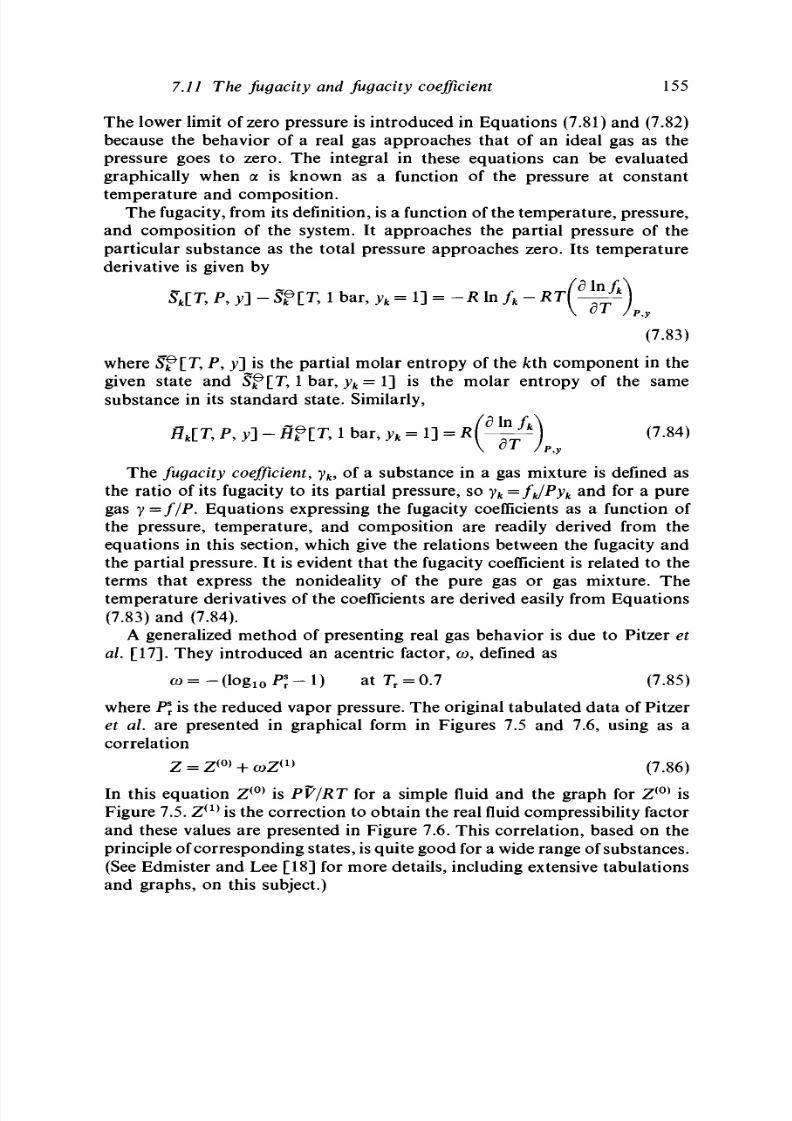
8/11/2019 Thermodynamics of Chemical Systems.pdf
http://slidepdf.com/reader/full/thermodynamics-of-chemical-systemspdf 175/456
7.11 The fugacity and fugacity coefficient
155
The lower limit of zero pressure is introduced in Equations (7.81) and (7.82)
because the behavior of a real gas approaches that of an ideal gas as the
pressure goes to zero. The integral in these equations can be evaluated
graphically when a is known as a function of the pressure at constant
temperature and composition.
The fugacity, from its definition, is a function of the temperature, pressure,
and composition of the system. It approaches the partial pressure of the
particular substance as the total pressure approaches zero. Its temperature
derivative is given by
S
fc
[T, P , y] - Sf [T, 1 bar, y
k
= 1] = -R In f
k
- RT^-^f]
(7.83)
where Sjp[T, P, y] is the partial molar entropy of the fcth component in the
given state and
Sf[T, 1
bar,
y
k
=
1] is the molar entropy of the same
substance in its standard state. Similarly,
jff
t
[T, P, y] - Hf [T, 1 bar, y
k
= 1] = R(^^) (7-84)
\
d T
/P,y
The
fugacity
coefficient,
y
k
,
of a substance in a gas mixture is defined as
the ratio of its fugacity to its partial pressure, so
y
k
=f
k
/Py
k
and for a pure
gas
y =f/P.
Equations expressing the fugacity coefficients as a function of
the pressure, temperature, and composition are readily derived from the
equations in this section, which give the relations between the fugacity and
the partial pressure. It is evident that the fugacity coefficient is related to the
terms that express the nonideality of the pure gas or gas mixture. The
temperature derivatives of the coefficients are derived easily from Equations
(7.83) and (7.84).
A generalized method of presenting real gas behavior is due to Pitzer et
al.
[17]. They introduced an acentric factor, co, defined as
co=- ( l og
1 0
P
s
r
-l) atT
r
= 0.7 (7.85)
where
P\
is the reduced vapor pressure. The original tabulated data of Pitzer
et al.
are presented in graphical form in Figures 7.5 and 7.6, using as a
correlation
Z = Z
(0)
+ coZ
(1)
(7.86)
In this equation Z
(0)
is PV/RT for a simple fluid and the graph for Z
(0)
is
Figure 7.5. Z
(1)
is the correction to obtain the real fluid compressibility factor
and these values are presented in Figure 7.6. This correlation, based on the
principle of corresponding states, is quite good for a wide range of substances.
(See Edmister and Lee [18] for more details, including extensive tabulations
and graphs, on this subject.)

8/11/2019 Thermodynamics of Chemical Systems.pdf
http://slidepdf.com/reader/full/thermodynamics-of-chemical-systemspdf 176/456
156 Ideal gases and real gases
7.12 The integration constant, g
k
(T)
In the preceding work it was not necessary to consider the
dependence of the integration constant on the temperature and in many
cases it is not necessary to do so. At a given temperature it is a constant
and, as long as only differences in the thermodynamic functions are
considered at the same temperature, this constant cancels.
It is informative, how ever, to consider the dep endence of this function on
the tem per atur e. Since we know it is characteristic of the pur e gas , we consider
only 1 mole of a pure gas. Moreover, we limit the discussion to an ideal gas.
There are two possible method s, one concerning the energy and en tropy and
the other the enthalpy and entropy, but we use only the energy and entropy
here. The differential of the energy of
1
mole of ideal gas is d£
=
C
v
dT.
O n
Figure 7.5. Compressibility factor for simple fluids.
0.2 0.3 0.4 0.50.6 0.8 1.0
2.0 3.0 4.05.06.0 8.0 10.0
1.2
0.2 0.3 0.4 0.50.6 0.8 1.0 2.0 3.0 4.0 5.06.0 8.0 10.0
P
r
Reduced Pressure

8/11/2019 Thermodynamics of Chemical Systems.pdf
http://slidepdf.com/reader/full/thermodynamics-of-chemical-systemspdf 177/456
7.12 The integration constant, g
k
(T)
integration, the energy is given as
E=
I
C
v
dT
+ e
157
(7.87)
where e is a constant having units of any energy unit per mole, and is
characteristic of the gas. Similarly, if the entropy is a function of the
temperature and volume,
R ~
f
dV
for an ideal gas. On integration, the entropy is given as
c
T
J
I U n F
because C
v
is independent of the volume for an ideal gas. In this equation,
s is a constant, characteristic of the gas and having molar entropy units.
Since
G =
E
+
PV-TS and PV
=
RT,we can obtain the Gibbs energy of
1 mole of an ideal gas as
I
C
V
&T-T l ^
J
T
RTln P - RT\n(R T) + R T + e - Ts
(7.88)
Figure 7.6. Compressibility factor correction for deviation from simple fluids.
o
0.8
1.0 1.1 1.2 1.3 1.4 1.5 1.7 1.9 2.2 2.6 3.0 4.0
N
0.9
1.0 1.1 1.2 1.3 1.4 1.6 1.8 2.0 2.4 2.8 4.0
T
r
Reduced Temperature
-0.4

8/11/2019 Thermodynamics of Chemical Systems.pdf
http://slidepdf.com/reader/full/thermodynamics-of-chemical-systemspdf 178/456
158
Ideal gases and real gases
By comparisong with Equation (7.50), we find that
f f C
g
(T) =
\C
v
dT-T \—dT-RT\n(RT)
+ RT +
e-Ts (7.89)
j J •*•
Although the heat capacity is d e t e r m i n a te , e and s are not kn ow n, and
hence the value of g(T) is not kn ow n. W hen we consider the difference,
g(T
2
)
—
g(T
1
), the integrals involving the heat capacities can be evaluated,
but the term (T
2
—
T
x
)s still remains. As long as s is unk now n, this term
cannot be evaluated. The evaluation of s is the province of the third law of
thermodynamics .

8/11/2019 Thermodynamics of Chemical Systems.pdf
http://slidepdf.com/reader/full/thermodynamics-of-chemical-systemspdf 179/456

8/11/2019 Thermodynamics of Chemical Systems.pdf
http://slidepdf.com/reader/full/thermodynamics-of-chemical-systemspdf 180/456
160 Liquids and solids: reference and standard states
intensive dependent variables are chosen to be the tem perature, the pressure,
and the composition variables of all but one of the components. For pure
substances it is then sufficient to choose a given temperature and pressure
for the standard state. For solutions we must also consider the composition
variables.
Although the choice of standard states is arbitra ry, two choices have been
established by convention and international agreement. For some systems,
when convenient, the pure component is chosen as the substance in the
standard state. For other systems, particularly dilute solutions of one or
more solutes in a solvent, another state that is not a standard state is chosen
as a
reference
state [19]. This choice determines the standard state, which
may or may not be a physically realizable state. The
reference
state
of a
component or species is that state to which all measurements are
referred.
The standard state is that state used to determine and report the differences
in the values of the thermodynam ic functions for the com ponents or species
between some state and the chosen standard state. When pure substances
are used in the definition of a standard state, the standard state and the
reference state are identical.
8.1 Single-phase, one-component system s
The state of a single-phase, one-component system may be defined
in terms of the temperature, pressure, and the number of moles of the
component as independent variables. The problem is to determine the
difference between the values of the thermodynamic functions for any state
of the system and those for the chosen standard state. Because the variables
are not separable in the differential expressions for these functions, the
integrations cannot be carried out directly to obtain general expressions for
the thermodynamic functions without an adequate equation of state.
However, each of the thermodynam ic functions is a function of the state of
the system, and the changes of these functions are independent of the path.
The problem can be solved for specific cases by using the method outlined
in Section 4.9 and illustrated in Figure 4.1.
The enthalpy is discussed first. The differential expression is
d i/ = C
P
d T + K - T [ —) dP + ifd n (8.1)-T[ —
L
\dTj
Pn
A
from Equation (4.86), where H is the molar enthalpy of the substance. Each
of the coefficients is a function of the independent variables T, P, and n. At
constant pressure and mole number,
dH = C
P
dT (8.2)
where C
P
is a function of the temperature and is to be evaluated at the
particular constant pressure of interest. When Equation (8.2) is integrated

8/11/2019 Thermodynamics of Chemical Systems.pdf
http://slidepdf.com/reader/full/thermodynamics-of-chemical-systemspdf 181/456
8.1
Single-phase, one-component systems
161
with the use of an indefinite integral, we obtain
H
[T ,
P ] =
\C
P
dT
+ /i[P , n] (8.3)
where /i[P , w] is the integration constant. Its value depends upon the chosen
pressure and mole number. The enthalpy is a homogenous function of the
first degree in the mole number at constant temperature and pressure, and
consequently h[P,ri] must also be. We can then write h\_P,ri] as n/i[P],
where /z[P] is a molar quantity. This quantity cannot be evaluated, and it
is evident that standard states must be introduced. When Equation (8.2) is
integrated with the use of a definite integral, we obtain
= J f [ r
2
, P ] - f f | T
1
, P ] = C
P
dT (8.4)
J
This difference can be evaluated. If we choose to define a standard state of
the substance to be the state of the substance at the pressure P and the
temperature T
o
, the difference in the value of the enthalpy at any temperature
T and the given pressure P and that of the standard state is
4
T
C
P
dT
(8.5)
To
where //
e
[ T
0
, P] represents the enthalpy of the substance in the chosen
standard state.
The differential of the enthalpy at a constant temperature and mole number
is
where
[_V —
T(dV/dP)
T
J is to be evaluated at the particular chosen
temperature and is a function of the pressure. We again consider three
different integrals. An indefinite integral might be used, so
J
(8.7)
In this equation the concept that the enthalpy is a homogenous function of
the first degree in the mole numbers at constant temperature and pressure
has again been introduced. The quantity h(T) is an undeterminable quantity,
and again it is necessary to define a standard state. For the definite integral,
we choose any two pressures, P
x
and P
2
, and consider the integral between
these two limits. The change of enthalpy of the system in going from the

8/11/2019 Thermodynamics of Chemical Systems.pdf
http://slidepdf.com/reader/full/thermodynamics-of-chemical-systemspdf 182/456
162
Liquids
and solids:
reference
and
standard states
pressure P
x
to the pressure
P
2
at the given temperature Tis obtained from
AH =
H[T,
P
2
] -
H[T,
i \ ]
= I
2
\V-
T(^J
1
dP
(8.8)
We may then choose the standard state of the system at the temperature
T
to be at some arbitrary pressure P
o
, so that the difference of the enthalpy of
the system at the temperature
T
and pressure
P
and this standard state is
given by
AH = HIT, P] - H
e
[T, P
o
] = I V- T\— dP (8.9)
J PO L \dTJ
Pn
_\
where i /
e
[ T ,
P
o
]
represents
the
enthalpy
of the
substance
in
this standard
state.
It may be convenient to define the standard state of the system as the
state at an arbitrary temperature, T
o
, and an arbitrary pressure, P
o
. The
enthalpy of the system in any state defined by the temperature
T
and the
pressure P may then be calculated by a combination of Equations (8.5) and
(8.8).
Two alternate equations, depending on the path we choose, are
obtained. These are
^
f
r
[ T ( ^ )
1 dp
(8.10)
and
/ f [T ,P] - / /
e
[T
0
, P
0
] =
\
T
(C
P
)
P
dT+
P
\V-T(
8
^) 1 dP
JTO JPOL \8TJ
Ttn
_\
To
(8.11)
Equation (8.10)
is
based
on the two
successive changes
of
state
#ITo>
p
o] = B[T
9
Po] =B[T,P\ where B represents the substance, whereas
Equation (8.11) is based on the successive changes of state, £[T
0
, P
o
] =
£[ r
0
, P] and B[T
0
, P] = £[T, P] . The subscripts to the integrands represent
the value of the pressure or temperature at which the integrands must be
evaluated. For the purposes of tabulating data, the usual standard state was
taken at 298.15 K and 1 atm pressure (101.325 kPa). The new internationally
recommended standard state is at 1 bar or 10
5
Pa [20-23].
Exactly the same methods as used above may be applied to the entropy.
When
the
entropy
is
considered
as a
function
of the
temperature, pressure,
and mole number, the differential of the entropy is

8/11/2019 Thermodynamics of Chemical Systems.pdf
http://slidepdf.com/reader/full/thermodynamics-of-chemical-systemspdf 183/456
8.1 Single-phase, one-component systems 163
where S is the molar entropy of the substance and each coefficient is a
function of the temperature, pressure, and mole number. Again, the variables
are not separable and must be considered individually. At constant pressure
and mole number
dS = (C
P
/T)dT
from which we obtain the three alternate equations:
rr
2
r
AS= \ —dT (8.12)
• - S J
r . n - f e
[T,P]=
| —
dT
+ ns(P)
(8.13)
'
T
C
P
P] (8.14)
T
0
T
Similarly, at constant temperature and mole number
from which
A S = - | { — ) dP (8.15)
S [ T , P ] = - | { —) dP + ns(T) (8.16)
and
dT/
PtH
5[T,
P ] = - f
P
(— j dP +
nS° [T,
P
o
] (8.17)
JPo\
dT
/P
The standard state used in Equations (8.14) and (8.17) are defined in the
same way as the standard states for the enthalpy in Equations (8.5) and
(8.8). If we choose the standard state as the state of the substance at
the temperature T
o
and the pressure P
o
, the entropy of the system at the
temperature T and the pressure P may be determined by either of the
equat ions
d T -
I II —I I
dP
To \
1
/ Po
(8.18)

8/11/2019 Thermodynamics of Chemical Systems.pdf
http://slidepdf.com/reader/full/thermodynamics-of-chemical-systemspdf 184/456
164
Liquids and solids: reference and standard states
and
e r f e )
fT |£ )
1
dP
T
O
(8.19)
The change of the Gibbs energy with temperature, pressure, and mole
number is given by
Again, the variables are not separable and each term must be considered
alone. No difficulty occurs when the pressure of a closed system is changed
at constant temperature. Then
d G = F d P
and
AG = VdP (8.20)
G[T,F|
= VdP + ng(T) (8.21)
or
G | T , P ] = K d P + ^
e
[ T , P
0
] (8.22)
Po
In Equation (8.22) ^
e
[ T , P
o
] is the molar Gibbs energy of the substance
in its standard state defined at the temperature T and the arbitrary pressure
P
o
. The change of the Gibbs energy with temperature cannot be determined,
because the absolute value of the entropy is not known, as stated before.
For open systems the change in the mole number that corresponds to the
addition or removal of material from the system would be done at constant
temperature and pressure. The molar enthalpy, the molar entropy, and the
chemical potential would then be constant and the change in the enthalpy,
entropy, and Gibbs energy of the system would be the product of the molar
quantities and the change in the number of moles. Again, such changes
cannot be calculated, because the absolute values are not known. However,
the concept of the operation is used in later chapters.
8.2 Changes of the state of aggregation in one-component system s
The changes of the temperature and pressure for one-component
systems discussed in Section 8.1 are limited in range, because a change of
phase might take place in the system with the change of temperature or

8/11/2019 Thermodynamics of Chemical Systems.pdf
http://slidepdf.com/reader/full/thermodynamics-of-chemical-systemspdf 185/456
8.3 Two-phase, one-component systems 165
pressure. Such changes of phase may be represented by
B'(T, P)
=
F'(T, P )
where B' represents the substance in the prime phase and B" represents the
substance in the double-prime phase. The change of phase takes place under
equilibrium conditions, so the temperature and pressure of the two phases
are the sam e. Th e chan ge of enth alpy is simply the difference in the enth alpies
of the two phases. Moreover, the molar enthalpies are constant at the given
temp erature a nd pressure. Th us, the change of enthalpy m ay be expressed as
AH = H" -H' = n{H" - H') (8.23)
where
n
is the number of moles of the substance that have undergone the
change of phase. This quantity may be determined by calorimetric methods
at constant pressure because AH is equal to the heat absorbed by the system
for the constant-pressure processes. It may also be determined indirectly by
means of the Clapeyron equation (Eq. 5.73)).
By use of similar arguments,
AS = (S" - S') = n( 3" - S') = AH IT (8.24)
is obtained for the change of the entropy. Finally, the chemical potentials
of the substance in the two states of aggregation are equal at equilibrium,
and consequently AG = 0.
8.3 Two-phase, one-component systems
A one-component system that exists in two phases is univariant and
hence indifferent. In order to define the state of the system, at least two of
the independent variables must be extensive. We choose the temperature,
volume, and number of moles as the independent variables, and consider
the enthalpy, entropy, and Gibbs energy as functions of these variables.
The two condition equations
n = n
f
+ n" (8.25)
and
V = n'V
f
+ n"V"
(8.26)
must always be satisfied; n' and n" represent the number of moles of the
substance in the two separate phases, and V' and V" represent the molar
volumes of the substance in the two phases. The first of the two condition
equations expresses the condition of mass balance, and the second expresses
the condition that the total volume of the system must be the sum of the
volumes of the two phases. The two equations can be combined with the
elimination of either n' or n". If we choose to eliminate n", then
V = n'{V' -V") + nV" (8.27)

8/11/2019 Thermodynamics of Chemical Systems.pdf
http://slidepdf.com/reader/full/thermodynamics-of-chemical-systemspdf 186/456
166 Liquids and solids: reference an4 standard states
This equation makes it possible to determine the number of moles of the
component in each phase or to use n' as an independent variable rather than
V,
if
we
so
choose.
The
mo lar volumes
are
properties
of
the separate phases,
and consequently can be considered as functions of the temp erature and
pressure. However, the system is univariant, and consequently the pressure
is a function of the temp erature when the temperature is taken as the
independent variable. The relation between the temp erature and pressure
m ay
be
determ ined experimentally
or
may
be
determined
by
means
of
the
Clapeyron equat ion. The differential of each m olar volume may then be
expressed by
+(*)
(<?)
ldr
( 8 . 2 8 ,
W ith this intro du ction , we consider the enthalpy of the system as a function
of the temperature , volume, and number of moles. The differential of the
enthalpy is given by
d T +
(
—)
dK
+ ( —)
An
(8.29)
and the problem reduces to obtaining expressions for the derivatives. The
enthalpy of the system is the sum of the enthalpies of the two phases, so
H
= n'H' +
n"H" (8.30)
the differential of which is
AH = (H' - H") An'
+
ri AH'
+
(n - n') AH"
+
H" An
(8.31)
From this equation
we may
write
V,n
(8.32)
From Equation (8.27)
'dri\ (V-nV')(dV"/8T)
sat
-(V-nV")(dV'/dT)
sal
—^ ^— ( O . J J )
(V - V")
2
and each
(dV/dT)
S ll
may
be written as
)
+ ( ) (
dTj
P
\dPj
T
\dT
on the basis of Eq ua tion (8.28).
The
mo lar enthalpies of each of
the
phases
which are satura ted with respect to the other phase are functions of the

8/11/2019 Thermodynamics of Chemical Systems.pdf
http://slidepdf.com/reader/full/thermodynamics-of-chemical-systemspdf 187/456
8.3 Two-phase, one-component systems
167
temperature
and
pressure
in
general,
but the
pressure
is a
function
of the
temperature
for the
two-phase system.
We
then express (dH/dT)
Vn
as
for each
of the
pha ses. Eq uatio ns (8.27), (8.33). (8.34),
and
(8.35) when
substituted into Equation (8.32)
are
sufficient
to
evaluate (dH/dT)
v
„
at any
permitted
set of
values
of
the independent variables.
The evaluation of
(dH/dV)
T n
is also based on E qu atio n (8.31). At c onsta nt
temperature both
AH'
and
AH"
are zero, and consequently
AH =
(H'-H")An'
(8.36)
Tha t
is, the
change
of
enthalpy
of a
closed system
for a
change
in
volume
at cons tant te m per ature is simply the m olar chan ge of entha lpy for the change
of phase multiplied
by the
number
of
moles that undergo
the
change
of
phase. The equat ion
for the
derivative m ay
be
written either
as
(8.37)
or
as
H'-H"
V -V
with
the use of
Eq ua tion (8.27).
The expression
for
(dH/dn)
T
v
is
derived a lso from Eq ua tio n (8.31), from
which
we
obtain
fdH
) ={H'-H")(
d
f) +£" (8.39)
JT,V \8nJ
TtV
From Equation (8.27) we have
(8.40)
v -v
and therefore
'dH
V -V
( j U 1 )
The evaluation
of
Eq ua tio n (8.41) pres ents some difficulty.
The
molar
volumes, V'
and
V",
can be
determ ined experim entally,
as can
(H' — H").
However ,
the
equation contains
the
m olar enthalpy
of the
double-primed
phase,
and the
absolute value
of
this q uantity
is not
known.
It
would then

8/11/2019 Thermodynamics of Chemical Systems.pdf
http://slidepdf.com/reader/full/thermodynamics-of-chemical-systemspdf 188/456
168 Liquids and solids: reference and standard states
appear that the derivative cannot be evaluated. This difficulty is overcome
by suitable choices of standard states for the system. We choose a standard
state at each temperature and define it to be the double-primed phase; the
value zero is assigned to the enthalpy of this phase at each temperature.
Equation (8.41) then becomes
_ _ , * £ .
(8
.
42)
dnJ
TtV
V'-V"
where H' is actually the molar change of enthalpy for the change of state of
aggregation at each temperature. The derivative can thus be evaluated, and
the change of enthalpy for the addition of the component to the system at
constant temperature can be calculated by integration of this equation at
each temperature. All values of the enthalpy thus calculated are relative to
these star dard states, which are different for each temperature.
With these standard states, comparison between the values of (dH/dn)
TV
at different tem pera tures c ann ot be ma de . In orde r to do so, we could ch oose
the standard state to be the double-primed phase at some arbitrary
temperature , T
o
, with the condition that this phase is saturated with respect
to the prime d ph ase ; the pressure of the stan dar d state, P
o
, is thus determined
by the temperature. We then define the enthalpy of the double-primed phase
to be zero at T
o
. The molar enthalpy of the double-primed phase at any
other temperature at which the two phases are at equilibrium may be
calculated by the use of Equation (8.35), so
It must be remembered that C
P
, V\ and (dV"/dT)
P
are , in gen eral, functions
of the pressure as well as the te m pe ratu re, bu t in this special case the pressure
is a f m ction of the tem pe ratu re. Th e expression for
(dH/dn)
TV
finally becom es
To \ L \ v
l
/ P,n
(H'-H )V
V'-V"
(8.44)
with the use of this last standard state. The enthalpy of the system can thus
be determined relative to the chosen standard state.
The integration of Equation (8.29) to determine the change of enthalpy
of the system for a finite change of state would be rather a formidable task.
If we represent the system by the symbol B and designate the initial state as
[T
1 ;
V
u
n{\ and the final state as [T
2
, V
2
, n
2
] , we wish to consider the chang e

8/11/2019 Thermodynamics of Chemical Systems.pdf
http://slidepdf.com/reader/full/thermodynamics-of-chemical-systemspdf 189/456
8.3 Two-pha se, one-component systems
169
of state
F o r a specific case it would be more convenient to integrate along the path
designated by the three successive changes of state
BlT
29
V
l9
n
1
]=BlT
29
V
29
n
1
-]
and
BlT
29
V
29
n
1
]=BlT
29
V
29
n
2
]
so that only
one
independent variable
is
changed
at a
t ime.
Of
course, other
equivalent paths could be set up. The first of the three changes of state
involves the integration of Equation (8.32). The integrand, represented by
the right-hand expression of Eq ua tion (8.32) with the use of Equations (8.27)
and (8.33)—8.35), is a function of the temperature alone. The pressure -
volume-temperature data for the two saturated phases must be known in
order to carry out the integration. The integrals required for the other two
changes of state present no difficulty because, according to Equations (8.38)
and (8.41) or (8.44), only the molar quantit ies of the two saturated phases
appear
in the
integrands,
and
these quantities
are
constant
at
constant
temperature . One final comment concerning the molar heat capacity in
Equations (8.35) and (8.43) needs to be made . The heat capacity may not
be known as a function of the temperature and pressure. However, if it is
known as a function of the temperature at some pressure P
o
and if the
pressure-volume-temperature data are known, then we may use (dC
P
/dP)
Tn
to determin e the heat capacity at any pressure P. The derivative is given by
dP)
T
,
n
~\dT
2
/
P
,
n
( 8
"
4 5 )
and consequently,
on
integration between
the
limits
P
o
and
P,
dP (8.46)
P,n
Eq uation s, similar to those for the enthalpy, can be derived for the entropy
and the problems related to standard states are identical. The relations for
the Gibbs energy are
dT)
v
,
n

8/11/2019 Thermodynamics of Chemical Systems.pdf
http://slidepdf.com/reader/full/thermodynamics-of-chemical-systemspdf 190/456
170 Liquids and solids: reference and standard states
and
dn/
TV
(8.49)
8.4 Three-phase, one-component systems
A one-component system that exists in three phases is indifferent
and has no degrees of freedom. In order to define the state of the system
then, three extensive variables must be used. We choose for discussion the
enthalpy, volume, and number of moles of the components. The enthalpy
of the system is additive in the molar enthalpies of the three phases, as is
the volume. We can then write three equations:
H = n'H' + ri'H" + ri"H'" (8.50)
V=n'V'
+ ri'V" +
n'"V'"
and
n = n
r
+ n" + ri"
For a given set of values for
H
, F, and n, values of
ri ,
n", and
ri"
can be
calculated if the molar enthalpies and molar volumes of the three phases can
be determined. The molar volumes can be obtained experimentally, but the
absolute values of the molar enthalpies are not known. In order to solve
this problem, we make use of the concept of standard states. We choose one
of the three phases and define the standard state to be the state of the system
when all of the component exists in that phase at the temperature and
pressure of the triple point. If we choose the triple-primed phase as the
standa rd ph ase, we subtract nH'" from each side of Eq uatio n (8.50) and obtain
(H - nH
1
) = ri(H
f
- H'") + n"(H" - H'") (8.51)
This equation gives the enthalpy of the system relative to the standard state,
and the independent variable would now be (H
—
nH'") rather than H itself.
The quantit ies (H
f
—
H'") and (H"
—
H'") are the changes of enthalpy when
the state of aggreg ation of 1 mo le of the com pon ent is changed from the
triple-primed state to the primed state and to the double-primed state,
respectively, at the temperature and pressure of the triple point. These
quantities can be determined experimentally or from the Clapeyron equation,
as discussed in Section 8.2. The three simultaneous, independent equations
can now be solved, provided values that permit a physically realizable
solution have been given to (if
—
nH'"),
F, and
n.
If such a solution is not
obtained, the system cannot exist in three phases for the chosen set of
indep ende nt v ariables. Actually, the stand ard state could be defined as one of
the phases at any arbitrarily chosen temperature and pressure. The values
of the enthalpy and entropy for the phase at the temperature and pressure

8/11/2019 Thermodynamics of Chemical Systems.pdf
http://slidepdf.com/reader/full/thermodynamics-of-chemical-systemspdf 191/456
8.5 Solutions
111
of the triple point would then
be
calculated
by
the m etho ds discussed
in
Section 8.1.
The values of the other thermodynamic functions are readily obtained for
these indep ende nt variables. The chemical potentia l is identical in each phas e,
and consequently G = n\i. If we choose the same standard state for the Gibbs
energy as we did for the enthalpy, we have
G-nfi ' = 0 (8.52)
{H-nH' )=T(S-nS
f
) (8.53)
and
S -
nS"
r
= n'(S' - S
f
")
+
n"(S" - S'")
(8.54)
8.5 Solutions
The equations developed in Section 8.1 for single-phase, one-
component systems are all applicable to single-phase, mu lticom ponen t
systems with the condition that the composition
of
the system
is
constant.
The dependence of the thermo dynam ic functions on concentration are
introduced through the chemical potentials because, for such a system,
G = £
nui
t
(8.55)
and the other functions can be obtained from this equation by appropriate
differentiation. In this equatio n the sub script i refers to a component or
species and the sum is taken over all components or species. The dependence
of the chemical potentials on composition is of special imp ortan ce because
the cond itions of equilibrium are expressed in terms of the chemical pote ntials.
It is through these conditions of equilibrium and the dependence of the chemical
potentials on composition that all of the relations involving phase equilibrium
and chemical equilibrium are obtained.
In addition,
a
change of phase in multico m pon ent systems does not take
place, in general , under co nditions of both constan t tem perature and constant
pressu re, or with consta nt co mp osition of the individual pha ses. W e consider,
as an example,
a
change of state represented
as
n M [ s , T
l9
P ]
=
nM[/
9
T
29
P ]
where M represents 1 mo le
of
solution. Changes
in the
thermodynamic
functions are desired for this change of state. We may separate
it
into three
steps such
as
nM[s, T, P] = nM[£
9
T\ P ]
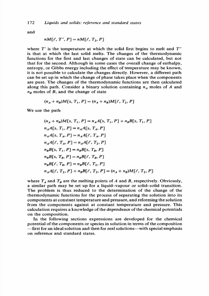
8/11/2019 Thermodynamics of Chemical Systems.pdf
http://slidepdf.com/reader/full/thermodynamics-of-chemical-systemspdf 192/456
172
Liquids and solids: reference and standard states
and
n M | 7 ,
T" , P] = nM[/, T
2
, P ]
where T" is the temperature at which the solid first begins to melt and T"
is that at which the last solid melts. The changes of the thermodynamic
functions for the first and last changes of state can be calculated, but not
that for the second. Although in some cases the overall change of enthalpy,
entropy, or Gibbs energy including the effect of temperature may be known,
it is not possible to calculate the changes directly. However, a different path
can be set up in which the change of phase takes place when the components
are pure. The changes of the thermodynamic functions are then calculated
along this path. Consider a binary solution containing
n
A
moles of
A
and
n
B
moles of B, and the change of state
(n
A
+ n
B
)M[s , T
l9
P ] = (n
A
+ n
B
)M[t
9
T
2
, P ]
We use the path
(n
A
+ n
B
)M[s , T
l9
P ] = n
A
A[s, T
l9
P] + n
B
B[s, T
l9
P ]
n
A
A\i
9
T
A
, P ] =
n
A
A[S
9
T
2
, P ]
s, T
B9
P ] = njfi\e
9
T
B9
P ]
9
T
B9
P ] = n
B
B\t
9
T
l9
P ]
n
A
A\t
9
T
29
P ] +
n
B
B\{
9
T
l9
P ] =
(n
A
+
n
B
)M[f
9
T
29
P ]
where T
A
and T
B
are the melting points of A and B, respectively. Obviously,
a similar path may be set up for a liquid-vapour or solid-solid transition.
The problem is thus reduced to the determination of the change of the
thermodynamic functions for the process of separating the solution into its
com pone nts at constant tem perature an d pressure, and reforming the solution
from the components against at constant temperature and pressure. This
calculation requires a knowledg e of the dependen ce of the chemical potentials
on the composit ion.
In the following sections expressions are developed for the chemical
pote ntial of the com pon ents or species in solution in terms of the c om position
—irst for an idea l so lut ion a nd the n for real solu tion s—with sp ecial em ph asis
on reference and standard states.

8/11/2019 Thermodynamics of Chemical Systems.pdf
http://slidepdf.com/reader/full/thermodynamics-of-chemical-systemspdf 193/456
8.6 The ideal solution
173
8.6 The ideal solution
The ideal solution is defined thermodynamically as one in which the
dependence
of
the chemical potential
of
each comp onent
on the
composit ion
is expressed by
l*klT
9
P, x] =
RT In x
k
+ iif[T
9
P]
(8.56)
at all temperatures and pressures. The symbol x within the brackets refers
to
a set of (C
—
1)
values
of the
mole fractions
of the
C com ponents .
The
quantity /zjp[T,
P] is
first considered
as an
undetermined constant
at
each
temperature
and
pressure. Meaning
is
given
to
this quantity
by
considering
a system
in
which x
k
= 1
and
therefore
the
value
of all
other mole fractions
is zero. Then
and we interpr et this sym bol to represent the chemical potential of the pure
fcth component at the same temp erature and pressure of the solution and in
the same state
of
aggregation
as the
solution.
The
complete expression
of
Equation (8.56) is then written as
li
k
[T, P, x] = RT In x
k
+ ( if IT, P, x
k
= 1] (8.57)
The
standard state
for the
chemical potential
of
each component
in the
solution is thus defined as the pure component at the same temperature and
pressure and in the same state of aggregation as the solution. We say that
the chemical potential of the kth component in a solution at the tem perature
T, pressure P, and composit ion x referred to the pure kth component at the
same T and P and in the same state of aggregation is equal to RT In x
k
.
Th is difference is also know n as the
change
of the
chemical potential on mixing
at constant temperature and pressure, so
A <
= ii
k
[T
9
P, x] - iif\T
9
P, x
k
= 1] = RT In x
k
(8.58)
The Gibbs energy
of the
solution
is
given
by
GIT, P, x]
=
£
n
t
RT In x
t
+ £
n^T, P, x
t
=
1] (8.59)
f = l
i=l
according to Equation (8.55). The change of the Gibbs energy for the
formation of the solution at the temperature T and pressure P from the
components at the same temperature and pressure and in the same state of
aggregation
as the
solution
is
given
by
AG
M
[T , P, x] = GIT, P, x] - X n^fU, P, x
t
= 1] = £ n
t
RT In x,
i = 1 i = 1
(8.60)

8/11/2019 Thermodynamics of Chemical Systems.pdf
http://slidepdf.com/reader/full/thermodynamics-of-chemical-systemspdf 194/456
174 Liquids and solids: reference and standard states
The quantity AG
M
is called the change of G ibbs energy o n mixing at con stant
temperature and pressure or, more briefly, the Gibbs energy of mixing.
By appropriate differentiation of Equations (8.57), (8.59), and (8.60), we
obtain the corresponding expressions for the entropy. Thus,
S
k
[7; P, x] = -R In x
k
+ Sf
[T ,
P , x
fc
= 1] (8.61)
SIT, P, x] = - £ n
t
R In x
t
+ £
n
t
5f>lT
9
P , x
t
= 1] (8.62)
and
AS
M
[T, P , x ] = - X n
£
K In
Xi
(8.63)
The quantity AS
M
[T, P, x] is referred to as the change of entropy on mixing
at consta nt tem pera ture a nd pressures or, more briefly, the entrop y of mixing.
Similarly, we obtain
H
k
\T,
P , x] =
Rf\T,
P , x, = 1] (8.64)
c
ii\_l
9
r , X j
— 2 ^
tlirli\_l
9
r,Xi=ij
(O .O J J
and
A H
M
[ T , P , x ] = 0 ( 8 . 6 6 )
The change of enthalpy on mixing, Af/
M
[T, P, x], at constant temperature
and pressure is seen to be zero for an ideal solution. The change of the heat
capacity on mixing at constant temperature and pressure is also zero for an
ideal solution, as are all higher derivatives of AH
M
with respect to both
the temperature and pressure at constant composition. Differentiation of
Equations (8.57), (8.59), and (8.60) with respect to the pressure yields
\ x
k
= 1] (8.67)
, P, x] = £ ^ f [ T , P, x, = 1] (8.68)
i = l
and
A K
M
[ T , P , x ] = 0 ( 8 . 6 9 )
Thus, the change of the volume on mixing at constant temperature and
pressure, AF
M
[T , P , x ] , is also ze ro, as are all higher derivatives of AV
M
with respect to both the temp erature and pressure at constant com posit ion.
In review, we see that, for an ideal solution, the change of the Gibbs
energy on mixing and the change of the entropy on mixing both at constant

8/11/2019 Thermodynamics of Chemical Systems.pdf
http://slidepdf.com/reader/full/thermodynamics-of-chemical-systemspdf 195/456
8.7 Real solutions: reference and standard states
175
temperature
and
pressure a re given
by
Eq uatio ns (8.60)
and
(8.63), respectively,
at
all
temperatures
and
pressures;
and
that
the
enthalpy,
the
heat capacity,
and
the
volume
are all
additive
in the
corresponding quantit ies
of the
components
at all
temperatures
and
pressures.
8.7 Real solutions: reference
and
standard states
The dependence on composit ion of the thermodynamic properties
of a component in a real solution is developed in terms of the deviations of
these properties from those of an ideal solution at the same temperature,
pressure, and composit ion. We know that the chemical poten tial is a function
of
the
state
of the
system, that
it is an
intensive variable,
and
that
it is a
homogenous function of zeroth degree in the mole num bers . Thus, we know
that the chemical potential of a component in a single phase is a function
of the composit ion and that its value, a l though unknown, is fixed when
values have been assigned to the necessary nu mb er of intensive, independent
variables. We choose these variables to be the temperature, pressure, and
(C —1) mole fractions, where C represents the number of components . We
now introduce a quant i ty , iif[T, P] that will refer eventually to the standard
state but which for the present remains undefined. It is introduced to account
for
our
lack
of
knowledge
of the
absolute value
of the
chemical potential.
We need only
to
know that this quantity
is a
function
of the
temperature
and pressure
and is a
constant , independent of composition,
for any
chosen
set
of
values
of
the tem perature
and
pressure.
We
then consider
the
difference
between ^
fc
[T,
P, x] and
jaf
[T ,
P ] .
It is
this difference, once ixf[T,
P] has
been defined, that
is
determined experimentally.
The
experimental determi-
nat ion
of
this difference
is
discussed
in
Chapte r
10;
throu gho ut this chapter
it must
be
remembered that
the
difference
can be
determined.
We
expect this
difference
for a
real solution
to
approximate RT
In
x
k
(except
for a
constant)
on
the
basis
of the
behavior
of an
ideal solution.
We
therefore write
/i
fc
[T, P, x] - iif\T
9
P] = RT In x
k
+ A ^
E
X
[T , P, x] (8.70)
or
li
k
\T,
P, x] =
RT
In
x
k
+ A/i* J T , P, x] +
fif
[T , P]
(8.71)
where A/i
k
E
x
represents the difference between the actual behaviour of
(/x
k
[T, P, x] -
fi f
[T , P]) and RT In x
k
(except for a constant) and is called
the excess change of the chemical potential on mixing. The subscript x is
used
to
designate
the use of
mole fractions
as the
composit ion variables.
Equation (8.71) relates
two
undefined quantities, Afif
x
and
/xJpET,
P], in
one equat ion. The first quantity is a function of the temperature, pressure,
and (C —1) mole fractions, but the zero of the function is not defined, and
the second is a function of the temperature and pressure, but the state of

8/11/2019 Thermodynamics of Chemical Systems.pdf
http://slidepdf.com/reader/full/thermodynamics-of-chemical-systemspdf 196/456
176 Liquids and solids: reference and standard states
the system to which it refers is not defined. Alternately, we may use
A J I E J T , P , x] =
ft
[T, P, x] - / ^ [ T , P ] (8.72)
for the second quantity. Then, A/x^
x
[T, P , x] is a function of the tem pera ture,
pressure, and (C —1) mole fractions, but its zero is not defined. The arbitrary
assignment of the zero value to one of the two quantities, Ajx
kx
or A/^
x
,
fixes the zero value for the other because the two are related thro ug h Eq uatio n
(8.71). There are thus two ways to define these quantities. We may choose
a state of the system at every temperature and pressure of interest and define
the value of Afi
ktX
to be zero for this state. It is convenient to call this state
th e reference state of the kih component, because all measurements are
actually referred to this state. Alternately, we may define A/i^
x
[T, P, x] for
th e kth component to be zero for a given state of the system at every
temperature and pressure of interest. This state is called the standard state
of the fcth component, and iif[T,P~\ is equa l to the chemical poten tial of
the feth component in this state according to Equation (8.72). When the
reference state of a component is defined at the same composition of the
system for every temperature and pressure, the temperature and pressure
derivatives of Afi
ktX
at the reference state must be zero. Similarly, if the
standard state of a component is defined rather than the reference state, and
if the stan dar d state is defined at the same co m position for every tem pera ture
and pressure, then the temperature and pressure derivatives of Ap^
tX
must
be zero at the standard state.
The nom enc lature a nd sym bols used by Lewis and Ran dall [2 4] are closely
related to those introduced here. The activity coefficient,
y
k
,
is related to
Afi
k
by
Atf =
RTlny
k
(8.73)
and the activity, a
k
, is related to A^J
1
by
$
k
(8.74)
Thus , the reference state of a component is the state of the system for which
the activity coefficient of the component is defined to be unity and the standard
state is the state of the system for which the activity of the component is unity
or defined to be unity.
In this discussion the temperature and pressure of the reference state and
of the standard state have been taken to be those of the solution; this usage
is consistent with the recommendations of the Commission on Symbols,
Terminology, and Units of the Division of Physical Chemistry of the
International Union of Pure and Applied Chemistry. For the standard state
however, a fixed, arbitrary pressure (presumably 1 bar) might be chosen. If
we define
, P, x]
-iif\T
9
P
o
] (8.75)

8/11/2019 Thermodynamics of Chemical Systems.pdf
http://slidepdf.com/reader/full/thermodynamics-of-chemical-systemspdf 197/456
8.7 Real solutions: reference and standard states 177
where P
o
is the fixed, arbitrary pressure, the difference between Afif and
AtflT,P,x]is
A/C -
Arf&T,
P, x] = vflT, P] - tf[T, P
o
]
(8.76)
according to Equation (8.72). This difference can be calculated because
(dfi
k
/dP)
T
x
= V
k
and the integration can be performed when V
k
is known as
a function of the pressure for the kth component at the composit ion of the
standard state. In this book the pressure of the standard state is always taken
to be that of the solutio n, which may be variable, rather th an a fixed arbitra ry
pressure. A fixed, arbitrary temperature cannot be used, in general, to define
the standard state with respect to temperature, because the absolute values
of the enthalpy or entropy are generally not known.
Similar arguments and definitions can be applied to the other partial
molar thermodynamic functions and properties of the components in
solution. By differentiation of Equation (8.71), the following expressions for
the partial molar entropy, enthalpy, volume, and heat capacity of the kth
component are obtained:
5
k
[T, P,x] = -R\nx
k
+ A5EJT, P , x] + Sf
[T ,
P ] (8.77)
H
k
\T
9
P, x] = A Jjs jT , P, x] + Hf[T, P ] (8.78)
V
k
lT,
P, x] = A F= JT , P, x] +
Vf [T ,
P ] (8.79)
and
C
Ptk
[T,
P , x ] = AC
E
PXx
[T, P ,
x]
+
Cf^T,
P ] (8.80)
The excess quantities in each equation represent the corresponding tem-
perature and pressure derivatives of the excess chemical potential of mixing.
When the values of the temperature and pressure derivatives of Afi
kx
for the
reference state or A/iJ^ for the standard state are defined, then all quantities
in Equations (8.77)-(8.80) are also defined.
In summary, a reference state or standard state must be defined for each
component in the system. The definition may be quite arbitrary and may be
defined for convenience for any thermodynamic system, but the two states
cannot be defined independently. When the reference state is defined, the
standard state is determined; conversely, when the standard state is defined,
the reference state is determined. There are certain conventions that have
been developed through experience but, for any particular problem, it is not
necessary to hold to these conventions. These conventions are discussed in
the following sections.
The general practice is to define the reference state.
This state is then a physically realizable state and is the one to which
experimental measurem ents are referred. The standa rd state may or may not
be physically realizable, and in some cases it is convenient to speak of the
standard state for the chemical potential, for the enthalpy, for the entropy,

8/11/2019 Thermodynamics of Chemical Systems.pdf
http://slidepdf.com/reader/full/thermodynamics-of-chemical-systemspdf 198/456
178
Liquids and solids: referen ce and standard states
for
the
volume,
etc.
However,
the
definition
of the
standard state
of a
component may be more convenient than the definition of the reference state
in some instances. This question
is
discussed more fully in Chapters
10
and 11.
8.8 Definitions based on mole fractions
We may choose the reference state of any or all of the components
to be the pure component or components in the same state of aggregation
as the solution at all temperatures and pressures of interest. Then, according
to Equation (8.71),
^ [ r , P , x , = l ] = ^ [ T , P] (8.81)
that is, the chemical potential of the component in its standard state is also
that of the pure component at all temperatures and pressures of interest.
Similarly, we find that
(8.82)
]
(8.83)
] (8.84)
and
Cp
J
lT,P,x
t
= l = Cf
J
lT,F]
(8.85)
Thus, the properties of the component in its standard state are identical to
those of the component in its reference state. This reference state is primarily
used for systems whose properties can be studied over the entire range of
composition even though a region of partial immiscibility may exist.
The reference state of each component in a system may be defined in
many other ways. As an example, we may choose the reference state of each
component
to be
that
at
some composition with
the
condition that
the
composition of the reference state is the same at all temperatures and pressures
of interest. For convenience and simplicity, we may choose a single solution
of fixed composition to be the reference state for all components, and
designate xjf to be the mole fraction of the /cth component in this solution.
If (A/i^)' represents the values of the excess chemical potential based on
this reference state, then
(A/uf
tX
*)'[T
9
P, x*]
is
zero
at all
temperatures
and
pressures
at the
composition
of the
reference state. That this definition
determines
the
standard state
is
seen from Equation (8.71),
for
then
H?IT
9
P] =
iiRT,
P, x*] -
RT
In x* (8.86)
where x* in the brackets represents the (C — 1) values of the mole fractions
in the reference state. The value of /ijf is the chemical potential of the fcth
component in the reference state, but is unknown, when values of the

8/11/2019 Thermodynamics of Chemical Systems.pdf
http://slidepdf.com/reader/full/thermodynamics-of-chemical-systemspdf 199/456
8.8 Definitions based on mole fractions 179
temperature, pressure, and mole fractions in the reference state are given.
Therefore, the value of jujp[T, P] is fixed but is also unknown.
The question of what the mole fraction of a component is in its standard
state for the chemical potential seldom arises; the important point is that
the value of the chemical potential of the component in its standard state is
fixed when the reference state of the component has been defined. It is of
interest to discuss this question when the pure components are not the
reference states, so that a better understanding of the standard state may be
obta ined . The mole fraction of the /cth comp one nt in its stand ard state ca nno t
be determined from Equation (8.86), because the absolute values of the
chemical potential are unknown. However, according to Equations (8.71)
and (8.72),
RT In x
k
+ (AtfJlT, P, x] = 0 (8.87)
for the standard state. The excess change of the chemical potential is a
function of (C —1) mole fractions, and we assume th at this function has been
determ ined experimen tally. W e can then calculate the value of
x
k
that satisfies
Equation (8.87) after assigning values to (C —2) other mole fractions. The
value of x
k
obviously depends upon the arbitrary values that are assigned
to the other mole fractions. We thus observe that, except in a binary system,
the value of the mole fraction of a component in its standard state in a
multicomponent system does not have a fixed value. Moreover, the values
so obtained may be greater than unity, or possibly negative, and therefore
do not correspond to a physically realizable state. We may consider that
Aju^
x
represents a surface in a multidimensional space of (C —1) coordinates
at a fixed temperature and pressure. All points on this surface that satisfy
Equation (8.87) represent standard states of the /cth component at the given
tem pera ture and p ressure. A different surface is obtain ed for each tem pera ture
and each pressure; thus, the standard state is a function of the temperature
and pressure.
The determination of the mole fraction of the /cth component in its
standard state for the entropy follows the same argument that was used for
the chemical potential. By the use of Equation (8.77) and the condition that
, P, x] must equal S
e
[ T , P ] for the standard state, we find that
-R In x
k
+ (AS*
X
)'[T, P , x ] = 0 (8.88)
must be satisfied. The arguments are the same, and we can calculate a value
for
x
k
when arbitrary values have been assigned to (C
—
2) other mole
fractions. This value is generally a different value from that obtained from
Equation (8.87) for the chemical potential for the same set of values assigned
to the (C —2) indep ende nt mole fractions. T hu s, the value of the mole fraction
of the /cth component in its standard state for the entropy depends upon the

8/11/2019 Thermodynamics of Chemical Systems.pdf
http://slidepdf.com/reader/full/thermodynamics-of-chemical-systemspdf 200/456
180 Liquids and solids: reference and standard states
temperature, pressure, and the arbitrary values assigned to the (C —2) mole
fractions; it need not have physical reality.
A different result is obtained when we consider the partial molar
enthalpy, the partial molar volume, the partial molar heat capacity, and all
other higher derivatives taken with respect to the temperature or pressure.
At the composition of the reference state, AHjr
x
*, AV^
tX
*, and ACp
Xx
* are
all equal to zero. Then we have, from Equations (8.78)-(8.80),
T,P] (8.89)
T,P] (8.90)
and
C U T , P , x * ] = C ^ [ r , P ] (8.91)
where x* represents the set of values of the mole fractions at the reference
state. We find that the partial molar enthalpy, volume, and heat capacity of
the feth component in its standard state is equal to the same quantities at
the reference state. This result is also true of the higher derivatives with
respect to the temperature and pressure.
We
find
from this discussion that, when the reference state of a component
in a multicomponent system is taken to be the pure component at all
temperatures and pressures of interest, the properties of the standard state
of the component are also those of the pure component. When the reference
state of a component in a multicomponent system is taken at some fixed
concentration of the system at all temperatures and pressures of interest, the
system or systems that represent the standard state of the component are
different for the chemical potential, the partial molar entropy, and for the
partial molar enthalpy, volume, and heat capacity. There is no real state of
the system whose properties are those of the standard state of a component.
In such cases it may be better to speak of the standard state of a component
for each of the thermodynamic quantities.
The usual choice of a reference state other than the pure components is
the infinitely dilute solution for which the mole fractions of all solutes are
infinitesimally small and the mole fraction of the solvent approaches unity;
that is, the values of the thermodynamic properties of the system in the
reference state are the limiting values as the mole fractions of all the solutes
approach zero. However, this is not the only choice, and care must be taken
in defining a reference state for multicomponent systems other than binary
systems. We use a ternary system for purposes of illustration (Fig. 8.1). If
we choose the component A to be the solvent, we may define the reference
state to be the infinitely dilute solution of both B and Cm A. Such a reference
state would be useful for all possible compositions of the ternary systems.
In other cases it may be advantageous to take a solution of A and B of fixed

8/11/2019 Thermodynamics of Chemical Systems.pdf
http://slidepdf.com/reader/full/thermodynamics-of-chemical-systemspdf 201/456
8.8 Definitions based on mole fractions 181
composition, such as that at M, as the solvent. The ratio of the moles of A
to the moles of B in any solution whose composition lies on the line CM is
a constant and is equal to that at the point
M.
We could then choose a
reference state as the infinitely dilute solution of C in the mixed solvent M.
The values of the thermodynamic properties of the reference state are those
obtained in the limit as the mole fraction of C approaches zero along the
line CM. A different reference state is ob tain ed for each arbitr arily chosen
value of M.
The problem of reference and standard states is illustrated in Figures
8.2-8.8 for a binary solution, for which there is only one independent mole
fraction. In the first case we choose the reference state of the first component
to be the pure co mp onent at all temperatures, and assume that A//f
= 500x1
at 298 K an d 200x1 at 373 K, in J m ol~ *. The curves for these two equ ations
(curve A for 298 K an d cu rve B for 373 K ) are given in F igur e 8.2, wh ere
the mole fraction scale is continued beyond unity for illustrative purposes.
The corresponding curves for A/^
1
are given in Figure 8.3. The curve for ASf
is given in Figure 8.4, that for AS*? is given in the upper curve of Figure 8.5,
and that for A/?f is given in Figure 8.6. These last curves are determined
on the assumption that A/if is a linear function of the temperature, and
consequently ASf,
AS
1
}
1
,
and AHf are independent of the temperature. As a
consequence of the chosen reference state, the value of each of the functions
is zero for the pure component. If, however, we choose the reference state
for the first component to be the system in which the mole fraction of the
first com pon ent is
0.3,
then A/if is zero at this mole fraction at all tem per atur es
and pressures. This definition simply shifts the zero on the axis for A/^ and
the tw o eq ua tio ns beco m e Afif = 500x^ - 245 at 298 K an d 200*2 - 98
a t
373 K. These curves are given in F igure 8.7. Th e corre spon ding curves for
Afi™
are given in Figure 8.8. The zero value of this function now occurs at
a hy po thetic al m ole fraction of 1.37 at 298 K a t 1.14 at 373 K. T he cu rves
Figure 8.1. A ternary system.
C
n
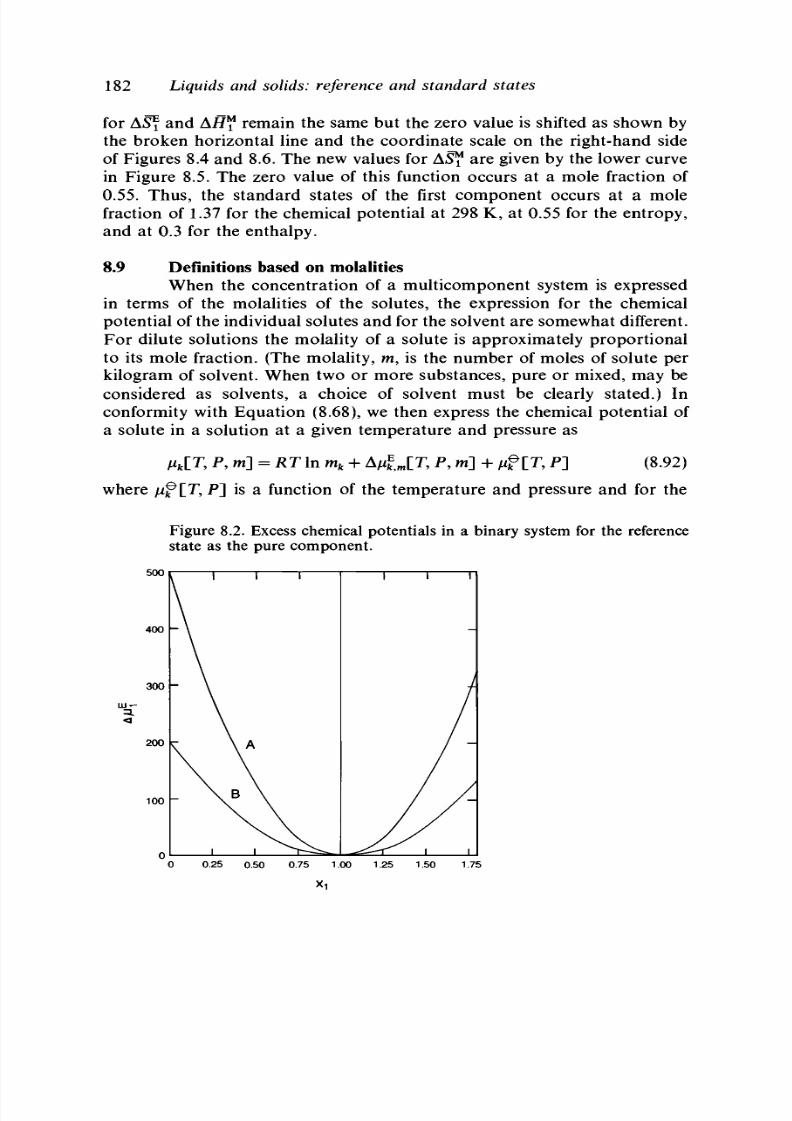
8/11/2019 Thermodynamics of Chemical Systems.pdf
http://slidepdf.com/reader/full/thermodynamics-of-chemical-systemspdf 202/456
182 Liquids and solids: reference and standard states
for ASf and AH™remain the same but the zero value is shifted as shown by
the broken horizontal line and the coordinate scale on the right-hand side
of Figures 8.4 and 8.6. The new values for
AS™
are given by the lower curve
in Figure 8.5. The zero value of this function occurs at a mole fraction of
0.55.
Thus, the standard states of the first component occurs at a mole
fraction of 1.37 for the chemical potential at 298 K, at 0.55 for the entropy,
and at 0.3 for the enthalpy.
8.9 Definitions based on molalities
When the concentration of a multicomponent system is expressed
in terms of the molalities of the solutes, the expression for the chemical
potential of the individual solutes and for the solvent are somewhat different.
For dilute solutions the molality of a solute is approximately proportional
to its mole fraction. (The molality, m, is the number of moles of solute per
kilogram of solvent. When two or more substances, pure or mixed, may be
considered as solvents, a choice of solvent must be clearly stated.) In
conformity with Equation (8.68), we then express the chemical potential of
a solute in a solution at a given temperature and pressure as
T,
P , m] = RT
In
m
k
+ A ^
t l l l
[r, P, m] + ^ f [ T , P ] (8.92)
where
iif[T,
P] is a function of the temperature and pressure and for the
Figure 8.2. Excess chemical potentials in a binary system for the reference
state as the pure component.
UJT -
<
ouu
400
300
200
100
n
<
I
\
\
I
I I
\ A
B \
i ^T-^^,
I I I
-
-
/ /
0 0.25 0.50 0 .75 1.00 1.25 1.50 1.75
X1

8/11/2019 Thermodynamics of Chemical Systems.pdf
http://slidepdf.com/reader/full/thermodynamics-of-chemical-systemspdf 203/456
8.9 Definitions based on molalities
183
present is undetermined otherwise. The excess quantity, A$
m
, is a function
of the molalities of all the solutes as well as the temperature and pressure.
It may alternatively be written as
RT
In
y
Km
.
The quantiy
y
Km
is called the
activity coefficient of the /cth component based on molalities. The subscript
m in both A^
m
and y
Km
is used to indicate that the quantities are expressed
in terms of the molality rather than the mole fraction. The symbol m in the
brackets represents the molalities of all of the solutes. The reference state
when molalities are used is usually taken to be the infinitely dilute solution
with respect to all solutes at every temp eratu re and pressure of interest. W ith
this definition A/i£
m
is defined to go to zero as all molalities go to zero at a
constant temperature and pressure. Alternately, the value of the activity
coefficient must go to unity as all molalities go to zero. In addition, the
values of all the temp eratu re a nd pressure derivatives of A/^
m
,
such as ASf
m
,
A/?k
m
, and AP£
m
,
ACf
km
,
mu st go to zero as all molalities go to zero. The
stan dar d states for the' chemical po tential, the entro py, a nd all the other
thermodynamic properties of the /cth solute are then determined. Thus, from
Figure 8.3. Chemical potentials of mixing in a binary system for reference
state as the pure component.
+500
0
-500
-1000
-1500
I I I
-
- / /
- / /
' I I I
I I I
-
i i r
0.25 0.50 0.75 1.00 1.25 1.50 1.75

8/11/2019 Thermodynamics of Chemical Systems.pdf
http://slidepdf.com/reader/full/thermodynamics-of-chemical-systemspdf 204/456
184 Liquids and solids: reference and standard states
Equation (8.92)
tflT, P ] = fi\T
9
P
9
rn< »]-RTIn m
fc
° °
(8.93)
where m
00
refers to the very small molalities of the solutes in the reference
state an d m£° to th e par ticu lar mo lality of the fcth solute in the reference
state. Similarly, for the entropy,
S f IT , P ] = S?[T, P , m
00
] + R In
(8.94)
These two equations are useful only to change from one reference state to
another. As described in Section 8.8 for mole fractions, the compositions of
the standard states of the fcth solute for the chemical potential and for the
entropy can only be determined by the solution of such equations as
RT
In
m
k
+ A//Jr
m
[T, P , m] = 0
(8.95)
and
- R In m
k
+ ASf
>m
[T, P , m] = 0 (8.96)
respectively. The standard states of the /cth solute for the other functions are
identical to the reference states as shown by the equations
HflT,
P ] = H?[T, P , m
00
] (8.97)
V?[T
9
P ] =
V?\T
9
P , m
00
] (8.98)
Figure 8.4. Excess entropy of mixing in a binary system.
1.75
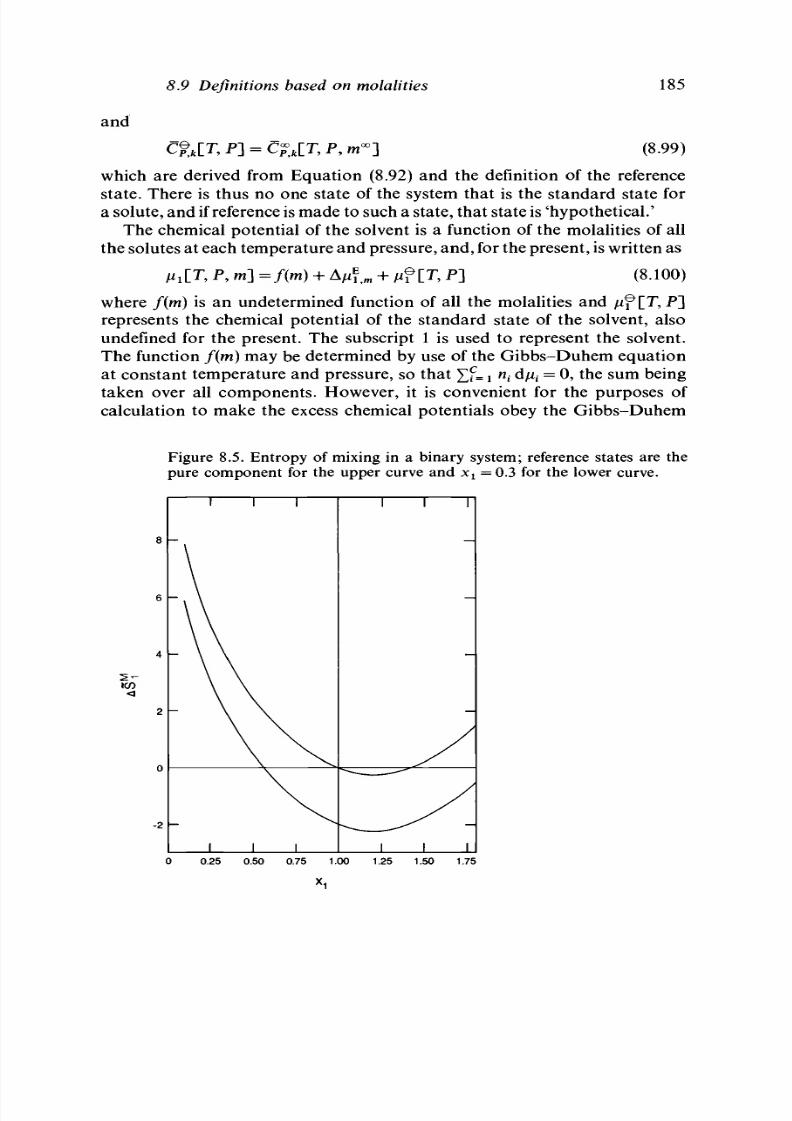
8/11/2019 Thermodynamics of Chemical Systems.pdf
http://slidepdf.com/reader/full/thermodynamics-of-chemical-systemspdf 205/456
8.9 Definitions based on molalities
185
and
(8.99)
which are derived from Equation (8.92) and the definition of the reference
state.
There is thus no one state of the system that is the standard state for
a solute, and if reference is made to such a state, that state is 'hypothetical.'
The chemical potential of the solvent is a function of the molalities of all
the solutes at each temperature and pressure, and, for the present,
is
written as
fi
x
lT
9
P, m]
=f(m)
+
+
/,
where
f(m)
is an undetermined function
represents the chemical potential of the
undefined for the present. The subscript
The function
f(m)
may be determined by
at constant temperature and pressure, so
taken over all components. However, it
calculation to make the excess chemical
[T,P] (8.100)
of all the molalities and
jaf [T,
P]
standard state of the solvent, also
1 is used to represent the solvent,
use of the Gibbs-Duhem equation
that
YA=
I
n
t
djUj = 0, the sum being
is convenient for the purposes of
potentials obey the Gibbs-Duhem
Figure 8.5. Entropy of mixing in a binary system; reference states are the
pure component for the upper curve and x
1
= 0.3 for the lower curve.
<
0.25 0.50 0.75 1.00 1.25 1.50 1.75
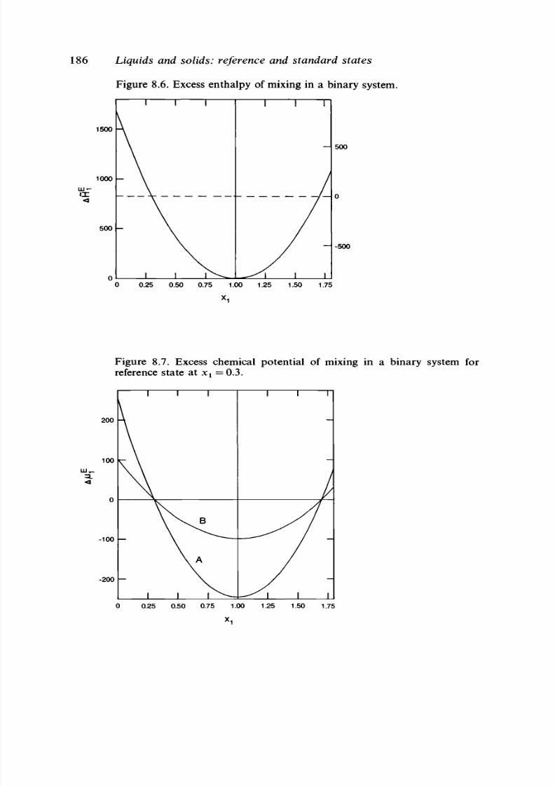
8/11/2019 Thermodynamics of Chemical Systems.pdf
http://slidepdf.com/reader/full/thermodynamics-of-chemical-systemspdf 206/456
186 Liquids and solids: reference and standard states
Figure
8.6.
Excess entha lpy
of
mixing
in a
binary system.
1500
1000
500
n
I I I
\
- \
- \
I I l ^ v ^
I I I
/
/ _
^x^ l | |
-
500
— 0
-
-500
0
0.25 0.50 0.75 1.00 1.25 1.50 1.75
Figure
8.7.
Excess chemical p otential
of
mixing
in a
binary system
for
reference state
at x
x
—
0.3.
200
100
100
200
I
I I
\
\
\
A
I
I I
-
-
1/
/
0.25
0.50 0.75 1.00 1.25 1.50 1.75

8/11/2019 Thermodynamics of Chemical Systems.pdf
http://slidepdf.com/reader/full/thermodynamics-of-chemical-systemspdf 207/456
8.9 Definitions based on molalities
187
equation, so that
Y A =
I
n
t
dA/xf = 0 at co nstan t tem pera ture and pressure.
When this condition is applied, we find that
n
1
df(m) + YJ
n
i
ii = 0
with the use of Equation (8.92), so that
C ri RT
However,
n
i
/n
1
=
m^Mi
and, therefore,
1000
(8.101)
Figure 8.8. Chemical potential of mixing in a binary system for reference
state at x
x
=0 .3 .
500
E^ 0
3 .
-500
-1000
-1500
I I I
-
-
, / ^
- B
_ ' /
I
I I
I
I I
-
-
I
I I
0 0.25 0.50 0.75 1.00 1.25 1.50 1.75
X
1

8/11/2019 Thermodynamics of Chemical Systems.pdf
http://slidepdf.com/reader/full/thermodynamics-of-chemical-systemspdf 208/456
188 Liquids and solids: reference and standard states
Then, on integration, we find that
where /( T , P ) is a function of the temp eratur e an d pre ssure. The comp lete
equation for the chemical potential of the solvent becomes
^ ^ ^ m, + Afil
m
+ ^ f
[T ,
P ] (8.102)
i = 2
1 UUU
When the infinitely dilute solution with respect to all solutes is chosen as
the reference state for the solvent, the first two terms on the right-hand side
of Equation (8.102) become zero at the reference state and
/ i f [ 7
1
, P ] = A i ' [ T , P , w
f l 0
] (8.103)
Thus, the standard state of the solvent is the pure solvent and is identical
to the reference state for the solvent in all of its therm ody nam ic prop erties.
8.10 Definitions based on molarities
Th e definitions b ased on m olarities, c, are very similar to those based
on molalities, and again the solvent must be considered separately from the
solutes. (The molarity is defined as the number of moles per liter of solution,
and is dependent on the pressure and temperature.) Molarities, like the
mo lalities, are used primarily for solution s for which the conce ntration ranges
are limited. For dilute solutions the molarities of the solutes are approximately
proportional to their mole fractions. We thus express the chemical potential
of the /cth solute in solution at a given temperature and pressure as
li
k
\T
9
P ,
c] = RT
In
c
k
+ AA£
C
[T, P ,
C]
+
fif
[T , P ] (8.104)
where A/ ^
c
may be written alternately as
RT
In
y
kc
.
The quantity
y
kc
is called
the activity coefficient of the /cth component in terms of molarity. The
subscript c in b oth Afi
kc
and y
kc
is used to indicate that these quantities are
expressed in terms of the molarity. In this equation c, in the brackets,
represents the set of values of the molarities of all the solutes and iif[T, P ]
is again undefined at present. The reference state is usually defined to be the
infinitely dilute solution for all solutes at all temperatures and pressures.
Thus , each A ^
c
is defined to go to zero as all molarities go to zero, and all
the temperature and pressure derivatives of each Aju{r
c
must go to zero under
these conditions. For the standard state for each solute we have the set of
equat ions
J"f
IT ,
P ] = j4k° [T, P , c
00
] - RT In c2° (8.105)
T, P ] = 5
fc
° ° [T, P , c
00
] + R In c
fc
° ° (8.106)

8/11/2019 Thermodynamics of Chemical Systems.pdf
http://slidepdf.com/reader/full/thermodynamics-of-chemical-systemspdf 209/456
8.10 Definitions based on molarities
189
H?[T, P ] = H
fc
° ° [T, P , c
00
] (8.107)
V?[T,
P] =
V?[T,
P, c
00
] (8.108)
and
C?,
k
[J, P ] = Cf t JT , P , c
00
] (8.109)
The first two of these equations are useful, in addition to showing that the
standard state of the feth solute for the chemical potential and the entropy
are determined, only in converting from one reference state to another. If it
is ever necessary, the composition of the standard state for the chemical
potential and the entropy would have to be determined by solution of
equations such as
RT In c
k
+ Ainl
c
= 0 (8.110)
and
-Rlnc
k
+ ASf
9C
= 0 (8.111)
when A/^
c
and AS*
>C
are kn ow n as functions of the m olarities of all of the
solutes. We see from Equations (8.107)-(8.109) that the standard states for
the volume, enthalpy, and heat capacity are identical to the reference state.
Thus, again
it is
better to speak of the sta nd ard state of
a
solute for the
various functions, rather than a single stand ard for the solute. Indeed, such
a single state is hypothetical.
For the solvent, we must again make use of the Gibbs-Duhem equation
to find a suitab le function of the m olarities of the so lutes. We set
^ [ T ,
P , c] =f(c) + A /^
C
[T , P , c] + / x
e
[T , P ] (8.112)
where f(c) represents a function of the m olarities of all of the so lutes. Th en ,
according to the G ibbs-Du hem equa tion at constant tempe rature and
pressure,
n
x
df(c)
+
RT
£ + £
Wl
.dA^
c
=
0
(8.113)
where the solvent is excluded in the first sum but is included in the second
sum. Then
df(c)=-RTY
j
n
±
d
^ (8.114)
when YJ = I
n
t
dAnf,
c
is set equ al to zero. T he num ber of moles of a given
solute in 1 liter of solution is c
i
and the num ber of moles of solvent is
(lOOOp —
YA = I
c
i^i)/^i^
where p is the density of the solution in un its of
g m l "
1
and M
t
and M
x
are the mo lecular masses of the solute and solvent,

8/11/2019 Thermodynamics of Chemical Systems.pdf
http://slidepdf.com/reader/full/thermodynamics-of-chemical-systemspdf 210/456
190 Liquids and solids: reference and standard states
respectively. Then
CiM
>
(8.115)
Wl
iooop-xf=
2
Integration of Equation (8.114) after substitution of Equation (8.115) cannot
be performed easily, because p is a function of the concentrations of the
solutes and is generally different for each system. However, for dilute solutions
lOOOp is large with respect to £f
=2
c
t
M
{
and p approximates p
l 5
the density
of the pure solvent. If these approximations are made, then
dc,
(8.116)
and
£ ^
i
I > ] (8.117)
The chemical potential of the solvent is then written as
£
Ci
+
Aii
E
UT
9
P
9
c-]+^lT
9
P^
(8.118)
The difference between the integral of Equation (8.114) and that of Equation
(8.116) is contained in the excess chemical potential, and consequently
XfL
t
n
i
dA/^
c
cannot strictly be zero and can only approximate zero
for dilute solutions. Thus, Equation (8.113), after substitution of Equation
(8.116), must always be used for the Gibbs-Duhem equation when molarities
are used for the composition variable.
When the infinitely dilute solution, with respect to all solutes, is used as
the reference state of the solution at all temperatures and pressures, A f
c
approaches zero as all c,s approach zero. Thus, the standard state of the
solvent is the pure solvent at all temperature and pressures and is identical
to the reference state of the solvent for all thermodynamic functions.
8.11 The osmotic coefficient
Another function, the
osmotic coefficient,
has been used in place of
the excess chemical potential or the activity coefficient. It is a multiplicative
factor rather than additive, and is defined in terms of the chemical potential
of the solvent. Two such functions are used, one based on molalities and
the other on molarities. The first is defined, except for its absolute value,
by
R
™
>
[_T,p-]
(8.119)

8/11/2019 Thermodynamics of Chemical Systems.pdf
http://slidepdf.com/reader/full/thermodynamics-of-chemical-systemspdf 211/456
8.12 The depend ence on temperature 191
and the other, except for its absolute value, by
/iilT,
P, c ]
=
-
R
^ ^
I
c, +
nflT,
F]
(8.120)
The definition is completed by assigning a value to </>
m
and
< \>
c
in some
reference state. To conform with the definitions made in Sections 8.9 and
8.10, the infinitely dilute solution with respect to all molalities or molarities
is usually used as the reference state at all temperatures and pressures, and
both
4>
m
and < j>
c
are made to approach unity as the sum of the molalities or
molarities of the solutes approaches zero. The standard state of the solvent
is again the pure solvent, and is identical to its reference state in all of its
thermodynamic functions.
8.12 The dependence
of
the
activity
and the
activity coefficient
on temperature
In this chapter we have introduced the four quantities, A/ijJ
1
, Ajuf,
a
k
,
and
y
k
.
The tem pera ture d ependen ce of these quan tities are easily ob tained
from their definitions. Thus,
(^F) =-(S
k
~Sf)= -ASf (8.121)
and with the relation that
we have
ASJ
1
=
-R
In a
k
-
RT(
d]
^
a
l j (8.122)
Moreover ,
fS(Afi
k
/T)\
=
- fj o
=
AlJ
M (8.123)
V d(l/T) )
P
,
n
and
(8.124)
dT J
P
,
n
RT
2
Similarly, when we differentiate A ^ with respect to the temp eratu re, we
obtain
(8.125)
P,n
If we use the alternate differentiation with respect to tem pera ture, we o btain
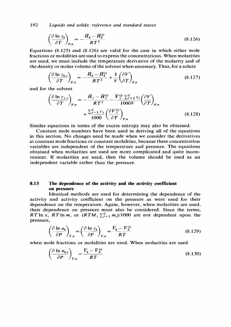
8/11/2019 Thermodynamics of Chemical Systems.pdf
http://slidepdf.com/reader/full/thermodynamics-of-chemical-systemspdf 212/456

8/11/2019 Thermodynamics of Chemical Systems.pdf
http://slidepdf.com/reader/full/thermodynamics-of-chemical-systemspdf 213/456
8.14 Conversion from one reference state to another
193
for both the solvent and solute, but
_V
k
-Vf 1 (dV\
8P J
T
,
n
RT V\dPj
T
,
n
for
a
solute and
( l f L
2
T
,n RT
1000
V ^ / r , n
1000
V dP J
T
,
n
(8.132)
for
the
solvent.
The
same com ments concerning
the
constancy
of the
concentration variables made
in
Section 8.12 are applica ble h ere.
8.14 Conversion from one reference state to another
Occasionally the prob lem arises of conve rting values of various
thermodynamic functions of the com ponents of a solution that have been
determined on the basis of one reference state to values based on another
reference state. To do so we equate the two relations of the thermodynamic
function of interest obtained for the tw o reference s tates , becau se the value
of the function at a given tempe rature, pressure, and com posit ion must be
the same irrespective
of
the reference state. W e also eq uate the relation
for
the thermodynamic function for the com ponent in the new reference state
expressed in terms of the new reference sta te to that for the same state
expressed in terms of the old reference state. The desired relation is obtained
when the chemical poten tials of the com ponent in the different sta nd ard
states are eliminated from the two equations. For examples, we use only the
chemical potentials and discuss three cases.
(A) Consider that the reference sta te of a component of a solution has
been chosen
to be the
pure compo nent
and it is
desired
to
change
to a
solution of a specific composition, the temperature and the pressure being
the same. Let mo le fractions be used to express the composit ion. For the
first reference state
T, P , x] = RT In x
k
+ A ^ . J T , P, x] + / / f [T , P, x
k
= 1] (8.133)
and for the second
H
k
lT, P,
x] =
RT In x
k
+ (ArfJIT, P,
x] +
nf [T,
P]
(8.134)
for any solution, where the prime indicates the values
of
A/if
x
based
on
the
new reference state. These two equations must be identical, and we have
AnlJLT, P, x] + nflT, P, x
k
= 1] = (AntJlT, P, x] + jtf [T, P]
(8.135)

8/11/2019 Thermodynamics of Chemical Systems.pdf
http://slidepdf.com/reader/full/thermodynamics-of-chemical-systemspdf 214/456
194
Liquids and solids: reference and standard states
A solution in which the mole fractions are given by a set of values, x*, is
chosen as the new reference state. Then the chemical potential of the /cth
component
is
expressed
as
/z*[T, P, x*] =
RT
In x* + tflT, P] (8.136)
at the composition of the new reference state whereas, based on the old
reference state, it is expressed as
lit\T
9
P, x*] = RT In x
k
* + A/iJUT, P, x*] +
M
f[T, P, x
k
= 1]
(8.137)
where Aju^
X
[T , P, x*] is the excess chemical potential of the /cth component
in
a
solution having mole fractions
x*
when
the
reference state
is the
pure
substance. These two equations must be identical, therefore
AftUT, P, *•] + fif IT, P, x
k
= 1] = /if [T, P] (8.138)
On substitution of this equation into Equation (8.135), we obtain
A^
X
[T,
P, x] =
(AfiJIT,
P, x] + AfiJiT, P, x*] (8.139)
or
(AtfJlT,
P, x]
=
A J IE JT ,
P ,
x]
-
AnlJLT,
P ,
x*]
(8.140)
This becomes
yi . , = Wvf.x (8-141)
in terms of the activity coefficients (Eq. (8.73)). The relation for the activities is
(8.142)
The particular conversion is discussed in Section 11.8 and illustrated in
Figures 8.1 and 8.6. It is seen from Equation (8.140) that the conversion in
terms
of
the excess chemical potentials
is
simply the shifting
of
the zero point
as illustrated in the two
figures.
(B) As a second example, suppose that the original reference state of the
/cth component, considered as a solute, is the pure substance and that mole
fractions are used as the composition variable. It is then desired to make
the infinitely dilute solution the reference state and to use the molality for
the composition variable. Here, again, we express the chemical potential of
the /cth component in the two equivalent ways:
T,
P, x] = RT
In
x
k
+
AnlJLT,
P, x] + fif
[T ,
P, x
k
= 1]
(8.143)
and
li
k
\T
9
P, m] =
RT
In
m
k
+ A/£
m
[T,
P, nt\
+ ^ [ T , P] (8.144)

8/11/2019 Thermodynamics of Chemical Systems.pdf
http://slidepdf.com/reader/full/thermodynamics-of-chemical-systemspdf 215/456
8.14 Conversion from
one
reference state
to
another
195
so
RT In x
k
+ A/x
E
x
[T, P , x] + / if [T, P , x
fc
= 1] = R T In m
fe
+ A/i
E
m
+ / i f [ T ,P ] (8.145)
The second reference state yields the two equations
/i*[T, P, m*] = R T In m* + /if [T, P ] (8.146)
and
/i*[T, P , x*] = RT In x* + A/i
fe
E
x
[r, P , x*] + /if [T, P , x
k
= 1]
(8.147)
where x£ is the mole fraction of the component corresponding to the molality
m*. Therefore
RT In x
fc
* + A ^
X
*[T , P, x*] + ^ f [T, P , x
k
= 1] = KT In m?
+ / /f [ T ,P ] (8.148)
When the constant terms are eliminated from Equations (8.145) and (8.148),
the resultant equation is
RT
In
^ + A/i
E
x
[T, P, x] - A /if /[T , P, x*] =
+ A/i
E
,
m
[T,P,m] (8.149)
or
A/i
E
m
[T, P, m] = A/i
E
x
[T, P, x] - A/i
E
x
[T, P, x*] +
m
(8.150)
However,
and, because each mf is very small with respect to
(8.152)
1OOO/M
X
F u r t h e r m o r e ,
1000 / /1000
< 8
-
1 5 3 )

8/11/2019 Thermodynamics of Chemical Systems.pdf
http://slidepdf.com/reader/full/thermodynamics-of-chemical-systemspdf 216/456

8/11/2019 Thermodynamics of Chemical Systems.pdf
http://slidepdf.com/reader/full/thermodynamics-of-chemical-systemspdf 217/456
8.15 Reference and standard states for species 197
On elimination of the constant terms,
A ^
t C
[T , P , c ] = A ^,
m
[T, P,m] + RT ln(m
k
c*/m
fc
*c
fc
) (8.160)
However ,
c
t
= ^ ^ (8-161)
100 0+ £f= 2 M ^ -
(8.162)
onsequently,
T,
P,
c]
= A t f J T . P,»] +
JIT In ( * « » £
T , P, c] = AtfJ T . P ,»] + JIT In ( * «»+ £ •» M ^ )
( 8
.
1 6 3 )
This equation in terms of the activity coefficients is
8.15 Reference and standard states for species
In the previous sections concerning reference and standard states we
have developed expressions for the thermodynamic functions in terms of the
components of the solution. The equations derived and the definitions of the
reference an d s tan da rd states for co m pon ents are the same in terms of species
when reactions take place in the system so that other species, in addition to
the components, are present. Experimental studies of such systems and the
thermodynamic treatment of the data in terms of the components yield the
values of the excess thermodynamic quantities as functions of the temperature,
pressure, and composition variables. However, no information is obtained
concerning the equilibrium constants for the chemical reactions, and no
correlations of the observed quantities with theoretical concepts are possible.
Such information can be obtained and correlations made when the thermo-
dynamic functions are expressed in terms of the species actually present or
assumed to be present. The methods that are used are discussed in Chapter
11 .
He re, general relations concern ing the expressions for the therm ody nam ic
functions in terms of species and certain problems concerning the reference
states are discussed.
When the state of a system is defined by assigning values to the necessary
independent variables, the values of all of the thermodynamic functions are
fixed. For a single-phase, multicomponent system the independent variables
are usually the tem perature , pressure, and mole num bers of the com ponen ts.
The Gibbs energy of such a system at a given temperature and pressure is
additive in the chemical potentials of the components by Equation (5.62),

8/11/2019 Thermodynamics of Chemical Systems.pdf
http://slidepdf.com/reader/full/thermodynamics-of-chemical-systemspdf 218/456
198 Liquids and solids: reference and standard states
but, by the same arguments used to obtain Equation (5.62), we can show
that the Gibbs energy is also additive in the chemical potentials of the species.
Thus, for a given state of the system we can write
i=l 7 = 1
where the unprimed quantities refer to components and the primed quantities
refer to species.
2
The sums are to be carried over all of the components i
and all of the species
j .
We can show from this equation that the chemical
potential of a given compound is the same whether we consider it as a
component or as a species. As an example, we consider a four-component
system in which three of the co m pon ents react to form a new species, resulting
in a system containing five species. Equation (8.165) becomes
G = n
1
jx
1
+ n
2
fi
2
+ ^ 3 + n
5
fi
5
(8.166)
(8.167)
where the subscript 4 represents the new species.
If we let the chemical reaction be represented as
v
l
B + v
2
B
2
= v
3
B
3
+ v
4
B
4
then, by mass balance
n\ = n
1
— (v
i
/v
4
)n
f
4
.
n'i = n
2
-
(v
2
/v
4
)n
4
a n d
w'a =
n
3 + (V3/V4K
When this set of equations is substituted into Equation (8.167), we obtain
(
v
3
v
2
v±
4
v
4
3
v
4
2
v
4
but
v
4
v
4
v
4
X
according to the condition of chemical equilibrium. Also, n
5
must equal n'
5
,
so
G =
2
The m olar G ibbs energy of a system based on c om pone nts need not be the same as that based
on species, because the total number of moles in the system based on components need not be
the same as that based on species.

8/11/2019 Thermodynamics of Chemical Systems.pdf
http://slidepdf.com/reader/full/thermodynamics-of-chemical-systemspdf 219/456
8.15 Reference and standard states for species 199
For this equation to equal Equation (8.166), the chemical potential of a
substanc e considered as a species mu st be identical to the chem ical poten tials
of the same substance considered as a component. We must emphasize that
the chemical potential of the component and that of the species must refer
to the same mass of the substance.
When the same substance may be taken either as a component or as a
species, we can write, in terms of mole fractions,
li
k
=
RT In x
k
+ Afil
x
+
n?=RT In x
k
+ {AtfJ + (fif)' (8.168)
There are four undetermined quantit ies A/^
x
, (A/^ J ' , pf, an d Gujp)' an d
two equations. We must, therefore, define two of the four quantities, which
in turn determines the other two quantities and the relationship between
them. We can define the reference states for the component and the species.
The difference between the standard chemical potential of the component
and that of the species is then expressed in terms of the mole fractions in
the reference state. The problem is the determination of this difference. The
different species may be known from our knowledge of the chemical system,
or they may be assumed. However, a definite decision must be made
concerning the species, and all calculations must be carried out based upon
this decision. Several examples concerning reference and standard states are
discussed here and in the following sections.
The simplest case is one in which we can use the pure substance as the
reference state for both the component and the species. If, then, the pure
substance consists entirely of the same molecular entity and this entity is
taken as the com po nen t and the species, the stand ard states for the com pon ent
and the species are identical. Equation (8.168) becomes
RT In x
k
+ Anl = RT In x'
k
+ (A/**)' (8.169)
This case is applicable when the components of the system are simple
substances that react to form new species in solution.
Fo r the second case the com pon ent m ay actually be a solution of polymeric
entities of some monomer. As a simple example we consider that only
monomers and dimers exist, so that we have the equilibrium, 2B = B
2
. When
we choose the unit mass for the chemical potential of the component to be
equal to the molecular mass of the monomer, we have
^ = /4 = i/4
(8-170)
where the subscripts M and D refer to the monomer and the dimer,
respectively. The second equality arises from the condition of chemical
equilibriu m. W hen we use only the first equa lity, Equ ation (8.168) becomes
' + ii$ (8.171)
We choose the reference state for the component to be the pure component

8/11/2019 Thermodynamics of Chemical Systems.pdf
http://slidepdf.com/reader/full/thermodynamics-of-chemical-systemspdf 220/456
200 Liquids and solids: reference and standard states
and the reference state for the monomer to be the pure monomer. The
standard state of the component is then the pure component in the same
state of aggregation as the solution, whereas th at of the m ono m er is a fictitious
substance in the same state of aggregation as the solution but containing
only monomeric entities. The problem is to find a relationship between the
standard chemical potentials of the component and of the species. We do
so by recognizing that the pure component is also a solution of monomers
and dimers. Again, the chemical potential of the pure component based on
the molecular mass of the monomer must be equal to the chemical potential
of the monomer in the pure component. Thus,
/ i f
[T ,
P , x
k
= 1] =
AI*[T,
P , x*] = RT In x* + (A /4)* + ^ (8.172)
where the asterisk is used here to designate quantities applicable to the
mo nom er in the pure com ponen t. When Equ ation (8.172) is substi tuted into
Equation (8.171), we obtain
RT
In
x
k
+
Atf
=
RT
ln(x
M
/x*) + [A /4 - (A /4)*] (8.173)
where
x&
is the mole fraction of the mo nom er in the pure com pon ent and
(A/4)* is the excess chemical potential of monomer in the pure component.
In general (A/4)* cannot be evaluated, but it is only the difference
[ A / 4
—
(A/4)*] with which we are concerned. The arguments are similar if
we use the second equality in Equation (8.170) so that /i
fc
=
^fi'
D
or if we use
the molecular mass of the dimer as the mass unit for the chemical potential
of the component so that fi
k
= fi'
D
= 2 / 4 -
The problems of the reference and standard states are slightly different
when we use the infinitely dilute so lution of all solutes as the reference states .
When we take the reference state of both the component and the species as
the infinitely dilute solution, Equation (8.168) becomes
^ e _ e>
=
RT
i
n
(
x
£)* _ RT In x* (8.174)
where the asterisks again refer to the reference states. The problem is the
evaluation of the difference of the two standard chemical potentials. When
there is only one molecular entity that can be associated with the component,
the ratio of the mole fraction of the species to that of the component must
approach unity as the mole fraction of the component approaches zero. In
such a case the two standard chemical potentials are equal and Equation
(8.168) becomes
RT In x
k
+ Afif = RT In x '
k
+ (A /^) ' (8.175)
This case applies to the systems in which the components react together to
form new species.
A different problem is met when the component is polymerized. Again,
we take the case in which the com pon ent exists in solution in both mo nom eric

8/11/2019 Thermodynamics of Chemical Systems.pdf
http://slidepdf.com/reader/full/thermodynamics-of-chemical-systemspdf 221/456
8.16 Solutions of strong electrolytes 201
and dimeric forms so that the equilibrium IB = B
2
exists. As the mo le fraction
of the com pon ent is decreased, the equilibrium shifts to the m ono m eric form.
If we choose the unit of mass for the chemical potential of the component
to be the molecular mass of the dimer, the ratio of (x'
D
)*/x% approaches zero
as xjf goes to zero; that is, no dimer exists in the infinitely dilute solution.
Under such conditions the difference between the values of the two standard
chemical potentials (Eq. (8.174)) goes to —oo. To avoid such an infinity, we
choose the unit of mass for the chemical potential of the component to be
the molecular mass of the monomer. The ratio (x'
M
)*/x% then approaches
unity as xj approaches zero and the two standard chemical potentials are
identical. Equation (8.168) reduces to Equation (8.175) for this case. This
result is quite general and , whenever a comp one nt can un dergo a n asso ciation
or dissociation in solution, the basis for the chemical potential of the
component must be the simplest molecular entity that the component exhibits
in solution.
8.16 Solutions of strong electrolytes
Solutions of electrolytes form a class of thermodynamic systems for
which the concept of species is all-important. In this section we discuss the
problems of reference and standard states for strong electrolytes as solutes
dissolved in some solvent.
We consider an electrolyte having the general formula M
v +
A
v
, where v
+
and v_ represent the number of positive and negative ions, respectively,
formed from one molecule of the electrolyte. The only species present in
solution, based on the concepts of strong electrolytes, are stipulated to be
the ions M
+
and A_. The symbols M
+
and A_ are used to represent the
ions without reference to the actual charge. Under this condition we cannot
equate the chemical potential of the component to the chemical potential of
the nonionized species. Th e required relation is obtain ed by the same m ethod s
used in Section 8.15. If we consider a binary system having
n
1
moles of
solvent and n
2
moles of solute, the Gibbs energy is given by
G = n
l
fi
1
+ n
2
\i
2
(8.176)
We also have
G = n
1
fi
1
+ n
+
n
+
+ n_fi_ (8.177)
in terms of the species. For the general electrolyte that we are considering,
n
+
= v
+
n
2
and n_ = v_ n
2
. On substituting these relations into Equation
(8.177) and equating Equations (8.176) and (8.177), we find that
/z
2
= v
+
/ *
+
+v_^_ (8.178)
Equation (8.178) is the basic equation that is needed, and is applicable to
all solutes that are assumed to be strong electrolytes.

8/11/2019 Thermodynamics of Chemical Systems.pdf
http://slidepdf.com/reader/full/thermodynamics-of-chemical-systemspdf 222/456
202 Liquids and solids: reference and standard states
We recognize that we cannot determine experimentally the thermo-
dynamic properties of a single type of ion in solution, because both positive
and negative ions must be present to satisfy the condition of electrical
neutrality. However, we can use equations based on those previously derived,
and express the chemical potential of a single type of ion in terms of the
concentration variables at a given temperature and pressure. We follow
convention here and use molalities and activity coefficients. Then we
have
jK
+
|T, P, m] = RT In m
+
+ RT In y
+
[T, P, m] + ^ [ T , P] (8.179)
and
H_[T, P, m] = RT In m_ + RT In y_[T, P, m] + /^[T , P] (8.180)
When we substitute these two equations into Equation (8.178), we obtain
^
2
[T, P, m] = RT In m\
+
m
v
s + RT
In
y\
+
y
v
s[T, P, m]
+ v
+
^ [ T , P] + v_/^[T, P] (8.181)
The mean activity coefficient is defined as
v
v
±
=yV7
v
- (8.182)
and the mean molality as
m
v
±
=m\
+
m
v
_-
(8.183)
where
v
=
v +
+ v_. Equation (8.181) can then be written as
li
2
[T
9
P, m] =
vRT
In
m
±
+ vflT In
y
±
[T, P, m] + v
+
/i?|T, P]
H-v_^[T,P] (8.184)
The reference state of the electrolyte can now be defined in terms of thi
I
equation. We use the infinitely dilute solution of the component in the solvent
and let the mean activity coefficient go to unity as the molality or mean
molality goes to zero. This definition fixes the standard state of the solute
on the basis of Equation (8.184). We find later in this section that it is neither
profitable nor convenient to express the chemical potential of the component
in terms of its molality and activity. Moreover, we are not able to separate
the individual quantities, and //? . Consequently, we arbitrarily define
the standard chemical potential of the component by
Ai
e
[7,
P] = v
+
/i ?[r, P] + v _^ [ T , P] (8.185)
With this definition, Equations (8.181) and (8.184) can be written as
//
2
[T, P, m] = RT In m\
+
m
v
s + vRT In
y+
[T, P, m] + /if IT, P]
(8.186)

8/11/2019 Thermodynamics of Chemical Systems.pdf
http://slidepdf.com/reader/full/thermodynamics-of-chemical-systemspdf 223/456
8.16 Solutions of strong electrolytes
203
or
/x
2
[T , P , m] = vRT In
m+
+ vR T In y
±
[T, P,
rri]
+ / z
e
[ T , P ] (8.187)
These equations are used whenever we need an expression for the chemical
potential of a strong electrolyte in solution. We have based the development
only on a binary system. The equations are exactly the same when several
strong electrolytes are present as solutes. In such cases the chemical po tential
of a given solute is a function of the molalities of all solutes through the
mean activity coefficients. In general the reference state is defined as the
solu tion in which the m olality of all solutes is infinitesimally sma ll. In special
cases a mixed solvent consisting of the pure solvent and one or more solutes
at a fixed molality may be used. The reference state in such cases is the
infinitely dilute solution of all solutes except those whose concentrations are
kept constant. Again, when two or more substances, pure or mixed, may
be considered as solvents, a choice of solvent must be made and clearly
stated.
It is useful to review the problems when we express the chemical potential
of the solute in terms of its molality and activity coefficient as well as by
Equation (8.181). When we do so, we obtain
\i
2
= RT
In m
2
+
RT
In y
2
+ M? =
RT l n
mini's
+
vRT
In
y
±
If we define the reference state for both y
2
and y
±
as the infinitely d ilute
solution, we have
m
2
for the reference state. The ratio of the molalities in the reference state is
zero, and co nsequen tly the difference between / i
e
and
( V + / J ^
+
V_JU1?)
is
— oo. When we define the reference state as the infinitely dilute solution for
y+ and use Equation (8.185), we obtain
m
2
so that yf is zero rather than unity in the reference state. It is for these
reasons that we do not use y
2
, the activity coefficient of the component when
the com po ne nt is a strong electro lyte. T hu s, the activity coefficient of a stro ng
electrolyte taken as a component in solution remains undefined.
The situation with the activities is different. When we use Equation (8.74)
for the component and the separate ions, we have
fi
2
= RT\n a
2
+ jif = RT ln a\
+
a
v
s + v
+ i
u ? + v_/n®

8/11/2019 Thermodynamics of Chemical Systems.pdf
http://slidepdf.com/reader/full/thermodynamics-of-chemical-systemspdf 224/456
204 Liquids and solids: reference and standard states
We
can
define
the
mean activity
as
a\=a\
+
a
v
s
(8.188)
Then, with
the
definition
of the
standard chemical potentials given
in
Equation (8.185),
a
2
= a\ =a\
+
a
v
s
(8.189)
8.17 Solutions
of
weak electrolytes
The methods
for
obtaining expressions
for
the chemical potential of
a component that
is a
weak electrolyte
in
solution
are the
same
as
those
used for strong electrolutes. For illustration we choose
a
binary system whose
components are
a
weak electrolyte represented
by
the formula M
2
A and
the
solvent.
We
assume that
the
species
are
M
+
, MA",
A
2
" , and
M
2
A.
We
further assume that the species are
in
equilibrium with each other according
to
(8.190)
and
M A - = M
+
+ A
2
- (8.191)
The first problem
is to
obtain relations between
the
chemical potential
of
the component
and
those
of the
species.
The
Gibbs energy
of a
solution
containing n
x
moles
of
solvent
and
n
2
moles
of
solute
is
given
by
G
=
n
1
/i
1
+
n
2
^
2
(8.192)
In terms of the species, we have
G
= n
l
^i
1
+ n
M+
fi
M+
+
n
MA
-n
MA
-
+ n
A2
-n
A
i- +
n
UlA
^
UlA
(8.193)
Neither the mole numbers of the species nor their chemical potentials are
all independent,
but are
subject
to the
condition
of
mass balance
the condition
of
electroneutrality
"M + =n
UA
- +2n
A2
-
and
the
two conditions
of
chemical equilibrium
/ % + + M M A - - / ' M
2
A = 0 (8.194)
and
= 0 (8.195)
When these four condition equations
are
used
in
Equation (8.193)
to
make
all
of
the remaining mole numbers and chemical potentials independent, we

8/11/2019 Thermodynamics of Chemical Systems.pdf
http://slidepdf.com/reader/full/thermodynamics-of-chemical-systemspdf 225/456
8.18 Mixtures of molten salts 205
obtain one of the following three equations:
/^2 = /^M
2
A (8.196)
i"2 = / % + + / W - (8.197)
or
(8.198)
dep end ing o n which va riables are elimin ated. G iven on e of Eq ua tio ns (8.196)—
(8.198), the other two can be obtained by use of Equations (8.194) and
(8.195). Thus, the three equations are equivalent. When we express the
chemical potential of each of the species in terms of its molality and activity
coefficient, we obtain
li
2
= RT In m
M2A
+ RT In y
M2A
+
fig
A
(8.199)
li
2
= RT In m
M+
m
MA
- + RT In 7
M +
7 M A - + / ^ + + l4L- (8.200)
and
fi
2
= RT In m^m^- + RT In y
2
u+
y
A
2- + 2 /i
M+
+ / j§
2
. (8.201)
We define the reference state as the infinitely dilute solution of the component
in the solvent, so that y
M2A
,
7M
+
7 M A >
a n
d
7 M
+
7 A
2
-
a
U 8 ° *
o
unity as
m
2
goes
to zero. This definition fixes the values of the quantities /x^
2A
,
(JI$+
+ A*MA-)>
and ( 2 / ^ + + / ^ - ) according to Equat ions (8.199), (8.200) , and (8.201),
respectively.
The quant i ty , fi§
2A 9
represents the chemical potential of the undissociated
species M
2
A in i ts standard state, and not that of the component. The other
standard-state quantities represent the chemical potential of the designated
species in their standard states, but, for the present, we cannot separate the
two standard chemical potentials from the sums, neither is it important to
do so. The standard-state quantities appearing in Equations (8.199)—8.201)
are not all independent, because the three equations are equivalent. If we
equate Equations (8.199) and (8.200), we obtain an expression that can be
evaluated experimentally for the quantity (fi§
+
+ fi§
A
- —
f i§
2A
).
Similarly, we
obtain an expression that can be evaluated experimentally for the quantity
(2/4^+
+
fif
2
- —
JJM
2
A)
when we equate Equations (81.99) and (8.201). These
last two quantities are related to the equilibrium constants for the chemical
reaction s. This relation is developed in Cha pp ter 11 and the basic experimental
methods are discussed in Chapters 10 and 11.
8.18 Mixtures of molten salts
Salts,
when in the liquid sta te, con tinue to exhibit the ionic p roperties
of the solid state. It is therefore advantageous to consider the pure molten
salts and mixtures of molten salts as systems composed of ionic species, and

8/11/2019 Thermodynamics of Chemical Systems.pdf
http://slidepdf.com/reader/full/thermodynamics-of-chemical-systemspdf 226/456
206
Liquids and solids: reference and standard states
to express the thermodynamic functions in terms of the concentrations of
the ionic species and their excess chemical potentials. The methods are very
similar to those used in the previous few sections. We consider separately
systems that are completely dissociated into the simplest ions and those that
may have complex ions.
For the first case we consider a salt having the general formula M
v+
A
v
_
and assume that the only species are M+ ions and A_ ions. The chemical
potential of the component can be expressed as
/i
k
= v
+
/i
+
+v_/i_ (8.202)
in terms of the chemical potentials of the ions. This relation is obtained by
the use of the methods used previously. Before proceeding, however, we must
choose the composition variables that we wish to use. We choose mole
fractions, because of the lack of a solvent and because many molten salt
mixtures can be studied over the whole range of concentration. In studying
thermodynamic properties of mixtures, we wish to interpret the excess
chemical potentials as deviations from some ideal or theoretical behavior.
Such considerations, which are beyond the scope of this book, indicate that
positive-ion fractions and negative-ion fractions are appropriate for the
mixtures discussed in this section. (Other composition variables can be used,
and the decision concerning which variables to use is an individual choice.)
The positive-ion fraction of a given positive ionic species is defined as the
number of moles of the given species divided by the total number of moles
of positively charged ionic species contained in the system. The
negative-ion
fraction is defined in the same way for the negatively charged species. We
then write for the chemical potential of the M + species
H
+
= RT In x
+
+ A/4 + /*? (8.203)
and a similar expression for the A_ species:
H
k
= v+RTlnx
+
+ v_RT\nx_ -hv+A/4 +v_A/x*i + v
+
/4
>
+ v_/^
>
(8.204)
We choose the pure component to be the reference state for the compound,
and therefore also the standard state. We choose the reference state of the
M
+
species to be a fictitious system that contains only M
+
molecular entities
and the reference state of
A _
species to be a fictitious system containing only
A_ molecular entities according to Equation (8.203). The symbols,
i$
+
and
fif_
then represent the chemical potentials of the M+ and A_ species,
respectively, in their standard state—he fictitious systems. However, the
pure component is also a mixture of
the
two ions and, according to Equations
(8.202) and (8.203), we have
/if = v
+
/it+v_/i* (8.205)

8/11/2019 Thermodynamics of Chemical Systems.pdf
http://slidepdf.com/reader/full/thermodynamics-of-chemical-systemspdf 227/456
8.18 Mixtures of molten salts 207
fi? = v
+
RTIn x* + v.RTln x* + v
+
(A/z
E
)* + v_(A/*
E
)*
+ v
+
/i ? + v_ /i? (8.206)
where the asterisks refer to the indicated quantities in the pure liquid
component. Actually both x&
+
and
x%_
are unity because only one positive
ionic species and o ne negative ionic species are present in the pure com pon ent.
Elimination of (v
+i
u§
+
+ v_fif_) from E qu atio ns (8.204) an d (8.206) yields
f
k
+
+
+
v_
J
RTlnx_
+ {v
+
[A ^
E
- (A^
E
)*] + v_ [A/*
E
_ - (A/x
E
_ )*]} +
ii f
(8.207)
None of the individual quantities within the brackets can be evaluated,
neither can the two differences. It is therefore convenient to define the excess
chemical potential of the component as the quantity within the brackets, so
that finally
x
+
+ v _ i m n x _ + A/z
E
+ /ijp (8.208)
Some salts may not dissociate completely into the simplest ion, so some
more complex ions are present in solution. For illustrative purposes we
choose a salt having the formula M
2
A, and assume that the species are M
+
,
MA" , and A
2
~. The derivation of the equations for the chemical potential
of the component follows the methods used before. We first have
^ = / * M + + / W - (8.209)
or
(8.210)
Equations similar to Equation (8.203) are written for the chemical potentials
of the ionic species. We take the pure liquid component as the reference
state, and hence the standard state for the component, and express the
chemical potential of the component in terms of the chemical potentials of
the ionic species to obtain equations similar to Equation (8.206). In this
particular case x^
+
is unity but both x^
A
- and x%
2
- have fixed values whose
sum m ust be unity. Finally, with app rop riate definitions of the excess chemical
potentials, we obtain either
li
k
= RT\n x
M +
+ K T l n ( x
M A
- / x *
A
-) + A/i
E
+ fif (8.211)
or
j
u
fc
= 2 ^ T l n x
M +
+ K T l n ( x
A 2
- / ^
2
-) + (A/i
E
y + ^ (8.212)
The two quantit ies A^
E
and (A/i
E
) ' are not equal, but are related by the
two equat ions.

8/11/2019 Thermodynamics of Chemical Systems.pdf
http://slidepdf.com/reader/full/thermodynamics-of-chemical-systemspdf 228/456
208
Liquids and solids: reference and standard states
Throughout the discussions in Sections 8.15-8.18, we have emphasized
methods for obtaining expressions for the chemical potential of a component
when we choose to treat the thermodynamic systems in terms of the species
tha t ma y be present in solution . A com plete presen tation of all possible types
of systems containing charged or neutral molecular entities is not possible.
However, no matter how complicated the system is, the pertinent equations
can always be developed by the use of the methods developed here, together
with the careful definition of reference states or standard states. We should
also recall at this point that it is the quantity Gu
fc
—xjp) tha t is d ete rm ined
directly or indirectly from experiment.

8/11/2019 Thermodynamics of Chemical Systems.pdf
http://slidepdf.com/reader/full/thermodynamics-of-chemical-systemspdf 229/456
9
Thermochemistry
Thermochemistry is concerned with the determination of the heat
absorbed by a system when some process occurs within the system. The
quantity of heat absorbed may be determined experimentally by the use of
calorimeters or by calculation from prior knowledge of the thermodynamic
properties of the system. The equations relating the heat absorbed by a
system for a given process to the change of energy or enthalpy of the system
for the change of state that occurs during the process are the mathematical
statements of the first law of thermodynamics. They are Equations (2.26)
and (2.30), written here as
dQ = dE +
PdV-dW
(9.1)
and
dQ = dH-VdP-&W (9.2)
In the use of these equations, care must be taken to define the system and
its surrounding s in order to assure the prop er interpretation of both the heat
absorbed and the work done by the system. The equations in their integral
form may be interpreted in two ways: the quantity of heat absorbed by the
system may be measured calorimetrically, from which either the change of
energy or the change of enthalpy for the change of state that takes place is
calculated by use of Equations (9.1) or (9.2) or, conversely, the quantity of
heat absorbed by the system for a given process may be calculated from
prior knowledge of the change of energy or enthalpy for the change of state
that takes place.
Because of the close relationship between the quantity of heat absorbed
by a system for a given process and the accompanying change of energy
or enthalpy for the change of state that takes place, the concept of
thermochemistry has been extended to include studies of the changes of
enthalpy or of energy for changes of state of thermodynamic systems without
reference to heat. This chapter is concerned primarily with this extended

8/11/2019 Thermodynamics of Chemical Systems.pdf
http://slidepdf.com/reader/full/thermodynamics-of-chemical-systemspdf 230/456
210
Thermochemistry
concept of therm och em istry. Pro blem s associated with the change of enthalpy
for various types of changes of state are discussed. The enthalpy is used in
preference to the energy, because of the convenience of using the pressure
rather than the volume as an experimental variable. The methods developed
for the enthalpy are also applicable to the energy.
Several subjects that might be considered under the title of thermo-
chemistry are discussed in previous chapters. Such subjects are the heat
capacities of a single-phase system, the dependence of the enthalpy of a
single-phase system on temperature and pressure, and the dependence of the
enthalpy of a one-com ponen t, multiphase system on the temp erature, volume,
and mole numbers. Here we are concerned with heat capacities of multiphase
systems, with changes of enthalpy for the formation of a solution and for a
change of concentration of the solution, and with changes of enthalpy of
systems in which chemical reactions occur. First the basic concepts of
calorimetry are reviewed.
9.1 Basic concepts of calorimetry
We may classify all calorimeters into two groups when we limit the
processes to those that involve only the work of expansion or compression:
those that operate at constant volume and those that operate at constant
pressure. The application of Equation (9.1) to constant-volume calorimeters
shows that the heat absorbed by the system equals the change of energy of
the system for the change of state that takes place in the system. Similarly,
the heat absorbed by the system in constant-pressure calorimeters is equal to
the change of enthalpy for the change of state that takes place in the system
according to Equation (9.2).
We must define the system and determine the initial and final states of
the system very carefully. Although our interest may be the change of energy
or enthalpy of a system comprising only the chemical substances undergoing
a given change of state, even then the therm ody nam ic system may be defined
in at least two ways. We may consider the chemical substances whose
properties we wish to determine as the thermodynamic system. Then the
container and all other parts of the calorimeter are considered as the
surroundings. Alternately, we may consider the chemical substances and all
the other parts of the calorimeter as the thermodynamic system. In either
case the heat absorbed by or the work done on the thermodynamic system
across the boundary is the quantity that is measured experimentally. This
heat or work is equal to the change of energy or the change of enthalpy, as
the case may be, of the thermodynamic system. If the chemical system is
identical to the thermodynamic system, of course the change of energy or
enthalpy of the chemical system must be equal to that of the thermodynamic
system. When the container and other parts of the calorimeter are considered
to be parts of the thermodynamic system in addition to the chemical system,

8/11/2019 Thermodynamics of Chemical Systems.pdf
http://slidepdf.com/reader/full/thermodynamics-of-chemical-systemspdf 231/456
9.1 Basic concepts of calorimetry 211
the change of energy or enthalpy of the thermodynamic system is equal to
the sum of the changes of the individual parts of the system. In order to
determine the changes of energy or en thalpy of the chemical system, we mu st
determine the changes of the other parts of the thermodynamic system.
Finally, one small correction m ay arise in constant-vo lum e calorime ters when
the thermodynamic system includes parts of the calorimeter as well as the
chemical system. In this case the volume of the thermodynamic system is
kept constant, but the volume of the various parts of the system might
change. Then corrections have to be ma de according to Eq uation (9.1). Such
corrections would not occur in constant-pressure calorimeters unless the
parts of the thermodynamic system were separated by a membrane that
would sustain a pressure difference across it. Of course, the end-result of
determining the change of energy or enthalpy for a given change of state
must be the same; the requirement of carefully defining the system leads to
correct reasoning and results.
The calorimetric determination of changes of energy or enthalpy for
changes of states that involve chemical reactions needs some elaboration.
We have seen from the above discussion that we obtain the change of energy
or enthalpy for the change of state that occurs in the calorimeter for the
given process. However, this change of state is not usually the change of state
that is desired. In order to determine the change of energy or enthalpy for
the desired change of state from that obtain ed calorimetrically, we must first
know or determine the change of state that occurs in the calorimeter; that
is , we must know or determine the initial and final states of the chemical
system in the calorimeter. We then devise paths connecting the two changes
of state and calculate the changes of energy or enthalpy along these paths.
If we consider the two changes of state and the connecting paths as a cyclic
change of state, then the net change of energy or enthalpy must be zero.
This relation then enables us to calculate the change of energy or enthalpy
for the desired change of state. As an example, we may want to determine
the change of energy or enthalpy for the change of state
C H
4
[g , 298 K, 1 bar, ideal] + 2 O
2
[g, 298 K, 1 bar, ideal]
= C O
2
[g, 298 K, 1 bar, ideal] + 2H
2
O[Y , 298 K, 1 ba r]
Fo r the experimental determination, we use a bom b calorimeter and assume
that the process takes place at constant volume, so that the volume of the
chemical system remains constant. An excess of oxygen must be used to
ensure complete combustion. The initial state of the chemical system is then
a mixture of CH
4
and O
2
with known mole numbers of CH
4
and O
2
at a
tem pera ture equ al or close to 298 K an d at a measured total pressure. The
individual gases as well as the gas mixture are not ideal gases. The final state
is a two-phase system at a known temperature and measured (or calculated)

8/11/2019 Thermodynamics of Chemical Systems.pdf
http://slidepdf.com/reader/full/thermodynamics-of-chemical-systemspdf 232/456
212 Thermochemistry
pressure, one phase being a real gas mixture of CO
2
, H
2
O, and O
2
and the
second phase being a liquid phase containing CO
2
, H
2
O, and O
2
as
components. The temperature of this final state may or may not be equal
to the initial tem per ature . The devising of the connecting p aths between these
two changes of state is straightforward.
9.2 Molar heat capacities of saturated phases
The heat capacities that have been discussed previously refer to
closed, single-phase systems. In such cases the variables that define the state
of the system are either the temperature and pressure or the temperature
and volume, and we are concerned with the heat capacities at constant
pressure or co nstan t vo lume . In this section and Section 9.3 we are con cerned
with a more general concept of heat capacity, particularly the molar heat
capacity of a phase that is in equilibrium with other phases and the heat
capacity of a thermodynamic system as a whole. Equation (2.5), C =
dQ/dT,
is the basic equation for the definition of the heat capacity which, when
com bined with Eq ua tion (9.1) or (9.2), gives the relations by which the m ore
general heat capacities can be calculated. Actually dQ/dT is a ra tio of
differentials and has no value until a path is defined. The general problem
becomes the determination of the variables to be used in each case and of
the restrictions that must be placed on these variables so that only the
temperature is independent.
As a first example for saturated phases, we consider one phase of a
two-phase, single-component system that is closed. The molar enthalpy, and
hence the molar heat capacity, of a phase is a function of the temperature
and pressure. However, the pressure of the saturated phase is a function of
the temperature because, in the two-phase system, there is only one degree
of freedom. The differential of the molar enthalpy is given by
for these conditions, and by use of Equation (9.2) becomes
dQ = C
sa t
dT = dH - V dP (9.4)
The molar heat capacity of a saturated phase is thus determined to be
This equation may be writ ten as
Atf
,A T

8/11/2019 Thermodynamics of Chemical Systems.pdf
http://slidepdf.com/reader/full/thermodynamics-of-chemical-systemspdf 233/456

8/11/2019 Thermodynamics of Chemical Systems.pdf
http://slidepdf.com/reader/full/thermodynamics-of-chemical-systemspdf 234/456
214 Thermochemistry
Two equations are possible when one of the mole fractions is held constant.
If the mole fraction is one of the mole fractions of the saturated phase of
interest, then Equation (9.9) becomes
) ) f(
e
l)
f*s) p.,,,
A.JWA, W A w
where Xj indicates the mole fraction tha t is held constan t a nd the sum is
taken over (C — 2) mole fractions. If the constant mole fraction is one of the
mole fractions of another phase, then Equation (9.9) becomes
where x' j represents the m ole fraction tha t is held con stan t. The derivatives
(dx
t
/dT)
P
,
(dP/dT)
x
j , and (dx
t
/dT)
x
, ma y be determined experimentally or
by use of the Gibbs-Duhem equations subject to the indicated conditions.
The extension to systems having a larger number of degrees of freedom is
obvious.
Equations (9.9), (9.10), (9.11), or (9.12) in conjunction with Equation (9.2)
give expressions for the molar heat capacity of a saturated phase. However,
each equation contains the quantity (dH/dx^j
Px
, which in turn contains
terms such as
(H
t
— H
k
)
when
x
k
is taken to be the dependent mole fraction.
Evaluation of such quantities requires the knowledge of the absolute values
of the enthalpies. Therefore, such terms cannot be evaluated, and the values
of the molar heat capacities cannot be calculated. The necessity of knowing
the absolute values of the enthalpies arises from the fact that a number of
moles of some com pone nts m ust be added to, and the same num ber of moles
of other components must be removed from the 1 mole of saturated phase
in order to chang e the mo le fractions of the pha se. How ever, if the saturate d
phase is pure, even though it is in equilibrium with other phases that are
solutions, the molar enthalpy of the phase is not a function of the mole
fractions an d Eq ua tio ns (9.9)—9.12) reduc e to E qu atio n (9.3).
9.3 Heat capacities of multiphase, closed system s
In this section we consider the heat capacity of a complete system
rather than that of a single phase. Equation (9.2) continues to be the basic
equation with the condition that dW = 0. The development of the appro priate
equations requires expressions for the differential of the enthalpy with a
sufficient number of conditions that the heat capacity is defined completely.
There are two general cases: univariant systems and multivariant systems.
The state of a closed, univariant system is defined by assigning values to
the temperature, the volume, and the mole numbers of the components. For
a closed system the mole numbers are constant. Then, to define the heat

8/11/2019 Thermodynamics of Chemical Systems.pdf
http://slidepdf.com/reader/full/thermodynamics-of-chemical-systemspdf 235/456
9.3 Heat capacities of multiphase, closed systems 215
capacity, we must make the volume constant or an arbitrary function of the
temperature. The simplest case is to make the volume constant. The heat
capacity of the system is then given by
where
H
represents the enthalpy of the system,
V
the volume of the system,
and (dP/dT)
sa t
the rate of chan ge of the pressure of the univ aria nt system
with the temperature. The enthalpy of the system is the sum of the enthalpies
of the phases, so
H =
Y
j
n
f
H
f
(9.14)
where the primes refer to the phases and the sum is taken over all of the
phases. When it is possible to make the standard state of a component the
same for all phases, it may be convenient to write Equation (9.14) as
(9.15)
where the enthalpies of the components in the standard states have been
added and subtracted. The advantage is that the first term on the right-hand
side of Equation (9.15) can be written as
| ) (j j (9.16)
Equation (9.14) is subject to the condition equations
x\V\\ (9.17)
and one equation of the form
for each component. Equation (9.17) expresses the volume of the system,
whose value has been assigned, in terms of the molar volumes and number
of moles of each phase, and Equation (9.18) expresses the mass balance
relation for each component. The additional condition equations are
(dV/dT) = 0 a nd (dn° /dT) = 0 for each com po ne nt; these relations express
the condition of constant volume and constant mole numbers. The molar
enthalpy of a phase, the partial molar enthalpies, the molar volume of a
phase, and the partial molar volumes are all functions of the temperature,
pressure, and (C—1) mole fractions of a phase. The derivatives of these
quantities with respect to the temperature under the given conditions can

8/11/2019 Thermodynamics of Chemical Systems.pdf
http://slidepdf.com/reader/full/thermodynamics-of-chemical-systemspdf 236/456

8/11/2019 Thermodynamics of Chemical Systems.pdf
http://slidepdf.com/reader/full/thermodynamics-of-chemical-systemspdf 237/456
9.4 Changes
of
enthalpy
for
changes
of
state 217
and does not enter into the calculations, and that the derivatives of the
various enthalpy functions
are
simpler because
of the
constancy
of the
pressure.
9.4 Changes of enthalpy for changes of state involving solutions
Changes of enthalpy for changes of state involving solutions are
important because of their close relation to the heat absorbed for a process
associated with such
a
change
of
state,
and
because
of the
relationship
of
the enthalpy
to the
temperature dependence
of the
Gibbs energy
and the
chemical potential.
In
this section
we
discuss
the
change
of
enthalpy
for the
formation
of a
solution from
the
com ponents,
the
change
of
enthalpy
for
the change
of
composit ion
of a
solution
by the
addition
of one of the
components ,
and the
change
of
enthalpy when
two
solutions tha t c ontain
the same components
but
have different compositions
are
m ixed
to
form
a
third solution.
The
relations between
the
actual change
of
enthalpy
and the
partial molar enthalpies
are
developed
and the
m ethods
by
which
the
partial
molar enthalpies relative
to
suitable standard states
may be
determined
are
outlined.
It is
assumed that
no
chemical reactions take place. Moreover,
all
changes
of
state
are
assumed
to be
isothermal
and
isopiestic.
The change
of
state
for the
formation
of a
solution from
the
components
for
a
binary system
is
n^tf, T, P] + n
2
B
2
tf, T
9
P] = ( n
x
+ n
2
)M[Y, T, P]
with the condition that the temperature and pressure of the final state (the
solution) and of the initial state (the separate components) are the same. In
this change of state, B
1
and B
2
refer to the components and M refers to
the solution; the subscripts 1 and 2 refer to the components B
x
and B
2
,
respectively. The state of agg regation of all su bstances has been indicated in
this case as liquid, but this is not a limitation of the general considerations.
The change
of
state could involve
all
gases
or all
solids,
or
some
of the
components may be in different state s of aggregation. The change of enthalpy
is always the enthalpy of the final state minus that of the initial state, so
AH = H- n
x
H[ - n
2
H
2
(9.24)
where
the
standard states
of the
components
are the
pure substances
in the
state
of
aggregation indicated
in the
equation
for the
change
of
state.
The
change
of
enthalpy
for
this change
of
state
has
been called
the
integral change
of enthalpy
of
solution
(the
integral heat
of
solution).
By
Euler 's theorem,
H = n
1
H
1
+ n
2
H
2
(9.25)
at constant tem perature an d pressure, and consequently AH may be w ritten
as
-H
2
)
(9.26)

8/11/2019 Thermodynamics of Chemical Systems.pdf
http://slidepdf.com/reader/full/thermodynamics-of-chemical-systemspdf 238/456
218 Thermochemistry
This equation gives the relation between the change of enthalpy for this
change of state and the partial molar enthalpies of the components relative
to the chosen stand ard states.
1
Eq ua tio n (9.26) can easily be generalized to
Aif=£ ntiHt-Bl) (9.27)
for the chang e of state in which a solution is formed from several com po ne nts .
A change of standa rd state of one of the com pon ents can easily be
accomplished when the pure component at the given tem pera ture and
pressure is chosen as the standard state. As an example we assume that AH
given by Equation (9.26) for the change of state
w ^ C s , T, P ] +
n
2
B
2
[/,
T, P ] = (« + n
2
)M|7 , T , P]
has been determined by calorimetric methods, but that it is desirable to
change the standard state of the component B
x
from the solid state to the
liquid state. The chan ge of stan dar d state can be accomp lished by determ ining
AH for the change of state
for which AH is (H[(s)
—
H[(£))
a n
d adding this quantity to the original
change of enthalpy for the formation of the solution. Thus,
(9.28)
for the change of state
n
x
BJJ, T, P ] + n
2
B
2
[f, T, P ] = (n
x
+ w
2
)M[7, T, P ]
If the solid is the stable phase of component B
1
at the given tem peratu re
and pressure, the liquid state is unstable and the value of (H[(s) —H[(<?))
must be calculated rather than measured. This calculation requires the
calculation of the change of enthalpy for each of the changes of state
and
where
T
mp
represents the melting point of B
t
at the pressure P. The calculation
of the change of enthalpy for the first change of state of this series requires
1
Lewis used the symbol L. for the quantities (if.
—
Hf) and named them the relative partial
molar enthalpies. Because of our emphasis on standard states, we prefer the symbol
(H.
—H
e
) ,
which is much more explicit.

8/11/2019 Thermodynamics of Chemical Systems.pdf
http://slidepdf.com/reader/full/thermodynamics-of-chemical-systemspdf 239/456

8/11/2019 Thermodynamics of Chemical Systems.pdf
http://slidepdf.com/reader/full/thermodynamics-of-chemical-systemspdf 240/456
220 Thermochemistry
infinitely dilute solution. Then
we
have
n
1
(H
1
-Hl)
+
n
2
(H
2
-H?)-n
2
(H-
2
(s)-H?) (9.31)
This equation gives the change
of
enthalpy
in
terms
of
the partial molar
enthalpies of the solvent relative
to
the molar enthalpy of the pure solvent
and of the partial molar enthalpy
of
the solute and the molar enthalpy of
the pure solid, both relative to its partial molar enthalpy in the infinitely
dilute solution.
Experimental measurements give
AH for a
given change
of
state
as a
function
of n
1
and n
2
,
from which
the
separate quantities,
(H
1
—H[),
(H
2
-H^), and (H
2
(s)-H^), can be
determined.
If
Equation (9.31)
is
expressed
as
AH = H- n l - n
2
H? - n
2
(H
2
(s)
- H?)
(9.32)
we find that
) -R.-B; (9.3)
n
l /T,P,n
2
Thus,
if
AH
is plotted as a function of
n
1
at constant n
2
or AH/n
2
as a
function oinjn
2
, the slope of the curve so obtained gives values of (H
1
—H[
).
Similarly,
we
find that
( ~ J =
(H
2
- H?) - (i?
2
(s) - Hf) (9.34)
V
S n
2
J
TtPiKl
However, in order to determine the values of (H
2
—
H
2
), the quantity
(H
2
(s) —
H
2
) must be determined separately. If AH is plotted as a function
of
n
2
at constant
n
1
or
AH/n
1
as a function of n
2
/n
1
, the slope of the curve
gives the difference between
(H
2
—
H
2
) and (H
2
(s)
—
H
2
).
The limiting slope
at
n
2
= 0 gives the value - (H
2
(s) -
H
J) because in the limit (H
2
-
H^)
goes
to zero. Alternately,
we can
write Equation (9.31)
as
^ =
~(H
l
-H[)
+
(H
2
-H )-(H
2
(s)-H?) (9.35)
n
2
n
2
As n
x
becomes large, (H
x
—H[) and (H
2
—H
2
) both approach zero, so
lim
—=-(H'
2
(s)-H
2
c
)
(9.36)
Thus, —H
2
(s) —H
2
) is
obtained
as
the limiting value
of the
curve
as n
1
becomes large when
AH/n
2
is
plotted as
a
function
of njn
2
.
Experimental
values of
AH
are reported in the literature as the change of enthalpy per
mole of solute, per mole of solvent, or per 1000 g of solvent and as a function
of the molality or
the
mole ratios,
n
1
/n
2
or
n
2
/n
1
.
The methods discussed in

8/11/2019 Thermodynamics of Chemical Systems.pdf
http://slidepdf.com/reader/full/thermodynamics-of-chemical-systemspdf 241/456
9.4 Changes of enthalpy for changes of state
221
Section
6.3, in
addition
to
those discussed here,
can be
used
to
determine
the quantities (H
1
—
H[)
and
(H
2
—H
2
)
coupled with
the
determination
of
(H
2
(s)
—H
2
)
from
the
limiting values
of
appropriate quantities.
For another change of state, we consider the change of composition of
a
solution from one composition
to
another represented by the equation
H
2
(B•— H
2
O J[T, P] + n;H
2
O|7, T, P]
The change
of
enthalpy
is
written
as the
difference between
the
enthalpies
of
the
system
in the
final
and
initial states,
so
AH = H'-H- n\H[
(9.37)
where
H' is the
enthalpy
of the
final solution
and H is
that
of the
initial
solution. This equation
can be
written
as
-n
1
(H
1
-Hl)-n
2
{H
2
-H
2
*)
(9.38)
when Equation (9.25)
is
introduced. We observe that AH
is
the difference
between the changes of enthalpy for the formation of the two solutions from
the components. This is the expected result, because the change of state can
be obtained
as
the difference of the two changes
of
state
, T,
P] +
(n
x
+ n;)H
2
O|7,
T,
P] =
n /f *. " ^
H
2
o W
P]
\ n
2
)
and
n
2
fl[s,
T, P] +
W l
H
2
O[^
T, P] =
nJ
B— H
2
O J[T, P]
\ n
2
)
Similarly,
if we mix two
solutions
to
form
a
third solution according
to the
change
of
state
^ H
2
oW P] +
AB^
H
2
O W P]
)
\ ' )
n
2
+
n
2
the change
of
enthalpy
is the
algebraic
sum of the
changes
of
enthalpy
for

8/11/2019 Thermodynamics of Chemical Systems.pdf
http://slidepdf.com/reader/full/thermodynamics-of-chemical-systemspdf 242/456
222 Thermochemistry
the three changes of state:
n
2
B[T,
P ] +
n
x
H
2
O[/
9
T
9
P ]
=
niB>—
H
2
O V r , P ]
V
»2 /
n
2
£ [ T , P ] + n ; H
2
O [ / , T , P ] =
n 'Y B
H
2
o W P ]
and
(n
2
+ n
2
)B[T, P ] + (* + n i )H
2
O [ 7 , T, P ]
Instead of diluting a solution by the ad dition of solvent, we might increase
the composition of the solution by the addition of the solute. The
corresponding change of state is
n
2
B[s , T, P ] + niB^ H
2
O )[T, P] = (n
2
+ n'
2
)( B——[T, P]
\ n
2
/ \ n
2
+ n'
2
J
for which the change of enthalpy is given by
AH =
n i
(H\ - H
x
)
+
n
2
{H'
2
-
H
2
)
+ n
2
(H '
2
-
H
2
(s))
(9.39)
or
- n
2
( i7
2
-
Hf) - n'
2
(H'
2
(s) - H?)
(9.40)
Again, the change of enthalpy is the difference between the changes of
enthalpy for the formation of the two solutions from the components.
Two further concepts need to be defined. First we consider the addition
of a very small quantity of solvent to a solution. The change of enthalpy,
based on 1 mole of solvent, for the change of state is called the
differential
or partial change of enthalpy on dilution.
If we designate
An
1
as the small
qua ntity of solvent added to the solution, Eq uatio n (9.38) can be written as
AH = A w ^ H i -R{) + n ^ H i - H J +
n
2
(H'
2
- H
2
) (9.41)
Then, in the limit as An
1
goes to zero, we find that
AH
lim = H
1
-H [ (9.42)
because both (H\ —H^) and (H'
2
—
H
2
) go to zero in the limit. Thus, the
differential change of enthalpy on dilution is equal to (H
1
—H[). We note
that Equation (9.42) is equivalent to Equation (9.33).

8/11/2019 Thermodynamics of Chemical Systems.pdf
http://slidepdf.com/reader/full/thermodynamics-of-chemical-systemspdf 243/456
9.5 Changes of enthalpy for changes of state
223
Second, we consider the addition of a very small quantity of solute to a
solution. The change of enthalpy, based on 1 mole of solute, for the change
of state
is
called
the
differential
or
partial cha nge
of
enthalpy
of
solution.
If
the solute is a solid and the solution a liquid, and if we designate An
2
as the
small quantity of solute added to the solution, then Equation (9.39) can be
written as
(9.43)
In
the
limit
as
An
2
goes
to
zero,
we
find that
lim
^L=(H
2
- H?) -
(H
2
(s )
- H?)
(9.44)
An
2
^O
An
2
because both
(H\ —H^
and (H'
2
—H
2
)
go to zero in the l imit . Thus, the
differential change of enthalpy of solution is equal to
We again no te that E qu atio n (9.44) is equivalent to Eq uatio n (9.34). Althou gh
we have primarily discussed aqueous solutions, the principles and methods
applied in this section are applicable to any solvent, pure or mixed at constant
concentration.
9.5 Changes of enthalpy for changes of state involving
chemical reactions
The change
of any
therm odyn am ic function
for any
change
of
state
is always the difference between the value of the function for the final state
and that for the initial state . The refore, for a change of state represented by
aBfe, T, P] + bB
2
[t
9
T, P] = m £
3
[g , T, P] + n £
4
[ s , T, P]
the change
of
enthalpy
is
AH
= mH
B4
+
nH
Bi
- aH
Bl
- bH
Bl
(9.45)
In these equations the capital letters represent the substance, the lower case
letters represent the moles of each substance taking part in the change of
state, and the
Hs
represent the molar enthalpies of the substances in the
state given in the expression for the change of state. The state of aggregation
of each substance is generally the stable phase at the given tem perature and
pressure. The temp erature and pressure of each substance need not be the
same.
In
general terms
we
represent
the
change
of
state
for any
chemical
reaction as

8/11/2019 Thermodynamics of Chemical Systems.pdf
http://slidepdf.com/reader/full/thermodynamics-of-chemical-systemspdf 244/456
224 Thermochemistry
where the v
t
s are the stoichiometric coefficients for the chemical reaction and
are positive for the products of the reaction and negative for the reactants.
The state of each substance,
B
i9
must be stated explicitly. For such a
generalized change of state, the change of enthalpy is given by
AJJ = £ > , # , (9 .46)
i
This equation indicates a relation between the change of enthalpy for the
change of state and the absolute enthalpies of the substances taking part in
the change of state. In order to avoid the problem of determining experi-
mentally the change of enthalpy for every possible chemical reaction, we
seek a method to replace the absolute enthalpies in Equation (9.46) by
quantities whose values can be obtained. We know that every chemical
reaction can be written as a sum of the reactions for the formation of the
com pou nds th at take par t in the reaction from the elements. Th en, the change
of state for a chemical reaction can be expressed as the sum of the changes
of state for the formation of the compounds from the elements, provided the
state of an element is the sam e in each chan ge of state. The change of enthalpy
for the given change of state involving a chemical reaction can then be written
as the algebraic sum of the changes of enthalpies for the formation of the
compounds. This is true because the change of enthalpy in going from some
initial state to a final state is independent of the path.
2
Consequently, the changes of enthalpy for the formation of a compound
from the eleme nts, AH
{ h
m ay be substituted for each H
t
in Eq ua tion (9.46), so
AH = Xv,.Afl
ffI
. (9.47)
i
As an example we consider the change of state
N H
3
[g , T, P ] + H Cl[g, T, P ] = N H
4
Cl[s , T, P]
The changes of state for the formation of each compound from the elements
are
±N
2
[g , T, P ] + 2 H
2
[g , T, P ] + |C l
2
[ g , T, P ] = NH
4
Cl [ s , T, P ]
i N
2
[ g , T, P ] + |H
2
[ g , T, P ] = NH
3
[ g , T, P ]
2
Th e additivity of chang es of enth alpy on th e add ition of chang es of state is identical to a
modification of the law that Hess announced in 1840. This law stated that the heat associated
with a chemical reaction was independent of the path used in going from the initial to the final
state, and thus the heats of chemical reactions were additive. This statement, of course, is not
exactly true, because the heat does depend on the path. It is the changes of the state functions
such as the enthalpy that are independent of the path.

8/11/2019 Thermodynamics of Chemical Systems.pdf
http://slidepdf.com/reader/full/thermodynamics-of-chemical-systemspdf 245/456
9.6 Standard enthalpies of formation
225
and
i H
2
[g, T, P] + |Cl
2
[ g ,
T,
P ] = HC l[g ,
T,
P ]
from which we obtain
AH =
A H
f
(N H
4
Cl) - A #
f
(N H
3
) - Aif
f
(HCl) (9.48)
for the cha nge of entha lpy. W e emphasize here th at the state of each element
in the set of changes of state of formation must be the same in each change
of state; otherwise the cancellation of the element in the algebraic addition
of the changes of state and the absolute enthalpy of the element implied in
Equation (9.48) would not cancel.
9.6 Standard changes of enthalpy (standard enthalpies) of formation
3
Equation (9.47) relates the change of enthalpy for a change of state
involving a chemical reaction and the changes of enthalpy of formation of
the substances involved in the change of state. Thus, AH may be calculated
when each AH
{ t
is kn ow n. It is adv antag eou s the n to com pile tables of values
of the change of enthalp y on the formation of a com po und from the elements.
Only the values of the change of enthalpy on the formation of a compound
in one standard state from the elements in their standard states need be
listed. The change of enthalp y of forma tion when the com po und and elements
are not in their standard states can be calculated from the standard changes
of enthalpy of formation.
The standard states of both pure compounds and elements are usually
the natural state of aggregation at a pressure of 1 bar and some arbitrarily
chosen temperature . In actual practice the two temperatures 18° C and 25° C
have generally been used, with the former being found in the older literature.
It is important in using any table to determine the particular temperature
used to define the standard state. For a specific purpose, any other standard
state may be defined. (See the appendices for tables of data.)
Several comments need to be made concerning the state of aggregation
of the substances. For gases, the standard state is the ideal gas at a pressure
of 1 ba r; this definition is consistent w ith the stan dar d state developed in
Chapter 7. When a substance may exist in two allotropic solid states, one
state must be chosen as the standard state; for example, graphite is usually
chosen as the stand ard form of carbo n, rathe r tha n diam ond . If the chemical
reaction takes place in a solution, there is no added complication when the
standard state of the components of the solution can be taken as the pure
com po nen ts, because the chang e of enthalp y on the formation of
a
compound
in its standard state is identical whether we are concerned with the pure
3
We use the expression standard change of enthalpy, because we wish to emphasize a standard
change of state. The alternate expression, enthalpy of formation relative to a standard state,
could also be used. These expressions are frequently shortened to 'standard enthalpies. '

8/11/2019 Thermodynamics of Chemical Systems.pdf
http://slidepdf.com/reader/full/thermodynamics-of-chemical-systemspdf 246/456

8/11/2019 Thermodynamics of Chemical Systems.pdf
http://slidepdf.com/reader/full/thermodynamics-of-chemical-systemspdf 247/456
9.7 Dependence on the temperature and pressure 227
or
Ai/
/
= v
+
[H
00
(M
+
) - H
e
( M ) ] + v _ [ H
c 0
( A _ ) - H
e
(A)] (9.52)
because H'(H
2
O)
=
i7° ° (HO). The two quantities #
e
( M ) and H
B
(A) in
Equations (9.51) and (9.52) represent the sum of the enthalpies of the elements
that are contained in the ion; for a monatomic metal ion such as zinc or
silver, H° (M) represents the molar standard enthalpy of the metal; for the
ammonium ion, H° (M) represents ^ /?
e
(N
2
) + 2 #
e
( H
2
); for the chloride
ion, H° (A) represents |f f
e
(C l
2
); and for the sulfate ion, H
e
(A) represents
/ /
e
(S ) + 2 / f
e
(O
2
). The two quantities in the brackets in Equation (9.52)
are the standard changes of enthalpy for the formation of the ion from the
elements, represented by the changes of state
M[T, P] + ooH
2
0 = (M
+
•
o oH
2
0)[T, P ] + z
+
e~
and
T, P ] + oo H
2
0 + z_e~ = (A_ • ooH
2
0)[T, P]
where z+ and z_ represents the absolute values of the number of electronic
charges on the respective ions and e~ represents the electron. The enthalpies
associated with the electrons in these changes of state are not included in
the change of enthalpy. In the addition of these changes of state to give the
change of state for the formation of the solution from the elements, the
electrons must cancel and, in the corresponding addition of the change of
enthalpies, the enthalpies of the electrons also cancel.
If we define the change of enthalpy for one of these changes of state to
be zero, then the standard of enthalpy for the other change of state must
equal AH'. Standard changes of enthalpy for the formation of ions can thus
be defined relative to that for some arbitrarily chosen ion. In practice, this
ion is the hydrogen ion and the change of enthalpy for the change of state
iH
2
[g, ideal,
T,
P] + oo H
2
0 [/ , T, P ] - (H
+
.
ooH
2
0)[T, P] +
e~
is defined to be zero at all temperatures and pressures.
9.7 The dependence of the change of enthalpy for a chemical
reaction on the temperature and pressure
We may know the change of enthalpy for a given change of state and
need to determine the change of enthalpy for a change of state in which the
same substances are used but in which the states of the substances are
different. We may consider the initial change of state to be given by
Y,t
VjBflT;, P J = 0, where T
t
and P, represent the temperature and pressure
of each substance. These temperatures and pressures need not be the same.
The state of aggregation of each substance—as, liquid, or solid—r the

8/11/2019 Thermodynamics of Chemical Systems.pdf
http://slidepdf.com/reader/full/thermodynamics-of-chemical-systemspdf 248/456
228 Thermochemistry
concentrations of a substance in solution would have to be given to define
the change of state completely. Fo r this change of state, the change of enthalpy
is given by
AH =
Y
J
vMT
i
,P
i
-] (9.53)
i
In this equation and those immediately following, the tilde represents, as
usual, the molar quantity, but a partial molar quantity symbolized as /?,
may be substituted when necessary. The new change of state may be
represented by
where T\ and P- represent the new temperatures and pressures of the
substances. Again, the states of aggregation or concentrations would have
to be specified. T he ch ang e of enth alpy for th e new ch ang e of state is given by
XvA[T;,PJ] (9.54)
i
The substraction of Equation (9.53) from (9.54) yields
AH' = AH + £
Vl
(B
t
in
P|] - B,{T,, PJ ) (9.55)
i
The determination of AH' when AH is known requires then the evaluation
of each quantity
(HJiT
i9
P |] -H
t
lT
h
P J ) . If the substance is in solution,
evaluation of the qua ntity (/?,[T-, P-, x j —
H^T^ P
h
xj )
is requ ired with
the condition of constant composition. No further distinction is made in this
section because the calculations are the same whether the substance is pure
or in solution.
Two cases must be considered: one in which the state of aggregation is
the same in the initial and final state, and the other in which the state of
aggregation is different in the two states. In the first case the enthalpy is a
continuous function of the temperature and pressure in the interval between
(T
h
P
t
) and (T'
i9
PJ). E qu atio n (4.86) can b e used for a closed system and
the integration of this equa tion is discussed in Section
8.1,
where the emp hasis
is on sta nd ard states of pure sub stances. The result of the integration is valid
in the present instance w ith chan ge of the limits of integra tion and limitation
to molar quantities. Equations (8.10) and (8.11) then become
B i r » P ; . ]
-
B I T ,, P J = p ( C
Pi
)
Pi
d T + p [V ,
-
J
dp
(9.56)

8/11/2019 Thermodynamics of Chemical Systems.pdf
http://slidepdf.com/reader/full/thermodynamics-of-chemical-systemspdf 249/456
9.7 Dependence on the temperature and pressure
229
and
Sm P ;]
- HlT
h
P J =
P
(C
Pi
)
Pi
d T +
P lv
t
- T{^\ 1 dP
(9.57)
respectively. We use only Equation (9.56) for further discussion because the
two equations are equivalent. Substitution of Equation (9.56) into Equation
(9.55) yields
P i f l ^ ) dP
»Jr, i J
Pi
L
\STjJ
(9.58)
The calculation of the value of
AH',
knowing the value of
AH,
thus requires
knowledge of the molar heat capacity of each substance as a function of the
temperature at the pressure
P
t
and knowledge of the equation of state of
each substance as a function of the pressure at the temperature T-. The last
term in Equations (9.56)-(9.58) is usually small unless the difference in the
pressures is greater than several hundred bars.
In the special case that the limits of integration for the temperature and
for the pressure are the same for each substance, the summation signs can
be placed inside the integral signs. We can also define a quantity (AC
P
)
P
. as
P i
= £ v ; ( C
P i
)
P i
(9.59)
i
and a quantity
[ _ A V
t
- T(d
AV
i
/dT)
P
J
T
.
as
T
J
r
J
T
,
;
- • [* • - i % )X
<960)
Equation (9.58) can then be written as
AH' = AH+
I
l
(ACp)
P
.dT+ |
?
TAV
{
- T(
d
-^
) 1 dP (9.61)
Jr, '
J
Pi
L V
ST
/
P
J
r
,
subject to the above condition and definitions. The numerical calculations
required by this equation are considerably less than those required by
Equation (9.58). Further simplification is obtained when the pressure of each
substance is the same in the initial and final changes of state, so Equation
8/11/2019 Thermodynamics of Chemical Systems.pdf
http://slidepdf.com/reader/full/thermodynamics-of-chemical-systemspdf 250/456
230 Thermochemistry
(9.61) reduces to
AH' = AH +
I
(AC
P
)
Pi
dT
(9.62)
AC
P
)
P<
<JTi
An alternate equation may be obtained by differentiation of this e qua tion
to give
=
(ACp)p
f
(9.63)
with the concept that the upper limit of integration is a variable rather than
a fixed value. It is im po rtan t to note th at for Equ ation (9.62) it is the pressu re
of each substance that is kept constant in both equations but the condition
that each pressure be the same is no longe r nece ssary. S imilarly, when the
temperature of a substance is the same in bo th the initial and final changes
of state, Equation (9.61) reduces to
AH=AH+\
lAVi-Tl
dP (9.64)
Jp
t
L V
dT JPJT.
which,
on
differentiation with respect
to
the pressure, yields
Here, in this case, the temperature of each su bstance need no t be the same,
but the differentiation of Eq ua tion (9.64) or the integration of Equat ion
(9.65) requires the temperature
of
each substance
to be
constant.
The determination of (H
t
lT
f
h
PJ] —H
t
[T
h
PJ) for a pure substance is only
a little more complex when
the
state
of
aggregation
is
different
in the two
states. The molar enthalpy of a pure substance considered as a function of
the temperature and pressure is discontinuous at all poin ts where a change
of phase occurs. The m olar heat ca pacity a nd the equa tion of state is different
on either side of the discontinuity. It is therefore necessary to carry out the
integrations discussed in the previous pa ragra ph in par ts , so tha t any single
integration is carried out only over those regions tha t are con tinuo us. Th e
change of enthalpy for the change of phase mu st be included in determining
the overall change of enthalpy. As an example we may be required to
determine the change
of
enthalpy
for
the change
of
state
H
2
O|Y, 298 K, 1 bar ] = H
2
O [g , 500, K, 3 bar]
This change of state may be considered to be the sum of the following

8/11/2019 Thermodynamics of Chemical Systems.pdf
http://slidepdf.com/reader/full/thermodynamics-of-chemical-systemspdf 251/456
9.7 Dependence on the temperature and pressure 231
changes of state:
H
2
O [ / , 298 K, 1 bar ] = H
2
O [ / , 373 K, 1 ba r ]
H
2
O|Y, 373 K, 1 bar] = H
2
O [g , 373 K, 1 b a r ]
H
2
O [g , 373, K, 1 ba r] = H
2
O [g , 500 K, 1 bar ]
and
H
2
O [g , 500 K, 1 ba r] = H
2
O [g , 500 K, 3 bar]
The total change of enthalpy is the sum of the changes of enthalpy for the
four changes of state. Methods for determining the change of enthalpy for
each step have been given previously.
For a solution it would be necessary to consider the changes of enthalpy
for the separation of the solution into its components, the change of enthalpy
for the change of temperature, pressure, and state of aggregation of the
components and, finally, the change of enthalpy for the reformation of the
solution from the com pon ents u nde r the new condition , as outlined in Section
8.5.
In concluding this chapter, we briefly review the general concepts related
to the chang es of entha lpy associated w ith changes of state involving chemical
reactions. The enthalpy of a system is a point function of the variables used
to define the state of the system. A change of enthalpy for a change of state
then depends only upon the initial and final states, and not at all upon the
path. Therefore, when it is necessary to calculate the change of enthalpy for
a chang e of state und er o ne set of con dition s, having know ledge of the change
of enthalpy for a change of state involving the same substances but under
another set of conditions, it is only necessary to set up a path between the
two changes of state along which the change of enthalpy can be calculated.
The path, in general, consists of simple changes of state in which only one
variable is changed at a time.

8/11/2019 Thermodynamics of Chemical Systems.pdf
http://slidepdf.com/reader/full/thermodynamics-of-chemical-systemspdf 252/456
10
Phase equilibrium
Th e study of phase equ ilibrium affords m ethod s by which the excess
chemical potentials of the components in a solution may be determined. It
is concerned with the relations that exist between the intensive variables—
tem pe ratu re, pressure, and com position of the phases—when two or m ore
phases are in equilibrium. In this respect, such studies also yield information
on the colligative properties of a solution. For single-component systems
without restrictions, the temperature and pressure are the only variables of
interest. When restrictions are applied, an additional number of temperature
or pressure variables must be introduced. In experimental studies, conditions
are set so that any given system is univariant and it is possible to determine
the dependence of one variable, a temperature or pressure, on one other
variable, again a temperature or a pressure. Composition variables must be
used for multicomponent systems, in addition to the temperature and
pressure, and are introduced here through the chemical potentials. The total
number of intensive variables and the number of independent intensive
variables for a given system can be determined from the appropriate set of
Gibbs-Duhem equations, consistent with any restrictions that may or may
not be placed upon the system. The experimental and thermodynamic study
of such a system then requires that a sufficient number of limitations be
placed on the system so that it is univariant. Thus, we determine the
dependence of one dependent variable on one independent variable, all other
independent variables being held constant.
Two methods may be used, in general , to obtain the thermodynamic
relations that yield the values of the excess chemical potentials or the values
of the derivative of one intensive variable. One method, which may be called
an
integral
method,
is based on the condition that the chemical potential of
a component is the same in any phase in which the component is present.
The second method, which may be called a differential method, is based on
the solution of the set of G ibb s-D uh em equations applicable to the particular
system under study. The results obtained by the integral method must yield

8/11/2019 Thermodynamics of Chemical Systems.pdf
http://slidepdf.com/reader/full/thermodynamics-of-chemical-systemspdf 253/456
10.1 Phase transitions 233
on differentiation those obtained by the differential method, and the result
obtained by the differential method must give on integration those obtained
by the integral metho d. The choice between the two metho ds for any problem
depends upon the nature of the problem. The integral method may be used
to advantage when evaluation of the excess chemical potentials is desired.
W hen a certain de rivative is desired o r is of intere st, the differential m eth od
may be advantageous. Also, the differential method may be most convenient
for multiphase, multicomponent systems. Both methods are i l lustrated in
this chapter.
One-component, two-phase systems are discussed in the first part of this
chapter. The major part of the chapter deals with two-component systems
with emphasis on the colligative properties of solutions and on the
determination of the excess chemical potentials of the components in the
solution . In the last pa rt of the chapte r three-c om pon ent systems are discussed
briefly.
ONE-COMPONENT SYSTEMS
10.1 Phase transitions
The common characteristics of phase transitions are that the
Gibbs energy is continuous. Although the conditions of equilibrium and the
continuity of the Gibbs energy demand that the chemical potential must be
the same in the two phases at a transition point, the molar entropies and
the molar volumes are not. If, then, we have two such phases in equilibrium,
we have a set of two Gibbs-Duhem equations, the solution of which gives
the Clapeyron equation (Eq. (5.73))
d P S - S A S
d T V"-V' AV
Th e primes distinguish the sepa rate phase s. This equatio n m ay also be written
as
dT T(V -V;) TAV
because the chemical potentials are equal at equilibrium and therefore
(//"
- H') = T{S" - S').
These equations relate the slope of the saturation
curve with the change of molar entropy or enthalpy and the change of
molar volume for the phase transition at an equilibrium point. A knowledge
of any two of these quantities permits the calculation of the third. The
integration of either equation is not possible in the general case, because the

8/11/2019 Thermodynamics of Chemical Systems.pdf
http://slidepdf.com/reader/full/thermodynamics-of-chemical-systemspdf 254/456
234 Phase equilibrium
entropies or enthalpies and the volumes are functions of the temperature
and pressure and the variables are not separable.
The entropy, enthalpy, and volume quantit ies appearing in Equations
(10.1) and (10.2) are molar quantities, but care must be taken that such
quantities refer to the same mass of material. This requirement is readily
proved. Consider one phase, the primed phase, to contain (n?)' moles of
component based on a specified chemical formula, and assume that no
chemical reaction takes place in this phase. Assume that the double-primed
phase contains (nj)" moles of component but that a reaction, possibly
polymerization or decomposition, takes place in this phase. The chemical
reaction may be expressed as £f
= 1
v
t
Bi = 0, where the sum is tak en over all
reacting species. The two Gibbs-Duhem equations may then be writ ten as
S' dT - V dP + (n?)' d ^ - 0 (10.3)
and
s
S" dT -
V
dP + X
n
W i = °
(
10
-
4
)
If a is the fraction of the original number of moles of component 1 which
reac t, the num be r of mo les of species 1 at equ ilibrium is (n?)"(l — a) and the
number of moles of each new species is
(x>(n^)"vjv
1
.
Then Equation (10.4)
may be written as
5" d T -
V" dP
+ (n?)" d/i
x
+ ° ^ X
v
t
< K
=
0
V i ; = i
However, £f
=
i v
f
d/ij ' = 0 by the condition of equilibrium, and thus
S" dT - V" dP
+ (n?)" d/^ = 0 (10.5)
The comparison of Equations (10.3) and (10.5) shows that the molar
quantities obtained by dividing Equation (10.3) by (nj) ' and Equation (10.5)
by (n?)" must refer to the same mass of component.
10.2 Gas and condensed phase equilibrium:
the Clausius-Clapeyron equation
The Clapeyron equation can be simplified to some extent for the
case in which a condensed phase (liquid or solid) is in equilibrium with a
gas phase. At temperatures removed from the critical temperature, the molar
volume of the gas phase is very much larger than the molar volume of the
condensed phase. In such cases the molar volume of the condensed phase
may be neglected. An equation of state is then used to express the molar
volume of the gas as a function of the temperature and pressure. When the
virial equation of state (accurate to the second virial coefficient) is used,

8/11/2019 Thermodynamics of Chemical Systems.pdf
http://slidepdf.com/reader/full/thermodynamics-of-chemical-systemspdf 255/456
10.3 The dependence of the boiling point on pressure
235
Equation (10.2) may be written as
dP _ AH
df~(RT
2
/P) + pT
or
d In P AH
dT
(10.6)
(10.7)
When the vapor pressure is sufficiently small that the ideal gas equation of
state may be used, Equation (10.7) becomes
(10.8)
dT RT
2
This equation is called the Clausius-Clapeyron equation
The integration of Equation (10.8) still presents a problem. For integration,
the equation may be written as
A/?
dT (10.9)
l n P =
K1
However,
AH,
the difference between the molar enthalpy of the gas and the
condensed phase, depends in general on both the temperature and the
pressure. The enthalpy for an ideal gas is independent of pressure and,
fortunately, the enthalpy for the condensed phase is only a slowly varying
function of the pressure. It is therefore possible to assume that
AH
is
independent of the pressure and a function of
the
temperature alone, provided
that the limits of integration do not cover too large an interval. With this
final assumption, the integration can be carried out. When the molar heat
capacities of the two phases are known as functions of the temperature,
AH
is obtained by integration. If AC
P
, the difference in the molar heat capacities
of the two phases, is expressed as
AC
P
= A + BT+CT
2
(10.10)
then
AH = AH
0
+ AT + \BT
2
+
\CT
Z
(10.11)
where
AH
0
is the integration constant. Substitution of Equation (10.11) into
Equation (10.9) would permit the integration to be carried out.
10.3 The dependence of the boiling point on pressure
The reciprocal of dP/dT in Equation (10.2) gives the basic relation
for the change of the boiling point of a liquid with pressure, so that dT/dP
may be calculated from a knowledge of
AH
and AV. However, the integration
8/11/2019 Thermodynamics of Chemical Systems.pdf
http://slidepdf.com/reader/full/thermodynamics-of-chemical-systemspdf 256/456
236 Phase equilibrium
cannot be performed directly. Of course, any equation giving the vapor
pressure of a liquid as a function of the temperature or the integrated form
of the Clausius-Clapeyron equation may be used to calculate the boiling
poin t at variou s pressures within the range of the applicability of the eq uatio n.
A simple but approximate equation is obtained by writing the reciprocal
of Equation (10.8) as
^ ^ 1
( 1 0. 12 )
1
dP PAH
If P
o
is any arbitrary pressure and the change in pressure from P
o
is small,
the right-hand side of Equation (10.12) can be considered a constant. Then,
on integration,
^ - P
0
) (10.13)
where T
o
is the boiling point at P
o
and T is the boiling point at P. It must
be emphasized again that this equation is only approximate and cannot be
used for work of precision.
10.4 Dependence of the vapor pressure of a condensed
phase on total pressure
Whenever the total pressure is increased on a condensed phase, the
chemical potential of the phase is increased. As a consequence, the pressure
of the vapor in equilibrium with the condensed phase must also increase.
The discussion here is limited to the liquid phase, but the basic equations
that are developed are applicable also to a solid phase.
Two cases arise. The simpler case is one in which we imagine that the
liquid is confined in a piston-and-cylinder arrangement with a rigid
membrane that is permeable to the vapor but not to the liquid, as indicated
in Figure 10.1. Pressu re may then be exerted on the liquid indepen dently of
the pressure of the vapor. The temperatures of the two phases are equal and
are held constant. The Gibbs-Duhem equation for the vapor phase is
-F (g )d P (g ) + d// = 0 (10.14)
and that for the liquid is
d
i
u = 0 (10.15)
Because of the condition of equilibrium, the chemical potentials can be
eliminated in the two equations to yield
Vi&)
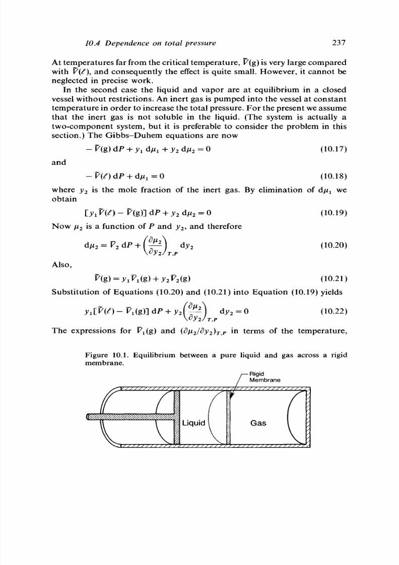
8/11/2019 Thermodynamics of Chemical Systems.pdf
http://slidepdf.com/reader/full/thermodynamics-of-chemical-systemspdf 257/456
10.4 Dependence on total pressure 237
At temp eratu res far from the critical tem per ature , F(g) is very large com pared
with V{i\ an d conse que ntly the effect is qu ite sma ll. Ho w ever, it can no t be
neglected in precise work.
In the second case the liquid and vapor are at equilibrium in a closed
vessel w ithout restrictions. An inert gas is pum ped into the vessel at con stant
tem per ature in orde r to increase the total pressure . Fo r the present we assume
that the inert gas is not soluble in the liquid. (The system is actually a
two-component system, but it is preferable to consider the problem in this
section.) The Gibbs-Duhem equations are now
and
(10.17)
(10.18)
where y
2
is the mole fraction of the inert gas. By elimination of d/^ we
obtain
P + y
2
dfi
2
= 0 (10.19)
(10.20)
Now ju
2
is a function of
P
and
y
2
,
and therefore
=
V
2
dP
dy
:
dy
2
2 / T,P
Also,
Substitution of Equations (10.20) and (10.21) into Equation (10.19) yields
yilW) ~ Ki(g)] dP + y
2
(
d
-p) dy
2
= 0 (10.22)
The expressions for P^g) and
(d/^
2
/dy
2
)
T P
in terms of the temperature,
Figure 10.1. Equilibrium between a pure liquid and gas across a rigid
membrane.
/—Rig id
/ Membrane
Liquid
Gas

8/11/2019 Thermodynamics of Chemical Systems.pdf
http://slidepdf.com/reader/full/thermodynamics-of-chemical-systemspdf 258/456
238
Phase equilibrium
pressure, and mole fraction depend upon the particular equation of state
used for the gas phase. For an ideal gas, Equation (10.22) becomes
— jdP-RTdy
1
=0 (10.23)
where the relation dy
2
=—dy
1
is used. Th e p artial pressure P
x
can be
introd uced by its definition, P
1
=Py
1
. After substitution and rearrang em ent
dP (RT/Py,) (RT/PJ
is obtained. This equation is the same as Eq uatio n (10.16) when it is
recognized that
RT/P
X
is the m olar volum e of the pure vap or at the partial
pressure P
lm
10.5 Second-order transitions
The transitions between phases discussed in Section 10.1 are classed
as first-order transitions. Ehrenfest [25] pointed out the possibility of higher-
order transitions, so that second-order transitions would be those transitions
for which both the Gibbs energy and its first partial derivatives would be
cont inuous
at a
transition po int, but the second partial derivatives w ould
be discontinuous. Under such conditions the entropy and volume would be
continuous. However, the heat capacity at constant pressure, the coefficient
of expansion, and the coefficient of compressibility would be discontinuous.
If we consider two systems, on eithe r side of the tran sition point but
infinitesimally close to it, then the molar entropies of the two systems must
be equal. Also, the change of the m olar entropies mu st be the same for a
change of temperature or pressure. If we designate the two systems
by a prime and a double prime, we have
or
d T + ^ Y d P ^ Y d T + f Y d P ( 1 0.25 )
T) \dTj
P
\TJ \dTj
and, therefore,
dT_ T[(dV/dT)'
P
- (dV/dT)
P
~]
dp ~
(c
P
y
-
(c
P
y
Similarly, we obtain
d T _ (dV/dP)'
T
- {dV/dP)r
W~ (dV/dT)
P
-(dV/dT)
P
(10.26)
(10.27)

8/11/2019 Thermodynamics of Chemical Systems.pdf
http://slidepdf.com/reader/full/thermodynamics-of-chemical-systemspdf 259/456

8/11/2019 Thermodynamics of Chemical Systems.pdf
http://slidepdf.com/reader/full/thermodynamics-of-chemical-systemspdf 260/456
240
Phase equilibrium
10.6 Liquid-vapor equilibria at constant temperature
The condition of equilibrium, in addition to the equality of the
temperature and pressure of the two phases, demands that the chemical
potential of a component in each phase in which it exists must be the same.
The problem is to obtain expressions for the chemical potential of a component
in terms of quantities that are experimentally observable.
The particular equations developed depend upon the experimental
methods that are used and on the particular reference states that are chosen.
The methods are the same for either component when both components are
volatile and, consequently, we consider only one component and use the
subscript 1 to indicate this com po nen t.
The condition of equilibrium in terms of the chemical potential is
A i
1
[T ,P ,x] =
A
i
1
[T,P,y] (10.28)
where y is used to represent the mole fraction of the component in the gas
phase. For the purposes of illustration, we choose to use the virial equation
of state accurate through the second virial coefficient for the gas phase. When
both components are volati le, we can express /^[T, P, y] as
[T , 1 bar, ideal,
y
x
=
1] (10.29)
where S
12
= 2/?
12
— j 8
n
— P
2
i- If only ° ne com ponen t were volatile, then y
would be zero. We choose to express the composition of the liquid phase in
terms of the mole fraction, so
, P , x] = RT In x
x
+ A ^ [ T , P , x ] + / if
[T ,
P ] (10.30)
according to Equation (8.71). A relationship between the two standard states
can be obtained if the pure component exists as a liquid at the experimental
temperature and is volati le. Under such conditions we choose the pure
component at the temperature and pressure of the experiment to be the
reference state and, thus, the standard state for the component in the liquid
phase. We then measure the vapor pressure, PJ, of the pure l iquid, and by
the condition of equilibrium we have
^ [ T ,
P[x
x
= 1] = RTln PJ + j ?
n
P ; + , u f
[T ,
1 bar , ideal, ^ = 1]
(10.31)
where we have assumed that the vapor phase is also pure. The combination
of Equations
(10.28)-(10.31)
yields
+ li{\T
9
P[,x
1 =
1] - fif
[T ,
P, xj = 1]
(10.32)

8/11/2019 Thermodynamics of Chemical Systems.pdf
http://slidepdf.com/reader/full/thermodynamics-of-chemical-systemspdf 261/456
10.6 Liquid-vapor equilibria at constant temperature 241
where [if[T, P , x
1
= 1] represents th e stan dar d state of the com pon ent in
the liquid phase. The standard state for the gas phase has been eliminated,
but instead we have the difference of the chemical potential of the pure liquid
at two pressures. This difference is evaluated by the integral
_
_ r
V[dP (10.33)
where V[ is the mo lar volume of the pure l iquid com ponen t at th e
experimental tem perature .
1
While the combination of Equations (10.32) and
(10.33) eliminates the standard states, so that values of A/if
[T ,
P , x] can be
determined from the experimental methods suggested, we are still faced with
one problem.
A
two -pha se, binary system
at
constant tempe rature
is
univariant, and thus the pressure is a function of the m ole fraction. Th e
values of A/zf
[T ,
P , x] so determined depend only on the mole fraction, but
the pressure is not constant. In order to obtain values of the excess chemical
potential at some arbitrary pressure, P
o
, the correction
(V.-VDdP (10.34)
must be made. The final equation for the excess chemical potential is then
+ V[AP -\ (V.-VDdP (10.35)
Jp
Jp
The values of the excess chemical potential obtained by the use of Equation
(10.32) after substitution of Equation (10.33) refer to the liquid phase in
equilibrium with a vapor phase. In contrast, the values obtained by the use
of Equation (10.35) refer to the liquid phase alone at the temperature T and
the pressure P
o
. The concept of an equilibrium between the liquid phase and
a gas phase has been removed by Equation (10.34).
The dynamic method of studying vapor-liquid equilibria requires the use
of an inert gas that is passed over the liquid phase under conditions that
equilibrium is attained. Under such conditions the total pressure is controlled
and can be made the same in each experiment. The system is actually a
three-component system in which the solubility of the inert gas in the liquid
phase is extremely small and its effect is neglected. The chemical potential
of the first component in the gas phase in equilibrium with the solution is
1
We note that it is the quantity A/^
=
RT\nx
1
-\- A^ that is obtained on elimination of the
standard states. This point was simply accepted in Chapter 8.

8/11/2019 Thermodynamics of Chemical Systems.pdf
http://slidepdf.com/reader/full/thermodynamics-of-chemical-systemspdf 262/456
242 Phase equilibrium
now given by
+ (<5i2 + <5i3 - ^23 )^2 ^3 + lit\T, 1 bar, ideal, y, = 1]
(10.36),
where the subscript 3 refers to the inert gas, d
13
is (2j8
13
-
/?
1X
- j?
33
), and
(5
23
is (2j?23 —
P22
—
/?
33
).
When the second component is not volatile, y
2
is ,
of course, zero. The chemical potential of the component in the gas phase
in equilibrium with the pure component is given by
Mi[T,
P,
/ ] =
RTlniPy'J
+ j8
n
P +
S
13
P(y'
3
)
2
+ nf\T
9
1 bar, ideal, y
x
= 1] (10.37)
The conditions of equilibrium are for the solution
M i [ r , P , x ] = | i
1
[T,P,y] (10.38)
and for the pure component
| i f [ T , P , x
1
= l] =
A
i
1
[T,P,y] (10.39)
Combination of these four equations yields
, P , x ] = KT In - A - + (5
12
P(>;
2
)
2
+ 3
13
l( y
3
)
2
- (/
3
)
2
]P
(10.40)
Because of the experimental conditions, the excess chemical potential is
obtained at the constant pressure P, and no corrections need be made.
In many systems the pure liquid phase of a component is not attainable
under the experimental conditions and thus cannot be used as the reference
state for the component. It is then necessary to choose some other state,
usually the infinitely dilute solution of the component in the liquid, as a
reference state. We choose to illustrate the development under such circum-
stances by the use of Equations (10.28)-(10.30) under the appropriate
experimental conditions. The combination of these equations yields
RT In x
1
+ A/^[T , P, x] + fif[T, P ]
=
RT\n(P
yi
)
+
P
n
P
+
S
12
Py
2
2
+ /if
[T ,
1
bar, ideal,
y
x
=
1]
(10.41)
We define the reference state of the component to be the infinitely dilute
solution of the component in the second component, so that A/x? approaches

8/11/2019 Thermodynamics of Chemical Systems.pdf
http://slidepdf.com/reader/full/thermodynamics-of-chemical-systemspdf 263/456
10.7 Raoulfs law
243
zero
as x
x
approaches zero. Then,
in
the limit,
li?
[T, P]
-
/if [T, ideal, 1 bar
, y, = 1]
'* i° ) + £ i i^ ° ° + ^nP^iyi)
2
(10.42)
where the superscript oo is used to indicate the limiting values at infinite
dilution. The elimination of the chemical p otentials for the stand ard states
in Equation (10.41) by the use of Eq uatio ns (10.42) and
V?[T
9
P«
>
]-[i?[T,P'] =
P?dP=
V?
dP (10.43)
Jp
Jp
yields
/
Py. \ P^yf
Ajuf[T, P, x]
=
I RT In + j 8
n
P
+
S
12
Pyl I —RT\n
r
p x
_
+ jS^P
00
+ (5
12
P
oo
(y
2
° )
2
+ 7 f dP (10.44)
Jp
In Equations (10.43) and (10.44) Vf represents the partial mo lar volume of
the component in the infinitely dilute solution, which is also the partial m olar
volume of the component in the stand ard state. The right-han d side of
Equation (10.44) contains only quantities that can be determined experi-
mentally, and thus A/ii[T, P, x] can be determined. However, just as in the
previous case, the pressure is a function of the m ole fraction. There fore, if
we require values of A/zf at some arbitra ry c onsta nt pressu re, the correction
expressed in Eq uatio n (10.34) mu st be made w ith the sub stitution of Vf for
Vf.
10.7 Raoult's law
The relation between Raoult 's
law and the
definition
of an
ideal
solution given by Equation (8.57) is obtained by
a
study
of
Equation (10.35)
or (10.40).
If a
solution
is
ide al, the n A/xf m us t
be
zero
and the
right-hand
side
of
both equations must
be
zero.
If
we write Py
x
in
both equations
as
P
l 5
the
partial pressure
of
the com ponent ,
and
Py\
in
Eq uatio n (10.40)
as
PJ, then
the
logarithm ic term becomes
\n(P
1
/P[x
1
),
which
is
zero when
Raoult 's law, given
in the
form
P
t
=
P J x
1 ?
is
obeyed. We then
see
that
to
define
an
ideal solution
in
terms
of
Ra oult 's law and still
be
cons istent with
Equation (10.57) requires that
the
experimental measurem ents
be
made
at
the same total pressure and that the vapor behaves
as an
ideal g as.

8/11/2019 Thermodynamics of Chemical Systems.pdf
http://slidepdf.com/reader/full/thermodynamics-of-chemical-systemspdf 264/456
244 Phase equilibrium
10.8 Henry's
law
The simplest approach
to
Henry's
law is by the use of
equations
(10.38), (10.30),
and
(10.36) under
the
experimental condition
of
constant
total pressure. Combination
of
these equations results
in
A ^ [ T , P, x] = RT H PyJx,) + j ?
n
P + S
12
Py
2
2
+ S
13
Pyl
+ lif\T
9
1 bar,
ideal y, = 1]
-
/*f
[T,
P]
(10.45)
We choose
the
reference state
to be the
infinitely dilute solution,
so
nf[T, 1
bar,
ideal, y = 1]
-
nf[T,
P]
(
Pv
RT In
- 4 - + /J
n
P +
S
l2
P(y?)
2
+
S
13
P(yf)
2
(10.46)
We
now
define
the
Henry's
law
constant (some authors call
it the
Henry
coefficient
or the
Henry constant), fe,
by
lif[T,
1
bar,
ideal,
y, =
1]
-
fif
[T ,
P] =
- R T l n
fc
(10.47)
Equation (10.47) indicates that fe s a function of the temperature and pressure.
For
a
given series
of
experiments
at the
constant pressure
P, fe s a
function
of the temperature alone,
and not a
function of the composition. Substitution
of Equation (10.47) into Equation (10.46) gives
RT\n(PyT/kx?) =
- [ /
^ ] (10.48)
Henry's
law in the
form
Pyf/kx™
=
1
can be
true only with
the
assumption
that
the
gas phase behaves
as an
ideal gas
or
that
the
corrections
for
nonideal
behavior
are
negligible.
When the Henry's law constant has been evaluated according to E quations
(10.46)
and
(10.47)
for a
series
of
experiments
at
constant temperature
and
pressure, Equation (10.45)
may be
written
as
RTHPyJkx,) = AfilT, P, x] - [f i
lx
P + S
12
Py
2
2
+ S
l3
Py
2
3
(10.49)
Henry's law in the form Pyjkx
1
= 1 can be valid over a finite range of
composition only when the right-hand side of Equation (10.49) is zero. The
corrections for the nonideality of the gas must be negligible and A/zf must

8/11/2019 Thermodynamics of Chemical Systems.pdf
http://slidepdf.com/reader/full/thermodynamics-of-chemical-systemspdf 265/456
10.8 Henry's law 245
remain zero over the range of composition starting from the infinitely dilute
solution. In the strict sense, then, Henry's law is only a limiting law, being
obeyed in the limit as x
x
approaches zero with the assumption of ideal gas
behavior.
The development of Henry's law is only a little more complicated when
the experimental measurements are made without the use of an inert gas.
The Henry's law constant is defined in terms of Equation (10.42) so that
/if
[T,
P
00
] -
nf\T, 1
bar, ideal,
y
x
=
1] =
RT
In
k
(10.50)
We see from this definition that
k
is not a function of the composition, but
it is a function of the temperature and the pressure. For a given series of
experiments in which the mole fraction is varied at constant temperature,
k
is evaluated at the limiting pressure P
00
whereas the total pressure is different
for each experiment. If we wished to evaluate
k
at any given pressure, then
V?
(10.51)
would be used. In most cases the corrections are small and are usually
omitted. Moreover, when Henry's law is used in the form P
1
= kx
l
, the
deviations from ideal behavior in the gas phase must be negligible.
Another approach to Henry's law based on Equation (10.35) is of interest.
When the deviations from ideal gas behavior and the corrections for the
pressure on the liquid phase are negligible, this equation may be written
in the form
P
x
= P[x
1
exp(An
E
JRT)
(10.52)
Here we have chosen the pure liquid to be the reference state. If now we
assume that measurements can be made over the entire range of composition,
so that the
limiting
value of A/if can be obtained as
x
x
approaches zero,
we have
Pf = P[ Qxp(Aj4/RT)xT = kx?
(10.53)
This definition involves indirectly the change of the reference state from the
pure liquid to the infinitely dilute solution.
Henry's law is also used in some cases as a limiting expression of the
behavior of a component in a single condensed phase at a given temperature
and an arbitrary constant pressure P
o
with no concept of an equilibrium
between the condensed phase and a vapor phase. In order to obtain the
concept of Henry's law under these conditions, two different expressions are
required for the chemical potential of the component with the use of two
different standards states. In terms of mole fractions, the usual practice is to

8/11/2019 Thermodynamics of Chemical Systems.pdf
http://slidepdf.com/reader/full/thermodynamics-of-chemical-systemspdf 266/456
246
Phase equilibrium
use Equation (10.30)
for one
expression
and
MilT, P
o
, x] = ^^ l n A + /if
IT, 1
bar, ideal, ^ - 1] (10.54)
for the other expression. This equation defines the fugacity of the component
in the phase with the ideal gas at
1
bar as the standard state. When the two
expressions are equated,
RT In x
x
+ A//f [T, P
o
, x] + j ^ [ T , P
o
]
= #T ln A + /if [T, 1 bar, ideal, y
x
= 1] (10.55)
We choose the reference state for the left-hand side of this equation as the
infinitely dilute solution, so
V?[T, P
o
l -
fiflT, 1 bar, ideal ^ = 1] =
RT Iniff/x?)
(10.56)
We then define the Henry's law constant in terms of the difference between
the chemical potentials of the component in the two standard states by
/*f
IT,
P
o
l ~ /i?IT,
1
bar, ideal, y, = 1] = RT In k (10.57)
and
k=f?/
x
™
(10.58)
Here
k is
determined
at the
temperature
T and the
arbitrary pressure
P
o
.
When the ratio offjx
1
has the same value over a finite range of concentration
as that in the limit, we have
f
1
= kx
1
(10.59)
The experimental determination of the fugacity, and hence the value of /c,
requires
the
study
of the
equilibrium between
a
vapor phase
and the
condensed phase. The problem becomes identical to those already discussed.
10.9 Limited uses
of
the
Gibbs-Duhem equation
Three different uses of the Gibbs-Duhem equation associated with
the integral method are discussed in this section: (A) the calculation of the
excess chemical potential of one component when that of the other component
is known; (B) the determination of the minimum number of intensive
variables that must be measured in a study of isothermal vapor-liquid
equilibria and the calculation of the values of other variables; and (C) the
study
of the
thermodynamic consistency
of the
data when
the
data
are
redundant.
(A) When only one of the two components in a binary solution is volatile,
the excess chemical potential of the volatile component can be determined
by the methods that have been discussed. However, we require the values
of the excess chemical potential of the other component or of the molar

8/11/2019 Thermodynamics of Chemical Systems.pdf
http://slidepdf.com/reader/full/thermodynamics-of-chemical-systemspdf 267/456
10.9 Limited uses of the Gibbs-Duhem equation 247
G ibbs energy. Let us assume th at A/if [T, P , x ] has been determined over a
range of composit ion at constant temperature and pressure. Then, by the
Gibbs-Duhem equation for the single phase at constant temperature and
pressure,
i ^ (10.60)
or
r sr
>,*'] = -
J x'i
A/if[T,
P, x"] - Af4lT, P, x'] = - (x
t
/x
2
)d{Afi) (10.61)
J x'i
where xi and x'[ represent the limits of integration. In general, the upper
limit may be variable rather than a fixed value. However, in order to obtain
A/if as a function of the mole fraction, A/if
[T ,
P, x'] must be evaluated by
choosing an appropriate reference state. When A/i
E
has been determined so
that its value may be extrapolated to x
x
= 0, the pure liquid may be used as
the reference state of the second component. Otherwise the limit of x
x
is
usually x
1
= 1 a nd th e reference state of the second c om po ne nt is the infinitely
dilute solution.
An alternative calculation, particularly applicable when the experimental
studies can be carried out over the entire range of composition, involves the
direct calculation of the molar excess Gibbs energy. We have
AG
E
= x
x
Afi
E
x
+ x
2
Ajuf (10 .62)
and
| (10.63)
so that
AG
E
=
X l
A/z
E
- x
2
[
^ (xjx
2
)
d(A ^f) (10.64)
J
where we have chosen the reference state of the second component to be the
pure component. Integration by parts yields
A G
E
= - x
2
P' (A^/xDdx, (10.65)
Jxi
(B) We have pointed out that experimental studies are usually arranged
so tha t the system is univ arian t. The experimen tal measu rem ents then involve
the determ ination of the values of the dep ende nt intensive variables for chosen
values of the one independent variable. Actually, the values of only one
dependent variable need be determined, because of the condition that the
Gibbs-Duhem equations, applicable to the system at equilibrium, must be

8/11/2019 Thermodynamics of Chemical Systems.pdf
http://slidepdf.com/reader/full/thermodynamics-of-chemical-systemspdf 268/456
248 Phase equilibrium
satisfied. In two of the type of systems that we have discussed, another
dependent variable exists but its values can be determined by use of the
Gibbs-Duhem equations, with appropriate choice of variables.
First we consider the binary systems when no inert gas is used. When
only one of the components is volatile, the intensive variables of the system
are the temperature, the pressure, and the mole fraction of one of the
components in the l iquid phase. When the temperature has been chosen, the
pressure must be determined as a function of the mole fraction. When both
components are volatile, the mole fraction of one of the components in the
gas phase is an additional variable. At constant temperature the relation
between two of the three variables P
l9
x
l 5
and j ^ must be determined
experimentally; the values of the third variable might then be calculated by
use of the Gibbs-Duhem equations. The particular equations for this case
are
- V(g) dP + y
x
dji + y
2
dfi
2
= 0 (10.66)
and
- V(t) dP + x
x
d/* + x
2
d/*
2
= 0 (10.67)
When dju
2
is eliminated from these two equations, Equation (10.29) is used
to express jU
x
as a function of
P
and
y
x
with the relation
iy
x
(10.68)
T,y \
u
yi/T,P
and the equation of state
V(g) = (RT/P) + fi
liyi
+ /}
22
y
2
+ S
12yi
y
2
(10.69)
is used for K(g), the relation
> l n i ^
x
2
p
22
P
+ 6
12
P{y\x
2
(10.70)
is obtained. When P is measured as a function of y
l9
x
x
can be calculated
by a series of approximations. When y
x
is measured as a function of x
l 9
P
can be calculated by integration, again using a series of approximations.
However , y
1
cannot be calculated when P is measured as a function of x
l
.
Similar conditions prevail when an inert gas is used. In this case both the
temperature and pressure are fixed and made constant. When only one of
the components in the liquid phase is volatile, the two variables are the mole

8/11/2019 Thermodynamics of Chemical Systems.pdf
http://slidepdf.com/reader/full/thermodynamics-of-chemical-systemspdf 269/456
10.9 Limited uses
of the
Gibbs-Duhem equation 249
fraction of one of the com ponents in the liquid phase and the mole fraction
of either the volati le component or the inert gas in the gas phase.
Experimentally
one of
these variables must
be
determined
as a
function
of
the other. An additional variable, a second mole fraction in the gas phase,
mus t be considered when both components in the liquid phase are volatile.
Th en, of the three variables, say
x
l9
y
l9
and
y
3
,
on e variable m ust be measured
as a function of another variable, properly chosen, and the third may be
calculated. H owever, it should be noted that, according to Equation (10.40),
y
3
needs to be known only to correct for the nonideality of the gas phase.
The two Gibbs-D uhem equa tions for this case are
x
1
dfi
1
+ x
2
dii
2
= 0 (10.71)
and
y
1
dfi
1
+
y
2
d/i
2
+
y
3
dfi
3
= 0
(10.72)
With the elimination of djx
2
and the evaluation of d/^ and d/z
3
in terms of
dy
x
and dy
3
,
(10.73)
is obtained. The partial derivatives can be expressed in terms of T, P, y
l9
and y
3
by means of a suitable equation of state. When the virial equation
of state is used as before, only terms containing the d quantit ies appea r and
no term appears containing a /? alone . Th en, for ideal mixtures of real gases,
Equation (10.73) becomes
,
, ,.
(10-74)
We observe that when
y
3
and
y
Y
are determined, x
x
can be calculated and,
when x
x
and
y
1
are determined,
y
3
may be calculated. However,
y
1
cannot
be obtained when
y
3
and
x
x
are determined.
(C ) In many experimental studies, all of the intensive variables are
determined, giving a redundancy of experimental data. However, Equ ations
(10.70) and (10.73) afford a means of checking the therm odyn am ic consistency
of the data at each experimental point for the separate cases. Thus, for
Equation (10.70),
the
required slope
of the
curve
of P
versus
y
l9
consistent
with the thermod ynamic requirements of the Gibbs-D uhem equa tions, can
be calculated at each experimental point from the measured values of P,
x
l9
and
y
Y
at the experimental temperature. This slope must agree within the
experimental error with the slope, at the same com position, of the best curve

8/11/2019 Thermodynamics of Chemical Systems.pdf
http://slidepdf.com/reader/full/thermodynamics-of-chemical-systemspdf 270/456
250 Phase equilibrium
drawn through all of the experimental points. When this agreement is not
achieved for a given set of data, that set
is
thermodynamically inconsistent.
Many other tests, too numerous to discuss individually, have been devised,
all
of which are based on the Gibbs-Duhem equation. Only one such test,
given by Redlich, is discussed here and is applicable to the case in which
both components are volatile and in which experimental studies can be made
over the entire range of composition. The reference states are chosen to be
the pure liquid at the experimental temperature and a constant arbitrary
pressure
P
o
.
The values of A/if
[T,
P
o
, x] and A/if
[T,
P
o
, x] will have been
calculated from the experimental data. The molar excess Gibbs energy is
given by Equation (10.62), from which we conclude that AG
E
= 0 when
x
1
= 0
and when x
l
= l. Therefore,
d
* i = ° (
10
-
75
)
Differentiation of Equation (10.62) with respect to x
x
at constant temperature
and pressure gives
=A^-AAI
(10.76)
x
l
J
TP
because
( ) =0 ,,0.77,
T,P \ Sx J
according to the Gibbs-Duhem equation. Therefore,
(A/if-A/if) dx
1 =
0 (10.78)
f
Jo
Thus, when values of (A/if
—
A/if) are plotted as a function of x
l9
the area
between the best smooth curve drawn through the points and the composition
axis must be zero within the experimental accuracy. This test concerns the
thermodynamic consistency of the data as a whole rather than that of each
individual set of experimental values. It also applies strictly to the liquid
solution at the arbitrary pressure P
o
and only to the two-phase system at
equilibrium through the calculation of A/if and A/if from the experimental
data.
10.10 Liquid-vapor equilibria
at
constant pressure
The thermodynamic treatment of data obtained from the study of
the liquid-vapor equilibria at constant pressure differs from that used in
constant-temperature experiments in the treatment of the standard states.
This difference arises because we cannot calculate the change in the chemical

8/11/2019 Thermodynamics of Chemical Systems.pdf
http://slidepdf.com/reader/full/thermodynamics-of-chemical-systemspdf 271/456
10.10 Liquid-vapor equilibria
at
constant pressure 251
potential
of a
single-phase system with temperature
in
the general case.
We
consider the case for which the pu re liquid state of a volatile com pon ent can
be used
as the
reference state ,
and
thus
the
stand ard state.
No
inert gas
is
used as a thi rd component in the system. The condition of equ ilibrium is
again
the
equality
of
the chem ical poten tials
of
the component
in the two
phases . When we use the mo le fraction as the comp osit ion variable in the
liquid phase, we have
« T l n x
1
+ A ^ [ T , P , x ] + / i i [ T , P , x
1
= l] = / i i [ T , i
>
,y] (10.79)
W e
can
sub tract from each side, JJL[[T,
P,y=
1 ] ,
the
chemical poten tial
of
the pure, real gas at the same temp erature and pressure as the experiment.
We then have
= /*ilT
9
P
9
y-]-iiiLT,P,
yi
= ll
(10.80)
By Equation (10.29)
/ ^ [ T ,
P ,
y\- ii[
[T , P ,
yi
=
1] =
RT
In
y i
+5
12
Py
2
2
(10.81)
The difference between the chemical poten tials of the pure co m pon ent in the
liquid
and gas
phases
is
calculated, with
the
knowledge that
the
chemical
potentials must be equal at the boiling poin t of the pu re substance, T", at
the pressure
P.
We choose
the
series
of
changes
of
state
where
B
represents the component , and then make use of the relation
(Eq. 4.41))
\
dT J
PtX
T
2
For the first change of state
H
^dT (10.82)
T
m
T ]
r
T
and
for the
third change
of
state
li\\T
9
P,
x
t
=
1]
ii[{T\P
9
x, = 1]
f
r
01V)
}
r
T>
dT
IWM>
8/11/2019 Thermodynamics of Chemical Systems.pdf
http://slidepdf.com/reader/full/thermodynamics-of-chemical-systemspdf 272/456
252 Phase equilibrium
so
• " 1 (S) " 1 (// im
d T
*
(10.84)
with the condition that
/x i [T - ,P ,x
1
= l ] = / x f [ T - , P , y
1
= l ] (10.85)
Substitution of Equations (10.81) and (10.84) into Equation (10.80) yields
(10.86)
Thus, values of A//i[T, P, x] can be calculated from the measured values of
the equilibrium temperature
T
and the two mole fractions, x
x
and y
x
. The
same equation with change of subscripts is valid for the second component
when its standard state can be taken as the pure liquid component.
Some comments need to be made concerning the integral in Equations
(10.84) and (10.86). Certainly , when the m olar heat capacities at the con stant
pressure P are known as a function of the temperature for both phases, the
integral can be evalua ted. How ever, the integration req uires the e xtrapo lation
of the heat capacity of one of the phases into a region where the phase is
metastable with respect to the other phase. Figures 10.2 and 10.3 illustrate
this point (refer also to Fig. 5.7). The curve in Figure 10.2 represents the
vapor pressure curve of the component and T", the boiling point of the
component at the chosen pressure. When the equilibrium temperature of the
solution is greater than T \ the integration is carried out along the path a
into the region of the gas phase; the liquid phase is then metastable. When
the equilibrium temperature of the solution is less than T', the integration
is carried out along the path b into the liquid region; the gas phase is then
metastable. The same problem is illustrated in Figure 10.3 in terms of the
chemical poten tials. The curves in this figure rep resent the chemical p otential
of the pure component in the two different phases as a function of the
temperature at constant pressure. The curve labeled // ' represents the liquid
and the curve labeled gg' represents the gas. When the integration is carried
to temperatures greater than T', the chemical potential of the gas phase
follows the solid portion of the gas curve whereas that for the liquid phase
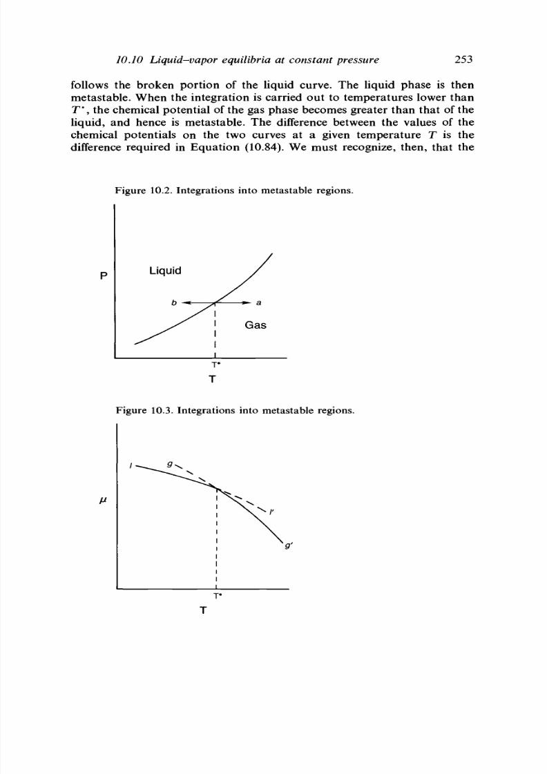
8/11/2019 Thermodynamics of Chemical Systems.pdf
http://slidepdf.com/reader/full/thermodynamics-of-chemical-systemspdf 273/456
10.10 Liquid-vapor equilibria at constant pressure
253
follows the broken portion of the liquid curve. The liquid phase is then
metastable. When the integration is carried out to temperatures lower than
T*
, the chemical potential of the gas phase becomes greater than that of the
liquid, and hence is metastable. The difference between the values of the
chemical potentials on the two curves at a given temperature T is the
difference required in Equation (10.84). We must recognize, then, that the
Figure 10.2. Integrations into metastable regions.
Liquid
b
- *
Gas
T*
T
Figure 10.3. Integrations into m etastable regions.

8/11/2019 Thermodynamics of Chemical Systems.pdf
http://slidepdf.com/reader/full/thermodynamics-of-chemical-systemspdf 274/456
254
Phase equilibrium
value of the integral used in the calculation of A/if is uncertain to some
unknown amount .
The values of A^f[T, P, x] at different compositions obtained by the case
of Equation (10.86) are not isothermal, because in the univariant system the
temperature is a function of the mole fractions. Corrections must be made
to obtain isothermal values of A/xf. We choose some arbitrary temperature
T
o
. Then, according to Equation (11.120),
In order to evaluate this integral, (H
1
—H[(tf)) must be known at each
composition over the indicated range of temperature, or the value must be
known at one temperature together with the values of (C
P l
—C'
Pl
(£)). Just
as AJLL^IT, P
o
, x] in the isothermal case refers to the liquid phase alone, so
here A/if
[T
o
,
P , x] refers to the liquid ph ase alo ne, with no concept of an
equilibrium between the two phases.
The experimental determination of T, y
u
and x
x
is actually redundant.
How ever, the equatio n corres pon ding to E qu ation (10.70) involves the partial
molar entropies of the components in the two phases. In many cases the
values of these quantities are not known. Therefore, a test of the thermo-
dynamic consistency of each experimental point generally cannot be made,
neither can the value of one of the three q uantities T, y
u
and x
1
be calculated
when the other two are measured. The test for the consistency of the overall
data according to Equation (10.78) can be made when the isothermal values
of both A/zf
[T
o
,
P, x] and A/if
[T
o
,
P, x] have been determined.
The use of the infinitely dilute solution as the reference state of a volatile
component is not convenient for the experimental study of isopiestic
vapor-liquid equilibria. Equation (10.79) may be written as
KT
00
In
X l
+
nf
[T
0 0
, P ] =
fif
[T
0 0
, P , y f ] (10.88)
for the infinitely dilute solution w ith the condition tha t A /^[T ° ° , P, x f ] is
zero. Here T
00
is the temperature at which the infinitely dilute solution is in
equilibrium w ith the vap or at the con stant pressure P. When E qu ation (10.88)
is subtracted from Equation (10.79) and use is made of Equation (10.29),
we obtain
+ (fi?[T
00
, P ] - nf\T° > , 1 bar, y
x
= 1])
- QiflT, P ] - | i f
[T ,
1 bar , y
x
= 1]) (10.89)

8/11/2019 Thermodynamics of Chemical Systems.pdf
http://slidepdf.com/reader/full/thermodynamics-of-chemical-systemspdf 275/456
10.12 Liquid-pure solid equilibria at constant pressure 255
The differences between the standard states of the component in the
condensed and gaseous states at the two temperatures cannot be evaluated
without knowledge of the composition of standard states in the condensed
phases. However, this requires prior knowledge of the excess chemical
potentials. The experimental study of the isothermal vapor-liquid equilibria
is therefore more convenient and yields the same information.
10.11 The boiling point elevation
The study of the elevation of the boiling point of a solvent by the
addition of a nonvolatile solute is a special case of isopiestic vapor-liquid
equilibria. The solvent is the only volatile component, and the standard state
of the solvent is chosen as the pure solvent. Un de r these cond itions Eq uatio n
(10.81) may be written as
, -rf
(10.90)
This equatio n can be interpreted as giving the tem pera ture of the equilibrium
system as a function of the m ole fraction of the liquid p hase w hen A/if
[T ,
P, x~\
is known as a function of the temperature and mole fraction. For values of
x
1
very close to unity, A/if may be taken as zero, and (H[ (g) — H[ (/)) may
be considered to be independent of the temperature and equal to the molar
change of enthalpy on evaporation of the pure liquid at T[. Then we obtain
on integration
Afr
(
rr;)
1
R T T [
When we write ( T —T{) = AT and let T be approximately TJ, we have
R(T* )
2
AT =
~
A ir
n X l ( 10
'
9 2 )
H e r e [ R ( T ; )
2
/A#;] is a property of the pure solvent. Equation (10.92) is
the basic equation for the simpler expressions involving the mole fraction
or molality of the solute of the equation for the boiling point elevation, but
it must be emphasized that it is only an approximate equation, valid in the
limit as x
x
approaches unity. Even for the approximation of ideal solutions,
Eq ua tion (10.90) should be used for the calculation of the boiling point when
x
1
is remo ved from unity.
10.12 Liquid-pure solid equilibria at constant pressure
The study of the equilibria between a liquid solution and a pure
solid phase of one of the components is generally made under conditions of
constant pressure. The temperature is then a function of the composition of

8/11/2019 Thermodynamics of Chemical Systems.pdf
http://slidepdf.com/reader/full/thermodynamics-of-chemical-systemspdf 276/456
256 Phase equilibrium
the liquid, or the composition of the liquid is a function of the temperature.
In the first case we usually speak of the freezing point of the solution,
whereas in the second case we speak of the solubility of the solid. The
thermodynamic treatment is identical in either case, and the difference is
simply one of interpretation . The condition of equilibrium is the equality of
the chemical potential of the component in the two phases, so we write
J
u
1
[ T , P , x
1
]=^[T,P,5] (10.93)
We again choose to use Equation (10.30) to express the chemical potential
of the component in the liquid phase in terms of the mole fraction and choose
the pure liquid to be the standard state. Then we have
« T l n x
1
+ A / i ? [ r , P , x ] = ^ [ T , P , s ] - | i i [ 7
1
, P , x
1
= l ] (10.94)
The difference in the chemical potential of the pure component in the liquid
and solid phases can be evaluated in the same manner as was done in Section
10.10, because of the equality of the two chemical potentials at the melting
point for the pressure P. The result is
= l] = - T
JT
- "
1
( r / " l V V
*
dT (10.95)
where
T[
is the melting point of the pure component. Substitution of
Equation (10.95) into Equation (10.94) yields
(10.96)
Thus, values of Ajuf
[T ,
P, x] can be calculated when the equilibrium values
of T and x
x
are determined.
The evaluation of the integral requires, as in Section 13.10, a knowledge
of the molar heat capacities of the pure solid and liquid phases as a function
of the temperature. In this case the equilibrium temperature for the solution
is always less than the melting point of the pure substance. Then the heat
capacity of the liquid phase is extrapolated into the region in which the
liquid is metastable with respect to the solid phase. Because of this, there is
always some uncertainty in the evaluation of the integral and the range of
temperature over which the integration
is
carried out should not
be
too large.
The values of A ^ [T , P , x] obtained from Equation (10.96) are not
isothermal. When isothermal values are desired at some arbitrary temperature
T
o
,
the same correction as that given in Equation (10.87) must be applied.
When the excess chemical potential of the solute in the liquid phase is
required as a function of the mole fraction at the constant temperature T
o
and pressure P, an integration of the Gibbs-Duhem equation must be used.
For this the infinitely dilute solution of the solute in the solvent must be

8/11/2019 Thermodynamics of Chemical Systems.pdf
http://slidepdf.com/reader/full/thermodynamics-of-chemical-systemspdf 277/456
10.14 Liquid-solid solution equilibria at constant pressure 257
used as the reference state for the solute, because the experimental
me asurem ents can be m ade only over a limited range of com position starting
with the pure solvent.
10.13 Freezing point lowering and solubility
The comments concerning the lowering of the freezing point of a
solvent by a solute, based on Equation (10.96), are the same as those made
concerning the boiling point elevation. Equation (10.96) gives indirectly the
tem pera ture as a function of the comp osition w hen A/if is kno wn as a function
of these two variables. In the limit as x
1
approaches unity, A/if approaches
zero and (H[
(£) —
H[ (s)) app roac hes the mola r change of enthalp y o n fusion,
AHf
, of the com pon ent a t its melting point at the pressure
P.
We may then
write Equation (10.96) as
R(T:)
2
AT=
1-JLLinx (10.97)
AH; *
V
where
AT= (T[ —T)
and
T
is set approximately to
T[.
This equation, of
the same form as Equation (10.92), is the basic equation for the elementary
formula for the freezing point lowering in terms of the mole fraction or
molality of the solute, but again we emphasize that it is an approximation,
valid only in the limit.
Equation (10.96) should be used for an ideal solution,
with A/if set equal to zero, to calculate the freezing point as a function of
the mole fraction for values of x
1
not close to unity.
When we consider the solubility of a solid component in a solvent, the
emphasis is placed on obtaining the mole fraction or other composition
variable as a function of the temperature. Thus, Equation (10.96) gives the
solubility as a function of the tem pera ture in this interpre tation . Th e solubility
in an ideal solution is given by
——_ , *
S
dT
(10.98)
10.14 Liquid-solid solution equilibria at constant pressure
When a liquid solution and a solid solution are in equilibrium, both
components exist in both phases. We again develop the pertinent equations
for only one component, because the equations for the second component
are identical except for the change of subscripts. The condition of equilibrium
is the equality of the chemical potential of the component in the two phases,
so
/ i
1
[ T , P , x ] = / x
1
[T,P,z] (10.99)
where z represents the mole fraction in the solid phase. With the use of
Equation (10.30) to express the chemical potentials in terms of the mole

8/11/2019 Thermodynamics of Chemical Systems.pdf
http://slidepdf.com/reader/full/thermodynamics-of-chemical-systemspdf 278/456
258 Phase equilibrium
fraction, Equation (10.99) becomes
RT In
X l
+ A/i?[T, P , x] +
fi[
[T, P, x
t
= 1]
.
= RT In z
x
+ A J I ? | T , P, z] + //J [T, P, z = 1] (10.100)
where we have chosen the pure liquid and the pure solid to be the standard
states. This choice is made because we can determine the difference between
the chemical potentials of the component in the two states by knowing the
melting point of the pure component at the experimental pressure according
to Equation (10.95). We then have
(10.101)
It is apparent from this equation that we can determine only the difference
between the two excess chemical potentials at the experimental conditions.
If one is known from other studies, then the other can be determined. It
must be pointed out that the difference is not isothermal and, if isothermal
quantities are desired, the same corrections as discussed in Section 10.12
must be made by the use of Equation (10.87).
The equilibrium temperature may be intermediate between the freezing
points of the two components, or may be above or below both freezing
points. Two special cases are worthy of additional comment. The mole
fractions are equal at the composition of a maximum or minimum in the
temperature-composition curve. Then, at such an extremum,
A/i?[T, P, x] - A J I ? [ T , P,z^ = -T |
H
i ( f l -
H
i f e )
dT
(10.102)
For a maximum, T> T[, the right-ha nd side of Eq uatio n (10.102) is positive,
and therefore (A/i?[T, P, x]
—
A/if [T , P, z]) must be positive. Fo r a m inimum ,
(A/if
[T ,
P , x ] — A^f
[T ,
P , z]) must be negative. The same con ditions must
apply to the excess chemical potential for the second component.
10.15 Liquid-liquid equilibria at constant pressure
When a system exhibits partial immiscibility, we encounter an
equilibrium between two phases in the same state of aggregation. In this
case the same standard state of a component can be used for both phases.
W ith the use of the con dition of equilibrium in terms of the chemical p otentials
and Equation (10.30), we have
RT In xi + A//?[T, P, x'J = RT In x'[ + A/xf
[T ,
P , x" ] (10.103)
where the primes and double primes are used to distinguish the two phases.
The measurement of the composition of the two saturated phases at a given
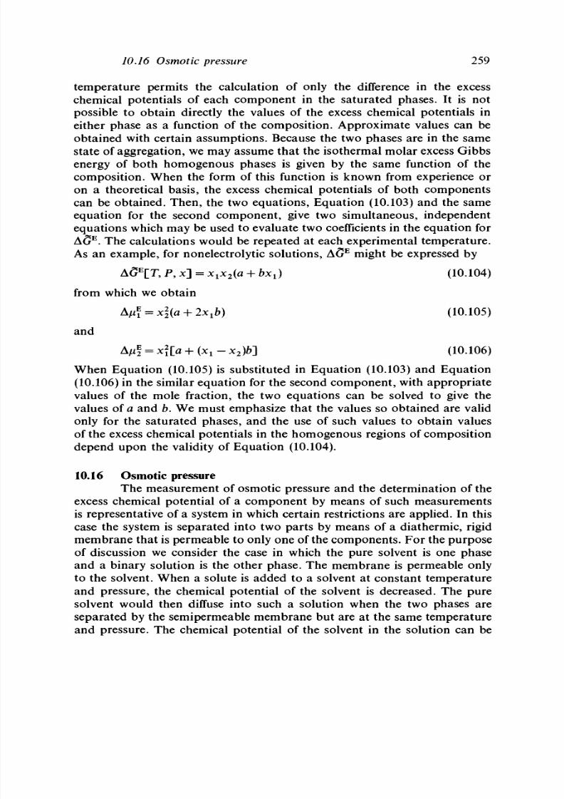
8/11/2019 Thermodynamics of Chemical Systems.pdf
http://slidepdf.com/reader/full/thermodynamics-of-chemical-systemspdf 279/456
10.16 Osmotic pressure 259
temperature permits the calculation of only the difference in the excess
chemical potentials of each component in the saturated phases. It is not
possible to obtain directly the values of the excess chemical potentials in
either phase as a function of the composition. Approximate values can be
obtained with certain assumptions. Because the two phases are in the same
state of aggregation, we may assume that the isothermal molar excess Gibbs
energy of both homogenous phases is given by the same function of the
composition. When the form of this function is known from experience or
on a theoretical basis, the excess chemical potentials of both components
can be obtained. Then, the two equations, Equation (10.103) and the same
equation for the second component, give two simultaneous, independent
equ ation s which m ay be used to evaluate tw o coefficients in the equ ation for
AG
E
. The calculations would be repeated at each experimental temperature.
As an example, for nonelectrolytic solutions, AG
E
might be expressed by
AG
E
[T, P , x] = x
1
x
2
(a + bx
x
) (10.104)
from which we obtain
A^
E
= x | (a + 2x
1
b) (10.105)
and
(10.106)
When Equation (10.105) is substituted in Equation (10.103) and Equation
(10.106) in the similar equation for the second component, with appropriate
values of the mole fraction, the two equations can be solved to give the
values of
a
and
b.
We must emphasize that the values so obtained are valid
only for the saturated phases, and the use of such values to obtain values
of the excess chemical potentials in the homogenous regions of composition
depend upon the validity of Equation (10.104).
10.16 Osm otic pressure
The measurement of osmotic pressure and the determination of the
excess chemical potential of a component by means of such measurements
is representative of a system in which certain restrictions are applied. In this
case the system is separated into two parts by means of a diathermic, rigid
m em brane that is permeable to only one of the comp onen ts. For the purpose
of discussion we consider the case in which the pure solvent is one phase
and a binary solution is the other phase. The membrane is permeable only
to the solvent. When a solute is added to a solvent at constant temperature
and pressure, the chemical potential of the solvent is decreased. The pure
solvent would then diffuse into such a solution when the two phases are
separated by the semipermeable membrane but are at the same temperature
and pressure. The chemical potential of the solvent in the solution can be

8/11/2019 Thermodynamics of Chemical Systems.pdf
http://slidepdf.com/reader/full/thermodynamics-of-chemical-systemspdf 280/456
260
Phase equilibrium
increased by an increase of pressure on the solution until equilibrium is
achieved. The excess pressure is the osmotic pressure.
A binary system consisting
of two
parts separated
by a
diathermic, rigid
membrane
has
three degrees
of
freedom.
The
particular system under
discussion
can be
made univar iant
by
fixing
the
temperature
and
pressure
of the pu re so lvent;
the
equilibrium pressure
on the
solution
is
then
a
function
of
the
composit ion
of the
solution.
The
condition
of
equ ilibrium
is
,
P', x] =
ft
[T, P,
Xl
=
1]
(10.107)
and when Equation (10.30) is used, the equation becomes
RT
In
Xl
+
A J I ? [ T ,
P', x] +
n\
[T, P',
x
x
=
1] =
fi[
[T, P,
x, =
1]
(10.108)
Th e difference betw een the chemical pote ntia l for the two stan dard states is
i ; [ r , p , x
1
=
i ] - ^ ; [ r , p ' , x
1
= i ] =
v\ dp (10.109)
so
JP '
[dP
(10.110)
A measurement
of
P'
for a
given mole fraction,
x
l 5
permits
the
calculation
of the value
of A//f at
P'
and x
x
.
Such values
are not at a
constant pressure.
When values
of A/xf are
desired
at the
pressure
of the
solvent,
P, the
correction
A/if[T,P,x]-A/if[T,P',x]= I (V.-VDdP (10.111)
J p
1
must be made. With this correction we have
F
x
dP (10.112)
F or
an
ideal solution, Equation (10.112) becomes
(10.113)
l
=
f
P
F ; d p
Jp'
where
the
partial molar volume
is now
equal
to the
molar volume
of the
pure component . If V[ is assumed to be constant over the range of pressure,
we can write Equation (10.113) as
1
=
-nV[ (10.114)

8/11/2019 Thermodynamics of Chemical Systems.pdf
http://slidepdf.com/reader/full/thermodynamics-of-chemical-systemspdf 281/456
10.18 Solutions of strong electrolytes 261
where n = P'
—
P and is the osmotic pressure. This equation is the basic
equation for the more-elementary expressions for the dependence of the
osmotic pressure on the mole fraction or molality of the solute. It is also
valid for solutions that are not ideal in the limit as x
1
approaches unity
because, in these cases, A/if approaches zero and V
x
approaches V[.
10.17 Other concentration variables
We have used the mole fraction as the composition variable
throu gho ut the previous discussion. W here app ropria te, we could have used
the molality or molarity instead of the mole fraction. For the molality,
Equation (8.92) would be used for the solute and either Equation (8.102) or
Equation (8.119) for the solvent. For the molarity, Equation (8.104) would
be used for the solute and Equation (8.118) or Equation (8.120) for the
solvent. The methods used to develop the corresponding equations are
identical to those that have been used for the mole fractions.
10.18 Solutions of strong electrolytes
The thermodynamic treatment of systems in which at least one
component is an electrolyte needs special comment. Such systems present
the first case where we must choose between treating the system in terms of
components or in terms of species. No decision can be based on thermo-
dynamics alone. If we choose to work in terms of components, any effect of
the presence of new species that are different from the components, would
appear in the excess chemical potentials. No error would be involved, and
the thermodynamic properties of the system expressed in terms of the excess
chemical potentials and based on the components would be valid. It is only
when we wish to explain the observed behavior of a system, to treat the
system on the basis of some theoretical concept or, possibly, to obtain
additional information concerning the molecular properties of the system,
that we turn to the concept of species. For example, we can study the
equilibrium between a dilute aqueous solution of sodium chloride and ice
in terms of the com pon ents: water and sodium chloride. How ever, we know
that the observed effect of the lowering of the freezing point of water is
approximately twice that expected for a nondissociable solute. This effect is
explained in terms of the ionization. In any given case the choice of the
species is dictated largely by our knowledge of the system obtained outside
of the field of thermodynamics and, indeed, may be quite arbitrary.
In the discussion presented here, we consider the electrolytic component
to be the solute dissolved in some nonelectrolytic liquid solvent. We express
the chemical formula of the solute as M
v +
A
v
where v+ and v_ represent
the number of positive ions and negative ions, respectively, present in one
molecule of the component. We choose the species in solution to be only
the positive and negative ions represented as M+ and A_ and solvent. We

8/11/2019 Thermodynamics of Chemical Systems.pdf
http://slidepdf.com/reader/full/thermodynamics-of-chemical-systemspdf 282/456
262 Phase equilibrium
introduce by this means the concept of strong electrolytes; the thermo-
dynamic treatment concerning solutions of weak electrolytes is discussed in
Chapter
11.
The reference state of the ions is chosen as the infinitely dilute
solution of both ions in the solvent; the choice is the usual one dictated by
the limited concentration range of most electrolytic solutions. The chemical
potential of the solute is
liJLT,
P , m] = v
+
^
+
[T, P , m
+
] + v_ ^_ [T , P , m_] (10.115)
according to Equation (8.178). With the use of Equations (8.179) and (8.180),
we have Equation (8.181)
/i
2
[T, P , m] = RT In m\
+
m
v
s + RT In
y\
+
y
v
s
+ v
+
^ | T , P ]
+ v _ / ^ [ T ,P ] (10.116)
If m represents the molality of the solute, m
+
=v
+
m and m_ =v_m. With
the introduction of the mean activity coefficient, Equation (10.116) becomes
i
2
[T, P , m] = vRT In m + vRT In y+ + RT In v\
+
v
v
s + v
+
[T, P ]
+ v _ /^ [ T ,P ] (10.117)
where v = v+ + v _ . This equation is the basic equation for the chemical
potential of a strong electrolyte considered as a solute. The factor v present
in the first two terms on the right-hand side of the equation is to be noted;
it is this factor that distinguishes the behavior of solutions of strong
electrolytes from that of nonelectrolytic solutions. The third term is a new
term, and is independent of the molality and pressure.
When the solute is present in both phases, the condition of equilibrium
is again the equality of the chemical potential of the component in the two
phases. The same methods used in the previous sections of this part of the
chapter are used to develop the equations for the specific type of equilibrium.
As an example, when the solute is volatile, the conditions of equilibrium lead
to
vRT
In m
+ vRT
In
y
±
+ RT
In
v
v
+
+
v
v
_r + v
+
/x?[T, P] + v _/i
e
[T, P]
= RT
In
Py
2
+f(fi)P + fif [T , 1 bar, ideal, y
2
= 1] (10.118)
where /(/?) is used to express the deviations of the vapor phase from ideality
in a general form. With due consideration of the pressure as discussed in
Section 10.8, Henry's law constant may be defined as
fiflT,
1
bar, ideal,
y
2
=
1] - (v
+
/ i?[T, P] + v_ /^ [T , P]) =
RT
In
k
(10.119)
In many cases the solute will not be present in the second phase. Then
values of the excess chemical potential, the activity coefficient of the solvent,
8/11/2019 Thermodynamics of Chemical Systems.pdf
http://slidepdf.com/reader/full/thermodynamics-of-chemical-systemspdf 283/456
10.20 Applications of the Gibbs-Duhem equations 263
or the osmotic coefficient will be obtained from the study of the phase
equilibria. The values of the mean activity or mean activity coefficient of the
solute would then be obtained by use of the Gibbs-Duhem equation. The
experimental studies must be made over a range of compositions starting at
m = 0, when the infinitely d ilute so lution is used as th e reference sta te of the
ions. The appropriate expression for the chemical potential of the solvent
must be used. The correct expressions based on Equation (8.102) or (8.120)
are
or
, P , m] = - ^ i vm + Afi
m
+
/xf [T , P ] (10.120)
lU U
, P, m] = -
R
^ ^ ~ vm + nflT, P] (10.121)
10.19 Solutions of fused salts
The same choice of using component or species is also met in the
study of binary systems of molten salts. We could choose to deal solely with
components, but because of the concept of the ionic nature of the melts we
choose to express the chemical potential of the component in terms of the
chemical potential of the species. Equation (8.202) gives the relation for the
chemical potential of the general salt M
v +
A
v
in term s of the chem ical
potentials of the ions. The discussion given in Section 8.18 results in the
m ore conv enient e qu ation for the chemical poten tial of the salt (Eq. (8.208))
/^[T , P , x ] =
RT
In x
v
+
+
x
v
_- + A/xf [T , P , x ] + /xf [T , P ,
x, =
1]
(10.122)
where the subscript 1 is used to indicate the com pon ent witho ut distinction
between a solvent and solute. However, at times it may be advantageous to
define an average of the excess chemical potentials of the ions based on
Equations (8.207) and (8.208) such that
A/x? = vA^f = v
+
[A/x* _ (A/4)
0 0
] + v_[A/x* - (A/x* )° ° ] (10.123)
Equation (10.122) is the basic equation that would be used in obtaining
expressions for the excess chemical potential by means of the condition for
phase equilibrium.
10.20 Applications of the Gibbs-Duhem equations
We discuss in the next few sections the applications of the
Gibbs-Duhem equations to various phase equilibria. In so doing we obtain
expressions for the derivatives of one intensive variable with respect to

8/11/2019 Thermodynamics of Chemical Systems.pdf
http://slidepdf.com/reader/full/thermodynamics-of-chemical-systemspdf 284/456
264
Phase equilibrium
another under the condition that the system is univariant. In this section we
discuss the general problem, and then we consider a few cases of special
interest in the following sections.
Consider a binary, two-phase system without specifying the specific phases.
The two Gibbs-Duhem equations on a molar basis are
3'
dT - V' dP + x i df i
x
+ x
f
2
dfi
2
= 0 (10.124)
and
3"
dT - V" dP + x'[ d/ii + x'2 d/i
2
= 0 (10.125)
where the single and double primes are used to distinguish the two phases.
The problem is to solve these two equations under the particular conditions
of a given system, with the provision that one of the variables must be kept
cons tant in order to m ake the system un ivarian t. There are 24 such derivatives
when the chemical potentials are used as variables. The number is reduced
to seven if we consider a derivative and its reciprocal to be the same, and
if we exclude the in terch ang e of fi
x
and \i
2
as giving a new derivative. Alth oug h
some of the derivatives may be useful in special cases, such derivatives in
general are not convenient, because of the use of the chemical potentials as
variables and because, in some of the derivatives, values of the absolute
entropies are required.
More-useful derivatives are obtained when com position variables are used,
rath er than the chemical pote ntials. W e use the mole fraction thro ug ho ut,
although the molality or the molarities could be used. The four intensive
variables that are used are T, P, xi, and
x'[.
There are again seven derivatives
between the four variables under the same conditions stated in the previous
paragraph except that, rather than excluding the interchange of
fi
x
and
\i
2
as giving a new derivative, we exclude the interchange of xi and
x'{;
th e
seven derivatives are
(dT/dP)^, (dT/dx'Jp, (dT/dx'J^, (dP/dx\)
Ti
(dP/dx\)
x
,
{
,
(dx'JdxVr, and (dx'JdxDp.
Four examples are used to illustrate the methods that can be used. First
we consider the derivative (dT/dx[)p. At constant pressure, Equa tions
(10.124) and (10.125) become
3'
dT + x i dfi
x
+ x'
2
dfi
2
= 0 (10.126)
S" dT + x i d/i
x
+
x"
2
d\x
2
= 0 (10.127)
We eliminate dfi
2
to obtain
X
^]i
1
=0
(10.128)
x'
2
Then dfi
x
can be written as
i = -S\ dT + (^±) dxi (10.129)

8/11/2019 Thermodynamics of Chemical Systems.pdf
http://slidepdf.com/reader/full/thermodynamics-of-chemical-systemspdf 285/456
10.20 Applications
of
the Gibbs-Duhem equations 265
where \i
x
is used to introduce xi as the independent variable. After
substitution and simplification, we have
[
r//o>/ F> \ ,
V
"/O>' CM"|
AT \[
_ i 11 ^
1
I
AY'
—0
•^ 1V
1 1 / "• 2v 2 2 /J ^^ 1 ii I VJ-A/^ —v/
V x
2
J\Sx\J
TP
(10.130)
or
/HT\ rv
r/
_ v
r
v ^ i / / ^ v ' )^
D
_
r >p
_ (10.131)
S'
2
-
S
2
)]
We note here that the value of this derivative is zero when the compositions
of the two phases are equal in accordance with one of the Gibbs-Konovalov
theorems. The second derivative which we choose to evaluate is (dT/dP)
X
'
r
We choose to work again with JX \ in order to introduce xi as a variable.
Therefore,
we
first eliminate
d\i
2
from Equation (10.124)
and
(10.125)
to
obtain
( x" \ ( x"V'\ ( x"x'\
15"
yS'
IdT
—
I
V"
^— dP
+
I
xi ^
Id/^
= 0
(10.132)
\
X
2 /
\
X
2
) \
X
2
/
Then
jn
l
is a
function
of
the temperature and pressure
at
constant
x[,
so
d/Li
1
= - S ;
dT+ V\ dP
(10.133)
After substituion and simplification, we obtain
s;) + x;(S2-si)
Some care must be used in evaluating the two derivatives (dTldx\)
x
» and
(dx'Jdx'^p. In these derivatives both \i± and
\i
2
must be retained and not
eliminated
as
such,
in
order
to
introduce both mole fractions.
If
we choose
to introduce
xi by
means
of
//
1?
then we must
use fi
2
to
introduce x'[.
At
constant xi, /i
2
is a
function only
of
the temperature and pressure,
so
d/i
2
= dy '
2
=
-SI dT
+
V
2
dP (10.135)
Also, dfi
1
may be written as
dfi, = d/ii = - S i
dT+ V\
dP +
(
^ ] dxi (10.136)
\dx'J
TfP
Substitution
of
these
two
equations into Equations (10.127)
and
(10.128)
and elimination
of
dP yields
\
- V\) -
x'
2
(V'
2
-

8/11/2019 Thermodynamics of Chemical Systems.pdf
http://slidepdf.com/reader/full/thermodynamics-of-chemical-systemspdf 286/456
266
Phase equilibrium
Similar methods are used for the last derivative, (dx\/dx'[)
P
. We introduce
x\
by m eans of fi\ and x'[ by means of \i
2
. Then, we have
dpi = dfi[ =
- S i
dT
+ ( —)
dx[
(10.138)
\dx'J
TtP
and
(^ )
//
2
= d /^ = - S S d r + l - ^ l dx'[ (10.139)
Substitution of these equations into Equations (10.124) and (10.125) and
elimination of
dT
gives
(10.140)
^ 5 x i /
P
x'i[x
2
(S
2
- S
r
2
) + xi(S i - Si)](5/ i i /5x i)
T fP
or
M
In order to evaluate each of the derivatives, such quantities as
(V'{ —
K-),
(Si — SI), and {dn'Jx'^j
P
need to be evaluated. The difference in the partial
mo lar volumes of a compo nent between the two phases presents no p roblem ;
the dependence of the molar volume of a phase on the mole fraction must
be known from experiment or from an equation of state for a gas phase. In
order to determine the difference in the partial molar entropies, not only
must the dependence of the molar entropy of a phase on the mole fraction
be known, but also the difference in the molar entropy of the component in
the two standard states must be known or calculable. If the two standard
states are the same, there is no problem. If the two standard states are the
pure component in the two phases at the temperature and pressure at which
the derivative is to be evaluated, the difference can be calculated by methods
similar to that discussed in Sections 10.10 and 10.12. In the case of
vapor-liquid equilibria in which the reference state of a solute is taken as
the infinitely dilute solution, the difference between the molar entropy of the
solute in its two standard states may be determined from the temperature
dependence of the Henry's law constant. Finally, the expression used for fi
t
in evaluating (dx
f
Jdx")
T P
must be appropriate for the particular phase of
interest. This phase is dictated by the particular choice of the mole fraction
variables.
Alternate forms of the equatio ns for the various derivatives which contain
the partial molar entropies are obtained by substituting
HJT
for each partial
molar entropy. The substitution is possible because the chemical potential

8/11/2019 Thermodynamics of Chemical Systems.pdf
http://slidepdf.com/reader/full/thermodynamics-of-chemical-systemspdf 287/456
10
of
a
component
is
.20 Applications of the Gibbs-Duhem equations 267
(10.142)
and under
the
conditions
of
equilibrium ju-
= fi".
The expressions
for the
derivatives become somewhat simpler when
one
of
the
components
is not
present
in one of the
phases.
For the
purposes
of
discussion
we
assume that
the
second component
is not
present
in the
double-primed phase. Then
the two
Gibbs-Duhem equations become
S' dT -V' dP
+ xi
dfi,
+ x
2
dfi
2
=
0
(10.143)
and
(S{)" dT - (V [)" dP
+
d/a
1
=0 (10.144)
We
can
immediately eliminate
ji^
from
the two
equations,
to
obtain
IS'
-
xi(5j)"] dT
-
IV'
-x\{V[
)"] dP + x'
2
djx
2
= 0 (10.145)
where (S{)"
and
(V{)"
are the
molar entropy
and
volume
of the
pure
component
in the
double-primed phase
at the
temperature
and
pressure
at
which
the
derivative
is to be
evaluated. There
are
three derivatives involving
the three variables
T, P, and
either
xi or
x'
2
when aderivative
and its
reciprocal
are
considered
to be
equivalent.
The
three derivatives
are
(dT/dP)
X2
, (dT/dx'
2
)
P
,
and
(dP/dx'
2
)
T
.
For the
first
of
these derivatives JA\
is
a function
of the
temperature
and
pressure,
so
d[i'
2
= - S
2
d T +
V'
2
dP
(10.146)
Then,
on
substitution
and
simplification,
we
obtain
_
~ J
(10.147)
For
the
second
and
third derivatives
we
write
d//
2
as
dn'
2
=
-S'
2
dT +
V'
2
dP +
(dfi
2
/dx
2
)
Tt
p
dx
2
(10.148)
Then,
on
substitution
and
simplification under
the
appropriate conditions,
we obtain
dT\ x'ltftfiidxilT,?
v xES n
and
dP
s
2\J*2I 2UF
(10.150)
Here,
as in the other derivatives, each entropy quantity can be substituted

8/11/2019 Thermodynamics of Chemical Systems.pdf
http://slidepdf.com/reader/full/thermodynamics-of-chemical-systemspdf 288/456
268 Phase equilibrium
by
the
corresponding enthalpy term divided
by the
temperature .
The
evaluation of the differences between the entropy quantities or the enthalpy
quantit ies requires,
as
before, the know ledge
of or
the ability
to
calculate
the difference of the molar entropy
or
enthalpy in the two s tand ard states.
10.21 Raoult's law
In order to illustrate Raoult 's law most simply, we choose a system
in which the solvent, indicated by the subscript 1, is the only volatile
com pon ent, and ma ke use of Equation (10.150). We change the independent
variable from
x
2
to
x
l9
so that the equation is written as
dP
,
_ _ _ , , „ (10.151)
where we now indicate specific phases. The derivative (dju
2
/dx
2
)
r P
is
(10.152)
K
2 /
T,P
A
2 \
U
-
K
2 / T,P
SO
'8P\ RT[l+x
2
(dAi4
(10.153)
In the limit of x
x
going to unity a nd with the use of the ideal gas equ ation
of state, the equation becomes
(10.154)
This equation approximates Raoult 's law and becomes equal to it when the
molar volume
of
the pu re liquid solvent
is
negligibly small with respect
to
the molar volume of the gas. W e see, once aga in, tha t Ra ou lt 's law is a
limiting law, strictly valid only when the equation of state for the ideal gas
is applicable to the gas phase, and that the molar volume of the pure liquid
is negligibly small with respect to tha t of the gas p hase .
10.22 Henry's law
In order to discuss Henry's law
in
the simplest m ann er, we assum e
that the solute indicated by the subscript
2 is
the only volatile com pon ent.
Equation (10.150) may be written as
dP
dx

8/11/2019 Thermodynamics of Chemical Systems.pdf
http://slidepdf.com/reader/full/thermodynamics-of-chemical-systemspdf 289/456
10.23 Boiling point elevation
269
Again, we change the independent variable to x
2
, so
'd P
, ^ _ ~ ( 1 0 . 1 5 6 )
With the relations that
—I — I = — — ] (10.157)
and
K T f d
^ >
(10.158)
\d
X
l/T,P
X
2 \
u
*l /T,P
we have
10.159)
Then, in the limit as x
2
goes to zero, with the use of the equation of state
for an ideal gas and with the assumption that the partial molar volume of
the solute in solution is negligibly small with respect to the molar volume
of the gas, Equation (10.159) becomes
= — (10.160)
x
2
Such a relation requires
P/x
2
to be a constan t, and consequently
lim( —)
=k
(10.161)
We see again that H enry's law is a limiting law valid when the molar volume
of the gas is large with respect to the partial molar volume of the solute.
When the pressure is used as the dependent variable, the applicability of the
ideal gas equation of state is also required.
10.23 Boiling point elevation
For the boiling point elevation, we require the solvent, indicated by
the subscript 1, to be the only volatile com po nen t. The applicable equ ation is
3T\
=
_RT
+ X2
(8A,l/8
X2
)
T
,
P
dxJ
P
CS^OSIfe)]

8/11/2019 Thermodynamics of Chemical Systems.pdf
http://slidepdf.com/reader/full/thermodynamics-of-chemical-systemspdf 290/456
270 Phase equilibrium
from Equation (10.149), where we have used the relation given by Equation
(10.152). In the limit as x
2
approaches zero, x
2
(d Afi^/dx
2
)
TfP
approaches
zero,
T
appro ach es T ' , the boiling point of the pure solvent at the pressure
P , and S
x
( / ) approaches S[(f). Then
s ; ( ) s ; ( O
where the difference between the molar entropies are determined at the boiling
point of the pure solvent. An alternate expression is
-^^L, (HUM)
because H[ (g) — H[ (£) = T[ [S[ (g) — S[ (/)] at the boiling poin t of the p ure
solvent. The quan tities given in Equa tion s (10.162) and (10.164) are the usu al
constants for the boiling point elevation in terms of the mole fraction.
More information can be obtained for real systems by the use of Equation
(10.162). This equation can be written, alternately, in two forms:
L
RT\ dx
2
J
TfP
j
(10.165)
L
RT\
dx
2
A J
and
(
n X l
) = _
H
ite>~
H
wJ— (10.166)
RT\ dx
2 / r j
Thus, the value of (S[ (g) — 5
X
(/)) at a given temperature may be determined
from the slope of the curve of In x
x
plotted as a function of In T at the given
temperature, provided that
(d Afi^/dx
2
)
T P
can be evaluated from experiment
or theo ry. Similarly, (H[ (g) — H^)) can be calculated at a given tem pera ture
from the slope of the curve of In x
x
plotted as a function of \/ T at the given
temperature with the same provision. The values so determined are not
isothermal; when isothermal values are desired, then a knowledge of the
partial molar heat capacity of the solvent in the liquid phase and the molar
heat capacity of the component in the gas phase would be required.
10.24 Solubility and
freezing
point lowering
In the study of the solubility of a solid component in a solution or
the lowering of the freezing point of a solvent by the presence of a solute,
the solid phase must be considered as the pure component. We indicate this
component, the one that is present in both phases, by the subscript 1. The

8/11/2019 Thermodynamics of Chemical Systems.pdf
http://slidepdf.com/reader/full/thermodynamics-of-chemical-systemspdf 291/456
10.24 Solubility and
reezing
point lowering 271
applicable equations are identical to those developed in Section 10.23 when
the molar entropy or enthalpy of the pure phase is changed from that of the
gas to tha t of the solid. However, it is convenient to change the order of the
entropies or enthalpies with an accompanying change of sign in order to
make the differences between the entropies or enthalpies positive. The
pertinent equations then are:
Km (° I) = - .
RT
i (10.167)
\ d x J S i V ) S [ ( s )
W Hi(S)-Hi(s)
K
'
( 1 0 1 6 9 )
, r
L
RT\
and
|i
;
- U
( .0.70,
(
RT\dx
2
/
The first two of these equations give alternate forms of the constant for the
freezing point lowering of the solvent on the addition of a solute, with the
use of mole fractions as the composition variable. Equations (10.169) and
(10.170) can be used to determine (S^f)-§[($)) or {H{/)-H[(s)) as
discussed in Section 10.23.
The various curves of
In
x
x
considered as a function of 1/T are illustrated
in Figure 10.4. At the melting poin t, indicated by T[, the mole fraction must
be equal to unity and In x
x
must be zero. All curves showing the solubility
of a component in some liquid phase must terminate at this point. We assume
here that the melting point of the pure component is not too far removed
from the experimental temperatures of interest. The slope for an ideal solution
is given by
n x A ^ ( Q - f l ; ( s )
\d(l/T)J
P
R
based on Equation (10.170). The solubility of a component in an ideal liquid
solution is thus dependent only on the properties of that component, and
not at all on the properties of the second component. The curve for ideal
solubility is illustrated by curve A in the figure. When the deviations from
ideal behavior are positive; that is, when the values of A/zf are positive, the
solubility of the component is less than ideal according to Equation (10.96)

8/11/2019 Thermodynamics of Chemical Systems.pdf
http://slidepdf.com/reader/full/thermodynamics-of-chemical-systemspdf 292/456
272 Phase equilibrium
and the slope is given by E qu atio n (10.170). Curv e
B
illustrates the solubility
for a system in which the deviations from ideal behavior are not too large.
When the deviations are large and positive, the liquid phase exhibits partial
immiscibility, as illustrated by curves C and F. Curve C illustrates the
solid-liquid equilibria. The broken portio n of the continuous curve represents
the states of the system which are metastable or unstable. Curve F represents
the liquid-liquid equilibria. The vertical broken line is the tie-line that
connects the points of intersection of curve F with curve C. These points of
intersection give the composition of the two liquid phases when they are in
equilibrium with the solid phase. Curve D represents the solubility curve
that passes through the upper critical solution temperature and critical
solution composition of a given system. At the critical solution temperature,
the curve has an infinite point of inflection. This behavior is consistent with
Equation (5.165), because at the critical solution point the denominator must
be zero based on the condition that (8fi
1
/dx
1
)
T P
must be zero at this point.
The b rok en curve which is just tang ent at the poin t of inflection represents
the unstable liquid-liquid equilibria. When the deviations from ideality are
negative, the solubility is greater than ideal according to Equation (10.96),
whereas the slope of the curve is still given by Equation (10.193). Curve E
illustrates the solubility when negative deviations occur. The limiting value
of the slop e of each c urve a s x
x
app roac hes unity is the slope of the ideal curve.
When the solute is a strong electrolyte, the expression for the dependence
of the temperature on the molality is
dT\ _ vRTM[l+m(d]ny
±
/dm)
TtP
]
~dm)
P
~
(10.172)
Figure 10.4. Solubility relations as a function of temperature.
1/T

8/11/2019 Thermodynamics of Chemical Systems.pdf
http://slidepdf.com/reader/full/thermodynamics-of-chemical-systemspdf 293/456
10.24 Solubility and freezing point lowering 273
In the limit as m goes to zero, m(d In y+/m) goes to zero and
,. fdT\ vRT[M
hm — = —
m^o\8mJ
P
1
- (10.173)
Thus ,
the limiting value of the slope of the curve of the temperature taken
as a function of the m olality is v times the value for a nonio nic solute .
When the solute is completely polymerized in solution, the change in the
temperature with the concentration is less than that for an unpolymerized
solute. As an example we assume that the solute is completely dimerized at
all concentrations including the infinitely dilute solution. Then,
[i
2
=y
2
(10.174)
and
\i
2
yz=RTIn x'
2
+ A/if + (/z
2
)
e
(10.175)
where \i
2
is the chemical potential of the monomeric solute and ji'
2
is that
of the dimer a nd x'
2
is the mole fraction of the dimer. F or these two equ ations
we find that
\dxJ
T
,
P
2 - x
2
| _
+
RT\ dx'
2
)
TtP
]
(10
.
176)
with the relation that x
2
= 2 x'
2
(l + x'
2
). The relation
dx'
2
T
J
T V dx
is obtained by the same methods that have been used previously. We observe
that in the limit at x
2
goes to zero, the value of [<3 In x
1
/ 3 ( l / T ) ]
P
is twice
that for a monomeric solute or, inversely, the dependence of the temperature
on the m ole fraction is half that for a m ono m eric so lute. The p roblem s related
to incomplete ionization or polymerization are discussed in Chapter 11.
Some systems exhibit the phenomena known as
retrograde solubility.
In
such cases the solubility decreases in the normal way as the temperature is
decreased, passes throug h a minimu m, and then increases as the tempe rature
is continually decreased. The curve of In jq plotted as a function of 1/T then
passes through a minimum and, at the minimum, (H^)
—
H[(s)) must be
zero according to Equation (10.170). The quantity (H^)
—
H[(s)) may be
written as
+ [ H
1
- ( / ) - H
1
'(s)] (10.178)
Then, at the minimum solubility, the partial molar enthalpy of mixing of

8/11/2019 Thermodynamics of Chemical Systems.pdf
http://slidepdf.com/reader/full/thermodynamics-of-chemical-systemspdf 294/456
274 Phase equilibrium
the component must be equal to the negative of the difference between the
molar enthalpies of the pure component in the liquid and solid phases.
10.25 Liquid solu tion-solid solution equilibria
The equations for (dT/dx^p and (dP/dx^j for systems in which
both the liquid and the solid phases are solutions are somewhat more
complex than those discussed in Section 10.24, and little new information
can be obtained. A comparison of the slopes of the curves of In x considered
as a function of 1/T when the solid phase is a solution and when it is pure,
however, is of some interest. The equation
- H
2
(s)]}
is based on Equation (10.131), where z has been used to represent the mole
fraction in the solid phase, the primed phase has been chosen as the liquid
phase, and the double-primed phase has been chosen as the solid phase. The
entire term on the right-hand side of the equation, neglecting the negative
sign, is generally positive except for the factor (z
1
—x
1
). Th e sign of
[3 In x
1
/ 3 ( l / T ) ]
P
then must be consistent with the sign of (z
1
—
x j and can
be positive or negative. For the purposes of discussion, which can only be
qualitative, we consider the limiting value of [<3 In x
1
/d(l/T)]p as x
x
approaches unity. In the limit, Equation (10.179) becomes
Hm ( ^ = -*«}z£i< <)
l im
1
( 1
0 . 1 8 0 )
The limiting value of x
2
/z
2
is determ ined by
H
2
(/)-H
2
(s)
dT ( 1 0 > 1 8 1 )
In the limit as
x
x
approaches unity,
T
becomes
T[
and both of the excess
chemical potentials remain finite. Therefore,
x
2
/z
2
is finite and m ay have the
entire range of positive values from approximately zero to extremely large
values. Figures 10.5 and 10.6 illustrate this behavior. In Figure 10.5 the
limiting slopes of curve of In x
x
taken as a function of
1/T
are illustrated.
The terminal point of all of the lines is at TJ, the melting point of the pure
first component, and In x
x
= 0. Curve A illustrates an extreme case in which
z
2
is very large with respect to
x
2
and the slope approaches zero. Curve
B
illustrates a more normal case in which z
2
>x
2
. Curve C is a special case
for which the ratio of z
2
/x
2
is one in the limit. Cu rve D represents the case
for which z
2
< x
2
. Th e ideal curve represen ts the limit of this family of curve s.
A negative limiting slope more positive than the ideal would require the

8/11/2019 Thermodynamics of Chemical Systems.pdf
http://slidepdf.com/reader/full/thermodynamics-of-chemical-systemspdf 295/456
10.25 Liquid solution-solid solution equilibria 275
ratio of z
2
/x
2
to be negative, which is impossible. Figure 10.6 illustrates the
liquidus and solidus curves of the temperature taken as a function of x
2
or
z
2
in the region of large values of
x
1
for the same cases given in Figure 10.5.
For the set of curves A, the liquid curve is almost vertical, and the solid
curve has a very small positive slope in order to make z
2
/x
2
extremely large.
Figure 10.5. Limiting curves for liquid solution-solid solution equilibria.
B
Ideal
Ti-
Figure 10.6. Various liquid solution-solid solution equilibria.
X
2
A
B
X2 or Z2

8/11/2019 Thermodynamics of Chemical Systems.pdf
http://slidepdf.com/reader/full/thermodynamics-of-chemical-systemspdf 296/456
276 Phase equilibrium
The set of curves B represents the general behavior when the temperature
increases with increasing x
2
. Curves C and C" represent a special case in
which a minimum (curve C) or a maximum (curve C) in the temperature
occurs just at the ordinate axis (x
1
= 1). Curve D illustrates the general
behavior when the temperature decreases with increasing values of x
2
.
10.26 Indifferent systems
Binary systems that have a maximum or minimum in the temperature-
composition or pressure-composition curves become indifferent at the
composition of the maximum or minimum. The Gibbs-Duhem equations
applicable to each phase are Equations (10.124) and (10.125). The compo-
sitions of the two phases are equal at the maximum or minimum and,
therefore, the solution of these two equations becomes
r ~ (i
r
dT V"-V
This equation gives the change of pressure with a change of temperature at
the maximum or minimum. The system becomes univariant. However,
because of the cancellation of the terms containing the chemical potentials,
the determination of the change of the composition of the phases at the
maximum or minimum with change of temperature or pressure cannot be
determined from the Gibbs-Duhem equations alone. In order to do so we
introduce the equality of the differentials of the chemical potentials in the
two phases for one of the components, so
d/ii=d/i'i (10.183)
or
—J
S\ dT + V\ dP +
I
^ - i
I
dxi = -S 'l dT + V\ dP
+
( ^ T ) dx i (10.184)
where we use xi to indicate the mole fraction in both phases. From Equation
(10.184) we have either
ax
1
S
l
—
S
x
,
Vx
~
V
\ — (10.185)
dx\ )T p —(du\/dx\ )T p] dT

8/11/2019 Thermodynamics of Chemical Systems.pdf
http://slidepdf.com/reader/full/thermodynamics-of-chemical-systemspdf 297/456
10.27 Three-phase systems 277
or
dx\
S'i'-S'i
dT
dP [(dfii/dx'^T
P
—(Sfi[/dx[)
T
p] dP
V" —V'
-,,——
~,
; (10.186)
The two equations obtained by substituting Equation (10.182) for dP/dT in
Equations (10.185) and (10.186) then give the dependence of the composition
at the maximum or minimum with temperature or pressure, respectively.
10.27 Three-phase systems
The three Gibbs-Duhem equations may be written as
§' d T - V' dP + xi dju
x
+ x'
2
dfi
2
= 0
3" dT - V" dP + x'i dn
x
+ x"
2
dpi
2
= 0 (10.187)
and
3'" dT - V'" dP + x"; d/u
1
+ x"
2
d[i
2
= 0
where the primes are used to indicate the phases. It is evident that the system
is univariant. The elimination of the two chemical potentials yields
di^
=
S (x, - x,
) +
S (xi-
x J + ^
(x, -
x
t
)
( 1 0 1 g 8 )
which gives the change of the pressure with a change of temperature for the
three-phase system. This equation could be written as
d
L
=
AS
_ (10.189)
dT AV
but we must determine the change of state to which both AS and
AV
refer.
In order to do so, let us imagine that, when heat is removed from the system
at constant temperature and pressure, 1 mole of the triple-primed phase
is formed from n' moles of the primed phase and (1 —ri) moles of the
double-primed phase. By mass balance on the first component,
n'xi + (1 -
n')x'[
= x"{ (10.190)
so
Y' Y
ri =
1
~ * (10.191)
Y '
—
Y"
Xl Xx
and
l-» = 4 ^ (10-192)

8/11/2019 Thermodynamics of Chemical Systems.pdf
http://slidepdf.com/reader/full/thermodynamics-of-chemical-systemspdf 298/456
278 Phase equilibrium
Then,
the
change of entropy
per
mole of
the
triple-primed phase is
AS =
S -
X
±^S-
X
±^S
(10.193)
x
l
— x
x
x
x
—
x
t
W e see by inspection that AS and
AV
refer to the formation of (xi — xi)
moles of the triple-p rime d p has e from (xi"
—
x'[) moles of the primed phase
and (xi — xi") mo les of the double-primed phase.
The three Gibbs-Duhem equat ions can also be used to determine the
change in the mole fraction of one of the phases with temperature or with
pressure. We choose here to determine dx i /dT . We first eliminate d\x
2
from
the three equations, to obtain
(x%5' -x'
2
S
f
") dT -(x"
2
'V' -x'
2
V
m
)
dP
+ (xi -xi") d/ = 0 (10.194)
and
(x'^'S"
-
x'
2
S
f
") dT
-
(x"
2
'V"
-x"
2
V'")
dP + (xi
-
xi") d ^ = 0
(10.195)
We then choose /u
1
to be //
l5
so
dfi
x
=dfi\ =
-S i dT+
V\ dP +
A dxi
(10.196)
\dx'J
TP
Substitution of Equation (10.196) into Equations (10.194) and (10.195) with
the subsequent elimination of dP yields
[(xi
-
x J K F "
-
x"
2
V"
-(xi -
xi")Fi]
_
dxj _
-
(xj
-
xj")[x^F-
-
x'
2
V'"
-
(xi
- xW&jdii'Jdx'DTf
dT [x"
2
'$
-
x'
2
S'"
-
(xi
-
xi")Si][x ' ;K"
-
x"
2
V'"
-
(xi
-
x i " )F i ]
- [x '^"
-
x"
2
T
-
(xi
-
xi" )5 i ] [x^K '
-
x'
2
V'"
-
(xi
-
xi")Ki]
(10.197)
The evaluation of the derivatives thus requires a knowledge of the entropies
and volumes of the three p hases as well as a knowledge of the excess chem ical
potential of the first component in the primed phase.
10.28 Calculation
of
phase equilibria from
the
chemical potentials
In th e foregoing we have discussed
the
determination
of
the chemical
potentials as functions of the tem peratu re, pressure, and comp osit ion by
means
of
experimental studies
of
phase equilibria.
The
converse problem
of
determining the pha se equilibria from a knowledge of the chemical potentials
is of some importance. For any given p hase equilibrium the required
equat ions are the same as those developed for the integral me thod. The
solution of the equat ion or equa tions requires tha t a sufficient number of

8/11/2019 Thermodynamics of Chemical Systems.pdf
http://slidepdf.com/reader/full/thermodynamics-of-chemical-systemspdf 299/456
10.28 Calculation of phase equilibria 279
conditions be set that the number of variables equals the number of equa tions.
Thus, when both components are present in both phases for two-phase
systems, two equations, one for each of the components, are available.
However, there are four variables: the temperature, the pressure, and the
mole fraction of one component in each phase. Therefore, two of the four
variables must be
fixed
and the equations solved for the other two variables.
The usual practice would be to
fix
he values of
the
temperature and pressure,
and solve for the two mole fractions. In the case that one of the components
is not present in one of the phases, only one equation is available, but there
is also one less variable. The situation is then the same. The solution of the
equations requires knowledge of the excess chemical potentials as a function
of the mole fraction at the equilibrium temperature and pressure that have
been chosen. When isothermal and isobaric values are not available,
appropria te corrections must be made to obtain values under the equilibrium
conditions. These corrections are identical to those used to obtain isothermal
values when nonisothermal values were obtained experimentally and isobaric
values when nonisobaric values were obtained.
The equations are transcendental equations, which must be solved by
approximation methods. This presents no problem with the use of modern
computers. However, it is still appropriate to discuss graphical aids to the
solution of the equations. We discuss only one example. Let us consider the
equilibrium between a solid solution and a liquid solution at a constant
pressure. For the present we choose the pure solid phases and the pure liquid
phases as the standard states of the two components for each phase. The
equation for equilibrium for the first component is
RT In * + A/if[T, P, x j = RT In z
x
+ A/^[T, P, z
x
]
+
fiflT,
P , z
x
= 1] - /if [T , P ,
Xl
= 1] (10.198)
based on Equation (10.30). The difference between the chemical potentials
in the two standard states is
Tl
The equation for the second component
is
the same with change of subscripts.
The problem is to determine values of x
x
and z
x
at specified temperatures
by the use of the two equations. We define the quantity A/i^[T, P] as equal
to both sides of Equation (10.198). This quantity
is
the change of the chemical
potential on mixing for the liquid phase that has been defined previously;
however, for the solid phase the standard state is now the pure liquid
component. A similar definition is made for A/i^[T, P]. The conditions of
equilibrium then become
A < [ T , P, / ] = A /iftr, P, s] (10.199)

8/11/2019 Thermodynamics of Chemical Systems.pdf
http://slidepdf.com/reader/full/thermodynamics-of-chemical-systemspdf 300/456
280
Phase
equilibrium
and
A/^[T, P, f\ = A^[ T, P, s] (10.200)
We must emphasize that these conditions are valid only when the standard
state of a component is the same for both phases. We now choose a
temperature, calculate values of Aft™ and AjJ% for each phase for various mole
fractions and plot A/^ against A/^f for each phase. Two curves are obtained,
one for each phase. The point of intersection of the curves gives the
equilibrium values of A ^ and Afi™ according to Equations (10.199) and
(10.200). The calculation of x
1
by the use of the left-hand side of Equation
(10.198) and z
1
by the use of the right-hand side of Equation (10.198) is then
relatively simple. If no intersection occurs, then no equilibrium between the
two phases exists at the chosen temperature and pressure. The calculation
must be repeated for each temperature. Activities could be used in place of
Afi
M
provided the same standard state for a component is used for both
phases.
For other examples, the reader
is
referred to the original literature [26].
THREE-COMPONENT SYSTEMS
The experimental studies of three-component systems based on phase
equilibria follow the same principles and methods discussed for two-
component systems. The integral form of the equations remains the same.
The added complexity is the additional composition variable; the excess
chemical potentials become functions of two composition variables, rather
than one. Because of the similarity, only those topics that are pertinent to
ternary systems are discussed in this section of the chapter. We introduce
pseudobinary systems, discuss methods of determining the excess chemical
potentials of two of the components from the experimental determination
of the excess chemical potential of the third component, apply the set of
Gibbs-Duhem equations to only one type of phase equilibria in order to
illustrate additional problems that occur in the use of these equations, and
finally discuss one additional type of phase equilibria.
10.29 Pseudobinary systems
In some cases we are concerned with systems in which the mole
ratio of two of the components is kept constant. Such a mixture can be
considered as a solvent of fixed composition with the third component acting
as a solute and is, therefore, a pseudobinary system.
The thermodynamic relations for such pseudobinary systems are readily
developed from those of a ternary system. The molar Gibbs energy of a
8/11/2019 Thermodynamics of Chemical Systems.pdf
http://slidepdf.com/reader/full/thermodynamics-of-chemical-systemspdf 301/456
10.30 Determination of excess chemical potentials 281
ternary system is expressed by
G =
x
1
fi
1
+ x
2
\i
2
+ x
3
/ i
3
(10.201)
If we take the second and third components as those that form the mixed
solvent and express the ratio x
2
/x
3
as /c, a co ns tan t, then we can elim inate
x
2
from Eq uatio n (10.201), so
G = x
1
n
1
+x
3
(kfi
2
+ fi
3
)
(10.202)
Furthermore, if we choose to express the composition of the system in terms
of the mole fraction of the solute, x
l9
and a mo le fraction of the solvent, x
s
,
we have
x
s
= x
2
+
x
3
= x
3
(k
+ 1) (10.203)
Then the molar Gibbs energy may be writ ten as
(^) (10.204)
or
e = x
1
A i
1
+ x
A
(10.205)
where
The quant i ty fi
s
can be considered as the chemical potential of the mixed
solvent. The Gibbs-Duhem equation may be writ ten as
SdT- VdP + x
x
dfi, + x
s
d/x
s
= 0 (10.207)
after the use of the same arguments.
Equations (10.205) and (10.207), together with Equation (10.206), comprise
the basic equations to use in considering a ternary system that has a constant
ratio of x
2
/x
3
as a pseudo binary system.
10.30 Determination of excess chemical potentials
The study of a ternary system over the entire range of composition
presents a formidable experimental problem. Several methods have been
developed by which the excess chemical potentials of two of the components
can be calculated from known values of only one component. Only two of
these metho ds are discussed here. Thro ugh out the discussion we assume th at
the values of the excess chemical pote ntial of the first com pon ent are mea sured
or known at constant temperature and pressure.
Darken [27] has made use of the concept of pseudobinary systems and
has developed equations by which the molar excess Gibbs energy can be
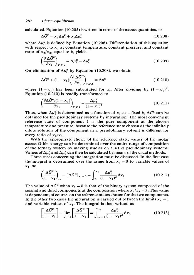
8/11/2019 Thermodynamics of Chemical Systems.pdf
http://slidepdf.com/reader/full/thermodynamics-of-chemical-systemspdf 302/456
282
Phase equilibrium
calcu lated. E qu atio n (10.205) is written in term s of the excess qu an tities, so
AG
E
=
Xl
Afi + x
s
A/*
E
(10.208)
where A^
E
is defined by Equation (10.206). Differentiation of this equation
with respect to x
x
at constant temperature, constant pressure, and constant
ratio of x
2
/ x
3
, equal to /c, yields
) = A
f
i
E
-A
f
i
E
(10.209)
T,P,k
On elimination of A/x
E
by Equation (10.208), we obtain
= A ^
E
(10.210)
where (1 —x
x
) has been substituted for x
s
. After dividing by (1 —x
x
)
2
,
Equation (10.210) is readily transformed to
Thus, when A^
E
is determined as a function of x
x
at a fixed k, AG
E
can be
obtained for the pseudobinary systems by integration. The most convenient
reference state of com pon ent 1 is the pure co m pon ent at the chosen
temperature and pressure, because the reference state chosen as the infinitely
dilute solution of the component in a pseudobinary solvent is different for
every ratio of x
2
/x
3
.
With the appropriate choice of the reference state, values of the molar
excess Gibbs energy can be determined over the entire range of composition
of the ternary system by making studies on a set of pseudobinary systems.
Values of A/if a nd A/zf can th en be calculated by mea ns of the usual m eth od s.
Three cases concerning the integration must be discussed. In the first case
the integral is determined over the range from x
x
= 0 to variable values of
x
u
so
^ P ^ X ,
(.0.2,2,
The value of AG
E
when x
x
= 0 is that of the binary system composed of the
second and third comp onen ts at the com posit ion where x
2
/ x
3
= k. This value
is dep end ent, of cou rse, on the reference states chosen for the two c om pon ents.
In the other two cases the integration is carried out between the limits x
x
= 1
and variable values of x
x
. The integral is then written as
d , , (.O2IJ)

8/11/2019 Thermodynamics of Chemical Systems.pdf
http://slidepdf.com/reader/full/thermodynamics-of-chemical-systemspdf 303/456
1030 Determination of excess chemical potentials 283
The integrand must be finite as x
x
approaches zero. In the case of a
dissociating substance, a prope r choice of the compon ents or species is
required. The value of AG
E
/(1
—
x
x
) becomes indeterminate in the limit as
x
l
goes to unity, but can be determ ined by the use of 1'HopitaFs theorem.
We have
^
8
^ (10.214)
m - — = - lim
8
- -
xi-ll_l~~*lJ
xi- lL
3*1 -JT,P,
With the use of Equations (10.208) and (10.209), together with Equation
(10.206) expressed in terms of the excess chemical potentials, we obtain
( I 0 2 1 5 )
When the reference state of the first com pon ent is chosen as the pure
component and that of each of the other two components as the infinitely
dilute solution of the component in the first component, each of the excess
chemical potentials become zero in the limit and Equation (10.214) can be
written as
[
Xl
A/i
* ( 1 0 . 2 1 6 )
The third case occurs when we choose the reference state of each of the
components as the pure components. In this case A/if becomes zero in the
limit, and the values of A/zf and A/if are limiting values in the binary systems
composed of the first and second co mp onen ts and of the first an d third
components, respectively. We then have
-r
-
-dx, (10.217)
The second method for studying ternary systems, which has been
developed by Gok cen [2 8] , m akes use of such equatio ns expressed in general
form as
(10.218)
The equations are derived from the differential of the Gibbs energy for a
one-phase, multicomponent system Equation (2.33). The differential is exact,
and therefore the condition of exactness must be satisfied. Two equations

8/11/2019 Thermodynamics of Chemical Systems.pdf
http://slidepdf.com/reader/full/thermodynamics-of-chemical-systemspdf 304/456
284 Phase equilibrium
and
( —
=
(~ ) (10.220)
\V
n
l/ T,P,n
2
,ti3 \^
n
3/
T,P,m,n
2
are obtained for ternary systems. When values of fi
x
are known for various
values of two of the composition variables, values of \i
2
and \i
3
can be
obtained by the use of Equations (10.219) and (10.220), respectively.
We limit our discussion here to Equation (10.219) and make use of the
excess chemical potentials rather than the chemical potentials themselves.
We then start with
4\
, \ a , <
1 0
-
2 2 1 )
i
1
/T
Pn2n3
\ Cn
2
/ T P ni n
3
New composition variables are defined as
p
= —^ _ = -^— = ^ (10.222)
n
1
+ n
3
x
x
4- x
3
1 — x
2
a n d
q
= "
3
= *
3
= -*^-
(10.223)
* ) ,,0.224,
We
and
and
then have
fdAfi
1
1
Equat ion
V
dp
I)
/T,P,n
2
,n
3
Jr .
(10.
/ T
,P,ni,ri3
.221)
,P,q
_ / 3 A / x f
V dp
V dq
becomes
P
2
V Sq
8q
> (10.225)
(10.226)
T,P,p
Values of A/zf can be obtained from known values of
(d
A^i\/dq)
T P p
on
integration.
The actual calculations associated with the integrations are outlined with
reference to Figure 10.7, where the equilateral triangle gives the usual
representation of the composition of a ternary system. Each apex of the

8/11/2019 Thermodynamics of Chemical Systems.pdf
http://slidepdf.com/reader/full/thermodynamics-of-chemical-systemspdf 305/456
10.30 Determination of excess chemical potentials 285
triangle represents a pure component as given by the numbers 1, 2, and 3.
The solid straight line from apex 2 to the 1-3 edge represents all systems
that have a given, constant value of
p .
Similarly, the solid straight line drawn
from apex 1 to the 2-3 edge represents all systems tha t have a given, constan t
value of q. The values of q along any line of constant p range from unity at
the 1-3 edge to zero at the apex, and the values of p along any line of con stant
q range from unity at the 2-3 edge to zero at the apex. We assume for the
purp oses of discussion th at the integration is carried ou t along the line draw n
from 1 to q. We need to know values of A/zf as a function of q for various
constant values of p; e.g., along the line drawn from 2 to p. With this
knowledge, values of (d
^^/dq)
TtPtP
are obtain ed at the chosen value of q for
various values of
p.
The integration is then carried out after multiplication
b y
p
2
/q
2
.
Two choices of the lower limit for the integration are apparent. In one
case the lower limit of p is chosen as unity, for which case x
t
= 0. Then the
integral of Equation (10.226) becomes
P
~
2
(^±) dp (10.227)
P=IP
\ 3q J
TtPtP
Here A^f[p = 1,
q~]
is the excess chemical potential of the second component
in the binary system composed of the second and third components at the
composition equal to q. The reference state of the second component may
be either the pure component or the infinitely dilute solution of the second
comp onent in the thi rd com ponent . In the limit of p = l , q/ p becomes
l/(/c+ 1), where k = x
2
/x
3
and , with the proper choice of com ponen ts or
Figure 10.7. Ternary systems.
1

8/11/2019 Thermodynamics of Chemical Systems.pdf
http://slidepdf.com/reader/full/thermodynamics-of-chemical-systemspdf 306/456
286 Phase equilibrium
species,
(d
Ajuf/dg)
r P p
remains finite in the limit. Hence, the integrand is
finite in the limit.
The second choice of the lower limit is to set
p
= 0. Th e integral then
becomes
dp (10.228)
/T,P,p
The line for which p = 0 is the 1-2 edge of the trian gle. Therefo re, the limiting
value of A/xf as p goes to zero along any line of constant q is that of the
second component in the infinitely dilute solution of the component in the
first component. Whereas a knowledge of the 2-3 binary system is required
when the lower limit is at
p =
1, here a knowledge of the 1-2 binary system
is required. From the definitions of p and q given in Equations (10.222) and
(10.223), we observe that the value of q/ p becomes large as p goes to zero.
At the same time the value of (d Af^/dq)
T P p
becomes small. Experimental
work has shown that the product of the two quantities generally remains
finite and the integral is well behaved. The proper choice of components or
species may be required in some cases, particularly for electrolytic so lutions.
In any case, studies should be made to determine that the integrand does,
indeed, remain finite in the limit. Values of A/zf are determined over the
entire range of com position by integrating alon g various lines of con stant
q.
Values of A/zf are determined similarly by the use of Equation (10.220)
expressed in terms of the excess chemical potentials. In this case the new
variables would be
If V V
(10.229)
n
1
+n
2
x
1
-\-x
2
1 — x
3
and
t=
Hl
=
*
2
= ^ — (10.230)
Lines of con stan t 5 in Figure 10.7 wou ld be draw n from the apex ma rked 3
to the 1-2 edge of the triangle, and lines of constant t are the same as those
at constant
p.
Gokcen has pointed out a method of determining the
com position s to be studied in a ternary system in order to achieve a minim um
of experimental work. Each angle of the triangle is divided into an equal
number of parts by drawing lines of constant
p, q,
and s. The intersections
of the three lines then determine the compositions that are to be used.
Wagner [29] and Schuhmann [30] have developed similar methods based
on
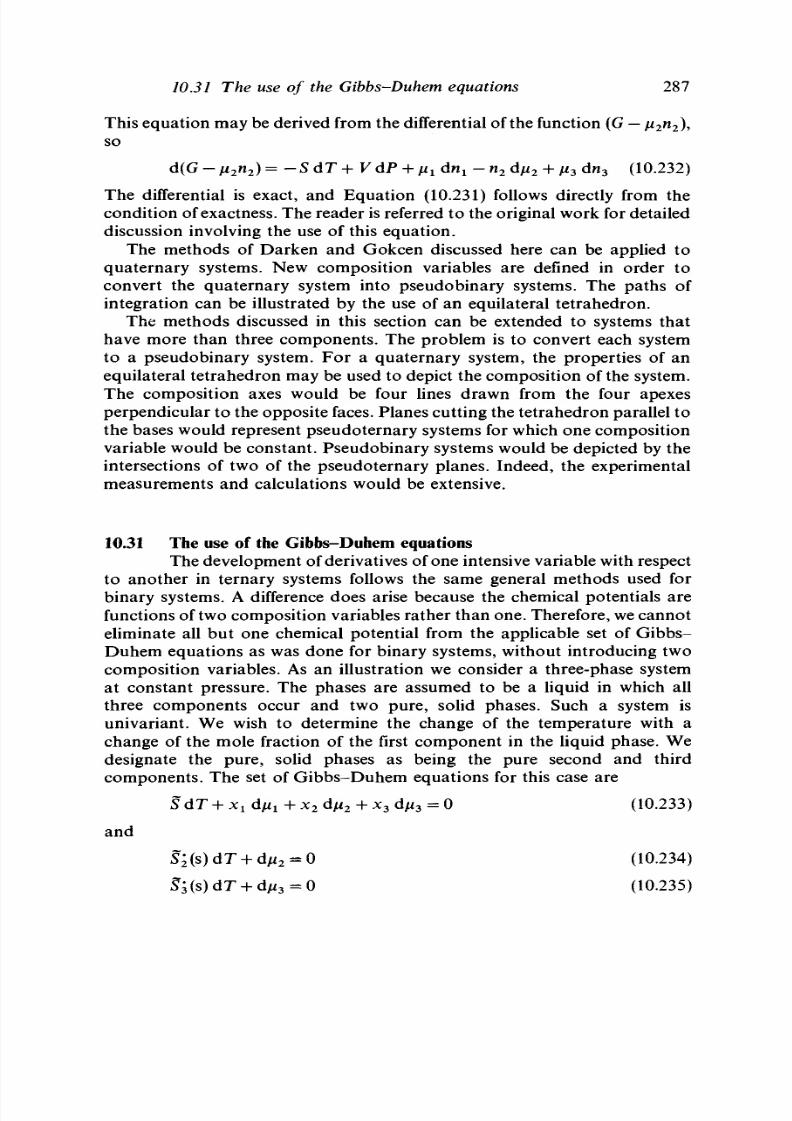
8/11/2019 Thermodynamics of Chemical Systems.pdf
http://slidepdf.com/reader/full/thermodynamics-of-chemical-systemspdf 307/456
10.31 The use of the Gibbs-Duhem equations
287
This equation may be derived from the differential of the function (G — ii
2
n
2
\
so
d(G -
fi
2
n
2
) =-SdT+VdP + n
1
dn
l
-n
2
dn
2
+ ii
3
dn
3
(10.232)
The differential is exact, and Equation (10.231) follows directly from the
con dition of exactness. The rea der is referred to the original w ork for detailed
discussion involving the use of this equation.
The methods of Darken and Gokcen discussed here can be applied to
quaternary systems. New composition variables are defined in order to
convert the quaternary system into pseudobinary systems. The paths of
integration can be illustrated by the use of an equilateral tetrahedron.
The methods discussed in this section can be extended to systems that
have more than three components. The problem is to convert each system
to a pseudobinary system. For a quaternary system, the properties of an
equilateral tetrahedron may be used to depict the composition of the system.
The composition axes would be four lines drawn from the four apexes
perpendicular to the opposite faces. Planes cutting the tetrahedron parallel to
the bases would represent pseudoternary systems for which one composition
variable would be constant. P seudo binary systems would be depicted by the
intersections of two of the pseudoternary planes. Indeed, the experimental
measurements and calculations would be extensive.
10.31 The use of the Gibbs-Duhem equations
The develop me nt of derivatives of one intensive variable w ith respect
to another in ternary systems follows the same general methods used for
binary systems. A difference does arise because the chemical potentials are
functions of two composition variables rather than one. Therefore, we cannot
eliminate all but one chemical potential from the applicable set of Gibbs-
Duhem equations as was done for binary systems, without introducing two
composition variables. As an illustration we consider a three-phase system
at constant pressure. The phases are assumed to be a liquid in which all
three components occur and two pure, solid phases. Such a system is
univariant. We wish to determine the change of the temperature with a
change of the mole fraction of the first component in the liquid phase. We
designate the pure, solid phases as being the pure second and third
components. The set of Gibbs-Duhem equations for this case are
S dT
+
x
l
dfi
x
+
x
2
d[i
2
+
x
3
d/i
3
= 0 (10.233)
and
= 0 (10.234)
= 0 (10.235)
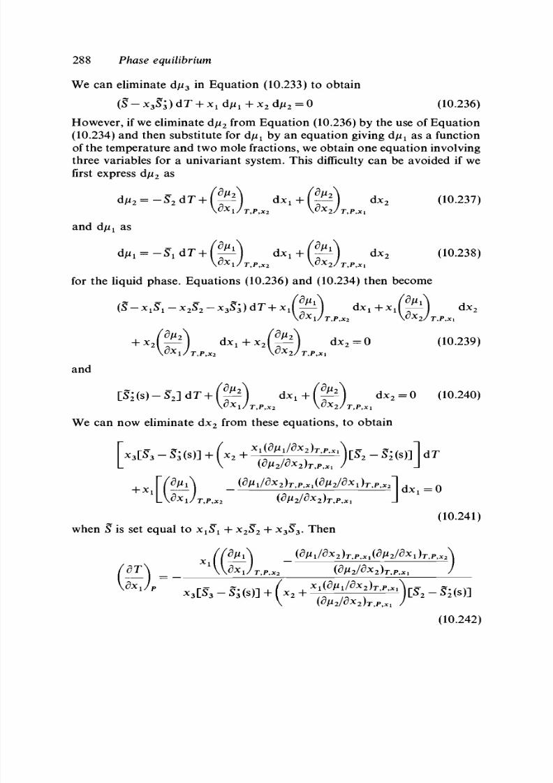
8/11/2019 Thermodynamics of Chemical Systems.pdf
http://slidepdf.com/reader/full/thermodynamics-of-chemical-systemspdf 308/456
288
Phase equilibrium
We can eliminate d/x
3
in Equation (10.233) to obtain
(S-
x
3
S
3
)
AT
+
x
1
dfi
1
+ x
2
d\i
2
=
0 (10.236)
However, if we eliminate dfx
2
from Equation (10.236) by the use of Equation
(10.234) and then substitute for d ^ by an equation giving d/z
x
as a function
of the temperature and two mole fractions, we obtain one equation involving
three variables for a univariant system. This difficulty can be avoided if we
first express d/i
2
as
(^) f ^ ) dx
2
(10.237)
and
dfi
t
as
( ^ ( ^ dx
2
(10.238)
for the liquid phase. Equations (10.236) and (10.234) then become
dx
2
=
0 (10.239)
and
[S
2
(s)
-
S
2
] d T
+
(
^ j dx
x
+
l
8
^
j
dx
2
=
0 (10.240)
We can now eliminate dx
2
from these equations, to obtain
x
3
LS
3
- S
3
(s)] + (x
2
+
x
^Vildx
2
)
T
^
x
\-^
_
^ .
( s ) ]
dT
(10.241)
when
S
is set equal to x ^ +
x
2
<S
2
+ x
3
S
3
. Then
,-S
3
(s)] + (x
2
+ -
T
^ — ^ )[5
2
-5
2
(s)]
(10.242)
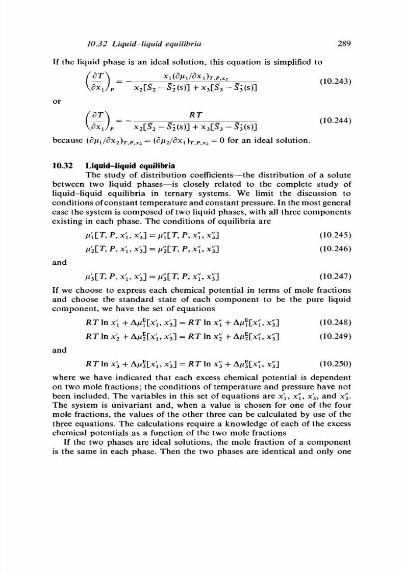
8/11/2019 Thermodynamics of Chemical Systems.pdf
http://slidepdf.com/reader/full/thermodynamics-of-chemical-systemspdf 309/456
10.32 Liquid-liquid
equilibria
289
If the liquid phase is an ideal solution, this equation is simplified to
)r,P,»
2
1 0 2 4 3 )
[ S S
r
5 ( ) ]
(10.244)
\dx
1/ P
or
RT
K
dxJ
P
x
2
[S
2
- S
2
(s)]
+ x
3
[S
3
- ^(s )]
because (djLi
1
/dx
2
)
T9
p
fX 2
=
(djujdx^j
Px2
=
®
f°
r a n
ideal solution.
10.32 Liquid-liquid equilibria
The study of distribution coefficients—he distribution of a solute
between two liquid phases—s closely related to the complete study of
liquid-liquid equilibria in ternary systems. We limit the discussion to
conditions of constant temperature and constant pressure. In the most general
case the system is composed of two liquid phases, with all three components
existing in each phase. The conditions of equilibria are
Aii[T,P,xi,x'
3
] = ^ [ r , P, x ^ x 5 ] (10.245)
^ [ T ,
P, xi, x'
3
] =
»"
2
IT
9
P, xl x£] (10.246)
and
ALT, P, xi , x'
3
] = ^[T, P, xl x5] (10.247)
If we choose to express each chemical potential in terms of mole fractions
and choose the standard state of each component to be the pure liquid
component, we have the set of equations
RT In xi + A/i?[xi, x'
3
] - RT In
x'[
+ Aji?[x'J, x£] (10.248)
RT
In
x'
2
4- Af4lx'
u
x'
3
] =
RT
In x"
2
+ A/ifK,
x"{\
(10.249)
and
KT In x
3
+ A^if [xi, x
3
] =
RT
In x£ + A/ifK, xj] (10.250)
where we have indicated that each excess chemical potential is dependent
on two mole fractions; the conditions of temperature and pressure have not
been included. The variables in this set of equations are xi, xi', x
3
, and x
3
.
The system is univariant and, when a value is chosen for one of the four
mole fractions, the values of the other three can be calculated by use of the
three equations. The calculations require a knowledge of each of the excess
chemical potentials as a function of the two mole fractions
If the two phases are ideal solutions, the mole fraction of a component
is the same in each phase. Then the two phases are identical and only one

8/11/2019 Thermodynamics of Chemical Systems.pdf
http://slidepdf.com/reader/full/thermodynamics-of-chemical-systemspdf 310/456
290 Phase equilibrium
liquid phase actually exists. The solutions must be nonideal when two liquid
phases do exist. It is evident that the ratio of the activities of each component
in the two phases is always unity. The distribution ratio in terms of mole
fractions for each component is given by
RT\n{x'Jx'l) = A/ if K, xj] - A/if[x;, x'
3
] (10.251)
Here we see that the ratio is dependent upon the difference between the
excess chemical potentials of the component in each of the two phases. This
ratio is not constant.
The thermodynamic distribution coefficient is introduced when one of the
components can be considered as a solute in each phase, and when we choose
the reference states of that component to be the infinitely dilute solution in
each phase. For discussion, we designate the first and second components
as those that form the solvents and the third component as the solute.
Equations (10.245), (10.246), (10,248), and (10.249) are still applicable when
we choose the pure liquid phase as the standard state for each of the two
components. When we introduce expressions for the chemical potential of
the third component into Equation (10.247), Equation (10.250) becomes
RT
In x
3
+ A/if [x;, x'
3
] + [/if]' =
RT
In x£ + A/if [x?, x'3] + [/ if ]"
(10.252)
or, in terms of the activity,
RT In a
3
+ [/if]' = RT In a\ + [/if ]" (10.253)
Two reference states, one for each phase, must be defined. As we decrease
the mole fraction of the third component, we approach the two-liquid-phase
binary system composed of the first and second components. We thus define
the reference states of the third component as the infinitely dilute solutions
of the component in the two liquid phases that are at equilibrium in the 1-2
binary system. Thus, the value of A/if[xi,x
3
] approaches zero as x'
3
approaches zero, and xi approaches its value in the 1-2 system, and the value
of A/i
3
[x'i, x'
3
] also approaches zero, and
x'[
approaches its value in the 1-2
system. In the limit Equation (10.251) becomes
RT ln[(x'
3
/x5n = [/ if ]" - [/i f] ' (10.254)
where the infinity sign is used to designate the ratio of
(x'
3
/x
f
^)
in the infinitely
dilute system. Both [/ if]" and [/if] ' are functions of the temperature and
pressure, but not of the composition. Therefore, the difference is a constant
at constant temperature and pressure. We choose to write this difference as
\Ji?Y
~
l>f ]'
=~RT\nk
(10.255)
where k is a function of the temperature and pressure, and is a constant at
constant temperature and pressure. The quantity k is called the thermo-

8/11/2019 Thermodynamics of Chemical Systems.pdf
http://slidepdf.com/reader/full/thermodynamics-of-chemical-systemspdf 311/456
10.32 Liquid-liquid equilibria
291
dynamic distribution coefficient. We see from Equation (10.253) that k can
be evaluated by determining the value of the ratio x'
3
/x
3
in the limit as x'
3
goes to zero, i.e.,
k= lim (xS/x'a) (10.256)
x'3-0
With the definition of the thermodynamic distribution coefficient, Equation
(10.252) can be written as
RT]n(x'
3
/x'£ + A/xf
[ x i ,
x'
3
] - A/if [x?, x'3] = -RT\nk (10.257)
and Equation (10.253) as simply
aya's = k
(10.258)
We see that the ratio of the activities is always constant at constant
temperature and pressure; the ratio of the mole fractions is not constant
over a range of concentrations of x'
3
, and the variation of the value of the
ratio depends upon the difference of the excess chemical potentials.
If we had expressed the chemical potential of the third component in
terms of its molality and activity coefficient rather than the mole fraction
and excess chemical potential, Equation (10.258) would be expressed as
y x
=k (10.259)
my /
3
If the solute were a salt, having the formula M
v +
A
v
and was nonionized in
one phase and completely ionized in the other phase, the distribution
coefficient would be expressed as
y ±
r - i
=
y
_|
3
I ,, . (
1 0
-
2 6
° )
The relations that obtain when the solute is partially polymerized or ionized
are discussed in Chapter 11.

8/11/2019 Thermodynamics of Chemical Systems.pdf
http://slidepdf.com/reader/full/thermodynamics-of-chemical-systemspdf 312/456
11
Chemical equilibrium
We turn our attention in this chapter to systems in which chemical
reactions occur. We are concerned not only with the equilibrium conditions
for the reactions themselves, but also the effect of such reactions on phase
equilibria and, conversely, the possible determination of chemical equilibria
from kno wn therm odyn am ic prope rties of solutions. Various expressions for
the equilibrium constants are first developed from the basic condition of
equilibrium. We then discuss successively the experimental determination of
the values of the equilibrium constants, the dependence of the equilibrium
constants on the temperature and on the pressure, and the standard changes
of the Gib bs energy of form ation. Equ ilibria involving the ionization of weak
electrolytes and the determination of equilibrium constants for association
and complex formation in solutions are also discussed.
11.1 Basic considerations
In Section 5.4 we develop the condition of equilibrium for a chemical
reaction: for any chemical reaction written as £
k
v
k
B
k
= 0, the co ndition of
equilibrium is £
fc
v
fe
/x
fe
= 0. In these equations each
v
k
represents the stoichio-
metric coefficient of the substance B
k
in the balanced chemical equation; the
sign is positive for products and negative for reagents. Expressions for the
equilibrium constants are readily obtained from this condition. For a general
relation we express the chemical potentials in terms of the activities, so
?lT
9
p-]
(11.1)
Then, according to the condition of equilibrium,
I f ]>? (1 12 )
when the temperature of every reacting substance is the same. In Equation
(11.2),
rifc
a
fe
k
represents the product of the activities of the reacting
substances, each activity being raised to the appropriate power. At constant

8/11/2019 Thermodynamics of Chemical Systems.pdf
http://slidepdf.com/reader/full/thermodynamics-of-chemical-systemspdf 313/456
11.1 Basic considerations 293
temperature and pressure, the left-hand side of Equation (11.2) is constant,
and hence the right-hand side must be constant. We can therefore define the
thermodynamic equilibrium constant for the reaction as
so
: ( i i .4 )
As defined here, the equilibrium constant is a function of the temperature
and pressure in general. The form of Equation (11.3) is consistent with the
conventional method of expressing the equilibrium constant, in that the
activities of the products appear in the numerator and those of the reagents
in the denominator of the expression for the equilibrium constant. In many
cases
Y,k
y
kl
x
f is written as A G
e
to represent the change of the Gibbs energy
for the change of state given by the balanced chemical equation when all
reagents and products a
r
e in their standard states at the given temperature
and pressure.
With this general basis we consider the development of specific expressions
for different types of chemical reactions. We first consider a homogenous
reaction in the gas phase, and use the virial equation of state accurate to
the second virial coefficient. The chemical potential of the /cth substance is
given by Equation (7.72)
T,
P, y\ = RT\n Py
k
+ £ I (2j&* - PtMyf + ^ IT ] (11.5)
*
j
For equilibrium,
X v
k
RT \n(Py
k
) + £
v
k
£ I (2jB
tt
- P^yf = - £ v ^ f [T ]
k k i j k
(11.6)
and the equilibrium constant in terms of partial pressures is given by
|~X
v
k
X Z Wik - PkMyjP /Rr
L k i j
K
P
=
n
Pl
k
e x
P
|X
v
k
X Z Wik - PkMyjP/Rr]
(i 1.7)
k
L J
where P
k
= Py
k
. The constant is a function of the temperature alone, and
is independent of the pressure according to Equation (11.6). If we choose
the standard state of each substance as the pure substance in the ideal gas
state at the pressure P ra ther tha n 1 ba r, the chem ical poten tial of the /cth
substance is given by
, P
9
y] = RT In y
k
+ £ £ (2p
ik
- p^yf + / i f
[T ,
P ] (11.8)
i j
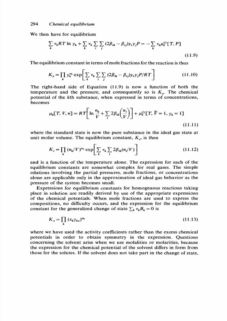
8/11/2019 Thermodynamics of Chemical Systems.pdf
http://slidepdf.com/reader/full/thermodynamics-of-chemical-systemspdf 314/456
294 Chem ical equilibrium
We then have for equilibrium
£ v
k
RT In y
k
+ £ v
k
£ £ (2j»
tt
- j8y)jWjP = " Z v ^ f
[T,
P ]
(11.9)
The equ ilibrium con stant in terms of mole fractions for the reaction is thus
K,
=
El
yl
k
e x p f l
v,
X X (2/»
tt
- P,j)y
t
yjP/RT\ (n.io)
k L k
iI
j J
The right-hand side of Equation (11.9) is now a function of both the
temperature and the pressure, and consequently so is
K
y
.
The chemical
potential of the fcth substance, when expressed in terms of concentrations,
becomes
(11.11)
, V, n\ = RT^ln ** + X 2 / ?
t t
^ + [ T , K =
where the standard state is now the pure substance in the ideal gas state at
unit molar volume. The equilibrium constant, K
c
, is then
v
k
^ 2p
ik
{n
i
/V)\
i J
(11.12)
and is a function of the temperature alone. The expression for each of the
equilibrium constants are somewhat complex for real gases. The simple
relations involving the partial pressures, mole fractions, or concentrations
alone are applicable only in the approximation of ideal gas behavior as the
pressure of the system becomes small.
Expressions for equilibrium constants for homogenous reactions taking
place in solution are readily derived by use of the appropriate expressions
of the chemical potentials. When mole fractions are used to express the
compositions, no difficulty occurs, and the expression for the equilibrium
constant for the generalized change of state £&
v
k
B
k
=
0 is
where we have used the activity coefficients rather than the excess chemical
potentials in order to obtain symmetry in the expression. Questions
concerning the solvent arise when we use molalities or molarities, because
the expression for the chemical potential of the solvent differs in form from
those for the solutes. If the solvent does not take part in the change of state,

8/11/2019 Thermodynamics of Chemical Systems.pdf
http://slidepdf.com/reader/full/thermodynamics-of-chemical-systemspdf 315/456
11.1 Basic considerations 295
there is no problem and the equilibrium constants are
in terms of molalities, and
in terms of molarity. When the solvent does take part in the change of state,
its chemical poten tial occu rs in the expression for the co ndition of equilibrium .
Then, if we use Equation (8.102)
X m
k
+RTln
7l+
l
if IT, P^ (11.16)
for the chemical potential of the solvent, the expression for the equilibrium
constant becomes
K
m
=
n w n
?
If we choose to express the chemical potential of the solvent in terms of the
osmotic coefficient, so that (Eq. (8.119))
i
+
nflT,p-} (11.18)
The expression for the equilibrium constant is
K
m
=
[ I
( m ^ r e x p F - ^ ^ ^
I m j
(11.19)
Expressions similar to Equations (11.17) and (11.19) are obtained when
molarities are used rather than molalities (refer to Eqs. (8.118) and (8.120)).
In each case £
fc
v
k
nf is a function of the tem pera ture and pressu re, and
therefore each equilibrium con stant is also a function of the same va riables.
The condition of equilibrium is also applicable to changes of state that
involve heterogenous reactions, and the same me thods used for hom ogeno us
reactions to obtain expressions of the equilibrium constant are used for
heterog eno us reaction s. O ne difference is tha t in ma ny hetero geno us reactions
one or more of the substances taking part in the change of state is a pure
phase at equilibrium. In such cases the standard state of the substance is
chosen as the pure phase at the experimental temperature and pressure. The
chemical potential of the pure substance in its standard state still appears
in Y,k
v
fcj"jP> but the activity of the substance is unity and its activity does
not appear in the expression for the equilibrium constant.
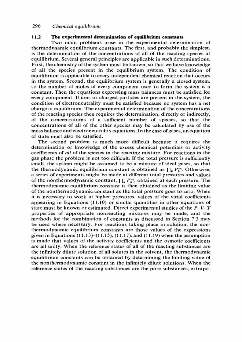
8/11/2019 Thermodynamics of Chemical Systems.pdf
http://slidepdf.com/reader/full/thermodynamics-of-chemical-systemspdf 316/456
296
Chem ical equilibrium
11.2 The experimental determination of equilibrium constants
Two main problems arise in the experimental determination of
thermodynamic equilibrium constants. The first , and probably the simplest ,
is the determination of the concentrations of all of the reacting species at
equilibrium . Several general principles are applicable in such d eterm ination s.
First, the chemistry of the system m ust be kno wn , so that we have kn owledge
of all the species present in the equilibrium system. The condition of
equilibrium is applicable to every independent chemical reaction that occurs
in the system. Second, the equilibrium system is generally a closed system,
so the number of moles of every component used to form the system is a
constant. Then the equations expressing mass balances must be satisfied for
every component. If ions or charged particles are present in the system, the
condition of electroneutrality must be satisfied because no system has a net
charge at equilibrium. The exp erimental determination of the concentrations
of the reacting species then requires the d eterm ination , directly or indirectly,
of the concentrations of a sufficient number of species, so that the
concentrations of all of the other species may be calculated by use of the
mass balan ce and electron eutrality eq uatio ns. In the case of
gases,
an eq uation
of state must also be satisfied.
The second problem is much more difficult because it requires the
determination or knowledge of the excess chemical potentials or activity
coefficients of all of the species in the reacting mixture. For reactions in the
gas phase the problem is not too difficult. If the total pressure is sufficiently
small, the system might be assumed to be a mixture of ideal gases, so that
the thermodynamic equilibrium constant is obtained as
Ylk Pl
k
-
Otherwise,
a series of experiments might be made at different total pressures and values
of the nonthermodynamic constant ,
Y\
k
P£
k
, obtained at each pressure. The
thermodynamic equilibrium constant is then obtained as the limiting value
of the nonthermodynamic constant as the total pressure goes to zero. When
it is necessary to work at higher pressures, values of the virial coefficients
appearing in Equations (11.10) or similar quantities in other equations of
state must be known or estimated. Direct experimental studies of the P-V-T
properties of appropriate nonreacting mixtures may be made, and the
methods for the combination of constants as discussed in Section 7.3 may
be used where necessary. For reactions taking place in solution, the non-
thermodynamic equilibrium constants are those values of the expressions
given in Eq ua tio ns (11.13)—11.15), (11.17), an d (11.19) when th e assu m ptio n
is made that values of the activity coefficients and the osmotic coefficients
are all unity. When the reference states of all of the reacting substances are
the infinitely dilute solution of all solutes in the solvent, the thermodynamic
equilibrium constants can be obtained by determining the limiting value of
the nonthermodynamic constant in the infinitely dilute solutions. When the
reference states of the reacting substances are the pure substances, extrapo-

8/11/2019 Thermodynamics of Chemical Systems.pdf
http://slidepdf.com/reader/full/thermodynamics-of-chemical-systemspdf 317/456
113 Effect of temperature on equilibrium constant 297
lations to a single system in which all activity or o sm otic coefficients are
unity cannot be made. It is then necessary to d eterm ine th e values of the
coefficients experim entally (when possible), or to estim ate them on theoretical
gro un ds. The activity coefficients of m any c om pon ents in binary systems and
some in ternary systems have been measured. However, general methods
have not been developed for the calculation of the activity coefficients of
substances in multicomponent systems from those in binary systems. In some
cases
it
may be necessary to use only the non therm ody nam ic equilibrium
constants. An appreciation of the effect of activity or osmotic coefficients on
the equilibrium constants can come only with experience and with
an
understanding of the present theories of solutions.
11.3 The effect of temperature on the equilibrium constant
The dependence of the equilibrium constant on the temperature is
easily obta ine d from E qu ati on (11.4) with the use of the relation (Eq. (4.41))
[d(G/T)l
=
_H_
L dT , „ T
2
From Equation (11.4)
\ dT J
P
V 8T ) ~ "V ST
However ,
8T J
P
V V
8T
On combining these equations,
r
d
In
K\
y
t
vM°
A H
e
(11.20)
=
y iw_ _\
=
_y
V
ffo
/T
2
( 1 1 2
i )
dT J
P
RT
2
RT
2
( 1 L 2 2 )
The quant i ty AH° isthe change of enthalpy for the change of state
represented by a balance d chem ical equ ation und er the condition th at all
substances are in their standard states at the temperature and pressure in
question. The overbar is used here because some of the individual enthalpies,
Hf' , may be partial mo lar quantit ies.
Equation (11.22) may be written as
\d(l/T)J
P
R
when the independent variable is changed from Tto l/T. According to this
equat ion, R times the s lope of the curve In K versus l/Tgives the negative
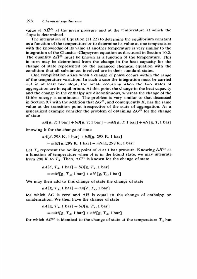
8/11/2019 Thermodynamics of Chemical Systems.pdf
http://slidepdf.com/reader/full/thermodynamics-of-chemical-systemspdf 318/456
298
Chem ical equilibrium
value of AH° at the given pressure and at the tem pera ture at which the
slope is determined.
The integration of Equation (11.22) to determine the equilibrium constant
as a function of the temperature or to determine its value at one temperature
with the knowledge of its value at another temperature is very similar to the
integration of the Clausius-Clapeyron equation as discussed in Section 10.2.
The quantity AH° mu st be kno wn as a function of the tem pera ture. This
in turn may be determined from the change in the heat capacity for the
change of state represented by the balanced chemical equation with the
condition that all substances involved are in their standard states.
One complication arises when a change of phase occurs within the range
of the temperature variation. In such a case the integration must be carried
out in at least two steps, the break occurring when the two states of
aggregation are in equilibrium. At this point the change in the heat capacity
and the change in the enthalpy are discontinuous, whereas the change of the
Gibbs energy is continuous. The problem is very similar to that discussed
in Section 9.7 with the add ition th at A G
e
, and consequently K, has the same
value at the transition point irrespective of the state of aggregation. As a
generalized example consider the problem of obtain ing A G
e
for the change
of state
g,
T,
1
bar] + b£[g, T,
1
b ar] = mM [g, T,
1
ba r ]
4-
nJV[g,
T , 1
ba r ]
knowing it for the change of state
aA\f
9
298 K, 1 bar ] + bB[g, 298 K, 1 bar]
= m M [g, 298 K, 1 bar] + nJV[g, 298 K, 1 bar]
Let
T
A
represent the boiling point of
A
at 1 bar pressure. Knowing A/7
e
as
a function of temperature when
A
is in the liquid state, we may integrate
from 298 K to
T
A
.
Then , AG
e
is known for the change of state
aA[f, T
A9
1 bar] + &B[g,
T
A
,
1 ba r ]
= mM[g , T
A
, 1 bar ] + nN [g , T
A9
1 bar ]
We may then add to this change of state the change of state
aA[g, T
A9
1 bar] = aA\t
9
T
A
, 1 bar ]
for which AG is zero and AH is equal to the change of enthalpy on
condensation. We then have the change of state
aA[£, T
A9
1 bar] + 6B[g, T
A9
1 b a r ]
= wM[g ,
T
A9
1 bar] + nAT[g,
T
A9
1 bar ]
for which A G
e
is identical to the change of state at the temperature T
A
but

8/11/2019 Thermodynamics of Chemical Systems.pdf
http://slidepdf.com/reader/full/thermodynamics-of-chemical-systemspdf 319/456
11.4 The effect of pressure on the equilibrium constant 299
involving liquid
A,
bu t
AH°
differs by the chan ge of enth alpy on
condensation. These two quantities are used to determine the necessary
integration constants for the succeeding integrations. The first of these is the
obtaining of AH° as a function of tem pera ture when gaseous A is involved
using the corresponding ACf. Hav ing the correct function for A / 7
e
, the
integration of Equation (11.24) is then carried out between the limits of T
A
and T. When several changes of phase occur over the given temperature
range, it is necessary to carry out the integration in a series of such steps.
11.4 The effect of pressure on the equilibrium constant
The dependence of the equilibrium constant on pressure for a
chemical reaction is easily determined from Equation (11.4) with the aid of
Equation (4.38), which gives the change of the Gibbs energy with pressure
at constant temperature and constant number of moles. Thus, we have
) «
(
n.24)
dPj
T
\ 3P )
T
\ 8P J
However ,
f
T k
\ or /
T
k
On combining these equations, we obtain
dP L RT RT
(11.26)
Here AV° is the change of volum e that occ urs for the change of state
represented by the balanced chemical equation under standard state
conditions at a given temperature and pressure.
The integration of Equation (11.26) follows the methods discussed in
Section 11.3. The qu antity
AV°
mu st be kno wn as a function of pressure,
which may be obtained from an equation of state or the compressibility of
each substance in its standard state. Again, the integration must be taken
in steps whenever a change of phase takes place within the range of the
pressure change. This is occasioned by a difference in the compressibilities
of a substance in different states of aggregation, and by the change in volume
tha t occurs when such a change of phase tak es place. The limits of integration
in the various steps must be chosen so that the changes of phase take place
under equilibrium conditions, because only then does the chemical potential
of the sub stance hav e the same value in the two different phase s. The ch ange
of the standard Gibbs energy is continuous at the transition point, whereas
both the volume change and the compressibility are discontinuous.

8/11/2019 Thermodynamics of Chemical Systems.pdf
http://slidepdf.com/reader/full/thermodynamics-of-chemical-systemspdf 320/456
300 Chem ical equilibrium
11.5 The standard Gibbs energy of formation
The calculation of the equilibrium constant for a given chemical
reaction from thermodynamic data requires the knowledge of AG
e
for the
change of state represented by the balanced chemical equation under standard
state conditions. For its definition, the calculation of AG
e
would appear to
require the knowledge of absolute values of the chemical potential of each
reacting substance in its standard state. This problem is avoided by making
use of the changes of the Gibbs energy for the formation of a compound
from the elements, the compound and the elements being in their standard
state, as was done in the case for the change of enthalpy for a change of
state involving a chemical reaction. Every chemical equation can be
considered as a sum of equations representing the formation of each
compound from the elements. Then
, F] = X
v
kf
i?[T,
F] = £ v,(AG p)
t
[T, P ] (11.27)
k k
where (AGP)
fc
[T, P] represents the molar change of the Gibbs energy for
the formation of the fcth substance from the elements, all substances being
in their standard states at the temperature T and pressure P. (In general,
the standard state for gases would still be the ideal gas state at a pressure
of
1
bar.) The experimental determination of the standard molar Gibbs
energies of formation follows from Equations (11.4) and (11.27). The value
of AG
e
[T, P] for a chemical reaction is obtained from the experimentally
determined value of the equilibrium constant; then, if values of all but one
of the quantities (AGp)
fc
[T, P], in the sum in Equation (11.27) are known,
the value of the remaining one can be calculated. Some changes of state
involve only the formation of a compound from the elements; in such cases
the standard molar Gibbs energy of formation of the compound is obtained
directly from the equilibrium constant.
Conventions followed in the compilation of standard molar Gibbs
energies of formation are similar to and consistent with those used for the
standard molar enthalpies of formation. A standard tem perature of 298.15 K
and a standard pressure of 1 bar is usually used. Values at other temperatures
and pressures are calculated by the methods discussed in Sections 11.3 and
11.4. The state of aggregation of a substance is the
naturally
occurring state
at the standard temperature and pressure. When a substance exists in two
or more allotropic forms in the solid state , one state is chosen as the standard
state; for example, graphite is chosen as the standard form of carbon, rather
than diamond. An additional definition must be given to the standard molar
Gibbs energy of formation of a solute when the reference state for the solute
is taken as the infinitely dilute solu tion. Here we include the difference between
the chemical potential of the solute in its standard state in solution and that
of the pure compound in its natural state of aggregation, in addition to the

8/11/2019 Thermodynamics of Chemical Systems.pdf
http://slidepdf.com/reader/full/thermodynamics-of-chemical-systemspdf 321/456
11.6
Gibbs energy
of
formation
of
ions
in
solution 301
standard molar Gibbs energy
of
formation
of the
pure compound. Thus,
the standard molar Gibbs energy of formation of solute is given by
(AGf[T,
P,
soln])
k
=
(AGf[T,
P,
pure]),
+
fif
[T ,
P,
soln]
- / ^ [ T , P , pu re] (11.28)
where,
for
purposes
of
compiling data ,
the
temperature would
be
298.15
K
and
the
pressure would
be
1
bar.
11.6 The standard Gibbs energy of formation of ions in solution
We consider only aqueous solutions here,
but the
methods used
are
applicable
to any
solvent system.
The
standard Gibbs energy
of
formation
of
a
strong electrolyte dissolved
in
water
is
obtained according
to
Equation
(11.28).
In
such solutions
the
ions
are
considered
as the
species
and we are
concerned with
the
thermodynamic functions
of the
ions rather than
the
component
itself. We
express
the
chemical potential
of the
electrolyte,
considered
to be
M
v+
A
v
_,
in its
standard state
as
fiflT, P] = v
+J
u?[T, P] + v__^[T, P] (11.29)
according
to
Equation (8.185). Here
and fi®
represent
the
standard
chemical potentials
of the
positive
and
negative ions, respectively.
The
equivalent
of
Equation (11.29)
is
[AGP]
2
= V +
[ A G P ] +
+ V _ [ A G P ] _ (11.30)
in terms
of the
standard Gibbs energies
of
formation. Although values
for
the individual ions cannot
be
determined from experimental data,
the
arbitra ry definition
of
the value
of
AGP
for one
ionic species determines
the
values
of
all other ionic species. By
convention
the
standard Gibbs energy
of
formation of the hydrogen ion is defined as zero at all
temperatures
and
pressures. Thus,
AGP is
defined
as
zero
for
| H
2
=
H
+
+£>- (11.31)
where e~ represents 1 mole of electrons. S tandard state conditions are implied
but
not
stated
in the
equation.
The
standard state
of the
electron
and its
chemical potential
is not
defined. This creates
no
problem because every
solution must
be
electrically neutral
and
Equation (11.31) must
be
used
in
conjunction with
a
change
of
state
for the
formation
of a
negative
ion
requiring 1 mole
of
electrons
as a
reagent.
The
symbol
for the
electron
and
its chemical potential thus cancel
on the
required addition.
As
an
example,
we
consider hydrochloric acid
in
aqueous solution,
for
which
the
standard molar Gibbs energy
of
formation
is
known. According
to Equation (11.30),
AGf(HCl)
=
AG f(H
+
) +
A G p (C r) (11.32)

8/11/2019 Thermodynamics of Chemical Systems.pdf
http://slidepdf.com/reader/full/thermodynamics-of-chemical-systemspdf 322/456
302
Chemical equilibrium
We define AGP(H
+
) as zero and, therefore,
(11.33)
that is, the standard molar Gibbs energy of formation of the chloride ion is
identical to that of the hydrochloric acid. The change of state to which
AGP(HCl) refers is
iH
2
+ iCl
2
= H
+
+ C r (11.34)
and that to which AGP(C1~) refers is
£Cl
2
+ e - = c r (11.35)
The addition of Equations (11.31) and (11.35) yields Equation (11.34).
The standard molar Gibbs energies of other ions are obtained by use of
the same methods. Thus, for sodium chloride solutions we have
(11.36)
from which AGP(Na
+
) can be obtained once AGP(C1~) is determined.
Similarly, for sulfuric acid
AGp(H
2
SO
4
) = 2AGf(H
+
) + A G f( S O D (11.37)
when we assume that the only species present are hydrogen ions and sulfate
ions in addition to water. Then, AGf(SOl~)
=
AGP(H
2
SO
4
). Finally, for
sodium sulfate
AGP(Na
2
SO
4
) = 2AGf(Na
+
) + A 5P (SO j") (H.38)
The value of AGf(Na
2
SO
4
) calculated from the values of AGp(Na
+
) and
AGP(SO
4
~) according to Equation (11.38) must be consistent with the value
obtained directly from experimental data. Moreover, it must be consistent
with the value determined by
AGp(Na
2
SO
4
) = 2AGf(NaCl) + AGP(H
2
SO
4
) - 2AGp(HCl)
(11.39)
according to Equations (11.32), (11.36), and (11.38).
11.7 Conventions concerning solvated species
When dissolved in a solvent, some solutes combine with the solvent
to form solvated species. The two outstand ing examples in aqueous solution
are carbon dioxide to form CO
2
(aq) (carbonic acid) and ammonia to form
NH
3
(aq) (ammonium hydroxide). In many cases the equilibrium constant
for the reaction is unknown or not known with sufficient accuracy for
thermodynamic purposes. Conventions have been established for treating
such systems thermodynamically. Here we discuss the carbon dioxide-water

8/11/2019 Thermodynamics of Chemical Systems.pdf
http://slidepdf.com/reader/full/thermodynamics-of-chemical-systemspdf 323/456
11.7 Conventions
concerning
solvated species
303
system. The methods used are applicable to any solute in any solvent. In
addition, we discuss the thermodynamic relations between the hydrogen ion
and the hydronium ion, because of the similarity of this problem to that of
solvated species.
The extent of the reaction of carbon dioxide with water to form carbonic
acid is fairly well known—ess than 1%. However, for thermodynamic
purposes we make no distinction between the two nonionized species, CO
2
and H
2
CO
3
. We are thus concerned with the sum of the concentration of
these species, a quantity that can be determined experimentally. We must
therefore develop the methods used to define the standard state of the
combined nonionized species and the standard molar Gibbs energies of
formation.
Two methods are possible. In the first method we assume the nonionized
species to be carbonic acid, H
2
CO
3
, and define its molality as the sum of
the molalities of the actual nonionized species. If we designate the molalities
of the actual species by primes, then the chemical potential of the assumed
species is written as
ju(H
2
CO
3
) =
RT
In m(H
2
CO
3
) +
RT
In y(H
2
CO
3
) + /z
e
(H
2
CO
3
)
(11.40)
where
m(H
2
CO
3
) = m'(H
2
CO
3
) + m'(CO
2
) (11.41)
We define the reference state in the usual way, so that y(H
2
CO
3
) goes to
unity as m(H
2
CO
3
) goes to zero. This definition defines the standard state
of the assumed species. The change of state for the first ionization of carbonic
acid may then be written as
H
2
CO
3
= H
+
+ HCO
3
" (11.42)
so that at equilibrium
H(H
+
) + MHCO
3
") - /i(H
2
CO
3
) = 0 (11.43)
The expression for the equilibrium constant becomes
, ( H > ( H C O 3 )
a(H
2
CO
3
)
in terms of activities.
In the second method we assume that the only nonionized species is
carbon dioxide, CO
2
, dissolved in water, and we equate its molality to the
sum of the molalities of the actual nonionized species, so
m(CO
2
) = m'(H
2
CO
3
) + m'(CO
2
) (11.45)

8/11/2019 Thermodynamics of Chemical Systems.pdf
http://slidepdf.com/reader/full/thermodynamics-of-chemical-systemspdf 324/456
304
Chem ical equilibrium
The chemical potential of the assumed species is expressed as usual as
/i(CO
2
) = RT In m(C O
2
) + RT In y(CO
2
) + ju
e
(C O
2
) (11.46)
and we choose the reference state as the infinitely dilute solution, so that
y(CO
2
) goes to unity as m(CO
2
) goes to zero. The standard state is thus
fixed. The change of state for the first ionization is now written as
C O
2
+ H
2
O = H
+
+ HCO
3
- (11.47)
Then, at equilibrium,
j
u(H
+
)
+ M H C O
3
- ) - / i ( C O
2
) -
i
u ( H
2
O ) = 0 (11.48)
and the equilibrium constant becomes
q ( H > ( H C O
3
- )
a(CO
2
)a(H
2
O)
The relations between the chemical potential of the carbonic acid given
in Equation (11.40) and that of carbon dioxide given in Equation (11.46),
between the corresponding chemical potentials, and between the two
equilibrium constants still need to be defined in order to make the two
methods consistent. By use of the methods developed in Section 8.15, we
can show that
(11.50)
Ai(H
2
CO
3
) = / / (C O
2
) + /i '(H
2
O) (11.51)
and
M C O
2
) = / i ' (CO
2
) (11.52)
where the primes refer to the actual species. Equations (11.50) and (11.51)
are consistent with the condition of equilibrium for the reaction H
2
O +
C O
2
= H
2
C O
3
. W hen we write expressions for the chemical potentials given
in Equation (11.50), we obtain
RT In m (H
2
C O
3
) + RT In y( H
2
C O
3
) + /x
e
( H
2
C O
3
)
= RT In m (H
2
C O
3
) ' + RT In y( H
2
C O
3
) ' +
i
u
e
( H
2
C O
3
)' (11.53)
This equation becomes
RT In m ° ° (H
2
CO
3
) + ju
e
(H
2
C O
3
) = RT In m ° ° (H
2
C O
3
) '
+
RT
In y° ° (H
2
C O
3
) ' + j i
e
( H
2
C O
3
)' (11.54)
in the infinitely dilute solution. We now, in principle, define y
00
(H
2
C O
3
)
/
in
a manner such that
(11.55)

8/11/2019 Thermodynamics of Chemical Systems.pdf
http://slidepdf.com/reader/full/thermodynamics-of-chemical-systemspdf 325/456
11.7 Conventions concerning solvated species 305
in the limit as m
Q 0
(H
2
CO
3
) goes to zero. Then
/ ^ ( H
2
C O
3
) = /x
e
(H
2
C O
3
X (11.56)
According to Equation (11.51), we have
RT In m° ° (H
2
CO3) + ju
e
(H
2
C O
3
) = RT In m'(CO
2
)° °
+ RT In / (C O
2
) ° ° +
i
u
e
( C O
2
)
/
+ ^
e
( H
2
O ) (11.57)
in the very dilute solut ion when y° ° (H
2
CO
3
) is set equa l to unity an d /i (H
2
O )'
becomes equal to ju
e
(H
2
O ), the chemical poten tial of the water in its stan dard
state. Here we define y(CO
2
) ' in a manner such that
m
00
(C O
2
)
/
7
00
(C O
2
)
/
= m ° ° (H
2
C O
3
) (11.58)
in the lim it as m° ° (H
2
CO
3
) goes to zero. Then
' + / i° ( H
2
O) (11.59)
When the same definitions are applied to Equation (11.52) with Equation
(11.58) (m° ° (CO
2
) = m
Q 0
(H
2
CO
3
) by definition), we obtain
^(co
2
) = ^(co
2
y (n.60)
These definitions of the activity coefficients of the actual species yield
relations between the chemical potentials of the actual species and the
assumed species for the standard states according to Equations (11.56),
(11.59), and (11.60). The com bina tion of Eq uatio ns (11.56) and (11.59) yields
' + ii f (H
2
O) (11.61)
The result, then, is that the equilibrium constant for the reaction H
2
O +
C O
2
= H
2
C O
3
has been defined as unity. Conversely, we could have
originally defined the value of the equilibrium constant to be unity and then
show that this definition is required in the definitions of the activity
coefficients of the a ctu al species as expressed in E qu atio ns (11.55) and (11.58).
The combination of Equations (11.59) and (11.60) yields
j i
e
( H
2
C O
3
) = M
e
(C O
2
) + ^
e
( H
2
O ) (11.62)
in terms of the assumed species. The relation
A G P ( H
2
C O
3
) = AGp(CO
2
) + AGp(H
2
O) (11.63)
is readily obtained from Equation (11.62), so the difference between the
standard molar Gibbs energy of formation of carbonic acid and that of
carbon dioxide in aqueous solution is simply the standard molar Gibbs
energy of formation of water. Finally, the values of the two equilibrium
constants given in Equations (11.44) and (11.49) are identical because of the
relation given in Equation (11.62).

8/11/2019 Thermodynamics of Chemical Systems.pdf
http://slidepdf.com/reader/full/thermodynamics-of-chemical-systemspdf 326/456
306 Chem ical equilibrium
The relation between the standard molar Gibbs energy of hydrogen ion
and that of hydronium ion is obtained by two methods that differ only in
the assumption used. The result is the same. In the first method we choose
to define the acid species either as hydrogen ion or as hydronium ion, and
we do not consider an equilibrium between the two species and the solvent.
In this case the chemical potential of the hydrogen ion is related to that of
the hydronium ion in aqueous solution by
(11.64)
with the use of the methods discussed in Section 8.15. We thus can write
= RTIn m(H
3
O
+
) + RTln y (H
3
O
+
)
(11.65)
The molality of the hydrogen ion must be equal to the molality of the
hydronium ion and both y( H
+
)
and y(H
3
O
+
) are defined as going to unity
as the molality goes to zero. Therefore,
/ ^ ( H
+
) = / ^ ( H
3
O
+
) - / ^ ( H
2
O ) (11.66)
and, in terms of the standard Gibbs energies of formation,
A G P ( H
3
O
+
) = AGP(H
+
) + A G p ( H
2
O) (11.67)
When the standard Gibbs energy of formation of the hydrogen ion is defined
as zero, the standard molar Gibbs energy of hydronium ion must equal
that of water. The change of state related to AGP(H
3
O
+
) is
| H
2
+ i O
2
= H
3
O
+
+ e - (11.68)
Equation (11.66) and, consequently, Equation (11.67) can be obtained on
the assumption of an equilibrium between hydrogen ion and hydronium ion
with water by the same methods used for carbonic acid. We assume the acid
species to be either hydrogen ion or hydronium ion at a molality equal to
the sum of the actual molalities of the two species, so
m(H
+
) = m(H
+
)' + ro(H
3
O
+
)
/
(11.69)
or
m (H
3
O
+
) = m(H
+
)' + m(H
3
O
+
) (11.70)
where primes are used to denote quantities related to the actual species. The
relations between the chemical potentials of the assumed species and those

8/11/2019 Thermodynamics of Chemical Systems.pdf
http://slidepdf.com/reader/full/thermodynamics-of-chemical-systemspdf 327/456
11.7 Conventions concerning solvated species 307
of the actual species are
/i(H
+
) = Ai (H
+
) (11.71)
or
/i(H
3
O
+
) = / i ' (H
3
O
+
) (11.72)
together with
M H
+
) = / / (H
3
O
+
) - ^ ' ( H
2
O ) (11.73)
which is obtained from Equation (11.71) by use of the condition of
equilibrium. Equations (11.71) and (11.72) become
- RT In m(H
+
y + RT In y(H
+
)' + jU
e
(H
+
)' (11.74)
and
RT In m (H
3
O
+
) + RT In y(H
3
O
+
) +
i
u
e
( H
3
O
+
)
- RT In m (H
3
O
+
)' + K T ln y (H
3
O
+
)' +
i
u
e
( H
3
O
+
)
/
(11.75)
when written in terms of the molalities. We now let y(H
+
) and y(H
3
O
+
)
appro ach unity as m(H
+
) and m(H
3
O
+
) approach zero, and define y(H
+
) ' such
that m(H
+
)'y(H
+
)' approaches m(H
+
) and m(H
3
O
+
) 'y(H
3
O
+
)' approaches
m (H
3
O
+
) as m(H
+
) and m(H
3
O
+
) approach zero. Then, we have
/ i
e
( H
+
) = j i
e
( H
+
)' (11.76)
and
A i
e
(H
3
O
+
)
= / i
e
( H
3
O
+
)'
(11.77)
We also obtain
) = / i
e
( H
3
O
+
y - / i
e
( H
2
O ) (11.78)
from Equation (11.73) by the use of the same definitions. Appropriate
combination of Equations (11.76)—11.78) yields Equation (11.66) and
/ i
e
( H
+
y = / i
e
( H
3
O
+
y - / i
e
( H
2
O ) (11.79)
Equation (11.79) indicates that the definitions of y(H
+
)' and y(H
3
O
+
)' given
here result in assigning the value of unity to the equilibrium constant for the
change of state
H
+
+ H
2
O = H
3
O
+
(11.80)

8/11/2019 Thermodynamics of Chemical Systems.pdf
http://slidepdf.com/reader/full/thermodynamics-of-chemical-systemspdf 328/456
308 Chem ical equilibrium
11.8 Ionization constants of weak acids
The ionization of a weak acid, HA, in aqueous solution can be
written
as
(11.81)
or
HA + H
2
O = H
3
O
+
+ A" (11.82)
depending on the way in which we choose to consider the acid species. The
change of the standard Gibbs energy on ionization is
A G
e
= A G p [ A ~ ] - A G p[H A ] (11.83)
for Equation (11.81)
and
A G
e
= A G P [ H
3
O
+
] + A G P [ A ~ ] - A G f [ H A ] - A G P [ H
2
O ]
(11.84)
for Equation (11.82). Thus, the values of the ionization constants for the
two equilibria given in Equations (11.81) and (11.82) are the same according
to the conventions established in Section 11.7. The expressions for the
ionization constants are
M H +
MA- )
m(HA)y(HA)
and
K
_ m ( H
3
O
+
)m(A-)y(H
3
O
+
MA-)
m(HA)y(HA)fl(H
2
O)
The m olalities
and the
activity coefficients
of
the anion
and of
the nonionized
acid must be equal, respectively, in the two expressions. We have chosen
also to make m(H
+
) and m (H
3
O
+
) equal. Then the activity coefficients of
the hydrogen
and
hydronium ions must
be
related
by the
equat ion
1
If we choose to combine the activity coefficients of the ions to obtain the
mean activity coefficients, Equation (11.87) would become
{y+)
2
H+
Jl±^l
( 1 L 8 8 )
1
We have assumed throughout this discussion that the formula for the hydronium ion is H
3
O
+
.
If the formula were written more generally as H
+
•
v H
2
O , then the specific equations discussed
here would be changed, but the arguments used to develop the equations would be the same.
In fact, there is considerable evidence to indicate that the predominant species in water is
IT

8/11/2019 Thermodynamics of Chemical Systems.pdf
http://slidepdf.com/reader/full/thermodynamics-of-chemical-systemspdf 329/456
11.9 Aqueous solutions of sulfuric acid
309
where the subscripts are used to designate the formula assumed for the acid
species. (We use subscripts in Equation (11.88) for clarity of presentation.)
According to either equation, the two activity coefficients approach each
other in dilute solution as the activity of water approaches unity.
The difficulties of considering solvated hydrogen ions increase when a
weak acid is dissolved in a mixed solvent of two o r m ore c om pon ents , several
of which form solvated species with the hydrogen ion. If, or when, the
individual species can be identified and their concentrations determined, the
norm al therm odyn am ic m ethods in terms of all of the independent equilibria
involved could be used without any assumptions. Without this information,
the assu m ption of unso lvated acid species is justified and mo st convenient.
11.9 Aqueous solutions of sulfuric acid
The discussion in the previous sections concerning solvated species
indicates that a complete knowledge of the chemical reactions that take place
in a system is no t necessary in order to ap ply therm ody nam ics to th at system,
provided th at the assum ptions m ade are applied consistently. The application
of thermodynamics to sulfuric acid in aqueous solution affords another
illustration of this fact. We choose the reference state of sulfuric acid to be
the infinitely dilute solution. However, because we know that sulfuric acid
is dissociated in aqueous solution, we must express the chemical potential
in terms of the dissociation products rather than the component (Sect. 8.15).
Either we can assume that the only solute species present are hydrogen ion
and sulfate ion (we choose to designate the acid species as hydrogen rather
than hydronium ion), or we can take into account the weak character of
the bisulfate ion and assume that the species are hydrogen ion, bisulfate ion,
and sulfate ion. With the first assumption, the effect of the weakness of the
bisulfate ion is contained in the mean activity coefficient of the sulfuric acid,
whereas with the second assumption, the ionization constant of the bisulfate
ion is involved indirectly.
With the first assumption, the chemical potential of the sulfuric acid is
written as
/ i (H
2
S O
4
) = 2/i(H
+
) + MSOJ ~) (11.89)
where the chemical potentials of the ions are to be expressed in terms of the
stoichiometric molality of the sulfuric acid. With the second assumption, the
chemical potential of the sulfuric acid is written either as Equation (11.89)
or as
M H
2
S O
4
) = /x(H
+
) + MHSO4 ) (11 -90)
where in each case the chemical potentials of the ions are to be expressed
in terms of the actual molalities of the ionic species. Three equations can

8/11/2019 Thermodynamics of Chemical Systems.pdf
http://slidepdf.com/reader/full/thermodynamics-of-chemical-systemspdf 330/456
310 Chem ical equilibrium
then be written for the chemical potential of sulfuric acid. These are
ju(H
2
SO
4
)) = RT ln(4m
3
) + RT ln(y%) + 2 j i
e
( H
+
) + A ^ M " )
(11.91)
(11.92)
ju(H
2
SO
4
) =
(11.93)
where the primed quantities refer to the actual species. The three equations
must be mutually consistent if we wish to use them interchangeably. We
have therefore chosen the standard chemical potentials of the hydrogen ion
in the three equations to be equal, and those of the sulfate ion in the first
two equ ation s. The re are then seven undefined quan tities—he three stan dar d
chem ical po ten tia ls and four activity coefficients—which are related by the
three equations. We can then define the four activity coefficients in terms of
the usual reference state by making each one go to unity as the molality of
the sulfuric acid goes to zero. With these definitions Equations (11.91) and
(11.92) become identical in the reference state.
The equating of Equations (11.92) and (11.93) yields
^
T l n
[ m ( H
+
y ] [ m ( s o r y ]
|
^
T l n
[ y ( H
+
y ] [
7
( s o r y ]
[m(Hso
4
-y] [y(HSO
4
y]
= - G u
e
( H
+
) + | x
e
(S O j" ) - / *
e
(HSC>4)) = - RT In K (11.94)
which is the expression for the ionization constant of the bisulfate ion. The
thermodynamic value of the ionization constant cannot be obtained experi-
mentally without knowledge of the generalized product of the activity
coefficients. However, extrapolation to zero molality of the approximate
values obtained by assuming that the value of the product of the activity
coefficients is unity yields the thermodynamic value of the constant.
The mean activity coefficient of sulfuric acid is usually calculated in terms
of Equation (11.91), where the weakness of the bisulfate ion is ignored. The
relationship between the various activity coefficients when the incomplete
ionization of the ion is included, and when it is not, is now readily obtained
by the combination of the appropriate equations. Thus, when Equations
(11.91) and (11.92) are equated,
']=^5
(11.95)
is ob taine d. He re the contrib utio n of the ionization c ons tant is self-evident.

8/11/2019 Thermodynamics of Chemical Systems.pdf
http://slidepdf.com/reader/full/thermodynamics-of-chemical-systemspdf 331/456
11.10 Nonstoichiometric solid solutions or compounds 311
11.10 Non stoichiometric solid solutions or compounds
Nonstoichiometric solid solutions are substances whose composition
approximates that of stoichiometric compounds, but which have a range of
compositions. The problem of applying thermodynamics to such substances
is primarily how to express the composition of the solution. The simplest
choice would be to use the mole fractions or atom fractions in terms of the
components. In such a case the effects of the formation of the compound
from the components would be contained in the values of the activity
coefficients or excess chemical potentials.
In some systems, particularly metal oxides or nitrides, different states of
oxidation of the metal or metals could be assumed or actually determined.
Expressions for equilibrium constants related to reactions between the atoms
in different oxidation states could be set up in terms of the mole fractions
of the reacting species. The expressions for the chemical potentials could
also be written in terms of these mole fractions. As an example, consider the
substance U^PUyC^-jc- The question might be to determine how the
pressure of oxygen varies with the value of x at constant temperature and
constant y. We assume that the uranium is all in the oxidation state of + 4
and that the plutonium exists in the + 3 and + 4 oxidation states for positive
values of x. The equilibrium change of state is
P u
3 +
+ i O
2
[g] = Pu
4 +
+ i O
2
~
By the conditions of mass balance and electroneutrality, we determine the
mole fractions to be
x(Pu
3 +
) = 2 x /( 3 - x ) (11.96)
x(Pu
4 +
) = (y - 2x)/(3 - x) (11.97)
x(U
4 +
H ( l - > ; ) / ( 3 - x ) (11.98)
x(O
2
") = (2 - x)/(3 - x) (11.99)
With the mole fractions and the expression for the nonthermodynamic
equilibrium constant for the postulated reaction, we can obtain the relation
between the pressure of oxygen and x.
For the expression for the chemical potentials, we choose to use U
4 +
as
an example. We may write
/i[U
4 +
, T,P^ = RT ln[(l -
y)/(3
- x)] + A//
E
[U
4 +
, T, P ] + c[_T, P ]
(11.100)
where c is a constant at constant T and P. We may choose to take the
standard state to be the stoichiometric compound, U
1
_
y
Pu
y
O
2
. We may

8/11/2019 Thermodynamics of Chemical Systems.pdf
http://slidepdf.com/reader/full/thermodynamics-of-chemical-systemspdf 332/456
312 Chem ical equilibrium
then write an equation similar to Equation (11.100) as
= RT ln[ (l - y)/3] + A /i
E
[U
4 +
in U, _
y
P u
y
O
2
, T, P] + c[T, P ]
(11.101)
With the elimination of the constant,
/z[U
4 +
, T, P ] = KT ln[3 /(3 - x)] + (A,u
E
[U
4 +
, T, P ] - A / i
E
[U
4 +
in
U ^ P u / ^ , T , P ]) + /z[U
4 +
in U ^ P u / ^ , T , P ] (11.102)
A suggested third method might be based on the concept of defects in the
crystal lattice. Whatever methods are used may be chosen for convenience,
but m ust be consistent with the chemistry or assumed chemistry of the system
and with the particular problem of interest.
11.11 Association and complex formation in condensed phases
In many solutions strong interactions may occur between like
molecules to form polymeric species, or between unlike molecules to form
new compounds or complexes. Such new species are formed in solution or
are present in the pure substance and usually cannot be separated from the
solution. Basically, thermodynamics is not concerned with detailed knowledge
of the species present in a system; indeed, it is sufficient as well as necessary
to define the state of a system in terms of the mole nu m bers of the com pon ents
and the two other required variables. We can make use of the expressions
for the chemical potentials in terms of the components. In so doing all
deviations from ideal behavior, whether the deviations are caused by the
formation of new species or by the intermolecular forces operating between
the molecules, are included in the excess chemical potentials. However,
additional information concerning the formation of new species and the
equilibrium constants involved may be obtained on the basis of certain
assumptions when the experimental data are treated in terms of species. The
fact that the data may be explained thermo dynamically in terms of species is
no proof of their existence. Extra-thermodynam ic studies are required for the
proof.
We consider only binary solutions in this discussion. The standard states
of the two components are defined as the pure components, and the chemical
potentials of the components are based on the molecular mass of the
m ono m eric species. We designate the comp one nts by the subscripts 1 and 2
and the monomeric species by the subscripts A
1
and B
l9
respectively. From
the discussion given in Section 8.15 we know that the chemical potential of
a substance considered in terms of the species present in a solution must be

8/11/2019 Thermodynamics of Chemical Systems.pdf
http://slidepdf.com/reader/full/thermodynamics-of-chemical-systemspdf 333/456
11.11 Association and complex formation in condensed phases 313
equal to the chemical potential of the same substance in terms of the
component. Then, the basic equations relating the chemical potential of the
components to the species are
,x ] = Ai
il l
[T,P,x] (11.103)
and
, x ] = / i
B l
[T,P,x] (11.104)
We consider only the first of these two equations, because the development
of the necessary relations for the two components are identical. We express
each of the chemical potentials in terms of the mole fractions, so Equation
(11.103) becomes
RTlnXi + Afi + fif = RT In x
Al
+
Afi
E
Al
+ iiZ (UAO S)
The chemical potentials in the two standard states are related by the
conditions that the chemical potential of the monomeric species in the pure
component must equal the chemical potential of the pure component. Then
fif = Li*
Al
= RTlnx*
Al
+ (A&r
+
nZ (11.106)
where the asterisks refer to the monomeric species in the pure liquid
component. Equation (11.105) is now written as
A/if = RT In -^dJL- + A / 4 - (A /4 )* (11.107)
Thermodynamic studies yield values of A/if as a function of
the
mole fraction
in terms of the components at constant temperature and pressure. We must
now assume which species are present, basing the assumptions on our
knowledge of the chemical behavior of the component and of the system as
a whole, and values of the equilibrium constants relating to the formation
of the species from the components. The most convenient independent
variable is the mole fraction of the monomeric species, x
Al
. A sufficient
number of equations to calculate all mole fractions of the species and the
components in terms of x
Al
are obtained from the expressions for the assumed
independent equilibrium constants and the fact that the sum of the mole
fractions in terms of species must equal unity. The assumed values of the
equilibrium constants are adjusted and the species changed until Equation
(11.107) is satisfied. The equivalent equation for the second component must
also be satisfied.
For exact calculations, values of the excess chemical potentials of all the
species must be known or calculable on some theoretical basis. Unfortunately,
this is not generally the case. Under such circumstances it is convenient to
assume that the species form an ideal solution and that all deviations based

8/11/2019 Thermodynamics of Chemical Systems.pdf
http://slidepdf.com/reader/full/thermodynamics-of-chemical-systemspdf 334/456
314 Chemical equilibrium
on the components result from the formation of the new species. Such
solutions are called
quasi-ideal solutions
or ideal solu tions in term s of species.
Several examples of bo th asso ciation an d com plex formation are discussed
in detail in the following paragraphs. Quasi-ideal solutions are assumed in
all cases. First we assume that the first component exists in monomeric and
dimeric forms only. The equilibrium reaction is
2A
1
=A
2
(11.108)
for which the expression for the equilibrium constant is
K
=
x
A2
/x
2
Al
(11.109)
The sum of the mole fractions of the species must equal unity, so
x
Al
+x
Al
+ x
Bl
= l (11.110)
Then the value of
x
Bl
is given by
x
Bl
= l-x
Al
-K x
2
Al
(11.111)
with Equation (11.109). We consider the system as one that contains 1 mole
of solution in terms of the species. Then the number of moles of the first
component contained in the system is
ni
=x
Al
+ 2x
A2
(11.112)
ni
=x
Al
+ 2Kx
2
Al
(11.113)
and that of the second component is:
n
2
= x
Bl
= l-x
Al
-K x
2
Al
(11.114)
The mole fraction of the first component is obtained from
x
Al
+ Kx
Al
X ( 1
Th e activity coefficient of the first com po ne nt is equ al to x
Al
/x
1
x
A
i
l
according
to Equation (11.107) and, therefore,
^
l+KX
' (11.116)
By the use of similar methods we find that
y
= =l +
Kx
2
Al
(11.117)
x
2
Here we see that, according to Equations (11.115)—11.117),
y
x
and
y
2
can
be calculated as a function of x
x
for various values of
K
with the use of
x
Al
as the independent variable. According to Equation (11.117),
y
2
is always

8/11/2019 Thermodynamics of Chemical Systems.pdf
http://slidepdf.com/reader/full/thermodynamics-of-chemical-systemspdf 335/456
11.11 Association and complex formation in condensed phases 315
greater than unity because both K and x
Al
are positive. Th us, deviations
from ideality in terms of the components are always positive. In the limit as
x
t
approa ches unity,
y
x
approaches unity and
y
2
app roaches [1 +
^ ( x J J
2
] .
In the limit as x
x
approac hes zero, y
x
approaches l /x*
t
and y
2
approaches
unity.
A second example is one in which we assume that the first component
forms of continuous series of polymers, called chain association, according
to the series of equations
2A
X
=A
2
A
1
+A
2
= A
3
= A
4
(11.118)
The assumption is usually made that the values of the equilibrium constants
for the reactions given in Equation (11.118) are all equal, for reasons of
simplicity. With this assumption, we have the set of equations
X
f ^
- ^ = - - .
(11.119)
X
Ai
x
Ai
X
A
2
X
Ai
X
A3
The value of x
Bl
is given by
x
Bl
= l - t ^ = 1 - * ^ I K^
Al
(11.120)
where the sum is taken to infinity. Now
V
K*x
A
=
1
(11.121)
i = 0
A
~
^
X
A
X
SO
*
J
, =
1
7 V
K X i
(1L122)
1 - Kx
Al
The number of moles of the first component contained in
1
mole of solution
based on the species is
n
l
=x
Al
+ 2x
A2
+ 3x
A3
+..- (11.123)
+ 3 K
2
x i
1
+ - . . ) (11.124)
(11.125)

8/11/2019 Thermodynamics of Chemical Systems.pdf
http://slidepdf.com/reader/full/thermodynamics-of-chemical-systemspdf 336/456
316
Chem ical equilibrium
and that of the second componen t is
n
2
= x
Bl
(11.126)
The mole fraction of the first compo nent is then
x
x
= -^ (11.127)
x
Al
+(l-x
Ai
-Kx
Al
)(l-Kx
Al
)
and that of the second component is
*
2
= ( 1 - * * - * »* ) ( - * * * )
x
Al
+
(l-x
Al
-Kx
Al
)(l-Kx
Al
)
The activity coefficient
of
the first component
is
given
by
7i = lx
Al
+
(l-x
Al
-Kx
Al
){l-Kx
Ai
mi+K)
(11-129)
according to Equation (11.107), where
x*
Al
=
l/(l+K) (11.130)
Similarly,
y a
(1
(1 -K x
Al
)
These values of y
l9
y
2
> and x
x
can be calculated for various values of K with
the use of x
Al
as an independent variable. The limiting value of y
2
as x
x
approaches unity is also (1 + K) in the present case. The dev iations from
ideal behavior on the basis of components are again positive.
The methods used when complexes are formed between th e unlike
molecules
are the
same
as
those discussed in
the
previous paragraphs.
We
consider here two cases, one in which only one complex,
A
S
B
V
is assumed
to
be
present
in
solution
and the
other
in
which
two
complexes,
A
s
B
t
and
A
U
B
V
,
are assumed to be present. The basic equation is again Equ ation
(11.105), bu t in the cases discussed h ere nf and fi% are equal and, therefore,
A/i? = RT Inixjxi) + Anl (11.132)
where we use the subscript A rather than A
1
because we have assumed that
polymeric species are not present. We again assume that the solutions are
ideal in terms of the species present. The equilibrium reaction for the first
case is
sA + tB = A
s
B
t
(11.133)
for which
K
=
x
AsBt
/x
A
x<
B
(11.134)

8/11/2019 Thermodynamics of Chemical Systems.pdf
http://slidepdf.com/reader/full/thermodynamics-of-chemical-systemspdf 337/456
11.11 Association and complex formation in condensed phases 317
The equation relating x
A
and x
B
is
X
A +
X
B
+
x
A
s
B
t
= X
A + x
B
+ Kx
s
A
x
t
B
= 1
(11.135)
which is based on the condition that the sum of the mole fractions of the
species must equal unity. This equation permits the calculation of values of
x
B
for various values of x
A
when arbitrary values have been assigned to K.
The mole number of the first component per mole of solution in terms of
species is given by
n
1
=x
A
+ sKx
s
A
x
t
B
(11.136)
and that of the second component by
n
2
= x
B
+
tKx
s
AxB
(11.137)
Then the mole fractions of the components are given by
x
A
+ sKx
A
x
B
l + (s + t-l)Kx
s
A
x
B
and
X2 =
x
B + tKx
A
x
B
\ + {s + t-\)Kx
s
A
x
B
Finally, the activity coefficients are
t-l)Kx
s
A
x
B
(11.140)
1 +
SKX
A
*X
B
and
\ + {s + t-\)Kx
s
A
x
B
Thus ,
values of y
l
and y
2
can be calculated as functions of x
1
for arbitrarily
assumed values of
K
by the u se of Eq ua tio ns (11.135) an d (11.138)—11.141).
Several interesting relations are derivable from Equations (11.140) and
(11.141). In the limit as
x
x
approaches zero,
y
1
approaches unity when
s >
1
and 1/(1 +
K)
when s = 1. Th us, when 5 > 1, the limiting value of
y
x
is unity
bo th for Xj = 1 an d for
x
1
=
0. Otherwise, the limiting value of
y
x
for
x
x
=
0
gives the value of
K.
The limiting values of
y
2
for x
x
= 1 are unity when
t >
1 an d 1/(1 +
K)
when
t=\.
Also , a plot of the values of
y
1
and
y
2
as
functions of
x
1
consists of two intersecting curves. At the point of intersection
x
A
/x
B
= s/t (11.142)
This ratio of x
A
/x
B
is obtain ed only when xj x
2
also equals s/t; that is, the

8/11/2019 Thermodynamics of Chemical Systems.pdf
http://slidepdf.com/reader/full/thermodynamics-of-chemical-systemspdf 338/456
318 Chem ical equilibrium
composition of the solution in terms of the components is the same as the
composition of the complex. Thus, when only one complex is assumed to
be present in the solution, the graphs of
y
x
and
y
2
as functions of x
x
yield
informa tion concern ing the comp osition of the complex an d may yield values
of the equilibrium constant for the formation of the complex.
The effect of the formation of complex on the activity coefficients is
illustrated for three different complexes in Figures 11.1-11.3. The value of
the equilibrium constant for each of the three systems has been chosen as
10. For Figure
11.1,
the complex
AB
has been assumed. The deviations from
ideality are negative over the entire range of composition. The value of
y
1
at
x
x
=
0 and tha t of
y
2
at
x
2
=
0 is 1/(1 +
K),
and the two curves intersect
at a mole fraction of
0.5,
in accordance with Equation (11.142). The complex
A
3
B has been assumed for Figure 11.2. For this system the values of
y
1
are negative over the entire range of composition, whereas
y
2
has both
positive and negative values. The value of y
x
at both x
1
= 0 a n d x
1
= 1 is
unity. The value of y
2
a t x
2
= 0 is 1/(1 + K). The two curves intersect at
Xl
= 0.75. Fo r Figu re 11.3 the complex
A
3
B
3
has been assumed. In this case
both y
1
and y
2
have positive and negative values and the values at x
1
=0
and x
x
= 1 are one for bo th com po nen ts. The tw o curves intersect at the
mole fraction of 0.5.
The behavior of systems are much the same when we assume that two
Figure 11.1. Activity coefficients for a binary quasi-ideal solution involving
a 1-1 complex.
1.2
1.0
0.8
0.6
0.4
0.2
0.0
\
\
y
/
/
\
Yi
0.0 0.2 0.4 0.6 0.8 1.0

8/11/2019 Thermodynamics of Chemical Systems.pdf
http://slidepdf.com/reader/full/thermodynamics-of-chemical-systemspdf 339/456
11.11 Association and complex formation in condensed phases
319
Figure 11.2. Activity coefficients for a binary quasi-ideal solution involving
a 3-1 complex.
1.2
1.0
0.8
0.6
0.4
0.2
0.0
\
\
\
\
x
\
/
\\\
0.0 0.2 0.4 0.6 0.8 1.0
Figure 11.3. Activity coefficients for a binary quasi-ideal solution involving
a 3-3 complex.
1.2
1.0
0.8
Y 0.6
0.4
0.2
0.0
.
—-—
Y^
X
Y2
7
0.0 0.2 0.4 0.6 0.8 1.0

8/11/2019 Thermodynamics of Chemical Systems.pdf
http://slidepdf.com/reader/full/thermodynamics-of-chemical-systemspdf 340/456
320 Chem ical equilibrium
complexes are formed. For discussion we assume that the species presen t in
the solution are
A, B,
A
S
B
V
and A
U
B
V
. The equilibrium reactions for the
formation
of the
complexes
are
sA + tB =
A
s
B
t
(11.143)
and
uA
+
vB
=
A
u
B
v
(11.144)
and the expressions for the corresponding equilibrium constants are
^I=W*B
(H-145)
and
K
2
= x
Au B
Jx
A
x
B
(11.146)
The mole numb ers of the compon ents in 1 mole of solution in terms of species
are
n
1
=
x
A
+ sx
AsBt
+ ux
AuBv
=
x
A
+ SK^XB + uK
2
x
u
A
x
v
B
(11.147)
and
n
2
=
X
B
+
tX
A
s
B
t
+
VX
A
U
B
V
=
X
B
+ t
K
l
X
A
X
B +
vK
2
X
A
X
B (11.148)
Then the mole fractions of the com ponents are given by
x
Xl
1 + (s + t - ^K^XB +{U + V-
1)K
2
X
U
A
X
V
B
and
x
x^X+tK^Xz-' + vK^xY')
2
l + ( +
t l ) K
t
+ ( +
l)K
uv
where we have used the condition that the sum of the mole fractions of the
species must be equal to unity. Finally, the expressions for y
1
and y
2
are
_
1 + (s + t - 1 )K
lX
s
A
x'
B
+{u + v- l)K
2
x"
A
x"
B
71
l + K ^ - ' '
+ K Y ' l
and
_ 1 + (s + t - 1)K
IXA
X>
B
+ (U + V- l)K
2
x
A
x
v
B
y
—
I I I . I J Z )
l+tK
l
x
A
x'
B
-
l
+vK
2
x
u
A
x
B
'
1

8/11/2019 Thermodynamics of Chemical Systems.pdf
http://slidepdf.com/reader/full/thermodynamics-of-chemical-systemspdf 341/456
11.11 Association and complex formation in condensed phases
321
The limiting values of
y
x
as
x
t
goes to zero are
/ 1
lim
y
t
=
1+K
1
+K
2
1
when s = 1 and u = 1
when
s
=
1
and
u >
1
when s > 1 and w = 1
1 when
s> 1
and w> 1.
Similarly,
1
lim y
2
=
i
•K i +X ,
when t = 1 and v=\
1
1
when £ = 1 and i? > 1
when r > 1 and t; = 1
1 +K
2
1 when t > 1 and i? > 1
In general the deviations from ideality in terms of components are again
negative, as evidenced by the limiting values of the activity coefficients.
However, it is not readily apparent from Equations (11.150) and (11.152)
whether A/if or A/if can have positive as well as negative values.
We have discussed the problems concerning association and complex
formation separately. There is no reason why species formed by association
and by complex formation should not be present in the same solution. The
methods used in the thermodynamic treatment of such systems, no matter
how complicated, would be the same as those discussed here.
Once the species present in a solution have been chosen and the values
of the various equilibrium constants have been determined to give the best
fit to the experimental data, other thermodynamic quantities can be evaluated
by use of the usual relations. Thus, the excess molar Gibbs energies can be
calculated when the values of the excess chemical potentials have been
determined. The molar change of enthalpy on mixing and excess molar
entropy can be calculated by the appropriate differentiation of the excess
Gibbs energy with respect to temperature. These functions depend upon the
temperature dependence of the equilibrium constants.
We conclude this section by emphasizing again that, throughout the
discussion, the solution has been assumed to be ideal in terms of the species

8/11/2019 Thermodynamics of Chemical Systems.pdf
http://slidepdf.com/reader/full/thermodynamics-of-chemical-systemspdf 342/456
322 Chem ical equilibrium
present. This assumption is actually not valid. Although we may be able to
estimate the excess chemical potentials of the species in some simple systems,
we cannot do so generally. We then need to make the assumption used in
this section. The thermodynamic treatment of a solution in terms of species
is justified w hen th e species present ha ve been identified by ex tra-t he rm o-
dynamic means or when the deviations from ideality are much larger than
those related to the intermolecular forces. A knowledge of the behavior of
the excess chemical potentials of the components as functions of the mole
fraction, as developed here, is helpful, of cours e, in deciding wh ether to treat
a solution in terms of species or not [31].
11.12 Phase equilibria in terms of species
We may, with appropriate attention to the reference state, develop
the relations in terms of com pon ents betw een the intensive variables pertinent
to multiphase systems that contain species other than the components. Such
relations would be rather complex, because no account would be taken of
the effect of the chemical reactions that occur in the system. All deviations
from ideality would appear either in the activity coefficients for substances
in condensed phases or in the coefficients used in some equations of state
for the gas phase. Simpler relations are obtained when the conditions of
phase equilibrium are based on species rather than components, once the
species have been identified.
The fundamental condition for equilibrium between phases, the equality
of the chemical potential of a component in every phase in which the
component is present still applies. We then substitute for the chemical
potential of a component the equivalent chemical potential of the same
substance in terms of species or appropriate sums of chemical potentials
of the species, as determined by the methods of Section 8.15 and used in
the preceding sections. Several examples are discussed in the following
paragraphs .
Many vapors of substances, such as those of certain metals, are mixtures
of monomers and dimers and, possibly, of even higher polymers. This must
be taken into account when the chemical potential of the substance in a
condensed phase, either pure or a solution, is determined by a study of the
vapor-liquid equilibrium. We choose to consider only the components in
the condensed phase, and use the molecular mass of the monomer to
determine the mole numbers. We designate the component whose chemical
pote ntial is to be determined by the subscript 1. Th e condition of equilibrium
is then
,y l (11.153)
where the subscript A represents the monomeric species in the vapor. The

8/11/2019 Thermodynamics of Chemical Systems.pdf
http://slidepdf.com/reader/full/thermodynamics-of-chemical-systemspdf 343/456
11.12 Phase equilibria in terms of species 323
chemical poten tial of A is expressed in terms of the partial pressure of A. Then
VilT,
P, x] = RT
In
P
A
+ fiflZ
1
bar, y
A
= 1] (11.154)
where we have assumed, for simplicity, that the vapor follows the ideal gas
equation of state in terms of species. When the condensed phase is the pure
substance, the condition of equilibrium is
, ^ ] (11.155)
|T ,
P ] = RT
In
P
A
+ [i f [T ,
1
bar, y
A
= 1] (11.156)
where we have again assumed ideal gas behavior. It is to be noted that
Raoult's law is approximated, when the effects of total pressure on the
condensed phase is ignored, only in terms of the monomeric species. If no
monomeric species are present in the vapor but dimeric species are present,
the condition of equilibrium becomes
VilT
9
P
9
x]=fr
A2
lT
9
P,y
A2
-] (11.157)
where the subscript A
2
represents the dimeric species. In this case the partial
pressure of the dimer is used to evaluate the chemical potentials.
The same conditions of equilibrium as given in Equations (11.153) and
(11.155) are obtained when the vapor of the substance dissociates incompletely
so that some monomeric species are present in the vapor.
When a solute is distributed between two immiscible liquids, different
species, formed from the solute, may exist in the two liquids. Thus, when an
organic liquid such as benzene or carbon tetrachloride and water are used
as
the two liquids, a weak acid may dimerize in the organic phase and partially
ionize in the aqueous phase. The condition of equilibrium is the equality of
the chemical potential of the monomeric, nonionized species in the two
phases. If
the
dimerization is complete, the condition of equilibrium involves
half of the chemical potential of the dimer in the organic phase.
An interesting case of solid-liquid equilibrium is one in which a solvent
dissociates at least to some extent in the liquid phase and a solute is one of
the species formed by the dissociation. We show in Section 10.20 that the
experimental temperature-composition curve has a maximum at the compo-
sition of the pure solvent. We consider here that the solid phase is the pure,
undissociated component, designated by the subscript 1; that this component
dissociates in the liquid phase according to the reaction
AB
=
A + B (11.158)
and that the second component, the solute in the liquid phase is
A.
The
condition of equilibrium is
,x]=/xf[s ,T,P] (11.159)
where \i
AB
represents the chemical potential of the species AB. We assume,

8/11/2019 Thermodynamics of Chemical Systems.pdf
http://slidepdf.com/reader/full/thermodynamics-of-chemical-systemspdf 344/456
324
Chem ical equilibrium
again for simplicity, ideal behavior and write
RT In x
AB
+ p%lT
9
F} = *?[*, T,P] (11.160)
We have two alternate developments that depend on whether we choose to
use the experimental molar enthalpy of fusion of the solvent or the difference
between the molar enthalpy of the pu re , liquid species AB and that of the
solid. In the first case we must introduce the chemical potential of the pure
liquid component and eliminate the chemical p otential of the AB species. In
order to do so we consider the pur e liquid at the experimental tempe rature
T indicated in Equation (11.160). Then
li?V
9
T,p-]
= RT]nx'
AB
+
fi
B
(11.161)
where the solid dot is used to designate the mo le fraction of the species AB
in the pure l iquid com ponent . Com binat ion of Equations (11.160) and
(11.155) yields
RTMx
AB
/x-
AB
) = fif[s, T , P ] - A * ? | 7 , T,P1 (11.162)
The difference between
the two
stan da rd chemical potentials
is
determined
in terms of the m olar entha lpy of fusion by the m etho ds developed in Section
10.12.
Fo r real solution s, the equatio n co rrespo nding to Eq uatio n (11.162) is
RT\n(x
AB
/x
AB
)
+
(Afi
E
AB
- A^
AB
)
=
fi
[s,
T,
P] - /i f
|Y,
T,
P]
(11.163)
This equation requires
a
knowledge of both x
AB
and
x'
AB
in order to determine
the difference between
the
excess chemical potentials.
The
quantity Afi%
cannot
be
evaluated generally,
and it is the
difference (Afi^
B
—Afi
E
AB
)
that
is
determined experimentally.
Equation (11.160) or the corresponding equation
RT In
x
AB
+ Aii
E
AB
=
fif[s,T, PI-fi%[T,
PI
(11.164)
for real solutions
is
used directly
in the
second case.
The
difference betw een
the standard chemical potentials
is
given
by
, - r f
JT
(11.165)
The difficulty in the use of Eq uatio n (11.165) is that b oth T
mp AB
, the melting
point of the pure species
AB,
and (H'
AB
( /f) —H'
AB
(s)), the difference betw een
the molar enthalpies
of the
pure species
AB
in the
liquid
and
solid states,
can be determined only by extrapolation of the experimental tem pe ratu re-
composition curve. Figure
11.4
illustrates these p oints .
The
solid curve
represents
the
experimental curve
in the
neighborhood
of the
composit ion
of
the
species AB,
and
shows
a
t rue maximum
at
this composit ion.
The

8/11/2019 Thermodynamics of Chemical Systems.pdf
http://slidepdf.com/reader/full/thermodynamics-of-chemical-systemspdf 345/456
11.13 Use of the Gibbs-Duhem equations
325
broken lines represent the extrapolation of the experimental curve consistent
with Equation (11.160) or (11.164) and Equation (11.165). The slope of the
two branches of the curve must be the same at the composition
AB,
and
this slope yields the value of (H
AB
(S)- H
AB
(s)) at T
nPtAB
. The strict
integration of Equation (11.158) requires a knowledge of the molar heat
capacity of the solid phase and that of the pure liquid species. This latter
quantity cannot be determined experimentally and must be calculated or
estimated on some theoretical basis. The choice of which method to use in
any given case depends on the complexity of the system and on what
information is desired.
A final example concerning phase equilibria in terms of species involves
the use of Equation (8.102) or similar equations. We discuss only Equation
(8.102) here, which is
= - (RTM J1000 ) £
m
1.166)
for a solvent that does no t dissociate or polymerize. W e assume that ( fi
1
—
fif)
is determined experimentally. This equation can then be used to determine
the total molality of solutes, £ m, if the activity coefficient can be estimated
or if the solution is sufficiently dilute that it may be set equal to unity. With
a knowledge of the total effective molality and the molality of solutes in
terms of the components, an estimate of the number of solute species present
in the solution is obtained.
11.13 Us e of the Gibbs-D uhem equations
The use of the Gibbs-Duhem equations for phase equilibria when
no chem ical reactio ns oc cur in the system is discussed in Section 10.20. Useful
expressions for the derivatives of one intensive variable with respect to
Figure 11.4. Alternate curves for the freezing point diagram when a
compound dissociates in the liquid phase.
T
m p
A B )
T
AB
Mole Fraction

8/11/2019 Thermodynamics of Chemical Systems.pdf
http://slidepdf.com/reader/full/thermodynamics-of-chemical-systemspdf 346/456
326 Chem ical equilibrium
another intensive variable in univariant systems when chemical reactions
occur can also be obtained by the solution of the appropriate set of
G ibb s-D uh em equa tions. Two examples are discussed here. In each case we
consider the gas-condensed phase equilibria in a binary system at constant
temp erature. The com ponen ts are designated by the subscripts 1 and 2.
In the first example we assume that the species in the gas phase are A, £ ,
and A
2
B, where A and B represent the same molecular entities as the
com ponen ts 1 and 2, respectively. The G ibb s-D uh em equations are
- V(c) dP + x
x
dfi
t
+ x
2
d\i
2
= 0 (11.167)
and
-
V(g)dP
+
y
A
dn
A
+
y
B
dii
B
+
y
AlB
dfi
Al B
=
0 (11.168)
These equations are subject to the equilibrium conditions that
fi
A2 B
-2^i
A
-fi
B
= 0 (11.169)
and
fi
2
= ti
B
(11.171)
There are six variables and five equations, and the system is univariant. We
wish to determine the change of the partial pressure of the species
A
2
B
with
change of composition of the condensed phase; that is, the derivative
(din P^/dx^j. In the solution of the set of G ibb s-D uh em equ ations, we
therefore must retain \i
AB
and \i
x
or expressions equivalent to these
quantities. The solution can be obtained by first eliminating \i
2
and \i
B
from
Equations (11.167) and (11.168) by use of Equations (11.169) and (11.171).
The expressions
d/i = - P\(c) dP + (duJdxJrj d
Xl
(11.172)
and
A2 B
(11.173)
can then be introd uce d. (We have assumed ideal gas beha vior in Eq. (11.173)
for simplicity; for real gases, a term involving dP would be present in Eq.
(11.173).) Equations (11.172) and (11.173) introduce the variables x
1
and
P
AlB
. After the introduc tion of these equations into the G ibb s-D uh em
equat ions,
dP
can be eliminated. The resultant equation is
( (y
A
-
x
2
RT((y
Al B
+ y
B
)L V
2
(c) + 2P,(c)] + (y
A
- 2j;
1
,)P
1
(c) - F(g ))
(11.174)

8/11/2019 Thermodynamics of Chemical Systems.pdf
http://slidepdf.com/reader/full/thermodynamics-of-chemical-systemspdf 347/456
11.14 Equilibria between pure solids and liquids 327
If the pa rtial m olar volumes of the condensed phase are negligibly small with
respect to the molar volume of the gas phase, this becomes
dx
1
J
T
x
2
RT
We see that under these conditions the value of the derivative becomes zero
(a maximum ) when x
1
= 2x
2
. The maximum then occurs when the composition
of the condensed phase is that of the species A
2
B. When the partial molar
volumes of the condensed phase are not negligibly small and when the
nonideality of the gas is included, the maximum does not occur at this exact
composition, but does occur very close to it [32].
In the second example we assume that the species in the gas phase are
A, B,
and
AB,
and wish to obtain an expression for
(d
In
P
AB
/d
In
P
A
)
T
.
The
Gibbs-Duhem equa t ions a re
- V(c) dP + x
x
dfi
x
+ x
2
d\i
2
= 0 (11.176)
and
- V(g) dP + y
A
d\x
A
+ y
B
d/i
B
+ y
AB
dfi
AB
= 0 (11.177)
The condition equations are
•H
A
-H
B
= 0 (11.178)
and Equations (11.170) and (11.171). First,
d\i
2
and
djx
B
are eliminated by
use of Equations (11.178) and (11.171). The partial pressures of AB and A
are introduced by the equations
dfi
AB
= RTd\nP
AB
(11.179)
and
dfi
A
= dfi
x
= RT In P
A
(11.180)
where we have used Equation (11.170) and again have assumed ideality of
the gas phase for simplicity. After introduction of Equations (11.179) and
(11.180) into the G ibb s-D uh em equa tions, the quantity dP can be eliminated.
The resultant equation is
^nP
AB
\ _(y
A
-y
B
)V(c)-(x
i
-x
2
)V(g)
(
d in p
A
)
T
(y
A
B +
y
B
)V(c)-x
2
v(
g
)
The interest in this equation is that it affords the calculation of the
composition of the condensed phase in equilibrium with the gas phase when
the values of the derivative,
y
A
, y
B
,
and
y
AB
can be determined [32].
11.14 Equilibria between pure solids and liquids
Consideration of the condition of equilibrium applied to reactions
between p ure con densed pha ses, liquid or solid only, leads to some interesting

8/11/2019 Thermodynamics of Chemical Systems.pdf
http://slidepdf.com/reader/full/thermodynamics-of-chemical-systemspdf 348/456
328 Chem ical equilibrium
conclusions. We consider a closed system consisting of P phases, each of
which is a pure phase. The temperature and pressure of each phase is the
same. Because each phase is pure, there are P species. We assume that one
chemical reaction may take place between the species. The condition of
equilibrium for the reactions is £
fc
v
k
fi
k
= 0. However, each fi
k
is equal to the
chemical potential of the /cth species in its standard state at the given
tem pera ture a nd p ressure, so the condition of equilibrium m ay be written as
E v
t /
i f [ r ,p ]
= o
(n.182)
k
This becomes
X p )
f c
[ T , P ] = 0 (11.183)
with the introduction of the standard molar Gibbs energies of formation.
Equations (11.182) and (11.183) are implicit functions of the temperature
and pressure; therefore, the temperature at which equilibrium exists is a
function of the pressure or, conversely, the pressure is a function of the
temperature. Actually, the dependence on pressure is usually small because
of the small changes of volume associated with the changes of state. The
attainment of equilibrium is solely dependent upon the temperature when
the effect of pressu re is neglected a nd , if the expression given in either eq ua tion
is a single-valued function of the temperature, there is only one possible
temperature at which the equilibrium condition is satisfied. There may be
systems for which there is no positive root and, hence, no temperature at
which the equations are satisfied. In general the value of £
fc
v
k
(AG^)
k
is eithe r
positive or negative, but not zero. Then the reaction proceeds, unless
prevented by passive forces, in the direction to minimize the Gibbs energy
of the system until one of the species no longer exists in the system.
In a system in which there are P pure condensed phases and one chemical
reaction at equilibrium, there are (P—1) components. The system is thus
univariant and hence indifferent. The state of the system is defined by
assigning a value to at least one extensive variable in addition to the mole
numbers of the species. The extent of the reaction taking place within the
system is dependent upon the value of the additional extensive variable. A
simple example is a phase transition of a pure compound when the change
of phase is considered as a reaction. We consider the two phases as two
species in the one-component system. In order to define the state of the
system, we assign values to the volume of the system in addition to the
temperature and mole number of the component. For the given temperature
and mole number, the number of moles of the component in each phase is
determined by the assigned volume.

8/11/2019 Thermodynamics of Chemical Systems.pdf
http://slidepdf.com/reader/full/thermodynamics-of-chemical-systemspdf 349/456
11.15 The change of the Gibbs energy 329
11.15 The change of the Gibbs energy for a chemical change of state
under arbitrary conditions
We consider a change of state involving a chemical reaction indicated
as Y,k
v
kBk = 0> bu t w ith the cond ition tha t the state of each su bstance is set
arbitrarily, and with the exception that the temperature of each substance
must be the same. The change of the Gibbs energy for this change of state
is given by
AG = £v
fc
/z
fe
(11.184)
k
W hen we express each chem ical potential in terms of activities, this becomes
(11.185)
or
AG = AG
e
+ RT ln( n aA (11.186)
This equation permits the calculation of AG for any arbitra ry co ndition when
A G
e
is known from a study of the equilibrium condition or calculable from
standard Gibbs energies of formation.

8/11/2019 Thermodynamics of Chemical Systems.pdf
http://slidepdf.com/reader/full/thermodynamics-of-chemical-systemspdf 350/456
12
Equilibria in electrochemical systems
In the previous chapters the condition of electroneutrality was
applied to all systems that contained charged species. In this chapter we
study the results when this condition is relaxed. This leads to studies of
electrochemical systems, especially those involving galvanic cells. Cells
with out transference are empha sized, altho ugh simple cells with transference
are discussed. At the end of the chapter the conditions of equilibrium across
membranes in electrochemical systems are outlined.
12.1 Electrically charged phases and phases of identical composition
The effect of relaxing the condition of electroneutrality in terms of
the electrical po tential of a charged phas e mu st first be considered. W e choose
a single-phase system containing 10"
1 0
mol of an ionic species with a charge
num ber of + 1 . The phase is assumed to be spherical with a radius of 1 cm
and surrounded by empty space. Essentially, all of the excess charge will
reside on the surface of the sphere. The electrical potential of the sphere is
given by
il/
= Q/s
o
r (12.1)
where Q is the charge on the sphere, s
0
is the permittivity of free space and
r is the radius of the sphere. With the numerical values of these quantities
Q = 9.6x 10 ~
6
coulombs (C)
e
o
= l . l l x 10 "
1 0
coulombs vol t "
1
m e t e r "
1
( C V ^ m "
1
)
r = 10 "
2
meter (m)
\jj
becomes 8.6 x 10
6
V. We conclude that an excess quantity of ions far too
small to be detected by chemical methods results in an exceedingly large
electrostatic potential. The potentials found under normal conditions are
very much smaller. We can thus make use of the concept of two phases
having
identical composition
but
different electrical potentials.
The two phases

8/11/2019 Thermodynamics of Chemical Systems.pdf
http://slidepdf.com/reader/full/thermodynamics-of-chemical-systemspdf 351/456
12.3 Differences in electrical potentials 331
actually have slightly different composition, but the excess quantity of an
ion is so small that it can be detected only by electrical methods.
12.2 Conditions of equilibrium
A charge is always associated with m atter in real systems. Therefore,
the energy of a homogenous system is still expressed as a function of the
entropy, volume, and mole numbers of the species, so
d £ = T dS - P dV + X fit
d n
i (
1 2
-
2
)
i
where the sum is taken over all of the species. The symbol Jx
{
is used here
for the chemical poten tial to emph asize tha t we are now dealing with systems
in which the electrical potentials of the phase must be considered.
1
Equation (12.2) is applicable to every phase in a heterogenous system.
Because of the identity of this equation with Equation (4.12) with the
exclusion of other work terms, the conditions of equilibrium must be the
same as those developed in Chapter 5; in a heterogenous system without
restrictions, the temperature of every phase must be the same, the pressure
of every phase must be the same, and the chemical potential of a species
must be the same in every phase in which the species exists. For phase
equilibrium, then,
# = # = & " = ••• (12-3)
where the primes are used to designate the phases. Equation (12.3) is
applicable to every species. For a chemical reaction written as £
;
v,B, = 0,
2 > A =
0
(12.4)
i
at equilibrium.
12.3 Differences in electrical potentials
The energy of 1 mole of a charged substance in a single, electrically
conducting phase which has an electrical potential
(/>
is z^cj), relative to
zero potential. In this expression z
i
is the charge number of the species
including the sign and J* represents the value of the faraday. The electrical
potential is constant throughout the phase when no current flows. It is
customary to express the chemical potential of a charged species as a sum
of two terms, one of which is z^cj) and the other a function which is
independent of the charge, so
(12.5)
1
Guggenheim [36] calls this the
electrochemical potential.
However, it is not distinct from the
chemical potential, and we prefer to continue the use of the term 'chemical potential. '

8/11/2019 Thermodynamics of Chemical Systems.pdf
http://slidepdf.com/reader/full/thermodynamics-of-chemical-systemspdf 352/456
332
Equilibria in electrochemical systems
F or
a
ne utra l species
(12-6)
W e recognize from our previous experience that fi
t
is a function of the en trop y,
volume, temperature ,
or
pressure
in
app ropriate com binations and the
composition variables. The splitting of /2
f
into these two terms is not an
op eration al definition, bu t its justification is obtain ed from experim ent. Th e
quantity a s the quantity that is measured experimentally, relative to some
standard state, whereas the electrical potential
of a
phase cannot
b e
determined. Neither can the difference between the electrical potentials of
two phases alone a t the sam e tem pera ture and pressure generally be
measured. Only
if
the two phases ha ve identical comp osition can this be
done. If the two phases are designated by primes,
K-K-tf-ri
+ z w -p )
( 12 . 7)
We see that
((/>"
— (/>') can be obtained only from known values of {ft" — /ij)
w h e n ft" = fi[.
In order to clarify these concepts, we consider
a
length of cop per wire
along which there exists
a
poten tial g radien t, such
as a
slidewire
in a
potentiom eter. The potentials at two po ints a and b in the wire are des ignated
as
4>
a
and
( j)
b
,
so that the potential difference between the two points is given
by
(cj)
b
—
( f)
a
).
If we attach a piece of copper wire at each point, the potential
difference between the two pieces of wire is still
(cj)
b
—
</>
a
).
Th e o nly species
that can transfer across the boundary at each junction is electrons, and these
electrons are in equilibrium. We have, from Equation (12.3),
(12.8)
and
#
#
(12.9)
where the term s on the left of these equatio ns refer to the poten tiom eter wire
and those on the right refer to the pieces of copper wire. The difference
between the electrical potentials is given by
-
( j )
a
)
(12.10)
according to Equation (12.5). Then
# ( C u )
-
/^(Cu) =
-F(4>
h
- (j>
a
)
(12.11)
because /4(Cu) = jtf"(Cu). The fact that current may be flowing through the
slidewire does not alter the condition of equilibrium across the junction
between the slidewire and the pieces of copper wire. If we attach a piece of
silver wire to each of the coppe r w ires, electrons can cross the bou nd ary and
the equilibrium condition for the electrons in the silver and copper wire is

8/11/2019 Thermodynamics of Chemical Systems.pdf
http://slidepdf.com/reader/full/thermodynamics-of-chemical-systemspdf 353/456
12.3 Differences in electrical potentials
333
achieved. For this equilibrium
and
# (C u ) = #( A g) (12.13)
We may write these two conditions as
/ j&Cu) - ^ " ( C u ) = //
e
(Ag) - J ^ «(A g ) (12.14)
and
/
e
(Cu) - ^(t>
b
(Cu) = /iJ(Ag) - J ^ * ( A g ) (12.15)
according to Equation (12.5). On subtraction,
(12.16)
so that the difference between the electrical potentials in the two silver wires
is equal to that between the copper wires and between the points
a
and
b
of the potentiometer wire. However, the difference of potential between the
silver wire and copper wire to which it is attached cannot be determined
becau se we ca nn ot ev alua te the difference betwe en jU
e
(Cu) an d /x
e
(Ag). Ide ally,
we assume that the transfer of copper or silver ions or atoms across the
boundary is restricted and no transfer can take place. In actuality, the
diffusion across the boundary is extremely slow, so the effect of irreversible
processes across the boundary is negligible. Finally, we contact two portions
of a solution con taining silver ions, each por tion being in an insulated vessel,
with the silver wires. The difference between the electrical potentials of the
two solutions is obtained from
£
A g+
(soln) - /iA
(12.17)
becau se /i
Ag
+ = /i
Ag
+ • Th at this difference of po ten tials is equ al to th at betwee n
the silver wires is proved by the fact that the silver ions in solution are in
equilibrium with silver ions in the silver metal and these, in turn, are in
equilibrium with silver atoms and electrons in the metal. Thus,
£
A g+
(soln) = /i
Ag+
(Ag) = /i
Ag
(Ag) - & (Ag ) (12.18)
and therefore
/i
A g+
(soln) - ft
g+
(soln) = " C^(Ag) - £
ae
(Ag)] (12.19)
Again, we cannot determine the difference in potential between the
solution and the silver wire because, from Equation (12.18), the difference
[jU
Ag+
(soln) — jU
Ag
+(Ag)] is not known or measurable.

8/11/2019 Thermodynamics of Chemical Systems.pdf
http://slidepdf.com/reader/full/thermodynamics-of-chemical-systemspdf 354/456
334 Equilibria in electrochem ical systems
The solution containing silver ions must contain at least one species of
negative ion, and the chemical potential of the salt must be considered. If
we assume that the negative ions in the solutions containing silver ion are
nitrate ions, the chemical potential of the salt is written as
AAgNO
3
= / W + / W (12.20)
according to Equation (11.178). However,
p A g
+
= / * A g
+
+ ^ (12.21)
and
/ W r = J"NO
3
- -
&<$>
(12.22)
We therefore see that
(12.23)
i.e., the chemical potential of the salt is independent of the electrical potential
of the solution.
12.4 An electrochemical cell
With an understanding of the meaning and measurement of the
difference of electrical potential, we can develop the thermodynamics of a
galvan ic cell. W e choo se a specific cell, bu t on e in which m any of the principles
related to the obtaining of thermodynamic data from measurement of the
electromotive forces (emf) of the cell are illustrated. The specific cell is
depicted as
C u | P t , H
2
HC1 (m)
satd. with H
HC1 (m)
satd. with AgCl
AgCl-Ag|Cu (12.24)
where the vertical lines indicate boundaries between phases. The left-hand
electrode consists of a piece of copper wire attached to a piece of platinum
which is in contact with hydrogen gas. The combination of platinum and
hydrogen constitutes the hydrogen electrode. This electrode in turn is
immersed in an aqueous solution of hydrochloric acid at a given molality.
The solution is saturated with hydrogen. Another aqueous solution of
hydrochloric acid is in contact with the first solution. This second solution
has the same molality of hydrochloric acid as the first, but it is saturated
with silver chloride rather than hydrogen. A silver wire, on which silver
chloride has been deposited, is immersed in the second solution. Finally, a
length of copper wire is attached to the silver wire. The state of the
thermodynamic system consisting of the cell must be specified by assigning
values to the temperature, the molality of the hydrochloric acid, and to the
total pressure or the pressure of the hydrogen or both, depending on the
restrictions that may be used.

8/11/2019 Thermodynamics of Chemical Systems.pdf
http://slidepdf.com/reader/full/thermodynamics-of-chemical-systemspdf 355/456
12.4 An electrochemical cell 335
The difference between the electrical potentials in the two copper wires is
determined by the difference K'(Cu) —
jx'
e
{C\i)~]
un der equilibrium conditions
with certain restrictions. (The single prime refers here to all parts of the cell
to the left of the boundary between the two solutions, and the double prime
to all parts to the right of the boundary.) The restrictions are that the
bo und aries betw een the various p arts of the cell are perme able only to certain
species. Without such restrictions the electrical potential difference of the
electrons in the copper wires would be zero at equilibrium. The boundary
between the copper and platinum or between the copper and silver is
permeable only to electrons; that between the platinum with adsorbed
hydrogen and the first solution is permeable to hydrogen ions but not
electrons; that between the second solution and the silver chloride is
permeable to chloride ions but not electrons; and that between the silver
chloride and silver is permeable only to silver ions. We ignore the presence
of the boundary between the two solutions, for the present. The conditions
of equilibrium in terms of the chemical potentials are then:
(12.25)
+
(Ag Cl) + Aci- (AgCl) = ji
AgC1
(s)
These conditions yield
K( Cu ) - &(C u) = fi
f
H+
(m) + /% - (m) + ji
Ag
(s) - ^
A g a
(s ) - i |x
Ha
(g )
(12.26)
on appropria te addi t ion
If the cell is short-circuited, we find that the reaction
-> (H
+
) '[m, T, P ] + (C r) " [m , T, P ] + Ag[s, T, P ] (12.27)
takes place as current passes through the cell without the change of state of
the system. The chan ge of the G ibbs energy for the change of state represented
by Equation (12.27) is
AG =
fi'
H+
[m, T, P ] + /% - [m, T, P ] + //
A g
[s, T, P]
- W g , T, P
H
J - ^
A gC
i[s, T, P ] (12.28)

8/11/2019 Thermodynamics of Chemical Systems.pdf
http://slidepdf.com/reader/full/thermodynamics-of-chemical-systemspdf 356/456
336 Equilibria in electrochemical systems
This relation is identical to the right-hand side of Equation (12.26), and
therefore
AG = # ; (Cu) - &(Cu) = - < W - 0 ' ) (12.29)
This equation gives the relation between the electrical potential difference
between the copper wires attached to the electrodes when the cell is at
equilibrium and the change of the Gibbs energy for the change of state that
would take place in the cell if the cell were short-circuited. We point out
here that the chemical potentials of electrons refer to 1 mole of electrons or
1 faraday of electricity. Therefore, AG refers to th e chang e of state per faraday .
If the change of state requires n faradays,
AG =
n[fi
e
(Cu) -
&(C u)] =
-r&W - 4>')
(12.30)
The electromotive force (emf) of the cell is defined as the difference between
the electrical potentials under open-circuit conditions (the requirement of
reversibility is discussed in Section 12.6), so ((/>" —(/>') equals
S
and
AG=-n3?£ (12.31)
in general. The emf of a cell is defined for open-circuit conditions. Its value
is therefore the same whether current passes through the cell or not. On the
other h an d, the value of ( 0" —(/>') does change when curren t is passed th rou gh
the cell (an irreversible process).
The relation expressed in Equation (12.31) is consistent with the relation
between a change of the Gibbs energy and the maximum work (excluding
pressure-volum e w ork) that a system m ay do on the surrou ndings. A galvanic
cell may be considered as a closed system operating at constant temperature
and pressure. Then, from Equations (7.7) and (12.31),
AG=~W'
r
= -
and the quantity n^S is the maximum electrical work that the system can
perform on the surroundings for n faradays of electricity when the values of
all of the intensive variables are held constant.
Throughout this discussion we have ignored the effect of the boundary
between the two solutions. We have indicated that the solution to the left
of the boundary is saturated with hydrogen and to the right of the boundary
with silver chloride. The two solutions are not identical and not at
equilibrium. There would be an electrical potential difference across the
boundary. However, the solubilities of hydrogen and silver chloride in the
solutions are very small. The chemical potential of the hydrogen ion is
essentially independent of the concentration of hydrogen in the solution, and
tha t of the chloride ion is essentially inde pend ent of the con centra tion of the
silver chloride. Therefore, the two solutions are considered to be identical,

8/11/2019 Thermodynamics of Chemical Systems.pdf
http://slidepdf.com/reader/full/thermodynamics-of-chemical-systemspdf 357/456
12.5 The convention of signs for a galvanic cell 337
so that no boundary exists. We may then write
£ H + I > ]
+ A c i - M =
A H + M
+ A c i - M (12.32)
and, by Equation (12.5),
(12.33)
Equation (12.28) is then written as
AG - ^ . [ m , T, P ] + / ic i -[m, T, P ] + f i
Ag
[s, T, P]
- i/%
2
[g
?
T, P
H 2
] - /x
AgCI
[s, T, P ] (12.34)
We observe that no term on the right-hand side is dependent upon an
electrical potential. In actual practice only one solution is used. There are
concentration gradients of hydrogen and silver chloride within the solution,
but the effect of the hydrogen and silver chloride on the chemical potentials
of the hydrogen and chloride ions is small and negligible.
Cells in which only one electrolytic solution is used are called cells without
liquid junction. Cells in which it is necessary to use two solutions with a
boundary between them are called cells with liquid junction. Such cells are
discussed in Section 12.12.
12.5 The convention of signs for a galvanic cel l
2
Equation (12.31) relates the emf of a cell to the change of the Gibbs
energy for the change of state, based on n faradays, that takes place within
the cell when the leads are short-circuited. T he change of state is spo ntan eou s,
the value of AG is negative, and therefore the emf is positive. We conclude
that the emf of any actual cell is always positive. However, the representation
of a cell may be written in two ways. For the particular cell that we have
been discussing, we may depict it as either
H
2
[g, T, P
H 2
] |HCl[m, T , P ] | Ag Cl[s, T, P ] - A g[s, T, P ] (12.35)
or
Ag[s,
T , P ] - A g C l [ s , T , P ] |H C l [ m , T , P ] | H
2
[g ,
T,P
H
J
(12.36)
where the presence of platinu m and the identical metallic leads is u nde rstoo d.
The d irection of the flow of current, an d h ence tha t of the associated chemical
reaction, may also be considered in two directions in each case.
Conventions have been established to obviate these difficulties. For any
The convention discussed here is consistent with those adopted by the Physical Chemistry
Section of the Commission on Physico-Chemical Symbols and Terminology of IUPAC in
Stockh olm, 1953; i .e., the 'Stockh olm Co nve ntion. ' See Christiansen, A . (1960). J. Am. Chem.
Soc., 82, 5517.

8/11/2019 Thermodynamics of Chemical Systems.pdf
http://slidepdf.com/reader/full/thermodynamics-of-chemical-systemspdf 358/456
338 Equ ilibria in electrochem ical systems
cell, depicted as above, the direction of current within the cell is assumed to
be from left to right, so that positively charged species flow from left to right
and negatively charged species flow from right to left.
The chemical reaction
associated with the flow of current must be consistent with this convention.
Thus ,
the reaction for the cell depicted in Equation (12.35) is
i H
2
+ AgCl = H
+
+ C\~ + Ag (12.37)
and that depicted in Equation (12.36) is
Ag + H
+
+ C l " = iH
2
+ AgC l (12.38)
We have already stated that the change of Gibbs energy for the change of
state related to Equation (12.37) is negative and that the emf of the cell
depicted in Equation (12.35) is positive. Therefore, the change of the Gibbs
energy for the change of state related to Equation (12.38) is positive and the
value of the emf of the cell dep icted in E qu ati on (12.36) is given a negative sign.
An equivalent statement of the convention is obtained by considering the
type of reaction that takes place at each electrode. If we consider negative
charges as flowing from right to left through the cell, then electrons enter
the cell and reduction occurs at the electrode on the right, whereas electrons
leave the cell and oxidation occurs at the electrode on the left. The cathode
is defined as the electrode at which reduction takes place, and the anode is
defined as the electrode at which oxidation takes place. Therefore, the
convention is that the electrode on the left of any representation of a cell is
taken to be the anode and that on the right to be the cathode. If the emf of
the cell so represented is negative, the cell reaction occurs spontaneously in
the opposite direction.
A third statement is obtained when we wish to assign signs to the
electrodes. The electrode on the right is assigned a positive sign, and that
on the left is assigned a negative sign.
12.6 Conditions of reversibility
The emf of a cell has been defined as being equal to the difference
between the electrical potentials of the two identical leads of the cell under
equilibrium and open-circuit conditions. The measurement of the emf must
therefore be made under conditions that approach reversible conditions, so
tha t the equilibrium con ditions of the cell are not disturb ed to any great extent
and essentially no curre nt flows thr ou gh the cell. These con ditions are closely
app rox im ated by the use of a potentio m eter in which the poten tial difference
between the cell leads is balanced by an essentially equal potential drop
along the slide wire (or its equivalent) of the potentiometer. Under such
conditions no current flows through the cell within the sensitivity of the
galvanometer. Modern high-input impedance digital voltmeters essentially

8/11/2019 Thermodynamics of Chemical Systems.pdf
http://slidepdf.com/reader/full/thermodynamics-of-chemical-systemspdf 359/456
12.7 The standard electromotive force of a cell
339
satisfy the same conditions for zero current flow, but are not adjustable in
the sense of being able to vary the opposing voltage.
In addition, the cell reaction must also be reversible. The concept of
equilibrium requires tha t, for a given system, the same state is obtaine d when
equilibrium is approached from any direction. For a cell, the chemical
reaction that takes place when the potential drop along the slide wire of the
potentiometer is slightly greater than the emf of the cell must be the same
as, but in the opposite direction to, that which takes place when the potential
drop is slightly less than the emf of the cell.
Finally, no irreversible process can take place within the cell. All of the
reac ting species m ust be pres ent in the cell, bu t these species m ust be sep arate d
in some way to prevent an irreversible reaction. In the cell that we have
been discussing, hydrogen and silver chloride are slightly soluble in the
solution but, by suitable construction of the cell, it is possible to avoid a
relatively high concentration of hydrogen near the cathode and a relatively
high conce ntratio n of silver chloride near the anod e. Fortu nate ly, the reaction
between hydrogen and silver chloride is slow and the effect of the
irreversibility is negligible.
12.7 The standard electromotive force of a cell
When we write the cell reaction as £
f
v,i?j = 0, the cha nge of th e
Gibbs energy for the change of state can be written as
AG = X
Vilii
= RT In
n a]
+ £ W? (12.39)
i i i
according to Equation (11.179) where, for simplicity, we have expressed the
chemical potentials in terms of the activities. We now define the standard
emf of a cell by
X
v&f
= A G
e
=
-n&g*
(12.40)
i
correspond ing to E qua tion (12.31). The qu antity S° is the emf of a cell in
which all reacting species are in their standard states. With the use of
Equations (12.31), (12.39), and (12.40), we can express the emf of a cell in
terms of its standard emf and the activities of the reacting species as
R T
<? = < ?
e
- —I n n * * ?
1
(12.41)
fit/ i
Thus , for the cells represented in Equations (12.35) and (12.36), Equation
(12.41) becomes
R
l
a
^
a
c^
( 1 2 4 2 )

8/11/2019 Thermodynamics of Chemical Systems.pdf
http://slidepdf.com/reader/full/thermodynamics-of-chemical-systemspdf 360/456
340 Equilibria in electrochem ical systems
and
£ = £*- —n
aA
*
clP
">
(12.43)
& a^a
QX
-a
K%
respectively, where we have assumed for simplicity that hydrogen behaves
as an ideal gas. We note that the sign of the numerical values $ and <f
e
are
opposite in the two equations. These equations express the dependence of
the emf of a cell on the concentration of the species in solution at constant
temperature and pressure.
The determination of the value of S° m ay be illustrated by the use of
Equation (12.42). We choose the standard state of silver and silver chloride
to be the solid state at the experimental temperature and pressure, so that
the activities are unity. We also express the activities of the hydrogen and
chloride ions in terms of their molalities and activity coefficients. Equation
(12.41) then becomes
fy
H+
7c,- ( 1 2 . 4 4 )
where all experimentally measured quantities have been replaced on the
left-hand side of the equation. When we choose the reference state of the
hydrochloric acid to be the infinitely dilute solution at the experimental
temperature and pressure, we find that
lim
\s + —
In
i
m-»OL
^
Thus , S° is the value of the left-hand side of E qu atio n (12.44) in the limit
of zero molality.
12.8 The temperature dependence of the emf of a cell
Equation (12.31) gives the relation between the emf of a cell and the
change of the Gib bs energy for the cell reaction . Tem pera ture differentiation
gives
()
(*£
T
, , 2 .46 ,
where the subscripts indicate that the system is a closed system in which the
pressure on each phase is constant. For all reversible cells
(d AG/dT)
Pn
m ay
be equated to the negative of a change of entropy, so
= AS
(12.47)

8/11/2019 Thermodynamics of Chemical Systems.pdf
http://slidepdf.com/reader/full/thermodynamics-of-chemical-systemspdf 361/456
12.8 The temperature dependence of the emf of a cell
341
From Equations (12.31) and (12.47), we also have
\dT) &
or
V dT J
Pt n
This equation is known as the Gibbs-Helmholtz equation.
Care must be taken to use or determine the correct change of state to
which the change of entropy and enthalpy refers. The difficulty arises when
one or more equilibrium reactions are present in addition to those used in
determ ining the cell reaction . Such conditions occur w hen two or mo re ph ases
are in equilibrium; for example, the electrolytic solution may be saturated
with a solid phase, or one of the electrodes may consist actually of a liquid
solution th at is satur ated with a solid solution or with ano ther liquid so lution.
Such equilibria do not alter the change of the Gibbs energy or the emf. Let
the cell reaction be represented as £
f
vfii and an equilibrium reaction as
Y,j
v
jBj- The usu al algebraic sum of these two reactions yields a third reaction,
represented as £
fc
v
k
B
k
. The change of the Gibbs energy for the first reaction
is AG = X; v ^ j, but tha t for the eq uilibrium reaction is zero. Therefore, the
change of the Gibbs energy for the third reaction is the same as that for the
first. How ever, the changes of the entrop y or the enth alpy for the equilibrium
reaction are not zero. Therefore, the changes of the entropy for the first and
third reactions are not equal, neither are the changes of enthalpy.
W ith this un ders tand ing, we can derive the correct expression for Eq uatio n
(12.47) from Equation (12.46). We emphasize that the cell is a closed system
at equilibrium (open-circuit) at constant temperature and with a constant
pressure on each pha se. We let the cell reaction as determined from inspection
of the repres entation of the cell in accorda nce with the established conve ntions
be represented as £, vfi^ Then
AG = £ v ^ (12 .50)
i
and
$F),M% )
TJ
Pn
The chemical poten tials are functions of the temp eratu re and the com position
variables in general, so each (d^
k
/dT)
Pn
is given by

8/11/2019 Thermodynamics of Chemical Systems.pdf
http://slidepdf.com/reader/full/thermodynamics-of-chemical-systemspdf 362/456
342
Equ ilibria in electrochem ical systems
where the sum is taken over all mole fractions except one. When the
com position of each phas e in the cell is indep enden t of the tem pera ture, each
(dx
i
/dT)
Pn
is zero and
, = - S » (12.53)
8Tj
P
,
n
\dTj
P
,
x
In this case
= -^v
i
S
i
=-AS (12.54)
Here AS refers to the cha nge of state asso ciated with the simple cell reac tion.
When two or more phases are in equilibrium in the cell so that other
equilibrium reactions must be considered, some of the derivatives (dx
i
ldT)
Pn
will not be zero. Thus, if we have a solution saturated with respect to a pure
solid phase or one of constant composition, a change of temperature will
change the solubility of the solid in the liquid. If a liquid solution and a
solid solution are in equilibrium, then a change of temperature will cause a
redistribution of the components between the two phases, resulting in a
change of composition of each phase. The cell considered as a system is
univariant under the given conditions. The phases between which matter is
transferred with a change of temperature may be considered as a subsystem
that also must be univariant. The derivatives {dx
i
/dT)
Pn
are evaluated by
solution of the appropriate set of Gibbs-Duhem equations applicable to the
subsystem. The result is a difference in entropies which, when substituted
into Equations (12.52) and (12.51), yields a change of entropy for a specific
change of state.
We discuss two different examples. Consider the cell
M
M A ( m )
M A p H
2
O ( s )
(12.55)
where the electrolyte is assumed to be an aqueous solution of the salt MA
at molality m, which is satur ated with respect to the solid hyd rate M A • p H
2
O .
We assume that the simple cell reaction per faraday for AG and $ is
M + A = MA (m) (12.56)
so that AG = /LL
MA
-fi
M
-n
A
and
dAG\
where the subscript 2 refers to the solute M A. M and A are pure p hases, so
l
A =-Su ( 1 2 . 58 )

8/11/2019 Thermodynamics of Chemical Systems.pdf
http://slidepdf.com/reader/full/thermodynamics-of-chemical-systemspdf 363/456
12.8
The
temperature dependence of the
emf
of
a
cell 343
and
(<W\
=
r W )
=-5'
A
(12.59)
\O
T
/P,n \VTJ
P
However,
\dTj \d
2
dTj
PtH
\dTj
Pfm
\dm)
TiP
\dTj
P
2
\dm)
T
,
P
\dTj
P
(12.60)
We
are
concerned with intensive variables
and the
requirements
of
the closed
system
for the
cell
has
no
meaning
in
Equation (12.60).
The
Gibbs-Duhem
equations
for the
two-phase subsystem
are
S(<0
AT +
n
t
dfi
x
+
n
2
dfi
2
= 0
(12.61)
and
S-(s)dT + d/i(s) = 0 (12.62)
where the solid is MA-/?H
2
O and the subscript
1
refers to the solvent. The
equilibrium condition is
M
2
- W i = 0 (12.63)
The solution of Equations (12.61)—12.63) is
dmJ
TtP
\dT/
P
p-njn
2
p-njn
2
where
S(£) is the
entropy
of the
solution
per mole
of
solute. The
result
is in
terms of the mole ratio (n
l
/n
2
) in the solution. Equation (12.57) then becomes
dAG\
( p ~
njn
2 g
~ *.\
n i
,^
-^r)
=-[ ^S ( O ^
s
(s)-S
M
-S
A
) (12.65)
dTJ
P
^
n
\p-njn
2
p-njn
2
)
The expression in the parentheses is the change
of
entropy
for
the change
of state
M
+ A +
ni
'
ni
(MA •
pH
2
O)(s)
= (MA •
(nJn
2
)Yi
2
O)(t)
p-njn
2
P~njn
2
(12.66)
or, if (n
1
/n
2
)>p,
M
+
A + —Z-
(MA
•
(nJn
2
)H
2
OW)
(njn
2
)-p
(MA-pH
2
O)(s) (12.67)
(njn
2
)-p

8/11/2019 Thermodynamics of Chemical Systems.pdf
http://slidepdf.com/reader/full/thermodynamics-of-chemical-systemspdf 364/456
344 Equilibria in electrochemical systems
Either Equation (12.66)
or
Equation (12.67)
is the
correct change
of
state
to which AS
in
Equation (12.47) refers.
F o r
the
second example, consider
the
cell
M
M A ( m )
NB(s)
in which
the
aqueous electrolytic solution
is
saturated with respect
to a
salt
N B , which
is
different from
the
salt formed
by the
cell reaction.
The
cell
reaction
is
given
by
Equation (12.56),
and
(d AG/dT)
Pn
,
by
Eq uatio n (12.57).
The problem
is to
evaluate (dfi
2
/dT)
Pn
for the
two-phase subsystem
of the
liquid solution
and the
pure solid.
The two
Gibbs-Duhem equa t ions
are
1
d/* +
n
2
d\x
2
+
n
3
d/z
3
= 0
(12.68)
and
H
3
= 0 (12.69)
where the subscripts 1, 2, and 3 refer to H
2
O, MA, and NB, respectively. It
would appear that the subsystem is divariant rather than univariant.
However, the molality of MA is constant and the two variables T and m
3
are related by
[S(*f)
-
n
3
S'
(s)]
dT + nx
dii
x
+ n2 d//2 = 0
(12.70)
obtained after elimination
of
dju
3
from Equations (12.68)
and
(12.69).
N ow
d
i
u
1
= -S
1
dT + ( - ^ ) dm (12.71)
\dm
3
)T,P,m
2
and
dfi
2
= —S
2
dT + l
—I dm
(12.72)
\dm
3
)T,p,m
2
3
Moreover ,
5 ( / )
=
n
1
S
1
+ n
2
S
2
+
n
3
S
3
(12.73)
Equation (12.70) becomes
-
r
(8u\\
f8fi
2
\ i , .
n
3[^ 3 "" 3(
S
)] dT +
n J 1 +^2 I dm
3
= 0
(12.74)
when Equations (12.71)—12.73)
are
substituted into
it, so

8/11/2019 Thermodynamics of Chemical Systems.pdf
http://slidepdf.com/reader/full/thermodynamics-of-chemical-systemspdf 365/456
12.8
The
temperature dependence
of the emf of a
cell
345
At constant temperature and pressure,
Jp)
12 .76)
3
/
TPm2
\om
3
/
TPmi
\om
3
/
TPm2
Then Equation (12.60) may be written as
This equation
can be
simplified
to
some extent.
We
know that
(12.78)
from
the
calculation
of
exactness based
on
dG
= -
S AT
+
V dP
+
n
x
dn
1
+
/x
2
dn
2
+
/x
3
dn
3
(12.79)
Equation (12.78)
may be
written
as
^ J ( 1 2 .8 0 )
Therefore,
the
ratio
(dfi
2
/dm
3
)
TtPtm2
/(dfi
3
/dm
3
)
TtPtm2
is
equal
to
(dn
3
/dm
2
)
T
^
m
J
(dfi
3
/dm
3
)
T
^
m2
. However ,
(dfi
3
/dm
2
)
TmPtn3
fdm
3
=
i* ,* =~
P
(12
-
81 )
(d/i
3
/dm
3
)
TtPtn2
\dm
2
J
TtPtll3
The derivative (dm
3
/dm
2
)
T Pyfl3
is the
change
of the
solubility
of NB as the
molality
of MA is
changed
at
constant temperature
and
pressure. Equation
(12.77)
is
then written
as
(12.82)
Finally, Equation (12.51) becomes
(12.83)
P
The expression in the bracke ts is the change of entropy for the chang e of state
NB(s)
=
MA(m
2
)
+ ( ^
J NB(m
3
)
(12.84)
These two cases illustrate the problem associated with the use of Equat ion
(12.47). Although this equation is valid for all reversible cells, we must

8/11/2019 Thermodynamics of Chemical Systems.pdf
http://slidepdf.com/reader/full/thermodynamics-of-chemical-systemspdf 366/456
346 Equilibria in electrochem ical systems
ascertain the correct change of state to which AS refers. This change of state
can always be determined by the methods used here.
12.9 The pressure dependence of the emf of a cell
The p roblem s related to the chan ge of the emf of a cell with a change
of pressure are idenitcal to those discussed in Section 12.8. The general
equations are easily derived from Equation (12.31), so
When we write AG as £
f
v
t
fi
h
fr)u\
(12.86)
0
, .
Each partial derivative of the chemical potentials can be equated to a partial
molar volume or a change of volume, so we may write in general
(12.87)
However, when we do so we must be careful to make use of the correct AV
and to associate this AV with the correct change of state.
A cell may be considered as a heterogenous system at equilibrium with
restrictions. In m ost cells the pressure on each phase is the same and a change
of pressure of the system would cause the same change of pressure on all
phases. However, it is possible to construct a cell so that the various phases
m ay have different pressures . Th en the pressures of some phases m ay be held
constant while the pressures of other phases are changed. In such cases some
of the derivatives of the chemical potentials in Equation (12.86) would be
zero unless m atter w ould have to be transported across the bound ary between
phases in order to maintain the equilibrium conditions with a change of
pressure.
When matter must be transported from one phase to another with a
change of pressure in order to maintain the equilibrium conditions,
calculations similar to those discussed in Section 12.8 must be carried out
in order to obtain the appropriate AV and the corresponding correct change
of state. In such cases the systems considered must be univariant, and the
chemical potentials are considered as functions of the pressure and those
concentration variables whose values can be changed.

8/11/2019 Thermodynamics of Chemical Systems.pdf
http://slidepdf.com/reader/full/thermodynamics-of-chemical-systemspdf 367/456
12.10 Half-cell potentials 347
12.10 Half-cell potentials
3
We have defined the emf of a cell in terms of the difference of the
electrical potential in two identical pieces of metal connected to the two
electrodes when the cell is at equilibrium. In the same manner we can define
the standard emf of the cell as the difference of electrical potential in two
identical pieces of metal connected to the electrodes when the cell is at
equilibrium and all reacting species are in their standard states, so
<ye = (0 e y _ ( 0 e y
(12
.88)
where </>
e
represents the potential under the standard state conditions. The
division of the standard emf into two potentials is nonoperational and it is
only the standard emf that can be determined, directly or indirectly, from
the experimental studies of cells.
The cell reaction for cells without liquid junction can be written as the
sum of an oxidation reaction and a reduction reaction, the so-called half-cell
reactions. If there are C oxidation reactions, and therefore C reduction
reactions, there are \C(C— 1) possible cells. Not all such cells could be
studied because of irreversible phenomena that would take place within the
cell. Still, a large number of cells are possible. It is therefore convenient to
consider half-cell reactions and to associate a potential with each such
reaction or electrode. Because of Equation (12.88), there would be (C—1)
independe nt p otentials. We can thus assign an arbitrary value to the potential
associated with one half-cell reaction or electrode. By convention, and for
aqueous solutions, the value of zero has been assigned to the hydrogen half-cell
when the hydrogen gas and the hydrogen ion are in their standard states,
independent both of the temperature and of the pressure on the solution.
However, in addition to this assignment we must adopt the sign of the
half-cell potentials and the terminology to be used. Two conventions based
on the representations of cells have been used. In each case we consider a
cell consisting of a hydrogen electrode in which the reacting substances are
in their standard states (a standard hydrogen electrode) and any second
electrode in which the reacting species are at arbitrarily chosen states. In
the first case the hydrogen electrode is always placed on the left-hand side
of the representation. The emf of the cell is defined as the difference
(bright ~ ^left)
o r
(^c ~ $a)> where the subscripts
c
and
a
refer to the cathode
and the anode, respectively. Thus,
$ = </>
c
—
c/>
a
.
How ever,
</>
a
for the standard
hydrogen electrode has been
defined
as zero, and therefore 0
C
equals the emf
of the cell. The symbol
<\>
represents the
electrode potential
of the given
electrode. This is the only meaning associated with the term
electrode
3
The conventions discussed here are consistent with those adopted by the Physical Chemical
Section of the Physico-Chemical Symbols and Terminology of IUPAC in Stockholm, 1953
(Compt. rend. 17th conf. union intern, chim. pure et appl., 1953, pp. 82-85). Also, see [22].

8/11/2019 Thermodynamics of Chemical Systems.pdf
http://slidepdf.com/reader/full/thermodynamics-of-chemical-systemspdf 368/456
348 Equilibria in electrochem ical systems
potential. If all of the reacting substances of the chosen electrode were in
their standard states, the value of (j)° would be called the standard electrode
potential.
For this convention, which is the current international convention,
the electrode on the right of the represen tation is always taken as the cath od e,
the electrode at which reduction takes place. Therefore, the term reduction
potential is an alternative to the term electrode potential and emphasizes the
nature of the reaction taking place at the electrode.
In the second case the standard hydrogen electrode is placed on the
right-hand side of the representation of the cell, and the other electrode
would be placed on the left-hand side. The emf of the cell would then be
written as $ =
\j/
a
—ij/
c
.
Th e value of i//f is defined to be zero and th e po tentia l
of the electrode on the left,
i//
a
,
is the emf of the cell. The symbol
\jj
is called
the oxidation potential. When all of the reacting substances of the electrode
are in their standard states, then
\//
would become \j/° and would be called
the standard oxidation potential. This terminology is that of Latimer and
emphasizes the nature of the reaction taking place at the electrode. We
present it here for completeness, knowing that reduction potentials are now
the standard convention, but that some of the older literature used oxidation
potentials.
As examples of these conventions, we again consider the cell
H
2
( l ba r ) |HCl(a= l ) |AgCl(s ) -Ag(s )
for which (f
e
is +0 .22 2 V at 298 K. The stand ard electrode potential of the
silver chloride-silver electrode is therefore +0 .22 2 V at 298 K. W hen we
represent the cell as
Ag(s>-AgCl(s) |HCl(fl= 1) |H
2
(1 bar)
the standard emf is -0.222 V at 298 K. The standard
oxidation potential
of
the silver-silver chlorid e is therefore —.222 V at 298 K. W e may represe nt
the electrodes and the values of the potentials at 298 K as
C l - | A g C l - A g
or }
(P°
= +0.222 V
AgCl(s) + e~= Ag(s) + C r (a = 1)
and (12.89)
A g - A g C l | C r
or
= - 0 . 2 2 2 V
Ag(s) + C r (a = 1) = AgC l(s) + e~
With these conventions, the standard emf of any cell without liquid

8/11/2019 Thermodynamics of Chemical Systems.pdf
http://slidepdf.com/reader/full/thermodynamics-of-chemical-systemspdf 369/456
12.11 Some
galvanic
cells without
liquid
junction
349
junction may be determined by the relations
*ttt = <l>?-<l>? = *?-'/'? ( 1 2 - 9 0 )
A third possible convention is due to Gibbs. Here the emphasis is on the
cell itself, rather than the depiction of the cell. The emf of the cell is always
positive and the difference between the standard half-cell potentials is taken
to yield positive values. Then
^ . .
=
< thode-4>?node 12-91)
where the cathode and anode potentials refer to the actual cathode and
anode of the cell. However, Gibbs did not separate the potentials of the
electrode and did not discuss half-cell potentials.
Throughout this discussion we have considered cells in which the
electrolytic solution is an aqueous solution. The same methods can be used
to define standard half-cell potentials in any solvent system. However, it is
important to remember that when the reference state is defined as the infinitely
dilute solution of a solute in a particular solvent, the standard state depends
upon that solvent. The values so obtained are
not
interchangeable between
the different solvent systems. Only if the standard states could all be defined
independently of the solvent would the values be applicable to all solvent
systems.
12.11 Some galvanic cells without liquid junction
A large amount of thermodynamic data has been and can be obtained
from the experimental study of galvanic cells. We have already related the
emf of a cell to the change of the Gibbs energy for the change of state
corresponding to the cell reaction. The determination of the emf of the cell
as a function of the temperature yields values of the changes of enthalpy and
entropy for the change of state associated with the cell reaction. The same
relations hold between the standard emf of the cell and AG
e
, A//
e
, and
A S
e
for the standard change of state. By Equations (12.40) and (11.4), we
also have
RT
S° =
lnX (12.92)
a relation between the standard emf of the cell and the equilibrium constant
for the cell reaction. From a knowledge of AG
e
and values of AGP for all
but one of the reacting species, a value of AGP can be calculated for that
species. Values of AGP of some compounds can be obtained directly from
the emf of some cells; for example, the cell reaction of the cell
Ag-AgCl|NaCl(m)|Cl
2
(g, 1 bar)
is the formation of AgCl from the elements.

8/11/2019 Thermodynamics of Chemical Systems.pdf
http://slidepdf.com/reader/full/thermodynamics-of-chemical-systemspdf 370/456
350 Equilibria in electrochem ical systems
Values of activity coefficients can also be obtained from the emf of cells.
For the purposes of discussion we continue with the cell
H 2 ( g , l b a r ) | H C l ( m ) | A g C l - A g
for which we have already obtained the expression (Eq. (12.42))
and have shown how to determine the value of <f
e
(Eq. (12.44)). Equation
(12.44) can be written as
% ^
H t ] ; c i
.
( 1 2
.
9 3 )
We cannot determine values of the activity coefficients of the individual ions,
but by definition of the mean activity coefficients (Eq. (11.182)), we have
( 1 2 9 4 )
Then, when values of $ for various molalities and S° are kno wn , values of
the mean activity coefficient can be calculated.
The same type of cell has been used to determine values of the ionization
constants of weak acids and weak bases. We use as an example a weak acid,
HA. The representation of the cell is
H
2
(g , 1 bar)
HA(m
x
)
NaA(m
2
)
NaCl(m
3
)
AgCl-Ag
The electrolyte solution is a buffered solution of the acid and one of its salts,
and contains sodium chloride to make the cell reversible. The emf of the cell
is given by Eq ua tio n (12.93). Th e activity of the hyd rog en ion can be expressed
as
a
H+
=
so that Equation (12.93) becomes
y
^ ^
(12.95)
m
A
-
The value of
K
can be calculated provided that we know the molalities and
activity coefficients of the species which are indicated. The molality of HA
is
(m
1
—m
H
+
) and tha t of A " is (m
2
+ m
H +
) . When
K
is sufficiently small,

8/11/2019 Thermodynamics of Chemical Systems.pdf
http://slidepdf.com/reader/full/thermodynamics-of-chemical-systemspdf 371/456
12.12
Galvanic
cells with
liquid
junction
351
m
H
+ may be negligible with respect to m
x
and m
2
. When this condition is
not satisfied, an iterative calculation may be carried out. We may initially
neglect m
H+
and obtain a first approximation to K. This value of K may be
used to obtain a first approximation of m
H+
, which in turn may be used to
obtain a second approximation of
K.
The calculation is repeated until a
constant value of
K
is obtained to the desired precision. The activity
coefficient of HA is very close to unity in dilute solutions, and the
approximation that it is unity is usually made. The activity coefficients of
C l" and A~ may be calculated according to some theory. On the other hand,
values of
K
may be calculated at various molalities of the solutes with the
assumption that all of the activity coefficients are unity. The values so
obtained are not thermodynamic values but are functions of the molalities.
The thermodynamic value is then obtained by extrapolation of the nonthermo-
dynamic values to the infinitely dilute solution, where all of the activity
coefficients are unity by the choice of the infinitely dilute solution as the
reference state for all of the solutes.
A different type of cell is one represented by
M|MA|M(B)
in which M is a metal that may be liquid or solid, MA is a compound of
M that may be pure or in solution and may be liquid or solid, and M(B) is
a liquid or solid alloy. The change of state associated with the cell reaction is
M(/ or s) = M(alloy, / or s)
so
R T
S
l n a
M
(12.96)
where a
M
is the activity of M in the alloy referred to pure M as the standard
state and n is the number of faradays required for the change of state.
12.12
Galvanic cells with liquid junction
Cells in which at least two electrolytic solutions are in contact are
known
as
cells with liquid junction
or
with transference. Such cells are inherently
irreversible and a complete thermodynamic development of them is beyond
the scope of this book. However, cells with liquid junction are of sufficient
importance that we discuss here the type that approximates a reversible cell
most closely.
We consider a cell having the same electrodes and in which the electrolytic
solutions differ only in the concentration of the single solute; such a cell may
be represented as
m J l M ^ A ^ K ^ M (12.97)

8/11/2019 Thermodynamics of Chemical Systems.pdf
http://slidepdf.com/reader/full/thermodynamics-of-chemical-systemspdf 372/456

8/11/2019 Thermodynamics of Chemical Systems.pdf
http://slidepdf.com/reader/full/thermodynamics-of-chemical-systemspdf 373/456
12.12 Galvanic cells with liquid junction 353
When we mu ltiply Eq ua tion (12.102) written as
JdS\ _ 1
d)
x)
TtP
z
+
\ dx )
T t P
by (z
2
+
L
+
+ z
2
_LJ) and add Equation (12.104) to the result, we obtain
TtP
_\
( )
( 1 2
.
1 O 5 )
+ \
dx J
TP
z_ V
dx J
TtP
_\
The quantity
[_z
2
L
k
/Y,t
zfL is the
transference number
of the /cth ion as
determined by the Hittorf method and, therefore, Eq uatio n (12.105) may be
written as
/a/\ AUemA _Um^)\
1
(12106)
\dxJ
TP
\_z
+
\ dx J
T
^
P
Z_ \ dx J
TP
_]
We assume that the electrolyte is a strong electrolyte, so
d/i(M
v+
A
v
_) = v
+
djS(M
+
) + v_ d/i(A _) (12.107)
On substitution into Equation (12.106), we obtain
dx)
TP
z_v_ V dx /r,P ^ + v
+
\ 5x
)
T t P
(12.108)
where we have used the relation z
+
v
+
+z_v_ =0. The chemical potential
is in terms of 1 mole of salt and division byz + v
+
orz_v_ conver t s the unit
of mass into equivalents.
W e
can now
return
to the
cell depicted
in
Equation (12.97).
We
must
assume that
the
conce ntration of the solute is con tinuo us across
the
boundary
between
the two
solutions. Th en
the
cell
may be
regarded
as a
series
of
cells
given
in
Equation (12.101).
In
such
a
series
the
potential
of
the intermediate
electrodes cancel, leaving only the po tentials of the two end-electrodes. The
emf of the cell is given by the integral of Eq ua tion (12.108) between the limits
of
x
x
and x
2
, where
x
x
locates some plane within the solution on the left
where the concentration is definitely m
2
, and
x
2
locates a plane on the right
where the concentration is definitely m
2
. Thus ,
dxJ
TP
z
+
v
+
J
Xl
\ dx
(12.109)

8/11/2019 Thermodynamics of Chemical Systems.pdf
http://slidepdf.com/reader/full/thermodynamics-of-chemical-systemspdf 374/456
354
Equilibria in electrochem ical systems
For a single solute the transference number is a function of the molality but
not of
x
u
and the integral is a pro per integral. The n
z + v + J
d/i(M
v+
A
v
_) (12.110)
When £_ is independent of the molality or when the difference between m
x
and m
2
is sufficiently small that t_ may be considered to be independent of
the molality, the integration is easily performed and
L A
v
. , m i ) ] (12.111)
+ v 2
) ^
v + v
i
z + v +
This equation provides a means of determining the transference number of
the negative ions from measurement of the emf of the cell with the conditions
that all of the assumptions made in obtaining the equation are valid and
that the values of the mean activity coefficients in the solutions are known.
An eq uatio n can be derived by use of the sam e meth ods for the case in which
the solutions co ntain several solutes. W hen the electrodes are reversible w ith
respect to the M+ ion, the equation is
When the electrodes are reversible to the A_ ion, the equation is
T,P
These equations can be expressed in terms of the chemical potentials of the
salts when the usual definition of the chemical potentials of strong electrolytes
is used. The transference numbers may be a function of
x
as well as the
molali ty. Argum ents which are not therm odyn am ic mu st be used to evaluate
the integrals in such cases (see Kirkwood and Oppenheim [33]). One special
type of cell to which either Equation (12.112) or Equation (12.113) applies
is one in which a strong electrolyte is present in both solutions at
concentrations that are large with respect to the concentrations of the other
solutes. Such a cell, based on that represented in Equation (12.97), is
,
K
*--v
+
- - v - v i z M
v
A
v
_(j?l2)
M KCl(m
3
) K C l(m
3
)
M (12.114)
in which m
3
is large with respect to both m
x
and m
2
. The chemical potential
of the potassium chloride is approximately the same in both solutions.
Moreover, the transference numbers of M+ and A_ ions are small. The emf

8/11/2019 Thermodynamics of Chemical Systems.pdf
http://slidepdf.com/reader/full/thermodynamics-of-chemical-systemspdf 375/456
12.13 Membrane equilibrium 355
of the cell is given by
1A
tK+
+
tci
~
) (12.115)
Z
M +
V
M +
Z
M
+
where MC1
ZM
is the form ula for the chlo ride of M. With the approximation
that t
A
_ = 0 and that ( t
K+
+ t
cl
-) = 1, Equation (12.115) becomes
& d£ = — dti( MC l
ZM
) (12.116)
Z
M +
and
1
[ ^
)
(12.117)
Z
M+ J mi
The integrand is not dependent upon x and the integration is easily
performed.
Th e emf of a cell with transference of the typ e discussed b ut with different
electrodes is readily obtained. Consider the cell
H
2
(g , 1 ba r ) |H Cl (mJ |H Cl (m
2
) |AgCl-Ag (12.118)
This cell is identical to the two cells
H
2
(g , 1 barJIHC Um JIAgC l-Ag (12.119)
and
Ag-AgCl |HCl(m
1
)HCl(m
2
) |AgCl-Ag (12.120)
connected in series. The emf of the cell shown in Equation (12.118) is the
sum of the emfs of the two cells shown in Equations (12.119) and (12.120).
12.13 Mem brane equilibrium
An electrochemical system, important particularly in biological
systems, is one in which the species are ions and the system is separated into
two parts by a rigid membrane that is permeable to some but not all of the
species. We are interested in the conditions attained at equilibrium, the
Donnan equilibrium. Tw o cases, one in which the m em brane is not permeable
to the solvent (nonosmotic equilibrium) and the other in which the membrane
is perm eable to th e solvent (osmotic equilibrium ), are considered. T he system
is at cons tant tem per ature an d, for the purp oses of discussion, we take sodium
chloride, some salt NaR, and water as the components. The membrane is
assumed to be permeable to the sodium and chloride ions, but not to the
R-ions. We designate the quantities pertinent to the solution on one side of
the membrane by primes and those pertinent to the solution on the other
side by double primes.

8/11/2019 Thermodynamics of Chemical Systems.pdf
http://slidepdf.com/reader/full/thermodynamics-of-chemical-systemspdf 376/456
356 Equilibria in electrochemical systems
When the membrane is not permeable to the solvent, the pressures on
the two parts of the system are independent and need not be the same. The
conditions of equilibrium for this case are
/ i ' [Na
+
, m
l9
P ' ] = /T[Na
+
, m
4
, P "] (12.121)
and
A ' [ C r , m
2
, P ' ] = / i " [Cr , m
5
, P "] (12.122)
These equations imply that a difference of electrical potential exists across
the membrane. However, we can add the two equations to give
£ [ N a
+
, m
1?
P ' ] + / i [ C r , m
2
, F ] = /2 [Na
+
, m
4
, P" ] + /2 [C r , m
5
, P"]
(12.123)
from which we obtain
RT In m ^ + 2RT In y'
±
[ F ] + j *
e
[ N a C l , F ]
= K T In m
4
m
5
+ 2K T In y'
±
[P" ] + / i
e
[N aC l, P"] (12.124)
The standard states are eliminated by
J
F
e
(NaCl )dP (12 .125 )
Moreover, if we choose to make use of the mean activity coefficients at the
same pressure P' , we have
2RT\n
y"
±
[ F ] = 2RTIn
y"
±
[P ' ] + [K
e
" (Na Cl ) - K
e
( N a C l ) ] dP
(12.126)
by Equation (8.129). Substitution of Equations (12.125) and (12.126) into
Equation (12.124) yields
F"[NaCl]dP (12 .127)
m
4
m
5
When the two pressures are identical,
)
2
= m
4
m
5
(7 ' ; )
2
(12.128)
Equations (12.127) and (12.128) give the relation between the molalities of
the sodium and chloride ions at equilibrium under the app ropriate conditions.
The molalities,
m
x
and m
2
, are not equal but are related by the condition
of electroneutrality, so
m i
= m
2
+
m
'
3
(R-) (12.129)

8/11/2019 Thermodynamics of Chemical Systems.pdf
http://slidepdf.com/reader/full/thermodynamics-of-chemical-systemspdf 377/456
12.13 Membrane equilibrium
357
Similarly,
m
4
= m
5
+ m'3(R~) (12.130)
Also, we denote that the mean activity coefficients are determined at the
ionic strengths of the solutions.
When the membrane is permeable to the solvent, the two pressures are
no longer independent.
The
relation between
the two
pressures
is
obtained
by use of
the
added condition of equilibrium
/i'(H
2
O,
m\ F)
= //'(H
2
O,
m",
P") (12.131)
where m' and
m"
refer to the sets of molalities in the two parts at equilibrium.
If
we
use
Equation (8.102)
to
express
the
chemical potential
of
the
solvent,
we have
1
£ ml
+
RT In y'[H
2
O,
p' ] +
/ /
e
[H
2
O,
F ]
1000
RTM
l
1000
The elimination
of
the standard states yields
nil
+ RT In y"[H
2
O, P"] + /x
e
[H
2
O, P"] (12.132)
Im;
+
/mn/[H
2
O,P1
+
1000 T 1000 t
p
_
-
RT In y"[H
2
O,
P"] = K
e
[H
2
O] dP
(12.133)
J
P
This equation gives the relation between P' and P" when the equilibrium
molalities of the ionic species and the activity coefficient of the water at the
two pressures are known. If we choose to make use of the activity coefficient
of water
at the
same pressure
P', the
equation becomes
] dP
i
mmRTn
IOOO
t
y"[H
2
o,P']
(12.134)
Equation (12.134) gives the required relation between the equilibrium
molalities, the activity coefficients, and the two pressures for osmotic
equilibrium. It is evident that the two pressures are not independent. We
could write
P"
as P'
+
II,
where
IT
is the
difference
of
the
osmotic pressures
of the two solutions referred to the pure solvent. The solution of the two
equations would then give a value of II.
The difference
of the
electrical potential across
the
membrane
can be
determined from either Equation (12.121)
or
Equation (12.122). We choose

8/11/2019 Thermodynamics of Chemical Systems.pdf
http://slidepdf.com/reader/full/thermodynamics-of-chemical-systemspdf 378/456
358
Equilibria in electrochemical systems
to use Equation (12.122). This equation may be written as
fiTcr, m
59
P " ] - / x ' [ c r , m
2
, P '] = -&w -
4>')
(12.135)
where (<j>"
—
(/)') gives the difference of the electrical potential. When the
chemical potentials a re written in terms of the molalities a n d activity
coefficients,
we
have
RT In —+ RT In ^ ^ +
j u
e
[ C r ,
P" ] -
A *
e
[ C r ,
P ' ]
m
2
( y _ )
2
- 0 ' ) (12.136)
We note, however, that this equation contains quantities related to the
individual ions rather than salts. Nonthermodynamic methods have been
developed to estimate these properties, but a general discussion is not
included in this book [34]. Equation (12.136) can be simplified to
RT In —+ RT In ^ ^ = - W - (/>') (12.137)
()
when the two pressures are the same. Also, the activity coefficient of the
chloride ion may be approximated by the mean activity coefficient of the
salt , NaCl, consistent with
the
ionic strength
of the
solutions. Then
RT In ~ + RT In ^ = - ^ ( 0 " - </>') (12.138)
m
2
(y
±
)
2
In this discussion we have emphasized th e difference of electrical potential
across a membrane without reference to a galvanic cell. Cells can be devised
by which such differences can be experimentally determin ed.
12.14 Som e final com men ts
In all of the discussion of this chapter we have used an aqueous
solution as the electrolyte, and electrodes suitable to those aque ous solutions.
However, cells are not limited to aqueous solutions. Indeed, other solvents
have been used for which liquid ammonia would be an example. Molten
salts, such as mixtures of lithium chloride an d p otassium chloride, have been
used for the study of cells at high temperatures. Some studies have been
m ade a t higher tem pera tures, in which solid electrolytes were used. E lectrodes
compatible with such solvents have also been devised. For example, a
zirconium-zirconium oxide electrode stabilized with calcium oxide was used
to measure the oxygen potential in nonstoichiometric metal oxides. However,
no m atter wh at the electrolytes or the electrodes are , the principles discussed
in this chapter such as reversibility and proper measurement must be
followed.

8/11/2019 Thermodynamics of Chemical Systems.pdf
http://slidepdf.com/reader/full/thermodynamics-of-chemical-systemspdf 379/456
13
Surface effects
In all of the preceding discussion we have neglected the effect of
surfaces on the therm ody nam ic prop erties of a system. The bou nd ary between
two phases has been considered to be a mathematically defined surface at
which certain properties, such as the density, are discontinuous. Actually,
the surface is a thin region of matter (approximately
10"
7
cm) across which
the properties vary continuously.
Surface effects are negligible in many cases. However, when the surface-
to-volum e r atio of the system is large, surface effects ma y beco me apprec iable.
Moreover, there are phenomena associated with surfaces that are important
in themselves. Only an introduction to the thermodynamics of surfaces can
be given here, and the discussion is limited to fluid phases and the surfaces
between such phases. Thus, consideration of solid-fluid interfaces are
omitted, although the basic equations that are developed are applicable to
such interfaces provided that the specific face of the crystal is designated.
Also,
the thermodynamic properties of fi lms are omitted.
We first consider two-phase systems in which the surface is planar, and
treat such systems in terms of the properties of the system as a whole. Then
we consider the thermodynamic properties of the surface by use of a defined
surface as used by Gibbs. We finally consider certain properties of systems
in which the surface is curved [35].
13.1 Surface phenomena related to the
system
We consider a two-phase, multicomponent system in which there is
one planar surface. The state of the system is defined by assigning values to
the entropy and volume of the system, the area of the surface, and the mole
numbers of the components. The differential of the energy of the system is

8/11/2019 Thermodynamics of Chemical Systems.pdf
http://slidepdf.com/reader/full/thermodynamics-of-chemical-systemspdf 380/456
360 Surface effects
then written as
(dE\ (dE\ fdE\
dE
=
I—
dS
+ —
dV
+ [
—
da
\dSj
v
,
a
,
n
\dvJ
SM
\daJ
StVtH
^ ) dn
t
- (13.1)
l
i/S,V,a,n
where a represents the area of the surface. Under equilibrium conditions the
value of the temperature is the same in all parts of the system. This is also
true for the values of the pressure and of the chemical potentials. (These
conditions are proved in the next section.) Equation (13.1) can then be
written as
Y
d
to
dn
t
(13.2)
i
where
(£) (133.
The quantity
y
is usually called the surface tension for liquid-gas interfaces
and the interfacial tension for liquid-liquid interfaces. We see from Equation
(13.2) tha t
y
da is the differential qu an tity of w ork th at m ust be do ne reversibly
on the system to increase the area of the system by the differential amount
da at constant entropy, volume, and mole numbers.
The additional equations
(13.4)
i dn
t
(13.5)
i
dG = -S dT
+
V dP
+
y da +
£
fi
t
dn
t
(13.6)
i
are obtained from the definition of the additional thermodynamic functions.
We observe from these equations that
, . ( » ) J£) _(*?) ,,3.7,
\Sa/s,p,
n
\da/
TtVtn
\da/
TtPtn
in addition to Equation (13.3). Moreover,
y da
is always the differential
quantity of work that must be done on the system to increase the area of
the surface by the differential amount da.
Many relations between the surface tension or the area and other variables
can be obtained by the application of the mathematical properties of

8/11/2019 Thermodynamics of Chemical Systems.pdf
http://slidepdf.com/reader/full/thermodynamics-of-chemical-systemspdf 381/456
13.1 Surface phenomena related to the system 361
Equations (13.3)—13.6). Six of the more important relations are obtained
by application of the conditions of exactness to Equations (13.5) and (13.6).
These six are
(13.8)
(13.9)
(13.10)
dT/v,
a
,n
\
Sa
J
T
,
V
,n
and
Sn
j/T.V,a,n
from Equation (13.5), and
' ^ \ --(*) (13 . . 1)
and
/
from Equation (13.6). Each of the quantities on the left-hand side of these
equations can presumably be measured experimentally. We therefore have
a means of determining the change of the entropy, pressure, or volume of
the system, and the chemical potential of a component of the system with a
change of area of the surface under the appropriate constant conditions. We
mu st emphasize th at these quantities are properties of the entire system u nder
the condition of constant mole numbers. A change of area under the
appropriate conditions presumably results in a redistribution of the com-
po nen ts between the phases and the surface. W e can not inte rpret, for example,
the change of volume given in Equation (13.12) to a change of the volume
of the surface.
If we multiply Equations (13.8) and (13.11) by the temperature, we find
that
T(dy/dT)
VtatH
and
T{dyldT)
Pa n
give the differential qu an tity of heat
absorbed by the system for a reversible differential increase in the area for
the specified conditions of constant T, V
9
and n or constant T, P, and n,
respectively.
Equations (13.10) and (13.13) yield relations that are of considerable

8/11/2019 Thermodynamics of Chemical Systems.pdf
http://slidepdf.com/reader/full/thermodynamics-of-chemical-systemspdf 382/456
362 Surface effects
interest. We have
and
After substitution and rearrangement, we obtain
fSnA
=
_ (dy/dnj)
TtVtatH ( 1 3 1 6 )
and
The derivatives on the right-hand side of Equations (13.16) and (13.17) can
presumably be determined experimentally; thus, the left-hand side can be
evalua ted. These qua ntities give the differential qua ntity of the ith com pon ent
that must be added to the system for a differential increase in the area under
the app ropria te conditions. The ith com ponen t may be any of the comp onents,
including the jth.
The dependence of the energy and enthalpy of the system is easily derived
from Equations (13.2) and (13.4). From these equations we have
d
J ) ,
\daJ
T
,
v
,
n
and
With the use of Equations (13.8) and (13.11), we obtain
( —
=y
~
T
(
d
^J (13.20)
and
dH
Here, again, the right-hand side of Equations (13.20) and (13.21) can be
determined experimentally. Thus, the left-hand side can be evaluated.

8/11/2019 Thermodynamics of Chemical Systems.pdf
http://slidepdf.com/reader/full/thermodynamics-of-chemical-systemspdf 383/456
13.2 Surface phenomena related to a defined surface
363
13.2 Surface phenomena related to a defined surface
We may be concerned with the thermodynamic properties of the
surface
itself,
rather than those of the system. In ord er to develop the necessary
relatio ns we follow the m eth od used by Gib bs , w ho used the device of defining
a two-dimensional surface that lies within the actual surface, attributing
the changes of the therm ody nam ic prop erties of the system resulting from the
surface to the thermodynamic properties of the defined surface.
We consider a multicomponent system consisting of two phases separated
by a planar surface in a container of fixed volume. The surface has some
thickness, as shown by the slant lines in Figure 13.1. We have already stated
that some properties, such as the density or the concentration of the
components, change rapidly but continuously across the surface. Such
beha vior is illustrated by the curve in Fig ure 13.2, where / is me asured along
a line normal to the surface. Imaginary boundaries (a and b in Figs. 13.1
and 13.2) are placed in the system so that each boundary lies close to the
real surface but at a position within the bulk phases where the properties
are those of the bulk phases. The system is thus made to consist of three
Figure 13.1. Illustration of a real and a defined surface.
Figure 13.2. Definition of a defined surface in a one-component system.
Density or
Concentration
a c b

8/11/2019 Thermodynamics of Chemical Systems.pdf
http://slidepdf.com/reader/full/thermodynamics-of-chemical-systemspdf 384/456
364 Surface effects
parts: the two bulk phases and a part that contains the surface. The cross
section of the container is kept constant in the region that contains the
surface. We know that the thermodynamic properties of the system are
functions of the entropy, volume, and m ole numbers of the com ponen ts, and
therefore the prop erties of each par t are functions of the entropy and volume
of the pa rt, an d the mole nu m bers in each p art . The differential of the energy
of each part is given by the usual expression
d £ = T dS - P dV + £ ^ dn
£
(13.22)
t
and the differential of the energy of the entire system is given by the sum of
the differentials of the three pa rts . F or eq uilibriu m , the var iation of the energy
of the system must be equal to or greater than zero. Here, then, we have the
same condition that we had when we ignored the surface, and the conditions
of equilibrium are that the temperature of each part, the pressure of each
part, and the chemical potential of a component in each part must be the
same.
We now move the two surfaces a and b toward each other so that they
coincide at some position c to give one two-dimensional surface lying wholly
within the real surface. The system is thus divided into two parts, and we
assume that the properties of each of the two parts are continuous and
identical to the properties of the bulk parts up to the single two-dimensional
surface. Certain properties of the system are then discontinuous at the
surface. The extensive properties of the two-dimensional surface are defined
as the difference between the values of the total system and the sum of the
values of the two parts. Thus, we have for the energy, entropy, and mole
number of the c components :
E
a
= E-E'-E (13.23)
S° = S-S' -S"
(13.24)
n^-nl-w; (13.25)
/?2
=
^2 — 2 —
n>
2 ( 1 3 . 2 6 )
r%
= n
c
-ri
c
-n"
(13.27)
where the superscript o refers to the defined surface and the primes to the
bulk parts. The volume of the surface is zero. When we combine Equations
(13.2) and (13.20) with Equations (13.23)-(13.27) subject to the conditions
of equilibrium, we obtain the fundamental thermodynamic equation for the
surface
dE
a
= T dS
a
+ y da + £ ^ dnf (13.28)

8/11/2019 Thermodynamics of Chemical Systems.pdf
http://slidepdf.com/reader/full/thermodynamics-of-chemical-systemspdf 385/456
13.2 Surface phenomena related to a defined surface 365
The surface energy, E
ff
, is a homogenous function of the first degree in S
a
,
a, and nf, so we can write
170" TQ O I nisi I \
1
v,O,, (\ O 0Q\
L L
=
1 o
~T ~
y& ~r 2-i i ^i yiJ.jLy)
i
Differentiation of Equation (13.29) and comparison with Equation (13.28)
gives
S
a
dT
+
a dy
+ £
nf dfi
t
=
0 (13.30)
i
which is the equivalent of the Gibbs-Duhem equation applied to the surface.
This equation, when divided by the area, becomes
S
a
dT + dy + £ T
t
dfii = 0 (13.31)
i
where S
a
is the entropy density of the surface and F
t
is the surface
concentration defined by Gibbs. Equations (13.30) and (13.31) are used
further in Section 13.3..
The enthalpy function for the surface is obtained from the defining
equat ion
H
a
=
H-H'-H
(13.32)
similar to Equation (13.23). From this equation we find that
dH
a
= T dS
a
+
y da
+ £ ^ dnf (13.33)
i
This equation is identical to Equation (13.28). Consequently, we conclude
that the energy function and the enthalpy function are identical for the
surface. By similar arguments we find that
dA° = dG
a
= - S ° dT
+
y da
+ £
^
dnf (13.34)
i
where A
a
is the Helmholtz energy of the surface and G
a
is the Gibbs energy
of the surface. We note that these two functions are identical for the surface.
Comparison of Equations (13.34) and (13.28) shows that
(13.35)
so
A° =G° = ya + Y*
n
° tl*i (
13
-
36
)
i
The Gibbs energy and Helmholtz energy densities are obtained by dividing

8/11/2019 Thermodynamics of Chemical Systems.pdf
http://slidepdf.com/reader/full/thermodynamics-of-chemical-systemspdf 386/456
366
Surface effects
this equation by a, so
^ =
G
ff
= y + l r ^ (13.37)
i
Differentiation gives
dA
a
= AG
a
= dy + X r, d
Mi
+ X ft dr.. (13.38)
i i
and when we eliminate d^,- by the use of Equation (13.31) we obtain
dTi
(13.39)
Equations (13.33) and (13.34) are both exact differential expressions and
the conditions of exactness can be applied. One expression, obtained from
Equation (13.34), is
(13.40)
We find from Equation (13.33) that
. j m
+7
,,3.4,,
n
<r \da/
TtH
a
Combination of these two equations gives
^ =y-r(
d
?-)
(13.42)
dJ \dTj
which may be compared with Equations (13.20) and (13.21). In making this
comparison we note that the temperature, pressure, and the volume of each
part must be constant to make each nf constant when the area is variable.
We have developed the basic equations for the thermodynamic functions
of the defined surface in the preceding paragraphs, but have not discussed
the determination of the position of the boundary. Actually, the position is
somewhat arbitrary, and as a result we must also discuss the dependence of
the properties of the surface on the position. The position can be fixed by
assigning the value of zero to one of Equations (13.25)—13.27); that is, by
making one of the nf equal to zero. For a one-component system there is
only one such equation. For multicomponent systems we have to choose
one of the components for which
nf
is made zero. The value of wf for the
other components then would not be zero in general . The most appropriate
choice for dilute solutions would be the solvent. The position of the surface
for a one-component system is illustrated in Figure 13.2, where the line c is
determined by making the areas of the two shaded portions equal.

8/11/2019 Thermodynamics of Chemical Systems.pdf
http://slidepdf.com/reader/full/thermodynamics-of-chemical-systemspdf 387/456
13.2 Surface phenomena related to a defined surface 367
In order
to
determine
the
dependence
of the
thermodynamic quantities
of
the
surface
on the
position
of the
surface,
we
consider
two
positions,
indicated
by
subscripts 1
and
2,
and
determine
the
difference between values
of the quantities for these two positions. Position 2 is obtained by moving
the surface toward the prime phase (Fig. 13.1). The state of the real system
is maintained constant and the area of the surface is also constant. Then
AE* = £ 2 - E ? = - ( F
2
-£;)-(££-£?) (13.43)
from Equation (13.23). Now
E'
2
-E\ = - (E'/V) AV (13.44)
and
E"
2
-E"
x
= +
(E"IV")
AV (13.45)
where
V
and
V"
are the initial volumes of the two phases and
AV
(equal
to
a
A/) is the change of volume of the two parts. We then have
(
F
f
F \
)AV
(13.46)
By similar arguments we obtain
)AV
(13.47)
V V )
V
'
)AV (13.48)
V V )
We conclude that the values of the surface energy, surface entropy, surface
mole numbers, and surface concentrations are in general dependent upon the
position of the surface and independent of it only when the value of the
corresponding quantity within the parentheses is zero.
We use Equation (13.29) for the surface tension, so we write
Ay = - \AE
a
- T AS° -
Y
^
Anf ) (13.49)
a\
t J
When Equations (13.45)—13.47) are substituted into this equation we obtain
J(E' - TS> -1,- .,,;•) _ ( £ " - 7 y -
£ l W
, r ) ]
A f (135O)
I V V J
Each term within the brackets is equal to the negative of the pressure, so
this equation may be written as
Ay=-(F-P )Al
(13.51)

8/11/2019 Thermodynamics of Chemical Systems.pdf
http://slidepdf.com/reader/full/thermodynamics-of-chemical-systemspdf 388/456
368
Surface effects
For plane surfaces
the two
pressures
are
equal,
and
therefore
the
surface
tension is independent of the posit ion of the surface.
The dependence
of the
derivatives
of the
surface tension with respect
to
the properties of the bulk phases on the position of the surface can be
determined with
the use of
Equation (13.31).
We
assume that T
x
= 0
at
the
position 1. Then
S
ff(1)
dT
+ d y + £ r ,d ^ = 0 (13.52)
i = 2
from which we obtain
At the second position Equation (13.31) may be written as
Ay + T
1(2)
dju + T
2(2)
d^
2
= 0 (13.54)
at constant temperature and constant values of / x
3
, . . . , ju
c
. Application of
the Gibbs-Duhem equa t ions for each of the two phases yields
(nyK)(n^)
{n'JV')-{n"JV")
*
2
so Equation (13.54) becomes
(
( n
^^
n
^
)
V
1( 2 )
(13.56)
The distance between the two surfaces is r
1 ( 2 )
/ [ ( n
/
1
/ ^
/
) —( H I / K " ) ] according
to Equation (13.48), so F
2(2)
is given by
V
)
(
i 3 . 5 7 )
)
{n'JV')-{ri'JV")j
Substi tution of Equation (13.57) into Equation (13.54) gives
= - r
2 ( 1 )
(13.58)
The value of
the
derivative is thus
the
same at
the two
posit ions,
and we
conclude that the value of all such de rivatives is independent of the position
of the surface.
13.3 The surface tension and surface concentrations
W e are interested in this section in the dependence of the surface
tension on the temperature , the pressure, and the concentration
of
one of

8/11/2019 Thermodynamics of Chemical Systems.pdf
http://slidepdf.com/reader/full/thermodynamics-of-chemical-systemspdf 389/456
13.3 The surface tension and surface concentrations 369
the phases as related to the thermodynamic properties of the surface. We
are also concerned with the determination of the surface concentrations. The
basic equation that we use is Equation (13.31) subject to the condition that
the two phases are in equilibrium. We choose the position of the surface
such that I \ = 0 . Equatio n (13.31) then becomes
dy=-S
ail)
dT-Y
d
r^dft (13.59)
i = 2
We choose to use the chemical potentials for the double-primed phase, so
that, on substituting the usual expression for the chemical potentials, we
obtain
lu
-
£
r
i ( 1 )
sAdr-
£
r
i(1)
f;'dp
x = 2 / i = 2
; (13.60)
i = 2
j=2
\O X
On eliminating the chemical potential of the first component between the
two Gibbs-Duhem equations applicable to the two phases, we obtain
(13.61)
When we introduce the usual expressions for the differentials of the chemical
potentials for the double-primed phase, Equation (13.61) becomes
£ n;(s;-s; ')dr-£ n'
t
(V'
t
-
j= 2 \
C)X
j/T,P,x
after some simplification. This equation is the condition equation that must
be used in conjunction with Equation (13.60). In so doing we must apply
sufficient additional conditions to make the system univariant.
We first consider the determination of the surface concentrations. We
eliminate the pressure between the two equations under the condition of
constant temperature. When this is done, the single equation
,
_
I ^ r
; ( 1 )
P : r
f (
_
*r*A
(dri\
r
i(1)
£
( M )
dx;
(13.63)
\
CX
j/
T,P,x

8/11/2019 Thermodynamics of Chemical Systems.pdf
http://slidepdf.com/reader/full/thermodynamics-of-chemical-systemspdf 390/456
370 Surface effects
is obtained. For a two-component system this equation becomes
dy=
- F
2 ( 1 )
_
v
i
lf
2
_ ^ —+ 1
-^
d x j
(13.64)
The quantity within the large parentheses and the derivative, (d//
2
/dx
2
)
r P
,
depen d up on the prope rties of the bulk phases and can therefore be evaluated.
If we then determine the change of the surface tension with the composition
of the double-primed phase, the value of F
2 ( 1 )
can be determined. When the
primed phase is a gas and the molar volume of the gas is very large with
respect to that of the other phase, Equation (13.64) simplifies to
f ) dx£ (13.65)
dx
2
J
TP
In general, for a multicomponent system, there are (C
—
1) different
Y
i{l)
to
be evaluated. We can measure the surface tension of a series of solutions in
each of which the mole fraction of one of the components is slightly different
from that in all of the other solutions while the values of the other (C
—
2)
independent mole fractions are the same. There would be C solutions. By
taking the differences between the surface tensions and between the mole
fractions and applying these differences to Equation (13.63), we obtain
(C— 1) indep end ent equ ation s, from which the value of each F
i ( 1 )
can be
calculated.
The derivative of the surface tension with respect to the temperature at
constant composit ion of the double-primed phase is
From Equation (13.61) we have
(dP\ ^Ef-xxXSJ-S?)
( 1 3
.
6 7 )
\
( j l
/ x , s a t
2 - » = l
x
i \
y
i
v
i )
SO
dy
\
-
(s Y F
(13.68)
With a knowledge of the value of each F
I (1 )
and the properties of the bulk
phases, the quantity (S
ff(1)
—YA = I ^niyS'l)
c a n
t>
e
evaluated. For a one-

8/11/2019 Thermodynamics of Chemical Systems.pdf
http://slidepdf.com/reader/full/thermodynamics-of-chemical-systemspdf 391/456
13.3 The surface tension and surface concentrations
371
component system this equation reduces to
= - S , (13.69 )
so that the ent rop y de nsity of the surface is given by the value of the deriv ative.
For a two-component system the equation becomes
=
- ( s
f f ( 1 )
- r
2 ( 1 )
^ ) - r
2 ( 1 )
F ^ | ^
(13.70)
If the primed phase is a gas and the temperature is sufficiently below the
critical temperature that the molar volume of the double-primed phase is
small with respect to that of the primed phase, Equation (13.70) becomes
= - ( S
f f ( 1 )
- r
2 ( 1 )
^ ) (13.71)
We could evaluate the derivative
(dy/dT)
PX
,
iC
_
2
)
where the pressure is kept
constant. In order to make the system univariant, (C —2) mole fractions
would have to be kept constant, and the remaining mole fraction would be
dependent rather than independent. Such experiments would be somewhat
difficult and no additional knowledge would be obtained. This derivative
therefore has little importance.
We obtain the equation, for a change of pressure,
c
V
-
L
(13.72)
by use of the arguments similar to those used to obtain Equation (13.68).
Here the temperature is a dependent variable and would have to be adjusted
at each experimental pressure to make the composition of the double-primed
phase constant. Although the experimental evaluation of the derivative may
be difficult, the derivative can be evaluated because we observe that
from comparison of Equations (13.68) and (13.72).
The comments that were made concerning the derivative
(8y/dT)
P
^
iC
_
2
)
are also applicable to the derivative (dy/dP)
TiX
:
{C
-
2)
.
We finally consider the change of the surface tension with respect to the
change of the mole fraction of one component when the mole fractions of
all the other (C —2) components are held constant at constant pressure or

8/11/2019 Thermodynamics of Chemical Systems.pdf
http://slidepdf.com/reader/full/thermodynamics-of-chemical-systemspdf 392/456
372 Surface effects
at constant temperature. Equations (13.60) and (13.62) become
- E
r
^ ) ( S )
d
^
(13
-
74)
i = 2
\Vj/TPx
and
We obtain from these two equations the two relations
i
=
2
1
T
{
M
(13.76)
i = 2 \
CX
j/TPx
and
dy\
\ °
l
" ,f
2
>v
"
7 «f
2
l X
' ~
i = 2
-1 r«,,(g) 03.77)
Equation (13.76) may be written as
Xj/ T,X (C-2 ) i= 2 \Vj/ TP,x
for a liquid-gas system when the molar volume of the gas is very large with
respect to the molar volume of the liquid. For a binary system Equation
(13.78) is
£) «)
C3.79)
x
2
J
TP
\dx

8/11/2019 Thermodynamics of Chemical Systems.pdf
http://slidepdf.com/reader/full/thermodynamics-of-chemical-systemspdf 393/456
13.4 Curved surfaces
373
which is identical to E qu atio n (13.65). Eq uatio n (13.77) canno t be simplified
easily, but we have seen from our previous discussion that all quantities on
the right-hand side can be evaluated, and thus the value of the derivatives
can be calculated.
13.4 Curved surfaces
We have considered only planar surfaces in the previous discussion.
Here we consider curved surfaces and discuss two effects related to the curved
surface. The defined surface is constructed in a fashion sim ilar to tha t used
for planar surfaces. It lies wholly w ithin th e real surface a nd parallel t o it .
We assume that the principal curvatures of the surface a re un iform. W e
further assume that the surface tension
is
independent
of
the curvature.
Experiments have shown that this assumption is valid when the two radii of
curvature are very large with respect to the thickness of the real surface. We
have already stated that this thickness is approximately 10 ~
7
cm. Great care
must be used when this second assumption is not valid.
With these assumptions, the thermodynamic quantit ies
for
the defined
surface are defined in the same way as for planar surfaces. The conditions
of equilibrium are determined by the use of the three equations
8E' =
T
dS'
-
P' 8V
+ X
ti
dn[
(13.80)
i
6E" = T" dS"
-
P" bV"
+
X
A dri[
(13.81)
i
5E
a
=T° 8S + y5a +
Y
1
rtSn''i
(13-82)
i
As usual, the condition of equilibrium is that
SE = 8E'
+
8E"
+
8E
a
^
0 (13.83)
at constant entropy, volume, and mole numbers. By the usual arguments
we find that the temperatures of the three parts must be equal and that the
chemical potentials of the separate components must be the same in the three
parts. We are then left with the condition
yda-P'SV'-P SV = 0 (13.84)
where we have used the equality sign because all variations may be either
positive
or
negative. W e now vary the system by mov ing all parts
of
th e
defined surface by an equal distance
61
normal to the surface. The variation
in the area is given by
+ —)a8l (13.85)
r
2
j

8/11/2019 Thermodynamics of Chemical Systems.pdf
http://slidepdf.com/reader/full/thermodynamics-of-chemical-systemspdf 394/456
374 Surface effects
where r
1
and r
2
are the two radii of curvature and the variations of the two
volumes are
dV =-5V'
= adl
(13.86)
When these quantities are substituted into Equation (13.84) we obtain
y(- + - \ + F- P" \aSl =
(13.87)
The value of
61
may be positive or negative, and therefore
(13.88)
This equation is the new condition of equilibrium, and we observe that the
pressures on the two sides of the surfaces are not equal, the difference being
given by Equation (13.88). The difference (P"
—
P') is positive when the
centers of the radii are in the double-primed phase. Equations similar to
those obtained in Section 13.3 can be obtained subject to this difference of
pressure, but we observe that only one pressure is independent. Both r
1
and
r
2
are equal to infinity for a planar surface, and thus for such a surface the
pressures are equal.
The second subject is the effect of the surface on the chemical potential
of a component contained in a small drop. We consider a multicomponent
system in which one phase is a bulk phase and the second phase is kept
constant with the conditions that the interface between the two phases is
contained wholly within the bulk phase and does not affect the external
pressure. The differential of the Gibbs energy of a two-phase system may be
written as
dG = - S dT + V dP + y da + £ /x
£
dn
t
(13.89)
i
For a planar surface between two phases, material can be added to one of
the phases at constant area as well as constant temperature and constant
pressure. However, if we add material to the small drop at constant
temperature and constant pressure on the large phase, the area of the drop
must change. Now
V (13.90)
and
dV = Y
J
V
i
dn
i
(13.91)

8/11/2019 Thermodynamics of Chemical Systems.pdf
http://slidepdf.com/reader/full/thermodynamics-of-chemical-systemspdf 395/456
13.4 Curved surfaces 375
Substitution of Equations (13.90) and (13.91) into Equation (13.89) gives
dG = - S dT + V dP + X L i + ( - + ~ W J
dn
t
(
1392
)
We therefore find that the chemical potential of a component within the
drop is given by
where /if is the chemical potential of the component when the surface is
planar. Thus, the chemical potential of a com pon ent in a small dr op is greater
than that in a phase of the same composition with a planar surface.

8/11/2019 Thermodynamics of Chemical Systems.pdf
http://slidepdf.com/reader/full/thermodynamics-of-chemical-systemspdf 396/456
14
Equilibrium conditions in the presence
of an external field
In all of the studies of thermodynamic equilibrium that have been
prese nted in the prev ious c ha pte rs, we hav e neglected the effects of an extern al
field on the equ ilibrium prop erties of a system. This ha s been justified because
the field may be present only in specific cases, the effect of the field may be
negligible, or the position of the system in the field may be unchanged. The
conditions of equilibrium in the presence of a gravitational or centrifugal
field, an elec trostatic field, an d a m agn etic field are developed in this cha pte r.
A distinction must be made between gravitational effects for which the
presence of material in the field does not change the intensity of the field,
and the electrostatic and magnetic effects for which the presence of material
within the field does alter the intensity. A com plete treatm ent of electrostatic
and magnetic effects would require a discussion of electromagnetic theory
and the use of Maxwell 's equations. However, we wish only to illustrate the
thermodynamic effects of electric and magnetic fields. We therefore accept
the results of a comp lete treatm ent and apply the results to simple systems.
T H E G R A V I T A T I O N A L A N D C E N T R I F U G A L F I E L D
14.1 The gravitational and centrifugal potential
The gravitational field of the Earth is characterized by a potential,
O, th at h as a definite value at each p oin t in the field. F or all prac tical pu rpos es
this field is independent of the presence of matter in the quantities used in
normal thermodynamic systems. Within this approximation the field is
independent of the state of a thermodynamic system within it. The potential
can be written as
® (r)=-gr (14.1)
where g is the acceleration due to gravity and r is the distance from the
center of the Ea rth to the position of the therm ody nam ic system. A centrifugal

8/11/2019 Thermodynamics of Chemical Systems.pdf
http://slidepdf.com/reader/full/thermodynamics-of-chemical-systemspdf 397/456
14.2
The
fundamental equations
111
field has the same properties as a gravitational field. The potential for a
centrifugal field is given as
0>(r)=-\oj
2
r
2
(14.2)
where
co
is the angular velocity of rota t ion and
r
is the distance from the
axis of rota t ion to the system.
The thermodynamic proper t ies of a system in a gravitational field are
emphasized in the following sections. How ever, b ecause of the similarity of
the tw o fields, the concep ts and equ ation s for the centrifugal field are the sam e.
14.2 The fundamental equations
The work done
on a
system
of
mass
m in
raising
the
system from
r
x
to
r
2
in the gravitation al field is
) -<D( r
1
)] (14.3)
and the difference in the energy of the system at
r
2
and that at
r^
is
E(r
2
) - E(
ri
) = ml*>(r
2
) - O(r
x
)] (14.4)
when all other variables th at define the state of the system are kep t con stant.
Equations (14.3) and (14.4) are the basic new equ ations with w hich we
will
be
concerned. However,
we
mu st d istinguish between
two
cases.
We
know that certain properties of a system depend upon the position in the
gravitational field. When
the
system extends over
a
sufficient distance
in the
field, this dependence
is
quite evident. However, when
the
extension
of the
system
in the
direction
of the
field
is
small,
the
difference
in the
properties
in the direction of the field is quite small and usually negligible. In the latter
case we may consider the entire system to be at a single position in the field.
Any change in the posit ion of the entire system simply changes the energy
by the a m o u n t of work done in moving the system from one position to the
other according
to
Equation (14.4). This change
of
energy
is the
change
of
the potential energy of the en tire system, and is trivial from the point of view
of the conditions of equilibrium in a thermodynamic system. In fact, it is
this latter case that has been studied in all of the material presented in
previous chapters.
F o r the first case we consider any isolated system having extension in the
gravitational field. The system may be homogenous or heterogenous; that
is ,
it may have one or more phases in the sense that a phase is a region of
m atter whose properties are either constant or continuously varying. Certain
properties
of
any single phase
are
continuously varying
in the
gravitational
field. We then consider the phase to be divided into a continuous sequence
of regions, each region differing infinitesimally from its neighbors. The
properties of each region are assumed to be constant in the direction of the
field. This concep t is illustrated in Figure 14.1, where
r
0
designates any base

8/11/2019 Thermodynamics of Chemical Systems.pdf
http://slidepdf.com/reader/full/thermodynamics-of-chemical-systemspdf 398/456
378 Equ ilibrium conditions in the presence of an external field
from which a distance may be measured and dr is the distance between
adjacent boundaries separating the phases. The distance dr is conceived to
be infinitesimal w hen referred to macro scopic dim ensions bu t large c om pared
with molecular dimensions or mean distance between molecules. With this
concept the entire system is divided into a large number of homogenous
regions whose volumes are fixed.
The differential qu antity of wo rk d one in moving d n
t
moles of a co mp onent
of the system from one homogenous region to another is given by
dW=M
i
($>"-Q>')dn
i
(14.5)
where M
t
is the m olecu lar ma ss of the co m po ne nt an d <D" an d <£' are the
potentials in the double-primed and primed regions, respectively. The
increase in the value of the energy function of the double-primed region due
solely to the work done in transferring dn
t
moles of the component to the
region is thus M^>" dn
t
. If now we consider the energy of the region to be
a function of its entropy, volume, and mole numbers, the differential of the
energy is
dE" = T" dS" - P" dV" + + M&")
dn'l
(14.6)
This equation is the fundamental equation for the energy function, and one
such equation is applicable to each homogenous region.
The quantity (T" dS" - P" dV" + £. /// dn'l) represents the differential of
the energy function in the absence of the field. Yet it is this quantity which
has been used throughout this book to express the differential of the energy
Figure 14.1. Division of a phase in a gravitational field into homogenous
regions.
i
T
dr

8/11/2019 Thermodynamics of Chemical Systems.pdf
http://slidepdf.com/reader/full/thermodynamics-of-chemical-systemspdf 399/456
14.2 The fundamental equations 379
of a thermodynamic system at a fixed position in the gravitational field of
the Earth rather than at a position where the field is zero. Actually, there is
no problem. First, we do not know the absolute value of the energy for any
system and can only determine the difference between the energies of a system
in different
states.
Then, for any substance the quantity MO at a fixed position
in the field is constant, and this quantity would cancel in obtaining the
differences. Second, when we consider a gravitational field we are concerned
only with the differences between the potentials at different positions in the
field as indicated by Equations (14.3) and (14.5). Therefore, we are not
concerned with the absolute value of the field , but can assign the zero value
of the field at any arbitrary position in the field. Such a position might be
depicted generally as r
0
in Figure 14.1. Such positions could be sea level or
any arbitrary position in the laboratory. In the case of centrifugal fields, the
zero point can easily be taken as the axis of rotation.
The fundamental equations for the enthalpy and the Gibbs and H elmholtz
energies are obtained from Equation (14.6) by the same methods used
previously. Then we have, for each homogenous region,
&H" = T" dS" + V" dP + X W + M&") <K (14.7)
i= i
c
&A" = -S" AT" - P" dV" + X W +
M
i®")
dn
" (
14
-
8
)
i = l
and
dG" = -S" dT" + V" dP" + I
(Mi
+ M.O") dn'/ (14.9)
i = i
Other equations can now be obtained. The energy of a region is still a
homogenous function of first degree in the entropy, volume, and mole
numbers. Then
E" = V'S" - P'V"
+ X
{p i
+ M <D "K (14.10)
i = l
From this equation we obtain
if" = T'S" + X W + M,<D"K (14.11)
and
A"= -P'V" + X [ix'l + M ^")n'l (14.12)
G"
= £
{n'l +
M,4>")< (14.13)

8/11/2019 Thermodynamics of Chemical Systems.pdf
http://slidepdf.com/reader/full/thermodynamics-of-chemical-systemspdf 400/456
380
Equilibrium conditions in the presence of an external field
The equation corresponding
to
the Gibbs-Duhem equation
is
c c
S" &T"
-
V" dP"
+ X
n
"
d
J<
+ Z
n
"
M
t
da>
"
= °
(14.14)
Note that each
of
Equations (14.6)—14.14) reduces
to the
same previous
equation when we choose
a
fixed position
in
the field and define Q>"
to be
zero
at
that position.
The partial molar entropies and volumes
in a
region are independent of
the position
in
the gravitational field, because the field
is an
external field
and independent
of
the state
of a
system
in
the field. Thus,
by
use
of
the
conditions of exactness applied to Equation (14.9), we obtain for the partial
molar entropy
'
P,n
Similarly,
dV\ J^+^A
f^\
=
y»
( H 1 6 )
^kJ
T
,P,n \ 3? /T,n \
dP
/T,n
14.3 Conditions of equilibrium
The same methods used
in
Chapter
5 are
used here.
The
basic
condition
of
equilibrium
is
that the variation
of
the energy
of
an isolated,
closed system
at
equilibrium must
be
zero
or
greater than zero
for any
possible variation
of
the system. The total energy
of
the system
is
the sum
of the energies of all of the homogenous regions. Similarly, the entropy and
volume of the system is the sum of the entropies and volumes of all of the
regions. Then, for equilibrium,
>0
(14.17)
S,V,n
where the sum is over all of the regions. The variation of the energy of any
region is given by
c
SE' = T SS
f
+ X
<J*'i
+
M,-®') K (14.18)
A term
P'V
does not appear
in
Equation (14.18), because the volumes of
the regions are fixed by definition and bV
=
0. The condition that the entropy
of the system is constant for any possible variation leads to the determination
that the temperature
is
uniform throughout
the
system. The condition
of
constant mass of each component
in
the system leads
to
the new condition

8/11/2019 Thermodynamics of Chemical Systems.pdf
http://slidepdf.com/reader/full/thermodynamics-of-chemical-systemspdf 401/456
14.5 Dependence of pressure on the potential 381
of equilibrium that
fi'i +
M
t
Q>'
= ix' + Mi® " = ixx'l' + M&"' = • • • (14.19)
where the prim es refer to the variou s regions in the system. This equality is
valid for each region in which the com ponen t exists. It is the quantity
(fii
+
Mi<t>)
rather than /i
f
alone that determines the equilibrium cond ition
related to the components . When a component does not exist in a given
region, then the q uantity
(p,
t
+ M
f
G>) in this region must have a value greater
than that in a region in which the com ponen t does exist .
If the mole numbers in Equation (14.18) referred to species rather than
components, then the condition of constant mass of com ponen ts would lead
to
the
condition
for
chemical equilibrium
£ v ^ ; + M ; 0 ') = O (14.20)
for each independent chemical reaction written as £
f
v
f
B
f
= 0, where
B
t
refers
to the individual species entering the reaction. The expansion of Equat ion
(14.20) yields
Z v ^ + O J ^ V iM —O (14.21)
i
i
However ,
£ ,
v^M;
= 0
because
of
the conservation
of
mass and , therefore, we
have for chemical equilibrium the condition
1 ^
= 0 (14.22)
i
We thus determine that the condition for chemical equilibrium is independent
of the field and is the same throug hout the entire system.
14.4 Dependence of pressure on the potential
We were
not
able
to
obtain
a
condition
of
equilibrium with reg ard
to the pressure in the previou s section, because a change of volume of a
region was no t considered to be
a
possible variatio n. We consider the problem
of the dependence
of
pressure
on the
potential
in
this section.
Let us consider a closed, single-phase system containing C components
in a gravitational field. The state of the system is fixed and the system is in
equilibrium. The condition of equilibrium is that for each component the
quantity (n
t
+ M
{
0>) must have the same value in each homo genou s region
of the ph ase. In general, ( ^ + M
t
4>) is a function of the tem per ature , pressure,
(C
—
1)
mole fractions,
and the
potential ,
so the
differential
of (/^ +
M
t
4>)
m ay be written as
d(/i
i
+ M
i
O>)=-S
;
dT+F
i
dP+ £ I T "
1
) dxy + M.dO
I j
'
M
(14.23)

8/11/2019 Thermodynamics of Chemical Systems.pdf
http://slidepdf.com/reader/full/thermodynamics-of-chemical-systemspdf 402/456
382
Equilibrium cond itions in the presence of an external field
With the knowledge that the pressure and each mole fraction are continuous
functions of r and the temperature is independent of r, we can obtain the
derivative
dr J
T
\drJ
T
j
=i\dx
j
J
T
^
x
^\drJ
T
l
dr
(14.24)
However , [<3(jU; + M , ® ) /d r ]
r
= 0. Therefore,
V i\ I
I / I
I I I I
^ ' ^ £
Xj/T,p,
x
,q>\dr/
T
dr
W hen we mu ltiply E qu atio n (14.25) by x
t
and sum over all of the components
we obtain
(14.26)
with the knowledge th at V = £f=
t
xfc and £f
=
i x
t
Y.%1 (dfJLi/dXj)
TtPtXt<s
> dXj = 0
from the Gibbs-Duhem equat ion.
Equation (14.26) gives the dependence of the pressure in the phase as a
function of r, the variable that determines the position in the field, in terms
of the molar volume and the average molecular mass. Both of these latter
quantities are themselves dependent on the position of the field.
In a system that contains one or more phases, Equation (14.26) is
applicable to each phase. The pressure of the system must be a continuous
function of r even in a heterogenous system, but the derivative (dP/dr)
T
is
discontinuous at a phase boundary. Then the pressure must be the same on
either side of a phase boundary (neglecting surface effects) when the boundary
is wholly within a single region, no matter how small the thickness of the
region. The derivative
(dP/dr)
T
however, will have a different value on either
side of the boundary.
14.5 Dependence of composition on the potential
We first consider a closed, single-phase system containing C
components in a gravitational field. The state of the system is fixed and the
system is in equilibrium. Equation (14.25) is applicable to each component
in the system. We have th en a set of equatio ns, C in num ber, relating (dP/dr)
T
and the (C—1) derivatives (dXj/dr)
T
. The solution of this set of equations
then gives equations for each of the derivatives. Equation (14.26) might be
used to replace (dP/dr)
T
, but this equation is not independent of the set of
equations given by Equation (14.25) because it is derived from this set. If
Eq uat ion (14.26) is used, then one of the
C
equations from Equation (14.25)
would be omitted.

8/11/2019 Thermodynamics of Chemical Systems.pdf
http://slidepdf.com/reader/full/thermodynamics-of-chemical-systemspdf 403/456
14.5 Dependence of composition on the potential 383
The complete solution of the problem would require the integration of
the derivatives to obtain P and each independent x
t
as a function of r, with
the know ledge of the required integ ration c on stan ts. These would be obtain ed
by fixing the value of the pressure at some position in the field and also fixing
the value of each mole fraction at some position in the field.
As an illustration let us consider a two-component system, make use of
Equation (14.26), and use x
x
as the independent mole fraction. The set of
equations are
)
+
(£) (£)+«.£-<> < > 4 2 7
\ J
T
\ d x i /
r
, p ,
0
\ dr J
T
dr
and
(^)
+ [ M
2
+ (M
x
- M
2
)x{\ ^ = 0 (14.28)
dr
This set may be solved in principle to yield P and x
l9
each as a function of
r, with the knowledge of a value of P and x
x
for fixed values of r. The
solution is easily obtained on the assumption that the ideal solution laws
are applicable and that either the ideal gas equation is followed in the case
of a gas phase or the volumes are independent of the pressure. Then, for an
ideal liquid solution, Equation (14.27) becomes
~ (dP\ RTfdxA dO
V l( — )
+ — —
+ M
x
— = 0
(14.29)
\drJ
T
x
x
V
dr J
T
dr
The elimination of (dP/dr)
T
between Equations (14.28) and (14.29) yields
(14.30)
,x
2
xJ\drJ
T
RT dr
which on integration gives
(14.31)
where x? is the value of
x
1
at r
0
. The substitution of this equation for
x
x
in
Equation (14.28) and subsequent integration gives
P
as a function of r, given
P
o
at r
0
.
Similar calculations would be carried out for heterogenous systems
provided the phase boundary was wholly confined in a single region. The
pressure at the phase boundary would be the same on either side of the
boundary, as described in Section 14.4. The composition on one side of the
boundary would be determined from knowledge of the composition on the

8/11/2019 Thermodynamics of Chemical Systems.pdf
http://slidepdf.com/reader/full/thermodynamics-of-chemical-systemspdf 404/456
384 Equilibrium conditions in the presence of an external field
other side of the boun dary by the condition that
fif = fif
for each component
or species, where a and jS de signate the two phases.
14.6 The Gibbs-Duhem equation and the phase rule
The Gibbs-D uhem equa tion
for a
homogenous region
in any
phase
is given by E qu ation (14.14). This equ ation , expressed in mo lar qu antities, is
5' dT - V' dP' + X x 'i d(jii + M;O) = 0 (14.32)
i
with the use of the con ditions of equilibrium . Such
an
equation can be written
for
one
arbitrarily chosen hom ogeno us region
in
each phase,
so we
would
have
P
such equations
for a
system containing
P
phases.
The
pressures
of
the homogenous regions
are not
independent,
but are
determined
by
Equation (14.26)
and one
pressure, P',
in one
region. This
one
pressure,
then , is the pressure va riable. The set of P such equations are now equivalent
to the set of equations used in Section 5.10 with the intensive variables being
T, P\
and the C variables
( j i
t
+ M
£
O) rather than T, P, and /i
t
. The phase
rule is therefore un chan ged when
( fi
t
+ M
f
O) is used in place of /x
f
.
Each ( ji
t
+ M
f
O)is a function of (C —1) m ole fractions and O. Therefore,
in terms of indepe nden t v ariables, the mole fraction of a com pon ent at a fixed
position
in the
po ten tial field,
x
i9
may be
substituted
for the
corresponding
fo
+ Af,® ).
14.7 The definition of the state of the system
We have discussed only the dependence of the intensive variables,
temperature, pressure, and mole fractions, on the position in the field. W ith
this knowledg e we can now discuss the definition of the state of a system in a
pote ntial field. W e consider a heterogenous system containing C components
and divide the entire system into hom ogen ous regions of infinitesimal de pth .
The energy
of a
given region
is
given
by
Eq uatio n (14.10).
The
energy
of a
phase, indicated by superscript Gree k letters, is the sum of the energies of
all of the regions in the phase. Then
£«
= £ F = T £ S ' - £ F K ' + £
(Hi + MMin't
(14.33)
i = l
where we have used
the
know ledge th at T an d (ju,
+
M^)
are
both constant
throughout the system. T he e ntropy of the phase is the sum of the entropies
of the regions, and the moles of a component in each phase is the sum of
the moles
of the
component
in
each region. Also,
if the
volumes
of
each
region are infinitesimal we can write
Jv
PdV (14.34)

8/11/2019 Thermodynamics of Chemical Systems.pdf
http://slidepdf.com/reader/full/thermodynamics-of-chemical-systemspdf 405/456
14.7 The definition of the state of the system
385
where the integral is over the volume of the phase. Then Equation (14.34)
can be written as
E«=TS
a
-
I
PdV+
X
fa
+
Mflfrt
(14.35)
J
The energy of the total system is the sum of the energies of the phases, so
£
sys
= TS
sys
- I P dV + X fa + M
t
9)n
Um
(14.36)
JV i = l
where
and the integral is over the entire volume of the system.
Equation (14.35) shows that the energy of the system is a function of the
entropy , volume, and m ole numb ers, as before, but w ith one add ition. E ither
from Equation (14.4) or from the fact that
Js,V,n
it is evident that the energy of the system depends also upon the potential.
Th e pote ntial is a function of r by E qu ation s (14.1) and (14.2) an d, therefore,
to define the potential we need only to fix the position of one homogenous
region in the field. It is accepted that all of the homogenous regions are
cont iguous.
The concept of the volume as an independent variable needs further
discussion. W e are interested in the extension of the system in the field. Here
we are actually concerned with the variable
r
rather than the volume. In so
doing we need to h ave inform ation concerning the cross section of the system
perpendicular to the field. The cross section may or may not be a function
of the extension in the field. This requirement is consistent with Equation
(14.10) and the equations that have been developed in this section from
Equation (14.10), because we have used the concept of the volume of a
homogenous region but have defined only the thickness, dr, of the region in
the direction of the field. A know ledge of the cross section is thus required.
We then see that the state of a system is defined by assigning values to
the entropy, volum e, mole num bers, and the posit ion of a single h om ogeno us
region in the field. However, in so doing we need also to have a knowledge
of the cross section of the system.
The possibility of substituting an intensive variable for an extensive
variable is determ ined by the num ber of degrees of freedom tha t are p ermitted

8/11/2019 Thermodynamics of Chemical Systems.pdf
http://slidepdf.com/reader/full/thermodynamics-of-chemical-systemspdf 406/456
386 Equilibrium cond itions in the presence of an external field
for the system, as discussed in Chapter 5. Thus, when such substitutions are
permitted, the temperature may be used in place of the entropy, and the
pressure at som e fixed position in the field may be used instead of the volum e.
As an illustration consider a single-component, two-phase system in a
potential field. Let the phases be a gas and a liquid phase. Such a system
has one degree of freedom, and we then choose the temperature, volume,
and moles of the component to be the variables that define the state of the
system. The cross section of the container, A, is uniform. Let the bottom of
the container be at the position r
x
in the field. Figure 14.2 illustrates this
system where r
0
is the position of the phase boundary. With knowledge of
the volume of the system and the cross section of the container, (r
2
—r
x
) is
known. The unknown quantit ies are r
0
and the moles of the component in
each phase. The pressure at the phase boundary is the vapor pressure of the
liquid at the chosen tem peratu re. Then the num ber of moles of the com ponent
in the gas phase is
n(g)= jr—
and the moles of the component in the liquid phase is
Adr
Jr i
(14.37)
(14.38)
Finally, the sum of the moles of the component in the two phases must equal
the original number of moles of component, n. Therefore
ro
A dr C'
2
A d r
H W) Jro % )
(14.39)
Figure 14.2. A two-phase, one-component system in a gravitational field.

8/11/2019 Thermodynamics of Chemical Systems.pdf
http://slidepdf.com/reader/full/thermodynamics-of-chemical-systemspdf 407/456
14.9 The condenser in a dielectric medium 387
This equation is sufficient to determine r
0
and hence n(g) and n{£) when the
molar volumes of each phase are known as a function of T, P, and r. The
pressure can be determined as a function of
r
by means of Equation (14.26)
and the knowledge of the pressure at r
0
.
SYSTEMS IN AN ELECTROSTATIC FIELD
In studying systems in an electrostatic field, we must consider two
systems because of the dependence of the field on matter within the field.
One system is a parallel-plate condenser in empty space. The area of the
plates is designated by A, and the distance between the plates by /. The other
is an identical condenser immersed in an isotropic, homogenous, dielectric
medium. The conductivity of the medium is zero, so no free charges are
present in the medium. Edge effects are neglected and rational units are used
throughout .
14.8 The condenser in empty space
We consider a parallel-plate condenser that has charges +Q and
—Q
on the plates. A
potential difference,
A3>, is defined so th at the work
required to move a differential quantity of positive charge from the negative
to the positive plate is given by A<D dQ . The electric field stren gth , E, is given
by AO//. The permittivity of empty space, s
0
, is given by
£
0
E = Q/A (14.40)
where Q/A is the charge density on either one of the plates.
14.9 The condenser in a dielectric medium
We now consider the same parallel-plate condenser immersed in the
dielectric medium. The charges on the two plates are represented again by
the symbols +Q and —Q. The permittivity of the fluid, s, is defined by
sE = Q/A (14.41)
similar to Equation (14.40). If we write this as
eE =
Ql/V
c
(14.42)
where V
c
is the volu m e of the con den ser, w e see tha t aE is the electric m om ent
of the charged condenser per unit volume of the condenser. When edge effects
are neglected, V
c
is also the volum e of the liquid co ntained between the p lates
of the condenser.
The dielectric medium is polarized when it is contained between the
charged plates of the condenser. The electric moment of the condenser then

8/11/2019 Thermodynamics of Chemical Systems.pdf
http://slidepdf.com/reader/full/thermodynamics-of-chemical-systemspdf 408/456
388 Equilibrium cond itions in the presence of an external field
may be considered as the sum of the electric moment of the condenser itself
and the polariz ation of the medium . Th us, Equ ation (14.42) ma y be written as
Ql/V
c
= eE = e
0
E +
i>
(14.43)
where p is the polarization of the medium per unit volume. The electric
displacement,
D, is defined as
D = eE = e
0
E + p (14.44)
We see that p may be written as
0
(14.45)
The quantity e/e
0
is called the dielectric constant when E is independent of
the field, and [(e/e
0
) —1] is called the electric susceptibility, whose usual
symbol is %
e
.
Of the three quantities D, E, and p, only one is independent according
to Equation (14.44). In the case of the parallel-plate condenser and an
isotropic medium, all of the vectors are parallel and normal to the plates of
the condenser. We are primarily concerned with their scalar values; however,
we continue to use the vector symbols for clarity.
14.10 Work associated with electrostatic fields
The differential quantity of work done on the system when a
differential quantity of charge is transferred from the positive to the negative
plate is given by
AQ>dQ (14.46)
where
A<& = El = Ql/Ae (14.47)
Then
dQ = A d(eE ) (14.48)
and
dW = V
C
E d(eE) = V
C
E d D (14.49)
In this derivation it is assumed that the field and displacement are uniform
throughout the volume of the condenser, and that the field is zero outside
the con denser. This is true for the iso tropic dielectric med ium with the edge
effects neglected. If this were not true, then the work done on differential
volumes would have to be considered and the total work would be obtained
by integration over the volume of the condenser.

8/11/2019 Thermodynamics of Chemical Systems.pdf
http://slidepdf.com/reader/full/thermodynamics-of-chemical-systemspdf 409/456
14.11 Thermodynamics of the total system 389
14.11 Thermodynamics of the total system
We choose the total system to be the condenser and the entire
dielectric medium. The condenser is immersed in the medium which, for
purposes of this discussion, is taken to be a single-phase, multicomponent
system. Th e pressure on the system is the pressure exerted by the su rroun dings
on a surface of the dielectric. In setting up the thermodynamic equations we
omit the properties of the metal plates, because these remain constant except
for a change of temperature. The differential change of energy of the system
is expressed as a function of the entropy, volume, and mole numbers, but
with the addition of the new work term. Thus,
AE
=
T AS - P AV
+ £
Ik
dn
t
+
V&
d D (14.50)
i
where V
c
is the volume of the condenser. The differentials of the Helmholtz
and Gibbs energies are expressed by
AA = - S AT - P AV + X fi
t
An
t
+ V
C
E d D (14.51)
i
and
AG = - S AT
+
V AP
+ X
ft An
{
+
V
C
E
d D (14.52)
i
It is evident th at fi
t
represents the chemical potential of the ith component
when E = 0. How ever, we must determ ine the expression for the chemical
potential of the components that are contained in the volume of the
condenser. We use the symbol //• for this chemical potential. With the use
of Equation (14.51) we extend the definition of the chemical potential, so
)
( i 4
-
5 3 )
i/7\K,ii,D
We see from Equations (14.41) and (14.44) that D is actually the charge
density, and it is the quantity that is held constant. However, D = eE and
it is this product that is held constant while both e and E depend upon the
mole numbers . Thus
dD = d(eE) =
s
dE + E
As
(14.54)
and, when D is constant,
EAe=-eAE
(14.55)
Now, assuming
s
is constant,
V
C
E d D = V
C
E A(sE) = \V
C
d(eE
2
) (14.56)

8/11/2019 Thermodynamics of Chemical Systems.pdf
http://slidepdf.com/reader/full/thermodynamics-of-chemical-systemspdf 410/456
390 Equ ilibrium cond itions in the presence of an external field
so
M
+ ivfOfl)
( , 4 . 5 7 )
or, by Equation (14.55),
(14.58)
where n* refers to the chem ical poten tial of the ith co m pon ent in the fluid
within the condenser excluding the contribution of the term involving the
field. The co ndition of equilibrium between the ma terial within the con denser
and that outside of the condenser must be that the chemical potentials, /jf
and \x
h
must be equal.
There are several relations, similar to the Maxwell relations, that can be
obtained from Equations (14.51) and (14.52). Upon application of the
con ditions of exactness to each of the E qu ation s (14.51) and (14.52) we obtain
I ) - -
l\»,D
) ^ ( .4.6, ,
from Equation (14.51) and
^ , , 4 . 63 ,
i ( .4.64,
P,n,D
from Equation (14.52). The far right-hand side of each of these equations is
expressed in terms of the volume of the condenser, the electric field, and the
properties of the dielectric constant (relative permittivity) of the fluid. For
sufficiently low field strengths the left-hand side of the equations could be
expressed in terms of the variable E or p by use of Equation (14.44).
The dielectric constant of most substances decreases with increasing
tem pe ratu re, so the entrop y of the system generally decreases with an increase
of the displacement according to Equations (14.59) and (14.62). The volume

8/11/2019 Thermodynamics of Chemical Systems.pdf
http://slidepdf.com/reader/full/thermodynamics-of-chemical-systemspdf 411/456
14.12 Thermodynamics of the dielectric medium 391
of the system usually decreases with increasing displacement according to
Equation (14.63), because the dielectric constant usually increases with
increasing pressure. The effect
is
called electrostriction.
14.12 Thermodynamics of the dielectric medium
It is of interest to obtain thermodynamic relations that pertain to
the dielectric medium alone. The system is identical to that described in
Section 14.11. However, in developing the equations we exclude the electric
moment of the condenser in empty space. We are concerned, then, with the
work done on the system in polarizing the medium. Instead of D we use
(D — £
0
E), which is equal to the polarization per unit volume of the medium,
p.
Finally, we define
P, the
total polarization,
to be
equal
to
V
c
p. Now
the
equation for the differential of the energy is
dE=TdS-P dK + X/i;dn; + EdP (14.65)
i
The differentials of the Helmholtz and Gibbs energies could be written in
the usual manner. However, it is convenient to use the functions (A — EP)
and (G —EP) in order to change the independent variable from P to E.
When this is done we obtain
(14.66)
i
and
d(G - EP) = -
S dT
+
V dP
+ X
ft dn
t
- P dE (14.67)
i
The dependence of the total polarization on the field can be expressed in
either of two ways. From Equation (14.44) we have
P=V
c
(s-e
0
)E
(14.68)
and from Equation (14.45), with the definition of #
e
P=V
c
e
oXe
E
(14.69)
From the conditions of exactness we obtain the six equations
(14.70)
\dEj
TtVtH
=
\ d v )
Tt H
,
E
= VcG
°
E
[ dV \
T
^
E
= KGc
(14.71)

8/11/2019 Thermodynamics of Chemical Systems.pdf
http://slidepdf.com/reader/full/thermodynamics-of-chemical-systemspdf 412/456
392
Equilibrium conditions in the presence
of
an external field
' T,V,n,E L
un
k JT,V,n,E
= - K
c
e
0
E ( - ^ j (14.72)
from Equation (14.66)
and
(14.73)
8V\
J8P\
(14.74)
T,n,E
5 P \ |^(e/£
0
) I
Vftk/ T,P,n,E
L
Uftk Jr,P,n,E
(14.75)
from Equation (14.67). Again,
we
observe that both
the
entropy
and
the
volume decrease with
an
increase
of
the field.
The chemical potential for the material within the condenser is obtained
from
dA = -SdT-PdV + Yfrdni + EdP (14.76)
and
the
definition
of (dA/dn^jy
nP
=\i\. The
same methods used
in
Section
14.11 are used in this section, with the result that
) (14.77)
T
,v,n,p \ ^ ^ /
Partial molar quantities can be defined as the change of an extensive
variable with respect to the mole number of
one
component at constant
temperature, pressure,
electric
field,
and
mole numbers of
all
other
com-
ponents. Then, with Equations (14.73)
and
(14.74),
the
change
of
the partial
molar entropy
and
partial molar volume with
the
electric field is given by
4 7 8 )
f
d
A\
= V c S o E
[ ± f
8
jA
1

8/11/2019 Thermodynamics of Chemical Systems.pdf
http://slidepdf.com/reader/full/thermodynamics-of-chemical-systemspdf 413/456
14.12 Thermodynamics of the dielectric medium
393
and
\dEj
TP>n
° °
\_dP\dnJ
TtPtntE
]
The chan ge of the chemical potential of a com pon ent with the field at co nstan t
temperature, pressure, and mole numbers is given by Equation (14.75). We
note tha t the electric susceptibility is a function of the tem pera ture, pressure,
and mole numbers. It is also a function of the field, but may be taken as
independent of the field except for high fields when saturation effects may
occur.
It is of interest to discuss the changes in the dielectric fluid with a change
of the field. We continue to consider a single-phase, closed system composed
of
C
components with the condenser immersed in the fluid. The temperature
and pressure on the fluid external to the condenser are constant. We treat
the fluid as consisting of two p arts , the ma terial con tained within the volum e
of the condenser and the material external to the condenser. Single primes
refer to quantities applicable to the material within the condenser. When the
field is increased, the number of moles of material within the condenser will
change because of the electrostriction effect, and the mole fractions of the
components in both parts may change. The problem is to determine each
of these effects. The variables are C mole numbers for the material within
the condenser and C mole numbers for the external material. There is no
special designation for quantities that refer to the material outside the
con den ser. Th e volume of the condense r may b e considered as a variable even
tho ugh it is con stan t for a given conden ser. The re are thus (2C + 1) variables.
The condition equations are C equations expressing the equality of the
chemical potential of a component in each part, C mass balance equations,
and the equation expressing the volume of the material within the condenser,
which is con stan t, in terms of the m ole num ber s. There are (2C + 1) such
condition equations, and the problem can be solved. We consider only
one- and two-co mp onen t systems.
Fo r a one -com pon ent system the chemical potential of the ma terial outside
the condenser is con stant, because the temp erature and pressure are c onstant.
We assume for simplicity that the pressure within the condenser is constant
and equal to the pressure on the material outside the condenser. (For a
condensed phase,
(dV/dP)
T
is very sma ll an d, even if the pr essure is different
within reason, the effect may be neglected.) We are then concerned only with
the electrostriction. When Equation (14.74) is integrated between the limits
0 and E, we obtain
(14.80)
We emphasize that AV is the change of volume of the entire system and

8/11/2019 Thermodynamics of Chemical Systems.pdf
http://slidepdf.com/reader/full/thermodynamics-of-chemical-systemspdf 414/456
394 Equilibrium cond itions in the presence of an external field
therefore An is the change of the num ber of mo les, and V is the m olar volume
of the material outside the condenser. Thus, An can be determined. Then,
from the condition that
V
c
must be constant, the change of the molar volume
of the material inside the condenser may be calculated.
For a two-component system we have
(14.81)
l
J
TVnJi
)
(14.82)
n? = n
/
1
+ n
1
(14.83)
n°
2
= ri
2
+ n
2
(14.84)
and
V
c
= con stan t (14.85)
together with Equation (14.74). These equations are sufficient to determine
the distribution of the components between the condenser and the volume
outside the condenser an d the partial mo lar volumes of the two co mp onents
within the charged condenser.
SYSTEMS IN A MAGNETIC FIELD
The treatment of systems in a magnetic field follows very closely the
development of the thermodynamics of systems in an electrostatic field. We
again consider two systems. One is a long solenoid with uniform windings,
in empty space. The second is the same solenoid in which the total volume
within the solenoid is filled with isotropic matter. Edge effects are neglected.
Ferromagnetic effects and hysteresis are omitted.
14.13 The solenoid in empty space
If i is the current in the windings of the solenoid and / the length
of the solenoid per tu rn , the vector B, called the m agnetic induction, is defined
by
B = / i
0
i/ l (14.86)
where / i
0
is the permeability of vacuum.
1
This relation is written in terms of
1
Distinction must be made in this section in the use of the symbol \i for both the chemical
potential and the permeability.

8/11/2019 Thermodynamics of Chemical Systems.pdf
http://slidepdf.com/reader/full/thermodynamics-of-chemical-systemspdf 415/456
14.14 The solenoid filled with isotropic matter 395
the volume within the solenoid as
1
= ^
(14.87)
Ho ^S
where n is the total number of turns, A is the cross section of the solenoid,
and V
s
= nlA. The product niA may be called the magnetic moment and B/fi
0
is thus the magnetic moment per unit volume of the solenoid. The magnetic
field strength is given by
U = B/fi
0
(14.88)
The vectors are parallel to the axis of the solenoid.
14.14
The
solenoid filled with isotropic matter
We now consider the same solenoid, the volume of which is filled
with some isotropic matter. We discuss only the case in which this material
is homogenous and mult icomponent . A
magnetic moment per unit volume,
m, is induced in the substance within the solenoid by the current. The net
magnetic moment per unit volume is then given by
l - m = L ^ (14.89)
fio
I V
s
The magnetic strength is then expressed as
H = ~ -m (14.90)
Ho
With the omission of hysteresis, B may be taken to be proportional to H,
so
H = B//x (14.91)
where fi is called the permeability and is a function of the temperature,
pressure , and com position of the ma tter. It may be a function of the m agnetic
field strength, but for our purpose we assume that it is independent of the
field strength. When B is eliminated between Equations (14.90) and (14.91),
we obtain
( ^ ) (14.92)
where
Xu
*
s
the
magnetic susceptibility.
The ratio
fi/ja
0
is called the
relative
permeability. Diamagnetic substances have values of /VJU
0
less than unity
and, for such substances, the induced moment opposes the vector H.
Paramagnetic substances have values of the ratio greater than unity and the
induced moment adds to the vector.

8/11/2019 Thermodynamics of Chemical Systems.pdf
http://slidepdf.com/reader/full/thermodynamics-of-chemical-systemspdf 416/456
396 Equ ilibrium conditions in the presence of an external field
For the system that we consider here, the vectors H, B, and m are all
parallel, and scalar values could be used for these quantities. However, we
continue to use the vector symbolism for clarity.
14.15 Work associated with magnetic effects
The work done on the total system when B is increased from zero
to some value B is given by
W= dV HdB (14.93)
Jvs Jo
where the integration is taken over the volume of the system. For the simple
case which we have chosen, B and H are uniform throughout the volume.
The integration over the volume then can be made so that Equation (14.92)
becomes
B
H dB (14.94)
o
The differential quantity of work done on the system for a differential change
in B is then
d P y = F
s
H d B (14.95)
We could make use of Equation (14.91) and change the variable from B to
H for our simple system. However, we continue to use B because // may be
dependent on the field in the general case.
14.16 Thermodynamics of the total system
When we assume that the mole numbers of the materials that
com pose the solenoid are co nsta nt, the energy of the total system is a function
of the entropy, volume, mole numbers of the material within the solenoid,
and the m agnetic ind uctio n. T hu s, we have for the differential of the energy
of the system
d £ = T dS - P dV + X
Hi
d
n
t + ^sH dB (14.96)
i
where we have accepted the fact that both the temperature and the pressure
of the solenoid have the same values as those of the substance within the
solenoid. Differential expressions for the total enthalpy and the Gibbs and
Helmholtz energies can be obtained from the usual definitions of these
functions. Then the application of the condition of exactness to such
expressions and Equation (14.96) yields a number of expressions involving
the magnetic induction as the independent variable. However, the interest
is in the thermodynamic properties of the material within the solenoid.

8/11/2019 Thermodynamics of Chemical Systems.pdf
http://slidepdf.com/reader/full/thermodynamics-of-chemical-systemspdf 417/456
14.17 Thermodynamics of a dia- or paramagn etic substance 397
14.17 Thermodynamics of a dia- or paramagnetic substance
The same method used
in
Section 14.12 can b e applied here
to
obtain
a differential expression
for
the
energy
of
the
substance.
In
order
to do so
we subtract from the magnetic induction
of
the to tal system, B,
the
m agnetic
induction of the em pty solenoid w hen
the
current is
the
same
as
that
of the
filled solenoid. Thus,
dE = T dS - P dV + X Hi dn
t
+ V
S
H d(B -
JU
0
H)
(14.97)
i
by use of Eq uatio ns (14.90) and (14.92). However,
B - / i
0
H
=
/i
0
m (14.98)
We define M
= F
s
m,
where
M
is
the
total magnetic moment. Then Equat ion
(14.97) becomes
c
d £ = T dS - P dV + X Hi
dn
i +
J "O
H d M
(14.99)
W e can ob tain expressions for the differentials of the enthalpy and the Gibbs
and Helmholtz energies from the usual definitions. In such expressions M is
an independent variable. Because it is more convenient to use H as an
independent variable,
the new
functions
(H
—
/ i
0
H M ) ,
(A
—
jU
0
HM),
and
(G — jU
0
HM)
are
used.
The
differential exp ressio ns
for
these functions are
c
d (H
-
/x
0
HM )
=TdS+VdP+% Hi dn
t
- ju
0
M
dH
(14.100)
and
c
d 0 4 - j U
o
H M ) = - S d T - P d F + £ ^ d ^ - ^ M d H (14.101)
c
d ( G - / i
0
H M )=-S dr+ Kd P+ £ ^ dn
f
-
ju
0
M
dH (14.102)
Again, the condition of exactness may be applied to such equations.
Particularly, from Equation (14.102)
we
have
C4..03)
T,n,H
and
with
the
use
of
Eq ua tion (14.92). These
two
equations give
the
change
of

8/11/2019 Thermodynamics of Chemical Systems.pdf
http://slidepdf.com/reader/full/thermodynamics-of-chemical-systemspdf 418/456
398 Equilibrium conditions in the presence of an external field
the volume and the chemical potential, respectively, with
a
change
of
th e
magnetic field strength. Again, partial molar quantities may
be
defined
as
the derivative
of
an extensive var iable with respect
to
the mole nu mb er
of
a component
at
constan t tem peratu re, pressure, mole num bers of the other
components, and magnetic field strength.
An expression
of
particu lar interest
is
obtaine d from Eq uatio n (14.100).
We have
?l\ = -U
1^
I (14.105)
Cn
/S,P,n \ t/O / r,P,«,H
With the use
of
Eq ua tion (14.92) and the introdu ce
of
the temperature,
1^1 = - / ^ o K H
{d
^l
VnM
(14.106)
At low temperatures (dx
M
/dT)
P
„
H
is large and negative, so the value of the
derivative (dT/dH)
sP n
is
positive, i.e.,
the
tem pera ture decreases with
an
isentropic decrease of the field strength. This equation provides the basis for
the attainment of low temperatures by adiabatic demagnetization.
8/11/2019 Thermodynamics of Chemical Systems.pdf
http://slidepdf.com/reader/full/thermodynamics-of-chemical-systemspdf 419/456
15
The third law of thermodynamics
The energy and entropy functions have been defined in terms of
differential quantities, with the result that the absolute values could not be
known. We have used the difference in the values of the thermodynamic
functions between two states and, in determining these differences, the process
of integration between limits has been used. In so doing we have avoided
the use or requirement of integration constants. The many studies concerning
the possible determination of these constants have culminated in the
third
law of thermodynamics.
We can obtain a concept of the problem by referring to the discussion in
Section 7.12. There we derive expressions for the thermodynamic functions
for an ideal gas by expressing the energy and entropy in terms of the heat
capacities and the required integration constants. The result is that the
expression for the Gibbs energy contains the term
(e —
Ts), where
e
a nd
s
are
the required integration constants for the energy and entropy, respectively.
When we consider the difference between the values of the Gibbs energy of
the ideal gas at two temperatures,
e
cancels but the quantity
(T
1
—
T
2
)s
remains. Therefore, in order to make the calculation, we need to know the
value of s. The result is the same when we consider substances other than
an ideal gas. We are, therefore, concerned with the possible determination
of the absolute value of the entropy.
The same problem arises when we consider the question of being able to
determine equilibrium conditions of thermodynamic systems from thermal
measurements alone; that is, by measurements of heat capacities, changes
of enthalpy for changes of phase, and changes of enthalpy for chemical
reaction s. In all cases of equilibrium we need kno wledge of the G ibbs energy,
the Helmholtz energy, or the chemical potentials. This in turn requires
knowledge of
e
and
s
or their equivalents. For a chemical reaction given by
]T
f
ViB
i9
we shall see that we can obtain the equivalent of £
f
v ^ from therm al
measurements but we need information concerning £
f
v^. We might choose
a standard state for each element and assign a value of zero to the entropy
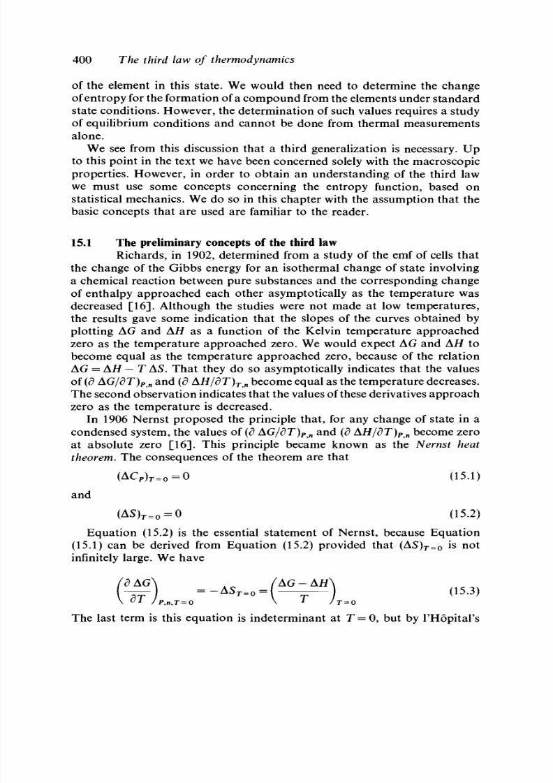
8/11/2019 Thermodynamics of Chemical Systems.pdf
http://slidepdf.com/reader/full/thermodynamics-of-chemical-systemspdf 420/456
400 The third law of thermodynam ics
of the element in this state. We would then need to determine the change
of entro py for the form ation of a com po un d from the elements under stan dard
state conditions. However, the determination of such values requires a study
of equilibrium conditions and cannot be done from thermal measurements
alone.
We see from this discussion that a third generalization is necessary. Up
to this point in the text we have been concerned solely with the macroscopic
properties. However, in order to obtain an understanding of the third law
we must use some concepts concerning the entropy function, based on
statistical mechanics. We do so in this chapter with the assumption that the
basic concepts that are used are familiar to the reader.
15.1 The preliminary concepts of the third law
Richards, in 1902, determined from a study of the emf of cells that
the change of the Gibbs energy for an isothermal change of state involving
a chemical reaction between pure substances and the corresponding change
of enthalpy approached each other asymptotically as the temperature was
decreased [16]. Although the studies were not made at low temperatures,
the results gave some indication that the slopes of the curves obtained by
plott ing AG and AH as a function of the Kelvin temperature approached
zero as the temperature approached zero. We would expect AG and
AH
to
become equal as the temperature approached zero, because of the relation
AG = AH — T AS. That they do so asymptotically indicates that the values
of (<5 AG/dT)
Pn
and (d AH/dT)
T n
becom e equal as the temp erature decreases.
The second o bserv ation indicates tha t the values of these derivatives a pp roac h
zero as the temperature is decreased.
In 1906 Nernst proposed the principle that, for any change of state in a
condensed system, the values of
(d
AG/dT)
Pn
and (d AH/dT)
Pn
become zero
at absolute zero [16]. This principle became known as the Nernst heat
theorem.
The consequences of the theorem are that
( A C
P
)
r = o
= 0 (15.1)
and
( A S )
r = o
= 0 (15.2)
Equation (15.2) is the essential statement of Nernst, because Equation
(15.1) can be derived from Equation (15.2) provided that (AS)
r = 0
is not
infinitely large. We have
dAG\
A o
/ A G - A / A
¥~)
P T
= -
A S
T = O = [
^ - J <
1 5
-
3
)
The last term is this equ ation is indete rm inan t at T = 0, but by l 'Ho pital 's

8/11/2019 Thermodynamics of Chemical Systems.pdf
http://slidepdf.com/reader/full/thermodynamics-of-chemical-systemspdf 421/456
15.2 Experimental determination of absolute entropies 401
rule
A G - A f A
=
V(dAG/dT)
P
,
n
-(dAH/dT)
P
J
L _Lo
(15.4)
J
T=0
Combination of Equations (15.3) and (15.4) gives
0
+ (AC
F
)
r = 0
(15.5)
from which we conclude th at
(AC
P
)
T = 0
m ust b e zero if (AS)
T
= 0
is no t infinitely
large. Of course, if (AS)
T
= 0
= 0, then (AC
F
)
T
= 0
must also be zero.
The postulates of Nernst are those that are required when we wish to
determine equilibrium conditions for chemical reactions from thermal data
alone. In order to calculate the equilibrium conditions, we need to know the
value of A G
e
for the change of state involved. We take the standard states
of the individual substances to be the pure substances at the chosen
temperature and pressure. The value of A/f
e
can be determ ined from
measurements of the heat of reaction. We now have
C
T
A C
e
A S
e
= —
P
~& T
(15.6)
where we have set A S
e
at 0 K as zero according to Eq uatio n (15.2). The
integral can be evaluated from knowledge of the heat capacities of the
reactants, because ACf/T remains finite as the tem pera ture app roach es zero.
Because all sub stance s (except liquid helium ) are solids at 0 K, E qu atio n
(15.6) is strictly applicable only to reactions taking place between the solid
reactants. Additional terms including the changes of entropy for a change of
phase would be included if we needed values of A 5
e
when some or all of
the reactants are in the liquid or gaseous state.
Planck, in 1912, postulated that the value of the entropy function for all
pure substances in condensed states was zero at 0 K. This statement may be
taken as a preliminary statement of the third law. The postulate of Planck
is more extensive than, but certainly is consistent with, the postulate of
Nerns t .
15.2 Experimental determination of absolute entropies
The stable phase of all substances, except helium, at sufficiently low
temperatures is the solid phase. We therefore consider the solid phase as the
conden sed state whose entrop y is zero at 0 K, a nd exclude helium from the
discussion for the present. The absolute entropy of a pure substance in some
state at a given temp eratu re a nd p ressure is the value of the entrop y function
for the given state taking the value of the entropy of the solid phase at 0 K

8/11/2019 Thermodynamics of Chemical Systems.pdf
http://slidepdf.com/reader/full/thermodynamics-of-chemical-systemspdf 422/456
402 The third law of thermodynamics
as zero independent of the pressure. In so doing, we have assigned the value
of the integration constant in integrating the relation (dS/dT)
P
= C
P
/T.
Let us consider the change of state
£ [ s , 0 K , P ] ^ £ [ g , T , P ] ( 1 5 . 7 )
The change of entropy for this change of state is S[g, T, P ] - S
e
[s , 0 K, P]
but S
e
[ s , 0 K, P ] is zero according to the third law. Thus, the absolute value
of the entropy in the state £[g, T, P] is equal to the change of entropy for
the given change of state. The change of state is equivalent to the sum of
the changes of state
(15.8)
and
where T
mp
and T
b
represents the m elting and boiling points of the substance,
respectively, at the pressure P. We have assumed that only one solid phase
exists between 0 K and the melting point. The absolute entropy in the state
g, T, P] is then obtained from
0
+
T
r
'^
1
d r (15.9)
Jr
b
where Aif
mp
and A//
vap
are the changes of enthalpy on melting and
evaporation at the melting and boiling points, respectively at the pressure
P. We observe that the thermal data required are the heat capacities at the
chosen constant pressure and changes of enthalpy for the changes of phase
at the same pressure.
Equation (15.9) illustrates the type of calculations that must be made to
obtain the value of the entropy function of a substance in a given state. We
must include all increases in entropy for the increase of temperature of a
single phase and for changes of phase that are required to reach the desired
state from the state at 0 K.
Two points concerning the evaluation of the first integral in Equation
(15.9) require further discussion. In most experimental determinations of
absolute entropies, the lowest temperature attained ranges from 1 to 15 K;

8/11/2019 Thermodynamics of Chemical Systems.pdf
http://slidepdf.com/reader/full/thermodynamics-of-chemical-systemspdf 423/456
15.4 Understanding the third law 403
we then write the integral as
Jo T J
o
where T' represents the lowest experimental temperature. The evaluation of
the first integral on the right-hand side of this equation requires the
extrapolation of the integrand from T" to zero. Moreover, the integrand
must remain finite at 0 K. The extrapolation is generally made according to
the Debye theory of the heat capacity of solids, in which the heat capacity
of a solid is shown to be proportional to the cube of the temperature; the
proportionality constant is determined from the experimental data in the
neighborhood of
T'.
We observe that with this dependence of temperature,
the value of C
P
(s)/T becomes zero at 0 K and thus is finite. As experimental
methods have improved and lower temperatures attained, the Debye theory
extrapolation accounts for only a very small part of absolute entropy
measurements .
15.3 Confirmation of the third law
Over the years, many experiments have been carried out which
confirm the third law. The experiments have generally been of two types. In
one type the change of entropy for a change of phase of a pure substance
or for a stand ard change of state for a chemical reaction h as been d etermined
from equilibrium measurements and compared with the value determined
from the absolute entropies of the substances based on the third law. In the
other type the absolute entropy of a substance in the state of an ideal gas
at a given temperature and pressure has been calculated on the basis of
statistical mechanics and compared with those based on the third law. Except
for well-known, specific cases the agreement has been within the experimental
error. The specific cases have been explained on the basis of statistical
mechanics or further experiments. Such studies have led to a further
understanding of the third law as it is applied to chemical systems.
15.4 Understanding the third law
According to statistical mechanics, the value of zero for the entropy
function of a system is obtained when all molecules comprising the system
are in the same quantum state. This statement applies to any state of
aggreg ation: gas, l iquid, or solid. No w all substances
1
have an infinite num ber
of possible quantum states, and consequently the state in which all the
1
We do n ot consider here the case in which a nuclear magnetic subsystem or any other subsystem
that has a limited number of quantum states may be considered as a thermodynamic system
separate from the other parts of the total molecular system.

8/11/2019 Thermodynamics of Chemical Systems.pdf
http://slidepdf.com/reader/full/thermodynamics-of-chemical-systemspdf 424/456
404
The third law of thermodynamics
molecules of a system have the same quantum state (the lowest possible
quantum state) is approached only as the temperature is decreased. At
sufficiently low temperatures all substances become solid except helium (at
pressures of <25 bar) and, therefore, the third law applies primarily to the
solid phase.
The condition discussed in the previous paragraph demands certain care
in the experimental determination of absolute entropies, particularly in the
cooling of the sample to the lowest experimental temperature. In order to
approach the condition that all molecules are in the same quantum state at
OK, we must cool the sample under the condition that thermodynamic
equilibrium is maintained within the sample at all times. Otherwise some
state may be obtained at the lowest experimental temperature that is
metastable with respect to another state and in which all the molecules may
not be in the same quantum state at 0 K.
We must also consider the conditions that are implied in the extrapolation
from the lowest experime ntal tem pera ture to 0 K. Th e Debye theo ry of the
heat capacity of solids is concerned only with the linear vibrations of
molecules about the crystal lattice sites. The integration from the lowest
expe rimen tal tem pera ture to 0 K the n determines the decrease in the value
of the entropy function resulting from the decrease in the distribution of the
molecules among the quantum states associated solely with these vibrations.
Therefore, if all of the molecules are not in the same quantum state at the
lowest experimental temperature, excluding the lattice vibrations, the state
of the system, figuratively obtained on extrapolating to 0 K, will not be one
for which the value of the entropy function is zero.
We can now discuss certain systems for which we expect the third law
to be valid, other systems for which the law is not valid at all, and some
specific systems that appear to deviate from the law.
In the first discussion of equilibrium (Ch. 5) we recognized that there may
be states of a system that are actually metastable with respect to other states
of the system but which appear to be stable and in equilibrium over a time
period . Let us consider, then, a pure su bstance th at can exist in two crystalline
states, a and /?, and let the a pha se be m etastable with respect to the fi phase
at normal temperatures and pressures. We assume that, on cooling the a
phase to the lowest experimental temperature, equilibrium can be maintained
within the sample, so tha t on ex trapo lation the value of the entropy function
becomes zero. If, now, it is possible to cool the fi phase under the conditions
of maintaining equilibrium with no conversion to the a phase, such that all
molecules of the phase attain the same quantum state excluding the lattice
vibra tions, then the value of the entrop y function of the jS phase also becomes
zero on the extrapolation. The molar absolute entropy of the a phase and
of the j8 phas e at the equilibrium transition tem pera ture, T
tr
, for the chosen

8/11/2019 Thermodynamics of Chemical Systems.pdf
http://slidepdf.com/reader/full/thermodynamics-of-chemical-systemspdf 425/456
15.4 Understanding the third law 405
pressure are given by
S [ a , T
t r
, P ] =
t r (
^ * d T (15.11)
Jo T
and
•,T
tt
,F]= P ^ d r
(15.12)
Jo
1
respectively. Then the change of entropy for the transition of 1 mole of the
P
phase to
1
mole of the a phase at the transition temperature is
[a , T
lr
, F] - S[fi, T
tr
, P] = f"
C
^
g
> -
C
^ >
d
T
Jo *
(15.13)
according to the third law. This quantity must agree with the value
determined experimentally by measuring the change of enthalpy for the
transition by calorimetric means or from the Clapeyron equation when the
third law is valid for both phases. Examples of this behavior are monoclinic
and rhombic sulfur, different crystalline forms of phosphine, and diamond
and graphite.
Liquid helium presents an interesting
case
leading to further understanding
of the th ird law. When liquid
4
He, the abundant isotope of helium, is cooled at
pressures of < 25 bar, a second-order transition takes place at approximately
2 K to form liquid H el l. On further cooling H ell remains liquid to the lowest
observed temperature at 10 "
5
K. Hell does become solid at pressures greater
than about 25 bar. The slope of the equilibrium line between liquid and solid
helium apparently becomes zero at temperatures below approximately 1 K.
Thus, dP/dT becomes zero for these temperatures and therefore AS, the
difference between the molar entropies of liquid Hell and solid helium, is
zero because
AV
remains finite. We may assume that liquid Hell remains
liquid as 0 K is approached at pressures below 25 bar. Then, if the value of
the entropy function for solM helium becomes zero at 0 K, so must the value
for liquid Hell. Liquid
3
He apparently does not have the second-order
transition, but like
4
He it appears to remain liquid as the temperature is
lowered at pressures of less than approximately 30 bar. The slope of the
equilibrium line between solid and liquid
3
He appears to become zero as
the temperature approaches 0 K. If, then, the slope is zero at 0 K, the value
of the entropy function of liquid
3
He is zero at 0 K if we assume that the
entropy of solid
3
He is zero at 0 K. Helium is the only known substance
that apparently remains liquid as absolute zero is approached under
appropriate pressures. Here we have evidence that the third law is applicable
to liquid helium and is not restricted to crystalline phases.

8/11/2019 Thermodynamics of Chemical Systems.pdf
http://slidepdf.com/reader/full/thermodynamics-of-chemical-systemspdf 426/456
406 The third law of thermodynamics
Solutions and glasses do not follow the third law. If a solid solution
continues to persist on cooling a sample to the lowest possible temperature,
then at this temperature the molecules of the several components are
distributed in some fashion in the same crystal lattice. U nd er such con ditions
all of the molecules of the substance could not attain the same quantum
state on further cooling to 0 K in the sense of the required extra pola tion.
Only if the solid solution was separated into the pure components would
the value of zero be obtained for the entropy function at OK. If the
molecules of the components were randomly distributed in the crystal lattice,
as in an ideal solution, then the entropy of the substance at absolute zero
would be equal to the ideal entropy of mixing, so
S
e
[ so l id so ln ., 0 K, P ] = - £ n
t
R In x
t
(15.14)
i
If the distribution were no t ran do m , the entro py a t 0 K w ould be less tha n
the value calculated from Equation (15.14) but it would not be zero. Thus,
the third law can be applied only to pure substances.
Some pure substances from a glass-like solid, on cooling, rather than a
crystalline solid. In such solids the molecules have a certain randomness in
their spatial distributio n, m ore like a liquid th an a crystal. This is an example
in which a metastable state rather than an equilibrium state is obtained on
cooling. If such a solid is obtained on cooling to the lowest experimental
tem per atur e, then the value of the entrop y function at 0 K, ob tained on
extrapolation, will be greater than zero.
Another type of nonequilibrium state that may be obtained on cooling a
sample is a certain amount of randomness of orientation of the molecules
in the crystal. Some of the substances that exhibit this effect are CO, NO,
N
2
O , N
2
O
2
, H
2
O ( D
2
O ) , 1-olefins with more than 10 carbon atom s, and
certain hydrates such as Na
2
S O
4
- 1 0 H
2
O. In each case the molecules may
have different states of orientations with respect to their neighbors, each
state having almost the same energy. Consequently, when a temperature is
reached at which rotational motion no longer exists, the distribution of the
molecules among the possible states of orientation becomes fixed and may
be somewhat random. Further lowering of the temperature will not change
the distribution to one in which all of the molecules are in the same state
of orien tation and the value of the entrop y function will not be zero at 0 K.
The presence of isotopes presents a different problem, the solution of
which depends on our interests and our choice of the components of the
system. If the system contains a pure substance without regard to its isotopic
composition, then we may choose that pure substance with a fixed isotopic
composition as the component or we may choose the individual molecular
species that have the same isotopes as the components. In the latter case the
actual system is considered as a solution of the isotopic molecular species,

8/11/2019 Thermodynamics of Chemical Systems.pdf
http://slidepdf.com/reader/full/thermodynamics-of-chemical-systemspdf 427/456
15.4 Understanding the third law 407
and there is an entro py of mixing in forming the solution from its com pon ents.
Now, in the determination of the entropy of the substance, the distribution
of the isotopes am on g the individual isotopic molecules is essentially ran do m
and remains constant on cooling the substance to the lowest experimental
temperature in ordinary cases. In the extrapolation from this temperature
to 0 K, we do not consider any change of the distribution. Thus, the entropy
of mixing of the isotopic molecular species to obtain the solution is not
decreased on approaching 0 K and remains positive with respect to the value
of the entropy function of the system that consists of the unmixed isotopic
species. The value of the entropy function of each of the isotopic molecular
species presum ably does becom e zero at 0 K. (Here we ignore any possible
spatial orientation of the molecules on the lattice sites identified only by the
different isotopes.) In the general case we may take the value of the entropy
function of an isotopic solution of constant isotopic composition to be zero
at 0 K prov ided tha t, in any use of the abso lute value of the entrop y function
based on this zero, the isotopic composit ion remains unchanged. We are
permitted to do this because the contribution of the entropy of mixing is the
same at 0 K as at any higher tem per atur e. How ever, when the changes of
state in which we are interested involve changes of the isotopic composition
or the distribution of the isotopes among the isotopic molecular species, we
must take the isotopic molecular species as the components. The state of
the system wh ose value of the entro py function at 0 K is zero is then tha t
of the unmixed isotopic molecular species at 0 K.
The effect of nuclear spin on the values of the entropy function is the final
effect to be considered. When the atoms that are contained in a molecule
have nuclear spin, there are various possible orientations of the spins. The
differences between the energies associated with the different orientations are
generally small, and consequently the orientations are randomly distributed
among the possible states. The distribution remains random on cooling a
substance to the lowest experimental temperature and, consequently, the
value of the entrop y function at 0 K o btaine d by the usual extra pola tion is
greater than that of a system in which the orientations are not randomly
distributed. This situation is similar to what we encountered in considering
the presence of isotopes. The value of the entropy function associated with
the distribution of the nuclear spins for a given substance remains constant
independent of the temperature within the temperature range of interest.
Also, for a given set of atoms with nuclear spin, it is independent of the
chemical com pou nds in which the atom s occur. Co nsequently, we can assign
the value of zero to the entropy function for chemical substances in the state
obtained on cooling the substances to the lowest experimental temperature
and performing the usual extrapolation.
Hydrogen substance (including the three isotopes) is the one substance
in which the equilibrium distribution of the orientation of the nuclear spins

8/11/2019 Thermodynamics of Chemical Systems.pdf
http://slidepdf.com/reader/full/thermodynamics-of-chemical-systemspdf 428/456
408 The third law of thermodynamics
is not random, and hence is an exception to the previous statements. We
briefly discuss here only the light isotope
1
H
1
H. The spin quantum number
is
\
and the spins of the two nuclei can orient in two ways, either parallel
or antiparallel. The net result is that two species of hydrogen exist, one of
which has only even values of the rotational qua ntum num ber J (antiparallel
orientation) and the other only odd values of J (parallel orientation). The
first species is called parahydrogen and the second is called orthohydrogen.
The equilibrium mixture at sufficiently high temperatures is one-fourth para
and three-fourths ortho. In contrast to other substances, the differences of
energy between the ro tatio nal states is large, with the result tha t the transition
of hydrogen molecules between the even and odd states is extremely slow.
The lowest possible rotational quantum state is the state for which
J
= 0.
Yet, when solid hydrogen is obtained at low temperatures merely by cooling,
the lowest rotational quantum state for parahydrogen has a J-value of zero
and that for orthohydrogen has a J-value of unity with the consequence that
not all of the molecules are in the same quantum state. However, if the
transition from the odd to even quantum states is catalyzed by an appropriate
catalyst, all of the molecules become para at sufficiently low temperatures
and the lowest possible quantum state for all of the molecules is the state
for which J = 0. Co nseq uen tly, the value of the entro py function of the solid
hydrogen which is a mixture of
orthohydrogen
and
parahydrogen
is greater
than that which is composed of only parahydrogen.
It is extremely difficult to make a single, unequivocal statement of the
third law. Instead, we have attemp ted to discuss the problem of u nderstanding
the third law from the viewpoint that the value of the entropy function for
a su bstance is zero at 0 K. Fr om a statistical mecha nical po int of view we
consider the contribution of the translational, electronic, vibrational, and
rotational degrees of freedom, and of the intermolecular forces to the value
of the entropy function. However, we exclude all contributions of the nuclei
of the atoms. From a macroscopic and experimental point of view we are
required to reduce the temperature of the experimental sample of a substance
to the lowest possible experimental temperature in such a way that
equilibrium conditions are maintained within the sample in the process of
cooling. We are finally forced to extrapolate the entropy function from the
lowest experim ental tem pera ture to 0 K acc ording to some theoretical
equation. In so doing we ignore any contribution of the nuclear degrees of
freedom to the value of the entropy function. Thus, any concept of a zero
value of the entropy function as used at present excludes the contributions
of the nuclei. It is interesting to recall at this point the arbitrariness of the
definition of temperature scales. Instead of the Kelvin scale we could have
used an exponential scale for which the lowest possible temperature is — oo.
On the exponential scale to the base e, 10~
5
K is only —1.5 degrees. What
new phenomena might be observed as the temperature is decreased from

8/11/2019 Thermodynamics of Chemical Systems.pdf
http://slidepdf.com/reader/full/thermodynamics-of-chemical-systemspdf 429/456
75.5 Practical basis for absolute values of the entropy 409
—1.5 to minus infinity can only be surmised. We can assume on the basis
of our present knowledge of physical systems that such phenomena would
be associated with the nuclei.
With the exclusion of nuclear phenomena, we
can state that the value of the entropy function for most pure crystalline
substances and for pure liquid
4
He and
3
He is zero at 0 K . Glasses and
solutions are excluded. Substances in the crystalline state, which may have
some randomness in the orientation of the molecules on the lattice sites,
would not have a zero value at 0 K. Finally, in the strict sense, substances
composed of isotopes would not be pure but actually solutions, and would
not have a zero value of the entropy function at 0 K.
15.5 Practical basis for absolute values of the entropy
We can now return to the original problem of calculating the
equilibrium properties of a system from thermal data alone. In Section 15.2
we show that absolute values of the entropy can be obtained at given
temperatures and pressures, provided that we can take the value of the
entropy function as zero at 0 K. We have seen in Section 15.4 that this is
not always true; however, the answer to the dilemma is approached in the
same section. Let us assume that some effect results in a nonzero value of
the entropy of one or more substances at OK. If the contribution of this
effect to the value of the entropy at some temperature and pressure of interest
is the same as that at 0 K and, further, if the contribution remains the same
for any change of state at the temperature of interest, such contributions
cancel, with the result that we can assign the value of zero to the entropy
function of such substances at 0 K. In order to illustrate this argument, we
consider the standard change of entropy for some isothermal change of state,
A 5
e
[ T ] , as the sum of two terms, one of which includes all contributions
to the entropy of the reacting substances excluding the effects that result in
nonzero values at 0 K, AS
e
'[T], and the other of which includes only the
con tributions resulting from these effects, A S
e
" [T ]. Then
A S
e
[T] - AS
e
' [T ] + A S
e
"[r| (15.15)
We write AS°
f
(T) as £
£
v
t
ASflT] for the change of state. The quantity that
is actually observed from the thermal measurements on each substance as
discussed in Section 15.2 is (SP'[T]-Sf''[()]), where Sf"[0] is the
nonzero value of the entropy of the ith substance at 0 K. Equation (15.15)
is then written as
Sp"[0]) +
i
(15.16)

8/11/2019 Thermodynamics of Chemical Systems.pdf
http://slidepdf.com/reader/full/thermodynamics-of-chemical-systemspdf 430/456
410 The third law of thermodynamics
If we can express A S
0
" ^ ] as (condition 1)
A S
e
"m=Iv;Sf"[T] (15.17)
i
then
A S
e
m = X v,(SP'[T] - Sp"[0]) + X v
;
(SP"[r] - Sp"[0])
i (
(15.18)
When S P "[ T ] = SP "[0 ] (condi tion 2) , A S
e
[ T ] can be expressed as
Zi Vi(S P'[T] - S P "[ 0 ]); that is, in terms of the observed qu antities. We use
the difference ( S f '[ T ] - SP "[ 0] ) as the abso lute value of the entro py, which
is equivalent to assigning the value of zero to SP"[O]. The two effects for
which this assignment is valid are: (1) the nuclear effects including those of
nuclear spin, provided that the isothermal change of state does not involve
a nuclear reaction; and (2) the isotopic effects, provided there is no change
in the isotopic composition of the substances.
We thus can obtain a consistent set of absolute values of the entropy
function for pure substances from thermal measurements alone on the
practical basis of assigning the value of zero to the entropy function at 0 K
with the exclusion of nuclear and isotopic effects, within the understanding
of the third law as discussed in Section 15.4. The calculation of the entropy
function of pure substances in the ideal gas state by the methods of statistical
mech anics must be consistent with the practical basis. In addition to o btaining
absolute values by the methods that have been discussed, values can also be
obtain ed from equ ilibrium m easurem ents from which A S
e
can be determined
for some change of state. If all but one of the absolute values in the equivalent
su m Y,i
V
;SP are known, then the value of that one can be calculated.
15.6 Therm odynamic functions based on the third law
We have seen that absolute values of the entropy function based on
the third law can be obtained from measurements of the heat capacity and
heats of transitions. A more general equation than Equation (15.9) may be
written as
^ (15.19)
The first term on the right-hand side of this equation represents the required
extrapolation from 0 K to the lowest experimental temperature. The second
term represents the sum of the contributions to the entropy for the change
of temperature of a single phase, and the subscript i refers to the different
phases. The third term represents the sum of the contributions for all of the

8/11/2019 Thermodynamics of Chemical Systems.pdf
http://slidepdf.com/reader/full/thermodynamics-of-chemical-systemspdf 431/456
15.6 Thermodynamic functions based
on the
third law
411
phase transit ions, where the subscript j refers to the different tran sitio ns.
Values of the enthalpy function can be calculated by the similar equ ation
- i f
e
(0)[s,0,P]=
i
JTl'
(15.20)
so
the
symbol H
e
(0)[s, 0, P ] refers
to the
unknown value
of
the enthalpy
of
the
pure substance
at
0 K
and the
experimental pressure.
The
left-
hand side
of
this equation
is
usually written
as [//
e
—#
e
( 0 ) ]
r
or as
[H ° ( T)
-
#
e
(0)] (which is preferred) where the
0
refers
to
0 K. The molar
values
of S° (T) and
[ i ?
e
( T ) - i ?
e
(0)] are combined
to
give the values
of
the function [G
e
( T ) - H
e
( 0 ) ]
by
- TS° (T) (15.21)
Alternately, values for the same function can be obtained by the appro-
priate integration of either Equation (15.19) or Equation (15.20). An
equivalent function is [ G
e
( T ) - / ?
e
( 0 ) ] / T . We thus have the functions
S° {T ), [ / ?
e
( T ) - i ?
e
( 0 ) ] , and [ 5
e
( T ) - 5
e
( 0 ) ] or the equivalent
[ G
e
( T ) - f /
e
( 0 ) ] / T .
For any compilation of values of these functions the standard states must
be completely defined.
In
essentially
all
cases
the
pressure
is
1
bar and
for gases
the
state
is
usually
the
ideal
gas at
1 bar.
For
compilations
at a
single temperature,
the
temperature
is
usually 298.15 K. When values
at
various tem peratures are required, it is easier to compile values at convenient
temperature intervals rather than to obtain algebraic functions of the value. In
such cases the function [G ° ( T)
—
H
e
(0 ) ]/ T is used because the interpolation
between
the
listed values
is
more nearly linear than between
the
values
of
Another set of thermodynamic functions is based on the values of the
enthalpy at 298.15 K. W ith a knowledge of the heat capacities and changes of
enthalpy
for
changes
of
phase, values
of
the function
[/?
e
(T)
—5 ° (2 98 )]
are obtained.
The
corresponding function
for the
Gibbs energy
is
[ G
e
( T ) - i ?
e
(298)]
or
[ G
e
( T ) - / f
e
(298)] /r . Values
for
these functions
are obtained
by
[ G
e
(T ) - i?
e
(298)] = [H ° ( T)
-
i?
e
(298)] - TS° ( T) (15.22)
These functions
are
particularly useful when
the
low-temperature thermal
data are not available. Under such circumstances the values
of S° (T)
must
be obtained from equilibrium measurements
as
indicated
in
Section 15.5.
The two sets
of
functions must
be
related
to
each other. Thus,
- #
e
(298 ) ]
=
[ i ?
e
( T )
-
i?
e
(0 ) ]
-
[ i/
e
(298)
-
(15.23)

8/11/2019 Thermodynamics of Chemical Systems.pdf
http://slidepdf.com/reader/full/thermodynamics-of-chemical-systemspdf 432/456
412 The third
law
of
thermodynamics
and
[G
e
(T) - i?
e
(298)] = [G ° ( T) - /?
e
(0 ) ] - [i?
e
(298) -
(15.24)
15.7 Uses
of
the thermodynamic functions
We consider
a
change
of
state involving
a
chemical reaction, and
wish to calculate the equilibrium conditions. We assume that the change of
state is isothermal and that the standard states of all of the reacting substances
are the pure substances at the temperature and 1 bar pressure. When the
pressure is not 1 bar, the appropriate corrections are easily made. When the
change of state is written as £
f
v
f
B,- = 0, the condition of equilibrium becomes
AG
e
(T) = £,- vfi^iT^ =-RT\nK
The values of AG
e
(T) are obtained by
A G
e
(T) = X v,[G
e
(T ) - # e
(
o ) ] . + £
v
^ ( 0 ) ; (15.25)
i
i
or
A G
e
(T) =
£
v lG® (T)
-
i?
e
(298)],.
+
£
v,fl
e
(298), (15.26)
i
i
The calculation then reverts to the determination of Z ;
v
^
e
( 0 ) i or
£,- v
I
J?° (298)
I
-. These can be obtained from the knowledge of the change of
enthalpy
for
the same change of state because
(15.27)
or
A H
e
(T ) = X v
f
[H
e
(T ) - H
e
(298)]
(
+ £ v
;
H
e
(298)]
;
(15.28)
i
i
Thus, in order to make the calculations we need values of A H° (T) for the
change of state, of [ 5
e
( T ) - i?
e
(0 ) ] or
[ /?
e
(T)-
H
e
(298)] and of
[G ° ( T)
-
H
e
(0 ) ] or [G ° ( T) - H
e
(298)] for each of the substances taking
part in the reaction. Similar calculations of the temperature-pressure
relations
for a
two-phase, one-component system can be made.
The concepts of the standard changes of enthalpy of formation and
standard changes of the Gibbs energy of formation are developed in Chapters
9 and 11. These functions can be combined with the set of functions based
on the third law. From the definitions of the standard changes on formation,

8/11/2019 Thermodynamics of Chemical Systems.pdf
http://slidepdf.com/reader/full/thermodynamics-of-chemical-systemspdf 433/456
15.7 Uses of the thermodynam ic functions 413
we have
for any
pure substance j
AG
f
(T)j
=
G(T)j - X vfi^in
(15.29)
i
where G ° ( T)j refers
to the
Gibbs energy
of the
compound, G
B
(T)
t
refers
to the elements, and the sum is taken over the elements. We can then write
Equation (15.29) as
- B
B
(0)]
t
(15.30)
The quantity
lH° (0)-Y
ji
v
i
H
o
(0 )
i
'] can be
written
as
[ A 5
e
(0 ) J , wh ich
would be the stand ard change of the enthalpy
on
formation
of
the com pound
at
0 K. For the
standard enthalpies
of
formation
we
have
AH?(T)j
=
(15.31)
The quant i ty Af/^O), required in Equation (15.30) is thus ob tained from
Equation (15.31).
If the
basis
of the
enthalpy functions
is at
298
K, the
equivalent
of
Eq uation (15.30)
is
(15.32)
where A/fP(298)j
is the
stand ard change
of the
enthalpy
of
formation
at
298
K.
Similarly,
the
equation corresponding
to
Equation (15.31)
is
AHf>(T)j = [H&(T)
- #
e
( 2 9 8 ) ] , .
- £ vlG&(T)
- H
e
(298) ]
t
-
i
+ A/fp(298),- (15.33)
Equations (15.32)
and
(15.33) illustrate another advantage
of the use of
functions based
on the
enthalpy
at
298
K, in
that many more values
of
A/?P(298) are known than of A/?P(0) . The stand ard change of entropy for
formation of a compound can be obtained from the absolute values as
AS?(T)j =
S(T)j
-
1
VtSPin
(15.34)
i
We finally have
j = AR?(T)J- TAS?(T)J (15.35)

8/11/2019 Thermodynamics of Chemical Systems.pdf
http://slidepdf.com/reader/full/thermodynamics-of-chemical-systemspdf 434/456
414 The third law of thermodynamics
so one quantity in this equation can be determined when the other two are
known.
Equations (15.25) and (15.26) afford a means of determining the validity of
experimental data when values of [G ° ( T) - i /
e
( 0 ) ] o r [G
B
{T) - tf
e
(298)]
are know n for each of the reacting substances . Assume tha t values of A G
e
( T )
have been determined at various temperatures for some standard change of
state from the experimental measurement of the equilibrium conditions of
the system. Then the value of
£,-
V;/?
e
(0);
O
r £
£
v
£
5
e
( 2 9 8 )
i
is calculated from
the value of AG
e
(T) for each experimental point. All of the values of
Y,i v
i
H° (0)
i
or £\ v
i
H ° ( 29S )
i
mu st be equal within the experimen tal error,
because such values must be independent of the temperature for a fixed
pressure.

8/11/2019 Thermodynamics of Chemical Systems.pdf
http://slidepdf.com/reader/full/thermodynamics-of-chemical-systemspdf 435/456
Appendix A
SI units and fundamental constants
Table A.I. Base SI units.
Quant i ty
Length
Mass
Time
Electric current
Thermodynamic temperature
1
Amount of substance
2
Luminous intensity
N a m e
meter
kilogram
second
ampere
kelvin
mole
candela
Symbol
m
kg
s
A
K
m ol
cd
1
The 13th General Conference on Weights and Measures in 1967 recommended that
the kelvin, symbol K, be used both for thermodynamic temperature and for
thermodynam ic temperature interval, and that the unit symbols ° K and deg be
abandoned. The kelvin is defined as 1/273.16 of the thermodynamic temperature of
the triple point of water.
2
The a mo unt of substance should be expressed in units of moles, 1 mole being
Avogadro's constant number of designated particles or group of particles, whether
these are electrons, atoms, molecules, or the reactants and products specified by a
chemical equation.
Table A.2.
Si-derived units.
Quant i ty
Force
Pressure
Energy, work,
quantity of heat
Power
Electric charge
Electric potential,
electromotive force
Celsius temperature
Heat capacity, entropy
N a m e
newton
pascal
bar
joule
wat t
coulomb
volt
degree Celsius
joule per kelvin
Symbol
N
Pa
bar
J
W
C
V
° c
Expression in terms
of other units
m k g s "
2
N m "
2
N m "
2
N m
Is "
1
A s
WA"
1
, JC"
1
K
J K
1

8/11/2019 Thermodynamics of Chemical Systems.pdf
http://slidepdf.com/reader/full/thermodynamics-of-chemical-systemspdf 436/456
416 Appendix A
Table A3. 1986
recommend ed values
of the
fundam ental physical constan ts.
Quantity
Speed of light
in vacuum
Permeability of
vacuum
Permittivity of
vacuum
Newtonian constant
of gravitation
Planck constant
h/2n
Elementary charge
Electron mass
Proton mass
Proton-electron
mass ratio
Fine-structure constant,
j fi
0
ce
2
/h
inverse fine-structure
constant
Rydberg constant,
jm
e
ca
2
/h
Avogadro constant
Faraday constant, N
A
e
Molar gas constant
Boltzmann constant,
R/N
A
Stefan-Boltzmann constant
( T T
2
/ 6 0 ) / C
4
/ ^
3
C
2
Electron-volt,
(e/C)J = {e}J
(Unified) atomic mass unit,
l u = m
u
=
1
L
m (
. 2
C )
Symbol
c
s
0
G
h
h
e
m
e
m
p
m
p
/m
e
a
a"
1
N
A
,L
R
k
9
G
Value
299 792458
4 T I X 1 0 -
7
= 12.566370614-••
l//x
o
c
2
= 8.854187 817
6.672 59(85)
6.626075 5(40)
1.054 572 66(63)
1.602177
33(49)
9.109 389 7(54)
1.6726231(10)
1836.152 701(37)
7.297
353
08(33)
137.035989 5(61)
10973 731.534(13)
6.0221367(36)
96485.309(29)
8.314 510(70)
1.380658(12)
5.67051(19)
Non-SI units used with
eV
u
1.602177 33(49)
1.6605402(10)
Unit
m s "
1
NA -
2
10"
7
NA"
2
10 F m
10" m ks~ s~
10"
3 4
Js
10"
3 4
Js
10"
19
C
10~
31
kg
10"
27
kg
10~
3
m "
1
10
23
mol"
1
Cmol"
1
J m o l " ^ "
1
10~
2 3
J K "
1
1 0 "
8
W m -
2
K -
4
SI
1 0 "
1 9
J
10'
2 7
kg
Relative
uncertainty
(ppm)
(exact)
(exact)
(exact)
128
0.60
0.60
0.30
0.59
0.59
0.020
0.045
0.045
0.001 2
0.59
0.30
8.4
8.5
34
0.30
0.59

8/11/2019 Thermodynamics of Chemical Systems.pdf
http://slidepdf.com/reader/full/thermodynamics-of-chemical-systemspdf 437/456
Appendix
B
Molar heat capacities at constant pressure
for
selected substances
1
B(T/K) + C(T/K)
2
+ D(T/K)
3
Substance
Argon
Hydrogen
Nitrogen
Oxygen
Carbon monoxide
Carbon dioxide
Chlorine
Ammonia
Water
Methane
Ethane
Propane
n-Butane
n-Pentane
Ethyne
Benzene
Cyclohexane
Toluene
A
4.969
6.483
7.440
6.713
7.373
4.728
6.432
6.524
7.701
4.598
1.292
-1.009
2.266
-0.866
6.406
-8.101
-13.027
-5.817
10
3
£
-0.007 67
2.215
-3.42
-0.000879
-3.07
17.54
8.082
5.692
0.459
5
12.45
42.54
73.15
79.13
116.4
18.10
113.3
146.0
122.4
10
6
C
0.012 34
-3.298
6.400
4.170
6.662
-13.38
-9.241
4.078
2.521
2.860
-16.57
-37.89
-26.47
-61.63
-11.96
-72.06
-60.27
-66.05
10
9
D
1.826
-2.790
-2.544
-3.037
4.097
3.695
-2.830
-0.859
-2.703
2.081
7.678
-0.674
12.67
3.373
17.03
3.156
11.73
Reid, R. C, Prausnitz, J. M., and Sherwood, T. K. (1977). The Properties of Gases and Liquids,
3rd
edn. New York: McGraw-Hill. These values are for substances in the vapor or gas state.
cal
th
= 4.184 J.

8/11/2019 Thermodynamics of Chemical Systems.pdf
http://slidepdf.com/reader/full/thermodynamics-of-chemical-systemspdf 438/456
Appendix C
Thermodynamic data
Table C.I. Entha lpies and G ibbs energies of formation at 298.15 K.
1
Substance
H ( g )
O ( g )
N ( g )
C ( g )
C l ( g )
B r ( g )
C O ( g )
C O
2
(g)
N H
3
(g)
H
2
O (g)
H
2
O (/)
C H
4
(g)
C
2
H
6
(g)
C
3
H
8
(g)
n -C
4
H
1 0
(g)
n -C
5
H
1 2
(g)
C
2
H
2
(g)
Benzene (/)
Benzene (g)
Cyclohexane (g)
Toluene (g)
A H P / k J m o l "
1
217.965
249.17
472.679
716.677
121.679
111.884
- 1 1 0 . 5 3
- 3 9 3 . 5 1
- 4 5 . 9 4
- 2 4 1 . 8 1 8
- 2 8 5 . 8 3 0
- 7 4 . 5 2
- 8 3 . 8 2
- 1 0 4 . 6 8
- 1 2 5 . 7 9
- 1 4 6 . 7 6
227.48
49.08
82.93
- 2 9 . 4 3
50.17
A G P / k J m o l "
1
203.263
231.731
454.805
671.285
105.680
82.396
-137 .168
-394 .359
- 1 6 . 4 5
- 2 2 8 . 5 1 2
-237 .129
- 5 0 . 4 9
- 3 1 . 9 2
- 2 4 . 3 9
- 1 6 . 7 0
- 8 . 8 1
209.97
124.42
129.65
7.60
122.42
1
Various sources: The NBS Tables of Chemical Thermodynamic Properties
(1982), J. Ph ys. Chem. Ref. Data, 11 (Supplement No . 2); TRC Thermodynamics
Tables
—
Hydrocarbons.
College Station, TX: Thermodynam ics Research C enter.

8/11/2019 Thermodynamics of Chemical Systems.pdf
http://slidepdf.com/reader/full/thermodynamics-of-chemical-systemspdf 439/456
Appendix C
Table C.2.
Absolute entropies at 298.15 K.
1
419
Substance
He
N e
Ar
K r
Xe
C(gr)
H
2
N
2
O
2
C O
co
2
Cl
2
(g)
Br
2
(/)
N H
3
^ / J m o l - K -
126.150
146.328
154.843
164.082
169.683
5.734
130.566
191.464
205.15
197.56
213.68
222.066
152.231
192.77
1
Substance
H
2
O(g)
H
2
O(/)
C H
4
C
2
H
6
n - C
4
H
1 0
n -C
5
H
1 2
C
2
H
2
Benzene
(g)
Benzene
(/)
Cyclohexane (if)
Toluene
tfVJmol-K-i
188.711
69.915
186.27
229.12
270.20
309.91
349.45
200.79
269.45
173.45
298.24
320.13
Various sources including
the
TRC Thermodynamic Tables—Hydrocarbons. College Station,
TX: Thermodynamics Research Center .

8/11/2019 Thermodynamics of Chemical Systems.pdf
http://slidepdf.com/reader/full/thermodynamics-of-chemical-systemspdf 440/456
420 Appendix C
Table
C.3. Enthalpy increment function T~
l
[H° (T) - H
e
( 0 ) ] .
1 2
Substance
H
2
(g)
O
2
(g )
N
2
(g )
C(gr)
CO(g)
C O
2
(g)
H
2
O (g)
Methane (g)
Ethane (g)
Propane (g)
Ethyne (g)
Benzene (g)
Toluene (g)
Afl&AJmor'
-113.82
-393.14
-238.915
-66.505
-68.20
-81.67
227.313
100.416
73.220
L
298.15
28.401
29.124
29.08
21.921
29.109
31.415
33.213
33.60
39.83
49.45
33.560
47.74
60.42
400
28.504
29.272
29.10
21.642
29.137
33.423
33.380
34.72
44.69
58.20
37.041
60.29
76.02
[ H
e
( T ) - H
e
( 0 ) ] / J m o r
600
28.794
29.879
29.28
21.363
29.366
37.119
33.999
38.65
55.73
76.19
42.727
85.69
106.94
800
28.958
30.649
29.65
21.221
29.817
40.211
34.865
43.51
66.53
92.72
47.066
107.78
134.01
1000
29.146
31.386
30.13
21.135
30.365
42.758
35.882
48.49
76.36
107.19
50.585
126.19
156.69
1500
29.836
32.854
31.38
21.023
31.679
47.371
38.664
59.54
96.11
135.48
57.296
160.00
198.74
1
TRC Thermodynamic Tables—Hydrocarbons. College Station, TX: Thermodynamics Research Center.
2
These values
are
calculated
for a
standard state
of
1
atm. The
difference with 1
bar is not
significant.

8/11/2019 Thermodynamics of Chemical Systems.pdf
http://slidepdf.com/reader/full/thermodynamics-of-chemical-systemspdf 441/456
Appendix C
421
Table CA. Gibbs energy increment function r "
1
[ G
e
( r ) - / /
e
( 0 ) ] .
1
-
2
Substance
H
2
(g )
O
2
(g )
N
2
(g )
C{g)
CO(g)
C O
2
(g)
H
2
O
(g)
Methane
(g)
Ethane (g)
Propane (g)
Ethyne (g)
Benzene
(g)
Toluene
(g)
298.15
102.165
176.024
-162.53
-136.07
-168.44
-182.26
-155.503
-152.67
-189.28
-220.75
-167.260
-221.45
-260.06
40 0
-110.550
-184.500
-171.08
-142.47
-177.00
-191.77
-165.285
-162.67
-201.67
-236.48
-177.615
-237.24
-280.16
r - i [ G e ( T ) - t f
600
-122.177
-196.572
-182.90
-151.18
-188.85
-206.04
-178.925
-177.44
-221.84
-263.47
-193.774
-266.79
-317.33
^(Ofl/Jmol^K-
1
800
-130.486
-205.273
-191.37
-157.31
-197.37
-217.15
-188.816
-189.20
-239.37
-287.73
-206.690
-294.87
-352.29
1000
-136.959
-212.192
-198.04
-162.03
-204.09
-226.41
-196.707
-199.45
-255.31
-309.99
-217.589
-321.24
-385.02
1500
-148.904
-225.213
-210.50
-170.58
-216.69
-244.69
-211.777
-221.29
-290.20
-359.15
-239.455
-379.82
-457.65
1
TRC
Thermodynamic Tables
—
Hydrocarbons.
College Station,
TX:
Thermodynamics Research Center .
2
These values are calculated for a s tandard s tate of 1 atm. The difference with 1 bar is negligible.

8/11/2019 Thermodynamics of Chemical Systems.pdf
http://slidepdf.com/reader/full/thermodynamics-of-chemical-systemspdf 442/456
Appendix D
Standard
reduction potentials in aqueous
solutions
1
'
2
Reaction
Li
+
(aq) + e~ = Li(s)
Ca
2 +
(aq) + 2e~ = Ca(s)
Na
+
(aq) + e~ = Na(s)
Mg
2 +
(aq) + 2e ~ = Mg(s)
Zn
2 +
(aq) + 2e~ = Zn(s)
Cr
3 +
(aq) +
3e~
= Cr(s)
Fe
2 +
(aq) +
2e~
= Fe(s)
Cr
3 +
(aq) + e~ = Cr
2 +
(aq)
Cd
2 +
(aq) + 2e~ = Cd(s)
PbSO
4
(s) + 2e~ = Pb(s) + SOj"(aq)
C o
2 +
(aq) + 2e~ = Co(s)
P b
2 +
(aq) + 2<?~ = Pb(s)
2H
+
(aq) +
2e~
= H
2
(g)
Cu
2 +
(aq) + e~ =Cu
+
(aq)
AgCl(s) + e~ = Ag(s) + Cl"(aq)
Hg
2
Cl
2
(s) + 2^" =2Hg(/) + 2Cl"(aq)
Cu
2 +
(aq) + 2e~
=
Cu(s)
F e
3 +
(aq) +
e
~
= F e
2 +
(aq)
Hg
2
+
(aq) +
2e
~ —2Hg(/)
Ag
+
(aq) + e~ = Ag(s)
2Hg
2 +
(aq) +
2e
~
=
Hg
2
.
+
(aq)
O
2
(g) + 4H
+
(aq) + 4e~ = 2H
2
O(/)
Cl
2
(g) + 2e~ =2Cl"(aq)
PbO
2
(s) + 4H
+
(aq) + 2e~ = Pb
2 +
(aq) + 2H
2
O(/)
C o
3 +
(aq) +
e
~ =
C o
2 +
(aq)
F
(g) + 2 «-- 2F -( aq |
-3.045
-2.84
-2.714
-2.356
-0.762 6
-0.744
-0.447
-0.424
-0.402 5
-0.3505
-0.277
-0.1251
0
0.159
0.222 3
0.268
0
0.340
0.771
0.7960
0.799
1
0.9110
1.229
1.358 3
1.468
1.92
2.87
(d^ /dTVmVK"
1
-0.534
-0.175
-0.772
+ 0.103
+
0.099
+ 0.468
+
0.052
-0.093
-1.015
-0.060
-0.451
0
+ 0.073
-0.543
-0.317
+ 0.008
+ 1.188
-1.000
-0.846
-1.260
-0.238
-1.830
1
Acidic solutions. See (2) below for more-complete compilations.
2
From: Bard, A. J., Parsons, R., and Jordan, J. (1985). Standard Potentials in Aqueous Solutions.
New York: Marcel Dekker; Milazzo, G., Caroli, S., and Sharma, V. K. (1978). Tables of
Standard Electrode Potentials.
New York: John Wiley.
8/11/2019 Thermodynamics of Chemical Systems.pdf
http://slidepdf.com/reader/full/thermodynamics-of-chemical-systemspdf 443/456
Cited refernces and selected bibliography
I. Cited references
1.
Bridgman, P. W. (1936). Condensed Collection of Thermodynamic Formulas. Cambridge,
MA: Harvard Universi ty Press.
2. Shaw, A. M. (1935).
Phil. Trans. Roy. Soc. (London), A234,
299. See also: Pinkerton, R. C.
(1952). J. Phys. Chem.,
56, 799.
3.
Gibbs, J. W. (1961).
Collected Works, Thermodynamics,
Vol. 1, p. 56. New Yo rk: D over
Publicat ions.
4.
A complete d iscussion of the sufficiency and necessity of these cond itions is given in: Gibb s,
J. W.,
op. cit.,
pp. 56-62.
5. Gibbs, J . W.,
op. cit.,
p. 67.
6. Prigogine, I. , and DeFay, R. (1954).
Chemical Thermodynamics
(transl. D. H. Everett),
pp . 175, 468-96. New York: Lo ngm ans, Green and C o.
7. A very complete discussion of indifferent states of thermodynamic systems is given in:
Prigogine, I. , and DeFay, R., op. cit., pp. 450-509.
8. Prigogine, I. , and DeFay, R., op. cit., pp . 450-5 , 479-86.
9. Rowlinson, J. S. (1955). Trans. Faraday Soc, 51 , 1317. D ata for Figu re 7.1 are based on
th e P-V-T relation s of the heavier inert gases.
10.
Schneider, G. (1950).
J. Chem. Phys.,
18, 1269. Figure 7.2 gives the second virial coefficient
of carbon dioxide as a function of the temperature.
II . Dy m ond , J. H., and Smith, E. B. (1980). Th e Virial Coefficients of Pure Gases and Mixtures.
Oxford: Oxford University Press.
12. Cholinski, J. , Szafranski, A., and Wyrzykowska-Stankiewicz, D. (1986).
Computer-aided
Second Virial Coefficient Data for Organic Individual Compou nds and Binary Systems.
Warszawa: Polish Scientific Publishers.
13. Mason, E. A., and Spurling, T. H. (1969).
The Virial Equation of State.
Oxford: Pergamon
Press.
14. Stryjek, R., and Vera, J. H. (1986). An improved equation of state. In:
Equations of State.
Theories and Applications,
eds. K. C. Ch ao , and R. L. Robinson , Jr. , pp. 561-70.
Washington: American Chemical Society.
15. Gibbs, J . W., op. cit., pp. 155.
16. Lewis, G. N., and Randall, M. (1923). Thermodynamics (revised by Pitzer, K. S., and
Brewer, L. (1961) as 2nd edn.). New Yo rk: M cGraw -Hill, p . 191 (1st edn.); p. 153 (2nd edn.).

8/11/2019 Thermodynamics of Chemical Systems.pdf
http://slidepdf.com/reader/full/thermodynamics-of-chemical-systemspdf 444/456
424 Cited references and selected bibliography
17. Pitzer, K. S., Lippmann, D. Z., Curl, R. F., Huggins, C. M., and Peterson, D. E. (1955).
J. Am. Chem. Soc, 11,
3433.
18.
Em ister, W . C , a nd L ee, B. I. (1984). Applied Hydrocarbon Thermodynamics, Vol. 1 (2nd
edn.) . Houston: Gulf Publishing Company.
19. Prigogine, I. , and DeFay, R., op. cit., p. 88.
20 . Freeman, R. D. (1984). J. Chem. Eng. Data., 29, 105-11.
21. Freeman, R. D. (1985). J. Chem. Ed., 62, 681-6.
22 . IUPAC (1979). Manual of Symbols and Terminology for Physicochemical Quantities and
Units , Pure Appl. Chem. Appendix IV, 51, 1-41; (1982) Pure Appl. Chem., 54, 1239-50;
(1982) J. Chem. Thermodyn., 14, 805-15.
23 . IUPAC (1979).
op. cit.
See also: Mills, I., Critas , T., Hom an n, K., Kallay , N., and Ku chitsu, K.
(1988).
U nits and Symbols
in
Physical Chem istry.
Oxford: Blackwell Scientific Publications.
24 .
Lewis, G. N., and Randall, M.,
op. cit.,
p p. 254^9, 328-9 (1st edn.); pp.
242-3,
249-52 (2nd
edn.). The term 'reference state' as used by Lewis and Randall/Pitzer and Brewer has an
entirely different meaning from that used in this book.
25 . Callen , H. B. (1985).
Thermodynam ics and an Introduction to Thermostatics
(2nd edn.). New
York: John Wiley. Prigogine, I. , and DeFay, R.,
op. cit.,
p. 305.
26 . Examples are found in: (a) Scatchard, G. (1940).
J. Am. Chem. Soc,
62, 2426; (b) W ood ,
S. E. (1946).
J. Am. C hem. Soc,
68,1962; and (c) W oo d, S. E. (1950).
Ind. Eng. Chem.,
42,660.
27 . Darken, L. S. (1950).
J. Am. Chem. Soc,
72, 2909.
28 . Gokcen, N. A. (1960).
J. Phys. Chem.,
64, 401.
29 . Wagner, C. (1952).
Thermodynamics of Alloys,
Reading, MA: Addison-Wesley Publishing
C o.
30 . Schuhmann, R. Jr. (1955).
Acta Met.,
3, 219.
31 .
References for illustrative purpo ses ar e: Hogfeldt, E. (1954).
Arkiv for Kemi, 1,
315; (1956)
Rec Trav. Chim. Pays-Bas,
45, 790; Fischer, A. K., Johnso n, S. A., and W ood , S. E. (1967).
J. Phys. Chem.,
71, 1465; Wood, S. E., Fine, B. D., and Isaacson, L. M. (1957).
J. Phys.
Chem., 6 1, 1605.
32 . Edw ards, R. K. (1969).
High Temp. Sci.,
1,232; see also: Edward s, R. K., C hand rasekh arich,
M. S., and Danielson, P. M. (1969).
High Temp. Sci.,
1, 98.
33 . Kirkwood, J. G., and Oppenheim, I. (1961). Chemical Thermodynamics. New York:
McGraw-Hi l l .
34 .
Fo r example, see: Scatcha rd, G. (1953).
J. Am. Chem. Soc,
75,288 3; Keenan, A. G. , Notz, K. ,
and Wilcox, F. L. (1968). J. Phys. Chem., 72, 1085.
35 . An excellent review and discussion of the main features of the therm ody nam ic and
mechanical treatment of surfaces is given by: Melrose, J. C. (1968). Ind. Eng. Chem., 60,
53 . This article contains n um erous references to more-com plete studies. See also: A dam son,
A. W. (1982). The Physical Chemistry of Surfaces (4th edn.). New York: John Wiley.
36 . Guggenheim, E. A. (1929).
J. Phys. Chem.,
33, 842.
II.
Bibliography
(1941—.
Temperature. Its Measurement and Control in Science and Industry,
New York:
Reinhold Publishing.
Acree, W. E. Jr. (1984).
Thermodynamic Properties of Nonelectrolyte Solutions,
New York:
Academic Press.
Ad amso n, A. W. (1982). The Physical Chemistry of Surfaces (4th edn.). New Yo rk: John Wiley.
Beattie, J. A., and Op penh eim , J. (1980). Principles of Thermodynamics. Am sterdam : Elsevier.

8/11/2019 Thermodynamics of Chemical Systems.pdf
http://slidepdf.com/reader/full/thermodynamics-of-chemical-systemspdf 445/456
Cited references and selected bibliography 425
Ben-Nairn, A. (1987).
Solvation Thermodynamics.
New York: Plenum Publishing Co.
Bett, K. E., Rowlinson, J. S., and Saville, G. (1975). Thermodynamics for Chemical Engineers.
Cambridge, MA: MIT Press.
Blander, M. (ed.) (1964). Molten Salt Chemistry, New York: John Wiley.
Bockris, J. O'M., et al. (eds.) (1980 et
seq.).
Comprehensive Treatise of Electrochemistry. New
York: Plenum Publishing Co.
Callen, H. B. (1985).
Thermodynamics and an Introduction to Thermostatics
(2nd edn.). New
York: John Wiley.
Ch ao , K. C , an d R obinson , R. L. (eds.) (1979). Equations of State in Engineering and Research.
Washington: American Chemical Society.
Ch ao, K. C , an d R obinson , R. L. (eds.) (1986). Equations of State. Theories and Applications.
Washington: American Chemical Society.
Chattoraj, D. K., and Birdi, K. S. (1984).
Adsorption and the Gibbs Surface Energy.
New York:
Plenum Publishing Co.
DeFay, R., and Prigogine, I. 1966. Surface Tension and Adsorption, Ann Arbor: Books Demand
U M I .
Den bigh, K. G. (1981). The Principles of Chemical Equilibrium (4th edn.). Cam bridg e: Cam bridge
University Press.
Edm ister, W . C , and Lee, B. I. (1985).
Applied Hydrocarbon Thermodynamics
(2nd edn.), Vol. 1.
Houston: Gulf Publishing Co.
Everett, D. H. (1960). Introduction to the Study of Chemical Thermodynamics. L ondon :
Longmans .
Gib bs, J. W. (1961).
Collected Works,
Vol. 1,
Thermodynamics.
New Y ork: Dover Publicat ions.
Gokcen, N. A. (1975). Thermodynamics. Hawthorne, CA: Techscience Inc.
Guggenheim, E. A. (1968). Thermodynamics (5th edn.). New York: Wiley Interscience.
Guggenheim, E. A. (1985). Thermodynamics: An Advanced Treatise for Chemists and Physicists.
Amsterdam: Elsevier.
Guggenheim, E. A., and Stokes, R. H. (1969).
Equilibrium Properties of Aqueous Solutions of
Single Strong Electrolytes.
Oxford: Pergamon Press.
Harned, H. S., and Owen, B. B. (1959).
The Physical Chemistry of Electrolytic Solutions
(3rd
edn.).
New York: Reinhold Publishing Corp.
Harned, H. S., and Robinson, R. A. (1969).
Multicomponent Electrolyte So lutions.
Oxford:
Pergamon Press.
Hatsopoulos, G. M., and Keenan, J. H. (1981). (reprint of 1961 edn.) Principles of General
Thermodynamics. Melbourne, FL: Krieger.
Hildebrand, J. H., Scott, R. L., and Prausnitz, J. M. (1970). Regular and Related Solutions.
Melbourne, FL: Krieger.
Honig, J. M. (1982). Thermodynamics. Amsterdam: Elsevier.
Hougen, O. A., Watson, K. M., and Ragatz, R. A. (1959). Chem ical Process Principles. Part 2.
Thermodynamics (2nd edn.). New York: John Wiley.
Janz, G. J., et al. (1968-). Molten Salts. Washington: US National Bureau of Standards
(available Supt. of Docs., US Gov't. Print. Off.).
Jones, M. N. (1988).
Biochemical Thermodynamics.
Amsterdam: Elsevier.
Kehiaian, H. V., and Renon, H. (1986). Measurement, Evaluation and Prediction of Phase
Equilibria. Amsterdam: Elsevier.
Kestin, J. J. (ed.) (1976). The Second Law of Thermodynamics. New York: Academic Press.
Kes tin, J. (1979). A Course in Thermodynamics, 2 Vols. W altham , M A: Blaisdell Publishing Co .
8/11/2019 Thermodynamics of Chemical Systems.pdf
http://slidepdf.com/reader/full/thermodynamics-of-chemical-systemspdf 446/456
426 Cited references and selected bibliography
Kirkwood, K. G., and Oppenheim, I. (1961). Chemical Thermodynamics. New York: McGraw-
Hill.
Klotz, I. M., and Rosenberg, R. M . (1986). Chemical T hermodynamics: Basic Theory and Methods
(4th edn.) . Menlo Park: Benjamin/Cummings.
Kubaschewski, O., Evans, L., and Alcock, C. B. (1979). Metallurgical Thermochemistry (5th
edn.).
Oxford: Pergamon Press.
Lehninger, A. L. (1971). Bioenergetics. The Molecular Basis of Biological Energy Transformation
(2nd edn.) . Menlo Park: Benjamin/Cummings.
Lewis, G. N., and Randall, M. (1923).
Thermodynamics.
New York: McGraw-Hill. Revised
edn.: Pitzer, K. S., and Brewer, L. (1961). New York: McGraw-Hill.
Lupis, C. H. P. (1983). Chemical Thermodynamics of Materials. Amsterdam: Elsevier.
McGlashan, M. L. (1980). Chemical Thermodynamics. New York: Academic Press.
Mamantov, G. (ed.) (1969).
Molten Salts: Characterization and Analysis.
New York: Marcel
Dekker .
M ason , E. A., and Spurling, T. H. (1969).
The
Viral
Equation of State.
Oxford: Pergamon Press.
Oon k, H. A. 1981. Phase Th eory: The Thermodynamics of Heterogeneous E quilibria. Am sterdam:
Elsevier.
Planck, M. (1945).
Treatise on Thermodynamics
(3rd ed.) (transl. A. Ogg). New York: Dover
Publicat ions.
Prausnitz, J. M., Lichtenthaler, R. N., and Gomes de Azevedo, E. (1986).
Molecular
Thermodynamics of Fluid-Phase Equilibria
(2nd edn.). Englewood Cliffs, NJ: Prentice-Hall.
Prigogine, I. (1957).
The Molecular Theory of Solutions.
New York: Interscience Publishers.
Prigogine, I. , and DeFay, R. (1954).
Chemical Thermodynamics
(transl. D. H. Everett). New
York: Longmans, Green and Co.
Redlich, O. (1976). Th ermodynam ics Fundam entals, Applications. Amsterdam: Elsevier.
Reid, R. C , Prau snitz, J. M ., and S herwo od, T. K. (1977).
The Properties of Gases and Liquids
(3rd edn.) . New York: McGraw-Hil l .
Robinson, R. A., and Stokes, R. H. (1959).
Electrolyte Solutions
(2nd edn.) . London:
Butterworths.
Rock, P. A. (1983).
Chemical Thermodynamics.
Mill Valley, CA: University Science Books.
Rowlinson, J. S., and Swinton, F. L. (1982).
Liquids and Liquid Mixtures
(3rd edn.). Lon don :
Butterworth:
Scatchard, G. (1976). Equilibrium
in Solutions, Surface and Colloid Ch emistry.
Cambridge, MA:
Harvard University Press.
Van Ness, H. C. (1983). Understanding Thermodynamics. New York: Dover Publicat ions.
Van Ness, H. C , and Abbott, M. M. (1982). C lassical Th ermodynam ics of Non-electrolyte
Solutions. New York: McGraw-Hil l .
Van Wylen, G. J., and Sonntag, R. E. (1986). Fundamentals of Classical Thermodynamics (3rd
edn.). New York: John Wiley.
Wagner, C. (1952). Thermodynamics of Alloys. Reading, MA: Addison-Wesley.
W all, F. T. (1974). Chemical Thermodynamics (3rd edn.). San Franc isco: W . H. Freem an and C o.
Zemansky, M. W., and Dittman, R. (1981). Heat and Thermodynamics (6th edn.). New York:
McGraw-Hi l l .

8/11/2019 Thermodynamics of Chemical Systems.pdf
http://slidepdf.com/reader/full/thermodynamics-of-chemical-systemspdf 447/456
Cited references and selected bibliography
427
III. Com pilations of thermodynamic data
1
(1937). Contributions to the Data on Theoretical Metallurgy. Bureau of Mines Bulletins.
Washington, DC: Supt . of Documents.
(1940). Selected Values of Properties of Hydrocarbons and Related Compounds: Thermo-
dynamics Research Center Hydrocarbon Project, API 44 Tables. College Station, TX:
Thermodynamics Research Center .
(1947). Selected Values of the Properties of Hydrocarbons. National Bureau of Standards
Circular C461.
(1952).
Selected Values of Chemical Thermodynamic Properties.
National Bureau of
Standards Circular 500 plus supplements.
(1956,1959).
Phase Diagrams for Ceramicists.
Colum bus, O H : American Ceramic Society.
(1979).
Solubility Data Series.
International Union of Pure and Applied Chemistry,
Commission on Solubility Data. Oxford: Pergamon Press.
(1981).
Engineering Data Book
(9th edn.). Tulsa: Pennwell Books.
(n.d.). Selected Values for the Thermodynam ic Properties of Metals and Alloys.
Minerals
Research Laboratory, Berkeley, CA: Institute of Engineering Research.
(n.d.)
Selected Values of the Properties of Chemical Compounds.
College Station, TX:
Thermodynamics Research Center .
Angus, S. International Thermodynamics Tables of the Fluid State, series. Oxford: Pergam on
Press.
Bard, A. J., Parsons, R., and Jordan, J. (1985).
Oxidation-Reduction Potentials in Aqueous
Solutions: A Selective and Critical Source Book.
New York: Marcel Dekker.
Bard, A. J., Parsons, R., and Jordan, J. (eds.) (1985).
Standard Potentials in Aqueous Solutions.
New York: Marcel Dekker.
Barin, I. , and Knacke, O. (1973).
Thermochemical Properties of Inorganic Substances.
Berlin:
Springer- Verlag.
Benedek, P., and Olti, F. (1985).
Computer Aided Chemical Thermodynam ics of Gases and
Liquids.
New York: John Wiley.
deBethune, A. D., and Loud, N. A. S. (1964).
Standard Aqueous Electrode Potentials and
Temperature Coefficients at 25° C,
Skokie, IL: C.A. Hampel Publishing Co.
Boublik, T., Fried, V., and Hala, E. (eds.) (1984).
Vapor Pressure of Pure Substances
(2nd
revised edn.). Amsterdam: Elsevier.
Cho linski, J., Szafranski, A., and W yrzykowski-Stankiewicz, D . (1986).
Computer-aided Second
Virial Coefficient Data for Organic Individual Compounds and Binary Systems. Warsaw:
PWN-Polish Scientific Publishers.
Clark, W. M. (1960). Oxidation-Reduction Potentials of Organic Systems. Baltimo re: Williams
and Wilkins.
CODATA: see their publicat ions for data compilat ions and data handling. CODATA
Secretariat, 51 Blvd. de Montmorency, 75016 Paris, France.
Cox , J. C , an d Pilcher, G. (1969). Thermochemistry of Organic and Organometallic Compounds.
New York: Academic Press.
Dreisbach, R. R. (Vol. I, 1955), (Vol. II, 1959), (Vol. Ill, 1961). Physical Properties of Chemical
Compounds.
Washington: American Chemical Society.
1
Many data are also currently available in databases that are accessible via phone lines or
purchasable floppy disks. None are cited here.

8/11/2019 Thermodynamics of Chemical Systems.pdf
http://slidepdf.com/reader/full/thermodynamics-of-chemical-systemspdf 448/456
428 Cited references and selected bibliography
Dymond, J. H., and Smith, E. B. (1980). Th e V irial Coefficients of Pure G ases and Mixtures.
Oxford: Clarendon Press.
Gmehling, J . , and Onken, U.
Vapor-Liquid Equilibrium Data Collection,
series. Great Neck,
NY: Scholium Internat ional .
Horvath, A. L. 1982. Halogenated Hydrocarbons. Solubility-Miscibility with W ater. New York:
Marcel Dekker.
/Hultgren, R. H., Orr, R., Anderson, P., and Kelley, K. K. (1963). Selected Values for the
Th ermodynam ic Properties of Metals and Alloys. New York: John Wiley-Books Demand
U M I .
Ives, D . G., and Jan z, G. J. (eds.) (1969). Reference E lectrodes: Th eory and Practice. New York:
Academic Press.
Janz, G. J. (1967). Th ermodynam ic Properties of Organic Com pounds: Estimation Meth ods,
Principles and Practice.
New York: Academic Press.
Janz, G. J. (1967).
Molten Salts Handbook.
New York: Academic Press.
Janz, G. J., and Tomkins, R. P. T. (1972, 1974).
Non-aqueous Electrolytes Handbook.
New
York: Academic Press.
Jor dan , T. E. (1954). Vapor Pressure of Organic Compounds. New Yo rk: Interscience Publishers.
Kub achew ski, O., and Catterall, J. A. (1956). Thermodynamic Data of Alloys. Oxford: Pergamon
Press.
Landolt, H. H.,
et al.
(1950).
Landolt-Bornstein: Zah lenwerte und Funktionen aus Physik, Chem ie,
Astronomie, Geophysik und Technik.
Berlin: Springer-Verlag.
Latimer, W. M. (1952).
Th e Oxidation States of the Elements and Th eir Potentials in Aqueous
Solutions.
New York: Prentice-Hall .
Levin, E. M., Robbins, C. R., and McMurdie, H. F. (1964).
Phase Diagrams for Ceramists.
Columbus, OH: The American Ceramic Society.
Lyman, W. J., Reehl, W. F., and Rosenblatt, D. H. (1982).
Handbook of Chemical Property
Estimation Methods.
New York: McGraw-Hil l .
Majer, V., and Svoboda, V. (1985). En thalpies of
Vaporization
of Organic Compounds. Oxford:
Blackwells Scientific Publications.
Milazzo, G., Caroli, S., and Sharma, V. K. (1978). Tables of Standard Electrode Potentials.
New York: John Wiley.
Nesmeeilanov, A. M. (1963). Vapor Pressure of the Elements. New York: Academic Press.
Pedley, J. B.,
et al.
(1985).
Thermoch emical Data of Organic Compounds.
London: Chapman
and Hall.
Perry, R. H., and Chilton, C. H. (1984). Chemical Engineers Handbook (6th edn.). New York:
McGraw-Hil l .
Selover, T. B., Jr. (ed.) (1987). National Standard Reference Data Services of the USS R: A Series
of Property Tables.
New York: Hemisphere Publishing Corp.
Sohnel, O., and Novotny, P. (1985). Densities of Aqueous Solutions in Inorganic Substances.
Amsterdam: Elsevier.
Stull, D . R., Sinke, G. C , and G erard , C. (eds.) (1956).
Thermodynamic Properties of the
Elements.
Washington: American Chemical Society.
Stul l , D. R. , and Prophet , H. (I960-) .
JANAF Thermochemical Tables.
Midland, MI: Dow
Chemical Co. (Available Supt. Docs., US Govt. Printing Office.)
Stull, D. R., Westrum, E. F., Jr. , and Sinke, G. C. (1986). The Chemical Thermodynamics of
Organic Compounds. Melbourne, FL: Krieger.
Tamir, A., Tamir, E., and Stephan, K. (1983). Heats of Phase Change of Pure Compounds and

8/11/2019 Thermodynamics of Chemical Systems.pdf
http://slidepdf.com/reader/full/thermodynamics-of-chemical-systemspdf 449/456
Cited references and selected bibliography 429
Mixtures. A Literature Guide. Amsterdam: Elsevier.
Timmermans, J. (1950-65). Physico-chemical C onstants of P ure Organic Compounds. Amsterdam:
Elsevier.
Timmermans, J. (1959-). Th e Physico-chem ical Constants of Binary Systems in Concentrated
Solutions. New York: Interscience Publishers.
To ulo uk ian , Y. S., and H o, C . Y. (1971—. Thermophysical Properties of Matter, 13 Vols. New
York: Plenum Publishing.
Wichterle, I., Linek, J., and Hala, E. (1973-). Vapor-Liquid Equilibrium Data Bibliography.
Amsterdam: Elsevier.
Wicks, C. E., and Block, F. E. (1963). Thermodynamic Properties of 65 Elements—Th eir Oxides,
Halides, Carbides, and Nitrides.
Bureau of Mines Bulletin 605. W ashing ton, DC : US G ovt.
Printing Office.
Wisniak, J. (1981).
Phase Diagrams.
Amsterdam: Elsevier; (1986). Supplement 1.
Wisniak, J., and Herskowitz, M. (1984). Solubility of Gases and Solids: A Literature Source
Book. Amsterdam: Elsevier.
Wisniak, J., and Tamir, A. (1980, 1981). Liquid-Liquid Equilibrium a nd Extraction: A Literature
Source
Book. Amsterdam: Elsevier.
Wisniak, J., and Tamir, A. (1982, 1986). Mixing and Excess T herm odynamic Properties: A
Literature Source Book. Amsterdam: Elsevier.

8/11/2019 Thermodynamics of Chemical Systems.pdf
http://slidepdf.com/reader/full/thermodynamics-of-chemical-systemspdf 450/456

8/11/2019 Thermodynamics of Chemical Systems.pdf
http://slidepdf.com/reader/full/thermodynamics-of-chemical-systemspdf 451/456
Index
Absolute entropy, experimental
determination of, 401-3
Acentric factor, 155
Activity
coefficient
based on molalities, 183
based on molarities, 188
definition, 176
dependence on pressure, 192-3
dependence on temperature, 191-2
strong electrolytes, 201-4
weak electrolytes, 205
definition, 176
dependence on pressure, 192-3
dependence on temperature, 191-2
strong electrolytes, 201-4
Adiabatic wall, 7
ideal, 7
Amagat volume, 136-7
Amagat's law, 136
Anode, defined, 338
Apparent molar quantities, defined, 129
Association in condensed phases, 312-22
Boiling point
dependence on pressure, 235-6
elevation, 255, 269-70
Boundary, defined, 3
Boyle temperature, 137-8
Calorie, definition, 8
Calorimeters, 210
Calorimetry, basic concepts, 210-12
Carbon dioxide-water system, 302-5
Carnot cycle, 30-2
Carnot's function, 33
Carnot 's theorem, 38-40
Cathode, defined, 338
Cells
with liquid junction, 351-5
with transference, 351-5
without liquid junction, 337, 349-51
Centrifugal potential, 376-7
Chain association, 315
Change
of chemical potential on mixing, 173
of entropy on mixing, 174
of Gibbs energy on mixing, 173-4
of state of the system, defined, 4
Changes of state, representation, 22-3
Chemical equilibrium, basic considerations,
292-5
Chemical potential, 75-6
calculation of phase equilibria, 278-80
defined, 51-2
electrochemical systems, 331
equality of for a component and
corresponding species, 198
of a component in a small drop, 374
strong electrolytes, 201-4
weak electrolytes, 204-5
Clapeyron equation, 82, 165, 233
Clausius-Clapeyron equation, 234-5
Clausius statement of the second law, 38, 45
Closed system, defined, 3
Coefficient of performance, 37
Combinations of coefficients, 140-3
Complex formation in condensed phases,
312-22
Composition, dependence on gravitational
potential, 382-4
Compressibility factor, 137
Condensed phases, association and complex
formation in, 312-22
Condenser
in a dielectric medium, 387-8
in empty space, 387
Condit ion equation, 23

8/11/2019 Thermodynamics of Chemical Systems.pdf
http://slidepdf.com/reader/full/thermodynamics-of-chemical-systemspdf 452/456
432 Index
Condit ions
of equilibrium
chemical reactions, 70-3
electrochemical, 331
gravitational potential, 380-1
heterogenous systems, 67-70
other , 74-5
with various restrictions, 73-4
of stability, 89-98
Conjugate generalized forces, 16
Critical phase, 100
Critical phenomena, 98-105
binary solutions, 102
gas-liquid binary system, 104
pure fluid, 99
ternary systems, 103
Curved surfaces, 373-5
Dalton pressure, 136
Dalton's law, 136
Dependent variable, defined, 4
Derived surface, 109-10
Deviation functions, 128
Diamagnetic substance, thermodynamics of,
397-8
Diathermic wall, 7
Dielectric constant, 388
Dielectric medium, thermodynamics of,
391-4
Differential change of enthalpy
on dilution, 222
on solution, 223
Distr ibut ion
between immiscible liquids, 323
coefficient, 290-1
Donnan equilibrium, 355
Duhem's theorem, 80
Efficiency of a heat engine, 32-3
reversible engines, 36
Ehrenfest 's equations, 238-9
Electric
field strength, 387
susceptibility, 388
Electrical potentials, differences in, 331-4
Electrochemical cell, 334-7
representation of, 334
Electrochemical potential, 331
Electrode potential, 347-8
Electromotive force (emf) of a cell, 336
pressure dependence, 346
standard, 339^10
temperature dependence, 340-6
Electrostatic field
systems in, 387-94
thermodynamics of total system, 389-91
work associated with, 388
Electrostriction, 391
Energy
defined, 17
function, defined, 17
Enthalpy
change for a chemical reaction,
dependence on temperature and
pressure, 227-31
changes for changes of state involving
chemical reactions, 223-5
changes for solutions, 217-23
defined, 19
formation, 225-7
function, defined, 19
ions, 227
mixing, 174
standard changes of formation, 225-7
Entropy
absolute, experimental determination of,
401-3
change for change of state of aggregation,
46
change for mixing, 174
defined, 40-1
function, defined, 40-1
Envelope, defined, 3
Equilibria between pure solids and liquids,
327-8
Equilibrium
basic considerations, chemical, 292-5
pressure, 153
Equilibrium constant, 293-5
effect of pressure on, 299
effect of temperature on, 297-9
experimental determination of, 296-7
Euler's theorem, 76
partial molar properties, 122
Exact differential, 8
Excess change of the chemical potential on
mixing, 175
Extensive variable, defined, 4
8/11/2019 Thermodynamics of Chemical Systems.pdf
http://slidepdf.com/reader/full/thermodynamics-of-chemical-systemspdf 453/456
Index
433
First law of thermodynamics, 16-19
First-order transition, defined, 52
Force, 9
Format ion
standard enthalpy changes of, 225-7
standard Gibbs energy of, 300-1
standard Gibbs energy of ions in solution,
301-2
Freezing point lowering and solubility, 257,
271-4
Fugacity
coefficient, defined, 155
defined, 153
Fused salts, solutions of, 263
Galvanic cell
sign conventions, 337-8
with liquid junction, 351-5
without liquid junction, 349-51
Generalized coordinates, 16
Gibbs-Duhem equat ion , 76-7
applications of, 263-8
Gibbs phase ru le and , 8 2 ^
indifferent systems and, 276-7
limited uses in phase equilibria, 246-50
liquid-solution solid-solution equilibria,
274-6
phase equilibria, 325-7
phase rule for gravitational potentials, 384
three-component systems, 287-9
Gibbs energy
change for a chemical change of state
under arbitrary conditions, 329
defined, 49-50
formation, 300-1
formation of ions in solution, 301-2
mixing, 173-4
Gibbs-Helmholtz equation, 56-7, 341
Gibbs-Konovalow theorems, 88-9
Gibbs phase rule, 78-9
Graphical representation, 105-18
energy-entropy-volume surface, 105
Gibbs energy-mole fraction diagrams, 116
Gibbs energy-temperature-pressure
surface, 112
Gravitational potential, 376-7
conditions of equilibrium, 380-1
dependence of composition on, 382-4
dependence of pressure on, 381-2
Gravitational potential (cont.)
fundamental equations, 377-80
Gibbs-Duhem equation and, 384
Half-cell
potentials, 347-9
reactions, 347
Heat
capacity, 7, 9
constant pressure, 9, 20
constant volume, 9, 19
multiphase, closed systems, 214-7
sa tura ted phases , 212^
defined, 7
engine, 25
reservoir, 24
sign of, 8
Helmholtz energy
defined, 47-9
function, 47-9
Henry's law, 244-6, 268-9
Henry's law constant, 244
strong electrolytes, 262
Hydrogen
half-cell, 347
ion and hydronium ion, 306-7
Hydronium ion and hydrogen ion, 306-7
Ideal gas, defined, 20
thermodynamic functions, 146
Ideal mixture of real gases, 143, 152
Ideal solubility, 257
Ideal solution, 173-5
Identity of Kelvin and ideal gas temperature
scales, 34-6
Independent variable, defined, 4
Indifferent states, 81, 85-8
at the triple point, 109
Indifferent systems, 276-7
Inequality of Clausius, 44
Inexact differential, 8
Integral heat of solution, 217
Integrat ion constant ,
g
k
(T),
156
Intensive variable, defined, 4
Interfacial tension, defined, 360
Inversion temperature, 144-5
Ionization constants of weak acids, 308-9

8/11/2019 Thermodynamics of Chemical Systems.pdf
http://slidepdf.com/reader/full/thermodynamics-of-chemical-systemspdf 454/456
434 Index
Ions, standard enthalpy of formation of, 227
Irreversible process, 25, 29
Isenthalpic process, 144
Isolated system, defined, 3
natural cyclic process in, 29
Isothermal Joule-Thomson
coefficient, 146
experiment, 146
Joule coefficient, 22, 143
Joule effect, 21, 143
Joule experiment, 21, 44
Joule-Kelvin experiment, 143
Joule-Thomson coefficient, 144
Joule-Thomson effect, 143-6
Joule-Thomson experiment, 143—
Kelvin-Planck statement of the second law,
37
Magnetic strength, 395
Magnetic susceptibility, 395
Maxwell relations, 57
Mean activity, strong electrolytes, 204
Membrane equilibrium, 355-8
Mixing of ideal gases, thermodynamic
functions, 148-9
Mixtures
molten salts, 205-8
real gases, 140
Molalities, reference and standard states
based on, 182-90
Molarities, reference and standard states
based on, 188-90
Mole fractions, reference and standard
states based on, 178-82
Molten salts
mixtures, 205-8
reference states, 205-8
standard states, 205-8
Multiphase closed systems, heat capacities
of, 214-17
Lambda points , 239
Liquid-liquid equilibria
constant pressure, 258-9
distribution coefficient, 290-1
three-component systems, 289-91
Liquid-liquid solution equilibria at constant
pressure, 257-8
Liquid-pure solid equilibria at constant
pressure, 255-7
Liquid solution-solid solution equilibria,
274-6
Liquid-vapor equil ibria
constant pressure, 250-5
constant temperature, 240-3
Magnetic field
strength, 395
systems in, 394-8
thermodynamics of, 396-8
work associated with, 396
Magnetic induction, 394
Magnetic moment, 395
per unit volume, 395
Natural process, irreversible nature of, 29
Negative-ion fraction, 206
Nernst heat theorem, 400
Nonstoichiometric solid solutions or
compounds, 311-12
Notation, xvi-xix
Number
of degrees of freedom, 78
of variances, 78
One-component systems, phase transitions,
233-4
Open systems, 50-2
defined, 3
Osmotic coefficient, 190-1
Osmotic pressure, 259-61
Oxidation potential, 348
Paramagnetic substance, thermodynamics of,
397-8
Partial molar property
algebraic determination, 122-9
defined, 119

8/11/2019 Thermodynamics of Chemical Systems.pdf
http://slidepdf.com/reader/full/thermodynamics-of-chemical-systemspdf 455/456
Index
435
Partial molar property (cont.)
graphical determination, 131-2
Partial pressure, 136
Passive resistance, 66
Path, defined, 4
Permeability, 395
relative, 395
vacuum, 394
Permittivity
empty space, 387
fluid, 387
Perpetual motion machines
of the first kind, 18
of the second kind, 37
Phase
definition, 377
equilibria, 232-91
Gibbs-Duhem equation and, 325-7
in terms of species, 322-5
rule, 78-9
and gravitational fields, 384
transitions, one-component systems, 233-4
Planck statement of the second law, 45
Polarization of the medium per unit volume,
388
Positive-ion fraction, 206
Pressure dependence
activity, 192-3
activity coefficient, 192-3
boiling point, 235-6
emf of a cell, 346
enthalpy change, 227-30
equilibrium constant, 299
gravitational potential, 381-2
Primitive surface, 107
Process, defined, 4
Pseudobinary systems, 280-1
Quasi-ideal solutions, 314
Quasistatic process, 14
Quaternary systems, 287
Raoult 's law, 243, 268
Real gases
combinations of coefficients, 140
mixtures of, 140
Real solutions, reference and standard states,
175-8
Reduction potential, 348
Reference state, 160, 176, 177
based on molalities, 182-8
based on molarities, 188-90
based on mole fractions, 178-82
conversion from one to another, 193-7
for species, 197-201
molten salts, 206-7
strong electrolytes, 201-4
Refrigeration cycle, 37
Relative permeability, 395
Retrograde solubility, 273
Reversibility of cells, 338-9
Reversible process, 29
Reversible transfer of heat, 30
Saturated phases, molar heat capacities of,
212-14
Second law of thermodynamics
Clausius statement, 38, 45
Kelvin-Planck statement, 37
one statement of, 29
Planck statement, 45
Second-order transition, defined, 52
one-component systems, 238-9
Sign conventions for a galvanic cell, 337-8
Single-phase, one-component systems, 160-4
Solenoid
empty space, 394-5
filled with isotropic matter, 395-6
Solid solutions, nonstoichiometric, 311-12
Solubility
freezing point lowering, 257
ideal solution, 257
Solutions, 171-2
fused salts, 263
strong electrolytes, 201-4, 261-3
Solvated species, 302-7
Species, reference and standard states for,
197-201
Specific heat capacity, 8
Standard electrode potential, 348
Standard electromotive force of a cell, 339-
40
Standard Gibbs energy
formation, 300-1
ions in solution, 301-2

8/11/2019 Thermodynamics of Chemical Systems.pdf
http://slidepdf.com/reader/full/thermodynamics-of-chemical-systemspdf 456/456
436
Index
Standard oxidation potential, 348
Standard state, 160, 176
based on molalities, 182-8
based on molarities, 188-9
based on mole fractions, 178-82
hydrogen half-cell, 347
ions, 301
molten salts, 206-7
strong electrolytes, 201-4
three-phase, one-component systems, 170
two-phase, one-component systems, 168
State of aggregation, changes in one-
component system, 164-5
State of an isolated system, variables
required to define, 79-81
State of the system
defined, 3
in a potential field, 384-7
Stoichiometric coefficient, defined, 71
Strong electrolytes
phase equilibria, 201-4
reference states, 2 0 1 ^
solutions of, 261-3
standard states, 201-4
Sulfuric acid, aqueous solutions, 309-10
Surface
concentration, 365
determination of, 369
phenomena
related to a defined surface, 363-8
Ternary systems
Gibbs-Duhem equation, 287-9
liquid-liquid equilibria, 289-91
Thermochemistry, 209
Thermodynamic distribution coefficient,
290-1
Thermodynamic functions
based on the third law, 410-12
mixing ideal gases, 148
mixing real gases, 152
real gases, 149
Thermodynamic temperature scale, 32-4
Thermodynamics of the dielectric medium,
391-4
Third law of thermodynamics, 399^14
definition, 409
Planck statement, 401
preliminary concepts, 400-1
thermodynamic functions based on,
410-12
Three-component systems, 280-91
determination of excess chemical
potentials of, 281-7
liquid-liquid equilibria, 289-91
pseudobinary systems, 280-1
use of the Gibbs-Duhem equations, 287-9
Three-phase, one-component systems, 170-1
Three-phase systems, 277-8
Total magnetic moment, 397
Total polarization, 391