thermodynamic availability analysis: usage in ...ijcsit.com/docs/volume...

Thermodynamic Availability Analysis: Usage in Quantification of Resilience Modulus, Modulus of

Elasticity and Yield Stress for an Absorber Column System

Sirshendu Guha* and Sudip Kumar Das

Department of Chemical Engineering, University of Calcutta 92 A. P. C. Road, Kolkata – 700 009, INDIA

Abstract Resilience of a material is commonly understood as the ability of the material to absorb energy when deformed elastically and to return it when unloaded. However, in the domain of process systems, a formal definition and quantification of the magnitude of resilience is still elusive. The discussions and data provided in this paper illustrate that quantification of resilience for process systems is feasible and the quantitative model is aligned with fundamental concept of resilience. This paper provides general formulae for quantification of system resilience for many kinds of process systems. Based on the approach presented, it is possible to quantify resilience modulus, elastic modulus, and yield stress for an absorber column system. This work uses fundamentals of thermodynamic availability analysis for achieving this goal. It is found that resilience figure becomes considerably poor for increment of any operating variable from mid operating point vis-a-vis decrement of the same. Likewise a material, absorber system resilience modulus varies inversely with its modulus of elasticity. Additionally, a new efficiency parameter termed as “Thermodynamic Coefficient of Performance (THCOP)” has been conceived. Finally, an example is described detailing the procedure of incorporating 50% over capacity resiliency in the absorber by adding 4 new valve trays.

Keywords: System Resilience, Thermodynamic Availability Analysis, Waste Work, Thermodynamic Coefficient of Performance (THCOP)

1.0 INTRODUCTION System resilience is the ability of a system to recover from/adjust easily/reduce efficiently both the magnitude and duration to misfortune/change from the targeted system performance levels (Linh et al.[1]). Materials science describes the material resilience as the ability of a material to absorb energy when deformed elastically and to return it when unloaded. Material resilience, in other words, is the extent to which energy may be stored in a material by elastic deformation (Nostrand[2]). Likewise, resilience of a process system can also be defined as the amount of energy the system can store before reaching its point of instability (Mitchell and Mannan [3]). System instability may be understood as inability of the system to perform efficiently at its targeted performance levels. Resilience of a material may be quantified as the area under the stress-strain curve from zero stress to yield stress. Thus, it is the strain energy per unit volume required to stress the material from zero

stress to yield stress (Mitchell and Mannan[3]). In line with above, we believe that the resilience magnitude of a process system may also be quantified as the area under the system stress-strain curve from the stress value corresponding to a minimum operating condition to the stress value corresponding to a maximum allowable operating condition. Stress value corresponding to a maximum allowable operating condition will be limited by the design condition up to which the system will be able to maintain its targeted performance levels. Flexibility and resiliency of process systems were first described by Morari[4]. Designing of resilient engineered systems and its usefulness in the design were described by Mitchell and Mannan[3]. Guha and Das [5] recently reported that in an insulated pipe segment system which carries superheated steam as process fluid, magnitude of inherent system resilience decreases from 927.8 KJ/m3-sec to 43 KJ/m3-sec and 31.5 KJ/m3-sec for variation of mass flow rate, inlet pressure and inlet temperature respectively. They also introduced a useful correlation 1 which can be used to estimate flowing steam temperature T at any pipe length L. The descriptions of other notations used in the correlation are given in the nomenclature section. Slocum[6] assessed system resilience for a known stress gradient, applied by introducing experimental disturbances and then measuring recovery rates. Flexibility index (FI), which provides the maximum range of a parameter, tolerable during a feasible steady state operation was proposed by Swaney and Grossmann[7]. Zhen Zhang et. al.[8] described the procedure for quantification of resilience of water networks. They proposed that a new parameter, “TaWN (tolerance amount of a water network)” can be used to quantify resilience of a water network system. Shirali et.al.[9] identified the challenges in the procedure of building resilience or “adaptive capacity” of a chemical plant. Tan et.al. [10] used Monte Carlo simulation technique for evaluation of sensitivity of water networks to noisy mass loads. Their methods could select the most robust network design from available alternatives. Eric et.al.[11] described resilience of a system is the system’s ability to reduce efficiently both the magnitude and the duration of the deviation from targeted system performance levels. They provided a resilience assessment framework to

Sirshendu Guha et al, / (IJCSIT) International Journal of Computer Science and Information Technologies, Vol. 6 (4) , 2015, 3630-3649

www.ijcsit.com 3630

demonstrate the utility of such framework through application to two hypothetical scenarios involving the disruption of a petrochemical supply chain by hurricanes. D.Henry et.al.[12] defined resilience as the ability of an entity to recover from an external disruptive event. They presented an approach to analyze resilience as a time dependent function. They also described metrics of network and system resilience, time for resilience and the total cost of resilience. P.V.R. Carvalho[13] used Functional Resonance Analysis Method (FRAM) to understand and analyze characteristics of the air traffic management (ATM) system resilience. His analysis showed that under normal variability conditions, the ATM system was not able to close the control loops of the flight monitoring functions using feedback and feed forward strategies to achieve an adequate control of an aircraft flying in the controlled air space. Liu,X et.al.[14] used set theoretic approach for resilience analysis of critical infrastructure systems. They interpreted resilience as a system property related to the prevention of, robustness to and recovery from undesired disturbances and events. They also highlighted that such resilience property of interconnected systems depends on their structure and design parameters. Zhuang, B et.al [15] used Monte Carlo simulation based framework for the resilience analysis of water distribution systems (WDSs). They considered the impact of adaptive pump operations and isolation valve locations. They identified that the framework consists of four steps: (1) random event generation for nodal demand fluctuations and pipe breaks; (2) identification of isolated segments based on valve layout; (3) hydraulic simulation with regular and adaptive operations; and (4) identification of responses and the evaluation of system resilience/availability. Blackmore, J. and Plant, R.[16] presented a rationale for enhancing well-established risk assessment and management tools with concepts of ecosystem resilience. Based on their conceptual analysis of two key resilience metaphors, the “stability landscape” and the “adaptive cycle,” they investigated pathways toward risk-based IUWS (integrated urban water system) design and management that explicitly include system resilience as an overarching measure of sustainability. As described above, system resilience can be defined as the amount of energy a system can store before reaching a point of instability (Mitchell and Mannan[3]). Mitchell and Mannan[3] also described that when there is a deviation in the input thermodynamic value, the absorbed exergy loads change. Moreover, like material resilience which can be visualized and quantified using a stress-strain diagram, similar diagrams for system resilience can be developed and used to evaluate resilience modulus (Ur) for a system. Resilience modulus for a process system (Ur) can be evaluated easily by estimating the area under system stress-strain diagram described above. We believe that all systems are designed to withstand a range of energy amounts or energy inputs. If an energy input outside the tolerance range is applied to a system, the system may experience a failure since the system was not designed to operate under such operating conditions. In this context, failure of a system is to be understood as its inability to

perform efficiently at the targeted performance levels and it does not refer to loss of containment due to rupture or other kinds of physical failures. Thus, accurately determining the system tolerance range of applied energy input and behavior of the system at different energy inputs will help determine the tolerable range of operating conditions. The concept of resilience, described above will aid in the determination of these appropriate or tolerable operating ranges.

2.0 METHODOLOGY 2.1 Background We can state that in line with Hooke’s law, modulus of resilience “UR” of a linearly elastic material may be expressed in terms of the area under the stress-strain diagram up to the elastic limit and this area may be expressed in terms of the yield stress (Ωyield) and modulus of elasticity (E) as :

21

2R

yieldU

E

(1)

Thus, resilient materials have lower modulus of elasticity (E), and higher yield stress (Ωyield). 2.1.1 Evaluation of System Resilience In line with (Eq.1) given above for a material, in this work, the following methodologies have been adopted in order to develop quantitative correlations for the quantification of system resilience modulus for an absorption column system of different sizes which are used in sweetening of Sour Natural Gas (Natural gas containing 1.28 wt% H2S) in a Gas Sweetening Unit(designed for treated gas H2S specification of < 1 ppmw).The study covers variations of mass in-flow rate, inlet temperature, inlet pressure and composition of sour feed (natural) gas. System resilience modulus data has been generated by estimating the area under the system Stress-Strain curve for deviations in mass in-flow rate, inlet temperature, inlet pressure and composition of sour feed (natural) gas. In order to estimate variation of Stress and Strain with deviation of independent variables such as in-flow rate, inlet temperature, inlet pressure and composition of sour feed (natural) gas, mathematical modeling and computer simulation have been carried out. High accuracy process simulator (Pro/II) has been utilized for carrying out steady state simulation of a Gas Sweetening Unit (GSU) which is designed to sweeten natural gas containing 1.28 wt% H2S using Di-ethanol amine as solvent. The unit is designed for a treated gas H2S specification of < 1 ppmw. The absorber column is a part of the GSU and has been simulated considering equilibrium stages. Special amine package thermodynamic model has been considered for the entire simulation input file. Inside-out algorithm with 100 IO (inside-out) iterations was used for simulation convergence. The number of theoretical stages required to meet the design specification of treated gas (H2S concentration in treated gas < 1 ppmw) has also been optimized. The physical and thermodynamic property data of all process streams (external and internal of absorber column) obtained from the process simulator output files are utilized in the quantitative correlations which are developed and


www.ijcsit.com 3631

used in order to estimate variation of Stress and Strain with varying operating conditions for the absorption column system which is used in sweetening of Sour Natural Gas. In this work, System Stresses for unsteady and steady flow conditions are defined as:

(a) For unsteady state flow condition, it is the net rate of change of internal energy of the material contained in the system per unit volume of the system with time.

(b) For steady state flow condition, it is the rate of net energy input into the system per unit volume of the system.

The system stress equation for unsteady flow condition can be derived by using the first law of thermodynamics as:

2

21j li i

sys isu

sys sys

mumh mgz q w

d MUS

V dt V

(2) It is worth noting here that (Eq. 2) is basically derived from the general energy balance equation used for flow processes. Since energy is conserved, the time rate of change of energy within a control volume equals the net rate of energy transfer into the control volume. Also, streams flowing into and out of the control volume have associated with them energy in its internal, potential and kinetic forms and all contribute to the net energy change of the system. Moreover, energy can also flow across the control surface as heat and work. Smith, Van Ness and Abbott [17] show that the general energy balance for flow processes is:

∆ . . . (2a)

For steady state flow systems, the general energy balance equation (Eq. 2a) reduces to

∆ . . . (2b)

In (Eq.2a) and (Eq.2b), stands for control volume and stands for flow system.

Since, for steady flow condition in absorption column system, d(MU)sys/dt = 0, the general system stress equation (Eq. 2) is necessarily modified as :

2

2 in j linin

sssys

mumh mgz q w

SV

(3)

For the absorption column system under steady state, one can neglect kinetic and potential energy terms shown in (Eq. 3) and since for an adiabatic absorption column system there is no energy flow across the column as heat and work, we can consider ∑qj = 0 and ∑wl = 0. The system stress equation (Eq. 3) then reduces to Ss(abs) = [(mh)in]/V(abs) = 1/ V(abs)[ Lsl hsl + Vfghfg] (4) (Eq. 4) indicates that stress in an absorber column is simply total input thermal energy (measured in terms of stream enthalpies) per unit volume of the absorber column system. Since entropy can be considered as a substance-like quantity (Mitchell and Mannan [3]) and the energy carried

into a system by it by virtue of flow of a process fluid into the system, one can imagine easily that entropy change in a system leads to assimilation of unavailable energy (i.e.,waste work) in the system and the same may be comparable with irreversible substance-like deformation in the system vis-à-vis elastic deformation of a material. In material science, a material is known to absorb energy under loaded or stressed condition and it releases the energy reversibly when unloaded or de-stressed. However, in case of a process system, the assimilation of waste work or unavailable energy is irreversible. Hence, in line with the above concepts one can consider that for both steady and unsteady flow conditions, the System Strain can be a function of system Irreversibility, I, i.e., Exergy lost or waste work. Using the first and second law of thermodynamics, Fitzmorris & Mah[18] derived the general equation for computation of Irreversibility or waste work for any system handling flowing streams under steady state as,

1 oo o j li

j

TI T m h T s q w

T

(5)

For an adiabatic absorber system under steady state with well defined system boundaries (refer Fig-1), (Eq. 5) can be rewritten as: I = (T0β)abs

= ∑[m(h- T0s)]i = [m(h- T0s)]in - [m(h- T0s)]out = [mb]in – [mb]out = Exergylost (6) Taking into account the absorber system boundaries as defined in Fig-1, one can elaborate (Eq.6) as given below: I = (T0β)abs = [Lslbsl + Vfgbfg] – [Vtgbtg + Lsrbsr] = Exergylost

= Waste work (7) In material science, strain of a material under applied stress is defined as the ratio of deformation of the material to initial dimensions of the material. This definition of strain leads us to understand that strain of a material may be visualized as the ratio of absorbed energy by the material under applied stressed condition to initial energy content of the material under de-stressed or no-load condition. Going by the similar lines of thought, in this work, system strain under steady flow condition is proposed to be equal to ratio of total Exergy lost or Waste work or Irreversibility to total Input Exergy. Thus, system strain can be measured by applying the knowledge of “Exergy”. Exergy is a measure of the useful energy available in a system or stream. System strain being ratio of Exergylost to Exergyin, Exergylost may then be visualized as a measure of deformation analogous to deformation of a material under applied stress. Total input exergy of an absorber column system is estimated using following equation: Exergyin

= Lsl[(hsl – h0sl) –T0(ssl - s

0sl)]+Vfg[(hfg – h0

fg) –T0(sfg - s0fg)]

(8)


www.ijcsit.com 3632

Thus strain values for an absorber column system as defined in Fig-1 can be estimated using the following equation: Ssn(abs) = [Lslbsl + Vfgbfg] – [Vtgbtg + Lsrbsr] / Lsl[(hsl – h0

sl) –T0(ssl - s

0sl)]+Vfg[(hfg – h0

fg) – T0(sfg - s0fg)]

(9) (Eq. 9) indicates that strain in an absorber column can be estimated easily by having knowledge of stream enthalpy and entropy data at the absorber system operating conditions (temperature and pressure) and the same at the datum conditions (set at 21oC temperature and 1.0 Kg/cm2a pressure in this work) along with the knowledge of flow rates of feed gas, lean solvent, treated gas and rich solvent. From the preceding analysis, it can be construed that the system resilience modulus for the absorber column system can be evaluated easily by estimating the area under the plot of stress versus strain data generated for an absorber column system using the above-described methodology. 2.2 Assessment of thermodynamic efficiencies In addition to estimation of stress, strain and system resilience modulus figures, one can use the above-described methodology for assessment of thermodynamic efficiencies of the absorber column system in several ways depending on view points. Conventionally, one can define thermodynamic efficiency of the absorber column system as: ηabs = [(Vtgbtg + Lsrbsr)- (Lslbsl + Vfgbfg)]/ [(Vtgbtg + Lsrbsr)- (Lslbsl + Vfgbfg)] + [(T0β)abs] (9a) Where, the expression, [(Vtgbtg + Lsrbsr)- (Lslbsl + Vfgbfg)] signifies minimum work (wmin) required for separation of H2S from the sour feed gas and [(T0β)abs] is the waste work as already defined in (Eq. 7). However, since, [(T0β)abs] = - wmin, ηabs which is equal to wmin/ wmin + (-wmin), becomes infinite which is meaningless. Due to this reason, for the absorber column system, a new meaningful measure of thermodynamic efficiency of the absorption process is proposed in this work and it is termed as thermodynamic Coefficient of Performance (THCOP) of absorber column system. Thermodynamic Coefficient of Performance (THCOP) of an absorber column system has been defined in this work, as the ratio of rate of entropy outflow from the absorber column system to the rate of entropy inflow into the absorber column system or [THCOP]abs = misiout/ misiin (10) For any real absorption system under steady state, one can write the following entropy balance equation: misiout = misiin + β (11) Substituting (Eq.11) into (Eq.10), [THCOP]abs can be written as: [THCOP]abs = [1 + β/ misiin] = [1+ β / (Lsl ssl+ Vfg sfg)] (12) [THCOP]abs is a measure of thermodynamic efficiency of an absorption process. The absorption process is most efficient when [THCOP]abs value is equal to 1 or the rate of irreversible entropy creation (β) is equal to zero. However, for all real absorption processes, [THCOP]abs is greater than 1 as β values are always greater than zero due to stage mixing (mixing of streams at non-equilibrium temperatures and compositions) in absorber column stages.

2.3 Determination of modulus of elasticity, mean modulus of elasticity and order of magnitude of yield stress In order to evaluate the modulus of elasticity, mean modulus of elasticity of the absorber column system and the order of magnitude of yield stresses (stress values at which the absorber column performance gets adversely affected and the treated gas specification of < 1ppmw H2S concentration is no longer met) for cases of variations of mass flow rate, inlet temperature, inlet pressure and composition of feed sour gas, following procedure can be followed. In the system stress-strain plot, stress can be expressed as a function of strain (e.g., power law relation such as

, where A is a constant, y is stress in KJ/m3-sec and x is strain, n is an exponent) and then one can easily evaluate the modulus of elasticity of the absorber column system (Esys) as a function of strain (x) as:

Esys = .

. . (12a)

Using (Eq.12a), mean modulus of elasticity of a system (Ēsys) can be evaluated as:

Ēsys = .

= . .

(12b)

Where, is maximum strain value in the system stress-strain plot and is minimum strain value in this plot. Once Ēsys value is evaluated from (Eq.12b) and assuming that yield strain value is very close to minimum or maximum strain value in the system stress-strain plot, the order of magnitude of system yield stress (Ysys

yield) can be estimated by linear interpolation as: Ysys

yield = ymin + Ēsys ∆x (12c) Where, ymin is the minimum stress value in the system stress-strain plot and ∆x is the difference in maximum and minimum strain values in this plot. It should be noted here, that Ēsys and Ysys

yield values are to be evaluated separately for each case of variation of mass flow rate, inlet temperature, inlet pressure and composition of feed sour gas. Ysys

yield, estimated for each case, will correspond to certain flow rate value, inlet temperature, inlet pressure and composition of feed sour gas and these values can be determined from plots of system stress as functions of feed sour gas flow rate, inlet temperature, inlet pressure and composition respectively.

3.0 DISCUSSION OF RESULTS As already illustrated in preceding paragraphs, system resilience regime figures have been evaluated by mathematical modeling and computer simulation for an absorber column system with regard to deviations in temperature, pressure, flow and composition of feed sour gas, one needs to refer Table-1 for details of the operating parameters used in the system. Initially, four cases (Case-I, II, III and IVa) of variations of operating conditions have been considered as detailed in Table-1. However, one additional check case (Case-IVb), as detailed in Table-1, with higher absorber size (i.e.,volume) has also been explored in order to critically evaluate system resilience with regard to deviation in feed sour gas composition.


www.ijcsit.com 3633

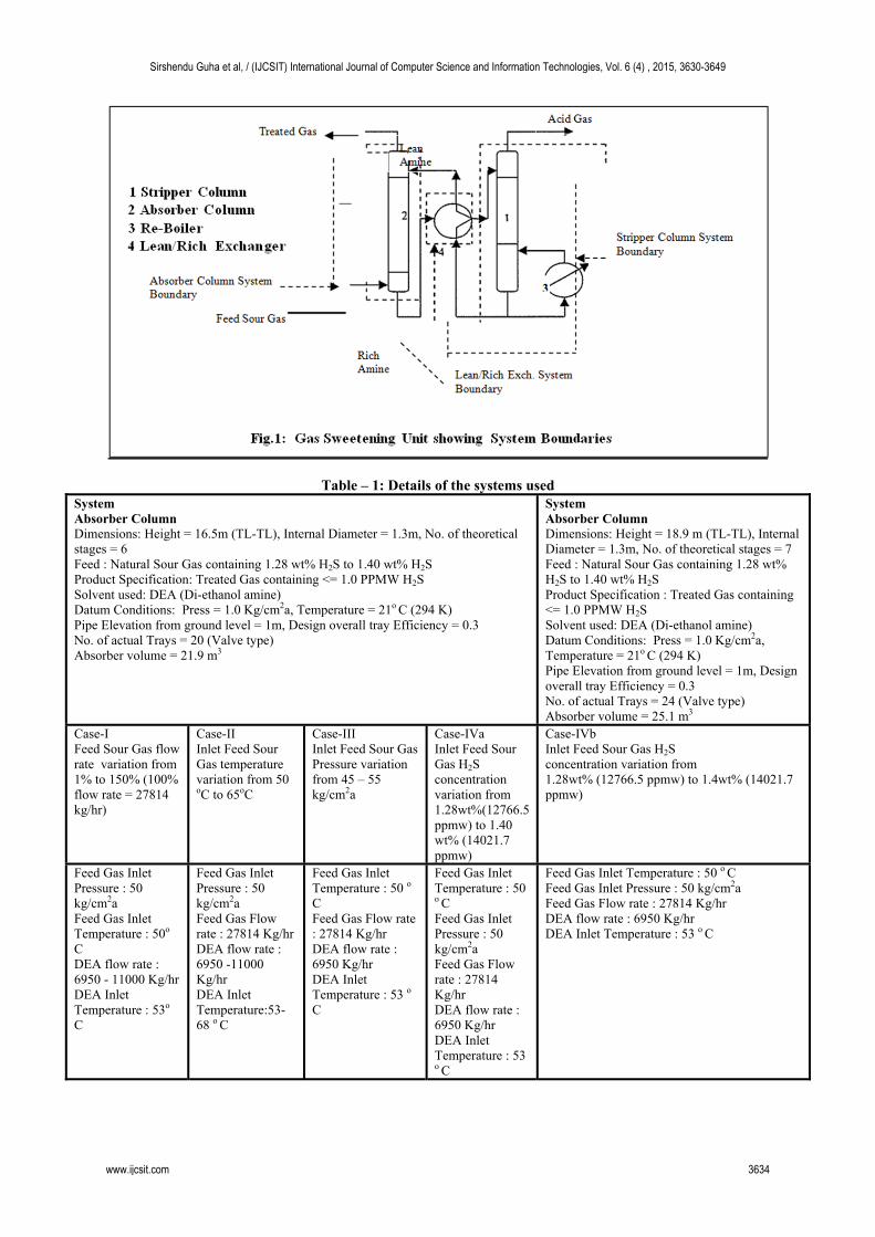
Table – 1: Details of the systems used System Absorber Column Dimensions: Height = 16.5m (TL-TL), Internal Diameter = 1.3m, No. of theoretical stages = 6 Feed : Natural Sour Gas containing 1.28 wt% H2S to 1.40 wt% H2S Product Specification: Treated Gas containing <= 1.0 PPMW H2S Solvent used: DEA (Di-ethanol amine) Datum Conditions: Press = 1.0 Kg/cm2a, Temperature = 21o C (294 K) Pipe Elevation from ground level = 1m, Design overall tray Efficiency = 0.3 No. of actual Trays = 20 (Valve type) Absorber volume = 21.9 m3

System Absorber Column Dimensions: Height = 18.9 m (TL-TL), Internal Diameter = 1.3m, No. of theoretical stages = 7 Feed : Natural Sour Gas containing 1.28 wt% H2S to 1.40 wt% H2S Product Specification : Treated Gas containing <= 1.0 PPMW H2S Solvent used: DEA (Di-ethanol amine) Datum Conditions: Press = 1.0 Kg/cm2a, Temperature = 21o C (294 K) Pipe Elevation from ground level = 1m, Design overall tray Efficiency = 0.3 No. of actual Trays = 24 (Valve type) Absorber volume = 25.1 m3

Case-I Feed Sour Gas flow rate variation from 1% to 150% (100% flow rate = 27814 kg/hr)

Case-II Inlet Feed Sour Gas temperature variation from 50

oC to 65oC

Case-III Inlet Feed Sour Gas Pressure variation from 45 – 55 kg/cm2a

Case-IVa Inlet Feed Sour Gas H2S concentration variation from 1.28wt%(12766.5 ppmw) to 1.40 wt% (14021.7 ppmw)

Case-IVb Inlet Feed Sour Gas H2S concentration variation from 1.28wt% (12766.5 ppmw) to 1.4wt% (14021.7 ppmw)

Feed Gas Inlet Pressure : 50 kg/cm2a Feed Gas Inlet Temperature : 50o

C DEA flow rate : 6950 - 11000 Kg/hr DEA Inlet Temperature : 53o

C

Feed Gas Inlet Pressure : 50 kg/cm2a Feed Gas Flow rate : 27814 Kg/hr DEA flow rate : 6950 -11000 Kg/hr DEA Inlet Temperature:53-68 o C

Feed Gas Inlet Temperature : 50 o

C Feed Gas Flow rate : 27814 Kg/hr DEA flow rate : 6950 Kg/hr DEA Inlet Temperature : 53 o

C

Feed Gas Inlet Temperature : 50 o C Feed Gas Inlet Pressure : 50 kg/cm2a Feed Gas Flow rate : 27814 Kg/hr DEA flow rate : 6950 Kg/hr DEA Inlet Temperature : 53 o C

Feed Gas Inlet Temperature : 50 o C Feed Gas Inlet Pressure : 50 kg/cm2a Feed Gas Flow rate : 27814 Kg/hr DEA flow rate : 6950 Kg/hr DEA Inlet Temperature : 53 o C


www.ijcsit.com 3634

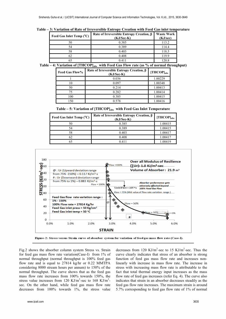
Table – 3: Variation of Rate of Irreversible Entropy Creation with Feed Gas inlet temperature

Feed Gas Inlet Temp (oC) Rate of Irreversible Entropy Creation, β

(KJ/Sec-K) Waste Work

(KJ/sec) 50 0.385 113.2 54 0.389 114.4 58 0.403 118.5 62 0.408 119.9 65 0.411 120.8

Table – 4: Variation of [THCOP]abs with Feed Gas Flow rate (as % of normal throughput)

Table – 5: Variation of [THCOP]abs with Feed Gas Inlet Temperature

Fig.2 shows the absorber column system Stress vs. Strain for feed gas mass flow rate variation(Case-I) from 1% of normal throughput (normal throughput is 100% feed gas flow rate and is equal to 27814 kg/hr or 0.22 MMTPA considering 8000 stream hours per annum) to 150% of the normal throughput. The curve shows that as the feed gas mass flow rate increases from 100% towards 150%, the stress value increases from 120 KJ/m3-sec to 168 KJ/m3-sec. On the other hand, while feed gas mass flow rate decreases from 100% towards 1%, the stress value

decreases from 120 KJ/m3-sec to 15 KJ/m3-sec. Thus the curve clearly indicates that stress of an absorber is strong function of feed gas mass flow rate and increases non-linearly with increase in mass flow rate. The increase in stress with increasing mass flow rate is attributable to the fact that total thermal energy input increases as the mass flow rate of feed gas increases (refer Eq. 4). The curve also indicates that strain in an absorber decreases steadily as the feed gas flow rate increases. The maximum strain is around 5.7% corresponding to feed gas flow rate of 1% of normal

Feed Gas Flow% Rate of Irreversible Entropy Creation, β

(KJ/Sec-K) [THCOP]abs

1 0.036 1.00229 10 0.097 1.00348 50 0.214 1.00413 75 0.282 1.00414

100 0.385 1.00415 150 0.578 1.00416

Feed Gas Inlet Temp (oC) Rate of Irreversible Entropy Creation, β

(KJ/Sec-K) [THCOP]abs

50 0.385 1.00415 54 0.389 1.00415 58 0.403 1.00417 62 0.408 1.00417 65 0.411 1.00419


www.ijcsit.com 3635

throughput whereas minimum strain is around 2.8% corresponding to feed gas flow rate of 150%. Apparently, the inverse relation of feed gas flow rate with strain is complex to comprehend. However, referring Table-2 in which exergy lost or waste work is tabulated against the feed gas flow rate, one can easily construe that although exergy lost or waste work is directly proportional to feed gas flow rate, the ratio of exergy lost to the total input exergy can vary inversely with feed gas flow rate. This is due to the fact that rise in input exergy with rise in feed gas flow rate can offset rise in exergy lost or waste work with rise in feed gas flow rate to the absorber column. Since strain is ratio of exergy lost to total input exergy into the absorber column, it can eventually vary inversely with feed gas flow rate. In this regard, one can refer Table-4 wherein rate of irreversible entropy creation (β) and THCOP figures have been tabulated against feed sour gas inflow rate. The tabulated data clearly indicate that waste work (Toβ) increases with rise in sour gas inflow rate and consequently THCOP values become poorer with such rise in sour gas inflow rate.

Table – 2: Variation of Waste Work,Minimum work, ∆T1 ,∆T2 with Feed Gas flow percent

Feed Gas Flow%

Waste Work

(KJ/sec)

Minimum Work

(KJ/sec)

∆T1

(oC) ∆T2 (oC)

1 10.7 -10.7 3.14 1.27 10 28.5 -28.5 3.7 4.56 50 63.0 -63.0 6.82 4.56 75 83.0 -83.0 8.27 1.8

100 110.8 -110.8 8.86 0.54 150 170.0 -170.0 8.73 0.09

∆ T1 = Temperature difference between treated gas and feed gas ∆ T2 = Temperature difference between rich amine and lean amine Table-2 also indicates that minimum work required to separate H2S from feed sour gas is always negative, i.e., surplus work or energy is available in the absorber column system and as a consequence the temperature differences between treated gas and feed gas (∆T1) as well as the temperature differences between rich amine and lean amine (∆T2) are all positive. It is also worth noting here that feed gas mass flow rate variation of 1% of normal throughput signifies absorber column start-up or shut down scenarios. On the other hand, feed gas mass flow rate variation of 150% of normal throughput is the maximum through put up to which one can imagine to run the absorber column. The curve also enables us to identify feed gas flow deviation regimes (upward & downward) from the mid-value of flow rate variation range. The overall modulus of resilience is the sum of these individual resilience data and is estimated as 1.0 KJ/m3-s. In this context, one can refer Table-8, wherein resilience modulus (Ur) and Elastic modulus (Esys) figures have been tabulated for three flow regimes (1%-50%, 50%-100% and 100%-150%) under Case-I. The tabulated data clarify that overall modulus of resilience is the sum of these individual resilience data and is estimated as 1.0 KJ/m3-s. These Ur and Esys figures also indicate that Ur is inversely proportional to Esys when Ur and Esys values are compared for all the three flow regimes. In

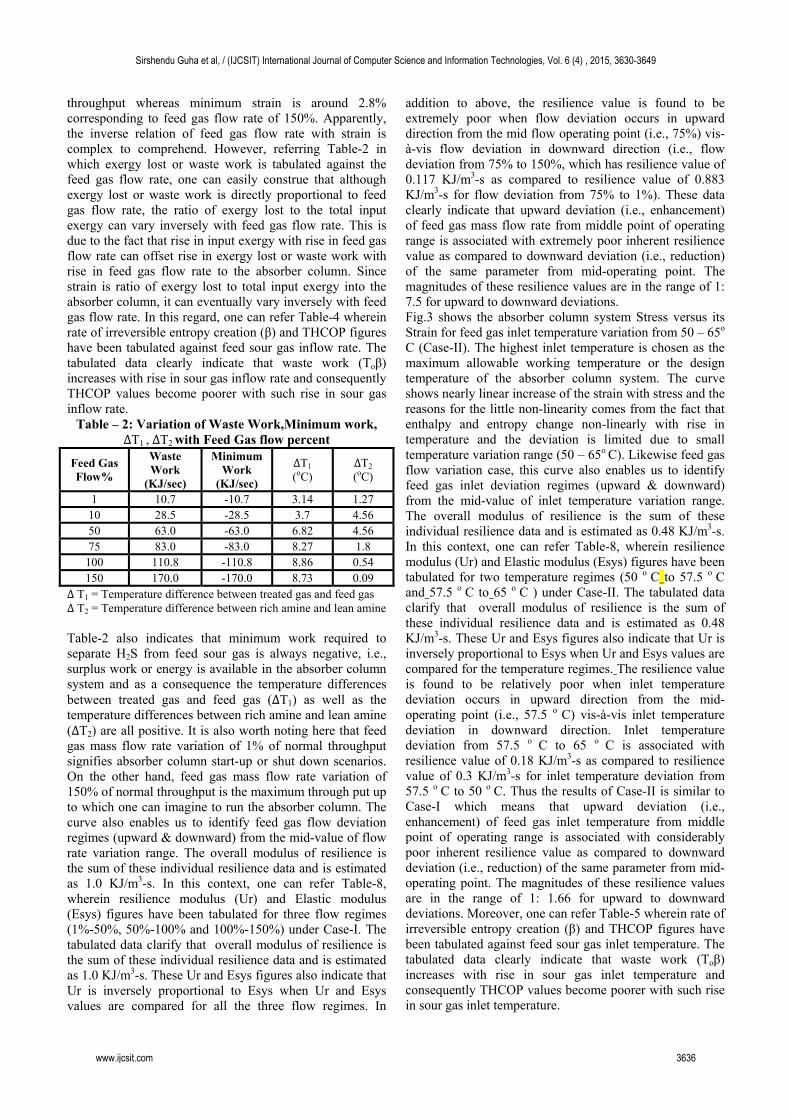
addition to above, the resilience value is found to be extremely poor when flow deviation occurs in upward direction from the mid flow operating point (i.e., 75%) vis-à-vis flow deviation in downward direction (i.e., flow deviation from 75% to 150%, which has resilience value of 0.117 KJ/m3-s as compared to resilience value of 0.883 KJ/m3-s for flow deviation from 75% to 1%). These data clearly indicate that upward deviation (i.e., enhancement) of feed gas mass flow rate from middle point of operating range is associated with extremely poor inherent resilience value as compared to downward deviation (i.e., reduction) of the same parameter from mid-operating point. The magnitudes of these resilience values are in the range of 1: 7.5 for upward to downward deviations. Fig.3 shows the absorber column system Stress versus its Strain for feed gas inlet temperature variation from 50 – 65o

C (Case-II). The highest inlet temperature is chosen as the maximum allowable working temperature or the design temperature of the absorber column system. The curve shows nearly linear increase of the strain with stress and the reasons for the little non-linearity comes from the fact that enthalpy and entropy change non-linearly with rise in temperature and the deviation is limited due to small temperature variation range (50 – 65o C). Likewise feed gas flow variation case, this curve also enables us to identify feed gas inlet deviation regimes (upward & downward) from the mid-value of inlet temperature variation range. The overall modulus of resilience is the sum of these individual resilience data and is estimated as 0.48 KJ/m3-s. In this context, one can refer Table-8, wherein resilience modulus (Ur) and Elastic modulus (Esys) figures have been tabulated for two temperature regimes (50 o C to 57.5 o C and 57.5 o C to 65 o C ) under Case-II. The tabulated data clarify that overall modulus of resilience is the sum of these individual resilience data and is estimated as 0.48 KJ/m3-s. These Ur and Esys figures also indicate that Ur is inversely proportional to Esys when Ur and Esys values are compared for the temperature regimes. The resilience value is found to be relatively poor when inlet temperature deviation occurs in upward direction from the mid-operating point (i.e., 57.5 o C) vis-à-vis inlet temperature deviation in downward direction. Inlet temperature deviation from 57.5 o C to 65 o C is associated with resilience value of 0.18 KJ/m3-s as compared to resilience value of 0.3 KJ/m3-s for inlet temperature deviation from 57.5 o C to 50 o C. Thus the results of Case-II is similar to Case-I which means that upward deviation (i.e., enhancement) of feed gas inlet temperature from middle point of operating range is associated with considerably poor inherent resilience value as compared to downward deviation (i.e., reduction) of the same parameter from mid-operating point. The magnitudes of these resilience values are in the range of 1: 1.66 for upward to downward deviations. Moreover, one can refer Table-5 wherein rate of irreversible entropy creation (β) and THCOP figures have been tabulated against feed sour gas inlet temperature. The tabulated data clearly indicate that waste work (Toβ) increases with rise in sour gas inlet temperature and consequently THCOP values become poorer with such rise in sour gas inlet temperature.


www.ijcsit.com 3636

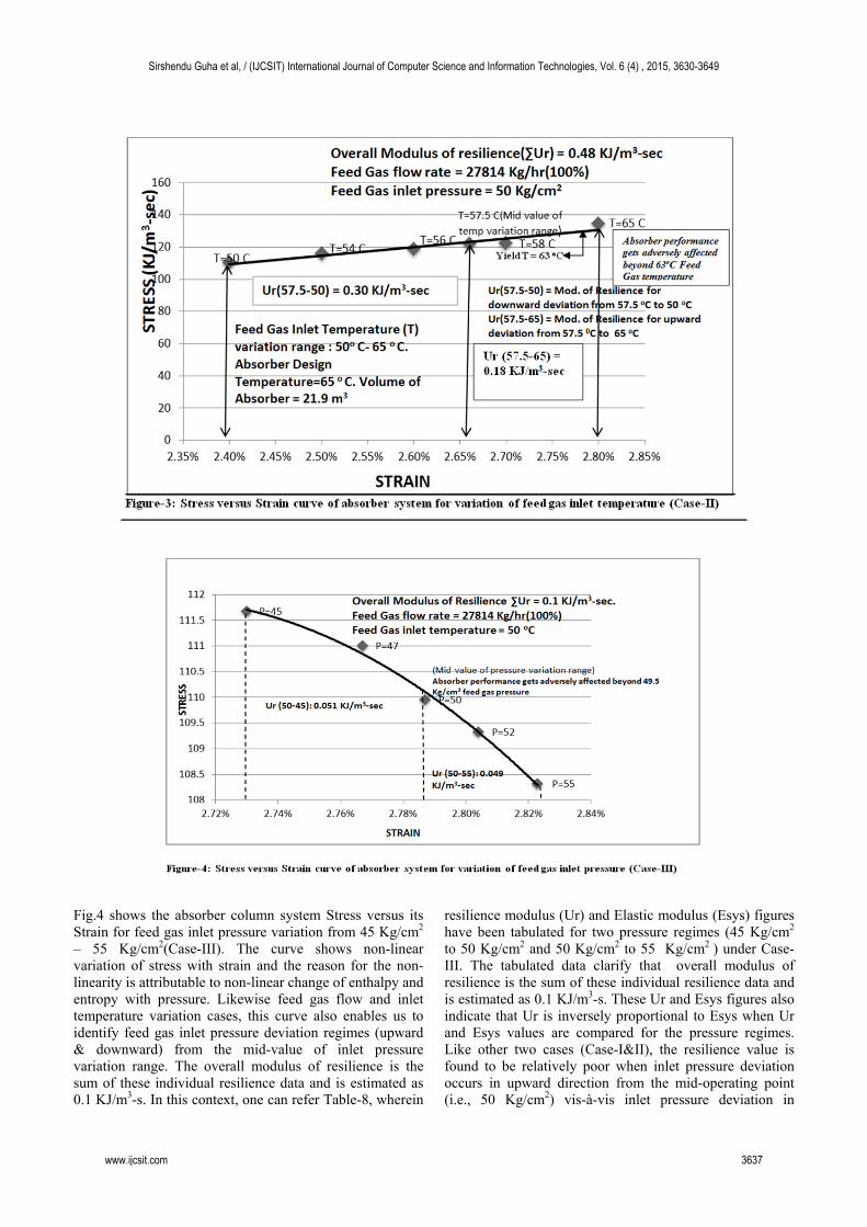
Fig.4 shows the absorber column system Stress versus its Strain for feed gas inlet pressure variation from 45 Kg/cm2 – 55 Kg/cm2(Case-III). The curve shows non-linear variation of stress with strain and the reason for the non-linearity is attributable to non-linear change of enthalpy and entropy with pressure. Likewise feed gas flow and inlet temperature variation cases, this curve also enables us to identify feed gas inlet pressure deviation regimes (upward & downward) from the mid-value of inlet pressure variation range. The overall modulus of resilience is the sum of these individual resilience data and is estimated as 0.1 KJ/m3-s. In this context, one can refer Table-8, wherein

resilience modulus (Ur) and Elastic modulus (Esys) figures have been tabulated for two pressure regimes (45 Kg/cm2 to 50 Kg/cm2 and 50 Kg/cm2 to 55 Kg/cm2 ) under Case-III. The tabulated data clarify that overall modulus of resilience is the sum of these individual resilience data and is estimated as 0.1 KJ/m3-s. These Ur and Esys figures also indicate that Ur is inversely proportional to Esys when Ur and Esys values are compared for the pressure regimes. Like other two cases (Case-I&II), the resilience value is found to be relatively poor when inlet pressure deviation occurs in upward direction from the mid-operating point (i.e., 50 Kg/cm2) vis-à-vis inlet pressure deviation in


www.ijcsit.com 3637

downward direction. Inlet pressure deviation from 50 Kg/cm2 to 55 Kg/cm2 is associated with resilience value of 0.049 KJ/m3-s as compared to resilience value of 0.051 KJ/m3-s for inlet pressure deviation from 50 Kg/cm2 to 45 Kg/cm2. Thus the results of Case-III is similar to Case-I & Case-II which means that upward deviation (i.e., enhancement) of feed gas inlet pressure from middle point of operating range is associated with somewhat poor inherent resilience value as compared to downward deviation (i.e., reduction) of the same parameter from mid-operating point. The magnitudes of these resilience values are in the range of 1: 1.04 for upward to downward deviations. Fig.4 also indicates that stress decreases with rise in feed gas inlet pressure or absorber operating pressure. The reason for decrement of stress with rise in inlet pressure is attributable to the fact that specific enthalpy of feed gas reduces with rise in pressure at constant temperature (here it is 50 oC) and thereby the stress becomes lesser. However, strain increases with rise in inlet pressure as difference between available energy at absorber system inlet and absorber system outlet increases due to higher waste work on account of higher degree of stage mixing(mixing of streams at non-equilibrium temperatures and compositions) etc. In this regard, one can refer Table-6 wherein rate of irreversible entropy creation (β) and THCOP figures have been tabulated against absorber operating pressure. The tabulated data clearly indicate that waste work (Toβ) increases with rise in inlet

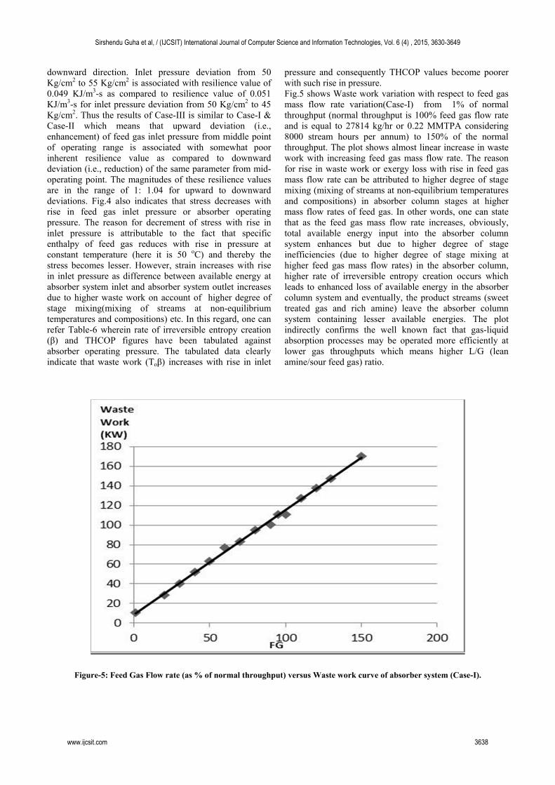
pressure and consequently THCOP values become poorer with such rise in pressure. Fig.5 shows Waste work variation with respect to feed gas mass flow rate variation(Case-I) from 1% of normal throughput (normal throughput is 100% feed gas flow rate and is equal to 27814 kg/hr or 0.22 MMTPA considering 8000 stream hours per annum) to 150% of the normal throughput. The plot shows almost linear increase in waste work with increasing feed gas mass flow rate. The reason for rise in waste work or exergy loss with rise in feed gas mass flow rate can be attributed to higher degree of stage mixing (mixing of streams at non-equilibrium temperatures and compositions) in absorber column stages at higher mass flow rates of feed gas. In other words, one can state that as the feed gas mass flow rate increases, obviously, total available energy input into the absorber column system enhances but due to higher degree of stage inefficiencies (due to higher degree of stage mixing at higher feed gas mass flow rates) in the absorber column, higher rate of irreversible entropy creation occurs which leads to enhanced loss of available energy in the absorber column system and eventually, the product streams (sweet treated gas and rich amine) leave the absorber column system containing lesser available energies. The plot indirectly confirms the well known fact that gas-liquid absorption processes may be operated more efficiently at lower gas throughputs which means higher L/G (lean amine/sour feed gas) ratio.

Figure-5: Feed Gas Flow rate (as % of normal throughput) versus Waste work curve of absorber system (Case-I).


www.ijcsit.com 3638

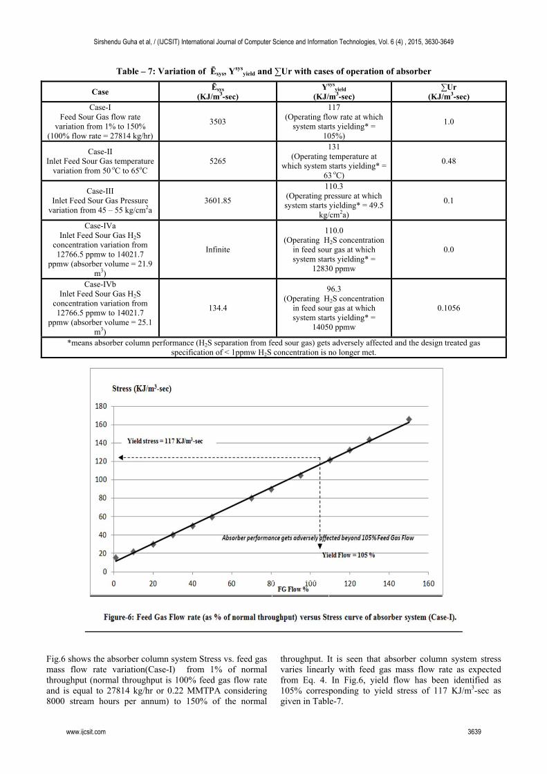
Table – 7: Variation of Ēsys, Ysys

yield and ∑Ur with cases of operation of absorber

Fig.6 shows the absorber column system Stress vs. feed gas mass flow rate variation(Case-I) from 1% of normal throughput (normal throughput is 100% feed gas flow rate and is equal to 27814 kg/hr or 0.22 MMTPA considering 8000 stream hours per annum) to 150% of the normal

throughput. It is seen that absorber column system stress varies linearly with feed gas mass flow rate as expected from Eq. 4. In Fig.6, yield flow has been identified as 105% corresponding to yield stress of 117 KJ/m3-sec as given in Table-7.

Case Ēsys

(KJ/m3-sec) Ysys

yield

(KJ/m3-sec) ∑Ur

(KJ/m3-sec) Case-I

Feed Sour Gas flow rate variation from 1% to 150%

(100% flow rate = 27814 kg/hr)

3503

117 (Operating flow rate at which

system starts yielding* = 105%)

1.0

Case-II Inlet Feed Sour Gas temperature

variation from 50 oC to 65oC 5265

131 (Operating temperature at

which system starts yielding* = 63 oC)

0.48

Case-III Inlet Feed Sour Gas Pressure

variation from 45 – 55 kg/cm2a 3601.85

110.3 (Operating pressure at which system starts yielding* = 49.5

kg/cm2a)

0.1

Case-IVa Inlet Feed Sour Gas H2S

concentration variation from 12766.5 ppmw to 14021.7

ppmw (absorber volume = 21.9 m3)

Infinite

110.0 (Operating H2S concentration

in feed sour gas at which system starts yielding* =

12830 ppmw

0.0

Case-IVb Inlet Feed Sour Gas H2S

concentration variation from 12766.5 ppmw to 14021.7

ppmw (absorber volume = 25.1 m3)

134.4

96.3 (Operating H2S concentration

in feed sour gas at which system starts yielding* =

14050 ppmw

0.1056

*means absorber column performance (H2S separation from feed sour gas) gets adversely affected and the design treated gas specification of < 1ppmw H2S concentration is no longer met.


www.ijcsit.com 3639

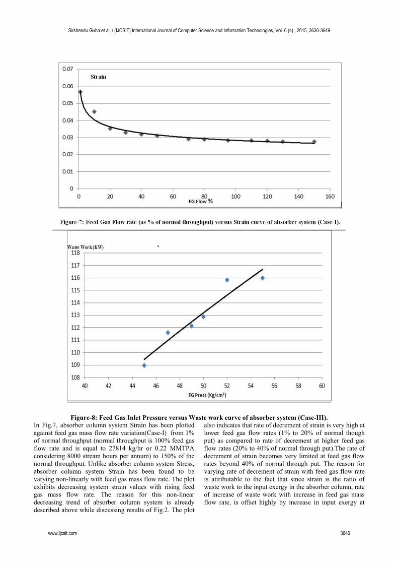
Figure-8: Feed Gas Inlet Pressure versus Waste work curve of absorber system (Case-III). In Fig.7, absorber column system Strain has been plotted against feed gas mass flow rate variation(Case-I) from 1% of normal throughput (normal throughput is 100% feed gas flow rate and is equal to 27814 kg/hr or 0.22 MMTPA considering 8000 stream hours per annum) to 150% of the normal throughput. Unlike absorber column system Stress, absorber column system Strain has been found to be varying non-linearly with feed gas mass flow rate. The plot exhibits decreasing system strain values with rising feed gas mass flow rate. The reason for this non-linear decreasing trend of absorber column system is already described above while discussing results of Fig.2. The plot

also indicates that rate of decrement of strain is very high at lower feed gas flow rates (1% to 20% of normal though put) as compared to rate of decrement at higher feed gas flow rates (20% to 40% of normal through put).The rate of decrement of strain becomes very limited at feed gas flow rates beyond 40% of normal through put. The reason for varying rate of decrement of strain with feed gas flow rate is attributable to the fact that since strain is the ratio of waste work to the input exergy in the absorber column, rate of increase of waste work with increase in feed gas mass flow rate, is offset highly by increase in input exergy at


www.ijcsit.com 3640

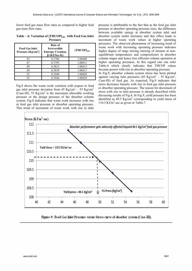
lower feed gas mass flow rates as compared to higher feed gas mass flow rates. Table – 6: Variation of [THCOP]abs with Feed Gas Inlet

Pressure

Fig.8 shows the waste work variation with respect to feed gas inlet pressure deviation from 45 Kg/cm2 – 55 Kg/cm2

(Case-III). 55 Kg/cm2 is the maximum allowable working pressure or the design pressure of the absorber column system. Fig.8 indicates that waste work increases with rise in feed gas inlet pressure or absorber operating pressure. This trend of increment of waste work with rise in inlet

pressure is attributable to the fact that as the feed gas inlet pressure or absorber operating pressure rises, the difference between available energy at absorber system inlet and absorber system outlet increases and this effect leads to increment of waste work values at higher operating pressures. The observed phenomena of increasing trend of waste work with increasing operating pressure indicates higher degree of stage mixing (mixing of streams at non-equilibrium temperatures and compositions) in absorber column stages and hence less efficient column operation at higher operating pressures. In this regard one can refer Table-6 which clearly indicates that THCOP values become poorer with rise in absorber operating pressure. In Fig.9, absorber column system stress has been plotted against varying inlet pressures (45 Kg/cm2 – 55 Kg/cm2, Case-III) of feed gas. As expected, Fig.9 indicates that stress decreases linearly with rise in feed gas inlet pressure or absorber operating pressure. The reason for decrement of stress with rise in inlet pressure is already described while discussing results of Fig.4. In Fig.9, yield pressure has been identified as 49.5 Kg/cm2 corresponding to yield stress of 110.3 KJ/m3-sec as given in Table-7.

Feed Gas Inlet Pressure (Kg/cm2)

Rate of Irreversible

Entropy Creation, β (KJ/Sec-K)

[THCOP]abs

45 0.3706 1.00400 47 0.3795 1.00411 49 0.3813 1.00413 50 0.3839 1.00417 52 0.3940 1.00428 55 0.3944 1.00429


www.ijcsit.com 3641

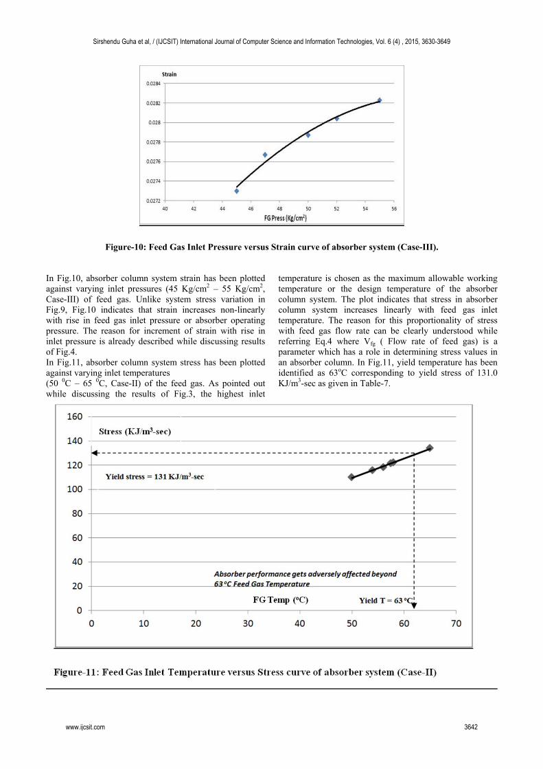
Figure-10: Feed Gas Inlet Pressure versus Strain curve of absorber system (Case-III). In Fig.10, absorber column system strain has been plotted against varying inlet pressures (45 Kg/cm2 – 55 Kg/cm2, Case-III) of feed gas. Unlike system stress variation in Fig.9, Fig.10 indicates that strain increases non-linearly with rise in feed gas inlet pressure or absorber operating pressure. The reason for increment of strain with rise in inlet pressure is already described while discussing results of Fig.4. In Fig.11, absorber column system stress has been plotted against varying inlet temperatures (50 0C – 65 0C, Case-II) of the feed gas. As pointed out while discussing the results of Fig.3, the highest inlet

temperature is chosen as the maximum allowable working temperature or the design temperature of the absorber column system. The plot indicates that stress in absorber column system increases linearly with feed gas inlet temperature. The reason for this proportionality of stress with feed gas flow rate can be clearly understood while referring Eq.4 where Vfg ( Flow rate of feed gas) is a parameter which has a role in determining stress values in an absorber column. In Fig.11, yield temperature has been identified as 63oC corresponding to yield stress of 131.0 KJ/m3-sec as given in Table-7.


www.ijcsit.com 3642

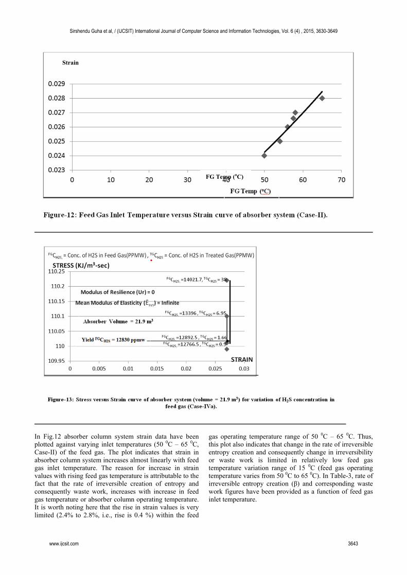
In Fig.12 absorber column system strain data have been plotted against varying inlet temperatures (50 0C – 65 0C, Case-II) of the feed gas. The plot indicates that strain in absorber column system increases almost linearly with feed gas inlet temperature. The reason for increase in strain values with rising feed gas temperature is attributable to the fact that the rate of irreversible creation of entropy and consequently waste work, increases with increase in feed gas temperature or absorber column operating temperature. It is worth noting here that the rise in strain values is very limited (2.4% to 2.8%, i.e., rise is 0.4 %) within the feed

gas operating temperature range of 50 0C – 65 0C. Thus, this plot also indicates that change in the rate of irreversible entropy creation and consequently change in irreversibility or waste work is limited in relatively low feed gas temperature variation range of 15 0C (feed gas operating temperature varies from 50 0C to 65 0C). In Table-3, rate of irreversible entropy creation (β) and corresponding waste work figures have been provided as a function of feed gas inlet temperature.

Strain

FG Temp (oC)


www.ijcsit.com 3643


www.ijcsit.com 3644

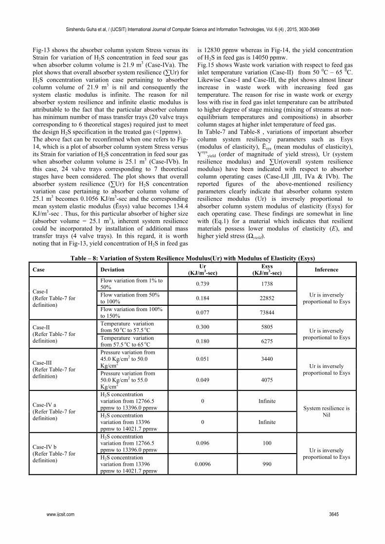
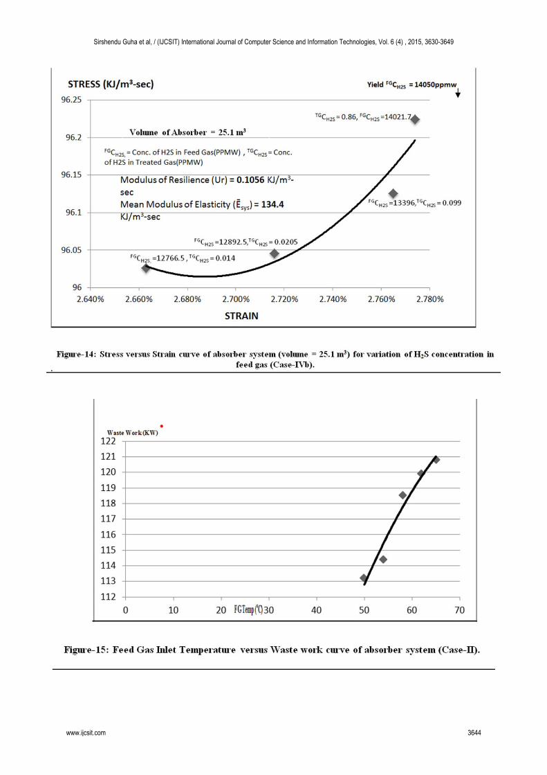
Fig-13 shows the absorber column system Stress versus its Strain for variation of H2S concentration in feed sour gas when absorber column volume is 21.9 m3 (Case-IVa). The plot shows that overall absorber system resilience (∑Ur) for H2S concentration variation case pertaining to absorber column volume of 21.9 m3 is nil and consequently the system elastic modulus is infinite. The reason for nil absorber system resilience and infinite elastic modulus is attributable to the fact that the particular absorber column has minimum number of mass transfer trays (20 valve trays corresponding to 6 theoretical stages) required just to meet the design H2S specification in the treated gas (<1ppmw). The above fact can be reconfirmed when one refers to Fig-14, which is a plot of absorber column system Stress versus its Strain for variation of H2S concentration in feed sour gas when absorber column volume is 25.1 m3 (Case-IVb). In this case, 24 valve trays corresponding to 7 theoretical stages have been considered. The plot shows that overall absorber system resilience (∑Ur) for H2S concentration variation case pertaining to absorber column volume of 25.1 m3 becomes 0.1056 KJ/m3-sec and the corresponding mean system elastic modulus (Ēsys) value becomes 134.4 KJ/m3-sec . Thus, for this particular absorber of higher size (absorber volume = 25.1 m3), inherent system resilience could be incorporated by installation of additional mass transfer trays (4 valve trays). In this regard, it is worth noting that in Fig-13, yield concentration of H2S in feed gas

is 12830 ppmw whereas in Fig-14, the yield concentration of H2S in feed gas is 14050 ppmw. Fig.15 shows Waste work variation with respect to feed gas inlet temperature variation (Case-II) from 50 0C – 65 0C. Likewise Case-I and Case-III, the plot shows almost linear increase in waste work with increasing feed gas temperature. The reason for rise in waste work or exergy loss with rise in feed gas inlet temperature can be attributed to higher degree of stage mixing (mixing of streams at non-equilibrium temperatures and compositions) in absorber column stages at higher inlet temperature of feed gas. In Table-7 and Table-8 , variations of important absorber column system resiliency parameters such as Esys (modulus of elasticity), Ēsys (mean modulus of elasticity), Ysys

yield (order of magnitude of yield stress), Ur (system resilience modulus) and ∑Ur(overall system resilience modulus) have been indicated with respect to absorber column operating cases (Case-I,II ,III, IVa & IVb). The reported figures of the above-mentioned resiliency parameters clearly indicate that absorber column system resilience modulus (Ur) is inversely proportional to absorber column system modulus of elasticity (Esys) for each operating case. These findings are somewhat in line with (Eq.1) for a material which indicates that resilient materials possess lower modulus of elasticity (E), and higher yield stress (Ωyield).

Table – 8: Variation of System Resilience Modulus(Ur) with Modulus of Elasticity (Esys)

Case Deviation Ur

(KJ/m3-sec) Esys

(KJ/m3-sec) Inference

Case-I (Refer Table-7 for definition)

Flow variation from 1% to 50%

0.739 1738

Ur is inversely proportional to Esys


0.184 22852


0.077 73844

Case-II (Refer Table-7 for definition)

Temperature variation from 50 oC to 57.5 oC

0.300 5805 Ur is inversely

proportional to Esys Temperature variation from 57.5 oC to 65 oC

0.180 6275

Case-III (Refer Table-7 for definition)

Pressure variation from 45.0 Kg/cm2 to 50.0 Kg/cm2


proportional to Esys Pressure variation from 50.0 Kg/cm2 to 55.0 Kg/cm2

0.049 4075

Case-IV a (Refer Table-7 for definition)

H2S concentration variation from 12766.5 ppmw to 13396.0 ppmw

0 Infinite System resilience is

Nil H2S concentration variation from 13396 ppmw to 14021.7 ppmw

0 Infinite

Case-IV b (Refer Table-7 for definition)

H2S concentration variation from 12766.5 ppmw to 13396.0 ppmw


proportional to Esys H2S concentration variation from 13396 ppmw to 14021.7 ppmw

0.0096 990


www.ijcsit.com 3645

4.0 DISCUSSION ON APPLICATION OF THE PROPOSED

METHODOLOGY TO PROCESS DESIGN The system yield stress (Ysys

yield) figures predict that the absorber column performance (with respect to H2S separation capability) is expected to be affected adversely beyond 105% of design throughput of 27814 Kg/hr (deviation range: 1% to 150%), beyond operating temperature of 63oC(deviation range: 50 oC to 65 oC) , beyond operating pressure of 49.5Kg/cm2(deviation range: 45 Kg/cm2 to 55 Kg/cm2) and beyond feed sour gas H2S concentration of 12830 ppmw (deviation range: 12766.5 ppmw to 14021.7 ppmw). These findings clearly indicate that operation of the absorber column will not be advisable beyond the identified yield point figures as the column will not be able to tolerate these deviations in process conditions and eventually will fail to meet treated gas specification of < 1ppmw H2S. However, for example, if the absorber column system is required to be designed for a pre-defined over-capacity factor, say 50% over and above its normal operating capacity, the design engineer may use the overall system resilience modulus data to provide in-built over capacity handling capability or resilience in the system. The design engineer can easily incorporate the desired over capacity handling capability in the absorber column system by considering higher number of mass transfer trays than the actual number of trays considered while carrying out simulation and keeping all other process variables fixed. As an illustration, the following simple process calculations may be worth highlighting for estimation of number of additional trays required for this purpose. Let us suppose, one needs to provide 50% in-built over capacity handling capability in the absorber column system, studied in this work. Referring Fig.2, one identifies that Ur for downward flow deviation from 75% to 1% is as high as 0.883 KJ/m3-sec whereas the same for upward flow deviation from 75% to 150% is only 0.117 KJ/m3-sec. Hence, if the absorber column is required to handle feed gas flow rate as high as 150% of its normal design capacity, Ur value for upward flow deviation from 75% to 150% need to be same as it is for the down ward flow deviation range (i.e., 75% to 1%) which is equal to 0.883 KJ/m3-sec. In order to enhance the Ur value for upward flow deviation range, one needs to find out the system strain required for achieving the Ur value of 0.883 KJ/m3-sec. The system strain value can be back calculated from the knowledge of curve-fit equation of Fig.2 in the following way: Curve -fit equation of Fig.2 is: 0.001 . , where y is stress in KJ/m3-sec and x is strain. It may be reasonable to mention here that the curve-fit equation of Fig.2 is quite similar to power relationship which is often used to express the true stress (σ) as a function of true strain (ε) for a ductile material (σ = Kεn, where K is strength co-efficient and n is work hardening exponent). Now it is known that for the absorber column system:

Ur = 0.883 = 0.001 .. 13)

where, sm = strain required at 150% flow point for design Ur value of 0.883 KJ/m3-sec and 0.029 is strain

corresponding to 75% feed gas flow point in Fig.2. When Eq.13 is solved for sm, sm value is obtained as 0.023. From Fig.2, one can read strain at 100% feed gas flow point as 0.028 and that at 1% flow point as 0.057. Thus, nearly 100% feed gas flow variation corresponds to 2.9% strain variation and since minimum six theoretical stages are required (as per computer simulation using process simulator Pro/II) to achieve absorber column treated gas H2S specification of < 1 ppmw, number of additional theoretical stages which are required to be considered in order to provide 50% in-built over capacity handling capability in the absorber column may be estimated as:

∆. ∆ 150 (14)

Where, number of additional theoretical stages for 150% capacity = Na, Minimum number of theoretical stages required for 100% capacity = Nm, Strain variation corresponding to flow variation from 100% to 1% = ∆ 100 and Strain variation corresponding to flow variation from 100% to 150% =∆ 150. In this work, Nm = 6, ∆ 100 = 0.029, ∆ 150 = (0.028-0.023) = 0.005 and

hence, .

∗ 0.005 1.034. Since, design

overall tray efficiency in the absorber column (Refer Table-1) is 0.3, actual number of additional trays required forproviding 50% in-built over capacity in the absorber column becomes 1.034/0.3 = 3.446 = 4 (round). In similar ways, one can provide pre-defined over design margins in cases of temperature, pressure and feed sour gas H2S concentration variations of feed sour gas beyond normally envisaged maximum operating temperature and pressure conditions and then, in each case, the actual number of additional trays will be calculated and consequently the absorber column may be provided with the highest number of additional trays.

5.0 CLOSING REMARKS The analysis described in this paper enables us to determine the resilient feed sour gas flow, temperature, pressure and composition regimes pertaining to an absorber column. Hence, in this work, the magnitudes of system resilience modulus figures have been estimated for all cases of variations of operating conditions. The Stress-Strain curves developed for the absorber column indicate that inherent system resilience figures are always very poor for deviations of feed sour gas in-flow rate, inlet temperature & inlet pressure from mid operating points towards upward directions as compared to deviations in downward directions. In other words, these results mean that while operating an absorber column in a GSU, enhancement of throughput beyond its design capacity (usually 100%) or operating the column at more stringent conditions (pressure and temperature) or near to design conditions is always associated with very limited system tolerance regime or resiliency with regard to its efficient performance at the targeted performance levels. It is interesting to note that the magnitude of the over-all system resilience modulus for variation of H2S concentration in feed gas has been found to be nil for the absorber column of 21.9 m3 volume since the particular absorber column has minimum number of


www.ijcsit.com 3646

mass transfer trays (20 valve trays corresponding to 6 theoretical stages) required just to meet the design H2S specification in the treated gas (<1ppmw). The above fact can be reconfirmed when one refers to Fig-14. This figure indicates that overall absorber system resilience modulus for H2S concentration variation case pertaining to a higher absorber volume (25.1 m3) becomes 0.1056 KJ/m3-sec. Thus, for this particular absorber of higher size (absorber volume = 25.1 m3 corresponding to 24 valve trays pertaining to 7 theoretical stages), inherent system resilience could be incorporated by installation of additional mass transfer trays (4 valve trays). It is illustrated in this work, that thermodynamic co-efficient of performance (THCOP) is the only meaningful measure of thermodynamic efficiency for an absorber column and the results indicate that in case of DEA based sweetening processes where absorber columns are used can be operated more efficiently from thermodynamic considerations at such operating conditions for which THCOP values are closer to 1. As evident from Table-2, surplus work or energy is available in the absorber column system and as a consequence the temperature differences between treated gas and feed gas (∆T1) as well as the temperature differences between rich amine and lean amine (∆T2) are all positive. However, recovering this surplus work or energy is industrially impractical owing to low absorber column operating temperature range (500C to 65 0C). In addition to evaluation of inherent system resilience (Ur) figures for an absorber column system and the thermodynamic co-efficient of performance (THCOP) figures, modulus of elasticity figures (Esys), mean modulus of elasticity (Ēsys) figures for the system along with the order of magnitude of yield stresses (Ysys

yield) for cases of variations of mass flow rate, inlet temperature, inlet pressure and inlet H2S concentration of feed sour gas have also been evaluated and the results are reported by means of Table-7 & Table-8. The reported figures of the above-mentioned resiliency parameters clearly indicate that absorber column system resilience (Ur) is inversely proportional to absorber column system modulus of elasticity (Esys) for all cases of variations of operating variables. These findings are somewhat in line with (Eq.1) for a material which indicates that higher the resiliency of a material, lower is the modulus of elasticity (E), and higher is the yield stress (Ωyield). The theoretical analysis presented in this paper will provide useful guidelines for determination of tolerable range of operating conditions in a DEA based absorption process. The concept of resilience, described above will also aid in the determination of requirement of system augmentation (e.g., incorporation of additional trays etc) for providing in-built over capacity handling capability or resiliency etc., in the system. This analysis also provides an insight in the absorber column system performance efficiencies in terms of the thermodynamic co-efficient of performance (THCOP) values which are newly envisaged in this work.

6.0 FUTURE WORK OUTLINE The methodology described in section-2 for development of quantitative correlations for the quantification of inherent system resilience (system resilience modulus) etc., can be applied easily for any process system. In order to illustrate the same, correlations for quantification of system resilience for the amine stripper column, the lean amine-rich amine exchanger which are commonly downstream systems for an amine absorber column are provided below. Evaluation of resilience modulus (Ur), modulus of elasticity (Esys), mean modulus of elasticity (Ēsys) and order of magnitude of yield stresses (Ysys

yield) for these systems can be undertaken in future research work. 6.1 Correlations for amine stripper column General system stress equation for steady flow condition is reproduced below for its application in development of correlations for quantification of inherent system resilience (modulus of resilience) for the stripper column system:

2

21j li i

sys isu

sys sys

mumh mgz q w

d MUS

V dt V

Since, for steady flow condition in stripper column system, d(MU)sys/dt = 0, the above general system stress equation is necessarily modified as :

2

2 in j linin

sssys

mumh mgz q w

SV

As for the stripper column system under steady state, one can neglect kinetic and potential energy terms shown in above equation and since for this system, ∑wl = 0, the stress equation for the stripper column system which is usually utilized in a Gas Sweetening Unit (refer Fig-1) can be written as: Ss(stripper) = [(mh)in + ∑qj]/V(stripper) = 1/ V(stripper)[ Lsrhsr + Qreb] In line with preceding analysis, the system strain for a stripper column can be also considered as functions of system Irreversibility, I, i.e., exergy lost or waste work. Thus, the general equation for computation of Irreversibility or waste work for any system handling flowing streams under steady state is also applicable for the stripper column system or

1 oo o j li

j

TI T m h T s q w

T

= Exergy lost = Waste work For the stripper column system under steady state with well defined system boundaries (refer Fig-1), the above equation can be rewritten as: I = (T0β)stripper = ∑[m(h- T0s)]i + ∑(1- T0/ Tj)qj = [m(h- T0s)]in - [m(h- T0s)]out +(1- T0/ Treb)Qreb

= Waste work = Exergy lost


www.ijcsit.com 3647

Taking into account the stripper column system boundaries as defined in Fig-1, one can elaborate the above equation as: I = (T0β)stripper = [Lsr bsr ] – [ Vag bag + Lsl bsl ] + (1- T0/ Treb)Qreb = Waste work = Exergy lost Since, likewise any other flow systems, system strain under steady flow condition for stripper column system is also equal to ratio of total Exergy lost or Waste work or Irreversibility to total Input Exergy, the system strain for stripper column system can also be estimated using following equation: Ssn(stripper) = [Lsr bsr ] – [ Vag bag + Lsl bsl ] + (1- T0/ Treb)Qreb / Lsr[(hsr – h0

sr) –T0(ssr - s0

sr)] + (1- T0/ Treb)Qreb In the above equation, denominator is the total input exergy for the stripper column system or Lsr[(hsr – h0

sr) –T0(ssr - s0sr)]+ (1- T0/ Treb)Qreb = Total

Exergy Input. 6.2 Correlations for lean amine-rich amine exchanger One can develop and use the following equations in order to estimate variation of stress and strain with varying operating conditions for the lean-rich exchanger system which is usually used in pre-heating of H2S rich Di-ethanol amine (solvent) by exchange of heat with H2S lean Di-ethanol amine (solvent) in a GSU. The lean-rich exchanger system can be considered to be a Shell and Tube heat exchanger of fixed length and diameter. In this exchanger, the H2S rich Di-ethanol amine is usually the shell side fluid whereas the H2S lean Di-ethanol amine is the tube side or channel side fluid. The general system stress equation for steady flow condition is reproduced below for its application in development of correlations for quantification of inherent system resilience (modulus of resilience) for the lean-rich exchanger system:

2

2 in j linin

sssys

mumh mgz q w

SV

For the lean-rich exchanger system under steady state, one can neglect kinetic and potential energy terms shown in the above equation and also for the lean-rich exchanger system, ∑qj = 0 (considering no auxiliary heat transfer from the environment) and ∑wl = 0. Thus, the system stress equation for the lean-rich exchanger system, which is utilized in the GSU (refer Fig-1) can be written as:

Ss(LRRxch) = [(mh)in]/V(LRExch) = 1/ V(LRExch)[ Lsrhsr + Lsl hsl]at inlet

Like absorber, stripper etc., system strain for lean-rich exchanger is also function of system Irreversibility, I, i.e., Exergy lost or waste work. Thus, the general equation for computation of Irreversibility or waste work for any system handling flowing streams under steady state is also applicable for the lean-rich exchanger system:

1 oo o j li

j

TI T m h T s q w

T

For the lean-rich exchanger system under steady state with well defined system boundaries (refer Fig-1), the above equation can be rewritten as:

I = (T0β)LRExch = ∑[m(T0s)]i = T0 [mshellin(sshellout-sshellin) + mtubein(stubeout-stubein)] = Exergylost

Taking into account the lean-rich exchanger system boundaries as defined in Fig-1, one can elaborate the above equation as:

I = (T0β)LRExch = T0 [Lsr (ssrout-ssrin) + Lsl(sslout-sslin)] = Exergylost

Since, likewise absorber, stripper etc, system strain under steady flow condition for lean-rich exchanger system is also equal to ratio of total Exergy lost or Waste work or Irreversibility to total Input Exergy. Therefore, the system strain for lean-rich exchanger system can be estimated using following equations: Total input exergy for the lean-rich exchanger system can be estimated as:

Exergyin = Lsr[(hsr – h0sr) –T0(ssr - s

0sr)]+ Lsl[(hsl – h0

sl) –T0(ssl - s

0sl)]

Hence, the strain values for the lean-rich exchanger system as defined in Fig-1 can be estimated using the following equation:

Ssn(LRExch) = T0 [Lsr (ssrout-ssrin) + Lsl(sslout-sslin)] / Lsr[(hsr – h0

sr) –T0(ssr - s0sr)]+ Lsl[(hsl – h0

sl) –T0(ssl - s0sl)]

7.0 CONCLUSIONS

In this work, system resilience correlations have been developed and these correlations have been verified for their usefulness pertaining to an absorber column system. Moreover, in this work, the challenge of applying the material resiliency definition to systems for determining the system yield stress values, modulus of system resilience and modulus of elasticity have been successfully overcome by estimation of these critical resiliency parameters for the absorber column system with regard to deviations of all possible operating variables namely flow, temperature, pressure and composition. A new thermodynamic efficiency parameter termed as “thermodynamic Coefficient of Performance (THCOP)” has been introduced and its usefulness in determination of absorber column efficiency has been established. One example has also been cited on how a design engineer can incorporate about 50% over capacity factor or inherent resiliency in the absorber column by augmentation of number of column trays. Finally, useful mathematical correlations pertaining to amine stripper column, lean amine-rich amine exchanger (which are commonly used downstream of an amine absorber) have been provided for their verification in future research works in this field of study.

8.0 NOMENCLATURE b = Availability function and is equal to (h- T0s), KJ/Kg bsl = Availability function of lean solvent, KJ/Kg bfg = Availability function of lean feed gas, KJ/Kg btg = Availability function of treated gas, KJ/Kg bsr = Availability function of rich solvent, KJ/Kg bag = Availability function of acid gas, KJ/Kg [THCOP]abs = Thermodynamic Coefficient of Performance of absorber column E = Modulus of elasticity, N/m2

g = Acceleration due to gravity, m/sec2


www.ijcsit.com 3648

hi = Enthalpy of the material in stream i, KJ/Kg hin = Enthalpy of the material in input stream, KJ/Kg hsl = Enthalpy of lean solvent, KJ/Kg hsr = Enthalpy of rich solvent, KJ/Kg ho

sl = Enthalpy of lean solvent at datum conditions, KJ/Kg ho

sr = Enthalpy of rich solvent at datum conditions, KJ/Kg hfg = Enthalpy of feed gas, KJ/Kg ho

fg = Enthalpy of feed gas at datum conditions, KJ/Kg h = Enthalpy of incoming and outgoing streams, KJ/Kg H = Enthalpy, KJ/Kg I = Irreversibility, KW Lsl = Flow rate of lean solvent, Kg/sec Lsr = Flow rate of rich solvent, Kg/sec Msys = Mass of material contained in the system, Kg m = Mass of material contained in the control volume, Kg mi = Flow rate of stream i, Kg/sec min = Flow rate of input stream, Kg/sec mshellin = Flow rate of shell side input stream, Kg/sec mtubein = Flow rate of tube side input stream, Kg/sec . = Mass flow rate of a stream, Kg/sec

n = . .

. , where = heat flux to ambient air, outside pipe

diameter, mass flow rate of steam and heat capacity of steam qj = Rate of heat exchange between the system and an external heat reservoir maintained at temperature Tj, KW . = Rate of heat transfer into the control volume, KW.

Qreb = Re-boiler Duty, KW Ssu = System stress for unsteady state condition, KJ/m3-sec Sss = System stress for steady state condition, KJ/m3-sec Ss(abs) = Absorber system stress, KJ/m3-sec Ss(stripper) = Stripper system stress, KJ/m3-sec Ss(LRRxch) = Lean-Rich Exchanger system stress, KJ/m3-sec ssl = Entropy of lean solvent, KJ/Kg-K ssr = Entropy of rich solvent, KJ/Kg-K si = Entropy of material in stream i, KJ/Kg-K so

sl = Entropy of lean solvent at datum conditions, KJ/Kg-K so

sr = Entropy of rich solvent at datum conditions, KJ/Kg-K sfg = Entropy of feed gas, KJ/Kg-K so

fg = Entropy of feed gas at datum conditions, KJ/Kg-K Ssn(abs) = Absorber system strain Ssn(stripper) = Stripper system strain sshellin = Entropy of shell side inlet stream KJ/Kg-K sshellout = Entropy of shell side outlet stream KJ/Kg-K stubein = Entropy of tube side inlet stream KJ/Kg-K stubeout = Entropy of tube side outlet stream KJ/Kg-K ssrin = Entropy of rich solvent inlet stream, KJ/Kg-K ssrout = Entropy of rich solvent outlet stream, KJ/Kg-K sslin = Entropy of lean solvent inlet stream, KJ/Kg-K sslout = Entropy of lean solvent outlet stream, KJ/Kg-K t = Time, sec T0 = Temperature of the environment (datum condition), K Tj = Temp of auxiliary heat reservoir, K Ta = Ambient temperature, K Ts = Steam inlet temperature, K Treb = Re-boiler temperature, K Ur = Modulus of Resilience for system, KJ/m3-sec UR = Modulus of Resilience for material, KJ/m3 ui = Velocity of stream i, m/sec U = Internal energy, KJ/Kg u = Velocity, m/sec Usys = Internal energy of system, KJ/Kg uin = Velocity in input stream,m/sec Vsys = System volume, m3 V(abs) = Absorber volume, m3

V(stripper) = Stripper volume, m3

V(LRExch) = Lean-Rich Exchanger volume, m3 Vfg = Flow rate of feed gas, Kg/sec Vtg = Flow rate of treated gas, Kg/sec Vag = Flow rate of acid gas, Kg/sec wl = Work done per unit time by a part of the system bearing label, l, KW

. = Work done by the system per unit time, KW wmin = Minimum work required for separation, KW z = Elevation of control volume from grade level, m zi = Elevation of stream i w.r.t grade level, m

zin = Elevation of input stream w.r.t grade level, m β = Rate of irreversible entropy creation, KJ/sec-K T0β = Irreversibility or waste work, KJ/sec [(T0β)abs] = Irreversibility or waste work for absorber column system, KW [(T0β)stripper] = Irreversibility or waste work for stripper column system, KW Ωyield = Yield stress of material, N/m2 ηabs = Thermodynamic efficiency of absorber column Ēsys = Mean modulus of elasticity for absorber column system, KJ/m3-sec Ysys

yield = Order of magnitude of yield stress for absorber column system, KJ/m3-sec Exergylost = Exergy Lost, KW Exergyin = Exergy Input, KW

REFERENCES

[1] Linh T.T. Dinh, Hans Pasman, Xiaodan Gao, M.Sam Mannan (2012), “Resilience engineering of industrial processes: Principles and contributing factors”, Journal of Loss Prevention in the Process Industries, 25,233-241

[2] “Resilience”, in “Van Nostrands Scientific Encyclopedia,” 6th ed., Van Nostrand Reinhold, New York, p.2433 (1983).

[3] Mitchell S M. and M. Sam Mannan, “Designing Resilient Engineered Systems”, CEP, April (2006).

[4] Morari, M. (1983), “Flexibility and resiliency of process systems”, Comp.Chem. Engg., 7, 423-437.

[5] Guha, S., and Das, S.K. (2014), “Resilience Analysis of a Pipe Segment System Carrying Superheated Steam”, Advanced Materials Research, 917, pp. 232-243.

[6] Slocum, M.G.(2007), “Use of experimental disturbances to assess resilience along a known stress gradient”, Ecological Indicators,8,181-190

[7] Swaney, R.E.,Grossmann, L.E.(1985), “An index for operational flexibility in chemical process design. 2: Computational algorithms”,AIChE Journal, 31,631-641.

[8] Zhen Zhang, Xiao Feng and Feng Qian (2009), “Studies on resilience of water networks”,Chem.Engg.Journal.,147,117-121.

[9] Shirali,G.H.A.,Motamedzade,M.,Mohammadfam,I.,Ebrahimipour,V., Moghimbeigi,A.(2012), “Challenges in building resilience engineering (RE) and adaptive capacity: A field study in a chemical plant”,Proc.Safety & Environ.Protect.,90,83-90.

[10] R.R. Tan, D.C.Y. Foo, Z.A. Manan(2007), “ Assessing the sensitivity of water networks to noisy mass loads using Monte Carlo simulation”,Comp.Chem.Eng, 31, 1355-1363.

[11] Eric D. Vugrin, Drake E. Warren, and Mark A. Ehlen(2011), “ A resilience assessment framework for infrastructure and economic systems: Quantitative and qualitative resilience analysis of petrochemical supply chains to a hurricane”, Process Safety Progress, 30(3), 280-290.

[12] D. Henry, J.Emmanuel Ramirez-Marquez (2012), “Generic metrics and quantitative approaches for system resilience as a function of time”, Reliability Eng. Sys. Safety,99, 114-122.

[13] P.V.R. de Carvalho (2011), “The use of Fundamental Resonance Analysis Method (FRAM) in a mid-air collision to understand some characteristics of the air traffic management system resilience”, Reliability Eng. Sys. Safety,96, 1482-1498.

[14] Liu, X., Prodan, I., Zio, E. (2014), “On the resilience analysis of interconnected systems by a set-theoretic approach”, Safety and Reliability: Methodology and Applications - Proceedings of the European Safety and Reliability Conference, ESREL (2014).

[15] Zhuang, B., Lansey, K., and Kang, D. (2013). “Resilience/Availability Analysis of Municipal Water Distribution System Incorporating Adaptive Pump Operation.” J. Hydraul. Eng., 139(5), 527–537.

[16] Blackmore, J. and Plant, R. (2008). “Risk and Resilience to Enhance Sustainability with Application to Urban Water Systems.” J. Water Resour. Plann. Manage., 134(3), 224–233.

[17] Smith, Van Ness and Abbott, “Introduction to Chemical Engineering Thermodynamics”, 7th ed.,pp. 47-48, McGraw-Hill, New York (2005).

[18] Fitzmorris R.E. and R.S.H. Mah (1980), “Improving Distillation Column Design Using Thermodynamic Availability Analysis”, AIChE Journal, 26, 2, 265-273.


www.ijcsit.com 3649

thermodynamic availability analysis: usage in ...ijcsit.com/docs/volume...

Documents