Clemson UniversityTigerPrints

All Theses Theses

12-2014

Thermo-physical Property Models and Effect onHeat Pipe ModellingDevakar DhingraClemson University, ddhingr@g.clemson.edu

Follow this and additional works at: https://tigerprints.clemson.edu/all_theses

Part of the Mechanical Engineering Commons

This Thesis is brought to you for free and open access by the Theses at TigerPrints. It has been accepted for inclusion in All Theses by an authorizedadministrator of TigerPrints. For more information, please contact kokeefe@clemson.edu.

Recommended CitationDhingra, Devakar, "Thermo-physical Property Models and Effect on Heat Pipe Modelling" (2014). All Theses. 2052.https://tigerprints.clemson.edu/all_theses/2052

THERMO-PHYSICAL PROPERTY MODELS

AND

EFFECT ON HEAT PIPE MODELING

A Thesis Presented to

the Graduate School of Clemson University

In Partial Fulfillment of the Requirements for the Degree

Master of Science Mechanical Engineering

by Devakar Dhingra November 2014

Accepted by: Dr. Jay M. Ochterbeck, Committee Chair & Advisor

Dr. Xiangchun Xuan, Committee member Dr. Chenning Tong, Committee member

ii

ABSTRACT

Heat transfer devices find applications in various aspects of life. Be it residential,

commercial or industrial application, efficient heat transfer is a challenge to all. Other

than geometric design considerations and wick selection, the optimization of heat

transfer in the heat pipe also depends on fluid selection. Heat pipe technology has

proven to work efficiently with properly selected thermal fluid, from cryogenic

temperatures to very high temperatures. Higher heat transfer ability through small

temperature differences makes the heat pipe an efficient technology. Hence, it can be

stated that selecting a proper working fluid enhances the heat transfer performance of a

heat pipe. For selecting the working fluid, important thermo-physical properties to be

considered are density, viscosity, surface tension, latent heat of vaporization and vapor

saturation pressure at every working temperature.

The operating range of the working fluid starts from the triple point and till the

critical point. The performance of the working fluid is not optimum at both ends of the

operating range of temperature. At critical temperature, it is impacted by low surface

tension and latent heat of vaporization, whereas near the triple point low vapor density

and high viscosity affects the performance.

One of the first indices for evaluating the performance of the working fluid is

called “Merit Number” This merit number considers a single pressure gradient, i.e. the

liquid pressure drop. Later, substantial works have been done to implement the same

idea in a system utilizing multiple pressure gradients (losses). In all the methods

comparing the merit number of the fluids, the higher the merit number, better is the heat

transfer capacity of the pipe.

iii

For theoretical calculations and geometrical design considerations, thermo-

physical property data of the working fluid at every operating temperature is not available

and if available, the reliability of this data is a reason of concern. The present work

constitutes of dividing the working fluids into two main categories polar fluids (i.e.

ammonia, water and methanol) and nonpolar fluids (i.e. ethane) and thus validating the

methods used for formulating these thermo-physical properties as a function of

temperature.

As per conventional available data (in several reliable resources), these thermo-

physical properties are formulated as a polynomial function of the temperature. The main

problem though with such formulation is the data reliability outside the specified

temperature range. This work tries to formulate such properties as a function of intensive

properties and molecular structure of the working fluid. Thereafter the most useful

method for thermo-physical property formulation was chosen after calculating the error

percentage (relating to the experimental data obtained from various sources)

The latter part of this work focuses on the uncertainty of the value about the

mean obtained from the methods used and thereafter the percent deviation (between the

mean obtained and the experimental data available) which can give the clear idea about

the selection of the method for formulating the properties.

The last part of this work link the different methods used with the merit number

for both liquid and vapor driven heat pipe. This part also includes the error percent and

deviation percentage of the capillary limited maximum heat transferring capacity of the

heat pipe.

iv

DEDICATION

This work is dedicated to my family and friends whose unconditional support, love and

belief in me, encouraged me in every shape of life.

v

ACKNOWLEDGEMENT

I would like to express my sincere gratitude to my advisor Dr. Jay M. Ochterbeck for his

continued and extensive support and relevant feedback throughout the work.

vi

TABLE OF CONTENTS

Page

ABSTRACT ...................................................................................................................... II

DEDICATION ................................................................................................................... IV

ACKNOWLEDGEMENT ................................................................................................... V

LIST OF TABLES .......................................................................................................... VIII

LIST OF FIGURES ........................................................................................................... X

NOMENCLATURE .......................................................................................................... XII

CHAPTER 1

INTRODUCTION ............................................................................................................... 1

CONVENTIONAL HEAT PIPE .............................................................................................. 1 LOOP HEAT PIPE ............................................................................................................. 4

CHAPTER 2

LITERATURE REVIEW .................................................................................................... 8

MERIT NUMBER ............................................................................................................... 8 FLUID SELECTION .......................................................................................................... 15 THERMO-PHYSICAL PROPERTIES ................................................................................... 18

CHAPTER 3

RESULTS AND DISCUSSION ....................................................................................... 38

THERMAL FLUIDS AND WORKING TEMPERATURE RANGE ................................................ 38 LATENT HEAT OF VAPORIZATION .................................................................................... 40 LIQUID DENSITY ............................................................................................................ 44 VAPOR DENSITY ............................................................................................................ 48 SURFACE TENSION ........................................................................................................ 52 LIQUID VISCOSITY ......................................................................................................... 55 VAPOR VISCOSITY ......................................................................................................... 57 MERIT NUMBER ............................................................................................................. 59 MAXIMUM HEAT TRANSFER ............................................................................................ 62 DISCUSSION .................................................................................................................. 65

vii

Table of contents (Continued)

Page

CHAPTER 4

CONCLUSION ................................................................................................................ 68

CHAPTER 5

RECOMMENDATIONS FOR FUTURE WORK .............................................................. 70

APPENDICES ................................................................................................................. 71

APPENDIX A: LYCKMAN ET AL. [30] GENERALIZED REDUCED TEMPERATURE PARAMETERS 72 APPENDIX B: SCALING VOLUME AND CRITICAL VOLUME FOR GUNN ET AL. [32]. ............... 73 APPENDIX C: SUDGEN [18] ATOMIC AND PARACHOR VALUES........................................... 73 APPENDIX D: QUALE [21] ATOMIC AND STRUCTURAL PARACHOR VALUES ........................ 74

REFERENCE .................................................................................................................. 75

viii

LIST OF TABLES

Table Page

TABLE 1: WORKING FLUID TEMPERATURE TABLE (AT 1 ATM) ................................................. 8

TABLE 2: THERMODYNAMIC PROPERTIES OF SEVERAL WORKING FLUIDS AND MERIT NUMBER

(AT NORMAL BOILING TEMPERATURE) .......................................................................... 11

TABLE 3: LIQUID DENSITY TO SURFACE TENSION RATION .................................................... 18

TABLE 4: CONSTANTS FOR CUBIC EQUATION OF STATE ....................................................... 30

TABLE 5: OPERATING TEMPERATURE RANGE FOR FLUIDS ................................................... 39

TABLE 6: PITZER EQUATION PARAMETER TABLE ................................................................. 40

TABLE 7: WATSON-RIEDEL EQUATION PARAMETER TABLE................................................... 41

TABLE 8: WATSON-CHEN EQUATION PARAMETER TABLE ..................................................... 42

TABLE 9: WATSON-VISWANATH EQUATION PARAMETER TABLE ............................................ 43

TABLE 10: FRANCIS ET AL. EQUATION PARAMETER TABLE ................................................... 44

TABLE 11: RIEDEL EQUATION PARAMETER TABLE ............................................................... 45

TABLE 12: YEN ET AL. EQUATION PARAMETER TABLE .......................................................... 46

TABLE 13: PARAMETER GUNN ET AL. EQUATION PARAMETER TABLE .................................... 47

TABLE 14: VAN-DER WAAL’S EQUATION PARAMETER TABLE ................................................ 48

TABLE 15: REDLICH-KWONG EQUATION PARAMETER TABLE ................................................ 49

TABLE 16: SOAVE EQUATION PARAMETER TABLE ................................................................ 50

TABLE 17: PENG-ROBINSON EQUATION PARAMETER TABLE ................................................ 51

TABLE 18: MACLEOD-SUDGEN EQUATION PARAMETER TABLE ............................................. 52

TABLE 19: QUALE EQUATION PARAMETER TABLE ................................................................ 53

TABLE 20: BROOK’S ET AL. EQUATION PARAMETER TABLE................................................... 54

TABLE 21: VOGEL EQUATION PARAMETER TABLE ................................................................ 55

ix

List of Tables (Continued)

Table Page

TABLE 22: LEWIS-SQUIRE EQUATION PARAMETER TABLE .................................................... 56

TABLE 23: CHUNG EQUATION PARAMETER TABLE ............................................................... 57

TABLE 24: LUKAS EQUATION PARAMETRIC TABLE ............................................................... 58

TABLE 25: LATENT HEAT RECOMMENDATION ..................................................................... 65

TABLE 26: LIQUID DENSITY RECOMMENDATION .................................................................. 65

TABLE 27: VAPOR DENSITY RECOMMENDATION .................................................................. 66

TABLE 28: SURFACE TENSION RECOMMENDATION ............................................................. 66

TABLE 29: LIQUID VISCOSITY RECOMMENDATION ............................................................... 67

TABLE 30: VAPOR VISCOSITY RECOMMENDATION .............................................................. 67

x

LIST OF FIGURES

Figure Page

FIGURE 1: CONVENTIONAL HEAT PIPE [1] ............................................................................. 1

FIGURE 2: HEAT PIPE LIMITATIONS [1] ................................................................................. 4

FIGURE 3: LOOP HEAT PIPE [5] ............................................................................................ 5

FIGURE 4: P-T DIAGRAM FOR LHP [5]. ................................................................................. 6

FIGURE 5: LIQUID MERIT NUMBER FOR DIFFERENT WORKING FLUIDS [9] .............................. 11

FIGURE 6: LHP EVAPORATOR. [9] ..................................................................................... 13

FIGURE 7: MERIT NUMBER AND VAPOR PRESSURE CURVE FOR WATER. ............................... 21

FIGURE 8: SURFACE TENSION OF VARIOUS FLUIDS [3, 35] .................................................. 31

FIGURE 9: PITZER EQUATION ERROR ................................................................................. 40

FIGURE 10: WATSON-RIEDEL EQUATION ERROR ................................................................. 41

FIGURE 11: WATSON-CHEN EQUATION ERROR ................................................................... 42

FIGURE 12: WATSON-VISWANATH EQUATION ERROR .......................................................... 43

FIGURE 13: FRANCIS ET AL. EQUATION ERROR ................................................................... 44

FIGURE 14: RIEDEL EQUATION ERROR ............................................................................... 45

FIGURE 15: YEN ET AL. EQUATION ERROR .......................................................................... 46

FIGURE 16: GUNN ET AL. EQUATION ERROR ....................................................................... 47

FIGURE 17: VAN-DER WAAL’S EQUATION ERROR ................................................................ 48

FIGURE 18: REDLICH-KWONG ERROR ................................................................................ 49

FIGURE 19: SOAVE ERROR................................................................................................ 50

FIGURE 20: PENG-ROBINSON EQUATION ERROR ................................................................ 51

FIGURE 21: MACLEOD-SUDGEN EQUATION ERROR ............................................................. 52

FIGURE 22: QUALE EQUATION ERROR ................................................................................ 53

xi

List of Figures (Continued)

Figure Page

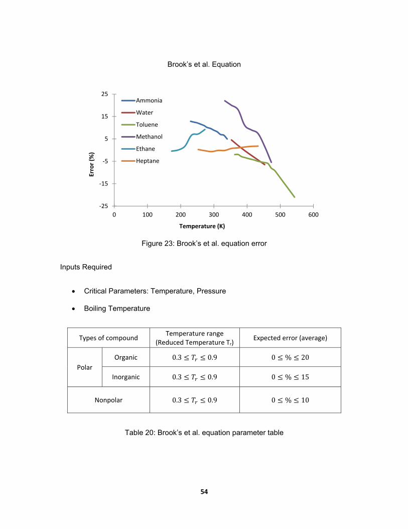
FIGURE 23: BROOK’S ET AL. EQUATION ERROR ................................................................... 54

FIGURE 24: VOGEL EQUATION ERROR ............................................................................... 55

FIGURE 25: LEWIS-SQUIRE EQUATION ERROR .................................................................... 56

FIGURE 26: CHUNG EQUATION ERROR ............................................................................... 57

FIGURE 27: LUKAS EQUATION ERROR ................................................................................ 58

FIGURE 28: LIQUID MERIT NUMBER UNCERTAINTY (STANDARD DEVIATION) .......................... 59

FIGURE 29: VAPOR MERIT NUMBER UNCERTAINTY (STANDARD DEVIATION) .......................... 60

FIGURE 30: LIQUID MERIT NUMBER ERROR ........................................................................ 61

FIGURE 31: VAPOR MERIT NUMBER ERROR ....................................................................... 61

FIGURE 32: MAXIMUM HEAT TRANSFER ERROR PERCENTAGE ............................................. 62

FIGURE 33: AMMONIA QMAX WITH ERROR .......................................................................... 63

FIGURE 34: ETHANE QMAX WITH ERROR ............................................................................ 64

FIGURE 35: METHANOL QMAX WITH ERROR ....................................................................... 64

xii

NOMENCLATURE

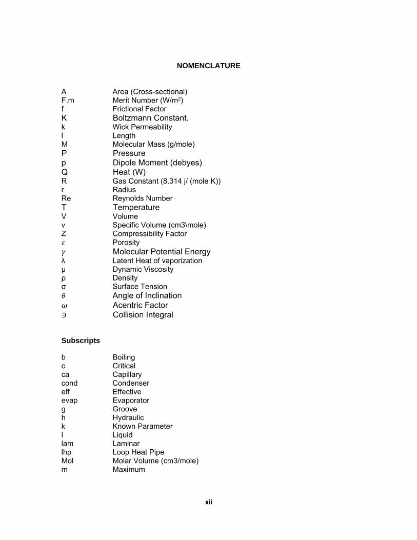
A Area (Cross-sectional) F.m Merit Number (W/m2) f Frictional Factor K Boltzmann Constant. k Wick Permeability l Length M Molecular Mass (g/mole) P Pressure p Dipole Moment (debyes) Q Heat (W) R Gas Constant (8.314 j/ (mole K)) r Radius Re Reynolds Number T Temperature V Volume v Specific Volume (cm3\mole) Z Compressibility Factor Porosity Molecular Potential Energy

λ Latent Heat of vaporization μ Dynamic Viscosity ρ Density σ Surface Tension

Angle of Inclination Acentric Factor

∋ Collision Integral

Subscripts

b Boiling c Critical ca Capillary cond Condenser eff Effective evap Evaporator g Groove h Hydraulic k Known Parameter l Liquid lam Laminar lhp Loop Heat Pipe Mol Molar Volume (cm3/mole) m Maximum

xiii

Nomenclature (Continued)

p Pore r Reduced s Saturation turb Turbulence v Vapor vl Vapor-Liquid w Wick

1

CHAPTER 1

INTRODUCTION

Heat pipe is a highly efficient heat transfer mechanism, which works upon the

evaporation and the condensation cycle of the thermal fluid [1]. The latent heat of

vaporization is absorbed by the working fluid at the evaporator section, which starts the

heat transfer mechanism by reducing the temperature at the hot evaporator end, after

which the heat is transported towards the condenser end where it is rejected out.

Conventional Heat Pipe

In its simplest form, a conventional heat pipe is a closed cylinder, consisting of three

main sections: the evaporator, the condenser and the adiabatic transport section as

shown in Fig. 1. The porous wick that runs throughout the cylindrical casing is always

saturated with working fluid if the heat pipe is operating correctly.

Figure 1: Conventional heat pipe [1]

2

These sections are usually defined by the thermal boundary conditions, as the

internal section is typically uniform [2]. The evaporator section is exposed to the heat

source, once the heat is conducted through the casing and into the wick, the fluid

vaporizes and flows through the adiabatic section to the condenser section and finally

the vapor is condensed in the condenser section. The capillary forces thus developed in

the porous wick, pumps the condensed liquid back to the evaporator [1]. The closed

cylinder container should be thermally and chemically stable (non-reactive to the working

fluid even at high temperature and pressures) and should have good thermal

conductivity. The purpose of the wick defined in [3] is to provide:

1 The necessary flow passage for the returning fluid.

2 Development of the required capillary pressure

3 A heat flow path between the inner wall and the working fluid.

During the steady state operation of the heat pipe, when the fluid, in the form of the

vapor flows from evaporator to condenser, there exists a vapor pressure gradient

(∆ Pv) along its flow. After condensation, when the liquid returns to the evaporator, there

exists a liquid pressure gradient (∆ Pl). For the continuous operation, the maximum

pressure or the capillary pressure (Eq. 1) must exceed all the other pressure gradients

(Eq. 2) at all times.

∆P 2 ∗σr

∗ cos θ 1

∆P ∆P ∆P ∆P 2

3

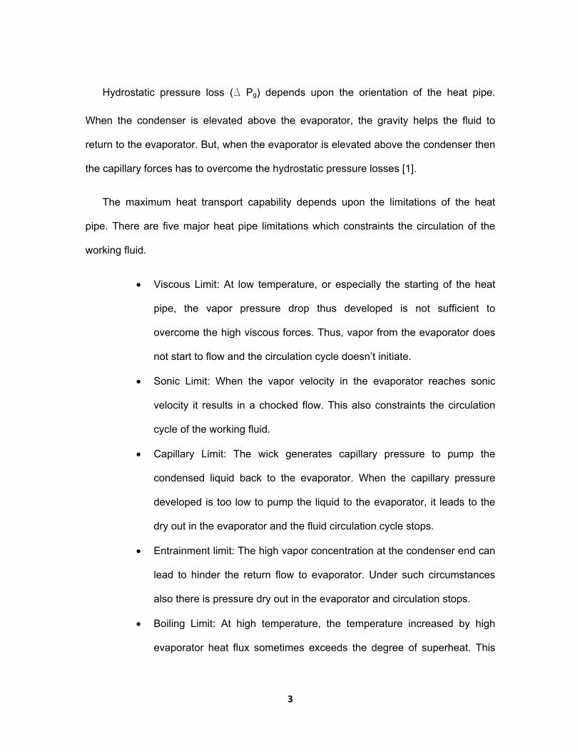
Hydrostatic pressure loss (D Pg) depends upon the orientation of the heat pipe.

When the condenser is elevated above the evaporator, the gravity helps the fluid to

return to the evaporator. But, when the evaporator is elevated above the condenser then

the capillary forces has to overcome the hydrostatic pressure losses [1].

The maximum heat transport capability depends upon the limitations of the heat

pipe. There are five major heat pipe limitations which constraints the circulation of the

working fluid.

Viscous Limit: At low temperature, or especially the starting of the heat

pipe, the vapor pressure drop thus developed is not sufficient to

overcome the high viscous forces. Thus, vapor from the evaporator does

not start to flow and the circulation cycle doesn’t initiate.

Sonic Limit: When the vapor velocity in the evaporator reaches sonic

velocity it results in a chocked flow. This also constraints the circulation

cycle of the working fluid.

Capillary Limit: The wick generates capillary pressure to pump the

condensed liquid back to the evaporator. When the capillary pressure

developed is too low to pump the liquid to the evaporator, it leads to the

dry out in the evaporator and the fluid circulation cycle stops.

Entrainment limit: The high vapor concentration at the condenser end can

lead to hinder the return flow to evaporator. Under such circumstances

also there is pressure dry out in the evaporator and circulation stops.

Boiling Limit: At high temperature, the temperature increased by high

evaporator heat flux sometimes exceeds the degree of superheat. This

4

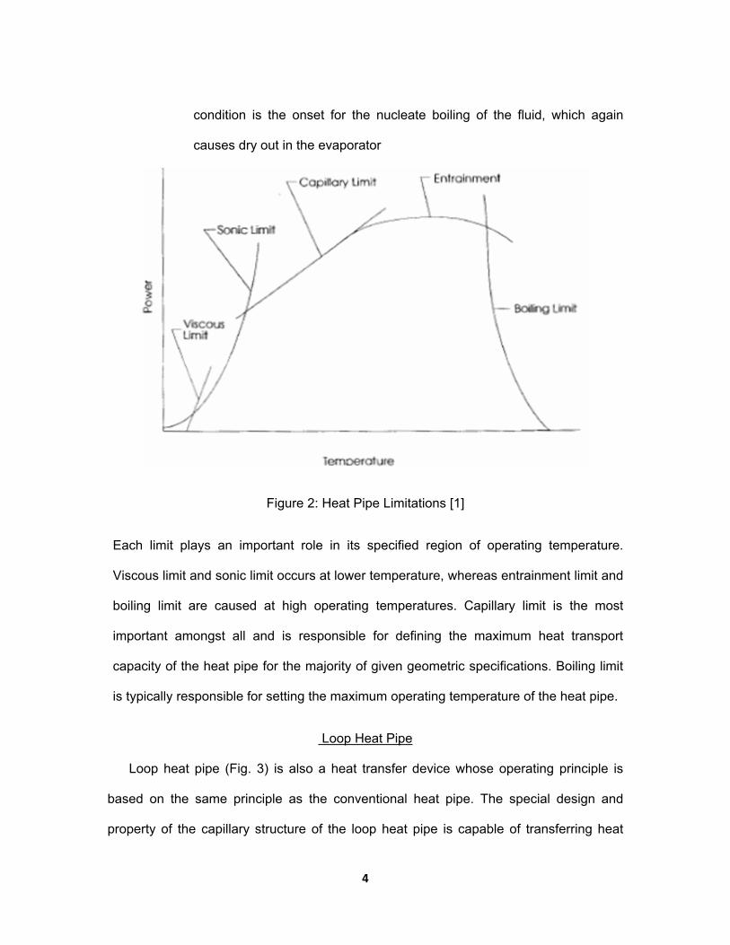
condition is the onset for the nucleate boiling of the fluid, which again

causes dry out in the evaporator

Figure 2: Heat Pipe Limitations [1]

Each limit plays an important role in its specified region of operating temperature.

Viscous limit and sonic limit occurs at lower temperature, whereas entrainment limit and

boiling limit are caused at high operating temperatures. Capillary limit is the most

important amongst all and is responsible for defining the maximum heat transport

capacity of the heat pipe for the majority of given geometric specifications. Boiling limit

is typically responsible for setting the maximum operating temperature of the heat pipe.

Loop Heat Pipe

Loop heat pipe (Fig. 3) is also a heat transfer device whose operating principle is

based on the same principle as the conventional heat pipe. The special design and

property of the capillary structure of the loop heat pipe is capable of transferring heat

5

efficiently for distance up to several meters at all orientation in the gravity field and even

further when place horizontally [4].

Figure 3: Loop heat pipe [5]

The key components of the loop heat pipe are evaporator, condenser,

compensation chamber and liquid/vapor line [2]. The secondary wick (Fig. 3) maintains

the proper supply of the working fluid to the evaporator. Whereas, the wick in the

evaporator main section is known as the primary wick, is made of extremely fine pores

for the purpose of developing high capillary pressures [4]. The secondary wick has larger

pores than the primary wick, as its main function is to connect the compensation

chamber and the evaporator. For the loop heat pipe, a pressure-temperature diagram of

the fluid circulation is given in Fig. 4.

6

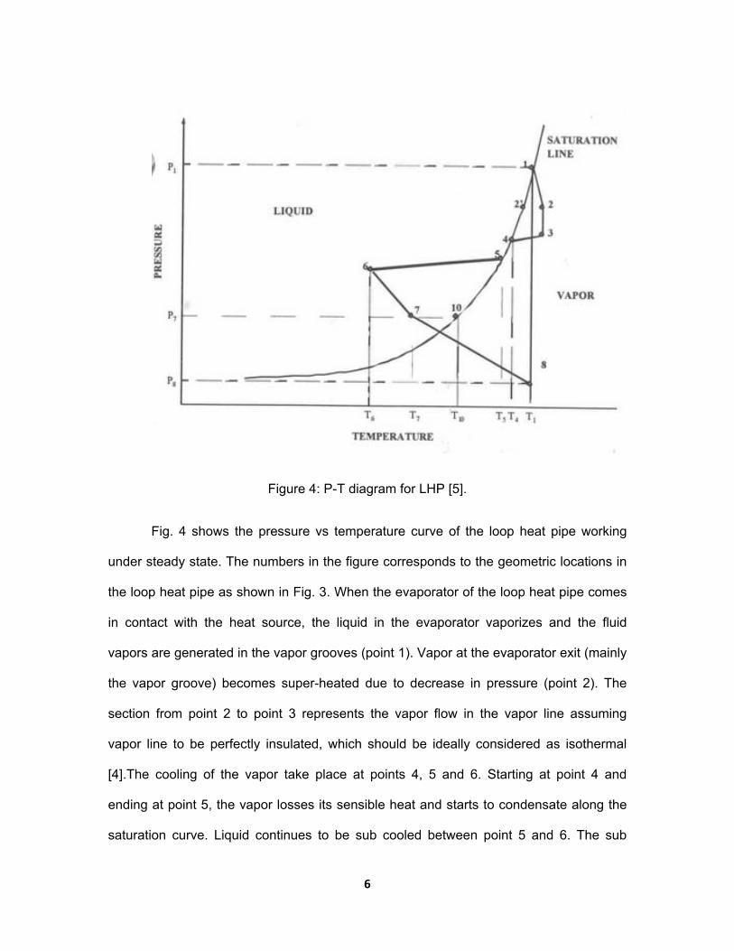
Figure 4: P-T diagram for LHP [5].

Fig. 4 shows the pressure vs temperature curve of the loop heat pipe working

under steady state. The numbers in the figure corresponds to the geometric locations in

the loop heat pipe as shown in Fig. 3. When the evaporator of the loop heat pipe comes

in contact with the heat source, the liquid in the evaporator vaporizes and the fluid

vapors are generated in the vapor grooves (point 1). Vapor at the evaporator exit (mainly

the vapor groove) becomes super-heated due to decrease in pressure (point 2). The

section from point 2 to point 3 represents the vapor flow in the vapor line assuming

vapor line to be perfectly insulated, which should be ideally considered as isothermal

[4].The cooling of the vapor take place at points 4, 5 and 6. Starting at point 4 and

ending at point 5, the vapor losses its sensible heat and starts to condensate along the

saturation curve. Liquid continues to be sub cooled between point 5 and 6. The sub

7

cooled liquid flows in the liquid line and reaches the evaporator core (point 7). Since

there is no flow between compensation chamber and evaporator core during the steady

state operation, the pressure at the evaporator core (point 7) and that of the

compensation chamber (point 10) must be equal [5]. Point 10 shows higher temperature

due to the heat leak form evaporator core to the compensation chamber through the

secondary wick.

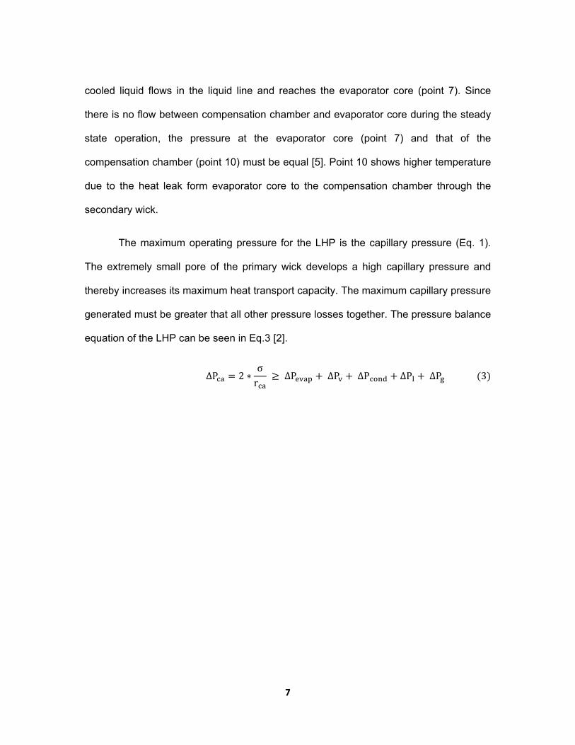
The maximum operating pressure for the LHP is the capillary pressure (Eq. 1).

The extremely small pore of the primary wick develops a high capillary pressure and

thereby increases its maximum heat transport capacity. The maximum capillary pressure

generated must be greater that all other pressure losses together. The pressure balance

equation of the LHP can be seen in Eq.3 [2].

∆P 2 ∗σr

∆P ∆P ∆P ∆P ∆P 3

8

CHAPTER 2

LITERATURE REVIEW

Merit Number

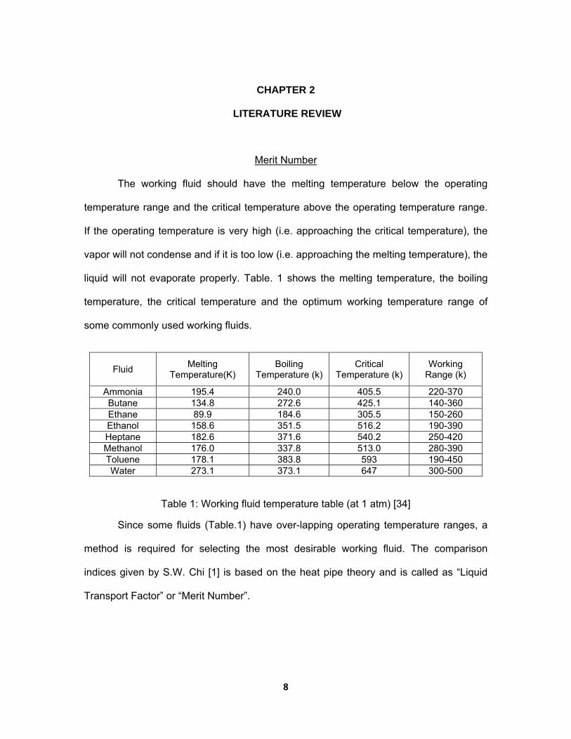
The working fluid should have the melting temperature below the operating

temperature range and the critical temperature above the operating temperature range.

If the operating temperature is very high (i.e. approaching the critical temperature), the

vapor will not condense and if it is too low (i.e. approaching the melting temperature), the

liquid will not evaporate properly. Table. 1 shows the melting temperature, the boiling

temperature, the critical temperature and the optimum working temperature range of

some commonly used working fluids.

Fluid Melting

Temperature(K) Boiling

Temperature (k) Critical

Temperature (k) Working

Range (k)

Ammonia 195.4 240.0 405.5 220-370 Butane 134.8 272.6 425.1 140-360 Ethane 89.9 184.6 305.5 150-260 Ethanol 158.6 351.5 516.2 190-390 Heptane 182.6 371.6 540.2 250-420 Methanol 176.0 337.8 513.0 280-390 Toluene 178.1 383.8 593 190-450 Water 273.1 373.1 647 300-500

Table 1: Working fluid temperature table (at 1 atm) [34]

Since some fluids (Table.1) have over-lapping operating temperature ranges, a

method is required for selecting the most desirable working fluid. The comparison

indices given by S.W. Chi [1] is based on the heat pipe theory and is called as “Liquid

Transport Factor” or “Merit Number”.

9

Chi developed a parameter for selecting the working fluid for conventional heat

pipes using only the important thermo-physical properties of the fluids. This parameter

compares the merits of the working fluid over the entire operating temperature. For a

cylindrical heat pipe with uniform evaporator heat flux, the merit number is given by

Eq. 4. There are six assumptions considered by Chi [1] for deriving the liquid merit

number.

1) The pipe is capillary limited.

2) The vapor pressure losses are negligible.

3) Heat flux density is uniform at the evaporator and condenser section.

4) The heat pipe is operating in zero gravity field.

5) Fluid flow is laminar.

6) Capillaries are properly wetted

F.mρ ∗ σ ∗ λ

μ 4

According to the heat pipe theory [1], pressure losses in the system is dominated

only by the liquid pressure drop (Eq. 5). The second parenthesis represents

∆Pμ

ρ ∗ λ∗

f ∗ Re

2 ∗ r∗Q ∗ lA

5

the wick property. The hydraulic radius (rh) is defined as the ratio of wick cross-sectional

area to the wetted perimeter. For circular or cylindrical geometry, the hydraulic radius is

considered to be capillary pore radius [1] and f ∗ Re 16 [7]. The maximum heat

transport capacity (Eq. 6) of the liquid pressure gradient driven heat pipe depends on 3

factors (i) the fluid properties (ii) the wick property (wick permeability) and (iii) the wick

10

geometry. The fluid properties (given in the first parenthesis of Eq. 5) were collectively

called as the Liquid Transport Number by Chi or the Merit Number. Therefore by

rearranging the terms (Eq. 5) it became clear that for designing the heat pipe, fluid

selection plays an important role.

Q 2 ∗ρ ∗ σ ∗ λ

μ∗

Kr

∗Al

6

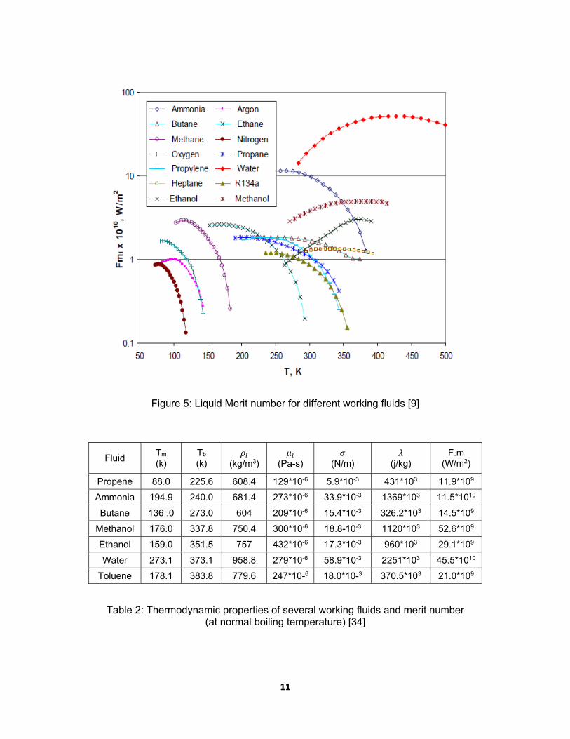
For a given fluid, the liquid merit number is a temperature dependent parameter

which loses its significance at or near the critical temperature (see Fig. 5). The

importance of the boiling temperature with respect to merit number was first studied by

Asselman et al. [8]. Merit number for most working fluids, starts to increase from the

triple point to a maximum around or after its normal boiling point, then decreases

gradually, and vanishes near the critical temperature. Merit number for some fluids has

been calculated at their respective normal boiling point (Table 2). A definite trend was

observed relating higher merit number for the fluids having higher boiling temperature.

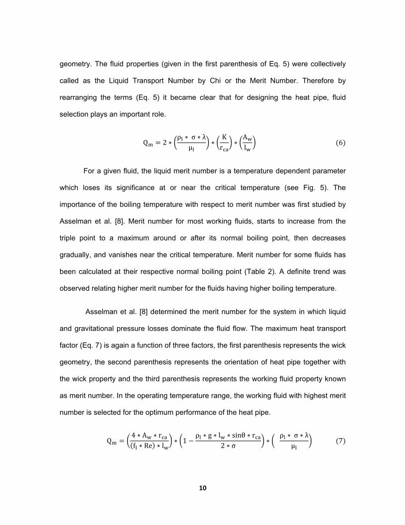
Asselman et al. [8] determined the merit number for the system in which liquid

and gravitational pressure losses dominate the fluid flow. The maximum heat transport

factor (Eq. 7) is again a function of three factors, the first parenthesis represents the wick

geometry, the second parenthesis represents the orientation of heat pipe together with

the wick property and the third parenthesis represents the working fluid property known

as merit number. In the operating temperature range, the working fluid with highest merit

number is selected for the optimum performance of the heat pipe.

Q4 ∗ A ∗ rf ∗ Re ∗ l

∗ 1ρ ∗ g ∗ l ∗ sinθ ∗ r

2 ∗ σ∗

ρ ∗ σ ∗ λμ

7

11

Figure 5: Liquid Merit number for different working fluids [9]

Fluid Tm (k)

Tb

(k)

(kg/m3)

(Pa-s)

(N/m)

(j/kg) F.m

(W/m2)

Propene 88.0 225.6 608.4 129*10-6 5.9*10-3 431*103 11.9*109

Ammonia 194.9 240.0 681.4 273*10-6 33.9*10-3 1369*103 11.5*1010

Butane 136 .0 273.0 604 209*10-6 15.4*10-3 326.2*103 14.5*109

Methanol 176.0 337.8 750.4 300*10-6 18.8-10-3 1120*103 52.6*109

Ethanol 159.0 351.5 757 432*10-6 17.3*10-3 960*103 29.1*109

Water 273.1 373.1 958.8 279*10-6 58.9*10-3 2251*103 45.5*1010

Toluene 178.1 383.8 779.6 247*10-6 18.0*10-3 370.5*103 21.0*109

Table 2: Thermodynamic properties of several working fluids and merit number (at normal boiling temperature) [34]

12

Dunbar and Cadell [10] studied the heat pipe in which capillary pressure is only

balanced by vapor pressure losses. The vapor pressure drop, given by Dunbar and

Cadell (Eq. 8), which assumes very small vapor diameter lines and proper wick wetting.

For zero gravity operation, the hydrostatic pressure loss is neglected. The maximum

heat transport factor equation given by Dunbar and Cadell is shown in Eq. 9 and the

vapor merit number is given in Eq. 10.

ΔP 0.24 ∗ l ∗Qλ

.

∗ 2 ∗ r . ∗ μ . ∗ ρ 8

2 ∗σr

0.24 ∗ l ∗Qλ

.

∗ 2 ∗ r . ∗ μ . ∗ ρ 9

F.mσ

λ . ∗ μ . ∗ ρ 10

For a Loop heat pipe, the complex geometry (Fig. 6) of the evaporator section

makes it challenging to support the fact that the vapor pressure losses are the only

dominant losses. According to Mishkinis et al. [9], in some practical application the

evaporator wick pressure loss is even higher than the vapor pressure loss. Changing

some geometric parameters, such as reducing the length of the liquid line, increasing

wick thickness or decreasing the effective pore radius can lead to dominating liquid

pressure losses or wick pressure losses. Therefore, none of the previously mentioned

merit number would hold true for such complex geometry alone.

13

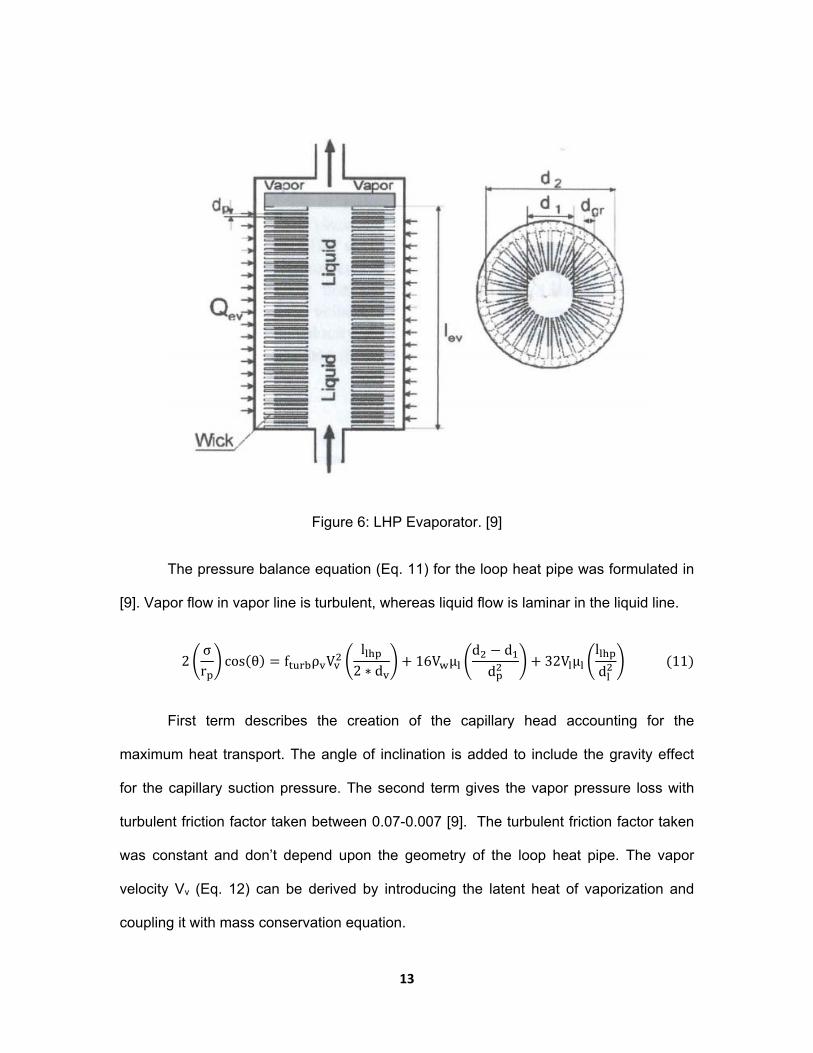
Figure 6: LHP Evaporator. [9]

The pressure balance equation (Eq. 11) for the loop heat pipe was formulated in

[9]. Vapor flow in vapor line is turbulent, whereas liquid flow is laminar in the liquid line.

2σr

cos θ f ρ Vl

2 ∗ d16V μ

d dd

32V μl

d 11

First term describes the creation of the capillary head accounting for the

maximum heat transport. The angle of inclination is added to include the gravity effect

for the capillary suction pressure. The second term gives the vapor pressure loss with

turbulent friction factor taken between 0.07-0.007 [9]. The turbulent friction factor taken

was constant and don’t depend upon the geometry of the loop heat pipe. The vapor

velocity Vv (Eq. 12) can be derived by introducing the latent heat of vaporization and

coupling it with mass conservation equation.

14

V4 ∗ Q

π ∗ h ∗ ρ ∗ d 12

The third term (Eq. 11) denotes the wick pressure losses. The wick velocity, often

described by Darcy as seepage velocity is a complex parameter to define. Hence it is

important to average the wick velocity over the entire seepage area. The wick velocity in

integral form and the actual profile equation is given in Eq. 13.

V∗

∗

∗ ∗ ∗ ∗ ∗ 13

The liquid velocity (Eq. 14) is calculated in the same way the vapor velocity is

calculated.

V4 ∗ Q

π ∗ ρ ∗ λ ∗ d 14

The pressure losses which are not considered to have a significant effect on the

maximum heat transport capacity of the loop heat pipe occurs in evaporator vapor

grooves, condenser section and compensation chamber. The above pressure balance

equation (Eq.11) contains a second order heat transfer equation for maximum heat flux.

The one positive root for heat transfer gives the vapor-liquid merit number for the

working fluid selection. This approach directly depends upon the geometry of the

evaporator of loop heat pipe as well as all the important thermo-physical properties of

the working fluid. Therefore enclosing the geometry with all the important thermo-

physical properties like viscosity, surface tension, density and latent heat, gives a better

15

understanding of working fluid selection for loop heat pipe. Mishkinis et al. [9] solution for

the vapor-liquid merit number is given in Eq. 15, taking fturb as 0.0385.

F.m2.55K 0.031K . 2.55K

0.016K 15

Where,

K∗K

∗

Geo∗ ∗ ∗

∗ ∗

Geo∗

F ∗ ρ ∗ σ ∗ λ

μ∗ cos θ F ∗ ρ ∗ λ ∗ σ ∗ cos θ

Fluid Selection

Selection of working fluid is always directly connected with the respective

thermo-physical properties of the fluid in its operating temperature range. Wallin [11],

defined some important parameters to be considered in selecting the working fluid.

1. Compatibility with wick and wall materials.

2. Wettability of wick and wall materials.

3. Vapor pressure in the operating temperature range.

4. High latent heat.

5. High thermal conductivity.

6. Low liquid and vapor viscosities.

7. High surface tension.

16

Vapor pressure plays an important role in determining the maximum operating

temperature of the fluid. Latent heat of vaporization transports much more heat than

sensible heat, hence a high value of latent heat results in greater and efficient heat

transfer. During the circulation of fluid, the flow resistance should be low and therefore

the selected fluid should have a lower viscosity value. Vapor density decreases as the

temperature decreases along the saturation curve, therefore at low temperatures the

vapor velocity reaches the sonic velocity and thus choking the fluid flow. The

temperature at which sonic limit is the lowest operating temperature of the fluid. A higher

surface tension value indicates greater energy is required (in the form of heat) for the

fluid molecule at the boundary to break free from the surface. If a fluid has low surface

tension value then the returning fluid would be vaporized before reaching the evaporator

and thus limiting the fluid circulation cycle.

Working fluids used in a heat pipe find their applications from 4 K [12] up to 1500

K [13]. Water works best in the temperature range 300-500 K, where its closest

competitor is ammonia which works exceptionally well from 220-370 K. Ammonia and

water performs well in their operating temperature range due to high latent heat of

vaporization and surface tension. The uniqueness of water starts to fade after 450 K as

the vapor pressure of water increases rapidly after it, whereas ammonia requires careful

handling.

Chandratilleke et al. [12] demonstrated for the first time that a loop heat pipe can

also function properly in cryogenic temperature. Heat pipes were demonstrated to work

at 70 K, 28 K, 15 K and 4 K using different working fluids such as nitrogen, neon,

hydrogen and helium respectively. Anderson et al [14] investigated different working fluid

17

in the working temperature range of 450 K to 700 K. He observed that in the above

temperature range several of the Halide salts, including titanium tetrachloride, tetra

bromide and tetra iodide appears to be potential working fluids. Other potential fluids

include aluminum, beryllium, bismuth, gallium, antimony, silicon and tin halides. Some of

the organic fluids that work as expected in this temperature range are aniline,

naphthalene, toluene, hydrazine, and phenol as long as they are not exposed to

radiation.

Mercury find’s its temperature range of application from 600-900 K due to its

supportive thermo-physical properties. Mercury was initially considered but later rejected

as a working fluid liquid due to its wetting properties. Mercury does not properly wets the

wick due to high contact angle. Although Deverall [13] reported successful functioning of

mercury heat pipe when coarse magnesium was added to increase wetting. Apart from

being a non-wetting liquid, mercury is also difficult to handle due to its toxicity.

In the temperature range 1200-2000 K [3] some liquid metals that find

applications are cesium, potassium, sodium and lithium. Lithium with the highest merit

number is the best in the group but lacks compatibility with almost all metal casing. At

high temperatures lithium attacks almost every metal casing, it is therefore more

convenient to use the next best in group i.e. sodium. Lithium at high temperature is

compatible with only some elements in the periodic table and those are tungsten,

tantalum, niobium and molybdenum. Use of such casing to resolve the compatibility

issue is well documented by Wei [15].

For a fluid to return to the evaporator, a fluid with low liquid density and high

surface tension is recommended. This phenomenon was studied by Asselman et al. [8]

18

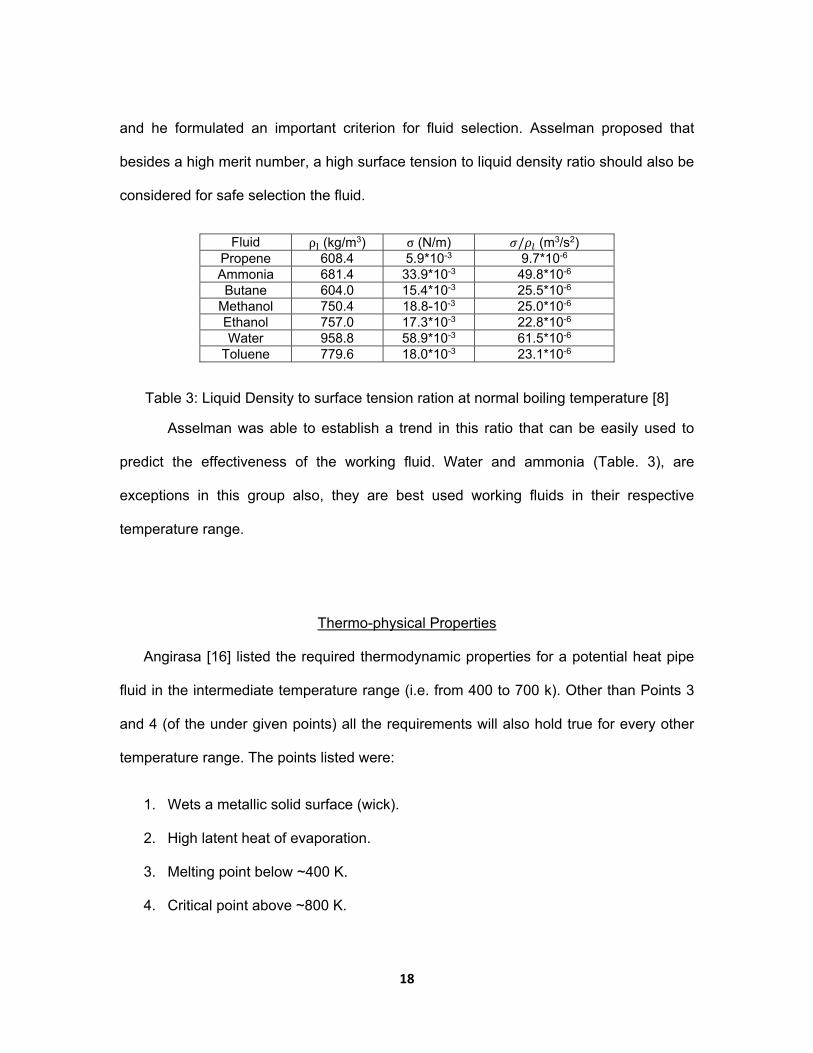
and he formulated an important criterion for fluid selection. Asselman proposed that

besides a high merit number, a high surface tension to liquid density ratio should also be

considered for safe selection the fluid.

Fluid ρ (kg/m3) σ (N/m) / (m3/s2) Propene 608.4 5.9*10-3 9.7*10-6 Ammonia 681.4 33.9*10-3 49.8*10-6 Butane 604.0 15.4*10-3 25.5*10-6

Methanol 750.4 18.8-10-3 25.0*10-6 Ethanol 757.0 17.3*10-3 22.8*10-6 Water 958.8 58.9*10-3 61.5*10-6

Toluene 779.6 18.0*10-3 23.1*10-6

Table 3: Liquid Density to surface tension ration at normal boiling temperature [8]

Asselman was able to establish a trend in this ratio that can be easily used to

predict the effectiveness of the working fluid. Water and ammonia (Table. 3), are

exceptions in this group also, they are best used working fluids in their respective

temperature range.

Thermo-physical Properties

Angirasa [16] listed the required thermodynamic properties for a potential heat pipe

fluid in the intermediate temperature range (i.e. from 400 to 700 k). Other than Points 3

and 4 (of the under given points) all the requirements will also hold true for every other

temperature range. The points listed were:

1. Wets a metallic solid surface (wick).

2. High latent heat of evaporation.

3. Melting point below ~400 K.

4. Critical point above ~800 K.

19

5. Chemically stable at high temperature.

6. Low liquid viscosity.

7. High surface tension.

8. Non-toxic.

9. Non-volatile.

In this part of the literature review we would specifically discuss the important

properties of fluids and their methods of formulation as a function of temperature using

only the intensive property and chemical structure. There are several ways of

formulating such properties as a function of temperature, the best being is to obtain the

data experimentally. Theoretically speaking, representing the property of the specified

fluid as a polynomial function over the entire temperature range has been better utilized

until now. But, there are some problems associated with such methods,

1. The polynomial coefficient varies with fluids.

2. They are calculated for only specified (mentioned) temperature range.

3. The polynomial function is usually curve fit, which increase the percentage error

outside the temperature range.

For property formulation, we have tried to exclude the polynomial function

completely. Instead, we have only used the pre-defined thermodynamic properties to

formulate them as a function of operating temperature. This system of formulation is

better than the previously used method in several ways. First, the thermodynamic

properties are easily available and we do not have to worry about the polynomial

functions. Second, it works well from the triple point to the critical point. Third, it does not

20

requires a curve fitting procedure in order to specify points of relevance in any specific

temperature range. The basic thermodynamic inputs for methods formulation are,

1. Intensive properties: Acentric factor, normal boiling and melting temperature.

2. Critical point parameters: Temperature, molar volume, pressure, compressibility

factor.

3. Universal constants: Gas constant (R) and Stefan-Boltzmann constants (K).

Vapor Pressure and Latent Heat of Vaporization

The vapor pressure of the fluid in the operating temperature is an important

parameter for fluid selection. High vapor pressure requires thick envelope walls as well

as stronger welds to withstand the increasing pressure. The increased mass for stronger

casing reduces the heat pipe performance. Low vapor pressure will result in a greater

temperature gradient along the length of the heat pipe which makes it non-working at

higher temperatures [16]. Anderson et al [14] observed that merit number for water was

still increasing after the normal boiling point (which makes water a potential fluid to use),

but the problem he noticed was that the vapor pressure had started to increase

exponentially (see Fig. 7) just after the normal boiling temperature (from 1 atm @ 273 K

to 25.16 atm @ 500 K), after which it was not considered safe to use water as a heat

pipe fluid. Due to these limitations, alkali metals came into existence and were

considered best after water from 450 K onwards.

21

Figure 7: Merit number and vapor pressure curve for water.

Clausius-Clapeyron equation is a first order differential equation subjecting the

dependence of saturation pressure and temperature for all fluids. When vapor and liquid

exist in equilibrium close to the saturation curve, there exists an equality of chemical

potential, temperature and pressure [17] which leads to the derivation of the Clausius-

Clapeyron equation (Eq. 16). The two important characteristics of the equation are:

1. ln (P) vs (1/T) graph always gives a negative slope.

2. The slope is always equal to. /

16

Vapor pressure for all fluids is calculated by integrating the above equation and

assuming latent heat of vaporization to be constant (at the normal boiling point). Eq. 17

gives the Clausius-Clapeyron equation in its exact form (“A” being the integration

constant).

0

5E+10

1E+11

1.5E+11

2E+11

2.5E+11

3E+11

3.5E+11

4E+11

4.5E+11

5E+11

0

20

40

60

80

100

120

140

160

180

200

250 350 450 550 650

Merit Number (W

/m2)

Vap

or Pressure(atm

)

Temperature (K)

Vapor Pressure (atm)

Merit Number (W/m2)

22

/ 17

Antoine [18] (Eq. 18) corrected the Clausius-Clapeyron equation by introducing a

constant to the temperature term. Antoine believed that Clausius-Clapeyron equation

cannot be accurately applied over on the larger range of temperature (specifically for TR

over 0.75 and for the fluids with low boiling point). Adding the constant make the

equation suitable for a larger temperature range.

/ 18

Wagner [19] used the statistical method combined with Clausius-Clapeyron equation to

develop an empirical formula for vapor pressure of argon and nitrogen on the entire

temperature range (whose experimental values were known). It was later established as

an equation (Eq. 19), which can be used for all fluids and was found accurate even over

0.7. The constants in Eq.19 were calculated by Forero et al. [20], who developed a

method to calculate the constant for more than 274 pure substances with high accuracy.

The vapor pressure from 0.01 atm to critical pressure was calculated with an average

deviation of 0.039% only. Forero et al. even established a generalized relation of all the

constants (Francis Constants A, B C and D in the Eq. 19) making then a function of

acentric factor only.

lnPP

Ar Br . Cr . Dr

1 r 19

wherer 1TT

These equations work well in estimating the vapor pressure over the entire range of

temperature except near the critical temperature, where λ is a weak function of

23

temperature and vapor pressure is is tend to achieve abnormally high values. Hence it

become clear that in order to increase the accuracy of the vapor pressure at higher

temperatures, mainly Tr > 0.7, a three parameter equation must be preferred over

Clausius-Clapeyron two parameter state equations. Pitzer [21] in 1955 suggested that a

third parameter is required for defining all the thermodynamic states of the fluid and

gasses. Since the intermolecular forces in complex molecules is a sum of interaction

between various part of the molecule and is not concentrated around the central part of

the molecule, hence a new concept of acentric factor was suggested. Acentric factor

(Eq. 20) was defined by Pitzer as the measure of the deviation in the properties over

reduced temperature of 0.7. Acentric factor is a temperature independent property,

whose values differ for different fluids. The reduced pressure Pr is calculated at Tr = 0.7.

Pitzer three parameter equation (Eq. 21) was suggested after realizing the fact that

vapor pressure can also a function of reduced temperature. The values of zo and z1 for

different fluids are tabulated in his paper over the entire range of reduced temperature.

ω log P 1.0 20

ln P z T ω ∗ z T 21

Lee et al. [22] (Eq. 21) described a method of representing a thermodynamic

function based on Pitzer’s three parameter state. This analytical form tends to increase

the reliability of values near the critical temperature. The idea which lead them to realize

that highly accurate vapor pressure can be now formulated was inspired by the fact that

the compressibility factor constants (z0 and z1) were also the function of reduced

temperature (Eq. 22 a & b)

24

z 5.927146.09648

T1.28862 ∗ ln T 0.169347 ∗ T 22a

z 15.251815.6875

T13.4721 ∗ ln T 0.43577 ∗ T 22b

Latent heat of vaporization gradually decreases with increase in temperature and

vanishes at the critical temperature. Watson [23] (Eq. 23) expressed the dependence of

latent heat of vaporization on reduced temperature through the following empirical

formula. Subscript “k” is the reference latent heat of vaporization at a known

temperature.

λ λ1 T1 T

23

The indices “n” was decided as 0.38 by Watson, but Viswanath et al. [24]

(Eq. 24) recommended that this parameter not to be a constant but differs for different

fluids (although very close to 0.38 for all fluids).

n 0.00264λRT

0.8794 24

Watson’s equation requires the latent heat of vaporization at a known

temperature, for which latent heat of vaporization at the normal boiling point was

considered as a potential solution. Riedel [25] (Eq. 25 a) proposed one of the first

equations for latent heat at normal boiling temperature. His equation used only critical

parameters and R (universal gas constant). Chen [26] (Eq. 25 b) and Viswanath et al.

[24] (Eq. 25 c) gave the same kind of empirical formula. Chen and Viswanath et al. did

not used any other constants (like “R”) to better fit the values.

25

λ 1.093RT ln P 1.0130.93 T

25a

λ T 7.11 log P 7.9T 7.82

1.07 T 25b

λ 4.7T log P 1 P

.

1 25c

Pitzer [27] also established a formula in which latent heat of vaporization is a

function of critical temperature and acentric factor. The analytical representation of the

latent heat as a function of temperature is given below (Eq. 26). This equation was found

to work very accurately in the range 0.5 1.0 .

7.08 1 . 10.95 1 . 26

Density

Density of the fluid is a property which finds its presence directly or indirectly in

every thermo-dynamical system and in wide variety of engineering calculations. An

extensive literature is available by different researchers determining the densities of

various compounds (in their pure state or in mixtures). The calculative form of density

(vapor density) founded its application back in 1873 in the form of Van der Waals

equation (Eq. 27) of state for gasses.

ρP ∗ MR ∗ T

27

26

A. Liquid Density

Liquid density varies inversely as a function of temperature which can be written in

the form of Eq. 28. The critical point was again the problem and the percentage

deviation of the property values near the critical point were extremely high. Francis [28]

ρ ABT 28

stated that saturated liquid densities can be expressed as a quadratic function (as

initially it was treated linear, see Eq. 28) over the entire range of temperature. His

equation (Eq. 29) tries to correct the liquid density as close as possible to the critical

point. Introducing a linear temperature variation term to the equation improved the

accuracy at higher temperatures. The constants in Eq. 29 were uniquely chosen “A” is

slightly higher than the liquid density at low temperature (close to normal-melting point),

ρ A BtC

E t 29

“B” is slightly less than the temperature coefficient of liquid density, “C” is a small integer

depending upon the slope of the isochor (dP/dt)V and E is usually slightly larger than the

critical temperature [28]. These constants for approximately 130 pure compounds are

listed in his work.

Yen et al. [29] gave a generalized equation (Eq. 30) relating reduced density to

reduced temperature. Being a continuation to Francis works Eq. 30 reduces the average

percentage deviation and near the critical temperature by introducing the compressibility

factor at the critical point for the first time. Yen et al. believed that increasing the

polynomial index of the equation would give good results at lower temperatures. The

constants in the equation were applied to sixty-two pure compounds whose critical

27

compressibility factor ranged from 0.21 to 0.29, the calculated value had a maximum

deviation of only 2.1 % [29].

ρρρ

1 A 1 T B 1 T D 1 T 30

A 17.4425 214.578 ∗ Z 989.625 ∗ Z 1522.06Z 30a

B 3.28257 13.6377Z 107.4844Z 384.211Z ifZ 0.26 30b

B 60.2091 402.063Z 501Z 641.0Z ifZ 0.26 30c

D 0.93 B 30d

Riedel [30] in 1954 changed the form of the equation from two parameter state

equation to three parameter state equation by introducing acentric factor to his equations

(Eq. 31). His endeavors were initially focused on the molar volume (cm3/mole) but finally

an equation for liquid density was formulated (see Eq. 31).

ρρρ

VV

1 1.69 0.984ω 1 T 0.85 1 T 31

Pitzer et al in 1965 gave an empirical formula for showing the dependence of the

liquid molar density on temperature in terms of critical parameters. Lyckman et al. [27] in

1964 showed that due to the linear nature of the Pitzer equation, the calculated molar

densities were deviating the literature data therefore he modified the Pitzer equation and

presented a corrected equation (Eq. 32) which was a quadratic equation in acentric

factor. The generalized parameters are a function of the reduced temperature and are

VV

V ωV ω V 32

experimentally calculated by the studying density data of argon, nitrogen, ethylene,

propane, carbon tetrachloride, benzene and heptane. Appendix “A” describes the nature

28

of the generalized functions. The generalized function increases with increasing

temperature and returns a unity value at the critical parameter. The other generalized

function also follows a similar pattern. An equation for the critical molar volume was also

given by Lyckman et al. (Eq. 33).

V R ∗TP

0.291 0.08ω 33

Gunn et al. [31], replaced critical molar volume from scaling molar volume. His

equation (Eq. 34) was valid over the entire range of the temperature i.e. 0.2 1.00.

The equation was linear in acentric factor.

VV

V 1.0 ω ∗ δ 34

The generalized parameter V andδ are a function of reduced temperature

only, which were calculated from the density data available for the following 10

substances: argon, methane, nitrogen, propane, n-pentane, n-heptane, n-octane,

benzene, ethyl-ether and ethyl-benzene [31]. Gunn et al used scaling volume instead of

the critical volume which increased its accuracy near the critical point. The generalized

function . (Eq. 35) is the molar volume of the fluid at reduced temperature of 0.6. The

value of for some compounds can be found in Appendix B, for other the formula (Eq.

35) works fine.

VV .

0.3862 0.0866ω 35

29

B. Vapor Density

The first successful attempt of modifying and correcting the ideal gas equation to be

applicable for real gasses was done by Van Der Waals in 1873 [32]. Some changes

were proposed in the specific volume and pressure terms (Eq. 36) after studying the

behavioral pattern of intermolecular forces at high pressures. The constants “a” and

Pav

v b RT 36

“b” used in Eq. 36 are obtained by evaluating the isothermal properties of fluid at the

point of inflection or at the critical point (Eq. 37).

∂P∂ν 0

∂ P∂ ν

0 37

Redlich-Kwong (1949) introduced some corrections in the van der waals

equation which can be seen in Table. 4. Stepping up from two parameter corresponding

state equation to three parameter corresponding state equation, Soave (1972) and

Peng-Robinson (1976) introduced the acentric factor to the parameter “b”. All these

equations are individually known as the cubic equation of state (Eq. 38), since the

equation is cubic in molar volume. The constants can be calculated from the Table. 4.

PRTv b

av ubv wb

38

30

Equation u w a b

Van Der Waals

0 0 RT8P

2764

Redlich-Kwong

1 0 0.08664RT

P 0.42748

.

Soave 1 0 0.08664RT

P

0.42748 1 1

0.48 1.574 0.176

Peng-Robinson

2 -1 0.07780RT

P

0.45724 1 1

0.37464 1.54226

0.26992

Table 4: Constants for cubic equation of state [33]

Surface Tension

Surface Tension is defined as the force exerted on the phase boundary per unit

length, making it an extremely relevant property associated with fluid selection. The

surface tension of the fluid varies linearly with the temperature i.e. with the increase in

temperature, the surface tension of the fluid decreases linearly and vanishes at the

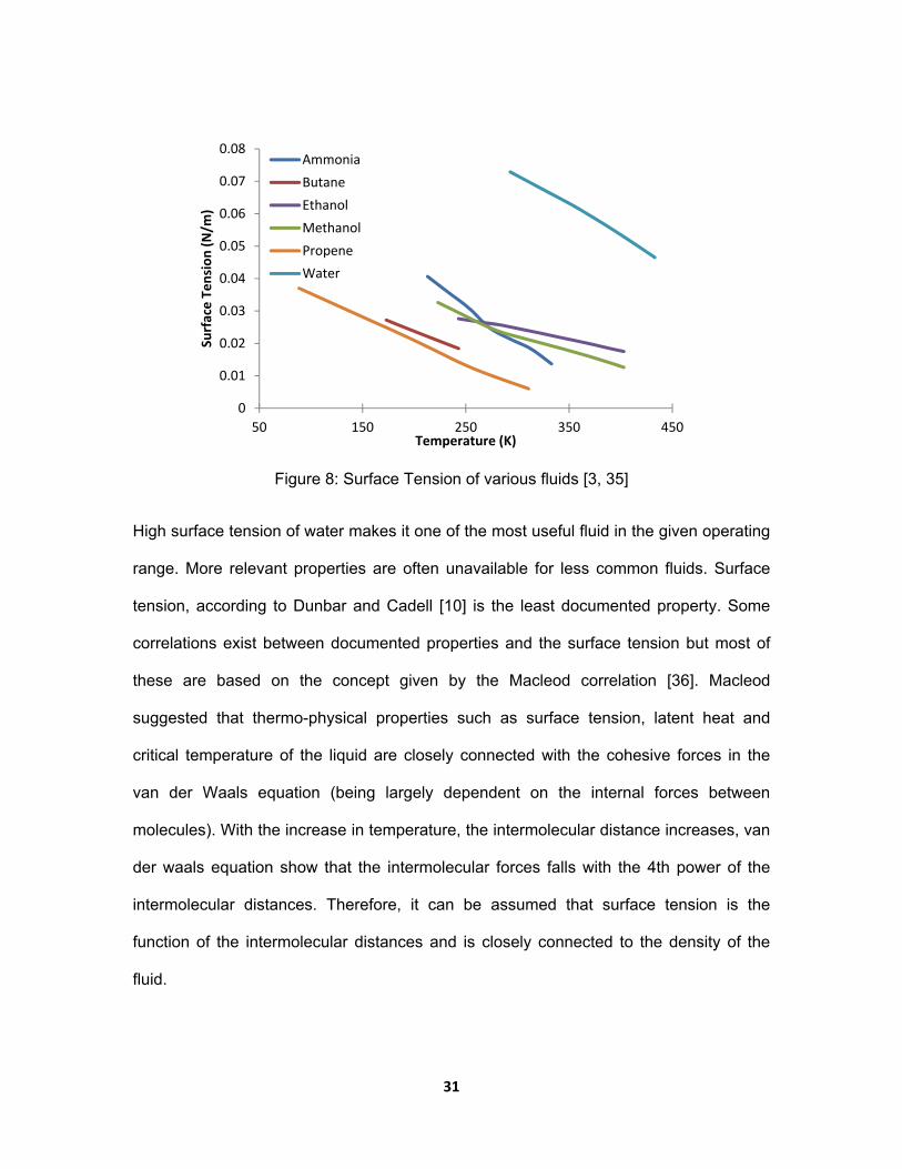
critical temperature. Fig. 8 shows the variation of surface tension with temperature of

various fluids. In the reduced temperature range 0.45 to 0.65, the surface tension for

most of the organic fluids range from 0.02 to 0.04 N/m [33]. The surface tension of water

at 293 K is 0.0728 N/m [34] and for various liquid metals it ranges from 0.3 to 0.6 N/m

[34].

31

Figure 8: Surface Tension of various fluids [3, 35]

High surface tension of water makes it one of the most useful fluid in the given operating

range. More relevant properties are often unavailable for less common fluids. Surface

tension, according to Dunbar and Cadell [10] is the least documented property. Some

correlations exist between documented properties and the surface tension but most of

these are based on the concept given by the Macleod correlation [36]. Macleod

suggested that thermo-physical properties such as surface tension, latent heat and

critical temperature of the liquid are closely connected with the cohesive forces in the

van der Waals equation (being largely dependent on the internal forces between

molecules). With the increase in temperature, the intermolecular distance increases, van

der waals equation show that the intermolecular forces falls with the 4th power of the

intermolecular distances. Therefore, it can be assumed that surface tension is the

function of the intermolecular distances and is closely connected to the density of the

fluid.

0

0.01

0.02

0.03

0.04

0.05

0.06

0.07

0.08

50 150 250 350 450

Surface Tension (N/m

)

Temperature (K)

Ammonia

Butane

Ethanol

Methanol

Propene

Water

32

The Empirical formula given by Macleod [36] in 1923 suggested a linkage between

surface tension and respective state densities (liquid and gaseous) which can be seen in

Eq. 39. “C” fits the experimental data for all fluids with good accuracy from melting point

to approximately 40 K below the critical temperature. Macleod further observed that C is

a temperature independent property over the entire operating range.

σρ ρ

C 39

Samuel Sudgen [37], after carefully studying the behavioral pattern of the Macleod’s

correlation gave two empirical relations which involve surface tension and the critical

parameters as a function of temperature (see Eq. 40a and Eq. 40b). “K1” and “K2” are

σ K T Vc ∗ 1 T . 40a

σ K T Pc ∗ 1 T . 40

constants. Sudgen even worked on the temperature independent parameter of Macleod

and indicated how it may be calculated from the structure of the fluid. He also

acknowledged Macleod findings with relevance to experimental data and summarized

that Macleod’s relation between surface tension and density is found to be true from the

melting point to 40 K below the critical temperature. He called this constant as Parachor

and changed the liquid and vapor density to respective molar liquid and vapor density.

The Sudgen atomic and structural Parachor value can be found in appendix C.

Vargaftik et al. [34] in 1983 working on the surface tension of water established

experimental surface tension relation of water as a function of temperature from melting

33

temperature to the critical temperature (Tr = 0.9). Verifying the work of Sudgen [18] with

the critical temperature of water as 647.15 K, he interpolated the equation of surface

tension (Eq. 41) as a function of temperature in the pattern suggested by Sudgen.

σ 235.8 ∗ 10 ∗ 1 0.625 1 T ∗ 1 T . 41

Quale [38] studied the experimental surface tension value and density data for

various compounds and calculated his structural Parachor. He then suggested the

additive pattern for calculating the Parachor. The Quale structural Parachor can be

found in appendix D.

Brock et al. [39] in 1955 related all the work that has been done on surface

tension and suggested that surface tension can also be accurately estimated using an

empirical equation relating critical properties and normal boiling points. This method was

helpful in estimating surface tension again as a function of temperature without having

the knowledge of the structure of the compound. Brock’s equation (Eq. 42) is an

extended work of Sudgen’s correlation (Eq. 40 b)

σ P T Q 1 T 42a

where Q 0.1196 1 . 0

34

Viscosity

Viscosity, also known as the internal friction of fluid, is defined as the shear

stress over the velocity gradient. It tends to oppose any change in the dynamics of the

fluid movement by acting as an opposing force between fluid layers. A low viscosity

between fluid layers signifies higher velocity gradient which in turn results in less

opposed fluid flow. Viscosity is not the equilibrium property as density is, which when

grouped with different thermodynamic data is useful for developing co-relations between

complex fluid flows.

A. Liquid Viscosity

Liquid viscosity is higher than the vapor viscosity at the same saturation temperature.

For example, the liquid viscosity of water at the normal boiling point is approximately 23

times higher than the vapor viscosity, which is about 34 times for ammonia. For a

temperature range from the melting point to the normal boiling point and further to the

critical temperature, it is often a good approximation to assume that ln is inversely

proportional to temperature The simplest explanation for this approximation was first

mentioned by Guzman in 1913 (Eq. 43). Vogel equation (Eq. 44) was only an

improvement of previous equation by adding a constant term to temperature.

ln μ ABT 43

ln μ AB

T C 44

35

If the value of liquid viscosity at a temperature is known, then Lewis-Squire chart

can be used to extrapolate the viscosity over the entire temperature range, or simply by

using Eq. 45. Given a known value at any temperature, liquid viscosity can be easily

formulated over the entire temperature range.

μ . μ . T T233

45

Reid and Polling [33] have used the three equations given below (Eq. 46 a - c) to

formulate viscosity as a function of temperature for almost all know fluids, for which

constants can also be found in their work.

μ AT 46a

ln μ ABT 46b

ln μ ABT

CT DT 46c

B. Vapor Viscosity

Molecular Collisions of gaseous particle cause a change of momentum. Chapman-

Enskog [10] after studying this transport property of momentum at the molecular level

developed a vapor viscosity relation (Eq. 47) for a rigid, non-interacting sphere model.

The Collision integral was assumed to be 1 for the nonpolar molecules and slightly

μ 26.69 ∗M ∗ T

d ∋ 47

higher than 1 for polar molecules. Chapman-Enskog proposed the empirical relation but

spherical diameter and the collision integral were still a point of concern. The collision

integral has been now determined by a number of researchers, but the most used

method was given by Neufeld et al. [40]. He defined a dimensionless temperature

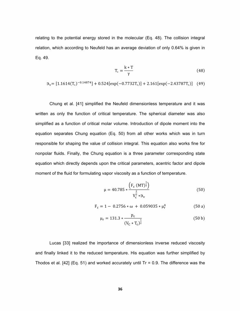
36

relating to the potential energy stored in the molecular (Eq. 48). The collision integral

relation, which according to Neufeld has an average deviation of only 0.64% is given in

Eq. 49.

T∗k ∗ Tγ

48

∋ 1.1614 T∗ . 0.524 exp 0.7732T∗ 2.161 exp 2.43787T∗ 49

Chung et al. [41] simplified the Neufeld dimensionless temperature and it was

written as only the function of critical temperature. The spherical diameter was also

simplified as a function of critical molar volume. Introduction of dipole moment into the

equation separates Chung equation (Eq. 50) from all other works which was in turn

responsible for shaping the value of collision integral. This equation also works fine for

nonpolar fluids. Finally, the Chung equation is a three parameter corresponding state

equation which directly depends upon the critical parameters, acentric factor and dipole

moment of the fluid for formulating vapor viscosity as a function of temperature.

μ 40.785 ∗F MT

V ∗∋ 50

F 1 0.2756 ∗ ω 0.059035 ∗ μ 50a

μ 131.3 ∗p

V ∗ T 50b

Lucas [33] realized the importance of dimensionless inverse reduced viscosity

and finally linked it to the reduced temperature. His equation was further simplified by

Thodos et al. [42] (Eq. 51) and worked accurately until Tr = 0.9. The difference was the

37

use of a compressibility factor at the critical point, hence making it a two parameter

corresponding state equation.

μϵ 0.606T F 51

ϵ 0.176T

M P 51a

F 1 30.55 0.292 Z . ; 0.022 52.46 ∗p PT

; F 1 51b

38

CHAPTER 3

RESULTS AND DISCUSSION

Thermal Fluids and Working Temperature Range

In this work, we have classified thermal fluids as Polar and Nonpolar fluids. The polar

fluids were sub classified as organic and Inorganic fluids. The fluids of interest are water,

ammonia, methanol and ethane. The entire temperature range was covered from

cryogenic (ammonia) to intermediate temperature of 450-500 K (water).

1. Polar Fluids

a. Inorganic fluids: Water and Ammonia.

b. Organic Fluids: Methanol

2. Nonpolar Fluids: Ethane

The important thermodynamic properties of all these four fluids were calculated using

the methods briefly described in chapter 2. Error graphs (discussed later in this chapter)

were plotted with reference to the experimental data available in [43]. Every method of

property formulation was evaluated on the basis of the following parameters:

1. Input requirements

2. Works good with which type of fluid.

3. Operational temperature range.

4. Expected error percentage.

The critical parameters, as the input parameters for every fluids are critical

temperature, pressure, molar volume and compressibility factor, which are taken for

[33, 35]. Other input parameters include the molecular weight, acentric factor, normal

39

freezing point, normal boiling point, dipole moment, some structural parameters like

generalized reduced temperature parameter (Appendix A) , scaling molar volume

(Appendix B), Sudgen structural Parachor (Appendix C) and Quale structural Parachor

(Appendix D).

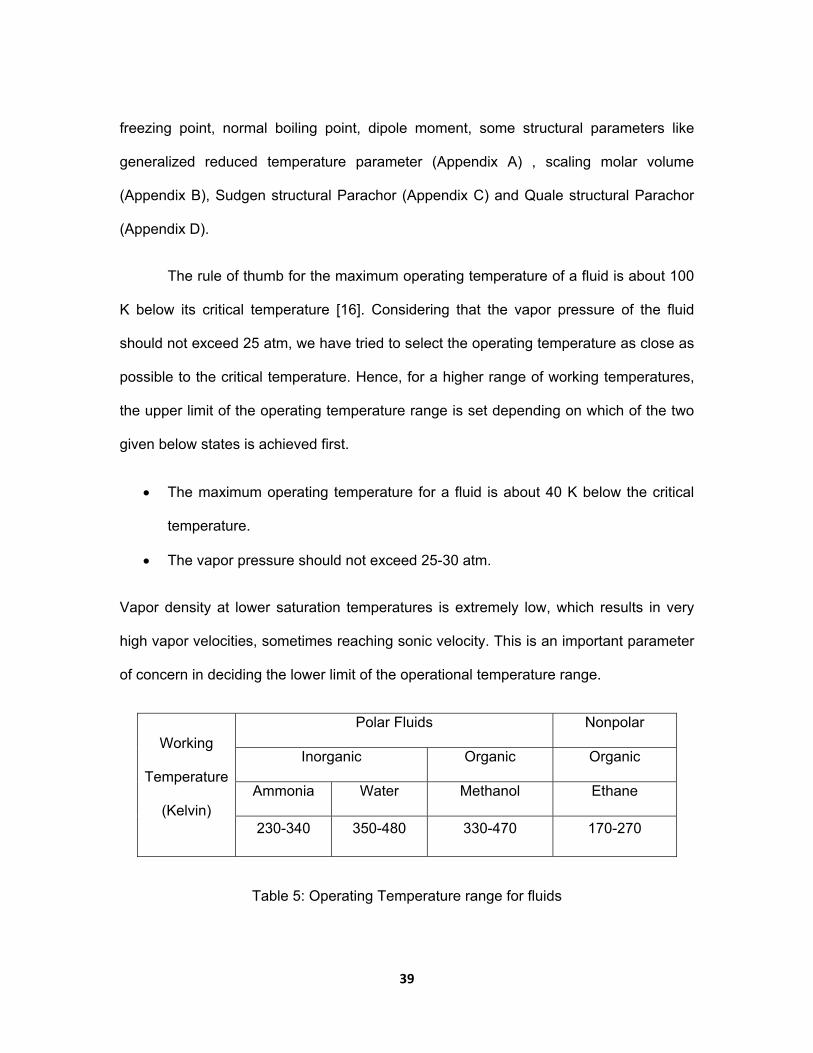
The rule of thumb for the maximum operating temperature of a fluid is about 100

K below its critical temperature [16]. Considering that the vapor pressure of the fluid

should not exceed 25 atm, we have tried to select the operating temperature as close as

possible to the critical temperature. Hence, for a higher range of working temperatures,

the upper limit of the operating temperature range is set depending on which of the two

given below states is achieved first.

The maximum operating temperature for a fluid is about 40 K below the critical

temperature.

The vapor pressure should not exceed 25-30 atm.

Vapor density at lower saturation temperatures is extremely low, which results in very

high vapor velocities, sometimes reaching sonic velocity. This is an important parameter

of concern in deciding the lower limit of the operational temperature range.

Working

Temperature

(Kelvin)

Polar Fluids Nonpolar

Inorganic Organic Organic

Ammonia Water Methanol Ethane

230-340 350-480 330-470 170-270

Table 5: Operating Temperature range for fluids

40

Latent Heat of Vaporization

Pitzer Equation

Figure 9: Pitzer equation error

Inputs Required

Critical Parameters :Temperature

Acentric Factor

Universal Gas Constant (R)

Types of compound Temperature range

(Reduced temperature Tr) Expected error (average)

Polar

Organic 0.3 0.9 0 % 3

Inorganic 0.3 0.9 0 % 4

Nonpolar 0.3 0.9 0 % 3

Table 6: Pitzer equation parameter table

‐4

‐2

0

2

4

0 100 200 300 400 500 600

Error (%

)

Temperature (K)

Ammonia

Water

Toluene

Methanol

Ethane

Heptane

41

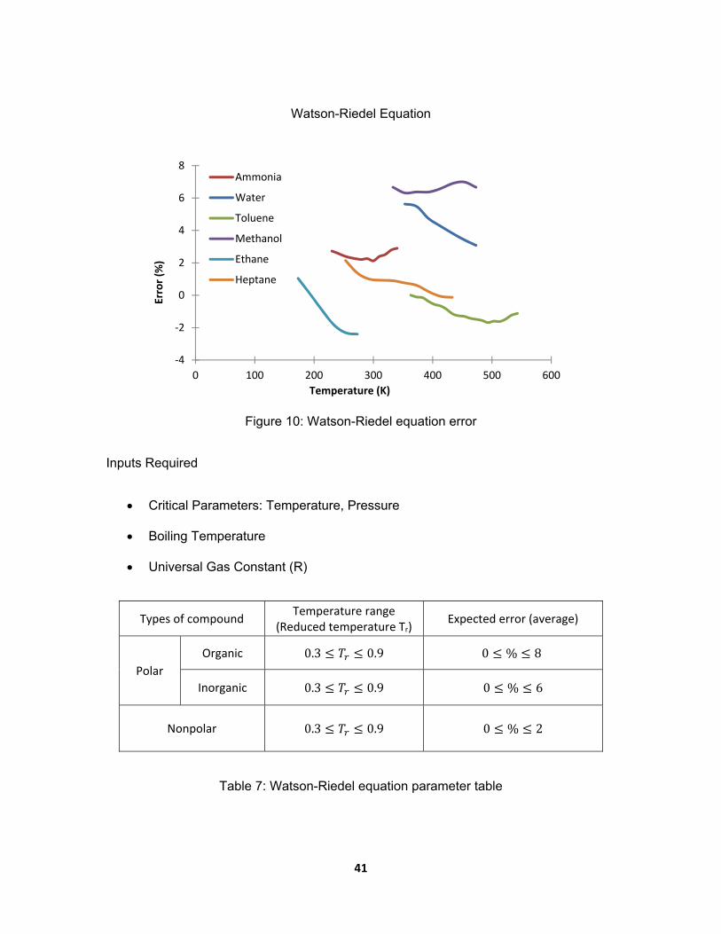
Watson-Riedel Equation

Figure 10: Watson-Riedel equation error

Inputs Required

Critical Parameters: Temperature, Pressure

Boiling Temperature

Universal Gas Constant (R)

Types of compound Temperature range

(Reduced temperature Tr) Expected error (average)

Polar

Organic 0.3 0.9 0 % 8

Inorganic 0.3 0.9 0 % 6

Nonpolar 0.3 0.9 0 % 2

Table 7: Watson-Riedel equation parameter table

‐4

‐2

0

2

4

6

8

0 100 200 300 400 500 600

Error (%

)

Temperature (K)

Ammonia

Water

Toluene

Methanol

Ethane

Heptane

42

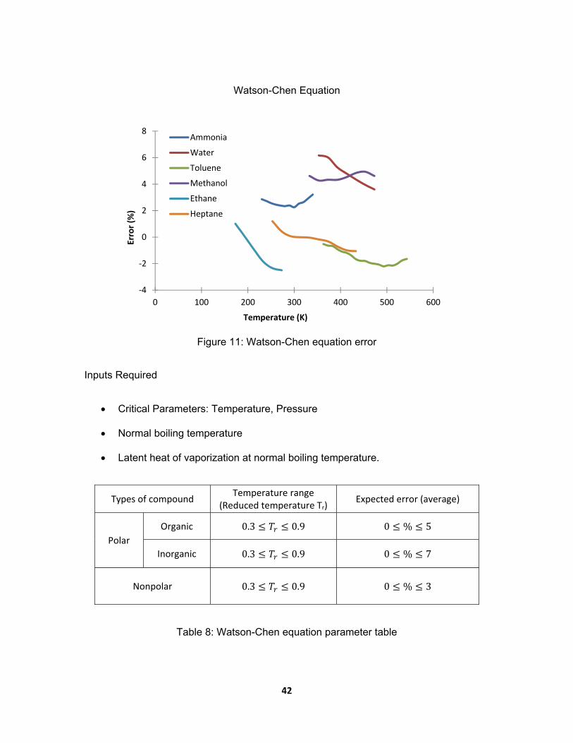
Watson-Chen Equation

Figure 11: Watson-Chen equation error

Inputs Required

Critical Parameters: Temperature, Pressure

Normal boiling temperature

Latent heat of vaporization at normal boiling temperature.

Types of compound Temperature range

(Reduced temperature Tr) Expected error (average)

Polar

Organic 0.3 0.9 0 % 5

Inorganic 0.3 0.9 0 % 7

Nonpolar 0.3 0.9 0 % 3

Table 8: Watson-Chen equation parameter table

‐4

‐2

0

2

4

6

8

0 100 200 300 400 500 600

Error (%

)

Temperature (K)

Ammonia

Water

Toluene

Methanol

Ethane

Heptane

43

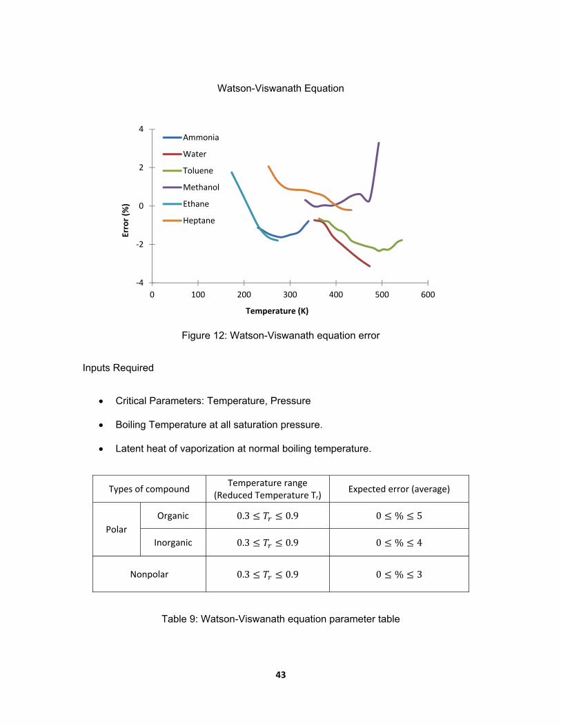
Watson-Viswanath Equation

Figure 12: Watson-Viswanath equation error

Inputs Required

Critical Parameters: Temperature, Pressure

Boiling Temperature at all saturation pressure.

Latent heat of vaporization at normal boiling temperature.

Types of compound Temperature range

(Reduced Temperature Tr) Expected error (average)

Polar

Organic 0.3 0.9 0 % 5

Inorganic 0.3 0.9 0 % 4

Nonpolar 0.3 0.9 0 % 3

Table 9: Watson-Viswanath equation parameter table

‐4

‐2

0

2

4

0 100 200 300 400 500 600

Error (%

)

Temperature (K)

Ammonia

Water

Toluene

Methanol

Ethane

Heptane

44

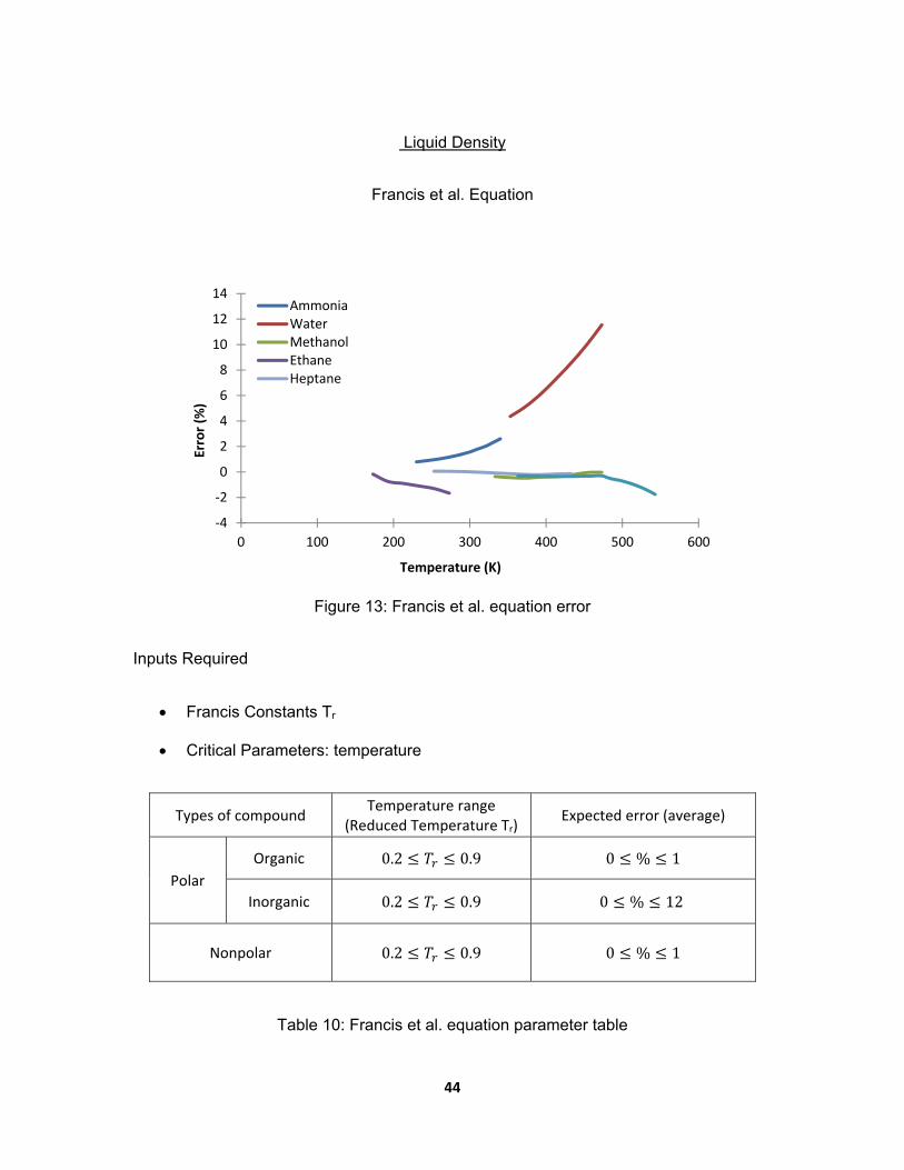
Liquid Density

Francis et al. Equation

Figure 13: Francis et al. equation error

Inputs Required

Francis Constants Tr

Critical Parameters: temperature

Types of compound Temperature range

(Reduced Temperature Tr) Expected error (average)

Polar

Organic 0.2 0.9 0 % 1

Inorganic 0.2 0.9 0 % 12

Nonpolar 0.2 0.9 0 % 1

Table 10: Francis et al. equation parameter table

‐4

‐2

0

2

4

6

8

10

12

14

0 100 200 300 400 500 600

Error (%

)

Temperature (K)

AmmoniaWaterMethanolEthaneHeptane

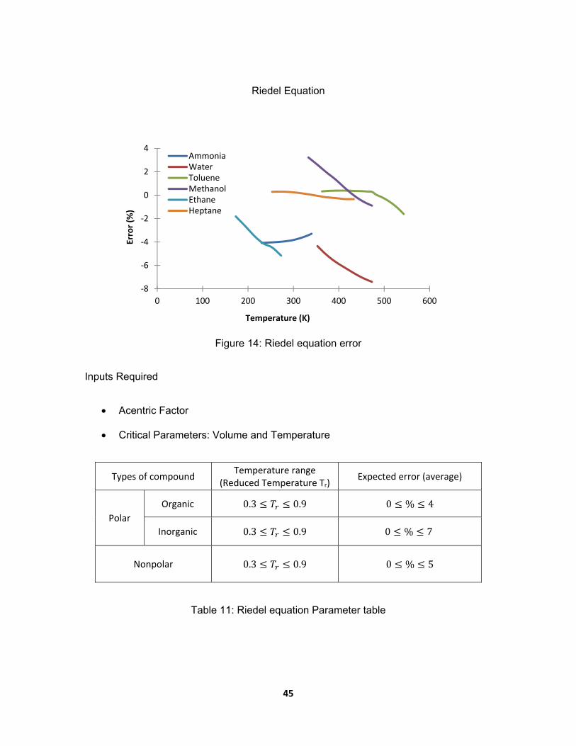
45

Riedel Equation

Figure 14: Riedel equation error

Inputs Required

Acentric Factor

Critical Parameters: Volume and Temperature

Types of compound Temperature range

(Reduced Temperature Tr) Expected error (average)

Polar

Organic 0.3 0.9 0 % 4

Inorganic 0.3 0.9 0 % 7

Nonpolar 0.3 0.9 0 % 5

Table 11: Riedel equation Parameter table

‐8

‐6

‐4

‐2

0

2

4

0 100 200 300 400 500 600

Error (%

)

Temperature (K)

AmmoniaWaterTolueneMethanolEthaneHeptane

46

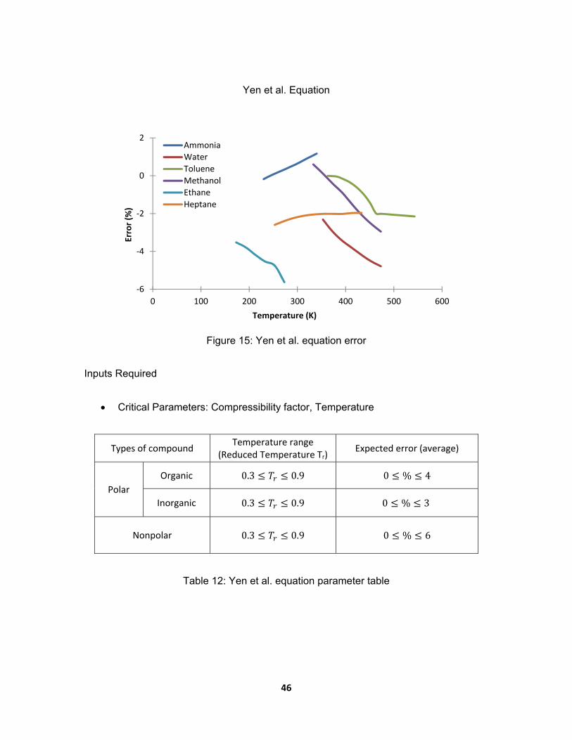
Yen et al. Equation

Figure 15: Yen et al. equation error

Inputs Required

Critical Parameters: Compressibility factor, Temperature

Types of compound Temperature range

(Reduced Temperature Tr) Expected error (average)

Polar

Organic 0.3 0.9 0 % 4

Inorganic 0.3 0.9 0 % 3

Nonpolar 0.3 0.9 0 % 6

Table 12: Yen et al. equation parameter table

‐6

‐4

‐2

0

2

0 100 200 300 400 500 600

Error (%

)

Temperature (K)

Ammonia

Water

Toluene

Methanol

Ethane

Heptane

47

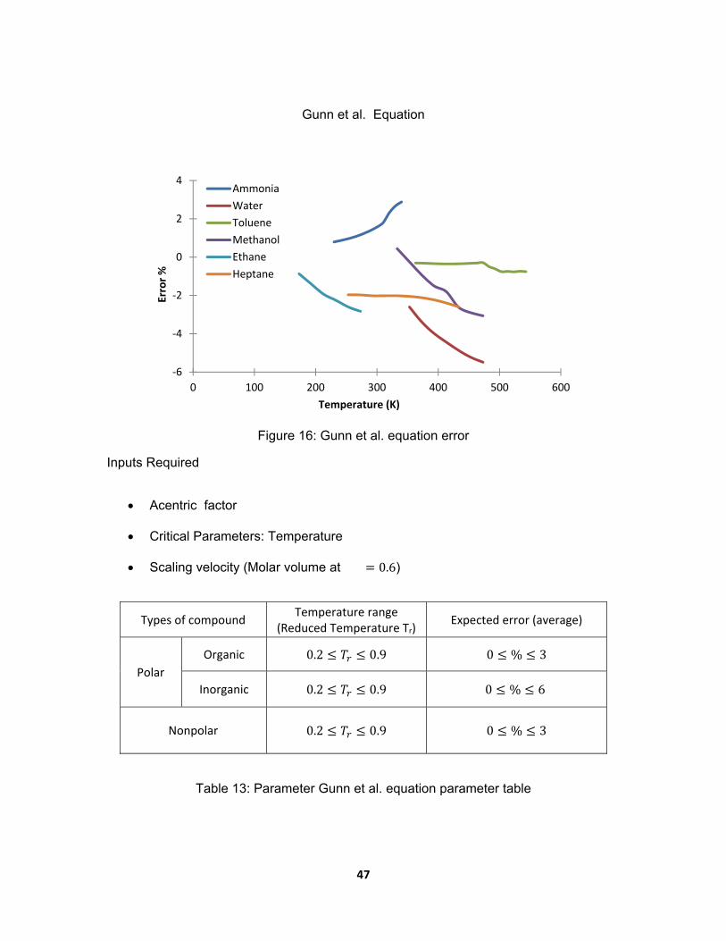
Gunn et al. Equation

Figure 16: Gunn et al. equation error

Inputs Required

Acentric factor

Critical Parameters: Temperature

Scaling velocity (Molar volume at 0.6)

Types of compound Temperature range

(Reduced Temperature Tr) Expected error (average)

Polar

Organic 0.2 0.9 0 % 3

Inorganic 0.2 0.9 0 % 6

Nonpolar 0.2 0.9 0 % 3

Table 13: Parameter Gunn et al. equation parameter table

‐6

‐4

‐2

0

2

4

0 100 200 300 400 500 600

Error %

Temperature (K)

Ammonia

Water

Toluene

Methanol

Ethane

Heptane

48

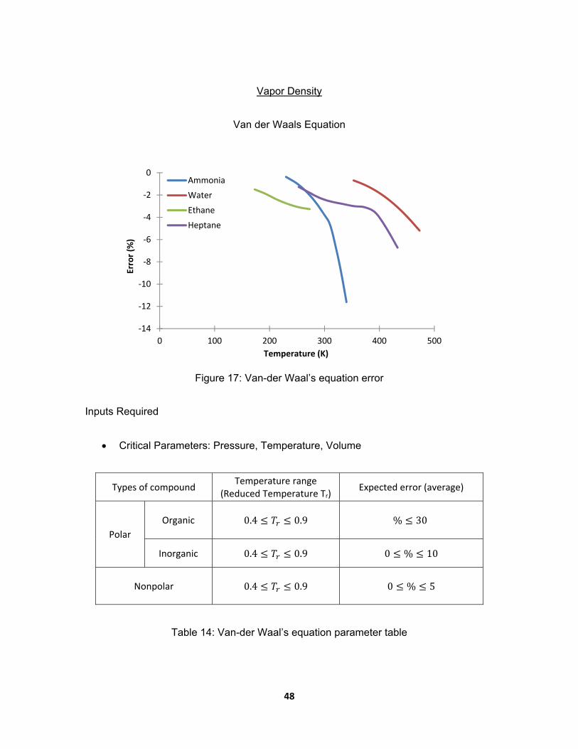
Vapor Density

Van der Waals Equation

Figure 17: Van-der Waal’s equation error

Inputs Required

Critical Parameters: Pressure, Temperature, Volume

Types of compound Temperature range

(Reduced Temperature Tr) Expected error (average)

Polar

Organic 0.4 0.9

% 30

Inorganic 0.4 0.9 0 % 10

Nonpolar 0.4 0.9 0 % 5

Table 14: Van-der Waal’s equation parameter table

‐14

‐12

‐10

‐8

‐6

‐4

‐2

0

0 100 200 300 400 500

Error (%

)

Temperature (K)

Ammonia

Water

Ethane

Heptane

49

Redlich-Kwong Equation

Figure 18: Redlich-Kwong Error

Inputs Required

Critical Parameters: Pressure, Temperature, Volume

Types of compound Temperature range

(Reduced Temperature Tr) Expected error (average)

Polar

Organic 0.4 0.9

% 30

Inorganic 0.4 0.9 0 % 6

Nonpolar 0.4 0.9 0 % 5

Table 15: Redlich-Kwong equation parameter table

‐8

‐6

‐4

‐2

0

0 100 200 300 400 500

Error (%

)

Temperature (K)

Ammonia

Water

Ethane

Heptane

50

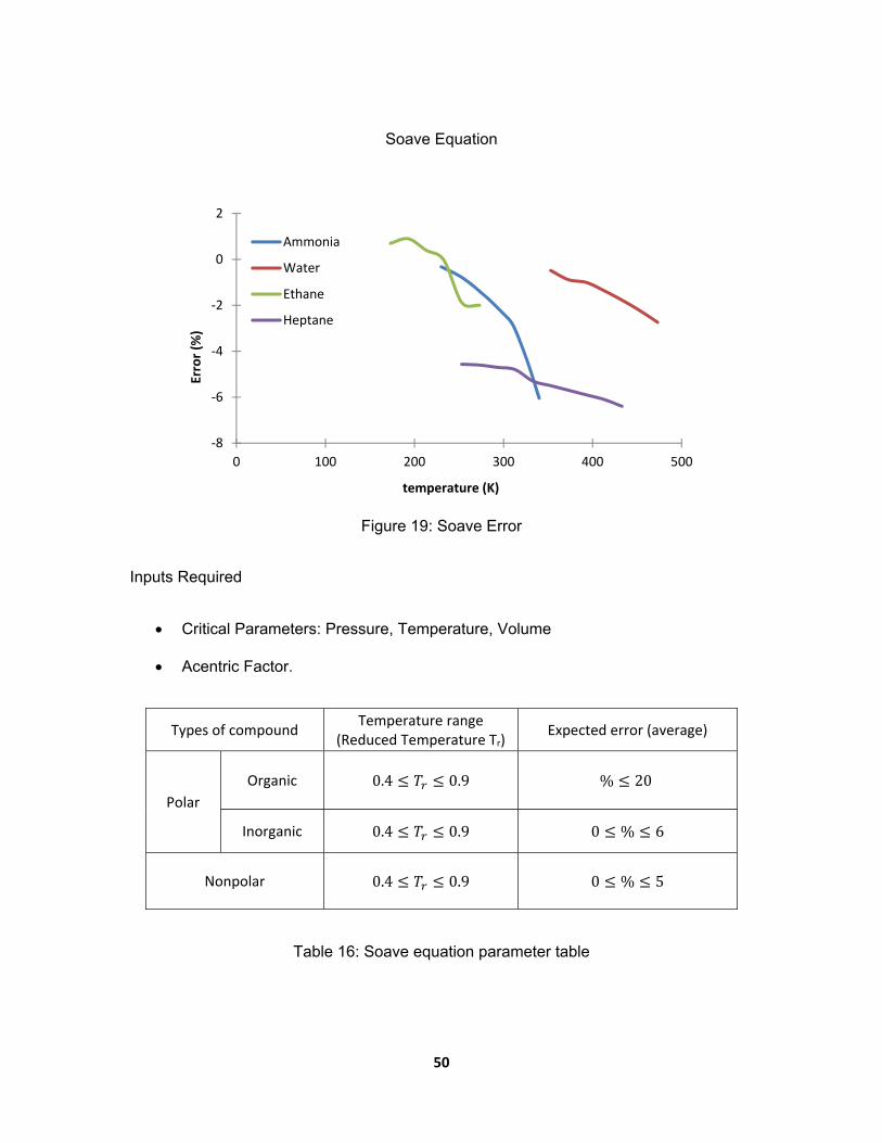
Soave Equation

Figure 19: Soave Error

Inputs Required

Critical Parameters: Pressure, Temperature, Volume

Acentric Factor.

Types of compound Temperature range

(Reduced Temperature Tr) Expected error (average)

Polar

Organic 0.4 0.9

% 20

Inorganic 0.4 0.9 0 % 6

Nonpolar 0.4 0.9 0 % 5

Table 16: Soave equation parameter table

‐8

‐6

‐4

‐2

0

2

0 100 200 300 400 500

Error (%

)

temperature (K)

Ammonia

Water

Ethane

Heptane

51

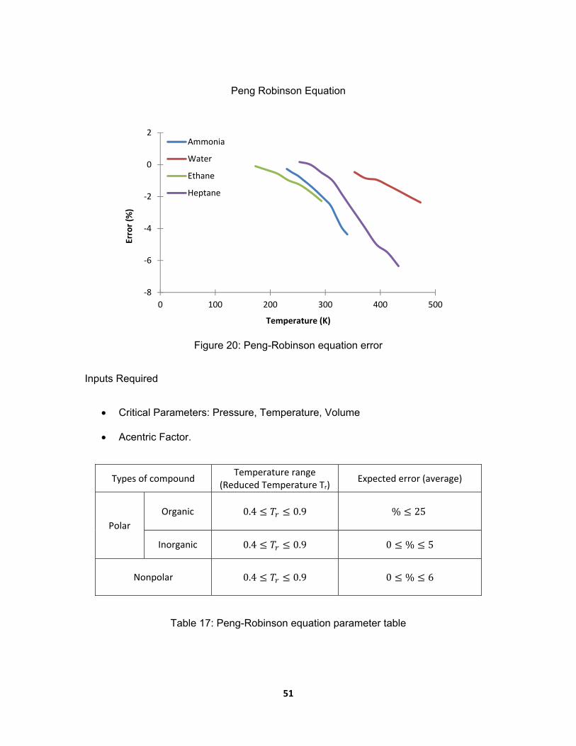
Peng Robinson Equation

Figure 20: Peng-Robinson equation error

Inputs Required

Critical Parameters: Pressure, Temperature, Volume

Acentric Factor.

Types of compound Temperature range

(Reduced Temperature Tr) Expected error (average)

Polar

Organic 0.4 0.9

% 25

Inorganic 0.4 0.9 0 % 5

Nonpolar 0.4 0.9 0 % 6

Table 17: Peng-Robinson equation parameter table

‐8

‐6

‐4

‐2

0

2

0 100 200 300 400 500

Error (%

)

Temperature (K)

Ammonia

Water

Ethane

Heptane

52

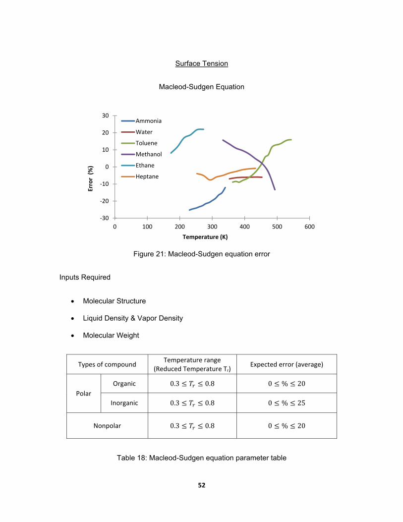
Surface Tension

Macleod-Sudgen Equation

Figure 21: Macleod-Sudgen equation error

Inputs Required

Molecular Structure

Liquid Density & Vapor Density

Molecular Weight

Types of compound Temperature range

(Reduced Temperature Tr) Expected error (average)

Polar

Organic 0.3 0.8 0 % 20

Inorganic 0.3 0.8 0 % 25

Nonpolar 0.3 0.8 0 % 20

Table 18: Macleod-Sudgen equation parameter table

‐30

‐20

‐10

0

10

20

30

0 100 200 300 400 500 600

Error (%)

Temperature (K)

Ammonia

Water

Toluene

Methanol

Ethane

Heptane

53

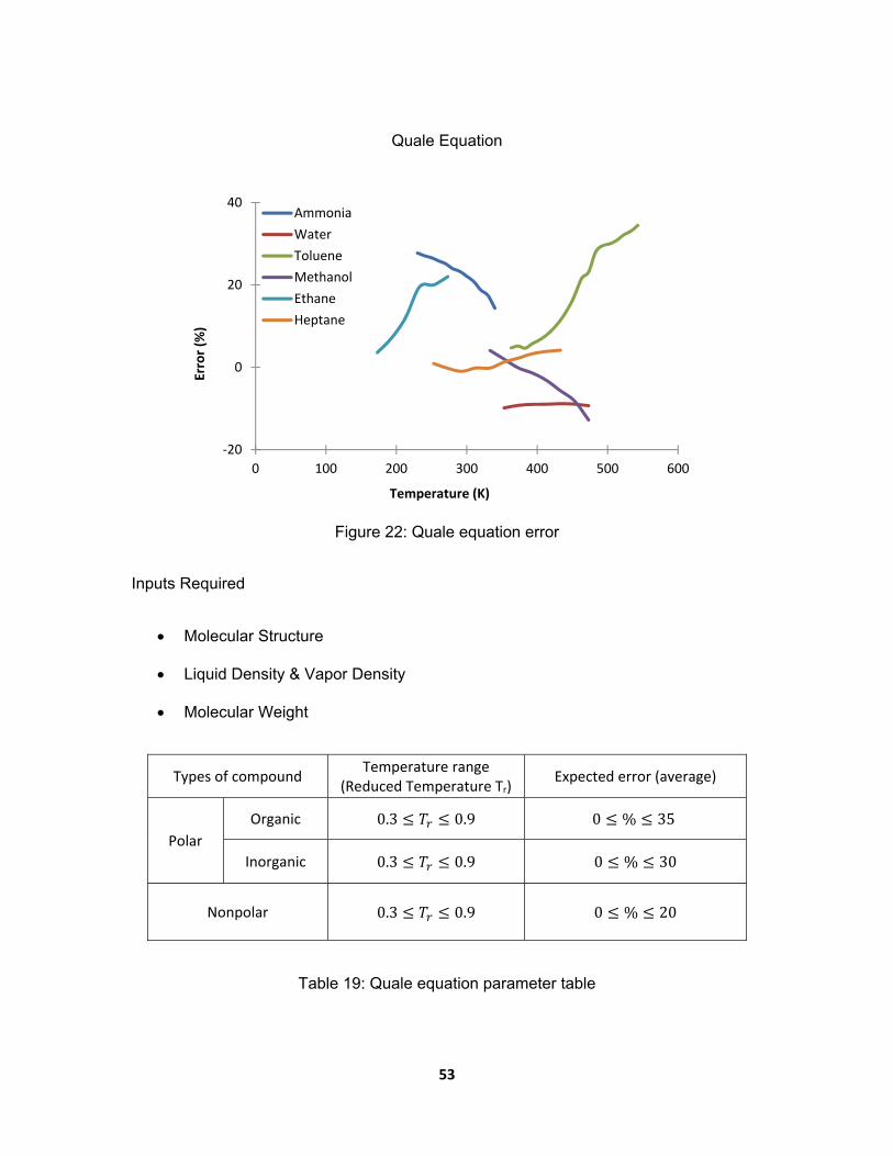
Quale Equation

Figure 22: Quale equation error

Inputs Required

Molecular Structure

Liquid Density & Vapor Density

Molecular Weight

Types of compound Temperature range

(Reduced Temperature Tr) Expected error (average)

Polar

Organic 0.3 0.9 0 % 35

Inorganic 0.3 0.9 0 % 30

Nonpolar 0.3 0.9 0 % 20

Table 19: Quale equation parameter table

‐20

0

20

40

0 100 200 300 400 500 600

Error (%

)

Temperature (K)

Ammonia

Water

Toluene

Methanol

Ethane

Heptane

54

Brook’s et al. Equation

Figure 23: Brook’s et al. equation error

Inputs Required

Critical Parameters: Temperature, Pressure

Boiling Temperature

Types of compound Temperature range

(Reduced Temperature Tr) Expected error (average)

Polar

Organic 0.3 0.9 0 % 20

Inorganic 0.3 0.9 0 % 15

Nonpolar 0.3 0.9 0 % 10

Table 20: Brook’s et al. equation parameter table

‐25

‐15

‐5

5

15

25

0 100 200 300 400 500 600

Error (%

)

Temperature (K)

Ammonia

Water

Toluene

Methanol

Ethane

Heptane

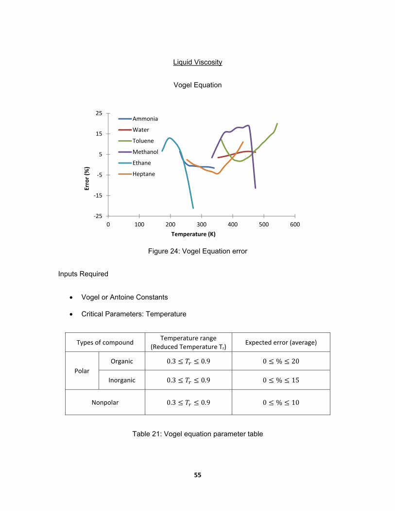
55

Liquid Viscosity

Vogel Equation

Figure 24: Vogel Equation error

Inputs Required

Vogel or Antoine Constants

Critical Parameters: Temperature

Types of compound Temperature range

(Reduced Temperature Tr) Expected error (average)

Polar

Organic 0.3 0.9 0 % 20

Inorganic 0.3 0.9 0 % 15

Nonpolar 0.3 0.9 0 % 10

Table 21: Vogel equation parameter table

‐25

‐15

‐5

5

15

25

0 100 200 300 400 500 600

Error (%

)

Temperature (K)

Ammonia

Water

Toluene

Methanol

Ethane

Heptane

56

Lewis-squire Equation

Figure 25: Lewis-Squire equation error

Inputs Required

Critical Parameters: Temperature, Pressure

Liquid viscosity at a known point.

Types of compound Temperature range

(Reduced Temperature Tr) Expected error (average)

Polar

Organic 0.3 0.9 0 % 20

Inorganic 0.3 0.9 0 % 20

Nonpolar 0.3 0.9 0 % 10

Table 22: Lewis-Squire equation parameter table

‐30

‐10

10

30

0 100 200 300 400 500 600

Error (%

)

Temperature (K)

Ammonia

Water

Toluene

Methanol

Ethane

Heptane

57

Vapor Viscosity

Chung Equation

Figure 26: Chung equation error

Inputs Required

Critical Parameters: Temperature, Pressure, Volume

Molar weight

Acentric Factor

Dipole moment (Debye)

Types of compound Temperature range

(Reduced Temperature Tr) Expected error (average)

Polar

Organic 0.3 0.9 0 % 2

Inorganic 0.3 0.9 0 % 10

Nonpolar 0.3 0.9 0 % 5

Table 23: Chung equation parameter table

‐12

‐10

‐8

‐6

‐4

‐2

0

2

4

6

0 100 200 300 400 500 600

Error (%

)

Temperature (K)

Ammonia

Water

Toluene

Methanol

Ethane

Heptane

58

Lukas Equation

Figure 27: Lukas equation error

Inputs Required

Critical Parameters: Temperature, Pressure, Volume, Compressibility Factor

Dipole moment (Debye)

Molar weight

Types of compound Temperature range

(Reduced Temperature Tr) Expected error (average)

Polar

Organic 0.3 0.9 0 % 2

Inorganic 0.3 0.9 0 % 10

Nonpolar 0.3 0.9 0 % 4

Table 24: Lukas equation parametric table

‐12

‐8

‐4

0

4

8

0 100 200 300 400 500 600

Error (%

)

Temperature (K)

Ammonia

Water

Toluene

Methanol

Ethane

Heptane

59

Merit Number

The theory of uncertainty using standard deviation as the mode of tolerance was

first used to calculate the percentage deviation of the important thermo-physical

properties for all of the four considered working fluid. Every thermo-physical property in

the working temperature range was expressed in the form of x x s. d, where s.d

is the standard deviation about the mean at the given temperature. The percent

deviation of the liquid and the vapor merit number is shown in Eq. 52.The standard

deviation for the liquid merit number is shown in Fig. 28 and that of vapor in Fig. 29.

. ,

. ,

. .

.

.

,

52

Figure 28: Liquid merit number uncertainty (standard deviation)

0

4

8

12

16

20

0 100 200 300 400 500

(f.m

)/(f.m

) %

Temperature (K)

Ammonia

Water

Ethane

Methanol

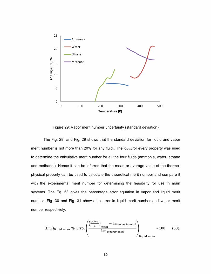
60

Figure 29: Vapor merit number uncertainty (standard deviation)

The Fig. 28 and Fig. 29 shows that the standard deviation for liquid and vapor

merit number is not more than 20% for any fluid.. The xmean for every property was used

to determine the calculative merit number for all the four fluids (ammonia, water, ethane

and methanol). Hence it can be inferred that the mean or average value of the thermo-

physical property can be used to calculate the theoretical merit number and compare it

with the experimental merit number for determining the feasibility for use in main

systems. The Eq. 53 gives the percentage error equation in vapor and liquid merit

number. Fig. 30 and Fig. 31 shows the error in liquid merit number and vapor merit

number respectively.

f. m , %Error

∗ ∗ f. m

f.m,

∗ 100 53

0

5

10

15

20

25

0 100 200 300 400 500

(∆ f

.m)/

(f.m

) %

Temperature (K)

Ammonia

Water

Ethane

Methanol

61

Figure 30: Liquid Merit number error

Figure 31: Vapor Merit number Error

‐15

‐10

‐5

0

5

10

15

20

25

0 100 200 300 400 500

Error (%

)

Temperature( k)

Amonia

Water

Methanol

Ethane

‐20

‐10

0

10

20

0 100 200 300 400 500

Error(%)

Temperature(K)

Ammonia

Water

Methanol

Ethane

62

Maximum Heat Transfer

In the literature review, it was discussed through Eq. (6) that the maximum heat

carrying capacity of the cylindrical liquid pressure driven heat pipe depends on three

factors i.e. the thermo-physical properties of the fluid, the wick properties and

geometrical design of the heat pipe. In this work, the fluid selection was only considered

for performance optimization in this work, for which maximum heat transfer capability is

a key concept to evaluate. For considering the maximum heat carrying capacity which

directly reflects the effectiveness of the heat pipe an uncertainty analysis was done on

the Eq. (6) considering 5% uncertainty in geometric design of the heat pipe.

..

,

54

Figure 32: Maximum heat transfer error percentage

0

4

8

12

16

20

0 100 200 300 400 500

Uncertainity %

Temperature (k)

Ammonia

Water

Methanol

Ethane

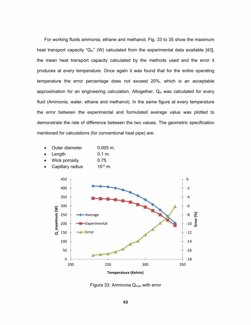
63

For working fluids ammonia, ethane and methanol, Fig. 33 to 35 show the maximum

heat transport capacity “Qm” (W) calculated from the experimental data available [43],

the mean heat transport capacity calculated by the methods used and the error it

produces at every temperature. Once again it was found that for the entire operating

temperature the error percentage does not exceed 20%, which is an acceptable

approximation for an engineering calculation. Altogether, Qm was calculated for every

fluid (Ammonia, water, ethane and methanol). In the same figure at every temperature

the error between the experimental and formulated average value was plotted to

demonstrate the rate of difference between the two values. The geometric specification

mentioned for calculations (for conventional heat pipe) are:

Outer diameter 0.005 m. Length 0.1 m. Wick porosity 0.75. Capillary radius 10-5 m.

Figure 33: Ammonia Qmax with error

‐18

‐16

‐14

‐12

‐10

‐8

‐6

‐4

‐2

0

0

50

100

150

200

250

300

350

400

450

200 250 300 350

Error (%

)

Q_m

axim

um (W)

Temperature (Kelvin)

Average

Experimental

Error

64

Figure 34: Ethane Qmax with error

Figure 35: Methanol Qmax with error

0

1

2

3

4

5

6

7

8

9

0

10

20

30

40

50

60

70

80

90

150 170 190 210 230 250 270 290

Error (%

)

Q_m

axim

um (W)

Temperature(K)

Average

Experimental

Error

‐15

‐10

‐5

0

5

10

15

20

0

20

40

60

80

100

120

140

160

180

300 350 400 450 500

Error (%

)

Q m

ax

Temperature (K)

Aerage

experminetal

Error

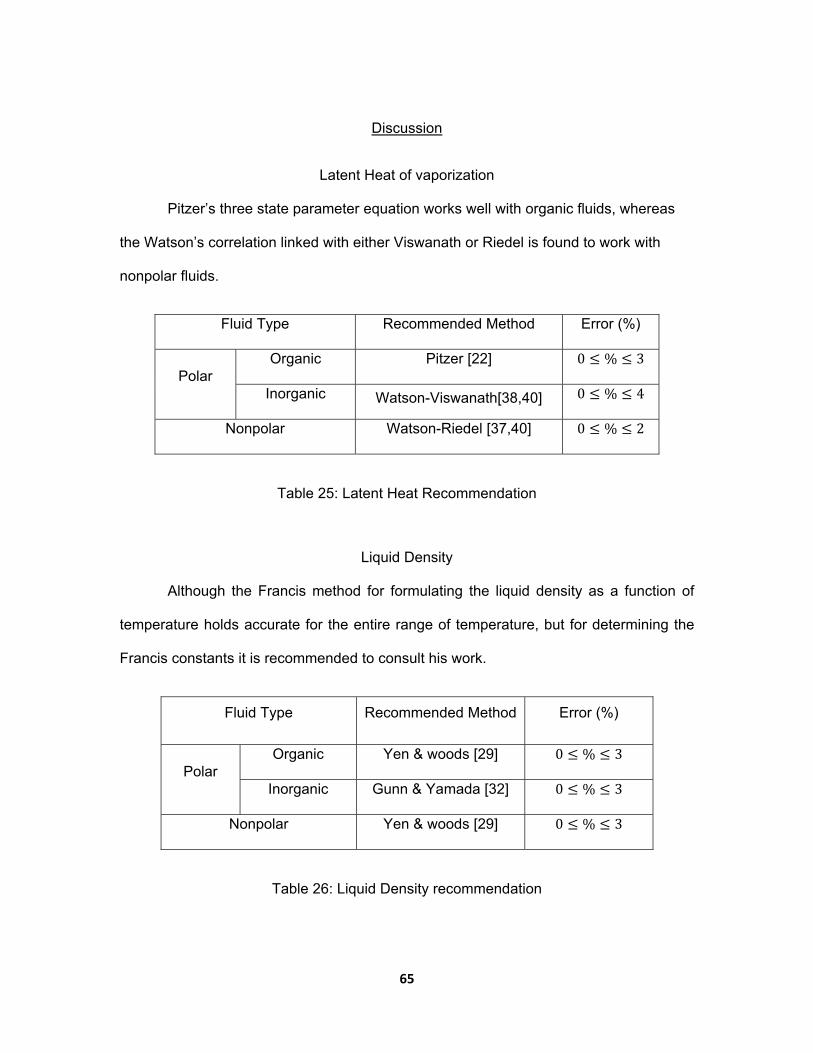
65

Discussion

Latent Heat of vaporization

Pitzer’s three state parameter equation works well with organic fluids, whereas

the Watson’s correlation linked with either Viswanath or Riedel is found to work with

nonpolar fluids.

Fluid Type Recommended Method Error (%)

Polar Organic Pitzer [22] 0 % 3

Inorganic Watson-Viswanath[38,40] 0 % 4

Nonpolar Watson-Riedel [37,40] 0 % 2

Table 25: Latent Heat Recommendation

Liquid Density

Although the Francis method for formulating the liquid density as a function of

temperature holds accurate for the entire range of temperature, but for determining the

Francis constants it is recommended to consult his work.

Fluid Type Recommended Method Error (%)

Polar Organic Yen & woods [29] 0 % 3

Inorganic Gunn & Yamada [32] 0 % 3

Nonpolar Yen & woods [29] 0 % 3

Table 26: Liquid Density recommendation

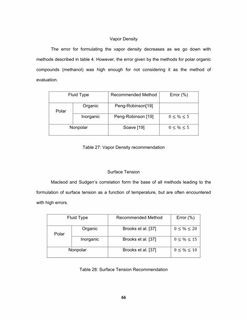
66

Vapor Density

The error for formulating the vapor density decreases as we go down with

methods described in table 4. However, the error given by the methods for polar organic

compounds (methanol) was high enough for not considering it as the method of

evaluation.

Fluid Type Recommended Method Error (%)

Polar Organic Peng-Robinson[19]

Inorganic Peng-Robinson [19] 0 % 5

Nonpolar Soave [19] 0 % 5

Table 27: Vapor Density recommendation

Surface Tension

Macleod and Sudgen’s correlation form the base of all methods leading to the

formulation of surface tension as a function of temperature, but are often encountered

with high errors.

Fluid Type Recommended Method Error (%)

Polar Organic Brooks et al. [37] 0 % 20

Inorganic Brooks et al. [37] 0 % 15

Nonpolar Brooks et al. [37] 0 % 10

Table 28: Surface Tension Recommendation

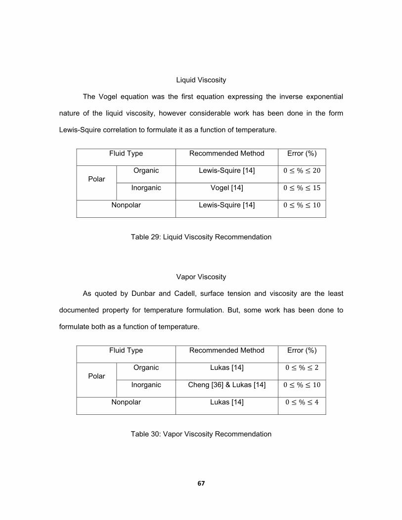
67

Liquid Viscosity

The Vogel equation was the first equation expressing the inverse exponential

nature of the liquid viscosity, however considerable work has been done in the form

Lewis-Squire correlation to formulate it as a function of temperature.

Fluid Type Recommended Method Error (%)

Polar Organic Lewis-Squire [14] 0 % 20

Inorganic Vogel [14] 0 % 15

Nonpolar Lewis-Squire [14] 0 % 10

Table 29: Liquid Viscosity Recommendation

Vapor Viscosity

As quoted by Dunbar and Cadell, surface tension and viscosity are the least

documented property for temperature formulation. But, some work has been done to

formulate both as a function of temperature.

Fluid Type Recommended Method Error (%)

Polar Organic Lukas [14] 0 % 2

Inorganic Cheng [36] & Lukas [14] 0 % 10

Nonpolar Lukas [14] 0 % 4

Table 30: Vapor Viscosity Recommendation

68

CHAPTER 4

CONCLUSION

Four thermal fluids ammonia, water, ethane and methanol were selected for

model formulation in order to consider various methods for evaluation of the liquid and

vapor merit number in a conventional heat pipe. The evaluation criteria were based upon

calculating the error percent with the reference data and determining the uncertainty

deviation about the mean. Thereafter, the analysis was continued on maximum heat

transfer capacity of the working fluid.

For considering the calculation of merit number, irrespective of it being a vapor or

a liquid merit number, the most important thermo-physical properties of interest are

latent heat of vaporization, density (liquid and vapor), surface tension, viscosity(liquid

and vapor) and vapor pressure. This work formulates vapor pressure so as to have an

idea of the operating temperature range of the thermal fluid.

Latent heat of vaporization has several unique methods of formulation using only

the intensive properties of the thermal fluid. Pitzer equation is considered to work well for

polar fluids, whereas Watson-Riedel equation works well for nonpolar fluids. The

maximum error using any method was 8% and the minimum was 2% using the

recommended methods.

Liquid density, reports a minimum error of 3% using Yen & Woods equation for

polar organic fluid and nonpolar fluid, whereas Gunn & Yamada equation for polar

inorganic fluids. The maximum error reports for liquid density is 7%. Since vapor density

69

gives higher errors when compared to liquid density, it is recommended to not be used

for polar organic fluids. When using Peng-Robinson equation, the minimum error was

calculated as 5 % whereas, the maximum error was calculated as 25%.

Brook’s equation, using the critical parameters for surface tension formulation

reports the minimum error of 10% for nonpolar fluids and 15-20% error for polar

compounds. Macleod’s correlation accounts for approximately 25% error for all fluids.

Using Lewis-squire equation, 10% and 15% error was calculated in nonpolar and

polar fluids respectively. A maximum of 20% error was calculated for polar fluids using

vogel equation. An average of 2% error was calculated in polar organic fluids by using

Chung equation and Lukas equation, whereas a 5% error was seen in non-polar fluids.

Polar inorganic fluid like ammonia and water exhibits 10% standard deviation in

liquid and vapor merit number for the conventional heat pipe. The maximum heat

transport capability of ammonia and water accounts for a maximum of 20% error which

improves to a minimum of 6% at 340 K for ammonia and 5% at 450 K for water.

Methanol, a polar organic thermal fluid accounts for a maximum of 15% standard

deviation for liquid and vapor merit number. The maximum heat transport capability of

methanol is calculated as 15% at the extreme ends of the working temperature.

Ethane, a nonpolar organic fluid accounts for 15% standard deviation for liquid

and vapor merit number. The maximum heat transport capability of ethanol is calculated

to be a maximum of 8%.

70

CHAPTER 5

RECOMMENDATIONS FOR FUTURE WORK

Liquid density has been formulated perfectly over the entire temperature range

and does not require any further work.

New methods for formulating vapor density for polar organic fluids are needed.

There has been some work in formulating critical compressibility factor as a

function of reduced temperature which can be helpful.

Introduction of acentric factor in latent heat of vaporization calculation in Watson

methods may decrease the error even further.

Some work can be done in reducing the error in surface tension and liquid

density to 5-10%. All methods described accounts for a minimum of 15% error.

The analysis should be extended to more fluids to validate the results.

As we have not considered any fluid (whether polar or nonpolar) over 500 K, So

further study of temperature above 500 K is needed to validate the study.

Work on metal fluids (in molten states) from 800 K to 1500 K should be extended

with the most potential candidates as lithium, cesium and sodium.

This work is related to heat transport calculation of only liquid pressure gradient

driven heat pipe, but there have been theories which relate vapor as well as

gravity pressure gradient driven heat pipes. Such theories should also be

validated.

71

APPENDICES

72

Appendix A: Lyckman et al. [30] Generalized reduced temperature parameters

73

Appendix B: Scaling Volume and Critical Volume for Gunn et al. [32]

Appendix C: Sudgen [18] atomic and Parachor values

74

Appendix D: Quale [21] Atomic and structural Parachor values

75

Reference

1. Chi, S. W., Heat Pipe Theory and Practice a Sourcebook, McGraw-Hill, New York, 1976.

2. Long, J.B., “Alternate Working fluids for capillary driven two-phase loops”, MS Thesis, Clemson University, 2001.

3. Dunn, P.D., Reay, D.A., Heat Pipes, 2nd Ed., Pergamon Press, 1978.

4. Maydanik, Yu F. "Loop heat pipes." Applied Thermal Engineering 25.5: 635-657, 2005.

5. Ku, Kentung, "Operating characteristics of loop heat pipes. No. 1999-01-2007” SAE Technical Paper, 1999.

6. Launay, Stéphane, Valérie S., and Jocelyn B., "Parametric analysis of loop heat pipe operation: a literature review." International Journal of Thermal Sciences 46.7: 621-636, 2007.

7. Munson, B.R., Young, D.F., Fundamentals of fluid mechanics, 4th Ed., John Wiley & Sons, 2002. 8. Asselman, G.A.A., Green, D.B., “Heat Pipes. I. Operation and Characteristics”,

Philips Technical Review, Vol. 33, Issue. 4, pp. 104-13, 1973.

9. Mishkinis, D., Ochterbeck, J.M., Sodtke, C., “Non-Dimensional Analysis and Scaling issues in Loop Heat Pipe”, 41s Aerospace Sciences Meeting and

Exhibit, 6-9 Jan; Paper AIAA-2003-0341, 2003.

10. Dunbar, N. and Cadell, P., “Working Fluids and Figure of Merit for CPL/LHP Application”, The Aerospace Corporation, CPL-98 Workshop, 1998.

11. Wallin P, Heat Pipe Selection of working fluid, Project Report, MVK160 Heat and Mass Transfer, Lund, Sweden, 2012.

12. Chandratilleke, R., Hatakeyama, H., and Nakagome, H., "Development of cryogenic loop heat pipes." Cryogenics 38.3, 1998.

76

13. Deverall, J.E., “Mercury as a Heat Pipe Fluid”, ASME Paper 70-HT/Spt-8, 1970.

14. Anderson, W.G., Rosenfeld J.K., Angirasa, D., Mi,Y., “Evaluation of heat Pipe working fluid in the temperature range 450 to 700 K”, STAIF 2005,

Albuquerque, NM, February 13-17, 2005.

15. Wei, Q., “Super High Temperature Heat Pipes”, Institute of Engineering, Chinese Academy of Science, Beijing, China.

16. Devarakonda, A., Anderson, W.G. , “Thermo-physical properties of intermediate temperature heat pipe fluids”, Space Technology & Applications International Forum (STAIF) Conference, vol. 746, American Institute of Physics, New York, 2005.

17. http://www.thermopedia.com/

18. Thomson, G. W., "The Antoine equation for vapor-pressure data”. Chemical reviews 38.1: 1-39, 1946.

19. Wagner, W. "New vapor pressure measurements for argon and nitrogen and a New method for establishing rational vapor pressure equation”, Cryogenics 13.8: 470-482, 1973.

20. Forero G, Luis A., and. Velásquez J. A., "Wagner liquid–vapor pressure equation constants from a simple methodology." The Journal of Chemical Thermodynamics 43.8: 1235-1251, 2011.

21. Pitzer, K.S., “The Volumetric and Thermodynamic Properties of fluids. II. Compressibility Factor, Vapor Pressure and Entropy of Vaporization 1”, Journal of the American Chemical Society 77.13: 3433-3440, 1950.

22. Lee, B.K. and Kesler, M.G., "A generalized thermodynamic correlation based on three-parameter corresponding states." AIChE Journal 21.3: 510-527, 1975.

23. Watson, K. M. "Thermodynamics of the liquid state." Industrial & Engineering Chemistry 35.4: 398-406, 1943.

24. Viswanath, D. S., and Kuloor, N. R., “On a generalized Watson's Relation for Latent heat of vaporization." The Canadian Journal of Chemical Engineering 45.1: 29-31, 1967.

77

25. Mehmandoust, B., Ehsan S., and Mostafa V., "An efficient reliable method to estimate the vaporization enthalpy of pure substances according to the normal boiling temperature and critical properties." Journal of Advanced Research 5.2: 261-269, 2014.

26. Chen, N. H. "Generalized Correlation for Latent Heat of Vaporization." Journal of

Chemical and Engineering Data 10.2: 207-210, 1965.

27. Lyckman, E. W., Eckert, C. A. and Prausnitz, J. M. "Generalized liquid volumes and solubility parameters for regular solution application." Chemical Engineering Science 20.7: 703-706, 1965.

28. Francis, Alfred W. "Pressure-temperature-density relations of pure liquids”, Chemical Engineering Science 10.1 (1959): 37-46.

29. Yen, Lewis C., and S. S. Woods. "A generalized equation for computer calculation of liquid densities." AIChE Journal 12.1: 95-99, 1966.

30. Riedel, L.,’ Density of liquids in the state of saturation. Investigations on the widening of the theorem of corresponding states. II”, Chemie ingenieur technik 20: 259-264, 1954.

31. Gunn, R. D., and Tomoyoshi Yamada. "A corresponding states correlation of saturated liquid volumes." AIChE Journal 17.6: 1341-1345, 1971.

32. Kenneth, W., Thermodynamics. New York: McGraw-Hill, 1977.

33. Poling, Bruce E., Prausnitz,J.M. and Reid, R. C., The properties of gases and liquids, 4th Ed., New York: McGraw-Hill, 1986.

34. Vargaftik, N. B., Volkov, B. N. and Voljak, L. D., "International tables of the surface tension of water." Journal of Physical and Chemical Reference Data 12.3: 817-820, 1983.

35. Vargaftik, N. B. "Handbook of thermo physical properties of gases and liquids." 1972.

36.Macleod, D. B. "On a relation between surface tension and density." Transactions of the Faraday Society 19.July: 38-41, 1923.

78

37. Sudgen, S. "VI.—the variation of surface tension with temperature and some related functions." Journal of the Chemical Society, Transactions 125: 32-41, 1924.

38. Quayle, O. R., "The Parachors of Organic Compounds. An Interpretation and Catalogue." Chemical Reviews 53.3: 439-589, 1953.

39. Brock, J. R. and Bird, R. B. "Surface tension and the principle of corresponding states." AIChE Journal 1.2: 174-177, 1955.

40. Neufeld, P. D., Janzen, A. R. and Aziz, R. A., “Empirical Equations to Calculate 16 of the Transport Collision Integrals Ω (l, s)* for the Lennard‐Jones (12–6) Potential." The Journal of Chemical Physics 57.3:1100-1102, 2003.

41. Chung, T. H., Lloyd L. L. and Starling, K.E., "Applications of kinetic gas theories and multi-parameter correlation for prediction of dilute gas viscosity and thermal conductivity." Industrial & engineering chemistry fundamentals 23.1: 8-13, 1984.

42. Yoonm, P., and George T., "Viscosity of nonpolar gaseous mixtures at normal pressures." AIChE Journal 16.2: 300-304, 1970.