Tadej Kodelja

COBIK, Solkan, Slovenia

Supervisor

Prof.dr. B Šarler

•Continuous casting of steel and its physics

•Approximative numerical models based on artificial neural network (ANN)

•Modelling of continuous casting of steel by ANN

•Conclusions and future work

•Introduction to steel process modelling

•Introduction and motivation for ANN

modelling

•Assessment of physical and ANN modelling of

continuous casting of steel

Final Measured Material

Properties

Elongation (A)

Tensile strength (Rm)

Yield stress (Rp)

Hardness after rolling (HB)

Necking (Z)

•Process was developed in the 1950s

•The most common process for production of steel

•90% of all steel grades are produced by this

technique

•Types

• Vertical, horizontal, curved, strip casting

•Typical products

• Billets, blooms, slab, strip

•Regimes

•LIQUID (liquid, particles,

inclusions,…)

•SLURRY (equiaxed

dendrites + liquid)

•POROUS (columnar

dendrites + liquid)

•SOLID (dendrites)

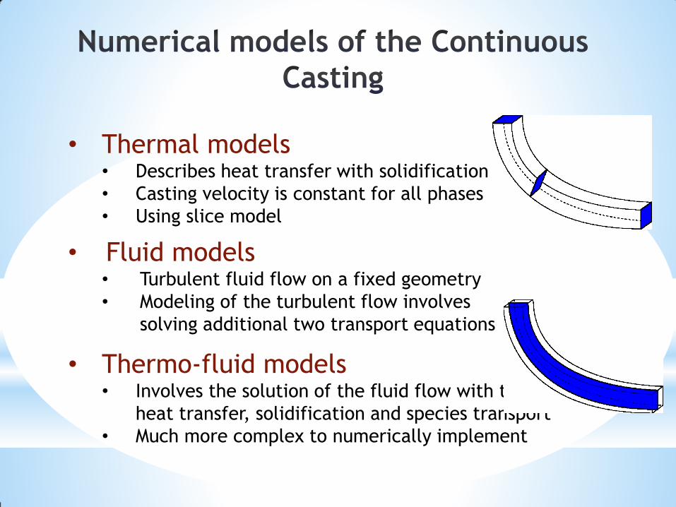
• Thermal models

• Describes heat transfer with solidification

• Casting velocity is constant for all phases

• Using slice model

• Fluid models • Turbulent fluid flow on a fixed geometry

• Modeling of the turbulent flow involves

solving additional two transport equations

• Thermo-fluid models • Involves the solution of the fluid flow with the

heat transfer, solidification and species transport

• Much more complex to numerically implement

• Slice traveling schematics in the billet

• Fast calculation time

• x-y cross sectional slide is moving from top horizontal to

bottom vertical position

• Temperature and boundary condition are assumed as time

dependent

•Governing equations

• Enthalpy transport

• Mixture and phase enthalpies

• Solved based on initial and boundary conditions that relate

the enthalpy transport with the process parameters

h k Tt

L L S Sh f h f h

L L S L sol fh c T c c T h

S Sh c T

28 x 28 points

•An information-processing system that has certain

performance characteristic similar to biological

neural networks

•Have been developed as generalizations of

mathematical models of human cognition

• Information processing occurs at many simple elements

called neurons

• Signals are passed between neurons over connection links

• Each link has an associated weight

• Each neuron applies an activation function

•Feedforward NN

•Feedforward backporpagation NN

•Self organizing map (SOM)

•Hopfield NN

•Recurrent NN

•Modular NN

•…

Is an extremely interdisciplinary field

• Signal processing

• Suppressing noise on a telephone line

•Control

• Provide steering direction to a trailer truck attempting to back up

to a loading dock

•Pattern recognition

• Recognition of handwritten characters

•Medicine

• Diagnosis and treatment

• Speech production / recognition, business…

• Architecture - pattern of connections between the

neurons

• Training or learning – method of determining the weights

on the connections

• Activation function

Input

units Hidden

units

Output

units

The arrangement of neurons into layers and the

connection patterns between layers

• Single-layer net

• Input and output units

•Multi-layer net

• Input, output and hidden units

• Competitive layer

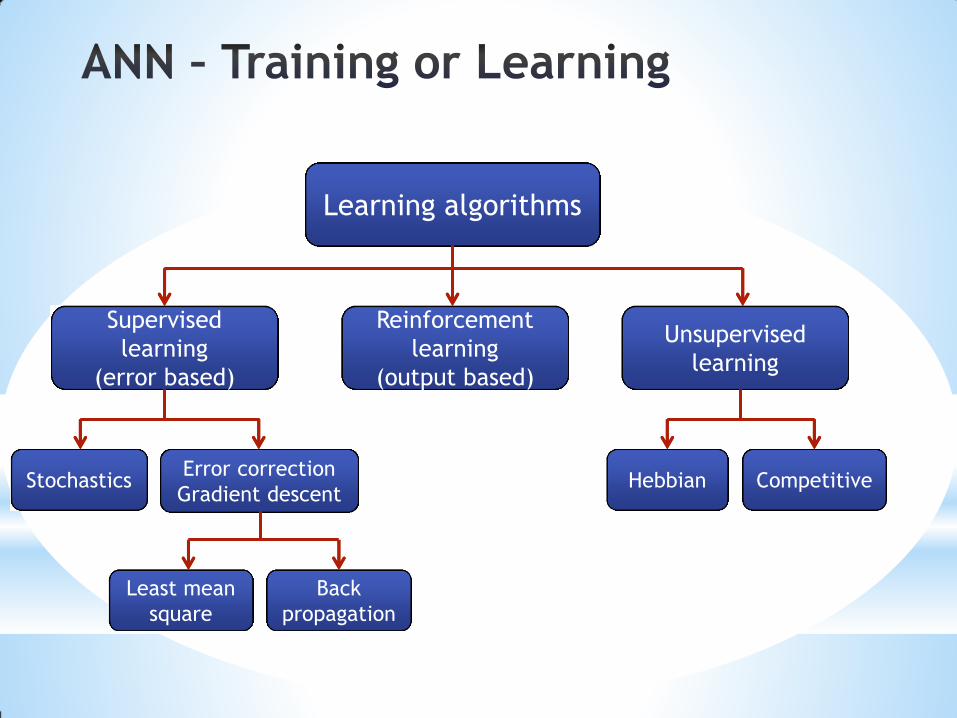
Supervised

learning

(error based)

Reinforcement

learning

(output based)

Unsupervised

learning

Hebbian Competitive Stochastics Error correction

Gradient descent

Least mean

square

Back

propagation

Learning algorithms

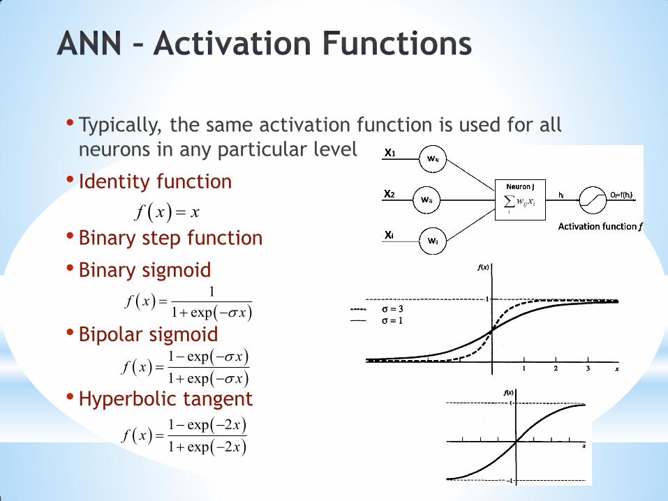
• Typically, the same activation function is used for all

neurons in any particular level

• Identity function

• Binary step function

• Binary sigmoid

• Bipolar sigmoid

• Hyperbolic tangent

f x x

1

1 expf x

x

1 exp

1 exp

xf x

x

1 exp 2

1 exp 2

xf x

x

•A gradient descent method to minimize the total

squared error of the output

•A backpropagation (multilayer, feedforward, trained

by backpropagation) can be used to solve problems

in many areas

•The training involves three stages

• The feedforward of the input training pattern

• The calculation and

backpropagation of the

associated error

• The adjustment of the

weights

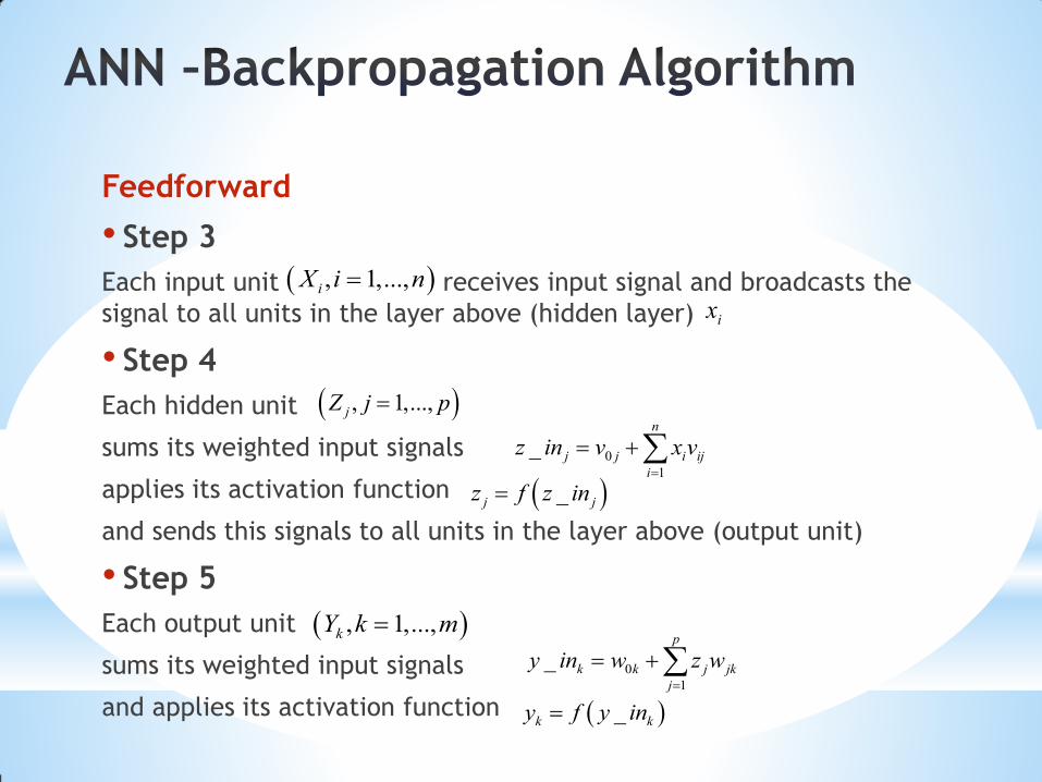
Feedforward

• Step 3

Each input unit receives input signal and broadcasts the

signal to all units in the layer above (hidden layer)

• Step 4

Each hidden unit

sums its weighted input signals

applies its activation function

and sends this signals to all units in the layer above (output unit)

• Step 5

Each output unit

sums its weighted input signals

and applies its activation function

, 1,...,iX i n

ix

, 1,...,jZ j p

0

1

_n

j j i ij

i

z in v x v

_j jz f z in

, 1,...,kY k m

0

1

_p

k k j jk

j

y in w z w

_k ky f y in

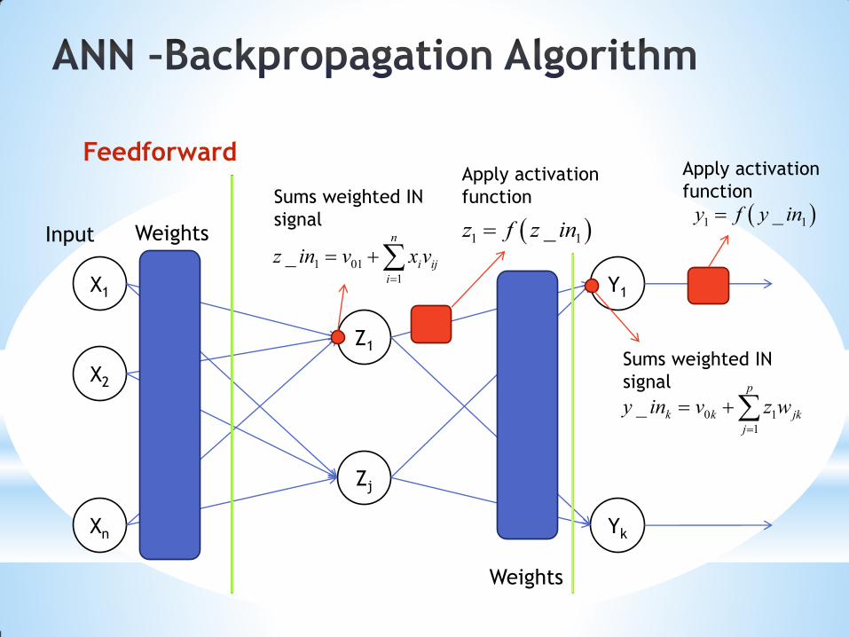
Feedforward

X1

X2

Xn

Z1

Zj

Y1

Yk

11v

1 jv

1nv

njv

21v

2 jv

Weights Input

1 01

1

_n

i ij

i

z in v x v

Sums weighted IN

signal 1 1_z f z in

Apply activation

function

11w

1jw

1kw

jkw

Weights

0 1

1

_p

k k jk

j

y in v z w

1 1_y f y in

Sums weighted IN

signal

Apply activation

function

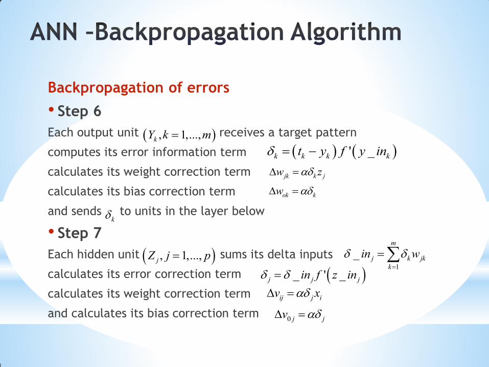
Backpropagation of errors

• Step 6

Each output unit receives a target pattern

computes its error information term

calculates its weight correction term

calculates its bias correction term

and sends to units in the layer below

• Step 7

Each hidden unit sums its delta inputs

calculates its error correction term

calculates its weight correction term

and calculates its bias correction term

, 1,...,kY k m

' _k k k kt y f y in

jk k jw z

ok kw

k

, 1,...,jZ j p1

_m

j k jk

k

in w

_ ' _j j jin f z in

ij j iv x

0 j jv

Backpropagation of errors

X1

X2

Xn

Z1

Zj

Y1

Yk

11v

1 jv

1nv

njv

21v

2 jv

Weights Input

Weight correction

term

11w

1jw

1kw

jkw

Weights

1 1 1 1' _t y f y in

Output

Error information

term

11 1 1w z

Bias correction

term

01 1w

1

1

_m

k jk

k

in w

Delta inputs

1 1 1_ ' _in f z in

Error information

term

01 1v

11 1 1v x

Weight correction

term

Bias correction term

Update weights and biases

• Step 8

Each output unit updates its bias and weights

Each hidden unit updates its bias and weights

, 1,...,kY k m 0,...,j p

jk jk jkw new w old w

ij ij ijv new v old v

, 1,...,jZ j p 0,...,i n

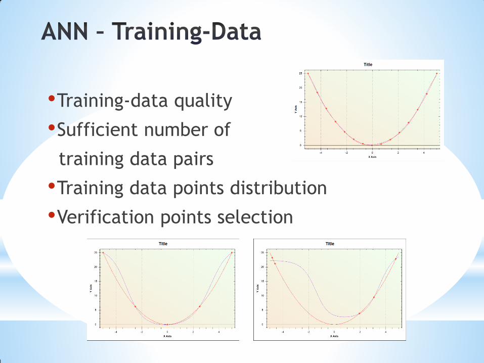
•Training-data quality

•Sufficient number of

training data pairs

•Training data points distribution

•Verification points selection

After training, a backpropagation NN is using only the

feedforward phase of the training algorithm

• Step1

Initialize weights

• Step2

For set activation of input unit

• Step3

For

• Step4

For

1,...,i n ix

1,...,j p 0

1

_n

j j i ij

i

z in v x v

_j jz f z in

1,...,k m 0

1

_p

k k j jk

j

y in w z w

_k ky f y in

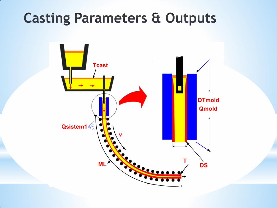
•21 Input parameters • Charge number

• Steel type

• Concentration: Cr, Cu, Mn, Mo, Ni, Si, V, C, P, S

• Billet dimension

• Casting temperature

• Casting speed

• Delta temperature

• Cooling flow rate in the mold

• Cooling water temperature in sprays

• Cooling flow rate in wreath spray system

• Cooling flow rate in 1st spray system

•21 Output parameters

• ML

• DS

• T

JMatPro Training Data Generator

Input parametrs Input parametrs Input parametrs

Physical

symulator

Physical

symulator

Physical

symulator

Training data file

. . .

. . .

Node 1 Node 2 Node i

ID Name & units Description Range in the training

set

1 Tcast [oC] Casting temperature 1515 - 1562

2 v [m/min] Casting speed 1.03 - 1.86

3 DTmold [oC] Temperature difference of cooling water

in the mold

5 - 10

4 Qmold [l/min] Cooling flow rate in the mold 1050 - 1446

5 Qwreath [l/min] Cooling flow rate in wreath spray

system

10 - 39

6 Qsistem1 [l/min] Cooling flow rate in 1st spray system 28 - 75

ID Name & units Description & units Range in the training

set

1 ML [m] Metallurgical length 8.6399 - 12.54

2 DS [m] Shell thickness at the end of the mold 0.0058875 - 0.0210225

3 T [oC] Billet surface temperature at

straightening start position

1064.5 - 1163.5

•NeuronDotNet open source library

•200000 total IO pairs

•100000 training IO pairs

•100000 verification IO pairs

•Settings for ANN

• Epochs 50000

• Hidden layers 1

• Neurons in

hidden layer 25

• Learning rate = 0.3

• Momentum = 0.6

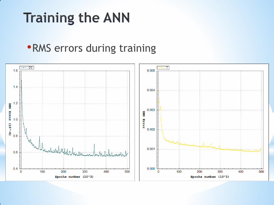
•RMS errors during training

•Relations between training time, training

data and errors

•Relative errors in verification points

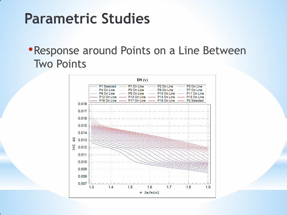
•Response around Points on a Line Between

Two Points

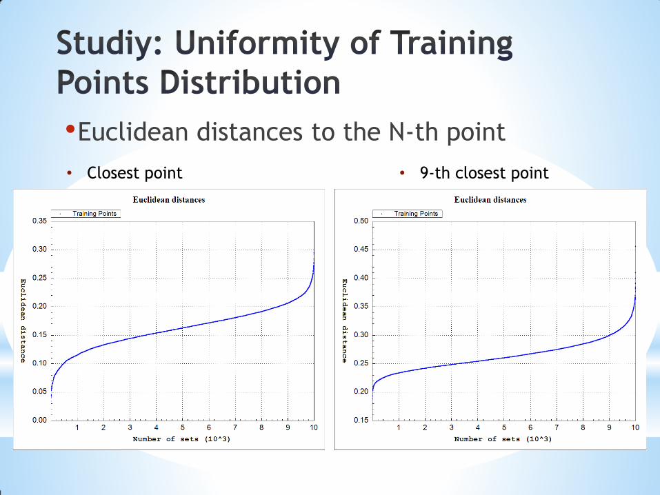
•Euclidean distances to the N-th point

• Closest point • 9-th closest point

•Dedicated SW framework was developed

• Studies to examine the accuracy of ANN based on physical model

•ANN approximation is much faster than physical simulation

•Complementing physical models with ANNs

•Replacing physical models with ANNs

•Upgrading of the ANN model for continuous casting with the model of the whole production chain

•Development of new methods for checking the quality of training-data

• ŠARLER, Božidar, VERTNIK, Robert, ŠALETIĆ, Simo, MANOJLOVIĆ, Gojko,

CESAR, Janko. Application of continuous casting simulation at Štore Steel.

Berg- Huettenmaenn. Monatsh., 2005, jg. 150, hft. 9, str. 300-306. [COBISS.SI-

ID 418811]

• Fausett L.. Fundamentals of neural networks: architectures, algorithms and

applications. . Englewood Cliffs, NJ: Prentice-Hall International, 1994.

• I. Grešovnik, T. Kodelja, R. Vertnik and B. Šarler: A software Framework for

Optimization Parameters in Material Production. Applied Mechanics and

Materials, Vols. 101-102, pp. 838-841. Trans Tech Publications, Switzerland,

2012.

• I. Grešovnik: IGLib.NET library, http://www2.arnes.si/~ljc3m2/igor/iglib/.

Prof.dr.Božidar Šarler, dr. Igor Grešovnik, dr. Robert Vertnik