thermal simulation of loudspeakers - freecyrille.pinton.free.fr/electroac/lectures_utiles... ·...

THERMAL SIMULATION OF LOUDSPEAKERS

Peter John ChapmanElectroacoustics Reasearch & Development

Bang & Olufsen ANStruer, Denmark

e:mail [email protected] fax 004597841250

1. Abstract

The paper describes the development of a system to simulate accurately the temperatures ofthe voice coil and magnet assembles in moving coil loudspeakers in real-time for anyprogramme material.

After initial parameter measurements on the loudspeaker there is no further need forconnection to the loudspeaker, the temperatures can be simulated independently. Thesimulation has been verified through measurements performed on bass, midrange, and tweeterunits.

2. Introduction

A great problem for loudspeaker designers and drive unit manufacturers is loudspeakerburn-out. This is caused by the heating effect of the voice coil when a signal is applied to it. Apoint is reached where either the resin on the voice coil melts causing short circuits or theflux of the magnet structure is darnaged causing loss of sensitivity and control. A 10 ?40 loss influx can occur for temperature changes of-90 degrees Celsius (OC) for neodymium magnets[1]. Failure of the unit results. The temperatures at which these phenomena occur depends onthe drive unit, for some units, temperatures exceeding 250 “C close to the voice coil can begenerated.

Another problem associated with this heating effect is thermal compression. Due to theincrease in temperature, the impedance of the drive unit also increases causing a lower powerto be applied to the loudspeaker resulting in a lower acoustic output. Also, the electrical Q ofthe drive unit is dependent on the DC resistance of the voice coil, which changes withtemperature, thus effecting the transfer fi-mction of the whole system.

To solve the problems mentioned above we need a knowledge of the actual voice coiltemperature that would occur during operation. Some systems have been developed tocalculate the temperature of the voice coil during operation of the loudspeaker system. Dr. IngGottfried Behler [2] created a system that measured the loudspeaker’s impedance duringoperation as a way to extract the DC resistance of the coil and hence extract the temperature.The author quotes an error of less than 5 “C.

However, a system that could give temperature data for a loudspeaker system without a needfor the loudspeaker to be under operation would be advantageous and allow flexiblesimulations to be made at any time, with any programme, without the risk of damaging anyunits.

3. Our Requirements For A Thermal Simulation System

The system should be capable of,

. receiving a standard digital audio signal from Compact Disc (CD) in S/P DIF format.

. filtering the input signal with a high order crossover.

. introducing an amplifier by means of a voltage gain and clipping function.

. calculating accurately the temperatures of the voice coil and magnet assemblies.

. running in real-time for up to a four-way, stereo, loudspeaker system withoutconnection to the loudspeaker.

4. Thermal Modelling A Moving Coil Loudspeaker - A New Model

The first consideration is modelling the thermal behaviour of the loudspeaker drive unit. Thissection describes the development of an accurate thermal model, a model that is different tothe model used previously by Henricksen [3] and other authors [1,4], a defence of which isgiven.

Previous work in this area has led to a model that is widely accepted and has been used forthe derivation of temperatures. The model is shown in figure 1 and is a lumped-elementmodel consisting of two cascaded parallel RC networks. The current flowing into the modelis the power, P, applied to the drive unit and the two RC time constants (RICI, R2C2)represent the thermal time constants of the voice coil and magnet systems respectively. T,represents the surrounding air temperature or ambient temperature and the voltages T,Cand T.represent the temperatures of the voice coil and magnet as lumped elements, above ambient.

The s-plane transfer functions (weres = jco) for this model are,

~ =P RI +R2+S(RIRZCZ +RlRZCl)Vc

1 +S(RICI +RZCZ)+S2(R1C1RLCZ)

T.=P ‘21 +S(R2C2)

Eqn 1

Eqn 2

Consider now a new model, shown in figure 2. The current flowing into the model is againthe power, P, applied to the drive unit and the time constants RICI and RZCZrepresent thethermal time constants of the voice coil and magnet systems respectively. T, represents thesurrounding air temperature or ambient temperature. The voice coil temperature, T,C, is nowgiven by the potential across the thermal capacitance Cl and the magnet temperature, T~, bythe potential across the capacitor Cz. The s-plane transfer functions for this model are,

T,c = PR1+R2+S(R1R2C2)

1 +s(RICl +RzC1 +RZCZ)+S2(R1C1RZCZ)Eqn 3

Tm=PR2

Eqn 41 +s(RICl +R2Cl +RZ@+S2(RlCl~ZCZ)

By comparing equations 1 and 3, it is clear that the two models can have the same inputimpedance and are therefore both equally valid for the calculation of the voice coiltemperature. However, it is not possible to obtain equal magnet temperature functions.

4.1 Second Order Thermal Model Step Responses

Consider now the step response of the new model. The instant a step isapplied, power Pflows into the voice coil and energy is dissipated in the coil. The remaining energy, P2, is fedthrough to the magnet system. Initially the powers will be different but will become equalwhen the current flow through Cl has stopped i.e. thermal conditions in the voice coil havestabilised.

Applying a step input to the model in figure 1, it is seen that equal power, P, must flow intoboth the voice coil and magnet systems. Hence, there can be no initial settling of the voicecoil system to effect the magnet temperature. Figures 3 and 4 show the voice coil and magnettemperatures, respectively, for the first few seconds when a step is applied to each model. Thecomponent values used are the actual thermal component values for a 19 mm tweeter. Thecomponent values for the model in figure 2 are (rounded to 3 s.f.),

R, = 9.25 c1 = 0.0910

%’ 35.1 c, = 15.2

The values for the model in figure 1 have then been adjusted to give the same voice coiltemperature for the first 40 seconds, within 2x10-7 ‘C. The values are (rounded to 3 s.f.),

R, = 9.14 c, = 0.0916Rz = 35.2 c, = 15.2

The time constant of the voice coil (RIC1 = 0.84 s) and its effect on the magnet temperature,in figure 4, given by the new model (solid curve) can be clearly seen. However, the magnettemperature given by model shown in figure 1 (dotted curve) does not account for thepresence of the voice coil. Therefore, the time constant of the voice coil has no effect on themagnet temperature.

One may argue that the difference between the two models is small, which is true in thisexample of a tweeter with a very short voice coil time constant, but the difference will beexaggerated for voice coils with much longer time constants and for signals other than stepfunctions, for example music.

For the above reasons and due to the interest in simulating both the voice coil temperatureand magnet temperatures, the new model in figure 2 was initially chosen to model a movingcoil loudspeaker.

4.2 A New Third Order Thermal Model

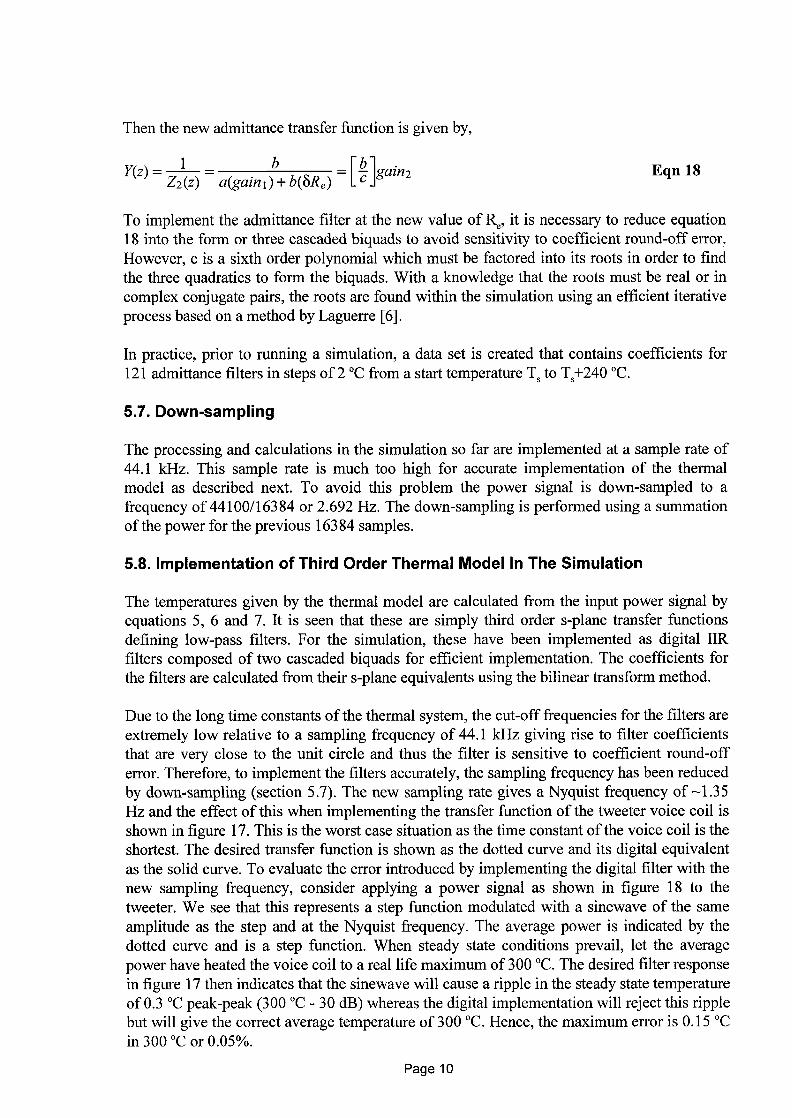
After development of the new second order model it was found that two time constants wasnot sufficient to model the thermal behaviour accurately. A third order model was thendeveloped and used for the simulation system. This model is shown in figure 5.

Figures 7,8 and 9 reveal the limitations of the second order model. They show the measuredand modelled voice coil temperature step responses for a 170 mm woofer. The measuredresponse is the same in all three figures and was measured as described in section 4.3.1.Figure 7 shows the early part of the step response.

It is clear that with two time constants it is not possible to model the complete step responseof the system. However, three time constants allow the complete thermal behaviour of thedrive unit to be modelled. The modelled thermal component values for the second ordermodel are (to 4 s.f.),

RI = 4.936 c, = 2.962 (RIC, = 14.62 S)

%= 2.843 c, = 741.4 (R,C, = 2108 S)

and the third order model,

RI = 3.927 c, = 2.358 (R,C, = 9.260 S)

Rz = 1.158 C* = 71.49 (R,C, = 82.79 S)

R, = 2.634 c, = 664.3 (R,C, = 1750 s)

It is seen that the shortest and longest time constants in each model correspond and that thethird order model introduces another time constant relatively close to that of the voice coil.Therefore, the temperatures given by the third order model, indicated in figure 5, are the voicecoil temperature TV,,the magnet temperature T. and a third temperature T~ relating to the gaptemperature or the temperature of the magnet surface close to the voice cod, above ambient.

Thoughts that the longest time constant in the third order model relates to the cabinet can bequickly expelled by monitoring the ambient temperature within the cabinet duringmeasurement of the step response. Also, for measurements and simulations with a musicsignal it is seen how the voice coil temperature quickly cools to the surrounding magnettemperature and in the case of a tweeter it is seen how the magnet temperature (as calculatedwith the third order model) fluctuates which is clearly not the cabinet temperature (figure 28).

The transfer functions for the third order model in figure 5 are as follows. The voice coiltemperature above ambient,

T,. = PRI +Rz+R3 +s(RIRzcz+RIRjcz+RIRjcj +RzRjc3)+s2(RlRzRjczcj)

1 +s(RzCz+RsCz+RsCs+RICl -t-R2C1 +Rscl)+s2(RzR3czcs +RlRzclcz

+f?lR3clc2 +R1R3C1C3 +R2R3C1C3) +S3(R1R2R3C1C2C3)

Eqn 5

The gap temperature,

Tg=PR2 +R3 +s(RzRscs)

1 +S(R2C2 +R3cz +R3C3 +RIC1 +R2C1 +Rjcl)+s2(RzRjczcj +RIRzclCz

+R]Rsclcz +RIRsclcs +RzRsclcs) +s3(RlRzR3clczcj)Eqn 6

The magnet temperature,

Tm=PR3

1 +s(RzCZ+RjCz+RjCj +RIC1 +RzC1 +Rjcl)+s2(RzRjczcj +RIRzcl Cz

+RIRsc]cz +RIRjclcj +RzRsclcs) +s3(RlRzRsclczcj)Eqn 7

The voice coil step response of the third order model is of the form,

H,c(t)=Ao +Alea]( +A2ea2t +A3ea3f Eqn 8

Where the coefficients An and an are related to the thermal component values ~ and C, andthe power P by multiplying equation 5 by 1/s and performing the inverse Laplace transform.The derivation is lengthy, requiring the use of partial fractions and the solving of third orderpolynomials. Hence, the derivation has not been reproduced here.

4.3 Measurement Of The Thermal Component Values

We have seen that the third order thermal model can accurately describe the thermalbehaviour of a moving coil loudspeaker. It now remains for the component values, ~ and Cn,in the model to be determined for any drive units of interest. With these parameters it is thenpossible to use the model in a simulation to obtain the temperatures of the voice, coil etc. froma knowledge of the power, P, applied to the loudspeaker unit.

The thermal parameters of the model, ~ and Cn, are derived from a measurement of the stepresponse of the loudspeaker. This step response is the rise in voice coil temperature when aconstant voltage is applied to the drive unit.

A constant voltage (or step) is applied in the form of a constant amplitude sinewave at afrequency where the impedance phase shift of the loudspeaker unit in the cabinet is zero. Atthis frequency the loudspeaker presents a resistive load and the precise power dissipated isthen known. With an applied rms voltage v, the current flowing in the voice coil is given by,

~= (Re :Rm)Eqn 9

Where R. is the initial DC resistance of the voice coil and R~+~ is the initial magnitude ofthe impedance at the chosen frequency of zero phase shift. The power, P, is then given by,

P=i2Re Eqn 10

In practice R, is a fimction of temperature, given by equation 14 (section 5.5). The voice coiltemperature is then measured while the step is applied to the loudspeaker. The voltage ischosen such that the drive unit is not damaged during the measurement which has to besufficiently long to allow determination of all three time constants of the third order model.Measurement of the voice coil temperature and determination of the thermal parameters forthree drive units is now described.

4.3.1 Measuring The Voice Coil Temperature

For the purpose of calculating the thermal component values and for verifjing the simulation,the voice coil temperature was measured using two methods. Firstly, by measuring the changein DC resistance of the voice coil where a small DC current flow in the coil allows thetemperature of the coil to be calculated from the increase in voltage, and secondly, in thespecial case of a 170 mm woofer, using a thermocouple wound into the voice coil. Thiswoofer was specially constructed by Peerless Fabrikkerne AUSof Denmark.

In each case, the voltage measured (either due to the change in DC resistance of the coil orfrom the thermocouple) is recorded using an 8 bit datalogger inside a personal computer. Thisgives a measurement resolution of -0.5 “C for measurements using the change in DCresistance of the coil (the precise resolution is given for the particular drive unit) and aresolution of 0.78 ‘C for measurements using the thermocouple. The datalogger samples dataat a frequency of 10 kHz and exports an average at intervals specified, for example eachsecond.

In practice, two measurements of the step response are made with the same voltage and withthe system at the same initial temperature equal to the ambient temperature (which ismonitored during measurements to ensure there are no changes to influence the results). Thetwo measurements are a long measurement and a much shorter measurement, the duration ofwhich are determined such that all time constants fall well within the long measuring time.The datalogger exports data at a much higher rate in the short measurement. This allowsaccurate derivation of all three time constants which are calculated from a curve fittingalgorithm that fits the model (described by equation 8) to the measurements. Details of themeasurements are given below for three difference drive units.

4.3.2 Measurement Of The Loudspeaker’s Impedance

For the step response it is necessary to apply a sinewave to the drive unit at a frequency wherethe impedance of the unit in the cabinet has zero phase shift. Therefore, it is necessary tomeasure the impedance of the driver in the cabinet. Measurements for this study have beenmade using a Bruel & Kjzer Audio Analyser type 2012. A frequency can then be selected fromthe measurement where the phase is zero. Note, however, that the phase will shift throughzero several times (twice for a driver in a sealed cabinet). The higher of the frequenciesshould be selected as the gradient of the phase shift is lower and therefore minimises errorscaused by slight variations in the frequency for the step response, also the oscillations of thesinewave will not be transposed onto the measurement as the frequency is not close to DC.The temperature at which the impedance measurement is made should also be recorded andthe step response measurements made at the same temperature, thus the DC resistance R. andthe value R, + ~ from the impedance measurement can be used for direct calculation of thepower applied during the step response. The impedance curve is also required for calculationof the power in the simulation as described in section 5.5.

4.3.3 Thermal Components For A 170 mm Woofer

The woofer was placed in a 50 litre sealed cabinet to give a smooth bass response with a -3dB frequency of 40 Hz. For measurement of the thermal step response a sinewave frequencyof 212 Hz was used at 11.12 Vrms. At this frequency the phase shift was 0.03° and the

magnitude of the impedance 6.02 ~. The DC resistance R. was 5.60 fl. The ambient

temperature during measurement of the impedance and measurement of the step response was22.5 “C.

Figure 9 shows the long measurement, where the rise in voice coil temperature has beenrecorded at 1 Hz (1 sample per second) for 5500 seconds. Figure 10 shows the shortmeasurement, measured at a rate of 1 sample every 20 ms for 110 seconds. The first 4096points of each measurement are then used as target curves for an algorithm to fit the thirdorder thermal model to the measurements. The resolution of the measurement is 0.78 ‘C.

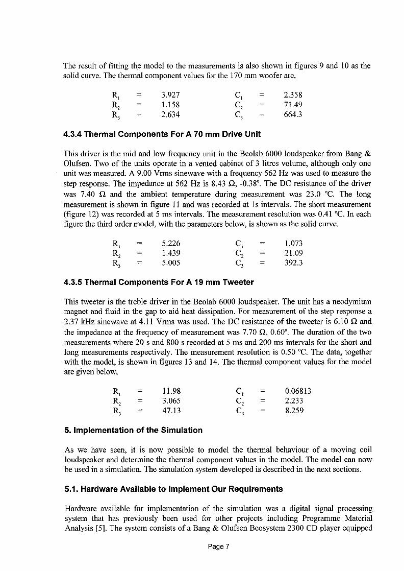
The result of fitting the model to the measurements is also shown in figures 9 and 10 as thesolid curve. The thermal component values for the 170 mm woofer are,

RI = 3.927 c1 = 2.358Rz = 1.158 c, = 71.49R, = 2.634 c, = 664.3

4.3.4 Thermal Components For A 70 mm Drive Unit

This driver is the mid and low frequency unit in the Beolab 6000 loudspeaker from Bang &Olufsen. Two of the units operate in a vented cabinet of 3 litres volume, although only oneunit was measured. A 9.00 Vrrns sinewave with a frequency 562 Hz was used to measure the

step response. The impedance at 562 Hz is 8.43 S2, -0.38°. The DC resistance of the driver

was 7.40 Cl and the ambient temperature during measurement was 23.0 “C. The long

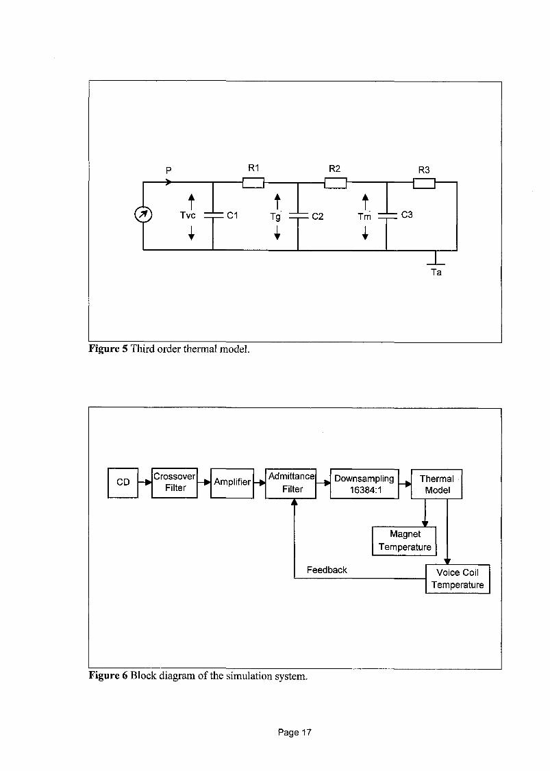
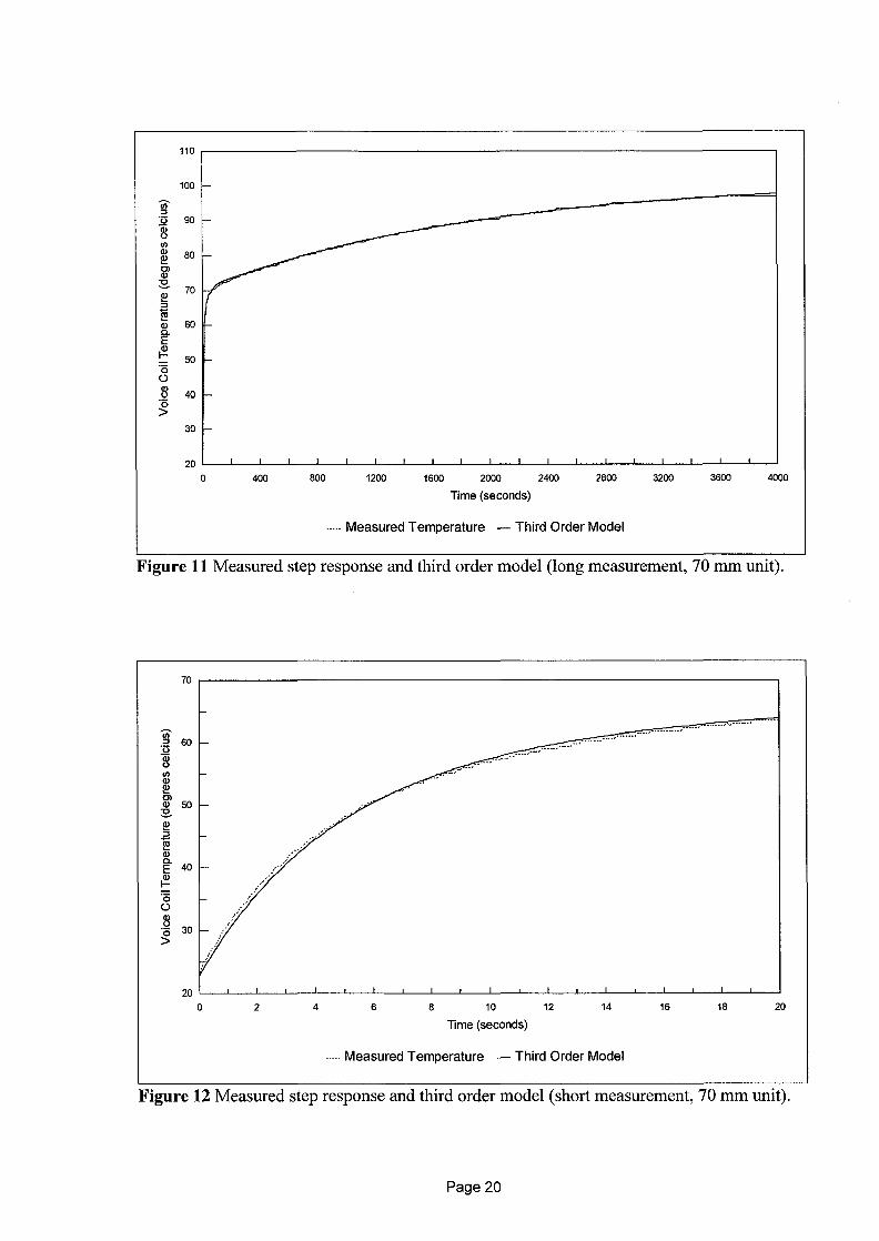
measurement is shown in figure 11 and was recorded at 1s intervals. The short measurement(figure 12) was recorded at 5 ms intervals. The measurement resolution was 0.41 “C. In eachfigure the third order model, with the parameters below, is shown as the solid curve.

R, = 5.226 c, = 1.073R, = 1.439 C* = 21.09R, = 5.005 C3 = 392.3

4.3.5 Thermal Components For A 19 mm Tweeter

This tweeter is the treble driver in the Beolab 6000 loudspeaker. The unit has a neodymiummagnet and fluid in the gap to aid heat dissipation. For measurement of the step response a

2.37 kHz sinewave at 4.11 Vrms was used. The DC resistance of the tweeter is 6.10 ~ and

the impedance at the frequency of measurement was 7.70 Q, 0.60°. The duration of the two

measurements where 20 s and 800 s recorded at 5 ms and 200 ms intervals for the short andlong measurements respectively. The measurement resolution is 0.50 “C. The data, togetherwith the model, is shown in figures 13 and 14. The thermal component values for the modelare given below,

R, = 11.98 c, = 0.06813Rz = 3.065 C2 = 2.233R~ = 47.13 c, = 8.259

5. Implementation of the Simulation

As we have seen, it is now possible to model the thermal behaviour of a moving coilloudspeaker and determine the thermal component values in the model. The model can nowbe used in a simulation. The simulation system developed is described in the next sections.

5.1. Hardware Available to Implement Our Requirements

Hardware available for implementation of the simulation was a digital signal processingsystem that has previously been used for other projects including Programme MaterialAnalysis [5]. The system consists of a Bang & Olufsen Beosystem 2300 CD player equipped

with a digital audio output in S/P DIF format. This signal is input to an audio input interfaceand format conversion board prior to the digital signal processor (DSP). The DSP comprisesof four 40 MHz floating-point Motorola DSP96002 boards from Loughborough SoundImages, UK. The host PC is a Compaq SystemPro LT. The DSP boards are programmed inMotorola assembly code and the host PC in Borland C++.

5.2. Overview of the Simulation

A block diagram of the complete simulation for one audio channel and a single crossover isshown in figure 6. In practice, two audio channels can each be filtered using a four-waycrossover system simultaneously, outputting 16 temperatures (2 channels x 4 x voice coil andmagnet temperatures) in real time.

5.3. Input Signal & Crossover

The input signal is standard digital audio in S/P DIF format from compact disc at a samplingrate of 44.1 kHz. For the purpose of modelling a crossover in the loudspeaker system, thesignal can then be filtered using up to a tenth order filter, This IIR filter is implemented in theform of 5 cascaded biquads, to reduce the effects of coefficient sensitivity, and a gaincoefficient. If no crossover is required, then the coefficients can simply be set to zero with aunity gain coefficient. An example of the z-plane transfer function for a fourth ordercrossover is shown below,

H(z) =[ 1[1 +aolz-1 +a(Dz-2 1 + allz-1 +alzz-z

1 +/?012-1 +b02z-2 1 +bllz-l +b12z 1_2win Eqn 11

5.4. Amplifier Section

For the purposes of modelling an amplifier a simple voltage gain was chosen that scales thevoltages to actual level, for example +/- 50 V peak. This is somewhat ideal but it could beargued that amplifiers used are sufficiently linear and of low distortion for this simple modelto be accurate.

However, high temperatures within a loudspeaker are generated by large voltages beingapplied and this often implies clipped output signals from the amplifier. For this reason, thesimple amplifier model above has been extended by including a hard clipping function, thatclips the signal at a specified level, for both positive and negative signal.

The signal now represents the voltage as a function of time, v(t), appearing at the terminals ofthe loudspeaker.

5.5. Calculation Of Signal Power -An Admittance Filter

To calculate the power applied to the loudspeaker and hence the thermal model, one needs aknowledge of the instantaneous current flowing in the voice coil. If the loudspeaker presenteda purely resistive load that was independent of temperature then the power could becalculated from the squared voltage divided by this resistance. However, the loudspeaker hasa complex impedance that is dependant upon frequency (f) and temperature (T). Figure 15shows a typical impedance curve magnitude, Z(f,T).

The current flowing in theinverse of the impedance, orfor the impedance in figure

voice coil can be calculated by filtering the voltage with thethe admittance function Y(f,T). The admittance curve magnitude15 is shown in figure 16. The current in the voice coil is now

given by,

i(t,j T) = V(f)&?

Where the current in the

= v(t) Y(JT) Eqn 12

voice coil is a function of time, frequency and temperature. It can be

seen that the admittance function is dependant upon temperature. However, data given byGottfried [2], shows that the change due to temperature is almost entirely a shift in DCresistance R,. Therefore, the simulation considers a single impedance measurement made atnormal ambient temperature and introduces the temperature dependence through the changein R.. This method then avoids having to measure the loudspeaker’s impedance at manytemperatures.

The power flowing into the thermal model in then given by,

P(l,j 1“)= [i(t,j T)]2R.(T) Eqn 13

Where, T is initially the start temperature or ambient and then subsequently the voice coiltemperature as calculated by the model. R, at a temperature T for a voice coil wound fromcopper wire is given by,

R,(T) =

u is the

R,(TO)[l +(x(T– T())]

temperature coefficient

Eqn 14

of copper (0.004 K-l) and R~(TO)is the DC resistance of the

coil at ambient temperature (or the temperature at which the impedance measurement wasmade).

5.6. Implementing the Admittance Filter

Filtering the voltage signal v(t) to obtain the current is performed in the simulation with asixth order IIR filter. This is sufficient to model the admittance curve for a vented boxloudspeaker. Initially a sixth order transfer fimction in the form of three cascaded biquads isfitted to the impedance measurement. This z-plane transfer fiction maybe written as,

Zl(z) =[ 1[ 1[1 +aolz-l + ao2z-2 1 +allz-l +a12z-2 1 +a21z-1 + a22z-21_2win1 Eqn 15

1 +bolz-1 +b02z-2 1 +bllz-1 +blzz-z 1 +b21z-1 +I)22Z

Which can be written as,

[1Z1(z)= ~ gainl

With the increased DC resistance, the new impedance will be,

Z2(Z) = Z1(z) + 6Re =[1~gain ~i- 6Re =a(gain 1) + b(bR.)

b

Eqn 16

Eqn 17

Then the new admittance transfer function is given by,

Y(z) = ~ = b [1bZZ(Z) a(gainl) + b(Me) = z ‘ain2

Eqn 18

To implement the admittance filter at the new value of R., it is necessary to reduce equation18 into the form or three cascaded biquads to avoid sensitivity to coefficient round-off error.However, c is a sixth order polynomial which must be factored into its roots in order to findthe three quadratics to form the biquads. With a knowledge that the roots must be real or incomplex conjugate pairs, the roots are found within the simulation using an efficient iterativeprocess based on a method by Laguerre [6].

In practice, prior to running a simulation, a data set is created that contains coefficients for121 admittance filters in steps of 2 “C from a start temperature T, to T,+240 ‘C.

5.7. Down-sampling

The processing and calculations in the simulation so far are implemented at a sample rate of44.1 kHz. This sample rate is much too high for accurate implementation of the thermalmodel as described next. To avoid this problem the power signal is down-sampled to afrequency of 44100/16384 or 2.692 Hz. The down-sampling is performed using a summationof the power for the previous 16384 samples.

5.8. Implementation of Third Order Thermal Model In The Simulation

The temperatures given by the thermal model are calculated from the input power signal byequations 5, 6 and 7. It is seen that these are simply third order s-plane transfer functionsdefining low-pass filters. For the simulation, these have been implemented as digital IIRfilters composed of two cascaded biquads for efficient implementation. The coefficients forthe filters are calculated from their s-plane equivalents using the bilinear transform method.

Due to the long time constants of the thermal system, the cut-off frequencies for the filters areextremely low relative to a sampling frequency of 44.1 kHz giving rise to filter coefficientsthat are very close to the unit circle and thus the filter is sensitive to coefficient round-offerror. Therefore, to implement the filters accurately, the sampling frequency has been reducedby down-sampling (section 5.7). The new sampling rate gives a Nyquist frequency of-1.35Hz and the effect of this when implementing the transfer function of the tweeter voice coil isshown in figure 17. This is the worst case situation as the time constant of the voice coil is theshortest. The desired transfer function is shown as the dotted curve and its digital equivalentas the solid curve. To evaluate the error introduced by implementing the digital filter with thenew sampling frequency, consider applying a power signal as shown in figure 18 to thetweeter. We see that this represents a step function modulated with a sinewave of the sameamplitude as the step and at the Nyquist frequency. The average power is indicated by thedotted curve and is a step function. When steady state conditions prevail, let the averagepower have heated the voice coil to a real life maximum of 300 ‘C. The desired filter responsein figure 17 then indicates that the sinewave will cause a ripple in the steady state temperatureof 0.3 ‘C peak-peak (300 “C -30 dB) whereas the digital implementation will reject this ripplebut will give the correct average temperature of 300 “C. Hence, the maximum error is 0.15 ‘Cin 300 ‘C or 0.05°/0.

With the new sampling frequency, the simulation will calculate voice coil and magnettemperatures approximately three times each second (441 00/1 6384 per second). Thetemperature T~ could easily be calculated, although it has not been in this simulation system.

6. Running The Simulation

Through a measurement of the step response of the loudspeaker drive units it is possible todetermine the thermal component values of the third order thermal model for each unit. Theresults for three units have been presented. In order to make any simulations it is necessary tocompile a data set for a particular simulation. This data set contains,

.

.

.

.

.

.

.

.

Filter coefficients for up to a tenth order crossover filter.A peak amplifier output voltage.A clipping voltage (to implement hard clipping of the signal if necessary).The ambient temperature at which the impedance and step responses were measured.The DC resistance of the voice coil at the above ambient temperature.An ambient temperature at which to start the simulation.121 sets of filter coefficients for the admittance filter generated from the coefficientsfor a sixth order filter modelling the impedance curve of the drive unit and thetemperature coefficient of the voice coil material.Filter coefficients for the fourth order filters to implement the thermal model.

The data set is created using software written for the simulation system in Borland C++ andtakes a matter of seconds to be compiled. The data can now be used for simulation of thetemperatures of the particular loudspeaker at any time and for any programme material. If anew crossover is required for example, a new data set can simply be made.

7. Simulations And Measurements With Music

For verification of the simulation system, the temperature of the voice coil and magnet foreach of the three drive units mentioned has been measured and simulated. The Pink Floydalbum “Dark Side of the Moon” on EMI Record Ltd was used. The period for themeasurements and simulations was 3000 s. This period includes the complete album andseveral minutes extra. The temperatures were recorded at 1 s intervals for the measurements.The left audio channel was measured. For each drive unit the complete 3000 s period ispresented together with a 600s period from within the complete period to show detail.

Figures 19-22 show results for the 170 mm woofer. The measured voice coil temperature,obtained using the thermocouple wound into the voice coil, is shown in figures 19 and21. Nocrossover filter was used and the peak, unclipped voltage from the amplifier was 45.7 V.Figures 20 and 22 show the simulated temperature of the voice coil and magnet.

Figures 23-26 show results for the 70 mm driver. The music signal in this case was low passfiltered at 3 kHz with a 24 dB/octave Linkwith-Riley filter. No high pass filter was used. Theconsequence of not using a high pass filter is that bleed-through of the music signal appearson the measurement. This is seen as noise on the measurements in figures 23 and 25. Theunclipped peak voltage on the driver was 38.6 V. The simulation of the temperatures isshown in figures 24 and 26.

Measurements and simulations for the 19 mm tweeter are displayed in figures 27 to 30. Thesignal to the tweeter was high pass filtered at 3 kHz with a 24 dB/octave Linkwith-Rileyfilter. The unclipped peak voltage on the tweeter was 38.6 V.

8. Discussion Of Results

Firstly, let us consider the difference in resolution between the simulations and themeasurements for verification of the simulations. There are two differences, in time and intemperature:

c Resolution In Time:The music signal measurements of voice coil temperature are written to file at intervals of 1 s.Each of these temperatures is an average of 10000 samples made by the datalogger eachsecond. Therefore, the measurements are short term averages. The simulations however,calculate temperatures at intervals of 0.372 s. The effect of this time discretisation will causedifferences in the short term peak and short term low temperatures. The simulation willindicate slightly higher peak temperatures and slightly lower low temperatures due to themeasurement to some extent averaging away these short term peaks and dips,

● Resolution In Temperature:The simulated temperatures written to file by the simulation system and are rounded to thenearest 0.01 “C. The temperature resolution of the measurements is limited by the 8 bitdatalogger. In the case of the 170 mm woofer, this resolution is 0.78 “C and for the 70 mmunit and tweeter is 0.41 “C and 0.50 ‘C respectively. This quantisation is seen as ‘steps’ in themeasurements, particularly visible for the 600 s periods of the music signal and for thetweeter measurements.

The results for each of the three loudspeaker units are now discussed.

● Results for the 170 mm Woofer:Considering the 3000 s period in figures 19 and 20, it is seen that the simulation calculatestemperatures above approximately 35 “C to within 1.5 ‘C of the measurement. Below 35 “C,when the voice coil cools during periods of relative quiet in the music, the simulationindicates lower temperatures than the measurement but the error is never greater than 2 “C.This is caused by the voice coil in the measurement cooling to its surrounding temperature,the temperature of the magnet close to the voice coil. However, the simulation assumes thesystem is composed of lumped elements and thus the voice coil will cool to a temperaturecloser to the average temperature of the magnet system. Figures 21 and 22 show the 600 speriod and indicate that the simulation reveals more details in the temperature than it has beenpossible to measure.

● Results for the 70 mm Unit:The results are shown in figures 23 to 26. The measurement circuit used to extract the DCresistance of the voice coil and hence the temperature is essentially a first order low pass filterwill a very low cut off frequency. The loudspeaker was driven with the music signal low passfiltered below 3 kHz. Consequently, low frequency music signals are passed through themeasuring circuit resulting in noise on the measurement. Hence, it is not possible to comparedetail although one sees that the simulated temperature lies within the noisy measurement.

At the end of the 3000 s period when the music signal has ended (when there is no noise onthe measurement) the simulation is 0.5 ‘C below the measurement.

● Results for the 19 mm Tweeter:Figures 27 to 30 show the simulation of the tweeter temperatures to be very close to themeasurement. However, the resolution in the measurement causes detail to be lost, the resultbeing that the simulation indicates higher short term peaks in the voice coil temperature.Comparing figures 29 and 30, the 600 s period, we see the simulated temperature showingevery detail of the temperature fluctuations, within 0.7 ‘C of the measurement. During periodsof quiet in the music signal it is seen that the voice coil temperature cools to the magnettemperature in the simulation. This also closely matches the cooling of the measured voicecoil temperature. The simulation is much more accurate during periods of quiet for thetweeter because the tweeter thermal behaviour is much closer to a lumped system. Also, thetweeter has fluid in the gap giving more efficient heat dissipation from voice coil to magnet.

Comparing the complete 3000 s period for the tweeter, figures 27 and 28, the simulation isvery close to the measurement for the initial 1600s. After this time the simulation slowly fallsbelow the measurement to 1.5 “C lower at the end of the period. This is most likely caused bya small increase in the ambient temperature towards the end of the measurement period.

8.1. Possible Errors in the Simulation Process

● Possible errors in the measurement of the step response:“ During measurement of the step response for derivation of the thermal component values, asinewave is applied at a frequency of zero phase shift. However, the phase shift may not beexactly zero and also during the long measurements, changes in the loudspeaker parametersmay cause the phase to change. This will cause small variations in the power applied.● The measuring circuit used to measure changes in the DC resistance of the voice coil hasitself a step response. However, the time constant of the measuring circuit is approximately0.1 s and hence is still small relative to the time constant of the tweeter voice coil.● The ambient temperature during measurements may change and small variations may beunnoticed.● Some power during the measurement will be dissipated in the mechanical resistance ~,however this is somewhat taken into account (section 4.3).

● Possible errors in the simulation:● The amplifier model in the simulation assumes no distortion of the signal unless hardclipping is implemented.● The admittance filter used for calculation of the current flowing in the voice coil is a sixthorder digital filter calculated from the measured impedance curve of the loudspeaker. Thepeaks in the impedance and the high frequency increase caused by L. are modelled usingbiquad sections. Hence, there will be differences between the digital filter and the trueimpedance.● The simulation assumes the increase in temperature causes a simple increase in DCresistance R..● During operation of the loudspeaker there is forced air cooling of parts of the system by themovement of the cone. This effect is not included directly in the simulation, however, it isincluded during measurement of the step response of the loudspeaker and derivation of thethermal component values.

“ The thermal model is implemented as digital filters and errors caused by this are evaluatedin section 5.8.● The thermal model assumes the thermal system is composed of lumped elements. Errorscaused by this will be most obvious for drive units with large magnets. This has beensomewhat included by using a third time constant close to that of the voice coil.

9. Conclusion

From the results for the music signals it is seen that the simulations are accurate, with errorsbetween the measurements and simulations being less than 2 ‘C. For the 19 mm tweeter,which has given the most accurate results, the error on average being approximately 0.7 “C. Itis also possible to conclude that the simulation reveals more detail in the temperature of thevoice coil than it has been possible to measure.

It can also be concluded from the results that errors introduced by non-linearities, forcedcooling, and the effects of the cabinet are small. This is because the simulation is based on ameasurement that includes, to a large extent, these effects. Largely, any errors in the systemcome from errors in the measurement of the step response of the loudspeaker and calculationof the thermal component values. Calculational errors in the simulation are very small.

With an accurate means of simulating the temperatures in a loudspeaker, it is now possible touse this knowledge to eliminate thermal compression and to protect the drive units fromdamage caused by the heating effect of the signal. Also, with a simulation that does notrequire connection to the loudspeaker, any investigations into power handling or thedevelopment of protection systems can be made without damaging any drive units.

10. Acknowledgements

Many thanks for their assistance to Gert Munch and Jan Abildgaard Pedersen of Bang &Olufsen and Knud Bank Christensen, originally of Bang & Olufsen but now of TC Electronic,Aarhus Denmark.

11. References

[1]

[2]

[3]

[4]

[5]

[6]

‘Heat Dissipation and Power Compression in Loudspeakers’, D. J.Button, J. AudioEng. Sot., Vol 40 No 1/2, January/February 1992.‘Measuring the Loudspeaker’s Impedance During Operation for the Derivation of theVoice Coil Temperature’, Dr. Ing Gottfried Behler, a paper of the 98th AESConvention Paris, preprint No 4001, February 1995.‘Heat Transfer Mechanisms in Loudspeakers: Analysis, Measurement and Design’,C.A.Henricksen, J. Audio Eng. Sot., Vol 35 No 10, October 1987.‘Modelling of the Thermal Behaviour of High Power Loudspeakers’, Dr. Ing GottfriedBehler, a paper of the 15th International Congress on Acoustics, Trondheim Norway,June 1995.‘Programme Material Analysis’, P.J. Chapman, a paper of the 10Oth AES ConventionCopenhagen, preprint No 4277, May 1996.Laguerre’s Method, ‘Numerical Recipes in C’, The Art Of Scientific ComputingSecond Edition, Cambridge University Press, ISBN O 521431085, Chapter 9.5.

RI R2

P P\

“1

II II

Tvc Cl Tm C2 IfP

1 1I

Figure 1 Previously used second order thermal model of a moving coil loudspeaker.

P RI p2 R2\

“ Ir ‘ r

\

~“Tvc = = cl Tm = — C2

1 1I

Figure 2 New second order thermal model of a moving coil loudspeaker.

Tvcl(t)

Tvc2( t )

2 –

n I I I I I I I

0,5 1 1.5 2 2.5 3 3.5 4

t

~igure3 Voice coil step responses for each second order thermal model (19 mm tweeter).

0,3

0.25

0.2

Tml(t)0,15

Tm2(t)

0.1

0.05.-

/-

.-()* - I I I I“o 0.5 1 1,5 2 2.5 3 3.5 4

t

Figure 4 Magnet step responses for each second order thermal model(19 mm tweeter).

P RI R2 R3

tTrn — C3

iT

Ta

Figure 5 Third order thermal model.

I

CDCrossover

+ Amplifier -bAdmittance ~ Downsampling Thermal

Filter Filter 16384:1 Model

A

*Magnet

Temperature

●

Feedback Voice Coil

Temperature

Figure 6 Block diagram of the simulation system.

140

120

100

80

60

40

20 I 1 1 1 I 1 I t 1 t I I I I t I I I 1

0 40 80 120 160 200 240 280 320 3W 400

Time (seconds)

--- Measured Temperature — Third Order Model + Second Order Model

Figure 7 Measured and simulated step responses for 170 mm woofer.

140

120

Iw

80

60

40

20

.————

~..-

1 I I k I I I I I I I 1 I I I I t I I

0 400 800 1200 1600 2000 2400 2800 3200 3600 4000

Time (seconds)

.----Measured Temperature + Second Order Model

Figure 8 Measured step response and second order model(170 mm woofer).

140

120

100

80

60

40

I 1 1 1 I I I 1 I 1 1 I I I I I I I I

o 400 800 1200 1800 2000 2400 2800 3200 360Q 4000

Time (8econds)

..... Measured Temperature — Third Order Model

~igure 9 Measured step response and third order model (long measurement, 170 mmwoofer).

140

120

lm

80

60

40

20

----------.... ...... . . ... ..........-,.-,,.,,...........,.......... . .-.-,

I I I I 1 I 1 I I [ I I 1 I I I , I

o 10 20 30 40 50 60 70 60 90 100

Time (seconds)

.----Measured Temperature — Third Order Model

Figure 10 Measured step response and third order model (short measurement, 170 mmwoofer).

110

100

90

80

70

60

50

40

30

20 I I 1 I I 1 I I 1 1 I I I 1 1 I [ I I

0 400 800 1200 160+3 2000 2400 2800 3200 3600 4000

Time (seconds)

. Measured Temperature — Third Order Model

Figure 11 Measured step response and third order model (long measurement, 70 mm unit).

70

20 1 I t 1 I I 1 I t I I 1 I 1 , 1 ,

0 2 4 6 6 10 12

Time (seconds)

.. Measured Temperature — Third Order M(

4 16 18 20

del

Figure 12 Measured step response and third order model (short measurement, 70 mm unit).

110

100

90

80

70

60

50

40

30

20 — 1 1 1 I I 1 I I I I I I I I 1 1 I I I

o 80 160 240 320 400 460 560 640 720 8W

Time (seconds)

..... Measured Temperature — Third Order Model

Figure 13 Measured step response and third order model (long measurement, 19 mmtweeter).

70

20 I , I I , I I I I 1 I I ,

0 2 4 8 8 10 12 14 16 18 20

lime (seconds)

-----Measured Temperature — Third Order Model

Figure 14 Measured step response and third order model (short measurement, 19 mmtweeter).

30

20

10

0

..

. .

.-

-...

7

10 100

1)

—

—

.—

.-.

k

—

...—.—-.

-...—-

--.—.

P--’-....

-1000

Frequency (Hz)

—-—..-...

/ -..—-

—-—.

10000

...

---

---

..

-.

..

..

100000

Figure 15 Typical impedance of a loudspeaker unit in a vented cabinet.

0,14

0.12

0.10

0.04

0.02

0.00

..

.

.

1...

{

—-

-----

.-.

.

r

.-

.

.

.

10

Frequency (Hz)

—,

—..

\

---

.—..

..

-.

-.

\

.

.—.—

.—-..

.—--

.. . ..

..—---

\

.-

—-

—

.-..

.-.,

..—

)0

’60

70

L’800

—

-.:

----

0.001

—

—0.01

—

—

—

. .

—

—

-’---

—

0.1

—

---

—1

—

—

~igure 17 Transfer function of thermal model for the 19 mm tweeter voice coil.

2.5 I I 1 I

2 –

g 1,5 –

s~

~

$1 – ,

/“ ‘- ‘--””- ‘-

0,5 –

0 I / I J–1 0 1 2 3 4

Time (s)

Figure 18 Example of an applied power signal to indicate error caused by digital filterimplementation of thermal model for tweeter voice coil.

This page is left blankintentionally

70

60

30 A L

120 I I I I ~

o 300 600 900 1200 15011 1800 2100 2400 2700 3000

Tme (seconds)

‘igure 19 Measured 170 mm woofer voice coil temperature (3000 s period).

70

60

30

20

L____----...................-..-’--—-——-----

I I I I I I I I I

o 300 600 900 1200 1500 1800 2100 2400 2700 3000

i

Tme (seconds)

‘igure 20 Simulated 170 mm woofer voice coil and magnet temperatures (3000 s period).

70

60

30

20

J+

I I I I I I I I t

900 960 1020 1080 1140 1200 1260 1320 1380 1440 1500

Tme (seconds)

Figure 21 Measured 170 mm woofer voice coil temperature (600 s period).

70

60

30

20

900 960 1020 1080 1140 1200 12641 1320 1380 1440 1500

ilme (seconds)

‘igure 22 Simulated 170 mm woofer voice coil and magnet temperatures (600 s period).

70 —

60

~.-2E 50

%$2g=~

~ ~o _

j

30

I

20 —

o 300 600 900 12W 1500 18(MI 2100 2400 2700 3000

Tme (seconds)

~igure23 Measured 70 mm unit voice coil temperature (3000s period).

70

60

z.2~E 50

8P!8=g3

2 40

ep

30

20

0 300 600 9CJJ 1200 1500 180Q 2100 2400 2700 3000

lime (seconds)

Figure 24 Simulated 70 mm unit voice coil and magnet temperatures (3000s period).

70

50

40

30

20 I I I I 1 I I I I

900 960 1020 1080 1140 1200 1260 1320 1380 1440 1500

ilme (seconds)

,. ---- --- . . . .Igure 23 Measured ‘/Umm umt voice coil temperature (600 s period).

70

60

30

20

900 960 1020 1060 1140 1200 1260 1320 1380 1440 1500

Tme (seconds)

igure 26 Simulated 70 mm unit voice coil and magnet temperatures (600s period).

70

30

20

0 300 600 900 1200 1500 1800 2100 2400 2700 30W

lime (seconds)

70

60

30

I

20

0 300 600 900 1200 1500 1800 21W 2400 2700 30113

Time (seconds)

Figure 28 Simulated 19 mm tweeter voice coil and magnet temperatures (3000s period).

70

60

~.-=: so

~al=g

~ 40

eP

30

20

900 960 1020 1080 1140 1200 1280 1320 1380 1440 15CCJTime (seconds)

r Igure ZY lweasureci 1Y mm tweeter voice coil temperature (600s period).

50

40

20 I I I I I I I I I I

900 960 1020 1080 1140 1200 1280 1320 1380 1440 1500Time (seconds)

Figure 30 Simulated 19 mm tweeter voice coil and magnet temperatures (600 s period).

thermal simulation of loudspeakers - freecyrille.pinton.free.fr/electroac/lectures_utiles... ·...

Documents