thermal properties of building materials evaluated by a dynamic simulation of a test cell

Solar Energy Vol. 69, No. 4, pp. 295–304, 20002000 Elsevier Science Ltd

Pergamon PII: S0038 – 092X( 00 )00102 – X All rights reserved. Printed in Great Britain0038-092X/00/$ - see front matter

www.elsevier.com/ locate / solener

THERMAL PROPERTIES OF BUILDING MATERIALS EVALUATED BY ADYNAMIC SIMULATION OF A TEST CELL

†G. LEFTHERIOTIS and P. YIANOULISDepartment of Physics, University of Patras, Patras 26500, Greece

Received 8 February 2000; revised version accepted 25 May 2000

Communicated by VOLKER WITTWER

Abstract—A method for the measurement of thermal properties of building components under controllableconditions is presented. It is based on the use of a test cell designed to enable calculation of thermal propertiessolely from temperature readings, without the need for power measurements. The test cell’s low thermal inertiaallows short testing times (about 3 h). Using an appropriate thermal network to simulate the dynamic behaviorof the test cell, predicted results were found to have a 0.68C maximum temperature deviation with measuredtest cell responses. The thermal transmittance (U-value) of an insulating block, a single glass sheet and adouble glazing have been measured with an accuracy of about 5%. A simulation of a scaled-up test cell withdimensions 6.0 m 3 6.0 m 3 4.5 m has revealed that the test cell’s response to temperature changes dependsstrongly on the amount of wall insulation. The scaled-up test cell exhibits a relatively fast response totemperature changes (9 to 18 h) due to its low thermal mass. 2000 Elsevier Science Ltd. All rightsreserved.

1. INTRODUCTION The hot box method can be used to measure thesteady-state thermal transmittance (U-value) and

Precise measurement of the thermal properties ofthermal conductivity. There are however several

building components (such as walls, windows,drawbacks to the hot box technique: In a ‘guarded

insulation blocks etc.) is of great importance inhot box’, care must be taken so that the tempera-

the thermal analysis of buildings. Several tech-tures of the guard and test chambers are nearly

niques have been developed for determiningequal, (equilibrium conditions, as described in

overall heat transfer coefficients (U-values), twoISO 8990, 1994), in order to minimize heat

of which are the most commonly used. One is thetransfer between them. The equilibrium resolution

steady-state measurement of thermal propertiesis limited by the accuracy of the control instru-

with a ‘hot box’. This device has two chambers, aments used, as well as by non-uniformities in the

hot and a cold one in which air temperatures aretemperature distributions of the two chambers.

known. The test specimen is placed between theEquilibrium cannot be achieved in a satisfactory

two chambers and the air and surface tempera-degree when inhomogeneous samples are tested

tures are recorded as well as the power input to(ISO 8990, 1994). Heat losses through the rest of

the hot side chamber. From these measurementsthe guarded hot box walls must be carefully

the thermal properties of the specimen are calcu-measured and taken into account in calculating

lated (Miller, 1987; Burch et al., 1990; ISO 8990,the specimen properties. In the case of a ‘cali-

Anon, 1994; Nadwani et al., 1997). The otherbrated hot box’, the so-called ‘flanking losses’ i.e.

method is the dynamic simulation of a ‘test cell’heat flux flanking the specimen through the

which is a well insulated chamber with the testsurrounding walls must also be estimated accord-

specimen placed on one of its walls. Measurementing to ISO 8990 (1994). In both types of hot

and simulation of the test cell transient responseboxes, the power input to the hot chamber must

to varying ambient conditions yields the thermalbe measured with precision in order to calculate

properties of the specimen (Balcomb et al., 1977;thermal properties. Furthermore, the requirement

Athienitis et al., 1986; Hassid, 1986; Carter,for steady state conditions may result in long

1990; Meroni et al., 1994; Hahne and Pfulger,waiting periods, in case the hot box exhibits large

1996; Lenzen and Collins, 1997).thermal inertia.

† The dynamic simulation of test cells is a moreAuthor to whom correspondence should be addressed. Tel.:versatile method. Its advantages are: (i) calcula-130-61-997-449; fax: 130-61-997-472; e-mail:

[email protected] tion of heat losses through the test cell walls do

295

296 G. Leftheriotis and P. Yianoulis

not present difficulties, as they can be determined it is possible to calculate the thermal properties ofduring calibration and incorporated into the simu- building components.lation, (ii) the otherwise useless transition period In the following, the test cell and the dynamicto steady state conditions (waiting time for the hot model are presented in detail. Furthermore, thebox method) is used for the dynamic simulation, results of several of the tests conducted areand (iii) apart from thermal transmittance and reported and analyzed.thermal conductivity values, the dynamic mea-surement provides information on features of the

2. DESCRIPTION AND TESTING PROCEDUREtest samples (such as thermal capacity and specific

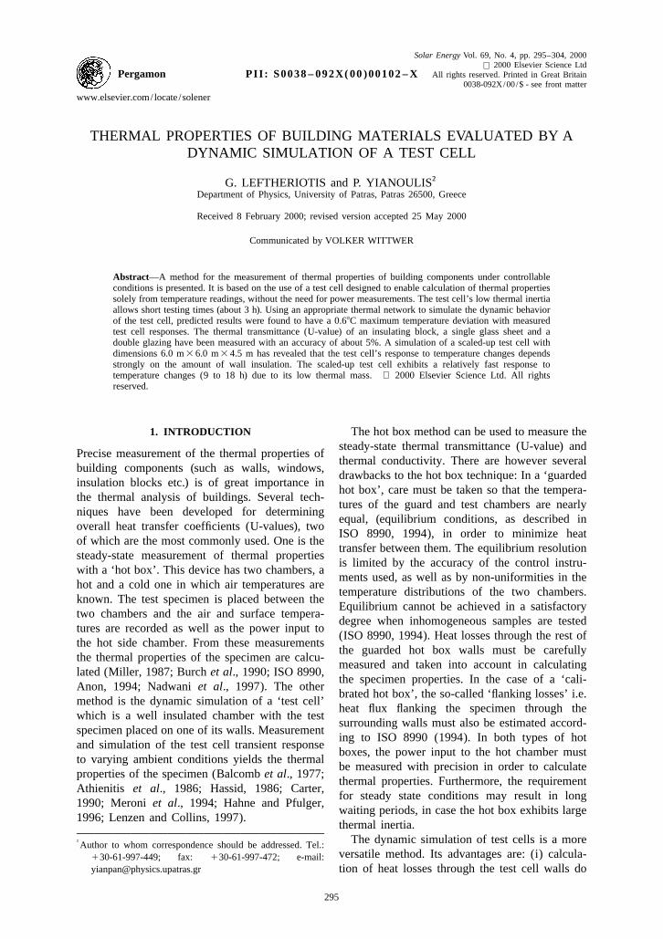
OF THE TEST CELLheat) that cannot be established in steady stateconditions. This method also relies on the accur- This test cell consists of two chambers, (seeate measurement of the power input to the test Fig. 1), which share a common front wall. Thecell. Most of the test cells presented in the outer chamber, (dimensions: 1.6 m 3 1.6 m 3 1.2 m)literature have large thermal mass in order to equipped with an air cooling unit, acts as a heatexhibit properties similar to those of real build- exchanger. The inner chamber (dimensions: 1.2ings and this leads to large testing times. In the m 3 1.2 m 3 0.65 m) is designed to dampen thePASSYS test cell for example, a testing cycle may outer chamber temperature fluctuations that arisetake as long as 2–8 weeks (Vandaele and Woul- by the non-uniform operation of the air coolingters, 1994; Hahne and Pfulger, 1996). unit. The sample is fixed on the face wall of the

The improved test cell version reported here test cell and exchanges heat with the outeralleviates the need for power measurements, chamber through the inner chamber.allowing the determination of thermal properties The construction of the two chambers and thesolely from temperature measurements. The test front wall is described below: The test cell wallscell was designed to have a low thermal mass and are fixed on a metal framework that acts as athus fast response to temperature changes. In support structure. The walls are made of 5 cmorder to minimize construction costs, common thick insulating polystyrene blocks. They arematerials and commercial heating /cooling equip- arranged so that the metal structure is in thement have been used to build the test cell instead external part of the insulation to avoid thermalof purpose-built heat pumps. bridges. All walls, edges and corners were sealed

A model simulating the dynamic behavior of air-tight by silicone. In order to avoid heat lossesthe test cell was developed, based on thermal through the wall edges and corners, grooves werenetwork analysis. The identification of model constructed in the polystyrene blocks so that aparameters was achieved by fitting the model part of one block was inserted into the other at theresponse to the measured temperatures of the test joining points. A skin of aluminum foil was addedcell. With satisfactory identification of parameters, to the external surface of the outer chamber and

Fig. 1. Sketch of the test cell showing thermocouple positions.

Thermal properties of building materials evaluated by a dynamic simulation of a test cell 297

front wall, to reduce emissive heat losses and to In order to measure the properties of the testform a Faraday cage for the reduction of electro- sample with high precision the following testingmagnetic interference to the measuring instru- procedure was specified. The tests were conductedments within the test cell. On top of the aluminum indoors, in a controlled environment with constantskin, a 5 mm thick plywood sheet of white color ambient temperature and in the absence of signifi-was added. It was fixed on the structure only at cant solar radiation either direct or diffuse. Thisthe edges of the walls in order to form air gaps enabled measurements with the low ‘noise’ level,with the underlying layer and thus improve ther- avoiding the effects of passing clouds and am-mal insulation. The inner chamber could slide to bient temperature fluctuations. Indoor testingits position within the outer chamber on specially gives uniform surface and air temperatures, as hotbuilt rails on the outer chamber floor. The front spots or partial shading of the apparatus arewall, which contains the test sample, is remov- avoided.able. It is held in position by eight threaded rods, The test cell and specimen are in thermalfour on the outer chamber framework and four on equilibrium with the ambient prior to testing. Thethe inner chamber. At the joining points of the requirement for testing to begin is that all mea-front wall with the two chambers, an insulating sured temperatures of the cell do not exceed thetape was applied for air-tightness. The whole measurement error (ie 0.28C).assembly is on wheels so that both indoor and The testing procedure is as follows: The airoutdoor tests can be performed. cooling unit is switched on and the cooling

The test sample was placed at the center of the sequence of the test cell is monitored until steadyfront wall. It was fixed on the internal surface of state is reached (this takes about 3 h).the wall, into a grooved frame with appropriate The cooling procedure is enough for the calcu-dimensions. Silicone was used to seal air-tight the lation of specimen properties. However, if de-sample and wall. sired, a ‘natural’ heating process can follow: The

Twenty T-type thermocouples (TCs) have been air cooling unit is then turned off and the cell isused for measuring temperatures at different allowed to heat-up to equilibrium temperaturepositions in the two chambers, as shown in Fig. 1. (this takes about 6 h).Twelve TCs were placed at various positions onthe test sample (6 at each surface). Aluminum-

3. PRESENTATION OF THE DYNAMICcoated adhesive tape was used to fix thermocou-

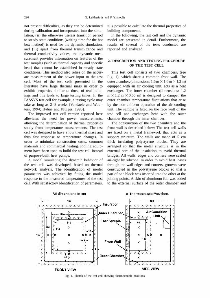
MODELples on the wall and sample surfaces. The 32 TCreadings were collected by a Campbell Scientific The thermal network used for the simulation ofCR-10 data logger, with use of a 32–2 channel the test cell is shown in Fig. 2. It consists of 14multiplexer. Differential temperature calculations nodes, representing all test cell components. Eachwere performed with the data logger, using a component is modeled as a three-node elementreference thermopile. The thermopile was placed containing two resistors in series connected to ain an insulated constant temperature box together capacitor at the middle node. Emissive exchangewith the data logger and multiplexer. The overall between walls would require the addition ofaccuracy of the differential temperature readings ‘bridging’ resistances between nodes 3 and 5, 7exceeded 0.28C. Ambient temperature was also and 9. It was neglected in the present model duemonitored at another channel of the data logger. A to the low emissivity of the walls (e 50.39).2.61 kW commercial air cooling unit was used as Emissive exchange between the test sample anda heat pump. the inner chamber walls was also neglected (it

Fig. 2. The thermal network for the test cell.


N11would require a ‘bridging’ resistance between O u (i 5 j)iknodes 5 and 14). This is justified by the low A 5 Kk50ij

emissivity of the test samples (the glazings tested 2 u (i ± j)ij

have e 50.18–0.20), the walls (e 50.39) and theandsmall temperature differences observed (2–38C).

N11In the case of an N-node thermal network, theB 5 Q 1OM u Ti i j ij jdifferential equation for the ith node with tem-

j50perature T , thermal capacitance C , heat flow ratei i

withQ , connected to the rest ( j) nodes with thermali

conductances u is given by Kirchoff’s Law 1 Mass-EdgeijM 5 (6)Kj(Sebald, 1985): 0 Massless

N11 Solution of Eqs. (2) and (5) for consecutivedTi]C 5O u T 2 T 1 Q (1) time intervals t yields the temperature response ofs di ij j i idt j50 the thermal network.

The U-value of a specimen is given by:Since not all nodes of the thermal networkpossess thermal mass, the distinction between Q

]]U 5 (7)nodes with and without mass must be made. Thus, A DTfor an ith node possessing mass, discretization of with Q the heat flow rate through the specimen, AEq. (1) with forward differencing the specimen area and DT the temperature differ-

ence between indoors air and ambient.dT T (k 1 1) 2 T (k)i i i Q is given by:] ]]]]]dt ¯ t and ¯dt tDT]]Q 5 (8)yields: R total

N11t where R is the total resistance of the specimen,total]T (k 1 1) 5 O u T (k) 2 T (k) 1 Q (k)F s d Gi ij j i iC i.e. the resistance from ambient air to inneri j50

chamber air through the test sample.1 T (k) (2)i Hence, combining Eqs. (7) and (8) we get:

with k and k11 denoting consecutive time inter- 1]]U 5 (9)vals t. The use of massless nodes (C 50) leads toi A R totalalgebraic equations. For the mth massless node,

A FORTRAN program has been written toEq. (1) is reduced to:solve the thermal network. The steps of the

N11 algorithm devised are:O u T 2 T 1 Q 5 0 (3)s d 1. Initial conditions. Look-up tables providingmj j m mj50

initial values of C , u , Q for each node arei ij i

read as inputs by the program. The initialor:values (for t50) of the edge (ambient) tem-

N11 peratures as well as those of the nodes withO u T 2 O u T 5 O u Tmj m mj j mj j mass are also specified. The time interval t isj50 jMASSLESS jMASS,EDGE

also given.1 Q (4)m 2. Eq. (5) is solved by Gaussian elimination with

partial pivoting for the temperatures of mass-with jMASS,EDGE summing over nodes with

less nodes at t50 (and t 5 kt later).thermal mass (C ±0) and the ‘edge’ nodes withi 3. The new values T (k 1 1) for the nodes withitemperatures equal to T as shown in Fig. 2.ambient mass are calculated from Eq. (2).By applying equations similar to (4) for all 4. Steps 2 and 3 are repeated M times, until themassless nodes, a linear system of algebraic termination time Mt is reached.equations is obtained which enables the evalua- It should be noted that the formulation of thetion of the temperatures of massless nodes. This problem is a general one, and applies to any kindsystem of equations can be represented in matrix of thermal network with appropriate modifica-form as: tions. For example, inclusion in the model of

emissive heat exchanges between walls can beA ? T 5 B (5)f g f g f gdone by a mere alteration of the thermal con-ductivity look-up table of the program.The values of the matrix elements are given by:


4. IDENTIFICATION OF MODEL of STEP 1, and only minor alterations to thesePARAMETERS values may be required.

The power absorbed from the air cooling unitThe values of conductances and capacitances

was not measured, thus, it is not possible to obtainshown in Fig. 2 must closely correspond to the

a good match between theory and experiment formeasured behavior of the test cell. The devised

the outer chamber air temperature. However, asparameter identification procedure is divided into

the inner chamber walls dampen the large tem-two stages.

perature swings, it is sufficient to match the upperIn the first stage, the test cell is calibrated. The

and lower limits of the temperature variation inthermal response of the cell and of a calibration

the outer chamber to obtain a good approximationwall (i.e. the front wall and a specimen with

in the inner chamber. This was achieved asidentical properties as the wall) is monitored.

follows: The cooling unit was automaticallyThus, an 11 node network will need to be solved

turned on and off by its internal control mecha-(the test sample branch is incorporated into the

nism when certain air temperature limits of thefront wall), which has less parameters to be

outer chamber were reached (see Fig. 3). We haveidentified. In the second stage, testing of the test

simulated this operation by setting two tempera-sample takes place. The test sample branch is

ture levels, one for operation and one for pause.added in the model in order to calculate the

The power removed during operation was as-sample properties. The parameter identification

sumed to remain constant at a specified value.includes the following steps:

STEP 3. The values of u and C for the innerij iSTEP 1. The conductance and capacitance for chamber walls and air are adjusted, so that theeach node are estimated using data for (i) thermal predicted temperatures agree with the measuredconductivity, (ii) specific heat, and (iii) heat values. The average wall temperature of the innertransfer coefficients of the constituent materials. chamber is calculated from experimental data at

the five wall surfaces.

STEP 2. The values of u and C of the outerij i

STEP 4. ((Only in stage 2)) The values of u andchamber air temperature (Node 8), the external ij

C for the test sample are altered until thewalls (Nodes 9–10–11) and the front wall (Nodes i

predictions for the specimen surface temperatures1–2–3), are altered (by trial and error) until theare consistent with those measured experimental-theoretical predictions of the outer chamber airly. For the measured test sample temperatures,temperature match as close as possible the mea-values in the center were used unless considerablesured values. For the calculation of the average airvariations occur.temperature, the measured data obtained at 5

locations of the outer chamber are used. Theexternal wall temperature was not monitored As the identification procedure progresses,during the experiment, as it is not of great some minor adjustments to values of elementsimportance. from previous steps (those of nodes 8, 9, 10, 11,

Fig. 2) may be needed to fine tune the model.However, in the sequence of steps given above,The surface ratio between the front wall (Nodesthe largest area elements are treated first, so that1–2–3) and the outer walls of the test cell (Nodesthey do not affect considerably the properties of9–10–11) is approximately equal to 1 /10

2 2 smaller area elements.(1.21 m /11.5 m ). The two components areThe thermal network methodology enables themade of the same material, thus, their conduct-

calculation of U-values for building componentsance and capacitance must follow the 1/10 ratio.with simple temperature measurements. Thus, theFurthermore, convective and radiative heat trans-need for an exact calculation of heat flux throughfer from these surfaces to the environment havethe test samples is removed. Furthermore, thermalthe same coefficients (h and h ) and it follows thatr equilibrium is not required for the calculations tou /u 51/10. In case solar radiation isAmb,1 11,Amb be performed.absorbed by these surfaces, the ratio 1 /10 must

also be observed. Thus, nodes (1–2–3) and (9–10–11) are related and alterations to their prop-

5. ERROR ESTIMATIONerties must be done simultaneously. This sim-plifies STEP 2. The external wall conductances The errors associated with this method haveare approximated well by the initial calculations been estimated. Errors that arise from the numeri-


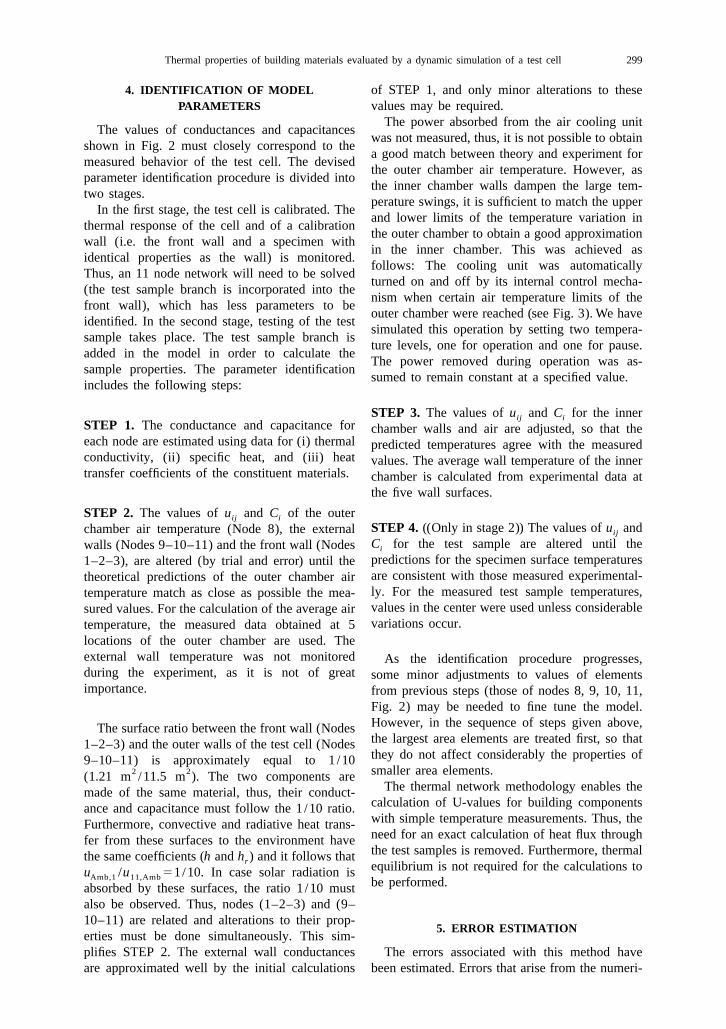
Fig. 3. Calibration of the test cell.

cal techniques used in the thermal network model- tested at representative conditions with two differ-ing are: ent values of t, namely 60 s and 10 s. Comparing

the results, it was found that errors between t 560 sand t 510 s are maximum (2%) at the first few5.1. Solution of the linear system by Gaussiansteps of the simulation, when (dT /dt) is large.EliminationThey reduce rapidly to less than 0.1% as theThe residual errors were found to be of thesimulation progresses. Similar comparisons of213 217order 10 to 10 8C. It is therefore concludedsimulation results between t 510 s and 1 sthat the accuracy of this method is satisfactory.revealed deviations of the predicted temperaturesless than 0.05%.The time interval chosen in this

5.2. Stability of the finite difference calculations study was t 560 s as a compromise betweenIn order for the forward differencing routine accuracy and computing speed. The parameter

used in this model to converge, all nodes must identification procedure requires many repetitionsfollow the rule: of the simulation with slightly different model

parameters in order to find the best fit to theN11 Ci experimental data. It is therefore essential to have]O u # 10 (10)ij tj50 a fast simulation routine.

This rule was derived by iterative trial of 5.4. Sensitivity of U-value calculationsvarious configurations of conductances, capaci- The sensitivity of the predicted U-value intances and time intervals and by observing the variations of R was also estimated. Since Rtotal Totalstability of the procedure. A similar, but more is the sum of several partial resistances (see Fig.rigorous convergence criterion has been derived 2), it follows that the maximum error in RTotaltheoretically (Sebald, 1985). Eq. (10) is a rule of will be the sum of absolute errors of the partialthumb for the selection of t. In the present resistances. Assuming that all partial resistancesthermal network the maximum value of t allowed have the same relative error (e), it follows thatfor convergence was found to be about 400 s. The (dR /R )5e. Thus, from Eq. (9) can beTotal totalvalue of t finally chosen was reduced to 60 s, to shown that the maximum relative error in U-valuesuppress discretization errors. is (dU /U )5(dR /R )5e. It is thereforeTotal total

concluded that the U-value calculated with this5.3. Discretization errors method is insensitive to errors in the calculation

of partial resistances (or conductances u ,The major contribution to the numerical model Amb,12

u , u and u in Fig. 2), since a relativeerror is discretization of Eq. (1). The model was 12,13 13,14 14,4


error e in each of the partial resistances causes the the inner chamber air are illustrated. Their maxi-same error in the calculation of U-value and not a mum value does not exceed 0.48C. The ex-multiple of e. perimental results correspond closely with the

theoretical predictions. From this it was concludedthat neglecting the emissive exchange between

6. RESULTSwalls in the model did not introduce significanterrors.6.1. Calibration of the test cell

It can be observed from Fig. 3 that after 3 h theIn Fig. 3, the results of an indoor cooling and

inner chamber air of the test cell reached steady-natural heating process for calibrating the test cell

state conditions. The simulated results for theare shown. As can be seen in Fig. 3, the large

inner chamber air temperature reveal oscillationsswings in the outer chamber air temperature are

with amplitude of 0.28C when steady state isdue to the operation of the air cooling unit. We

reached. Such oscillations were not observedhave found that the inner chamber insulation

experimentally, as the errors in temperature read-dampens these temperature swings and it is

ings are of the same magnitude. Once the airpossible to obtain good predictions of the inner

cooling unit stopped, natural heating began. Thechamber temperatures with fair predictions of the

inner chamber air temperature started to increaseouter chamber behavior, as shown in Fig. 3. The

when the outer chamber temperature increased,values of the thermal network elements (in ac-

and the heat flow was reversed.cordance with Fig. 2, omitting the test samplebranch) are given in Table 1. 6.2. Test of sample glazings

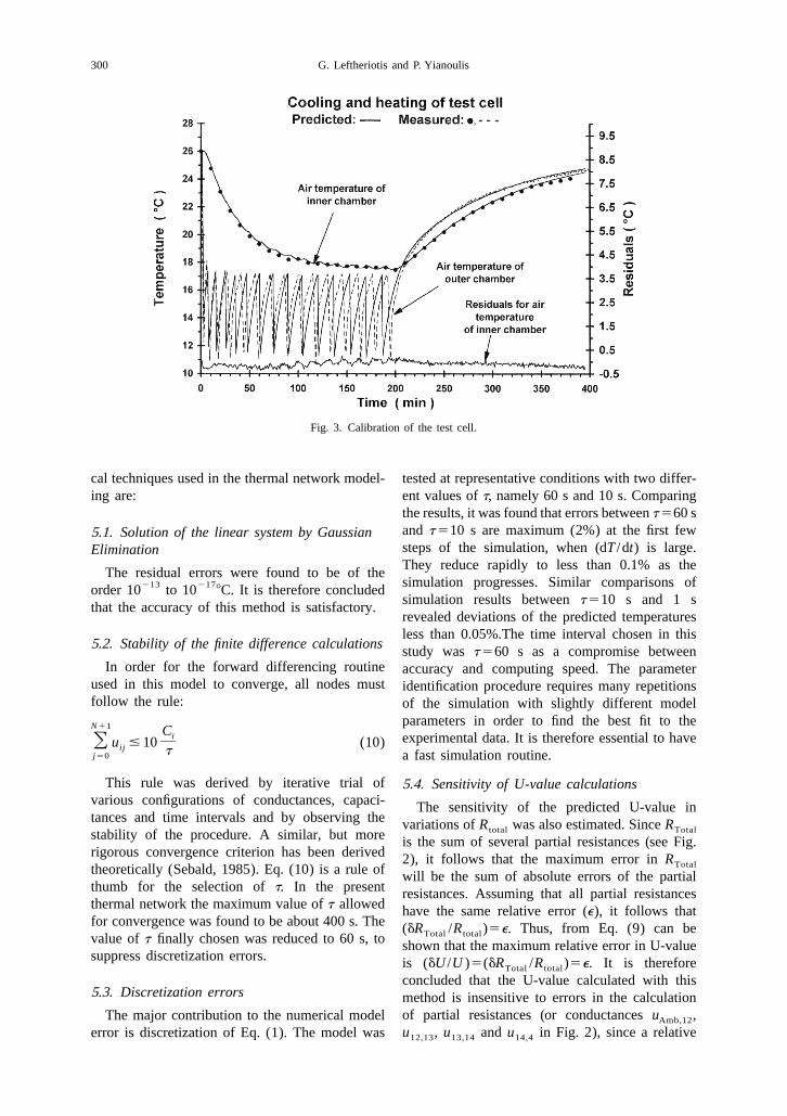
The thermal properties of the front and outerAs a further example of the above calculations,

test cell walls were found to be:the results of an indoor cooling process of the test

22 21 2U-Value: 0.440 W m K . cell with a 0.06 m double glazing (THERMOP-LUS manufactured by FLACHGLAS AG) are

21 21Thermal Conductivity: 0.028 W m K . shown in Fig. 4. The experimental and theoreticalcurves agree well, both for the inner and outer

21 21Specific Heat: 1950 J kg K . glass surfaces as well as for the inner chamber airtemperature (0.68C maximum temperature devia-

The thermal conductivity of the front and outer tion). The temperature distribution on both sur-test cell walls was found to agree with that faces of the glazing was found to be uniformspecified by the insulation manufacturer. The during testing: The maximum temperature devia-initial values of conductances for the front and tion between thermocouples on the glazing sur-outer chamber walls remained unchanged after the face did not exceed 0.48C.parameter identification procedure. This implies Using the predicted values for the doublethat the test cell is well insulated and that there glazing thermal resistance, (see Fig. 2), we haveare no thermal bridges. calculated the glazing U-value which was found

22 21In Fig. 3, the residuals (T 2T ) for to be 1.34 W m K . This value differs by 3%measured predicted

Table 1. Values of the thermal network elements

Thermal network elements for calibration of the test cell21 21Conductances in W K , Capacitances in J K

u u u u u u u u u u u uAmb,1 1,2 2,3 3,4 4,5 5,6 6,7 7,8 8,9 9,10 10,11 11,Amb

3.39 1.356 1.356 9.177 9.177 5.108 5.108 20.8 20.8 12.98 12.98 32.5

C C C C C2 4 6 8 10

4000 800 8000 10,000 47,280

Operation of air cooling unit: Q 521000 W (Cooling unit paused and T .178C),8 8

0 W (Cooling unit operating and T ,128C)8

Thermal network elements for the tested double glazing (Flachglas AG).21 21Conductances in W K , capacitances in J K .

u u u uAmb,12 12,13 13,14 14,4

0.175 0.420 0.420 0.200C13

500


Fig. 4. Test of a double glazing (Flachglas).

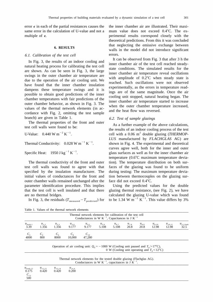
22 21from that given by the glass manufacturer (51.30 was found to be equal to 5.15 W m K , which22 21W m K ). The values of the thermal network is lower than the value given by Collins et al.

22 21elements for the double glazing (in accordance (1992) for a single uncoated glazing (6 Wm K ),with Fig. 2) are given in the Table 1. due to reduced emissive losses.

We have also tested a single glazing coated6.3. Scaling-up of the test cellwith a low-emittance film (K-glass by Pilkington).

The measured and simulated results are shown in In order to compare the performance of theFig. 5. The temperature difference between the present test cell with full-scale cells that areinternal and external glass surfaces at steady state available, the dynamic behavior of a scaled-up(about 0.58C), is low compared to that of the test cell was predicted. The scaling-up was donedouble glazing. The U-value of the single pane as follows: The inner chamber volume was

Fig. 5. Test of a single glazing (K-Glass).


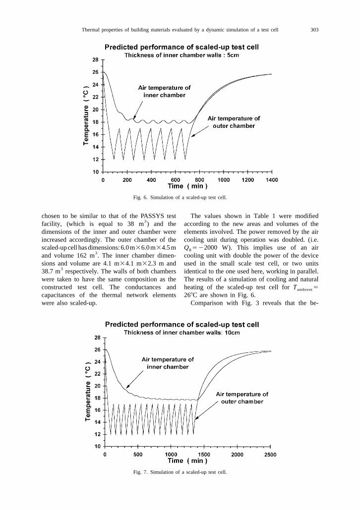
Fig. 6. Simulation of a scaled-up test cell.

chosen to be similar to that of the PASSYS test The values shown in Table 1 were modified3facility, (which is equal to 38 m ) and the according to the new areas and volumes of the

dimensions of the inner and outer chamber were elements involved. The power removed by the airincreased accordingly. The outer chamber of the cooling unit during operation was doubled. (i.e.scaled-up cell has dimensions: 6.0 m36.0 m34.5 m Q 522000 W). This implies use of an air8

3and volume 162 m . The inner chamber dimen- cooling unit with double the power of the devicesions and volume are 4.1 m34.1 m32.3 m and used in the small scale test cell, or two units

338.7 m respectively. The walls of both chambers identical to the one used here, working in parallel.were taken to have the same composition as the The results of a simulation of cooling and naturalconstructed test cell. The conductances and heating of the scaled-up test cell for T 5ambient

capacitances of the thermal network elements 268C are shown in Fig. 6.were also scaled-up. Comparison with Fig. 3 reveals that the be-

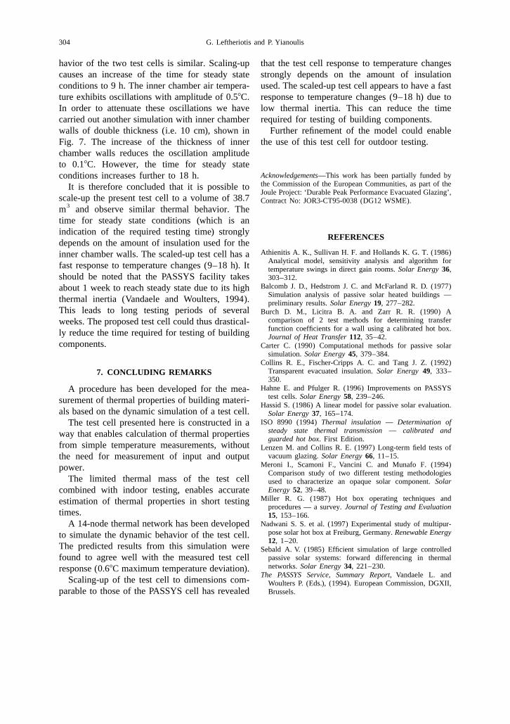
Fig. 7. Simulation of a scaled-up test cell.


havior of the two test cells is similar. Scaling-up that the test cell response to temperature changescauses an increase of the time for steady state strongly depends on the amount of insulationconditions to 9 h. The inner chamber air tempera- used. The scaled-up test cell appears to have a fastture exhibits oscillations with amplitude of 0.58C. response to temperature changes (9–18 h) due toIn order to attenuate these oscillations we have low thermal inertia. This can reduce the timecarried out another simulation with inner chamber required for testing of building components.walls of double thickness (i.e. 10 cm), shown in Further refinement of the model could enableFig. 7. The increase of the thickness of inner the use of this test cell for outdoor testing.chamber walls reduces the oscillation amplitudeto 0.18C. However, the time for steady state

Acknowledgements—This work has been partially funded byconditions increases further to 18 h.the Commission of the European Communities, as part of theIt is therefore concluded that it is possible toJoule Project: ‘Durable Peak Performance Evacuated Glazing’,

scale-up the present test cell to a volume of 38.7 Contract No: JOR3-CT95-0038 (DG12 WSME).3m and observe similar thermal behavior. The

time for steady state conditions (which is anindication of the required testing time) strongly

REFERENCESdepends on the amount of insulation used for the

Athienitis A. K., Sullivan H. F. and Hollands K. G. T. (1986)inner chamber walls. The scaled-up test cell has aAnalytical model, sensitivity analysis and algorithm forfast response to temperature changes (9–18 h). It temperature swings in direct gain rooms. Solar Energy 36,

should be noted that the PASSYS facility takes 303–312.Balcomb J. D., Hedstrom J. C. and McFarland R. D. (1977)about 1 week to reach steady state due to its high

Simulation analysis of passive solar heated buildings —thermal inertia (Vandaele and Woulters, 1994). preliminary results. Solar Energy 19, 277–282.This leads to long testing periods of several Burch D. M., Licitra B. A. and Zarr R. R. (1990) A

comparison of 2 test methods for determining transferweeks. The proposed test cell could thus drastical-function coefficients for a wall using a calibrated hot box.ly reduce the time required for testing of building Journal of Heat Transfer 112, 35–42.

components. Carter C. (1990) Computational methods for passive solarsimulation. Solar Energy 45, 379–384.

Collins R. E., Fischer-Cripps A. C. and Tang J. Z. (1992)Transparent evacuated insulation. Solar Energy 49, 333–7. CONCLUDING REMARKS350.

Hahne E. and Pfulger R. (1996) Improvements on PASSYSA procedure has been developed for the mea-test cells. Solar Energy 58, 239–246.surement of thermal properties of building materi-

Hassid S. (1986) A linear model for passive solar evaluation.als based on the dynamic simulation of a test cell. Solar Energy 37, 165–174.

ISO 8990 (1994) Thermal insulation — Determination ofThe test cell presented here is constructed in asteady state thermal transmission — calibrated andway that enables calculation of thermal propertiesguarded hot box. First Edition.

from simple temperature measurements, without Lenzen M. and Collins R. E. (1997) Long-term field tests ofvacuum glazing. Solar Energy 66, 11–15.the need for measurement of input and output

Meroni I., Scamoni F., Vancini C. and Munafo F. (1994)power.Comparison study of two different testing methodologies

The limited thermal mass of the test cell used to characterize an opaque solar component. SolarEnergy 52, 39–48.combined with indoor testing, enables accurate

Miller R. G. (1987) Hot box operating techniques andestimation of thermal properties in short testingprocedures — a survey. Journal of Testing and Evaluation

times. 15, 153–166.Nadwani S. S. et al. (1997) Experimental study of multipur-A 14-node thermal network has been developed

pose solar hot box at Freiburg, Germany. Renewable Energyto simulate the dynamic behavior of the test cell.12, 1–20.

The predicted results from this simulation were Sebald A. V. (1985) Efficient simulation of large controlledpassive solar systems: forward differencing in thermalfound to agree well with the measured test cellnetworks. Solar Energy 34, 221–230.response (0.68C maximum temperature deviation).

The PASSYS Service, Summary Report, Vandaele L. andScaling-up of the test cell to dimensions com- Woulters P. (Eds.), (1994). European Commission, DGXII,

parable to those of the PASSYS cell has revealed Brussels.

thermal properties of building materials evaluated by a dynamic simulation of a test cell

Documents