thermal modelling of a transformer based...
TRANSCRIPT

Thermal Modelling of a Transformer based on
PT-1000 Sensor
ELEVE
Junxing HUANG
TUTEUR UNIVERSITE
Torbjörn Thiringer
TUTEUR ESIEE
Olivier MALOBERTI
Rap
po
rt d
e S
TA
GE
I
4 G
ED
D 2013 -
2014


Thermal Modelling of a Transformer based on
PT-1000 Sensor
Fourth year project (I4 STAGE en Chalmers)
Junxing HUANG
Department of Energy and Environment
Division of Electric Power Engineering
CHALMERS UNIVERSITY OF TECHNOLOGY
SE-412 96 Gothenburg, Sweden 2014


Thermal Modelling of a Transformer based on
PT-1000 Sensor
Department of Energy and Environment
Division of Electric Power Engineering
CHALMERS UNIVERSITY OF TECHNOLOGY
SE-412 96 Gothenburg, Sweden 2014

Thermal Modelling of a Transformer based on PT-1000 Sensor
Junxing HUANG
© Junxing HUANG 2014
Department of Energy and Environment
Division of Electric Power Engineering
CHALMERS UNIVERSITY OF TECHNOLOGY
SE-412 96 Gothenburg,
Sweden 2014
Telephone +46 (0)31–772 1000
Cover:
A thermal image from a transformer
Chalmers Bibliotek Reproservice
Gothenburg, Sweden 2014

i
Thermal Modelling of a Transformer based on PT-1000 Sensor
Junxing HUANG
Department of Energy and Environment
Division of Electric Power Engineering
CHALMERS UNIVERSITY OF TECHNOLOGY
Abstract
We can calculate the Joule losses according to the principle P=RI2
in an electrical machine
and transformer. However, the total loss is harder to determine because of the complicated
electromagnetic factor, such as excess iron losses or the way the heat is transferred for
example, it will be a difficulty to evaluate the temperature rise which is likely to exceed the
limit of temperature during its use. Thus a temperature prediction based on an accurate
measurement system is needed.
This work aims at the thermal modelling of a multilayer wire-wound transformer and its
verification by using the temperature sensors of the type PT-1000. In order to achieve this
goal, firstly, a brief introduction about the data acquisition system including PCB and
LabVIEW was made. Then two main tests were carried out. For the first one, a transformer
without any interlayer thermal insulation was constructed. This test focused on the
measurement of thermal resistance by using an external heating source to create a one-
dimension heat flow. On the basis of these results, the temperature of each layer could be
predicted when the windings were conducted with DC power in a real application. This
prediction model applied to any DC current but was only suitable for the transformer made in
test 1. For the second test, the theoretical thermal resistances were firstly calculated based on
the material which was used to manufacture the transformer. Then the comparison between
the theoretical and measured values was performed. The most important usage of this model
lied on the applicability to all the similar transformers.
When all the thermal resistances in each part were decided, a whole thermal network was
presented.
Key words: Thermal Modelling, PT-1000, Transformer, PLECS, LabVIEW Software.

ii

iii
Acknowledgement
This project has been fund by Conseil Régional de Picardie and ERASMUS. I express my
greatest gratitude for their financial supports.
I would like to give my sincere and respectful thanks to my examiner Torbjörn Thiringer in
Chalmers University of Technology and my examiner Olivier MALOBERTI in ESIEE-
Amiens. They could always give me the constructive advice and helpful guidance through my
entire project. I really appreciate their patience, immense knowledge and enthusiasm to the
work. Thank you!
My thanks also go to my supervisors Mohammadamin Bahmani and Tarik Abdulahovic,
who gave me many insightful comments and the best suggestions.
Besides, my acknowledgements go to Robert Karlsson and Magnus Ellsen for providing me
the necessary materials and equipment as well as an advanced experiment platform.
In addition, I am grateful to the coordinators within ERASMUS, especially Anne
LEMAIRE and Ing-Britt Carlsson, for their administrative supports.
Last but not least, I would like to thank my families, my beloved fiancée for their love and
giving me the chance to go abroad.
Junxing HUANG
Gothenburg, Sweden 2014

iv

v
Contents
Abstract ....................................................................................................................................... i Acknowledgement ..................................................................................................................... iii 1. Introduction ............................................................................................................................ 1
1.1 Problem background .................................................................................................... 1
1.2 Delimitations ................................................................................................................ 1 1.3 Purpose of the work ...................................................................................................... 2
2. Technical background ............................................................................................................ 3 2.1 General theory of transformer ...................................................................................... 3 2.2 Energy losses in a real transformer .............................................................................. 4
2.3 Temperature coefficient of resistance .......................................................................... 6 2.4 Thermal theory ............................................................................................................. 6
3. Temperature measurement system ....................................................................................... 11
3.1 Introduction of the temperature measurement system ............................................... 11 3.2 The function blocks of the temperature measurement system ................................... 12
3.2.1 RTD PT-1000 Sensor ...................................................................................... 12 3.2.2 PT-1000 sensor in the Wheatstone bridge ....................................................... 13
3.2.3 Amplifier INA122 ........................................................................................... 15 3.2.4 Low-pass filter circuit ..................................................................................... 16
3.2.5 Introduction of the Printed Circuit Board ....................................................... 18 3.3 Data handling system ................................................................................................. 21
3.3.1 LabVIEW ........................................................................................................ 21
3.3.2 Calibration ....................................................................................................... 23 3.3.3 Matlab .............................................................................................................. 25
4. Manufacture procedure......................................................................................................... 27
4.1 Materials for the construction of transformer ............................................................ 27
4.2 Characteristic parameters of the materials ................................................................. 28 4.3 Transformer construction ........................................................................................... 29
4.3.1 Construction step ............................................................................................. 31 5. Experiment set-up and test analysis ..................................................................................... 35
5.1 Experiment set-up ...................................................................................................... 35 5.1.1 Thermal model ................................................................................................ 35 5.1.2 Determination of the excitation resource P ..................................................... 37
5.2 Test 1- No interlayer thermal insulation .................................................................... 37 5.2.1 External heating source ................................................................................... 37
5.2.2 Internal heating source .................................................................................... 42 5.2.3 Simulation in PLECS ...................................................................................... 46 5.2.4 Conclusion for test 1 ....................................................................................... 51
5.3 Test 2- With interlayer thermal insulation ................................................................. 51 5.3.1 Heating source ................................................................................................. 51 5.3.2 Coil former test ................................................................................................ 52 5.3.3 Core test ........................................................................................................... 55
5.3.4 Windings test ................................................................................................... 59 5.3.5 The whole thermal network ............................................................................. 65
6. Conclusion and future work ................................................................................................. 67 6.1 Conclusion .................................................................................................................. 67 6.2 Future work ................................................................................................................ 67
References ................................................................................................................................ 69

vi
Appendix A .............................................................................................................................. 71
Appendix B .............................................................................................................................. 79 Appendix C .............................................................................................................................. 91

1
Chapter 1
1. Introduction
1.1 Problem background
Nowadays, many studies about thermal modelling of large transformers based on FEM (Finite
Element Method) have been made. However, the studies on building a thermal model of a
small inductor or a small transformer are less frequent. In most cases, they are considered to
be an ideal component by neglecting electrical or magnetic losses which occur in the
materials used to construct the device.
With the rapid development in industries regarding lowering power dissipation, the
miniaturization of electronic products is becoming an inevitable trend. In other words, the
problem of heat dissipation in a compact system will turn out to be a bottleneck to this
development.
An inductor or a small transformer is one essential part for most electronic systems. For a
compact design, the heat dissipation cannot be neglected. It is necessary to know the
electrical and thermal properties in a certain system for the purpose of calculating a safe
current range. Under this condition, we do not need to worry about the risk of a system crash
because of an over load, on the other hand, we do not want to waste copper material caused
by an over dimensioning. So these aspects must be considered in designing some functional
block such as a filter circuit or a DC chopper circuit.
To sum up, the temperature has become one of the most vital factors to predict the behavior
of a system. Accordingly, there is a need for good thermal models and also measurement
verification of the models.
1.2 Delimitations
This internship aims at performing thermal modelling in order to predict the temperature
behavior of a small inductor or small transformer. It is not suitable for larger transformers
such as oil transformers, resinated dry type transformer or planar transformers. Moreover, this
project has to be finished within a timeframe of 14 weeks which is far away from the time
needed to take everything into consideration. So for the component of interface between data
collecting and handling it was possible to use an existing PCB.

2
1.3 Purpose of the work
The first purpose of this thesis work is to build a transformer entity in which we can collect
the measurement data based on PT-1000 temperature sensors and LabVIEW.
Secondly, according to the measured data and the analysis of the results we can deduce a
practical thermal modelling which will compare with the thermal model based on theories.
Moreover, by setting up a thermal modelling we can know precisely the energy loss during
the energy transformation. Thus we can offer some necessary parameters to design an
electronic circuit taking the heat flow into consideration.
In this training course, the winding will be mainly connected to DC voltage to measure its
Joule losses. Compare to the using of AC voltage, the biggest difference lies on the omission
of total magnetic losses into the iron core.

3
Chapter 2
2. Technical background
This chapter concerns the principle of a transformer and the losses generated by a transformer.
At the same time, it presents some thermal theories.
2.1 General theory of transformer
A transformer is a static electrical device which transfers energy between two circuits through
electromagnetic induction. It may be used as a safe and efficient voltage converter to change
the AC voltage at its input to a higher or lower voltage at its output. In an electrical system,
the transformer plays a very important role in the power energy economical transportation and
the flexible distribution as well as the safe energy use.
Commonly, a transformer consists of two windings of wire (single-phase transformer) or
more windings of wire that are wrapped around a common core to provide tight
electromagnetic coupling between the windings. The primary winding must be connected to
an alternating voltage source (Vp) in order to generate a flow of alternating flux ( whose
magnitude depends on the voltage and number of turns of the primary winding (Np). The
alternating flux links the secondary winding and induces a voltage (Vs) in it with a value that
depends on the number of turns of the secondary winding (Ns). This model is shown in Fig.
2.1[1].
Fig. 2.1: Transformer Ideal Model

4
We assume that the Electromotive Force (EMF) produced in the primary winding is ξ1 and
the EMF in the second winding is ξ2. According to the Faraday’s law, we can deduce
(neglecting the winding resistance):
In the primary winding,
(2.1)
In the secondary winding,
(2.2)
As a result we can represent
(2.3)
where n is the ratio of transformation for voltage.
For an ideal transformer, the instantaneous power transferred in both sides is equal. Thus we
can get,
(2.4)
Combining (2.3) and (2.4), we have,
(2.5)
Hence the current ratio is the inverse of the voltage ratio.
2.2 Energy losses in a real transformer
The ideal transformer model above does not include any energy loss. Nevertheless for a real
transformer, it is just 95% to 99.5% efficient because of several losses mechanisms which are
presented below:
5
Winding joule losses
These losses are also known as copper losses and they are caused by the internal
resistance in both sides of the real transformer. They can be conducted by the formula,
P=RI2
(2.6)
Thus the Joule losses depend upon the load of a transformer. When frequency increases,
skin effect and proximity effect also cause an additional winding resistance and, hence,
an increase to losses.
Core losses
These losses include Hysteresis Losses and Eddy Current Losses. For the former, basing
on the Steinmetz's formula, the heat energy is given by,
(2.7)
where f is the frequency, η is the hysteresis coefficient and is the peak flux density.
When the transformer is subjected to an alternating current (AC), an induced current
(eddy current) will be created in the core made of ferromagnetic materials. These eddy
current losses in a transformer are denoted as,
(2.8)
where is the eddy current coefficient and is the coefficient of the form.
From (2.7) and (2.8), we can notice that the core losses depend on magnetic properties of the
materials other than the load current, so these losses can be considered to be constant once the
transformer is made.
In this thesis work, the second winding will not be made. The equivalent circuit can be
presented in Fig. 2.2,

6
Fig. 2.2: Equivalent circuit for a transformer conducted with DC
2.3 Temperature coefficient of resistance
During the thermal modelling, we cannot neglect the resistance variation caused by the
temperature. For most metals, they have a positive temperature coefficient (PTC) which
means that the resistance increases with the temperature and the change in resistance is
expected to be proportional to the temperature change,
(2.9)
where
T: the temperature at which the resistance is measured
T0: the reference temperature
α: the temperature coefficient
R0: the resistance measured at temperature T0
RT: the resistance measured at temperature T
For copper and pure platinum at T0=20 , α will be 0.393%. [2]
2.4 Thermal theory
A transformer mainly consists of coils and iron core. So its heat dissipations mainly include
two parts: losses of coils and losses of iron core. For the former, most of it are dissipated
directly into the air and only a small percentage of it will get through the iron core and then is
dissipated into the air. For the latter, the great part of it will also be dissipated directly into the
air and a small proportion is dissipated through the coils.
Generally, there are three thermal transports mechanisms as following,
Conduction: ‘is the transfer of energy through matter from particle to particle’ [3] that is
to say the conduction can take place in all sorts of materials such as liquids, solids, gases
or plasmas. The premise is that the materials must have contact directly or indirectly. In

7
the transformer, the heat will be conducted between the coils and the iron core. For one-
dimensional form, Fourier’s law of heat conduction can be used,
(2.10)
where is the heat-transfer rate, k is the thermal conductivity, A is the area,
is the
temperature gradient in the direction of the heat flow, the minus sign means the direction
of the heat flow.
Convection: is a more complicated method of heat transport than conduction.
‘Convection is the transfer of heat by the actual movement of the warmed matter. ’ [3] It
can take place in gas or liquid by movement of currents. So convection depends upon the
temperature difference and the heat area. It can be presented as
(2.11)
where, : Heat transferred per unit time (W)
ΔT : Temperature difference between the surface and the bulk fluid (ºC)
h: Convective heat transfer coefficient of the process (W .m-2
. ºC-1
)
A: Heat transfer area of the surface (m2) [4]
Radiation: is a process in which the electromagnetic waves (EMR) travel. As we know
that the EMR can propagate even in a vacuum, it transfers the energy regardless of
nothing. So it’s the same for radiation.
For a small size transformer, the conduction and the convection are the two predominant
modes during the heat dissipation [5]. Thus for simplicity reasons, we can replace the
radiation by augmenting the coefficient h of the convection.
In this work, while we conduct with DC, the iron core losses will in this case be zero. In
order to avoid some misunderstandings or misconception, it is essential to know the
difference as well as the similarity between the electrical and thermal domains. See Table 2.1.

8
Table 2.1: Definition of physical magnitudes
Electrical Thermal
Description symbol units symbol units
“Ohm’s Law” R = V / I “Ohm’s Law” Rth =ΔT/Pth
Electrical
Potential V Volts Temperature difference T ºC or K
Electrical
Resistance R Ohms Thermal Resistance Rth
ºC/W or
K/W
Electrical
Capacitance C
F or
Coulombs/V Thermal Capacitance Cth J /ºC
Electrical current I A or
Coulombs/s Heat flow Pth W or J /s
From the table above, we can deduce easily the energy loss led by the coils,
Pele=RI2
(2.12)
These electrical losses Pele turn into the heat effect and equal to Pth,, so we have,
Pth=
(2.13)
where ΔT is the difference in temperature .
We also can say
Pth=
(2.14)
where ΔQ is heat flow difference , Δt is time difference.
So we get two equivalent circuits illustrated in Fig. 2.3 for the general cases,

9
(a)
(b)
Fig. 2.3: Equivalent circuit for electrical circuit (a) and thermal circuit (b)

10

11
Chapter 3
3. Temperature measurement system
In this chapter, several parts will be presented:
Firstly, an introduction of the temperature measurement system will be given and the reason
why this system is chosen will be given. Secondly, some work about the calibration during the
experiment will be made. Finally the procedure of how to build a transformer will be
explained.
3.1 Introduction of the temperature measurement system
To measure the temperature, we presently have many choices, for example, Mercury-in-glass
Thermometer, Alcohol Thermometer, Kerosene Thermometer etc. All of them are designed
according to the principle of heat-expansion and cold-contraction. They have advantages of
low-cost and simplicity but also have limits such as narrow measurable range and low-
accuracy. Besides, we can use the other type of thermometers, such as resistance
thermometers also called Resistance Temperature Detectors (RTDs) which are made from the
pure materials. Even more you can choose a Thermocouple consisting of two dissimilar
conductors that connect to each other at one or more spots [6].
Generally, in order to decide which measurement method is the preferable one, the factors
as follow should be taken into account,
Firstly, the environment conditions in which the measurement element will be used: the
temperature range, the pressure, the weather condition etc. Then the sensed medium: the
element will be attached to a surface or immersed in solid, liquid or gas; finally the precise
requirement in sensing accuracy, repeatability, stability and response time and so on [7].
In this thesis work, the temperature elements will be wrapped into the transformer windings
which have five layers, so they must be contact-temperature sensors. Moreover, according to
the Insulation Class, the highest temperature of an operating transformer can reach 180 (H
class), [8] which means we need a sensor that can measure the temperature varying from the
ambient temperature (about 20 ) to less than 200 . Furthermore, we have a high demand
in accuracy and expect to change the measured temperature signals into electrical signals.
Thus we can choose thermocouple or RTD. For the case where temperature exceeds 500 ,
the thermocouple is the best choice. But for those situations where temperature is below

12
500 , the RTD will be more preferable due to its higher accuracy and lower drift
characteristic. So I decided to use a RTD based measurement system [9].
3.2 The function blocks of the temperature measurement
system
3.2.1 RTD PT-1000 Sensor
As it has been mentioned above, the RTD element is made from a pure material having a PTC
which means that its resistance increases with temperature. Theoretically, all the metal can be
used to make a RTD, but platinum, nickel or copper are used frequently. More precisely, the
platinum is the best and the most popular metal for RTD due to its stable and linear
resistance-temperature relationship over the largest temperature range (-272.5 to 961.78 )
as well as its chemical inertness.
From (2.9), we can derive the temperature coefficient
(3.1)
where is the significant characteristic of a metal used as a resistive element in RTD. It can
be defined by the linear approximation between the resistance and the temperature from 0 to
100 . So (3.1) can be presented
(3.2)
where is the resistance of the sensor at 100
is the resistance of the sensor at 0
In order to determine the resistance-temperature relationship, an important equation which
is known as Callendar–Van Dusen equation is commonly used [10],
(3.3)

13
where R0: RTD resistance at 0
Rt: RTD resistance at t
A,B,C: Callendar-Van Dusen coefficients
t: temperature ( )
Among the three constants above, C is used for temperature below 0 only. So in the
measurement of the transformer, C=0. We can turn (3.3) into
√
(3.4)
As long as we know the value of Callendar-Van Dusen coefficients, R0 and Rt, we can
calculate the temperature.
The typical value of A, B and C in the equation (3.3) for Platinum RTD can be defined by
one of the three standards shown in Table 3.1 [11],
Table 3.1: Callendar-Van Dusen Coefficients
Standard
Temperature Coefficient α (/ ) A (/ ) B (/ 2
) C (/ 4)
DIN 43760 0.00385 3.9080 x 10⁻³
-5.8019 x 10⁻⁷
-4.2735 x 10⁻¹²
American 0.003911 3.9692 x 10⁻³
-5.8495 x 10⁻⁷
-4.2325 x 10⁻¹²
ITS-90 0.003926 3.9848 x 10⁻³
-5.870 x 10⁻⁷
-4.0000 x 10⁻¹²
In this work, the parameters of PT-1000 sensor will be taken from the standard DIN 43760
and its nominal resistance at 0 is 1000Ω. Table 3.2 shows the main parameters of the PT-
1000 sensor used in this work.
Table 3.2: The main parameters of the PT-1000 sensor
Type Inaccuracy Dimension L*W*H Temperature
coefficient
Measuring
range
FK422 PT-1000 B Class B
4.0 x 2.2 x 0.9 mm 3.850 × 10
−3(C
−1) -70...+500 °C
3.2.2 PT-1000 sensor in the Wheatstone bridge
To measure the resistance of PT-1000 sensor, one easy way is that we can pass a known
current and then measure the voltage, according to Ohms law the resistance can be computed.
14
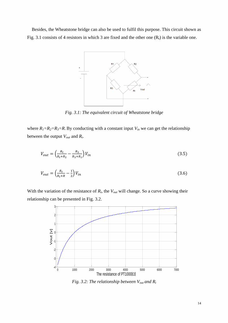
Besides, the Wheatstone bridge can also be used to fulfil this purpose. This circuit shown as
Fig. 3.1 consists of 4 resistors in which 3 are fixed and the other one (Rt) is the variable one.
Fig. 3.1: The equivalent circuit of Wheatstone bridge
where R1=R2=R3=R. By conducting with a constant input Vin we can get the relationship
between the output Vout and Rt.
(
)
(
)
With the variation of the resistance of Rt, the Vout will change. So a curve showing their
relationship can be presented in Fig. 3.2.
Fig. 3.2: The relationship between Vout and Rt
0 1000 2000 3000 4000 5000 6000 7000-4
-3
-2
-1
0
1
2
3
The resistance of PT1000[]
Vo
ut
[v]

15
3.2.3 Amplifier INA122
As the nominal resistance of PT-1000 sensor at 0 has been chosen to 1000Ω, the value of
R1, R2 and R3 will be set to 1000Ω so that the output Vout equals zero at 0 . With the
augmentation in Rt, the Wheatstone bridge becomes unbalanced and Vout will change.
Generally, the output Vout is so small that it can lead to a slight error during the calculation,
thus we need an amplifier circuit.
Here an amplifier INA122 has been chosen due to its characteristic in accurate, low noise
differential signal acquisition [12].
Fig. 3.3: INA122 amplifier circuit
This is a differential amplifier circuit, the voltage signal Vout coming from the Wheatstone
bridge will be connected to VIN+ and VIN-. The final output V0 is determined by the equation
as follows,
(3.7)
where G is the gain of INA122.
Through the amplifier circuit, the input voltage signal will be amplified by G times. Here G
is decided by the value of the external resistor RG according to the equation below,
(3.8)

16
where the 200kΩ term comes from the internal metal film resistors in INA122. By connecting
with different RG, we can vary the gain level from 5 to 10000 as shown in Table 3.3.
Table 3.3:The gain of the amplifier for different RG values
Desired gain (V/V) RG (Ω)
5 NC
10 40k
20 13.33k
50 4444
200 1026
500 404
1000 201
2000 100.3
5000 40
10000 20
where NC means no connection.
In this experiment, G is selected to be 5. So RG is not connected. Equation (3.7) can be
transferred to
(3.9)
The INA122 has a wide power supply range which can vary from 2.2V to 36V DC. Here it
will be powered by 5V DC. In order to stabilize the source, an IC of stabilizer 78L05 is used
as well as a capacitor of 0.1uF is connected between the pin V+ and the ground [12].
3.2.4 Low-pass filter circuit
As shown above in Fig. 3.3, a simply RC low-pass filter circuit is presented for the purpose of
eliminating the possible interference originating the output Vo. This part is shown in Fig. 3.4,
Fig. 3.4: Low-pass filter circuit

17
By applying the Laplace transform, we can get the transfer function of the low-pass filter as
follows [13].
(3.10)
where H(s) is the coefficient of the transfer function.
For the practical frequency
(3.11)
The cut-off frequency can be presented by
(3.12)
when R=1k, C=470uF,
Combining (3.10) , (3.11) and (3.12), we can derive
(3.13)
So the amplitude of H(s) is
√
(3.14)
The angle of H(s) is
(3.15)
From (3.12), we can easily derive how a low-pass filter circuit works,
If which means
tends to be , so
If which includes in the DC input, 1

18
If which means the magnitude decreases by 3db, ,
. Refer to Fig. 3.5.
To sum up, the low-pass filter circuit rejects a signal with high frequency. Table 3.4 shows
the main output noise frequencies in INA122 [12].
Table 3.4: The main output noise frequencies in INA122
Voltage Noise Typical Values Unit
f = 1kHz 60 nV/√Hz
f = 100Hz 100 nV/√Hz
f = 10Hz 110 nV/√Hz
fB = 0.1Hz to 10Hz 2 µVp-p
From Table 3.4, we can know that the principal noises vary from 10Hz to 1 kHz. Thus most
of the noises can be filtered because of .
Fig. 3.5 shows the Bode diagram of the amplitude-frequency response and the phase-
frequency response obtained in Matlab.
Fig. 3.5: Amplitude-frequency response and phase-frequency response
3.2.5 Introduction of the Printed Circuit Board
In order to impact and stabilize the temperature measurement system, the Wheatstone bridge,
the amplifier circuit, the low-pass filter circuit and the other necessary accessories have been
integrated into a Printed Circuit Board (PCB). PCB is an isolated board where all the
electrical components are connected electrically by using copper traces in each layer. For

19
designing the PCB we can use the software PROTEUS to convert a schematic circuit to a
PCB layout. PROTUES is an Electronic Design Automation (EDA) tool provided by the
British company Labcenter Electronics. It is also a platform which combines the circuit
simulation, the PCB design and the visual mode simulation [14].
In this work, because of the limit of time, I will use directly two existing PCBs to
implement the measurement. Each PCB contains 5 input ports which mean it has 5
Wheatstone bridges inside. For obtaining a stable 5V voltage source, a three terminal voltage
regulator (78L05) is also used. The PCB has 2 layers in which the top one is used for the
positive supply voltage and the bottom one for the ground.
Fig. 3.6 shows the schematic circuit of the PCB,
Fig. 3.6: Temperature measurement PCB
As each PCB just has 5 channels, we need 2 PCBs for this experiment.
Fig. 3.7 presents one of the PCB entities,
VI3
VO1
GN
D2
U0 78L05
R1
1k
R3
1k
R4
1k
+tc RT1
PT1000
3
2
RG18
RG21
4
7
6
REF5
U1
INA122
R6
1k
+tc RT2
PT1000
3
2
RG18
RG21
4
7
6
REF5
U2
INA122
3
2
RG18
RG21
4
7
6
REF5
U3
INA122
3
2
RG18
RG21
4
7
6
REF5
U4
INA122
3
2
RG18
RG21
4
7
6
REF5
U5
INA122
R16
1k
R17
1k
R18
1k
R19
1k
R20
1k
C1470u
C2470u
C3470u
C4470u
C5470u
C6
100n
C7
100n
C8
100n
C9
100n
C10
100n
Voltage Input SW1
SW-ROT-6
C11
10uF
C12
10uF
Output 1
Output 2
Output 3
Output 4
Output 5
Edit in Protues 10/04/2014
R2
1k
+tc RT3
PT1000
R5
1k
+tc RT4
PT1000
R7
1k
+tc RT5
PT1000

20
Fig. 3.7: The PCB entity
Each part corresponds to the one in schematic circuit drawn by PROTUES.
Part 1: output ports which will connect to the LabVIEW
Part 2: low-pass filter circuit
Part 3: amplifier circuit
Part 4: Wheatstone bridges
Part 5: voltage input and three terminal regulator (78L05)
After the introductions of all the function blocks above, an overall
temperature measurement system can be presented as follows,
Fig. 3.8: The overall diagram of the temperature measurement system

21
3.3 Data handling system
3.3.1 LabVIEW
In this part, the software LabVIEW will be used to accomplish the task of acquiring data.
LabVIEW (Laboratory Visual Instrument Engineering Workbench) is a system-design
platform and development environment for a visual programming language designed by
National Instruments (NI). For communicating with the data acquisition hardware, a DAQmx
Assistant will be needed at the software. This tool helps us to create the necessary
applications without programming through a graphical interface for configuring both simple
and complex data acquisition tasks. Fig. 3.8 shows the block diagram in which a DAQmx, 8
channels have been designed. The data acquired in each period from the channels through the
hardware will be calculated by the block MEAN. So the average values will be shown in the
front panel, see Fig. 3.9.
Fig. 3.8: The Block Diagram in LabVIEW
In order to make the data acquisition proceed continuously, it needs also a circulation
While-Loop that means it will keep running until the stop button is pressed. Eventually the
acquired data will be saved into the file under the format of Text or Binary.

22
Fig. 3.9: The Front Panel in LabVIEW
As visualized in Fig. 3.9, the sample frequency has been set to be 1000Hz, which means
that each iteration 1000 acquisition operations will be executed. The sample makes an average
among the number of samples obtained from each channel.
Table 3.5 shows the voltages in each channel corresponding to sampling data from 30 to
130 .
Table 3.5: The sampling data from LabVIEW
In order to reflect the relationship between the output voltage in each channel and the
temperature, some mathematical transformations are necessary. From (3.8) we know the
amplification factor equals 5, so (3.6) can be transferred into
(3.16)
Reference
Temperature
[ ]
Ch0 [V] Ch1 [V] Ch2 [V] Ch3 [V] Ch4 [V] Ch5 [V] Ch6 [V] Ch7 [V]
33.1 0.752134 0.753633 0.751973 0.751978 0.751934 0.752539 0.747778 0.756914
34.5 0.787563 0.791045 0.789619 0.786597 0.786685 0.788032 0.785068 0.790898
38.8 0.873174 0.874209 0.873613 0.871563 0.872803 0.874014 0.869365 0.875879
41.8 0.947227 0.947349 0.947173 0.946519 0.944292 0.947202 0.942783 0.950176
46 1.027930 1.029731 1.025635 1.025474 1.026299 1.029204 1.022666 1.030469
49.7 1.098652 1.100083 1.098579 1.097563 1.098364 1.098931 1.094146 1.101436
54.3 1.186265 1.187134 1.186328 1.184722 1.186094 1.188286 1.181816 1.187939
58.4 1.259897 1.262368 1.260190 1.259814 1.259800 1.261021 1.256865 1.264585
64.8 1.380786 1.382109 1.380093 1.377852 1.379082 1.381895 1.376997 1.384492
68.7 1.450229 1.450737 1.450073 1.450117 1.450405 1.450815 1.445552 1.455293
75.6 1.577217 1.578608 1.576934 1.576548 1.577134 1.578018 1.572349 1.581655
80 1.660117 1.660859 1.659600 1.658047 1.659077 1.660298 1.655020 1.661333
84.5 1.733564 1.735991 1.733379 1.731865 1.733174 1.734990 1.728750 1.737354
89.3 1.816421 1.816914 1.816318 1.816006 1.816323 1.816914 1.811943 1.820273
94.7 1.904121 1.904409 1.903745 1.902715 1.903877 1.904468 1.899585 1.908921
99.6 1.987808 1.991250 1.987490 1.987212 1.987563 1.990415 1.982954 1.992173
104.3 2.060552 2.061694 2.060493 2.060571 2.060630 2.063604 2.057671 2.065679
109.8 2.148716 2.151567 2.148555 2.148452 2.148765 2.152139 2.146699 2.153462
114 2.211089 2.212051 2.210371 2.209697 2.211357 2.212104 2.207148 2.216309
120 2.316572 2.319150 2.315112 2.314834 2.315957 2.319150 2.313838 2.321147
125.5 2.402100 2.402432 2.402070 2.401514 2.402134 2.402681 2.397871 2.406221
129 2.445713 2.446514 2.444619 2.445117 2.446001 2.446685 2.441489 2.451016

23
where the constant 4.93 is the voltage output from the three terminal regulator 78L05, Vchannel
is the voltage of each channel. The constant 1000 is the resistance of R1, R2 and R3 in the
Wheatstone bridge.
Then the temperature equation based on (3.4) can be shown as follows,
√
(3.17)
where the constant 1000 is the value of R0 for the PT-1000 sensor, A=3.9080 * 10-3
,
B=-5.8019 * 10-7
.
3.3.2 Calibration
The device performance can change over time. For example a zero-drift error occurs in the
amplifier circuit. So the measurement results will not correspond to the theoretical ones
exactly. In order to put the accuracy to the test, the precision and the repeatability within the
specification limits of the data acquisition system, the procedure of calibration is a must [15].
The first important factor to this procedure is the creation of an environment with
homogeneous temperature. At the same time, a temperature measurement instrument will be
used, as a reference. All the results measured in any other channel will refer to this value. Fig.
3.10 (a) shows the thermometer FLUKE 489 that can display the temperature directly with a
thermocouple probe in this experiment.
Then all the PT-1000 sensors along with the thermocouple will be placed into the same test
environment. The test temperature will vary from 200 to 20 within an arbitrary interval.
The voltage levels of each channel and the temperature of the thermometer are registered.
Dealing with the data in Matlab, we can obtain a mathematical temperature function (T = f (v))
curve for each channel exclusively.
As heating source, 3 possibilities are proposed as below,
Water in the pan
Halogen lamp
Canola oil in the oil bath

24
The first method can be approached easily because its needed medium is water. But the big
drawback is that the boiling point for water is 100 , we cannot calibrate the sensors above
100 with the same procedure. Moreover, it is necessary to control the depth of the sensors
immersed in the water for the reason that water is a conducting medium.
The second method is visualized in Fig. 3.10 (b). Ideally, the halogen lamp can create an
ambient with the temperature above 100 , but the temperature inside is not exactly
homogeneous. Highest in the center and then attenuated gradually with the increase of
distance to the center. The most important point is that during the measurement, the
temperature increases so slowly that some plastic cover protections of the sensor begin to melt
before the temperature reaches 200 .
The third method refers to Fig. 3.10 (c) is the final one taken in this test. It combines the
advantages of the first and the second method. All the sensors will be immersed in the Canola
oil, whose boiling point exceeds 300 . Canola oil is also an excellent insulating medium and
it has been used as insulation oil in Toshiba transformers.
(a) (b) (c)
Fig. 3.10: (a) FLUKE thermometer, (b) Halogen lamp test method, (c) Canola oil in the oil
bath test method.
Fig. 3.11 presents the whole calibration system in this experiment.
Fig. 3.11: The calibration system

25
3.3.3 Matlab
In this part, the data registered by LabVIEW will be implemented in Matlab. Fig. 3.12 shows
the function of temperature and voltage for Channel 0. The abscissa stands for voltage and the
ordinate represents temperature. The fitting curve is drawn by Fitch0=fit (ch0, Tem,'poly2')
c.f Appendix [B] in Matlab. Obviously the fitting curve matches strictly the theoretical curve
in the temperature range which we need during this test (from 30 to 125 ). Besides the
calibration points match the fitting curve properly and a quadratic function is given which is
only valid for the associated channel. In this case, the quadratic function for Channel 0 is
presented as follows,
(3.18)
Fig. 3.12: T=f(V) for Channel 0
0 0.5 1 1.5 2 2.5 30
20
40
60
80
100
120
140
160
180
T0= 5.578V2 + 38.83V + 0.4425
Voltage[V]
Te
mp
era
ture
[ ]
Fitting curve
Theoretical curve
Calibration value

26

27
Chapter 4
4. Manufacture procedure
4.1 Materials for the construction of transformer
As it has been mentioned before, the aim of this work is to measure the thermal resistances of
the transformer and then compare them with the theoretical ones. In order to make sure that
the measured and theoretical values match each other perfectly, several models with different
parameters and thermal insulation materials will be constructed.
Generally, for each model, some necessary components are the same, e.g. coil former, core,
PT-1000 sensors, copper wire and thermal insulation tape etc. Fig. 4.1 shows the main parts of
the model.
Fig. 4.1: The main components for each model
The PT-1000 sensor is used to measure the temperature of each specified point and the tape
is for increasing the interlayer thermal resistance. Besides, some other auxiliary components
to facilitate the experiment are needed. Table 4.1 shows the list of the necessary devices
during the test.

28
Table 4.1: The bill of the needed materials
Product Model Specification
Coil-former CPH-ETD59-1S-24P [Fig. 4.2]
Core ETD59 [Fig. 4.3]
PT-1000 Heraeus FK422 PT-1000 B [Appendix A]
Copper wire BELDEN 8053 =0.4 mm
Insulation tape TESA - 50600-00001-00 [Fig. 4.4]
Heat Transfer Compound Electrolube HTS35SL k=0.9 W/m.K
Thermal camera FLIR i7 -
where k is the thermal conductivity, is the diameter of the copper wire.
4.2 Characteristic parameters of the materials
For calculating the theoretical thermal resistance, we need to know the characteristic
parameters of each relevant material. Fig. 4.2 illustrated the dimensions of the ETD-59 coil
former.
Fig. 4.2: The dimension of ETD 59 coil former
The three most important dimensions of the coil former in this work are the length
(41.2mm), the external diameter (24.9mm) and the internal diameter (22.4mm).
Fig. 4.3: The dimensions of ETD 59 core

29
Fig. 4.3 shows the detail of the core ETD 59. By comparing it with Fig. 4.2 we can observe
that the diameter of the cylindrical central leg (22.1-0.9mm) does not equal the bobbin's
internal diameter, which means that there are some air gaps between the two assembly units.
In order to eliminate the influence brought by the air, several layers of tape with known heat
conductivity will be wrapped to the core. Fig. 4.4 lists the main characteristics of the thermal
insulation tape.
Fig. 4.4: The main parameters of the thermal insulation tape
The manufacturer does not provide its heat conductivity, but we can use an approximate
value k=0.15W/m.k for the tape since its backing material is PET [16]. Besides, its
temperature resistance is up to 220 , which is sufficient for the test.
4.3 Transformer construction
In this subsection, a short description of the manufacture procedure and the position of the PT
sensors in the transformer will be given.
All the tested transformers in this work consist of 5 layers and needs 8 PT sensors totally.
For the first test, there will not be any interlayer thermal insulation tape, which differs from
the second one. But the positions of the PT sensors during two tests are the same.
Table 4.2 shows the positions of the PT sensors in the transformer as well as their labels.
Table 4.2: Position and mark for each PT sensor
PT Position Mark
1 Under layer 1 T1
2 Under layer 2 T2
3 Under layer 3 T3
4 Under layer 4 T4
5 Under layer 5 T5
6 On the surface of layer 5 TY
7 On the surface of the core or coil former TC
8 Outside the transformer TA

30
For clearer reason, the positions of the PT sensors are visualized in Fig. 4.5 and Fig. 4.6
from top view and side view respectively.
Fig. 4.5: Position of the PT sensors in the transformer, top view
Fig. 4.6: Position of the PT sensors in the transformer, side view
In test 2, the thermal resistance between the first layer and the ferrite core RthC1 will be
decided, so the position of PT7 differs from the previous ones. Fig. 4.7 illustrates the
schematic when the core is plugged into the coil former.

31
Fig. 4.7: Position of the PT sensors in the transformer, side view with core
4.3.1 Construction step
In this section the procedure of construction will be explained. Even though several different
models will be made, the principal manufacture procedures are the same.
STEP 1: Choose the appropriate copper wire. The larger copper's diameter that is chosen, the
smaller its steady state resistance will be. It can lead to a bigger error during the calculation of
how much energy is dissipated in the windings. In this case, copper with a diameter of 0.4mm
will be chosen. Then we fix the coiling tool on the table and keep the wire tense enough to
make sure all the coils are placed next to each other properly. In addition, the length of the
copper in each layer should be recorded which is needed in the theoretical part. This step is
visualized in Fig. 4.8.
Fig. 4.8: Choosing and wrapping the copper wire
32
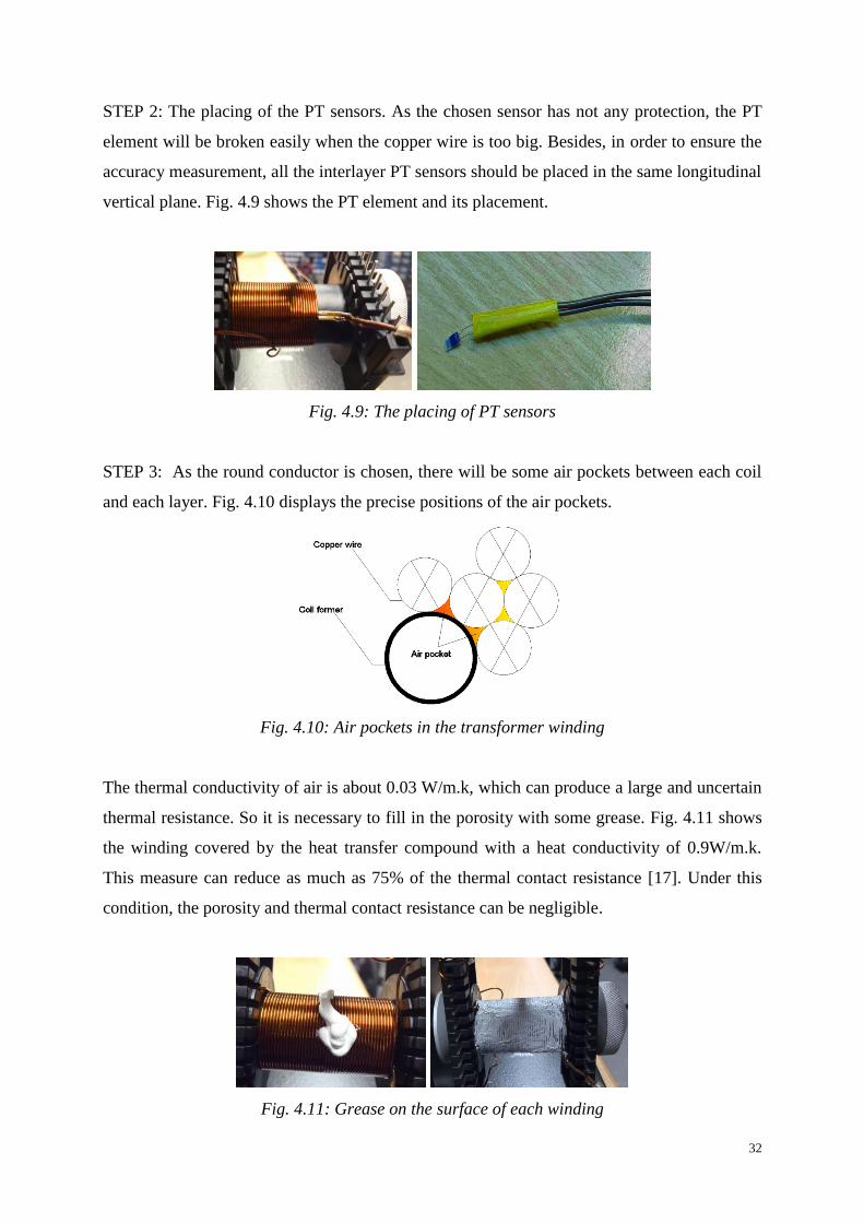
STEP 2: The placing of the PT sensors. As the chosen sensor has not any protection, the PT
element will be broken easily when the copper wire is too big. Besides, in order to ensure the
accuracy measurement, all the interlayer PT sensors should be placed in the same longitudinal
vertical plane. Fig. 4.9 shows the PT element and its placement.
Fig. 4.9: The placing of PT sensors
STEP 3: As the round conductor is chosen, there will be some air pockets between each coil
and each layer. Fig. 4.10 displays the precise positions of the air pockets.
Fig. 4.10: Air pockets in the transformer winding
The thermal conductivity of air is about 0.03 W/m.k, which can produce a large and uncertain
thermal resistance. So it is necessary to fill in the porosity with some grease. Fig. 4.11 shows
the winding covered by the heat transfer compound with a heat conductivity of 0.9W/m.k.
This measure can reduce as much as 75% of the thermal contact resistance [17]. Under this
condition, the porosity and thermal contact resistance can be negligible.
Fig. 4.11: Grease on the surface of each winding

33
STEP 4: When the fifth layer is finished, a layer of electrical insulation tape will be wrapped
on to the winding's surface. Then all the PT sensors wires are welded to the metal terminals of
the coil former. Fig. 4.12 illustrates the final assembly model.
Fig. 4.12: Final assembly unit

34
35
Chapter 5
5. Experiment set-up and test analysis
5.1 Experiment set-up
5.1.1 Thermal model
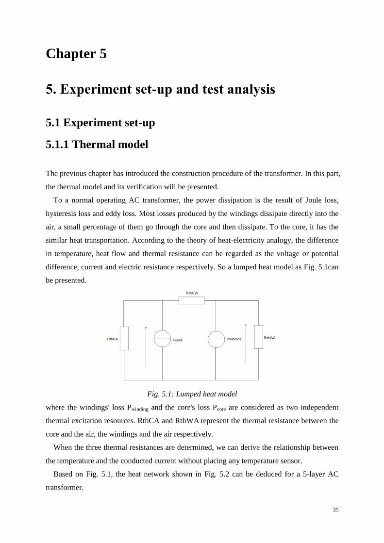
The previous chapter has introduced the construction procedure of the transformer. In this part,
the thermal model and its verification will be presented.
To a normal operating AC transformer, the power dissipation is the result of Joule loss,
hysteresis loss and eddy loss. Most losses produced by the windings dissipate directly into the
air, a small percentage of them go through the core and then dissipate. To the core, it has the
similar heat transportation. According to the theory of heat-electricity analogy, the difference
in temperature, heat flow and thermal resistance can be regarded as the voltage or potential
difference, current and electric resistance respectively. So a lumped heat model as Fig. 5.1can
be presented.
Fig. 5.1: Lumped heat model
where the windings' loss Pwinding and the core's loss Pcore are considered as two independent
thermal excitation resources. RthCA and RthWA represent the thermal resistance between the
core and the air, the windings and the air respectively.
When the three thermal resistances are determined, we can derive the relationship between
the temperature and the conducted current without placing any temperature sensor.
Based on Fig. 5.1, the heat network shown in Fig. 5.2 can be deduced for a 5-layer AC
transformer.

36
Fig. 5.2: 5-layer transformer heat network
Table 5.1 shows the meaning of all the signs from Fig. 5.2.
Table 5.1: Meaning of the signs
Sign Meaning Sign Meaning Sign Meaning
T1 Temperature of layer 1 P1 Heat flow of layer 1 RthCA Thermal resistance between core and
ambient
T2 Temperature of layer 2 P2 Heat flow of layer 2 RthC1 Thermal resistance between core and layer 1
T3 Temperature of layer 3 P3 Heat flow of layer 3 Rth12 Thermal resistance between layer 1 and layer
2
T4 Temperature of layer 4 P4 Heat flow of layer 4 Rth23 Thermal resistance between layer2 and layer
3
T5 Temperature of layer 5 P5 Heat flow of layer 5 Rth34 Thermal resistance between layer 3 and layer
4
TY Surface temperature on layer 5
Pcore Heat flow of the core Rth45 Thermal resistance between layer 4 and layer
5
TA Ambient temperature
Rth5Y
Thermal resistance between layer 5 and its
surface
TC Core temperature
RthYA Thermal resistance between ambient and
surface of layer 5
In this work, in order to determinate the thermal resistance, all the test will be conducted
with DC supply, so that Pcore will not exist anymore, Fig. 5.2 can turn to be,
Fig. 5.3: 5-layer transformer heat network without core loss

37
5.1.2 Determination of the excitation resource P
For each layer, the heat dissipation is expressed thanks to the Joule principle P=I2R. The
currency can be read through an ampere meter. For the resistance, nevertheless, it will be a bit
more complicated as it varies when the temperature changes. Suppose that we have a length
of 20m copper wire with a diameter of 0.85mm, its resistance coefficient at 20 is
ρ=1.68×10⁻⁸
Ω•m and its temperature coefficient is . According to (2.9), we
can calculate its resistance R0=0.6Ω. When the temperature rises up to 100 , its resistance
becomes 0.78Ω which means that it has changed about 31%. As the temperature of each layer
is so close, for simple reason, they can be considered to be equal; when the total power is read
by the power meter, the length of each layer will be the unique factor to decide each layer's
heat dissipation. Fig. 5.2 shows the length and the rate of each layer for test 1.
Table 5.2: The length and the rate of each layer
Layer NO. Length(m) Rate
1 3.73 17%
2 4.05 19%
3 4.14 19%
4 4.45 21%
5 4.94 23%
total 21.3 100%
5.2 Test 1- No interlayer thermal insulation
In this test, there is not any thermal tape between each layer. To stop the outside air flow and
make a balanced temperature without any fluctuation, the tested model is put into a plastic
chamber which is visualized in Fig. 5.4.
5.2.1 External heating source
In the first phase, a power resistor is put inside the coil former to act as the heating source;
when the outside of the coil former is wrapped with thermal insulation material, all the heat
dissipates through the windings. This heat transport can be regarded as just one dimensional.

38
Fig. 5.5 shows the schematic of the heat flow. Then the resistor is conducted with different
DC power (about 1W, 2W, 3W) to get an average value.
Fig. 5.4: Test without interlayer thermal insulation
Fig. 5.5: Tested model with external heat resource
In order to ensure the thermal insulation effect is good enough, we can use a thermal
camera to examine the outside temperature of the tested model. Fig. 5.6 shows the thermal
images captured by a FLIR i7 thermal camera.

39
(a)
(b) (c)
Fig. 5.6: (a) FLIR i7 thermal camera (b) Primal thermal insulation (c) Improved thermal
insulation
Based on Fig. 5.5, the thermal resistances can be derived as
(5.1)
(5.2)
(5.3)
(5.4)
(5.5)
(5.6)
(5.7)
By applying Matlab, the relationship between temperature and measured times can be
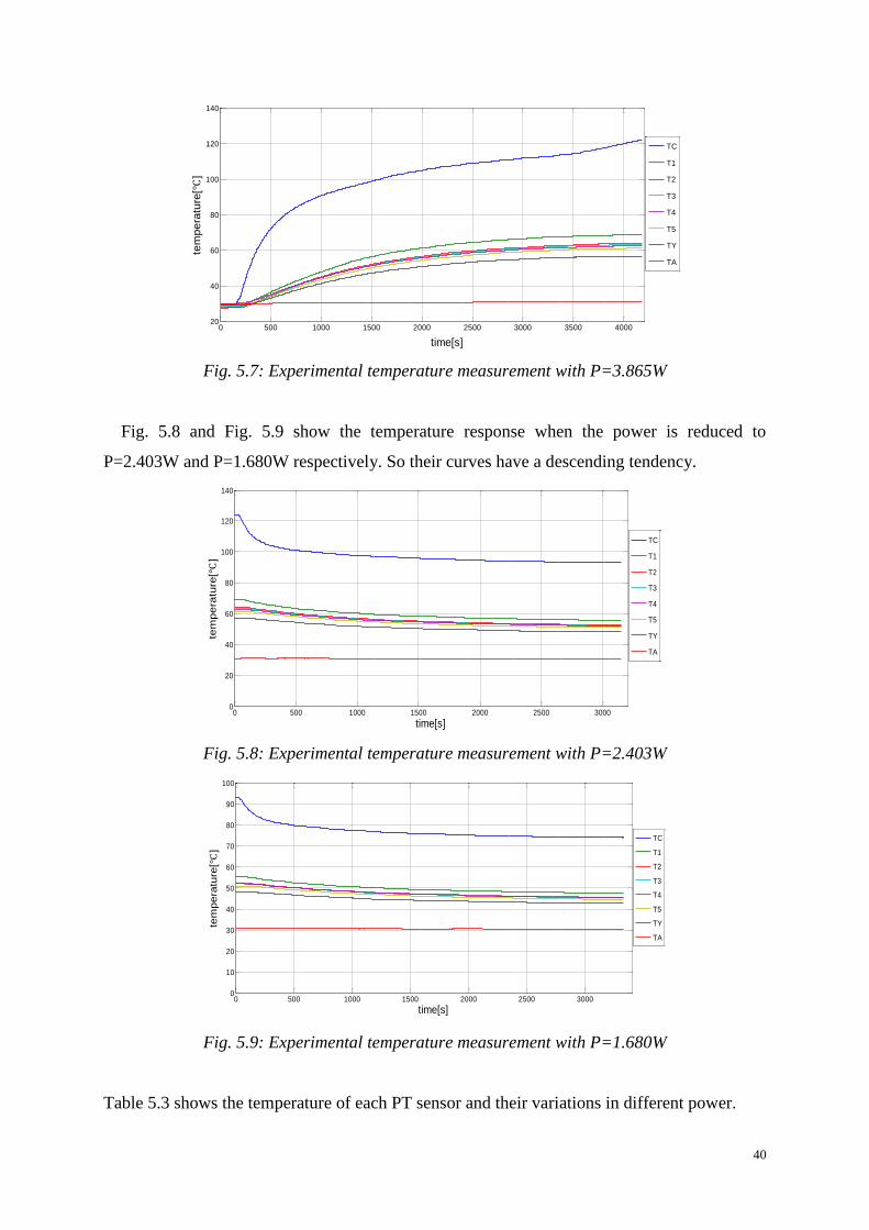
illustrated in curves. Fig. 5.7 shows the response of the temperature of each part from an
original ambient temperature when the power resistor is conducted with P=3.865W.
40
Fig. 5.7: Experimental temperature measurement with P=3.865W
Fig. 5.8 and Fig. 5.9 show the temperature response when the power is reduced to
P=2.403W and P=1.680W respectively. So their curves have a descending tendency.
Fig. 5.8: Experimental temperature measurement with P=2.403W
Fig. 5.9: Experimental temperature measurement with P=1.680W
Table 5.3 shows the temperature of each PT sensor and their variations in different power.
0 500 1000 1500 2000 2500 3000 3500 400020
40
60
80
100
120
140
time[s]
tem
pera
ture
[ ]
TC
T1
T2
T3
T4
T5
TY
TA
0 500 1000 1500 2000 2500 30000
20
40
60
80
100
120
140
time[s]
tem
pera
ture
[ ]
TC
T1
T2
T3
T4
T5
TY
TA
0 500 1000 1500 2000 2500 30000
10
20
30
40
50
60
70
80
90
100
time[s]
tem
pera
ture
[ ]
TC
T1
T2
T3
T4
T5
TY
TA

41
Table 5.3: Temperature versus different power
No. P(W) T1( ) T2( ) T3( ) T4( ) T5( ) TY( ) TC( ) TA( )
1 3.865 68.92 63.97 63.20 62.41 61.08 56.67 121.98 30.96
2 2.403 55.72 52.62 52.21 52.08 51.04 48.14 92.97 30.87
3 1.680 47.48 45.27 45.18 45.49 44.54 42.68 73.93 30.49
Combining Table 5.3 and (5.1) to (5.7), the thermal resistances can be calculated in Table 5.4.
Table 5.4: Thermal resistance versus different power
No. Rth_total
( /w)
RthC1
( /w)
Rth12
( /w)
Rth23
( /w)
Rth34
( /w)
Rth45
( /w)
Rth5Y
( /w)
RthYA
( /w)
1 23.551 13.73 1.28 0.20 0.20 0.35 1.14 6.65
2 25.838 15.50 1.29 0.17 0.06 0.43 1.21 7.18
3 25.853 15.74 1.32 0.05 -0.18 0.56 1.11 7.26
Mean 25.081 14.99 1.30 0.14 0.03 0.45 1.15 7.03
Fig. 5.10 to Fig. 5.12 illustrate the variation tendency of the thermal impedance, but no
matter how the power changes, the thermal impedance can trend to a similar value at steady
state, which proves that thermal resistance depends on the characteristics of the object rather
than the outside excitation.
Fig. 5.10: Experimental thermal impedance measurement with P=3.865W
0 500 1000 1500 2000 2500 3000 3500-2
0
2
4
6
8
10
12
14
time[s]
therm
al im
pedance Z
th[K
/W]
RthC1
Rth12
Rth23
Rth34
Rth45
Rth5Y
RthYA

42
Fig. 5.11: Experimental thermal impedance measurement with P=2.403W
Fig. 5.12: Experimental thermal impedance measurement with P=1.680W
5.2.2 Internal heating source
In the first phase, the thermal resistances have been calculated from the measured
temperatures. Based on the thermal resistances, the temperature of each point can be predicted.
When the temperature measurement in this phase is done, the comparison between the
theoretical and measured values can be made.
Fig. 5.13 shows the winding directly connected with a DC supply to simulate the real
operating situation.
0 500 1000 1500 2000 2500 3000
0
5
10
15
20
time[s]
the
rma
l im
pe
da
nce
Zth
[K
/W]
RthC1
Rth12
Rth23
Rth34
Rth45
Rth5Y
RthYA
0 500 1000 1500 2000 2500 3000-5
0
5
10
15
20
25
time[s]
therm
al im
pedance Z
th [
K/W
]
RthC1
Rth12
Rth23
Rth34
Rth45
Rth5Y
RthYA

43
Fig. 5.13: Tested model with internal heat resource
As the heat flow merely goes through the winding, theoretically there is no heat dissipating
from the core. So RthC1 does not exist in this test.
For the calculation of the heat network, the Mesh-Current-Analysis can be applied [18].
Fig. 5.14 shows the whole 'Mesh' and the imagined 'Mesh Currencies' PL1 to PL5 which
mean the heat flow in each 'Mesh'.
Fig. 5.14: Mesh-Current-Analysis for the heat network
In Fig. 5.14, there are six to-be-solved temperatures, but only five constraint equations can
be established, so an additional equation between T5 and TY will be added.
Based on Fig. 5.14, the relevant equations can be deduced as
(5.8)
(5.9)
(5.10)

44
(5.11)
(5.12)
(5.13)
(5.14)
(5.15)
(5.16)
(5.17)
Then the solution for temperature can be,
(5.18)
(5.19)
(5.20)
(5.21)
(5.22)
(5.23)
When the winding is conducted with different powers, the measured and model-check results
are demonstrated as Table 5.5 and Table 5.6 respectively.
Table 5.5: Measured results
No. P(W) T1( ) T2( ) T3( ) T4( ) T5( ) TY( ) TA( )
1 2.815 55.28 55.96 55.94 55.67 54.73 51.21 30.67
2 7.983 99.78 101.84 101.40 99.19 97.41 86.83 31.91
3 12.062 134.23 137.11 136.64 133.68 130.60 113.22 33.10
Table 5.6: Model-check results
No. P(W) T1( ) T2( ) T3( ) T4( ) T5( ) TY( ) TA( )
1 2.815 55.49 54.71 54.71 54.66 53.70 50.46 30.67
2 7.983 102.31 100.49 100.09 99.97 97.24 88.04 31.91
3 12.062 139.46 136.73 136.11 135.94 131.81 117.91 33.10

45
In order to compare the difference between the measured and theoretical values, the curve
of each temperature is illustrated as Fig. 5.15, Fig.5.16 and Fig. 5.17.
Fig. 5.15: Temperature difference of each point with P=2.815W
Fig. 5.16: Temperature difference of each point with P=7.983W
0 500 1000 1500 2000 2500 30000
20
40
60
time[s]
tem
pera
ture
[ ]
T1 measurement
T1 theory
0 500 1000 1500 2000 2500 30000
20
40
60
time[s]
tem
pera
ture
[ ]
T2 measurement
T2 theory
0 500 1000 1500 2000 2500 30000
20
40
60
time[s]
tem
pera
ture
[ ]
T3 measurement
T3 theory
0 500 1000 1500 2000 2500 30000
20
40
60
time[s]
tem
pera
ture
[ ]
T4 measurement
T4 theory
0 500 1000 1500 2000 2500 30000
20
40
60
time[s]
tem
pera
ture
[ ]
T5 measurement
T5 theory
0 500 1000 1500 2000 2500 30000
20
40
60
time[s]
tem
pera
ture
[ ]
TY measurement
TY theory
0 500 1000 1500 2000 2500 30000
50
100
time[s]
tem
pera
ture
[ ]
T1 measurement
T1 theory
0 500 1000 1500 2000 2500 30000
50
100
time[s]
tem
pera
ture
[ ]
T2 measurement
T2 theory
0 500 1000 1500 2000 2500 30000
50
100
time[s]
tem
pera
ture
[ ]
T3 measurement
T3 theory
0 500 1000 1500 2000 2500 30000
50
100
time[s]
tem
pera
ture
[ ]
T4 measurement
T4 theory
0 500 1000 1500 2000 2500 30000
50
100
time[s]
tem
pera
ture
[ ]
T5 measurement
T5 theory
0 500 1000 1500 2000 2500 30000
50
100
time[s]
tem
pera
ture
[ ]
TY measurement
TY theory

46
Fig. 5.17: Temperature difference of each point with P=12.062W
Table 5.7 shows the percentage of error between the measured and theoretical values in
different conducted powers. The biggest absolute error is about 4% which proves that the
thermal resistances measured in the first phase are correct.
Table 5.7: Error percentage of each temperature
No. P(W) T1( ) T2( ) T3( ) T4( ) T5( ) TY( )
1 2.815 -0.4% 2.3% 2.3% 1.8% 1.9% 1.5%
2 7.983 -2.5% 1.3% 1.3% -0.8% 0.2% -1.4%
3 12.062 -3.8% 0.3% 0.4% -1.7% -0.9% -4.0%
5.2.3 Simulation in PLECS
A good way to validate the measured results is to simulate in program. In real life, it is
difficult to test all the parameters of every new product. So it will be easier and more
economical to effectuate some simulations in software. In this part, a brief introduction of the
software PLECS (Piecewise Linear Electrical Circuit Simulation) and how to organize the
program will be given.
PLECS is a Simulink toolbox developed by Plexim for system-level simulation of electrical
circuits [19]. It is one of the best design platforms for power electronics systems because of its
0 500 1000 1500 2000 2500 30000
50
100
150
time[s]
tem
pera
ture
[ ]
T1 measurement
T1 theory
0 500 1000 1500 2000 2500 30000
50
100
150
time[s]
tem
pera
ture
[ ]
T2 measurement
T2 theory
0 500 1000 1500 2000 2500 30000
50
100
150
time[s]
tem
pera
ture
[ ]
T3 measurement
T3 theory
0 500 1000 1500 2000 2500 30000
50
100
150
time[s]
tem
pera
ture
[ ]
T4 measurement
T4 theory
0 500 1000 1500 2000 2500 30000
50
100
150
time[s]
tem
pera
ture
[ ]
T5 measurement
T5 theory
0 500 1000 1500 2000 2500 30000
50
100
150
time[s]
tem
pera
ture
[ ]
TY measurement
TY theory

47
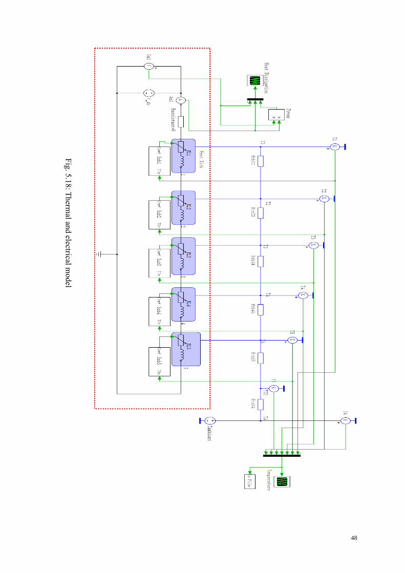
high-speed simulation. In this part, both the electrical and thermal circuits are visualized in
Fig. 5.18 where the module Heat Sink acts as their interface.
For the electrical part (dash-line-rectangle), five variable resistors are used to represent the
five layers of windings of the transformer. As it was mentioned in (2.9), copper wire has a
positive temperature coefficient (PTC) which should be taken into account during the
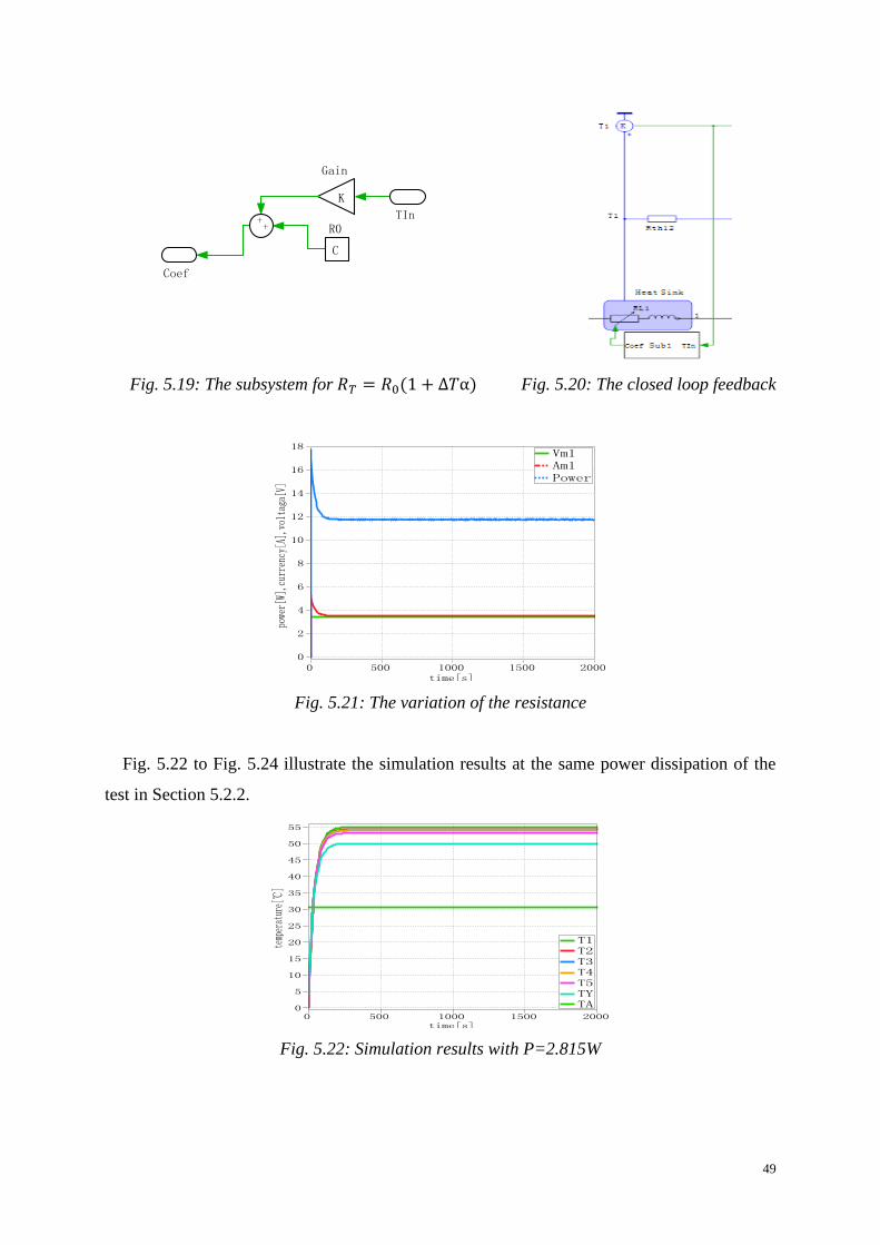
calculation of its actual resistance. So a subsystem shown in Fig. 5.19 can be designed to
control the change of the variable resistor. The input of the subsystem comes from the
temperature of each thermal resistance. Thus each variable resistor and each thermal
resistance constitute a closed loop feedback system. See Fig. 5.20. When the thermal
resistance of each layer is determined, the temperature will be decided by the input voltage
uniquely.
Fig. 5.21 shows the input power has a decreasing tendency because of the increasing
resistance.
48
Fig
. 5.1
8: T
herm
al and electrical m
odel
49
Fig. 5.19: The subsystem for Fig. 5.20: The closed loop feedback
Fig. 5.21: The variation of the resistance
Fig. 5.22 to Fig. 5.24 illustrate the simulation results at the same power dissipation of the
test in Section 5.2.2.
Fig. 5.22: Simulation results with P=2.815W

50
Fig. 5.23: Simulation results with P=7.983W
Fig. 5.24: Simulation results with P=12.026W
Table 5.8 shows the temperature of each point simulated in PLECS. Table 5.9 is the
comparison between the temperature measured in the experiment and produced in PLECS.
We can see that the biggest absolute error percentage is 3.2% which means the simulation is
correct.
Table 5.8: Simulation results
No. P(W) T1( ) T2( ) T3( ) T4( ) T5( ) TY( )
1 2.815 54.98 54.35 54.21 54.17 53.23 50.05
2 7.983 101.07 99.28 98.88 98.77 96.08 87.04
3 12.062 136.56 133.87 133.27 133.10 129.07 115.55
Table 5.9: Error between the simulated and measured results
No. P(W) T1( ) T2( ) T3( ) T4( ) T5( ) TY( )
1 2.815 0.5% 2.9% 3.2% 2.8% 2.8% 2.3%
2 7.983 -1.3% 2.6% 2.5% 0.4% 1.4% -0.2%
3 12.062 -1.7% 2.4% 2.5% 0.4% 1.2% -2.0%

51
5.2.4 Conclusion for test 1
In test 1, the thermal resistances were derived from the measured temperatures and they were
used to predict the temperature in different power dissipations. Then the other measurement
and simulation were effectuated successively and their results proved the thermal resistances
were correctly calculated. Nevertheless there exists a large inconvenience because in the
industrial domain, it is impossible to place the sensors in each product to measure their
temperatures. So we need to be able to calculate the thermal resistance basing on the material
used in the transformer and the theoretical results should match the measured ones. The
largest significance of that case lies on the general applicability to all the similar products as
long as the module's parameters are established. That is the reason why test 2 is carried out.
5.3 Test 2- With interlayer thermal insulation
In this section, at first a theoretical calculation of the thermal resistance will be made. Then on
the basis of the theory, a new model will be built to examine if the theoretical and measured
values match each other properly. From test 1, we can notice that the thermal resistance of
each layer was so small because of the high heat conductivity of copper wire (about 380
W/m.k), which can be beyond the resolving ability of the PT sensor. So some interlayer
thermal insulation tapes with known thermal conductivity will be added. Fig. 4.5 to Fig. 4.7
showed the manufacture sketch for test 2.
5.3.1 Heating source
In the first phase of test 1, an external resistor put inside the coil former was used to act as the
heating source. But it is not so perfect because the resistor can't be placed manually exactly in
the middle of the coil former. In most cases, the resistor inclines to one side of the coil former.
According to the data sheet provided by manufacturer, the coil former is made of PET
(Polyethylene Terephthalate) which has low heat conductivity (about 0.15W/m.k), so the
temperature of the whole coil former is not homogeneous. To some extent, ∆T depends on the
position where the PT sensor is located. There is why some negative thermal resistances
occurred in test 1. Thus in test 2, an extra layer of winding that has not any electrical
connection to the other ones is made to act as the heating source.

52
5.3.2 Coil former test
The characteristic parameter of the coil former has been visualized in Fig. 4.2. Even though
its heat conductivity is not provided, we can apply the one of PET for the calculation. Fig.
5.25 (a) shows the construction of the coil former test. The layer of copper wire is used to get
a homogeneous heating environment. Fig. 5.25 (b) and (c) show the structure and the heat
flow direction respectively.
(a)
(b) (c)
Fig. 5.25: (a) Construction of the coil former test (b) Structure form top view (c) Heat flow
direction from side view
5.3.2.1 Theoretical calculation and measured results
For hollow cylinder, the calculation of thermal resistance can be presented as
(5.24)
where, r1 is inside radius, r2 is outside radius, k is heat conductivity and l is length [20].

53
Fig. 5.25 shows the precise dimensions and the heat flow direction of the coil former test.
Fig. 5.26: Coil former dimensions for test
According to the property of the material, the theoretical thermal resistance can be
presented in Table 5.10 by using (5.24).
Table 5.10: Theoretical thermal resistance of the coil former
Item Theoretical value
Coil former r2(m) r1(m) l(m) K(w/m.k) Rth( /w)
0.01245 0.0112 0.0412 0.15 2.725
Then the extra winding is conducted with different DC powers to measure the real thermal
resistance of the coil former.
Figs 5.27 to Fig. 5.29 show the difference between the theoretical and measured values.
Fig. 5.27: Thermal impedance difference with P=2.159W
0 500 1000 1500 2000 2500 3000 3500 40000
0.5
1
1.5
2
2.5
3
3.5
time[s]
the
rma
l im
pe
da
nce
Zth
[K
/W]
Rth theory=2.725Mesured RthC1
Theoretical RthC1

54
Fig. 5.28: Thermal impedance difference with P=2.898 W
Fig. 5.29: Thermal impedance difference with P=3.524 W
From Table 5.11, we can see that the average error is about 9% and the measured values are
always larger than the theoretical ones. This is probably caused by the thermal conductivity of
the coil former material for the reason that it is made by impure PET.
Table 5.11: Comparison between theoretical and measured values
measurement theory Error
NO. P(w) ∆T( ) Rth( /w) Rth( /w) -
1 1.440 4.262 2.959
2.725
9%
2 2.159 6.463 2.993 10%
3 2.898 8.657 2.987 10%
4 3.524 10.404 2.952 8%
Average - - 2.973 9%
0 500 1000 1500 2000 2500 3000 35000
0.5
1
1.5
2
2.5
3
3.5
time[s]
therm
al im
pedan
ce Z
th [
K/W
]
Rth theory=2.725Mesured RthC1
Theoretical RthC1
10%
0 500 1000 1500 2000 2500 3000 3500 40000
0.5
1
1.5
2
2.5
3
3.5
time[s]
therm
al im
pedance Z
th [
K/W
]
Rth theory=2.725Mesured RthC1
Theoretical RthC1
8%

55
The entire test for the coil former should be effectuated under the condition that the coil
former is in the erect position which is visualized as Fig. 5.30 (a). If it is placed horizontally
as Fig. 5.30 (b), it can bring a larger error. See Table 5.12.
Fig. 5.30: (a) Upright position, (b) horizontal position
Table 5.12: Measured result in horizontal position
measured theoretical error
NO. P(w) ∆T( ) Rth( /w) Rth( /w) -
1 1.402 6.127 4.369 2.725 60%
Fig. 5.31 shows the temperature difference between the top side and bottom side of the coil
former when it was placed horizontally. This is because of the heat convection causes the hot-
air accumulates at the top side.
Fig. 5.31: (a) Top side temperature, (b) bottom side temperature
5.3.3 Core test
In this part, the EPCOS ferrite core ETD59 is used to test. The dimensions of the core are
visualized in Fig. 4.3. In order to fill in the air gap between the coil former and the core, three
layers of insulation tape with heat conductivity (0.9w/m.k) are added which is shown in Fig.
5.32.

56
Fig. 5.32: Test for the core ETD59
When the core is plugged into the coil former, the outside of the core is covered with
thermal insulation material except for its top side middle. See Fig. 5.33.
Fig. 5.33: Sketch for the core test
This measurement bases on the test of the coil former, so the equivalent thermal network is
presented as Fig. 5.34.
Fig. 5.34: Thermal network of the core and coil former
where Rth-coil formr is the thermal resistance of the coil former, Rth-tape is the thermal resistance
of the insulation tape, Rth-core is the thermal resistance of the ferrite core, P1 is the heating
source, T1 is the temperature on the surface of the coil former, Tc is the temperature on the
surface of the ferrite core.

57
According to the parameter provided by manufacturer, the thermal resistance of ETD59
core is 4 /w, but in this test, the core is regarded as two halves which are connected parallelly,
so the equivalent value is 1 /w in this thermal network.
Fig. 5.35: Thermal network the core and coil former
5.3.3.1 Theoretical calculation and measured results
The thermal resistance of the coil former is taken from the average measured value in the
previous test, so the theoretical thermal resistance of the test is presented in Table 5.13.
Table 5.13: Theoretical value
Item coil former insulation tape ferrite core Total
Rth( /w) 2.973 0.052061 1.0 4.025
The thermal impedance differences are visualized in Fig. 5.36 to Fig. 5.38 with different power
dissipations.
Fig. 5.36: Thermal impedance difference with P=2.016W
0 500 1000 1500 2000 2500 3000 35000
0.5
1
1.5
2
2.5
3
3.5
4
4.5
time[s]
therm
al im
pedance Z
th [
K/W
]
Rth theory=4.0251
Mesured Rth core
Theoretical Rth core

58
Fig. 5.37: Thermal impedance difference with P=2.531W
Fig. 5.38: Thermal impedance difference with P=3.043W
Table 5.14 shows the error between the theoretical and measured values. The biggest
absolute error is about 0.4% which proves that the theoretical and measured values match
each other perfectly.
Table 5.14: Comparison between the theoretical and measured values
measurement theory Error
NO. P(w) ∆T( ) Rth( /w) Rth( /w) -
1 2.016 8.149 4.042
4.025
-0.4%
2 2.531 10.171 4.019 0.2%
3 3.043 12.263 4.030 -0.1%
0 500 1000 1500 2000 2500 3000 35000
0.5
1
1.5
2
2.5
3
3.5
4
4.5
time[s]
therm
al im
pedance Z
th [
K/W
]
Rth theory=4.0251
Mesured Rth core
Theoretical Rth core
0 500 1000 1500 2000 2500 30000
0.5
1
1.5
2
2.5
3
3.5
4
4.5
time[s]
the
rma
l im
pe
da
nce
Zth
[K
/W]
Rth theory=4.0251
Mesured Rth core
Theoretical Rth core

59
5.3.4 Windings test
In this test, an extra layer of copper wire is added besides the five layers windings to act as the
heating source. The heat flow dissipates through the five layer windings and the core. Once
the temperature difference between each layer is measured, the thermal resistance can be
decided by (2.12). Fig. 5.39 shows the experiment model.
Fig. 5.39: Windings test
5.3.4.1 Theoretical calculation
RthCA test:
For the calculation of RthCA, it is much more complex as it involves energy dissipation
between a solid surface and the air. Three thermal transport mechanisms occur at the same
time. But because of the low heat conductivity of the air (k=0.032W/m.k), for simple reason,
the heat transported by conduction can be negligible.
According to Newton’s law of cooling, the energy transported by convection can be derived
as
(5.25)
where h is convection heat-transfer coefficient, A is area, T1 is the temperature of the core, TA
is the ambient temperature.
In this test, the model is put into a chamber, so the convection can be considered as natural
convection. It concerns three dimensionless parameters: Nusselt number (Nu), Prandtl number
(Pr) and Grashof number (Gr). The relationship between h and Nu can be presented as

60
(5.26)
where L is a characteristic dimension of the solid object, k is the thermal conductivity of the
fluid.
If Nu is decided, h can be easily deduced.
Generally, the three dimensionless parameters follow the relationship as
(5.27)
where c is the thermal property of the air, n is decided by the product of GrPr: if GrPr<108, the
convection is laminar flow, n=0.33; if GrPr>108, n=0.25 for turbulent flow.
In most cases, we can judge the state of the flow by using the product of L3∆T, if L
3∆T>1, it
can be considered as turbulent flow, otherwise it is laminar flow. In this test, the temperature
difference is small enough, so the convection is laminar flow. Then an empirical equation can
be used to calculate h [21].
(5.28)
For the radiation, the transferred energy can be presented by Stefan-Boltzmann law
(5.29)
where ε is emissivity of the core ,σ is Stefan-Boltzmann constant, σ=5.669×10⁻⁸
W.m-2
·K-4
,
T1 and TA are thermodynamic temperature in Kelvin.
So the total heat dissipation can be presented as
(5.30)
(5.31)
The total thermal resistance can be written as
(5.32)

61
Table 5.15 shows the difference between the theoretical and measured values. This error
may be caused by the imperfect thermal insulation which means that not all the energies
dissipate through the core.
Table 5.15: Comparison between the theoretical and measured values
theoretical measured error
N0 A(m2) h(W/m
2. ) ∆T( ) ε Rth( /w) Rth( /w) -
1 0.00264 8.4 27.01 0.9 25.413 27.682 -8%
2 0.00264 9.3 41.04 0.9 23.254 27.705 -16%
Interlayer thermal resistance calculation:
For the calculation of the thermal resistance of each layer, (5.24) can be applied. The diameter
of the copper wire used in this test is 0.40mm and the thickness of the tape is 80um. Table
5.16 shows the theoretical values of each layer.
Table 5.16: Theoretical calculation
material K(w/m.k) D2(2*r2) D1(2*r1) l(m) Rth( /w)
Rth12
copper 377 0.0257 0.0249 0.0412 0.00032
Tape 0.15 0.02666 0.0257 0.0412 0.94446
total 0.94478
Rth23
copper 377 0.02746 0.02666 0.0412 0.00030
Tape 0.15 0.02842 0.02746 0.0412 0.88495
total 0.88525
Rth34
copper 377 0.02922 0.02842 0.0412 0.00028
Tape 0.15 0.03018 0.02922 0.0412 0.83250
total 0.83278
Rth45
copper 377 0.03098 0.03018 0.0412 0.00027
Tape 0.15 0.03178 0.03098 0.0412 0.65659
total 0.65685
Rth5Y
copper 377 0.03258 0.03178 0.0412 0.00025
Tape 0.15 0.03338 0.03258 0.0412 0.62473
total 0.62498
where D1 and D2 are diameters for each layer.
After the measurement, the results and the comparison are listed at Table 5.17.
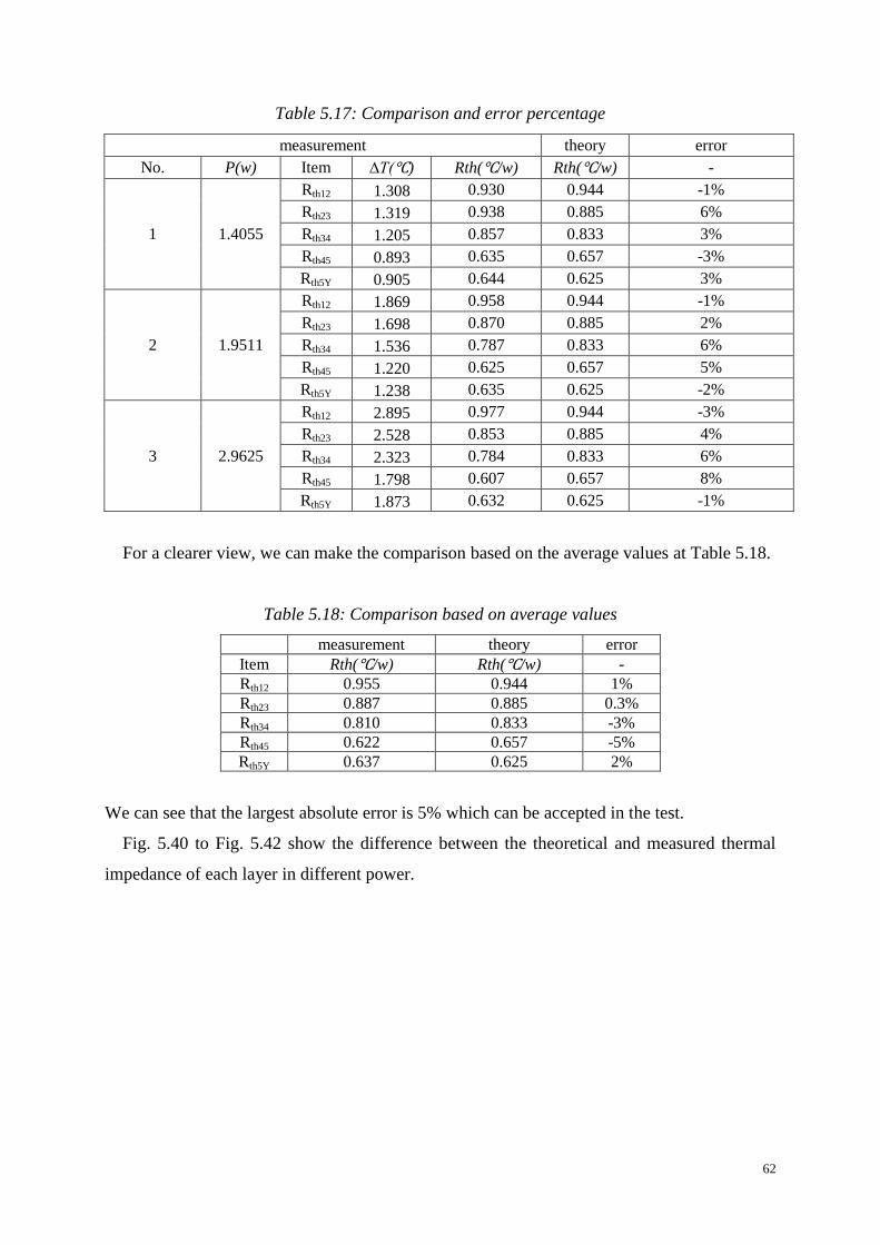
62
Table 5.17: Comparison and error percentage
measurement theory error
No. P(w) Item ∆T( ) Rth( /w) Rth( /w) -
1 1.4055
Rth12 1.308 0.930 0.944 -1%
Rth23 1.319 0.938 0.885 6%
Rth34 1.205 0.857 0.833 3%
Rth45 0.893 0.635 0.657 -3%
Rth5Y 0.905 0.644 0.625 3%
2 1.9511
Rth12 1.869 0.958 0.944 -1%
Rth23 1.698 0.870 0.885 2%
Rth34 1.536 0.787 0.833 6%
Rth45 1.220 0.625 0.657 5%
Rth5Y 1.238 0.635 0.625 -2%
3 2.9625
Rth12 2.895 0.977 0.944 -3%
Rth23 2.528 0.853 0.885 4%
Rth34 2.323 0.784 0.833 6%
Rth45 1.798 0.607 0.657 8%
Rth5Y 1.873 0.632 0.625 -1%
For a clearer view, we can make the comparison based on the average values at Table 5.18.
Table 5.18: Comparison based on average values
measurement theory error
Item Rth( /w) Rth( /w) -
Rth12 0.955 0.944 1%
Rth23 0.887 0.885 0.3%
Rth34 0.810 0.833 -3%
Rth45 0.622 0.657 -5%
Rth5Y 0.637 0.625 2%
We can see that the largest absolute error is 5% which can be accepted in the test.
Fig. 5.40 to Fig. 5.42 show the difference between the theoretical and measured thermal
impedance of each layer in different power.

63
Fig. 5.40: Thermal impedance difference with P=1.406W
Fig. 5.41: Thermal impedance difference with P=1.951W
0 500 1000 1500 2000 2500 3000 3500 4000 4500 50000
0.5
1
time[s]
therm
al im
pedance Z
th [
K/W
]
Rth12 measured
Rth12 theoretical
0 500 1000 1500 2000 2500 3000 3500 4000 4500 50000
0.5
1
time[s]
therm
al im
pedance Z
th [
K/W
]
Rth23 measured
Rth23 theoretical
0 500 1000 1500 2000 2500 3000 3500 4000 4500 50000
0.5
1
time[s]
therm
al im
pedance Z
th [
K/W
]
Rth34 measured
Rth34 theoretical
0 500 1000 1500 2000 2500 3000 3500 4000 4500 50000
0.5
1
time[s]
therm
al im
pedance Z
th [
K/W
]
Rth45 measured
Rth45 theoretical
0 500 1000 1500 2000 2500 3000 3500 4000 4500 50000
0.5
1
time[s]
therm
al im
pedance Z
th [
K/W
]
Rth5Y measured
Rth5Y theoretical
0 500 1000 1500 2000 2500 3000 3500 4000 4500 50000
0.5
1
time[s]
therm
al im
pedance Z
th [
K/W
]
Rth12 measured
Rth12 theoretical
0 500 1000 1500 2000 2500 3000 3500 4000 4500 50000
0.5
1
time[s]
therm
al im
pedance Z
th [
K/W
]
Rth23 measured
Rth23 theoretical
0 500 1000 1500 2000 2500 3000 3500 4000 4500 50000
0.5
1
time[s]
therm
al im
pedance Z
th [
K/W
]
Rth34 measured
Rth34 theoretical
0 500 1000 1500 2000 2500 3000 3500 4000 4500 50000
0.5
1
time[s]
therm
al im
pedance Z
th [
K/W
]
Rth45 measured
Rth45 theoretical
0 500 1000 1500 2000 2500 3000 3500 4000 4500 50000
0.5
1
time[s]
therm
al im
pedance Z
th [
K/W
]
Rth5Y measured
Rth5Y theoretical

64
Fig. 5.42: Thermal impedance difference with P=2.963W
RthYA test:
In this test, the heat transportation direction is inverse compare to the winding test. So the first
layer copper wire is used to be the heating source. Fig. 5.43 illustrates the precise form.
Fig. 5.43: RthYA test
By applying the same principles at 5.3.1, the theoretical and measured values is presented in
Table 5.19
0 500 1000 1500 2000 2500 3000 3500 40000
0.5
1
time[s]
therm
al im
pedance Z
th [
K/W
]
Rth12 measured
Rth12 theoretical
0 500 1000 1500 2000 2500 3000 3500 40000
0.5
1
time[s]
therm
al im
pedance Z
th [
K/W
]
Rth23 measured
Rth23 theoretical
0 500 1000 1500 2000 2500 3000 3500 40000
0.5
1
time[s]
therm
al im
pedance Z
th [
K/W
]
Rth34 measured
Rth34 theoretical
0 500 1000 1500 2000 2500 3000 3500 40000
0.5
1
time[s]
therm
al im
pedance Z
th [
K/W
]
Rth45 measured
Rth45 theoretical
0 500 1000 1500 2000 2500 3000 3500 40000
0.5
1
time[s]
therm
al im
pedance Z
th [
K/W
]
Rth5Y measured
Rth5Y theoretical

65
Table 5.19: Comparison between the theoretical and measured values
theoretical
measured error
N0 A(m2) h(W/m
2. ) ∆T( ) ε σ(W/m
2·K
4) Rth( /w) Rth( /w) -
1 0.00432 7.4 24.02 0.9 5.67e-8 16.830 14.489 -14%
2 0.00432 8.0 32.87 0.9 5.67e-8 15.817 14.342 -9%
3 0.00432 8.4 40.58 0.9 5.67e-8 15.111 13.567 -10%
5.3.5 The whole thermal network
After all the thermal resistances have been measured and compared, the complete thermal
network can be illustrated as Fig. 5.44. This network applies to both AC and DC. For the
usage in AC, firstly, the core losses should be calculated by taking the eddy loss and the
hysteresis loss into account.
(a)
(b)
Fig. 5.44: The complete thermal network for a five-layer transformer

66

67
Chapter 6
6. Conclusion and future work
6.1 Conclusion
The main objective of this project is to establish a thermal model of a transformer based on
measurement data. The model should apply to any similar transformer and has not limit in the
number of layer. Under this condition, a series of tests have been carried out.
Chapter 3 mainly described the temperature measurement system which was needed
during the whole project. This system was the combination of hardware and software. For the
hardware, a brief description for PCB was made. As to the software, it consisted of LabVIEW
and Matlab.
Then two main tests were implemented. Test 1 aimed at the prediction of the temperature
based on the measured thermal resistance. This prediction was compared to the measured
values and they matched each other perfectly. Besides, a simulation using PLECS was also
effectuated to verify this thermal modelling. The important significance of Test 1 lied on the
precise prediction of the temperature according to the conducted current. However, this
thermal model was suitable uniquely to the transformer made in Test 1.
That was the reason why Test 2 was done. It focused on the theoretical calculation of the
thermal resistance on the basis of the material used in the transformer. These values
practically conformed to the measured ones. The advantage of the thermal model in Test 2
was that it was applicable for any similar transformer at any number of layers.
6.2 Future work
For the next step of this work, some points need to be improved.
Firstly, the key factors which decide the interlayer thermal resistances should be
determinated. As it was mentioned before, the copper wires were greased to reduce the
influence of the contact thermal resistance as well as the porosities. In the industrial product,
this phenomenon is very rare.

68
Secondly, a better method FEM should be carried out to analyze the thermal situation. The
best challenge of that is the modelling of the 3-Dimensions coordinate system which can take
some time.
Then the final model should be conducted with AC to verify its response.
Lastly, the capacitance of each layer can be derived based on the curves. According to a RC
circuit, the time constant can be described as presents the time it takes for the
system response to reach 63.2% of its final value. Since R is already know, can be read from
the curve, and then C can be calculated. If so, a totally complete thermal network will be
constructed and the transient response can be displayed.

69
References
[1] "Transformer," web page. Available: http://en.wikipedia.org/wiki/Transformer
[2] Olivier MALOBERTI, "Material of Electrical Energy," ESIEE-Amiens, appendix-1, 2013
[3] “Convection, conduction and radiation,” Web page. Available:
http://www.mansfieldct.org/Schools/MMS/staff/hand/convcondrad.htm
[4] “Thermal analysis of semiconductor systems,” Web page. Available:
http://cache.freescale.com/files/analog/doc/white_paper/BasicThermalWP.pdf pp.6
[5] JI Hai-ning, LAN Zhong-wen, ZHANG Huai-Wu, Zhang Yue, "Thermal Simulation of
Switching Mode Power Supply Transformer With ANSYS," Journal of Magnetic
Materials and Devices, pp.1, 2006
[6] "Thermometer," web page. Available: http://baike.baidu.com/view/41148.htm
[7] "Select a sensor," web page. Minco. Available:
http://www.minco.com/Sensors-and-Instruments/Support-and-Tools/Select-a-Sensor
[8] "Transformer," web page. Available: http://baike.baidu.com/view/30130.htm
[9] "Resistance thermometer," web page. Available:
http://en.wikipedia.org/wiki/Resistance_thermometer#cite_note-2
[10] P. R. N. Childs, "Practical temperature measurement," Oxford, Boston: Butterworth-
Heinemann, pp.149, 2001
[11] “Measuring temperature with rtds-a tutorial,” National instruments, 1996. Available:
http://newton.ex.ac.uk/teaching/CDHW/Sensors/an046.pdf
[12] "Ina122 instrumentation amplifier data sheet,” Texas instrument, 2013. Available:
http://www.ti.com/lit/ds/symlink/ina122.pdf
[13] Kang Hua guang, "Technology of analog signal,” pp.415-417, 2005
[14] "Protues", web page. Available:
http://baike.baidu.com/view/1639293.htm?fr=wordsearch
[15] "Calibration", web page. Available: http://en.wikipedia.org/wiki/Calibration
[16] "Polytéréphthalate d'éthylène ", web page. Available:
http://fr.wikipedia.org/wiki/Polytéréphtalate_d'éthylène
[17][20][21] J.P. Holman, "Heat Transfer," pp.59, pp.55, pp.346, 2008
[18] Qiu Guanyuan, "Circuit theory," pp.60-64, 2006
[19] "Electrical engineering software,” Plexim, 2013, web page. Available:
http://www.plexim.com/

70

71
Appendix A
Component data sheet

72
Fig. A.1: INA122 data sheet

73
Fig. A.2: INA122 data sheet

74
Fig. A.3: INA122 data sheet
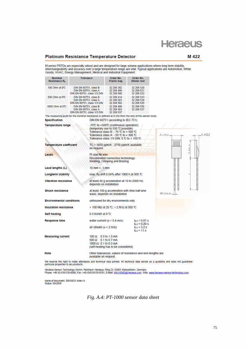
75
Fig. A.4: PT-1000 sensor data sheet

76
Fig. A.5: 3M tape data sheet

77
Fig. A.6: 3M tape data sheet

78

79
Appendix B
Matlab code

80
%*********************************************
% Relationship between Vout and Rt
% for Fig. 3.2
% HUANG JUNXING
%********************************************
R=1000;
Vin=7.5;
Rt=0:10:7000
siz=size(Rt);
Ni=siz(2);
for i=1:Ni
Vout(i)=(Rt(i)/(Rt(i)+R)-1/2)*Vin;
end
plot(Rt,Vout)
grid
%*********************************************
% Bode diagram of the amplitude-frequency response and the phase-frequency response
% for Fig. 3.5
% HUANG JUNXING
%********************************************
num=[0,1];%numerator
den=[0.47,1];%denominator
system=tf(num,den);
bode(system)
grid
%*********************************************
% Calibration Data Handling
% 20-04-2014
% HUANG JUNXING
%********************************************
clear
close all
clc
load temperature3.txt;
loadfile=temperature3;
% Load the data into each channel
Tem=loadfile(:,1);
ch0=loadfile(:,2);
ch1=loadfile(:,3);
ch2=loadfile(:,4);
ch3=loadfile(:,5);
ch4=loadfile(:,6);
ch5=loadfile(:,7);
ch6=loadfile(:,8);
ch7=loadfile(:,9);
% Draw the Polynome for each Channel
Fitch0=fit(ch0,Tem,'poly2')
Fitch1=fit(ch1,Tem,'poly2')
Fitch2=fit(ch2,Tem,'poly2')
Fitch3=fit(ch3,Tem,'poly2')
Fitch4=fit(ch4,Tem,'poly2')
Fitch5=fit(ch5,Tem,'poly2')
Fitch6=fit(ch6,Tem,'poly2')

81
Fitch7=fit(ch7,Tem,'poly2')
V=[0:0.1:3.5];
T0=Fitch0(V);
T1=Fitch1(V);
T2=Fitch2(V);
T3=Fitch3(V);
T4=Fitch4(V);
T5=Fitch5(V);
T6=Fitch6(V);
T7=Fitch7(V);
% Plot the theoretical curve
A=3.9080*10^(-3);
B=-5.8019*10^(-7);
C=-4.2735*10^(-12);
R=1000;
R0=1000;
Vout2=[0:0.1:3.5];
Vout1=Vout2/5; %The time of the amplifier INA122 equal 5
Vin=4.93; %The output voltage of the 78L05 is 4.93
Ni=length(Vout1)
for i=1:Ni
Rt(i)=((2*Vout1(i)+Vin)*R)/(Vin-2*Vout1(i));
Ttheory(i)=(-R0*A+sqrt((R0*A)^2-4*R0*B*(R0-Rt(i))))/(2*R0*B);
end
%Plot Channel 0
subplot(4,2,1)
plot(V,T0,'k','linewidth',1.5)
title('T0= 5.578V^2 + 38.83V + 0.4425')
hold on
plot(Vout2,Ttheory,'r','linewidth',2)
plot(ch0,Tem,'*')
grid on
legend('Fitting curve','Theoretical curve','Calibration value')
%Plot Channel 1
subplot(4,2,2)
plot(V,T1,'k','linewidth',1.5)
title('T1= 5.567V^2 + 38.86V + 0.3545')
hold on
plot(Vout2,Ttheory,'r','linewidth',2)
plot(ch1,Tem,'*')
grid on
%Plot Channel 2
subplot(4,2,3)
plot(V,T2,'k','linewidth',1.5)
title('T2= 5.573V^2 + 38.88V + 0.3973')
hold on
plot(Vout2,Ttheory,'r','linewidth',2)
plot(ch2,Tem,'*')
grid on
%Plot Channel 3
subplot(4,2,4)

82
plot(V,T3,'k','linewidth',1.5)
title('T3= 5.548V^2 + 38.93V + 0.4366')
hold on
plot(Vout2,Ttheory,'r','linewidth',2)
plot(ch3,Tem,'*')
grid on
%Plot Channel 4
subplot(4,2,5)
plot(V,T4,'k','linewidth',1.5)
title('T4= 5.569V^2 + 38.83V + 0.4987')
hold on
plot(Vout2,Ttheory,'r','linewidth',2)
plot(ch4,Tem,'*')
grid on
%Plot Channel 5
subplot(4,2,6)
plot(V,T5,'k','linewidth',1.5)
title('T5= 5.585V^2 + 38.75V + 0.4796')
hold on
plot(Vout2,Ttheory,'r','linewidth',2)
plot(ch5,Tem,'*')
grid on
%Plot Channel 6
subplot(4,2,7)
plot(V,T6,'k','linewidth',1.5)
title('T6= 5.509V^2 +39.08V + 0.4723')
hold on
plot(Vout2,Ttheory,'r','linewidth',2)
plot(ch6,Tem,'*')
grid on
%Plot Channel 7
subplot(4,2,8)
plot(V,T7,'k','linewidth',1.5)
title('T7= 5.527V^2 + 38.89V + 0.2754')
hold on
plot(Vout2,Ttheory,'r','linewidth',2)
plot(ch7,Tem,'*')
grid on
%*********************************************
% T=f(t),5.2.1
% for Fig. 5.7-Fig. 5.9
% HUANG JUNXING
%********************************************
clear
close all
clc
%No1
load coreheating1326.txt;
loadfile=coreheating1326;

83
N=33440;
%No2
% load coreheating1426.txt;
% loadfile=coreheating1426;
% N=25192;
%No3
% load coreheating1526.txt;
% loadfile=coreheating1526;
% N=26648;
for i=1:(N-1)/8
T1(i)=loadfile(8*i+1,2);
T2(i)=loadfile(8*i+2,2);
T3(i)=loadfile(8*i+3,2);
T4(i)=loadfile(8*i+4,2);
T5(i)=loadfile(8*i+5,2);
TY(i)=loadfile(8*i+6,2);
TC(i)=loadfile(8*i+7,2);
TA(i)=loadfile(8*i+8,2);
end
k=length(T1);
x=1:k
plot(x,TC,x,T1,x,T2,x,T3,x,T4,x,T5,x,TY,x,TA,'red','linewidth',1)
xlabel('time[s]')
ylabel('temperature[¡æ]')
legend('TC','T1','T2','T3','T4','T5','TY','TA')
axis([0 4000 0 85])
grid
%*********************************************
% Rth=f(t),5.2.1
% for Fig. 5.10-Fig. 5.12
% HUANG JUNXING
%********************************************
clear
close all
clc
%No1
load coreheating1326.txt;
loadfile=coreheating1326;
N=33440;
P=3.86508;
%No2
% load coreheating1426.txt;
% loadfile=coreheating1426;
% N=25192;
% P=2.40345;
%No3
% load coreheating1526.txt;

84
% loadfile=coreheating1526;
% N=26648;
% P=1.68018;
for i=1:(N-1)/8
T1(i)=loadfile(8*i+1,2);
T2(i)=loadfile(8*i+2,2);
T3(i)=loadfile(8*i+3,2);
T4(i)=loadfile(8*i+4,2);
T5(i)=loadfile(8*i+5,2);
TY(i)=loadfile(8*i+6,2);
TC(i)=loadfile(8*i+7,2);
TA(i)=loadfile(8*i+8,2);
end
RthC1=(TC-T1)/P;
Rth12=(T1-T2)/P;
Rth23=(T2-T3)/P;
Rth34=(T3-T4)/P;
Rth45=(T4-T5)/P;
Rth5Y=(T5-TY)/P;
RthYA=(TY-TA)/P;
k=length(T1);
x=1:k
plot(x,RthC1,x,Rth12,x,Rth23,x,Rth34,x,Rth45,x,Rth5Y,x,RthYA,'linewidth',3)
legend('RthC1','Rth12','Rth23', 'Rth34','Rth45','Rth5Y','RthYA')
xlabel('time[s]')
ylabel('thermal resistance[k/w]')
axis([0 4000 0 3.5])
grid
%*********************************************
% Mesh-Current-Analysis for the heat network,5.2.2
% for Table 5.6
% HUANG JUNXING
%********************************************
clc
close all
clear all
Rtotal=25.0808431450213;
RC1=14.9896738074409;
R12=1.29654886395014;
R23=0.139566655661111;
R34=0.0261246739263876;
R45=0.445597388536415;
R5Y=1.1525258110241;
RYA=7.03080594448218;
% test1
TA=30.6651902;
P1=0.492406530612245;
P2=0.534808204081633;
P3=0.547118367346939;

85
P4=0.588152244897959;
P5=0.652438653061225;
% % test2
% TA=31.9106088;
% P1=1.39645014577259;
% P2=1.51670001943635;
% P3=1.55161127308066;
% P4=1.66798211856171;
% P5=1.85029644314869;
% % test3% TA=33.0970498;
% P1=2.11004081632653;
% P2=2.2917387755102;
% P3=2.34448979591837;
% P4=2.52032653061224;
% P5=2.79580408163265;
PL1=P1;
PL2=PL1+P2;
PL3=PL2+P3;
PL4=PL3+P4;
PL5=PL4+P5;
T1=T2+R12*PL1;
T2=T3+R23*PL2;
T3=T4+R34*PL3;
T4=T5+R45*PL4;
T5=(R5Y+RYA)*PL5;
TY=RYA*PL5;
[T1,T2,T3,T4,T5,TY]=solve('T1=T2+R12*PL1','T2=T3+R23*PL2','T3=T4+R34*PL3','T4=T5+R45*
PL4','T5=(R5Y+RYA)*PL5','TY=RYA*PL5')
%*********************************************
% Difference between theoretical and measured values,5.2.2
% for Fig. 5.15-Fig. 5.17
% HUANG JUNXING
%********************************************
clear
close all
clc
%No.1
load wingdingheating1634.txt;
loadfile=wingdingheating1634;
N=25584;
P=2.814924;
T1_theory=55.49;
T2_theory=54.71;
T3_theory=54.71;
T4_theory=54.66;
T5_theory=53.70;
TY_theory=50.46;
TA=30.67;

86
%No.2
% load wingdingheating1735.txt;
% loadfile=wingdingheating1735;
% N=26880;
% P=7.98304;
% T1_theory= 102.31 ;
% T2_theory= 100.49 ;
% T3_theory= 100.09 ;
% T4_theory= 99.97 ;
% T5_theory= 97.24 ;
% TY_theory= 88.04 ;
% TA= 31.91 ;
%No.3
% load wingdingheating1836.txt;
% loadfile=wingdingheating1836;
% N=26784;
% P=12.0624;
% T1_theory= 139.46 ;
% T2_theory= 136.73 ;
% T3_theory= 136.11 ;
% T4_theory= 135.94 ;
% T5_theory= 131.81 ;
% TY_theory= 117.91 ;
% TA= 33.10 ;
for i=1:(N-1)/8
T1(i)=loadfile(8*i+1,2);
T2(i)=loadfile(8*i+2,2);
T3(i)=loadfile(8*i+3,2);
T4(i)=loadfile(8*i+4,2);
T5(i)=loadfile(8*i+5,2);
TY(i)=loadfile(8*i+6,2);
TC(i)=loadfile(8*i+7,2);
TA(i)=loadfile(8*i+8,2);
end
k=length(T1);
x=1:k;
subplot(3,2,1)
plot(x,T1,'blue',x,T1_theory,'red','linewidth',2)
legend('T1 measurement','T1 theory')
xlabel('time[s]')
ylabel('temperature[¡æ]')
axis([0 3200 0 65]),grid
subplot(3,2,2)
plot(x,T2,'blue',x,T2_theory,'red','linewidth',2)
legend('T2 measurement','T2 theory')
xlabel('time[s]')
ylabel('temperature[¡æ]')
axis([0 3200 0 65]),grid
subplot(3,2,3)
plot(x,T3,'blue',x,T3_theory,'red','linewidth',2)

87
legend('T3 measurement','T3 theory')
xlabel('time[s]')
ylabel('temperature[¡æ]')
axis([0 3200 0 65]),grid
subplot(3,2,4)
plot(x,T4,'blue',x,T4_theory,'red','linewidth',2)
legend('T4 measurement','T4 theory')
xlabel('time[s]')
ylabel('temperature[¡æ]')
axis([0 3200 0 65]),grid
subplot(3,2,5)
plot(x,T5,'blue',x,T5_theory,'red','linewidth',2)
legend('T5 measurement','T5 theory')
xlabel('time[s]')
ylabel('temperature[¡æ]')
axis([0 3200 0 65]),grid
subplot(3,2,6)
plot(x,TY,'blue',x,TY_theory,'red','linewidth',2)
legend('TY measurement','TY theory')
xlabel('time[s]')
ylabel('temperature[¡æ]')
axis([0 3200 0 65]),grid
%*********************************************
% Coil former test,5.3.2
% for Fig. 5.27-Fig. 5.29
% HUANG JUNXING
%********************************************
clear
close all
clc
% NO1
load coilformer1001.txt;
loadfile=coilformer1001;
N=31840;
P=1.597*1.352;
%NO2
% load coilformer1101.txt;
% loadfile=coilformer1101;
% N=27744;
% P=1.816*1.596;
%NO3
% load coilformer1208.txt;
% loadfile=coilformer1208;
% N=31176;
% P=2.016*1.748;
for i=1:(N-1)/8
T1(i)=loadfile(8*i+1,1);
T2(i)=loadfile(8*i+2,1);
T3(i)=loadfile(8*i+3,1);
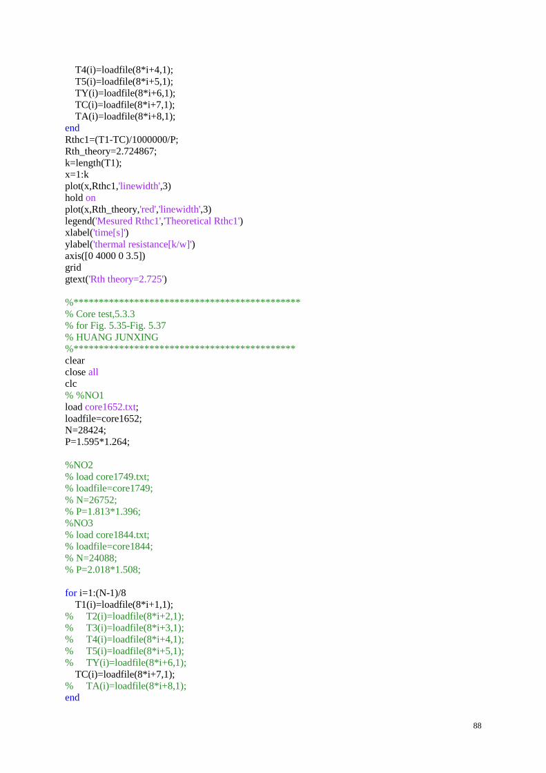
88
T4(i)=loadfile(8*i+4,1);
T5(i)=loadfile(8*i+5,1);
TY(i)=loadfile(8*i+6,1);
TC(i)=loadfile(8*i+7,1);
TA(i)=loadfile(8*i+8,1);
end
Rthc1=(T1-TC)/1000000/P;
Rth_theory=2.724867;
k=length(T1);
x=1:k
plot(x,Rthc1,'linewidth',3)
hold on
plot(x,Rth_theory,'red','linewidth',3)
legend('Mesured Rthc1','Theoretical Rthc1')
xlabel('time[s]')
ylabel('thermal resistance[k/w]')
axis([0 4000 0 3.5])
grid
gtext('Rth theory=2.725')
%*********************************************
% Core test,5.3.3
% for Fig. 5.35-Fig. 5.37
% HUANG JUNXING
%********************************************
clear
close all
clc
% %NO1
load core1652.txt;
loadfile=core1652;
N=28424;
P=1.595*1.264;
%NO2
% load core1749.txt;
% loadfile=core1749;
% N=26752;
% P=1.813*1.396;
%NO3
% load core1844.txt;
% loadfile=core1844;
% N=24088;
% P=2.018*1.508;
for i=1:(N-1)/8
T1(i)=loadfile(8*i+1,1);
% T2(i)=loadfile(8*i+2,1);
% T3(i)=loadfile(8*i+3,1);
% T4(i)=loadfile(8*i+4,1);
% T5(i)=loadfile(8*i+5,1);
% TY(i)=loadfile(8*i+6,1);
TC(i)=loadfile(8*i+7,1);
% TA(i)=loadfile(8*i+8,1);
end

89
Rthc1=(T1-TC)/P;
Rth_theory=4.0251;
k=length(T1);
x=1:k
plot(x,Rthc1,'linewidth',3)
% axis([0 3500 2.5 3.5])
hold on
plot(x,Rth_theory,'red','linewidth',3)
legend('Mesured Rth core','Theoretical Rth core')
xlabel('time[s]')
ylabel('thermal resistance[k/w]')
axis([0 4000 0 4.5])
grid
gtext('Rth theory=4.0251')
%*********************************************
% Winding test,5.3.4
% for Fig. 5.39-Fig. 5.41
% HUANG JUNXING
%********************************************
clear
close all
clc
% %NO1
load allwinding1250.txt;
loadfile=allwinding1250;
N=39824;
P=1.4055;
%NO2
% load allwinding1409.txt;
% loadfile=allwinding1409;
% N=36920;
% P=1.9511;
%NO3
% load allwinding1515.txt;
% loadfile=allwinding1515;
% N=30432;
% P=2.9625;
for i=1:(N-1)/8
T1(i)=loadfile(8*i+1,1);
TA(i)=loadfile(8*i+2,1);
T2(i)=loadfile(8*i+3,1);
T3(i)=loadfile(8*i+4,1);
T4(i)=loadfile(8*i+5,1);
T5(i)=loadfile(8*i+6,1);
TC(i)=loadfile(8*i+7,1);
TY(i)=loadfile(8*i+8,1);
end
Rth12=(T2-T1)/P;
Rth23=(T3-T2)/P;
Rth34=(T4-T3)/P;
Rth45=(T5-T4)/P;
Rth5Y=(TY-T5)/P;

90
Rth12_theory=0.9445;
Rth23_theory=0.8850;
Rth34_theory=0.8325;
Rth45_theory=0.6566;
Rth5Y_theory=0.6247;
k=length(T1);
x=1:k
subplot(3,2,1)
plot(x,Rth12,x,Rth12_theory,'red','linewidth',2)
legend('Rth12 measured','Rth12 theoretical'),grid
xlabel('time[s]')
ylabel('thermal resistance[k/w]')
axis([0 4000 0 1.2])
subplot(3,2,2)
plot(x,Rth23,x,Rth23_theory,'red','linewidth',2)
legend('Rth23 measured','Rth23 theoretical'),grid
xlabel('time[s]')
ylabel('thermal resistance[k/w]')
axis([0 4000 0 1.2])
subplot(3,2,3)
plot(x,Rth34,x,Rth34_theory,'red','linewidth',2)
legend('Rth34 measured','Rth34 theoretical'),grid
xlabel('time[s]')
ylabel('thermal resistance[k/w]')
axis([0 4000 0 1.2])
subplot(3,2,4)
plot(x,Rth45,x,Rth45_theory,'red','linewidth',2)
legend('Rth45 measured','Rth45 theoretical'),grid
xlabel('time[s]')
ylabel('thermal resistance[k/w]')
axis([0 4000 0 1.2])
subplot(3,2,5)
plot(x,Rth5Y,x,Rth5Y_theory,'red','linewidth',2)
legend('Rth5Y measured','Rth5Y theoretical'),grid
xlabel('time[s]')
ylabel('thermal resistance[k /w]')
axis([0 4000 0 1.2])

91
Appendix C
Quadratic function for each channel
0 0.5 1 1.5 2 2.5 30
100
200T0= 5.578V2 + 38.83V + 0.4425
Fitting curve
Theoretical curve
Calibration value
0 0.5 1 1.5 2 2.5 30
100
200T1= 5.567V2 + 38.86V + 0.3545
0 0.5 1 1.5 2 2.5 30
100
200T2= 5.573V2 + 38.88V + 0.3973
0 0.5 1 1.5 2 2.5 30
100
200T3= 5.548V2 + 38.93V + 0.4366
0 0.5 1 1.5 2 2.5 30
100
200T4= 5.569V2 + 38.83V + 0.4987
0 0.5 1 1.5 2 2.5 30
100
200T5= 5.585V2 + 38.75V + 0.4796
0 0.5 1 1.5 2 2.5 30
100
200T6= 5.509V2 +39.08V + 0.4723
0 0.5 1 1.5 2 2.5 30
100
200T7= 5.527V2 + 38.89V + 0.2754

92
Titre: Modèle thermique d'un transformateur à la base de capteur PT-1000
Title: Thermal Modelling of a Transformer based on PT-1000 Sensor
Université/University: Chalmers University of Technology
RESUME Ce travail vise à la modélisation thermique d'un transformateur à enroulement multicouche à base de
capteur de température PT-1000. Afin de réaliser cet objectif, d'une part, une brève introduction sur le
système d'acquisition de données, y compris PCB et LabVIEW a été faite. Ensuite, deux tests ont été
effectués principales. Pour la première, un transformateur sans aucune couche intermédiaire d'isolation
thermique a été construit. Cet essai a porté sur la mesure de la résistance thermique à l'aide d'une
source de chauffage externe afin de créer un flux de chaleur d'une seule dimension. Sur la base des
résultats précédents, la température de chaque couche peut être prédite lorsque les enroulements ont
été réalisés avec une puissance à courant continu dans l'application réelle. Ce modèle de prédiction
appliquée à n'importe quelle DC courant, mais était uniquement pour le certain transformateur. Pour le
deuxième essai, les résistances thermiques théoriques ont été calculées sur la base d'une part le
matériau qui a été utilisé pour la fabrication du transformateur. Ensuite, la comparaison entre les
valeurs théoriques et mesurées est accomplie. Le plus grand sens de ce modèle a menti sur
l'applicabilité de tous les transformateurs similaires.
Lorsque toutes les résistances thermiques de chaque partie ont été décidées, le réseau thermique entier
a été présenté.
ABSTRACT
This work aims at the thermal modelling of a multilayer wire-wound transformer and its verification
by using the temperature sensors of the type PT-1000. In order to achieve this goal, firstly, a brief
introduction about the data acquisition system including PCB and LabVIEW was made. Then two
main tests were carried out. For the first one, a transformer without any interlayer thermal insulation
was constructed. This test focused on the measurement of thermal resistance by using an external
heating source to create a one-dimension heat flow. On the basis of these results, the temperature of
each layer could be predicted when the windings were conducted with DC power in the realistic
application. This prediction model applied to any DC current but was only suitable for the transformer
made in test 1. For the second test, the theoretical thermal resistances were firstly calculated based on
the material which was used to manufacture the transformer. Then the comparison between the
theoretical and measured values was performed. The most important usage of this model lied on the
applicability to all the similar transformers.
When all the thermal resistances in each part were decided, a whole thermal network was presented.
Mots clés:
1. Modèle thermique
2. PT-1000
3. Transformateur
4. PLECS
5. LabVIEW
Key words: 1. Thermal Modelling
2. PT-1000
3. Transformer
4. PLECS
5. LabVIEW