thermal modeling of satellites - diva931359/fulltext01.pdf · thermal modeling of satellites heat...
TRANSCRIPT
IN DEGREE PROJECT VEHICLE ENGINEERING, SECOND CYCLE, 30 CREDITS
, STOCKHOLM SWEDEN 2016
THERMAL MODELING OF SATELLITESHEAT PIPES AND PAYLOAD OF A SPACEBUS NEO SATELLITE
LE MENN ALEXANDRE
KTH ROYAL INSTITUTE OF TECHNOLOGYSCHOOL OF ELECTRICAL ENGINEERING

TRITA -EE 2016:015
www.kth.se
1
MASTER THESIS REPORT
THERMAL MODELING OF SATELLITES :
HEAT PIPES AND PAYLOAD OF A SPACEBUS NEO SATELLITE
LE MENN ALEXANDRE
ENGINEERING STUDENT AT KUNGLIGA TEKNISKA HÖGSKOLAN
JULY THE 6TH, 2015 – DECEMBER THE 18TH, 2015

2

3
Abstract
Thales Alenia Space is currently developing an innovative satellite platform with a
two-phase fluid loop on board. The company uses two softwares in order to create models
that are meaningful regarding physics: Amesim and e-Therm. The first one is used to
describe fluid behavior in a circuit, while the second one is used to simulate conductive
and radiative heat transfers in a satellite model but cannot be used to model fluid
components. The interconnection of both software through a cosimulation module would
allow to create dynamic models that would take into account both physical aspects. My
internship was initially supposed to deal with the debugging of that cosimulation module,
however a delay for its delivery forced me to reorient myself. First, I used e-Therm to
model 3D heat pipes profiles, before working on the thermal model of a Spacebus Neo
satellite in order to check the validity of the design choices that were kept for that satellite.
Résumé
Thales Alenia Space développe actuellement une plateforme de satellite innovante
embarquant une boucle fluide diphasique. Dans le but de créer des modèles de satellites
représentatifs de la réalité physique, l’entreprise dispose de deux logiciels : Amesim et e-
Therm. Le premier décrit très bien les circuits fluidiques, tandis que le second modélise
les échanges conductifs et radiatifs dans un modèle de satellite mais ne peut pas modéliser
d’élément fluidique. La mise en relation de ces deux logiciels par un module de
cosimulation permettrait de créer des modèles dynamiques prenant en compte les deux
aspects physiques. Mon stage s’inscrivait dans le développement de ce module de
cosimulation, mais un retard sur sa livraison m’a forcé à me réorienter. Mon travail a donc
consisté à utiliser e-Therm pour modéliser des profilés de caloducs dans un premier
temps, avant de travailler sur un modèle de satellite Spacebus Neo dans le but de vérifier
si les choix de design qui avaient été retenus étaient valides.
Key words
Fluid loop, two-phase, heat pipe, profile, space engineering, thermal, model, nodal
4
Sommaire
Abstract ................................................................................................................................................... 3
Résumé .................................................................................................................................................... 3
Key words ............................................................................................................................................... 3
Figures ..................................................................................................................................................... 6
Tables ...................................................................................................................................................... 8
List of abbreviations ................................................................................................................................ 9
Introduction ........................................................................................................................................... 10
Chapter I | Company presentation ......................................................................................................... 11
The THALES group .......................................................................................................................... 11
Some figures about the group ........................................................................................................ 11
Main activities ............................................................................................................................... 12
Thales Alenia Space .......................................................................................................................... 13
The Cannes facility ........................................................................................................................ 13
A complete offer ............................................................................................................................ 14
An unprecedented industrial capacity ........................................................................................... 15
The telecommunications department ................................................................................................. 16
The Spacebus 4000 line ................................................................................................................. 16
NEOSAT : European future for telecommunications satellites ..................................................... 18
Chapter II | Space thermal engineering presentation ............................................................................. 21
Space, an extreme environment ......................................................................................................... 21
Telecommunication satellites ............................................................................................................ 22
Presentation ................................................................................................................................... 22
Telecommunication satellite usual structure ................................................................................. 22
The need for thermal control ......................................................................................................... 23
The thermal control ........................................................................................................................... 26
Passive thermal control ................................................................................................................. 26
The active thermal control ............................................................................................................. 29
Chapter III | Two phase fluid loop description ...................................................................................... 31
MPL presentation .............................................................................................................................. 31
Fluid choice discussion ..................................................................................................................... 33
Chapter IV | Heat pipe thermal modeling .............................................................................................. 34
The thermal modeling ....................................................................................................................... 34
The nodal method .......................................................................................................................... 35
Types of profiles to be modelled ....................................................................................................... 36
First method: quick calculus .......................................................................................................... 39
Second method: layer calculus ...................................................................................................... 44

5
Third method : e-Therm simulation .............................................................................................. 48
Conclusion about the heat pipe modeling...................................................................................... 49
Chapter V | Satellite thermal modeling ................................................................................................. 50
The nodal method applied to satellites .............................................................................................. 50
General aspects .............................................................................................................................. 50
Creation of a satellite model using e-Therm ................................................................................. 51
Standard rules to keep in mind for the nodal modeling of a satellite ............................................ 51
Rules about the components to model ........................................................................................... 52
Modeling of a SpaceBus Neo satellite Payload Module ................................................................... 59
MPL influence on the satellite design ........................................................................................... 60
MPL modeling in e-Therm ............................................................................................................ 60
Calculation cases ........................................................................................................................... 62
Chapter VI | Amesim and the cosimulation ........................................................................................... 67
Amesim presentation ......................................................................................................................... 67
Two phase correlations comparison .................................................................................................. 68
McAdams correlation .................................................................................................................... 69
Müller-Steinhagen correlation ....................................................................................................... 71
Friedel correlation ......................................................................................................................... 72
The cosimulation ............................................................................................................................... 74
Conclusion ............................................................................................................................................. 75
6
Figures
Figure 1 : THALES group shareholders ............................................................................................... 11
Figure 2 : Thales Alenia Space offer distribution ................................................................................. 15
Figure 3 : TAS missions distribution ..................................................................................................... 15
Figure 4 : SpaceBus satellite various models ....................................................................................... 16
Figure 5 : SpaceBus satellite central tube ............................................................................................ 16
Figure 6 : Geostationary satellite positioning from its transfer orbit ................................................... 19
Figure 7 : Differences between chemical propulsion (on the left) ........................................................ 19
Figure 8 : Simplified drawing of the structure of a Spacebus telecommunication satellite ................ 233
Figure 9 : Earth orbit representation with the days of the solstices and equinoxes according to our
calendar ............................................................................................................................................... 254
Figure 10 : Drawing of the orbit of a geostationary satellite during the Winter Solstice. Solar light hits
the green satellite with a 23.5° angle .................................................................................................. 255
Figure 11 : Musis satellite representation .......................................................................................... 266
Figure 12 : Drawing of the various heat transfers around a satellite external face. .......................... 277
Figure 13 : Drawing showing the effect of heat pipes. On the left without heat pipe, in the middle with
heat pipe. The red area means high temperatures while the orange one means moderate temperatures.
............................................................................................................................................................. 288
Figure 14 : Loop Heat Pipe drawing .................................................................................................... 29
Figure 15 : MPL drawing. .................................................................................................................. 311
Figure 16 : Condenser profile drawing. Created on Paint by hand, it doesn’t represent any design used
by Thales. ............................................................................................................................................ 333
Figure 17 : Jason-3 satellite in front of the Espace 70 Jason tank ..................................................... 344
Figure 18 : Example of a NIDA layer ................................................................................................. 366
Figure 19 : Heat transfer from an equipment to a heat pipe .............................................................. 377
Figure 20 : Heat pipe drawing. This heat pipe design was made by hand and do not represent any heat
pipe used by Thales Alenia Space. ...................................................................................................... 388
Figure 21 : The first method cuts the profile in half as shown by the red dots ..................................... 39
Figure 22 : Equivalent geometry for the first method ......................................................................... 400
Figure 23 : Top profile part that is modeled by node 1 ...................................................................... 411
Figure 24 : Bottom part of the profile – the thickness or width is bigger than one of the length that
characterize the heat transfer section for nodes 3 and 4 .................................................................... 422
Figure 25 : Second method profile description along the red lines .................................................... 444
Figure 26 : Drawing of the three heat paths for the second method. Two similar path through the matter
and one going through the fluid. ......................................................................................................... 444
Figure 27 : Considered profile part for the calculation of one conductive path ................................ 455
Figure 28 : Equivalent electric drawing for the second method. Only the four first layers are shown.
............................................................................................................................................................. 455
Figure 29 : Fluid contribution to the thermal path that has to be considered .................................... 466

7
Figure 30 : Example of geometry cutting for e-Therm meshing ......................................................... 488
Figure 31 : Example of a geometry meshed by e-Therm. This geometry is not representative of any
profile used by Thales Alenia Space. ................................................................................................... 488
Figure 32 : Example of equipment that is set on two heat pipes and its recommended description ... 533
Figure 33 : Drawing of a heat pipe crossing. The green heat pipe are put within the NIDA while the
purple heat pipe are put on the NIDA. ................................................................................................ 544
Figure 34 : Heat pipe description depending on the situation ............................................................ 544
Figure 35 : Structure nodal description under MLI ............................................................................ 566
Figure 36 : Nodal description example with interface nodes between a North panel and an Earth panel.
............................................................................................................................................................. 577
Figure 37 : Telecommunication satellite basic drawing ....................................................................... 59
Figure 38 : Drawing of the new layout made possible by the use of the MPL. ................................... 600
Figure 39 : MPL modeling method within e-Therm ............................................................................ 611
Figure 40 : Drawing showing the sunligh incidence for the two Winter Solstice cases. .................... 622
Figure 41 : Case study layout drawing, with the condensers and evaporators areas ........................ 644
Figure 42 : Amesim component definition .......................................................................................... 677
Figure 43 : Two phase vertical flows with mixed air and water examples : ....................................... 688
Figure 44 : Vapor and liquid path section .......................................................................................... 690

8
Tables
Table 1: THALES offer in details ……………………..………………………………….…………...12
Table 2 : Spacebus line mass specifications and thermal loads…………………………..…………. 17
Table 3: Conductance of heat conduction through matter for half a profile
……………………...………………………………………………………………………………….47
Table 4: Conduction and global conductance for half a profile by taking the fluid into account
…………………………………………………………………………………………………………48
Table 5: Comparison of the results obtained from the various calculation methods
…………………………………………………………………………………………………………50
Table 6: Temperature values for the WS hot case. These are fake values that were created for this
report....……………………………………………………………………………………………… 65
Table 7: Temperature values for the eclipse case. These are fake values that were created for this
report.………….……………………………………………………………………………………....66

9
List of abbreviations
CNES: Centre National des Études Spatiales, French national space organization
GS : Générateur Solaire / Solar panels
ISS: International Space Station
LHP: Loop Heat Pipe
MPL: Mechanically Pumped Loop
NIDA: Nid D’Abeille, the satellite structure’s material
TAS: Thales Alenia Space

10
Introduction
After the Second World War, the space industry went through a great expansion.
This growth was caused thanks to the US and the URSS and their run to the stars that was
one of Cold War’s biggest aspect. First seen as a token showing the power of the nation,
the space conquest enabled industries such as the telecommunications and the digitals to
reach Earth’ orbit. Following the growth of internet at the beginning of the third millennia,
these industry went through an unprecedented soaring. In nowadays society, they are
holding so many vital roles that it is not possible anymore to live without them. As a
consequence, the space industry actors had to adapt in order to cope with the never
ending need for satellites more efficient so as to satisfy the demands from the
telecommunications operators.
Knowing that, Thales Alenia Space decided to get involved in the development
program of a new satellite platform, “Neosat”, in partnership with Airbus Defense and
Space. That new platform funded by ESA and the CNES is supposed to allow both
companies to build innovative and competitive new satellites. Thales’ sub-program for
Neosat is named “Spacebus Neo”.
The building of the two phase fluid loop with mechanical pumping (known as MPL
standing for Mechanically Pumped Loop) is part of Thales’ will to innovate. Being
developed since 2001, it contributes to making Spacebus Neo the state of the art in terms
of satellite thermal regulation. Indeed, it allows the use of a great number of highly
dissipative components in a quite confined volume. The volume restriction being set by
the size of the launching rocket fairing, a smaller satellite is always interesting since it will
be able to adapt to more launchers. My internship took place within this program. Its
precise subject was quite modified over time though: after learning how to use both
Amesim and e-Therm softwares, I was supposed to analyze the results produced by the
cosimulation module enabling Amasim and e-Therm to work together. However, that
module was not delivered on time and so I was first given the task of modeling 3D heat
pipe profiles, before dealing with a quite ambitious project for the last month of my
internship: the modeling of a Spacebus Neo characteristic payload.
This report will explain the various studies I led during my internship. First
describing quickly the company and the Neosat program, it will then deal with thermal
considerations within the space industry before talking a bit about the MPL. It will then
present my work on heat pipe profiles and on the Spacebus Neo payload modeling. The
report concludes by explaining the future of my satellite model: the cosimulation.

11
Chapter I | Company presentation
The THALES group
THALES is a world renowned group within many industries, since it is a
technological leader within defense, security, aeronautics and space.
Some figures about the group
THALES group wishes to create critical information systems. During 2012, the
group earned 13.4 billion euros. Its backlog reaches 25.4 billion euros representing two
years of activity. Near to 68,000 employees work at THALES across 56 countries.
The French State has an important place within the group since it owns 27% of its
shares, as can be seen in figure 1. More than 50% of THALES’ employees are French, and
the group owns 70 facilities in France.
Figure 1 : THALES group shareholders
« Flottant » stands for « Miscellaneous », « État français » for « French State »
THALES is also quite innovative since it uses 18% of its turnover (2.2 billion euros)
to fund its R&D department. 25,000 researchers work at THALES, which counts about 300
inventions per year and owns more than 15,000 patents.
12
Main activities
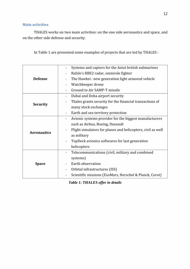
THALES works on two main activities: on the one side aeronautics and space, and
on the other side defense and security.
In Table 1 are presented some examples of projects that are led by THALES :
Defense
- Systems and captors for the Astut british submarines
- Rafale’s RBE2 radar, omnirole fighter
- The Hawkei : new generation light armored vehicle
- Watchkeeper drone
- Ground to Air SAMP-T missile
Security
- Dubaï and Doha airport security
- Thales grants security for the financial transactions of
many stock exchanges
- Earth and sea territory protection
Aeronautics
- Avionic systems provider for the biggest manufacturers
such as Airbus, Boeing, Dassault
- Flight simulators for planes and helicopters, civil as well
as military
- TopDeck avionics softwares for last generation
helicopters
Space
- Telecommunications (civil, military and combined
systems)
- Earth observation
- Orbital infrastructures (ISS)
- Scientific missions (ExoMars, Herschel & Planck, Corot)
Table 1: THALES offer in details
13
Thales Alenia Space
Thales Alenia Space is, with its competitor and partner Airbus Defense and Space, the European leader for satellites and one of the biggest actors concerning orbital infrastructure
The Cannes facility
2,500 employees work at the Cannes facility, including 2,000 Thales employees
and 500 persons that are subcontractors or doing an internship. The facility covers many
aspects of the satellites conception process such as R&D activity or the building factory.
Jean-Loïc GALLE is the CEO.
I joined the thermal engineering department led by Caroline MASQUELIER, whose
activities consist in the development of new hardware (materials as well as for the
informatics), in thermal analysis and in the search of new innovative solutions.

14
A complete offer
Thales Alenia Space offers solution in every aspects of the space industry T
ele
com
mu
nic
ati
on
s
Thales Alenia Space covers the whole domain
by offering complete satellite systems to
operators and industries over the world, as
well as payloads or high performance
hardware
Ob
serv
ati
on
Meteorology as MTG builder (Thales Alenia
Space provides all Meteosats for Eumetsat)
Climatology as SMOS (Soil Moisture and
Ocean Salinity) industrial partner
Oceanography with the building of the Jason
satellite using the Poseidon dual frequency
altimeter.
Na
vig
ati
on
Satellite constellations, as Iridium NEXT,
Globalstar 2nd generation and O3b architect
(more than 150 satellites)
Building of the four first IOV (In-Orbit
Validation) satellites of the Galileo
constellation.
Ex
plo
rati
on
/S
cie
nce
ExoMars missions architect – one of the most
ambitious exploration mission of the coming
years
Herschel & Planck missions architect, the
most complex european spatial observatories
ever built
Orbital infrastructure and spatial
transportation by providing 50% of ISS
pressurized volume

15
An unprecedented industrial capacity
Thales Alenia Space (TAS) is a joint venture of Thales (67%) and Finmeccanica
(33%). Thales Alenia Space is a world class reference in terms of telecommunications,
navigation, meteorology, environment handling, defense, security, observation and
science. With its 7,200 employees scattered over 11 industrial facilities, it is located in
France, Great Britain, Italy, Spain, Belgium and Germany. It also owns a few design offices
in the US.
Thales earned a turnover of 2 billion euros in 2010, more that 15% of the group’s
turnover. The company activities are divided as shown in figure 2.
Also, the missions Thales Alenia Space deals with are quite balanced between
telecommunications and scientific ones, showing the company competitiveness in both
domains, as shown in figure 3.
In 2012, TAS took part in 16 satellite launches using various rockets (Ariane 5,
Proton, Atlas, …). The company is also the second biggest industrial provider for the ISS.
Figure 2 : Thales Alenia Space offer distribution
Globalstar,
Iridium
Figure 3 : TAS missions distribution
16
The telecommunications department
The Spacebus 4000 line
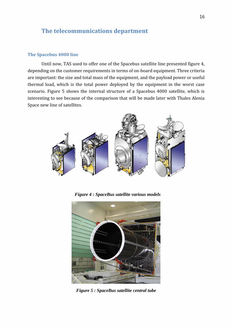
Until now, TAS used to offer one of the Spacebus satellite line presented figure 4,
depending on the customer requirements in terms of on-board equipment. Three criteria
are important: the size and total mass of the equipment, and the payload power or useful
thermal load, which is the total power deployed by the equipment in the worst case
scenario. Figure 5 shows the internal structure of a Spacebus 4000 satellite, which is
interesting to see because of the comparison that will be made later with Thales Alenia
Space new line of satellites.
Figure 5 : SpaceBus satellite central tube
Figure 4 : SpaceBus satellite various models

17
The Neosat project has been joined by Thales with the aim to create a new satellite
platform in order to substitute this SpaceBus line. The new satellite platform should be
able to offer satellites with restricted size able to embark components that are even more
dissipative, despite the limited radiative surfaces. Table 2 shows the payload power limits
that were available using the former SpaceBus satellites.
Table 2 : Spacebus line mass specifications and thermal loads

18
NEOSAT : European future for telecommunications satellites
The new generation Neosat satellite platform project was first issued by ESA in
cooperation with the CNES for telecommunications satellites. The first launches are
scheduled before 2020. This project aims at offering innovations enabling efficiency and
competitiveness gains in order to take a strong position on the world’s satellite market.
ESA indeed hopes to own 50% of its market shares between 2018 and 2030 for a
cumulated turnover of 25 billion euros. Neosat’s architects are Airbus Defense and Space
and Thales Alenia Space. They are currently putting their providers in competition to join
the industrial consortium that will be in charge of developing both Neosat platforms, one
led by Airbus, the other by Thales.
According to Magali Vaissière, ESA’s director of Telecommunications and
integrated applications: “This is a unique opportunity for the European providers since
80% of the European satellite platforms get their parts thanks to industrials from the ESA
member states. These industrials should earn sales as high as 7 billion euros.”
Two prototypes, one per architect, will be launched in 2018-2019 in order to show
their validity. These prototypes are being built through an agreement between public
institutions, the industrial partners and the satellite operators.
The technologies and innovations that will be used in this project are many:
electric propulsion for the positioning and orbit & attitude control of the satellite, active
thermal regulation systems and new generation batteries. Neosat aims at offering
satellites 30% cheaper than the ones that are available today on the market. To do so, the
supply chain of both architects will be put together, enabling economies of scale.
Various setups will be available to match the mission needs: full electric, hybrid or
full chemical. The great advantage of the chemical propulsion consists in its reactivity and
speed. The satellite positioning lasts only a few days using chemical propulsion, whereas
it needs a few months with electric propulsion. However, the electric propulsion requires
less propellant mass, thus allowing for cheaper launches.
19
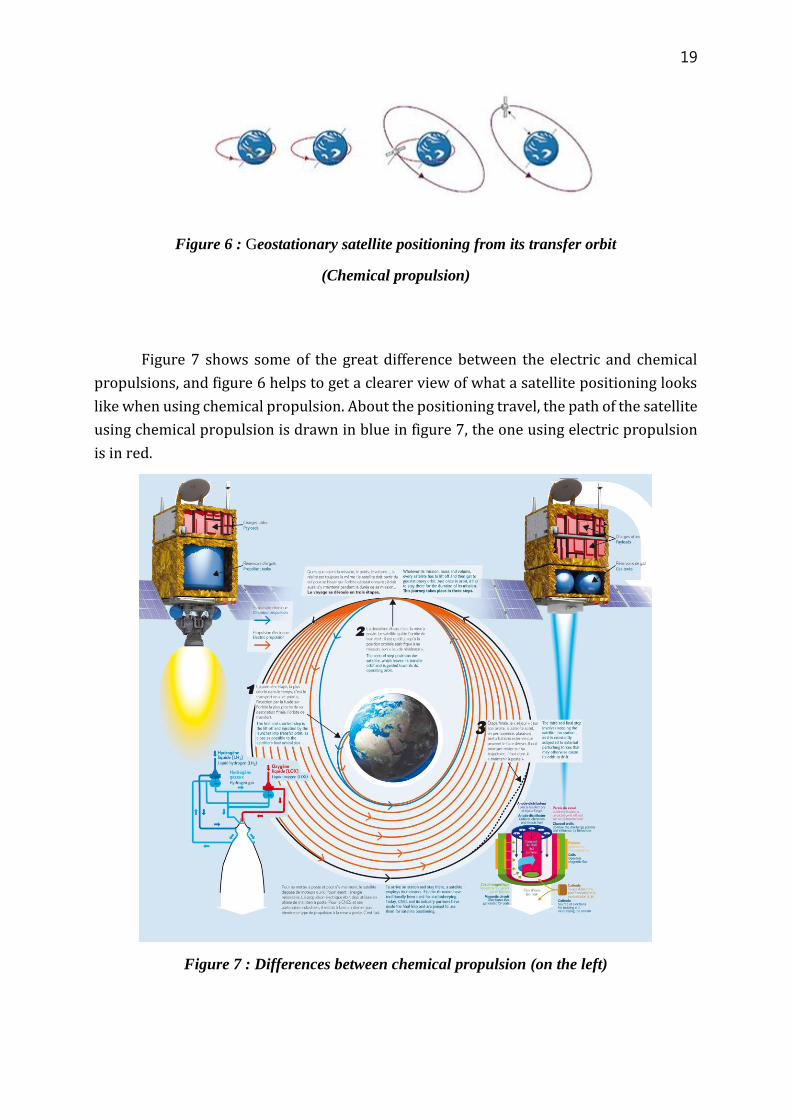
Figure 6 : Geostationary satellite positioning from its transfer orbit
(Chemical propulsion)
Figure 7 shows some of the great difference between the electric and chemical
propulsions, and figure 6 helps to get a clearer view of what a satellite positioning looks
like when using chemical propulsion. About the positioning travel, the path of the satellite
using chemical propulsion is drawn in blue in figure 7, the one using electric propulsion
is in red.
Figure 7 : Differences between chemical propulsion (on the left)
20
and electric propulsion (on the right). Source : CNES 2014
It is easy to notice that the second one has to travel a lot more to get to its final
orbit. This delay has three disadvantages: the customer will have to wait longer for the
satellite to be operational, the positioning time will be longer meaning it will cost more to
the builder since it will have to rent Command Centers for a longer period of time, and the
satellite will suffer from an efficiency loss, especially on the solar cells. Indeed, during the
positioning, the satellite will travel through aggressive environments such as the Van
Allen belts. The longer it stays in these belts, the more it will suffer from the interaction
of its materials with the ambient plasma. For a geostationary satellite, the positioning can
be as long as 8 months with electric propulsion. However, about the satellite layout, the
one using chemical propulsion will require a bigger and heavier propellant tank than the
one using electric propulsion, allowing the latter to embark more payload. But the layout
is more complicated for the electric propulsion since corrosion phenomena appear with
the creation of ions that are able to chemically react with the satellite structure.
21
Chapter II | Space thermal engineering presentation
Space, an extreme environment
Each spatial mission is a technological challenge because of many aspects, but
especially because of the specific environment spacecraft will have to bear with during
their lifetime.
In space, all objects are deprived of the comfortable conditions offered by the Earth
at its surface. Without any atmosphere, the pressure is extremely low, causing the
outgassing of materials. If this outgassing is not foreseen, a parasitic gas can from around
the satellite. Such a gas could crystalize on the satellite cold areas such as the Star Tracker
optics for example, modifying its measures to such an extent that it can make it detect fake
stars. The depressurization during the launch can also tear the MLI veils if these contain
air bubbles and do not present enough openings to let them out. Another consequence of
the lack of atmosphere: the convection that is so useful on Earth to expel heat to the
ambient air is not available, limiting thermal transfers to conduction in the materials and
radiation. Moreover, space can be considered on the thermal aspect as a 4K cold source.
For a geostationary satellite, the infrared earth radiation is negligible, limiting heat
sources to equipment dissipation and solar radiation. This radiation will hit only three
sides of a box-shaped satellite, creating temperature gradients between the faces in the
shadow and the ones that are lit. On the mechanical and electrical aspects, the photon-
material ionizing interaction forces the lit faces to charge positively, while faces in the
shadow get charged negatively because of the surrounding plasma. This can create
torques in the structure because of electrical attraction, as well as electrical arcs. Micro
meteorites also have to be considered: on the Earth surface, we are protected from them
thanks to the atmosphere, but it is quite possible that they hit a satellite and pierce
through its critical systems. Phenomenon linked to gravity are also denied because of the
free falling state, making the design and testing process more complicated, especially
when it comes to fluidic systems. Finally, despite the fact that telecommunication
satellites do not leave the magnetosphere, they suffer from a greater exposition to
radiations, impacting the materials and electronic hardware aging process.
22
Thus, when it comes to designing a satellite, the engineers will have to go through all
these points in order to make sure that the satellite will fulfill the customer’s
requirements. Offering a technical solution dealing with these constraints while
proposing the required functionalities, within well-defined time and money budgets, will
require to do many tradeoffs on various parameters that require analyses from many
scientific disciplines simultaneously.
Telecommunication satellites
Presentation
My internship was centered on a telecommunication satellite. Such a satellite is
used to transmit data from one point of the globe to another, may it be phone calls,
internet data transmission, satellite communication or TV broadcasts.
Telecommunication satellites being in orbit at a high altitude (communication satellites
orbit at 36,000 km), the signal is transmitted directly to a first satellite. That satellite
might be able to directly redirect the signal to its destination if it is in his field of vision, if
not, it will transmit the signal to a second satellite, that will again look for the destination
in its field of vision, or send it to another satellite, and so on.
The telecommunication satellite industry is the only space industry that earns a lot
more that its cost. The customers are usually private companies or former international
organisms that got privatized. These organizations usually own a fleet of orbiting
satellites.
Telecommunication satellite usual structure
A satellite is an object that must fulfill precise functions in a given space
environment. Its architecture is a result of the consideration of both its mission objectives
and the specific constraints it will have to deal with.
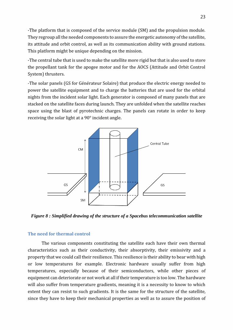
A satellite is characterized by its four principal parts, as shown in figure 8:
- The communication module (CM) or payload that embarks the mission equipment and
many other boxes containing filters, amplifiers, transmitters to send the signal back to
Earth or to transmit it to the on-board informatics. The CM module fulfill the customer
needs. It is composed of two subsystems: the antenna subsystem that takes care of
receiving and emitting telecommunication signals, and the repeating subsystem that
modifies the signal (usually to amplify it) between reception ant retransmission.
23
-The platform that is composed of the service module (SM) and the propulsion module.
They regroup all the needed components to assure the energetic autonomy of the satellite,
its attitude and orbit control, as well as its communication ability with ground stations.
This platform might be unique depending on the mission.
-The central tube that is used to make the satellite more rigid but that is also used to store
the propellant tank for the apogee motor and for the AOCS (Attitude and Orbit Control
System) thrusters.
-The solar panels (GS for Générateur Solaire) that produce the electric energy needed to
power the satellite equipment and to charge the batteries that are used for the orbital
nights from the incident solar light. Each generator is composed of many panels that are
stacked on the satellite faces during launch. They are unfolded when the satellite reaches
space using the blast of pyrotechnic charges. The panels can rotate in order to keep
receiving the solar light at a 90° incident angle.
Figure 8 : Simplified drawing of the structure of a Spacebus telecommunication satellite
The need for thermal control
The various components constituting the satellite each have their own thermal
characteristics such as their conductivity, their absorptivity, their emissivity and a
property that we could call their resilience. This resilience is their ability to bear with high
or low temperatures for example. Electronic hardware usually suffer from high
temperatures, especially because of their semiconductors, while other pieces of
equipment can deteriorate or not work at all if their temperature is too low. The hardware
will also suffer from temperature gradients, meaning it is a necessity to know to which
extent they can resist to such gradients. It is the same for the structure of the satellite,
since they have to keep their mechanical properties as well as to assure the position of

24
many pieces of equipment with regards to the others. It is also important to make sure
that the hardware will not suffer from too many temperature fluctuations in order to
optimize its lifetime, and to keep the number of on/off cycles operated by the heaters to
the minimum for the same goal.
In order to take all these conditions into account, the thermal engineer will have to
simulate and analyze various thermal situations. At Thales Alenia Space, the engineers
check only the situations that are called “sizing”, meaning the worst case in terms of hot
case and cold case. During a hot case, all the payload is on, meaning its dissipation is
maximum. A first hot case is usually simulated at the Winter Solstice, when the Earth is at
the closest point of its orbit to the Sun. In such case the solar flux received by the satellite
reaches its peak at 1420 W/m² approximately. The solar flux is incident on the satellite’s
South face with an angle of 23.5° as shown in figure 10, and at some moments of the orbit
the East or the West face is lit with a 90° incident angle, which is the maximum in terms
of solar flux incidence. During the Winter Solstice the North face stays in the shadow the
whole time. Thus this analysis is usually completed with the Summer Solstice case.
Despite the fact that the solar flux reaches its minimum of 1330W/m² approximately, it
represents the hot case for the North face of the satellite, while the South face this time
stays in the shadow the whole orbit. Considering the absorptivity of the materials of the
external faces of the satellite, the hot cases are simulated considering a satellite at the end
of its life, when its materials have aged and therefore absorb more the solar light than
when they were brand new. These cases allow the engineers to size the needed OSR
(Optical Solar Reflector) surfaces that allow the satellite to expel its heat by radiating it to
space. Figure 9 shows the dates and positioning of the Earth with regard to the Sun for the
various solstices and equinoxes.
The cold case considers an inactive payload with a minimal dissipation. Such a case
is used to size the satellite’s intern heaters or other systems such as deployable MLI
(Multi-Layer Insulation) veils that can cover the OSR surfaces in order to lower their
radiative power. The simulated case is the Spring Equinox, because during this case the
satellite will go through orbital eclipses, with the lowest materials’ absorptivity.

25
Figure 9 : Earth orbit representation with the days of the solstices and equinoxes according
to our calendar
Figure 10 : Drawing of the orbit of a geostationary satellite during the Winter Solstice.
Solar light hits the green satellite with a 23.5° angle

26
The thermal control assures the optimal functioning of the satellite by making sure the
hardware and the structure stay in a reasonable range of temperatures. In order to do so,
the thermal engineer can use two types of thermal control: active and passive.
The thermal control
Passive thermal control
The systems allowing a passive thermal control are by definition autonomous
systems, meaning they do not require any energy input to work. An examples of such
systems is the MLI material that is used to prevent heat from going through it. Such
material is used to keep the heat inside the satellite, or to isolate some hot areas of the
satellite from others that need to be colder. The OSR is another example of such passive
control system, they are used to transfer the heat they receive by radiating it, making them
helpful when the satellite is too hot and need to cool down. Figure 11 shows an example
of a satellite where both MLI and OSR surfaces can be observed on its external faces, while
figure 12 shows the various heat exchanges the thermal engineer will have to deal with,
but also to use, in order to regulate his or her satellite.
Figure 11 : Musis satellite representation

27
Figure 12 : Drawing of the various heat transfers around a satellite external face.
In green, conductive thermal transfers, in red, radiative transfers.
Inside the satellite, other tools can be used such as paint in order to make sure that
the hardware and the structure show the right emissivity coefficient to the other faces
that stand in their field of vision. Surface treatments can also be made towards the same
goal, with the advantage of limiting the overweight added by the use of paint. Lastly, on
the external faces, heat pipes are used to distribute the heat from a hot area over the whole
radiative surface. These heat pipes are long tubes filled with a two phase fluid such as
ammoniac for example that is chosen for its convective properties. The liquid fluid will
receive the heat at the hot area and will evaporate when at the same time at the colder
areas of the heat pipe, the gaseous fluid will condensate, giving its heat to the tube. Thus,
a pressure gradient is created between the hot and cold areas, putting the gas phase into
movement, while the liquid phase will also move from the cold to the hot area because of
capillarity.
28
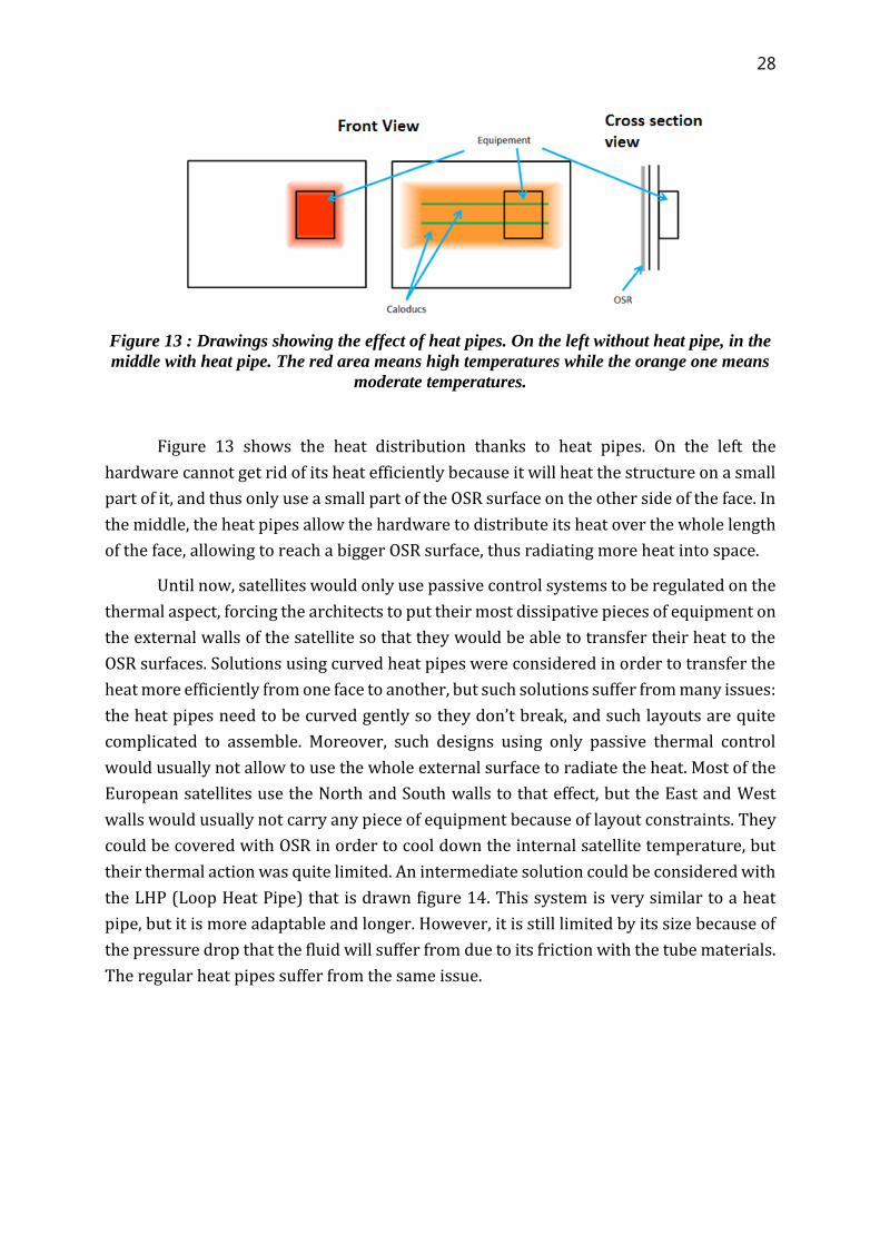
Figure 13 : Drawings showing the effect of heat pipes. On the left without heat pipe, in the
middle with heat pipe. The red area means high temperatures while the orange one means
moderate temperatures.
Figure 13 shows the heat distribution thanks to heat pipes. On the left the
hardware cannot get rid of its heat efficiently because it will heat the structure on a small
part of it, and thus only use a small part of the OSR surface on the other side of the face. In
the middle, the heat pipes allow the hardware to distribute its heat over the whole length
of the face, allowing to reach a bigger OSR surface, thus radiating more heat into space.
Until now, satellites would only use passive control systems to be regulated on the
thermal aspect, forcing the architects to put their most dissipative pieces of equipment on
the external walls of the satellite so that they would be able to transfer their heat to the
OSR surfaces. Solutions using curved heat pipes were considered in order to transfer the
heat more efficiently from one face to another, but such solutions suffer from many issues:
the heat pipes need to be curved gently so they don’t break, and such layouts are quite
complicated to assemble. Moreover, such designs using only passive thermal control
would usually not allow to use the whole external surface to radiate the heat. Most of the
European satellites use the North and South walls to that effect, but the East and West
walls would usually not carry any piece of equipment because of layout constraints. They
could be covered with OSR in order to cool down the internal satellite temperature, but
their thermal action was quite limited. An intermediate solution could be considered with
the LHP (Loop Heat Pipe) that is drawn figure 14. This system is very similar to a heat
pipe, but it is more adaptable and longer. However, it is still limited by its size because of
the pressure drop that the fluid will suffer from due to its friction with the tube materials.
The regular heat pipes suffer from the same issue.

29
Figure 14 : Loop Heat Pipe drawing
As we have seen, the needs of the customers evolve as they keep asking for bigger
and more powerful payloads. It was a necessity for the satellite architect to use a new type
of thermal control in order to stay competitive on the satellite market.
The active thermal control
Active thermal control use an energy input to work and usually increase the
satellite mass compared to a satellite embarking only passive control systems since a
satellite using active systems cannot work without the use of passive control systems as
well. However the benefits from using active control systems quickly overcome that
drawback.
The active thermal control system will fetch the hardware’s heat and scatter it to
all the radiative surfaces. It is not a necessity anymore to put the dissipative pieces of
equipment near the OSR, the thermal system will take care of transferring the heat from
the equipment to the right place, thus leaving more freedom for the satellite layout. It also
allows to use the full external satellite surface to radiate heat, enabling to radiate more
heat than previously for the same satellite volume. As a consequence it allows to offer
missions with greater payloads. The heat distribution over the satellite being more
flexible, it is easier to heat the cold areas with the heat from the hotter ones, allowing to
optimize the use of heaters. Finally, the use of such a system requires less analysis time
30
because the thermal models and simulations are simplified, reducing the financial needs
for these tasks.
The MPL, which stands for Mechanically Pumped Loop, is one of these active
thermal control system. A fluid is put into motion thanks to a pump, with an adjustable
flow to adapt to the situation. The pressure gradient applied by the pump allows to control
the fluid change of state, but also allows the fluid to get over the pressure losses we
described previously for the LHP. This allows the MPL tubing to cover a greater length,
enabling the thermal coupling of the satellite external faces. This last point is quite useful
since during the Earth movement around the Sun, the satellite will have different faces lit
by sunlight while others will be in the shadow, so coupling lit faces with shadowed ones
allows to prevent temperature differences between the faces by distributing the heat on
the faces depending on the temperature they already reached, optimizing the satellite
overall rejection capacity.
31
Chapter III | Two phase fluid loop description
MPL presentation
As of Thales, one of its biggest innovations for its SpaceBus Neo platform consist in
an active thermal control system: the MPL. We will see in this chapter its various
components.
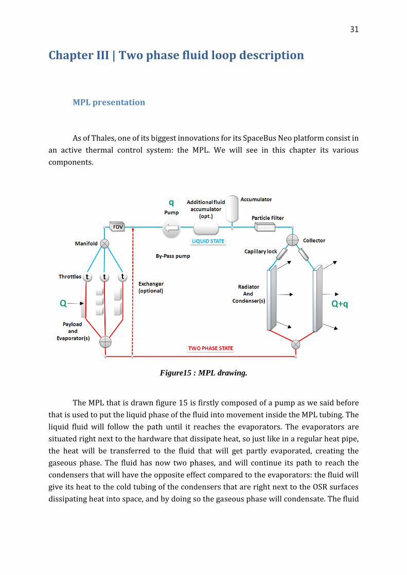
Figure15 : MPL drawing.
The MPL that is drawn figure 15 is firstly composed of a pump as we said before
that is used to put the liquid phase of the fluid into movement inside the MPL tubing. The
liquid fluid will follow the path until it reaches the evaporators. The evaporators are
situated right next to the hardware that dissipate heat, so just like in a regular heat pipe,
the heat will be transferred to the fluid that will get partly evaporated, creating the
gaseous phase. The fluid has now two phases, and will continue its path to reach the
condensers that will have the opposite effect compared to the evaporators: the fluid will
give its heat to the cold tubing of the condensers that are right next to the OSR surfaces
dissipating heat into space, and by doing so the gaseous phase will condensate. The fluid

32
will then go through a capillary lock that will make sure only the liquid phase can continue
but not the vapor, since the pump works with liquid phase fluids only.
Capillary locks are also interesting for another aspect, since they play a great role
in the distribution of heat between the satellite external faces. Let’s take the situation of a
Winter Solstice. The South wall receives sun light during the whole orbit while the North
wall is constantly in the shadow. In this case, more vapor will be created in the South wall
than in the North wall. The capillary locks not letting the vapor go through, they will create
more pressure loss in the South wall than in the North wall because of this vapor portion
difference between the two walls. The fluid flow will be more important in the cold wall
than in the hot one, thus more power will be transferred to the North condensers than to
the South ones, allowing the system to balance the temperature of both walls.
To make sure that the fluid entering the pump is actually liquid, the MPL design
applies a sub cooling to the fluid, meaning that the fluid getting out of the condensers part
is cooled below the saturation temperature. Hence the usefulness of a heat exchanger, as
can be seen in the picture. Indeed, the MPL efficiency relies on the fact that the fluid
reaches a two phase state in the evaporators and condensers since the convective heat
exchange coefficient reaches its peak during the change of state. When going out of the
pump, the fluid is still subcooled. To make sure it will reach a two phase state as fast as
possible in the evaporators, it is possible to get rid of the sub cooling by taking some heat
from the fluid getting out of the evaporators. However, it is important to check the fluid
vapor title and to limit it to a maximum value since the heat exchange coefficient will start
to drop if the vapor title is high, and eventually reach values that are too low to be efficient,
limiting the heat transfer with the tubing too much. The hardware dissipation being fixed,
it is the saturation temperature that has to be controlled. The “accumulator” component
on the picture is in reality a two phase tank that plays the role of an expansion tank in
order to compensate for the fluid volume variation inside the loop. These variations can
be created by variations of the power to dissipate or by variations of the sun light received.
This tank allows to regulate the saturation pressure, and thus the saturation temperature,
of the loop. It is quite important to remember that during a change of state, the fluid
temperature remains constant. So in the two phase part of the MPL, the fluid temperature
is almost the same everywhere, but some little variations can be created because of the
pressure losses created by the tubing.

33
Figure 16 : Condenser profile drawing. Created on Paint by hand, it doesn’t represent any
design used by Thales.
Figure 16 shows a condenser profile. It is made of a flat part in contact with the
structure to transfer the heat by conduction, and of a cylindrical part in which the fluid
circulates. This cylindrical part has teeth in order to have a greater surface of interaction
with the fluid, optimizing the heat exchange. The evaporators have teeth as well but the
design of the condensers and of the evaporators is different in order to match their
respective situations.
Fluid choice discussion
The two phase loop efficiency also depends on the fluid that was chosen because
of its thermodynamic properties. Usually, the wanted properties are as such:
-Boiling point below the working temperature
-Low freezing point
-High vaporization latent heat
-Gaseous phase with a high enough density
-High enough critical temperature
-Chemical stability
-Not corrosive
-Not inflammable
-Not explosive
-Not polluting

34
Chapter IV | Heat pipe thermal modeling
The thermal modeling
The thermal modeling aims at creating a virtual model representing the reality. In
order to do so, it is a necessity to use a thermal modeling software with a solver whose
results were correlated with tests, especially TVT (Thermal Vacuum Test). Figure 17
shows an example of the tank used to lead a TVT for the Jason-3 satellite. Tests are realized
in big tanks where pressure is lowered so as to simulate the spatial environment the
satellite will live in during its mission. The tank temperature can be modified in order to
model hot or cold cases and the satellite electrical powering is also adjustable in order to
simulate various situations. The results from these tests and the ones produced by the
software are then compared to check the solver validity.
Figure 17 : Jason-3 satellite in front of the Espace 70 Jason tank
35
Two modeling procedures are available: the finite elements discretization or the
nodal discretization. The first method defines a new geometry for the problem by creating
polygonal or polyhedral sub-elements and tries to solve the partial derivatives equations
that are representative of the problem on this new geometry by finding a solution for each
sub-element. However it is not a necessity to explain this method further since Thales
Alenia Space intern thermal software is e-Therm, which uses the nodal method.
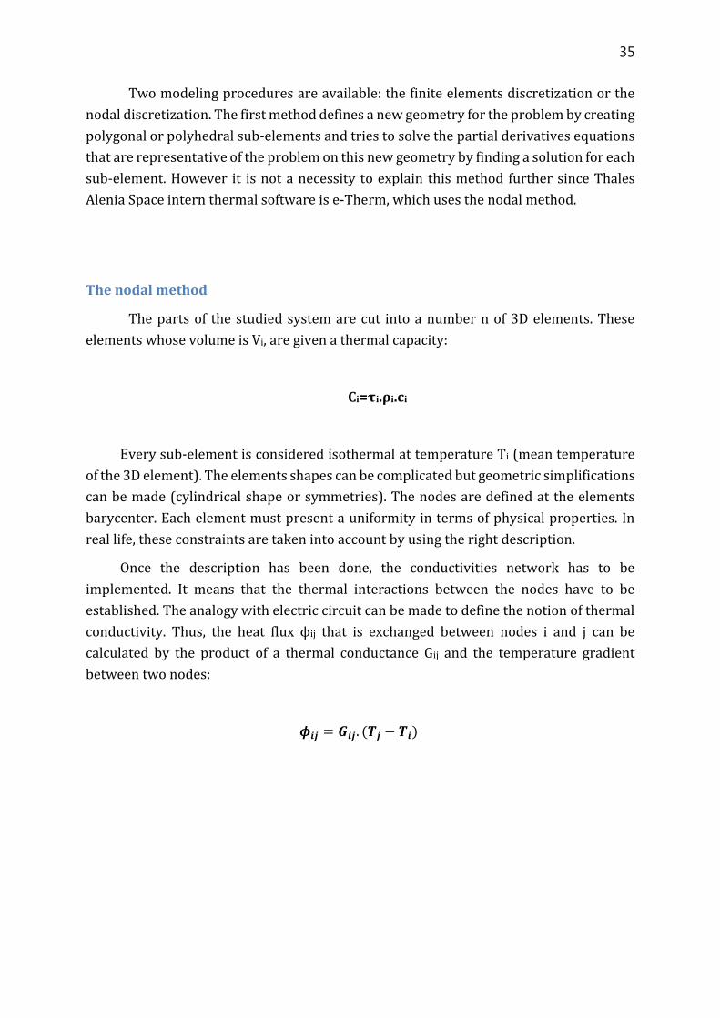
The nodal method
The parts of the studied system are cut into a number n of 3D elements. These
elements whose volume is Vi, are given a thermal capacity:
Ci=τi.ρi.ci
Every sub-element is considered isothermal at temperature Ti (mean temperature
of the 3D element). The elements shapes can be complicated but geometric simplifications
can be made (cylindrical shape or symmetries). The nodes are defined at the elements
barycenter. Each element must present a uniformity in terms of physical properties. In
real life, these constraints are taken into account by using the right description.
Once the description has been done, the conductivities network has to be
implemented. It means that the thermal interactions between the nodes have to be
established. The analogy with electric circuit can be made to define the notion of thermal
conductivity. Thus, the heat flux ϕij that is exchanged between nodes i and j can be
calculated by the product of a thermal conductance Gij and the temperature gradient
between two nodes:
𝝓𝒊𝒋 = 𝑮𝒊𝒋. (𝑻𝒋 − 𝑻𝒊)

36
Types of profiles to be modelled
As we saw previously, the SpaceBus Neo platform embarks passive and active
thermal control systems. But more specifically it embarks systems using fluids to work.
In fact, the heat pipes as well as the MPL use the heat transfer from the solid structure to
the fluid, and then through this fluid. In order to model correctly these heat transfers using
e-Therm and Amesim, the two programs used by TAS, it is a necessity to quantify the
conductivity between the structure and the fluid node in contact with it. According to the
software, it may be needed to give a conductivity value for a specific part of a profile, or a
global value for the whole profile. Let’s take the example of a heat transfer from a piece of
equipment to a heat pipe. As can be seen figure 18, the dissipated heat from the piece of
equipment will first go through an aluminum layer used to get a great thermal contact
between the equipment and the NIDA (NIDA stands for Nid D’Abeilles, which is the
material that is used to create the structure of every satellite. This material is made of
several thin sheets of aluminum that are put together in a way that creates mostly cavities,
its shape looks like a bee nest, hence its name).
Figure 18 : Example of a NIDA layer
The heat will then go through the solid structure until it reaches the heat pipe and
the fluid inside of it. The heat pipe will then distribute this heat on its whole length.
Eventually, the heat will be radiated thanks to the OSR surfaces.
37
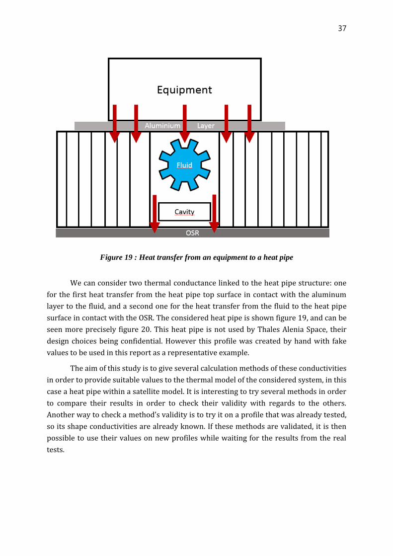
Figure 19 : Heat transfer from an equipment to a heat pipe
We can consider two thermal conductance linked to the heat pipe structure: one
for the first heat transfer from the heat pipe top surface in contact with the aluminum
layer to the fluid, and a second one for the heat transfer from the fluid to the heat pipe
surface in contact with the OSR. The considered heat pipe is shown figure 19, and can be
seen more precisely figure 20. This heat pipe is not used by Thales Alenia Space, their
design choices being confidential. However this profile was created by hand with fake
values to be used in this report as a representative example.
The aim of this study is to give several calculation methods of these conductivities
in order to provide suitable values to the thermal model of the considered system, in this
case a heat pipe within a satellite model. It is interesting to try several methods in order
to compare their results in order to check their validity with regards to the others.
Another way to check a method’s validity is to try it on a profile that was already tested,
so its shape conductivities are already known. If these methods are validated, it is then
possible to use their values on new profiles while waiting for the results from the real
tests.
38
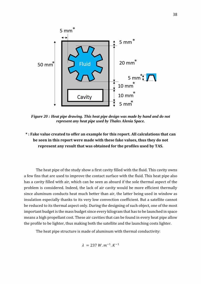
Figure 20 : Heat pipe drawing. This heat pipe design was made by hand and do not
represent any heat pipe used by Thales Alenia Space.
* : Fake value created to offer an example for this report. All calculations that can
be seen in this report were made with these fake values, thus they do not
represent any result that was obtained for the profiles used by TAS.
The heat pipe of the study show a first cavity filled with the fluid. This cavity owns
a few fins that are used to improve the contact surface with the fluid. This heat pipe also
has a cavity filled with air, which can be seen as absurd if the sole thermal aspect of the
problem is considered. Indeed, the lack of air cavity would be more efficient thermally
since aluminum conducts heat much better than air, the latter being used in window as
insulation especially thanks to its very low convection coefficient. But a satellite cannot
be reduced to its thermal aspect only. During the designing of such object, one of the most
important budget is the mass budget since every kilogram that has to be launched in space
means a high propellant cost. These air cavities that can be found in every heat pipe allow
the profile to be lighter, thus making both the satellite and the launching costs lighter.
The heat pipe structure is made of aluminum with thermal conductivity:
𝜆 = 237 𝑊. 𝑚−1. 𝐾−1
39
This value is the standard thermal conductivity for pure aluminum. To calculate
the thermal resistance of a wall with thickness e, cross section S and made of a material
with a thermal conductivity λ, it is given by the following formula:
𝑅𝑡ℎ =𝑒
𝜆 ∗ 𝑆
The thermal conductance, named B, is the inverse of the thermal resistance Rth.
Next the convective exchange coefficient at the walls h has to be considered for the fluid.
This coefficient depends on the fluid that is used, on the profile shape, as well as on the
fluid two phase state since h varies as a function of the vapor title. However it is possible
to use a mean value for our study, and the one that will be used is the following one:
ℎ = 10000 𝑊. 𝑚−2. 𝐾−1
Once again, the value that is used in this report is fake, it is not the real one used
by TAS engineers.
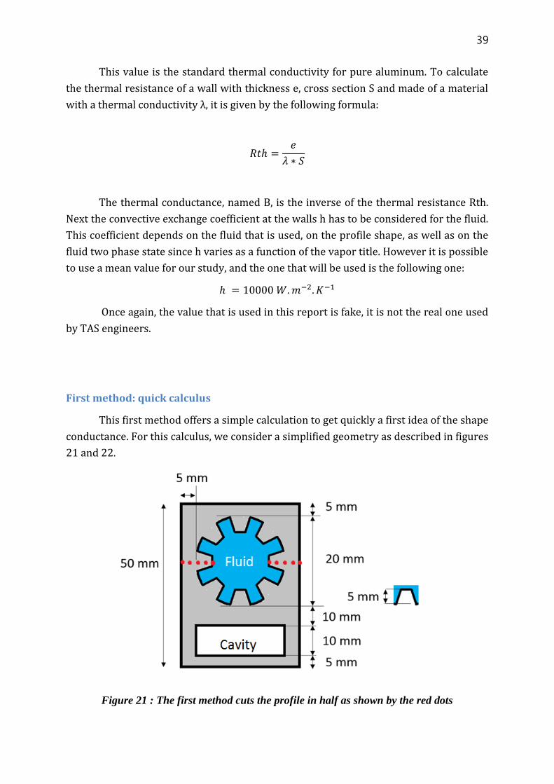
First method: quick calculus
This first method offers a simple calculation to get quickly a first idea of the shape
conductance. For this calculus, we consider a simplified geometry as described in figures
21 and 22.
Figure 21 : The first method cuts the profile in half as shown by the red dots

40
Figure 22 : Equivalent geometry for the first method
This simplified method do not consider thermal transfers between nodes 1 and 2,
which may seem absurd since in reality they are linked by conduction in the aluminum.
This method takes as a first hypothesis in fact that the heat preferred path is through the
fluid and not through the aluminum, meaning that the fraction of heat directly the profile
is negligible. This calculus also considers that the fluid is in the two phase state, thus its
temperature is the same at any point of the fluid.
The calculations consider a 1m long heat pipe in the direction of the axis that is
perpendicular to the cross section plan. The shape conductance of the part that goes from
the interface with the aluminum layer on top to the fluid is given by the inverse of the
thermal resistance of node 1 in figure 22 and shown more precisely figure 23. This node
is made of as much matter as the top part of the real profile, thus the need to calculate the
top part section surface.

41
Figure 23 : Top profile part that is modeled by node 1
This surface can be calculated this way:
𝑆 = 𝑙 ∗ 𝐿 − 𝑆𝑓𝑙𝑢𝑖𝑑
𝑆𝑓𝑙𝑢𝑖𝑑 = 𝜋∗𝑟²
2 ,
with l being 15mm, L being 30mm and r being the mean radius of the fluid cavity, meaning
the radius that is the mean of the radius from the center to the tip of the fins, and the other
radius from the center to the base of the fins. Thus:
𝑟 = 10 + (10 − 5)
2= 7,5𝑚𝑚
𝑆 = 362 𝑚𝑚²
It is now possible to calculate node’s 1 thickness:
𝑒 = 𝑆
𝐿= 12𝑚𝑚
The shape conductance will be the series conductance of the one through the matter of
node 1 and the one representing the fluid interface. The first one, B1mat, is λ*S/e, or 592.5
W/K for a one meter long heat pipe. The second one is the product of the convective
coefficient with the interaction surface, hence:
𝐵1𝑖𝑛𝑡 = ℎ ∗2 ∗ 𝜋 ∗ 𝑟
2∗ 1 = 235.5 𝑊. 𝐾−1
42
We can now calculate the conductance for the profile’s top part:
𝐵1 = 𝐵𝑠𝑢𝑝 = 1
1𝐵1𝑚𝑎𝑡 +
1𝐵1𝑖𝑛𝑡
= 168.5 𝑊. 𝐾−1
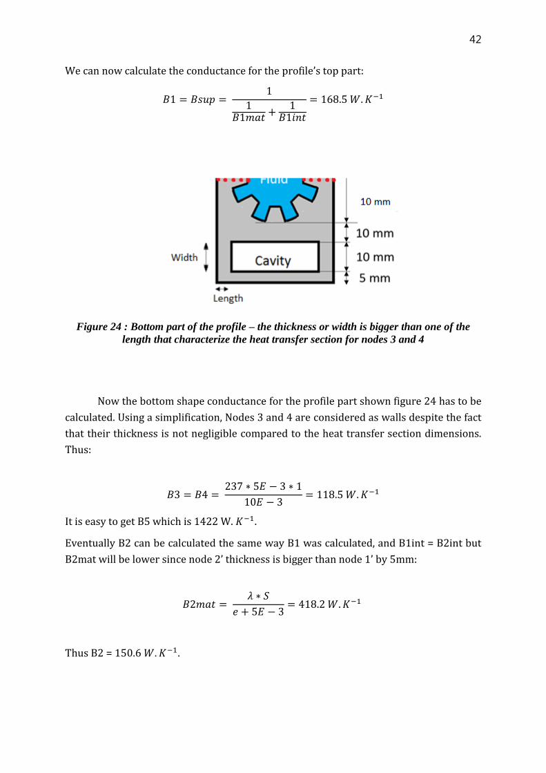
Figure 24 : Bottom part of the profile – the thickness or width is bigger than one of the
length that characterize the heat transfer section for nodes 3 and 4
Now the bottom shape conductance for the profile part shown figure 24 has to be
calculated. Using a simplification, Nodes 3 and 4 are considered as walls despite the fact
that their thickness is not negligible compared to the heat transfer section dimensions.
Thus:
𝐵3 = 𝐵4 = 237 ∗ 5𝐸 − 3 ∗ 1
10𝐸 − 3= 118.5 𝑊. 𝐾−1
It is easy to get B5 which is 1422 W. 𝐾−1.
Eventually B2 can be calculated the same way B1 was calculated, and B1int = B2int but
B2mat will be lower since node 2’ thickness is bigger than node 1’ by 5mm:
𝐵2𝑚𝑎𝑡 = 𝜆 ∗ 𝑆
𝑒 + 5𝐸 − 3= 418.2 𝑊. 𝐾−1
Thus B2 = 150.6 𝑊. 𝐾−1.
43
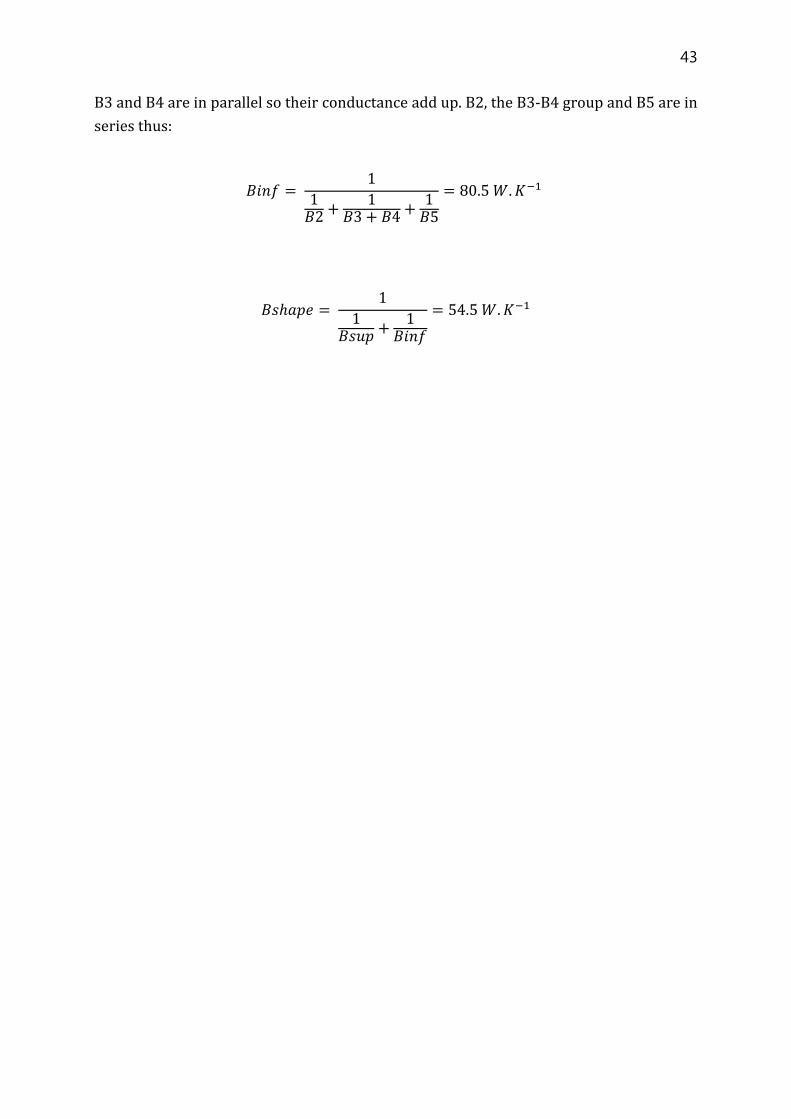
B3 and B4 are in parallel so their conductance add up. B2, the B3-B4 group and B5 are in
series thus:
𝐵𝑖𝑛𝑓 = 1
1𝐵2 +
1𝐵3 + 𝐵4 +
1𝐵5
= 80.5 𝑊. 𝐾−1
𝐵𝑠ℎ𝑎𝑝𝑒 = 1
1𝐵𝑠𝑢𝑝 +
1𝐵𝑖𝑛𝑓
= 54.5 𝑊. 𝐾−1

44
Second method: layer calculus
This second method offers a thinner description of the heat pipe as shown figure
25. We can consider it as an amelioration of the previous method. We take the same
hypothesis of a two phase fluid, only this time we consider conduction through the matter
as a path the heat might take rather than only going to the fluid.
Figure 252 : Second method profile description along the red lines
We consider in that case the conduction through matter and to the fluid layer by
layer. The three paths shown figure 26 are put in parallel.
Figure 26 : Drawing of the three heat paths for the second method. Two similar
path through the matter and one going through the fluid.
45
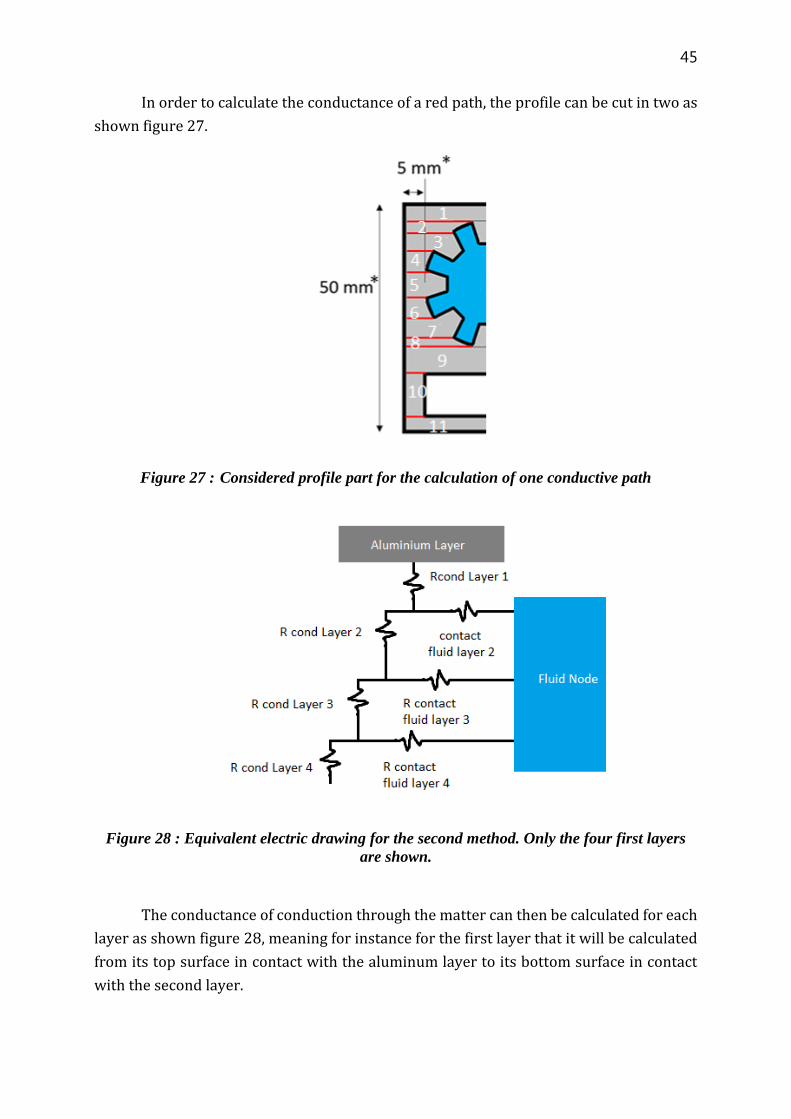
In order to calculate the conductance of a red path, the profile can be cut in two as
shown figure 27.
Figure 27 : Considered profile part for the calculation of one conductive path
Figure 28 : Equivalent electric drawing for the second method. Only the four first layers
are shown.
The conductance of conduction through the matter can then be calculated for each
layer as shown figure 28, meaning for instance for the first layer that it will be calculated
from its top surface in contact with the aluminum layer to its bottom surface in contact
with the second layer.

46
Layer Bcond
Top 1 711
2 948
3 395
4 237
5 316
6 237
7 395
8 948
9 355.5
10 118.5
Bottom 11 711
Table 3: Conductance of heat conduction through matter for half a profile
However the conductance linked to each part of the profile cannot be calculated
directly because the path that goes to and out of the fluid has to be considered as shown
figure 29. Thus the conductance relative to this part,
𝐵 = ℎ ∗ 𝑆𝑖𝑛𝑡𝑒𝑟𝑓𝑎𝑐𝑒 ,
has to be added to the calculations for layers 1 to 9:
Figure 29 : Fluid contribution to the thermal path that has to be considered

47
Adding these contact conductance leads to the results presented in table 4.
Layer Bcond Btot
Top 1 711 786
2 948 998
3 395 545
4 237 287
5 316 466
6 237 287
7 395 545
8 948 998
9 355.5 786
10 118.5 118.5
Bottom 11 711 711
Table 4: Conduction and global conductance for half a profile by taking the fluid into
account
Eventually it is possible to put into series these global conductance to get B values
for the profile and its top and bottom parts. The top B value considers layers 1 to 8 while
the bottom one goes from 3 to 11. The number of layers that were considered was decided
freely and might be adjusted.
𝐵𝑓𝑜𝑟𝑚 = 73.6 𝑊. 𝐾−1
𝐵𝑠𝑢𝑝 = 124.5 𝑊. 𝐾−1
𝐵𝑖𝑛𝑓 = 80.3 𝑊. 𝐾−1
It can be noticed that layers 3 to 8 are considered twice if we look at Bsup and Binf
(they are not considered twice in Bform). This can but understood by the fact that the
thermal flux do not consider only a part of the profile, top or bottom in our case, but is
diffused in a larger area. However the number of layers that are considered for Bsup and
Binf was decided freely, so they might have to be modified by comparing the results of
this method with other methods or tests. Before comparing the results of the second with
those of the first method, let’s first see the third modeling method.

48
Third method : e-Therm simulation
The third method consists in using the nodal thermal software e-Therm to model
the heat pipe. This modeling needs a 3D geometry file that describes the system to model.
Then, once the file has been opened in e-Therm, the engineer has to create the external
meshing of the geometry, as shown figure 30. The software indeed works with faces. To
calculate conduction through solids, e-Therm will fill the model made of external faces
with intern faces by creating the 3D meshing as shown figure 31, and give each of these
faces a thickness and a material.
It is a necessity to create enough sub-elements in the profile in order to describe it
precisely enough. Since each face could be a node, these faces have to be small because
the nodal modeling is not valid if a thermal gradient is too high within a node.
Figure 30 : Example of geometry cutting for e-Therm meshing
Figure 31 : Example of a geometry meshed by e-Therm. This geometry is not representative
of any profile used by Thales Alenia Space.
49
Once the external faces are made, e-Therm can be asked to create the 3D meshing
for the internal part of the geometry. To start the calculations, e-Therm needs that each
face receives a node number. In our case the fluid also get a node number and a dissipation
is given on one side of the profile to model an equipment. E-Therm then simulates a steady
case that allows to get temperature results for the whole profile. The temperature
gradient then calculated are used to get the thermal conductance of the profile, knowing
the dissipation going through the profile.
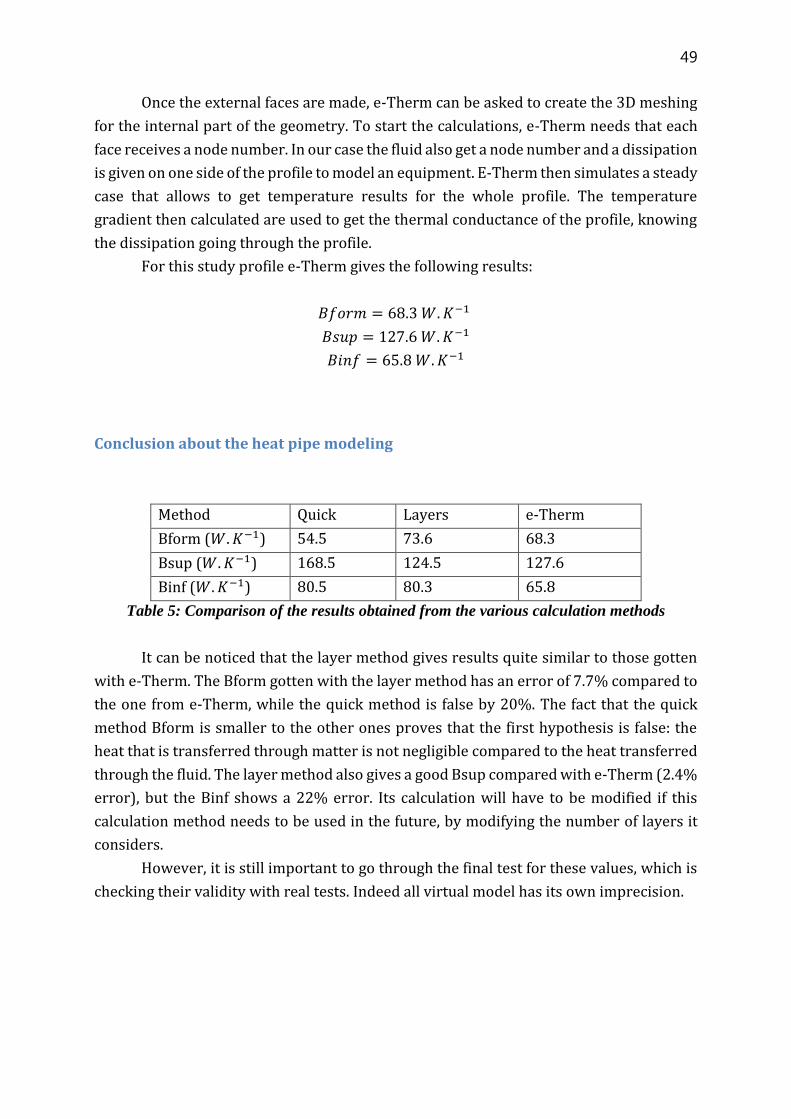
For this study profile e-Therm gives the following results:
𝐵𝑓𝑜𝑟𝑚 = 68.3 𝑊. 𝐾−1
𝐵𝑠𝑢𝑝 = 127.6 𝑊. 𝐾−1
𝐵𝑖𝑛𝑓 = 65.8 𝑊. 𝐾−1
Conclusion about the heat pipe modeling
Method Quick Layers e-Therm
Bform (𝑊. 𝐾−1) 54.5 73.6 68.3
Bsup (𝑊. 𝐾−1) 168.5 124.5 127.6
Binf (𝑊. 𝐾−1) 80.5 80.3 65.8
Table 5: Comparison of the results obtained from the various calculation methods
It can be noticed that the layer method gives results quite similar to those gotten
with e-Therm. The Bform gotten with the layer method has an error of 7.7% compared to
the one from e-Therm, while the quick method is false by 20%. The fact that the quick
method Bform is smaller to the other ones proves that the first hypothesis is false: the
heat that is transferred through matter is not negligible compared to the heat transferred
through the fluid. The layer method also gives a good Bsup compared with e-Therm (2.4%
error), but the Binf shows a 22% error. Its calculation will have to be modified if this
calculation method needs to be used in the future, by modifying the number of layers it
considers.
However, it is still important to go through the final test for these values, which is
checking their validity with real tests. Indeed all virtual model has its own imprecision.
50
Chapter V | Satellite thermal modeling
The nodal method applied to satellites
General aspects
The process of getting from a real life satellite to a thermal model that can be used
by a calculus program is made thanks to the nodal description, which meshes the system’s
physical equations.
As we saw before, the nodal description of a thermal system is valid when each sub-
element show a restricted thermal gradient. This can be found for compact elements with
a high thermal conductivity or for heat pipes where the fluid makes sure to distribute the
heat quite evenly over its length with an almost null thermal resistance. To the contrary,
for structural elements with low conductivity such as a NIDA panel, thermal gradients are
no longer negligible. It can be shown that in this case the panel can still be described by
only one element with a mean temperature, so that the overall radiated power is the same.
A satellite, once described as a bunch of nodes, is a set S of nodes I at the temperature
Ti. Each node i has a volume τi, a density ρi and a specific heat ci. So each node has a thermal
capacity (expressed in J/K):
Ci=τi.ρi.ci
This node can be linked to the other nodes j of the satellite through conductive
couplings GL(i,j) and radiative couplings GR(i,j). Moreover, it can receive internal powers
(dissipations) and external ones (incident fluxes). The sum of these fluxes is Qi.
The various quantities defined here are linked together in the thermal balance
equations for each node. The set of all these equations is the model of the satellite.
From a standard point of view, the balance equation for one node in the case of
spatial thermal modeling is:
𝑀𝑖𝐶𝑃𝑖
𝑑𝑇𝑖
𝑑𝑡= 𝛼𝑖𝐴𝑖(𝜙𝑆𝑖
+ 𝜙𝐴𝑖) + 𝜀𝑖𝐴𝑖𝜙𝑇𝑖
+ 𝑃𝑖 + ∑ 𝑅𝑖𝑗𝜎(𝑇𝑗4 − 𝑇𝑖
4) + ∑ 𝐶𝑖𝑗(𝑇𝑗 − 𝑇𝑖)𝑛𝑗=1
𝑛𝑗=1 ,
51
with :
n the system’s number of nodes
𝑀𝑖𝐶𝑃𝑖 node i specific heat (J/K)
𝛼𝑖 node i absorptivity
𝜀𝑖 node i emissivity
𝐴𝑖 node i (m²) external area
𝜙𝑆𝑖 solar flux density received by node i (W/m²)
𝜙𝐴𝑖 albedo flux density received by node i (W/m²)
𝜙𝑇𝑖 earth flux density received by node i (W/m²)
𝑃𝑖 dissipated power on node i (W)
𝑅𝑖𝑗 radiosity between nodes i and j (m²)
𝐶𝑖𝑗 thermal conductance between nodes i and j (W/K)
σ Stefan-Boltzman constant (5.67E-8 W/(m²𝐾4))
Creation of a satellite model using e-Therm
e-Therm is a software that was created by Thales Alenia Space to create a thermal
model of a satellite and to simulate its thermal behavior. Creating a thermal model works
by following two steps: first, the thermal engineer will have to create a conductive model
of the satellite to model the conductive interactions. It is a 2D model where the panels are
drawn, with the equipment and heat pipe layout drawn as well on the panels. Then the
radiative model of the satellite will have to be created. The radiative model will be in two
parts, an external and an internal. The external part will model the fluxes received by the
satellite and its heat radiation towards space. The internal part will model the radiative
interaction in-between the satellite components and structure panels.
Standard rules to keep in mind for the nodal modeling of a satellite
The following list is not exhaustive but it shows the most important modeling rules
to follow.
A thermal node needs to stay at a low thermal gradient in order to not lose too
much information
52
A nodal description has to model the power dissipation in a good way (heaters,
hardware, heat pipes) so as to guarantee a good precision.
The nodal description has to be adapted accordingly to the analysis objectives: if
a model has to be used to calculate MLI hot spots temperatures, the MLI nodal
description has to be refined for example.
For the external elements, the nodal description has to take sunlight into account
in order to avoid averaging the external faces temperatures as well as averaging
within various parts of the same face since the MLI and OSR temperature can be
very different one from another
Interfaces have to be modelled in order to simulate fluxes between elements
Rules about the components to model
The equipment
Every single piece of equipment whose temperature has to be calculated needs to
be associated to a node. That node do not have to be an equipment node since it can be a
structure node if its temperature is representative (for example some small pieces of
equipment that do not dissipate heat will have the structure temperature).
The nodal description of the equipment has to allow to simulate and calculate the
extreme temperatures in the various operational configurations. The calculation tools
being powerful, it is recommended to describe each piece of equipment with one or
several nodes, allowing the model to calculate their hot spots and the heat dissipation
repartition within an equipment. Indeed, thanks to the processers with continuous
improvements on their performances and the solvers optimization, the rules of the past
that used to recommend to limit the number of nodes to reduce calculation times by
lowering the size of the calculation matrix are obsolete. The thermal engineer however
needs to be aware of the calculation tools limits.
In order to create a model that is easy to use and to modify, the node attribution
and the equipment names have to be described and written down in order to understand
easily the link between a piece of equipment and its nodes.

53
Many satellite models have already been created on e-Therm, hence many reduced
equipment models have already been created. A reduced equipment model is an e-Therm
model with the nodal description of an equipment. When such a reduced model is
available and if it matches with a satellite model objectives in terms of precision, it is
interesting to directly import the equipment reduced model to include it to the satellite
model.
The nodal description of the pieces of equipment that are put on a heat pipe has to
model to the best the heat transfer to the heat pipe. Indeed, it will allow the software to
calculate correctly the power that is transferred to the heat pipe and to check if the chosen
heat pipe works with the amount of heat that needs to be transferred. In order to predict
that heat transfer, the providers are asked to give details on their hardware in order to
create reduced equipment models with enough precision.
Thus a piece of equipment put on two heat pipes will have to be described
accordingly as shown figure 32. If the equipment is described as only one node with one
temperature, it will create parasitic couplings between the heat pipes that have no
physical meaning.
Figure 32 : Example of equipment that is set on two heat pipes and its recommended
description

54
Heat pipes
Each heat pipe is modelled with only one node or one sub-node since the heat pipe
is considered isothermal. Heat pipe crossings as shown figure 33, meaning heat pipes with
various directions that overlap each other, can be considered in one node or one sub-
node.
Figure 33 : Drawing of a heat pipe crossing. The green heat pipe are put within the NIDA
while the purple heat pipe are put on the NIDA.
The software also allows to calculate the energy that is transferred to the structure.
This allows the calculation of the heat that is transferred by the heat pipes. It might be
interesting to cut the heat pipe node into sub nodes for special cases where the energy
transfer will be different according to the studied area. Examples of this type of situation
could be a heat pipe that covers structure partly covered by MLI, and partly by OSR
surfaces. Examples of these situations are presented figure 34.
Figure 44 : Heat pipe description depending on the situation
55
If the thermal engineer has to simulate a malfunction where the behavior of one or
more heat pipe is modified, the heat pipe node also needs to be described with several
sub-nodes.
North and South structures
The North and South panels’ description in terms of nodes should not be handled
lightly, because their modeling is extremely important to calculate the correct equipment
temperatures.
Usually, the North and South structure is cut into 2 nodes along the width in order
to implement the transverse gradient inside the NIDA. Thus there is an internal and an
external node for one unit of structure.
The structure description is made accordingly to the heat pipe network. The heat
pipe being isothermal, two structural nodes (inter/extern) are made for the area around
a heat pipe. However it might be acceptable to give one duo inter/extern nodes to several
heat pipes when the equipment layout has no influence on the gradients. This can be the
case for pieces of equipment are set on a panel with enough heat pipes to distribute the
heat on the whole panel area.
The nodal description is made following several steps. Usually in a satellites the
equipment layout regroups pieces of equipment according to their qualifications. A
qualification is the maximum temperature at which a piece of equipment has been tested
in operation successfully for a required amount of time. TWTs (Traveling Wave Tubes that
are used to amplify a signal) have a high temperature of qualification because they
dissipate a lot of heat and can resist to relatively high temperatures so they are all put
together. The electronics that is more delicate is put in another area of the satellite. From
one equipment area to another, there might be a 20° difference. In each of these areas, the
description is made accordingly to the gradients that will appear. It is true that heat pipes
are supposed to homogenize the temperature along them, but between them there is still
gradients because the design do not always use heat pipe crossings. One or more nodes
are added between areas of different qualifications because the in-between area is a
gradient area. Interface nodes are also introduced in order to model the conductive
coupling between perpendicular panels that intersect. The nodal description is also made
accordingly to the areas covered with MLI as described in figure 35.
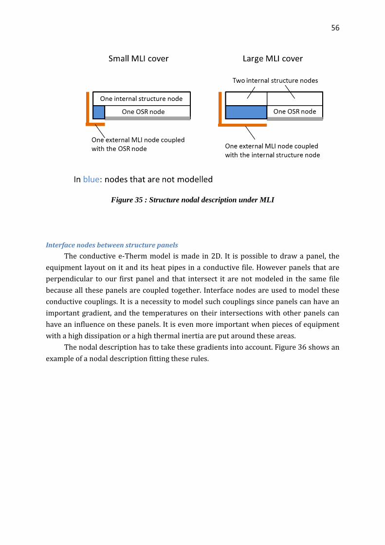
56
Figure 35 : Structure nodal description under MLI
Interface nodes between structure panels
The conductive e-Therm model is made in 2D. It is possible to draw a panel, the
equipment layout on it and its heat pipes in a conductive file. However panels that are
perpendicular to our first panel and that intersect it are not modeled in the same file
because all these panels are coupled together. Interface nodes are used to model these
conductive couplings. It is a necessity to model such couplings since panels can have an
important gradient, and the temperatures on their intersections with other panels can
have an influence on these panels. It is even more important when pieces of equipment
with a high dissipation or a high thermal inertia are put around these areas.
The nodal description has to take these gradients into account. Figure 36 shows an
example of a nodal description fitting these rules.
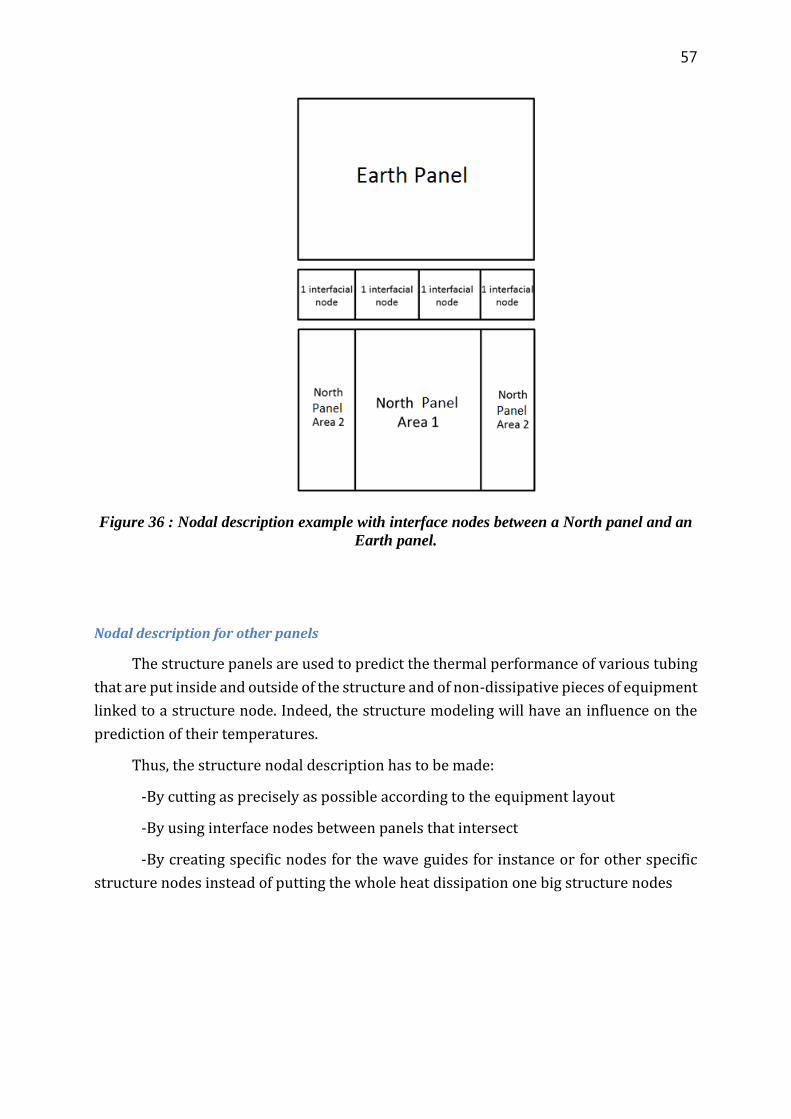
57
Figure 36 : Nodal description example with interface nodes between a North panel and an
Earth panel.
Nodal description for other panels
The structure panels are used to predict the thermal performance of various tubing
that are put inside and outside of the structure and of non-dissipative pieces of equipment
linked to a structure node. Indeed, the structure modeling will have an influence on the
prediction of their temperatures.
Thus, the structure nodal description has to be made:
-By cutting as precisely as possible according to the equipment layout
-By using interface nodes between panels that intersect
-By creating specific nodes for the wave guides for instance or for other specific
structure nodes instead of putting the whole heat dissipation one big structure nodes

58
IMUXes
IMUXes are “Input MUltipleXers” that are used for the signal treatment. These
pieces of equipment are not dissipative, hence their sensitivity to their environment. The
radiative modeling especially has to take their size into account and to give them an
equivalent geometry because of their complex geometry since they are modelled by boxes
in the thermal model. The emissivity that is used for the model was calculated using
correlations made on the basis of real life tests.
Wave Guides
Wave guides are cables that convey the signal treated by the satellite. Usually they
dissipate a lot of heat because the signal they convey is quite energetic. In the thermal
model they are modelled using two radiative faces since the wave guide usually have a
box-like shape, very thin and very long. The two faces are put on the wave guides paths,
they radiate to opposite directions. Their modeling is quite important since on the one
side they dissipate quite a lot of heat, and on the other side they “cover” parts of the
structure since they are quite close to a wall usually. This cover will affect the ability of
the wall to radiate within the satellite internal volume.
The heaters
Heaters don’t need to be modeled when there are set on heat pipes because their
dissipated power can be given to the heat pipe node directly. However, in the case there
are not put on heat pipes, it is recommended to create heaters nodes instead of giving
their dissipation to the structure node directly.
The MLI
The MLI nodal description depends on the model use and on the MLI position
regarding critical elements. For predicting a telecommunication satellite temperatures,
an MLI nodal description of one or two nodes per face is enough. Such a model is valid if
only the energy input and output through the MLI need to be calculated.
But if there is a radiative area with MLI in its field of vision, or if we want to know
the temperature of a precise MLI part, it is then a necessity to describe the MLI with one
or several nodes. The MLI nodal description will then have to take into account the areas
that receive sunlight and those staying in the shadow as well as the various view factors
towards space.
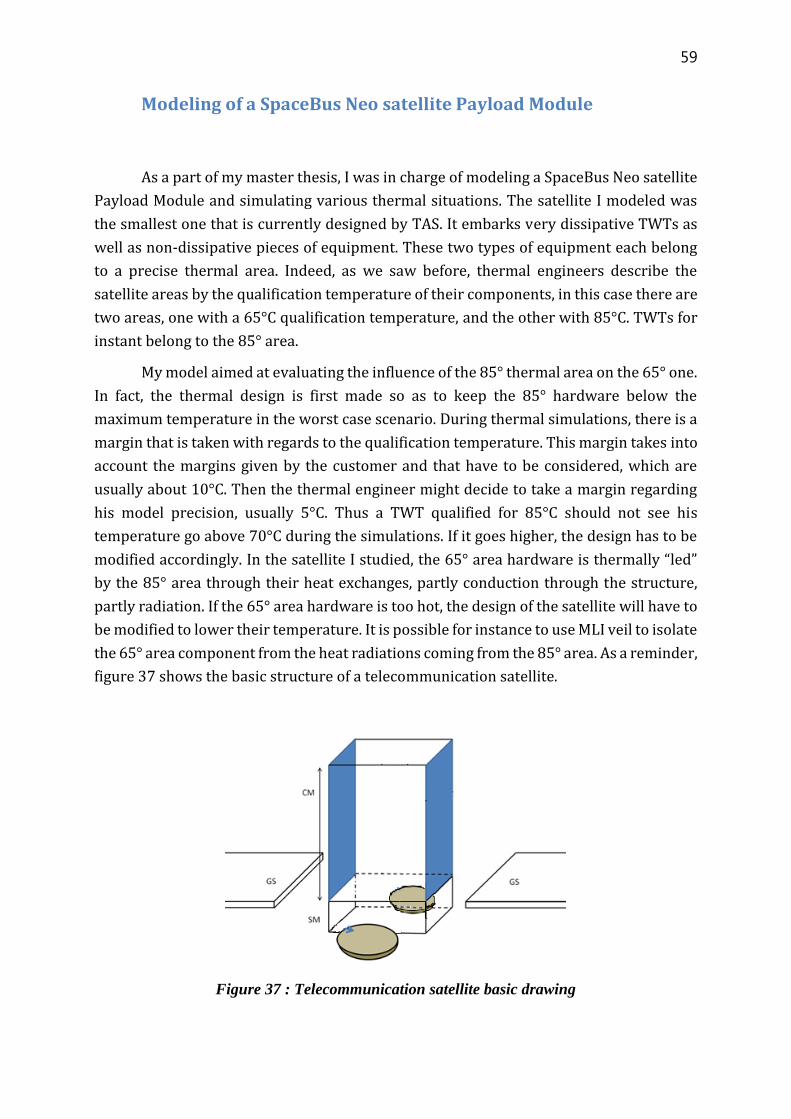
59
Modeling of a SpaceBus Neo satellite Payload Module
As a part of my master thesis, I was in charge of modeling a SpaceBus Neo satellite
Payload Module and simulating various thermal situations. The satellite I modeled was
the smallest one that is currently designed by TAS. It embarks very dissipative TWTs as
well as non-dissipative pieces of equipment. These two types of equipment each belong
to a precise thermal area. Indeed, as we saw before, thermal engineers describe the
satellite areas by the qualification temperature of their components, in this case there are
two areas, one with a 65°C qualification temperature, and the other with 85°C. TWTs for
instant belong to the 85° area.
My model aimed at evaluating the influence of the 85° thermal area on the 65° one.
In fact, the thermal design is first made so as to keep the 85° hardware below the
maximum temperature in the worst case scenario. During thermal simulations, there is a
margin that is taken with regards to the qualification temperature. This margin takes into
account the margins given by the customer and that have to be considered, which are
usually about 10°C. Then the thermal engineer might decide to take a margin regarding
his model precision, usually 5°C. Thus a TWT qualified for 85°C should not see his
temperature go above 70°C during the simulations. If it goes higher, the design has to be
modified accordingly. In the satellite I studied, the 65° area hardware is thermally “led”
by the 85° area through their heat exchanges, partly conduction through the structure,
partly radiation. If the 65° area hardware is too hot, the design of the satellite will have to
be modified to lower their temperature. It is possible for instance to use MLI veil to isolate
the 65° area component from the heat radiations coming from the 85° area. As a reminder,
figure 37 shows the basic structure of a telecommunication satellite.
Figure 37 : Telecommunication satellite basic drawing
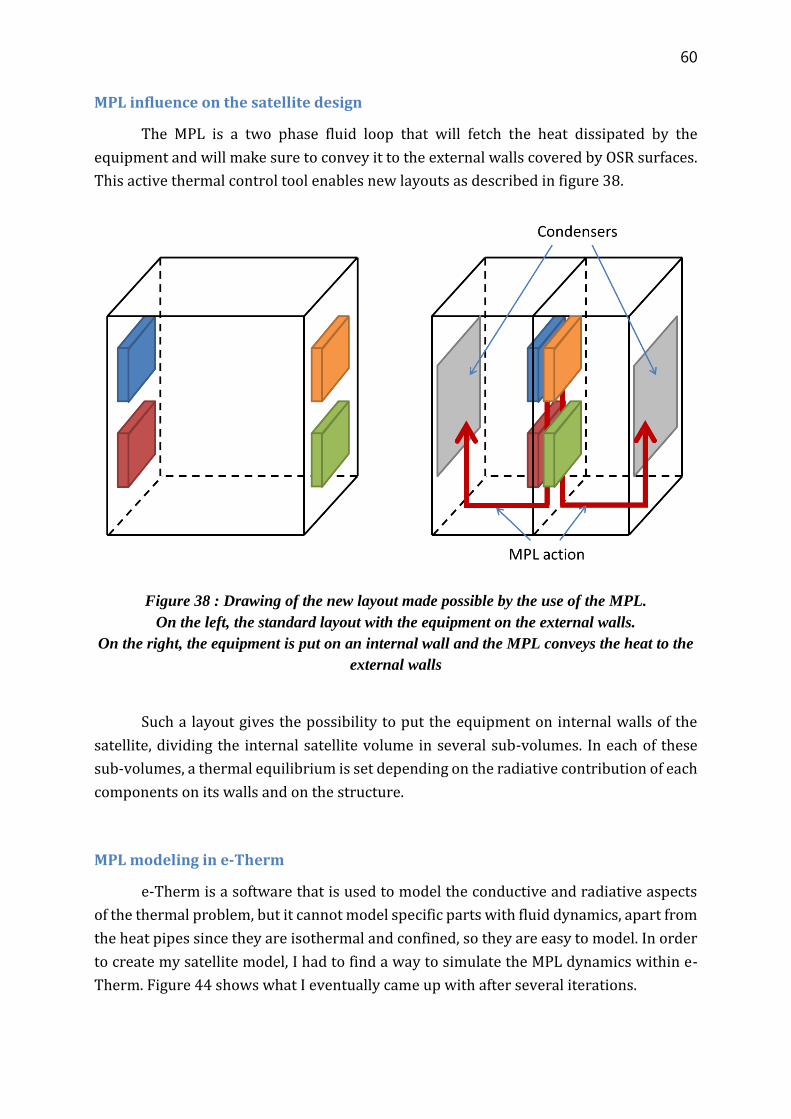
60
MPL influence on the satellite design
The MPL is a two phase fluid loop that will fetch the heat dissipated by the
equipment and will make sure to convey it to the external walls covered by OSR surfaces.
This active thermal control tool enables new layouts as described in figure 38.
Figure 38 : Drawing of the new layout made possible by the use of the MPL.
On the left, the standard layout with the equipment on the external walls.
On the right, the equipment is put on an internal wall and the MPL conveys the heat to the
external walls
Such a layout gives the possibility to put the equipment on internal walls of the
satellite, dividing the internal satellite volume in several sub-volumes. In each of these
sub-volumes, a thermal equilibrium is set depending on the radiative contribution of each
components on its walls and on the structure.
MPL modeling in e-Therm
e-Therm is a software that is used to model the conductive and radiative aspects
of the thermal problem, but it cannot model specific parts with fluid dynamics, apart from
the heat pipes since they are isothermal and confined, so they are easy to model. In order
to create my satellite model, I had to find a way to simulate the MPL dynamics within e-
Therm. Figure 44 shows what I eventually came up with after several iterations.
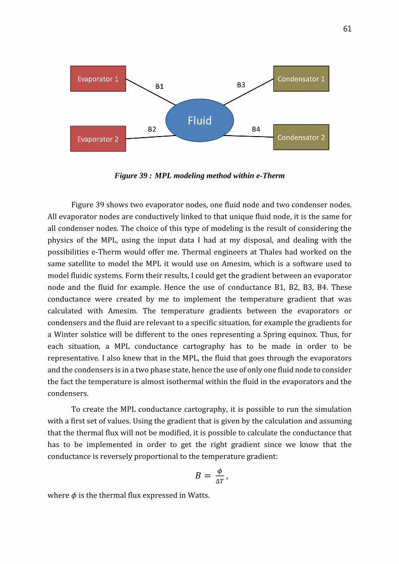
61
Figure 39 : MPL modeling method within e-Therm
Figure 39 shows two evaporator nodes, one fluid node and two condenser nodes.
All evaporator nodes are conductively linked to that unique fluid node, it is the same for
all condenser nodes. The choice of this type of modeling is the result of considering the
physics of the MPL, using the input data I had at my disposal, and dealing with the
possibilities e-Therm would offer me. Thermal engineers at Thales had worked on the
same satellite to model the MPL it would use on Amesim, which is a software used to
model fluidic systems. Form their results, I could get the gradient between an evaporator
node and the fluid for example. Hence the use of conductance B1, B2, B3, B4. These
conductance were created by me to implement the temperature gradient that was
calculated with Amesim. The temperature gradients between the evaporators or
condensers and the fluid are relevant to a specific situation, for example the gradients for
a Winter solstice will be different to the ones representing a Spring equinox. Thus, for
each situation, a MPL conductance cartography has to be made in order to be
representative. I also knew that in the MPL, the fluid that goes through the evaporators
and the condensers is in a two phase state, hence the use of only one fluid node to consider
the fact the temperature is almost isothermal within the fluid in the evaporators and the
condensers.
To create the MPL conductance cartography, it is possible to run the simulation
with a first set of values. Using the gradient that is given by the calculation and assuming
that the thermal flux will not be modified, it is possible to calculate the conductance that
has to be implemented in order to get the right gradient since we know that the
conductance is reversely proportional to the temperature gradient:
𝐵 = 𝜙
∆𝑇 ,
where 𝜙 is the thermal flux expressed in Watts.

62
My tests showed that my assumption about the thermal flux not being modified
was almost right, this method allowing to get the desired gradient (usually a few Celsius
degrees) to a tenth of a degree precision which is totally acceptable for a thermal model.
Because of the MPL, each thermal case has to be considered twice. It is indeed a
necessity to consider a failure mode for the MPL where it functions less efficiently, thus
cooling less the equipment. Such case is the worst hot case scenario.
Calculation cases
The study was mostly made around three cases: hottest point during the Winter
Solstice satellite orbit at the end of life for the hot sizing case, coldest point during the
Winter Solstice satellite orbit at the end of life and lastly an orbital eclipse case for the
cold sizing case. All these simulations were made as steady cases. It was also possible with
e-Therm to create transient calculation cases, but I have not had the time to get to that
point. During the Winter Solstice, the South face constantly receives sunlight at a 23.5°
angle approximately. The sunlight incidence for the two Sinter Solstice cases are shown
figure 40. The North panel hot case was also simulated (as a reminder, it was during the
Summer Solstice) but it is not interesting to describe it since during the Summer Solstice,
the solar flux reaches it minimum and the MPL has such a powerful coupling action
between the external walls that it almost negates the temperature difference between the
OSR surfaces of the South and North faces. This conclusion was accepted after a few
simulations of a Summer Solstice case were made.
Figure 40 : Drawing showing the sunlight incidence for the two Winter Solstice cases.

63
In the hottest case, the satellite receives the maximum of solar flux it could possibly
receive on one of its four relevant external faces (N, S, E, W) concerning the heat rejection
using the OSR surfaces. In this case the Sun hits the East or West face with a 90° incident
angle. In the case I studied the East face received sunlight, but the case with the West face
receiving sunlight would have been valid to study as well, the satellite layout being almost
symmetrical. The East face also receives a reflected light from the reflectors which are
part of the satellite’s antennas.
The cold point of the Winter Solstice satellite orbit is the moment when the
sunlight hits the back of the reflectors that act as masks in this case, preventing a part of
the sunlight to reach the satellite faces. Furthermore the sunlight will hit the anti-earth
face with a 90° incident angle, but that face is a part of the Service Module thus it doesn’t
have a direct influence on the Payload Module which is being studied here. In fact the
Service Module will be represented by a node with a fixed temperature in this study, the
temperature being modified accordingly to the case in order to be representative.
It might seem useless to simulate the coldest moment of the Winter Solstice
satellite orbit. It is indeed not a sizing case at all. However Thales engineers found it
interesting to simulate this case in order to see the MPL fluid maximum temperature
variations during an orbit, hence the need for this calculation.
The cold sizing case is an orbital eclipse, where the satellite do not receive any
sunlight because of the Earth masking the Sun.
This report will cover the analysis of four components, two A and B pieces of
equipment that belong to the 65°C area, and two pieces of equipment C and D that belong
to the 85°C area. The A component is put on a different wall than the one that carry the
components B, C and D. So the B component will receive some heat by conduction through
the panel from the 85°C area. The conduction between perpendicular panels that intersect
is neglected. The A component is put near to the evaporators, and we consider that the
85°C area is put on the MPL evaporators that are put inside the panel. Components A, B, C
and D are put in the same internal volume thus they see each other. They will exchange
heat by radiation. The layout is shown figure 41.

64
Figure 41 : Case study layout drawing, with the condensers and evaporators areas
The dissipated heat values that are given in tables 6 and 7 are fakes and will only
be used to give an example for this report in order to have the discussion that I had during
my master thesis about the thermal impact of the 85°C area on the 65°C area.
During the modeling, the thermal engineer has to check his model validity. In order
to do so, he will run a few thermal cases in order to analyze the first temperature results
that are produced. The heat exchanges between nodes can also be checked to detect
anomalies.
Equipment Dissipation (W) Hot WS
temperatures,
MPL failure
mode (°C)
Hot WS
temperatures,
MPL nominal
mode (°C)
Qualification
temperatures
(minus the
15°C margin)
A 30 42 44 50
B 30 49 45 50
C 400 76 71 70
D 200 59 52 70
Table 6: Temperature values for the WS hot case.
These are fake values that were created for this report.

65
Table 6 shows the results for the hot sizing case, with the MPL functioning
normally or in its failure case. It can be noticed that during the MPL failure mode, the C
component goes up to 76°C. If we consider a 15°C margin as we explained before, the
maximum temperature it is allowed to reach is 70°C. It shows that the evaporator design
under that component has to be modified in order to fetch more of its heat. However, we
can see that even with a C component that is too hot, the other components are below the
maximum temperature that can be allowed. It is especially interesting for the 65°C area
components since it shows that they will still be below that maximum temperature after
the design lowered the C component temperature.
The A component shows an interesting phenomena. Its temperature is higher
when the MPL functions normally than when does not. This comes from the fact that when
the MPL functions normally, there is more heat from the hot components that is
transferred to the evaporators, and then to the condensers, making the condensers hotter
in the nominal case. The A component gets more heat by conduction inside its panel than
by radiation from the hot components. However in the nominal case, it stays under its
maximum temperature.
A question arises from these considerations: would it be possible that, by taking
more heat from the C component to lower it down to 70°C, the A component goes above
the 50°C that are requested as its maximal temperature? From the results that are
presented here, it doesn’t seem very likely. Between the failure and the nominal cases, the
C component temperature went down by 5°C, the D component also went down, by 7°C
while the A component went up by only 2°C. If we consider that the C and D components
are quite similar in terms of size and dissipated heat, then the design modifications that
have to be made to lower the C component temperature by 6°C would heat the A
component up by 1°C approximately, which is still acceptable.
Equipment Dissipation (W) Temperatures
during the
eclipse, MPL
failure (°C)
Temperatures
during the
eclipse, nominal
MPL (°C)
A 30 -2 0
B 30 10 5
C 400 27 22
D 200 15 8
Table 7: Temperature values for the eclipse case.
These are fake values that were created for this report.
66
This second table shows the result from the cold case that was calculated, the
orbital eclipse. The components’ temperatures go down by 40°C but only the A component
goes below the 0°C. In this calculation case, the equipment dissipation was kept as normal
and was not put off so this case is not really the cold sizing case, because the cold sizing
case happens when the payload dissipate its minimum of heat. Nevertheless this
calculation case is quite interesting, because it shows that the 65°C area components that
are not very dissipative don’t drop to low in terms of temperature. It shows the MPL
ability to distribute the heat over the whole satellite, in this case the heat from the 85°C
area components helps keeping the 65°C area components at a reasonable temperature,
thus heaters are not needed here. This is very interesting because for a regular satellite,
in this case, heaters are needed for the 65°C area. Of course for the heater sizing, the real
cold sizing case should be computed, but when I modelled by satellite the heaters’ layout
was not yet defined, so I could not model them.
This study concludes that MLI veils are not needed to keep the 65°C area
components from overheating because of the heat they receive from the 85°C area.
However the evaporators’ design under the C component has to be improved in order to
make sure it doesn’t heat up too much in the hottest case.
The eclipse case is especially interesting as it really shows the MPL ability to
distribute the heat within the satellite, allowing to not use any heater in a case where a
regular satellite would. This will improve the SpaceBus Neo heaters’ lifespan as they will
be used less frequently.

67
Chapter VI | Amesim and the cosimulation
Amesim presentation
Amesim is the software that was chosen by the TAS thermal engineers that design
the MPL. Developed by SIEMENS LMS, this software uses the complex equations of two
phase fluids. Various components are modeled (tube, heater, plaques, thermal joints, …)
by giving their characteristics (mass, volume, pressure losses, …).
Figure 42 : Amesim component definition
As can be seen in figure 42, Amesim works with two kinds of components: resistive
and capacitive. Capacitive components are volume components where temperature and
pressure are calculated from the enthalpy at its ports while resistive components are
those defining the enthalpy and the system flow from the temperature and pressure.
That’s why a thermal-hydraulic model is always built with resistive and capacitive
components succeeding one another. It is interesting to understand that way of
functioning since it can explain numerical solving issues.
Amesim is not only a fluidic thermal software but can be used to model electric,
mechanical, energetic or electromagnetic control. It is a program that has more and more
users in the industry.
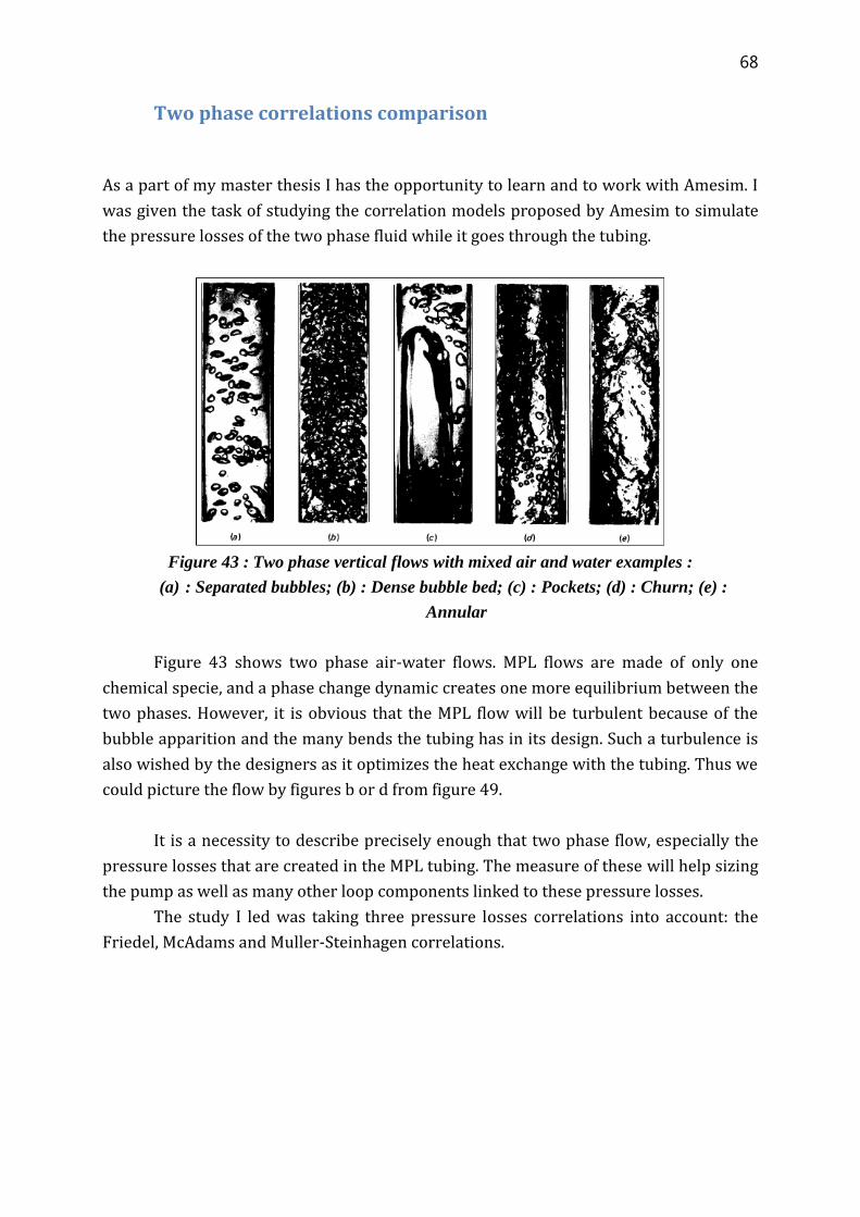
68
Two phase correlations comparison
As a part of my master thesis I has the opportunity to learn and to work with Amesim. I
was given the task of studying the correlation models proposed by Amesim to simulate
the pressure losses of the two phase fluid while it goes through the tubing.
Figure 43 : Two phase vertical flows with mixed air and water examples :
(a) : Separated bubbles; (b) : Dense bubble bed; (c) : Pockets; (d) : Churn; (e) :
Annular
Figure 43 shows two phase air-water flows. MPL flows are made of only one
chemical specie, and a phase change dynamic creates one more equilibrium between the
two phases. However, it is obvious that the MPL flow will be turbulent because of the
bubble apparition and the many bends the tubing has in its design. Such a turbulence is
also wished by the designers as it optimizes the heat exchange with the tubing. Thus we
could picture the flow by figures b or d from figure 49.
It is a necessity to describe precisely enough that two phase flow, especially the
pressure losses that are created in the MPL tubing. The measure of these will help sizing
the pump as well as many other loop components linked to these pressure losses.
The study I led was taking three pressure losses correlations into account: the
Friedel, McAdams and Muller-Steinhagen correlations.
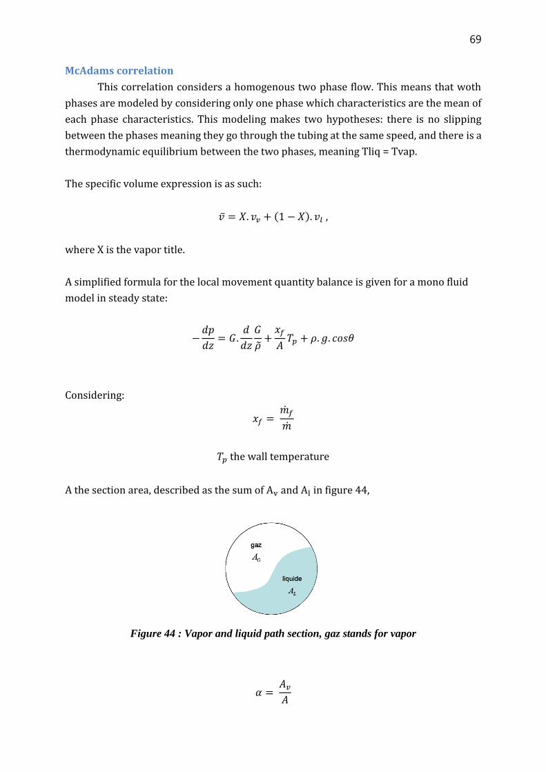
69
McAdams correlation
This correlation considers a homogenous two phase flow. This means that woth
phases are modeled by considering only one phase which characteristics are the mean of
each phase characteristics. This modeling makes two hypotheses: there is no slipping
between the phases meaning they go through the tubing at the same speed, and there is a
thermodynamic equilibrium between the two phases, meaning Tliq = Tvap.
The specific volume expression is as such:
�̅� = 𝑋. 𝑣𝑣 + (1 − 𝑋). 𝑣𝑙 ,
where X is the vapor title.
A simplified formula for the local movement quantity balance is given for a mono fluid
model in steady state:
−𝑑𝑝
𝑑𝑧= 𝐺.
𝑑
𝑑𝑧
𝐺
�̃�+
𝑥𝑓
𝐴𝑇𝑝 + 𝜌. 𝑔. 𝑐𝑜𝑠𝜃
Considering:
𝑥𝑓 = �̇�𝑓
�̇�
𝑇𝑝 the wall temperature
A the section area, described as the sum of Av and Al in figure 44,
Figure 44 : Vapor and liquid path section, gaz stands for vapor
𝛼 = 𝐴𝑣
𝐴

70
𝜌 = 𝛼. 𝜌𝑣 + (1 − 𝛼)𝜌𝑙
1
�̃�=
𝑥𝑣²
𝛼. 𝜌𝑣+
(1 − 𝑥𝑣)²
(1 − 𝛼)𝜌𝑙
𝐺 = 𝛼. 𝜌𝑣. 𝑢𝑣 + (1 − 𝛼). 𝜌𝑙 . 𝑢𝑙 ,
and θ is the angle between the flow axis and the vertical axis.
The pressure loss can be written as the sum of three terms:
𝑑𝑝
𝑑𝑧= (
𝑑𝑝
𝑑𝑧)
𝑎+ (
𝑑𝑝
𝑑𝑧)
𝑔+ (
𝑑𝑝
𝑑𝑧)
𝑓
One term is linked to the acceleration, one to the gravity, and the last one to frictions.
The two phase homogenous flow hypothesis lead to that formula for the friction term:
− (𝑑𝑝
𝑑𝑧)
𝑓=
𝑓𝑡𝑝. 𝐺². �̅�
2. 𝐷
Where D is the hydraulic diameter and 𝑓𝑡𝑝 the mean friction over the two phases.
The acceleration term is calculated in the same fashion as for a one phase flow:
− (𝑑𝑝
𝑑𝑧)
𝑎= 𝐺²
𝑑(�̅�)
𝑑𝑧
The gravity term may be written as such:
− (𝑑𝑝
𝑑𝑧)
𝑔=
𝑔. 𝑐𝑜𝑠𝜃
�̅�
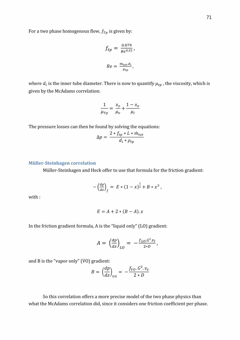
71
For a two phase homogenous flow, 𝑓𝑇𝑝 is given by:
𝑓𝑡𝑝 = 0.079
𝑅𝑒0.25 ,
𝑅𝑒 = �̇�𝑡𝑜𝑡.𝑑𝑖
𝜇𝑡𝑝 ,
where 𝑑𝑖 is the inner tube diameter. There is now to quantify 𝜇𝑡𝑝 , the viscosity, which is
given by the McAdams correlation:
1
𝜇𝑇𝑝=
𝑥𝑣
𝜇𝑣+
1 − 𝑥𝑣
𝜇𝑙
The pressure losses can then be found by solving the equations:
∆𝑝 = 2 ∗ 𝑓𝑡𝑝 ∗ 𝐿 ∗ �̇�𝑡𝑜𝑡
𝑑𝑖 ∗ 𝜌𝑡𝑝
Müller-Steinhagen correlation
Müller-Steinhagen and Heck offer to use that formula for the friction gradient:
− (𝑑𝑝
𝑑𝑧)
𝑓= 𝐸 ∗ (1 − 𝑥)
1
3 + 𝐵 ∗ 𝑥3 ,
with :
𝐸 = 𝐴 + 2 ∗ (𝐵 − 𝐴). 𝑥
In the friction gradient formula, A is the “liquid only” (LO) gradient:
𝐴 = (𝑑𝑝
𝑑𝑧)
𝐿𝑂= −
𝑓𝐿𝑂.𝐺².𝑣𝑙
2∗𝐷 ,
and B is the “vapor only” (VO) gradient:
𝐵 = (𝑑𝑝
𝑑𝑧)
𝑉𝑂= −
𝑓𝑉𝑂 . 𝐺². 𝑣𝑣
2 ∗ 𝐷
So this correlation offers a more precise model of the two phase physics than
what the McAdams correlation did, since it considers one friction coefficient per phase.
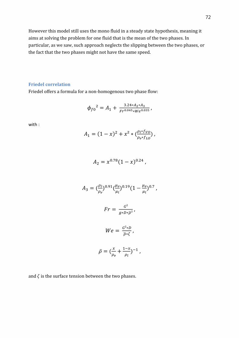
72
However this model still uses the mono fluid in a steady state hypothesis, meaning it
aims at solving the problem for one fluid that is the mean of the two phases. In
particular, as we saw, such approach neglects the slipping between the two phases, or
the fact that the two phases might not have the same speed.
Friedel correlation
Friedel offers a formula for a non-homogenous two phase flow:
𝜙𝑓0² = 𝐴1 + 3.24∗𝐴2∗𝐴3
𝐹𝑟0.045∗𝑊𝑒0.035 ,
with :
𝐴1 = (1 − 𝑥)2 + 𝑥² ∗ (𝜌𝑙∗𝑓𝑉𝑂
𝜌𝑣∗𝑓𝐿𝑂) ,
𝐴2 = 𝑥0.78(1 − 𝑥)0.24 ,
𝐴3 = (𝜌𝑙
𝜌𝑣)0.91(
𝜇𝑣
𝜇𝑙)0.19(1 −
𝜇𝑣
𝜇𝑙)0.7 ,
𝐹𝑟 = 𝐺²
𝑔∗𝐷∗�̅�² ,
𝑊𝑒 = 𝐺²∗𝐷
�̅�∗𝜁 ,
�̅� = (𝑥
𝜌𝑣+
1−𝑥
𝜌𝑙)−1 ,
and 𝜁 is the surface tension between the two phases.
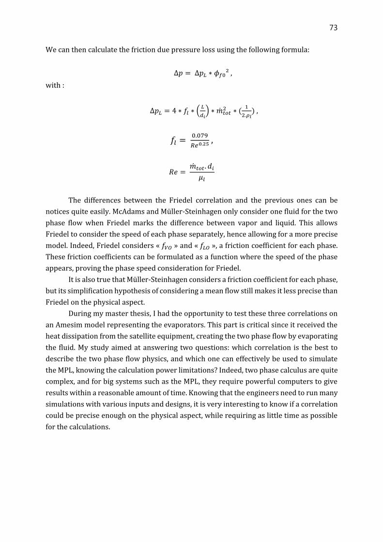
73
We can then calculate the friction due pressure loss using the following formula:
∆𝑝 = ∆𝑝𝐿 ∗ 𝜙𝑓0² ,
with :
∆𝑝𝐿 = 4 ∗ 𝑓𝑙 ∗ (𝐿
𝑑𝑖) ∗ �̇�𝑡𝑜𝑡
2 ∗ (1
2.𝜌𝑙) ,
𝑓𝑙 = 0.079
𝑅𝑒0.25 ,
𝑅𝑒 = �̇�𝑡𝑜𝑡. 𝑑𝑖
𝜇𝑙
The differences between the Friedel correlation and the previous ones can be
notices quite easily. McAdams and Müller-Steinhagen only consider one fluid for the two
phase flow when Friedel marks the difference between vapor and liquid. This allows
Friedel to consider the speed of each phase separately, hence allowing for a more precise
model. Indeed, Friedel considers « 𝑓𝑉𝑂 » and « 𝑓𝐿𝑂 », a friction coefficient for each phase.
These friction coefficients can be formulated as a function where the speed of the phase
appears, proving the phase speed consideration for Friedel.
It is also true that Müller-Steinhagen considers a friction coefficient for each phase,
but its simplification hypothesis of considering a mean flow still makes it less precise than
Friedel on the physical aspect.
During my master thesis, I had the opportunity to test these three correlations on
an Amesim model representing the evaporators. This part is critical since it received the
heat dissipation from the satellite equipment, creating the two phase flow by evaporating
the fluid. My study aimed at answering two questions: which correlation is the best to
describe the two phase flow physics, and which one can effectively be used to simulate
the MPL, knowing the calculation power limitations? Indeed, two phase calculus are quite
complex, and for big systems such as the MPL, they require powerful computers to give
results within a reasonable amount of time. Knowing that the engineers need to run many
simulations with various inputs and designs, it is very interesting to know if a correlation
could be precise enough on the physical aspect, while requiring as little time as possible
for the calculations.
74
On the physical aspect, Friedel is the best correlation as explained above. Then
Müller-Steinhagen is the second correlation, since its hypotheses make less
simplifications than McAdams. On the numerical calculations point of view, the results are
quite different: Friedel is no longer the most interesting correlation to model the MPL.
Indeed, calculations using Friedel as a correlation would need at least twice as much time
as the ones using Müller-Steinhagen for the same evaporators design. Even worse, the use
of the Friedel correlation would even create numerical divergences, which is
unacceptable. These divergences were caused by a software bug affecting the Friedel
correlation, and would later be patched, but at the time of my study this fact only would
prevent the thermal engineers from using the Friedel correlation. The time needed by the
calculations using Müller-Steinhagen would be quite similar to the time needed by those
using McAdams as they would only need 8% more time in the most complex simulation I
ran. With all these results, my conclusion at the time of my study was that the Müller-
Steinhagen correlation was the most suitable correlation for the MPL modeling on
Amesim.
The cosimulation
As we could see in the fourth chapter, e-Therm lacks an important part to simulate
completely a SpaceBus Neo satellite that embarks a MPL: that program do not have any
module enabling it to simulate a two phase flow. Amesim can do that, but it does not have
the ability to simulate the radiative heat exchanges inside and outside of the satellite,
which is just one of the things e-Therm can do.
In the scope of putting together all the SpaceBus Neo platform aspects within one
thermal simulation so as to be more precise, the Thales Alenia Space and Dorea engineers
work on the development of a cosimulation module. The idea is to create an e-Therm
model and an Amesim model for the same satellite, and to run simulations on the two
software simultaneously. The e-Therm model will take care of the radiative and
conductive heat exchanges within the satellite structure and equipment while the Amesin
model will take care of simulating the MPL flow physics. After each calculation time step,
the two softwares exchanges their results that are used as inputs for the next calculation
cycle. Once both software converged, the simulation stops and gives its final results.
This idea is extremely interesting but also very ambitious since its needs two
software developed independently to talk together. The cosimulation needs a module that
will be able to do that while making sure each information that has to be transmitted will
be sent to the right place at the right time, for both sides of the simulation.

75
Conclusion
The two phase fluid loop, one of the SpaceBus Neo key elements, shows impressive
performances that will definitely help Thales Alenia Space to deal with the satellite
thermal control and its challenges for the coming years. Despite harsh functioning
conditions, we know today that the MPL will be able to satisfy the customers’ needs.
Through my master thesis I had the opportunity to understand the functioning of
the two phase fluid loop designed by TAS. I realized how complicated it is to create a
numerical model that describes physical phenomenon, at various scales of a satellite
architecture: from a heat pipe profile, a detail within the whole satellite structure, up to
almost the whole satellite. The knowledge I was given about Amesin, e-Therm and the
MPL allowed me to design a solution answering the problem of modeling the MPL within
e-Therm while waiting for the cosimulation to work.
This experience was very fulfilling. It first allowed me to discover the space
industry, and more precisely the telecommunication satellite industry. I discovered its
challenges and took part in the design process of a new product for this market. It also
offered me a unique situation where I was asked to solve a problem dealing with many
scientific disciplines by using what was at my disposal, in this case Amesim and e-Therm,
in order to propose solutions.
My integration within the Thales Alenia Space engineer team allowed me to
continue my discovery of the company world. I was given the possibility of watching and
taking part in the dynamics of a team within a department, and I could also see the
difficulties that a big company suffer from when for example several departments have to
work together. However I could also witness the many advantages that such entity can
profit from.
Lastly, I am convinced that the work I led during my master thesis had some utility
for society. It was not a scientific breakthrough that will help humanity for the centuries
to come, but I would describe it as one little brick, one of the many that are being made
right now and put together to pave the way to more efficient satellites that are definitely
needed to address the world’s ever growing demand for faster and better means of
communication.