thermal inactivation kinetics of escherichia...
TRANSCRIPT

THERMAL INACTIVATION KINETICS OF Escherichia coli AND Alicyclobacillus
acidoterrestris IN ORANGE JUICE
By
VERTIGO MOODY
A DISSERTATION PRESENTED TO THE GRADUATE SCHOOL OF THE UNIVERSITY OF FLORIDA IN PARTIAL FULFILLMENT
OF THE REQUIREMENTS FOR THE DEGREE OF DOCTOR OF PHILOSOPHY
UNIVERSITY OF FLORIDA
2003

ACKNOWLEDGMENTS
The author would like to express sincere gratitude to his major advisor, Dr. Arthur
A. Teixeira for his confidence and enthusiasm throughout this research project. His
guidance and support were essential for successful completion of this body of work. The
author would also like to express gratitude and appreciation to his supervisory committee
(Dr. Glen H. Smerage, Dr. Mickey Parish, Dr. Robert Braddock, and Dr. Spiros
Svorounous) for their guidance and suggestions related to the research and the
completion of this publication.
Special thanks go to the faculty and staff of the Agricultural and Biological
Engineering Department, especially Dr. David Chynoweth and Dr. Roger Nordstedt for
the use of their lab space and equipment as well as Ms. Veronica Campbell for her
guidance and technical skills in assisting with the laboratory aspect of this research
project. Special thanks go to Dr. Braddock, Rockey Bryan and the staff at the Citrus
Research and Education Center for assisting the author in coordinating visits to the center
to conduct research and for troubleshooting problems with equipment. The author wishes
to thank Dr. Parish and Lorrie Friedrich for their assistance with the microbiological
aspect of this research project. Their help facilitated the completion of this project and
enhanced the skills of the author for handling microorganisms in a laboratory setting.
Finally, the author would like to thank his family and friends for their continued support
and patience throughout this milestone in life.
ii

TABLE OF CONTENTS
Page
ACKNOWLEDGMENTS .................................................................................................. ii
TABLE OF CONTENTS................................................................................................... iii
LIST OF TABLES............................................................................................................. vi
LIST OF FIGURES ......................................................................................................... viii
ABSTRACT....................................................................................................................... xi
CHAPTER
1 ESTIMATING THERMAL KINETIC PARAMETERS FOR Escherichia coli IN SINGLE-STRENGTH ORANGE JUICE USING TRADITIONAL ANALYSIS OF ISOTHERMAL BATH EXPERIMENTAL DATA.....................................................1
Introduction...................................................................................................................1 Literature Review .........................................................................................................2
Microbiology of Fruit Juices .................................................................................2 Mechanism of Acid Tolerance ..............................................................................5 Spoilage .................................................................................................................6
Objectives .....................................................................................................................7 Methods and Materials .................................................................................................8
Scope of Work.......................................................................................................8 Preliminary Experiments .......................................................................................9 Preparation of Cultures..........................................................................................9
Source of strains .............................................................................................9 Acid adaptation preparation .........................................................................11
Experimental Apparatus ......................................................................................12 Isothermal Inactivation Experiments...................................................................12 Estimating D- and z-values .................................................................................13
Results and Discussion ...............................................................................................14 Preliminary Experiments .....................................................................................14
Saccharomyces cerevisiae ............................................................................14 Escherichia coli cultured at neutral pH........................................................14 Acid-tolerant Escherichia coli cultures........................................................16
Thermal Inactivation of Escherichia coli ............................................................17
iii

2 ESTIMATING KINETIC PARAMETERS FOR THERMAL INACTIVATION OF Escherichia coli IN ORANGE JUICE USING THE PAIRED EQUIVALENT ISOTHERMAL EXPOSURES (PEIE) METHOD WITH A CONTINUOUS HIGH TEMPERATURE SHORT TIME (HTST) PROCESS TREATMENT .....................47
Introduction.................................................................................................................47 Literature Review .......................................................................................................48
First-order kinetics...............................................................................................49 The PEIE Method ................................................................................................51
Objectives ...................................................................................................................52 Methods and Materials ...............................................................................................53
Preparation of Cultures........................................................................................53 Experimental Apparatus ......................................................................................53 Calibration of Thermocouples.............................................................................54 Continuous Dynamic Thermal Treatments .........................................................55 Temperature Profiles ...........................................................................................56 Estimating D- and z-Values with the PEIE Method............................................57 Validation Experiments .......................................................................................59
Results and Discussion ...............................................................................................61 Continuous Dynamic Thermal Experiments – Parameter Estimation.................61 Comparing PEIE and 3-Neck Flask Isothermal Methods ...................................62 Validation Experiments .......................................................................................64
3 ESTIMATION OF KINETIC PARAMETERS FOR THERMAL INACTIVATION OF Alicyclobacillus acidoterrestris IN ORANGE JUICE .........................................85
Introduction.................................................................................................................85 Literature Review .......................................................................................................86
Occurrences of Alicyclobacillus acidoterrestris in Juice Products .....................86 The PEIE Method in Arrhenius Kinetics.............................................................87 The PEIE Method and TDT Kinetics ..................................................................90
Objectives ...................................................................................................................92 Methods and Materials ...............................................................................................92
Preparation of Cultures........................................................................................92 Experimental Apparatus ......................................................................................93 Continuous Dynamic Thermal Treatments .........................................................93 Temperature Profiles ...........................................................................................94
Results and Discussion ...............................................................................................96 Parameter Estimation by PEIE ............................................................................96 Parameter Estimation using F value and TDT kinetics .......................................96
iv

APPENDIX
A MATHCAD PROGRAM FOR THE PEIE METHOD WITH Escherichia coli USING ARRHENIUS KINETICS...........................................................................109
B MATHCAD PROGRAM FOR THE PEIE METHOD WITH Escherichia coli USING THERMAL DEATH TIME (TDT) KINETICS..........................................118
C MATHCAD PROGRAM FOR THE PEIE METHOD WITH Alicyclobacillus acidoterrestris USING ARRHENIUS KINETICS ..................................................126
D MATHCAD PROGRAM FOR THE PEIE METHOD WITH Alicyclobacillus acidoterrestris USING THERMAL DEATH TIME (TDT) KINETICS .................134
LIST OF REFERENCES.................................................................................................141
BIOGRAPHICAL SKETCH ...........................................................................................144
v

LIST OF TABLES
Table page 1-1. Plate counts of survivors grown in standard nutrient broth and pH-modified nutrient
broth for inducing acid tolerance .............................................................................23
1-2. D-values (seconds) for Escherichia coli in orange juice cultured at neutral pH (standard culture) in preliminary experiments .........................................................31
1-3. D-values (seconds) for Escherichia coli in orange juice cultured at low pH (acid adapted culture) in preliminary experiments............................................................37
1-4. D-values (seconds) from thermal inactivation experiments for Escherichia coli cultured at low pH ....................................................................................................44
1-5. Comparison of TDT kinetic parameters with published data from Mazzotta (2001) and Splittstoesser et. al. (1996) using acid adapted and non-acid adapted Escherichia coli in orange juice ...............................................................................46
2-1. Calibration of thermocouples ....................................................................................69
2-2. Reynolds numbers for each flow rate for the continuous system..............................70
2-3 - Rate constants used in Equation 2-1 for the heater section temperature profile. ......74
2-4. Rate constants used in Equation 2-2 for the chiller section temperature profile. ......74
2-5. Population survivor data for continuous experiments ...............................................75
2-6. Estimation of D- and z-values from each iteration of the PEIE method ...................76
2-7. Comparison of D- and z-values estimated by traditional method using isothermal treatments and PEIE method using continuous dynamic treatments .......................78
2-8. Kinetic parameters of thermal inactivation of Alicyclobacillus acidoterrestris spores in Cupuacu nector using the PEIE method and Isothermal method *......................78
2-9. Results of validation experiments, comparison of predicted number of survivors for PEIE analysis and Traditional isothermal batch analysis with experimental number of survivors...............................................................................................................84
vi

3-1. Rate constants used in Equation 2-1 and 2-2 for the heater and chiller sections temperature profile for experimental set 1 .............................................................101
3-2. Rate constants used in Equation 2-1 and 2-2 for the heater chiller sections temperature profile for experimental set 2 .............................................................101
3-3. Population survivor data from Ultra High Temperature (UHT) heat treatments with Alicyclobacillus acidoterrestris in orange juice.....................................................102
3-4. Estimation of k and Ea values from each iteration of the PEIE method using Arrhenius kinetics ..................................................................................................103
3-5. Estimation of D- and z-values from each iteration of the PEIE method using TDT kinetics ...................................................................................................................105
3-6. Comparison of TDT kinetic parameters with published data from various sources using Alicyclobacillus acidoterrestris ....................................................................107
vii

LIST OF FIGURES
Figure Page 1-1. Growth curve showing light absorbance at a wavelength of 600 nanometer vs time
for Saccharomyces cerevisiae in yeast extract peptone dextrose (YEPD) broth. Sets are runs conducted on separate days.................................................................21
1-2. Growth curve showing absorbance of light at wavelength of 600 nanometer vs time for Escherichia coli ATCC #9637 in nutrient broth. Sets are experiments conducted on separate days ......................................................................................22
1-3. Experimental apparatus (photograph) ......................................................................24
1-4. Experimental apparatus (diagram)............................................................................25
1-5. Survivor curves from preliminary experiments at 50oC, 54oC and 56oC for Saccharomyces cerevisiae in orange juice cultured at neutral Ph (standard culture)26
1-6. Preliminary experiments survivor curve at 59oC for Escherichia coli in orange juice cultured at neutral pH (standard culture)..................................................................27
1-7. Preliminary experiments survivor curves at 62oC for Escherichia coli in orange juice cultured at neutral pH (standard culture).........................................................28
1-8. Preliminary experiments survivor curves at 64oC for Escherichia coli in orange juice cultured at neutral pH (standard culture).........................................................29
1-9. TDT curve from preliminary experiments with Escherichia coli in orange juice cultured at neutral pH (standard culture). R2 value of 0.90......................................30
1-10. Survivor curves from preliminary experiments at 52oC with Escherichia coli in orange juice cultured at low pH (acid adapted culture). ..........................................32
1-11. Survivor curves from preliminary experiments at 55oC with Escherichia coli in orange juice cultured at low pH (acid adapted culture) ...........................................33
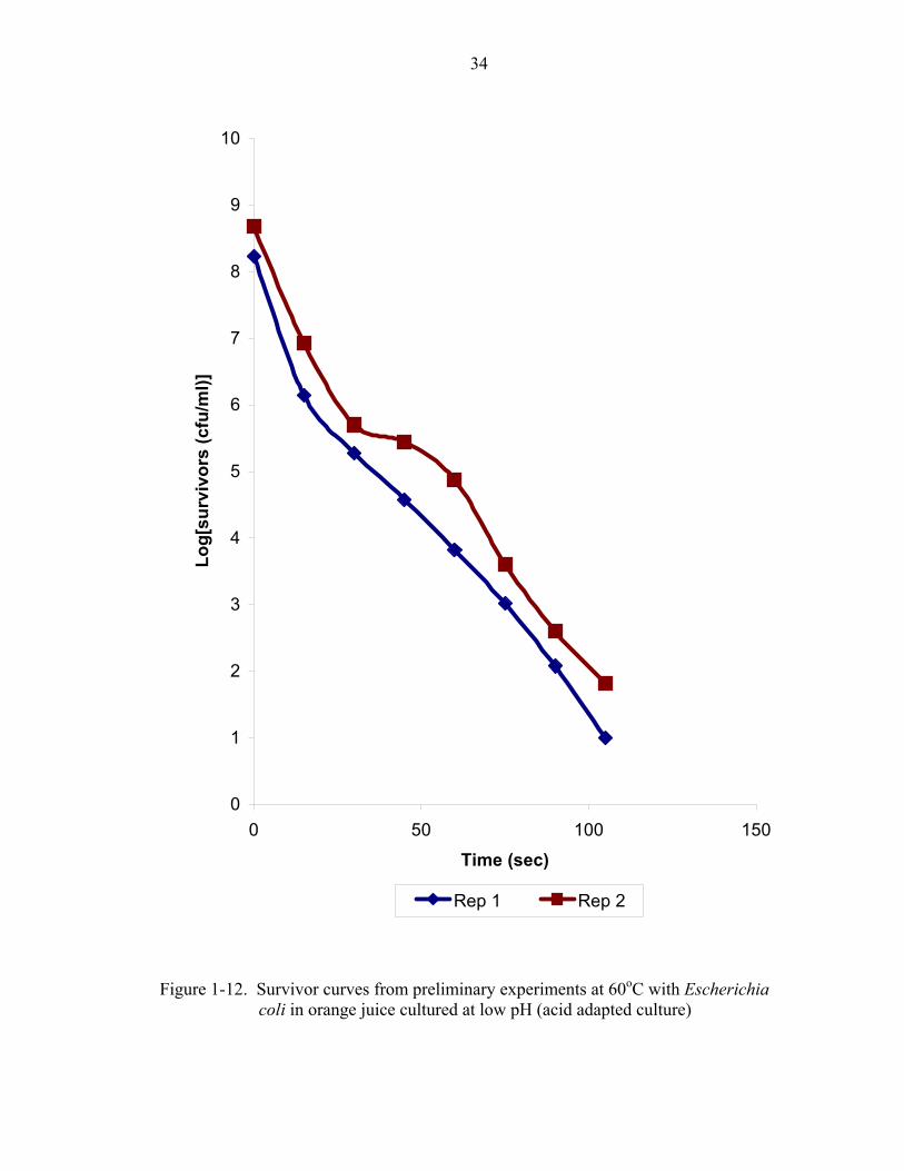
1-12. Survivor curves from preliminary experiments at 60oC with Escherichia coli in orange juice cultured at low pH (acid adapted culture) ...........................................34
1-13. Family of survivor curves from preliminary experiments at 52oC, 55oC, and 60oC with Escherichia coli in orange juice cultured at low pH (acid adapted culture).....35
viii

1-14. TDT curve from preliminary experiments with Escherichia coli in orange juice cultured at low pH (acid adapted culture). R2 value of 0.99 ...................................36
1-15. pH of broth vs. pH of orange juice product for Saccharomyces cerevisiae preliminary experiments...........................................................................................38
1-16. Survivor curve from thermal inactivation experiments at 52oC with Escherichia coli in orange juice cultured at low pH (acid adapted culture) .......................................39
1-17. Survivor curve from thermal inactivation experiments at 55oC with Escherichia coli in orange juice cultured at low pH (acid adapted culture) .......................................40
1-18. Survivor curve from thermal experiments at 58oC with Escherichia coli in orange juice cultured at low pH (acid adapted culture) .......................................................41
1-19. Survivor curve from thermal inactivation experiments at 60oC with Escherichia coli in orange juice cultured at low pH (acid adapted culture) .......................................42
1-20. Family of survivor curves at 52oC, 55oC, 58oC and 60oC with Escherichia coli in orange juice cultured at low pH (acid adapted culture) ...........................................43
1-21. TDT curve from the thermal inactivation experiment with Escherichia coli in orange juice cultured at low ph (acid adapted culture). R2 value of 0.98 ...............45
2-1. Photo of the Microthermics HTST Lab 25 Labscale Pasteurizer.............................67
2-2. Schematic Diagram of the flow of the Microthermics pasteurizer...........................68
2-3. Thermal profile of product at a hold tube nominal temperature of 58oC and residence times of 60 and 90 seconds ......................................................................71
2-4. Thermal profile of product at a hold tube nominal temperature of 60oC and residence times of 30 and 60 seconds ......................................................................72
2-5. Thermal profile of product at a hold tube nominal temperature of 62oC and residence times of 15 and 30 seconds ......................................................................73
2-6. TDT curve for acid tolerant Escherichia coli in orange juice using kinetic parameters from the PEIE method ...........................................................................77
2-7. TDT curve for acid tolerant Escherichia coli in orange juice using kinetic parameters from the PEIE method ...........................................................................79
2-8. Comparison of TDT curves based upon data from the traditional and PEIE methods80
2-9. Comparison of TDT curves based upon data from the traditional and PEIE methods for Alicyclobacillus acidoterrestris spores in Cupuacu nectar (Vieira et. al. 2002) (Estimated curve based upon reference D-value and z-value) .................................81
ix

2-10. Temperature history and measured and predicted survivor responses for validation experiment I (10 second hold tube)..........................................................................82
2-11. Temperature history and measured and predicted survivor responses for validation experiment II (15 second hold tube) ........................................................................83
3-1. Thermal profile of product at a hold tube nominal temperature of 95oC, 100oC, and 104oC for experimental set one ................................................................................99
3-2. Thermal profile of product at a hold tube nominal temperature of 95oC, 100oC, and 104oC for experimental set two. .............................................................................100
3-3. Arrhenius curve for Alicyclobacillus acidoterrestris in orange juice using kinetic parameters from the PEIE method .........................................................................104
3-4. TDT curve for Alicyclobacillus acidoterrestris in orange juice using kinetic parameters from the PEIE method .........................................................................106
3-5. Comparison of TDT curves based upon data from the PEIE method using TDT kinetics and Arrhenius kinetics ..............................................................................108
x

Abstract of Dissertation Presented to the Graduate School of the University of Florida in Partial Fulfillment of the Requirements for the Degree of Doctor of Philosophy
THERMAL INACTIVATION KINETICS OF Escherichia coli AND Alicyclobacillus acidoterrestris IN ORANGE JUICE
By
Vertigo Moody
December 2003
Chair: Arthur A. Teixeira Co-chair: Glen H. Smerage Major Department: Agricultural and Biological Engineering
Growing concern about the safety of unpasteurized low-pH foods has changed the
view of the microbial loads supported by these products. Recent outbreaks of Salmonella
in single-strength unpasteurized orange juice and Escherichia coli O157:H7in apple juice
have prompted food processors to seek ways of ensuring the safety of their products
without compromising consumer acceptance. Spoilage is also a concern as it relates to
the shelf life of fruit juice products. In order to achieve an optimum balance between
safety, shelf life, and quality, good estimation of thermal inactivation parameters is
essential for designing pasteurization processes that achieve all three goals.
The purpose of this study was to validate a method for estimating thermal
inactivation kinetic parameters of specific microorganisms. The method, called the
Paired Equivalent Isothermal Exposures (PEIE) method, may be applied to products that
are heated under non-isothermal conditions. This method simplifies the estimation of
xi

parameters by eliminating the need to perform tedious isothermal bath experiments, while
still obtaining accurate estimations. The study was performed in three phases:
1) Estimating thermal kinetic parameters for Escherichia coli in single strength orange
juice using traditional analysis of isothermal bath experimental data; 2) Estimating
kinetic parameters for thermal inactivation of Escherichia coli in orange juice using the
PEIE method with end-point data from continuous high-temperature short-time (HTST)
process treatments and validation for each set of kinetic parameters, and 3) Estimating
kinetic parameters for thermal inactivation of Alicyclobacillus acidoterrestris using the
PEIE method.
Estimating kinetic parameters from isothermal bath and continuous dynamic
thermal treatment data gave parameters that were different. To confirm which
parameters were more accurate, validation experiments were conducted at higher
temperatures. Using the parameters from both methods the number of survivors from
each experiment were compared with those predicted by each set of kinetics parameters.
Results from validation experiments with Escherichia coli showed that model predictions
agreed more closely with experimental data when kinetic parameters used were estimated
by the PEIE method rather than the traditional isothermal bath method. The process
conditions determined from the kinetic parameters estimated by the PEIE method yielded
a 39.7% shorter time than that determined by the isothermal bath method. The PEIE
method was used as the preferred method for estimating the kinetic parameters for
Alicyclobacillus acidoterrestris in single-strength orange juice.
xii

CHAPTER 1 ESTIMATING THERMAL KINETIC PARAMETERS FOR Escherichia coli IN
SINGLE-STRENGTH ORANGE JUICE USING TRADITIONAL ANALYSIS OF ISOTHERMAL BATH EXPERIMENTAL DATA
Introduction
Recent outbreaks of Escherichia coli and Samonella in low-pH fruit juices
(including apple and orange) have prompted reevaluation of the ability of pathogenic
microorganisms to survive in these high-acid food products. Unpasteurized fruit juices
have become popular consumer products because flavor and texture quality are better
than in pasteurized juices. Escherichia coli O157:H7 and Salmonella contaminated
orange and apple juice and apple cider have raised the attention of the Food and Drug
Administration, which previously considered high-acid foods with pH below 4.6 not to be
potentially hazardous to consumers. These outbreaks provide a compelling reason to
study these organisms’ tolerance to low pH and to study their effect on the safety and
shelf life of these products. The design of pasteurization processes depends on estimating
the thermal inactivation kinetic parameters. Performing thermal inactivation experiments
on the acid-tolerant bacteria allows engineers to design thermal processes that more
completely reduce the number of pathogenic microorganisms in the product to more safe
levels. Accurate estimation of kinetic parameters is essential to food engineers. The
purpose of this study is to characterize the thermal inactivation behavior of potentially
pathogenic bacteria in orange juice.
1

2
Literature Review
Microbiology of Fruit Juices
Up to the latter part of the 20th century it was widely assumed that pathogenic
microorganisms could not survive in low-pH, high-acid foods because of the belief that
organic acids had an inhibitory and sometimes microbicidal effect (Parish 1997). The
Food and Drug Administration generally considers foods with a pH greater than 4.6 to be
potentially hazardous to consumers. Unpasteurized fruit juices have become a popular
consumer food product because their flavor retention is better than that of pasteurized
fruit juices. However, recent outbreaks of foodborne illness stemming from
unpasteurized fruit juices have brought to the forefront the need for pasteurization of all
processed fruit juices. Outbreaks involving Escherichia coli O157:H7 and Salmonella
enterica in orange and in apple juices and apple cider have changed long held views on
the safety of fruit juices and other low-pH products.
Escherichia coli O157:H7 was first confirmed as a health concern in juices after an
apple cider related outbreak in 1991 (Besser et. al. 1993). An outbreak of diarrhea and
Hemolytic Uremic Syndrome (HUS) in southern Massachusetts was traced back to
contamination of fresh-pressed apple cider (Besser et. al. 1993). Twenty-three persons
were identified with Escherichia coli O157:H7 infections between October 23 and
November 24 of 1991. An epidemiological study based on this case showed that when
apple cider, with a pH ranging between 3.7 and 3.9, was inoculated with Escherichia coli
O157:H7, bacteria survived for 20 days at refrigerated conditions (8oC) (Besser et. al.
1993). Another outbreak of Hemolytic Uremic Syndrome (HUS) caused by the
consumption of unpasteurized apple juice that was contaminated with Escherichia coli
O157:H7 was documented in 1996 (Parish 1997). In this outbreak a large producer of

3
fresh unpasteurized fruit products was implicated in the distribution of contaminated
product.
Salmonella has been isolated from apple cider samples (pH from 3.7 to 4.0)
associated with an outbreak of gastroenteritis (Besser et. al. 1993). In 1989 an incident of
typhoid fever caused by consuming orange juice contaminated with Salmonella typhi was
documented in a New York hotel restaurant in which there were 45 confirmed and 24
probable cases of typhoid fever with 21 hospitalizations (Parish 1997). In 1996 (on June
19, in the state of Washington and on June 23, in the state of Oregon) health officials
investigated clusters of outbreaks of diarrhea attributed to Salmonella and associated with
a commercially distributed unpasteurized orange juice (CDC 1999). Samples of the
unpasteurized orange juice yielded cultures of Salmonella when analyzed by the Food
and Drug Administration (FDA). There were approximately 300 confirmed cases
associated with this outbreak (CDC 1999).
These recent outbreaks of food poisoning from Salmonella and Escherichia coli
O157:H7 have called into question the safety of unpasteurized fruit juices and other low-
pH, high-acid food products. Pasteurization is the traditional method of inactivating
pathogenic and some spoilage-causing microorganisms in citrus products. The
inhibitory effect of acid concentration and low pH toward the growth of most pathogenic
bacteria alone does not ensure product safety (Parish 1997). Pathogens such as
Salmonella, Escherichia coli O157:H7, Shigella, Vibrio, and Staphyloccocus have been
shown to survive from hours to days and even weeks in various fruit juice products
(Parish 1997).

4
Miller and Kaspar (1994) showed the acid tolerance and survival of Escherichia
coli O157:H7 in apple cider by testing two different strains. In their study they
inoculated Trypticase soy broth (TSB) adjusted to various pHs, and commercial apple
cider with those strains and observed the survival at each pH. Viable cells of Escherichia
coli O157:H7 were still detectable in TSB at pH 2 after 24 hours of storage at refrigerated
conditions. In apple cider cells were still detectable after 14 days of storage at 4oC.
Leyer et al. (1995) showed that acid-adapted Escherichia coli O157:H7 survived for 81
hours in apple cider with a pH of 3.42 stored at 6oC, whereas the non adapted cells
survived for only 28 hours.
Semanchek and Golden (1996) showed that pathogenic Escherichia coli O157:H7
is capable of survival in apple cider for at least 10 days at a storage temperature of 20oC
with a minimal decrease in population of viable cells. In a study by Zhao et al. (1993)
Salmonella survived in apple juice stored at 4oC for more than 30 days at pH 3.6. These
studies revealed that storage conditions affect the resistance to acid of these pathogens.
Storage at refrigerated temperatures increases the time at which cells remain viable in the
product. Zhao et al. (1993) showed that Escherichia coli O157:H7 was more rapidly
inactivated in apple cider stored at 25oC than at 4oC. Ingham and Uljas (1998) reported
that 84% to 91% of their inoculum of Escherichia coli cells was still viable in apple
cider, without preservatives, after 21 days when stored at 4oC. Similar studies conducted
in different low-pH products showed an increase in the thermotolerance of Escherichia
coli O157:H7. Leyer et al. (1995) reported that acid-adapted Escherichia coli O157:H7
in fermented meats showed a higher thermotolerance.

5
Mechanism of Acid Tolerance
The mechanism of acid tolerance of bacteria is not completely understood. Several
theories have been proposed in an attempt to explain how bacteria are able to adjust and
maintain their internal pH within homeostatic limits. These theories include the buffering
capacity of cytoplasm, the low proton permeability of cells, and the extrusion of protons
from the cytoplasm by a membrane-bound proton pump (Benjamin and Datta 1995).
The antimicrobial effect of acids has been explained by the ability of
undisassociated molecules to enter the cell membrane and release protons. This release
of protons disrupts the electron transport system of the bacterial cell draining cellular
energy resources (Diez-Gonzalex and Russell 1997). The electron transport system is
highly dependent on the maintenance of a constant chemiosmotic potential across the
inner mitochondrial membrane to ensure steady production of adenosine triphosphate
(ATP) in the cellular environment. Bacteria capable of surviving in low pH (such as
lactic acid bacteria) are able to decrease intracellular pH when extracellular pH decreases
to maintain a low transmembrane pH gradient (Diez-Gonzalez and Russell 1997), thus
decreasing the dissipation of the proton-motive force.
Diez-Gonzalez and Russell (1997) studied the ability of Escherichia coli O157:H7
to change its intracellular pH in response to a change in the extracellular pH as a
mechanism of acid tolerance and the ability to survive in low-pH products. They showed
that Escherichia coli O157:H7 had a greater ability to control the level of acetate
concentration within its internal environment than a non-pathogenic Escherichia coli
strain. The O157:H7 strain maintained a maximum internal concentration of acetate less
than 300 mM while the non-pathogenic strain accumulated as much as 500 mM of acetate
internally when the external pH dropped to 5.9. The significance of the concentration of

6
acetate in the cytoplasm gives insight into the ability of the bacteria to regulate the ions
and thus reduce the impact of dramatic changes in external pH. Protein synthesis appears
to be an essential aspect of the acid tolerance response of cells. O’Hara and Glenn (1994)
showed inhibiting protein synthesis with compounds such as chloramphenicol prevented
the development of acid tolerance in the cells. The nature of these proteins and their role
in the acid tolerance response are not known. They also reported that the capacity to
maintain alkaline intracellular pH is essential for the survival of root nodule bacteria in
acidic environments.
Spoilage
In addition to product safety, the population size of viable microorganisms that
remain in the product also affects the shelf life of the product with significant economic
implications. Pasteurized single-strength juices and frozen juice concentrates are the
predominant types of processed fruit juices commercially available. Yeasts, molds, and
lactic acid bacteria have been implicated in the spoilage of fruit juices (Deak et al. 1993).
Yeasts are the most problematic because of their ability to tolerate low-pH environment.
In particular, Saccharomyces cerevisiae is the most commonly isolated species of yeasts
from fruit juices that is responsible for spoilage. Twenty-five percent of yeast isolates
from frozen concentrate were identified as Saccharomyces cerevisiae in a survey
conducted in 1993 (Deak and Beuchat 1993). Yeasts lead to formation of films,
alteration of color, and change in viscosity. The fermentation caused by yeasts produce
products such as ethanol, carbon dioxide, and ethyl acetate, which alter the flavor of the
products. The production of gases may also compromise the integrity of product
packaging. The aim of pasteurization has been to eliminate the pathogenic

7
microorganisms, reduce the population of spoilage-causing microorganisms and to
inactivate enzymes for product safety and extended shelf life.
Recent outbreaks of Salmonella and Escherichia coli O157:H7 in orange and apple
juice and in apple cider provide a compelling reason to understand these microorganisms’
tolerance to low pH in relation to their ability to cause disease and how that tolerance
affects thermal inactivation characteristics in those products for the purpose of food
safety. Estimating the thermal inactivation characteristics of these pathogenic organisms
in low-pH environments has both a food safety and economic impact on the design and
processing of fruit juice products. Because the assumption (that inactivation caused by
acid is sufficient) may no longer be valid, performing isothermal inactivation experiments
on the acid tolerant strains of pathogenic microorganisms such as Escherichia coli allows
engineers to design thermal processes that more completely reduce the number of viable
microorganisms to levels that ensure the safety of the product. Economic impacts of
microorganisms are also important in the food industry from a safety viewpoint and also
from a shelf-life viewpoint. Yeasts such as Saccharomyces cerevisiae are implicated as
the primary microorganisms responsible for spoilage of fruit juices and their limited shelf
life at refrigerated conditions.
Objectives
Because of these impacts on the fruit juice processing industry, the objectives of
this study were the following:
• To characterize the thermal inactivation kinetics of Saccharomyces cerevisiae and Escherichia coli in orange juice
• To estimate thermal-death-time parameters (D- and z-value) for Escherichia coli subjected to an acid adaptation procedure vs. standard cultures in orange juice

8
• To compare the estimated parameters for Escherichia coli and Saccharomyces cerevisiae with published data.
Methods and Materials
Scope of Work
The scope of work undertaken in this study has been divided into two parts to
determine the thermal inactivation kinetics of Escherichia coli and Saccharomyces
cerevisiae in single-strength orange juice. The Saccharomyces cerevisiae strain was a
wild type isolated from orange juice, and the Escherichia coli strain was obtained from
the American Type Culture Collection. Growth curves were created for each
microorganism to determine logarithmic and stationary phases of growth. Preliminary
experiments were used to help determine the temperature range in which thermal
inactivation of both microorganisms would yield measurable numbers of survivors in
order to plot survivor curves.
After the appropriate temperatures were selected, microorganisms were subjected
to different time-temperature combinations in order to estimate the thermal-death-time
(TDT) kinetic parameters. These kinetic parameters were estimated by traditional
methods of analyzing the survivor curves at each constant temperature. This method
entailed estimating the decimal reduction times (D-values) using linear regression to
construct the straight line of best fit on a semilog plot of survivors vs time (survivor
curve). The D-value is the reciprocal slope of this curve expressed as time required for
the curve to cross one log cycle, or time for one log cycle reduction of the population.
A semilog plot of D-values vs. temperatures allows estimation of the z-value, by taking
the reciprocal of the slope of the curve. The z-value is expressed as the number of
degrees of temperature change required for one log cycle change in D-value.

9
Preliminary Experiments
Analysis of the survivor curves generated from the preliminary experiments helped
determine at which temperatures to conduct the thermal inactivation experiments. For
the Escherichia coli, a procedure was developed and implemented to adapt the cells to
survival in a low-pH medium similar to the pH of single-strength orange juice. This
procedure more closely modeled the conditions experienced by Escherichia coli that
survive in contaminated orange juice.
Two sets of preliminary experiments were conducted. The first set involved the
thermal inactivation of both microorganisms grown in neutral-pH broth. The second set
involved acid-adapted Escherichia coli grown in low-pH broth.
Preparation of Cultures
Source of strains
The strain of Saccharomyces cerevisiae chosen for this study was obtained from
the yeast culture collection maintained in the microbiology laboratory at the University of
Florida’s Citrus Research and Education Center, Lake Alfred, FL (Zook 1997). Stock
cultures were streaked onto potato dextrose agar (PDA) and incubated at 30oC for 72
hours. A loop full of cells was aseptically transfered to 200 mL screw-cap flasks of yeast
extract peptone dextrose (YEPD) broth and incubated for 48 hours at 30oC while
continuously shaken at 120 rpm on a junior orbit table shaker. Small aliquots of this
broth were then put into 1 mL vials placed into a –4oC freezer and maintained as a stock
culture. A small loop full of broth was streaked onto slants of PDA refrigerated at 10oC
and used as a working culture for a period of 3 weeks. After 3 weeks a new working
culture was created from the stock culture using the above procedure.

10
Growth curves for this particular strain of Saccharomyces cerevisiae were
documented by Zook (1997). A new set of growth curves was created to verify those
results. A small aliquot of working culture was inoculated into a flask of 200 mL of
YEPD broth and incubated at 30oC. One-millimeter samples were withdrawn at
predetermined timed intervals for 30 hours. Turbidity of the samples was measured
optically using a Spectronic 40 spectrophotometer (Figure 1-1). As documented by Zook
(1997), the yeast completed their logarithmic phase after approximately 17 hours of
incubation.
The strain of Escherichia coli (preceptol culture ATCC #9637) used in this study
was obtained from the American Type Culture Collection (ATCC). Working and stock
cultures of this strain were made from the original freeze-dried culture obtained from
ATCC. The reconstituted cultures were inoculated into 200 mL of nutrient broth and
incubated at 37oC while shaken at 120 rpm for 48 hours. Small aliquots of broth were
placed in 1 mL vials placed in a –4oC freezer and maintained as a stock culture. A small
loop full of broth was streaked onto slants of nutrient agar, incubated for growth and
refrigerated at 10oC. These slants were used as the working culture and maintained for a
period of 3 weeks. Thereafter new slants were prepared from stock cultures.
Growth curves for Escherichia coli were created in the same manner as those for
the Saccharomyces cerevisiae. In addition to measuring turbidity, the culture was plated
out after reaching logarithmic phase to estimate the concentration of cells. The average
concentration was 7.6 x 10⁷ colony forming units (cfu)/mL after 25 hours and 13 x 108
cfu/mL after 36 hours. These numbers were used to estimate the proportion of inoculum
to medium in order to maintain a high initial concentration during the thermal

11
inactivation experiments (Figure 1-2). For the Saccharomyces cerevisiae it was
desirable to use the cells while in the logarightmic phase (Zook 1997); whereas, for the
Escherichia coli cells in the stationary phase were used (Buchanan and Edelson 1996,
O’Hara and Glenn 1994, Parish 1999).
Acid adaptation preparation
During the first set of preliminary experiments with Escherichia coli, thermal
inactivation was conducted by inoculating the medium with standard cultures (strains
grown at approximately neutral-pH conditions). Results showed that these cultures had
no resistance at all to the low-pH conditions of the orange juice at any lethal temperature.
It was reasoned that the cells should be subjected to an acid adaptation procedure in order
to increase their thermal resistance at low pH. This procedure would provide a closer
approximation of the growth environment the microorganisms would experience if
growing in contaminated orange juice.
For the second set of preliminary experiments, the Escherichia coli cells were
subjected to an acid adaptation procedure before thermal inactivation. In this procedure,
200mL of nutrient broth was inoculated with 1 mL of stock culture and incubated at 37oC
for 24 hours. After 24 hours 6 mL of sterile 5% citric acid solution was injected into the
broth to lower the pH to approximately 4.5. The broth was then incubated for an
additional 24 hours. Then another 6mL of sterile 5% citric acid was injected into the
broth to lower the pH to approximately 3.5. The broth was then incubated for an
additional 48 hours. After 48 hours of incubation, the cells were ready to be used in the
thermal inactivation experiments. The final pH of the broth was at approximately 3.4.
A sample of broth was extracted and plated out for enumeration and to measure
final pH at each incubation interval. Below pH 3.7 there was a one or two log cycle

12
reduction in viable cells between the standard culture grown in neutral-pH broth and
those grown in low-pH broth (Table 1-1).
Experimental Apparatus
Heating at constant temperature was accomplished by using a three-neck flask
apparatus to reduce the thermal lags associated with glass or stainless steel tubes
submersed in a constant temperature bath. The flask was equipped with a mercury-in-
glass thermometer, rubber stoppers, a reflux condenser, a set of 9 needles, a 10 mL
syringe, eight 3 mL syringes, and a heating plate (Figure 1-3 and 1-4). The inoculated
orange juice was continuously mixed with a magnetic stirrer. A condenser placed in the
middle neck of the flask recovered evaporated water vapor from the orange juice to
assure a constant volume of inoculum.
Isothermal Inactivation Experiments
The flask, magnet, needles, rubber stoppers, condenser, and syringes were sterilized
before each experimental run. The thermometer was submerged in 10% ethanol alcohol
for 30 min to sanitize. The orange juice was reconstituted using sterile filtered deionized
water. The orange juice concentrate was a commercial brand at 44o Brix. Reconstitution
was performed under aseptic conditions using the recipe shown on the label (1 part
concentrate to 3 parts water). A 100mL sample of reconstituted orange juice was
aseptically poured into the flask. The flask was resealed using the rubber stopper, placed
on a heating plate, and allowed to reach equilibrium at the desired treatment temperature.
Then 7 mLs of inoculum was suctioned into one 10 mL sterile syringe (under aseptic
conditions) and injected into the flask. The effect of injecting the inoculum, which was at
incubation temperature, on the equilibrium temperature of the flask was determined by
allowing a 100mL sample of orange juice to equilibrate at each experimental

13
temperature. A thermocouple probe was used to measure the temperature drop of the
heated sample as the inoculum was injected into the three-neck flask apparatus. While
maintaining equilibrium conditions the temperature was observed over a period of 30
minutes for any significant change. The results indicated that for each 7 mL of inoculum
injected into the flask the temperature of the orange juice was lowered by precisely 1oC.
This lowered temperature was held constant throughout the experiment, and recorded as
the lethal temperature of exposure for the survivor curve resulting from that experiment.
A sample of inoculum was plated out before thermal inactivation to determine the
dilution of cells to be injected into the 100 mL of orange juice in the flask. After
injecting the inoculum into the flask, the timer was started, and eight successive 1 mL
samples were taken from each run at predetermined time intervals. The extracted 1 mL
samples were quickly transferred by injection into 9 mL of sterile peptone water
maintained in an ice water bath to immediately quench further thermal inactivation.
After the last sample was taken, three dilutions at each time interval were prepared and
plated in duplicate. Isothermal experiments were performed at 52oC, 55oC, 58oC, and
62oC.
Estimating D- and z-values
Four replicate experiments were conducted at each temperature. The D-values
obtained from each replicate at the same temperature were averaged for a single
representative D-value at each temperature. Statistical analysis was performed on these
values to determine the standard deviation. The z-value (oC) was estimated from the
negative inverse slope of the linear regression line of the log D-value vs temperature.
Statistical analysis was performed using Microsoft Excel spreadsheet program using the 4
replicates at each testing temperature.

14
Results and Discussion
Preliminary Experiments
Saccharomyces cerevisiae
Survivor curves for preliminary experiments conducted at 50oC, 54oC, and 56oC for
Saccharomyces cerevisiae are shown in Figure 1-5. Note that tailing was observed in all
of the survivor curves. This tailing phenomenon can probably be attributed to the
presence of two variant populations in the inoculum. For Saccharomyces cerevisiae the
two populations consist of spores and vegetative cells. Saccharomyces cerevisiae is
known to produce spores under normal growth patterns (Zook 1997). At the relatively
low temperature used in the preliminary experiments the more heat-resistant spores
remained viable to germinate in the media on enumeration of the survivors while the heat
quickly inactivated the vegetative population of cells.
To assure a more uniform population of yeasts, it would be necessary to separate
the spores from the vegetative cells. This separation requires growing the yeast on media
that encourages sporulation, separating the spores by centrifugation, and verifying
uniformity of population by microscopy. Our laboratory was not equipped for this
purpose, so further work on Saccharomyces cerevisiae was set aside for future study.
Escherichia coli cultured at neutral pH
Temperatures chosen for the preliminary experiments were based upon work by
Line et al. (1991) and Blackburn et al. (1997). Line et al. (1991) estimated the D- and
z-values of Escherichia coli O157:H7 in ground beef subjected to various temperatures.
Although the heating characteristics for ground beef are different than those of orange
juice, it was useful to know the expected D- and z-values for nonpathogenic Escherichia
coli. Line et al. (1997) estimated D-values of 78.2 min at 51.6oC, 4.1 min at 57oC, and 18

15
sec at 62.7oC in fatty ground beef. Blackburn et al. (1997) performed experiments with E
coli O157:H7 in solutions that varied with pH and NaCl concentration. At 0.5% w/w
concentration of NaCl and pH of 4.3 (closest to pH of the orange juice at 3.8) the D-
values at 62.5oC were 19 seconds, 34 seconds, 15 seconds, and 33 seconds for each
specific strain of O157:H7. Using the results from both of these studies, the temperatures
chosen for the preliminary experiments were 59oC, 62oC, and 64oC in an attempt to show
a significant difference between the D-values at each respective temperature.
Survivor curves obtained from preliminary experiments conducted at 59oC, 62oC,
and 64oC with Escherichia coli cultured at neutral pH are shown in Figures 1-6 to 1-8.
The TDT curve resulting from these experiments is shown in Figure 1-9, with a z-value
of 6.4oC. As shown in Figures 1-6 and 1-7 nearly all survivor curves showed tails at
59oC and 62oC. Therefore, D-values were obtained from the initial linear portion of the
curves. Results of these replicates at each temperature are shown in Table 1-2. It should
be noted that at the highest temperature (64oC) the effective D-value was 1.2 seconds.
With such a rapid decrease in the population of survivors over a 10 second interval, a
sample extraction interval time of less than 5 seconds was needed to get countable plates
which yielded at least 4 data points for each survivor curve. With the current technique
for conducting isothermal bath experiments, this sample extraction interval was too short
for one individual to perform accurately.
The tailing phenomenon was observed only at the lower temperatures of 59oC and
62oC. The presence of tails suggested that a small fraction of the population was more
tolerant of these conditions. It was postulated that the two populations likely differed in
their tolerance to the acidic conditions of the orange juice. During this first set of

16
preliminary experiments the Escherichia coli cells were cultured in neutral-pH broth and
inactivated in low-pH orange juice. Existence of an acid-tolerant culture within the
inoculum was suspected to account for the appearance of tailing. Since acid will
inactivate vegetative cells the combination of it and the heat quickly kills the population
that is relatively susceptible to acid, whereas the more resistant population persists. The
lower temperatures used during the preliminary experiments were not high enough to
inactivate the remaining resistant population of Escherichia coli, yet this was the
population of greatest concern. Therefore, it became necessary to achieve a more heat-
resistant acid-tolerant population.
Acid-tolerant Escherichia coli cultures
To test this hypothesis of the existence of acid tolerant subpopulations in the
inoculum, a second set of preliminary experiments for the Escherichia coli was
conducted using acid-tolerant cultures. Figures 1-10 to 1-12 show survivor curves
obtained from these preliminary experiments for the acid-tolerant cultures at 52oC, 55oC,
and 60oC (Figure 1-13 shows the family of curves). Figure 1-14 shows the TDT curve
resulting from these experiments at low pH. Table 1-3 lists the D-values obtained from
analysis of the survivor curves at each temperature. The acid-adapted cultures displayed
more resistance to heat than the non-acid-adapted Escherichia coli cultures. A
comparison of the Escherichia coli grown in nutrient broth where the pH had not been
adjusted vs adjusted pH nutrient broth showed a clear distinction between the thermal
resistances of the cultures. The tailing observed in the survivor curves of the Escherichia
coli grown in neutral broth did not show up in the survivor curves of the Escherichia coli
grown in low-pH broth. At each replicate a sample was taken at a sufficiently long
interval and plated out. The plates showed no growth at any of the temperatures for the

17
isothermal experiments conducted with the acid adapted cultures. At 52oC, 55oC, 58oC,
and 60oC the extended interval where no growth appeared on the plates was 56 min,15
min, 3 min, and 1.5 min, respectively. These results show that a more uniform
population existed among the cells of the acid-adapted Escherichia coli. The acid
adaptation procedure was successful in achieving its goals (elimination of the tailing
phenomenon and higher thermal resistance). The difference in the thermal resistance
between the two cultures along with the elimination of the tailing phenomenon
demonstrated the importance of acid adaptation of the inoculum when working with low-
pH fruit juices such as orange juice.
Thermal Inactivation of Escherichia coli
Based on results from the acid-tolerant preliminary experiments the best
temperatures selected to give a significant difference between D-values were 52oC, 55oC,
58oC, and 60oC. At these temperatures the extraction intervals ranged from 7 minutes to
10 seconds. These times were appropriate to allow a sample to be taken at precise time
intervals.
Since pH was a major factor contributing to thermal inactivation of Escherichia
coli, it was important to measure the pH for consistency during each experimental run.
The pH of the orange juice used in the isothermal inactivation experiments vs the pH of
the growth broth before inoculation of the Escherichia coli into the orange juice is shown
in Figure 1-15. The pH of the orange juice ranged from 3.74 to 4.11 (a difference of
0.36) whereas the pH of the broth ranged from 3.29 to 4.09 (a difference of 0.8). For
the orange juice the difference between the minimum and the maximum pH yielded no
change in the number of survivors. To account for the difference in pH ranges, dilutions

18
were plated out at one above and one below the target dilution. This method would also
account for any variation in the initial concentration of cells.
The isothermal survivor curves for Escherichia coli at 52oC, 55oC, 58oC, and 60oC
are shown in Figures 1-16 through 1-19, respectively (Figure 1-20 shows the family of
curves). Table 1-4 shows the results of the thermal inactivation experiments for
Escherichia coli. The D-values were determined by taking an average of all the D-values
for all the replications at each temperature. The standard deviation for D-values at each
temperature was within 10% of the average value, thus the variation in the D-values
among replications was not a significant source of experimental error. The TDT curve
for the z-value of Escherichia coli in orange juice is shown in Figure 1-21. The z-value
for this microorganism in orange juice was found to be 6.0oC. This value agrees closely
with the z-value from the preliminary experiments with the acid tolerant cultures. The R2
-value from regression analysis was 0.98.
These results were compared with those reported in the literature for the thermal
inactivation of Escherichia coli in orange juice (Table 1-5). The cultures in this study
were subjected to an acid-adaptation laboratory procedure before inoculation using a non-
acid-resistant, low-heat-resistant strain of generic Escherichia coli, whereas Mazotta
(2001) and Splittstoesser et al. (1996) used a naturally-occuring, acid-tolerant, pathogenic
strain isolated from patients who had consumed contaminated product and showed
clinical symptoms of Eshcherichia coli infection. Because of the natural genetic
differences between generic and pathogenic strains of Escherichia coli, difference in heat
resistance results among the three studies were expected. More importantly the Mazotta
(2001) and Splittstoesser et al. (1996) study was expected to produce TDT kinetics

19
different than those estimated in this study. Mazotta used single-strength orange juice
adjusted to a pH of 3.9 with 1 N NaOH while Splittstoesser and colleagues used freshly
prepared apple cider and commercial brand apple juice concentrates. Similar to this
study, Mazotta conducted two sets of experiments using acid adapted and non-acid
adapted cultures. Both this study and Mazotta’s showed a significant difference in the
heat resistance between acid adapted and non-acid adapted cultures. This difference has
a significant impact on the kinetic parameters estimated by thermal inactivation
experiments with orange juice. Table 1-5 shows the D-values for Escherichia coli from
all three studies. For both our study and Mazotta’s study, thermal inactivation kinetic
parameters differ significantly between cultures grown in standard broth and those grown
in pH-adjusted broth. In both studies acid-adapted cultures were at least twice as
resistant as the non-acid-adapted cultures to thermal inactivation.
The acid tolerance of Escherichia coli is important to their survival in low-pH
products and may prove to be an important component of virulence for this species of
bacteria (as it is able to survive the acidic conditions of the stomach, which relates to the
infective dose). The acid tolerance of Escherichia coli significantly affects its thermal
inactivation characteristics. Our study shows the value of acid adaptation before
performing thermal inactivation experiments in low-pH products. The traditional
recommended pasteurization treatment for orange juice (98oC for 10 seconds)
significantly affects the flavor of orange juice when compared with fresh untreated
orange juice (Parish 1998). Parish (1998) showed that a 23 degree decrease in the
temperature with the same treatment time had an impact on the sensory characteristics of
orange juice.

20
Most consumers prefer unpasteurized orange juice products to pasteurized
products. However the recent outbreaks of disease associated with unpasteurized fruit
juices has magnified the risk to consumer of these products. Data in this study suggest
that a minimal treatment process can achieve the necessary reduction in population of
pathogenic Escherichia coli in orange juice to a level that is safe for the consumer. With
parameters estimated in this study the calculated thermal process time that will reduce the
population of the acid-adapted Escherichia coli by 6 log cycles at a hold tube temperature
of 67oC is 11 seconds; whereas for the non-acid-adapted culture it would be 3.2 seconds,
and could result in an unsafe product. The same difference in process time between acid-
adapted and non-acid-adapted cultures was shown for the strain used in Mazotta’s study.
The thermal process time for a 6.0 log cycle reduction of the acid-adapted culture at 67oC
is 22.81 seconds; whereas for the non-acid-adapted culture the thermal process time at the
same hold tube temperature is 13.74 seconds. These process times differ by 39.7%.
Results of both studies emphasize the importance of conducting experiments with
cultures that are similar to those found in the product. Using the thermal inactivation
kinetics from the non acid-adapted cultures from both studies leads to a significant
difference in the final population of microorganisms present in the product.

21
0
0.5
1
1.5
2
2.5
0 5 10 15 20 25 30
Time (Hrs)
AB
S@60
0 nm
Set One Rep 1 Set One Rep 2Set One Rep 3 Set Two Rep 1Set Two Rep 2
Figure 1-1. Growth curves showing light absorbance at a wavelength of 600 nanometer
vs time for Saccharomyces cerevisiae in yeast extract peptone dextrose (YEPD) broth. Sets are runs conducted on separate days

22
0
0.1
0.2
0.3
0.4
0.5
0.6
0 10 20 30 40 50 60 70 8
Time (Hrs)
AB
S@60
0 nm
0
Set two Rep 1 Set two Rep 1 Set threeSet two Rep 2 Set two Rep 1
Figure 1-2. Growth curves showing absorbance of light at wavelength of 600 nanometer
vs time for Escherichia coli ATCC #9637 in nutrient broth. Sets are experiments conducted on separate days

23
Table 1-1. Plate counts of survivors grown in standard nutrient broth and pH-modified nutrient broth for inducing acid tolerance
Acid-adapted Culture Non-acid-adapted
Culture Incubation Hours
Total Amount of Acid added (mL)
pH of broth Plate Count (cfu)
pH of broth Plate Count (cfu)
48 3 6.729 2.8 x 10⁹
2.5 x 10⁹
8.1 4.3 x 10⁹
3.2 x 10⁹
72 6 4.760 2.2 x 10⁹
2.4 x 10⁹
8.2 3.6 x 10⁹
1.7 x 10⁹
96 10 3.694 1.6 x 10⁸
1.4 x 10⁸
8.4 3.1 x 10⁹
1.2 x 10⁹
120 12 3.360 1.2 x 10⁷
1.5 x 10⁷
8.4 1.4 x 10⁹
7.6 x 10⁸

24
Figure 1-3. Experimental apparatus (photograph)

25
Figure 1-4. Experimental apparatus (diagram)

26
0
1
2
3
4
5
6
7
8
9
0 100 200 300 400 500 600 700
Time (sec)
Log[
surv
ivor
s(cf
u/m
l)]
50 C 54 C 56 C
Figure 1-5. Survivor curves from preliminary experiments at 50oC, 54oC and 56oC for
Saccharomyces cerevisiae in orange juice cultured at neutral Ph (standard culture)

27
0
2
4
6
8
10
0 50 100 150 200 250 300
Time (sec)
Log[
surv
ivor
s(cf
u/m
l)]
Run 1 Run 2Run 3
Figure 1-6. Survivor curves from preliminary experiments at 59oC for Escherichia coli in orange juice cultured at neutral pH (standard culture)

28
0
2
4
6
8
10
0 50 100 150 200 250 300
Time (sec)
Log[
surv
ivor
s(cf
u/m
l)]
Run 1 Run 2 Run 3
Figure 1-7. Survivor curves from preliminary experiments at 62oC for Escherichia coli in orange juice cultured at neutral pH (standard culture)

29
0
2
4
6
8
10
0 5 10 15 20
Time (sec)
Log[
surv
ivor
s(cf
u/m
l)]
Run 1 Run 2
Figure 1-8. Survivor curves from preliminary experiments 64oC for Escherichia coli in orange juice cultured at neutral pH (standard culture)

30
0
0.1
0.2
0.3
0.4
0.5
0.6
0.7
0.8
0.9
1
58 59 60 61 62 63 64 65
Temperature (oC)
Log[
D-v
alue
(min
)]
Figure 1-9. TDT curve from preliminary experiments with Escherichia coli in orange juice cultured at neutral pH (standard culture). R2 value of 0.90

31
Table 1-2. D-values (seconds) for Escherichia coli in orange juice cultured at neutral pH (standard culture) in preliminary experiments
Temperature
Replicate 59oC 62oC 64oC
1 6.25 4.81 1.1
2 7.14 3.57 1.3
3 6.55 2.95 NA
Average 6.64 3.77 1.2
Std Deviation 0.45 0.94 0.14
z-value = 7.0oC

32
0
2
4
6
8
10
12
0 1000 2000 3000 4000Time (sec)
Log[
surv
ivor
s (c
fu/m
l)]
Run 1 Run 2
Figure 1-10. Survivor curves from preliminary experiments at 52oC with Escherichia coli in orange juice cultured at low pH (acid adapted culture).

33
0
1
2
3
4
5
6
7
8
9
10
0 200 400 600 800
Time (sec)
Log[
surv
ivor
s (c
fu/m
l)]
Rep 1 Rep 2 Rep 3
Figure 1-11. Survivor curves from preliminary experiments at 55oC with Escherichia coli in orange juice cultured at low pH (acid adapted culture)
34
0
1
2
3
4
5
6
7
8
9
10
0 50 100 150
Time (sec)
Log[
surv
ivor
s (c
fu/m
l)]
Rep 1 Rep 2
Figure 1-12. Survivor curves from preliminary experiments at 60oC with Escherichia coli in orange juice cultured at low pH (acid adapted culture)

35
0
1
2
3
4
5
6
7
8
9
10
0 500 1000 1500 2000 2500 3000
Time (sec)
Log
[sur
vivo
rs(c
fu/m
l)]
52 C 55 C 60 C
Figure 1-13. Family of survivor curves from preliminary experiments at 52oC, 55oC, and 60oC with Escherichia coli in orange juice cultured at low pH (acid adapted culture)

36
1
1.2
1.4
1.6
1.8
2
2.2
2.4
2.6
2.8
50 52 54 56 58 60 62
Temperature (oC)
Log[
D-v
alue
(min
)]
Figure 1-14. TDT curve from preliminary experiments with Escherichia coli in orange juice cultured at low pH (acid adapted culture). R2 value of 0.99

37
Table 1-3. D-values (seconds) for Escherichia coli in orange juice cultured at low pH (acid adapted culture) in preliminary experiments
Temperature
Replicate 52oC 55oC 60oC
1 424.25 112.21 16.05
2 342.2 100.4 16.46
3 136.9
Average 383.2 116.4 16.3
Std Dev 58.01 18.79 0.29

38
3
3.2
3.4
3.6
3.8
4
4.2
0 5 10 15 20
Replicates
pH
Orange Juice Broth
Figure 1-15. pH of broth vs. pH of orange juice product for Saccharomyces cerevisiae preliminary experiments

39
0
1
2
3
4
5
6
7
8
9
10
0 500 1000 1500 2000 2500 3000
Time (sec)
Log[
surv
ivor
s (c
fu/m
l)]
Rep 1 Rep 2 Rep 3 Rep 4
Figure 1-16. Survivor curves from thermal inactivation experiments at 52oC with Escherichia coli in orange juice cultured at low pH (acid adapted culture)

40
0
1
2
3
4
5
6
7
8
9
0 100 200 300 400 500 600 700
Time (sec)
Log[
surv
ivor
s (c
fu/m
l)]
Rep 1 Rep 2 Rep 3 Rep 4 Rep 5
Figure 1-17. Survivor curves from thermal inactivation experiments at 55oC with
Escherichia coli in orange juice cultured at low pH (acid adapted culture)

41
0
1
2
3
4
5
6
7
8
9
0 50 100 150 200
Time (sec)
Log[
surv
ivor
s (c
fu/m
l)]
Rep 1 Rep 2 Rep 3
Figure 1-18. Survivor curves from thermal experiments at 58oC with Escherichia coli in
orange juice cultured at low pH (acid adapted culture)

42
0
1
2
3
4
5
6
7
8
0 20 40 60 80 10
Time (sec)
Log[
surv
ivor
s (c
fu/m
l)]
0
Rep 1 Rep 2 Rep 3 Rep 4
Figure 1-19. Survivor curves from thermal inactivation experiments at 60oC with Escherichia coli in orange juice cultured at low pH (acid adapted culture)

43
0
2
4
6
8
10
12
0 500 1000 1500 2000 2500
Time (sec)
Log
[sur
vivo
rs (c
fu/m
l)]
52 C 55 C 60 C 58 C
Figure 1-20. Family of survivor curves at 52oC, 55oC, 58oC and 60oC with Escherichia coli in orange juice cultured at low pH (acid adapted culture)

44
Table 1-4. D-values (seconds) from thermal inactivation experiments for Escherichia coli cultured at low pH
D-values at various temperatures (seconds)
Replicate 52oC 55oC 58oC 60oC
1 398 151 36 16
2 370 148 32 20
3 308 146 34 18
4 336 147 19
Average 353 148 34 18
Std Deviation 39.08 2.18 2.27 1.52
z-value = 6.0 oC

45
1
1.2
1.4
1.6
1.8
2
2.2
2.4
2.6
50 52 54 56 58 60 62
Temperature (oC)
Log
[D-v
alue
(sec
)]
Figure 1-21. TDT curve from the thermal inactivation experiment with Escherichia coli in orange juice cultured at low ph (acid adapted culture). R2 value of 0.98

46
Table 1-5. Comparison of TDT kinetic parameters with published data from Mazzotta (2001) and Splittstoesser et. al. (1996) using acid adapted and non-acid adapted Escherichia coli in orange juice
D58 (sec) Acid Adapted This study 34
Mazzotta 300
Non-acid Adapted This study 10
Mazzotta 198
Splittstoesser et al. 60

CHAPTER 2
ESTIMATING KINETIC PARAMETERS FOR THERMAL INACTIVATION OF Escherichia coli IN ORANGE JUICE USING THE PAIRED EQUIVALENT
ISOTHERMAL EXPOSURES (PEIE) METHOD WITH A CONTINUOUS HIGH TEMPERATURE SHORT TIME (HTST) PROCESS TREATMENT
Introduction
Achieving the best balance between quality retention and safety in heat sensitive
products that must be pasteurized is important in the fruit juice processing industry.
Recent outbreaks of Escherichia coli O157:H7 and Salmonella in products such as
orange juice, apple juice, and apple cider have emphasized the ability of these
microorganisms to survive and grow in low-pH environments. Processing these products
to sufficiently reduce the probability of microbial survival for food safety and spoilage is
an essential design objective for food engineers. However, the popularity of
unpasteurized fruit juice is growing because of better flavor and texture retention over
heat pasteurized products. Understanding the thermal inactivation behavior of the target
microorganisms in the product is one key requirement to achieve a good balance between
food safety and quality retention. This behavior can be quantified by estimation of the D-
and z-values of the target microorganisms if first-order inactivation kinetics are observed.
The temperature-time combination for specific process goals can be determined using
these estimated thermal inactivation parameters. The greater the accuracy of these
estimations the more precise the temperature-time process condition can be determined
47

48
for the product. There are several methods used to estimate the thermal inactivation
parameters of microbial and chemical constituents. These methods include the following:
• Isothermal bath immersion with vials • Isothermal three-neck flask • Isothermal hold tube with sampling ports • Paired equivalent isothermal exposures (PEIE) from non-isothermal data
Because estimated thermal inactivation parameters can have a significant impact on
the design of thermal treatment processes, it is essential to know which method provides
the best estimation of the parameters. The purpose of this study was to compare the
thermal inactivation kinetic parameters estimated by the traditional method of isothermal
bath analysis with those estimated by the PEIE method. It is possible to determine which
method provides the best estimation of the kinetic parameters by comparing the number
of survivors from a dynamic thermal process predicted mathematically using parameters
from each method with actual experimental survivor data.
Literature Review
Accurate estimation of kinetic parameters describing thermal inactivation of
microbial populations is of crucial importance in designing thermal treatments for
sterilization or pasteurization of liquid food products. Difficulty in achieving accurate
parameter estimation often leads to over processing in order to minimize risk to public
health. For products that are sensitive to heat this over processing comes at the expense
of flavor and nutrient degradation. In a study performed by Parish (1998) to compare
orange juice quality after treatment by thermal and isostatic high pressure pasteurization,
the orange juice processed at 75oC for 10 seconds had a closer sensory score to fresh
extracted, frozen orange juice than that processed at 98oC for 10 seconds. The study also
indicated that the flavor degradation after 16 weeks of storage at 4oC and 8oC was worse

49
for the product processed at the higher temperature. The results of this study showed the
importance of minimizing the thermal exposure to heat-sensitive products. Greater
accuracy in estimating kinetic parameters of thermal inactivation will allow food
processors to achieve maximum product quality without compromising food safety.
The logarithmic order of bacterial death is commonly described by a straight line
on a semilog plot of concentration of viable microorganisms vs. time of exposure to a
constant lethal temperature called a survivor curve. Survivor curves and their
temperature dependency are used as a mathematical model to determine the temperature-
time requirements for a pasteurization process. Commercial pasteurization processes rely
on such modeling of microbial population dynamics to design and operate thermal
processes for proper application of heat necessary to assure stability and safety of food
products, while reducing unnecessary overexposure of the products to heat, which can
severely degrade the quality of the products. Consumer demand for high quality
processed foods often drives the need for designing processes that are less detrimental to
product quality such as flavor and texture, while still reducing the microbial population to
levels that ensure safety from food borne illness.
First-order kinetics
The classical model of a first order reaction has been used for decades to predict the
processing temperature-time relationship of microbial thermal inactivation. Food
scientists and engineers have used survival curves, obtained from isothermal bath
experiments at different temperatures, as a means to estimate the kinetic parameters
describing these first-order reactions. These experiments are conducted by inoculating a
sample with a specific population of viable microorganisms and submerging vials
containing the sample into a constant temperature bath. These vials are removed at

50
different time intervals to obtain different extents of reaction that can be represented by
points on a survivor curve. The significant problems with isothermal bath experiments
are:
• Limited temperature range from which to calculate parameters for a wide range of temperatures and to select parameters with good statistical confidence (Welt et al. 1997).
• Time lag of heat transfer encountered when the samples are heated from ambient to reaction temperature and when cooled down from reaction temperature.
• Tedious preparation of small samples required to reduce thermal lags.
• Need for using buffer solutions rather than actual food product in many cases.
• Significant difference between experimental and actual processing conditions.
• Difficulty in obtaining statistically valid data at high temperatures when very rapid reaction rates require short exposure times that cannot be accurately controlled.
Because of these problems, the use of kinetic parameters estimated by analysis of
data from isothermal batch experiments performed using vials submerged in a constant
temperature bath has often lead to inaccurate results when characterizing a continuous
ultra high temperature (UHT) or high temperature-short time (HTST) process such as
those used in commercial pasteurizations. An alternative technique for conducting
isothermal experiments involves using a three-neck flask instead of submerged vials into
an isothermal bath. This technique dramatically minimizes the thermal lags experienced
by the sample but it still has many of the problems associated with isothermal bath
experiments.
Wescott et al. (1995) proposed using a continuous thermal process to gather
isothermal data for the construction of survivor curves used to determine the thermal
inactivation kinetics of microorganisms. Measuring the number of survivors at various
locations in the hold tube and assuming a constant temperature (isothermal) over the

51
entire length of the hold tube, survivor curves can be constructed for various
temperatures. The D- or k-values can be determined for each temperature and used to
construct a TDT curve or an Arrhenius plot from which a z-value or activation energy
value can be determined. This type of analysis of a continuous dynamic process from
obtaining isothermal data has been termed traditional analysis of a continuous dynamic
thermal process.
One problem with this method is the assumption of isothermal conditions along
the hold tube. Because UHT/HTST systems operate at very high temperatures the rate of
inactivation is very rapid and a small change in the temperature will yield different
thermal inactivation parameters from those based upon nominal operating temperature.
This method also can be highly dependent upon the experimental technique of the
researcher and how well the UHT/HTST system maintains constant temperature along its
hold tube.
The PEIE Method
To facilitate the design of a UHT/HTST process, Swartzel (1984) developed the
Equivalent Point Method (EPM) as a practical non-isothermal method for kinetic
parameter estimation. The EPM operates on the premise that any number of equivalent
isothermal processes may be obtained for a given dynamic thermal process so long as a
temperature-time profile is known as well as the extent of reaction. These equivalent
temperature-time combinations will fall on a straight line when plotted on a semilog
temperature-time graph for any assumed value of activation energy. He further
postulated that other straight lines constructed for different values of activation energy
would have different slopes and all intersect at a common universal “equivalent point”
from which the true value for the rate constant and activation energy could be determined

52
when two such ”equivalent points” are found from two different dynamic processes with
different extents of reaction.
Welt et al. (1997 a, b) discovered that although Swartzel’s universal “equivalent
point” did not exist, the concept of substituting dynamic processes with equivalent
isothermal processes could still be used to obtain kinetic parameters by employing an
iterative technique called the Paired Equivalent Isothermal Exposures method (PEIE).
They demonstrated the use of this method to estimate values for kinetic parameters that
were close to published values determined from traditional analysis of isothermal bath
data for Bacillus stearothermophilus spores in pea puree. Vieira et al. (2001) used this
method to estimate kinetic parameters for ascorbic acid degradation and later for thermal
inactivation parameters of Alicyclobacillus acidoterrestris spores in fruit nectar (Vieira et
al. 2002). With the PEIE method, it is no longer necessary to perform isothermal bath
experiments in order to estimate the reaction kinetics of reactants, whether they are
microorganisms, vitamins, or flavor components. Using a UHT/HTST process that more
accurately simulates the conditions the product will experience, the kinetic parameters
can be more accurately estimated and the temperature used is only dependent upon the
design parameters of the equipment and/or process. The PEIE method is a potential tool
for obtaining the kinetic parameters of a first order reaction more accurately than from
isothermal bath experiments.
Objectives
The purpose of this study was to apply the PEIE method to estimate thermal
inactivation kinetic parameters of Escherichia coli in orange juice and compare those
with parameters estimated using traditional analysis of survivor curves from isothermal
experiments. To achieve these goals the objectives of this project were the following:

53
• Estimate the kinetic parameters for thermal inactivation of Escherichia coli in orange juice using the PEIE method with a continuous HTST process treatment.
• Compare the kinetic parameters estimated from the PEIE method with those estimated from a traditional isothermal bath method.
• Validate the results by subjecting samples of inoculated product to random dynamic temperature exposures beyond the range of temperatures used for parameter estimation and then comparing the final population of surviving microorganisms predicted from both sets of model parameters with the actual population of microorganisms enumerated in the laboratory.
Methods and Materials
Preparation of Cultures
The strain of Escherichia coli used in these experiments was a preceptol culture
ATCC #9637. The microorganism was prepared in the same manner as detailed in
Chapter 1. These cells were also subjected to an acid adaptation procedure prior to
thermal inactivation as detailed in Chapter 1.
Experimental Apparatus
The experimental apparatus used in these experiments was the Microthermics
UHT/HTST Lab-25 lab-scale pasteurizer unit (Figure 2-1). All the heat exchangers of
the apparatus were shell and tube. The unit had two product inlets leading to the product
pump (Figure 2-2). Each inlet was equipped with a plug valve to control product flow.
The system was started by connecting a product reservoir to one inlet and a water
reservoir to the other inlet. The valve to the water reservoir was opened to provide water
to the system while operating conditions were being established and stabilized. Once the
system had reached steady state (stabilized at the desired operating conditions), the valve
to the product reservoir was opened to introduce product as the valve to the water
reservoir was closed. The main body of the pasteurizer was divided into three sections
consisting of the heater, hold tube, and chiller sections. Both the heater and chiller

54
sections were shell and tube heat exchangers made of stainless steel tubing with an outer
diameter of 0.375 in (0.9525 cm), wall thickness of 0.049 in (0.1244 cm) and length of
228 in (579.12 cm). The hold tubes also had an outer diameter of 0.375 in (0.975 cm) but
wall thickness of 0.035 in (0.0889 cm) and length of 200 in (508 cm) for each section of
the hold tube for a total length of 400 in (1016 cm). Using hot water as the heating
medium, the temperature of the product exiting the heater was controlled by adjusting the
steam pressure used to generate the hot water by a manual pressure flow control valve.
The hold tube section consisted of a series of tubes whose length could be adjusted by
adding extension tubes at the hold tube jumper panel. Hold times varied according to the
flow rate of the product and extension tubes used to extend the length of the hold tube
section for the appropriate residence time. Adjusting the speed of the product pump
controlled the flow rate of the system, which was measured by collecting a volume of
product exiting the system in a known period of time. The chiller section used a 50/50
mixture of water and propylene glycol as the cooling medium. To maintain pressure
when the product temperatures approached their boiling point in the system, an adjustable
back-pressure valve was located after the chiller section prior to the product exiting the
system. To monitor the temperature of the product and heating medium, thermocouple
probes were located at various points within the flow stream of the product and heating
medium.
Calibration of Thermocouples
Thermocouples were calibrated by comparing the temperature reading from each
thermocouple with the temperature reading from a standardized mercury-in-glass tube
thermometer (Arthur H. Thomas Company, National Bureau of Standards, Bureau file
117084) in a constant water bath. Correction factors for each thermocouple are shown in

55
Table 2-1. The average offset for each thermocouple was programmed into the
datalogger to eliminate the temperature reading as a significant source of experimental
error.
Continuous Dynamic Thermal Treatments
A commercial brand orange juice concentrate at 44o Brix was reconstituted using
sterile filtered deionized water. The reconstitution was performed following the recipe
indicated on the label (1 part concentrate to 3 parts water). Although the orange juice
was not reconstituted under aseptic conditions, the resident population of Escherichia coli
in the product was negligible when compared with the number of cells in the inoculum,
and the product was subjected to a thermal treatment within 30 minutes of reconstitution.
The product was inoculated with an acid-adapted Escherichia coli cell suspension prior to
thermal exposure to achieve a minimum initial concentration of 1 x 10⁸ cfu/mL. Five
liters of orange juice were prepared along with 800ml of cell suspensions. The
pasteurizer was sanitized by circulating hot water at 83oC through the heater, hold tube,
chiller sections and accessory tubes for a minimum of 30 minutes.
Once the sanitation cycle was completed the temperature of the pasteurizer was
adjusted to the desired experimental temperature and allowed to reach steady-state
conditions, upon which the product flow control valve was opened to allow the
inoculated product to flow through the unit. Temperatures at various locations
throughout the system were recorded using a datalogger attached to a notebook computer.
The pasteurizer unit had three thermocouples installed in the product flow stream and one
in the heating medium flow stream of the unit. The thermocouples were located after the
heating section, after the hold tube section, after the chiller section, and the flow tube of
the heating medium. All thermocouples were copper-constantan type T. The thermal

56
profile (temperature vs. time) of each experimental run was captured from each port and
saved as a text file that was used in the PEIE method. To produce replicate data for each
temperature, samples were collected in triplicate for each experimental run, and a
minimum of two experimental runs were conducted for each temperature-time
combination. An experiment involved a product cycle whereby a batch of product was
pumped through the system after using water to achieve a stable steady state condition.
Then the product and water reservoir valves were switched to allow water to run through
the system at the same conditions while another sample of product was being prepared.
Then the valves were switched and the product was pumped through the system and
samples were taken once again. Reynolds numbers for each experimental run indicated
transitional flow (Table 2-2). Although the PEIE method is not dependent upon the flow
behavior of the fluid in the pasteurizer unit, the flow behavior characteristics will
influence the designed residence times.
Temperature Profiles
The temperature was measured at the inlet of the product (initial product
temperature), after the heating section (at the entrance to the hold tube), after the hold
tube, and after the chiller section. Using the recorded temperature at each point, the
heater and chiller portions of the profile were constructed from heat transfer equations,
while the hold tube portions were constructed based upon measured data. The standard
profile for a shell and tube heat exchanger follows an exponential increase that can be
described by Equation 2-1,
)-1( -hteBAT += (2-1)

57
where T is the temperature at any point within the heat exchanger at a specific time t, A is
the initial temperature of the product, B is the temperature of the product upon exit from
the heat exchanger, and h is the rate constant for the temperature change through the heat
exchanger. This equation yielded the calculated temperatures along the heater section of
the pasteurizer. The hold tube inlet and outlet temperatures were measured directly by
thermocouples. The temperature along the chiller section of the pasteurizer was
calculated using Equation 2-2.
)( -cteBT = (2-2)
where B is the temperature of the product upon entrance into the chiller section, T is the
temperature at any point within the chiller section at a specific time t and c is the rate
constant for the temperature change through the chiller section. Knowing the residence
time of the product within the heater and chiller section of the pastuerizer, the
temperature profile was constructed by determining the parameters of Equations 2-1 and
2-2 using the boundary conditions of each section. The residence times for each section
were determined based upon the flow rate of the product and the diameters and lengths of
the tubes in all sections of the pasteurizer with the assumption of plug flow for simplicity.
The flow rates of the product were determined by measuring the amount collected in a
graduated cylinder over a specific time period.
Estimating D- and z-Values with the PEIE Method
The PEIE method uses the knowledge that for a given dynamic thermal exposure,
there exist any number of equivalent isothermal exposures (EIEs) that would yield the
same reduction in concentration of reactant. From two different dynamic thermal
exposures for a given reactant, the kinetic parameters for thermal inactivation of that

58
reactant can be estimated. The PEIE method as detailed by Welt et al. (1997a,b) is
carried out in Arrhenius kinetics to estimate first order rate constants (k) and activation
energy (Ea.) These parameters were converted into D- and z-values at the end of the
process. The following steps were taken from Welt et al. (1997a, b) and outline the PEIE
method used in this work:
1. The temperature histories along with the initial and final concentration of the reactants from at least two distinct dynamic thermal processes were recorded. Distinct means that each process produced a different extent of reaction.
2. One Ea value (Ea1) was arbitrarily selected and the other Ea value (Ea2) was arbitrarily chosen at 1.5 times Ea1.
3. Using the recorded temperature-time data and the selected Ea1 and Ea2 values, the respective EIEs (equivalent time (te) and temperature (Te)) for the pair of dynamic thermal experiments were determined by equation 2-3, where G is the product constituent reduction relationship factor, R is the universal gas constant (J/mole-K), T(t) is temperature-time data, te is the equivalent time, and Te is the equivalent temperature.
⋅−
⋅=
∗
−= ∫e
ae
ta
TRE
tdttTR
EG exp
)(exp
0
(2-3)
Equation 2-3 was applied twice for each data set using Ea1 first, then Ea2. This application yielded two lines, each of which represented an infinite set of temperature time combinations that were equivalent isothermal exposures for respective Ea-values. The intersection of these two lines gave the equivalent time and temperature for an isothermal process that would yield the same extents of reaction as the dynamic thermal exposure for the reactants characterized by the Ea1 and Ea2. This point is an Equivalent Isothermal Exposure.
4. The isothermal rate constants, k, for each process pair were calculated using the EIE specification (te and Te) from step 3, the extent-of-reaction data from step 1 and Equation 2-4, where Co is the initial concentration at time zero and C is the concentration of survivors remaining at the end of the process time.
e
o
tCC
k
=ln
(2-4)
Equation 2-5 determined the D-value.

59
kvalueD 303.2
=− (2-5)
5. Each pair of k values calculated from step 4 along with the equivalent temperature from step 3 was used in Equation 2-6 to estimate an Ea value.
)(
ln
21
21
2
1
ee
eea
TTTTkkR
E
⋅−
⋅= (2-6)
6. The newly estimated Ea value was used as the initial guess (Step 2) for the next iteration. The process was repeated until the estimated Ea value from step 5 stopped changing. A TDT curve of D-value versus temperature was plotted to estimate the z-value.
An algorithm using a commercial software package (Mathcad for Windows
Version 8.0) was used to execute the PEIE steps using the recorded thermal history, and
population survivor data (extent of reaction). It is important to note that the PEIE method
only works with constituents that follow a first order reaction.
Validation Experiments
The validation aspect of this study involved comparing the predicted number of
survivors for a particular process using the kinetic parameters estimated by the PEIE
method and those estimated by the 3-neck flask isothermal method (see Chapter 1) with
the actual number of survivors obtained from plate count enumeration of inoculated
orange juice. The validation experiments were performed with the same strain of
Escherichia coli and the same lab-scale pasteurizer unit. The inoculated orange juice
product was subjected to a dynamic process whereby the temperature of the heating
medium was varied to give a changing hold tube temperature. Samples of the product
were collected at a predetermined interval and serial dilutions were prepared, plated out
on nutrient broth and incubated for 48 hours. To observe if any injured cells were able

60
to recover the plates were incubated for an additional 24 hours and the number of
survivors was compared with those from the first 48 hours for any significant differences.
There were not significant differences between the two plant counts. The predicted
number of survivors was calculated by using numerical integration over the temperature-
time profile of each validation process, as follows.
Inactivation of vegetative cells at a constant lethal temperature follows a first-order
reaction process that is described by Equation 2-7 when C represents the concentration of
surviving viable cells, D, decimal reduction time, is the time interval required to reduce
the population of viable cells one log cycle (90%) of its former value (D=ln(10)/k), t is
the exposure time, and Co is the initial number of viable cells.
−
= Dt
oCC 10 (2-7)
Since the rate of population reduction is dependent on temperature, Equation 2-8 was
used to describe the variation of D with temperature T,
−
= zTT
o
o
DTD 10)( (2-8)
where Do is reference D-value at reference temperature To and z is the temperature
interval required to change the value of D by one log cycle.
For a non-isothermal process where T varies with time, the lethal effect of the
changing temperature on the population can be determined by dividing the temperature
history into small time intervals (∆t) of constant temperature, use Equation 2-8 to
compute the D-value for each interval, and estimate the reduction in the population from
its former value using Equation 2-7 for each time interval. This process yields Equation

61
2-9, which can be used to find the change in the initial concentration of survivors over the
time interval ∆t for a given temperature history, T (t).
t
Dttt
zoTtT
oCC
∆
−
∆+
−
=)(
10
1
10 (2-9)
For a time increment of differential magnitude, the total lethal effect over the total
process time is found by adding the contribution of all the time intervals to yield
Equation 2-10.
∫
−
−
=t
t
dt
Do
o
zoTtT
oCC)(
10
1
10 (2-10)
Using the Do value obtained from the TDT curve from both methods, Equation 2-
10 was solved by numerical integration to estimate the number of surviving viable cells
(C) for each validation process. Equation 2-10 is the mathematical model used to predict
the relationship between survival response and the temperature history for a given set of
kinetic parameters. The predicted number of survivors was compared directly with the
number of survivors enumerated from plate count techniques.
Results and Discussion
Continuous Dynamic Thermal Experiments – Parameter Estimation
Figures 2-3 through 2-5 show the temperature histories for the continuous
dynamic thermal experiments with hold tube temperatures at 58oC, 60oC, and 62oC,
respectively. Each temperature included two different residence times in order to get two
processes with different extents of reaction. Temperature rate constants determined for
the heater and chiller sections were used to construct temperature profiles (Table 2-2 and

62
2-3). They were used with the measured hold tube temperatures to create a complete
profile for use in the PEIE method. These profiles along with the survivor data were used
to estimate the thermal inactivation parameters for Escherichia coli in single strength
orange juice.
Table 2-5 shows the population survivor data for all the continuous thermal
treatment experimental runs. The initial population was enumerated by plating out a
sample of the untreated inoculated orange juice before and after each experimental run.
Since the experimental runs were completed within 30 minutes after the orange juice was
inoculated, the inactivation of the cells due to low-pH environment in the orange juice
was not a significant source of error.
The final values of the activation energy from each set of related kinetic parameters
were determined after three iterations of the PEIE method (Table 2-6). The TDT curve
for Escherichia coli in orange juice yielded a z-value of 6.16 Celsius degrees with an R2
value from regression analysis of 0.99 (Figure 2-6). Three experiments were conducted
yielding six experimental pairs, and 13 sets of parameters. These parameters were
compared with the parameters estimated from the isothermal method with a 3-neck flask
described in Chapter 1.
Comparing PEIE and 3-Neck Flask Isothermal Methods
The isothermal bath temperatures ranged from 52oC to 60oC while the continuous
dynamic HTST hold tube temperatures ranged from 58oC to 62oC. The ranges
overlapped between the two processes at 58oC and 60oC. The D- and z-values obtained
from the traditional method using isothermal bath data and the PEIE method using
continuous dynamic data was compared (Table 2-7). At the two overlapping
temperatures there was a 16% difference at 58oC and a 36% difference at 60oC between

63
the D-values estimated by the two methods. The PEIE method yielded essentially the
same z-value as the 3-neck flask method. There is a slight difference in the slopes
between the TDT curves but the most noticeable difference is the shift of each curve
(Figure 2-7). This shift reflects the difference in reference D-values and will have an
impact on the predicted number of survivors when used in the mathematical model
(Equation 2-10).
Vieira et al. (2002) observed this phenomena when comparing the kinetic
parameters estimated by the PEIE method from continuous dynamic experiments with
those estimated by a traditional method using vials submerged in an isothermal bath
(Table 2-8 and Figure 2-9). The purpose of that study was to estimate the kinetic
parameters for Alicyclobacillus acidoterrestris spores in Cupuacu nector. It is important
to note that Vieira et al. estimated a reference D-value that was lower than with the PEIE
method, while this study estimated a value that was higher. This difference in the
comparisons between method between these studies can be explained by the
methodology used to generate the isothermal bath data (submerge vials in a water bath
vs. 3-neck flask). One of the significant problems with using vials submerged in an
isothermal bath is the thermal lag experienced by the cell suspension. This lag is
significant particularly when cooling the vials, where the temperature remains in the
lethal range well after the sample has been extracted from the bath leading to additional
inactivation beyond the measured time interval, thus over estimating the killing effect
within that time interval. For the 3-neck flask method the primary source of error is the
inability to extract the sample and quench the thermal inactivation process at the precise
time interval planned and recorded.
64
In this study the samples were extracted from the flask a few seconds prior to the
prescribed time interval in order to account for anticipated transit time for injection into
the chilled peptone water. Although this technique eliminated the possibility of any
thermal inactivation occurring after the planned time interval, the anticipated transit time
from the flask to the chilled water may lead to premature withdrawal reducing the lethal
effect experienced by the cell suspension by 2 to 3 seconds shorter than the prescribed
time interval, thus under-estimating the killing effect within that time interval. These
sources of error for both isothermal bath methods can have a significant impact on the
accuracy of estimating the thermal inactivation kinetic parameters when operating in the
UHT/HTST temperature ranges where the D-values range from a few seconds to less
than a second.
Validation Experiments
To verify which method yielded more accurate results, a series of validation
experiments was performed whereby continuous pasteurizations were carried out using
the lab scale pasteurizer with single strength orange juice. The purpose of these
experiments was to compare the number of survivors predicted mathematically using the
kinetic parameters from both the traditional and PEIE methods with the actual number of
survivors obtained by plate count enumeration. The temperature histories along with the
predicted and measured survivor responses from both sets of experiments are shown in
Figures 2-10 and 2-11. The hold tube temperatures were chosen to be above the range in
which the parameters were estimated to challenge the robustness of the model. The hold
tube residence time was set at 10 seconds for experiment one and 15 seconds for two.
Temperatures were recorded throughout the experimental run using a datalogger. The

65
results show that the model predictions with PEIE parameters were closer to the actual
number of survivors than those predicted with the 3-neck flask parameters (Table 2-9).
These results were not surprising because of the shift in the TDT curve between the
two methods and the implications of this shift as discussed previously. The significance
of this finding is that using the 3-neck flask to generate isothermal bath data over-
estimates the thermal inactivation rate constants, while using vials submerged in a
constant temperature water bath to generate isothermal bath data underestimates the
kinetic parameters.
For processing thermally sensitive products, this difference can have a significant
impact on the quality components of the product, such as flavor and vitamin retention.
The microbiological characterization of systems and processes is important to validate
lethality. Because of the short times for such high temperatures, using the traditional
method with isothermal bath experiments often leads to imprecise kinetic parameter
estimation. Cautious extrapolation is needed to relate parameters estimated under
laboratory conditions to UHT/HTST process conditions in the manufacturing facility.
This extrapolation may lead to further uncertainty. This extrapolation along with the
tedious nature of isothermal bath experiments, have made characterizing continuous high
temperature processes difficult. The PEIE method offers a valid alternative to isothermal
bath experiments for estimating thermal inactivation kinetics of microbiological
populations for the characterization of UHT/HTST systems with reasonable degree of
confidence.
For processing thermally sensitive products this difference can have a significant
impact on the quality components of the product, such as flavor and vitamin retention.

66
For example, if designing a process that will reduce the population of Escherichia coli in
orange juice by 6 log cycles at a temperature of 66oC, the required hold tube residence
time would be 11 seconds based upon parameters from the traditional method and 8
seconds based upon those from the PEIE method. The advantage of the PEIE method
would be a 10% retention of components such as vitamin C. Using Veira et al. (2002)
data for Alicyclobacillus acidoterrestris, a six log cycle reduction in the population at
95oC would result in a 10.08 minutes difference between the PEIE method and the
isothermal method, a significant impact on shelf-life of the product.
The PEIE method was developed to overcome some of the problems associated
with isothermal bath experiments. The method is easier and faster for estimating kinetic
parameters by saving laboratory time and equipment, and the kinetic parameters
estimated using this method would provide better results than those from isothermal bath
experiments. These parameters can be used in optimization techniques to determine the
best balance in thermal processes between food safety and quality. The PEIE method can
be applied to estimate kinetic parameters describing thermal inactivation of
microorganisms or thermal degradation of quality factors in a more realistic way using
real time processing equipment and conditions.
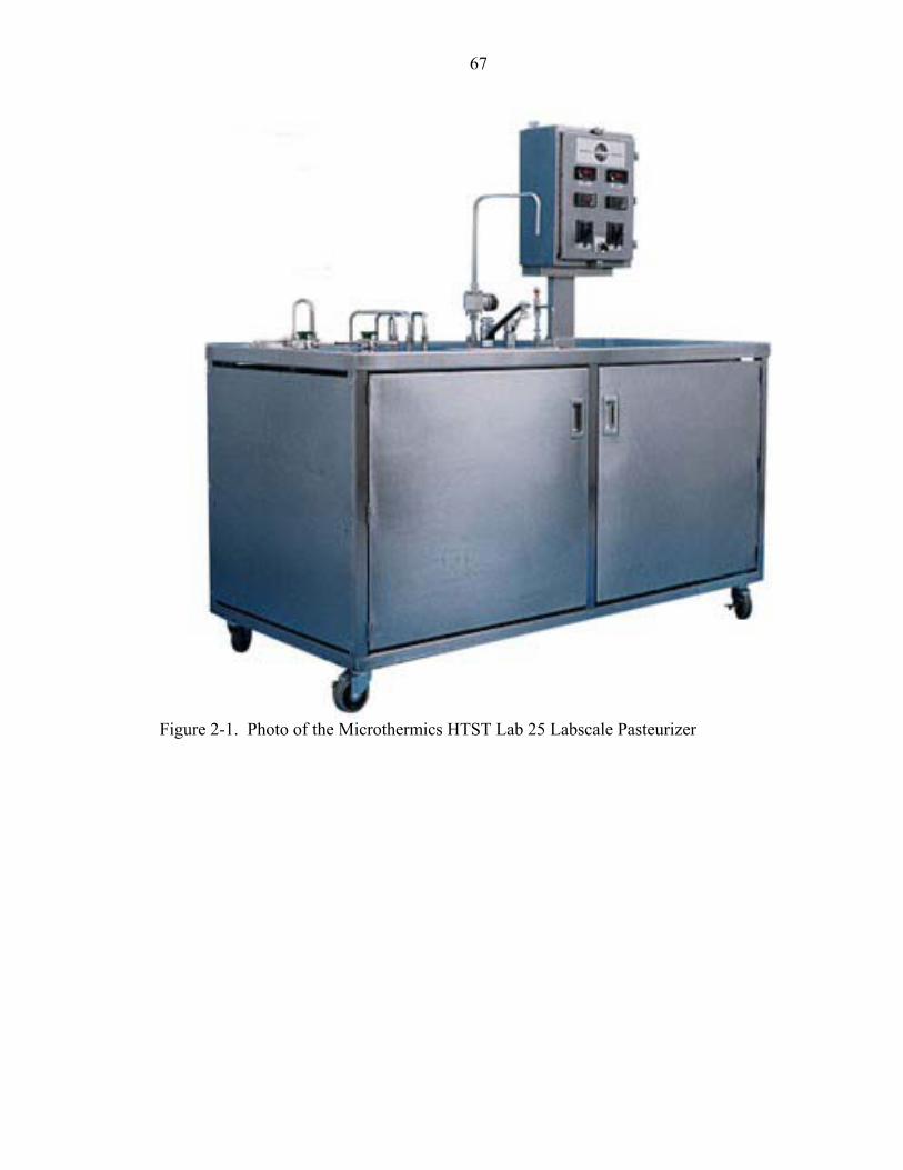
67
Figure 2-1. Photo of the Microthermics HTST Lab 25 Labscale Pasteurizer

68
Figure 2-2. Schematic Diagram of the flow of the Microthermics pasteurizer

69
Table 2-1. Calibration of thermocouples
Replicate Thermocouples #
Mercury in glass reading (oC)
Thermocouple reading (oC)
Correction Factor (oC)
1 1 71.8±0.02 69.5±1.0 2.3±1.0 2 72.0±0.02 70.2±1.0 1.8±1.0 3 72.5±0.02 71.0±1.0 1.5±1.0
2 1 75±0.02 73.4±1.1 1.6±1.1 2 75±0.02 72.7±1.1 2.3±1.1 3 75±0.02 74.1±1.1 1.5±1.1
3 1 75.6±0.02 74±1.1 1.6±1.1 2 75.6±0.02 74.5±1.1 1.1±1.1 3 75.6±0.02 74.1±1.1 1.5±1.1
4 1 75.7±0.02 74.2±1.1 1.5±1.1 2 75.6±0.02 74.2±1.1 1.4±1.1 3 75.6±0.02 74.3±1.1 1.5±1.1

70
Table 2-2. Reynolds numbers for each flow rate for the continuous system
Temperature (oC) Residence Time (sec) Flow Rate (ml/min) Reynolds Number 58 60 480 619 90 320 413
60 30 960 1239 60 480 619
62 15 640 2491 30 960 1032

71
0
10
20
30
40
50
60
70
0 50 100 150
Time(sec)
Tem
pera
ture
(o C)
0
10
20
30
40
50
60
70
0 50 100 150 200
Time (sec)
Tem
pera
ture
(o C)
Figure 2-3. Thermal profile of product at a hold tube nominal temperature of 58oC and
residence times of 60 and 90 seconds

72
0
10
20
30
40
50
60
70
0 20 40 60 80
Time(sec)
Tem
pera
ture
(o C)
0
10
20
30
40
50
60
70
0 50 100 150
Time(sec)
Tem
pera
ture
(o C)
Figure 2-4. Thermal profile of product at a hold tube nominal temperature of 60oC and
residence times of 30 and 60 seconds

73
0
10
20
30
40
50
60
70
0 10 20 30 4
Time (sec)
Tem
pera
ture
(o C)
0
0
10
20
30
40
50
60
70
0 20 40 60 8
Time (sec)
Tem
pera
ture
(o C)
0
Figure 2-5. Thermal profile of product at a hold tube nominal temperature of 62oC and
residence times of 15 and 30 seconds

74
Table 2-3 - Rate constants used in Equation 2-1 for the heater section temperature profile.
Temperature (oC)
Residence Time (sec) B h
58 60 58.6 -0.03273 90 58.6 -0.02101
60 30 59.91 -0.06545 60 59.91 -0.03152
62 15 61.34 -0.13558 30 61.34 -0.06779 Table 2-4. Rate constants used in Equation 2-2 for the chiller section temperature profile.
Temperature (oC)
Residence Time (sec) B c
58 60 58.27 -0.09105 90 57.92 -0.64
60 30 60.28 -0.185 60 60.62 -0.093
62 15 61.23 -0.3742 30 61.94 -0.18285

75
Table 2-5. Population survivor data for continuous experiments
Hold tube Temperature (oC)
Replication Residence Time (sec)
Initial Population (cfu)
Number of Survivors (cfu)
C/Co
58 1 60 5.6x10⁸ 5.2x10⁶ 9.3x10⁻³
2 60 4.3x10⁸ 7.8x10⁶ 1.8x10⁻²
1 90 5.6x10⁸ 3.0x10⁴ 5.4x10⁻⁵
2 90 3.9x10⁸ 2.1x10⁴ 5.4x10⁻⁵
60 1 30 6.1x10⁸ 3.1x10⁶ 5.1x10⁻³
2 30 7.3x10⁸ 4.2x10⁶ 5.8x10⁻³ 3 30 3.9x10⁸ 7.0x10⁵ 1.8x10⁻³ 1 60 5.6x10⁸ 2.5x10⁴ 4.5x10⁻⁵
2 60 7.0x10⁸ 7.9x10⁴ 1.1x10⁻⁴
3 60 5.2x10⁸ 2.6x10⁵ 5.0x10⁻⁴
4 60 5.1x10⁸ 1.4x10⁵ 2.8x10⁻⁴
62 1 15 7.0x10⁸ 4.9x10⁶ 7.0x10⁻³
2 15 7.0x10⁸ 8.0x10⁶ 1.1x10⁻²
1 30 6.9x10⁸ 3.2x10³ 5.0x10⁻⁶
2 30 1.7x10⁸ 3.3x10³ 1.9x10⁻⁵

76
Table 2-6. Estimation of D- and z-values from each iteration of the PEIE method
Iteration 1 Iteration 2 Iteration 3 Iteration 4 Initial Ea Guess
20,000 J 62,089 J 267,398 J 342,711 J
oC Residence Time (sec)
D(sec) k(sec-1) D(sec) k(sec-1) D(sec) k(sec-1) D(sec) k(sec-1)
58 60 27.3 0.084 29.53 0.078 29.53 0.078 29.53 0.078 32.0 0.072 34.56 0.067 34.56 0.067 34.56 0.067
90 27.5 0.084 25.5 0.09 27.51 0.084 27.51 0.084 25.6 0.09 27.58 0.083 27.59 0.083 27.59 0.083
60 30 12.0 0.191 13.02 0.177 13.03 0.177 13.03 0.177 12.42 0.185 13.41 0.172 13.41 0.172 13.41 0.172 10.14 0.227 10.94 0.21 10.95 0.21 10.95 0.21
60 12.76 0.18 13.77 0.167 13.77 0.167 13.77 0.167 14.08 0.163 15.20 0.151 15.20 0.151 15.20 0.151
62 15 2.69 0.854 6.95 0.331 6.95 0.331 6.95 0.331 2.99 0.769 7.73 0.298 7.73 0.298 7.73 0.298
30 5.20 0.442 5.63 0.409 5.63 0.409 5.63 0.409 5.89 0.391 6.37 0.362 6.4 0.362 6.4 0.362
Estimated Ea 62,089 J 267,398 J 342,711 J 342,711 J

77
0
0.2
0.4
0.6
0.8
1
1.2
1.4
1.6
57 58 59 60 61 62 63
Temperature (oC)
Log
D-v
alue
(sec
)
Iteration 1 Iteration 2 Iteration 3
Figure 2-6. TDT curve for acid tolerant Escherichia coli in orange juice using kinetic parameters from the PEIE method

78
Table 2-7. Comparison of D- and z-values estimated by traditional method using isothermal treatments and PEIE method using continuous dynamic treatments
Isothermal (3-neck flask)
Dynamic (PEIE)
Temperature (oC)
Average D-value (sec)
Standard Deviation
D-value (sec)
Standard Deviation
52 353 39.08 55 148 2.18 58 34.7 2.27 29.8 3.3 60 18 1.52 13.27 1.54 62 6.93 0.47 z-value (oC) 5.99 6.16
Table 2-8. Kinetic parameters of thermal inactivation of Alicyclobacillus acidoterrestris
spores in Cupuacu nectar using the PEIE method and Isothermal method *
PEIE Method Isothermal (submerged vials) D95
oC (min) 5.5 ± 1.2 3.82 ± 0.48
z (oC) 31 ± 29 ± 10 R2 0.87 0.98 No. of observations 22 26 *Source: Veira et al. (2002)

79
0
0.2
0.4
0.6
0.8
1
1.2
1.4
1.6
57 58 59 60 61 62 63
Temperature (oC)
Log
D-v
alue
(sec
)
Iteration 1 Iteration 2 Iteration 3
Figure 2-7. TDT curve for acid tolerant Escherichia coli in orange juice using kinetic
parameters from the PEIE method

80
0
0.5
1
1.5
2
2.5
3
50 52 54 56 58 60 62 64
Temperature (oC)
Log
[D-v
alue
(sec
)]
Traditional PEIE
Figure 2-8. Comparison of TDT curves based upon data from the traditional and PEIE
methods

81
0
0.2
0.4
0.6
0.8
1
1.2
1.4
80 85 90 95 100 105 110 115
Temperature (oC)
Log
[D-v
alue
(min
)]
PEIE Isothermal
Figure 2-9. Comparison of TDT curves based upon data from the traditional and PEIE
methods for Alicyclobacillus acidoterrestris spores in Cupuacu nectar (Vieira et. al. 2002) (Estimated curve based upon reference D-value and z-value)

82
0
1
2
3
4
5
6
7
8
9
10
0 10 20 30 40 50 60
Time (seconds)
Log
[sur
vivo
rs(c
fu/m
l)]
0
10
20
30
40
50
60
70
IsothermalPEIEExperimentalTemperature
Figure 2-10. Temperature history and measured and predicted survivor responses for
validation experiment I (10 second hold tube)

83
0
1
2
3
4
5
6
7
8
9
10
0 5 10 15 20 25 30 35 40
Time (seconds)
Log
[sur
vivo
rs (c
fu/m
l)]
0
10
20
30
40
50
60
70
IsothermalPEIEExperimentalTemperature
Figure 2-11. Temperature history and measured and predicted survivor responses for
validation experiment II (15 second hold tube)

84
Table 2-9. Results of validation experiments, comparison of predicted number of survivors for PEIE analysis and Traditional isothermal batch analysis with experimental number of survivors
Hold Tube Survivors (cfu) Experiment Time
(sec) Temp (oC) Initial
(cfu) PEIE Predicted
Isothermal Predicted
Experimental
I 15 65 5.4x10⁸ 3.51x10³ 4.95x10⁴ 5.15x10³
8.0x10³
II 10 65 5.4x10⁸ 1.98x10³ 8.59x10⁴ 1.0x10³ 1.25x10³

CHAPTER 3 ESTIMATION OF KINETIC PARAMETERS FOR THERMAL INACTIVATION OF
Alicyclobacillus acidoterrestris IN ORANGE JUICE
Introduction
The recent discovery of Alicyclobacillus acidoterrestris in high-acid pasteurized
fruit juices and its ability to cause spoilage in these products have become concerns for
processors in the design of thermal pasteurization processes. Alicyclobacillus
acidoterrestris are sporeforming thermophilic bacteria that grow well in low pH
environments. These characteristics of the bacteria can be problematic since all shelf
stable and refrigerated fruit juices are pasteurized at temperatures below the lethal range
of Alicyclobacillus. This inadequate processing can lead to premature spoilage of the
product with risk of recall from the marketplace. Accurate estimation of the thermal
inactivation kinetic parameters that are used in a model to predict the number of survivors
is essential to establish optimum process conditions to assure a low probability of
spoilage of the product without over processing the product, which leads to degradation
of juice quality important to consumers. It has been shown in chapters 1 and 2 that the
Paired Equivalent Isothermal Exposures (PEIE) method is valid and accurate for the
estimation of kinetic parameters. The PEIE method is not just limited to using Arrhenius
kinetics for estimation of thermal inactivation kinetic parameters (k and Ea). It may also
be possible to use the PEIE method with Thermal Death Time (TDT) kinetics (D- and z-
value) which are more commonly used by food scientists. Orange juice was the product
85

86
chosen for this study because of the spoilage problems that have been documented
involving Alicyclobacillus acidoterrestris in orange juice. Using the PEIE method to
analyze continuous dynamic thermal treatment data, thermal inactivation kinetic
parameters were estimated for Alicyclobacillus acidoterrestris in orange juice.
Literature Review
Occurrences of Alicyclobacillus acidoterrestris in Juice Products
Fruit juices with a pH below 4.0 have been considered susceptible to spoilage only
by microorganisms of low heat resistance such as molds and acid-tolerant non-
sporeforming bacteria (Eiroa et al. 1999). Because of the low resistance to heat by these
microorganisms, pasteurization processes designed with temperatures ranging from 85oC
to 95oC were thought to be sufficient to inactivate these spoilage-causing microorganisms
(Eiroa et. al. 1999). The first reported incidence of a food product being spoiled by
acidophilic sporeformers was in Germany with apple juice (Walls and Chuyate, 1998). It
was determined that this spoilage microorganism was Bacillus acidoterrestris, which was
later named Alicyclobacillus acidoterrestris. Spoilage by this microorganism leads to off
flavors in the products similar to the taste of phenolic substances, odors of a disinfectant
and pronounced cloudiness (Eiroa et. al. 1999; Walls and Chuyate 1998).
Fortunately, Alicyclobacillus acidoterrestris does not appear to be pathogenic
according to Walls and Chuyate (2000), who conducted pathogenicity studies with the
bacteria in mice and guinea pigs. Although Alicyclobacillus acidoterristris is not a safety
concern for industry, it is a serous economic issue. During the 1990’s Alicyclobacillus
acidoterrestris was presenting itself as a spoilage problem in shelf stable juice products
(Walls and Chuyate 1998). In 1994 there was a report of off odors in apple juice caused
by gram positive rods isolated from the juice and showing characteristics similar to

87
Alicyclobacillus acidoterrestris (Eiroa et. al. 1999). Spoilage of juices by these bacteria
is not readily detected since there is often little sedimentation and no gas produced that
would distort the product package. In juice inoculation studies, it was discovered that
Alicyclobacillus acidoterrestris grew well in orange, apple, tomato, and grape juice in
which the pH of the juices ranged from 3.47 to 4.27 (Walls and Chuyate 2000).
Alicyclobacillus acidoterrestris is a new spoilage microorganism that must addressed by
the juice industry and other processors of low pH food products.
Current temperatures used for pasteurization are insufficient to inactivate spores of
these bacteria in fruit juices, yet thermally overprocessing the product can lead to
unacceptable quality degradation of the product. Because sporeforming bacteria of
importance in foods are rarely as acid tolerant as Alicyclobacillus acidoterrestris, it is
important to characterize the thermal inactivation behavior in populations of this
microorganism in order to design processes that will reduce the probability of spoilage
for shelf stable products while maintaining quality factors acceptable to the consumer.
The PEIE method has been reported in recent literature to be useful in obtaining greater
accuracy in parameter estimation (Welt et al. 1997a, b). Using the PEIE method to obtain
thermal inactivation kinetic parameters for Alicyclobacillus acidoterrestris will insure a
more accurate estimation of those parameters. In this work the PEIE method will be
carried out in both Arrhenius kinetics and Thermal Death Time (TDT) kinetics using
process lethality (F-value), which is more familiar to food scientists.
The PEIE Method in Arrhenius Kinetics
Recall that a first-order rate process is described by
kCdtdC
−= (3-1)

88
where C is the concentration of a reactant at a time, t, and k is the rate constant of the
reaction. Solving Equation 3-1 by integration yields Equation 3-2.
)(ln oo
ttkCC
−⋅−=
(3- 2)
The temperature dependency of the rate constant, k, is described by Equation 3-3, the
Arrhenius equation,
−
−⋅=
R
aR TTR
Ekk 11exp (3- 3)
where kR is the rate constant at reference temperature TR, Ea is the activation energy, T is
the desired operating temperature, and R is the ideal gas law constant. Under isothermal
conditions, the Arrhenius equation that describes the behavior of a reactant that follows a
first-order reaction process is shown in Equation 3-4.
)(expln oRo
ttTREk
CC
−⋅
⋅−
⋅−=
(3- 4)
This equation can be used to determine the extent of reaction for a given constituent at a
constant temperature. Under non-isothermal conditions, Equation 3-4 is integrated as
shown in Equation 3-5 using the temperature history, T(t), to give the extent of reaction.
Combining Equations 3-4 and 3-5 to equate a dynamic process to an
dttTR
EkCC t
tR
o o
∫
⋅−
⋅−=
)(
expln (3- 5)
isothermal and normalizing to eliminate kR introduces a new factor called G, the decimal
reduction factor, and the equation becomes

89
∫
⋅−
⋅=
⋅−
==−
t
t e
ae
a
R
o
oTR
Etdt
tTRE
GkCC
exp)(
expln
(3- 6)
where te is the equivalent time needed to obtain the same reduction in the constituent at a
constant temperature, Te, for a given dynamic process.
The PEIE method uses Equation 3-6 to represent an isothermal process as
⋅−
⋅=e
ae TR
EtG exp (3- 7)
and taking two sets of Ea and G values yields two equations that can be used to solve for
te and Te (using the elimination method) as follows:
e
ae
e
ae
TRE
tG
TRE
tG
⋅+−=−
⋅−=
2
1
)ln()ln(
)ln()ln(
2
1
(3- 8)
where
⋅
−=
2
1ln
)(12
GGR
EET aa
e (3- 9)
and
⋅
−=
e
ae
TRE
Gtexp
(3- 10)
These isothermal combinations, when plotted on a semilog plot of time versus
temperature would appear as a straight line, and at any point on this line the combinations
of Te and te are equivalent isothermal exposures (EIE) yielding the same extent of
reaction as the given non isothermal process. As shown in Chapter 2, using these EIEs
along with the measured extents of reactions allows the estimation of the kinetic

90
parameters k and Ea. These parameters can then be used in the model (Equation 2.10) to
predict the number of survivors from a process at a given time and temperature history.
The PEIE Method and TDT Kinetics
The conceptual approach to the PEIE method is not new to the food industry. A
similar means to equate a dynamic process to an isothermal process for microorganisms
that has been used in the food industry for many years is the Process Lethality Value (F).
Recall, Equations 2-7 and 2-8 from Chapter 2 describe first order thermal inactivation
kinetics using thermal death-time (TDT) parameters D- and z-value. Equations 3-11
and 3-12 are restatements of these equations where D is the decimal reduction time (the
time needed for a one-log cycle reduction in the population at a given constant
temperature. Thus, the
−
= Dt
oCC 10 (3- 11)
D-value is related to the first order rate constant (k), since both show the relationship
between time and population reduction at a given temperature. The relationship between
D-value and temperature (the D-values temperature dependency) is assumed to be log-
linear and given by Equation 3-12 where Do is reference D-value at reference temperature
To and z is the temperature interval required to change the value of D by one log cycle.
−
= zTT
o
o
DTD 10)( (3- 12)
Equation 3-13 determines the F value for a process under isothermal conditions.
tF ZRTT
−
=10 (3- 13)
When the product temperature varies the F value delivered by the process must be
integrated mathematically as shown in Equation 3-14. This equation determines the F

91
value delivered by a process that has experienced a dynamic temperature history, in
which temperature varies as a function of time, T(t). In TDT kinetics F value is
equivalent to the G value in Arrhenius kinetics.
dtFt
t
ZTtT
o
R
∫
−
=)(
10 (3- 14)
Like the PEIE method, isothermal combinations of temperature and time that would
achieve the same F value would appear as a straight line on a semilog plot of time versus
temperature known as the thermal death time (TDT) curve. Any point on this line of
temperature-time is an EIE. Combining Equations 3-13 and 3-14 to equate a dynamic
process to an isothermal the equation becomes
eZTTt
t
ZTtT
tdtFRe
o
R
⋅==−
−
∫ 1010)(
(3- 15)
For a dynamic process where the temperature history has been recorded and a z-value
chosen, an accumulated F value can be determined using Equation 3-14. An isothermal
process derived from two z-values may be interpreted as an equivalent exposure that
would result in the same lethalities for reactant characterized by the respective z-values.
These EIEs can be used to solve for te and Te (using substitution) as follows:
22
11
)log()log(
)log()log(
ZTT
tF
ZTT
tF
Ree
Ree
−+=
−+=
(3- 16)
where

92
Re T
ZZ
FF
T +
−
=
21
2
1
11
log (3- 17)
and
−
=Z
TTeRe
Ft
10 (3- 18)
The extent of reaction data along with the equivalent times can be used to estimate the D-
values at the respective equivalent temperature.
Objectives
The purpose of this study was to apply the PEIE method to estimate thermal
inactivation kinetic parameters of Alicyclobacillus acidoterrestris in orange juice. To
achieve this goal the objectives of this project were the following:
• Estimate the kinetic parameters for thermal inactivation of Alicyclobacillus acidoterrestris in orange juice by the PEIE method in Arrhenius kinetics from data generated by continuous dynamic thermal treatments
• Estimate the kinetic parameters for thermal inactivation of Alicyclobacillus acidoterrestris in orange juice by the PEIE method in TDT kinetics from the same data.
• Compare results from both methods.
Methods and Materials
Preparation of Cultures
The strain of Alicyclobacillus acidoterrestris used in this study was obtained from
the American Type Culture Collection (ATCC #49025). Working and stock cultures of
this strain were made from frozen stock cultures of the original freeze-dried culture
obtained from ATCC. The cultures were thawed and streaked onto acidified K agar and

93
incubated at 45oC for 3 to 5 days, depending on the date of each experimental run. The K
agar was acidified using 2.5 mg of malic acid per 700 ml of media to give a final pH of
3.7 ± 0.1. The cultures, containing vegetative cells and spores were harvested from the
agar plates using a sterile pipette to submerge the culture in sterile buffer solution. A
sterile spreader was used to gently separate the cells and spores from the agar and
suspend them in buffer solution. The solution containing the cell/spore suspension was
aseptically poured off the agar plate and into a sterile container of buffer solution. This
procedure was repeated with twelve plates and the resulting concentration of cell/spore
suspension was used as the inoculum for the orange juice. The inoculum was heat
shocked at 75oC for 10 minutes prior to inoculation into the orange juice to inactivate
vegetative cells in order to have a more uniform population of heat resistant spores.
Experimental Apparatus
The experimental apparatus used in these experiments was the Microthermics
UHT/HTST Lab-25 lab-scale pasteurizer unit. A photo and schematic diagram of the
unit are shown in Figures 2-1 and 2-2. Refer to Chapter 2 for a detailed description of the
pasteurizer unit.
Continuous Dynamic Thermal Treatments
The orange juice was reconstituted from concentrate using sterile filtered
deionized water. The orange juice concentrate was a commercial brand orange juice
concentrate at 44o Brix. The reconstitution was performed following the manufacturer’s
directions on the label (1 part concentrate to 3 parts water). Although the orange juice
was not reconstituted under aseptic conditions, the resident population of Alicyclobacillus
acidoterrestis in the product was negligible when compared with the number of
spores/cells in the inoculum. The product was inoculated with an Alicyclobacillus

94
acidoterrestis cell suspension prior to thermal exposure to achieve a minimum initial
concentration of 1 x 10⁶ cfu/mL. Two liters of orange juice were prepared along with
200ml of spore/cell suspensions. The pasteurizer was sanitized by circulating hot water
at 83oC through the heater, hold tube, chiller sections and accessory tubes for a minimum
of 30 minutes.
After being sanitized, the temperature of the pasteurizer was adjusted to the desired
experimental temperature and allowed to reach steady-state conditions. Then the product
flow control valve was opened to allow the inoculated product to flow through the unit.
Temperatures at various locations throughout the system were recorded using a
datalogger attached to a notebook computer. The thermal profile (temperature vs. time)
of each experimental run was captured from each port and saved as a text file that was
used in the PEIE method. To produce replicate data for each temperature, 2 samples
were collected for each experimental run and a minimum of two experimental runs were
conducted for each residence temperature-time combination. An experiment involved a
product cycle whereby a batch of product was pumped through the system after using
water to achieve a stable steady state condition, then the product and water reservoir
valves were switched to allow water to run through the system at the same conditions
while another sample of product was being prepared. Then the valves were switched and
the product pumped through the system and samples taken again. The residence time for
each run was 90 seconds, with the exception at 104oC for Day 2, which was set for
residence time of 60 seconds.
Temperature Profiles
The temperature was measured at the inlet of the heating section (initial product
temperature), after the heating section (at the entrance to the hold tube), after the hold

95
tube (at the entrance to the chiller section), and after the chiller section. Using the
recorded temperature at each point, the heater and chiller portions of the profile were
constructed from heat transfer equations, while the hold tube portions were constructed
based upon measured data. Recall from Chapter 2 that the standard profile for a shell and
tube heat exchanger follows an exponential increase that can be described by
Equation 3-1,
)-1( -hteBAT += (3-1)
where T is the temperature at any point within the heat exchanger at a specific time t, A is
the initial temperature of the product, B is the temperature of the product upon exit from
the heat exchanger, and h is the rate constant for the temperature change through the heat
exchanger. This equation yielded the calculated temperatures along the heater section of
the pasteurizer. The hold tube inlet and outlet temperatures were measured directly by
thermocouples. The temperature along the chiller section of the pasteurizer was
calculated using Equation 3-2.
)( -cteBT = (3-2)
where B is the temperature of the product upon entrance into the chiller section, T is the
temperature at any point within the chiller section at a specific time t and c is the rate
constant for the temperature change through the chiller section. Knowing the residence
time of the product within the heater and chiller section of the pasteurizer, the
temperature profile was constructed by determining the parameters of Equations 3-1 and
3-2 using the boundary conditions of each section. The residence times for each section
were determined based upon the flow rate of the product and the diameters and lengths of
the tubes in all sections of the pasteurizer with the assumption of plug flow for simplicity.

96
The flow rates of the product were determined by measuring the amount collected in a
graduated cylinder over a specific time period.
Results and Discussion
Parameter Estimation by PEIE
Figures 3-1 and 3-2 show the temperature histories for the continuous dynamic
thermal experiments with hold tube temperatures at 95oC, 100oC and 104oC. Tables 3-1
and 3-2 show the temperature profile rate constants determined for the heater and chiller
sections, respectively. Once the temperature profiles were constructed, they were used
with the measured hold tube temperatures to create a complete profile for use in the PEIE
method. These profiles along with the survivor data were used to estimate the thermal
inactivation parameters for Alicyclobacillus acidoterretris in single strength orange juice.
Table 3-3 shows the population survivor data for all the continuous thermal
treatment experimental runs. The initial population was verified by plating out (in
triplicate) a sample of the untreated inoculated orange juice before and after each
experimental run. Table 3-4 shows the four iterations of the PEIE method needed to
converge on a final solution for the EIE's using Arrhenius kinetics. From Table 3-4, k-
values of 0.021 seconds-1, 0.070 seconds-1, and 0.119 seconds-1 were estimated at
equivalent temperatures of 94.4oC, 100.7oC, and 104.2oC respectively. Figure 3-3 shows
the Arrhenius curve for Alicyclobacillus acidoterrestris, with an Ea-value of 204 kJ/mol.
Parameter Estimation using F value and TDT kinetics
Table 3-5 shows the four iterations of the PEIE method needed to converge on a
final solution for EIEs using TDT kinetics. From Table 3-5, D-values of 107.4 seconds
(1.79 minutes), 34.22 seconds (0.57 minutes), and 17.65 seconds (0.30 minutes) were
estimated at equivalent temperatures of 95oC, 100oC, and 104oC respectively. The z-

97
value for Alicyclobacillus acidoterrestis in orange juice from this study was determined
to be 13.1oC, as shown in Figure 3-4. When compared to work performed by other
researchers using Alicyclobacillus in orange juice, these values fall within published
ranges as shown in Table 3-6. Eiroa et. al. (1999) reported D95-values for four strains of
Alicyclobacillus acidoterrestris spores in orange juice that ranged from 2.5 min to 8.7
min and z-values that ranged from 7.2oC to 11.3oC. Splittstoesser et. al. (1998) reported a
D95-value for Alicyclobacillus acidoterrestris in concord grape juice at 16oBrix and a pH
of 3.5 of 1.9 minutes and a z-value of 6.9oC. Komitopoulou et. al. (1999) reported a
D95-value of 3.9 minutes in single strength orange juice with a pH of 3.9 and a z-value of
12.9oC and McIntyre et. al. (1995) reported a D95-value of 1.0 minute. Komitopoulou et
al. (1995) used a wide-necked flask apparatus (equivalent to a three-necked flask
apparatus) to generate heat inactivation data whereas Spittstoesser et. al. (1998) and Eiroa
et. al. (1999) used glass vials submersed in an isothermal water bath..
Figure 3-4 shows a comparison between the TDT curves generated by the kinetic
parameters from Arrhenius kinetics versus those generated by TDT kinetic. There is a
slight difference in the offset of the curves and in the slopes of the curves. The effect of
this difference would be amplified as temperatures move further away from the range
used in this experiment. Jones (1968) and Jonsson et al. (1977) showed that sterilization
times based on parameters obtained by both methods could show important discrepancies
at higher temperatures. Using the TDT and Arrhenius curves the D-value at both
extremes of the temperature range was estimated. From the TDT curve, D-values of 136
seconds and 20 seconds for temperatures of 93oC and 104oC respectively were estimated.
From the Arrhenius, curve D-values of 156 seconds and 18 seconds at the same

98
temperatures were estimated. There was a difference of 12.8% in D-values at the lower
temperature and 10% at the higher temperature. Using each curve to estimate the F
value for a 6 log cycle reduction in the population of Alicyclobacillus in orange juice at a
temperature of 90oC, the TDT method would yield a value of 23 minutes whereas the
Arrhenius method would yield a value of 29 minutes. Ocie et al. (1994) conducted a
study to compare the TDT and Arrhenius methods for rate constant predictions of
Bacillus stearothermophilus and concluded that using the TDT method to generate
kinetic parameters could introduce unsafe process times, whereas Jones concluded that
the appropriate method to generate parameters depends on which gives the most
conservative values for the kinetic parameters. In this study both converged on the same
time-temperature combinations in the given temperature range (95oC – 104oC) that would
give the same estimated values for the kinetic parameters. The significance of this
finding is that the PEIE method can be successfully executed in both Arrhenius and TDT
kinetics. Since TDT kinetics have been used extensively in the food industry for
establishing thermal processes and determining the lethality of a process, the reasonable
agreement between the kinetic parameters estimated by the PEIE method in this study
and those estimated by traditional methods from published work shows that the method is
a valid and trustworthy method for estimating thermal inactivation kinetic parameters
using data generated from a continuous dynamic thermal treatment process. However,
the PEIE method as presented here can only be used to estimate the parameters of first
order kinetics with a uniform population of organisms.

99
0.00
20.00
40.00
60.00
80.00
100.00
120.00
0 50 100 150 200 250Time (sec)
Tem
pera
ture
(o C)
95 C100 C104 C
Figure 3-1. Thermal profile of product at a hold tube nominal temperature of 95oC, 100oC, and 104oC for experimental set one

100
0.00
20.00
40.00
60.00
80.00
100.00
120.00
0 50 100 150 200 250
Time (sec)
Tem
pera
ture
(o C)
95 C100 C104 C
Figure 3-2. Thermal profile of product at a hold tube nominal temperature of 95oC, 100oC, and 104oC for experimental set two.

101
Table 3-1. Rate constants used in Equation 2-1 and 2-2 for the heater and chiller sections temperature profile for experimental set 1
Heater profile parameters Chiller profile parameters Temperature B h B c 90 88.9 -0.028 87.8 -0.056 95 94.3 -0.033 94.2 -0.063 100 101.1 -0.046 100.9 -0.069 104 104.2 -0.051 104.1 -0.069
Table 3-2. Rate constants used in Equation 2-1 and 2-2 for the heater chiller sections temperature profile for experimental set 2
Heater profile parameters Chiller profile parameters Temperature B h B c 95 94.9 -0.0325 95.06 -0.065 100 100.4 -0.039 100.83 -0.065 104 104.2 -0.079 104.3 -0.12

102
Table 3-3. Population survivor data from Ultra High Temperature (UHT) heat treatments with Alicyclobacillus acidoterrestris in orange juice
Hold tube Temperature (oC)
Replication Residence Time (sec)
Initial Population (cfu)
Number of Survivors (cfu)
C/Co
95 1 90 3.46x10⁶ 2.42x10⁵ 6.9x10⁻²
2 90 1.08x10⁶ 1.06x10⁵ 9.8x10⁻²
3 86 1.98x10⁶ 8.18x10⁴ 7.1x10⁻²
4 86 7.37x10⁵ 1.4x10⁵ 1.9x10⁻¹
100 1 90 3.46x10⁶ 1.35x10³ 3.0x10⁻⁴-
2 90 1.08x10⁶ 5.38x10² 5.0x10⁻⁴
3 86 1.98x10⁶ 1.65x10³ 8.0x10⁻⁴
4 86 7.37x10⁵ 8.4x10² 1.1x10⁻³
104 1 90 3.46x10⁶ 3.0x101 8.7x10⁻⁶
2 90 1.08x10⁶ 2.7x101 2.5x10⁻⁵
3 62 1.98x10⁶ 4.70x10² 2.3x10⁻⁴
4 60 7.37x10⁵ 3.35x10² 4.5x10⁻⁴

103
Table 3-4. Estimation of k and Ea values from each iteration of the PEIE method using Arrhenius kinetics
Iteration 1 Iteration 2 Iteration 3 Iteration 4
Initial Ea Guess 20,000 J 214,000 J 188,000 J 203,000 J oC Residence Time (sec) k(sec-1) k(sec-1) k(sec-1) k(sec-1) 95 102 0.02077 0.02191 0.0223 0.02232 0.01847 0.01948 0.01983 0.01985 99 0.0124 0.01912 0.01886 0.01901
0.01401 0.0216 0.02131 0.02149
100 102 0.04742 0.07426 0.07356 0.07399 0.04373 0.0685 0.06784 0.06824 99 0.04526 0.07131 0.0705 0.07099
0.04298 0.06772 0.06695 0.06742
104 102 0.07044 0.1097 0.1089 0.1094 0.06809 0.106 0.1053 0.1058 57 0.08645 0.1327 0.1324 0.1326
0.08578 0.1317 0.1314 0.1316
Estimated Ea 214,000 J 188,000 J 203,000 J 204,000 J

104
-4.5
-4
-3.5
-3
-2.5
-2
-1.5
0.0026 0.00265 0.0027 0.00275
Inverse Absolute Temperature (K-1)
ln[k
(sec
-1)]
Iteration 1 Iteration 2 Iteration 3 Iteration 4
Figure 3-3. Arrhenius curve for Alicyclobacillus acidoterrestris in orange juice using kinetic parameters from the PEIE method

105
Table 3-5. Estimation of D- and z-values from each iteration of the PEIE method using TDT kinetics
Iteration 1 Iteration 2 Iteration 3 Iteration 4
Initial z-value Guess (oC) 20 14.79 13.18 13.11 oC Residence Time (sec) D(sec) D(sec) D(sec) D(sec) 95 102 110.8 105.1 103.2 103.2 124.7 118.2 116.1 116 99 185.7 120.4 122.1 121.1
164.4 106.6 108 107.2
100 102 48.56 31.01 31.3 31.12 52.65 33.62 33.94 33.74 99 50.87 32.29 32.66 32.43
53.57 34 34.39 34.15
104 102 32.69 20.99 21.14 21.04 33.82 21.71 21.86 21.77 57 26.63 17.35 17.39 17.36
26.84 17.48 17.52 17.5
Estimated z-value (oC) 14.79 13.18 13.11 13.11

106
1
1.2
1.4
1.6
1.8
2
2.2
2.4
94 96 98 100 102 104 106
Temperature (oC)
Log[
Dva
lue(
sec)
]
Iteration 1 Iteration 2Iteration 3 Iteration 4
Figure 3-4. TDT curve for Alicyclobacillus acidoterrestris in orange juice using kinetic parameters from the PEIE method

107
Table 3-6. Comparison of TDT kinetic parameters with published data from various sources using Alicyclobacillus acidoterrestris
Study (strain) D95 (minutes) z-value (oC) Eiroa et. al. (46) 2.5 7.2 Eiroa et. al . (70) 8.7 11.3 Eiroa et. al. (145) 3.8 7.2 Eiroa et. al. (DSM2498) 2.7 7.9 Splittstoesser et. al. 1.9 6.9 Komitopoulou et. al. 3.9 12.9 McIntyre et. al. 1.0 This study 1.8 13.1

108
1
1.2
1.4
1.6
1.8
2
2.2
92 94 96 98 100 102 104 106
Temperature (oC)
Log
[Dva
lue(
sec)
]
Arrhenius Kinetics TDT Kinetics
Figure 3-5. Comparison of TDT curves based upon data from the PEIE method using
TDT kinetics and Arrhenius kinetics

APPENDIX A
MATHCAD PROGRAM FOR THE PEIE METHOD WITH Escherichia coli USING ARRHENIUS KINETICS
Step 1: Retrieal of the dynamic temperature history and survival data
Constants:
Universal Gas constant: Rval 8.314 J/mol - K
Reading in temperature and concentration files:
Conc58 READPRN "c:\phd\58Ca.txt"( ) Conc58
60
60
90
90
5.6 108.
4.25 108.
5.6 108.
3.85 108.
5.2 106.
7.8 106.
3 105.
2.1 105.
=
Conc60 READPRN "c:\phd\60Ca.txt"( ) Conc60
30
30
30
60
60
60
60
6.13 108.
7.25 108.
3.85 108.
5.6 108.
7 108.
5.2 108.
5.1 108.
3.05 106.
4.2 106.
7 105.
2.46 104.
7.9 104.
2.64 105.
1.39 105.
=
Conc62 READPRN "c:\phd\62Ca.txt"( ) Conc62
15
15
30
30
7.05 108.
7 108.
6.9 108.
1.7 108.
4.9 106.
8 106.
3.2 103.
3.3 103.
=
109

110
Conc62 READPRN "c:\phd\62Ca.txt"( ) Conc62
15
15
30
30
7.05 108.
7 108.
6.9 108.
1.7 108.
4.9 106.
8 106.
3.2 103.
3.3 103.
=
Step 2: Selection of two arbitrary Ea values and determination of the corresponding G values
Ea1 200000 Ea2 1.5 Ea1.
Ea2 300000=
Temperature = 58C
Temp58 READPRN "c:\PhD\58C Profile.txt"( )
T5860 v( ) Temp58v 1, 273 T5890 v( ) Temp58v 3, 273
G58_601
0
116
v
expEa1
Rval T5860 v( )( ).=
G58_601 1.83601408027491 10 30.=
G58_602
0
116
v
expEa2
Rval T5860 v( )( ).=
G58_602 2.95926098664273 10 46.=
G58_901
0
174
v
expEa1
Rval T5890 v( )( ).=
G58_901 2.80954716946208 10 30.=
G58_902
0
174
v
expEa2
Rval T5890 v( )( ).=
G58_902 4.5534 10 46.=
Temperature = 60C
Temp60 READPRN "c:\PhD\60C Profile.txt"( )
*

111
T6030 v( ) Temp60v 1, 273 T6060 v( ) Temp60v 3, 273
G60_301
0
60
v
expEa1
Rval T6030 v( )( ).=
G60_301 1.50740195154320 10 30.=
G60_302
0
60
v
expEa2
Rval T6030 v( )( ).=
G60_302 3.0526 10 46.=
G60_601
0
116
v
expEa1
Rval T6060 v( )( ).=
G60_601 3.05983039701529 10 30.=
G60_602
0
116
v
expEa2
Rval T6060 v( )( ).=
G60_602 6.4232 10 46.=
Temperature = 62C
Temp62 READPRN "c:\PhD\62C Profile.txt"( )
T6215 v( ) Temp62v 1, 273 T6230 v( ) Temp62v 3, 273
G62_151
0
29
v
expEa1
Rval T6215 v( )( ).=
G62_151 1.01299314933432 10 30.=

112
G62_152
0
29
v
expEa2
Rval T6215 v( )( ).=
G62_152 2.4353 10 46.=
G62_301
0
60
v
expEa1
Rval T6230 v( )( ).=
G62_301 2.05078675095581 10 30.=
G62_302
0
60
v
expEa2
Rval T6230 v( )( ).=
G62_302 4.9138 10 46.=
Step 3: Equate G values to the isothermal form to determine the respective equivalent isothermal exposure for each pair of dynamic thermal experiments.
58C; 60 and 90 second residence time
TeEa2 Ea1( )
Rval lnG58_601G58_602
.
te58_60G58_601
expEa1
Rval Te.
Temp58_60 Te
Temp58_60 330.764=
te58_60 70.674=
TeEa2 Ea1( )
Rval lnG58_901G58_902
.

113
te58_90G58_901
expEa1
Rval Te.
Temp58_90 Te
Temp58_90 330.814=te58_90 106.966=
60C; 30 and 60 second residence time
TeEa2 Ea1( )
Rval lnG60_301G60_302
.
te60_30G60_301
expEa1
Rval Te.
Temp60_30 Te
Temp60_30 332.853=
te60_30 36.757=
TeEa2 Ea1( )
Rval lnG60_601G60_602
.
te60_60G60_601
expEa1
Rval Te.
Temp60_60 Te
Temp60_60 333.185=
te60_60 69.436=
62C; 15 and 30 second residence time
TeEa2 Ea1( )
Rval lnG62_151G62_152
.

114
te62_15G62_151
expEa1
Rval Te.
Temp62_15 Te
Temp62_15 334.441=
te62_15 17.527=
TeEa2 Ea1( )
Rval lnG62_301G62_302
.
te62_30G62_301
expEa1
Rval Te.
Temp62_30 Te
Temp60_30 332.853=
te62_30 35.721=
Temp58aTemp58_60
Temp58_90Temp60a
Temp60_30
Temp60_60Temp62a
Temp62_15
Temp62_30
Temp58 mean Temp58a( ) Temp60 mean Temp60a( ) Temp62 mean Temp62a( )
Temp58 330.789= Temp60 333.019= Temp62 334.426=
Temp58std stdev Temp58a( )
Temp60std stdev Temp60a( ) Temp62std stdev Temp62a( )
Temp58std 0.025= Temp60std 0.166= Temp62std 0.016=
Step 4: Calculate the k values at equivalent temperatures from the equivalent time determined in step 3

115
Conc58
60
60
90
90
5.6 108.
4.25 108.
5.6 108.
3.85 108.
5.2 106.
7.8 106.
3 105.
2.1 105.
=Conc60
30
30
30
60
60
60
60
6.13 108.
7.25 108.
3.85 108.
5.6 108.
7 108.
5.2 108.
5.1 108.
3.05 106.
4.2 106.
7 105.
2.46 104.
7.9 104.
2.64 105.
1.39 105.
=
Conc62
15
15
30
30
7.05 108.
7 108.
6.9 108.
1.7 108.
4.9 106.
8 106.
3.2 103.
3.3 103.
=
k58601
lnConc580 1,
Conc580 2,
te58_60k60301
lnConc600 1,
Conc600 2,
te60_30k62151
lnConc620 1,
Conc620 2,
te62_15
k62152
lnConc621 1,
Conc621 2,
te62_15k58602
lnConc581 1,
Conc581 2,
te58_60k60302
lnConc601 1,
Conc601 2,
te60_30
k58601 0.066= k62151 0.284=k58602 0.057= k62152 0.255=
k60303
lnConc602 1,
Conc602 2,
te60_30k60301 0.144=k60302 0.14=k60303 0.172=
k58901
lnConc582 1,
Conc582 2,
te58_90k60601
lnConc603 1,
Conc603 2,
te60_60k62301
lnConc622 1,
Conc622 2,
te62_30

116
k62302
lnConc623 1,
Conc623 2,
te62_30k58902
lnConc583 1,
Conc583 2,
te58_90k60602
lnConc604 1,
Conc604 2,
te60_60
k58901 0.07= k62301 0.344=k58902 0.07= k62302 0.304=
k60603
lnConc605 1,
Conc605 2,
te60_60
k60601 0.144=k60602 0.131=k60603 0.109=
k58a
k58601
k58602
k58901
k58902
k60a
k60301
k60302
k60303
k60601
k60602
k60603
k62a
k62151
k62152
k62301
k62302
k58 mean k58a( ) k60 mean k60a( ) k62 mean k62a( )
k58std stdev k58a( ) k60std stdev k60a( ) k62std stdev k62a( )
k58 0.066= k60 0.14= k62 0.297=
k58std 0.006= k60std 0.019= k62std 0.032=
D582.303k58
D602.303k60
D622.303k62
D58 34.968= D60 16.436= D62 7.766=
Step 5: Estimation of the activation energy
Ea0 0,
Rval lnk58k60
.
Temp58 Temp60Temp58 Temp60.
Ea0 0, 310049.417=

117
Ea0 1,
Rval lnk58k62
.
Temp58 Temp62Temp58 Temp62.
Ea0 1, 380539.569=
Ea0 2,
Rval lnk60k62
.
Temp60 Temp62Temp60 Temp62.
Ea0 2, 493535.73=
Step 6: Used the newly estimated activation energy value as the initial guess istep 2
stdeviationA stdev Ea( ) meannA mean Ea( )
stdeviationA 75574.996= meannA 394708.238=

APPENDIX B
MATHCAD PROGRAM FOR THE PEIE METHOD WITH Escherichia coli USING THERMAL DEATH TIME (TDT) KINETICS
Step 1: Retrieal of the dynamic temperature history and survival data
Constants:
Universal Gas constant: Rval 8.314 J/mol - K
Reading in temperature and concentration files:
Conc58 READPRN "c:\phd\58Ca.txt"( )
Conc58
60
60
90
90
5.6 108.
4.25 108.
5.6 108.
3.85 108.
5.2 106.
7.8 106.
3 105.
2.1 105.
=
Conc60 READPRN "c:\phd\60Ca.txt"( )
Conc60
30
30
30
60
60
60
60
6.13 108.
7.25 108.
3.85 108.
5.6 108.
7 108.
5.2 108.
5.1 108.
3.05 106.
4.2 106.
7 105.
2.46 104.
7.9 104.
2.64 105.
1.39 105.
=
Conc62 READPRN "c:\phd\62Ca.txt"( )Conc62
15
15
30
30
7.05 108.
7 108.
6.9 108.
1.7 108.
4.9 106.
8 106.
3.2 103.
3.3 103.
=
118

119
Step 2: Selection of two arbitrary z-values and determination of the correspondinF values
zvalue1 5.468 zvalue2 zvalue11.5.
zvalue2 8.202=
Temperature = 58C
Temp58 READPRN "c:\PhD\58C Profile.txt"( )
T5890 v( ) Temp58v 3, 273T5860 v( ) Temp58v 1, 273
F58_601
0
116
t
10
T5860 t( ) 273( ) 121zvalue1
=
F58_601 1.94652 10 10.=
F58_602
0
116
t
10
T5860 t( ) 273( ) 121zvalue2
=F58_602 1.37706 10 6.=
F58_901
0
174
t
10
T5890 t( ) 273( ) 121zvalue1
=F58_901 3.00828 10 10.=
F58_902
0
174
t
10
T5890 t( ) 273( ) 121zvalue2
=
F58_902 2.11369 10 6.=
Temperature = 60C
Temp60 READPRN "c:\PhD\60C Profile.txt"( )
*

120
T6060 v( ) Temp60v 3, 273T6030 v( ) Temp60v 1, 273
F60_301
0
60
t
10
T6030 t( ) 273( ) 121zvalue1
=
F60_301 2.43902 10 10.=
F60_302
0
60
t
10
T6030 t( ) 273( ) 121zvalue2
=F60_302 1.28777 10 6.=
F60_601
0
116
t
10
T6060 t( ) 273( ) 121zvalue1
=F60_601 5.30349 10 10.=
F60_602
0
116
t
10
T6060 t( ) 273( ) 121zvalue2
=F60_602 2.66973 10 6.=
Temperature = 62C
Temp62 READPRN "c:\PhD\62C Profile.txt"( )
T6230 v( ) Temp62v 3, 273T6215 v( ) Temp62v 1, 273
F62_151
0
29
t
10
T6215 t( ) 273( ) 121zvalue1
=
F62_151 2.26949 10 10.=
F62_152
0
29
t
10
T6215 t( ) 273( ) 121zvalue2
=

121
F62_152 9.59042 10 7.=
F62_301
0
60
t
10
T6230 t( ) 273( ) 121zvalue1
=F62_301 4.5695 10 10.=
F62_302
0
60
t
10
T6230 t( ) 273( ) 121zvalue2
=
F62_302 1.93744 10 6.=
Step 3: Equate G values to the isothermal form to determine the respective equivalent isothermal exposure for each pair of dynamic thermal experiments.
58C; 60 and 90 second residence time
Te58_60log
F58_601F58_602
1zvalue1
1zvalue2
121
te58_60F58_602
10
Te58_60 121zvalue2
Te58_60 57.85=
te58_60 68.919=
Te58_90log
F58_901F58_902
1zvalue1
1zvalue2
121
te58_90F58_902
10
Te58_90 121zvalue2

122
Te58_90 57.898=
te58_90 104.35=
60C; 30 and 60 second residence time
Te60_30log
F60_301F60_302
1zvalue1
1zvalue2
121
te60_30F60_302
10
Te60_30 121zvalue2
Te60_30 59.934=
te60_30 35.899=
Te60_60log
F60_601F60_602
1zvalue1
1zvalue2
121
te60_60F60_602
10
Te60_60 121zvalue2
Te60_60 60.274=
te60_60 67.651=
62C; 15 and 30 second residence time
Te62_15log
F62_151F62_152
1zvalue1
1zvalue2
121
te62_15F62_152
10
Te62_15 121zvalue2

123
Te62_15 61.521=
te62_15 17.126=
Te62_30log
F62_301F62_302
1zvalue1
1zvalue2
121
te62_30F62_302
10
Te62_30 121zvalue2
Te62_30 61.497=
te62_30 34.829=
Te58aTe58_60
Te58_90Te60a
Te60_30
Te60_60Te62a
Te62_15
Te62_30
Te58 mean Te58a( ) Te60 mean Te60a( ) Te62 mean Te62a( )
Te58 57.874= Te60 60.104= Te62 61.509=
Te58std stdev Te58a( )Te60std stdev Te60a( )Te62std stdev Te62a( )
Te58std 0.024= Te60std 0.17= Te62std 0.012=
Step 4: Calculate the k values at equivalent temperatures from the equivalent time determined in step 3
Conc58
60
60
90
90
5.6 108.
4.25 108.
5.6 108.
3.85 108.
5.2 106.
7.8 106.
3 105.
2.1 105.
= Conc62
15
15
30
30
7.05 108.
7 108.
6.9 108.
1.7 108.
4.9 106.
8 106.
3.2 103.
3.3 103.
=

124
Conc60
30
30
30
60
60
60
60
6.13 108.
7.25 108.
3.85 108.
5.6 108.
7 108.
5.2 108.
5.1 108.
3.05 106.
4.2 106.
7 105.
2.46 104.
7.9 104.
2.64 105.
1.39 105.
=
D58601te58_60
logConc580 1,
Conc580 2,
D60301te60_30
logConc600 1,
Conc600 2,
D62151te62_15
logConc620 1,
Conc620 2,
D58602te58_60
logConc581 1,
Conc581 2,
D62152te62_15
logConc621 1,
Conc621 2,
D60302te60_30
logConc601 1,
Conc601 2,
D58601 33.914= D62151 7.936=D60303
te60_30
logConc602 1,
Conc602 2,
D58602 39.693= D62152 8.819=
D60301 15.587=D60302 16.047=D60303 13.1=
D58901te58_90
logConc582 1,
Conc582 2,
D60601te60_60
logConc603 1,
Conc603 2,
D62301te62_30
logConc622 1,
Conc622 2,
D58902te58_90
logConc583 1,
Conc583 2,
D62302te62_30
logConc623 1,
Conc623 2,
D60602te60_60
logConc604 1,
Conc604 2,

125
D58901 31.901= D62301 6.53=D60603
te60_60
logConc605 1,
Conc605 2,
D58902 31.977= D62302 7.392=
D60601 15.526=D60602 17.138=D60603 20.535=
D58a
D58601
D58602
D58901
D58902
D60a
D60301
D60302
D60601
D60602
D62a
D62151
D62152
D62301
D62302
D58 mean D58a( ) D60 mean D60a( ) D62 mean D62a( )
D58std stdev D58a( ) D60std stdev D60a( ) D62std stdev D62a( )
D62 7.669=D58 34.371= D60 16.075=D62std 0.832=D58std 3.177= D58std 3.177=
k622.303D62k58
2.303D58
k602.303D60
k62 0.3=k58 0.067= k60 0.143=
Step 5: Estimation of the activation energy
z0 0,Te60 Te58
log D58( ) log D60( ) z0 0, 6.757=
z0 1,Te62 Te58
log D58( ) log D62( ) z0 1, 5.579=
z0 2,Te62 Te60
log D60( ) log D62( ) z0 2, 4.371=

APPENDIX C MATHCAD PROGRAM FOR THE PEIE METHOD WITH Alicyclobacillus
acidoterrestris USING ARRHENIUS KINETICS
Step 1: Retrieal of the dynamic temperature history and survival data
Constants: Universal Gas constant: Rval 8.314 J/mol - K Reading in temperature and concentration files:
Conc11 READPRN "c:\phd\Abacillus Batch 1 Day 1.txt"( )
Conc11
0
90
95
100
3.467 106.
2.423 105.
7.45 104.
1.35 103.
=
Conc12 READPRN "c:\phd\abacillus Batch 2 Day 1.txt"( )
Conc12
0
95
100
104
1.988 106.
8.183 104.
1.675 103.
27
=
Conc21 READPRN "c:\phd\abacillus batch 1 day 2.txt"( )
Conc21
0
95
100
104
1.08 106.
1.063 105.
583.3
395
=
Conc22 READPRN "c:\phd\abacillus batch 2 day 2.txt"( )
Conc22
0
95
100
104
7.375 105.
1.407 105.
840
485
=
126

127
Step 2: Selection of two arbitrary Ea values and determination of the corresponding G values
Ea1 300000 Ea2 1.5 Ea1.
Ea2 450000=
Day 1
Temp95 READPRN "c:\PhD\95C Profile 1.txt"( )
T95 v( ) Temp95v 1, 273
G95_1
0
198
v
expEa1
RvalT95 v( ).=
G95_1 2.26420794727142 10 41.=
G95_2
0
198
v
expEa2
RvalT95 v( ).=
G95_2 0.000000000000000=
Temp100 READPRN "c:\PhD\100C Profile 1.txt"( )
T100 v( ) Temp100v 1, 273
G100_1
0
198
v
expEa1
RvalT100 v( ).=
G100_1 1.36708252925621 10 40.=
G100_2
0
198
v
expEa2
RvalT100 v( ).=
G100_2 0=
*

128
Temp104 READPRN "c:\PhD\104C Profile 1.txt"( )
T104 v( ) Temp104v 1, 273
G104_1
0
198
v
expEa1
RvalT104 v( ).=
G104_1 2.96560721040572 10 40.=
G104_2
0
198
v
expEa2
RvalT104 v( ).=
G104_2 0.000000000000000=
Day 2
Temp902 READPRN "c:\PhD\90C Profile 2.txt"( )
T902 v( ) Temp902v 1, 273
G902_1
0
194
v
expEa1
RvalT902 v( ).=
G902_1 1.27644860207958 10 41.=
G902_2
0
194
v
expEa2
RvalT902 v( ).=
G902_2 0.000000000000000=
Temp952 READPRN "c:\PhD\95C Profile 2.txt"( )
T952 v( ) Temp952v 1, 273
G952_1
0
194
v
expEa1
RvalT952 v( ).=

129
G952_1 2.61450135370291 10 41.=
G952_2
0
194
v
expEa2
RvalT952 v( ).=
G952_2 0.000000000000000=
Temp1002 READPRN "c:\PhD\100C Profile 2.txt"( )
T1002 v( ) Temp1002v 1, 273
G1002_1
0
194
v
expEa1
RvalT1002 v( ).=
G1002_1 1.08885615139237 10 40.=
G1002_2
0
194
v
expEa2
RvalT1002 v( ).=
G1002_2 0.000000000000000=
Temp1042 READPRN "c:\PhD\104C Profile 2.txt"( )
T1042 v( ) Temp1042v 1, 273
G1042_1
0
112
v
expEa1
RvalT1042 v( ).=
G1042_1 1.66968831118335 10 40.=
G1042_2
0
112
v
expEa2
RvalT1042 v( ).=

130
G1002_2 0.000000000000000=
Step 3: Equate G values to the isothermal form to determine the respective equivalent isothermal exposure for each pair of dynamic thermal experiments.
95C and 90 second residence time 100C and 90 second residence time
Te1Ea2 Ea1( )
Rval lnG95_1G95_2
.Te
Ea2 Ea1( )
Rval lnG100_1G100_2
.
te95_1G95_1
expEa1
RvalTe.
te100_1G100_1
expEa1
RvalTe.
Temp95_1 Te1 Temp100_1 Te
Temp95_1 367.252= Temp100_1 374.206=
te95_1 17.094= te100_1 103.212=
Te2Ea2 Ea1( )
Rval lnG952_1G952_2
.Te
Ea2 Ea1( )
Rval lnG1002_1G1002_2
.
te95_2G952_1
expEa1
RvalTe.
te100_2G1002_1
expEa1
RvalTe.
Temp95_2 Te2 Temp100_2 Te
Temp95_2 367.887= Temp100_2 373.42=
te95_2 24.176= te100_2 100.684=
104C and 90 second residence time
TeEa2 Ea1( )
Rval lnG104_1G104_2
.
te104_1G104_1
expEa1
RvalTe.

131
Temp104_1 Te
Temp104_1 377.218=
te104_1 103.652=
TeEa2 Ea1( )
Rval lnG1042_1G1042_2
.
te104_2G1042_1
expEa1
RvalTe.
Temp104_2 Te
Temp104_2 377.235=
te104_2 58.108=
Temp95aTemp95_1
Temp95_2Temp100a
Temp100_1
Temp100_2Temp104a
Temp104_1
Temp104_2
Temp95 mean Temp95a( ) Temp100 mean Temp100a( )
Temp104 mean Temp104a( )
Temp95 367.569= Temp100 373.813= Temp104 377.227=
Temp95std stdev Temp95a( ) Temp100std stdev Temp100a( )
Temp104std stdev Temp104a( )
Temp95std 0.317= Temp100std 0.393= Temp104std 8.469 10 3.=
Step 4: Calculate the k values at equivalent temperatures from the equivalent time determined in step 3
Conc11
0
90
95
100
3.467 106.
2.423 105.
7.45 104.
1.35 103.
= Conc12
0
95
100
104
1.988 106.
8.183 104.
1.675 103.
27
=

132
k9511
lnConc110 1,
Conc112 1,
te95_1k10011
lnConc110 1,
Conc113 1,
te100_1k10411
lnConc120 1,
Conc123 1,
te104_1
k10412
lnConc120 1,
Conc123 1,
te104_1k9512
lnConc120 1,
Conc121 1,
te95_1k10012
lnConc120 1,
Conc122 1,
te100_1
k9511 0.225= k10011 0.076= k10411 0.108=k9512 0.187= k10012 0.069= k10412 0.108=
Conc21
0
95
100
104
1.08 106.
1.063 105.
583.3
395
= Conc22
0
95
100
104
7.375 105.
1.407 105.
840
485
=
k9521
lnConc210 1,
Conc211 1,
te95_2k10021
lnConc210 1,
Conc212 1,
te100_2k10421
lnConc210 1,
Conc213 1,
te104_2
k10422
lnConc220 1,
Conc223 1,
te104_2k9522
lnConc220 1,
Conc221 1,
te95_2k10022
lnConc220 1,
Conc222 1,
te100_2k9521 0.096= k10021 0.075= k10421 0.136=k9522 0.069= k10022 0.067= k10422 0.12609=
k95a
k9511
k9512
k9521
k9522
k100a
k10011
k10012
k10021
k10022
k104a
k10411
k10412
k10421
k10422
k95 mean k95a( ) k100 mean k100a( ) k104 mean k104a( )
k95std stdev k95a( ) k100std stdev k100a( ) k104std stdev k104a( )
k95 0.144= k100 0.072= k104 0.12=
k95std 0.064= k100std 0.004= k104std 0.012=

133
D952.303k95
D1002.303k100
D1042.303k104
Step 5: Estimation of the activation energy
Ea0 0,
Rval lnk95k100
.
Temp95 Temp100Temp95 Temp100.
Ea0 0, 127557.147=
Ea0 1,
Rval lnk95k104
.
Temp95 Temp104Temp95 Temp104.
Ea0 1, 22070.511=
Ea0 2,
Rval lnk100k104
.
Temp100 Temp104Temp100 Temp104.
Ea0 2, 175926.015=
Step 6: Used the newly estimated activation energy value as the initial guessstep 2
stdeviation stdev Ea( ) meann mean Ea( )
stdeviation 125800.585= meann 8766.119=

APPENDIX D MATHCAD PROGRAM FOR THE PEIE METHOD WITH Alicyclobacillus
acidoterrestris USING THERMAL DEATH TIME (TDT) KINETICS
Step 1: Retrieal of the dynamic temperature history and survival dataConstants: Universal Gas constant: Rval 8.314 J/mol - K Reading in temperature and concentration files:
Conc11 READPRN "c:\phd\Abacillus Batch 1 Day 1.txt"( )
Conc11
0
90
95
100
3.467 106.
2.423 105.
7.45 104.
1.35 103.
=
Conc12 READPRN "c:\phd\abacillus Batch 2 Day 1.txt"( )
Conc12
0
95
100
104
1.988 106.
8.183 104.
1.675 103.
27
=
Conc21 READPRN "c:\phd\abacillus batch 1 day 2.txt"( )
Conc21
0
95
100
104
1.08 106.
1.063 105.
583.3
395
=
Conc22 READPRN "c:\phd\abacillus batch 2 day 2.txt"( )
Conc22
0
95
100
104
7.375 105.
1.407 105.
840
485
=
134

135
Step 2: Selection of two arbitrary Ea values and determination of thcorresponding G values
zvalue1 13.11 zvalue2 zvalue11.5.
zvalue2 19.665=
Day 1
Temp95 READPRN "c:\PhD\95C Profile 1.txt"( )
T95 v( ) Temp95v 1, 273
F95_1
0
198
t
10
T95 t( ) 273( ) 121zvalue1
=
F95_1 0.98078=
F95_2
0
198
t
10
T95 t( ) 273( ) 121zvalue2
=
F95_2 4.81836=
Temp100 READPRN "c:\PhD\100C Profile 1.txt"( )
T100 v( ) Temp100v 1, 273
F100_1
0
198
t
10
T100 t( ) 273( ) 121zvalue1
=
F100_1 3.21794=
F100_2
0
198
t
10
T100 t( ) 273( ) 121zvalue2
=F100_2 10.45777=
Temp104 READPRN "c:\PhD\104C Profile 1.txt"( )
*

136
T104 v( ) Temp104v 1, 273
F104_1
0
198
t
10
T104 t( ) 273( ) 121zvalue1
=
F104_1 5.4672=
F104_2
0
198
t
10
T104 t( ) 273( ) 121zvalue2
=F104_2 14.82268=
Day 2
Temp952 READPRN "c:\PhD\95C Profile 2.txt"( )
T952 v( ) Temp952v 1, 273
F952_1
0
194
t
10
T952 t( ) 273( ) 121zvalue1
=
F952_1 1.06957=
F952_2
0
194
t
10
T952 t( ) 273( ) 121zvalue2
=
F952_2 5.06584=
Temp1002 READPRN "c:\PhD\100C Profile 2.txt"( )
T1002 v( ) Temp1002v 1, 273
F1002_1
0
194
t
10
T100 t( ) 273( ) 121zvalue1
=F100_1 3.21794=

137
F1002_2
0
194
t
10
T100 t( ) 273( ) 121zvalue2
=F100_2 10.45777=
Temp1042 READPRN "c:\PhD\104C Profile 2.txt"( )
T1042 v( ) Temp1042v 1, 273
F1042_1
0
112
t
10
T1042 t( ) 273( ) 121zvalue1
=F1042_1 3.06341=
F1042_2
0
112
t
10
T1042 t( ) 273( ) 121zvalue2
=
F1042_2 8.22173=
Step 3: Equate F values to the isothermal form to determine the respective equivalent isothermal exposure for each pair of dynamic thermal experiments.
95C and 90 second residence time 100C and 90 second residence time
Te95_1log
F95_1F95_2
1zvalue1
1zvalue2
121 Te100_1log
F100_1F100_2
1zvalue1
1zvalue2
121
te95_1F95_2
10
Te95_1 121zvalue2
te100_1F100_2
10
Te100_1 121zvalue2
Te95_1 93.81= Te100_1 100.869=
te95_1 116.294= te100_1 110.449=
Te100_2log
F1002_1F1002_2
1zvalue1
1zvalue2
121Te95_2log
F952_1F952_2
1zvalue1
1zvalue2
121

138
te100_2F1002_2
10
Te100_2 121zvalue2
te95_2F952_2
10
Te95_2 121zvalue2
Te95_2 94.435= Te100_2 100.869=
te95_2 113.641= te100_2 110.449=
104C and 90 second residence time
Te104_1log
F104_1F104_2
1zvalue1
1zvalue2
121
te104_1F104_2
10
Te104_1 121zvalue2
Te104_1 103.964=te104_1 108.956=
Te104_2log
F1042_1F1042_2
1zvalue1
1zvalue2
121
te104_2F1042_2
10
Te104_2 121zvalue2
Te104_2 104.137=te104_2 59.221=
Te95aTe95_1
Te95_2Te100a
Te100_1
Te100_2Te104a
Te104_1
Te104_2
Te95 mean Te95a( ) Te100 mean Te100a( ) Te104 mean Te104a( )

139
Te95 94.122= Te100 100.869= Te104 104.05=
Te95std stdev Te95a( )Te100std stdev Te100a( )Te104std stdev Te104a( )
Te95std 0.312= Te100std 3.826 10 6.= Te104std 0.087=
Step 4: Calculate the D-values at equivalent temperatures from the equivalent time determined in step 3
Conc11
0
90
95
100
3.467 106.
2.423 105.
7.45 104.
1.35 103.
= Conc12
0
95
100
104
1.988 106.
8.183 104.
1.675 103.
27
=
D9511te95_1
logConc110 1,
Conc112 1,
D10011te100_1
logConc110 1,
Conc113 1,
D10411te104_1
logConc120 1,
Conc123 1,
D9512te95_1
logConc120 1,
Conc121 1,
D10412te104_1
logConc120 1,
Conc123 1,
D10012te100_1
logConc120 1,
Conc122 1,
D9511 69.731= D10011 32.394= D10411 22.386=D9512 83.933= D10012 35.924= D10412 22.386=
Conc21
0
95
100
104
1.08 106.
1.063 105.
583.3
395
= Conc22
0
95
100
104
7.375 105.
1.407 105.
840
485
=
D9521te95_2
logConc210 1,
Conc211 1,
D10021te100_2
logConc210 1,
Conc212 1,
D10421te104_2
logConc210 1,
Conc213 1,

140
D9522te95_2
logConc220 1,
Conc221 1,
D10022te100_2
logConc220 1,
Conc222 1,
D10422te104_2
logConc220 1,
Conc223 1,
D9521 112.841= D10021 33.802= D10421 17.231=D9522 157.986= D10022 37.523= D10422 18.611=
D95a
D9511
D9512
D9521
D9522
D100a
D10011
D10012
D10021
D10022
D104a
D10411
D10412
D10421
D10422
D95 mean D95a( ) D100 mean D100a( ) D104 mean D104a( )
D95std stdev D95a( ) D100std stdev D100a( ) D104std stdev D104a( )D95 106.122= D100 34.911= D104 20.154=D95std 33.733= D100std 1.963= D104std 2.285=
k952.303D95
k1002.303D100
k1042.303D104
Step 5: Estimation of the activation energy
z0 0,Te100 Te95
log D95( ) log D100( ) z0 0, 13.971=
z0 1,Te104 Te95
log D95( ) log D104( ) z0 1, 13.761=
z0 2,Te104 Te100
log D100( ) log D104( ) z0 2, 13.335=
Step 6: Used the newly estimated activation energy value as the initial guess in step 2
stdeviation stdev z( ) meann mean z( )
stdeviation 0.265= meann 13.689=

LIST OF REFERENCES
Benjamin, M. M. and Datta, A. R. 1995. Acid tolerance of enterohemorrhagic Escherichia coli. Applied and Environmental Microbiology. 61(4): 1669-1672. Besser, R. E., Lett, S. M., Weber, J. T., Doyle, M. P., Barrett, T. J., Wells, J. G., Griffin, P. M. 1993. An outbreak of diarrhea and hemolytic uremic syndrome from Escherichia coli O157:H7 in fresh-pressed apple cider. Journal of the American Medical Association. 269(17): 2217-2220. Blackburn, C. W., Curtis, L. M., Humpheson, L., Billon, C., and McClur, P. J. 1997. Development of thermal inactivation models for Salmonella enteritidis and Escherichia coli O157:H7 with temperature, pH and NaCl as controlling factors. International Journal of Food Microbiology. 38: 31-44. Buchanan, R. L. and Edelson, S. G. 1996. Culturing enterohemorrhagic Escherichia coli in the presence and absence of glucose as a simple means of evaluating the acid tolerance of stationary-phase cells. Applied and Environmental Microbiology. 62(11): 4009-4013. Center for Disease Control (CDC). 1996. Outbreak of Escherichia coli O157:H7 infections associated with drinking unpasteurized commercial apple juice – British Columbia, California, Colorado, and Washington, October 1996. Morbidity and Mortality Weekly Review. 45(44): 974-975 Center for Disease Control (CDC). 1999. Outbreak of Salmonella serotype Muenchen infections associated with unpasteurized orange juice – United States and Canada, June 1999. Morbidity and Mortality Weekly Review. 48(27):582-585 Deak, T. and Beuchat, L.R. 1993 Yeasts associated with fruit juice concentrates. Journal of Food Protection. 56 (9): 777-782 Diez-Gonzalez, F. and Russell, J. B. 1997. The ability of Escherichia coli O157:H7 to decrease its intracellular pH and resist the toxicity of acetic acid. Microbiology. 143: 1175-1180. Eiroa, M. N. U., Junqueira, Valeria C. A., and Schmidt, F. L. 1999. Alicyclobacillus in orange juice: occurrence and heat resistance of spores. Journal of Food Protection. 62 (8): 883-886.
141

142
Ingham, S. C. and Uljas, H. E. 1998. Prior storage conditions influence the destruction of Escherichia coli O157:H7 during heating of apple cider and juice. Journal of Food Protection. 61(4): 390-394. Jones, M. C. 1968. The temperature dependence of the lethal rate in sterilization calculations. Journal of Food Technology. 3: 31-38. Komitopoulou, E., Boziaris, I. S., Davies, E. A., Broughton-Delves, J., Adams, M. R. 1999. Alicyclobacillus acidoterrestris in fruit juices and its control by nisin. International Journal of Food Science and Technology. 34: 81-85. Leyer, G. J., Wang, L., and Johnson, E. A. 1995. Acid adaptation of Escherichia coli O157:H7 increases survival in acidic foods. Applied and Environmental Microbiology. 61(10): 3752-3755. Mazzotta, A. S. 2001. Thermal inactivation of stationary-phase and acid-adapted Escherichia coli 0157:H7, Salmonella, and Listeria monocytogenes in fruit juices. Journal of Food Protection. 64(3): 315-320. McIntyre, S. J., Ikawa, N. P., Haglund, J., and Lee, J. 1995. Charateristics of an acidophilic Bacillus strain isolated from shelf stable juices. Journal of Food Protection. 58: 319-321. Miller, L. G. and Kasper, C. W. 1994. Escherichia coli 0157:H7 acid tolerance and survival in apple cider. Journal of Food Protection. 57(6): 460-464. Ocio, M. J., Fernandez, P. S., Alvarruiz, A., Martinez, A. 1994. Comparison of TDT and Arrhenius models for rate constant inactivation predictions of Bacillus sterothermophilus heated in mushroom-alginate substrate. Letters in Applied Microbiology. 19: 114-117. O’ Hara, G. W. and Glenn, A. R. 1994. The adaptive acid tolerance response in root nodule bacteria and Escherichia coli. Archives of Microbiology. 161: 286-292. Parish, M. E. 1997. Public health and nonpasteurized fruit juices. Critical Reviews in Microbiology. 23(2): 109-119. Parish, M. E. 1998. Orange juice quality after treatment by thermal pasteurization or isostatic high pressure. Lebensmittel-Wissenschaft and Technologie (Food science and technology). 31(5): 439-442. Semanchek, J. J. and Golden, D. A. 1996. Survival of Escherichia coli O157:H7 during fermentation of apple cider. Journal of Food Protection. 59(12): 1256-1259. Splittstoesser, D. F., Lee, C. Y. and Churey, J. J. 1998. Control of Alicyclobacillus in the juice industry. Dairy, Food and environmental Sanitation. 18(9): 585-587

143
Splittstoesser, D. F., McLellan, M. R. and Churey, J. J. 1996. Heat resistance of Escherichia coli 0157:H7 in apple juice. Journal of Food Protection. 59(3): 226-229. Swartzel, K. R. 1984. A continous flow procedure for reaction kinetic data generation. Journal of Food Science. 49: 803-806. Vieira, M. C., Teixeira, A. A., Silva, C. L. M. 2001. Kinetic parameters estimation for ascorbic acid degradation in fruit nectar using the partial equivalent isothermal exposures (PEIE) method under non-isothermal continuous heating conditions. Biotechnology Progress. 17: 175-181. Vieira, M. C., Teixeira, A. A., Silva, F. M., Gaspar, N. and Silva, C. L. M. 2002. Alicyclobacillus acidoterrestris spores as a target for Cupuacu nectar thermal processing: kinetic parameters and experimental methods. International Journal of Food Microbiology. 77: 71-81. Walls, I. and Chuyate, R. 1998. Alicyclobacillus – Historical perspective and preliminary characterization study. Dairy, Food and Environmental Sanitation 18(8): 499-503. Walls, I. and Chuyate, R. 2000. Spoilage of fruit juices by Alicyclobacillus acideterrestris. Food Australia. 52(7): 286-288. Welt, B. A., Teixeira, A. A., Balaban, M. O., Smerage, G. H., Hintinlang, D. E., and Smittle, B. J. 1997a. Kinetic parameter estimation in conduction heating foods subjected to dynamic thermal treatments. Journal of Food Science. 62(3): 529-534 & 538. Welt, B. A., Teixeira, A. A., Balaban, M. O., Smerage, G. H., and Sage, D. S. 1997b. Iterative method for kinetic parameter estimation from dynamic thermal treatments. Journal of Food Science. 61(1): 8-14. Wescott, G. G., Fairchild, T. M., and Foegeding, P. M. 1995. Bacillus cereus and Bacillus stearothermophilus spore inactivation in batch and continuous flow systems. Journal of Food Science. 60(3): 446-450. Winniczuk, P. P. and Parish, M. E. Minimum inhibitory concentrations of antimicrobials against micro-organisms related to citrus juice. 1997. Food Microbiology. 12: 373-381. Zhao, T., Doyle, M. P., Besser, R. E. 1993. Fate of enterohemorrhagic Escherichia coli O157:H7 in apple cider with and without preservatives. Applied and Environmental Microbiology. 59(8): 2526-2530. Zook, C. D. 1997. Isostatic high pressure inactivation kinetics of Saccharomyces cerevisiae ascospores and storage study of pressurized Valencia orange juice. M. S. Thesis, University of Florida.

BIOGRAPHICAL SKETCH
Vertigo Moody was born March 30, 1971 in Ft. Lauderdale, Florida. He began his
academic life in 1989 after graduating from Ft. Lauderdale High School. He received a
Bachelor of Science degree and a Master of Engineering degree in Agricultural and
Biological Engineering at the University of Florida. He was awarded a McKnight
Graduate fellowship and a General Electric graduate fellowship to complete his Master of
Engineering degree and Doctor of Philosophy degree.
144