thermal and kinematic modeling of bedrock and detrital ... · pdf filethermal and kinematic...

Thermal and kinematic modeling of bedrock and detrital cooling

ages in the central Himalaya

I. D. Brewer1 and D. W. Burbank2

Received 7 July 2004; revised 17 March 2006; accepted 1 June 2006; published 30 September 2006.

[1] We introduce a new method that convolves detrital mineral cooling ages with digitalelevation models to test numerical models of erosion in collisional orogens. Along aTrans-Himalayan transect in central Nepal, we develop a kinematic and thermal model topredict variations in bedrock cooling ages in modern Himalayan topography. The modelassumes a thermal steady state and utilizes a simple ramp-and-flat-style decollement,representing the Main Himalayan Thrust. The model also assumes a topographic steadystate, such that overthrusting is balanced by erosion to maintain a constant topographicprofile. Erosion rates display strong spatial variations as a function of the anglebetween the slope of the topographic surface and the trajectories of rock particlesapproaching the surface. To predict the detrital cooling-age signal, we combine thedistribution of bedrock cooling ages within a catchment with the rate of erosion anddistribution of muscovite. Predicted cooling-age distributions are compared withdetrital 40Ar/39Ar muscovite data to assess varying tectonic and erosion scenarios. Suchcooling-age distributions are very sensitive to how much of the total plate convergence isexpressed as erosion of the overthrusting plate. The best fit model assigns 4–6 km Myr�1

of overthrusting (equivalent to as much as 1.5–2 km Myr�1 of vertical erosion) tothe Asian plate. Although a trade-off exists between ramp geometry along the decollementand the best fit rate, only a narrow range of ramp dips, decollement depths, and erosionallycompensated overthrusting rates are compatible with the observed detrital ages.

Citation: Brewer, I. D., and D. W. Burbank (2006), Thermal and kinematic modeling of bedrock and detrital cooling ages in the

central Himalaya, J. Geophys. Res., 111, B09409, doi:10.1029/2004JB003304.

1. Introduction

[2] The complexities of the growth and erosion oforogenic belts underlie current debates on steady stateorogens, tectonic impacts on climate change, and erosionalcontrols on orogenic evolution. These debates commonlyinvoke the Himalaya, the icon of continental collision,because the temporal evolution of this orogen has beenproposed as a prominent Cenozoic driving mechanism forstrontium and carbon geochemical cycles [Derry andFrance-Lanord, 1996; Raymo et al., 1988], climate change[Kutzbach et al., 1993; Ruddiman and Kutzbach, 1989], andenhanced Late Cenozoic erosion [Zhang et al., 2001].Recent numerical models have greatly increased our insightinto how orogenic systems may operate [e.g., Beaumont etal., 1992, 2001, 2004; Koons, 1989, 1995; Willett, 1999],and despite the inevitable simplifications of numericalmodels, their results can provide new ideas and hypothesesto be evaluated with field data.

[3] Such data frequently include bedrock cooling agesthat are used as a proxy for the erosion rate in order to inferspatial variations in deformation rates (e.g., Spotila et al.[1998], Fitzgerald et al. [1995], or Ruhl and Hodges[2005]). The amount of information one can extract fromsuch analyses, however, is commonly limited by assump-tions, including (1) vertical particle trajectories toward thesurface, (2) horizontal isotherms, and (3) an estimated lineargeothermal gradient. Given the intricacies of orogenic belts,these assumptions are frequently invalid. In collisionalorogens, lateral advection of rock is usually faster thanvertical advection and therefore dominates particle path-ways through the orogen. This lateral rock movement, incombination with the effects of erosion and topography, willdeflect isotherms and produce local, nonlinear, geothermalgradients [e.g., Batt and Braun, 1999; Beaumont et al.,1992, 2001, 2004; Willett et al., 2003]. Thus, to extract themaximum amount of geological information from detritalcooling ages, some of the complexities of regional tectonicsneed to be incorporated into numerical simulations. Onlythen can we understand how variations in deformationpathways, tectonic rates, topography, heat production, ero-sion rates, and lithology influence the spatial distribution ofbedrock cooling ages.[4] Increasingly complex numerical models, however,

need to be tested against more comprehensive sets of fielddata. Thus we focus here on using modern detrital cooling-

JOURNAL OF GEOPHYSICAL RESEARCH, VOL. 111, B09409, doi:10.1029/2004JB003304, 2006ClickHere

for

FullArticle

1Department of Geosciences, Pennsylvania State University, UniversityPark, Pennsylvania, USA.

2Department of Earth Science, University of California, Santa Barbara,California, USA.

Copyright 2006 by the American Geophysical Union.0148-0227/06/2004JB003304$09.00

B09409 1 of 23

http://dx.doi.org/10.1029/2004JB003304

age signals to constrain models of erosion in mountain belts.A detrital sample may be more advantageous than tradi-tional bedrock thermochronology, because it is easily col-lected and provides an integration of cooling ages from anentire drainage basin, irrespective of glacial coverage oraccessibility. In contrast, bedrock cooling ages are restrictedto single locations, typically valley floors, and commonlycomprise a limited number of samples that are difficult andexpensive to collect.[5] Investigations of individual basins [Brewer et al.,

2003; Stock and Montgomery, 1996; Ruhl and Hodges,2005] and drainage networks [Brewer et al., 2006] provideevidence that, given some simple assumptions, the detritalcooling-age signal can be systematically predicted, anddetrital ages from the foreland can yield information aboutthe tectonics of the hinterland [Bernet et al., 2001; Carrapaet al., 2003]. Yet, few such models account for the increas-ingly recognized effect of lateral advection of rock massthrough an orogen. Geodynamic models [e.g., Beaumont etal., 1992, 2001; Koons, 1989, 1995; Willett, 1999; Willett etal., 2001] have addressed lateral advection, and severalpredict how the spatial distribution of bedrock cooling agesmay change across an orogen [Willett and Brandon, 2002;Batt and Brandon, 2002; Jamieson et al., 2004]. Althoughrecent thermal and metamorphic investigations have alsomore commonly included lateral advection [Bollinger et al.,2004; Harrison et al., 1998; Henry et al., 1997; Jamieson etal., 1998, 2004], few combine advection with topography topredict the variability of cooling ages as a function of bothtopographic relief and kinematic pathways [Ehlers andFarley, 2003].[6] Here, we present a methodology that allows us to

combine geodynamic models with a digital elevation model(DEM) to predict detrital cooling ages in the central Nepal-ese Himalaya. Building on previous investigations, thismethodology predicts both the spatial distribution of cool-ing ages within a landscape and the resulting detrital signalderived from eroding that bedrock. Whereas our thermalmodel does not have the sophistication of ramp timing,metamorphism, or melt generation that have been incorpo-rated into some previous models [Harrison et al., 1998;Henry et al., 1997; Jamieson et al., 2004], we have addedthe complexities of local topographic relief and catchmentgeometry in order to predict the detrital cooling-age signal.[7] When combined with an assumed steady state topog-

raphy, a basic two-dimensional (2-D) kinematic and thermalgeodynamic model predicts (1) the position of the closureisotherm, (2) the distance a rock has to travel along apathway to the surface, and (3) the rate of movement alongthat path. In conjunction with digital topography, this 2-Dtransect is extrapolated along strike into a 3-D model ofbedrock cooling ages. The resulting map of bedrockcooling ages can be manipulated with GIS software tocorrect for variations in erosion rate and lithology in orderto predict the detrital cooling-age signal from a catchmentwithin the orogen. Comparison with the modern detritalcooling-age results allows us to place limits on 2-Dkinematic-and-thermal models that are compatible withobserved data, thereby providing insights into rates ofHimalayan deformation.[8] Although our area of investigation is the Marsyandi

catchment in Nepal, the technique of predicting detrital

cooling-age signals from geodynamic models may be ap-plied to other orogens and tectonic settings. With thismethodology, detrital cooling-age signals derived fromorogen-scale drainage basins can be used to evaluatecompeting tectonic and erosion hypotheses. To help cali-brate models of mountain belt evolution through time,samples from foreland stratigraphic successions [Bernet etal., 2001; Carrapa et al., 2003] can be compared withmodel predictions of changing age distributions in hinter-land source areas as a function of the kinematics ofdeformation and associated erosion.

2. Geological Background

[9] The Himalaya mark the southern boundary of a wide-spread expression of continental collision throughout centralAsia. Since collision of India with Asia at 55 ± 5 Ma [Searle,1996], some �2500 km of subsequent continental conver-gence has been accommodated by thickening and uplift of theTibetan Plateau [e.g., Dewey et al., 1988; England andMcKenzie, 1982], underthrusting of India [e.g., Powelland Conaghan, 1973; Nelson et al., 1996], intracontinentalorogeny [e.g.,Molnar and Tapponnier, 1975], and strike-sliptectonics [e.g., Tapponnier et al., 1986, 1982, 2001; Yin andHarrison, 2000]. The geodetic convergence rate betweenIndia and Asia is �40 km Myr�1 [Bilham et al., 1997;Wang et al., 2001], a rate consistent with recent revisions[Paul et al., 2001] of the NUVEL-1A estimates of LateCenozoic convergence rates [DeMets et al., 1994]. Al-though along-strike rate variations exist [Chen et al.,2004], �40–50% of the modern Indo-Asian convergenceis currently absorbed across the main Himalayan chain.Spirit leveling investigations [Jackson et al., 1992; Jacksonand Bilham, 1994] predict that present-day convergenceresults in vertical rock uplift rates of up to 7 mm yr�1 overthe topographic divide of the Greater Himalaya [Bilhamet al., 1997].[10] Our study area is located in central Nepal, where the

Marsyandi River drains the southern edge of the TibetanPlateau before flowing south through the main Himalayanchain (Figure 1) and debouching into the Ganges forelandbasin. The Tibetan Zone in the north is characterized by asequence of lower Paleozoic to lower Tertiary marine sedi-mentary rocks [Gansser, 1964; Le Fort, 1975; Ratschbacheret al., 1994]. Tibetan zone strata are bound in the south by theSouth Tibetan Detachment (STD) system, a suite of down-to-the-north normal faults that includes the newly describedMachapuchare-Phu Detachment [Searle and Godin, 2003],as well as the previously mapped Chame Detachment[Coleman, 1996]. In the study area, brittle faulting on theSTD occurred after 18–19 Ma [Searle and Godin, 2003].The southernmost part of the Tibetan Zone strata typicallycap the highest Himalayan peaks, although in the studyarea, many high peaks lie south of the STD.[11] Situated beneath the STD, the Greater Himalaya

sequence comprises kyanite-to-sillimanite grade metasedi-mentary and metaigneous rocks of Neo-Proterozoic toCambrian-Ordovician age [Amidon et al., 2005a; DeCelleset al., 2000; Ferra et al., 1983; Gehrels et al., 2003; Parrishand Hodges, 1996]. Anatectic melting within the GreaterHimalaya, commonly of the lower kyanite-grade schists offormation I [Barbey et al., 1996; Harris and Massey, 1994],

B09409 BREWER AND BURBANK: MODELING OF HIMALAYAN COOLING AGES

2 of 23

B09409

produces leucogranites that intrude the top of the sequence.In the study area, the crystallization of the Manaslu leuco-granite has been dated at 22.4 ± 0.5 Ma using 232Th/208Pb inmonazite [Harrison et al., 1995] and contains an olderinherited-Pb monazite population of �600 Ma [Copelandet al., 1988]. The Manaslu granite typically yields 40Ar/39Armuscovite plateau dates of �17 to 18 Ma [Coleman andHodges, 1995; Copeland et al., 1990].[12] The south vergent Main Central Thrust (MCT) is

traditionally defined as the base of the kyanite-grade GreaterHimalaya sequence where it overthrusts the Lesser Hima-layan sequence [Colchen et al., 1986]. This structuralboundary is characterized by abrupt changes in eNd and inpopulations of U/Pb zircon ages [Martin et al., 2005]. Earlymotions on the MCT were synchronous with the regionalmetamorphism of the Greater Himalaya sequence at 20 to23 Ma [Hodges et al., 1996]. Major motion of the MCT istypically interpreted to have stopped in the Middle Mio-cene. Recently, several studies have inferred significantPliocene or younger reactivation of the MCT, or youngerthrusts in its proximal footwall, on the basis of ages ofsynkinematic monazites [Catlos et al., 2001; Harrison etal., 1997], late Miocene and younger 40Ar/39Ar bedrock anddetrital cooling ages [Edwards, 1995; Macfarlane et al.,

1992; Wobus et al., 2003], steep topographic gradients[Wobus et al., 2003, 2005], brittle faulting of ductile fabrics[Hodges et al., 2004], and the southern limit of significantHimalayan metamorphism [Searle and Godin, 2003].[13] The Lesser Himalayan sequence predominantly com-

prises greenschist grade metasediments [Colchen et al.,1986] that are Mesoproterozoic to Early Cambrian in age[see Hodges [2000] for review). The southern limit is boundby the south vergent Main Boundary Thrust, interpreted tohave initiated between 9 and 11 Ma [Meigs et al., 1995]. Itsmost recent movement is difficult to constrain, but must beyounger than early Pliocene in Nepal [DeCelles et al.,1998]. The Main Frontal Thrust (MFT) represents the distalexpression of Himalayan deformation in the foreland. Incentral Nepal, the MFT displays a well-documented short-ening rate of �20 km Myr�1 over the Holocene [Lave andAvouac, 2000], indicating that it is currently the majoractive fault in the study area. Although this rate suggeststhat all of the Himalayan geodetic convergence is accom-modated on this southernmost structure, lower rates on theanalogous structure in India [Wesnousky et al., 1999] implythat the fraction of the total shortening accommodated bythe MFT varies along strike. Similarly, abrupt discontinu-ities in cooling ages and erosion rates suggest the presence

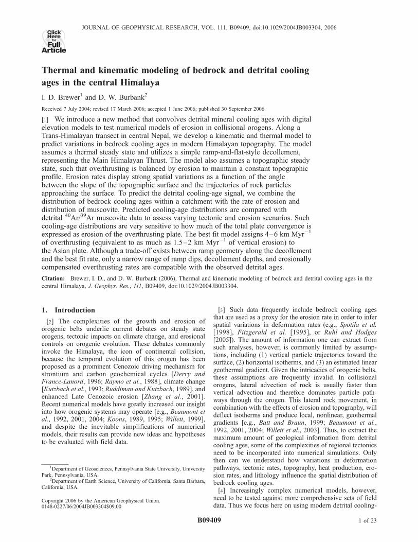
Figure 1. Location of the Marsyandi drainage basin and the study area, aligned with the strike of theorogen. The white dot indicates the location of the detrital thermochronological sample at the mouth ofthe Marsyandi catchment (S-24 [Brewer et al., 2006]). The topography is derived from a 90-m DEM andGTOPO30 where 90-m data are missing. The approximate location of the topographic axis and the majorfaults are shown for reference. The hatched area shows a representation of the strike-parallel swath that isscrolled normal to the strike to define mean topographic characteristics (see Figure 3). Inset showsgeneral location of study area. MBT, Main Boundary Thrust; MFT, Main Frontal Thrust; MCT, MainCentral Thrust; STD, South Tibetan Detachment.


3 of 23

B09409

of Quaternary faults within the Lesser Himalaya [Wobus etal., 2003, 2005].

3. Thermal and Kinematic Modeling

[14] As opposed to simple vertical motion of rocks, lateraladvection during continental collision often represents thedominant component of the deformation field [Willett,1999]. Yet, within the geochronological community, coolingages have typically been interpreted considering only onedimension, with erosion rates calculated assuming that therock column is moving vertically toward the surface [e.g.,Fitzgerald et al., 1995]. In contrast to most such studies,Harrison et al. [1998] and Jamieson et al. [2002, 2004]used 2-D kinematic-and-thermal modeling to investigateanatexis and metamorphism in the Himalaya. Their modelsshould provide a better comparison to thermochronologicaldata because bedrock ages are predicted by tracing particletrajectories through the orogen.[15] We adopt a similar approach and present a 2-D

kinematic-and-thermal model to determine the depth ofthe closure temperature and calculate the path of rockparticles through an orogenic transect. To do this, we definea decollement geometry within the Himalaya (section 3.1)and specify the thermal characteristics of the orogen (sec-tion 3.2). We subsequently extrapolate the 2-D solution

along strike to predict the 3-D spatial distribution ofbedrock cooling ages over the entire landscape (Figure 2).Correcting for spatial variations in the abundance of thetarget mineral for dating (section 3.3), GIS software allowsus to use the resulting ‘‘age maps’’ to extract a modeleddetrital cooling-age signal. We then compare signals pre-dicted from different scenarios to observed detrital coolingages [Brewer et al., 2006] to assess which model parametersare consistent with the data and to test the model’s sensi-tivity to variations in these parameters.

3.1. Constraints on Thrust Geometry

[16] In an active orogen, a bedrock cooling age representsthe time elapsed since a rock particle passed through theclosure temperature and subsequently reached the surface.Therefore, in order to predict a bedrock cooling age, weneed to know (1) the position of the closure isotherm withrespect to the surface, (2) the particle trajectory toward thesurface, and (3) the rate of particle transport along thistrajectory. Because of the strong dependence of the thermalstructure on the rate of rock advection toward the surface[Batt and Brandon, 2002; Mancktelow and Grasemann,1997; Stuwe et al., 1994], the kinematic structure of themountain belt is a primary parameter to constrain. Bycombining heat production with the velocity (speed anddirection) of particles through the orogen, we model thermal

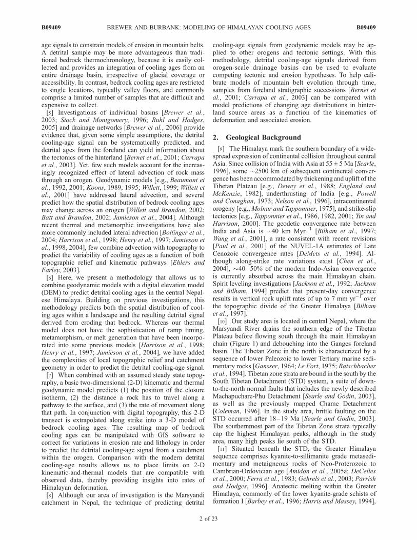
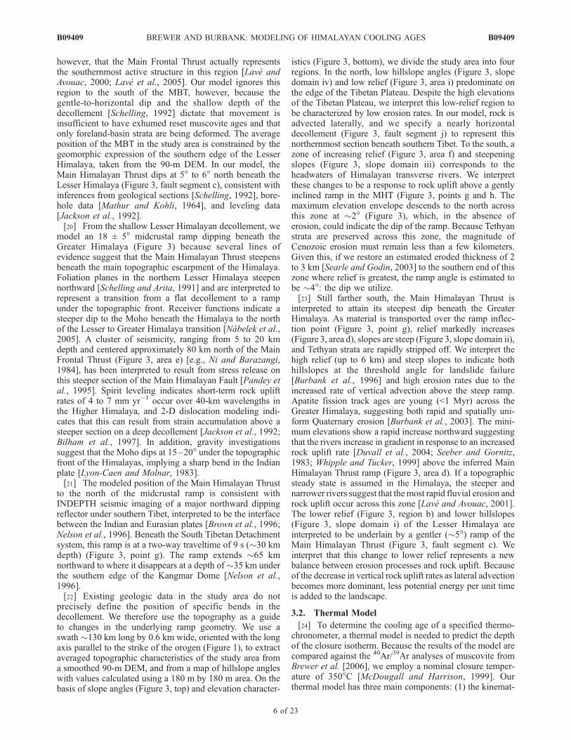
Figure 2. Conceptual basis for the combined thermal, kinematic, and detrital model. With a simplifiedramp flat geometry and known overthrusting rate, the velocity (speed and trajectory angle) of particlesthrough the orogen can be calculated. Within the predetermined kinematic framework, the thermalstructure after 20 Myr is calculated, and the depth of the closure temperature (white dashed line) formuscovite (350�C) is extracted. The 2-D thermal structure is extrapolated along strike into threedimensions, and a 90-m DEM is used to calculate how long it takes each point in the landscape to passfrom the depth of the closure isotherm to the surface along the specified particle path (distance of theblack arrows divided by the overthrusting rate of Eurasia with respect to the decollement/surfacesingularity (DSS) which is used as a reference marker). The youngest ages are created by trajectory bbecause the 350�C isotherm is closest to the surface along this trajectory. Trajectory a produces the oldestcooling ages because it travels along a flat (under the Lesser Himalaya) before reaching the surface.Particles moving along trajectory c travel the further than trajectory b and give intermediate ages, whereastrajectory d advects rock into the orogen above the closure temperature and so can be assigned an originalrock age. The insert depicts a hypothetical probability (P) distribution of detrital ages from the outlinedcatchment.


4 of 23

B09409

conditions and, more specifically, the position of the closureisotherm.[17] We invoke several simplifications and assumptions

to define the kinematic structure. First, we use a 2-D model.Because of sparse subsurface structural data, it is necessaryto extrapolate geometrical constraints along strike to cali-brate our modeled transect. Given the remarkable lateralcontinuity in the overall structure of the Himalayan orogen[Hodges, 2000], a 2-D approximation is probably reason-able for the along-strike scale of 100 to 200 km in ourmodel. Second, despite the complex structural architectureof the Himalaya, we use a single decollement to model thekinematics. A major plate-scale decollement, the MainHimalayan Thrust, has been proposed to underlie theHimalaya, with surface faults soling out into this decolle-ment [Bollinger et al., 2004; Schelling, 1992; Seeber et al.,1981]. Third, we specify a decollement comprising planarsegments that meet at kink bends [Suppe, 1983]. Whereasfew data exist to assess whether, at the scale of theHimalayan orogenic belt, fault surfaces are approximatelyplanar and fault dips change abruptly (as assumed with kink

bends), these assumptions do allow simple tracking ofparticle paths.[18] Because our focus is on the major kinematic char-

acteristics of the orogen, rather than local complexities, weadopt this simple orogenic-scale decollement model. Asimilar approach was taken by Henry et al. [1997], whomodeled the 2-D thermal structure of the Himalaya using asingle crustal-scale decollement dipping at 10� northwardfrom the surface outcrop of the Main Boundary Thrust. Weuse a more complex decollement that has 4 dip domains(Figures 2 and 3), with kink band folding in the overlyingthrust sheet, to mimic the assumed large-scale structure ofthe orogen [Lave and Avouac, 2001; Bollinger et al., 2004].In our analysis, the Main Himalayan Thrust is defined as themain active boundary between the Indian and Asian plates,even though rocks derived from the Indian plate have beenaccreted to the Asian plate and now lie above the basaldetachment to form the modern Himalaya.[19] With our simplified structure, the Main Boundary

Thrust (MBT) represents the surface expression of the MainHimalayan Thrust (Figure 3, point a). It is recognized,

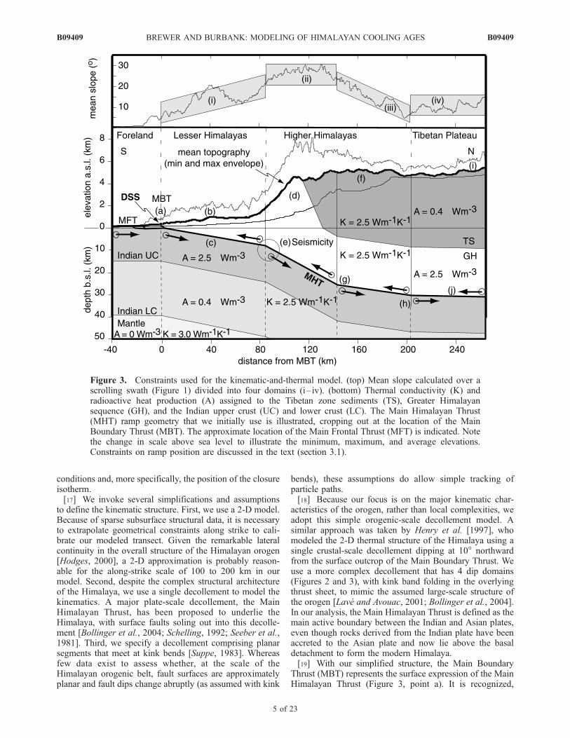
Figure 3. Constraints used for the kinematic-and-thermal model. (top) Mean slope calculated over ascrolling swath (Figure 1) divided into four domains (i–iv). (bottom) Thermal conductivity (K) andradioactive heat production (A) assigned to the Tibetan zone sediments (TS), Greater Himalayansequence (GH), and the Indian upper crust (UC) and lower crust (LC). The Main Himalayan Thrust(MHT) ramp geometry that we initially use is illustrated, cropping out at the location of the MainBoundary Thrust (MBT). The approximate location of the Main Frontal Thrust (MFT) is indicated. Notethe change in scale above sea level to illustrate the minimum, maximum, and average elevations.Constraints on ramp position are discussed in the text (section 3.1).


5 of 23

B09409

however, that the Main Frontal Thrust actually representsthe southernmost active structure in this region [Lave andAvouac, 2000; Lave et al., 2005]. Our model ignores thisregion to the south of the MBT, however, because thegentle-to-horizontal dip and the shallow depth of thedecollement [Schelling, 1992] dictate that movement isinsufficient to have exhumed reset muscovite ages and thatonly foreland-basin strata are being deformed. The averageposition of the MBT in the study area is constrained by thegeomorphic expression of the southern edge of the LesserHimalaya, taken from the 90-m DEM. In our model, theMain Himalayan Thrust dips at 5� to 6� north beneath theLesser Himalaya (Figure 3, fault segment c), consistent withinferences from geological sections [Schelling, 1992], bore-hole data [Mathur and Kohli, 1964], and leveling data[Jackson et al., 1992].[20] From the shallow Lesser Himalayan decollement, we

model an 18 ± 5� midcrustal ramp dipping beneath theGreater Himalaya (Figure 3) because several lines ofevidence suggest that the Main Himalayan Thrust steepensbeneath the main topographic escarpment of the Himalaya.Foliation planes in the northern Lesser Himalaya steepennorthward [Schelling and Arita, 1991] and are interpreted torepresent a transition from a flat decollement to a rampunder the topographic front. Receiver functions indicate asteeper dip to the Moho beneath the Himalaya to the northof the Lesser to Greater Himalaya transition [Nabelek et al.,2005]. A cluster of seismicity, ranging from 5 to 20 kmdepth and centered approximately 80 km north of the MainFrontal Thrust (Figure 3, area e) [e.g., Ni and Barazangi,1984], has been interpreted to result from stress release onthis steeper section of the Main Himalayan Fault [Pandey etal., 1995]. Spirit leveling indicates short-term rock upliftrates of 4 to 7 mm yr�1 occur over 40-km wavelengths inthe Higher Himalaya, and 2-D dislocation modeling indi-cates that this can result from strain accumulation above asteeper section on a deep decollement [Jackson et al., 1992;Bilham et al., 1997]. In addition, gravity investigationssuggest that the Moho dips at 15–20� under the topographicfront of the Himalayas, implying a sharp bend in the Indianplate [Lyon-Caen and Molnar, 1983].[21] The modeled position of the Main Himalayan Thrust

to the north of the midcrustal ramp is consistent withINDEPTH seismic imaging of a major northward dippingreflector under southern Tibet, interpreted to be the interfacebetween the Indian and Eurasian plates [Brown et al., 1996;Nelson et al., 1996]. Beneath the South Tibetan Detachmentsystem, this ramp is at a two-way traveltime of 9 s (�30 kmdepth) (Figure 3, point g). The ramp extends �65 kmnorthward to where it disappears at a depth of�35 km underthe southern edge of the Kangmar Dome [Nelson et al.,1996].[22] Existing geologic data in the study area do not

precisely define the position of specific bends in thedecollement. We therefore use the topography as a guideto changes in the underlying ramp geometry. We use aswath �130 km long by 0.6 km wide, oriented with the longaxis parallel to the strike of the orogen (Figure 1), to extractaveraged topographic characteristics of the study area froma smoothed 90-m DEM, and from a map of hillslope angleswith values calculated using a 180 m by 180 m area. On thebasis of slope angles (Figure 3, top) and elevation character-

istics (Figure 3, bottom), we divide the study area into fourregions. In the north, low hillslope angles (Figure 3, slopedomain iv) and low relief (Figure 3, area i) predominate onthe edge of the Tibetan Plateau. Despite the high elevationsof the Tibetan Plateau, we interpret this low-relief region tobe characterized by low erosion rates. In our model, rock isadvected laterally, and we specify a nearly horizontaldecollement (Figure 3, fault segment j) to represent thisnorthernmost section beneath southern Tibet. To the south, azone of increasing relief (Figure 3, area f) and steepeningslopes (Figure 3, slope domain iii) corresponds to theheadwaters of Himalayan transverse rivers. We interpretthese changes to be a response to rock uplift above a gentlyinclined ramp in the MHT (Figure 3, points g and h. Themaximum elevation envelope descends to the north acrossthis zone at �2� (Figure 3), which, in the absence oferosion, could indicate the dip of the ramp. Because Tethyanstrata are preserved across this zone, the magnitude ofCenozoic erosion must remain less than a few kilometers.Given this, if we restore an estimated eroded thickness of 2to 3 km [Searle and Godin, 2003] to the southern end of thiszone where relief is greatest, the ramp angle is estimated tobe �4�: the dip we utilize.[23] Still farther south, the Main Himalayan Thrust is

interpreted to attain its steepest dip beneath the GreaterHimalaya. As material is transported over the ramp inflec-tion point (Figure 3, point g), relief markedly increases(Figure 3, area d), slopes are steep (Figure 3, slope domain ii),and Tethyan strata are rapidly stripped off. We interpret thehigh relief (up to 6 km) and steep slopes to indicate bothhillslopes at the threshold angle for landslide failure[Burbank et al., 1996] and high erosion rates due to theincreased rate of vertical advection above the steep ramp.Apatite fission track ages are young (<1 Myr) across theGreater Himalaya, suggesting both rapid and spatially uni-form Quaternary erosion [Burbank et al., 2003]. The mini-mum elevations show a rapid increase northward suggestingthat the rivers increase in gradient in response to an increasedrock uplift rate [Duvall et al., 2004; Seeber and Gornitz,1983; Whipple and Tucker, 1999] above the inferred MainHimalayan Thrust ramp (Figure 3, area d). If a topographicsteady state is assumed in the Himalaya, the steeper andnarrower rivers suggest that themost rapid fluvial erosion androck uplift occur across this zone [Lave and Avouac, 2001].The lower relief (Figure 3, region b) and lower hillslopes(Figure 3, slope domain i) of the Lesser Himalaya areinterpreted to be underlain by a gentler (�5�) ramp of theMain Himalayan Thrust (Figure 3, fault segment c). Weinterpret that this change to lower relief represents a newbalance between erosion processes and rock uplift. Becauseof the decrease in vertical rock uplift rates as lateral advectionbecomes more dominant, less potential energy per unit timeis added to the landscape.

3.2. Thermal Model

[24] To determine the cooling age of a specified thermo-chronometer, a thermal model is needed to predict the depthof the closure isotherm. Because the results of the model arecompared against the 40Ar/39Ar analyses of muscovite fromBrewer et al. [2006], we employ a nominal closure temper-ature of 350�C [McDougall and Harrison, 1999]. Ourthermal model has three main components: (1) the kinemat-


6 of 23

B09409

ics which are controlled by the decollement geometry (asdiscussed) coupled with rates of overthrusting and erosion,(2) the geometry and thermal properties assigned to eachthermo-lithological unit (radioactive heat production, con-ductivity, and diffusivity), and (3) a shear heating term thatrepresents frictional heating on the main decollement. Theparameterization of our thermal model (Figure 3) closelyresembles that of Henry et al. [1997], with a thermallyinhomogeneous crust underlain by mantle characterized bynegligible heat production and a conductivity of 3.0 W(m �K)�1 [Schatz and Simmons, 1972]. The Indian crust isassumed to be bilayered with a 15-km-thick upper crustwith heat production of 2.5 �W m�3 [England et al., 1992],and a 25-km-thick lower crust with heat production of0.4 �W m�3 [Pinet, 1992]. With our kinematic model,the Lesser Himalaya and the Greater Himalaya sequencefunction as a single tectonic unit and are assigned a heatproduction of 2.5 �W m�3 due to high concentrations ofradioactive elements [England et al., 1992].[25] The thickness of the Greater Himalaya sequence

varies laterally within the Marsyandi study area, perhapsdue to South Tibetan Detachment system normal faulting atthe top of the slab (which is not included in this model).Nevertheless, we specify a constant thickness of 22 km forthe Greater Himalaya sequence that is consistent with theINDEPTH geological section, measured from the MainHimalayan Thrust to the South Tibetan Detachment system[Nelson et al., 1996]. As a consequence, Tethyan rocks cropout on the highest peaks in our model, matching the typicalgeology of the range [Colchen et al., 1986]. Because of thenormal faulting and lateral thickness variations, however,the thickness of 22 km is simply a thermal parameter forthe model, rather than an accurate predictor of the surfaceoutcrop of Tethyan strata. Because they contain a lowerabundance of radioactive isotopes, the Tethyan strataare assigned heat production of 0.4 �W m�3. Crustalconductivity and thermal diffusivity are set uniformly to2.5 W (m �K)�1 and 0.8 mm2 s�1, respectively. Thesurface boundary condition is set to 0�C, with the mor-phology of the interface determined by the mean elevation(Figure 3).[26] Because of our 2-D approach, the cooling effects of

relief variations along strike are ignored, and when extrap-olating the thermal model laterally, we assume no signifi-cant deflection of the 350�C isotherm by local topography[Brewer et al., 2006]. The basal boundary is set to aconstant mantle heat flow of 15 �W m�2 that is consistentwith values from Precambrian cratons [Gupta, 1993]. Aconstant geothermal gradient is applied to lateral boundariesexperiencing an influx of rock mass into model space, whilezero heat flow boundaries are specified if there is a net lossof mass from the system. A shear heating term, described byHenry et al. [1997], is used to account for frictional heatingalong the basal decollement fault. Heat production is afunction of the shear stress and strain rate in both the brittleand the ductile regime. Shear stress is calculated asthe minimum of a brittle lithostatic pressure-dependentlaw (1/10th the lithostatic pressure) or a ductile tempera-ture-dependent power law, with parameters taken from themoderate friction flow law of Hansen and Carter [1982]. Inthe ductile regime, the fault zone is 1000 m wide andundergoes uniform strain and heating. This model predicts

that the brittle-to-ductile transition occurs at �420�C in theundeformed Indian Plate (see discussion by Henry et al.[1997]).[27] The initial condition of the model is set by calculat-

ing a geothermal gradient [Pollack, 1965] for the thermalstructure undergoing no heat advection. A 2-D finite differ-ence algorithm [Fletcher, 1991] is used to define thethermal structure after �20 Myr of advection of rock massthrough the orogen. This approximates a steady statesolution, given the thermal response times of the 350�Cisotherm: from initial static conditions, for a crustal columnundergoing vertical erosion from depths of 35 km at rates of0.1 to 3.0 km Myr�1, 90 to 95% of the steady state solutionis obtained in <10 Myr [Brewer et al., 2003]. The morphol-ogy of the surface boundary in our model is not time-dependent, i.e., the topography is in steady state and, as aconsequence, spatial fluctuations in the mean elevationacross the orogen are invariant over timescales >1 Myrand spatial scales of >100 km. This implies that the rockinflux into the orogenic front by overthrusting is necessarilybalanced by denudation over these timescales.

3.3. Particle Trajectories and DetritalCooling-Age Signals

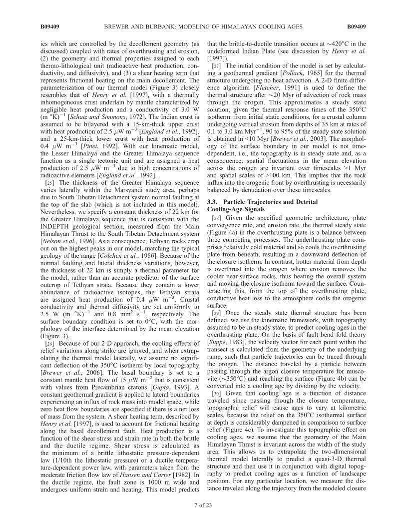
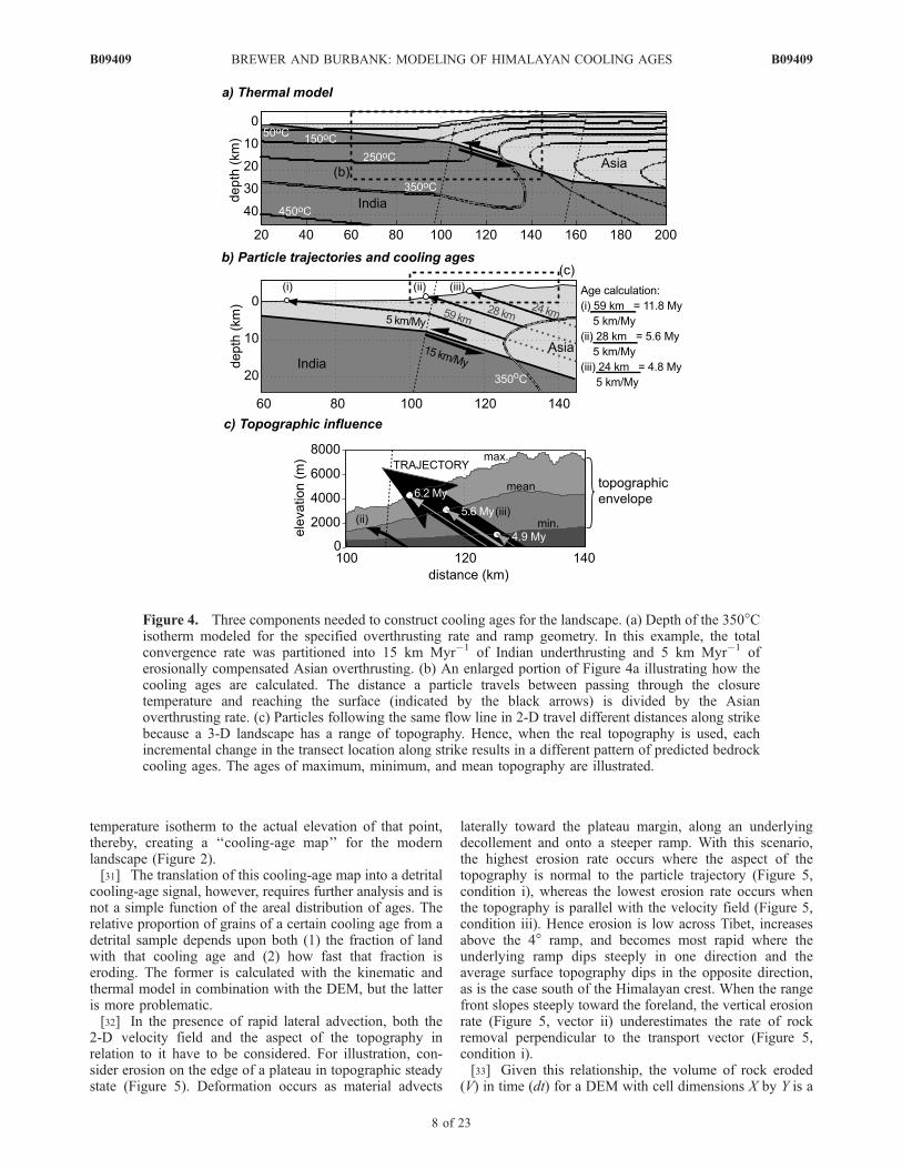
[28] Given the specified geometric architecture, plateconvergence rate, and erosion rate, the thermal steady state(Figure 4a) in the overthrusting plate is a balance betweenthree competing processes. The underthrusting plate com-prises relatively cold material and so cools the overthrustingplate from beneath, resulting in a downward deflection ofthe closure isotherm. In contrast, hotter material from depthis overthrust into the orogen where erosion removes thecooler near-surface rocks, thus heating the overall systemand moving the closure isotherm toward the surface. Coun-teracting this, from the top of the overthrusting plate,conductive heat loss to the atmosphere cools the orogenicsurface.[29] Once the steady state thermal structure has been

defined, we use the kinematic framework, with topographyassumed to be in steady state, to predict cooling ages in theoverthrusting plate. On the basis of fault bend fold theory[Suppe, 1983], the velocity vector for each point within thetransect is calculated from the geometry of the underlyingramp, such that particle trajectories can be traced throughthe orogen. The distance traveled by a particle betweenpassing through the argon closure temperature for musco-vite (�350�C) and reaching the surface (Figure 4b) can beconverted into a cooling age by dividing by the velocity.[30] Given that cooling age is a function of distance

traveled since passing though the closure temperature,topographic relief will cause ages to vary at kilometricscales, because the relief on the 350�C isothermal surfaceat depth is considerably dampened in comparison to surfacerelief (Figure 4c). To investigate this topographic effect oncooling ages, we assume that the geometry of the MainHimalayan Thrust is invariant across the width of the studyarea. This allows us to extrapolate the two-dimensionalthermal model laterally to predict a quasi-3-D thermalstructure and then use it in conjunction with digital topog-raphy to predict cooling ages as a function of landscapeposition. For any particular location, we measure the dis-tance traveled along the trajectory from the modeled closure


7 of 23

B09409

temperature isotherm to the actual elevation of that point,thereby, creating a ‘‘cooling-age map’’ for the modernlandscape (Figure 2).[31] The translation of this cooling-age map into a detrital

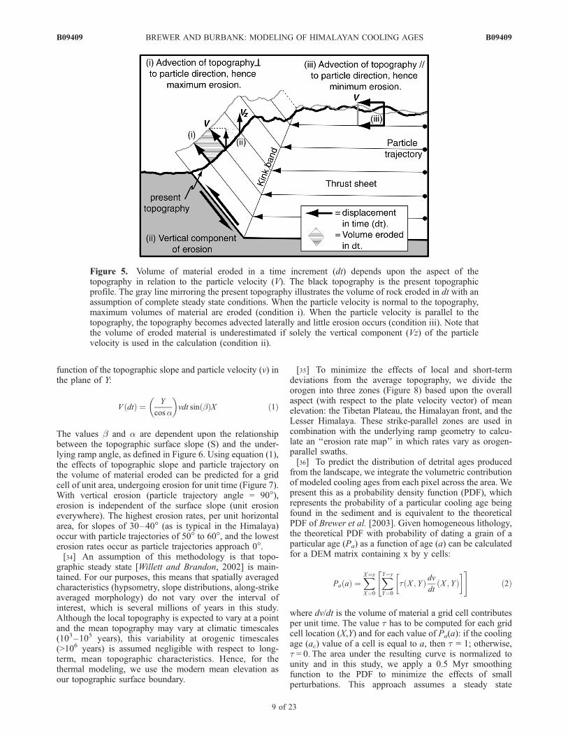
cooling-age signal, however, requires further analysis and isnot a simple function of the areal distribution of ages. Therelative proportion of grains of a certain cooling age from adetrital sample depends upon both (1) the fraction of landwith that cooling age and (2) how fast that fraction iseroding. The former is calculated with the kinematic andthermal model in combination with the DEM, but the latteris more problematic.[32] In the presence of rapid lateral advection, both the

2-D velocity field and the aspect of the topography inrelation to it have to be considered. For illustration, con-sider erosion on the edge of a plateau in topographic steadystate (Figure 5). Deformation occurs as material advects

laterally toward the plateau margin, along an underlyingdecollement and onto a steeper ramp. With this scenario,the highest erosion rate occurs where the aspect of thetopography is normal to the particle trajectory (Figure 5,condition i), whereas the lowest erosion rate occurs whenthe topography is parallel with the velocity field (Figure 5,condition iii). Hence erosion is low across Tibet, increasesabove the 4� ramp, and becomes most rapid where theunderlying ramp dips steeply in one direction and theaverage surface topography dips in the opposite direction,as is the case south of the Himalayan crest. When the rangefront slopes steeply toward the foreland, the vertical erosionrate (Figure 5, vector ii) underestimates the rate of rockremoval perpendicular to the transport vector (Figure 5,condition i).[33] Given this relationship, the volume of rock eroded

(V) in time (dt) for a DEM with cell dimensions X by Y is a

Figure 4. Three components needed to construct cooling ages for the landscape. (a) Depth of the 350�Cisotherm modeled for the specified overthrusting rate and ramp geometry. In this example, the totalconvergence rate was partitioned into 15 km Myr�1 of Indian underthrusting and 5 km Myr�1 oferosionally compensated Asian overthrusting. (b) An enlarged portion of Figure 4a illustrating how thecooling ages are calculated. The distance a particle travels between passing through the closuretemperature and reaching the surface (indicated by the black arrows) is divided by the Asianoverthrusting rate. (c) Particles following the same flow line in 2-D travel different distances along strikebecause a 3-D landscape has a range of topography. Hence, when the real topography is used, eachincremental change in the transect location along strike results in a different pattern of predicted bedrockcooling ages. The ages of maximum, minimum, and mean topography are illustrated.


8 of 23

B09409

function of the topographic slope and particle velocity (v) inthe plane of Y:

V dtð Þ ¼ Y

cos�

� �vdt sin �ð ÞX ð1Þ

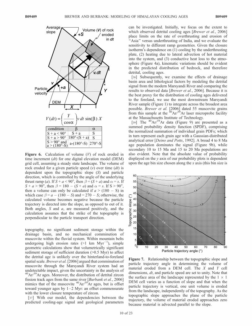
The values � and � are dependent upon the relationshipbetween the topographic surface slope (S) and the under-lying ramp angle, as defined in Figure 6. Using equation (1),the effects of topographic slope and particle trajectory onthe volume of material eroded can be predicted for a gridcell of unit area, undergoing erosion for unit time (Figure 7).With vertical erosion (particle trajectory angle = 90�),erosion is independent of the surface slope (unit erosioneverywhere). The highest erosion rates, per unit horizontalarea, for slopes of 30–40� (as is typical in the Himalaya)occur with particle trajectories of 50� to 60�, and the lowesterosion rates occur as particle trajectories approach 0�.[34] An assumption of this methodology is that topo-

graphic steady state [Willett and Brandon, 2002] is main-tained. For our purposes, this means that spatially averagedcharacteristics (hypsometry, slope distributions, along-strikeaveraged morphology) do not vary over the interval ofinterest, which is several millions of years in this study.Although the local topography is expected to vary at a pointand the mean topography may vary at climatic timescales(103–105 years), this variability at orogenic timescales(>106 years) is assumed negligible with respect to long-term, mean topographic characteristics. Hence, for thethermal modeling, we use the modern mean elevation asour topographic surface boundary.

[35] To minimize the effects of local and short-termdeviations from the average topography, we divide theorogen into three zones (Figure 8) based upon the overallaspect (with respect to the plate velocity vector) of meanelevation: the Tibetan Plateau, the Himalayan front, and theLesser Himalaya. These strike-parallel zones are used incombination with the underlying ramp geometry to calcu-late an ‘‘erosion rate map’’ in which rates vary as orogen-parallel swaths.[36] To predict the distribution of detrital ages produced

from the landscape, we integrate the volumetric contributionof modeled cooling ages from each pixel across the area. Wepresent this as a probability density function (PDF), whichrepresents the probability of a particular cooling age beingfound in the sediment and is equivalent to the theoreticalPDF of Brewer et al. [2003]. Given homogeneous lithology,the theoretical PDF with probability of dating a grain of aparticular age (Pa) as a function of age (a) can be calculatedfor a DEM matrix containing x by y cells:

Pa að Þ ¼XX¼x

X¼0

XY¼y

Y¼0

� X ; Yð Þ dvdt

X ; Yð Þ� �" #

ð2Þ

where dv/dt is the volume of material a grid cell contributesper unit time. The value � has to be computed for each gridcell location (X,Y) and for each value of Pa(a): if the coolingage (ac) value of a cell is equal to a, then � = 1; otherwise,� = 0. The area under the resulting curve is normalized tounity and in this study, we apply a 0.5 Myr smoothingfunction to the PDF to minimize the effects of smallperturbations. This approach assumes a steady state

Figure 5. Volume of material eroded in a time increment (dt) depends upon the aspect of thetopography in relation to the particle velocity (V). The black topography is the present topographicprofile. The gray line mirroring the present topography illustrates the volume of rock eroded in dt with anassumption of complete steady state conditions. When the particle velocity is normal to the topography,maximum volumes of material are eroded (condition i). When the particle velocity is parallel to thetopography, the topography becomes advected laterally and little erosion occurs (condition iii). Note thatthe volume of eroded material is underestimated if solely the vertical component (Vz) of the particlevelocity is used in the calculation (condition ii).


9 of 23

B09409

topography, no significant sediment storage within thedrainage basin, and no mechanical comminution ofmuscovite within the fluvial system. Within mountain beltsundergoing high erosion rates (>1 km Myr�1), simplegeometric calculations show that volumetrically significantsediment storage of sufficient duration (>0.5 Myr) to affectthe detrital age is unlikely over the hinterland-to-forelandspatial scale.Brewer et al. [2006] argued that comminution ofmuscovite through the Marsyandi River system had anundetectable impact, given the uncertainty in the analysis of40Ar/39Ar ages. Moreover, the distribution of detrital zirconfission track ages from the same river [Burbank et al., 2006]mimics that of the muscovite 40Ar/39Ar ages, but is offsettoward younger ages by 1–2 Myr: an offset commensuratewith the lower closure temperature of zircon.[37] With our model, the dependencies between the

predicted cooling-age signal and geological parameters

can be investigated. Initially, we focus on the extent towhich observed detrital cooling ages [Brewer et al., 2006]place limits on the rate of overthrusting and erosion of‘‘Asia’’ versus underthrusting of India, and we evaluate thesensitivity to different ramp geometries. Given the closureisotherm’s dependence on (1) cooling by the underthrustingplate, (2) heating due to lateral advection of hot materialinto the system, and (3) conductive heat loss to the atmo-sphere (Figure 4a), kinematic variations should be evidentin the predicted distribution of bedrock, and thereforedetrital, cooling ages.[38] Subsequently, we examine the effects of drainage

basin area and lithological factors by modeling the detritalsignal from the modern Marsyandi River and comparing theresults to observed data [Brewer et al., 2006]. Because it isthe best proxy for the distribution of cooling ages deliveredto the foreland, we use the most downstream MarsyandiRiver sample (Figure 1) to integrate across the broadest areapossible. Brewer et al. [2006] dated 55 muscovite grainsfrom this sample at the 40Ar/39Ar laser microprobe facilityat the Massachusetts Institute of Technology.[39] The 40Ar/39Ar data (Figure 9) are presented as a

summed probability density function (SPDF), comprisingthe normalized summation of individual grain PDFs; whichin turn represent each grain age with a Gaussian-distributedanalytical error [Deino and Potts, 1992]. A broad 4 to 8 Maage population dominates the signal (Figure 9b), whilesecondary 10 to 15 Ma and 15 to 20 Ma populations arealso evident. Note that the absolute value of probabilitydisplayed on the y axis of our probability plots is dependentupon the age bin size chosen along the x axis (this bin size is

Figure 6. Calculation of volume (V) of rock eroded intime increment (dt) for one digital elevation model (DEM)grid cell, assuming a steady state landscape. The volume ofrock eroded for a given particle speed (v) over time (dt) isdependent upon the topographic slope (S) and particledirection, which is controlled by the angle of the underlyingthrust ramp (a). If S + a < 90�, then � = (S + a) and � = s. IfS + a > 90�, then � = 180 � (S + a) and � = s. If S > 90�,then a volume can only be calculated if a > (180 � S) inwhich case � = a � (180 � S) and = 270 � S; otherwise, thecalculated volume becomes negative because the particletrajectory is directed into the slope, as opposed to out of it.Both angles, S and a, are measured positively, and thecalculation assumes that the strike of the topography isperpendicular to the particle transport direction.

Figure 7. Relationship between the topographic slope andparticle trajectory angle in determining the volume ofmaterial eroded from a DEM cell. The X and Y celldimensions, dt, and particle speed are set to unity. Note thatthe surface area of the landscape represented by the 1 � 1DEM cell varies as a function of slope and that when theparticle trajectory is vertical, one unit volume is erodedfrom the landscape, independently of the topography. As thetopographic slope approaches the plane of the particletrajectory, the volume of material eroded approaches zerobecause material is advected parallel to the slope.


10 of 23

B09409

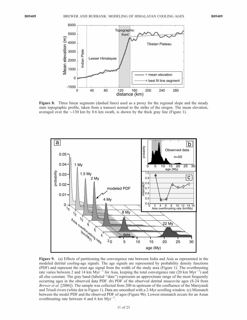
Figure 8. Three linear segments (dashed lines) used as a proxy for the regional slope and the steadystate topographic profile, taken from a transect normal to the strike of the orogen. The mean elevation,averaged over the �130 km by 0.6 km swath, is shown by the thick gray line (Figure 1).

Figure 9. (a) Effects of partitioning the convergence rate between India and Asia as represented in themodeled detrital cooling-age signals. The age signals are represented by probability density functions(PDF) and represent the reset age signal from the width of the study area (Figure 1). The overthrustingrate varies between 2 and 14 km Myr�1 for Asia, keeping the total convergence rate (20 km Myr�1) andall else constant. The gray band (labeled ‘‘data’’) represents an approximate range of the most frequentlyoccurring ages in the observed data PDF. (b) PDF of the observed detrital muscovite ages (S-24 fromBrewer et al. [2006]). The sample was collected from 200 m upstream of the confluence of the Marsyandiand Trisuli rivers (white dot in Figure 1). Data are smoothed with a 2-Myr scrolling window. (c) Mismatchbetween the model PDF and the observed PDF of ages (Figure 9b). Lowest mismatch occurs for an Asianoverthrusting rate between 4 and 6 km Myr�1.


11 of 23

B09409

constant in all plots to allow the direct comparison ofrelative probability).

4. Himalayan Kinematics and Controls onCooling Ages

4.1. Kinematics: Asian Overthrustingand Erosion Rates

[40] Geodetic studies suggest that the convergence rate ofIndia with southern Tibet ranges from 13 to 21 km Myr�1

[Bilham et al., 1997; Wang et al., 2001; Juanne et al., 2004]and geologic studies in the Himalayan foreland [Lave andAvouac, 2000] yield well-defined convergence rates aver-aging �20 km Myr�1 over the past 9 kyr. We thereforeassign a rate of 20 km Myr�1 to represent the Indo-Tibetanconvergence, but need to partition this between Indianunderthrusting and Asian overthrusting. For this model,

the intersection of the Main Himalayan Thrust decollementwith surface topography (decollement/surface singularity(DSS), Figure 3) is our reference frame; this theoreticalpoint is independent of how total convergence is partitionedbetween the two plates.[41] Notably, in the absence of erosion, no difference

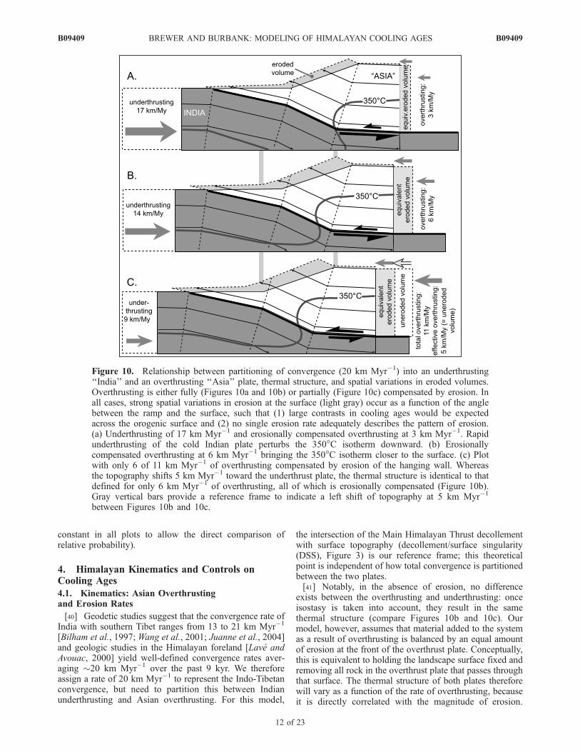
exists between the overthrusting and underthrusting: onceisostasy is taken into account, they result in the samethermal structure (compare Figures 10b and 10c). Ourmodel, however, assumes that material added to the systemas a result of overthrusting is balanced by an equal amountof erosion at the front of the overthrust plate. Conceptually,this is equivalent to holding the landscape surface fixed andremoving all rock in the overthrust plate that passes throughthat surface. The thermal structure of both plates thereforewill vary as a function of the rate of overthrusting, becauseit is directly correlated with the magnitude of erosion.

Figure 10. Relationship between partitioning of convergence (20 km Myr�1) into an underthrusting‘‘India’’ and an overthrusting ‘‘Asia’’ plate, thermal structure, and spatial variations in eroded volumes.Overthrusting is either fully (Figures 10a and 10b) or partially (Figure 10c) compensated by erosion. Inall cases, strong spatial variations in erosion at the surface (light gray) occur as a function of the anglebetween the ramp and the surface, such that (1) large contrasts in cooling ages would be expectedacross the orogenic surface and (2) no single erosion rate adequately describes the pattern of erosion.(a) Underthrusting of 17 km Myr�1 and erosionally compensated overthrusting at 3 km Myr�1. Rapidunderthrusting of the cold Indian plate perturbs the 350�C isotherm downward. (b) Erosionallycompensated overthrusting at 6 km Myr�1 bringing the 350�C isotherm closer to the surface. (c) Plotwith only 6 of 11 km Myr�1 of overthrusting compensated by erosion of the hanging wall. Whereasthe topography shifts 5 km Myr�1 toward the underthrust plate, the thermal structure is identical to thatdefined for only 6 km Myr�1 of overthrusting, all of which is erosionally compensated (Figure 10b).Gray vertical bars provide a reference frame to indicate a left shift of topography at 5 km Myr�1

between Figures 10b and 10c.


12 of 23

B09409

Partitioning of the remaining convergence (that which is notcompensated by erosion) into overthrusting or underthrust-ing has no additional effect on thermal structure. Therefore,for the sake of simplicity, we assign to the underthrustingIndian plate all convergence that is not erosionally compen-sated. We choose to use the term ‘‘overthrusting rate’’,rather than erosion, to indicate the rate at which materialenters the model and is removed from the hanging wall,thereby maintaining mass balance. The rate at which mate-rial moves vertically toward the topographic surface variesas a function of ramp angle, such that the erosion rate variesspatially in the overthrusting plate and no single value canbe assigned to it (Figure 10). Because partitioning ofconvergence into underthrusting and erosionally compen-sated overthrusting affects the calculated thermal and ve-locity structure of the system, it modulates the predicted

cooling ages. Consequently, this partitioning becomes aprimary unknown, yet testable, variable.[42] Simulations indicate that detrital cooling ages are

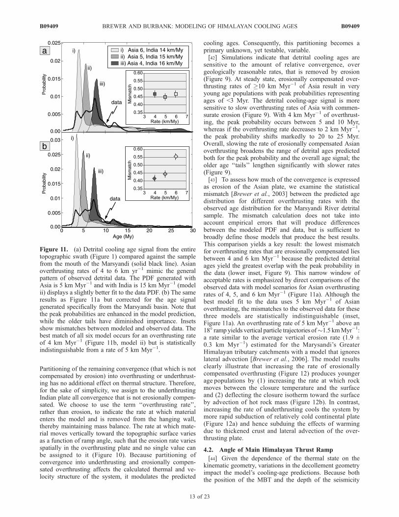
sensitive to the amount of relative convergence, overgeologically reasonable rates, that is removed by erosion(Figure 9). At steady state, erosionally compensated over-thrusting rates of �10 km Myr�1 of Asia result in veryyoung age populations with peak probabilities representingages of <3 Myr. The detrital cooling-age signal is moresensitive to slow overthrusting rates of Asia with commen-surate erosion (Figure 9). With 4 km Myr�1 of overthrust-ing, the peak probability occurs between 5 and 10 Myr,whereas if the overthrusting rate decreases to 2 km Myr�1,the peak probability shifts markedly to 20 to 25 Myr.Overall, slowing the rate of erosionally compensated Asianoverthrusting broadens the range of detrital ages predictedboth for the peak probability and the overall age signal; theolder age ‘‘tails’’ lengthen significantly with slower rates(Figure 9).[43] To assess how much of the convergence is expressed

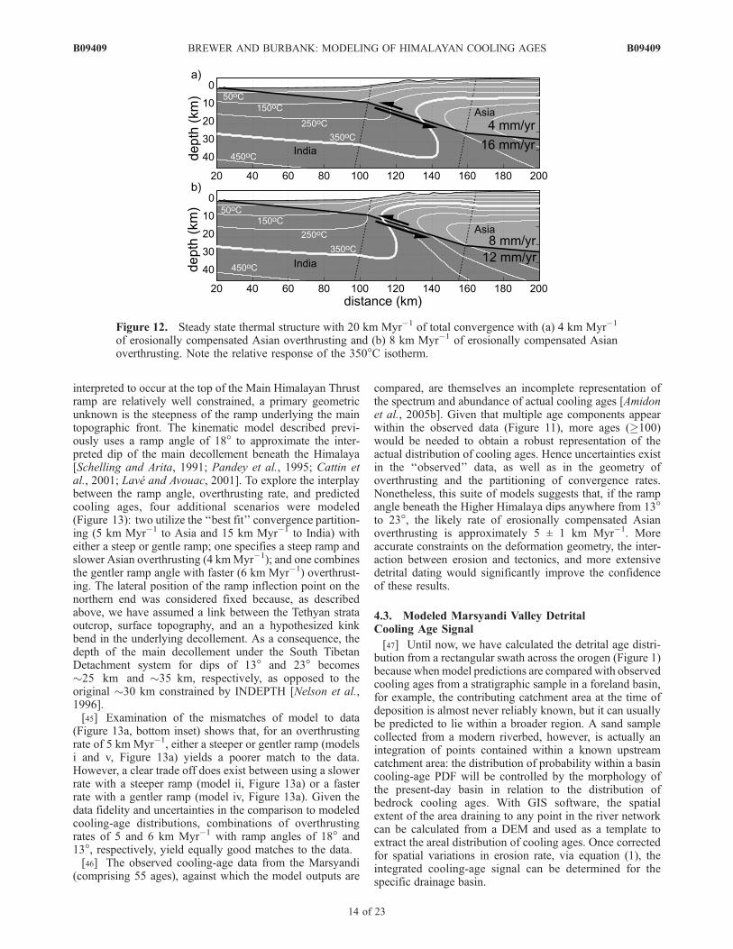
as erosion of the Asian plate, we examine the statisticalmismatch [Brewer et al., 2003] between the predicted agedistribution for different overthrusting rates with theobserved age distribution for the Marsyandi River detritalsample. The mismatch calculation does not take intoaccount empirical errors that will produce differencesbetween the modeled PDF and data, but is sufficient tobroadly define those models that produce the best results.This comparison yields a key result: the lowest mismatchfor overthrusting rates that are erosionally compensated liesbetween 4 and 6 km Myr�1 because the predicted detritalages yield the greatest overlap with the peak probability inthe data (lower inset, Figure 9). This narrow window ofacceptable rates is emphasized by direct comparisons of theobserved data with model scenarios for Asian overthrustingrates of 4, 5, and 6 km Myr�1 (Figure 11a). Although thebest model fit to the data uses 5 km Myr�1 of Asianoverthrusting, the mismatches to the observed data for thesethree models are statistically indistinguishable (inset,Figure 11a). An overthrusting rate of 5 km Myr�1 above an18� ramp yields vertical particle trajectories of�1.5 kmMyr�1:a rate similar to the average vertical erosion rate (1.9 ±0.3 km Myr�1) estimated for the Marysandi’s GreaterHimalayan tributary catchments with a model that ignoreslateral advection [Brewer et al., 2006]. The model resultsclearly illustrate that increasing the rate of erosionallycompensated overthrusting (Figure 12) produces youngerage populations by (1) increasing the rate at which rockmoves between the closure temperature and the surfaceand (2) deflecting the closure isotherm toward the surfaceby advection of hot rock mass (Figure 12b). In contrast,increasing the rate of underthrusting cools the system bymore rapid subduction of relatively cold continental plate(Figure 12a) and hence subduing the effects of warmingdue to thickened crust and lateral advection of the over-thrusting plate.

4.2. Angle of Main Himalayan Thrust Ramp

[44] Given the dependence of the thermal state on thekinematic geometry, variations in the decollement geometryimpact the model’s cooling-age predictions. Because boththe position of the MBT and the depth of the seismicity

Figure 11. (a) Detrital cooling age signal from the entiretopographic swath (Figure 1) compared against the samplefrom the mouth of the Marsyandi (solid black line). Asianoverthrusting rates of 4 to 6 km yr�1 mimic the generalpattern of observed detrital data. The PDF generated withAsia is 5 km Myr�1 and with India is 15 km Myr�1 (modelii) displays a slightly better fit to the data PDF. (b) The sameresults as Figure 11a but corrected for the age signalgenerated specifically from the Marsyandi basin. Note thatthe peak probabilities are enhanced in the model prediction,while the older tails have diminished importance. Insetsshow mismatches between modeled and observed data. Thebest match of all six model occurs for an overthrusting rateof 4 km Myr�1 (Figure 11b, model ii) but is statisticallyindistinguishable from a rate of 5 km Myr�1.


13 of 23

B09409

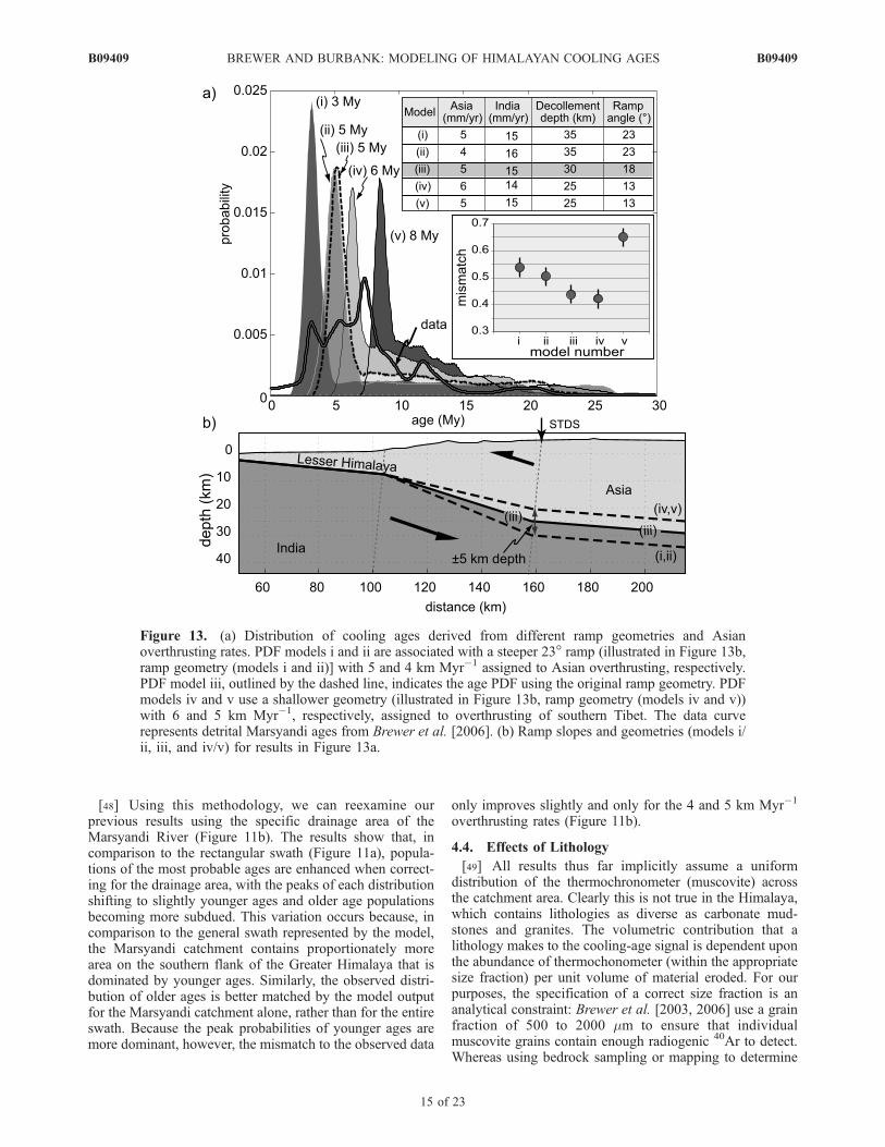
interpreted to occur at the top of the Main Himalayan Thrustramp are relatively well constrained, a primary geometricunknown is the steepness of the ramp underlying the maintopographic front. The kinematic model described previ-ously uses a ramp angle of 18� to approximate the inter-preted dip of the main decollement beneath the Himalaya[Schelling and Arita, 1991; Pandey et al., 1995; Cattin etal., 2001; Lave and Avouac, 2001]. To explore the interplaybetween the ramp angle, overthrusting rate, and predictedcooling ages, four additional scenarios were modeled(Figure 13): two utilize the ‘‘best fit’’ convergence partition-ing (5 km Myr�1 to Asia and 15 km Myr�1 to India) witheither a steep or gentle ramp; one specifies a steep ramp andslower Asian overthrusting (4 kmMyr�1); and one combinesthe gentler ramp angle with faster (6 km Myr�1) overthrust-ing. The lateral position of the ramp inflection point on thenorthern end was considered fixed because, as describedabove, we have assumed a link between the Tethyan strataoutcrop, surface topography, and an a hypothesized kinkbend in the underlying decollement. As a consequence, thedepth of the main decollement under the South TibetanDetachment system for dips of 13� and 23� becomes�25 km and �35 km, respectively, as opposed to theoriginal �30 km constrained by INDEPTH [Nelson et al.,1996].[45] Examination of the mismatches of model to data

(Figure 13a, bottom inset) shows that, for an overthrustingrate of 5 km Myr�1, either a steeper or gentler ramp (modelsi and v, Figure 13a) yields a poorer match to the data.However, a clear trade off does exist between using a slowerrate with a steeper ramp (model ii, Figure 13a) or a fasterrate with a gentler ramp (model iv, Figure 13a). Given thedata fidelity and uncertainties in the comparison to modeledcooling-age distributions, combinations of overthrustingrates of 5 and 6 km Myr�1 with ramp angles of 18� and13�, respectively, yield equally good matches to the data.[46] The observed cooling-age data from the Marsyandi

(comprising 55 ages), against which the model outputs are

compared, are themselves an incomplete representation ofthe spectrum and abundance of actual cooling ages [Amidonet al., 2005b]. Given that multiple age components appearwithin the observed data (Figure 11), more ages (�100)would be needed to obtain a robust representation of theactual distribution of cooling ages. Hence uncertainties existin the ‘‘observed’’ data, as well as in the geometry ofoverthrusting and the partitioning of convergence rates.Nonetheless, this suite of models suggests that, if the rampangle beneath the Higher Himalaya dips anywhere from 13�to 23�, the likely rate of erosionally compensated Asianoverthrusting is approximately 5 ± 1 km Myr�1. Moreaccurate constraints on the deformation geometry, the inter-action between erosion and tectonics, and more extensivedetrital dating would significantly improve the confidenceof these results.

4.3. Modeled Marsyandi Valley DetritalCooling Age Signal

[47] Until now, we have calculated the detrital age distri-bution from a rectangular swath across the orogen (Figure 1)because whenmodel predictions are compared with observedcooling ages from a stratigraphic sample in a foreland basin,for example, the contributing catchment area at the time ofdeposition is almost never reliably known, but it can usuallybe predicted to lie within a broader region. A sand samplecollected from a modern riverbed, however, is actually anintegration of points contained within a known upstreamcatchment area: the distribution of probability within a basincooling-age PDF will be controlled by the morphology ofthe present-day basin in relation to the distribution ofbedrock cooling ages. With GIS software, the spatialextent of the area draining to any point in the river networkcan be calculated from a DEM and used as a template toextract the areal distribution of cooling ages. Once correctedfor spatial variations in erosion rate, via equation (1), theintegrated cooling-age signal can be determined for thespecific drainage basin.

Figure 12. Steady state thermal structure with 20 km Myr�1 of total convergence with (a) 4 km Myr�1

of erosionally compensated Asian overthrusting and (b) 8 km Myr�1 of erosionally compensated Asianoverthrusting. Note the relative response of the 350�C isotherm.


14 of 23

B09409

[48] Using this methodology, we can reexamine ourprevious results using the specific drainage area of theMarsyandi River (Figure 11b). The results show that, incomparison to the rectangular swath (Figure 11a), popula-tions of the most probable ages are enhanced when correct-ing for the drainage area, with the peaks of each distributionshifting to slightly younger ages and older age populationsbecoming more subdued. This variation occurs because, incomparison to the general swath represented by the model,the Marsyandi catchment contains proportionately morearea on the southern flank of the Greater Himalaya that isdominated by younger ages. Similarly, the observed distri-bution of older ages is better matched by the model outputfor the Marsyandi catchment alone, rather than for the entireswath. Because the peak probabilities of younger ages aremore dominant, however, the mismatch to the observed data

only improves slightly and only for the 4 and 5 km Myr�1

overthrusting rates (Figure 11b).

4.4. Effects of Lithology

[49] All results thus far implicitly assume a uniformdistribution of the thermochronometer (muscovite) acrossthe catchment area. Clearly this is not true in the Himalaya,which contains lithologies as diverse as carbonate mud-stones and granites. The volumetric contribution that alithology makes to the cooling-age signal is dependent uponthe abundance of thermochonometer (within the appropriatesize fraction) per unit volume of material eroded. For ourpurposes, the specification of a correct size fraction is ananalytical constraint: Brewer et al. [2003, 2006] use a grainfraction of 500 to 2000 �m to ensure that individualmuscovite grains contain enough radiogenic 40Ar to detect.Whereas using bedrock sampling or mapping to determine

Figure 13. (a) Distribution of cooling ages derived from different ramp geometries and Asianoverthrusting rates. PDF models i and ii are associated with a steeper 23� ramp (illustrated in Figure 13b,ramp geometry (models i and ii)] with 5 and 4 km Myr�1 assigned to Asian overthrusting, respectively.PDF model iii, outlined by the dashed line, indicates the age PDF using the original ramp geometry. PDFmodels iv and v use a shallower geometry (illustrated in Figure 13b, ramp geometry (models iv and v))with 6 and 5 km Myr�1, respectively, assigned to overthrusting of southern Tibet. The data curverepresents detrital Marsyandi ages from Brewer et al. [2006]. (b) Ramp slopes and geometries (models i/ii, iii, and iv/v) for results in Figure 13a.


15 of 23

B09409

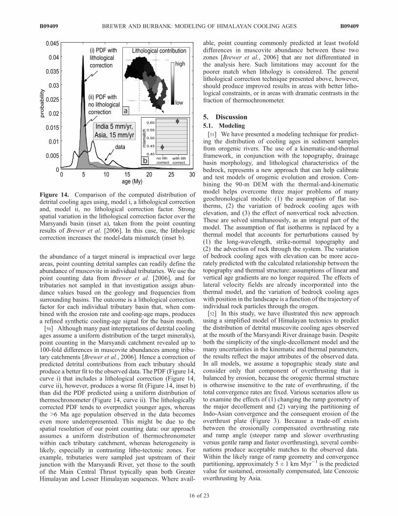
the abundance of a target mineral is impractical over largeareas, point counting detrital samples can readily define theabundance of muscovite in individual tributaries. We use thepoint counting data from Brewer et al. [2006], and fortributaries not sampled in that investigation assign abun-dance values based on the geology and frequencies fromsurrounding basins. The outcome is a lithological correctionfactor for each individual tributary basin that, when com-bined with the erosion rate and cooling-age maps, producesa refined synthetic cooling-age signal for the basin mouth.[50] Although many past interpretations of detrital cooling

ages assume a uniform distribution of the target mineral(s),point counting in the Marsyandi catchment revealed up to100-fold differences in muscovite abundances among tribu-tary catchments [Brewer et al., 2006]. Hence a correction ofpredicted detrital contributions from each tributary shouldproduce a better fit to the observed data. The PDF (Figure 14,curve i) that includes a lithological correction (Figure 14,curve ii), however, produces a worse fit (Figure 14, inset b)than did the PDF predicted using a uniform distribution ofthermochronometer (Figure 14, curve ii). The lithologicallycorrected PDF tends to overpredict younger ages, whereasthe >6 Ma age population observed in the data becomeseven more underrepresented. This might be due to thespatial resolution of our point counting data: our approachassumes a uniform distribution of thermochronometerwithin each tributary catchment, whereas heterogeneity islikely, especially in contrasting litho-tectonic zones. Forexample, tributaries were sampled just upstream of theirjunction with the Marsyandi River, yet those to the southof the Main Central Thrust typically span both GreaterHimalayan and Lesser Himalayan sequences. Where avail-

able, point counting commonly predicted at least twofolddifferences in muscovite abundance between these twozones [Brewer et al., 2006] that are not differentiated inthe analysis here. Such limitations may account for thepoorer match when lithology is considered. The generallithological correction technique presented above, however,should produce improved results in areas with better litho-logical constraints, or in areas with dramatic contrasts in thefraction of thermochronometer.

5. Discussion

5.1. Modeling

[51] We have presented a modeling technique for predict-ing the distribution of cooling ages in sediment samplesfrom orogenic rivers. The use of a kinematic-and-thermalframework, in conjunction with the topography, drainagebasin morphology, and lithological characteristics of thebedrock, represents a new approach that can help calibrateand test models of orogenic evolution and erosion. Com-bining the 90-m DEM with the thermal-and-kinematicmodel helps overcome three major problems of manygeochronological models: (1) the assumption of flat iso-therms, (2) the variation of bedrock cooling ages withelevation, and (3) the effect of nonvertical rock advection.These are solved simultaneously, as an integral part of themodel. The assumption of flat isotherms is replaced by athermal model that accounts for perturbations caused by(1) the long-wavelength, strike-normal topography and(2) the advection of rock through the system. The variationof bedrock cooling ages with elevation can be more accu-rately predicted with the calculated relationship between thetopography and thermal structure: assumptions of linear andvertical age gradients are no longer required. The effects oflateral velocity fields are already incorporated into thethermal model, and the variation of bedrock cooling ageswith position in the landscape is a function of the trajectory ofindividual rock particles through the orogen.[52] In this study, we have illustrated this new approach

using a simplified model of Himalayan tectonics to predictthe distribution of detrital muscovite cooling ages observedat the mouth of the Marsyandi River drainage basin. Despiteboth the simplicity of the single-decollement model and themany uncertainties in the kinematic and thermal parameters,the results reflect the major attributes of the observed data.In all models, we assume a topographic steady state andconsider only that component of overthrusting that isbalanced by erosion, because the orogenic thermal structureis otherwise insensitive to the rate of overthrusting, if thetotal convergence rates are fixed. Various scenarios allow usto examine the effects of (1) changing the ramp geometry ofthe major decollement and (2) varying the partitioning ofIndo-Asian convergence and the consequent erosion of theoverthrust plate (Figure 3). Because a trade-off existsbetween the erosionally compensated overthrusting rateand ramp angle (steeper ramp and slower overthrustingversus gentle ramp and faster overthrusting), several combi-nations produce acceptable matches to the observed data.Within the likely range of ramp geometry and convergencepartitioning, approximately 5 ± 1 km Myr�1 is the predictedvalue for sustained, erosionally compensated, late Cenozoicoverthrusting by Asia.

Figure 14. Comparison of the computed distribution ofdetrital cooling ages using, model i, a lithological correctionand, model ii, no lithological correction factor. Strongspatial variation in the lithological correction factor over theMarsyandi basin (inset a), taken from the point countingresults of Brewer et al. [2006]. In this case, the lithologiccorrection increases the model-data mismatch (inset b).


16 of 23

B09409

[53] Throughout this model and similar to other bedrockcooling models for the Himalaya [e.g., Jamieson et al.,2004], we have assumed the commonly cited closuretemperature of 350�C for muscovite. Given the mean coolingrate in the model, an average closure temperature of 380�Ccould be more appropriate [Dodson, 1973]. On the basis ofthe modeled variations in rates of cooling in this study,�90%of our ages would be predicted to have closure temperaturesof 380� ± 10�C. By ignoring such rate-dependent varia-tions, we introduced an additional uncertainty into thecalculated mismatches. The magnitude of this effect,however, is modest compared to other uncertainties inthe model. For example, the most rapidly cooled rocksin the model (14 km Myr�1 of overthrusting and erosion,Figure 9), would be most affected by use of a low closuretemperature, but utilization of a higher closure temperaturewould only shift the predicted mean age �0.1 Myr andwould have little impact on the calculated mismatch to thedata. Our interpretations of which overthrusting rates orkinematic geometry provide the best matches to the datawould be unchanged, if a nonuniform closure temperaturehad been incorporated.[54] We have assessed the agreement between various

models and the observed data by comparing the fractionalmismatch between their associated PDFs [Brewer et al.,2003]. Whereas pronounced differences in the magnitude ofmismatch exist among some models (e.g., Figure 9), nomodel has <40% mismatch. These mismatches are primarily

due to the apparent overprediction of the abundance ofyoung cooling ages in most model runs and to the omissionof empirical grain age errors in the model PDFs. Although asmaller mismatch could be achieved by tuning the modelusing more complex ramp geometries and variable over-thrusting rates, few data exist to further constrain thesevariables. Additional possible explanations for these persis-tent mismatches include (1) violations of the assumption ofa thermal steady state over the duration of the modeledinterval and (2) an observed age distribution that does notaccurately reflect the actual cooling age distribution. If, forexample, the rate of erosion had accelerated in the last fewmillion years, the model could correctly predict the youngcooling ages, but would underpredict the residuum of olderages that would be derived from the highest topography orregions with the longest path length from the closureisotherm to the surface. Indeed, apatite fission track datesthat average �0.5 Ma for bedrock samples along theMarsyandi valley in the Greater Himalaya [Burbank et al.,2003] require Quaternary cooling rates approaching 300�CMyr�1 and would support an interpretation of acceleratedrates of cooling and erosion in the past 1 to 2 Myr. Ourobserved data PDF comprises only 55 ages. Samplingstatistics of complex distributions of actual ages [Amidonet al., 2005b; Anderson, 2005] suggest persistent mis-matches of �20%, even when 100 ages are drawn fromand then matched against a known age distribution.

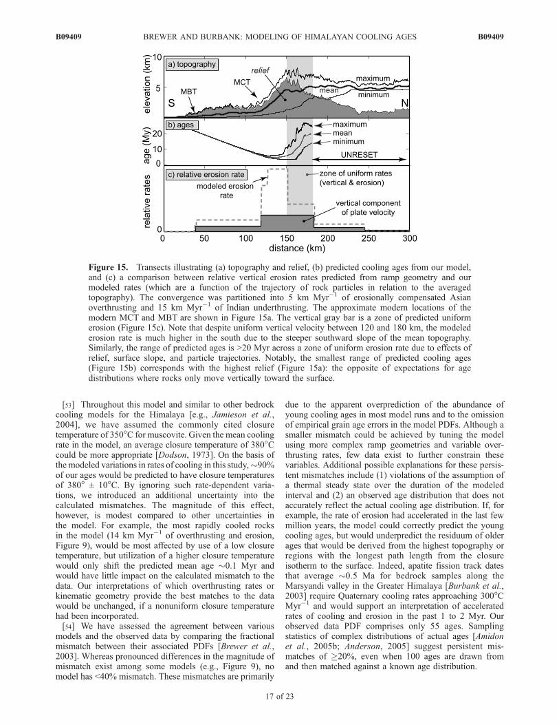
Figure 15. Transects illustrating (a) topography and relief, (b) predicted cooling ages from our model,and (c) a comparison between relative vertical erosion rates predicted from ramp geometry and ourmodeled rates (which are a function of the trajectory of rock particles in relation to the averagedtopography). The convergence was partitioned into 5 km Myr�1 of erosionally compensated Asianoverthrusting and 15 km Myr�1 of Indian underthrusting. The approximate modern locations of themodern MCT and MBT are shown in Figure 15a. The vertical gray bar is a zone of predicted uniformerosion (Figure 15c). Note that despite uniform vertical velocity between 120 and 180 km, the modelederosion rate is much higher in the south due to the steeper southward slope of the mean topography.Similarly, the range of predicted ages is >20 Myr across a zone of uniform erosion rate due to effects ofrelief, surface slope, and particle trajectories. Notably, the smallest range of predicted cooling ages(Figure 15b) corresponds with the highest relief (Figure 15a): the opposite of expectations for agedistributions where rocks only move vertically toward the surface.


17 of 23

B09409

[55] To illustrate some of the differences between ourapproach and traditional thermochronology, we examine thepredictions of our optimal model along a strike-normaltransect (Figure 15). The predicted bedrock cooling ages(Figure 15b) increase both northward over the topographicfront and southward over the Lesser Himalaya as a functionof particle trajectory (Figure 2). We can compare thedistribution of ages to (1) the erosion rate predicted fromour model of erosion rate (equation (1)) and (2) thatpredicted using only the vertical component of the over-thrusting vector (Figure 15c). The former predicts muchhigher volumes of rock eroded from the topographic frontalregion, whereas the latter predicts uniform volumes erodedacross broach swaths of the orogen. This contrast occursbecause, with lateral advection, the erosion rate is a sensi-tive function of both ramp angle and of topographic slopeand orientation, whereas the vertical component dependsonly on ramp angle.[56] Both models, however, suggest significant variations

in bedrock cooling age across modeled zones of equalerosion. Within a zone for which both models predictuniform erosion (shaded region in Figure 15), the modeledcooling ages vary from a minimum of �3 Myr to amaximum of �28 Myr. This range has important implica-tions because traditional thermochronological approaches,assuming vertical erosion and horizontal isotherms, couldinterpret such cooling rates (120�C Myr�1 versus 12�CMyr�1) to represent up to tenfold differences in relativeerosion rates, instead of the actual uniform rate. Furthermore,the mean cooling ages across this zone of uniform erosionvary by �15 Myr, ranging from 5 to 20 Ma (Figure 15b).This striking difference is a consequence of where particlepaths within the orogen intersect the 350�C isotherm: oldermean cooling ages represent rocks that cooled and moved tothe surface on a gently inclined trajectory beneath theTibetan Plateau, whereas younger ages correspond withrocks that cooled within the Greater Himalaya and movedto the surface on a much steeper trajectory. The impact oflateral advection on cooling ages increases in importance asthe rate of lateral movement approaches or exceeds thevertical rates, i.e., for ramp angles <45�, as is common inmost convergent orogens. Our model results emphasizethat, when cooling-rate studies are used as a proxy forerosion, the effects of both lateral advection and reliefneed to be integrated into the analysis whenever possi-ble, especially in convergent orogenic belts [Batt andBrandon, 2002; Batt and Braun, 1999; Willett andBrandon, 2002].[57] Notably, the correspondence between the range of

cooling ages and topographic relief (Figure 15) is markedlydifferent than that predicted for ‘‘vertical relief sections’’.Within a zone of uniform erosion in vertical motion models,the greatest topographic relief should correspond with thelargest range of cooling ages. Whereas this could also betrue for a lateral advection model, our results predict just theopposite for the central Himalaya: the smallest range of agescorresponds with the greatest relief (Figure 15). On average,the largest range of cooling ages is found north of the highHimalayan peaks where the difference between the shortestand longest particle pathways between the valley bottomsand summits is maximized.

[58] Some verification of the model can be undertaken bycomparing the predicted range of ages from a particular partof the orogen (Figure 15b) with observed ages from thatarea. For example, the model predicts ages ranging from�10 to 25 Ma in the region of the north of the highestpeaks, and observed detrital ages for that region (sample Ain Figure 16) display a range from �9 to 22 Ma [Brewer etal., 2006]. Closer to the MCT, the model predicts bothyounger ages and a more restricted range of ages. Data fromthree tributary catchments that straddle the MCT (samplesx, y, z in Figure 16) record ages primarily between 2 and10 Ma [Brewer et al., 2006]. The model also suggests thatthe preponderant zone of erosion will occur on the southernflank of the Himalaya (Figure 15c). Such erosion shouldproduce a significant influx of young cooling ages from thispart of the orogen. In fact, the young ages emerging fromcatchments on the southern flank of the range (samples x, y, zin Figure 16) appear to largely overwhelm the older detritalages from the upstream samples, as seen in the detrital sampleat the mouth of the Marsyandi (sample C in Figure 16).Further testing of the model could involve extracting specifictributary catchments from the DEM and comparing the PDFsof modeled ages from these catchments with observed agesfrom the same catchment. Such a test is beyond the scope ofthe present paper, but clearly the observed detrital ages areconsistent with the spatial trend in ages predicted by themodel.

5.2. Stratigraphic Record

[59] One major motivation for trying to understand how acooling-age signal is created is that, in addition to testingnumerical models of modern tectonics, dating detrital min-erals from the stratigraphic record provides a means toconstrain orogenic evolution through time [Bernet et al.,2001; Carrapa et al., 2003; Cerveny et al., 1998; Najman etal., 1997; White et al., 2002]. Such investigations are oftenimpractical using bedrock thermochronology, because sam-pling is typically limited to the rocks exposed at the surfacetoday.[60] This investigation indicates that the foreland cooling-

age data should be representative of the orogenic signalproviding that a major transverse river is sampled and thatthe hinterland does not vary widely along strike. Forexample, when comparing the entire swath (Figure 11a)and the Marsyandi valley (Figure 11b), the overall pattern re-mains consistent despite minor modifications of the cooling-age signal. Given the analytical uncertainties in single-crystaldating of Late Cenozoic basin sediments, small changes inthe areal extent of the drainage system through time shouldresult in insignificant changes in the observed age spectrum.Whether temporal changes in topographic characteristics,drainage basin shape, and lithological contribution couldbe extracted from the geological record would depend uponthe sensitivity of the thermochronometer and the numberof grains dated from the detrital sample [Brewer et al.,2003; Amidon et al., 2005b; Anderson, 2005]. In contrast,major changes in ramp geometry or the erosionally com-pensated overthrusting rate should be detectable. For exam-ple, doubling of the overthrusting rate is predicted to havea profound effect on the distribution of cooling ages(Figure 9) and should be readily observable in the detritalrecord. To extract maximum information, however, two


18 of 23

B09409

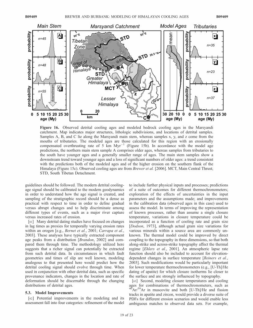
guidelines should be followed. The modern detrital cooling-age signal should be calibrated to the modern geodynamicsin order to understand how the age signal is created, andsampling of the stratigraphic record should be a dense aspractical with respect to time in order to define gradualversus abrupt changes and to help discriminate amongdifferent types of events, such as a major river captureversus increased rates of erosion.[61] Many detrital dating studies have focused on changes

in lag times as proxies for temporally varying erosion rateswithin an orogen [e.g., Bernet et al., 2001; Carrapa et al.,2003]. These analyses have typically extracted componentage peaks from a distribution [Brandon, 2002] and com-pared them through time. The methodology utilized heresuggests that a richer signal can potentially be extractedfrom such detrital data. In circumstances in which faultgeometries and times of slip are well known, modelinganalogous to that presented here would predict how thedetrital cooling signal should evolve through time. Whenused in conjunction with other detrital data, such as specificprovenance indicators, changes in the location and rate ofdeformation should be discernable through the changingdistributions of detrital ages.

5.3. Model Improvements

[62] Potential improvements in the modeling and itsassessment fall into four categories: refinement of the model

to include further physical inputs and processes; predictionsof a suite of outcomes for different thermochronometers;exploration of the effects of uncertainties in the inputparameters and the assumptions made; and improvementsin the calibration data (observed ages in this case) used toassess the model. In terms of improving the representationof known processes, rather than assume a single closuretemperature, variations in closure temperature could beincorporated as a function of cooling rate and grain size[Dodson, 1973], although actual grain size variations forvarious minerals within a source area are commonly un-known. The thermal model could be improved by directcoupling to the topography in three dimensions, so that bothalong-strike and across-strike topography affect the thermalregime [Ehlers et al., 2001]. An atmospheric lapse ratefunction should also be included to account for elevation-dependent changes in surface temperature [Reiners et al.,2003]. Such modifications would be particularly importantfor lower temperature thermochronometers (e.g., [U-Th]/Hedating of apatite) for which closure isotherms lie closer tothe surface and are strongly influenced by topography.[63] Second, modeling closure temperatures and cooling

ages for combinations of thermochronometers, such as40Ar/39Ar in muscovite and both [U-Th]/He and fissiontracks in apatite and zircon, would provide a diverse suite ofPDFs for different erosion scenarios and would enable lessambiguous matches to observed data sets. For example,

Figure 16. Observed detrital cooling ages and modeled bedrock cooling ages in the Marsyandicatchment. Map indicates major structures, lithologic subdivisions, and locations of detrital samples.Samples A, B, and C lie along the Marsyandi main stem, whereas samples x, y, and z come from themouths of tributaries. The modeled ages are those calculated for this region with an erosionallycompensated overthrusting rate of 5 km Myr�1 (Figure 15b). In accordance with the model agepredictions, the northern main stem sample A comprises older ages, whereas samples from tributaries tothe south have younger ages and a generally smaller range of ages. The main stem samples show adownstream trend toward younger ages and a loss of significant numbers of older ages: a trend consistentwith the predictions both of the modeled ages and of the higher erosion on the southern flank of theHimalaya (Figure 15c). Observed cooling ages are from Brewer et al. [2006]. MCT, Main Central Thrust;STD, South Tibetan Detachment.


19 of 23

B09409

modeling of two or more thermochronometers with higherand lower closure temperatures could define an accelerationin the rate of cooling or test the predicted minimum durationrequired to reach a thermal steady state. Reliance onminerals with higher closure temperatures, however, hasto be balanced against the assumptions of steady state orkinematic rates. The older the cooling ages, the more likelythat rates and topography have changed since the closuretemperature was passed by a rock now found at the surface.In order to test model predictions of ages, either individualor combinations of modeled thermochronometers could beextracted from DEM-defined tributaries across an orogenand then compared against observed detrital ages from thesame catchments. A robust model should predict spatialtrends of ages that are mimicked by observed detrital ages.[64] Third, many assumptions and simplifications, such

as the existence of thermal and topographic steady states orthe presence of a single, geometrically simple detachment,underpin the present model. In future work, the impact ofthese should be explored and more complex input data andcontrols should be used, as they become available. Remov-ing the thermal steady state assumption and allowingerosionally compensated overthrusting rates to change dur-ing a model run might, for example, provide a more realisticthermal evolution, if the many complications related tounknown changes in the surface topography and in thetiming of changes in rates could be constrained. For furtheranalysis, reliable field data are important both to define therange of acceptable model inputs and to provide goodcalibration data.[65] Although improved knowledge of heat production

and thermal conductivity would also be helpful, the geom-etry of the deformation system is the largest unknown.Balanced cross sections and seismic data can help definemore reliable fault geometries. Both the distributed natureof seismicity within many active orogens [e.g., Seeber et al.,1981] and predictions for deformation within criticallytapered wedges where differential erosion removes massin the wedge’s internal parts [Sobel et al., 2003; Wobus etal., 2003, 2005] indicate that single decollement models areunlikely to capture the complexity of actual deformationhistories [Pearson and DeCelles, 2005]. Incorporation ofadditional fault surfaces with known geometries into modelsand prediction of cooling ages resulting from slip alongthem would provide another template against which toassess and interpret observed data. In our model, the over-thrusting and underthrusting plates are persistently separatedby a single decollement and no material passes across thatfault. A model permitting transfer of material from theunderthrust to the overthrust plate would be more consistentwith the observed accretion from the underthrust plate to thehanging wall of the decollement. Such accretion couldexplain the presence of unrest ages in the Lesser Himalaya[Bollinger et al., 2004; Jamieson et al., 2004; Wobus et al.,2003].[66] In the northern reaches of the Marsyandi, recent

structural mapping suggests multiple, large-scale folds inthe northern Greater Himalaya [Searle and Godin, 2003],implying kinematic pathways that are more complicatedthan our simple fault bend fold model. In the BurhiGandaki, just east of the Marsyandi, an abrupt discontinuityin muscovite cooling ages occurs �20 km south of the MCT

and is interpreted as a major MCT footwall thrust [Wobus etal., 2003, 2005]. South of this zone, no Tertiary muscovitecooling ages are reported. Our kinematic model with asingle, uniformly dipping ramp extending to the MBT isincompatible with the absence of Tertiary cooling ages inthe southern Lesser Himalaya. Although Brewer et al.[2006] show that only 2 out of >200 detrital muscovitedates from catchments traversing the Lesser Himalaya in theMarsyandi have cooling ages >30 Ma, it is possible that aPaleozoic age signal from the Lesser Himalaya was unde-tected due to smaller mica grain sizes that were below ourcutoff for measurement. The conflicts in interpretationsdescribed above are relevant to the cross-sectional structuralgeometry of the orogen. Along-strike changes in kinematicsadd still further complexity to particle paths through theorogen. However, given the difficulty of defining the detailsof geometric and kinematic variability, simple kinematicmodels that capture the essence of a system without tryingto recreate every detail may be best for providing anunderstanding of the geological processes and interactionsthat affect the cooling-age signal.[67] In the context of comparing modeled age predictions

with observed detrital ages, our model does not explicitlyincorporate the variability introduced by using observeddata sets comprising limited numbers of grain ages (55 usedhere). Such age distributions almost always incompletelyrepresent the parent distribution from which they weredrawn. Rather than comparing observed data, containingN ages, with the PDF of all ages across the model space,Monte Carlo sampling of N predicted ages, with appropriateage uncertainties, from the modeled PDF [Brewer et al.,2003; Ruhl and Hodges, 2005] and statistical analysis of theMonte Carlo predictions would provide a better basis forassessing model-data mismatches.[68] Incorporation of spatial changes in the bedrock

abundance and grain size of target thermochronologicmineral(s) would improve predictions of how erosion ratesconvolve with mineralogic abundances to modulate thefrequency of cooling ages in a detrital sample. Whereaswe accounted for measured spatial changes in mica abun-dance, we ignored the effect of potential variations in micagrain size. For example, if Lesser Himalayan schists yieldabundant, but small micas (<500 �m), we would havemissed these because we only analyzed micas >500 �m.[69] Fourth, improvements in the quality of the observed

data would assist in choosing among diverse model pre-dictions. Rather than assuming that no downstream commi-nution occurs, tests of attrition could be implemented viacomparisons of age distributions for resistant (zircon) versusmore abrasion-susceptible (micas, apatite) minerals. Simi-larly, the grain size dependence of the age signal [Ruhl andHodges, 2005] could be routinely assessed, whereas in-creasing the number of detrital ages to >100 would producea more robust PDF for the purposes of comparison.

6. Conclusions

[70] Few previous kinematic-and-thermal chronologicalmodels have considered either detrital cooling-age signalsor the effects of actual topography upon the distribution ofcooling ages. In this paper, we have introduced a newmethod of combining digital elevation models with numer-


20 of 23

B09409

ical kinematic-and-thermal modeling to predict spatial var-iations in bedrock cooling ages. Once corrected for (1) therelative erosion rate and (2) the relative abundance of themineral utilized as a thermochronometer, the cooling-agesignal can be determined for any catchment area. Notably,even in regions overlying a planar thrust ramp, the erosionrate can vary considerably as a function of the anglebetween the average surface topography and particle trajec-tories approaching the surface. Because detrital mineralsamples are easily collected and dated, and also representan integration of information from a large spatial area, theyprovide a good method of rapid testing of increasinglycomplex numerical simulations. On the other hand, bedrocksampling to provide a comparable suite of observed ages isimpractical and may be impossible in high relief andglaciated alpine regions.[71] A striking model result is the prediction that, even

within a zone of uniform erosion in a convergent orogen, acooling age population can display a broad range of ages. Inthis study, the youngest and oldest model ages differ by afactor of 9, ranging from 3 to 28 Myr (Figure 15). Formodels in which rock only moves vertically toward thesurface at a uniform erosion rate, the largest range of agescorrelates with the largest topographic relief. In contrast,lateral advection of rocks causes the relationship betweenrelief and the range of cooling ages to decouple, and in thisparticular case study, the smallest range of ages within azone of uniform erosion occurs where the relief is highest.[72] We have applied this new methodology to modeling

the detrital cooling-age signal of the Marsyandi River incentral Nepal. The results illustrate that the distribution ofbedrock cooling ages is sensitive to the amount of over-thrusting that is compensated by erosion, because thiserosion modulates the thermal structure of the orogen. Witha single decollement, and the surface outcrop of the MBTrepresenting the modern Main Himalayan Thrust, the detri-tal cooling age data of Brewer et al. [2006] are most closelymatched by partitioning the total convergence rate betweenIndia and southern Tibet (�20 km Myr�1), such that �5 kmMyr�1 of Asian overthrusting is removed by erosion. In thecontext of the modeled distribution of bedrock cooling ages,a trade-off exists between ramp angle and erosion rates ofthe overthrust plate. Within reasonable geometrical limits onthe ramp, however, the partitioning of the convergence ratecan be constrained to approximately ±1 km Myr�1, given anappropriate thermal structure. The modification of thedetrital cooling-age signal by drainage basin shape anddistribution of thermochronometer is a secondary effectwithin the Marsyandi drainage basin.[73] This study provides insights into how the detrital

cooling-age signal reflects the deformation pattern within acollisional orogen. Detrital-mineral thermochronology canprovide an efficient way to test ideas of orogenic develop-ment, and the methodology introduced here can be com-bined with many other numerical models to predict thedistribution of detrital cooling ages. With better temporalcontrols on the timing and activity of faults, future kinematic-and-thermal models for the Himalaya would be greatlyimproved. The effects of topographic deflection of theclosure isotherm, particularly important for lower tempera-ture thermochronometers such as apatite fission track and(U-Th)/He dating, could be investigated with fully 3-D

thermal models. The greatest advantage to detrital, asopposed to bedrock, thermochronology is that the strati-graphic record provides a window into the past. Thereforesequential reconstructions of orogenic evolution, once cal-ibrated with the modern detrital cooling-age signal, can beassessed against detailed, quantitative field data derivedfrom foreland basin sediments.

[74] Acknowledgments. This work was funded by National ScienceFoundation grants EAR-9627865, EAR-9896048, and EAR-9909647.The Chevron Corporation also provided financial support. We thank R.Malserversi, C. Guzofski, and T. Ehlers for helpful discussions aboutthe thermal modeling, and K. Hodges and J. Lave for discussions ofHimalayan geology. This manuscript was significantly improved throughthe comments and questions of K. Whipple, J. Braun, R. Jamieson, and ananonymous reviewer.

ReferencesAmidon, W. H., D. W. Burbank, and G. E. Gehrels (2005a), Constructionof foreland mineral populations: Insights from mixing of U-Pb zirconages in Himalayan rivers, Basin Res., 17, 463 –485, doi:410.1111/j.1365-2117.2005.00279.x.

Amidon, W. H., D. W. Burbank, and G. E. Gehrels (2005b), U-Pb zirconages as a sediment mixing tracer in the Nepal Himalaya, Earth Planet.Sci. Lett., 235, 244–260.

Anderson, T. (2005), Detrital zircons as tracers of sedimentary provenance:Limiting conditions from statistics and numerical simulation, Chem.Geol., 216, 249–270.

Barbey, P., M. Brouand, P. Le Fort, and A. Pecher (1996), Granite-migma-tite genetic link: The example of the Manaslu Granite and Tibetan Slabmigmatites in central Nepal, Lithos, 38(1–2), 63–79.

Batt, G. E., and M. T. Brandon (2002), Lateral thinking: 2-D interpretationof thermochronology in convergent orogenic settings, Tectonophysics,349, 185–201.

Batt, G. E., and J. Braun (1999), The tectonic evolution of the SouthernAlps, New Zealand: Insights from fully thermally coupled dynamicalmodelling, Geophys. J. Int., 136, 403–420.

Beaumont, C., P. Fullsack, and J. Hamilton (1992), Erosional control ofactive compressional orogens, in Thrust Tectonics, edited by K. R.McClay, pp. 1–18, CRC Press, Boca Raton, Fla.

Beaumont, C., R. A. Jamieson, M. H. Nguyen, and B. Lee (2001), Hima-layan tectonics explained by extrusion of a low-viscosity crustal channelcoupled to focused surface denudation, Nature, 414, 738–742.

Beaumont, C., R. A. Jamieson, M. H. Nguyen, and S. Medvedev (2004),Crustal channel flows: 1. Numerical models with applications to thetectonics of the Himalayan-Tibetan orogen, J. Geophys. Res., 109,B06406, doi:10.1029/2003JB002809.

Bernet, M., M. Zattin, J. I. Garver, M. T. Brandon, and J. A. Vance (2001),Steady-state exhumation of the European Alps, Geology, 29, 35–38.

Bilham, R., K. Larson, J. Freymueller, and P. I. Members (1997), GPSmeasurements of present-day convergence across the Nepal Himalaya,Nature, 386, 61–64.

Bollinger, L., J. P. Avouac, O. Beyssac, E. J. Catlos, T. M. Harrison,M. Grove, B. Goffe, and S. Sapkota (2004), Thermal structureand exhumation history of the Lesser Himalaya in central Nepal,Tectonics, 23, TC5015, doi:10.1029/2003TC001564.

Brandon, M. T. (2002), Decomposition of mixed grain-age distributionsusing BINOMFIT, On Track, 24, 13–18.

Brewer, I. D., D. W. Burbank, and K. V. Hodges (2003), Modelling detritalcooling-age populations: Insights from two Himalayan catchments, BasinRes., 15, 305–320.

Brewer, I. D., D. W. Burbank, and K. V. Hodges (2006), Downstreamdevelopment of a detrital cooling-age signal: Insights from 40Ar/39Armuscovite thermochronology in the Nepalese Himalaya, in Tectonics,Climate, and Landscape Evolution, edited by S. D. Willett et al., Spec.Pap. Geol. Soc. Am., 398, 321–338, doi:10.1130/2006.2398(20).

Brown, L. D., W. Zhao, K. D. Nelson, M. Hauk, D. Alsdorf, A. Ross,M. Cogan, M. Clark, X. Liu, and J. Che (1996), Bright spots, struc-ture, and magmatism in Southern Tibet from INDEPTH seismic reflec-tion profiling, Science, 274, 1688–1690.

Burbank, D., J. Leland, E. Fielding, R. Anderson, N. Brozovic, M. Reid,and C. Duncan (1996), Bedrock incision, rock uplift and threshold hill-slopes in the northwestern Himalayas, Nature, 379, 505–510.

Burbank, D. W., A. E. Blythe, J. Putkonen, B. Pratt-Sitaula, E. Gabet,M. Oskin, A. Barros, and T. P. Ojha (2003), Decoupling of erosionand precipitation in the Himalayas, Nature, 426, 652–655.


21 of 23

B09409

Burbank, D. W., I. D. Brewer, E. R. Sobel, and M. E. Bullen (2006), Single-crystal dating and the detrital record of orogenesis, Int. Assoc. Sedimen-tol. Spec. Publ., in press.

Carrapa, B., J. Wijbrans, and G. Bertotti (2003), Episodic exhumation in thewestern Alps, Geology, 31, 601–604.

Catlos, E. J., T. M. Harrison, M. J. Kohn, M. Grove, F. J. Ryerson, C. E.Manning, and B. N. Upreti (2001), Geochronologic and thermobaro-metric constraints on the evolution of the Main Central Thrust, centralNepal Himalaya, J. Geophys. Res., 106, 16,177–16,204.

Cattin, R., G. Martelet, P. Henry, J. P. Avouac, M. Diament, and T. R.Shakya (2001), Gravity anomalies, crustal structure and thermo-mechan-ical support of the Himalaya of central Nepal, Geophys. J. Int., 147, 381–392.

Cerveny, P. F., N. D. Naeser, P. K. Zeitler, C. W. Naeser, and N. M. Johnson(1998), History of uplift and relief of the Himalaya during the past18 million years: Evidence from sandstones of the Siwalik Group, in NewPerspectives in Basin Analysis, edited by K. L. Kleinspehn and C. Paola,pp. 43–61, Springer, New York.

Chen, Q., J. T. Freymueller, Z. Yang, C. Xu, W. Jiang, Q. Wang, and J. Liu(2004), Spatially variable extension in southern Tibet based on GPS mea-surements, J. Geophys. Res., 109, B09401, doi:10.1029/2002JB002350.

Colchen, M., P. LeFort, and A. Pecher (1986), Annapurna–Manaslu–Ganesh Himal, 136 pp., Centre Natl. de la Rech. Sci., Paris.

Coleman, M. E. (1996), Orogen-parallel and orogen-perpendicular exten-sion in the central Nepalese Himalayas, Geol. Soc. Am. Bull., 108,1594–1607.

Coleman, M., and K. Hodges (1995), Evidence for Tibetan Plateau upliftbefore 14 Myr ago from a new minimum age for E-W extension, Nature,374, 49–52.

Copeland, P., R. Parrish, and M. Harrison (1988), Identification of inheritedradiogenic Pb in monazite and its implications for U-Pb systematics,Nature, 333, 760–763.

Copeland, P., T. M. Harrison, and P. Le Fort (1990), Age and cooling historyof the Manaslu granite: Implications for Himalayan tectonics, J. Volcanol.Geotherm. Res., 44, 33–50.

DeCelles, P. G., G. E. Gehrels, J. Quade, and T. P. Ojha (1998), Eocene-early Miocene foreland basin development and the history of Himalayanthrusting, western and central Nepal, Tectonics, 17, 741–765.

DeCelles, P. G., G. E. Gehrels, J. Quade, B. Lareau, and M. Spurlin (2000),Tectonic implications of U-Pb zircon ages of the Himalayan orogenic beltin Nepal, Science, 288, 497–499.

Deino, A., and R. Potts (1992), Age-probability spectra for examination ofsingle-crystal 40Ar/39Ar dating results: Examples from Olorgesailie,southern Kenya Rift, Quat. Int., 13/14, 47–53.

DeMets, C., R. G. Gordon, D. F. Argus, and D. Stein (1994), Effect ofrecent revisions to the geomagnetic reversal time scale and estimates ofcurrent plate motions, Geophys. Res. Lett., 21, 2191–2194.

Derry, L. A., and C. France-Lanord (1996), Changing riverine 87Sr/86Sr andNeogene Himalayan weathering history: Impact on the marine Sr record,Earth Planet. Sci. Lett., 142, 59–74.

Dewey, J., J. R. Shackleton, C. Chengfa, and S. Yiyin (1988), The tectonicevolution of Tibet, in The Geological Evolution of Tibet: Report of the1985 Royal Society-Academia Sinica Geotraverse of the Qinghai-XizangPlateau, pp. 379–413, R. Soc. London, London.

Dodson, M. (1973), Closure temperature in cooling thermochronologicaland petrological systems, Contrib. Mineral. Petrol., 40, 259–274.

Duvall, A., E. Kirby, andD. Burbank (2004), Tectonic and lithologic controlson bedrock channel profiles and processes in coastal California, J. Geo-phys. Res., 109, F03002, doi:10.1029/2003JF000086.

Edwards, R. M. (1995), 40Ar/39Ar geochronology of the Main CentralThrust (MCT) region: Evidence for late Miocene to Pliocene disturbancesalong the MCT, Marsyangdi River valley, west-central Nepal Himalaya,J. Nepal Geol. Soc., 10, 41–46.

Ehlers, T. A., P. A. Armstrong, and D. S. Chapman (2001), Normal faultthermal regimes and the interpretation of low-temperature thermochrono-meters, Phys. Earth Planet. Inter., 126, 179–194.

Ehlers, T. A., and K. A. Farley (2003), Apatite (U-Th)/He thermochrono-metry: Methods and applications to problems in tectonic and surfaceprocesses, Earth Planet. Sci. Lett., 206, 1–14.

England, P., and D. McKenzie (1982), A thin viscous sheet modelfor continental deformation, Geophys. J. R. Astron. Soc., 70,295–321.

England, P., P. Le Fort, P. Molnar, and A. Pecher (1992), Heat sources forTertiary metamorphism and anatexis in the Annapurna-Manaslu region,central Nepal, J. Geophys. Res., 97, 2107–2128.

Ferra, G., B. Lombardo, and S. Tonarini (1983), Rb/Sr geochronology ofgranites and gneisses from the Mount Everest region, Nepal Himalaya,Geol. Rundsch., 72, 119–136.

Fitzgerald, P. G., R. B. Sorkhabi, T. F. Redfield, and E. Stump (1995),Uplift and denudation of the central Alaska Range: A case study in the

use of apatite fission track thermochronology to determine absolute upliftparameters, J. Geophys. Res., 100, 20,175–20,191.

Fletcher, C. A. J. (1991), Computational Techniques for Fluid Dynamics,420 pp., Springer, New York.

Gansser, A. (1964), Geology of the Himalayas, 289 pp., Wiley-Interscience,Hoboken, N. J.

Gehrels, G. E., P. G. DeCelles, A. J. Martin, T. P. Ojha, G. Pinhassi, andB. N. Upreti (2003), Initiation of the Himalayan orogen as an earlyPaleozoic thin-skinned thrust belt, GSA Today, 13, 4–9.

Gupta, M. L. (1993), Is the Indian Shield hotter than other Gondwanashields?, Earth Planet. Sci. Lett., 115, 275–285.

Hansen, F. D., and N. L. Carter (1982), Creep of selected crustal rocks at1000 MPa, Eos Trans. AGU, 63, 437.

Harris, N., and J. Massey (1994), Decompression and anatexis of Himala-yan metapelites, Tectonics, 13, 1537–1546.

Harrison, T. M., K. D. McKeegan, and P. LeFort (1995), Detection ofinherited monazite in the Manaslu leucogranite by 208Pb/232Th ion mi-croprobe dating: Crystallization age and tectonic implications, EarthPlanet. Sci. Lett., 133, 271–282.

Harrison, T. M., F. J. Ryerson, P. Le Fort, A. Yin, O. M. Lovera, and E. J.Catlos (1997), A late Miocene-Pliocene origin for the central Himalayaninverted metamorphism, Earth Planet. Sci. Lett., 146, E1–E7.

Harrison, T., M. Grove, L. Oscar, and E. Catlos (1998), A model for theorigin of Himalayan anatexis and inverted metamorphism, J. Geophys.Res., 103, 27,017–27,032.

Henry, P., X. Le Pichon, and B. Goffe (1997), Kinematic, thermal andpetrological model of the Himalayas: Constraints related to metamorph-ism within the underthrust Indian crust and topographic elevation, Tecto-nophysics, 273, 31–56.

Hodges, K. V. (2000), Tectonics of the Himalaya and southern Tibet fromtwo perspectives, Geol. Soc. Am. Bull., 112, 324–350.

Hodges, K. V., R. R. Parrish, and M. P. Searle (1996), Tectonic evolutionof the central Annapurna Range, Nepalese Himalayas, Tectonics, 15,1264–1291.

Hodges, K., C. Wobus, K. Ruhl, T. Schildgen, and K. Whipple (2004),Quaternary deformation, river steepening, and heavy precipitation atthe front of the Higher Himalayan ranges, Earth Planet. Sci. Lett, 220,379–389.

Jackson, M., and R. Bilham (1994), Constraints on Himalayan deformationinferred from vertical velocity fields in Nepal and Tibet, J. Geophys. Res.,99, 13,897–13,912.

Jackson, M., S. Barrientos, R. Bilham, D. Kyestha, and B. Shrestha (1992),Uplift in the Nepal Himalaya revealed by spirit leveling, Geophys. Res.Lett., 19, 1539–1542.

Jamieson, R. A., C. Beaumont, P. Fullsack, and B. Lee (1998), Barrovianregional metamorphism: Where’s the heat, in What Drives Metamorph-ism and Metamorphic Reactions, edited by P. J. Treloar and P. J. O’Brien,Geol. Soc. Spec. Publ., 138, 23–51.

Jamieson, R. A., C. Beaumont, M. H. Nguyen, and B. Lee (2002), Inter-action of metamorphism, deformation and exhumation in large conver-gent orogens, J. Meteorol. Geol., 20, 9–24.

Jamieson, R. A., C. Beaumont, S. Medvedev, and M. H. Nguyen (2004),Crustal channel flows: 2. Numerical models with implications for meta-morphism in the Himalayan-Tibetan orogen, J. Geophys. Res., 109,B06407, doi:10.1029/2003JB002811.

Juanne, F., J.-L. Mugnier, J. F. Gamond, P. Le Fort, M. R. Pandey,L. Bollinger, M. Flouzat, and J.-P. Avouac (2004), Current shorteningacross the Himalayas of Nepal, Geophys. J. Int., 157, 1–14.

Koons, P. O. (1989), The topographic evolution of collisional mountainbelts: A numerical look at the Southern Alps, New Zealand, Am. J.Sci., 289, 1041–1069.

Koons, P. O. (1995), Modeling the topographic evolution of collisionalbelts, Annu. Rev. Earth Planet. Sci. Lett., 23, 375–408.

Kutzbach, J. E., W. L. Prell, and W. F. Ruddiman (1993), Sensitivity ofEurasian climate to surface uplift of the Tibetan Plateau, J. Geol., 100,177–190.

Lave, J., and J.-P. Avouac (2000), Active folding of fluvial terraces acrossthe Siwaliks Hills, Himalayas of central Nepal, J. Geophys. Res., 105,5735–5770.

Lave, J., and J.-P. Avouac (2001), Fluvial incision and tectonic upliftacross the Himalaya of central Nepal, J. Geophys. Res., 106, 26,561–26,591.

Lave, J., D. Yule, S. Sapkota, K. Basant, C.Madden,M. Attal, and R. Pandey(2005), Evidence for a great medieval earthquake (�1100 A.D.) in thecentral Himalayas, Nepal, Science, 307, 1302–1305.

Le Fort, P. (1975), Himalayas: The collided range. Present knowledge of thecontinental arc, Am. J. Sci., 275A, 1–44.

Lyon-Caen, H., and P. Molnar (1983), Constraints on the structure of theHimalaya from an analysis of gravity anomalies and a flexural model ofthe lithosphere, J. Geophys. Res., 88, 8171–8191.


22 of 23

B09409

Macfarlane, A. M., K. V. Hodges, and D. Lux (1992), A structural analysisof the Main Central Thrust zone, Langtang National Park, central Nepal,Geol. Soc. Am. Bull., 104, 1389–1402.

Mancktelow, N. S., and B. Grasemann (1997), Time-dependent effectsof heat advection and topography on cooling histories during erosion,Tectonophysics, 270, 167–195.

Martin, M. A., P. G. DeCelles, G. E. Gehrels, P. J. Patchett, and C. Isachsen(2005), Isotopic and microstructural constraints on the location of theMain Central Thrust in the Annapurna Range, central Nepal Himalaya,Geol. Soc. Am. Bull., 117, 926–944.

Mathur, L. P., and G. Kohli (1964), Exploration and development for oilin India, Proc. World Pet. Congr. Actes Doc. Congres Mondial Pet.,633–658.

McDougall, I., and T. M. Harrison (1999), Geochronology and Thermo-chronology by the 40Ar/39Ar Method, 269 pp., Oxford Univ. Press, NewYork.

Meigs, A. J., D. W. Burbank, and R. A. Beck (1995), Middle-late Miocene(>10 Ma) formation of the Main Boundary Thrust in the western Hima-laya, Geology, 23, 423–426.

Molnar, P., and P. Tapponnier (1975), Cenozoic tectonics of Asia: Effects ofa continental collision, Science, 189, 419–425.

Nabelek, J. L., J. Vergne, G. Hetenyi, and Hi-CLIMB Team (2005), ProjectHi-CLIMB: A synoptic view of the Himalayan collision zone and south-ern Tibet, Eos Trans. AGU, 86(52), Fall Meet. Suppl., Abstract T52A-02.

Najman, Y. M. R., M. S. Pringle, M. R. W. Johnson, A. H. F. Robertson,and J. R. Wijbrans (1997), Laser (super 40) 40Ar/39Ar dating of singledetrital muscovite grains from early foreland-basin sedimentary depositsin India; implications for early Himalayan evolution (1997), Geology, 25,535–538.

Nelson, K. D., et al. (1996), Partially molten middle crust beneath southernTibet: Synthesis of project INDEPTH results, Science, 274, 1684–1687.

Ni, J., and M. Barazangi (1984), Seismotectonics of the Himalayan colli-sion zone: Geometry of the underthrusting Indian plate beneath theHimalaya, J. Geophys. Res., 89, 1147–1163.

Pandey, M., R. Tandukar, J. Avouac, J. Lave, and J. Massot (1995), Inter-seismic strain accumulation on the Himalayan crustal ramp (Nepal),Geophys. Res. Lett., 22, 751–754.

Parrish, R., and K. Hodges (1996), Isotopic constraints on the age andprovenance of the Lesser and Greater Himalayan sequences, Geol. Soc.Am. Bull., 108, 904–911.

Paul, J., et al. (2001), The motion and active deformation of India, Geophys.Res. Lett., 28, 647–650.

Pearson, O. N., and P. G. DeCelles (2005), Structural geology and regionaltectonic significance of the Ramgarh thrust, Himalayan fold-thrust belt ofNepal, Tectonics, 24, TC4008, doi:10.1029/2003TC001617.

Pinet, C. (1992), Structure thermique et evolution des continents: Thermalstructure and evolution of the continents, Doctoral thesis, Univ. de ParisVII, Paris.

Pollack, H. N. (1965), Steady heat conduction in layered mediums: Thehalf-space and sphere, J. Geophys. Res., 70, 5645–5648.

Powell, C. M., and P. J. Conaghan (1973), Plate tectonics and the Hima-layas, Earth Planet. Sci. Lett., 20, 1–12.

Ratschbacher, L., W. Frisch, G. Liu, and C. Chen (1994), Distributed de-formation in southern and western Tibet during and after the India-Asiacollision, J. Geophys. Res., 99, 19,917–19,945.

Raymo, M. E., W. F. Ruddiman, and P. N. Froelich (1988), Influence of lateCenozoic mountain building on ocean geochemical cycles, Geology, 16,649–653.

Reiners, P. W., Z. Zhou, T. A. Ehlers, C. Xu, M. T. Brandon, R. A. Donelick,and S. Nicolescu (2003), Post-orogenic evolution of the Dabie Shan, east-ern China, from (U-Th)/He and fission-track dating, Am. J. Sci., 303,489–518.

Ruddiman, W. F., and J. E. Kutzbach (1989), Forcing of the late Cenozoicnorthern hemisphere climate by plateau uplift in southeast Asia and theAmerican southwest, J. Geophys. Res., 94, 18,409–18,427.

Ruhl, K. W., and K. V. Hodges (2005), The use of detrital mineral coolingages to evaluate steady-state assumptions in active orogens: An examplefrom the central Nepalese Himalaya, Tectonics, 24, TC4015, doi:10.1029/2004TC001712.

Schatz, J. F., and G. Simmons (1972), Thermal conductivity of Earth ma-terials at high temperatures, J. Geophys. Res., 77, 6966–6983.

Schelling, D. (1992), The tectonostratigraphy and structure of the easternNepal Himalaya, Tectonics, 11, 925–943.

Schelling, D., and K. Arita (1991), Thrust tectonics, crustal shortening, andthe structure of the far-eastern Nepal Himalaya, Tectonics, 10, 851–862.

Searle, M. P. (1996), Cooling history, erosion, exhumation, and kinematicsof the Himalaya-Karakoram-Tibet orogenic belt, in Asian Tectonics,

edited by A. Yin and M. A. Harrison, pp. 110–137, Cambridge Univ.Press, New York.

Searle, M. P., and L. Godin (2003), The South Tibetan detachment and theManaslu leucogranite: A structural reinterpretation and restoration of theAnnapurna-Manaslu Himalaya, Nepal, J. Geol., 111, 506–523.

Seeber, L., and V. Gornitz (1983), River profiles along the Himalayan arc asindicators of active tectonics, Tectonophysics, 92, 335–367.

Seeber, L., J. G. Armbruster, and R. C. Quittmeyer (1981), Seismicity andcontinental subduction in the Himalayan arc, in Zagros, Hindu Kush,Himalaya Geodynamic Evolution, Geodyn. Ser., vol. 3, edited by H. K.Gupta and F. M. Delaney, pp. 215–242, AGU, Washington, D. C.

Sobel, E. R., G. E. Hilley, and M. R. Strecker (2003), Formation of internallydrained contractional basins by aridity-limited bedrock incision, J. Geo-phys. Res., 108(B7), 2344, doi:10.1029/2002JB001883.

Spotila, J. A., K. A. Farley, and K. Sieh (1998), Uplift and erosion of theSan Bernardino Mountains associated with transpression along the SanAndreas fault, California, as constrained by radiogenic helium thermo-chronometry, Tectonics, 17, 360–378.

Stock, J. D., and D. R. Montgomery (1996), Estimating palaeorelief fromdetrital mineral age ranges, Basin Res., 8(3), 317–328.

Stuwe, K., L. White, and R. Brown (1994), The influence of erodingtopography on steady-state isotherms: Application to fission track analy-sis, Earth Planet. Sci. Lett., 124, 63–74.

Suppe, J. (1983), Geometry and kinematics of fault-bend folding, Am. J.Sci., 283, 684–721.

Tapponnier, P., G. Peltzer, and R. Armijo (1986), On the mechanics of thecollision between India and Asia, in Collision Tectonics, edited by M. P.Coward and A. C. Ries, Geol. Soc. Spec. Publ., 19, 115–157.

Tapponnier, P., G. Peltzer, A. Y. Ledain, R. Armijo, and P. Cobbold (1982),Propagating extrusion tectonics in Asia: New insights from simple ex-periments in plasticine, Geology, 10, 611–616.

Tapponnier, P., Z. Xu, F. Roger, B. Meyer, N. Arnaud, G. Wittlinger, andJ. Yang (2001), Oblique stepwise rise and growth of the Tibetan Plateau,Science, 394, 1671–1677.

Wang, Q., et al. (2001), Present-day crustal deformation in China con-strained by Global Positioning System measurements, Science, 294,574–577.

Wesnousky, S. G., S. Kumar, R. Mohindra, and V. C. Thakur (1999), Upliftand convergence along the Himalayan frontal thrust of India, Tectonics,18, 967–976.

Whipple, K. X., and G. E. Tucker (1999), Dynamics of the stream-powerriver incision model; implications for height limits of mountain ranges,landscape response timescales, and research needs, J. Geophys. Res., 104,17,661–17,674.

White, N. M., M. Pringle, E. Garzanti, M. Bickle, Y. Najman, H. Chapman,and P. Friend (2002), Constraints on the exhumation and erosion of theHigh Himalayan Slab, NW India, from foreland basin deposits, EarthPlanet. Sci. Lett., 195, 29–44.

Willett, S. D. (1999), Orogeny and orography; the effects of erosion on thestructure of mountain belts, J. Geophys. Res., 104, 28,957–28,982.

Willett, S. D., and M. T. Brandon (2002), On steady states in mountainbelts, Geology, 30, 175–178.

Willett, S. D., R. Slingerland, and N. Hovius (2001), Uplift, shortening, andsteady state topography in active mountain belts, Am. J. Sci., 301,455–485.

Willett, S. D., D. Fisher, C. Fuller, E.-C. Yeh, and C.-Y. Lu (2003), Erosionrates and orogenic-wedge kinematics in Taiwan inferred from fission-track thermochronometry, Geology, 31, 945–948.

Wobus, C. W., K. V. Hodges, and K. X. Whipple (2003), Has focuseddenudation sustained active thrusting at the Himalayan topographicfront?, Geology, 31, 861–864.

Wobus, C., A. Heimsath, K. X. Whipple, and K. V. Hodges (2005), Activesurface thrust faulting in the central Nepalese Himalaya, Nature, 434,1008–1011.

Yin, A., and T. M. Harrison (2000), Geologic evolution of the Himalayan-Tibetan orogen, Annu. Rev. Earth Planet. Sci., 28, 211–280.

Zhang, P., P. Molnar, and W. R. Downs (2001), Increased sedimentationrates and grain sizes 2–4 Myr ago due to the influence of climate changeon erosion rates, Nature, 410, 891–897.

��I. D. Brewer, Department of Geosciences, Pennsylvania State University,

University Park, PA 16802, USA. ([email protected])D. W. Burbank, Department of Earth Science, University of California,

Mail Code 1100, 1140 Girvetz Hall, Santa Barbara, CA 93106, USA.([email protected])


23 of 23

B09409

thermal and kinematic modeling of bedrock and detrital ... · pdf filethermal and kinematic...

Documents