The Real Effects of Share Repurchases∗

Heitor Almeida, Vyacheslav Fos, and Mathias Kronlund

University of Illinois at Urbana-Champaign

October 22, 2014

Abstract

We employ a regression discontinuity design to identify the real effects of sharerepurchases on other firm outcomes. The probability of share repurchases that increaseearnings per share (EPS) is sharply higher for firms that would have just missed the EPSforecast in the absence of the repurchase, when compared with firms that “just beat”the EPS forecast. We use this discontinuity to show that EPS-motivated repurchasesare associated with reductions in employment and investment, and a decrease in cashholdings in the four quarters following the repurchase. Stock returns and futureprofitability of firms that change the sign of their earnings surprises from negative topositive using repurchases are on average similar to those of firms that surprise positivelywithout conducting repurchases. However, valuation and performance consequencesof EPS-motivated repurchases are more negative for firms that cut real variables, inparticular R&D and employment. Our evidence suggests that managers are willing totrade off investments and employment for stock repurchases that allow them to meetanalyst EPS forecasts.

∗We thank seminar participants at the University of Illinois at Urbana-Champaign, 2013 London BusinessSchool Summer Symposium, 2013 WFA, 2013 China International Conference in Finance, 2013 EFA, 2014NFA, as well as Azizjon Alimov (discussant), Pablo Moran (discussant), Urs Peyer (discussant), Zach Sautner(discussant), Roni Michaely, Marina Niessner, Jacob Oded, and Kelly Shue for helpful comments. Almeida:halmeida@illinois.edu; Fos: vfos@illinois.edu; Kronlund: kronlund@illinois.edu

1 Introduction

This paper studies the consequences of share repurchases for firm investment and employment.

Understanding the consequences of share repurchases is specially important, given the high

levels of cash on US company balance sheets. Companies face intense pressure from activist

shareholders, institutional investors, the government, and the media to put their cash to

good use. Existing evidence appears to suggest that a share repurchase is a good way

for companies to return cash to investors, as cash-rich companies tend to generate greater

abnormal announcement returns when starting new repurchase programs (Grullon and

Michaely (2004)). However, some observers complain that the cash that is spent in repurchase

programs should instead be used to increase research and employment, and that the recent

increase in share repurchases is undermining both the recovery from the recent recession

and the economy’s long-term prospects.1 Repurchases have also been cited as a possible

explanation for why the increase in corporate profitability following the recent financial crisis

has not led to growth in employment, and overall economic prosperity (Lazonick, 2014).2 Is

there any ground for these claims? Do share repurchases have real effects on other corporate

policies such as employment and R&D?

Previous studies have documented a negative correlation between share repurchases and

investment, but the standard interpretation for this correlation is that it is driven by variation

in growth opportunities (Grullon and Michaely (2004)). That is, firms with poor growth

opportunities reduce investment, and direct resources towards share repurchases. If this

standard interpretation is correct, then claims that repurchases reduce economic growth are

incorrect - the reductions in investment would have occurred irrespective of the amount of

repurchases. In order to test whether repurchases have causal effects on firm outcomes, we1See, for example, a New York Times article of Nov 21, 2011, entitled “As Layoffs Rise, Stock Buybacks

Consume Cash”.2See also “The Repurchase Revolution”, The Economist, September 13th, 2014.

2

need to measure variation in repurchases that is not related to unobservable variation in

growth opportunities.

Our paper proposes such a test. It does so by exploiting a discontinuity in the likelihood

of share repurchases that is caused by earnings management considerations. As first shown

by Hribar, Jenkins, and Johnson (2006), there is a strong discontinuity in the probability

of accretive share repurchases around the threshold at which the firm would narrowly miss

the analyst earnings consensus, without conducting share repurchases (see Figure 1 for an

illustration). Thus, companies that would just miss their earnings per share (EPS) forecasts

by a few cents absent executing a repurchase, are significantly more likely to repurchase

shares than companies that beat their EPS forecasts by a few cents.

In order to estimate the causal effect of repurchases on investments (Capex, Employment

and R&D), we regress changes in investment on share repurchases, instrumented with an

indicator for whether or not a firm would announce a negative EPS surprise without a

repurchase. These regressions compare firms that “just miss” the EPS consensus forecast (the

treatment group) with firms that “just beat” the consensus forecast (the control group). To

ensure that we are identifying off the discontinuity in the likelihood of share repurchases, we

limit the sample to a small window around zero pre-repurchase EPS surprises. In addition,

we control throughout for any linear association between pre-repurchase EPS surprises and

the outcome variables.

We find that an increase in share repurchases made by firms that would have a small

negative EPS surprise is associated with significant changes in other corporate policies.

Companies tend to decrease employment, Capex, and R&D in the four quarters following

increases in EPS-induced repurchases. The effects correspond to approximately 10% of the

mean capital expenditures, 3% of the mean R&D expenses, and 5% of the average number

of employees in our sample. In addition, we find a significant decrease in cash holdings,

3

but no significant changes in debt or equity issuance. The results support anecdotal and

survey evidence that companies are willing to trade off employment and investment for stock

repurchases.

The key identification assumption behind this exercise is as follows: in the absence of a

discontinuous jump in share repurchases around zero pre-repurchase EPS surprises, there are

no other discontinuous changes in firm policies around zero pre-repurchase EPS surprises that

directly affect our outcome variables. Our specification controls for time-invariant observable

or unobservable characteristics, since the outcome variable is defined in differences. Because

we control for the level of earnings surprise, our test set-up also addresses the possibility that

earnings surprises may proxy for stronger future economic fundamentals. A violation of the

identification assumption would not only require an unobservable time-varying characteristic

that independently predicts the outcome, but also a discontinuity in such a characteristic.

If our identification assumption is correct, then firms that fall on either side of the

pre-repurchase EPS surprise should behave similarly to each other in the period prior to the

earnings announcement date (the parallel trends assumption). To test for parallel trends, we

compare pre-existing changes in or levels of Employment, Capex, R&D, cash, equity issuance,

or debt issuance across firms with small negative and small positive pre-repurchase EPS

surprises. We find no differences in trends in these variables between the two groups, which

supports our identification assumption.

A potential concern with our strategy is that just missing or beating the analyst con-

sensus could be contemporaneously related to other earnings management strategies (e.g.,

reclassifying expenses). Because of this possibility, we do not consider the contemporaneous

relationship between share repurchases and our outcome variables. For such contempora-

neous earnings management strategies to be a concern, they would have to directly affect

future outcome variables. For example, firms might reclassify expenses from R&D to capital

4

expenditures if they are concerned about meeting the analyst consensus, resulting in lower

R&D expenses in the same quarter as the earnings-management-driven share repurchase.

But even in this case, we would not expect such reclassifications to have a direct effect on

future R&D expenses or other outcome variables.3

We further exploit cross-sectional heterogeneity in the magnitude of the discontinuity in

share repurchases around the zero surprise threshold. Such heterogeneity allows us to further

weaken the assumptions that are required to interpret our results causally. The key idea is

that, if the effects that we document in the paper are indeed due to repurchases, then we

should not observe a relationship between negative earnings surprises and outcomes, if the

likelihood of share repurchases is not discontinuous. But if the effect on outcomes is due

to an unobservable variable that jumps right at the zero earnings surprise threshold, then

we should still observe differences in outcomes across firms that miss or beat EPS forecasts,

even in the absence of repurchases. We show that the discontinuity in share repurchases is

much weaker or absent among firms that are financially constrained and among firms that

do not mention “EPS” or “Earnings Per Share” in their proxy statements. The idea is that

financially constrained firms are less able to engage in large share repurchases to manage

EPS and firms that do not mention EPS in their proxy statement arguably care less about

managing EPS. In addition, among these firms there is little or no relationship between

having a negative pre-repurchase EPS surprise and future employment/investment. These

results help confirm that the channel through which having a negative pre-repurchase EPS3We also examine pre-existing differences in both total and discretionary accruals around zero pre-

repurchase EPS surprises (Jones (1991); Dechow, Sloan, and Sweeney (1995)), and find no differences ineither changes or levels of total and discretionary accruals when we compare firms with small negative andsmall positive pre-repurchase EPS surprises. We also control for the amount of discretionary accruals in someof our tests and do not find significant changes in the main results. Thus, it seems that companies do notresort to repurchases when they have exhausted other ways of managing earnings.

5

surprise affects outcomes is share repurchases, and not some other discontinuous difference

across this threshold.4

Lastly, we study the consequences of EPS-induced repurchases for firm valuation and

performance. First, we study the stock market reaction to earnings announcements, to

measure how the market reacts to managing earnings through share repurchases. We find that

firms that change the sign of EPS surprise from negative to positive by using repurchases have

an earnings announcement CAR that is positive and significant, and is virtually identical to

the earnings announcement CAR for firms that report positive surprises without repurchasing

shares.5 Second, further analysis uncovers interesting cross-sectional variation in stock price

reactions. Firms that cut some type of real variable (either capex, or employment, or R&D)

in the same quarter of the earnings announcement show a a stock price reaction that is on

average 0.23% lower than that of firms that can change the sign of the surprise without

cutting real investments (e.g., these firms could be using internal cash to do so). This result

is particularly strong for firms that decrease R&D and Employment—firms get no significant

reward for changing the sign of EPS surprise using share repurchases, when they cut R&D or

employment. Third, using the same identification strategy as above, we find that companies

that repurchase shares because they would just miss EPS forecasts have operating performance

(measured by ROA) that is on average similar to the performance of firms that just beat the

forecast. These performance consequences also depend on how companies finance repurchases.

Consistent with the valuation results, firms that cut investments (particularly R&D and4Because EPS-managing firms are likely to be financially unconstrained, they may find it easier to conduct

repurchases without necessarily disrupting real activities. Thus, this finding makes it harder for us to findreal effects of EPS-motivated repurchases.

5This result is distinct from that of Hribar et al. (2006), who also examine the valuation consequences ofEPS-driven stock repurchases. They find that investors assign significantly less value to repurchase-inducedEPS surprises than to non-repurchase-related surprises. As we explain in Section 5, the key difference inapproaches is that Hribar et al. do not focus on a small window around zero EPS surprises as we do here, andthus do not fully exploit the discontinuity in stock prices at the zero earnings surprise level. We do replicateHribar et al. when using the full sample (i.e., not only in a small window around the threshold) to conductthe event studies.

6

employment) in the same quarter of the earnings announcement have more adverse subsequent

performance consequences than firms that finance repurchases with cash or internal cash

flow.

How should we interpret these results? It is clear that EPS-induced repurchases are on

average not detrimental to shareholder value or subsequent performance. The interpretation of

the cross-sectional evidence is a bit trickier. First, the choice of how to finance a repurchase is

endogenous, and may be driven by factors that also influence stock price reactions to earnings

announcements. Second, since we are trying to infer the market reaction to investment cuts

from the reaction to earnings announcements, the results may be confounded by the market’s

perception about the earnings announcement itself. With these caveats in mind, these results

provide suggestive evidence that some firms are willing to sacrifice valuable investments to

finance share repurchases.

This paper is related to the extensive finance literature on share repurchases. This

literature suggests that firms repurchase stock when their stock price is undervalued (Ikenberry,

Lakonishok, and Vermaelen (1995)),6 when they lack future growth opportunities (Grullon

and Michaely (2004)), to signal strong future performance (Lie (2005)), to boost employee

incentives (Babenko (2009)), to mitigate the dilutive effect of stock option exercises (Kahle

(2002) and Bens, Nagar, Skinner, and Wong (2003)), and to distribute excess capital (Dittmar

(2000)). We contribute to this literature by providing evidence pertaining to the real

consequences of repurchases for investment, employment, and R&D.

There is also a large body of literature that studies earnings manipulation to meet analyst

forecasts. In principle, increasing EPS is a dubious reason to conduct a share repurchase.

However, surveys of real-world managers find that EPS management is an important driver

of payout policy. In particular, Brav, Graham, Harvey, and Michaely (2005) find that the6See also Brockman and Chung (2001) and Peyer and Vermaelen (2007).

7

ability to increase EPS using accretive repurchases is an important consideration driving

managers’ choice between repurchases and dividends. 7 Other related papers are Gong, Louis,

and Sun (2008), who show that firms manage earnings downwards prior to the announcement

of new repurchase programs, and Cheng et al. (forthcoming), who show that the likelihood

and magnitude of repurchases increase when a CEO’s bonus is directly tied to earnings per

share (EPS). The closest related paper is Hribar et al. (2006), the first to report discontinuity

in the probability of share repurchases around zero earnings surprises. Hribar et al. (2006)

do not study the consequences of EPS-induced repurchases for other policies as we do in this

paper. Overall, our main contribution to this literature is to provide evidence that earnings

management through repurchases can have real consequences for other firm policies.

Finally, our paper is related to the literature that examines managerial short-termism

as a motivation for earnings management. Huang (2011) finds that CEOs with shorter pay

duration (measured as in Gopalan, Milbourn, Song, and Thakor (2010)) are more likely to

repurchase shares following good stock performance. Bhojraj, Hribar, and Picconi (2009) find

that firms that reduce discretionary expenses such as R&D to meet earnings forecasts have

short-term valuation gains but underperform relative to other firms in the long run. These

results are consistent with our valuation and performance results.

The real effects of repurchases that we document in the paper are estimated by examining

firms that are close to the threshold of zero earnings surprise. These firms appear to conduct

repurchases to be able to meet EPS forecasts. The downside of focusing on this sample is

that we cannot speak to the real consequences of other motives to conduct share repurchases,

such as undervaluation and signalling. This limitation is standard in papers that employ

instrumental variables or other related identification strategies. Having said that, we believe

that EPS-motivated repurchases are interesting in their own right. First, they appear to be7See also Graham and Harvey (2001), Graham, Harvey, and Rajgopal (2005), who find that EPS

management is an important factor driving equity issuance decisions.

8

quantitavely important. For example, our evidence suggests that 37% of repurchased dollars

represent repurchases by firms in the small region just to the left of zero pre-repurchase EPS

surprise (see Section 2 for further details and discussion). Second, EPS management is at the

heart of the popular debate about repurchases, since EPS management is one of the most

controversial motives to conduct repurchases.8 Thus, showing evidence that firms reduce

R&D and fire employees to meet EPS forecasts through repurchases is particularly interesting

in light of the current debate.

The paper is organized as follows. Section 2 describes the data. Section 3 describes the

main results and identification strategy. Section 4 studies the performance and valuation

consequences of share repurchases. Section 5 presents final remarks.

2 Data description

2.1 Sample selection

Our main data source is Standard and Poor’s Compustat. We start with all firm-quarter

observations in the Compustat quarterly file between 1988 and 2010. We exclude regulated

utility firms (SIC 4800–4829 and 4910-d-4949) and financials (SIC 6000–6999) as well as

firm-quarters with missing or non-positive assets. Next, we merge these observations with

stock-level data from CRSP and analyst forecast data from IBES. The final sample consists of

385,488 firm-quarter observations for which we can match the firm’s identifier in Compustat

to the identifiers in both CRSP and IBES.8A recent article by the Wall Street Journal (May 5, 2013, “As Companies Step Up Buybacks, Executives

Benefit, Too”) conjectures that in some cases EPS-motivated repurchases may be driven by executivecompensation plans that have explicit EPS performance yardsticks. Cheng et al. (forthcoming) show formalevidence consistent with this conjecture.

9

2.2 Definition of variables and summary statistics

This paper studies the incentive to execute share repurchases to change a firm’s EPS surprise,

and the relationship between such repurchases, investment (employment, capital expenditures,

and R&D), financial policies (cash and leverage), and firm performance. Table 1 presents

summary statistics for the main variables employed in the analysis across all firm-quarters.

The definitions for these variables are listed in Table 1.

[Insert Table 1 around here]

Panel A describes firms’ repurchase activity. Firms repurchase shares (have positive net

repurchases) in 23% of all firm-quarters. If we condition on firm-quarters with positive net

repurchases, the average dollar amount of share repurchases is $21.65 million. This represents

1% of all shares outstanding as of the end of the previous quarter (median 0.4%), and 1.2%

of total lagged book assets (median 0.4%). Panel B reports statistics on earnings surprises

and earnings announcement returns, and Panel C reports summary statistics on other firm

characteristics in our sample.

3 The effect of share repurchases on firms’ investment

3.1 OLS results

We begin by presenting OLS results on the relationship between repurchases and investment,

in Table 2:

Y i,(t+1,t+4) − Y i,(t−4,t−1) = α + β1Repurchasesit + controls+ θt + εit. (1)

The investment outcome variables we consider are Employment, Capital Expenditures,

and R&D. The regression relates repurchases at t = 0, normalized by Assetst−4, to a change

10

in outcome variables. The change in outcome variables is measured as the difference between

the average level of the outcome variables over the next four quarters after the quarter of the

share repurchase, compared with the average over the four quarters before the repurchase,

where this difference is normalized by Assetst−4.9 The regressions control for year-quarter

fixed effects.

[Insert Table 2 around here]

In univariate OLS regressions, we find that repurchases are associated with a negative

change in Employment as well as Capital Expenditures, but no change in R&D (Panel A).

Following Rauh (2006), we add two common controls in these investment regressions: Q

and Cash flow (Panel B). We find that adding these controls makes the relation between

repurchases and investment variables stronger, and the effect on R&D now also becomes

negative and significant. However, these results are subject to standard endogeneity concerns.

For example, suppose a firm does not have profitable investment opportunities, and therefore

decides both to cut investments and increase share repurchases (omitted variables). In that

case, Table 2 would not capture a causal relationship. Or suppose a firm decides to ramp up

investment; then there will be less money left for payouts (reverse causality). To address these

concerns, we need a strategy that can identify a causal effect of repurchases on investment.

3.2 Identification strategy

To address these endogeneity concerns, we exploit a discontinuity in the level of share

repurchases. In this section, we show evidence that there is a discontinuity in the propensity

to execute share repurchases around having a zero pre-repurchase EPS surprise. This9We exclude the outcome variable in the quarter concurrent with the repurchase (t = 0) when calculating

the average outcome variables before and after the quarter of the repurchase; this will be important foridentification purposes (see further discussion in Section 4.3).

11

discontinuity is originally documented by Hribar et al. (2006). Our paper is the first to

build on this discontinuity to study the consequences of these repurchases for firm investment

policy, which we do in the following section.

To understand the discontinuity, consider the following example. Suppose that the existing

analyst EPS consensus forecast is $3.00 dollars a share, and that the company has 1 billion

shares outstanding. A manager learns that the actual reported EPS number is going to

be $2.99 a share. The manager can meet the forecast by increasing share repurchases. For

example, using $600 million to repurchase stock at an assumed price of $60 a share would

reduce shares outstanding to 990 million. The company’s earnings would also tend to decrease

because the company forgoes interest payments on its cash holdings. Assuming, for example,

that the interest rate is 5%, the firm’s marginal tax rate is 30%, and the company forgoes

one quarter of interest, the foregone interest is 1.25%*(1-30%)*$600 million = $5.25 million.

Thus, total earnings would decrease from $2.99 billion to $2.98475 billion, resulting in a new

EPS equal to $3.01 (rounded to the nearest cent). This example illustrates how firms can

move from a pre-repurchase EPS of $2.99 to an actual EPS of $3.01, or equivalently, moving

the EPS surprise (relative to the analyst consensus) from -1 cent to +1 cent. Note that

the required repurchases are economically large: changing EPS by just two cents involves

spending cash representing 1% of the firm’s equity value—this is more than four times larger

than firms’ average quarterly repurchases in our sample.

Figure 1 shows evidence that managers do appear to use accretive share repurchases

to meet earnings forecasts. We define an accretive share repurchase as a repurchase that

increases the EPS by at least one cent, as in Hribar et al. (2006).10 The figure shows that

companies with slightly negative pre-repurchase EPS surprises are more likely to engage in

accretive share repurchases. For example, the probability of executing an accretive share10The exact formula used to calculate the pre-repurchase EPS surprise is described in Figure 1.

12

repurchase increases from less than 1.5% to around 3.5% when the sign of the pre-repurchase

EPS surprise changes from positive to negative. That is, there is a discontinuity in the

probability of executing an accretive share repurchase around the zero surprise threshold.11

[Insert Figure 1 around here]

To analyze this relationship more formally, we estimate the following regression:

Iaccr.rep.,it = α + β1INegative Sueadj ,it + β2Sueadj,it + β3Sue2adj,it + β4Sue

3adj,it

+β5Sueadj,itINegative Sueadj ,it + β6Sue2adj,itINegative Sueadj ,it (2)

+β7Sue3adj,itINegative Sueadj ,it + β8Xit + ηi + θt + εit,

where Iaccr.rep. is an indicator for executing an accretive repurchase, Sueadj is the pre-

repurchase EPS surprise, INegative Sueadjis an indicator of having a negative pre-repurchase

EPS surprise, X is a vector of controls (an indicator of whether the firm paid a dividend in

the previous year, ROA, quarterly stock returns, and the ratio of cash to assets), ηi are firm

fixed effects, and θt are year-quarter fixed effects.

[Insert Table 3 around here]

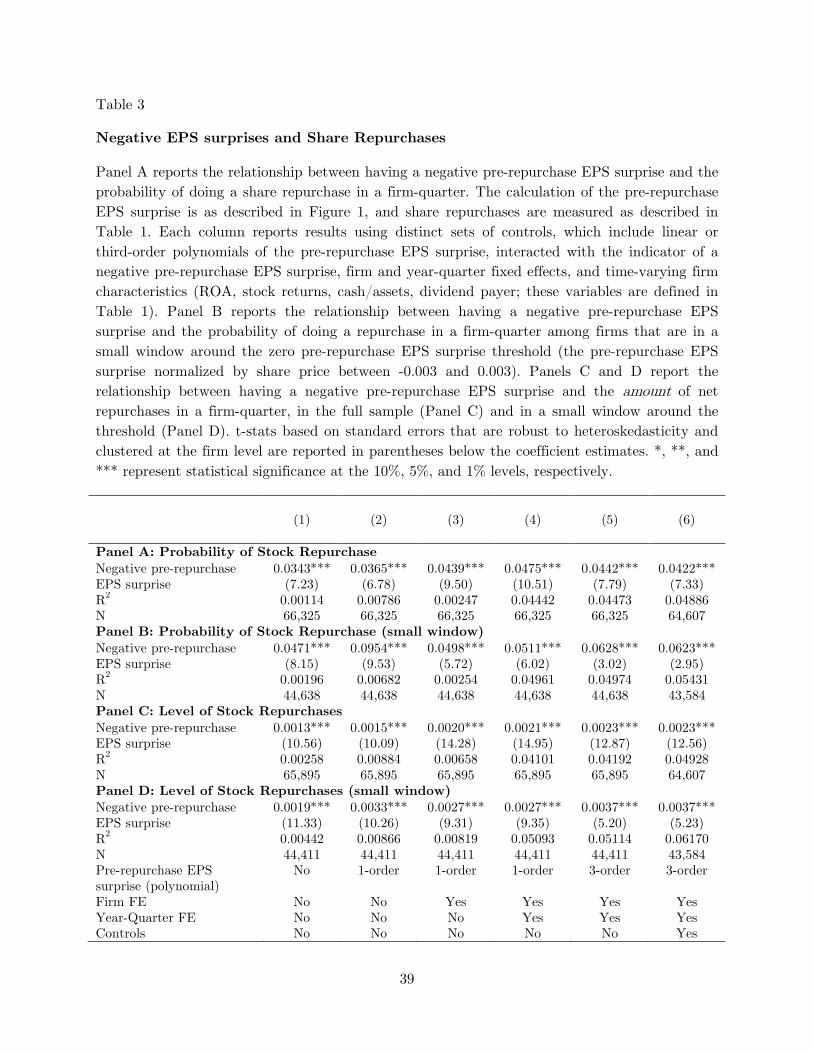
Table 3 reports the result. The evidence, reported in Panel A of Table 3, suggests

that having a negative pre-repurchase EPS surprise significantly predicts an accretive share

repurchase.12 Specifically, the probability of an accretive share repurchase increases by

3%-5% around the zero pre-repurchase EPS surprise threshold. When we consider a small11As in Hribar et al. (2006), we also find no discontinuity in the probability of a decretive share repurchase

around a zero earnings surprise (Figure A1 in the Appendix).12In untabulated results, we also find that having a negative pre-repurchase EPS surprise predicts initiations

of new repurchase programs. The increase in share repurchases is thus driven both by increased use of existingprograms (intensive margin) and new programs (extensive margin).

13

window around a zero pre-repurchase EPS surprise (Panel B), −0.003 ≤ Sueadj ≤ 0.003, the

discontinuity is even stronger (Table A1 in the appendix shows that the main results are

not sensitive to the choice of bandwidth for this small window). As Panel B indicates, the

probability of an accretive share repurchase increases by 5%-10% when companies experience

a negative pre-repurchase EPS surprise. Given that the unconditional likelihood of a positive

net repurchase is 23%, the effect constitutes a significant economic effect on the probability

of share repurchase.13

Next we show that having a small negative pre-repurchase EPS surprise has a significant

impact also on the total size of share repurchases, by estimating the following regression:

Repurchasesit = α + β1INegative Sueadj ,it + β2Sueadj,it + β3Sue2adj,it + β4Sue

3adj,it

+β5Sueadj,itINegative Sueadj ,it + β6Sue2adj,itINegative Sueadj ,it (3)

+β7Sue3adj,itINegative Sueadj ,it + β8Xit + ηi + θt + εit,

Results are reported in Panel C and Panel D of Table 3. The ratio of net share repurchases

to assets is 0.13%–0.37% higher when companies would narrowly miss the target EPS without

a repurchase. Given that the unconditional ratio of net share repurchases to assets is around

0.28%, this effect on share repurchases is economically important.14

To exploit this discontinuity to analyze the effect of share repurchases on outcome variables

of interest (Employment, Capex, and R&D), we need to make the following identifying13The t-statistic is also very large, which enables this discontinuity to serve as a strong instrument. In

untabulated results, we also compute Kleibergen-Paap F-statistics of this first-stage regression and findextremely high F-stats (above 100), which supports the strength of the instrument.

14The unconditional ratio of net share repurchases to assets is the product of the unconditional likelihoodof a positive net repurchase (23%) and the net share repurchases to assets among firms conditional on positivenet repurchases (1.2%).

14

assumption: in the absence of a jump in share repurchases around a zero pre-repurchase EPS

surprise, there are no other discontinuous differences in firm characteristics around the zero

pre-repurchase EPS surprise. In Section 3.4, we further weaken this assumption by exploiting

cross-sectional heterogeneity: here, we need only assume that any other discontinuity around

this threshold does not differ systematically across groups of firms.

A standard way to test the assumption is to evaluate whether there are systematic pre-

existing differences or trends in the policies of firms that fall on either side of a pre-repurchase

EPS surprise. To perform the test, we examine the characteristics of firms with small negative

and small positive pre-repurchase EPS surprises. To isolate any differences around the

threshold, we limit the sample to a small window around a zero pre-repurchase EPS surprise,

−0.003 ≤ Sueadj ≤ 0.003, and in addition control for any linear association between the

pre-repurchase EPS surprise and firm characteristics.

Table 4 reports the results. When we compare firms with small negative and small positive

pre-repurchase EPS surprises, firms on either side of the pre-repurchase EPS surprise have

very similar characteristics. We find no systematic pre-existing differences in either changes

in or levels of Employment, Capex, or R&D.15

[Insert Table 4 around here]

Overall, firms on either side of a pre-repurchase EPS surprise have very similar charac-

teristics, which supports the use of the regression discontinuity framework. This allows us

to use INegative Sueadj ,it (i.e., having a negative pre-repurchase EPS surprise) to identify the

effect of EPS-driven repurchases on employment and investment using a fuzzy regression

discontinuity (RD) framework.15Because the ability to complete an accretive repurchase depends on a firm’s P/E ratio, we further test

for pre-trends and pre-existing level differences in P/E ratios (these results are not reported). We findno differences in P/E levels or pre-trends between firms shown on the left and the right, which furthersupports the notion of no discontinuous difference between firms with slightly negative and slightly positivepre-repurchase EPS surprises.

15

3.3 Main results

This section estimates the effect of share repurchases on firms’ employment/investment

policies, employing a fuzzy regression discontinuity (RD) framework. We begin by reporting

the reduced form relation between having a small negative pre-repurchase EPS surprise and

investment policies, by estimating the following equation:

Y i,(t+1,t+4)−Y i,(t−4,t−1) = α+β1INegative Sueadj ,it+β2Sueadj,it+β3Sueadj,itINegative Sueadj ,it+θt+εit.

(4)

Panels A and B of Table 5 presents the reduced form results. These coefficients represent

the differences in outcome variables across firms with negative pre-repurchase EPS surprises

and those that just meet their EPS forecast without repurchasing stock. They can be directly

compared with the coefficients reported in the parallel trends test in Table 4. Firms that are

on the left reduce employment by 0.5 employees per million dollars in assets, invest on average

0.10%–0.22% of assets less in capital expenditures, and invest around 0.03-0.06% of assets

less in R&D, relative to firms that are on the right of the threshold. These figures represent

around 5% of the average number of employees, 10% of the mean capital expenditures, and

3% of the mean R&D expenses in our sample (Table 1). Overall, the evidence suggests that

repurchases result in significant decreases in both Employment, Capital Expenditures, and

R&D spending.

We next estimate the corresponding two-stage least squares regression, where in the first

stage we include INegative Sueadj ,it as a predictor of the level of share repurchases (based on

Equation (3)).

16

Y i,(t+1,t+4)−Y i,(t−4,t−1) = α+γ1Repurchasesit+γ2Sueadj,it+γ3Sueadj,itINegative Sueadj ,it+θt+εit.

(5)

Under the identification assumption discussed in the previous section, the coefficients

of these regressions can be interpreted causally. As in every instrumental variables (IV)

research design, we identify the Local Average Treatment Effect (LATE) of these repurchases

on investment. The two-stage results are reported in Panels C and D of Table 5. Consistent

with the reduced form effects, we show that repurchases made by firms that would have a

negative pre-repurchase EPS surprise result in lower employment, capex, and R&D.16

[Insert Table 5 around here]

The economic interpretation of the coefficients are similar to those in the reduced form

regressions. Table 1 shows that the average repurchase by firm-quarter of $21.65 million,

while 37% of these repurchase dollars are spent by firms in the small region just to the left of

zero pre-repurchase EPS surprise. For example, given the estimated average effect on capital

expenditures in Table V, Column II (-0.301), the predicted impact on capital expenditures

would be a reduction of 37%*21.65*0.301=$2.4 million. This figure represents 9% of the

average firm’s quarterly capital expenditures ($26.57 million), which is close to the 10% figure

that we obtain in the reduced form regressions.

Our identification strategy is robust to several potential concerns.

First, to fully exploit the RD design, we focus specifically on results in a small window

around the threshold rather than the full sample. The reason for limiting the sample in

this way is that the results for the full sample may be driven by companies that have large16As a robustness test, in Table A2 in the appendix, we additionally also include firms for which a repurchase

would have a decretive impact on EPS. We find that the results are qualitatively and quantitatively similarto those in Table 5 where we only include firms for which repurchases are accretive.

17

negative or positive surprises away from the threshold, rather than companies that are close

to the threshold (Bakke and Whited (2012)). In Table A1, we show that the results reported

in Table 5 are not sensitive to the choice of bandwidth for the small window. Our base result

uses a window between −0.003 ≤ Sueadj ≤ 0.003, while Table A1 further presents results for

window sizes varying between abs(0.001) and abs(0.005).

Second, another potential concern with the identification assumption might be that

firms that just miss or just beat the analyst consensus are discontinuously different in some

time-invariant observable or unobservable characteristic (for example, the firm’s management

team). To address this concern, the outcome variable is defined in differences and therefore

controls for any such time-invariant characteristics that might affect the outcome variables.

A related concern is that the earnings surprise threshold may be related to some time-varying

characteristic that affects the outcome variables. As discussed in the previous section, we

find no systematic pre-existing differences or trends in the policies of firms that fall on either

side of the pre-repurchase EPS surprise. Thus, firms on either side of the pre-repurchase EPS

surprise have very similar characteristics and therefore are likely to be distributed around

the threshold as if randomly assigned.

A third potential concern is that firms use other ways to manage earnings in addition

to share repurchases. This is an omitted variable concern, and thus, to affect our results,

would have to both directly affect the outcome variables and be discontinuous around the

zero pre-repurchase EPS surprise. We address this concern in two complementary ways. Two

of the main methods for managing earnings are accruals and guidance. In Table A3 (in the

appendix), we therefore explicitly control for several measures of accruals (Panels A–B) and

guidance (Panel C). These results show that our results are not affected by controlling for

other earnings management strategies.17 In addition to controlling for accruals and guidance,17The point estimates are smaller in Panel C where we control for guidance. However, this happens not

because the guidance variables mediate the relation between repurchases and investment, but because the

18

we measure our outcome variables only as the difference between four quarters after and

four quarters before the quarter of repurchases, and exclude the quarter concurrent with the

repurchase (t = 0). Our concern is that in order to beat analyst EPS forecasts, a firm could

both employ share repurchases and reclassify R&D expenses as capital expenditures: this

would result in abnormally high capital expenditures and abnormally low R&D expenses in the

same quarter as the earnings-management-motivated repurchase. By excluding the quarter

concurrent with the repurchase t = 0, we eliminate this concern about the contemporaneous

reclassification of R&D expenses as capital expenditures.

Finally, another possible omitted variable concern is that having a negative pre-repurchase

EPS surprise might be correlated with having an actual negative EPS surprise (even after

controlling for the magnitude of the EPS surprise), and that having an actual negative

surprise might have a direct discontinuous effect on investment, for example, by increasing

the cost of raising capital. To address this concern, we limit the sample to only firms that

have a small positive actual EPS surprise—some of which would have had a negative surprise

without executing a repurchase—and analyze the relationship between instrumented share

repurchases and changes in future employment/investment outcomes among these firms.

Because we include only firms with an actual positive surprise, we thus eliminate any omitted

variable concern based on having a negative actual surprise. Results are reported in Table A4

(in the appendix). The results are similar to the results in Table 5, which indicates that the

main results are unlikely to be driven by companies that have an actual negative surprise.

relationship between share repurchases and our outcome variables is somewhat lower in the time period forwhich we have data on guidance (1995–2009) compared with the other years in the sample.

19

3.4 Cross-sectional variation tests

In the preceding sections, we assume that in the absence of a discontinuous jump in share

repurchases around a zero pre-repurchase EPS surprise there are no other discontinuous

changes in firm characteristics around the zero pre-repurchase EPS surprise. In this section, we

further weaken this assumption by exploiting cross-sectional heterogeneity in the magnitude

of the discontinuity in share repurchases around the zero surprise. To understand this idea,

suppose that we can observe a sample of firms that do not conduct repurchases in response

to a negative surprise. If the effects that we document above are due to repurchases, then we

should not observe a relationship between negative surprises and employment, investment,

or R&D for this sample of firms. If, however, the effect is due to an unobservable variable

that jumps precisely at the zero earnings surprise level, then we should still observe effects

on outcomes, even in the absence of repurchases.

Which firms are more likely to repurchase shares to change the sign of the EPS surprise?

We hypothesize that firms in which managers are explicitly evaluated based on EPS should

be more likely to care about the sign of the earnings surprise. To test this hypothesis, we

collect data on whether “EPS” or “Earnings Per Share” occur in firms’ proxy statements,

by “scraping” all proxy statements for the firm-years in our sample. On average, around

35% of all firm-years explicitly mention EPS or Earnings Per Share. Figure 2 supports the

hypothesis by showing that the firms that mention EPS or Earnings Per Share in their annual

proxy statement display a much stronger discontinuous jump in the probability of executing

a share repurchase around the zero surprise threshold.

[Insert Figure 2 around here]

Panel A of Table 6 further supports this hypothesis by showing that the jump in the size

of repurchases around the threshold is significantly larger for firms that mention EPS in their

20

proxy compared with firms that don’t mention EPS. Panel A in Table 7 completes the analysis

by showing that the reduced-form relationship between having a negative pre-repurchase

EPS surprise and employment/investment is mainly driven by firms that mention EPS in the

proxy statement.

[Insert Table 6 around here]

[Insert Table 7 around here]

Our second cross-sectional variation test is based on the hypothesis that financially

unconstrained firms will be better able to execute share repurchases to manage earnings

around the threshold, because share repurchases require spending a lot of cash—on the order

of 1% of a firm’s total equity value—to move EPS by even one or a couple of cents (as

illustrated in our example in Section 3.2). Supporting this hypothesis, Figure 3 shows that

firms that are financially unconstrained display a much stronger discontinuous jump in the

probability of executing a share repurchase around the zero surprise threshold. We classify

firms as financially unconstrained (constrained) based on whether the Hadlock-Pierce (2010)

measure of financial constraints is below (above) median. Furthermore, Panel B in Table 6

shows that the jump in the size of repurchases around the threshold is significantly larger for

firms that are financially unconstrained. Panel B in Table 7 completes the analysis by showing

that the reduced form relationship between having a negative pre-repurchase EPS surprise

and employment/investment is driven by firms that are financially unconstrained. In fact,

there is no significant relationship between earnings surprises and outcomes for constrained

firms.

[Insert Figure 3 around here]

The main benefit of these cross-sectional tests is that the identification assumption that

underlies these tests is even weaker than that in our base results. In the base results, we

21

assume that—except for the jump in share repurchases—there are no other discontinuous

characteristics around the threshold that directly affect our outcome variables. By additionally

exploiting this cross-sectional variation, we can allow for even such discontinuous jumps in

other characteristics. We need only assume that any other discontinuity around this threshold—

one that would directly affect our outcome variables—does not differ systematically across

these groups of firms. Thus, a strong (weak) first-stage result (Table 6) combined with

corresponding strong (weak) reduced-form results (Table 7) supports the identification

assumption that the channel through which having a negative pre-repurchase EPS surprise

affects investment is share repurchases and not some other discontinuous difference across

this threshold.

3.5 Share repurchases and financial policies

The evidence found above suggests that firms that execute share repurchases to manage EPS

subsequently reduce investments and employment. An alternative way of financing these

repurchases is to change financial policieis. For example, companies could decrease cash

holdings, or raise external financing (debt or equity). In this section, we analyze the effect of

share repurchases on cash, equity issuance, and debt issuance.

We first perform a pre-trends analysis (similar to Table 4) to test for whether there are

any differential trends in these financial variables among firms that are on either side of the

discontinuity. Table 8 reports the results. When we compare firms with small negative and

small positive pre-repurchase EPS surprises, firms on either side of the threshold have very

similar financial policies. We find no systematic pre-existing differences in either changes in

or levels of cash, equity issuances, or debt issuances.

[Insert Table 8 around here]

22

Next, as in the analysis in Section 3.3, we estimate the effect of share repurchases on

financial policies. We report the results in Panels A–B of Table 9. The evidence shows

that repurchases indeed result in lower cash holdings going forward. However, we find no

impact on either equity or debt issuances when we control for the running variable around

the threshold (pre-repurchase EPS surprise). Thus, while firms do use cash to finance some

of these repurchases, they do not rely on external financing to pay for these repurchases.

[Insert Table 9 around here]

Next, as a robustness test, in Panels C–D of Table 9, we repeat the analysis but instead

of using net repurchases as the main independent variable, we use raw repurchases instead

(raw repurchases are measured using the variable ’prstkcy’ in Compustat). The reason for

performing this robustness test is that equity issuances may directly affect the net repurchases

measure, which in turn could affect the result in the equity issuance test (column (2)). We

find no difference in the estimated coefficients between Panels B and D, showing that any

confounding effect of equity issuances on net repurchases, if any, is small.18

4 Performance and valuation consequences

Our results so far support the conjecture that companies trade off employment and investment

for stock repurchases. In this section we examine the valuation and performance consequences

that are associated with this trade-off.18We repeat this robustness tests, where we substitute raw repurchases for net repurchases, for the main

results (Table 5). The results are reported in Table A5 in the appendix, which also show that any confoundingeffect of equity issuances on the net repurchase measure, if any, is small.

23

4.1 Valuation consequences

In this section we show how the market reacts to EPS-motivated share repurchases. Specifically,

we estimate the following regression within the sample that comprises companies in a small

window (between -0.003 and 0.003) around the zero-surprise threshold:

CARit = α0+α1ISueadj,it>0+α2ISueadj,it<0+α3ISue sign change,it+α4Sueadj,it+α5Sueadj,itISueadj,it>0+εit

(6)

CAR is the cumulative abnormal return over three trading days around the quarterly earnings

announcement date, Sueadj is the pre-repurchase EPS surprise, defined as the difference

between the reported EPS adjusted for the effect of repurchases and the median analyst EPS

forecast at the end of the quarter, and ISueadj,it>0 and ISueadj,it<0 are indicators of whether the

pre-repurchase EPS surprise is positive or negative (zero surprise is the omitted category).19

The main variable of interest, ISue sign change, is an indicator of whether an accretive share

repurchase changes the sign of the EPS surprise from negative to positive. A positive

coefficient on ISue sign change would imply that investors reward a change in the EPS surprise

sign (from negative to positive) that is induced by repurchases. The third column additionally

controls for an indicator of a repurchase, to control for the possibility of an abnormal return

from a repurchase itself independently of changing the sign of earnings surprise.

[Insert Table 10 around here]

The evidence reported in Table 10 suggests that investors reward companies that change

the sign of the EPS surprise using share repurchases. Because we control for the magnitude

of the surprise, these abnormal returns represent the discontinuous effect on stock prices of19For companies that don’t repurchase any shares in the quarter, the pre-repurchase EPS surprise (Sueadj)

is, naturally, equal to the actual earnings surprise.

24

just missing or just beating the EPS target. The coefficient on the first row suggests that

companies that just meet the forecast are rewarded with a 0.23%-0.61% increase in their

stock prices, after controlling for the magnitude of the surprise. In contrast, companies that

just miss the forecast observe a decline of 0.33%-0.43% in their stock prices (second row).20

Most importantly, companies that change the sign of their EPS surprise using repurchases

observe an earnings announcement CAR that is positive and also indistinguishable from the

CAR of companies that just beat the forecast without using repurchases. To see this, notice,

for example, in the third column, that the CAR for firms that meet the forecast because of

the repurchase is given by the sum of the coefficients on the second and third rows (-0.34% +

0.57%, which is equal to 0.23%).21 Results of an F-test, reported at the bottom of Table 10,

show that the abnormal returns for companies that changed the sign of the EPS surprise from

negative to positive are positive and statistically significant.22 In fact, the second F-test in

Table 10 shows that when we control for the polynomials of the pre-repurchase EPS surprise,

we cannot reject the hypothesis that the market treats positive EPS surprises produced with

share repurchases in the same way as it treats other positive EPS surprises.

This result is distinct from that of Hribar et al. (2006), who also examine the valuation

consequences of EPS-driven stock repurchases. They find that investors assign significantly

less value to repurchase-induced EPS surprises than to non-repurchase-related surprises. The

key difference in approaches is that Hribar et al. do not focus on a small window around

zero EPS surprises as we do here, and thus do not fully exploit the discontinuity in stock

prices at the zero earnings surprise level. When using the full sample (i.e., not only in a20Bartov et al. (2002) also show evidence that stock prices are discontinuous at the level of zero EPS-

surprises, although they do not examine the role of repurchases.21We also examine returns from -1 to 10 and 90 days following earnings announcements, and find very

similar results. For all windows, we cannot reject that firms that repurchase to meet EPS forecasts havereturns that are the same as firms that meet EPS forecasts without repurchases(these results are not reported).

22The abnormal returns for firms that change the sign from negative to positive can be estimated as α2 +α3from Equation 6; in column (3), this is significantly different from 0 only at the 10% level.

25

small window around the threshold) to conduct this analysis, we do find evidence consistent

with Hribar et al. (2006): firms that meet forecasts using repurchases observe smaller CARs

than companies that surprise without resorting to repurchases. However, as discussed above,

these results could be driven by companies that have large negative or positive surprises,

even after controlling for polynomials of the EPS surprise.

The results in Table 10 suggest that the market doesn’t care whether firms surprise

positively using repurchases, or not. However, these average results may be hiding interesting

cross-sectional variation. Is there a firm characteristic that is correlated with market reaction

and performance? Given the evidence that firms cut both cash and real investments following

EPS-motivated repurchases, one possibility is that the stock price reaction to earnings

announcements may depend on how firms finance repurchases. We examine this possibility

next.

Among the firms that do a repurchase and are in the neighbourhood immediately left of

the zero pre-repurchase EPS surprise threshold, we measure whether they cut cash, capex,

R&D, or employment in that quarter (relative to the previous quarter). As Table 11 shows

(third row), in approximately one half (47%) of firm-quarters, cash decreases in the quarter

of the earnings announcement. Capital expenditures, R&D, and Employment are decreased

in 45%, 16%, and 6% of firm-quarters respectively.23 Thus, there is significant variation in

the type of cut that firms make: While some firms finance repurchases with cash, others cut

real investments.24

This variation allows to explore whether the valuation consequences of changing the sign

of EPS surprises depend on how these repurchases were financed. Before we discuss the23These categories are not mutually exclusive because firms can cut both cash and real investments or

neither. For example, about two-thirds of firms that drop cash also drop at least one of the real investmentvariables (employment, R&D, or capex), while one-third do not drop any of these variables.

24In addition they can fund repurchases with internal cash flow, so for a significant fraction of firm-quarters(18%) there is no cut in either cash or real investments.

26

results, it is important to note that the interpretation of these results is subject to some

important caveats. First, because firms choose how to finance repurchases, we should not give

a causal interpretation to the correlation between financing choices and stock price reactions.

Second, it is important to note that we are trying to infer the market reaction to investment

cuts from the reaction to earnings announcements. Ideally, what we would like to do is to

conduct an event study directly on investments. However, this is not possible because there

is no natural date to measure the market reaction to changes in investments. Thus, the

results will be confounded by the market’s perception about the earnings announcement itself.

Despite these caveats, evidence that the market reaction to meeting EPS forecasts is lower

when firms cut real investments would provide at least suggestive evidence that some firms

are cutting valuable investments to help finance repurchases.

To operationalize this idea, we split the indicator Sue sign change into Sue sign change ∗

Drop and Sue sign change ∗ NoDrop, where Drop and NoDrop are indicators for whether

the firm cut a given variable (cash, or real investments). The variable “drop investment”

takes a value of one if there is a cut in any type of real activity (inevstment, employment, or

R&D). We also define this variable for each variable in isolation. For example, the variable

drop R&D assumes a value of one if R&D falls, and is zero otherwise. Columns 1–5 of Table

11 present results for each of these variables.

[Insert Table 11 around here]

Our results do show that financing is correlated with the market reaction to earnings

announcements. Firms that cut cash to help finance EPS-driven repurchases continue to

have the same market reaction as that of firms that surprise positively without repurchases

(column 1). However, firms that cut some type of real variable (either capex, or employment,

or R&D) to meet an EPS forecast show a lower reaction to beating the forecast. For example,

27

column 2 of Table 11 shows that firms that cut some type of real investment have a stock

price reaction that is on average 0.23% lower than that of firms that can change the sign of

the surprise without cutting real investments (these firms are using cash or cash flow to do so).

Columns 3 to 5 show that these results are particularly strong for firms that decrease R&D

and Employment - these firms get no significant reward for changing the sign of EPS surprise

using share repurchases when they cut R&D or employment. These results are consistent

with firms sacrificing valuable investments to finance share repurchases, particularly so when

they cut R&D and employment to do so.

4.2 Performance consequences

We complete the analysis by examining the effect of EPS-driven repurchases on future

profitability as measured by accounting performance. To do so, we employ the same fuzzy

regression discontinuity framework as in Section 3.3, and use return on assets (ROA) as

the outcome variable. ROA is measured as quarterly operating income before depreciation

(oibdpq) divided by contemporaneous assets (atq). Column (1) of Table 12 shows the baseline

result.

[Insert Table 12 around here]

The result suggests that EPS-driven repurchases on average do not cause significant

subsequent changes in accounting performance, after controlling for the level of the EPS

surprise. Following the analysis in Table 11, we next examine whether the performance

consequences depend on whether companies cut cash, capex, R&D, or employment to finance

the repurchase. Consistent with the valuation analysis in Table 11, Columns 2–6 in Table

12 show that firms that cut investments (particularly R&D and employment) to finance the

EPS-motivated repurchases have more adverse subsequent performance consequences.

28

5 Conclusion

This paper studies the consequences of share repurchases that are motivated by earnings

management considerations. Firms’ incentives to “just meet” analyst forecasts create a

discontinuity in the probability of a share repurchase around the zero earnings surprise

level. We use this discontinuity to identify the causal effect of such repurchases on other

corporate policies in a fuzzy regression discontinuity framework. The evidence suggests that

firms that repurchase shares subsequently reduce employment and investment in capital,

and hold less financial slack. Firms that change the sign of an earnings surprise using

repurchases experience positive stock market reactions to their earnings announcements,

which are on average indistinguishable from those of firms that just meet earnings targets.

However, the stock price reactions to earnings announcement are lower when firms cut real

variables to help finance repurchases, in particular R&D and employment. Overall, our results

support the conjecture that companies are willing to trade off employment and investment

for stock repurchases. While on average this trade-off does not appear to be detrimental to

shareholder value, EPS-motivated repurchases can have more negative consequences for value

and performance if they are associated with contemporaneous cuts in real investments.

Our paper contributes to the literature on repurchases by providing evidence that EPS-

driven repurchases cause firms to decrease investment, employment, and R&D. As we discuss

in the paper, the interpretation of our valuation and performance results is a bit more

complicated, because firms endogenously choose how to finance repurchases. It would be

interesting to explore additional sources of identification to confirm our preliminary evidence

that some firms are willing to sacrifice valuable investments to finance EPS-motivated share

repurchases. In addition, we cannot speak to other motives for why firms conduct repurchases

such as undervaluation and signalling. While EPS-motivated repurchases are interesting

29

in their own right, future literature could look for ways to shed light on a broader set of

trade-offs between stock repurchases and other important firm policies.

30

References

Babenko, I, 2009, Share Repurchases and Pay-Performance Sensitivity of Employee Compen-

sation Contracts, The Journal of Finance 64, 117–150.

Bakke, Tor-Erik, and Toni M. Whited, 2012, Threshold events and identification: A study of

cash shortfalls, The Journal of Finance 67, 1083–1111.

Bens, Daniel A, Venky Nagar, Douglas J Skinner, and M H Franco Wong, 2003, Employee

Stock Options, EPS Dilution, and Stock Repurchases, Journal of Accounting and Economics

36, 51–90.

Bhojraj, S., P. Hribar, and M. amd J. McInnis Picconi, 2009, Making sense of cents: An

examination of firms that marginally miss or beat analyst forecasts, The Journal of Finance

64, 2361–2388.

Brav, Alon, John R Graham, Campbell R Harvey, and Roni Michaely, 2005, Payout Policy

in the 21st Century, Journal of Financial Economics 77, 483–527.

Brockman, P., and D.Y. Chung, 2001, Managerial timing and corporate liquidity: Evidence

from actual share repurchases, Journal of Financial Economics 61, 417–448.

Dittmar, A K, 2000, Why Do Firms Repurchase Stock, The Journal of Business 73, 331–355.

Gong, G., H Louis, and A X Sun, 2008, Earnings Management and Firm Performance

Following Open-Market Repurchases, The Journal of Finance 63, 947–986.

Gopalan, R., T. Milbourn, F. Song, and A. Thakor, 2010, The optimal duration of executive

compensation: theory and evidence, Working paper.

31

Graham, J R, and C R Harvey, 2001, The Theory and Practice of Corporate Finance:

Evidence from the Field, Journal of Financial Economics 60, 187–243.

Graham, John R, Campbell R Harvey, and Shiva Rajgopal, 2005, The economic implications

of corporate financial reporting, Journal of accounting and economics 40, 3–73.

Grullon, G, and R Michaely, 2004, The Information Content of Share Repurchase Programs,

The Journal of Finance 59, 651–680.

Hribar, Paul, Nicole Thorne Jenkins, and W Bruce Johnson, 2006, Stock Repurchases as an

Earnings Management Device, Journal of Accounting and Economics 41, 3–27.

Huang, S., 2011, Executive compensation and horizon incentives: An empirical investigation

of corporate cash payout, Working paper.

Ikenberry, David Lawrence, Josef Lakonishok, and Theo Vermaelen, 1995, Market Underreac-

tion to Open Market Share Repurchases, Journal of Financial Economics 39, 181–208.

Kahle, K., 2002, When a buyback isn’t a buyback: Open market repurchases and employee

options, Journal of Financial Economics 63, 235–261.

Lie, Erik, 2005, Operating Performance Following Open Market Share Repurchase Announce-

ments, Journal of Accounting and Economics 39, 411–436.

Peyer, U, and T Vermaelen, 2007, The Nature and Persistence of Buyback Anomalies, Review

of Financial Studies 22, 1693–1745.

Rauh, Joshua, 2006, Investment and financing constraints: Evidence from the funding of

corporate pension plans, The Journal of Finance 61, 33–71.

32

33

Figure 1

Probability of accretive share repurchases.

This figure plots the probability of doing an accretive share repurchase as a function of a pre-repurchase earnings surprise. For every earnings surprise bin, the dots represent the probability of an accretive share repurchase—the fraction of firm-quarters with an accretive repurchase out of all firm-quarters in that bin. The lines are second-order polynomials fitted through the estimated probabilities on each side of the zero pre-repurchase earnings surprise. We define a share repurchase as accretive if it increases EPS by at least 1 cent. The pre-repurchase earnings surprise is the difference between the repurchase-adjusted (“pre-repurchase”) earnings per share (EPS) and the median EPS forecast at the end of the quarter; this difference is normalized by the end-of-quarter stock price. The pre-repurchase EPS is calculated as follows: 𝐸𝐸𝑆𝑎𝑎𝑎 = 𝐸𝑎𝑎𝑎

𝑆𝑎𝑎𝑎=

𝐸+𝐼𝑆+∆𝑆

, where 𝐸 is reported earnings, 𝐼 is the estimated forgone interest due to the repurchase, 𝑆 is the number of shares at the end of the quarter, and ∆𝑆 is the estimated number of shares repurchased (the repurchase amount divided by the average daily share price). The forgone interest is the after-tax interest that would be earned on an amount of funds equal to that used to repurchase shares if it were instead invested in a 3-month T-Bill.

0.0%

0.5%

1.0%

1.5%

2.0%

2.5%

3.0%

3.5%

4.0%

-0.01 -0.005 0 0.005 0.01

Pre-repurchase EPS surprise

34

Figure 2

Probability of accretive share repurchases: EPS in proxy statement

This figure plots the probability of doing an accretive share repurchase as a function of a pre-repurchase earnings surprise. The data and axes are as described in Figure 1. The Figure shows a split in the probability of doing an accretive share repurchase between firms that have “EPS” or “Earnings Per Share” explicitly mentioned in the proxy statement for the year and firms that do not.

0.0%0.5%1.0%1.5%2.0%2.5%3.0%3.5%4.0%4.5%5.0%5.5%6.0%6.5%

-0.008 -0.006 -0.004 -0.002 0 0.002 0.004 0.006 0.008Pre-repurchase EPS surprise

Left No EPS Right No EPS Left EPS Right EPS

35

Figure 3

Probability of accretive share repurchases: Financially constrained vs. unconstrained firms

This figure plots the probability of doing an accretive share repurchase as a function of a pre-repurchase earnings surprise. The data and axes are as described in Figure 1. The Figure shows a split in the probability of doing executing an accretive share repurchase between firms that are financially constrained (above the Hadlock-Pierce (2010) index median) and firms that are financially unconstrained (below the median).

0.0%

0.5%

1.0%

1.5%

2.0%

2.5%

3.0%

3.5%

4.0%

4.5%

-0.008 -0.006 -0.004 -0.002 0 0.002 0.004 0.006 0.008Pre-repurchase EPS surprise

Left Constrained Right Constrained Left Unconstrained Right Unconstrained

36

Table 1

Descriptive Statistics

This table reports summary statistics. The observations are at the firm-quarter level. Panel A reports summary statistics on share repurchases. Net Repurchases are measured following Fama and French (2001), i.e., as the increase in common treasury stock if treasury stock is not zero or missing. If treasury stock is zero in the current and prior quarter, we measure repurchases as the difference between stock purchases and stock issuances from the statement of cash flows. If either of these amounts is negative, repurchases are set to zero. The quantity of repurchased shares is measured as the repurchase amount divided by the average daily share price during the quarter. Panel B reports summary statistics on earnings surprises and abnormal returns around earnings announcements. An earnings surprise is the difference between the reported EPS and the median EPS forecast at the end of the quarter, and this difference is normalized by the end-of-quarter stock price. The abnormal return around an earnings announcement is the cumulative return within three trading days around the earnings announcement minus the cumulative return of the CRSP market portfolio over the same period. Panel C reports statistics on additional firm characteristics employed in the study. All asset-scaled measures use lagged assets from the end of the previous quarter. ROA is defined as net income (times 4) divided by lagged assets. Q is defined as the book value of liabilities plus the market value of common equity divided by the book value of assets [(atq-ceqq+marketcap)/atq]. Cash flow is defined as Net Income plus Depreciation, and is divided by lagged assets. Market-to-book is defined as the market value of common equity divided by the book value of common equity [marketcap/(seqq-pstkq)]. Total accruals are measured as the absolute value of total accruals divided by lagged assets � 𝑇𝑇𝑖𝑖

𝑇𝑖𝑖−1� = �∆𝐶𝑇𝑖𝑖− ∆𝐶𝐶𝑖𝑖−∆𝐶𝑎𝐶ℎ𝑖𝑖+∆𝑆𝑇𝐷𝑖𝑖−𝐷𝐷𝐷𝑖𝑖

𝑇𝑖𝑖−1�. Discretionary

accruals are measured using the modified Jones (1991) model of Dechow, Sloan, and Sweeney (1995). The guidance indicators capture whether the firm issues positive, negative, or any (including unsigned) earnings guidance during the quarter (from First Call). The measure of Financial Constraints follows Hadlock and Pierce (2010). Stock return is the quarterly raw stock return from CRSP. Dividend payer indicates whether the firm has paid any dividends in the last four quarters (including the current quarter). Equity Issuance is prstkcy(Purchase of common and preferred stock)-Net Repurchases. Debt issuance is the change in total debt.

Mean Sd p1 p5 p25 p50 p75 p95 p99 N PANEL A: Repurchase statistics Positive net repurchases (indicator) 0.23 0.42 0 0 0 0 0 1 1 341,483 If repurchases > 0 Repurchases ($M) 21.65 49.52 0.00 0.00 0.13 1.25 11.99 178.69 205.15 77,457 Repurchased shares/Shares outstanding 1.0% 1.4% 0.0% 0.0% 0.1% 0.4% 1.4% 5.0% 5.6% 69,740 Repurchases/Assets 1.2% 1.8% 0.0% 0.0% 0.1% 0.4% 1.5% 6.2% 6.8% 75,137

37

Table 1 – cont. PANEL B: Earnings surprise statistics mean sd p1 p5 p25 p50 p75 p95 p99 N Earnings surprise/Stock price -0.3% 1.6% -10.7% -2.6% -0.2% 0.0% 0.2% 1.1% 3.5% 140,805 Positive earnings surprise (indicator) 0.48 0.50 0.00 0.00 0.00 0.00 1.00 1.00 1.00 140,805 Negative earnings surprise (indicator) 0.40 0.49 0.00 0.00 0.00 0.00 1.00 1.00 1.00 140,805 Zero earnings surprise (indicator) 0.12 0.33 0.00 0.00 0.00 0.00 0.00 1.00 1.00 140,805 Abnormal return around earnings announcement (%) 0.1% 3.0% -9.0% -4.8% -1.4% 0.0% 1.5% 5.2% 10.3% 345,310 mean sd p1 p5 p25 p50 p75 p95 p99 N PANEL C: Firm characteristics Market Capitalization ($M) 1,622 5,249 2 8 42 164 741 7,549 39,544 367,995 Assets ($M) 1,563 4,838 2 8 42 159 727 7,622 34,848 385,488 Cash and Cash Equivalents/Assets 19.8% 24.4% 0.0% 0.3% 2.3% 9.2% 28.9% 73.2% 116.1% 365,631 Total Debt/Assets 22.3% 21.9% 0.0% 0.0% 2.2% 18.0% 35.1% 63.8% 100.5% 368,752 Capital Expenditures/Assets 1.7% 2.3% -0.4% 0.0% 0.4% 1.0% 2.0% 6.1% 13.9% 352,041 R&D/Assets 1.5% 3.2% 0.0% 0.0% 0.0% 0.0% 1.8% 7.7% 18.5% 366,651 Employees/Assets (per $M) 9.70 12.27 0.10 0.64 2.77 5.787 11.53 32.06 78.25 357,915 ROA -4.1% 29.0% -153.1% -62.1% -5.2% 3.3% 8.8% 21.6% 45.7% 365,837 Q 2.17 1.95 0.59 0.80 1.12 1.52 2.38 5.85 12.86 366,557 Market to book 3.4 4.3 0.3 0.6 1.2 2.1 3.6 10.3 30.3 353,149 Cash flow/Assets 0.35% 7.14% -35.97% -13.88% -0.04% 2.02% 3.58% 6.97% 13.26% 328,425 Total accruals (absolute) 0.04 0.05 0.00 0.00 0.01 0.02 0.05 0.13 0.26 310,692 Discretionary accruals (absolute) 0.07 0.12 0.00 0.00 0.01 0.03 0.08 0.22 0.47 242,926 Positive guidance 0.08 0.27 0.00 0.00 0.00 0.00 0.00 1.00 1.00 249,856 Negative guidance 0.08 0.27 0.00 0.00 0.00 0.00 0.00 1.00 1.00 249,856 Any guidance 0.27 0.44 0.00 0.00 0.00 0.00 1.00 1.00 1.00 249,856 Financial constraints (Hadlock and Pierce) -3.09 0.77 -4.64 -4.48 -3.57 -3.08 -2.58 -1.78 -1.20 367,992 Stock return (quarter) 3.3% 30.4% -63.1% -41.6% -14.3% 0.6% 16.5% 56.8% 125.0% 355,526 Dividend payer 0.35 0.48 0 0 0 0 1 1 1 385,488 Equity Issuance / Assets 1.4% 7.1% 0.0% 0.0% 0.0% 0.0% 0.2% 3.5% 57.9% 319,214 Debt Issuance / Assets 0.7% 6.6% -20.3% -6.7% -0.8% 0.0% 0.9% 10.3% 37.5% 346,329

38

Table 2

Share Repurchases and Investment: OLS regressions

This table reports the relationship between share repurchases and changes in future employment/investment outcomes. The outcome variables are changes in employment (EMP), capital expenditures (CAPEXY), and R&D (XRNDQ, set to zero if missing). To measure the changes we take the average of each of these variables over four quarters after the quarter of repurchases minus the average over four quarters before repurchases, and scale the difference by assets lagged by four quarters. Repurchases are defined as in Fama and French (2001) and scaled by lagged assets. Panel A reports the univariate regression, and Panel B adds the most common control variables. Q and CashFlow/Assets are defined as in Table 1. The regressions are at the firm-quarter level. We control for year-quarter effects throughout. t-stats based on standard errors that are robust to heteroskedasticity and clustered by firm are reported in parentheses below the coefficient estimates. *, **, and *** represent statistical significance at the 10%, 5%, and 1% levels, respectively.

Dependent variable: Employment Capex R&D (1) (2) (3)

PANEL A Repurchases / Assets -9.189*** -0.045*** 0.002 (-6.29) (-8.35) (0.68) N 75,699 73,939 77,065 PANEL B Repurchases / Assets -17.729*** -0.083*** -0.020*** (-11.32) (-12.69) (-5.77) Q 17.070*** 0.138*** 0.017*** (10.10) (14.12) (5.40) Cash flow / Assets 0.344*** 0.001*** 0.001*** (7.48) (2.61) (11.88) N 70,311 68,874 71,562 Year-Quarter FE Yes Yes Yes

39

Table 3

Negative EPS surprises and Share Repurchases

Panel A reports the relationship between having a negative pre-repurchase EPS surprise and the probability of doing a share repurchase in a firm-quarter. The calculation of the pre-repurchase EPS surprise is as described in Figure 1, and share repurchases are measured as described in Table 1. Each column reports results using distinct sets of controls, which include linear or third-order polynomials of the pre-repurchase EPS surprise, interacted with the indicator of a negative pre-repurchase EPS surprise, firm and year-quarter fixed effects, and time-varying firm characteristics (ROA, stock returns, cash/assets, dividend payer; these variables are defined in Table 1). Panel B reports the relationship between having a negative pre-repurchase EPS surprise and the probability of doing a repurchase in a firm-quarter among firms that are in a small window around the zero pre-repurchase EPS surprise threshold (the pre-repurchase EPS surprise normalized by share price between -0.003 and 0.003). Panels C and D report the relationship between having a negative pre-repurchase EPS surprise and the amount of net repurchases in a firm-quarter, in the full sample (Panel C) and in a small window around the threshold (Panel D). t-stats based on standard errors that are robust to heteroskedasticity and clustered at the firm level are reported in parentheses below the coefficient estimates. *, **, and *** represent statistical significance at the 10%, 5%, and 1% levels, respectively.

(1) (2) (3) (4) (5) (6) Panel A: Probability of Stock Repurchase Negative pre-repurchase EPS surprise

0.0343*** 0.0365*** 0.0439*** 0.0475*** 0.0442*** 0.0422*** (7.23) (6.78) (9.50) (10.51) (7.79) (7.33)

R2 0.00114 0.00786 0.00247 0.04442 0.04473 0.04886 N 66,325 66,325 66,325 66,325 66,325 64,607 Panel B: Probability of Stock Repurchase (small window) Negative pre-repurchase EPS surprise

0.0471*** 0.0954*** 0.0498*** 0.0511*** 0.0628*** 0.0623*** (8.15) (9.53) (5.72) (6.02) (3.02) (2.95)

R2 0.00196 0.00682 0.00254 0.04961 0.04974 0.05431 N 44,638 44,638 44,638 44,638 44,638 43,584 Panel C: Level of Stock Repurchases Negative pre-repurchase EPS surprise

0.0013*** 0.0015*** 0.0020*** 0.0021*** 0.0023*** 0.0023*** (10.56) (10.09) (14.28) (14.95) (12.87) (12.56)

R2 0.00258 0.00884 0.00658 0.04101 0.04192 0.04928 N 65,895 65,895 65,895 65,895 65,895 64,607 Panel D: Level of Stock Repurchases (small window) Negative pre-repurchase EPS surprise

0.0019*** 0.0033*** 0.0027*** 0.0027*** 0.0037*** 0.0037*** (11.33) (10.26) (9.31) (9.35) (5.20) (5.23)

R2 0.00442 0.00866 0.00819 0.05093 0.05114 0.06170 N 44,411 44,411 44,411 44,411 44,411 43,584 Pre-repurchase EPS surprise (polynomial)

No 1-order 1-order 1-order 3-order 3-order

Firm FE No No Yes Yes Yes Yes Year-Quarter FE No No No Yes Yes Yes Controls No No No No No Yes

40

Table 4

Pre-existing differences in investment variables among firms with slightly negative/positive pre-repurchase EPS surprises

This table reports results for pre-existing differences in outcome variables around the zero pre-repurchase EPS surprise threshold. Panel A reports results for differences in pre-existing levels and Panels B-E reports results for changes (“trends”) in these variables. Each column reports results for a different outcome variable. The test is performed in a sample that consists of observations in a small window around the zero pre-repurchase EPS surprise threshold (between -0.003 and 0.003). We control throughout for the level of the pre-repurchase EPS surprise, interacted with the sign of the surprise, as well as firm- and year-quarter fixed effects. t-stats based on standard errors that are robust to heteroskedasticity and clustered at the firm level are reported in parentheses below the coefficient estimates. *, **, and *** represent statistical significance at the 10%, 5%, and 1% levels, respectively.

Dependent variable: Employment Capex R&D (1) (2) (3) PANEL A: Levels (t-1) Negative pre-repurchase EPS surprise -0.0093 0.0003 0.0001 (-0.10) (1.11) (0.46) PANEL B: Changes (t-2 to t-1) Negative pre-repurchase EPS surprise -0.0408 -0.0004 0.0003* (-1.09) (-1.36) (1.72) PANEL C: Changes (t-3 to t-1) Negative pre-repurchase EPS surprise 0.0345 -0.0004 0.0002 (0.61) (-1.55) (1.00) PANEL D: Changes (t-4 to t-1) Negative pre-repurchase EPS surprise 0.0408 -0.0005* 0.0003 (0.61) (-1.67) (1.33) PANEL E: Changes (t-5 to t-1) Negative pre-repurchase EPS surprise 0.0763 -0.0001 0.0000 (1.09) (-0.30) (0.34) Linear control in pre-repurchase EPS surprise Yes Yes Yes Firm FE Yes Yes Yes Year-Quarter FE Yes Yes Yes

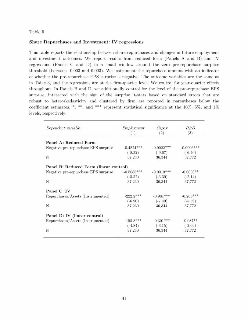
41

Table 5

Share Repurchases and Investment: IV regressions

This table reports the relationship between share repurchases and changes in future employment and investment outcomes. We report results from reduced form (Panels A and B) and IV regressions (Panels C and D) in a small window around the zero pre-repurchase surprise threshold (between -0.003 and 0.003). We instrument the repurchase amount with an indicator of whether the pre-repurchase EPS surprise is negative. The outcome variables are the same as in Table 3, and the regressions are at the firm-quarter level. We control for year-quarter effects throughout. In Panels B and D, we additionally control for the level of the pre-repurchase EPS surprise, interacted with the sign of the surprise. t-stats based on standard errors that are robust to heteroskedasticity and clustered by firm are reported in parentheses below the coefficient estimates. *, **, and *** represent statistical significance at the 10%, 5%, and 1% levels, respectively.

Dependent variable: Employment Capex R&D (1) (2) (3) Panel A: Reduced Form Negative pre-repurchase EPS surprise -0.4824*** -0.0022*** -0.0006*** (-8.32) (-9.67) (-6.46) N 37,230 36,344 37,772 Panel B: Reduced Form (linear control) Negative pre-repurchase EPS surprise -0.5085*** -0.0010*** -0.0003** (-5.52) (-3.30) (-2.14) N 37,230 36,344 37,772 Panel C: IV Repurchases/Assets (Instrumented) -222.2*** -0.981*** -0.265*** (-6.90) (-7.49) (-5.59) N 37,230 36,344 37,772 Panel D: IV (linear control) Repurchases/Assets (Instrumented) -155.8*** -0.301*** -0.087** (-4.84) (-3.15) (-2.09) N 37,230 36,344 37,772

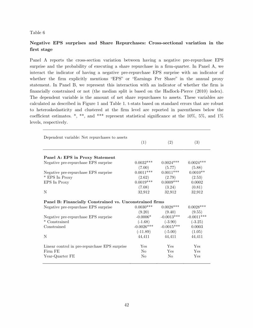
42

Table 6

Negative EPS surprises and Share Repurchases: Cross-sectional variation in the first stage

Panel A reports the cross-section variation between having a negative pre-repurchase EPS surprise and the probability of executing a share repurchase in a firm-quarter. In Panel A, we interact the indicator of having a negative pre-repurchase EPS surprise with an indicator of whether the firm explicitly mentions “EPS” or “Earnings Per Share” in the annual proxy statement. In Panel B, we represent this interaction with an indicator of whether the firm is financially constrained or not (the median split is based on the Hadlock-Pierce (2010) index). The dependent variable is the amount of net share repurchases to assets. These variables are calculated as described in Figure 1 and Table 1. t-stats based on standard errors that are robust to heteroskedasticity and clustered at the firm level are reported in parentheses below the coefficient estimates. *, **, and *** represent statistical significance at the 10%, 5%, and 1% levels, respectively.

Dependent variable: Net repurchases to assets (1) (2) (3) Panel A: EPS in Proxy Statement Negative pre-repurchase EPS surprise 0.0032*** 0.0024*** 0.0024***

(7.00) (5.77) (5.88) Negative pre-repurchase EPS surprise * EPS In Proxy

0.0011*** 0.0011*** 0.0010** (2.62) (2.79) (2.53)

EPS In Proxy 0.0019*** 0.0009*** 0.0002 (7.08) (3.24) (0.81)

N 32,912 32,912 32,912 Panel B: Financially Constrained vs. Unconstrained firms Negative pre-repurchase EPS surprise 0.0030*** 0.0028*** 0.0028***

(9.20) (9.40) (9.55) Negative pre-repurchase EPS surprise * Constrained

-0.0006* -0.0013*** -0.0011*** (-1.68) (-3.90) (-3.25)

Constrained -0.0026*** -0.0015*** 0.0003 (-11.89) (-5.00) (1.05)

N 44,411 44,411 44,411 Linear control in pre-repurchase EPS surprise Yes Yes Yes Firm FE No Yes Yes Year-Quarter FE No No Yes

43

Table 7

Share Repurchases and Investment: Cross-sectional variation in reduced form

This table reports results for the cross-sectional variation in the relationship between having a negative pre-repurchase EPS surprise and changes in future employment and investment outcomes (i.e., this is the reduced-form version of the IV regressions in Table 5). In Panel A, we interact the indicator of having a negative pre-repurchase EPS surprise with an indicator of whether the firm explicitly mentions “EPS” or “Earnings Per Share” in the annual proxy statement. This is the reduced form of the instrumented regression in Table 5, plus the new interactions. In Panel B, we represent this interaction with an indicator of whether the firm is financially constrained (the median split is based on the Hadlock-Pierce (2010) index). We control for year-quarter effects throughout and, in Panel B, we additionally control for the level of the pre-repurchase EPS surprise, interacted with the sign of the surprise. t-stats based on standard errors that are robust to heteroskedasticity and clustered by firm are reported in parentheses below the coefficient estimates. *, **, and *** represent statistical significance at the 10%, 5%, and 1% levels, respectively.

Dependent variable: Employment Capex R&D (1) (2) (3) Panel A: EPS in Proxy Negative pre-repurchase EPS surprise * EPS In Proxy

-0.3569*** -0.0010*** -0.0003* (-3.74) (-2.82) (-1.67)

Negative pre-repurchase EPS surprise * No EPS In Proxy

-0.2858** -0.0006 -0.0001 (-1.98) (-1.08) (-0.55)

N 28,914 28,376 29,165 Panel B: Financial Constraints Negative pre-repurchase EPS surprise * Unconstrained

-0.3157*** -0.0008*** -0.0003** (-4.06) (-2.76) (-2.11)

Negative pre-repurchase EPS surprise * Constrained

-0.0656 -0.0006 0.0005 (-0.16) (-0.41) (1.07)

N 37,230 36,344 37,772 Linear control in pre-repurchase EPS surprise Yes Yes Yes Year-Quarter FE Yes Yes Yes

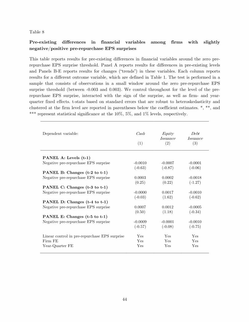
44

Table 8

Pre-existing differences in financial variables among firms with slightly negative/positive pre-repurchase EPS surprises

This table reports results for pre-existing differences in financial variables around the zero pre-repurchase EPS surprise threshold. Panel A reports results for differences in pre-existing levels and Panels B-E reports results for changes (“trends”) in these variables. Each column reports results for a different outcome variable, which are defined in Table 1. The test is performed in a sample that consists of observations in a small window around the zero pre-repurchase EPS surprise threshold (between -0.003 and 0.003). We control throughout for the level of the pre-repurchase EPS surprise, interacted with the sign of the surprise, as well as firm- and year-quarter fixed effects. t-stats based on standard errors that are robust to heteroskedasticity and clustered at the firm level are reported in parentheses below the coefficient estimates. *, **, and *** represent statistical significance at the 10%, 5%, and 1% levels, respectively.

Dependent variable: Cash Equity Issuance

Debt Issuance

(1) (2) (3) PANEL A: Levels (t-1) Negative pre-repurchase EPS surprise -0.0010 -0.0007 -0.0001 (-0.63) (-0.87) (-0.06) PANEL B: Changes (t-2 to t-1) Negative pre-repurchase EPS surprise 0.0003 0.0002 -0.0018 (0.25) (0.22) (-1.27) PANEL C: Changes (t-3 to t-1) Negative pre-repurchase EPS surprise -0.0000 0.0017 -0.0010 (-0.03) (1.62) (-0.62) PANEL D: Changes (t-4 to t-1) Negative pre-repurchase EPS surprise 0.0007 0.0012 -0.0005 (0.50) (1.18) (-0.34) PANEL E: Changes (t-5 to t-1) Negative pre-repurchase EPS surprise -0.0009 -0.0001 -0.0010 (-0.57) (-0.08) (-0.75) Linear control in pre-repurchase EPS surprise Yes Yes Yes Firm FE Yes Yes Yes Year-Quarter FE Yes Yes Yes

45

Table 9

The Effect of Share Repurchases on Cash Holdings, Equity Issuances, and Debt Issuances

This table repeats the analysis from Table 5 with new outcome variables: Cash holdings, Equity Issuance, and Debt Issuance. All outcome variables are defined in Table 1. Cash holdings are measured by CHEQ, equity issuance debt issuances by (DLCQ + DLTTQ), all normalized by assets. The regressions are at the firm-quarter level. We report results from IV regressions (equation (3)) in a small window around the zero-surprise threshold (between -0.003 and 0.003). In Panel B, we control for the level of the pre-repurchase EPS surprise, interacted with the sign of the surprise. In Panels C-D, we replace Net Repurchases with Raw Repurchases as measured by prstkcy (Purchase of common and preferred stock) in Compustat. We control for year-quarter effects throughout. t-stats based on standard errors that are robust to heteroskedasticity and clustered by firm are reported in parentheses below the coefficient estimates. *, **, and *** represent statistical significance at the 10%, 5%, and 1% levels, respectively.

Dependent variable: Cash Equity

Issuance Debt

Issuance (1) (2) (3) Panel A: IV Repurchases / Assets (Instrumented) -10.310*** -0.575*** -0.240

(-9.02) (-2.94) (-0.80) N 37681 32083 34359 Panel B: IV (linear control) Repurchases / Assets (Instrumented) -3.796*** -0.069 -0.190

(-5.25) (-0.38) (-0.58) N 37681 32083 34359 Panel C: IV Raw Repurchases / Assets (Instrumented)

-10.263*** -0.613*** -0.268 (-8.33) (-2.90) (-0.87)

N 36679 32069 33420 Panel D: IV (linear control) Raw Repurchases / Assets (Instrumented)

-3.379*** -0.069 -0.185 (-4.90) (-0.38) (-0.58)

N 36679 32069 33420 Year-Quarter FE Yes Yes Yes

46

Table 10

The changes in earnings surprises induced by repurchases and abnormal returns

This table reports the relationship between cumulative abnormal returns during three trading days around a quarterly earnings announcement and changes in EPS surprise induced by repurchases. The pre-repurchase EPS surprise is described in Figure 1. The indicator for a change in sign of EPS surprise due to repurchases is 1 if the sign of pre-repurchase EPS surprise is negative but the sign of actual reported EPS surprise is positive. The test is performed in a small window around the threshold of zero pre-repurchase EPS surprise (between -0.003 and 0.003). t-stats based on standard errors that are robust to heteroskedasticity and clustered by date are reported in parentheses below the coefficient estimates. *, **, and *** represent statistical significance at the 10%, 5%, and 1% levels respectively.

Dependent variable: Cumulative abnormal return around earnings announcement (-1 to +1 days) (%)

(1) (2) (3)

Indicator (positive pre-repurchase EPS surprise) 0.61*** 0.24*** 0.23*** (25.20) (7.82) (7.54) Indicator (negative pre-repurchase EPS surprise) -0.43*** -0.33*** -0.34*** (-16.39) (-9.49) (-9.72) Indicator (change in sign of EPS surprise from negative to positive due to repurchases)

0.68*** 0.64*** 0.57*** (5.28) (4.90) (4.37)

Indicator (repurchase) 0.11*** (5.28) Constant -0.05** -0.05** -0.08*** (-2.35) (-2.35) (-3.73) Linear control in pre-repurchase EPS surprise No Yes Yes R2 3% 4% 4% N 74,784 74,784 74,784

F-test: Indicator (negative pre-repurchase EPS surprise) + Indicator (change in sign of EPS surprise from negative to positive due to repurchases) = 0 Sum of coefficients 0.25 0.31 0.23 F-stat 3.88 5.47 3.06 p-value 0.049 0.019 0.080 F-test: Indicator (negative pre-repurchase EPS surprise) + Indicator (change in sign of EPS surprise from negative to positive due to repurchases) = Indicator (positive pre-repurchase EPS surprise) Difference of coefficients 0.36 -0.07 0.00 F-stat 7.34 0.27 0.00 p-value 0.007 0.603 0.990

47

Table 11

Value implications of changes in cash and investment during the event quarter

In this table, we split the effect of the main variable of interest from Table 10, Indicator (change in sign of EPS surprise from negative to positive due to repurchases), into two parts: firms that cut cash or specific investment variables, and firms that don’t cut these variables during the quarter in which they perform the EPS-motivated repurchase. Each column represents a split on a different variable: For example, column (1) splits the effect for firms that cut cash and firms that don’t cut cash. Columns (2)-(4) perform similar splits for Capex, R&D, and Employment respectively. t-stats based on standard errors that are robust to heteroskedasticity and clustered by date are reported in parentheses below the coefficient estimates. *, **, and *** represent statistical significance at the 10%, 5%, and 1% levels respectively.

Dependent variable: Cumulative abnormal return around earnings announcement (-1 to +1 days) (%) “Drop” variable Cash Capex R&D Employ-

ment Fraction of firms with drop 47% 45% 16% 6% (1) (2) (3) (4) Indicator (positive pre-repurchase EPS surprise)

0.22*** 0.23*** 0.22*** 0.22*** (7.18) (7.42) (7.15) (7.18)

Indicator (negative pre-repurchase EPS surprise) -0.33*** -0.31*** -0.33*** -0.32*** (-9.22) (-8.72) (-9.22) (-9.06)

Indicator (change in sign of EPS surprise from negative to positive due to repurchases) * Drop

0.56*** 0.46** 0.01 -0.48 (3.16) (2.01) (0.02) (-0.54)

Indicator (change in sign of EPS surprise from negative to positive due to repurchases) * No Drop

0.57*** 0.65*** 0.66*** 0.61*** (2.79) (4.12) (4.63) (4.57)

Indicator (repurchase) 0.12*** 0.11*** 0.12*** 0.12*** (5.79) (5.70) (5.78) (5.85)

Constant -0.09*** -0.09*** -0.09*** -0.09*** (-3.83) (-4.01) (-3.79) (-3.90) Linear control in pre-repurchase EPS surprise Yes Yes Yes Yes R2 0.040 0.040 0.040 0.040 N 73,386 71,766 73,448 72,687

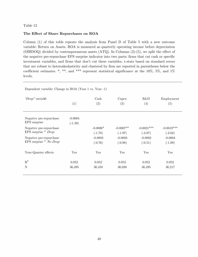
48

Table 12

The Effect of Share Repurchases on ROA

Column (1) of this table repeats the analysis from Panel D of Table 5 with a new outcome variable: Return on Assets. ROA is measured as quarterly operating income before depreciation (OIBDOQ) divided by contemporaneous assets (ATQ). In Columns (2)-(5), we split the effect of the negative pre-repurchase EPS surprise indicator into two parts: firms that cut cash or specific investment variables, and firms that don’t cut these variables. t-stats based on standard errors that are robust to heteroskedasticity and clustered by firm are reported in parentheses below the coefficient estimates. *, **, and *** represent statistical significance at the 10%, 5%, and 1% levels.

Dependent variable: Change in ROA (Year 1 vs. Year -1) “Drop” variable Cash Capex R&D Employment (1) (2) (3) (4) (5) Negative pre-repurchase EPS surprise

-0.0004 (-1.39)

Negative pre-repurchase EPS surprise * Drop

-0.0006* -0.0007** -0.0021*** -0.0019*** (-1.78) (-1.97) (-3.87) (-2.62)

Negative pre-repurchase EPS surprise * No Drop

-0.0003 -0.0003 -0.0002 -0.0004 (-0.76) (-0.98) (-0.51) (-1.09)

Year-Quarter effects Yes Yes Yes Yes Yes R2 0.052 0.052 0.052 0.052 0.052 N 36,495 36,458 36,038 36,495 36,217

49

Appendix

Figure A1

Placebo test: Probability of decretive share repurchases.

This figure plots the probability of doing a decretive share repurchase as function of the pre-repurchase earnings surprise. For every bin of earnings surprise, the dots represent the probability of an decretive share repurchase—the fraction of firm-quarters with a decretive repurchase out of all firm-quarters in that bin. We define a share repurchase as decretive if it decreases EPS by at least 1 cent. The pre-repurchase earnings surprise is the difference between the repurchase-adjusted (“pre-repurchase”) earnings per share (EPS) and the median EPS forecast at the end of the quarter; this difference is normalized by the end-of-quarter stock price. The pre-repurchase EPS is calculated as follows: 𝐸𝐸𝑆𝑎𝑎𝑎 = 𝐸𝑎𝑎𝑎

𝑆𝑎𝑎𝑎= 𝐸+𝐼

𝑆+∆𝑆, where 𝐸 is reported

earnings, 𝐼 is the estimated forgone interest due to the repurchase, 𝑆 is the number of shares at the end of the quarter, and ∆𝑆 is the estimated number of shares repurchased (repurchase amount divided by the average daily share price). The forgone interest is the after-tax interest that would be earned on an amount of funds equal to that used to repurchase shares if it were instead invested in a 3-month T-Bill.

0.00%

0.10%

0.20%

0.30%

-0.01 -0.005 0 0.005 0.01

Pre-repurchase EPS surprise

50

Table A1

Share Repurchases and Investment: Bandwidth sensitivity analysis

This table reports the results of a sensitivity analysis of the choice of bandwidth in the relationship between share repurchases and changes in future employment and investment outcomes. Panels A–E report the results for varying bandwidths, from 0.001 to 0.005 of the pre-repurchase EPS surprise. The base result from Panel B in Table 5 (bandwidth=0.003) is reported here in Panel C. t-stats based on standard errors that are robust to heteroskedasticity and clustered by firm are reported in parentheses below the coefficient estimates. *, **, and *** represent statistical significance at the 10%, 5%, and 1% levels, respectively.

Dependent variable: Employment Capex R&D (1) (2) (3) Panel A: abs(Pre-repurchase EPS surprise)<=0.001 Repurchases/Assets (Instrumented) -137.0*** -0.259** -0.096* (-4.09) (-2.55) (-1.91) N 21,480 21,017 21,772 Panel B: abs(Pre-repurchase EPS surprise)<=0.002 Repurchases/Assets (Instrumented) -124.8*** -0.262** -0.128*** (-4.01) (-2.56) (-2.77) N 31,439 30,720 31,879 Panel C (base result): abs(Pre-repurchase EPS surprise)<=0.003 Repurchases/Assets (Instrumented) -155.8*** -0.301*** -0.087** (-4.84) (-3.15) (-2.09) N 37,230 36,344 37,772 Panel D: abs(Pre-repurchase EPS surprise)<=0.004 Repurchases/Assets (Instrumented) -153.8*** -0.369*** -0.128*** (-5.03) (-3.74) (-3.05) N 41,103 40,114 41,716 Panel E: abs(Pre-repurchase EPS surprise)<=0.005 Repurchases/Assets (Instrumented) -164.7*** -0.498*** -0.150*** (-5.33) (-4.84) (-3.47) N 43,685 42,619 44,355 Linear control in pre-repurchase EPS surprise Yes Yes Yes Year-Quarter FE Yes Yes Yes

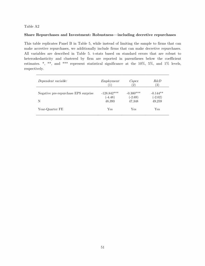
51

Table A2

Share Repurchases and Investment: Robustness—including decretive repurchases

This table replicates Panel B in Table 5, while instead of limiting the sample to firms that can make accretive repurchases, we additionally include firms that can make decretive repurchases. All variables are described in Table 5. t-stats based on standard errors that are robust to heteroskedasticity and clustered by firm are reported in parentheses below the coefficient estimates. *, **, and *** represent statistical significance at the 10%, 5%, and 1% levels, respectively.

Dependent variable: Employment Capex R&D (1) (2) (3) Negative pre-repurchase EPS surprise -128.842*** -0.300*** -0.144** (-4.48) (-2.69) (-2.02) N 48,393 47,348 49,259 Year-Quarter FE Yes Yes Yes

52

Table A3

Share Repurchases and Investment: Robustness—controlling for earnings management

This table reports the results for the relationship between share repurchases and changes in future employment and investment outcomes, where we additionally control for proxies of earnings management and analyst guidance. Panel A controls for total accruals, Panel B controls for discretionary accruals, and Panel C controls for earnings guidance. Total accruals, discretionary accruals, and the guidance variables are defined as in Table 1. Our guidance data (from First Call) are limited to 1995–2009, which results in a smaller sample in Panel C. t-stats based on standard errors that are robust to heteroskedasticity and clustered by firm are reported in parentheses below the coefficient estimates. *, **, and *** represent statistical significance at the 10%, 5%, and 1% levels, respectively.

Dependent variable: Employment Capex R&D (1) (2) (3) Panel A: Total accruals control Repurchases/Assets (Instrumented) -169.103*** -0.279** -0.112** (-4.39) (-2.50) (-2.31) Total accruals 12.205*** 0.038*** 0.005** (8.94) (7.60) (2.05) Panel B: Discretionary accruals control Repurchases/Assets (Instrumented) -175.414*** -0.350*** -0.113** (-4.86) (-3.01) (-2.54) Discretionary accruals 9.935*** 0.026*** 0.009*** (9.17) (6.79) (5.70) Panel C: Earnings guidance control Repurchases/Assets (Instrumented) -83.410*** -0.231*** -0.043 (-3.40) (-2.70) (-1.19) Positive guidance 0.179* 0.001*** 0.000** (1.71) (2.89) (2.26) Negative guidance -0.128 -0.001** 0.000 (-1.23) (-2.51) (0.74) Any guidance 0.229** -0.002*** -0.000*** (2.05) (-5.27) (-2.73) Linear control in pre-repurchase EPS surprise Yes Yes Yes Year-Quarter FE Yes Yes Yes

53

Table A4

Share Repurchases and Investment: Positive actual surprises

This table repeats the analysis from Table 5, but only among firms that experience a small positive actual EPS surprise. The sample is constructed in the following way: We first limit the sample to firm-quarters that fall within a small area around a zero pre-repurchase EPS surprise (a pre-repurchase EPS surprise normalized by share price between -0.003 and 0.003). Then, we further require the firm-quarters to exhibit a positive actual EPS surprise. The regressions are at the firm-quarter level. We control for year-quarter effects throughout. In Panel B, we additionally control for the level of the pre-repurchase EPS surprise, interacted with the sign of the surprise. t-stats based on standard errors that are robust to heteroskedasticity and clustered by firm are reported in parentheses below the coefficient estimates. *, **, and *** represent statistical significance at the 10%, 5%, and 1% levels, respectively.

Dependent variable: Employment Capex R&D (1) (2) (3) Panel A: IV Repurchases/Assets (Instrumented) -24.563*** -0.108*** -0.019*** (-5.85) (-7.10) (-2.80) N 27,759 27,100 28,128 Panel B: IV (linear control) Repurchases/Assets (Instrumented) -28.693*** -0.105*** -0.017* (-3.98) (-3.98) (-1.67) N 27,759 27,100 28,128 Year-Quarter FE Yes Yes Yes

54

Table A5

Share Repurchases and Investment: Using raw share repurchases

This table replicates Panels A and B of Table 5, but substitutes net repurchases with raw repurchases. Raw repurchases is measured as the variable prstkcy (Purchase of common and preferred stock) in Compustat. t-stats based on standard errors that are robust to heteroskedasticity and clustered by firm are reported in parentheses below the coefficient estimates. *, **, and *** represent statistical significance at the 10%, 5%, and 1% levels, respectively.

Dependent variable: Employment Capex R&D (1) (2) (3) Panel A: IV Repurchases/Assets (Instrumented) -222.2*** -0.981*** -0.265*** (-6.90) (-7.49) (-5.59) N 37,230 36,344 37,772 Panel B: IV (linear control) Repurchases/Assets (Instrumented) -155.8*** -0.301*** -0.087** (-4.84) (-3.15) (-2.09) N 37,230 36,344 37,772 Year-Quarter FE Yes Yes Yes

55

Table A6

Reported changes in corporate policies during the event quarter

This figure shows the distribution of cuts in cash and investment variables (capex, R&D, employment) among firms that do a repurchase and would have had a slightly negative pre-repurchase EPS surprise. These cuts are measured during the same quarter as the EPS-motivated repurchase, and thus are in the information set of investors at the quarterly earnings announcement date of the repurchase.

Policy change Frequency % Drop nothing 1,134 18.8% Drop Cash 1,126 18.6% Drop Capex 667 11.0% Drop Employment 338 5.6% Drop R&D 92 1.5% Subtotal (one drop) 2,223 36.8% Drop Capex and Cash 638 10.6% Drop Employment and Capex 524 8.7% Drop Employment and Cash 386 6.4% Drop R&D and Capex 102 1.7% Drop R&D and Cash 92 1.5% Drop Employment and R&D 45 0.7% Subtotal (two drops) 1,787 29.6% Drop Employment, Capex and Cash 477 7.9% Drop Employment, R&D and Capex 144 2.4% Drop R&D, Capex, and Cash 83 1.4% Drop Employment, R&D and Cash 74 1.2% Subtotal (three drops) 778 12.9% Drop All 125 2.1% Total 6,047 100.0%