there is a risk-return trade-oﬀ after all

There is a risk-return trade-off after all

Eric Ghyselsa, Pedro Santa-Clarab, Rossen Valkanovb,∗

aKenan-Flagler Business School, McColl Building, Suite 4100, University of NorthCarolina, Chapel Hill NC 27599-3490, USA

bThe John E. Anderson Graduate School of Management, University of California at LosAngeles, Los Angeles, CA 90095-1481, USA

(Received 2 May 2003; accepted 4 March 2004)

AbstractThis paper studies the intertemporal relation between the conditional mean and the condi-

tional variance of the aggregate stock market return. We introduce a new estimator that forecastsmonthly variance with past daily squared returns, the mixed data sampling (or MIDAS) approach.Using MIDAS, we find a significantly positive relation between risk and return in the stock market.This finding is robust in subsamples, to asymmetric specifications of the variance process and tocontrolling for variables associated with the business cycle. We compare the MIDAS results withtests of the intertemporal capital asset pricing model based on alternative conditional variancespecifications and explain the conflicting results in the literature. Finally, we offer new insightsabout the dynamics of conditional variance.

JEL classification: G12; C22

Keywords: risk-return trade-off; ICAPM; MIDAS; conditional variance

We thank Michael Brandt, Tim Bollerslev, Mike Chernov, Rob Engle, Shingo Goto, Amit Goyal,Campbell Harvey, David Hendry, Francis Longstaff, Nour Meddahi, Eric Renault, Matt Richardson, NeilShephard, and seminar participants at Barclays Global Investors, Centro de Estudios Monetarios y Fi-nancieros (Madrid), Emory University, the Global Association of Risk Professionals, Instituto TecnologicoAutonomo de Mexico (Mexico City), Instituto Superior de Ciencias do Trabalho e da Empresa (Lisbon), theCentre Interuniversitaire de Recherche en Analyse des Organisations Conference on Financial Econometrics(Montreal), Lehman Brothers, London School of Economics, Morgan Stanley, New York University, OxfordUniversity, University of Cyprus, University of North Carolina, and University of Southern California forhelpful comments. We especially thank an anonymous referee whose suggestions greatly improved the paper.Arthur Sinko provided able research assistance.∗Corresponding author. Tel: (310) 825-7246E-mail address: [email protected]

1. Introduction

The Merton (1973) intertemporal capital asset pricing model (ICAPM) suggests thatthe conditional expected excess return on the stock market should vary positively with themarket’s conditional variance:

Et[Rt+1] = µ+ γVart[Rt+1], (1)

where γ is the coefficient of relative risk aversion of the representative agent and, accordingto the model, µ should be equal to zero. The expectation and the variance of the marketexcess return are conditional on the information available at the beginning of the returnperiod, time t. This risk-return trade-off is so fundamental in financial economics that itcould be described as the “first fundamental law of finance.”1 Unfortunately, the trade-offhas been hard to find in the data. Previous estimates of the relation between risk and returnoften have been insignificant and sometimes even negative.

Baillie and DeGennaro (1990), French, Schwert, and Stambaugh (1987), and Campbelland Hentschel (1992) do find a positive albeit mostly insignificant relation between theconditional variance and the conditional expected return. In contrast, Campbell (1987)and Nelson (1991) find a significantly negative relation. Glosten, Jagannathan, and Runkle(1993), Harvey (2001), and Turner, Startz, and Nelson (1989) find both a positive and anegative relation depending on the method used.2 The main difficulty in testing the ICAPMrelation is that the conditional variance of the market is not observable and must be filteredfrom past returns.3 The conflicting findings of the above studies are mostly the result ofdifferences in the approach to modeling the conditional variance.

In this paper, we take a new look at the risk-return trade-off by introducing a newestimator of the conditional variance. Our mixed data sampling, or MIDAS, estimatorforecasts the monthly variance with a weighted average of lagged daily squared returns. Weuse a flexible functional form to parameterize the weight given to each lagged daily squaredreturn and show that a parsimonious weighting scheme with only two parameters works well.We estimate the coefficients of the conditional variance process jointly with µ and γ fromthe expected return Eq. (1) with quasi-maximum likelihood.

Using monthly and daily market return data from 1928 to 2000 and with MIDAS as amodel of the conditional variance, we find a positive and statistically significant relationbetween risk and return. The estimate of γ is 2.6, which lines up well with economic

1However, Abel (1988), Backus and Gregory (1993), and Gennotte and Marsh (1993) offer models inwhich a negative relation between return and variance is consistent with equilibrium. Campbell (1993)discusses general conditions under which the risk-return relation holds as an approximation.

2See also Chan et al. (1992), Lettau and Ludvigson (2002), Merton (1980), and Pindyck (1984). Goyaland Santa-Clara (2003) find a positive trade-off between market return and average stock variance.

3We could think of using option implied volatilities as do Santa-Clara and Yan (2001) to make varianceobservable. Unfortunately, option prices are available only since the early 1980s, which is insufficient toreliably make inferences about the conditional mean of the stock market.

1

intuition about a reasonable level of risk aversion. The MIDAS estimator explains about40% of the variation of realized variance in the subsequent month and its explanatory powercompares favorably to that of other models of conditional variance such as the generalizedautoregressive conditional heteroskedasticity (GARCH). The estimated weights on the laggeddaily squared returns decay slowly, thus capturing the persistence in the conditional varianceprocess. More impressive still is that, in the ICAPM risk-return relation, the MIDASestimator of conditional variance explains about 2% of the variation of next month’s stockmarket returns (and 5% in the period since 1964). This is substantial given previous resultsabout forecasting the stock market return. For instance, the forecasting power of the dividendyield for the market return does not exceed 1.5%. (see Campbell, Lo, and MacKinlay, 1997,and references therein) Finally, the above results are qualitatively similar when the sampleis split into two subsamples of approximately equal sizes, 1928–1963 and 1964–2000.

To better understand MIDAS and its success in testing the ICAPM risk-return trade-off, we compare our approach to previously used models of conditional variance. Frenchet al. (1987) propose a simple and intuitive rolling window estimator of the monthly variance.They forecast monthly variance by the sum of daily squared returns in the previous month.Their method is similar to ours in that it uses daily returns to forecast monthly variance.However, when French et al. use that method to test the ICAPM, they find an insignificant(and sometimes negative) γ coefficient. We replicate their results but also find somethinginteresting and new. When the length of the rolling window is increased from one month tothree or four months, the magnitude of the estimated γ increases and the coefficient becomesstatistically significant. This result nicely illustrates the point that the window length playsa crucial role in forecasting variances and detecting the trade-off between risk and return.By optimally choosing the weights on lagged squared returns, MIDAS implicitly selects theoptimal window size to estimate the variance, and that in turn allows us to find a significantrisk-return trade-off.

The ICAPM risk-return relation has also been tested using several variations ofGARCH-in-mean models. However, the evidence from that literature is inconclusive andsometimes conflicting. Using simple GARCH models, we confirm the finding of French et al.(1987) and Glosten et al. (1993), among others, of a positive but insignificant γ coefficient inthe risk-return trade-off. The absence of statistical significance comes from both GARCH’suse of monthly return data in estimating the conditional variance process and the inflexibilityof the parameterization. The use of daily data and the flexibility of the MIDAS estimatorprovide the power needed to find statistical significance in the risk-return trade-off.

A comparison of the time series of conditional variance estimated according to MIDAS,GARCH, and rolling windows reveals that while the three estimators are correlated, somedifferences affect their ability to forecast returns in the ICAPM relation. We find that theMIDAS variance process is more highly correlated with both the GARCH and the rollingwindows estimates than these last two are with each other. This suggests that MIDAScombines some of the unique information contained in the other two estimators. We alsofind that MIDAS is particularly successful at forecasting realized variance both in high and

2

low volatility regimes. These features explain the superior performance of MIDAS in findinga positive and significant risk-return relation.

It has long been recognized that volatility tends to react more to negative returnsthan to positive returns. Nelson (1991) and Engle and Ng (1993) show that GARCH modelsthat incorporate this asymmetry perform better in forecasting the market variance. However,Glosten et al. (1993) show that when such asymmetric GARCH models are used in testing therisk-return trade-off, the γ coefficient is estimated to be negative (sometimes significantly so).This stands in sharp contrast with the positive and insignificant γ obtained with symmetricGARCH models and remains a puzzle in empirical finance. To investigate this issue, weextend the MIDAS approach to capture asymmetries in the dynamics of conditional varianceby allowing lagged positive and negative daily squared returns to have different weights in theestimator. Contrary to the asymmetric GARCH results, we still find a large positive estimateof γ that is statistically significant. This discrepancy between the asymmetric MIDAS andasymmetric GARCH tests of the ICAPM turns out to be interesting.

We find that what matters for the tests of the risk-return trade-off is not so muchthe asymmetry in the conditional variance process but its persistence. In this respect,asymmetric GARCH and asymmetric MIDAS models prove to be very different. Consistentwith the GARCH literature, negative shocks have a larger immediate impact on the MIDASconditional variance estimator than do positive shocks. However, we find that the impact ofnegative returns on variance is only temporary and lasts no more than one month. Positivereturns have an extremely persistent impact on the variance process. In other words, whileshort-term fluctuations in the conditional variance are mostly the result of negative shocks,the persistence of the variance process is primarily driven by positive shocks. This isan intriguing finding about the dynamics of the variance process. Although asymmetricGARCH models allow for a different response of the conditional variance to positive andnegative shocks, they constrain the persistence of both types of shocks to be the same.Because the asymmetric GARCH models load heavily on negative shocks and these havelittle persistence, the estimated conditional variance process shows little to no persistence.The only exception is the two-component GARCH model of Engle and Lee, 1999, who reportfindings similar to our asymmetric MIDAS model. They obtain persistent estimates ofconditional variance while still capturing an asymmetric reaction of the conditional varianceto positive and negative shocks. In contrast, by allowing positive and negative shocks tohave different persistence, the asymmetric MIDAS model still obtains high persistence forthe overall conditional variance process. Since only persistent variables can capture variationin expected returns, the difference in persistence between the asymmetric MIDAS and theasymmetric GARCH conditional variances explains their success and lack thereof in findinga risk-return trade-off.

Campbell (1987) and Scruggs (1998) point out that the difficulty in measuring a positiverisk-return relation could stem from misspecification of Eq. (1). Following Merton (1973),they argue that if changes in the investment opportunity set are captured by state variablesin addition to the conditional variance itself, then those variables must be included in the

3

equation of expected returns. In parallel, an extensive literature on the predictability ofthe stock market finds that variables that capture business cycle fluctuations are also goodforecasters of market returns (see Campbell, 1991; Campbell and Shiller, 1988; Fama, 1990;Fama and French, 1988, 1989; Ferson and Harvey, 1991; and Keim and Stambaugh, 1986,among many others). We include business cycle variables together with both the symmetricand asymmetric MIDAS estimators of conditional variance in the ICAPM equation and findthat the trade-off between risk and return is virtually unchanged. The explanatory power ofthe conditional variance for expected returns is orthogonal to the other predictive variables.

We conclude that the ICAPM is alive and well.

The rest of the paper is structured as follows. Section 2 explains the MIDAS model anddetails the main results. Section 3 offers a comparison of MIDAS with rolling window andGARCH models of conditional variance. In Section 4, we discuss the asymmetric MIDASmodel and use it to test the ICAPM. In Section 5, we include several often-used predictivevariables as controls in the risk-return relation. Section 6 concludes.

2. MIDAS tests of the risk-return trade-off

In this section, we introduce the mixed data sampling, or MIDAS, estimator ofconditional variance and use it to test the ICAPM relation between risk and return of thestock market.

2.1. Methodology

The MIDAS approach mixes daily and monthly data to estimate the conditionalvariance of the stock market. The returns on the left-hand side of Eq. (1) are measuredat monthly intervals because higher frequency returns could be too noisy to use in a studyof conditional means. On the right-hand side of the equation, we use daily returns in thevariance estimator to exploit the advantages of high-frequency data in the estimation ofsecond moments explained by the well-known continuous-record argument of Merton (1980).4

We allow the variance estimator to load on a large number of past daily squared returns withoptimally chosen weights.

The MIDAS estimator of the conditional variance of monthly returns, Vart[Rt+1], is

4Recently, several authors, including Andersen et al. (2001), Andreou and Ghysels (2002), Barndorff-Nielsen and Shephard (2002), and Taylor and Xu (1997) suggest various methods using high-frequency datato estimate variances. Alizadeh et al. (2002) propose an alternative measure of realized variance using thedaily range of the stock index.

4

based on prior daily squared return data:

V MIDAS

t = 22∞∑

d=0

wdr2t−d, (2)

where wd is the weight given to the squared return of day t − d. We use the lower caser to denote daily returns, which should be distinguished from the upper case R used formonthly returns; the corresponding subscript t− d stands for the date t minus d days. Rt+1

is the monthly return from date t to date t + 1 and rt−d is the daily return d days beforedate t. Although this notation is slightly ambiguous, it has the virtue of not being overlycumbersome. With weights that sum up to one, the factor 22 ensures that the variance isexpressed in monthly units because a month typically has 22 trading days.

We postulate a flexible form for the weight given to the squared return on day t− d:

wd(κ1, κ2) =exp{κ1d+ κ2d

2}∑∞i=0 exp{κ1i+ κ2i2}

. (3)

This scheme has several advantages. First, it guarantees that the weights are positive, whichin turn ensures that the conditional variance in Eq. (2) is also positive. Second, the weightsadd up to one. Third, the functional form in Eq. (3) can produce a wide variety of shapesfor different values of the two parameters. Fourth, the specification is parsimonious, withonly two parameters to estimate. Fifth, as long as the coefficient κ2 is negative, the weightsgo to zero as the lag length increases. The speed with which the weights decay controlsthe effective number of observations used to estimate the conditional variance. Finally, wecan increase the order of the polynomial in Eq. (3) or consider other functional forms.For instance, all the results shown below are robust to parameterizing the weights as a Betafunction instead of the exponential form in Eq. (3). See Ghysels, Santa-Clara, and Valkanov,2004, for a general discussion of the functional form of the weights. As a practical matter,the infinite sum in Eq. (2) and Eq. (3) needs to be truncated at a finite lag. In all theresults that follow, we use 252 days (which corresponds to roughly one year of trading days)as the maximum lag length. The results are not sensitive to increasing the maximum laglength beyond one year.

The weights of the MIDAS estimator implicitly capture the dynamics of the conditionalvariance. A larger weight on distant past returns induces more persistence on the varianceprocess. The weighting function also determines the statistical precision of the estimatorby controlling the amount of data used to estimate the conditional variance. When thefunction decays slowly, a large number of observations effectively enter in the forecast of thevariance and the measurement error is low. Conversely, a fast decay corresponds to using asmall number of daily returns to forecast the variance with potentially large measurementerror. To some extent, a tension exists between capturing the dynamics of variance andminimizing measurement error. Because variance changes through time, we would like touse more recent observations to forecast the level of variance in the next month. However, to

5

the extent that measuring variance precisely requires a large number of daily observations,the estimator could still place significant weight on more distant observations. The Appendixoffers a more formal treatment of the MIDAS estimator.

To estimate the parameters in the weight function, we maximize the likelihood ofmonthly returns. We use the variance estimator Eq. (2) with the weight function Eq. (3) inthe ICAPM relation Eq. (1) and estimate the parameters κ1 and κ2 jointly with µ and γ bymaximizing the likelihood function, assuming that the conditional distribution of returns isnormal5

Rt+1 ∼ N (µ+ γV MIDAS

t , V MIDAS

t ) (4)

In this way, the conditional mean and the conditional variance of the monthly return inApril (from the close of the last day of March to the close of the last day of April) dependson daily returns up to the last day of March. Because the true conditional distribution ofreturns could depart from normality, our estimator is only quasi-maximum likelihood. Theparameter estimators are nevertheless consistent and asymptotically normally distributed.Their covariance matrix is estimated using the Bollerslev and Wooldridge (1992) approachto account for heteroskedasticity.6

We have thus far used monthly returns as a proxy for expected returns in Eq. (1)and daily returns in the construction of the conditional variance estimator. However, usinghigher frequency returns at, say, weekly or daily intervals could improve the estimate ofγ because of the availability of additional data points. Alternatively, quarterly returnscould increase the efficiency of the estimator of γ because they are less volatile. A generalanalytical argument is difficult to formulate without making additional assumptions aboutthe data-generating process. Similarly, the returns used to forecast volatility can be sampledat different frequencies from intradaily to weekly or even monthly observations. Fortunately,the MIDAS approach can easily be implemented at different frequencies on the left-handand on the right-hand side. This can be achieved with the same parametric specificationand with the same number of parameters. Hence, we can directly compare the estimates ofγ and their statistical significance across different frequencies.

2.2. Empirical analysis

We estimate the ICAPM with the MIDAS approach using excess returns on the stockmarket from January 1928 to December 2000. We use the Center for Research in SecurityPrices (CRSP) value-weighted portfolio as a proxy for the stock market and the yield of thethree-month Treasury bill as the risk-free interest rate. Daily market returns are obtained

5Alternatively, we could use generalized methods of moments (GMM) for more flexibility in the relativeweighting of the conditional moments in the objective function.

6More specifically, using Theorem 2.1 in Bollerslev and Wooldridge, 1992, we compute the covariancematrix of the parameter estimates as A−1

T BT A−1T /T , where A−1

T is an estimate of the Hessian matrix of thelikelihood function and BT is an estimate of the outer product of the gradient vector with itself.

6

from CRSP for the period July 1962 to December 2000 and from William G. Schwert’s websitefor the period January 1928 to June 1962 (see Schwert, 1990a, for a description of those data).The daily risk-free rate, obtained from Ibbotson Associates, is constructed by assuming thatthe Treasury bill rates stay constant within the month and suitably compounding them.Monthly excess returns are obtained by compounding the daily excess returns. In whatfollows, we refer to excess returns simply as returns.

Table 1 displays summary statistics for the monthly returns and the monthly realizedvariance of returns computed from within-month daily data, as explained in Eq. (5). Weshow the summary statistics for the full 1928–2000 sample and, for robustness, we alsoanalyze two subsamples of approximately equal length, 1928 to 1963 and 1964 to 2000.

[Insert Table 1 near here]

The monthly market return has a mean of 0.649% and a standard deviation of 5.667%(variance of 0.321 × 102). This and later tables report variances instead of more customarystandard deviations because the risk-return trade-off postulates a relation between returnsand their variance, not their standard deviation. Returns are negatively skewed and slightlyleptokurtic. The first order autoregressive coefficient of monthly returns is 0.068. Theaverage market return during 1928-1963 is considerably higher than that observed during1964-2000. The variance of monthly returns is also higher in the first subsample. Bothsubsamples exhibit negative skewness and high kurtosis. The realized variance has a meanof 0.262 in the overall sample, which closely matches the variance of monthly returns (thesmall difference between the two numbers is attributable to Jensen’s inequality). The meanof the variance in the first subsample is much higher than in the second, mostly becauseof the period of the Great Depression. The realized variance process displays considerablepersistence, with an autoregressive coefficient of 0.608 in the entire sample. Again, the firstsubsample shows more persistence in the variance process. As expected, realized variance ishighly skewed and leptokurtic. The results from these summary statistics are well known inthe empirical finance literature.

Table 2 contains the main result of the paper, the estimation of the risk-return trade-offequation with the MIDAS conditional variance. The estimated ICAPM coefficient γ is 2.606in the full sample, with a highly significant t-statistic (corrected for heteroskedasticity withthe Bollerslev and Wooldridge method) of 6.710. Most important, the magnitude of γ linesup well with the theory. According to the ICAPM, γ is the coefficient of relative risk aversionof the representative investor and a risk aversion coefficient of 2.606 matches a variety ofempirical studies (see Hall, 1988, and references therein). The significance of γ is robust inthe subsamples, with estimated values of 1.547 and 3.748, and t-statistics of 3.382 and 8.612.These results are consistent with Mayfield (2003), who uses a regime-switching model forconditional volatility and finds that the risk-return trade-off holds within volatility regimes.The estimated magnitude and significance of the γ coefficient in the ICAPM relation areremarkable in light of the ambiguity of previous results. The intercept µ is always significant,

7

which, in the framework of the ICAPM, could capture compensation for covariance of themarket return with other state variables (which we address in Section 5) or compensationfor jump risk (see Pan, 2002; and Chernov, Gallant, Ghysels, and Tauchen, 2002).


Table 2 also reports the estimated parameters of the MIDAS weight function Eq.(3). Both coefficients are statistically significant in the full sample and the subsamples.Furthermore, a likelihood ratio test of their joint significance, κ1 = κ2 = 0, has a p-valuesmaller than 0.001. Because the restriction κ1 = κ2 = 0 corresponds to placing equalweights on all lagged squared daily returns, we conclude that the estimated weight functionis statistically different from a simple equally weighted scheme. We cannot interpret themagnitudes of the coefficients κ1 and κ2 individually but only jointly in the weighting functionEq. (3). In Fig. 1, we plot the estimated weights, wd(κ1, κ2), of the conditional varianceon the lagged daily squared returns for the full sample and the subsamples. In all cases, weobserve that the weights are a slowly declining function of the lag length. For example, only31% of the weight is placed on the first lagged month of daily data (22 days), 56% on thefirst two months, and it takes more than three months for the cumulative weight to reach75%. The weight profiles for the subsamples are very similar. We conclude that it takesa substantial amount of daily return data to accurately forecast the variance of the stockmarket. This result stands in sharp contrast to the common view that one month of dailyreturns is sufficient to reliably estimate the variance.

[Insert Fig. 1 near here]

To assess the predictive power of the MIDAS variance for the market return we runa regression of the realized return in month t + 1, Rt+1, on the forecasted variance for thatmonth, V MIDAS

t . The coefficient of determination for the regression using the entire sample,R2

R, is 1.9%, which is a reasonably high value for a predictive regression of returns at monthlyfrequency. This coefficient increases to 5.0% in the second subsample.

We also examine the ability of the MIDAS estimator to forecast realized variance. Weestimate realized variance from within-month daily returns as

σ2t+1 =

22∑

d=0

r2t+1−d. (5)

Table 2 reports the coefficient of determination, R2σ2 , from regressing the realized variance,

σ2t+1, on the MIDAS forecasted variance, V MIDAS

t . MIDAS explains over 40% of thefluctuations of the realized variance in the entire sample. Given that σ2

t+1 in Eq. (5) isonly a noisy proxy for the true variance in the month, the R2

σ2 obtained is impressively

8

high. Andersen and Bollerslev (1998) and Andersen et al. (2004) show that the maximumR2 obtainable in a regression of this type is much lower than 100%, often on the order of40%. The high standard deviation of the realized variance and the relatively low persistenceof the process, shown in Table 1, indicate a high degree of measurement error. The value ofR2

σ2 in the second subsample is only 0.082, because of the crash of 1987. If we eliminate the1987 crash from the second subsample, the R2

σ2 jumps to 0.283. Fig. 2 displays the realizedvariance together with the MIDAS forecast for the entire sample. We see that the estimatordoes a remarkable job of forecasting next month’s variance.


Thus far we have estimated γ in a MIDAS regression of monthly returns on varianceestimated from daily returns. However, this is not the only possible frequency choice. Withhigher frequency data on the left-hand side, we have more observations, but also more noisein the returns. With lower frequency data, we have a better estimate of expected returns,but fewer observations. We now investigate what return horizon in the left-hand side ofthe MIDAS regression yields the most precise estimates of the risk-return trade-off. Table3 presents estimates of γ in the ICAPM regression of returns at daily, weekly, monthly,bimonthly, and quarterly horizons on the MIDAS conditional variance, estimated with dailysquared returns. We find that the estimates of γ range from 1.964 to 2.880 as the frequencyof returns varies. The t-statistics of γ increase systematically from 1.154 at daily frequencyto 6.710 at monthly frequency. The standard error of the estimates does not change muchacross horizons, so the improvement in the t-statistics is mostly the result of the higher pointestimate of γ at the monthly horizon.


A similar pattern emerges from the goodness-of-fit measures R2R and R2

σ2 in Table 3.The use of high-frequency data as a proxy for the conditional mean of returns decreases theability of the MIDAS estimator to forecast realized variance. The R2

σ2 at daily and weeklyhorizons are only 0.059 and 0.119. At monthly, bimonthly, and quarterly horizons, theyare markedly higher at 0.407, 0.309, and 0.329. The realized variances at daily or weeklyfrequency are a very noisy measure of the true variance because they are estimated with onlyone or five daily returns. The subsamples in Table 3 yield similar results. We conclude thatthe choice of monthly frequency strikes the best balance between sample size and signal-to-noise ratio. Hence, in the subsequent analysis, we use only monthly returns on the left-handside of our MIDAS models.

3. Why MIDAS works: comparison with other tests

9

To understand why tests based on the MIDAS approach support the ICAPM when theextant literature offers conflicting results, we compare the MIDAS estimator with previouslyused estimators of conditional variance. We focus our attention on rolling window andGARCH estimators of conditional variance. For conciseness, we report results for the entiresample, but the conclusions also hold in the subsamples.

3.1. Rolling window tests

As an example of the rolling window approach, French et al. (1987) use within-monthdaily squared returns to forecast next month’s variance:

V RW

t = 22D∑

d=0

1

Dr2t−d, (6)

where D is the number of days used in the estimation of variance.French, Schwert, andStambaugh (1987) include a correction for serial correlation in the returns that we ignorefor now. We follow their example and do not adjust the measure of variance by the squaredmean return as this is likely to have only a minor impact with daily data. In addition, French,Schwert, and Stambaugh use the fitted value of an autoregressive moving average (ARMA)process for the one-month rolling window estimator to model the conditional variance. Again,daily squared returns are multiplied by 22 to measure the variance in monthly units. French,Schwert, and Stambaugh choose the window size to be one month, or D = 22. Besides itssimplicity, this approach has a number of advantages. First, as with the MIDAS approach,the use of daily data increases the precision of the variance estimator. Second, the stockmarket variance is very persistent (see Officer, 1973, and Schwert, 1989), so the realizedvariance on a given month ought to be a good forecast of next month’s variance.

However, it is not clear that we should confine ourselves to using data from the lastmonth only to estimate the conditional variance. We perhaps want to use a larger windowsize D in Eq. (6), corresponding to more than one month’s worth of daily data. This choicehas a large impact on the estimate of γ.

We estimate the parameters µ and γ of the risk-return trade-off Eq. (1) with maximumlikelihood using the rolling window estimator Eq. (6) for the conditional variance. Table 4reports the estimates of the risk-return trade-off for different sizes D of the window used toestimate the conditional variance. The first line corresponds to using daily data from theprevious month only so the measure of V RW

t is similar to the one reported in French et al.(1987). The estimate of γ is 0.546 and statistically insignificant. In their study, French et al.(1987) estimate a γ of -0.349, also insignificant. The difference between the estimates stemsfrom the difference in sample periods. When we use their sample period from 1928 to 1984,we obtain the same results as French et al. (1987).


10

As we increase the window size to two through four months, the magnitude of γincreases and becomes significant, with a higher R2

R. When the rolling window includesfour months of data, the estimated γ coefficient is 2.149 and statistically significant. Thesefindings are consistent with Brandt and Kang, 2004, and Whitelaw, 1994, who report alagged relation between the conditional variance and the conditional mean. This coefficientis very similar to the estimated γ with the MIDAS approach; only the level of significanceis lower. Finally, as the window size increases beyond four months, the magnitude of theestimated γ decreases as does the likelihood value. This suggests that there is an optimalwindow size to estimate the risk-return trade-off.

These results are striking. They confirm our MIDAS finding, namely, that a positiveand significant trade-off exists between risk and return. The rolling window approach can bethought of as a robust check of the MIDAS regressions because it is such a simple estimatorof conditional variance with no parameters to estimate. Moreover, Table 4 helps us reconcilethe MIDAS results with the findings of French et al. (1987). That paper missed out on thetrade-off by using too small a window size (one month) to estimate the variance. One month’sworth of daily data simply is not enough to reliably estimate the conditional variance andto measure its impact on expected returns.

The maximum likelihood across window sizes is obtained with a four-month window.This window size implies a constant weight of 0.011 in the lagged daily squared returns of theprevious four months. Of the different window lengths we analyze, these weights are closestto the optimal MIDAS weights shown in Fig. 1, which puts roughly 80% of the weight inthose first four months of past daily squared returns.

The rolling window estimator is similar to MIDAS in its use of daily squared returnsto forecast monthly variance. But it differs from MIDAS in that it constrains the weightsto be constant and inversely proportional to the window length. This constraint on theweights affects the performance of the rolling window estimator compared with MIDAS. Forinstance, the rolling window estimator does not perform as well as the MIDAS estimator inforecasting realized returns or realized variance. The coefficient of determination for realizedreturns is 1.2% compared with 1.9% for MIDAS, and for realized variance it is 38.4% whichis lower than the 40.7% obtained with MIDAS.

3.2. GARCH tests

The most popular approach to study the ICAPM risk-return relation has been withGARCH-in-mean models estimated with monthly return data (see Engle, Lilien, and Robins,1987; French, Schwert, and Stambaugh, 1987; Campbell and Hentschel, 1992; Glosten,Jagannathan, and Runkle, 1993, among others). The simplest model in this family canbe written as

V GARCH

t = ω + αε2t + βV GARCH

t−1 , (7)

11

where εt = Rt − µ − γV GARCHt−1 . The squared innovations ε2t in the variance estimator play

a role similar to the monthly squared return in the MIDAS or rolling window approachesand, numerically, they are very similar (because the squared average return is an order ofmagnitude smaller than the average of squared returns). For robustness, we also estimatean absolute GARCH model, ABS-GARCH:

(V ABSGARCH

t )1/2 = ω + α |εt| + β(V ABSGARCH

t−1 )1/2. (8)

The GARCH model Eq. (7) can be rewritten as

V GARCH

t =ω

1 − β+ α

∞∑

i=0

βiε2t−i. (9)

The GARCH conditional variance model is thus approximately a weighted average of pastmonthly squared returns. Compared with MIDAS, the GARCH model uses monthly insteadof daily squared returns. Moreover, the functional form of the weights implied by thedynamics of variance in GARCH models exhibits less flexibility than the MIDAS weightingfunction. Even though the GARCH process is defined by three parameters, the shape ofthe weight function depends exclusively on β. This shape is similar to MIDAS when theparameter κ2 is set to zero.

Table 5 shows the coefficient estimates of the GARCH and the ABS-GARCH models,estimated with quasi-maximum likelihood. Both models yield similar results, so weconcentrate on the simple GARCH case. For that model, the estimate of γ is 1.060 andinsignificant, with a t-statistic of 1.292 (obtained using Bollerslev and Wooldridge standarderrors). French et al. (1987) obtain a higher estimate for γ of 7.809 in a different sample, butthey also find it to be statistically insignificant. Using a symmetric GARCH model, Glostenet al. (1993) estimate γ to be 5.926 and again insignificant. In similar sample periods, wereplicate the findings of these studies. As a further robustness check, we estimate higherorder GARCH(p,q) models (not shown for brevity), with p = 1, . . . , 3 and q = 1, . . . , 3,and obtain estimates of γ that are comparable in magnitude and still insignificant. In sum,although GARCH models find a positive estimate of γ, they lack the power to find statisticalsignificance for the coefficient. Also, the coefficients of determination from predicting returns,R2

R, and realized variances, R2σ2 , are 0.5% and 35.9% for the GARCH model and appear low

when compared with the coefficients of 1.9% and 40.7% percent obtained with MIDAS.


The success of MIDAS relative to GARCH in finding a significant risk-return trade-offresides in the extra power that mixed-data frequency regressions obtain from the use of dailydata in the conditional variance estimator. Put differently, MIDAS has more power thanGARCH because it estimates two, not three, parameters and uses many more observations to

12

do it. Also, relative to GARCH, MIDAS has a more flexible functional form for the weightson past squared returns. The interplay of mixed-frequency data and flexible weights explainthe higher estimates of γ and the higher t-statistics obtained by MIDAS. In Section 3.4 wecome back to this comparison in more detail.

3.3. Comparison of filtered variance processes

To further understand the similarities and differences among MIDAS, GARCH, androlling window estimators, we turn our attention to the filtered time series of conditionalvariance produced by each of the three approaches. For the rolling window estimator, weuse a window length of one month, which is similar to what has been used in the literature.Panel A of Table 6 presents summary statistics of the three conditional variance processes.The GARCH forecast is the most persistent with an AR(1) coefficient of 0.970 and has thehighest mean (0.325) and the lowest variance (0.187). The rolling window forecast is theleast persistent with an AR(1) coefficient of 0.608 and has a much lower mean (0.262) andthe highest variance (0.323). The high variance and low persistence partly stems from thisestimator’s high measurement error. The high mean of the GARCH variance relative to therealized variance (which has the same mean as the rolling windows) indicates that GARCHhas some bias. With an AR(1) of 0.872, the persistence of MIDAS conditional variance isbetween that of the GARCH and the rolling windows approaches. MIDAS variance has amean of 0.256, which is very similar to the rolling windows mean and is lower than theGARCH mean. Finally, the variance of the MIDAS conditional variance is between that ofGARCH and of rolling windows.


The difference among MIDAS, GARCH, and rolling windows is also apparent from aplot of the time series of their (in-sample) forecasted variances displayed against the realizedvolatility in Fig. 2. In the top graph, the MIDAS forecasts (solid line) and the realizedvariance (thin dotted line) are similar. In particular, MIDAS is successful at capturingperiods of extreme volatility such as during the first 20 years of the sample and aroundthe crash of 1987. GARCH forecasts, shown in the middle graph (again in solid line), aresmoother than realized variance. This is not surprising because GARCH uses only data atmonthly frequency. More important, in periods of relatively low volatility, GARCH forecastsare higher than the realized variance. This translates into higher unconditional means offiltered GARCH variances, as observed in Table 6. Finally, the variances filtered with rollingwindows, shown in the bottom graph, are the shifted values of the realized variance. Fromvisual inspection of the time series of the conditional variance processes, MIDAS producesthe best forecasts of realized volatility.

As a more systematic way of analyzing the differences between realized variance and thefiltered series, we show in Fig. 3 scatterplots of realized variance against forecasted variances.

13

The scatterplots are displayed in log-log scale to facilitate comparison of the series duringperiods of low- and high-volatility periods. If a model fits the realized variances well, weexpect a tight clustering of points around the 45 degree line. In the top graph, the MIDASforecasts do plot closely to the realized variance observations. While some outliers are onboth sides of the 45 degree line, there are no discernible asymmetries. In contrast, GARCHforecasts, shown in the middle graph, are systematically higher than realized variance atthe low end of the variance scale (between 10−4 and 10−3), while the fit at the high endof the scale is no better than MIDAS. This is yet another manifestation of the finding thatGARCH forecasts have higher mean and are too smooth when compared with the realizationsof the variance process. Finally, the bottom scatterplot displays the realized variance plottedagainst the rolling window forecasts. There are no systematic biases, but the scatterplot ismuch more dispersed when compared with the MIDAS and GARCH plots. This is true forall variances but is especially evident at the high end of the variance scale (between 10−2

and 10−1).


We now examine in more detail the dynamics of the three estimators of conditionalvariance. Previously, we argued that the MIDAS weights implicitly determine the dynamicbehavior of the monthly filtered variance. The MIDAS weights in Fig. 1 suggest that theestimated volatility process is persistent, and the time series plotted in Fig. 2 confirmsthat intuition. It is instructive to analyze the dynamics of V MIDAS

t in the frameworkof ARMA(p,q) models. A theoretical correspondence between the weight function andthe ARMA(p,q) parameters is difficult to derive largely because of the mixed-frequencynature of the problem. Instead, we pursue a data-driven approach. Using the filteredtime series of MIDAS conditional variance, we estimate Φ(L)V MIDAS

t = Ψ(L)et, whereΦ(L) = 1 − φ1L − φ2L

2 . . . − φpLp and Ψ(L) = 1 − ψ1L − ψ2L

2 . . . − ψqLq. We study

all combinations of p = 1, . . . , 12 and q = 0, 1, . . . , 12.

In the AR(1) case, we obtain an estimate of φ1 = 0.872. In general, for the purelyautoregressive ARMA(p,0) models, the persistence of the process is captured by the highestautoregressive root of the corresponding polynomial. In the AR(2), AR(3), and AR(4)cases, the highest autoregressive roots are 0.853, 0.859, and 0.864, respectively, which arecomparable to the estimate of φ1 in the AR(1) case. We choose the best-fitting ARMA(p,q)model using the Akaike Information Criterion (AIC) and the Schwartz Criterion (SC), whichnot only maximize fit but also penalize for the number of estimated parameters. The AICand SC select an ARMA(7,5) and an ARMA(7,3), respectively, as the models that best fitV MIDAS

t .7 It is remarkable that MIDAS can generate such rich dynamics for the conditional

7The estimated autoregressive parameters are 1.007, -0.050, -0.711, 0.918, -0.220, -0.030, 0.014 and themoving average parameters are 0.089, 0.255, -0.577, 0.360, 0.257 in the ARMA(7,5) case. For the ARMA(7,3),the autoregressive parameters are 1.002, -0.045, -0.710, 0.904, -0.221, -0.032, 0.017 and the moving averageparameters are 0.112, 0.313, -0.409.

14

variance process from a parsimonious representation of the weight function. For comparison,the realized variance process is best approximated by an ARMA (5,6) (selected by both theAIC and the SC). The ARMA process that best captures the dynamics of the conditionalvariance filtered with GARCH is a simple AR(1). We conclude that MIDAS approximates thedynamic structure of realized variance better than GARCH. The rolling window estimatortrivially inherits the dynamics of the realized variance process.

In Panel B of Table 6, we investigate whether the filtered conditional variancescan adequately capture fluctuations in the realized variances. If a forecasted varianceapproximates closely the true conditional variance, then the standardized residuals from therisk-return trade-off should be approximately standard normally distributed (with a meanof zero and variance of unity). We take the demeaned monthly returns and divide them bythe square root of the forecasted variance according to each of the methods. We find thatthe standardized residuals using the MIDAS approach are the closest to standard normality.Their variance, skewness, and kurtosis are closer to one, zero, and three, respectively, thanwith the other two methods. They are still skewed and leptokurtic but much less so thanusing rolling windows and GARCH.

The above statistics provide a good idea of the statistical properties of the filteredvariances. However, because the time-series properties of the filtered series are different, itis not clear which one of the three methods provides the most accurate forecasts (in a meansquare error (MSE) sense). To judge the forecasting power of the three methods, we computea goodness-of-fit measure, which is defined as one minus the sum of squared forecastingerrors (i.e., the sum of squared differences between forecasted variance and realized variance)divided by the total sum of squared realized variance. This goodness-of-fit statistic measuresthe forecasting power of each method for the realized variance. This measure is similar tothe previously used R2

σ2 of a regression of realized variance on the forecasted variance. Theonly difference is that now the intercept of the regression is constrained to be zero andthe slope equal to one. It measures the total forecasting error, instead of the correlationbetween realized variance and forecasted variance. It is not enough for a forecast to behighly correlated with the realized variance; its level must also be on target. For instance,a forecast that always predicts twice the realized variance would have an R2 of one in aregression but would have a modest goodness-of-fit value. The goodness-of-fit statistics areshown in the last column of Table 6, Panel B. MIDAS produces the most accurate forecastswith a goodness-of-fit measure of 0.494. For comparison, the goodness-of-fit of GARCH is0.440, while that of rolling windows is 0.354.

Panel C of Table 6 presents the correlation matrix of the MIDAS, GARCH, rollingwindow, and realized variance series. MIDAS correlates highly with GARCH and rollingwindows, 0.802 and 0.798, respectively. In contrast, the correlation between GARCH androlling windows is only 0.660. The correlation of the three forecasts with the realizedvolatility is shown as a reference point. Not surprisingly, realized variance has the highestcorrelation of 0.638 with the MIDAS forecasts, as the squared correlation is identical to theR2

σ2 in Tables 2, 4, and 5. This evidence, in conjunction with the statistics in Panels A and

15

B, suggests that MIDAS combines the information of GARCH and rolling windows and thateach of these individually has less information than MIDAS.

The high volatility of rolling windows compared with the other methods suggeststhat it is a noisy measure of conditional variance. Similarly, rolling windows displays littlepersistence, which is also likely the result of measurement error. These two related problemshinder the performance of this estimator in the risk-return trade-off. The errors-in-variablesproblem will bias downward the slope coefficient and lower the corresponding t-statistic inthe regression of monthly returns on the rolling windows conditional variance. The GARCHestimator does not suffer from either of these problems. However, it does show a bias as aforecaster of realized variance, especially in periods of low volatility. In addition, the filteredvariance process from GARCH is too smooth when compared with the other estimators andthe realized variance. These problems undoubtedly affect the ability of GARCH to explainthe conditional mean of returns. The MIDAS estimator has better properties than GARCHand rolling windows: It is unbiased both in high- and low-volatility regimes, displays littleestimation noise, and is highly persistent. These properties make it a good explanatoryvariable for expected returns.

3.4. Mixed frequencies and flexible weights

Thus far, we have found a positive and significant risk-return trade-off with the MIDASestimator that cannot be obtained with either rolling windows or GARCH. The MIDAS testshave two important features: They use mixed-frequency data and the weights of forecastedvariance on past squared returns are parameterized with a flexible functional form. Thisraises the question of whether one of the two features is predominantly responsible for thepower of the MIDAS tests or whether they interact in a particularly favorable fashion. Toanswer this question, we run two comparisons. First, to isolate the effect of the weightfunction, we compare MIDAS with GARCH estimated with mixed-frequency data. Second,we study the impact of using mixed-frequency data by comparing monthly GARCH withMIDAS estimated from monthly data alone.

To assess the importance of flexibility in the functional form of the weights, we comparethe MIDAS results with GARCH estimated with mixed-frequency data. To estimate themixed-frequency GARCH, we assume that daily variance follows a GARCH(1,1) process asin Eq. (7). At any time, this process implies forecasts for the daily variance multiple daysinto the future. Summing the forecasted variances over the following 22 days yields a forecastof next month’s variance.8 We can then jointly estimate the coefficients of the daily GARCH

8The one-month-ahead forecast of the variance in GARCH(1,1) is

22∑

d=1

(α + β)dV GARCHt +

(1 − (α + β)d)ω1 − α − β

.

16

and the parameter γ by quasi-maximum likelihood using monthly returns and the forecastof monthly variance together in the density Eq. (4).9

The first row of Table 7 displays the tests of the risk-return trade-off using this mixed-frequency GARCH process. For comparison, we reproduce the results of the MIDAS testfrom Table 2, which is estimated with the same mixed-frequency data. The estimate of γusing the mixed-frequency GARCH estimator is still low at 0.431 and insignificant, with at-statistic of 0.592, which compare poorly with the MIDAS estimate of 2.606 and t-statisticof 6.710. The estimator has low explanatory power for monthly returns, with an R2

R of0.3% (1.9% for MIDAS), and low explanatory power for future realized variance, with anR2

σ2 of 29.1% (40.7% for MIDAS). These results point to the importance of having a flexiblefunctional form for the weights on past daily squared returns. The only difference betweenthe MIDAS and the mixed-frequency GARCH estimator is the shape of the weight function.Fig. 4 plots the weights of the two estimators (plotted as a solid line and labeled “dailyMIDAS” and “daily GARCH”) on past daily squared returns. The decay of the dailyGARCH weights is much faster than in the corresponding MIDAS model. In other words,the persistence of the estimated GARCH variance process is lower than that of MIDAS. Thefirst-order serial correlation of the monthly variance estimated from daily GARCH is 0.781,which is considerably less than the 0.872 serial correlation of the MIDAS variance. Also, thedaily GARCH estimator performs worse than the previously studied monthly GARCH, withstatistics also reported in the table for comparison (reproduced from Table 5).


To analyze the gains from mixing frequencies, we compare the daily MIDAS and dailyGARCH results with the same models estimated with monthly (not mixed-frequency) data.We define a MIDAS variance estimator using only monthly data by

V MIDAS

t =

∞∑

m=1

wmR2t−m (10)

where the functional form of the weights on lagged monthly squared returns is still given byEq. (3).For practical purposes, we truncate the infinite sum at one year lag. Although thisestimator no longer uses mixed-frequency data, we still refer to it as a MIDAS estimator. Thesecond row of Table 7 shows the tests of the risk-return trade-off with the monthly GARCHand monthly MIDAS estimators. We see that the monthly MIDAS estimator performs well,with an estimate of γ of 2.553 and a t-statistic of 2.668. The major difference relative to thedaily MIDAS model is the significance of the γ coefficient (the t-statistic drops from 6.710 to

9We also tried a two-step procedure whereby we first estimate a daily GARCH model (not GARCH inmean) and then run a regression of monthly returns on the forecasted monthly variance from the dailyGARCH. The results are similar, albeit slightly less significant, to those from the procedure described aboveand are not reported.

17

2.668) and the lower explanatory power for monthly returns (R2R drops from 1.9% to 1.1%)

and future realized variance (R2σ2 drops from 40.7% to 38.2%). We conclude that using

mixed-frequency data increases the power of the risk-return trade-off tests. The first panelof Fig. 4 compares the weights placed by monthly MIDAS on lagged returns (shown as a stepfunction with the weights constant within each month) with the daily MIDAS weights. Littledifference exists between the two weight functions, which translates into similar persistenceof the corresponding variance processes [AR(1) coefficients of 0.893 and 0.872, respectively].Finally, we see that the tests using monthly MIDAS dominate the monthly GARCH tests.The estimate of γ and its t-statistic are more than twice as large. The forecasting power ofthe monthly MIDAS variance for returns and realized variance is also higher.

We conclude that the power of the MIDAS tests to uncover a trade-off between riskand return in the stock market comes both from the flexible shape of the weight functionand the use of mixed-frequency returns in the test.

4. Asymmetries in the conditional variance

In this section, we present a simple extension of the MIDAS specification that allowspositive and negative returns not only to have an asymmetric impact on the conditionalvariance, but also to exhibit different persistence. We compare the asymmetric MIDASmodel with previously used asymmetric GARCH models in tests of the ICAPM. Our resultsclarify the puzzling findings in the literature.

4.1. Asymmetric MIDAS tests

It has long been recognized that volatility is persistent and increases more followingnegative shocks than positive shocks.10 Using asymmetric GARCH models, Nelson (1991)and Engle and Ng (1993) confirm that volatility reacts asymmetrically to positive andnegative return shocks. Glosten, Jagannathan, and Runkle (1993) use an asymmetricGARCH-in-mean formulation to capture the differential impact of negative and positivelagged returns on the conditional variance and use it to test the relation between theconditional mean and the conditional variance of returns. See also Campbell and Hentschel,1992, for an examination of the risk-return trade-off with asymmetric variance effects. Theyfind that the sign of the trade-off changes from insignificantly positive to significantly negativewhen asymmetries are included in GARCH models of the conditional variance. This resultis puzzling, and below we explain its provenance.

10This is the so-called feedback effect, based on the time variability of the risk-premium induced by changesin variance. See French et al. (1987), Pindyck (1984), and Campbell and Hentschel (1992). Alternatively,Black (1976) and Christie (1982) justify the negative correlation between returns and innovations to thevariance by the leverage effect. Bekaert and Wu (2000) conclude that the feedback effect dominates theleverage effect.

18

To examine whether the risk-return trade-off is robust to the inclusion of asymmetriceffects in the conditional variance, we introduce the asymmetric MIDAS estimator:

V ASYMIDAS

t = 22

[φ

∞∑

d=0

wd(κ−1 , κ

−2 )1−

t−dr2t−d + (2 − φ)

∞∑

d=0

wd(κ+1 , κ

+2 )1+

t−dr2t−d

], (11)

where 1+t−d denotes the indicator function for {rt−d ≥ 0}, 1−

t−d denotes the indicator functionfor {rt−d < 0}, and φ is in the interval (0, 2). This formulation allows for a differential impactof positive and negative shocks on the conditional variance. The coefficient φ controls thetotal weight of negative shocks on the conditional variance. A coefficient φ between zeroand two ensures that the total weights sum up to one because the indicator functions aremutually exclusive and each of the positive and negative weight functions add up to one. Avalue of φ equal to one places equal weight on positive and negative shocks. The two sets ofparameters {κ−1 , κ−2 } and {κ+

1 , κ+2 } characterize the time profile of the weights from negative

and positive shocks, respectively.

Table 8 reports the estimates of the risk-return trade-off Eq. (1) with the conditionalvariance estimator in Eq. (11). The estimated coefficient γ is 2.482 and highly significantin the entire sample. In contrast to the findings of Glosten, Jagannathan, and Runkle(1993) with asymmetric GARCH models, in the MIDAS framework, allowing the conditionalvariance to respond asymmetrically to positive and negative shocks does not change the signof the risk-return trade-off. Hence, asymmetries in the conditional variance are consistentwith a positive coefficient γ in the ICAPM relation.

In agreement with previous studies, we find that asymmetries play an important rolein driving the conditional variance. The statistical significance of the asymmetries can easilybe tested using a likelihood ratio test. The restricted likelihood function under the nullhypothesis of no asymmetries is presented in Table 2, whereas the unrestricted likelihoodwith asymmetries appears in Table 8. The null of no asymmetries, which is a joint test ofκ+

1 =κ−1 , κ+2 =κ−2 , and φ = 1, is easily rejected with a p-value of less than 0.001.


The κ coefficients are of interest because they parameterize the weight functionswd(κ

−1 , κ

−2 ) and wd(κ

+1 , κ

+2 ). We plot these weight functions in Fig. 5. The weight profiles

of negative and positive shocks are markedly different. All the weight of negative shocks(dash-dot line) on the conditional variance is concentrated in the first 30 daily lags. In otherwords, negative shocks have a strong impact on the conditional variance, but that impactis transitory. It disappears after only one month. In contrast, positive returns (dash-dashline) have a much smaller immediate impact, but their effect persists up to a year after theshock. Their decay is much slower than the usual exponential rate of decay obtained in thecase of GARCH models.

19


We find that the estimated value of φ is less than one. Because φ measures the totalimpact of negative shocks on the conditional variance, our finding implies that positiveshocks have overall a greater weight on the conditional variance than do negative shocks.This asymmetry is statistically significant. A t-test of the null hypothesis of φ = 1 is rejectedwith a p-value of 0.009. The combined effect of positive and negative shocks, weighted by φ,is plotted as a thick solid line in Fig. 5 (the symmetric weight is also plotted for reference asa thin solid line). In the short run, negative returns have a higher impact on the conditionalvariance because their estimated weight in the first month is so much larger than the weighton positive shocks in the same period. For longer lag lengths, the coefficient φ determinesthat positive shocks become more important.

We thus find that the asymmetry in the response of the conditional variance to positiveand negative returns is more complex than previously shown. Negative shocks have ahigher immediate impact but are ultimately dominated by positive shocks. Also, a clearasymmetry exists in the persistence of positive and negative shocks, with positive shocksbeing responsible for the persistence of the conditional variance process beyond one month.

Our results are consistent with the recent literature on multifactor variance models(Alizadeh, Brandt, and Diebold, 2002; Chacko and Viceira, 2003; Chernov, Gallant, Ghysels,and Tauchen, 2002; and Engle and Lee, 1999, among others), which finds reliable supportfor the existence of two factors driving the conditional variance. The first factor is found tohave high persistence and low volatility, whereas the second factor is transitory and highlyvolatile. The evidence from estimating jump-diffusions with stochastic volatility points ina similar direction. For example, Chernov, Gallant, Ghysels, and Tauchen (2002) showthat the diffusive component is highly persistent and has low variance, whereas the jumpcomponent is by definition not persistent and is highly variable.

Using the asymmetric MIDAS specification, we are able to identify the first factorwith lagged positive returns and the second factor with lagged negative returns. Engle andLee (1999) have a similar finding using a two-component asymmetric GARCH model. Ifwe decompose the conditional variance estimated with Eq. (11) into its two components,φ

∑∞d=0 wd(κ

−1 , κ

−2 )1−

t−dr2t−d and (2 − φ)

∑∞d=0wd(κ

+1 , κ

+2 )1+

t−dr2t−d, we verify that their time-

series properties match the results in the literature on two-factor models of variance. Moreprecisely, the positive shock component is very persistent, with an AR(1) coefficient of 0.989,whereas the negative shock component is temporary, with an AR(1) coefficient of only 0.107.Also, the standard deviation of the negative component is twice the standard deviation ofthe positive component. These findings are robust in the subsamples.

4.2. Asymmetric GARCH tests

For comparison with the asymmetric MIDAS results, we estimate three different

20

asymmetric GARCH-in-mean models: an asymmetric GARCH (ASYGARCH), anexponential GARCH (EGARCH), and a quadratic GARCH (QGARCH). The ASYGARCHand EGARCH formulations are widely used to model asymmetries in the conditional varianceand have been used in the risk-return trade-off literature by Glosten, Jagannathan, andRunkle (1993). The QGARCH model was introduced by Engle (1990) and is used in therisk-return trade-off context by Campbell and Hentschel (1992). We also estimate a moregeneral GARCH-in-mean class of models, proposed by Hentschel (1995), that nests notonly the previous three GARCH specifications, but also the simple GARCH and the ABS-GARCH from Section 3, as well as several other GARCH models. Following Hentschel(1995), a general class of GARCH models can be written as

V λt − 1

λ= ω + αV λ

t−1 (|ut + b| + c(ut + b))ν + βV λ

t−1 − 1

λ, (12)

where ut is the residual normalized to have a mean of zero and unit variance. This Boxand Cox (1964) transformation of the conditional variance is useful because it nests all thepreviously discussed models. The simple GARCH model obtains when λ = 1, ν = 2, andb = c = 0, and the ABS-GARCH obtains when λ = 1/2, ν = 1, and b = c = 0.

The asymmetric GARCH models are nested when we allow the parameters b or c to bedifferent from zero. The ASYGARCH model corresponds to the restrictions λ = 1, ν = 2,and b = 0, with the value of c unrestricted. The coefficient c captures the asymmetricreaction of the conditional variance to positive and negative returns. A negative c indicatesthat negative returns have a stronger impact on the conditional variance. When c = 0, theASYGARCH model reduces to simple GARCH. The EGARCH model obtains when λ → 0,ν = 1, b = 0, and c is left unrestricted, because limλ→0

V λ−1λ

= lnV . This model is similar inspirit to ASYGARCH but imposes an exponential form on the dynamics of the conditionalvariance as a more convenient way of ensuring positiveness. Again, when c is negative, thevariance reacts more to negative return shocks. The QGARCH model corresponds to therestrictions λ = 1, ν = 2, and c = 0, with b left unrestricted.11 When b is negative, thevariance reacts more to negative returns, and when b = 0, the QGARCH model collapses intothe simple GARCH specification. For more details on these models, see Hentschel (1995).

In Table 9, we first estimate Eq. (12) by imposing the coefficient restrictions ofASYGARCH, EGARCH, and QGARCH to facilitate comparison of the results with theprevious literature. We also estimate the unrestricted version of Eq. (12) to show thatnone of the results is driven by the restrictions. The estimated coefficients of the restrictedand unrestricted asymmetric GARCH models are shown in Table 9. We confirm the findingin Glosten, Jagannathan, and Runkle (1993) that asymmetries in the ASYGARCH andEGARCH produce a negative, albeit statistically insignificant, estimate of the risk-returntrade-off parameter γ. Our estimates of the model are similar to theirs. The QGARCH model

11The formulation of Campbell and Hentschel (1992) has a negative sign in front of the b term. We writethe QGARCH model differently to maintain the interpretation of a negative b corresponding to a higherimpact of negative shocks on the conditional variance.

21

also produces a negative and statistically insignificant estimate of γ, which is comparable(although lower in absolute terms) to the negative and statistically insignificant estimatesobtained in Campbell and Hentschel (1992). In addition to this result, Campbell andHentschel estimate the risk-return trade-off imposing a constraint from a dividend-discountmodel. In that case, they estimate a positive and significant γ. In all three restrictedmodels, the estimates of b or c are negative and statistically different from zero, indicatingthat the asymmetries are important and that, in asymmetric GARCH models, negativeshocks tend to have a higher impact on the conditional variance than positive shocks. Thesame observations hold true for the unrestricted GARCH model, where the estimate of γis slightly lower in absolute value, but still negative and insignificant. Our results are ingeneral agreement with Hentschel (1995), who uses daily data and a slightly shorter timeperiod. Finally, comparing the R2

σ2 from Tables 5 and 9, we notice that the asymmetricGARCH models produce forecasts of the realized variance that are better than those fromthe symmetric GARCH models.


The persistence of the conditional variance in the above asymmetric GARCH modelsis driven by the β parameter. The asymmetric GARCH specifications do not allow fordifferences in the persistence of positive and negative shocks. In other words, positive andnegative shocks decay at the same rate, determined by β. Furthermore, the estimatedconditional variance in such asymmetric GARCH processes loads heavily on negative shocks,which we know from the MIDAS results (Fig. 5) have a strong immediate impact on volatility.However, we have also seen that the impact of negative shocks on variance is transitory.Hence, the estimates of the persistence parameter β in the asymmetric GARCH modelsshown in Table 9 (similar to Glosten, Jagannathan, and Runkle, 1993), not surprisingly aremuch lower than in the symmetric GARCH models.12 This implicit restriction leads Glostenet al. to conclude that “the conditional volatility of the monthly excess return is not highlypersistent.” In contrast, the asymmetric MIDAS model allows the persistence of positiveand negative shocks to be different, resulting in overall higher persistence of the varianceprocess.

To demonstrate the implications of the asymmetric GARCH restriction on thepersistence of positive and negative shocks, we compute the AR(1) coefficient of the filteredvariance processes. The AR(1) coefficients of the ASYGARCH, EGARCH, QGARCH, andgeneralized asymmetric GARCH conditional variance processes are only 0.457, 0.414, 0.284,and 0.409, respectively. In the subsamples, we observe AR(1) coefficients close to zero or evennegative. These coefficients are surprisingly low given what we know about the persistenceof conditional variance (Officer, 1973; and Schwert, 1989). The constraint that asymmetric

12This constraint can be relaxed in the GARCH framework. Using a two-component GARCH model,Engle and Lee (1999) show that only the persistent component of variance has explanatory power for stockmarket returns. Also, Hentschel (1995) finds higher estimates of β using daily data.

22

GARCH models place, that positive and negative shocks be equally persistent, thus imposesa heavy toll on the overall persistence of the forecasted variance process. In contrast, theAR(1) coefficient of the symmetric GARCH and the symmetric MIDAS estimators (reportedin Table 6) are 0.970 and 0.872, respectively. The lack of persistence is not the result of theasymmetry in the variance process as specification Eq. (12) allows for a flexible form ofasymmetries. Contrary to the asymmetric GARCH models, the AR(1) coefficient of theasymmetric MIDAS estimate is still high at 0.844, showing that the conditional varianceprocess can have both asymmetries and high persistence.

It is thus not surprising that asymmetric GARCH models are incapable of explainingexpected returns in the ICAPM relation.13 This explains the puzzling findings of Glosten,Jagannathan, and Runkle (1993) that the risk-return trade-off turns negative whenasymmetries in the conditional variance are taken into account. Their results are not drivenby asymmetries. Instead, they depend on the lack of persistence in the conditional varianceinduced by the restriction in the asymmetric GARCH processes. To adequately capturethe dynamics of variance, we need both asymmetry in the reaction to negative and positiveshocks and a different degree of persistence of those shocks. When we model the conditionalvariance with the asymmetric MIDAS specification, the ICAPM continues to hold.

5. The risk-return trade-off with additional predictivevariables

In this section, we extend the ICAPM relation between risk and return to include otherpredictive variables. Specifically, we modify the ICAPM Eq. (1) as

Et[Rt+1] = µ+ γVart[Rt+1] + θ>Zt (13)

where Zt is a vector of variables known to predict the return on the market and θ is aconforming vector of coefficients. The variables in Zt are known at the beginning of thereturn period.

Campbell (1991), Campbell and Shiller (1988), Chen, Roll, and Ross (1986), Fama(1990), Fama and French (1988; 1989), Ferson and Harvey (1991), and Keim and Stambaugh(1986), among many others, find evidence that the stock market can be predicted by variablesrelated to the business cycle. At the same time, Schwert (1989; 1990b) shows that thevariance of the market is highly counter-cyclical. Therefore, our findings about the risk-return trade-off could simply stem from the market variance proxying for business cyclefluctuations. To test this proxy hypothesis, we examine the relation between the expectedreturn on the stock market and the conditional variance using macro variables as controlsfor business cycle fluctuations.

13Poterba and Summers (1986) show that persistence in the variance process is crucial for it to have anyeconomically meaningful impact on stock prices.

23

Alternatively, specification Eq. (13) can be understood as a version of the ICAPMwith additional state variables. When the investment opportunity set changes through time,Merton shows that

Et[Rt+1] = µ+ γVart[Rt+1] + π>Covt[Rt+1, St+1], (14)

where the term Covt[Rt+1, St+1] denotes a vector of covariances of the market return withinnovations to the state variables, S, conditional on information known at date t. If therelevant information to compute these conditional covariances consists of the variables inthe vector Zt, we can interprete the term θ>Zt in Eq. (13) as an estimate of the conditionalcovariance term, π>Covt[Rt+1, St+1] in Eq. (14). Campbell (1987) and Scruggs (1998)emphasize this version of the ICAPM, which predicts only a partial relation between theconditional mean and the conditional variance after controlling for the other covarianceterms. Scruggs uses the covariance between stock market returns and returns on long bondsas a control and finds a significantly positive risk-return trade-off.

The predictive variables that we study are the dividend-price ratio, the relativeTreasury bill rate, the default spread, and the lagged monthly return (all available at monthlyfrequency). These variables have been widely used in the predictability literature (Campbelland Shiller, 1988; Campbell, 1991; Fama and French, 1989; Torous, Valkanov, and Yan, 2003;and, for a good review, Campbell, Lo, and MacKinlay, 1997). The dividend-price ratio iscalculated as the difference between the log of the last 12 month dividends and the log ofthe current level of the CRSP value-weighted index. The three-month Treasury bill rate isobtained from Ibbotson Associates. The relative Treasury bill stochastically detrends the rawseries by taking the difference between the interest rate and its 12-month moving average.The default spread is calculated as the difference between the yield on BAA- and AAA-ratedcorporate bonds, obtained from the Federal Reserve Board database. We standardize thecontrol variables (subtracting the mean and dividing by the standard deviation) to ensurecomparability of the µ coefficients in Eqs. (1) and (13).

An additional reason can be cited for including the lagged squared return as a controlvariable.14 The MIDAS estimator uses lagged squared returns as a measure of conditionalvariance. This is not strictly speaking a measure of variance but a measure of the second(uncentered) moment of returns. In particular, it includes the squared conditional mean ofreturns. Omitting serial correlation from the return model and including the mean return inthe variance filter could induce a spurious relation between conditional mean and conditionalvariance. To illustrate this point, consider the lagged monthly squared return as a simpleestimator of variance. Assume further that returns follow an AR(1) process:

Rt+1 = φRt + εt+1

σ2t = R2

t . (15)

In this system, the autocorrelation of returns and the inclusion of the mean in the variance

14We thank the referee for this insight and the following example.

24

filter imply that

Cov(Rt+1, σ2t ) = φCov(Rt, R

2t )

= φ(ER3

t + ER2t ERt

). (16)

Hence, a mechanical correlation exists between returns and conditional variance unlessreturns are not autocorrelated (φ = 0), or returns have zero skewness and zero mean, orthere is some fortuitous cancellation between skewness and mean. Adding lagged returns asa control variable in the risk-return relation addresses this problem.

Once the effect of the control variables in the conditional expected return is removed,γ captures the magnitude of the risk-return trade-off, while the MIDAS weight coefficientsstill determine the lag structure of conditional variance. Table 10 presents the results fromestimating Eq. (13) with both the simple MIDAS weights Eq. (3) (in Panel A) and theasymmetric MIDAS weights Eq. (11) (in Panel B). The results strongly suggest that neitherbusiness cycle fluctuations nor serial correlation in returns account for our findings. Thecoefficients of the risk-return relation with controls are remarkably similar to those estimatedwithout controls (shown in Tables 2 and 8). The estimates of µ and γ are almost identicalin the two tables across all sample periods. This indicates that the explanatory power ofthe forecasted variance for returns is largely orthogonal to the additional macro variables.Although lagged market returns are significant in the first subsample, in which returns exhibitstronger serial correlation, as noted in Table 1, controlling for their effect has no significanteffect on the estimates of γ. Moreover, the estimates of κ1, and κ2 are also very similar tothe estimates without controls, implying that the weights placed on past squared returns arenot changed.


The macro variables and lagged market returns enter significantly in the ICAPMconditional mean either in the sample or in the subsamples. A likelihood ratio test oftheir joint significance in the entire sample has a p-value of less than 0.001. The coefficient ofdetermination of the regression of realized returns on the conditional variance and the controlvariables, R2

R, is 2.8% in the full sample. This is significantly higher than the correspondingcoefficient without the control variables, which is only 1.9%. The adjusted R2

σ2 is unchangedby the inclusion of the predetermined monthly variables.

We conclude that the risk-return trade-off is largely unaffected by including extrapredictive variables in the ICAPM equation and the forecasting power of the conditionalvariance is not merely proxying for the business cycle. Also, the estimated positive risk-return trade-off is unlikely to be the result of serial correlation in the conditional mean ofreturns.

6. Conclusion

25

This paper takes a new look at Merton’s ICAPM, focusing on the trade-off betweenconditional variance and conditional mean of the stock market return. In support of theICAPM, we find a positive and significant relation between risk and return. This relationis robust in subsamples, does not change when the conditional variance is allowed to reactasymmetrically to positive and negative returns, and is not affected by the inclusion of otherpredictive variables.

Our results are more conclusive than those from previous studies because of the addedpower obtained from the new MIDAS estimator of conditional variance. This estimator isa weighted average of past daily squared returns, and the weights are parameterized witha flexible functional form. We find that the MIDAS estimator is a better forecaster of thestock market variance than rolling window or GARCH estimators, which is the reason thatour tests can robustly find the ICAPM’s risk-return trade-off.

We obtain new results about the asymmetric reaction of volatility to positive andnegative return shocks. We find that, compared with negative shocks, positive shocks havea bigger impact overall on the conditional mean of returns, are slower to be incorporatedinto the conditional variance, and are much more persistent and account for the persistentnature of the conditional variance process. Surprisingly, negative shocks have a large initial,but temporary, effect on the variance of returns.

The MIDAS estimator offers a powerful and flexible way of estimating economic modelsby taking advantage of data sampled at various frequencies. While the advantages of theMIDAS approach have been shown in the estimation of the ICAPM and conditional volatility,the method itself is general in nature and can be used to tackle several other importantquestions.

26

References

Abel, A. B., 1988. Stock prices under time-varying dividend risk: an exact solution in aninfinite-horizon general equilibrium model. Journal of Monetary Economics 22 (3), 375–393.

Alizadeh, S., Brandt, M. W., Diebold, F. X., 2002. Range-based estimation of stochasticvolatility models. Journal of Finance 57 (3), 1047–1091.

Andersen, T., Bollerslev, T., 1998. Answering the skeptics: yes, standard volatility modelsdo provide accurate forecasts. International Economic Review 39, 885–905.

Andersen, T., Bollerslev, T., Meddahi, N., 2004. Analytic evaluation of volatility forecasts.International Economic Review, forthcoming.

Andersen, T. G., Bollerslev, T., Diebold, F. X., Ebens, H., 2001. The distribution of realizedstock return volatility. Journal of Financial Economics 61 (1), 43–76.

Andreou, E., Ghysels, E., 2002. Time variations and covariations in the expectation andvolatility of stock market returns. Journal of Business and Economic Statistics 20, 363–376.

Backus, D. K., Gregory, A. W., 1993. Theoretical relations between risk premiums andconditional variance. Journal of Business and Economic Statistics 11 (2), 177–185.

Baillie, R. T., DeGennaro, R. P., 1990. Stock returns and volatility. Journal of Financial andQuantitative Analysis 25 (2), 203–214.

Barndorff-Nielsen, O. E., Shephard, N., 2002. Econometric analysis of realised volatility andits use in estimating stochastic volatility models. Journal of the Royal Statistical Society,Series B, 64, 253–280.

Bekaert, G., Wu, G., 2000. Asymmetric volatility and risk in equity markets. Review ofFinancial Studies 13 (1), 1–42.

Black, F., 1976. Studies in stock price volatility changes. In: Proceedings of AmericanStatistical Association, Business and Economic Statistics Section. pp. 177–181.

Bollerslev, T., Wooldridge, J. M., 1992. Quasi-maxmimum likelihood estimation andinference in dynamic models with time-varying covariances. Econometric Reviews 11, 143–172.

Box, G. E., Cox, D. R., 1964. An analysis of transformations. Journal of the Royal StatisticalSociety, Series B, 26, 211–243.

Brandt, M., Kang, Q., 2004. On the relationship between the conditional mean and volatilityof stock returns: A latent VAR approach. Journal of Financial Economics 72, 217–257.

27

Campbell, J. Y., 1987. Stock returns and the term structure. Journal of Financial Economics18 (2), 373–399.

Campbell, J. Y., 1991. A variance decomposition for stock returns. Economic Journal101 (405), 157–179.

Campbell, J. Y., 1993. Intertemporal asset pricing without consumption data . AmericanEconomic Review 83, 487–512.

Campbell, J. Y., Hentschel, L., 1992. No news is good news: an asymmetric model ofchanging volatility in stock returns. Journal of Financial Economics 31 (3), 281–318.

Campbell, J. Y., Lo, A. W., MacKinlay, A. C., 1997. The Econometrics of Financial Markets.Princeton University Press, Princeton, New Jersey.

Campbell, J. Y., Shiller, R. J., 1988. Stock prices, earnings, and expected dividends. Journalof Finance 43 (3), 661–676.

Chacko, G., Viceira, L., 2003. Spectral GMM estimation of continuous-time processes.Journal of Econometrics 116, 259–292.

Chan, K. C., Karolyi, G. A., Stulz, R. M., 1992. Global financial markets and the riskpremium on U.S. equity. Journal of Financial Economics 32 (2), 137–167.

Chen, N.-F., Roll, R., Ross, S. A., Jul. 1986. Economic forces and the stock market. Journalof Business 59 (3), 383–403.

Chernov, M., Gallant, A. R., Ghysels, E., Tauchen, G., 2002. Alternative models for stockprice dynamics. Journal of Econometrics 116, 225–257.

Christie, A. A., Dec. 1982. The stochastic behavior of common stock variances: value,leverage and interest rate effects. Journal of Financial Economics 10 (4), 407–432.

Engle, R., Lilien, D., Robins, R., 1987. Estimation of time varying risk premia in the termstructure: the arch-m model. Econometrica 55, 391–407.

Engle, R. F., 1990. Discussion: Stock market volatility and the crash of ’87. Review ofFinancial Studies 3, 103–106.

Engle, R. F., Lee, G., 1999. A long-run and short-run component model of stock returnvolatility. In: Engle, R. F., White, H. (Eds.), Cointegration, Causality and Forecasting -A Festschrift in Honour of Clive W. J. Granger. Oxford University Press.

Engle, R. F., Ng, V., 1993. Measuring and testing the impact of news on volatility. Journalof Finance 48, 1749–1778.

Fama, E. F., 1990. Stock returns, expected returns, and real activity. Journal of Finance45 (4), 1089–1108.

28

Fama, E. F., French, K. R., 1988. Dividend yields and expected stock returns. Journal ofFinancial Economics 22 (1), 3–25.

Fama, E. F., French, K. R., 1989. Business conditions and expected returns on stocks andbonds. Journal of Financial Economics 25 (1), 23–49.

Ferson, W. E., Harvey, C. R., 1991. The variation of economic risk premiums. Journal ofPolitical Economy 99 (2), 385–415.

Foster, D. P., Nelson, D. B., 1996. Continuous record asymptotics for rolling sample varianceestimators. Econometrica 64 (1), 139–174.

French, K. R., Schwert, W., Stambaugh, R. F., 1987. Expected stock returns and volatility.Journal of Financial Economics 19 (1), 3–29.

Gennotte, G., Marsh, T. A., 1993. Variations in economic uncertainty and risk premiums oncapital assets. European Economic Review 37 (5), 1021–1041.

Ghysels, E., Santa-Clara, P., Valkanov, R., 2004. Predicting volatility: getting the most outof return data sampled at different frequencies. Journal of Econometrics, forthcoming.

Glosten, L. R., Jagannathan, R., Runkle, D. E., Dec. 1993. On the relation between theexpected value and the volatility of the nominal excess return on stocks. Journal of Finance48 (5), 1779–1801.

Goyal, A., Santa-Clara, P., 2003. Idiosyncratic risk matters! Journal of Finance 58, 975–1007.

Hall, R. E., 1988. Intertemporal substitution in consumption. Journal of Political Economy96, 339–357.

Harvey, C. R., 2001. The specification of conditional expectations. Journal of EmpiricalFinance 8 (5), 573–638.

Hentschel, L., 1995. All in the family: nesting symmetric and asymmetric GARCH models.Journal of Financial Economics 39, 71–104.

Keim, D. B., Stambaugh, R. F., 1986. Predicting returns in the stock and bond markets.Journal of Financial Economics 17 (2), 357–390.

Lettau, M., Ludvigson, S. C., 2002. Measuring and modeling variation in the risk-returntradeoff. In: Ait-Sahalia, Y., Hansen, L. P. (Eds.), Handbook of Financial Econometrics.North Holland, Holland.

Mayfield, E. S., 2003. Estimating the market risk premium. Journal of Financial Economics,forthcoming.

Merton, R. C., 1973. An intertemporal capital asset pricing model. Econometrica 41 (5),867–887.

29

Merton, R. C., 1980. On estimating the expected return on the market: an exploratoryinvestigation. Journal of Financial Economics 8 (4), 323–361.

Nelson, D. B., 1991. Conditional heteroskedasticity in asset returns: a new approach.Econometrica 59 (2), 347–370.

Officer, R. R., 1973. The variability of the market factor of the New York Stock Exchange.Journal of Business 46 (3), 434–53.

Pan, J., 2002. The jump-risk premia implicit in options: evidence from an integrated time-series study. Journal of Financial Economics 63, 3–50.

Pindyck, R. S., 1984. Risk, inflation, and the stock market. American Economic Review74 (3), 335–351.

Poterba, J. M., Summers, L. H., 1986. The persistence of volatility and stock marketfluctuations. American Economic Review 76 (5), 1142–1151.

Santa-Clara, P., Yan, S., 2001. Risk and return in the stock market: Lessons from optiondata, unpublished working paper. University of Arizona, Arizona.

Schwert, G. W., 1990a. Indexes of united states stock prices from 1802 to 1987. Journal ofBusiness 63, 399–426.

Schwert, W. G., 1989. Why does stock market volatility change over time? Journal of Finance44 (5), 1115–1153.

Schwert, W. G., 1990b. Stock volatility and the crash of 87. Review of Financial Studies3 (1), 77–102.

Scruggs, J. T., 1998. Resolving the puzzling intertemporal relation between the market riskpremium and conditional market variance: a two-factor approach. Journal of Finance52 (3), 575–603.

Taylor, S. J., Xu, X., 1997. The incremental volatility information in one million foreignexchange quotations. Journal of Empirical Finance 4, 317–340.

Torous, W., Valkanov, R., Yan, S., 2003. On Predicting Stock Returns with Nearly IntegratedExplanantory Variables. Journal of Business 77 (4), 157–191.

Turner, C. M., Startz, R., Nelson, C. R., 1989. A markov model of heteroskedasticity, risk,and learning in the stock market. Journal of Financial Economics 25 (1), 3–22.

Whitelaw, R. F., 1994. Time variations and covariations in the expectation and volatility ofstock market returns. Journal of Finance 49 (2), 515–541.

30

Appendix

To better understand the MIDAS estimator, consider a continuous-time model of theinstantaneous return dpt (where pt is the log price) with stochastic volatility:

dpt = µ(σt)dt+ σtdW1t

dσ2t = ζ(σt)dt+ δ(σt)dW2t, (17)

where W1 and W2 are standard Brownian motions (possibly correlated) and the functionsµ(·) and ζ(·) are continuous and δ(·) is strictly positive. Merton (1980) considers modelswhere σt is constant over nonoverlapping time intervals and µ(σt) is a linear function ofvariance. Appendix A of Merton’s paper shows that sampling data at very high frequencyyields arbitrarily accurate volatility estimates. This insight prompted Merton to considerestimating volatility with equally weighted block-sampled data, which is a simple rollingwindow estimator. This approach has been used extensively by Merton (1980), French,Schwert, and Stambaugh (1987), and Schwert (1989), who typically use a month’s worth ofequally weighted daily data in the rolling window estimator.

Foster and Nelson (1996) extend this line of work to processes with stochastic volatility,i.e., where the diffusion governing volatility dynamics in Eq. (17) is genuinely taken intoaccount. Foster and Nelson use continuous-record asymptotic theory (which assumes that afixed span of data is sampled at ever finer intervals) and propose volatility estimators basedon sampling returns at a frequency 1/m that can generically be written as

∑

τ

ωt−τ (r(m)t−τ )

2, (18)

where ωt−τ is some weighting scheme and r(m)t denotes returns sampled at frequency 1/m.

This estimator assumes that the drift over short intervals is negligible, which is justified bythe analysis in Merton, 1980. Given the temporal dependence of volatility, one would expectthat recent squared returns get more weight than distant ones. This intuition is correct.Theorem 5 of Foster and Nelson (1996, p. 154) shows that the optimal weights for a classof stochastic volatility diffusions are of the form ωt−τ = α expατ . Hence, the weights areexponentially declining at rate α.15 Unfortunately, estimating α is involved. To the best ofour knowledge, apart from the small empirical application in Foster and Nelson (1996), noimplementations of this estimator are available in the literature.

The MIDAS regression approach allows us to bypass the estimation of α in the Fosterand Nelson (1996) optimal weighting scheme. Instead, the weighting function is chosen

15Foster and Nelson show that α =√

Λ/θ, where, intuitively, θ is closely related to the local martingalecomponent of the Doob-Meyer decomposition associated with Eq. (17), and Λ is the variance of theconditional variance process (in the example above that would be δ2). Formal expressions for θ and Λrequire definitions and concepts that are not of direct interest here. Details can be found in Foster andNelson (1996, pp. 142-143).

31

to maximize the likelihood of the data. The Foster and Nelson scheme is optimal in aminimum mean square error sense, yet this optimality is established only for a restrictedclass of diffusions. In particular, optimal weighting schemes have not been explicitly derivedfor more general data generating processes such as diffusions involving asymmetric volatility.The MIDAS approach relies on a different optimality principle, namely that of maximumlikelihood. It is not directly comparable with the optimality criterion of Foster and Nelsonbut has the advantage of being easy to implement and widely applicable.

32

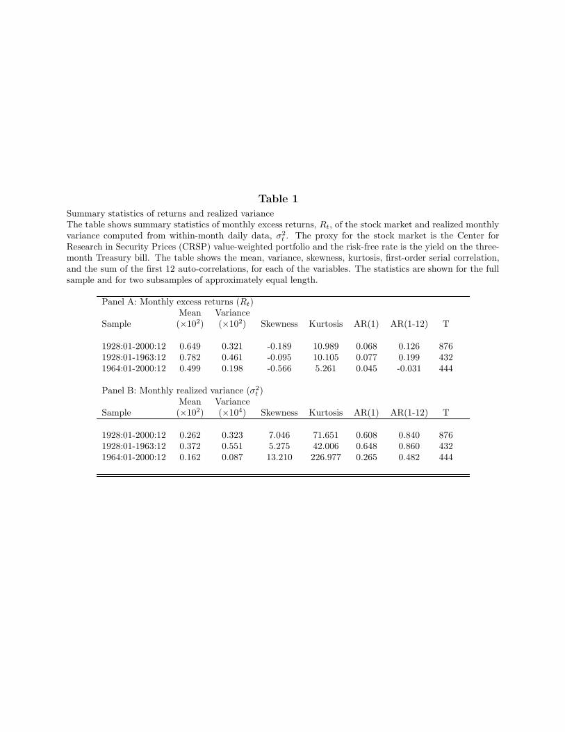
Table 1

Summary statistics of returns and realized varianceThe table shows summary statistics of monthly excess returns, Rt, of the stock market and realized monthlyvariance computed from within-month daily data, σ2

t . The proxy for the stock market is the Center forResearch in Security Prices (CRSP) value-weighted portfolio and the risk-free rate is the yield on the three-month Treasury bill. The table shows the mean, variance, skewness, kurtosis, first-order serial correlation,and the sum of the first 12 auto-correlations, for each of the variables. The statistics are shown for the fullsample and for two subsamples of approximately equal length.

Panel A: Monthly excess returns (Rt)Mean Variance

Sample (×102) (×102) Skewness Kurtosis AR(1) AR(1-12) T

1928:01-2000:12 0.649 0.321 -0.189 10.989 0.068 0.126 8761928:01-1963:12 0.782 0.461 -0.095 10.105 0.077 0.199 4321964:01-2000:12 0.499 0.198 -0.566 5.261 0.045 -0.031 444

Panel B: Monthly realized variance (σ2t )

Mean VarianceSample (×102) (×104) Skewness Kurtosis AR(1) AR(1-12) T

1928:01-2000:12 0.262 0.323 7.046 71.651 0.608 0.840 8761928:01-1963:12 0.372 0.551 5.275 42.006 0.648 0.860 4321964:01-2000:12 0.162 0.087 13.210 226.977 0.265 0.482 444

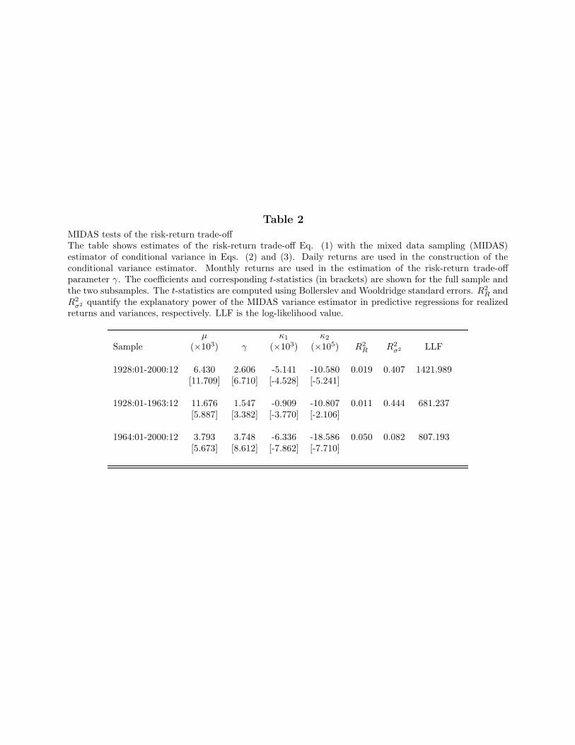
Table 2

MIDAS tests of the risk-return trade-offThe table shows estimates of the risk-return trade-off Eq. (1) with the mixed data sampling (MIDAS)estimator of conditional variance in Eqs. (2) and (3). Daily returns are used in the construction of theconditional variance estimator. Monthly returns are used in the estimation of the risk-return trade-offparameter γ. The coefficients and corresponding t-statistics (in brackets) are shown for the full sample andthe two subsamples. The t-statistics are computed using Bollerslev and Wooldridge standard errors. R2

R andR2

σ2 quantify the explanatory power of the MIDAS variance estimator in predictive regressions for realizedreturns and variances, respectively. LLF is the log-likelihood value.

µ κ1 κ2

Sample (×103) γ (×103) (×105) R2R R2

σ2 LLF

1928:01-2000:12 6.430 2.606 -5.141 -10.580 0.019 0.407 1421.989[11.709] [6.710] [-4.528] [-5.241]

1928:01-1963:12 11.676 1.547 -0.909 -10.807 0.011 0.444 681.237[5.887] [3.382] [-3.770] [-2.106]

1964:01-2000:12 3.793 3.748 -6.336 -18.586 0.050 0.082 807.193[5.673] [8.612] [-7.862] [-7.710]

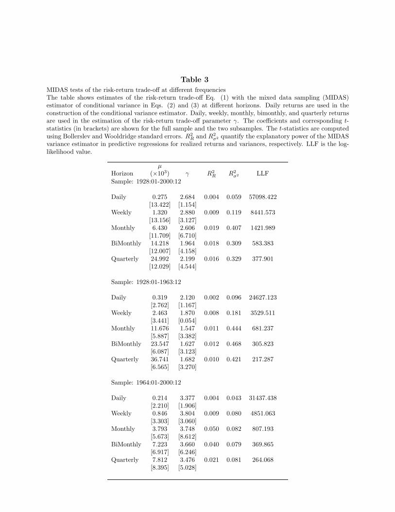
Table 3

MIDAS tests of the risk-return trade-off at different frequenciesThe table shows estimates of the risk-return trade-off Eq. (1) with the mixed data sampling (MIDAS)estimator of conditional variance in Eqs. (2) and (3) at different horizons. Daily returns are used in theconstruction of the conditional variance estimator. Daily, weekly, monthly, bimonthly, and quarterly returnsare used in the estimation of the risk-return trade-off parameter γ. The coefficients and corresponding t-statistics (in brackets) are shown for the full sample and the two subsamples. The t-statistics are computedusing Bollerslev and Wooldridge standard errors. R2

R and R2σ2 quantify the explanatory power of the MIDAS

variance estimator in predictive regressions for realized returns and variances, respectively. LLF is the log-likelihood value.

µHorizon (×103) γ R2

R R2σ2 LLF

Sample: 1928:01-2000:12

Daily 0.275 2.684 0.004 0.059 57098.422[13.422] [1.154]

Weekly 1.320 2.880 0.009 0.119 8441.573[13.156] [3.127]

Monthly 6.430 2.606 0.019 0.407 1421.989[11.709] [6.710]

BiMonthly 14.218 1.964 0.018 0.309 583.383[12.007] [4.158]

Quarterly 24.992 2.199 0.016 0.329 377.901[12.029] [4.544]

Sample: 1928:01-1963:12

Daily 0.319 2.120 0.002 0.096 24627.123[2.762] [1.167]

Weekly 2.463 1.870 0.008 0.181 3529.511[3.441] [0.054]

Monthly 11.676 1.547 0.011 0.444 681.237[5.887] [3.382]

BiMonthly 23.547 1.627 0.012 0.468 305.823[6.087] [3.123]

Quarterly 36.741 1.682 0.010 0.421 217.287[6.565] [3.270]

Sample: 1964:01-2000:12

Daily 0.214 3.377 0.004 0.043 31437.438[2.210] [1.906]

Weekly 0.846 3.804 0.009 0.080 4851.063[3.303] [3.060]

Monthly 3.793 3.748 0.050 0.082 807.193[5.673] [8.612]

BiMonthly 7.223 3.660 0.040 0.079 369.865[6.917] [6.246]

Quarterly 7.812 3.476 0.021 0.081 264.068[8.395] [5.028]

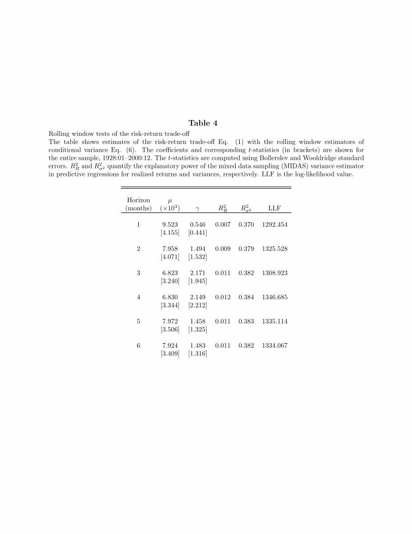
Table 4

Rolling window tests of the risk-return trade-offThe table shows estimates of the risk-return trade-off Eq. (1) with the rolling window estimators ofconditional variance Eq. (6). The coefficients and corresponding t-statistics (in brackets) are shown forthe entire sample, 1928:01–2000:12. The t-statistics are computed using Bollerslev and Wooldridge standarderrors. R2

R and R2σ2 quantify the explanatory power of the mixed data sampling (MIDAS) variance estimator

in predictive regressions for realized returns and variances, respectively. LLF is the log-likelihood value.

Horizon µ(months) (×103) γ R2

R R2σ2 LLF

1 9.523 0.546 0.007 0.370 1292.454[4.155] [0.441]

2 7.958 1.494 0.009 0.379 1325.528[4.071] [1.532]

3 6.823 2.171 0.011 0.382 1308.923[3.240] [1.945]

4 6.830 2.149 0.012 0.384 1346.685[3.344] [2.212]

5 7.972 1.458 0.011 0.383 1335.114[3.506] [1.325]

6 7.924 1.483 0.011 0.382 1334.067[3.409] [1.316]

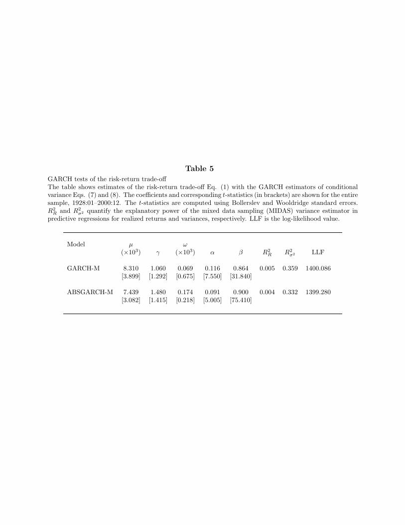
Table 5

GARCH tests of the risk-return trade-offThe table shows estimates of the risk-return trade-off Eq. (1) with the GARCH estimators of conditionalvariance Eqs. (7) and (8). The coefficients and corresponding t-statistics (in brackets) are shown for the entiresample, 1928:01–2000:12. The t-statistics are computed using Bollerslev and Wooldridge standard errors.R2

R and R2σ2 quantify the explanatory power of the mixed data sampling (MIDAS) variance estimator in

predictive regressions for realized returns and variances, respectively. LLF is the log-likelihood value.

Model µ ω(×103) γ (×103) α β R2

R R2σ2 LLF

GARCH-M 8.310 1.060 0.069 0.116 0.864 0.005 0.359 1400.086[3.899] [1.292] [0.675] [7.550] [31.840]

ABSGARCH-M 7.439 1.480 0.174 0.091 0.900 0.004 0.332 1399.280[3.082] [1.415] [0.218] [5.005] [75.410]

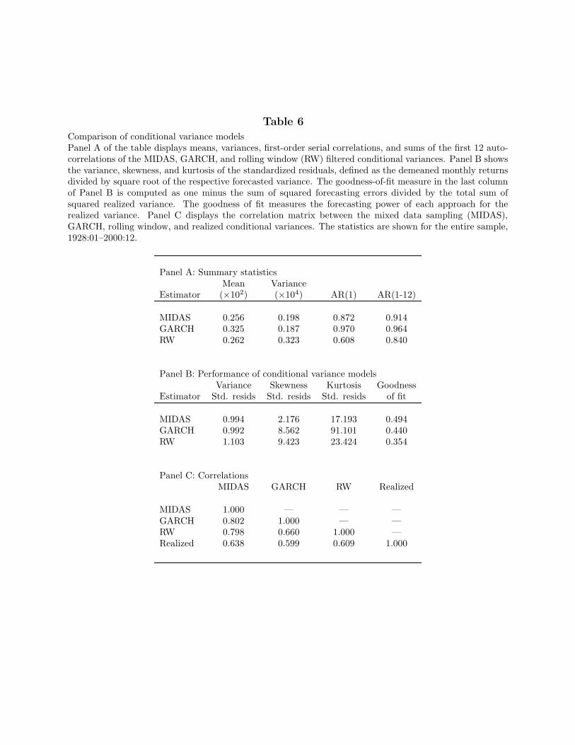
Table 6

Comparison of conditional variance modelsPanel A of the table displays means, variances, first-order serial correlations, and sums of the first 12 auto-correlations of the MIDAS, GARCH, and rolling window (RW) filtered conditional variances. Panel B showsthe variance, skewness, and kurtosis of the standardized residuals, defined as the demeaned monthly returnsdivided by square root of the respective forecasted variance. The goodness-of-fit measure in the last columnof Panel B is computed as one minus the sum of squared forecasting errors divided by the total sum ofsquared realized variance. The goodness of fit measures the forecasting power of each approach for therealized variance. Panel C displays the correlation matrix between the mixed data sampling (MIDAS),GARCH, rolling window, and realized conditional variances. The statistics are shown for the entire sample,1928:01–2000:12.

Panel A: Summary statisticsMean Variance

Estimator (×102) (×104) AR(1) AR(1-12)

MIDAS 0.256 0.198 0.872 0.914GARCH 0.325 0.187 0.970 0.964RW 0.262 0.323 0.608 0.840

Panel B: Performance of conditional variance modelsVariance Skewness Kurtosis Goodness

Estimator Std. resids Std. resids Std. resids of fit

MIDAS 0.994 2.176 17.193 0.494GARCH 0.992 8.562 91.101 0.440RW 1.103 9.423 23.424 0.354

Panel C: CorrelationsMIDAS GARCH RW Realized

MIDAS 1.000 — — —GARCH 0.802 1.000 — —RW 0.798 0.660 1.000 —Realized 0.638 0.599 0.609 1.000

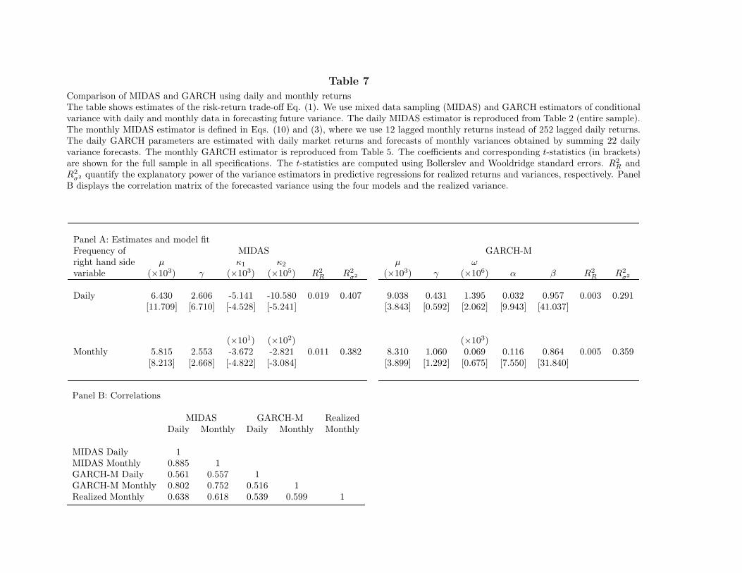
Table 7

Comparison of MIDAS and GARCH using daily and monthly returnsThe table shows estimates of the risk-return trade-off Eq. (1). We use mixed data sampling (MIDAS) and GARCH estimators of conditionalvariance with daily and monthly data in forecasting future variance. The daily MIDAS estimator is reproduced from Table 2 (entire sample).The monthly MIDAS estimator is defined in Eqs. (10) and (3), where we use 12 lagged monthly returns instead of 252 lagged daily returns.The daily GARCH parameters are estimated with daily market returns and forecasts of monthly variances obtained by summing 22 dailyvariance forecasts. The monthly GARCH estimator is reproduced from Table 5. The coefficients and corresponding t-statistics (in brackets)are shown for the full sample in all specifications. The t-statistics are computed using Bollerslev and Wooldridge standard errors. R2

R andR2

σ2 quantify the explanatory power of the variance estimators in predictive regressions for realized returns and variances, respectively. PanelB displays the correlation matrix of the forecasted variance using the four models and the realized variance.

Panel A: Estimates and model fitFrequency of MIDAS GARCH-Mright hand side µ κ1 κ2 µ ωvariable (×103) γ (×103) (×105) R2

R R2σ2 (×103) γ (×106) α β R2

R R2σ2

Daily 6.430 2.606 -5.141 -10.580 0.019 0.407 9.038 0.431 1.395 0.032 0.957 0.003 0.291[11.709] [6.710] [-4.528] [-5.241] [3.843] [0.592] [2.062] [9.943] [41.037]

(×101) (×102) (×103)Monthly 5.815 2.553 -3.672 -2.821 0.011 0.382 8.310 1.060 0.069 0.116 0.864 0.005 0.359

[8.213] [2.668] [-4.822] [-3.084] [3.899] [1.292] [0.675] [7.550] [31.840]

Panel B: Correlations

MIDAS GARCH-M RealizedDaily Monthly Daily Monthly Monthly

MIDAS Daily 1MIDAS Monthly 0.885 1GARCH-M Daily 0.561 0.557 1GARCH-M Monthly 0.802 0.752 0.516 1Realized Monthly 0.638 0.618 0.539 0.599 1

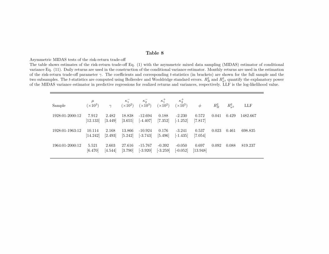
Table 8

Asymmetric MIDAS tests of the risk-return trade-offThe table shows estimates of the risk-return trade-off Eq. (1) with the asymmetric mixed data sampling (MIDAS) estimator of conditionalvariance Eq. (11). Daily returns are used in the construction of the conditional variance estimator. Monthly returns are used in the estimationof the risk-return trade-off parameter γ. The coefficients and corresponding t-statistics (in brackets) are shown for the full sample and thetwo subsamples. The t-statistics are computed using Bollerslev and Wooldridge standard errors. R2

R and R2σ2 quantify the explanatory power

of the MIDAS variance estimator in predictive regressions for realized returns and variances, respectively. LLF is the log-likelihood value.

µ κ−1 κ−

2 κ+1 κ+

2

Sample (×103) γ (×102) (×103) (×102) (×105) φ R2R R2

σ2 LLF

1928:01-2000:12 7.912 2.482 18.838 -12.694 0.188 -2.230 0.572 0.041 0.429 1482.667[12.133] [3.449] [3.655] [-4.407] [7.352] [-1.252] [7.817]

1928:01-1963:12 10.114 2.168 13.866 -10.924 0.176 -3.241 0.537 0.023 0.461 698.835[14.242] [2.493] [5.242] [-3.743] [5.496] [-1.435] [7.054]

1964:01-2000:12 5.521 2.603 27.616 -15.767 -0.392 -0.050 0.697 0.092 0.088 819.237[6.470] [4.544] [3.790] [-3.920] [-3.259] [-0.052] [13.948]

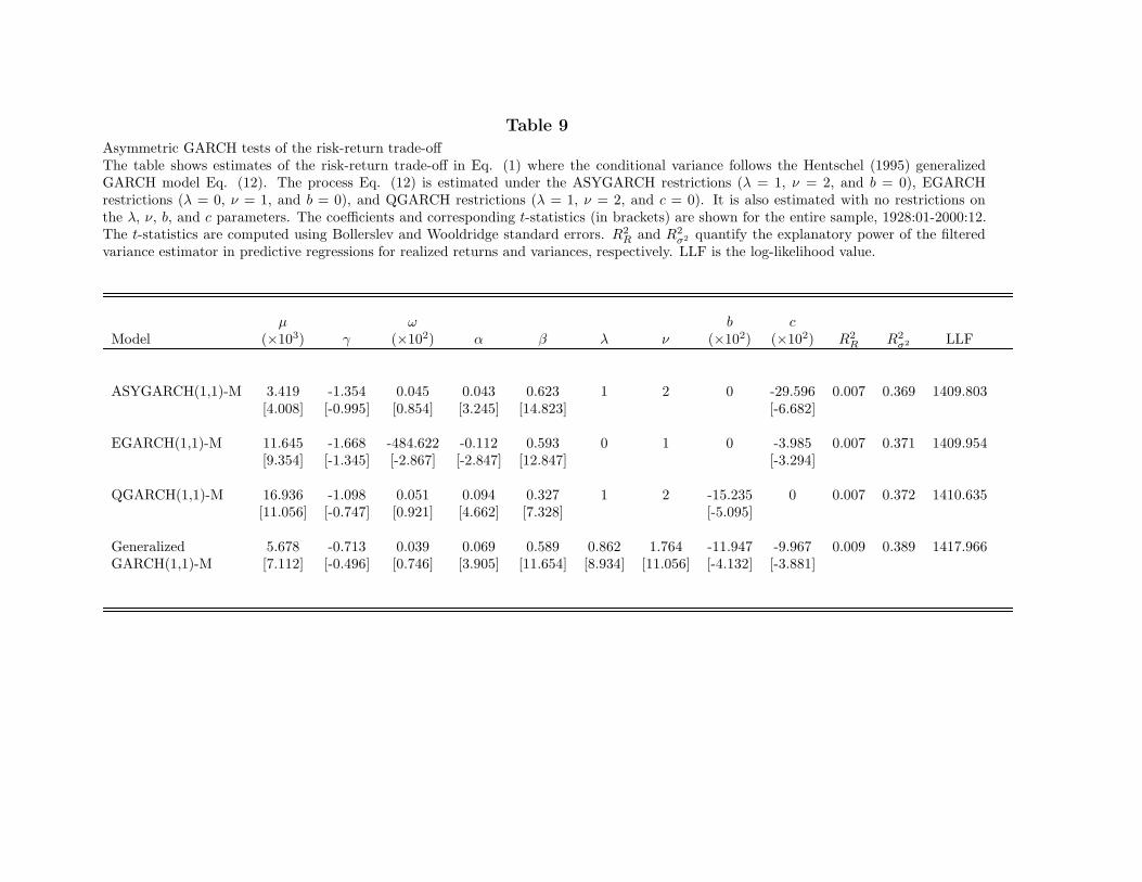
Table 9

Asymmetric GARCH tests of the risk-return trade-offThe table shows estimates of the risk-return trade-off in Eq. (1) where the conditional variance follows the Hentschel (1995) generalizedGARCH model Eq. (12). The process Eq. (12) is estimated under the ASYGARCH restrictions (λ = 1, ν = 2, and b = 0), EGARCHrestrictions (λ = 0, ν = 1, and b = 0), and QGARCH restrictions (λ = 1, ν = 2, and c = 0). It is also estimated with no restrictions onthe λ, ν, b, and c parameters. The coefficients and corresponding t-statistics (in brackets) are shown for the entire sample, 1928:01-2000:12.The t-statistics are computed using Bollerslev and Wooldridge standard errors. R2

R and R2σ2 quantify the explanatory power of the filtered

variance estimator in predictive regressions for realized returns and variances, respectively. LLF is the log-likelihood value.

µ ω b cModel (×103) γ (×102) α β λ ν (×102) (×102) R2

R R2σ2 LLF

ASYGARCH(1,1)-M 3.419 -1.354 0.045 0.043 0.623 1 2 0 -29.596 0.007 0.369 1409.803[4.008] [-0.995] [0.854] [3.245] [14.823] [-6.682]

EGARCH(1,1)-M 11.645 -1.668 -484.622 -0.112 0.593 0 1 0 -3.985 0.007 0.371 1409.954[9.354] [-1.345] [-2.867] [-2.847] [12.847] [-3.294]

QGARCH(1,1)-M 16.936 -1.098 0.051 0.094 0.327 1 2 -15.235 0 0.007 0.372 1410.635[11.056] [-0.747] [0.921] [4.662] [7.328] [-5.095]

Generalized 5.678 -0.713 0.039 0.069 0.589 0.862 1.764 -11.947 -9.967 0.009 0.389 1417.966GARCH(1,1)-M [7.112] [-0.496] [0.746] [3.905] [11.654] [8.934] [11.056] [-4.132] [-3.881]

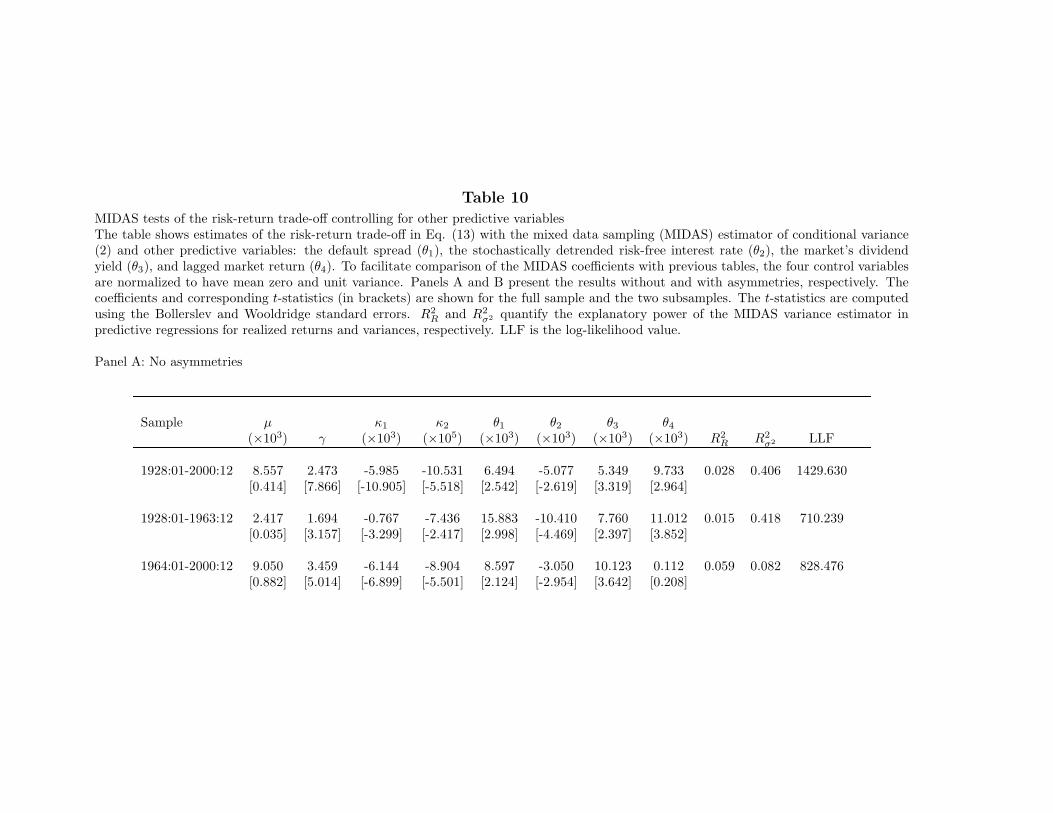
Table 10

MIDAS tests of the risk-return trade-off controlling for other predictive variablesThe table shows estimates of the risk-return trade-off in Eq. (13) with the mixed data sampling (MIDAS) estimator of conditional variance(2) and other predictive variables: the default spread (θ1), the stochastically detrended risk-free interest rate (θ2), the market’s dividendyield (θ3), and lagged market return (θ4). To facilitate comparison of the MIDAS coefficients with previous tables, the four control variablesare normalized to have mean zero and unit variance. Panels A and B present the results without and with asymmetries, respectively. Thecoefficients and corresponding t-statistics (in brackets) are shown for the full sample and the two subsamples. The t-statistics are computedusing the Bollerslev and Wooldridge standard errors. R2

R and R2σ2 quantify the explanatory power of the MIDAS variance estimator in

predictive regressions for realized returns and variances, respectively. LLF is the log-likelihood value.

Panel A: No asymmetries

Sample µ κ1 κ2 θ1 θ2 θ3 θ4

(×103) γ (×103) (×105) (×103) (×103) (×103) (×103) R2R R2

σ2 LLF

1928:01-2000:12 8.557 2.473 -5.985 -10.531 6.494 -5.077 5.349 9.733 0.028 0.406 1429.630[0.414] [7.866] [-10.905] [-5.518] [2.542] [-2.619] [3.319] [2.964]

1928:01-1963:12 2.417 1.694 -0.767 -7.436 15.883 -10.410 7.760 11.012 0.015 0.418 710.239[0.035] [3.157] [-3.299] [-2.417] [2.998] [-4.469] [2.397] [3.852]

1964:01-2000:12 9.050 3.459 -6.144 -8.904 8.597 -3.050 10.123 0.112 0.059 0.082 828.476[0.882] [5.014] [-6.899] [-5.501] [2.124] [-2.954] [3.642] [0.208]

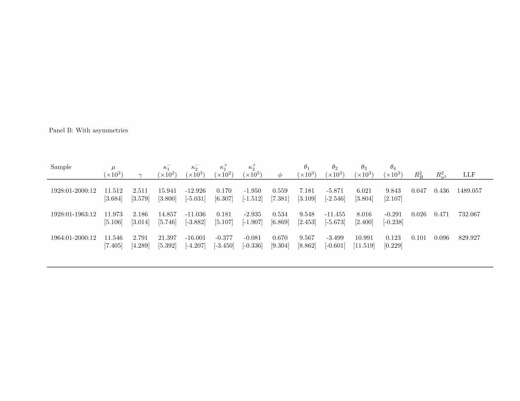
Panel B: With asymmetries

Sample µ κ−1 κ−

2 κ+1 κ+

2 θ1 θ2 θ3 θ4

(×103) γ (×102) (×103) (×102) (×105) φ (×103) (×103) (×103) (×103) R2R R2

σ2 LLF

1928:01-2000:12 11.512 2.511 15.941 -12.926 0.170 -1.950 0.559 7.181 -5.871 6.021 9.843 0.047 0.436 1489.057[3.684] [3.579] [3.800] [-5.031] [6.307] [-1.512] [7.381] [3.109] [-2.546] [3.804] [2.107]

1928:01-1963:12 11.973 2.186 14.857 -11.036 0.181 -2.935 0.534 9.548 -11.455 8.016 -0.291 0.026 0.471 732.067[5.106] [3.014] [5.746] [-3.882] [5.107] [-1.907] [6.869] [2.453] [-5.673] [2.400] [-0.238]

1964:01-2000:12 11.546 2.791 21.397 -16.001 -0.377 -0.081 0.670 9.567 -3.499 10.991 0.123 0.101 0.096 829.927[7.405] [4.289] [5.392] [-4.207] [-3.450] [-0.336] [9.304] [8.862] [-0.601] [11.519] [0.229]

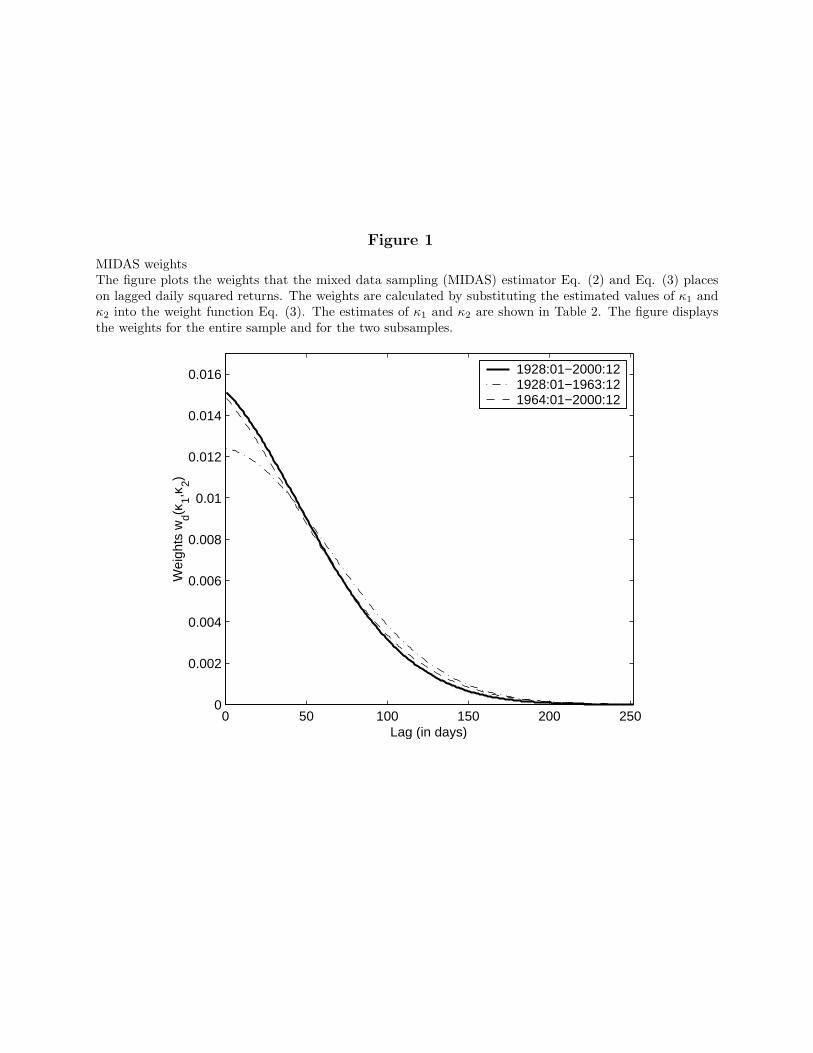
Figure 1

MIDAS weightsThe figure plots the weights that the mixed data sampling (MIDAS) estimator Eq. (2) and Eq. (3) placeson lagged daily squared returns. The weights are calculated by substituting the estimated values of κ1 andκ2 into the weight function Eq. (3). The estimates of κ1 and κ2 are shown in Table 2. The figure displaysthe weights for the entire sample and for the two subsamples.

0 50 100 150 200 2500

0.002

0.004

0.006

0.008

0.01

0.012

0.014

0.016

Wei

ghts

wd(κ

1,κ2)

Lag (in days)

1928:01−2000:121928:01−1963:121964:01−2000:12

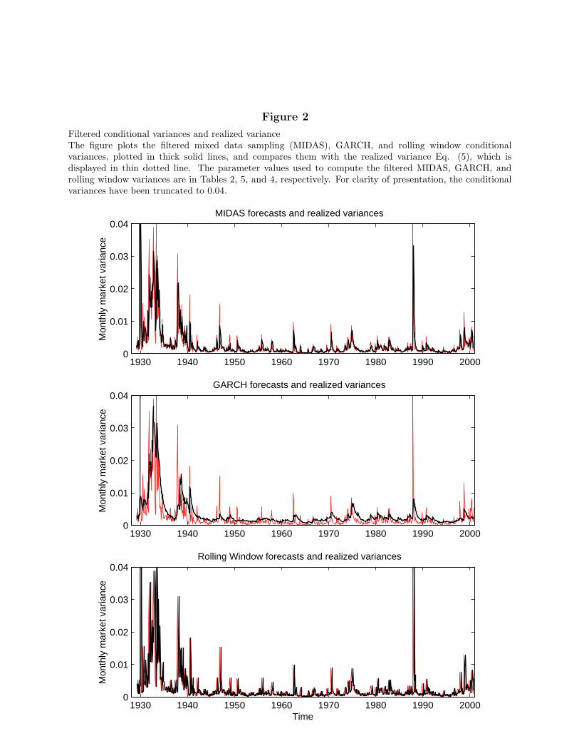
Figure 2

Filtered conditional variances and realized varianceThe figure plots the filtered mixed data sampling (MIDAS), GARCH, and rolling window conditionalvariances, plotted in thick solid lines, and compares them with the realized variance Eq. (5), which isdisplayed in thin dotted line. The parameter values used to compute the filtered MIDAS, GARCH, androlling window variances are in Tables 2, 5, and 4, respectively. For clarity of presentation, the conditionalvariances have been truncated to 0.04.

1930 1940 1950 1960 1970 1980 1990 20000

0.01

0.02

0.03

0.04

Mon

thly

mar

ket v

aria

nce

MIDAS forecasts and realized variances

1930 1940 1950 1960 1970 1980 1990 20000

0.01

0.02

0.03

0.04

Mon

thly

mar

ket v

aria

nce

GARCH forecasts and realized variances

1930 1940 1950 1960 1970 1980 1990 20000

0.01

0.02

0.03

0.04

Time

Mon

thly

mar

ket v

aria

nce

Rolling Window forecasts and realized variances

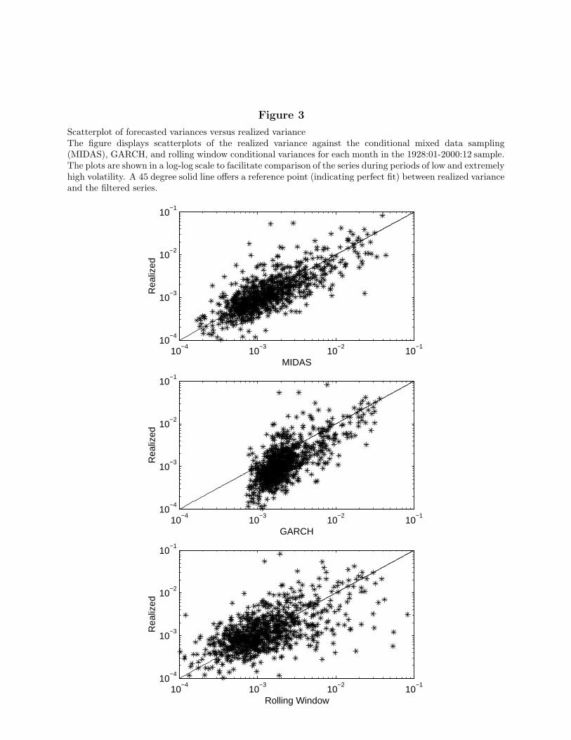
Figure 3

Scatterplot of forecasted variances versus realized varianceThe figure displays scatterplots of the realized variance against the conditional mixed data sampling(MIDAS), GARCH, and rolling window conditional variances for each month in the 1928:01-2000:12 sample.The plots are shown in a log-log scale to facilitate comparison of the series during periods of low and extremelyhigh volatility. A 45 degree solid line offers a reference point (indicating perfect fit) between realized varianceand the filtered series.

10−4

10−3

10−2

10−1

10−4

10−3

10−2

10−1

MIDAS

Rea

lized

10−4

10−3

10−2

10−1

10−4

10−3

10−2

10−1

GARCH

Rea

lized

10−4

10−3

10−2

10−1

10−4

10−3

10−2

10−1

Rolling Window

Rea

lized

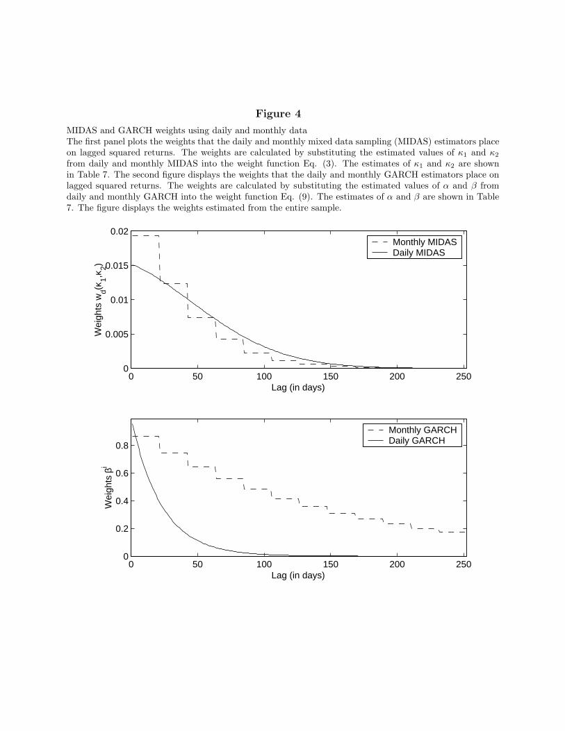
Figure 4

MIDAS and GARCH weights using daily and monthly dataThe first panel plots the weights that the daily and monthly mixed data sampling (MIDAS) estimators placeon lagged squared returns. The weights are calculated by substituting the estimated values of κ1 and κ2

from daily and monthly MIDAS into the weight function Eq. (3). The estimates of κ1 and κ2 are shownin Table 7. The second figure displays the weights that the daily and monthly GARCH estimators place onlagged squared returns. The weights are calculated by substituting the estimated values of α and β fromdaily and monthly GARCH into the weight function Eq. (9). The estimates of α and β are shown in Table7. The figure displays the weights estimated from the entire sample.

0 50 100 150 200 2500

0.005

0.01

0.015

0.02

Lag (in days)

Wei

ghts

wd(κ

1,κ2)

Monthly MIDASDaily MIDAS

0 50 100 150 200 2500

0.2

0.4

0.6

0.8

Lag (in days)

Wei

ghts

βi

Monthly GARCHDaily GARCH

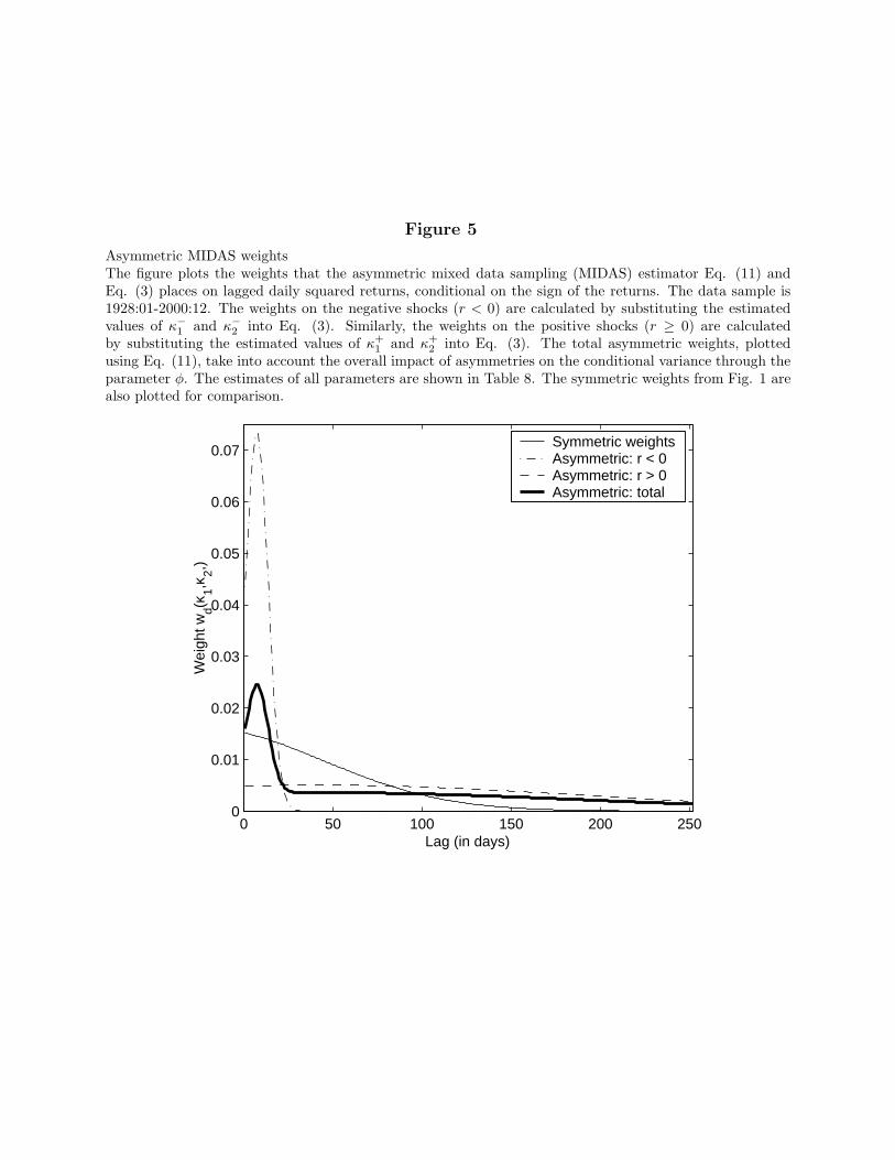
Figure 5

Asymmetric MIDAS weightsThe figure plots the weights that the asymmetric mixed data sampling (MIDAS) estimator Eq. (11) andEq. (3) places on lagged daily squared returns, conditional on the sign of the returns. The data sample is1928:01-2000:12. The weights on the negative shocks (r < 0) are calculated by substituting the estimatedvalues of κ−

1 and κ−2 into Eq. (3). Similarly, the weights on the positive shocks (r ≥ 0) are calculated

by substituting the estimated values of κ+1 and κ+

2 into Eq. (3). The total asymmetric weights, plottedusing Eq. (11), take into account the overall impact of asymmetries on the conditional variance through theparameter φ. The estimates of all parameters are shown in Table 8. The symmetric weights from Fig. 1 arealso plotted for comparison.

0 50 100 150 200 2500

0.01

0.02

0.03

0.04

0.05

0.06

0.07

Lag (in days)

Wei

ght w

d(κ1,κ

2,)

Symmetric weightsAsymmetric: r < 0Asymmetric: r > 0Asymmetric: total

there is a risk-return trade-oﬀ after all

Documents