theory of screws eng. - blank title

Gesammelte mathematische Abhandlungen, pp. 525-554.

XXIX. On Sir Robert Ball’s Theory of Screws

By Felix Klein

Translated D. H. Delphenich

[Zeitschr. Math. u. Physik Bd. 47 (1902); published again with an appendix in the Math. Annalen, Bd. 62 (1906).]

________

In the previous year, Sir Robert Ball has summarized his investigations into the theory of screws over a long period of time in an imposing volume 1), which cannot fail to renew the general interest in this geometric redepiction of the mechanics of rigid bodies. Two particular advantages of the Ball works that assure it of a large circle of readers from the outset are the intuitive and elementary character of his ground-breaking developments. I wish to vigorously acknowledge these advantages, but, on the other hand, it will emerge that they will be accompanied by a certain sacrifice in the representation of the deeper questions that necessarily come under consideration as a result of further consequences of this theory (which, by the way, the author himself has discussed clearly in various places in his books 2)). In any case, I would like to give an extension of Ball’s works in what follows that many readers might welcome. This extension involves, firstly, the general systematics of the subject in the sense of modern invariant-theoretic (or group-theoretic) principles, and second, however, the employment of screw theory in the study of the finite motions of rigid bodies (where I will, by the way, mainly compile systematically only what is scattered throughout the existing literature). I may perhaps add that I have repeatedly brought the concepts to be discussed to bear for some years in my lectures and occasional talks; in particular, I connect the presentation in the next paragraph with my own contributions on line geometry and the theory of screws in the years 1869 and 1871 3), as well as in the argument of my Erlanger Programm of 1872 4) on. It makes good sense

1) A Treatise on the Theory of Screws, Cambridge 1900. 2) One might cf., e.g., the amusing argument that the author presented in 1887 before the British Association in Manchester on the objective of his investigations, and which is now reprinted in the relevant Reports on pp. 496-509 of the present volume. A commission was established to examine the motions of a rigid body. “Let it suffice for us,” said the president of the commission right at the outset, “to experiment upon the dynamics of this body so long it remains in or near the position it now occupies. We may leave to some more ambitious committee the task of following the body in all conceivable gyrations through the universe.” 3) Math. Annalen, Bd. 2 and 4 [Abh. II and XIV of this collection]. In particular, cf., the “Notiz, betreffend den Zusammenhang der Liniengeometrie mit der Mechanik starrer Körper” in Bd. 4 itself. [See Abh. XIV of this collection.] 4) “Vergleichende Betrachtungen über neuere geometrische Forschungen” (Erlangen 1872), printed in Bd. 43 of the Math. Annalen and elsewhere. [See Abh. XXVII of this collection.]

XXIX. On Sir Robert Ball’s theory of screws 2

that I therefore avail myself of the methods of analytic geometry from the outset; in fact, I intend to define the relations that come into consideration more concisely and precisely than is possible in any other way.

§ 1.

On the rational classification of geometrical and mechanical quantities.

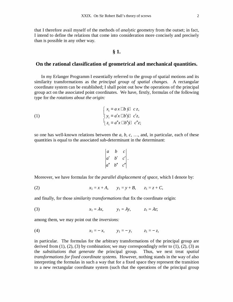
In my Erlanger Programm I essentially referred to the group of spatial motions and its similarity transformations as the principal group of spatial changes. A rectangular coordinate system can be established; I shall point out how the operations of the principal group act on the associated point coordinates. We have, firstly, formulas of the following type for the rotations about the origin:

(1) 1

1

1

,

,

;

x a x b y c z

y a x b y c z

z a x b y c z

= + + ′ ′ ′= + + ′′ ′′ ′′= + +

so one has well-known relations between the a, b, c, …, and, in particular, each of these quantities is equal to the associated sub-determinant in the determinant:

a b c

a b c

a b c

′ ′ ′′′ ′′ ′′

.

Moreover, we have formulas for the parallel displacement of space, which I denote by: (2) x1 = x + A, y1 = y + B, z1 = z + C, and finally, for those similarity transformations that fix the coordinate origin: (3) x1 = λx, y1 = λy, z1 = λz; among them, we may point out the inversions: (4) x1 = − x, y1 = − y, z1 = − z, in particular. The formulas for the arbitrary transformations of the principal group are derived from (1), (2), (3) by combination; we may correspondingly refer to (1), (2), (3) as the substitutions that generate the principal group. Thus, we next treat spatial transformations for fixed coordinate systems. However, nothing stands in the way of also interpreting the formulas in such a way that for a fixed space they represent the transition to a new rectangular coordinate system (such that the operations of the principal group


completely represent the most general transformations of rectangular coordinate systems). In the sequel, we will prefer this way of looking at things, which seems to be somewhat more convenient for the generalizations, in particular. The formulas (1) and (2) then collectively yield the most general change of rectangular coordinate system by a motion, formula (4), the transition to an inverse coordinate system, and formula (3), for the ones that involve only positive values of λ¸ which is the most general change that results from another choice of unit length. We now establish not merely points, but arbitrary geometric structures, with respect to our coordinate system by means of “coordinates,” such that we think of the structures as defined in a special way as points whose “coordinates” are couplings between various sequences of point coordinates. We shall nonetheless refer to the essence of the coordinates that serve to establish geometrical structures in that way as “geometrical quantities.” Furthermore, the rational classification of geometric quantities, which we will start with in what follows, simply rests upon the fact that we shall observe how coordinates that come under consideration are preserved by the operations (1), (2), (3), (4), resp. (and thus, all of the operations of the principal group). We will regard those and only those geometrical quantities as similar whose coordinates suffer the same changes under the operations of the principal group. However, if the coordinates of structures suffer different changes then the geometrical relation yields the two types of geometrical quantities immediately, and in an exhaustive way, from the comparison of the two changes. The implementation of this principle can be found, inter alia, in the recently-appearing article of Abraham on the basic geometric concepts in the mechanics of deformable bodies, Bd. IV of the Math. Enzyklopädie, art. 14 (1901) 5). In fact, one obviously has always proceeded from the principle correspondingly. In particular, the customary differentiation of geometric quantities in terms of their dimension in mechanics (and physics) is nothing but a taking into account of the substitutions (3) in the sense of our principle (when one tacitly restricts oneself to positive values of λ). In this remark, one likewise finds how our principle is extended to general mechanical or physical quantities. It is, moreover, convenient to think of introducing, along with the unit of length and unit of time, not, as is customary, a unit of mass, but a unit of force. One will, consequently, along with formulas (3), also set down the ones that relate to the change in time unit (the change in force unit, resp.): (5) t1 = ρ t, (6) P1 = σ P; one will then say that formulas (1) to (6) collectively define the principal group of mechanics (of physics, resp.), and furthermore classify the mechanical (physical, resp.) quantities according to the behavior of their coordinates under the operations of this principal group. Incidentally, we will come back to these extended assumptions only occasionally; for the present purposes, it will suffice for us to consider the spatial principal group. 5) [Cf., as well, the article of H. E. Timerding, Geometrische Grundlegung der Mechanik eines starren Körpers. Bd. IV of the Math. Enzyklopädie, art. 2 (1902)].


§ 2.

Coordinates for the infinitely small motion of a rigid body as well as for the force system that is attached to it.

An infinitely small motion may be represented by the following formula:

(7)

( ) ,

( ) ,

( ) .

dx ry qz u dt

dy pz rx v dt

dz qx py w dt

= − + + = − + + = − + +

We refer to the quantities: (8) p, q, r, u, v, w as the coordinates of the instantaneous velocity, while the quantities: (9) p dt, q dt, r dt, u dt, v dt, w dt, are the coordinates of the infinitely small motion itself. We represent forces on the rigid body in the usual way by line segments that lie on a certain straight line and can be displaced along this line. Thus, we will set the lengths of these line segments equal to the magnitude of the forces; it is immaterial whether we think of the forces collectively as impulsive forces or continuously-acting forces 6). Let x, y, z (x′, y′, z′, resp.) be the starting point (end point, resp.) of a “transitory” line segment. One then has, in the usual way, for the coordinates themselves:

x′ − x, y′ − y, z′ − z, y z′ – y′ z, z x′ – z′ x, x y′ – x′ y;

the same six quantities will serve as the coordinates of the force, as long as one chooses the length l of the line segment equal to the number P that measures the magnitude of the force. If we would like to clearly emphasize the independence of the choice of force unit and length unit then it would be more convenient to let the following six quantities:

( )P

x xl

′ − , ( )P

y yl

′ − , ( )P

z zl

′ − ,

( )P

yz y zl

′ ′− , ( )P

zx z xl

′ ′− , ( )P

xy x yl

′ ′− ,

denote the coordinates of the force. We use the term force system to refer to the concept of arbitrarily many isolated forces acting on the rigid body, and choose its coordinates to be the sums of the

6) The difference first comes into play when we go on to kinetics, where the situation will be that the unit of impulsive force of any mass point instantaneously produces the same change in velocity as the unit of continuous force does during the unit of time.


respective coordinates of the individual forces. In such a way, we obtain the coordinates of a force system in the form of the six quantities:

(10)

( ), ( ), ( ),

( ), ( ), ( ).

i i ii i i i i i

i i i

i i ii i i i i i i i i i i i

i i i

P P PX x x Y y y Z z z

l l l

P P PL y z y z M z y z x N x y x y

l l l

′ ′ ′= − = − = −

′ ′ ′ ′ ′ ′= − = − = −

∑ ∑ ∑

∑ ∑ ∑

It will, moreover, be of interest to see how the coordinates p, q, r, u, v, w in (8) and the X, Y, Z, L, M, N that we just introduced behave under the operations (1) to (6) of the principal group. I shall simply summarize the results: 1. Rotation around the coordinate origin (formula (1)). The coordinates p, q, r and u, v, w, and, on the other hand, the X, Y, Z and the L, M, N experience precisely the same substitutions as the point coordinates x, y, z. (This result rests essentially on the previously-established fact that the coefficients of the substitution a, b, c, ... are equal to their respective sub-determinants.) 2. Displacement (formula (2)). The p, q, r and the X, Y, Z remain unchanged. By comparison, the u, v w suffer the following substitution:

(11) 1

1

1

,

,

,

u u Cq Br

v v Aq Cr

w w Bq Ar

= − + = − + = − +

and precisely analogous formulas are true for L, M, N:

(11′) 1

1

1

,

,

.

L L CY BZ

M M AZ CX

N N BX AY

= − + = − + = − +

3. Similarity transformation (formula (3) [(4), resp.]). If λ is positive then: (12) p1, q1, r1, u1, v1, w1 will be equal to p, q, r, λu, λv, λw, resp. just as: (12′) X1, Y1, Z1, L1, M1, N1 will be equal to X, Y, Z, λL, λM λN, resp. By contrast, for negative λ a difference emerges that arises, at the most elementary level, from the fact that under an inversion:


(13) p1, q1, r1, u1, v1, w1 will be equal to p, q, r, − u, − v, − w, resp., but: (13′) X1, Y1, Z1, L1, M1, N1 will be equal to − X, − Y, − Z, L, M N, resp. (This difference comes about from the fact that the lengths l i that appear in formulas (10) are absolute values, which do not change their sign under inversion, as such.) 4. Change of time unit (formula (5)).

(14) p1, q1, r1, u1, v1, w1 will be equal to p

ρ,

q

ρ,

r

ρ,

u

ρ,

v

ρ,w

ρ, resp.;

the coordinates of the force system remain unchanged. 5. Change of force unit (formula (6)). The p, q, r, u, v, w remain unchanged, but: (15) X1, Y1, Z1, L1, M1, N1 will be equal to σX, σY, σZ, σL, σM, σN, resp. When we, for the sake of brevity, restrict ourselves to the principal group of spatial changes, we can say, in summation: Under nothing but motions of the coordinate system, as with similarity transformations with positive similarity modulus, as well, the force coordinates:

X, Y, Z, L, M, N transform precisely like the velocity coordinates:

p, q, r, u, v, w. By contrast, under inversion of the coordinate system a deviant behavior emerges; whereas the:

p, q, r, u, w, v go over to p, q, r, − u, − v, − w, the

X, Y, Z, L, M, N change into − X, − Y, − Z, L, M, N, resp.

§ 3.

The analogy between infinitely small motions and force systems (for rigid bodies). Screw quantities of the first and second type. Ball screws. The analogy between infinitely small motions and force systems, which pervades all of the mechanics of rigid bodies, and especially Ball’s theory of screws, is most clearly founded and likewise limned out by the formulas of the previous paragraphs. We first remark that by means of formulas (7), with no further assumptions, the system of quantities:

p dt, q dt, r dt, u dt, v dt, w dt means an (infinitely small) screw in the space of x, y, z (with a certain axis, pitch, and amplitude), while the system of quantities:

p, q, r, u, v, w correspondingly means a screw velocity. In that sense, I would like to refer to the concept of p, q, r, u, v, w from now on as a screw quantity, or, more precisely, when it is of issue, a screw quantity of the first type. Moreover, one would like to compare this with the concept of the coordinates of a force system, i.e., the:

X, Y, Z, L, M, N that were defined in (10). In particular, we would like to connect a force system with a screw quantity of the first type by setting:

X = p, Y = q, Z = r, L = u, M = v, N = w, and ask to what extent this arrangement has a meaning that is independent of the coordinate system (thus, is invariant under the operations of the principal group). Next, formulas (14), (15) of the previous paragraphs yield that this arrangement is independent of the choice of time unit and force unit. However, for rotation, parallel displacement, and similarity transformations with positive similarity modulus the formulas yield that the arrangement is independent of all of the changes of spatial coordinate systems included in these words. Finally, we have, from formulas (13), (13′), that under inversion the arrangement goes over to its opposite: (17) X1 = − p1, Y1 = − q1, Z1 = − r, L1 = − u1, M1 = − v1, N1 = − w1. The geometric considerations naturally confirm the result thus formulated step-by-step. In order to expand upon this detail, I would like to assume that the axis of the screw velocity p, q, r, u, r, w has the line coordinates: (18) p : q : r : u – kp : v – kq : w – kr, where the “parameter”:


(18′) k = 2 2 2

pu qv rw

p q r

+ ++ +

,

and that the rotational velocity around this axis possesses the components p, q, r and the translational velocity along the axis possesses the components kp, kq, kr. In precise analogy, for a force system X, Y, Z, L, M, N one can find a central axis whose line coordinates are given by: (19) X : Y : Z : L – kX : M – kY : N – kZ, in which one understands k to mean the quantity:

(19′) k = 2 2 2

XL YM ZN

X Y Z

+ ++ +

,

and the force system may then be reduced to a single force with the components X, Y, Z along this axis and a couple with the components kX, kY, kZ in a plane that perpendicular to the axis. The combination demands that one likewise puts the rotational velocity around the axis, the isolated force acts along the axis, the translational velocity points in the direction of the axis, and a couple lies, in a plane perpendicular to the axis. Thus, it is obvious that a prior understanding on the time unit and force unit is necessary. When this does happen, one can say that the intensity of a force system (measured by

2 2 2X Y Z+ + ) is like the intensity of a velocity that is measured by 2 2 2p q r+ + . For

this, however, we need an agreement on which sense around the axis one would like to ascribe to a sense along the axis: we choose either the sense around the axis that is given by the motion of a clock hand as one looks along the axis in the given direction or its opposite. Once one has agreed upon this, the relationship between the force system and the velocity becomes unique. However, as is well-known, any such convention goes over to its opposite under inversion of the figure, and this is what formula (17) expresses. The concept of (XYZLMN) is then indeed quite closely related to the concept of (pqruvw) – i.e., a screw quantity – but it is not in itself a screw quantity; we will call it a screw quantity of the second type. However, we will collectively put the two types of quantities into words by saying: Once one has established the time unit and force unit, to a screw quantity of the second type there always belongs two (equal and opposite) screw quantities of the first type, and conversely; the association will become unique once one agrees upon the sense of left and right. Along with the aforementioned screw quantities of the first and second type, there also arises a third type, the closely-related geometric structure of the Ball screw. The Ball screw is the concept of a helix of given winding sense and a definite pitch around an axis, or, as Ball says, the concept of a central axis and parameter (i.e., pitch). The Ball screw thus defined is associated, in a one-to-one manner, with the null system that is defined by each point of the normal plane to the helix that goes through it, or also to the linear line complex that is composed of all normals to the helix; whether I speak of the Ball screw, the null system, or the linear complex, from the standpoint taken here, it amounts to the same thing. Each of these structures will be established by the ratios X : Y


: Z : L : M : N of the coordinates of a screw quantity of the second type, or also by the ratios p : q : r : u : v : w of the coordinates of a screw quantity of the first type. In fact, when one restricts oneself to the consideration of these “ratios,” the difference between the two types of screw quantities vanishes. Accordingly, there is only one type of Ball screw. Each Ball screw is associated with infinitely many screw quantities of the first, as well as second, type, and they differ from each other in their intensity and sense. Thus, the connection between the various structures that are under consideration can be represented completely, as one might wish. The individual “screw” is the carrier of infinitely many “screw quantities of the first and second type.” When we wish to expressly distinguish between the latter, it is to prevent the possible recurring misunderstanding that comes from treating the arrangement between the two types of screw quantities as a causal connection 7).

§ 4.

On the invariants of the screw quantities and the basis for the difference in types in terms of the notion of work.

The reciprocal relationship between the two types of screw quantities finds a very incisive expression when one considers its invariants; i.e., those rational entire functions that can be constructed from its coordinates that are either completely unchanged under the operations of the principal group or are changed by a factor. For the sake of brevity, I will restrict myself to those operations of the principal group that represent either motions or motions that involve an inversion, and which I, along with Study, will refer to as transfers (Umlegungen). As invariants of the individual screw quantities, as is well-known, we first obtain the expressions: (20) p2 + q2 + r2, (X2 + Y2 + Z2, resp.), which remain unchanged under both motions and transfers, and second, the following ones: (21) pu + qv + rw (XL + YM + ZN, resp.); these remain unchanged under arbitrary motions, but change sign under transfers (which follows from their behavior under inversions). We will, accordingly, refer to the (20) as even invariants, the (21) as skew, or also the (20) as scalars of the first type, and the (21) as scalars of the second type 8)

7) Cf., the comments in my aforementioned Notiz, Math. Annalen, Bd. 4 [See Abhandlung XIV of this collection.] The stubbornness of the misunderstanding obviously has a psychological root. As we go through our daily affairs, when we think of an isolated force acting upon a body, we think of it as acting on the center of mass, which naturally produces a translation of the body. This defines an association between the two things (isolated force and translation), which is then not arbitrary in our considerations if one does not expressly separate them again by an explicit clarification and possibly a less ambiguous nomenclature. 8) Cf., the previously-cited article of Abraham in Bd. IV of the Math. Enzyklopädie, art. 14 (no. 11 in it).


The difference thus introduced obviously carries over to the “simultaneous” invariants of two screw quantities of the same type, which arise from (20) [(21), resp.] by “polarization.” Here, I would like to consider only the polars of the expression (21):

(22) ,

.

pu qv rw p u q u r w

XL YM ZN X L Y M Z N

′ ′ ′ ′ ′ ′+ + + + + ′ ′ ′ ′ ′ ′+ + + + +

If the scalars in them are also of the second type, in their own right, then it follows: Theorem I. The:

p, q, r, u, v, w are directly contragredient to the:

u, v, w, p, q, r, and likewise, the:

X, Y, Z, L, M, N are directly contragredient to the:

L, M, N, X, Y, Z under motions, and under transfers, they are contragredient with a change of sign. As opposed to them, one now considers the expression that one assembles, by analogy with (22), bilinearly from the coordinates of two screw quantities of different types: (23) X u + Y v + Z w + L p + M q + N r. It follows immediately that this remains entirely unchanged, not only under motions, but (due to its behavior under inversion) also under transfers; it is a scalar of the first type. From this, it follows: Theorem II. The:

X, Y, Z, L, M, N are reverse-contragredient to the:

u, v, w, p, q, r, under motions, as well as transfers. The inter-relationship between the two types of screw quantities can be described in the simplest way by means of this theorem. If we link it with theorem I then we revert to the analogy between the two types of screw quantities, which was the purpose of the previous paragraphs. This may be expressed in the following way: Theorem III. The:

X, Y, Z, L, M, N are then directly cogredient to:

p, q, r, u, v, w


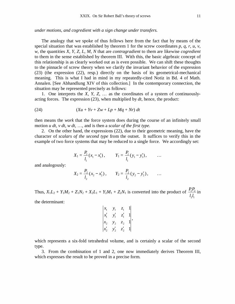
under motions, and cogredient with a sign change under transfers. The analogy that we spoke of thus follows here from the fact that by means of the special situation that was established by theorem 1 for the screw coordinates p, q, r, u, v, w, the quantities X, Y, Z, L, M, N that are contragradient to them are likewise cogredient to them in the sense established by theorem III. With this, the basic algebraic concept of this relationship is as clearly worked out as is even possible. We can shift these thoughts to the pinnacle of screw theory when we clarify the invariant behavior of the expression (23) (the expression (22), resp.) directly on the basis of its geometrical-mechanical meaning. This is what I had in mind in my repeatedly-cited Notiz in Bd. 4 of Math. Annalen. [See Abhandlung XIV of this collection.] In the contemporary connection, the situation may be represented precisely as follows: 1. One interprets the X, Y, Z, … as the coordinates of a system of continuously-acting forces. The expression (23), when multiplied by dt, hence, the product: (24) (Xu + Yv + Zw + Lp + Mq + Nr) dt then means the work that the force system does during the course of an infinitely small motion u dt, v dt, w dt, …, and is then a scalar of the first type. 2. On the other hand, the expressions (22), due to their geometric meaning, have the character of scalars of the second type from the outset. It suffices to verify this in the example of two force systems that may be reduced to a single force. We accordingly set:

X1 = 11 1

1

( )P

x xl

′− , Y1 = 11 1

1

( )P

y yl

′− , …

and analogously:

X2 = 22 2

2

( )P

x xl

′− , Y2 = 22 2

2

( )P

y yl

′− , …

Thus, X1L2 + Y1M2 + Z1N2 + X2L1 + Y2M1 + Z2N1 is converted into the product of 1 2

2 1

PP

l lin

the determinant:

1 1 1

1 1 1

2 2 2

2 2 2

1

1

1

1

x y z

x y z

x y z

x y z

′ ′ ′

′ ′ ′

,

which represents a six-fold tetrahedral volume, and is certainly a scalar of the second type. 3. From the combination of 1 and 2, one now immediately derives Theorem III, which expresses the result to be proved in a precise form.

§ 5.

Group-theoretical characterization of the different types of screw theories.

Up to now, we have defined the substitutions that the screw coordinates p, q, r, u, v, w (if they are the only ones being discussed) experience under the motions and transfers by first defining the behavior of the p, q, … under the generating operations (1), (2), (3). It is of interest to characterize the essence of these substitutions by the invariants:

p2 + q2 + r2 and pu + qv + rw.

In this regard, I pose the following theorem: The p, q, r undergo all ternary linear substitutions of determinant + 1 that leave p2 + q2 + r2 unchanged, the p, q, r, u, v, w together, however, undergo all senary linear substitutions of determinant ±1 [under which p, q, r will only be transformed into themselves, and p2 + q2 + r2 remains unchanged, among other things] that take pu + qv + rw into ± (pu + qv + rw). The first part of this theorem (the one that relates to ternary substitutions of p, q, r) then no longer needs the assumption that we made on the behavior of the p, q, r under the generating operations; it only expresses the well-known relationship between the rotations around the coordinate origin O to the ternary orthogonal substitutions. Now, suppose we have any ternary orthogonal substitution of the p, q, r of determinant ± 1 that converts (pu + qv + rw) into ± (pu + qv + rw), resp. We combine it with a rotation around O that takes the p, q, r back to their original values (and also yields precisely the same ternary substitution of determinant + 1 for the u, v, w, with the givens of § 2, as it does for the p, q, r themselves, such that the value of pu + qv + rw and the value of the senary substitution determinant thus remains unchanged). We further apply an inversion, if need be, in order to make pu + qv + rw equal to its original value; thus, the senary substitution determinant acquires the value + 1, in its own right. The thus-simplified substitution now necessarily (since pu + qv + rw must go to itself) has the form:

1 1

1 1

1 1

, ,

, ,

, ,

p p u u Cq Br

q q v v Ar Cp

r r w w Bp Aq

= = − + = = − + = = − +

where only the A, B, C are still arbitrary. However, from (11), § 2, such a substitution represents a translation. Thus, our initial substitution yields a translation when we link it with a suitable rotation, and possibly an inversion – it thus represents either a motion or a transfer to begin with, which was to be proved. So much for the substitutions of the p, q, r, u, w, v. The substitutions X, Y, Z, L, M, N are then immediately obtained from them, as long as we establish only that the u, v, w, p, q, r are contragredient to them.


With that assumption, from the basic theorems of my Erlanger Programm, the two groups of substitutions completely characterize the associated screw theory. We go on to the statements above about Ball’s theory of screws in the narrower sense where we consider only the ratios p : q : r : u : v : w (X : Y : Z : L : M : N, resp.) (where the difference between the two types of screw theory disappears). The p : q : r : u : v : w (to be specific) suffer such (and only such) linear substitutions for which the equations:

p2 + q2 + r2 = 0 and pu + qv + rw = 0

go into themselves, while the parameter 2 2 2

pu qv rw

p q r

+ ++ +

either remains completely

unchanged or differs by a sign change. Along with the motions and transfers, we would

also like to consider the similarity transformations, such that 2 2 2

pu qv rw

p q r

+ ++ +

can change by

an arbitrary factor; the restriction on the substitution relative to the parameter then drops away. The Ball theory of screws, thus constrained, is essentially identical with the line geometry that uses the null system (or, what amounts to the same thing, the linear complex) as its spatial element, according to the classification scheme of § 1. However, when we express matters that way, we naturally mean the line geometry that is based on the principal group of spatial transformations; I would like to call it concrete line geometry. In place of this, in my own older work (which has since then also appeared in a multitude of German and Italian works), line geometry was treated in a more abstract form, namely, by basing it on the 15-parameter group that, on the one hand, includes all projective transformations of our space, and , on the other, the dualistic transformations. For this abstract line geometry (which I would like to call the opposite one here) then the theorem is true that I presented in Bd. 4 of the Math. Annalen, pp. 356 [“Über ein geometrische Repräsentation der Resolventen algebraischer Gleichungen,” see Bd. II of this collection], that it is based upon the group of all linear substitutions of the p : q : r : u : v : w that take the equation pv + qu + rw = 0 to itself. The reference to the quadratic form p2 + q2 + r2 simply drops away. With the confrontation of the associated groups thus given, the relationship between my own older work and, for example, the work of Sturm, on line geometry 9), to that of Ball is made precise. However, this is not the place to go into the details.

§ 6.

Linear screw systems.

Now that we have established the basics of screw theory, we may, like Ball, then go on to the study of linear systems of screws – i.e., manifolds of screws whose coordinates can be linearly and homogeneously composed from the coordinates of 2, 3, 4, 5 screws

9) Die Gebilde ersten und zweiten Grades der Liniengeometrie in synthetischer Behandlung, 3 Teile, Leipzig 1892-1896.


with the help of a corresponding number of varying parameters. In his discussion of this, Ball restricted himself essentially to the statement of the general cases, or gave only examples of special cases. However, it seems desirable to carry out the discussion systematically 10). I would like to only sketch this out for the two-parameter family, and thus restrict myself, for the sake of brevity, to considering only the ratios of the six coordinates. Accordingly, let: (25) ρ p = λ1 p1 + λ2 p2 , ρ q = λ1 q1 + λ2 q2 , …, ρ w = λ1 w1 + λ2 w2 , in which we understand ρ to mean a proportionality factor. It simplifies the terminology if we refer to the p : q : … : w thus defined as homogeneous point coordinates in a space of five dimensions. The formulas (25) then represent a straight line in this space, and we will be dealing with the study (classification, resp.) of all of those lines in relation to the two quadratic manifolds p2 + q2 + r2 = 0 and pu + qv + rw = 0. Thus, our initial remarks shall be directed along the lines of the intersection points that our line has in common in these manifolds. The intersection points with each of the two manifolds can be separate, coincident, or undetermined. In addition, the intersection points that the straight line has in common with the one manifold can coincide, piecewise or entirely, with the ones that it has in common in with the other manifold. One might regard the latter as a difference from reality. That yields an, a priori, assessable series of special case distinctions that can not only be enumerated with little effort, but likewise, their screw-theoretic interpretation can be discussed. Any geometer who is somewhat familiar with the algebraic considerations in multidimensional space will proceed with this with no further assumptions; it seems unnecessary to dwell upon this any longer. All the same, it will be good to bring up a difference between the Ansatz sketched out with the developments of Ball. Ball principally considered only real phenomena, while here both real and imaginary were regarded as equivalent, and the question of reality considerations was first introduced at the conclusion. In order to point out an example of the advantage that the latter process possesses, we consider the ruled surface that is defined by the screw axis (25) – the so-called cylindroid. For Ball, it is of third order, in general; however, if the component screws p1, q1, r1, … and p2, q2, r2, … reduce to two rotations whose axes intersect then it degenerates into a plane pencil of rays to which the axes belong. Instead of a surface of third order, we then have one of first order. How does this degeneracy come about? When we look at the imaginary axis, we first find that there are rotations with indeterminate axes (they are the screw motions for which the parameter that is given by formula (19′) takes on the value 0/0). They leave fixed all minimal lines that run through a fixed point of the sphere circle in a fixed tangent plane to it, and thus define a pencil of rays, in their own right. Such rotations appear now in two of the special cases of the family (25), corresponding to the two minimal lines, which are included among the rays of Ball’s pencil of rays. The consequence is that two imaginary planes split off from the cylindroid, namely, the two planes that go through the normal to Ball’s pencil of rays and the two minimal lines. The rest, like Ball’s pencil of

10) In a similar vein, Study exposed this on pp. 226-228 of the first (and, to date, the only one to appear) version of his Geometrie der Dynamen (Leipzig 1901), and proposed more extensive developments in the next version to appear.


rays, is the naturally of first order. The reader must decide whether the gain in insight that results here and in similar cases is equivalent to the voluminous expansion of scope that seems unavoidable when one operates, safe and sound, with imaginary elements in geometry. By the way, I would like to propose no less than an elaboration of the theory of linear screw systems in terms of their actual mechanical aspects. The discussion of linear screw systems that I just spoke of provides us with a finite number of different cases for the motion of rigid bodies in the realm of the infinitely small; one can thus treat the sequence of 2, 3, 4, 5 degrees of freedom. One now finds a simple mechanism described in the Natural Philosophy of Thomson and Tait (2nd ed., v. I, pp. 155 (no. 201)), by means of which one can endow a rigid body of fifth degree with mobility in the infinitely small in a general way: The body rotates around a threaded spindle (Schraubenspindel) that is established by means of two Hookean wrenches linked together on a pedestal. I pose the problem of distinguishing all real cases of infinitesimal mobility for a rigid body, according to our discussion, that can be realized by mechanisms as simply as possible. A final remark on the theory of linear screw systems might lean towards group theory. Camille Jordan, as is well-known, first presented all continuous and discontinuous groups that can be defined by real motions in space 11). Among them, we will be interested here only in the continuous groups. One finds them clearly presented and geometrically characterized by Study in volume 39 of the Math. Annalen, pp. 486-487 (1891); Lie gave a table of the associated infinitely small motions in v. 3 of his Transformationsgruppen (Leipzig 1893), pp. 385. Of these groups, I cite only the simplest ones, namely: a) The totality of all ∞3 translations, b) The totality of all ∞4 motions that leave an infinitely distant point fixed (or, what amounts to the same thing, an infinitely distant line), c) The totality of all ∞3 motions that leave a finite point fixed, d) The totality of all ∞3 motions that leave a finite plane fixed. Obviously, it is advisable to elaborate on the mechanics of such rigid bodies that have the mobility of these groups (as has been done for the bodies with a finite fixed point all along). The infinitely small motions of each such subgroup, however, define a linear screw system, and thus underscores the importance of the thus-arising linear screw system in mechanics; I will call them linear screw systems of group-theoretic origin. If I choose the coordinate system in a suitable way then I obtain, in cases a) through d), the coordinates:

p q, r, u, v, w,

of the screws in question in the following way: a) 0, 0, 0, λ1, λ2, λ3; b) 0, 0, λ1, λ2, λ3, λ4; c) λ1, λ2, λ3, 0, 0, 0;

11) Annali di Matematica, Ser. 2, v. 2 (1869).


d) 0, 0, λ1, λ2, λ3, 0. Here, the λ1, λ2 are, as in (25), arbitrarily varying parameters. One should use each of the thus-obtained linear screw systems for the mechanics of the finite motions associated with it in precisely the same way that is done immediately for the system c) for the rotation of a body around a fixed point, and then for the totality of all screws for the rigid body that moves in the most general way.

§ 7.

Transition to kinetics. Difference between holonomic and non-

holonomic differential expressions (differential conditions, resp.)

The fact that for n ≥ 2 any differential expression: (26) 1( , , )i n ix x dxϕ∑ ⋯

is an exact differential dF of a function of x1, …, xn , and that for n ≥ 3 not every differential condition: (26′) i idxϕ∑ = 0

is equivalent to an equation dF = 0, is sufficiently well-known; the classification of the various possibilities that come about in that regard is developed in the theory of “Pfaff problems.” We shall use the terminology of Hertz in all of the cases where the differential expression or the differential condition can be replaced, not simply by some dF, but by a non-holonomic differential expression (a non-holonomic differential condition, resp.). In mechanics, it is the case, generally speaking, and now especially, that one indeed has good reason to consider non-holonomic differential expressions and conditions, but that it is only in recent years that this situation has been particularly addressed 12). What first arises in non-holonomic differential expressions now enters into our present considerations, that the coordinates p dt, q dt, r dt of an infinitely small rotation around O, and even more so, the screw coordinates p dt, q dt, …, w dt of an arbitrary infinitely small displacement of a rigid body are already non-holonomic couplings of the differentials of the three or six finite parameters, through which one might establish the position of the body in both cases; we will give explicit formulas for this here. However, the matters that concern non-holonomic condition equations are not merely exceptional cases, but appear in the mechanical phenomena that we observe quite often on a daily basis. Thus, in his works on the principles of mechanics 13), Hertz remarked that a sphere that rolls on a plane gives an example of a mechanical system with five degrees of freedom that is linked with a non-holonomic condition equation. Perhaps even

12) Cf., various places in Voss, Die Principien der rationellen Mechanik (Enzyklopädie der Math. Wiss. IV, 1 (1901)), in particular, no. 38. 13) Introduction, pp. 23.


simpler is the example of a cart or sled that moves on a horizontal plane that (due to the friction at the interface) can always only proceed in the direction of its axis; here, we have the non-holonomic condition equation dy – tan ϑ ⋅ dx = 0, in which we understand ϑ to mean the azimuth. We conclude that the consideration of non-holonomic condition equations in mechanics is not merely an artifice, but must be considered from the outset if we are to understand the nature of motion that is given to us in reality. We will thus always refer to non-holonomic condition equations in the sequel. For Ball, this did not happen and did not need to happen, since Ball restricted his considerations to infinitely small changes in position from the outset in such a way that he only involved the first powers of the differentials. Consequently, Ball can also briefly refer to rigid bodies that are subject to any k differential relations of type (26) as mechanical systems of (6 – k) degrees of freedom. This would not be correct in the case of finite motions: The rolling sphere may, despite the non-holonomic condition that its infinitesimal motion is subject to, may take on ∞5 positions, just as the cart moving in the (x, y)-plane assumes ∞5 positions (x, y, ϑ), in all.

§ 8.

On the use of the velocity coordinates p, q, r in the kinetics of rigid bodies with a fixed point.

Before we go into the use of screw coordinates p, q, r, u, v, w in the kinematics of arbitrary rigid bodies, we may consider the use of the p, q, r in the kinetics of rigid bodies with a fixed point. Indeed, in principle one thus treats basically well-known things, but one does not generally find them all together in the simplest and most precise form that we would like to give them here, and which would then immediately carry over to the screw coordinates p, q, r, u, v, w. The detailed proofs of the individual facts can hardly be necessary; I shall refer to the potential derivation of the results, as far as the German literature is concerned, preferably the lectures that Sommerfeld and I gave on the Theorie des Kreisels (Part I, Leipzig 1897); in particular, one finds in it (pp. 138, et seq.) the derivation of the Euler equations of motion (in connection with the original development by Hayward 14)) in exactly the same way that will be sketched out in what follows. 1. Connection between the p, q, r and the velocity coordinates ϕ′, ψ′, ϑ′. We take a coordinate system XYZ that is fixed in the body and an xyz system that is fixed in space (with a common origin), whose reciprocal relationship will be established by any three parameters, which we would like to make the Euler angles ϕ, ψ, ϑ, due to their elementary character (Kreisel, pp. 19). Let the transition from the position ϕ, ψ, ϑ to the position ϕ + ϕ′ dt, ψ + ψ′ dt, ϑ + ϑ′ dt be equivalent to a rotation through p dt, q dt, r dt around the axes of the XYZ-system when it is in the position that corresponds to the parameter values ϕ, ψ, ϑ. The juxtaposition of the relevant formulas the yields the

14) [This derivation was already given by P. Saint-Guilhem, Journ. de math. (1) 19 (1854).]


following connection between the p, q, r and the ϕ, ψ, ϑ (ϕ′, ψ′, ϑ′ , resp.) [Kreisel, pp. 45]:

(27)

cos sin sin ,

sin sin cos ,

cos .

p

q

r

ϑ ϕ ψ ϑ ϕϑ ϕ ψ ϑ ϕ

ϕ ψ ϑ

′ ′= + ′ ′= − + ′ ′= +

One recognizes that the p, q, r are non-holonomic couplings of the ϕ′, ψ′, ϑ′ . The consequence is that I can indeed replace the ϕ′, ψ′, ϑ′ with the p, q, r in the equations of motion for the rigid body, but that I must nonetheless establish the ϕ, ψ, ϑ for the determination of the position of the body, which are then coupled to the p, q, r by the equations (27), which shall call the kinematical equations. 2. Force coordinates. If one has chosen velocity coordinates (which are then the p, q, r here) for any mechanical system then one must generally take the coordinates of the continuously-acting forces to be those quantities that multiply the coordinates of the infinitely small motion in the expression for the work. In the present cases, the work is given by (24) above (in which the u, v, w vanish):

dA = (Lp + Mq + Nr) dt; we will thus have to establish the force system that acts upon the rigid body by its rotational moments L, M, N around the axis of the body coordinate system. In precisely the same way, one will choose the coordinates of a pressure force to be its corresponding rotational moments, which we will not go into further. 3. Presentation of the kinetic equations for the p, q, r. The presentation of the actual equations of motion for the p, q, r (the Euler equations of motion) now results, most concisely, in the following manner: a) One expresses the animating force of the rotating body in terms of the p, q, r. As a unit of mass, it is natural, on the basis of our previous reasoning, to choose it in such a way that under the action of a continuous force of magnitude 1 over a unit of time it gains the velocity 1. Since the p, q, r relate to a body-fixed coordinate system, one obtains a quadratic form with constant coefficients: (28) T = 1

2 (A p2 + B q2 + C r2 + 2Dqr + 2Erp + 2Fpq).

b) From this, one defines the coordinates L, M, N of the so-called “impulse,” i.e., those of the system of pressure forces that would have to be present in order to instantaneously transfer the body in question to a velocity state of p, q, r when it is at rest in its momentary position. From the basic laws of kinetics, as they are expressed in the so-called “first objective of Lagrange’s equations,” one obtains the same from T by differentiation with respect to the corresponding velocity coordinates. The formulas are:


(29) L = T

p

∂∂

, M =T

q

∂∂

, N =T

r

∂∂

.

c) From here on, one now obtains the desired kinetic equations when one considers that the coordinates L, M, N of the impulse will change by an infinitely small amount during the time element dt for two reasons. Firstly, there is fact that our body is acted upon externally by an appropriate system of continuously-acting forces. We call the coordinates of this system (i.e., its rotational moments around the X, Y, and Z axes) Λ, Μ, Ν. The changes in L, M, N that then result are: (30) d′L = Λ dt, d′M = Μ dt, d′N = Ν dt. Secondly, however, during the time element dt the L, M, N then change in such a way that the coordinate system XYZ, to which they refer, has rotated compared to its original position by p dt, q dt, r dt. We can just as well say that we have rotated space (and therefore the impulse vector, which is fixed in space) compared to the X, Y, Z coordinate system by – p dt, − q dt, − r dt. This gives, as the changes in the L, M, N: (31) d″L = (rM – qN) dt, d″M = (pN – rL) dt, d″N = (qL – pM) dt. The total change in the L, M, N is the sum of the changes (30), (31); it thus comes about, when we divide by dt, that:

(32)

( ) ,

( ) ,

( ) ,

dLrM qN

dtdM

pN rLdtdN

qL rLdt

= − + Λ = − + Μ = − + Ν

and these are the desired kinetic equations. The Λ, Μ, Ν will thus have to be functions of the ϕ, ψ, ϑ. 4. Remarks on the equations thus obtained. Finally, we have the equations of motion represented by (27), (28), (29), (32), where we can insert the values of L, M, N that follow from (29) into (32). We then have six differential equations of first order for the ϕ, ψ, ϑ, p, q, r. In particular, if any (holonomic or non-holonomic) condition equation is given for the ϕ′, ψ′, ϑ′ then it can be converted into a linear equation for the p, q, r (whose coefficients, generally speaking, are functions of the ϕ, ψ, ϑ): (33) Pp + Qq + Rr = 0.


Along with the terms that relate to the otherwise external forces, terms will then appear in the Λ, Μ, Ν that have the following form: (34) − λP, − λQ, − λR, in which λ is understood to mean a Lagrange multiplier that is determined in such a way that equation (33) is continually fulfilled.

§ 9.

Continuation. Cases in which the p, q, r can be used as

Lagrangian velocity coordinates.

The considerations that we gave in the previous paragraph under 3. are essentially based on the assumption that the p, q, r are not Lagrangian velocity coordinates; i.e., there is no holonomic coupling of the ϕ′, ψ′, ϑ′. In the other case, we need only to address the “second objective” of the general Lagrangian equations of motion. It is then of interest to see into which Ansätzen and problems the difference between the p, q, r and the Lagrangian velocity coordinates enters; we thus liberate a relatively elementary piece of the general theory of rotation of a rigid body. In this regard, we next arrive at the following summary: 1. The condition equations that suitably restrict the mobility of the body in the realm of the infinitely small are likewise linear in the p, q, r, like the ϕ′, ψ′, ϑ′ (cf., eq. (33)). 2. The difference further vanishes for the questions of statics, insofar as for them the p, q, r (and therefore also the L, M, N) are to be set equal to zero consistently. 3. Finally, it vanishes in the theory of pressure; in fact, the form of equations (29), which give the connection between the impulse with the velocity coordinates p, q, r that generates it, is entirely independent of fact that the p, q, r are non-holonomic velocity coordinates. This is simply that part of mechanics that leads to the presentation of the equations of motion that relate to continuous forces. However, when one allows approximate calculations, yet a fourth point enters into it. It comes about when one treats the theory of small oscillations of our rigid body around an equilibrium position, and allows the usual omissions to enter in. Namely, one assumes that one can neglect the “second-order terms” in the right-hand side of (32) – thus, the (rM – qN), etc. – compared to the remaining terms – thus, the dL / dt and Λ, etc. In this way, one obtains the simplified formulas:

(35)

,

,

,

dL

dtdM

dtdN

dt

= Λ = Μ = Ν


and this is, in fact, connected with the expression (28) for the animating force as if the p, q, r were Lagrangian velocity coordinates. As long as one neglects terms of higher order, absolutely nothing stands in the way of setting the p, q, r equal to the exact differential quotients of functions of the ϕ, ψ, ϑ with respect to time. We will have an infinitely small rotation before us when we take ϑ and ϕ + ψ = χ to be infinitely small. If we correspondingly replace sin ϑ with ϑ in (27), cos ϑ with 1, ψ ′⋅ϑ with – ϕ′⋅ ϑ, and ϕ′ + ψ′ with χ′ then we get:

(36)

( cos )cos sin ,

( sin )sin cos ,

.

dp

dtd

qdt

dr

dt

ϑ ϕϑ ϕ ϕ ϑ ϕ

ϑ ϕϑ ϕ ϕ ϑ ϕ

χχ

′ ′= − ⋅ =

− ′ ′= − − ⋅ = ′= =

In this, ϑ cos ϕ, − ϑ sin ϕ, χ are the infinitely small angles through which the body rotates from its initial position around the axes OX, OY, OZ. The enumeration of the four points before us is of immediate importance for the understanding of Ball’s screw investigations. We may anticipate this by mentioning that the screw coordinates p, q, r, u, v, w (like any non-holonomic velocity coordinates whatsoever) can be treated just like Lagrangian velocity coordinates in the corresponding four cases. Moreover, it now happens that Ball, in his original investigations into the application of screw theory to the mechanics of rigid bodies, has addressed precisely the four issues referred to here. Also, the deeper question that he addressed later, and of which we shall speak later on, the question of the ever-present permanent screws, may be addressed from the same viewpoint. This is certainly not accidental, but well-known, corresponding to the idea that in mechanics, above all, one must always clarify the simplest relations and phenomena.

§ 10.

Use of the screw coordinates for the general kinetics of rigid bodies.

The development in § 7 may now be carried over, step-by-step, to the question of the use of screw coordinates in the general kinetics of rigid bodies. 1. We fix the actual change in position of a rigid body by any six parameters, perhaps in such a way that we again introduce an XYZ coordinate system that is fixed in the body, and whose position is established in an xyz system that is fixed in space by the displacement components ξ, η, ζ of the origin and the three Euler angles ϕ, ψ, ϑ (which admittedly yield very asymmetric formulas). The screw coordinates p, q, r, u, v, w of the instantaneous velocity relative to the XYZ coordinate system will then be represented in the following way as linear, non-holonomic couplings of the ξ′, η′, ζ′, ϕ′, ψ′, ϑ′ :


(37)

cos sin sin ,

sin sin cos ,

cos ,

(cos cos cos sin sin ) (cos sin cos sin cos )

sin sin ,

( sin cos cos cos sin ) ( sin sin cos cos cos )

sin cos ,

sin sin

p

q

r

u

v

w

ϑ ϕ ψ ϑ ϕϑ ϕ ψ ϑ ϕ

ϕ ψ ϑξ ϕ ψ ϑ ϕ ψ η ϕ ψ ϑ ϕ ψ

ζ ϑ ϕξ ϕ ψ ϑ ϕ ψ η ϕ ψ ϑ ϕ ψ

ζ ϑ ϕξ ϑ ψ η

′ ′= +′ ′= − +

′ ′= +′ ′= − + +

′+′ ′= − − + − +

′+′ ′= − sin cos cos .ϑ ψ ζ ϑ

′+

We again refer to these equations as the kinematic equations. 2. In order to now come to the kinetic equations, we first express the animating force on the body in terms the p, q,r, u, v, w; we obtain a quadratic form with constant coefficients: (38) T = F(p, q, r, u, v, w). According to the first objective of the Lagrange equations and the expression (24) for the virtual work of a force system, we further compute the screw coordinates X, Y, Z, L, M, N of the impulses that belong to the velocity coordinates p, q, r, u, v, w by the formulas:

(39) X = T

u

∂∂

, Y = T

v

∂∂

, Z = T

w

∂∂

, L =T

p

∂∂

, M = T

q

∂∂

, N = T

r

∂∂

.

We finally consider that these impulse coordinates experience two basic changes during the time element dt which are superposed, namely, the one from the externally-acting forces on the body, which can be given collectively by the coordinates:

Ξ, Η, Ζ, Λ, Μ, Ν,

and by the motion of the coordinate system that is fixed in the body with the body. From this, we obtain:

(40)

( ) , ( ) ( ) ,

( ) , ( ) ( ) ,

( ) , ( ) ( ) ,

dX dLrY qZ wY vZ rM qN

dt dtdY dM

pZ rX uZ wX pN rLdt dtdZ dN

qX pY vX uY qL pMdt dt

= − + Ξ = − + − + Λ = − + Η = − + − + Μ = − + Ζ = − + − + Ν

and these are the desired kinetic equations. 3. This development is then connected with exactly the same remarks as in § 7, is particular, what is involved with the consideration of any condition equations.


§ 11.

Specific examples of the development of the previous paragraphs.

In order to confirm the developments in the previous paragraphs by specific examples, we first and foremost address the case of an isolated, freely moving body. Things then become eminently simple, but likewise lose a good part of their specific meaning. We then lay the origin of the coordinate system at the center of mass of the body. The animating force (38) then assumes the following well-known simple form:

(41) T = 2

m(u2 + v2 + w2) + f(p, q, r),

in which f is understood to mean a quadratic form of the arguments inside of it with constant coefficients. The impulse coordinates (39) will thus be:

(42) X = mu, Y = mv, Z = mw, L =f

p

∂∂

, M =f

q

∂∂

, N =f

r

∂∂

.

Therefore, the last three equations in (40) take on the following simple form:

(43)

( ) ,

( ) ,

( ) .

dLrM qN

dtdM

pM rLdtdN

pL pMdt

= − + Λ = − + Μ = − + Ν

We would now assume that the Λ, Μ, Ν depend only upon the ϕ, ψ, ϑ (but not on the ξ, η, ζ), so we obviously have precisely the same Ansatz for the determination of the p, q, r – i.e., the rotation of the center of mass – that we have used all along. The peculiarity of screw theory vanishes. One will then treat the problem most simply, in such a way that by determining the rotation around the center of mass one directly determines the resulting motion of the latter; i.e., one presents the ordinary equations of motion for the ξ, η, ζ. Here, screw theory thus suffers a failure, so to speak. On the basis of this failure, it might be true that the great validity of screw theory, which it undoubtedly possesses in the mechanics of rigid bodies, has only been partially achieved. If there are no other problems in the mechanics of rigid bodies than the ones we just mentioned then it would be superfluous to develop a particular screw theory. However, there are other problems in the set. I mention here the motion of a rigid body in a resistive medium (where the Λ, Μ, Ν certainly do not depend upon the ϕ, ψ, ϑ alone), and furthermore, the motion of a rigid body that is constrained to roll or glide on other rigid bodies.


I would like to point out the problem in which screw theory, so far, may have found its most shining application, the problem of the motion of a rigid body in a frictionless, incompressible fluid 15) In these cases, the animating force of the system that is composed of the body and fluid can, with no further assumptions, be written down in the form (38), upon which the entire development of the previous paragraphs was founded. In fact, these developments are nothing but the transcription of the Ansätze that Lord Kelvin and Kirchhoff originally made for the body in a fluid; one can confer the presentation in Lamb, Hydrodynamics (Cambridge, 1895; chap. 6), which is directly connected with the terminology of screw theory, as well as the reference by Love in IV, 15 and IV, 16 of the Mathematischen Enzyklopädie (1901). The various forms that the animating force T can take on due to the symmetry of the body that is immersed in the fluid, the actual connection between the instantaneous velocity screw and the impulse screw, and finally, the resulting motion of the body itself are likewise great matters that might also be eminently suited to an intuitive-geometric discussion in the sense of Ball’s screw theory. This would be a direct and still non-trivial expansion of Poinsot’s illustrious investigations on the rotation of a rigid body around a fixed point. For this, one should confer the work of Minkowski in the Sitzungsberichten der Berliner Akademie in 1888.

§ 12.

Concluding remarks on the mechanical chapter of Ball’s works. – Generalization of the Ansatz given in § 7 and § 9.

It was already suggested in § 8 that the investigation of the mechanics of rigid bodies that Ball carried out in his work 16) exhibits an agreeable character: Ball consistently treated those problems for which the screw coordinates p, q, r, u, v, w of the velocity could be used like Lagrangian velocity coordinates. I have carried this out here only with regard to the last question that was mentioned in § 8, the question of the actual permanent screw. This comes about in the simplest way in connection with the kinetic equations (40). Namely, one finds that Ball thus treated the search for such values of the p, q, r, u, v, w (ϕ, ψ, ϑ, ξ, η, ζ, resp.) for which the right-hand side of the kinetic equations (40) vanishes; what then remains are the X, Y, Z, L, M, N of the impulse and thus, also the p, q, r, u, v, w, at least for a constant time element, and for just that reason Ball spoke of a permanent screw in such a case. As a simple example, I would like to cite Staude’s example of a permanent triad in a heavy body that rotates around a point (Journal für Mathematik, Bd. 113, 1894), as well as Kirchhoff’s theorem that for every body in a frictionless, incompressible fluid in the absence of external forces there exist three

15) Unfortunately, the mathematical elegance of our examination is no yardstick for its physical importance; moreover, the domain of practical utility itself is a very humble one, due to the viscosity that is present in all cases and the turbulent motions that appear for large velocities. 16) Only the mechanical developments of Ball’s works are discussed in the present article, not the closely-connected geometrical ones. However, I would like to neglect to point out that Ball has recently pursued the geometrical questions further in a special treatise in the Transactions of the R. Irish Academy (vol. 31, part 12, Dublin 1901); it bears the title: Further developments of the geometrical theory of six screws.


mutually perpendicular directions of uniform translation. Minkowski, loc. cit, discussed all of the case of stationary motion that can occur in the stated cases for bodies in fluids. In these examples, the p, q, r, u, v, w are not just ephemeral, but always constant, such that one can speak of permanence of the resp. screws in the strictest sense of the word. The latter fact is obviously connected with the fact that that the rotations around a point, like the motions of a free body, on the other hand, define a group: If an infinitely small motion belongs to the group then so does the finite motion that arises from it by infinite repetition, as well. That this is, in no way, always the case for the motion of rigid bodies is shown by the simplest example of a cylinder that rolls on the plane. Thus, the group of motions that was mentioned in § 5 (the system of linear screws of “self-evident group-theoretic meaning” that was linked with it, resp.) steps to the foreground here. In fact, the kinetics of all of these groups may employ the same approach as in the kinetics of rotations around a point in § 7 and that of the free motions (of a rigid body) in § 9; one can say that in all of these cases the method of Euler equations finds a natural generalization 17). The totality of all motions that a rigid body can perform, by the very nature of the conditions imposed upon it, should the occasion arise, is always included in a smallest group of motions. It may suggest that one present the kinetic equations for body in each case in such a way that one takes this group as the starting point, and thus present “kinematical equations” and the analogues of the Euler equations. Göttingen, 3 September 1901.

___________

Additional remarks 18)

The present article, which presents the meaning of Ball’s theory of screws for the entire connected domain of mechanics and shall likewise bound it, was drafted up by me at the time because I desired to have such a presentation on hand for the editing of Band IV of the Mathematischen Enzyklopädie (which treated mechanics); in that regard, I refer to article IV.2 (Timerding, geometrische Grundlegung der Mechanik eines starren Körpers (1902)) and IV.6 (Stäckel, elementare Dynamik; to appear soon). When I now reprinted this article in the Math. Annalen, it was because the classification principle of § 1 that I attributed general meaning to, along with the detailed argument that was connected with it, seemed to have since been overlooked, which I deemed inappropriate. Perhaps I may make some remarks on the historical origins of this principle. The thought of classifying all commonly-occurring quantities by their behavior under arbitrary linear transformations permeates all of invariant theory, as is well-known, and already defined the basis for the first invariant-theoretical works of Cayley and Sylvester. In my Erlanger Programm (1872), then, the viewpoint was presented that the totality of linear transformations is only an example of any other group of transformations that one think of as subjected to particular primitive variables. In physics and mechanics one has every right to choose such a group to be the principal group of spatial changes – i.e., the essence of the motions of space and its similarity transformations – and this then yields, by an analogous interpretation of the way of thinking of the invariant theorist, the classification principle of § 1 by necessity. I have asserted this for years in my lectures, which Abraham also made reference to in the Enzyklopädie article IV,14 (Geometrische Grundbegriffe für die Mechanik der deformierbaren Körper (1901)), where he applied the classification principle we spoke of consistently.

17) These remarks stand in close proximity to certain general considerations on dynamical problems that Volterra published in the years 1899 to 1900 in the Atti di Torino; see, in particular, the article: Sopra una classe di equazioni dinamiche in v. 33, as well as: Sopra una classe di moti permanenti stabili in v. 34. 18) [Appended to the impression in Math. Ann., Bd. 62 (1906). The exceptionally comprehensive reference by Stäckel appeared in 1908.]


Apart from that, I would like to expressly suggest a certain latitude for the presentation and execution of the principle, while keeping to the basic laws of my Erlanger Programm. In order to devote only one page to this, we say: The “principal group” of spatial changes is a subgroup of the totality of all affine transformations. One can this perform our classification in such a way that one first constructs a schema for affine classification and then sorts out the finer details of the metric classification in hindsight. However, there is, in no way, any scientific necessity for proceeding in such a manner. I suggest this in order to comment upon the differences in meaning that arise in the recent discussions on the foundations of the vector calculus between Mehmke and Prandtl (Jahresbericht der Deutschen Mathematiker-Vereinigung, Bd. 13, 1903). In conclusion, I would like to cite some recently appearing literature that has a close relationship to the present reprinted developments. First, a Lehrbuch der analytischen Geometrie, in which the difference between projective, affine, and metric (or, as the authors say, “equiform”) geometry is carried out in the sense that is used here from the outset with its consequences. It is the textbook of Heffter and Köhler (Leipzig, Part I, 1905). Then, for investigations into screw theory, above all else, there is the now-complete Geometrie der Dynamen of Study (Leipzig 1903), which includes, in particular, a completely thorough discussion of the different types of linear screw systems, along with many other novelties that go beyond the realm of the presently-printed essay. Furthermore, the investigations of Grünwald in volumes 48, 49, and 52 of the Zeitschrift für Mathematik und Physik (1901, 1902, 1905), whose titles I would like to at least mention here: 1. Sir Robert Balls lineare Schraubengebiete. 2. Zur Veranschaulichen des Schraubenbündels, 3. Darstellung aller Elementarbewegungen eines starren Körpers von beliebigem Freiheitsgrad. Finally, as far as it concerns the examination of holonomic and non-holonomic velocity coordinates at the conclusion of my essay, the most recent publications: Hamel, Die Lagrange-Eulerschen Gleichungen der Mechanik (in Bd. 80 of the Zeitschrift für Mathematik und Physik, 1903), and Appell, Traité de Mécanique rationelle, v. 2, 2nd ed. (Paris, 1904). Göttingen, in May 1906.

theory of screws eng. - blank title

Documents