theory of recursive generation of systems of orthogonal ... · theory of recursive generation of...

Journal of Computational and Applied Mathematics 12&13 (1985) 299-318 North-Holland

299

Theory of recursive generation of systems of orthogonal polynomials: An illustrative example

C.C. Grosjean Seminarie uoor Wiskundige Natuurkunde, Rijksuniversiteit -Gent, B - 9000 Gent, Belgium

Received 10 October 1984

Abstract: Pending its publication in full detail, the theory of recursive generation of systems of orthogonal polynomials is verbally described and illustrated by means of a typical example of practical application. For this purpose, the theory is applied to the polynomials of Legendre, chosen as initially given orthogonal sequence.

Keywords: Orthogonal polynomials, associated polynomials of the second kind, recurrence formulae, Legendre polynomials

1. Introduction

At the 1984 International Conference commemorating the tenth anniversary of the creation of the Journal of Computational and Applied Mathematics, I presented a formalism which I have called theory of recursive generation of systems of orthogonal polynomials. It is applicable to any given sequence of orthogonal polynomials corresponding to a distribution function ‘k(s), VS E R, which is one-valued, real, bounded, non-decreasing and having a piece-wise continuous derivative. This theory, with the many facets, proofs and results which it embodies, exceeds in length by far the average number of pages allowed for the articles comprised in the Proceedings of the conference. The inevitable consequence is that the general theory will have to be published in a future extensive monograph. In the present paper, I shall restrict myself to give a verbal outline of the general formalism, as well as one fully-detailed illustrative example of practical application, with the polynomials of Legendre chosen as a starting point.

2. Brief description of the general theory

Let q(s) be a one-valued, real, bounded, non-decreasing function with a piece-wise continuous derivative, defined on R, and [a, b] the smallest real interval comprising all points of increase of q(s), finite or infinite in number. Via d9(s) = w( s)ds, there corresponds to q(s) a weight function w(s), zero outside [a, b] and positive semi-definite on [a, b], giving rise to a system of orthogonal polynomials { p,(z) 1 z E C}. Associated with { p,,(z)}, one can consider the functions

0377-0427/85/$3.30 0 1985, Elsevier Science Publishers B.V. (North-Holland)

300 C. Grosjean / Orthogonal po!vnomials

of the second kind {q,(z)} and through their intermediary the so-called polynomials of the second kind { pL1’( t)}. According to Favard’s theorem applied to their recurrence formula, the polynomials in { pi”} also constitute a set of orthogonal polynomials. There exists a simple relation between their functions of the second kind (qi”( z)} and the mentioned (q,,(z)}

permitting the deduction of an explicit formula to calculate the weight function W,(S) and a procedure to obtain the real basic interval [a , (‘) b”‘] c [a, b] associated with the orthogonality property of the sequence { p,?(z)}. Several characteristic features of the polynomials ( p,?(z)} are also established explicitly, for instance, the moments of W+(S) in terms of the moments of w(s). All these results are obtained quite generally, for u.(s) being piece-wise continuous as well as involving a finite or infinite number of Dirac S-functions in the interval [a, b]. Since in turn the weight function wi(s) happens to be positive semi-definite on [a”‘, b”‘], the process described above may be repeated starting from the system of orthogonal polynomials { p,?(z)}. Their associated polynomials of the second kind { pi2’( z)} again form an orthogonal set with a calculable positive semi-definite weight function w2(s) defined on some real basic interval

]a 9 (2) b’2’] c [a (I) b”‘] It becomes clear that the same process may be repeated over and over .

again, giving t-is; to a formalism of recursive nature from which there results almost always an infinity of new systems of orthogonal polynomials when the initially given sequence { p,,(z)} involves infinitely many polynomials t, but certainly only a finite number of new systems if { p,,(z)} consists of a finite number of polynomials (which is the case when w(s) is represented by a finite sum of Dirac &functions). Due to the fact that in practice the formulae to deduce w2(s) from wi(s), WJS) from w2(s), etc., usually tend to become of rapidly increasing complex- ity, the theory also contains all the necessary formulae to jump an arbitrary number of steps in the cascade process, in other words, formulae directly connecting wk( s), [ dk), bck’] and { PA”‘< z)}

yielded by the k th recursive step to the originally given w(s), [a, b] and { p,(z)}. A thorough study of the formalism reveals the existence of a considerable number of relations between the various resulting sets of orthogonal polynomials and their functions of the second kind. For instance, pik)( z) with k E { 2, 3,. . . } may be simply expressed in terms of two polynomials taken from ( p,,(z)} and two from { p,?(z)}, or two polynomials taken from { pi”(z)} and two from { p(j+‘)(z)} whereby j E { 1, 2,. . . , k - 2) when k E { 3, 4,. . . }_ It may be regarded as remarkable thit the many formulae which the theory embodies, remain tractable throughout. The formalism also leads to a number of results whose future applications to special cases may be expected to yield a multitude of new integrals which cannot be found at present in the existing literature, as well as particular solutions of certain differential equations which have not yet been studied.

3. Example of practical application

3.1. Preliminary remarks

Solely for the sake of simplicity, I have chosen as illustrative example the application of the theory to the special case of the polynomials of Legendre since they correspond to the simplest possible weight function. I am fully aware of the fact that, inevitably, several formulae in this

’ Three examples of exceptional cases will be mentioned in section 3.2.

C. Grosjean / Orthogonal polynomials 301

example will either coincide with or be comprised in results previously obtained by Barrucand and Dickinson [2] who introduced the associated Legendre polynomials by means of the recurrence relation

(n+v)P,(v, x)=(2n+2v-l)XP”_*(v, x)-(n+v-l)P,_,(v, x), VnEN,,

together with the initial conditions P_,(v, x) = 0, P,,(v, x) = 1. This recursion originates from applying a linear shift v to the discrete variable n in the coefficients of the well-known recurrence relation of the ‘ordinary’ Legendre polynomials

n&(x) = (2n - 1)x&_,(x) -(n - l)&_,(x), vn EN,.

For instance, they obtained as orthogonality relation:

J &(v, x>&(v, x) :i [vQ._,(x)]‘+ [;v’~~p,_t(x)]~

dx= 2 6 2n+2v+l mn’

v(m, n) E N2, (I)

in which v denotes a positive real value, not necessarily an integer. A study of the associated Laguerre and Hermite polynomials, also defined by generalizing the

recurrence formula for { Lz( x)} and for { H,(x)} by means of a continuously varying linear shift on n, was very recently published [l]. In that paper, the associated Meixner-Pollaczek polynomials were used as a starting point.

In the theory of recursive generation where associated orthogonal polynomials are constructed through the intermediary of the functions of the second kind, hence yielding a cascade process consisting of discrete steps, it turns out that the linear shift on n in the recurrence formula corresponding to the initially given sequence of orthogonal polynomials, is restricted to the set of positive integers. From that point of view, my formalism is less general than what has been accomplished with the classical orthogonal polynomials so far, but on the contrary it presents the advantages of being self-consistent and applicable at once to all systems of orthogonal polynomials for which the distribution function ‘k(s) has the properties enumerated at the beginning of Section 2.

3.2. The example

As was announced, we start from the polynomials of Legendre

P&)=1, P&)=2, P,(z)=;z2--),...,

which are known to satisfy

/ ’ P,(s)P,(s) ds = 26

2n+l mn’ v(m, n) E N2,

-1

with weight function p(s) = 1 in [ - l,l], as well as

(n+1)P,+,(z)-(2n+1)zP,(z)+nP,_,(z)=0, VnEN,

and

(1 s-,,z - z’) +n(n+l)P,(z)=o, VnEN.

(2)

(3)

(4

(5)

302 C. Grosjean / Orthogonal polynomials

With every P,,(z), there is associated a function of the second kind, in Hobson’s notation Q,(z) [6, p. 631, defined by

Q,(z)=; j1 mds, -*z--s

VnEN, VzEC\[-l,l], (6)

having a branch-line on [ - 1, 11. Q,(z) may be decomposed as follows:

Q,(z)=:P,(z)I’ ““-t/l P”(z;;;(s)ds=P,,(z)Q,,(z)- W,_,(z) _iz--s -1

= teIt4 Logy-q- - ‘+’ %-i(z) [6,p.51], V’nEN, VzEC\[-l,l] (7)

in which Log represents the principal branch of the multi-valued logarithmic function of a complex variable, satisfying

--n < Im(Log( - - - )) < T.

It is clear that W_ i( z) = 0 for all z E C, and that W, _ r( z) is a polynomial of degree n - 1 for all nEN*

w,(z) = 1, w,(z) = ;z, 2 w2(z)=;z2-j, . . . . (8)

Shifting the subscript by one unit, we have in general

Among the various known formulae expressing W,_,(z) in terms of Legendre polynomials, we select the following three:

Vn E N, (Christoffel’s formula),

as a consequence of W,_,(z) satisfying the inhomogeneous linear differential equation

(9)

and also on account of the equality

“:I” =(2n--l)P,_,(z)+(2n-5)Pn_,(z)+(2n-9)&_,(z)+ -a-

which follows from repeated application of the recurrence relation

dPn+Jz) _ dPn-l(z) = pn + l)fgz).

dz dz ,

(3 W,-lb) = m>P,.&> ++JwP,_,(z) +9gz)P,_,(z) + - - *

00)

(11)


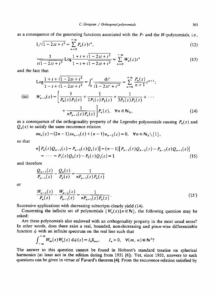
as a consequence of the generating functions associated with the P- and the W-polynomials, i.e.,

l/KG?= +c” P,(z)t”, (12) n=O

1 /

1+t+i1-2zt+t2

t/l - 2zt + t* Log I

l-t+il-2zt+t2 = “c” w,(z)t”

n=O

and the fact that

Log l+t+/l-22tt-kt2 = f dt’

l--t/l-2zt+t2 /y 0 1 - 2zt’ + tf2 = go 5$,.+1;

(iii) K-l(z) = [ Po(z;Pl(z) + 2Pl(zfP2(z) + 3P2(z;P,(z) + - * *

1

+ nP,_,(z)P,(z) pn(z)y v’n E Noy 1

(13)

(14)

as a consequence of the orthogonality property of the Legendre polynomials causing P,,(z) and Q,(z) to satisfy the same recurrence relation

I1U,(Z) - (2n - 1) z~,_~(z)+(~-l)u,_,(z)=o, VnW0\{1},

so that

+‘n(z)Qn-I(Z) -P,-dz)Qn(z)] =b - ~)[P,,-,(z)Q,_~(z) - P,_,(z)Q,_,(z)] = . . . = P,b)Qo(z) -P&)Q,(z) = 1 05)

and therefore

Q,-,(z) _ e,(r) = 1

P,-,(z) pn(z> c-l(Z>PnW or

W,-I(4 _ K2W 1

P,(z) P,-,(z) = nP,-,(z)P,(z) * (15’)

Successive applications with decreasing subscripts clearly yield (14). Concerning the infinite set of polynomials { W,(z) 1 n E N}, the following question may be

asked: Are these polynomials also endowed with an orthogonality property in the most usual sense?

In other words, does there exist a real, bounded, non-decreasing and piece-wise differentiable function # with an infinite spectrum on the real line such that

J +mKWK(s) d+(s) = ULln, 1,>0, v(m, n)EN2? --m

The answer to this question cannot be found in Hobson’s standard treatise on spherical harmonics (at least not in the edition dating from 1931 [6]). Yet, since 1935, answers to such questions can be given in virtue of Favard’s theorem [4]. From the recurrence relation satisfied by


Legendre’s polynomials by Legendre’s and functions of the second kind, one easily deduces that the polynomials of the second kind { W,(z)} satisfy

(n + 2)W,+,(z) -(2n + 3)zW,(z) +(n + l)W,_,(z) = 0, v’n E N, 2 (16) difference equation which determines the W-polynomials uniquely when the initial conditions

W_,(z) = 0, W,(z)=1

are combined with it. On account of Favard’s conditions 3 being fulfilled, one can directly state that { W,(z)} is an orthogonal sequence with respect to some real distribution d+ on the real line in C, but Favard’s paper does not include a procedure to calculate JI explicitly.

The theory of recursive generation of systems of orthogonal polynomials not only confirms the orthogonality property of { W,(z)}, but enables one to establish the following orthogonality relation for { W, ( z)} :

1 wn(Ml(4

5 i

1+s l+Ln2 ds=m mn, 2 6 v(m, n) E N2, (17)

-1 )ln-

l-s 4

in agreement with (1) for v = 1. Hence, {W,(z) 1 n E N} constitutes an infinite system of orthogonal polynomials in the same basic interval [ - 1, l] as Legendre’s polynomials, with weight function

being the result of calculating the right-hand side of

(19)

Notice the shift of one unit on n in the coefficients with respect to those appearing in the recurrence relation (4). Favard’s sufficient (as well as necessary) conditions for orthogonality, which we recall here for convenience. are most simply expressed for a sequence of monk polynomials {p,(z)}:

Let {p,,(z)} be defined by

1

P,(Z) = (Z -i%l)P”-,(Z)-%P”-2(Z), Vn EN09

p-l(z)=09 PO(Z) =I.

If I.r,, P27.s. are real and v2, u3,... are positive real, then {p,(z)} is an orthogonal sequence with respect to a real distribution drl, on the real line in C. In the case of (W”(z)}, the monk polynomial W,(Z) proportional to W,(z) is

Wn(Z) = [2”+l[(n +l)!]a/(2, +2)!] W”(Z), Vn EWI,

formula which can also be used for n = - 1 to define w-i(z). The sequence { w,(z)} satisfies the recursion

W”(Z) = ZWn_l(Z)- [ t12/(4n2 -I)] Wn_2(Z), Vn E&,

and since w_ t( z) = 0, wo( I) = 1, Favard’s conditions are clearly fulfilled. This weight function seems to have been obtained for the first time by Sherman [9]. See also (3, p. 2021. This general formula is in essence the same as formula (1.7) obtained independently by Maroni in a paper which he presented at the Colloque d’Analyse Numtrique, Belgodere, Corsica (1982), [7].

C. Grosjean / OrthogonaIpo[vnomiaIs 305

in which p(s) = 1, a = - 1, b = 1, M,, = j,“p( s) ds = 2 and 9 means Cauchy’s principal value. The weight function (18) is continuous, differentiable and positive definite in ] - 1, l[, and it tends to zero as s approaches - 1 and 1 (as a consequence of ln[(l + s)/(l - s)] tending to infinity). It is a solution of a non-linear differential equation of the second order, since

(1 - s’)’ d2p1 -- pi(s) ds2

’ _ 2.s(1 - s2) dp,

PlW ,+2p&)=0, -l<s<l.

On the contrary, l/p,(s) is a solution of an inhomogeneous linear differential equation of the second order which closely resembles (10) when n is put equal to zero, Indeed,

(I-s2)$-&2s$-=-$ -l<s<l. (21)

Another such peculiarity concerns the homogeneous linear differential equations of the fourth order satisfied by W,_,(z) and l/p,(s), respectively:

(1 - z2)2dzd-1 - lOz(1 - z2) dzs-l + [8(3z2 - 1) + 2n(n + l)(l - z2)] dz2-’

-6(n - l)(n + 2)~~ +(n - l)n(n + l)(n + 2)W,_,(z) = 0, (22)

and

(l_s2)2~~-l~s(l-s2)~~+8(3s2-l)~~+~2s~~=0. (23) 1

The second equation has the form of the first one for n = 0. These are characteristics which are not the exclusivity of the polynomials of Legendre, but hold for all classical orthogonal polynomials. Note that, in contrast to Legendre’s polynomials, { W,(z)} does not constitute a sequence of classical orthogonal polynomials.

Logically, the next step in this search for orthogonality is that one constructs the functions of the second kind associated with the W-polynomials:

R,(z) =j;-$) PlW wj~lPl(4 ds

i J 1 w,(s) =

1+s 1 2+1,2 1 ds, V’~EIW, VZEC\[-1, 11, (24)

-1 ( iln- l-s 4

also having a branch-line on [ - 1, 11, and that one decomposes R,(z) in the same manner as was done with Q,(z):

&z(z) = tm4j1 -r(z-s)[[$ln&~+$r2]

-t / l w,(z) - w,(s)

-1 z-s (iInLg)2++T2* (2%


From the general theory, one deduces a simple relation between the R- and the Q-functions:

R,(r) = 3Q,+,b>/Qob>, v’n E N. (26) For n = 0, (24) and (26) yield:

R,(z) =: j-T, (z_s),(;ln~~+~.2, =3%

Therefore, (25) becomes

R,(z) = W,(z)R,(z) -t/l q’z; 1 sw,(s) -1 2

+ hr2 4

= 3[ W)( tz Log% - l)/( iLog%) -L(z)],

VnEN, VzE@\[-1,1] 6 (28)

whereby X_,(z) = 0 for all z E C and X,,_,(z) is a polynomial of degree n - 1 for all n E N,:

X&)=3, X,(z)=Sz, X2(z)=%z2-$, . . . . (29)

Shifting the subscript by one unit, we have in general:

(29’)

Now it can be asked whether there exist counterparts of (9), (11) and (14), or some other formula expressing X, _i( ) z in closed form as a simple function of the P- and W-polynomials. The answer is affirmative on the whole line. Indeed, a combination of (26), (27) and (28) yields

Q,(z) Q,+,(z) -- x”-l(z) = w,(‘) Q,(z) Q,(z) y

and in virtue of (7), there comes

x-1(4 =&J { K(z>[P&)Q,(z) - w,(z)] - [P,+,(z)Qdz) - Wn(z)] >

6 By writing the factor 3 in front of the square brackets in (28), we slightly deviate from the corresponding formula in the general theory. The same can be said of the generalization of (28), namely (53), where (2 k + 1)/k is written as coefficient in front of the square brackets. The reason is that in the special case of the Legendre polynomials, the way in which we proceed leads to formulae which are somewhat simpler as far as their proportionality factors are concerned. This striving for greater overall simplicity has also induced us to prefer not to choose the proportionality factor in (28) in such a manner that X,(r) would become equal to 1, in contrast to Barrucand and Dickinson who put P~(Y, x) = 1 by definition.

C. Grosjean / Orthogonal polynomials

or, since W,(z) = 1

x,-,(Z>=z~,(z)--P,+~(z), V’nEfY.

From this result, one can deduce the counterpart of Christoffe’s formula (9)

1 xn-l(Z) = E

(2n - 1)(2n + 1)

n(n + 1) L(z) + n 2 (2n-5)(2n-l)p_ (z)

(n-1)n n 3

3 (2n-9)(2n-3)p_ (z)+ . . . . +57 (n-2)(n-1) R s

V’nENo.

The analogues of (11) and (14) are, respectively

~,-,(~)=t~,(~)~,_,(~)+f~,(~)~,_,(z)+$P2(z)P,_,(z)+ .a*

and

JG-l(Z) 1 1 1 1 = 2W,(z)W,(z) + 3W,(z)W*(z) + 4W,(z)W,(z) + **.

+ (n + l)w,l,(z)W~(z) w,(Z) 1 = z 2P,(z;Pz(z) + 3P,(z;P3(z) + 4P3(zfP,(z) + - - - [

+ (n + l)P.;r)P,,,(z) 1 P,+1(z), v’n l No.

307

(30)

(31)

(32)

(33)

Considering that the polynomials { W,(z)} and their functions of the second kind { R,(z)} satisfy the same recursion from n = 1 onward, one easily obtains

(n+3)X,,+,(z)-(2n+S)zX,,(z)+(n+2)X,_,(z)=O, VWEN,’ (34)

and Favard’s theorem, applied to the manic polynomials which are proportional to { X,,(z)} furnishes a direct proof of an orthogonality property of the latter. The theory of recursive generation yields in this case

J 1 xP”ts)xh) ds= 2 6

2n + 5 mn’ v(m, n) E N2, *

-1 (35)

’ Here, one notices a shift of 2 on n in the coefficients compared to those appearing in the recurrence relation (4). * There is no disagreement between this orthogonality relation and (1) into which v = 2 is inserted, although the

denominator of the integrand in the left-hand side of (1) differs from the one in (35) by a factor 4. The reason is that X”(Z) = :P”(2, z). *

308 C. Grosjean / Orthogonal pobnomials

and the new weight function

Pzb) = 1

-l<s<l, (36)

has the same properties as pi(s): continuous, differentiable and positive definite in ] - 1, l[. and tending to zero as s approaches - 1 and 1. It results from the calculation of either one of the two following expressions:

(37)

in which pi(s) is given by (18) and

J/f+ l / P+> ds=3

-1

on account of (17) and W,(z) = 1. This is in fact the apphcation of (19) to { W,(z)} regarded as initial sequence of orthogonal polynomials, apart from the proportionality factor 9 ( = 3’) which appears on account of splitting off a factor 3 in the definition of X,_,(z) (see (28)). Explicitly, we have

P*(S) =

((Jjln~~+f=*)-’

I

ii@ /

1

-1

-l<s<l. (38)

The remaining integral (constituting the principal value of an improper integral) can be deduced from (27)

It-s t_ln-

2

= ($ln:‘:j ’ - s, -l<s<l. (39)

+ hr* 4

Inserting this result into (38), one obtains (36) after some manipulations;

(ii) The general theory also provides a formula for the direct calculation of p*(s) in terms of p(s). In the case of the Legendre polynomials, there comes

P2W = PW

d1)2 + (tTC(s)p(s))’ ’

-lgs<l, (40)

C. Grogean / Orthogonal po!vnomials

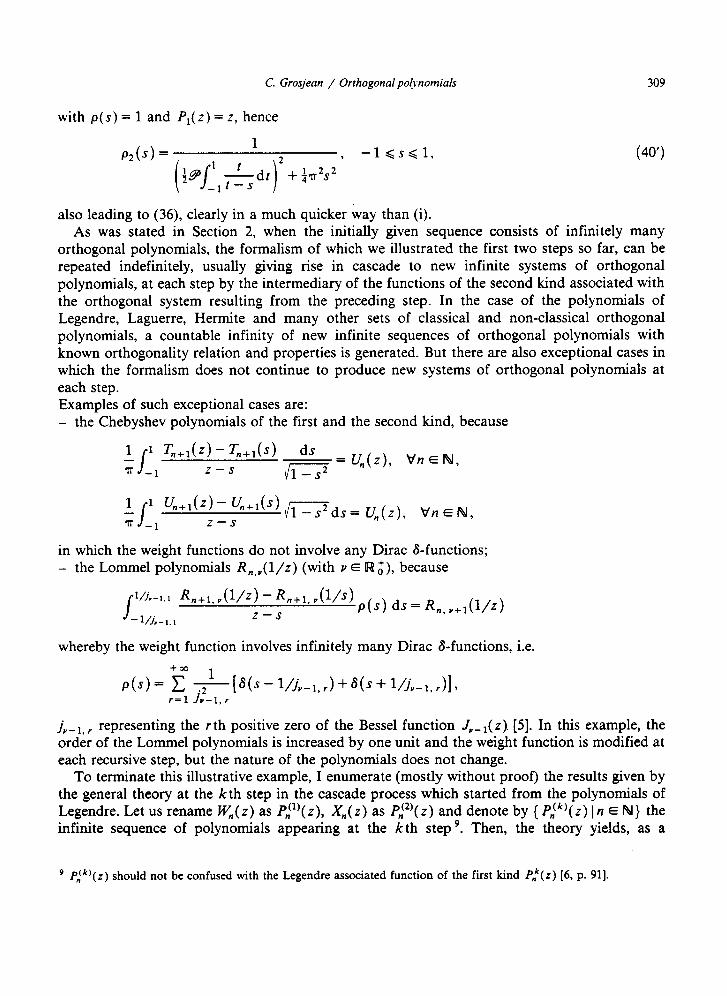
with p(s) = 1 and Pi(z) = z, hence

309

(40’)

also leading to (36), clearly in a much quicker way than (i). As was stated in Section 2, when the initially given sequence consists of infinitely many

orthogonal polynomials, the formalism of which we illustrated the first two steps so far, can be repeated indefinitely, usually giving rise in cascade to new infinite systems of orthogonal polynomials, at each step by the intermediary of the functions of the second kind associated with the orthogonal system resulting from the preceding step. In the case of the polynomials of Legendre, Laguerre, Hermite and many other sets of classical and non-classical orthogonal polynomials, a countable infinity of new infinite sequences of orthogonal polynomials with known orthogonality relation and properties is generated. But there are also exceptional cases in which the formalism does not continue to produce new systems of orthogonal polynomials at each step. Examples of such exceptional cases are: - the Chebyshev polynomials of the first and the second kind, because

1 - J 1 T,+,(+T,+,(s) ds = un(z) vnEN

= -1 Z-S c-7 ’ ’

’ - J ’ u,+l(z) - u,+lb) r/l-& = un(z) , vn E N 7 = -1 Z-S

in which the weight functions do not involve any Dirac b-functions; - the Lommel polynomials R,,,(l/z) (with v E Ri), because

/

l/jv-l.l &t+1, “(l/Z) - &l+1, “(l/4 P(S) ds = Rn, v+lW) -l/j,-1.1 Z-S

whereby the weight function involves infinitely many Dirac S-functions, i.e.

L-l,, representing the r th positive zero of the Bessel function J,,_ 1( z). [5]. In this example, the order of the Lommel polynomials is increased by one unit and the weight function is modified at each recursive step, but the nature of the polynomials does not change.

To terminate this illustrative example, I enumerate (mostly without proof) the results given by the general theory at the kth step in the cascade process which started from the polynomials of Legendre. Let us rename W,(z) as P,,(“)(z), X,,(z) as P,,(‘)(z) and denote by { PJk’(z) 1 n E N} the infinite sequence of polynomials appearing at the k th step 9. Then, the theory yields, as a

9 P,,(k’(r) should not be confused with the Legendre associated function of the first kind P,“(z) [6, p. 911.

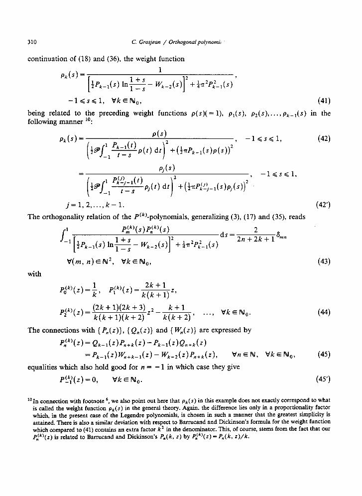
310 C. Grogean / Orthogonal polynomi:

continuation of (18) and (36) the weight function

P/c(S) = 1

i&-h) In e - wk&)]* + $&P;_,(s) ’

-l<sgl, VkEN,, (41)

being related to the preceding weight functions p(s)( = l), pi(s), p*(s), . . . , P~_~(s) in the following manner lo:

P/h) = PM

i P / -1 1 ‘*-‘(‘)p(t) t-s dt 1 2+(:d’k_l(s)p(s))2’

-l<s<l,

PjCs> = -l<s<l, ( 9 J 1 P&(t)

-1 t-s pj( t) dt 2 + (fTP~‘_:_,(S)Pj(s))* ’

j=l,2 ,..., k-l.

The orthogonality relation of the PCk) -polynomials, generalizing (3), (17) and (39, reads

J 1 P~k’(s)zJ,kyS)

+$ - W,+,(s)]* + &r*P,Z_&s)

ds= 2 s

-’ {P,_,(s) In 2n+2k+l mR

with

V(m, n)H*, VkENo,

p(k)(+ (2k+1)(2k+3)Z2_ k+l 2 k(k+l)(k+2) k(k+2)’

. . . . VkEtVo.

The connections with { P,(z)}, { Q,(z)} and { W,(z)} are expressed by

p,‘“‘(r) = Q,-,(r)&+,(z) - %,(r)Q,+&>

= Pk-l(z)W,+k-l (z) - ~,-,(z)&+,(z), vn E N, V’k E No,

equalities which also hold good for n = - 1 in which case they give

PI’;‘(z) = 0, VkEN,.

(42)

(42’)

(43)

(44)

(45)

(45’)

lo In connection with footnote 6, we also point out here that pk( S) in this example does not exactly correspond to what is called the weight function pk(r) in the general theory. Again, the difference lies only in a proportionality factor which, in the present case of the Legendre polynomials, is chosen in such a manner that the greatest simplicity is attained. There is also a similar deviation with respect to Barrucand and Dickinson’s formula for the weight function which compared to (41) contains an extra factor k2 in the denominator. This, of course, stems from the fact that our P,‘&‘(z) is related to Barrucand and Dickinson’s P,,(k, z) by Pik’(z) = P,,(k, z)/k.

C. Grosjean / Orthogonalpo~nomiaIs 311

More generally, we have:

p,‘“‘(z)=I[~~‘_‘,_,(z)P,‘:+,‘l,_,(r)-~~’_;”,(r)P,‘~,_,(z)],

VnE{-l,O,l)... }, VkEN,\{l}, WE{l,2 )..., k-l}, (46)

formula which can be made to hold also for I= 0, and consequently for k = 1, if the coefficient 1 is replaced by l/P,‘)(z) and under the convention that P,“)(z) stands for P,(z). Other interesting formulae for Pi!{(z) generalizing (ll), (32) and (14), (33) are, respectively

+ ,+~_,p”-~tz)p,(z)~ vnEN),~ Vk f No, (47)

and

1

kI’&,(:)Z’j”,(z) + (k+ l)P~!,(z)P~~,+,(z)

1

+ (k + n - l)P,“‘,+,_,( z)Pi!!,+,-,( z) 1 p~‘I,-,(z)P~‘ll+n_l(z), tfn~f+A~, VkENo, IE (0, 1,2 ,..., k-l},

whereby I$‘“)( z) = P,(z)_ The PCk’-polynomials satisfy the following recurrence relation:

(48)

(n+k+1)P,‘~‘,(z)-(2n+2k+1)zP,k)(~)+(n+k)P,(k)l(z)=0,

V’~EN, VkEfY, (49)

which extends (4), (16) and (34). Note the shift of integer value k on n in the coefficients with respect to those appearing in the recursion (4). Regarded as a difference equation with n as discrete variable running over N while k (E No) is kept fixed, (49) defines the sequence ( Pi’“‘(z)} uniquely when the initial conditions Plkj( z) = 0, P,‘“)(z) = l/k are combined with it.

Returning to (41), it is clear that every weight function comprised in it is continuous, differentiable and positive definite in ] - 1, l[, and tends to zero as s approaches - 1 and 1 (in virtue of fn[(l + s)/(l - s)] tending to infinity and p&t(l) = 1, pk_r( - 1) = (- l)k-‘). Hence, each theorem which has been established in the standard theory of systems of orthogonal polynomials with non-negative weight function and which expresses a property of such polynomials (for instance, concerning the nature, the location and the boundaries of their zeros), holds for the infinite set of sequences { Pi’“)< z) 1 n E f+J}.

The function of the second kind associated with P,‘k’(z) is

Q;"'(z) = ( /_L1 ‘T;‘;’ &) ds / flPkb) ds), ) ( (50) V~EN, VkEN,, Vz~a:\[-l,l].


From (43) and (44), one easily deduces

M,$“=j_;rp,(s) ds=&

and so, the explicit integral form of QLk’( t) reads:

Q’“‘(+ 2k+1 /

’ Pn’“‘( s)

e - w*_=(s)]= + ;n=P;-l(s)}

ds. n

2k2 -I (z -s)

(1 +Pk_,(s) h

(50’)

Every function of the second kind Qik)( z) (with k E No) can be expressed as a ratio of two Q-functions. The generalization of (26) appears to be

2k + 1 Q,+,(Z) Q;“‘(z)=-

k= Q,-,(Z) (51)

and therefore, according to (7),

Pik’( s)

’ l,(z-s)i[iPk_l(s) hi ‘z j

- - wk-2(s)]2

ds

+ $T=P;_l(s)

’ + 1 tPn+ktZ> Logz - w,+,-l(z> =

+&-r(z) Logs - w,-,(z) ’

VzEC\[-l,l]. (52)

The decomposition of Qik)(z) which is the analogue of (7) and (25) and which gives rise to the polynomial of the second kind associated with P,,(‘)(t), can be written as

Q(“)(z) _ 2k + 1 1 p,k’(s) -- n 2k2 j -1 z-s Pk(s) ds

= ~~~k’(z)~~l+ds - %?&;1 pJk’(zi 1 Fk’(‘) Pk(S) ds.

But on acount of PJk)(z) = l/k and (51) in which we put n = 0, there comes:

Q,(z) FP.“‘(z) j;l~ds=kP;k)(z)Q~k)(z)=~P;kJ(z) Qk_,(Z)

and hence the generalization of (28) reads

2k+1 Q;“‘(z) = kP,‘k’(z)Q6k’(z) y-g- j

1 P,k’(z)-P,fk’(s) z-s Pkb) ds

-1

w,-,(z)

fP,-,(z) L”gz _ =+- W,-,(z) I

. (53)

C. Grosjean / Orthogonal po[vnomials

Clearly, the relation in integral form between the PC’)- and the P(k+l)-polynofials is

pc*+‘yz)=LJ+l el%(4 - f-%l(s) n ds

1

( - )N z s fPk_l(~) ln+-$ - W,,(s)]* + &r*P~__i(s))

VnE{-l,O,l,... }, VkENO, VZEQ=,

in agreement with (45’) and (29’). The Q ‘k’-functions satisfy the recurrence formulae

i

(k+l)Q~k’(z)-(2k+1)zQ~k)(z)= -(2k+l)/k

(n+k+l)Q~~,(z)-(2n+2k+l)~Q~~)(z)+(.+k)Q~k,~(z)=O,

V’n~fiJ,, VkEN,,,

313

(54)

(55)

the same as (49) except that now the first equation is inhomogeneous. In virtue of (55), by successive elimination of Qfk’( z)/Q$,“‘( z), Qi”‘( z)/Qik’( z), etc., the following infinite continued fraction representation of Qhk’( z) holds:

Qh”‘( z) = (2k + 1)/k

(2k + 1)z - (k + l)*

, VkEN,,. (56)

(k + 2)’ (2k + 3)z - (2k + 5)z - . . .

Continued fraction representations will play an important role in the development of the general theory.

When (49) and (55) are linearly combined in such a way as to make the middle terms cancel each other, the result is

(n + k + ~)[P,‘:‘,(z)Q:~‘(z) -P,,(k’(~)Q;$)l(~)]

=(n+k)[P,‘k’(z)Qj;k_‘,(z)-P,(“~(z)Q~k’(z)], V’~EN,, VkE&,.

Successive applications of this equality, with n replaced by n - 1, n - 2,. . . , 1, give rise to a chain of equalities, and when use is made of (44) and the first equality of (55) in order to calculate the last side, there comes

or equivalently,

Qi”‘(z) _ Q:“?,(z) 2k+l 1

P,‘k’( z) P,‘:\(z) = k2(n + k+ 1) P,jk)(z)P,$(z) ’

(57)

V’~EN, VkENo. (57’)

On account of (53), we also have

pCk+l)(z) _ P,‘“‘;“(Z) =

G::(z)

1

P,‘“‘(z) k(n + k + l)P,‘k’(z)P,‘:;(z) ’ V~EN, VkEN,,

314

or

C. Groaean / Orthogonal polynomials

P,‘k{( z) P,(k{( z)

P,‘“-“(z) - P,‘!;“(z) = (k - l)(n + k - l);‘l;“(z)P.‘x-“(z) ’

v’n E N,, VkE {2,3,...},

formula whose validity is extended to k = 1 by replacing l/( k - 1) by Po(k-l)(~), taking into account (15’). Hence

P,‘fr’l( z) P,(k)Z( z) p(jk-“( z)

P,k-“(z) - P,!,“(z) = (k+n-l)P;k;‘)(~)P;~-~)(z)’

V’~EN,, VkEN,, P,‘“‘(z)=P,,(z). (58)

From this, we deduce

P,!k_( z) P,?,(z)

I

II 1

P;!-“(z) - f$il’( z) = pc”-“(z)n~, (k + n’ - l)p;.“_;“( z)p,‘?( z)

or, in virtue of Plki(z) = 0, Vk E No

P,‘ff’l( z)

Py”( z) = pd*-l’(z)nil (k + n’ _ l)P’;“(l)b-‘j(z) ’ n’ 1

V’neN,, VkEN,,

which proves (48) in the case of I = k - 1. More generally, replacing k by I + 1 and n by k + n - I- 1 in (58), we have

~Kt2,-2(4 _ et+;~,-3(z) = P,“(Z)

Pi’!,-H(Z) Pk(:)n-,-2(z) (k + n - 1) P,$-,-2( z) P&_,_l( z) ’

V(k+n)E {2,3,4 ,... }, VIE (0, l,..., k+n-2).

The set of conditions V( k + n) E { 2, 3,4,. . . }, Vl E (0, 1, . . . , k + n - 2) contains as a subset

V’~EN,, VkENo, V/E {O,l,..., k-l}.

For these new conditions, we certainly have:

k P&+&_,(z) _ P&+;)_,-J(z)

tl’=l P&_[_l( 2) P&L,-2( z) I

= p”‘l’(z),,$l (k + n’- l)P~~n~_~_2(z)P,$!n~_~_l(z)


or

~[P~‘l,_*(z,P~~~~,_2(z) -Pp/?2(z)P~I_)n_,_1(Z)] PJ"( z)

.gl (k + n’ _ 1)pi’!n,_f_2( )p(/, _ _ ( Z k+n' I 1 z V’nENo, V’kENo, V’IE {OJ )..., k-l}.

The right-hand side is clearly that of (48) and according to (46), the left-hand side is simply P,‘!\(z). Thus, (48) is completely proven.

In Section 2, I mentioned that the application of the theory of recursive generation can be expected to yield a multitude of new integrals not comprised in the existing specialized literature. Here follow two examples of general formulae in which p(s) represents a given weight function not containing any Dirac S-functions

(i) Let the moments belonging to p(s) be

M,,, = J

‘s”‘P(s) ds, VmEN.

Then recalling (y9) which gives the weight function pt(s) corresponding to the orthogonal polynomials of the second kind, and denoting by Mz’, m = 0, 1, 2,. . . , its moments, we have

4 M2 Ml ‘MO = wr+l : : : :

M,“+’ ;M m

;M _ m 1 k-* k-3

M m+l Mm Mm-, wn-2 M m+t Mm+1 Jcl Mn-1

. . . 0 0 0

. . . 0 0 *o

. . . 0 0 0

if* ito b . . . M2 Ml MO

. . . 4 M2 Ml

, V’mEN,

(59) being a finite representation of the value of a definite integral which usually turns out to be far from elementary in most practical applications. For instance, in the special case of the Legendre plynomials where

M,,,= 1 J

S”‘ds=- ,il [1+(-l)“] = -1

when m is even, VmEN,

when m is odd,

there comes

ds

+ +Tr’


0 1 0 0 + 0 1 0

0 ) 0 1

f 0 : 0 =(_l)m+l, ! ; ;

From this result, we deduce

-1 _2n+l

. . .

. . .

..*

. . .

. . .

. . .

. . .

. . .

0 0 0

0 0 0

0 0 0

0 0 0 . . . . . .

b i b + 0 1

0 + 0

f 0 f

) VrnEfv.

which is trivial since the integrand is an odd continuous function of s in - 1 G s Q 1, and

which yields

2n + 3

1

+

i

1 2n-1

1 2n+l

0

1

f

1 2n - 3

1 2n - 1

. . . 0 0

. . . 0 0

. . . 0 0 . . . . . .

. . . f 1

. . . f i

The determinant representation of yn also tells us that yO, /t, . . . , fn are connected by way of the following recurrence relation:

from which the successive $values can be obtained more easily than from the determinant representation.

(ii) If {~&)W~) is a sequence of orthogonal polynomials, with corresponding weight function p(s) in a G s G b( a c b) which does not involve any Dirac S-functions, and the notations

Pm(z) = a,z” + b,z”-’ + - - - +I,,

I” = / bp,2(+(s) ds 0

C. Grosjean / Orthogonal po&nomials 317

are used, then

Pb>

~(4 dt ’ +hnb)~(s))’

ds

) 1 ” Pn+l(Z) + a 1 _

VnEN. a n+l~n P,(Z)

P,&)[~~P(~) ds ’ vzEQ=\[a, 61,

The integral represents a function which has a branch-line on [a, b]. In order to complement the preceding result, one can insert into it successively z = x + 0 - i and z = x - 0 - i whereby a < x < b, and take the arithmetic mean. This yields

Bb J P(S) ds LI

( xs 9

- )[( J bP w

~ *p(t) dt 2 +(~P~(s)P~))~ 1 bP (4

an =- Pn+lb) + B J “-p(s) ds

o s-x

a n+l~n P,(X) g[b$$~(s) dsj2 +(vnb)p(x))2 1

, VnEN.

p,,(x)

Note added after completion of the preceding text

A few weeks after the oral presentation of my paper entitled “Theory of recursive generation of systems of orthogonal polynomials” at the Journal C.A.M. Conference, I had the opportunity to study the important and truly magnificent article of Prof. Dr. P. Nevai [8]. I wish to point out that there is a slight interference between this work and mine. In his fourth example, Nevai gives an expression for the weight functions of the sets of orthogonal polynomials associated with an initial sequence which is orthogonal with respect to a generalized Jacobi weight in the interval [ - 1, 11 (p. 414, (15)). This formula is, apart from some proportionality factor, the same as the one appearing in my theory in the general case of a given weight function not involving Dirac Speaks (compare, e.g., with (42)). Nevai’s result (15) is a special case of formula (3) appearing in his main theorem. My future paper will comprise a more elementary way to find the weight functions of the sets of associated orthogonal polynomials of all orders, as well as many relations existing between the polynomials, their functions of the second kind and the corresponding infinite continued fractions of the Jacobi type, both for a given weight without mass-points and one involving a finite or infinite number of Dirac S-functions.

Acknowledgment

The author is indebted to Prof. Dr. A. Magnus (U.C.L., Louvain-la-Neuve) and Dr. H. De Meyer (R.U.G., Gent) for stimulating discussions and also for drawing his attention upon some important literature references.


References

[l] R. Askey and J. Wimp, Associated Laguerre and Hermite polynomials, Proc. Roy. Sot. Edinb. %A (1984) 15-37. [2] P. Barrucand and D. Dickinson, On the associated Legendre polynomials, in: D. Haimo, Ed., Orthogonal

Expansions and Their Continuous Analogues (Southern Illinois University Press, Carbondale, IL, 1967) 43-50. [3] T. Chihara, An Introduction to OrthogonaI Polynomials (Gordon and Breach, New York, 1978). [4] J. Favard, Sur les polynomes de Tchebicheff, C.R. Acad. Sci. Paris 200 (1935) 2052-2053. [S] C.C. Grosjean, The orthogonality property of the Lommel polynomials and a twofold infinity of relations between

Rayleigh’s u-sums, J. Comput. Appl. Math. 10 (1984) 355-382. [6] E.W. Hobson, The Theory of Spherical and Ellipsoidal Harmonics (Cambridge University Press, London, 1931). [7] P. Maroni, Sur la continuitt absolue de la mesure like a la suite des polynomes orthogonaux associee a une suite

orthogonale don&e, Colloque d’analyse numtrique, Belgodere, Corsica (1982). manuscript. [8] P. Nevai, A new class of orthogonal polynomials, Proc. Amer. Math. Sot. 91 (3) (1984) 409-415. [9] J. Sherman, On the numerators of the convergents of the Stieltjes continued fractions, Trans. Amer. Math. Sot. 35

(1933) 64-87.

theory of recursive generation of systems of orthogonal ... · theory of recursive generation of...

Documents