GENERAL INTRODUCTIONThis course unit is designed to provide students with an in-depth introduction to the theory of microeconomics and its modern application. The course unit is particularly suitable to first year undergraduate students who are studying degree courses in economics, business studies and other fields of study, which among other course units include an introductory course in microeconomic analysis. No prior knowledge of economics is required as a pre-requisite for reading this course unit.

The overall aims of this course are three fold. First, it aims at providing the students with a sound understanding of scope and methods economic analysis. Second, it aims at equipping the students with sufficient knowledge and skills on the basics of demand and supply; theory of consumer’s behaviour and theory of production and cost. Third, it aims at preparing the students for an intermediate course on microeconomics, which demands rigorous quantitative techniques in solving and analyzing economic problems.

UNIT OBJECTIVESAfter reading this course unit you should be able to:(i) Define economics, scarcity, opportunity cost and production

possibility frontier.(ii) Describe how economic theories are formulated.(iii) State the law of demand and outline the determinants of demand

and supply(iv) Distinguish between change in demand (supply) and change in

quantity demanded (supplied)(v) Illustrate the market equilibrium both graphically and

algebraically. (vi) Show graphically and algebraically the consequences of

government intervention in the market in the form of price controls and indirect taxes

(vii) Calculate and interpret different elasticities of demand and supply and show the relationship between elasticity and total revenue

(viii) Explain both the cardinal and ordinal theories of consumers’ behaviour, and show how the demand curve is derived from these theories.

(ix) Analyze consumer behaviour under uncertainty/risk environment.(x) Describe production functions, average product, and marginal

product and state the law of diminishing returns.(xi) Describe various types of cost and explain the reasons for their

shapes.

ORGANIZATION OF THE COURSE UNITThis course unit is organized in the form of lecture series covering four major parts: scope and methods of economics; theory of demand and supply; consumer theory and theory of production and cost. Understanding this unit will install a solid grounding to proceed with OEC 107, which completes the introductory course in microeconomics.

i

Each lecture in this unit begins with a brief introduction designed to explain the importance of the materials to be covered. This is followed by a set of learning objectives, which underline the key concepts and other theoretical issues, which we believe first year students, should target to learn from that particular lecture. At the end of each lecture, we have provided a summary and a set of exercises. The exercises are designed to reinforce student’s understanding and familiarity on the lectures. The solutions for selected questions with asterisks are appended at the end of this course unit.

Lecture one defines the term economics and distinguishes microeconomics from macroeconomics. The lecture also surveys the scope of economics and introduces you to the basic concepts like, scarcity, opportunity cost and production possibility frontier. Thereafter, we will learn fundamental economic problems that microeconomics addresses and the kind of answers it provides. At the end of lecture one, we will describe several methods of economic analysis and chart out potential pitfalls that are prevalent in the methodology of economic analysis.

Lecture two contains one of the most important tools of microeconomic theory: the theory of demand. This lecture will explain and describe individual’s demand schedule, individual’s demand curve and the market demand curve. Furthermore, the lecture will attempt to explain and distinguish the difference between change in demand and change in quantity demanded. We will learn the law of demand and single out exceptions, which are inherent to this law. Lecture two will also elucidate inasmuch as possible various factors, which influence demand for a particular good.

Lecture three covers the elementary theory of supply. This lecture will provide you with an insight on various concepts such as an individual’s supply curve, supply schedule and market supply curve. The distinction between the movement along the supply curve and shift in the supply curve is also presented both verbally and graphically. The lecture will equally point out a variety of factors that determine change in supply of goods in the market. The concept of producer surplus is introduced in the last section of this lecture.

The central focus of lecture four is on market equilibrium and disequilibrium. In this lecture you will see how the interaction of demand and supply curves you learned in lecture two and three respectively can be used to determine equilibrium price and quantity of a particular good. The lecture also illustrates the impact of sales tax on equilibrium price and quantity. Moreover, the lecture utilizes the concepts of price ceilings and price floors to analyze disequilibrium in the market. In the last section, we describe the Cobweb model.

Lecture five is devoted to explaining different types of elasticity of demand and supply. The important types of elasticity that you should learn are: price elasticity of demand and supply, income elasticity and cross price elasticity of demand. You should learn how to calculate those elasticities and also to give an economic interpretation. You should also learn the relationship between the elasticity of demand and total revenue. Finally, you should outline factors, which govern the coefficients of elasticity of demand and supply.

ii

Lecture six explores the theory of consumer behavior from the Cardinal Utility theory. In brevity, the Cardinal Utility theory ascertains why an individual’s demand curve slopes downward from left to the right following the thinking of cardinal economists such as Walras, Jevons and Marshal. Key definitions on various concepts of cardinal utility theory are presented. The law of diminishing marginal utility, which is a vital ingredient in deriving an individual’s demand curve, is also introduced. The important concepts of consumer’s surplus and paradox of value are articulated. The last section provides a critique on the cardinalist theory.

Lecture seven provides an alternative explanation of the theory of consumer behavior from the ordinal perspective. Two approaches are presented: indifference curve approach and the Revealed Preference Theory. This lecture differs from lecture six in that it discards the measurability of utility as a crucial cornerstone in deriving an individual demand curve. You will see how consumer’s choice between two goods is made given the budget constraint and a set of indifference curves. Concomitantly, the lecture further presents and analyses how income and substitution effects of a price change on a particular commodity operate. The synthesis of substitution and income effects will enable you to derive an individual demand curve, which slopes down- ward from left to the right.

Lecture eight introduces an element of uncertainty/risk to the theory of consumer behaviour. In doing so, the lecture employs mathematical tools such as probability, expected value and standard deviation in an attempt to measure and compare the degree of risk among different commodities. The lecture also describes consumer’s attitude towards risk, which involves the concepts of risk loving, risk neutral and risk averse. The lecture, too, illustrates the relationship between attitude towards risk and the shape of indifference curves. The concept of risk premium is also explained. The final part of this lecture discusses risk diversification. This includes buying insurance and/or investing in more than one portfolio.

Theory of production is expounded in lecture nine. We shall analyze the theory of production in two steps. In the first step, we shall particularly be concerned with the short run production function, which allows for variation in one factor of production. Briefly, short run production is divided into three stages of production. You shall learn that in the short run, a rational producer will always operate in stage two of production. In the second step, we shall be examining production in the long run, which allows for variation in more than one factor of production. Long run production invokes the concept of isoquant. In this step, you shall learn the least-cost production technique.

The last lecture in this unit is on the theory of the cost. In this lecture, various types of costs are defined, with special emphasis on the distinction between economic and accounting costs. In order to grasp the theory of cost in sequence, economists have traditionally found it useful to study theory of cost in the short run and in the long run. In the short run, you shall see that the curvature of the short run cost curves are largely influenced by the law of diminishing marginal return. In the long run, the curvature of cost curves is shaped by economies and diseconomies of scale.

iii

The approach adopted in this unit is that of partial equilibrium analysis. We will be examining the behavior of buyers and sellers in isolation from the conditions prevailing in other markets. The interaction of all individual units as studied by the general equilibrium analysis is presented in the Introduction to Microeconomics II (OEC 107), which as said earlier; you are required to read OEC 107 in order to complete the introductory course in Microeconomics.

COURSE ASSESSMENT CRITERIA In order to complete successfully this course, a student is required to attempt both coursework and a final examination. There will be two assignments, two tests and one final examination. The first assignment covers lectures 1-5, whereas the second assignment covers lectures 6-10. Similarly the first test will cover lectures 1-5 whereas the second test will cover lectures 6-10. At the end of the academic year you will attempt a final examination, which cover all the lectures.

SELECTED REFERENCESIt is important to underscore that the explanation/discussion of topics provided in this reading material on its own is neither exhaustive nor does it pretend to be unique in terms of coverage. The discussion is meant to introduce you to the subject matter and open the door for further and extensive readings. Consequently, we expect that students will consult a variety of textbooks to supplement the notes contained in this reading material in order to expand their knowledge frontier. The following texts are useful throughout this course.

1. David Begg, Stanley Fischer and Rudiger Dornbusch (2003), Economics, Seventh Edition McGraw Hill

2. Edwin Mansfield (1991) Microeconomics, Seventh Edition, Norton New York

3. Lipsey R.G and K. Alec Crystal (2004) Economics; Tenth Edition, Oxford University Press.

4. Salvatore Dominick (2002) Microeconomic Theory and Applications, Fourth Edition, Oxford University Press

5. Nicholson, Walter (2004) Intermediate Microeconomic with Its Application . Ninth Edition, Business Higher Education.

6. Paul Samuelson and William Nordhaus (2001) Economics, Seventeenth Edition, McGraw Hill.

7. Philip Hardwick, Bahadur Khan and John Langmead (1999) An Introduction to Modern Economics, Fifth Edition, Longman; London and New York

iv

8. Roberts S.Pindyck and Daniel Rubinfeld (2005) Microeconomics, Sixth Edition, Pearson, Prentice Hall.

9. Varian, Hal R (2006) Intermediate Microeconomics: A Modern Approach . Seventh Edition, New York; London: W. W. Norton

© The Open University of Tanzania, 2004All rights reserved. No part of this publication may be reproduced, stored in a retrieval system, or transmitted in any form or by any means, mechanical, photocopying, recording or otherwise without the prior written permission of the publisher.

The author of this publication is entitled to the copyright according to the provision of the agreement made with the Open University of Tanzania

Khatibu.G.M.Kazungu

v

TABLE OF CONTENTSGENERAL INTRODUCTION IUNIT OBJECTIVES IORGANIZATION OF THE COURSE UNIT ICOURSE ASSESSMENT CRITERIA IVSELECTED REFERENCES IVTABLE OF CONTENTS VILIST OF FIGURES XILIST OF TABLES XIILECTURE ONE 1SCOPE AND METHODS OF ECONOMICS 11.1 Introduction 11.2 Definition of Economics 11.3 Choice and Opportunity Cost 21.4 Production Possibility Frontier (PPF) 31.5 The Central Economic Problems 4

1.5.1 What to Produce 41.5.2 How to Produce 51.5.3 For Whom to Produce 5

1.6 Economic Systems and the Solutions to the Central Economic Problems 51.6.1 Market Economy 51.6.2 Limitations of the Price Mechanisms: Market failures 61.6.3 Planned (Command) economy 7

1.7 Methodology of Economic Analysis 81.7.1 Theoretical Approach 81.7.2 Deduction and Empirical Approach 101.7.3 Induction Approach 13

1.8 Pitfalls of Methodology of Economic Analysis 141.8.1 Fallacy of Composition 141.8.2 Post hoc Fallacy 141.8.3 Ceteris Peribus Assumption 141.8.4 Subjectivity 15

1.9 Positive versus Normative Economics 15LECTURE TWO 18THEORY OF DEMAND 182.1 Introduction 182.2 Definition of Demand 182.3 Individual’s Demand Curve for a Commodity 182.4 The Law of Demand 202.5 Exceptions to the Law Of Demand 22

2.5.1 Giffen Goods 222.5.2 Veblen Goods 22

2.6 Determinants of Demand for a Commodity Other than Own Price 232.6.1 Demand for Commodity X and the Price of Commodity Y 232.6.2 Demand for Commodity and the Consumer’s Income 232.6.3 Demand for a Commodity and the Consumer’s Taste 24

vi

2.6.4 Demand for a Commodity and the Size of the Population 242.6.6 Expectation and Demand for a Commodity 252.6.7 Other Related Factors and the Demand for a Commodity. 25

2.7 Change in Demand versus Movement along the Demand Curve 252.8 The Market Demand for a Commodity 27LECTURE THREE 32THEORY OF SUPPLY 323.1 Introduction 323.2 The meaning of Supply 323.3 A Single Producer’s Supply of a Commodity 323.4 The Shape of the Supply Curve 333.5 The Market Supply of a Commodity 343.6 Determinants of Market Supply 35

3.6.1 The Objective of the Firms 353.6.2 Price of Goods X (Px) 363.6.3 Prices of Other Goods (Po) 363.6.4 Prices of Factors of Production (Pf) 373.6.5 State of Technology (T) 373.6.6 Expectation (E) 373.6.7 Tastes of the Producers (Tp) 373.6.8 Government Tax and Subsidy Policy (G) 373.6.9 Other Relevant Variables (Z) 37

3.7 Change in Supply and Change in the Quantity Supplied 383.8 Producer Surplus 38LECTURE FOUR 42MARKET EQUILIBRIUM 424.1 Introduction 424.2 Market 424.3 Market Equilibrium 424.5 Types of Equilibrium 45

4.5.1 Stable Equilibrium 454.5.2 Unstable Equilibrium 45

4.6 The Impact of Shift in Demand and Supply Curves on Equilibrium 474.7 Sales Tax and Market Equilibrium 49Numerical Example 514.8 Market Disequilibrium 51

4.8.1 Artificial Restriction on Price and Quantity. 524.8.2 Unstable Equilibria 534.8.3 Failure of Production Plans to be Realized 534.8.4 Lagged Responses 53

4.9 Cobweb Model 54LECTURE FIVE 59ELASTICITY OF DEMAND AND SUPPLY 595.1 Introduction 595.2 Price Elasticity Of Demand 595.3 Measurement of Price Elasticity 60

vii

5.3.1 Point Elasticity of Demand 605.3.2 Arc Elasticity of Demand 60

5.4 Elasticity along the Linear Demand Curve 625.5 Interpretation of Price Elasticity of Demand 63

5.5.1 Inelastic Demand 635.5.2 Elastic Demand 645.5.3 Unitary Elasticity 65

5.6 Elasticity and Slope of Demand Curve 665.7 Determinants of Price Elasticity of Demand 675.8 The Income Elasticity of Demand 685.9 The Cross Elasticity of Demand 695.10 Relationship between Elasticity and Total Revenue 705.11 Elasticity of Supply 735.12 Determinant of Elasticity of Supply 75

5.12.1 Time 755.12.2 Excess capacity and unsold stocks 765.12.3 Ease of Factor Substitution 76

SUMMARY 77LECTURE SIX 80CONSUMER BEHAVIOR: 80THE CARDINAL UTILITY THEORY 806.1 Introduction 806.2 The Cardinal Utility Theory 806.4 Marginal Utility 816.5 Consumer Equilibrium 826.6 The Link between Demand Curve and Marginal Utility 856.7 Consumer Surplus 866.8 Utility and Value: "The Paradox of Value" 886.10 Some Criticisms on the Cardinalist Theory 89LECTURE SEVEN 94CONSUMER BEHAVIOR: 94ORDINAL UTILITY THEORY 947.1 Introduction 947.2 Ordinal Utility Theory 947.3 Indifference Curve Approach 947.3.1 Indifference Curves 967.3.2 The Marginal Rate of Substitution 987.4 Budget Line and Consumer's Equilibrium 99

7.4.1 The Budget Line 997.4.2 Consumer's Equilibrium 100

7.5 Income Changes and the Budget Line 1017.6 Price Change and the Budget Line 1037.9 Demand Curve from Price Consumption Curve 1097.10 Critique of the Indifference Curve Approach 1117.11 Revealed Preference Theory 111LECTURE EIGHT 118

viii

UNCERTAINTY AND CONSUMER BEHAVIOUR 1188.1 Introduction 1188.2 Risk /Uncertain Choice 118

8.2.1 Probability 1188.2.2 Expected value 1198.2.3 Standard Deviation 121

8.3 Preferences towards Risk 1228.3.1 Risk-averse Individual 1228.3.2 Risk Loving Individual 1248.3.2 Risk Neutral 125

8.4 Risk aversion and Indifference curves 1258.5 Reducing Risk 127

8.5.1 Diversification 1278.5.2 Insurance 127

LECTURE NINE 132THEORY OF PRODUCTION 1329.1 Introduction 1329.2 Production Unit: A Firm 132

9.2.1 Sole Proprietorship 1329.2.2 Partnership 1329.2.3 Limited Company 1339.2.4 Cooperatives 133

9.3 Assumption of Profit Maximization 1339.4 Inputs or Factors of Production 134

9.4.1 Land 1349.4.2 Labor 1349.4.3 Capital 1349.4.4 Entrepreneurship 135

9.5 The Production Function 1359.6 The Short Run: Production with One Variable Input 1359.7 The Shapes of the Average and Marginal Product Curves 1389.8 The Law of Diminishing Marginal Return 1399.9 Three Stages of Production 1399.10 The Long Run: Production with Two Variable Inputs 141

9.10.1 Isoquant 1419.10.2 Properties of Isoquants 1429.10.3 Marginal Rate of Technical Substitution 1449.10.4 Isocost lines 145

9.11 Producer Equilibrium 1459.12 Expansion Path 1489.13 Effect of Change in Input Prices on Output 1499.14 Elasticity of Technical Substitution 1509.15 Returns to Scale and Homogeneity 151LECTURE TEN 158THEORY OF COSTS 15810.1 Introduction 158

ix

10.2 Accounting Cost versus Economic Cost 15810.3 Private and Social Cost 16010.4 Sunk Cost 16010.5 Costs in the Short Run 16010.6 Short-Run per Unit Cost Curves 162

10.6.1 Marginal Cost 16210.6.2 Average Total Cost 162

10.7 The Relationship between Marginal Cost and Marginal Product 16410.8 The Long-Run Average Total Cost Curve 16610.9 Economies of Scale 16910.10 External Economies of Scale 17010.11 Diseconomies of Scale 170ANSWERS TO SELECTED QUESTIONSANSWERS TO SELECTED QUESTIONS 175

x

LIST OF FIGURESFIGURE 1.1: PRODUCTION POSSIBILITY FRONTIER 3FIGURE 1.2: DEDUCTION AND EMPIRICAL TESTING. 11FIGURE 2.1: INDIVIDUAL’S DEMAND CURVE FOR COMMODITY X 20FIGURE 2.2: DEMAND CURVE FOR A GIFFEN OR VEBLEN GOODS 22FIGURE 2.3: ENGEL CURVE 24FIGURE 2.4: CHANGE IN DEMAND 26FIGURE 2.5: CHANGE IN QUANTITY DEMANDED 26FIGURE 2.6: MARKET DEMAND CURVE FOR COMMODITY X 28FIGURE 3.1: PRODUCER’S SUPPLY CURVE 33FIGURE 3.2: MARKET SUPPLY CURVE 35FIGURE 3.3: OBJECTIVE OF THE FIRM 36FIGURE 3.4: SHIFT IN THE SUPPLY CURVE 38FIGURE 3.5: PRODUCER’S SURPLUS 39FIGURE 4.1: MARKET EQUILIBRIUM 43FIGURE 4.2: EXCESS DEMAND AND EXCESS SUPPLY 45FIGURE 4.3(A): UNSTABLE EQUILIBRIUM 46FIGURE 4.3(B): UNSTABLE EQUILIBRIUM 47FIGURE 4.4: A SHIFT IN MARKET SUPPLY CURVE 48FIGURE 4.5: A SHIFT IN MARKET DEMAND CURVE AND EQUILIBRIUM 48FIGURE 4.6: A SHIFT IN MARKET DEMAND AND SUPPLY CURVES 49FIGURE 4.7: SALES TAX ON EQUILIBRIUM PRICE AND QUANTITY 50FIGURE 4.8: A PRICE CEILING 52FIGURE 4.9: A PRICE FLOOR 53FIGURE 4.10: THE CONVERGENT COBWEB MODEL "DUMPED" 54FIGURE 5.1: ARC ELASTICITY. 61FIGURE 5.2 ELASTICITY ALONG THE LINEAR DEMAND CURVE 62FIGURE 5.3: TWO INTERSECTING DEMAND CURVES 63FIGURE 5.4: PERFECTLY INELASTIC DEMAND CURVE 64FIGURE 5.5: PERFECTLY ELASTIC DEMAND CURVE 64FIGURE 5.6: RECTANGULAR HYPERBOLA DEMAND CURVE 65FIGURE 5.7: ELASTICITY MEASURED ON LINEAR DEMAND CURVE 66FIGURE 5.8: INCOME ELASTICITY OF DEMAND AND THE LEVEL OF INCOME 69FIGURE 5.9: ELASTICITY AND TOTAL REVENUE 72FIGURE 5.10: PERFECTLY INELASTIC SUPPLY CURVE 73FIGURE 5.11: PERFECTLY ELASTIC SUPPLY CURVE 74FIGURE 5.12: UNITARY ELASTIC SUPPLY CURVE 74FIGURE 5.13: MOMENTARY, SHORT RUN AND LONG RUN SUPPLY CURVES 76FIGURE 6.1: TOTAL AND MARGINAL UTILITY 82FIGURE 6.2: DEMAND CURVE FROM THE MARGINAL UTILITY CURVE 86FIGURE 6.3: CONSUMER'S SURPLUS 87FIGURE 7.1: AN INDIFFERENCE MAP 96FIGURE 7.2: INTERSECTING INDIFFERENCE CURVES 97FIGURE 7.3: CONVEXITY OF AN INDIFFERENCE CURVE 98FIGURE 7.4: CONSUMER'S EQUILIBRIUM 100FIGURE 7.5: INCOME CONSUMPTION CURVE AND ENGEL’S CURVE 102FIGURE 7.6: EFFECT OF A PRICE CHANGE ON THE BUDGET LINE 103FIGURE 7.7: THE PRICE CONSUMPTION CURVE 104FIGURE 7.8: INCOME AND SUBSTITUTION EFFECTS FOR A NORMAL GOOD 105FIGURE 7.9: INCOME AND SUBSTITUTION EFFECTS FOR AN INFERIOR GOOD 106FIGURE 7.10: INCOME AND SUBSTITUTION EFFECTS FOR A GIFFEN GOOD 106FIGURE 7.11: DEMAND CURVE FROM PRICE CONSUMPTION CURVE 109FIGURE 7.12: REVEALED PREFERENCE THEORY 112FIGURE 7.13: DEMAND CURVE FROM THE REVEALED PREFERENCE THEORY 114FIGURE 8.1: RISK AVERSE INDIVIDUAL 123

xi

FIGURE 8.2: RISK LOVING INDIVIDUAL 124FIGURE 8.3: RISK NEUTRAL INDIVIDUAL 125FIGURE 8.4: RISK AVERSION AND INDIFFERENCE CURVES 126FIGURE 8.5: RISK AVERSION AND INDIFFERENCE CURVES 126FIGURE 9.1: PRODUCTION FUNCTION OF CORN IN THE SHORT RUN. 136FIGURE 9.2: TOTAL, MARGINAL AND AVERAGE PRODUCTS 138FIGURE 9.3: THREE STAGES OF PRODUCTION 139FIGURE 9.4: AN ISOQUANT MAP 142FIGURE 9.5: TWO INTERSECTING ISOQUANTS 143FIGURE 9.6: AN ISOQUANT CONVEX TO THE ORIGIN 143FIGURE 9.7: ISOCOST LINES 145FIGURE 9.8: EXPANSION PATH 148FIGURE 9.9: SUBSTITUTION AND SCALE EFFECT 149FIGURE 9.10: ELASTICITY OF TECHNICAL SUBSTITUTION 150FIGURE 10.1: A FIRM'S SHORT RUN COST CURVES 162FIGURE 10.2: SHORT RUN COST CURVES 164FIGURE 10.3: MARGINAL PRODUCT AND MARGINAL COST 165FIGURE 10.4: LONG RUN AVERAGE TOTAL COST 167Figure 10.5: Long run Marginal Cost 167

LIST OF TABLES TABLE 2.1: AN INDIVIDUAL’S DEMAND SCHEDULE FOR COMMODITY X 19TABLE 2.2: MARKET DEMAND SCHEDULE FOR COMMODITY X 27TABLE 3.1: PRODUCER’ SUPPLY SCHEDULE FOR COMMODITY X 33TABLE 3.2: MARKET SUPPLY SCHEDULE 34TABLE 4.1: QUANTITIES DEMANDED AND SUPPLIED AT DIFFERENT PRICES 50TABLE 5.1: MARKET DEMAND SCHEDULE AND ARC ELASTICITY 61TABLE 5.2: ELASTICITY AND TOTAL REVENUE 71TABLE 6.1: ILLUSTRATION OF DIMINISHING MARGINAL UTILITY 82TABLE 6.2: HAVIJAWA'S MARGINAL UTILITY FOR BEVERAGES 83TABLE 6.3: HAVIJAWA'S MARGINAL UTILITIES PER SHILLING 84TABLE 6.4: CONSUMER SURPLUS 86TABLE 8.1: SHARE PRICES 120TABLE 8.2: DEVIATION 121TABLE 8.3: STANDARD DEVIATION 122TABLE 9.1: PRODUCTION FUNCTION OF CORN IN THE SHORT RUN 136TABLE 9.2: MARGINAL AND AVERAGE PRODUCT OF LABOR 137TABLE 10.1: P/L ACCOUNT FOR THE YEAR ENDED 31ST DECEMBER 200X 159TABLE 10.2: A FIRM'S SHORT RUN SCHEDULE 161Table 10.3: A Firm's Per Unit Short Run Cost 163

xii

LECTURE ONESCOPE AND METHODS OF ECONOMICS

1.1 Introduction The major purpose of this lecture is to explain the scope and methods of economics. Among other issues, you will learn that economics essentially focuses on the problem of making the best use of resources in order to satisfy the human wants. Since there are numerous wants that we cannot fulfill with our meager resources, economics is very much concerned with a science of choice. A good grasp of microeconomics is thus extremely vital for: making rational economic choices, formulating managerial decision and in designing public policy.

This lecture provides a framework upon which subsequent lectures are built. It first defines economics and explains the differences between microeconomics and macroeconomics. It then introduces you to the basic concepts in economics such as the “opportunity cost” and the “production possibility frontier”. The lecture also identifies three fundamental questions that every society must answer and discusses the approaches used by economist to solve them. Finally, the lecture introduces you to the methodology of economic analysis with practical examples.

ObjectivesAfter reading this lecture, you should be able to:(i) Define the term economics.(ii) Make a distinction between microeconomics and

macroeconomics.(iii) Explain the basic economic problems that microeconomics

addresses.(iv) Define and explain the concept of opportunity cost and

illustrate this concept graphically using the production possibility frontier.

(v) Explain how different economic systems attempt to solve the central economic problems.

(vi) Outline the limitations of price mechanism(vii) Define an economic model and describe how economic

theory is developed.(viii) List and explain the limitations of methods of economic

analysis(ix) Distinguish between positive and normative economics.

1.2 Definition of EconomicsEconomics is a branch of social science, which studies how different societies allocate scarce resources among alternative uses in order to satisfy human wants. Human wants are many and generally include goods and services that people desire. Typically, all human societies for example need schools, roads, buildings, hospitals, recreation facilities and many others. Economic resources on the other hand are inputs such as land, capital

1

and labors, which are used to produce goods and services which are in turn used to satisfy human wants.

Economic resources are usually scarce while free resources such as air are so abundant that they can be obtained without charge. Economic resources command non-zero price but free resources do not. Virtually, all societies are faced with a common problem of allocating scarce resources to satisfy their wants. The most pressing wants are food, housing and clothing. Since resources are scarce in relation to their demand, the study of economics has become a major discipline over the past three centuries. The question of how resources should be allocated for production of different products at different time has warranted the study of economics.

Economics is divided into two major branches. These are: microeconomics and macroeconomics. Microeconomics is the study of the behavior and the relationship among the individual parts of the economy such as consumers, producers, buyers and sellers and how their interaction both determine and are determined by a system of market prices. Microeconomics examines the factors that affect individual economic choices, how changes in these factors affect such choices, and how markets coordinate the choices of various decision makers.

On the other hand, macroeconomics is the study of the entire economy in terms of the total amount of goods and services produced, total income earned, the level of employment of productive resources, and the general behavior of prices. Macroeconomics can be used to analyze how best to influence policy goals such as economic growth, price stability, full employment, interest rate and the attainment of a sustainable balance of payments.

It is important to note that the boundary between microeconomics and macroeconomics has increasingly become narrow in recent years. The reason is that, just like microeconomics, macroeconomics also involves the analysis of aggregate markets for goods, services and factors of production. To understand how these aggregate markets operate, one must first understand the behavior of the firms, consumers, and investors who make up those aggregate markets. Thus, macroeconomic analysis has become increasingly concerned with the microeconomic foundations of aggregate economic phenomenon, and much of macroeconomics is actually an extension of microeconomic analysis.

1.3 Choice and Opportunity CostChoices are necessary because resources are scarce. Since we cannot produce every thing we would like to consume or spend, there must be some mechanism to determine what goods and services should be produced and what should be left out; whose wants should be satisfied and whose should remain unsatisfied. A decision to satisfy one set of wants necessarily means sacrificing some other sets. We usually call this sacrifice the opportunity cost. The Opportunity cost is the next best alternative, which is foregone whenever an economic decision is made.

2

The concept of opportunity cost is relevant to anyone who is allocating his/her limited incomes on alternative goods and services. For example, a student’s decision to purchase a music system may mean giving up the purchase of economics’ textbooks. The notion of opportunity cost can also be extended to government. A decision by the government to build a new bridge may mean for example giving up the opportunity for construction of maternal wards in the hospital.

Opportunity cost of a decision to produce or to consume more of one commodity is the next best-foregone alternative. A decision to buy a luxurious car for example, might mean giving up the construction of a decent bungalow.

1.4 Production Possibility Frontier (PPF)The Production possibility frontier is the locus of points that join together the different combinations of goods/services with which a country can produce using all available resources and the most efficient techniques of production. With limited resources, any economy is usually confronted with limited production possibilities for production of goods and services. We can use production possibility frontier to illustrate the concepts of choice, scarcity and opportunity cost.

Assume for simplicity that the economy of Tanzania produces only two commodities: food and cloth. Figure 1.1 shows different combinations of these two commodities that can be produced. The vertical axis measures the quantity of food in kilograms and the horizontal axis measures the quantity of cloth in meters. The curve FC is the production possibility frontier, which is concave to the origin. It shows that when all resources are efficiently employed in the production of food, 0F kilograms can be produced and when all resources are efficiently employed in the production of cloth, 0C meters can be produced. The quantity of food, which has to be foregone, is called the opportunity cost of producing cloth.

Food (Kilograms)

F

F0 A E

F1

D B

3

0 C0 C1 C Cloth (Meters) Figure 1.1: Production Possibility Frontier

All points on the production possibility frontier represent combination of food and cloth, which the country can just produce when all its resources are employed. All points inside the line, such as points D, represent combinations, which can be produced using less than the available supply of resources or by using the available supply with less than maximum efficiency. Points outside the line, such as E, represent the combinations, which are not feasible due to scarcity of resources.

The production possibility frontier in Figure 1.1 is drawn with a slope that gets steeper as one moves along it from left to the right. The increasing slope indicates increasing opportunity cost as more and more of either product is produced. In other words, if the country decides to produce some cloth, we might expect the opportunity cost of the first few meters of cloth to be relatively small as those resources which are more efficient in the production of cloth move from food production into cloth production. As more and more meters of cloth are produced, however, it becomes necessary to move into cloth production those factors, which are more efficient in the production of food. As this happens, the opportunity cost of the extra meters of cloth produced will get larger and larger.

A single production possibility frontier illustrates three concepts: choice, scarcity and opportunity cost. Scarcity is implied by the unattainable combinations beyond the boundary; choice by the need to choose among the attainable points on the boundary; opportunity cost by the negative slope of the boundary which shows that obtaining more of one type of output requires having less of the other.

It is important to stress that production possibility frontier is an important pedagogical device in microeconomic analysis. Theoretically, one of the most powerful assumptions that underlie microeconomic analysis is that the economy is operating under full employment of resources. In other words, the economy is operating along the production possibility frontier shown in figure 1. Any point along the production possibility frontier tells us that production (i.e supply) is equal to consumption (i.e. demand). This last point lays the theoretical foundation in establishing equilibrium price and quantity to be discussed in lecture four.

1.5 The Central Economic ProblemsEconomic problems arise because human wants are unlimited whilst the resources available to satisfy such wants are limited. If an economy were to have unlimited wants and unlimited resources, there would be no need to study economics! Moreover, there would be no economic problems because the economy would be able to satisfy all its wants from the available resources. Economic resources are not only limited but also have many competing ends. Consequently, every economy is faced with three core problems: what to produce, how to produce and for whom to produce. Let us look at each problem in turn.

4

1.5.1 What to Produce What to produce refers to those goods and services and the quantity of each that the economy should produce. Since resources are scarce or limited, no economy can produce as much of every goods or services desired by all members of the society. More of goods or services usually means less of others. Therefore, every society must choose exactly which goods and services to produce and how much of each to produce.

1.5.2 How to ProduceHow to produce refers to the choice of the combination of factors and the particular technique to use in producing goods or services. Since goods or services can normally be produced with different factor combinations and different techniques, the problem arises as to which of these to use. Since resources are limited in any economy, when more of them are used to produce some goods and services, less are available to produce others. Therefore, society faces the problem of choosing the technique, which results in the least possible cost to produce each unit of the good or services it wants.

1.5.3 For Whom to Produce For whom to produce refers to how much of the wants of each consumer are to be satisfied. Since resources and thus goods and services are scarce in every economy, no society can satisfy all of the wants of its people. In every society, the production and supply of goods and services is always smaller than the demand for them. For this reason, the economy should find a method to distribute the goods and services among the people as equitably as possible.

It is important to note here that the above economic problems constitute the scope of microeconomics. In other words, microeconomics analysis is very much pre-occupied with the analysis of the three central economic problems. In the remainder of this course unit, our discussion and analysis shall revolve on the above economic problems.

The economic problem arises because the individuals’ wants are virtually unlimited, whilst the resources available to satisfy those wants are scarce.

1.6 Economic Systems and the Solutions to the Central Economic ProblemsAn economic system is a mechanism which deals with the production, distribution and consumption of goods and services in a particular society. We are going to explain three types of economic system: market economy, planned economy (commanding economy) and mixed economy.

1.6.1 Market Economy A market economy also called a free market economy is an economic system in which the production and distribution of goods and services takes place through the mechanism of free markets guided by a free price system.

5

What to produce in a market economy is solved by producing and supplying those goods and services for which consumers are willing to pay a price per unit, sufficiently high to cover at least the cost of production in the long run. By paying a higher price, consumers can normally induce producers to increase the quantity of the commodity that they supply per unit of time. On the other hand, the reduction in price will normally result in a reduction in the quantity supplied.

How to produce in a market economy is solved by using the best available technique that usually results in the least cost of production. If the price of the factor rises in relation to the others used in the production of goods or services, the producer will switch to a technique that uses less of the more expensive factors in order to minimize their cost of production. The opposite occurs when the price of a factor falls in relation to the price of other factors.

For whom to produce in a market economy is solved by producing those commodities that satisfy the wants of those people who have money to pay for them. The higher the income of the individual, the more the economy will be geared to produce the commodities he wants (if he /she is also willing to pay for them).

Thus, in a market economy, economic problems can easily be solved with the help of the price mechanism. The market economy is considered to be the most efficient system because the society produces only those goods and services required by the consumers. As a result, the consumer’s welfare is maximized under the price mechanism.

Is the price mechanism always efficient in allocating scarce resources?

1.6.2 Limitations of the Price Mechanisms: Market failuresIn short, the price mechanism is not always efficient and it may generate market failure. Market failure is the term used to describe situations in which a reliance on the market mechanism would not lead to the desired outcomes as viewed from society’s perspective. The following are limitations of price mechanism:

First, the price mechanism relies heavily on the free play of supply and demand factors. But the market mechanism has many imperfections. It is common for a few producers to influence certain markets. In such a situation, the producers will not produce the right quantity required by the market. Worse still, the producers at time fix the prices especially in monopolist markets.1 For these reasons, the market prices do not always reflect the actual demand and supply. Therefore, the price mechanism does not always lead to the most efficient allocation of resources.

1 The theory of Monopoly is presented in Introduction to Microeconomics Part II—OEC 107

6

Secondly, the price mechanism relies heavily on consumers’ sovereignty. Consumer’ sovereignty is an economic condition in which consumers dictate which goods and services will be produced by businesses. Consumer sovereignty is based on the assumption that each individual is the best judge of what makes him/her better off. But consumers may sometimes be responsible for wrong choices. They may demand goods or services, which do not yield utility but are meant for prestige or destruction in human health.

Thirdly, efficient markets require well-informed participants. However, markets are characterized by information asymmetry. Information asymmetry occurs when one party to a transaction has more or better information than the other party. Typically, it is the seller that knows more about the product than the buyer; but it is entirely possible for the reverse to be true—for the buyer to know more than the seller. What we are saying here is that in the presence of asymmetrical information between buyers and sellers, market mechanism may not generate efficient outcome. Charging the price above the equilibrium point is a common thing in a market characterized by information asymmetry.2

Fourth, in the presence of externalities market prices and market equilibrium will be socially sub-optimal.3 An externality is an effect of one economic agent’s activities on another’s well being that is not taken into account by the normal operations of the price system. Externalities can be classified as either being positive or negative; depending on whether individuals/firms enjoy extra benefits they did not pay for or suffer extra cost they did not incur. Positive externalities generally include things like public goods and research. Negative externalities on the other hand include things like air pollution. In general, goods and services that generate positive externalities will tend to be under supplied in the market. On the other hand, goods and services that generate negative externalities in the society such as air pollution will tend to be oversupplied.

Fifth, in the presence of public goods, the market may fail to generate optimal allocation of resources from the society’s point of view. Public goods are goods that can be provided to users at zero marginal cost and are provided on nonexclusive basis to every one such as national defense. Once public goods are produced, it is impossible (or at least very costly) to exclude anyone from using them. There is also an incentive for each person to refuse to pay for the public good in the hope that others will purchase it and thereby provide benefits to all. The nature of this incentive means that inadequate resources would be allocated to public goods. To avoid this problem, government intervention is justified to supply and finance public goods through compulsory taxation.4

1.6.3 Planned (Command) economy A planned economy is an economic system in which a single agency makes all decisions about the production and allocation of goods and services and about the distribution of income. A planned economy may either consist of state owned enterprises, private enterprises who are directed by the state, or a combination of both. In short, in a 2 Information asymmetry is particularly profound in market characterized by moral hazards and adverse selection. 3 The concept of externality is discussed in detail Introduction to Microeconomics Part II—OEC 107. 4 The concept of public good is discussed in detail in OEC 107

7

command economy, a planning commission appointed by the president or ruling party determine exactly what to produce, how to produce and for whom to produce. Tanzania for example tried to practice this type of economic system after the promulgation of the Arusha Declaration in 1967 up to the mid 1980s.

1.6.4 Mixed EconomiesA mixed economy is defined as an economy that contains both private-owned and state-owned enterprises or a mix of market economy and command economy. There is no single definition for a mixed economy, but relevant aspects include; a degree of private economic freedom (including privately owned industry) intermingled with centralized economic planning. In the name of equity and fairness, government in mixed enterprise economy usually modifies the working of price mechanism by taking from the rich through taxation and redistributing to the poor through subsidies and welfare payments. They also raise taxes in order to provide for certain" public goods" such as education, law, order and defense. As said earlier, the existence of a public good in the economy means that the same good may simultaneously benefit many consumers and that if the good is made available it is not possible to restrict consumers from enjoying the benefits.

1.7 Methodology of Economic AnalysisMethodology is defined as a system of principles, practices, procedures and techniques used to collect and analyze information in order to formulate economic theories. An economic theory is a generalization, based on a variety of facts, about why or how an economic event occurs. The theory is generalization because it explains how economic variables generally behave when certain conditions exist.

An economic model is a simplified representation of real situation. A model implies abstraction from reality, which is achieved by a set of meaningful, and consistent assumptions, which aim at the simplification of the phenomenon or behavioral pattern that the model is designed to study.

A theory consists of a set of definitions of variables to be employed, a set of assumptions about how things behave, and the conditions under which the theory is meant to apply. In general, the methodology of economic analysis is divided into three major categories: theoretical, deduction and induction approaches. Let us look at each of these approaches.

1.7.1 Theoretical ApproachUnder this approach, a real world economic problem is analyzed by economists through a set of assumptions, which, in effect reduce the problem to manageable proportions, analyzable within the framework of a simplified model. In this way economists proceed through the logical deduction within the framework of the model to arrive at generalized conclusions, which are used in tackling the problem. In other words, this method deduces conclusions from certain fundamental assumptions established through logical process of reasoning.

It is important to mention that a theoretical approach can be illustrated in graphical or mathematical model. Indeed, in the subsequent lectures we shall use graphical models

8

intensively. If the model is mathematical, however, it will usually involve a set of equations, which are designed to describe the structure of the model. By relating a number of variables to one another, these equations are translated into a model, which is compatible with the set of assumptions. Then, through application of the relevant mathematical operations to these equations, we can deduce a set of conclusion, which logically follow from those assumptions. As an example, consider a simplified model of demand and supply. The model is specified as follows:

(1.1) and (1.2)

(1.3)Where P is the product’s price, and denote the quantity demanded and quantity supplied respectively, and are parameters. A parameter is a constant that is variable. Equations (1.1) and (1.2) are known as behavioral equations, while equation 1.3 is known as equilibrium condition. A behavioral equation is an equation, which specifies the manner in which a variable behaves in response to changes in other variables.

The restriction in parameters in equation (1.1) are meant to ensure that the quantity demanded is positive when the price is zero, i.e., and that the demand curve has a negative slope, i.e., . On the other hand, the restrictions on parameters in equation (1.2) are meant to ensure that the supply curve is positively sloped, i.e., , and that more quantity will be demanded than supplied when the price is zero, i.e., . Substituting equations (1.1) and (1.2) into equation (1.3) yields an expression for the equilibrium price as follows:

Expressing P as a function of other parameters yields the following market equilibrium price:

(1.4)

It is also straightforward to obtain an expression for market equilibrium quantity. To do so, we plug (1.4) into (1.1). This gives:

(1.5)

There are now two equations, which express the two dependent variables (i.e., P and Q) as a function of the four parameters: and .

Predictions of the Model of demand and SupplyWe can now use these four parameters (i.e., and ) to make prediction and derive conclusion on our model. A closer examination in equations 1.4 and 1.5 reveals the following. An increase in must increase both price (P) and quantity (Q). Analogously, a reduction in reduces both Price (P) and quantity (Q). On the other hand increase in lower the equilibrium price but increase the equilibrium quantity.

9

As an illustrative example, let us define the initial values of parameters in the equilibrium price as follows: α=0.5, β=0.2, γ=0.2, and δ=0.5. Plugging these initial values into equation (1.4) yield the following equilibrium price:

Now assume that while the values of other parameters remain unchanged, the parameter changes from the initial value of 0.5 to 0.8. Substituting the new value of =0.8 for

initial value of =0.5 in the above equation yields new equilibrium price as follows:

Clearly, by changing the value of parameter from 0.5 to 0.8 the equilibrium price has risen from 1 to 2. As an exercise, you can substitute different initial values of parameters

and with new values of the same parameters to make predictions on the equilibrium quantity (i.e., equation 1.5.)

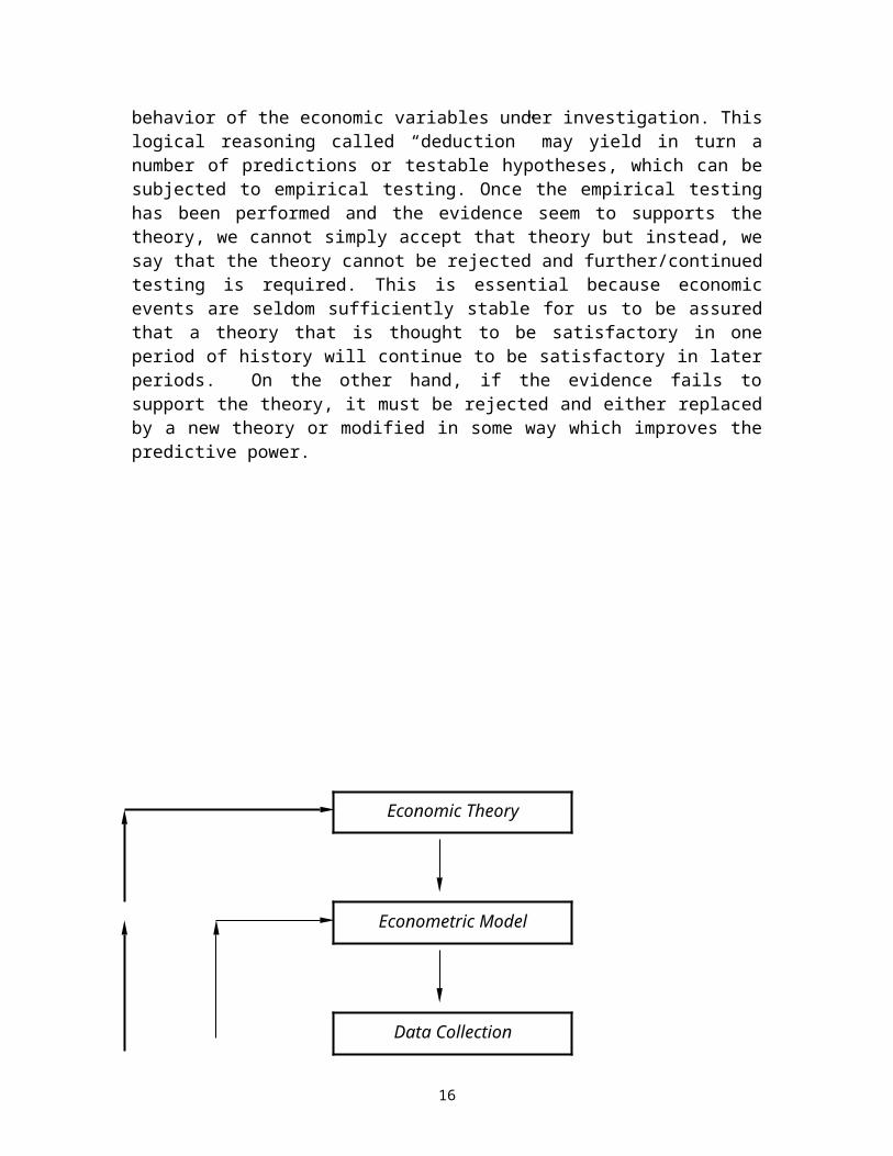
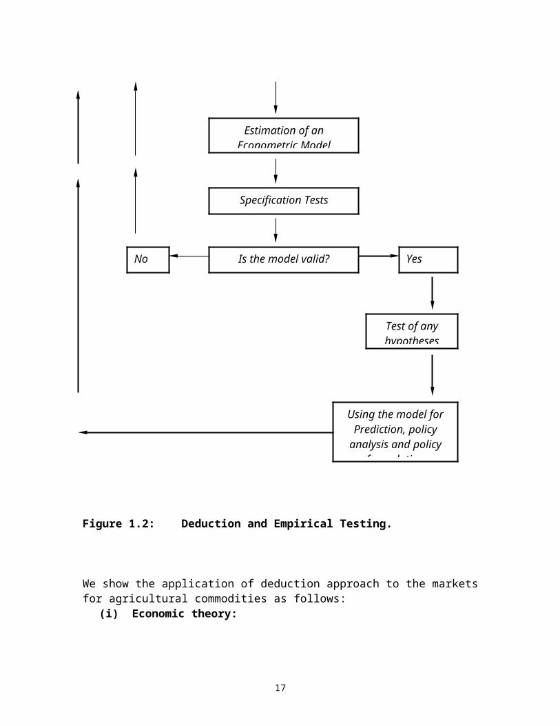
1.7.2 Deduction and Empirical ApproachThe empirical approach is the most widely used method followed by applied economists. It is illustrated in Fig. 1.2. The starting point is an economic theory or proposition. This proposition or a theory is then summarized logically in the context of a simple model, which is set up by specifying the number of assumptions concerning the behavior of the economic variables under investigation. This logical reasoning called “deduction” may yield in turn a number of predictions or testable hypotheses, which can be subjected to empirical testing. Once the empirical testing has been performed and the evidence seem to supports the theory, we cannot simply accept that theory but instead, we say that the theory cannot be rejected and further/continued testing is required. This is essential because economic events are seldom sufficiently stable for us to be assured that a theory that is thought to be satisfactory in one period of history will continue to be satisfactory in later periods. On the other hand, if the evidence fails to support the theory, it must be rejected and either replaced by a new theory or modified in some way which improves the predictive power.

10

Economic Theory

Figure 1.2: Deduction and Empirical Testing.

We show the application of deduction approach to the markets for agricultural commodities as follows:

11

Econometric Model

Data Collection

Estimation of an Econometric Model

Specification Tests

No Yes

Test of any hypotheses

Using the model for Prediction, policy

analysis and policy formulation

Is the model valid?

(i) Economic theory: The price of a commodity is determined by demand and supply of that commodity. The following set of assumptions is crucial in supporting this theory:(a) There are many buyers and sellers of the good so that the market is

competitive(b) Quantity demanded rises as price falls and falls as prices rises(c) Quantity supplied rises as price rises and falls as price falls

(ii) Econometric Model:

Where and denote the quantity demanded and quantity supplied respectively, are parameters. P is the product’s price. The first equation represents demand function. The second equation represents supply function. Note that and are meant to capture other variables that have not been included in econometric model. Such variable for example would include: the price of other commodities, level of income, taste, etc. .

(iii) DataAfter formulating an economic model, the next task is to collect data. There are two types of data: secondary data and primary data. Secondary data are published accessible data from a variety of sources such as books, articles, bureau of statistics, etc. Primary data on the other hand are data collected by researcher through fieldwork and they are specifically for the particular problem or issue under study.

(iv) Estimation of an Econometric ModelThis is usually performed by different statistical or econometrics’ packages/softwares. There are so many statistical/econometrics software available to perform estimation.

(v) Specification testing One of the most serious problems in estimation is that we are not certain about the form or specification of the equation we want to estimate. For example, one of the most common specification errors is to estimate an equation, which omits one or more influential explanatory variable or an equation that contains the explanatory variables, which do not belong to the “true” specification. In short, specification tests provide ways of resolving these problems.

(vi) Validity of the modelThe validity of a model may be judged on several criteria. Its predictive power, the consistency and realism of its assumptions, the extent of information it provides, its generality and its simplicity. However, there is no general agreement regarding which of the above attributes of a model is more important. The views of economists vary. While the late Milton Friedman

12

argued that the most important criterion of the validity of the model is its predictive performance, Paul Samuelson argues that realism of assumptions and power of the model in explaining behavior of the economic agents is the most important attribute of the model.

(vii) Hypotheses testingIf specification tests suggest that the model is adequate/valid, then the next step is to test hypothesis in order to check the validity of theoretical predictions.

(viii) Using the model for prediction/forecast and policy formulationIf the specification test and hypothesis testing display good results, then the model can be used for prediction and policy analysis. On the one hand, if it is to be found that the specification tests suggest that the model is not appropriate one, then an econometrician will have to go back to the econometric model formulation stage and revise the model, repeating the whole procedure from the beginning. On the other hand, if the theory is accepted, this is not the end of the story. Further testing is required using different source of data and new econometric methods.

In short, it is through the above process, carried out systematically by econometricians that economic theories are formulated. Econometrics involves the application of statistical and mathematical methods in the field of economics to test and quantify economic theories and the solutions to economic problems. In short, the main purposes of econometrics are to give empirical content to the economic theory and to subject economic theory to potentially counterintuitive tests. For example, economic theory predicts that there is a negative relationship between the price and the quantity demanded of a particular commodity. The role of econometrics is to verify or reject that prediction, and shed light on the magnitude of the effect.

1.7.3 Induction ApproachAn alternative methodology in economics is known as induction. This involves, first, the collection, presentation and analysis of economic data and then the derivation of relationship among the observed variables. In other words, the statistics are closely examined in the search for the general principles. A major problem with this approach is that economic statistics are so complex that it is often difficult to disentangle them, and of course, economists cannot perform laboratory experiment in the same way as the physical scientist can. Another difficulty is that some economic variables cannot be directly measured or are extremely difficult to measure accurately.

Deduction involves beginning with a set of theories or a theory. These theories are supported by hypotheses. In turn these hypotheses are tested via prediction and observation. Hypotheses, predictions and testing can be seen at the heart of this approach. Induction begins from particular observations from

13

which empirical generalizations are made. These generalizations, in turn, can form the basis for theory building. They are then turned into hypotheses and tested and the circle moves on.

1.8 Pitfalls of Methodology of Economic Analysis In the process of formulating an economic theory, we can easily make some mistakes in reasoning. Let us examine some mistakes that are prevalent in the methodology of economic analysis.

1.8.1 Fallacy of CompositionThe fallacy of composition can be summarized as follows: what is good (or bad) for one is necessarily good (or bad) for all. Generally we make fallacy of composition when we assume that what is true for one person or part of the economy is also necessarily true for society as a whole or the entire economy. The fallacy of composition is especially profound in macroeconomics where economic units (households, firms, etc) are treated as if they are one unit. When individual parts (households, firms, etc) interact with each other, the outcome for the whole economy may be different from that intended by the individual part. Consider a situation where a firm lays off its workers in order to cut down expenses and increase profits. If all firms in the economy do the same, national income and spending will fall. As a result, the sales of the firm, which intended to cut down expenses, may be reduced significantly and profit may not increase.

1.8.2 Post hoc FallacyThe post hoc fallacy refers to the common mistake made when a person observes one event happening after another and concludes that the first event necessarily caused the second one. For example, an economic observer may conclude: "as a result of increased food production in the late 1997 in Tanzania, inflation rate dropped sharply to the level of 12.9% in 1998 from 21.0% level recorded in 1996". We need to ask ourselves; was the increased food production necessarily the reason for lower rate of inflation in 1998? The reason for lower rate of inflation in 1998 could be a result of tight fiscal and monetary policies that the country pursued in order to restore macroeconomic stability.5

1.8.3 Ceteris Peribus AssumptionEconomic analysis is based on the ceteris peribus clause, which implies that "other thing should be held equal" in the due course of formulating economic theories. However, in reality, "things are not always equal". Most economic problems involve several forces interacting at the same time. For example, the number of cars bought in a given year is determined by the prices of cars, consumers' income, taste and price of fuels. However, in the next lecture you will see that in order to derive an individual demand curve in a rudimentary way we will only consider the price of the commodity and keeping other factor under the ceteris peribus assumption.

5 Fiscal policies are concerned with the change in government spending and the level of taxation. Monetary policies on the other hand are concerned with the change in the overall supply of money and interest rate in the economy.

14

1.8.4 SubjectivityThe greatest challenge to mastering economics arises from subjectivity. Different economists have different views and opinions on approaching and tackling an economic problem. As we have seen in the previous sections, some economists believe that price mechanism or "invisible hands" is a powerful tool to allocate resources in the economy while others believe in "visible hand" or government intervention. Yet, some believe in the mix of "visible" and "invisible" hands.

1.9 Positive versus Normative EconomicsBecause of scientific nature of economic analysis, it is important to understand the difference between positive economics and normative economics. Positive economics is the economics of model building and deals with what will occur assuming the model is properly constructed. Positive economics is concerned with the investigation of the ways in which different economic agents in society seek to achieve their goals. For example positive economists may analyze how a firm behaves in trying to make as much profit as it can or how a household behaves in trying to reach the highest attainable level of satisfaction from the consumption.

Normative economics on the other hand, is concerned with making suggestions about the ways in which the society’s goals might be more efficiently realized. From the standpoint of policy recommendations, this approach involves economists in ethical question of what should or ought to be, so much so that they may take up strong moral positions. For example, the present high level of unemployment in Tanzania ought to be reduced is a normative statement. In general, the lectures that follow will be concerned with positive economics.

Positive economics is concerned with proposition that can be tested by reference to empirical evidence. It relates to statement of what is, was or will be. Normative economics is concerned with the propositions that are based on value judgements, that is statements which are expression of opinions. Normative economics therefore relates to statements of what should or ought to be.

SUMMARY1. Economics is a branch of social science, which studies how

different societies allocate scarce resources among alternative uses in order to satisfy human wants.

15

2. Microeconomics is concerned with the activities of individual firms, industries and consumers. Macroeconomics on the other hand, is concerned with broad economic aggregates such as national income, the general price level and unemployment.

3. The basic economic problem confronting all societies is that of

scarcity of resources. All societies must have a system for deciding what goods and services to produce, how to produce, and for whom to produce.

4. A decision to satisfy one set of wants necessarily means sacrificing some other sets. We usually call this sacrifice the opportunity cost. The Opportunity cost is the next best alternative, which is foregone whenever an economic decision is made.

5. Production possibility frontier joins together the different combinations of goods and services which a country can produce using all available resources and the most efficient techniques of production.

6. Market failure is the term used to describe situations in which areliance on the market mechanism would not lead to the desiredoutcomes as viewed from society’s perspective especially under the following situation: information asymmetry, externalities, public goods, and imperfect markets.

7. Methodology is defined as a system of principles, practices, and procedures applied to a specific branch of knowledge. In economic analysis, methodology includes the methods, procedures, and techniques used to collect and analyze information in order to formulate economic theories.

8. An economic theory is a generalization, based on a variety of facts, about why or how an economic event occurs. The theory is generalization because it explains how economic variables generally behave when certain conditions exist.

9. Positive economics is concerned with what is, what was, what

will be. Normative economics is concerned with what should be or what ought to be.

16

EXERCISES1. Write short notes on the following pair of concepts:

(a) Microeconomics and macroeconomics.(b) Positive economics and normative economics(c) Central economic problems and price mechanism(d) Economic system and Economic models(e) Opportunity cost and Production possibility frontier.

2. Consider the hypothetical economy of Chalinze, which produces a combination of coffee and wheat when its resources are fully and efficiently employed.

Combination Coffee (Units) Wheat (Units) A 0 38,000B 10,000 36,000C 20,000 32,000D 30,000 27,000E 40,000 20,000F 50,000 0(a) Sketch the production possibility curve for this economy with coffee

on the vertical axis and wheat on the horizontal axis. (b) If Chalinze is currently producing at combination D, what is the

opportunity cost of producing 10,000 more units of coffee?(c)* What is the difference between a straight-line production possibility

frontier and a concave to the origin production possibility frontier in terms of the opportunity cost?

3. Outline the limitations of price mechanisms.

4. Using illustrative example of your choice, explain how economic theories are formulated.

5*. Economic theories are abstractions from reality. Explain.

6*. The following model of demand for Mbege has been estimated by econometrician: QC=0.25—0.5PC—0.42Y, , DW=2.00

(0.10) (0.2) (0.12)The model was estimated in logarithmic form. Standard errors are reported in parentheses. QC is litres of Mbege, PC is the price of Mbege and Y is the level of consumers’ income.

(a) Interpret the above model(b) Interpret the meaning of (c) Does this model mirror the behaviour of mbege drinkers?

17

LECTURE TWOTHEORY OF DEMAND

2.1 IntroductionIn the first lecture we learnt that the basic economic problem faced by all societies is that of allocating scarce resources among competing uses in an attempt to satisfy the unlimited demands. We have also learnt how allocation of resources is done under different economic systems. In short, we saw that under free enterprise economy, the market forces of demand and supply are left to determine prices. Before looking in detail at the working of the price mechanism we first study separately the theory of demand and supply. In this lecture, we are going to concentrate on the theory of demand.

ObjectivesBy the end of this lecture, you should be able to:(i) Explain the meaning of an individual’s demand for a

commodity;(ii) State and explain the law of demand;(iii) Describe individual’s demand schedule and individual’s

demand curve;(iv) Mention the exceptions to the law of demand.(v) Distinguish between change in demand and change in

quantity demanded;(vi) Explain the meaning of market demand and the difference

between market demand and individual’s demand;(vii) Outline and explain the factors that influence change in

demand;

2.2 Definition of DemandDemand is defined as the ability and willingness to buy a particular commodity or service at a given period of time. Demand for a commodity in economic sense arises when there is a need for the commodity and when the consumers have the money to pay for it.

Demand refers to effective demand rather than simply a need.

2.3 Individual’s Demand Curve for a CommodityDemand curve may be defined as the graphic representation of the individual’s demand schedule. The individual demand schedule for commodity X on the other hand shows the alternative quantities of commodity X that the consumer is willing to purchase at various alternative prices for commodity X while keeping other factors constant in a given period of time.

The quantity of the commodity that an individual is willing to purchase over a specific time period depends on the price of the commodity, his/her money income, prices of

18

other commodities, tastes, advertisement, population, expectation and other relevant variables. By varying the price of the commodity under consideration, while keeping constant every thing else (ceteris peribus), we get the individual’s demand schedule for the commodity.

The assumption that every thing else is kept constant implies that all other parameters that determine the demand have no influence on the quantity demanded when the price of the commodity changes. For instance, if the price of a corrugated iron sheet falls from T.Shs 5000/= to T.Shs 2500/=, the number of corrugated iron sheets demanded are likely to increase after the price fall. In this example, we have ignored the level of income and tastes of consumers as well as other relevant variables, which influence demand. For example, it is unquestionable that some consumers prefer tiles to corrugated iron sheet. Indeed, some people have no enough cash to pay for corrugated iron sheets despite the fall in the price level.

Example 2.1Assume that an individual demand for commodity X is given as follows: Qdx = 6 -Px, Ceteris peribus. Where, Qdx is the quantity demanded of commodity X, and Px is the price of commodity X. By substituting various prices of X into this demand function, we get an individual’s demand schedule as presented in Table 2.1.

Table 2.1: An individual’s demand schedule for commodity XPx (T.Shs) Qdx

6543210

0123456

By plotting each pair of values of quantity demanded and their corresponding prices on a graph and joining the resulting points, we get the individual’s demand curve for a commodity X depicted in figure 2.1 below.

19

Price (T.Shs)

6

5

4

3

2

1 0 1 2 3 4 5 6 Quantity of X/time

Figure 2.1: Individual’s Demand Curve for Commodity X

The demand curve plotted in figure 2.1, shows that at a particular point in time, if the price of X is T.Shs 5/=, the individual is willing to purchase one unit of commodity X over a given period of time. The time might be a week, a year, or any other relevant length of time. When the price of X is T.Shs 4/=, an individual is willing to purchase two units of X over a specified period of time. Thus, all the points on the demand curve represent alternatives as seen by the individual at a particular point in time.

The graphic representation of the individual’s demand schedule gives us individual's demand curve.

2.4 The Law of DemandThe law of demand states that "the lower the price the greater is the quantity demanded at a given point in time", ceteris peribus. In the demand schedule presented in Table 2.1, we have seen that the lower the price the greater the quantity of X is demanded. This inverse relationship between the price and quantity demanded is essentially reflected in the negative slope of demand curve as shown in figure 2.1. With an exception of rare cases (Giffen goods and Veblen goods to be explained in section 2.5), the demand curve always slopes downward from left to the right, implying that as the price of the commodity falls, more of it is purchased.

The behavioral equation for the law of demand is written as follows: . This equation states that, the quantity demanded of commodity X is a function of the price of commodity X, all other things being equal. Qdx is the quantity of commodity X demanded by the consumer per unit of time, Px is Price of commodity X as distinct from the price of other related goods. You can see from the equation that, we do

20

not explicitly state all the parameters that are being held constant as shown in the following equation;

Qdx = f (Px, Po, Y, T, A, P, E, Z)

The quantity demanded of commodity X by the consumer over a specific period of time depends on the price of the commodity X (Px ), price of other commodities, (Po), the income level,(Y) and taste (T), advertisement(A), population (P), expectation (E) and other relevant variables(Z).

Why does the quantity demanded tend to fall as price rises

There are three reasons explaining why the quantity demanded tends to fall as price of the commodity rises. First is the substitution effect. When the price of a particular good rises, usually the consumers tend to substitute this commodity for others whose prices have remained unchanged. Second is the real income effect. When the price of a particular good rises, real income of the consumer falls and less of the goods are purchased. Third reason is because of diminishing marginal utility (for more detail on diminishing marginal utility, please see section 6.6 and figure 6.2 in lecture 6). The law of diminishing marginal utility presented in lecture 6 refers to the fact that as successive units of goods or services are consumed during some short period of time in which the consumer's tastes do not change, the utility derived from each additional unit decreases beyond some points. The law of diminishing marginal utility is used to explain the downward slope of demand curve. If successive units of product yield smaller and smaller amounts of marginal, or extra utility, the amount that the consumer will pay for additional units will decline as well. We will discuss these concepts (the law diminishing marginal utility, substitution and income effect) in more detail in lecture six and seven.

The law of diminishing marginal utility helps economists understand the law of demand and the negative sloping demand curve. The less of something you have, the more satisfaction you gain from each additional unit you consume; the marginal utility you gain from that product is therefore higher, giving you a higher willingness to pay more for it. Prices are lower at a higher quantity demanded because your additional satisfaction diminishes, as you demand more.

21

2.5 Exceptions to the Law Of DemandThere are a few exceptions to the law of demand when it comes to, Giffen goods and Veblen goods.

2.5.1 Giffen GoodsGiffen goods, named after the nineteenth century economist Sir Robert Giffen are very inferior goods for which quantity demanded increases as price rises, and quantity demanded decreases as price falls. An example of this may be found where consumers are so poor that most of their income is spent on a commodity necessary for subsistence. Suppose that the commodity in question, “Sukuma wiki” for example is traded in Kariakoo market in Dar es salaam City. If the price of “Sukuma wiki" falls in such circumstances, consumer may reduce their demand for “Sukuma wiki" and use their extra income to purchase some other nutritious food.

Is there any relationship between Inferior and Giffen goods?

2.5.2 Veblen GoodsA Veblen good is a good whose quantity demanded rises when its price rises. Veblen goods are sometimes called goods of ostentation, like jewellery and the work of original arts. Veblen goods have been named after the American sociologist, Thorsen Veblen. If goods of this type are sold at a very low price, they will lack snob appeal and consequently they will be in less demand. The more expensive these goods are, the snob appeal rises, and more people will desire them.

Price (T.Shs) D

P3

P2

P1

D

0 Q1 Q2 Q3 Quantity of X/timeFigure 2.2: Demand curve for a Giffen or Veblen goods

22

In short, the existence of Giffen goods and Veblen goods may adequately explain the reason as to why an individual demand curve may be positively sloped as illustrated in figure 2.2 rather than negatively sloped as shown in figure 2.1

2.6 Determinants of Demand for a Commodity Other than Own PriceSo far we have been discussing the effect of the price change on the quantity demanded. Let us now look at the relation between the demand for a commodity and the determinants of demand, other than own price.

2.6.1 Demand for Commodity X and the Price of Commodity Y An increase (decrease) in the price of commodity Y may decrease (increase) the quantity demanded of commodity X. In particular, whenever a fall in price of commodity Y causes a fall in the demand for commodity X, then X and Y are substitutes. Substitutes are goods that compete with each other. For simplicity consider tea and coffee to be substitutes. Assuming that coffee is superior to tea, when the price of coffee falls while the price of tea remaining constant, consumers will tend to purchase more coffee than tea. This implies that the quantity of tea purchased would tend to fall as the price of substitute coffee falls. For the case of complementary goods, the story is different. Complementary goods are jointly consumed e.g. tealeaves and sugar. Under normal circumstances, when the price of a kilogram of sugar falls, more of sugar and tealeaves will be purchased

Substitutes are goods that compete with each other. Complements are goods that are jointly consumed.

2.6.2 Demand for Commodity and the Consumer’s IncomeWhen an individual’s money income rises, while other determinants of demand are held constant, the consumer’s demand for that commodity will increase. This increase is reflected in the shift of demand curve to the right. However, for the case of inferior goods, the resultant effect of increased money income would be to reduce the demand for that good. On the other hand, if the demand for the commodity remains unchanged after a certain period of time following a rise in consumer’s income, we usually say that commodity is a necessity. e.g. salt.

Why is it that when the money income of individual increases, less of inferior goods are purchased while more of normal goods are purchased?

The relationship between demand and the level of income, ceteris peribus, could also be represented in a graphically by using the Engel curve. Engel curves are useful in distinguishing between normal and inferior commodity as illustrated in Figure 2.3.

Quantity

23

Normal goods

Necessity

Inferior goods

0 Consumer’s IncomeFigure 2.3: Engel Curve

In Figure 2.3, the vertical axis shows the quantity of goods per unit of time while the horizontal axis shows the level of consumer’s income per unit of time. When an individual’s money income rises, ceteris peribus, the individual demand for the commodity usually increases indicating that at the same price the consumer will purchase more unit of a commodity per unit of time. Consumer demand for beef will shift up as a result of increased income assuming that beef is a normal commodity. However, there are some goods whose demand usually shifts down when consumer’s income increases. These are called inferior goods.

Which goods in your community are regarded to be inferior? Can superior goods be at the same time inferior?

2.6.3 Demand for a Commodity and the Consumer’s TasteWhen the consumer’s taste changes in favour of a particular commodity, usually there is a corresponding change in the quantity demanded. For instance when a particular commodity comes into fashion, usually there is a tendency to buy more of the commodity. This tendency is reflected in the outward shift to the right of the demand curve. On the contrary, if a particular commodity is no longer fashionable to the consumer, the demand curve shifts downward to the left.

2.6.4 Demand for a Commodity and the Size of the PopulationThe larger the population of consumers the larger is the demand since in general the larger population will purchase more goods and services than a smaller population. Demand for housing is greater in populous cities compared with low populated cities. 2.6.5 Demand for a Commodity and Advertisement.

24

Lack of information concerning the price and availability of a particular commodity is one of the factors, which may prevent the commodity from reaching those consumers who would benefit from it. Advertising is thus meant to provide information to consumers to buy a particular brand name rather than rivals. In this way, the demand for a particular product may be purchased in large quantities as a result of rigorous advertisement.

2.6.6 Expectation and Demand for a CommodityDemand for a particular good may rise in the face of mounting uncertainties with regard to the possible rise in the price of a particular good in the future. This is particularly so during the inflationary period when prices are persistently and abruptly rising. In such a situation, consumers may buy a plethora of goods as a hedge against price rise. Another case is when the consumer speculate future price rise following an increase in tax, increase in the cost of production, or sometimes declined production as a result of natural and man made catastrophes.

2.6.7 Other Related Factors and the Demand for a Commodity.Other factors such as religious beliefs, taboos, social and cultural differences may have an impact on demand for a commodity. In purely Muslim communities for examples, it is strictly forbidden to eat pork. In such communities, pork is not a commodity to be sold to whoever demands it regardless of his/her religion denomination. In fact, it is not only unlawful but also strictly prohibited to keep pigs since it is against the prophecy of holy Qur'an.

The following are the factors that influence demand other than own price:1. Price of another commodity, say Y 2. Consumer’s income3. Consumer’s taste4. Size of the Population5. Advertisement.6. Expectation

2.7 Change in Demand versus Movement along the Demand Curve Change in demand refers to shift in demand curve whereas change in quantity demanded refers to the movement along the same demand curve. Change in demand is caused by change in any of the factors other than own price changes. Figure 2.4 shows a shift in demand curve.

Price

25

D D*

P*

D D*

0 X1 X2 Quantity of X/unit of timeFigure 2.4: Change in Demand

The demand curve shifting to the right indicates an increase in demand. This is explicitly seen from Figure 2.4. You should note from Figure 2.4 that as the price of commodity X remains constant at P*, an increase in the consumer's income or a positive change in the consumer’s taste for the commodity or an increase in the price of other commodities brings about an increase in the quantity of the commodity purchased. That is, the demand curve shifts to the right from DD to D*D*. Conversely, if the price of the commodity X remains constant at P*, an opposite change in one of these demand determinants will result in the demand curve shifting to the left. This is to be contrasted with change in quantity demanded as shown in figure 2.5

Px (T.Shs)

6 dx

5 A

4 B

3 C

2 D

1 E dx

0 1 2 3 4 5 6 Quantity of X/Unit of time Figure 2.5: Change in Quantity Demanded

26

Figure 2.5 shows that when the price of commodity X changes from T.Shs 5/= to T.Shs 2/=, the quantity demanded of commodity X changes from 1 unit to 4 units per unit of time. The demand curve does not shift. The change in quantity demanded is seen as movement along the same demand curve from point A to D

2.8 The Market Demand for a CommodityThe market demand for a commodity gives the alternative amounts of the commodity demanded per time periods at various alternative prices, by all the individuals in the market. The market demand for a commodity thus depends on all the factors that determine the individual’s demand and in addition on the number of buyers of the commodity in the market. Geometrically, the market demand curve for a commodity is obtained by the horizontal summation of all individuals' demand curves for a commodity.

Algebraically, consider a market where there are 20,000 identical individuals in the market, each with a demand function given by, Qdx = 6-Px ceteris peribus, the market demand schedule and market demand curve for commodity X are obtained as follows:

Qdx = 6-Px, ceteris peribus (individual Qdx)QDx = 20,000(Qdx)

=20,000(6-Px)=120,000 – 20,000Px

Table 2.2: Market Demand Schedule for Commodity XPx (T.Shs) QDx

6 05 20,0004 40,0003 60,0002 80,0001 100,0000 120,000

Just as we have seen in the individual demand schedule, the market demand curve for commodity X (QDx) will similarly shift when individual demand curve shifts (unless the shift of the later neutralizes each other) and will change with time as the number of consumers in the market for X changes.

27

Px (T.Shs)

6

5

4

3

2

1

0 20 40 60 80 100 120 Qdx (‘000)

Figure 2.6: Market Demand Curve for Commodity X

28

SUMMARY1. The demand for a good may be defined as the quantity that

consumers are willing and able to buy during some time period. Demand refers to effective demand rather than simply a need.

2. A demand curve shows the relationship between the quantity demanded of goods and the goods' price on the assumption that all other influencing factors remain unchanged. i.e. (ceteris peribus).

3. The law of demand states that "the lower the price the greater is the quantity demanded at a given point in time", ceteris peribus.

4. Giffen goods and Veblen goods are exceptions to the law of demand. Giffen goods are very inferior goods for which quantity demanded increases as price rises, and quantity demanded decreases as price falls.

5. A Veblen good is a good whose quantity demanded rises when its price rises. If Veblen goods are sold at a very low price, they will lack snob appeal and consequently they will be in less demand. The more expensive these goods are, the snob appeal rises, and more people will desire them.

5. The effect on quantity demanded of a price change in a goods' price could be traced out by moving along the goods' demand curve. The demand curve will shift if any of other influencing factors change.

6. An Engel curve shows the relationship between quantity demanded and income, ceteris peribus. Normal goods have an Engel curve with a positive slope. Inferior goods have an Engel curve with a negative slope.

7. Determinants of demand for a commodity other than own price are; price of related commodity, consumer’s income, taste, size of the population, advertisement, expectation and other factors such as religious beliefs, taboos, social and cultural differences

8. The market demand for a commodity gives the alternative amounts of the commodity demanded per time periods at various alternative prices, by all the individuals in the market. The market demand for a commodity thus depends on all the factors that determine the individual’s demand and in addition on the number of buyers of the commodity in the market.

29

EXERCISES1 Write short notes on the following concepts

(a) Demand function, Demand Schedule and Demand curve(b) Giffen goods and Inferior goods(c) Normal goods and superior goods(d) Engel Curve

2 What is the law of demand? Why does it generally hold? What are the exceptions to this law?

3. Using relevant diagrams, distinguish the change in demand from the change in the quantity demanded

4. Suppose that the following demand function for commodity X has been estimated by an econometrician at the suburb of Dar es salaam city: Qx = 3,848 - 2Px + 0.004Y + 3Py; where Qx is the quantity of commodity X, Px is the price of commodity X, Y is the income, and Py is the price of related commodity.

(a) Develop a demand schedule for commodity X over the price range Px = T.Shs 800 to Px = T.Shs 400; if Y= T.Shs 12,000 and Py = T.Shs 600. (Hint: Use T.Shs 100 change in Px over the range.

(b) Assuming that the values of Y and Py are held constant, write an equation for the demand curve for commodity X

(c)Explain how the demand curve would shift if the level of income increases

(d)Discuss the relationship between commodity X and commodity Y.

5*. Suppose that the demand function for maize flour is given by Q=500-50P where Q is the Kilograms of maize flours demanded per week and P is the price in Tanzanian Shillings.

(a) How many Kilograms of maize flour are demanded at a price of 2? Price of 3? Price of 5?

(b) Assume that during the month of December, demand function shifts to Q=1,000-50P. Repeat part (a) for this new demand function.

6. The demand for a good is given as: Q = 120 – 2P + 2Y + 0.4A, Where Q, P, Y and A denote quantity demanded, price, and income and advertisement expenditure respectively.(a) Calculate demand when P = 10, Y = 20 and A = 5.(b) Assuming that price and income are fixed, calculate the

increase in advertising expenditure required to raise demand to 150 units.

(c) Does the demand for this good increase or decrease with the higher income? Explain with example.

30

7. Outline the market determinants for the commodity.

8. * Suppose that the demand curve for new cars is described by the following equation

Qd=50,000-PWhere Qd is the number of new cars per years and P is the average price of cars in shillings.

(a) What is quantity of cars demanded when the average price of a car is 10,000? 15,000? 25,000?

(b) Sketch the demand curve for cars. Does this demand curve obey the law of demand? Explain

31

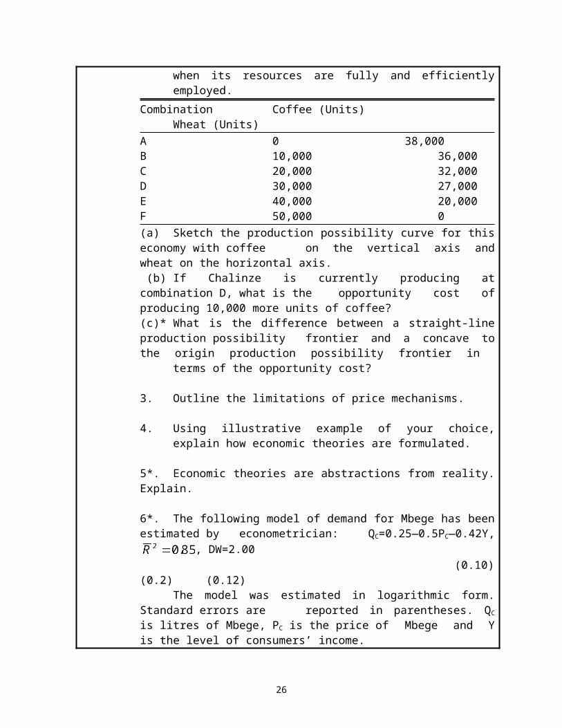
LECTURE THREETHEORY OF SUPPLY

3.1 IntroductionIn lecture two of this unit you have studied the theory of demand. In this lecture, we are going to study the theory of supply. Understanding the theory of supply will help us to describe the working of the price mechanism, which combines demand and supply in lecture four.

Objectives

By the end of this lecture, you should be able to:(i) Define the meaning of supply and interpret the supply curve.(ii) Describe the shape of the supply curve and explain the difference;

between the shape of the demand curve and the supply curve.(iii) Describe the main determinants of supply and interpret the meaning

of a supply function.(iv) Identify the factors which bring about movements along the supply

curve and a shift in a supply curve;(v) Explain the difference between the producer’s supply curve and

market supply curve.(vi) Define producer’s surplus.

3.2 The meaning of SupplySupply is the ability and willingness to offer for sale a certain quantity of commodities at a given price, in a given location over a given period of time. We can see that the definition of supply shares several features with the definition of demand. Once again, ability and willingness are important here. Suppliers must be willing and able to offer commodities for sale for there to be a supply. Like demand, supply is a price-quantity relation, relating a quantity supplied to each level of price.

3.3 A Single Producer’s Supply of a CommodityThe quantity of a commodity that a single producer is willing to sell over a specific time period depends on the price of the commodity and the producer’s cost of production. In order to get the producer’s supply schedule and the supply curve of a commodity, certain factors, which influence cost of production, must be held constant (ceteris peribus). These are technology, the supply of inputs necessary to produce the commodity and for agricultural commodities, climate and weather conditions.

By keeping all of the above factors constant while varying the price of the commodity, we get the individual producer’s supply schedule and supply curve. Suppose that a single producer supply function for commodity X is QSx = - 20+10Px ceteris peribus. Where; QSx is the quantity supplied of commodity X and Px is the price of commodity X. By substituting various “relevant” prices of X into this supply function we get the producer’s supply schedule shown in Table 3.1.Table 3.1: Producer’ Supply Schedule for Commodity X

32

Px (T.Shs) Qsx

765432

50403020100

Again, by plotting each pair of values from the supply schedule in Table 3.1 we get the producer’s supply curve (Fig. 3.1). As in the case of demand, the points in the supply curve represent alternatives as seen by the producer at a particular point in time

Price of X QSx = - 20+10Px

7

6

5

4

3

2

1

0 10 20 30 40 50 Qty /unit of time

Figure 3.1: Producer’s Supply Curve

3.4 The Shape of the Supply CurveThere is much that needs to be said on the relationship between supply and price. More detailed explanations/derivation of the supply curve is illustrated in OEC 107 under the theory of market structure (see for example short run supply curve in lecture 1, OEC 107). However, for the moment we should be comfortable with the intuitively plausible hypothesis that, ceteris peribus, the quantity of commodities offered for sale will increase following the increase in price. This hypothesis has a strong common sense appeal that the higher the price of the commodity, the greater are the profits that can be earned and thus, the greater are the incentives to produce the commodity and its offer for sale.

In the supply curve schedule of Table 3.1, we have seen that the lower the price of commodity X, the smaller the quantity of X supplied. The reverse is of course, also true. This direct relationship is reflected in the positive slope of the supply curve in Figure 3.1. However, while in the case of demand curve we could talk about “the law of negatively

33

sloped demand”, in the case of supply we cannot talk of the law of positively sloped supply. Even though the supply curve is usually positively sloped, it could also have a zero, infinite or even negative slope and no generalizations are possible.

3.5 The Market Supply of a CommodityThe market or aggregate supply curve of a commodity gives the alternative amounts of the commodity supplied per time period at various alternative prices by all the producers of this commodity in the market. The market supply of a commodity depends on all the factors that determine the individual producer's supply and, in addition on the number of producers of the commodity in the market.

Example 3.1Consider a situation where there are 1000 identical producers in the market, each producer with a supply of commodity X given by the supply function Qsx = -20+10Px

ceteris peribus the market supply Qsx is obtained as follows:

Qsx = -20+10Px (single producer sx)QSx = 1000(-20+10Px) (market supply Sx) = -20,000+10,000Px

Table 3.2: Market Supply Schedule

Px (T.Shs) QSx

765432

50,00040,00030,00020,00010,000

0

The market supply curve (Sx) will shift when the individual producers’ supply curves shift.

34

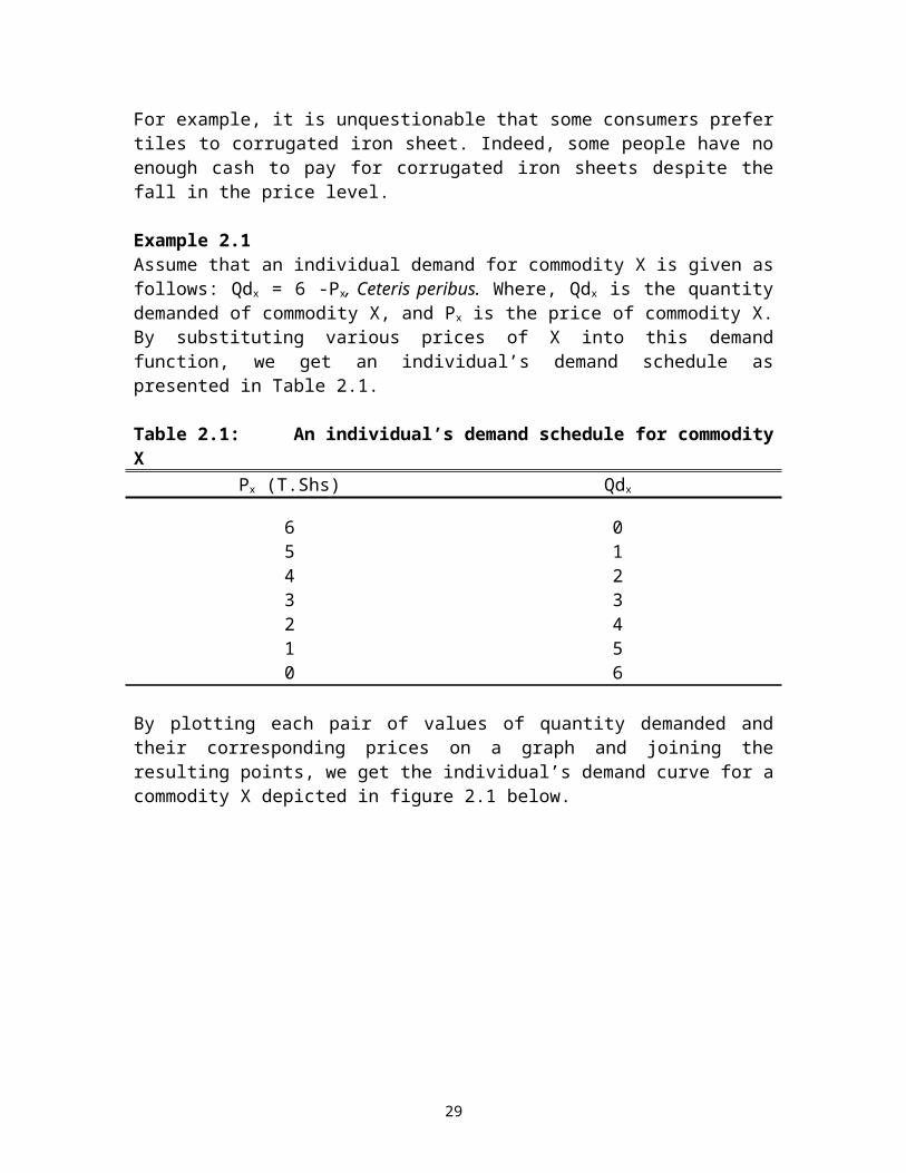
Price of X

7 6

QSx = - 20,000+10,000Px

5

4

3

2

1

0 10 20 30 40 50 ('000)Qty of X/time

Figure 3.2: Market Supply Curve

3.6 Determinants of Market SupplyThe main determinants of market supply of goods X are: the objective of the firms in the industry; the price of goods X; the price of other certain goods; the prices of factors of production; the state of technology and expectation. Let us have a look at these factors in turn.

3.6.1 The Objective of the FirmsThe nature of the firm’s objective will affect the decision it takes. A firm, which aims at maximizing sales revenue, will generally supply a greater quantity than a firm aiming at maximizing profits. This is illustrated in Fig 3.3 where a firm’s total costs and total revenues are plotted against the quantity supplied – the difference between the two curves representing the firm’s profits. Sales revenue is maximized at output 0X2 where the total revenue curve reaches its maximum. Profits are maximized at output 0X1 where the difference between the total revenue and total the cost curves is the greatest. This is also a point where the profit curve reaches its maximum.

35

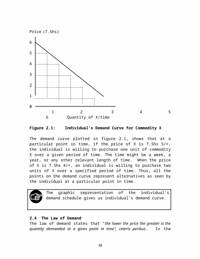
Revenue/Cost Total Cost

Total Revenue

Profit

0 X1* X1 X2 X2* Output/timeFigure 3.3: Objective of the Firm

It is clear from figure 3.3 that the total market supply of good X depends on the primary objectives of all the firms in the industry. Changes of these objectives will usually lead to changes in the quantity supplied. Note from the above figure that when total cost and total revenue are equal, the profit is zero. We have denoted the point of zero profits as X1* and X2*

3.6.2 Price of Goods X (Px)As the price of goods X rises while all the costs and the prices of all goods remaining unchanged, production of X becomes more profitable. Existing firms are likely, therefore, to expand their outputs and eventually new firms will be attracted to the industry. Hence, the total market supply will expand when price increases.

3.6.3 Prices of Other Goods (Po)If the price of some other goods, say Y, rises, with the price of goods X remaining unchanged, some of the firms now producing X may be attracted to move into Y production, motivated by their search for profit. A producer of wheat in Babati (Manyara Region)for example, who sees that the price of barley has risen may decide to use more land for barley production and thus reducing wheat output. Wheat and barley are said to be substitutes in production and in this case there is an inverse relationship between the supply of one goods and the price of the other. However this is not the result we should expect for goods which are complements like car and petrol. An increase in demand for cars will lead to an increased demand for petrol: this should raise the price of petrol and so leading to an expansion rather than a contraction in supply.

36

3.6.4 Prices of Factors of Production (Pf)As the prices of those factors of production used intensively by X producers rise, the firms' costs of production will also rise. This will cause supply to fall as some of firms reduce output and others, less efficient, firms make losses and eventually leave the industry. Similarly, if the price of one factor of production should rise say, land, some firms may be tempted to move out of production of land intensive products, like wheat, into the production of another type of goods which are intensive in some other factors of production. 3.6.5 State of Technology (T)Technological improvements such as the invention of new machines or the development of a more efficient technique of production will reduce cost and increase the profit margin on each unit sold.

3.6.6 Expectation (E)Production decisions are not influenced by just current prices, but they are also influenced by the expected future prices. Thus, for example, if the price of goods X is expected to rise, firms may decide to reduce the amount they supply in the current period. This will enable them to build up stocks, which can be offered for sale when the price rises in future.

3.6.7 Tastes of the Producers (Tp)The supply of a commodity may as well be influenced by the tastes of producers. If producers prefer to engage in the production of one commodity rather than another, even though the profits from both lines of production are similar, it will affect the supplies of these two commodities. A change in producer's taste in favor of producing a commodity will increase its supply, while a change in tastes against producing the commodity will reduce its supply.

3.6.8 Government Tax and Subsidy Policy (G)Increased tax on a product will cause its supply to shift to the left since it increases the cost of production (see figure 4.7, in lecture 4). Subsidies have the opposite effects of tax; for they provide incentives to production with a result being increased output produced.

3.6.9 Other Relevant Variables (Z)This category of variable involves those factors, which are really hard to predict as they are far beyond the horizon of the firm. Such unpredictable variables include things like drought, pest and diseases, which seriously destroy agricultural produces. Policy change within a country may harm some sectors in the economy while some sector may benefit.

We may now summarize the preceding discussion as follows: the market supply of the commodity is a function of price of goods, price of other goods, prices of factors of production, state of technology, expectation, taste of producers, government tax and subsidy policy and other relevant variables like weather or an invasion of pests which destroy agricultural crops. Algebraically, we can write the supply function as follows;

QSx = f (Px, P0, Pf, T, E, Pp, G, Z)Variables are defined in bracket for each in each subsection.

37

3.7 Change in Supply and Change in the Quantity SuppliedAs with demand, it is essential to distinguish between a movement along a supply curve and the shift of the entire supply curve. When the factors that we kept constant in defining a supply schedule and a supply curve (the ceteris peribus assumption) change, the entire supply curve shifts. This is referred to as a change or shift in supply and must be clearly distinguished from change in quantity supplied which is a movement along the same supply curve (see figure 3.1).

Suppose that there is an improvement in technology so that the producer cost of production falls. The fall in the cost of production will result in the downward shift of the supply curve (see figure 3.4). This downward shift is referred to as an increase in supply. This is to say that, at the same price for the commodity X, the producer offers more of it for sale per time period.

Price (T.Shs)

SX SX1

P

0 X1 X2 Quantity of X/Unit of timeFigure 3.4: Shift in the Supply Curve

3.8 Producer SurplusProducer surplus is a measure of the difference between the actual price received and the price at which producers are willing to supply given goods. To understand this concept, consider the market supply curve SXSX in figure 3.5, which shows the quantity of goods, X that producers are willing and able to supply over a given period of time at different prices. Suppose the prevailing market price is actually 0P0 so that quantity 0X0 is being supplied. The firm in the industry are receiving a total revenue of 0P0 x 0X0, represented by the total area 0P0 AX0. It can be seen from the graph that the producer in the industry would have been prepared to supply the first unit at the price 0P1, the second unit at 0P2,

and the third unit at 0P3. Since all the firms are receiving the same price (0P0) for each unit sold, the area above the supply curve and below the price line is called producer surplus.

38

Price (T.Shs) SX

P0 A

P3

P2

P1

SX

0 1 2 3 X0 Quantity of X/timeFigure 3.5: Producer’s Surplus

Producer surplus is measured by the area above the supply curve and below the prevailing market price.

SUMMARY

39

1. Supply is the ability and willingness to offer for sale a certain quantity of commodities at a given price, in a given location over a given period of time. We can see that the definition of supply shares several features with the definition of demand. Once again, ability and willingness are important: here, suppliers must want and able to offer commodities for sale for there to be a supply.

2. Supply is likely to depend on a number of factors, including the goods price, the price of other related goods, the objective of the firms in the industry, the prices of factors of production, the state of technology and expectation.

3. A supply curve shows the relationship between the quantity supplied of goods and a goods' price, on the assumption that all other influencing factors remain unchanged (that is ceteris peribus).

4. It is essential to distinguish between a movement along a supply curve and the shift of the entire supply curve. When the factors that we kept constant in defining a supply schedule and a supply curve (the ceteris peribus assumption) change, the entire supply curve shifts. This is referred to as a change or shift in supply and must be clearly distinguished from change in quantity supplied which is a movement along the same supply curve.

5. The market or aggregate supply curve of a commodity gives the alternative amounts of the commodity supplied per time period at various alternative prices by all the producers of this commodity in the market. The market supply of a commodity depends on all the factors that determine the individual producer's supply and, in addition on the number of producers of the commodity in the market.

6. The market supply of the commodity is a function of price of goods, price of other goods, prices of factors of production, state of technology, expectation, taste of producers, government tax and subsidy policy and other relevant variables like weather.

7. Producer surplus may be defined as the difference between the total amount that producers receive for any given quantity of goods and the minimum amount they would have been willing to accept for it.

EXERCISES

40

1. Write short notes on the following items:(a) Supply curve(b) Supply function(c) Supply schedule(d) Producer surplus

2. Use supply and demand curves to illustrate how each of the following events would affect the price of butter and the quantity of butter bought and sold.

(a) An increase in the price of the margarine(b) An increase in the price of milk(c) A decrease in average income levels

3. “A good harvest in rural areas will generally lower the income of the farmers”. Illustrate this proposition using a supply and demand diagram

4. Define the concept of the supply schedule or curve. Show that an increase in the supply means a rightward and a downward shift of the supply curve. Contrast this with the right ward and upward shift in the demand curve implied in by an increase in demand. Why the difference?

5. "Change in supply and change in quantity supplied is essentially the same thing". Examine this statement, using relevant diagram(s) if any.

6. Discuss the factors which influence the market supply for maize in Tanzania

7*. Suppose that the supply of maize in the country is described by the following equation:

QS=50,000+PWhere QS is the quantity of maize (in thousand tons) and P is the price of maize per ton.

(a) What is the quantity of maize supplied when the price of maize is 10,000? 20,000? 30,000? 40,000?

(b) Sketch the supply curve for maize.

41

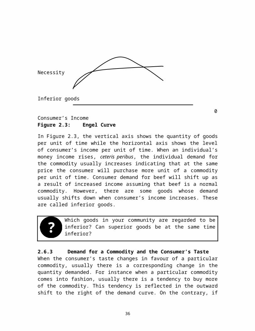
LECTURE FOURMARKET EQUILIBRIUM

4.1 IntroductionIn lectures two and three we have analyzed separately the theories of demand and supply. This lecture brings these two theories together with an objective of determining the market equilibrium. We start by defining market and explaining the meaning of equilibrium in economics. We then illustrate the effects of shifts in the demand and supply curves on market equilibrium. Finally, this lecture describes disequibrium in the market.

ObjectivesBy the end of this lecture, you should be able to:(i) Define market(ii) Define market equilibrium and distinguish between stable

and unstable equilibrium(iii) Analyze graphically and algebraically the effects of

imposing a sales tax on equilibrium price and quantity. (iv) Show the effects of imposing artificial restrictions in a

market by using price ceiling and price floor.(v) Describe market disequilibrium and its application using a

Cobweb model.(vi) Describe the cobweb model

4.2 MarketA market is a mechanism, which allows people to trade, normally governed by the theory of demand and supply. It is not necessary that market should be in identifiable place. What is important in the market is that those willing to buy a product/service meet those willing to sell it. Modern markets do not require these two parties (seller and buyer) to be in the same place or even to communicate their desires at the same time. A good example is e-commerce (i.e., electronic commerce) in which buying and selling of goods and services is done via the Internet.

4.3 Market EquilibriumMarket equilibrium occurs when the quantity of a commodity demanded in the market per unit of time is exactly equal to the quantity of the commodity supplied to the market over the same time period. Geometrically, equilibrium occurs at the intersection of the market demand curve and the market supply curve. The price and quantity at which equilibrium exists are known respectively as the equilibrium price and equilibrium quantity.

42

Equilibrium market price is the price at which the quantity demanded is equal to the quantity supplied. It is also known as the market-clearing price.

Px (T.Shs)

D S

Pe

S D 0 Xe Quantity/Unit of timeFigure 4.1: Market Equilibrium

Figure 4.1 shows the demand and supply curves of “normal” goods X. Remember from lecturers 2 and 3 that these curves are drawn on the assumption that all factors other than the price of that particular good remain unchanged. When the price of X is 0Pe, the demand for X and the supply for X are exactly the same. This is called an equilibrium position and 0Pe is called the equilibrium market price. At this price the amount that producers are willing and able to supply to the market is equal to the amount that buyers are willing and able to buy.

Example 4.1 Consider a hypothetical situation at the Kariakoo Market in Dar es Salaam (Tanzania) where there are 1000 identical individuals buying coconuts, hereafter, to be called commodity X. Each of these individuals has a demand function given by Qd x = 6-Px. In the same market there are also 100 identical producers of coconut from Zanzibar, each with a supply function given by Qsx = 10Px.

(a) Find the market demand function and market supply function (b) Obtain the equilibrium price and quantity mathematically

Solution(a) The market demand function is given as the horizontal summation of

individual demand curves. This is given as:Qdx = 1000(6-Px), ceteris peribus

= 6,000 – 1,000Px, ceteris peribus

43

The market supply function is given as the horizontal summation of individual supply curves. This is given as:

Qsx = 100(10Px) = 1,000 Px

(b) Equilibrium price and quantity obtain where the market clears.i.e. At the point where demand equals supply

Qdx = Qsx 6,000 – 1,000Px, = 1,000 Px

6,000 = 2,000 Px

3 = Px

Substituting equilibrium price into either the market demand or market supply function should give us the equilibrium quantity;

Market demand function = 6,000 – 1,000(3)= 3,000

Market supply function = 1,000(3)= 3,000

Thus, the equilibrium price for coconut is T.Shs 3/= while the equilibrium quantity is 3,000 coconuts.

Can you plot the market demand and supply function (example 4.1) and illustrate both the equilibrium price and quantity.

4.4 Excess Demand versus Excess Supply

What do we mean by excess demand in the market? What do we mean by excess supply in the market?

Excess demand exists whenever the quantity demanded is greater than the quantity supplied at prevailing market price. Excess supply exists whenever the quantity demanded is less than the quantity supplied at the prevailing market price. Both excess demand and excess supply arise when the price charged in the market differs from the equilibrium price. This is shown in figure 4.2. When the price of X is 0P1, quantity demanded is 0X1, but producers are willing to supply 0X2. There is an excess supply of X equal to X1X2. Producers may react to this by reducing price in an attempt to sell off their unsold stocks- excess supply, causing an economic force that exerts downward pressure on price. When the price of X is 0P2, however, quantity demanded is 0X4 but producers are only willing to supply 0X3. Now there is an excess demand for X, which is equal to X3X4.

44

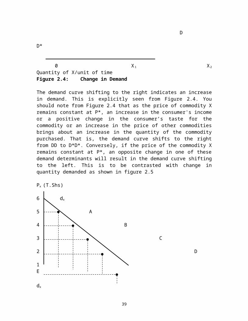
Px (T.Shs)

D S

P1

Pe

P2

S D

0 X3 X1 Xe X2 X4 Quantity/Unit of timeFigure 4.2: Excess Demand and Excess Supply

In the case of excess demand, Producers are in a position to decide where they will sell all they are producing and more at higher prices. Excess demand then, is an economic force, which exerts upward pressure on the price. Prices on 0P1 and 0P2 and all other prices except 0Pe are called disequilibrium price. The exercise of comparing one equilibrium state with another at a moment in time is called comparative statics equilibrium analysis.

4.5 Types of EquilibriumThere are two types of equilibria which are studied in Microeconomics. These are stable and unstable equilibria. Let us have a look on each of these.

4.5.1 Stable EquilibriumAn equilibrium condition is said to be stable if any deviation from the equilibrium will bring into operation market forces which push it back toward equilibrium. This is the case in the market for goods X illustrated in figures 4.1 and 4.2. The equilibrium at price Pe in figure 4.2 is stable because the establishment of any disequilibrium price, like 0P1 or 0P2, sets up economic forces (excess supply in the case of 0P1 and excess demand in the case of 0P2) which, given competition among buyers and sellers, tend to push the price back towards 0Pe.

4.5.2 Unstable EquilibriumEquilibrium is unstable when any deviation from the equilibrium caused by external disturbances, tend to move further away from equilibrium. Consider figure 4.3 (a) below which illustrate the market demand for good X, which has demand curve sloping upwards from left to the right. Goods X might be Giffen or Veblen goods. Price 0P e is the equilibrium price and the quantity 0Xe is the equilibrium quantity. This equilibrium, however, is an unstable one. To show this, suppose the disequilibrium price, 0P1 is established (see figure 4.3a). This creates an excess demand equal to X1X2 which pushes

45

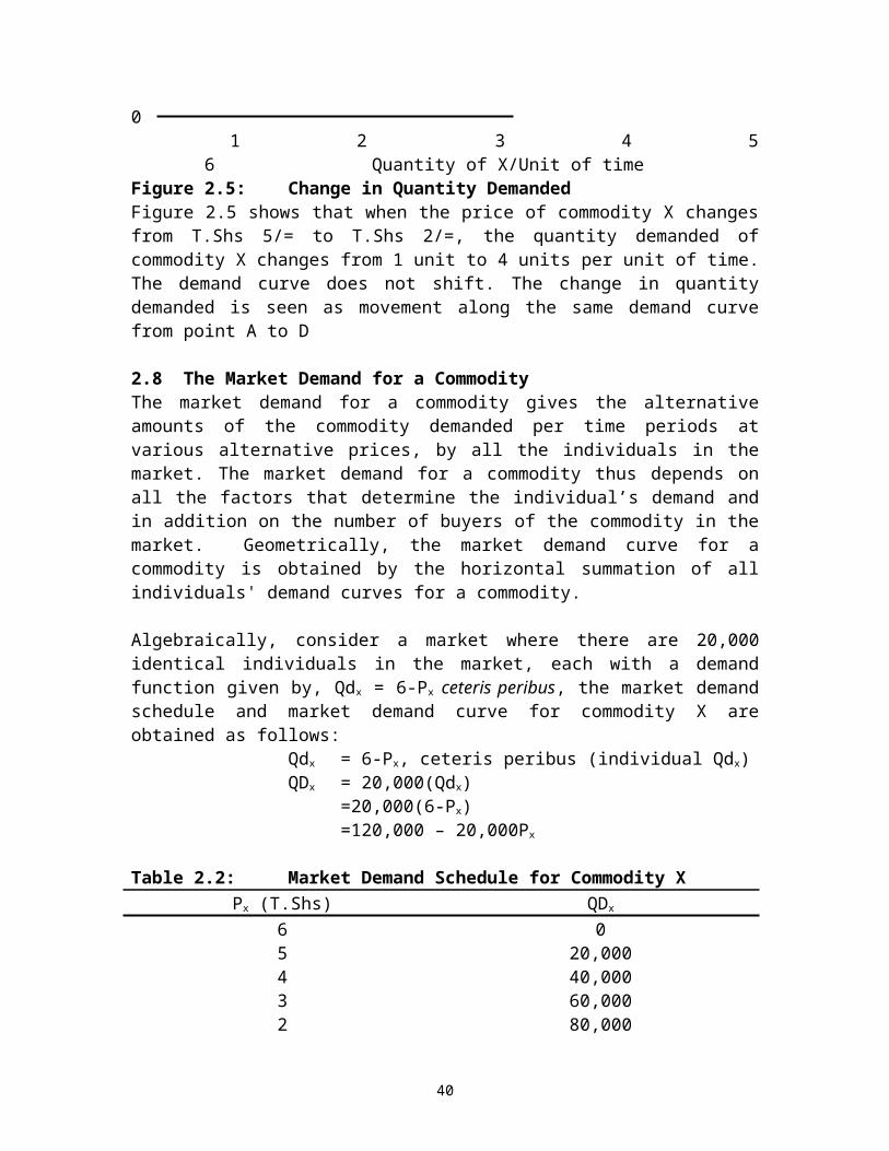
the price upwards, even further away from 0Pe. Similarly, if the price were 0P2, the excess supply equal to X3X4 would tend to push the price even further downwards.

Price (T.Shs) SX DX

P1

Pe

P2

0 X3 X4 Xe X1 X2 Quantity of X/timeFigure 4.3(a): Unstable Equilibrium

In another scenario for unstable equilibrium to occur, the market supply curve must be negatively sloped and less steeply inclined than (the negatively sloped) market demand curve as shown in figure 4.3 (b). If a price in this figure falls from equilibrium price P 1 to P2, the quantity demanded increases a little to X2 while the quantity supplied increases substantially to X3, creating a surplus. Hence the situation results in the tendency for the price to move further away from the equilibrium, rather than towards it. This situation occurs with a commodity like oranges, which have to be offered for sale at once in season because they are perishable.

Price (T.Shs)

46

P3

P1

P2

DX SX

0 X4 X5 X1 X2 X3 Qty of X/time Figure 4.3(b): Unstable Equilibrium

One can also notice in the figure 4.3(b) how a price rising above equilibrium, i.e. to P3

shows a decrease in the quantity supplied and an increase in quantity demanded to X4 and X5, respectively. This situation creates a shortage which implies that the price will move further away from the equilibrium rather than towards it. This can occur with the same oranges when they are out of season and scarce.

4.6 The Impact of Shift in Demand and Supply Curves on EquilibriumThis section illustrates the impact of a shift in demand and supply curves on equilibrium. If the market demand curve or the market supply curve or both shift, the equilibrium point will change. An increase in demand causes an increase in the equilibrium price and equilibrium quantity, ceteris peribus. On the other hand, given the market demand for a commodity, an increase in the market supply causes a reduction in the equilibrium price but an increase in equilibrium quantity. The opposite occurs for a decrease in demand or supply. If both the market demand and the market supply increase, the equilibrium quantity rises but the equilibrium price may rise, fall or remain unchanged.

Price of X(T.Shs)

47

DX SX1 SX2

P2

P1

SX1 SX2 DX

0 X1 X2 Quantity of X/unit of timeFigure 4.4: A shift in Market Supply Curve

Figure 4.4 shows that an increase in market supply from Sx1 Sx

1 to Sx2 Sx

2 with a given demand Dx Dx will result in a reduction in equilibrium price from P2 to P1 and an increase in equilibrium quantity from X1 to X2 .

Price of X (T.Shs)

D0 DX1 SX

P1

P0

SX D0 DX1

0 X0 X1 Quantity of X/Unit of timeFigure 4.5: A shift in Market Demand Curve and Equilibrium

Figure 4.5 shows that an increase in market demand which implies a shift in market demand curve from D0 to Dx

1 with a given supply curve Sx Sx causes an increase in both

equilibrium price from P0 to P1 and the equilibrium quantity from X0 to X1 as shown in figure 4.5.

Price of X

48

DX D1X SX S1

X

P2

P1

SX S1X DX D1

X

0 X1 X2 X3 Quantity of X/Unit of timeFigure 4.6: A shift in Market Demand and Supply Curves

An increase in both the market demand and supply results in the equilibrium quantity rising but the equilibrium price may either rise, fall or remain unchanged depending on the position of demand and supply curves. When demand and supply curves shift from DxDx and SxSx to D1

xD1x and S1

xS1x respectively, equilibrium quantity increases at all

levels of prices. The same figure also indicates that price has remained at P1 regardless of a shift in both demand and supply curves.

4.7 Sales Tax and Market Equilibrium In this section, we are going to illustrate the effect of a sales tax on goods. This is one of the many areas where the concept of equilibrium has an important application. Consider Table 4.1 which shows the quantities demanded and supplied of goods X at different prices. The demand and supply curves are shown as DD and SS respectively in figure 4.7. The initial equilibrium price is T.Shs 3 per unit and the equilibrium quantity is 60,000 units.

Table 4.1: Quantities Demanded and Supplied at Different Prices

Price per unit (T.Shs) Quantity demanded Quantity supplied65

020,000

120,000100,000

49

43210

40,00060,00080,000100,000120,000

80,00060,00040,00020,000

0

Now suppose that the government imposes a sales tax of T.Shs 2 per unit sold. In other words, for every unit of X sold the supplier have to pay T.Shs 2 as a sales tax to the government. What is the impact of such a sales tax on equilibrium price and quantity?

Price of X (T.Shs)

S1x6 Dx

Sx5

T.Shs 2.00/=4 E*

3 E

2

1

0 Dx 20 40 60 ('000) Quantity of X /unit of time Figure 4.7: Sales Tax on Equilibrium Price and Quantity As it can be seen from figure 4.7, suppliers are willing to supply 60,000 units of commodity X at a price of T.Shs 3 before the imposition of a sales tax. The introduction of a sales tax affects the supply curve. In other words, the imposition of tax causes the market supply curve for goods X to shift up by a vertical distance of T.Shs 2. The new market supply curve is S1x which is parallel to Sx and the new equilibrium point is E*. At this new equilibrium (i.e., point E), the price of commodity X is T.Shs 4 and the quantity of commodity X is 40,000 units.

The imposition of a sales tax has the following implications. First, consumers now pay T.Shs 4 instead of T.Shs 3. Second, sellers of good X now receive T.Shs 2 instead of T.Shs 3. The difference between what the consumers pay and what the sellers receive is the tax collected by the government. In this particular case, the incidence of tax falls equally on both the consumers and sellers. The total amount of taxes collected by the government is amounting to T.Shs 80,000 represented by the shaded area. The distribution of the tax burden between consumers (buyers) and producers (sellers) is called the incidence of the tax. Further discussion on the incidence of taxation is beyond the scope of this course and it is omitted in this course unit.

50

Numerical ExampleSuppose that the supply function is given by: P = 10Q + 100. The demand function is given by: P = 500 - 30Q.(a) Find the equilibrium price and quantity algebraically (b) If the government imposes a fixed tax of T.Shs.80.00 on each unit of a good,

show how the supply curve is affected algebraically.(c) Find the equilibrium price and quantity following the imposition of the tax.(d) Find the government tax revenue.(e) Compare prices paid by the consumer before and after the imposition of the tax,

determine the proportion of the T.Shs.80.00 per unit tax that is paid by the consumers.

Solution(a) Equilibrium occurs at the point of intersection between demand and supply. That

is,10Q+100=500-30Q

40Q=400Q=10

Equilibrium price is 200(b) The imposition of a tax on the supply curve is shown as follows

P=10Q+100+TAXP=10Q+100+80P=10Q+180

(c) The new equilibrium price following the imposition of a tax is given as:10Q+180= 500-30Q

40Q=320Q=8

The equilibrium price is 260(d) Government tax revenue is 80x8=640

(e) Price paid by consumer is P = 500 - 30Q.P= 500-30(8)P=260

Consumers are now paying more as a result of imposition of tax (i.e, 260-200= 60). The sellers pay the remaining T.Shs 20.

4.8 Market Disequilibrium Market disequilibrium occurs when the quantity demanded is not equal to the quantity supplied. In other words, it is a state in which either excess demand or excess supply exists. Disequilibrium normally persists in markets under the following circumstances: where the government or other bodies impose artificial restriction on either price or quantity; where the market equilibrium is unstable one; when production plans are not realized; and where there are lagged responses. Let us look on each of these in turn.

51

4.8.1 Artificial Restriction on Price and Quantity.The government may set price ceiling in an attempt to stop the price of a particular good from rising to an "unacceptable levels". Such price ceiling were common in Tanzania during the socialism era particularly on items which played a big part in the cost of living such as sugar, maize flours, kerosene, fertilizers, etc. Alternatively, in order to guarantee producers a certain return on their sales, government can impose price floors below which the price cannot legally fall.

A price ceiling or a maximum price control sets a price above which a commodity or service cannot be sold. Price floor or minimum price control sets a price below which a commodity or service cannot be sold.

The effects of these two forms of government intervention are illustrated for goods X in figures 4.8 and 4.9. Figure 4.8 shows that an excess demand for goods X occurs when a price ceiling is imposed at 0P1, which is below the equilibrium price. Since the price is not allowed to rise back towards the equilibrium, excess demand exists shown by X1X2.

Price of X

Dx Sx

P1

Excess Demand

Sx Dx

0 X1 X2 Quantity of X/Unit of timeFigure 4.8: A Price Ceiling

Figure 4.9 shows the effect of price floor at OP2 which is above the equilibrium price. This time there is an excess supply of goods X, some times called a glut. Where the price floor is established by the authorities intervening to purchase excess supplies, the glut will show itself mainly in an increase in the authorities stock of goods. It is important to note that in the event of a price ceiling or price floor being set on a commodity at a price which is not the equilibrium one, the economic forces of excess demand and excess supply will not be able to restore equilibrium.

52

Price of X

Dx Sx

Glut P2

Pe

0 X1 Xe X2 Quantity of X/Unit of timeFigure 4.9: A Price Floor

4.8.2 Unstable EquilibriaDisequilibrium may also arise where an equilibrium is unstable one so that any divergence from it generates an economic force, which pushes the market even further away from it. We have already explained the concept of unstable equilibrium in the previous sections.

4.8.3 Failure of Production Plans to be RealizedIn some industries, because of the possibility of unforeseen events happening, the quantities that producers plan to supply may fail to be achieved for a variety of reasons. One reason is that actual supply can fall short of planned supply if events under the producers' control (for example strikes) render production targets unachievable. The second reason is that actual supply may exceed planned supply if producers underestimate the productive capacity of their resources.

4.8.4 Lagged ResponsesSometimes lags may cause the market to remain in disequilibrium for some period of time. Lags may occur because of imperfect information, expectations and technological reasons among others. Basically there are two sources of lags: lags on supply side and lags on the demand side.

With lags on the supply side, firms can quickly respond to the increased demand if they are fully aware that there is an increase in demand for their products on the market. However, if firms have imperfect information, it may take sometime before increased sales figures or an increased number of enquiries concerning their products convince them that an actual increase in demand has taken place. Even if this is known, sometimes it takes time for firms to organize the additional factors of production necessary to increase output.

53

On the demand side, lags may generally arise following consumers' expectations especially when consumers are not sure if the price change of a particular product is permanent or temporary. The other source of lag in demand side may emanate from consumer's knowledge on the availability of substitutes and their prices.

4.9 Cobweb ModelThe Cobweb model is a model of cyclical supply and demand in which there is a lag between responses of producers to a change of price. Farming is a good example, as there is a lag between planting and harvesting. This model enables us to trace out the time path from a disequilibrium position towards an equilibrium position, given the presence of production lag. To illustrate the cobweb model, consider a situation where by demand for potatoes depends on this year market price, but the supply of potatoes in this year depend on last year's price. Using functional notation, we can write;

Dp = f (Pt) (4.1)Sp = f (Pt-1)

(4.2)Dp and Sp represent the demand for and supply of potatoes respectively, Pt is this year's price and Pt-1, is the price which farmers last year expected would prevail this year, which of course is the last year's price. The important point to remember is that any change in price leads to an immediate change in quantity demanded, but only a lagged change in quantity supplied, the production lag being one year.

Price of Potatoes Dp Sp= f (Pt-1)

P1

P3

P2

Sp Dp= f (Pt)

0 X3 X4 X2 Qty/Unit of timeFigure 4.10: The Convergent Cobweb Model "Dumped"

Consider figure 4.10. Suppose we start in year 1 with disequilibrium price 0P1. The quantity supplied in year 2 (which depends on the price in year 1) will be 0X2, but to sell this quantity of potatoes the price in year 2 will have to be reduced to 0P 2. This price will bring forth a supply of 0X3 in year 3. This quantity can, however, be sold at the higher price 0P3 and this will bring forth a supply of 0X4 in year 4. This process will continue

54

year after year, tracing out a cobweb pattern on the graph, with the market slowly approaching the equilibrium position.

One criticism of this model is its assumption that producers are extremely shortsighted; they are fundamentally unable to judge market conditions or learn from their pricing mistakes that result in surplus/shortfall cycles. This assumption is seen to be unrealistic.

Dumped cobweb model depicts a market that moves over a number of periods towards equilibrium price and quantity. Explosive cobweb model depicts a market that moves over a number of periods away from the equilibrium price and quantity.

Can you plot the explosive cobweb model?

SUMMARY

55

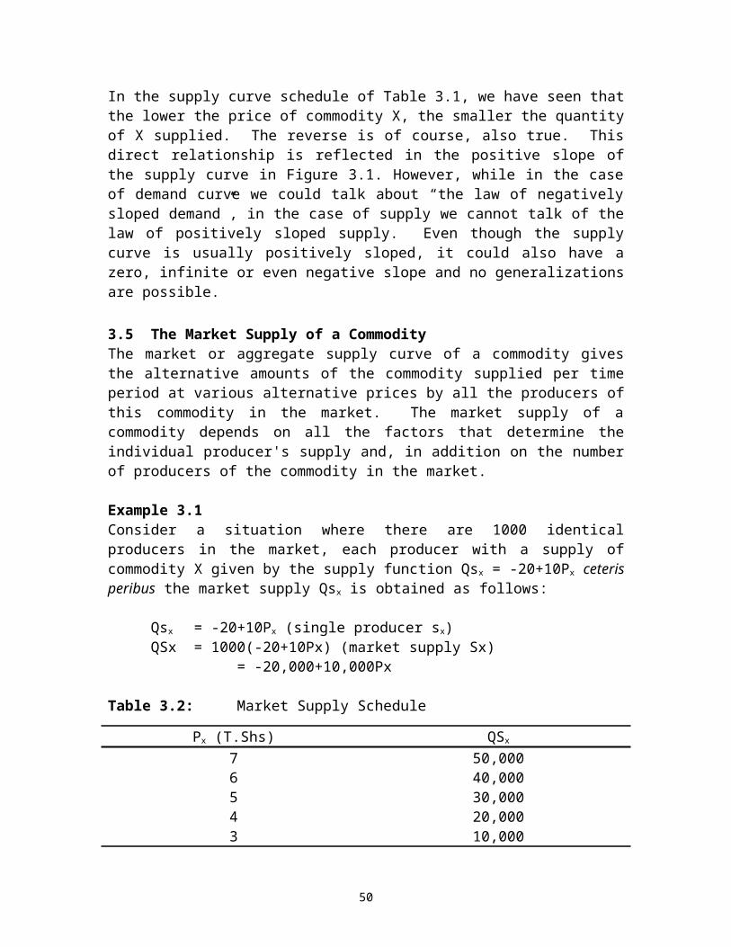
1. A market is a mechanism, which allows people to trade, normally governed by the theory of supply and demand. A market for a particular commodity/service consists of all buyers and sellers of that commodity/service. It is not necessary that market should be in identifiable place. What is important in market is that those willing to pay a price for a product/service meet those willing to sell

2. Market equilibrium occurs when the quantity of a commodity demanded in the market per unit of time is exactly equal to the quantity of the commodity supplied to the market over the same time period. Geometrically, equilibrium occurs at the intersection of the market demand curve and the market supply curve

3. In a stable equilibrium, economic forces tend to push the market towards the equilibrium. In unstable equilibrium, any divergence from the equilibrium creates economic forces which tend to push the market further away from the equilibrium.

4. A market will tend to remain in disequilibrium in the following circumstances; where artificial restriction are placed on price or quantity; where the market equilibrium is unstable; where production plans cannot be realised; and where there are lagged responses.

5. If the market demand curve or the market supply curve or both shift, the equilibrium point will change. An increase in demand (an upward shift) causes an increase in both the equilibrium price and equilibrium quantity, ceteris peribus. On the other hand, given the market demand for a commodity, an increase in the market supply (a downward shift in supply) causes a reduction in the equilibrium price but an increase in equilibrium quantity

6. A price ceiling or a maximum price control sets a price above which a good or service cannot be sold. Price floor or minimum price control sets a price below which a commodity or service cannot be sold.

7. The Cobweb model is a model of cyclical supply and demand in which there is a lag between responses of producers to a change of price. Farming is a good example, as there is a lag between planting and harvesting. This model enables us to trace out the time path from a disequilibrium position towards an equilibrium position, given the presence of production lag.

EXERCISES

56

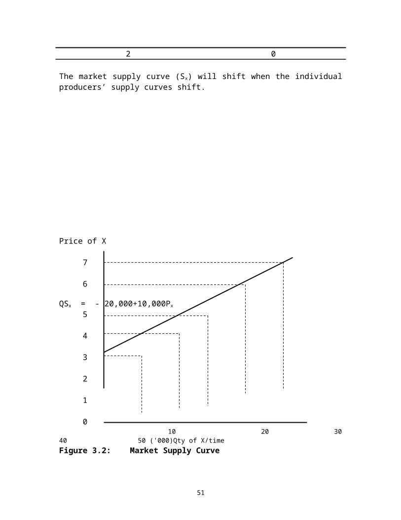
1. Write short notes on the following:(a) Unstable equilibrium(b) Price ceiling(c) Price flow(d) Market equilibrium(e) Comparative Statics(f) Partial equilibrium versus general equilibrium

2.* Suppose the government of Tanzania regulates the prices of chicken and set it below the market clearing level. Explain why shortages of chicken will develop and what factors will determine the size of the shortage. What will happen to the price of beef? Explain briefly.

3. Consider a competitive agricultural market with the following demand and supply functions respectively

Qd = 100 - 2PQs = 4 + 4PQd = Qs

(a) Sketch the demand and supply curves and find the equilibrium price and quantity

(b) Find the equilibrium price and quantity mathematically(c) Is the equilibrium stable? Why? Or why not? Give reasons.

4. Consider the hypothetical economy of Chalinze having 10,000 identical individuals for commodity X, each with a demand function given by Qdx = 12 – 2Px, and 1,000 identical producer of commodity X, each with a supply function given by Qsx = 20Px.

(a) Find the equilibrium price and quantity mathematically and graphically

(b) Is the equilibrium stable? Why? or why not? Give reasons.(c) What would happen if the government of Chalinze imposed a

price flow of T.Shs 4/= on commodity X?(d) Suppose the government of Chalinze decides to collect a sales

tax of T.Shs 2/= per unit sold from each of the 1,000 sellers of commodity X. Analyze the effects of sales tax on equilibrium price and quantity of commodity X?

(e) Suppose, instead, that a subsidy of T.Shs 2/= were levied on each unit of X. How does affect the equilibrium price and quantity? Do consumers reap any benefit from a subsidy.(Note: a subsidy is a negative tax)

57

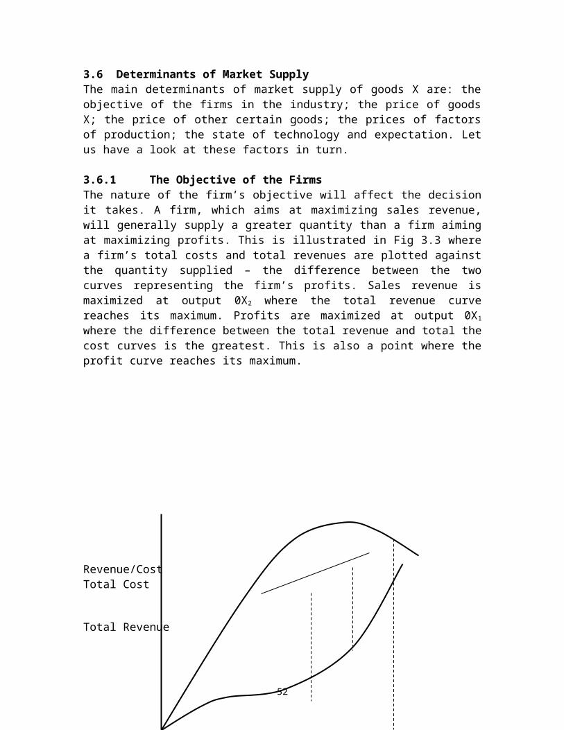
5. * The demand for vegetables is given by Qd = 500 – P and supply is given by Qs= P-100 where Q represents quantity of vegetables in kilos and P represents the price of vegetable. In an attempt to increase the amount of vegetables consumption, the government has imposed a price ceiling on the price of vegetables at T.Shs 200. (a) Explain the effects of such a policy on the market for

vegetables; explicitly stating what will happen to equilibrium price and quantity on this market.

(b) At the price ceiling, determine whether or not there is excess demand or excess supply.

(c) Will this policy have the desired effect on the amount of vegetables consumed? Explain

6. What is the Cobweb model? Is it a satisfactory model of price formation in agricultural sector? Explain using relevant diagrams.

7. * Suppose the market demand and supply for cigarette in Dar es salaam are respectively represented by the equations:

And

(a) Find the equilibrium price and quantity.Suppose that the city of Dar es salaam wants to reduce smoking and therefore decides to impose a T.Shs 10/pack excise tax on producers.

(b) Given the tax, what is the market-clearing price and quantity? (c) How much of the tax revenue is paid by consumers?(d) How much of the tax revenue is paid by sellers? (e) What are government tax revenues?

8. *. The government decides to protect supplier and introduces a per-unit subsidy for the good produced by that supplier.(a) Using a diagram, carefully explain the consequences of this

action on the equilibrium price and quantity in the market for this good.

(b) Discuss the pros and cons of such a policy.

58

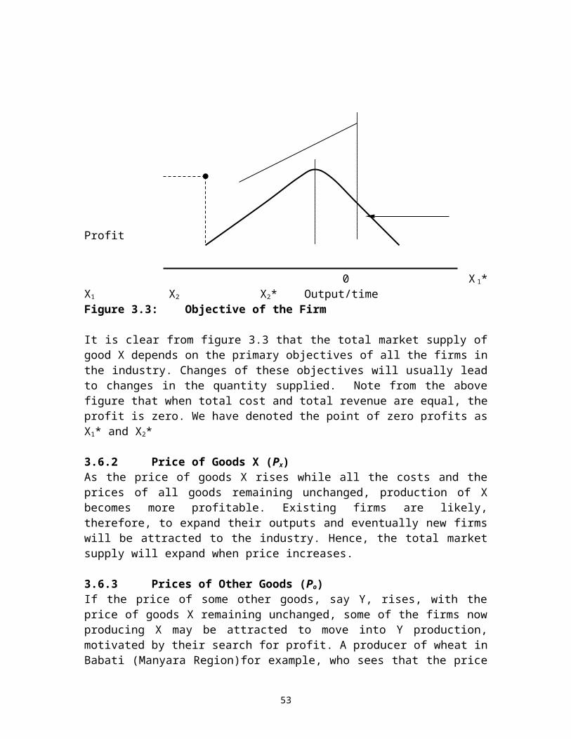
LECTURE FIVEELASTICITY OF DEMAND AND SUPPLY

5.1 IntroductionIn lectures two and three, among other things, it has been shown that the demand for a particular commodity depends on the price of that commodity, consumer’s income and on the prices of other commodities. Similarly, supply depends on price, as well as on the variables that affect the cost of production. Generally, it has been shown that if the price of a commodity X increases, the quantity demanded of that particular commodity will fall, ceteris peribus.

However, quite often we are interested to know by how much the quantity supplied or demanded for a particular commodity will rise or fall following the changes in the price of the commodity. For example, how sensitive is the demand for sugar to its price? Suppose that the price of sugar is increased by 10 percent, by how much will quantity demanded change? What will be the impact of an increase in the price of sugar on the demand for Bread? Milk? Coffee? Similarly, we are interested to know by how much will demand for sugar change if consumer's income increases by 5 percent? The concept of elasticity is very useful in answering those questions.

ObjectivesAfter reading this chapter, you should be able to:

(i) Define price elasticity of demand and supply, income elasticity of demand, and cross elasticity of demand and supply.

(ii) Compute price elasticity of demand, income elasticity and cross elasticity.

(iii) Interpret the coefficients of price, cross and income elasticity of demand

(iv) Explain the determinants of elasticity of demand and elasticity of supply.

(v) Describe the relationship between the price elasticity of demand and total revenue.

5.2 Price Elasticity Of DemandPrice elasticity of demand is the percentage change in the quantity demanded divided by the percentage change in price of the commodity. It is usually symbolized by the Greek letter, called eta.

(5.1)

Algebraically, price elasticity of demand is written as follows:

(5.2)

59

Where; Q/Q represents the change in quantity demanded and P/P represents the change in price. P denotes initial price and Q denotes initial quantity. Since price and quantity are inversely related, the coefficient of price elasticity of demand is a negative number. In order to avoid negative values, a minus sign is often introduced into the formula for elasticity as shown in equation 5.2.

5.3 Measurement of Price ElasticityThere are two ways of measuring the price elasticity of demand. If the changes in price are very small we use point elasticity of demand as a measure of the responsiveness of demand. If, on the other hand, changes in price are not so small, we use arc elasticity of demand as the relevant measure. Let us explain these two elasticities.

5.3.1 Point Elasticity of DemandThe point elasticity of demand is defined as the proportionate change in the quantity demanded resulting from a very small proportionate change in price. The formula for price elasticity of demand given in equation 5.2 is also applicable for the point elasticity of demand.

5.3.2 Arc Elasticity of DemandArc elasticity is a measure of average elasticity. That is, the elasticity at the midpoint of the chord that connects the two points (A and B) on the demand curve defined by the initial and new price levels as shown in figure 5.1. To calculate the arc elasticity, we use the following formula:

(5.3)

It should be clear that the measure of the arc elasticity is an approximation of the true elasticity of section AB of the demand curve shown in figure 5.1 which is used only when we know only two points A and B from the demand curve, but not the intermediate ones.

60

Price (T.Shs)

P1 A

Point Elasticity

P2 B

0 Q1 Q2 Quantity/timeFigure 5.1: Arc elasticity.

Example 5.1: Arc Elasticity

In example 5.1 we are going to compute the arc elasticity. In the next section we shall see that the coefficient of price elasticity of demand in general differs at every point along a demand curve. Arc elasticity is, therefore, only an estimate. This estimate improves as the arc becomes smaller and approaches a point in the limit.

Table 5.1: Market demand Schedule and Arc Elasticity

Point Px (T.Shs) QxA 7 500B 6 750C 5 1,250D 4 2,000F 3 3,250G 2 4,750H 1 8,000

Given the market demand schedule in Table 5.1, we can find the arc elasticity for a movement midway between C and F as follows i.e. at point D as follows;

61

5.4 Elasticity along the Linear Demand CurveThe elasticity of downward sloping linear demand curve varies from infinity () at the price axis to zero at the quantity axis. The reason is that a straight line has a constant slope, so that the ratio P/Q is the same anywhere on the line. Therefore, its reciprocal, Q/P, must also be constant. We can infer the changes in elasticity () by inspecting changes in P/Q as we move along the demand curve. At the price axis, Q = 0, and P/Q is undefined. However, if we let Q approach zero, without ever quite reaching it, we see that the ratio P/Q increases without limit. Thus, elasticity increases without limit as Q approaches zero. In general, we say that elasticity is infinity when Q is zero.

Price

δ/β η= because Qd=0

½ (δ/β) η=1

η=0 because P=0 0 ½(δ) δ QuantityFigure 5.2 Elasticity along the Linear Demand CurveIn plotting figure 5.2, we have used the linear demand function of the following form: Qd=δ-βP. Where Qd is the quantity demanded and P is price. δ and β are parameters. It is clear from this equation that when P=0, Qd= δ. This is shown in the horizontal axis of where η=0. Analogously, when Qd=0, P= δ/β. This is shown in the vertical axis where η=. It is much easier to verify these points once you use the elasticity formula given in equation 5.2.

Elasticities of two intersecting straight lines demand curves can be compared at the point of intersection merely by comparing the slope, the steeper curve being the less elastic. Figure 5.3 shows two intersecting curves and proves that the steeper curve is less elastic than the flatter curve when elasticity is measured at the point where the two curves intersect. The intuitive reason is that at the point of intersection P and Q are common to both curves, so all that differs in elasticity formula is their relative slopes.

Px (T.Shs)

62

P2

P1

Q

Df

Ds

0 Q Qty/unit of timeFigure 5.3: Two Intersecting Demand Curves

From figure 5.3 it is evident that the absolute value of the slope of the steeper curve, P2/Q, is larger than the absolute value of the slope P1/Q, of the flatter curve. Thus, the absolute value of the ratio Q/P2 is smaller on the steeper curve than the ratio Q/P1 on the flatter curve, so that elasticity is lower.

Measured at the point of intersection of two demand curves, the steeper curve has the lower elasticity.

5.5 Interpretation of Price Elasticity of DemandAs we have pointed out earlier, the coefficient of price elasticity of demand is a negative sign due to the inverse relationship between price and quantity demanded. In terms of interpretation, the negative sign is ignored and only absolute value is considered. In the following sub-section, we are going to provide an interpretation of: inelastic demand, elastic demand and unitary elasticity.

5.5.1 Inelastic Demand Inelastic demand occurs whenever the percentage change in quantity is less than the percentage change in price. In other words, demand is not very responsive to change in price. Under inelastic demand, the numeric value of the coefficient of price elasticity of demand is less than 1. In the extreme cases where the coefficient of price elasticity of demand is zero, demand is said to be perfectly inelastic. This is shown in figure 5.4. Under perfectly inelastic demand, a change in price has no whatsoever influence on quantity demanded. The demand curve for such a product is thus vertical.

Price (T.Shs) DX

63

0 X* Quantity of X/timeFigure 5.4: Perfectly Inelastic Demand Curve

5.5.2 Elastic DemandElastic demand occurs whenever the percentage change in quantity demanded exceeds the percentage change in price. In other words, demand is more responsive to change in price. Under elastic demand, the numeric value of the coefficient of price elasticity is usually greater than 1 but less than infinity. In the extreme cases where the price elasticity of demand is infinitely large, demand is said to be perfectly elastic. The demand curve for such a product is thus horizontal. This is shown in figure 5.5.

Price (T.Shs)

P*

0 Quantity of X/time

Figure 5.5: Perfectly Elastic Demand Curve

64

5.5.3 Unitary ElasticityThe other peculiar case occurs when price elasticity of demand is equal to one. Under this particular case, the percentage change in price is exactly equal to the percentage change in quantity demanded. This case, which is called the unit elasticity, is the boundary between elastic and inelastic demand. A demand curve having unit elasticity over its whole range is shown in figure 5.6.

Price (T.Shs) Dx

PX1

PX2 Dx

0 X1 X2 Quantity of X/timeFigure 5.6: Rectangular Hyperbola Demand Curve

Figure 5.6 has unit elasticity. It implies that, a given percentage increase in price brings an equal percentage decrease in quantity demanded at all points on the curve. It is a rectangular hyperbola (or curve linear demand curve)) for which price (P) times quantity (Q) is a constant. That is; PQ=K, where K can assume any positive constant. Given this simple equation (i.e., PQ=K), we can compute the elasticity of demand along this curve linear as follows. Elasticity is given as:

Note that the QxPx=K could be written as: . Clearly,

. Plugging this expression into the elasticity formula and further

manipulation yields:

65

5.6 Elasticity and Slope of Demand CurveIs the slope of demand curve the same as elasticity?

The slope of the demand curve is not the same as elasticity because the demand curve’s slope depends upon the change in Q and P, where as the elasticity depends upon their percentage change. In other words, elasticity depends on the slope of demand curve and the point at which the measurement is made. This is illustrated in figure 5.7.

Px (T.Shs)

D

B

P A

P Q

Q QuantityFigure 5.7: Elasticity Measured on Linear Demand Curve

Note that as we move from point A to point B in figure 5.7, the ratio P/Q gives us the slope of the line, which is the reciprocal of the first term in the percentage definition of elasticity (see equation 5.2). The second term P/Q, is the ratio of the coordinates of the point A. Since the slope P/Q is constant, it is clear that the elasticity along the curve varies with the ratio P/Q, which is zero where the curve intersects the quantity axis and infinity where it intersects with the price axis.

66

5.7 Determinants of Price Elasticity of DemandOur analysis of elasticity has concentrated solely on the measurement of elasticity of demand. But why do some goods display elastic demands while others seem quite unresponsive to price? The following are the factors, which influence the price elasticity of demand.

(a) Number of closeness of substitute for the commodity.

The more and better the available substitute for the commodity, the greater its price elasticity of demand is likely to be. Thus, when the price of tea rises, consumers readily switch to commodity substitute such as coffee and cocoa, so the coefficient of price elasticity of demand for tea is likely to be high. On the other hand, since there are no commodity substitutes for salt, its elasticity is likely to be very low.

(b) Number of uses of the commodity. The greater the number of uses of a commodity, the greater is its price elasticity. For example the elasticity of aluminum is likely to be much greater than that of butter since butter can be used only as food while aluminum has hundred of uses (e.g. air craft, electrical wiring, appliances and so on).

(c) Expenditure on the commodity. The greater the percentage of income spent on a commodity the greater its elasticity is likely to be. Thus the demand for car is likely to be much more price elastic.

(d) Adjustment time: The longer the allowed period of adjustment in the quantity of a commodity demanded, the more elastic its demand is likely to be. This is so because it takes time for consumer to learn new prices and products. In addition, even after a decision is made to switch to other products, some time may pass before the switch is actually made. In general, elasticity tend to be inelastic in the short run but elastic in the long run.

(e) Level of price:

If the ruling price is toward the upper hand of the demand curve, demand is likely to be more elastic than if it were toward the lower end. This always true for a negatively sloped straight line demand curve (see figure 5.8) and is usually true for curve linear demand curves.

(f) Nature of the commodity: It is a common observation that different commodities depending on their nature tend to display different elasticities. For example, necessity commodities such as food tend to be inelastic while luxury commodities such as articles of ostentation tend to be more elastic.

67

(g) Habit: Some commodities such as tobacco and alcoholic drink are habit forming and demand will tend to be more inelastic over a fairly wide range of prices. In some countries the prices of tobacco and alcoholic drinks have been greatly increased by taxation, but demand has been relatively unaffected. Smoking and drinking seem to be acquired habits which consumers are reluctant to change. Hence demand tends to be inelastic.

5.8 The Income Elasticity of DemandThe coefficient of income elasticity of demand (m) measures the percentage change in the amount of the commodity purchased per unit of time (Qx/ Qx) resulting from a given percentage change in consumer’s income (M/M). Thus,

(5.4)

Normal goods have a positive income elasticity of demand. This implies that as income rises more is demanded at each price level. Necessities have an income elasticity of demand of between 0 and +1. Demand rises with income, but less than proportionately. Often this is because we have a limited need to consume additional quantities of necessary goods as our real income rise. Luxuries on the other hand are said to have an income elasticity of demand greater than 1. Demand rises more than proportionate to a change in income). Luxuries are items we can (and often do) manage to do without during periods of below average income and falling consumer confidence. Inferior goods have a negative income elasticity of demand. Demand falls as income rises. Determinants of Income elasticity of demand are:

(a) Initial level of incomeThe initial level of income of a particular individual or society is one of the major determinants of income elasticity of demand. At very low levels of income, income elasticity of demand tends to be equal to zero. However, as the level of income starts to rise gradually, income elasticity of demand tends to be positive. Beyond certain level of income such as Y2 in figure 5.8, income elasticity tends to be negative. What is clear from figure 5.8 is that a particular commodity might be considered as a normal good at very low levels of income but also the same commodity might be considered as an inferior good at the high levels of income. An inferior good for a millionaire is not necessarily an inferior good to a poor person.

68

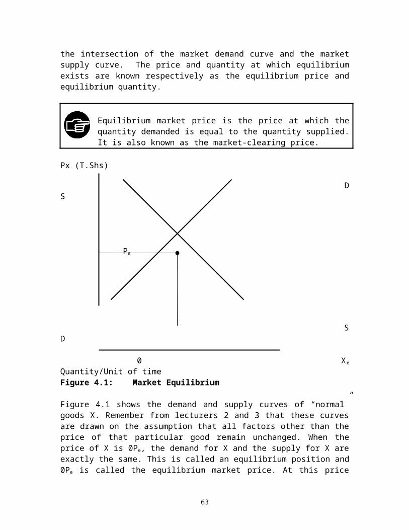
Quantity Q*

0 Y1 Y2 Income (Y) /time Figure 5.8: Income Elasticity of demand and the Level of income

(b) TimeThe income elasticity of demand for a product will also change over time – the vast majority of products have a finite life cycle. Consumer perceptions of the value and desirability of a good or service will be influenced not just by their own experiences of consuming it (and the feedback from other purchasers) but also the appearance of new products onto the market. Consider the income elasticity of demand for flat-screen colour televisions as the market for plasma screens develops and the income elasticity of demand for TV services provided through satellite dishes set against the growing availability and falling cost (in nominal and real terms) and integrated digital televisions.

When m (i.e., income elasticity of demand) is negative, the commodity is inferior. If m is positive, the commodity is normal. A normal commodity is usually a luxury if its m >1, otherwise it is a necessity. Depending on the level of the consumer’s income, m is likely to vary considerably. Thus a commodity may be a luxury at “low” levels of income, a necessity at the “intermediate” levels of income and an inferior commodity for “high” levels of income

5.9 The Cross Elasticity of Demand The cross elasticity of demand is defined as the proportionate change in the quantity demanded of commodity X resulting from proportionate change in the price of commodity Y. The cross elasticity of demand is given by the following formula:

69

Zero income elasticity

Positive income elasticity

Negative incom

e elasticity

(5.5)

Cross elasticity can vary from minus infinity to plus infinity. Complementary goods have negative cross elasticities and substitute goods have positive cross elasticities. Bread and butter for example, are complements: a fall in the price of the butter causes an increase in consumption of both products. Thus change in the price of butter and in the quantity of bread demanded will have opposite signs. In contrast, butter and margarine are substitutes: a fall in the price of butter increases the quantity of butter demanded, but reduces the quantity of margarine demanded. Changes in the price of butter and in the quantity of margarine demanded will, therefore, have the same sign.

If X and Y are substitutes, xy is positive. On the other hand, if X and Y are complements (xy) is negative. When commodities are non related (when they are independent of each other on zero), xy = 0

The main determinant of cross elasticity of demand is the nature of commodities relative to their uses. If two commodities can satisfy equally well the same need, the cross elasticity is high and vice versa.

5.10 Relationship between Elasticity and Total Revenue The relationship between price elasticity of demand and total revenue is of particular importance to producers when setting the price of the commodity.

Why should producers be interested in the price elasticity of demand?

Producers are interested in the price elasticity of demand because they are interested in questions like: will an increase in price result in an increase in the total amount spent by the consumers on the product? Or will an increase in price result in a decrease in the total amount spent by consumers on the product? The answers to these questions depend on the price elasticity of demand.

Suppose that the demand for the product is price elastic, i.e. the price elasticity of demand exceeds one. The total amount of money spent by consumers on the product equals the quantity demanded times price per unit. In this situation, if the price is reduced, the percentage increase in quantity demanded is greater than the percentage reduction in price. It then follows that a price reduction must lead to an increase in the total amount spent by the consumers on the commodity. If the demand is price elastic, a price increase leads to a reduction in the amount of money spent on the commodity. If the demand is price inelastic, a price decrease leads to a reduction in the total amount spent on the commodity, and a price increase leads to an increase in the amount spent on the

70

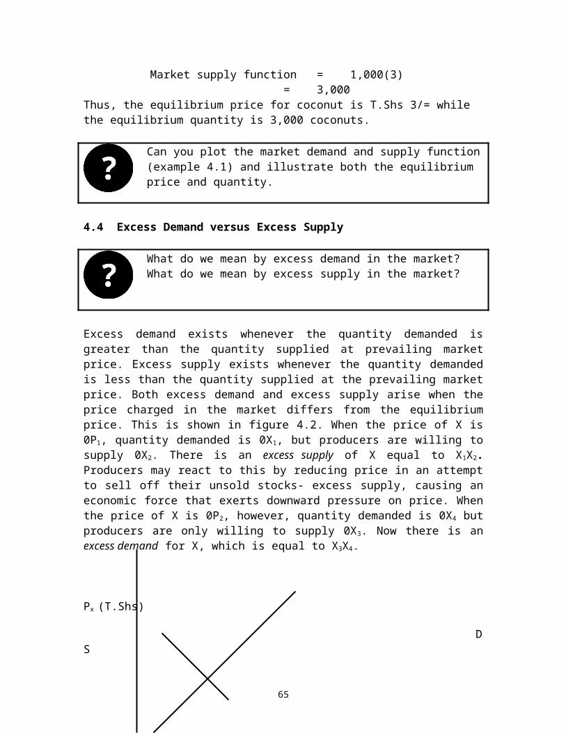
commodity. If the demand is of unitary elasticity, an increase or a decrease in price has no effect on the amount spent on the commodity.

If elasticity of demand exceeds unit (elastic demand), a fall in price increases total expenditure on the commodity and a rise in price reduces it.

If elasticity is less than unit (demand is inelastic), a fall in price reduces total expenditure on the commodity and a rise in price increases it.

If elasticity of demand is unity, a rise or a fall in price leaves the total expenditure on the commodity unaffected.

The relationship between price elasticity and total revenue can be illustrated with the linear demand curve in Figure 5.9 which is plotted using data in Table 5.2. By now you should be able to compute price elasticity of demand given a data set such as the one provided in Table 5.2

Table 5.2: Elasticity and Total Revenue

Points Px (T.Shs) Quantity of X Total Expenditure ElasticityA 8 0 0B 7 1,000 7,000 7C 6 2,000 12,000 3D 5 3,000 15,000 5/3E 4 4,000 16,000 1F 3 5,000 15,000 3/5G 2 6,000 12,000 1/3H 1 7,000 7,000 1/7I 0 8,000 0

As we move down the demand curve from A to E, the elasticity of demand gets smaller, but always exceed one. Thus the total amount spent on the good increases continually as we move from A to E. At point E, since there is unitary elasticity, there is no change in the total amount spent on the goods. Moving from E to I, the elasticity of demand is always less than one. Thus, the total amount spent on the goods decreases continually as we move from E to I.

Price

71

8 A

7 B Elasticity is greater than one

6 C

5 D

4 E Unitary elasticity

3 F

2 G Elasticity is less than one

1 H

0 10 20 30 40 50 60 70 80 Qty/time (00)

TR (000)

16

15

12

7

0 10 20 30 40 50 60 70 80 Qty/time (00)

Figure 5.9: Elasticity and Total Revenue

72

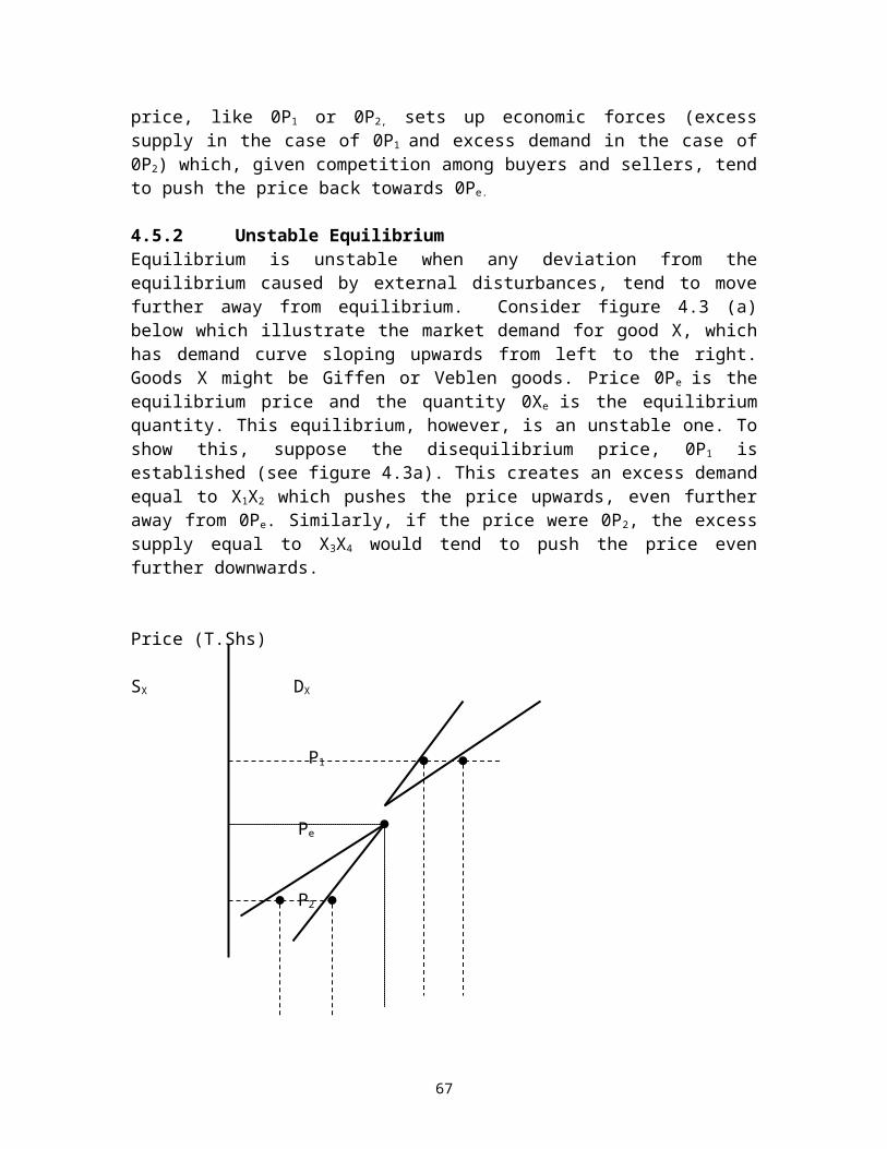
5.11 Elasticity of SupplyElasticity of supply is defined as the percentage change in quantity supplied divided by the percentage change in the price that brought it about. Letting the Greek letter epsilon,, stand for this measure, its formula is:

(5.6)

Or in symbols, elasticity of supply can be written as;

(5.7)

Where; Q/Q represents the change in quantity supplied and P/P represents change in price. Since supply curves normally have positive slope, elasticity of supply is normally positive.

Price (T.Shs)

S

S

0 Q1 Quantity of X/time

Figure 5.10: Perfectly Inelastic Supply Curve

Supply is said to be inelastic (<1) when a given percentage change in price causes a smaller percentage change in quantity supplied. It is said to be elastic (>1) when a given percentage change in price causes a bigger percentage change in quantity. Figure 5.10 illustrates perfect supply inelasticity (=0). This means that the fixed quantity 0Q1 will be supplied at any price including at a zero price.

How does the perfect elastic supply curve differ from the perfect elastic demand curve? What about perfect inelastic supply curve and perfect inelastic demand curve?

73

Price (T.Shs)

P1

0 Quantity of X/timeFigure 5.11: Perfectly Elastic Supply Curve

Now consider the other extreme illustrated in Figure 5.11: that of perfect elastic supply ( = ). In this case, nothing at all will be supplied at prices below 0P1. Although these extremes of elasticity are possible over a certain range of prices or quantities, they are extremely unlikely over the entire range of a supply curve.

Price (T.Shs)

10 B

5 A

0 8 16 Quantity of X/timeFigure 5.12: Unitary Elastic Supply Curve

74

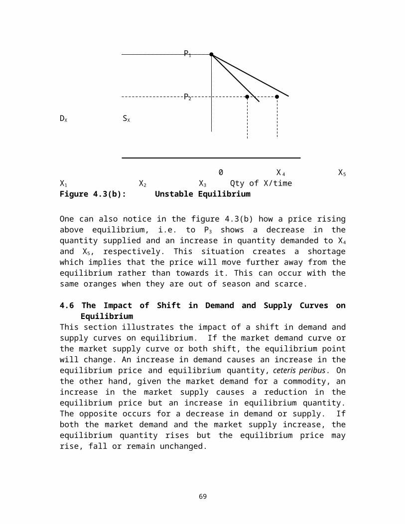
Figure 5.12 illustrates unitary elasticity of supply (=1). This is the case where the percentage change in quantity supplied is exactly equal to the percentage change in price. Thus, in moving from point A to point B along the supply curve in figure 5.12, a 100 percent rise in price causes a 100 percent rise in the quantity supplied.

(i) A vertical supply curve exhibits perfectly inelastic supply curve(ii) A horizontal supply curve exhibits perfectly elastic supply curve(iii) A straight-line supply curve passing through origin has an elasticity

equal to one at every point.

5.12 Determinant of Elasticity of SupplyWhat determines the response of producers to a change in the price of the product that they supply?

5.12.1 TimeIn the momentary period, supply is limited to the quantities already available in the market and it cannot be increased even if a substantial rise in price occurs. Supply is therefore, perfectly inelastic and is represented by supply curve S1 in figure 5.13. A rise in price from 0P1 to 0P2 leaves the quantity supplied unchanged at 0X1. For example, the supply of bread in a single day is limited to the quantities delivered to bread shops.

In the short run, supply can be increased by employing more variable factors of production. For example, more bread can be produced (in response to a rise in price) by encouraging the baker to work overtime or by employing more bakers. In this case, the supply curve will slope upwards from left to the right exhibiting some degree of elasticity, but there is a limit to the increase in supply that is possible without an expansion of the scale of operations. The short run supply curve is illustrated by S2 S2 in figure 5.13 and this time a rise in price from 0P1 to 0P2 brings forth an increase in supply from 0X1 to 0X2.

In the long run, the quantities of all factors of production can be increased. Existing firms can be expanded and new firms may enter the industry. In our example of bread production, existing bakeries can be expanded and new ovens and other forms of capital equipment can be installed; new bakeries may also be set up. Supply in the long run, then, is likely to be much more elastic than in the short run and the long run supply curve is illustrated by S3S3 in figure 5.13. A rise in price from 0P1 to 0P2 this time brings forth an increase in supply from 0X1 to 0X3.

75

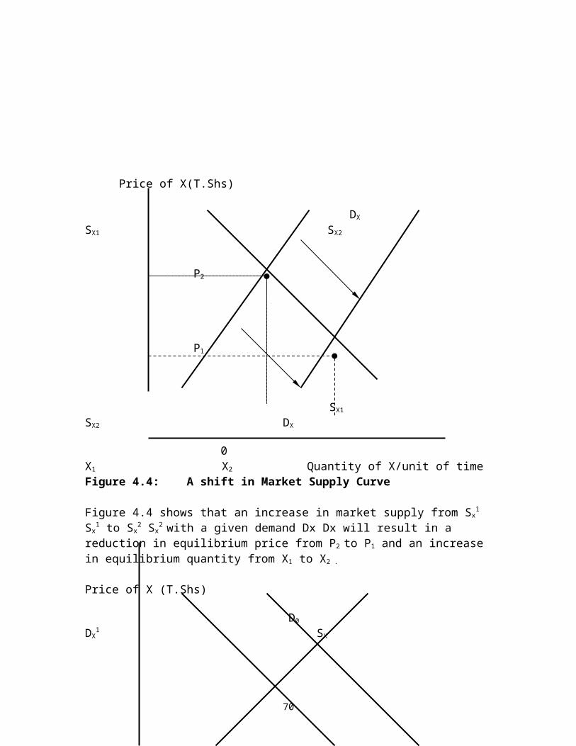
PX S1 S2

S3

P2

P1

S3

S2

0 X1 X2 X3 Quantity of X/timeFigure 5.13: Momentary, Short run and Long run Supply Curves

5.12.2 Excess capacity and unsold stocks

In the short run, it may be possible to increase supply considerably if there is a pool of unemployed labor and unused machinery (known as excess capacity) in the industry. Similarly, if the industry has accumulated large stock of unsold goods, supply can quickly be increased. It follows that supply will be more elastic the greater the excess capacity in the industry and the higher is the level of unsold stock.

5.12.3 Ease of Factor SubstitutionThe ease with which resources can shift from one industry to another is another determinant, which influence elasticity of supply. There are, however, problems, which may limit the mobility of factors between industries. For example, labor may be reluctant to move away from family and friends and may need retraining before it is suitable for the new occupation. Similarly, capital equipment which is suitable for one use may be totally unsuitable for another. In certain industries this is not such a serious problem and, given sufficient time, supply can be very elastic. In agriculture for example, it is quite possible for both labor and capital to shift from barley production to wheat production in response to a rise in wheat prices, though in this particular example time must be allowed for reaping the old crop and sowing the new one.

Determinants of elasticity of supply are: (i) Time(ii) Excess capacity and unsold stocks. (iii) The ease with which resources can shift from one industry to another.

76

SUMMARY

1. Elasticity of demand (also called price elasticity of demand) is defined as the percentage change in the quantity divided by the percentage change in price. Since price and quantity are inversely related, the coefficient of price elasticity of demand is a negative number. In order to avoid negative values, a minus sign is often introduced into the formula for elasticity.

2. When the percentage change in quantity is less than the percentage change in price demand is said to be inelastic and a fall in price lowers the total amount spent on the product. When the percentage change in quantity is greater than the percentage change in price, demand is said to be elastic and a fall in prices raises the total revenue.

3. Elasticity of demand tends to be greater the longer the time over which adjustment occurs. Items that have a few substitutes for the product in the short run may develop ample substitutes when consumers and producers have time to adapt.

4. The coefficient of price elasticity of demand is governed by the following factors: number of closeness of substitute for the commodity, number of uses of the commodity, expenditure on the commodity, adjustment time, level of price, nature of the commodity and habit.

5. The coefficient of income elasticity of demand (m) measures the percentage change in the amount of the commodity purchased per unit of time (Qx/ Qx) resulting from a given percentage change in consumer’s income (M/M).

6. The coefficient of price elasticity of demand of commodity X with respect to commodity Y (xy) (cross elasticity) measures the percentage change in the amount of X purchased per unit of time (Qx/ Qx) resulting from the given percentage change in the price of Y (Py/ Py)

7. Elasticity of supply measures the ratio of the percentage change in the quantity supplied of the product to the percentage change in its price. A vertical supply curve exhibits perfectly inelastic supply curve. A horizontal supply curve exhibits perfectly elastic supply curve. A straight-line supply curve passing through origin has elasticity equal to one at every point.

8. The main determinant of elasticity of supply are; time, the existence of excess capacity, and the ease with which resources can be shifted from one use to another.

EXERCISES

77

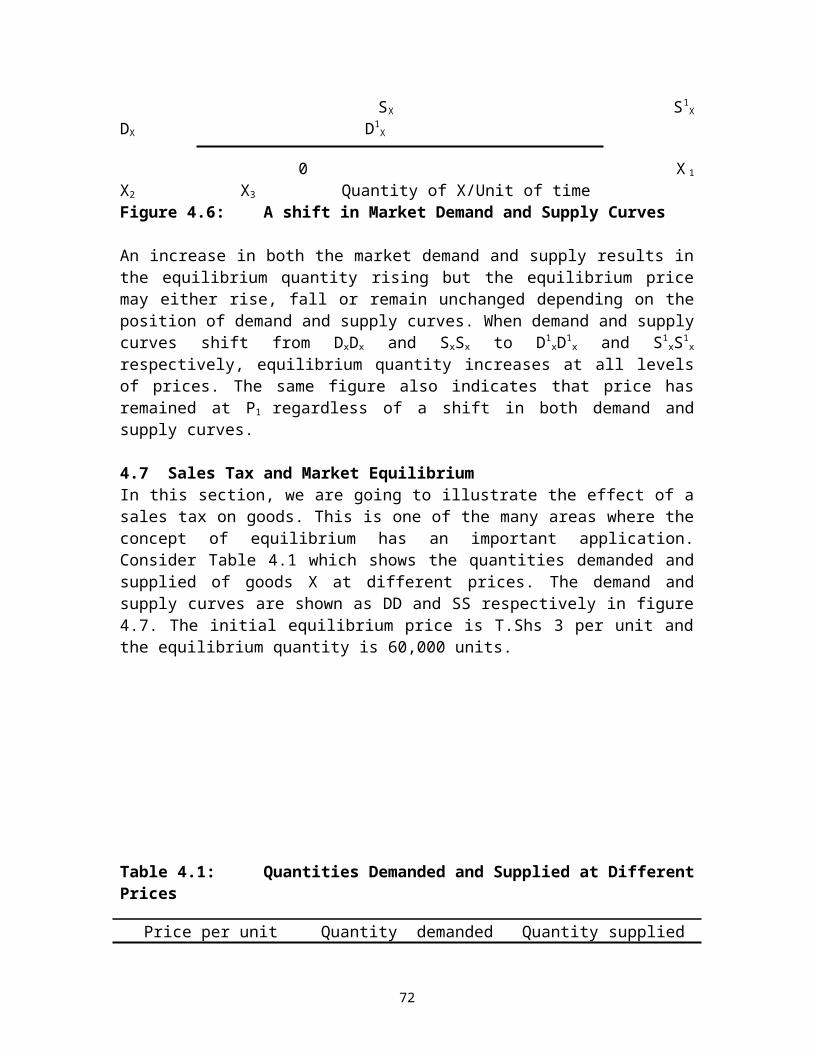
1. Write short notes on the following:(a) Cross price elasticity

(b) Income elasticity(c) Inelastic demand versus elastic demand(d) Inelastic supply versus elastic supply(e) Perfectly elastic supply versus perfectly elastic demand(f) Arc elasticity(g) Point elasticity(h) Determinants of elasticity of supply

2. Briefly explain why the slope of demand curve is a poor index of elasticity.

3. “Demand for salt is price inelastic”. Comment.

4. Assume that the coefficient of price elasticity of demand is -1.5. Find the percentage change in total expenditure on it when its price falls by 10%.

5. Outline the factors that determine the price elasticity of demand.

6. “The price elasticity of a straight-line demand curve varies from infinity at the price axis to zero at the quantity axis.” Is it true or false? Why or why not?

7. “Two parallel straight-line demand curves have different price elasticity at each price.” Is it true or false? Why?

8. Is positive income elasticity of demand a necessary condition for the inverse relation ship between the price of the commodity and the quantity demanded? Explain

9. The market demand function of a commodity is represented by Qx = 20-2Px -0.5Py + 0.01M; where Qx is quantity demanded for commodity X, Px is the price of commodity X, Py is the price of commodity Y and M is the consumer's income. Calculate price and cross elasticities of demand for commodity X when Px =5, Py=10 and M =1000.

10. From the demand function Q=800/P, show that the total expenditure

remains unchanged as price falls. Estimate elasticity of demand along the demand curve at P= T.Shs 4, P= T.Shs 2.

11. Prove that the supply curve that passes through the origin has a unitary elasticity. Use the following equation: Qs= +P

12. Demand function is given by Q = 45 – 2P + 3PA + 0.2Y

78

Assume that a price of the product P = 5, a price of alternative product PA = 3 and an income level Y = 30.(a) Find a quantity demanded.(b) Find the own price elasticity of demand. Is demand elastic or

inelastic?(c) Find the cross price elasticity of demand. Is alternative

product a substitute or a complement?(d) Find the income elasticity of demand. Is the product normal

or inferior13. * If a 3% increase in the price of maize flour causes a 6% decline in

the quantity demanded, what is the price elasticity of demand?

14* Suppose that the demand curve for the product is given by Q=1000-20P+PS, where P is the price of commodity and PS is the price of the substitute commodity. The price of a substitute commodity is 20. Suppose that P=10.

(a) Find the price elasticity of demand(b) Find cross-price elasticity of demand

15. Why is demand for many commodities likely to be more elastic in the long run than in the short run?

16. Calculate the elasticity of supply for the supply curve P=10+3Q when P=25 and Q=5

79

LECTURE SIXCONSUMER BEHAVIOR:

THE CARDINAL UTILITY THEORY

6.1 IntroductionIn lecture two, we have learned both an individual demand and the market demand for a single commodity only. In reality, of course, consumers have to choose from the many thousands of different goods available on the market. In other words, consumers are faced with the problem of choice. In examining the shape of a demand curve for a single good, therefore, we must closely look at the behavior of the consumers when faced with this problem of choice.

In this lecture, we are going to discuss the theory of consumer's behavior from the cardinalist paradigm. In the first part, we are going to explain the Cardinal approach to the theory of consumer behaviour. In the second part, we are going to define the concepts of utility and marginal utility. In the third part, we are going to describe how the demand curve is derived from the hypothesis of diminishing marginal utility. Fourthly, we shall learn the consumer surplus and the paradox of value. Finally, the lecture shall provide a critique on the cardinalist paradigm.Objectives

After reading this chapter, you should be able to:(i) Explain the Cardinal Utility theory(ii) Define marginal utility and state the law of diminishing

marginal utility(iii) Describe the consumer equilibrium condition (iv) Derive the demand curve from the law of diminishing

marginal utility(v) Explain how the concept of marginal utility answers an

important questions of consumer surplus and paradox of value(vi) Discuss the relationship between total utility, elasticity and

marginal utility;(vii) Provide a critique on the cardinal utility theory.

6.2 The Cardinal Utility Theory The cardinal utility theory asserts that the utility (i.e., satisfaction) gained from a particular good or service can be measured in numbers. The theoretical unit of utility’s measurement is called ‘util’. If utility can be measured in this way, it should then be possible to say that an individual will get 4200 utils from good A and 4500 utils from good B, for example. Majority of economist believe that utility cannot be measured in a cardinal approach and that only ordinal utility to be presented in lecture seven in this course unit is relevant. Despite this limitation, we can use cardinal utility theory to explain why the individual demand curve slopes downward from left to the right. Central to this theory are the concepts of marginal utility and the hypothesis of diminishing of marginal utility.

80

6.3 UtitityUtility is a measure of the relative happiness or satisfaction gained by consuming different bundles of goods and services. Given this measure, one may speak meaningfully of increasing or decreasing utility, and thereby explain economic behavior in terms of attempts to increase one's utility. In choosing from thousands of goods and services, a consumer will attempt to gain the greatest possible utility subject to the size of his/her income.

6.4 Marginal UtilityMarginal utility is defined as the extra utility derived from the consumption of one more unit of a good, while the consumption of other goods are kept constant. As more and more units of a commodity consumed per unit of time increase, total utility also increases. However, although the total utility increases, the marginal utility from consuming each additional unit of the commodity usually decreases.

Indeed, at some level of consumption, the total utility received by the individual from consuming the commodity will reach a maximum and the marginal utility will be zero. This is the saturation point. Additional units of the commodity cause total utility to fall and marginal utility to become negative because of storage or disposal problems. This is called the assumption of diminishing marginal utility.

(i) Marginal utility is the extra utility derived from the consumption of one more unit of a good, the consumption of all other goods remaining unchanged.

(ii) The hypothesis of diminishing marginal utility states that as the quantity of goods consumed by an individual increases, the marginal utility of that good, will eventually decline.

Table 6.1 shows the consumer's total utility and marginal utility. The first two columns of Table 6.1 give an individual’s hypothetical total utility (TU) schedule from consuming various alternative quantities of commodity X per unit of time. Columns (1) and (3) give this individual’s marginal utility (MU) schedule for commodity X. Each value of column (3) is obtained by subtracting two successive values of column (2). For example, if the consumption of X rose from 1 unit to 2 units, the TUx rises from 10 to 15, giving a MUx of 5.

81

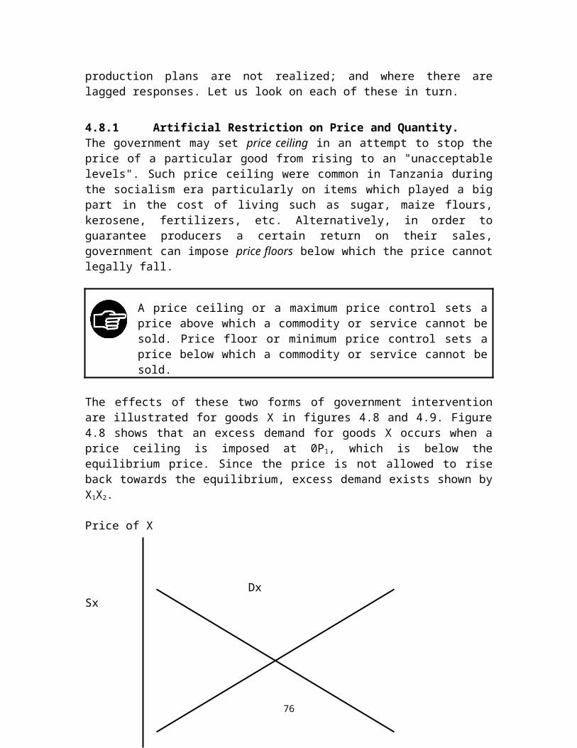
Table 6.1: Illustration of Diminishing Marginal Utility(1) Qx (2) TUx (3) MUx

1 102 15 53 21 64 28 75 36 86 46 107 54 88 54 09 49 -510 40 -911 25 -15

If we plot the total and marginal utility schedules of Table 6.1, we get the total and marginal utility curves. The saturation point (MUx = 0) is reached when the individual increases consumption of X from 7 to 8 units. The falling MUx curve illustrates the principle of diminishing marginal utility.

Figure 6.1: Total and Marginal Utility

6.5 Consumer Equilibrium The consumer equilibrium occurs where the ratio of marginal utility between different goods is equal to their respective price ratios. Consider a consumer who has to choose between two types of commodity, X and Y, which have prices Px and Py respectively. Let us assume that the individual is rational and so wishes to maximize utility subject to the size of his income. The consumer will be maximizing total utility when his income has been allocated in such a way that the utility to be derived from the consumption of one extra shilling's worth of X, is equal to the utility to be derived from the consumption of one extra shilling's worth of Y. In other words, the marginal utility per shilling of X is equal to the marginal utility per shilling of Y. Only when this is true it will not be

82

possible to increase total utility by switching expenditure from one commodity to the other. The condition for consumer's equilibrium can thus be written as follows;

(6.1)

Where; MUx = marginal utility of commodity X

MUy = marginal utility of commodity Y

Px = Price of commodity X

Py = Price of commodity Y

In the world with many commodities (e.g., A, B, C, D, up to Z), the above equation can be re-written as follows:

(6.1a)

Where, MU stands for marginal utility, P stands for price, and the subscript stands for individual commodities.

Example 6.1Miss Havijawa wishes to celebrate her birthday. She is thus contemplating on how many bottles of soda, beer and wine to buy in order to maximize her utility. Assume for simplicity that a bottle of beer costs T.Shs 2, a bottle of soda cost T.Shs 1 and a bottle of wine costs T.Shs 4. Assume further that her marginal utility figures for soda, beer and wine are as presented in table 6.2.

Table 6.2: Havijawa's Marginal Utility for Beverages Unit of the product MU of soda (utils) MU of beers (utils) MU of wine (utils)FirstSecondThirdForthFifthSixth

1098765

504030201612

604032242016

If Miss Havijawa has T.Shs 17 at disposal, what combination of beverages should she select in order to maximize her total utility?

83

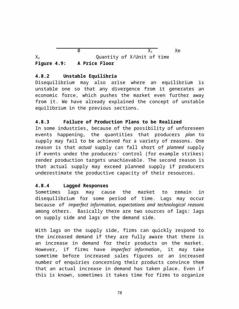
Establishing the maximum utility in this problem requires one to use equation 6.1. Note that since beverages are priced differently, you should compute the ratio of marginal utility for each bottle to its corresponding price. In other words, the ratio of marginal utility of soda to the price of soda is given as; MUsoda/T.Shs1, for beer, divide MU by 2 and lastly for wine divide MU by 4. Table 6.3 shows these calculations.

Table 6.3: Havijawa's Marginal Utilities per Shilling

Bottle (s) Soda Beer WineMU MU/shilling MU MU/shilling MU MU/shilling

FirstSecondThirdFourthFifthSixth

1098765

1098765

504030201612

2520151086

604032242016

15108654

Your next task now is to pick the highest possible value in the columns marked "MU/shilling" for each product. You should also keep in mind that Miss. Havijawa has only T.Shs 17 to spend.

Now, going across the first unit row, you will note that the greatest satisfaction per shilling will come from the first bottle of beer because it gives 25 MU/shilling. The second bottle of beer still yields more utility per shilling than either the first bottle of soda or the first bottle of wine. Automatically, the second bottle of beer will also be bought. This leaves Miss. Havijawa with only T.Shs 13 because the two bottles of beer cost T.Shs 4. The third bottle of beer gives Miss. Havijawa 15 MU/shilling just as the first bottle of wine as shown in the first row. Because the third bottle of beer and the first bottle of wine provide her with the same level of MU/shilling, Miss. Havijawa buys both of them this time, leaving her with only T.Shs 7. Then finally, Miss. Havijawa buys one bottle of beer (T.Shs 2), one bottle of wine (T.Shs 4) and one bottle of soda (T.Shs 1). This exhausts her budget.

You can easily see that if Miss. Havijawa wished to maximize utility, she would buy a total of 1 bottle of soda, 4 bottles of beer, and 2 bottles of wine. Total utility can be found by adding up the total utilities for each of the purchases. TUsoda = 10; TUbeer = 50+40+30+20=140; TUwine = 60+40=100; so TU = 10+140+100=250. To show this is a maximum, find MU/price for the last unit purchased of each beverage:

MUsoda / Pricesoda = 10/1 =10

MUbeer / Pricebeer = 20/2 =10

MUwine / Pricewine = 40/4=10

Since they are equal and all of the T.Shs 17 has been spent, this combination is the utility maximizing one.

84

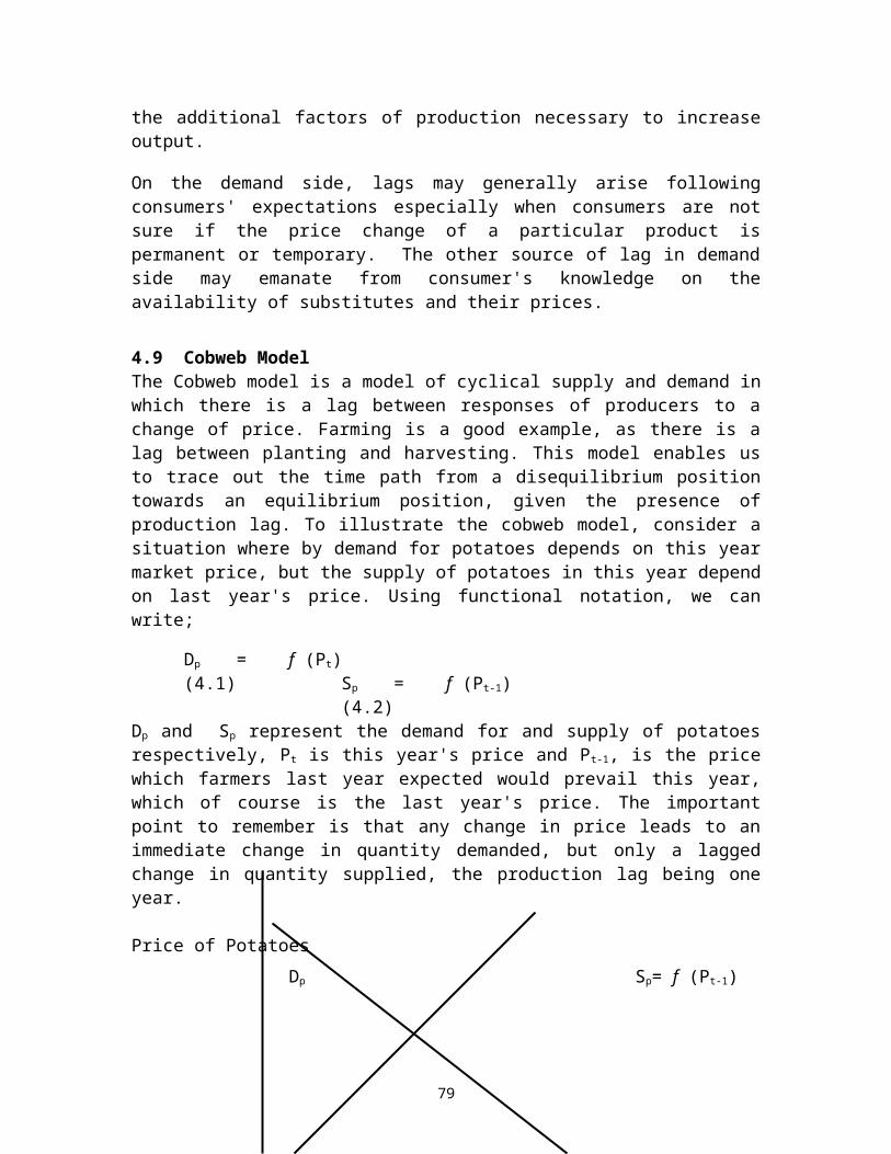
6.6 The Link between Demand Curve and Marginal Utility One of the main objectives of this lecture is to derive the demand curve using the concepts of marginal utility and the law of diminishing marginal utility. In order to derive the individual's demand curve for commodity X, let us now consider what happens to the consumer's equilibrium condition (section 6.4) when the price of X falls. It must be true (assuming the price of Y remains unchanged) that:

(6.2)

The consumer can now increase his or her total utility by consuming more units of goods X. This will have the effect of decreasing marginal utility of X because of the hypothesis of diminishing marginal utility. As a result, consumer will continue increasing his or her expenditure on X until the equality is restored. We now have the result we have been seeking: that a fall in the price of goods will, ceteris peribus, give rise to an increase in consumer's demand for it. That is to say, the demand curve slopes downward from left to the right. Note that equation 6.2 can be re-written as:

(6.2a)

This implies that each point on the demand curve; MUx=Px or MUy=Py. That is, we can draw the demand curve shown in figure 6.2 by using equation 6.2. Each point on the MUx

curve corresponds to a particular quantity level. At X1 the marginal utility of X is MU1, at X2 the marginal utility is MU2 and at X3 the marginal utility is MU3. Since we know that at equilibrium, the MUx = Px, and hence MU1 = P1, it follows automatically that P1

corresponds to Q1, P2 corresponds to Q2 and P3 corresponds to Q3. From this logic, one can unequivocally conclude that a demand curve is identical to a marginal utility curve when expressed in monetary units.

MU Price (T.Shs)

MU1 P1

MU2 P2

MU3 P3

MUx Dx

0 Q1 Q 2 Q3 Qty/time 0 Q1 Q2 Q3 Qty/time

85

Figure 6.2: Demand Curve from the Marginal Utility Curve

The negative slope of demand curve has an interesting consequences: all consumers pay less than they would be willing to pay for the total amount of any product that they consume. This takes us to the concept of consumer’s surplus.

6.7 Consumer Surplus

The consumer surplus is defined as the difference of what the consumer would be willing to pay which is the value of total utility he or she derives from consuming a commodity and what he or she actually pays which is his or her total expenditure on that commodity.

Table 6.4 gives the hypothetical data for the weekly consumption of beers by Mr. Edwards. Column 1 and 2 show various level of total utility and marginal utility enjoyed by Mr. Edwards. Assume that the market price for a bottle of beer is T.Shs.1, 000. It is clear from the table that Mr. Edwards will maximize total utility by consuming 3 bottles of beer because the marginal utility of the third bottle of beer is equal to the price. Note that Mr. Edwards makes a profit of T.Shs 2,000 when consuming the first bottle of beer. This is because Mr. Edwards’ marginal utility for the first bottle of beer is T.Shs 3,000 but he pays only T.Shs, 1,000. Note that we are using the condition: MUX=PX. Again, note that Mr. Edwards makes a profit of T.Shs 500 when consuming the second bottle of beer. This is because Mr. Edwards’ marginal utility for the second bottle of beer is T.Shs 1,500 but he pays only T.Shs, 1,000. These profits are called consumer’s surplus and are shown in the last column of table 6.4. The total surplus is thus, 2,500. We can arrive at the same total surplus, however, by first summing the maximum that Mr. Edwards would be willing to pay for all three bottles of beers he has bought (which is T.Shs 3,000+1,500+1,000=5,500) and then subtract T.Shs.3, 000 that he has actually paid (i.e, 1,000x3 bottles).

Table 6.4: Consumer SurplusBottles of

beersTotal Utility

T.Shs Marginal Utility

T.Shs Consumer surplus if each bottle

of beers costs T.Shs 100012345678910

3000450055006300690074007800810083508550

300015001000800600500400300250200

20005000.00

--------------

The data in columns (1) and (3) of table 6.4 gives the demand curve for bottles of beers. Again the condition MUX=PX tells us that when the price of bottle of beer is 3,000, Mr. Edwards will buy 1 bottle; when the price is 1500, Mr. Edwards will buy 2 bottles and when the price is 1000, Mr. Edwards will buy 3 bottles. The total consumption value is

86

the area below her demand curve, and the consumer surplus is that part of the area that lies above the price line. This is shown in figure 6.3. Note that shaded area gives the total consumer surplus (2000+500=2500)

Price (T.Shs) 3000

2500

2000 Demand Curve

1500

1000

0 1 2 3 Bottles of beers/time

Figure 6.3: Consumer's Surplus

Numerical exampleSuppose that the following equation represents a consumer’s demand curve for beer: Q=8000-2P, where Q is number of bottles of beers purchased when the price of is P per bottle. Find the consumer surplus if the price of beer is T.Shs 3000 per bottle

SolutionThe figure below shows the demand curve for beers. When the price of beer is T.Shs 3000, the consumer will buy 2000 bottles of beers. The consumer surplus is the area under the demand curve and above the price of T.Shs 3,000. Since the demand curve given in the exercise is a straight line, the area representing the consumer surplus is triangle CS.

87

Price 4,000

CS

3,000

0 2000 8,000 Bottle of beers

The area of CS is

6.8 Utility and Value: "The Paradox of Value"

Early economists struggling with the problem of what determines the relative prices of goods encountered what they called the paradox of value. The paradox goes as follows: many necessary products such as water, have prices that are low compared with the prices of luxurious products such as diamonds. Does it not seem odd, these economists asked:

Why is it that water, which is essential to life, has little market value while diamonds, which are much less important have higher market value?

Several explanations may explain this paradox. One of the explanations would be that the supply and demand curve for water intersects at a very low price while supply and demand for diamonds are such that the equilibrium price of diamond is very high. But one would ask, why supply and demand for water do intersects at such a low price? The answer would be that diamonds are very scarce and the cost of getting extra one is very high, while water is relatively abundant and cost little in many parts of the world. However this answer still does not consider the fact that water is more useful than world’s supply of diamond.

The resolution of paradox of value lies in the distinction between total and marginal utility. Utility of water as whole does not determine its price or demand, rather, the price of water is determined by its marginal utility, that is the usefulness of the last glass of water. Because there is so much water, the last glass sells very little. Therefore, we can say that: the more there is a commodity, the less is the relative desirability of its last unit.

88

It is thus clear that why an absolute necessity like air could become a free commodity. In both cases, it is the large quantities that pull the marginal utilities down and thus reduce the prices of these vital goods. The “law of marginal utility ” does not tell us such things as why diamonds are naturally less abundant on the earth than is water, but helps us to understand how this affects the value imputed to a given diamond and the price of diamonds in a market.

6.9 Total Utility, Elasticity and Marginal UtilityIn our daily life we normally distinguish between necessities such as food and water and luxurious goods such as diamonds, gold and other articles of ostentation. Quite often a frequent error occur when people try to use knowledge of total utility to predict elasticity of demand. It is argued that, since goods like diamonds can be given up, they have highly elastic demand; when the price rises consumer can stop buying them. Conversely, it is argued that indispensable goods such as food have highly inelastic demand, because whenever prices rise, consumers have no choice but to continue using them.

However, it is important to underscore that elasticity of demand depends on marginal utilities and not total utilities. The relevant question for predicting the response to a price change is " how much do they value all that they are consuming. When a price of a product rises, each consumer will reduce his or her purchase of that commodity until he or she values the last unit consumed at the price that must be paid for that unit.

Elasticity of demand depends on the value consumers place on having a bit more or a bit less of a commodity (marginal utility); it has no necessary relation to the value they place on the total consumption of a commodity (total utility)

6.10 Some Criticisms on the Cardinalist Theory The idea that utility could be measured in unit dates back in the nineteenth century. It was popularized by economists such as Leon Walras, Stanley Jevons and Alfred Marshall. Economists at that particular time believed that utility could similarly be measured in its own units called “utils”. Those economists are known as cardinalists because they believed cardinal numbers could be used to express utility measurements. For example, a consumer may obtain 10 utils from dancing but 2 utils from attending a political rally. The cardinalist would conclude from this that the consumer obtains five times utility from dancing as from attending a political rally.

Can you measure utility in the way addressed by the cardinalists?

Utility, however, is an abstract, subjective concept and there are three major problems involved in trying to measure it. These problems are:

89

(a) It is difficult to find an appropriate unit of measurement. By the way, if we define a unit of utility as a "util", what is a util? Moreover, how do we calculate the number of utils enjoyed by an individual in a moment of time?

(b) Yet, another problem is connected to the interpersonal comparison of utility. Are 10 utils enjoyed by one person equivalent to 10 utils enjoyed by another person? In other words, can we make interpersonal comparison of utility?

(c) To measure the utility derived by an individual in consuming a commodity requires that all the other factors, which affect level of satisfaction, be held constant and it is clearly impossible to carry out such a controlled experiment. There are too many other factors (economic, social and psychological) which influence an individual level of utility.

If utility is not measurable where do we stand?

In the 1930s, a group of economists pioneered by the British economist in the name of John Hicks had the view that utility could not be measured cardinally and that cardinal measurement was not necessary for a theory of consumer behavior. As a result, it was argued that an individual could rank bundles of goods in order of preference and say that he/she derives more utility from one bundle than from another, or that the consumer derives equal utility from two or more bundles. For example, a consumer may prefer dancing to political rally but the consumer will be completely unable to attach a numerical measure to the degree of preference. In this case, only ordinal numbers; first, second, third and so on can be used to measure utility. In the light of weaknesses contained in the cardinalist approach studied in this lecture, we move on to the ordinalist approach in the next lecture.

SUMMARY1. Cardinal utility theory states that the utility (satisfaction) gained

from a particular good or service can be measured in numbers and

90

can therefore be compared across persons. The theoretical unit of measurement of utility is the ‘util’. Cardinal utility theory, despite its limitation, is useful in explaining why the individual demand curve slopes downward from left to the right. Central to this theory are the concepts of marginal utility and the hypothesis of diminishing of marginal utility.

2. Utility may be defined as the benefit or satisfaction derived from the consumption of a product. According to cardinalists, utility can be measured using cardinal numbers.

3. Marginal utility is the extra utility derived from the consumption of one more unit of a good, the consumption of all other goods remaining unchanged.

4. The hypothesis of diminishing marginal utility states that as the quantity of goods consumed by an individual increases, the marginal utility of that good, will eventually decline

5. A consumer is said to reach equilibrium when the utility he or she derives from the last shilling spent on each product is equal. Another way of putting this phrase is that the marginal utilities derived from the last unit of each product consumed will be proportional to their prices.

6. Demand curves have negative slopes because, when the price of one product, let say X, falls, each consumer restores equilibrium by increasing purchases of X sufficiently to restore the ratio of X's marginal utility to its new lower price (MUx/Px), to the ratio that has been achieved for all other products.

7. Consumer surplus is defined as the difference of what the consumer would be willing to pay which is the value of total utility he or she derives from consuming a commodity and what he or she actually pays which is his or her total expenditure on that commodity

8. The resolution of paradox of value lies in the distinction between total and marginal utility. Utility of water as whole does not determine its price or demand, rather, the price of water is determined by its marginal utility, that is the usefulness of the last glass of water. Because there is so much water, the last glass sells very little

EXERCISES

91

1. Write short notes on the following:(a) Cardinal utility(b) The law of diminishing marginal utility(c) Consumer surplus(d) Paradox of value

2. How is the law of demand derived from the law of diminishing marginal utility?

3. What constraints does the consumer face in seeking to maximize the

total utility from his/her expenditures?

4. In this lecture we have assumed that utility is cardinally measurable. However, it remains questionable that utility can be measured cardinally. The cardinal utility theory is thus futile. Explain.

5. Suppose that the demand function Prawns is given by Q= 10-2P0.5. Calculate the consumer surplus at prices T.Shs 4.00 and T.Shs 1.00

6. Suppose that the marginal utility of Mr.Bernard for product A is defined by the function MUA = 10 -X, where X is the number of units of commodity A. Similarly, the marginal utility for commodity B is given by the following equation: MUB = 21-2Y, where Y is the number of units of commodity B. Assume that the price of A = price of B = T.Shs 1. How much of A and B would Mr.Bernard buy if he had T.Shs 7 to spend?

7. A consumer Marginal utilities for commodities X and Y are given as MUx = 40-10X and MUy = 30-6Y respectively.

(a) What is the consumer's marginal rate of substitution (MRS) in consumption at the consumption basket X=3, Y=4?

(b) If Px =10 and Py=6, is the basket a consumption equilibrium? Make sure that you show all the steps.

8. Suppose that the marginal utility of apples is 5A, where A is the number of apples consumed, i.e. MUA = 5A, and MUB = 3B is the marginal utility of bananas. Find the marginal rate of substitution of apples for bananas. Next suppose that the price of an apple is 25 cents and the price of a banana is 10 cents. If the consumer is maximizing utility, what is the ratio of apples to bananas consumed? Finally, suppose that the consumer has 5 dollars to spend on apples and bananas. How many of each does the consumer choose?

9. * The table below shows the marginal utility schedule for orange (X)

92

and apples (Y). Suppose that oranges and apples are the only two commodities available, the price of orange is T.Shs 10 the price of apple is T.Shs 10, and individual income is T.Shs 800 per time period and all is spent. Quantity Marginal utility of X Marginal Utility of Y

10203040506070

1101009080706050

19017015013012010080

(a) Indicate how this individual should spend her income in order to maximize utility

(b) What is the total amount of utility received by this individual when she/he is in equilibrium?

(c) Show the equilibrium of this consumer.

10. The table below gives the total and marginal utilities for good X and good Y for a representative consumer.

QX MUX MUX/PX

(PX=4)QY MUY MUY/PY

(PY=2)12345

10080604020

12345

8060402010

403020105

(a) Fill in the MUX/PX column when PX=4 (i.e., column 3)(b) How many units of good X and good Y will this utility

maximizing consumer buy if the level of income is T.Shs 14(c) How much total utility will this consumer enjoy at this level of

consumption of X and Y(d) Is this consumer maximizing utility? Explain.

93

LECTURE SEVEN CONSUMER BEHAVIOR:

ORDINAL UTILITY THEORY

7.1 IntroductionIn lecture six, we have presented a theory of consumer behavior from the cardinalists' perspective. This lecture provides an alternative explanation of the theory of consumer behaviour based on ordinal perspective. The main ordinal theories that we are going to learn in this lecture are: Indifference Curve approach and the Revealed Preference Theory.

In presenting and explaining the ordinal theories, we shall first outline the assumptions behind the indifference curve approach. Secondly, we will derive the equilibrium of the consumer, a concept which combines together the budget line and indifference curves. This will enable us to derive the demand curve introduced in lecture two. We will also provide a critique on the indifference curve approach. In the final section of this lecture, we are going to explain in brief the main gist of the revealed preference theory.

ObjectivesAfter reading this lecture, you should be able to:(i) Outline the assumptions behind the difference curve

approach;(ii) Define an indifference curve and set out three main

properties of indifference curves;(iii) Derive the budget line from the knowledge of prices of two

goods and the consumer's income;(iv) Explain the concept of consumer's equilibrium;(v) Derive the income and price consumption curves;(vi) Use indifference curve analysis to distinguish between

normal, inferior, and Giffen goods;(vii) Derive the demand curve from the price consumption curve;(viii) Outline the basics of the Revealed Preference Theory.(ix) Derive the demand curve from the revealed preference

theory

7.2 Ordinal Utility TheoryOrdinal utility theory takes the position that utility cannot be measured cardinally. It is taken axiomatically that the consumer can rank his or her preferences (order the various "basket of goods") according to the satisfaction of each basket. Consumer needs not to know precisely the amount of satisfaction. It suffices that a consumer expresses his/her preferences for the various bundles of commodities using only ordinal numbers such as first, second, third, fourth, etc.

94

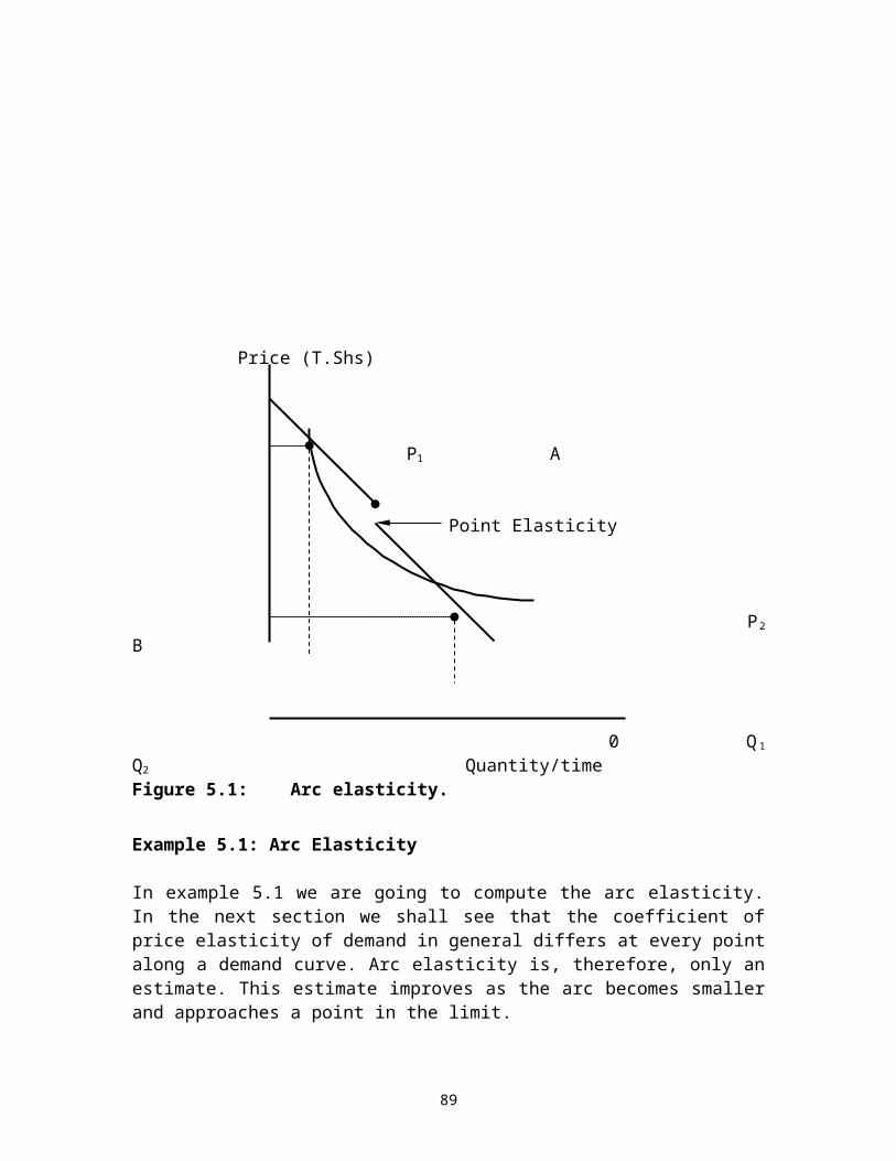
7.3 Indifference Curve ApproachIndifference curve approach is basically concerned with income and substitution effects of a change in price. By looking at substitution and income effects, we can easily see why the quantity demanded of commodity declines as its price rises. The indifference curve approach is based on the following assumptions:

(i) Preferences are complete: this means that the consumer is able to compare and rank all possible baskets. For example, given two commodity bundles (A and B), consumer will prefer A to B, B to A, or will be indifferent between the two bundles. The word indifferent means that a consumer will be equally satisfied with either commodity A or B.

(ii) Preferences are transitive: this means that preferences are consistent, in that if bundle A is preferred to bundle B and bundle B is preferred to bundle C, then we should be able to conclude that bundle A is preferred to bundle C.

(iii) More is preferred to less: this means that all goods are desirable, and that the consumer will always prefer to have more of a good. This assumption is made for pedagogic reasons; it simplifies the graphical analysis.

(iv) Diminishing marginal rate of substitution: this means that indifferences curves are convex, and that the slope of the indifference curve increases (become less negative) as we move down along the curve. As a consumer moves down along her indifference curve she is willing to give up fewer units of the good on the vertical axis in exchange for one more unit of the good on the horizontal axis. This assumption also means balanced market baskets are preferred to the baskets that have a lot of one good and very little of the other good.

Numerical exampleSuppose that utility function is given as . Marginal utilities of X and Y are expressed by the following equations:

(a) Show that a consumer with this utility function believes that more is better for each good

(b) Show that the marginal utility of X is diminishing(c) Show that the marginal utility of Y is diminishing

Solution

95

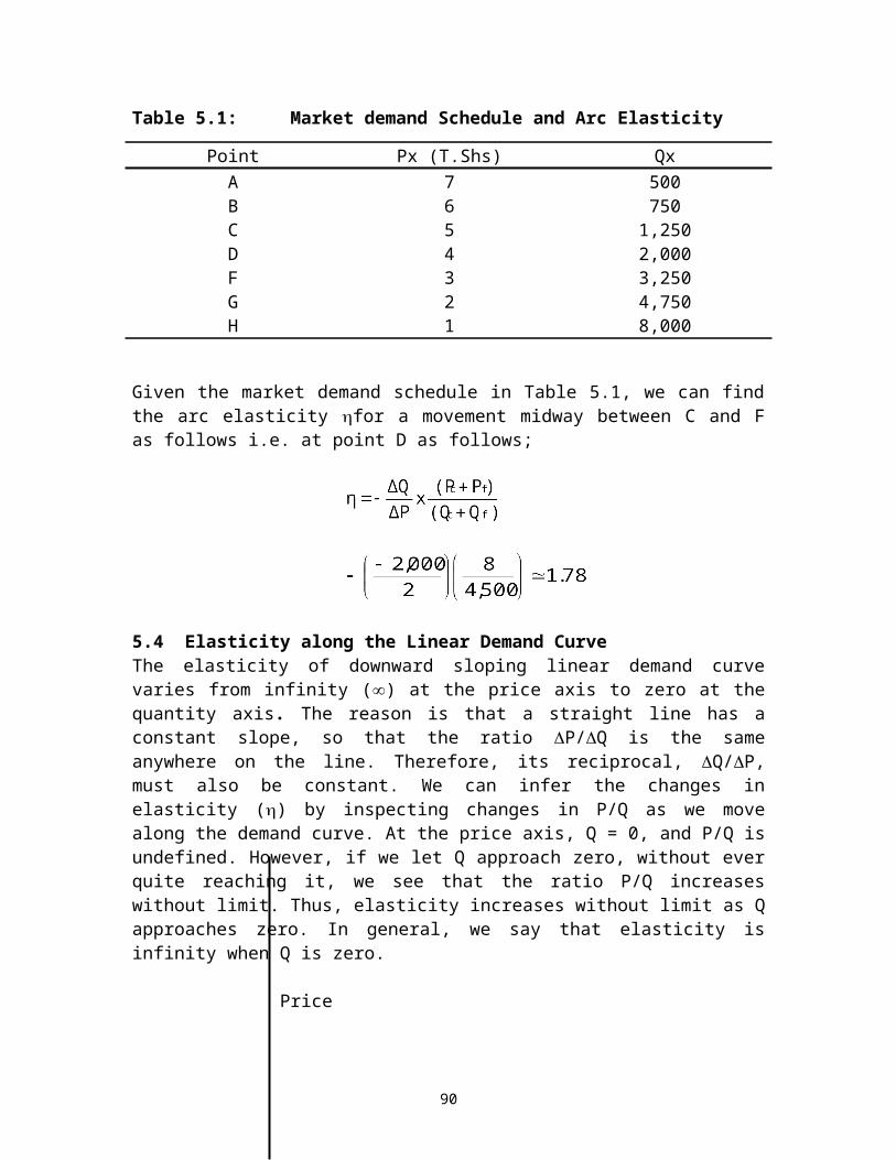
(a) By the examining the utility function, we can see that U increases whenever X or Y increases. This means that the consumer likes more of each good. More is better simply means that the marginal utility is positive. Therefore, we can also see that for each good by looking at the marginal utilities MUX and MUY. When the consumer is buying positive amounts of X and Y, both the marginal utilities are positive, and so the consumer’s utility.

(b) Examine . As X increases (holding Y constant), MUX falls.

Therefore, the consumer’s marginal utility of X is diminishing.

(c) Examine . As Y increases, MUY falls. Therefore, the marginal

of Y is diminishing.

7.3.1 Indifference CurvesAn indifference curve is the locus of points that join different combinations of two goods (X and Y), which yield the same level utility to the consumer. Figure 7.1 shows the consumer's preferences for X and Y. The vertical axis measures the quantity of goods Y and the horizontal axis measures the quantity of goods X. Every point on figure 7.1 represents some combination of X and Y. Points close to the origin like point A, represent very small quantities of X and Y; points further away from the origin represent bigger quantities.

Y

D

2 B

E

1 C IC2

A IC1

0 1 2 X

Figure 7.1: An Indifference Map

Since combinations B (2 units of Y and 1 units of X) and C (1 units of Y and 2 units of X) are on the same indifference curve, the consumer is said to be indifferent between them. That is to say, both combinations yield the same utility to the consumer.

96

Combination D, however, is on the higher indifference curve than B or C. Since D is higher than B or C, the consumer prefers D to either B or C. The following are the characteristics of indifference curves:(i) Indifference curves do not intersect. The reason is that if they do

intersect, the point of their intersection would imply two different levels of satisfaction, which is impossible. Figure 7.2 shows two intersecting indifferent curves. Since both combinations of A and C are on the same indifference curve, the consumer must be indifferent between them. However, combinations B and C are on the same indifference curve, so the consumer must be indifferent between them as well. By the axiom of transitivity, the consumer must be indifferent between A and B which is unreasonable because bundle A contains more of Y and X than bundle B. This kind of confusion occurs whenever indifference curves cross.

Y

A

B Y* C

IC2

IC1

0 X* X

Figure 7.2: Intersecting Indifference Curves

(ii) Indifference curves are convex to the origin. This implies that the slope of an indifference curve decreases in absolute term as we move along the curve from the left downward to the right: the marginal rate of substitution of commodities is diminishing. This axiom of decreasing marginal rate of substitution expresses the observed behavioral rule that the number of units of Y the consumer is willing to sacrifice in order to obtain an additional unit of X decreases as he/she moves down an indifference curve. Figure 7.3 shows that the movement from point A to point B requires more Y to be sacrificed. However, the movement from point B to point C requires less of Y to be sacrificed, i.e. ΔY>ΔY*.

97

Y

Y3 A

ΔY

B Y2

ΔY* Y1 C ΔX ΔX*

0 X1 X2 X3 XFigure 7.3: Convexity of an Indifference Curve

This axiom (i.e. convexity axiom) implies that commodities can substitute one another, but are not perfect substitute. If the commodities are perfect substitutes the indifference curve becomes a straight line with negative slope. On the other hand, whenever the commodities are complements the indifference curve takes the shape of the right angle.

(iii) Indifference Curves have negative slope. The negative slope denotes that if the quantity of one commodity decreases, the quantity of the other must increase if the consumer is to stay on the same level of satisfaction. (See figure 7.3).

Indifference curves exhibit three basic characteristics: they are negatively sloped, they are convex to the origin, and they cannot intersect.

7.3.2 The Marginal Rate of SubstitutionThe marginal rate of substitution of X for Y (MRSxy) refers to the amount of commodity Y that a consumer is willing to give up in order to gain one additional unit of commodity X (and still remain on the same indifference curve). As the individual moves down the indifference curve the MRSxy diminishes. This is because an individual is to give up less and less of commodity Y in order to gain each additional unit of commodity X (i.e., the MRSxy diminishes). Put it differently, as individual demands more and more of commodity X, commodity Y becomes more valuable. So he/she is willing to give up less

98

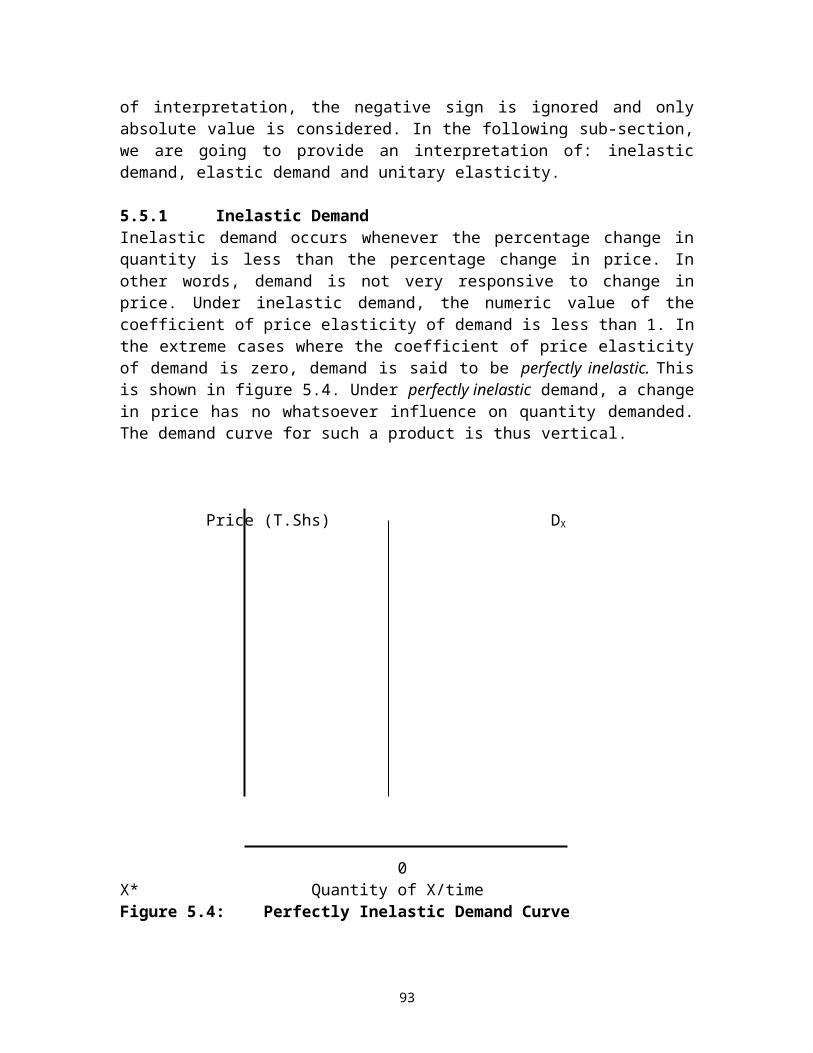
and less of commodity Y to get each additional unit of commodity X. As a result, the MRSxy diminishes.

7.4 Budget Line and Consumer's EquilibriumAn indifference map described above tells us a person's preferences concerning various combinations of goods and services. But preferences alone do not explain consumer's entire behavior. Individual choices are also affected by budget constraints, which limit people's ability to consume in light of the prices they must pay for goods and services.

7.4.1 The Budget LineThe budget line shows all the different combinations of commodities that a consumer can purchase, given his money income and the prices of commodities. The budget line can be written as follows:

Px.X + Py.Y = M (7.1)Where: Px is the price of commodity X,

Py is the price of commodity YM is the consumer’s income

Subtracting Px.X from both sides of the equation 7.1 givesPy.Y = M - Px.X (7.2)

Divide each side of equation 7.2 by Py yields;

(7.3)

Slope is given by the change in Y due to change in X;

- (7.4)

ExampleSuppose that the consumer’s money income is T.Shs, 1000, price of commodity X is T.Shs 100, and the price of commodity Y is T.Shs 200.

(a) Indicate the quantity of X the consumer could purchase if she spent all her income on commodity X

(b) Indicate the quantity of Y the consumer could purchase if she spent all her income on commodity Y

(c) What is the equation for the budget line?(d) Find the slope of the budget line.

Solution(a) The quantity of X would be: 1000/100=10(b) The quantity of Y would be: 1000/200=5(c) Equation for the budget line would be: 100PX+200PY=1000

99

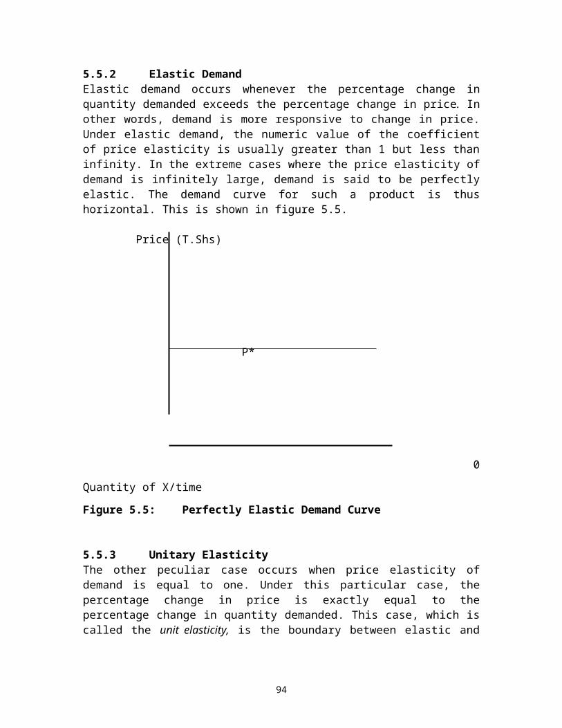
(d) Slope of the budget line is –½

7.4.2 Consumer's EquilibriumEquilibrium of the consumer occurs at the point of where the slope of the budget line is exactly equal to the slope of an indifference curve. Figure 7.4 shows the indifference map and the budget line on the same diagram. Assuming that all the income is spent on commodity X and Y, the consumer will choose the combination represented by point A. This is the point where the budget line is just tangent to an indifference curve. Point A is called the consumer equilibrium point.

Y

M/PY

YE A

I3

I2

I1

0 XE M/PX XFigure 7.4: Consumer's Equilibrium

Since the budget line is tangent to the indifference curve at point A, it must be true that the slope of the indifference curve (the marginal rate of substitution) is equal to the slope of the budget line at that point. Note that if an individual consumer spends all of his/her income (M) on commodity X, he/she will purchase M/PX units of commodity X. Similarly, if he/she spend all of his/her income on commodity Y, he/she will purchase M/PY units of commodity Y. By joining these two extreme points (i.e., M/PX and M/PY), we get the budget line shown in figure 7.4

Example: Consumer equilibriumA consumer purchases two goods, food and clothing. The utility function is U(F,C), where F denotes the amount of food consumed and C the amount of clothing. The marginal utilities are MUF=C and MUC=F. The price of food is PF=2,000, the price of clothing is PC=4,000, and the income M=80,000. Find the equilibrium of this consumer.

100

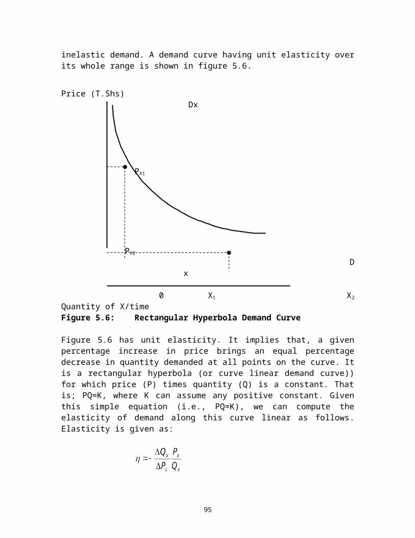
SolutionThe indifference curve represented by U (F, C) = FC is convex to the origin and do not intersect the axes. The equilibrium condition says that the slope of indifference curve must be tangent to the budget line. The budget line is given as:

2,000F+4,000C=8,000We know that the tangent condition requires that:

Or more simply, F=2C

So, we have two equations with two unknowns: 2,000F+4,000C=8,000 (i.e., the budget line) and F=2C (coming from the tangency condition). If we substitute F=2C into the equation for the budget line, we get:

2,000(2C) +4,000C=80,000

Solving for F and C, yields: C=10 and F=20. So, the optimal bundles involve purchase of 20 units of food and 10 units of clothes.

7.5 Income Changes and the Budget LineChanges in consumer's income (i.e., increase) will shift the budget line upward remaining parallel to the original budget line. Similarly, when the consumer's income falls, the budget line will shift downward remaining parallel to the original budget line. This is shown in figure 7.5. Assume that the initial level of income is M1. Change in money income from M1 to M2 shifts the budget line from M/PY1, M/PX1 to M/PY2, M/PX2. Analogously, change in money income from M2 to M3 shifts the budget line from M/PY2,

M/PX2 to M/PY3, M/PX3.

101

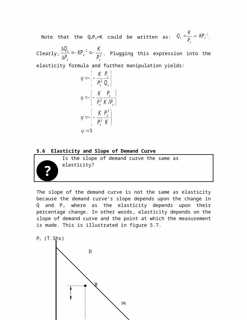
Y Income consumption curve (ICC)

M/PY3

M/PY2 B A IC3 M/PY1 IC2

C IC1

0 M/PX1 M/PX2 M/PX3 X

Income Engel’s curve

M3

M2

M1

0 C A B XFigure 7.5: Income Consumption Curve and Engel’s Curve

By changing the consumer’s money income while keeping constant his tastes and prices of X and Y, we have automatically derived consumer’s income consumption curve and Engel curve in Fig 7.5. The income-consumption curve is the locus of points of consumer equilibrium resulting when only the consumer’s income is varied. The Engel curve shows the amount of commodity that the consumer would purchase per unit of time at various levels of his or her income.

102

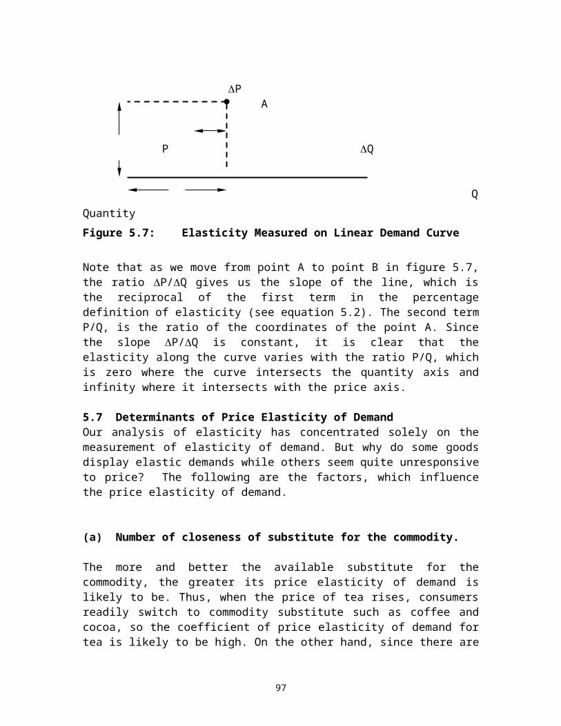
7.6 Price Change and the Budget LineTo examine the effect of a price change and the budget line, suppose that the price of X falls, ceteris peribus. The effect of a fall in the price of the commodity from PX1 to PX2 is reflected in pivotal shift of the budget line from M/PY, M/PX1 to M/PY to M/PX2. As the price of X falls, it becomes relatively cheaper and Y becomes relatively more expensive. The consumer is therefore induced to substitute X for Y. This is called the substitution effect. Y

M/PY

0 M/PX1 M/PX2 M/PX3 XFigure 7.6: Effect of a Price Change on the Budget Line

We now introduce indifference curves in figure 7.6 in order to uncover the price consumption curve. This is shown in figure 7.7. In particular, when the price of commodity X falls from PX1 to PX2, while the price of commodity Y remains unchanged, consumer moves to a new indifference curve, which is tangent to the new budget line. This is shown in figure 7.7 as a movement from point A to point B. Similarly, when the price of commodity X falls from PX2 to PX3, while the price of commodity Y remains unchanged, consumer moves to a new indifference curve, which is tangent to the new budget line. This is shown in figure 7.7 as a movement from point B to point C. Along the line ABC there are many points of consumer’s equilibrium. By joining all points along the line ABC, we get the price consumption curve.

103

Y

MPY

PCC C B

A

0 M/PX1 M/PX2 MPX3 XFigure 7.7: The Price Consumption Curve

7.8 Separation of Income and Substitution EffectsThe movement from one point of consumer equilibrium to another can be broken down into a substitution effect and an income effect. The substitution effect can be explained as follows. When the price of a commodity falls, the consumer substitutes this cheaper commodity for others whose prices have remained unchanged. That is, the substitution effect increases the quantity demanded of the commodity whose price has fallen if that commodity is a normal good. On the other hand, if the commodity is Giffen, less of that commodity will be purchased. The income effect can be explained as follows. If the price of a commodity falls (ceteris peribus), the purchasing power of the individual's constant money income increases. When this occurs, the individual tends to buy more of the commodity whose price has fallen if the commodity is a normal good, less of it if the commodity is an inferior one.

It is possible to identify these two effects graphically and this is done in Figure 7.8. The first step is to eliminate the income effect: to do this we assume that, accompanying the fall in the price of X, there is compensating variation in income which leaves the consumer at the level of utility as before the price change. In Figure 7.8, the original budget line is labeled M/PY1, M/PX1. To make the compensating variation in income, we shift the budget line to the left, keeping it parallel to M/PY1, M/PX1 until it becomes tangential to the original indifference curve IC1. This is the budget line M/PY2, M/PX2. The movement from A1 to A3 is the substitution effect. The movement from point A3 to A2 is the income effect.

104

Y

M/PY1

M/PY2

Y1 A1

Y2 A2

A3

Y3 IC2

IC1

M/PX1 M/PX2 M/PX1*

0 X1 X3 X2 XFigure 7.8: Income and Substitution Effects for a Normal Good

It is important to note that income effect can work in either way- when the consumer income rises, more or less of commodity can be bought. If more is bought, the commodity is said to be a normal good; this is the case illustrated in figure 7.8, where both X and Y are normal goods. If less is bought the commodity is said to be an inferior one; this is illustrated in Figure 7.9 where the movement from A3 to A2 is the negative income effect. If the consumer buys less, and the income effect is actually bigger than the substitution effects so that the overall effect of the price fall is a decrease in consumption, then the commodity is said to be Giffen good. This is illustrated in Figure 7.10 where the negative income effect (A3 to A2) is bigger than the substitution effect (A1 to A3)

105

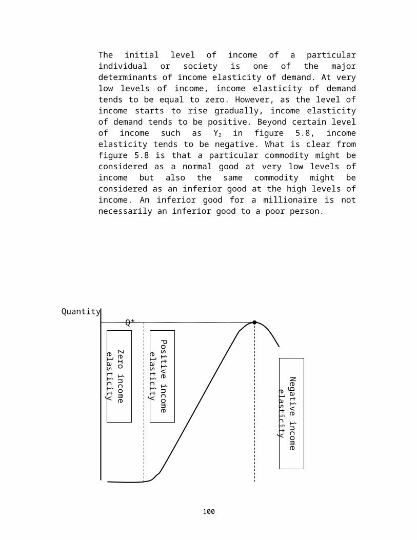
Y

M/PY1

M/PY2 A2

A1 IC2

A3

IC1

0 X1 X2 X3 M/PX1 M/PX2 M/PX1* XFigure 7.9: Income and Substitution Effects for an Inferior Good

For normal goods, an increase in consumer's real income leads to an increase in demand. For inferior goods, an increase in consumer's real income leads to a fall in demand. Giffen goods are strongly inferior goods with an upward sloping demand curve.

Y

M/PY1

A2

M/PY2 IC2

A1

A3

IC1

0 X2 X1 X3 M/PX1 M/PX2 M/PX1* X

106

Figure 7.10: Income and Substitution Effects for a Giffen Good

Numerical Example: Income and substitution effects Consider the following utility function: U(X, Y) =XY. The marginal utility of X is Y and the marginal utility of Y is X. Suppose that individual’s money income is T.Shs 80,000 per month and that the prices of commodity Y and X are T.Shs 1,000 and T.Shs 4,000 respectively. Suppose that price of commodity X falls from T.Shs 4,000 to T.Shs 1,000.

(a) Obtain numerical value of income and substitution effects. (b) Graph your results.

SolutionFirst stepFirst find the initial consumption bundle. Let us call this initial point of consumption bundle, point A when the price of commodity Y is T.Shs.1, 000 and price of commodity X is T.Shs.4, 000. It is clear that an optimal consumption bundle will be on the budget line is given as:

1,000Y+4,000X=80,000Second, the tangency condition must hold. That is, at the point of optimum consumption bundle, the following condition must hold: MUX/MUY=PX/PY. Given the above utility function, tangency condition is:

We can simplify the above condition and re-write it as: Y=4X. So, we have two equations with two unknowns. The first equation is 1,000Y+4,000X=8,000 coming from the budget line and the second equation is Y=4X coming from the tangency condition. Now plug the tangency condition into the budget line as follows:

1,000Y+4,000X =80,0001,000(4X) +4,000X=80,0008,000X=80,000X=10, Y=40

Note that the initial level of utility is 400. This is obtained by plugging X=10 and Y=40 into the utility function U=XY.

Second stepFind the optimal bundle when the price of X falls from T.Shs 4,000 to T.Shs.1, 000. What this means is that we repeat the first step but now using T.Shs 1,000 as the price of commodity X. It is clear that an optimal consumption bundle will be on the budget line:

1,000Y+1,000X=80,000Second, the tangency condition must hold. That is, at the point of optimum consumption bundle, the following condition must hold: MUX/MUY=PX/PY. Given the above utility function, tangency condition is:

107

We can simplify the above condition and re-write it as: Y=X. So, we have two equations with two unknowns. The first equation is 1,000Y+1,000X=80,000 coming from the budget line and the second equation is Y=X coming from the tangency condition. Now plug the tangency condition into the budget line as follows:

1,000X +1,000X =80,0002,000X=80,000X=40, Y=40

Note that the new level of utility is 1,600. This is obtained by plugging X=40 and Y=40 into the utility function U=XY.

Y U1=400 U2=1600

40 A C

20 B

0 10 20 40 X

Third stepFind the substitution effects (i.e., the decomposition of consumption bundle denoted by point B). The substitution effects must satisfy two conditions. First, substitution effect (point B) must lie on the original indifference curve. That is, the amount of X and Y must yield the level of utility equal to U1=400. Second, point B and the budget line must be tangent to one another. The final price of X determines the decomposition of the slope of the budget line. The tangency occurs when MUX/MUY=PX/PY or when Y/X=1/1. The tangency condition requires that Y=X.

We now have all the information that is required to find the substitution effect. We know that the purchase of commodity X and Y at point B must allow the consumer to reach the initial level of utility XY=400 and that the tangency condition with the new price of X will be satisfied Y=X. These two equations imply that the substitution effects will contain Y=20; X=20. These two baskets are computed as follows:

Plug Y=X into XY=400X2=400X=20, Y=20

108

7.9 Demand Curve from Price Consumption Curve The price consumption curve is used to derive the consumer's demand curve. This is done in Figure 7.11 where X is normal goods. As the price of X is reduced from 0PX1 to 0PX2 to 0PX3, the quantity demanded of X expands from 0X1 to 0X2 to 0X3. The resulting demand curve is downward sloping from left to the right.

Y

M/PY

PCC

I3 I2

I1

0 M/PX1 M/PX2 M/PX3 X

PX

DX

PX1

PX2

PX3

DX

0 X1 X2 X3 Quantity of X/unit of time Figure 7.11: Demand Curve from Price Consumption Curve

The upper diagram in figure 7.11 shows that the budget line pivots as the price of commodity X falls whilst the price of commodity Y is held constant. Associated with each budget line is an optimal quantity of both goods, as shown by the point of tangency

109

between the indifference curves and the budget lines. Note that with each reduction in price, the consumer moves to a higher indifference curve; implying that more of good X is purchased. In the lower diagram, the price consumption curve is transcribed into the demand curve.

Can you derive the demand curve for Giffen goods from the PCC?

Numerical example: derivation of demand curve from indifference curve approach. Consider the following utility function: U(X, Y) =XY. The marginal utilities of this utility function are: MUX=Y and MUY=X.

(a) Find the demand curve for good X(b) Is good X a normal good? (c) What can you say about the cross price elasticity of demand of X with respect to

the price of commodity Y?

Solution(a) The consumer is said to be in equilibrium when

Substitute the marginal utilities: MUX=Y and MUY=X in the above equilibrium condition.

Then, plug into the budget line as follows:

2PXX=M

Thus, the demand curve for commodity X is:

(b) Yes, commodity X is a normal good. Holding the price of commodity X constant, an increase in income (i.e., M) would result into an increases demand for X.

(c) The cross-price elasticity of demand of X with respect to the price of

commodity Y is zero. This is because demand for X (i.e., )does not

depend on the price of Y.

110

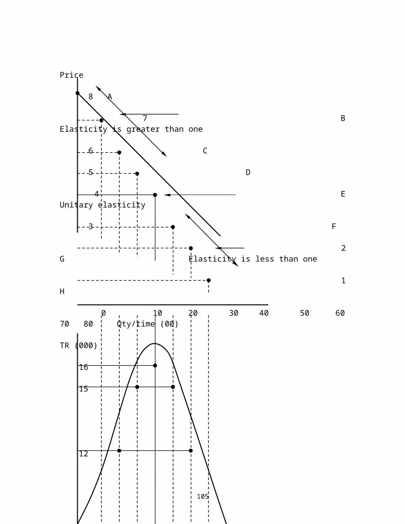
7.10 Critique of the Indifference Curve ApproachThe indifference curve analysis has been a major advance in the field of consumer's demand. The assumptions of this theory are less stringent than for the cardinal utility approach. However, the main weakness of this theory is its axiomatic assumption of the existence and the convexity of the indifference curves. The theory does not establish either the existence or the shape of the indifference curves. It assumes that they exist and have the required shape of convexity.

Furthermore, it is questionable whether the consumer is able to order his preferences as precisely and rationally as the theory implies. Also the preference of the consumer changes continuously under the influence of various factors, so that any ordering of these preferences, even if possible should be considered for the short run. Finally, this theory has retained most of the weaknesses of cardinalist school with the strong assumption of rationality and the concept of marginal utility implicit in the definition of the marginal rate of substitution.

7.11 Revealed Preference TheorySo far, you have learned how to find a consumer’s equilibrium given indifference curves and the budget line. In other words, if you know how consumer ranks baskets, you can determine the optimal basket for any budget constraint the consumer faces.

Suppose that indifference curves are not known, can you infer how the consumer ranks basket by observing his/her behavior as his/her budget line changes? In other words, can the consumer choices of basket reveal information about his preferences?

The Revealed Preference Theory, pioneered by American economist Paul Samuelson, is a method by which it is possible to reveal the preferences of consumers by observing their purchasing habits. Revealed preference theory came about because the theories of consumer demand described in the previous sections are based on a diminishing marginal rate of substitution (MRS). The diminishing MRS is based on the assumption that consumers make consumption decisions based on their intent to maximize their utility. While utility maximization is not a controversial assumption, the underlying utility functions cannot be measured with great certainty. Revealed preference theory is meant to reconcile demand theory by creating a means to define utility functions by observing behavior.

The main idea behind Revealed Preference Theory is very simple. If the consumer chooses basket A when basket B is affordable, then we say that basket A is preferred to basket B. Therefore if the consumer ever purchases basket B then it must be the case that the basket A is unaffordable. This theory can help us to derive indifference curves which adhere to the already developed indifference curve approach described in the previous sections. The theory of revealed preferences is based on the following assumptions:

(a) The individual tastes do not change over the period under consideration

111

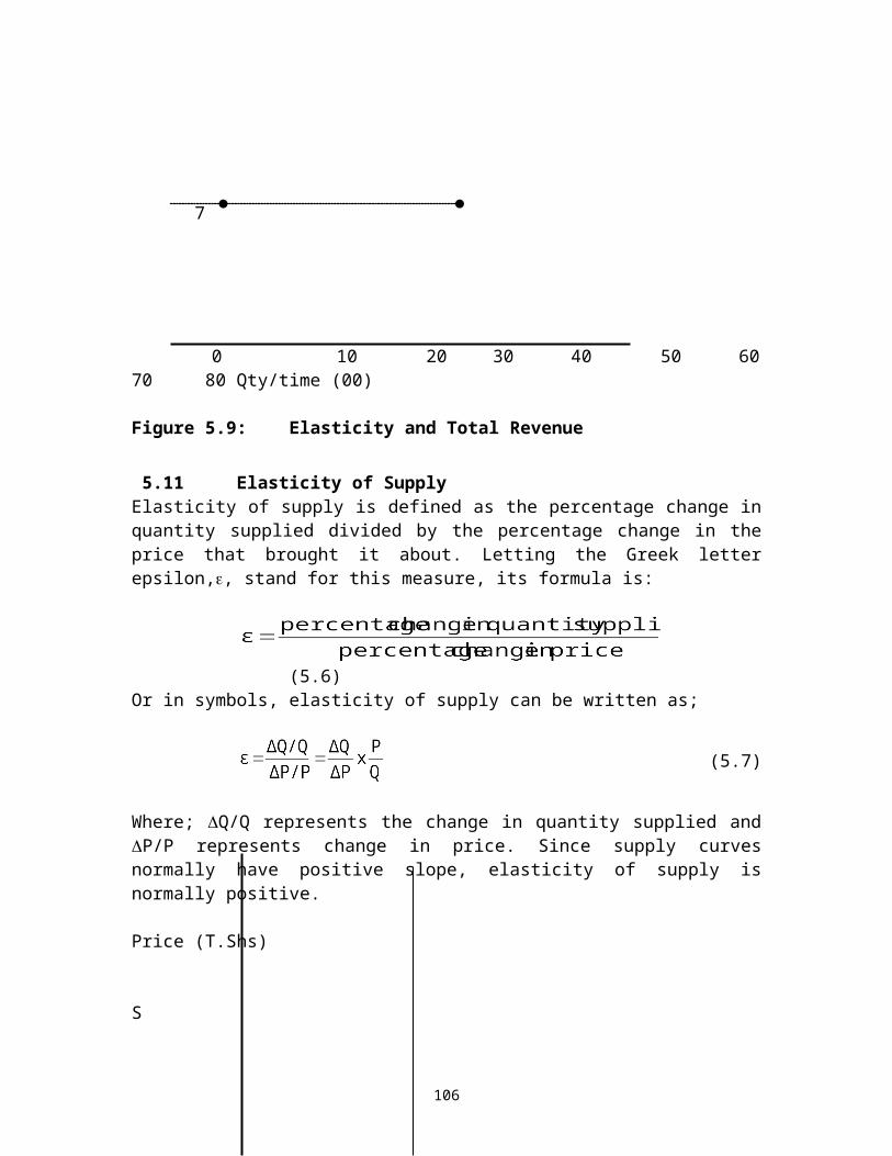
(b) Preferences are consistent in that if the consumer is observed to prefer bundle A to bundle B, then this consumer will never prefer B to A

(c) Preferences are transitive, in that if bundle A is preferred to bundle B and bundle B is preferred to bundle C, then we should be able to conclude that bundle A is preferred to bundle C.

(d) The consumer can be induced to purchase on basket of goods if its price is made sufficiently attractive.

Y G

A

B C F D H E

A* B* 0 XFigure 7.12: Revealed Preference Theory

Figure 7.12 illustrates how consumer’s behaviour can reveal information about preferences. Given the initial level of income and the price of two goods, the consumer faces AA*as the budget line. When the budget line is AA*, the consumer chooses point D. Suppose that prices (both PX and PY) and income change so that the new budget line becomes BB* and the consumer chooses point F. What can we deduce from the behaviour of this consumer towards his preferences?

The following points are worth noting. First, since the consumer chooses basket D (i.e., point D) when he could afford any other baskets on the budget line AA* or inside the budget line AA* his behaviour reveals that D is preferred to F. The consumer has revealed how he ranks D and F. Consider basket C (i.e., point C) on the budget line AA*. Since this consumer chooses D when he could afford F, we know that the consumer prefers either D or C. Moreover, since C lies to the northeast of F, C must be strongly preferred to D. Then by transitivity axiom, basket D must be strongly preferred to basket F.

112

Second, the behaviour of this consumer also helps us to learn about the shape of the indifference curve through point D. All baskets to the north, east, and north east of D are strongly preferred to D (including basket in the shaded area). On the other hand, point D is strongly preferred to all baskets below it, and at least as preferred as any other basket along the segment AE. We also know that D is strongly preferred to any basket on the segment EB*because D is strongly preferred to F, and F is weakly preferred as any basket on the budget line BB*.Therefore, although we do not know exactly where the indifference curves through D lies, it must pass somewhere through GDH and AEB*

The revealed preference theory can demonstrate that the consumer's demand curve for normal goods will be downward sloping from left to the right so long as the consumer is observed to increase purchases of goods when his or her income increases. Consider Figure 7.13. Suppose that the line AB is a consumer's budget line and that point C is the combination of X and Y that the consumer prefers to all the other attainable combinations in the triangle A0B. If the price of commodity X falls, the budget line will shift to AB'. We can eliminate the income effect of this price change, as before, by shifting the budget line back to A'B'' (parallel to AB'). Having revealed point C preferred to all other points in the triangle A0B, the consumer will clearly not choose any points along the section A'C. The consumer must, therefore, choose a point on the line CB'', say point D.

Note that the movement from C to D is the substitution effect of a price fall; according to this effect, the consumer purchases more of X following the price fall. If, as we have assumed, the income effect also causes the consumer to buy more of X, then he or she must end up at a point on the budget line AB' somewhere to the right of point D, say at E. Since the price of X has caused the consumer to buy more, ceteris peribus, we can conclude that the consumer's demand curve slopes downward from left to the right. This is shown in figure 7.13.

113

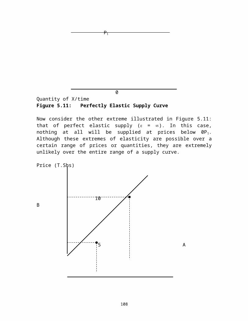
Y

A

A'

C E

D

0 X1 B X2 B'' B' X

PX

PX1 C

PX2 E

Demand curve

0 X1 X2 XFigure 7.13: Demand Curve from the Revealed Preference Theory

It is important to note that, in arriving at the above conclusion, no mention was made of the abstract concept of utility. The Revealed Preference Theory can be described as a more objective approach to the theory of consumer behavior. However, it cannot be denied that some subjective valuation is implicit when consumers reveal their preferences for goods.

114

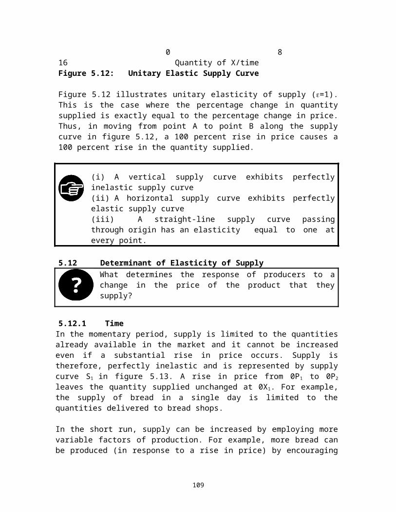
SUMMARY1. Ordinal utility theory takes the position that utility cannot be

measured cardinally. It is taken axiomatically that the consumer can rank his or her preferences according to the satisfaction of each basket.

2. The theory of consumer behaviour based on ordinalist approach is built on the assumption that people behave rationally in an attempt to maximize the satisfaction that they can obtain by purchasing a particular combinations of good and services

3. Consumers make their choices by comparing commodity bundles. Their preferences are assumed to be complete and transitive. In addition we have also assumed that more of each commodity is always preferred to the less

4. Indifference curves, which represent all combinations of goods and services that give the same level of satisfaction, are downward sloping and cannot intersect one another.

5. Marginal rate of substitution of X for Y is the amount of Y that a person is willing to give up to obtain one additional unit of X. The marginal rate of substitution diminishes as we move down along an indifference curve.

6. Budget line represents all combinations of goods for which consumer spend all his or her income. Budget line shifts outward in response to an increase in consumer's income, but it pivots and rotate when the price of one commodity changes while keeping constant the price of the other commodity and income level.

7. When the consumer maximises satisfaction by consuming some of each of the two types of goods, the marginal rate of substitution is equal to the ratio of prices of the two types of goods.

8. The main weakness of indifference curve approach is that it does not establish either the existence or the shape of the indifference curves. It assumes that they exist and have the required shape of convexity. Moreover, indifference curve approach has retained most of the weaknesses of cardinalist school with the strong assumption of rationality and the concept of marginal utility implicit in the definition of the marginal rate of substitution

9. We can use " The Theory of Revealed Preference" to derive a consumer's downward sloping demand curve without using subjectivity of utility nor the assumption of diminishing marginal utility. All that is required is that the consumer behaved consistently

115

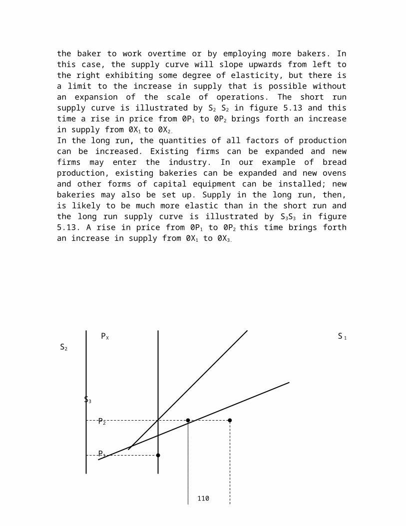
EXERCISES1. Write short notes on the following:

(a) Ordinal utility theory(b) Indifference curves(c) Budget line(d) Compensated demand curves(e) Axioms of consumer preferences(f) Marginal rate of substitution

2. (a) Since indifference curves cannot intersect must they be

parallel? Yes or No? Explain.(b) On the same set of axes, draw indifference curves showing

increasing MRSxy as we move down the indifference curve. (c)

3. (a) Distinguish between inferior goods and giffen goods. With the help of indifference curves show which of these is an exception to the law of demand.

(b) “Price effect is a combination of income and substitution effects.” Is this proposition true or false? Explain with the help of diagrams.

4. What is the difference between the ordinal utility and cardinal utility? Explain why the assumption of cardinal utility is not needed in order to rank consumers’ choices.

5. * Explain why a person’s marginal rate of substitution between two goods must equal the ratio of the price of the goods for the person to achieve maximum satisfaction?

6. Outline the main differences between indifference curve approach and revealed preference theory.

7. Consider the following utility function U (X, Y) = X2/3Y4/5

(a) Find expressions for marginal utilities(b) Find an expression for the marginal rate of substitution

8.* Can a set of indifference curves be upward sloping? If so, what would this tell you about the two goods?

9.* Describe the indifference curves associated with two goods that are perfect substitutes. What if the two goods are complements?

10.* John is willing to trade one bottle of Coke for one bottle of Pepsi, or one bottle of Pepsi for one bottle of Coke.

(a) What is John’s marginal rate of substitution (b) Draw a set of indifference curves for John

116

(c) Draw the two budget lines with different slopes and illustrate the utility maximizing choice. What conclusion can you draw?

11. * Suppose that an individual allocates his entire budget on the two goods, food and clothing. Can both good be inferior? Explain

12*. The level of utility increases as an individual moves downward along the demand curve. True or false? Explain.

13*. A consumer purchases two goods, food and clothing. The utility function is U(X, Y), where X denotes the amount of food consumed and Y the amount of clothing. The marginal utilities are MUX=Y and MUY=X. the price of food is PX, the price of clothing is PY, and the income is I. (a) Show that the equation for the demand curve for food is

(b) Is food a normal good?

14. Consider the following utility function: U(X, Y) = XY+X. The marginal utilities of X and Y are MUX=Y+1 and MUY=X respectively. The price of commodity X is T.Shs.1.00 per unit, and the price of commodity Y is T.Shs.2.00 per unit. Suppose that Isaac’s income is T.Shs.22.00, answer the following questions.

(a) Suppose that Isaac is currently spending all of his income. He is buying 8 units of X. How many units of commodity Y is he consuming?

(b) Plot Mr. Isaac’s budget line. Place the number of units of Y on the vertical axis and X on the horizontal axis. Plot Isaac’s consumption basket

(c) Draw the indifference curve associated with a utility level of 32 and another associated with the utility level of 64. Are indifference curves convex to the origin?

(d) Find the marginal rate of substitution of X forY when utility is maximized.

(e) Does Isaac has a diminishing of X for Y? Show graphically and algebraically.

117

LECTURE EIGHTUNCERTAINTY AND CONSUMER BEHAVIOUR

8.1 Introduction

In both lectures 6 and 7, among other things, we have derived the consumer’s demand curve under the assumption that the prices of commodities and the level of income are known with certainty. In practice, such assumptions are far from reality in a risky world. In a risky world, consumers are typically uncertain of changes in the price of the commodities they buy; and moreover, consumers are uncertain about the future levels of their income. On the other hand, given the level of income and market prices, the level of utility derived from different commodity bundles is also uncertain. Given the nature of uncertainty associated with the level of utility several questions naturally arise. Should a consumer buy the low priced product or a high priced product? And what are some of the risks involved in each type of the product? And how might consumer reduce risk while making choices? The major purpose of this lecture is to answer these questions.

ObjectivesBy the end of this lecture, you should be able to:

(i) Describe how risk is measured(ii) Describe how do consumers make choices when the outcome

of any choice is uncertain(iii) Explain what is meant by expected utility(iv) Explain the patterns of consumers preferences when

uncertainty or risk is involved(v) Determine the amount of money that individuals are willing to

pay to reduce risk.(vi) Explain how consumers can diversify/reduce risk

8.2 Risk /Uncertain ChoiceThe terms “risk” and “uncertainty” are used interchangeably in this lecture.6 Risk commodities refer to those commodities which are characterized by uncertainties of future market values and of the size of the future income, caused by the fluctuation in the market prices. Examples of these commodites are shares in the the stock markets and lottery. A stock market is a market where stocks and shares are bought and sold. In order to study consumer behaviour towards uncertain choice or choice characterized by risks; we need to understand three important concepts. These are: probability, expected value and standard deviation.

8.2.1 ProbabilityThe likelihood of a specific event or outcome, measured by the ratio of specific events or outcomes to the total number of possible events or outcomes is called probabilitly. Probabilities are expressed as numbers between 0 and 1. The probability of an impossible

6 Risk is present when future events occur with measurable probability. Uncertainty is present when the likelihood of future events is indefinite or incalculable. See, Frank, H.Knight (1921) Risk, Uncertainty and Profits, Boston, MA: Hart, Schaffner & Marx; Houghton Mifflin Company

118

event is 0, while an event that is certain to occur has a probability of 1. In short, probability is a measure of certainty on a scale of 0 to 1.

The probability of flipping a coin that it will show up a head is ½, because there is 1 way of getting a head and the total number of possible outcomes is 2 (a head or tail). We write P (heads) = ½. Analogously, the probability of flipping a coin that it will show up a tail is ½. The probability of something not happening is 1 minus the probability that it will happen.

To apply the concept of probability in this lecture, consider an individual who is contemplating to buy a share in one of the “Soft Drinks Companies” registered in the stock market. In this example, shares are commodities just like any other commodities we have studied in the previous lectures. The only difference is that shares are characterized by risk as explained in section 8.2. Let us assume that the price per share is T.Shs 3,000. Let us further assume that if the company is successful in terms of making profit at the end of the year, the value of price per share will increase from T.Shs 3,000 to T.Shs 4,000. On the other hand, if the company is unsuccessful in the sense that it makes losses, the value of price per share will fall from T.Shs 3,000 to T.Shs 2,000.

Suppose it is known that out of 100 registered companies in the stock market last year, 25 companies made profits while 75 made losses. We can use this information to compute probabilities of success (i.e., making profits) and failure (i.e., making losses). In short, probability of success is computed as 25/100 and probability of failure is computed as 75/100. These probabilities are called objective probabilities because they are based directly on the frequency of historical performance.

There is one question here, however. Suppose that the information on the past historical performance of the Soft Drinks Companies is unknown, how can we compute probabilities? The answer is that we usually use subjective probabilities. A subjective probability is the perception that an outcome will occur. This perception may be based on person’s judgement but not necessarily on the frequency with which a particular outcome has actually occurred. In a situation where probabilities are subjectively determined, different people may attach different probabilities to different outcomes and thereby making different choices.

When probabilities are used to describe a particular event, they are describing the likelihood of that event happening. The value of a probability will range from 0 to 1.

8.2.2 Expected valueThe expected value associated with an uncertain situation is a weighted average of the values associated with possible outcome. The probabilities of each outcome are used as

119

weights. Returning to our previous example, buying a share in the company had two possible outcomes: either the company is successful or unsuccessful. The expected value can be expressed as:

Expected Value=(Probability of success 4,000) + (Probability of Failure 2,000) =

Thus, the expected share price (i.e., expected average share price) is T.Shs 2,500.

But how would an individual make decision when faced with more than one choice?

To answer this question, consider an individual who is contemplating to buy shares from one of the two companies (Soft Drinks and Hard Drinks) but is uncertain about which of the two companies is less risky. For simplicity, the share price and the associated probabilities in the Soft Drinks Company are the same as those shown in the previous example. However, the share price for Hard Drinks Company is different. Suppose that the share price in the Hard Drink Company is T.Shs 5,000 if the company makes profit and T.Shs 1,875 if the company makes losses. Suppose that out of 100 Hard Drinks Company registered in stock market last year, 20 companies made profit and 80 companies made losses. The expected value of share price for Hard Drinks Company can be computed in the same way as what we have done for the case of Soft Drinks Company. This information is summarized in Table 8.1

Table 8.1: Share pricesSoft Drink Company Hard Drinks Company

Probability Share price Probability Share price Successful 1/4 4,000 1/5 5,000

Failure 3/4 2,000 4/5 1,875Expected value 2,500 2,500

Both companies have the same expected values, although the possible payoff for each company is different. To reiterate, the possible payoff shows that if the soft drink company makes profits the share price would increase to 4,000 while that of hard drink would increase to 5,000. On the other hand, if both Soft Drink and Hard Drink companies make losses, the payoffs are 2,000 and 1,875 respectively.

120

How do consumers make choices if the expected values are the same like those shown in table 8.1?

In order to overcome the above problem, we introduce the concept of standard deviation.

8.2.3 Standard Deviation Standard deviation is statistical measurement of dispersion about an average, which depicts how widely returns vary over a certain period of time. In short, when the standard deviation is large, buying share in the company is more risky assuming that an individual is risk averse. The lower the standard deviation, the lower is the degree of risk.

Before computing standard deviation one should first calculate deviation. Deviation is the difference between an observed value and the expected value of a variable. That is, deviation is used to denote the difference of a variable from its mean. If we denote the observed value as and expected value (i.e., mean) as , deviation can be written as:

Applying the above formula in the information given in table 8.1, one can compute deviation as shown in table 8.2. Note that

Table 8.2: Deviation Soft Drinks Company Hard Drinks Company

Share price Deviation Share price Deviation Successful 4,000 1,500 5,000 2,500

Failure 2,000 -500 1,875 -625

However, the problem with deviations is that they can result into both positive and negative values as shown in Table 8.2. This implies that the average of the probability-weighted deviation is always zero. This can be shown as follows:

(i) For a Soft Drink Company, the average of a weighted deviation is

(ii) For a Hard Drink Company, the average of a weighted deviation is

To resolve this problem, we need to square the deviation. This is shown in table 8.3. The next thing that you are supposed to do is to compute the weighted average deviation of the squared deviation. Thus:(i) The weighted average of the squared deviation for the Soft Drinks Industry is:

==750,000

121

The standard deviation for Soft Drinks Company is equal to the square root of 750,000. That is:

(ii) The weighted average of squared deviation for the Hard Drinks Company is:

==1,562,500

The standard deviation for Hard Drinks Company is equal to the square root of 1,562,500. That is:

Table 8.3: Standard Deviation Soft Drinks Company Hard Drinks Company

Share price Deviation squared

Share price Deviation squared

Successful 4,000 2,250,000 5,000 6,250,000Failure 2,000 250,000 1,875 390,625

Weighted average deviation squared

750,000 1,562,500

Standard deviation 866 1250

Which of the two companies would you buy a share?

The Soft Drink Company is less risky than the Hard Drink Company because the standard deviation of share price is much lower. 8.3 Preferences towards Risk

In the previous section we have shown that high standard deviation in share price is risky. In the real world however, individual preferences towards risky differ widely. Some individuals are risk lovers while others are risk averse. Yet, some individual are indifferent in taking risk. In this section, we introduce the concept of utility to the analysis of uncertain choice. In particular, this section shows the relationship between the shape of utility function and degree of risk.

8.3.1 Risk-averse IndividualAn individual is said to be risk averse if he/she prefers a certain given income to a risky income with the same expected value. Usually such a person has a diminishing marginal utility of income. Figure 8.1 describes individual preferences towards risk shown by the curve 0AFDB. The vertical axis shows the level of utility that an individual is deriving from different levels of income plotted on the horizontal axis. Note that the marginal

122

utility is diminishing as the level of income increases. That is, when income increases from 7,000 to 8,000 the marginal utility is 2,700; whereas the marginal utility declines to 200 as the level of income increases from 8,000 to 10,000.

Utility

8,900 B

8,700 D

7,450 F C

6,000 A

0 7,000 8,000 9,000 IncomeFigure 8.1: Risk Averse Individual Suppose that an individual with a certain amount of income (T.Shs, 8,000) is contemplating to buy a share, which would give him/her an extra 1,000 with a probability of ½ or loss of 1,000 with a probability of ½. Figure 8.1 shows that the utility associated with 7,000 is 6,000 and the utility level associated with an income 9,000 is 8,900. The expected utility must be compared with utility is 8,700 which corresponds to the certain income (i.e., T.Shs 8,000). The expected utility E (U) is therefore given as:

Expected Utility = ½Utility (6,000) + ½Utility (8,900) = 3,000+4450= 7,450

Expected income = ½ Income (7,000) + ½Income (9,000) =3,500+4,500=8,000

Expected utility is a weighted average of the utilities of the different prospects, i.e., weighted by their respective probabilities. Since the expected level of utility (i.e., 7,450) is less than the level of utility attached to the income of 8,000, this individual will not buy a share. This is the case of a risk-averse individual.

Expected utility is the sum of utilities associated with all possible outcomes, weighted by the probability that each outcome will occur.

123

8.3.2 Risk Loving IndividualAn individual is said to be risk lover if he/she prefers an uncertain income to a certain income, even if the expected value of uncertain income is less than that of a certain income. Figure 8.2 shows individual preference towards the risk loving person. The vertical axis shows the level of utility that an individual is deriving from different levels of income plotted on the horizontal axis. Note that the marginal utility is increasing as the level of income increases. That is, when income increases from 7,000 to 8,000 the marginal utility is 2,000; whereas the marginal utility rose to 4,000 as the level of income increases from 8,000 to 9,000.

Utility 12,000 E

9,000 C F

8,000 D 7,000 A 0 7,000 8,000 9,000 IncomeFigure 8.2: Risk Loving IndividualSuppose that an individual with a certain amount of income (T.Shs, 8,000) is contemplating to buy a share, which would give him/her an extra 1,000 with a probability of ½ or loss of 1,000 with a probability of ½. Figure 8.2 shows that the utility associated with 7,000 is 7,000 and the utility level associated with an income 9,000 is 12,000. The expected utility must be compared with utility is 8,000 which corresponds to the certain income (i.e., T.Shs 8,000). The expected utility E (U) is therefore given as:

Expected Utility = 0.5(7,000) +0.5(12,000)= 9,000

The expected level of income is given as:E (Income) = 0.5(7,000) +0.5(9,000)

= 8,000

8.3.2 Risk NeutralAn individual is said to be risk neutral if he/she is indifferent between a certain income and uncertain with the same expected value. Figure 8.3 shows the risk loving person shows the preferences of the risk neutral individual. As you can see, the marginal utility is constant for a risk neutral individual.

124

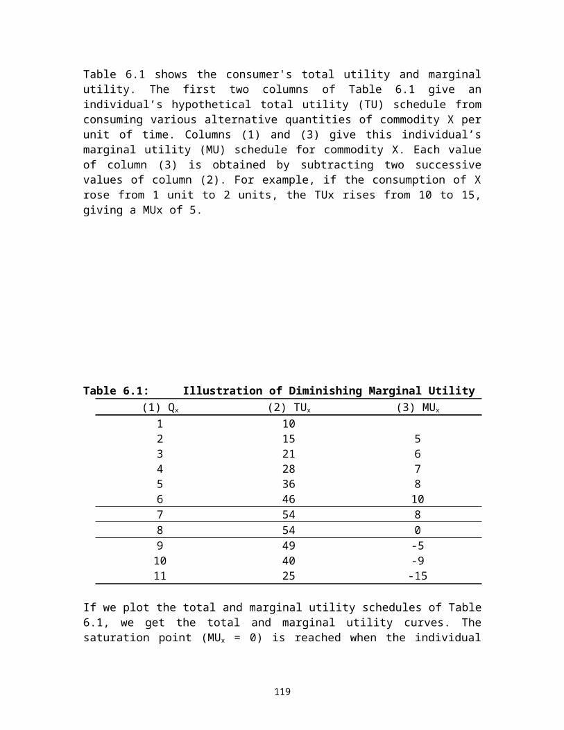
Expected Utility

9,000

8,000

7,000

0 7,000 8,000 9,000 IncomeFigure 8.3: Risk Neutral Individual

(i) An individual is a risk averse if he/she prefers certain income to a risky income with the expected value.

(ii) An individual is risk neutral if he/she is indifferent between a certain income to uncertain income with the same expected value

(iii) An individual is a risk lover if he/she prefers a risky income to a certain income with the same expected value.

8.4 Risk aversion and Indifference curvesThis section describes risk aversion within the context of the indifference curves. Indifference curves here relate the expected income and variability of income, where the latter is measured by standard deviation. Figure 8.4 shows indifference curves for an individual who is highly risk averse. Note that indifference curves are upward sloping. Because risk is undesirable, the greater the amount of risk, the greater the expected income needed to make the individual equally well off.

Expected Income U1 U2

125

0 Standard deviation of income Figure 8.4: Risk Aversion and Indifference CurvesFigure 8.4 shows a person who is highly risk averse. An increase in the standard deviation of income requires a large increase in expected income if she/he has to remain equally well off. Figure 8.5 shows an individual who is slightly risk averse. An increase in standard deviation of income requires only a small increase in the expected income if she/has to remain equally well off. Expected income

U2

U1

0 Standard deviation of income Figure 8.5: Risk Aversion and Indifference Curves8.5 Reducing RiskThere are various ways in which consumers may adopt to avoid risk. However, in this course unit we are going to concentrate on two items: diversification and insurance.

126

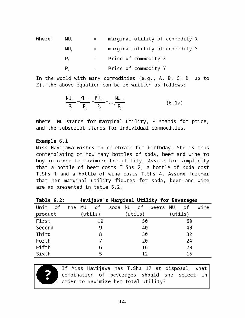
8.5.1 DiversificationDiversification is especially important for people who are investing in the stock market. Since price in stock markets are volatile, risks can be reduced though not eliminated by investing in portfolio of more than one asset. Portfolio is a collection of investments held by an institution or a private individual. The assets in the portfolio could include stocks, bonds, options, real estate, futures contracts, production facilities, or any other item that is expected to retain its value. Like wise, you can diversify risk in Mutual fund. Mutual fund is an organization that pools fund of individual investor to buy a large number of different stocks or other financial assets.

It is important to stress that not all risk are diversifiable in the stock market. Stock prices are to some extent positively correlated variables. That is, they tend to move in the same direction in response to change in economic conditions. For example, an economic recession usually tends to reduce profits of many companies. This implies that even with a diversified portfolio of stocks, investor still face some risk.

8.5.2 Insurance

Insurance is a system under which individuals, businesses, and other organizations or entities, in exchange for payment of a sum of money (called a premium), are guaranteed compensation for losses resulting from certain perils under specified conditions in a contract. An individual contract is known as an insurance policy, and the periodic payment is known as an insurance premium. In that contract, one party agrees to pay another party's financial loss resulting from a specified event.

Suppose individual’s income is 9,000 but he/she is facing the prospect of losing 2,000. The probability of losing T.Shs 2,000 is ½. If this individual does not insure, the expected utility is given by point C in figure 8.1. If we draw the horizontal line CF in figure 8.1, we note that point F corresponds to the same level of utility as point C. Thus, if the insurance company gives this individual a guarantee income of 8000-CF, the utility of this individual would be given by point F. Provided that the insurance company guarantees this individual that he/she would get T.Shs 9,000 in the event of loss, this individual would be prepared to pay the insurance company a premium equal to:

9,000-(8,000-CF)=1,000+CF

On average, the insurance company would pay this individual 1,000, and so the expected profits of an insurance company is CF. The income 8,000-CF is called the certainty equivalent value of a risk situation. It is that level of income offered with certainty that yields the same utility as the expected utility with risks. The difference between the expected income (8000) and the certainty equivalent income is called the cost of risk. In our example, the cost of risk is CF. The amount of money that a risk-averse person would pay to avoid taking a risk is called risk premium. The size of the risk premium depends on the magnitude and probability of the alternatives that the person faces.

127

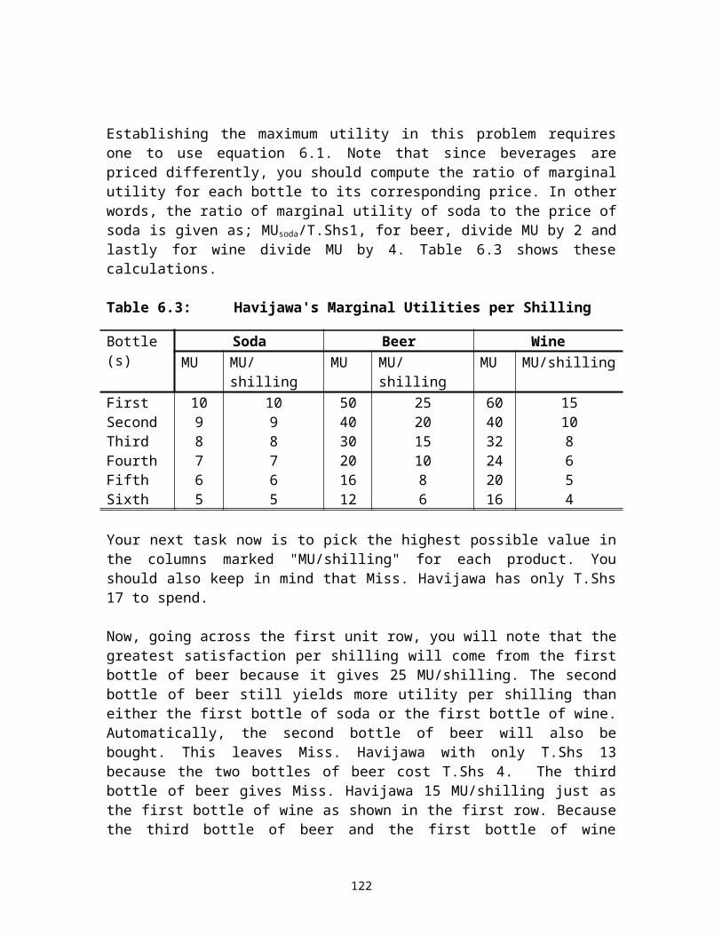
Despite the fact that the major objective of insurance companies is to supply insurance services to overcome the risks, the cost of risk premium is sometimes too prohibitive for genuine clients. There are two major problems why risk premium is too high. These are: moral hazard and adverse selections.

8.5.2.1 Adverse Selection

Adverse selection is the tendency of higher risk persons or groups to seek coverage more than less risky persons or groups. Adverse selection arises from the fact that the seller of insurance has relevant information that the buyer does not have, or vice versa. As a result, there is a tendency for buyers or sellers to exploit these asymmetries in information to their own advantage. When adverse selection increases, insurance companies experience greater expenses and may raise rates.

8.5.2.2 Moral Hazard

Moral hazard occurs when someone insured against risks purposely engage in risky behaviour, knowing that any costs incurred will be compensated by the insurer. Put differently, moral hazard is a situation in which one of the parties to an agreement has an incentive, after the agreement is made, to act in a manner that brings additional benefits to himself or herself at the expense of the other party. It is difficult for the principal to detect and punish opportunistic behaviour on the part of the agent.

SUMMARY1. The likelihood of a specific event or outcome, measured by the ratio of

specific events or outcomes to the total number of possible events or

128

outcomes is called probability. Probabilities are expressed as numbers between 0 and 1. The probability of an impossible event is 0, while an event that is certain to occur has a probability of 1.

2. The expected value associated with an uncertain situation is a weighted average of the values associated with possible outcome. The probabilities of each outcome are used as weights.

3. Standard deviation is measure of the variation of measurements around their average value, defined as the square root of the sum of squared differences between the average value and all observed values

4. An individual is said to be risk averse if he/she prefers a certain given income to a risky income with the same expected value. Usually such a person has a diminishing marginal utility of income.

5. An individual is said to be risk lover if he/she prefers an uncertain income to a certain income, even if the expected value of uncertain income is less than that of a certain income.

6. An individual is risk neutral if he/she is indifferent between a certain income to uncertain income with the same expected value

7. Risk premium is the amount of money that a risk-averse person would pay to avoid taking a risk. The size of the risk premium depends on the magnitude and probability of the alternatives that the person faces.

8. Diversification is especially important for people who are investing in the stock market. Since price in stock markets are volatile, risks can be reduced though not eliminated by investing in portfolio of more than one asset. Portfolio is a collection of investments held by an institution or a private individual. The assets in the portfolio could include stocks, bonds, options, real estate, futures contracts, production facilities, or any other item that is expected to retain its value.

9. Insurance is a system under which individuals, businesses, and other

organizations or entities, in exchange for payment of a sum of money (called a premium), are guaranteed compensation for losses resulting from certain perils under specified conditions in a contract. Insurance has two major problems. These are adverse selection and moral hazards.

EXERCISES

129

1. Write short notes on the following concepts(a) Expected utility(b) Adverse selection(c) Moral hazard(d) Risk loving, Risk Neutral and Risk averse individuals(e) Diminishing marginal utility of income(f) Risk premium(g) Insurance

2. Draw a utility function, which shows that an individual is a risk averse at low levels of income and risk lover at higher levels of income. Explain why such a utility function might reasonably describe individual preferences?

3*. Consider buying a lottery with three possible outcome: 250, will be received with probability 0.2; 200 with a probability 0.30; and 100 with probability of 0.50

(a) What is the expected value of the lottery?(b) What is the variance of the outcomes of the lottery?(c) Would a risk neutral person buy the lottery?

4. Suppose that Naomi’s utility function is given by , where Y is the annual income in thousands of shillings.

(a) Is Naomi risk loving, risk neutral or risk averse? Explain

(b) Suppose that Naomi is currently earning an income of T.Shs 40,000 (Y=40) and can earn that income next year with certainty. She wants to buy a share that offers 0.6 probability of earning T.Shs 44,000 and a 0.4 probability of earning T.Shs 33,000. How would you advise her?

(c) Given your answer in part (b) would Naomi be willing to buy insurance to protect against the variable income associated with fluctuation in share prices? If so, how much would she be willing to pay for that insurance?

5*. Mr Sunday is considering buying shares in either company A or company B. If he buys shares in company A, there is a 0.90 probability that he will earn zero profit and a 0.10 probability that he will earn a profit of T.Shs 400 at the end of the year. On the contrary, if he buys shares in company B, there is a 0.50 probability that he will earn a profit of T.Shs 30 and a 0.50 probability that he will earn a profit of T.Shs 50 at the end of the year.

(a) Compute the expected value of profit in each company

130

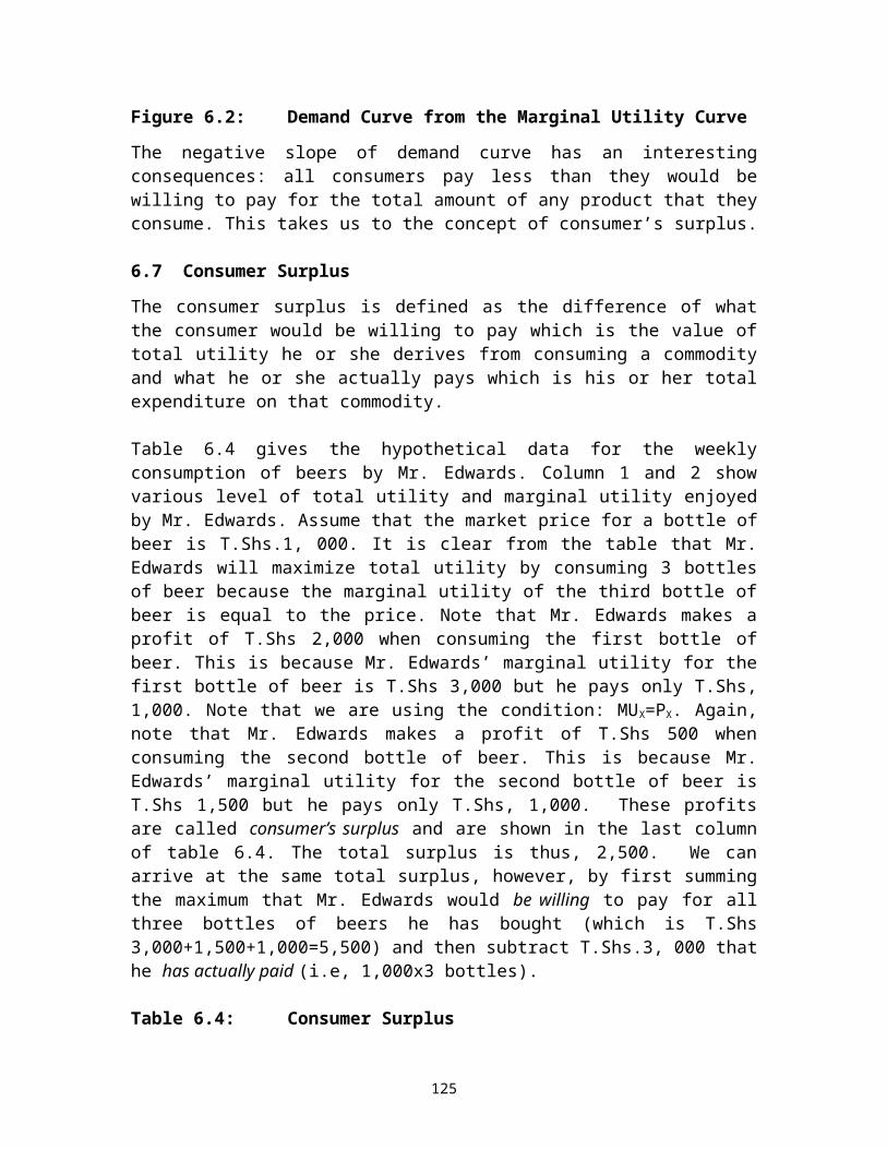
(b) Compute variance and standard deviation of profit in each company.

(c) Suppose that Mr.Sunday’s utility function is given as . Compute the risk premium of the two shares.

6*. Esther is contemplating whether to buy shares or not. Each share costs T.Shs 100 and the probability of increase in share’s price is given as follows:

Probability Return 0.50 00.25 1000.20 2000.05 750(a) What is the expected value of share’s return?

Variance? Standard deviation?(b) If Esther is a risk averse, would she buy a share?(c) Suppose that Esther is offered insurance against losing

money, how much would she be willing to pay?

LECTURE NINETHEORY OF PRODUCTION

9.1 IntroductionThis lecture is about the theory of production and is divided into three main parts. The first part explains different forms of business organization, the assumption of profit

131

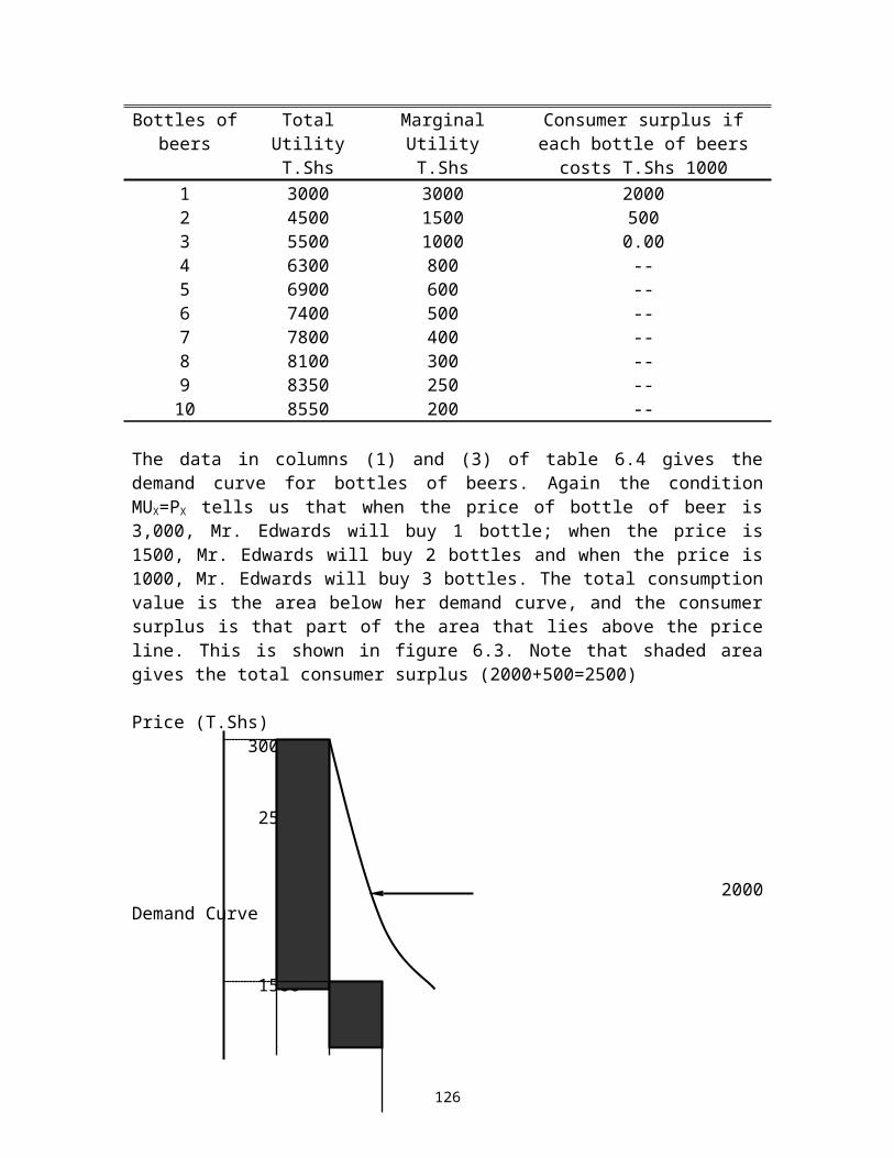
maximization and factors of production. The second part deals with the short run production. The third part deals with production in the long run. The last part considers the concept of return to scale. Objectives

By the end of this lecture, you should be able to:(i) Define and describe the production function(ii) Define and describe total product, average product and marginal

product.(iii) Describe the relationship among total product, average product and

marginal product curves;(iv) Define the law of diminishing return and identify the three stages

of production;(v) Differentiate the short run production from the long run production.(vi) State and explain the conditions for producer equilibrium both in

the short run and in the long run;(vii) Derive the firm's expansion path.(viii) Explain the meaning of returns to scale.

9.2 Production Unit: A FirmProduction is defined as the process of transforming inputs into output. Inputs are also called factors of production. Output are products derived from a production process and they are usually goods and services. Production process is carried out by firms. A firm is defined as unit of production that takes decision with respect to production and sale of goods and services. The concept of the firms covers a variety of business organizations from the single proprietorship, partnership, limited company to the cooperatives. Let us look at various forms of firms or business organization

9.2.1 Sole ProprietorshipThis is a business organization owned and managed by a single person. Usually it is a small-scale operation with small capital. This form of business is highly dominant in the Tanzanian business activities.

9.2.2 PartnershipA partnership is a concern owned by a small group of individuals. In Tanzania a partnership firm can have up to 10 partners. In a partnership there is joint management. Every partner is entitled to participate in the management. There is also unlimited liability. Every partner is responsible for all the debts of the firm. A partnership can raise more capital than a sole proprietorship.

9.2.3 Limited CompanyThis describes an association of a number of individuals formed for a common purpose and registered according to company law. The usual purpose is earning profit by production and trade. A company is formed by issuing shares, each share having a face value. The shareholders are proprietors of the company. The liability of a shareholder is limited to the face value of the share. He is not personally liable for the debts of the

132

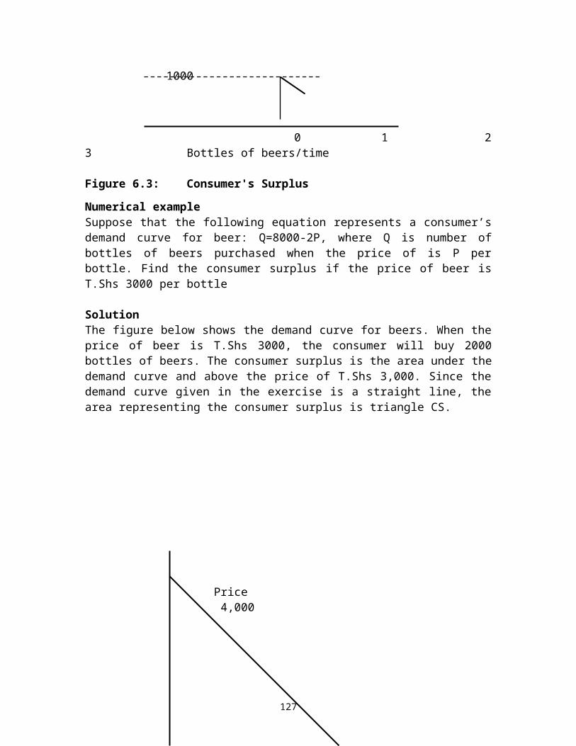
company. Companies may be of different types e.g. Private Companies and Public Companies. For most private companies membership is limited to the original owners and therefore capital can only be raised from this limited group. A public company is usually managed by directors elected by shareholders. Shares in a public company are transferable and the company can therefore raise additional capital from the capital market through new share issues.

9.2.4 CooperativesA cooperative is a form of business organization where people work together for business purpose on the basis of mutual benefit. Members of a cooperative organization own it, work for it and share the profits. Cooperative Societies are democratically organized on the basis of equality and free association. Examples of cooperatives include the credit and consumer societies.

9.3 Assumption of Profit MaximizationThe assumption of profit maximization is very crucial in the theory of production because it permits us to simplify the analysis for one major reason. The reason is that different firms have different objectives of doing business. In particular, with the rise of the public limited company, ownership and control are increasingly separated, with the ownership in the hands of shareholders and daily control in the hands of management. If managers have different goals from shareholders then the possibility of conflict arises. Baumol (1959) argues that manager-controlled firms are likely to pursue sales revenue rather than profits motives (see also figure 3.3 in lecture 3).7 On the other hand, although Williamson’s managerial theory (1963) of the firms is similar to Baumol’s in stressing the growth of sales revenue as a major objective, it goes beyond than that with manager seeking to increase satisfaction in terms of salary, job security, power within the firm, professional excellence and bonus.8 Marris (1964) on the hand argues that the overriding objective, which both managers and owners have, is growth of the firm.9 Managers seek a growth in demand for the firm’s product or services, to raise power or status. Owners seek a growth in the capital value of the firm to increase personal wealth.

In this lecture, therefore, we abstract from those complications, and we assume that our firms are operating on profit motives. A firm’s profit is the difference between the revenues it receives from selling its output and its cost of producing that output. Algebraically; profit is defined as

π = TR - TC (9.1)Where; π = Profit

TR = Total RevenueTC = Total Cost

7 Baumol, W. J (1959) Business Behaviour, Value and Growth. Macmillan8 Williamson, O.E (1963) Managerial Discretion and Business Behaviour, American Economic Review, Vol. 53, No. 5. pp. 1032-1057 9 Marris, R (1964) The Economic theory of Managerial Italism. Macmillan

133

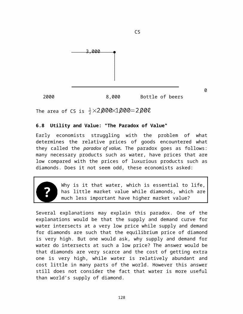
The above equation tells us that what happens to profit depends on what happens to revenue and costs. The cost of production depends on quantity and quality of factors of production that the firm employs in the production process.

9.4 Inputs or Factors of Production Production processes usually require a wide variety of inputs, an input being anything that the firm uses in its production process. For example some of the inputs in corn cultivation include fertilizers, pesticides, labor, etc. In representing and analyzing the production process, we assume that all inputs can be divided into two categories: fixed inputs and variable inputs. A fixed input is an input whose quantity cannot be changed during the period of time under consideration. The firm's plant and equipment are examples of inputs that are often included in this category.

On the other hand a variable input is an input whose quantity can be changed during the period under consideration. For example, the number of workers hired to perform job like construction can often be increased or decreased on short notice. Both fixed and variable inputs are generally classified into four groups: land, labor, capital and entrepreneurship or management.

9.4.1 LandLand as a factor of production includes minerals, forests, water, and all other natural resources as well as soil used in agriculture and a site upon which economic activities take place. Land as a factor of production has three main features; it is fixed in supply; it is a gift of nature; and it varies in quality.

9.4.2 LaborLabor in its simplest term describes the human effort or other work done by human beings. Labor is so important in production activities that some radical economists like Karl Marx and other socialist oriented economists believe that labor is the only embodiment in production. Labor as a factor of production can be classified into skilled and unskilled labor, as well as technicians and professionals like engineers, doctors, lawyer etc. Labor can be more productive through training and education.

9.4.3 CapitalCapital can be defined as man made wealth that is used in the production of goods and services. It is defined as a “produced means of production” and it includes raw materials, machinery, buildings, factories, tools and other manufactured inputs.

9.4.4 EntrepreneurshipIt is the entrepreneur who coordinates all the factors of production by bringing them together in the production process. It involves the use of initiatives, skills as well as the willingness and ability of the decision-maker to take risk

9.5 The Production FunctionThe production function is the technical relationship between output and quantities of various inputs used per period of time. More specifically, production function for any

134

commodity is an equation, table or graph showing the (maximum) quantity of the commodity that can be produced per unit of time for each of a set of alternative inputs, when the best production techniques available are used. The simplest production function for corn can be specified algebraically as follows;

Qc = f (L, K) (9.2)

Where; Qc = is the output of corn in kilograms per time period.K= capital which is assumed to be fixed. L= labor

The above equation states that kilograms of cones depend on the quantities of two inputs: labor and capital. Table 9.1 shows how corn production varies as additional workers are employed on a fixed area of land.

9.6 The Short Run: Production with One Variable InputThe short run is defined to be that period of time in which some of the firm's inputs are fixed. More specifically, since the firm's plant and equipment are among the most difficult inputs to change quickly, the short run is generally understood to mean the length of time during which the firms plant and equipment are fixed.

Short run is that period of time over which the input of at least one factor of production cannot be varied.

To illustrate the concept of short run production function, consider the simplest case when there is one fixed input and one variable input. Suppose that the fixed input is land in acres, the variable input is labor (in man-days), and the output is the corn (in bags). Suppose that a scientifically inclined farmer decides to find out what the effect on annual output will be if he applies various numbers of man-days of labor during the year to the acre of land. If he obtains the results in Table 9.1, then this result might be regarded as the production function in this situation.

Table 9.1: Production function of Corn in the Short runLand Labour TPL

1 0 01 1 31 2 71 3 141 4 251 5 35

135

1 6 441 7 521 8 591 9 651 10 701 11 741 12 771 13 791 14 801 15 80

Alternatively, the Total Product (TP) curve in Figure 9.1, which presents exactly the same results, might be regarded as the production function. The figure is constructed on the assumption that, land (i.e., the fixed input) is equal to one acre.

Figure 9.1: Production Function of Corn in the Short run.

Production function is an important starting point in the analysis of theory of the firm. But we need to know more about the average and marginal product of labour. The average product of labor (APL) is defined as total product (TP) divided by the number of units of labor used. Algebraically, it can be expressed as:

(9.3)

136

Where; APL is the average product of labor; TP is the total product and L is the labor. The marginal product of labor (MPL) is given by the change in TP per unit change in the quantity of labor used. Algebraically, it can be expressed as:

(9.4)

Where; ΔTP is the change in the total product and ΔL is the change in labor input. On the basis of production function shown in Table 9.1, we can compute the average product and marginal product of labor. This is shown in table 9.2. The average product of labor (AP) in column (4) is obtained by dividing each quantity in column (3) by the corresponding quantity in column (2). The marginal product of labor (MP) in column (5) is obtained by finding the differences between the successive quantities in column (3)

Table 9.2: Marginal and Average Product of Labor

Land Labour TPL APL MPL1 0 0 01 1 3 3 31 2 7 3.5 41 3 14 4.66 71 4 25 6.25 111 5 35 7 101 6 44 7.33 91 7 52 7.42 81 8 59 7.37 71 9 65 7.22 61 10 70 7 51 11 74 6.72 41 12 77 6.41 31 13 79 6.07 21 14 80 5.71 11 15 80 5.33 0

The TP, APL and MPL schedules of Table 9.2 are plotted in Fig.9.1. It is shown from Figure 9.1 that the average product curve for labor rises, reaches a maximum, and falls. The marginal product of curve for labor also rises, reaches a maximum and then falls. From the same figure it is shown that marginal products exceed the average product when the latter is increasing, equals average product when the latter reaches a maximum, and is less than the average product when the latter is decreasing. This is simply a matter of arithmetic: if the addition to total is greater than the average, the average is bound to increase; if addition to total is less than the average, the average is bound to decrease!

Average product of a factor of production is the total output per unit of the factor input. Marginal product of a factor of production is the change in the total output as a result of a unit change in factor input.

137

9.7 The Shapes of the Average and Marginal Product CurvesThe shapes of the APL and MPL curves are determined by the shape of the corresponding TP curve. The APL at any point on the TPL curve is given by the slope of the line from the origin to that point on the TPL curve. For example in figure 9.2, the APL at point A on the TP curve is equal to the slope of OA. As we have said before, the APL curve usually rises at first, reaches a maximum and then falls, but it remains positive as long as the TP is positive.

TP

A TP

B

APL

0 L1 L2 L3 MPL LaborFigure 9.2: Total, Marginal and Average Products

On the other hand, the MPL between two points on the TP curve is equal to the slope of the TP curve between the two points. For example, the MPL between the origin and point B on the TP curve is equal to the slope of 0B. As we have pointed out earlier, the MPL

curve also rises at first, reaches a maximum (before the APL reaches its maximum) and then declines. The MPL becomes zero when the TP reaches maximum and it becomes negatives as TP falls. The falling portion of the MPL curve illustrates the law of diminishing returns.

9.8 The Law of Diminishing Marginal Return The law of diminishing marginal returns states that, as additional units of a variable factor are added to a given quantity of fixed factors, with a given state of technology, the marginal product of the variable factor will eventually decline. Table 9.1 illustrates this law; beyond 5 units of labor the marginal product of labor decreases.

138

Several things should be noted about this law. First, it assumes that technology remains fixed. The law of diminishing marginal returns cannot predict the effect of an additional unit of input when technology is allowed to change. Second, it is assumed that there is at least one input whose quantity is being held constant. The law of diminishing marginal returns does not apply to cases where there is a proportional increase in all inputs.

9.9 Three Stages of Production Let us now define three stages of production, each being characterized by the extent of utilization of the variable input. An understanding of these three stages is very useful in showing that many types of input combinations are clearly inefficient.

TP

TP

Stage I Stage II Stage III

APL

0 MPL LaborFigure 9.3: Three Stages of Production

Why do you think that a rational producer will never operate in either stage one or three of production?

Stage I goes from the origin to the point where the APL is maximum. Stage II goes from the point where the APL is maximum to the point where the MPL is zero. Stage III covers the range over which the MPL is negative. The producer will not operate in Stage III, even with free labor, because he could increase total output by using less labor in one acre of land. Similarly, the producer will not operate in stage I because average product of labor is still increasing as a result of utilization of variable input. In stage I, an increase in variable input result in larger and larger increases in total output. Thus the firm will try to operate in stage II, which is defined to include the range of utilization of the variable input from the point at which the average product of the variable input is a

139

maximum to the point at which the marginal product is zero. In stage II, the marginal product of both inputs is positive.

Stage I in production goes from the origin to the point where the APL is maximum. Stage II goes from the point where the APL is maximum to the point where the MPL is zero. Stage III covers the range over which the MPL is negative

Numerical example:The short run production function of MBARA company is represented by the following equation: Q=6L2-0.2L3. Where L denotes the number of workers.

(a) Determine the size of the workforce which maximizes output (Hint: where MPL=0)

(b) Determine the size of the workforce, which maximizes the average product of labour. Compute MPL and APL at this value of workforce.

Solution(a) In the first part of this example we want to find the value of labour (L) which

maximizes: Q=6L2-0.2L3. We know that at the point of maximum, marginal product of labour is zero. This is shown as:

The solution to this equation indicates that L=20.

(b) In the second part of this example we want to find the value of L, which maximizes the average product of labour.

At the maximum point of APL, the slope of APL=0. That is:

Thus, the average product of labour is at maximum when the firm employs 15 workers. In fact the corresponding average product of labour is:

APL =6L-0.2L2

=6(15)-0.2(15)2

=45

Finally, we are required to compute the value of MPL at the maximum point of APL. This is shown as follows:

140

MPL =12L-0.6L2

=12(15)-0.6(15)2

=45We have thus shown that when the average product of labour is maximum, the marginal product of labour is equal to the average product of labour.

9.10 The Long Run: Production with Two Variable InputsLong run is defined as that period of time in which all factors of productions are variable. Firms wishing to maximize their profits, therefore, will attempt to produce their chosen output by employing combinations of capital and labor which minimizes their production costs. We can illustrate this cost-minimization graphically with the use of isoquant and isocost lines. These also enable us to trace the path along which a firm can expand in the long-run.

Long run is that period of time over which the inputs of all factors of production can be varied.

9.10.1 Isoquant An isoquant shows the different combinations of labor (L) and capital (K) with which a firm can produce a specific quantity of output. A higher isoquant such as Q2 in figure 9.4 indicates greater quantity of output and a lower one such as Q1, indicates smaller quantity of output.

Capital

141

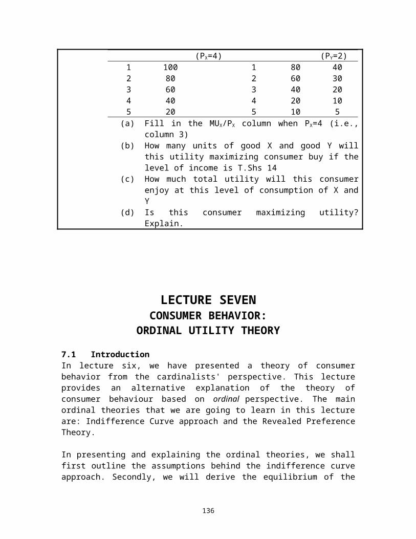
D

K2 B

E

K1 C Q2

A Q1

0 L1 L2 Labour

Figure 9.4: An Isoquant Map

In the Figure 9.4, point B on the isoquant labeled Q1, represents just one possible combination of capital and labor (0K1 units of capital and 0L1units of labor) with which a firm can produce Q1units of output. There are in fact an infinite number of other points on the isoquant Q1 all of which represent different combinations of capital and labor which can be used to produce output Q1. An output of Q2 units bigger than Q1 can be produced using any of the combinations of capital and labor represented by points along the isoquant labeled Q2, such as point D and E.

9.10.2 Properties of IsoquantsIsoquants have three important properties. First, isoquant can never intersect. Figure 9.5, shows two intersecting isoquants, Q1 and Q2. As drawn, point A represents a combination of capital and labor which, when used efficiently, can apparently produce two different quantities of Q1and Q2. This absurd result confirms the statement that two isoquants can never intersect.

Capital

Y

142

K* A

Q2

Q1

0 L* LabourFigure 9.5: Two Intersecting Isoquants

Secondly, isoquants are negatively sloped. If both capital and labor have positive marginal products (so that the employment of extra units increases total output), then it follows that to maintain a given level of output when the quantity of one of factors is reduced, the quantity of other must be increased.

K

K3 A

ΔK

B K2

ΔK* K1 C ΔL ΔL*

0 L1 L2 L3 Labour Figure 9.6: An Isoquant Convex to the Origin

Thirdly, isoquants are convex to the origin. As units of capital are given up, successively bigger quantities of labor must be employed to keep the output level unchanged. This makes the isoquants convex to the origin as shown in Figure 9.6. Note that the slope of isoquant is sometimes called the Marginal Rate of Technical Substitution. Figure 9.6 shows that the movement from point A to point B requires more K to be sacrificed. However, the movement from point B to point C requires less of K to be sacrificed, i.e. ΔK>ΔK*.

143

Numerical example. Consider the following Cobb-Douglas production function: Q=K½L½. Find the equation for an isoquant when the level of output is 100.

SolutionThe Q=100 isoquant shows all the combinations of labour and capital that a firm can produce given the level of technology. Given our production function, the combinations of labour and capital must satisfy the following conditions: 100= K½L½

To find the equation for 100 unit isoquant, we must solve this equation for K in terms of L. This yield:

Thus, gives the equation for 100 unit isoquant.

Can you compare and contrast between the indifference curves that you have learned in lecture seven and isoquants learned in this lecture?

9.10.3 Marginal Rate of Technical SubstitutionThe marginal rate of technical substitution of labor (L) for capital (K), (i.e., MRTSLK) refers to the amount of capital that firm can give up by increasing the amount of labor by one unit and still remain on the same isoquant. The MRTSLK is also equal to the ratio of marginal product of labor (MPL) to the marginal product of capital (MPK) or MPL /MPK. As the firm moves down an isoquant the MRTSLK diminishes.

Can you compare and contrast between the marginal rate of substitution learned in lecture seven and marginal rate of technical substitution learned in this lecture?

9.10.4 Isocost linesAn isocost line is defined as the locus of points that join all the combination of factors of production such as capital and labor that can be bought for a given monetary outlay. Algebraically, the isocost is as follows:

TO = PL (L) + PK (K) (9.5)

144

Where; TO is Total outlay, PL is price of labour (wage rate), PK is price of capital (rental rate of capital), L is labour, and K is capital. Subtracting PL (L) from each side of equation 9.5 yields;

PK (K) = TO - PL(L) (9.6)

Divide each side of equation 9.6 by PK yields,

(9.7)

Finally, the slope of the isocost is given by

- (9.8)

Capital

TO/PK

0 TO/PL LaborFigure 9.7: Isocost Line

9.11 Producer Equilibrium A producer’s equilibrium occurs where an isoquant is tangent to the isocost. At the point of tangency, the absolute slope of the isoquant is equal to the absolute slope of the isocost. That is, at equilibrium, MRTSLK = PL/PK (This is completely analogous to the concept of consumer equilibrium in lecture seven) Since MRTSLK = MPL/MPK at equilibrium

(9.9)

Where; MPL denotes the marginal product of labor, MPK denotes the marginal product of capital, PL denotes the price of labor and PK denotes the price of capital. Equation 9.9 tells us that at equilibrium, the marginal product of the last shilling spent on labor is the same

145

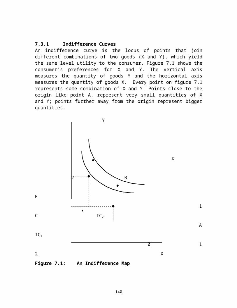
as last shilling spent on capital. The same would be true for other factors, if the firm had more than two factors of production.

Example 9.1: Producer’s Equilibrium

Consider a hypothetical situation where by Salawa Footwear Limited Company (SFLC) is one amongst the biggest companies that manufactures genuine and quality leather shoes in the country. Assume that the production function for SFLC product is given by Q= 100KL.

What is the minimum cost of producing 1000 pairs of shoes if the price of capital and labor per day are T.Shs 120 and 30 respectively?

The above economic problem is a typical of producer’s equilibrium. Stated differently, least cost combination of capital and labor occurs where the marginal rate of technical substitution of labor for capital is exactly equal to the ratio of wage rate and rental rate of capital.

Solving for marginal products requires the knowledge of elementary calculus. It is easy to show that the marginal product of labor is dQ/dL=100K. Also, the marginal product of capital is dQ/dK=100L. Therefore, the marginal rate of technical substitution is:

To determine the optimal capital labor ratio, set the marginal rate of technical substitution equal to the ratio of the wage rate to the rental rate of capital

Then, substitute K for L in the production function and solve for the value of K at 1,000 pairs of shoes. This should give you the following results:

1,000 = (100) (K)(4K), or K=1.58

By now you should note that L = 6.32 because L equals 4K. Moreover, given the two levels of inputs that we have solved for, the minimum cost of producing 1,000 pairs of shoes is T.Shs 379.20.

146

How do we arrive at T.Shs 379.20?

Substitute values of K, L, w and r in the total cost function. Remember that the total outlay function is given by the following equation:

TO = PL (L) + PK (K)

TO is Total outlay (Isocost), PL is the price of labour (wage rate), L is labor units, PK is the price of capital (rental rate of capital) and K is capital. More specifically, this is how we have arrived at the cost-minimizing figure:

TO = (30)(6.32)+(120)(1.58)= T.Shs 379.20

How are we sure that T.Shs 379.20 is the minimum cost of producing 1,000 pairs of shoes?

To prove if K=1.58 and L= 6.32 are the cost minimizing level of inputs; consider a small change in K and L around 1.58 and 6.32 respectively. At K=1.6 and L=6.32, total cost is T.Shs 381.60, and at K=1.58 and L= 6.4, total cost is T.Shs 381.6, both greater than T.Shs 379.20.

Now suppose that the SFLC production manager, Mr. Adam has fortunately discovered the cheapest sources of capital and labor. The SFLC production function is subsequently changed to F (K, L)= KL2, with the price of capital and labor fixed at T.Shs 10 and T.Shs 15 respectively. What combination of capital and labor minimizes the cost of producing any given level of pairs of shoes? As a general rule, the cost minimizing combination of capital and labor occurs where;

Applying calculus reveals that the marginal product of labor is dQ/dL=2KL. Similarly, the marginal product of capital is dQ/dK=L2. Then, set the Marginal Rate of Technical Substitution of labor for capital equal to the input price ratio to determine the optimal capital-labor ratio:

Therefore, the capital labor ratio should be 0.75 to minimize the cost of producing any given pairs of shoes.

147

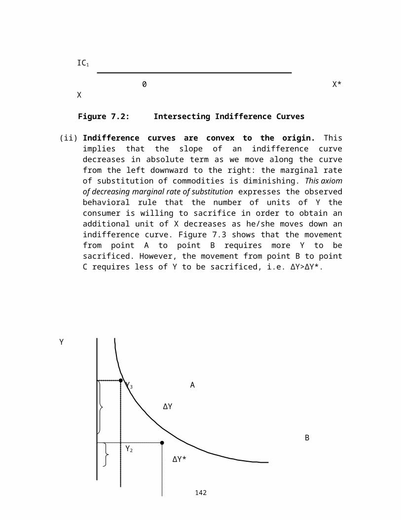
9.12 Expansion PathThe firm’s expansion path is defined as the locus of points of tangency between isoquant and isocost line. If the firm changes its total outlay while the prices of labor and capital remain constant, firm's isocost shifts parallel to itself up and to the right if total outlay is increased or down and to the left if total outlay is decreased. These different isocosts will be tangent to different isoquants, thus defining different equilibrium points for the producer. By joining these points of producer equilibrium, we get firm’s expansion path illustrated in Figure 9.8 below. Capital

TO/PK3

TO/PK2

Firm’s Expansion Path

TO/PK1

C B Q3

A Q2 Q1

0 TO/PL1 TO/PL2 TO/PL3 Labour

Figure 9.8: Expansion Path

The locus of points CAB is referred to as the firm’s long-run expansion path. This is analogous to the income-consumption curve discussed in lecture seven.

Can you compare and contrast between the income consumption curve learned in lecture seven and the production expansion path in this lecture?

9.13 Effect of Change in Input Prices on Output The analysis of the effects of changes in input prices on output proceeds along exactly the same lines as the analysis of the effects of changes in the prices of goods in consumer theory. If one of the price of input, say PL (i.e., price of labor) falls while the price of other input (i.e., capital) and the isocost remain constant, then we can separate the effect of a price change into two components. The first component is the substitution effect. This is movement along the original isoquant. The second component is the scale effect. This is a movement to the higher isoquant.

148

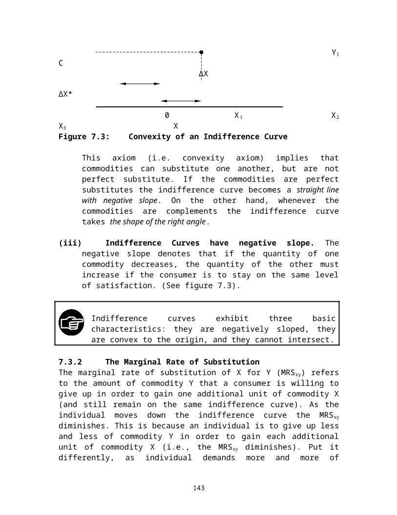
The impact of a fall in the price of labor is illustrated in figure 9.9, which is essentially the same as figure 7.9. However, note the following. First, here we are dealing with isoquants rather than indifference curves. Second, while on the horizontal axis we have got labor instead of commodity X; on the vertical axis we have got capital instead of commodity Y. Third, the movement to a higher curve is called scale effect instead of income effect.

K

TO/PK1

TO/PK2

K1 E1

K2 E3

E2

K3 Q2

Q1

TO/PL1 TO/PL2 TO/PL1*

0 L1 L2 L3 LFigure 9.9: Substitution and Scale Effect Figure 9.9 show that a fall in the price of labor pivots the isocost line from TO/PK1, TO/PL1

to TO/PK1, TO/PL1*. Substitution effect shows that following a fall in the price of labor, a firm moves along an isoquant from E1 to E2. It is evident that a firm now hires more unit of labor than before (i.e., 0L2>0L1). This result is obtained by drawing a parallel isocost (i.e., TO/PK2, TO/PL2), which is just below the new isocost TO/PK1, TO/PL1*. The scale effect on the other hand shows that a firm would employ both labor and capital where the new isocost TO/PK1, TO/PL1* is tangent to the new isoquant (i.e. Q2). Thus, the movement from E2 to E3 is called the scale effect. The total effect is denoted by movement from E1

to E3.

9.14 Elasticity of Technical Substitution Elasticity of technical substitution is defined as the percentage change in capital labor ratio, divided by the percentage change in the marginal rate of technical substitution. In other words, elasticity of technical substitution tells us “how easy” it is to substitute capital for labour. Along an isoquant, marginal rate of technical substitution will decrease as the capital labour ratio decreases (that is, as K/L decreases) and our central aim is to define some parameters, which measures this degree of responsiveness. If marginal rate of technical substitution does not change at all, for change in K/L, we may say that substitution is easy. If on the other hand, marginal rate of technical substitution changes

149

rapidly for small change in K/L, we would say it is difficult substitution. Technically, along an isoquant elasticity of the technical substitution is measured by:

Where, σ is the elasticity of substitution. Note that since along an isoquant, K/L and MRTS are assumed to move in the same direction, the value of elasticity of technical substitution is always a positive number. Graphically, the concept of elasticity of technical substitution is illustrated in Figure 9.10 as a movement from point A to point B on an isoquant. Capital

2000 A MRTSL, K at point A is 4

1000 B MRTS L,K at point B is 1

0 500 1000 labour Figure 9.10: Elasticity of Technical Substitution

In this movement, both MRTS and the ratio K/L will change and we are interested in the magnitude of these changes. If elasticity of technical substitution is high, the MRTS will not change much relative to the K/L ratio and the isoquant is relatively flat. On the other hand, a value of elasticity of technical substitution implies rather sharply curved isoquant: the MRTS will change by a substantial amount as the K/L changes. From figure 9.10 we can compute the elasticity of technical substitution as follows. The change in the marginal rate of technical substitution is

=1-4 =-3

The percentage change in MRTSL, K is:

%∆MRTSL, K=

150

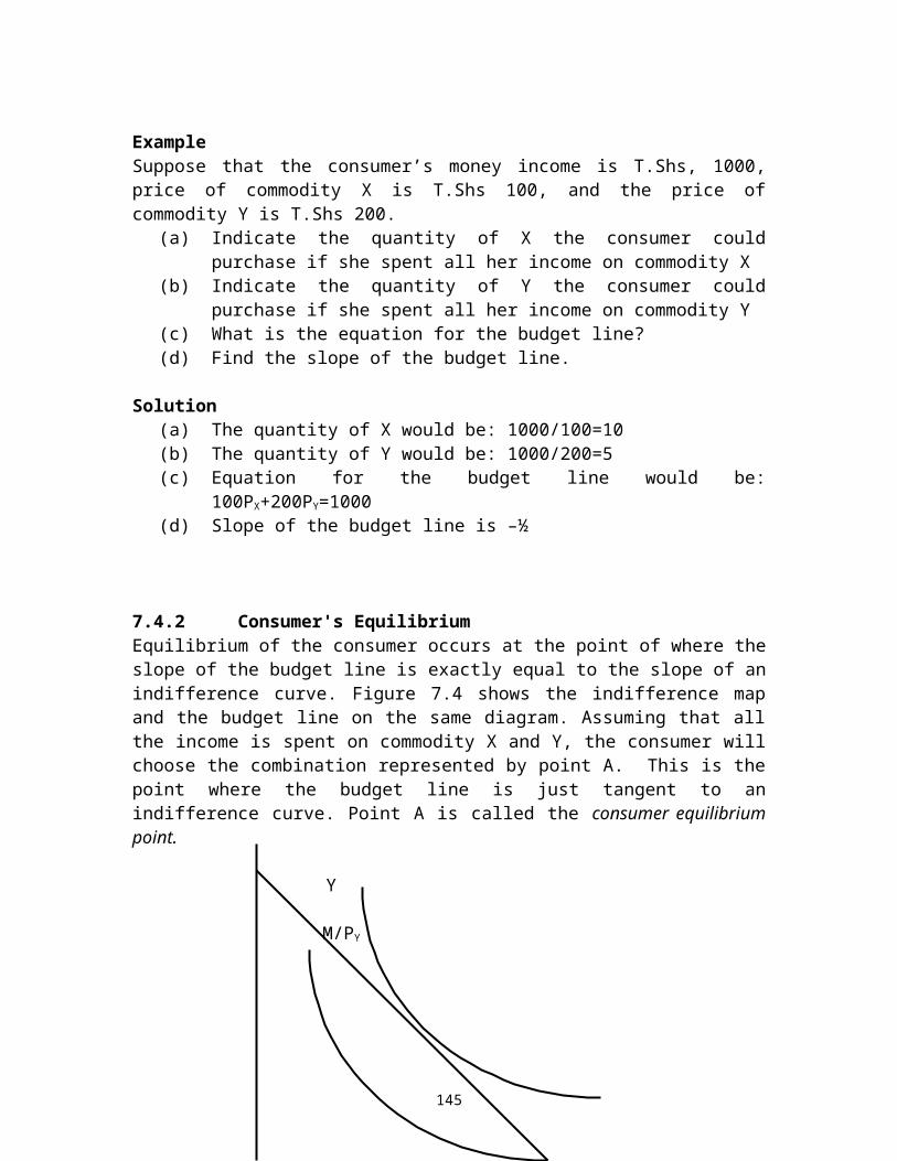
= (-¾) x100=-75%The change in capital labour ratio [i.e., ∆ (K/L)] as we move from point A to point B is given as:

=1-4 =-3

The percentage change in the capital-labour ratio is ∆ (K/L)/ (KA/LA) x100 =-75%. Thus, using the above formula 9.10 implies:

9.15 Returns to Scale and Homogeneity

The concept of returns to scale is used to describe the size of the increase in output when all inputs are increased by the same proportional rate. Return to scale may be constant, decreasing or increasing. Let us have a look on each of these.

9.15.1 Constant Returns to ScaleConstant returns to scale arise when a proportionate increase in output is matched exactly by an equal proportionate increase in inputs, e.g., doubling output requires twice the volume of inputs. In figure 9.11, the production function exhibits constant returns if 0A=0B. When this is the case, production of Q units of output, requires L+K inputs, whilst 2Q units of output requires 2(L+K) inputs.

Capital (K)

2K B 2Q

K A Q

151

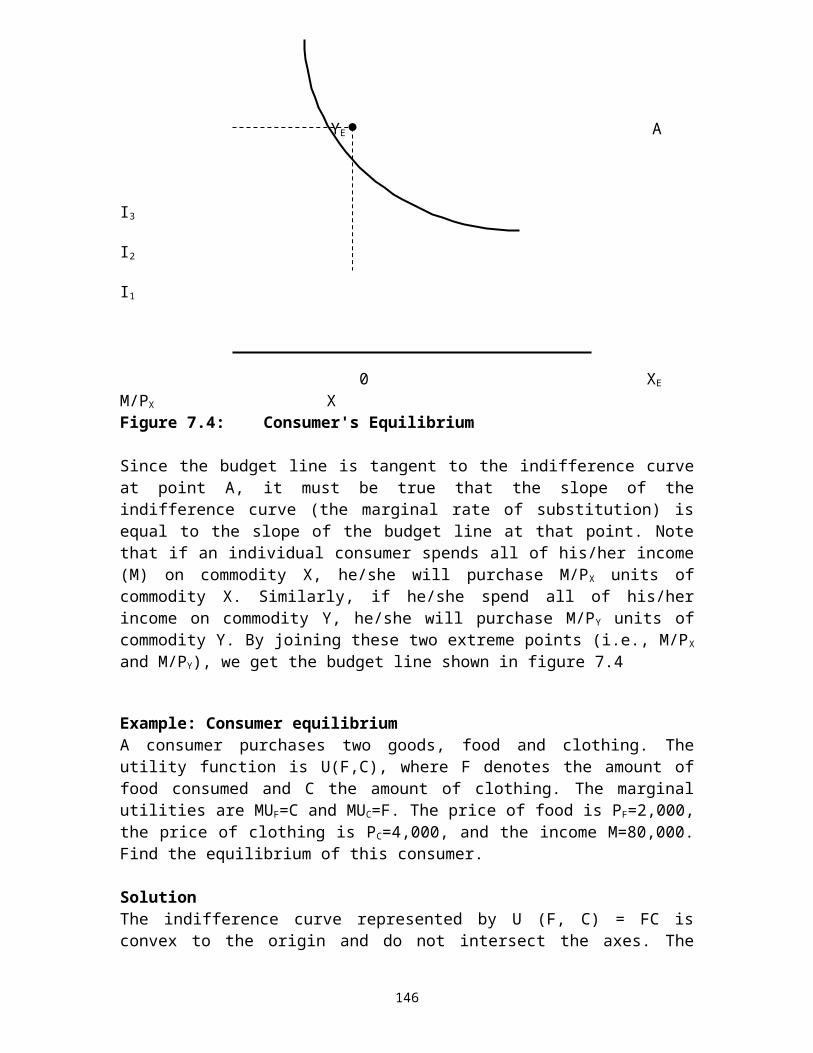
0 L 2L Labour (L)Figure 9.11: Constant Returns to Scale

9.15.2 Decreasing Returns to ScaleDecreasing returns to scale arises when a proportionate increase output is less than the proportionate increase in inputs. From figure 9.11, this would occur if 0A<0B. In other words, the distance between the isoquant as measured on the straight line from the origin is increasing. The proportional increase in inputs therefore exceeds the proportional increase in output.

9.15.3 Increasing Returns to Scale Increasing returns to scale arise when the proportionate increase in output exceeds the proportionate increase in inputs, e.g., doubling inputs leads to a 150 per cent increase in output. In terms of figure 9.11, this would mean that 0A>0B, i.e., the isoquants move closer together as they move away from the origin.

We have constant, increasing or decreasing returns to scale if, when all inputs are increased in a given proportion, the output of the commodity increases in the same, in a greater or in a smaller proportion, respectively.

9.15.4 Homogeneous production function The concept of returns to scale is closely related to the concept of homogeneity in the neo-classical production function. One of the most commonly used production functions in applied economics work is the Cobb-Douglass production function, put forth by Cobb and Douglass in 1928.10 In its simplest form, Cobb-Douglass production function can be written as:

Q=ALαKβ

We can further express the above Cobb-Douglass production function in logarithmic form as follows:

LogQ=LogA+ αLogL+ βLogK

Where: Q=output; A=Constant; L=Labour; and K=Capital. The coefficients α and β can be interpreted as the elasticities of output with respect to the labour and capital inputs respectively. The important feature of Cobb-Douglass production function is that (α+β) measures returns to scale. For example, suppose we double L and K by λ. Then the new output Q is given by:

Q = A (λL) α (λK) β Q = λ α+β (ALαKβ)

The production function Q=ALαKβ is said to be homogeneous of degree (α+β), if given any positive A, doubling inputs by λ, raises output by λ α+β . When α+β > 1, the function exhibits increasing returns, and decreasing returns when α+β < 1. When α+β =1, it is 10 C.W. Cobb and P.H.Douglas (1928) “A Theory of Production”, American Economic Review, 18: 139-165

152

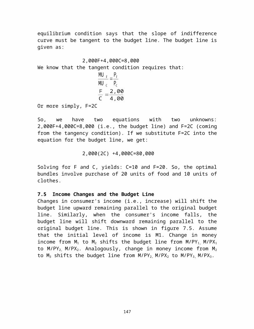
homogeneous of degree 1, and it exhibits constant returns. Homogeneous functions are a special class of Homothetic function, where for the later the marginal rate of technical substitution (i.e., slope of an isoquant) is constant along the ray from the origin.

SUMMARY1. The production function is the technical relationship between

output and quantities of various inputs used per period of time. More specifically, production function for any commodity is an equation, table or graph showing the (maximum) quantity of the commodity that can be produced per unit of time for each of a set of alternative inputs, when the best production techniques available are used

2. The short run is a period of time over which the input of at least one factors of production cannot be changed. In this situation, the law of diminishing returns eventually operates, whereby the marginal product of variable factor begins to decline.

3. The long run is the period of time over which the input of all

153

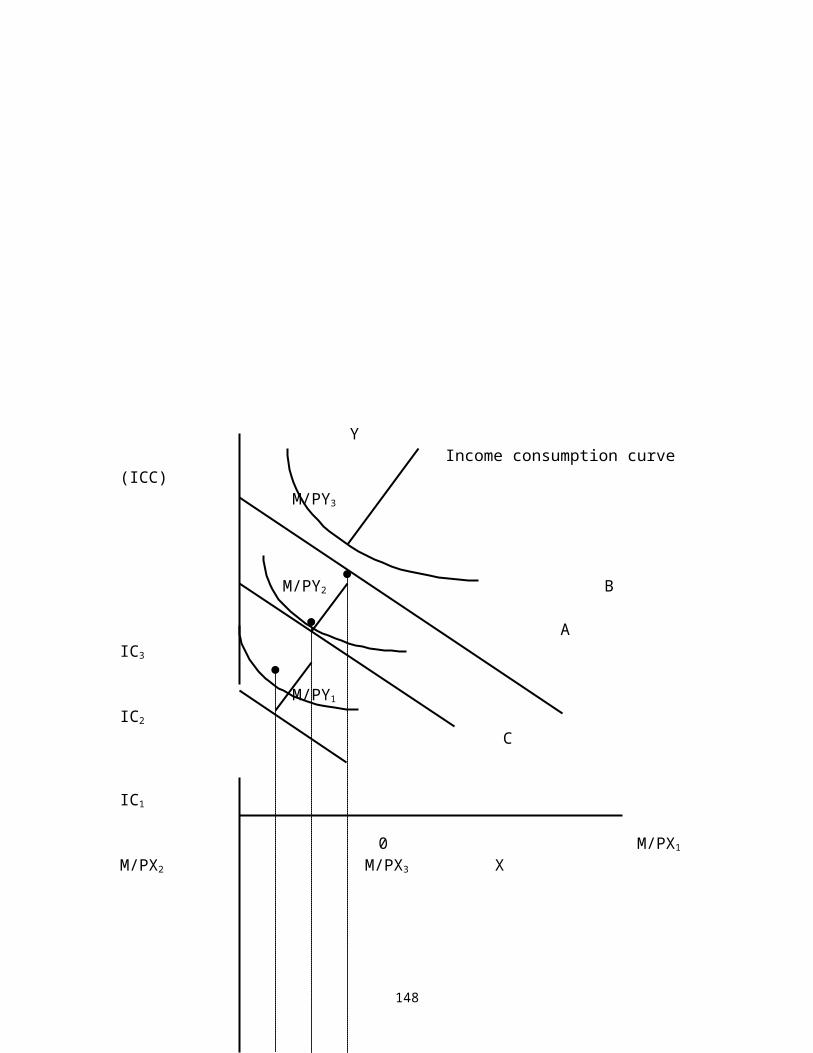
factors of production can be varied. In the long run therefore, the firm can change the whole scale of production. It may experience constant, increasing or decreasing returns to scale. The production function is illustrated by isoquant.

4. An isoquant is a curve that shows all combinations of inputs that yield a given level of output. Isoquants emphasise the flexibility that firms have in the production process. Isoquants have three important properties. First, isoquant can never intersect. Secondly, isoquants are negatively sloped. Thirdly, isoquants are convex to the origin.

5. The marginal rate of technical substitution of labor (L) for capital (K), MRTSLK refers to the amount of capital that firm can give up by increasing the amount of labor by one unit and still remain on the same isoquant

6. The firm’s expansion path is defined as the locus of points of tangency between isoquant and isocost line. If the firm changes its total outlay while the prices of labor and capital remain constant, firm's isocost shifts parallel to itself up and to the right if total outlay is increased or down and to the left if total outlay is decreased.

7. A producer is in equilibrium when he reaches the highest isoquant, given his isocosts. This occurs where an isoquant is tangent to the isocost. At the point of tangency, the absolute slope of the isoquant is equal to the absolute slope of the isocost. That is, at equilibrium, MRTSLK = PL/PK

8. Elasticity of technical substitution is defined as the percentage change in capital labor ratio, divided by the percentage change in the marginal rate of technical substitution.

9. We have constant, increasing or decreasing returns to scale if, when all inputs are increased in a given proportion, the output of the commodity increases in the same, in a greater or in a smaller proportion, respectively

154

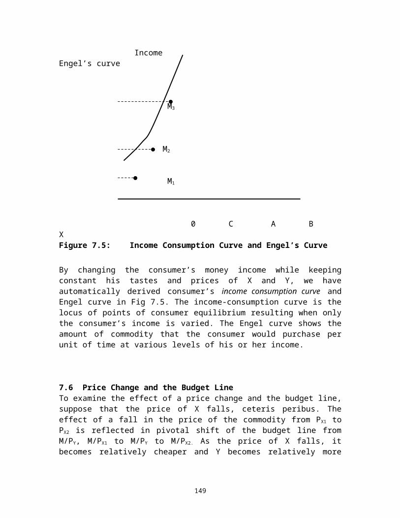
EXERCISES1. Write short notes on the following:

(a) Production function(b) Characteristics of isoquants(c) Isocost(d) The law of diminishing marginal returns(e) Elasticity of technical substitution

2. The marginal product of labor is known to be greater than the average product of labor at a given level of employment. Is the average product increasing or decreasing? Explain

3. Consider the short run production function below; only labour input

155

is varied. Labor input/day Output/day

0 01 352 803 1224 1565 1776 180

(a) Calculate the marginal product of labour and average product of labor

(b) Using graph paper, plot the MPL and APL

(c) At approximately what level of labour input do diminishing set in?(d) At approximately what level of labour input does the MPL cut the

APL?(e) How would you expect the MPL curve to be affected by the change

in the level of capital input?

4. What is the marginal product of labour in the production function Q = 2K1/3 L1/3 if K is fixed at 27?

5. Explain what is meant by: Constant return to scale? Increasing return to scale? Decreasing return to scale? Explain briefly how each of these might arise.

6. Calculate the elasticity of technical substitution between labour and capital from the following table

Amount of labour Amount of capital MPL MPK

5 4 5 64 5 6 5

7.* Fill in the gaps in the table belowLabour Total output MPL APL

0123456

0225------

1140------

------300---225---

---300---------225

8. A firm short run production function is given by: Q=300L2-L4. Where L denotes the number of workers. Find the size of work force, which maximizes the average product of labour, and verify that at

156

this value of L, average product is equal to marginal product

9*. Isoquants can be convex, linear or L-Shaped. What does each of these imply about the nature of the production function? What does each of these shapes imply about the MRTS?

10*. The marginal product of labour in the production of computer chips is 50 chips per hour. The marginal rate of technical substitution of hours of labour for hours of machines capital is . What is the marginal product of capital?

LECTURE TENTHEORY OF COSTS

10.1 IntroductionIn the preceding lecture, we have learned the theory of production. The process of producing goods and services involves a cost, which is given in terms of the inputs or economic resources employed such as wages a firm pay its workers and the rent it pays for an office space. For a profit-maximizing firm, cost is a very important variable that must be controlled. Successful managers understand and appreciate that the level of cost relative to revenue determines the firm’s overall profitability. In this lecture we are going to study the theory of cost.

We begin by explaining how cost is defined and measured, distinguishing between the concepts of cost used by economists and accountants. We then examine how the characteristics of the firm's production technology affect costs, both in short run and in

157

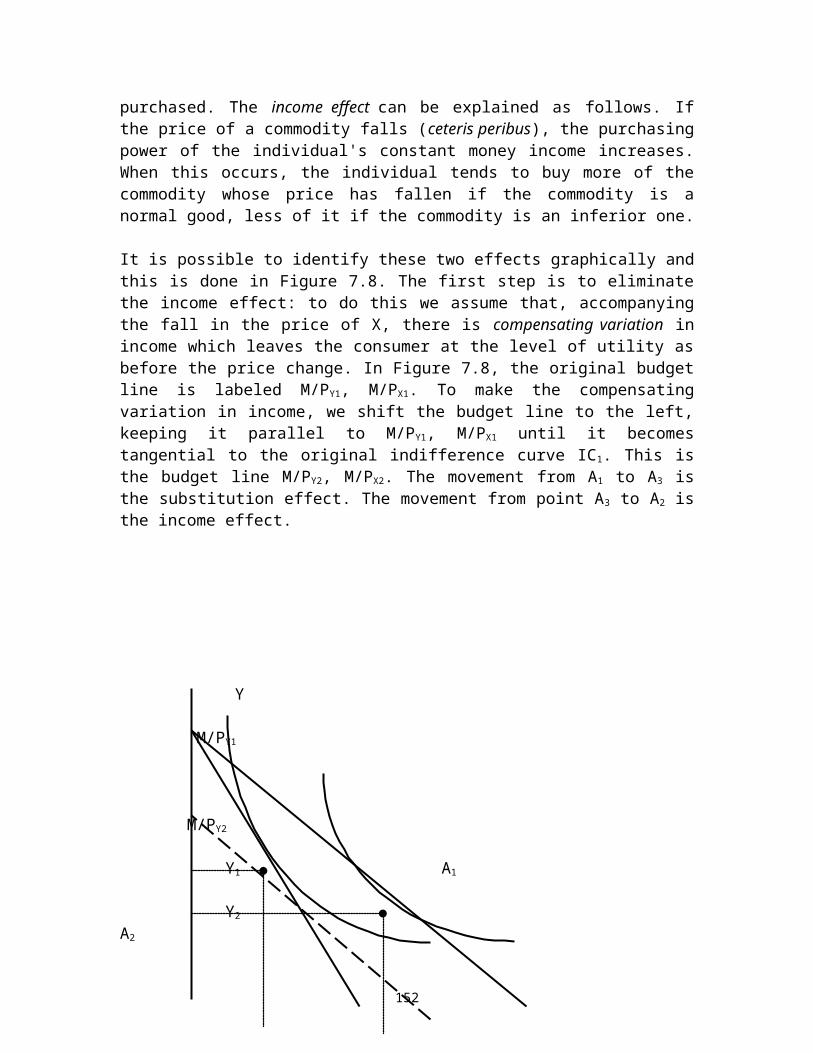
the long run. The lecture shows that the shape of short run cost curves are influenced by the law of diminishing marginal returns we have studied in lecture nine. Finally we show that the shape of long run average cost is influenced by economies and diseconomies of scales.

ObjectivesBy the end of this lecture, you should be able to:(i) Explain the difference between accounting and opportunity cost;(ii) Define the various types of cost and show that in the short-run

average and marginal costs will eventually rise as a result of diminishing returns.

(iii) Interpret the shape of various cost curves and show their relationship;

(iv) Establish a link between average product of labour and average variable cost;

(v) Establish the link between marginal product of labour and marginal cost;

(vi) Describe and explain how long run average cost is derived from short average cost;

(vii) Show that a firm's cost will be minimized at the point where the marginal cost curve cuts the average cost curve from below;

(viii) Explain the role of economies and diseconomies of scale in determining the shape of a firm’s long run average cost curves.

10.2 Accounting Cost versus Economic CostAccountants define cost in terms of resources consumed. Accounting costs reflect changes in stocks over a fixed period of time. Accounting cost measures are used in the evaluation of managerial performance and as a basis for economic cost estimation. Hence, from an accountant’s standpoint, costs are objective and retrospective in the sense that accountants have to keep the track of assets and liabilities in order to evaluate past performance.Economists define cost in terms of opportunities that are sacrificed when a choice is made. Hence, economic costs are defined in terms of opportunity costs—the cost associated with opportunities that are foregone by not putting the firm's resources to their best use. Economic costs are subjective as seen from the perspective of a decision maker not a detached observer. Moreover, economic costs are prospective in the sense that economists are concerned with what costs are expected to be in the future, and with how the firm might be able to lower its costs and improve its profitability. Economic cost estimates are used for making decisions about pricing, output levels, buying or making, alternative marketing tactics/strategies, product introductions, etc.

However, both accountants and economists include explicit costs, in their calculations. Explicit costs refers to contractual payments made by the firms to factor owners in the process of acquiring inputs required in production or provision of services. These includes among others, wages and salaries, payments for raw materials, payment for utilities, rent, taxes, and interest rate. Economists are thus concerned with both explicit

158

and implicit costs (i.e., opportunity cost). To illustrate the distinction between accounting costs and opportunity costs, consider the case of a trader who sells fish. For simplicity assume that the fishmonger has been selling fish for one year. The fishmonger's accountant might prepare the following simplified profit and loss (P/L) accounts for a particular year.

Table 10.1: P/L Account for the Year ended 31st December 200X T.Shs

Less

Less

SalesCost of salesGross Profit

ExpensesNet profit

430,000.00220,000.00110,000.00

60,000.0050,000.00

In table 10.1, the total sales by a fishmonger in one year is T.Shs 430,000. The cost of sales of T.Shs 220,000 reflects the purchase price that the fishmonger paid the fishermen. The expenses are the overheads incurred by fishmonger, say hire of a bicycle. According to the principles of financial accounting, the fishmonger has managed to make a net profit of T.Shs 50,000.

An economist adopting the opportunity cost principle, however, would argue that accounting profession has bypassed the opportunity cost of the fishmonger for using capital and labor. Suppose that the fishmonger has a capital worth T.Shs 150,000 tied up in fish business. The fishmonger could have lent the T.Shs 150,000 at the market rate of interest, say 10 percent per annum. In this case, he would have received T.Shs 15,000 per annum in interest payments, and this sum represent the opportunity cost of tying up capital in the business of selling fish.

Moreover, the fishmonger might have taken up employment elsewhere and earned, perhaps, T.Shs 600,000 per annum. This additional opportunity costs, totaling T.Shs 615,000 per annum, which are not included in the accountant calculations are added to the costs of sales and expense in the economist's calculation of opportunity costs. Thus, the total opportunity cost of a fishmonger is T.Shs 675,000 per annum (i.e., 615,000+60,000). With revenue from sales of only T.Shs 430,000, from the economist point of view the fishmonger has made a loss of T.Shs 245,000 over one year.

10.3 Private and Social CostPrivate cost of producing a particular commodity is the cost paid by the firm in the processing of producing and selling that commodity/service. These costs can also be described as the costs internal to the firm's production function. However, quite often, a firm may in the course of production process imposes costs on society in the form of externalities. An externality is a cost or benefit from an economic transaction that parties

159

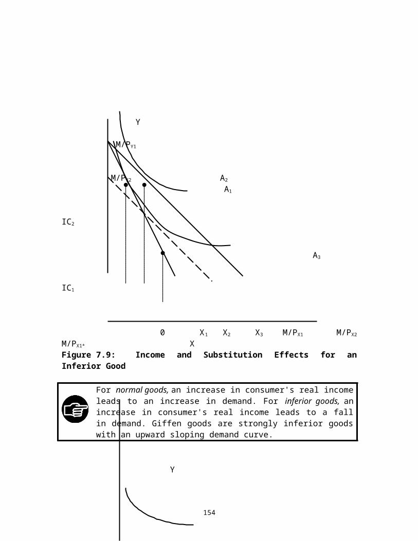
"external" to the transaction bear. Externalities can be either positive, when an external benefit is generated, or negative, when an external cost is imposed upon others.

Social cost of producing a commodity is equal to the private cost of producing it plus the cost to other people. It is the cost of production borne by all members of the society at large when a commodity is produced. A good example of social cost is that of a cement factory polluting air in the neighboring townships, which harms human health. Thus, social costs are the private costs of resources that the firm uses plus any additional costs imposed on society by the firm' s operation.

Social cost = private cost + external cost to the society.

10.4 Sunk Cost These are investment costs incurred before a certain activity takes place, which cannot be recovered by the possible sale of the asset they produced. Example of sunk costs includes specific investment in the research of product development. Sunk costs should be contrasted with incremental costs, which change with the level of production. In microeconomic theory, only incremental costs are relevant to a decision. Sunk costs have no relevance in evaluating future decisions.

10.5 Costs in the Short RunIn the short run, some of the firm's inputs to production are fixed, while others can be varied. The total cost (TC) of producing a given level of output has two components. These components are: the total fixed cost (TFC) and the total variable cost (TVC). Total fixed cost is the cost, which does not vary as the level of output varies. TFC may include expenditures for plant maintenance, insurance, and perhaps a manager of the firm. Total variable cost is the cost, which varies with the level of output. TVC includes expenditure for wages, salaries, and raw materials. These costs increase as output increases. Table 10.2 presents hypothetical TFC, TVC and TC schedules. These schedules are plotted in Figure. 10.1

(i) Total cost: the sum of total fixed cost and total variable cost(ii) Fixed cost: cost which does not vary as the level of output varies(iii) Variable cost: cost, which varies with the level of output.

Table 10.2: A Firm's Short Run ScheduleQ  TFC (T.Shs) TVC (T.Shs) TC (T.Shs)0 6,000 0 6,0001 6,000 3,000 9,0002 6,000 4,000 10,0003 6,000 4,200 10,200

160

4 6,000 6,000 12,0005 6,000 9,000 15,0006 6,000 14,000 20,0007 6,000 20,000 26,0008 6,000 26,000 32,0009 6,000 33,000 39,00010 6,000 39,000 45,00011 6,000 46,000 52,00012 6,000 55,000 61,000

From Table 10.2, we see that TFC are T.Shs 6,000 regardless of the level of output. This is reflected in Fig. 10.1 in a TFC curve, which is parallel to the quantity axis. TVC curve is zero when output is zero and rise as output rises. The particular shape of the TVC curve follows directly from the law of diminishing returns. Up to 3 units of output, the firm is using so few of the variable inputs together with its fixed inputs that the law of diminishing returns is not yet operating. So the TVC curve is concave downwards and TVC increase at a decreasing rate. Beyond 3 units of output, the law of diminishing returns begins to operate, so the TVC curve is concave upwards and TVC increase at an increasing rate. At every output level, TC equals TFC plus TVC. Thus the TC curve has the same shape as the TVC curve.

Figure 10.1: A Firm's Short Run Cost Curves

10.6 Short-Run per Unit Cost CurvesAlthough total cost curves are very important, per unit cost curves are even more important in the short-run analysis of the firm. This is because decision on how much to produce, depends on how variable costs increase with the level of output. The short-run

161

per unit cost curves that we will consider here are the marginal cost (MC), the average fixed cost, (AFC) the average variable cost (AVC), the average total cost (ATC) curves.

10.6.1 Marginal Cost Marginal cost is the change in total cost resulting from producing one extra unit of output. Because TFC does not change as the firm's level of output changes, marginal cost is just the change in variable cost that results from an extra unit of output. We can therefore write marginal cost as

(10.1)

Where; ΔTVC = change in total variable costΔQ = change in output.

10.6.2 Average Total CostAverage total cost is the cost per unit of output. There are three types of average cost: average fixed cost (AFC), average variable cost (AVC) and average total cost (ATC). Average total cost is obtained by adding together AFC and AVC. Alternatively, ATC can be obtained by dividing total cost by the level of output as written below.

(10.2)

In Table 10.3, ATC declines until output reaches 5 units as the fixed costs are spread over a larger output and initially the firm benefits from increasing return to the variable factor. Above 5 units of output, ATC increases as the influence of diminishing returns, which is pushing up AVC, outweighs the decline in AFC. Table 10.3: A Firm's Per Unit Short Run Cost OUTPUT TFC TVC TC AFC AVC ATC MC

1 6,000 3,000 9,000 6,000 3,000 9000 --2 6,000 4,000 10,000 3,000 2,000 5000 1,0003 6,000 4,500 10,500 2,000 1,500 3500 5004 6,000 6,000 12,000 1,500 1,500 3000 1,5005 6,000 9,000 15,000 1,200 1,800 3000 3,0006 6,000 13,000 19,000 1,000 2,167 3166.667 4,0007 6,000 18,000 24,000 857 2,571 3428.571 5,0008 6,000 24,000 30,000 750 3,000 3750 6,0009 6,000 31,000 37,000 667 3,444 4111.111 7,00010 6,000 39,000 45,000 600 3,900 4500 8,00011 6,000 48,000 54,000 545 4,364 4909.091 9,00012 6,000 58,000 64,000 500 4,833 5333.333 10,000

Table 10.3 presents the AFC, AVC, ATC and MC schedules derived from the TFC, TVC and TC schedules of Table 10.2. The AFC schedule (columns 5 ) is obtained by dividing

162

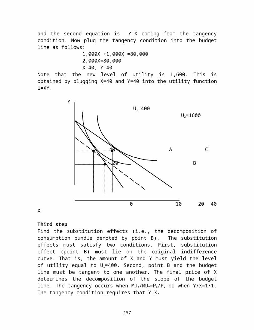
TFC (column 2) by the corresponding quantities of output produced (Q, in column 1). AFC can be written as:

(10.3)

The AVC schedule (columns 6) is obtained by dividing TVC (column 3) by Q. The ATC schedule (columns 7) is obtained by dividing TC (column 4) by Q. ATC at every output level also equals AFC (column 5) plus AVC (column 6). AVC can be written as:

(10.4)

From Table 10.3 we see that AVC reaches a minimum when output is 3 or 4 units per production period. This is the level at which average productivity of labor is at maximum. In other words, at this level of output, the proportions between the fixed factor and variable factor are at optimum. Note that at levels of output above 4 units, the variable factor has progressively less of the fixed factor to work with and its average productivity declines. This results in higher AVC as output increases. Conversely, AVC falls until output reaches 4 units because at low levels of output the variable factor has too much of the fixed factor to work with. The MC schedule (columns 8) is obtained by subtracting successive values of TC (column 4) or TVC (column 5). Thus MC does not depend on the level of TFC.

Average fixed cost (AFC) equals total fixed costs divided by output. Average variable cost (AVC) equals total variable costs divided by output. Average cost (ATC) equals total costs divided by output; ATC also equals AFC plus AVC. Marginal cost (MC) equals the change in TC or the change in TVC per unity change in output.

The AFC, AVC, ATC and MC schedules of Table 10.3 are plotted in Fig. 10.2. Note that while the AFC curve falls continuously as output is expanded, the AVC, the ATC and the MC curves are U-shaped. The MC curve reaches its lowest point at a lower level of output than either the AVC curve or the ATC curve. Also, the rising portion of the MC curve intersects the AVC and AC curves at their lowest points.

163

Figure 10.2: Short Run Cost Curves

10.7 The Relationship between Marginal Cost and Marginal ProductThe shape of the marginal cost (MC) curve is related to the behavior of the marginal product curve, which we discussed in lecture nine. If at low levels of output a firm benefits from increasing marginal returns to the variable factor (that is increasing MP), MC will be declining. MC reaches a minimum at the level of output at which the MP is at maximum. When the firm encounters diminishing marginal returns, so that MP is falling, MC begins to rise. Whenever there is a fixed factor, so that the law of diminishing returns comes into operation, the MC will eventually start to rise.

MPL, APL

APL

MPL

0 L1 L2 Labor

164

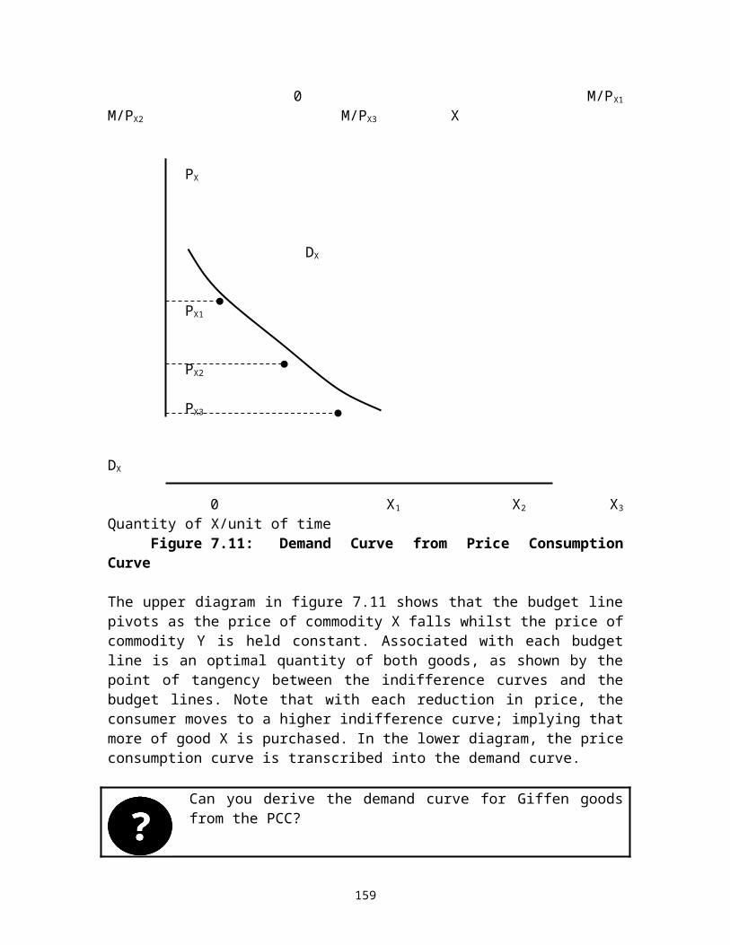
MC, ATCMC ATC

0 Q1 Q2 Output (Q)Figure 10.3: Marginal Product and Marginal Cost

The MC curve cuts the AVC and ATC curves at their minimum for arithmetical reasons, similar to those, which meant that the MP curve cut the AP curve at its maximum. We can also present the same results algebraically. We know that when labor is the only variable input, TVC equals price of labor times the number of units of labor used. That is;

(10.5)

We also know from production theory that the average product is given by the following formula;

(10.6)

The last item of equation 10.5 can be written as:

(10.7)

With our knowledge from production theory APL normally rises, reaches maximum and then falls. In the theory of cost, AVC behaves in the opposite direction. AVC normally falls, reaches a minimum and then rises. That is to say, AVC in a sense is a monetized image or reciprocal of the APL curve. Coming to the relationship between MC and MPL, the analysis follows the same logic. We know that in the short run marginal cost is defined as the change in the TVC dividing by change in output. That is;

(10.8)

But remember in lecture nine we showed that ΔQ/ΔL is MPL. We can therefore writeΔQ/ΔL as ΔL/ΔQ to imply 1/MPL. Equation 10.8 can be written as;

165

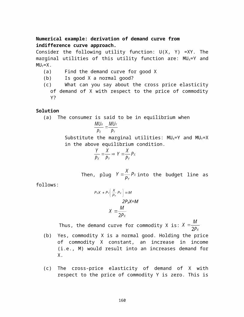
(10.9)

Now, since we know from lecture nine that normally MPL curve first rises, reaches a maximum and then falls, it follows that the MC curve falls first, reaches a minimum and then rises. Thus, the MC curve is in a sense a monetized mirror image or reciprocal of the MPL curve.

10.8 The Long-Run Average Total Cost CurveThe Long run Average Total Cost (LRATC) is illustrated in Figure 10.4. It indicates the minimum possible average cost of production for each level of output, given that the plant of the appropriate capacity has been constructed. Figure 10.4 shows that as the firm changes its level of output with the plant appropriate for minimum long run average cost of production at output OQ1, it moves along SRAC1, at output OQ2 it moves along SRAC2

and so on. In fact, at every point of tangent on the LRAC, there is an SRAC curve. Since each SRAC curve lies above the LRAC curve except at the point at which it is at a tangent, the LRAC curve is sometimes called and envelope curve.

Cost

SRAC1 C1

SRAC3 LRATC C3

SRAC1

C2

166

0 Q1 Q2 Q3 Output(Q)Figure 10.4: Long Run Average Total Cost

The curvature of the long run average cost is further determined by the position of the long run marginal cost. The LMC lies below the LAC when the LAC is falling, and above the long run average cost curve when the LAC is rising as shown in figure 10.5 below. The two curves intersect at point A where the LAC reaches its minimum.

Costs

LMC LAC

A C*

0 Q* Output (Q)Figure 10.5: Long run Marginal Cost

Numerical exampleConsider the following production function: Q=KL. The marginal product of labour is K and the marginal product of capital is L. Suppose that the price of labour is 2 and the price of capital is 1.

(a) Derive the equation for the long run total cost(b) Derive the equation for long run average cost

Solution (a) Start with the equilibrium condition

Substituting K=2L into the production function gives:Q=2L2

167

Plug into K=2L yields

Finally, substituting and into the total cost equation

yields:

(b) Average cost

What factors influence the shape of the firms Long Run Average Total Cost?

The factors leading to declining and rising long run average cost are linked to economies of scale and diseconomies of scales.

10.9 Economies of ScaleEconomies of scale refer to reductions in average cost resulting from increased production. Economies of scale can either be internal or external. Internal economies are those factors, which bring about a reduction in average cost as the scale of operation of individual firm rises. These may result from;

(a) Increased Specialization The larger the scale of production, the greater is the scope for the specialization of both labor and machinery. Normally workers can become very skilled and speedy by performing the same actions repeatedly if production process is broken down into many different stages.

(b) Factor Indivisibility Some factors of production can only be utilized efficiently if operations are on a large scale as compared to a small scale. More specialized and productive machinery can only be used when a firm operates a larger capacity. Put it differently, some type of capital equipment can only be employed efficiently in units of minimum size and this minimum may well be too large for small firms. For example, there is a lower limit to the size of car assembly line. Such indivisibility of equipment means that the firm with smaller output cannot take advantage of some highly specialized equipment.

168

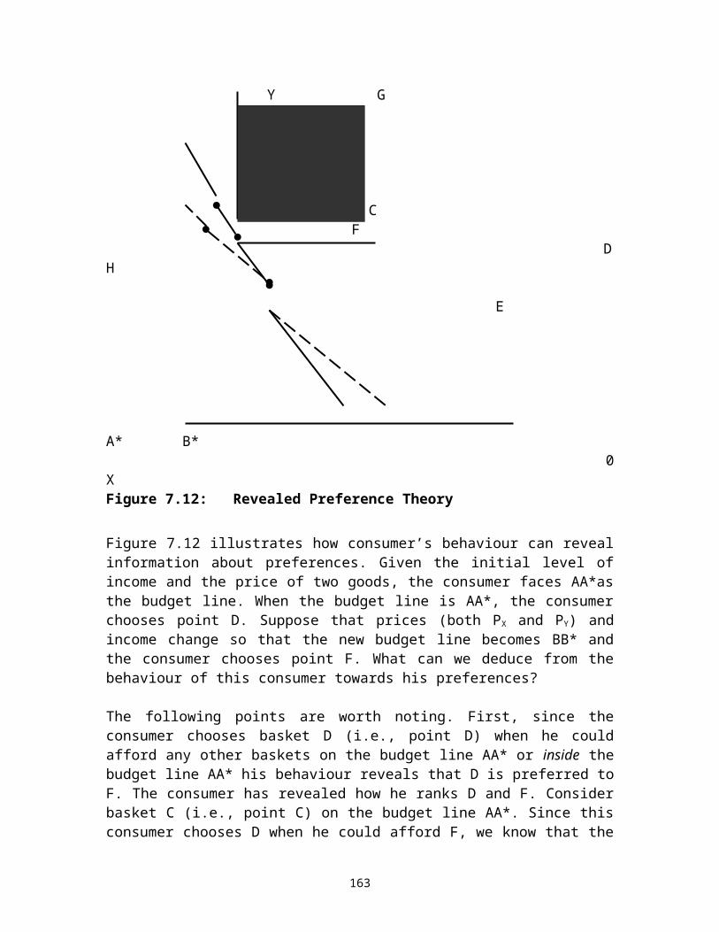
(c) Principles of MultiplesIf a production process involves the use of different types of machinery, a large firm can arrange to have more of the machines with a small output and fewer of the machines with a high output, thus achieving a high utilization rate. A small firm, on the other hand, with only one of each type of machine would find the capacity machines standing idle for much of the time.

(d) Research and Development A large firm may be able to support its own research and development program which can result in cost reducing innovations

(e) Financial Economies Large firms are normally able to obtain finance at lower rates of interest than small firms are. Large firms can often provide more collateral as security for loans and investors may be more likely to place money with well known, rather than with small firms. In addition, large companies have the option of making a new share issue on the stock exchanges.

(f) Marketing Economies This arises from the large-scale purchase of factors of production and from marketing and distributing the finished product in large quantities. A company selling a large volume may be able to use more expensive, but more cost effective, advertising. Large companies often receive quantity discounts in the purchase of raw materials.

(g) Risk Bearing Economies A large company that has diversified into several markets is likely to be better placed to withstand adverse trading conditions in one particular market. At the same time, other markets may have buoyant trading conditions. If a company is able to withstand risks, this may mean that it becomes more willing to take risks than smaller companies.

10.10 External Economies of ScaleExternal economies of scale arise from the simultaneous growth or interaction of a number of firms in the same area or related industries (i.e., localization of industry). (a) External economies due to the growth of the whole industry

All firms in the industry can benefit from the expansion of that industry regardless of their size. A large industry can support research in local universities from which several firms in an area can benefit.

(b) External economies from localization of industryWhen an industry is concentrated in a particular area, all firms can benefit from the specialist services that develop. These include the specialist companies for supplying and repairing machinery, the provision of training courses, and many others.

169

10.11 Diseconomies of ScaleDiseconomies of scale arises when per unit cost of production increases as the firm expands its scale of production. The following factors are the causes of diseconomies of scale(a) Control

Diseconomies of scale may be associated with difficulties of managing and controlling an enterprise as its size increases. A larger firm is harder to monitor, it is more complex and therefore co-ordination between different departments and divisions becomes more difficult. As well as making management less effective, and therefore indirectly imposing costs, the systems designed to cope with the extra complexity may also directly impose costs. In such a situation, monitoring how productive each worker is within a large firm is both imperfect and costly. This can lead to a loss of productive efficiency if worker dodging is common

(b) CoordinationLarge firms have long chains of command. Information from the top management may not be communicated to the production line properly and vice-versa. A firm with two workers requires one communication channel, directly between those two workers. A firm with three workers requires three communication channels (between employees A & B, B & C, and A & C). Moreover, as the firm becomes larger, managers may begin to pursue their own goals rather than devoting all of their efforts to pursuing the firm’s goal—making profits. For example, a manager might intentionally promote an incompetent worker knowing that the promoted worker will never be able to compete for his/her job.

(d) Industrial RelationLack of good relation between senior management and the junior work force may results into industrial disputes and production may suffer as a result. Senior managers may deny junior workers with payments for annual leave, salary increment and insurance policy for those working in dangerous conditions (e.g., workers unpacking steel from lorries). In such situations, people working within a larger firm may feel less committed to their jobs.

(e) InterdependencyIn large firms with many different departments, each part of the company becomes interdependent. Such interdependence may result into diseconomies of scale. When firms grow it is inevitable that someone, or even a team, will take on a job that is already being handled by another person or team

(e) External DiseconomiesDiseconomies of scale can also occur for reasons external to a firm. For example, as a firm becomes larger it may put pressure on its supplies of raw materials and labour, raising input prices.

170

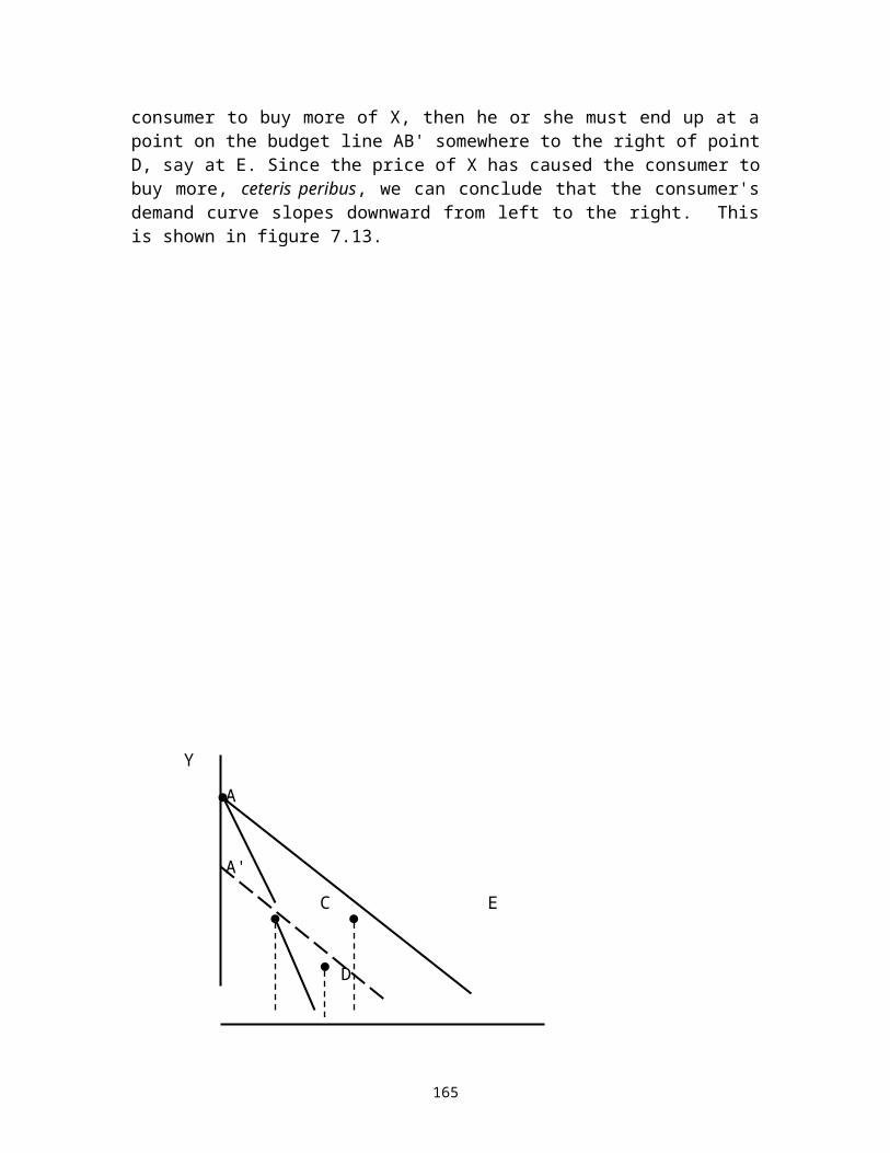
Economies of scale: falling long run average cost as the scale of output increases.Diseconomies of scale: rising long run average cost as the scale of output increases.

SUMMARY1. Economists estimate the cost of production on the basis of

opportunity costs. Opportunity cost is a term used in economics, to mean the cost of something in terms of an opportunity foregone (and the benefits that could be received from that opportunity), or the most valuable foregone alternative.

2. Explicit Costs: costs that involve direct money outlay for factors of production. Implicit Costs: costs that do not involve a direct money outlay (e.g. opportunity costs of the owner’s own inputs used - implicit wages, implicit rent, cost of capital).

4. Marginal cost is the change in total cost resulting from producing one extra unit of output. Because TFC does not change as the firm's level of output changes, marginal cost is just the change in variable cost that results from an extra unit of output.

5. Average total cost is the cost per unit of output. There are three types of average cost: average fixed cost (AFC), average variable

171

cost (AVC) and average total cost (ATC). Average total cost is obtained by adding together AFC and AVC. Alternatively, ATC can be obtained by dividing total cost by the level of output as written below.

6. When marginal cost is less than average total cost, average total cost is falling.  When marginal cost is greater than average total cost, average total cost is rising.

7. The U- shapes of the short run average and marginal cost curves are determined by the operation of diminishing marginal returns in production.

8. In the long run all factors are variables. The long run average total cost shows the lowest possible costs of producing different level of output, given the production function and factor prices.

9. Economies of Scale is the property whereby long-run average total cost falls as the quantity of output increases. Diseconomies of Scale is the property whereby long-run average total cost rises as the quantity of output increases

10. As the firm scale of operations increases, it may at first experience declining long run average costs because of the existence of economies of scale. Beyond a certain point, however, increasing long run average costs may be experienced as diseconomies of scale are encountered.

EXERCISES1. Write short notes on the following

(a) Marginal cost(b) Economies of scale(c) Returns to scale(d) Diseconomies of scale(e) Social cost and Sunk cost(e) Implicit cost and accounting cost.

2. With the increase in output of the firm, their average total cost and average variable cost curves come closer and closer to each other but never meet. Why?

3. How is the long run average cost derived? Can the short run average cost ever be less than the long run average total cost?

4. If the production function of the firm exhibit increasing return to scale at all levels of output then its long run average cost must be declining. Comment

172

5. If the marginal cost of production is increasing, does this tell you whether the average variable cost is increasing or decreasing? Explain

6. If the marginal cost of production is greater than the average variable cost, does this tell you whether the average variable cost is increasing or decreasing? Explain.

7. Salawa Footwear Leather Company (SFLC) has a total cost function represented by the following equation:

TC = 2q3 – 3q2 – 12q, Where q is the output (pair of shoes).(i) Find an expression for the marginal cost function(ii) Find an expression for the average cost function(iii)At what level of output is the average cost at minimum?

8. Suppose that the short run costs for Apollo Software Company is given by the following expression; TC = 150+2Q+0.01Q0.5.(i) What are the fixed costs of this company?(ii) What are the average costs and marginal costs at 50 units of

output?(iii) At what level of output is the average cost at minimum?

9. For a product produced by a firm demand is given by the expression: P = 40 – 2Q. Fixed cost is 10. Variable costs of producing Q units are VC (Q) = ½ Q2 + 5Q.

(a) Find expressions for total, average and marginal costs.(b) Find expressions for total, average and marginal revenue.(c) Sketch the graph for demand, marginal revenue and marginal

cost curves.

10* A firm has a fixed production cost of T.Shs 10,000 and a constant marginal cost of T.Shs 1000 per unit produced.

(a) What is the firm’s total cost function?(b) What is the firm’s average cost?

11. * Consider the following simple production function for Bernard Construction Company (BCC)

Q=5KLWhere Q is the level of output, K is capital and L is labour. The price of capital or rental rate of capital is T.Shs 10,000 per month and wage rate is T.Shs 5,000 per month. In addition to the price of labour and

173

capital, the firm pays T.Shs 2,000 as a cost of raw materials. The BCC industry has a fixed capital given by 5

(a) Find the cost function of BCC industry(b) What are the average and marginal costs of producing Q?(c) How do the average costs vary with the output (Q)?(d) How many units of labour are required to produce 250 level of

output? What is the average cost at this level of output?

12.* A car assembly industry in Dar es Salaam has a production function given by Q=KL; where Q is the output (assembled cars) per hour, K is the number of assembly machines, and L is the number of workers. The marginal product of capital is L and the marginal product of labour is K. The price of K is T.Shs 4 per hour and the price of labour is T.Shs 1 per hour, and the price of each car is T.Shs 3. The firm is currently assembling 20 cars per hour.

(a) Suppose that the company has exactly 4 machines and that, in the short run the amount of labor employed can be varied. Find the short run cost as a function of assembled cars

(b) Find the short run marginal cost and short run average cost

(c) Show that the firm is not currently minimizing its cost of production.

ANSWERS TO SELECTED QUESTIONSANSWERS TO SELECTED QUESTIONSLECTURE ONELECTURE ONE

Question number two(c) While a straight-line production possibility frontier represents constant

opportunity cost of production, a concave to the origin production possibility frontier represents increasing opportunity cost of production.

Question number fiveAn economic theory is a generalization, based on a variety of facts, about why or how an economic event occurs. The theory is generalization because it explains how economic variables generally behave when certain conditions exist. Theories are designed to explain and predict what we see. A theory consists of a set of definitions of variables to be employed, a set of assumptions about how things behave, and the conditions under which the theory is meant to apply

But, the world is very complex. Whenever there is an economic change, such as a decline in the value of the shilling, there are a myriad of factors that contributed to this change. It

174

would be impossible to measure the impact of each factor on the value of the shilling and be able to predict how the value of the shilling would change given the changes in the multitude of variables that influence the shilling. Economists have to simplify, so they concentrate on the primary factors that influence the value of shilling. By ignoring many of the minor factors that influence an economic variable (the change in the value of the shilling), economists abstract from reality, but they do so to better understand the world around them.

Question number six(a) This model shows that there is a negative relationship between the price and

demand for mbege (in liters). When the price of mbege decreases by one percent, the demand for mbege increase by 0.5 percent. The model also shows that there is negative correlation between the level of income and the litres of mbege consumed by alcohol drinkers. In particular, when the level of income increases by one percent, the consumed litres of mbege decreases by 0.42 percent. This may sound quite unusual, but it suggests that drinkers switch into other alcohols, perhaps beers when their income increase.

(b) is called a coefficient of determination. The coefficient of determination represents the proportion of the total variation in the dependent variable that is explained by the regression equation. ranges between 0 and 1. The higher the

, the more confidence one can have in the regression equation.

In our model, shows the explanatory power (i.e., coefficient of determination) is highly robust. In other words, this model says that 85% of demand for mbege is explained by these two variables (i.e, price of mbege and the level of income). Other omitted variables such as taste, price of beer, price of whiskey, price of grilled beef, price of grilled chicken, etc, explain about 15% of demand for mbege. Specification tests are not discussed here—we believe they are beyond the scope of this course.

(c) To some extent this model mirrors the behaviour of mbege drinkers. Typically, when the level of income increases, it is not unusual, ceteris peribus, to find some drinkers switching into other alcohols such as beers. Again under the ceteris peribus clause, we should expect the price of mbege to be negatively correlated with the quantity demanded. However, what is not clear about this model is whether the influence of omitted variables (i.e., taste, price of beer, price of whiskey, price of grilled beef, price of grilled chicken, etc) does not play any significant part in changing the signs and magnitudes of the estimated coefficients. So, further empirical testing is required in order to ascertain the accuracy and validity of this model.

LECTURE TWOLECTURE TWO

175

Question number five (a) How many Kilograms of maize flour are demanded at a price of 2? Price of 3?

Price of 5?

When P=5, Q=250When P=3,Q=350When P=2, Q=400

(b) When P=5, Q=750When P=3,Q=850When P=2, Q=900

Question number eight (a) To find the demand for cars when the price is 10,000, we plug this price into

the demand function as followsQd=50,000-10,000=40,000

To find the demand for cars when the price is 15,000, we plug this price into the demand function as follows

Qd=50,000-15,000=35,000To find the demand for cars when the price is 25,000, we plug this price into the demand function as follows

Qd=50,000-25,000=25,000

(b) Demand for curve for cars

Price of cars

25,000

20,000 15,000

10,000

5,000

176

0 10 20 25 30 35 40 Cars/year (000)

The above figure shows the demand curve for cars. To sketch it, plot the combinations of price and quantity (i.e., demand schedule) that we have obtained in part (a). The download slope of the demand curve in the above figure obeys the law of demand. That is, the lower the price the greater the quantity of cars, ceteris peribus.

LECTURE THREELECTURE THREE

Question number seven(a) It is easy to find the quantity of maize supplied at these various prices. To do

so, plug prices in the supply function as follows:QS=50,000+10,000=60,000QS=50,000+20,000=70,000QS=50,000+30,000=80,000QS=50,000+40,000=90,000

(b) Supply curve

Price of maize

40,000

30,000

20,000

10,000

177

0 10 20 30 40 50 60 70 80 90 maize/year

LECTURE FOURLECTURE FOUR

Question two

If the price of the commodity is set below its market clearing level, the quantity that firms are willing to supply is less than the quantity the consumers wish to purchase. The extent of the excess demand implied by this response will depend on the relative elasticities of demand and supply. For instance, if both demand and supply are elastic, the shortage is larger than if both are inelastic. Factors such as willingness of consumer to eat less chicken and the ability of the farmers to change the size of their poultry and hence produce less will determine these elasticities and influence the size of demand. Customers whose demands are not met will attempt to purchase substitutes, thus increasing demand for substitutes and raising their prices. If the price of chicken is set below market clearing levels, the price of beef will rise, assuming that beef is substitute for chicken.

Question five(a) The price in the market will equal the price floor price of T.Shs 200. The quantity

supplied is 100 and the quantity demanded is 300.(b) There will be an excess demand of 200 kilos of vegetables.(c) No, with an effective price ceiling price of T.Shs.200 the market is only willing to

supply 100 units even though demanders would like 300 units at that price.

Question Seven (a) The equilibrium price is T.Shs.80 and equilibrium quantity is 150(b) After the tax program, the supply function becomes P= 60 + (1/5) Qs. Therefore,

the new equilibrium price is T.Shs.88. The new equilibrium quantity is 140. (c) Tax paid by a consumer is T.Shs.1120.(d) Tax paid by a producer is T.Shs.280.(e) The tax revenue is T.Shs.1400.

Question EightIntroducing a per-unit subsidy has the following effects:

178

Q

P

Pe

Qe

S w/ subsidy

D

Quantity sold

Q1

S

Ps

Pb

Pb = price paidby buyers

Ps =price receivedby sellers

Pe = equilibriumprice

Cost of Subsidy= t * Q1

Q

P

Pe

Qe

S w/ subsidy

D

Quantity sold

Q1

S

Ps

Pb

Pb = price paidby buyers

Ps =price receivedby sellers

Pe = equilibriumprice

Cost of Subsidy= t * Q1

Relative to the equilibrium that existed before, the subsidy lowers the equilibrium price (that consumers pay) and increases the equilibrium quantity exchanged. It also raises the price that the producer/seller receives.

A subsidy is viewed as support for the producers of a particular good. By reducing the equilibrium price, a larger amount is sold and bought. Also, producers receive a higher price than in the absence of the subsidy. However, there are disadvantages. Subsidies are costly. For the government, they are expenditures that must be financed. The government generally raises revenues by taxing income or other goods. So, a subsidy for one good probably means higher taxes imposed on another good.

LECTURE FIVELECTURE FIVE

Question thirteen The elasticity of demand is the percentage change in the quantity demanded divided by

the percentage change in price. The elasticity of demand for maize is . This is

equivalent to saying that a 1% increase in price leads to a 2% decrease in quantity demanded.

Question fourteen (a) Price elasticity of demand

179

We must first compute the quantity demanded at the price of P=40. Q=1000-20(10) +40Q=1000-20(10) +20Q=780

The price elasticity of demand =

(b) Cross price elasticity of demand=

LECTURE SIXLECTURE SIX

Question number nine

(a) This individual should spend the first 10 shillings of her income to purchase the first 10 apples (commodity Y) because she derives 190 marginal utility. If she decides to spend the first 10 shillings on the first 10 units of oranges (commodity X), she would receive less marginal utility—that is, 110 utils. The next 20 units of Y give more marginal utility than 20 units of X. Thus, this individual should spend the second 10 shillings to purchase commodity Y. Again, it is also clear that 30 units of Y give more marginal utility than 30 units of X. Thus, this individual should spent the third 10 shillings to purchase commodity Y. Similarly, 40 units of Y give more marginal utility than 40 units of X. Thus, the fourth 10 shillings should be spent on commodity Y. You can also see from the table that the next 50 units of Y give more utility than 50 units of X. Thus, the fifth 10 shillings should be spent on commodity Y. This individual should spend the sixth 10 shillings to purchase 10 units of commodity X, because they give more marginal utility (i.e., 110) than 60 units of commodity Y (i.e., =100). Her seven and eight 10 shillings should be spent on 20 units of commodity X and 60 units of commodity Y because they give him/her the same level of marginal utility (i.e., 100). This individual cannot go on purchasing more units of X and Y because her income is exhausted.

(b) The total amount of utility when an individual is in equilibrium

Quantity Marginal utility of X

Total utility of X

Marginal utility of Y

Total utility of Y

10203040506070

1101009080706050

110210300380450510560

19017015013012010080

190360510640760860940

180

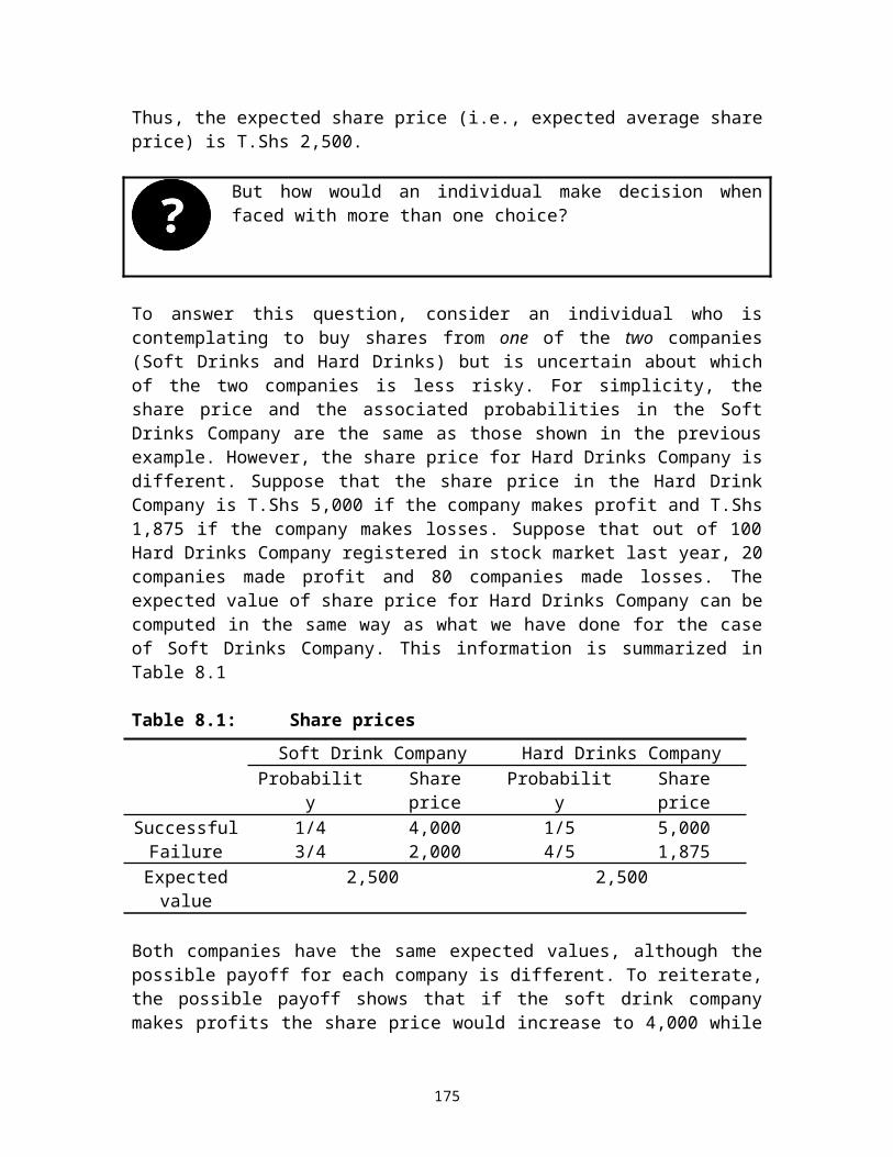
When this individual spends his/her income to purchase 20 units of X and 60 units of Y, the total utility is 1070. This is the maximum utility.

(c) The equilibrium requires the following condition to hold

10=10

So that PXQX+PYQY=80010(20) +10(60) =800

LECTURE SEVENLECTURE SEVEN

Question five

The MRS describes the rate at which the consumer is willing to trade one good for another to maintain the same level of satisfaction. The ratio of prices describes the trade off that the market is willing to make between the same two goods. The tangency of the indifference curves with the budget line represents the point at which the trade-offs are equal and consumer satisfaction is maximized. If the MRS between the good is not equal to the ratio of prices, then the consumer could trade one good for another at market prices to obtain higher levels of satisfaction. For example, if the slope of the budget line (the ratio of prices) is -4 then the consumer can trade 4 units of good 2 for one unit of good 1. If the MRS at the current bundle is -6, then the consumer is willing to trade 6 units of good 2 for one unit of good 1. Since the two slopes are not equal, the consumer is not maximizing satisfaction. The consumer is willing to trade 6 but only has to trade 4, so she could not make trade. This trading continues until the highest level of satisfaction is achieved. As trades are made, the MRS will change and become equal to the price ratio.Question eight A set of an indifference curve can be upward sloping when the assumption of more is better is violated. When a set of indifference curves is upward sloping, it means that one of the good is regarded as “bad” in the sense that consumer prefer less of the good rather than more of the good.

The positive slope means that the consumer will accept more of the “bad” good only if she/he also receives more of the other good in return. As we move up along the indifference curve the consumer has more of the good she likes and more of the good that she dislikes.

Good (Food)

181

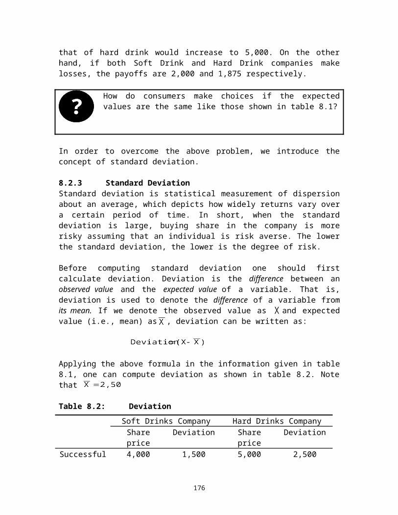
Bad (Smoking)

The above figure shows that more smoking (assuming that this consumer regards smoking as bad) with little food worsen her utility. On the other hand, more food (assuming that food is good) will increase her utility. In the extreme cases where a consumer dislikes smoking at all (i.e., s/he is non-smoker) the indifference curves will look like:

Good (Food)

182

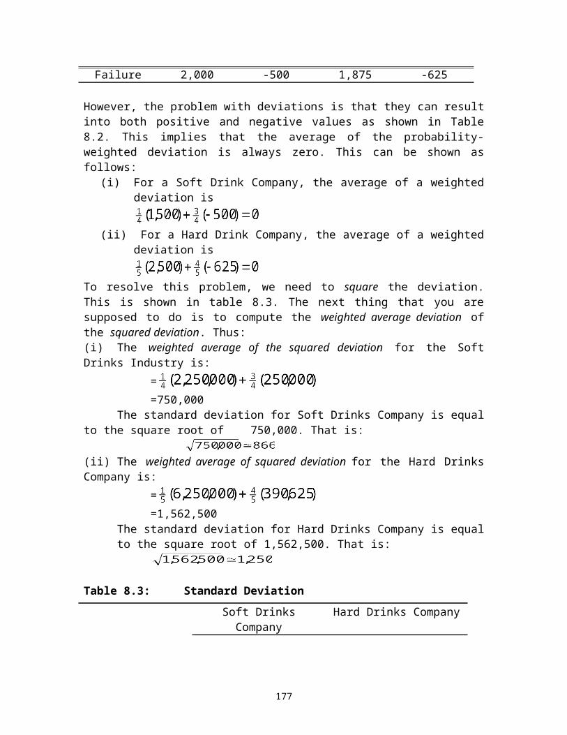
Bad (smoking)This means that consumer does not care completely about smoking. His/her indifference curves are horizontal line. The level of satisfaction increase upwards. On the other hand, if the consumer dislikes both smoking and food, the indifference curves look like:

Bad (Food)

Bad (Smoking) Indifference curves are concave to the origin.

Question nine (a) Substitute

Two goods are perfect substitutes if the Marginal rate of substitution between the two goods is a constant number. This implies that the slope of an indifference curve is constant and the indifference curve is linear as shown in the figure below.

Indifference curves for perfect substitutes

Y

Indifference curve 3

Indifference curve 2

Indifference curve 1

183

0X

(b) ComplementsWhenever the commodities are complements the indifference curve takes the shape of the right angle. In this case, an individual consumes the two goods in a fixed proportion; e.g., 1 unit of X for each unit of Y. The indifference curves take the following shapes.

Y

Indifference curve 3

Indifference curve 2

Indifference curve 1

0 X

Question tenSolution

(a) John’s marginal rate of substitution can be defined as the number of bottles of Coke he would be willing to give up in exchange for a bottle of Pepsi. Since he is always willing to trade one for one, his MRS is equal to 1

(b) Since John is always willing to trade one can of coke for one coke of Pepsi his indifference curve is linear with a slope of -1

(c) John’s indifference curves are linear with a slope of -1. If John’s budget line is steeper than his indifference curves then he will choose to consume only a good on the vertical axis. If John’s budget line is flatter than his indifference curves then he will choose to consume only the good on the horizontal axis. John will always choose corner solution, unless his budget line has the same slope as his indifference curves. In this case any combination of Coke and Pepsi that uses up his entire income will maximize his satisfaction.

Question elevenIf an individual consumes only food and clothing, then any increase in income must be spent on either food or clothing (note that the budget is spent on two goods and no

184

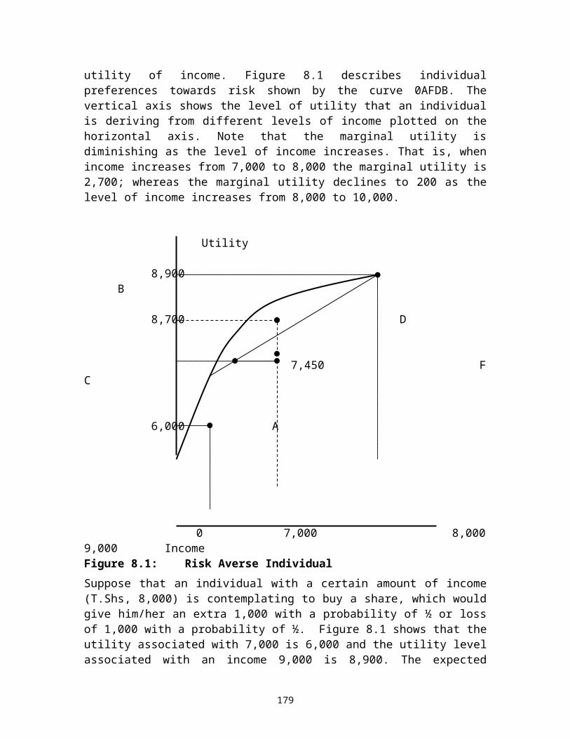
saving). If food is an inferior good, then as income increases, consumption falls. With constant prices, the extra income not spent on food must be spent on clothing. Therefore, as income increases, more is spent on clothing, i.e. clothing is a normal good. For both types of goods, normal and inferior, we still assume that more is preferred to less.

Question twelveThis is true. As the price of good falls, the budget line pivots outwards and the consumer is able to move to a higher indifference curves.

Question thirteen Solution(a) We know that the equilibrium of consumer must satisfy two conditions:

(i) An equilibrium basket will be on the budget line: PX (X)+PY (Y)=I

(ii) The tangency condition must hold.

The second condition implies that or simply,

In order to obtain the equation for the demand curve for food, substitute

into the budget line as follows:

Solving for X, implies that the demand curve is given as

This is the equation of the demand curve for food. Given any numerical values of income and the price of food, we can easily find the quantity of food the consumer will purchase.

(b) You can easily check that an increase in income, ceteris peribus, always increases the quantity of X. So, food is a normal good.

LECTURE EIGHTLECTURE EIGHT

Question three(a) The expected value of the lottery is equal to the sum of returns weighted by

their probabilities:

EV = 0.2(250) +0.3(200) +0.5(100)= 50+60+50= 160

185

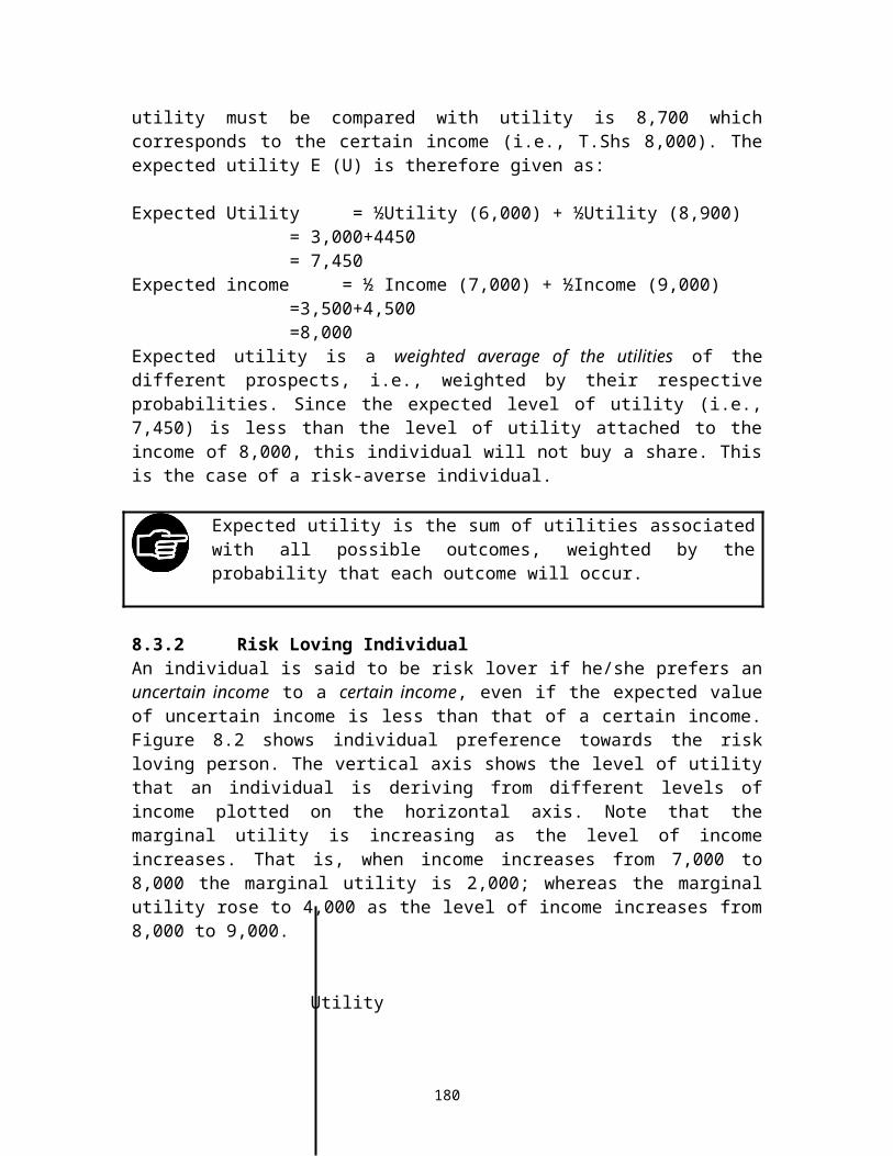
(b) Variance is the sum of squared deviation from the mean (i.e., the mean is 160 in this question) weighted by their respective probabilities:

Variance = 0.2(250-160) 2+0.3(200-160) 2+0.5(100-160) 2

= 0.2(8100) +0.3(1600) +0.5(3600)= 1620+480+1800= 3900

Standard deviation ≈ 62.44

(c) A risk neutral person would pay the expected value of the lottery; that is, T.Shs 160.

Question five(a) Expected value of profit in company A is computed as:

EV = 0.90(0) +0.10(400)= 40

Expected value of profit in company B is computed as:EV = 0.50(30) +0.50(50)

= 15+25= 40

(b) Variance in company A is computed as follows:Variance = 0.90(0-40)2+0.10(400-40)2

= 1440+12960= 14400

Standard deviation in company A is computed as follows:SD =

= 120

Variance in company B is computed as follows: Variance = 0.50(30-40)2 +0.50(50-40)2

= 50+50= 100

Standard deviation in company B is computed as follows: SD =

= 10

(c) Given the utility function , the risk premium associated with company A (i.e., RPA) is

0.90 +0.10 = 0+0.10(20) =

2 =

186

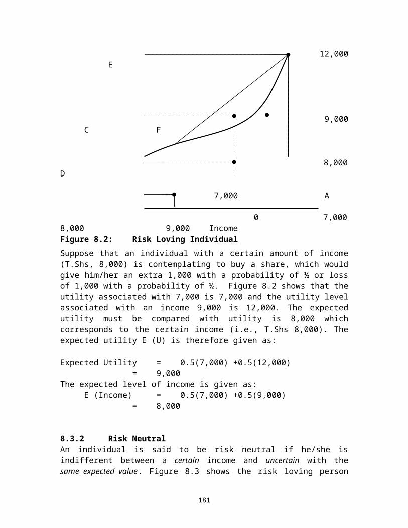
4 =40-RPA

36 =RPA

The risk premium associated with company B (i.e., RPB) is 0.50 +0.50 =0.50(5.48) +0.50(7.07) =

2.74+3.54=6.28=39.4=40-RPB

0.6=RPB

Question six(a) The expected value of the share price is equal to the sum of returns weighted

by their respective probabilities:EV = 0.5(0.00) +0.25(100) +0.2(200) +0.05(750)

= 0.00+25+40+37.5= 102.5

Variance = 0.5(0-102.5) 2+0.25(100-102.5) 2+0.2(200-102.5) 2+0.05(750-102.5) 2

= 5253.125+1.5625+1901.25+20962.812= 28118.749

Standard deviation ≈ 167.7

(b) Yes, she would buy a share because the expected value of the share price is greater than the actual share price. That is, 102.5>100

(c) If Esther buys 10000 shares, it is likely that she will have T.Shs 1,025,000 minus T.Shs 1,000,000 she has paid. She will not buy any insurance since the expected return is greater than cost. That is, 1,025,000>1,000,000

LECTURE NINELECTURE NINE

Question number Seven

Labour Total output MPL APL0123456

0225600900114013651350

225375300240225-15

225300300285273225

Question number nine

187

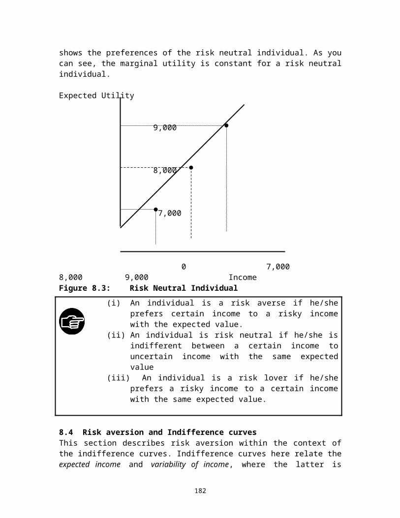
Convex isoquants imply that within some range, some number of units of one input can be substituted for a unit of the other input, and output can be maintained at the same level. In this case, the MRTS is diminishing as we move down along the isoquant. Linear isoquants imply that the slope, or the MRTS, is constant. This means that the same number of units of one input can always be exchanged for a unit of the other input and output can be maintained. The inputs are perfect substitutes. L-Shaped isoquant imply that the inputs are perfect complements, or that the firm is producing under a fixed proportion type of technology. In this case, the firm cannot give up one in exchange for the other and still maintain the same level of output. For example, the firm may require 4 units of capital for each unit of labour in which case one input can not be substituted for the other.

Question ten The marginal rate of technical of substitution is defined as the ratio of the two marginal products. Here, we are given the marginal product of labour and the marginal rate of technical substitution. To determine the marginal product of capital, substitute the given values for the marginal product of labour and the marginal rate of technical substitution into the following formula:

Computer chips per hour.

LECTURE TENLECTURE TEN

Question number ten(a) Since variable cost of producing an additional unit or marginal cost is T.Shs

1000, then the total variable cost would be 1000Q. Total cost is the sum of total variable cost and total fixed costs; i.e., TC=10000+1000Q

(b) Average cost is given as

Question number eleven

188

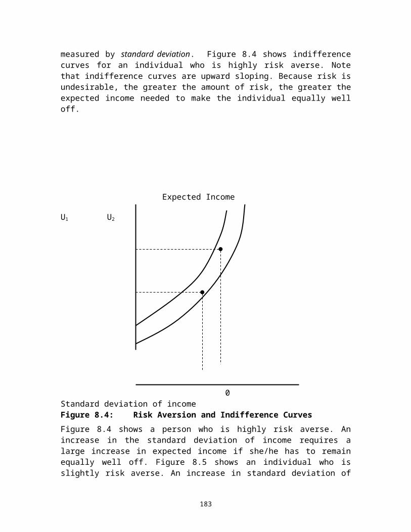
(a) Since K is fixed at 5, the short run production function becomes: Q=25L. This

implies that for any level of output Q, the units of labour employed is .

The total cost function is thus given by the sum of the costs of capital, labour and raw materials:

(b) The average and marginal costs functions are given by:

Marginal cost =2,200

(c) Marginal costs are constant and average cost will decrease as the quantity increases (due to a fixed cost of capital).

(d) In order to produce 250 units of output, we need 10 units of labour. That is,

Average cost at 250 units of output is given as

Question number Twelve

(a) Since Q=KL and K=4, we have Q=4L, or L=¼Q. Thus,

C (Q)=PKK+PLL = 4(4)+1(¼Q)

= 16+¼Q

(b) Since the cost is a linear function of output, marginal cost is just the slope of the cost curve. So, MC (Q) =¼. To find the average cost:

189

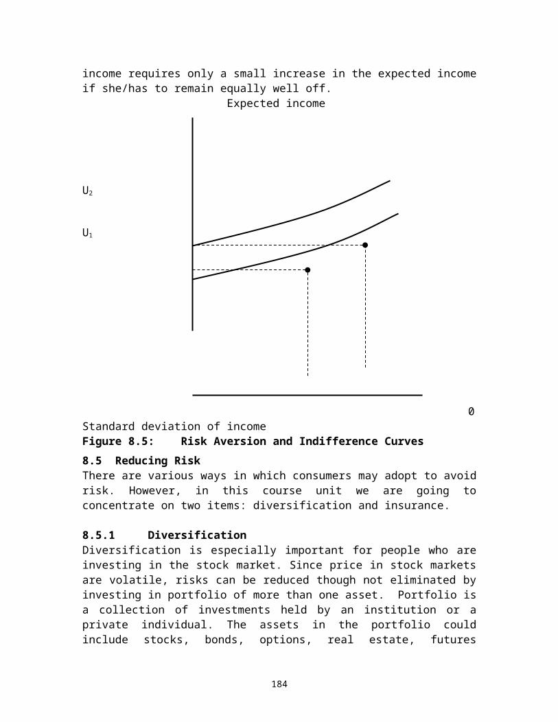
(c) Currently, Q=20 and K=4. So, the firm is currently employing units of

labour. However, cost minimization requires:

Since 5≠ (4)(4), the firm is not using the cost minimizing input combination.

190